Download Campbell Bowen Ratio Instrumentation Instruction manual

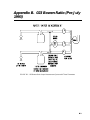
INSTRUCTION MANUAL
Bowen Ratio Instrumentation
Revision: 9/05
C o p y r i g h t ( c ) 1 9 8 7 - 2 0 0 5
C a m p b e l l S c i e n t i f i c , I n c .
Warranty and Assistance
The BOWEN RATIO INSTRUMENTATION is warranted by CAMPBELL
SCIENTIFIC, INC. to be free from defects in materials and workmanship
under normal use and service for twelve (12) months from date of shipment
unless specified otherwise. Batteries have no warranty. CAMPBELL
SCIENTIFIC, INC.'s obligation under this warranty is limited to repairing or
replacing (at CAMPBELL SCIENTIFIC, INC.'s option) defective products.
The customer shall assume all costs of removing, reinstalling, and shipping
defective products to CAMPBELL SCIENTIFIC, INC. CAMPBELL
SCIENTIFIC, INC. will return such products by surface carrier prepaid. This
warranty shall not apply to any CAMPBELL SCIENTIFIC, INC. products
which have been subjected to modification, misuse, neglect, accidents of
nature, or shipping damage. This warranty is in lieu of all other warranties,
expressed or implied, including warranties of merchantability or fitness for a
particular purpose. CAMPBELL SCIENTIFIC, INC. is not liable for special,
indirect, incidental, or consequential damages.
Products may not be returned without prior authorization. The following
contact information is for US and International customers residing in countries
served by Campbell Scientific, Inc. directly. Affiliate companies handle
repairs for customers within their territories. Please visit
www.campbellsci.com to determine which Campbell Scientific company
serves your country. To obtain a Returned Materials Authorization (RMA),
contact CAMPBELL SCIENTIFIC, INC., phone (435) 753-2342. After an
applications engineer determines the nature of the problem, an RMA number
will be issued. Please write this number clearly on the outside of the shipping
container. CAMPBELL SCIENTIFIC's shipping address is:
CAMPBELL SCIENTIFIC, INC.
RMA#_____
815 West 1800 North
Logan, Utah 84321-1784
CAMPBELL SCIENTIFIC, INC. does not accept collect calls.
Bowen Ratio Table of Contents
PDF viewers note: These page numbers refer to the printed version of this document. Use
the Adobe Acrobat® bookmarks tab for links to specific sections.
1. System Overview ......................................................1-1
1.1 Review of Theory ................................................................................. 1-1
1.2 System Description............................................................................... 1-3
1.2.1 Water Vapor Measurement ......................................................... 1-3
1.2.2 Air Temperature Measurement ................................................... 1-4
1.2.3 Net Radiation and Soil Heat Flux ............................................... 1-5
1.2.4 Power Supply.............................................................................. 1-5
2. Station Installation....................................................2-1
2.1
2.2
2.3
2.4
2.5
2.6
2.7
Sensor Height and Separation............................................................... 2-1
Soil Thermocouples and Heat Flux Plates ............................................ 2-2
Wiring................................................................................................... 2-4
Battery Connections.............................................................................. 2-7
System Startup ...................................................................................... 2-7
Routine Maintenance ............................................................................ 2-7
Cleaning the DEW 10........................................................................... 2-8
3. Sample CR23X Program...........................................3-1
4. Calculating Fluxes Using SPLIT ..............................4-1
4.1 Data Handling........................................................................................ 4-1
4.2 Calculating Fluxes ................................................................................ 4-1
Appendices
A. References............................................................... A-1
B. 023 Bowen Ratio (Pre July 1993) ........................... B-1
Tables
1.2-1. Component Power Requirements ..................................................... 1-5
2.3-1. CR23X/Sensor Connections for Example Program ......................... 2-4
3-1. Sample CR23X Bowen Ratio Program Flow Chart ............................ 3-2
3-2. Output From Example Bowen Ratio Program .................................... 3-5
4.2-1. Input Values for Flux Calculations .................................................. 4-3
i
Bowen Ratio Table of Contents
Figures
1.2-1. Vapor Measurement System............................................................. 1-3
1.2-2. Thermocouple Configuration............................................................ 1-4
2-1. CSI Bowen Ratio System .................................................................... 2-2
2.2-1. Placement of Thermocouples and Heat Flux Plates ......................... 2-3
2.2-2. TCAV Spatial Averaging Thermocouple Probe.............................. 2-4
2.3. A block diagram for the connections between the datalogger,
the BR relay driver and components, and the external battery................ 2-6
2.4-1. Terminal Strip Adapters for Connections to Battery ........................ 2-7
2.7-1. DEW 10 Circuit Board ..................................................................... 2-9
B-1. 023 Bowen Ratio Vapor Measurement System with Three
Flowmeters ............................................................................................. B-1
ii
Section 1. System Overview
1.1 Review of Theory
By analogy with molecular diffusion, the flux-gradient approach to vertical
transport of an entity from or to a surface assumes steady diffusion of the
entity along its mean vertical concentration gradient.
When working within a few meters of the surface, the water vapor and heat
flux densities, E and H, may be expressed as:
E = kv
∂ρ v
∂z
H = ρC p k H
∂T
∂z
(1)
(2)
Here ρv is vapor density, ρ is air density, Cp is the specific heat of air, T is
temperature, z is vertical height, and kv and kH are the eddy diffusivities for
vapor and heat, respectively. Air density and the specific heat of air should
account for the presence of water vapor, however, use of standard dry air
values usually causes negligible error. The eddy diffusivities are functions of
height. The vapor and temperature gradients reflect temporal and spatial
averages.
Applying the Universal Gas Law to Eq. (1), and using the latent heat of
vaporization, λ, the latent heat flux density, λ, can be written in terms of vapor
pressure (e).
Le =
λρεk v ∂e
P ∂z
(3)
Here P is atmospheric pressure and ε is the ratio of the molecular weight of
water to the molecular weight of dry air.
In practice, finite gradients are measured and an effective eddy diffusivity
assumed over the vertical gradient:
Le =
λρεk v ( e1 − e 2 )
P ( z1 − z2 )
(4)
( T1 − T2 )
.
( z1 − z2 )
(5)
H = ρCpk H
In general, kv and kH are not known but under specific conditions are assumed
equal. The ratio of H to Le is then used to partition the available energy at the
surface into sensible and latent heat flux. This technique was first proposed by
Bowen (1926). The Bowen ratio, β, is obtained from Eq. (4) and Eq. (5).
1-1
Section 1. System Overview
β=
H PC p ( T1 − T2 )
=
Le
λε (e1 − e 2 )
(6)
where PCp λε is the psychrometric constant.
The surface energy budget is given by,
Rn − G − H − L e = 0 ,
(7)
where Rn is net radiation for the surface and G is the total soil heat flux. The
sign convention used is Rn positive into the surface and G, H, and Le positive
away from the surface. Substituting βLe for H in Eq. (7) and solving for Le
yields:
Le =
Rn − G
1+ β
.
(8)
Measurements of Rn, G, and T and e at two heights are then required to
estimate sensible and latent heat flux.
Atmospheric pressure is also necessary, but seldom varies by more than a few
percent. It may be calculated for the site elevation, assuming a standard
atmosphere, or obtained from a nearby station and corrected for any elevation
difference (Wallace and Hobbes, 1977).
Eq. (6) shows that the sensitivity of β is directly related to the measured
gradients; a 1% error in a measurement results in a 1% error in β.
When the Bowen ratio approaches -1, the calculated fluxes approach infinity.
Fortunately, this situation usually occurs only at night when there is little
available energy, Rn - G. In practice, when β is close to -1 (e.g., -1.25 < β < 0.75), Le and H are assumed to be negligible and are not calculated. Ohmuna
(1982) describes an objective method for rejecting erroneous Bowen ratio data.
1-2
Section 1. System Overview
FIGURE 1.2-1. Vapor Measurement System
1.2 System Description
1.2.1 Water Vapor Measurement
It is common practice in Bowen ratio measurements to measure wet bulb
depression to develop the water vapor gradient. The position of the two
psychrometers is periodically reversed to cancel systematic sensor errors
(Suomi, 1957; Fuchs and Tanner, 1970).
In the Campbell Scientific system, vapor concentration is measured with a
single cooled mirror dew point hygrometer1, using a technique developed for
multiple level gradient studies (Lemon, 1960). Air samples from two heights
are routed to the cooled mirror after passing through mixing volumes (Figure
1.2-1). The problems associated with wick wetting and water supply in
psychrometers are avoided and systematic sensor errors are eliminated.
Air is drawn from both heights continuously through inverted 25 mm filter
holders fitted with Teflon filters with a 1 µm pore size. The filter prevents dust
contamination in the lines and on the cooled mirror. It also prevents liquid
water from entering the system.
A single low power DC pump aspirates the system. Manually adjustable
rotometers are used to adjust and match the flow rates. A flow rate of 0.4
liters/minute with 2 liter mixing chambers gives a 5 minute time constant.
1
Model Dew-10, General Eastern Corp. Watertown, MA
1-3
Section 1. System Overview
A datalogger is used to measure all sensors and control the valve that switches
the air stream through the cooled mirror.
The resolution of the dewpoint temperature measurement is ±0.003°C over a
±35°C range. The limitation is the stability of the Dew-10, approximately
0.05°C, yielding better than ±0.01 kPa vapor pressure resolution over most of
the environmental range.
Every 2 minutes the air drawn through the cooled mirror is switched from one
height to the other with the valve. Forty seconds is allowed for the mirror to
stabilize on the new dewpoint temperature and 1 minute and 20 seconds worth
of measurements for an individual level are obtained for each 2 minutes cycle.
The dewpoint temperature is measured every second and the vapor pressure is
calculated by the datalogger using the equation described by Lowe (1976).
The average vapor pressure at each height is calculated every 20 minutes.
CR23X
FIGURE 1.2-2. Thermocouple Configuration
1.2.2 Air Temperature Measurement
Air temperature is measured at two heights with chromel–constantan
thermocouples wired as in Figure 1.2-2. The differential voltage is due to the
difference in temperature between T1 and T2 and has no inherent sensor offset
error. The datalogger resolution is 0.006°C with 0.1 µV rms noise.
The thermocouples are not aspirated. Attempts to aspirate the TCs with the air
from the vapor measurement system were not successful. Testing under 1000
W m-2 solar radiation, with several radiation shield designs and aspiration rates
of up to 80 cm s-1 (1 l min-1), showed a significant increase in temperature due
to radiation from the shield/ducting.
Calculations indicate that a 25 µm (0.001 in) diameter TC experiences less
than 0.2°C and 0.1°C heating at 0.1 m s-1 and 1 m s-1 wind speeds, respectively,
under 1000 W m-2 solar radiation (Tanner, 1979). More importantly, error in
1-4
Section 1. System Overview
the gradient measurement is due only to the difference in the radiative heating
of the two TC junctions and their physical symmetry minimizes this.
Conversely, contamination of only one junction can cause larger errors.
Applying temperature gradients to the TC connectors was found to cause
offsets. The connector mounts were designed with radiation shields and
thermal conductors to minimize gradients.
The prototype systems used two sets of TCs on each system, one 25 µm and
one 76 µm diameter. It was hypothesized that the 25 µm diameter would
suffer less from radiation loading and the 76 µm would be less prone to
breakage. The current design uses a single set of TCs (76 µm standard) with
two parallel junctions at each height as a back up against breakage.
1.2.3 Net Radiation and Soil Heat Flux
Net radiation and soil heat flux are averaged over the same time period as the
vapor pressure and temperature differences.
To measure soil heat flux, heat flux plates are buried in the soil at a fixed depth
of between 5 to 10 cm to reduce errors due to vapor transport of heat.
Typically the plates are buried at a depth of 8 cm. The average temperature of
the soil layer above the plate is measured using 4 parallel thermocouples. The
heat flux at the surface is then calculated by adding the heat flux measured by
the plate to the energy stored in the soil layer. The storage term is calculated
by multiplying the change in soil temperature over the averaging period by the
soil heat capacity.
1.2.4 Power Supply
The current requirements of the components of the Bowen ratio system are
given in Table 1.2-1.
TABLE 1.2-1. Component Power
Requirements
Component
Cooled Mirror
Pump
CR23X
Current at 12 VDC
150 - 500 mA
60 mA
5 mA
A 20 watt solar panel (SP20R) and a 70 amp-hour battery are capable of
providing a continuous current of 300 - 350 mA. The solar panel is necessary
if the system is to be used for periods longer than 2-3 days. The datalogger
can control power to the cooled mirror and pump, and can shut down the
system if the battery voltage is low or if measurements are not needed at night.
1-5
Section 1. System Overview
This is a blank page.
1-6
Section 2. Station Installation
Figure 2-1 shows the typical Bowen ratio installation on the CM10 tripod. The 023A
enclosure, mounting arms, and SP20R solar panel all mount to the tripod mast (1 1/4 in.
pipe, inside diameter) with U-bolts. The size of the tripod allows the heights of the arms to
be adjusted from 0.5 to 3 meters. The mounting arms should be oriented due south to
avoid partial shading of the thermocouples.
The net radiometer is mounted on a separate stake (not provided by Campbell Scientific) so
that the tripod is not a significant portion of its field of view. It should be positioned so
that it is never shaded by the tripod or mounting arms and should be mounted so that it
points south.
2.1 Sensor Height and Separation
There are several factors which must be balanced against each other when
determining the height at which to mount the support arms for the temperature
and air intakes. The differences in temperature and moisture increase with
height, so the resolution on the measurements of the temperature and vapor
gradient will improve the farther apart the arms are.
The upper mounting arm must be low enough that it is not sampling air that is
coming from a different environment upwind. The air that the sensors see
must be representative of the soil/vegetation that is being measured. As a rule
of thumb, the surface being measured should extend a distance upwind that is
at least 100 times the height of the sensors. The following references discuss
fetch requirements in detail: Brutsaert (1982); Dyer and Pruitt (1962); Gash
(1986); Schuepp et al. (1990); and Shuttleworth (1992).
The lower mounting arm needs to be higher than the surrounding vegetation so
that the air it is sampling is representative of the bulk crop surface, and not a
smaller scale effect that might be seen in a row crop if the sensors were down
between rows.
2-1
Section 2. Station Installation
Q7-BR
(system)
FIGURE 2-1. CSI Bowen Ratio System
2.2 Soil Thermocouples and Heat Flux Plates
The soil thermocouples and heat flux plates are typically installed as shown in
Figure 2.2-1. The TCAV parallels four thermocouples together to provide the
average temperature, as shown in Figure 2.2-2). It is constructed so two
thermocouples can be used to obtain the average temperature of the soil layer
above one heat flux plate and the other two above the second plate. The
thermocouple pairs may be up to two meters apart.
The location of the two heat flux plates/ thermocouples should be chosen to be
representative of the area under study. If the ground cover is extremely varied,
it may be necessary to have additional sensors to provide a valid average.
Use a shovel to cut a vertical slice in the soil and remove the soil to one side of
the cut. Try to keep the soil that is removed intact so that it can be replaced
with as little disruption as possible.
The sensors are installed in the undisturbed face. The depths are measured
from the top of the soil. A horizontal cut is made with a knife to install the
heat flux plate, and the stainless steel tubes on the ends of the thermocouple are
pressed in, keeping the tubes horizontal. When removing the thermocouples,
grip the tubing, not the thermocouple wire.
2-2
Section 2. Station Installation
To minimize thermal conduction down the sensor lead wires, they should be
buried for a short distance back from the sensor. In particular, do not run the
leads directly to the surface, but wrap them around the edge of the hole,
keeping the leads at the same level as the sensor for as long as possible. Once
the sensors are installed, backfill the hole.
Install the CS616 as shown in Figure 2.2-1. See the CS616 manual (Section 5)
for detailed installation instructions.
Up to 1
m
2.5 cm
2 cm
Ground
6 cm
Surfac
e
8 cm
Partial emplacement of HFT3 and TCAV sensors
is shown for illustration purposes. All sensors
must be completely inserted into the soil face
before the hole is backfilled.
FIGURE 2.2-1. Placement of Thermocouples and Heat Flux Plates
2-3
Section 2. Station Installation
24 GAUGE
CHROMEL
CONSTANTAN
HI
(PURPLE)
LO
(RED)
40 GAUGE CHROMEL
CONSTANTAN
STAINLESS STEEL
TUBE
FIGURE 2.2-2. TCAV Spatial Averaging Thermocouple Probe
2.3 Wiring
Table 2.3-1 lists the connections to the CR23X for the standard Bowen ratio
sensors measured by the example program. Because the air temperature
measurements are so critical, the air temperature thermocouples are connected
to differential channel 4 (the channel that is closest to the reference
temperature thermistor). The input terminal strip cover for the CR23X must be
installed once all connections have been made and verified (Section 13.4 of
CR23X manual).
TABLE 2.3-1. CR23X/Sensor Connections for Example
Program
CHANNEL
1H
1L
2H
2L
3H
3L
4H
4L
2-4
SENSOR
Q7.1
Q7.1
SHIELD
HYGROMETER PRT
HYGROMETER PRT
HYGROMETER PRT
TCAV
TCAV
TCAV
UPPER 0.003 TC - CHROMEL
LOWER 0.003 TC - CHROMEL
COLOR
RED
BLACK
CLEAR
GREEN
WHITE
BLACK
PURPLE
RED
CLEAR
PURPLE
PURPLE
Section 2. Station Installation
UPPER/LOWER TCs - CONSTANTAN
TC SHIELD
HFT#1
HFT#2
HFT#1 AND HFT#2
WIND SENTRY
CS615
WIND SENTRY
CS615
RED/RED
CLEAR/CLEAR
BLACK
WHITE/WHITE
CLEAR/CLEAR
RED
GREEN
WHITE/CLEAR
BLACK/CLEA
R
EX1
EX2
GND
HYGROMETER EXCITATION
WIND SENTRY
HYGROMETER
RED
BLACK
CLEAR
C1
C2
C3
PULSE FOR LOWER AIR INTAKE
PULSE FOR UPPER AIR INTAKE
PULSE TO TURN ON POWER TO
MIRROR AND PUMP (FLAG 6)
PULSE TO TURN OFF POWER TO
MIRROR AND PUMP (FLAG 7)
GREEN
WHITE
BLACK
CS615 (TURN UNIT ON)
GROUND WIRE
ORANGE
CLEAR
WIND SENTRY
WIND SENTRY
CS615
CS615
BLACK
WHITE/CLEAR
GREEN
BLACK/CLEA
R
CS615
RED
5H
5L
6H
6L
C4
C7
G
PULS
E
1
2
+12 V
RED
2-5
Section 2. Station Installation
CR23X
FIGURE 2.3. A Block Diagram for the Connections between
the Datalogger, the BR Relay Driver and Components,
and the External Battery.
2-6
Section 2. Station Installation
2.4 Battery Connections
Two terminal strip adapters for the battery posts (P/N 4386) are provided with
the 023A (Figure 2.4-1). These terminal strips will mount to the wing nut
battery posts on most deep cycle lead acid batteries.
FIGURE 2.4-1. Terminal Strip Adapters for Connections to Battery
The SP20R solar panel, BR relay driver, and CR23X each have a separate
power cable. Once the system is installed, these power cables are then
connected to the external battery (red to positive, black to negative). The
CR23X power cable is shipped in the 023A enclosure and must be connected
to the +12 V (red from power cable) and ground (black from power cable)
terminals on the CR23X wiring panel.
2.5 System Startup
To bring the Bowen ratio system on-line, turn on the datalogger, set the
datalogger time, download the program, and set flag 6 high to activate the
hygrometer and pump.
2.6 Routine Maintenance
Change air intake filters
Clean mirror and adjust bias
Clean thermocouples
Clean Radiometer domes
1-2 weeks
1-2 weeks
as needed
as needed
Filters are Teflon, 25 mm diameter with a 1 µm pore size, i.e., Nuclepore
130610 or Gelman 66154
To write an array to Final Storage, while replacing filters and cleaning
thermocouples, set flag 4 high. Set flag 4 low when maintenance is complete.
The time that the site maintenance bean and ended will be written into Final
Storage.
Before removing the filters, turn the pump/mirror off by setting flag 7 high.
Install the clean filters with the glossy, textured side down. Be sure to remove
any protective paper from the filter. Remove all debris from the fine wire
2-7
Section 2. Station Installation
thermocouples. A camel-hair brush and tweezers can be used to clean the
thermocouples. To turn the hygrometer and pump on, set flag 6 high.
The thermocouples can also be dipped in a mild acid to dissolve spider webs.
For example, muratic acid (hydrochloric acid) is available in most hardware
stores. Rinse the thermocouples thoroughly with distilled water after dipping.
2.7 Cleaning the DEW 10
Mirror cleaning and optical bias adjustment are important periodic
maintenance functions. Adjustment of the optical bias determines the
thickness of the dew layer on which the system reaches its control point.
Proper adjustment of the bias is essential. The DEW 10 will not control on an
excessively thick dew layer, whereas controlling on a thin layer requires more
frequent mirror cleaning.
CAUTION
Gently spin the cotton swab to clean the mirror. Use a
dabbing motion to dry the mirror. Using excessive force to
clean the mirror will scratch it.
1.
Write time that site maintenance began by setting flag 4 high.
2.
Shut off the thermoelectric cooler by sliding switch S1 toward the nearest
end of the card, out of the operate position (OP) and into the balance
position (BAL).
3.
Remove the DEW 10 connector from the circuit board (Figure 2.7-1).
Pull firmly on the DEW 10 until it slides out of the mirror block.
4.
Locate the mirror, it is circular in shape and only the edge can be seen
when looking straight into the mirror cavity. The mirror is mounted on a
45° angle within the mirror cavity.
Gently clean the mirror with a cotton swab and the blue cleaning solution.
Remove any excess cleaning fluid by gently dabbing with a clean dry
swab.
Wait at least 2 minutes before continuing to the next step. This will allow
sufficient evaporation of the moisture from the mirror.
5.
Place the DEW 10 back into the chilled mirror block and reconnect it to
the circuit board.
To aid in reinserting the DEW 10 into the mirror block, twist the DEW 10
1/8 of a turn while firmly pushing it into the mirror block. Be sure the
mirror cavity is parallel to the flow through the mirror block, i.e., vertical.
6.
Use a small screwdriver to turn the potentiometer, R34, located on the top
edge of the circuit board (Figure 2.6-1).
If the LED is on, turn the screw counter clockwise until the red LED turns
off.
2-8
Section 2. Station Installation
If the LED is not already on, turn the potentiometer clockwise until it
turns on and then counter clockwise until it goes off.
Now, slowly turn the potentiometer clockwise until the LED comes on
again.
7.
Return the switch to its normal operating position. The LED will turn off
several seconds after the switch is moved to the normal operating
position.
8.
Set flag 4 low to write the time that site maintenance ended.
Cleaning the mirror with a cotton swab does not result in a surface condition
like the one reached after evaporation of a dew layer. Therefore, a more
appropriate bias adjustment is reached with a mirror surface on which a dew
layer has been formed and then evaporated.
By adding two steps to the above procedure, a more appropriate bias
adjustment can be made and the period between required mirror cleaning can
be further extended. These additional steps are:
9.
Allow the system to run under normal operation for 8 to 24 hours, after
completing steps 1 through 8.
10. Now repeat step 1, 2, and 6 through 8.
FIGURE 2.7-1. DEW 10 Circuit Board
2-9
Section 2. Station Installation
This is a blank page.
2-10
Section 3. Sample CR23X Program
The example program is available on the Campbell Scientific FTP site,
ftp://ftp.campbellsci.com/pub/outgoing/files/br_023a.exe. The example
program measures the standard Bowen ratio inputs: vapor pressure and air
temperature gradients, net radiation, and soil heat flux (flux at 8 cm and change
in temperature of the soil layer above). If additional measurements are to be
made or if a different installation is to be used, the program will have to be
altered. Note that even if this exact installation is used, the correct calibration
(multiplier and offset) must be entered for the net radiometer and soil heat flux
plates.
Table 3-1 is a flow chart of the example program and Table 3-2 lists the output
generated by the program.
Power to the pump and cooled mirror is switched on and off by the datalogger.
This can be under manual control by setting a flag in the *6 Mode (flag 6 to
turn on, flag 7 to turn off), or automatically by the program if the battery
voltage drops below 11.5 volts (subroutine 2).
3-1
Section 3. Sample CR23X Program
TABLE 3-1. Sample CR23X Bowen Ratio Program Flow Chart
Table 1
1 Second Execution Interval
Measure Panel Temperature
Measure Lower Thermocouple (Single Ended)
Measure Upper Thermocouple (Differential)
Measure RTD on Cooled Mirror
Subtract Upper TC Temp. from the Lower TC Temp.
Calculate RTD R/Ro
Calculate RTD Temperature
Calculate Vapor Pressure
Flag 5 Set?
Yes
No
20 Minute Interval ?
Yes
No
Set Flag 0 (Output)
Flag 4 Set ?
Yes
No
Set Flag 0 (Output)
Set Flag 5
[process]
Day, Hour:Minute (smpl)
Panel Temperature (smpl)
Lower Temperature (avg)
Temperature Gradient (avg)
Flag 2 Set ?
Yes
No
Set Flag 9
(Disable Intermediate Processing)
Flag 1 Set ?
Yes
No
Set Flag 9
(Disable Intermediate Processing)
[process]
Upper Dew Point (avg)
Upper Vapor Pressure (avg)
Reset Flag 9
Flag 2 Reset ?
Yes
No
Set Flag 9
(Disable Intermediate Processing)
Flag 1 Set ?
Yes
No
Set Flag 9
(Disable Intermediate Processing)
[process]
Lower Dew Point (avg)
Lower Vapor Pressure (avg)
3-2
Section 3. Sample CR23X Program
Table 2
10 Second Excitation Interval
40 Second Interval ?
Yes
No
Reset Flag 1
Flag 5 Set ?
Yes
No
Flag 4 Reset
?
Yes
Call Subroutine 1
No
2 Minute Interval ?
Yes
No
Set Flag 1
4 Minute
Interval ?
Yes
No
Set Port 2 High
Set Port 1 High
Set Flag 2
Reset Flag 2
Delay 0.01 Seconds
Set Port 1 Low
Set Port 2 Low
Measure Battery Voltage
Measure Net Radiation
Net Radiation Positive ?
Yes
No
Call Subroutine 3
Call Subroutine 4
(wind speed correction on
(wind speed correction on
positive radiation)
negative radiation)
Measure 2 Soil Heat Flux Plates
Measure Soil Temperature (Layer Average)
Scale Heat Flux Measurements
Wind Speed Wind Direction
Ten Minutes Into Interval ?
Yes
No
Measure CS615
Last 10 Minutes of a 20
Minute Interval ?
Yes
No
Compute Average Soil Temperature
20 Minute Interval ?
Yes
No
Calculate 10 Minute Soil Temp. (avg)
Calculate Change from Previous Soil Temp.
[output process]
Day, Hour:Minute
Net Radiation (avg)
2 Soil Heat Flux Plates (avg)
Soil Temp. 10 min. avg. (smpl)
Change in Soil Temp. (smpl)
CS615 mSec Soil Water Content
Soil Water Content Corrected for Temp.
Battery (avg)
Call Subroutine 2 (battery check)
3-3
Section 3. Sample CR23X Program
Subroutine 1
Output the time processing is re-enabled
Reset Flag 5 (Re-enable Output)
[output process]
Day, Hour:Minute
Subroutine 2
Turn the cooled mirror and pump on/off in response to a user flag or battery voltage
Flag 6 Set ?
Yes
No
Set Port 3 High
(Turn on Pump and Mirror)
Reset Flag 6
Flag 7 Set ?
Yes
No
Set Port 4 High
(Turn off Pump and Mirror)
Reset Flag 7
Battery Volts < 11.5 ?
Yes
No
Flag 3 Reset ?
Flag 3 Reset ?
Yes
No
Yes
No
Battery Voltage
≥ 12
Yes
Set Port 4 High
Delay 0.01 Seconds
Set Port 4 Low
Set Flag 3
[output process]
Day, Hour:Minute
Battery Voltage (smpl)
Set Port 3 High
Delay 0.01 Seconds
Set Port 3 Low
Reset Flag 3
[output process]
Day, Hour:Minute
Battery Voltage (smpl)
Subroutine 3
Positive net radiation
Apply positive wind speed correction to positive Net Radiation
Subroutine 4
Negative net radiation
Apply negative wind speed correction to negative Net Radiation
3-4
No
Section 3. Sample CR23X Program
TABLE 3-2. Output From Example Bowen Ratio Program
01:
02:
03:
04:
05:
06:
07:
08:
09:
10:
110 20 minute Bowen ratio data
Day
hhmm
Avg Reference Temperature
Avg T low
Avg dT
Avg DP low
Avg VP low
Avg DP high
Avg VP high
01:
02:
03:
04:
05:
06:
07:
08:
09:
10:
11:
12:
13:
14:
15:
237 20 minute Bowen ratio data
Day
hhmm
Avg RN
Avg soil heat flux #1
Avg soil heat flux #2
Avg soil temp (Last 10 min)
Change from previous soil temp
Avg wind speed
Avg wind direction
Standard deviation of wind direction
CS615 period
Volumetric soil water content
Volumeric soil water content corrected for temperature
Avg battery voltage
01: 302 Beginning of site maintenance
02: Day
03: hhmm
01: 303 End of site maintenance
02: Day
03: hhmm
01:
02:
03:
04:
317 Pump and cooled mirror shut off due to low battery
Day
hhmm
Batt volts
01:
02:
03:
04:
328 Pump and cooled mirror turned on, batt recharged
Day
hhmm
Batt volts
3-5
Section 3. Sample CR23X Program
This is a blank page.
3-6
Section 4. Calculating Fluxes Using
SPLIT
SPLIT (LoggerNet software) can be used to calculate the fluxes from the Bowen ratio
measurements. This section describes these calculations on the data output from the
example datalogger program. It requires two passes with SPLIT to compute the fluxes.
The first pass operates on the raw data files generated by the datalogger. The definitions
of points in this data is given in Table 3-2 which is the Output from the sample program.
The output file from this first pass (RAWBOW.PRN) is defined in the parameter file
RAWBOW.PAR. The fluxes are then calculated by SPLIT with the parameter file
CALCBOW.PAR.
The example SPLIT parameter files: SERVICE.PAR, SHUTDOWN.PAR, RAWBOW.PAR,
and CALCBOW.PAR are on the Campbell Scientific, Inc. FTP site,
ftp://ftp.campbellsci.com/pub/outgoing/files/br_023a.exe.
4.1 Data Handling
Before calculating the surface fluxes, first Quality Control the raw data. Use
the SPLIT parameter files SERVICE.PAR and SHUTDOWN.PAR to
determine when the station was down for service or when it shut itself down
because of low battery voltage.
Next, combine the air temperature and vapor pressure gradients with net
radiation, soil heat flux, soil temperature, wind speed, and wind direction,
using the SPLIT parameter file RAWBOW.PAR.
This parameter file assumes that the data files from the datalogger were saved
on disk under the name BOWEN.DAT. It creates a file with the raw data
necessary to calculate fluxes RAWBOW.PRN.
Plot the data in RAWBOW.PRN, check the temperature and vapor pressure
gradient, soil heat flux and temperature, and net radiation for anomalous
readings. Check the wind speed and direction data to determine if the fetch
conditions are adequate.
4.2 Calculating Fluxes
Once the necessary data is in one file the fluxes can be calculated. The
constants and parameters necessary for calculating the fluxes are listed in
Table 4.2-1.
Most of the calculations in CALCBOW.PAR are explained in the overview in
Section 1. The method used to calculate the heat storage term and hence soil heat
flux at the surface is explained below.
The soil heat flux at the surface is calculated by adding the measured flux at a fixed
depth, d, to the energy stored in the layer above the heat flux plates. The specific
4-1
Section 4. Calculating Fluxes Using SPLIT
heat of the soil and the change in soil temperature, ∆Ts, over the output interval, t,
are required to calculate the stored energy.
The heat capacity of the soil is calculated by adding the specific heat of the dry
soil to that of the soil water. The values used for specific heat of dry soil and
water are on a mass basis. The heat capacity of the moist is given by:
C s = ρ b (C d + θ m C w ) = ρ b C d + θ v ρ w C w
θm =
ρw
θv
ρb
(9)
(10)
where CS is the heat capacity of moist soil, ρb is bulk density, ρw is the density
of water, Cd is the heat capacity of a dry mineral soil, θm is soil water content
on a mass basis, θv is soil water content on a volume basis, and Cw is the heat
capacity of water.
This calculation requires site specific inputs for bulk density, mass basis soil
water content or volume basis soil water content, and the specific heat of the
dry soil. Bulk density and mass basis soil water content can be found by
sampling (Klute, 1986). The volumetric soil water content is measured by the
CS615 soil water content reflectometer. The value used for the heat capacity
of dry soil in the example SPLIT parameter file is a reasonable value for most
mineral soils (Hanks and Ashcroft, 1980).
The storage term is then given by Eq. (3).
S=
∆Ts C s d
t
(11)
Atmospheric pressure is a site-specific input. Pressure can be measured at the
site or obtained from a local meteorological station. An estimate of pressure
can be calculated for the site using a standard atmosphere with the following
equation:
⎡
⎤5.25328
E
P = 101325
.
1
−
⎢
⎥
⎣ 44307.69231⎦
(12)
where P is in kPa and the elevation, E, is in meters (Wallace and Hobbs, 1977).
4-2
Section 4. Calculating Fluxes Using SPLIT
TABLE 4.2-1. Input Values for Flux Calculations
VARIB.
VALUE
UNITS
DESCRIPTION
CP
CW
CS*
EW**
P*
1.01
4190.0
840.0
2450.0
87.18
kJ/(kg K)
J/(kg K)
J/(kg K)
kJ/kg
kPa
T**
D**
BD*
1200
0.08
1200
s
m
kg/m3
Specific heat of air
Specific heat of water
Specific heat of dry soil (estimate)
Latent heat of vaporization at 20°C
Atmospheric pressure, measure or
calculate for elevation
Output interval
Depth to flux plates
Soil bulk density, must be
measured for site
Soil water content, volume basis,
measured by the CS615
Soil heat flux measured at 8 cm.
Heat stored, calculated from soil
heat capacity and measured change
in temperature
Soil heat flux at surface (F+S)
Net radiation, measured
Bowen ratio
Latent heat flux
Sensible heat Flux
Molecular weight of
water/molecular weight of air.
W
F
S
vol-H2O/bulk
vol-soil
W/m2
W/m2
G
RN
BR
LE
H
W/m2
W/m2
—
W/m2
W/m2
0.622
* These values are for a particular site. Correct values must be entered for the
site under study.
** These values may need to change if the program or installation is changed.
4-3
Section 4. Calculating Fluxes Using SPLIT
This is a blank page.
4-4
Appendix A. References
Bowen, I. S., 1926: The ratio of heat losses by conduction and by evaporation
from any water surface. Phys. Rev., 27, 779-787.
Brutsaert, W., 1982: Evaporation into the Atmosphere. D. Reidel Publishing
Co., 300 pp.
Dyer, A. J., and W. O. Pruitt, 1962: Eddy flux measurements over a small
irrigated area. J. Appl. Meteor., 1, 471-473.
Fuchs, M. and C. B. Tanner, 1970: Error analysis of bowen ratios measured
by differential psychrometer. Ag. Meteor., 7, 329-334.
Gash, J. H. C., 1986: A note on estimating the effect of a limited fetch on
micrometeorological evaporation measurements. Bound.-Layer Meteor.,
35, 409-413.
Hanks, R. J., and G. L. Ashcroft, 1980: Applied Soil Physics: Soil Water and
Temperature Application. Springer-Verlag, 159 pp.
Klute, A., 1986: Method of Soil Analysis. No. 9, Part 1, Sections 13 and 21,
American Society of Agronomy, Inc., Soil Science Society of America,
Inc.
Lemon, E. R., 1960: Photosynthesis under field conditions: II. An
aerodynamic method for determining the turbulent carbon dioxide
exchange between the atmosphere and a corn field. Agron. J., 52, 697703.
Lowe, P. R., 1976: An approximating polynomial for computation of
saturation vapor pressure. J. Appl. Meteor., 16, 100-103.
Ohmura, A., 1982: Objective criteria for rejecting data for bowen ratio flux
calculations. J. Appl. Meteor., 21, 595-598.
Schuepp, P. H., M. Y. Leclerc, J. I. MacPherson, and R. L. Desjardins, 1990:
Footprint prediction of scalar fluxes from analytical solutions of the
diffusion equation. Bound.-Layer Meteor., 50, 355-373.
Shuttleworth, W. J., 1992: Evaporation (Chapter 4), Handbook of Hydrology,
Maidment, Ed., Mc Graw-Hill, 4.1-4.53.
Suomi, V. E., 1957: Double-psychrometer lift apparatus, Exploring the
Atmosphere’s First Mile, Pergamon, 183-187.
Tanner, C. B., 1960: Energy balance in approach to evapotranspiration from
crops, Soil Sci. Soc. Am. Proc., 24, 1-9.
Tanner, C. B., 1979: Temperature: Critique I. Controlled Environmental
Guidelines for Plant Research, T. W. Tibbits and T. T. Kozolowski, Eds.,
Academic Press, 117-130.
A-1
Appendix A. References
Wallace, J. M., and P. V. Hobbes, 1977: Atmospheric Science: An
Introductory Survey. Academic Press, 350 pp.
A-2
Appendix B. 023 Bowen Ratio (Pre July
1993)
FIGURE B-1. 023 Bowen Ratio Vapor Measurement System with Three Flowmeters
B-1
This is a blank page.
This is a blank page.
Campbell Scientific Companies
Campbell Scientific, Inc. (CSI)
815 West 1800 North
Logan, Utah 84321
UNITED STATES
www.campbellsci.com
[email protected]
Campbell Scientific Africa Pty. Ltd. (CSAf)
PO Box 2450
Somerset West 7129
SOUTH AFRICA
www.csafrica.co.za
[email protected]
Campbell Scientific Australia Pty. Ltd. (CSA)
PO Box 444
Thuringowa Central
QLD 4812 AUSTRALIA
www.campbellsci.com.au
[email protected]
Campbell Scientific do Brazil Ltda. (CSB)
Rua Luisa Crapsi Orsi, 15 Butantã
CEP: 005543-000 São Paulo SP BRAZIL
www.campbellsci.com.br
[email protected]
Campbell Scientific Canada Corp. (CSC)
11564 - 149th Street NW
Edmonton, Alberta T5M 1W7
CANADA
www.campbellsci.ca
[email protected]
Campbell Scientific Ltd. (CSL)
Campbell Park
80 Hathern Road
Shepshed, Loughborough LE12 9GX
UNITED KINGDOM
www.campbellsci.co.uk
[email protected]
Campbell Scientific Ltd. (France)
Miniparc du Verger - Bat. H
1, rue de Terre Neuve - Les Ulis
91967 COURTABOEUF CEDEX
FRANCE
www.campbellsci.fr
[email protected]
Campbell Scientific Spain, S. L.
Psg. Font 14, local 8
08013 Barcelona
SPAIN
www.campbellsci.es
[email protected]
Please visit www.campbellsci.com to obtain contact information for your local US or International representative.