Download Coma FW-C2800 User`s guide

100

101

102

103

104

105

106

107

108

109

110

111

112

113

114

115

116

117

118

119

120

121

122

123

124

125

126

127

128

129

130

131

132

133

134

135

136

137

138

139

140

141

142

143

144

145

146

147

148

149

150

151

152

153

154

155

156

157

158

159

160

161

162

163

164

165

166

167

168

169

170

171

172

173

174

175

176

177

178

179

180

181

182

183

184

185

186

187

188

189

190

191

192

193

194

195

196

197

198

199

200

201

202

203

204

205

206

207

208

209

210

211

212

213

214

215

216

217

218

219

220

221

222

223

224

225

226

227

228

229

230

231

232

233

234

235

236

237

238

239

240

241

242

243

244

245

246

247

248

249

250

251

252

253

254

255

256

257

258

259

260

261

262

263

264

265

266

267

268

269

270

271

272

273

274

275

276

Transcript

TMS320 DSP/BIOS
User’s Guide
Literature Number: SPRU423B
November 2002
IMPORTANT NOTICE
Texas Instruments Incorporated and its subsidiaries (TI) reserve the right to make corrections,
modifications, enhancements, improvements, and other changes to its products and services
at any time and to discontinue any product or service without notice. Customers should obtain
the latest relevant information before placing orders and should verify that such information is
current and complete. All products are sold subject to TI's terms and conditions of sale supplied
at the time of order acknowledgment.
TI warrants performance of its hardware products to the specifications applicable at the time of
sale in accordance with TI's standard warranty. Testing and other quality control techniques
are used to the extent TI deems necessary to support this warranty. Except where mandated
by government requirements, testing of all parameters of each product is not necessarily
performed.
TI assumes no liability for applications assistance or customer product design. Customers are
responsible for their products and applications using TI components. To minimize the risks
associated with customer products and applications, customers should provide adequate
design and operating safeguards.
TI does not warrant or represent that any license, either express or implied, is granted under
any TI patent right, copyright, mask work right, or other TI intellectual property right relating to
any combination, machine, or process in which TI products or services are used. Information
published by TI regarding third party products or services does not constitute a license from TI
to use such products or services or a warranty or endorsement thereof. Use of such information
may require a license from a third party under the patents or other intellectual property of that
third party, or a license from TI under the patents or other intellectual property of TI.
Reproduction of information in TI data books or data sheets is permissible only if reproduction
is without alteration and is accompanied by all associated warranties, conditions, limitations,
and notices. Reproduction of this information with alteration is an unfair and deceptive
business practice. TI is not responsible or liable for such altered documentation.
Resale of TI products or services with statements different from or beyond the parameters
stated by TI for that product or service voids all express and any implied warranties for the
associated TI product or service and is an unfair and deceptive business practice. TI is not
responsible or liable for any such statements.
Mailing Address:
Texas Instruments
Post Office Box 655303
Dallas, Texas 75265
Copyright  2002, Texas Instruments Incorporated
Preface
Read This First
About This Manual
DSP/BIOS gives developers of mainstream applications on Texas
Instruments TMS320 DSP devices the ability to develop embedded real-time
software. DSP/BIOS provides a small firmware real-time library and easy-touse tools for real-time tracing and analysis.
You should read and become familiar with the TMS320 DSP/BIOS API
Reference Guide for your platform. The API reference guide is a companion
volume to this user’s guide.
Before you read this manual, you should follow the "Using DSP/BIOS"
lessons in the online Code Composer Studio Tutorial. This manual discusses
various aspects of DSP/BIOS in depth and assumes that you have at least a
basic understanding of other aspects of DSP/BIOS as found in the help
systems.
Notational Conventions
This document uses the following conventions:
❏
Program listings, program examples, and interactive displays are shown
in a special typeface. Examples use a bold version of the
special typeface for emphasis; interactive displays use a bold version
of the special typeface to distinguish commands that you enter from items
that the system displays (such as prompts, command output, error
messages, etc.).
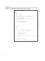
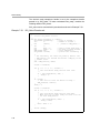
Here is a sample program listing:
Void copy(HST_Obj *input, HST_Obj *output)
{
PIP_Obj
*in, *out;
Uns
*src, *dst;
Uns
size;
}
iii
Related Documentation From Texas Instruments
❏
Square brackets ( [ and ] ) identify an optional parameter. If you use an
optional parameter, you specify the information within the brackets.
Unless the square brackets are in a bold typeface, do not enter the
brackets themselves.
❏
Throughout this manual, 54 can represent the two-digit numeric
appropriate to your specific DSP platform. If your DSP platform is C62x
based, substitute 62 each time you see the designation 54. For example,
DSP/BIOS assembly language API header files for the C6000 platform
will have a suffix of .h62. For the C2800 platform, the suffix will be .h28.
For a C64x, C55x, or C28x DSP platform, substitute 64, 55, or 28 for
each occurrence of 54. Also, each reference to Code Composer Studio
C5000 can be substituted with Code Composer Studio C6000 depending
on your DSP platform.
❏
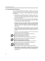
Information specific to a particular device is designated with one of the
following icons:
Related Documentation From Texas Instruments
The following books describe TMS320 devices and related support tools. To
obtain a copy of any of these TI documents, call the Texas Instruments
Literature Response Center at (800) 477-8924. When ordering, please
identify the book by its title and literature number.
TMS320C6000 DSP/BIOS Application Programming Interface (API)
Reference Guide (literature number SPRU403) describes the DSP/BIOS API
functions, which are alphabetized by name. The API Reference Guide is the
companion to this user’s guide.
TMS320C5000 DSP/BIOS Application Programming Interface (API) Reference Guide (literature number SPRU404) describes the DSP/BIOS API functions, which are alphabetized by name. The API Reference Guide is the companion to this user’s guide.
TMS320C28x DSP/BIOS Application Programming Interface (API) Reference
Guide (literature number SPRU625) describes the DSP/BIOS API functions,
which are alphabetized by name. The API Reference Guide is the companion
to this user’s guide.
DSP/BIOS Driver Developer's Guide (literature number SPRU616) describes
the IOM model for device driver development and integration into DSP/BIOS
applications.
iv
Related Documentation From Texas Instruments
TMS320C54x Assembly Language Tools User’s Guide (literature number
SPRU102) describes the assembly language tools (assembler, linker, and
other tools used to develop assembly language code), assembler directives,
macros, common object file format, and symbolic debugging directives for the
C5000 generation of devices.
TMS320C55x Assembly Language Tools User’s Guide (literature number
SPRU280) describes the assembly language tools (assembler, linker, and
other tools used to develop assembly language code), assembler directives,
macros, common object file format, and symbolic debugging directives for the
C5000 generation of devices.
TMS320C6000 Assembly Language Tools User's Guide (literature number
SPRU186) describes the assembly language tools (assembler, linker, and
other tools used to develop assembly language code), assembler directives,
macros, common object file format, and symbolic debugging directives for the
C5000 generation of devices.
TMS320C2000 Assembly Language Tools User's Guide (literature number
SPRU513) describes the assembly language tools (assembler, linker, and
other tools used to develop assembly language code), assembler directives,
macros, common object file format, and symbolic debugging directives for the
C2000 generation of devices.
TMS320C54x Optimizing C Compiler User’s Guide (literature number
SPRU103) describes the C54x C compiler. This C compiler accepts ANSI
standard C source code and produces TMS320 assembly language source
code for the C54x generation of devices.
TMS320C55x Optimizing C Compiler User’s Guide (literature number
SPRU281) describes the C55x C compiler. This C compiler accepts ANSI
standard C source code and produces TMS320 assembly language source
code for the C55x generation of devices.
TMS320C6000 Optimizing C Compiler User's Guide (literature number
SPRU187) describes the C6000 C/C++ compiler and the assembly optimizer.
This C/C++ compiler accepts ANSI standard C/C++ source code and produces assembly language source code for the C6000 generation of devices. The
assembly optimizer helps you optimize your assembly code.
TMS320C2000 Optimizing C/C++ Compiler User's Guide (literature number
SPRU514) describes the C2000 C/C++ compiler and the assembly optimizer.
This C/C++ compiler accepts ANSI standard C/C++ source code and produces assembly language source code for the C2000 generation of devices. The
assembly optimizer helps you optimize your assembly code.
Read This First
v
Related Documentation From Texas Instruments
TMS320C55x Programmer's Guide (literature number SPRU376) describes
ways to optimize C and assembly code for the TMS320C55x DSPs and
includes application program examples.
TMS320C6000 Programmer's Guide (literature number SPRU189) describes
the C6000 CPU architecture, instruction set, pipeline, and interrupts for these
digital signal processors.
TMS320C54x DSP Reference Set, Volume 1: CPU and Peripherals (literature
number SPRU131) describes the TMS320C54x 16-bit fixed-point generalpurpose digital signal processors. Covered are its architecture, internal register
structure, data and program addressing, the instruction pipeline, and on-chip
peripherals. Also includes development support information, parts lists, and
design considerations for using the XDS510 emulator.
TMS320C54x DSP Enhanced Peripherals Ref Set, Vol 5 (literature number
SPRU302) describes the enhanced peripherals available on the
TMS320C54x digital signal processors. Includes the multi channel buffered
serial ports (McBSPs), direct memory access (DMA) controller, interprocesor
communications, and the HPI-8 and HPI-16 host port interfaces.
TMS320C54x DSP Mnemonic Instruction Set Reference Set Volume 2
(literature number SPRU172) describes the TMS320C54x digital signal
processor mnemonic instructions individually. Also includes a summary of
instruction set classes and cycles.
TMS320C54x DSP Reference Set, Volume 3: Algebraic Instruction Set
(literature number SPRU179) describes the TMS320C54x digital signal
processor algebraic instructions individually. Also includes a summary of
instruction set classes and cycles.
TMS320C6000 Peripherals Reference Guide (literature number SPRU190)
describes common peripherals available on the TMS320C6000 family of
digital signal processors. This book includes information on the internal data
and program memories, the external memory interface (EMIF), the host port,
multichannel buffered serial ports, direct memory access (DMA), clocking and
phase-locked loop (PLL), and the power-down modes.
TMS320C54x Code Composer Studio Tutorial Online Help (literature number
SPRH134) introduces the Code Composer Studio integrated development
environment and software tools. Of special interest to DSP/BIOS users are
the Using DSP/BIOS lessons.
vi
Related Documentation
TMS320C55x Code Composer Studio Tutorial Online Help (literature number
SPRH097) introduces the Code Composer Studio integrated development
environment and software tools. Of special interest to DSP/BIOS users are
the Using DSP/BIOS lessons.
TMS320C6000 Code Composer Studio Tutorial Online Help (literature number
SPRH125) introduces the Code Composer Studio integrated development
environment and software tools. Of special interest to DSP/BIOS users are
the Using DSP/BIOS lessons.
Code Composer Studio Application Program Interface (API) Reference
Guide (literature number SPRU321) describes the Code Composer Studio
application programming interface, which allows you to program custom
analysis tools for Code Composer Studio.
DSP/BIOS and TMS320C54x Extended Addressing (literature number
SPRA599) provides basic run-time services including real-time analysis functions for instrumenting an application, clock and periodic functions, I/O modules, and a preemptive scheduler. It also describes the far model for extended
addressing, which is available on the TMS320C54x platform.
TMS320C6000 Chip Support LIbrary API Reference Guide (literature number
SPRU401) contains a reference for the Chip Support Library (CSL) application
programming interfaces (APIs). The CSL is a set of APIs used to configure
and control all on-chip peripherals.
TMS320C28x DSP CPU and Instruction Reference Guide (literature number
SPRU430).
Related Documentation
You can use the following books to supplement this reference guide:
The C Programming Language (second edition), by Brian W. Kernighan
and Dennis M. Ritchie, published by Prentice-Hall, Englewood Cliffs, New
Jersey, 1988
Programming in C, Kochan, Steve G., Hayden Book Company
Programming Embedded Systems in C and C++, by Michael Barr, Andy
Oram (Editor), published by O'Reilly & Associates; ISBN: 1565923545,
February 1999
Real-Time Systems, by Jane W. S. Liu, published by Prentice Hall; ISBN:
013099651, June 2000
Read This First
vii
Trademarks
Principles of Concurrent and Distributed Programming (Prentice Hall
International Series in Computer Science), by M. Ben-Ari, published by
Prentice Hall; ISBN: 013711821X, May 1990
American National Standard for Information Systems-Programming
Language C X3.159-1989, American National Standards Institute (ANSI
standard for C); (out of print)
Trademarks
MS-DOS, Windows, and Windows NT are trademarks of Microsoft
Corporation.
The Texas Instruments logo and Texas Instruments are registered
trademarks of Texas Instruments. Trademarks of Texas Instruments include:
TI, XDS, Code Composer, Code Composer Studio, Probe Point, Code
Explorer, DSP/BIOS, RTDX, Online DSP Lab, BIOSuite, SPOX, TMS320,
TMS320C54x, TMS320C55x, TMS320C62x, TMS320C64x, TMS320C67x,
TMS320C28x, TMS320C5000, TMS320C6000 and TMS320C2000.
All other brand or product names are trademarks or registered trademarks of
their respective companies or organizations.
viii
Contents
1
About DSP/BIOS . . . . . . . . . . . . . . . . . . . . . . . . . . . . . . . . . . . . . . . . . . . . . . . . . . . . . . . . . . .1-1
DSP/BIOS is a scalable real-time kernel. It is designed for applications that require real-time
scheduling and synchronization, host-to-target communication, or real-time instrumentation. DSP/
BIOS provides preemptive multi-threading, hardware abstraction, real-time analysis, and configuration tools.
1.1
DSP/BIOS Features and Benefits . . . . . . . . . . . . . . . . . . . . . . . . . . . . . . . . . . . . . . . . .1-2
1.2
DSP/BIOS Components . . . . . . . . . . . . . . . . . . . . . . . . . . . . . . . . . . . . . . . . . . . . . . . . .1-4
1.3
Naming Conventions . . . . . . . . . . . . . . . . . . . . . . . . . . . . . . . . . . . . . . . . . . . . . . . . . .1-10
1.4
For More Information . . . . . . . . . . . . . . . . . . . . . . . . . . . . . . . . . . . . . . . . . . . . . . . . . .1-16
2
Program Generation . . . . . . . . . . . . . . . . . . . . . . . . . . . . . . . . . . . . . . . . . . . . . . . . . . . . . . . .2-1
This chapter describes the process of generating programs with DSP/BIOS. It also explains which
files are generated by DSP/BIOS components and how they are used.
2.1
Development Cycle . . . . . . . . . . . . . . . . . . . . . . . . . . . . . . . . . . . . . . . . . . . . . . . . . . . .2-2
2.2
Using the Configuration Tool . . . . . . . . . . . . . . . . . . . . . . . . . . . . . . . . . . . . . . . . . . . . .2-3
2.3
Files Used to Create DSP/BIOS Programs . . . . . . . . . . . . . . . . . . . . . . . . . . . . . . . . .2-12
2.4
Compiling and Linking Programs . . . . . . . . . . . . . . . . . . . . . . . . . . . . . . . . . . . . . . . . .2-14
2.5
Using DSP/BIOS with the Run-Time Support Library. . . . . . . . . . . . . . . . . . . . . . . . . .2-18
2.6
DSP/BIOS Startup Sequence. . . . . . . . . . . . . . . . . . . . . . . . . . . . . . . . . . . . . . . . . . . .2-20
2.7
Using C++ with DSP/BIOS . . . . . . . . . . . . . . . . . . . . . . . . . . . . . . . . . . . . . . . . . . . . . .2-24
2.8
User Functions Called by DSP/BIOS . . . . . . . . . . . . . . . . . . . . . . . . . . . . . . . . . . . . . .2-27
2.9
Calling DSP/BIOS APIs from Main . . . . . . . . . . . . . . . . . . . . . . . . . . . . . . . . . . . . . . . .2-28
3
Instrumentation . . . . . . . . . . . . . . . . . . . . . . . . . . . . . . . . . . . . . . . . . . . . . . . . . . . . . . . . . . . .3-1
DSP/BIOS provides both explicit and implicit ways to perform real-time program analysis. These
mechanisms are designed to have minimal impact on the application’s real-time performance.
3.1
Real-Time Analysis. . . . . . . . . . . . . . . . . . . . . . . . . . . . . . . . . . . . . . . . . . . . . . . . . . . . .3-2
3.2
Instrumentation Performance . . . . . . . . . . . . . . . . . . . . . . . . . . . . . . . . . . . . . . . . . . . . .3-4
3.3
Instrumentation APIs . . . . . . . . . . . . . . . . . . . . . . . . . . . . . . . . . . . . . . . . . . . . . . . . . . .3-7
3.4
Implicit DSP/BIOS Instrumentation. . . . . . . . . . . . . . . . . . . . . . . . . . . . . . . . . . . . . . . .3-19
3.5
Kernel/Object View Debugger . . . . . . . . . . . . . . . . . . . . . . . . . . . . . . . . . . . . . . . . . . .3-29
3.6
Instrumentation for Field Testing . . . . . . . . . . . . . . . . . . . . . . . . . . . . . . . . . . . . . . . . .3-38
3.7
Real-Time Data Exchange . . . . . . . . . . . . . . . . . . . . . . . . . . . . . . . . . . . . . . . . . . . . . .3-38
ix
Contents
4
Thread Scheduling . . . . . . . . . . . . . . . . . . . . . . . . . . . . . . . . . . . . . . . . . . . . . . . . . . . . . . . . . 4-1
This chapter describes the types of threads a DSP/BIOS program can use, their behavior, and
their priorities during program execution.
4.1
Overview of Thread Scheduling . . . . . . . . . . . . . . . . . . . . . . . . . . . . . . . . . . . . . . . . . . 4-2
4.2
Hardware Interrupts . . . . . . . . . . . . . . . . . . . . . . . . . . . . . . . . . . . . . . . . . . . . . . . . . . 4-11
4.3
Software Interrupts . . . . . . . . . . . . . . . . . . . . . . . . . . . . . . . . . . . . . . . . . . . . . . . . . . . 4-26
4.4
Tasks. . . . . . . . . . . . . . . . . . . . . . . . . . . . . . . . . . . . . . . . . . . . . . . . . . . . . . . . . . . . . . 4-40
4.5
The Idle Loop . . . . . . . . . . . . . . . . . . . . . . . . . . . . . . . . . . . . . . . . . . . . . . . . . . . . . . . 4-53
4.6
Semaphores . . . . . . . . . . . . . . . . . . . . . . . . . . . . . . . . . . . . . . . . . . . . . . . . . . . . . . . . 4-55
4.7
Mailboxes . . . . . . . . . . . . . . . . . . . . . . . . . . . . . . . . . . . . . . . . . . . . . . . . . . . . . . . . . . 4-61
4.8
Timers, Interrupts, and the System Clock . . . . . . . . . . . . . . . . . . . . . . . . . . . . . . . . . . 4-67
4.9
Periodic Function Manager (PRD) and the System Clock . . . . . . . . . . . . . . . . . . . . . 4-74
4.10 Using the Execution Graph to View Program Execution . . . . . . . . . . . . . . . . . . . . . . . 4-78
5
Memory and Low-level Functions . . . . . . . . . . . . . . . . . . . . . . . . . . . . . . . . . . . . . . . . . . . . 5-1
This chapter describes the low-level functions found in the DSP/BIOS real-time multitasking kernel. These functions are embodied in three software modules: MEM, which manages allocation of
memory; SYS, which provides miscellaneous system services; and QUE, which manages
queues.
5.1
Memory Management . . . . . . . . . . . . . . . . . . . . . . . . . . . . . . . . . . . . . . . . . . . . . . . . . . 5-2
5.2
System Services . . . . . . . . . . . . . . . . . . . . . . . . . . . . . . . . . . . . . . . . . . . . . . . . . . . . . 5-11
5.3
Queues . . . . . . . . . . . . . . . . . . . . . . . . . . . . . . . . . . . . . . . . . . . . . . . . . . . . . . . . . . . . 5-14
6
Input/Output Overview and Pipes . . . . . . . . . . . . . . . . . . . . . . . . . . . . . . . . . . . . . . . . . . . . . 6-1
This chapter provides an overview on data transfer methods, and discusses pipes in particular.
6.1
I/O Overview . . . . . . . . . . . . . . . . . . . . . . . . . . . . . . . . . . . . . . . . . . . . . . . . . . . . . . . . . 6-2
6.2
Comparing Pipes and Streams . . . . . . . . . . . . . . . . . . . . . . . . . . . . . . . . . . . . . . . . . . . 6-5
6.3
Data Pipe Manager (PIP Module) . . . . . . . . . . . . . . . . . . . . . . . . . . . . . . . . . . . . . . . . . 6-6
6.4
Host Channel Manager (HST Module) . . . . . . . . . . . . . . . . . . . . . . . . . . . . . . . . . . . . 6-13
6.5
I/O Performance Issues . . . . . . . . . . . . . . . . . . . . . . . . . . . . . . . . . . . . . . . . . . . . . . . 6-15
7
Streaming I/O and Device Drivers . . . . . . . . . . . . . . . . . . . . . . . . . . . . . . . . . . . . . . . . . . . . 7-1
This chapter describes issues relating to writing and using device drivers, and gives several programming examples.
7.1
Overview of Streaming I/O and Device Drivers. . . . . . . . . . . . . . . . . . . . . . . . . . . . . . . 7-2
7.2
Creating and Deleting Streams . . . . . . . . . . . . . . . . . . . . . . . . . . . . . . . . . . . . . . . . . . . 7-5
7.3
Stream I/O—Reading and Writing Streams . . . . . . . . . . . . . . . . . . . . . . . . . . . . . . . . . 7-7
7.4
Stackable Devices. . . . . . . . . . . . . . . . . . . . . . . . . . . . . . . . . . . . . . . . . . . . . . . . . . . . 7-16
7.5
Controlling Streams. . . . . . . . . . . . . . . . . . . . . . . . . . . . . . . . . . . . . . . . . . . . . . . . . . . 7-23
7.6
Selecting Among Multiple Streams . . . . . . . . . . . . . . . . . . . . . . . . . . . . . . . . . . . . . . . 7-24
7.7
Streaming Data to Multiple Clients . . . . . . . . . . . . . . . . . . . . . . . . . . . . . . . . . . . . . . . 7-25
7.8
Streaming Data Between Target and Host . . . . . . . . . . . . . . . . . . . . . . . . . . . . . . . . . 7-27
7.9
Device Driver Template. . . . . . . . . . . . . . . . . . . . . . . . . . . . . . . . . . . . . . . . . . . . . . . . 7-28
7.10 Streaming DEV Structures . . . . . . . . . . . . . . . . . . . . . . . . . . . . . . . . . . . . . . . . . . . . . 7-30
7.11 Device Driver Initialization . . . . . . . . . . . . . . . . . . . . . . . . . . . . . . . . . . . . . . . . . . . . . . 7-33
7.12 Opening Devices . . . . . . . . . . . . . . . . . . . . . . . . . . . . . . . . . . . . . . . . . . . . . . . . . . . . . 7-34
x
Contents
7.13
7.14
7.15
7.16
7.17
Real-Time I/O . . . . . . . . . . . . . . . . . . . . . . . . . . . . . . . . . . . . . . . . . . . . . . . . . . . . . . . .7-38
Closing Devices . . . . . . . . . . . . . . . . . . . . . . . . . . . . . . . . . . . . . . . . . . . . . . . . . . . . . .7-41
Device Control . . . . . . . . . . . . . . . . . . . . . . . . . . . . . . . . . . . . . . . . . . . . . . . . . . . . . . .7-43
Device Ready . . . . . . . . . . . . . . . . . . . . . . . . . . . . . . . . . . . . . . . . . . . . . . . . . . . . . . . .7-43
Types of Devices . . . . . . . . . . . . . . . . . . . . . . . . . . . . . . . . . . . . . . . . . . . . . . . . . . . . .7-46
Contents
xi
Figures
Figures
1-1
1-2
1-3
1-4
1-5
2-1
2-2
2-3
2-4
3-1
3-2
3-3
3-4
3-5
3-6
3-7
3-8
3-9
3-10
3-11
3-12
3-13
3-14
3-15
3-16
3-17
3-18
3-19
3-20
3-21
xii
DSP/BIOS Components .................................................................................................1-4
Configuration Tool Interface.............................................................................................1-7
The DSP/BIOS Menu ......................................................................................................1-8
Code Composer Studio Analysis Tool Panels ................................................................1-9
DSP/BIOS Analysis Tools Toolbar ...................................................................................1-9
Configuration Tool Hierarchy and Ordered Collection Views...........................................2-6
DSP/BIOS Program Creation Files................................................................................2-12
Sample Code Composer Project Files List....................................................................2-14
MEM Module Properties Panel .....................................................................................2-15
Message Log Dialog Box.................................................................................................3-8
LOG Buffer Sequence ....................................................................................................3-9
RTA Control Panel Properties Dialog Box. ....................................................................3-10
Statistics View Panel .................................................................................................... 3-11
Target/Host Variable Accumulation................................................................................3-12
Current Value Deltas From One STS_set......................................................................3-14
Current Value Deltas from Base Value ..........................................................................3-15
RTA Control Panel Dialog Box.......................................................................................3-18
Execution Graph Window .............................................................................................3-19
CPU Load Graph Window ............................................................................................3-21
Monitoring Stack Pointers (C5000 platform)..................................................................3-23
Monitoring Stack Pointers (C6000 platform) .................................................................3-24
Calculating Used Stack Depth.......................................................................................3-25
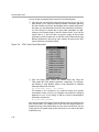
Selecting The Kernel/Object View Debugger.................................................................3-29
The Disabled Message ..................................................................................................3-30
The Kernel Page Dialog Box .........................................................................................3-30
The Task Page Dialog Box ............................................................................................3-31
The Mailboxes Page Dialog Box ...................................................................................3-32
Viewing a List of Tasks Currently Blocked .....................................................................3-33
The Semaphores Page Dialog Box ...............................................................................3-34
Viewing a List of Tasks Pending ....................................................................................3-35
Figures
3-22
3-23
3-24
4-1
4-2
4-3
4-4
4-5
4-6
4-7
4-8
4-9
4-10
4-11
4-12
4-13
4-14
4-15
4-16
4-17
4-18
4-19
4-20
4-21
4-22
4-23
5-1
5-2
5-3
6-1
6-2
6-3
6-4
7-1
7-2
7-3
7-4
7-5
7-6
The Memory Page Dialog Box ...................................................................................... 3-35
The Software Interrupts Page Dialog Box..................................................................... 3-36
RTDX Data Flow between Host and Target .................................................................. 3-40
Thread Priorities.............................................................................................................. 4-7
Preemption Scenario .................................................................................................... 4-10
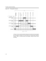
The Interrupt Sequence in Debug Halt State ................................................................ 4-15
The Interrupt Sequence in the Run-time State ............................................................. 4-17
Software Interrupt Manager .......................................................................................... 4-28
SWI Properties Dialog Box ........................................................................................... 4-29
Using SWI_inc to Post an SWI ..................................................................................... 4-33
Using SWI_andn to Post an SWI .................................................................................. 4-34
Using SWI_or to Post an SWI....................................................................................... 4-35
Using SWI_dec to Post an SWI .................................................................................... 4-36
Right Side of Task Manager Display ............................................................................ 4-43
TSK Properties Dialog Box ........................................................................................... 4-44
Execution Mode Variations .......................................................................................... 4-45
Trace Window Results from Example 4-8 .................................................................... 4-52
Execution Graph for Example 4-8................................................................................. 4-52
Trace Window Results from Example 4-12 .................................................................. 4-60
Trace Window Results from Example 4-16 .................................................................. 4-65
Interactions Between Two Timing Methods .................................................................. 4-67
CLK Manager Properties Dialog Box ............................................................................ 4-68
Trace Log Output from Example 4-17........................................................................... 4-73
Using Statistics View for a PRD Object ........................................................................ 4-77
The Execution Graph Window ...................................................................................... 4-78
RTA Control Panel Dialog Box ...................................................................................... 4-80
Allocating Memory Segments of Different Sizes ............................................................ 5-7
Memory Allocation Trace Window................................................................................. 5-10
Trace Window Results from Example 5-18 .................................................................. 5-18
Input/Output Stream ....................................................................................................... 6-2
Interaction Between Streams and Devices ..................................................................... 6-3
The Two Ends of a Pipe ................................................................................................. 6-6
Binding Channels.......................................................................................................... 6-13
Device-Independent I/O in DSP/BIOS ........................................................................... 7-2
Device, Driver, and Stream Relationship ........................................................................ 7-4
How SIO_get Works ...................................................................................................... 7-9
Output Trace for Example 7-5....................................................................................... 7-12
Results Window for Example 7-6.................................................................................. 7-14
The Flow of Empty and Full Frames ............................................................................ 7-17
Contents
xiii
Figures
7-7
7-8
7-9
7-10
7-11
7-12
7-13
7-14
7-15
xiv
inStreamSrc Properties Dialog Box ...............................................................................7-18
Sine Wave Output for Example 7-9 ...............................................................................7-22
Flow of DEV_STANDARD Streaming Model ................................................................7-38
Placing a Data Buffer to a Stream .................................................................................7-39
Retrieving Buffers from a Stream ..................................................................................7-39
Stacking and Terminating Devices ................................................................................7-46
Buffer Flow in a Terminating Device ..............................................................................7-47
In-Place Stacking Driver ...............................................................................................7-47
Copying Stacking Driver Flow .......................................................................................7-48
Tables
Tables
1-1
1-2
1-3
1-4
2-1
2-2
2-3
3-1
3-2
3-3
3-4
4-1
4-2
4-3
4-4
7-1
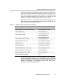
DSP/BIOS Modules ........................................................................................................ 1-5
DSP/BIOS Standard Data Types: ................................................................................. 1-12
Memory Segment Names ............................................................................................. 1-13
Standard Memory Segments ........................................................................................ 1-15
Methods of Referencing C6000 Global Objects.............................................................. 2-8
Files Not Included in rtsbios.......................................................................................... 2-18
Stack Modes on the C5500 Platform ............................................................................ 2-23
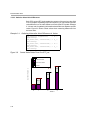
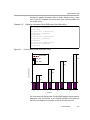
Examples of Code-size Increases Due to an Instrumented Kernel ................................ 3-6
TRC Constants: ............................................................................................................ 3-17
Variables that can be Monitored with HWI .................................................................... 3-26
STS Operations and Their Results ............................................................................... 3-27
Comparison of Thread Characteristics ........................................................................... 4-5
Thread Preemption ......................................................................................................... 4-9
SWI Object Function Differences ................................................................................. 4-32
CPU Registers Saved During Software Interrupt.......................................................... 4-37
Generic I/O to Internal Driver Operations ....................................................................... 7-3
Contents
xv
Examples
Examples
2-1
2-2
2-3
2-4
2-5
2-6
3-1
3-2
3-3
4-1
4-2
4-3
4-4
4-5
4-6
4-7
4-8
4-9
4-10
4-11
4-12
4-13
4-14
4-15
4-16
4-17
5-1
5-2
5-3
5-4
xvi
Creating and Referencing Dynamic Objects ................................................................ 2-11
Deleting a Dynamic Object .......................................................................................... 2-11
Sample Makefile for a DSP/BIOS Program .................................................................. 2-17
Declaring Functions in an Extern C Block .................................................................... 2-25
Function Overloading Limitation ................................................................................... 2-25
Wrapper Function for a Class Method.......................................................................... 2-26
Gathering Information About Differences in Values ..................................................... 3-14
Gathering Information About Differences from Base Value.......................................... 3-15
The Idle Loop................................................................................................................ 3-22
Interrupt Behavior for C28x During Real-Time Mode ................................................... 4-14
Code Regions That are Uninterruptible ........................................................................ 4-18
Constructing a Minimal ISR on C6000 Platform .......................................................... 4-24
HWI Example on C54x Platform ................................................................................. 4-24
HWI Example on C55x Platform .................................................................................. 4-25
HWI Example on C28x Platform .................................................................................. 4-25
Creating a Task Object ................................................................................................. 4-49
Time-Slice Scheduling .................................................................................................. 4-50
Creating and Deleting a Semaphore ............................................................................ 4-55
Setting a Timeout with SEM_pend ............................................................................... 4-56
Signaling a Semaphore with SEM_post ....................................................................... 4-56
SEM Example Using Three Writer Tasks ..................................................................... 4-57
Creating a Mailbox........................................................................................................ 4-61
Reading a Message from a Mailbox ............................................................................. 4-61
Posting a Message to a Mailbox................................................................................... 4-62
MBX Example With Two Types of Tasks ..................................................................... 4-63
Using the System Clock to Drive a Task ...................................................................... 4-72
Linker Command File (C6000 Platform) ......................................................................... 5-4
Linker Command File (C5000 and C28x Platforms) ....................................................... 5-4
Using MEM_alloc for System-Level Storage .................................................................. 5-5
Allocating an Array of Structures .................................................................................... 5-5
Examples
5-5
5-6
5-7
5-8
5-9
5-10
5-11
5-12
5-13
5-14
5-15
5-16
5-17
5-18
7-1
7-2
7-3
7-4
7-5
7-6
7-7
7-8
7-9
7-10
7-11
7-12
7-13
7-14
7-15
7-16
7-17
7-18
7-19
7-20
7-21
7-22
7-23
7-24
7-25
Using MEM_free to Free Memory .................................................................................. 5-6
Freeing an Array of Objects ........................................................................................... 5-6
Memory Allocation (C5000 and C28x Platforms)........................................................... 5-8
Memory Allocation (C6000 Platform) ............................................................................. 5-9
Coding To Halt Program Execution with SYS_exit or SYS_abort................................ 5-11
Using SYS_abort with Optional Data Values ............................................................... 5-12
Using Handlers in SYS_exit......................................................................................... 5-12
Using Multiple SYS_NUMHANDLERS ....................................................................... 5-12
DSP/BIOS Error Handling ........................................................................................... 5-13
Using doError to Print Error Information ...................................................................... 5-13
Managing QUE Elements Using Queues..................................................................... 5-14
Inserting into a Queue Atomically ................................................................................ 5-14
Using QUE Functions with Mutual Exclusion Elements ............................................... 5-15
Using QUE to Send Messages ................................................................................... 5-16
Creating a Stream with SIO_create ............................................................................... 7-5
Freeing User-Held Stream Buffers................................................................................. 7-6
Inputting and Outputting Data Buffers............................................................................ 7-7
Implementing the Issue/Reclaim Streaming Model ....................................................... 7-8
Basic SIO Functions .................................................................................................... 7-10
Adding an Output Stream to Example 7-5 ................................................................... 7-13
Using the Issue/Reclaim Model ................................................................................... 7-15
Opening a Pair of Virtual Devices ................................................................................ 7-16
Data Exchange Through a Pipe Device....................................................................... 7-20
Using SIO_ctrl to Communicate with a Device ............................................................ 7-23
Changing Sample Rate................................................................................................ 7-23
Synchronizing with a Device ....................................................................................... 7-23
Indicating That a Stream is Ready............................................................................... 7-24
Polling Two Streams .................................................................................................... 7-24
Using SIO_put to Send Data to Multiple Clients .......................................................... 7-25
Using SIO_issue/SIO_reclaim to Send Data to Multiple Clients .................................. 7-26
Required Statements in dxx.h Header File .................................................................. 7-29
Table of Device Functions ........................................................................................... 7-29
The DEV_Fxns Structure ............................................................................................. 7-30
The DEV_Frame Structure .......................................................................................... 7-30
The DEV_Handle Structure ......................................................................................... 7-31
Initialization by Dxx_init................................................................................................ 7-33
Opening a Device with Dxx_open................................................................................ 7-34
Opening an Input Terminating Device ......................................................................... 7-34
Arguments to Dxx_open .............................................................................................. 7-34
Contents
xvii
Examples
7-26
7-27
7-28
7-29
7-30
7-31
7-32
7-33
xviii
The Parameters of SIO_create.....................................................................................
The Dxx_Obj Structure .................................................................................................
Typical Features for a Terminating Device ...................................................................
Template for Dxx_issue for a Typical Terminating Device ...........................................
Template for Dxx_reclaim for a Typical Terminating Device ........................................
Closing a Device ..........................................................................................................
Making a Device Ready ...............................................................................................
SIO_Select Pseudocode .............................................................................................
7-35
7-35
7-36
7-40
7-40
7-41
7-43
7-44
Chapter 1
About DSP/BIOS
DSP/BIOS is a scalable real-time kernel. It is designed for applications that
require real-time scheduling and synchronization, host-to-target
communication, or real-time instrumentation. DSP/BIOS provides preemptive
multi-threading, hardware abstraction, real-time analysis, and configuration
tools.
Topic
Page
1.1
DSP/BIOS Features and Benefits . . . . . . . . . . . . . . . . . . . . . . . . . . . . 1-2
1.2
DSP/BIOS Components . . . . . . . . . . . . . . . . . . . . . . . . . . . . . . . . . . . . 1-4
1.3
Naming Conventions . . . . . . . . . . . . . . . . . . . . . . . . . . . . . . . . . . . . . 1-10
1.4
For More Information . . . . . . . . . . . . . . . . . . . . . . . . . . . . . . . . . . . . . 1-16
1-1
DSP/BIOS Features and Benefits
1.1 DSP/BIOS Features and Benefits
DSP/BIOS and its Analysis Tool for Code Composer Studio software are
designed to minimize memory and CPU requirements on the target. This
design goal is accomplished in the following ways:
❏
All DSP/BIOS objects can be created in the Configuration Tool and bound
into an executable program image. This reduces code size and optimizes
internal data structures.
❏
Instrumentation data (such as logs and traces) are formatted on the host.
❏
The APIs are modularized so that only those APIs that are used by the
program need to be bound into the executable program.
❏
The library is optimized to require the smallest possible number of
instruction cycles, with a significant portion implemented in assembly
language.
❏
Communication between the target and the DSP/BIOS Analysis Tools is
performed within the background idle loop. This ensures that the
DSP/BIOS Analysis Tools do not interfere with the program’s tasks. If the
target CPU is too busy to perform background tasks, the DSP/BIOS
Analysis Tools stop receiving information from the target until the CPU is
available.
❏
Error checking that would increase memory and CPU requirements has
been kept to a minimum. Instead, the API reference documentation
specifies constraints for calling API functions. It is the responsibility of the
application developer to meet these constraints.
In addition, the DSP/BIOS API provides many options for program
development:
1-2
❏
A program can dynamically create and delete objects that are used in
special situations. The same program can use both objects created
dynamically and objects created with the Configuration Tool.
❏
The threading model provides thread types for a variety of situations.
Hardware interrupts, software interrupts, tasks, idle functions, and
periodic functions are all supported. You can control the priorities and
blocking characteristics of threads through your choice of thread types.
❏
Structures to support communication and synchronization between
threads are provided. These include semaphores, mailboxes, and
resource locks.
❏
Two I/O models are supported for maximum flexibility and power. Pipes
are used for target/host communication and to support simple cases in
which one thread writes to the pipe and another reads from the pipe.
Streams are used for more complex I/O and to support device drivers.
DSP/BIOS Features and Benefits
❏
Low-level system primitives are provided to make it easier to handle
errors, create common data structures, and manage memory usage.
❏
The Chip Support Library (CSL) is a component of DSP/BIOS and can be
used within a DSP/BIOS application.
The DSP/BIOS API standardizes DSP programming for a number of TI
devices and provides easy-to-use powerful program development tools.
These tools reduce the time required to create DSP programs in the following
ways:
❏
The Configuration Tool generates code required to declare objects used
within the program.
❏
The Configuration Tool detects errors earlier by validation properties
before the program is even built.
❏
Logging and statistics for DSP/BIOS objects are available at run-time
without additional programming. Additional instrumentation can be
programmed as needed.
❏
The DSP/BIOS Analysis Tools allow real-time monitoring of program
behavior.
❏
DSP/BIOS provides a standard API. This allows DSP algorithm
developers to provide code that can be more easily integrated with other
program functions.
❏
DSP/BIOS is integrated within the Code Composer Studio IDE, requires
no runtime license fees, and is fully supported by Texas Instruments.
DSP/BIOS is a key a component of TI's eXpressDSPTM real-time
software technology.
❏
The Chip Support Library (CSL) provides an easier method of device
programming than traditional register programming. When you use CSL
APIs, portability between different DSP platforms with equivalent
peripheral devices is simpler and more efficient.
About DSP/BIOS
1-3
DSP/BIOS Components
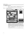
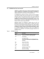
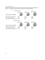
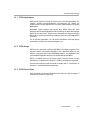
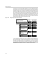
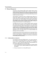
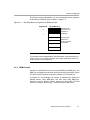
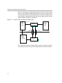
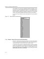
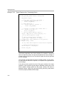
1.2 DSP/BIOS Components
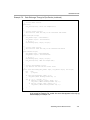
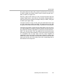
Figure 1-1 shows the components of DSP/BIOS within the program
generation and debugging environment of Code Composer Studio:
Figure 1-1.
DSP/BIOS Components
Host
Target
Code Composer Studio
source files
.cdb
(Config
database)
cfg.cmd
cfg.s54
cfg.h54
cfg_c.c
cfg.h
OLE
application
using RTDX
DSP
Code Composer editor
Configuration
Tool
.c
.h
.asm
DSP/BIOS API
Code Composer project
Code
generation
tools
Compiler,
assembler,
lnker...
RTDX
plug-ins
DSP/BIOS
Analysis
Tools
3rd party
plug-ins
Code Composer debugger
Host emulation support
executable
DSP application program
JTAG
RTDX
DSP/BIOS
Target hardware
On the host PC, you write programs (in C, C++ or assembly) that use the
DSP/BIOS API. The Configuration Tool lets you define objects to be used in
your program. You then compile or assemble and link the program. The
DSP/BIOS Analysis Tools let you test the program on the target device from
Code Composer Studio while monitoring CPU load, timing, logs, thread
execution, and more. (The term thread is used to refer to any thread of
execution, i.e., a hardware interrupt, a software interrupt, a task, an idle
function, or a periodic function.)
The following sections provide a brief overview of the DSP/BIOS components.
1-4
DSP/BIOS Components
1.2.1
DSP/BIOS Real-Time Kernel and API
DSP/BIOS is a scalable real-time kernel, designed for applications that require
real-time scheduling and synchronization, host-to-target communication, or
real-time instrumentation. DSP/BIOS provides preemptive multi-threading,
hardware abstraction, real-time analysis, and configuration tools.
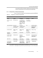
The DSP/BIOS API is divided into modules, however, the CSL is actually a
sub-component of BIOS, with many sub-modules of its own. For simplicity,
references to the CSL in this manual use the term, CSL module. Depending
on what modules are configured and used by the application, the size of
DSP/BIOS can range from about 500 to 6500 words of code. All the
operations within a module begin with the letter codes shown Figure 1-1. For
more information on the CSL, see TMS320C6000 Chip Support LIbrary API
Reference Guide, literature number SPRU401.
Application programs use DSP/BIOS by making calls to the API. All
DSP/BIOS modules provide C-callable interfaces. In addition, some of the
API modules contain optimized assembly language macros. Most C-callable
interfaces can also be called from assembly language, provided that C calling
conventions are followed. Some of the C interfaces are actually C macros
and therefore, cannot be used when called from assembly language. Refer
to the TMS320 DSP/BIOS API Reference Guide for your platform for
descriptions of the applicable C and assembly languages interfaces for all
DSP/BIOS modules.
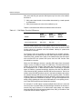
Table 1-1.
DSP/BIOS Modules
Module
Description
ATM
Atomic functions written in assembly language
C54, C55, C62, C64
Target-specific functions, platform dependent
CLK
Clock manager
Chip Support Library;
CSL
For more information, see the TMS320C6000 Chip
Support LIbrary API Reference Guide (literature number
SPRU401)
DEV
Device driver interface
GBL
Global setting manager
HOOK
Hook function manager
HST
Host channel manager
HWI
Hardware interrupt manager
IDL
Idle function manager
LCK
Resource lock manager
About DSP/BIOS
1-5
DSP/BIOS Components
1.2.2
Module
Description
LOG
Event log manager
MBX
Mailbox manager
MEM
Memory segment manager
PIP
Buffered pipe manager
PRD
Periodic function manager
QUE
Atomic queue manager
RTDX
Real-time data exchange settings
SEM
Semaphore manager
SIO
Stream I/O manager
STS
Statistics object manager
SWI
Software interrupt manager
SYS
System services manager
TRC
Trace manager
TSK
Multitasking manager
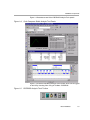
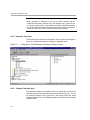
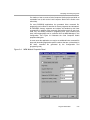
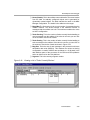
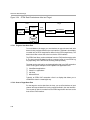
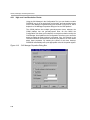
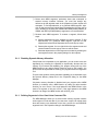
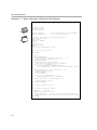
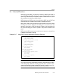
The DSP/BIOS Configuration Tool
The Configuration Tool has an interface similar to the Windows Explorer, and
has multiple roles:
1-6
❏
It lets you set a wide range of parameters used by the DSP/BIOS realtime library at run time.
❏
It serves as a visual editor for creating run-time objects that are used by
the target application’s DSP/BIOS API calls. These objects include
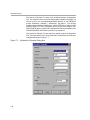
software interrupts, tasks, I/O streams, and event logs. You also use this
visual editor as shown in Figure 1-2 to set properties for these objects.
❏
It lets you set parameters for the Chip Support Library (CSL) and
modules. See the TMS320C6000 Chip Support Library, SPRU401 for
more information.
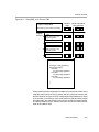
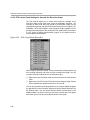
DSP/BIOS Components
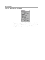
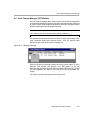
Figure 1-2.
Configuration Tool Interface
Using the Configuration Tool, DSP/BIOS objects can be pre-configured and
bound into an executable program image. Alternately, a DSP/BIOS program
can create and delete objects at run time. In addition to minimizing the target
memory footprint by eliminating run-time code and optimizing internal data
structures, creating static objects with the Configuration Tool detects errors
earlier by validating object properties before program compilation.
The Configuration Tool generates files that link with code you write. See
section 2.2, Using the Configuration Tool, page 2-3, for details.
About DSP/BIOS
1-7
DSP/BIOS Components
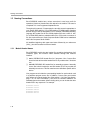
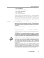
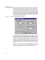
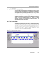
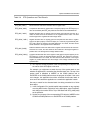
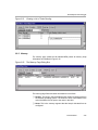
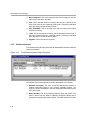
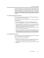
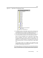
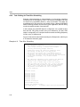
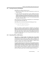
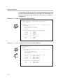
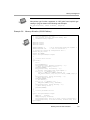
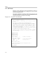
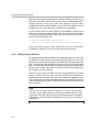
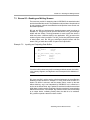
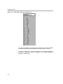
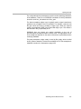
1.2.3
The DSP/BIOS Analysis Tools
The DSP/BIOS Analysis Tools complement the Code Composer Studio
environment by enabling real-time program analysis of a DSP/BIOS
application. You can visually monitor a DSP application as it runs with minimal
impact on the application’s real-time performance. The DSP/BIOS Analysis
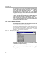
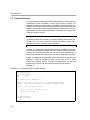
Tools are found on their own menu, as shown in Figure 1-3.
Figure 1-3.
The DSP/BIOS Menu
Unlike traditional debugging, which is external to the executing program,
program analysis requires the target program contain real-time instrumentation
services. By using DSP/BIOS APIs and objects, developers automatically
instrument the target for capturing and uploading real-time information to the
host through the Code Composer Studio DSP/BIOS Analysis Tools.
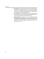
Several broad real-time program analysis capabilities are provided:
❏
Program tracing. Displaying events written to target logs, reflecting
dynamic control flow during program execution
❏
Performance monitoring. Tracking summary statistics that reflect use
of target resources, such as processor load and timing
❏
File streaming. Binding target-resident I/O objects to host files
When used in tandem with the other debugging capabilities of Code
Composer Studio, the DSP/BIOS real-time Analysis Tools provide critical
views into target program behavior during program execution—where
traditional debugging techniques that stop the target offer little insight. Even
after the debugger halts the program, information already captured by the
host with the DSP/BIOS Analysis Tools can provide insight into the sequence
of events that led up to the current point of execution
Later in the software development cycle, when regular debugging techniques
become ineffective for attacking problems arising from time-dependent
interactions, the DSP/BIOS Analysis Tools have an expanded role as the
software counterpart of the hardware logic analyzer.
1-8
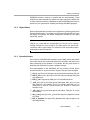
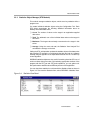
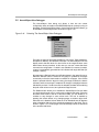
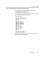
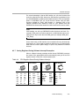
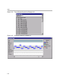
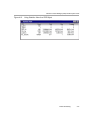
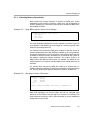
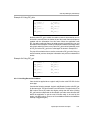
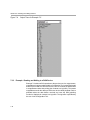
DSP/BIOS Components
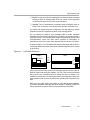
Figure 1-4 illustrates several of the DSP/BIOS Analysis Tools panels.
Figure 1-4.
Code Composer Studio Analysis Tool Panels
Figure 1-5 shows the DSP/BIOS Analysis Tools toolbar, which can be toggled
on and off by choosing View→Plug-in Toolbars→DSP/BIOS.
Figure 1-5.
DSP/BIOS Analysis Tools Toolbar
About DSP/BIOS
1-9
Naming Conventions
1.3 Naming Conventions
Each DSP/BIOS module has a unique name that is used as a prefix for
operations (functions), header files, and objects for the module. This name is
comprised of 3 or more uppercase alphanumerics.
Throughout this manual, 54 represents the two-digit numeric appropriate to
your specific DSP platform. If your DSP platform is C6200 based, substitute
62 each time you see the designation 54. For example, DSP/BIOS assembly
language API header files for the C6000 platform will have a suffix of .h62.
For a C5000 DSP platform, substitute either 54 or 55 for each occurrence of
54. Also, each reference to Code Composer Studio C5000 can be substituted
with Code Composer Studio C6000.
All identifiers beginning with upper-case letters followed by an underscore
(XXX_*) should be treated as reserved words.
1.3.1
Module Header Names
Each DSP/BIOS module has two header files containing declarations of all
constants, types, and functions made available through that module’s
interface.
❏
xxx.h. DSP/BIOS API header files for C programs. Your C source files
should include std.h and the header files for any modules the C functions
use.
❏
xxx.h54. DSP/BIOS API header files for assembly programs. Assembly
source files should include the xxx.h54 header file for any module the
assembly source uses. This file contains macro definitions specific to this
device.
Your program must include the corresponding header for each module used
in a particular program source file. In addition, C source files must include
std.h before any module header files. (See section 1.3.4, Data Type Names,
page 1-12, for more information.) The std.h file contains definitions for
standard types and constants. After including std.h, you can include the other
header files in any sequence. For example:
#include
#include
#include
#include
#include
1-10
<std.h>
<tsk.h>
<sem.h>
<prd.h>
<swi.h>
Naming Conventions
DSP/BIOS includes a number of modules that are used internally. These
modules are undocumented and subject to change at any time. Header files
for these internal modules are distributed as part of DSP/BIOS and must be
present on your system when compiling and linking DSP/BIOS programs.
1.3.2
Object Names
System objects that are included in the configuration by default typically have
names beginning with a 3- or 4-letter code for the module that defines or uses
the object. For example, the default configuration includes a LOG object
called LOG_system.
Note:
Objects you create with the Configuration Tool should use a common
naming convention of your choosing. You might want to use the module
name as a suffix in object names. For example, a TSK object that encodes
data might be called encoderTsk.
1.3.3
Operation Names
The format for a DSP/BIOS API operation name is MOD_action where MOD
is the letter code for the module that contains the operation, and action is the
action performed by the operation. For example, the SWI_post function is
defined by the SWI module; it posts a software interrupt.
This implementation of the DSP/BIOS API also includes several built-in
functions that are run by various built-in objects. Here are some examples:
❏
CLK_F_isr. Run by an HWI object to provide the low-resolution CLK tick.
❏
PRD_F_tick. Run by the PRD_clock CLK object to manage PRD_SWI
and system tick.
❏
PRD_F_swi. Triggered by PRD_tick to run the PRD functions.
❏
_KNL_run. Run by the lowest priority SWI object, KNL_swi, to run the
task scheduler if it is enabled. This is a C function called KNL_run. An
underscore is used as a prefix because the function is called from
assembly code.
❏
_IDL_loop. Run by the lowest priority TSK object, TSK_idle, to run the
IDL functions.
❏
IDL_F_busy. Run by the IDL_cpuLoad IDL object to compute the current
CPU load.
❏
RTA_F_dispatch. Run by the RTA_dispatcher IDL object to gather realtime analysis data.
About DSP/BIOS
1-11
Naming Conventions
❏
LNK_F_dataPump. Run by the LNK_dataPump IDL object to manage
the transfer of real-time analysis and HST channel data to the host.
❏
HWI_unused. Not actually a function name. This string is used in the
Configuration Tool to mark unused HWI objects.
Note:
Your program code should not call any built-in functions whose names
begin with MOD_F_. These functions are intended to be called only as
function parameters specified within the Configuration Tool.
Symbol names beginning with MOD_ and MOD_F_ (where MOD is any letter
code for a DSP/BIOS module) are reserved for internal use.
1.3.4
Data Type Names
The DSP/BIOS API does not explicitly use the fundamental types of C such
as int or char. Instead, to ensure portability to other processors that support
the DSP/BIOS API, DSP/BIOS defines its own standard data types. In most
cases, the standard DSP/BIOS types are uppercase versions of the
corresponding C types.
The data types, shown in Table 1-2, are defined in the std.h header file.
Table 1-2.
DSP/BIOS Standard Data Types:
Type
Description
Arg
Type capable of holding both Ptr and Int arguments
Bool
Boolean value
Char
Character value
Fxn
Pointer to a function
Int
Signed integer value
LgInt
Large signed integer value
LgUns
Large unsigned integer value
Ptr
Generic pointer value
String
Zero-terminated (\0) sequence (array) of characters
Uns
Unsigned integer value
Void
Empty type
Additional data types are defined in std.h, but are not used by DSP/BIOS
APIs.
1-12
Naming Conventions
In addition, the standard constant NULL (0) is used by DSP/BIOS to signify
an empty pointer value. The constants TRUE (1) and FALSE (0) are used for
values of type Bool.
Object structures used by the DSP/BIOS API modules use a naming
convention of MOD_Obj, where MOD is the letter code for the object’s
module. If your program code uses any such objects created by the
Configuration Tool, it should make an extern declaration for the object. For
example:
extern LOG_Obj trace;
The Configuration Tool automatically generates a C header to file that
contains the appropriate declarations for all DSP/BIOS objects created by the
Configuration Tool (<program>.cfg.h. This file can be included by the
application’s source files to accomplish the DSP/BIOS object declarations.
DSP/BIOS for the C54x platform was originally developed for the 16-bit
addressing model of the early C54x devices. Newer C54x devices
incorporate far extended addressing modes, and DSP/BIOS has been
modified to work in this environment. See the Application Report, DSP/BIOS
and TMS320C54x Extended Addressing, SPRA599, for more information.
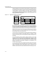
1.3.5
Memory Segment Names
The memory segment names used by DSP/BIOS are described in Table 1-3.
You can change the origin, size, and name of most default memory segments
using the Configuration Tool.
Table 1-3.
Memory Segment Names
a. C54x Platform
Segment
Description
IDATA
Internal (on-device) data memory
EDATA
Primary block of external data memory
EDATA1
Secondary block of external data memory (not contiguous with EDATA)
IPROG
Internal (on-device) program memory
EPROG
Primary block of external program memory
EPROG1
Secondary block of external program memory (not contiguous with EPROG)
USERREGS
Page 0 user memory (28 words)
BIOSREGS
Page 0 reserved registers (4 words)
VECT
Interrupt vector segment
About DSP/BIOS
1-13
Naming Conventions
Table 1.3 Memory Segment Names (continued)
b. C55x Platform
Segment
Description
IDATA
Primary block of data memory
DATA1
Secondary block of data memory (not contiguous with
DATA)
PROG
Program memory
VECT
DSP Interrupt vector table memory segment
c. Memory Segment Names, C6000 EVM Platform
Segment
Description
IPRAM
Internal (on-device) program memory
IDRAM
Internal (on-device) data memory
SBSRAM
External SBSRAM on CE0
SDRAM0
External SDRAM on CE2
SDRAM1
External SDRAM on CE3
d. Memory Segment Names, C6000 DSK Platform
Segment
Description
SDRAM
External SDRAM
e. Memory Segment Names, C2800 DSK Platform
1-14
Segment
Description
BOOTROM
Boot code memory
FLASH
Internal flash program memory
VECT
Interrupt vector table when VMAP=0
VECT1
Interrupt vector table when VMAP=1
OTP
One time programmable memory via flash registers
H0SARAM
Internal program RAM
L0SARAM
Internal data RAM
M1SARAM
Internal user and task stack RAM
Naming Conventions
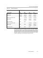
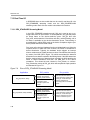
1.3.6
Standard Memory Sections
The Configuration Tool defines standard memory sections and their default
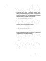
allocations as shown in Table 1-4.
You can change these default allocations using the MEM Manager in the
Configuration Tool. For more detail, see MEM Module in the TMS320
DSP/BIOS API Reference Guide for your platform.
Table 1-4.
Standard Memory Segments
a. C54x Platform
Sections
Segment
System stack Memory (.stack)
IDATA
Application Argument Memory (.args)
EDATA
Application Constants Memory (.const)
EDATA
BIOS Program Memory (.bios)
IPROG
BIOS Data Memory (.sysdata)
EDATA
BIOS Heap Memory
IDATA
BIOS Startup Code Memory (.sysinit)
EPROG
b. C55x Platform
Sections
Segment
System stack Memory (.stack),
System Stack Memory (.sysstack)
DATA
BIOS Kernel State Memory (.sysdata)
DATA
BIOS Objects, Configuration Memory (.*obj)
DATA
BIOS Program Memory (.bios)
PROG
BIOS Startup Code Memory (.sysinit, .gblinit,
.trcinit)
PROG
Application Argument Memory (.args)
DATA
Application Program Memory (.text)
PROG
BIOS Heap Memory
DATA
Secondary BIOS Heap Memory
DATA1
About DSP/BIOS
1-15
For More Information
Table 1.4 Standard Memory Segments (continued)
c. C6000 Platform
Sections
Segment
System stack memory (.stack)
IDRAM
Application constants memory (.const)
IDRAM
Program memory (.text)
IPRAM
Data memory (.data)
IDRAM
Startup code memory (.sysinit)
IPRAM
C initialization records memory (.cinit)
IDRAM
Uninitialized variables memory (.bss)
IDRAM
c. C2800 Platform
Sections
Segment
System stack memory (.stack)
M1SARAM
Program memory (.text)
IPROG
Data memory (.data)
IDATA
Applications constants memory (.const)
IDATA
Startup code memory (.sysinit)
IPROG
C initialization records memory (.cinit)
IDATA
Uninitialized variables memory (.bss)
IDATA
1.4 For More Information
For more information about the components of DSP/BIOS and the modules
in the DSP/BIOS API, see the DSP/BIOS section of the online help system,
the TMS320 DSP/BIOS API Reference Guide for your platform, or the "Using
DSP/BIOS" lessons in the online Code Composer Studio Tutorial .
1-16
Chapter 2
Program Generation
This chapter describes the process of generating programs with DSP/BIOS.
It also explains which files are generated by DSP/BIOS components and how
they are used.
Topic
Page
2.1
Development Cycle . . . . . . . . . . . . . . . . . . . . . . . . . . . . . . . . . . . . . . . 2-2
2.2
Using the Configuration Tool . . . . . . . . . . . . . . . . . . . . . . . . . . . . . . . 2-3
2.3
Files Used to Create DSP/BIOS Programs. . . . . . . . . . . . . . . . . . . . 2-12
2.4
Compiling and Linking Programs. . . . . . . . . . . . . . . . . . . . . . . . . . . 2-14
2.5
Using DSP/BIOS with the Run-Time Support Library. . . . . . . . . . . 2-18
2.6
DSP/BIOS Startup Sequence . . . . . . . . . . . . . . . . . . . . . . . . . . . . . . 2-20
2.7
Using C++ with DSP/BIOS . . . . . . . . . . . . . . . . . . . . . . . . . . . . . . . . . 2-24
2.8
User Functions Called by DSP/BIOS . . . . . . . . . . . . . . . . . . . . . . . . 2-27
2.9
Calling DSP/BIOS APIs from Main . . . . . . . . . . . . . . . . . . . . . . . . . . 2-28
2-1
Development Cycle
2.1 Development Cycle
DSP/BIOS supports iterative program development cycles. You can create
the basic framework for an application and test it with a simulated processing
load before the DSP algorithms are in place. You can easily change the
priorities and types of program threads that perform various functions.
A sample DSP/BIOS development cycle includes the following steps, though
iteration can occur for any step or group of steps:
1) Use the Configuration Tool to create objects for your program to use.
2) Save the configuration file, which generates files to be included when you
compile and link your program.
3) Write a framework for your program. You can use C, C++, assembly, or a
combination of the languages.
4) Compile and link the program using a Code Composer Studio makefile
or a project.
5) Test program behavior using a simulator or initial hardware and the DSP/
BIOS Analysis Tools. You can monitor logs and traces, statistics objects,
timing, software interrupts, and more.
6) Repeat steps 1-5 until the program runs correctly. You can add
functionality and make changes to the basic program structure.
7) When production hardware is ready, modify the configuration file to
support the production board and test your program on the board.
2-2
Using the Configuration Tool
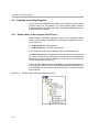
2.2 Using the Configuration Tool
The Configuration Tool is a visual editor with an interface similar to the
Windows Explorer. It allows you to initialize data structures and set various
parameters used by DSP/BIOS. When you save a file, the Configuration Tool
creates assembly source and header files and a linker command file to match
your settings. When you build your application, these files are linked with your
application programs. See the Configuration Tool lessons in the DSP/BIOS
section of the online help system for more details on using the Configuration
Tool.
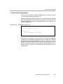
2.2.1
Creating a New Configuration File
1) In the Code Composer Studio program, open the Configuration Tool by
choosing File→New→DSP/BIOS Config. Alternatively, you can open the
Configuration Tool outside of the Code Composer Studio program from
the Start menu.
2) Choose the appropriate template and click OK.
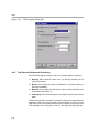
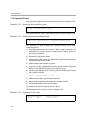
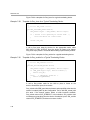
2.2.2
Creating a Custom Template
You can add a custom template or seed file by creating a configuration file
and storing it in your include folder. This saves time by allowing you to define
configuration settings for your hardware once. Then you can reuse the file as
a template.
For example, to build DSP/BIOS programs for a fixed or floating point DSP,
you can use the settings provided. Or you can instruct the Configuration Tool
to create a new custom template file for projects that should take advantage
of the appropriate run-time library.
To create a custom template, for example, to change the DSP MIPS on the
C54x platform, perform the following steps. Modify the steps as appropriate
for other DSP/BIOS platforms.
1) Invoke the Configuration Tool from outside the Code Composer Studio
software
via
Start→Programs→Code
Composer
Studio
C5000→Configuration Tool.
2) From the File menu, choose New.
3) In the New window choose c54xx.cdb and click OK.
4) Right-click on Global Settings and choose Properties.
5) Set DSP MIPS (CLKOUT) to 200 and click OK.
6) Choose File→Save As. In the Save As dialog box navigate to
ti\c5400\bios\include.
7) In the File Name box type c54x_200.cdb.
Program Generation
2-3
Using the Configuration Tool
8) In the Save as type box choose Seed files (*.cdb) and click Save.
9) In the Set Description dialog type a description and click OK.
10) In the Configuration Tool, choose File→Exit.
2.2.3
Setting Global Properties for a Module
1) When you choose a module (by clicking on it), the right side of the
window shows the current properties for the module. (If you see a list of
priorities instead of a property list, right-click on the module and choose
Property/value view. If the right side of the window is gray, this module
has no global properties.)
For help about a module, click
and then click on the module.
2) Right-click the icon next to the module and choose Properties from the
pop-up menu. This opens the property dialog.
3) Change properties as needed. For help on the module’s properties, click
Help in the property dialog.
2.2.4
Creating Objects Using the Configuration Tool
Most objects can be created either statically using the Configuration Tool or
dynamically by calling the function XXX_create. This section describes
objects created using the Configuration Tool. To create objects dynamically
see section 2.2.8, Creating, Referencing, and Deleting Dynamically-Created
DSP/BIOS Objects, page 2-10.
For typical DSP applications, most objects should be created with the
Configuration Tool because they are used throughout program execution. A
number of default objects are automatically defined in the configuration
template. Creating objects with the Configuration Tool provides the following
benefits:
2-4
❏
Improved access within DSP/BIOS Analysis Tools. The Execution Graph
shows the names of objects created with the Configuration Tool. In
addition, you can view statistics only for objects created with the
Configuration Tool.
❏
Reduced code size. For a typical module, the XXX_create and
XXX_delete functions contain 50% of the code required to implement the
module. If you avoid using any calls to TSK_create and TSK_delete, the
underlying code for these functions is not included in the application
program. The same is true for other modules. By creating objects with the
Configuration Tool you can dramatically reduce the size of your
application program.
Using the Configuration Tool
Note:
SYS_printf is probably the most memory intensive function in DSP/BIOS.
Use the LOG functions instead of SYS_printf to make your application
smaller.
❏
Improved run-time performance. In addition to saving code space,
avoiding dynamic creation of objects reduces the time your program
spends performing system setup.
Creating objects with the Configuration Tool has the following limitations:
❏
Objects are created whether or not they are needed. You can create
objects dynamically if they will be used only as a result of infrequent runtime events.
❏
You cannot delete objects created with the Configuration Tool at run time
using the XXX_delete functions.
Note:
No checks are performed to prevent an XXX_delete function from being
used on an object created with the Configuration Tool. If a program
attempts to delete an object that was not created dynamically, SYS_error
is called.
Follow these steps to create an object using the Configuration Tool:
1) Right-click on a module and choose Insert XXX, where XXX is the name
of the module. This adds a new object for the module. (You cannot create
an object for the GBL, HWI, or SYS modules.)
2) Rename the object. Right-click on the name and choose Rename from
the pop-up menu.
3) Right-click the icon next to the object and choose Properties to open the
property sheet.
4) Change property settings and click OK. For help on specific properties,
click Help in any property sheet.
Program Generation
2-5
Using the Configuration Tool
Note:
When specifying C functions to be run by various objects, add an
underscore before the C function name. For example, type _myfunc to run
a C function called myfunc. The underscore prefix is necessary because
the Configuration Tool creates assembly source, and C calling conventions
require an underscore before C functions called from assembly.
2.2.5
Hierarchy Tree View
The Hierarchy Tree View of the Configuration Tool, as seen in the left pane of
Figure 2-1, displays the instances of objects in alphabetic order.
Figure 2-1.
2.2.6
Configuration Tool Hierarchy and Ordered Collection Views
Ordered Collection View
The Ordered Collection View displays the list of objects per module in the
order the objects will be executed on the target as seen in Figure 2-1. To view
the Ordered Collection View, right-click on the module name and select
Ordered Collection View. The following objects can be listed in the Ordered
Collection View:
2-6
Using the Configuration Tool
❏
CLK - Clock Manager
❏
PRD - Periodic Function Manager
❏
SWI - Software Task Manager
❏
TSK - Task Manager
❏
IDL - Idle Function Manager
The order of objects in the Ordered Collection View can be rearranged by
dragging and dropping the object into its new position. For example, if you
require the CLK0 object to execute immediately after the PRD_clock object,
drag and drop CLK0 on top of the PRD_clock object. The dropped object is
placed in the list immediately after the object that it is dropped upon, and will
execute in that order. This is shown in Figure 2-1.
2.2.7
Referencing Static DSP/BIOS Objects Created with the Configuration Tool
Objects created using the Configuration Tool need to be declared using the
extern variable declaration and must be defined outside of all function bodies.
For example,
extern far
PIP_Obj inputObj;
/* C6000 devices
*/
or
extern PIP_Obj inputObj;
/* C5000 and C2800 devices */
The DSP/BIOS object is now visible in all functions that follow its definition in
the program.
The Configuration Tool creates these declarations automatically in a file of the
form program cfg.h, where program is the name of your application program.
This file can be # included in your C files that reference the DSP/BIOS object.
Although DSP/BIOS itself is compiled using the small model, you can compile
DSP/BIOS applications using either the C6000 compiler’s small model or any
variation of the large model. (See the TMS320C6000 Optimizing Compiler
User’s Guide .) In fact, you can mix compilation models within the application
code provided all global data that is accessed by using a displacement
relative to B14 is placed no more than 32K bytes away from the beginning of
the .bss section.
DSP/BIOS uses the .bss section to store global data. However, objects
created with the Configuration Tool are not placed in the .bss section. This
maximizes your flexibility in the placement of application data. For example,
the frequently accessed .bss can be placed in on-device memory while larger,
less frequently accessed objects can be stored in external memory.
Program Generation
2-7
Using the Configuration Tool
The small model makes assumptions about the placement of global data in
order to reduce the number of instruction cycles. If you are using the small
model (the default compilation mode) to optimize global data access, your
code can be modified to make sure that it references objects created with the
Configuration Tool correctly.
There are four methods for dealing with this issue. These methods are
described in the sections following and have the pros and cons as shown in
Example 2-1.
Table 2-1.
Methods of Referencing C6000 Global Objects
Method
Declare
objects
with far
Use global
object
pointers
Objects
adjacent
to .bss
Compile
with large
model
Code works independent of compilation model
Yes
Yes
Yes
Yes
Code works independent of object placement
Yes
Yes
No
Yes
C code is portable to other compilers
No
Yes
Yes
Yes
Size of all statically created objects not limited to 32K
bytes
Yes
Yes
No
Yes
Minimizes size of .bss
Yes
Yes
No
Yes
Minimizes instruction cycles
No
(3 cycles)
No
(2-6 cycles)
Yes
(1 cycle)
No
(3 cycles)
Minimizes storage per object
No
(12 bytes)
No
(12 bytes)
Yes
(4 bytes)
No
(12 bytes)
Easy to remember when programming; easy to find
errors
Somewhat
Error prone
Somewhat
Yes
2.2.7.1 Referencing Static DSP/BIOS Objects in the Small Model (C6000 Platform Only)
In the small model, all compiled code accesses global data relative to a data
page pointer register. The register B14 is treated as a read-only register by
the compiler and is initialized with the starting address of the .bss section
during program startup. Global data is assumed to be at a constant offset
from the beginning of the .bss section and this section is assumed to be at
most 32K bytes in length. Global data, therefore, can be accessed with a
single instruction like the following:
LDW
2-8
*+DP(_x), A0
; load _x into A0 (DP = B14)
Using the Configuration Tool
Since objects created with the Configuration Tool are not placed in the .bss
section, you must ensure that application code compiled with the small model
references them correctly. There are three ways to do this:
❏
Declare static objects with the far keyword. The DSP/BIOS compiler
supports this common extension to the C language. The far keyword in a
data declaration indicates that the data is not in the .bss section.
For example, to reference a PIP object called inputObj that was created
with the Configuration Tool, declare the object as follows:
extern far PIP_Obj inputObj;
if (PIP_getReaderNumFrames(&inputObj)) {
. . .
}
❏
Create and initialize a global object pointer. You can create a global
variable that is initialized to the address of the object you want to
reference. All references to the object must be made using this pointer,
to avoid the need for the far keyword. For example:
extern PIP_Obj inputObj;
/* input MUST be a global variable */
PIP_Obj *input = &inputObj;
if (PIP_getReaderNumFrames(input)) {
. . .
}
Declaring and initializing the global pointer consumes an additional word
of data (to hold the 32-bit address of the object).
Also, if the pointer is a static or automatic variable this technique fails.
The following code does not operate as expected when compiled using
the small model:
extern PIP_Obj inputObj;
static PIP_Obj *input = &inputObj;
/* ERROR!!!! */
if (PIP_getReaderNumFrames(input)) {
. . .
}
❏
Place all objects adjacent to .bss. If all objects are placed at the end of
the .bss section, and the combined length of the objects and the .bss data
is less than 32K bytes, you can reference these objects as if they were
allocated within the .bss section:
extern PIP_Obj inputObj;
if (PIP_getReaderNumFrames(&inputObj)) {
. . .
}
Program Generation
2-9
Using the Configuration Tool
You can guarantee this placement of objects by using the Configuration
Tool as follows:
a) Declare a new memory segment by inserting a MEM object with the
MEM Manager and setting its properties (i.e., the base and length);
or use one of the preexisting data memory MEM objects.
b) Place all objects that are referenced by small model code in this
memory segment.
c) Place Uninitialized Variables Memory (.bss) in this same segment by
right-clicking on the MEM Manager and choosing Properties.
2.2.7.2 Referencing Static DSP/BIOS Objects in the Large Model (C6000 Platform Only)
In the large model, all compiled code accesses data by first loading the entire
32-bit address into an address register and then using the indirect addressing
capabilities of the LDW instruction to load the data. For example:
MVKL
MVKH
LDW
_x, A0
_x, A0
*A0, A0
; move low 16-bits of _x’s address into A0
; move high 16-bits of _x’s address into A0
; load _x into A0
Application code compiled with any of the large model variants is not affected
by the location of static objects. If all code that directly references objects
created with the Configuration Tool is compiled with any large model option,
code can reference the objects as ordinary data:
extern PIP_Obj inputObj;
if (PIP_getReaderNumFrames(&inputObj)) {
. . .
}
The -ml0 large model option is identical to small model except that all
aggregate data is assumed to be far. This option causes all static objects to
be assumed to be far objects but allows scalar types (such as int, char, long)
to be accessed as near data. As a result, the performance degradation for
many applications is quite modest.
2.2.8
Creating, Referencing, and Deleting Dynamically-Created DSP/BIOS Objects
You can create many, but not all, DSP/BIOS objects by calling the function
XXX_create where XXX names a specific module. Some objects can only be
created in the Configuration Tool. Each XXX_create function allocates
memory for storing the object’s internal state information, and returns a
handle used to reference the newly-created object when calling other
functions provided by the XXX module.
2-10
Using the Configuration Tool
Most XXX_create functions accept as their last parameter a pointer to a
structure of type XXX_Attrs which is used to assign attributes to the newlycreated object. By convention, the object is assigned a set of default values
if this parameter is NULL. These default values are contained in the constant
structure XXX_ATTRS listed in the header files, enabling you to first initialize
a variable of type XXX_Attrs and then selectively update its fields with
application-dependent attribute values before calling XXX_create. Sample
code that creates a dynamic object using the TSK_create is shown in
Example 2-1.
Example 2-1.
Creating and Referencing Dynamic Objects
#include <tsk.h>
TSK_Attrs
attrs;
TSK_Handle task;
attrs = TSK_ATTRS;
attrs.name = "reader";
attrs.priority = TSK_MINPRI;
task = TSK_create((Fxn)foo, &attrs);
The XXX_create function passes back a handle that is an address to the
task’s object. This handle is can then be passed as an argument when
referencing, for example, deleting the object, as shown in Example 2-2.
Objects created with XXX_create are deleted by calling the function
XXX_delete. This frees the object’s internal memory back to the system for
later use.
Use the global constant XXX_ATTRS to copy the default values, update its
fields, and pass as the argument to the XXX_create function.
Example 2-2.
Deleting a Dynamic Object
TSK_delete (task);
Dynamically-created DSP/BIOS objects allow for a program to adapt at
runtime.
Program Generation
2-11
Files Used to Create DSP/BIOS Programs
2.3 Files Used to Create DSP/BIOS Programs
When you save a configuration file for your program with the Configuration
Tool, the following files are created. These files are described below. The
numeric 62 is applicable to the C62x platform only. Replace the 62 in the
extensions with 54, 55, or 64 depending on your platform.
❏
❏
❏
❏
❏
❏
program.cdb
programcfg.h54
programcfg.s54
programcfg.cmd
programcfg.h
programcfg_c.c
Figure 2-2 shows the files used to create DSP/BIOS programs. Files you
write are represented with a white background; generated files are
represented with a gray background. The word program represents the name
of your project or program.
Figure 2-2.
DSP/BIOS Program Creation Files
program.cdb
*.asm, *.c, or
*.cpp (optional)
program.c
program.cmd
(optional)
generate
include
programcfg.h54
programcfg_c.c
programcfg.cmd
module.h54
module.h
programcfg.s54
assemble
programcfg.h
compile
compile or
assemble
program.obj
*.obj
programcfg_c..obj
programcfg.obj
link
program.out
2-12
❏
program.c. Program source file containing the main function. You can
also have additional .c source files and program .h files. For user
functions, see section 2.8, User Functions Called by DSP/BIOS.
❏
*.asm. Optional assembly source file(s). One of these files can contain
an assembly language function called _main as an alternative to using a
C or C++ function called main.
Files Used to Create DSP/BIOS Programs
2.3.1
❏
module.h. DSP/BIOS API header files for C or C++ programs. Your
source files should include std.h and the header files for any modules the
program uses.
❏
module.h54. DSP/BIOS API header files for assembly programs.
Assembly source files should include the *.h54 header file for any module
the assembly source uses.
❏
program.obj. Object file(s) compiled or assembled from your source file(s)
❏
*.obj. Object files for optional assembly source file(s)
❏
program.cdb. Configuration file, that stores configuration settings. This
file is created by the Configuration Tool and used by both the
Configuration Tool and the DSP/BIOS Analysis Tools.
❏
programcfg.h54. Header file generated by the Configuration Tool. This
header file is included by the programcfg.s54 file.
❏
programcfg.s54. Assembly source generated by the Configuration Tool
❏
programcfg.cmd. Linker command file created by the Configuration Tool
and used when linking the executable file. This file defines DSP/BIOSspecific link options and object names, and generic data sections for DSP
programs (such as .text, .bss, .data, etc.).
❏
programcfg.obj. Object file created from the source file generated by
the Configuration Tool.
❏
*.cmd. Optional linker command file(s) that contains additional sections
for your program not defined by the Configuration Tool.
❏
program.out. An executable program for the target (fully compiled,
assembled, and linked). You can load and run this program with Code
Composer Studio commands.
❏
programcfg.h. File containing declarations of objects created with the
Configuration Tool. It also contains the definition of the CSL_xxxx macro
where xxxx is the Chip Type property of the Global Settings module.
❏
programcf_c.c. File containing program code for CSL settings,
generated automatically when a configuration file is saved. It # includes
the programcfg.h file.
Files Used by the DSP/BIOS Analysis Tools
The following files are used by the DSP/BIOS Analysis Tools:
❏
program.cdb. The configuration file provides object names and other
program information.
❏
program.out. The executable file provides symbol addresses and other
program information.
Program Generation
2-13
Compiling and Linking Programs
2.4 Compiling and Linking Programs
You can build your DSP/BIOS executables using a Code Composer Studio
project or using your own makefile. The Code Composer Studio software
includes gmake.exe, the GNU make utility, and sample makefiles for gmake
to build the tutorial examples.
2.4.1
Building With a Code Composer Studio Project
When building a DSP/BIOS application using a Code Composer Studio
project, you must add the following files to the project in addition to your own
source code files:
❏
❏
program.cdb. The configuration file.
programcfg.cmd. The linker command file.
Code Composer Studio software adds programcfg.s54 automatically.
In a DSP/BIOS application, programcfg.cmd is your project's linker command
file. This file already includes directives for the linker to use the appropriate
libraries (e.g., bios.a54, rtdx.lib, rts5401.lib), so you do not need to add any
of these library files to your project.
Code Composer Studio software automatically scans all dependencies in
your project files, adding the necessary DSP/BIOS and RTDX header files for
your configuration to your project's include folder. Figure 2-3 shows a sample
project files list.
Figure 2-3.
2-14
Sample Code Composer Project Files List
Compiling and Linking Programs
For details on how to create a Code Composer Studio project and build an
executable from it, refer to the Code Composer Studio User’s Guide or the
online help.
For most DSP/BIOS applications the generated linker command file,
programcfg.cmd, suffices to describe all memory segments and allocations.
All DSP/BIOS memory segments and objects are handled by this linker
command file. In addition, most commonly used sections (such as .text, .bss,
.data, etc.) are already included in programcfg.cmd. Their locations (and
sizes, when appropriate) can be controlled from the MEM Manager in the
Configuration Tool. Figure 2-4 illustrates the Code Composer Studio
properties dialog box.
In some cases the application can require an additional linker command file
(app.cmd) describing application-specific sections that are not described in
the linker command file generated by the Configuration Tool
(programcfg.cmd).
Figure 2-4.
MEM Module Properties Panel
Program Generation
2-15
Compiling and Linking Programs
Note:
Code Composer Studio software allows only one linker command file per
project. When both programcfg.cmd and app.cmd are required by the
application, the project should use app.cmd (rather than programcfg.cmd)
as the project's linker command file. To include programcfg.cmd in the
linking process, you must add the following line to the beginning of
app.cmd:
-lprogramcfg.cmd
(This line begins with a dash character and then a lower-case L character.
It is not the numeric one character. ) It is important that this line appear at
the beginning, so that programcfg.cmd is the first linker command file used
by the linker, and program is the name of the executable program being
linked as well as the name of the associated configuration file.
2.4.2
Makefiles
As an alternative to building your program as a Code Composer Studio
project, you can use a makefile.
In the following example, the C source code file is volume.c, additional
assembly source is in load.asm, and the configuration file is volume.cdb. This
makefile is for use with gmake, which is included with the Code Composer
Studio software. You can find documentation for gmake on the product CD in
PDF format. Adobe Acrobat Reader is included. This makefile and the source
and configuration files mentioned are located in the volume2 subdirectory of
the tutorial directory of Code Composer Studio distribution CD.
A typical makefile for compiling and linking a DSP/BIOS program is shown in
Example 2-3. You can copy an example makefile to your program folder and
modify the makefile as necessary.
Unlike the Code Composer Studio project, makefiles allow for multiple linker
command files. If the application requires additional linker command files you
can easily add them to the CMDS variable in the example makefile shown in
Example 2-3. However, they must always appear after the programcfg.cmd
linker command file generated by the Configuration Tool.
2-16
Compiling and Linking Programs
Example 2-3.
Sample Makefile for a DSP/BIOS Program
# Makefile for creation of program named by the PROG variable
# The following naming conventions are used by this makefile:
#
<prog>.asm
- C54 assembly language source file
#
<prog>.obj
- C54 object file (compiled/assembled source)
#
<prog>.out
- C54 executable (fully linked program)
#
<prog>cfg.s54 - configuration assembly source file
#
generated by Configuration Tool
#
<prog>cfg.h54 - configuration assembly header file
#
generated by Configuration Tool
#
<prog>cfg.cmd - configuration linker command file
#
generated by Configuration Tool
include $(TI_DIR)/c5400/bios/include/c54rules.mak
#
# Compiler, assembler, and linker options.
# -g enable symbolic debugging
CC54OPTS = -g
AS54OPTS =
# -q quiet run
LD54OPTS = -q
# Every BIOS program must be linked with:
#
$(PROG)cfg.o54 - object resulting from assembling
#
$(PROG)cfg.s54
#
$(PROG)cfg.cmd - linker command file generated by
#
the Configuration Tool. If additional
#
linker command files exist,
#
$(PROG)cfg.cmd must appear first.
#
PROG
= volume
OBJS
= $(PROG)cfg.obj load.obj
LIBS
=
CMDS
= $(PROG)cfg.cmd
# Targets:
all:: $(PROG).out
$(PROG).out: $(OBJS) $(CMDS)
$(PROG)cfg.obj: $(PROG)cfg.h54
$(PROG).obj:
$(PROG)cfg.s54 $(PROG)cfg.h54 $(PROG)cfg.cmd:
@ echo Error: $@ must be manually regenerated:
@ echo Open and save $(PROG).cdb within the BIOS Configuration Tool.
@ check $@
.clean clean::
@ echo removing generated configuration files ...
@ remove -f $(PROG)cfg.s54 $(PROG)cfg.h54 $(PROG)cfg.cmd
@ echo removing object files and binaries ...
@ remove -f *.obj *.out *.lst *.map
Program Generation
2-17
Using DSP/BIOS with the Run-Time Support Library
2.5 Using DSP/BIOS with the Run-Time Support Library
The linker command file generated by the Configuration Tool automatically
includes directives to search the necessary libraries including a DSP/BIOS,
RTDX, and a run-time support library. The run-time support library is created
from rts.src, which contains the source code for the run-time support
functions. These are standard ANSI functions that are not part of the C
language (such as functions for memory allocation, string conversion, and
string searches). A number of memory management functions that are
defined within rts.src are also defined within the DSP/BIOS library. These are
malloc, free, memalign, calloc, and realloc. The libraries support different
implementations. For example, the DSP/BIOS versions are implemented
with the MEM module and therefore make use of the DSP/BIOS API calls
MEM_alloc and MEM_free. Because the DSP/BIOS library provides some of
the same functionality found within the run-time support library, the DSP/
BIOS linker command file includes a special version of the run-time support
library called rtsbios that does not include the files shown in Table 2-2.
Table 2-2.
Files Not Included in rtsbios
C54x Platform
C55x Platform
C6000 Platform
memory.c
memory.c
memory.c
autoinit.c
boot.c
sysmem.c
boot.c
autoinit.c
boot.c
In many DSP/BIOS projects, it is necessary to use the –x linker switch in
order to force the rereading of libraries. For example, if printf references
malloc and malloc has not already been linked in from the DSP/BIOS library,
it forces the DSP/BIOS library to be searched again in order to resolve the
reference to malloc.
The run-time support library implements printf with breakpoints.
Depending on how often your application uses printf and the frequency of
the calls, printf() can interfere with RTDX, thus affecting real-time analysis
tools such as the Message Log and Statistics View, and preventing these
tools from updating. This is because the printf breakpoint processing has
higher priority processing than RTDX. It is therefore recommended to use
LOG_printf in place of calls to printf wherever possible within DSP/BIOS
applications.
2-18
Using DSP/BIOS with the Run-Time Support Library
Note:
It is recommended to use the DSP/BIOS library version of malloc, free,
memalign, calloc and realloc within DSP/BIOS applications. When you are
not referencing these functions directly in your application but call another
run-time support function which references one or more of them, add '-u
_symbol', (for example, -u _malloc) to your linker options. The -u linker
option introduces a symbol, such as malloc, as an unresolved symbol into
the linker's symbol table. This causes the linker to resolve the symbol from
the DSP/BIOS library rather than the run-time support library. If in doubt,
you can examine your map file for information on the library sources of your
application.
Program Generation
2-19
DSP/BIOS Startup Sequence
2.6 DSP/BIOS Startup Sequence
When a DSP/BIOS application starts up, the calls or instructions in the
boot.s54 (C54x platform), or autoinit.c and boot.snn (C6000 and C55x
platforms) files determine the startup sequence. Compiled versions of these
files are provided with the bios.ann and biosi.ann libraries and the source
code is available on the distribution disks received with your product. The
DSP/BIOS startup sequence, as specified in the source code of the boot files
is shown below. You should not need to alter the startup sequence.
1) Initialize the DSP. A DSP/BIOS program starts at the C or C++
environment entry point c_int00. The reset interrupt vector is set up to
branch to c_int00 after reset.
For the C54x platform, at the beginning of c_int00, the system stack
pointer (SP) is set up to point to the end of .stack. Status registers such
as st0 and st1 are also initialized
At the beginning of c_int00 for the C55x platform, the data (user) stack
pointer (XSP) and the system stack pointer (XSSP) are both set up to
point to the bottom of the user and system stacks, respectively.
Additionally, the XSP is aligned to an even address boundary.
For the C6000 platform, at the beginning of c_int00, the system stack
pointer (B15) and the global page pointer (B14) are set up to point to the
end of the stack section and the beginning of .bss, respectively. Control
registers such as AMR, IER, and CSR are also initialized.
2) Initialize the .bss from the .cinit records. Once the stacks are set up,
the initialization routine is called to initialize the variables from the .cinit
records.
3) Call BIOS_init to initialize the modules used by the application.
BIOS_init performs basic module initialization. BIOS_init invokes the
MOD_init macro for each DSP/BIOS module used by the application.
BIOS_init is generated by the Configuration Tool and is located in the
programcfg.snn file.
■
2-20
HWI_init sets up the ISTP and the interrupt selector registers, sets
the NMIE bit in the IER on the C6000 platform, and clears the IFR on
all platforms. See the HWI Module Section in the TMS320 DSP/BIOS
API Reference Guide for your platform for more information.
DSP/BIOS Startup Sequence
Note:
When configuring an interrupt with the Configuration Tool, DSP/BIOS plugs
in the corresponding ISR (interrupt service routine) into the appropriate
location of the interrupt service table. However, DSP/BIOS does not enable
the interrupt bit in IER. It is your responsibility to do this at startup or
whenever appropriate during the application execution.
■
HST_init initializes the host I/O channel interface. The specifics
of this routine depend on the particular implementation used for the
host to target link. For example, in the C6000 platform, if RTDX is
used, HST_init enables the bit in IER that corresponds to the
hardware interrupt reserved for RTDX.
■
IDL_init calculates the idle loop instruction count. If the Auto
calculate idle loop instruction count box was chosen in the Idle
Function Manager in the Configuration Tool, IDL_init calculates the
idle loop instruction count at this point in the startup sequence. The
idle loop instruction count is used to calibrate the CPU load displayed
by the CPU Load Graph (see section 3.4.2, The CPU Load, page 320).
4) Process the .pinit table. The .pinit table consists of pointers to
initialization functions. For C++ programs, class constructors of global
objects execute during .pinit processing.
5) Call your program’s main routine. After all DSP/BIOS modules have
completed their initialization procedures, your main routine is called. This
routine can be written in assembly, C, C++ or a combination. Because the
C compiler adds an underscore prefix to function names, this can be a C
or C++ function called main or an assembly function called _main.
Since neither hardware nor software interrupts are enabled yet, you can
take care of initialization procedures for your own application (such as
calling your own hardware initialization routines) from the main routine.
Your main function can enable individual interrupt mask bits, but it should
not call HWI_enable to globally enable interrupts.
6) Call BIOS_start to start DSP/BIOS. Like BIOS_init, BIOS_start is also
generated by the Configuration Tool and is located in the programcfg.snn
file. BIOS_start is called after the return from your main routine.
BIOS_start is responsible for enabling the DSP/BIOS modules and
invoking the MOD_startup macro for each DSP/BIOS module. If the TSK
Manager is enabled in the Configuration Tool, the call to BIOS_start does
not return. For example:
Program Generation
2-21
DSP/BIOS Startup Sequence
■
CLK_startup sets up the PRD register, enables the bit in the IER
(C6000 platform) or the IMR (C5400 platform) for the timer chosen in
the CLK Manager, and finally starts the timer. (This macro is only
expanded if you enable the CLK Manager in the Configuration Tool.)
■
PIP_startup calls the notifyWriter function for each created pipe
object.
■
SWI_startup enables software interrupts.
■
HWI_startup enables hardware interrupts by setting the GIE bit in the
CSR on the C6000 platform or clearing the INTM bit in the ST1
register on the C5400 platform.
■
TSK_startup enables the task scheduler and launches the highest
priority task that is ready to run. If the application has no tasks that
are currently ready, the TSK_idle executes and calls IDL_loop. Once
TSK_startup is called, the application begins and thus execution
does not return from TSK_startup or from BIOS_start. TSK_startup
runs only if the Task Manager is enabled in the Configuration Tool.
7) Execute the idle loop. You can enter the idle loop in one of two ways. In
the first way, the Task Manager is enabled. The Task scheduler runs
TSK_idle which calls IDL_loop. In the second way, the Task Manager is
disabled and thus the call to BIOS_start returns and a call to IDL_loop
follows. By calling IDL_loop, the boot routine falls into the DSP/BIOS idle
loop forever. At this point, hardware and software interrupts can occur
and preempt idle execution. Since the idle loop manages communication
with the host, data transfer between the host and the target can now take
place.
2.6.1
Advanced Startup: C5500 Platform Only
On the C5500 platform, the architecture allows the software to reprogram the
start of the vector tables (256 bytes in overall length) by setting the registers
IVPD and IVPH. By default, the hardware reset loads 0xFFFF to both these
registers and the reset vector is fetched from location 0xFF – FF00. To move
the vector tables to a different location, it is necessary to write the desired
address into IVPD and IVPH after the hardware reset and then do a software
reset, at which time the new values in IVPD and IVPH take effect.
The macro HWI_init loads the configured vector table address into IVPD and
IVPH but must be followed by a software reset to actually bring the new IVPD
and IVPH into effect.
2-22
DSP/BIOS Startup Sequence
The C5500 platform also allows for three possible stack modes (see
Table 2-3). To configure the processor in any of the non-default modes, the
user is required to set bits 28 and 29 to the reset vector location appropriately
using the Code Composer Studio debugger tool and then to apply a software
reset. For more information, please see the TMS320C55x DSP CPU
Reference Guide.
Table 2-3.
Stack Modes on the C5500 Platform
Stack Mode
Description
Reset Vector Settings
2x16 Fast Return
SP/SSP independent,
RETA/CFCT used for fast
return functionality
XX00 : XXXX : <24-bit vector address>
2x16 Slow Return
SP/SSP independent,
RETA/CFCT not used
XX01 : XXXX : <24-bit vector address>
1x32 Slow Return
(Reset default)
SP/SSP synchronized,
RETA/CFCT not used
XX02 : XXXX : <24-bit vector address>
In addition, the DSP/BIOS configuration file should set the Stack Mode
property of the HWI Manager to match the mode used by the application. See
the TMS320C5000 DSP/BIOS API Reference Guide for details.
Program Generation
2-23
Using C++ with DSP/BIOS
2.7 Using C++ with DSP/BIOS
DSP/BIOS applications can be written in C++. An understanding of issues
regarding C++ and DSP/BIOS can help to make C++ application
development proceed smoothly.
These issues concern memory
management, name mangling, calling class methods from the Configuration
Tool, and special considerations for class constructors and destructors.
2.7.1
Memory Management
The functions new and delete are the C++ operators for dynamic memory
allocation and deallocation. Within DSP/BIOS applications, these operators
are reentrant because they are implemented with the DSP/BIOS memory
management functions MEM_alloc and MEM_free. However, memory
management functions require that the calling thread obtain a lock to memory
before proceeding if the requested lock is already held by another thread,
blocking results. Therefore, new and delete should be used by TSK objects
only.
The functions new and delete are defined by the run-time support library, not
the DSP/BIOS library. Since the DSP/BIOS library is searched first, some
applications can result in a linker error stating that there are undefined
symbols that were first referenced within the rtsbios (the run-time support)
library. This linker error is avoided by using the -x linker option which forces
libraries to be searched again in order to resolve undefined references. See
section 2.5, Using DSP/BIOS with the Run-Time Support Library for more
information.
2.7.2
Name Mangling
The C++ compiler implements function overloading, operator overloading,
and type-safe linking by encoding a function's signature in its link-level name.
The process of encoding the signature into the linkname is referred to as
name mangling. Name mangling could potentially interfere with a DSP/BIOS
application since you use function names within the Configuration Tool to
refer to functions declared in your C++ source files. To prevent name
mangling and thus to make your functions recognizable within the
Configuration Tool, it is necessary to declare your functions in an extern C
block as shown in the code fragment of Example 2-4.
2-24
Using C++ with DSP/BIOS
Example 2-4.
Declaring Functions in an Extern C Block
extern "C" {
Void function1();
Int function2();
}
This allows you to refer to the functions within the Configuration Tool
(preceded by an underscore, as with other C function names). For example,
if you had an SWI object which should run function1() every time that the SWI
posts, you would enter _function1 into the function property of that SWI
object.
Functions declared within the extern C block are not subject to name
mangling. Since function overloading is accomplished through name
mangling, function overloading has limitations for functions that are called
from within the Configuration Tool. Only one version of an overloaded
function can appear within the extern C block. The code in Example 2-5
would result in an error.
Example 2-5.
Function Overloading Limitation
extern “C” {
Int addNums(Int x, Int y);
Int addNums(Int x, Int y, Int z); // error, only one version
// of addNums is allowed
}
While you can use name overloading in your DSP/BIOS C++ applications,
only one version of the overloaded function can be called from the
Configuration Tool.
Default parameters is a C++ feature that is not available for functions called
from the Configuration Tool. C++ allows you to specify default values for
formal parameters within the function declaration. However, a function called
from the Configuration Tool must provide parameter values. If no values are
specified, the actual parameter values are undefined.
2.7.3
Calling Class Methods from the Configuration Tool
Often, the function that you want to reference within the Configuration Tool is
the member function of a class object. It is not possible to call these member
functions directly from the Configuration Tool, but it is possible to accomplish
the same action through wrapper functions. By writing a wrapper function
which accepts a class instance as a parameter, you can invoke the class
member function from within the wrapper.
Program Generation
2-25
Using C++ with DSP/BIOS
A wrapper function for a class method is shown in Example 2-6.
Example 2-6.
Wrapper Function for a Class Method
Void wrapper (SampleClass myObject)
{
myObject->method();
}
Any additional parameters that the class method requires can be passed to
the wrapper function.
2.7.4
Class Constructors and Destructors
Any time that a C++ class object is instantiated, the class constructor
executes. Likewise, any time that a class object is deleted, the class
destructor is called. Therefore, when writing constructors and destructors,
you should consider the times at which the functions are expected to execute
and tailor them accordingly. It is important to consider what type of thread will
be running when the class constructor or destructor is invoked.
Various guidelines apply to which DSP/BIOS API functions can be called from
different DSP/BIOS threads (tasks, software interrupts, and hardware
interrupts). For example, memory allocation APIs such as MEM_alloc and
MEM_calloc cannot be called from within the context of a software interrupt.
Thus, if a particular class is instantiated by a software interrupt, its constructor
must avoid performing memory allocation. Similarly, it is important to keep in
mind the time at which a class destructor is expected to run. Not only does a
class destructor execute when an object is explicitly deleted, but also when a
local object goes out of scope. You need to be aware of what type of thread
is executing when the class destructor is called and make only those DSP/
BIOS API calls that are appropriate for that thread. For further information on
function callability, see the TMS320 DSP/BIOS API Reference Guide for your
platform.
2-26
User Functions Called by DSP/BIOS
2.8 User Functions Called by DSP/BIOS
User functions called by DSP/BIOS objects (IDL, TSK, SWI, PIP, PRD, and
CLK objects) need to follow specific conventions in order to ensure that
registers are used properly and that values are preserved across function
calls.
On the C6x and C55x platforms, all user functions called by DSP/BIOS
objects need to conform to C compiler register conventions for their
respective platforms. This applies to functions written both in C and
assembly languages.
The compiler distinguishes between C and assembly functions by assuming
that all C function names are preceded by an underscore, and assembly
function names are not preceded by an underscore. On the C54x platform,
this distinction becomes especially important because C and assembly
functions conform to two different sets of rules. Functions that are preceded
by an underscore (this includes C functions and any assembly functions
whose names are preceded by an underscore) must conform to the C
compiler conventions. On the C54x platform, assembly functions (functions
that are not preceded by an underscore) must conform to the following rules:
❏
The first argument is passed in register AR2
❏
The second argument is passed in register A
❏
The return value is passed in register A
Note:
The above rules do not apply to user functions called by TSK objects. All
user functions (both C and assembly) called by TSK objects follow C
register conventions.
On the C54x platform when a C function (or an assembly function whose
function name is preceded by an underscore) is executing, the CPL
(Compiler Mode) bit is required to be set. When an assembly function (one
whose name is not preceded by an underscore) begins executing, the CPL
bit is clear and must be clear upon return.
For more information on C register conventions, see the optimizing compiler
user’s guide for your platform.
Program Generation
2-27
Calling DSP/BIOS APIs from Main
2.9 Calling DSP/BIOS APIs from Main
The main routine in a DSP/BIOS application is for user initialization purposes
such as configuring a peripheral, or enabling individual hardware interrupts.
It is important to recognize that main does not fall into any of the DSP/BIOS
threads types (HWI, SWI, TSK, or IDL), and that when program execution
reaches main, not all of the DSP/BIOS initialization is complete. This is
because DSP/BIOS initialization takes place in two phases: during BIOS_init
which runs before main, and during BIOS_start which runs after your program
returns from main.
Certain DSP/BIOS API calls should not be made from the main routine,
because the BIOS_start initialization has not yet run. BIOS_start is
responsible for enabling global interrupts, configuring and starting the timer,
and enabling the schedulers so that DSP/BIOS threads can start executing.
Therefore, DSP/BIOS calls that are not appropriate from main are APIs which
assume hardware interrupts and the timer are enabled, or APIs that make
scheduling calls that could block execution. For example, functions such as
CLK_gethtime and CLK_getltime should not be called from main because the
timer is not running. HWI_disable and HWI_enable should not be called
because hardware interrupts are not globally enabled. Potentially blocking
calls, such as SEM_pend or MBX_pend, should not be called from main
because the scheduler is not initialized. Scheduling calls such as
TSK_disable, TSK_enable, SWI_disable, or SWI_enable are also not
appropriate within main.
BIOS_init, which runs before main, is responsible for initialization of the MEM
module. Therefore, it is okay to call dynamic memory allocation functions
from main. Not only are the MEM module functions allowed (MEM_alloc,
MEM_free, etc.), but APIs for dynamic creation and deletion of DSP/BIOS
objects, such as TSK_create and TSK_delete, are also allowed.
While blocking calls are not permitted from main, scheduling calls that make
a DSP/BIOS thread ready to run are permitted. These are calls such as
SEM_post or SWI_post. If such a call is made from main, the readied thread
is scheduled to run after the program returns from main and BIOS_start
finishes executing.
See the TMS320 DSP/BIOS API Reference Guide for your platform for more
information on a particular DSP/BIOS function call. The Constraints and
Calling Context sections indicates if the API cannot be called from main.
2-28
Chapter 3
Instrumentation
DSP/BIOS provides both explicit and implicit ways to perform real-time
program analysis. These mechanisms are designed to have minimal impact
on the application’s real-time performance.
Topic
Page
3.1
Real-Time Analysis . . . . . . . . . . . . . . . . . . . . . . . . . . . . . . . . . . . . . . . 3-2
3.2
Instrumentation Performance . . . . . . . . . . . . . . . . . . . . . . . . . . . . . . . 3-4
3.3
Instrumentation APIs . . . . . . . . . . . . . . . . . . . . . . . . . . . . . . . . . . . . . . 3-7
3.4
Implicit DSP/BIOS Instrumentation . . . . . . . . . . . . . . . . . . . . . . . . . 3-19
3.5
Kernel/Object View Debugger . . . . . . . . . . . . . . . . . . . . . . . . . . . . . . 3-29
3.6
Instrumentation for Field Testing . . . . . . . . . . . . . . . . . . . . . . . . . . . 3-38
3.7
Real-Time Data Exchange . . . . . . . . . . . . . . . . . . . . . . . . . . . . . . . . . 3-38
3-1
Real-Time Analysis
3.1 Real-Time Analysis
Real-time analysis is the analysis of data acquired during real-time operation
of a system. The intent is to easily determine whether the system is operating
within its design constraints, is meeting its performance targets, and has
room for further development.
Note:
On platforms where RTDX is not
updated only in stop mode. That is,
host PC while the target program is
reach a breakpoint, analysis data
Composer Studio.
supported, instrumentation data is
the data is not communicated to the
running. When you halt the target or
is transferred for viewing in Code
RTDX is currently not supported on the C28x and on certain boards such
as the ’C6416 TEB.
3.1.1
Real-Time Versus Cyclic Debugging
The traditional debugging method for sequential software is to execute the
program until an error occurs. You then stop the execution, examine the
program state, insert breakpoints, and reexecute the program to collect
information. This kind of cyclic debugging is effective for non-real-time
sequential software. However, cyclic debugging is rarely as effective in realtime systems because real-time systems are characterized by continuous
operation, nondeterministic execution, and stringent timing constraints.
The DSP/BIOS instrumentation APIs and the DSP/BIOS Analysis Tools are
designed to complement cyclic debugging tools to enable you to monitor realtime systems as they run. This real-time monitoring data lets you view the
real-time system operation so that you can effectively debug and
performance-tune the system.
3.1.2
Software Versus Hardware Instrumentation
Software monitoring consists of instrumentation code that is part of the target
application. This code is executed at run time, and data about the events of
interest is stored in the target system’s memory. Thus, the instrumentation
code uses both the computing power and memory of the target system.
The advantage of software instrumentation is that it is flexible and that no
additional hardware is required. Unfortunately, because the instrumentation
is part of the target application, performance and program behavior can be
affected. Without using a hardware monitor, you face the problem of finding
3-2
Real-Time Analysis
a balance between program perturbation and recording sufficient information.
Limited instrumentation provides inadequate detail, but excessive
instrumentation perturbs the measured system to an unacceptable degree.
DSP/BIOS provides a variety of mechanisms that allow you to control
precisely the balance between intrusion and information gathered. In
addition, the DSP/BIOS instrumentation operations all have fixed, short
execution times. Since the overhead time is fixed, the effects of
instrumentation are known in advance and can be factored out of
measurements.
Instrumentation
3-3
Instrumentation Performance
3.2 Instrumentation Performance
When all implicit DSP/BIOS instrumentation is enabled, the CPU load
increases less than one percent in a typical application. Several techniques
have been used to minimize the impact of instrumentation on application
performance:
❏
Instrumentation communication between the target and the host is
performed in the background (IDL) thread, which has the lowest priority,
so communicating instrumentation data does not affect the real-time
behavior of the application.
❏
From the host, you can control the rate at which the host polls the target.
You can stop all host interaction with the target if you want to eliminate all
unnecessary external interaction with the target.
❏
The target does not store Execution Graph or implicit statistics
information unless tracing is enabled. You also have the ability to enable
or disable the explicit instrumentation of the application by using the TRC
module and one of the reserved trace masks (TRC_USER0 and
TRC_USER1).
❏
Log and statistics data are always formatted on the host. The average
value for an STS object and the CPU load are computed on the host.
Computations needed to display the Execution Graph are performed on
the host.
❏
LOG, STS, and TRC module operations are very fast and execute in
constant time, as shown in the following list:
❏
3-4
■
■
■
■
LOG_printf and LOG_event: approximately 30 instructions
STS_add: approximately 30 instructions
STS_delta: approximately 40 instructions
TRC_enable and TRC_disable: approximately four instructions
■
■
■
■
LOG_printf and LOG_event: approximately 25 instructions
STS_add: approximately 10 instructions
STS_delta: approximately 15 instructions
TRC_enable and TRC_disable: approximately four instructions
■
■
■
■
LOG_printf and LOG_event: approximately 32 instructions
STS_add: approximately 18 instructions
STS_delta: approximately 21 instructions
TRC_enable and TRC_disable: approximately six instructions
Each STS object uses only eight or four words of data memory, for the
C5000 platform or the C6000 platform, respectively. This means that the
host always transfers the same number of words to upload data from a
statistics object.
Instrumentation Performance
3.2.1
❏
Statistics are accumulated in 32-bit variables on the target and in 64-bit
variables on the host. When the host polls the target for real-time
statistics, it resets the variables on the target. This minimizes space
requirements on the target while allowing you to keep statistics for long
test runs.
❏
You can specify the buffer size for LOG objects. The buffer size affects
the program’s data size and the time required to upload log data.
❏
For performance reasons, implicit hardware interrupt monitoring is
disabled by default. When disabled, there is no effect on performance.
When enabled, updating the data in statistics objects consumes between
20 and 30 instructions per interrupt for each interrupt monitored.
Instrumented Versus Non-instrumented Kernel
It is possible to disable support for the kernel instrumentation by changing the
global properties of the application. Within the Configuration Tool, the Global
Settings module has a property called Enable Real Time Analysis. By
unchecking this checkbox, you can achieve optimal code size and execution
speed. This is accomplished by linking with a DSP/BIOS library that does not
support the implicit instrumentation. However, this also has the effect of
removing support for DSP/BIOS Analysis Tools and explicit instrumentation
such as the LOG, TRC, and STS module APIs.
The Table 3-1 presents examples of code size increases when working with
the instrumented versus non-instrumented kernel. These figures provide a
general idea of the amount of code increase that can be expected when
working with the instrumented kernel. Table 3-1 uses as samples two
example projects that are shipped with Code Composer Studio software
which utilize many of the DSP/BIOS features. By including DSP/BIOS
modules, the example applications incorporate the instrumentation code.
Therefore the following numbers are representative of the amount of code
size incurred by the instrumentation, and are not affected by the size or
variations among users' applications. The first example, Slice, contains the
TSK, SEM, and PRD modules, while the second example, Echo, uses the
PRD and SWI modules. Neither example application is specifically designed
for minimizing code size.
For information on DSP/BIOS kernel performance benchmarks, including a
comparison of the instrumented versus non-instrumented kernels’
performances, see Application Report SPRA662, DSP/BIOS Timing
Benchmarks on the TMS320C6000 DSP.
Instrumentation
3-5
Instrumentation Performance
Table 3-1.
Examples of Code-size Increases Due to an Instrumented Kernel
a. Example: Slice
C54x Platform
C55x Platform
C6000 Platform
Size with non-instrumented kernel
12,500
32,000
78,900
Size with instrumented kernel
14,350
33,800
86,600
1,800
7,700
C54x Platform
C55x Platform
C6000 Platform
Size with non-instrumented kernel
11,600
41,200
68,800
Size with instrumented kernel
13,000
42,800
76,200
1,600
7,400
Description (all sizes in MADUs)
Size increase with instrumented kernel 1,850
b. Example: Echo
Description (all sizes in MADUs)
Size increase with instrumented kernel 1,400
3-6
Instrumentation APIs
3.3 Instrumentation APIs
Effective instrumentation requires both operations that gather data and
operations that control the gathering of data in response to program events.
DSP/BIOS provides the following three API modules for data gathering:
❏
LOG (Event Log Manager). Log objects capture information about
events in real time. System events are captured in the system log. You
can create additional logs using the Configuration Tool. Your program can
add messages to any log.
❏
STS (Statistics Object Manager). Statistics objects capture count,
maximum, and total values for any variables in real time. Statistics about
SWI (software interrupt), PRD (period), HWI (hardware interrupt), PIP
(pipe), and TSK (task) objects can be captured automatically. In addition,
your program can create statistics objects to capture other statistics.
❏
HST (Host Channel Manager). The host channel objects described in
Chapter 7, Input/Output Overview and Pipes, allow a program to send
raw data streams to the host for analysis.
LOG and STS provide an efficient way to capture subsets of a real-time
sequence of events that occur at high frequencies or a statistical summary of
data values that vary rapidly. The rate at which these events occur or values
change may be so high that it is either not possible to transfer the entire
sequence to the host (due to bandwidth limitations) or the overhead of
transferring this sequence to the host would interfere with program operation.
DSP/BIOS provides the TRC (Trace Manager) module for controlling the data
gathering mechanisms provided by the other modules. The TRC module
controls which events and statistics are captured either in real time by the
target program or interactively through the DSP/BIOS Analysis Tools.
Controlling data gathering is important because it allows you to limit the
effects of instrumentation on program behavior, ensure that LOG and STS
objects contain the necessary information, and start or stop recording of
events and data values at run time.
3.3.1
Explicit versus Implicit Instrumentation
The instrumentation API operations are designed to be called explicitly by the
application. The LOG module operations allow you to explicitly write
messages to any log. The STS module operations allow you to store statistics
about data variables or system performance. The TRC module allows you to
enable or disable log and statistics tracing in response to a program event.
Instrumentation
3-7
Instrumentation APIs
The LOG and STS APIs are also used internally by DSP/BIOS to collect
information about program execution. These internal calls in DSP/BIOS
routines provide implicit instrumentation support. As a result, even
applications that do not contain any explicit calls to the DSP/BIOS
instrumentation APIs can be monitored and analyzed using the DSP/BIOS
Analysis Tools. For example, the execution of a software interrupt is recorded
in a LOG object called LOG_system.
In addition, worst-case ready-to-completion times for software interrupts and
overall CPU load are accumulated in STS objects. The occurrence of a
system tick is also shown in the Execution Graph. See section 3.3.4.2,
Control of Implicit Instrumentation, page 3-16, for more information about
what implicit instrumentation can be collected.
3.3.2
Event Log Manager (LOG Module)
This module manages LOG objects, which capture events in real time while
the target program executes. You can use the Execution Graph, or view userdefined logs orchestrated with the Configuration Tool.
User-defined logs contain any information your program stores in them using
the LOG_event and LOG_printf operations. You can view messages in these
logs in real time with the Message Log as shown in Figure 3-1. To access the
Message Log, select DSP/BIOS→Message Log.
Figure 3-1.
Message Log Dialog Box
The Execution Graph, which is the system log, can also be viewed as a graph
of the activity for each program component.
A log can be either fixed or circular. This distinction is important in
applications that enable and disable logging programmatically (using the
TRC module operations as described in section 3.4.4, Trace Manager (TRC
Module), page 3-13).
3-8
Instrumentation APIs
❏
Fixed. The log stores the first messages it receives and stops accepting
messages when its message buffer is full. As a result, a fixed log stores
the first events that occur since the log was enabled.
❏
Circular. The log automatically overwrites earlier messages when its
buffer is full. As a result, a circular log stores the last events that occur.
You create LOG objects using the Configuration Tool with which you assign
properties such as the length and location of the message buffer.
You can specify the length of each message buffer in words. Individual
messages use four words of storage in the log’s buffer. The first word holds a
sequence number. The remaining three words of the message structure hold
event-dependent codes and data values supplied as parameters to
operations such as LOG_event, which appends new events to a LOG object.
As shown in Figure 3-2, LOG buffers are read from the target and stored in a
much larger buffer on the host. Records are marked empty as they are copied
up to the host.
Figure 3-2.
LOG Buffer Sequence
Target
LOG object
Host
read
&
clear
LOG buffer
LOG_printf uses the fourth word of the message structure for the offset or
address of the format string (for example, %d, %d). The host uses this format
string and the two remaining words to format the data for display. This
minimizes both the time and code space used on the target since the actual
printf operation (and the code to perform the operation) are handled on the
host.
LOG_event and LOG_printf both operate on logs with interrupts disabled.
This allows hardware interrupts and other threads of different priorities to
write to the same log without having to worry about synchronization.
Instrumentation
3-9
Instrumentation APIs
Using the RTA Control Panel Properties dialog box as shown in Figure 3-3,
you can control how frequently the host polls the target for log information. To
access the RTA Control Panel select DSP/BIOS→RTA Control Panel. Rightclick on the RTA Control Panel and choose the Property Page to set the
refresh rate. If you set the refresh rate to 0, the host does not poll the target
for log information unless you right-click on a log window and choose Refresh
Window from the pop-up menu. You can also use the pop-up menu to pause
and resume polling for log information.
Figure 3-3.
RTA Control Panel Properties Dialog Box.
Log messages shown in a message log window are numbered (in the left
column of the trace window) to indicate the order in which the events
occurred. These numbers are an increasing sequence starting at 0. If your log
never fills up, you can use a smaller log size. If a circular log is not long
enough or you do not poll the log often enough, you may miss some log
entries that are overwritten before they are polled. In this case, you see gaps
in the log message numbers. You may want to add an additional sequence
number to the log messages to make it clear whether log entries are being
missed.
The online help in the Configuration Tool describes LOG objects and their
parameters. See LOG Module in the TMS320 DSP/BIOS API Reference
Guide for your platform for information on the LOG module API calls.
3-10
Instrumentation APIs
3.3.3
Statistics Object Manager (STS Module)
This module manages statistics objects, which store key statistics while a
program runs.
You create individual statistics objects using the Configuration Tool. Each
STS object accumulates the following statistical information about an
arbitrary 32-bit wide data series:
❏
Count. The number of values on the target in an application-supplied
data series
❏
Total. The arithmetic sum of the individual data values on the target in
this series
❏
Maximum. The largest value already encountered on the target in this
series
❏
Average. Using the count and total, the Statistics View Analysis Tool
calculates the average on the host
Calling the STS_add operation updates the statistics object of the data series
being studied. For example, you might study the pitch and gain in a software
interrupt analysis algorithm or the expected and actual error in a closed-loop
control algorithm.
DSP/BIOS statistics objects are also useful for tracking absolute CPU use of
various routines during execution. By bracketing appropriate sections of the
program with the STS_set and STS_delta operations, you can gather realtime performance statistics about different portions of the application.
You can view these statistics in real time with the Statistics View as shown in
Figure 3-4. To access the Statistics View, select DSP/BIOS→Statistics View.
Figure 3-4.
Statistics View Panel
Instrumentation
3-11
Instrumentation APIs
Although statistics are accumulated in 32-bit variables on the target, they are
accumulated in 64-bit variables on the host. When the host polls the target for
real-time statistics, it resets the variables on the target. This minimizes space
requirements on the target while allowing you to keep statistics for long test
runs. The Statistics View can optionally filter the data arithmetically before
displaying it as shown in Figure 3-5.
Figure 3-5.
Target/Host Variable Accumulation
Target
Host
32
64
Accumulate
Previous
Count
Total
Max
read
&
clear
0
Filter = (A*x + B) / C
Display
Count
Count
Count
Total
(A x total + B) / C
Total
(A x max + B) / C
Maximum
(A x total + B) /
(C x count)
Average
Max
By clearing the values on the target, the host allows the values displayed to
be much larger without risking lost data due to values on the target wrapping
around to 0. If polling of STS data is disabled or very infrequent, there is a
possibility that the STS data wraps around, resulting in incorrect information.
While the host clears the values on the target automatically, you can clear the
64-bit objects stored on the host by right-clicking on the STS Data window
and choosing Clear from the shortcut menu.
The host read and clear operations are performed with interrupts disabled to
allow any thread to update any STS object reliably. For example, an HWI
function can call STS_add on an STS object and no data is missing from any
STS fields.
This instrumentation process provides minimal intrusion into the target
program. A call to STS_add requires approximately 20 instructions on the
C5000 platform and 18 instructions on the C6000 platform. Similarly, an STS
object uses only eight or four words of data memory on the C5000 or C6000
platforms, respectively. Data filtering, formatting, and computation of the
average is done on the host.
You can control the polling rate for statistics information with the RTA Control
Panel Property Page. If you set the polling rate to 0, the host does not poll the
target for information about the STS objects unless you right-click on the
Statistics View window and choose Refresh Window from the pop-up menu.
3-12
Instrumentation APIs
3.3.3.1 Statistics About Varying Values
STS objects can be used to accumulate statistical information about a time
series of 32-bit data values.
For example, let Pi be the pitch detected by an algorithm on the ith frame of
audio data. An STS object can store summary information about the time
series {Pi}. The following code fragment includes the current pitch value in the
series of values tracked by the STS object:
pitch = `do pitch detection`
STS_add(&stsObj, pitch);
The Statistics View displays the number of values in the series, the maximum
value, the total of all values in the series, and the average value.
3.3.3.2 Statistics About Time Periods
In any real-time system, there are important time periods. Since a period is
the difference between successive time values, STS provides explicit support
for these measurements.
For example, let Ti be the time taken by an algorithm to process the ith frame
of data. An STS object can store summary information about the time series
{Ti}. The following code fragment illustrates the use of CLK_gethtime (highresolution time), STS_set, and STS_delta to track statistical information
about the time required to perform an algorithm:
STS_set(&stsObj, CLK_gethtime());
`do algorithm`
STS_delta(&stsObj, CLK_gethtime());
STS_set saves the value of CLK_gethtime as the contents of the previous
value field (set value) in the STS object. STS_delta subtracts this set value
from the new value it is passed. The result is the difference between the time
recorded before the algorithm started and after it was completed; that is, the
time it took to execute the algorithm (Ti). STS_delta then invokes STS_add
and passes this result as the new contents of the previous value field to be
tracked.
The host can display the count of times the algorithm was performed, the
maximum time to perform the algorithm, the total time performing the
algorithm, and the average time.
The set value is the fourth component of an STS object. It is provided to
support statistical analysis of a data series that consist of value differences,
rather than absolute values.
Instrumentation
3-13
Instrumentation APIs
3.3.3.3 Statistics About Value Differences
Both STS_set and STS_delta update the contents of the previous value field
in an STS object. Depending on the call sequence, you can measure specific
value differences or the value difference since the last STS update. Example
3-1 shows code for gathering information about differences between specific
values. Figure 3-6 shows current values when measuring differences from
the base value.
Example 3-1.
Gathering Information About Differences in Values
STS_set(&sts, targetValue);
"processing"
STS_delta(&sts, currentValue);
"processing"
STS_delta(&sts, currentValue);
"processing"
STS_delta(&sts, currentValue);
"processing"
Figure 3-6.
/* T0 */
/* T1 */
/* T2 */
/* T3 */
Current Value Deltas From One STS_set
Current value
Previous value
Delta
C u rr e n t V a lu e x
Dx 3
Dx 2
Dx 1
T
0
3-14
T
1
T
2
T
Time T
3
Instrumentation APIs
Example 3-2 gathers information about a value’s difference from a base
value. Figure 3-7 illustrates the current value when measuring differences
from a base value.
Example 3-2.
Gathering Information About Differences from Base Value
STS_set(&sts, baseValue);
"processing"
STS_delta(&sts, currentValue);
STS_set(&sts, baseValue);
"processing"
STS_delta(&sts, currentValue);
STS_set(&sts, baseValue);
"processing"
STS_delta(&sts, currentValue);
STS_set(&sts, baseValue);
"processing"
Current Value Deltas from Base Value
Base value
Dx 4
STS_set
STS_delta
Dx 3
Current Value x
Figure 3-7.
Dx 2
Dx 1
T
0
T
1
T
set
T
2
T
set
T
3
T
set
T
4
Time T
The online help in the Configuration Tool describes statistics objects and their
parameters. See STS Module in the TMS320 DSP/BIOS API Reference
Guide for your platform for information on the STS module API calls.
Instrumentation
3-15
Instrumentation APIs
3.3.4
Trace Manager (TRC Module)
The TRC module allows an application to enable and disable the acquisition
of analysis data in real time. For example, the target can use the TRC module
to stop or start the acquisition of data when it discovers an anomaly in the
application’s behavior.
Control of data gathering is important because it allows you to limit the effects
of instrumentation on program behavior, ensure that LOG and STS objects
contain the necessary information, and start or stop recording of events and
data values at run time.
For example, by enabling instrumentation when an event occurs, you can use
a fixed log to store the first n events after you enable the log. By disabling
tracing when an event occurs, you can use a circular log to store the last n
events before you disable the log.
3.3.4.1 Control of Explicit Instrumentation
You can use the TRC module to control explicit instrumentation as shown in
this code fragment:
if (TRC_query(TRC_USER0) == 0) {
`LOG or STS operation`
}
Note:
TRC_query returns 0 if all trace types in the mask passed to it are enabled,
and is not 0 if any trace types in the mask are disabled.
The overhead of this code fragment is just a few instruction cycles if the
tested bit is not set. If an application can afford the extra program size
required for the test and associated instrumentation calls, it is very practical
to keep this code in the production application simplifying the development
process and enabling field diagnostics. This is, in fact, the model used within
the DSP/BIOS instrumented kernel.
3.3.4.2 Control of Implicit Instrumentation
The TRC module manages a set of trace bits that control the real-time
capture of implicit instrumentation data through logs and statistics objects.
For greater efficiency, the target does not store log or statistics information
unless tracing is enabled. (You do not need to enable tracing for messages
explicitly written with LOG_printf or LOG_event and statistics added with
STS_add or STS_delta.)
3-16
Instrumentation APIs
DSP/BIOS defines constants for referencing specific trace bits as shown in
Figure 3-2. The trace bits allow the target application to control when to start
and stop gathering system information. This can be important when trying to
capture information about a specific event or combination of events.
Table 3-2.
TRC Constants:
Constant
Tracing Enabled/Disabled
TRC_LOGCLK
Logs low-resolution clock interrupts
off
TRC_LOGPRD
Logs system ticks and start of periodic functions
off
TRC_LOGSWI
Logs posting, start, and completion of software interrupt functions
off
TRC_LOGTSK
Logs events when a task is made ready, starts, becomes blocked, resumes
execution, and terminates. This constant also logs semaphore posts.
off
TRC_STSHWI
Gathers statistics on monitored register values within HWIs
off
TRC_STSPIP
Counts the number of frames read from or written to data pipe
off
TRC_STSPRD
Gathers statistics on the number of ticks elapsed during execution of
periodic functions
off
TRC_STSSWI
Gathers statistics on number of instruction cycles or time elapsed from post
to completion of software interrupt
off
TRC_STSTSK
Gather statistics on length of TSK execution from when a task is made
ready to run until a call to TSK_deltatime() is made; measured in timer
interrupt units or CLK ticks.
off
TRC_USER0
Enables or disables sets of explicit instrumentation actions. You can use
TRC_query to check the settings of these bits and either perform or omit
calls based on the result. DSP/BIOS does not use or set these bits.
off
TRC_GBLHOST
Simultaneously starts or stops gathering all enabled types of tracing. This bit
must be set in order for any implicit instrumentation to be performed. This
can be important if you are trying to correlate events of different types. This
bit is usually set at run time on the host with the RTA Control Panel.
off
TRC_GBLTARG
Controls implicit instrumentation. This bit must also be set in order for any implicit
instrumentation to be performed, and can only be set by the target program.
on
and
TRC_USER1
Default
Note: Updating Task Statistics
If TSK_deltatime is not called by a task, its statistics will never be updated
in the Statistics View, even if TSK accumulators are enabled in the RTA
Control Panel.
TSK statistics are handled differently than other statistics because TSK
functions typically run an infinite loop that blocks while waiting for other
threads. In contrast, HWI and SWI functions run to completion without
blocking. Because of this difference, DSP/BIOS allows programs to identify
the "beginning" of a TSK function's processing loop by calling TSK_settime
and the "end" of the loop by calling TSK_deltatime.
Instrumentation
3-17
Instrumentation APIs
You can enable and disable these trace bits in the following ways:
❏
From the host, use the RTA Control Panel as shown in Figure 3-8. This
panel allows you to adjust the balance between information gathering
and time intrusion at run time. By disabling various implicit instrumentation types, you lose information but reduce the overhead of processing.
You can control the refresh rate for trace state information by rightclicking on the Property Page of the RTA Control Panel. If you set the
refresh rate to 0, the host does not poll the target for trace state
information unless you right-click on the RTA Control Panel and choose
Refresh Window from the pop-up menu. Initially, all boxes on the RTA
Control Panel are checked by default.
Figure 3-8.
RTA Control Panel Dialog Box.
❏
From the target code, enable and disable trace bits using the
TRC_enable and TRC_disable operations, respectively. For example,
the following C code disables tracing of log information for software
interrupts and periodic functions:
TRC_disable(TRC_LOGSWI | TRC_LOGPRD);
For example, in an overnight run you might be looking for a specific
circumstance. When it occurs, your program can perform the following
statement to turn off all tracing so that the current instrumentation
information is preserved:
TRC_disable(TRC_GBLTARG);
Any changes made by the target program to the trace bits are reflected in the
RTA Control Panel. For example, you could cause the target program to
disable the tracing of information when an event occurs. On the host, you can
simply wait for the global target enable check box to be cleared and then
examine the log.
3-18
Implicit DSP/BIOS Instrumentation
3.4 Implicit DSP/BIOS Instrumentation
The instrumentation needed to allow the DSP/BIOS Analysis Tools to display
the Execution Graph, system statistics, and CPU load are built automatically
into a DSP/BIOS program to provide implicit instrumentation. You can enable
different components of DSP/BIOS implicit instrumentation by using the RTA
Control Panel Analysis Tool in Code Composer, as described in section
3.4.4.2, Control of Implicit Instrumentation, page 3-15.
DSP/BIOS instrumentation is efficient—when all implicit instrumentation is
enabled, the CPU load increases less than one percent for a typical
application. See section 3.2, Instrumentation Performance, page 3-4, for
details about instrumentation performance.
3.4.1
The Execution Graph
The Execution Graph is a special graph used to display information about
SWI, PRD, TSK, SEM and CLK processing. You can enable or disable
logging for each of these object types at run time using the TRC module API
or the RTA Control Panel in the host. Semaphore posts on the Execution
Graph are controlled by enabling or disabling TSK logging. The Execution
Graph window, as shown in Figure 3-9, shows the Execution Graph
information as a graph of the activity of each object.
Figure 3-9.
Execution Graph Window
Instrumentation
3-19
Implicit DSP/BIOS Instrumentation
CLK and PRD events are shown to provide a measure of time intervals within
the Execution Graph. Rather than timestamping each log event, which is
expensive (because of the time required to get the timestamp and the extra
log space required), the Execution Graph simply records CLK events along
with other system events. As a result, the time scale on the Execution Graph
is not linear.
In addition to SWI, TSK, SEM, PRD, and CLK events, the Execution Graph
shows additional information in the graphical display. Assertions are
indications that either a real-time deadline has been missed or an invalid
state has been detected (either because the system log has been corrupted
or the target has performed an illegal operation). The LOG_message state,
which has the color green associated with it, appears on the Assertions trace
line for LOG_message calls made by the user’s application. Errors generated
by internal log calls are shown in red on the Assertions trace line. Red boxes
on the Assertions trace indicate a break in the information gathered from the
system log.
See section 4.1.5, Yielding and Preemption, page 4-8, for details on how to
interpret the Execution Graph information in relation to DSP/BIOS program
execution.
3.4.2
The CPU Load
The CPU load is defined as the percentage of instruction cycles that the CPU
spends doing application work. That is, the percentage of the total time that
the CPU is:
❏
❏
❏
Running hardware interrupts, software interrupts, tasks, or periodic
functions
Performing I/O with the host
Running any user routine
When the CPU is not doing any of these, it is considered idle, including when
the CPU is in a power-save or hardware-idle mode. To view the CPU Load
Graph window, as seen in Figure 3-10, select DSP/BIOS→CPU Load Graph.
3-20
Implicit DSP/BIOS Instrumentation
Figure 3-10.
CPU Load Graph Window
All CPU activity is divided into work time and idle time. To measure the CPU
load over a time interval T, you need to know how much time during that
interval was spent doing application work (tw) and how much of it was idle
time (ti). From this you can calculate the CPU load as follows:
- × ---
Since the CPU is always either doing work or in idle it is represented as
follows:
You can rewrite this equation:
× ------------- You can also express CPU load using instruction cycles rather than time
intervals:
× --------------- 3.4.2.1 Measuring the CPU Load
In a DSP/BIOS application, the CPU is doing work when any of the following
are occurring:
❏
hardware interrupts are serviced
❏
software interrupts and periodic functions are run
❏
task functions are run
❏
user functions are executed from the idle loop
❏
HST channels are transferring data to the host
❏
real-time analysis data is uploaded to the DSP/BIOS Analysis Tools
Instrumentation
3-21
Implicit DSP/BIOS Instrumentation
When the CPU is not performing any of those activities, it is going through the
idle loop, executing the IDL_cpuLoad function, and calling the other DSP/
BIOS IDL objects. In other words, the CPU idle time in a DSP/BIOS
application is the time that the CPU spends doing the routine in Example 3-3.
To measure the CPU load in a DSP/BIOS application over a time interval T, it
is sufficient to know how much time was spent going through the loop, shown
in Figure 3-3, and how much time was spent doing application work.
Example 3-3.
The Idle Loop
’Idle_loop:
Perform IDL_cpuLoad
Perform all other IDL functions (user/system functions)
Goto IDL_loop’
Over a period of time T, a CPU with M MIPS (million instructions per second)
executes M x T instruction cycles. Of those instruction cycles, cw are spent
doing application work. The rest are spent executing the idle loop shown in
Example 3-3. If the number of instruction cycles required to execute this loop
once is l1, the total number of instruction cycles spent executing the loop is
N x l1 where N is the number of times the loop is repeated over the period T.
Hence, you have total instruction cycles equals work instruction cycles plus
idle instruction cycles.
From this expression you can rewrite cw as:
3.4.2.2 Calculating the Application CPU Load
Using the previous equations, you can calculate the CPU load in a DSP/BIOS
application as:
-------- × ------------------------ ×  --------- × 

To calculate the CPU load you need to know l1 and the value of N for a chosen
time interval T, over which the CPU load is being measured.
The IDL_cpuLoad object in the DSP/BIOS idle loop updates an STS object,
IDL_busyObj, that keeps track of the number of times the IDL_loop runs, and
the time as kept by the DSP/BIOS high-resolution clock (see section 4.8,
Timers, Interrupts, and the System Clock, page 4-67). This information is
used by the host to calculate the CPU load according to the equation above.
3-22
Implicit DSP/BIOS Instrumentation
The host uploads the STS objects from the target at the polling rate set in the
RTA Control Panel Property Page. The information contained in IDL_busyObj
is used to calculate the CPU load. The IDL_busyObj count provides a
measure of N (the number of times the idle loop ran). The IDL_busyObj
maximum is not used in CPU load calculation. The IDL_busyObj total
provides the value T in units of the high-resolution clock.
To calculate the CPU load you still need to know l1 (the number of instruction
cycles spent in the idle loop). When the Auto calculate idle loop instruction
count box is checked in the Idle Function Manager in the Configuration Tool,
DSP/BIOS calculates l1 at initialization from BIOS_init.
The host uses the values described for N, T, l1, and the CPU MIPS to
calculate the CPU load as follows:
--------- 3.4.3
Hardware Interrupt Count and Maximum Stack Depth
You can track the number of times an individual HWI function has been
triggered by using the Configuration Tool to set the monitor parameter for an
HWI object to monitor the stack pointer. An STS object is created
automatically for each hardware ISR that is monitored as shown in Figures
3-11 and 3-12.
Figure 3-11.
Monitoring Stack Pointers (C5000 platform)
Default Configuration
Monitoring isr1
IVT
IVT
00 : br isr0
isr0
00 : br isr0
isr0
02 : br isr1
isr1
02 : br stub1
stub1
2n : br isrn
isrn
2n : br isrn
isrn
Instrumentation
isr1
3-23
Implicit DSP/BIOS Instrumentation
Figure 3-12.
Monitoring Stack Pointers (C6000 platform)
Default Configuration
Monitoring isr1
IST
IST
00 : b isr0
isr0
00 : b isr0
isr0
20 : b isr1
isr1
20 : b stub1
stub1
20n : b isrn
isrn
20n : b isrn
isrn
isr1
For hardware interrupts that are not monitored, there is no overhead—control
passes directly to the HWI function. For interrupts that are monitored, control
first passes to a stub function generated by the Configuration Tool. This
function reads the selected data location, passes the value to the selected
STS operation, and finally branches to the HWI function.
The enable HWI accumulations check box in the RTA Control Panel must be
selected in order for HWI function monitoring to take place. If this type of
tracing is not enabled, the stub function branches to the HWI function without
updating the STS object.
The number of times an interrupt is triggered is recorded in the Count field of
the STS object. When the stack pointer is monitored, the maximum value
reflects the maximum position of the top of the system stack when the
interrupt occurs. This can be useful for determining the system stack size
needed by an application. To determine the maximum depth of the stack,
follow these steps (see Figure 3-13):
1) Using the Configuration Tool right-click on the HWI object and select
Properties, and change the monitor field to Stack Pointer. You should
also change the operation field to STS_add(–*addr) and leave the other
default settings as they are.
These changes give you the minimum value of the stack pointer in the
maximum field of the STS object. This is the top of the stack, since the
stack grows downward in memory.
2) Link your program and use the nmti program, which is described in
Chapter 2, Utility Programs in the TMS320 DSP/BIOS API Reference
Guide for your platform, to find the address of the end of the system
stack. Or, you can find the address in Code Composer by using a
Memory window or the map file to find the address referenced by the
GBL_stackend symbol. (This symbol references the top of the stack.)
3-24
Implicit DSP/BIOS Instrumentation
3) Run your program and view the STS object that monitors the stack
pointer for this HWI function in the Statistics View window.
4) Subtract the minimum value of the stack pointer (maximum field in the
STS object) from the end of the system stack to find the maximum depth
of the stack.
The Kernel Object View displays stack information for all targets. (See
section 3.5, Kernel/Object View Debugger)
Figure 3-13.
Calculating Used Stack Depth
Low
Address
GBL_stackbeg
Configured Stack
free
SP
Used
Stack
GBL_stackend
High
Address
used stack depth = {GBL_stackend - min(SP)}
STS_add(--*addr) = min(SP)
3.4.4
Monitoring Variables
In addition to counting hardware interrupt occurrences and monitoring the
stack pointer, you can monitor any register or data value each time a
hardware interrupt is triggered.
This implicit instrumentation can be enabled for any HWI object. Such
monitoring is not enabled by default. The performance of your interrupt
processing is not affected unless you enable this type of instrumentation in
the Configuration Tool. The statistics object is updated each time hardware
interrupt processing begins. Updating such a statistics object consumes
between 20 and 30 instructions per interrupt for each interrupt monitored.
Instrumentation
3-25
Implicit DSP/BIOS Instrumentation
To enable implicit HWI instrumentation:
1) Open the properties window for any HWI object and choose a register to
monitor in the monitor field.
You can monitor any variable shown in Table 3-3, or you can monitor
nothing. When you choose to monitor a variable, the Configuration Tool
automatically creates an STS object to store the statistics for the variable.
Table 3-3.
Variables that can be Monitored with HWI
C54x Platform
C55x Platform
C6000 Platform
C28x Platform
Data Value
Data Value
Data Value
Data Value
Top of system stack
Top of system stack
Stack pointer
Stack pointer
Stack Pointer
Stack Pointer
General purpose register:
General purpose
register:
General purpose
register:
General purpose
register:
ag
ah
al
ar0
ar1
ar2
ar3
ar4
ar5
ac0
ac1
ac2
ac3
brc0
brc1
ifr0
ifr1
imr0
imr1
reta
rea0
a0
a1
a2
a3
a4
a5
a6
a7
a8
a9
a10
a11
ah
al
idp
ifr
ier
ar6
ar7
bg
bh
bk
bl
brc
ifr
imr
pmst
rea
rsa
st0
st1
t
tim
trn
rea1
rptc
rsa0
rsa1
st0
st1
st2
st3
t0
t1
t2
t3
trn0
trn1
xar0
xar1
xar2
xar3
xar4
xar5
xar6
xar7
xcdp
xdp
a12
a13
a14
a15
a16a31
(C64x
only)
b0
b1
b2
b3
b4
b5
b6
b7
b8
b9
b10
b11
b12
b13
b14
b1
b16b31
ph
pl
st0
st1
t
tl
xar0
xar1
xar2
xar3
xar4
xar5
xar6
xar7
(C64x
only)
2) Set the operation parameter to the STS operation you want to perform on
this value.
You can perform one of the operations shown in Table 3-4 on the value
stored in the variable you select. For all these operations, the number of
times this hardware interrupt has been executed is stored in the count
field (see Figure 3-5). The max and total values are stored in the STS
object on the target. The average is computed on the host.
3-26
Implicit DSP/BIOS Instrumentation
Table 3-4.
STS Operations and Their Results
STS Operation
Result
STS_add( *addr )
Stores maximum and total for the data value or register value
STS_delta( *addr )
Compares the data value or register value to the prev property of the STS object (or a
value set consistently with STS_set) and stores the maximum and total differences.
STS_add( -*addr )
Negates the data value or register value and stores the maximum and total. As a
result, the value stored as the maximum is the negated minimum value. The total
and average are the negated total and average values.
STS_delta( -*addr )
Negates the data value or register value and compares the data value or register
value to the prev property of the STS object (or a value set programmatically with
STS_set). Stores the maximum and total differences. As a result, the value stored
as the maximum is the negated minimum difference.
STS_add( |*addr| )
Takes the absolute value of the data value or register value and stores the maximum
and total. As a result, the value stored as the maximum is the largest negative or
positive value. The average is the average absolute value.
STS_delta( |*addr| )
Compares the absolute value of the register or data value to the prev property of the
STS object (or a value set programmatically with STS_set). Stores the maximum
and total differences. As a result, the value stored as the maximum is the largest
negative or positive difference and the average is the average variation from the
specified value.
3) You may also set the properties of the corresponding STS object to filter
the values of this STS object on the host.
For example, you might want to watch the top of the system stack to see
whether the application is exceeding the allocated stack size. The top of the
system stack is initialized to 0xBEEF on the C5000 platform and to
0xC0FFEE on the C6000 platform when the program is loaded. If this value
ever changes, the application has either exceeded the allocated stack or
some error has caused the application to overwrite the application’s stack.
One way to watch for the allocated stack size being exceeded is to follow
these steps:
1) In the Configuration Tool, enable implicit instrumentation on any regularly
occurring HWI function. Right-click on the HWI object, select Properties,
and change the monitor field to Top of SW Stack with STS_delta(*addr)
as the operation.
2) Set the prev property of the corresponding STS object to 0xBEEF on the
C5000 and C2800 platform or to 0xC0FFEE on the C6000 platform.
Instrumentation
3-27
Implicit DSP/BIOS Instrumentation
3) Load your program in Code Composer and use the Statistics View to
view the STS object that monitors the stack pointer for this HWI function.
4) Run your program. Any change to the value at the top of the stack is seen
as a non-zero total (or maximum) in the corresponding STS object.
3.4.5
Interrupt Latency
Interrupt latency is the maximum time between the triggering of an interrupt
and when the first instruction of the HWI executes. You can measure interrupt
latency for the timer interrupt by following the appropriate steps for your
platform:
1) Configure the HWI_TINT object to monitor the tim register.
2) Set the operation parameter to STS_add(-*addr).
3) Set the host operation parameter of the HWI_TINT_STS object to A*x +
B. Set A to 1 and B to the value of the PRD Register (shown in the global
CLK properties list).
Note:
It is currently not possible to calculate interrupt latency on the C5500 using
DSP/BIOS because the C55x timer access is outside data space.
1) Configure the HWI object specified by the CPU Interrupt property of the
CLK Manager to monitor a Data Value.
2) Set the addr parameter to the address of the timer counter register for the
on-device timer used by the CLK Manager.
3) Set the type to unsigned.
4) Set the operation parameter to STS_add(*addr).
5) Set the Host Operation parameter of the corresponding STS object,
HWI_INT14_STS, to A * X + B. Set A to 4 and B to 0.
1) Configure the HWI_TINT object to monitor the tim register.
2) Set the operation parameter to STS_add(*addr).
3) Set the host operation parameter of the HWI_TINT_STS object to A*x +
B. Set A to -1 and B to the value of the PRD register.
The STS objects HWI_TINT_STS (C5000) or HWI_INT14_STS (C6000) then
display the maximum time (in instruction cycles) between when the timer
interrupt was triggered and when the Timer Counter Register was able to be
read. This is the interrupt latency experienced by the timer interrupt. The
interrupt latency in the system is at least as large as this value.
3-28
Kernel/Object View Debugger
3.5 Kernel/Object View Debugger
The Kernel/Object View debug tool allows a view into the current
configuration, state, and status of the DSP/BIOS objects currently running on
the target. To start Kernel/Object View in Code Composer Studio software, go
to DSP/BIOS→Kernel/Object View as shown in Figure 3-14.
Figure 3-14.
Selecting The Kernel/Object View Debugger.
There are six pages of object data available to you: Kernel, Tasks, Mailboxes,
Semaphores, Memory, and Software Interrupts. The Kernel/Object View can
display names that are labels for other items on the target because some
labels share memory locations. In this case you can see a name that does
not match the configuration. If a label is not available for a memory location,
a name is automatically generated and is indicated with angle brackets (for
example, <task1>).
All pages have a Refresh button and a Disable button in the upper left corner.
When the Refresh button is clicked on any page, it updates all the pages
concurrently so that the data remains consistent on all pages. If the refresh
button is pressed while the target is running, the target is halted, the data is
collected, and then the target is restarted. All changes in displayed data are
indicated by red text. If a stack overflow is detected, the data field containing
the peak used value turns red, and yellow text flags the error.
The Disable button allows you to disable the Kernel/Object View tool while
you single-step through code or run through multiple break points. Since the
tool takes some time to read all of the kernel data, you can disable it on
occasion to step through to some critical code. The tool is enabled by
pressing the refresh button or by changing pages to another object view.
When the tool is disabled, Kernel Mode is set to !Disabled! and will displace
other information that may have previously appeared in that field. This is
shown in Figure 3-15. The six pages of the Kernel/Object View are described
in the sections that follow.
Instrumentation
3-29
Kernel/Object View Debugger
Figure 3-15.
3.5.1
The Disabled Message
Kernel
The kernel page (select the tab labeled KNL) shows system-wide information
as shown in Figure 3-16.
Figure 3-16.
The Kernel Page Dialog Box
The Kernel page fields and other information are as follows:
❏
3-30
Mode. The value in this field indicates the current operating mode of the
target. When Kernel appears, it indicates that the program is currently
executing inside DSP/BIOS while Application indicates that the
application is executing.
Kernel/Object View Debugger
3.5.2
❏
Target. The Target field indicates the target processor and whether it is
an emulator or simulator.
❏
Time. This is the current value of the clock that is used for timer functions
and alarms for tasks. The clock is set up during configuration (PRD_clk)
in CLK - Clock Manager. This is only used when tasks are enabled in the
Task Manager (TSK). When tasks are disabled, the time field remains
zero.
❏
System Stack. The four boxes on the right edge indicate system stack
information.
❏
Tasks Blocked with Timers Running. This list contains all tasks that
are currently blocked and have timers running. The timers are used to
unblock the tasks in the case that they are not made ready by any other
means. The tasks are unblocked with a semaphore, a message in a
mailbox and so on.
Tasks
The tasks page (select the tab labeled TSK) shows all task information as
illustrated in Figure 3-17.
Figure 3-17.
The Task Page Dialog Box
The task page fields and other information are as follows:
❏
Task(s). The value in this field indicates the number of tasks present in
the currently operating system. The number of lines of information in the
main information field is equal to the value in this field.
Instrumentation
3-31
Kernel/Object View Debugger
3.5.3
❏
Name (Handle). This is the task name and handle. The name is taken
from the label for statically configured objects and is generated for
dynamically created objects. The label matches the name in the task
manager configuration. The handle is the address on the target.
❏
State. The current state of the task: Ready, Running, Blocked, or
Terminated.
❏
Priority. This is the task’s priority as set in the configuration or as set by
the API. Valid priorities are 0 through 15.
❏
Peak Used. This is the peak stack usage for the task. Since it shows the
maximum ever used by the task, a warning appears if this value ever
matches the Stack Size value in the next column. A warning is indicated
when this field is red and the text is yellow.
❏
Stack Size. This is the stack size.
❏
Previous. Yes indicates that this task was the one running before the
current task started.
❏
Start/End. This indicates the beginning and end of the stack in memory.
Mailboxes
The mailboxes page (select the tab labeled MBX) shows all mailbox
information as illustrated in Figure 3-18.
Figure 3-18.
The Mailboxes Page Dialog Box
The mailboxes page fields and other information are as follows:
❏
3-32
Mailbox(es). The value in this field indicates the number of mailboxes
present in the currently operating system. The number of lines of
information in the main information field is equal to the value in this field.
Kernel/Object View Debugger
Figure 3-19.
❏
Name (Handle). This is the mailbox name and handle. The name is taken
from the label for statically configured objects and is generated for
dynamically created objects. The label matches the name in the MBX
Manager configuration. The handle is the address on the target.
❏
Msgs/Max.The first number is the current number of messages that the
mailbox contains. The second number is the maximum number of
messages that the mailbox can hold. The maximum matches the value
set in the configuration.
❏
Tasks Pending. This is the number of tasks currently blocked waiting to
read a message from the mailbox. If the value is non-zero you can click
on the number to see the list of tasks.
❏
Tasks Posting. This is the number of tasks currently blocked waiting to
write a message to the mailbox. If the value is non-zero you can click on
the number to see the list of tasks as shown in Figure 3-19.
❏
Msg Size. This is the size of each message in the processor’s minimum
adressable data units (MADUs). This matches the values set during
configuration or creation. MADUs are equivalent to a 16-bit word in the
data address space of the processor on the C54x and C55x platforms
and to an 8-bit word on the C6x platforms.
❏
Segment. This is the memory segment number.
Viewing a List of Tasks Currently Blocked
Instrumentation
3-33
Kernel/Object View Debugger
3.5.4
Semaphores
The semaphores page (select the tab labeled SEM) shows all semaphore
information as illustrated in Figure 3-20.
Figure 3-20.
The Semaphores Page Dialog Box
The semaphores page fields and other information are as follows:
3-34
❏
Semaphore(s). The value in this field indicates the number of
semaphores present in the currently operating system. The number of
lines of information in the main information field is equal to the value in
this field.
❏
Name (Handle). This is the semaphore name and handle. The name is
taken from the label for statically configured objects and is generated for
dynamically created objects. The label matches the name in the SEM
Manager configuration. The handle is the address on the target.
❏
Count. This is the current semaphore count. This is the number of pends
that can occur before blocking.
❏
Tasks Pending. This is the current number of tasks pending on the
semaphore. If the value is non-zero you can click on the number to see
a list of tasks that are pending as shown in Figure 3-21.
Kernel/Object View Debugger
Figure 3-21.
3.5.5
Viewing a List of Tasks Pending
Memory
The memory page (select the tab labeled MEM) shows all memory heap
information as illustrated in Figure 3-22.
Figure 3-22.
The Memory Page Dialog Box
The memory page fields and other information are as follows:
❏
Heap(s). The value in this field indicates the number of heaps present in
the currently operating system. The number of lines of information in the
main information field is equal to the value in this field.
❏
Name. This is the memory segment that the heap is allocated from as
configured.
Instrumentation
3-35
Kernel/Object View Debugger
3.5.6
❏
Max Contiguous. This is the maximum amount of contiguous memory
that is free to allocate in the heap.
❏
Free. This is the total amount of memory that is free to allocate in the
heap. If this value is zero a warning will be given. A warning is indicated
when this field is red and the text is yellow.
❏
Size (Start/End). This is the heap size and the starting and ending
locations in memory.
❏
Used. This is the amount of memory that is allocated from the heap. If
this value is equal to the size, a warning is given. A warning is indicated
when this field is red and the text is yellow.
❏
Segment. This is the memory segment.
Software Interrupts
The software interrupts page (select the tab labeled SWI) shows all software
interrupt information.
Figure 3-23.
The Software Interrupts Page Dialog Box
The software interrupts page fields and other information are as follows:
3-36
❏
Software Interrupt(s). The value in this field indicates the number of
software interrupts present in the currently operating system. The
number of lines of information in the main information field is equal to the
value in this field.
❏
Name (Handle). This is the software interrupt name and handle. The
name is taken from the label for statically configured objects and is
generated for dynamically created objects. The label matches the name
Kernel/Object View Debugger
in the SWI Manager configuration. The handle is the address on the
target.
❏
State. This is the software interrupt’s current state. Valid states are
Inactive, Ready, or Running.
❏
Priority. This is the software interrupt’s priority as set in the configuration
or during creation. Valid priorities are 0 through 15.
❏
Mailbox. This is the software interrupt’s current mailbox value.
❏
Fxn (arg0, arg1) / Fxn Handle: This is the software interrupt’s function
and arguments as set in the configuration or during creation. The handle
is the address on the target. The two function names, indicated by the
angle brackets that surround the name, are functions that are generated
by DSP/BIOS.
Instrumentation
3-37
Instrumentation for Field Testing
3.6 Instrumentation for Field Testing
The embedded DSP/BIOS run-time library and DSP/BIOS Analysis Tools
support a new generation of testing and diagnostic tools that interact with
programs running on production systems. Since DSP/BIOS instrumentation
is so efficient, your production program can retain explicit instrumentation for
use with manufacturing tests and field diagnostic tools, which can be
designed to interact with both implicit and explicit instrumentation.
3.7 Real-Time Data Exchange
Real-Time Data Exchange (RTDX) provides real-time, continuous visibility
into the way DSP applications operate in the real world. The RTDX plug-ins
allow system developers to transfer data between a host computer and DSP
devices without interfering with the target application. The data can be
analyzed and visualized on the host using any OLE automation client. This
shortens development time by giving you a realistic representation of the way
your system actually operates.
Note:
RTDX is not supported on certain platforms. Currently, RTDX is not
supported on the C28x and on certain boards such as the ’C6416 TEB.
RTDX consists of both target and host components. A small RTDX software
library runs on the target DSP. The DSP application makes function calls to
this library’s API in order to pass data to or from it. This library makes use of
a scan-based emulator to move data to or from the host platform via a JTAG
interface. Data transfer to the host occurs in real time while the DSP
application is running.
On the host platform, an RTDX host library operates in conjunction with Code
Composer Studio. Displays and analysis tools communicate with RTDX via
an easy-to-use COM API to obtain the target data and/or to send data to the
DSP application. Designers can use their choice of standard software display
packages, including:
❏
❏
❏
LabVIEW from National Instruments
Real-Time Graphics Tools from Quinn-Curtis
Microsoft Excel
Alternatively, you can develop your own Visual Basic or Visual C++
applications. Instead of focusing on obtaining the data, you can concentrate
on designing the display to visualize the data in the most meaningful way.
3-38
Real-Time Data Exchange
3.7.1
RTDX Applications
RTDX is well suited for a variety of control, servo, and audio applications. For
example, wireless telecommunications manufacturers can capture the
outputs of their vocoder algorithms to check the implementations of speech
applications.
Embedded control systems also benefit from RTDX. Hard disk drive
designers can test their applications without crashing the drive with improper
signals to the servo-motor. Engine control designers can analyze changing
factors (like heat and environmental conditions) while the control application
is running.
For all of these applications, you can select visualization tools that display
information in a way that is most meaningful to you.
3.7.2
RTDX Usage
RTDX can be used with or without DSP/BIOS. The target programs in the
volume4, hostio1, and hostio2 examples in the c:\ti\tutorial folder tree use
RTDX in conjunction with various DSP/BIOS modules. The examples in the
c:\ti\examples\target\rtdx folder tree use RTDX without DSP/BIOS
RTDX is available with the PC-hosted Code Composer Studio running
Windows 98, or Windows NT version 4.0. RTDX in simulation is supported.
This document assumes that the reader is familiar with C, Visual Basic or
Visual C++, and OLE/ActiveX programming.
3.7.3
RTDX Flow of Data
Code Composer Studio data flow between the host (PC) and the target (TI
processor) as shown in Figure 3-24.
Instrumentation
3-39
Real-Time Data Exchange
Figure 3-24.
RTDX Data Flow between Host and Target
Host
OLE
automation
client
OLE
interface
Target
Code
Composer
RTDX host
library
JTAG
interface
User interface
RTDX Target
Library
Target DSP
application
(optional)
log file
3.7.3.1 Target to Host Data Flow
To record data on the target, you must declare an output channel and write
data to it using routines defined in the user interface. This data is immediately
recorded into an RTDX target buffer defined in the RTDX target library. The
data in the buffer is then sent to the host via the JTAG interface.
The RTDX host library receives this data from the JTAG interface and records
it. The host records the data into either a memory buffer or to an RTDX log
file (depending on the RTDX host recording mode specified).
The data can be retrieved by any host application that is an OLE automation
client. Some typical examples of OLE-capable host applications are:
❏
❏
❏
❏
Visual Basic applications
Visual C++ applications
Lab View
Microsoft Excel
Typically, an RTDX OLE automation client is a display that allows you to
visualize the data in a meaningful way.
3.7.3.2 Host to Target Data Flow
For the target to receive data from the host, you must first declare an input
channel and request data from it using routines defined in the user interface.
The request for data is recorded into the RTDX target buffer and sent to the
host via the JTAG interface.
3-40
Real-Time Data Exchange
An OLE automation client can send data to the target using the OLE
Interface. All data to be sent to the target is written to a memory buffer within
the RTDX host library. When the RTDX host library receives a read request
from the target application, the data in the host buffer is sent to the target via
the JTAG interface. The data is written to the requested location on the target
in real time. The host notifies the RTDX target library when the operation is
complete.
3.7.3.3 RTDX Target Library User Interface
The user interface provides the safest method of exchanging data between a
target application and the RTDX host library.
The data types and functions defined in the user interface handle the
following functions:
❏
Enable a target application to send data to the RTDX host library
❏
Enable a target application to request data from the RTDX host library
❏
Provide data buffering on the target. A copy of your data is stored in a
target buffer prior to being sent to the host. This action helps ensure the
integrity of the data and minimizes real-time interference.
❏
Provide interrupt safety. You can call the routines defined in the user
interface from within interrupt handlers.
❏
Ensure correct utilization of the communication mechanism. It is a
requirement that only one datum at a time can be exchanged between
the host and target using the JTAG interface. The routines defined in the
user interface handle the timing of calls into the lower-level interfaces.
3.7.3.4 RTDX Host OLE Interface
The OLE interface describes the methods that enable an OLE automation
client to communicate with the RTDX host library.
The functions defined in the OLE interface:
❏
Enable an OLE automation client to access the data that was recorded in
an RTDX log file or is being buffered by the RTDX Host Library
❏
Enable an OLE automation client to send data to the target via the RTDX
host library
Instrumentation
3-41
Real-Time Data Exchange
3.7.4
RTDX Modes
The RTDX host library provides the following modes of receiving data from a
target application:
❏
Non-continuous. The data is written to a log file on the host.
Noncontinuous mode should be used when you want to capture a finite
amount of data and record it in a log file.
❏
Continuous. The data is simply buffered by the RTDX host library; it is
not written to a log file. Continuous mode should be used when you want
to continuously obtain and display the data from a DSP application, and
you don't need to store the data in a log file.
Note:
To drain the buffer(s) and allow data to continuously flow up from the target,
the OLE automation client must read from each target output channel on a
continual basis. Failure to comply with this constraint may cause data flow
from the target to cease, thus reducing the data rate, and possibly resulting
in channels being unable to obtain data. In addition, the OLE automation
client should open all target output channels on startup to avoid data loss
to any of the channels.
3.7.5
Special Considerations When Writing Assembly Code
The RTDX functionality in the user library interface can be accessed by a
target application written in assembly code.
See TMS320C54x Optimizing Compiler User’s Guide, TMS320C55x
Optimizing Compiler User’s Guide, or TMS320C6000 Optimizing Compiler
User’s Guide for information about the C calling conventions, run-time
environment, and run-time-support functions applicable to your platform.
3.7.6
Target Buffer Size
The RTDX target buffer is used to temporarily store data that is waiting to be
transferred to the host. You may want to reduce the size of the buffer if you
are transferring only a small amount of data. Alternately, you may need to
increase the size of the buffer if you are transferring blocks of data larger than
the default buffer size.
Using the Configuration Tool you can change the RTDX buffer size by rightclicking on the RTDX module and selecting Properties.
3-42
Real-Time Data Exchange
3.7.7
Sending Data From Target to Host or Host to Target
The user library interface provides the data types and functions for:
❏
❏
Sending data from the target to the host
Sending data from the host to the target
The following data types and functions are defined in the header file rtdx.h.
They are available via DSP/BIOS or standalone.
❏
Declaration Macros
■
■
❏
Functions
■
■
■
■
■
■
■
■
■
❏
RTDX_CreateInputChannel
RTDX_CreateOutputChannel
RTDX_channelBusy
RTDX_disableInput
RTDX_disableOutput
RTDX_enableOutput
RTDX_enableInput
RTDX_read
RTDX_readNB
RTDX_sizeofInput
RTDX_write
Macros
■
■
RTDX_isInputEnabled
RTDX_isOutputEnabled
See the TMS320 DSP/BIOS API Reference Guide for your platform for
detailed descriptions of all RTDX functions.
Instrumentation
3-43
Chapter 4
Thread Scheduling
This chapter describes the types of threads a DSP/BIOS program can use,
their behavior, and their priorities during program execution.
Topic
Page
4.1
Overview of Thread Scheduling . . . . . . . . . . . . . . . . . . . . . . . . . . . . . 4-2
4.2
Hardware Interrupts . . . . . . . . . . . . . . . . . . . . . . . . . . . . . . . . . . . . . . 4-11
4.3
Software Interrupts . . . . . . . . . . . . . . . . . . . . . . . . . . . . . . . . . . . . . . . 4-26
4.4
Tasks . . . . . . . . . . . . . . . . . . . . . . . . . . . . . . . . . . . . . . . . . . . . . . . . . . 4-40
4.5
The Idle Loop . . . . . . . . . . . . . . . . . . . . . . . . . . . . . . . . . . . . . . . . . . . . 4-53
4.6
Semaphores. . . . . . . . . . . . . . . . . . . . . . . . . . . . . . . . . . . . . . . . . . . . . 4-55
4.7
Mailboxes . . . . . . . . . . . . . . . . . . . . . . . . . . . . . . . . . . . . . . . . . . . . . . . 4-61
4.8
Timers, Interrupts, and the System Clock . . . . . . . . . . . . . . . . . . . . 4-67
4.9
Periodic Function Manager (PRD) and the System Clock. . . . . . . . 4-74
4.10 Using the Execution Graph to View Program Execution. . . . . . . . . 4-78
4-1
Overview of Thread Scheduling
4.1 Overview of Thread Scheduling
Many real-time DSP applications must perform a number of seemingly
unrelated functions at the same time, often in response to external events
such as the availability of data or the presence of a control signal. Both the
functions performed and when they are performed are important.
These functions are called threads. Different systems define threads either
narrowly or broadly. Within DSP/BIOS, the term is defined broadly to include
any independent stream of instructions executed by the DSP. A thread is a
single point of control that can contain a subroutine, an interrupt service
routine (ISR), or a function call.
DSP/BIOS enables your applications to be structured as a collection of
threads, each of which carries out a modularized function. Multithreaded
programs run on a single processor by allowing higher-priority threads to
preempt lower-priority threads and by allowing various types of interaction
between threads, including blocking, communication, and synchronization.
Real-time application programs organized in such a modular fashion—as
opposed to a single, centralized polling loop, for example—are easier to
design, implement, and maintain.
DSP/BIOS provides support for several types of program threads with
different priorities. Each thread type has different execution and preemption
characteristics. The thread types (from highest to lowest priority) are:
❏
❏
❏
❏
Hardware interrupts (HWI), which includes CLK functions
Software interrupts (SWI), which includes PRD functions
Tasks (TSK)
Background thread (IDL)
These thread types are described briefly in the following section and
discussed in more detail in the rest of this chapter.
4.1.1
Types of Threads
The four major types of threads in a DSP/BIOS program are:
❏
4-2
Hardware interrupts (HWI). Triggered in response to external
asynchronous events that occur in the DSP environment. An HWI
function (also called an interrupt service routine or ISR) is executed after
a hardware interrupt is triggered in order to perform a critical task that is
subject to a hard deadline. HWI functions are the threads with the highest
priority in a DSP/BIOS application. HWIs should be used for application
tasks that need to run at frequencies approaching 200 kHz, and that need
to be completed within deadlines of 2 to 100 microseconds. See section
4.2, Hardware Interrupts, page 4-11, for details about hardware
interrupts.
Overview of Thread Scheduling
❏
Software interrupts (SWI). Patterned after hardware interrupt (HWIs).
While HWIs are triggered by a hardware interrupt, software interrupts are
triggered by calling SWI functions from the program. Software interrupts
provide additional priority levels between hardware interrupts and TSKs.
SWIs handle threads subject to time constraints that preclude them from
being run as tasks, but whose deadlines are not as severe as those of
hardware ISRs. Like HWI’s, SWI’s threads always run to completion.
Software interrupts should be used to schedule events with deadlines of
100 microseconds or more. SWIs allow HWIs to defer less critical
processing to a lower-priority thread, minimizing the time the CPU spends
inside an interrupt service routine, where other HWIs can be disabled. See
section 4.3, Software Interrupts, page 4-26, for details about software
interrupts.
❏
Tasks (TSK). Tasks have higher priority than the background thread and
lower priority than software interrupts. Tasks differ from software
interrupts in that they can be suspended during execution until necessary
resources are available. DSP/BIOS provides a number of structures that
can be used for inter task communication and synchronization. These
structures include queues, semaphores, and mailboxes. See section 4.4,
Tasks, page 4-40, for details about tasks.
❏
Background thread. Executes the idle loop (IDL) at the lowest priority in
a DSP/BIOS application. After main returns, a DSP/BIOS application
calls the startup routine for each DSP/BIOS module and then falls into the
idle loop. The idle loop is a continuous loop that calls all functions for the
IDL objects. Each function must wait for all others to finish executing
before it is called again. The idle loop runs continuously except when it is
preempted by higher-priority threads. Only functions that do not have
hard deadlines should be executed in the idle loop. See section 4.5, The
Idle Loop, page 4-53, for details about the background thread.
There are several other kinds of functions that can be performed in a
DSP/BIOS program. These are performed within the context of one of the
thread types in the previous list.
❏ Clock (CLK) functions. Triggered at the rate of the on-device timer
interrupt. By default, these functions are triggered by a hardware interrupt
and are performed as HWI functions. See section 4.8, Timers, Interrupts,
and the System Clock, page 4-67, for details.
❏ Periodic (PRD) functions. Performed based on a multiple of either the
on-device timer interrupt or some other occurrence. Periodic functions
are a special type of software interrupt. See section 4.9, Periodic
Function Manager (PRD) and the System Clock, page 4-74, for details.
❏ Data notification functions. Performed when you use pipes (PIP) or
host channels (HST) to transfer data. The functions are triggered when a
frame of data is read or written to notify the writer or reader. These
functions are performed as part of the context of the function that called
PIP_alloc, PIP_get, PIP_free, or PIP_put.
Thread Scheduling
4-3
Overview of Thread Scheduling
4.1.2
Choosing Which Types of Threads to Use
The type and priority level you choose for each thread in an application
program has an impact on whether the threads are scheduled on time and
executed correctly. The Configuration Tool makes it easy to change a thread
from one type to another.
Here are some rules for deciding which type of object to use for each task to
be performed by a program:
4-4
❏
SWI or TSK versus HWI. Perform only critical processing within
hardware interrupt service routines. HWIs should be considered for
processing hardware interrupts (IRQs) with deadlines down to the
5-microsecond range, especially when data may be overwritten if the
deadline is not met. Software interrupts or tasks should be considered for
events with longer deadlines—around 100 microseconds or more. Your
HWI functions should post software interrupts or tasks to perform lowerpriority processing. Using lower-priority threads minimizes the length of
time interrupts are disabled (interrupt latency), allowing other hardware
interrupts to occur.
❏
SWI versus TSK. Use software interrupts if functions have relatively
simple interdependencies and data sharing requirements. Use tasks if the
requirements are more complex. While higher-priority threads can
preempt lower priority threads, only tasks can be suspended to wait for
another event, such as resource availability. Tasks also have more options
than SWIs when using shared data. All input needed by a software
interrupt’s function should be ready when the program posts the SWI. The
SWI object’s mailbox structure provides a way to determine when
resources are available. SWIs are more memory efficient because they all
run from a single stack.
❏
IDL. Create background functions to perform noncritical housekeeping
tasks when no other processing is necessary. IDL functions do not
typically have hard deadlines. Instead, they run whenever the system has
unused processor time.
❏
CLK. Use CLK functions when you want a function to be triggered directly
by a timer interrupt. These functions run as HWI functions and should take
minimal processing time. The default CLK object, PRD_clock, causes a
tick for the periodic functions. You can add additional CLK objects to run
at the same rate. However, you should minimize the time required to
perform all CLK functions because they run as HWI functions.
❏
PRD. Use PRD functions when you want a function to run at a rate based
on a multiple of the on-device timer’s low-resolution rate or another event
(such as an external interrupt). These functions run as SWI functions.
❏
PRD versus SWI. All PRD functions run at the same SWI priority, so one
PRD function cannot preempt another. However, PRD functions can post
lower-priority software interrupts for lengthy processing routines. This
Overview of Thread Scheduling
ensures that the PRD_swi software interrupt can preempt those routines
when the next system tick occurs and PRD_swi is posted again.
4.1.3
A Comparison of Thread Characteristics
Table 4-1 provides a comparison of the thread types supported by DSP/BIOS.
Table 4-1.
Comparison of Thread Characteristics
Characteristic
HWI
SWI
TSK
IDL
Priority
Highest
2nd highest
2nd lowest
Lowest
Number of priority
levels
DSP-dependent
15. Periodic functions run at priority of
the PRD_swi SWI
object. Task scheduler runs at lowest
priority.
16 (Including 1
for the ID loop)
1
Can yield and pend
No, runs to
completion except
for preemption
No, runs to
completion except
for preemption
Yes
Should not; would
prevent PC from
getting target
information
Execution states
Inactive, ready,
running
Inactive, ready,
running
Ready, running,
blocked,
terminated
Ready, running
Scheduler
disabled by
HWI_disable
SWI_disable
TSK_disable
Program exit
Posted or made
ready to run by
Interrupt occurs
SWI_post,
SWI_andn,
SWI_dec, SWI_inc,
SWI_or
TSK_create
main() exits and no
other thread is currently running
Stack used
System stack
(1 per program)
System stack
(1 per program)
Task stack
(1 per task)
Task stack used by
default (see Note 1)
Context saved
when preempts
other thread
Customizable
Certain registers
saved to system
stack (see Note 2)
Entire context
saved to task
stack
--Not applicable--
Notes:
1) If you disable the TSK Manager in the Property dialog for the TSK Manager, IDL threads use the system stack.
2) See section 4.3.7, Saving Registers During Software Interrupt Preemption, page 4-37, for a list of saved registers.
Thread Scheduling
4-5
Overview of Thread Scheduling
Table 4.1.
Comparison of Thread Characteristics (continued)
Characteristic
HWI
SWI
TSK
IDL
Context saved
when blocked
--Not applicable--
--Not applicable--
Saves the C register set (see optimizing compiler
user’s guide for
your platform)
--Not applicable--
Share data with
thread via
Streams, queues,
pipes, global
variables
Streams, queues,
pipes, global
variables
Streams, queues,
pipes, locks,
mailboxes, global
variables
Streams, queues,
pipes, global
variables
Synchronize with
thread via
--Not applicable--
SWI mailbox
Semaphores,
mailboxes
-Not applicable--
Function hooks
No
No
Yes: initialize, create, delete, exit,
task switch, ready
No
Static creation
Included in default
configuration
template
Yes
Yes
Yes
Dynamic creation
Yes (see Note 3)
Yes
Yes
No
Dynamically
change priority
No (see Note 4)
Yes
Yes
No
Implicit logging
None
Post and
completion events
Ready, start, block,
resume, and
termination events
None
Implicit statistics
Monitored values
Execution time
Execution time
None
3) HWI objects cannot be created dynamically because they correspond to DSP interrupts. However, interrupt
functions can be changed at run time.
4) When a HWI function calls HWI_enter, it can pass a bitmask that indicates which interrupts to enable while the
HWI function runs. An enabled interrupt can preempt the HWI function even if the enabled interrupt has a lower
priority than the current interrupt.
4-6
Overview of Thread Scheduling
4.1.4
Thread Priorities
Within DSP/BIOS, hardware interrupts have the highest priority. The
Configuration Tool lists HWI objects in order from highest to lowest priority as
shown in Figure 4-1, but this priority is not maintained implicitly by DSP/BIOS.
The priority only applies to the order in which multiple interrupts that are ready
on a given CPU cycle are serviced by the CPU. Hardware interrupts are
preempted by another interrupt unless that interrupt is disabled by resetting
the GIE bit in the CSR, or by setting the corresponding bit in the IER.
Thread Priorities
Priority
Figure 4-1.
Hardware
Interrupts
(HWI)
Clock
Functions
(CLK)
Software
Signals
(SWI)
14 levels
Periodic
Functions
(PRD)
Tasks
(TSK)
15 levels
Background
Thread
(IDL)
Software interrupts have lower priority than hardware interrupts. There are 14
priority levels available for software interrupts. Software interrupts can be
preempted by a higher-priority software interrupt or any hardware interrupt.
Software interrupts cannot block.
Tasks have lower priority than software interrupts. There are 15 task priority
levels. Tasks can be preempted by any higher-priority thread. Tasks can block
while waiting for resource availability and lower-priority threads.
The background idle loop is the thread with the lowest priority of all. It runs in
a loop when the CPU is not busy running another thread.
Thread Scheduling
4-7
Overview of Thread Scheduling
4.1.5
Yielding and Preemption
The DSP/BIOS schedulers run the highest-priority thread that is ready to run
except in the following cases:
❏
The thread that is running disables some or all hardware interrupts
temporarily (with HWI_disable or HWI_enter), preventing hardware ISRs
from running.
❏
The thread that is running disables software interrupts temporarily (with
SWI_disable). This prevents any higher-priority software interrupt from
preempting the current thread. It does not prevent hardware interrupts
from preempting the current thread.
❏
The thread that is running disables task scheduling temporarily (with
TSK_disable). This prevents any higher-priority task from preempting the
current task. It does not prevent software and hardware interrupts from
preempting the current task.
❏
The highest-priority thread is a task that is blocked. This occurs if the task
calls TSK_sleep, LCK_pend, MBX_pend, or SEM_pend.
Both hardware and software interrupts can interact with the DSP/BIOS task
scheduler. When a task is blocked, it is often because the task is pending on
a semaphore which is unavailable. Semaphores can be posted from HWIs
and SWIs as well as from other tasks. If an HWI or SWI posts a semaphore
to unblock a pending task, the processor switches to that task if that task has
a higher priority than the currently running task.
When running either an HWI or SWI, DSP/BIOS uses a dedicated system
interrupt stack, called the system stack. Each task uses its own private stack.
Therefore, if there are no TSK tasks in the system, all threads share the same
system stack. Because DSP/BIOS uses separate stacks for each task, both
the application and task stacks can be smaller. Because the system stack is
smaller, you can place it in precious fast memory.
Table 4-2 shows what happens when one type of thread is running (top row)
and another thread becomes ready to run (left column). The results depend
on whether or not the type of thread that is ready to run is enabled or disabled.
(The action shown is that of the thread that is ready to run.)
4-8
Overview of Thread Scheduling
Table 4-2.
Thread Preemption
Thread Running
Thread Posted
HWI
SWI
TSK
IDL
Enabled HWI
Preempts
Preempts
Preempts
Preempts
Disabled HWI
Waits for
reenable
Waits for
reenable
Waits for
reenable
Waits for
reenable
Enabled, higher-priority SWI
——
Preempts
Preempts
Preempts
Disabled SWI
Waits
Waits for
reenable
Waits for
reenable
Waits for
reenable
Lower priority SWI
Waits
Waits
——
——
Enabled, higher-priority TSK
——
——
Preempts
Preempts
Disabled TSK
Waits
Waits
Waits for
reenable
Waits for
reenable
Lower priority TSK
Waits
Waits
Waits
——
Figure 4-2 shows the execution graph for a scenario in which SWIs and HWIs
are enabled (the default), and a hardware interrupt routine posts a software
interrupt whose priority is higher than that of the software interrupt running
when the interrupt occurs. Also, a second hardware interrupt occurs while the
first ISR is running. The second ISR is held off because the first ISR masks
off (that is, disables) the second interrupt during the first ISR.
Thread Scheduling
4-9
Overview of Thread Scheduling
Figure 4-2.
Preemption Scenario
In Figure 4-2, the low priority software interrupt is asynchronously preempted
by the hardware interrupts. The first ISR posts a higher-priority software
interrupt, which is executed after both hardware interrupt routines finish
executing.
4-10
Hardware Interrupts
4.2 Hardware Interrupts
Hardware interrupts handle critical processing that the application must
perform in response to external asynchronous events. The DSP/BIOS HWI
module is used to manage hardware interrupts.
In a typical DSP system, hardware interrupts are triggered either by ondevice peripherals or by devices external to the DSP. In both cases, the
interrupt causes the processor to vector to the ISR address. The address to
which a DSP/BIOS HWI object causes an interrupt to vector can be a user
routine or the common system HWI dispatcher.
Hardware ISRs can be written using assembly language, C, or a combination
of both. HWI functions are usually written in assembly language for efficiency.
To allow an HWI object’s function to be written completely in C, the system
HWI dispatcher should be used.
All hardware interrupts run to completion. If an HWI is posted multiple times
before its ISR has a chance to run, the ISR runs only one time. For this
reason, you should minimize the amount of code performed by an HWI
function. If the GIE bit is enabled, a hardware interrupt can be preempted by
any interrupt that is enabled by the IEMASK.
If an HWI function calls any of the PIP APIs—PIP_alloc, PIP_free, PIP_get,
PIP_put—the pipe's notifyWriter or notifyReader functions run as part of the
HWI context.
Note:
The interrupt keyword or INTERRUPT pragma must not be used when
HWI objects are used in conjunction with C functions. The
HWI_enter/HWI_exit macros and the HWI dispatcher contain this
functionality, and the use of the C modifier can cause catastrophic results.
4.2.1
Configuring Interrupts with the Configuration Tool
In the DSP/BIOS configuration template, the HWI Manager contains an HWI
object for each hardware interrupt in your DSP.
Using the HWI Manager in the Configuration Tool, you can configure the ISR
for each hardware interrupt in the DSP.
Thread Scheduling
4-11
Hardware Interrupts
You need to enter only the name of the ISR that is called in response to a
hardware interrupt in the Property Page of the corresponding HWI object in
the Configuration Tool. DSP/BIOS takes care of setting up the interrupt table
so that each hardware interrupt is handled by the appropriate ISR. The
Configuration Tool also allows you to select the memory segment where the
interrupt table is located.
The online help in the Configuration Tool describes HWI objects and their
parameters. See HWI Module in the TMS320 DSP/BIOS API Reference
Guide for your platform for reference information on the HWI module API
calls.
4.2.2
Disabling and Enabling Hardware Interrupts
Within a software interrupt or task, you can temporarily disable hardware
interrupts during a critical section of processing. The HWI_disable and
HWI_enable/HWI_restore functions are used in pairs to disable and enable
interrupts.
When you call HWI_disable, interrupts are globally disabled in your
application. On the C6000 platform, HWI_disable clears the GIE bit in the
control status register (CSR). On the C5000 and C2800 platforms,
HWI_disable sets the INTM bit in the ST1 register. On both platforms, this
prevents the CPU from taking any maskable hardware interrupt. Hardware
interrupts, therefore, operate on a global basis, affecting all interrupts, as
opposed to affecting individual bits in the interrupt enable register. To
reenable interrupts, call HWI_enable or HWI_restore. HWI_enable always
enables the GIE bit on the C6000 platform or clears the INTM bit in the ST1
register on the C5000 and C2800 platforms, while HWI_restore restores the
value to the state that existed before HWI_disable was called.
4.2.3
Impact of Real-Time Mode Emulation on DSP/BIOS
TI Emulation supports two debug execution control modes:
❏
Stop mode
❏
Real-time mode
Stop mode provides complete control of program execution, allowing for
disabling of all interrupts. Real-time mode allows time-critical interrupt service
routines to be performed while execution of other code is halted. Both
execution modes can suspend program execution at break events, such as
occurrences of software breakpoint instructions or specified program space
or data-space accesses.
4-12
Hardware Interrupts
In real-time mode, background codes are suspended at break events while
continuing to execute the time-critical interrupt service routines (also referred
to as foreground code.)
4.2.3.1 Interrupt Behavior for C28x During Real-Time Mode
Real-time mode for C28x is defined by three different states:
❏
Debug Halt state
❏
Single Instruction state
❏
Run state
Debug Halt State: This state is entered through a break event, such as the
decoding of a software breakpoint instruction or the occurrence of an analysis
breakpoint/watchpoint or a request from the host processor.
When halted, time-critical interrupts can still be serviced. An interrupt is
defined as time critical interrupt/real-time interrupt if the interrupt has been
enabled in the IER and DBGIER register. Note that the INTM bit is ignored in
this case.
However, the DBGM bit can be used to prevent the CPU from entering the
halt state (or perform debug access) in undesirable regions of code. If INTM
and DBGM are used together, then it is possible to protect regions of code
from being interrupted by any type of interrupt. It also ensures that debugger
updates of registers/memory cannot occur in that region of code.
SETC INTM, DEGM
/ Uninterruptable, unhaltable region of code
CLRC INTM, DBGM
If the breakpoint is present in real-time, it halts the CPU and causes it to enter
into DEBUG HALT mode. This is identical to the behavior of breakpoints
when in stopmode. Note that software breakpoints replace the original
instruction -- so it is not possible to safely ignore or delay the software
breakpoint’s execution; otherwise, you will not be executing the intended set
of instructions. However, other forms of causes of halting the CPU can be
delayed. It’s important to note that placing software breakpoints is a
"deliberate act" -- you know exactly where you are going to halt, whereas with
other forms of halting (such as via the CCS Halt command or a watchpoint or
other triggering event), the user will often not know where in the program
execution the halt will occur.
The user should never place breakpoints in locations where interrupts or halts
are forbidden. However, it is possible that a halt from a CCS Halt or
watchpoint could be initiated when the CPU is in the uninterruptible,
Thread Scheduling
4-13
Hardware Interrupts
unhaltable region of code, in which case the halt will be delayed until DBGM
is no longer set. This is just like an interrupt, which will be delayed until INTM
is no longer set.
As an example, assume there is a variable called Semaphore, which is
incremented in an ISR, and decremented in the main loop. Because of the
way interrupts and debug accesses are handled, neither can occur in the
italicized regions below:
Example 4-1.
Interrupt Behavior for C28x During Real-Time Mode
MAIN_LOOP:
; Do some stuff
SETC INTM, DBGM
/ Uninterruptible, unhaltable region of code
MOV ACC, @Semaphore
SUB ACC, #1
;Let’s do "*Semaphore--;" really inefficiently!
MOV @Semaphore, ACC
CLRC INTM, DBGM
; Do some more stuff
B MAIN_LOOP
; By default, INTM and DBGM are set in an ISR so you can’t halt
or interrupt
RT_ISR:
; Do some stuff
MOV ACC, @Semaphore
ADD ACC, #1
;Let’s do "*Semaphore--;" really inefficiently!
MOV @Semaphore, ACC
; Do some more stuff
IRET
Note:
The code above is safe if the debugger issues a halt; you cannot halt in the
italicized regions above, so the PC will always be at the B MAIN_LOOP
instruction. If the user sets a watchpoint to occur when the address
Semaphore is accessed, the CPU will not be able to halt until after CLRC
INTM, DBGM is executed. The same result will occur if the user sets a
hardware breakpoint on RT_ISR. If the user sets a software breakpoint in
the italicized regions above, the CPU will halt, but the debugger will report
this as an error and indicate that this is an improper operation. In this case,
an atomic C28x instruction, such as DEC or INC, should have been used.
4-14
Hardware Interrupts
Figure 4-3.
The Interrupt Sequence in Debug Halt State
Interrupt request sent to CPU
No
Check DBGIER bit
Yes
No
Check IER bit
Yes
Clear corresponding IER bit
Empty pipeline
Increment and temporarily store PC
Fetch interrupt vector
Increment SP by 1
Perform automatic context save
Clear corresponding IER bit
Set INTM & DBGM, Clear loop,
EALLOW, IDLESTAT
Load PC with fetch vector
Execute interrupt service routine
Program continues
Thread Scheduling
4-15
Hardware Interrupts
Single Instruction State: This state is entered when you tell the debugger
to execute a single instruction by using RUN 1 or a STEP 1 command. The
CPU executes the single instruction pointed to by PC and then returns to the
debug halt state. If an interrupt occurs in this state and RUN 1 command was
used to enter the state, CPU can service the interrupt. However, if STEP 1
was used to enter the state, CPU cannot service the interrupt. This is true for
both stop mode and real-time mode.
Note that it is safe to assume that INTM will be respected while singlestepping. Also, if you single-step the code from the previous example, all of
the uninterruptible, unhaltable code will be executed as "one instruction" as
follows:
PC initially here -> SETC INTM, DBGM
; Uninterruptible, unhaltable region of code
MOV ACC, @Semaphore
SUB ACC, #1
;Let’s do "*Semaphore--;" really inefficiently!
MOV @Semaphore, ACC
CLRC INTM, DBGM
; Do some more stuff
PC will stop here -> B MAIN_LOOP
4-16
Hardware Interrupts
Run State: This state is entered when you use a run command from the
debugger interface. CPU services all the interrupts, depending on the INTM
bit and the IER register value.
Figure 4-4.
The Interrupt Sequence in the Run-time State
Interrupt request sent to CPU
No
Check INTM bit
Yes
No
Check IER bit
Yes
Clear corresponding IER bit
Empty pipeline
Increment and temporarily store PC
Fetch interrupt vector
Increment SP by 1
Perform automatic context save
Clear corresponding IER bit
Set INTM & DBGM, Clear loop,
EALLOW, IDLESTAT
Load PC with fetch vector
Execute interrupt service routine
Program continues
Thread Scheduling
4-17
Hardware Interrupts
DSP/BIOS has some code segments that need to be protected from
interrupts; these code sections are called critical sections. If these segments
are interrupted, and interrupt calls some DSP/BIOS API, it is bound to corrupt
the program results. Therefore, it is important to surround the code with SET
INTM, DBGM and CLRC INTM, DBGM.
Figure 4-2 shows two code examples of regions protected from all interrupts.
Example 4-2.
Code Regions That are Uninterruptible
(a) Assembly Code
.include hwi.h54
...
HWI_disable A ; disable all interrupts, save the old intm
value in reg A
’do some critical operation’
HWI_restore A0
(b) C Code
.include hwi.h
Uns oldmask;
oldmask = HWI_disable();
’do some critical operation; ’
’do not call TSK_sleep(), SEM_post, etc.’
HWI_restore(oldmask);
Using HWI_restore instead of HWI_enable allows the pair of calls to be
nested. If the calls are nested, the outermost call to HWI_disable turns
interrupts off, and the innermost call to HWI_disable does nothing. Interrupts
are not reenabled until the outermost call to HWI_restore. Be careful when
using HWI_enable because this call enables interrupts even if they were
already disabled when HWI_disable was called.
Note:
DSP/BIOS kernel calls that can cause task rescheduling (for example,
SEM_post and TSK_sleep) should be avoided within a block surrounded by
HWI_disable and HWI_enable since the interrupts can be disabled for an
indeterminate amount of time if a task switch occurs.
4-18
Hardware Interrupts
4.2.4
Context and Interrupt Management Within Interrupts
When a hardware interrupt preempts the function that is currently executing,
the HWI function must save and restore any registers it uses or modifies.
DSP/BIOS provides the HWI_enter assembly macro to save registers and the
HWI_exit assembly macro to restore registers. Using these macros gives the
function that was preempted the same context when it resumes running. In
addition to the register context saving/restoring functionality, the
HWI_enter/HWI_exit macros perform the following system level operations:
❏
ensure the SWI and TSK schedulers are called at the appropriate times
❏
disable/restore individual interrupts while the ISR executes
The HWI_enter assembly macro must be called prior to any DSP/BIOS API
calls that could post or affect a software interrupt or semaphore. The
HWI_exit assembly macro must be called at the very end of the function’s
code.
In order to support interrupt routines written completely in C, DSP/BIOS
provides an HWI dispatcher that performs these enter and exit macros for an
interrupt routine. An HWI can handle context saving and interrupt disabling
using this HWI dispatcher or by explicitly calling HWI_enter and HWI_exit.
The Configuration Tool allows you to choose whether the HWI dispatcher is
used for individual HWI objects. The HWI dispatcher is the preferred method
for handling interrupts.
The HWI dispatcher, in effect, calls the configured HWI function from within
an HWI_enter/HWI_exit macro pair. This allows the HWI function to be written
completely in C. It would, in fact, cause a system crash were the dispatcher
to call a function that contains the HWI_enter/HWI_exit macro pair. Using the
dispatcher therefore allows for only one instance of the HWI_enter and
HWI_exit code.
Note:
The interrupt keyword or INTERRUPT pragma must not be used when
HWI objects are used in conjunction with C functions.The
HWI_enter/HWI_exit macros and the HWI dispatcher contain this
functionality, and the use of the C modifier can cause catastrophic results.
Thread Scheduling
4-19
Hardware Interrupts
Whether called explicitly, C55 or by the HWI dispatcher, the HWI_enter and
HWI_exit macros prepare an ISR to call any C function. In particular, the ISR
is prepared to call any DSP/BIOS API function that is allowed to be called
from the context of an HWI. (See Functions Callable by Tasks, SWI Handlers,
or Hardware ISRs in the TMS320 DSP/BIOS API Reference Guide for your
platform for a complete list of these functions.)
Note:
When using the system HWI dispatcher on the C6000 and C54x platforms,
the HWI function must not call HWI_enter and HWI_exit.
Regardless of which HWI dispatching method is used, DSP/BIOS uses the
system stack during the execution of both SWIs and HWIs. If there are no
TSK tasks in the system, this system stack is used by all threads. If there are
TSK tasks, each task uses its own private stack. Whenever a task is
preempted by an SWI or HWI, DSP/BIOS uses the system stack for the
duration of the interrupt thread.
HWI_enter and HWI_exit both take two parameters on the C54x platform:
❏
The first, MASK, specifies which CPU registers are to be saved and
restored by the ISR.
❏
The second parameter of HWI_enter and HWI_exit on the C54x platform,
IMRDISABLEMASK, is a mask of those interrupts that are to be disabled
between the HWI_enter and HWI_exit macro calls.
When an interrupt is triggered, the processor disables interrupts globally
(by setting the INTM bit in the status register ST1) and then jumps to the
ISR set up in the interrupt vector table. The HWI_enter macro reenables
interrupts by clearing the INTM bit in the ST1 register. Before doing so,
HWI_enter selectively disables some interrupts by clearing the
appropriate bits in the interrupt mask register (IMR). The bits that are
cleared in the IMR are determined by the IMRDISABLEMASK input
parameter passed to the HWI_enter macro. Hence, HWI_enter gives you
control to select what interrupts can and cannot preempt the current HWI
function.
4-20
Hardware Interrupts
When HWI_exit is called, you can also provide an IMRRESTOREMASK
parameter. The bit pattern in the IMRRESTOREMASK determines what
interrupts are restored by HWI_exit, by setting the corresponding bits in
the IMR. Of the interrupts in IMRRESTOREMASK, HWI_exit restores
only those that were disabled with HWI_enter. If upon exiting the ISR you
do not wish to restore one of the interrupts that was disabled with
HWI_enter, do not set that interrupt bit in IMRRESTOREMASK in
HWI_exit. HWI_exit does not affect the status of interrupt bits that are not
in IMRRESTOREMASK.
The C55x platform can have seven parameters in all, the first five specify
which CPU registers to save as context, and the last two can specify two
interrupt mask bitmaps.
HWI_enter and HWI_exit both take four parameters on the C6000 platform:
❏
The first two, ABMASK and CMASK, specify which A, B, and control
registers are to be saved and restored by the ISR.
❏
The third parameter on the C6000 platform, IEMASK, is a mask of those
interrupts that are to be disabled between the HWI_enter and HWI_exit
macro calls.
When an interrupt is triggered, the processor disables interrupts globally
(by clearing the GIE bit in the control status register (CSR)) and then
jumps to the ISR set up in the interrupt service table. The HWI_enter
macro reenables interrupts by setting the GIE in the CSR. Before doing
so, HWI_enter selectively disables bits in the interrupt enable register
(IER) determined by the IEMASK parameter. Hence, HWI_enter gives
you control to select what interrupts can and cannot preempt the current
HWI function.
When HWI_exit is called, the bit pattern in the IEMASK determines what
interrupts are restored by HWI_exit by setting the corresponding bits in
the IER. Of the interrupts in IEMASK, HWI_exit restores only those that
were disabled with HWI_enter. If upon exiting the ISR you do not want to
restore one of the interrupts that was disabled with HWI_enter, do not set
that interrupt bit in IEMASK in HWI_exit. HWI_exit does not affect the
status of interrupt bits that are not in IEMASK.
Thread Scheduling
4-21
Hardware Interrupts
❏
The fourth parameter on the C6000 platform, CCMASK, specifies the
value to place in the cache control field of the CSR. This cache state
remains in effect for the duration of code executed between the
HWI_enter and HWI_exit calls. Some typical values for this mask are
defined in c62.h62 (for example, C62_PCC_ENABLE). You can OR the
PCC code and DCC code together to generate CCMASK. If you use 0 as
CCMASK, a default value is used. You set this value in the Global
Settings Properties in the Configuration Tool by right-clicking and
selecting Properties.
CLK_F_isr, which handles one of the on-device timer interrupts when the
Clock Manager is enabled, also uses the default cache value set by the
Configuration Tool. HWI_enter saves the current CSR status before it
sets the cache bits as defined by CCMASK. HWI_exit restores CSR to its
value at the interrupted context.
The predefined masks C62_ABTEMPS and C62_CTEMPS (C62x) or
C64_ABTEMPS and C64_CTEMPS (C64x) specify all of the C language
temporary A/B registers and all of the temporary control registers,
respectively. These masks can be used to save the registers that can be
freely used by a C function. When using the HWI dispatcher on the C6000
platform, there is no ability to specify a register set, so the registers specified
by these masks are all saved and restored.
For example, if your HWI function calls a C function you would use:
HWI_enter C62_ABTEMPS, C62_CTEMPS, IEMASK, CCMASK
`isr code`
HWI_exit C62_ABTEMPS, C62_CTEMPS, IEMASK, CCMASK
HWI_enter should be used to save all of the C run-time environment registers
before calling any C or DSP/BIOS functions. HWI_exit should be used to
restore these registers.
In addition to saving and restoring the C run-time environment registers,
HWI_enter and HWI_exit make sure the DSP/BIOS scheduler is called only
by the outermost interrupt routine if nested interrupts occur. If the HWI or
another nested HWI triggers an SWI handler with SWI_post, or readies a
higher priority task (for example, by calling SEM_ipost or TSK_itick), the
outermost HWI_exit invokes the SWI and TSK schedulers. The SWI
scheduler services all pending SWI handlers before performing a context
switch to a higher priority task (if necessary).
HWI_enter and HWI_exit both take four parameters on the C2800 platform:
❏
4-22
The first parameter, AR_MASK, specifies which CPU registers (xar0xar7) are to be saved and restored by the ISR.
Hardware Interrupts
❏
The second parameter of HWI_enter and HWI_exit on the C28x platform,
ACC_MASK, specifies the mask of ACC, p, and t registers to be stored
and restored by the ISR.
❏
The third parameter, MISC_MASK, specifies the mask of registers ier, ifr,
DBGIER, st0, st1, and dp.
❏
The fourth parameter, IERDISABLEMASK, specifies which bits in the IER
are to be turned off.
When an interrupt is triggered, the processor switches off IER bits and
disables interrupts globally (by setting the INTM bit in the status register ST1)
and then jumps to the ISR setup in the interrupt vector table. The HWI_enter
macro reenables interrupts by clearing the INTM bit in the ST1 register.
Before doing so, HWI_enter selectively disables some interrupts by clearing
the appropriate bits in the Interrupt Enable Register (IER). The bits that are
cleared in the IER register are determined by the IERDISABLEMASK input
parameter passed as fourth parameter to the HWI_enter macro. Hence,
HWI_enter gives you control to select what interrupts can and cannot
preempt the current HWI function. When HWI_exit is called, you can also
provide the IERRESTOREMASK parameter. The bit pattern in the
IERRESTOREMASK determines what interrupts are restored by HWI_exit,
by setting the corresponding bits in the IER. Of the interrupts in
IERRESTOREMASK, HWI_exit restores only those that were disabled with
HWI_enter. If upon exiting the ISR you do not wish to restore one of the
interrupts that was disabled with HWI_enter, do not set that interrupt bit in the
IERRESTOREMASK in HWI_exit. HWI_exit does not affect the status of
interrupt bits that are not in IERRESTOREMASK.
See Functions Callable by Tasks, SWI Handlers, or Hardware ISRs in the
TMS320 DSP/BIOS API Reference Guide for your platform for a complete list
of functions that can be called by an ISR.
Note:
HWI_enter and HWI_exit must surround all statements in any DSP/BIOS
assembly or C language HWIs that reference DSP/BIOS functions. Using
the HWI dispatcher satisfies this requirement.
Example 4-3 provides assembly language code for constructing a minimal
HWI on the C6000 platform when the user has selected not to use the HWI
dispatcher. Example 4-4 provides a code example on the C54x platform and
an example on the C55x is shown in Example 4-5. These examples use
HWI_enter and give you more precise control.
Thread Scheduling
4-23
Hardware Interrupts
Example 4-3.
Constructing a Minimal ISR on C6000 Platform
;
; ======== myclk.s62 ========
;
.include "hwi.h62" ; macro header file
IEMASK
.set 0
CCMASK
.set c62_PCC_DISABLE
.text
;
; ======== myclkisr ========
;
global _myclkisr
_myclkisr:
; save all C run-time environment registers
HWI_enter C62_ABTEMPS, C62_CTEMPS, IEMASK, CCMASK
b
mvkl
mvkh
_TSK_itick
tiret, b3
tiret, b3
nop
3
; call TSK itick (C function)
tiret:
; restore saved registers and call DSP/BIOS scheduler
HWI_exit C62_ABTEMPS, C62_CTEMPS, IEMASK, CCMASK
.end
Example 4-4.
HWI Example on C54x Platform
;
; ======== _DSS_isr ========
;
; Calls the C ISR code after setting cpl
; and saving C54_CNOTPRESERVED
;
.include "hwi.h54"
; macro header file
_DSS_isr:
HWI_enter
C54_CNOTPRESERVED, 0fff7h
; cpl = 0
; dp = GBL_A_SYSPAGE
; We need to set cpl bit when going to C
ssbx
cpl
nop
; cpl latency
nop
; cpl latency
call
_DSS_cisr
rsbx
cpl
; HWI_exit precondition
nop
; cpl latency
nop
; cpl latency
ld
#GBL_A_SYSPAGE, dp
HWI_exit
C54_CNOTPRESERVED, 0fff7h
4-24
Hardware Interrupts
Example 4-5.
HWI Example on C55x Platform
;
; ======== _DSS_isr ========
;
_DSS_isr:
HWI_enter C55_AR_T_SAVE_BY_CALLER_MASK,
C55_ACC_SAVE_BY_CALLER_MASK,
C55_MISC1_SAVE_BY_CALLER_MASK,
C55_MISC2_SAVE_BY_CALLER_MASK,
C55_MISC3_SAVE_BY_CALLER_MASK,
0FFF7h,0
; macro has ensured ’C’ convention,
; including SP alignment!
call
_DSS_cisr
HWI_exit C55_AR_T_SAVE_BY_CALLER_MASK,
C55_ACC_SAVE_BY_CALLER_MASK,
C55_MISC1_SAVE_BY_CALLER_MASK,
C55_MISC2_SAVE_BY_CALLER_MASK,
C55_MISC3_SAVE_BY_CALLER_MASK,
0FFF7h,0
Example 4-6.
HWI Example on C28x Platform
;
; ======== _DSS_isr ========
;
_DSS_isr:
HWI_enter
AR_MASK,ACC_MASK,MISC_MASK,IERDISABLEMASK
lcr
_DSS_cisr
HWI_exit
AR_MASK,ACC_MASK,MISC_MASK,IERDISABLEMASK
4.2.5
Registers
DSP/BIOS registers saved and restored with C functions conform to standard
C compiler code. For more information, either about which registers are
saved and restored, or by the TMS320 functions conforming to the Texas
Instruments C run-time model, see the optimizing compiler user’s guide for
your platform.
Thread Scheduling
4-25
Software Interrupts
4.3 Software Interrupts
Software interrupts are patterned after hardware ISRs. The SWI module in
DSP/BIOS provides a software interrupt capability. Software interrupts are
triggered programmatically, through a call to a DSP/BIOS API such as
SWI_post. Software interrupts have priorities that are higher than tasks but
lower than hardware interrupts.
The SWI module should not be confused with the SWI instruction that exists
on many processors. The DSP/BIOS SWI module is independent from any
processor-specific software interrupt features.
SWI threads are suitable for handling application tasks that occur at slower
rates or are subject to less severe real-time deadlines than those of hardware
interrupts.
The DSP/BIOS APIs that can trigger or post a software interrupt are:
❏
❏
❏
❏
❏
SWI_andn
SWI_dec
SWI_inc
SWI_or
SWI_post
The SWI Manager controls the execution of all software interrupts. When the
application calls one of the APIs above, the SWI Manager schedules the
function corresponding to the software interrupt for execution. To handle all
software interrupts in an application, the SWI Manager uses SWI objects.
If a software interrupt is posted, it runs only after all pending hardware
interrupts have run. An SWI routine in progress can be preempted at any time
by an HWI; the HWI completes before the SWI handler resumes. On the other
hand, SWI handlers always preempt tasks. All pending software interrupts
run before even the highest priority task is allowed to run. In effect, an SWI
handler is like a task with a priority higher than all ordinary tasks.
Note:
Two things to remember about SWI are:
An SWI handler runs to completion unless it is interrupted by a hardware
interrupt or preempted by a higher priority SWI.
When called within an HWI ISR, the code sequence calling any of the SWI
functions which can trigger or post a software interrupt must be either
wrapped within an HWI_enter/HWI_exit pair or invoked by the HWI
dispatcher.
4-26
Software Interrupts
4.3.1
Creating SWI Objects
As with many other DSP/BIOS objects, you can create SWI objects either
dynamically (with a call to SWI_create) or statically (with the Configuration
Tool). Software interrupts you create dynamically can also be deleted during
program execution.
To add a new software interrupt with the Configuration Tool, create a new SWI
object for the SWI Manager in the Configuration Tool. In the Property Page of
each SWI object, you can set the function each software interrupt is to run
when the object is triggered by the application. The Configuration Tool also
allows you to enter two arguments for each SWI function.
In the Property Page of the SWI Manager, you can determine from which
memory segment SWI objects are allocated. SWI objects are accessed by
the SWI Manager when software interrupts are posted and scheduled for
execution.
The online help in the Configuration Tool describes SWI objects and their
parameters. See SWI Module in the TMS320 DSP/BIOS API Reference
Guide for your platform for reference information on the SWI module API
calls.
To create a software interrupt dynamically, use a call with this syntax:
swi = SWI_create(attrs);
Here, swi is the interrupt handle and the variable attrs points to the SWI
attributes. The SWI attribute structure (of type SWI_Attrs) contains all those
elements that can be configured for an SWI using the Configuration Tool. attrs
can be NULL, in which case, a default set of attributes is used. Typically, attrs
contains at least a function for the handler.
Note:
SWI_create can only be called from the task level, not from an HWI or
another SWI.
SWI_getattrs can be used to retrieve all the SWI_Attrs attributes. Some of
these attributes can change during program execution, but typically they
contain the values assigned when the object was created.
SWI_getattrs(swi, attrs);
Thread Scheduling
4-27
Software Interrupts
4.3.2
Setting Software Interrupt Priorities in the Configuration Tool
There are different priority levels among software interrupts. You can create
as many software interrupts as your memory constraints allow for each
priority level. You can choose a higher priority for a software interrupt that
handles a thread with a shorter real-time deadline, and a lower priority for a
software interrupt that handles a thread with a less critical execution deadline.
To set software interrupt priorities with the Configuration Tool, follow these
steps:
1) In the Configuration Tool, highlight the Software Interrupt Manager.
Notice SWI objects in the right half of the window shown in Figure 4-5.
They are organized by priority in priority level folders. (If you do not see
a list of SWI objects in the right half of the window, right-click on the SWI
Manager, then choose View→Ordered collection view.)
Figure 4-5.
4-28
Software Interrupt Manager
Software Interrupts
2) To change the priority of a SWI object, drag the software interrupt to the
folder of the corresponding priority. For example, to change the priority of
SWI0 to 3, select it with the mouse and drag it to the folder labeled
Priority 3.
Software interrupts can have up to 15 priority levels. The highest level is
SWI_MAXPRI (14). The lowest is SWI_MINPRI (0). The priority level of
0 is reserved for the KNL_swi object, which runs the task scheduler. See
section 4.3.3, Software Interrupt Priorities and Application Stack Size,
page 4-29, for stack size restrictions. You cannot sort software interrupts
within a single priority level.
The Property window for an SWI object shows its numeric priority level (from
0 to 14; 14 is the highest level). You can also set the priority by selecting the
priority level from the menu in the Property window as shown in Figure 4-6.
Figure 4-6.
4.3.3
SWI Properties Dialog Box
Software Interrupt Priorities and Application Stack Size
All threads in DSP/BIOS, excluding tasks, are executed using the same
system stack.
The system stack stores the register context when a software interrupt
preempts another thread. To allow the maximum number of preemptions that
can occur at run time, the required stack size grows each time you add a
software interrupt priority level. Thus, giving software interrupts the same
priority level is more efficient in terms of stack size than giving each software
interrupt a separate priority.
The default system stack size for the MEM module is 256 words. You can
change the sizes in the Configuration Tool. The estimated sizes required are
shown in the status bar at the top of the Configuration Tool.
Thread Scheduling
4-29
Software Interrupts
You can have up to 15 software interrupt priority levels, but each level
requires a larger system stack. If you see a pop-up message that says “the
system stack size is too small to support a new software interrupt priority
level,” increase the Application Stack Size property of the Memory Section
Manager.
Creating the first PRD object creates a new SWI object called PRD_swi (see
section 4.9, Periodic Function Manager (PRD) and the System Clock, page
4-74, for more information on PRD). If no SWI objects have been created
before the first PRD object is added, adding PRD_swi uses the first priority
level, producing a corresponding increase in the required system stack.
If the TSK Manager has been enabled, the TSK scheduler (run by an SWI
object named KNL_swi) reserves the lowest SWI priority level. No other SWI
objects can have that priority.
4.3.4
Execution of Software Interrupts
Software interrupts can be scheduled for execution with a call to SWI_andn,
SWI_dec, SWI_inc, SWI_or, and SWI_post. These calls can be used virtually
anywhere in the program—interrupt service routines, periodic functions, idle
functions, or other software interrupt functions.
When an SWI object is posted, the SWI Manager adds it to a list of posted
software interrupts that are pending execution. Then the SWI Manager
checks whether software interrupts are currently enabled. If they are not, as
is the case inside an HWI function, the SWI Manager returns control to the
current thread.
If software interrupts are enabled, the SWI Manager checks the priority of the
posted SWI object against the priority of the thread that is currently running.
If the thread currently running is the background idle loop or a lower priority
SWI, the SWI Manager removes the SWI from the list of posted SWI objects
and switches the CPU control from the current thread to start execution of the
posted SWI function.
If the thread currently running is an SWI of the same or higher priority, the
SWI Manager returns control to the current thread, and the posted SWI
function runs after all other SWIs of higher priority or the same priority that
were previously posted finish execution.
4-30
Software Interrupts
Note:
Two things to remember about SWI:
When an SWI starts executing it must run to completion without blocking.
When called from within an HWI, the code sequence calling any of the SWI
functions which can trigger or post a software interrupt must be either
wrapped within an HWI_enter/HWI_exit pair or invoked by the HWI
dispatcher.
SWI functions can be preempted by threads of higher priority (such as an
HWI or an SWI of higher priority). However, SWI functions cannot block. You
cannot suspend a software interrupt while it waits for something—like a
device—to be ready.
If an SWI is posted multiple times before the SWI Manager has removed it
from the posted SWI list, its SWI function executes only once, much like an
HWI is executed only once if the hardware interrupt is triggered multiple times
before the CPU clears the corresponding interrupt flag bit in the interrupt flag
register. (See section 4.3.5, Using an SWI Object’s Mailbox, page 4-31, for
more information on how to handle SWIs that are posted multiple times
before they are scheduled for execution.)
Applications should not make any assumptions about the order in which SWI
handlers of equal priority are called. However, an SWI handler can safely post
itself (or be posted by another interrupt). If more than one is pending, all SWI
handlers are called before any tasks run.
4.3.5
Using an SWI Object’s Mailbox
Each SWI object has a 32-bit mailbox for C6000 and a 16-bit mailbox for
C5400, which are used either to determine whether to post the software
interrupt or as values that can be evaluated within the SWI function.
SWI_post, SWI_or, and SWI_inc post an SWI object unconditionally:
❏
SWI_post does not modify the value of the SWI object mailbox when it is
used to post a software interrupt.
❏
SWI_or sets the bits in the mailbox determined by a mask that is passed
as a parameter, and then posts the software interrupt.
❏
SWI_inc increases the SWI's mailbox value by one before posting the
SWI object.
Thread Scheduling
4-31
Software Interrupts
SWI_andn and SWI_dec post the SWI object only if the value of its mailbox
becomes 0:
❏
SWI_andn clears the bits in the mailbox determined by a mask passed
as a parameter.
❏
SWI_dec decreases the value of the mailbox by one.
Table 4-3 summarizes the differences between these functions.
Table 4-3.
SWI Object Function Differences
Action
Treats
Mailbox as
Bitmask
Treats
Mailbox as
Counter
Does not
Modify
Mailbox
Always post
SWI_or
SWI_inc
SWI_post
Post if it becomes zero
SWI_andn
SWI_dec
—
The SWI mailbox allows you to have tighter control over the conditions that
should cause an SWI function to be posted, or the number of times the SWI
function should be executed once the software interrupt is posted and
scheduled for execution.
To access the value of its mailbox, an SWI function can call SWI_getmbox.
SWI_getmbox can be called only from the SWI's object function. The value
returned by SWI_getmbox is the value of the mailbox before the SWI object
was removed from the posted SWI queue and the SWI function was
scheduled for execution.
When the SWI Manager removes a pending SWI object from the posted
object’s queue, its mailbox is reset to its initial value. The initial value of the
mailbox is set from the Property Page when the SWI object is created with
the Configuration Tool. If while the SWI function is executing it is posted
again, its mailbox is updated accordingly. However, this does not affect the
value returned by SWI_getmbox while the SWI functions execute. That is, the
mailbox value that SWI_getmbox returns is the latched mailbox value when
the software interrupt was removed from the list of pending SWIs. The SWI's
mailbox however, is immediately reset after the SWI is removed from the list
of pending SWIs and scheduled for execution. This gives the application the
ability to keep updating the value of the SWI mailbox if a new posting occurs,
even if the SWI function has not finished its execution.
For example, if an SWI object is posted multiple times before it is removed
from the queue of posted SWIs, the SWI Manager schedules its function to
execute only once. However, if an SWI function must always run multiple
times when the SWI object is posted multiple times, SWI_inc should be used
to post the SWI as shown in Figure 4-7.
4-32
Software Interrupts
When an SWI has been posted using SWI_inc, once the SWI Manager calls
the corresponding SWI function for execution, the SWI function can access
the SWI object mailbox to know how many times it was posted before it was
scheduled to run, and proceed to execute the same routine as many times as
the value of the mailbox.
Figure 4-7.
Using SWI_inc to Post an SWI
Mailbox
value
Program configuration
SWI object myswi Function myswiFxn()
Program
execution
Value returned by
SWI_getmbox
0
· Calls SWI_inc(&myswi)
· myswi is posted
1
· Calls SWI_inc(&myswi)
· myswi is posted again
before it is scheduled
for execution
2
· SWI manager removes
myswi from the posted
SWI queue
· myswiFxn() is
scheduled for execution
0
2
· myswiFxn() starts
execution
0
2
· myswiFxn() is
preempted by ISR that
calls SWI_inc(&myswi)
· myswi is added to the
posted SWI queue
1
2
· myswiFxn() continues
execution
1
2
myswiFxn()
{ ...
repetitions = SWI_getmbox();
while (repetitions --){
‘run SWI routine‘
}
...
}
Thread Scheduling
4-33
Software Interrupts
If more than one event must always happen for a given software interrupt to
be triggered, SWI_andn should be used to post the corresponding SWI object
as shown in Figure 4-8. For example, if a software interrupt must wait for input
data from two different devices before it can proceed, its mailbox should have
two set bits when the SWI object was created with the Configuration Tool.
When both routines that provide input data have completed their tasks, they
should both call SWI_andn with complementary bitmasks that clear each of
the bits set in the SWI mailbox default value. Hence, the software interrupt is
posted only when data from both processes is ready.
Figure 4-8.
Using SWI_andn to Post an SWI
Program configuration
Value returned by
SWI_getmbox
0 ... 1 1
...
· Calls
SWI_andn(&myswi, 0x1)
· myswi is not posted
0 ... 1 0
...
· Calls
SWI_andn(&myswi, 0x2)
· myswi is posted
0 ... 0 0
...
· SWI manager removes
myswi from the posted
SWI queue
· myswiFxn() is scheduled
for execution
0 ... 1 1
0 ... 0 0
· myswiFxn() starts
execution
0 ... 1 1
0 ... 0 0
SWI object myswi Function myswiFxn()
Program
execution
Mailbox
value
In some situations the SWI function can call different routines depending on
the event that posted it. In that case the program can use SWI_or to post the
SWI object unconditionally when an event happens. This is shown in Figure
4-9. The value of the bitmask used by SWI_or encodes the event type that
triggered the post operation, and can be used by the SWI function as a flag
that identifies the event and serves to choose the routine to execute.
4-34
Software Interrupts
Figure 4-9.
Using SWI_or to Post an SWI.
Program configuration
Value returned by
SWI_getmbox
0 ... 0 0
...
· Calls
SWI_or(&myswi, 0x1)
· myswi is posted
0 ... 0 1
...
· myswiFxn() is executed†
0 ... 0 0
· Calls
SWI_or(&myswi, 0x2)
· myswi is posted
0 ... 1 0
· myswiFxn() is executed
0 ... 0 0
SWI object myswi Function myswiFxn()
Program
execution
Mailbox
value
0 ... 0 1
...
0 ... 1 0
myswiFxn()
{
...
eventType = SWI_getmbox();
switch (eventType) {
case '0x1':
'run processing algorithm 1'
case '0x2':
'run processing algorithm 2'
case '0x4':
'run processing algorithm 3'
...
}
...
}
If the program execution requires that multiple occurrences of the same event
must take place before an SWI is posted, SWI_dec should be used to post
the SWI as shown in Figure 4-10. By configuring the SWI mailbox to be equal
to the number of occurrences of the event before the SWI should be posted
and calling SWI_dec every time the event occurs, the SWI is posted only after
its mailbox reaches 0; that is, after the event has occurred a number of times
equal to the mailbox value.
Thread Scheduling
4-35
Software Interrupts
Figure 4-10.
Using SWI_dec to Post an SWI
Program configuration
SWI object myswi Function myswiFxn()
Program
execution
4.3.6
Mailbox
value
Value returned by
SWI_getmbox
2
· Calls SWI_dec(&myswi)
· myswi is not posted
1
· Calls SWI_dec(&myswi)
· myswi is posted
0
· SWI manager removes
myswi from the posted
SWI queue
· myswiFxn() is scheduled
for execution
2
0
· myswiFxn() starts
execution
2
0
Benefits and Tradeoffs
There are two main benefits to using software interrupts instead of hardware
interrupts.
First, SWI handlers can execute with all hardware interrupts enabled. To
understand this advantage, recall that a typical HWI modifies a data structure
that is also accessed by tasks. Tasks therefore need to disable hardware
interrupts when they wish to access these data structures in a mutually
exclusive way. Obviously, disabling hardware interrupts always has the
potential to degrade the performance of a real-time system.
Conversely, if a shared data structure is modified by an SWI handler instead
of an HWI, mutual exclusion can be achieved by disabling software interrupts
while the task accesses the shared data structure (SWI_disable and
SWI_enable are described later in this chapter). Thus, there is no effect on
the ability of the system to respond to events in real-time using hardware
interrupts.
It often makes sense to break long ISRs into two pieces. The HWI takes care
of the extremely time-critical operation and defers the less critical processing
to an SWI handler.
4-36
Software Interrupts
The second advantage is that an SWI handler can call some functions that
cannot be called from an HWI, because an SWI handler is guaranteed not to
run while DSP/BIOS is updating internal data structures. This is an important
feature of DSP/BIOS and you should become familiar with the table,
Functions Callable by Tasks, SWI Handlers, or Hardware ISRs in the
TMS320 DSP/BIOS API Reference Guide for your platform that lists
DSP/BIOS functions and the threads from which each function can be called.
Note:
SWI handlers can call any DSP/BIOS function that does not block. For
example, SEM_pend can make a task block, so SWI handlers cannot call
SEM_pend or any function that calls SEM_pend (for example, MEM_alloc,
TSK_sleep).
On the other hand, an SWI handler must complete before any blocked task
is allowed to run. There might be situations where the use of a task might fit
better with the overall system design, in spite of any additional overhead
involved.
4.3.7
Saving Registers During Software Interrupt Preemption
When a software interrupt preempts another thread, DSP/BIOS preserves
the context of the preempted thread by automatically saving all of the CPU
registers shown in Table 4-4 onto the system stack.
Table 4-4.
CPU Registers Saved During Software Interrupt
C54x Platform
ag
ah
al
ar0
ar1
ar2
ar3
ar4
ar5
ar6
ar7
bg
bh
bk
bl
brc
pmst
rea
rsa
sp
st0
st1
t
trn
C55x Platform
ac0
ac1
ac2
ac3
brc1
brs1
csr
rea0
rea1
rptc
rsa0
rsa1
st0
st1
st2
st3
C28x Platform
C6000 Platform
t0
t1
trn1
xar1
xar2
xar3
xar4
a0–a9
a16- a31
(C64x
only)
b0–99
b16b31
(C64x
only)
CSR
AMR
al
ah
xar0
xar4
xar5
xar6
xar7
xt
ph
pl
dp
Thread Scheduling
4-37
Software Interrupts
All registers listed in Table 4-4 are saved when a software interrupt preempts
another thread. It is not necessary for a SWI handler written in either C or
assembly to save any registers. However, if the SWI handler is written in
assembly, it is safest to follow the register conventions and save the "save on
entry" registers, since future DSP/BIOS implementations may not save these
registers. These "save on entry" registers are ar1,ar6, and ar7 for ’C54x and
a10 through a15 and b10 through b15 for C6000. (See the optimizing
compiler user’s guide for your platform for more details on C register
conventions.)
An SWI function that modifies the IER register should save it and then restore
it before it returns. If the SWI function fails to do this, the change becomes
permanent and any other thread that starts to run or that the program returns
to afterwards can inherit the modification to the IER.
The context is not saved automatically within an HWI function. You must use
the HWI_enter and HWI_exit macros or the HWI dispatcher to preserve the
interrupted context when an HWI function is triggered.
4.3.8
Synchronizing SWI Handlers
Within an idle loop function, task, or software interrupt function, you can
temporarily prevent preemption by a higher-priority software interrupt by
calling SWI_disable, which disables all SWI preemption. To reenable SWI
preemption, call SWI_enable.
Software interrupts are enabled or disabled as a group. An individual
software interrupt cannot be enabled or disabled on its own.
When DSP/BIOS finishes initialization and before the first task is called,
software interrupts have been enabled. If an application wishes to disable
software interrupts, it calls SWI_disable as follows:
key = SWI_disable();
The corresponding enable function is SWI_enable.
SWI_enable(key);
key is a value used by the SWI module to determine if SWI_disable has been
called more than once. This allows nesting of SWI_disable / SWI_enable
calls, since only the outermost SWI_enable call actually enables software
interrupts. In other words, a task can disable and enable software interrupts
without having to determine if SWI_disable has already been called
elsewhere.
4-38
Software Interrupts
When software interrupts are disabled, a posted software interrupt does not
run at that time. The interrupt is “latched” in software and runs when software
interrupts are enabled and it is the highest-priority thread that is read to run.
Note:
An important side effect of SWI_disable is that task preemption is also
disabled. This is because DSP/BIOS uses software interrupts internally to
manage semaphores and clock ticks.
To delete a dynamically created software interrupt, use SWI_delete.
The memory associated with swi is freed. SWI_delete can only be called from
the task level.
Thread Scheduling
4-39
Tasks
4.4 Tasks
DSP/BIOS task objects are threads that are managed by the TSK module.
Tasks have higher priority than the idle loop and lower priority than hardware
and software interrupts.
The TSK module dynamically schedules and preempts tasks based on the
task’s priority level and the task’s current execution state. This ensures that
the processor is always given to the highest priority thread that is ready to run.
There are 15 priority levels available for tasks. The lowest priority level (0) is
reserved for running the idle loop.
The TSK module provides a set of functions that manipulate task objects.
They access TSK object through handles of type TSK_Handle.
The kernel maintains a copy of the processor registers for each task object.
Each task has its own run-time stack for storing local variables as well as for
further nesting of function calls.
Stack size can be specified separately for each TSK object. Each stack must
be large enough to handle normal subroutine calls as well as a single task
preemption context. A task preemption context is the context that gets saved
when one task preempts another as a result of an interrupt thread readying a
higher priority task. If the task blocks, only those registers that a C function
must save are saved to the task stack. To find the correct stack size, you can
make the stack size large and then use Code Composer Studio software to
find the stack size actually used.
All tasks executing within a single program share a common set of global
variables, accessed according to the standard rules of scope defined for C
functions.
4.4.1
Creating Tasks
You can create TSK objects either dynamically (with a call to TSK_create) or
statically (with the Configuration Tool). Tasks that you create dynamically can
also be deleted during program execution.
4-40
Tasks
4.4.1.1 Creating and Deleting Tasks Dynamically
You can spawn DSP/BIOS tasks by calling the function TSK_create, whose
parameters include the address of a C function in which the new task begins
its execution. The value returned by TSK_create is a handle of type
TSK_Handle, which you can then pass as an argument to other TSK
functions.
TSK_Handle TSK_create(fxn, attrs, [arg,] ...)
Fxn
fxn;
TSK_Attrs *attrs
Arg
arg
A task becomes active when it is created and preempts the currently running
task if it has a higher priority.
The memory used by TSK objects and stacks can be reclaimed by calling
TSK_delete. TSK_delete removes the task from all internal queues and frees
the task object and stack by calling MEM_free.
Any semaphores, mailboxes, or other resources held by the task are not
released. Deleting a task that holds such resources is often an application
design error, although not necessarily so. In most cases, such resources
should be released prior to deleting the task.
Void TSK_delete(task)
TSK_Handle
task;
Note:
Catastrophic failure can occur if you delete a task that owns resources that
are needed by other tasks in the system. See TSK_delete, in the TMS320
DSP/BIOS API Reference Guide for your platform for details.
Thread Scheduling
4-41
Tasks
4.4.1.2 Creating Tasks with the Configuration Tool
You can also create tasks using the Configuration Tool. The Configuration
Tool allows you to set a number of properties for each task and for the TSK
Manager itself.
While it is running, a task that was created with the Configuration Tool
behaves exactly the same as a task created with TSK_create. You cannot
use the TSK_delete function to delete tasks created with the Configuration
Tool. See section 2.2.4, Creating Objects Using the Configuration Tool, page
2-4, for a discussion of the benefits of creating objects with the Configuration
Tool.
The default configuration template defines the TSK_idle task which must have the
lowest priority. It runs the functions defined for the IDL objects when no higherpriority task or interrupt is ready.
4.4.1.3 Setting Task Properties in the Configuration Tool
You can view the default TSK properties by clicking on the TSK Manager.
Some of these properties include default task priority, stack size, and stack
segment. Each time a new TSK object is inserted, its priority, stack size, and
stack segment are set to the defaults. You can also set these properties
individually for each TSK object. For a complete description of all TSK
properties, see TSK Module in the TMS320 DSP/BIOS API Reference Guide
for your platform.
To change the priority of a task:
1) Open the TSK module in the Configuration Tool to view all statically
created tasks.
2) If you select any task, you see its priority in the list of properties on the
right side of the window as shown in Figure 4-11.
Note:
DSP/BIOS splits the specified stack space equally between user (data)
stack memory and system stack memory.
4-42
Tasks
Figure 4-11.
Right Side of Task Manager Display
3) To change the priority of a task object, drag the task to the folder of the
corresponding priority. For example, to change the priority of TSK1 to 3,
select it with the mouse and drag it to the folder labeled Priority 3.
4) You can also change the priority of a task in the Properties window which
you can select when you right-click on the TSK object pop-up menu
When you use the Configuration Tool to create tasks of equal priority,
they are scheduled in the order in which they are listed in the
Configuration Tool window. Tasks can have up to 16 priority levels. The
highest level is 15 and the lowest is 0. The priority level of 0 is reserved
for the system idle task. You cannot sort tasks within a single priority
level.
If you want a task to be created in the suspended mode
(TSK_BLOCKED), drag it to the folder labeled Priority –1. For more
information on task suspend, see Figure 4-12.
The Property window for a TSK object shows its numeric priority level (from
0 to 15; 15 is the highest level). You can also set the priority by selecting the
priority level from the menu in the Property window as shown in Figure 4-12.
Thread Scheduling
4-43
Tasks
Figure 4-12.
4.4.2
TSK Properties Dialog Box
Task Execution States and Scheduling
Each TSK task object is always in one of four possible states of execution:
1) Running, which means the task is the one actually executing on the
system’s processor;
2) Ready, which means the task is scheduled for execution subject to
processor availability;
3) Blocked, which means the task cannot execute until a particular event
occurs within the system; or
4) Terminated, which means the task is “terminated” and does not execute
again.
Tasks are scheduled for execution according to a priority level assigned to the
application. There can be no more than one running task. As a rule, no ready
task has a priority level greater than that of the currently running task, since
TSK preempts the running task in favor of the higher-priority ready task.
4-44
Tasks
Unlike many time-sharing operating systems that give each task its “fair
share” of the processor, DSP/BIOS immediately preempts the current task
whenever a task of higher priority becomes ready to run.
The maximum priority level is TSK_MAXPRI (15); the minimum priority is
TSK_MINPRI (1). If the priority is less than 0, the task is barred from further
execution until its priority is raised at a later time by another task. If the priority
equals TSK_MAXPRI, the task execution effectively locks out all other
program activity except for the handling of hardware interrupts and software
interrupts.
During the course of a program, each task’s mode of execution can change
for a number of reasons. Figure 4-13 shows how execution modes change.
Figure 4-13.
Execution Mode Variations
TSK_create()
task is created
TSK_delete()
TSK_tick(),
SEM_post()
task is readied
TSK_READY
TSK_yield(),
preemption
task is deleted
TSK_RUNNING
TSK_TERMINATED
task suspends
TSK_sleep(),...
SEM_pend(),...
TSK_delete()
task is deleted
task exits
TSK_exit()
TSK_BLOCKED
Functions in the TSK, SEM, and SIO modules alter the execution state of task
objects: blocking or terminating the currently running task, readying a
previously suspended task, re-scheduling the current task, and so forth.
There is one task whose execution mode is TSK_RUNNING. If all program
tasks are blocked and no hardware or software interrupt is running, TSK
executes the TSK_idle task, whose priority is lower than all other tasks in the
system. When a task is preempted by a software or hardware interrupt, the
task execution mode returned for that task by TSK_stat is still
TSK_RUNNING because the task will run when the preemption ends.
Thread Scheduling
4-45
Tasks
Note:
Do not make blocking calls, such as SEM_pend or TSK_sleep, from within
an IDL function. Doing so prevents DSP/BIOS Analysis Tools from
gathering run-time information.
When the TSK_RUNNING task transitions to any of the other three states,
control switches to the highest-priority task that is ready to run (that is, whose
mode is TSK_READY). A TSK_RUNNING task transitions to one of the other
modes in the following ways:
❏
The running task becomes TSK_TERMINATED by calling TSK_exit,
which is automatically called if and when a task returns from its top-level
function. After all tasks have returned, the TSK Manager terminates
program execution by calling SYS_exit with a status code of 0.
❏
The running task becomes TSK_BLOCKED when it calls a function (for
example, SEM_pend or TSK_sleep) that causes the current task to
suspend its execution; tasks can move into this state when they are
performing certain I/O operations, awaiting availability of some shared
resource, or idling.
❏
The running task becomes TSK_READY and is preempted whenever
some other, higher-priority task becomes ready to run. TSK_setpri can
cause this type of transition if the priority of the current task is no longer
the highest in the system. A task can also use TSK_yield to yield to other
tasks with the same priority. A task that yields becomes ready to run.
A task that is currently TSK_BLOCKED transitions to the ready state in
response to a particular event: completion of an I/O operation, availability of
a shared resource, the elapse of a specified period of time, and so forth. By
virtue of becoming TSK_READY, this task is scheduled for execution
according to its priority level; and, of course, this task immediately transitions
to the running state if its priority is higher than the currently executing task.
TSK schedules tasks of equal priority on a first-come, first-served basis.
4.4.3
Testing for Stack Overflow
When a task uses more memory than its stack has been allocated, it can write
into an area of memory used by another task or data. This results in
unpredictable and potentially fatal consequences. Therefore, a means of
checking for stack overflow is useful.
4-46
Tasks
Two functions, TSK_checkstacks, and TSK_stat, can be used to watch stack
size. The structure returned by TSK_stat contains both the size of its stack
and the maximum number of MADUs ever used on its stack, so this code
segment could be used to warn of a nearly full stack:
TSK_Stat statbuf;
/* declare buffer */
TSK_stat(TSK_self(), &statbuf); /* call func to get status */
if (statbuf.used > (statbuf.attrs.stacksize * 9 / 10)) {
LOG_printf(&trace, "Over 90% of task's stack is in use.\n")
}
See the TSK_stat and TSK_checkstacks sections in the TMS320 DSP/BIOS
API Reference Guide for your platform, for a description and examples of
their use.
4.4.4
Task Hooks
An application may specify functions to be called for various task-related
events. Such functions are called hook functions. Hook functions can be
called for program initialization, task creation (TSK_create), task deletion
(TSK_delete), task exits (TSK_exit), task readying, and task context switches
(TSK_sleep, SEM_pend, etc.). Such functions can be used to extend a task’s
context beyond the basic processor register set.
A single set of hook functions can be specified for the TSK module manager.
To create additional sets of hook functions, use the HOOK module. For
example, an application that integrates third-party software may need to
perform both its own hook functions and the hook functions required by the
third-party software. In addition, each HOOK object can maintain a private
data environment for each task.
When you create the initial HOOK object with the Configuration Tool, any TSK
module hook functions you have specified are automatically placed in a
HOOK object called HOOK_KNL. To set any properties of this object other
than the Initialization function, use the TSK module properties. To set the
Initialization function property of the HOOK_KNL object, use the HOOK
object properties. If you configure only a single set of hook functions using the
TSK module, the HOOK module is not used.
Functions written in C must be specified with a leading underscore ( _ ) in the
Configuration Tool.
For details about hook functions, see the TSK Module and HOOK Module
topics in the TMS320 DSP/BIOS API Reference Guide for your platform.
Thread Scheduling
4-47
Tasks
4.4.5
Task Hooks for Extra Context
Consider, for example, a system that has special hardware registers (say, for
extended addressing) that need to be preserved on a per task basis. In
Example 4-7 the function doCreate is used to allocate a buffer to maintain
these registers on a per task basis, doDelete is used to free this buffer, and
doSwitch is used to save and restore these registers.
If task objects are created with the Configuration Tool, the Switch function
should not assume (as Example 4-7 does) that a task’s environment is always
set by the Create function.
4-48
Tasks
Example 4-7.
Creating a Task Object
#define CONTEXTSIZE
Void doCreate(task)
TSK_Handle
{
Ptr
`size of additional context`
task;
context;
context = MEM_alloc(0, CONTEXTSIZE, 0);
TSK_setenv(task, context);
/* set task environment */
}
Void doDelete(task)
TSK_Handle
{
Ptr
task;
context;
context = TSK_getenv(task);
/* get register buffer */
MEM_free(0, context, CONTEXTSIZE);
}
Void doSwitch(from, to)
TSK_Handle
from;
TSK_Handle
to;
{
Ptr
context;
static Int first = TRUE;
if (first) {
first = FALSE;
return;
}
context = TSK_getenv(from);
/* get register buffer */
*context = `hardware registers`; /* save registers */
context = TSK_getenv(to);
/* get register buffer /
`hardware registers` = *context; /* restore registers */
}
Void doExit(Void)
{
TSK_Handle
usrHandle;
/* get task handle, if needed */
usrHandle = TSK_self();
`perform user-defined exit steps`
}
Note:
Non-pointer type function arguments to LOG_printf need explicit type
casting to (Arg) as shown in the following code example:
LOG_printf(&trace, "Task %d Done", (Arg)id);
Thread Scheduling
4-49
Tasks
4.4.6
Task Yielding for Time-Slice Scheduling
Example 4-8 demonstrates an implementation of a time-slicing scheduling
model that can be managed by a user. This model is preemptive and does
not require any cooperation (which is, code) by the tasks. The tasks are
programmed as if they were the only thread running. Although DSP/BIOS
tasks of differing priorities can exist in any given application, the time-slicing
model only applies to tasks of equal priority.
In this example, the prd0 PRD object is configured to run a simple function
that calls the TSK_yield() function every one millisecond. The prd1 PRD
object is configured to run a simple function that calls the SEM_post(&sem)
function every 16 milliseconds.
Figure 4-14 shows the trace window resulting from Example 4-8, while Figure
4-15 shows the execution graph.
Example 4-8.
Time-Slice Scheduling
/*
*
*
*
*
*
*
*
*
*
*
*
*
*
*
*
*
*
*
*
*
*
*
*/
======== slice.c ========
This example utilizes time-slice scheduling among three
tasks of equal priority. A fourth task of higher
priority periodically preempts execution.
A PRD object
millisecond,
which forces
to the CPU.
a CLK object
as the clock
interrupt.
drives the time-slice scheduling. Every
the PRD object calls TSK_yield()
the current task to relinquish access to
The time slicing could also be driven by
(as long as the time slice was the same interval
interrupt), or by another hardware
The time-slice scheduling is best viewed in the Execution
Graph with SWI logging and PRD logging turned off.
Because a task is always ready to run, this program
does not spend time in the idle loop. Calls to IDL_run()
are added to force the update of the Real-Time Analysis
tools. Calls to IDL_run() are within a TSK_disable(),
TSK_enable() block because the call to IDL_run()
is not reentrant.
#include <std.h>
#include
#include
#include
#include
#include
#include
<clk.h>
<idl.h>
<log.h>
<sem.h>
<swi.h>
<tsk.h>
#include "slicecfg.h"
Void task(Arg id_arg);
Void hi_pri_task(Arg id_arg);
Uns counts_per_us;
/* hardware timer counts per microsecond */
4-50
Tasks
Example 4.8.
Time-Slice Scheduling (continued)
/* ======== main ======== */
Void main()
{
LOG_printf(&trace, "Slice example started!");
counts_per_us = CLK_countspms() / 1000;
}
/* ======== task ======== */
Void task(Arg id_arg)
{
Int id = ArgToInt(id_arg);
LgUns time;
LgUns prevtime;
/*
* The while loop below simulates the work load of
* the time sharing tasks
*/
while (1) {
time = CLK_gethtime() / counts_per_us;
/* print time only every 200 usec */
if (time >= prevtime + 200) {
prevtime = time;
LOG_printf(&trace, "Task %d: time is(us) Ox%x",
id, (Int)time);
}
/* check for rollover */
if (prevtime > time) {
prevtime = time;
}
/*
* pass through idle loop to pump data to the Real-Time
* Analysis tools
*/
TSK_disable();
IDL_run();
TSK_enable();
}
}
/* ======== hi_pri_task ======== */
Void hi_pri_task(Arg id_arg)
{
Int id = ArgToInt(id_arg);
while (1) {
LOG_printf(&trace, "Task %d here", id);
SEM_pend(&sem, SYS_FOREVER);
}
}
Thread Scheduling
4-51
Tasks
Figure 4-14.
Trace Window Results from Example 4-8
Figure 4-15.
Execution Graph for Example 4-8
4-52
The Idle Loop
4.5 The Idle Loop
The idle loop is the background thread of DSP/BIOS, which runs continuously
when no hardware interrupt service routines, software interrupt, or tasks are
running. Any other thread can preempt the idle loop at any point.
The IDL Manager in the Configuration Tool allows you to insert functions that
execute within the idle loop. The idle loop runs the IDL functions that you
configured with the Configuration Tool. IDL_loop calls the functions
associated with each one of the IDL objects one at a time, and then starts
over again in a continuous loop. The functions are called in the same order in
which they were created in the Configuration Tool. Therefore, an IDL function
must run to completion before the next IDL function can start running. When
the last idle function has completed, the idle loop starts the first IDL function
again. Idle loop functions are often used to poll non-real-time devices that do
not (or cannot) generate interrupts, monitor system status, or perform other
background activities.
The idle loop is the thread with lowest priority in a DSP/BIOS application. The
idle loop functions run only when no other hardware interrupts, software
interrupts, or tasks need to run. Communication between the target and the
DSP/BIOS Analysis Tools is performed within the background idle loop. This
ensures that the DSP/BIOS Analysis Tools do not interfere with the program's
processing. If the target CPU is too busy to perform background processes,
the DSP/BIOS Analysis Tools stop receiving information from the target until
the CPU is available.
By default, the idle loop runs the functions for these IDL objects:
❏
LNK_dataPump manages the transfer of real-time analysis data (for
example, LOG and STS data), and HST channel data between the target
DSP and the host. This is handled using RTDX.
On the C54x platform, the RTDX_dataPump IDL object calls RTDX_Poll
to transfer data between the target and the host. This occurs within the
idle loop, which runs at the lowest priority.
On the C55x and C6000 platforms, the host PC triggers an interrupt to
transfer data to and from the target. This interrupt has a higher priority
than SWI, TSK, and IDL functions. The actual HWI function runs in a very
short time. Within the idle loop, the LNK_dataPump function does the
more time-consuming work of preparing the RTDX buffers and
performing the RTDX calls. Only the actual data transfer is done at high
priority. This data transfer can have a small effect on real-time behavior,
particularly if a large amount of LOG data must be transferred.
Thread Scheduling
4-53
The Idle Loop
4-54
❏
RTA_dispatcher is a real-time analysis server on the target that accepts
commands from DSP/BIOS Analysis Tools, gathers instrumentation
information from the target, and uploads it at run time. RTA_dispatcher
sits at the end of two dedicated HST channels; its commands/responses
are routed from/to the host via LNK_dataPump.
❏
IDL_cpuLoad uses an STS object (IDL_busyObj) to calculate the target
load. The contents of this object are uploaded to the DSP/BIOS Analysis
Tools through RTA_dispatcher to display the CPU load.
❏
RTDX_dataPump calls RTDX_Poll on the C5400 platform to transfer
data between the target and the host. This occurs only if the DSP has
enough free cycles to execute the IDL loop on a regular basis. For the
C55x and C6000 platforms, RTDX is an interrupt driven interface (as
described for the LNK_dataPump object), and there is no
RTDX_dataPump object.
Semaphores
4.6 Semaphores
DSP/BIOS provides a fundamental set of functions for intertask
synchronization and communication based upon semaphores. Semaphores
are often used to coordinate access to a shared resource among a set of
competing tasks. The SEM module provides functions that manipulate
semaphore objects accessed through handles of type SEM_Handle.
SEM objects are counting semaphores that can be used for both task
synchronization and mutual exclusion. Counting semaphores keep an
internal count of the number of corresponding resources available. When
count is greater than 0, tasks do not block when acquiring a semaphore.
The functions SEM_create and SEM_delete are used to create and delete
semaphore objects, respectively, as shown in Example 4-9. You can also use
the Configuration Tool to create semaphore objects. See section 2.2.8,
Creating, Referencing, and Deleting Dynamically-Created DSP/BIOS
Objects, page 2-10, for a discussion of the benefits of creating objects with
the Configuration Tool.
Example 4-9.
Creating and Deleting a Semaphore
SEM_Handle SEM_create(count, attrs);
Uns
count;
SEM_Attrs *attrs;
Void SEM_delete(sem);
SEM_Handle sem;
The semaphore count is initialized to count when it is created. In general,
count is set to the number of resources that the semaphore is synchronizing.
SEM_pend waits for a semaphore. If the semaphore count is greater than 0,
SEM_pend simply decrements the count and returns. Otherwise, SEM_pend
waits for the semaphore to be posted by SEM_post.
Note:
When called within an HWI, the code sequence calling SEM_post or
SEM_ipost must be either wrapped within an HWI_enter/HWI_exit pair or
invoked by the HWI dispatcher.
The timeout parameter to SEM_pend, as shown in Example 4-10, allows the
task to wait until a timeout, to wait indefinitely (SYS_FOREVER), or to not
wait at all (0). SEM_pend’s return value is used to indicate if the semaphore
was acquired successfully.
Thread Scheduling
4-55
Semaphores
Example 4-10.
Setting a Timeout with SEM_pend
Bool SEM_pend(sem, timeout);
SEM_Handle sem;
Uns
timeout; /* return after this many system clock ticks*/
Example 4-11 provides an example of SEM_post, which is used to signal a
semaphore. If a task is waiting for the semaphore, SEM_post removes the
task from the semaphore queue and puts it on the ready queue. If no tasks
are waiting, SEM_post simply increments the semaphore count and returns.
Example 4-11.
Signaling a Semaphore with SEM_post
Void SEM_post(sem);
SEM_Handle sem;
4.6.1
SEM Example
Example 4-12 provides sample code for three writer tasks which create
unique messages and place them on a queue for one reader task. The writer
tasks call SEM_post to indicate that another message has been enqueued.
The reader task calls SEM_pend to wait for messages. SEM_pend returns
only when a message is available on the queue. The reader task prints the
message using the LOG_printf function.
The three writer tasks, reader task, semaphore, and queues in this example
program were created with the Configuration Tool.
Since this program employs multiple tasks, a counting semaphore is used to
synchronize access to the queue. Figure 4-16 provides a view of the results
from Example 4-11. Though the three writer tasks are scheduled first, the
messages are read as soon as they have been enqueued because the
reader’s task priority is higher than that of the writer.
4-56
Semaphores
Example 4-12.
SEM Example Using Three Writer Tasks
*
/*
======== semtest.c ========
*
*
*
*
*
*
*
*
*
*
*
*
*
*
*
*
*
*
*
*
*/
Use a QUE queue and SEM semaphore to send messages from
multiple writer() tasks to a single reader() task. The
reader task, the three writer tasks, queues, and semaphore
are created by the Configuration Tool.
The MsgObj’s are preallocated in main(), and put on the
free queue. The writer tasks get free message structures
from the free queue, write the message, and then put the
message structure onto the message queue.
This example builds on quetest.c. The major differences are:
- one reader() and multiple writer() tasks.
- SEM_pend() and SEM_post() are used to synchronize
access to the message queue.
- ‘id’ field was added to MsgObj to specify writer()
task id.
Unlike a mailbox, a queue can hold an arbitrary number of
messages or elements. Each message must, however, be a
structure with a QUE_Elem as its first field.
#include
#include
#include
#include
#include
#include
#include
#include
<std.h>
<log.h>
<mem.h>
<que.h>
<sem.h>
<sys.h>
<tsk.h>
<trc.h>
#define NUMMSGS
#define NUMWRITERS
3 /* number of messages */
3 /* number of writer tasks created with */
/* Config Tool */
typedef struct MsgObj {
QUE_Elem
elem;
Int
id;
Char
val;
} MsgObj, *Msg;
/* first field for QUE */
/* writer task id */
/* message value */
Void reader();
Void writer();
/*
* The following semaphore, queues, and log, are created by
* the Configuration Tool.
*/
extern SEM_Obj sem;
extern QUE_Obj msgQueue;
extern QUE_Obj freeQueue;
extern LOG_Obj trace
Thread Scheduling
4-57
Semaphores
Example 4.12.
SEM Example Using Three Writer Tasks (continued)
/*
* ======== main ========
*/
Void main()
{
Int
i;
MsgObj
*msg;
Uns
mask;
mask = TRC_LOGTSK | TRC_LOGSWI | TRC_STSSWI | TRC_LOGCLK;
TRC_enable(TRC_GBLHOST | TRC_GBLTARG | mask);
msg = (MsgObj *)MEM_alloc(0, NUMMSGS * sizeof(MsgObj), 0);
if (msg == MEM_ILLEGAL) {
SYS_abort(“Memory allocation failed!\n”);
}
/* Put all messages on freequeue */
for (i = 0; i < NUMMSGS; msg++, i++) {
QUE_put(&freeQueue, msg);
}
}
/*
* ======== reader ========
*/
Void reader()
{
Msg
msg;
Int
i;
for (i = 0; i < NUMMSGS * NUMWRITERS; i++) {
/*
* Wait for semaphore to be posted by writer().
*/
SEM_pend(&sem, SYS_FOREVER);
/* dequeue message */
msg = QUE_get(&msgQueue);
/* print value */
LOG_printf(&trace, “read ‘%c’ from (%d).”, msg->val, msg>id);
/* free msg */
QUE_put(&freeQueue, msg);
}
LOG_printf(&trace, “reader done.”);
}
4-58
Semaphores
Example 4.12.
SEM Example Using Three Writer Tasks (continued)
/*
* ======== writer ========
*/
Void writer(Int id)
{
Msg
msg;
Int
i;
for (i = 0; i < NUMMSGS; i++) {
/*
* Get msg from the free queue. Since reader is higher
* priority and only blocks on sem, this queue is
* never empty.
*/
if (QUE_empty(&freeQueue)) {
SYS_abort(“Empty free queue!\n”);
}
msg = QUE_get(&freeQueue);
/* fill in value */
msg->id = id;
msg->val = (i & 0xf) + ‘a’;
LOG_printf(&trace, “(%d) writing ‘%c’ ...”, id, msg->val);
/* enqueue message */
QUE_put(&msgQueue, msg);
/* post semaphore */
SEM_post(&sem);
/* what happens if you call TSK_yield() here? */
/* TSK_yield(); */
}
LOG_printf(&trace, “writer (%d) done.”, id);
}
Note:
Non-pointer type function arguments to LOG_printf need explicit type
casting to (Arg) as shown in the following code example:
LOG_printf(&trace, "Task %d Done", (Arg)id);
Thread Scheduling
4-59
Semaphores
Figure 4-16.
4-60
Trace Window Results from Example 4-12
Mailboxes
4.7 Mailboxes
The MBX module provides a set of functions to manage mailboxes. MBX
mailboxes can be used to pass messages from one task to another on the
same processor. An intertask synchronization enforced by a fixed length
shared mailbox can be used to ensure that the flow of incoming messages
does not exceed the ability of the system to process those messages. The
examples given in this section illustrate just such a scheme.
The mailboxes managed by the MBX module are separate from the mailbox
structure contained within a SWI object.
MBX_create and MBX_delete are used to create and delete mailboxes,
respectively. You can also use the Configuration Tool to create mailbox
objects. See section 2.2.8, Creating, Referencing, and Deleting DynamicallyCreated DSP/BIOS Objects, page 2-10, for a discussion of the benefits of
creating objects with the Configuration Tool.
You specify the mailbox length and message size when you create a mailbox
as shown in Example 4-13.
Example 4-13.
Creating a Mailbox
MBX_Handle MBX_create(msgsize, mbxlength, attrs)
Uns
msgsize;
Uns
mbxlength;
MBX_Attrs *attrs;
Void MBX_delete(mbx)
MBX_Handle
mbx;
MBX_pend is used to read a message from a mailbox as shown in Example
4-14. If no message is available (that is, the mailbox is empty), MBX_pend
blocks. In this case, the timeout parameter allows the task to wait until a
timeout, to wait indefinitely, or to not wait at all.
Example 4-14.
Reading a Message from a Mailbox
Bool MBX_pend(mbx, msg, timeout)
MBX_Handle
mbx;
Void
*msg;
Uns
timeout;
/* return after this many */
/* system clock ticks */
Thread Scheduling
4-61
Mailboxes
Conversely, MBX_post is used to post a message to the mailbox as shown in
Example 4-15. If no message slots are available (that is, the mailbox is full),
MBX_post blocks. In this case, the timeout parameter allows the task to wait
until a timeout, to wait indefinitely, or to not wait at all.
Example 4-15.
Posting a Message to a Mailbox
Bool MBX_post(mbx, msg, timeout)
MBX_Handle mbx;
Void
*msg;
Uns
timeout;
/* return after this many */
/* system clock ticks */
4.7.1
MBX Example
Example 4-16 provides sample code showing two types of tasks created with
the Configuration Tool: a single reader task which removes messages from
the mailbox, and multiple writer tasks which insert messages into the mailbox.
The resultant trace from Example 4-16 is shown in Figure 4-17.
Note:
When called within an HWI, the code sequence calling MBX_post must be
either wrapped within an HWI_enter/HWI_exit pair or invoked by the HWI
dispatcher.
4-62
Mailboxes
Example 4-16.
MBX Example With Two Types of Tasks
/*
*
*
*
*
*
*
*
*
*
*
*
*
*/
======== mbxtest.c ========
Use a MBX mailbox to send messages from multiple writer()
tasks to a single reader() task.
The mailbox, reader task, and 3 writer tasks are created
by the Configuration Tool.
This example is similar to semtest.c. The major differences
are:
- MBX is used in place of QUE and SEM.
- the ‘elem’ field is removed from MsgObj.
- reader() task is *not* higher priority than writer task.
- reader() looks at return value of MBX_pend() for timeout
#include <std.h>
#include <log.h>
#include <mbx.h>
#include <tsk.h>
#define NUMMSGS
#define TIMEOUT
3
10
typedef struct MsgObj {
Int
id;
Char
val;
} MsgObj, *Msg;
/* number of messages */
/* writer task id */
/* message value */
/* Mailbox created with Config Tool */
extern MBX_Obj mbx;
/* "trace" Log created with Config Tool */
extern LOG_Obj trace;
Void reader(Void);
Void writer(Int id);
/*
* ======== main ========
*/
Void main()
{
/* Does nothing */
}
Thread Scheduling
4-63
Mailboxes
Example 4.16.
MBX Example With Two Types of Tasks (continued)
/*
* ======== reader ========
*/
Void reader(Void)
{
MsgObj
msg;
Int
i;
for (i=0; ;i++) {
/* wait for mailbox to be posted by writer() */
if (MBX_pend(&mbx, &msg, TIMEOUT) == 0) {
LOG_printf(&trace, "timeout expired for MBX_pend()");
break;
}
/* print value */
LOG_printf(&trace, "read ’%c’ from (%d).", msg.val, msg.id);
}
LOG_printf(&trace, "reader done.");
}
/*
* ======== writer ========
*/
Void writer(Int id)
{
MsgObj
msg;
Int
i;
for (i=0; i < NUMMSGS; i++) {
/* fill in value */
msg.id = id;
msg.val = i % NUMMSGS + (Int)(‘a’);
LOG_printf(&trace, "(%d) writing ‘%c’ ...", id,
(Int)msg.val);
/* enqueue message */
MBX_post(&mbx, &msg, TIMEOUT);
/* what happens if you call TSK_yield() here? */
/* TSK_yield(); */
}
LOG_printf(&trace, "writer (%d) done.", id);
}
After the program runs, review the trace log contents. The results should be
similar to that shown in Example 4-17.
4-64
Mailboxes
Figure 4-17.
Trace Window Results from Example 4-16
Associated with the mailbox at creation time is a total number of available
message slots, determined by the mailbox length you specify when you
create the mailbox. In order to synchronize tasks writing to the mailbox, a
counting semaphore is created and its count is set to the length of the
mailbox. When a task does an MBX_post operation, this count is
decremented. Another semaphore is created to synchronize the use of
reader tasks with the mailbox; this counting semaphore is initially set to zero
so that reader tasks block on empty mailboxes. When messages are posted
to the mailbox, this semaphore is incremented.
In Example 4-16, all the tasks have the same priority. The writer tasks try to
post all their messages, but a full mailbox causes each writer to block
indefinitely. The readers then read the messages until they block on an empty
mailbox. The cycle is repeated until the writers have exhausted their supply
of messages.
Thread Scheduling
4-65
Mailboxes
At this point, the readers pend for a period of time according to the following
formula, and then time out:
TIMEOUT*1ms/(clock ticks per millisecond)
After this timeout occurs, the pending reader task continues executing and
then concludes.
At this point, it is a good idea to experiment with the relative effects of
scheduling order and priority, the number of participants, the mailbox length,
and the wait time by combining the following code modifications:
4-66
❏
Creation order or priority of tasks
❏
Number of readers and writers
❏
Mailbox length parameter (MBXLENGTH)
❏
Add code to handle a writer task timeout
Timers, Interrupts, and the System Clock
4.8 Timers, Interrupts, and the System Clock
DSPs typically have one or more on-device timers which generate a
hardware interrupt at periodic intervals. DSP/BIOS normally uses one of the
available on-device timers as the source for its own system clock. Using the
on-device timer hardware present on most TMS320 DSPs, the CLK module
supports time resolutions close to the single instruction cycle.
You define the system clock parameters in the DSP/BIOS configuration
settings. In addition to the DSP/BIOS system clock, you can set up additional
clock objects for invoking functions each time a timer interrupt occurs.
On the C6000 platform, you can also define parameters for the CLK module’s
HWI object, since that object is pre-configured to use the HWI dispatcher.
This allows you to manipulate the interrupt mask and cache control mask
properties of the CLK ISR.
DSP/BIOS provides two separate timing methods—the high- and lowresolution times and the system clock. In the default configuration, the lowresolution time and the system clock are the same. However, your program
can drive the system clock using some other event, such as the availability of
data. You can disable or enable the CLK Manager’s use of the on-device
timer to drive high- and low-resolution times. You can drive the system clock
using the low-resolution time, some other event, or not at all. The interactions
between these two timing methods are shown in Example 4-18.
Figure 4-18.
Interactions Between Two Timing Methods
CLK module drives
system clock
Other event drives
system clock
No event drives
system clock
CLK manager
enabled
Default configuration:
Low-resolution time and
system clock are the same
Low-resolution time
and system clock
are different
Only low- and highresolution times available;
timeouts don't elapse
CLK manager
disabled
Not possible
Only system clock
available; CLK functions
don't run
No timing method;
CLK functions don't run;
timeouts don't elapse
Thread Scheduling
4-67
Timers, Interrupts, and the System Clock
4.8.1
High- and Low-Resolution Clocks
Using the CLK Manager in the Configuration Tool, you can disable or enable
DSP/BIOS’ use of an on-device timer to drive high- and low-resolution times
on the Clock Manager Properties dialog box as shown in Figure 4-19, which
depicts the CLK Manager Properties dialog box for the C54x platform.
The C6000 platform has multiple general-purpose timers, whereas, the
C5400 platform has one general-purpose timer. On the C6000, the
Configuration Tool allows you to select the on-device timer that is used by the
CLK Manager. On all platforms, the Configuration Tool allows you to enter the
period at which the timer interrupt is triggered. See CLK Module in the
TMS320 DSP/BIOS API Reference Guide for your platform, for more details
about these properties. By entering the period of the timer interrupt,
DSP/BIOS automatically sets up the appropriate value for the period register.
Figure 4-19.
4-68
CLK Manager Properties Dialog Box
Timers, Interrupts, and the System Clock
When the CLK Manager is enabled on the C6000 platform, the timer counter
register is incremented every four CPU cycles. When the CLK Manager is
enabled on the C5400 platform, the timer counter is decremented at the
following rate, where CLKOUT is the DSP clock speed in MIPS (see the
Global Settings Property dialog in the TMS320 DSP/BIOS API Reference
Guide for your platform) and TDDR is the value of the timer divide-down
register as shown in the following equation.
CLKOUT / (TDDR + 1)
When this register reaches 0 on the C5400 and C2800 platform, or the value
set for the period register on the C6000 platform, the counter is reset. On the
C5400 and C2800, it is reset to the value in the period register. On the C6000,
it is reset to 0. At this point, a timer interrupt occurs. When a timer interrupt
occurs, the HWI object for the selected timer runs the CLK_F_isr function,
which causes these events to occur:
❏
The low-resolution time is incremented by 1 on the C6000, C2800, and
C5000 platforms.
❏
All the functions specified by CLK objects are performed in sequence in
the context of that ISR.
Therefore, the low-resolution clock ticks at the timer interrupt rate and the
clock’s time is equal to the number of timer interrupts that have occurred. To
obtain the low-resolution time, you can call CLK_getltime from your
application code.
The CLK functions performed when a timer interrupt occurs are performed in
the context of the hardware interrupt that caused the system clock to tick.
Therefore, the amount of processing performed within CLK functions should
be minimized and these functions can invoke only DSP/BIOS calls that are
allowable from within an HWI.
Note:
CLK functions should not call HWI_enter and HWI_exit as these are called
internally when DSP/BIOS runs CLK_F_isr. Additionally, CLK functions
should not use the interrupt keyword or the INTERRUPT pragma in C
functions.
Thread Scheduling
4-69
Timers, Interrupts, and the System Clock
The high-resolution clock ticks at the same rate the timer counter register is
incremented on the C6000 platform and decremented on the C5400 and
C2800 platforms. Hence, the high-resolution time is the number of times the
timer counter register has been incremented or decremented. On the C6000
platform, this is equivalent to the number of instruction cycles divided by 4.
The CPU clock rate is high, therefore, the timer counter register can reach the
period register value (C6000 platform) or 0 (C5400 platform) very quickly.
On the C6000 platform, the 32-bit high-resolution time is calculated by
multiplying the low-resolution time (that is, the interrupt count) by the value of
the period register and adding the current value of the timer counter register.
To obtain the value of the high-resolution time you can call CLK_gethtime
from your application code. The value of both clock restart at 0 when the
maximum 32-bit value is reached.
On the C54x platform, the 32-bit high-resolution time is calculated by
multiplying the low-resolution time (that is, the interrupt count) by the value of
the period register and adding the difference between the period register
value and the value of the timer counter register. To obtain the value of the
high-resolution time you can call CLK_gethtime from your application code.
The value of the clock restarts at the value in the period register when 0 is
reached.
On the C28x platform, the 32-bit high resolution time is calculated by
multiplying the low-resolution time (that is, interrupt count) by the value of the
period register, and adding the difference between the period register value
and the value of the timer counter register. To obtain the value of the highresolution time, you can call CLK_gethtime from your application code, the
value of the clock restart at the value in the period register when 0 is reached.
Other CLK module APIs are CLK_getprd, which returns the value set for the
period register in the Configuration Tool; and CLK_countspms, which returns
the number of timer counter register increments or decrements per
millisecond.
Modify the properties of the CLK Manager with the Configuration Tool (Figure
4-19) to configure the low-resolution clock. For example, to make the lowresolution clock tick every millisecond (.001 sec), type 1000 in the CLK
Manager’s Microseconds/Int field. The Configuration Tool automatically
calculates the correct value for the period register.
You can directly specify the period register value if you put a checkmark in the
Directly configure on-device timer registers box as shown in Figure 4-19. On
the C6000 platform, to generate a 1 millisecond (.001 sec) system clock
period on a 160 MIPS processor using the CPU clock/4 to drive the clock, the
period register value is:
Period = 0.001 sec * 160,000,000 cycles per second / 4 cycles = 40,000
4-70
Timers, Interrupts, and the System Clock
To do the same thing on C5400 and C2800 platforms with a 40 MIPS
processor using the CPU to drive the clock, the period register value is:
Period = 0.001 sec * 40,000,000 cycles per second = 40,000
4.8.2
System Clock
Many DSP/BIOS functions have a timeout parameter. DSP/BIOS uses a
system clock to determine when these timeouts should expire. The system
clock tick rate can be driven using either the low-resolution time or an external
source.
The TSK_sleep function is an example of a function with a timeout parameter.
After calling this function, its timeout expires when a number of ticks equal to
the timeout value have passed in the system clock. For example, if the
system clock has a resolution of 1 microsecond and we want the current task
to block for 1 millisecond, the call should look like this:
/* block for 1000 ticks * 1 microsecond = 1 msec */
TSK_sleep(1000)
Note:
Do not call TSK_sleep or SEM_pend with a timeout other than 0 or
SYS_FOREVER if the program is configured without something to drive the
PRD module. In a default configuration, the CLK module drives the PRD
module.
If you are using the default CLK configuration, the system clock has the same
value as the low-resolution time because the PRD_clock CLK object drives
the system clock.
There is no requirement that an on-device timer be used as the source of the
system clock. An external clock, for example one driven by a data stream
rate, can be used instead. If you do not want the on-device timer to drive the
low-resolution time, use the Configuration Tool to delete the CLK object
named PRD_clock. If an external clock is used, it can call PRD_tick to
advance the system clock. Another possibility is having an on-device
peripheral such as the codec that is triggering an interrupt at regular intervals,
call PRD_tick from that interrupt’s HWI. In this case, the resolution of the
system call is equal to the frequency of the interrupt that is calling PRD_tick.
Thread Scheduling
4-71
Timers, Interrupts, and the System Clock
4.8.3
Example—System Clock
Example 4-17, clktest.c, shows a simple use of the DSP/BIOS functions that
use the system clock, TSK_time and TSK_sleep. The task, labeled task, in
clktest.c sleeps for 1000 ticks before it is awakened by the task scheduler.
Since no other tasks have been created, the program runs the idle functions
while task is blocked. The program assumes that the system clock is
configured and driven by PRD_clock. This program is included in the
c:\ti\examples\target\bios\clktest folder where target represents your
platform. The trace log output for the code in Example 4-17 would be similar
to that shown in Example 4-20.
Example 4-17.
Using the System Clock to Drive a Task
/*
*
*
======== clktest.c =======
In this example, a task goes to sleep for 1 sec and
prints the time after it wakes up. */
#include <std.h>
#include <log.h>
#include <clk.h>
#include <tsk.h>
extern LOG_Obj trace;
/* ======== main ======== */
Void main()
{
LOG_printf(&trace, "clktest example started.\n");
}
Void taskFxn()
{
Uns ticks;
LOG_printf(&trace, "The time in task is: %d ticks",
(Int)TSK_time());
ticks = (1000 * CLK_countspms()) / CLK_getprd();
LOG_printf(&trace, "task going to sleep for 1 second... ");
TSK_sleep(ticks);
LOG_printf(&trace, "...awake! Time is: %d ticks",
(Int)TSK_time());
}
4-72
Timers, Interrupts, and the System Clock
Note:
Non-pointer type function arguments to LOG_printf need explicit type
casting to (Arg) as shown in the following code example:
LOG_printf(&trace, "Task %d Done", (Arg)id);
Figure 4-20.
Trace Log Output from Example 4-17
Thread Scheduling
4-73
Periodic Function Manager (PRD) and the System Clock
4.9 Periodic Function Manager (PRD) and the System Clock
Many applications need to schedule functions based on I/O availability or
some other programmed event. Other applications can schedule functions
based on a real-time clock.
The PRD Manager allows you to create objects that schedule periodic
execution of program functions. To drive the PRD module, DSP/BIOS
provides a system clock. The system clock is a 32-bit counter that ticks every
time PRD_tick is called. You can use the timer interrupt or some other
periodic event to call PRD_tick and drive the system clock.
There can be several PRD objects but all are driven by the same system
clock. The period of each PRD object determines the frequency at which its
function is called. The period of each PRD object is specified in terms of the
system clock time; that is, in system clock ticks.
To schedule functions based on certain events, use the following procedures:
❏
Based on a real-time clock. Put a check mark in the Use CLK Manager
to Drive PRD box by right-clicking on the PRD Manager and selecting
Properties in the Configuration Tool. By doing this you are setting the
timer interrupt used by the CLK Manager to drive the system clock. When
you do this a CLK object called PRD_clock is added to the CLK module.
This object calls PRD_tick every time the timer interrupt goes off,
advancing the system clock by one tick.
Note:
When the CLK Manager is used to drive PRD, the system clock that drives
PRD functions ticks at the same rate as the low-resolution clock. The lowresolution and system time coincide.
❏
4-74
Based on I/O availability or some other event. Remove the check
mark from the Use the CLK Manager to Drive PRD box for the PRD
Manager. Your program should call PRD_tick to increment the system
clock. In this case the resolution of the system clock equals the frequency
of the interrupt from which PRD_tick is called.
Periodic Function Manager (PRD) and the System Clock
4.9.1
Invoking Functions for PRD Objects
When PRD_tick is called two things can occur:
❏
PRD_D_tick, the system clock counter, increases by one; that is, the
system clock ticks.
❏
An SWI called PRD_swi is posted if the number of PRD_ticks that have
elapsed is equal to a value that is the greatest power of two among the
common denominators of the PRD function periods. For example, if the
periods of three PRD objects are 12, 24, and 36, PRD_swi runs every
four ticks. It does not simply run every 12 or 6 ticks because those
intervals are not powers of two.
When a PRD object is created with the Configuration Tool, a new SWI object
is automatically added called PRD_swi.
When PRD_swi runs, its function executes the following type of loop:
for ("Loop through period objects") {
if ("time for a periodic function")
"run that periodic function";
}
Hence, the execution of periodic functions is deferred to the context of
PRD_swi, rather than being executed in the context of the HWI where
PRD_tick was called. As a result, there can be a delay between the time the
system tick occurs and the execution of the periodic objects whose periods
have expired with the tick. If these functions run immediately after the tick,
you should configure PRD_swi to have a high priority with respect to other
threads in your application.
4.9.2
Interpreting PRD and SWI Statistics
Many tasks in a real-time system are periodic; that is, they execute
continuously and at regular intervals. It is important that such tasks finish
executing before it is time for them to run again. A failure to complete in this
time represents a missed real-time deadline. While internal data buffering can
be used to recover from occasional missed deadlines, repeated missed
deadlines eventually result in an unrecoverable failure.
The implicit statistics gathered for SWI functions measure the time from when
a software interrupt is ready to run and the time it completes. This timing is
critical because the processor is actually executing numerous hardware and
software interrupts. If a software interrupt is ready to execute but must wait
too long for other software interrupts to complete, the real-time deadline is
missed. Additionally, if a task starts executing, but is interrupted too many
times for too long a period of time, the real-time deadline is also missed.
Thread Scheduling
4-75
Periodic Function Manager (PRD) and the System Clock
The maximum ready-to-complete time is a good measure of how close the
system is to potential failure. The closer a software interrupt’s maximum
ready-to-complete time is to its period, the more likely it is that the system
cannot survive occasional bursts of activity or temporary data-dependent
increases in computational requirements. The maximum ready-to-complete
time is also an indication of how much headroom exists for future product
enhancements (which invariably require more MIPS).
Note:
DSP/BIOS does not implicitly measure the amount of time each software
interrupt takes to execute. This measurement can be determined by
running the software interrupt in isolation using either the simulator or the
emulator to count the precise number of execution cycles required.
It is important to realize even when the sum of the MIPS requirements of all
routines in a system is well below the MIPS rating of the DSP, the system can
not meet its real-time deadlines. It is not uncommon for a system with a CPU
load of less than 70% to miss its real-time deadlines due to prioritization
problems. The maximum ready-to-complete times monitored by DSP/BIOS,
however, provide an immediate indication when these situations exist.
When statistics accumulators for software interrupts and periodic objects are
enabled, the host automatically gathers the count, total, maximum, and
average for the following types of statistics:
❏
SWI. Statistics about the period elapsed from the time the software
interrupt was posted to its completion.
❏
PRD. The number of periodic system ticks elapsed from the time the
periodic function is ready to run until its completion. By definition, a
periodic function is ready to run when period ticks have occurred, where
period is the period parameter for this object.
You can set the units for the SWI completion period by setting CLK Manager
parameters. This period is measured in instruction cycles if the CLK module’s
Use high resolution time for internal timings parameter is set to True (the
default). If this CLK parameter is set to False, SWI statistics are displayed in
units of timer interrupt periods. You can also choose milliseconds or
microseconds for Statistics Units on the Statistics View Property Page.
For example, if the maximum value for a PRD object increases continuously,
the object is probably not meeting its real-time deadline. In fact, the maximum
value for a PRD object should be less than or equal to the period (in system
ticks) property of this PRD object. If the maximum value is greater than the
period ( Figure 4-21), the periodic function has missed its real-time deadline.
4-76
Periodic Function Manager (PRD) and the System Clock
Figure 4-21.
Using Statistics View for a PRD Object
Thread Scheduling
4-77
Using the Execution Graph to View Program Execution
4.10 Using the Execution Graph to View Program Execution
You can use the Code Composer Studio Execution Graph to see a visual
display of thread activity by choosing DSP/BIOS→Execution Graph.
4.10.1 States in the Execution Graph Window
The Execution Graph, as seen in Figure 4-22, examines the information in the
system log (LOG_system in the Configuration Tool) and shows the thread
states in relation to the timer interrupt (Time) and system clock ticks (PRD
Ticks).
Figure 4-22.
The Execution Graph Window
White boxes indicate that a thread has been posted and is ready to run. Bluegreen boxes indicate that the host had not yet received any information about
the state of this thread at that point in the log. Dark blue boxes indicate that a
thread is running.
Bright blue boxes in the Errors row indicate that an error has occurred. For
example, an error is shown when the Execution Graph detects that a thread
did not meet its real-time deadline. It also shows invalid log records, which
can be caused by the program writing over the system log. Double-click on
an error to see the details.
4-78
Using the Execution Graph to View Program Execution
4.10.2 Threads in the Execution Graph Window
The SWI and PRD functions listed in the left column are listed from highest
to lowest priority. However, for performance reasons, there is no information
in the Execution Graph about hardware interrupt and background threads
(aside from the CLK ticks, which are normally performed by an interrupt).
Time not spent within an SWI, PRD, or TSK thread must be within an HWI or
IDL thread, so this time is shown in the Other Threads row.
Functions run by PIP (notify functions) run as part of the thread that called the
PIP API. The LNK_dataPump object runs a function that manages the host’s
end of an HST (Host Channel Manager) object. This object and other IDL
objects run from the IDL background thread, and are included in the Other
Threads row.
Note:
The Time marks and the PRD Ticks are not equally spaced. This graph
shows a square for each event. If many events occur between two Time
interrupts or PRD Ticks, the distance between the marks is wider than for
intervals during which fewer events occurred.
4.10.3 Sequence Numbers in the Execution Graph Window
The tick marks above the bottom scroll bar in Figure 4-22 show the sequence
of events in the Execution Graph.
Note:
Circular logs (the default for the Execution Graph) contain only the most
recent n events. Normally, there are events that are not listed in the log
because they occur after the host polls the log and are overwritten before
the next time the host polls the log. The Execution Graph shows a red
vertical line and a break in the log sequence numbers at the end of each
group of log events it polls.
You can view more log events by increasing the size of the log to hold the full
sequence of events you want to examine. You can also set the RTA Control
Panel to log only the events you want to examine.
Thread Scheduling
4-79
Using the Execution Graph to View Program Execution
4.10.4 RTA Control Panel Settings for Use with the Execution Graph
The TRC module allows you to control what events are recorded in the
Execution Graph at any given time during the application execution. The
recording of SWI, PRD, and CLK events in the Execution Graph can be
controlled from the host (using the RTA Control Panel as shown in Figure 4-23;
DSP/BIOS→ RTA Control Panel in Code Composer Studio software) or from
the target code (through the TRC_enable and TRC_disable APIs). See section
3.3.4.2, Control of Implicit Instrumentation, page 3-16, for details on how to
control implicit instrumentation.
Figure 4-23.
RTA Control Panel Dialog Box
When using the Execution Graph, turning off automatic polling stops the log
from scrolling frequently and gives you time to examine the graph. You can
use either of these methods to turn off automatic polling:
❏
Right-click on the Execution Graph and choose Pause from the shortcut
menu.
❏
Right-click on the RTA Control Panel and choose Property Page. Set the
Event Log/Execution Graph refresh rate to 0. Click OK.
You can poll log data from the target whenever you want to update the graph
by right-clicking on the Execution Graph and choose Refresh Window from
the shortcut menu. You can choose Refresh Window several times to see
additional data. The shortcut menu you see when you right-click on the graph
also allows you to clear the previous data shown on the graph.
4-80
Using the Execution Graph to View Program Execution
If you plan to use the Execution Graph and your program has a complex
execution sequence, you can increase the size of the Execution Graph in the
Configuration Tool. Right-click on the LOG_system LOG object and select
Properties to increase the buflen property. Each log message uses four
words, so the buflen should be at least the number of events you want to store
multiplied by 4.
In the case of the C55x platform, the large memory model data pointers are
23 bits in length and all long word access requires even address alignment.
This results in the log event buffer size doubling (that is, eight words).
Thread Scheduling
4-81
Chapter 5
Memory and Low-level Functions
This chapter describes the low-level functions found in the DSP/BIOS realtime multitasking kernel. These functions are embodied in three software
modules: MEM, which manages allocation of memory; SYS, which provides
miscellaneous system services; and QUE, which manages queues.
This chapter also presents several simple example programs that use these
modules. The system primitives are described in greater detail in Chapter 1,
in the TMS320 DSP/BIOS API Reference Guide for your platform.
Topic
Page
5.1
Memory Management . . . . . . . . . . . . . . . . . . . . . . . . . . . . . . . . . . . . . . 5-2
5.2
System Services . . . . . . . . . . . . . . . . . . . . . . . . . . . . . . . . . . . . . . . . . 5-11
5.3
Queues . . . . . . . . . . . . . . . . . . . . . . . . . . . . . . . . . . . . . . . . . . . . . . . . . 5-14
5-1
Memory Management
5.1 Memory Management
The Memory Section Manager (MEM module) manages named memory
segments that correspond to physical ranges of memory. If you want more
control over memory segments, you can create your own linker command file
and include the linker command file created by the Configuration Tool. It also
provides a set of functions that can be used to dynamically allocate and free
variable-sized blocks of memory.
Unlike standard C functions like malloc, the MEM functions enable you to
specify which segment of memory is used to satisfy a particular request for
storage. Real-time DSP hardware platforms typically contain several different
types of memory: fast, on-device RAMs; zero wait-state external SRAMs;
slower DRAMs for bulk data; and several others. Having explicit control over
which memory segment contains a particular block of data is essential to
meeting real-time constraints in many DSP applications.
The MEM module does not set or configure hardware registers associated
with a DSPs memory subsystem. Such configuration is your responsibility
and is typically handled by software loading programs, or in the case of Code
Composer Studio, the GEL start-up or menu options. For example, to access
external memory on a C6000 platform, the External Memory Interface (EMIF)
registers must first be set appropriately before any access. The earliest
opportunity for EMIF initialization within DSP/BIOS would be during the user
initialization function (see Global Settings in the TMS320 DSP/BIOS API
Reference Guide for your platform).
The MEM functions allocate and free variable-sized memory blocks. Memory
allocation and freeing are non-deterministic when using the MEM module,
since this module maintains a linked list of free blocks for each particular
memory segment. MEM_alloc and MEM_free must transverse this linked list
when allocating and freeing memory.
5.1.1
Configuring Memory Segments
The templates provided with DSP/BIOS define a set of memory segments.
These segments are somewhat different for each supported DSP board. If
you are using a hardware platform for which there is no configuration
template, you need to customize the MEM objects and their properties. You
can customize MEM segments in the following ways:
5-2
❏
Insert a new MEM segment and define its properties. For details on MEM
object properties, see the TMS320 DSP/BIOS API Reference Guide for
your platform.
❏
Change the properties of an existing MEM segment.
Memory Management
❏
Delete some MEM segments, particularly those that correspond to
external memory locations. However, you must first change any
references to that segment made in the properties of other objects and
managers. To find dependencies on a particular MEM segment, rightclick on that segment and select Show Dependencies from the pop-up
menu. Deleting or renaming the IPRAM and IDRAM (C6000 platform) or
IPROG and IDATA (C5000 platform) segments is not recommended.
❏
Rename some MEM segments. To rename a segment, follow these
steps:
a) Remove dependencies to the segment you want to rename. To find
dependencies on a particular MEM segment, right-click on that
segment and select Show Dependencies from the pop-up menu.
b) Rename the segment. You can right-click on the segment name and
choose Rename from the pop-up menu to edit the name.
c) Recreate dependencies on this segment as needed by selecting the
new segment name in the property dialogs for other objects.
5.1.2
Disabling Dynamic Memory Allocation
If small code size is important to your application, you can reduce code size
significantly by removing the capability to dynamically allocate and free
memory. If you remove this capability, your program cannot call any of the
MEM functions or any object creation functions (such as TSK_create). You
should create all objects that are used by your program with the Configuration
Tool.
To remove the dynamic memory allocation capability, put a checkmark in the
No Dynamic Memory Heaps box in the Properties dialog for the MEM
Manager.
If dynamic memory allocation is disabled and your program calls a MEM
function (or indirectly calls a MEM function by calling an object creation
function), an error occurs. If the segid passed to the MEM function is the
name of a segment, a link error occurs. If the segid passed to the MEM
function is an integer, the MEM function will call SYS_error.
5.1.3
Defining Segments in Your Own Linker Command File
The MEM Manager allows you to select which memory segment contains
various types of code and data. If you want more control over where these
items are stored, put a checkmark in the User .cmd file for non-DSP/BIOS
segments box in the Properties dialog for the MEM Manager.
Memory and Low-level Functions
5-3
Memory Management
You should then create your own linker command file that begins by including
the linker command file created by the Configuration Tool. For example, your
own linker command file might look like one of those shown in Example 5-1
or Example 5-2.
Example 5-1.
Linker Command File (C6000 Platform)
/* First include DSP/BIOS generated cmd file. */
-l designcfg.cmd
SECTIONS {
/* place high-performance code in on-device ram */
.fast_text: {
myfastcode.lib*(.text)
myfastcode.lib*(.switch)
} > IPRAM
/* all other
.text:
.switch:
.cinit:
.pinit:
user
{} >
{} >
{} >
{} >
code in off device ram */
SDRAM0
SDRAM0
SDRAM0
SDRAM0
/* user data in on-device ram */
.bss:
{} > IDRAM
.far:
{} > IDRAM
}
Example 5-2.
Linker Command File (C5000 and C28x Platforms)
/* First include DSP/BIOS generated cmd file. */
-l designcfg.cmd
SECTIONS {
/* place high-performance code in on-device ram */
.fast_text: {
myfastcode.lib*(.text)
myfastcode.lib*(.switch)
} > IPROG PAGE 0
/* all other
.text:
.switch:
.cinit:
.pinit:
user
{} >
{} >
{} >
{} >
code in off
EPROG0 PAGE
EPROG0 PAGE
EPROG0 PAGE
EPROG0 PAGE
device ram */
0
0
0
0
/* user data in on-device ram */
.bss:
{} > IDATA PAGE 1
.far:
{} > IDATA PAGE 1
}
5-4
Memory Management
5.1.4
Allocating Memory Dynamically
Basic system-level storage allocation is handled by MEM_alloc, whose
parameters specify a memory segment, a block size, and an alignment as
shown in Example 5-3. If the memory request cannot be satisfied, MEM_alloc
returns MEM_ILLEGAL.
Example 5-3.
Using MEM_alloc for System-Level Storage
Ptr MEM_alloc(segid, size, align)
Int segid;
Uns size;
Uns align;
The segid parameter identifies the memory segment from which memory is
to be allocated. This identifier can be an integer or a memory segment name
defined in the Configuration Tool.
The memory block returned by MEM_alloc contains at least the number of
minimum addressable data units (MADUs) indicated by the size parameter.
A minimum addressable unit for a processor is the smallest datum that can
be loaded or stored in memory. An MADU can be viewed as the number of
bits between consecutive memory addresses. The number of bits in an
MADU varies with different DSP devices, for example, the MADU for the
C5000 platform is a 16-bit word, and the MADU for the C6000 platform is an
8-bit byte.
The memory block returned by MEM_alloc starts at an address that is a
multiple of the align parameter; no alignment constraints are imposed if align
is 0. An array of structures might be allocated as shown in Example 5-4.
Example 5-4.
Allocating an Array of Structures
typedef struct Obj {
Int
field1;
Int
field2;
Ptr
objArr;
} Obj;
objArr = MEM_alloc(SRAM, sizeof(Obj) * ARRAYLEN, 0);
Many DSP algorithms use circular buffers that can be managed more
efficiently on most DSPs if they are aligned on a power of 2 boundary. This
buffer alignment allows the code to take advantage of circular addressing
modes found in many DSPs.
Memory and Low-level Functions
5-5
Memory Management
If no alignment is necessary, align should be 0. MEM’s implementation aligns
memory on a boundary equal to the number of words required to hold a
MEM_Header structure, even if align has a value of 0. Other values of align
cause the memory to be allocated on an align word boundary, where align is
a power of 2.
5.1.5
Freeing Memory
MEM_free frees memory obtained with a previous call to MEM_alloc,
MEM_calloc, or MEM_valloc. The parameters to MEM_free—segid, ptr, and
size—specify a memory segment, a pointer, and a block size respectively, as
shown in Example 5-5. The values of these parameters must be the same as
those used when allocating the block of storage.
Example 5-5.
Using MEM_free to Free Memory
Void MEM_free(segid, ptr, size)
Int segid;
Ptr ptr;
Uns size;
Example 5-6 displays a function call which frees the array of objects allocated
in Example 5-5.
Example 5-6.
Freeing an Array of Objects
MEM_free(SRAM, objArr, sizeof(Obj) * ARRAYLEN);
5.1.6
Getting the Status of a Memory Segment
You can use MEM_stat to obtain the status of a memory segment in the
number of minimum addressable data units (MADUs). In a manner similar to
MEM_alloc, MEM_calloc, and MEM_valloc (refer to Example 5-3), the size
used and length values are returned by MEM_stat.
5.1.7
Reducing Memory Fragmentation
Repeatedly allocating and freeing blocks of memory can lead to memory
fragmentation. When this occurs, calls to MEM_alloc can return
MEM_ILLEGAL if there is no contiguous block of free memory large enough
to satisfy the request. This occurs even if the total amount of memory in free
memory blocks is greater than the amount requested.
5-6
Memory Management
To minimize memory fragmentation, you can use separate memory segments
for allocations of different sizes as shown in Figure 5-1.
Figure 5-1.
Allocating Memory Segments of Different Sizes
Segment #
0
Target Memory
Allocate small
blocks from one
segment for
messages
1
Allocate large
blocks from
another segment
for streams
Note:
To minimize memory fragmentation, allocate smaller, equal-sized blocks of
memory from one memory segment and larger equal-sized blocks of
memory from a second segment.
5.1.8
MEM Example
Example 5-7 and Example 5-8 use the functions MEM_stat, MEM_alloc, and
MEM_free to highlight several issues involved with memory allocation. Figure
5-2 shows the trace window results from Example 5-7 or Example 5-8.
In Example 5-7 and Example 5-8, memory is allocated from IDATA and
IDRAM memory using MEM_alloc, and later freed using MEM_free.
printmem is used to print the memory status to the trace buffer. The final
values (for example, “after freeing...”) should match the initial values.
Memory and Low-level Functions
5-7
Memory Management
Example 5-7.
Memory Allocation (C5000 and C28x Platforms)
/* ======== memtest.c ========
* This code allocates/frees memory from different memory segments.
*/
#include <std.h>
#include <log.h>
#include <mem.h>
#define NALLOCS 2
#define BUFSIZE 128
/* # of allocations from each segment */
/* size of allocations */
/* "trace" Log created by Configuration Tool */
extern LOG_Obj trace;
#ifdef -54extern Int IDATA;
#endif
#ifdef -55extern Int DATA;
#endif
static Void printmem(Int segid);
/*
* ======== main ========
*/
Void main()
{
Int i;
Ptr ram[NALLOCS];
LOG_printf(&trace, "before allocating ...");
/* print initial memory status */
printmem(IDATA);
LOG_printf(&trace, "allocating ...");
/* allocate some memory from each segment */
for (i = 0; i < NALLOCS; i++) {
ram[i] = MEM_alloc(IDATA, BUFSIZE, 0);
LOG_printf(&trace, "seg %d: ptr = 0x%x", IDATA, ram[i]);
}
LOG_printf(&trace, "after allocating ...");
/* print memory status */
printmem(IDATA);
/* free memory */
for (i = 0; i < NALLOCS; i++) {
MEM_free(IDATA, ram[i], BUFSIZE);
}
LOG_printf(&trace, "after freeing ...");
/* print memory status */
printmem(IDATA);
}
/*
* ======== printmem ========
*/
static Void printmem(Int segid)
{
MEM_Stat
statbuf;
MEM_stat(segid, &statbuf);
LOG_printf(&trace, "seg %d: O 0x%x", segid, statbuf.size);
LOG_printf(&trace, "\tU 0x%x\tA 0x%x", statbuf.used, statbuf.length);
}
5-8
Memory Management
Note:
Non-pointer type function arguments to LOG_printf need explicit type
casting to (Arg) as shown in the following code example:
LOG_printf(&trace, "Task %d Done", (Arg)id);
Example 5-8.
Memory Allocation (C6000 Platform)
/* ======== memtest.c ========
* This program allocates and frees memory from
* different memory segments.
*/
#include <std.h>
#include <log.h>
#include <mem.h>
#define NALLOCS 2
#define BUFSIZE 128
/* # of allocations from each segment */
/* size of allocations */
/* "trace" Log created by Configuration Tool */
extern LOG_Obj trace;
extern Int IDRAM;
static Void printmem(Int segid);
/*
* ======== main ========
*/
Void main()
{
Int i;
Ptr ram[NALLOCS];
LOG_printf(&trace, "before allocating ...");
/* print initial memory status */
printmem(IDRAM);
LOG_printf(&trace, "allocating ...");
/* allocate some memory from each segment */
for (i = 0; i < NALLOCS; i++) {
ram[i] = MEM_alloc(IDRAM, BUFSIZE, 0);
LOG_printf(&trace, "seg %d: ptr = 0x%x", IDRAM, ram[i]);
}
LOG_printf(&trace, "after allocating ...");
/* print memory status */
printmem(IDRAM);
/* free memory */
for (i = 0; i < NALLOCS; i++) {
MEM_free(IDRAM, ram[i], BUFSIZE);
}
LOG_printf(&trace, "after freeing ...");
/* print memory status */
printmem(IDRAM);
}
/*
* ======== printmem ========
*/
static Void printmem(Int segid)
{
MEM_Stat
statbuf;
MEM_stat(segid, &statbuf);
LOG_printf(&trace, "seg %d: O 0x%x", segid, statbuf.size);
LOG_printf(&trace, "\tU 0x%x\tA 0x%x", statbuf.used, statbuf.length);
}
Memory and Low-level Functions
5-9
Memory Management
Figure 5-2.
Memory Allocation Trace Window
The program in Example 5-7 and Example 5-8 gives board-dependent
results. O indicates the original amount of memory, U the amount of memory
used, and A the length in MADUs of the largest contiguous free block of
memory. The addresses you see are likely to differ from those shown in
Example 5-2.
5-10
System Services
5.2 System Services
The SYS module provides a basic set of system services patterned after
similar functions normally found in the standard C run-time library. As a rule,
DSP/BIOS software modules use the services provided by SYS in lieu of
similar C library functions.
Using the Configuration Tool, you can specify a customized routine that
performs when the program calls one of these SYS functions. See the SYS
reference section in the TMS320 DSP/BIOS API Reference Guide for your
platform for details.
5.2.1
Halting Execution
SYS provides two functions as seen in Example 5-9 for halting program
execution: SYS_exit, which is used for orderly termination; and SYS_abort,
which is reserved for catastrophic situations. Since the actions that should be
performed when exiting or aborting programs are inherently systemdependent, you can modify configuration settings to invoke your own routines
whenever SYS_exit or SYS_abort is called.
Example 5-9.
Coding To Halt Program Execution with SYS_exit or SYS_abort
Void SYS_exit(status)
Int status;
Void SYS_abort(format, [arg,] ...)
String format;
Arg arg;
The functions in Example 5-9 terminate execution by calling whatever routine
is specified for the Exit function and Abort function properties of the SYS
module. The default exit function is UTL_halt. The default abort function is
_UTL_doAbort, which logs an error message and calls _halt. The _halt
function is defined in the boot.c file; it loops infinitely with all processor
interrupts disabled.
SYS_abort accepts a format string plus an optional set of data values
(presumably representing a diagnostic message), which it passes to the
function specified for the Abort function property of the SYS module as shown
in Example 5-10.
Memory and Low-level Functions
5-11
System Services
Example 5-10.
Using SYS_abort with Optional Data Values
(*(Abort_function)) (format, vargs)
The single vargs parameter is of type va_list and represents the sequence of
arg parameters originally passed to SYS_abort. The function specified for the
Abort function property can pass the format and vargs parameters directly to
SYS_vprintf or SYS_vsprintf prior to terminating program execution. To avoid
the large code overhead of SYS_vprintf or SYS_vsprintf, you can use
LOG_error instead to simply print the format string.
SYS_exit likewise calls whatever function is bound to the Exit function
property, passing on its original status parameter. SYS_exit first executes a
set of handlers registered through the function SYS_atexit as described
Example 5-11.
Example 5-11.
Using Handlers in SYS_exit
(*handlerN)(status)
...
(*handler2)(status)
(*handler1)(status)
(*(Exit_function))(status)
The function SYS_atexit provides a mechanism that enables you to stack up
to SYS_NUMHANDLERS (which is set to 8) clean-up routines as shown in
Example 5-12. The handlers are executed before SYS_exit calls the function
bound to the Exit function property. SYS_atexit returns FALSE when its
internal stack is full.
Example 5-12.
Using Multiple SYS_NUMHANDLERS
Bool SYS_atexit(handler)
Fxn
handler;
5-12
System Services
5.2.2
Handling Errors
SYS_error is used to handle DSP/BIOS error conditions as shown in
Example 5-13. Application programs as well as internal functions use
SYS_error to handle program errors.
Example 5-13.
DSP/BIOS Error Handling
Void SYS_error(s, errno, ...)
String
s;
Uns
errno;
SYS_error uses whatever function is bound to the Error function property to
handle error conditions. The default error function in the configuration
template is _UTL_doError, which logs an error message. In Example 5-14,
Error function can be configured to use doError which uses LOG_error to
print the error number and associated error string.
Example 5-14.
Using doError to Print Error Information
Void doError(String s, Int errno, va_list ap)
{
LOG_error("SYS_error called: error id = 0x%x", errno);
LOG_error("SYS_error called: string = '%s'", s);
}
The errno parameter to SYS_error can be a DSP/BIOS error (for example,
SYS_EALLOC) or a user error (errno >= 256). See TMS320 DSP/BIOS API
Reference Guide for your platform for a table of error codes and strings.
Note:
Error checking that would increase memory and CPU requirements has
been kept to a minimum in the DSP/BIOS APIs. Instead, the API reference
documentation specifies constraints for calling DSP/BIOS API functions. It
is the responsibility of the application developer to meet these constraints.
Memory and Low-level Functions
5-13
Queues
5.3 Queues
The QUE module provides a set of functions to manage a list of QUE
elements. Though elements can be inserted or deleted anywhere within the
list, the QUE module is most often used to implement a FIFO list—elements
are inserted at the tail of the list and removed from the head of the list. QUE
elements can be any structure whose first field is of type QUE_Elem. In
Example 5-15, QUE_Elem is used by the QUE module to enqueue the
structure while the remaining fields contain the actual data to be enqueued.
QUE_create and QUE_delete are used to create and delete queues,
respectively. Since QUE queues are implemented as linked lists, queues
have no maximum size. This is also shown in Example 5-15.
Example 5-15.
Managing QUE Elements Using Queues
typedef struct QUE_Elem {
struct QUE_Elem *next;
struct QUE_Elem *prev;
} QUE_Elem;
typedef struct MsgObj {
QUE_Elem
elem;
Char
val;
} MsgObj;
QUE_Handle QUE_create(attrs)
QUE_Attrs *attrs;
Void QUE_delete(queue)
QUE_Handle queue;
5.3.1
Atomic QUE Functions
QUE_put and QUE_get are used to atomically insert an element at the tail of
the queue or remove an element from the head of the queue. These functions
are atomic in that elements are inserted and removed with interrupts
disabled. Therefore, multiple threads can safely use these two functions to
modify a queue without any external synchronization.
QUE_get atomically removes and returns the element from the head of the
queue, whereas, QUE_put atomically inserts the element at the tail of the
queue. In both functions, the queue element has type Ptr to avoid
unnecessary type casting as shown in Example 5-16.
Example 5-16.
Inserting into a Queue Atomically
Ptr QUE_get(queue)
QUE_Handle queue;
Ptr QUE_put(queue, elem)
QUE_Handle queue;
Ptr
elem;
5-14
Queues
5.3.2
Other QUE Functions
Unlike QUE_get and QUE_put, there are a number of QUE functions that do
not disable interrupts when updating the queue. These functions must be
used in conjunction with some mutual exclusion mechanism if the queues
being modified are shared by multiple threads.
QUE_dequeue and QUE_enqueue are equivalent to QUE_get and QUE_put
except that they do not disable interrupts when updating the queue.
QUE_head is used to return a pointer to the first element in the queue without
removing the element. QUE_next and QUE_prev are used to scan the
elements in the queue—QUE_next returns a pointer to the next element in
the queue and QUE_prev returns a pointer to the previous element in the
queue.
QUE_insert and QUE_remove are used to insert or remove an element from
an arbitrary point within the queue.
Example 5-17.
Using QUE Functions with Mutual Exclusion Elements
Ptr QUE_dequeue(queue)
QUE_Handle queue;
Void QUE_enqueue(queue, elem)
QUE_Handle queue;
Ptr
elem;
Ptr QUE_head(queue)
QUE_Handle queue;
Ptr QUE_next(qelem)
Ptr qelem;
Ptr QUE_prev(qelem)
Ptr qelem;
Void QUE_insert(qelem, elem)
Ptr qelem;
Ptr elem;
Void QUE_remove(qelem)
Ptr qelem;
Note:
Since QUE queues are implemented as doubly linked lists with a header
node, QUE_head, QUE_next, or QUE_prev may return a pointer to the
header node itself (for example, calling QUE_head on an empty queue). Be
careful not to call QUE_remove and remove this header node.
Memory and Low-level Functions
5-15
Queues
5.3.3
QUE Example
Example 5-18 uses a QUE queue to send five messages from a writer to a
reader task. The functions MEM_alloc and MEM_free are used to allocate
and free the MsgObj structures.
The program in Example 5-18 yields the results shown in Figure 5-3. The
writer task uses QUE_put to enqueue each of its five messages and then the
reader task uses QUE_get to dequeue each message.
Example 5-18.
Using QUE to Send Messages
/*
*
*
*
*
*
*
*
*
*
*
*
*
*
*
*
*
*
*/
======== quetest.c ========
Use a QUE queue to send messages from a writer to a read
reader.
The queue is created by the Configuration Tool.
For simplicity, we use MEM_alloc and MEM_free to manage
the MsgObj structures. It would be way more efficient to
preallocate a pool of MsgObj's and keep them on a 'free'
queue. Using the Config Tool, create 'freeQueue'. Then in
main, allocate the MsgObj's with MEM_alloc and add them to
'freeQueue' with QUE_put.
You can then replace MEM_alloc calls with QUE_get(freeQueue)
and MEM_free with QUE_put(freeQueue, msg).
A queue can hold an arbitrary number of messages or elements.
Each message must, however, be a structure with a QUE_Elem as
its first field.
#include
#include
#include
#include
#include
<std.h>
<log.h>
<mem.h>
<que.h>
<sys.h>
#define NUMMSGS
5
typedef struct MsgObj {
QUE_Elem
elem;
Char
val;
} MsgObj, *Msg;
/* number of messages */
/* first field for QUE */
/* message value */
extern QUE_Obj queue;
/* Trace Log created with the Configuration Tool */
extern LOG_Obj trace;
Void reader();
Void writer();
5-16
Queues
Example 5.18.
Using QUE to Send Messages (continued)
/* ======== main ======== */
Void main()
{
/*
* Writer must be called before reader to ensure that the
* queue is non-empty for the reader.
*/
writer();
reader();
}
/* ======== reader ======== */
Void reader()
{
Msg
msg;
Int
i;
for (i=0; i < NUMMSGS; i++) {
/* The queue should never be empty */
if (QUE_empty(&queue)) {
SYS_abort("queue error\n");
}
/* dequeue message */
msg = QUE_get(&queue);
/* print value */
LOG_printf(&trace, "read '%c'.", msg->val);
/* free msg */
MEM_free(0, msg, sizeof(MsgObj));
}
}
/* ======== writer ======== */
Void writer()
{
Msg
msg;
Int
i;
for (i=0; i < NUMMSGS; i++) {
/* allocate msg */
msg = MEM_alloc(0, sizeof(MsgObj), 0);
if (msg == MEM_ILLEGAL) {
SYS_abort("Memory allocation failed!\n");
}
/* fill in value */
msg->val = i + 'a';
LOG_printf(&trace, "writing '%c' ...", msg->val);
/* enqueue message */
QUE_put(&queue, msg);
}
}
Memory and Low-level Functions
5-17
Queues
Note:
Non-pointer type function arguments to log_printf need explicit type casting
to (Arg) as shown in the following code example:
LOG_printf(&trace, "Task %d Done", (Arg)id);
Figure 5-3.
5-18
Trace Window Results from Example 5-18
Chapter 6
Input/Output Overview and Pipes
This chapter provides an overview on data transfer methods, and discusses
pipes in particular.
Topic
Page
6.1
I/O Overview. . . . . . . . . . . . . . . . . . . . . . . . . . . . . . . . . . . . . . . . . . . . . . 6-2
6.2
Comparing Pipes and Streams . . . . . . . . . . . . . . . . . . . . . . . . . . . . . . 6-5
6.3
Data Pipe Manager (PIP Module) . . . . . . . . . . . . . . . . . . . . . . . . . . . . . 6-6
6.4
Host Channel Manager (HST Module) . . . . . . . . . . . . . . . . . . . . . . . . 6-13
6.5
I/O Performance Issues. . . . . . . . . . . . . . . . . . . . . . . . . . . . . . . . . . . . 6-15
6-1
I/O Overview
6.1 I/O Overview
Input and output for DSP/BIOS applications are handled by stream, pipe, and
host channel objects. Each type of object has its own module for managing
data input and output.
Note:
An alternative to pipes and streams is to use the GIO class driver to
interface with IOM mini-drivers. The DSP/BIOS Driver Developer's Guide
(SPRU616) describes the GIO class driver and the IOM mini-driver model.
The information in this chapter related to stream and pipe objects is still
relevant if you are IOM mini-drivers with streams or pipes.
A stream is a channel through which data flows between an application
program and an I/O device. This channel can be read-only (input) or
write-only (output) as shown in Figure 6-1. Streams provide a simple and
universal interface to all I/O devices, allowing the application to be completely
ignorant of the details of an individual device’s operation.
Figure 6-1.
Input/Output Stream
Input
Application
Program
Output
An important aspect of stream I/O is its asynchronous nature. Buffers of data
are input or output concurrently with computation. While an application is
processing the current buffer, a new input buffer is being filled and a previous
one is being output. This efficient management of I/O buffers allows streams
to minimize copying of data. Streams exchange pointers rather than data,
thus reducing overhead and allowing programs to meet real-time constraints
more readily.
A typical program gets a buffer of input data, processes the data, and then
outputs a buffer of processed data. This sequence repeats over and over,
usually until the program is terminated.
Digital-to-analog converters, video frame grabbers, transducers, and DMA
channels are just a few examples of common I/O devices. The stream
module (SIO) interacts with these different types of devices through drivers
(managed by the DEV module) that use the DSP/BIOS programming
interface.
6-2
I/O Overview
Device drivers are software modules that manage a class of devices. For
example, two common classes are serial ports and parallel ports. These
modules follow a common interface (provided by DEV) so stream functions
can make generic requests, the drivers execute in whatever manner is
appropriate for the particular class of devices.
Figure 6-2 depicts the interaction between streams and devices. The shaded
area illustrates the material covered by this chapter: the stream portion of this
interaction, handled by the SIO module. Chapter 7 discusses the DEV
module and the relationship of streams with devices.
Figure 6-2.
Interaction Between Streams and Devices
Application
SIO
DEV
Driver
HWI
Device
Data pipes are used to buffer streams of input and output data. These data
pipes provide a consistent software data structure you can use to drive I/O
between the DSP device and all kinds of real-time peripheral devices. There is
more overhead with a data pipe than with streams, and notification is
automatically handled by the pipe manager. All I/O operations on a pipe deal
with one frame at a time; although each frame has a fixed length, the application
can put a variable amount of data in each frame up to the length of the frame.
Input/Output Overview and Pipes
6-3
I/O Overview
Separate pipes should be used for each data transfer thread, and a pipe
should only have a single reader and a single writer, providing point to point
communication. Often one end of a pipe is controlled by an HWI and the other
end is controlled by an SWI function. Pipes can also transfer data between
two application threads.
Host channel objects allow an application to stream data between the target
and the host. Host channels are statically configured for input or output. Each
host channel is internally implemented using a data pipe object.
6-4
Comparing Pipes and Streams
6.2 Comparing Pipes and Streams
DSP/BIOS supports two different models for data transfer. The pipe model is
used by the PIP and HST modules. The stream model is used by the SIO and
DEV modules.
Both models require that a pipe or stream have a single reader thread and a
single writer thread. Both models transfer buffers within the pipe or stream by
copying pointers rather than by copying data between buffers.
In general, the pipe model supports low-level communication, while the
stream model supports high-level, device-independent I/O. Table 6-1
compares the two models in more detail.
Table 6-1 Comparison of Pipes and Streams
Pipes
(PIP and HST)
Streams
(SIO and DEV)
Programmer must create own
driver structure.
Provides a more structured approach to
device-driver creation.
Reader and writer can be any
thread type or host PC.
One end must be handled by a task (TSK)
using SIO calls. The other end must be
handled by an HWI using Dxx calls.
PIP functions are non-blocking.
Program must check to make sure
a buffer is available before reading
from or writing to the pipe.
SIO_put, SIO_get, and SIO_reclaim are
blocking functions and causes a task to
wait until a buffer is available. (SIO_issue
is non-blocking.)
Uses less memory and is generally
faster.
More flexible; generally simpler to use.
Each pipe owns its own buffers.
Buffers can be transferred from one stream
to another without copying. (In practice,
copying is usually necessary anyway
because the data is processed.)
Pipes must be created statically
with the Configuration Tool.
Streams can be created either at run time
or statically with the Configuration Tool.
Streams can be opened by name.
No built-in support for stacking
devices.
Support is provided for stacking devices.
Using the HST module with pipes is
an easy way to handle data transfer
between the host and target.
A number of device drivers are provided
with DSP/BIOS.
Input/Output Overview and Pipes
6-5
Data Pipe Manager (PIP Module)
6.3 Data Pipe Manager (PIP Module)
Pipes are designed to manage block I/O (also called stream-based or
asynchronous I/O). Each pipe object maintains a buffer divided into a fixed
number of fixed length frames, specified by the numframes and framesize
properties. All I/O operations on a pipe deal with one frame at a time.
Although each frame has a fixed length, the application can put a variable
amount of data in each frame (up to the length of the frame).
As shown in Figure 6-3, a pipe has two ends. The writer end is where the
program writes frames of data. The reader end is where the program reads
frames of data.
Figure 6-3.
The Two Ends of a Pipe
Writer
Reader
1. PIP_alloc
2. Writes data into allocated frame
3. PIP_put (runs notifyReader)
1. PIP_get
2. Reads data from frame just received
3. PIP_free (runs notifyWriter)
Data notification functions (notifyReader and notifyWriter) are performed to
synchronize data transfer. These functions are triggered when a frame of
data is read or written to notify the program that a frame is free or data is
available. These functions are performed in the context of the function that
calls PIP_free or PIP_put. They can also be called from the thread that calls
PIP_get or PIP_alloc. When PIP_get is called, DSP/BIOS checks whether
there are more full frames in the pipe. If so, the notifyReader function is
executed. When PIP_alloc is called, DSP/BIOS checks whether there are
more empty frames in the pipe. If so, the notifyWriter function is executed.
A pipe should have a single reader and a single writer. Often, one end of a
pipe is controlled by an HWI and the other end is controlled by a software
interrupt function. Pipes can also be used to transfer data within the program
between two application threads.
During program startup (which is described in detail in section 2.6, DSP/BIOS
Startup Sequence, page 2-20), the BIOS_start function enables the DSP/
BIOS modules. As part of this step, the PIP_startup function calls the
notifyWriter function for each pipe object, since at startup all pipes have
available empty frames.
6-6
Data Pipe Manager (PIP Module)
There are no special format or data type requirements for the data to be
transferred by a pipe.
The online help in the Configuration Tool describes data pipe objects and
their parameters. See PIP Module in the TMS320 DSP/BIOS API Reference
Guide for your platform for information on the PIP module API.
6.3.1
Writing Data to a Pipe
The steps that a program should perform to write data to a pipe are as follows:
1) A function should first check the number of empty frames available to be
filled with data. To do this, the program must check the return value of
PIP_getWriterNumFrames. This function call returns the number of
empty frames in a pipe object.
2) If the number of empty frames is greater than 0, the function then calls
PIP_alloc to get an empty frame from the pipe.
3) Before returning from the PIP_alloc call, DSP/BIOS checks whether
there are additional empty frames available in the pipe. If so, the
notifyWriter function is called at this time.
4) Once PIP_alloc returns, the empty frame can be used by the application
code to store data. To do this the function needs to know the frame's start
address and its size. The API function PIP_getWriterAddr returns the
address of the beginning of the allocated frame. The API function
PIP_getWriterSize returns the number of words that can be written to the
frame. (The default value for an empty frame is the configured frame
size.)
5) When the frame is full of data, it can be returned to the pipe. If the number
of words written to the frame is less than the frame size, the function can
specify this by calling the PIP_setWriterSize function. Afterwards, call
PIP_put to return the data to the pipe.
6) Calling PIP_put causes the notifyReader function to run. This enables the
writer thread to notify the reader thread that there is data available in the
pipe to be read.
The code fragment in Figure 6-1 demonstrates how to write data to a pipe.
Input/Output Overview and Pipes
6-7
Data Pipe Manager (PIP Module)
Example 6-1 Writing Data to a Pipe
extern far PIP_Obj writerPipe;
/* pipe object created with*/
/* the Configuration Tool */
writer()
{
Uns size;
Uns newsize;
Ptr addr;
if (PIP_getWriterNumFrames(&writerPipe) > 0) {
PIP_alloc(&writerPipe); /* allocate an empty frame */
}
else {
return;
/* There are no available empty frames */
}
addr = PIP_getWriterAddr(&writerPipe);
size = PIP_getWriterSize(&writerPipe);
' fill up the frame '
/* optional */
newsize = 'number of words written to the frame';
PIP_setWriterSize(&writerPipe, newsize);
/* release the full frame back to the pipe */
PIP_put(&writerPipe);
}
6.3.2
Reading Data from a Pipe
To read a full frame from a pipe, a program should perform the following
steps:
1) The function should first check the number of full frames available to be
read from the pipe. To do this, the program must check the return value
of PIP_getReaderNumFrames. This function call returns the number of
full frames in a pipe object.
2) If the number of full frames is greater than 0, the function then calls
PIP_get to get a full frame from the pipe.
3) Before returning from the PIP_get call, DSP/BIOS checks whether there
are additional full frames available in the pipe. If so, the notifyReader
function is called at this time.
4) Once PIP_get returns, the data in the full frame can be read by the
application. To do this the function needs to know the frame's start
address and its size. The API function PIP_getReaderAddr returns the
address of the beginning of the full frame. The API function
PIP_getReaderSize returns the number of valid data words in the frame.
6-8
Data Pipe Manager (PIP Module)
5) When the application has finished reading all the data, the frame can be
returned to the pipe by calling PIP_free.
6) Calling PIP_free causes the notifyWriter function to run. This enables the
reader thread to notify the writer thread that there is a new empty frame
available in the pipe.
The code fragment in Example 6-2 demonstrates how to read data from a
pipe.
Example 6-2 Reading Data from a Pipe
extern far PIP_Obj readerPipe;
/* created with the
*/
/* Configuration Tool */
reader()
{
Uns size;
Ptr addr;
if (PIP_getReaderNumFrames(&readerPipe) > 0) {
PIP_get(&readerPipe);
/* get a full frame */
}
else {
return;
/* There are no available full frames */
}
addr = PIP_getReaderAddr(&readerPipe);
size = PIP_getReaderSize(&readerPipe);
' read the data from the frame '
/* release the empty frame back to the pipe */
PIP_free(&readerPipe);
}
6.3.3
Using a Pipe's Notify Functions
The reader or writer threads of a pipe can operate in a polled mode and
directly test the number of full or empty frames available before retrieving the
next full or empty frame. The examples in section 6.3.1, Writing Data to a
Pipe, page 6-7, and section 6.3.2, Reading Data from a Pipe, page 6-8,
demonstrate this type of polled read and write operation.
When used to buffer real-time I/O streams written (read) by a hardware
peripheral, pipe objects often serve as a data channel between the HWI
routine triggered by the peripheral itself and the program function that
ultimately reads (writes) the data. In such situations, the application can
effectively synchronize itself with the underlying I/O stream by configuring the
pipe's notifyReader (notifyWriter) function to automatically post a software
interrupt that runs the reader (writer) function.
Input/Output Overview and Pipes
6-9
Data Pipe Manager (PIP Module)
When the HWI routine finishes filling up (reading) a frame and calls PIP_put
(PIP_free), the pipe’s notify function can be used to automatically post a
software interrupt. In this case, rather than polling the pipe for frame
availability, the reader (writer) function runs only when the software interrupt
is triggered; that is, when frames are available to be read (written).
Such a function would not need to check for the availability of frames in the
pipe, since it is called only when data is ready. As a precaution, the function
can still check whether frames are ready, and if not, cause an error condition,
as in the following example code
if (PIP_getReaderNumFrames(&readerPipe) = 0) {
error(); /* reader function should not have been posted! */
}
Hence, the notify function of pipe objects can serve as a flow-control
mechanism to manage I/O to other threads and hardware devices.
6.3.4
Calling Order for PIP APIs
Each pipe object internally maintains a list of empty frames and a counter with
the number of empty frames on the writer side of the pipe, and a list of full
frames and a counter with the number of full frames on the reader side of the
pipe. The pipe object also contains a descriptor of the current writer frame
(that is, the last frame allocated and currently being filled by the application)
and the current reader frame (that is, the last full frame that the application
got and that is currently reading).
When PIP_alloc is called, the writer counter is decreased by one. An empty
frame is removed from the writer list and the writer frame descriptor is
updated with the information from this frame. When the application calls
PIP_put after filling the frame, the reader counter is increased by one, and the
writer frame descriptor is used by DSP/BIOS to add the new full frame to the
pipe's reader list.
Note:
Every call to PIP_alloc must be followed by a call to PIP_put before
PIP_alloc can be called again: the pipe I/O mechanism does not allow
consecutive PIP_alloc calls. Doing so would overwrite previous descriptor
information and would produce undetermined results. This is shown in
Example 6-3.
6-10
Data Pipe Manager (PIP Module)
Example 6-3 Using PIP_alloc
/* correct */
PIP_alloc();
...
PIP_put();
...
PIP_alloc();
...
PIP_put();
/* error! */
PIP_alloc();
...
PIP_alloc();
...
PIP_put();
...
PIP_put();
Similarly when PIP_get is called, the reader counter is decreased by one. A
full frame is removed from the reader list and the reader frame descriptor is
updated with the information from this frame. When the application calls
PIP_free after reading the frame, the writer counter is increased by one, and
the reader frame descriptor is used by DSP/BIOS to add the new empty frame
to the pipe's writer list. Hence, every call to PIP_get must be followed by a call
to PIP_free before PIP_get can be called again as shown in Example 6-4.
The pipe I/O mechanism does not allow consecutive PIP_get calls. Doing so
would overwrite previous descriptor information and produce undetermined
results.
Example 6-4 Using PIP_get
/* correct */
PIP_get();
...
PIP_free();
...
PIP_get();
...
PIP_free();
/* error! */
PIP_get();
...
PIP_get();
...
PIP_free();
...
PIP_free();
6.3.4.1 Avoiding Recursion Problems
Care should be applied when a pipe's notify function calls PIP APIs for the
same pipe.
Consider the following example: A pipe's notifyReader function calls PIP_get
for the same pipe. The pipe's reader is an HWI routine. The pipe's writer is an
SWI routine. Hence the reader has higher priority than the writer. (Calling
PIP_get from the notifyReader in this situation can make sense because this
allows the application to get the next full buffer ready to be used by the
reader—the HWI routine—as soon as it is available and before the hardware
interrupt is triggered again.)
Input/Output Overview and Pipes
6-11
Data Pipe Manager (PIP Module)
The pipe's reader function, the HWI routine, calls PIP_get to read data from
the pipe. The pipe's writer function, the SWI routine, calls PIP_put. Since the
call to the notifyReader happens within PIP_put in the context of the current
routine, a call to PIP_get also happens from the SWI writer routine.
Hence, in the example described two threads with different priorities call PIP_get
for the same pipe. This could have catastrophic consequences if one thread
preempts the other and as a result, PIP_get is called twice before calling PIP_free,
or PIP_get is preempted and called again for the same pipe from a different thread.
Note:
As a general rule to avoid recursion, you should avoid calling PIP functions
as part of notifyReader and notifyWriter. If necessary for application
efficiency, such calls should be protected to prevent reentrancy for the
same pipe object and the wrong calling sequence for the PIP APIs.
6-12
Host Channel Manager (HST Module)
6.4 Host Channel Manager (HST Module)
The HST module manages host channel objects, which allow an application
to stream data between the target and the host. Host channels are configured
for input or output. Input streams read data from the host to the target. Output
streams transfer data from the target to the host.
Note:
HST channel names cannot start with a leading underscore ( _ ).
You dynamically bind channels to files on the PC host by right-clicking on the
Code Composer Studio Host Channel Control. Then you start the data
transfer for each channel as shown in Example 6-4.
Figure 6-4.
Binding Channels
Each host channel is internally implemented using a pipe object. To use a
particular host channel, the program uses HST_getpipe to get the
corresponding pipe object and then transfers data by calling the PIP_get and
PIP_free operations (for input) or PIP_alloc and PIP_put operations (for
output).
The code for reading data might look like Example 6-5.
Input/Output Overview and Pipes
6-13
Host Channel Manager (HST Module)
Example 6-5 Reading Data Through a Host Channel
extern far HST_Obj input;
readFromHost()
{
PIP_Obj *pipe;
Uns size;
Ptr addr;
pipe = HST_getpipe(&input)
/* get a pointer to the host
channel's pipe object */
PIP_get(pipe);
/* get a full frame from the
host */
size = PIP_getReaderSize(pipe);
addr = PIP_getReaderAddr(pipe);
' read data from frame '
PIP_free(pipe);
/* release empty frame to the host */
}
Each host channel can specify a data notification function to be performed
when a frame of data for an input channel (or free space for an output
channel) is available. This function is triggered when the host writes or reads
a frame of data.
HST channels treat files as 16- or 32-bit words of raw data, depending on the
platform. The format of the data is application-specific, and you should verify
that the host and the target agree on the data format and ordering. For
example, if you are reading 32-bit integers from the host, you need to make
sure the host file contains the data in the correct byte order. Other than
correct byte order, there are no special format or data type requirements for
data to be transferred between the host and the target.
While you are developing a program, you can use HST objects to simulate
data flow and to test changes made to canned data by program algorithms.
During early development, especially when testing signal processing
algorithms, the program would explicitly use input channels to access data
sets from a file for input for the algorithm and would use output channels to
record algorithm output. The data saved to a file with the output host channel
can be compared with expected results to detect algorithm errors. Later in the
program development cycle, when the algorithm appears sound, you can
change the HST objects to PIP objects communicating with other threads or
I/O drivers for production hardware.
6-14
I/O Performance Issues
6.4.1
Transfer of HST Data to the Host
While the amount of usable bandwidth for real-time transfer of data streams
to the host ultimately depends on the choice of physical data link, the HST
Channel interface remains independent of the physical link. The HST
Manager in the Configuration Tool allows you to choose among the physical
connections available.
The actual data transfer to the host occurs within the idle loop on the C54x
platform, running at lowest priority.
On the C55x and C6000 platforms, the host PC triggers an interrupt to
transfer data to and from the target. This interrupt has a higher priority than
SWI, TSK, and IDL functions. The actual ISR function runs in a very short
time. Within the idle loop, the LNK_dataPump function does the more timeconsuming work of preparing the RTDX buffers and performing the RTDX
calls. Only the actual data transfer is done at high priority. This data transfer
can have a small effect on real-time behavior, particularly if a large amount of
LOG data must be transferred.
6.5 I/O Performance Issues
If you are using an HST object, the host PC reads or writes data using the
function specified by the LNK_dataPump object. This is a built-in IDL object
that runs its function as part of the background thread. Since background
threads have the lowest priority, software interrupts and hardware interrupts
can preempt data transfer on the C54x platform, whereas on the C55x and
C6000 platforms, the actual data transfer occurs at high priority.
The polling rates you set in the LOG, STS, and TRC controls do not control
the data transfer rate for HST objects. Faster polling rates actually slow the
data transfer rate somewhat because LOG, STS, and TRC data also need to
be transferred.
Input/Output Overview and Pipes
6-15
Chapter 7
Streaming I/O and Device Drivers
This chapter describes issues relating to writing and using device drivers, and
gives several programming examples.
Topic
Page
7.1
Overview of Streaming I/O and Device Drivers . . . . . . . . . . . . . . . . . 7-2
7.2
Creating and Deleting Streams . . . . . . . . . . . . . . . . . . . . . . . . . . . . . . 7-5
7.3
Stream I/O—Reading and Writing Streams. . . . . . . . . . . . . . . . . . . . . 7-7
7.4
Stackable Devices . . . . . . . . . . . . . . . . . . . . . . . . . . . . . . . . . . . . . . . . 7-16
7.5
Controlling Streams . . . . . . . . . . . . . . . . . . . . . . . . . . . . . . . . . . . . . . 7-23
7.6
Selecting Among Multiple Streams . . . . . . . . . . . . . . . . . . . . . . . . . . 7-24
7.7
Streaming Data to Multiple Clients . . . . . . . . . . . . . . . . . . . . . . . . . . 7-25
7.8
Streaming Data Between Target and Host . . . . . . . . . . . . . . . . . . . . 7-27
7.9
Device Driver Template. . . . . . . . . . . . . . . . . . . . . . . . . . . . . . . . . . . . 7-28
7.10 Streaming DEV Structures . . . . . . . . . . . . . . . . . . . . . . . . . . . . . . . . . 7-30
7.11 Device Driver Initialization . . . . . . . . . . . . . . . . . . . . . . . . . . . . . . . . . 7-33
7.12 Opening Devices . . . . . . . . . . . . . . . . . . . . . . . . . . . . . . . . . . . . . . . . . 7-34
7.13 Real-Time I/O . . . . . . . . . . . . . . . . . . . . . . . . . . . . . . . . . . . . . . . . . . . . 7-38
7.14 Closing Devices. . . . . . . . . . . . . . . . . . . . . . . . . . . . . . . . . . . . . . . . . . 7-41
7.15 Device Control . . . . . . . . . . . . . . . . . . . . . . . . . . . . . . . . . . . . . . . . . . . 7-43
7.16 Device Ready . . . . . . . . . . . . . . . . . . . . . . . . . . . . . . . . . . . . . . . . . . . . 7-43
7.17 Types of Devices . . . . . . . . . . . . . . . . . . . . . . . . . . . . . . . . . . . . . . . . . 7-46
7-1
Overview of Streaming I/O and Device Drivers
7.1 Overview of Streaming I/O and Device Drivers
Note:
This chapter describes devices the use the DEV_Fxns function table type.
The DSP/BIOS Driver Developer's Guide (SPRU616) describes a newer
device driver model—the IOM model, which uses a function table of type
IOM_Fxns. See that document for a description of how to create IOM minidrivers and how to integrate IOM mini-drivers into your applications.
The information in this chapter related to using SIO streams is still relevant
if you are using SIO streams with IOM mini-drivers.
Chapter 6 describes the device-independent I/O operations supported by
DSP/BIOS from the vantage point of an application program. Programs
indirectly invoke corresponding functions implemented by the driver
managing the particular physical device attached to the stream, using generic
functions provided by the SIO module. As depicted in the shaded portion of
Figure 7-1, this chapter describes device-independent I/O in DSP/BIOS from
the driver’s perspective of this interface.
Figure 7-1.
Device-Independent I/O in DSP/BIOS
Application
SIO
DEV
Driver
ISR
Device
7-2
Overview of Streaming I/O and Device Drivers
Unlike other modules, your application programs do not issue direct calls to
driver functions that manipulate individual device objects managed by the
SIO module. Instead, each driver module exports a specifically named
structure of a specific type (DEV_Fxns), which in turn is used by the SIO
module to route generic function calls to the proper driver function.
As illustrated in Table 7-1, each SIO operation calls the appropriate driver
function by referencing this table. Dxx designates the device-specific function
which you write for your particular device.
Table 7-1.
Generic I/O to Internal Driver Operations
Generic I/O Operation
Internal Driver Operation
SIO_create(name, mode, bufsize, attrs)
Dxx_open(device, name)
SIO_delete(stream)
Dxx_close(device)
SIO_get(stream, &buf)
Dxx_issue(device) and
Dxx_reclaim(device)
SIO_put(stream, &buf, nbytes)
Dxx_issue(device) and
Dxx_reclaim(device)
SIO_ctrl(stream, cmd, arg)
Dxx_ctrl(device, cmd, arg)
SIO_idle(stream)
Dxx_idle(device, FALSE)
SIO_flush(stream)
Dxx_idle(device, TRUE)
SIO_select(streamtab, n, timeout)
Dxx_ready(device, sem)
SIO_issue(stream, buf, nbytes, arg)
Dxx_issue(device)
SIO_reclaim(stream, &buf, &arg)
Dxx_reclaim(device)
SIO_staticbuf(stream, &buf)
none
These internal driver functions can rely on virtually all of the capabilities
supplied by DSP/BIOS, ranging from the multitasking features of the kernel
to the application-level services. Drivers use the device-independent I/O
interface of DSP/BIOS to communicate indirectly with other drivers,
especially in supporting stackable devices.
Streaming I/O and Device Drivers
7-3
Overview of Streaming I/O and Device Drivers
Figure 7-2 illustrates the relationship between the device, the Dxx device
driver, and the stream accepting data from the device. SIO calls the Dxx
functions listed in DEV_Fxns, the function table for the device. Both input and
output streams exchange buffers with the device using the atomic queues
device→todevice and device→fromdevice.
Figure 7-2.
Device, Driver, and Stream Relationship
open
ctrl
issue
reclaim
.
.
.
DEV_Fxns
Stream
todevice
fromdevice
DEV_FXNS
Dxx_open()
Dxx_ctrl()
Dxx_issue()
Dxx_reclaim()
.
.
.
SIO_create()
SIO_ctrl()
SIO_get()
SIO_put()
.
.
.
DEV_Frame
SIO
Device Driver
Device
For every device driver you need to write Dxx_open, Dxx_idle, Dxx_input,
Dxx_output, Dxx_close, Dxx_ctrl, Dxx_ready, Dxx_issue, and Dxx_reclaim.
7-4
Creating and Deleting Streams
7.2 Creating and Deleting Streams
To enable your application to do streaming I/O with a device, the device must
first be added with the Configuration Tool. You can add a device for any driver
included in the product distribution or a user-supplied driver. To use a stream
to perform I/O with a device, first configure the device in the Configuration
Tool. Then, create the stream object in the Configuration Tool or at runtime
with the SIO_create function.
7.2.1
Creating Streams with the Configuration Tool
You can create streams using the Configuration Tool. The Configuration Tool
allows you to set the stream attributes for each stream and for the SIO
Manager itself. You cannot use the SIO_delete function to delete streams
created with the Configuration Tool.
7.2.2
Creating and Deleting Streams Dynamically
You can also create a stream at run time with the SIO_create function as
shown in Example 7-1.
Example 7-1.
Creating a Stream with SIO_create
SIO_Handle SIO_create(name, mode, bufsize, attrs)
String
name;
Int
mode;
Uns
bufsize;
SIO_Attrs
*attrs;
SIO_create creates a stream and returns a handle of type SIO_Handle.
SIO_create opens the device(s) specified by name, specifying buffers of size
bufsize. Optional attributes specify the number of buffers, the buffer memory
segment, the streaming model, etc. The mode parameter is used to specify
whether the stream is an input (SIO_INPUT) or output (SIO_OUTPUT)
stream.
Note:
The parameter name must match the name given to the device in the
Configuration Tool preceded by a slash character ( / ). For example, for a
device called sine, name should be “/sine.”
Streaming I/O and Device Drivers
7-5
Creating and Deleting Streams
If you open the stream with the streaming model (attrs→model) set to
SIO_STANDARD (the default), buffers of the specified size are allocated and
used to prime the stream. If you open the stream with the streaming model
set to SIO_ISSUERECLAIM, no stream buffers are allocated, since the
creator of the stream is expected to supply all necessary buffers.
SIO_delete, shown in Example 7-2, closes the associated device(s) and frees
the stream object. If the stream was opened using the SIO_STANDARD
streaming model, it also frees all buffers remaining in the stream. User-held
stream buffers must be explicitly freed by the user’s code.
Example 7-2.
Freeing User-Held Stream Buffers
Int SIO_delete(stream)
SIO_Handle
stream;
7-6
Stream I/O—Reading and Writing Streams
7.3 Stream I/O—Reading and Writing Streams
There are two models for streaming data in DSP/BIOS: the standard model
and the Issue/Reclaim model. The standard model provides a simple method
for using streams, while the Issue/Reclaim model provides more control over
the stream operation.
SIO_get and SIO_put implement the standard stream model as shown in
Example 7-3. SIO_get is used to input the data buffers. SIO_get exchanges
buffers with the stream. The bufp parameter is used to pass the device a
buffer and return a different buffer to the application. SIO_get returns the
number of bytes in the input buffer. The SIO_put function performs the output
of data buffers, and, like SIO_get, exchanges physical buffers with the
stream. SIO_put takes the number of bytes in the output buffer
Example 7-3.
Inputting and Outputting Data Buffers
Int SIO_get(stream, bufp)
SIO_Handle
stream;
Ptr
*bufp;
Int SIO_put(stream, bufp, nbytes)
SIO_Handle
stream;
Ptr
*bufp;
Uns
nbytes;
Note:
Since the buffer pointed to by bufp is exchanged with the stream, the buffer
size, memory segment, and alignment must correspond to the attributes of
stream.
SIO_issue and SIO_reclaim are the calls that implement the Issue/Reclaim
streaming model as shown in Example 7-4. SIO_issue sends a buffer to a
stream. No buffer is returned, and the stream returns control to the task
without blocking. arg is not interpreted by DSP/BIOS, but is offered as a
service to the stream client. arg is passed to each device with the associated
buffer data. It can be used by the stream client as a method of communicating
with the device drivers. For example, arg could be used to send a time stamp
to an output device, indicating exactly when the data is to be rendered.
SIO_reclaim requests a stream to return a buffer.
Streaming I/O and Device Drivers
7-7
Stream I/O—Reading and Writing Streams
Example 7-4.
Implementing the Issue/Reclaim Streaming Model
Int SIO_issue(stream, pbuf, nbytes, arg)
SIO_Handle
stream;
Ptr
pbuf;
Uns
nbytes;
Arg
arg;
Int SIO_reclaim(stream, bufp, parg)
SIO_Handle
stream;
Ptr
*bufp;
Arg
*parg;
If no buffer is available, the stream will block the task until the buffer becomes
available or the stream’s timeout has elapsed.
At a basic level, the most obvious difference between the standard and Issue/
Reclaim models is that the Issue/Reclaim model separates the notification of
a buffer’s arrival (SIO_issue) and the waiting for a buffer to become available
(SIO_reclaim). So, an SIO_issue/SIO_reclaim pair provides the same buffer
exchange as calling SIO_get or SIO_put.
The Issue/Reclaim streaming model provides greater flexibility by allowing
the stream client to control the number of outstanding buffers at runtime. A
client can send multiple buffers to a stream, without blocking, by using
SIO_issue. The buffers are returned, at the client’s request, by calling
SIO_reclaim. This allows the client to choose how deep to buffer a device and
when to block and wait for a buffer.
The Issue/Reclaim streaming model also provides greater determinism in
buffer management by guaranteeing that the client’s buffers are returned in
the order that they were issued. This allows a client to use memory from any
source for streaming. For example, if a DSP/BIOS task receives a large
buffer, that task can pass the buffer to the stream in small pieces—simply by
advancing a pointer through the larger buffer and calling SIO_issue for each
piece. This works because each piece of the buffer is guaranteed to come
back in the same order it was sent.
7.3.1
Buffer Exchange
An important part of the streaming model in DSP/BIOS is buffer exchange. To
provide efficient I/O operations with a low amount of overhead, DSP/BIOS
avoids copying data from one place to another during certain I/O operations.
Instead, DSP/BIOS uses SIO_get, SIO_put, SIO_issue, and SIO_reclaim to
move buffer pointers to and from the device. Figure 7-3 shows a conceptual
view of how SIO_get works.
7-8
Stream I/O—Reading and Writing Streams
Figure 7-3.
How SIO_get Works
Application
Program
Device
Driver
SIO_get (stream, &bufp)
Exchange
Free Buffer
Full Buffer
In Figure 7-3, the device driver associated with stream fills a buffer as data
becomes available. At the same time, the application program is processing
the current buffer. When the application uses SIO_get to get the next buffer,
the new buffer that was filled by the input device is swapped for the buffer
passed in. This is accomplished by exchanging buffer pointers instead of
copying bufsize bytes of data, which would be very time consuming.
Therefore, the overhead of SIO_get is independent of the buffer size.
In each case, the actual physical buffer has been changed by SIO_get. The
important implication is that you must make sure that any references to the
buffer used in I/O are updated after each operation. Otherwise, you are
referencing an invalid buffer.
SIO_put uses the same exchange of pointers to swap buffers for an output
stream. SIO_issue and SIO_reclaim each move data in only one direction.
Therefore, an SIO_issue/SIO_reclaim pair result in the same swapping of
buffer pointers.
Note:
A single stream cannot be used by more than one task simultaneously.
That is, only a single task can call SIO_get/SIO_put or
SIO_issue/SIO_reclaim at once for each stream in your application.
Streaming I/O and Device Drivers
7-9
Stream I/O—Reading and Writing Streams
7.3.2
Example - Reading Input Buffers from a DGN Device
The program in Example 7-5 illustrates some of the basic SIO functions and
provides a straightforward example of reading from a stream. For a complete
description of the DGN software generator driver, see the DGN section in the
TMS320 DSP/BIOS API Reference Guide for your platform.
The configuration template for Example 7-5 can be found in the siotest
directory of the DSP/BIOS distribution. A DGN device called sineWave is
used as a data generator to the SIO stream inputStream. The task
streamTask calls the function doStreaming to read the sine data from the
inputStream and prints it to the log buffer trace. The output for Example 7-5
appears as sine wave data in Figure 7-4.
Example 7-5.
Basic SIO Functions
/*
*
*
*
*
*
*
*
*
*
*/
======== siotest1.c ========
In this program a task reads data from a DGN sine device
and prints the contents of the data buffers to a log buffer.
The data exchange between the task and the device is done
in a device independent fashion using the SIO module APIs.
The stream in this example follows the SIO_STANDARD streaming
model and is created using the Configuration Tool.
#include <std.h>
#include
#include
#include
#include
extern
extern
extern
extern
<log.h>
<sio.h>
<sys.h>
<tsk.h>
Int IDRAM1;
/* MEM segment ID defined by Conf tool */
LOG_Obj trace; /* LOG object created with Conf tool */
SIO_Obj inputStream; /* SIO object created w Conf tool */
TSK_Obj streamTask; /* pre-created task */
SIO_Handle input = &inputStream; /* SIO handle used below */
Void doStreaming(Uns nloops);
/* function for streamTask */
/*
* ======== main ========
*/
Void main()
{
LOG_printf(&trace, "Start SIO example #1");
}
/*
7-10
Stream I/O—Reading and Writing Streams
Example 7.5.
Basic SIO Function (continued)
* ======== doStreaming ========
* This function is the body of the pre-created TSK thread
* streamTask.
*/
Void doStreaming(Uns nloops)
{
Int i, j, nbytes;
Int *buf;
status = SIO_staticbuf(input, (Ptr *)&buf);
if (status ! = SYS_ok) {
SYS_abort(“could not acquire static frame:);
}
for (i = 0; i < nloops; i++) {
if ((nbytes = SIO_get(input, (Ptr *)&buf)) < 0) {
SYS_abort("Error reading buffer %d", i);
}
LOG_printf(&trace, "Read %d bytes\nBuffer %d data:",
nbytes, i);
for (j = 0; j < nbytes / sizeof(Int); j++) {
LOG_printf(&trace, "%d", buf[j]);
}
}
LOG_printf(&trace, "End SIO example #1");
}
Streaming I/O and Device Drivers
7-11
Stream I/O—Reading and Writing Streams
Figure 7-4.
7.3.3
Output Trace for Example 7-5
Example - Reading and Writing to a DGN Device
Example 7-6 adds new SIO operations to the previous one. An output stream,
outputStream, has been added with the Configuration Tool. streamTask reads
buffers from a DGN sine device as before, but now it sends the data buffers
to outputStream rather than printing the contents to a log buffer. The stream
outputStream sends the data to a DGN user device called printData. Device
printData takes the data buffers received and uses the DGN_print2log
function to display their contents in a log buffer. The log buffer is specified by
the user in the Configuration Tool.
7-12
Stream I/O—Reading and Writing Streams
Example 7-6.
Adding an Output Stream to Example 7-5
======== Portion of siotest2.c ========
/* SIO objects created with conf tool */
extern far LOG_Obj trace;
extern far SIO_Obj inputStream;
extern far SIO_Obj outputStream;
extern far TSK_Obj streamTask;
SIO_Handle input = &inputStream;
SIO_Handle output = &outputStream;
...
Void doStreaming(Uns nloops)
{
Void doStreaming(Arg nloops_arg)
{
Int i, nbytes;
Int *buf;
Long nloops = (Long) nloops_arg;
if ( SIO_staticbuf(input, (Ptr *)&buf) == 0) {
SYS_abort("Error reading buffer ");
}
for (i = 0; i < nloops; i++) {
if ((nbytes = SIO_get(input, (Ptr *)&buf)) < 0) {
SYS_abort("Error reading buffer %d", (Arg)i);
}
if (SIO_put(output, (Ptr *)&buf, nbytes) < 0) {
SYS_abort("Error writing buffer %d", (Arg)i);
}
}
LOG_printf(&trace, "End SIO example #2");
}
/* ======== DGN_print2log ========
* User function for the DGN user device printData. It takes as an argument
* the address of the LOG object where the data stream should be printed. */
Void DGN_print2log(Arg arg, Ptr addr, Uns nbytes)
{
Int
i;
Int
*buf;
buf = (Int *)addr;
for (i = 0; i < nbytes/sizeof(Int); i++) {
LOG_printf((LOG_Obj *)arg, "%d", buf[i]);
}
Note:
Non-pointer type function arguments to log_printf need explicit type casting
to (Arg) as shown in the following code example:
LOG_printf(&trace, "Task %d Done", (Arg)id);
Streaming I/O and Device Drivers
7-13
Stream I/O—Reading and Writing Streams
The complete source code and configuration template for Example 7-6 can
be found in the c:\ti\tutorial\target\siotest directory of the DSP/BIOS product
distribution (siotest2.c, siotest2.cdb, dgn_print.c). For more details on how to
add and configure a DGN device using the Configuration Tool, see the DGN
section in the TMS320 DSP/BIOS API Reference Guide for your platform.
In the output for this example, sine wave data appears in the myLog window
display.
Figure 7-5.
7.3.4
Results Window for Example 7-6.
Example - Stream I/O using the Issue/Reclaim Model
Example 7-7 is functionally equivalent to Example 7-6. However, the streams
are now created using the Issue/Reclaim model, and the SIO operations to
read and write data to a stream are SIO_issue and SIO_reclaim.
In this model, when streams are created dynamically, no buffers are initially
allocated so the application must allocate the necessary buffers and provide
them to the streams to be used for data I/O. For static streams, you can
allocate static buffers with the Configuration Tool by checking the Allocate
Static Buffer(s) check box for the SIO object.
7-14
Stream I/O—Reading and Writing Streams
Example 7-7.
Using the Issue/Reclaim Model
/* ======== doIRstreaming ======== */
Void doIRstreaming(Uns nloops)
{
Ptr
buf;
Arg
arg;
Int
i, nbytes;
/* Prime the stream with a couple of buffers */
buf = MEM_alloc(IDRAM1, SIO_bufsize(input), 0);
if (buf == MEM_ILLEGAL) {
SYS_abort("Memory allocation error");
}
/* Issue an empty buffer to the input stream */
if (SIO_issue(input, buf, SIO_bufsize(input), NULL) < 0) {
SYS_abort("Error issuing buffer %d", i);
}
buf = MEM_alloc(IDRAM1, SIO_bufsize(input), 0);
if (buf == MEM_ILLEGAL) {
SYS_abort("Memory allocation error");
}
for (i = 0; i < nloops; i++) {
/* Issue an empty buffer to the input stream */
if (SIO_issue(input, buf, SIO_bufsize(input), NULL) < 0) {
SYS_abort("Error issuing buffer %d", i);
}
/* Reclaim full buffer from the input stream */
if ((nbytes = SIO_reclaim(input, &buf, &arg)) < 0) {
SYS_abort("Error reclaiming buffer %d", i);
}
/* Issue full buffer to the output stream */
if (SIO_issue(output, buf, nbytes, NULL) < 0) {
SYS_abort("Error issuing buffer %d", i);
}
/* Reclaim empty buffer from the output stream to be reused */
if (SIO_reclaim(output, &buf, &arg) < 0) {
SYS_abort("Error reclaiming buffer %d", i);
}
}
/* Reclaim and delete the buffers used */
MEM_free(IDRAM1, buf, SIO_bufsize(input));
if ((nbytes = SIO_reclaim(input, &buf, &arg)) < 0) {
SYS_abort("Error reclaiming buffer %d", i);
}
if (SIO_issue(output, buf, nbytes, NULL) < 0) {
SYS_abort("Error issuing buffer %d", i);
}
if (SIO_reclaim(output, &buf, &arg) < 0) {
SYS_abort("Error reclaiming buffer %d", i);
}
MEM_free(IDRAM1, buf, SIO_bufsize(input));
}
The complete source code and configuration template for this example can
be found in the C:\ti\tutorial\target\siotest folder of the DSP/BIOS product,
where target represents your platform. The output for Example 7-7 is the
same as found in Example 7-5.
Streaming I/O and Device Drivers
7-15
Stackable Devices
7.4 Stackable Devices
The capabilities of the SIO module play an important role in fostering deviceindependence within DSP/BIOS in that logical devices insulate your
application programs from the details of designating a particular device. For
example, /dac is a logical device name that does not imply any particular DAC
hardware. The device-naming convention adds another dimension to deviceindependent I/O that is unique to DSP/BIOS—the ability to use a single name
to denote a stack of devices.
Note:
By stacking certain data streaming or message passing devices atop one
another, you can create virtual I/O devices that further insulate your
applications from the underlying system hardware.
Consider, as an example, a program implementing an algorithm that inputs
and outputs a stream of fixed-point data using a pair of A/D-D/A converters.
However, the A/D-D/A device can take only the 14 most significant bits of
data, and the other two bits have to be 0 if you want to scale up the input data.
Instead of cluttering the program with excess code for data conversion and
buffering to satisfy the algorithm’s needs, we can open a pair of virtual
devices that implicitly perform a series of transformations on the data
produced and consumed by the underlying real devices as shown in
Example 7-8.
Example 7-8.
Opening a Pair of Virtual Devices
SIO_Handle
SIO_Handle
Ptr
Int
input;
output;
buf;
n;
buf = MEM_alloc(0, MAXSIZE, 0);
input = SIO_create("/scale2/a2d", SIO_INPUT, MAXSIZE, NULL);
output = SIO_create("/mask2/d2a", SIO_OUTPUT, MAXSIZE, NULL);
while (n = SIO_get(input, &buf)) {
`apply algorithm to contents of buf`
SIO_put(output, &buf, n);
}
SIO_delete(input);
SIO_delete(output);
7-16
Stackable Devices
In Example 7-8, the virtual input device, /scale2/a2d, actually comprises a
stack of two devices, each named according to the prefix of the device name
specified in your configuration file.
❏
/scale2 designates a device that transforms a fixed-point data stream
produced by an underlying device (/a2d) into a stream of scaled fixedpoint values; and
❏
/a2d designates a device managed by the A/D-D/A device driver that
produces a stream of fixed-point input from an A/D converter.
The virtual output device, /mask2/d2a, likewise denotes a stack of two
devices. Figure 7-6 shows the flow of empty and full frames through these
virtual source and sink devices as the application program calls the SIO data
streaming functions.
Figure 7-6.
The Flow of Empty and Full Frames
Source Device
Sink Device
S I O_ge t ( )
/scale2
S I O_pu t ( )
Application
Program
/mask2
/a2d
7.4.1
/d2a
Example - SIO_create and Stacking Devices.
Example 7-9, illustrates two tasks, sourceTask and sinkTask, that exchange
data through a pipe device.
sourceTask is a writer task that receives data from an input stream attached
to a DGN sine device and redirects the data to an output stream attached to
a DPI pipe device. The input stream also has a stacking device, scale, on top
of the DGN sine device. The data stream coming from sine is first processed
by the scale device (that multiplies each data point by a constant integer
value), before it is received by sourceTask.
sinkTask is a reader task that reads the data that sourceTask sent to the DPI
pipe device through an input stream, and redirects it to a DGN printData
device through an output stream.
Streaming I/O and Device Drivers
7-17
Stackable Devices
The devices in Example 7-9 have been configured with the Configuration
Tool. The complete source code and configuration template for Example 7-9
can be found in the c:\ti\tutorial\target\siotest directory of the DSP/BIOS
product distribution (siotest5.c, siotest5.cdb, dgn_print.c). The devices
sineWave and printDat are DGN devices. pip0 is a DPI device. scale is a DTR
stacking device. For more information on how to add and configure DPI,
DGN, and DTR devices, see the DPI, DGN and DTR drivers description in the
TMS320 DSP/BIOS API Reference Guide for your platform.
The streams in Example 7-9 have also been added using the Configuration
Tool. The input stream for the sourceTask task is inStreamSrc and has been
configured as shown in Figure 7-7.
Figure 7-7.
7-18
inStreamSrc Properties Dialog Box
Stackable Devices
When you add an SIO stream in the Configuration Tool that uses a stacking
device, you must first enter a configured terminal device in the Device Control
Parameter property box. The name of the terminal device must be preceded
by a slash character ( / ). In the example we use /sineWave, where sineWave
is the name of a configured DGN terminal device. Then select the stacking
device (scale) from the dropdown list in the Device property. The
Configuration Tool will not allow you to select a stacking device in Device until
a terminal device has been entered in Device Control Parameter. The other
SIO streams created for Example 7-9 are outStreamSrc (output stream for
sourceTask), inStreamSink (input stream for sinkTask), and outStreamSink
(output stream for sinkTask). The devices used by these streams are the
terminal devices pip0 and printData.
Streaming I/O and Device Drivers
7-19
Stackable Devices
Example 7-9.
/*
*
*
*
*
*
*
*
*
*
*
*
*
*/
Data Exchange Through a Pipe Device
======== siotest5.c ========
In this program two tasks are created that exchange data
through a pipe device. The source task reads sine wave data
from a DGN device through a DTR device stacked on the sine
device, and then writes it to a pipe device. The sink task
reads the data from the pipe device and writes it to the
printData DGN device. The data exchange between the tasks
and the devices is done in a device independent fashion
using the SIO module APIs.
The streams in this example follow the SIO_STANDARD streaming
model and are created with the Configuration Tool.
#include <std.h>
#include
#include
#include
#include
#include
#include
<dtr.h>
<log.h>
<mem.h>
<sio.h>
<sys.h>
<tsk.h>
#define BUFSIZE 128
#ifdef _62_
#define SegId IDRAM
extern Int IDRAM;
#endif
#ifdef _54_
#define SegId IDATA
extern Int IDATA;
#endif
#ifdef _55_
#define SegId DATA
extern Int DATA;
#endif
extern
extern
extern
extern
extern
extern
extern
LOG_Obj
TSK_Obj
TSK_Obj
SIO_Obj
SIO_Obj
SIO_Obj
SIO_Obj
/* MEM segment ID defined with conf tool */
/* MEM segment ID defined with conf tool */
/* MEM segment ID defined with conf tool */
trace;
/* LOG object created with conf tool */
sourceTask; /* TSK thread objects created via conf tool */
sinkTask;
inStreamSrc; /* SIO streams created via conf tool */
outStreamSrc;
inStreamSink;
outStreamSink;
/* Parameters for the stacking device
DTR_Params DTR_PRMS = {
20,
/* Scaling factor */
NULL,
NULL
};
Void source(Uns nloops);
Void sink(Uns nloops);
"/scale" */
/* function body for sourceTask above */
/* function body for sinkTask above */
static Void doStreaming(SIO_Handle input, SIO_Handle output, Uns nloops);
/*
7-20
Stackable Devices
Example 7.9.
Data Exchange Through a Pipe Device (continued)
* ======== main ========
*/
Void main()
{
LOG_printf(&trace, "Start SIO example #5");
}
/*
* ======== source ========
* This function forms the body of the sourceTask TSK thread.
*/
Void source(Uns nloops)
{
SIO_Handle input = &inStreamSrc;
SIO_Handle output = &outStreamSrc;
/* Do I/O */
doStreaming(input, output, nloops);
}
/*
* ======== sink ========
* This function forms the body of the sinkTask TSK thread.
*/
Void sink(Uns nloops)
{
SIO_Handle input = &inStreamSink;
SIO_Handle output = &outStreamSink;
/* Do I/O */
doStreaming(input, output, nloops);
LOG_printf(&trace, "End SIO example #5");
}
/*
* ======== doStreaming ========
* I/O function for the sink and source tasks.
*/
static Void doStreaming(SIO_Handle input, SIO_Handle output, Uns nloops)
{
Ptr
buf;
Int
i, nbytes;
if (SIO_staticbuf(input, &buf) == 0){
SYS_abort("Eror reading buffer %d", i);
}
for (i = 0; i < nloops; i++) {
if ((nbytes = SIO_get (input, &buf)) <0) {
SYS_abort ("Error reading buffer %d", i);
}
if (SIO_put (output, &buf, nbytes) <0) {
SYS_abort ("Error writing buffer %d", i);
}
}
}
In the output for Example 7-9, scaled sine wave data appears in the myLog
window display in Example 7-8.
Streaming I/O and Device Drivers
7-21
Stackable Devices
Figure 7-8.
Sine Wave Output for Example 7-9
You can edit sioTest5.c and change the scaling factor of the DTR_PRMS,
rebuild the executable and see the differences in the output to myLog.
A version of Example 7-9, where the streams are created dynamically at
runtime by calling SIO_create is available in the product distribution
(siotest4.c, siotest4.cdb).
7-22
Controlling Streams
7.5 Controlling Streams
A physical device typically requires one or more specialized control signals in
order to operate as desired. SIO_ctrl makes it possible to communicate with
the device, passing it commands and arguments. Since each device admits
only specialized commands, you need to consult the documentation for each
particular device. The general calling format is shown in Example 7-10.
Example 7-10.
Using SIO_ctrl to Communicate with a Device
Int SIO_ctrl(stream, cmd, arg)
SIO_Handle stream;
Uns
cmd;
Ptr
arg;
The device associated with stream is passed the command represented by
the device-specific cmd. A generic pointer to the command’s arguments is
also passed to the device. The actual control function that is part of the device
driver then interprets the command and arguments and acts accordingly.
Assume that an analog-to-digital converter device /a2d has a control
operation to change the sample rate. The sample rate might be changed to
12 kHz as shown in Example 7-11.
Example 7-11.
Changing Sample Rate
SIO_Handle
stream;
stream = SIO_create("/a2d", ...);
SIO_ctrl(stream, DAC_RATE, 12000);
In some situations, you can synchronize with an I/O device that is doing
buffered I/O. There are two methods to synchronize with the devices:
SIO_idle and SIO_flush. Either function leaves the device in the idled state.
Idling a device means that all buffers are returned to the queues that they
were in when the device was initially created. That is, the device is returned
to its initial state, and streaming is stopped.
For an input stream, the two functions have the same results: all unread input
is lost. For an output stream, SIO_idle blocks until all buffered data has been
written to the device. However, SIO_flush discards any data that has not
already been written. SIO_flush does not block as shown in Example 7-12.
Example 7-12.
Synchronizing with a Device
Void SIO_idle(stream);
SIO_Handle
stream;
Void SIO_flush(stream);
SIO_Handle
stream;
An idle stream does not perform I/O with its underlying device. Thus, a stream
can be turned off until further input or output is needed by calling SIO_idle or
SIO_flush.
Streaming I/O and Device Drivers
7-23
Selecting Among Multiple Streams
7.6 Selecting Among Multiple Streams
The SIO_select function allows a single DSP/BIOS task to wait until an I/O
operation can be performed on one or more of a set of SIO streams without
blocking. For example, this mechanism is useful in the following applications:
❏
Non-blocking I/O. Real-time tasks that stream data to a slow device (for
example, a disk file) must ensure that SIO_put does not block.
❏
Multitasking. In virtually any multitasking application there are daemon
tasks that route data from several sources. The SIO_select mechanism
allows a single task to handle all of these sources.
SIO_select is called with an array of streams, an array length, and a time-out
value. SIO_select blocks (if timeout is not 0) until one of the streams is ready
for I/O or the time-out expires. In either case, the mask returned by
SIO_select indicates which devices are ready for service (a 1 in bit j indicates
that streamtab[ j ] is ready) as shown in Example 7-13.
Example 7-13.
Indicating That a Stream is Ready
Uns SIO_select(streamtab, nstreams, timeout)
SIO_Handle
streamtab[];
/* stream table */
Uns
nstreams;
/* number of streams */
Uns
timeout;
/* return after this many */
/* system clock ticks */
7.6.1
Programming Example
In Example 7-14, two streams are polled to see if an I/O operation will block.
Example 7-14.
Polling Two Streams
SIO_Handle
SIO_Handle
SIO_Handle
Uns
stream0;
stream1;
streamtab[2];
mask;
...
streamtab[0] = stream0;
streamtab[1] = stream1;
while ((mask = SIO_select(streamtab, 2, 0)) == 0) {
`I/O would block, do something else`
}
if (mask & 0x1) {
`service stream0`
}
if (mask & 0x2) {
`service stream1`
}
7-24
Streaming Data to Multiple Clients
7.7 Streaming Data to Multiple Clients
A common problem in multiprocessing systems is the simultaneous
transmission of a single data buffer to multiple tasks in the system. Such
multi-cast transmission, or scattering of data, can be done easily with DSP/
BIOS SIO streams. Consider the situation in which a single processor sends
data to four client processors.
Streaming data between processors in this context is somewhat different
from streaming data to or from an acquisition device, such as an A/D
converter, in that a single buffer of data must go to one or more clients. The
DSP/BIOS SIO functions SIO_get/SIO_put are used for data I/O.
SIO_put automatically performs a buffer exchange between the buffer
already at the device level and the application buffer. As a result, the user no
longer has control over the buffer since it is enqueued for I/O, and this I/O
happens asynchronously at the interrupt level. This forces the user to copy
data in order to send it to multiple clients. This is shown in Example 7-15.
Example 7-15.
Using SIO_put to Send Data to Multiple Clients
SIO_put(inStream, (Ptr)&bufA, npoints);
`fill bufA with data`
for (`all data points`) {
bufB[i] = bufC[i] = bufD[i]
}
SIO_put(outStreamA, (Ptr)&bufA,
SIO_put(outStreamB, (Ptr)&bufB,
SIO_put(outStreamC, (Ptr)&bufC,
SIO_put(outStreamD, (Ptr)&bufD,
... = bufA[i];
npoints);
npoints);
npoints);
npoints);
Copying the data wastes CPU cycles and requires more memory, since each
stream needs buffers. If you were double-buffering, Example 7-15 would
require eight buffers (two for each stream).
Example 7-16, illustrates the advantage of SIO_issue and SIO_reclaim in this
situation. The application performs no copying, and it uses only two buffers.
In each call, SIO_issue simply enqueues the buffer pointed to by bufA onto
outStream’s todevice queue without blocking. Since there is no copying or
blocking, this method greatly reduces the time between having a buffer of
data ready for transmission and the time the buffer can be sent to all clients.
In order to remove the buffers from the output devices, corresponding
SIO_reclaim functions must be called.
Streaming I/O and Device Drivers
7-25
Streaming Data to Multiple Clients
Example 7-16.
Using SIO_issue/SIO_reclaim to Send Data to Multiple Clients
SIO_issue(outStreamA,
SIO_issue(outStreamB,
SIO_issue(outStreamC,
SIO_issue(outStreamD,
(Ptr)bufA,
(Ptr)bufA,
(Ptr)bufA,
(Ptr)bufA,
SIO_reclaim(outStreamA,
SIO_reclaim(outStreamB,
SIO_reclaim(outStreamC,
SIO_reclaim(outStreamD,
npoints,
npoints,
npoints,
npoints,
(Ptr)&bufA,
(Ptr)&bufA,
(Ptr)&bufA,
(Ptr)&bufA,
NULL);
NULL);
NULL);
NULL);
NULL);
NULL);
NULL);
NULL, SYS_FOREVER);
Note:
Using SIO_issue to send the same buffer to multiple devices does not work
with device drivers that modify the data in the buffer, since the buffer is
simultaneously being sent to multiple devices. For example, a stacking
device that transforms packed data to unpacked data is modifying the
buffer at the same time that another device is outputting the buffer.
The SIO_issue interface provides a method for allowing all communications
drivers access to the same buffer of data. Each communications device
driver, which typically uses DMA transfers, then transfers this buffer of data
concurrently. The program does not return from the four SIO_reclaims until a
buffer is available from all of the streams.
In summary, the SIO_issue/SIO_reclaim functions offer the most efficient
method for the simultaneous transmission of data to more than one stream.
This is not a reciprocal operation: the SIO_issue/SIO_reclaim model solves
the scatter problem quite efficiently for output, but does not accommodate
gathering multiple data sources into a single buffer for input.
7-26
Streaming Data Between Target and Host
7.8 Streaming Data Between Target and Host
Using the Configuration Tool, you can create host channel objects (HST
objects), which allow an application to stream data between the target and
files on the host. In DSP/BIOS Analysis Tools, you bind these channels to
host files and start them.
DSP/BIOS includes a host I/O module (HST) that makes it easy to transfer
data between the host computer and target program. Each host channel is
internally implemented using an SIO stream object. To use a host channel,
the program calls HST_getstream to get the corresponding stream handle,
and then transfers the data using SIO calls on the stream.
You configure host channels, or HST objects, for input or output using the
Configuration Tool. Input channels transfer data from the host to the target,
and output channels transfer data from the target to the host.
Streaming I/O and Device Drivers
7-27
Device Driver Template
7.9 Device Driver Template
Since device drivers interact directly with hardware, the low-level details of
device drivers can vary considerably. However, all device drivers must
present the same interface to SIO. In the following sections, an example
driver template called Dxx is presented. The template contains (mainly) C
code for higher-level operations and pseudocode for lower-level operations.
Any device driver should adhere to the standard behavior indicated for the
Dxx functions.
You should study the Dxx driver template along with one or more actual
drivers. You can also refer to the Dxx functions in the TMS320 DSP/BIOS API
Reference Guide for your platform where xx denotes any two-letter
combination. For details about configuring device drivers, including both
custom drivers and the drivers provided with DSP/BIOS, you need to
reference the specific device driver.
7.9.1
Typical File Organization
Device drivers are usually split into multiple files. For example:
❏
dxx.h—Dxx header file
❏
dxx.c—Dxx functions
❏
dxx_asm.s##—(optional) assembly language functions
Most of the device driver code can be written in C. The following description
of Dxx does not use assembly language. However, interrupt service routines
are usually written in assembly language for efficiency, and some hardware
control functions also need to be written in assembly language.
We recommend that you become familiar at this point with the layout of one
of the software device drivers, such as DGN. In particular, you should note
the following points:
❏
7-28
The header file, dxx.h, typically contains the required statements shown
in Example 7-17 in addition to any device-specific definitions:
Device Driver Template
Example 7-17.
Required Statements in dxx.h Header File
/*
* ======== dxx.h ========
*/
#include <dev.h>
extern DEV_Fxns
Dxx_FXNS;
/*
* ======== Dxx_Params ========
*/
typedef struct {
`device parameters go here`
} Dxx_Params;
❏
Device parameters, such as Dxx_Params, are specified as properties of
the device object in the Configuration Tool.
The required table of device functions is contained in dxx.c. This table is used
by the SIO module to call specific device driver functions. For example,
SIO_put uses this table to find and call Dxx_issue/Dxx_reclaim. The table is
shown in Example 7-18.
Example 7-18.
Table of Device Functions
DEV_Fxns Dxx_FXNS = {
Dxx_close,
Dxx_ctrl,
Dxx_idle,
Dxx_issue,
Dxx_open,
Dxx_ready,
Dxx_reclaim
Streaming I/O and Device Drivers
7-29
Streaming DEV Structures
7.10 Streaming DEV Structures
The DEV_Fxns structure contains pointers to internal driver functions
corresponding to generic I/O operations as shown in Example 7-19.
Example 7-19.
The DEV_Fxns Structure
typedef struct DEV_Fxns {
Int
(*close)(DEV_Handle);
Int
(*ctrl)(DEV_Handle, Uns, Arg);
Int
(*idle)(DEV_Handle, Bool);
Int
(*issue(DEV_Handle);
Int
(*open)(DEV_Handle, String);
Bool
(*ready)(DEV_Handle, SEM_Handle);
Int
(*reclaim)(DEV_Handle);
} DEV_Fxns;
Device frames are structures of type DEV_Frame used by SIO and device
drivers to enqueue/dequeue stream buffers. The device→todevice and
device→fromdevice queues contain elements of this type (Example 7-20).
Example 7-20.
The DEV_Frame Structure
typedef struct
QUE_Elem
Ptr
Uns
Arg
Arg
Uns
Int
} DEV_Frame;
DEV_Frame {
link;
/*
addr;
/*
size;
/*
misc;
/*
arg;
/*
cmd;
/*
status; /*
/* frame object */
queue link */
buffer address */
buffer size */
reserved for driver */
user argument */
mini-driver command */
status of command */
Example 7-20 has the following parameters:
7-30
❏
link is used by QUE_put and QUE_get to enqueue/dequeue the frame.
❏
addr contains the address of the stream buffer.
❏
size contains the logical size of the stream buffer. The logical size can be
less than the physical buffer size.
❏
misc is an extra field which is reserved for use by a device.
❏
arg is an extra field available for you to associate information with a
particular frame of data. This field should be preserved by the device.
❏
cmd is a command code for use with mini-drivers that use the IOM model
described in the DSP/BIOS Driver Developer's Guide (SPRU616). The
command code tells the mini-driver what action to perform.
❏
status is a field set by an IOM mini-driver before calling a callback
function.
Streaming DEV Structures
Device driver functions take a DEV_Handle as their first or only parameter,
followed by any additional parameters. The DEV_Handle is a pointer to a
DEV_Obj, which is created and initialized by SIO_create and passed to
Dxx_open for additional initialization. Among other things, a DEV_Obj
contains pointers to the buffer queues that SIO and the device use to
exchange buffers. All driver functions take a DEV_Handle as their first
parameter.
Example 7-21.
The DEV_Handle Structure
typedef DEV_Obj *DEV_Handle;
typedef struct DEV_Obj { /* device object */
QUE_Handle
todevice;
/* downstream frames here */
QUE_Handle
fromdevice; /* upstream frames here */
Uns
bufsize;
/* buffer size */
Uns
nbufs;
/* number of buffers */
Int
segid;
/* buffer segment ID */
Int
mode;
/* DEV_INPUT/DEV_OUTPUT */
LgInt
devid;
/* device ID */
Ptr
params;
/* device parameters */
Ptr
object;
/* ptr to dev instance obj */
DEV_Fxns
fxns;
/* driver functions */
Uns
timeout;
/* SIO_reclaim timeout value */
Uns
align;
/* buffer alignment */
DEV_Callback *callback; /* pointer to callback */
} DEV_Obj;
Example 7-21 has the following parameters:
❏
todevice is used to transfer DEV_Frame frames to the device. In the
SIO_STANDARD (DEV_STANDARD) streaming model, SIO_put puts
full frames on this queue, and SIO_get puts empty frames here. In the
SIO_ISSUERECLAIM (DEV_ISSUERECLAIM) streaming model,
SIO_issue places frames on this queue.
❏
fromdevice is used to transfer DEV_Frame frames from the device. In the
SIO_STANDARD (DEV_STANDARD) streaming model, SIO_put gets
empty frames from this queue, and SIO_get gets full frames from here.
In the SIO_ISSUERECLAIM (DEV_ISSUERECLAIM) streaming model,
SIO_reclaim retrieves frames from this queue.
❏
bufsize specifies the physical size of the buffers in the device queues.
❏
nbufs specifies the number of buffers allocated for this device in the
SIO_STANDARD streaming model, or the maximum number of
outstanding buffers in the SIO_ISSUERECLAIM streaming model.
❏
segid specifies the segment from which device buffers were allocated
(SIO_STANDARD).
Streaming I/O and Device Drivers
7-31
Streaming DEV Structures
❏
mode specifies whether the device is an input (DEV_INPUT) or output
(DEV_OUTPUT) device.
❏
devid is the device ID.
❏
params is a generic pointer to any device-specific parameters. Some
devices have additional parameters which are found here.
❏
object is a pointer to the device object. Most devices create an object that
is referenced in successive device operations.
❏
fxns is a DEV_Fxns structure containing the driver’s functions. This
structure is usually a copy of Dxx_FXNS, but it is possible for a driver to
dynamically alter these functions in Dxx_open.
❏
timeout specifies the number of system ticks that SIO_reclaim will wait for
I/O to complete.
❏
align specifies the buffer alignment.
❏
callback specifies a pointer to a channel-specific callback structure. The
DEV_Callback structure contains a callback function and two function
arguments. The callback function is typically SWI_andnHook or a similar
function that posts a SWI. Callbacks can only be used with the issue/
reclaim model. This callback allows SIO objects to be used with SWI
threads.
Only the object and fxns fields should ever be modified by a driver’s functions.
These fields are essentially output parameters of Dxx_open.
7-32
Device Driver Initialization
7.11 Device Driver Initialization
The driver function table Dxx_FXNS is initialized in dxx.c, as shown in section
7.10, Streaming DEV Structures, page 7-30.
Additional initialization is performed by Dxx_init. The Dxx module is initialized
when other application-level modules are initialized. Dxx_init typically calls
hardware initialization routines and initializes static driver structures as
shown in Example 7-22.
Example 7-22.
Initialization by Dxx_init
/*
* ======== Dxx_init ========
*/
Void Dxx_init()
{
`Perform hardware initialization`
}
Although Dxx_init is required in order to maintain consistency with DSP/BIOS
configuration and initialization standards, there are actually no DSP/BIOS
requirements for the internal operation of Dxx_init. There is in fact no
standard for hardware initialization, and it can be more appropriate on some
systems to perform certain hardware setup operations elsewhere in Dxx,
such as Dxx_open. Therefore, on some systems, Dxx_init might simply be an
empty function.
Streaming I/O and Device Drivers
7-33
Opening Devices
7.12 Opening Devices
Dxx_open opens a Dxx device and returns its status seen in Example 7-23:
Example 7-23.
Opening a Device with Dxx_open
status = Dxx_open(device, name);
SIO_create calls Dxx_open to open a Dxx device as seen in Example 7-24.
Example 7-24.
Opening an Input Terminating Device
input = SIO_create("/adc16", SIO_INPUT, BUFSIZE, NULL)
This sequence of steps illustrates the opening process for an inputterminating device:
1) Find string matching a prefix of /adc16 in DEV_devtab device table. The
associated DEV_Device structure contains driver function, device ID,
and device parameters.
2) Allocate DEV_Obj device object.
3) Assign bufsize, nbufs, segid, etc. fields in DEV_Obj from parameters and
SIO_Attrs passed to SIO_create.
4) Create todevice and fromdevice queues.
5) If opened for DEV_STANDARD streaming model, allocate attrs.nbufs
buffers of size BUFSIZE and put them on todevice queue.
6) Call Dxx_open with pointer to new DEV_Obj and remaining name string
using syntax as shown:
status - Dxx_open (device, "16")
7) Validate fields in DEV_Obj pointed to by device.
8) Parse string for additional parameters (for example, 16 kHz).
9) Allocate and initialize device-specific object.
10) Assign device-specific object to device→object.
The arguments to Dxx_open are shown in Example 7-25.
Example 7-25.
Arguments to Dxx_open
DEV_Handle device;
String
name;
7-34
/* driver handle */
/* device name */
Opening Devices
The device parameter points to an object of type DEV_Obj whose fields have
been initialized by SIO_create. name is the string remaining after the device
name has been matched by SIO_create using DEV_match.
Recall that SIO_create takes the parameters and is called as shown in
Example 7-26.
Example 7-26.
The Parameters of SIO_create
stream = SIO_create(name, mode, bufsize, attrs);
The name parameter passed to SIO_create is typically a string indicating the
device and an additional suffix, indicating some particular mode of operation
of the device. An analog-to-digital converter might have the base name /adc,
while the sampling frequency might be indicated by a tag such as 16 for 16
kHz. The complete name passed to SIO_create would be /adc16.
SIO_create identifies the device by using DEV_match to match the string /
adc against the list of configured devices. The string remainder 16 would be
passed to Dxx_open to set the ADC to the correct sampling frequency.
Dxx_open usually allocates a device-specific object that is used to maintain
the device state, as well as necessary semaphores. For a terminating device,
this object typically has two SEM_Handle semaphore handles. One is used
for synchronizing I/O operations (for example, SIO_get, SIO_put,
SIO_reclaim). The other handle is used with SIO_select to determine if a
device is ready. A device object would typically be defined as shown in
Example 7-27.
Example 7-27.
The Dxx_Obj Structure
typedef struct Dxx_Obj {
SEM_Handle
sync;
/* synchronize I/O */
SEM_Handle
ready;
/* used with SIO_select() */
`other device-specific fields`
} Dxx_obj, *Dxx_Handle;
Example 7-28 provides a template for Dxx_open, showing the function’s
typical features for a terminating device.
Streaming I/O and Device Drivers
7-35
Opening Devices
Example 7-28.
Typical Features for a Terminating Device
Int Dxx_open(DEV_Handle device, String name)
{
Dxx_Handle objptr;
/* check mode of device to be opened */
if ( `device->mode is invalid` ) {
return (SYS_EMODE);
}
/* check device id */
if ( `device->devid is invalid` ) {
return (SYS_ENODEV);
}
/* if device is already open, return error */
if ( `device is in use` ) {
return (SYS_EBUSY);
}
/* allocate device-specific object */
objptr = MEM_alloc(0, sizeof (Dxx_Obj), 0);
`fill in device-specific fields`
/*
* create synchronization semaphore ... */
objptr->sync = SEM_create( 0 , NULL);
/* initialize ready semaphore for SIO_select()/
Dxx_ready() */
objptr->ready = NULL;
`do any other device-specific initialization required`
/* assign initialized object */
device->object = (Ptr)objptr;
return (SYS_OK);
}
The first two steps take care of error checking. For example, a request to
open an output-only device for input should generate an error message. A
request to open channel ten on a five-channel system should also generate
an error message.
The next step is to determine if the device is already opened. In many cases,
an opened device cannot be re-opened, so a request to do so generates an
error message.
If the device can be opened, the rest of Dxx_open consists of two major
operations. First, the device-specific object is initialized, based in part on the
device→params settings passed by SIO_create. Second, this object is
attached to device→object. Dxx_open returns SYS_OK to SIO_create, which
now has a properly initialized device object.
7-36
Opening Devices
The configurable device parameters are used to set the operating parameters
of the hardware. There are no DSP/BIOS constraints on which parameters
should be set in Dxx_init rather than in Dxx_open.
The object semaphore objptr→sync is typically used to signal a task that is
pending on the completion of an I/O operation. For example, a task can call
SIO_put, which can block by pending on objptr→sync. When the required
output is accomplished, SEM_post is called with objpt→sync. This makes a
task blocked in Dxx_output ready to run.
DSP/BIOS does not impose any special constraints on the use of
synchronization semaphores within a device driver. The appropriate use of
such semaphores depends on the nature of the driver requirements and the
underlying hardware.
The ready semaphore, objptr→ready, is used by Dxx_ready, which is called
by SIO_select to determine if a device is available for I/O. This semaphore is
explained in section 4.6, Semaphores, page 4-55.
Streaming I/O and Device Drivers
7-37
Real-Time I/O
7.13 Real-Time I/O
In DSP/BIOS there are two models that can be used for real-time I/O—the
DEV_STANDARD streaming model and the DEV_ISSUERECLAIM
streaming model. Each of these models is described in this section.
7.13.1 DEV_STANDARD Streaming Model
In the DEV_STANDARD streaming model, SIO_get is used to get a nonempty buffer from an input stream. To accomplish this, SIO_get first places
an empty frame on the device->todevice queue. SIO_get then calls
Dxx_issue, which starts the I/O and then calls Dxx_reclaim pending, until a
full frame is available on the device->fromdevice queue. This blocking is
accomplished by calling SEM_pend on the device semaphore objptr->sync
that is posted whenever a buffer is filled.
Dxx_issue calls a low-level hardware function to initiate data input. When the
required amount of data has been received, the frame is transferred to
device->fromdevice. Typically, the hardware device triggers an interrupt
when a certain amount of data has been received. Dxx handles this interrupt
by means of an HWI (ISR in Figure 7-9), which accumulates the data and
determine if more data is needed for the waiting frame. If the HWI determines
that the required amount of data has been received, the HWI transfers the
frame to device->fromdevice and then call SEM_post on the device
semaphore. This allows the task, blocked in Dxx_reclaim, to continue.
Dxx_reclaim then returns to SIO_get, which will complete the input operation
as illustrated in Figure 7-9.
Figure 7-9.
Flow of DEV_STANDARD Streaming Model
Application
SIO_get(inStream, &bufp)
SIO_module
1) Put bufp on todevice queue.
2) Call Dxx_issue function.
3) Call Dxx_reclaim function.
4) Get next buffer from
fromdevice queue.
5) Set bufp to point to this
buffer.
SIO_put(outStream, &bufp, BUFSIZE)
1) Put bufp on todevice queue.
2) Call Dxx_issue function.
3) Call Dxx_reclaim function.
4) Get next buffer from
fromdevice queue.
5) Set bufp to point to this
buffer.
7-38
Dxx_module
1) Get next buffer from todevice
queue and make “visible” to ISR.
2) If first “get,” enable interrupts.
3) Pend on semaphore for
non-empty buffer on fromdevice
queue.
1) Get next buffer from todevice
queue and make “visible” to ISR.
2) If first “put,” enable interrupts.
3) Pend on semaphore for empty
buffer on fromdevice queue.
Real-Time I/O
Note that objptr->sync is a counting semaphore and that tasks do not always
block here. The value of objptr->sync represents the number of available
frames on the fromdevice queue.
7.13.2 DEV_ISSUERECLAIM Streaming Model
In the DEV_ISSUERECLAIM streaming model, SIO_issue is used to send
buffers to a stream. To accomplish this, SIO_issue first places the frame on
the device->todevice queue. It then calls Dxx_issue which starts the I/O and
returns.
Dxx_issue calls a low-level hardware function to initialize I/O.
SIO_reclaim is used to retrieve buffers from the stream. This is done by
calling Dxx_reclaim, which blocks until a frame is available on the
device->fromdevice queue. This blocking is accomplished by calling
SEM_pend on the device semaphore objptr->sync, just as for Dxx_issue.
When the device HWI (ISR in Figure 7-10 and Figure 7-11) posts to
objptr->sync, Dxx_reclaim is unblocked, and returns to SIO_reclaim.
SIO_reclaim then gets the frame from the device->fromdevice queue and
returns the buffer. This sequence is shown in Figure 7-10 and Figure 7-11.
Figure 7-10.
Placing a Data Buffer to a Stream
Application
SIO_issue(outstream,bufp,nbytes,arg)
SIO_module
1) Put full bufp on
todevice queue
2) Call Dxx_issue()
1) Call Dxx_reclaim()
SIO_reclaim(outstream,&bufp,parg,timeout)
Figure 7-11.
2) Get empty bufp from
fromdevice queue
Dxx_module
1) Get next buffer from todevice
queue and make "visible" to ISR,
2) If first "issue," enable interrupts
Pend on semaphore until anempty
buffer is available on fromdevice
queue
Retrieving Buffers from a Stream
Application
SIO_issue(outstream,bufp,nbytes,arg)
SIO_module
1) Put empty bufp on
todevice queue
2) Call Dxx_issue()
1) Call Dxx_reclaim()
SIO_reclaim(outstream,&bufp,parg,timeout)
2) Get full bufp from
fromdevice queue
Dxx_module
1) Get next buffer from todevice
queue and make "visible" to ISR,
2) If first "issue," enable interrupts
Pend on semaphore until a full
buffer is available on fromdevice
queue
Streaming I/O and Device Drivers
7-39
Real-Time I/O
Figure 7-29 is a template for Dxx_issue for a typical terminating device.
Example 7-29.
Template for Dxx_issue for a Typical Terminating Device
/*
* ======== Dxx_issue ========
*/
Int Dxx_issue(DEV_Handle device)
{
Dxx_Handle objptr = (Dxx_Handle) device->object;
if ( `device is not operating in correct mode` ) {
`start the device for correct mode`
}
return (SYS_OK);
}
A call to Dxx_issue starts the device for the appropriate mode, either
DEV_INPUT or DEV_OUTPUT. Once the device is known to be started,
Dxx_issue simply returns. The actual data handling is performed by an HWI.
Figure 7-30 is a template for Dxx_reclaim for a typical terminating device.
Example 7-30.
Template for Dxx_reclaim for a Typical Terminating Device
/*
* ======== Dxx_reclaim ========
*/
Int Dxx_reclaim(DEV_Handle device)
{
Dxx_Handle objptr = (Dxx_Handle) device->object;
if (SEM_pend(objptr->sync, device->timeout)) {
return (SYS_OK);
}
else {
/* SEM_pend() timed out */
return (SYS_ETIMEOUT);
}
}
A call to Dxx_reclaim waits for the HWI to place a frame on the
device->fromdevice queue, then returns.
Dxx_reclaim calls SEM_pend with the timeout value specified at the time the
stream is created (either by the Configuration Tool or with SIO_create) with
this value. If the timeout expires before a buffer becomes available,
Dxx_reclaim returns SYS_ETIMEOUT. In this situation, SIO_reclaim does
not attempt to get anything from the device->fromdevice queue. SIO_reclaim
returns SYS_ETIMEOUT, and does not return a buffer.
7-40
Closing Devices
7.14 Closing Devices
A device is closed by calling SIO_delete, which in turn calls Dxx_idle and
Dxx_close. Dxx_close closes the device after Dxx_idle returns the device to
its initial state, which is the state of the device immediately after it was
opened. This is shown in Example 7-31.
Example 7-31.
Closing a Device
/*
* ======== Dxx_idle ========
*/
Int Dxx_idle(DEV_Handle device, Bool flush)
{
Dxx_Handle objptr = (Dxx_Handle) device->object;
Uns
post_count;
/*
* The only time we will wait for all pending data
* is when the device is in output mode, and flush
* was not requested.
*/
if ((device->mode == DEV_OUTPUT) && !flush)
{
/* first, make sure device is started */
if ( `device is not started` &&
`device has received data` ) {
`start the device`
}
/*
* wait for all output buffers to be consumed by the
* output HWI. We need to maintain a count of how many
* buffers are returned so we can set the semaphore later.
*/
post_count = 0;
while (!QUE_empty(device->todevice)) {
SEM_pend(objptr->sync, SYS_FOREVER);
post_count++;
}
if (`there is a buffer currently in use by the HWI` ) {
SEM_pend(objptr->sync, SYS_FOREVER);
post_count++;
}
`stop the device`
Streaming I/O and Device Drivers
7-41
Closing Devices
Example 7.31.
Closing a Device (continued)
/*
* Don't simply SEM_reset the count here. There is a
* possibility that the HWI had just completed working on a
* buffer just before we checked, and we don't want to mess
* up the semaphore count.
*/
while (post_count > 0) {
SEM_post(objptr->sync);
post_count--;
}
}
else {
/* dev->mode = DEV_INPUT or flush was requested */
`stop the device`
/*
* do standard idling, place all frames in fromdevice
* queue
*/
while (!QUE_empty(device->todevice)) {
QUE_put(device->fromdevice,
QUE_get(device->todevice));
SEM_post(objptr->sync);
}
}
return (SYS_OK);
}
The arguments to Dxx_idle are:
DEV_Handle
device;
/* driver handle */
Bool
flush;
/* flush indicator */
The device parameter is, as usual, a pointer to a DEV_Obj for this instance
of the device. flush is a boolean parameter that indicates what to do with any
pending data while returning the device to its initial state.
For a device in input mode, all pending data is always thrown away, since
there is no way to force a task to retrieve data from a device. Therefore, the
flush parameter has no effect on a device opened for input.
For a device opened for output, however, the flush parameter is significant. If
flush is TRUE, any pending data is thrown away. If flush is FALSE, the
Dxx_idle function does not return until all pending data has been rendered.
7-42
Device Control
7.15 Device Control
Dxx_ctrl is called by SIO_ctrl to perform a control operation on a device. A
typical use of Dxx_ctrl is to change the contents of a device control register
or the sampling rate for an A/D or D/A device. Dxx_ctrl is called as follows:
status = Dxx_ctrl(DEV_Handle device, Uns cmd, Arg arg);
❏
cmd is a device-specific command.
❏
arg provides an optional command argument.
Dxx_ctrl returns SYS_OK if the control operation was successful; otherwise,
Dxx_ctrl returns an error code.
7.16 Device Ready
Dxx_ready is called by SIO_select to determine if a device is ready for I/O.
Dxx_ready returns TRUE if the device is ready and FALSE if the device is not.
The device is ready if the next call to retrieve a buffer from the device will not
block. This usually means that there is at least one available frame on the
queue device->fromdevice when Dxx_ready returns as shown in Example 732. Refer to section 7.6, Selecting Among Multiple Streams, page 7-24, for
more information on SIO_select.
Example 7-32.
Making a Device Ready
Bool Dxx_ready(DEV_Handle dev, SEM_Handle sem)
{
Dxx_Handle objptr = (Dxx_Handle)device->object;
/* register the ready semaphore */
objptr->ready = sem;
if ((device->mode == DEV_INPUT) &&
((device->model == DEV_STANDARD) &&
`device is not started` )) {
`start the device`
}
/* return TRUE if device is ready */
return ( `TRUE if device->fromdevice has a frame or
device won't block` );
}
If the mode is DEV_INPUT, the streaming model is DEV_STANDARD. If the
device has not been started already, the device is started. This is necessary,
since in the DEV_STANDARD streaming model, SIO_select can be called by
the application before the first call to SIO_get.
Streaming I/O and Device Drivers
7-43
Device Ready
The device’s ready semaphore handle is set to the semaphore handle
passed in by SIO_select. To better understand Dxx_ready, consider the
following details of SIO_select.
SIO_select can be summarized in pseudocode as shown in Example 7-33.
Example 7-33.
SIO_Select Pseudocode
/*
* ======== SIO_select ========
*/
Uns SIO_select(streamtab, n, timeout)
SIO_Handle streamtab[];
/* array of streams */
Int
n;
/* number of streams */
Uns
timeout;
/*
passed to SEM_pend() */
{
Int
i;
Uns
mask = 1;
/* used to build ready mask */
Uns
ready = 0;
/* bit mask of ready streams */
SEM_Handle sem;
/* local semaphore */
SIO_Handle *stream;
/* pointer into streamtab[] */
/*
* For efficiency, the "real" SIO_select() doesn't call
* SEM_create() but instead initializes a SEM_Obj on the
* current stack.
*/
sem = SEM_create(0, NULL);
stream = streamtab;
for (i = n; i > 0; i--, stream++) {
/*
* call each device ready function with 'sem'
*/
if ( `Dxx_ready(device, sem)` )
ready = 1;
}
}
if (!ready) {
/* wait until at least one device is ready */
SEM_pend(sem, timeout);
}
ready = 0;
stream = streamtab;
for (i = n; i > 0; i--, stream++) {
/*
* Call each device ready function with NULL.
* When this loop is done, ready will have a bit set
* for each ready device.
*/
if ( `Dxx_ready(device, NULL)` )
ready |= mask;
}
mask = mask << 1;
}
return (ready);
}
7-44
Device Ready
SIO_select makes two calls to Dxx_ready for each Dxx device. The first call
is used to register sem with the device, and the second call (with sem =
NULL) is used to un-register sem.
Each Dxx_ready function holds on to sem in its device-specific object (for
example, objptr->ready = sem). When an I/O operation completes (that is, a
buffer has been filled or emptied), and objptr->ready is not NULL, SEM_post
is called to post objptr->ready.
If at least one device is ready, or if SIO_select was called with timeout equal
to 0, SIO_select does not block; otherwise, SIO_select pends on the ready
semaphore until at least one device is ready, or until the time-out has expired.
Consider the case where a device becomes ready before a time-out occurs.
The ready semaphore is posted by whichever device becomes ready first.
SIO_select then calls Dxx_ready again for each device, this time with sem =
NULL. This has two effects. First, any additional Dxx device that becomes
ready will not post the ready semaphore. This prevents devices from posting
to a semaphore that no longer exists, since the ready semaphore is
maintained in the local memory of SIO_select. Second, by polling each
device a second time, SIO_select can determine which devices have become
ready since the first call to Dxx_ready, and set the corresponding bits for
those devices in the ready mask.
Streaming I/O and Device Drivers
7-45
Types of Devices
7.17 Types of Devices
There are two main types of devices: terminating devices and stackable
devices. Each exports the same device functions, but they implement them
slightly differently. A terminating device is any device that is a data source or
sink. A stackable device is any device that does not source or sink data, but
uses the DEV functions to send (or receive) data to or from another device.
Refer to Figure 7-12 to see how the stacking and terminating devices fit into
a stream.
Figure 7-12.
Stacking and Terminating Devices
Task
SIO calls
SIO
DEV calls
Stackable
Device
Terminating
Device
Within the broad category of stackable devices, there are two distinct types.
These are referred to as in-place stacking devices and copying stacking
devices. The in-place stacking device performs in-place manipulations on
data in buffers. The copying stacking device moves the data to another buffer
while processing the data. Copying is necessary for devices that produce
more data than they receive (for example, an unpacking device or an audio
decompression driver), or because they require access to the whole buffer to
generate output samples and cannot overwrite their input data (for example,
an FFT driver). These types of stacking devices require different
implementation, since the copying device might have to supply its own
buffers.
Figure 7-13 shows the buffer flow of a typical terminating device. The
interaction with DSP/BIOS is relatively simple. Its main complexities exist in
the code to control and stream data to and from the physical device
7-46
Types of Devices
Figure 7-13.
Buffer Flow in a Terminating Device
Current
Device
todevice queue
fromdevice queue
To/From Physical Device
Figure 7-14 shows the buffer flow of an in-place stacking driver. All data
processing is done in a single buffer. This is a relatively simple device, but it
is not as general-purpose as the copying stacking driver.
Figure 7-14.
In-Place Stacking Driver
Issue
Reclaim
todevice queue
Current
Device
fromdevice queue
todevice queue
Underlying
Device
fromdevice queue
Streaming I/O and Device Drivers
7-47
Types of Devices
Figure 7-15 shows the buffer flow of a copying stacking driver. Notice that the
buffers that come down from the task side of the stream never actually move
to the device side of the stream. The two buffer pools remain independent.
This is important, since in a copying stacking device, the task-side buffers can
be a different size than the device-side buffers. Also, care is taken to preserve
the order of the buffers coming into the device, so the SIO_ISSUERECLAIM
streaming model can be supported
Figure 7-15.
Copying Stacking Driver Flow
todevice queue
Current
Device
fromdevice queue
outgoing buffer queue
incoming buffer queue
Output
Processing
Input
Processing
Issue
Reclaim
todevice queue
7-48
Underlying
Device
fromdevice queue
Index
*.cmd 2-13
*.obj 2-13
.bss section 2-9, 2-10
.c files 2-12
.cdb files 2-13
.cmd files 2-13
.h files 1-10, 2-13
.h54 file 1-10
.o29 files 2-13
.o50 files 2-13
.o54 files 2-13
.pinit table 2-21
BIOS_init 2-20, 2-21
BIOS_start 2-21
BIOSREGS memory segment
Bool 1-12
boot.c 2-20
buffer
length 3-9
buffer size
LOG objects 3-5
buffers
and devices 7-7
and streams 7-7
exchanging 7-4, 7-8, 7-9
A
addressing model 1-13
algorithm
times 3-13
alignment
of memory 5-6
Analysis Tools 1-8, 3-2, 3-19
application program
size 2-4
application stack
measuring 3-23
application stack size 4-30
Arg 1-12
assembly header files 2-13
assembly source files 2-13
assertions 4-78
atomic queue 5-14
attributes
assigning 2-11
autoinit.c 2-20
average 3-11
B
B14 register 2-7, 2-8
background processes
background threads
suggested use 4-4
4-2
1-13, 1-14
C
C run-time 4-22
C++ 2-24
calloc 2-18
catastrophic failure 4-41
channels 6-13
Char 1-12
Chip Support Library 1-3, 1-6, 2-13
circular logs. See log
class constructor 2-26
class destructor 2-26
class methods 2-25
clear 3-12
CLK
default configuration 4-71
CLK functions 4-69
CLK manager 2-22
CLK Manager Properties 4-68
CLK module 4-67
CLK_F_isr function 1-11
CLK_startup 2-22
clktest1.c 4-72
clock 4-67
CLK example 4-72
See also CLK module
clock functions 4-3
suggested use 4-4
clocks
Index-1
Index
real time vs. data-driven 4-74
Code Composer Studio
debugging capabilities of 1-8
code size 2-4
compiling 2-16
components 1-4
configuration files 2-13
creating 2-3
custom templates 2-3
See Also custom template files
Configuration Tool 1-3, 1-6, 2-3
constant 1-13
constants
trace 3-17
trace enabling 3-17
conventions 1-10
count 3-11, 3-24
counting semaphores. See semaphores
CPU load 1-11, 3-4, 3-20, 3-22
measuring 3-21
tracking 3-13
create function 4-47, 4-48
creating configuration files 2-3
creating custom template files 2-3
CSL 1-3, 1-5, 2-13
See also Chip Support Library 1-3
current value 3-14
custom template files
creating 2-3
See Also configuration files
cyclic debugging 3-2
D
data
exchange sequence 7-39
exchanging with devices 7-38
gathering 3-7, 3-16
data analysis 3-13
data notification functions 4-3
data transfer 6-15
data types 1-12
data value
monitoring 3-25
debugging 3-29
environment 1-4
delete function 4-47
DEV_ISSUERECLAIM. See Issue/Reclaim streaming
model
DEV_STANDARD. See standard streaming model
development cycle 2-2
device drivers 6-3
and synchronization semaphores 7-37
file organization 7-28
header file 7-28
Index-2
object 7-31
standard interface 7-28
structures 7-30
table of functions 7-3
devices
closing 7-41
See also Dxx_close, SIO_delete
communication 7-23
controlling 7-23, 7-43
See also Dxx_ctrl, SIO_ctrl
DEV module 6-3
DEV_Fxns table 7-4
DEV_Handle 7-31
DEV_Obj 7-31
device drivers 6-3
exchanging data 7-38, 7-39
frame structure 7-30
idling 7-41, 7-42, 7-43, 7-44
See also Dxx_idle
initialization of 7-33
interaction with streams 6-3
opening 7-34
parameters 7-29
readying 7-43
See also Dxx_ready, SIO_select
See also device drivers
stackable 7-46
stacking 7-16, 7-17
synchronizing 7-23
terminating 7-46
typedef structure 7-35
virtual 7-17
DSP/BIOS
Analysis Tools 1-8
DSP/BIOS Analysis Tools
files used by 2-13
DSP/BIOS Configuration Tool 1-6
files generated 2-12
dxx.h 7-28
Dxx_ctrl 7-43
Dxx_idle 7-41
example code 7-41, 7-42, 7-43, 7-44
Dxx_init 7-33
Dxx_input
initiating data input 7-38
Dxx_issue
initializing I/O 7-39
sample code for a terminating device 7-40
Dxx_open
and terminating device 7-35
error checking 7-36
operation of 7-36
Dxx_ready
example code 7-43
dynamic object 2-11
Index
E
EDATA memory segment 1-13, 1-14
EDATA1 memory segment 1-13, 1-14
environment registers 4-22
EPROG memory segment 1-13, 1-14
EPROG1 memory segment 1-13, 1-14
error handling
by Dxx_open 7-36
program errors 5-13
SPOX system services 5-13
Event Log Manager 3-7, 3-8
events 3-20
examples
controlling streams 7-23, 7-24, 7-25, 7-26, 7-29, 730, 7-31, 7-33, 7-34, 7-35, 7-36, 7-40, 7-41, 7-42,
7-43, 7-44
Dxx_idle 7-41, 7-42, 7-43, 7-44
Dxx_issue and terminating device 7-40
Dxx_ready 7-43
memory management 5-7
multiple streams 7-24
SIO_select 7-44
system clock 4-72
task hooks for extra context 4-48
virtual I/O devices 7-16
Excel
Microsoft 3-38
executable files 2-13
Execution Graph 2-4, 3-8, 3-19
execution mode
blocked 4-44
priority level 4-44
ready 4-44
running 4-44
terminated 4-44
TSK_BLOCKED 4-46
TSK_READY 4-46
TSK_RUNNING 4-45
TSK_TERMINATED 4-46
execution times 3-4
exit function 4-47
explicit instrumentation 3-7
F
FALSE 1-13
far
keyword 2-9, 2-10
far extended addressing 1-13
fast return 2-23
field testing 3-38
file names 2-12
file streaming 1-8
files
generated by Configuration Tool 2-12
used by DSP/BIOS Analysis Tools 2-13
fragmentation of memory, minimizing 5-6
free 2-18
frequencies
typical for HWI vs. SWI
function names 1-11, 2-24
C 2-6
G
generated files 2-13
global data 2-8
accessing 2-8
global object pointer 2-9
global properties 2-4
gmake 2-16
gmake.exe 2-14
H
halting program execution
SYS_abort 5-11
SYS_exit 5-11
handle 2-11
hardware interrupt
and SEM_post or SEM_ipost
hardware interrupts 4-2
counting 3-23
statistics 3-25
typical frequencies
header files 2-13
including 1-10
naming conventions 1-10
heap 3-35
end 3-36
size 3-36
start 3-36
Help 2-4
high-resolution times 4-68
hook functions 4-47
HOOK module 4-47
HOOK_KNL object 4-47
Host Channel Manager 3-7
host channels 6-13
host clear 3-12
host operation 3-28
HST module 6-13
for instrumentation 3-7
HST_init 2-21
HWI
dispatching 4-20
4-55
Index-3
Index
parameters 4-20
writing 4-11
HWI accumulations
enable 3-24
HWI dispatcher 4-19
HWI interrupt
triggering 4-11
HWI interrupts. See hardware interrupts
HWI ISR
and mailboxes 4-62
HWI module
implicit instrumentation 3-23
HWI_disable 4-12
HWI_enable 4-12
HWI_enter
and HWI_exit 4-20
HWI_restore 4-12
versus HWI_enable 4-18
HWI_startup 2-22
HWI_unused 1-12
I
I/O
and driver functions 7-3
performance 6-15
real-time 7-38
I/O devices, virtual 7-16
IDATA memory segment 1-13, 1-14
identifier 1-10
IDL manager 4-53
IDL thread 3-4
IDL_busyObj 3-22
IDL_cpuLoad 4-54
IDL_F_busy function 1-11
IDL_init 2-21
IDL_loop 1-11, 3-22
idle loop 2-22, 3-22, 4-7, 4-53
instruction count box 3-23
IDRAM0 memory segment 1-14
IDRAM1 memory segment 1-14
IER 2-21
implicit instrumentation 3-19
initialization function 4-47
initialize 2-21, 2-22
2-20
See also .bss section 2-20
instructions
number of 3-12
instrumentation 3-1, 3-2, 3-7, 3-16
explicit 3-16
explicit vs. implicit 3-7
hardware interrupts 3-25
implicit 3-18, 3-19, 3-25
Index-4
software vs. hardware 3-2
System Log 3-19
Int 1-12
interrupt
configuring 4-11
context and management 4-19
enabling and disabling 4-12
hardware 4-11
keyword 4-11
software 4-26
software triggering 4-26
interrupt latency 3-28
interrupt service routine 2-21
interrupt service table 2-21
interrupts 4-11
inter-task synchronization 4-55
IPRAM memory segment 1-14
IPROG memory segment 1-13, 1-14
ISR 2-21, 3-20
HWI_enter 4-22
HWI_exit 4-22
Issue/Reclaim streaming model 7-6, 7-7, 7-8, 7-31,
7-39
IVPD 2-22
IVPH 2-22
J
JTAG 3-40, 3-41
K
kernel 1-5
Kernel Object View 3-25
Kernel/Object View debug tool 3-29
KNL_run 1-11
L
LabVIEW 3-38
large model 2-10
LgInt 1-12
LgUns 1-12
linker
command file 2-15, 2-16, 2-18
options 2-19
linker command files 2-13
linker switch 2-18
linking 2-16
LNK_dataPump 4-53
LNK_dataPump object 6-15
LNK_F_dataPump 1-12
Index
log 3-8
circular 3-9
fixed 3-9
LOG module
explicit instrumentation 3-8
implicit instrumentation 3-19
overview 3-8
LOG_printf 2-18
LOG_system object 4-81
logs
objects 3-19
performance 3-4
sequence numbers 4-79
low-resolution times 4-68
M
MADU 5-10
mailbox
and SWI objects 4-31
length 4-66
memory segment number 3-33
message size 3-33
messages 3-33
name 3-33
priority 4-66
scheduling 4-66
wait time 4-66
mailboxes 3-32
creating. See MBX_create
deleting. See MBX_delete
MBX example 4-62
MBX module 4-61
posting a message to. See MBX_post
reading a message from. See MBX_pend
makefile 2-2, 2-14
makefiles 2-16
malloc 2-18
map file 2-19
mask
predefined 4-22
MAU 5-5
maximum 3-11
MBX_create 4-61
MBX_delete 4-61
MBX_pend 4-61
MBX_post 4-62
MEM manager 2-15
Mem manager 2-10
MEM module 5-2
MEM_alloc 5-5
MEM_free 5-6
MEM_stat 5-6
memory
contiguous 3-36
freeing 2-11
management functions 2-18
segment names 1-13
memory management 5-2
allocating. See MEM_alloc
freeing. See MEM_free
MEM example 5-7
reducing fragmentation 5-6
memory page
in Kernel View 3-35
memory segment
declare 2-10
memory, alignment of 5-6
message log
message numbering 3-10
message slots 4-65
Minimum addressable data units 5-10
minimum addressable unit. See MAU
MIPS 2-3
mode 3-30
continuous 3-42
non-continuous 3-42
multitasking. See tasks
N
name mangling 2-24, 2-25
name overloading 2-25
namespace
and device parameters 7-29
and devices 7-17
naming conventions 1-10, 2-24
near
keyword 2-10
nmti 3-24
notify function 6-14
notifyReader function 6-6
notifyWriter function 6-6
NULL 1-13
O
object
pre-configured 1-7
SWI 4-27
object files 2-13
object names 1-11
object structures 1-13
objects
deleting 2-5, 2-11
naming conventions 1-10
OLE 3-38, 3-41
automation client 3-42
OLE/ActiveX 3-39
Index-5
Index
opening, devices 7-34
operations
HWI objects 3-28
names 1-11
optimization
instrumentation 3-4
overview 1-4
Q
queue
QUE module 5-14
Quinn-Curtis 3-38
R
P
performance
I/O 6-15
instrumentation 3-4
real-time statistics 3-13
performance monitoring 1-8
period 3-13
Periodic Function Manager 4-74
periodic functions 4-3
suggested use 4-4
PIP_startup 2-22
poll rate 3-4
polling
disabled 3-12
portability 1-3, 1-12
PRD functions 4-74
PRD module
implicit instrumentation 4-76
PRD_F_swi 1-11
PRD_F_tick function 1-11
predefined masks 4-22
preemption 4-8
previous value field 3-14
printf 2-18
priorities
setting for software interrupts 4-28
processes 4-2
program
error handling. See SYS_error
halting execution of 5-11
program analysis 3-1
program tracing 1-8
program.cdb 2-12, 2-13, 2-14
programcfg.cmd 2-12, 2-14
programcfg.h 2-12
programcfg.h54 2-12
programcfg.obj 2-13
programcfg.s54 2-12, 2-14
programcfg_c.c 2-12
properties
current 2-4
property page 2-5
Ptr 1-12
Index-6
rate
clock ticks 4-70
polling 3-4, 3-12, 3-23
refresh 3-10, 3-18
ready function 4-47
realloc 2-18
real-time 3-7
deadlines 3-20
real-time analysis 3-2
See alsoRTA 1-5
Real-Time Data Exchange
See RTDX
real-time deadline 4-75
real-time I/O 7-38
Real-Time versus Cyclic Debugging
Refresh Window 3-12
register
monitoring 3-25
register context
extending 4-47
registers
monitoring in HWI 3-25
saving and restoring 4-25
saving when preempted 4-37
reserved function names 1-11
RTA Control Panel 3-10, 3-18
and the Execution Graph 4-80
RTA_dispatcher 4-54
RTA_F_dispatch function 1-11
RTDX 2-18, 3-38
data flow 3-40
header files 2-14
host library 3-40, 3-41
RTDX_dataPump 4-54
rts.src 2-18
run-time support library 2-18
S
SBSRAM memory segment 1-14
SDRAM0 memory segment 1-14
SDRAM1 memory segment 1-14
See also startup 2-20
seed file 2-3
SEM_create 4-55
3-2
Index
SEM_delete 4-55
SEM_pend 4-55
SEM_post 4-56
semaphore
count 3-34
name 3-34
semaphores 3-34, 4-55
creating. See SEM_create
deleting. See SEM_delete
signal. See SEM_post
synchronization, and device drivers 7-37
waiting on. See SEM_pend
servo 3-39
SIO module
mapping to driver function table 7-3
SIO_create
name passed to 7-35
to open devices 7-5
SIO_ctrl
general calling format 7-23
SIO_delete
to close devices 7-6
SIO_flush
to synchronize devices 7-23
SIO_get
exchanging buffers 7-7
SIO_idle
to synchronize devices 7-23
SIO_ISSUERECLAIM. See Issue/Reclaim streaming
model
SIO_put
outputting and exchanging buffers 7-7
SIO_reclaim
retrieving buffers 7-39
SIO_select
and multiple streams 7-24
calls to Dxx_ready 7-45
pseudo-code 7-44
SIO_STANDARD. See standard streaming model
slow return 2-23
small model 2-8, 2-10
software interrupt 3-20
and application stack size 4-29
creating 4-27
deleting 4-39
enabling and disabling 4-38
execution 4-30
mailbox 3-37
name 3-36
priorities 4-28
priority 3-37
priority levels 4-30
state 3-37
software interrupt handler (SWI handler) 4-26
creating and deleting 4-27
synchronizing 4-38
using 4-36
software interrupts 3-36, 4-2
benefits and tradeoffs 4-36
setting priorities 4-28
suggested use 4-4
software interrupts page
in Kernel Object View 3-36
software interrupts. See interrupts
source files 2-12
space requirements 3-12
SPOX error conditions 5-13
stack
end 3-32
size 3-32
start 3-32
stack modes 2-23
stack overflow 4-46
stack overflow check 4-46
stack pointer 3-24
stack size
and task objects 4-40
stackable devices
writing 7-46
standard streaming model 7-6, 7-31
and buffers 7-6
implementing 7-7
standardization 1-3
Start menu 2-3
startup 2-21
startup sequence
2-20
static objects 2-10
statistics 2-4, 3-4
accumulating 3-13
gathering 4-76
performance 3-4
units 4-76
Statistics Manager 3-11
Statistics Object Manager 3-7
Statistics View 3-11
std.h 1-10, 1-12
std.h header file 1-12
stream attributes 7-5
streaming models 7-6, 7-7
main description 7-38
See also Issue/Reclaim, standard streaming model
streams
buffer exchange 7-4
buffer management 7-8, 7-9
controlling 7-23
creating 7-5
creating. See SIO_create 7-5
data buffer input 7-7
data buffer input. See also SIO_get 7-7
Index-7
Index
data buffer output 7-7
data buffer output. See also SIO_put
definition of 6-2
deleting. See also SIO_delete 7-6
idle 7-23
input 6-2
interaction with devices 6-3
interaction with drivers 6-3
multiple 7-24
output 6-2
polling 7-24
reading data from 7-7
selecting among multiple 7-24
String
Uns 1-12
STS module
explicit instrumentation 3-11
implicit instrumentation 4-76
operations on registers 3-26
overview 3-11
STS operations 3-27
STS_add 3-11, 3-13
uses of 3-27
STS_delta 3-11, 3-13
uses of 3-27
STS_set 3-11, 3-13
suspended mode 4-43
SWI 4-26
and blocking 4-31
and preemption 4-31
posting 4-33
Property window 4-29
SWI module
implicit instrumentation 4-76
SWI object 4-27
SWI_getattrs 4-27
SWI_startup 2-22
switch function 4-48
synchronization 1-5
SYS module 5-11
SYS_error 2-5, 5-13
SYS_printf 2-5
system clock 4-67, 4-71
system clock parameters 4-67
System Log 3-19
viewing graph 4-78
system services
handling errors 5-13
SYS module 5-11
system stack 3-31, 4-8
T
target
Index-8
3-31
7-7
target executable 2-13
task
execution state 4-45
name 3-32
previous 3-32
priority 3-32, 4-42
scheduler 4-8
scheduling 4-44
stack usage 3-32
state 3-32
Task Manager 2-22
task object
changing priority 4-43
task stack
overflow checking 4-46
tasks 4-2
blocked 3-31, 4-46
creating 4-40, 4-42
creating. See TSK_create
deleting. See TSK_delete
execution modes. See execution mode
hook functions 4-47
idle 4-45
preserving hardware registers 4-48
priority levels 4-45
scheduling 4-45
task objects 4-40
terminating. See TSK_exit
TSK module 4-40
thread 1-4
preemption 4-9
priorities 4-7
type comparisons 4-5
threads
and the Execution Graph 4-79
choosing types 4-4
viewing execution graph 4-78
viewing states 4-78
tick marks
and the Execution Graph 4-79
time 3-31
idle 3-21
work 3-21
time marks
and the Execution Graph 4-79
timer
interrupt rate 4-69
timer counter register 4-69
time-slicing scheduling 4-50
timing methods 4-67
total 3-11
trace state 3-16
for System Log 4-81
performance 3-4
tracing 3-4
Index
TRC module 3-4
control of implicit instrumentation 3-16
explicit instrumentation 3-16
TRC_disable 3-18
constants 3-17
TRC_enable 3-18
constants 3-17
TRUE 1-13
TSK_create 4-41
TSK_delete 4-41
TSK_exit 4-46
when automatically called 4-46
TSK_startup 2-22
type casting 4-59, 4-73
V
U
W
underscore 2-6
Uninitialized Variables Memory 2-10
USER traces 3-17
user traces 3-4
user-defined logs 3-8
USERREGS memory segment 1-13, 1-14
words
data memory 3-4
of code 1-5
wrapper function 2-25
value
current 3-14
difference 3-14
previous 3-14
variables
monitoring 3-26
watching 3-25
VECT memory segment
Visual Basic 3-38
Visual C++ 3-38
visual editor 1-6
Void 1-12
1-13, 1-14
Index-9

Top types

Top brands

Top types

Top brands

Top types

Top brands

Top types

Top brands

Top types

Top brands

Top types

Top brands

Top types

Top brands

Top types

Top brands

Top types

Top brands

Top types

Top brands

Top types

Top brands

Top types

Top brands

Top types

Top brands

Download Coma FW-C2800 User`s guide