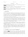
1
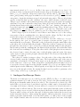
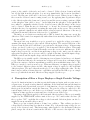
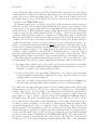
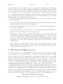
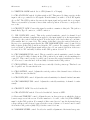
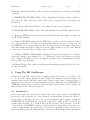
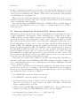
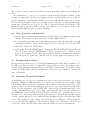
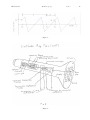
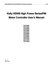
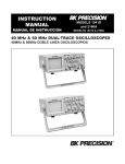
HB 01-26-09
Oscilloscope (1)
Oscilloscope
Lab 5
1
Lab 5
Equipment SWS, BK Precision model 2120B oscilloscope,Wavetek FG3C function generator,
2-3 foot coax cable with male BNC connectors,
Reading How To Use Science Workshop, pp. 170-183 (scope display). Review the “Voltage,
Current, and Resistance” writeup for the use of the SWS signal generator.
Remark The oscilloscope is a difficult instrument to understand, but it is also a very important instrument. Studying this write-up carefully before the lab will be worthwhile. This
lab cannot be approached casually.
1
Introduction
The standard instrument for examining time dependent voltages in a circuit is the oscilloscope, or “scope” for short. Even if you are doing a DC experiment it is a good idea to
look at the circuit with a scope. You might find a large AC signal symmetric with respect
to ground that does not show up on DC instruments but is affecting your experiment in
undesirable ways, such as overloading a sensitive amplifier. Oscilloscopes are ubiquitous in
the medical profession. They are seen next to hospital beds showing the electrical output of
a heart. They are used extensively in operating rooms.
A voltage which depends on time can be drawn on graph paper with the voltage on the
vertical axis and the time on the horizontal axis. If the voltage is periodic (repeats itself
after one cycle) an oscilloscope will present a similar curve. By adjusting the scope it is
possible to display part of one cycle or many cycles of the waveform. Properties of a periodic
voltage, such as shape, peak-to-peak amplitude and period, can be measured. Is that sine
wave from your signal generator distorted? Feed it into a scope and find out. Scopes have
other uses, but these are the primary subjects of this lab.
The oscilloscope is a sophisticated instrument. Competent use depends on understanding
how this instrument works. It is often necessary to consult the instruction manual for a
particular scope to use the scope effectively. The basic ideas are usually the same but are
implemented in different ways.
In this lab you will become familiar with 2 oscilloscopes, the model 2120B made by BK
Precision, and the SWS scope. Both these instruments do very much the same thing except
that the controls on the BK are mostly knobs and switches and those on the SWS are icons
such as buttons. The SWS scope is digital. The input waveform is digitized and stored, at
least for awhile. The BK scope is analogue. The input voltage may be amplified, but it is
not digitized and stored.
2
An Analogy, or the Case of the Vanishing Ink
A slowly varying periodic voltage is observed on a voltage meter. A curve of the voltage
versus time is desired. On a long strip of paper are put a vertical axis for voltage and a
horizontal axis for time. At time t1 a plot of voltage versus time is started when the voltage
has the value VT and a positive slope (voltage increasing). See Fig. 1. At time t2 it is noticed
that the ink around the point at time t1 has started to fade. There is good reason to believe
that after not too long a time the ink will vanish. The plotting is stopped at time t2 . The
HB 01-26-09
Oscilloscope (1)
Lab 5
2
time interval plotted is P = t2 − t1 . In Fig. 1 the curve to the right of t2 is dotted. No
plotting is done for a time interval N but the actual voltage is following the dotted curve. At
time t3 = t2 + N , when the voltage has positive slope and the value VT (the same values at
time t1 ) the plotting on the paper is resumed not at horizontal axis point t3 but at horizontal
axis point t1 . Again the plotting is stopped at horizontal axis point t2 . This second plotting
exactly overlays the first one and “refreshes” the curve, which otherwise would fade away.
This process is continued. Every time the plotting on the paper stops at point t2 it is resumed
after time N at point t1 when the voltage has positive slope and reaches the value VT . The
plotting always starts at the same point in the cycle. The “over” drawing of the same curve
is repeated again and again to get around the vanishing ink problem. (Note: It has been
assumed that for one cycle the same slope and VT occur only once. This will be true of all
the voltages you examine. Can you construct a periodic voltage where this is not true?)
If the voltage is periodic it should be noted that no more than one cycle of the voltage
is necessary to know everything there is to know about the voltage. In Fig. 1 the plotted
(solid) curve is more more than one cycle but less than two cycles.
Fortunately there is an instrument that does all this. It is the oscilloscope, or scope.
In the analogy, the “pen” is a pencil beam of energetic electrons and the “paper” is a
material known as a phosphor. When hit by the electrons the phosphor emits light at the
point where the electrons strike the phosphor. When the electron beam moves across the
phosphor the curve it traces can be observed by looking at the light emitted by the phosphor.
But in analogy with the vanishing ink, the light from the phosphor fades with time when
the electrons are not striking it. To keep the curve visible on the phosphor it is necessary for
the electron beam to retrace the same curve on the phosphor again and again. One sweep
of the electron beam across the phosphor takes the time P. The electron beam is shut off or
“blanked” for a time N.
The voltage VT stands for trigger voltage. It is the value of the voltage that tells the
electron beam to start the beginning of the curve. The horizontal time scale of the curve is
equivalent to how fast the electron beam is swept across the phosphor. This is determined
by the “time base” of the scope. If the voltage has a very high frequency the time base needs
to sweep the electron beam across the phosphor quickly. A good scope can display voltages
with frequencies in the MHz range. If the frequency is not high, the electron beam needs to
move across the phosphor slowly. By varying the time base it is possible to put many cycles
of the voltage on the scope or just part of one cycle.
3
Analogue Oscilloscope Basics
The heart of an analogue scope is a cathode ray tube (CRT). See Fig. 2. A cathode ray is
an historical name for a beam of electrons. The “tube” refers to the glass vacuum envelope.
Electrons are thermally emitted from a hot cathode. The electrons are accelerated (to 2 kV
in the BK scope) by an electrode and then focused into a thin beam by electrostatic lenses.
A vacuum is necessary so that the electrons will not be scattered by air molecules and so
that the cathode will not burn up. The electron beam is passed through 2 pairs of deflection
plates. A voltage across one pair of deflection plates deflects the electron beam in the vertical
direction, while a voltage across the other pair of deflection plates deflects the electron beam
in the horizontal direction. After passing through the deflection plates the electron beam
strikes a phosphor material that covers the inside surface of a flat portion of the vacuum
tube. Light is emitted where the electron beam strikes the phosphor and some of this light
HB 01-26-09
Oscilloscope (1)
Lab 5
3
passes to the outside of the tube and can be observed. If the electron beam is suddenly
cut off, the light from the phosphor does not stop immediately but decays in less than a
second. The flat part of the tube looked at is called the screen. When you are looking at
the screen the electron beam is coming toward you. By applying time dependent voltages
to the deflection plates the beam can be moved around the screen creating a pattern of light
on the phosphor often called a “trace.” As the light from the phosphor decays quickly the
trace must be continually refreshed by the electron beam so that the image on the screen
can be observed. When the trace is “stationary” or “frozen” the electron beam continually
refreshes the trace by repetitively executing the same path on the screen. The screen has
a grid or graticule, usually in cm, which enables voltages (vertical deflections of the trace)
and times (horizontal deflections of the trace) to be measured.
The image on a television screen that uses a CRT is formed the same way, except the
deflection of the beam is done magnetically rather than electrostatically. Many modern TV’s
do not use a CRT.
The most basic way in which a scope is operated is to apply the voltage you want to
examine (the input voltage) to the vertical deflection plates. The vertical deflection of the
electron beam and the trace will then be proportional to the input voltage. A linear ramp
voltage, produced by the scope, is applied to the horizontal deflection plates. This ramp
voltage sweeps the electron beam horizontally across the screen at a uniform rate. If the
input voltage is periodic, and the horizontal ramp voltage is also made periodic with an
appropriate frequency, the scope trace will be a graph of the time dependent input voltage,
with the vertical axis the input voltage and the horizontal axis the time.
The BK scope is actually capable of showing two traces (termed a dual trace or 2 channel
scope). When used this way one can input two voltages and observe how each input voltage
produces its own trace. In later experiments you will see how useful this feature can be. The
BK scope can also be used as an x-y scope. When used this way, one input voltage is applied
to the vertical deflection plates and the other input voltage is applied to the horizontal
deflection plates. The trace then shows the plot of one voltage against the other. For the
time being we will not discuss these two capabilities and will use the BK scope as a single
trace scope with the horizontal deflection voltage supplied by the scope.
4
Description of How a Scope Displays a Single Periodic Voltage
A periodic function in time is one that repeats itself again and again, such as a sine wave or
a square wave. A graph of such a function, with time on the horizontal axis and the function
on the vertical axis, repeats itself every period of the function. A scope can display a voltage
that is periodic in time in exactly the same way. The periodic voltage is connected to the
vertical input of the scope, and if the scope is adjusted correctly, a graph of the voltage as
a function of time appears as a stationary trace on the screen of the scope.
The ramp voltage that is applied to the horizontal deflection plates of the scope is usually
supplied by the TIME BASE oscillator unit of the scope. We consider that case here. (If
the scope has “X-Y” capability the voltage to the horizontal deflection plates can also be
supplied from an external voltage source.)
Every scope has a signal generator or time base oscillator. This oscillator produces a
voltage that is a linear ramp as a function of time. Fig. 3 shows the ramp voltage for one
sweep of the electron beam. This linear ramp, when applied to the horizontal deflection
plates, sweeps the electron beam from the left side of the screen to the right side of the
HB 01-26-09
Oscilloscope (1)
Lab 5
4
screen. When the ramp voltage across the horizontal deflection plates is VL , the electron
beam is at the left of the screen. When the ramp voltage is zero the beam is in the horizontal
center of the screen. When the ramp voltage is VR the beam is at the right of the screen.
We assume that |VL |=|VR |. How quickly the electron beam is swept across the screen is
controlled by the TIME BASE switch.
In the most usual mode of operation, the voltage on the horizontal deflection plates is
held at VL and the electron beam is blanked (shut off). If a “trigger” pulse is applied to the
circuit (source of the trigger pulse discussed in a moment) the electron beam is turned on
and the time base oscillator applies the ramp to the horizontal deflection plates. The input
voltage is applied to the vertical deflection plates. See Fig. 4. The electron beam is swept
across the screen from left to right at a constant speed. This takes a time P. At the same
time the vertical deflection of the electron beam is proportional to the input voltage. A spot
of light is observed to move across the screen if the sweep speed is slow enough. This spot
of light traces the input voltage for a time P. If the sweep speed is fast the trace will be too
faint to see unless many sweeps executing the same trace are made. When the ramp reaches
VR the electron beam and the light spot reach the right side of the screen. The sweep voltage
is then very quickly returned to VL . During this process the electron beam is shut off or
“blanked” so that a return trace is not seen. For a stationary trace to be properly observed
the trigger pulses must all occur at similar points of the input voltage waveform. Those
similar points are taken to be the same voltage and the same slope of the input voltage.
The trigger pulses, the pulses that start the sweep voltage, can be derived from one of the
following signals. The only one of these signals that is relevant to this lab is the first one.
1. the input voltage, which is the voltage whose waveform you are interested in examining. This is the voltage, which after suitable amplification or attenuation by the scope
electronics, is applied to the vertical deflection plates.
2. the line voltage (110 V AC wall outlet). This may be a good choice if you know that
your input signal is “synchronized” with the line voltage. The line voltage as a source
of trigger pulses is not used in this lab.
3. some other “external” voltage that is not the line voltage but that you think is synchronized with your input signal. This capability is not used in this experiment.
We consider the case where the trigger pulse is derived from the input voltage, which is the
voltage that is to be observed. The operator of the scope, by using a scope control usually
marked “trigger level”, chooses a value of the input voltage at which the trigger pulse is
to occur. We call this voltage VT . This can be a positive or negative voltage, but for the
trigger pulse to occur VT must be between between the maximum and minimum values of
the input voltage. If it is not, the trigger pulse will not occur. The scope operator can also
choose whether the trigger pulse occurs when the slope of the input voltage (with respect
to time) is positive or negative. Look at Fig. 4, which shows a sinusoidal input voltage
and the horizontal sweep voltage as a function of time. The trigger voltage VT has been
chosen as positive. The triggering slope has also been chosen as positive. Fig. 4 shows that
whenever the input voltage has a positive slope and reaches the value VT , a trigger pulse is
produced and the ramp voltage produced by the scope sweeps the electron beam horizontally
across the screen at a rate determined by the TIME BASE. In Fig. 4 the time it takes for
the electron beam to go from the left side of the screen to the right side of the screen is
designated by “P.” It does this repetitively, always starting at the “same” point of the input
HB 01-26-09
Oscilloscope (1)
Lab 5
5
voltage and always tracing out the same curve. The result is a stationary trace of the input
voltage on the scope screen. In the example shown in Fig. 4, note that somewhat less than
one cycle of the input voltage will be displayed. During the time intervals “N” the electron
beam is blanked and is not being swept across the phosphor. An additional point is that
once a sweep starts it is always completed, even if the trigger conditions are met during the
sweep. This allows the use of a low enough sweep speed so that a number of cycles of the
input waveform can be displayed on the screen.
You should understand the following statements. If you do not, please reread and study
the previous material.
• For a given input signal, if the electron horizontal sweep speed is increased, less of the
input waveform or fewer cycles will be displayed.
• If the electron horizontal sweep speed is decreased, more of the input waveform or more
cycles will be displayed.
• If the trigger voltage VT is changed, the trace of the input voltage can be shifted left or
right in a continuous fashion (exclude the square wave).
• If the trigger voltage VT is kept constant but the trigger slope is changed, the trace will
be shifted left or right. For example, Fig. 4 is drawn for triggering to occur on a positive
slope of the input voltage. If VT is kept the same but triggering were set to occur on
the negative slope of the input signal, at what points of the input signal in Fig. 4 might
triggering occur? How about a negative VT and positive slope? A negative VT and a
negative slope?
• Fig. 4 shows plots of three ramp or sweep voltages. A given ramp voltage, no matter
which of the three plots it is associated with, corresponds to the same horizontal position
of the electron beam on the screen.
5
BK Controls for Single Trace Use
This section describes the controls (knobs and switches) and connectors (jacks) of the BK
scope for single trace use. In what follows, we will use controls to mean knobs, switches,
buttons, connectors, etc. The controls that are used mainly for dual trace or x-y use will
not be discussed other than to adjust them for single trace use. There are a lot of controls,
and unless you have a physical picture of what the controls do you will not be able to use
the scope in a reasonable sort of way. Review the previous section and Fig. 1 as necessary.
Fig. 5 is a picture of the front panel of the BK scope. The controls are numbered. The
paragraphs that follow shortly are numbered according to the control being described.
At the left in Fig. 5 is the screen where the trace appear. On the right are the controls.
The controls are grouped in “boxes” according to function. All the boxes are named in Fig. 5
except the one containing items 9 and 10, which below is called GND and CAL. The boxes
are listed below along with the general function of the controls in each box. After the name
of the box, in parentheses, are the numbers of the controls that appear in that box. As you
read, identify the boxes in Fig. 5. The box names are hard to read; the number are not.
“FUNCTION” BOXES OF BK SCOPE
(Numbers in parentheses refer to the controls in the box)
HB 01-26-09
Oscilloscope (1)
Lab 5
6
• POWER(1,3)-Button (3) turns the scope on and off. LED (1) indicates when the scope
is on.
• CRT(4-6) (cathode ray tube)- controls the intensity and focus of the electron beam,
and the sharpness of the trace.
• GND and CAL(9-10)- This box is not named but provides a calibration voltage and
ground. These will not be used in this lab.
• VERTICAL(12-22)- This box is really divided into two boxes. The scope has two voltage
amplifiers for two possible input voltages. Recall that these voltages are applied to the
vertical deflection plates which is why these controls appear in the “vertical” box. The
controls for the gain of these amplifiers are in this box, channel 1 on the left and
channel 2 on the right. In this box are also controls for moving the traces up and down,
and for choosing single trace, dual trace, and x-y modes. There are also two connectors
for possible input voltages.
• HORIZONTAL(time base)(23, 26, 34)- Control the rate at which the horizontal deflection voltage is changed.
• TRIGGER(27, 29-33)- The ramp voltage that sweeps the electron beam horizontally
across the screen has to be told when to start. Rotating knob (33) enable you to select
VT . If knob (33) is in, the trigger pulse occurs on a positive slope of the input signal. If
this knob is out the trigger pulse occurs on a negative slope of the input signal. Knob
(27) moves the trace left and right.
There are a lot of knobs, switches, and connectors. If you keep the boxes in mind, and
the function of the controls in each box, you will be able to find the control(s) you need
expeditiously. The controls, numbered in Fig. 2, are now discussed, along with the initial
settings you should give them. The push button switches toggle between in and out. These
buttons should only be pushed (not pulled). Missing numbers are for controls not present
on model 2120B.
As you read through this list it tells you to set some controls at certain values or positions.
Be sure to do this so that when you turn the scope on you see a trace. With a strange scope
just finding a trace can be difficult!
1. ON indicator. Lights when scope is on.
3. POWER pushbutton. Turns scope on and off. Leave scope off (button out).
4. INTENSITY control knob. Adjusts the current in the electron beam and therefore the
brightness of the trace. Set pointer up.
5. Trace rotation. Do not adjust.
6. FOCUS control knob. Adjusts trace focus. Set pointer up.
9. Ground. Not used in this lab.
10. Calibrate. Provides a 2 V p-p 1 kH calibration square wave. Not used in this lab.
HB 01-26-09
Oscilloscope (1)
Lab 5
7
12. VERTICAL MODE switch. Set to CH1 (channel 1 or X input).
13. CH1 AC-GND-DC switch. Set this switch at AC. This puts a blocking capacitor in the
input to the scope, suitable for AC signals. If in the future you wish to look at DC signals,
choose DC. The GND position disconnects the input signal and grounds the scope input.
This is very useful if you want to know what vertical position of the trace corresponds to
zero volts.
14. CH1 INPUT JACK. Connect the signal you wish to examine to this jack. The jack is a
female Baby Type N connector, or BNC connector.
15. CH1 VOLTS/DIV control. This is the vertical sensitivity control for channel 1 and
determines the amount of amplification applied to the input signal before the input signal is
connected to the vertical deflection plates. It is the larger of two knobs that are concentric.
(The smaller knob is control 16.) The setting of this knob gives the vertical deflection of
the trace for a particular input signal if the CH1 VARIABLE/PULL control (control 16) is
fully clockwise in the CAL position and is in the “IN” position. For example, if this control
is set at 50 mV, a 100 mV input signal will produce a 2 cm vertical deflection of the trace
if control 16 is “IN” and fully clockwise in the CAL position. Set at 1 V.
16. CH1 VARIABLE/PULL control. This is a variable vertical sensitivity control for channel 1. It should be fully clockwise in the CAL position if you wish to use the markings for
control 15. This control can also be pulled out to increase the vertical sensitivity by a factor
of 5. For now, be sure the knob is in and fully clockwise in the CAL position.
17. CH1 POSITION control. Moves the trace vertically. Set the pointer up. This knob can
also be pulled out. Be sure that it is in.
18. CH2 POSITION control. Adjusts the vertical position of the channel 2 trace if there is
one. CH2 is not used in this lab.
19. CH2 VOLTS/DIV control. Adjusts the vertical sensitivity for channel 2 in fixed amounts.
20. CH2 VARIABLE/PULL control. Adjusts the vertically sensitivity of channel 2 continuously.
21. CH2 INPUT JACK. Not needed in this lab.
22. CH2 AC-GND-DC switch. Not needed in this lab, but set at GND.
23. Horizontal TIME/DIV control. Adjusts the rate, in discreet steps, at which the electron
beam is swept across the screen. For the numbers to be valid, control 26 (VAR SWEEP)
must be in the CAL position. For example, if this control is set a 5 ms, the horizontal sweep
voltage will move the electron beam across the screen a distance of 1 cm in 5 ms if control
26 is in the CAL position (fully CW). Set this control for 1 ms.
26. VARIABLE SWEEP control. Provides for variable adjustment of horizontal sweep rate.
HB 01-26-09
Oscilloscope (1)
Lab 5
8
When this control is in the CAL position, control 23 is calibrated. Set in CAL position (fully
clockwise).
27. HORIZONTAL POSITION/PULL control. Adjusts the horizontal position of the trace.
Set pointer up. This control knob can be pulled out to expand the trace horizontally. Set
the knob in.
29. X-Y button. This button should be out. (button is “in” for x-y operation.)
30. HOLDOFF/PULL CHOP control. Check that this knob is in and full counterclockwise.
31. Trigger SOURCE switch. Selects the signal from which the trigger pulse is derived. Set
at CH 1 (CH=channel).
32. Trigger COUPLING switch. In the AUTO mode, a sweep voltage is generated and a
trace appears whether or not there is an appropriate signal for the scope to trigger on. In
the NORMAL mode, a trigger pulse and trace are only generated if the input voltage has a
value that satisfies the trigger voltage level chosen. With a strange scope it is often difficult
to find a trace. For this reason, set this control at AUTO.
33. TRIGger LEVEL/PULL(-)SLOPE. Adjusts the trigger level voltage, VT . Set knob
pointer up, which is approximately VT = 0. When knob is in, scope triggers on positive
slope of signal. When knob is out, scope triggers on negative slope of input signal. Set knob
in for positive slope triggering.
34. External Trigger. The connector at which an external trigger signal is fed into the scope.
Not used in this lab.
6
Using The BK Oscilloscope
In this section the BK scope is used to examine various AC voltages. You will be able
to “see” how the voltage depends on time, measure the amplitude at various times, and
measure times between different points on the voltage vs time curve. It will probably be
helpful to refer to previous sections during these exercises. Reminder: the VOLTS/DIV and
TIME/DIV switches are not calibrated unless the knobs in the center of these switches are
fully clockwise in the calibrated positions.
6.1
Preliminaries
Remove any input cables to the scope. Turn on the scope (control 3) and observe LED (1).
In a few seconds you should see a trace which is a horizontal line (it takes the cathode a
few seconds to warm up). If you do not, check your initial control settings. Adjust the
INTENSITY (4) and FOCUS (6) controls for a sharp trace which is easy to view but not
brighter than necessary. Too bright is hard on the phosphor. Move the trace about the
screen with the 2 POSITION controls, 17 (vertical) and 27 (horizontal). Leave the trace
centered. Turn the time base switch (23) to 0.2 s and note the light spot move slowly across
the screen until it gets to the right hand side of the screen. What happens then? Investigate
HB 01-26-09
Oscilloscope (1)
Lab 5
9
the effect of turning the variable sweep rate knob (26). Increase the sweep speed one click
at a time and note how the moving spot becomes a solid line. Observe that there is a range
of sweep speeds for which the trace “flickers.” This is due to the persistence of the phosphor
or of the human eye, or perhaps both.
When you need to make measurements of an input signal (peak voltage, period, etc.), it
is useful to use the two position controls (17, 27) to move parts of the trace onto the gridlines
of the screen that have finer divisions.
Try setting the Trigger COUPLING switch (32) to NORMal. The trace should disappear,
as there is no input signal for the scope to trigger on. Set this switch back to AUTO to
retrieve the trace.
6.2
Observing Voltage From The Wavetek FG3C Function Generator
This function generator produces sine, square and triangular waveforms which are selected
by three pushbuttons. The frequency of these waveforms can be adjusted from 0.3 Hz to
3 MHz by means of a knob marked frequency and 7 pushbuttons. The output frequency
appears in the middle of the display panel. At the bottom of the display panel to the right
appear Hz, and in the middle of the bottom there may a multiplier for Hz such as k or
M. It is important to check for the k or M to determine whether the stated frequency is
in kHz or MHz. The multiplier appears and vanishes automatically as you cross certain
threshold frequencies such as 1 kHz. The amplitude of the output is varied by a knob at
the right marked AMPL. The knobs have “in” and “out” positions. The functions for the
knobs are marked in black for the “in” position and blue for the “out” position. In using
this instrument as a simple function generator be sure all the knobs at the bottom of the
front panel are in and that the only two green LED’s that are on are one for the waveform
chosen and one for the frequency range (buttons at top).
Connect the 50 Ω output of this oscillator to the CH1 vertical input (14) of the BK scope
using the coaxial cable. Set the AMPL knob full CCW and turn on both the oscillator and
scope. Adjust the Wavetek for about a 1 kHz sine wave and turn the AMPL knob CW until
you see a reasonable signal.
Vary all of the controls listed below leaving the parameters of the input voltage constant.
Note the effect on the trace of varying a control and understand why the trace changes in
the way it does. In answering the following questions make sketches of a trace if it will help
your explanation. How does the trace change if:
1. the VOLTS/DIV controls are changed (15 and 16)?
2. the TIME/DIV controls are changed (23 and 26)?
3. the trigger level (33) voltage is changed (33)? Note that if the trigger voltage is set too
high or too low the trace does not “freeze” but “runs” to the right or the left if the
trigger coupling switch is on AUTO.
4. With the trigger COUPLING switch in the NORMal mode, can you make the trace
disappear by rotating the TRIG LEVEL knob (33) both ways? Explain.
5. the triggering slope is changed from + to − (pull control 33).
6. the position controls 17 and 27 are changed?
HB 01-26-09
Oscilloscope (1)
Lab 5
10
The controls you have just used are the ones most frequently employed in adjusting the
trace.
It is instructive to look at a low frequency signal from the Wavetek oscillator. If the
frequency is appropriate, the time development of a trace as shown in Fig. 4 can be followed.
Set the frequency of the Wavetek oscillator to about 5 Hz and the time base to 50 ms.
Observe the development of the trace carefully and note the effect of changing the trigger
parameters. Change the sweep speed one click to 20 ms and increase the frequency of the
Wavetek function generator until about the same number of cycles appear on the scope.
Keep doing this until the trace becomes continuous.
6.3
Other Waveforms and Functions
• Observe square and triangular waveforms from the Wavetek by pushing the appropriate
buttons. The frequency is not critical, but around 1 kHz works well.
• Look at all the waveforms and observe what happens to the waveforms when you pull
out the Wavetek knob marked DUTY (short for duty cycle) and rotate the knob CW
and CCW. Push in the DUTY knob.
• Pull out the Wavetek OFFSET knob. Change the CH1 AC-GND-DC (13) switch from
AC to DC and rotate the OFFSET knob. What does the trace do? What does the
trace do if you change back to AC? Can you figure out how to measure the amount of
DC bias a periodic signal has? (The DC bias of a voltage signal is its average value.)
6.4
Maximum Input Voltage
An important specification of a scope is the maximum input voltage that is permitted. For
the BK scope this is ± 400 V. A small AC voltage riding on a large DC voltage can be
examined by putting the input switch (13) on AC. The average voltage of the input voltage
is removed by the input capacitor and the gain of the scope can be utilized to vet the AC
part of the signal.
6.5
Measuring Waveform Parameters
A useful function of a scope is to measure the peak to peak voltage and period of a voltage
waveform. Display a 1 kHz triangular wave on the scope. Controls 16 and 26 must be fully
CW in their calibrated positions. Adjust the other controls so that vertically the trace takes
up most of the screen and horizontally there is about one cycle of the input waveform on the
screen. Use the calibration of the VOLTS/DIV control and the horizontal grid lines on the
screen to determine the peak to peak voltage of the triangular wave. Use the calibration of
the TIME/DIV control and the vertical grid lines on the screen to determine the period of
the wave. For both of these measurements judicious use of both the horizontal and vertical
position controls will enable you to utilize the finer markings on some of the grid lines of the
screen. The amplitude of the output of the Wavetek is not calibrated. You are using the
scope to measure this amplitude. The frequency output of the Wavetek is calibrated and
you should compare the Wavetek’s stated frequency with your period measurement.
HB 01-26-09
6.6
Oscilloscope (1)
Lab 5
11
Scope Probes
In this experiment the function generator is connected to the scope by a cable with connectors
on both ends. Very often voltages in a circuit are of interest and a scope probe is used. This
is a cable with a connector on one end for plugging into the scope input. The other end of
the probe cable has an electrode for touching the point in the circuit whose voltage waveform
is desired. There is a clip for making a connection to ground. Probes often attenuate the
signal by a factor of 10 or a 100, but if they do, the resistance loading they present to the
circuit increases by a factor of 10 or a 100. Remember that in connecting a voltage measuring
device to a circuit the higher the resistance of this device the better. A probe is not used in
this lab.
7
Using The SWS Oscilloscope
One of the displays available with SWS is the oscilloscope. This is not actually an oscilloscope
but software that closely mimics an oscilloscope. In some respects the SWS scope is a more
powerful diagnostic tool than the BK scope. In particular:
1. There are 3 vertical inputs each of which has its own trace. (Three voltages can be
observed simultaneously as a function of time.) The 3 traces have different colors. The
input for each trace is selected by an input menu button.
2. This scope is a storage scope. When you stop monitoring data the last trace is stored
for further use and perusal.
3. There is a smart cursor which is used in a similar way as in the graph display.
On the other hand, the BK scope is a much faster scope. The highest frequency you can
examine with the BK scope is 30 MHz. With the SWS scope the highest frequency is 10 kHz.
The other main difference between using the BK and SWS scopes is that in the SWS scope
the controls are icon buttons, and a slider for the trigger level and slope. See page 178 of
the SWS manual for a description of adjusting the trigger level and slope. The picture in
the manual does not show this slider adequately. It is a small triangle in a vertical strip at
the very left of the scope screen. The default trigger voltage is 0 with positive slope.
There are only 2 trigger options in the SWS scope. The default is with the button at
the bottom of the scope display labeled TRIG in the in position. In this mode there must
be an appropriate input signal for a trace to be observed. This corresponds to NORMAL
for control 32 of the BK scope. If you are having trouble finding a trace, click the TRIG
button. With this button “out” the time base oscillator is free running and does not need
trigger pulses to produce a trace. This corresponds to AUTO for control 32 of the BK scope.
A difference here that that the TRIG button must be in to freeze the trace with the SWS
scope.
In using the SWS scope display, use MON rather than REC. An enormous amount of
data flows from the scope and if you use REC the storage capacity of SWS will be over
taxed.
7.1
Voltage From 750 Interface
In this section voltages from the SWS signal generator will be examined with the SWS scope.
In the right experiment setup window click the sample V button to open the signal generator
HB 01-26-09
Oscilloscope (1)
Lab 5
12
window. Click auto. Drag the scope display icon to the terminals labeled V to open the
scope display. Observe the different signals from the signal generator with the scope display
and thoroughly familiarize yourself with the controls of the SWS scope.
You may have trouble getting a trace with the 3 positive only waveforms from the SWS
signal generator. This may be due to the fact that the default trigger level is 0. Try adjusting
the trigger level for a slightly positive voltage.
A nice feature of the SWS scope is the Smart Cursor. With a good stable trace investigate
investigate this capability.
7.2
SWS Scope and the Voltage Sensor
If you are using the SWS scope to measure voltages in a circuit, use the voltage sensor. To
set this up, drag the scope icon to the voltage sensor icon. The voltage censor is not used in
this lab.
8
Analog versus Digital Scopes
In an analog scope the input voltage, after amplification or attenuation, is applied to the
vertical deflection plates of the scope. The scope trace is smooth. In a digital scope, such
as the SWS scope, the input signal is sampled at the “sampling rate” and the scope trace is
these values usually connected by straight lines. You may have noticed this fact in looking at
the SWS scope trace. One of the important specifications for a digital scope is its sampling
rate, which may be hundreds of kHz or higher. This number is the maximum sampling rate
and is the rate used at the highest sweep speeds. In reality, the actual sampling rate is lower
and is usually adjusted so that there are about a few hundred to a thousand samples per
sweep. If the sampling rate is not high enough severe distortion of the signal can result. To
get a reasonable portrayal of the signal the sampling rate should be at least ten times the
frequency of the signal.
In the SWS scope the sampling rate is adjusted automatically and is displayed at the
bottom of the scope near the Trigger button and sweep speed. For the SWS scope determine
the sampling rate for a sweep speed of 1 ms/div and then calculate the samples per sweep.
A div or division is a large division as indicated by extended lines on the graticule.
A digital scope is often a storage scope. The sampled voltages are stored and the traces
viewed after the input voltage has ceased to be sampled. In an analog scope the trace will
disappear once the signal is no longer applied to the scope.
9
Optional Exercises- NO Credit
If you fully understand the operation of the scope and have extra time, feel free to explore two
additional features of the Wavetek generator; sweep and modulation. Look at the waveforms
on the scope and adjust the controls so as to highlight the features of these waves. Although
you can use any waveform you want, it is suggested that you start with sine waves and with
setting of the TIME/DIV control of 1 ms.
• SWEEP In the sweep mode, the wavetek repetitively sweeps from a lower frequency to
a higher frequency. Set the frequency knob of the Wavetek at about 1 kHz and pull out
this knob to start the sweep function. The higher frequency is selected by this knob.
HB 01-26-09
Oscilloscope (1)
Lab 5
13
You will find that the two knobs labeled SWEEP TIME and MOD/DEPTH-SWEEP
RATE affect the waveform. Can you figure out exactly what these knobs do? Does it
make any difference whether these knobs are in or out? When you are finished, put the
frequency knob back in.
• MODULATION A “carrier (wave)” is a single frequency (sinusoidal) electromagnetic
wave. For radio broadcasting in the U.S. the carrier frequencies for AM stations lie
between 520 and 1610 kHz, and the carrier frequencies for FM stations lie between
87.5 and 108.0 MHz. Information, such as speech or music, has to be encoded on the
carrier wave. The process of encoding the information is called modulation. When
the amplitude of the carrier wave is varied it is called amplitude modulation or AM.
When the frequency of the carrier wave is varied it is called frequency modulation
or FM. Modulation at a single frequency corresponds to a pure tone. For example,
broadcasting “middle C” would require a sinusoidal modulation of about 261.6 Hz for
both AM and FM stations.
The output of the Wavetek function generator can be modulated at 400 Hz by an internally generated sine wave. The modulation can be either AM (amplitude modulation)
or FM (frequency modulation). To enable this function push the button marked MOD
ON. The knob marked MOD/DEPTH-SWEEP RATE controls whether the modulation is AM (knob in) or FM (knob out). The amount of modulation is controlled by
rotating this knob. An output or “ carrier” frequency of about 10 kHz is suggested. Observe the modulated signal on the scope. Can you measure the period of the amplitude
modulation of this wave?
10
Finishing Up
Please leave the bench as you found it. Thank you.
HB 01-26-09
Oscilloscope (1)
Figure 1:
Figure 2:
Lab 5
14
HB 01-26-09
Oscilloscope (1)
Figure 3:
Figure 4:
Lab 5
15
HB 01-26-09
Oscilloscope (1)
Figure 5:
Lab 5
16