Download B&K Precision 2530B Instruction manual

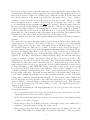
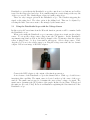
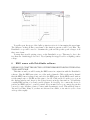
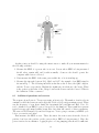
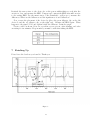
Oscilloscope and EKG sensor
Equipment DataStudio, BK Precision model 2530B oscilloscope, function generator, 2-3 foot
coax cable with male BNC connectors, BNC to female banana adapter, 1 voltage sensor, EKG
sensor, EKG Sensor Electrode Patches
Remark The oscilloscope is a difficult instrument to understand, but it is also a very important instrument. Studying this write-up carefully before the lab will be worthwhile. This
lab cannot be approached casually. The basics of a heart rate meter is an oscilloscope and
you will be using an EKG sensor to monitor your heart rate.
1
Introduction
The standard instrument for examining time dependent voltages in a circuit is the oscilloscope, or “scope” for short. Even if you are doing a DC experiment it is a good idea to
look at the circuit with a scope. You might find a large AC signal symmetric with respect
to ground that does not show up on DC instruments but is affecting your experiment in
undesirable ways, such as overloading a sensitive amplifier. Oscilloscopes are ubiquitous in
the medical profession. They are seen next to hospital beds showing the electrical output of
a heart. They are used extensively in operating rooms.
A voltage which depends on time can be drawn on graph paper with the voltage on the
vertical axis and the time on the horizontal axis. If the voltage is periodic (repeats itself
after one cycle) an oscilloscope will present a similar curve. By adjusting the scope it is
possible to display part of one cycle or many cycles of the waveform. Properties of a periodic
voltage, such as shape, peak-to-peak amplitude and period, can be measured. Scopes have
other uses, but these are the primary subjects of this lab.
The oscilloscope is a sophisticated instrument. Competent use depends on understanding
how this instrument works. It is often necessary to consult the instruction manual for a
particular scope in order to use it effectively. The basic ideas are usually the same but are
implemented in different ways.
In this lab you will become familiar with 2 oscilloscopes, the model 2530B made by
BK Precision, and the DataStudio scope. Both these instruments do very much the same
thing except that the controls on the BK are mostly knobs and switches and those on the
DataStudio are icons and buttons. The DataStudio scope is digital. The input waveform is
digitized and stored, at least for a while.
In the last section of the lab you will be using an EKG sensor. An EKG sensor monitors
your heart rate by measuring the distribution of dipoles in the heart. The EKG sensor will
be used in conjunction with the oscilloscope to see your heart cycle as a function time. You
will determine the time of your P, Q, R, S, T cardiac cycle. Each letter represents the wave
function of your heart. The P wave is the initial pulse and that goes through the atrial
muscle. The Q, R, S is the electrical waveform in the ventricular muscle The Q wave is
down, R is up and the S is down. The last part is the T wave form. It represents the
repolarization of the ventricles.
1
2
Description of How a Scope Displays a Single Periodic Voltage
A periodic function in time is one that repeats itself again and again, such as a sine wave
or a square wave. A scope can display a voltage that is periodic in time in exactly the same
way. The periodic voltage is connected to the vertical input of the scope, and if the scope is
adjusted correctly, a graph of the voltage as a function of time appears as a stationary trace
on the screen of the scope.
Figure 1:
Every scope has a signal generator or time base oscillator. This oscillator produces a
voltage that is a square wave as a function of time. Fig. 2 shows the ramp voltage for one
sweep of the electron beam. This linear ramp, when applied to the horizontal axis of the
scope screen, sweeps the beam from the left side of the screen to the right side of the screen.
When the ramp voltage across the horizontal deflection plates is VL , the beam is at the left
of the screen. When the ramp voltage is zero the beam is in the horizontal center of the
screen. When the ramp voltage is VR the beam is at the right of the screen. We assume
that |VL |=|VR |. How quickly the scope signal is swept across the screen is controlled by the
TIME/DIV switch.
Figure 2:
In the most usual mode of operation, the voltage on the horizontal axis is held at VL If a
“trigger” pulse is applied to the circuit (source of the trigger pulse discussed in a moment)
2
the electron beam is turned on and the time base oscillator applies the voltage ramp to the
horizontal axis. The input voltage is applied to the vertical axis. The signal is swept across
the screen from left to right at a constant speed. This takes a time P. At the same time
the vertical deflection of the signal is proportional to the input voltage. A spot of light is
observed to move across the screen if the sweep speed is slow enough. This spot of light
traces the input voltage for a time P. If the sweep speed is fast the trace will be too faint
to see unless many sweeps executing the same trace are made. When the ramp reaches VR
the electron beam and the light spot reach the right side of the screen. The sweep voltage
is then very quickly returned to VL . During this process the beam is shut off or “blanked”
so that a return trace is not seen. For a stationary trace to be properly observed the trigger
pulses must all occur at similar points of the input voltage waveform. Those similar points
are taken to be the same voltage and the same slope of the input voltage.
We’re interested in only one of these signals which is the voltage waveform you want to
examine.
We consider the case where the trigger pulse is derived from the input voltage, which is the
voltage that is to be observed. The operator of the scope, by using a scope control usually
marked “trigger level”, chooses a value of the input voltage at which the trigger is to occur.
We call this voltage VT . This can be a positive or negative voltage, but for the trigger to
occur VT , must be between between the maximum and minimum values of the input voltage.
If it is not, the trigger pulse will not occur. The scope operator can also choose whether the
trigger pulse occurs when the slope of the input voltage (with respect to time) is positive or
negative. Look at Fig. 3, which shows a sinusoidal input voltage and the horizontal sweep
voltage as a function of time. The trigger voltage VT has been chosen as positive. The
triggering slope has also been chosen as positive. Fig. 3 shows that whenever the input
voltage has a positive slope and reaches the value VT , a trigger pulse is produced and the
ramp voltage produced by the scope sweeps the electron beam horizontally across the screen
at a rate determined by the TIME/DIV. In Fig. 3 the time it takes for the electron beam
to go from the left side of the screen to the right side of the screen is designated by “P.” It
does this repetitively, always starting at the “same” point of the input voltage and always
tracing out the same curve. The result is a stationary trace of the input voltage on the scope
screen. In the example shown in Fig. 3, note that somewhat less than one cycle of the input
voltage will be displayed. During the time intervals “N” the electron beam is blanked and
is not being swept across the phosphor. An additional point is that once a sweep starts it is
always completed, even if the trigger conditions are met during the sweep. This allows the
use of a low enough sweep speed so that a number of cycles of the input waveform can be
displayed on the screen.
You should understand the following statements. If you do not, please reread and study
the previous material.
• For a given input signal, if the electron horizontal sweep speed is increased, less of the
input waveform or fewer cycles will be displayed.
• If the electron horizontal time/div sweep speed is decreased, more of the input waveform
or more cycles will be displayed.
• If the trigger voltage VT is changed, the trace of the input voltage can be shifted left or
right in a continuous fashion (exclude the square wave).
• If the trigger voltage VT is kept constant but the trigger slope is changed, the trace will
be shifted left or right. For example, Fig. 3 is drawn for triggering to occur on a positive
3
slope of the input voltage. If VT is kept the same but triggering were set to occur on
the negative slope of the input signal, at what points of the input signal in Fig. 3 might
triggering occur? How about a negative VT and positive slope? A negative VT and a
negative slope?
• Fig. 3 shows plots of three ramp or sweep voltages. A given ramp voltage, no matter
which of the three plots it is associated with, corresponds to the same horizontal position
of the beam on the screen.
Figure 3:
3
BK Controls for Single Trace Use
This section describes the controls (knobs and switches) and connectors (jacks) of the BK
scope for single trace use. In what follows, we will use controls to mean knobs, switches,
buttons, connectors, etc. There are a lot of controls, and unless you have a physical picture
of what the controls do you will not be able to use the scope in a reasonable sort of way.
Review the previous section and Fig. 4 as necessary.
Fig. 4 is a picture of the front panel of the BK scope. The controls are numbered. The
paragraphs that follow shortly are numbered according to the control being described.
At the left in Fig. 4 is the screen where the trace appear. On the right are the controls.
The controls are grouped in “boxes” according to function. All the boxes are named in
Fig. 4. The boxes are listed below along with the general function of the controls in each
4
box. After the name of the box, in parentheses, are the numbers of the controls that appear
in that box. As you read, identify the boxes in Fig. 4. The box names are hard to read; the
numbers are not.
“FUNCTION” BOXES OF BK SCOPE
(Numbers in parentheses refer to the controls in the box)
• POWER Button (2) turns the scope on and off.
• VERTICAL(3-4)- This box is really divided into two boxes. The scope has two possible
input voltages. The controls for the gain which are in this box, the gain for channel 1
is on the left and for channel 2 on the right. In this box are also controls for moving
the traces up and down. (11 and 12) There are also two connectors for possible input
voltages. Below the box (9 and 14)
• HORIZONTAL(time base)(5)- Controls the rate at which the horizontal deflection voltage is changed. This also affects the apperance of the signal.
• TRIGGER(6)- Determines the level at which the scope senses the signal. Rotating knob
enables you to select VT . Knob (6) moves the trace left and right.
Below is a number list that tells you the controls at certain values or positions. Be sure
to do this so that when you turn the scope on you can see a trace. With a strange scope
just finding a trace can be difficult!
Note: The controls for the gain (Voltage / Division) determines the visual appereance of
the signal on the screen.
1. Channel 1 and Run/Stop will be lit when the scope is on.
2. POWER pushbutton. Turns scope on and off. Leave scope off (button out).
6. Trigger LEVEL/KNOB. Adjusts the trigger level voltage, VT .
7. USB port to record and transfer wave forms. Not used in this lab.
8. Calibrate. Provides a 2 V p-p 1 kH calibration square wave. Not used in this lab.
9. CH1 INPUT JACK. Connect the signal you wish to examine to this jack. The jack is a
female Baby Type N connector, or BNC connector.
10. CH1 VOLTS/DIV control. This is the vertical sensitivity control for channel 1 and
determines the amount of amplification applied to the input signal before the input signal
is connected to the vertical deflection plates. The setting of this knob gives the vertical
deflection of the trace for a particular input signal. For example, if this control is set at
50 mV, a 100 mV input signal will produce a 2 cm vertical deflection of the trace.
11. CH1 POSITION control. Moves the trace vertically.
12. CH2 POSITION control. Adjusts the vertical position of the channel 2 trace if there is
one. CH2 is not used in this lab.
5
13. CH2 VOLTS/DIV control. Adjusts the vertical sensitivity for channel 2 in fixed amounts.
14. CH2 INPUT JACK. Not needed in this lab.
15. Horizontal TIME/DIV control. Adjusts the rate, in discreet steps, at which the electron
beam is swept across the screen.
16. HORIZONTAL POSITION control. Adjusts the horizontal position of the trace.
17. AUTO button.
19. External Trigger. The connector at which an external trigger signal is fed into the scope.
Not used in this lab.
Figure 4:
4
Using The BK Oscilloscope
In this section the BK scope is used to examine various AC voltages. You will be able to
“see” how the voltage depends on time, measure the amplitude at various times, and measure
times between different points on the voltage vs time curve. It will probably be helpful to
refer to previous sections during these exercises.
6
4.1
Preliminaries
Remove any input cables to the scope. Turn on the scope (2). In a few seconds you should
see a trace which is a horizontal line. If you do not, check your initial control settings and
press the AUTO button. Leave the trace centered. Turn the time base switch (15) to 0.25
s and note the light spot move slowly across the screen until it gets to the right hand side
of the screen. What happens then? Investigate the effect of turning the time base knob
(15). Increase the horizontal sweep speed one click at a time and note how the moving spot
becomes a solid line. Observe that there is a range of sweep speeds for which the trace
“flickers.”
When you need to make measurements of an input signal (peak voltage, period, etc.), it
is useful to use the two position controls (11, 16) to move parts of the trace onto the gridlines
of the screen that have finer divisions.
4.2
Observing Voltage From The Function Generator
This function generator produces sine, square and triangular waveforms which are selected
by three pushbuttons. The frequency of these waveforms can be adjusted from 0.3 Hz to
3 MHz by means of a knob marked frequency and 7 pushbuttons. The output frequency
appears in the middle of the display panel. At the bottom of the display panel to the right
appear Hz, and in the middle of the bottom there may a multiplier for Hz such as k or M.
It is important to check for the k or M to determine whether the stated frequency is in kHz
or MHz. The multiplier appears and vanishes automatically as you cross certain threshold
frequencies such as 1 kHz. The amplitude of the output is varied by a knob at the right
marked AMPL. The knobs have “in” and “out” positions. The functions for the knobs are
marked in black for the “in” position and blue for the “out” position. While using this
instrument as a simple function generator be sure all the knobs at the bottom of the front
panel are in and that the only two green LED’s that are on are one for the waveform chosen
and one for the frequency range (buttons at top). Below is an illustration of some of the
buttons and the output you will be using from the function generator.
7
Connect the 50 Ω output of this oscillator to the CH1 vertical input (9) of the BK scope
using the coaxial cable. See Fig. 5.
Figure 5:
Set the AMPL knob full CCW and turn on both the oscillator and scope. Adjust the
function generator for about a 1 kHz sine wave and turn the AMPL knob to the center.
On the Oscilloscope adjust the Time/DIV and Voltage/DIV knob until you see a reasonable
sinewave signal.
Vary all of the controls listed below leaving the parameters of the input voltage constant.
Note the effect on the trace of varying a control and understand why the trace changes in
the way it does. In answering the following questions make sketches of a trace if it will help
your explanation. How does the trace change if:
1. The VOLTS/DIV controls are changed?
2. The TIME/DIV controls are changed?
3. The trigger level voltage is changed? Note that if the trigger voltage is set too high
or too low the trace does not “freeze” but “runs” to the right or the left if the trigger
coupling switch is on AUTO.
4. Next step is to click on the AUTO button. Then rotate the TRIG LEVEL knob in both
directions? Can you make the trace disappear? Explain.
5. The triggering slope changed from + to −? (To change the slope, push the trig menu
button and then push the button next to ”slope” on the screen.)
6. The position controls are changed?
The controls you have just used are the ones most frequently employed in adjusting the
trace.
8
4.3
Other Waveforms and Functions
• Observe square and triangular waveforms from the function generator by pushing the
appropriate buttons. The frequency is not critical, but around 1 kHz works well.
4.4
Measuring Waveform Parameters
In this section you will be looking at AC waveforms again. A useful function of a scope is
to measure the peak to peak voltage and period of a voltage waveform. Display a 1 kHz
triangular wave on the scope. Adjust the other controls so that vertically the trace takes
up most of the screen and horizontally there is about one cycle of the input waveform on
the screen. Use the calibration of the VOLTS/DIV control to adjust how many volts per
box. On the left bottom corner of the screen will show the voltage division of horizontal grid
lines. Next, determine the peak to peak voltage of the triangular wave. Use the calibration
of the TIME/DIV control and the vertical grid lines on the screen to determine the period
of the wave. The display of the current time scale will be located in the middle bottom of
the screen. For both of these measurements judicious use of both the horizontal and vertical
position controls will enable you to utilize the finer markings on some of the grid lines of the
screen. The amplitude of the output of the function generator is not calibrated. You are
using the scope to measure this amplitude. The frequency output of the function generator is
calibrated and you should compare the function generator stated frequency with your period
measurement.
• Set the function generator to have a triangle wave output at 1Khz.
• On the function generator turn the amplitude knob fully clockwise.
• Use the oscilloscope to determine the peak and peak-to-peak voltages of the triangle
wave.
• Repeat for the sine and the square waveforms at 1 khz.
• On the function generator turn the the amplitude knob to the middle and determine
the peak and peak-to-peak voltages of all three waveforms at 1khz.
5
Using The DataStudio Oscilloscope
One of the displays available with DataStudio is the oscilloscope. This is not actually an
oscilloscope but software that closely mimics an oscilloscope.
1. The input for each trace is selected by an input menu button.
2. This scope is a storage scope. When you stop monitoring data the last trace is stored
for further use.
3. There is a smart cursor which is used in a similar way as in the graph display. It is
located on the top left of the DataStudio scope.
In comparison to the DataStudio oscilloscope, the BK scope is a much faster scope. The
highest frequency you can examine with the BK scope is 25 MHz. With the DataStudio
scope the highest frequency is 10 kHz. The other main difference between using the BK and
9
DataStudio scopes is that in the DataStudio scope the controls are icon buttons, and a slider
is used for the trigger level and slope. It is a small triangle in a vertical strip at the very left
of the scope screen. The default trigger voltage is 0 with positive slope.
There are only 2 trigger options in the DataStudio scope. The default is triggering the
signal on the rising level. The other option is the falling level. This can be adjusted by
selecting the little down arrow next to the triangle by the smart cursor.
5.1
Using the DataStudio Scope with the Voltage Sensor
In this section AC waveforms from the Wavetek function generator will be examined with
the DataStudio scope.
When you’re using the DataStudio scope to measure voltages in a circuit, use the voltage
sensor. To set up the voltage sensor, plug it into the 750 interface. In the DataStudio
experiment setup window click on the analog channel of the 750 interface that the voltage
sensor is plugged into. A drop down window will appear. Select voltage sensor. Next,
drag the scope icon to the voltage sensor icon. Plug the voltage sensor into the bnc banana
adapter. Below is an image of the BNC adapter.
Connect the BNC adapter to the output of the function generator.
A nice feature of the DataStudio scope is the Smart Cursor. With a good stable trace
investigate this capability. The smart cursor is located on the top left corner of the scope
window. The smart cursor is used to determine the exact voltage or time of a signal. The
smart cursor determines the (X,Y) values of the graph. In this case its (Time, Voltage) and
the units are (Seconds, Volts). Below is an illustration explaining the basic functions of the
DataStudio scope.
10
You will repeat the steps of the bullet points in section 4.4 of measuring the waveforms.
The difference is that all three waveforms of the function generator will be at 2 Khz. The
DataStudio scope will be used to determine the peak and the peak-to-peak voltages of all
three wave forms.
You may have trouble getting a trace on the DataStudio scope. This may be due to the
fact that the default trigger level is 0. Try adjusting the trigger level for a slightly positive
voltage.
6
EKG sensor with DataStudio software
BEFORE YOU START THIS SECTION OF THE EXPERIMENT RESTART THE DATASTUDIO SOFTWARE!
This time around you will be using the EKG sensor in conjunction with the DataStudio
software. Plug the EKG sensor into one of the analog channels. Click on the analog channel
that the EKG sensor is plugged into and select the EKG sensor. In the EKG sensor window
set the sample rate to 200 Hz and the gain to low 1X. Click and hold on the scope icon in
the displays window and drag it to the voltage heart icon in the data window. You will take
a resting EKG reading of you and your lab partner. Look at Fig. 6 to connect the electrode
patches and EKG sensor to your lab partner. Keep in mind before you connect the patches
you need to wipe all three points of contact with an antiseptic towel. This will help remove
dirt and dead skin. Many of you have not showered in a while, so its wise for you to clean
each spot thoroughly.
11
Figure 6:
At this point you should be using the smart cursor to make all your measurements for
the following activities.
1. Measure the EKG of a person who is at rest. Person whose EKG is being measured
should relax, remain still, and breathe normally. Someone else should operate the
computer while data is collected.
2. Next measure the EKG of the same person while she or he is standing up.
3. Measure the intervals between P-Q, QRS, and Q-T. An example of an EKG signal is
shown in Fig. 7. The following intervals are known as the P wave, the QRS complex,
and the T wave, respectively. Explain the significance in relation to the heart. What
is the peak-to-peak value of the voltage between the R wave and the S wave? What is
the definition of this occurrence?
6.1
Additional questions and exercise
The sequence from P wave to T wave represents on heart cycle. The number of such cycles in
a minute is called the heart rate and is typically 70-80 cycles (beats) per minute at rest. What
was the frequency of your heart during the experiment (in beats/min and Hz)? Note: Do
not be alarmed if your EKG does not correspond to the numbers. These numbers represent
typical averages and many healthy hearts have data that fall outside of these parameters.
The sensor is NOT intended for medical diagnoses. You’re going to meaure your EKG cycle
before you exercise and after!
First measure the EKG at rest. Then disconnect the sensor wires from the electrode
patches, but leave the patches on the person whose EKG is being measured. Have the
person exercise for two minutes. Jogging in place or doing jumping jacks should be sufficient.
12
Reattach the sensor wires to the electrodes on the person within thirty seconds after the
exercise is done, and measure the EKG. Compare and contrast the EKG after mild exercise
to the resting EKG. Use the smart cursor of the DataStudio oscilloscope to measure the
differences. What are the differences and the significances of said differences?
Now, reverse the placement of the electrodes (place the green alligator clip on the left
electrode and the red alligator clip on the right one). Measure the EKG again. What
happens to the signal? Note and explain briefly the difference. Print the graph.
Create a table as shown below for you when you are at rest, after standing, and after
exercising for two minutes. Keep in mind you must be still when taking the EKG.
7
Finishing Up
Please leave the bench as you found it. Thank you.
Figure 7:
13