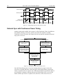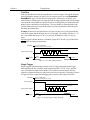
1
4411-0087 Version 2.H December 3, 2002 *4411-0087* Copyright 2002 Roper Scientific, Inc. 3660 Quakerbridge Rd Trenton, NJ 08619 TEL: 609-587-9797 FAX: 609-587-1970 All rights reserved. No part of this publication may be reproduced by any means without the written permission of Roper Scientific, Inc. Printed in the United States of America. IPLab is a trademark of Scanalytics, Inc. Logitech is a registered trademark of Logitech. Mac and Macintosh are registered trademarks of Apple Computer, Inc. NuBus is a trademark of Texas Instruments. Pentium is a trademark of Intel Corporation. Programmable Timing Generator is a trademark and PI-MAX is a registered trademark of Roper Scientific, Inc. Radio Shack is a registered trademark of TRS Quality, Inc. SpectraPro is a registered trademark of Acton Research Corporation. Windows, Windows 2000, Windows XP, Windows 95, and Windows NT are registered trademarks of Microsoft Corporation in the United States and/or other countries. The information in this publication is believed to be accurate as of the publication release date. However, Roper Scientific, Inc. does not assume any responsibility for any consequences including any damages resulting from the use thereof. The information contained herein is subject to change without notice. Revision of this publication may be issued to incorporate such change. Table of Contents Manual Overview ..................................................................................................7 Safety Related Symbols Used in This Manual ................................................................... 8 Chapter 1 Description ..........................................................................................9 Introduction......................................................................................................................... 9 Chapter 2 Getting Started ..................................................................................11 Introduction....................................................................................................................... 11 Unpacking......................................................................................................................... 11 Equipment and Parts Inventory......................................................................................... 11 Grounding and Safety ....................................................................................................... 12 Environmental Requirements ........................................................................................... 12 Power Requirements ......................................................................................................... 12 Computer Requirements ................................................................................................... 14 Controller Features ........................................................................................................... 15 Software Installation......................................................................................................... 24 Imaging Field of View...................................................................................................... 24 Summary........................................................................................................................... 25 Chapter 3 First Light ..........................................................................................27 Introduction to Imaging .................................................................................................... 27 Procedure .......................................................................................................................... 28 Introduction to Spectroscopy............................................................................................ 30 Spectroscopy Procedure.................................................................................................... 31 Summary........................................................................................................................... 34 Chapter 4 Temperature Control ........................................................................35 Introduction....................................................................................................................... 35 Cooling (TE, RTE, PI-MAX) ........................................................................................... 36 Cooling (LN) .................................................................................................................... 36 Cooling and Vacuum ........................................................................................................ 37 Problems ........................................................................................................................... 37 Chapter 5 Timing Modes....................................................................................39 Full Speed or Safe Mode .................................................................................................. 39 Standard Timing Modes ................................................................................................... 40 External Sync with Continuous Cleans Timing................................................................ 44 Internal Sync ..................................................................................................................... 45 Frame Transfer Mode ....................................................................................................... 45 Kinetics Mode................................................................................................................... 47 Timing Modes................................................................................................................... 48 iii iv ST-133/ST-133A Controller Manual Version 2.H Chapter 6 Exposure and Readout.....................................................................51 Exposure ........................................................................................................................... 51 Readout of the Array ........................................................................................................ 54 Digitization ....................................................................................................................... 59 Appendix A Specifications ................................................................................61 CCD Arrays ...................................................................................................................... 61 Temperature Control......................................................................................................... 61 Inputs ................................................................................................................................ 61 Outputs.............................................................................................................................. 62 A/D Converters ................................................................................................................. 62 Exposure (integration) Time............................................................................................. 62 Shutter Compensation Time ............................................................................................. 63 Computer Requirements ................................................................................................... 63 Miscellaneous ................................................................................................................... 63 Appendix B PTG Module....................................................................................65 Description........................................................................................................................ 65 Specifications.................................................................................................................... 66 Operation .......................................................................................................................... 69 Appendix C TTL Control ....................................................................................73 Introduction....................................................................................................................... 73 TTL In............................................................................................................................... 73 Buffered vs. Latched Inputs.............................................................................................. 74 TTL Out ............................................................................................................................ 74 TTL Diagnostics Screen ................................................................................................... 75 Hardware Interface ........................................................................................................... 75 Appendix D Cleaning Instructions....................................................................77 Controller and Camera...................................................................................................... 77 Optical Surfaces................................................................................................................ 77 Appendix E Outline Drawing of ST-133/ST-133A Controller .........................79 Appendix F Plug-In Modules ............................................................................81 Introduction....................................................................................................................... 81 Removing/Installing a Module ......................................................................................... 81 Appendix G Interline CCD Cameras .................................................................83 Introduction....................................................................................................................... 83 Camera .............................................................................................................................. 83 Overlapped vs. Non-Overlapped Operation ..................................................................... 84 Timing Options in Overlapped Readout Mode ................................................................ 84 Exposure ........................................................................................................................... 86 Readout of the Array ........................................................................................................ 88 Table of Contents v Appendix H DIF Camera (Double Image Feature)............................................93 Introduction....................................................................................................................... 93 Timing Modes................................................................................................................... 94 Tips and Tricks ............................................................................................................... 101 Appendix I Installing the Computer Interface ................................................103 Introduction..................................................................................................................... 103 PCI Serial Buffer Board.................................................................................................. 103 Installing the PCI Card Driver ........................................................................................ 104 ISA Serial Card............................................................................................................... 107 Warranty & Service...........................................................................................111 Limited Warranty: Roper Scientific Analytical Instrumentation ................................... 111 Contact Information........................................................................................................ 114 Index ..................................................................................................................115 Figures Figure 1. Power Input Module......................................................................................... 13 Figure 2. ST-133/ ST-133A front and rear panels........................................................... 15 Figure 3. Back panel of ST-133 or ST-133A with 70 V shutter option .......................... 16 Figure 4. Monitor display of CCD image center area ..................................................... 19 Figure 5. WinView/32 Controller/Camera Setup tab page.............................................. 20 Figure 6. and SHUTTER MONITOR signals..................................................... 21 Figure 7. Imaging field of view ....................................................................................... 24 Figure 8. System, TE camera connection diagram .......................................................... 29 Figure 9. System connection diagram, TE camera .......................................................... 31 Figure 10. Chart of Safe (ASynchronous) and Full Speed Mode (Synchronous) operation ...41 Figure 11. Free Run timing chart, part of the chart in Figure 10..................................... 42 Figure 12. Free Run timing diagram................................................................................ 42 Figure 13. Chart showing two External Sync timing options.......................................... 43 Figure 14. Timing diagram for the External Sync mode ................................................. 44 Figure 15. Continuous Cleans operation flow chart ........................................................ 44 Figure 16. Continuous Cleans timing diagram ................................................................ 45 Figure 17. Frame Transfer where tw1 + texp + tc < tR ...................................................... 46 Figure 18. Frame Transfer where tw1 + texp + tc > tR...................................................... 47 Figure 19. Frame Transfer where pulse arrives after readout ......................................... 47 Figure 20. Kinetics Readout ............................................................................................ 48 Figure 21. Hardware Setup dialog box ............................................................................ 48 Figure 22. Experiment Setup dialog box ......................................................................... 48 Figure 23. Free Run Timing Diagram ............................................................................. 49 Figure 24. Single Trigger Timing Diagram ..................................................................... 49 Figure 25. Multiple Trigger Timing Diagram ................................................................. 50 Figure 26. Block diagram of light path in system............................................................ 51 Figure 27. Exposure of the CCD with shutter compensation .......................................... 52 Figure 28. Full Frame at Full Resolution ........................................................................ 55 Figure 29. 2 × 2 binning for images ................................................................................ 57 vi ST-133/ST-133A Controller Manual Figure 30. Figure 31. Figure 32. Figure 33. Figure 34. Figure 35. Figure 36. Figure 37. Figure 38. Figure 39. Figure 40. Figure 41. Figure 42. Figure 43. Figure 44. Figure 45. Figure 46. Figure 47. Figure 48. Figure 49. Figure 50. Figure 51. Figure 52. Figure 53. Figure 54. Figure 55. Figure 56. Figure 57. Figure 58. Version 2.H Frame Transfer readout .................................................................................. 59 ST-133A with Programmable Timing Generator........................................... 65 Auxiliary Trigger Output ............................................................................... 66 Typical system cabling................................................................................... 69 Camera State dialog box ................................................................................ 70 PTG dialog box .............................................................................................. 71 Pulsers dialog box .......................................................................................... 71 Experiments with the PI-MAX....................................................................... 72 TTL In/Out Connector ................................................................................... 75 Controller dimensions .................................................................................... 79 Module Installation ........................................................................................ 82 Overlapped mode where tw1 + texp + tc < tR................................................... 85 Overlapped mode where tw1 + texp + tc > tR ................................................... 85 Overlapped mode where pulse arrives after readout...................................... 86 Exposure of the CCD with shutter compensation (non-overlapped mode) ... 87 Overlapped mode Exposure and Readout ...................................................... 89 Non-overlapped mode Exposure and Readout ............................................... 90 2 × 2 binning for images ................................................................................ 91 Freerun mode timing ...................................................................................... 95 Setup using to trigger an event........................................................ 95 Timing for experiment setup shown in Figure 49 .......................................... 95 Timing diagram for typical IEC measurement ............................................... 97 Setup for IEC experiment with two lasers ..................................................... 97 Timing diagram for IEC experiment with two lasers..................................... 98 Another hardware setup for an IEC measurement ......................................... 98 EEC timing example with exposure time in software set to tex ...................... 99 ESABI timing example; image exposure time = texp set in software............ 100 ISA board switch and jumper settings.......................................................... 108 Computer expansion slots for installing an ISA Buffer card ....................... 109 Tables Table 1. Shutter setting selection..................................................................................... 16 Table 2. Approximate temperature range vs. CCD model .............................................. 36 Table 3. Camera timing modes ........................................................................................ 39 Table 4. Approximate readout time of a single frame for some CCD arrays.................. 56 Table 5. Well capacity for some CCD arrays .................................................................. 58 Table 6. Bit values with decimal equivalents: 1 = High, 0 = Low ................................. 74 Table 7. TTL In/Out connector pinout ............................................................................ 75 Table 8. PCI Driver Files............................................................................................... 105 Table 9. I/O Address & Interrupt Assignments Before Installing Serial Card.............. 106 Table 10. I/O Address & Interrupt Assignments After Installing Serial Card .............. 106 Manual Overview Chapter 1, Description provides an overview of the ST-133 or ST-133A Controller and Camera. Chapter 2, Getting Started discusses introductory topics such as unpacking, equipment inventory, grounding and power requirements. It also includes detailed descriptions of the controller and camera features, together with information on mounting the camera and lens. Chapter 3, First Light provides a step-by-step procedure for placing the system in operation the first time. Chapter 4, Temperature Control discusses how to establish and maintain temperature control. Also provides information on the effects of long-term vacuum degradation on cooling capability and temperature control. Chapter 5, Timing Modes discusses the basic Controller timing modes and related topics, including Synchronous vs. Asynchronous, Free Run, External Sync, Continuous Cleans and Frame Transfer. Chapter 6, Exposure and Readout discusses Exposure and Readout, together with many peripheral topics, including shuttered and unshuttered exposure, saturation, dark charge, binning and frame-transfer readout. Appendix A, Specifications includes complete controller and camera specifications. Appendix B, PTG Module contains a description of the Programmable Timing Generator™ (PTG) together with the PTG specifications and operating instructions. Appendix C, TTL Control discusses the purpose and operation of the TTL In/Out function. Appendix D, Cleaning Instructions discusses how to clean the system Controller, Camera and optics. Appendix E, Outline Drawing contains outline drawings of the Controller and Camera. Appendix F, Plug-In Modules provides a brief overview of the plug-in modules, including directions for their installation and removal. Appendix G, Interline CCD Cameras describes operating considerations for cameras having an Interline CCD. Appendix H, MicroMAX DIF Camera describes DIF (Dual Image Feature) camera and its operation. Appendix I, Installing the Computer Interface provides detailed directions for mounting the High Speed Serial card in the computer and connecting it with the Controller. 7 8 ST-133/ST-133A Controller Manual Version 2.H Safety Related Symbols Used in This Manual Caution! The use of this symbol on equipment indicates that one or more nearby items should not be operated without first consulting the manual. The same symbol appears in the manual adjacent to the text that discusses the hardware item(s) in question. Caution! Risk of electric shock! The use of this symbol on equipment indicates that one or more nearby items pose an electric shock hazard and should be regarded as potentially dangerous. This same symbol appears in the manual adjacent to the text that discusses the hardware item(s) in question. Chapter 1 Description Introduction Overview: The Model ST-133 or ST-133A is a compact, high performance CCD Camera Controller for operation with Princeton Instruments* cameras. Designed for high speed and high performance image acquisition, the controller offers data transfer at speeds up to 1 megapixel per second, standard video output for focusing and alignment and a wide selection of A/D converters to meet a variety of different speed and resolution requirements. Function: Able to operate with a variety of different cameras and CCD arrays, with support for several popular computer platforms and application software packages, the ST-133 or ST-133A Controller makes it possible to assemble an image acquisition system precisely tailored to your specific needs. In operation, analog data acquired by the camera is routed to the controller where it is converted to digital data by specially designed, low-noise electronics supporting a scientific grade Analog-to-Digital (A/D) converter. Two complete analog channels, each with its own A/D converter, are available, with switching between the two channels under software control for total experiment automation.* Modular Design: In addition to containing the power supply, the controller contains the analog and digital electronics, scan control and exposure timing hardware, and controller I/O connectors, all mounted on user-accessible plug-in modules. A Programmable Timing Generator™ (PTG) module is also available that allows the controller to be used in conjunction with the PI-MAX® camera (formerly the ICCDMAX camera) in gated experiments without need for an external timing generator. This highly modularized design gives flexibility and allows for convenient servicing. Flexible Readout: There is provision for extremely flexible readout of the CCD. Readout modes supported include full resolution, simultaneous multiple subimages, and nonuniform binning. Single or multiple software-defined regions of interest can also be * The ST-133/ST-133A controller must be factory configured for operation with an LN detector. For this reason, a controller purchased for operation with an LN detector can only be used with an LN detector. Similarly, a controller purchased for operation with a TE or RTE detector cannot be used with an LN detector. * Depending on the camera with which the ST-133/ST-133A is intended to operate, a given ST-133 may support one or two A/D converters. The converter(s) must be specified at the time of purchase. 9 10 ST-133/ST-133A Controller Manual Version 2.H tested without having to digitize all the pixels of the array. Completely flexible exposure, set through software, is also fully supported. High Speed Data Transfer: Data is transferred directly to the host computer memory via a high-speed serial link. A frame buffer with standard composite video, either RS-170 (EIA) or CCIR, whichever was ordered, is also provided. The digital data at the output of the A/D converter is then transferred at high speeds to the host computer. A proprietary Interface card places the data from the controller directly into the host computer RAM using Direct Memory Access (DMA). The DMA transfer process ensures that the data arrives at sufficiently high speed to prevent data loss from the controller. Since the data transfer rate is much higher than the output rate from the A/D, the latter becomes the limiting factor for the data acquisition rate. Once the digital data is in RAM, the image acquisition program can transfer the image into its own working RAM for viewing and further processing. Applications: With its small size, fully integrated design, support for a variety of cameras, CCD arrays, and computers, temperature control, advanced exposure control timing, and sophisticated readout capabilities, the ST-133 or ST-133A Controller is well suited to both general spectroscopy, macro imaging and microscopy applications. Chapter 2 Getting Started Introduction This chapter will help you get off to a good start with your ST-133 or ST-133A Controller. In addition to descriptions of such basics as unpacking and grounding safety, the chapter includes discussions of the requirements that have to be met before the camera can be switched on. Included are environmental, power, computer, and software requirements. Also provided are descriptions of the front and rear panels of the components, together with discussions of mounting, imaging and other topics. Users are advised to read this chapter in its entirety before powering up the system. Unpacking During unpacking, check the controller for possible signs of shipping damage. If there are any, notify Roper Scientific and file a claim with the carrier. If damage is not apparent but controller specifications cannot be achieved, internal damage may have occurred in shipment. Equipment and Parts Inventory The complete system consists of a camera, a controller and other components as follows: • Camera to Controller cable: DB25 to DB25 cable. Standard length is 10 ft (6050-0321). Also available in 6’, 15’, 20’, and 30’ lengths. • Controller to Computer (TAXI) cable: DB9 to DB9 cable. Standard length is 25 ft (6050-0148-CE). Lengths up to 165 ft (50 m) are available. • PTG to PI-MAX cable: (6050-0369 or 6050-0406) if PTG is installed. This cable interconnects the Timing Gen connector on the PTG module with the Timing Gen connector on the PI-MAX. • Computer: Can be purchased from Roper Scientific or provided by user. • High Speed PCI Interface board: This board must be installed in the computer (computers purchased from Roper Scientific will be shipped with the board already installed). 11 12 ST-133/ST-133A Controller Manual • Version 2.H System Dependent Interface Components: Note: For convenience, in the following operating-procedure discussions, this manual refers to a Pentium™ PC equipped with a PCI high-speed interface card and using WinView/32 software. Nevertheless, the manual does apply as well to operation with other computers and software. Interface components, as follows, could be required. • Intensified cameras would additionally require a high-voltage power supply and/or gate pulser. Note: The PI-MAX camera is an exception because its high-voltage pulsing circuits are internal. It would, however, still require a PTG or DG535 Timing Generator. Grounding and Safety The apparatus described in this manual is of Class I category as defined in IEC Publication 348 (Safety Requirements for Electronic Measuring Apparatus). It is designed for indoor operation only. Before turning on the controller, the ground prong of the power cord plug must be properly connected to the ground connector of the wall outlet. The wall outlet must have a third prong, or must be properly connected to an adapter that complies with these safety requirements. WARNING If the equipment is damaged, the protective grounding could be disconnected. Do not use damaged equipment until its safety has been verified by authorized personnel. Disconnecting the protective earth terminal, inside or outside the apparatus, or any tampering with its operation is also prohibited. Inspect the supplied power cord. If it is not compatible with the power socket, replace the cord with one that has suitable connectors on both ends. WARNING Replacement power cords or power plugs must have the same polarity as that of the original ones to avoid hazard due to electrical shock. Environmental Requirements • Storage temperature -20°C to 55°C • Operating environment 0°C to 30°C • Operating temperature range over which specifications can be met is 18° C to 23° C • Relative humidity ≤80% noncondensing. Power Requirements The ST-133 or ST-133A controller can operate from any one of four different nominal line voltages: 100, 120, 220, or 240 V AC. The power consumption is nominally 300 watts and the line frequency can range from 47 to 63 Hz. The plug on the line cord supplied with the controller should be compatible with the linevoltage outlets in common use in the region to which the controller is shipped. If the line cord plug should prove to be incompatible, a compatible plug should be installed, taking Chapter 2 Getting Started 13 care to maintain the proper polarity to protect the equipment and assure user safety. EXT. TRIG. IN EXT. TRIG. IN PRE. TRIG. IN PRE. TRIG. IN T0 T0 SHUTTER CONTROL SHUTTER CONTROL TIMING GEN. TIMING GEN. REMOTE SETTING REMOTE SETTING 50-60Hz 300 W MAX. FUSES: LEFT: RIGHT: 100 - 120V ~ 0.75A - T 2.50A - T 220 - 240 V ~ 0.30A - T 1.25 A - T 300 W MAX. 50-60Hz FUSES: LEFT: RIGHT: 100 - 120V ~ 0.75A - T 2.50A - T 220 - 240 V ~ 0.30A - T 1.25 A - T AUX. TRIG. OUT AUX. TRIG. OUT ~ 120Vac TRIG. TRIG. Figure 1. Power Input Module The power module contains the voltage selector drum, fuses and the power cord connector. The appropriate voltage setting is set at the factory and can be seen on the back of the power module. Each setting actually defines a range and you should select the setting that is closest to the actual line voltage. The fuse and power requirements are printed on the panel above the power module. As shown in Figure 1, the Power Module contains two fuses. The two fuses are of different values and both change according to the value of the selected line voltage as indicated on the back panel. The correct fuses for the country where the ST-133 or ST-133A is to be shipped are installed at the factory. WARNING Be sure to use the proper fuse values and types for the controller and camera to be properly protected. To change the line-voltage setting or replace a fuse, proceed as follows. WARNING Before opening the power module, be sure to unplug the line cord. 1. Take a flat blade screwdriver, place the flat side parallel to the back of the controller and pointing downward behind the small tab at the top of the power module, and twist the screwdriver slowly but firmly to pop the module open. See Figure 1. 2. To change the voltage setting, roll the selector drum until the appropriate voltage setting is facing outwards. 14 ST-133/ST-133A Controller Manual Version 2.H 3. Confirm the fuse ratings by removing the white fuse holders. To do so, simply insert the flat blade of the screwdriver behind the front tab of each fuse holder and gently pry the assembly out. 4. After inspecting and if necessary, changing the fuses, reinstall the holders with the arrow facing to the right. 5. Close the power module and verify that the correct voltage setting is displayed. Computer Requirements Host Computer Type Note: The following information is only intended to give an approximate indication of the computer requirements. Please contact the factory to determine your specific needs. PC System • AT-compatible computer with 80486 (or higher) processor (50MHz or faster), Pentium or better recommended. • Windows® 95 (or higher) or Windows NT® (version 4.0 or higher) operating system. • High speed PCI serial card or at least one unused PCI card slot. Computers purchased from Roper Scientific are shipped with card installed. • Minimum of 32 Mbyte of RAM for CCDs up to 1.4 million pixels. Collecting multiple images or spectra at full frame or high speed may require 128 Mbytes or more of RAM. • CD-ROM drive • Hard disk with a minimum of 80 Mbytes available. A complete installation of the program files takes about 6 Mbytes and the remainder is required for data storage, depending on the number and size of images or spectra collected. Disk level compression programs are not recommended. • Super VGA monitor and graphics card supporting at least 256 colors with at least 1 Mbyte of memory. Memory requirement is dependent on desired display resolution. • Two-button Microsoft compatible serial mouse or Logitech three-button serial/bus mouse. Chapter 2 Getting Started 15 Controller Features Front Panel POWER Switch and Indicator: The power switch, which is located on the front panel as shown in Figure 2 (left), interrupts both sides of the controller’s AC power input. The switch’s indicator LED lights whenever the ST-133 or ST-133A is powered. Note that, when the power switch is actuated, there is a short delay before the indicator lights. This is normal and in no way indicative of a malfunction. EXT. TRIG. IN PRE. TRIG. IN T0 SHUTTER CONTROL TIMING GEN. REMOTE AUX. TRIG. OUT SETTING 50-60Hz 300 W MAX FUSES: LEFT: RIGHT: 100 - 120V ~ 0.75A - T 2.50A - T 220 - 240 V ~ 0.30A - T 1.25 A - T ~ 120Vac TRIG. I ROPER SCIENTIFIC, Inc. 0 Figure 2. ST-133/ ST-133A front and rear panels Back Panel Fan: There is an internal fan located at the back panel behind the exhaust grill. Its purpose is simply to cool the controller electronics. This fan runs continuously whenever the controller is powered. Air enters the unit through ventilation slots on the sides and bottom, flows past the warm electronic components as it rises, and is drawn out the rear of the controller by the fan. It is important that there be an adequate airflow for proper functioning. As long as both the controller’s intake ventilation slots and the fan aren’t obstructed, the controller will remain quite cool. Shutter Control:* Directly below the fan are the Shutter Power connector and the Shutter Setting dial. The Shutter Power connector can be used to drive an external shutter if the camera isn’t equipped with an internal shutter. * If an ST-133/ST-133A is shipped with a camera having an Interline CCD chip, the Shutter Control Remote connector and Setting dial may not be supplied. If this is the case, the corresponding panel openings will be plugged. 16 WARNING! ST-133/ST-133A Controller Manual Version 2.H If the camera is equipped with an internal shutter, then the Shutter Power connector should not be used to drive an external (second) shutter. This configuration will result in under-powering both shutters and may cause damage to the system. In a system that requires both an internal and an external shutter, use the TTL Shutter Monitor signal, provided as the default output at the connector, to control the external shutter. Suitable driver electronics will also be required. See the Note on page 20 for information on how the signal provided at the connector is selected. REMOTE: The shutter-drive pulses are provided at the Remote connector. WARNING: Dangerous live potentials are present at the Remote Shutter Power connector. To avoid shock hazard, the Controller power should be OFF when connecting or disconnecting a remote shutter. SETTING: The Shutter Setting selector sets the shutter hold voltage. Each shutter type, whether internal or external, requires a different setting. Consult the table below to determine the proper setting for your shutter. The Shutter Setting dial is correctly set at the factory for the camera’s internal shutter if one is present. Note: With a PI-MAX camera, the setting doesn’t matter, unless the system includes an external shutter (typically a slit shutter for spectroscopy) to be powered from the ST-133 or ST-133A. If this is the case, the correct setting would be “1.” Shutter Setting* SHUTTER CONTROL 70V OPT. 4 REMOTE Figure 3. Back panel of ST-133 or ST-133A with 70 V shutter option Shutter Type 1 25 mm Roper Scientific supplied External shutter (typically an Entrance slit shutter) 2 25 mm Roper Scientific Internal shutter 4 35 mm Roper Scientific Internal shutter (requires 70 V Shutter option) 5 40 mm Roper Scientific Internal shutter (supplied with LN camera having a 1340 × 1300 or larger CCD) * Shutter settings 0, 3, and 6-9 are unused and are reserved for future use. Table 1. Shutter setting selection SETTING Chapter 2 WARNING Getting Started 17 An incorrect setting may cause the shutter to malfunction or be damaged. Cameras having a 35 mm shutter, such as an NTE having the 1340 × 1300 CCD, must be used with an ST-133 or ST-133A having the 70 V shutter option installed (indicated on the back panel as shown in Figure 3). An ST-133 or ST-133A having this option cannot be used with a camera having the small (standard) shutter, even by selecting a lower number, because the shutter could be permanently damaged by the high drive voltage and larger stored energy required to drive the 70 V shutter. Power Input Module: This assembly, located at the lower right of the controller back panel, has three functions: • Connecting the AC power; • Selecting the line voltage, and • Protective Fusing. These functions are discussed in detail under Power Requirements on page 12. Controller Modules: There are three controller board slots. Two are occupied by the plug-in cards that provide various controller functions in all ST-133/ST-133As. The Programmable Timing Generator, if present, is installed in the third slot. Otherwise the third slot is covered by a blank panel. The left-most plug-in card is the Analog Control module. Adjacent to it is the Interface Control module. The modules align with top and bottom tracks and mate with a passive backplane. For proper operation, the location of the modules should not be changed. Each board is secured by two screws that additionally serve to ground each module’s front panel. A detailed discussion of how to remove and insert modules is provided in Appendix F, which begins on page 81. WARNING To minimize the risk of equipment damage, a module should never be removed or installed when the system is powered. WARNING If you should remove a module, take care not to overtighten the screws when you reinstall it. They should be tightened with a screwdriver to where they are snug and no further. Excessive tightening could damage the internal brackets. Analog/Control Module: This module, which should always be located in the leftmost slot, provides the following functions: • Pixel A/D conversion, • CCD scan control, • Timing and synchronization of readouts, • Video output control, and • Temperature control. In addition to the 25-pin connector provided for the camera cable, there are four BNC connectors and an LED, as discussed in the following paragraphs. 18 ST-133/ST-133A Controller Manual Version 2.H TEMP LOCK LED: This lights to indicate that the temperature control loop has locked and that the temperature of the CCD array will be stable to within ± 0.05°C. The actual lower temperature limit that can be achieved will depend on a number of factors, including the laboratory temperature, and on whether the optional fan accessory has been installed. Note: There is provision in the hardware for reading out the array temperature at the computer. This temperature feedback display is very convenient for monitoring the temperature control status as it progresses towards temperature lock. To determine when lock occurs, however, use the Temperature Lock indication (LED or locked message displayed in the WinView/32 Setup/Detector Temperature dialog box). Note that it may take another 20 minutes after lock is reported before maximum stability is achieved. VIDEO BNC connector: The composite video output is provided at this connector. The amplitude is 1 V pk-pk and the source impedance is 75 Ω. Either RS-170 (EIA) or CCIR standard video can be provided and must be specified when the system is ordered. The video should be connected to the monitor via 75 Ω coaxial cable and it must be terminated into 75 Ω. Many monitors have a switch to select either terminated or unterminated operation. Note: If more than one device is connected to the video output, the last device is the one that should to be terminated in 75 Ω. For example, to connect the video output to a VCR as well as to a monitor, the cable from the controller video output should be connected to the video input connector of the VCR, and another 75 Ω cable should extend from the video output connector of the VCR to the 75Ω input of the monitor. Do not use a BNC TEE to connect the controller video output to multiple devices. One of the limitations of scientific non-video rate cameras has been their difficulty in focusing and locating fields of view. The ST-133 or ST-133A solves this problem by its combination of high-speed operation with the implementation of true video output. This makes focusing and field location as simple as with a video camera. This video output also makes possible archiving an experiment on a VCR, producing hardcopy data on a video printer, or even implementing autofocusing stages. The video output must be selected by the Application software. In the case of WinView/32, this is done by selecting Video from the Acquisition menu. There is also provision in WinView/32 for intensityscaling the video output, that is, selecting the specific gray levels to be displayed on the 8 bit video output. In addition to intensity-scaling, you also need to be concerned about how the array pixels map to the video display. The 756×486 resolution of a typical video monitor corresponds well with the array size of an RTE/CCD-768-K (768×512) or RTE/CCD-512EFT (512×512). Chapter 2 Getting Started 19 In the case of an RTE/CCD-1317-K (1317×1035), the number of array pixels far exceeds the number of monitor pixels and mapping must be considered more carefully. WinView/32 software’s Video Focus mode (accessed from the Acquisition Menu) provides a Pan function that allows any one of nine different subsets of the array image to be selected for viewing on the video monitor with only a single-frame delay. An associated zoom function provides 1x, 2x, or 4x viewing. At 1x, the entire array image is displayed, but at reduced resolution (pixels are discarded and fine detail could be lost). At 2x, the mapping is 1:1 and the image portion selected by the Pan function is provided. The regions overlap, allowing the entire array image to be examined with no loss of resolution. At 4x, array pixels are enlarged so that a smaller part of the array image is displayed as selected by the Pan function. Once proper focus has been achieved, the user can transfer to normal dataacquisition operation. The video output remains operative, but with a more limited and fixed view because of the resolution limitation of RS-170 video. Although this view is sufficient to cover the image from a small CCD array in its entirety, it will not cover all the pixels from a large array. Instead, a subset from the center of the image will be shown. For example, in the case of the RTE/CCD-1317-K, the monitor would display the 756×486 area from the center of the CCD image as shown in Figure 4. 1317 × 1035 image (KAF 1400 CCD array) 756 × 486 RS-170 (EIA) monitor image from center of CCD image Figure 4. Monitor display of CCD image center area In post-acquisition processing the WinView/32 ROI (Region of Interest) capability allows any portion of an acquired image to be displayed on the computer monitor. Again, note that the described video output behavior applies specifically for the WinView/32 software only. Other application software may provide different video output capabilities. 20 ST-133/ST-133A Controller Manual Version 2.H EXT SYNC BNC connector: This TTL input, which has a 10 kΩ pullup resistor, allows data acquisition and readout to be synchronized with external events. In the External Sync mode, readout is initiated when the signal (typically a pulser trigger output) applied to the Ext Sync connector is detected. Through software you can select either positive or negative edge triggering (default = negative). See Chapter 5, Timing Modes for detailed information. Note: There are three sync modes, Free Run, External Sync and Internal Sync selectable via software (WinView/32 Experiment Setup Timing tab page). Internal Sync mode operation, which does not require a connection to Ext Sync, is only available if a PTG Timing Generator is installed. If the timing generator is a DG535, the D output of the DG535’s D output is applied to Ext Sync to initiate readout. BNC connector: In WinView/32 or WinSpec/32 (ver. 2.4 and higher) the signal ( (NOTSCAN) or SHUTTER MONITOR) provided at this connector is software-selectable. The default is SHUTTER MONITOR. Note: When the signal at the connector is softwareselectable, the Logic Out output on the Controller/Camera tab page (Figure 5) indicates the selected signal, either Shutter or Not Scan. If the selection Figure 5. WinView/32 Controller/Camera function isn’t present in the Setup tab page software, you may have an older controller and an internal jumper must be moved to change the selection. Contact the factory (see page 114) Technical Support Dept. for information on how to change the jumper setting. Because the default jumper selection is SHUTTER MONITOR, used to inhibit the pulser/timing generator, it is unlikely that the selection will require changing. reports when the controller is finished reading out the CCD array. is high when the CCD array is not being scanned, then drops low when readout begins, returning to high when the process is finished. SHUTTER MONITOR, the default selection, reports when the shutter is opened and can be used to synchronize external shutters. SHUTTER MONITOR is low when the shutter is closed and goes high when the shutter is activated, dropping low again after the shutter closes. As shown in Figure 6, except that the signal includes cleaning activity and tc, the shutter compensation time (time allowed for the shutter to close), the two signals are similar. Chapter 2 Getting Started 21 tc Scan texp tR Shutter texp = Exposure Time tR = Readout Time tc = Shutter Compensation Time Figure 6. and SHUTTER MONITOR signals Note: In frame-transfer operation, where the exposure cycle and readout cycle overlap, the timing changes as discussed in Chapter 5 and the system would not ordinarily include an operating shutter. When the ST-133 or ST-133A is controlling a Princeton Instruments intensified camera*, SHUTTER MONITOR has other functions. If shutter-mode operation is selected at the IIC-100, IIC-200 or MCP-100 and there is no signal applied to the SHUTTER IN connector of the IIC-100, IIC-200 or MCP-100, the intensifier is biased on continuously and the detector “sees light” for as long as the high voltage is applied. If the ST-133/ST-133A’s SHUTTER MONITOR output is applied to the SHUTTER IN connector of the IIC-100, IIC-200 or MCP-100, the intensifier can be turned ON or OFF in much the same way as it is in gated operation, but at slower speeds, allowing exposures from 50 µs to 2.3 hours to be set from software. In gated operation it is desirable that the intensifier be biased off when the array is being read out to prevent artifacts from being coupled into the video from the high-voltage switching. The Shutter Monitor signal normally provides this function. With an FG-100 Pulser, this signal would be applied to the pulser’s Enable input. With a PG-200 Pulser, it would be applied to the pulser’s input. With a DG535 Timing Generator, Shutter Monitor is applied to the DG535’s Inhibit input. BNC connector: After a Start Acquisition command, this output changes state on completion of the array cleaning cycles that precede the first exposure. Initially high, it goes low to mark the beginning of the first exposure. In free run operation it remains low until the system in halted. If a specific number of frames have been programmed, it remains low until all have been taken, then returns high. * SHUTTER MONITOR is not required to inhibit the intensifier if using a PI-MAX camera controlled by an ST-133A equipped with a PTG. With this combination, the inhibit function is accomplished by selecting the Internal Sync mode (WinView/32 or WinSpec/32; Acquisition Experiment Setup - Timing - Timing Mode selection). 22 ST-133/ST-133A Controller Manual Version 2.H F and S Zero adjustments: These 10-turn potentiometers control the offset values of the Fast (F) and Slow (S) A/D converters. The offset is a voltage that is added to the signal to bring the A/D output to a non-zero value, typically 50-100 counts. This offset value ensures that all the true variation in the signal can really be seen and not lost below the A/D “0” value. Since the offset is added to the signal, these counts only minimally reduce the range of the signal to a value in the range of 50100 counts lower. Adjusting a potentiometer clockwise increases the counts while rotating it counterclockwise decreases the counts. For controllers with only one A/D converter (F), the second pot (S) will not be activated. Note that the offset is preadjusted for optimum system performance at the factory and should not normally need adjusting. However, to accommodate the widest possible range of measurement conditions, these adjustments are made user accessible. CAUTION Do not adjust the offset values to zero, or some low-level data will be missed. Detector connector: A cable* that interconnects the Controller and the Camera connects to this 25-pin connector (type DB25). This connector, the cable, and the corresponding connector on the camera are configured so that the cable cannot be installed incorrectly. Note that this cable is secured by a slide-lock mechanism at the end that connects to the controller. The other end will be secured by screws or by a slide-lock as required by the camera. To ensure reliable operation, it is essential that both ends of the cable connector be secured before powering the controller. WARNING Always turn the power off at the Controller before connecting or disconnecting a cable that interconnects the camera and controller or serious damage to the CCD may result. This damage is NOT covered by the manufacturer’s warranty. Interface Control Module: This module, which should always be located in the center slot, provides the following functions: • TTL In/Out Programmable Interface, and • High-speed serial communications control. * If using a PI-MAX camera with an ST-133A equipped with a PTG, there will be two cables between the Controller and the Camera. The first goes from the Detector connector of the Controller to the Power/Signal connector of the PI-MAX. The second cable goes from the Timing Gen connector of the PTG to the Timing Gen connector of the PI-MAX. Chapter 2 Getting Started 23 TTL IN/OUT connector: This 25-pin connector (type DB25) provides a programmable interface. There are eight input bits and eight output bits that can be written to or polled to provide additional control or functionality. For the IN lines, a bit can be set to the buffered state, resulting in a real-time sample or it can be set to the latched state, where the signal is maintained once set. See Appendix C for a description of the pin assignments and refer to your software manual for calling conventions. AUX BNC connector: Not currently activated. Reserved for future use. SERIAL COM connector: The cable that goes to the computer connects to this DB9 connector. Its purpose is to provide two-way serial communication between the controller and the computer. When connecting this cable, it is essential that the cable connector locking screws be tightened securely to ensure reliable operation. If the application requires use of the optional fiber-optic data link to increase the maximum allowable distance between the Camera and the computer, the fiber-optic “pod” would be connected to the Serial Com connector with a short length of cable. Then the long-distance cable would be connected to the pod. A similar fiber-optic pod connection would be required at the computer. See Appendix I, Installing the Computer Interface, for detailed information on installing and testing the serial interface link. CAUTION To minimize any possible risk to system equipment, we recommend that the serial link cable not be connected or disconnected when the system is powered. Programmable Timing Generator Module: This module, which, if present, should always be located in the third slot, provides the following functions. See Appendix B for a more detailed description of the PTG and its operation. Ext. Trig. In: The PTG can be either internally or externally triggered as selected in software. If external triggering is selected, the PTG will be triggered by an externally derived trigger pulse applied to this input. The threshold (range ±5 V), slope, coupling mode (ac or dc), and input impedance (High or 50 Ω) are selectable in software. Pre. Trig. In: TTL level used only to start a bracket pulse. T0: TTL Trigger output coincident with PI-MAX gate. This output does not need to be connected to PI-MAX. Timing Gen: Gate Start/Stop and Bracket signals are provided at this connector. This output must be cabled to the PI-MAX Timing Gen connector. 24 ST-133/ST-133A Controller Manual Version 2.H Aux. Trig. Out: Ac coupled variable delay trigger output for synchronizing other system components with PTG. The host software sets the Delay Time of the auxiliary trigger output with respect to the PTG trigger time. This output does not need to be connected to PI-MAX. Trig. Indicator: LED trigger indicator. 100 ms flash is produced each time the PTG triggers. With repetition rates faster than 10 Hz, indicator glows continuously. Power Input Module: This module contains the line-cord socket, the Power On/Off switch and two fuses. The power and fuse requirements are printed on the panel above the module. For more detailed information, see Power Requirements on page 12. Software Installation It is necessary to install the application software before the controller can be operated and data acquired. The installation procedure will vary according to the computer type, operating controller, and type of application software. See your software manual for detailed software installation and software operation information. Imaging Field of View When used for two-dimensional imaging applications, Princeton Instruments LN/CCD, TE/CCD and RTE/CCD cameras closely imitate a standard 35 mm camera. Since the CCD is not the same size as the film plane of a 35 mm camera, the field of view at a given distance is somewhat different. The imaging field of view is indicated in Figure 7. CCD Object Lens S O B D Figure 7. Imaging field of view D = distance between the object and the CCD B = 46.5 mm for F mount; 17.5 mm for C mount F = focal length of lens S = CCD horizontal or vertical dimension O = horizontal or vertical field of view covered at a distance D M = magnification The field of view is: FD O = S M , where M = ( D – B) 2 Chapter 2 Getting Started Summary This completes Getting Started. You should now have a reasonable understanding of how the controller hardware is used. Other topics, which could be quite important in certain situations, are discussed in the following chapters. See the appropriate application software manual for information on using the software to control the controller. 25 26 ST-133/ST-133A Controller Manual This page intentionally left blank. Version 2.H Chapter 3 First Light Note: The instructions in this chapter are for an ST-133 or ST-133A operated with a series TE or RTE camera. They do not apply to the PI-MAX or LN/CCD. See the PI-MAX manual (formerly the ICCD-MAX manual) for detailed information regarding that camera. In the case of an LN/CCD detector, Dewar and liquid nitrogen considerations make placing the system in operation more complex. Because these issues are not discussed in this manual, if the system includes a type LN/CCD detector, refer to the LN detector manual for guidance. WARNING Image intensified CCD detectors (ICCDs) can be destroyed if continuously exposed to light levels higher than twice the A/D saturation level. If you are using an intensified detector, it is critical that you not establish conditions that could result in damage to the intensifier. High intensity sources such as lasers can even cause spot damage to occur without the protection circuits detecting the overload at all. For simplicity, the following checks are done in the shutter mode in which the intensifier sees light continuously. To prevent damage to the detector, do not turn on the controller power until directed to do so. Also, it is important that the lab lighting be subdued when working with an intensified detector. If a sustained alarm indication occurs when the controller is turned on, either completely cover the intensifier with a black cloth or reduce the laboratory illumination to reduce the light to a safe level still further until safe operating conditions are established. See your detector manual for additional information! Introduction to Imaging This section provides step-by-step instructions for making an imaging measurement. A section on making a spectroscopy measurement is also provided starting on page 30. At this point a lens should be mounted on the camera or the camera mounted on a microscope. See your camera manual for lens and camera mounting instructions. A suggested procedure for operating the system and viewing your first images follows. Note that the intent of this simple procedure is to help you gain basic familiarity with the operation of your ST-133 or ST-133A based system and to demonstrate that it is functioning properly. Once basic familiarity has been established, then operation with other operating configurations, ones with more complex timing modes, can be established as described in Chapter 5, Timing Modes. An underlying assumption of this procedure is that a video monitor is available. Although it is possible to dispense with the monitor and simply view the images on the computer monitor’s screen, operations such as focusing will be much easier with a video monitor because the displayed data is updated much more quickly and will be as close to current as possible. 27 28 ST-133/ST-133A Controller Manual Version 2.H To carry out this procedure, it will be necessary to have a basic grasp of the applications software. Refer to your software manual for the required information. WARNING Before You Start, if your system includes a microscope Xenon or Hg arc lamp, it is CRITICAL to turn off all electronics adjacent to the arc lamp, especially your digital camera system and your computer hardware (monitors included) before turning on the lamp power. Powering up a microscope Xenon or Hg arc lamp causes a large EMF spike to be produced that can cause damage to electronics that are running in the vicinity of the lamp. We advise that you place a clear warning sign on the power button of your arc lamp reminding all workers to follow this procedure. While Roper Scientific has taken great care to isolate its sensitive circuitry from EMF sources, we cannot guarantee that this protection will be sufficient for all EMF bursts. Therefore, in order to fully guarantee the performance of your system, you must follow this startup procedure. Procedure 1. If the system cables haven’t as yet been installed, connect them as follows (system power off). See Figure 8. • Connect the 25-pin cable from the DETECTOR connector on the Analog/Control module panel to the mating connector at the camera. Be sure to secure the cable at both ends. • Connect one end of the 9-pin serial cable to the SERIAL COM connector on the Interface Control module panel. Connect the other end to the computer interface as described in Appendix I. Be sure to secure both ends of the cable. • Connect a 75 Ω BNC cable from the VIDEO connector on the back of the controller to the video monitor’s 75 Ω input. This cable must be terminated in 75 Ω. Many monitors have a switch for selecting the 75 Ω termination. A video monitor isn’t required for viewing images, but it will provide the fastest refresh rate. • Connect the line cord from the Power Input assembly on the back of the controller to a suitable source of AC power. 2. If you haven’t already done so, install a lens on the camera or connect it to your microscope or other system optics, whichever applies. See the manual for your particular camera. The initial lens settings aren’t important but it may prove convenient to set the focus to approximately the anticipated distance and to begin with a small aperture setting. Chapter 3 First Light 110/220 29 Detector-Controller Inlet TAXI cable (Serial Com) Shutter 110/220 Coolant Camera Circulator Outlet Detector Serial 110/220 Controller Computer EXPERIMENT Figure 8. System, TE camera connection diagram 3. In the case of a TE series camera, connect a source of liquid coolant. For purposes of these checks, ordinary tap water will be fine. Liquid cooling may be necessary with TE cameras (some CCDs, such as the SITe 512x512, don’t operate correctly unless cooled to approximately -40°C.) With liquid cooling you will be able to cool TE cameras to -50°C. Without liquid cooling, a TE camera can only lock to -5°C, unless it is a model having forced air cooling, in which case temperature lock down to 40°C can be achieved. 4. Turn on the controller power. The Power On/Off switch is located on the front of the controller. The front-panel power-switch light should light after a few seconds. 5. Turn on the power at the computer and start the application software. 6. Set up the applications software for a temperature of -15°C. The temperature should drop steadily, reaching -15C° in about ten minutes (typical). At that point the green Temp Lock LED on the Analog/Control module will light and there will be a locked indication at the computer monitor, indicating that temperature lock has been established. Note that some overshoot may occur. This could cause temperature lock to be briefly lost and then quickly re-established. If you are reading the actual temperature reported by the application software, there may be a small difference, typically <01.5°C, between the set and reported temperature when lock is established. This is normal and does not indicate a system malfunction. Once lock is established, the temperature will be stable to within ±0.05°C. 7. At the computer, set up the applications software for your hardware setup. Be sure to activate the video output by clicking on Video on the Acquisition menu (there will be a check next to “Video” to indicate that it is selected). See your application software manual for detailed information. 8. If using WinView/32, select the Video Focus mode from the Acquisition menu. Then select a short Exposure Time (0.1 s), an RS170 Intensity Scaling setting of 4096 and a Pattern Zoom setting of 2x. If the CCD array of your chip is larger than the 756x486 (typical) provided by the video monitor, and the pan function is available (it is not currently supported for all arrays), select the region of the array to be used for making the focus adjustment. This completes the Interactive Camera Operation dialog box entries. 30 ST-133/ST-133A Controller Manual Version 2.H 9. Begin data collection by selecting RUN on the Interactive Camera Operation dialog box. The shutter, if present, will open and successive images will be sent to the monitor as quickly as they are acquired, giving as close to continuous video as possible. Note: Because the time to acquire and read out an image varies directly with the size of the CCD, the observed frame rate will vary greatly depending on the CCD installed. With a short exposure time, it is not uncommon for the frame readout time to be significantly longer than the exposure time. 10. Adjust the lens aperture, intensity scaling, and focus for the best image as viewed on the video monitor. Some imaging tips follow: • Begin with the lens blocked off. Set the lens at the smallest possible aperture (largest f-stop number). • Place a suitable target in front of the lens. An object with text or graphics works best. If working with a microscope, use any easily viewed specimen. It is generally not advisable to attempt fluorescence imaging during this Getting Started phase of operation. • Adjust the intensity scaling and lens aperture until a suitable setting is found. The initial intensity scaling setting of 4096 assures that the image won’t be missed altogether but could be dim. Once you’ve determined that the image is present, select a lower setting for better contrast. Check the brightest regions of the image to determine if the A/D converter is at full-scale. A 12-bit A/D is at full scale when the brightest parts of the image reach an intensity of 4095. Adjust the aperture to where it is just slightly smaller (higher f stop) than the setting where maximum brightness on any part of the image occurs. • Set the focus adjustment of the lens for maximum sharpness in the viewed image. • In the case of a camera with an F-mount, the camera lens adapter itself also has a focus adjustment. If necessary, this focus can be changed to bring the image into range of the lens focus adjustment. See your camera manual for instructions on how to do this. 11. Once optimum focus and aperture have been achieved, you can switch from Video Focus mode (WinView/32) to standard data-acquisition operation as determined via the Experiment Setup dialog box. (In WinView/32 you might want to begin with Free-Run Safe-Mode (Asynchronous) operation while gaining basic system familiarity.) Introduction to Spectroscopy The following paragraphs provide step-by-step instructions for placing your spectroscopy system in operation the first time. The intent of this simple procedure is to help you gain basic familiarity with the operation of your system and to demonstrate that it is functioning properly. Once basic familiarity has been established, then operation with other operating configurations, ones with more complex timing modes, can be performed. An underlying assumption for the procedure is that the detector is to be operated with a spectrograph such as the Acton SpectraPro® 300i (SP300i) on which it Chapter 3 First Light 31 has been properly installed. See your detector and spectrograph manual for mounting instructions. A suitable light source, such as a mercury pen-ray lamp, should be mounted in front of the entrance slit of the spectrograph. Any light source with line output can be used. Standard fluorescent overhead lamps have good calibration lines as well. If there are no “line” sources available, it is possible to use a broadband source such as tungsten for the alignment. If this is the case, use a wavelength setting of 0.0 nm for alignment purposes. Note: If you purchased an optical-fiber adapter and cable, install them only after the regular alignment procedure has been successfully completed. Consult the Optical Fiber Adapter manual for specific instructions. In a typical spectrograph, light enters the entrance slit and is collected by a collimating mirror. Collimated light strikes the grating and is dispersed into individual wavelengths (colors). Each wavelength leaves the grating at a different angle and is reimaged by a focusing mirror onto the intensifier photocathode at the exit focal plane. Essentially, what a spectrograph does is to form an image of the entrance slit in the exit focal plane with each position in the plane representing a different wavelength. As each wavelength images at a different horizontal position, the spectrum of the input light is spread across the CCD. Individual wavelengths focused at different horizontal positions along the exit port of the spectrograph are detected simultaneously. Rotating the diffraction grating scans wavelengths across the CCD, allowing the intensity at individual wavelengths to be readily measured. Spectroscopy Procedure If the system cables haven’t as yet been installed, connect them as follows (system power off). • Connect the 25-pin cable from the DETECTOR connector on the Analog/Control module panel to the mating connector at the camera. Be sure to secure the cable at both ends. • Connect one end of the 9-pin serial cable to the SERIAL COM connector on the Interface Control module panel. Connect the other end to the computer interface as described in Appendix I. Be sure to secure both ends of the cable. • Connect the line cord from the Power Input assembly on the back of the controller to a suitable source of AC power. 110/220 Detector-Controller Inlet TAXI cable (Serial Com) Shutter 110/220 Coolant Detector Circulator Outlet Detector Serial 110/220 Controller EXPERIMENT Spectrometer Figure 9. System connection diagram, TE camera Computer 32 ST-133/ST-133A Controller Manual Version 2.H Getting Started 1. Set the spectrometer entrance slit width to minimum (10 µm if possible). 2. Turn on the controller power. Note: The detector overload alarm may sound briefly and then stop. This is normal and is not a cause for concern. However, if the alarm sounds continuously, even with no light entering the spectrograph, something is wrong. Turn off the power and contact the factory for guidance. 3. Turn on the computer power. 4. Start the application software. Note: If using software other than WinSpec/32 or WinView/32, these instructions will have to be appropriately adapted. Setting the Parameters 5. Set the software parameters as follows (following settings are keyed to WinSpec32 software) Note: This procedure presupposes that the user is basically familiar with the software. If this is not the case, it may be advisable to review the software manual or to at least have it as a handy reference while performing this procedure. Controller/Camera tab page (Setup menu - Hardware) • Controller type (Setup-Hardware): ST-133 • Controller version: 3 or higher • Camera type (Setup-Hardware): Select array installed in your detector. • Shutter type: As appropriate for your detector. • Readout mode: As appropriate for your detector chip. Temperature: -15°C (set from Detector Temperature dialog box, accessed by selecting Detector Temperature on the Setup menu). The temperature should drop steadily, reaching -15°C in about ten minutes (typical). At that point the green Temp Lock LED on the Analog/Control module will light and there will be a locked indication at the computer monitor, indicating that temperature lock has been established. Note that some overshoot may occur. This could cause temperature lock to be briefly lost and then quickly re-established. If you are reading the actual temperature reported by the application software, there may be a small difference between the set and reported temperature when lock is established. This is normal and does not indicate a system malfunction. Once lock is established, the temperature will be stable to within ±0.05°C. Note: In the case of a TE series camera, connect a source of liquid coolant. For purposes of these checks, ordinary tap water will be fine. Liquid cooling may be necessary with type TE cameras (some CCDs, such as the SITe 512x512, don’t operate correctly unless cooled to approximately -40°C.) With liquid cooling you will be able to cool type TE cameras to -50°C. Without liquid cooling, a TE camera can only lock to -5°C, unless it is a model having forced air cooling, in which case temperature lock down to -40°C can be achieved. Chapter 3 First Light 33 Interface tab page (Setup Hardware): High Speed PCI Cleans and Skips tab page (Setup Hardware): Default Experiment Setup Main tab page • Exposure Time: 10 ms • Accumulations & Number of Images: 1 Experiment Setup Timing tab page • Timing Mode: Free Run • Shutter Control: Normal • Safe Mode vs. Full Speed: Safe (Asynchronous) Focusing The detector mounting hardware provides two degrees of freedom, focus and rotation. In this context, focus means to physically move the detector back and forth through the focal plane of the spectrograph. The approach taken is to slowly move the detector in and out of focus and adjust for optimum while watching a live display on the monitor, followed by rotating the detector and again adjusting for optimum. The following procedure, which describes the focusing operation with an Acton 300I spectrograph, can be easily adapted to other spectrographs. 1. Mount a light source such as a mercury pen-ray type in front of the entrance slit of the spectrograph. Any light source with line output can be used. Standard fluorescent overhead lamps have good calibration lines as well. If there are no “line” sources available, it is possible to use a broad band source such as tungsten for the alignment. If this is the case, use a wavelength setting of 0.0 nm for alignment purposes. 2. With the spectrograph properly connected to the controller, turn the power on, wait for the spectrograph to initialize. Then set it to 435.8 nm if using a mercury lamp or to 0.0 nm if using a broadband source. Hint: Overhead fluorescent lights produce a mercury spectrum. Use a white card tilted at 45 degrees in front of the entrance slit to reflect overhead light into the spectrograph. Select 435.833 as the spectral line. 3. Set the slit to 25 µm. If necessary, readjust the Exposure Time to maintain optimum (near full-scale) signal intensity. 4. Slowly move the detector in and out of focus. You should see the spectral line go from broad to narrow and back to broad. Leave the detector set for the narrowest achievable line. Note that the way focusing is accomplished depends on the spectrograph, as follows. • Long focal-length spectrographs such as the Acton 300i: The mounting adapter includes a tube that slides inside another tube to move the detector in or out as required to achieve optimum focus. 34 ST-133/ST-133A Controller Manual Version 2.H • Short focal-length spectrographs: There is generally a focusing mechanism on the spectrograph itself which, when adjusted, will move the optics as required to achieve proper focus. • No focusing adjustment: If there is no focusing adjustment, either provided by the spectrograph or by the mounting hardware, then the only recourse will be to adjust the spectrograph’s focusing mirror. 5. Next adjust the rotation. You can do this by rotating the detector while watching a live display of the line. The line will go from broad to narrow and back to broad. Leave the detector rotation set for the narrowest achievable line. Alternatively, take an image, display the horizontal and vertical cursor bars, and compare the vertical bar to the line shape on the screen. Rotate the detector until the line shape on the screen is parallel with the vertical bar. Note: When aligning other accessories, such as fibers, lenses, optical fiber adapters, first align the spectrograph to the slit. Then align the accessory without disturbing the detector position. The procedure is identical to that used to focus the spectrograph (i.e., do the focus and alignment operations while watching a live image). Summary This completes First Light. If the system functioned as described, you can be reasonably sure it has arrived in good working order. In addition, you should have a basic understanding of how the system hardware is used. Other topics, which are important under certain conditions, are discussed in the following chapters. See the appropriate application software manual for information on using the software to control the system. Chapter 4 Temperature Control Introduction Temperature control is done via software. Once the desired array temperature has been set, the hardware controls the thermoelectric cooling circuits in the camera so as to reduce the array temperature to the set value. On reaching that temperature, the control loop locks to the set temperature for stable and reproducible performance. The green TEMP LOCK indicator on the Analog/Control module panel lights to indicate that temperature lock has been reached (temperature stable to within ±0.05°C). If using WinView/32, there will also be a TEMP LOCK indication in the Detector Temperature dialog box. This on-screen indication allows easy verification of temperature lock in experiments where the computer and controller are widely separated. There is also provision for reading out the actual temperature at the computer so that the cooling progress can be monitored. Because the control loop is designed to achieve temperature lock as quickly as possible, overshoot may occur. If this happens, the TEMP LOCK indicator will light, then extinguish briefly during the overshoot, then light again and remain lighted as stable control is re-established. This is normal behavior and should not be a cause for concern. Should a low temperature be set initially and then a higher one, this overshoot would probably not occur because the temperature control loop doesn’t drive the temperature higher, but rather waits passively for temperature rise to occur. Optimum noise performance is achieved by operating at the lowest temperature at which temperature lock can be maintained. Typical values for the lowest temperature can vary over a wide range and will depend on a number of factors, including the camera type, as discussed in the individual camera manuals. With passive cooling alone, at an ambient temperature of 25°C, temperature lock to a temperature in the detector’s operating range should typically take about ten minutes. However, the time required to achieve lock can vary over a considerable range, depending on such factors as the camera type, CCD array type, type of cooling, etc. Also, if the lab is particularly warm, achieving temperature lock might take a little longer (30 minutes maximum), or the lowest temperature at which lock can be achieved could be a little higher. Once lock occurs, it’s okay to begin focusing. However, you should wait an additional twenty minutes before taking quantitative data so that the system has time to achieve optimum thermal stability. 35 36 ST-133/ST-133A Controller Manual Version 2.H Cooling (TE, RTE, PI-MAX) These cameras are ordinarily equipped with a multi-stage Peltier type cooler that is thermally coupled to the CCD. This device uses injected current to draw heat away from the CCD surface. The heat is sequentially transferred through the Peltier stages and from there to the outer shell of the camera via a heat transfer block. The method used to remove the heat from the camera depends on the camera type. In the case of RTE/CCD cameras, fins on the body of the camera radiate the heat to the surrounding atmosphere. In addition, there is provision for optional air cooling via an accessory fan for enhanced cooling performance. A cooling fan is standard in the PI-MAX camera. In the case of TE/CCD cameras, liquid coolant can be circulated through the camera to remove the heat, and there is provision for optional air cooling via an accessory fan. There are also cameras in which air cooling is standard. Cooling (LN) LN/CCD detectors have several sections. The front enclosure contains the CCD array seated on a cold finger. This finger is in contact with the LN Dewar and has a heater to regulate the CCD temperature. The front enclosure opens into the vacuum jacket that surrounds the internal LN Dewar. LN/CCD detectors use liquid nitrogen to reduce the temperature of the CCD. The liquid nitrogen is stored in a Dewar that is enclosed in a vacuum jacket for minimal external thermal losses. The chip temperature is regulated by a heating element driven by closedloop proportional control circuitry. A thermal sensing diode attached to the cooling block of the detector monitors the chip temperature. The temperature can be controlled over a 40° to 50° range Celsius. The exact range depends on the CCD device, as indicated in the Table 2. CCD Model Approximate Range 1024HER, 1024EHRB -50°C to -100°C All other arrays. -80°C to -120°C Table 2. Approximate temperature range vs. CCD model CAUTION LN/CCDs, because of their low operating temperatures, must always be connected to an operating controller. If the controller power is turned off with liquid nitrogen remaining in the Dewar, the CCD will quickly become saturated with charge, which cannot be readily removed without warming the detector to room temperature. WARNINGS Never remove the detector’s front window; ice will form immediately, destroying the array. Operations requiring contact with the device can only be performed at the factory. Never operate the detector cooled without proper evacuation. This could destroy the CCD! Chapter 4 Temperature Control 37 Cooling and Vacuum Many cameras incorporate a vacuum chamber for enhanced cooling performance. With time, there can be a gradual deterioration of the camera’s vacuum. This is turn may eventually affect temperature performance to where it may no longer be possible to achieve temperature lock at the lowest temperatures. In the kind of low-light imaging applications for which cooled CCD cameras are so well suited, it is highly desirable to maintain the controller’s temperature performance because the lower the temperature, the lower the thermal noise will be and the better the signal-to-noise ratio. Vacuum deterioration occurs primarily as a result of outgassing occurring in the vacuum chamber. Because outgassing normally diminishes with time, the rate of vacuum deterioration in new cameras will be faster than in older ones. As a result, for example, a camera that has to be repumped after perhaps a year of operation, may not have to be pumped again for several years. In any case, should you notice a gradual deterioration in temperature control performance indicative of vacuum deterioration, the camera can be repumped. Contact the factory Technical Support Dept. for information on refreshing the vacuum. See page 114 for contact information. WARNING The CCD array is subject to damage from condensation if exposed to atmospheric moisture when cold. For this reason, the camera should be kept properly evacuated. Problems If temperature lock cannot be achieved or maintained, it will be necessary to find and correct the problem to be assured of good measurement results. Possible causes could include: • The vacuum has deteriorated as described above and needs to be refreshed. • The connectors of the cable that interconnects the controller and the camera need to be secured (slide-lock latch or screws as required). • The internal temperature of the camera has gotten too high, such as might occur if the operating environment is particularly warm or if you are attempting to operate at a temperature colder than the specified limit. Both TE and RTE cameras are equipped with a thermal-protection switch that shuts the cooler circuits down if the internal temperature exceeds a preset limit. Typically, camera operation is restored automatically in about ten minutes. Although the thermo-protection switch will protect the camera, you are nevertheless advised to power down and correct the operating conditions that caused the thermal-overload to occur. 38 ST-133/ST-133A Controller Manual This page intentionally left blank. Version 2.H Chapter 5 Timing Modes The Princeton Instruments ST-133 or ST-133A Controller has been designed to allow the greatest possible flexibility when synchronizing data collection with an experiment. The chart below lists the timing mode combinations. Use this chart in combination with the detailed descriptions in this chapter to determine the optimal timing configuration. Mode Shutter Free Run Normal External Sync Normal External Sync PreOpen Continuous Cleans Normal Continuous Cleans PreOpen Table 3. Camera timing modes Full Speed or Safe Mode The WinView/32 Experiment Setup Timing tab page allows the user to choose Full Speed (Synchronous) or Safe Mode (Asynchronous). Figure 10 is a flow chart comparing the two modes. In Full Speed (Synchronous) operation, the ST-133 or ST-133A runs according to the timing of the experiment, with no interruptions from the computer. In Safe Mode operation, the computer processes each frame as it is received. The ST-133 or ST-133A cannot collect the next frame until the previous frame has been completely processed. Full Speed operation is primarily for collecting “real-time” sequences of experimental data, where timing is critical and events cannot be missed. Once the ST-133 or ST-133A is sent the Start Acquisition command (STARTACQ) by the computer, all frames are collected without further intervention from the computer. The advantage of this timing mode is that timing is controlled completely through hardware. A drawback to this mode is that the computer will only display frames when it is not performing other tasks. Image display has a lower priority, so the image on the screen may lag several images behind. A video monitor connected to the VIDEO output will always display the current image. A second drawback is that a data overrun may occur if the number of images collected exceeds the amount of allocated RAM or if the computer cannot keep up with the data rate. Safe Mode operation is primarily useful for experiment setup, including alignment and focusing, when it is necessary to have the most current image displayed on the screen. It is also useful when data collection must be coordinated with external devices such as 39 40 ST-133/ST-133A Controller Manual Version 2.H external shutters and filter wheels. As seen in Figure 10, in Safe Mode operation, the computer controls when each frame is taken. After each frame is received, the camera sends the Stop Acquisition command to the camera, instructing it to stop acquisition. Once that frame is completely processed and displayed, another Start Acquisition command is sent from the computer to the camera, allowing it to take the next frame. Display is therefore, at most, only one frame behind the actual data collection. One disadvantage of the Safe (Asynchronous) mode is that events may be missed during the experiment, since the ST-133 or ST-133A is disabled for a short time after each frame. Standard Timing Modes The basic ST-133 or ST-133A timing modes are Free Run, External Sync, External Sync with Continuous Cleans, and Internal Sync (available only if the ST-133 or ST-133A has a PTG installed). These timing modes are combined with the Shutter options to provide the widest variety of timing modes for precision experiment synchronization. The shutter options available include Normal, PreOpen, Disable Opened or Disable Closed. Disable simply means that the shutter will not operate during the experiment. Disable closed is useful for making dark charge measurements, or when no shutter is present in the controller. PreOpen, available in the External Sync and External Sync with Continuous Cleans modes, opens the shutter as soon as the ST-133 or ST-133A is ready to receive an External Sync pulse. This is required if the time between the External Sync pulse and the event is less than a few milliseconds, the time it takes the shutter to open. The shutter timing is shown in the timing diagrams that follow. Except for Free Run, where the modes of shutter operation are identical, both Normal and PreOpen lines are shown in the timing diagrams and flow chart. The timing diagrams are labeled indicating the exposure time (texp), shutter compensation time (tc), and readout time (tR). These parameters are discussed in more detail in Chapter 6. Chapter 5 Timing Modes 41 Safe Mode (Asynchronous) Full Speed Mode (Synchronous) Start Start Computer programs camera with exposure and binning parameters Computer programs camera with exposure and binning parameters STARTACQ issued from computer to camera STARTACQ issued from computer to camera Cleans performed Cleans performed 1 frame collected as per timing mode 1 frame collected as per timing mode STOPACQ issued from computer to camera Background or flatfield on? No Yes Background or flatfield on? Background and/or flatfield correction performed No Yes Background and/or flatfield correction performed Yes Frames complete? No During next acquisition frames are displayed as time permits Frame displayed Frames complete? No STOPACQ issued from computer to camera Yes Stop Stop Figure 10. Chart of Safe (ASynchronous) and Full Speed Mode (Synchronous) operation 42 ST-133/ST-133A Controller Manual Version 2.H Free Run timing In the Free Run mode the controller does not synchronize with the experiment in any way. The shutter opens as soon as the previous readout is complete, and remains open for the exposure time, texp. Any External Sync signals are ignored. This mode is useful for experiments with a constant light source, such as a CW laser or a DC lamp. Other experiments that can utilize this mode are high repetition studies, where the number of shots that occur during a single shutter cycle is so large that it appears to be continuous illumination. Shutter opens Shutter remains open for preprogrammed exposure time System waits while shutter closes Other experimental equipment can be synchronized to the ST-133 or ST-133A controller by using the signal. This TTL output for synchronous operation is shown in Figure 12. Figure 11. Free Run timing chart, part of the chart in Figure 10 Shutter Open Close Open Read SCAN tR Data First exposure stored texp Close Open Read Close Read tc Second exposure Data stored Third exposure Data stored Figure 12. Free Run timing diagram External Sync timing In this mode all exposures are synchronized to an external source. As shown in the flow chart, Figure 13, this mode can be used in combination with Normal or PreOpen Shutter operation. In Normal Shutter mode, the controller waits for an External Sync pulse, then opens the shutter for the programmed exposure period. As soon as the exposure is complete, the shutter closes and the CCD array is read out. The shutter requires 5-10 msec to open completely, depending on the model of shutter. (Shutter compensation time is discussed in Chapter 6.) Since the shutter requires up to 26 msec to fully open, the External Sync pulse provided by the experiment must precede the actual signal by at least that much time. If not, the shutter will not be open for the duration of the entire signal, or the signal may be missed completely. Also, since the amount of time from initialization of the experiment to the first External Sync pulse is not fixed, an accurate background subtraction may not be possible for the first readout. In multiple-shot experiments this is easily overcome by simply discarding the first frame. Chapter 5 Timing Modes 43 In the PreOpen Shutter mode, on the other hand, shutter operation is only partially synchronized to the experiment. As soon as the controller is ready to collect data, the shutter opens. Upon arrival of the first External Sync pulse at the ST-133 or ST-133A, the shutter remains open for the specified exposure period, closes, and the CCD is read out. As soon as readout is complete, the shutter reopens and waits for the next frame. (shutter preopen) (shutter normal) Shutter opens Controller waits for External Sync pulse Controller waits for External Sync pulse Shutter opens Shutter remains open for preprogrammed exposure time System waits while shutter closes Figure 13. Chart showing two External Sync timing options The PreOpen mode is useful in cases where an External Sync pulse cannot be provided 5-26 msec before the actual signal occurs. Its main drawback is that the CCD is exposed to any ambient light while the shutter is open between frames. If this ambient light is constant, and the triggers occur at regular intervals, this background can also be subtracted, providing that it does not saturate the CCD. As with the Normal Shutter mode, accurate background subtraction may not be possible for the first frame. Also note that, in addition to signal from ambient light, dark charge accumulates during the “wait” time (tw). Any variation in the external sync frequency also affects the amount of dark charge, even if light is not falling on the CCD during this time. Note: If EXT SYNC is still active at the end of the readout, the hardware will interpret this as a second sync pulse, and so on. 44 ST-133/ST-133A Controller Manual Shutter (Normal) Shutter (Preopen) Open Open Close Close Open Open Read SCAN Version 2.H Close Open Open Close Read Close Close Read External Sync (negative polarity shown) tw1 tc texp First wait and exposure tR Data stored Second wait and exposure Data stored Third wait and exposure Data stored Figure 14. Timing diagram for the External Sync mode External Sync with Continuous Cleans Timing Another timing mode available with a camera is called Continuous Cleans. In addition to the standard “cleaning” of the array, which occurs after the controller is enabled, Continuous Cleans will remove any charge from the array until the moment the External Sync pulse is received. (shutter preopen) (shutter normal) Shutter opens CCD is continuously cleaned until External Sync pulse is received CCD is continuously cleaned until External Sync pulse is received Shutter opens Shutter remains open for preprogrammed exposure time System waits while shutter closes Figure 15. Continuous Cleans operation flow chart Once the External Sync pulse is received, cleaning of the array stops as soon as the current row is shifted, and frame collection begins. With Normal Shutter operation the shutter is opened for the set exposure time. With PreOpen Shutter operation the shutter is open during the continuous cleaning, and once the External Sync pulse is received the shutter remains open for the set exposure time, then closes. If the vertical rows are Chapter 5 Timing Modes 45 shifted midway when the External Sync pulse arrives, the pulse is saved until the row shifting is completed, to prevent the CCD from getting “out of step.” As expected, the response latency is on the order of one vertical shift time, from 1-30 µsec depending on the array. This latency does not prevent the incoming signal from being detected, since photo generated electrons are still collected over the entire active area. However, if the signal arrival is coincident with the vertical shifting, image smearing of up to one pixel is possible. The amount of smearing is a function of the signal duration compared to the single vertical shift time. Note: If EXT SYNC is still active at the end of the readout, the hardware will interpret this as a second sync pulse, and so on. Open Shutter (Normal) Open Shutter (Preopen) SCAN Cont. Cleans Close Close Open Open Close Close Cont. Read Cleans Read Open Open Cont. Cleans Close Close Read Cont. Cleans External Sync Figure 16. Continuous Cleans timing diagram Internal Sync Internal Sync operation, in which the synchronization handshake is implemented via the backplane of an ST-133A, does not require a connection to the Ext Sync connector. With respect to timing considerations, the mode is very similar to the Ext Sync mode. Note that the Int. Sync. mode is only available if an ST-133A has a PTG installed. Frame Transfer Mode In frame transfer operation, half the CCD is used for sensing light and the other half for storage and readout. Not all CCD arrays are capable of readout in this mode, as it requires that charge be shifted independently in the two halves of the array. See Chapter 6 for a detailed discussion of readout in the frame-transfer mode operation; the primary focus of this section is frame-transfer timing. There are two timing options available in frame transfer mode, Free Run and External Sync. Both are similar to their counterparts in full frame (standard) operation, except that in frame transfer operation a shutter is not generally used. Because there is no shutter (or the shutter is only closed after the camera has collected a series of frames), shutter Normal, PreOpen, or Disable have no physical meaning here. The exposure half of the array sees light continuously. The actual exposure time is the time between data transfers from the exposure half of the array to the storage half of the array, and may be longer than the programmed exposure, texp. Data transfer from the exposure half of the array to 46 ST-133/ST-133A Controller Manual Version 2.H the storage half occurs very quickly at the start of each read. During the read, the stored data is shifted to the array’s output port, the same as in standard operation. In Free Run frame-transfer mode operation, half the array is exposed for the set exposure time (texp). Then the data transfer to the storage half of the array takes place, marking the start of the read and the beginning of a new exposure. In External Sync frame-transfer mode operation, the camera reads out one frame for every External Sync pulse received, providing the frequency of the External Sync pulse doesn’t exceed the maximum rate possible with the system. Other than for the first readout, initiated by starting acquisition, a Sync Pulse must be detected before the subsequent readout can occur. If operating without a shutter, the actual exposure time is set by the period of the sync signal. There is one exception, if the programmed exposure time is less than the readout time, then the actual exposure time is simply equal to tR, the readout time (marked by low). More specifically, if the readout time, tR, is greater than the sum of tw1, the time the controller waits for the first External Sync pulse, plus texp, the programmed exposure time, plus tc, the shutter compensation time, then the actual exposure time will equal tR. If an External Sync pulse is detected during each read, frames will follow one another as rapidly as possible as shown in Figure 17. In these figures, Shutter Monitor indicates the programmed exposure time. If a shutter were present and active, it would also be the actual exposure time. Prior to the first readout, clean cycles are performed on the array. When the software issues a Start Acquisition command, the first readout is generated in hardware and the rapid data transfer from the exposure half of the array to the storage half of the array occurs (marking the beginning of the first exposure). The initial data read are discarded because they are not meaningful. The first exposure continues until the next data transfer, which occurs at the beginning of the next readout, 50 ns after the first readout ends. The data acquired during the first exposure is then read out. This pattern continues for the duration of the experiment so that, during each frame, the data acquired during the previous frame is read out. texp Shutter Monitor actual exposure time 50ns min.pulse between frames tR SCAN tR tR tR External Sync (negative polarity shown) tw1 cleans acquisition Figure 17. Frame Transfer where tw1 + texp + tc < tR Figure 18 shows the case where the programmed storage time is greater than the time required to read out the storage half of the array, that is, where tw1 + texp + tc > tR. In this case, the programmed exposure time will dominate in determining the actual exposure time. In the situation depicted in Figure 18, the External Sync pulse arrives during the readout. As always, the External Sync pulse must be detected before the next readout can occur. However, there is no requirement as to when it must be applied or even that it be Chapter 5 Timing Modes 47 periodic. The timing of the External Sync pulse is entirely at the user’s discretion. In Figure 19, the External Sync pulse is shown arriving after the read. Detection of the External Sync pulse enables a new readout to occur on completion texp + tc. texp Shutter Monitor actual exposure time tR tR SCAN tR tR External Sync (negative polarity shown) tw1 tR tc cleans acquisition Figure 18. Frame Transfer where tw1 + texp + tc > tR texp Shutter Monitor SCAN actual exposure time tR tR tR tR External Sync (negative polarity shown) cleans acquisition tw1 tc Figure 19. Frame Transfer where pulse arrives after readout Kinetics Mode Kinetics mode uses the CCD to expose and store a limited number of images in rapid succession. The time it takes to shift each line (or row) on the CCD is as short as a few hundred nanoseconds to few microseconds, depending on the CCD. Therefore the time between images can be as short as a few microseconds. Kinetics mode allows frame transfer CCDs to take time-resolved images/spectra. Note: Kinetics mode is an option, so the controller must be programmed before your order is shipped. If the Kinetics option has been installed in the ST-133/ST-133A, this readout mode will be made available when you select the appropriate camera type on the Hardware Setup dialog box. Below is a simplified illustration of kinetics mode. Returning to our 4 × 6 CCD example, in this case 2/3 of the array is masked, either mechanically or optically. The shutter opens to expose a 4 × 2 region. While the shutter remains open, charge is quickly shifted just under the mask, and the exposure is repeated. After a third image is collected the shutter is closed and the CCD is read out. Since the CCD can be read out slowly, very high dynamic range is achieved. Shifting and readout are shown in Figure 20. 48 ST-133/ST-133A Controller Manual A1 B1 C1 Version 2.H A1 B1 C1 D1 A1 B1 C1 D1 A2 B2 C2 D2 A2 B2 C2 D2 A3 B3 C3 D3 A4 B4 C4 D4 D1 1 2 A2 B2 C2 3 D2 Expose Shift Expose A1 B1 C1 D1 A1 B1 C1 D1 A1 B1 C1 D1 A2 B2 C2 D2 A2 B2 C2 D2 A2 B2 C2 D2 A3 B3 C3 D3 A3 B3 C3 D3 A3 B3 C3 D3 A4 B4 C4 D4 A4 B4 C4 D4 A4 B4 C4 D4 A5 B5 C5 D5 A5 B5 C5 D5 A6 B6 C6 D6 A6 B6 D6 D6 4 5 Shift 6 Expose Readout Figure 20. Kinetics Readout Timing Modes Kinetics mode has three timing modes: Free Run, Single Trigger, and Multiple Trigger. Figure 21. Hardware Setup dialog box Figure 22. Experiment Setup dialog box Chapter 5 Timing Modes 49 Free Run In the Free Run Kinetics mode, the controller takes a series of images, each with the Exposure time set through the software (in WinView32, the exposure time is set on the Experiment Setup|Main tab page). The time between image frames, which may be as short as a few microseconds, is limited by the time required to shift an image under the mask: this interimage time equals the Vertical Shift rate (specified in µsec/row) multiplied by the Window Size (the number of rows allocated for an image frame). The exact number of frames depends on the selected Window Size and is equal to the number of pixels perpendicular to the shift register divided by the Window Size. Example: Referring to the readout shown in Figure 20, there are 6 pixels perpendicular to the shift register and the Window Size is 2 pixels high. The number of frames is 3. If the Vertical Shift Rate for the CCD is 1.6 µsec/row, the Shift time will be 3.2 µsec per frame. Integrate signals (Shutter Monitor) or Readout signals (NOT SCAN) are provided at the BNC for timing measurements. STARTACQ Sent when ACQUIRE or FOCUS is clicked on in the software. Exposure Shutter Monitor Signal Shift SCAN Signal Shutter open time Shutter close time Readout Figure 23. Free Run Timing Diagram Single Trigger Single Trigger Kinetics mode takes an entire series of images with each External Trigger Pulse (applied at the Ext. Sync BNC on the control board of ST-133/ST-133A). After the series is complete the shutter closes and the CCD is read out at normal speeds. Once the readout is complete the detector is ready for the next series of exposures. This timing is shown in Figure 24, where a single External trigger pulse is used to collect a burst of 6 frames. STARTACQ Sent when ACQUIRE or FOCUS is clicked on in the software. External Trigger Exposure Shutter Monitor Signal Shift SCAN Signal Shutter open time Figure 24. Single Trigger Timing Diagram Shutter close time Readout 50 ST-133/ST-133A Controller Manual Version 2.H Multiple Trigger Multiple Trigger Kinetics mode takes a single image in the series for each External Sync pulse received by the controller. Once the series is complete the shutter closes and readout begins. Since the shutter is open during the entire series of images, if the External Sync pulses are irregularly spaced then the exposures will be of different lengths. Once the series has been read out the detector is ready for the next series. This timing is shown in Figure 25, where a series of 6 frames is collected with 6 External Sync pulses. STARTACQ Sent when ACQUIRE or FOCUS is clicked on in the software. External Triggers Exposure Shutter Monitor Signal Shift SCAN Signal Shutter open time Figure 25. Multiple Trigger Timing Diagram Shutter close time Readout Chapter 6 Exposure and Readout Before each image from the CCD array appears on the computer screen, it must first be read, digitized, and transferred to the computer. Figure 26 is a block diagram of the image-signal path. Incoming photons Camera Controller Up/down integrator CCD Slow A/D Fast A/D Preamp Digital processor Video display Cable driver HS serial interface Computer HS serial buffer board Display Storage Figure 26. Block diagram of light path in system The remainder of this chapter describes the exposure, readout, and digitization of the image. Included are descriptions of binning for imaging applications and the specialized ST-133 or ST-133A timing modes. Exposure Charge coupled devices can be roughly thought of as a two-dimensional grid of individual photodiodes (called pixels), each connected to its own charge storage “well.” Each pixel senses the intensity of light falling on its collection area, and stores a proportional amount of charge in its associated “well.” Once charge accumulates for the specified exposure time, the pixels are read out serially. 51 52 ST-133/ST-133A Controller Manual Version 2.H CCD arrays perform three essential functions: photons are transduced to electrons, integrated and stored, and finally read out. CCDs are very compact and rugged. Unintensified, uncoated CCDs can withstand direct exposure to relatively high light levels, magnetic fields and RF radiation. They are easily cooled and can be precisely thermostated to within a few tens of millidegrees. Because CCD arrays, like film and other media, are always sensitive to light, light must not be allowed to fall on the array during readout. Unintensified full-frame CCD cameras like the ST-133 or ST-133A use a mechanical shutter to prevent light from reaching the CCD during readout. ICCD (intensified) cameras use an image intensifier to gate the light on and off. The software allows the user to set the length of time the camera is allowed to integrate the incoming light. This is called the exposure time. During each scan, the shutter or intensifier is enabled for the duration of the exposure period, allowing the pixels to register light. Exposure with a mechanical shutter For some CCD arrays, the ST-133 or ST-133A uses a mechanical shutter to control exposure of the CCD. The diagram in Figure 27 shows how the exposure period is measured. The output provided at the ST-133 or ST-133A Analog/Control panel can be used to monitor the exposure and readout cycle (tR). This signal is also shown in Figure 27. The value of tc is shutter type dependent, and will be configured automatically for cameras shipped with an internal shutter. Mechanical Shutter SCAN Open Closed Acquire texp Exposure time Readout tc Shutter compensation Figure 27. Exposure of the CCD with shutter compensation is low during readout, high during exposure, and high during shutter compensation time. Since most shutters behave like an iris, the opening and closing of the shutter will cause the center of the CCD to be exposed slightly longer than the edges. It is important to realize this physical limitation, particularly when using short exposures. Exposure with an image intensifier Although the standard camera is not intensified, it is possible to connect it to a lens-coupled intensifier, making the following general discussion of intensified operation applicable. ICCD (intensified) cameras use an image intensifier both to gate light on and off and to greatly increase the brightness of the image. In these cameras the image intensifier detects and amplifies the light, and the CCD is used for readout. Chapter 6 Exposure and Readout 53 The exposure programmed by software in this case refers to duration of gating of the intensifier. For shorter exposures, a Princeton Instruments pulser is required. The MCP (microchannel plate) of the intensifier is composed of more than 106 individual miniature electron multipliers with an excellent input to output spatial geometric accuracy. Intensifier gain is varied by adjusting the voltage across the MCP or the voltage across the MCP output and the phosphor. This second parameter is a factory adjustment, as it affects both the gain and the resolution of the intensifier. Detection of extremely weak Continuous Wave (CW) signals, e.g., luminescence and Raman scattering from solid state samples, is typically limited by the dark current of the intensifier’s photocathode, usually referred to as the equivalent brightness intensity (EBI). All standard intensified cameras made by Roper Scientific have the lowest EBI values possible. Continuous exposure (no shuttering) For full-frame CCDs, the standard camera is equipped with an integral shutter. However, inasmuch as it is possible to order the camera without a shutter, the following general discussion of unshuttered operation is provided. Unlike video rate CCD cameras, slow scan scientific cameras require a shutter to prevent “smearing” of features during readout. This is because during readout, charge is moved horizontally or vertically across the surface of the CCD. If light is falling on the CCD during readout then charge will continue to accumulate, blurring the image along one direction only. For some experimental applications a shutter is not required because no light falls on the CCD during readout. If the light source can be controlled electronically via the or SHUTTER MONITOR output, the CCD can be read out in darkness. Cameras with frame-transfer capability may be used with or without a shutter. When operating without a shutter, image smearing may occur, depending on the exact nature of the experiment. This effect, caused by light falling on the CCD array as the charge is shifted to the masked area, occurs only if the CCD is illuminated during shifting. In the case of intensified cameras (ICCDs), this effect can be eliminated by using a fast phosphor and gating the intensifier at the same frame rate as the CCD. The fraction of total signal due to smearing is the ratio of the amount of time spent shifting divided by the exposure time between frames. Faster shifting and/or longer exposure times will minimize this effect. Note that while 1% smear is insignificant in an 8-bit camera (256 gray levels), in a 12-bit camera (over 4,000 gray levels) 1% smearing is over 40 counts, enough to obscure faint features in a high dynamic range image. Saturation When signal levels in some part of the image are very high, charge generated in one pixel may exceed the “well capacity” of the pixel, spilling over into adjacent pixels in a process called “blooming.” In this case a more frequent readout is advisable, with signal averaging to enhance S/N (Signal-to-Noise ratio) accomplished through the software. For signal levels low enough to be readout-noise limited, longer exposure times, and therefore longer signal accumulation in the CCD, will improve the S/N ratio approximately linearly with the length of exposure time. There is, however, a maximum time limit for on-chip averaging, determined by either the saturation of the CCD by the 54 ST-133/ST-133A Controller Manual Version 2.H signal or the loss of dynamic range due to the buildup of dark charge in the pixels (see below). Dark Charge Dark charge (or dark current) is the thermally induced buildup of charge in the CCD over time. The statistical noise associated with this charge is known as dark noise. Dark charge values vary widely from one CCD array to another and are exponentially temperature dependent. At the typical operating temperature of an RTE/CCD camera, for example, dark charge is reduced by a factor of ~2 for every 6º reduction in temperature. In the case of cameras such as the RTE/CCD-768-K and RTE/CCD-1317-K, which have MPP type arrays, the average dark charge is extremely small. However, the dark-charge distribution is such that a significant number of pixels may exhibit a much higher dark charge, limiting the maximum practical exposure. Dark charge effect is more pronounced in the case of cameras having a non-MPP array. With the light into the camera completely blocked, the CCD will collect a dark charge pattern, dependent on the exposure time and camera temperature. The longer the exposure time and the warmer the camera, the larger and less uniform this background will appear. Thus, to minimize dark-charge effects, you should operate with the lowest CCD temperature possible. Note: Do not be concerned about either the DC level of this background or its shape unless it is very high, i.e., > 1000 counts with 16 bit A/D or 300 counts with a 12 bit A/D. What you see is not noise. It is a fully subtractable readout pattern. Each CCD has its own dark charge pattern, unique to that particular device. Simply acquire and save a dark charge “background image” under conditions identical to those used to acquire the “actual” image. Subtracting the background image from the actual image will significantly reduce dark-charge effects. Note: Offset and excess noise problems are more likely to occur if the controller and camera weren’t calibrated and tested as a system at the factory. CAUTION If you observe a sudden change in the baseline signal you may have excessive humidity in the vacuum enclosure of the camera. See your camera manual for information on having the camera vacuum repumped. Readout of the Array In this section, a simple 6 × 4 pixel CCD is used to demonstrate how charge is shifted and digitized. As described below, two different types of readout are available. Full frame readout, for full frame CCDs, reads out the entire CCD surface at the same time. Frame transfer operation assumes half of the CCD is for data collection and half of the array is a temporary storage area. Full Frame Readout The upper left drawing in Figure 28 represents a CCD after exposure but before the beginning of readout. The capital letters represent different amounts of charge, including both signal and dark charge. This section explains readout at full resolution, where every pixel is digitized separately. Chapter 6 Exposure and Readout 55 Readout of the CCD begins with the simultaneous shifting of all pixels one column toward the “shift register,” in this case the column on the far right. The shift register is a single line of pixels along one side of the CCD, not sensitive to light and used for readout only. Typically the shift register pixels hold twice as much charge as the pixels in the imaging area of the CCD. Readout of the CCD begins with the simultaneous shifting of all pixels one column toward the “shift register,” in this case the column on the far right. The shift register is a single line of pixels along one side of the CCD, not sensitive to light and used for readout only. Typically the shift register pixels hold twice as much charge as the pixels in the imaging area of the CCD. After the first column is moved into the shift register, the charge now in the shift register is shifted toward the output node, located at one end of the shift register. As each value is “emptied” into this node it is digitized. Only after all pixels in the first column are digitized is the second column moved into the shift register. The order of shifting in our example is therefore D6, C6, B6, A6, D5, C5, B5, A5, D4.... 1 A1 3 A1 B1 C1 D1 A1 B1 C1 D1 A2 B2 C2 D2 A2 B2 C2 D2 A3 B3 C3 D3 A3 B3 C3 D3 A4 B4 C4 D4 A4 B4 C4 D4 A5 B5 C5 D5 A5 B5 C5 D5 A6 B6 C6 D6 A6 B6 C6 D6 B1 C1 D1 C1 D1 A2 B2 C2 D2 A2 B2 C2 D2 A3 B3 C3 D3 A3 B3 C3 D3 A4 B4 C4 D4 A4 B4 C4 D4 A5 B5 C5 D5 A5 B5 C5 D5 A6 B6 C6 D6 A6 B6 C6 D6 2 B1 4 Figure 28. Full Frame at Full Resolution After charge is shifted out of each pixel the remaining charge is zero, meaning that the array is immediately ready for the next exposure. Below are the equations that determine the rate at which the CCD is read out. Tables of values for CCDs supported at the time of the printing of this manual also appear below. The time needed to take a full frame at full resolution is: tR + texp + tc (1) where tR is the CCD readout time, texp is the exposure time, and tc is the shutter compensation time. The readout time is approximately given by: tR = [Nx · Ny · (tsr + tv)] + (Nx · ti) (2) 56 ST-133/ST-133A Controller Manual Version 2.H where Nx is the smaller dimension of the CCD Ny is the larger dimension of the CCD tsr is the time needed to shift one pixel out of the shift register tv is the time needed to digitize a pixel ti is the time needed to shift one line into the shift register ts is the time needed to discard a pixel The readout times for a number of different CCD arrays are provided in Table 4 below. CCD Array 1 MHz Readout Time (tR) EEV CCD-37 512 x 512 0.28 sec. Kodak KAF-0400 768 x 512 0.5 sec. Kodak KAF-1400 1317 x 1035 1.5 sec. Table 4. Approximate readout time of a single frame for some CCD arrays A subsection of the CCD can be read out at full resolution, sometimes dramatically increasing the readout rate while retaining the highest resolution in the region of interest (ROI). To approximate the readout rate of an ROI, in Equation 2 substitute the x and y dimensions of the ROI in place of the dimensions of the full CCD. Some overhead time, however, is required to read out and discard the unwanted pixels. Image Readout with Binning Binning is the process of adding the data from adjacent pixels together to form a single pixel (sometimes called a super-pixel), and it can be accomplished in either hardware or software. Rectangular groups of pixels of any size may be binned together, subject to some hardware and software limitations. Hardware binning is performed before the signal is read out by the preamplifier. For signal levels that are readout noise limited this method improves S/N ratio linearly with the number of pixels grouped together. For signals large enough to render the camera photon shot noise limited, the S/N ratio improvement is roughly proportional to the square-root of the number of pixels binned. Figure 29 shows an example of 2 × 2 binning. Each pixel of the image displayed by the software represents 4 pixels of the CCD array. Rectangular bins of any size are possible. Chapter 6 Exposure and Readout 1 A1 B1 + + + A2 B2 57 A1 B1 C1 + + + D1 + A2 B2 C2 D2 A1 B1 C1 D1 A3 B3 C3 D3 A2 B2 C2 D2 A4 B4 C4 D4 A3 B3 C3 D3 A5 B5 C5 D5 A4 B4 C4 D4 A6 B6 C6 D6 A5 B5 C5 D5 A6 B6 C6 D6 C1 D1 + + C2 D2 A3 B3 C3 D3 A3 B3 C3 D3 A4 B4 C4 D4 A4 B4 C4 D4 A5 B5 C5 D5 A5 B5 C5 D5 A6 B6 C6 D6 A6 B6 C6 D6 2 C1 D1 + + + C2 3 D2 4 Figure 29. 2 × 2 binning for images Binning also reduces readout time and the burden on computer memory, but at the expense of resolution. Since shift register pixels typically hold only twice as much charge as image pixels, the binning of large sections may result in saturation and “blooming”, or spilling of charge back into the image area. The readout rate for n × n binning is approximated using a more general version of the full resolution equation. The modified equation is: tR = Nx Ny t sr n + tv n2 + Nx ti (3) 58 ST-133/ST-133A Controller Manual Version 2.H Binning in Software One limitation of hardware binning is that the shift register pixels and the output node are typically only 2-3 times the size of imaging pixels as shown in Table 5. Consequently, if the total charge binned together exceeds the capacity of the shift register or output node, the data will be lost. CCD Array Imaging Section Well Capacity Horizontal Shift Register Well Capacity Preamp Node Well Capacity EEV 512 x 512 100 x 103 electrons 200 x 103 electrons 400 x 103 electrons Kodak 768 x 512 85 x 103 electrons 170 x 103 electrons 340 x 103 electrons Kodak 1317 x 1035 45 x 103 electrons 90 x 103 electrons 180 x 103 electrons Table 5. Well capacity for some CCD arrays This restriction strongly limits the number of pixels that may be binned in cases where there is a small signal superimposed on a large background, such as signals with a large fluorescence. Ideally, one would like to bin many pixels to increase the S/N ratio of the weak peaks but this cannot be done because the fluorescence would quickly saturate the CCD. The solution is to perform the binning in software. Limited hardware binning may be used when reading out the CCD. Additional binning is accomplished in software, producing a result that represents many more photons than was possible using hardware binning. Software averaging can improve the S/N ratio by as much as the square-root of the number of scans. Unfortunately, with a high number of scans, i.e., above 100, camera 1/f noise may reduce the actual S/N ratio to slightly below this theoretical value. Also, if the light source used is photon-flicker limited rather than photon shot-noise limited, this theoretical signal improvement cannot be fully realized. Again, background subtraction from the raw data is necessary. This technique is also useful in high light level experiments, where the camera is again photon shot-noise limited. Summing multiple pixels in software corresponds to collecting more photons, and results in a better S/N ratio in the measurement. Frame Transfer Readout The ST-133 or ST-133A fully supports frame transfer readout. Operation in this mode is very similar to the operation of video rate cameras. Half of the CCD is exposed continuously, raising the exposure duty cycle to nearly 100%. The other half of the CCD is masked to prevent exposure, and it is here that the image is “stored” until it can be read out. Figure 30 shows the readout of a masked version of our sample 4 × 6 CCD. The shading represents the masked area (masking is on the array). Chapter 6 Exposure and Readout 1 Charge accumulates in unmasked cells during exposure. 2 Accumulated charge in exposed cells is quickly transferred under mask. 59 3 Charge from cells A1-D1 shifted to serial register. Exposed cells accumulate new charge. A1 B1 C1 D1 A1 B1 C1 D1 A2 B2 C2 D2 A2 B2 C2 D2 A3 B3 C3 D3 A3 B3 C3 D3 A1 B1 C1 D1 A4 B4 C4 D4 A2 B2 C2 D2 A5 B5 C5 D5 A3 B3 C3 D3 A6 B6 C6 D6 4 Charges in serial register shift into 5 Shifting continues until all masked 6 All data from first exposure has been data has been shifted into serial Output Node, emptying the register shifted out. Second exposure continues. register and from there to the Output so the next line can be transferred in. Initial conditions are restored. Node. A1 B1 C1 B3 D1 A2 B2 C2 D2 A3 B3 C3 D3 C3 D3 A3 B3 C3 D3 A3 B3 C3 D3 A4 B4 C4 D4 A4 B4 C4 D4 A4 B4 C4 D4 A4 B4 C4 D4 A4 B4 C4 D4 A5 B5 C5 D5 A5 B5 C5 D5 A5 B5 C5 D5 A6 B6 C6 D6 A6 B6 C6 D6 A6 B6 C6 D6 Figure 30. Frame Transfer readout Only the exposed region collects charge. At the end of the exposure, the charge is quickly shifted into the masked region. Since the shifting is accomplished in a short time, i.e., a few milliseconds, the incident light causes only minimal “smearing” of the signal. While the exposed region continues collecting data, the masked region is read out and digitized. The percentage of smearing given by the equation below is simply the time needed to shift all rows from the imaging area divided by the exposure time. Nxti t exp (4) Digitization During readout, an analog signal representing the charge of each pixel (or binned group of pixels) is digitized. The number of bits per pixel is based on both the hardware and the settings programmed into the camera through the software. The ST-133 or ST-133A can contain up to two A/D converters with different readout rates selectable through software. Dual A/D Converters Option There is provision in the controller for two complete analog channels including separate A/D converters. Because the readout noise of CCD arrays increases with the readout rate, it is sometimes necessary to trade off readout speed for high dynamic range. 60 ST-133/ST-133A Controller Manual Version 2.H Although slowing the readout speed of a high-speed A/D converter gives some improvement in signal-to-noise ratio, a fast A/D converter will always be noisier than one designed for optimum noise performance. The ST-133 or ST-133A controller can be provided with two analog converters, one optimized for high speed, the other for high precision, as a solution to this problem. For the most common controller configurations, there will be a 1 MHz converter for the fastest possible data collection, and a 100 kHz converter for use where noise performance is the paramount concern. Switching between the channels is completely under software control for total experiment automation. Appendix A Specifications CCD Arrays Spectral Range 400-1080 nm; 190-1080 nm with UV-to-visible coating on the CCD Types The ST-133 or ST-133A can be operated with many different Princeton Instruments cameras, each of which is available with a variety of different CCD chips as specified at the time of order. Contact the factory for up-to-date information on the performance characteristics of the array installed in your particular camera. Temperature Control Setting Mechanism: Temperature is set by the application software. Display: The actual temperature can be displayed at the computer by the application software. Stability: ±0.050°C over entire temperature range Temperature Range: A function of camera type; see manual for your particular camera. Time to Lock: A function of camera type; see manual for your particular camera. Inputs Note: See Appendix B, PTG Module, for information about the PTG connectors. EXT SYNC: TTL input (BNC) to allow data acquisition to be synchronized with external events. Sense can be positive or negative going as set in software. Synchronization and Trigger Modes are discussed in Chapter 5. 61 62 ST-133/ST-133A Controller Manual Version 2.H Outputs Note: See Appendix B, PTG Module, for information about the PTG connectors. VIDEO: 1 V pk-pk from 75 Ω, BNC connector. Either RS-170 (EIA) or CCIR standard video as specified when system was ordered. Requires connection via 75 Ω cable that must be terminated into 75 Ω. : TTL output (BNC) for monitoring camera status. TTL low when CCD is being read; otherwise high. Alternative signal to Shutter Monitor as selected by internal jumper or software (see note on page 20). Default selection is SHUTTER MONITOR. SHUTTER MONITOR: Alternative signal to as selected by internal jumper or software (see note on page 20). Precisely brackets shutter-open time (exclusive of shutter compensation) and can be used to control an external shutter or to inhibit a pulser or timing generator. : TTL output (BNC); marks start of first exposure. When run is initiated, remains high until completion of cleaning cycles preceding first exposure, then goes low and remains low for duration of run. SERIAL COMM: Data link to computer via proprietary cable connected to this 9-pin “D” connector. Cable lengths to 165 feet (50 m) available. A/D Converters The ST-133 or ST-133A is available in a number of different configurations. The configuration provided for a specific order is determined primarily by the choice of detector specified at the time of purchase. With some configurations it is possible to have two A/D converters installed. With others there can only be one. Both 12- and 16-bit converters are available at speeds as high as 1 MHz. Not all converters are available for all detectors. Some converters run at one speed only. Others can operate at more than one speed as selected in software. Low-speed operation gives better noise performance; highspeed operation allows faster data acquisition. Readout Rate: A function of the installed converter. Speeds as high as 1 MHz (12- and 16-bits) and as low as 50 kHz are currently available. Linearity: better than 1%. Readout noise: 1-1.2 counts RMS on standard controllers. Exposure (integration) Time 5 msec to 2.3 hours (full frame or frame transfer). Appendix A Specifications 63 Shutter Compensation Time The following numbers apply for a 1 MHz ST-133. Shutter Exposure Vincent (small) 8.0 msec Prontor 40 (large) 28.0 msec Prontor 23 (external) 8.0 msec Intensified (electronic) 6.0 msec NONE 200 nsec Computer Requirements The ST-133 or ST-133A is most commonly used with a Pentium computer configured as follows. Type: Any Pentium (or better) PC having a free slot for the Serial Buffer card (PCI is standard; other types may be available). Memory (RAM): Minimum of 32 Mbytes; possibly more depending on experiment design and size of CCD Array. Operating System: Windows 95®, Windows NT® or later for WinView/32 and WinSpec/32. Interface: PCI High-Speed Serial I/O card is standard. Other types may be available. Contact factory for information. Note: As described in Appendix I, Macintosh II support is available. Contact factory for details. Miscellaneous Dimensions: See Appendix E. Controller Weight: 5.45 kg. Power Requirements: Nominally 100, 120, 220 or 240 V AC , 47-63 Hz, 300 watts; required DC voltages are generated in the controller. Power to camera is applied via controller cable. Environmental Requirements: Storage temperature: -20° C to 55° C; Operating temperature range over which specifications can be met: 18° C to 23° C; Relative humidity: <80% noncondensing. TTL Requirements: Rise time ≤ 40 nsec, Duration ≥ 100 nsec. 64 ST-133/ST-133A Controller Manual This page intentionally left blank. Version 2.H Appendix B PTG Module Description The Princeton Instruments Programmable Timing Generator (PTG) is a plug-in module designed for operation in the ST-133A Controller. Incorporating the Timing Generator into the Controller in this manner allows pulsed operation of the PI-MAX *Intensified Camera in pulsed measurements without the inconvenience and expense of a separate timing generator. The novel and highly integrated design of the PTG, with its advanced high-speed electronics, low insertion delay and wide range of programmable functions, achieves superior performance as the ultimate gate controller for the PI-MAX Intensified Camera. EXT. TRIG. IN PRE. TRIG. IN T0 SHUTTER CONTROL TIMING GEN. REMOTE AUX. TRIG. OUT SETTING 50-60Hz FUSES: LEFT: RIGHT: 100 - 120V ~ 0.75A - T 2.50A - T 220 - 240 V ~ 0.30A - T 1.25 A - T ~ 120Vac TRIG. Figure 31. ST-133A with Programmable Timing Generator * The PI-MAX Intensified Camera was previously called the ICCD-MAX Intensified Camera. 65 66 ST-133/ST-133A Controller Manual Version 2.H Specifications Back panel I/O Pre-Trigger Input: BNC (10 kΩ impedance), TTL level used only to start a bracket pulse. External Trigger Input: BNC, fully configurable trigger input (see Trigger specifications below). T0 Output (Selected Trigger Output): BNC, TTL level, output of trigger selector. If burst pulsing is turned Off, the T0 Output is asserted after either an External or an Internal trigger and a pulse ensemble is then produced. The T0 Output is deasserted when a pulse ensemble is completed. A pulse ensemble consists of a Gate Start pulse, a Gate Stop pulse and an Auxiliary pulse. If burst pulsing is turned On, the T0 Output is deasserted when the last pulse ensemble is completed. Auxiliary Trigger Output: BNC, AC-coupled pulse output. The auxiliary timer's output is available to the user through a rear panel BNC for triggering other system components. The host software sets the Delay Time of the auxiliary trigger output with respect to the PTG trigger time. Figure 32 is an oscilloscope screen capture of the Auxiliary Trigger output. For proper timing, users should trigger on Figure 32. Auxiliary Trigger Output the leading edge of the output waveform (point 1 as indicated in Figure 32 and not at point 2, 3, or 4).Use positiveedge triggering and a positive trigger level from +1.0 to +1.5 V. If using it to drive logic, we suggest that the 74HCT or 74ACT logic-device families be used. Timing Gen Interface: DB9 connector carrying the Start, Stop and Bracket Pulse signals. These signals are connected to the head to control the photocathode and MCP gating and are not directly available. Gate Start pulse: switches photocathode On. Gate Stop pulse: switches photocathode Off. Bracket Pulse: In bracket pulsing On operation, biases MCP On; timing controlled by software; asserted before Gate Start* and deasserted after Gate Stop. * Value differs for each head (500 ns to 700 ns typical) and is stored in NV RAM. Appendix B PTG Module 67 Operating modes Continuous: Pulse Width and Pulse Delay remain constant over the course of the measurement for all triggers. Sequential: Pulse Width, Pulse Delay, or both change as the measurement progresses. Fixed: Incremental change in Pulse Width and/or Pulse Delay is constant for each trigger. Exponential: Incremental change in Pulse Width and/or Pulse Delay varies with each trigger; well suited to fluorescence decay experiments. Anticipated Trigger: Allows bracket pulsing operation with repetitive trigger source having a fixed period. Hardware determines trigger period and starts bracket pulse at specified interval prior to trigger. Trigger Modes: Internal: PTG generates triggers at the specified frequency; each trigger initiates a pulse ensemble that is applied to PI-MAX. External: Each trigger applied to Ext. Trig. In BNC initiates a pulse ensemble that is applied to PI-MAX. Readout Cycle: Readout cycle is triggered through the ST-133A backplane if Int. Sync. is selected on Experiment Setup Timing tab page. Enabling: Handshakes that prevent a readout from occurring while the PTG is busy and that prevent the PTG from pulsing the photocathode ON while a readout cycle is in progress are performed through the backplane. External Trigger: Levels: -6 V to + 6 V DC External Level Resolution: 48 mV Slope: selectable. Coupling: AC and DC selectable. Input Hysteresis: 100 mV Repetition Rate: up to 1 MHz Bandwidth: 700 MHz Internal Trigger: Repetition rate: minimum: 0.1 Hz maximum: 1 MHz resolution: 12.5 ns 68 ST-133/ST-133A Controller Manual Timing Trigger gate start delay: minimum: 24 ns maximum: 20 ms* resolution: 0.04 ns Gate Pulse width: minimum: 0.0 ns maximum: 20 ms* resolution: 0.04 ns Trigger to Auxiliary delay: minimum: 24 ns maximum: 10 ms resolution: 0.04 ns * start delay + gate width = 20 ms maximum Version 2.H Appendix B PTG Module 69 Operation Introduction Operation of the PTG module is quite simple. Most of the functions are performed automatically through the backplane and the parameters are set via the Pulser Setup screens of the host software (WinView/32 or WinSpec/32, version 2.4 and higher). Operated in the External Trigger mode, a trigger is applied to the Ext. Trig. In connector. No other connections to the PTG’s BNC connectors are required. When operated in the Internal Trigger mode, unless a PTG output is used to trigger a peripheral system component, no connections to the BNC connectors would be required at all. Figure 33 illustrates the connections in a typical system. ST-133A Controller PTG Trig IN EXT. TRIG. IN Serial Comm Detector PRE. TRIG. IN T0 High Speed Serial Link 6050-0336 TIMING GEN. Computer 6050-0369 Timing Gen AUX. TRIG. OUT Signal/ Power PI-MAX GPIB Spectrograph (320PI) TRIG. Figure 33. Typical system cabling Handshakes There are two possible conflicts that need to be avoided when pulsing an intensifier. • To prevent artifacts from the laser from affecting the data, a readout should not be initiated while the PTG is busy. • Triggering the timing generator should be inhibited while a readout is in progress to prevent high-voltage pulses from causing artifacts in the data. The handshakes to accomplish these enabling/inhibiting operations take place automatically, the necessary signals being exchanged via the backplane. No extra cabling or operator intervention is required. Internal Synchronization It is necessary to initiate a readout after each exposure. In a system having a PTG, this is accomplished automatically by operating the PTG in the Internal Sync mode. This mode is established by making the following Experiment Setup selections: 1. Experiment Setup Main tab page: Set the Exposure Time to 0. 70 ST-133/ST-133A Controller Manual Version 2.H 2. Experiment Setup Timing tab page: Select Internal Sync Timing Mode, deselect the Continuous Cleans check box, select Disabled Opened for the Shutter Control, and select the PreOpen check box. It is not necessary to connect a signal to the ST-133A’s Ext Sync BNC connector. Notes: Internal Sync only appears as a selection if PTG has been selected as the active timing generator via the Pulsers dialog box, which opens when Pulsers is selected on the host software Setup menu. Users also have the option of selecting either the Free Run or External Sync Timing mode. In the Ext Sync mode, each readout is initiated by applying an appropriately timed TTL edge to the ST-133A’s Ext Sync BNC connector. You can select either the positive-going or negative-going edge via the Trigger Edge parameter, which is also located on the Experiment Setup Timing tab page of the host software. Software Both WinView/32 and WinSpec/32 support the PTG. In both programs, pulser support must be selected when the software is installed, as discussed in the Installation chapter of the software manual. Procedure Basic PTG operation is reviewed in the following paragraphs. The individual dialog box and tab page selections are discussed in detail in the PTG manual. 1. Following the intensifier precautions stated in the hardware manuals, turn on the Controller (PTG installed). If the Controller isn’t turned on, the software won’t be able to control the PTG. 2. Select the WinView/32 or WinSpec/32 icon. Note: The gate functions of the PI-MAX camera are controlled by the PTG. If the system is equipped with a PI-MAX camera, the Camera State dialog box (Figure 34) will appear after the controller has been turned on and the software is started. Although the software always initially places the PI-MAX in Safe mode, the user has the Figure 34. Camera State dialog box option of restarting with the last settings or reverting to the factory defaults, which are: Mode: Safe Exposure Time: 10 ms Intensifier Gain: precisely midrange (128 on arbitrary 1 to 256 Intensifier Gain scale). Appendix B PTG Module 71 3. On the Setup menu select Pulsers to open the Pulsers dialog box. 4. Select PTG. Then click on the Setup Pulser button. The PTG dialog box (Figure 35) will open. If PTG is grayed out on the Pulsers dialog box, PTG support has not been installed. Figure 36. Pulsers dialog box Figure 35. PTG dialog box Triggers and Gating Setup The remainder of the setup information is detailed in the PTG manual. Please refer to that document when selecting trigger and gating modes and setting their respective timing parameters. Experiments The kinds of experiments that can be performed with a PI-MAX detector and PTG are shown in Figure 37. Of the many gated measurements that can be performed with a PI-MAX and PTG, most will fall into one of the following categories: • Static Gate: This type of experiment may also be referred to as “RepetitiveContinuous”. There is a repetitive trigger, and the Gate Width and Gate Delay are fixed. Some variable in the experiment such as pressure, concentration, wavelength or temperature is varied. • Swept Gate: In this type of experiment, Gate Width, Gate Delay, or both may be varied. Repetitive-Sequential 1: The Trigger is repetitive, Gate Width is fixed, and Delay is varied over the course of the measurement. The result of the experiment is a plot of intensity vs. time, such as might be obtained with a sampling oscilloscope. This technique is used to measure lifetime decays. 72 ST-133/ST-133A Controller Manual Version 2.H Repetitive-Sequential 2: The Trigger is repetitive and Gate Width and Delay are varied over the course of the measurement. Gate Width and Delay can be incremented in a linear fashion or in an exponential fashion. Increasing the Gate Width is useful for trying to find fine detail in a weak decaying signal. If you choose linear, you have to take a lot more points. Exponential lets you take data points closer together where the signal is changing rapidly and further apart where the signal is changing slowly. • Single Shot: A single shot experiment is one where you’ve only got one chance to catch the data. Any experiment that can’t be repeated more often than once a minute, such as high power lasers, and explosives, is considered a single shot. You have to catch the trigger when it comes. Prior to the event, the CCD runs in continuous cleans mode. You don’t have the luxury of having the CCD just sitting there doing nothing because the CCD will be accumulating dark current. When the trigger arrives, the intensifier gates, the continuous cleans stop, and the array is read out with a minimum of dark current. All ICCD Experiments Gated CW Cooled Photocathode Photon Starved Static Gate fixed gate width & delay 3rd variable (pressure, temperature, bo) Repetitive One Shot Swept Gate Single Shot sweep gate delay sweep gate width sweep both (linear or exponential) Streak Camera Kinetics Slow (10 ms to 100 ms) Multiple Spectra Single Shot Kinetics Fast (ns) F.O. delay array 2 ns to 100 ns Figure 37. Experiments with the PI-MAX Please refer to the PTG manual for detailed information on hardware and software setup for these types of experiments. Appendix C TTL Control Introduction This connector provides 8 TTL lines in, 8 TTL lines out and an input control line. Figure 38 illustrates the connector and lists the signal/pin assignments. Princeton Instrument’s WinView/32 and WinSpec/32 software packages incorporate WinX32 Automation, a programming language that can be used to automate performing a variety of data acquisition and data processing functions, including use of the TTL IN/OUT functions. WinX32 Automation can be implemented in programs written in Visual Basic. See the WinX32 documentation for more detailed information. TTL In The user controls the 8 TTL Input lines, setting them high (+5 V; TTL 1) or low (0 V; TTL 0). When the lines are read, the combination of highs and lows read defines a decimal number which the computer can use to make a decision and initiate actions as specified in the your program. If a TTL IN line is low, its numeric value is 0. If a TTL IN line is high, its numeric value is as follows. TTL IN 1 2 3 4 Value 1 2 4 8 TTL IN 5 6 7 8 Value 16 32 64 128 This coding allows any decimal value from 0 to 255 to be defined. Thus, as many as 256 different sets of conditions can be specified, at the user’s discretion, using the TTL IN lines. Any unused lines will default to TTL high (+5 V). For example, to define the number three, the user would simply set the lines TTL IN 1 and TTL IN 2 both high (+5 V). It would be necessary to apply TTL low to the remaining six lines because they would otherwise default to TTL high as well. TTL IN 1 2 3 4 Value High (1) High (2) Low (0) Low (0) TTL IN 5 6 7 8 Value Low (0) Low (0) Low (0) Low (0) 73 74 ST-133/ST-133A Controller Manual Version 2.H Table 6 illustrates this coding for decimal values 0 through 7. Obviously this table could easily be extended to show the coding for values all the way to 255. Decimal Equiv. TTL IN/OUT 8 1= dec 128 TTL IN/OUT 7 1=dec 64 TTL IN/OUT 6 1=dec 32 TTL IN/OUT 5 1=dec 16 TTL IN/OUT 4 1=dec 8 TTL IN/OUT 3 1=dec 4 TTL IN/OUT 2 1=dec 2 TTL IN/OUT 1 1=dec 1 0 0 0 0 0 0 0 0 0 1 0 0 0 0 0 0 0 1 2 0 0 0 0 0 0 1 0 3 0 0 0 0 0 0 1 1 4 0 0 0 0 0 1 0 0 5 0 0 0 0 0 1 0 1 6 0 0 0 0 0 1 1 0 7 0 0 0 0 0 1 1 1 Table 6. Bit values with decimal equivalents: 1 = High, 0 = Low Buffered vs. Latched Inputs In controlling the TTL IN lines, users also have the choice of two input-line states, buffered or latched. In the buffered state, the line levels must remain at the intended levels until they are read. With reference to the preceding example, the high level at TTL IN 1 and TTL IN 2 would have to be maintained until the lines are read. In the latched state, the applied levels continue to be available until read, even if they should change at the TTL IN/OUT connector. This control is accomplished using the EN/CLK TTL input (pin 6). If EN/CLK is open or high, buffered operation is established and the levels reported to the macro will be those in effect when the READ is made. With reference to our example, if pin 6 were left unconnected or a TTL high applied, TTL IN 1 and TTL IN 2 would have to be held high until read. If, on the other hand, EN/CLK were made to go low while TTL IN 1 and TTL IN 2 were high, those values would be latched for as long as EN/CLK remained low. The levels actually present at TTL IN 1 and TTL IN 2 could then change without changing the value that would be read by software. TTL Out The state of the TTL OUT lines is set from WinView/32. Typically, a program monitoring the experiment sets one or more of the TTL Outputs. Apparatus external to the ST-133 or ST-133A interrogates the lines and, on detecting the specified logic levels, takes the action appropriate to the detected condition. The coding is the same as for the input lines. There are eight output lines, each of which can be set low (0) or high (1). The combination of states defines a decimal number as previously described for the TTL IN lines. Appendix C TTL Control 75 Pin # Assignment Pin # Assignment 1 IN 1 14 IN 2 2 IN 3 15 IN 4 3 IN 5 16 IN 6 4 IN 7 17 IN 8 5 GND 18 GND 6 EN/CLK 19 Reserved 7 (future use) 20 GND 8 GND 21 OUT 2 9 OUT 1 22 OUT 4 10 OUT 3 23 OUT 6 11 OUT 5 24 OUT 8 12 OUT 7 25 GND 13 Reserved Table 7. TTL In/Out connector pinout Figure 38. TTL In/Out Connector TTL Diagnostics Screen Note that WinView/32 provides a TTL Diagnostics screen (located in WinView/32 under Hardware Setup - Diagnostics) that can be used to test and analyze the TTL In/Out lines. Hardware Interface A cable will be needed to connect the TTL In/Out connector to the experiment. The design will vary widely according to each user’s needs, but a standard 25-pin female type D-subminiature connector will be needed to mate with the TTL In/Out connector at the ST-133 or ST-133A. The hardware at the other end of the cable will depend entirely on the user’s requirements. If the individual connections are made using coaxial cable for maximum noise immunity (recommended), the center conductor of the coax should connect to the proper signal pin and the cable shield should connect to the nearest available ground (grounds are conveniently provided at pins 5, 8, 18 and 20). Connector hardware and cables of many different types are widely available and can often be obtained locally, such as at a nearby electronics store. A list of possibly useful items follows. Note that, although the items listed may be appropriate in many situations, they might not meet your specific needs. • 25-pin female type D-subminiature solder type connector (Radio Shack® part no. 276-1548B). 76 ST-133/ST-133A Controller Manual Version 2.H • RG/58U coaxial cable. • Shielded Metalized hood (Radio Shack part no. 276-1536A). • BNC connector(s) type UG-88 Male BNC connector (Radio Shack part no. 278-103). Example Suppose you needed to build a cable to monitor the line TTL OUT 1. One approach would be to build a cable assembly as described in the following paragraphs. This procedure could easily be adapted to other situations. 1. Begin with a 25-pin female type D-subminiature solder type connector (Radio Shack part no. 276-1548B). This connector has 25 solder points open on the back. 2. Referring to Table 7, note that pin 8 = GND and pin 9 = TTL OUT 1. 3. Using coaxial cable type RG/58U (6 feet length), strip out the end and solder the outer sheath to pin 8 (GND) and the inner line to pin 9 (TTL OUT 1). Then apply shielding to the lines to insulate them. 4. Mount the connector in a Shielded Metalized hood (Radio Shack part no. 276-1536A). 5. Build up the cable (you can use electrical tape) to where the strain relief clamp holds. 6. Connect a BNC connector (UG-88 Male BNC connector) to the free end of the cable following the instructions supplied by Radio Shack on the box (Radio Shack part no. 278-103). 7. To use this cable, connect the DB25 to the TTL IN/OUT connector on the back of the ST-133 or ST-133A controller. 8. To check the cable, start WinView/32 and open the TTL Diagnostics screen (located in WinView under Hardware Setup - Diagnostics). Click the Write radio button. Then click the Output Line 1 box. Next click the OK button to actually set TTL OUT 1 high. Once you set the voltage, it stays until you send a new command. 9. Measure the voltage at the BNC connector with a standard voltmeter (red on the central pin, black on the surrounding shielding). Before clicking OK at the TTL Diagnostics screen you should read 0 V. After clicking OK you should read +5 V. Note that adding a second length of coaxial cable and another BNC connector would be straightforward. However, as you increase the number of lines to be monitored, it becomes more convenient to consider using a multiple conductor shielded cable rather than individual coaxial cables. Appendix D Cleaning Instructions WARNING Turn off all power to the equipment and secure all covers before cleaning the units. Otherwise, damage to the equipment or injury to yourself could occur. Controller and Camera Although there is no periodic maintenance that must be performed on the ST-133 or ST-133A Controller or on the Camera, users are advised to clean these components from time to time by wiping them down with a clean damp cloth. This operation should only be done on the external surfaces and with all covers secured. In dampening the cloth, use clean water only. No soap, solvents or abrasives should be used. Not only are they not required, but they could damage the finish of the surfaces on which they are used. Optical Surfaces Optical surfaces may need to be cleaned due to the accumulation of atmospheric dust. We advise that the drag-wipe technique be used. This involves dragging a clean cellulose lens tissue dampened with clean anhydrous methanol over the optical surface to be cleaned. Do not allow any other material to touch the optical surfaces. 77 78 ST-133/ST-133A Controller Manual This page intentionally left blank. Version 2.H Appendix E Outline Drawing of ST-133/ST-133A Controller Note: Dimensions are in inches and mm. 13.63 8.75 5. 25 Figure 39. Controller dimensions 79 80 ST-133/ST-133A Controller Manual This page intentionally left blank. Version 2.H Appendix F Plug-In Modules Introduction ST-133 and ST-133A Controllers have three plug-in slots. The Analog/Control module (leftmost slot when the controller is viewed from the rear) and the Interface Control module (middle slot) are always provided. The third slot, however, is always covered with a blank panel unless a PTG module has been installed in an ST-133A Controller. If a module is ever removed for any reason, internal settings should not be disturbed. Changing a setting could radically alter the controller’s performance. Restoring normal operation again without proper equipment and guidance would be very difficult, and it might be necessary to return the unit to the factory for recalibration. WARNING Modules should never be removed or installed when the controller is under power. If a module is removed or installed when the controller is powered, permanent equipment damage could occur which would not be covered by the warranty. Removing/Installing a Module To remove a module, rotate the two locking screws (one at the top of the module and one at the bottom) counterclockwise until they release from the chassis. Then grasp the module and pull it straight out. Installing a module is a bit more complex because you first have to be sure the locking screws are aligned correctly. The following procedure is suggested. 1. Rotate the two locking screws counterclockwise until the threads on the screws engage those of the module panel. See Figure 40. By doing this, the screws will be perfectly perpendicular to the module panel and will align perfectly when the module is inserted. 2. Insert the module so that the top and bottom edges of the board are riding in the proper guides. 3. Gently but firmly push the module in until the 64-pin DIN connector at the back of the module mates with the corresponding connector on the backplane, leaving the module panel resting against the controller back panel. 4. Rotate the two locking screws clockwise. As the screws are rotated, they will first disengage from the module panel threads, and then begin to engage those of the bracket behind the controller panel. 81 82 WARNING ST-133/ST-133A Controller Manual Version 2.H Tighten the screws to where they are just snug. Do not tighten them any further because you could easily bend the mating bracket. Washer Screw Figure 40. Module Installation Appendix G Interline CCD Cameras Introduction This appendix discusses the operation and theory of a Princeton Instruments camera with an interline CCD. Operationally, a camera with a conventional CCD and one having an interline CCD are quite similar, the principal difference being that a shutter would ordinarily not be required if the camera has an interline chip. It is important to note that an interline chip can operate in either of two timing modes, overlapped or non-overlapped. The operating mode is always overlapped unless the exposure time is shorter than the readout time, in which case non-overlapped operation is automatically selected by the controlling software. Because overlapped operation is faster, to achieve the fastest possible operation, it is generally preferable to operate overlapped if possible. Thus there may be situations where increasing the exposure time slightly will cause the camera to switch from non-overlapped to overlapped operation. When this happens, the video may blank for a moment as the unit is reprogrammed, and then reappear with approximately double the frame rate that was available when it was operating non-overlapped. Detailed discussions of how the interline camera works and the implications for operation follow. Camera Introduction: The function of the camera is to collect very low intensity light and convert the energy into a quantitative, electronic signal (photo-electrons) over a two-dimensional space. To do this, light from the subject is focused onto an interline CCD array, in which imaging and light-insensitive readout registers alternate and where the specified number of columns of pixels for the chip is, in fact, the number of register pairs. Because the charge on each image pixel never has to transfer more than one row, the transfer can be made very quickly without smearing. Formats: Available formats include the RTE/CCD-1300-Y/HS and RTE/CCD-782Y/HS. These are interline CCD devices. A special clocking mode to minimize background signal is supported. See Roper Scientific brochures for detailed specifications. 83 84 ST-133/ST-133A Controller Manual Version 2.H Overlapped vs. Non-Overlapped Operation There are two basic operating modes, overlapped and non-overlapped. Operated in the overlapped mode, at the end of the exposure time, readout begins and a new exposure is initiated immediately. This mode allows the fastest possible speed. And, because the charge only has to transfer to the adjacent row, there is no smearing. Non-overlapped mode operation is selected automatically by the controlling software when the exposure time is less than the readout time. In non-overlapped operation, at the end of the exposure time, the image is transferred to the storage sites and no further accumulation occurs (the photo-receptors are switched off). The accumulated charge on each cell of the array is transferred out of the CCD array, amplified, and sent to the controller as an analog signal, where it is digitized prior to transfer to the computer. . Note that mechanical shuttering is not required in either mode, although it is available as an option. Mechanical shuttering allows a much higher on/off ratio to be attained, which may offer distinct advantages with short exposure times. Timing Options in Overlapped Readout Mode Interline CCD sensors have columns of imaging cells alternating with columns of storage cells. During readout, the charge stored in the photo-sensitive imaging cells move only one row to the adjacent storage cells. From there they move downwards to the readout register and from there to the output node. This scheme serves to allow high speeds, no smearing and shutterless operation, a distinct advantage over frame-transfer sensors where the cell contents can be contaminated by the charge in other cells as data is moved across the CCD and under the mask. There are two timing options available in the overlapped mode, Free Run and External Sync. Select None as the Shutter Type if using WinView/32 software and operating without a shutter. In both Free Run and External Sync operation, the array photosensors see light continuously. The actual exposure time is the time between data transfers from a photo-sensitive imaging cell to the adjacent storage cell, and may be longer than the programmed exposure, texp. Data transfer from the photo-sensitive imaging cells to the storage cells occurs very quickly at the start of each readout. During the read, the stored data is shifted to the array’s readout register and from there to the output node. In Free Run overlapped mode operation, the imaging cells are exposed for the set exposure time (texp). Then the data transfer to the storage cells takes place, marking the start of the read and the beginning of a new exposure. In the External Sync mode, overlapped operation only is provided. The camera reads out one frame for every External Sync pulse received, providing the frequency of the External Sync pulse does not exceed the maximum rate possible with the system. A sync pulse must be detected before the subsequent readout can occur. If operating without a shutter, the actual exposure time is set by the period of the sync signal. There is one exception as described in the following paragraph. If the programmed exposure time is less than the readout time in the External Sync mode, then the actual exposure time is simply equal to tR,the readout time (marked by low). More specifically, if the readout time, tR, is greater than the sum of tw1, the Appendix G Interline CCD Cameras 85 time the controller waits for the first External Sync pulse, plus texp, the programmed exposure time, plus tc, the shutter compensation time (zero with None selected as the Shutter type), then the actual exposure time will equal tR. If an External Sync pulse is detected during each read, frames will follow one another as rapidly as possible as shown in Figure 41. In the figures that follow, Shutter Monitor indicates the programmed exposure time. If a shutter were present and active, it would also be the actual exposure time. Prior to the first readout, clean cycles are performed on the array. When the software issues a Start Acquisition command, the first exposure begins. Time counting of the programmed Exposure Time begins when the sync pulse arrives at the Ext Sync connector. The exposure ends on completion of the programmed Exposure Time. Then the data acquired during the first exposure is read out while the next frame of data is being acquired. This pattern continues for the duration of the experiment so that, during each frame, the data acquired during the previous frame is read out. texp Shutter Monitor actual exposure time 50ns min.pulse between frames tR SCAN tR tR tR External Sync (negative polarity shown) tw1 cleans acquisition Figure 41. Overlapped mode where tw1 + texp + tc < tR Figure 42 shows the case where the programmed exposure time is greater than the time required to read out the storage half of the array, that is, where tw1 + texp + tc > tR. In this case, the programmed exposure time will dominate in determining the actual exposure time. In the situation depicted in Figure 42, the External Sync pulse arrives during the readout. As always, the External Sync pulse must be detected before the next readout can occur. However, there is no requirement as to when it must be applied or even that it be periodic. The timing of the External Sync pulse is entirely at the your discretion. In Figure 43, the External Sync pulse is shown arriving after the read. Detection of the External Sync pulse enables a new readout to occur on completion texp + tc. texp Shutter Monitor actual exposure time tR tR SCAN tR External Sync (negative polarity shown) tw1 tc tR cleans acquisition Figure 42. Overlapped mode where tw1 + texp + tc > tR tR 86 ST-133/ST-133A Controller Manual Version 2.H texp Shutter Monitor SCAN actual exposure time tR tR tR tR External Sync (negative polarity shown) cleans acquisition tw1 tc Figure 43. Overlapped mode where pulse arrives after readout Exposure CCD arrays perform three essential functions: photons are transduced to electrons, integrated and stored, and finally read out. The software allows you to set the length of time that incoming light will be allowed to integrated on the CCD. This time is called the exposure time. Interline transfer CCDs contain alternate columns of imaging and storage cells that work in pairs. Light impinging on the imaging cells cause a charge buildup. As previously explained, the operating mode is always overlapped unless the exposure time is shorter than the readout time, in which case non-overlapped operation is automatically selected. Note: The storage cells of an interline chip are quite light insensitive (the ratio of the light sensitivity of the storage cells, which are masked, to the light sensitivity of the imaging cells is ~4000:1). However, even with a rejection ratio of ~4000:1, there may be situations where this may not be sufficient to prevent light leakage from significantly affecting the data. That this is so becomes apparent when the on/off time factors are considered. In an experiment with a very short exposure compared to the readout rate, the ratio of the readout time to the exposure time may easily be of the same order as the rejection ratio of the interline chip storage cells. Where this is the case, the signal buildup in the storage cells during the readout time may equal the signal transferred from the imaging cells to the storage cells at the end of the exposure time. The effect of this signal will be to cause data smearing. The only solutions to this problem at this time are to increase the exposure time to where the effect is insignificant, use a shutter, or to use a gated light source. Exposure with a Mechanical Shutter As previously discussed, even though an interline CCD ordinarily doesn’t require a mechanical shutter, a mechanical shutter can be incorporated into the system advantageously in certain situations. The diagram in Figure 44 shows how the exposure period is measured in shuttered operation. The output can be used to monitor the exposure and readout cycle (tR). This signal is also shown in Figure 44. The value of tc is shutter type dependent, and will be configured automatically for systems shipped with an internal shutter. Appendix G Interline CCD Cameras Mechanical Shutter SCAN 87 Open Closed Acquire texp Exposure time Readout tc Shutter compensation Figure 44. Exposure of the CCD with shutter compensation (non-overlapped mode) is low during readout, high during exposure, and high during shutter compensation time. Since most shutters behave like an iris, the opening and closing of the shutter will cause the center of the CCD to be exposed slightly longer than the edges. It is important to realize this physical limitation, particularly when using short exposures. Continuous Exposure (no shuttering) Cameras with interline capability may be used with or without a shutter. When operating without a shutter, image smearing may occur due to a small amount of light leaking through to the storage cells during the readout time. In the case of lens-coupled intensified cameras (ICCDs), this effect can be eliminated by using a fast phosphor and gating the intensifier at the same frame rate as the CCD. The fraction of total signal due to smearing is the ratio of the readout time to the exposure time divided by ~4000. Faster readout or longer exposure times will minimize this effect. Note that while 1% smear is insignificant in an 8-bit camera (256 gray levels), in a 12-bit camera (over 4,000 gray levels) 1% smearing is over 40 counts, enough to obscure faint features in a high dynamic range image. 88 ST-133/ST-133A Controller Manual Version 2.H Readout of the Array In this section, a simple 6 × 4 pixel interline CCD is used to demonstrate how charge is shifted and digitized. As described below, two different types of readout, overlapped and non-overlapped can occur. In overlapped operation, each exposure begins while the readout of the previous one is still in progress. In non-overlapped operation (selected automatically if the exposure time is shorter than the readout time) each readout goes to completion before the next exposure begins. Overlapped Operation Exposure and Readout Figure 45 illustrates exposure and readout when operating in the overlapped mode. Figure 45 contains four parts, each depicting a later stage in the exposure-readout cycle. Eight columns of cells are shown. Columns 1, 3, 5 and 7 contain imaging cells while columns 2, 4, 6 and 8 contain storage cells. The readout register is shown below the array. Part 1 of the figure shows the array early in the exposure. The imaging cells contain charge proportional to the amount of light integrated on each of them. The storage cells are empty because no charge has been transferred to them. The arrows between adjacent imaging and storage cells indicate the direction the charge will be shifted when the transfer occurs. Part 2 of Figure 45 shows the situation early in the readout. The charge in the imaging cells has been transferred to the adjacent storage cells and down-shifting to the readout register has started. Note that a new exposure begins immediately. Part 3 of Figure 45 shows the transfer to the readout register continuing. The uppermost two cells in each column are shown empty. Each row of charges is moved in turn into the readout register and from there out of the array for further processing. The process continues until all charges have been completely transferred out of the array. The imaging cells continue accumulating charge throughout the readout process. Integrating in this way while the readout takes place achieves the maximum possible time efficiency. Part 4 of Figure 45 illustrates the situation at the end of the readout. The storage cells and readout register are empty, but charge accumulation in the imaging cells continues until the end of the programmed exposure. Appendix G Interline CCD Cameras 1.Transfer Image to Storage Registers 89 2. One cell shifted down to Readout Register. Second exposure begins. Empty Readout Register Readout Register with charge from first cell in each storage register. 3. Second cell shifted down to Readout Register. Second exposure continues. 4. All charges transferred. Storage registers empty. Second exposure continues. Readout Register with charge from second cell of each storage register. Empty Output Register. All charges have been shifted to output. Storage Cell Imaging Cell Output Register Cell Charge Absent First Exposure Charge Second Exposure Charge Figure 45. Overlapped mode Exposure and Readout Non-Overlapped Operation Exposure and Readout Figure 46 illustrates exposure and readout when operating in the non-overlapped mode. Non-overlapped operation occurs automatically any time the exposure time is shorter than the readout time. Figure 46 contains four parts, each depicting a later stage in the exposure-readout cycle. Part 1 of the figure shows the array early in the exposure. The imaging cells contain charge proportional to the amount of light integrated on each of them. The storage cells are empty because no charge has been transferred to them. The arrows between adjacent imaging and storage cells indicate the direction the charge will be shifted when the transfer occurs. Part 2 of Figure 46 shows the situation early in the readout cycle. The charge in the imaging cells has been transferred to the adjacent storage cells and down-shifting to the readout 90 ST-133/ST-133A Controller Manual Version 2.H register has started. Note that a second exposure doesn’t begin while the readout is in progress. Part 3 of Figure 46 shows the transfer to the readout register continuing. Two cells in each column are shown empty, indicating the continuing downward movement of charge. The charges are moved to the readout register and from there out of the array for further processing. The process continues until the storage cells’ contents have been completely transferred out of the array. The imaging cells are electronically switched off and do not accumulate any charge as the readout takes place. Because this scheme is less time efficient than that used in the overlapped mode, the frame rate may be lower in non-overlapped operation than it is in overlapped operation with the some exposure time settings. Part 4 of Figure 46 illustrates the situation at the end of the readout. Both the imaging and storage cells are empty. In Freerun operation, the imaging cells will be switched back on immediately, allowing charge accumulation to begin. In Ext Sync operation with no PreOpen, they are not switched back on until after the External Sync pulse is detected. 1.Transfer Image to Storage Registers 2. One cell shifted down to Readout Register. Empty Readout Register Readout Register with charge from first cell in each storage register. 3. Second cell shifted to Readout Register. 4. All charges transferred. Storage registers empty. Readout Register with charge from second cell of each storage register. Empty Output Register. All charges have been shifted to output. Storage Cell Imaging Cell Output Register Cell Charge Absent First Exposure Charge Second Exposure Charge Figure 46. Non-overlapped mode Exposure and Readout Appendix G Interline CCD Cameras 91 A subsection of the CCD can be read out at full resolution, sometimes increasing the readout rate while retaining the highest resolution in the region of interest (ROI). Image readout with binning Binning is the process of adding the data from adjacent cells together. It can be accomplished in either hardware or software. Rectangular groups of cells of any size may be binned together, subject to some hardware and software limitations. Hardware binning is performed before the signal is read out by the preamplifier. For signal levels that are readout noise limited this method improves S/N ratio linearly with the number of cells grouped together. For signals large enough to render the camera photon shot noise limited, the S/N ratio improvement is roughly proportional to the square-root of the number of pixels binned. Figure 47 shows an example of 2 × 2 binning. Each cell of the image displayed by the software represents 4 cells of the CCD array. Rectangular bins of any size are possible. 1. Imaging cells empty. Charges shifted to storage cells. 2. Charges from two storage cells in each column shifted to readout register and added. D1 C1 B1 A1 D2 C2 B2 A2 D3 C3 B3 A3 D1 C1 B1 A1 D4 C4 B4 A4 D2 C2 B2 A2 D5 C5 B5 A5 D3 C3 B3 A3 D6 C6 B6 A6 D4 C4 B4 A4 D5 C5 + B5 + C6 B6 A5 + A6 + D6 3. Four charges shifted to output node and added. D5 + D6 + C5 + C6 4. After sum of first four chages has been transferred out of output node, next four charges are shifted into output node and added. D1 C1 B1 A1 D1 C1 B1 A1 D2 C2 B2 A2 D2 C2 B2 A2 D3 C3 B3 A3 D3 C3 B3 A3 D4 C4 B4 A4 D4 C4 B4 A4 B5 + A5 + A6 B6 B5 + B6 + A5 + A6 Figure 47. 2 × 2 binning for images 92 ST-133/ST-133A Controller Manual This page intentionally left blank. Version 2.H Appendix H DIF Camera (Double Image Feature) Introduction This Appendix describes operation of a DIF system. Both the Controller and a Interline camera must have factory modifications installed for DIF operation. In addition to the internal changes and installation of a back panel switch, a camera modified for DIF operation would ordinarily include a mechanical shutter. Execution of the DIF functions is done via the WinView/32 software (v2.2 or higher), which, when controlling a DIF system, provides three timing modes unique to DIF systems. Basically, a DIF system is one that has been factory modified to allow images to be taken in pairs with very short exposure times (as small as 1 µs). This capability makes it ideal for use in experiments where the goal is to obtain two fast successive images for the purpose of characterizing a time-differentiated laser-strobed process. LIF and velocity measurements are specific measurements that can be easily performed using the DIF system. The ability of the interline chip to quickly transfer an image under the masked columns and hold it there makes this method of acquiring images possible. As soon as the first image is acquired, it is shifted under the masked area and held. The second exposure begins and is continuously held in the photodiode region until the mechanical shutter closes. Light entering the camera while waiting for the shutter to close is small compared to that captured during the strobed event and has little effect on the acquired data. In addition to the FreeRun mode, which allows single image acquisitions, three DIF timing modes, IEC (Internal Exposure Control), EEC (External Exposure Control) and ESABI (Electronic Shutter Active Between Images) are provided. Each works basically as follows. IEC: Allows two successive fast images of equal duration to be acquired, with the second image acquisition taking place immediately after the first. Acquisition is initiated by applying a single externally derived trigger to the controllers Ext. Sync connector. EEC: Allows two successive fast images of differing duration to be acquired, with the second image acquisition taking place immediately after the first. Acquisition is initiated by applying a single externally derived trigger to the controllers Ext. Sync connector, the same as in IEC operation. 93 94 ST-133/ST-133A Controller Manual Version 2.H ESABI: Allows two fast images of equal duration to be acquired. Unlike the IEC and EEC modes, in the ESABI mode, two pulses are applied to the Ext. Sync connector. Each initiates a separate acquisition, allowing the you to set the time between acquisitions by externally adjusting the time between the two applied pulses. When the data is saved, both images are saved in a single *.spe file. The header is followed by frame 1 and then immediately afterwards by frame 2. This system makes it convenient to later load the images from the file for post processing analysis. Notes: 1. A DIF camera has a switch on its back panel that is not present in standard cameras. This switch must be set to the ACTIVE position for operation in the ESABI timing mode. At all other times it must be set to INACTIVE. 2. The Readout Mode set on the Controller/Camera tab page (Hardware on the Setup menu) must be set to Full Frame for DIF operation. Do not select the Interline Readout mode, even though, intuitively, Interline may seem to be the logical choice. 3. In the IEC, EEC or ESABI timing mode, set the Number of Images to 2 and Accumulations to 1. 4. On the Cleans/Skips tab page (Hardware on the Setup menu), click the Load Factory Values button. This step is necessary for proper operation of the interline camera. Timing Modes The timing modes on the Timing tab page (Acquisition menu - Experiment Setup) when using a DIF camera area as follows: FREERUN (single shot), IEC: Internal Exposure Control (two shot), EEC: External Exposure Control (two shot), and ESABI: Electronic Shutter Active Between Images (two shot). Each of these modes is discussed in the following paragraphs. Free Run The Free Run mode allows the user to capture single images. The exposure time is set on the Experiment Setup Main tab page, the same as in non-DIF systems, with the difference that the exposure time can be as short as one 1 µs (maximum exposure time is 14.3 minutes). It often proves convenient to simply disable the mechanical shutter open in Free Run operation. The shutter requires ~8 ms to open and 8 ms to close. The camera waits until the shutter is completely open before acquiring the image, and in a typical experiment, the second image acquisition will be over long before the shutter closes. Readout doesn’t occur until the shutter closes. The signal output of the controller can be used to trigger external equipment, such as the laser. As soon as the shutter is completely opened and all of the cleans have been performed, goes low to indicate that the camera is ready to capture an image. As soon as the first exposure actually begins, returns high, as shown in Appendix H DIF Camera 95 Figure 48. Thus, the positive going edge of the first exposure. In Freerun operation, the time that in the range of 400 to 600 ns. output marks the start of the remains low will typically be READY 400 ns EXPOSURE Figure 48. Freerun mode timing Example: Figure 49 shows an experiment where the rising edge of the signal is used to trigger a DG535 Delay Generator, which provides the required delay and triggers a laser source, Q switch, or other device. Computer Controller READY Camera Head DG535 Q Switch Figure 49. Setup using to trigger an event Figure 50 illustrates the timing for a typical experiment like that shown in Figure 49. READY 400 ns EXPOSURE To Q Switch 1 µs 2 µs Figure 50. Timing for experiment setup shown in Figure 49 96 ST-133/ST-133A Controller Manual Version 2.H Summary of Free Run Timing mode • Allows user to capture single images. • Requires that the switch on the back of the DIF camera be set to INACTIVE. • Uses Exposure Time set via software Experiment Setup. • Exposure time range is 1 µs < Exp. Time < 14.3 minutes • Exposure does not occur until the mechanical shutter is completely open and readout does not begin until the mechanical shutter is completely closed. • The mechanical shutter may, however, be disabled open. • The signal on the back of the controller may be used as a trigger to other external hardware. goes low when the system is ready to capture an image, then is reset high once exposure begins. In the FREERUN timing mode, this will be a short (400 ns to 600 ns) TTL 0 pulse. IEC (Internal Exposure Control) In this mode, a single external trigger applied to Ext Sync initiates two successive image acquisitions of equal duration. The Exposure Time is set in software (Experiment Setup Main tab page and elsewhere) the same as in a standard system and can be as short as 1 µs. On initiating the acquisition (ACQ button or Acquire on the Acquisition menu), the initialization routine runs and the shutter opens. When the shutter is completely open, drops low and remains in that state until an external trigger is applied to Ext Sync. Continuous cleaning takes place until the trigger is applied. When the trigger is sensed, the first exposure begins and the first image is captured (shifted under the masked columns and held there). The exposure for capture of the second image begins. This sequence is illustrated in Figure 51. If an external trigger is applied before goes low, it will be ignored. Thus the trigger source could be running continuously at some repetition rate (as long as that rep rate is fairly slow), but capture wouldn’t occur until goes low. Once that trigger comes in, it begins exposure of the first image. The exposure time is that set on the Experiment Setup Main tab page. For example, if the exposure time is set to 5 µs, the first image will be 5 µs. After an additional 5 µs (second exposure), the shutter will begin to close. Even though the shutter takes ~8 ms to close, the presumption is that the strobe will be timed to occur during the 5 µs second exposure time. It would also be possible to strobe and capture while the shutter is in the act of closing. However, that would generally not be advisable because it would introduce non-linearity effects from the closing shutter. It is better to have capture occur during the time allotted for it. Once the shutter is closed, the readout begins. The first image captured is the first one read out. Example 1: An external trigger initiates the imaging process. goes low when the system is ready. Once is low, an external trigger applied to Ext Sync initiates the double image capture. Figure 51 illustrates the timing for a typical IEC experiment with an exposure time of 5 µs. Appendix H DIF Camera 97 READY 200 ns EXT. SYNC. ~200 ns Images Image1 Image 2 5 µs 5 µs SCAN Mechanical Shutter 8 ms 8 ms >200 ns Laser Output Laser 1 Laser 2 Figure 51. Timing diagram for typical IEC measurement Figure 52 illustrates the interconnections that might be used for such an experiment with two lasers. Figure 53 shows the timing for the two-laser experiment. Computer Delay Generator (i.e.,DG535) Controller A B C EXT SYNC A DG535 can run at a fairly slow rep rate or use READY signal as a trigger. Camera Head Laser 1 Sample Volume STOP Figure 52. Setup for IEC experiment with two lasers Laser 2 98 ST-133/ST-133A Controller Manual Version 2.H READY EXT. SYNC. 200 ns Images Image 1 5 µs Image 2 5 µs SCAN Mechanical Shutter 8 ms 8 ms >200 ns Laser Output Laser 1 Laser 2 Figure 53. Timing diagram for IEC experiment with two lasers Example 2: As shown in Figure 54, the signal from the controller can be used to trigger the controller by connecting it back into the EXT SYNC connector. At the same time, it can be used to trigger a DG535. EXT SYNC Computer READY Controller Delay Generator (i.e.,DG535) Ext. A B Laser 1 Camera Head Laser 2 Figure 54. Another hardware setup for an IEC measurement Note: This setup will not work in the EEC mode or the ESABI mode. Summary of IEC Timing mode • Gives the user the ability to capture two images before readout. • Requires that the switch on the back of the DIF camera be set to INACTIVE. • The Exposure Time set in software on the Experiment Setup Main tab page becomes the exposure time of the first image and also the wait before closing the mechanical shutter. • An external trigger is required to initiate the imaging process. The goes low when the system is ready. Once is low, an external trigger applied to the EXT SYNC connector initiates the double image capture. Appendix H DIF Camera 99 EEC (External Exposure Control) Gives the user the ability to capture two images before readout with a different exposure time for each. EEC uses the external trigger to control the exposure time of the first image and the exposure time set in software to control the exposure time of the second image. When the external trigger applied to Ext Sync is detected, the first exposure begins. The end of the trigger marks the end of the first image and the start of the second. After an interval equal to the exposure time set on the Experiment Setup Main tab page, the shutter closes. As in the IEC mode, the system is receptive to an applied trigger when goes low. Note that the shutter can be disabled open. With the shutter disabled open, if reading out a full array, the second exposure time would actually last ~1.4 s. If reading out a single strip, the readout time (and hence the second exposure) would be much shorter, on the order of a few hundred microseconds. Generally though, the experiment timing would be set up so that the second strobed event would occur during the second image time as set by the Exposure Time parameter on the Experiment Setup Main tab page. Example: The exposure time for the first image is controlled with the signal applied to the EXT. SYNC connector. The exposure time for the second image is the exposure time set in software under Experiment Setup. An external trigger supplied by the user is required to initiate the imaging process and control the first image exposure time. The controller signal goes low when the camera is ready to begin imaging. Figure 55 illustrates an EEC timing example. READY 200 ns EXT. SYNC. (A) Images Image 1 Image 2 tsync t exp SCAN Mechanical Shutter 8 ms 8 ms Figure 55. EEC timing example with exposure time in software set to tex Summary of EEC Timing mode • Enables double image capture under external control. • Requires that the switch on the back of the DIF camera be set to INACTIVE. • The width of the pulse applied to Ext Sync sets the exposure time of the first image. The Exposure Time set in software on the Experiment Setup Main tab page sets the second image time, at the end of which the shutter begins to close. • An external trigger is required to initiate the imaging process. The goes low when the system is ready. Once is low, an external trigger applied to the Ext Sync connector initiates the double image capture. 100 ST-133/ST-133A Controller Manual Version 2.H ESABI (Electronic Shutter Active Between Images) The last timing mode, ESABI, allows separation time between the two images. This mode gives the user the ability to capture two images and use the interline chip’s electronic shutter feature between images so that no signal is integrated in the time between. The exposure time for both images is the same but they can be separated in time. Each time the camera is ready to receive a trigger, goes low. Thus goes low twice during each ESABI cycle and the controller can be triggered once by a sync pulse applied to Ext Sync each time. Thus two sync pulses are required, one for each image, during each double capture. The programmed Exposure Time, as set on the Experiment Setup Main tab page, sets the first image time and the time after the start of the second image time when the shutter begins to close. Figure 56 illustrates ESABI mode timing. Note that charge produced by light impinging on the photosensors during the interval between the two images is discarded and does not affect the second image. The time between the first and second image can be as long as required according to the experimental requirements. This can be particularly useful in fluorescence measurements. By doing captures with different intervals between the two images, the fluorescence decay characteristics can be easily measured. READY EXT. SYNC. (A) Images 200 ns 200 ns t trig t trig Image 1 t exp Image 2 t exp No Signal Integration SCAN Mechanical Shutter 8 ms 8 ms Figure 56. ESABI timing example; image exposure time = texp set in software Note: To prevent the second image from occurring immediately after the first one, the input trigger pulse, ttrig, must be shorter than the exposure time texp. Summary of ESABI Timing mode • The exposure time selected in Experiment Setup sets the exposure time of both the first and second image. • Requires that the switch on the back of the DIF camera be set to ACTIVE. • An externally derived trigger edge applied to Ext Sync is required to begin each image exposure period. • goes low when the system is ready to capture each image. Appendix H DIF Camera 101 Tips and Tricks Lab Illumination In DIF measurements, it is necessary to remain mindful of the possibility of laboratory light affecting the images. Because the first image can be timed with precision, laboratory light that reaches the camera would generally not be a problem in the first image, particularly if the capture time is short (few microseconds). The second image, on the other hand, is much more susceptible to degradation from laboratory illumination because, even though the second image time may be set to just a few microseconds, the time to close the shutter, ~8 ms, must be added to that value. Light impinging on the photosensors during that time will be integrated with the second image. Unless the experiment is arranged so that background light can’t reach the camera, or unless the signal is quite bright, the possibility of the second image becoming degraded must be considered. Where this source of degradation is a problem, the solution may be to sharply reduce the laboratory illumination. It should be noted though, that the signal from many strobed measurements will be sufficiently bright to allow normal laboratory illumination to be maintained. Background Subtraction In any of the double imaging modes, a good idea would be to block both of your light sources and go ahead and take two images in the same DIF mode and with the same settings as will be used for the real measurements. The result will be two background images that can later be subtracted from the experimental data images. Background subtraction allows you to automatically subtract any constant background in your signal. This includes both constant offsets caused by the amplifier system in the controller as well as time-dependent (but constant for a fixed integration time) buildup of dark charge. The background subtract equation is: (Raw image data – Background) = Corrected image data. When background and flatfield operations are both performed, background subtraction is always performed first. Flatfield Correction Flatfield correction allows the user to divide out small nonuniformities in gain from pixel to pixel. Flatfield correction is done before the images are saved to RAM or disk. Directions for doing Flatfield correction are provided in the WinView/32 software manual. Mask Bleed-through Correction As described previously, the first image is stored under the mask while the second image is being acquired. Although the mask is basically opaque (light attenuation is on the order of 4000:1), a small amount of illumination does get through and could influence some measurements. One solution would be to establish a correction file by taking the first image with the light source dark, and the second image with the light source on. Any bleed through the mask during the second image will appear in the first image. This data could then be stored and used later to correct “real” first images in a post-processing math operation. 102 ST-133/ST-133A Controller Manual This page intentionally left blank. Version 2.H Appendix I Installing the Computer Interface Introduction This appendix will lead you through the process of installing the Serial Buffer card in the computer. Following these steps explicitly will help insure proper connection to your computer. Note: If the computer is purchased from Roper Scientific, it will be shipped with the Serial Buffer card already installed. PCI Interface boards are standard. However, the ISA interface is also supported in WinView/32 and WinSpec/32 through Version 2.5.X. ISA support will not be supported by Version 2.6 and higher. WARNING To avoid risk of dangerous electrical shock, the computer power should be OFF when installing the computer interface. Users are advised to review the documentation for their computer before performing the installation. PCI Serial Buffer Board Introduction If the computer is a PCI bus PC, it must be equipped with a PCI Serial Buffer board. Information about the installation and operation of this board follows. CAUTION A PCI Serial board must be installed in a free PCI slot. If WinView/32 or WinSpec/32 is the application software, the card can be used in either High Speed PCI or PCI(Timer) mode. High Speed PCI allows data transfer to be interrupt-driven and can give higher performance in some situations. PCI(Timer) allows data transfer to be controlled by a polling timer. This selection is accessed from the Hardware Setup menu. Note that, if using a 16-bit version of WinView or WinSpec, the displayed I/O Address and Interrupt Level values do not reflect the actual settings negotiated by the card and bus at startup. These parameters are determined automatically for the PCI card. A screwdriver may be needed to remove screws from the computer (the type varies from computer to computer). A small, flat-bladed screwdriver is needed to connect both ends of the serial cable. 103 104 ST-133/ST-133A Controller Manual Version 2.H Installing the PCI Card To Install a PCI Serial Buffer Card: 1. Review the documentation for your computer and PCI card before continuing with this installation. 2. To avoid risk of dangerous electrical shock and damage to the computer, verify that the computer power is OFF. 3. Remove the computer cover and verify that there is an available PCI slot. 4. Install the PCI card in the slot. 5. Make sure that the card is firmly seated and secure it. 6. Connect the standard TAXI* serial cable (6050-0148-CE) to the 9-pin cable connector on the PCI Serial Buffer Board mounting panel. The other end of the serial cable connects to the Controller’s high-speed serial output connector. Take care to tighten the screws at both ends of the cable using a small, flat-bladed screwdriver. Note: The PCI card has no user-changeable jumpers or switches. Apple Macintosh The PCI card can be installed and operated in any Macintosh having a PCI bus, allowing the ST-133 or ST-133A to be controlled from the Macintosh via IPLab™ software and the PI Extension. Installing the PCI Card Driver Administrator privileges are required under Windows NT, 2000, and XP to install software and hardware. The following information assumes that you have already installed the WinView/32 or WinSpec/32 software. After you have secured the PCI card in the computer and replaced the cover, turn the computer on. Unless an error occurs at bootup (See "Power-On Checks"), Windows will try to install the new hardware. If it cannot locate the driver, you will be prompted to enter the directory path, either by keyboard entry or by using the browse function. If you selected AUTO PCI during the application software installation, WinView/32 or WinSpec/32 automatically put the required INF file into the Windows/INF directory and put the PCI card driver file in the Windows/System32/ Drivers directory. * TAXI is a registered trademark of AMD Corporation. Appendix I Installing the Computer Interface Windows Version PCI INF Filename Located in "Windows"/INF directory* 105 PCI Device Driver Name Located in "Windows"/System32/Drivers directory Windows 2000 and XP rspi.inf in WINNT/INF, for example) rspipci.sys (in WINNT/System32/Drivers, for example) Windows NT N/A pi_pci.sys Windows 95, 98, and Windows ME pii.inf pivxdpci.vxd * The INF directory may be hidden. Table 8. PCI Driver Files Power-On Checks Introduction Before proceeding, be sure the PCI Serial Buffer Board is firmly mounted in the slot. Replace the cover of the computer and turn on the computer only. Conflicts One of the many advantages that PCI offers over ISA is that the whole issue of address and interrupt assignments is user transparent and under BIOS control. As a result, users typically do not have to be concerned about jumpers or switches when installing a PCI card. Nothing more should be required than to plug in the card, make the connections, and operate the system. As it turns out, however, in certain situations conflicts may nevertheless occur and user intervention will be required to resolve them. Typical PCI motherboards have both ISA and PCI slots and will have both PCI and ISA cards installed. In the case of the ISA cards, the I/O address and Interrupt assignments will have been made by the user and the BIOS will not know which addresses and interrupts have been user assigned. When a PCI card is installed, the BIOS checks for available addresses and interrupt levels and automatically assigns them so that there are no PCI address or interrupt conflicts. However, because the BIOS doesn't know about the user-assigned ISA I/O address and interrupt level assignments, it is possible that a PCI card will be assigned an address or interrupt that is already assigned to an ISA card. If this happens, improper operation will result. Specifically, the problems could range from erratic operation under specific conditions to complete system failure. If such a conflict occurs, because the user has no control over the PCI address and interrupt assignments, there will be no recourse but to examine the ISA assignments and change them to values that do not conflict. Most (but by no means all) ISA cards make provision for selecting alternative I/O addresses and interrupt levels so that conflicts can be resolved. Software is available to help identify specific conflicts. The following example may serve to illustrate the problem. Suppose you had a system with an ISA network card, a PCI video card and an ISA sound card. Further suppose that you were then going to install a PCI Serial Buffer card. Before installing the PCI Serial card, the I/O address and interrupt assignments for the installed cards might be as follows. 106 ST-133/ST-133A Controller Manual Slot Type Status Version 2.H I/O Address(s) Interrupt 1 (ISA) ISA Network Card 200-210 11 2 (PCI) PCI Video Card FF00-FFFF 15 3 (ISA) ISA Sound Card 300-304 9 4 (PCI) Empty N/A N/A Table 9. I/O Address & Interrupt Assignments Before Installing Serial Card As shown, there are no conflicts, allowing the three peripheral cards to operate properly. If the PCI Serial card were then installed, the BIOS would interrogate the PCI cards and may reassign them new address and interrupt values as follows. Slot Type Status I/O Address(s) Interrupt 1 (ISA) ISA Network Card 200-210 11 2 (PCI) PCI Video Card FE00-FEFF 11 3 (ISA) ISA Sound Card 300-304 9 4 (PCI) Princeton Instruments PCI Serial Card FF80-FFFF 15 Table 10. I/O Address & Interrupt Assignments After Installing Serial Card As indicated, there is now an interrupt conflict between the ISA Network Card and the PCI Video card (both cards have been assigned Interrupt 11), causing the computer to no longer function normally. This doesn't mean that the PCI Serial card is defective because the computer stops functioning properly when the Serial card is installed. What it does mean is that there is an interrupt conflict that can be resolved by changing the interrupt level on the conflicting Network card in this example. It is up to the user to consult the documentation for any ISA cards to determine how to make the necessary change. Note: Changing the order of the PCI cards, that is, plugging them into different slots, could change the address and interrupt assignments and possibly resolve the conflict. However, this would be a trial and error process with no guarantee of success. Diagnostics Software Many diagnostics programs, both shareware and commercial, are available to help resolve conflicts. Most often, all that's required is a program that will read and report the address and interrupt assignments for each PCI device in the computer. One such program available from Roper Scientific's Technical Support department is called PCICHECK. When the program is run, it reports the address and interrupt assignments for the first PCI device it finds. Each time the spacebar is pressed, it moves on to the next one and reports the address and interrupt assignments for that one as well. In a few moments this information can be obtained for every PCI device in the computer. Note that, even though there are generally only three PCI slots, the number of PCI devices reported may be larger because some PCI devices may be built onto the motherboard. A good strategy for using the program would be to run it before installing the PCI Serial card. Then run it again after installing the card and note any address or interrupt assignments that may have changed. This will allow you to easily focus on the ones that Appendix I Installing the Computer Interface 107 may be in conflict with address or interrupt assignments on ISA cards. It might be noted that there are many programs, such as the MSD program supplied by Microsoft, that are designed to read and report address and interrupt assignments, including those on ISA cards. Many users have had mixed results at best using these programs. Operation There are no operating considerations that are unique to the PCI Serial card. The card can easily accept data as fast as any Princeton Instruments System now available can send it. The incoming data is temporarily stored in the card’s memory, and then transferred to the main computer memory when the card gains access to the bus. The PCI bus arbitration scheme assures that, as long as every PCI card conforms to the PCI guidelines, the on-board memory will never overflow. Unfortunately, there are some PCI peripheral cards that do not fully conform to the PCI guidelines and that take control of the bus for longer periods than the PCI specification allows. Certain video cards (particularly those that use the S3 video chip) are notorious in this respect. Usually you will be able to recognize when memory overflow occurs because the displayed video will assume a split-screen appearance and/or the message Hardware Conflict will be displayed (WinView/32 or WinSpec/32). At the same time, the LED on the upper edge of the PCI Serial card will light. Users are thus advised not to take any actions that would worsen the possibility of memory overflow occurring when taking data. In that regard, avoid multitasking while taking data. Specific operations to avoid include multitasking (pressing ALT TAB or ALT ESC to start another program), or running a screensaver program. ISA Serial Card ISA Serial boards were available before the PCI board, now standard, was developed. ISA Serial Buffer boards are still supported through Version 2.5.X of the WinView/32 and WinSpec/32 application software. Version 2.6 and higher will not support ISA. Note: An ISA serial interface card operated in an ISA slot can support data transfer rates as high as 1 MHz (WinView or WinSpec software ver. 1.4.3 or later). A screwdriver may be needed to remove screws from the computer (the type varies from computer to computer). A small, flat-bladed screwdriver is needed to connect both ends of the serial cable. Checking the ISA Serial Board Jumpers Before installing an ISA Interface Board, its address should be confirmed. The factory default address is 0A00. This address can be confirmed or changed by comparing the 8 dip switches found on the board with Figure 57. The ISA Serial Buffer board is set to interrupt level 10 and uses DMA channels 5 and 6. The interrupt level can be changed by the user, as long as both hardware and software are set to the same interrupt. Figure 57 shows all possible configurations. If the default DMA channels present a problem, contact the factory for more information. CAUTION Since interrupts and DMA channels cannot be shared, make sure no other boards in your computer use this interrupt or these DMA channels. 108 ST-133/ST-133A Controller Manual Version 2.H Installation 1. Remove the expansion slot cover on the rear panel of the I/O slot selected. 2. Insert the ISA Serial Interface card as far as possible into the appropriate ISA socket. Then secure the Serial Buffer Board by reinstalling the expansion slot cover screw. 3. Connect the serial cable to the 9-pin cable on the ISA Serial Buffer Board mounting panel. The other end of the serial cable connects to the SERIAL COM connector on the Interface Control Module panel. Take care to tighten the screws at both ends of the cable using a small, flat-bladed screwdriver. Figure 57. ISA board switch and jumper settings Appendix I Installing the Computer Interface 109 Figure 58. Computer expansion slots for installing an ISA Buffer card Power-On Checks Replace the cover of the computer and turn on the computer only. If an error occurs at boot up, either the Serial Buffer Board is not installed properly or there is an address or interrupt conflict. Turn off the computer, try a new address or interrupt and reinstall the card. Be sure the Serial Buffer Board is firmly mounted in the slot. 110 ST-133/ST-133A Controller Manual This page intentionally left blank. Version 2.H Warranty & Service Limited Warranty: Roper Scientific Analytical Instrumentation Roper Scientific, Inc. makes the following limited warranties. These limited warranties extend to the original purchaser only and no other purchaser or transferee. Limited One (1) Year Warranty Roper Scientific warrants this product against defects in materials or workmanship for a period 1 year after the date of original invoice. During this period, Roper Scientific will repair a defective product or part, without charge to you. You must deliver the entire product to the Roper Scientific factory or, at our option, a factory authorized service center. You are responsible for all transportation and insurance charges to return the product to the service center and Roper Scientific will be responsible for all transportation charges and insurance to return the product to you. International customers should contact your local manufacturer's representative/distributor for repair information and assistance or visit our technical support page at www.roperscientific.com. Limited One (1) Year Warranty on Refurbished or Discontinued Products Roper Scientific warrants with the exception of the CCD imaging device (which carries no warranty expressed or implied) this product against defects in materials or workmanship for a period 1 year after the date of original invoice. During this period, Roper Scientific will repair a defective product or part, without charge to you. You must deliver the entire product to the Roper Scientific factory or, at our option, a factory authorized service center. You are responsible for all transportation and insurance charges to return the product to the service center, and Roper Scientific will be responsible for all transportation charges and insurance to return the product to you. International customers should contact your local manufacturer's representative/distributor for repair information and assistance or visit our technical support page at www.roperscientific.com. Shutter Warranty Roper Scientific warrants the standard, factory-installed shutter of all our products that incorporate an integrated shutter for a period of twelve (12) months. This warranty applies to the standard shutter installed in the camera system at the time of manufacture. Non-standard shutters, SPR (special product request) shutters, and third-party shutter drive equipment carry no warranty expressed or implied. Roper Scientific will supply, at no cost to the customer, up to one (1) replacement shutter during the warranty period. Roper Scientific will, at Roper Scientific's option, either ship a ready-to-install shutter to the customer site for installation by the customer according to the instructions in the product User Manual or arrange with the customer to return the camera system (or portion of the camera system) to the factory (or factory authorized service center) for shutter replacement by a factory-authorized agent. Responsibility for transportation and insurance charges is described above. 111 112 ST-133/ST-133A Controller Manual Version 2.H Sealed Chamber Integrity Warranty Roper Scientific warrants the sealed chamber integrity of all our products for a period of twenty-four (24) months. Open chamber products carry no warranty to the CCD imaging device expressed or implied. Vacuum Integrity Warranty Roper Scientific warrants the vacuum integrity of all our products for a period of twentyfour (24) months during which we guarantee the detector head will maintain the factoryset operating temperature without the requirement for customer pumping. Image Intensifier Detector Warranty All image intensifiers by nature are susceptible to Phosphor and/or Photocathode burn (physical) damage when exposed to high intensity light. Roper Scientific warrants, with the exception of an image intensifier that is found to have a Phosphor and/or Photocathode burn damage (which carries no warranty expressed or implied), all imageintensified products for a period of 1 year after the date of the original invoice. See the Limited One (1) year warranty terms and conditions above. X-Ray Detector Warranty Roper Scientific warrants, with the exception of the CCD imaging device and fiber optic assembly damaged due to x-ray (which carry no warranty expressed or implied), all x-ray products for a period of 1 year after the date of the original invoice. See the Limited One (1) year warranty terms and conditions above. Software Warranty Roper Scientific warrants the software discs are free from defects in materials and workmanship under normal use for a period of one (1) year from date of original invoice. Roper Scientific does not warrant that the function of the software will meet your requirements or that operation will be uninterrupted or error free. You assume responsibility for selecting the software to achieve your intended results and for the use and results obtained from the software. In addition, during the 12-month limited warranty the original purchaser is also entitled to receive free of charge minor version upgrades. A minor version upgrade is defined as an upgrade within the same version release (i.e., 2.4.1 to 2.4.2 and not 2.4. to 2.5). Minor version upgrades supplied free of charge will be in the form of a download from the Internet. Those customers who do not have access to the Internet may obtain the minor version upgrades on a CD-ROM from our factory for an incidental shipping and handling charge. See contacting us in the” Your Responsibility” section of this warranty for more information. Owner's Manual and Troubleshooting You should read the owner’s manual thoroughly before operating this product. In the unlikely event that you should encounter operation difficulties, the owner’s manual should be consulted before calling the factory for support. If you have consulted the owner's manual and the problem still persists, please contact the appropriate factory for support. See contacting us in the "Your Responsibility" section of this warranty for more information. Warranty and Service 113 Your Responsibility The above warranties are subject to the following conditions: 1. You must retain your bill of sale (invoice) or provide other proof of purchase. 2. You must notify the factory service center within the first thirty (30) days after you have taken delivery of a defective product or part. With the exception of customers who claim a “technical issue” with the operation of the product or part, all invoices must be paid in accordance with the terms of sale. Failure to pay invoices when due may result in the interruption of your one (1) year limited warranty and/or any other warranty expressed or implied. 3. All warranty service must be made by the factory or, at our option, an authorized service center. 4. Before products or parts can be returned for service the customer must contact the factory and receive a return authorization number (RMA). Products or parts returned for service without a return authorization will be sent back freight collect. 5. These warranties are effective only if purchased from the factory or one of our authorized manufacturer's representatives or distributors. 6. Unless specified as part of the original purchase agreement, Roper Scientific is not responsible for installation, setup, or disassembly at the customer’s location. 7. Warranties extend only to defects in materials or workmanship as limited above and do not extend to any product or parts which have been lost or discarded by you; to damage to products or parts caused by misuse in violation of instructions furnished by us; or to units which have had serial numbers removed altered, defaced, or rendered illegible. 8. At your option after the warranty period has expired, you may contact the factory for repair information and extended warranty plans. 9. Physically damaged units or units that have been modified by a customer are not acceptable for repair in or out of warranty and will be returned as received. 10. All warranties implied by state law or international laws, including the implied warranties of merchantability and fitness for a particular purpose, are expressly limited to the duration of the limited warranties set forth above. With the exception of any warranties implied by state law or international laws, as hereby limited, the forgoing warranty is exclusive and in lieu of all other warranties, guarantees, agreements, and similar obligations of manufacturer or seller with respect to the repair or replacement of any parts. In no event shall Roper Scientific liability exceed the cost of the repair or replacement of the defective product or part. 11. This warranty gives you specific legal rights and you may also have other rights that may vary from state to state and internationally from country to country. Some states and countries do not allow limitations on how long an implied warranty lasts, when an action may be brought, or the exclusion or limitation of incidental or consequential damages, so the above provisions may not apply to you. 12. When contacting us for technical support or service assistance, please refer to the factory of purchase, contact your manufacturer's representative or reseller, or visit our technical support page at www.roperscientific.com. 114 ST-133/ST-133A Controller Manual Version 2.H Contact Information Roper Scientific's manufacturing facility for this product is located at the following address: Roper Scientific 3660 Quakerbridge Road Trenton, NJ 08619 (USA) Tel: 609-587-9797 Fax: 609-587-1970 Technical Support E-mail: [email protected] For technical support and service outside the United States, see our web page at www.roperscientific.com. An up-to-date list of addresses, telephone numbers, and e-mail addresses of Roper Scientific's overseas offices and representatives is maintained on the web page. Index # 64-pin DIN connector 81 A A/D converters dual zero adjustments Ac power requirements Accessories, alignment of Actual exposure time Analog channels Analog/Control module AUX BNC connector Aux Trig Out Auxiliary Trigger output Auxiliary Trigger Output 59, 62 59 22 12 34 45, 84 59 17, 18 23 24 66 66 B Background DC level 54 Background subtraction 42 Back-plane 17 Baseline signal 54 excessive humidity 54 sudden change in 54 Binning computer memory burden 57 hardware 56, 91 readout time 57 resolution loss 57 restrictions due to well capacity 58 software 58 effect on S/N ratio 58 high light level measurements 58 shot-noise limited measurements58 Blooming 53 Bracket pulsing 66 Buffer board, PCI 103 C Cables Calibration for spectroscopy suitable light sources Camera State 11 33 70 Camera types 9 Cautions DMA and Interrupt 107 excessive humidity in CCD chamber54 offset adjustments 22 serial cable 23 CCD arrays blooming 53 dark charge effects 54 functions performed 52, 86 maximum on-chip integration 53 readout of 54, 88 readout theory 55 shift register 55 shutter function 52 signal-to-noise ratio vs on chip integration time 54 specifications 61 theory of operation 51 well capacity 53 table of 58 CCIR 18 Cleaning controller and camera 77 optics 77 Compensation time, shutter 52 Composite video output 18 Computer interface installation 103 Computer requirements 63 Contact information 114 Controller modules 17 Cooling 36 LN cameras 36 TE series camera 32 Cooling and vacuum 37 D Dark charge definition of dynamic range pattern temperature dependence 43 54 54 54 54 115 116 ST-133/ST-133A Controller Manual Dark charge (cont.) typical values Dark current Data smearing Data transfer DETECTOR connector Detectors, rotation of DIF camera background subtraction EEC timing mode Flatfield correction Free Run timing mode IEC timing mode laboratory illumination Mask Throughput correction Tips and Tricks Digitization Dual A/D converters Dual Image Feature (DIF) camera see DIF camera Dynamic range 54 54 86 10 22 34 93 101 99 101 94 96 101 101 101 59 59 93 54 E EBI 53 EEC timing mode 99 EIA 18 EMF spike 28 ENABLE Input (pulser) 21 Enabling 67 Environmental requirements 12 Equivalent Brightness Intensity (EBI)53 Excessive humidity 54 Experiment types 71 Exposure 52, 86 image intensifier 52 readout 51 shutter 52 Exposure time 40 actual 45, 84 programmed 45, 84 EXT SYNC connector 20 Ext Trig In 23 External shutter 16 External Sync background subtraction 42 dark charge accumulation 43 frame-transfer 46 input pulse 42 overlapped mode 84 shutter synchronization 42 External Sync (cont.) timing timing mode External synchronization Version 2.H 42 42 42 F F and S Zero adjustments 22 Fan 15 FG-100 Enable input 21 Fiber-optic data link 23 Field of view 24 First images procedure 31 First Light imaging 28 spectroscopy 30 Focusing and composite video output18 Frame transfer CCD requirements 45 external sync 46 Freerun 46 mode 45 readout 58 smearing 53 timing 45 Free Run DIF camera 94 experiments best suited for 42 Frame transfer 46 Overlapped mode 84 timing 42 timing diagram 42 timing flow chart 42 timing mode 42 Full frame readout 54 Full Speed (Synchronous) vs Safe (Asynchronous) flow chart 41 Full Speed mode 39 data acquisition 39 image update lag 39 G-I Gated operation, smearing 86 Grounding and safety 12 Hardware binning 56, 91 Humidity environmental operating range 12 I/O 66 I/O Address conflicts 105 ICCD 52 Index 117 ICCD-MAX camera See PI-MAX camera IEC Publication 348 12 IEC timing mode 96 IIC-100 21 IIC-100, IIC-200 or MCP-100 Shutter In connector 21 IIC-200 21 Image intensifier 52 Imaging 27 Imaging field of view 24 Indicator, TEMP LOCK 35 INHIBIT 21 Installation PCI card driver 104 PCI interface 103 Intensified CCD cameras 52 Intensifier EBI 53 fiber optic vs relay lens 52 MCP 53 theory and function 52 Interface Control module 17, 22 Interface type selection in WinView/32 103 Interline CCD camera 83 sensors 84 smearing 87 Internal Sync operation 45 Internal Synchronization 69 Interrupt conflicts 105 ISA serial interface card 107 I/O address, DMA channel, and interrupt level 107 installation 108 LN camera operation Cautions and Warnings coolant cooling of Logic-device families K Passive back-plane 17 PCI card driver installation 104 PCI installation and operation 103 diagnostics software 106 non-conforming peripheral cards 107 serial interface card 11 PCI serial interface card installation104 Peltier type cooler 36 PG-200 Inhibit input 21 PI-MAX camera cabling to PTG 11 cooling 36 experiment types 71 Kinetics mode option timing modes 47 47 48 L LCI Lens Coupled Intensifier (LCI) Line cord requirements Line voltage selection selection procedure selector drum 52 52 12 13 13 13 36 36 36 66 M MCP 53 MCP-100 21 Mechanical shuttering 86 Mercury spectrum, fluorescent lights 33 Microchannel Plate (MCP) 53 Microscopy arc lamp EMF spike damage warning28 Xenon or Hg lamp EMF spike 28 N Non-Overlapped operating mode 84 example 89 NOT READY connector 22 NOT SCAN 20 connector 20 timing 52, 87 O Operating modes Operating procedure Operation of the PTG module Optical-fiber adapter and cable Outgassing Outline drawing Overlapped operating mode example external sync Freerun readout 67 70 69 31 37 80 84 88 84 84 84 P 118 ST-133/ST-133A Controller Manual PI-MAX camera (cont.) first lightrefer to the PI-MAX manual gate functions 70 PTG 9 pulsed operation 65 shutter setting 16 Timing Gen connector 23 timing generators 12 Plug-in modules 17 installation and removal 81 Power cord 12 Power input module 17, 24 Power requirements 12 Power switch and indicator 15 Pre Trig In 23 Preopen Shutter mode 43 Procedures familiarization and checkout 28, 31 First images 28, 31 line voltage selection and line fuse13 plug-in module installation/removal 81 Programmable interface (PTG) 23 Aux Trig Out 24 Auxiliary Trigger output 66 connector 73 description 65 Ext Trig In 23 External Trigger 67 handshakes 69 Internal Sync operation 45 Internal Trigger 67 module 23 Pre Trig In 23 Sel Trig Out 23 software control 70 specifications 66 timing 68 Timing Gen 23 Timing Gen interface 66 Trig Indicator 24 triggering 67 R Readout binning hardware digitization frame transfer rate subsection of array 56, 91 56, 91 59 58 59 56, 91 Version 2.H Readout (cont.) time 40 Readout rate control of 59 precision vs speed tradeoff 59 Readout times (full frame) for several CCD types table of 56 Resolution, loss of with binning 57 ROI (Region of Interest) 20 RS-170 (EIA) 18 RTE/CCD-1300-Y/HS 83 RTE/CCD-782-Y/HS 83 S S/N ratio Safe (Asynchronous) mode as used for setting up fast image update missed events Saturation 53, 58 39 39 39 40 53 20 20 52, 87 81 23 103 23 55 connector timing Screws Sel Trig Out serial buffer board SERIAL COM connector Shift register Shutter compensation time 52 drive selector 16 exposure 52 external 16 shutter power connector 16 synchronization 21 modes Disable 40 Normal 40 Preopen 40, 43 physical limitations vs. exposure 52, 87 SHUTTER IN connector 21 SHUTTER MONITOR output 21 Shutter Power connector 16 Shutter Setting dial 16 Signal-to-noise ratio on-chip integration 53 Smearing 53, 86 frame transfer cameras 53 interline CCDs 87 Index 119 Smearing in gated operation Software binning Software installation Specifications inputs and outputs temperature control Spectroscopy Focusing and Alignment ST-133/ST-133A introduction and description Start pulse Stop pulse System components 86 58 24 61 61 61 30 33 9 66 66 11 T TE series camera cooling Technical support TEMP LOCK indicator Temperature effect of vacuum deterioration environmental operating range lock lock indicator overshoot problems readout specifications storage Termination of video output Timing control Timing Gen Timing Gen interface Timing modes table of Trig Indicator TTL In/Out connector hardware interface pin assignments 32 114 35 37 12 35 18 35 37 18 61 12 18 39 23 66 40 39 24 23 75 73 U Unpacking and initial inspection 11 V Vacuum deterioration VCR Ventilation requirements slots Video Focus mode 37 18 15 15 19 Video output constraints on during data acquisition19 focusing 18 W Warnings camera-controller cable 22 cleaning 77 condensation damage to CCD arrays37 damage from input light overload 27 fuse type 13 ice damage after removing front window 36 module installation/removal under power 81 module securing screws 17 opening the power module 13 operating unevacuated detector 36 overtightening the module screws 82 plug-in module removal under power17 protective grounding 12 replacement power cord 12 shutter drive limitations 16 shutter drive setting 17 Shutter Power Output voltage 16 Xenon and Hg arc lamps 28 Warranties 111 image intensifier detector 112 one year 111 one year on refurbished/discontinued products 111 owner's manual and troubleshooting112 sealed chamber 112 shutter 111 software 112 vacuum integrity 112 x-ray detector 112 your responsibility 113 Website 114 Well capacity 53 restrictions on hardware binning 58 WinView/32 ROI 20 Video focus mode 19 Z Zero adjustments A/D converters 22 22 120 ST-133/ST-133A Controller Manual This page intentionally left blank. Version 2.H