Download Agilent Technologies 35670A Service manual

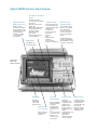
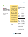
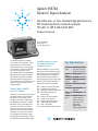
Agilent 35670A
Dynamic Signal Analyzer
Versatile two- or four-channel high-performance
FFT-based spectrum/network analyzer
122 μHz to 102.4 kHz 16-bit ADC
Product Overview
The Agilent 35670A
shown with four
channels (Option AY6)
The Agilent 35670A is a portable
two- or four-channel dynamic signal
analyzer with the versatility to be
several instruments at once. Rugged
and portable, it’s ideal for field work.
Yet it has the performance and
functionality required for demanding
R&D applications. Optional features
optimize the instrument for troubleshooting mechanical vibration and
noise problems, characterizing control
systems, or general spectrum and
network analysis.
Take the Agilent 35670A
where it’s needed!
Whether you’re moving an instrument
around the world or around the lab,
portability is a real benefit. Small
enough to fit under an airplane seat,
the 35670A goes where it’s needed.
But there’s more to portability than
size. Like a nominal 12- to 28-volt
DC power input and self-contained
features that do not require external
hardware, such as built-in piezoelectric integrated circuit power supply,
analog trigger and tachometer inputs,
and optional computed order tracking.
Versatile enough to be your
only instrument for low
frequency analysis
With the 35670A, you carry several
instruments into the field in one package. Frequency, time, and amplitude
domain analysis are all available in
the standard instrument. Build on
that capability with options that either
add new measurement capability or
enhance all measurement modes.
AY6
1D0
1D1
UK4
1D2
1D3
1D4
1C2
100
1G0
Add two channels (four total)
Computed order tracking
Real-time octave measurements
Microphone adapter and
power supply
Swept-sine measurements
Curve fit and synthesis
Arbitrary waveform source
Agilent Instrument BASIC
1D0 – 1D4 bundle
DataLink data transfer solution
Key Specifications
Frequency 102.4 kHz 1 channel
range:
51.2 kHz 2 channel
25.6 kHz 4 channel
Dynamic 90 dB typical
range:
Accuracy: ±0.15 dB
Channel
±0.04 dB and ±0.5
match:
degrees
Real-time 25.6 kHz/1 channel
bandwidth:
Resolution: 100, 200, 400 &
800 lines
Time
> 6 Msamples
capture:
Source
Random, burst
types:
random, periodic
chirp, burst chirp,
pink noise, sine,
swept-sine
(Option 1D2),
arbitrary (Option 1D4)
Agilent 35670A Dynamic Signal Analyzer
Versatile measurement
modes
Agilent Instrument
BASIC (Option 1C2)
Develop a custom
user-interface, integrate
several instruments and
peripherals into a system
using the 35670A as
the system controller,
or simply automate
measurements.
•
•
•
•
•
•
•
Standard and optional
measurement modes include:
FFT analysis
Real-time octave analysis
(Option 1D1)
Order analysis (Option 1D0)
Swept-sine (Option 1D2)
Correlation analysis
Histogram analysis
Time capture
All measurement options
may be retrofitted.
RPM display
Read RPM in any
measurement mode
Powerful markers
•
•
•
•
•
•
•
•
•
•
Extract information from
measurement data with
trace and special markers:
Individual trace
Coupled trace
Absolute or relative
Peak search
Harmonic
Band
Sideband power
Waterfall
Time parameter
Frequency and damping
Built-In 3.5 inch
flexible disk drive
Store instrument states,
programs, time captured
data, waterfall data,
trace data, limits, math
functions, data tables,
and curve fit/synthesis
tables.
Supported disk formats
are HP-LIF and MS-DOS®.
Internal RAM may also be
formatted as storage disk.
Shown with
Option AY6 –
add two channels
Online help
Precision
measurements
Applications
oriented help
is just a few
keystrokes away.
•
•
Large 6.3 inch
(17 cm) display
•
Display area is not
compromised by
portability.
•
2
Input channels
• 16-bit ADC
Analog A-weighted • ±0.15 dB spectrum
amplitude accuracy
filters (switchable)
• ±0.04 dB, ±0.5
Transducer
degrees channel
sensitivity input
match (full scale)
Engineering units:
• 90 dB dynamic range
g, m/s2, m/s, m,
(typical)
in/s2,
in/s, in, mil, kg, dyn, • 130 dB dynamic range
with swept-sine
lb, N, and pascals
(Option 1D2)
Built-in 4 mA
• Up/down autorange
constant current
• Up only autorange
power supply
Math functions
Powerful math and
data editing functions
to quickly modify
measurement results.
(Curve fit and
frequency response
synthesis available
with Option 1D3.)
Source types
•
•
•
•
•
•
•
Random noise
Burst random noise
Periodic chirp
Burst chirp
Pink noise
Fixed Sine
Arbitrary waveform
source (Option 1D4)
• Swept-sine source
(Option 1D2)
Note: The source
is located on the
front panel of a
standard twochannel 35670A.
GPIB connector
Parallel port
Integrate the 35670A
with other instruments
for system operation.
System controller for
GPIB (IEEE-488.1 and
488.2) compatible
instrumentation via
Agilent Instrument
BASIC (Option 1C2).
Print to older HP-GL
printers with PCL 5
capability, such as
an HP LaserJet 4000
series.
DC power
Low noise fan
Accepts 12 to 28 volts dc
(nominal). Use the 35250A
power cable for DC power
source connection, or the
35251A power cable with
cigarette-lighter adapter.
Fan may be turned off
for acoustic applications.
Running speed depends
on ambient temperature.
Serial port
AC power
External trigger
Tachometer
Power select
(42 Volt peak max)
No external signal
conditioning hardware
required. Triggers on
selected level between
±10 Volts.
(42 Volt peak max)
No external signal
conditioning hardware
required. Reads
frequency (RPM) on
selected levels
between ±20 Volts.
Switch between
AC and DC power
sources without
interrupting instrument operation.
Keyboard
External monitor
Use a standard PC
keyboard to title data,
edit Agilent Instrument
BASIC programs,
or to operate the
instrument.
Drive a VGA monitor for
remote viewing by large
groups.
3
Universal power
supply will
operate with any
combination of
voltage between
100 and 240 VAC
and line frequency
between 47 and
440 Hz. The
maximum power
requirement is
350 VA.
Spectrum Analysis
Laboratory-quality
measurements in the field
Obtain all of the performance of your
bench-top analyzer in a portable
instrument.
Ease-of-use
Portability, versatility, and performance are valued attributes, but to
be really valuable an instrument must
also be easy to use. The 35670A has
a friendly front panel, plus online help
that’s always available to answer
your questions. An interactive measurement state lets you configure
the instrument setup from a single
display.
FFT-based spectrum analyzers,
such as the 35670A, are ideal for
measuring the spectra of low-frequency signals like speech or mechanical
vibration. Transient components,
usually missed with swept-frequency
analyzers, are easily measured and
displayed at speeds fast enough
to follow trends. The 35670A has
both the performance and features
required to take full advantage of this
technology.
16-bits for high performance
With a 16-bit ADC (90 dB typical
dynamic range) and a real-time
bandwidth of 25.6 kHz, you can be
sure nothing will be missed. Resolve
signals using 100 to 1600 lines
resolution, or for really close-in analysis, use frequency zoom to resolve
signals with up to 61 µHz resolution.
Use time or RPM arming to develop
waterfalls of sequential vibration
spectra for trend analysis or for an
overview of device vibration.
Power and linear spectrums
Match your spectrum measurement
mode to the signal being tested.
Use linear spectrum analysis to
measure both the amplitude and
phase of periodic signals such as the
spectra of rotating machinery. Power
spectrum analysis is provided for
averaging nonrepetitive signals.
Two spectrums
of road induced
vibration measured at
different speeds are
compared using the
front/back mode of
the Agilent 35670A.
4
Averaging
Various averaging modes let you
further refine spectrum analysis measurements. Time averaging extracts
repetitive signals out of the noise
while rms averaging reduces the
noise to its mean value. Exponential
averaging, available for both time and
rms averaging, is useful for reducing
the noise while following changing
signals—tracking the resonance
shifts in a fatiguing structure for
example.
Time domain
Special markers
Use your spectrum analyzer as a
low-frequency oscilloscope or view
signals in the time and frequency
domains simultaneously.
Three special marker functions
facilitate analysis of your spectral
data. Sideband markers aid analysis
of modulation signals. Use this function to quickly locate sidebands in
(Note: anti-alias filters can be
switched off.) Special markers for
time-domain data facilitate extraction
of key control system performance
parameters: overshoot, rise time, setting time, and delay time.
the complicated spectra of rotating
machines. A band-power marker
reads the total power in a selected
band of frequencies and a total
harmonic distortion marker lets you
calculate total harmonic distortion
without including the effects of noise.
Simultaneous display
of frequency and
time domain data
facilitates analysis of
gear mesh vibration.
Data table
Use a tabular format to keep track
of key frequencies in the spectra of
rotating machinery. The amplitude
and frequency of the signal and a
16-character entry label field are
listed for each selected point.
Automatic units conversion
Measurement results
at key frequencies
can be labeled and
listed using data
table.
Display vibration data in the units
of your choice. Select g, m/sec2,
in/sec2, m/s, in/s, m, mil, inch, Kg, lb,
N, dyn, or pascals as appropriate for
your application. The instrument automatically converts frequency-domain
data from specified input transducer
units to the units you select for
display. For example, accelerometer
data is automatically converted and
displayed as mils when mils are
selected. Of course, dB, dBV, dBm
and volts are available for electrical
applications.
Harmonic markers
are used to calculate
the THD of a signal
without including the
effects of noise.
Markers
Markers streamline analysis by
helping you select and display specific data. Marker functions include
marker to peak, next right peak, and
coupled markers for selecting points
in multiple data displays. Markers
readouts are absolute or relative to
your selected reference.
5
Frequency Response Measurements
The 35670A has the flexibility to make
measurements of both electrical
networks and mechanical devices.
FFT-based network analysis is fast
enough to allow real-time adjustments of circuit parameters while the
swept-sine option provides exacting
measurements over more than six
frequency decades, and a 130 dB
dynamic range.
Source
Four channels (Option AY6)
Markers
Test up to three devices simultaneously with a four-channel 35670A.
Channel one is the common reference
channel and two, three, and four are
the response channels. Alternatively,
select channels one and three as
reference channels for two totally
independent network measurements.
See Option AY6 description for more
information.
A frequency and damping marker
provides the resonant frequency and
the damping ratio of single-degreeof-freedom frequency response
measurements.
Select the optimum stimulus for each
application—random noise, periodic
chirp, pink noise, fixed sine, burst
random, and burst chirp. For zoomed
network analysis measurements, the
source is band-translated to match
the zoom span at frequencies up to
51.2 kHz. An optional arbitrary source
lets you test your product using realworld signals. A ±10 Volt DC source
offset facilitates tests of control
systems.
Gain and phase margin markers
extract key frequency-domain stability
data from frequency response measurements of control systems.
Limits are used
for go/no go testing
in production. The
response of an
accelerometer is
being checked in
this example.
Impact testing
Force and exponential windows allow
impact testing for modal and structural analysis. Quality measurements are
ensured using preview and accept/
reject during averaging. A 4 mA
constant current transducer power
supply is built-in for true portability.
Characteristics of a
selected resonance
are automatically
calculated from an
impact measurement
using the frequency
and damping marker.
Limits
Test network measurements against
preset limits. Up to 800 separate line
segments are available for setting
upper and lower limits. Limits are also
used for testing spectrum measurements.
6
Time Capture
Capture transient events or time
histories for complete analysis in any
measurement mode (except sweptsine). Use either the entire timecapture record or a selected region of
interest for repetitive analysis in the
FFT, octave, order track, correlation or
histogram instrument modes.
An interval of
time-capture data
has been selected for
analysis in the octave
mode.
Standard 16 Mbytes of memory for
deep time-capture capability.
7
Using Measurement Results
Computed Order
Tracking (Option 1D0)
Taking the measurement is only half
the job. Raw measurement data must
be stored, recalled, printed, plotted,
integrated with other data for analysis,
and reported. The 35670A helps you
finish the job.
Entire display screens can be imported
directly into your word processing
program by plotting HP-GL files to
your named DOS file. HP-GL files
are interpreted and displayed directly
by Microsoft’s Word for Windows.
Documented results
For general digital signal processing and filtering, data files may be
stored as ASCII, and then imported
to MATLAB® or a Microsoft® Excel
spreadsheet via the floppy drive,
DataLink, or GPIB.
• Self-contained—no ratio synthesizer or tracking filter required
• Order maps
• Order tracking
• RPM or timetrigger
• Display RPM profile
• Track up to five orders/channel
• Up to 200 orders
• Composite power
• RPM measurements
The 35670A supports GPIB, serial
and parallel printers and plotters for
direct hardcopy output. The printers
and plotters that can be connected
directly to the 35670A are limited
to older HP-GL printers with PCL 5
capability (HP LaserJet 4000 series is
one such printer).
The internal 3.5 inch flexible disk
drive stores data (Standard Data
Format – SDF or ASCII), instrument
states, HP-GL plots and Agilent Instrument BASIC programs in HP-LIF or
MS-DOS formats for future recall or
use on a personal computer.
For specific applications, use
application software that reads SDF
files directly, such as STARModal
and STARAcoustics from Spectral
Dynamics and MEScope from Vibrant.
The slice marker
feature is used to
select and display
an order or suborder
from an order map.
Order tracking facilitates evaluation
of spectra from rotating machines by
displaying vibration data as a function
of orders (or harmonics) rather than
frequency. All measurement spectra
is normalized to the shaft RPM.
Now you can have order tracking
without compromising portability.
Traditional analog order tracking techniques require external tracking filters
and ratio synthesizers. With Agilent’s
computed order tracking algorithm,
external hardware is gone.
Because order tracking is implemented in the software, data is
more precise and your job is easier.
Compared to traditional analog order
tracking techniques, computed order
tracking offers:
• Improved dynamic range at high
orders
• More accurate tracking of rapidly
changing shaft speeds
• Accurate RPM labeled spectra with
exact RPM trigger arm
• Wide 64:1 ratio of start to stop RPMs
8
Order map
Oscilloscope-quality
orbit diagrams mean
you carry only one
instrument onto the
shop floor.
Use order maps for an overview of
vibration data versus RPM or time.
Display the amplitude profile of
individual orders and suborders using
the slice marker function.
Alternatively, use trace markers to
select individual traces for display.
Order tracking
Measure only the data you need.
Order tracking lets you measure the
amplitude profile of up to five orders
plus composite power simultaneously
on each channel. Up to four orders
or three orders and composite power
can be displayed simultaneously.
Order tracking is
used to simultaneously display up
to four orders or
a combination of
orders, composite
power and RPM
profile.
RPM profile
Use RPM profile to monitor the
variation of RPM with time during
order tracking measurements.
Composite power
Composite power provides the total
signal power in a selected channel as
a function of RPM.
Markers are used
to annotate shaft
speeds at selected
points in a run-up
measurement.
Run-up and run-down
measurements
Run-up and run-down measurements
of any order are made using external
trigger as the phase reference.
Display the results as bode or polar
plots; both are available. Markers
allow convenient notation of important shaft speeds.
Orbits
Obtain oscilloscope-quality orbit measurements with your 35670A. Unlike
traditional FFT analyzers, the 35670A
equipped with computed order tracking displays a selected number of
loops (usually one) as the shaft RPM
is varied.
9
Real-Time Octave Measurements (Option 1D1)
Microphone Adapter and Power Supply (Option UK4)
Real-time third octave to 40 kHz
ANSI S1.11-1986
ANSI S1.11-1986 filter shapes
All octave filters comply with filter
shape standards ANSI S1.11-1986
(Order 3, type 1-D), DIN 45651, and
IEC 225-1966. An 80 dB dynamic
range for the audio spectrum provides
the performance required by acousticians. Switchable analog A-weighting
filters in the input channels comply
fully with both ANSI S1.4-1983 and
IEC 651-1979 Type 0.
A-weighted overall SPL
RPM or time-triggered waterfalls
Eliminate the expense and inconvenience of multiple instruments in the
field. With optional real-time octave
analysis, and the optional microphone
adapter and power supply, you have
a complete real-time octave analyzer
added to your 35670A at a fraction
of the cost of a second instrument.
Now you can carry both your FFT and
real-time octave analyzers to the job
site in the same hand.
Advanced analysis
Use waterfall displays of octave data
for an overview of device noise versus
time or RPM. Display individual
frequency bands as a function of
RPM or time using the slice marker
function. Alternatively, use trace
markers to select individual traces
for display.
A pink noise source is available for
testing electro-acoustic devices.
Sound level meter
measurements
Peak hold, impulse, fast, slow, and
Leq are all provided with optional
real-time octave measurements.
All measurements conform to
IEC 651-1979 Type 0 – Impulse.
Real-time 1/3-octave to 40 kHz
on one channel
This waterfall display
of a flyover test can
be analyzed trace-bytrace or by selecting
time slices along the
z-axis.
With two input channels of 1/3octave real-time measurements at
frequencies up to 20 kHz, you get all
of the information you’ll ever need
to understand the noise performance
of your product. No misinterpreted
measurements because transient
components were missed. When
the frequency range requirement is
10 kHz or less, use four channels to
characterize spatial variations. For
those exceptional circumstances, use
1/3-octave resolution at frequencies
up to 40 kHz on a single channel.
Resolutions of 1/1- and 1/12-octave
are also available.
Real-time 1/3-octave
measurements at
frequencies up to
40 kHz.
Overall sound pressure level and
A-weighted sound pressure level can
be displayed with the octave bands
individually, together, or not at all.
A fan-off mode lets you use the
instrument in the sound field being
measured.
Agilent 35670A with
Option UK4 microphone
adapter and power supply.
10
Swept-Sine Measurements (Option 1D2)
130 dB dynamic range
Logarithmic sweep
Logarithmic or linear sweeps
Test devices over more than six
decades of frequency range using
logarithmic sweep. In this mode, the
frequency is automatically adjusted
to provide the same resolution over
each decade of frequency range. With
FFT-network analysis, resolution is
constant—not a problem when measuring over narrow frequency ranges.
“Auto” frequency resolution
While FFT-based network analysis
is fast and accurate, swept-sine
measurements are a better choice
when the device under test has a
wide dynamic range or covers several
decades of frequency range. Use
swept-sine measurements to extend
the network measurement capabilities of the 35670A.
Network analysis over a
130 dB range
With traditional swept-sine, the
35670A is optimally configured to
measure each individual point in the
frequency response. The result is
a 130 dB dynamic range. With FFTbased network analysis, all frequency
points are stimulated simultaneously
and the instrument configures itself
to measure the highest amplitude
response—thereby limiting the
dynamic range.
Characterize nonlinear networks
Flexible
Make the measurement your way.
Independently select logarithmic or
linear sweep, sweep up or down,
automatic or manual sweep, and
autoresolution.
Test multiple devices
simultaneously
Increase throughput in production.
Swept-sine measurements up to
25.6 kHz can be made on three devices simultaneously using swept-sine
on a four-channel 35670A. Channel
one is the common reference channel
for these measurements.
Alternatively, channels one and
three can be designated as independent reference channels for two
totally independent swept-sine
measurements.
Automatic frequency resolution
Use autoresolution to obtain the fastest sweep possible without sacrificing accuracy. With autoresolution, the
35670A automatically adjusts the frequency step according to the device
response. High rates of amplitude and
phase change are matched with small
frequency steps. Low rate-of-change
regions are quickly measured with
larger frequency steps.
Use the auto-level feature to hold the
input or output amplitude constant
during a sweep. This provides the
device response for a specific signal
amplitude. With FFT-based network
analysis using random noise, the random amplitudes of the stimulus tend
to “average out” the non-linearities
and therefore does not capture the
dependency of the response on the
stimulus amplitude.
The stability of
a control loop is
quickly characterized
using the gain and
phase margin marker
function.
11
Agilent Instrument BASIC (Option 1C2)
Realize the advantages of using
your instrument with a computer
without sacrificing portability.
Agilent Instrument BASIC provides
the power of a computer inside your
35670A.
• Create custom interfaces for
simplified operation.
• Use the 35670A as a system
controller to integrate it with other
instruments and peripherals.
• Enhance functionality by creating
custom measurements.
• Increase productivity with
automated operation.
Agilent Instrument BASIC is a
compatible subset of the Agilent
BASIC used in HP 9000 series 200,
300, 400 and 700 computers.
Over 200 Agilent Instrument
BASIC commands
•
•
•
•
•
•
•
•
•
•
•
•
•
•
•
•
•
•
•
Program entry and editing
Program debugging
Memory allocation
Relation operators
General math
Graphics control
Graphics plotting
Graphics axes and labeling
Program control
Binary functions
Trigonometric operations
String operations
Logical operators
GPIB control
Mass storage
Event initiated branching
Clock and calendar
General device I/O
Array operations
Easy programming
Keystroke recording
Most program development begins
with keystroke recording. Each
keystroke is automatically saved as
a program instruction as you set up
your measurement using the front
panel. The recorded sequence can be
used as the core of a sophisticated
program or run as an automatic
sequence.
Keystroke recording
quickly creates the
core of your Agilent
Instrument BASIC
program.
The Agilent Instrument BASIC
program editor supports:
• Line-by-line syntax checking
• Pre-run program verification
• Single step and debug
• Automatic line numbering
An optional PC-style 101-key
keyboard facilitates program development and editing. Simple programs
can be entered or edited using the
front-panel keys.
Agilent Instrument
BASIC can be used
to display measurement results in a new
format or to create
a new operator
interface.
12
Add Two Channels
(Option AY6)
Curve Fit and Synthesis
(Option 1D3)
51.2 kHz frequency range on
one and two channels
20 poles/20 zeros curve fitter
25.6 kHz frequency range on
four channels
Pole/zero, pole/residue and
polynomial format
One or two reference channels
Enhance your productivity by adding
two additional input channels to
your portable analyzer. Having four
channels often means the difference
between solving a problem in the
field and having to schedule time in a
test bay.
Monitor four signals simultaneously
or use channel one as the reference
channel for up to three simultaneous
cross-channel measurements. Two
totally independent cross-channel
measurements are made by selecting
channels one and three as independent reference channels. All channels
are sampled simultaneously.
Use triaxial measurements to simultaneously characterize the motion of
mechanical devices in three axes.
Frequency response synthesis
Use curve fit and synthesis in the
35670A to take the guesswork out
of your design process. The 20-pole
and 20-zero multiple-degree-of-freedom
curve fitter calculates a mathematical
model of your system or circuit from
measured frequency response data.
The model can be expressed in pole/
zero, pole/residue, or polynomial
format.
Transfer the circuit model to the
synthesis function to experiment
with design modifications. Add and
delete poles and zeros, change gain
factors, time delays, or frequency
scaling, then synthesize the frequency response from the modified
model. Design modifications are
tested without ever touching a
soldering iron.
For control systems, simultaneously
measure several points in a single
loop.
Curve fit provides an
exact mathematical
model of your circuit
or device.
13
Arbitrary Waveform
Source (Option 1D4)
Standard 16 Mbytes
RAM
Standard 2 Mbyte
Nonvolatile RAM
Store up to eight arbitrary
waveforms
Number of spectra stored per
channel
Use the 2 Mbyte nonvolatile RAM as
an alternative to the 3.5 inch flexible
disk drive. The memory functions as
a high-speed disk for storage of the
following information.
Test your products using real-world
signals. Measure a signal in either
the time or frequency domain, then
output it via the arbitrary waveform
source. Use math functions and data
edit to obtain precisely the output
waveform you need. An arbitrary
waveform may be output once or
repeatedly.
Standard source types can be
optimized for specific applications.
For example, random noise can be
shaped to improve the effective
dynamic range of your measurement.
Alternatively, you can use data edit
and math functions to create an
arbitrary waveform.
FFT–1 channel 1
FFT–2 channels 2
FFT–4 channels 3
1/3-octave
spectra 4
Time capture 1
Standard 16 Mbyte
1400
600
300
48000
>6 MSamples
1 Conditions: Preset with instrument mode
switched to 1 channel.
2 Conditions: Preset
3 Conditions: Preset with instrument mode
switched to 4 channels.
4 Conditions: Preset with instrument mode
switched to octave.
• Instrument setup states
• Trace data
• User math definitions
• Limit data
• Time capture buffers
• Agilent Instrument BASIC programs
• Waterfall display data
• Curve fit/synthesis tables
• Data tables
Information stored in nonvolatile
RAM is retained when the power
is off.
Use time capture as a digital tape
recorder, then playback captured
signals through the arbitrary waveform source.
Math functions are
used to optimize a
burst chirp signal for
a frequency response
measurement.
14
DataLink data transfer
solution (no charge
Option 1G0)
DataLink data transfer solution, a
no charge option for new 35670A’s,
provides all hardware and software
required to transfer data from the
non-volatile RAM, standard RAM,
or floppy drive to your PC. Hardware
provided includes the 82357B GPIB
to USB converter. Software provided
includes Instrument Basic installed
on the 35670A, plus DataLink software and I/O Libraries that are to be
installed on your computer.
Agilent 35670A Ordering Information
Agilent 35670A
Dynamic Signal Analyzer
standard configuration
1.4 Mbyte, 3.5-in. flexible disk drive
12+ Mbytes user RAM
2 Mbytes nonvolatile RAM
Impact cover
Standard data format utilities
AC power cord
Operating manual set including:
Operator’s guide
Quick start guide
Installation and verification guide
GPIB programming with the 35670A
GPIB commands: Quick reference
GPIB programmer’s guide
• Standard one-year warranty
•
•
•
•
•
•
•
Options for the Agilent 35670A
To upgrade your 35670A
Opt. Description
To add an option to your 35670A,
order 35670U followed by the option
number. Options AY6 and AN2 must
be installed by Agilent Technologies.
Option UE2 is available to upgrade
instrument firmware to latest version,
as appropriate.
AY6
1D0
1D1
UK4
1D2
1D3
1D4
1C2
1G0
1F0
AX4
100
UK5
0B1
0BU
0B3
UK6
W30
W50
1BP
W30
Add two channels (four total)
Computed order tracking
Real-time octave measurements
Microphone adapter and power
supply
Swept-sine measurements
Curve fit and synthesis
Arbitrary waveform source
Agilent Instrument BASIC
DataLink data transfer solution
PC-style keyboard
Rack mount without handles
Software bundle 1D0-1D4
Carrying case (for shipping)
Additional manual set
Additional Agilent Instrument
BASIC manual set
Add service manual
Commercial calibration with
test data
Two year extended service
contract
Four year extended service
contract
Military calibration
(meets MIL 45662A)
Two year extended service
contract
15
Option IGI provides a software
upgrade for the DataLink transfer
solution (includes DataLink SW,
Instrument Basic, and I/O Libraries).
Hardware required for DataLink, such
as the 82357B GPIB to USB converter,
is sold separately. A firmware
upgrade (Option UE2) may also be
required.
Accessories
DC power cables
The 35250A is a three meter cable
terminated with lugs for connecting
to most DC power sources. The
35251A is a three meter cable terminated with an adapter that plugs into
a cigarette lighter.
Summary of Features on Standard Instrument
Instrument modes
Display formats
Averaging controls
FFT analysis
Histogram/time
Correlation analysis Time capture
Single
Quad
Dual upper/lower traces
Small upper and large lower
Front/back overlay traces
Measurement state
Bode diagram
Waterfall display with skew,
-45 to 45 degrees
Trace grids On/Off
Display blanking
Screen saver
Overload reject
Fast averaging On/Off
Update rate select
Select overlap process percentage
Preview time record
Measurement
Frequency domain
Frequency response Power spectrum
Linear spectrum
Coherence
Cross spectrum
Power spectral
density
Time domain (oscilloscope mode)
Time waveform
Autocorrelation
Cross-correlation
Orbit diagram
Amplitude domain
Histogram, PDF, CDF
Trace coordinates
Linear magnitude
Log magnitude
dB magnitude
Group delay
Phase
Unwrapped
phase
Real part
Imaginary part
Nyquist diagram
Polar plot
Trace units
Y-axis Amplitude: combinations of
units, unit value, calculated value,
and unit format describe y-axis
amplitude
Units: volts, g, meters/sec2, inches/
sec2, meters/sec, inches/sec, meters,
mils, inches, pascals, Kg, N, dyn, lb,
user-defined EUs
Unit value: rms, peak, peak-to-peak
Calculated value: V, V2, V2/Hz,
V/√Hz, V2s/Hz, (ESD)
Unit format: linear, dB’s with user
selectable dB reference, dBm with
user selectable impedance.
Y-axis phase: degrees, radians
X-axis: Hz, cpm, order, seconds,
user-defined
Display scaling
Autoscale
Selectable
reference
Linear or log X-axis
Y-axis log
Manual scale
Input range
tracking
X & Y scale markers with expand and
scroll
Marker functions
Individual trace markers
Coupled multi-trace markers
Absolute or relative marker
Peak search
Harmonic markers
Band marker
Sideband power markers
Waterfall markers
Time parameter markers
Frequency response markers
Signal averaging (FFT mode)
Average types
(1 to 9,999,999 averages)
RMS
Time exponential
RMS exponential Peak hold
Time
16
Measurement control
Start measurement
Pause/continue measurement
Triggering
Continuous (freerun)
External (analog or TTL level)
Internal trigger from any channel
Source synchronized trigger
GPIB trigger
Armed triggers
Automatic/manual
RPM step
Time step
Pre- and post-trigger measurement
Delay
Tachometer input:
±4 V or ±20 V range
40 mV or 200 mV resolution
Up to 2048 pulses/rev
Tach hold-off control
Source outputs
Random
Burst random
Periodic chirp
Burst chirp
Pink noise
Fixed sine
Note: Some source types are not
available for use in optional modes.
See option description for details.
Input channels
Analysis
Calibration & memory
Manual range
Anti-alias filters On/Off
AC or DC coupling
Up-only auto range
Up/down auto range
LED half range and overload indicators
Floating or grounded
A-weight filters On/Off
Transducer power supplies
(4 ma constant current)
Limit test with pass/fail
Data table with tabular readout
Data editing
Single or automatic calibration
Built-in diagnostics & service tests
Nonvolatile clock with time/date
Time/date stamp on plots and saved
Data files
Frequency
20 spans from 195 mHz to 102.4 kHz
(1 channel mode)
20 spans from 98 mHz to 51.2 kHz
(2 channel mode)
Digital zoom with 244 mHz resolution
throughout the 102.4 kHz frequency
range.
Resolution
100, 200, 400, 800 and 1600 lines
Windows
Hanning
Flat top
Uniform
Force/exponential
Math
+,-,*, /
Conjugate
Magnitude
Real and imaginary
Square root
FFT, FFT-1
LN
EXP
*jω or /jω
PSD
Differentiation A, B, and C weighting
Integration
Constants K1 thru K5
Functions F1 thru F5
Time capture functions
Capture transient events for repeated
analysis in FFT, octave, order, histogram, or correlation modes (except
swept-sine). Time-captured data may
be saved to internal or external disk,
or transferred over GPIB. Zoom on
captured data for detailed narrowband analysis.
Data storage functions
Built-in 3.5 in., 1.44 Mbyte flexible
disk also supports 720 KByte disks,
and 2 Mbyte of NVRAM disk. Both
MS-DOS and HP-LIF formats are available. Data can be formatted as either
ASCII or binary (SDF). The 35670A
provides storage and recall from the
internal disk, internal RAM disk, internal NVRAM disk, or external GPIB
disk for any of the following
information:
Instrument setup states
Trace data
User-math
Limit data
Time capture buffers
Agilent Instrument BASIC programs
Waterfall display data
Curve fit/synthesis tables
Data tables
GPIB capabilities
Conforms to IEEE 488.1/ 488.2
Conforms to SCPI 1992
Controller with Agilent Instrument
Basic option
17
Online help
Access to topics via keyboard or index
Fan
On/Off
www.agilent.com
www.agilent.com/find/35670A
Agilent Email Updates
www.agilent.com/find/emailupdates
Get the latest information on the
products and applications you select.
Agilent Direct
www.agilent.com/find/agilentdirect
Quickly choose and use your test
equipment solutions with confidence.
MS-DOS and Microsoft are U.S. registered
trademarks of Microsoft Corporation.
MATLAB is a U.S. registered trademark of
The Math Works, Inc.
Remove all doubt
Our repair and calibration services
will get your equipment back to you,
performing like new, when promised. You will get full value out of
your Agilent equipment throughout its lifetime. Your equipment
will be serviced by Agilent-trained
technicians using the latest factory
calibration procedures, automated
repair diagnostics and genuine parts.
You will always have the utmost
confidence in your measurements.
For information regarding self maintenance of this product, please
contact your Agilent office.
Agilent offers a wide range of additional expert test and measurement
services for your equipment, including initial start-up assistance, onsite
education and training, as well as design, system integration, and project
management.
For more information on repair and
calibration services, go to:
For more information on Agilent
Technologies’ products, applications
or services, please contact your local
Agilent office. The complete list is
available at:
www.agilent.com/find/contactus
Americas
Canada
Latin America
United States
(877) 894-4414
305 269 7500
(800) 829-4444
Asia Pacific
Australia
China
Hong Kong
India
Japan
Korea
Malaysia
Singapore
Taiwan
Thailand
1 800 629 485
800 810 0189
800 938 693
1 800 112 929
0120 (421) 345
080 769 0800
1 800 888 848
1 800 375 8100
0800 047 866
1 800 226 008
Europe & Middle East
Austria
01 36027 71571
Belgium
32 (0) 2 404 93 40
Denmark
45 70 13 15 15
Finland
358 (0) 10 855 2100
France
0825 010 700*
*0.125 €/minute
www.agilent.com/find/removealldoubt
Product specifications and descriptions
in this document subject to change
without notice.
Germany
07031 464 6333
Ireland
1890 924 204
Israel
972-3-9288-504/544
Italy
39 02 92 60 8484
Netherlands
31 (0) 20 547 2111
Spain
34 (91) 631 3300
Sweden
0200-88 22 55
Switzerland
0800 80 53 53
United Kingdom 44 (0) 118 9276201
Other European Countries:
www.agilent.com/find/contactus
Revised: October 1, 2008
© Agilent Technologies, Inc. 2009
Printed in USA, January 12, 2009
5966-3063E