Download Agilent Technologies EXG User`s guide

Agilent X-Series
Signal Generators
N5171B/72B/73B EXG
N5181B/82B/83B MXG
User’s Guide
Agilent Technologies
Notices
© Agilent Technologies, Inc. 2014
Warranty
No part of this manual may be reproduced in
any form or by any means (including electronic storage and retrieval or translation
into a foreign language) without prior agreement and written consent from Agilent
Technologies, Inc. as governed by United
States and international copyright laws.
The material contained in this document is provided “as is,” and is subject to being changed, without notice,
in future editions. Further, to the maximum extent permitted by applicable
law, Agilent disclaims all warranties,
either express or implied, with regard
to this manual and any information
contained herein, including but not
limited to the implied warranties of
merchantability and fitness for a particular purpose. Agilent shall not be
liable for errors or for incidental or
consequential damages in connection with the furnishing, use, or performance of this document or of any
information contained herein. Should
Agilent and the user have a separate
written agreement with warranty
terms covering the material in this
document that conflict with these
terms, the warranty terms in the separate agreement shall control.
Manual Part Number
N5180-90056
Edition
February 2014
Printed in USA
Agilent Technologies, Inc.
3501 Stevens Creek Blvd.
Santa Clara, CA 95052 USA
Technology Licenses
The hardware and/or software described in
this document are furnished under a license
and may be used or copied only in accordance with the terms of such license.
Restricted Rights Legend
U.S. Government Restricted Rights. Software and technical data rights granted to
the federal government include only those
rights customarily provided to end user customers. Agilent provides this customary
commercial license in Software and technical data pursuant to FAR 12.211 (Technical
Data) and 12.212 (Computer Software) and,
for the Department of Defense, DFARS
252.227-7015 (Technical Data - Commercial
Items) and DFARS 227.7202-3 (Rights in
Commercial Computer Software or Computer Software Documentation).
Safety Notices
CAUTION
A CAUTION notice denotes a hazard. It calls attention to an operating procedure, practice, or the like
that, if not correctly performed or
adhered to, could result in damage
to the product or loss of important
data. Do not proceed beyond a
CAUTION notice until the indicated
conditions are fully understood and
met.
WA R N I N G
A WARNING notice denotes a
hazard. It calls attention to an
operating procedure, practice, or
the like that, if not correctly performed or adhered to, could result
in personal injury or death. Do not
proceed beyond a WARNING
notice until the indicated conditions are fully understood and
met.
Users Guide
Contents
1
Signal Generator Overview
Signal Generator Features . . . . . . . . . . . . . . . . . . . . . . . . . . . . . . . . . . . . . . . . . . . . . . .2
Modes of Operation . .
Continuous Wave .
Swept Signal . . . .
Analog Modulation
Digital Modulation
. . . . .
. . . . .
. . . . .
. . . . .
(Vector
. . . . .
. . . . .
. . . . .
. . . . .
Models
. . . . . . . . . . . . . . . .
. . . . . . . . . . . . . . . .
. . . . . . . . . . . . . . . .
. . . . . . . . . . . . . . . .
with Option 65x Only)
.
.
.
.
.
.
.
.
.
.
.
.
.
.
.
.
.
.
.
.
.
.
.
.
.
.
.
.
.
.
.
.
.
.
.
.
.
.
.
.
.
.
.
.
.
.
.
.
.
.
.
.
.
.
.
.
.
.
.
.
.
.
.
.
.
.
.
.
.
.
.
.
.
.
.
.
.
.
.
.
.
.
.
.
.
.
.
.
.
.
.
.
.
.
.
.
.
.
.
.
.
.
.
.
.
.
.
.
.
.
.4
.4
.4
.4
.4
.5
.5
.5
.6
.6
.6
.6
.6
.7
.7
.7
.7
.7
.7
.7
.7
.8
.8
.8
.8
.8
.8
.8
.9
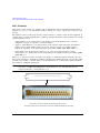
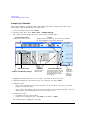
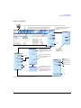
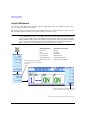
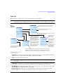
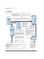
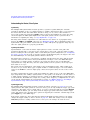
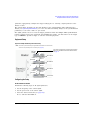
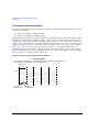
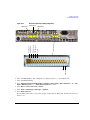
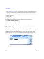
Front Panel Overview . . . . . . . . . . . . . . . . . . . . . .
1. Host USB . . . . . . . . . . . . . . . . . . . . . . . . . .
2. Display . . . . . . . . . . . . . . . . . . . . . . . . . . . .
3. Softkeys . . . . . . . . . . . . . . . . . . . . . . . . . . .
4. Numeric Keypad . . . . . . . . . . . . . . . . . . . . . .
5. Arrows and Select. . . . . . . . . . . . . . . . . . . . .
6. Page Up . . . . . . . . . . . . . . . . . . . . . . . . . . .
7. MENUS . . . . . . . . . . . . . . . . . . . . . . . . . . . .
8. Trigger . . . . . . . . . . . . . . . . . . . . . . . . . . . .
9. Local Cancel/(Esc) . . . . . . . . . . . . . . . . . . . .
10. Help . . . . . . . . . . . . . . . . . . . . . . . . . . . . .
11. Preset and User Preset . . . . . . . . . . . . . . . . .
12. RF Output (N5171B, N5172B, N5181B, N5182B)
12. RF Output (N5173B, N5183B) . . . . . . . . . . . .
13. RF On/Off and LED . . . . . . . . . . . . . . . . . . .
14. Mod On/Off and LED . . . . . . . . . . . . . . . . . .
15. Page Down . . . . . . . . . . . . . . . . . . . . . . . . .
16. I Input (vector models only) . . . . . . . . . . . . .
17. Q Input (vector models only) . . . . . . . . . . . . .
18. Knob. . . . . . . . . . . . . . . . . . . . . . . . . . . . .
19. Incr Set . . . . . . . . . . . . . . . . . . . . . . . . . .
20. Return . . . . . . . . . . . . . . . . . . . . . . . . . . .
21. More and LED . . . . . . . . . . . . . . . . . . . . . .
22. Power Switch and LEDs . . . . . . . . . . . . . . . .
.
.
.
.
.
.
.
.
.
.
.
.
.
.
.
.
.
.
.
.
.
.
.
.
.
.
.
.
.
.
.
.
.
.
.
.
.
.
.
.
.
.
.
.
.
.
.
.
.
.
.
.
.
.
.
.
.
.
.
.
.
.
.
.
.
.
.
.
.
.
.
.
.
.
.
.
.
.
.
.
.
.
.
.
.
.
.
.
.
.
.
.
.
.
.
.
.
.
.
.
.
.
.
.
.
.
.
.
.
.
.
.
.
.
.
.
.
.
.
.
.
.
.
.
.
.
.
.
.
.
.
.
.
.
.
.
.
.
.
.
.
.
.
.
.
.
.
.
.
.
.
.
.
.
.
.
.
.
.
.
.
.
.
.
.
.
.
.
.
.
.
.
.
.
.
.
.
.
.
.
.
.
.
.
.
.
.
.
.
.
.
.
.
.
.
.
.
.
.
.
.
.
.
.
.
.
.
.
.
.
.
.
.
.
.
.
.
.
.
.
.
.
.
.
.
.
.
.
.
.
.
.
.
.
.
.
.
.
.
.
.
.
.
.
.
.
.
.
.
.
.
.
.
.
.
.
.
.
.
.
.
.
.
.
.
.
.
.
.
.
.
.
.
.
.
.
.
.
.
.
.
.
.
.
.
.
.
.
.
.
.
.
.
.
.
.
.
.
.
.
.
.
.
.
.
.
.
.
.
.
.
.
.
.
.
.
.
.
.
.
.
.
.
.
.
.
.
.
.
.
.
.
.
.
.
.
.
.
.
.
.
.
.
.
.
.
.
.
.
.
.
.
.
.
.
.
.
.
.
.
.
.
.
.
.
.
.
.
.
.
.
.
.
.
.
.
.
.
.
.
.
.
.
.
.
.
.
.
.
.
.
.
.
.
.
.
.
.
.
.
.
.
.
.
.
.
.
.
.
.
.
.
.
.
.
.
.
.
.
.
.
.
.
.
.
.
.
.
.
.
.
.
.
.
.
.
.
.
.
.
.
.
.
.
.
.
.
.
.
.
.
.
.
.
.
.
.
.
.
.
.
.
.
.
.
.
.
.
.
.
.
.
.
.
.
.
.
.
.
.
.
.
.
.
.
.
.
.
.
.
.
.
.
.
.
.
.
.
.
.
.
.
.
.
.
.
.
.
.
.
.
.
.
.
.
.
.
.
.
.
.
.
.
.
.
.
.
.
.
.
.
.
.
.
.
.
.
.
.
.
.
.
.
.
.
.
.
.
.
.
.
.
.
.
.
.
.
.
.
.
.
.
.
.
.
.
.
.
.
.
.
.
.
.
.
.
.
.
.
.
.
.
.
.
.
.
.
.
.
.
.
.
.
.
.
.
.
.
.
.
.
.
.
.
.
.
.
.
.
.
.
.
.
.
.
.
.
.
.
.
.
.
.
.
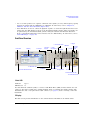
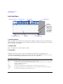
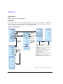
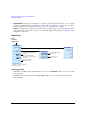
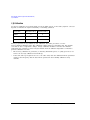
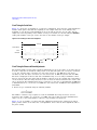
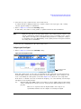
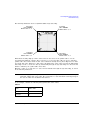
Front Panel Display . . . . . .
1. Active Function Area .
2. Frequency Area . . . .
3. Annunciators . . . . . .
4. Amplitude Area . . . .
5. Error Message Area. .
6. Text Area . . . . . . . .
7. Softkey Label Area . .
.
.
.
.
.
.
.
.
.
.
.
.
.
.
.
.
.
.
.
.
.
.
.
.
.
.
.
.
.
.
.
.
.
.
.
.
.
.
.
.
.
.
.
.
.
.
.
.
.
.
.
.
.
.
.
.
.
.
.
.
.
.
.
.
.
.
.
.
.
.
.
.
.
.
.
.
.
.
.
.
.
.
.
.
.
.
.
.
.
.
.
.
.
.
.
.
.
.
.
.
.
.
.
.
.
.
.
.
.
.
.
.
.
.
.
.
.
.
.
.
.
.
.
.
.
.
.
.
.
.
.
.
.
.
.
.
.
.
.
.
.
.
.
.
.
.
.
.
.
.
.
.
.
.
.
.
.
.
.
.
.
.
.
.
.
.
.
.
.
.
.
.
.
.
.
.
.
.
.
.
.
.
.
.
.
.
.
.
.
.
.
.
.
.
.
.
.
.
.
.
. 10
. 10
. 10
. 10
. 11
. 12
. 12
. 12
.
.
.
.
.
.
.
.
.
.
.
.
.
.
.
.
.
.
.
.
.
.
.
.
.
.
.
.
.
.
.
.
.
.
.
.
.
.
.
.
.
.
.
.
.
.
.
.
.
.
.
.
.
.
.
.
.
.
.
.
.
.
.
.
.
.
.
.
.
.
.
.
.
.
.
.
.
.
.
.
.
.
.
.
.
.
.
.
.
.
.
.
.
.
.
.
.
.
.
.
.
.
.
.
.
.
.
.
.
.
.
.
.
.
.
.
.
.
.
.
.
.
.
.
.
.
.
.
.
.
.
.
.
.
.
.
.
.
.
.
.
.
.
.
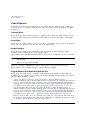
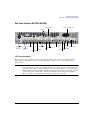
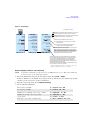
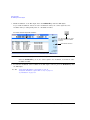
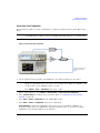
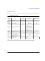
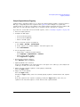
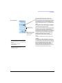
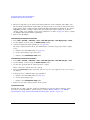
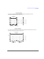
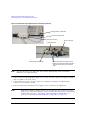
Rear Panel Overview (N5171B, N5172B, N5181B, & N5182B) . . . . . . . . . . . . . . . . . . . . . . . 13
1. AC Power Receptacle . . . . . . . . . . . . . . . . . . . . . . . . . . . . . . . . . . . . . . . . . . . . . 13
Agilent X-Series Signal Generators User’s Guide
iii
Contents
2. EXT 1 & EXT 2 . . . . . . . .
3. LF OUT . . . . . . . . . . . . .
4. SWEEP OUT . . . . . . . . . .
5. PULSE . . . . . . . . . . . . . .
6. TRIG 1 & 2 . . . . . . . . . . .
7. REF IN . . . . . . . . . . . . . .
8. 10 MHz OUT . . . . . . . . . .
9. GPIB . . . . . . . . . . . . . . .
10. LAN . . . . . . . . . . . . . . .
11. Device USB . . . . . . . . . .
12. Host USB . . . . . . . . . . .
13. SD Card . . . . . . . . . . . .
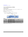
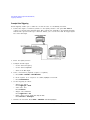
Digital Modulation Connectors
I OUT, Q OUT, OUT, OUT . .
BB TRIG 1 & BB TRIG 2 . . .
EVENT 1 . . . . . . . . . . . . . .
PAT TRIG . . . . . . . . . . . . . .
DIGITAL BUS I/O . . . . . . . .
AUX I/O Connector . . . . . . .
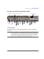
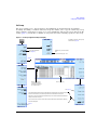
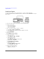
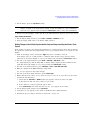
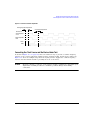
Rear Panel Overview (N5173B
1. AC Power Receptacle. .
2. EXT 1 & EXT 2 . . . . .
3. LF OUT . . . . . . . . . .
4. SWEEP OUT . . . . . . .
5. PULSE . . . . . . . . . . .
6. TRIG 1 & 2 . . . . . . . .
7. REF IN . . . . . . . . . . .
8. 10 MHz OUT . . . . . . .
9. GPIB . . . . . . . . . . . .
10. LAN . . . . . . . . . . . .
11. Device USB . . . . . . .
12. Host USB . . . . . . . .
13. SD Card . . . . . . . . .
14. ALC INPUT . . . . . . .
15. Z AXIS OUTPUT . . . .
2
& N5183B)
. . . . . . . .
. . . . . . . .
. . . . . . . .
. . . . . . . .
. . . . . . . .
. . . . . . . .
. . . . . . . .
. . . . . . . .
. . . . . . . .
. . . . . . . .
. . . . . . . .
. . . . . . . .
. . . . . . . .
. . . . . . . .
. . . . . . . .
. . . . . . . . . .
. . . . . . . . . .
. . . . . . . . . .
. . . . . . . . . .
. . . . . . . . . .
. . . . . . . . . .
. . . . . . . . . .
. . . . . . . . . .
. . . . . . . . . .
. . . . . . . . . .
. . . . . . . . . .
. . . . . . . . . .
Models Only) .
. . . . . . . . . .
. . . . . . . . . .
. . . . . . . . . .
. . . . . . . . . .
. . . . . . . . . .
. . . . . . . . . .
.
.
.
.
.
.
.
.
.
.
.
.
.
.
.
.
.
.
.
.
.
.
.
.
.
.
.
.
.
.
.
.
.
.
.
.
.
.
.
.
.
.
.
.
.
.
.
.
.
.
.
.
.
.
.
.
.
.
.
.
.
.
.
.
.
.
.
.
.
.
.
.
.
.
.
.
.
.
.
.
.
.
.
.
.
.
.
.
.
.
.
.
.
.
.
.
.
.
.
.
.
.
.
.
.
.
.
.
.
.
.
.
.
.
.
.
.
.
.
.
.
.
.
.
.
.
.
.
.
.
.
.
.
.
.
.
.
.
.
.
.
.
.
.
.
.
.
.
.
.
.
.
.
.
.
.
.
.
.
.
.
.
.
.
.
.
.
.
.
.
.
.
.
.
.
.
.
.
.
.
.
.
.
.
.
.
.
.
.
.
.
.
.
.
.
.
.
.
.
.
.
.
.
.
.
.
.
.
.
.
.
.
.
.
.
.
.
.
.
.
.
.
.
.
.
.
.
.
.
.
.
.
.
.
.
.
.
.
.
.
.
.
.
.
.
.
.
.
.
.
.
.
.
.
.
.
.
.
.
.
.
.
.
.
.
.
.
.
.
.
.
.
.
.
.
.
.
.
.
.
.
.
.
.
.
.
.
.
.
.
.
.
.
.
.
.
.
.
.
.
.
.
.
.
.
.
.
.
.
.
.
.
.
.
.
.
.
.
.
.
.
.
.
.
.
.
.
.
.
.
.
.
.
.
.
.
.
.
.
.
.
.
.
.
.
.
.
.
.
.
.
.
.
.
.
.
.
.
.
.
.
.
.
.
.
.
.
.
.
.
.
.
.
.
.
.
.
.
.
.
.
.
.
.
.
.
.
.
.
.
.
.
.
.
.
.
.
.
.
.
.
.
.
.
.
.
.
.
.
.
.
.
.
.
.
.
.
.
.
.
.
.
.
.
.
.
.
.
.
.
.
.
.
.
.
.
.
.
.
.
.
.
.
.
.
.
.
.
.
.
.
.
.
.
.
.
.
.
.
.
.
.
.
.
.
.
.
.
.
.
.
.
.
.
.
14
14
14
14
14
14
15
15
15
15
15
15
16
16
17
17
17
17
18
.
.
.
.
.
.
.
.
.
.
.
.
.
.
.
.
.
.
.
.
.
.
.
.
.
.
.
.
.
.
.
.
.
.
.
.
.
.
.
.
.
.
.
.
.
.
.
.
.
.
.
.
.
.
.
.
.
.
.
.
.
.
.
.
.
.
.
.
.
.
.
.
.
.
.
.
.
.
.
.
.
.
.
.
.
.
.
.
.
.
.
.
.
.
.
.
.
.
.
.
.
.
.
.
.
.
.
.
.
.
.
.
.
.
.
.
.
.
.
.
.
.
.
.
.
.
.
.
.
.
.
.
.
.
.
.
.
.
.
.
.
.
.
.
.
.
.
.
.
.
.
.
.
.
.
.
.
.
.
.
.
.
.
.
.
.
.
.
.
.
.
.
.
.
.
.
.
.
.
.
.
.
.
.
.
.
.
.
.
.
.
.
.
.
.
.
.
.
.
.
.
.
.
.
.
.
.
.
.
.
.
.
.
.
.
.
.
.
.
.
.
.
.
.
.
.
.
.
.
.
.
.
.
.
.
.
.
.
.
.
.
.
.
.
.
.
.
.
.
.
.
.
.
.
.
.
.
.
.
.
.
.
.
.
.
.
.
.
.
.
.
.
.
.
.
.
.
.
.
.
.
.
.
.
.
.
.
.
.
.
.
.
.
.
.
.
.
.
.
.
.
.
.
.
.
.
.
.
.
.
.
.
.
.
.
.
.
.
.
.
.
.
.
.
.
.
.
.
.
.
.
.
.
.
.
.
.
.
.
.
.
.
.
.
.
.
.
.
.
.
.
.
.
.
.
.
.
.
.
.
.
.
.
.
.
.
.
.
.
.
.
.
.
.
.
.
.
.
.
.
.
.
.
.
.
.
.
.
.
.
.
.
.
.
.
.
.
.
.
.
.
.
.
.
.
.
.
.
.
.
.
.
.
.
.
.
.
.
.
.
.
.
.
.
.
.
.
.
.
.
.
.
.
.
.
.
.
.
.
.
.
.
.
.
.
.
.
.
.
.
.
.
.
.
.
.
.
.
.
.
.
.
.
.
.
.
.
.
.
.
.
.
.
.
.
.
.
.
.
.
.
.
.
.
.
.
.
.
.
.
.
.
.
.
.
.
.
.
.
.
.
.
.
.
.
.
.
.
.
.
.
.
.
.
.
.
.
.
.
.
.
.
.
.
.
.
.
.
.
.
.
.
.
.
.
.
.
.
.
.
.
.
.
.
.
.
.
.
.
.
.
.
.
.
.
.
.
.
.
.
23
23
24
24
24
24
24
24
25
25
25
25
25
25
25
26
.
.
.
.
.
.
.
.
.
.
.
.
.
.
.
.
.
.
.
.
.
.
.
.
.
.
.
.
.
.
.
.
.
.
.
.
.
.
.
.
.
.
.
.
.
.
.
.
.
.
.
.
.
.
.
.
.
.
.
.
.
.
.
.
.
.
.
.
.
.
.
.
.
.
.
.
.
.
.
.
.
.
.
.
.
.
.
.
.
.
.
.
.
.
.
.
.
.
.
.
.
.
.
.
.
.
.
.
.
.
.
.
.
.
.
.
.
.
.
.
.
.
.
.
.
.
.
.
.
.
.
.
.
.
.
.
.
.
.
.
28
28
29
30
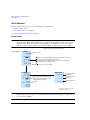
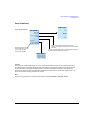
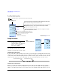
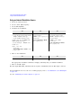
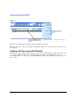
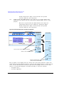
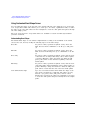
Setting Preferences & Enabling Options
User Preferences . . . . . . . . . . .
Display Settings . . . . . . . . .
Power On and Preset . . . . .
Front Panel Knob Resolution
iv
. . . . .
. . . . .
. . . . .
. . . . .
. . . . .
. . . . .
. . . . .
. . . . .
. . . . .
. . . . .
. . . . .
. . . . .
(Vector
. . . . .
. . . . .
. . . . .
. . . . .
. . . . .
. . . . .
.
.
.
.
.
.
.
.
.
.
.
.
.
.
.
.
.
.
.
.
.
.
.
.
Agilent X-Series Signal Generators User’s Guide
Contents
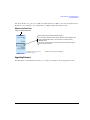
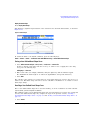
Setting Time and Date. . . . . . . . . . . . . . . . . . . . . . . . . . . . . . . . . . . . . . . . . . . . . . 30
Reference Oscillator Tune . . . . . . . . . . . . . . . . . . . . . . . . . . . . . . . . . . . . . . . . . . . 31
Upgrading Firmware . . . . . . . . . . . . . . . . . . . . . . . . . . . . . . . . . . . . . . . . . . . . . . . . . . 31
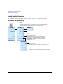
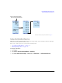
Remote Operation Preferences . . . . . . . . . . . . . . . . . . . . . .
GPIB Address and Remote Language . . . . . . . . . . . . . . .
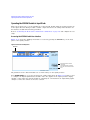
Configuring the LAN Interface . . . . . . . . . . . . . . . . . . .
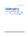
Enabling LAN Services: “Browser,” “Sockets,” and “VXI–11”
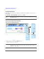
Configuring the Remote Languages . . . . . . . . . . . . . . . .
Configuring the Preset Languages . . . . . . . . . . . . . . . . .
.
.
.
.
.
.
.
.
.
.
.
.
.
.
.
.
.
.
.
.
.
.
.
.
.
.
.
.
.
.
.
.
.
.
.
.
.
.
.
.
.
.
.
.
.
.
.
.
.
.
.
.
.
.
.
.
.
.
.
.
.
.
.
.
.
.
.
.
.
.
.
.
.
.
.
.
.
.
.
.
.
.
.
.
.
.
.
.
.
.
.
.
.
.
.
.
.
.
.
.
.
.
.
.
.
.
.
.
.
.
.
.
.
.
.
.
.
.
.
.
. 32
. 32
. 33
. 34
. 35
. 37
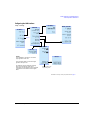
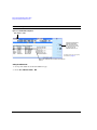
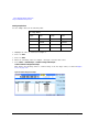
Enabling an Option . . . . . . . . . . . . . . . . . . . . . . . . . . . . . . . . . . . . . . . . . . . . . . . . . . 39
Viewing Options and Licenses . . . . . . . . . . . . . . . . . . . . . . . . . . . . . . . . . . . . . . . . . 40
Hardware Assembly Installation and Removal Softkeys. . . . . . . . . . . . . . . . . . . . . . . . . . . 41
3
Basic Operation
Presetting the Signal Generator. . . . . . . . . . . . . . . . . . . . . . . . . . . . . . . . . . . . . . . . . . . 44
Viewing Key Descriptions. . . . . . . . . . . . . . . . . . . . . . . . . . . . . . . . . . . . . . . . . . . . . . . 44
Entering and Editing Numbers and Text. . . . .
Entering Numbers and Moving the Cursor.
Entering Alpha Characters . . . . . . . . . . .
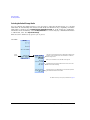
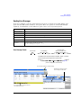
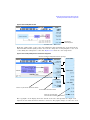
Example: Using a Table Editor . . . . . . . .
.
.
.
.
.
.
.
.
.
.
.
.
.
.
.
.
.
.
.
.
.
.
.
.
.
.
.
.
.
.
.
.
.
.
.
.
.
.
.
.
.
.
.
.
.
.
.
.
.
.
.
.
.
.
.
.
.
.
.
.
.
.
.
.
.
.
.
.
.
.
.
.
.
.
.
.
.
.
.
.
.
.
.
.
.
.
.
.
.
.
.
.
.
.
.
.
.
.
.
.
.
.
.
.
.
.
.
.
.
.
.
.
.
.
.
.
.
.
.
.
.
.
.
.
. 45
. 45
. 45
. 46
Setting Frequency and Power (Amplitude) . . . . . . . . . . . . . . . . . . . . . . . . . . . . . . . . . . . 47
Example: Configuring a 700 MHz, −20 dBm Continuous Wave Output. . . . . . . . . . . . . . . 48
Using an External Reference Oscillator . . . . . . . . . . . . . . . . . . . . . . . . . . . . . . . . . . . 48
Setting ALC Bandwidth Control . . . . . . . . . . . . . . . . . . . . . . . . . . . . . . . . . . . . . . . . . . 49
Configuring a Swept Output . . . . . . . .
Routing Signals . . . . . . . . . . . . .
Step Sweep . . . . . . . . . . . . . . . .
List Sweep . . . . . . . . . . . . . . . .
Example: Using a Single Sweep . . .
Example: Manual Control of Sweep
.
.
.
.
.
.
.
.
.
.
.
.
.
.
.
.
.
.
.
.
.
.
.
.
.
.
.
.
.
.
.
.
.
.
.
.
.
.
.
.
.
.
.
.
.
.
.
.
.
.
.
.
.
.
.
.
.
.
.
.
.
.
.
.
.
.
.
.
.
.
.
.
.
.
.
.
.
.
.
.
.
.
.
.
.
.
.
.
.
.
.
.
.
.
.
.
.
.
.
.
.
.
.
.
.
.
.
.
.
.
.
.
.
.
.
.
.
.
.
.
.
.
.
.
.
.
.
.
.
.
.
.
.
.
.
.
.
.
.
.
.
.
.
.
.
.
.
.
.
.
.
.
.
.
.
.
.
.
.
.
.
.
.
.
.
.
.
.
.
.
.
.
.
.
.
.
.
.
.
.
.
.
.
.
.
.
.
.
.
.
.
.
.
.
.
.
.
.
.
.
.
.
.
.
.
.
.
.
.
.
.
.
.
.
.
.
. 50
. 52
. 52
. 55
. 58
. 59
Modulating the Carrier Signal. . . . . . . . . . . . . . . . . . . . . . . . . . . . . . . . . . . . . . . . . . . . 59
Example . . . . . . . . . . . . . . . . . . . . . . . . . . . . . . . . . . . . . . . . . . . . . . . . . . . . . . . 59
Simultaneous Modulation . . . . . . . . . . . . . . . . . . . . . . . . . . . . . . . . . . . . . . . . . . . . 61
Working with Files . . . . . . . . . . . . .
File Softkeys . . . . . . . . . . . . . .
Viewing a List of Stored Files. . .
Storing a File . . . . . . . . . . . . .
Loading (Recalling) a Stored File.
Moving a File from One Media to
Agilent X-Series Signal Generators User’s Guide
. . . . . .
. . . . . .
. . . . . .
. . . . . .
. . . . . .
Another
.
.
.
.
.
.
.
.
.
.
.
.
.
.
.
.
.
.
.
.
.
.
.
.
.
.
.
.
.
.
.
.
.
.
.
.
.
.
.
.
.
.
.
.
.
.
.
.
.
.
.
.
.
.
.
.
.
.
.
.
.
.
.
.
.
.
.
.
.
.
.
.
.
.
.
.
.
.
.
.
.
.
.
.
.
.
.
.
.
.
.
.
.
.
.
.
.
.
.
.
.
.
.
.
.
.
.
.
.
.
.
.
.
.
.
.
.
.
.
.
.
.
.
.
.
.
.
.
.
.
.
.
.
.
.
.
.
.
.
.
.
.
.
.
.
.
.
.
.
.
.
.
.
.
.
.
.
.
.
.
.
.
.
.
.
.
.
.
.
.
.
.
.
.
.
.
.
.
.
.
.
.
.
.
.
.
. 61
. 62
. 63
. 65
. 66
. 67
v
Contents
Working with Instrument State Files . . . . . . . . . . . . . . . . . . . . . . . . . . . . . . . . . . . . 68
Selecting the Default Storage Media. . . . . . . . . . . . . . . . . . . . . . . . . . . . . . . . . . . . . 72
Reading Error Messages . . . . . . . . . . . . . . . . . . . . . . . . . . . . . . . . . . . . . . . . . . . . . . . 73
Error Message Format. . . . . . . . . . . . . . . . . . . . . . . . . . . . . . . . . . . . . . . . . . . . . . 73
4
Using Analog Modulation (Option UNT)
Analog Modulation Waveforms . . . . . . . . . . . . . . . . . . . . . . . . . . . . . . . . . . . . . . . . . . . 76
Analog Modulation Sources . . . . . . . . . . . . . . . . . . . . . . . . . . . . . . . . . . . . . . . . . . . . . 76
Using an Internal Modulation Source. . . . . . . . . . . . . . . . . . . . . . . . . . . . . . . . . . . . . . . 78
Using an External Modulation Source . . . . . . . . . . . . . . . . . . . . . . . . . . . . . . . . . . . . . . 79
Removing a DC Offset. . . . . . . . . . . . . . . . . . . . . . . . . . . . . . . . . . . . . . . . . . . . . . 79
Using Wideband AM . . . . . . . . . . . . . . . . . . . . . . . . . . . . . . . . . . . . . . . . . . . . . . . 79
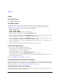
Configuring the LF Output (Option 303) . . . . . . . . . . . . . . . . . .
LF Out Modulation Sources . . . . . . . . . . . . . . . . . . . . . . . .
Configuring the LF Output with an Internal Modulation Source
Configuring the LF Output with a Function Generator Source .
5
.
.
.
.
.
.
.
.
.
.
.
.
.
.
.
.
.
.
.
.
.
.
.
.
.
.
.
.
.
.
.
.
.
.
.
.
.
.
.
.
.
.
.
.
.
.
.
.
.
.
.
.
.
.
.
.
.
.
.
.
.
.
.
.
.
.
.
.
.
.
.
.
81
81
82
83
Optimizing Performance
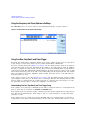
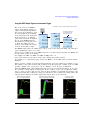
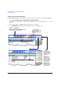
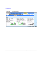
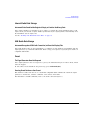
Using the Dual Power Meter Display . . . . . . . . . . . . . . . . . . . . . . . . . . . . . . . . . . . . . . . 86
Example: Dual Power Meter Calibration . . . . . . . . . . . . . . . . . . . . . . . . . . . . . . . . . . 89
Using the Power Meter Servo . . . . . . . . . . . . . . . . . . . . . . . . . . . . . . . . . . . . . . . . . . . . 94
Power Meter Servo Configuration . . . . . . . . . . . . . . . . . . . . . . . . . . . . . . . . . . . . . . 95
Example . . . . . . . . . . . . . . . . . . . . . . . . . . . . . . . . . . . . . . . . . . . . . . . . . . . . . . . 96
Using Flatness Correction . . . . . . . . . . . . . . . . . . . . . . . . . . . . . . . . . . . . . . . . . . . . . . 97
Creating a User Flatness Correction Array . . . . . . . . . . . . . . . . . . . . . . . . . . . . . . . . 99
Recalling and Applying a User Flatness Correction Array . . . . . . . . . . . . . . . . . . . . . 105
Using Internal Channel Correction (N5172B/82B Only) . . . . . . . . . . . . . . . . . . . . . . . . . . 106
Configure Internal Channel Correction . . . . . . . . . . . . . . . . . . . . . . . . . . . . . . . . . . 109
Perform Enhanced Factory Calibration . . . . . . . . . . . . . . . . . . . . . . . . . . . . . . . . . . 109
Using External Leveling (N5173B/83B Only) . . . . . . . . . . . . . . . . . . . . . . . . . . . . . . . . . 110
Option 1E1 Output Attenuator Behavior and Use . . . . . . . . . . . . . . . . . . . . . . . . . . . 113
Configure External Leveling . . . . . . . . . . . . . . . . . . . . . . . . . . . . . . . . . . . . . . . . . 114
Using Unleveled Operating Modes . . . . . . . . . . . . . . . . . . . . . . . . . . . . . . . . . . . . . . . . 118
ALC Off Mode . . . . . . . . . . . . . . . . . . . . . . . . . . . . . . . . . . . . . . . . . . . . . . . . . . 119
Power Search Mode . . . . . . . . . . . . . . . . . . . . . . . . . . . . . . . . . . . . . . . . . . . . . . 119
Using an Output Offset, Reference,
Setting an Output Offset . . . .
Setting an Output Reference. .
Setting a Frequency Multiplier
or
. .
. .
. .
Multiplier
. . . . . . .
. . . . . . .
. . . . . . .
.
.
.
.
.
.
.
.
.
.
.
.
.
.
.
.
.
.
.
.
.
.
.
.
.
.
.
.
.
.
.
.
.
.
.
.
.
.
.
.
.
.
.
.
.
.
.
.
.
.
.
.
.
.
.
.
.
.
.
.
.
.
.
.
.
.
.
.
.
.
.
.
.
.
.
.
.
.
.
.
.
.
.
.
.
.
.
.
.
.
.
.
.
.
.
.
.
.
.
.
.
.
.
.
.
.
.
.
.
.
.
.
.
.
.
.
.
.
.
.
122
122
123
124
Using the Frequency and Phase Reference Softkeys . . . . . . . . . . . . . . . . . . . . . . . . . . . . 126
vi
Agilent X-Series Signal Generators User’s Guide
Contents
Using Free Run, Step Dwell, and Timer Trigger . . . . . . . . . . . . . . . . . . . . . . . . . . . . . . . 126
Understanding Free Run, Step Dwell, and Timer Trigger Setup . . . . . . . . . . . . . . . . . . 126
Using a USB Keyboard . . . . . . . . . . . . . . . . . . . . . . . . . . . . . . . . . . . . . . . . . . . . . . . 128
6
Using Pulse Modulation (Option UNW or 320)
Pulse Characteristics. . . . . . . . . . . . . . . . . . . . . . . . . . . . . . . . . . . . . . . . . . . . . . . . . 131
The Basic Procedure . . . . . . . . . . . . . . . . . . . . . . . . . . . . . . . . . . . . . . . . . . . . . . . . . 133
Example . . . . . . . . . . . . . . . . . . . . . . . . . . . . . . . . . . . . . . . . . . . . . . . . . . . . . . . . . 133
Pulse Train (Option 320 – Requires: Option UNW) . . . . . . . . . . . . . . . . . . . . . . . . . . . . 135
7
Basic Digital Operation—No BBG Option Installed
I/Q Modulation . . . . . . . . . . . . . . . . . . . . . . . . . . . . . . . . . . . . . . . . . . . . . . . . . . . . 142
Configuring the Front Panel Inputs . . . . . . . . . . . . . . . . . . . . . . . . . . . . . . . . . . . . 143
8
Basic Digital Operation (Option 653/655/656/657)
Waveform File Basics . . . . . . . . . . . . . . . . . . . . . . . . . . . . . . . . . . . . . . . . . . . . . . . . 146
Signal Generator Memory. . . . . . . . . . . . . . . . . . . . . . . . . . . . . . . . . . . . . . . . . . . 146
Dual ARB Player . . . . . . . . . . . . . . . . . . . . . . . . . . . . . . . . . . . . . . . . . . . . . . . . 146
Storing, Loading, and Playing a Waveform Segment . . . . . . . .
Loading a Waveform Segment into BBG Media . . . . . . . . .
Storing/Renaming a Waveform Segment to Internal or USB
Playing a Waveform Segment . . . . . . . . . . . . . . . . . . . .
. . . . .
. . . . .
Media .
. . . . .
.
.
.
.
.
.
.
.
.
.
.
.
.
.
.
.
.
.
.
.
.
.
.
.
.
.
.
.
.
.
.
.
.
.
.
.
.
.
.
.
.
.
.
.
.
.
.
.
.
.
.
.
.
.
.
.
.
.
.
.
148
148
149
149
Waveform Sequences . . . . . . .
Creating a Sequence . . . .
Viewing the Contents of a
Editing a Sequence . . . . .
Playing a Sequence . . . . .
.
.
.
.
.
.
.
.
.
.
.
.
.
.
.
.
.
.
.
.
.
.
.
.
.
.
.
.
.
.
.
.
.
.
.
.
.
.
.
.
.
.
.
.
.
.
.
.
.
.
.
.
.
.
.
.
.
.
.
.
.
.
.
.
.
.
.
.
.
.
.
.
.
.
.
.
.
.
.
.
151
152
153
153
154
. . . . . . .
. . . . . . .
Sequence
. . . . . . .
. . . . . . .
.
.
.
.
.
.
.
.
.
.
.
.
.
.
.
.
.
.
.
.
.
.
.
.
.
.
.
.
.
.
.
.
.
.
.
.
.
.
.
.
.
.
.
.
.
.
.
.
.
.
.
.
.
.
.
.
.
.
.
.
.
.
.
.
.
.
.
.
.
.
.
.
.
.
.
.
.
.
.
.
.
.
.
.
.
.
.
.
.
.
.
.
.
.
.
Saving a Waveform’s Settings & Parameters . . . . . . . . . . . . . . . . . . . . . . . . . . . . . . . . . 155
Viewing and Modifying Header Information . . . . . . . . . . . . . . . . . . . . . . . . . . . . . . 157
Viewing & Editing a Header without Selecting the Waveform . . . . . . . . . . . . . . . . . . . 159
Using Waveform Markers . . . . . . . . . . . . . . . . . . . .
Waveform Marker Concepts . . . . . . . . . . . . . . .
Accessing Marker Utilities . . . . . . . . . . . . . . . .
Viewing Waveform Segment Markers. . . . . . . . . .
Clearing Marker Points from a Waveform Segment
Setting Marker Points in a Waveform Segment . . .
Viewing a Marker Pulse . . . . . . . . . . . . . . . . . .
Agilent X-Series Signal Generators User’s Guide
.
.
.
.
.
.
.
.
.
.
.
.
.
.
.
.
.
.
.
.
.
.
.
.
.
.
.
.
.
.
.
.
.
.
.
.
.
.
.
.
.
.
.
.
.
.
.
.
.
.
.
.
.
.
.
.
.
.
.
.
.
.
.
.
.
.
.
.
.
.
.
.
.
.
.
.
.
.
.
.
.
.
.
.
.
.
.
.
.
.
.
.
.
.
.
.
.
.
.
.
.
.
.
.
.
.
.
.
.
.
.
.
.
.
.
.
.
.
.
.
.
.
.
.
.
.
.
.
.
.
.
.
.
.
.
.
.
.
.
.
.
.
.
.
.
.
.
.
.
.
.
.
.
.
.
.
.
.
.
.
.
.
.
.
.
.
.
.
.
.
.
.
.
.
.
.
.
.
.
.
.
.
161
162
166
167
167
168
171
vii
Contents
Using the RF Blanking Marker Function. . . . . . .
Setting Marker Polarity . . . . . . . . . . . . . . . . . .
Controlling Markers in a Waveform Sequence . . .
Using the EVENT Output Signal as an Instrument
Triggering a Waveform . . . . . . . . . . . . .
Trigger Type . . . . . . . . . . . . . . . . .
Trigger Source . . . . . . . . . . . . . . . .
Example: Segment Advance Triggering
Example: Gated Triggering . . . . . . . .
Example: External Triggering . . . . . .
.
.
.
.
.
.
.
.
.
.
.
.
.
.
.
.
.
.
.
.
.
.
.
.
.
.
.
.
.
.
. . . . . .
. . . . . .
. . . . . .
Trigger .
.
.
.
.
.
.
.
.
.
.
.
.
.
.
.
.
.
.
.
.
.
.
.
.
.
.
.
.
.
.
.
.
.
.
.
.
.
.
.
.
.
.
.
.
.
.
.
.
.
.
.
.
.
.
.
.
.
.
.
.
.
.
.
.
.
.
.
.
.
.
.
.
.
.
.
.
.
.
.
.
172
174
174
177
.
.
.
.
.
.
.
.
.
.
.
.
.
.
.
.
.
.
.
.
.
.
.
.
.
.
.
.
.
.
.
.
.
.
.
.
.
.
.
.
.
.
.
.
.
.
.
.
.
.
.
.
.
.
.
.
.
.
.
.
.
.
.
.
.
.
.
.
.
.
.
.
.
.
.
.
.
.
.
.
.
.
.
.
.
.
.
.
.
.
.
.
.
.
.
.
.
.
.
.
.
.
.
.
.
.
.
.
.
.
.
.
.
.
.
.
.
.
.
.
.
.
.
.
.
.
.
.
.
.
.
.
.
.
.
.
.
.
.
.
.
.
.
.
.
.
.
.
.
.
.
.
.
.
.
.
.
.
.
.
.
.
.
.
.
.
.
.
.
.
.
.
.
.
178
179
180
181
182
184
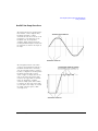
Clipping a Waveform . . . . . . . . . . . . . . . . . . . .
How Power Peaks Develop . . . . . . . . . . . . . .
How Peaks Cause Spectral Regrowth . . . . . . .
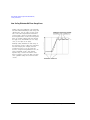
How Clipping Reduces Peak–to–Average Power
Configuring Circular Clipping . . . . . . . . . . . .
Configuring Rectangular Clipping . . . . . . . . .
.
.
.
.
.
.
.
.
.
.
.
.
.
.
.
.
.
.
.
.
.
.
.
.
.
.
.
.
.
.
.
.
.
.
.
.
.
.
.
.
.
.
.
.
.
.
.
.
.
.
.
.
.
.
.
.
.
.
.
.
.
.
.
.
.
.
.
.
.
.
.
.
.
.
.
.
.
.
.
.
.
.
.
.
.
.
.
.
.
.
.
.
.
.
.
.
.
.
.
.
.
.
.
.
.
.
.
.
.
.
.
.
.
.
.
.
.
.
.
.
.
.
.
.
.
.
.
.
.
.
.
.
.
.
.
.
.
.
.
.
.
.
.
.
.
.
.
.
.
.
.
.
.
.
.
.
.
.
.
.
.
.
.
.
.
.
.
.
185
186
188
189
192
193
Scaling a Waveform . . . . . . . . . . . . . . . . . . . . . .
How DAC Over–Range Errors Occur . . . . . . . .
How Scaling Eliminates DAC Over–Range Errors
Setting Waveform Runtime Scaling. . . . . . . . . .
Setting Waveform Scaling. . . . . . . . . . . . . . . .
.
.
.
.
.
.
.
.
.
.
.
.
.
.
.
.
.
.
.
.
.
.
.
.
.
.
.
.
.
.
.
.
.
.
.
.
.
.
.
.
.
.
.
.
.
.
.
.
.
.
.
.
.
.
.
.
.
.
.
.
.
.
.
.
.
.
.
.
.
.
.
.
.
.
.
.
.
.
.
.
.
.
.
.
.
.
.
.
.
.
.
.
.
.
.
.
.
.
.
.
.
.
.
.
.
.
.
.
.
.
.
.
.
.
.
.
.
.
.
.
.
.
.
.
.
.
.
.
.
.
.
.
.
.
.
194
195
196
197
198
Setting the Baseband Frequency Offset . . . . . . . . . . . . . . . . . . . . . . . . . . . . . . . . . . . . 200
DAC Over–Range Conditions and Scaling . . . . . . . . . . . . . . . . . . . . . . . . . . . . . . . . 202
I/Q Modulation . . . . . . . . . . . . . . . . . . . . . . . . . . . . . . . . . . . . . . . . . . . . . . . . . . . . 204
Using the Rear Panel I and Q Outputs. . . . . . . . . . . . . . . . . . . . . . . . . . . . . . . . . . 206
Configuring the Front Panel Inputs . . . . . . . . . . . . . . . . . . . . . . . . . . . . . . . . . . . . 207
I/Q Adjustments . . . . . . . . . . . . . . . . . . . . . . . . . . . . . . . . . . . . . . . . . . . . . . . . . . . 208
I/Q Calibration . . . . . . . . . . . . . . . . . . . . . . . . . . . . . . . . . . . . . . . . . . . . . . . . . . . . 210
Using the Equalization Filter . . . . . . . . . . . . . . . . . . . . . . . . . . . . . . . . . . . . . . . . . . . 212
Using Finite Impulse Response (FIR) Filters in the Dual ARB Real- Time Modulation Filter . . 214
Creating a User–Defined FIR Filter Using the FIR Table Editor . . . . . . . . . . . . . . . . . 215
Modifying a FIR Filter Using the FIR Table
Loading the Default Gaussian FIR File .
Modifying the Coefficients . . . . . . . . .
Storing the Filter to Memory . . . . . . .
Editor.
. . . . .
. . . . .
. . . . .
.
.
.
.
.
.
.
.
.
.
.
.
.
.
.
.
.
.
.
.
.
.
.
.
.
.
.
.
.
.
.
.
.
.
.
.
.
.
.
.
.
.
.
.
.
.
.
.
.
.
.
.
.
.
.
.
.
.
.
.
.
.
.
.
.
.
.
.
.
.
.
.
.
.
.
.
.
.
.
.
.
.
.
.
.
.
.
.
.
.
.
.
.
.
.
.
.
.
.
.
.
.
.
.
.
.
.
.
.
.
.
.
220
221
222
223
Setting the Real- Time Modulation Filter. . . . . . . . . . . . . . . . . . . . . . . . . . . . . . . . . . . . 224
Multiple Baseband Generator Synchronization .
Understanding the Master/Slave System . .
Equipment Setup . . . . . . . . . . . . . . . . .
Configuring the Setup . . . . . . . . . . . . . .
viii
.
.
.
.
.
.
.
.
.
.
.
.
.
.
.
.
.
.
.
.
.
.
.
.
.
.
.
.
.
.
.
.
.
.
.
.
.
.
.
.
.
.
.
.
.
.
.
.
.
.
.
.
.
.
.
.
.
.
.
.
.
.
.
.
.
.
.
.
.
.
.
.
.
.
.
.
.
.
.
.
.
.
.
.
.
.
.
.
.
.
.
.
.
.
.
.
.
.
.
.
.
.
.
.
.
.
.
.
.
.
.
.
.
.
.
.
.
.
.
.
.
.
.
.
225
228
229
229
Agilent X-Series Signal Generators User’s Guide
Contents
Making Changes to the Multiple Synchronization Setup and Resynchronizing the Master/Slave
System . . . . . . . . . . . . . . . . . . . . . . . . . . . . . . . . . . . . . . . . . . . . . . . . . . . . . . . 231
Understanding Option 012 (LO In/Out for Phase Coherency) with Multiple Baseband Generator
Synchronization . . . . . . . . . . . . . . . . . . . . . . . . . . . . . . . . . . . . . . . . . . . . . . . . . . . . 232
Configuring the Option 012 (LO In/Out for Phase Coherency) with MIMO . . . . . . . . . . . 232
Real- Time Applications . . . . . . . . . . . . . . . . . . . . . . . . . . . . . . . . . . . . . . . . . . . . . . . 236
Waveform Licensing . . . . . . . . . . . . . . . . . . . . . . . . . . .
Understanding Waveform Licensing . . . . . . . . . . . . . .
Installing an Option N5182- 22x or Option N5182B–25x
Licensing a Signal Generator Waveform . . . . . . . . . . .
9
.
.
.
.
.
.
.
.
.
.
.
.
.
.
.
.
.
.
.
.
.
.
.
.
.
.
.
.
.
.
.
.
.
.
.
.
.
.
.
.
.
.
.
.
.
.
.
.
.
.
.
.
.
.
.
.
.
.
.
.
.
.
.
.
.
.
.
.
.
.
.
.
.
.
.
.
.
.
.
.
.
.
.
.
.
.
.
.
237
237
237
237
Adding Real–Time Noise to a Signal (Option 403)
Adding Real–Time Noise to a Dual ARB Waveform . . . . . . . . . . . . . . . . . . . . . . . . . . . . . 245
Eb/No Adjustment Softkeys for Real Time I/Q Baseband AWGN . . . . . . . . . . . . . . . . . 248
Using Real Time I/Q Baseband AWGN . . . . . . . . . . . . . . . . . . . . . . . . . . . . . . . . . . . . . 251
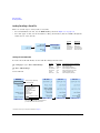
10 Digital Signal Interface Module (Option 003/004)
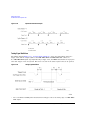
Clock Timing . . . . . . . . . . . . . . . . . . . . . . . . . .
Clock and Sample Rates . . . . . . . . . . . . . . .
Clock Source . . . . . . . . . . . . . . . . . . . . . . .
Common Frequency Reference . . . . . . . . . . .
Clock Timing for Parallel Data . . . . . . . . . . .
Clock Timing for Parallel Interleaved Data . . .
Clock Timing for Serial Data . . . . . . . . . . . .
Clock Timing for Phase and Skew Adjustments
.
.
.
.
.
.
.
.
.
.
.
.
.
.
.
.
.
.
.
.
.
.
.
.
.
.
.
.
.
.
.
.
.
.
.
.
.
.
.
.
.
.
.
.
.
.
.
.
.
.
.
.
.
.
.
.
.
.
.
.
.
.
.
.
.
.
.
.
.
.
.
.
.
.
.
.
.
.
.
.
.
.
.
.
.
.
.
.
.
.
.
.
.
.
.
.
.
.
.
.
.
.
.
.
.
.
.
.
.
.
.
.
.
.
.
.
.
.
.
.
.
.
.
.
.
.
.
.
.
.
.
.
.
.
.
.
.
.
.
.
.
.
.
.
.
.
.
.
.
.
.
.
.
.
.
.
.
.
.
.
.
.
.
.
.
.
.
.
.
.
.
.
.
.
.
.
.
.
.
.
.
.
.
.
.
.
.
.
.
.
.
.
.
.
.
.
.
.
.
.
.
.
.
.
.
.
.
.
.
.
.
.
.
.
.
.
.
.
.
.
.
.
.
.
253
253
256
257
259
262
264
264
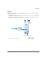
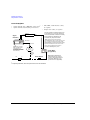
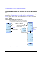
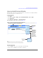
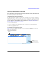
Connecting the Clock Source and the Device Under Test . . . . . . . . . . . . . . . . . . . . . . . . . 265
Data Types . . . . . . . . . . . . . . . . . . . . . . . . . . . . . . . . . . . . . . . . . . . . . . . . . . . . . . . 268
Output Mode . . . . . . . . . . . . . . . . . . . . . . . . . . . . . . . . . . . . . . . . . . . . . . . . . . . 268
Input Mode . . . . . . . . . . . . . . . . . . . . . . . . . . . . . . . . . . . . . . . . . . . . . . . . . . . . 268
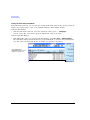
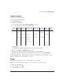
Operating the N5102A Module in Output Mode . . . .
Setting up the Signal Generator Baseband Data .
Accessing the N5102A Module User Interface. . .
Choosing the Logic Type and Port Configuration
Selecting the Output Direction . . . . . . . . . . . .
Selecting the Data Parameters . . . . . . . . . . . .
Configuring the Clock Signal . . . . . . . . . . . . .
Generating Digital Data . . . . . . . . . . . . . . . . .
.
.
.
.
.
.
.
.
.
.
.
.
.
.
.
.
.
.
.
.
.
.
.
.
.
.
.
.
.
.
.
.
.
.
.
.
.
.
.
.
.
.
.
.
.
.
.
.
.
.
.
.
.
.
.
.
.
.
.
.
.
.
.
.
.
.
.
.
.
.
.
.
.
.
.
.
.
.
.
.
.
.
.
.
.
.
.
.
.
.
.
.
.
.
.
.
.
.
.
.
.
.
.
.
.
.
.
.
.
.
.
.
.
.
.
.
.
.
.
.
.
.
.
.
.
.
.
.
.
.
.
.
.
.
.
.
.
.
.
.
.
.
.
.
.
.
.
.
.
.
.
.
.
.
.
.
.
.
.
.
.
.
.
.
.
.
.
.
.
.
.
.
.
.
.
.
.
.
.
.
.
.
.
.
.
.
.
.
.
.
.
.
.
.
.
.
.
.
.
.
.
.
.
.
.
.
.
.
.
.
.
.
.
.
.
.
269
269
269
271
272
272
274
279
Operating the N5102A Module in Input Mode . . . . . . . . . . . . . . . . . . . . . . . . . . . . . . . . 280
Accessing the N5102A Module User Interface. . . . . . . . . . . . . . . . . . . . . . . . . . . . . . 280
Selecting the Input Direction . . . . . . . . . . . . . . . . . . . . . . . . . . . . . . . . . . . . . . . . 282
Agilent X-Series Signal Generators User’s Guide
ix
Contents
Choosing the Logic Type and Port Configuration .
Configuring the Clock Signal . . . . . . . . . . . . . .
Selecting the Data Parameters . . . . . . . . . . . . .
Digital Data . . . . . . . . . . . . . . . . . . . . . . . . .
.
.
.
.
.
.
.
.
.
.
.
.
.
.
.
.
.
.
.
.
.
.
.
.
.
.
.
.
.
.
.
.
.
.
.
.
.
.
.
.
.
.
.
.
.
.
.
.
.
.
.
.
.
.
.
.
.
.
.
.
.
.
.
.
.
.
.
.
.
.
.
.
.
.
.
.
.
.
.
.
.
.
.
.
.
.
.
.
.
.
.
.
.
.
.
.
.
.
.
.
.
.
.
.
282
283
287
290
.
.
.
.
.
.
.
.
.
.
.
.
.
.
.
.
.
.
.
.
.
.
.
.
.
.
.
.
.
.
.
.
.
.
.
.
.
.
.
.
.
.
.
.
.
.
.
.
.
.
.
.
.
.
.
.
.
.
.
.
.
.
.
.
.
.
.
.
.
.
.
.
.
.
.
.
.
.
.
.
.
.
.
.
.
.
.
.
.
.
.
.
.
.
.
.
.
.
.
.
.
.
.
.
.
.
.
.
.
.
.
.
.
.
.
.
.
.
.
.
.
.
.
.
.
.
.
.
.
.
.
.
.
.
.
.
.
.
.
.
.
.
.
.
.
.
.
.
.
.
.
.
.
.
.
.
.
.
.
.
.
.
.
.
.
.
.
.
.
.
.
.
.
.
.
.
.
.
.
.
.
.
.
.
.
.
.
.
.
.
.
.
.
.
.
.
.
.
.
.
.
.
.
.
.
.
.
.
.
.
.
.
.
.
.
.
.
.
.
.
.
.
.
.
.
.
.
.
.
.
.
.
.
.
.
.
.
.
.
.
.
.
.
.
.
.
.
.
.
.
.
.
.
.
.
.
.
.
.
.
292
292
292
293
295
296
297
300
301
302
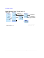
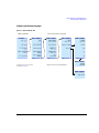
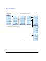
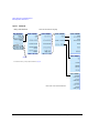
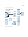
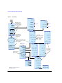
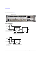
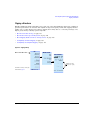
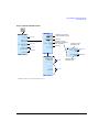
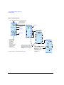
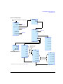
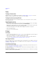
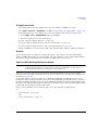
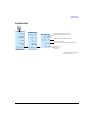
11 BERT (Option UN7)
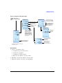
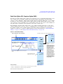
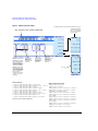
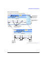
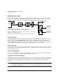
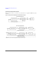
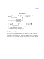
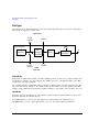
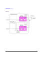
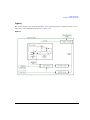
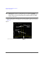
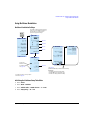
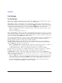
Bit Error Rate Tester–Option UN7 . . . . . . .
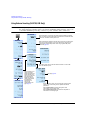
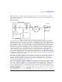
Block Diagram. . . . . . . . . . . . . . . . . .
Clock Gate Function . . . . . . . . . . . . . .
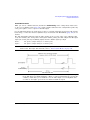
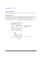
Clock/Gate Delay Function. . . . . . . . . .
Clock Delay Function . . . . . . . . . . . . .
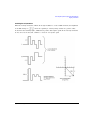
Gate Delay Function in the Clock Mode .
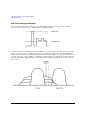
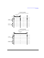
Triggering . . . . . . . . . . . . . . . . . . . . .
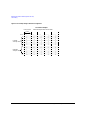
Data Processing . . . . . . . . . . . . . . . . .
Repeat Measurements . . . . . . . . . . . . .
Testing Signal Definitions . . . . . . . . . .
.
.
.
.
.
.
.
.
.
.
.
.
.
.
.
.
.
.
.
.
.
.
.
.
.
.
.
.
.
.
.
.
.
.
.
.
.
.
.
.
.
.
.
.
.
.
.
.
.
.
.
.
.
.
.
.
.
.
.
.
Verifying BERT Operation . . . . . . . . . . . . . . . . . . . . . . . . . . . . . . . . . . . . . . . . . . . . 304
Measurement Setup Using Self- Test Mode . . . . . . . . . . . . . . . . . . . . . . . . . . . . . . . . 304
Measurement Example Using Custom Digital Modulation (Requires Option 431) . . . . . . . 307
12
Real–Time Phase Noise Impairments (Option 432)
Real–Time Phase Noise Impairment. . . . . . . . . . . . . . . . . . . . . . . . . . . . . . . . . . . . . . . 310
The Agilent X- Series Phase Noise Shape and Additive Phase Noise Impairments . . . . . . . . . 311
Understanding the Phase Noise Adjustments . . . . . . . . . . . . . . . . . . . . . . . . . . . . . . . . . 313
DAC Over–Range Conditions and Scaling . . . . . . . . . . . . . . . . . . . . . . . . . . . . . . . . . . . 314
13
Custom Digital Modulation (Option 431)
Custom Modulation . . . . . . . . . . . . . . . . . . . . . . . . . . . . . . . . . . . . . . . . . . . . . . . . . 316
ARB Custom Modulation Waveform Generator . . . . . . . . . . . . . . . . . . . . . . . . . . . . . 316
Real- Time Custom Modulation Waveform Generator . . . . . . . . . . . . . . . . . . . . . . . . . 316
Creating and Using Bit Files . . . . . . .
Creating a User File . . . . . . . . . .
Renaming and Saving a User File .
Recalling a User File . . . . . . . . .
Modifying an Existing User File . .
Applying Bit Errors to a User File
x
.
.
.
.
.
.
.
.
.
.
.
.
.
.
.
.
.
.
.
.
.
.
.
.
.
.
.
.
.
.
.
.
.
.
.
.
.
.
.
.
.
.
.
.
.
.
.
.
.
.
.
.
.
.
.
.
.
.
.
.
.
.
.
.
.
.
.
.
.
.
.
.
.
.
.
.
.
.
.
.
.
.
.
.
.
.
.
.
.
.
.
.
.
.
.
.
.
.
.
.
.
.
.
.
.
.
.
.
.
.
.
.
.
.
.
.
.
.
.
.
.
.
.
.
.
.
.
.
.
.
.
.
.
.
.
.
.
.
.
.
.
.
.
.
.
.
.
.
.
.
.
.
.
.
.
.
.
.
.
.
.
.
.
.
.
.
.
.
.
.
.
.
.
.
.
.
.
.
.
.
.
.
.
.
.
.
.
.
.
.
.
.
.
.
.
.
.
.
.
.
.
.
.
.
.
.
.
.
.
.
.
.
.
.
.
.
324
325
327
328
328
329
Using Customized Burst Shape Curves. . . . . . .
Understanding Burst Shape . . . . . . . . . . .
Creating a User- Defined Burst Shape Curve
Storing a User- Defined Burst Shape Curve .
.
.
.
.
.
.
.
.
.
.
.
.
.
.
.
.
.
.
.
.
.
.
.
.
.
.
.
.
.
.
.
.
.
.
.
.
.
.
.
.
.
.
.
.
.
.
.
.
.
.
.
.
.
.
.
.
.
.
.
.
.
.
.
.
.
.
.
.
.
.
.
.
.
.
.
.
.
.
.
.
.
.
.
.
.
.
.
.
.
.
.
.
.
.
.
.
.
.
.
.
.
.
.
.
.
.
.
.
.
.
.
.
.
.
.
.
.
.
.
.
330
330
333
335
Agilent X-Series Signal Generators User’s Guide
Contents
Recalling a User- Defined Burst Shape Curve . . . . . . . . . . . . . . . . . . . . . . . . . . . . . . 335
Using the Arbitrary Waveform Generator . . . . . . . . . . . . . . . . . . . . . .
Using Predefined Custom Digital Modulation . . . . . . . . . . . . . . . . .
Creating a Custom Digital Modulation State . . . . . . . . . . . . . . . . .
Storing a Custom Digital Modulation State . . . . . . . . . . . . . . . . . .
Recalling a Custom Digital Modulation State . . . . . . . . . . . . . . . . .
Defining a Modulation . . . . . . . . . . . . . . . . . . . . . . . . . . . . . . . .
Creating a Custom Multicarrier Digital Modulation State . . . . . . . . .
Storing a Custom Multicarrier Digital Modulation State . . . . . . . . . .
Applying Changes to an Active Multicarrier Digital Modulation State .
.
.
.
.
.
.
.
.
.
.
.
.
.
.
.
.
.
.
.
.
.
.
.
.
.
.
.
.
.
.
.
.
.
.
.
.
.
.
.
.
.
.
.
.
.
.
.
.
.
.
.
.
.
.
.
.
.
.
.
.
.
.
.
.
.
.
.
.
.
.
.
.
.
.
.
.
.
.
.
.
.
.
.
.
.
.
.
.
.
.
.
.
.
.
.
.
.
.
.
.
.
.
.
.
.
.
.
.
.
.
.
.
.
.
.
.
.
337
337
339
341
343
344
350
352
352
Using Finite Impulse Response (FIR) Filters with Custom Modulation . . . . . . . . . . . . . . . 353
Understanding FIR Filters . . . . . . . . . . . . . . . . . . . . . . . . . . . . . . . . . . . . . . . . . . 353
Creating a User–Defined FIR Filter Using the FIR Table Editor . . . . . . . . . . . . . . . . . 355
Modifying a FIR Filter Using the FIR Table Editor .
Loading the Default Gaussian FIR File . . . . . .
Modifying the Coefficients . . . . . . . . . . . . . .
Storing the Filter to Memory . . . . . . . . . . . .
.
.
.
.
.
.
.
.
.
.
.
.
.
.
.
.
.
.
.
.
.
.
.
.
.
.
.
.
.
.
.
.
.
.
.
.
.
.
.
.
.
.
.
.
.
.
.
.
.
.
.
.
.
.
.
.
.
.
.
.
.
.
.
.
.
.
.
.
.
.
.
.
.
.
.
.
.
.
.
.
.
.
.
.
.
.
.
.
.
.
.
.
.
.
.
.
.
.
.
.
.
.
.
.
.
.
.
.
.
.
.
.
359
360
361
362
Differential Encoding . . . . . . . . . . . . . . . . . . . . . . . . . . . . . . . . . . . . . . . . . . . . . . . . 362
Using Differential Encoding . . . . . . . . . . . . . . . . . . . . . . . . . . . . . . . . . . . . . . . . . 366
14 Multitone and Two–Tone Waveforms (Option 430)
Creating a Custom Two–Tone Waveform . . . . . . . . . . . . . . . . . . . . . . . . . . . . . . . . . . . . 369
Creating a Custom Multitone Waveform . . . . . . . . . . . . . . . . . . . . . . . . . . . . . . . . . . . . 369
Using Two–Tone Modulation. . . . . . . . . . .
Two–Tone Modulation Softkeys . . . . . .
Creating a Two–Tone Waveform . . . . .
Viewing a Two–Tone Waveform . . . . . .
Minimizing Carrier Feedthrough . . . . .
Changing the Alignment of a Two–Tone
. . . . . . .
. . . . . . .
. . . . . . .
. . . . . . .
. . . . . . .
Waveform
Using Multitone Modulation . . . . . . . . . . . . . . . . .
Multitone Modulation Softkeys . . . . . . . . . . . .
Initializing the Multitone Setup Table Editor . . .
Configuring Tone Powers and Tone Phases . . . .
Removing a Tone . . . . . . . . . . . . . . . . . . . . .
Generating the Waveform . . . . . . . . . . . . . . . .
Configuring the RF Output . . . . . . . . . . . . . . .
Applying Changes to an Active Multitone Signal .
15
.
.
.
.
.
.
.
.
.
.
.
.
.
.
.
.
.
.
.
.
.
.
.
.
.
.
.
.
.
.
.
.
.
.
.
.
.
.
.
.
.
.
.
.
.
.
.
.
.
.
.
.
.
.
.
.
.
.
.
.
.
.
.
.
.
.
.
.
.
.
.
.
.
.
.
.
.
.
.
.
.
.
.
.
.
.
.
.
.
.
.
.
.
.
.
.
.
.
.
.
.
.
.
.
.
.
.
.
.
.
.
.
.
.
.
.
.
.
.
.
.
.
.
.
.
.
.
.
.
.
.
.
.
.
.
.
.
.
.
.
.
.
.
.
.
.
.
.
.
.
.
.
.
.
.
.
.
.
.
.
.
.
.
.
369
370
370
371
372
373
.
.
.
.
.
.
.
.
.
.
.
.
.
.
.
.
.
.
.
.
.
.
.
.
.
.
.
.
.
.
.
.
.
.
.
.
.
.
.
.
.
.
.
.
.
.
.
.
.
.
.
.
.
.
.
.
.
.
.
.
.
.
.
.
.
.
.
.
.
.
.
.
.
.
.
.
.
.
.
.
.
.
.
.
.
.
.
.
.
.
.
.
.
.
.
.
.
.
.
.
.
.
.
.
.
.
.
.
.
.
.
.
.
.
.
.
.
.
.
.
.
.
.
.
.
.
.
.
.
.
.
.
.
.
.
.
.
.
.
.
.
.
.
.
.
.
.
.
.
.
.
.
.
.
.
.
.
.
.
.
.
.
.
.
.
.
.
.
.
.
.
.
.
.
.
.
.
.
.
.
.
.
.
.
.
.
.
.
.
.
.
.
.
.
.
.
.
.
.
.
.
.
.
.
.
.
.
.
375
375
375
376
376
376
376
377
Working in a Secure Environment
How to Obtain the Security Features Document . . . . . . . . . . . . . . . . . . . . . . . . . . . . . . . 379
Agilent X-Series Signal Generators User’s Guide
xi
Contents
Using Secure Display . . . . . . . . . . . . . . . . . . . . . . . . . . . . . . . . . . . . . . . . . . . . . . . . 380
16 Troubleshooting
Display . . . . . . . . . . . . . . . . . . . . . . . . . . . . . . . . . . . . . . . . . . . . . . . . . . . . . . . . . 382
The Display is Too Dark to Read . . . . . . . . . . . . . . . . . . . . . . . . . . . . . . . . . . . . . 382
The Display Turns Black when Using USB Media. . . . . . . . . . . . . . . . . . . . . . . . . . . 382
Signal Generator Lock–Up . . . . . . . . . . . . . . . . . . . . . . . . . . . . . . . . . . . . . . . . . . . . . 382
RF Output . . . . . . . . . . . . . . . . . . . . . . . . . . . . . . . .
No RF Output . . . . . . . . . . . . . . . . . . . . . . . . . . .
Power Supply Shuts Down . . . . . . . . . . . . . . . . . . .
No Modulation at the RF Output. . . . . . . . . . . . . . .
RF Output Power too Low . . . . . . . . . . . . . . . . . . .
Distortion . . . . . . . . . . . . . . . . . . . . . . . . . . . . . .
Signal Loss While Working with a Spectrum Analyzer.
Signal Loss While Working with a Mixer . . . . . . . . .
.
.
.
.
.
.
.
.
.
.
.
.
.
.
.
.
.
.
.
.
.
.
.
.
.
.
.
.
.
.
.
.
.
.
.
.
.
.
.
.
.
.
.
.
.
.
.
.
.
.
.
.
.
.
.
.
.
.
.
.
.
.
.
.
.
.
.
.
.
.
.
.
.
.
.
.
.
.
.
.
.
.
.
.
.
.
.
.
.
.
.
.
.
.
.
.
.
.
.
.
.
.
.
.
.
.
.
.
.
.
.
.
.
.
.
.
.
.
.
.
.
.
.
.
.
.
.
.
.
.
.
.
.
.
.
.
.
.
.
.
.
.
.
.
.
.
.
.
.
.
.
.
.
.
.
.
.
.
.
.
.
.
.
.
.
.
.
.
.
.
.
.
.
.
.
.
.
.
.
.
.
.
.
.
382
382
382
382
383
383
383
384
Sweep . . . . . . . . . . . . . . . . . . . . . . . . . . . . . . . . . . . . . . .
Cannot Turn Off Sweep . . . . . . . . . . . . . . . . . . . . . . . .
Sweep Appears Stalled . . . . . . . . . . . . . . . . . . . . . . . . .
Incorrect List Sweep Dwell Time . . . . . . . . . . . . . . . . . .
List Sweep Information is Missing from a Recalled Register .
Amplitude Does Not Change in List or Step Sweep . . . . . .
.
.
.
.
.
.
.
.
.
.
.
.
.
.
.
.
.
.
.
.
.
.
.
.
.
.
.
.
.
.
.
.
.
.
.
.
.
.
.
.
.
.
.
.
.
.
.
.
.
.
.
.
.
.
.
.
.
.
.
.
.
.
.
.
.
.
.
.
.
.
.
.
.
.
.
.
.
.
.
.
.
.
.
.
.
.
.
.
.
.
.
.
.
.
.
.
.
.
.
.
.
.
.
.
.
.
.
.
.
.
.
.
.
.
386
386
386
386
386
386
Internal Media Data Storage . . . . . . . . . . . . . . . . . . . . . . . . . . . . . . . . . . . . . . . . . . . 387
Instrument State Saved but the Register is Empty or Contains the Wrong State . . . . . . 387
USB Media Data Storage . . . . . . . . . . . . . . . . . . . . . . . . . . . . . . . . . . . . . . . . . . . . . . 387
Instrument Recognizes USB Media Connection, but Does Not Display Files . . . . . . . . . . 387
Preset . . . . . . . . . . . . . . . . . . . . . . . . . . . . . . . . . . . . . . . . . . . . . . . . . . . . . . . . . . 387
The Signal Generator Does Not Respond . . . . . . . . . . . . . . . . . . . . . . . . . . . . . . . . 387
Pressing Preset Performs a User Preset . . . . . . . . . . . . . . . . . . . . . . . . . . . . . . . . . 387
Error Messages . . . . . . . . . . . . . . . . . . . . . . . . . . . . . . . . . . . . . . . . . . . . . . . . . . . . 388
Error Message Types . . . . . . . . . . . . . . . . . . . . . . . . . . . . . . . . . . . . . . . . . . . . . 388
. . . . . . . . . . . . . . . . . . . . . . . . . . . . . . . . . . . . . . . . . . . . . . . . . . . . . . . . . . . 388
Front Panel Tests . . . . . . . . . . . . . . . . . . . . . . . . . . . . . . . . . . . . . . . . . . . . . . . . . . 389
Self Test Overview . . . . . . . . . . . . . . . . . . . . . . . . . . . . . . . . . . . . . . . . . . . . . . . . . . 390
Licenses. . . . . . . . . . . . . . . . . . . . . . . . . . . . . . . . . . . . . . . . . . . . . . . . . . . . . . . . . 393
A Time–Based License Quits Working . . . . . . . . . . . . . . . . . . . . . . . . . . . . . . . . . . 393
Cannot Load a Time–Based License . . . . . . . . . . . . . . . . . . . . . . . . . . . . . . . . . . . 393
Contacting Agilent Technologies . . . . . . . . . . . . . . . . . . . . . . . . . . . . . . . . . . . . . . . . . 393
Returning a Signal Generator to Agilent . . . . . . . . . . . . . . . . . . . . . . . . . . . . . . . . . 393
xii
Agilent X-Series Signal Generators User’s Guide
Documentation Overview
Getting Started Guide
User’s Guide
Programming Guide
•
•
•
•
•
•
•
Safety Information
•
•
•
•
•
•
•
•
•
•
•
•
•
•
Signal Generator Overview
•
•
•
•
•
•
Getting Started with Remote Operation
Receiving the Instrument
Environmental & Electrical Requirements
Basic Setup
Accessories
Operation Verification
Regulatory Information
Setting Preferences & Enabling Options
Basic Operation
Optimizing Performance
Using Analog Modulation (Option UNT)
Using Pulse Modulation (Option UNW and 320)
Basic Digital Operation – No BBG Option Installed
Basic Digital Operation (Option 653/655/656/657)
Adding Real–Time Noise to a Signal (Option 403)
Real–Time Phase Noise Impairments (Option 432)
Custom Digital Modulation (Option 431)
Multitone and Two–Tone Waveform Generator (Option 430)
Working in a Secure Environment
Troubleshooting
Using IO Interfaces
Programming Examples
Programming the Status Register System
Creating and Downloading Files
Creating and Downloading User–Data Files
Agilent X-Series Signal Generators User’s Guide
xiii
SCPI Reference
•
•
•
•
•
•
•
SCPI Basics
Basic Function Commands
LXI System Commands
System Commands
Analog Modulation Commands
Arb Commands
Real–Time Commands
Programming
Compatibility Guide
Provides a listing of SCPI commands and programming codes for signal generator
models that are supported by the Agilent EXG and MXG X- Series signal
generators.
Service Guide
•
•
•
•
•
•
Troubleshooting
•
•
Key function description
Key Helpa
Replaceable Parts
Assembly Replacement
Post–Repair Procedures
Safety and Regulatory Information
Instrument History
Related SCPI commands
aPress the Help hardkey, and then the key for which you wish help.
xiv
Agilent X-Series Signal Generators User’s Guide
1
Signal Generator Overview
CAUTION
To avoid damaging or degrading the performance of the instrument, do not exceed
33 dBm (2W) maximum (27 dBm (0.5W) for N5173N/83B) of reverse power levels at the
RF input. See also Tips for Preventing Signal Generator Damage on www.agilent.com.
• Signal Generator Features on page 2
• Modes of Operation on page 4
• Front Panel Overview on page 5
• Front Panel Display on page 10
• Rear Panel Overview (N5171B, N5172B, N5181B, & N5182B) on page 13
• Rear Panel Overview (N5173B & N5183B) on page 23
Agilent X-Series Signal Generators User’s Guide
1
Signal Generator Overview
Signal Generator Features
Signal Generator Features
• N5171B/N5181B, RF analog models: 9 kHz to 1 (N5171B only), 3, or 6 GHz (Options 501, 503, and
506 respectively)
• N5172B/N5182B, RF vector models: 9 kHz to 3 or 6 GHz (Options 503, and 506 respectively)
• N5173B/N5183B, Microwave analog models: 9 kHz to 13, 20, 31.8 or 40 GHz (Options 513, 520,
532, and 540 respectively)
• electronic attenuator (N5172B, N5172B, N5181B, N5182B)
• mechanical attenuator (N5173B or N5183B, Option 1E1)
• vector models can include waveforms in list sweep
• automatic leveling control (ALC)
• real- time modulation filtering
• 8648/ESG code compatible
• 10 MHz reference oscillator with external output
• two channel power meter display
• user settable maximum power limit
• user flatness correction
• external analog I/Q inputs (vector models)
• enhanced assembly replacement
• GPIB, USB 2.0, and 100Base–T LAN interfaces
• deep amplitude modulation providing greater dynamic range
• manual power search (ALC off)
• SCPI and IVI–COM driver
• multiple baseband generator synchronization when using multiple signal generators (master/slave
setup)
• with Signal Studio Software, vector models can generate 802.11 WLAN, W–CDMA, cdma2000,
1xEV–DO, GSM, EDGE, and more
• real- time baseband generator (Option 660)
• pulse train generator (Option 320)
• LF multifunction generator (Option 303)
• narrow pulse modulation, including internal pulse generator (Option UNW)
• analog differential I/Q outputs (vector models, Option 1EL)
• analog modulation: AM, FM, and ΦM (Option UNT)
• arbitrary I/Q waveform playback up to 200 MSa/s (vector models, Option 656/657)
• external AM, FM, and ΦM inputs (Option UNT)
• Wideband AM (vector models, Option UNT)
2
Agilent X-Series Signal Generators User’s Guide
Signal Generator Overview
Signal Generator Features
• flexible reference input, 1 – 50 MHz (Option 1ER)
• LO In/Out for phase coherency (Option 012)
• phase noise interference (vector models, Option 432)
• expanded license key upgradability (Option 099)
For more details on hardware, firmware, software, and documentation features and options, refer to
the data sheet shipped with the signal generator and available from the Agilent Technologies website
at http://www.agilent.com/find/X- Series_SG.
Agilent X-Series Signal Generators User’s Guide
3
Signal Generator Overview
Modes of Operation
Modes of Operation
Depending on the model and installed options, the Agilent X- Series signal generator provides up to
four basic modes of operation: continuous wave (CW), swept signal, analog modulation, and digital
modulation.
Continuous Wave
In this mode, the signal generator produces a continuous wave signal. The signal generator is set to
a single frequency and power level. Both the analog and vector models can produce a CW signal.
Swept Signal
In this mode, the signal generator sweeps over a range of frequencies and/or power levels. Both the
analog and vector models provide list and step sweep functionality.
Analog Modulation
In this mode, the signal generator modulates a CW signal with an analog signal. The analog
modulation types available depend on the installed options.
Option UNT provides AM, FM, and ΦM modulations. Some of these modulations can be used together.
NOTE
The Mod On/Off hardkey and LED functionality are only valid for instruments with Option
UNT installed.
Refer to 14. Mod On/Off and LED.
Option 303 provides a multifunction generator that consists of seven waveform generators.
Option UNW provides standard and narrow pulse modulation capability.
Digital Modulation (Vector Models with Option 65x Only)
In this mode, the signal generator modulates a CW signal with an arbitrary I/Q waveform. I/Q
modulation is only available on vector models. An internal baseband generator (Option 65x) adds the
following digital modulation formats:
• Custom Arb Waveform Generator mode can produce a single–modulated carrier or
multiple–modulated carriers. Each modulated carrier waveform must be calculated and generated
before it can be output; this signal generation occurs on the internal baseband generator. Once a
waveform has been created, it can be stored and recalled, which enables repeatable playback of
test signals. To learn more, refer to “Using the Arbitrary Waveform Generator” on page 337.
• Custom Real- Time Waveform Generator mode can produce a single–modulated carrier or
multiple–modulated carriers. Each modulated carrier waveform must be calculated and generated
before it can be output; this signal generation occurs on the internal baseband generator. Once a
waveform has been created, it can be stored and recalled, which enables repeatable playback of
test signals. To learn more, refer to “Using the Arbitrary Waveform Generator” on page 337.
• Multitone mode produces up to 64 continuous wave signals (or tones). Like the Two Tone mode,
the frequency spacing between the signals and the amplitudes are adjustable. To learn more, refer
to “Creating a Custom Multitone Waveform” on page 369.
4
Agilent X-Series Signal Generators User’s Guide
Signal Generator Overview
Front Panel Overview
• Two–tone mode produces two separate continuous wave signals (or tones). The frequency spacing
between the signals and the amplitudes are adjustable. To learn more, refer to Chapter 14,
"Multitone and Two–Tone Waveforms (Option 430)".
• Dual ARB mode is used to control the playback sequence of waveform segments that have been
written into the ARB memory located on the internal baseband generator. These waveforms can
be generated by the internal baseband generator using the Custom Arb Waveform Generator
mode, or downloaded through a remote interface into the ARB memory. To learn more, refer to
“Dual ARB Player” on page 146.
Front Panel Overview
8. Trigger
5. Arrows and Select
7. MENUS
2. Display
1. Host USB
3. Softkeys
4. Numeric
Keypad
6. Page Up
18. Knob
21. More and LED
22. Power Switch and LEDs
20. Return
11. Preset
and User
10. Help Preset
9. Local
Cancel/(Esc)
19. Incr Set
12. RF
Output
16. I Input
15. Page Down
17. Q Input
14. Mod On/Off and LED
13. RF On/Off and LED
1. Host USB
Connector
Type A
USB Protocol
2.0
Use this universal serial bus (USB) to connect a USB Flash Drive (UFD) for data transfer. You can
connect or disconnect a USB device without shutting down or restarting the signal generator. The
instrument also has a rear panel device USB connector (see page 15) used to remotely control the
instrument.
2. Display
The LCD screen provides information on the current function. Information can include status
Agilent X-Series Signal Generators User’s Guide
5
Signal Generator Overview
Front Panel Overview
indicators, frequency and amplitude settings, and error messages. Labels for the softkeys are located
on the right hand side of the display. See also, “Front Panel Display” on page 10.
3. Softkeys
A softkey activates the function indicated by the displayed label to the left of the key.
4. Numeric Keypad
The numeric keypad comprises the 0 through 9 hardkeys, a decimal point hardkey, a minus sign
hardkey, and a backspace hardkey. See “Entering and Editing Numbers and Text” on page 45.
5. Arrows and Select
The Select and arrow hardkeys enable you to select items on the signal generator’s display for editing.
See “Entering and Editing Numbers and Text” on page 45.
6. Page Up
In a table editor, use this hardkey to display a previous page. See “Example: Using a Table Editor” on
page 46. When text does not fit on one page in the display area, use this key in conjunction with the
Page Down key (page 8) to scroll text.
7. MENUS
These hardkeys open softkey menus that enable you to configure instrument functions or access
information.
See page 145
See page 75
See page 86
See page 47
See page 73
See page 47
See page 27
See page 50
See page 81
Active only on
vector models.
6
See page 61
See page 129
See page 68
Agilent X-Series Signal Generators User’s Guide
Signal Generator Overview
Front Panel Overview
8. Trigger
When trigger mode is set to Trigger Key, this hardkey initiates an immediate trigger event for a
function such as a list or step sweep.
9. Local Cancel/(Esc)
This hardkey deactivates remote operation and returns the signal generator to front panel control,
cancels an active function entry, and cancels long operations (such an IQ calibration).
10. Help
Use this key to display a description of any hardkey or softkey. See “Viewing Key Descriptions” on
page 44.
11. Preset and User Preset
These hardkeys set the signal generator to a known state (factory or user–defined). See “Presetting
the Signal Generator” on page 44.
12. RF Output (N5171B, N5172B, N5181B, N5182B)
Connector
Standard:
Option 1EM:
Impedance:
Damage Levels
50 Vdc, 2 W maximum RF power
female Type–N
Rear panel output
50 Ω
12. RF Output (N5173B, N5183B)
Connector
Option 513/520:
Option 532/540:
Option 1ED
Option 1EM:
Impedance:
Damage Levels
0 Vdc, 0.5 W maximum RF power
male Pecision APC- 3.5
male Precision 2.4 mm
female Type–N
Rear panel output
50 Ω
13. RF On/Off and LED
This hardkey toggles the operating state of the RF signal present at the RF OUTPUT connector. The
RF On/Off LED lights when RF output is enabled.
14. Mod On/Off and LED
This hardkey enables or disables the modulation of the output carrier signal by an active modulation
format. This hardkey does not set up or activate a format (see “Modulating the Carrier Signal” on
page 59).
The MOD ON/OFF LED lights when modulation of the output is enabled.
Agilent X-Series Signal Generators User’s Guide
7
Signal Generator Overview
Front Panel Overview
NOTE
The Mod On/Off hardkey and LED functionality are only valid for instruments with Option
UNT installed.
15. Page Down
In a table editor, use this hardkey to display the next page. See “Example: Using a Table Editor” on
page 46. When text does not fit on one page in the display area, use this key in conjunction with the
Page Up key (page 6) to scroll text.
16. I Input (vector models only)
Impedance: 50 Ω
Connector
Type: female BNC
Signal
An externally supplied analog, in–phase component of I/Q modulation.
= 0.5 Vrms for a calibrated output level.
The signal level is
Damage Levels
1 Vrms
See also, “I/Q Modulation” on page 204.
17. Q Input (vector models only)
Impedance: 50 Ω
Connector
Type: female BNC
Signal
An externally supplied analog, quadrature–phase component of I/Q modulation.
The signal level is
Damage Levels
= 0.5 Vrms for a calibrated output level.
1 Vrms
See also, “I/Q Modulation” on page 204.
18. Knob
Rotating the knob increases or decreases a numeric value, or moves the highlight to the next digit,
character, or item in a list. See also, “Front Panel Knob Resolution” on page 30.
19. Incr Set
This hardkey enables you to set the increment value of the currently active function. The increment
value also affects how much each turn of the knob changes an active function’s value, according to
the knob’s current ratio setting (see “Front Panel Knob Resolution” on page 30).
20. Return
This hardkey enables you to retrace key presses. In a menu with more than one level, the Return key
returns to the prior menu page.
21. More and LED
When a menu contains more softkey labels than can be displayed, the More LED lights and a More
8
Agilent X-Series Signal Generators User’s Guide
Signal Generator Overview
Front Panel Overview
message displays below the labels. To display the next group of labels, press the More hardkey.
22. Power Switch and LEDs
This switch selects the standby mode or the power on mode. In the standby position, the yellow LED
lights and all signal generator functions deactivate. The signal generator remains connected to the
line power, and some power is consumed by some internal circuits. In the on position, the green LED
lights and the signal generator functions activate.
Agilent X-Series Signal Generators User’s Guide
9
Signal Generator Overview
Front Panel Display
Front Panel Display
1. Active Function Area
2. Frequency Area
3. Annunciators
4. Amplitude Area
Scroll Bar
If there is more
text than can be
displayed on one
screen, a scroll
bar appears here.
Use the Page Up
and Page Down
keys to scroll
through the text.
5. Error Message Area
6. Text Area
7. Softkey Label Area
1. Active Function Area
This area displays the currently active function. For example, if frequency is the active function, the
current frequency setting appears. If the currently active function has an increment value associated
with it, that value also appears.
2. Frequency Area
This area displays the current frequency setting.
3. Annunciators
Annunciators show the status of some of the signal generator functions, and indicate error
conditions. An annunciator position may be used by more than one annunciator; in this case, only
one of the functions sharing a given position can be active at a given time.
This annunciator appears when...
ΦM
Phase modulation is on. If you turn frequency modulation on, the FM annunciator replaces ΦM.
ARB
The ARB generator is on. ARB is running and not waiting on a trigger.
ALC OFF
The ALC circuit is disabled. The UNLEVEL annunciator appears in the same position if the ALC is enabled and
is unable to maintain the output level.
AM
Amplitude modulation is on.
ARMED
A sweep has been initiated and the signal generator is waiting for the sweep trigger event.
ATTNHOLD
The attenuator hold function is on. When this function is on, the attenuator is held at its current setting.
AWGN
Real Time I/Q Baseband additive white Gaussian noise is on.
10
Agilent X-Series Signal Generators User’s Guide
Signal Generator Overview
Front Panel Display
This annunciator appears when...
BBG DAC
A DAC overflow is occurring, adjust the runtime scaling adjust until the BBG DAC annunciator turns off.
Another annunciator, UNLOCK, appears in the same position and has priority over the BBG DAC annunciator
(see UNLOCK, below).
CHANCORR
The internal channel correction is enabled.
DETHTR
The ALC detector heater is not up to temperature. To meet ALC specifications the heater must be at
temperature.
DIGBUS
The digital bus is in use.
DIGMOD
Custom Arb waveform generator is on.
ERR
An error message is placed in the error queue. This annunciator does not turn off until you either view all of
the error messages or clear the error queue (see “Reading Error Messages” on page 73).
EXTREF
An external frequency reference is applied.
FM
Frequency modulation is on. If you turn phase modulation on, the ΦM annunciator replaces FM.
I/Q
I/Q vector modulation is on.
L
The signal generator is in listener mode and is receiving information or commands over the GPIB, USB, or
VXI–11/Sockets (LAN) interface.
M–TONE
Multitone waveform generator is on.
MULT
A frequency multiplier is set (see “Setting a Frequency Multiplier” on page 124).
OFFS
An output offset is set (see “Setting an Output Offset” on page 122).
PN
Phase noise interference is on.
PULSE
Pulse modulation is on.
R
The signal generator is remotely controlled over the GPIB, USB, or VXI–11/Sockets (LAN) interface. When the
signal generator is in remote mode, the keypad is locked out. To unlock the keypad, press Local.
REF
An output reference is set (see “Setting an Output Reference” on page 123).
RF OFF
The signal generator’s RF Output is not enabled.
S
The signal generator has generated a service request (SRQ) over the GPIB, USB, or VXI–11/Sockets (LAN)
interface.
SWEEP
The signal generator is currently sweeping in list or step mode.
SWMAN
The signal generator is in manual sweep mode.
T
The signal generator is in talker mode and is transmitting information over the GPIB, USB, or VXI–11/Sockets
(LAN) interface.
T–TONE
Two–Tone waveform generator is on.
UNLEVEL
The signal generator is unable to maintain the correct output level. This is not necessarily an indication of
instrument failure; unleveled conditions can occur during normal operation. Another annunciator, ALC OFF,
appears in the same position when the ALC circuit is disabled (see ALC OFF, above).
UNLOCK
Any of the phase locked loops cannot maintain phase lock. To determine which loop is unlocked, examine the
error messages (see “Reading Error Messages” on page 73).
WATRG
The current modulation mode is waiting on the Arb trigger.
WINIT
The signal generator is waiting for you to initiate a single sweep.
4. Amplitude Area
This area displays the current output power level setting (If the RF Output is off, this area is greyed
out).
Agilent X-Series Signal Generators User’s Guide
11
Signal Generator Overview
Front Panel Display
5. Error Message Area
This area displays abbreviated error messages. If multiple messages occur, only the most recent
message remains displayed. See “Reading Error Messages” on page 73.
6. Text Area
This area displays signal generator status information, such as the modulation status, and other
information such as sweep lists and file catalogs. This area also enables you to perform functions
such as managing information (entering information, and displaying or deleting files).
7. Softkey Label Area
This area displays labels that define the function of the softkeys located immediately to the right of
the display. Softkey labels change, depending on the function selected.
12
Agilent X-Series Signal Generators User’s Guide
Signal Generator Overview
Rear Panel Overview (N5171B, N5172B, N5181B, & N5182B)
Rear Panel Overview (N5171B, N5172B, N5181B, & N5182B)
1. AC Power Receptacle
Digital Modulation Connectors (Vector Models Only) on page 16
Option 1EM
only
See page 7
3. LF OUT
2. EXT 1 &
EXT 2
6. TRIG 1 & 2
5. PULSE
4. SWEEP OUT
9. GPIB
10. LAN
8. 10 MHz OUT
7. REF IN
13. SD Card
12. Host USB
11. Device USB
1. AC Power Receptacle
The AC power cord receptacle accepts a three–pronged AC power cord that is supplied with the
signal generator. For details on line setting requirements and the power cord, see the Getting
Started Guide.
CAUTION
To avoid the loss of data, GPIB settings, or current user instrument states that have not
been permanently saved to non- volatile memory, the signal generator should always be
powered down either via the instrument’s front panel power button or the appropriate
SCPI command. Signal generators installed in rack systems and powered down with the
system rack power switch rather than the instrument’s front panel switch display a
Error - 310 due to the instrument not being powered down correctly.
Agilent X-Series Signal Generators User’s Guide
13
Signal Generator Overview
Rear Panel Overview (N5171B, N5172B, N5181B, & N5182B)
2. EXT 1 & EXT 2
Impedance nominally 50 Ω
Connector
female BNC
Signal
An externally supplied ±1 Vp signal that produces the indicated depth.
Damage Levels
5 Vrms and 10 Vp
3. LF OUT
Impedance 50 Ω
Connector
female BNC
Signal
Voltage range: 0 to +5 Vp
Offset: - 5 V to +5 V, nominal
For more information, see page 81.
4. SWEEP OUT
Impedance <1 Ω
Connector
female BNC
Can drive 2 kΩ.
Signal
Voltage range: 0 to +10 V, regardless of sweep width
In swept mode: beginning of sweep = 0 V; end of sweep = +10 V
In CW mode: no output
This is a multiple use connector. For signal routing selections, see pages 52 and 129.
5. PULSE
Impedance nominally 50 Ω
Connector
female BNC
Signal
Externally supplied: +1 V = on; 0 V = off
Damage Levels
≤ −0.3 and ≥+5.3 V
6. TRIG 1 & 2
Connector
female BNC
Signal
An externally supplied TTL or CMOS signal for triggering operations, such as point to point
in manual sweep mode or an LF sweep in external sweep mode.
Triggering can occur on either the positive or negative edge.
Damage Levels
≤ −0.5 and ≥+5.5 V
Impedance high Z
7. REF IN
Impedance nominally 50 Ω
Connector
female BNC
Signal
An externally supplied −3.5 to +20 dBm signal from a timebase reference that is within ±1 ppm.
In its factory default mode, the signal generator can detect a valid reference signal at this connector
and automatically switch from internal to external reference operation. See “Presetting the Signal
Generator” on page 44. With Option 1ER (flexible reference input), you must explicitly tell the signal
generator the external reference frequency you wish to use; enter the information through the front
14
Agilent X-Series Signal Generators User’s Guide
Signal Generator Overview
Rear Panel Overview (N5171B, N5172B, N5181B, & N5182B)
panel or over the remote interface.
8. 10 MHz OUT
Impedance nominally 50 Ω
Connector
female BNC
Signal
A nominal signal level greater than 4 dBm.
9. GPIB
This connector enables communication with compatible devices such as external controllers, and is
one of three connectors available to remotely control the signal generator (see also 10. LAN and
11. Device USB).
10. LAN
The signal generator supports local area network (LAN) based communication through this connector,
which enables a LAN–connected computer to remotely program the signal generator. The LAN
interface supports auto−MDIX. The signal generator is limited to 100 meters on a single cable
(100Base–T). For more information on the LAN, refer to the Programming Guide.
11. Device USB
Connector
Type B
USB Protocol
Version 2.0
Use this universal serial bus (USB) connector to connect a PC to remotely control the signal
generator.
12. Host USB
Connector
Type A
USB Protocol
2.0
Use this universal serial bus (USB) to connect a USB Flash Drive (UFD) for data transfer. You can
connect or disconnect a USB device without shutting down or restarting the signal generator.
13. SD Card
Holds the Secure Digital (SD) non- volatile memory card.
Agilent X-Series Signal Generators User’s Guide
15
Signal Generator Overview
Rear Panel Overview (N5171B, N5172B, N5181B, & N5182B)
Digital Modulation Connectors (Vector Models Only)
I OUT, Q OUT, I OUT, Q OUT
NOTE
I OUT and Q OUT, require Option 1EL.
Connector
Type: female BNC
DC–coupled
Impedance: 50 Ω
Signal
I OUT
The analog, in–phase component of I/Q modulation from the internal baseband generator.
Q OUT
The analog, quadrature–phase component of I/Q modulation from the internal baseband
generator.
I OUT
Used in conjunction with the I OUT connector to provide a balanceda baseband stimulus.
Q OUT
Used in conjunction with the Q OUT connector to provide a balanceda baseband stimulus.
Damage Levels
> 1 Vrms
DC Origin Offset typically <10 mV
Output Signal Levels into a 50 Ω Load
•
•
•
•
a
0.5 Vpk, typical, corresponds to one unit length of the I/Q vector
0.69 Vpk (2.84 dB), typical, maximum crest factor for peaks for π/4 DQPSK, alpha = 0.5
0.71 Vpk (3.08 dB), typical, maximum crest factor for peaks for π/4 DQPSK, alpha = 0.35
Typically 1 Vp–p maximum
Balanced signals are signals present in two separate conductors that are symmetrical relative to ground, and are opposite in polarity
(180 degrees out of phase).
16
Agilent X-Series Signal Generators User’s Guide
Signal Generator Overview
Rear Panel Overview (N5171B, N5172B, N5181B, & N5182B)
BB TRIG 1 & BB TRIG 2
Impedance nominally 50 Ω
Connector
female BNC
Signal
Reserved for arbitrary and real- time baseband generators I/O, such as markers or trigger
inputs.
EVENT 1
Connector
female BNC Impedance: nominally 50 Ω
Signal
A pulse that can be used to trigger the start of a data pattern, frame, or timeslot.
Adjustable to ± one timeslot; resolution = one bit
Markers
Each Arb–based waveform point has a marker on/off condition associated with it.
Marker 1 level = +3.3 V CMOS high (positive polarity selected); –3.3 V CMOS low (negative
polarity selected).
Output on this connector occurs whenever Marker 1 is on in an Arb–based waveform (see
“Using Waveform Markers” on page 161).
Damage Levels
< −4 and > +8 V
PAT TRIG
Connector
female BNC Impedance: nominally 50 Ω
Signal
A TTL/CMOS low to TTL/CMOS high, or TTL/CMOS high to TTL/CMOS low edge trigger.
The input to this connector triggers the internal digital modulation pattern generator to start
a single pattern output or to stop and re–synchronize a pattern that is being continuously
output. To synchronize the trigger with the data bit clock, the trigger edge is latched, then
sampled during the falling edge of the internal data bit clock.
This is the external trigger for all ARB waveform generator triggers.
Minimum Trigger Input Pulse
Width
(high or low) = 100 ns
Minimum Trigger Delay (trigger edge to first bit of frame) = 1.5 to 2.5 bit clock periods
Damage Levels
< −4 and > +8 V
DIGITAL BUS I/O
This is a proprietary bus used by Agilent Technologies signal creation software. This connector is not
operational for general purpose use. Signals are present only when a signal creation software option
is installed (for details, refer to http://www.agilent.com/find/signalcreation).
NOTE
The X- Series’ Digital BUS I/O connector can be used for enabling operation with the Agilent
Technologies N5106A PXB MIMO Receiver Tester.
Agilent X-Series Signal Generators User’s Guide
17
Signal Generator Overview
Rear Panel Overview (N5171B, N5172B, N5181B, & N5182B)
AUX I/O Connector
This female 36- pin connector is available only on instruments with an internal baseband generator
(Option 653, 655, 656, 657). On signal generators without one of these options, this connector is not
present.
The AUX I/O connector allows the X- Series signal generator to interface with external equipment by
sending and/or receiving supplementary (auxiliary) signaling information. This information is non- RF
related signaling such as:
• output markers to an external device from Arbitrary waveform playback sent to external
equipment to trigger or respond to waveform changes.
• output of signal markers to an external device from real- time signal generation personalities.
Signals such as frame markers, pulse- per- second, and even- second, for example, may be
supported, depending on the signal generation personality (CDMA, 3GPP, GNSS, LTE, etc.).
• input signals from external devices under test to cause the signal generator to modify
characteristics of a signal being generated, depending on the signal generation personality (CDMA,
3GPP, LTE, etc.).
Table 1- 1 on page 20 describes the inputs and outputs accessible through the AUX I/O connector.
The specific functions controllable by auxiliary signaling vary significantly from one real- time signal
generation personality to another. Refer to the documentation for each real- time signal generation
personality for additional information.
NOTE
The AUX I/O connector supports standard 3.3V TTL signaling levels. Signals support data
rates up to 50 MHz with minimum rise and fall times of 3ns. Any pins that are not
connected will have a weak pull- up to 3.3V.
1
18
View looking into the rear panel female 36–pin connector
19
36
The AUX I/O connector is a shielded .050 series board mount connector.
The AUX I/O mating connector manufacturer’s part number is 3M® 10136-3000 (wire mount plug).
18
Agilent X-Series Signal Generators User’s Guide
Signal Generator Overview
Rear Panel Overview (N5171B, N5172B, N5181B, & N5182B)
Markers (pins 1-4)
Each Arb–based waveform point has a marker on/off condition associated with it.
Each real-time signal can be routed to the output marker signals using SCPI commands or the real-time
personalities.
Marker level = +3.3 V high (positive polarity selected); 0V low (negative polarity selected).
Event 1 (pin 1)
Pin 1 outputs a pulse that can be used to trigger the start of a data pattern, frame, or timeslot.
Adjustable to ± one timeslot; resolution = one bit
Data Clock Out (pin 7)
Pin 7 is used with an internal baseband generator. This pin relays a CMOS bit clock signal for synchronizing
serial data.
Data In (pin 23)
Pin 23 accepts an externally supplied CMOS-compatible signal data input used with digital modulation
applications. The expected input is a CMOS signal where a CMOS high is equivalent to a data 1 and a
CMOS low is equivalent to a data 0.
The maximum input data rate is 50 Mb/s. The data must be valid on the DATA CLOCK falling edges.
Symbol Sync In (pin 25)
Pin 25 accepts an externally supplied symbol sync signal for use with digital modulation applications.
Data Clock In (pin 29)
Pin 29 accepts an externally supplied CMOS-compatible signal data-clock input used with digital modulation
applications. The expected input is a MCOS bit clock signal where the rising edge is aligned with the
beginning data bit. The falling edge is used to clock the DATA and SYMBOL SYNC signals.
The maximum clock rate is 50 MHz.
Event 2 (pin 31)
Pin 31 outputs data enable signal for gating external equipment. The output is applicable when the external
data is clocked into internally generated timeslots. Data is enabled when the signal is low.
Data Out (pin 33)
Pin 33 is used with an internal baseband generator. This pin outputs data (CMOS) from the internal data
generator or the externally supplied signal at data input.
Symbol Sync Out (pin 35)
Pin 35 is used with an internal baseband generator. This pin outputs the CMOS symbol clock for symbol
synchronization, one data clock period wide.
Agilent X-Series Signal Generators User’s Guide
19
Signal Generator Overview
Rear Panel Overview (N5171B, N5172B, N5181B, & N5182B)
Table 1-1 AUX I/O Connector Configuration
MXG and EXG AUX I/O Connector Configuration
Pin #
ARB & ARB- Based
Applications
Real- Time Custom
Modulation
Input
Input
Output
Output
Real- Time
Applications
Input
Event 1
Output
1
Marker(1)
2
Marker(2)
Marker(2)
3
Marker(3)
Marker(3)
4
Marker(4)
Marker(4)
BERT Capability
Input
Output
Marker(1)
5
AUX
Strobe
6
7
Data
Clock
Output
10MHz
Clock
8
AUX(0)
9
AUX(1)
10
AUX(2)
11
AUX(3)
12
AUX(4)
13
AUX(5)
14
AUX(6)
15
AUX(7)
AUX I/O
BER Meas
Enda
16
AUX(8)
BER Sync
Lossa
20
Agilent X-Series Signal Generators User’s Guide
Signal Generator Overview
Rear Panel Overview (N5171B, N5172B, N5181B, & N5182B)
Table 1-1 AUX I/O Connector Configuration
MXG and EXG AUX I/O Connector Configuration
Pin #
ARB & ARB- Based
Applications
Real- Time Custom
Modulation
Input
Input
Output
Output
Real- Time
Applications
Input
Output
AUX(9)
17
BERT Capability
Input
Output
BER Test
Outa
AUX(10)
18
BER Gate
Outa
AUX(11)
19
BER No
Dataa
20
GND
GND
GND
GND
GND
GND
GND
GND
GND
GND
GND
GND
GND
GND
GND
GND
GND
GND
GND
31
Agilent X-Series Signal Generators User’s Guide
GND
GND
AUX(14)
GND
GND
GND
AUX(15)
GND
GND
Data
Clock
Input
29
30
GND
GND
AUX(13)
Burst
Input
27
28
GND
Symbol
Sync
Input
25
26
GND
Data
Input
23
24
GND
AUX(12)
21
22
GND
GND
AUX
Sample
Clock
GND
GND
GND
Event 2
21
Signal Generator Overview
Rear Panel Overview (N5171B, N5172B, N5181B, & N5182B)
Table 1-1 AUX I/O Connector Configuration
MXG and EXG AUX I/O Connector Configuration
Pin #
32
ARB & ARB- Based
Applications
Real- Time Custom
Modulation
Input
Input
GND
Output
GND
GND
GND
GND
GND
GND
GND
GND
GND
GND
GND
Output
BERT Capability
Input
Output
GND
AUX
Out(1)
GND
Symbol
Sync
Output
35
36
GND
Input
Data Out
33
34
Output
Real- Time
Applications
GND
AUX
Out(2)
GND
GND
aSettings shown are for the Error Out signal configuration of the AUX I/O connector (BERT > I/O Setup > Aux I/O Out). Press the Help
hardkey, then either Reference Out or PN9 Out for the respective signal configuration.
22
Agilent X-Series Signal Generators User’s Guide
Signal Generator Overview
Rear Panel Overview (N5173B & N5183B)
Rear Panel Overview (N5173B & N5183B)
14. ALC INPUT
1. AC Power Receptacle
15. Z AXIS
Option 1EM
only
See page 7
3. LF OUT
2. EXT 1 &
EXT 2
6. TRIG 1 & 2
5. PULSE
9. GPIB
10. LAN
8. 10 MHz OUT
7. REF IN
13. SD Card
12. Host USB
11. Device USB
4. SWEEP OUT
1. AC Power Receptacle
The AC power cord receptacle accepts a three–pronged AC power cord that is supplied with the
signal generator. For details on line setting requirements and the power cord, see the Getting
Started Guide.
CAUTION
To avoid the loss of data, GPIB settings, or current user instrument states that have not
been permanently saved to non- volatile memory, the signal generator should always be
powered down either via the instrument’s front panel power button or the appropriate
SCPI command. Signal generators installed in rack systems and powered down with the
system rack power switch rather than the instrument’s front panel switch display a
Error - 310 due to the instrument not being powered down correctly.
Agilent X-Series Signal Generators User’s Guide
23
Signal Generator Overview
Rear Panel Overview (N5173B & N5183B)
2. EXT 1 & EXT 2
Impedance nominally 50 Ω
Connector
female BNC
Signal
An externally supplied ±1 Vp signal that produces the indicated depth.
Damage Levels
5 Vrms and 10 Vp
3. LF OUT
Impedance 50 Ω
Connector
female BNC
Signal
Voltage range: 0 to +5 Vp
Offset: - 5 V to +5 V, nominal
For more information, see page 81.
4. SWEEP OUT
Impedance <1 Ω
Connector
female BNC
Can drive 2 kΩ.
Signal
Voltage range: 0 to +10 V, regardless of sweep width
In swept mode: beginning of sweep = 0 V; end of sweep = +10 V
In CW mode: no output
This is a multiple use connector. For signal routing selections, see pages 52 and 129.
5. PULSE
Impedance nominally 50 Ω
Connector
female BNC
Signal
Externally supplied: +1 V = on; 0 V = off
Damage Levels
≤ −0.3 and ≥+5.3 V
6. TRIG 1 & 2
Connector
female BNC
Signal
An externally supplied TTL or CMOS signal for triggering operations, such as point to point
in manual sweep mode or an LF sweep in external sweep mode.
Triggering can occur on either the positive or negative edge.
Damage Levels
≤ −0.5 and ≥+5.5 V
Impedance high Z
7. REF IN
Impedance nominally 50 Ω
Connector
female BNC
Signal
An externally supplied −3.5 to +20 dBm signal from a timebase reference that is within ±1 ppm.
In its factory default mode, the signal generator can detect a valid reference signal at this connector
and automatically switch from internal to external reference operation. See “Presetting the Signal
Generator” on page 44. With Option 1ER (flexible reference input), you must explicitly tell the signal
generator the external reference frequency you wish to use; enter the information through the front
24
Agilent X-Series Signal Generators User’s Guide
Signal Generator Overview
Rear Panel Overview (N5173B & N5183B)
panel or over the remote interface.
8. 10 MHz OUT
Impedance nominally 50 Ω
Connector
female BNC
Signal
A nominal signal level greater than 4 dBm.
9. GPIB
This connector enables communication with compatible devices such as external controllers, and is
one of three connectors available to remotely control the signal generator (see also 10. LAN and
11. Device USB).
10. LAN
The signal generator supports local area network (LAN) based communication through this connector,
which enables a LAN–connected computer to remotely program the signal generator. The LAN
interface supports auto−MDIX. The signal generator is limited to 100 meters on a single cable
(100Base–T). For more information on the LAN, refer to the Programming Guide.
11. Device USB
Connector
Type B
USB Protocol
Version 2.0
Use this universal serial bus (USB) connector to connect a PC to remotely control the signal
generator.
12. Host USB
Connector
Type A
USB Protocol
2.0
Use this universal serial bus (USB) to connect a USB Flash Drive (UFD) for data transfer. You can
connect or disconnect a USB device without shutting down or restarting the signal generator.
13. SD Card
Holds the Secure Digital (SD) non- volatile memory card.
14. ALC INPUT
This input connector is used for negative external detector leveling.
Connector
female BNC
Signal
- 0.2 mV to - 0.5 V
Impedance nominally 100 kΩ
Damage Levels - 12 to 1 V
Agilent X-Series Signal Generators User’s Guide
25
Signal Generator Overview
Rear Panel Overview (N5173B & N5183B)
15. Z AXIS OUTPUT
This female BNC connector supplies a +5 V (nominal) level during retrace and band- switch intervals
of a step or list sweep. During step or list sweep, this female BNC connector supplies a - 5 V
(nominal) level when the RF frequency is at a marker frequency and intensity marker mode is on.
This signal is derived from an operational amplifier output so the load impedance should be greater
than or equal to 5 kohms.
Impedance nominally 50 Ω
Connector
female BNC
Signal
A nominal signal level greater than 4 dBm.
26
Agilent X-Series Signal Generators User’s Guide
2
Setting Preferences & Enabling Options
The Utility menu provides access to both user and remote operation preferences, and to the menus in
which you can enable instrument options.
Remote Operation
GPIB Address and Remote Language on page 32
Configuring the LAN Interface on page 33
Enabling LAN Services: “Browser,” “Sockets,” and “VXI–11” on page 34
Configuring the Remote Languages on page 35
User Preferences
Front Panel Knob Resolution on page 30
Setting Time and Date on page 30
Reference Oscillator Tune on page 31
Display Settings on page 28
Power On and Preset on page 29
Enabling an Option on page 39
Upgrading Firmware on page 31
Hardware Assembly Installation and Removal Softkeys on page 41
Agilent X-Series Signal Generators User’s Guide
27
Setting Preferences & Enabling Options
User Preferences
User Preferences
From the Utility menu, you can set the following user preferences:
• Display Settings, below
• Power On and Preset on page 29
• Front Panel Knob Resolution on page 30
Display Settings
NOTE
X- Series signal generators are shipped from the factory with default display settings.
Automated Test Environment (ATE) users may benefit from display settings other than the
default settings. When the signal generator display is not required to be active for long
periods of time, consider using the Screen Saver Mode to extend the life of the display.
See also, Using Secure Display on page 380.
Utility > Display
Range: 0 to 100
Light Only: turns the display light off, leaving the text visible at a low intensity.
Light & Text: turns the display light and the text off.
If the display remains unchanged for long periods of time, use this mode to
prevent the text from burning the display.
Range: 1 to 12 hours, in 1 hour increments
Dark text on a light
background.
When on, commands executed through
the remote control bus update the signal
generator display accordingly.
Light text on a dark
background.
Bright without color
page 380
For details on each key, use key help
as described on page 44.
NOTE
28
With the brightness set to minimum, the display may be too dark to see the softkeys. If this
happens, use the figure above to locate the brightness softkey and adjust the value so that
you can see the display.
Agilent X-Series Signal Generators User’s Guide
Setting Preferences & Enabling Options
User Preferences
Power On and Preset
Utility > Power On/Preset
Restores persistent settings
(those unaffected by a power
cycle*, preset, or recall)
to their factory defaults.
Select the GPIB language desired after a preset.
See also, the Programming Guide and the SCPI Command
Reference.
Available only when 8648 is either the selected preset language or
the selected remote language (see page 32).
*Caution
To avoid the loss of data, GPIB settings, or current user instrument states that have not been permanently saved to
non-volatile memory, the X-Series signal generator should always be powered down either via the instrument’s front
panel power button or the appropriate SCPI command. X-Series signal generators installed in rack systems and
powered down with the system rack power switch rather than the instrument’s front panel switch display a Error -310
due to the instrument not being powered down correctly.
Note
To define a user preset, set the instrument up as desired and press User Preset > Save User Preset.
Agilent X-Series Signal Generators User’s Guide
29
Setting Preferences & Enabling Options
User Preferences
Front Panel Knob Resolution
Makes the increment value of the current function the active entry.
Utility >
Instrument Adjustments
The increment value and the step/knob ratio determine how much each
turn of the knob changes the active function value.
For example, if the increment value of the active function is 10 dB and the
step/knob ratio is 50 to 1, each turn of the knob changes the active
function by 0.2 dB (1/50th of 10 dB).
page 30.
page 31.
To change the amount for each turn of the knob, modify the increment
value, the step/knob ratio, or both.
Executes the ALC Modulator Bias Adjustment. When using
the ALC in open loop mode, this compensates for open loop
power drift due to temperature and humidity.
SCPI Commands:
:CALibration:ALC:MODulator:BIAS
For details on each key, use key help
as described on page 44.
Setting Time and Date
CAUTION Changing the time or date can
adversely affect the signal
generator’s ability to use time−based
licenses, even if a time−based
license is not installed.
Utility >
Instrument Adjustments >
The signal generator’s firmware tracks the
time and date, and uses the latest time
and date as its time/date reference point.
Setting the Time or Date Forward
If you set the time or date forward, be aware that you are using up any installed time–based licenses,
and that you are resetting the signal generator’s time/date reference point. When you set a new time
or date that is later than the signal generator’s current reference point, that date becomes the new
reference point. If you then set the date back, you run the risk described in the next section.
Original time/date reference point
New time/date reference point
Time
Setting the Time or Date Backward
When you set the time back, the signal generator notes that the time has moved back from the
reference point. If you set the time back more than a few hours, you disable the signal generator’s
ability to use time–based licenses, even if there is no license installed at the time that you set the
30
Agilent X-Series Signal Generators User’s Guide
Setting Preferences & Enabling Options
Upgrading Firmware
time back. In this case, you can re- enable the signal generator’s ability to use time–based licenses by
moving the clock forward to the original time or simply waiting that length of time.
Reference Oscillator Tune
Utility > Instrument Adjustments
Tunes the internal VCTXCO oscillator frequency.
The user value offsets the factory tuned value (the value is added to the
factory calibrated DAC value). The tune value of 0 sets the factory
calibrated value.
The range; –8192 to 8192, can be set by using the front panel keypad,
knob or remote command.
For details on each key, use key help
as described on page 44.
See also the SCPI Command Reference.
Upgrading Firmware
For information on new firmware releases, go to http://www.agilent.com/find/upgradeassistant.
Agilent X-Series Signal Generators User’s Guide
31
Setting Preferences & Enabling Options
Remote Operation Preferences
Remote Operation Preferences
For details on operating the signal generator remotely, refer to the Programming Guide.
GPIB Address and Remote Language
NOTES
USB is also available. It is not shown in the menu because it requires no configuration.
For details on using the instrument remotely, see the Programming Guide.
page 33
page 34
Select the desired language.
This setting is not persistent and is cleared by performing an
instrument Preset. In most cases, it is best to use Utility >
Power On/Preset > Language for a permanent language
change. See page 35.
Select On to place a copy of every subsequent SCPI command
executed in the log.
Select Off to stop logging. Selecting Off does not clear the log.
Press the Clear SCPI Log softkey to clear the log.
Select On to view the associated SCPI command for a key press.
For details on each key, use key help as described on page 44.
32
Agilent X-Series Signal Generators User’s Guide
Setting Preferences & Enabling Options
Remote Operation Preferences
Configuring the LAN Interface
Utility > I/O Config
page 34.
NOTES
Use a 100Base–T LAN cable to connect the
signal generator to the LAN.
Use a crossover cable to connect the signal
generator directly to a PC.
For details on using the instrument remotely,
refer to the Programming Guide and to
www.agilent.com and search on FAQs: Hardware
Configurations and Installation for the Agilent
MXG.
Values are listed in the
Programming Guide
For details on each key, use key help as described on page 44.
Agilent X-Series Signal Generators User’s Guide
33
Setting Preferences & Enabling Options
Remote Operation Preferences
Enabling LAN Services: “Browser,” “Sockets,” and “VXI–11”
Utility > I/O Config
Enable remote
(browser) access to the
instrument’s file system.
Use a browser to control
the signal generator.
License Manager Server
(On) allows updates of the
instrument licenses, disable
for additional instrument
security.
For details on each key, use key help
as described on page 44.
34
For more information refer to
the Programming Guide.
Agilent X-Series Signal Generators User’s Guide
Setting Preferences & Enabling Options
Remote Operation Preferences
Configuring the Remote Languages
Figure 2-1 N5171B/72B/81B/82B
Utility > I/O Config
For details on each key, use key help
as described on page 44.
Agilent X-Series Signal Generators User’s Guide
Select the desired Remote language.
Refer to the SCPI Command Reference.
35
Setting Preferences & Enabling Options
Remote Operation Preferences
Figure 2-2 N5173B/83B
Utility > I/O Config
Select the desired Remote language.
For details on each key, use key help as described on page 44.
Refer to the SCPI Command Reference.
36
Agilent X-Series Signal Generators User’s Guide
Setting Preferences & Enabling Options
Remote Operation Preferences
Configuring the Preset Languages
Figure 2-3 N5171B/72B/81B/82B
Utility > Power On/Preset
Select the desired Remote language.
page 29
For details on each key, use key help
as described on page 44.
Agilent X-Series Signal Generators User’s Guide
Refer to the SCPI Command Reference.
37
Setting Preferences & Enabling Options
Remote Operation Preferences
Figure 2-4 N5173B/83B
Utility > Power On/Preset
Select the desired Remote language.
page 29
For details on each key, use key help as described on page 44.
Refer to the SCPI Command Reference.
38
Agilent X-Series Signal Generators User’s Guide
Setting Preferences & Enabling Options
Enabling an Option
Enabling an Option
There are two ways to enable an option:
• Use the License Manager software utility:
1. Run the utility and follow the prompts.
2. Download the utility from www.agilent.com/find/LicenseManager and select license (.lic) files
from an external USB Flash Drive (UFD).
• Use SCPI commands, as described in the Programming Guide.
Agilent X-Series Signal Generators User’s Guide
39
Setting Preferences & Enabling Options
Enabling an Option
Viewing Options and Licenses
Utility >
Instrument Info
Service Software Licenses
appear here.
Instrument options appear
here. A check mark means that
an option is enabled.
Waveform licenses from some
Signal Studio applications appear here.
For details on each key, use key help
as described on page 44.
40
Agilent X-Series Signal Generators User’s Guide
Setting Preferences & Enabling Options
Hardware Assembly Installation and Removal Softkeys
Hardware Assembly Installation and Removal Softkeys
Utility > More 2 of 2 > Service
Verify output attenuator
operation using a power
meter at the RF Output.
Select either Enhanced Factory
Calibration or Factory Calibration to
calibrate your instrument.
For details on each key, use key help
as described on page 44.
Whether a softkey
is available depends
on the model of signal
generator.
Whether a softkey
is available depends
on the model of signal
generator.
The Enhanced Factory Calibration
requires a spectrum analyzer in
addition to a power meter.
The Factory Calibration uses only a
power meter.
Agilent X-Series Signal Generators User’s Guide
41
Setting Preferences & Enabling Options
Hardware Assembly Installation and Removal Softkeys
42
Agilent X-Series Signal Generators User’s Guide
3
Basic Operation
This chapter introduces fundamental front panel operation. For information on remote operation,
refer to the Programming Guide.
• Presetting the Signal Generator on page 44
• Viewing Key Descriptions on page 44
• Entering and Editing Numbers and Text on page 45
• Setting Frequency and Power (Amplitude) on page 47
• Setting ALC Bandwidth Control on page 49
• Configuring a Swept Output on page 50
• Modulating the Carrier Signal on page 59
• Working with Files on page 61
• Reading Error Messages on page 73
Agilent X-Series Signal Generators User’s Guide
43
Basic Operation
Presetting the Signal Generator
Presetting the Signal Generator
To return the signal generator to a known state, press either Preset or User Preset.
Preset is the factory preset; User Preset is a custom preset** (see also, page 29).
To reset persistent settings (those unaffected by preset, user preset, or power cycle*),
press: Utility > Power On/Preset > Restore System Defaults.
*Caution
To avoid the loss of data, GPIB settings, or current user instrument states that have not been permanently saved to
non-volatile memory, the instrument should always be powered down either via the instrument's front panel power
button or the appropriate SCPI command. instrument's installed in rack systems and powered down with the system
rack power switch rather than the instrument's front panel switch display a Error -310 due to the instrument not
being powered down correctly.
**You can create more than one user preset by giving each saved state file a different name (see Figure 3-9 on page 71).
Viewing Key Descriptions
The Help hardkey enables you to display a description of any hardkey or softkey.
To display help text:
1. Press Help.
2. Press the desired key.
The help displays and the key’s normal function does not execute.
44
Agilent X-Series Signal Generators User’s Guide
Basic Operation
Entering and Editing Numbers and Text
Entering and Editing Numbers and Text
Entering Numbers and Moving the Cursor
Use the number keys and decimal point to enter numeric data.
Up/down arrow keys increase/decrease a selected (highlighted) numeric value, and move the cursor vertically.
Page up/down keys move tables of data up and down within the display area.
Left/right arrow keys move the cursor horizontally.
Use the Select hardkey to choose part of an entry, as when entering alpha
characters. In some menus, the Select key also acts as a terminator, and is
equivalent to the Enter softkey.
To specify a negative value, enter the
negative sign either before or after
the numeric value (this key is a toggle).
Backspace moves the cursor to the left,
deleting characters as it goes.
Note: Rotating the knob increases or
decreases a numeric value, changes a
highlighted digit or character, or steps
through lists or items in a row.
See also, Front Panel Knob Resolution on page 19
For details on each key, see page 44.
Entering Alpha Characters
Note: File names are limited to 25 characters.
Data entry softkeys appear in various
menus. If their meaning is not clear in
context, use the help key (described on
page 44) to display an explanation. Use
the softkey next to the alpha table for
help on the table.
Selecting data that accepts alpha
characters, displays one of the menus
shown at right.
Use the arrow keys or knob to highlight
the desired letter, then press the Select
hardkey (or the softkey next to the
alpha table). To correct errors, use Bk
Sp or Clear Text.
to move the cursor
within the active value
rather than within the
alpha table, turn the
alpha table off.
Add/edit comments for saved
instrument state files (see page 68).
To terminate the entry, press the Enter
softkey.
A subset of this menu appears for hexadecimal characters. The character menu displays only the
letters A through F (use the numeric keypad for other values).
Agilent X-Series Signal Generators User’s Guide
45
Basic Operation
Entering and Editing Numbers and Text
Example: Using a Table Editor
Table editors simplify configuration tasks. The following procedure describes basic table editor
functionality using the List Mode Values table editor.
1. Preset the signal generator: Press Preset.
2. Open the table editor: Press Sweep > More > Configure List Sweep.
The signal generator displays the editor shown in the following figure.
Active Function Area
Displays the active item as you edit it.
Cursor
Highlighting indicates the selected item. To make this the active (editable)
item, either press Select, or simply enter the desired value.
(vector models only)
Table Editor Name
Current / Total Number of Pages
Table Items
Table items are also
called data fields.
Table Editor Softkeys
Used to load, navigate, modify, and
store table item values. For details
on each key, use the key help:
Press the Help hardkey and then
the desired key.
Indicates that
another menu
is available; to
display the
second menu,
press More.
3. Highlight the desired item: use the arrow keys or the knob to move the cursor.
4. (Optional) Display the selected item in the active function area: Press Select.
5. Modify the value:
• If the value is displayed in the active function area, use the knob, arrow keys, or numeric
keypad to modify the value.
• If the value is not displayed in the active function area, use the numeric keypad to enter the
desired value (which then appears in the active function area).
6. Terminate the entry:
• If available, press the desired units.
• If units are not displayed, press either Enter (if available) or Select.
The modified item is displayed in the table.
46
Agilent X-Series Signal Generators User’s Guide
Basic Operation
Setting Frequency and Power (Amplitude)
Setting Frequency and Power (Amplitude)
Figure 3-1 Frequency and Amplitude Softkeys
In Frequency mode, this menu is
automatically displayed when entering
a numeric value with the front panel
keypad.
In Amplitude mode, this menu is
automatically displayed when entering
a numeric value with the front panel
keypad.
Opens the
Atten/ALC
Control
menu.
page 122
dBuVemf terminates
the value as dBuV
electromotive force.
Emf is the output
voltage with no
load. This unit is
external only.
Internal
representation as
well as increment
and decrement
values are in dBm.
Note: dBuV, mV,
and nVemf behave
similarly (i.e. Values
are external only.
Internal
representation as
well as increment
and decrement
values are in dBm.).
This softkey sets a user
determined maximum power
level on the instrument that is
persistent.
page 48
Sets the current relative
phase of the RF output
signal as the zero
reference.
All subsequent
adjustments are relative
to this adjustment.
page 97
Available on vector
models with BBG.
Enables the instrument
to select between two
power levels with a
hardware marker or
using an external BNC.
page 49
Enables the mode to improve non-harmonics performance (low spurs mode).
Available on vector
models.
Note: When this mode is enabled, the instrument switching speed and behavior of
the source’s settled signal are affected.
To display the next menu, press More.
Enables the optimize signal-to-noise ratio state (Optimize S/N) On or Off.
The optimize signal–to–noise softkey changes the attenuator and alc setting to provide
optimal signal–to–noise performance; it does not change the RF output power.
Caution: When the optimize signal-to-noise ratio state is enabled, some increased levels of
harmonic distortion can occur. This increased harmonic distortion could degrade ACPR and
EVM.
Note: This mode is mutually exclusive with attenuator hold (Atten Hold), and any modulation
type. A settings conflict error will be generated if attentuator hold or any modulation is
activated when optimize signal–to–noise is active (On).
For details on each key, use key help
as described on page 44.
Agilent X-Series Signal Generators User’s Guide
Modifies the attenuator and ALC settings
for optimal performance. It does not
change the RF output power.
Refer to the SCPI Command Reference.
47
Basic Operation
Setting Frequency and Power (Amplitude)
Example: Configuring a 700 MHz, −20 dBm Continuous Wave Output
1. Preset the signal generator.
The signal generator displays its maximum specified frequency and minimum power level (the
front panel display areas are shown on page 10).
2. Set the frequency to 700 MHz: Press Freq > 700 > MHz.
The signal generator displays 700 MHz in both the FREQUENCY area of the display and the active
entry area.
3. Set the amplitude to −20 dBm: Press Amptd > –20 > dBm.
The display changes to −20 dBm in the AMPLITUDE area of the display, and the amplitude value
becomes the active entry. Amplitude remains the active function until you press another function
key.
4. Turn on the RF Output: Press RF On/Off.
The RF Output LED lights, and a 700 MHz, −20 dBm CW signal is available at the RF OUTPUT
connector.
Using an External Reference Oscillator
When using an external reference, you can select either narrow or wide bandwidth mode.
Freq > More
uses the signal generator’s internal reference oscillator.
uses the REF IN connector to get it’s Frequency Reference. Note: An
error screen is displayed if the reference is not connected or is tuned
to the wrong frequency.
uses the signal generator’s internal reference unless a signal is
present at the rear panel REF IN connector. If an external signal is
present, that signal is used as the reference.
uses the baseband generator clock (BBG) as the reference oscillator
source. Available on vector models with BBG.
Range: 1 to 50 MHz
For guaranteed operation below 2 MHz, select Narrow bandwidth; in Wide bandwidth,
operation using frequencies below 2 MHz is not guaranteed.
Figure 3-2 illustrates the better close in phase noise of the wide bandwidth mode. If the
external reference you are using is noisy or spurious, use the narrow bandwidth mode.
With Wide bandwidth selected, if you select a frequency less than 2 MHz, the signal
generator displays a warning message.
For details on each key, use key help as described on page 44.
48
Agilent X-Series Signal Generators User’s Guide
Basic Operation
Setting ALC Bandwidth Control
Figure 3-2 Using an External Reference Oscillator
Setting ALC Bandwidth Control
Figure 3-3 Amplitude Softkeys
Enables the
automatic ALC
bandwidth
mode (Auto).
For details on each key, use key help
as described on page 44.
Refer to the SCPI Command Reference.
Agilent X-Series Signal Generators User’s Guide
To display the next menu, press
More.
49
Basic Operation
Configuring a Swept Output
Configuring a Swept Output
The signal generator has two methods of sweeping through a set of frequency and amplitude points:
Step sweep (page 52) provides a linear or logarithmic progression from one selected frequency,
amplitude, or both, to another, pausing at linearly or logarithmically spaced points (steps) along the
sweep. The sweep can progress forward, backward, or manually.
List sweep (page 55) enables you to enter frequencies and amplitudes at unequal intervals, in
nonlinear ascending, descending, or random order. List sweep also enables you to copy the current
step sweep values, include an Arb waveform in a sweep (on a vector instrument), and save list sweep
data in the file catalog (page 66).
50
Agilent X-Series Signal Generators User’s Guide
Basic Operation
Configuring a Swept Output
Figure 3-4 Sweep Softkeys
During a sweep, the swept parameter (frequency, amplitude, or both) turns grey and changes as the parameter sweeps.
The selected sweep type determines the displayed parameter.
Selecting step sweep also displays the step spacing (Lin or Log).
Progress Bar: Note that very fast sweeps
can appear to sweep randomly or
backward.
page 52
Sweep without waiting for
a trigger at each point.
Point Trigger pauses for the dwell
time prior to the first sweep. See
page 126.
On vector models:
Available when
Sweep Type = List
Trigger on a remote command.
page 55
Apply a TTL/CMOS signal to the
Trigger In connector.
Down sweeps from
stop to start
frequency/amplitude.
Up sweeps from start
to stop
frequency/amplitude.
page 59
Periodically issue a trigger event to
whatever selects it as a source.
Using timer trigger with single
sweep results in a delay prior to the
first sweep. See page 126.
page 52
For details on each key, use key help as described on page 44.
Agilent X-Series Signal Generators User’s Guide
51
Basic Operation
Configuring a Swept Output
Routing Signals
Sweep > More > More > Route Connectors
Step Sweep
Step sweep provides a linear or logarithmic progression from one selected frequency, or amplitude, or
both, to another, pausing at linearly or logarithmically spaced points (steps) along the sweep. The
sweep can progress forward, backward, or be changed manually.
Figure 3-5 Signal Routing Softkeys
Routes Step or
List Sweep
signals.
Routes non Step
or List Sweep
signals (i.e. SCPI
command
development.
These softkeys are
only available for
the vector models
with a BBG.
Opens a menu for
routing Markers 1
through 4 to the
rear panel
baseband BNC
connectors.
Source Settled is
not affected by
Trig Out Polarity
Neg Pos softkey
selection.
Routes a signal to the Trig Out (Trig 1 or Trig 2) rear
panel connectors as follows:
None: No signals are routed to Trig 1 or Trig 2 BNCs
Sweep Trigger Out: Sweep Trigger Out signal (trigger
handshake)
Source Settled: Source Settled signal
Pulse Sync: Pulse Modulation Synchronization signal
Pulse Video: Pulse Modulation Video signal
LXI: LXI Trigger Output
Sweep Run: Sweep Run signal (sweep is running)
Other Trigger BNC: The signal on the other Trigger
BNC
Pulse BNC: The signal on the PULSE IN BNC
Swept Func Done: Swept Function Sweep Done signal
For details on each key, use key help as described on page 44.
52
Agilent X-Series Signal Generators User’s Guide
Basic Operation
Configuring a Swept Output
Figure 3-6 Sweep Softkeys
For details on each key, use key help
as described on page 44.
Dwell Time = the time that the signal is settled and you can make
a measurement before the sweep moves to the next point.
(Point to point time is the sum of the value set for the dwell plus
processing time, switching time, and settling time.)
Step Sweep and List Sweep dwell times are set
Lin = steps equally spaced over the sweep; the output
changes linearly.
Log = step spacing increases logarithmically over the
sweep; the output changes exponentially.
Sets the step size for a linear step sweep in frequency (the
difference between frequency points).
NOTE: Setting the step size will determine the number of
points in the step sweep based on the current start and stop
frequencies. Due to the integer number of step points, the
step size may be adjusted in order to yield a true linear
sweep between the start and stop frequencies.
Enables protection for the mechanical attenuator by automatically
turning on Atten Hold during frequency and/or power step sweeps.
This may cause unleveled RF output to occur for certain sweep
configurations. Disabling this attenuator protection will allow the
sweep to optimally set both the automatic leveling control (ALC) and
output attenuation at each sweep point.
When the attenuator protection is disabled, the step dwell time will be
set to a minimum of 50 ms as a precaution.
[:SOURce]:SWEep:ATTen:PROTection[:STATe] ON|OFF|1|0
[:SOURce]:SWEep:ATTen:PROTection[:STATe]?
Example: Configuring a Continuous, Linear Step Sweep
Output:
A signal that continuously sweeps from 500 to 600 MHz and from −20 to 0 dBm, with a dwell time
of 500 ms at each of six equally−spaced points.
1. Preset the instrument and open the Sweep/List menu: Press Preset > SWEEP.
Because continuous is the default sweep repeat selection, and linear is the default step spacing
selection, you do not need to set these parameters.
2. Open the step sweep menu: Press Configure Step Sweep.
3. Set the following parameters:
Start frequency 500 MHz:
Press Freq Start > 500 > MHz
Stop frequency 600 MHz:
Press Freq Stop > 600 > MHz
Amplitude at the beginning of the sweep, −20 dBm:
Press Amptd Start > −20 > dBm
Amplitude at the end of the sweep, 0 dBm:
Press Amptd Stop > 0 > dBm.
6 sweep points:
Press # Points > 6 > Enter
Dwell time at each point, 500 milliseconds:
Press More > Step Dwell > 500 > msec
Agilent X-Series Signal Generators User’s Guide
53
Basic Operation
Configuring a Swept Output
4. Sweep both frequency and amplitude: Press Return > Return > Sweep > Freq Off On > Amptd Off On.
A continuous sweep begins, from the start frequency/amplitude to the stop frequency/amplitude.
The SWEEP annunciator displays, and sweep progress is shown in the frequency display, the
amplitude display, and the progress bar.
5. Turn the RF output on: Press RF On/Off.
The RF LED lights, and the continuous sweep is available at the RF Output connector.
54
Agilent X-Series Signal Generators User’s Guide
Basic Operation
Configuring a Swept Output
List Sweep
List sweep enables you to enter frequencies and amplitudes at unequal intervals in nonlinear
ascending, descending, or random order. List sweep also enables you to copy the current step sweep
values, include a waveform in a sweep (on a vector instrument), and save list sweep data in the file
catalog (page 66). Dwell time is editable at each point. For fastest switching speeds, use list sweep.
Figure 3-7 List Sweep Configuration Softkeys and Display
For details on each key, use key help
as described on page 44.
Displays the selected
sweep type parameters
(see page 56)
Available only on vector models,
and
only when Sweep Type = List.
page 52
Each line defines the
corresponding point in
the sweep. For example,
line 1 defines point 1.
Vector models only
see page 56
The selected sweep determines which dwell time the signal generator uses. Step Sweep dwell
time is the same at each point; List Sweep dwell time can be different at each point.
Dwell Time = the time that the signal is settled and you can make a measurement before the
sweep moves to the next point.
Point–to–Point Time = the sum of the value set for the dwell plus processing time, switching
time, and settling time.
page 52
Agilent X-Series Signal Generators User’s Guide
55
Basic Operation
Configuring a Swept Output
Example: Configuring a List Sweep Using Step Sweep Data
1. Set up the desired step sweep, but do not turn the sweep on. This example uses the step sweep
configured on page 53.
2. In the SWEEP menu, change the sweep type to list:
Press SWEEP > Sweep Type List Step to highlight List.
The display shows sweep list parameters, as shown below.
3. Open the List Sweep menu: Press More > Configure List Sweep.
4. Clear any previously set values from the menu and load the points defined in the step sweep into
the list: Press More > Preset List > Preset with Step Sweep > Confirm Preset.
The display updates with the values loaded from the step sweep, as shown.
Vector Models:
Presetting the list clears any
previously selected waveforms.
For information on selecting a list
sweep waveform, see Example:
Editing List Sweep Points on
page 57.
Waveforms are available
only on vector models.
5. Sweep frequency and amplitude: Press SWEEP (hardkey) > Sweep > Freq Off On > Amptd Off On.
Setting the sweep turns on the sweep function; a continuous sweep begins. On the display, the
SWEEP annunciator appears, and the progress bar shows the progression of the sweep.
6. If not already on, turn the RF output on: Press RF On/Off.
The RF Output LED lights, and a continuous sweep is available at the RF OUTPUT connector.
56
Agilent X-Series Signal Generators User’s Guide
Basic Operation
Configuring a Swept Output
Example: Editing List Sweep Points
If you are not familiar with table editors, refer to page 46.
1. Create the desired list sweep. This example uses the list sweep created in the previous example.
2. If sweep is on, turn it off. Editing list sweep parameters with sweep on can generate an error.
3. Ensure that the sweep type is set to list: Press SWEEP > Sweep Type List Step to highlight List.
4. In the List Mode Values table editor, change the point 1 dwell time (defined in row 1) to 100 ms:
a. Press More > Configure List Sweep.
b. Highlight the point 1 dwell time.
c. Press 100 > msec.
The next item in the table (the frequency value for point 2) highlights.
5. Change the selected frequency value to 445 MHz: Press 445 > MHz.
6. Add a new point between points 4 and 5: Highlight any entry in row 4 and press Insert Row.
This places a copy of row 4 below row 4, creating a new point 5, and renumbers subsequent rows.
7. Shift frequency values down one row, beginning at point 5: Highlight the frequency entry in row
5, then press More > Insert Item.
This places a copy of the highlighted frequency value in row 6, shifting the original frequency
values for rows 6 and 7 down one row. The new row 8 contains only a frequency value (the
power and dwell time entries do not shift down).
8. Change the still active frequency value in row 5 to 590 MHz: Press 590 > MHz. The power in row 5
is now the active parameter.
9. Insert a new power value (−2.5 dBm) for point 5, and shift down the original power values for
points 5 and 6 by one row: Press Insert Item > −2.5 > dBm.
10. To complete the entry for point 8, insert a duplicate of the point 7 dwell time by shifting a copy
of the existing value down: Highlight the dwell time in row 7 and press Insert Item.
11. For an analog instrument, go to step 14. For a vector instrument, continue with step 12.
12. Select a waveform for point 2:
a. Highlight the waveform entry for point 2 and press the More > Select Waveform.
The signal generator displays the available waveforms, as shown in the following example.
Either select a waveform,
or
select no modulation.
b. Highlight the desired waveform (in this example, SINE_TEST) and press either the Select
hardkey or the Select Waveform softkey.
Agilent X-Series Signal Generators User’s Guide
57
Basic Operation
Configuring a Swept Output
13. As desired, repeat step 12 for the remaining points for which you want to select a waveform. The
following figure shows an example of how this might look.
The empty entry is equivalent to
choosing CW (no modulation).
14. Turn sweep on:
Press Return > Return > Return > Sweep > Freq Off On > Amptd Off On > Waveform Off On.
15. If it is not already on, turn the RF output on:
Press RF On/Off.
The SWEEP annunciator appears on the display, indicating that the signal generator is sweeping,
and the progress bar shows the progression of the sweep.
NOTE
If the instrument is in manual sweep (page 59), the active row (row 6 in the figure above) is
the selected (manual) point, and the signal generator outputs the settings for that selection
when the RF output is on.
Example: Using a Single Sweep
1. Set up either a step sweep (page 53) or a list sweep (page 56).
2. In the List/Sweep menu, set the sweep repeat to single:
Press Sweep Repeat Single Cont to highlight Single.
Sweep does not occur until you trigger it.
Note that the WINIT annunciator appears on the display, indicating that the sweep is waiting to
be initiated.
3. If not already on, turn the RF output on: Press RF On/Off.
4. Initiate the sweep: Press Single Sweep.
A single repetition of the configured sweep is available at the RF Output connector.
As the signal generator sweeps, the SWEEP annunciator replaces WINIT on the display, and the
progress bar shows the progression of the sweep.
At the end of the sweep, there is no progress bar, and the WINIT annunciator replaces SWEEP.
58
Agilent X-Series Signal Generators User’s Guide
Basic Operation
Modulating the Carrier Signal
Example: Manual Control of Sweep
1. Set up either a step sweep (page 53) or a list sweep (page 56).
2. In the Sweep/List menu, select a parameter to sweep: Press Sweep > parameter > Return.
3. Select manual mode: Press More > Manual Mode Off On.
When you select manual mode, the current sweep point becomes the selected manual point.
4. If it is not already on, turn the RF output on: Press RF On/Off.
5. Select the desired point to output: Press Manual Point > number > Enter.
The progress bar changes to indicate the selected point.
6. Use the knob or arrow keys to move from point to point. As you select each point, the RF output
changes to the settings in that selection.
The SWMAN annunciator
indicates that the sweep
is in manual mode.
The currently sweeping
parameter stops and
displays the selected point.
When you enter a manual point,
the progress bar moves to and
stops at the selected point.
The parameters of the selected sweep point (point 3
of 6 in this example) define the signal available at the
RF Output connector.
When you turn manual mode on, the
current sweep point becomes the
manual point.
Modulating the Carrier Signal
To modulate the carrier signal, you must have both
• an active modulation format
and
• modulation of the RF output enabled
Example
1. Preset the signal generator.
2. Turn on AM modulation: Press AM > AM Off On (requires Option UNT).
You can turn on the modulation format before or after setting signal parameters.
The modulation format generates, but does not yet modulate the carrier signal.
Once the signal generates, an annunciator showing the name of the format appears, indicating
that a modulation format is active.
Agilent X-Series Signal Generators User’s Guide
59
Basic Operation
Modulating the Carrier Signal
3. Enable modulation of the RF output: Press the Mod On/Off key until the LED lights.
If you enable modulation without an active modulation format, the carrier signal does not
modulate until you subsequently turn on a modulation format.
Annunciator indicates active AM modulation
A lit LED indicates that any active
modulation format can modulate
the carrier.
AM modulation format on.
NOTE
To turn modulation off, press the Mod On/Off key until the LED turns off.
When the Mod On/Off key is off, the carrier signal is not modulated, even with an active
modulation format.
4. To make the modulated carrier available at the RF output connector, press the RF On/Off key until
the LED lights.
See also:
60
“Using Analog Modulation (Option UNT)” on page 75
“Using Pulse Modulation (Option UNW or 320)” on page 129
“I/Q Modulation” on page 204
Agilent X-Series Signal Generators User’s Guide
Basic Operation
Working with Files
Simultaneous Modulation
NOTE
The Agilent X- Series signal generators are capable of simultaneous modulation. All
modulation types (AM, FM, φM, Pulse, and I/Q) may be simultaneously enabled, but there are
some exceptions. Refer to Table 3- 1.
Table 3-1 Simultaneous Modulation Type Combinations
AMa
FM
φM
Pulseb
I/Q
AM
--
x
x
x
x
FM
xc
--
not applicable
x
x
φM
xc
not applicable
--
x
x
Pulse
x
x
x
--
x
I/Q
x
x
x
x
--
a
Linear AM and Exponential AM cannot be enabled simultaneously. Refer to Chapter 4.
Pulse modulation requires Option UNW. Refer to Chapter 6.
c
FM and φM cannot be enabled simultaneously.
b
Working with Files
• File Softkeys on page 62
• Viewing a List of Stored Files on page 63
• Storing a File on page 65
• Loading (Recalling) a Stored File on page 66
• Moving a File from One Media to Another on page 67
• Working with Instrument State Files on page 68
• Selecting the Default Storage Media on page 72
The signal generator recognizes several types of files, such as instrument state files, license files, and
list sweep files. Files can be stored either in the signal generator’s internal storage or on the USB
media. This section provides an overview of how to navigate the signal generator’s file menus, and
how to view, store, load, and move files.
The Agilent MXG and EXG non- volatile internal memory is allocated according to a Microsoft
compatible file allocation table (FAT) file system. Refer to the Programming Guide.
See also: Storing, Loading, and Playing a Waveform Segment on page 148.
Agilent X-Series Signal Generators User’s Guide
61
Basic Operation
Working with Files
File Softkeys
For details on each key, use key help as described on page 44.
Note: Available file types depend on the installed options.
Instrument operating parameters (see page 68).
Display internal or USB
files, depending on the
selected storage media.
Sweep data from the List Mode Values table editor.
User flatness calibration corrections.
page 63
Displays IQ Files
Deletions require
confirmation.
Displays FSK
Files
Displays FIR
Files
Displays a list of
Pulse Train files.
Displays Bit
Files
page 72
page 379
Available only with USB connected
(i.e. Without external USB connected,
softkeys are greyed out).
The signal generator does not
format USB media or change file
permissions. Use a computer to
perform these operations.
Shows the current directory
The display indicates when the current directory is the default storage path.
For information on setting the default storage path, see page 72.
This key changes, depending on
the selected file. See page 66.
page 67
Available only when the
current directory is not the
top level directory.
Requires
confirmation
page 67
When you connect USB media to the instrument, the signal generator displays the USB Media menu and the message External USB Storage attached. When you
disconnect the USB media, the message External USB Storage detached displays. When you open the External Media menu without USB media connected, the
signal generator displays the message External Media Not Detected.
62
Agilent X-Series Signal Generators User’s Guide
Basic Operation
Working with Files
ARB File Softkeys
Waveform files and their associated
marker and header information.
Note: Available file types depend on the installed options.
For details on each key, use key help as described on page 44.
Viewing a List of Stored Files
The information in this section is provided with the assumption that default storage media is set to
Auto, as described on page 72.
Viewing a List of Files Stored in the Signal Generator
1. If USB media is connected, disconnect it. The signal generator’s storage media switches to
internal, so you can now use the file catalogs to see files stored in the signal generator.
2. Select the desired file catalog: Press File > Catalog Type > desired catalog (in this example, All). The
selected files appear in alphabetical order by file name, as shown in the following figure.
The selected file catalog and
the storage media
Agilent X-Series Signal Generators User’s Guide
63
Basic Operation
Working with Files
Viewing a list of Files Stored on USB Media
With USB media connected, you can view files on USB media using either the file catalogs, which can
display only a selected type of file, or the USB File Manager, which displays all files.
Using the File Catalogs:
• With the USB media connected, select the desired file catalog: press > Catalog Type >
desired catalog. The selected files appear in alphabetical order by file name.
Using the USB File Manager:
• With USB media connected, open the USB File Manager: press File > More > USB File Manager.
The instrument displays the default directory on the USB Media, as shown in the following figure.
Note that when you attach USB media, the display goes directly to this menu.
Use the Page Up and
Page Down hardkeys to scroll
through the contents of the
64
Agilent X-Series Signal Generators User’s Guide
Basic Operation
Working with Files
Storing a File
Several menus enable you to store instrument parameters. For example, you can store instrument
states, lists, and waveforms.
• An instrument state file contains instrument settings. For this type of file, use the Save hardkey
shown in Figure 3- 8 on page 68.
• For other types of data, use the Load/Store softkey (shown below) that is available through the
menu used to create the file.
File Type
List
State
Waveform
User Flatness
User Preset
Pulse Train
Save From
Sweep menu
Save menu
Mode menu
Amplitude menu
User Preset menu
Pulse Train menu
Use this menu to enter the file name,
as described on page 45.
For details on each key, use key help as described on page 44.
Agilent X-Series Signal Generators User’s Guide
File Length (including extension)
Internal Media: 25 characters
USB Media:
39 characters
65
Basic Operation
Working with Files
Loading (Recalling) a Stored File
There are several ways to load (recall) a stored file.
• For an instrument state file, use the Recall hardkey shown in Figure 3- 8 on page 68.
• For other types of data, use the Load/Store softkey (shown below) that is available through the
menu used to create the file.
File Type
List
State
Waveform
User Flatness
User Preset
Pulse Train
Recall From
Sweep menu
Save menu
Mode menu
Amplitude menu
User Preset menu
Pulse Train menu
Loading a File From USB Media
To load a file from USB media, use the USB file manager shown below.
File > Catalog Type > <type> > More > USB File Manager
or
File > More > USB File Manager
or
Insert the USB media
File Type
List
State
Waveform
User Flatness
User Preset
License
Pulse Train
Extension
.list
.state
.waveform
.uflat
.uprst
.lic
.ptrain
Pressing Select with file highlighted...
loads list and starts sweep
load instrument state
loads and plays waveform
loads and applies user flatness
loads and executes user preset
installs purchased license
loads and applies pulse train
This key changes, depending
on the selected file.
Copy & Select User Flatness
Copy & Play Waveform
Copy & Play Sequence
Enter Directory
Recall Instrument State
Load List
Load Pulse Train
Install licenses
No action (USB disconnected)
Use As
If the signal generator does not recognize the file,
you must select how the file is to be used.
For details on each key, use key help as described on page 44.
66
Agilent X-Series Signal Generators User’s Guide
Basic Operation
Working with Files
Moving a File from One Media to Another
Use the USB Media Manager to move files between USB and internal media.
File > Catalog Type > <type> > More > USB File Manager
or
File > More > USB File Manager
or
Selecting a waveform or
Insert the USB Flash Drive (UFD)
an unknown file type
displays this softkey.
This key changes,
depending on the selected
file. See page 66
Whether a menu is available
depends on the selected file.
Moves up one directory level
Requires confirmation
If the file type is recognized
the “Filename.xxx copied
to Internal Storage” is
displayed.
These softkeys are only
available on vector
models with BBG.
Catalog Type Menu
page 62
Requires confirmation
These softkeys are
only available on
vector models with
BBG.
For details on each key, use key help as described on page 44.
Agilent X-Series Signal Generators User’s Guide
67
Basic Operation
Working with Files
Working with Instrument State Files
• Saving an Instrument State on page 69
• Saving a User Preset on page 69
• Recalling an Instrument State on page 69
• Recalling an Instrument State and Associated Waveform File on page 70
• Recalling an Instrument State and Associated List File on page 70
• Moving or Copying a Stored Instrument State on page 71
Figure 3-8 Save and Recall Softkeys
When saved to the signal generator, instrument settings
(states) save to instrument state memory*. Instrument
state memory is divided into 10 sequences (0 through 9);
each sequence comprises 100 registers (00 through 99).
Delete softkeys in the Save and Recall menus enable you
to delete the contents of a specific register, or the contents
of all sequences in the state file catalog.
The signal generator requires that you confirm a deletion.
*Caution
To avoid the loss of data, GPIB settings, or current user
instrument states that have not been permanently saved
to non-volatile memory, the instrument should always be
powered down either via the instrument's front panel
power button or the appropriate SCPI command.
instrument's installed in rack systems and powered down
with the system rack power switch, rather than the
instrument's front panel switch display a Error -310 due to
the instrument not being powered down correctly.
For details on each key, use key help
as described on page 44.
The following information is not stored in a state file:
System Security Level
Sweep lists
Hostname
Remote Language
Step increment values
System Security Level Display
Pulse Train lists
IP Address
FTP Server
ARB Files
System Security Level State
Display State On/Off
Subnet Mask
Manual DHCP
MAC
Web Server (HTTP)
Files
Default Gateway
VXI–11 SCPI
User Power Correction
Sockets SCPI (TELNET)
I/Q Calibration Data
68
Agilent X-Series Signal Generators User’s Guide
Basic Operation
Working with Files
Saving an Instrument State
1. Preset the signal generator and set the following:
• Frequency: 800 MHz
• Amplitude: 0 dBm
• RF: on
2. (Optional, vector models only) Associate a waveform file with these settings:
a. Press Mode > Dual ARB > Select Waveform.
b. Highlight the desired file and press Select Waveform. If the file is not listed, you must first
move it from internal or external media to BBG media, see page 148.
3. Select the desired memory sequence (for this example, 1): Press Save > Select Seq > 1 > Enter.
4. Select the desired register (in this example, 01): Press Select Reg > 1 > Save Reg.
If a waveform is currently selected, saving the instrument state also saves a pointer to the
waveform file name.
5. Add a descriptive comment to sequence 1 register 01:
Press Add Comment to Seq[1] Reg[01], enter the comment and press Enter. The comment appears in
the Saved States list when you press Recall. If the instrument state has an associated waveform,
entering the waveform name in the comment makes it easy to identify which instrument state
applies to which waveform.
Saving a User Preset
A user preset is a special type of instrument state file.
1. Preset the signal generator and set as desired.
2. Press User Preset > Save User Preset.
This saves a state file named USER_PRESET, which the signal generator recognizes as containing
user preset information.
You can set up several preset conditions under different names:
1. After you save a user preset, rename it to something other than USER_PRESET (see page 71).
2. Save as many user presets as you wish, renaming the USER_PRESET file each time.
3. Give the desired file the name USER_PRESET.
Recalling an Instrument State
1. Preset the signal generator.
2. Press Recall.
The Select Seq softkey shows the last sequence used, and the display lists any states stored in the
registers in that sequence; RECALL Reg is the active entry.
3. Select the desired instrument state:
If the desired state is listed in the currently selected sequence, press desired number > Enter.
If not, press Press Select Seq > desired number > Enter > RECALL Reg > desired number > Enter.
Agilent X-Series Signal Generators User’s Guide
69
Basic Operation
Working with Files
Recalling an Instrument State and Associated Waveform File
1. Ensure that the desired waveform file exists, and that it is in BBG media (page 148).
If the waveform file is not in BBG media, this procedure generates an error.
Recalling an instrument state with an associated waveform file recalls only the waveform name. It
does not recreate the waveform file if it was deleted, or load the file into BBG media if it is in
internal or USB media.
2. Recall the desired instrument state (see previous example).
3. View the waveform file name recalled with the instrument state: press Mode > Dual ARB.
The name is displayed as the selected waveform.
4. Turn on the waveform file: Press Mode > Dual ARB > ARB Off On.
Recalling an Instrument State and Associated List File
Recalling an instrument state recalls only the list sweep setup. It does not recall the frequency
and/or amplitude values. Because you must load the list file from the file catalog, when you store a
list file, be sure to give it a descriptive name (up to 25 characters).
1. Recall the desired instrument state (see previous example).
2. Load the desired list file:
a. Press Sweep > More > Configure List Sweep > More > Load/Store.
b. Highlight the desired file and press Load From Selected File > Confirm Load From File.
Editing The Comment on an Instrument Comment
Use the following steps to change a comment on an instrument state saved using the Save key. This
is not the file name that appears in the State catalog (which is the file’s memory location).
1. Press Save
2. Highlight the desired register
3. Press Edit Comment In Seq[n] Reg [nn].
4. Press Re–SAVE Seq[n] Reg[nn].
This overwrites previously saved instrument state settings with the new comment.
70
Agilent X-Series Signal Generators User’s Guide
Basic Operation
Working with Files
Moving or Copying a Stored Instrument State
Figure 3-9 Instrument State File Catalog
Sequence
Register
The signal generator recognizes only the file named USER_PRESET as user preset information (page 69).
A user–created state file’s default name is its memory location (sequence and register).
To move the file, rename it to the desired sequence and register; you can not give a file the same
name as an existing file. If you rename a state file to something other than a valid sequence/register
name, the file does not appear in either the Save or Recall menu.
Agilent X-Series Signal Generators User’s Guide
71
Basic Operation
Working with Files
Selecting the Default Storage Media
You can configure the signal generator to store user files to either the internal storage or to external
USB media. To automatically switch between USB media and internal storage, depending on whether
USB media is attached, select Automatically Use USB Media If Present. To avoid storing any confidential
information in the instrument, select Use Only USB Media. To avoid storing any confidential information
to USB media, select Use Only Internal Storage.
This selection is unaffected by power−cycle or preset.
File > More >
Current
selection
This is the recommended selection. When USB media is attached to the
front panel, it is the selected media; when USB media is not attached,
internal storage is used.
Memory in the instrument is used, and USB media is ignored.
Media attached to the front panel USB connector is used, and no user
data is stored to internal storage.
Select the directory on the USB media to be used for all file operations
when USB media is attached and enabled.
For details on each key, use key help as described on page 44.
72
Agilent X-Series Signal Generators User’s Guide
Basic Operation
Reading Error Messages
Reading Error Messages
If an error condition occurs, the signal generator reports it to both the front panel display error
queue and the SCPI (remote interface) error queue. These two queues are viewed and managed
separately; for information on the SCPI error queue, refer to the Programming Guide.
Characteristic
Capacity (#errors)
30
Overflow Handling
Drops the oldest error as each new error comes in.
Viewing Entries
Press: Error > View Next (or Previous) Error Page
Clearing the Queue
Press: Error > Clear Error Queue(s)
Unresolved
No Errors
a
Front Panel Display Error Queue
Errorsa
Re–reported after queue is cleared.
When the queue is empty (every error in the queue has been read, or the queue is cleared), the
following message appears in the queue:
No Error Message(s) in Queue
0 of 0
Errors that must be resolved. For example, unlock.
Error Message Format
Error Number
−222
Error Message
Error Description
(May be truncated on the
Data out of range;
value clipped to lower limit.
Indicates that the user has entered a deviation, depth, or internal
source frequency that is beyond the specific limits
Explanation is provided in the Error Message file (see page 388)
(This is not displayed on the instrument)
The annunciator indicates an unviewed message.
new indicates a message generated
since messages were last viewed.
Message number and longer description
Error messages appear in the lower left corner
of the display as they occur.
Agilent X-Series Signal Generators User’s Guide
73
Basic Operation
Reading Error Messages
74
Agilent X-Series Signal Generators User’s Guide
4
NOTE
Using Analog Modulation (Option UNT)
The Mod On/Off hardkey and LED functionality are only valid for signal generators with
Option UNT installed.
Before using this information, you should be familiar with the basic operation of the signal generator.
If you are not comfortable with functions such as setting the power level and frequency, refer to
Chapter 3, “Basic Operation,” on page 43 and familiarize yourself with the information in that
chapter.
• Using an Internal Modulation Source on page 78
• Using an External Modulation Source on page 79
• Removing a DC Offset on page 79
• Using Wideband AM on page 79
• Configuring the LF Output (Option 303) on page 81
Agilent X-Series Signal Generators User’s Guide
75
Using Analog Modulation (Option UNT)
Analog Modulation Waveforms
Analog Modulation Waveforms
The signal generator can modulate the RF carrier with four types of analog modulation: amplitude,
frequency, phase, and pulse. For pulse modulation information, refer to Chapter 6, “Using Pulse
Modulation (Option UNW or 320),” on page 129.
Available internal waveforms include:
Sine
sine wave with adjustable amplitude and frequency
Triangle
triangle wave with adjustable amplitude and frequency
Square
square wave with adjustable amplitude and frequency
Pos Ramp
positive going ramp with adjustable amplitude and frequency
Neg Ramp
negative going ramp with adjustable amplitude and frequency
Analog Modulation Sources
The signal generator provides the following internal and external modulation input sources. Internal
modulation sources generate the five waveforms listed above unless noted otherwise.
Ext1 & Ext2
an externally applied signal is used as the modulation input. Connect the signal to
the EXT 1 or EXT 2 connector on the rear panel of the instrument.
Func Gen 1
sine wave from the internal function generator. Instruments with Option 303 have
additional waveform choices listed above.
Func Gen 2
Func Gen 2 has the same capability as Func Gen 1. Available on instruments with
Option 303.
Dual Func Gen
dual waveforms with individually adjustable frequencies and a percent- ofpeak- amplitude setting for the second tone. Available on instruments with Option
303.
Swept Func Gen
swept waveforms with adjustable start and stop frequencies, sweep time, and
sweep trigger settings. Available on instruments with Option 303.
Noise Gen 1 & 2
noise with adjustable amplitude generated as a peak- to- peak value (RMS value is
approximately 80% of the displayed value). Uniform and Gaussian distribution is
available. Available on instruments with Option 303.
76
Agilent X-Series Signal Generators User’s Guide
Using Analog Modulation (Option UNT)
Analog Modulation Sources
Figure 4-1 Analog Modulation Softkeys
page 79
page 79
page 79
For details on
each key, use
Agilent X-Series Signal Generators User’s Guide
77
Using Analog Modulation (Option UNT)
Using an Internal Modulation Source
Using an Internal Modulation Source
1. Preset the signal generator.
2. Set the carrier (RF) frequency.
3. Set the RF amplitude.
4. Configure the modulation:
AM
ΦM
FM
a. Press AM
a. Press FM/ΦM
a. Press FM/ΦM > FM ΦM
b. Set the AM type (Linear or Exponential):
AM Type to highlight desired type.
b. Set the deviation:
FM Dev > value > frequency unit
b. Set the BW (normal or high):
FM ΦM to highlight desired type
c. Set the AM Mode (Normal or Deep).
Default is Deep. To select Normal enable
More to highlight desired type.
c. Set the rate:
More > Setup FM Source > FM Rate >
value > frequency unit
c. Set the deviation:
ΦM Dev > value > pi rad
d. Set the AM Depth:
AM Depth > value
Default 0.01%
Range
d. Set the rate:
More > Setup ΦM Source > ΦM Rate >
value > frequency unit
0.01 to 100%
e. Set the rate:
More > Setup AM Source > AM Rate > value
> frequency unit
5. Turn on the modulation:
AM
AM Off On softkey to On
FM
FM Off On softkey to On
ΦM
ΦM Off On softkey to On
The appropriate modulation annunciator displays, indicating that you enabled modulation.
6. Turn on the RF output.
The RF output LED lights, indicating that the signal is transmitting from the RF output connector.
If the modulation does not seem to be working properly, refer to “No Modulation at the RF Output”
on page 382.
See also “Modulating the Carrier Signal” on page 59.
78
Agilent X-Series Signal Generators User’s Guide
Using Analog Modulation (Option UNT)
Using an External Modulation Source
Using an External Modulation Source
Currently selected
Default
Rear panel inputs are
described on page 13
AM, FM or ΦM inputs
Removing a DC Offset
To eliminate an offset in an externally applied FM or ΦM signal, perform a DCFM or DCΦM
Calibration.
NOTE
You can perform this calibration for internally generated signals, but DC offset is not usually
a characteristic of an internally generated signal.
1. Set up and turn on the desired modulation.
2. Press FM/ΦM > FM Source > Ext1 or Ext2 > More > Setup FM Source > Ext DC Cal.
Performing the calibration with a DC signal applied removes any deviation caused by the DC signal,
and the applied DC level becomes the new zero reference point. When you disconnect the DC signal,
perform the calibration again to reset the carrier to the correct zero reference.
Using Wideband AM
Wideband AM uses the I input of the I/Q modulation system. When the wideband AM is turned on,
the I/Q is turned on and the I/Q source is set to external. If the I/Q is turned off or the I/Q source
is set to internal, then the wideband AM turns off.
Agilent X-Series Signal Generators User’s Guide
79
Using Analog Modulation (Option UNT)
Using an External Modulation Source
NOTE
For frequencies between 9kHz and 5 MHz, Wideband AM turns off.
Figure 4-2 Wideband AM Softkey Menu
AM > AM Path 1 2 WB
Enables and disables the
wideband AM feature.
Note: If the I/Q is turned
off or the I/Q source is set
to internal, then the
wideband AM turns off.
For details on each key, use key help
as described on page 44.
When the Wideband AM is enabled, these fields are
active.
Setting the Wideband AM
1. Set up and enable the desired modulation type.
2. Press AM > AM Path 1 2 WB to WB.
80
Agilent X-Series Signal Generators User’s Guide
Using Analog Modulation (Option UNT)
Configuring the LF Output (Option 303)
Configuring the LF Output (Option 303)
The signal generator has a low frequency (LF) output. The LF output’s source can be switched
between an internal modulation source or an internal function generator.
Using internal modulation (Int Monitor) as the LF output source, the LF output provides a replica of
the signal from the internal source that is being used to modulate the RF output. The specific
modulation parameters for this signal are configured through the AM, FM, or ΦM menus. The internal
source (AM, FM, or ΦM) must be configured for the LF Out to provide a signal.
Using function generator as the LF output source, the function generator section of the internal
modulation source drives the LF output directly. Frequency and waveform are configured from the LF
output menu, not through the AM, FM, or ΦM menus. You can select the waveform shape from the
following choices:
Available internal waveforms include:
Sine
sine wave with adjustable amplitude and frequency
Triangle
triangle wave with adjustable amplitude and frequency
Square
square wave with adjustable amplitude and frequency
Pos Ramp
positive going ramp with adjustable amplitude and frequency
Neg Ramp
negative going ramp with adjustable amplitude and frequency
Pulse
pulse with adjustable period and width
LF Out Modulation Sources
The signal generator provides the following modulation input sources. Internal modulation sources
generate the five waveforms listed above unless noted otherwise.
Int Monitor
uses AM, FM or ΦM settings.
Func Gen 1
waveforms from the internal function generator
Func Gen 2
waveforms from the internal function generator
Dual Func Gen
dual waveforms with individually adjustable frequencies and a percent- ofpeak- amplitude setting for the second tone. Available on instruments with Option
303.
Swept Func Gen
swept waveforms with adjustable start and stop frequencies, sweep time, and
sweep trigger settings. Available on instruments with Option 303.
Noise Gen 1 & 2
noise with adjustable amplitude generated as a peak- to- peak value (RMS value is
approximately 80% of the displayed value). Uniform and Gaussian distribution is
available. Available on instruements with Option 303.
DC
selects a DC voltage level as the LF output BNC source
NOTE
The LF Out Off On softkey controls the operating state of the LF output. However when the LF
output source selection is Int Monitor, you have three ways of controlling the output. You can
use the modulation source (AM, FM, or ΦM) on/off key, the LF output on/off key, or the Mod
On/Off softkey.
Agilent X-Series Signal Generators User’s Guide
81
Using Analog Modulation (Option UNT)
Configuring the LF Output (Option 303)
The RF On/Off hardkey does not apply to the LF OUTPUT connector.
Configuring the LF Output with an Internal Modulation Source
In this example, the internal FM modulation is the LF output source. See Figure 4- 3.
NOTE
Internal modulation (Int Monitor) is the default LF output source.
Configuring the Internal Modulation as the LF Output Source
1. Press Preset.
2. Press the FM/ΦM hardkey.
3. Press FM Dev > 75 > kHz.
4. Press More > Setup FM Source > FM Rate > 10 > kHz.
5. Press Return > Return > FM Off On.
You have set up the FM signal with a rate of 10 kHz and 75 kHz of deviation. The FM annunciator is
activated indicating that you have enabled frequency modulation.
Configuring the Low Frequency Output
1. Press the LF Out hardkey.
2. Press LF Out Amplitude > 3 > V.
3. Press LF Out Off On.
You have configured the LF output signal for a 3 volt sine wave (default wave form) output which is
frequency modulated using the Int Monitor source selection (default source).
Figure 4-3 Configure the LF Out Source with FM
FM and LF annuciators indicate Frequency Modulation is the LF Out source
FM Modulation as the LF Out Source
LF Out using the Int Monitor source (default selection).
82
For details on each key, use key help
as described on page 44.
Agilent X-Series Signal Generators User’s Guide
Using Analog Modulation (Option UNT)
Configuring the LF Output (Option 303)
Configuring the LF Output with a Function Generator Source
In this example, the function generator is the LF output source.
Configuring the Function Generator as the LF Output Source
1. Press Preset.
2. Press the LF Out hardkey.
3. Press LF Out Source > Func Gen 1.
Configuring the Waveform
1. Press Setup LF Out Source > LF Out Waveform > Sine.
2. Press LF Out Freq > 500 > Hz.
3. Press Return.
This returns you to the top LF Output menu.
Configuring the Low Frequency Output
1. Press LF Out Amplitude > 3 > V.
This sets the LF output amplitude to 3 V.
2. Press LF Out Off On.
Figure 4- 4 shows that the LF output is now transmitting a signal using the function generator that is
providing a 3 V sine waveform.
Figure 4-4 LF Out Status Display
LF Out annunciator
LF Out configuration
Agilent X-Series Signal Generators User’s Guide
For details on each key, use key help
as described on page 44.
83
Using Analog Modulation (Option UNT)
Configuring the LF Output (Option 303)
84
Agilent X-Series Signal Generators User’s Guide
5
Optimizing Performance
Before using this information, you should be familiar with the basic operation of the signal generator.
If you are not comfortable with functions such as setting the power level and frequency, refer to
Chapter 3, “Basic Operation,” on page 43 and familiarize yourself with the information in that
chapter.
• Using the Dual Power Meter Display on page 86
• Using the Power Meter Servo on page 94
• Using Flatness Correction on page 97
• Using Internal Channel Correction (N5172B/82B Only) on page 106
• Using External Leveling (N5173B/83B Only) on page 110
• Using Unleveled Operating Modes on page 118
• Using an Output Offset, Reference, or Multiplier on page 122
• Using Free Run, Step Dwell, and Timer Trigger on page 126
• Using a USB Keyboard on page 128
Agilent X-Series Signal Generators User’s Guide
85
Optimizing Performance
Using the Dual Power Meter Display
Using the Dual Power Meter Display
The dual power meter display can be used to display the current frequency and power of either one
or two power sensors. The display outputs the current frequency and power measured by the power
sensors in the larger center display and in the upper right corner of the display. Refer to Figure 5- 2,
Figure 5- 2, and Figure 5- 3.
Figure 5-1 Dual Power Meter Display with Power Sensors A and B Calibrated
Once turned on, the
power meter
readings are always
visible, even if
another instrument
feature is selected
(i.e. Sweep, AM,
etc.).
This area is the main
display for the dual
power meter
calibration frequency
and current power
measured.
For details on each key, use key help as described on page 44.
86
If channel A or
channel B power
sensors or both are
displayed, and the
AMPTD or the FREQ
softkeys are pressed,
the large power
meter measurements
remains displayed.
After the first
connection, if the
connection is
successful, the
model number and
serial number of the
power sensor is
displayed.
Agilent X-Series Signal Generators User’s Guide
Optimizing Performance
Using the Dual Power Meter Display
Figure 5-2 Dual Power Meter Display Menu
Enables the power sensor on
channel A.
See
page 88
Enables the power sensor on
channel B.
Channel B is configured similarly to
channel A. See page 88
For details on each key, use key help
as described on page 44.
Agilent X-Series Signal Generators User’s Guide
87
Optimizing Performance
Using the Dual Power Meter Display
Figure 5-3 Configuring the Power Sensor Channels
AUX Fctn > Power Meter
Measurements
Note: This figure illustrates channel A; channel B is similar.
Enables the power meter
connection type: Sockets
LAN, VXI–11 LAN, or USB.
Note: The VXI–11 softkey is
used to communicate
remotely with a power meter
that has a GPIB connector
via LAN–GPIB gateway.
USB U2000A Series Power
Sensors do not require the
sensor to be calibrated.
The MXG/EXG use the
USB U2000A Series Power
Sensor’s “Internal” zero.
Refer to the USB U2000A
Series Power Sensor’s
documentation.
Selects the channel on the
external power meter that the
power sensor is connected to.
Zero Sensor and Calibrate
Sensor softkeys are
inactive during a
measurement.
Enables a power offset in dB for
the current channel.
Selects the frequency that channel
A has been calibrated to.
Enables averaging. Instrument
default is Auto with 1024 points.
Sockets LAN: Sets the
IP port to 5025 (standard)
or 5023 (telnet)
programming.
Sets the power meter’s IP
address or LAN–GPIB
gateway’s IP address (Sockets
LAN and VXI–11 LAN only).
Whether a softkey is available
depends on the selected
Connection Type.
For details on each key, use key help as
described on page 44.
88
VXI–11 LAN: Opens a
menu for entering a
device name for the
power meter being used.
Agilent X-Series Signal Generators User’s Guide
Optimizing Performance
Using the Dual Power Meter Display
Example: Dual Power Meter Calibration
In the following example a U2004A USB Power Sensor is connected to channel A and a N1912A
P–Series Power Meter and 8482A Power Sensor are connected to channel B and are zeroed and
calibrated, as required.
On the signal generator:
1. Setup for Step Sweep. “Configuring a Swept Output” on page 50.
CAUTION
Verify RF Output power is off before continuing.
2. Connecting the Channel A power sensor: Connect USB sensor to the signal generator. The
MXG/EXG should display a message across the bottom that reads similar to:
USB TMC488 device (USB POWER SENSOR,MY47400143) connected
Figure 5-4 MXG/EXG Displays Connection to U2000 USB Power Sensor
3. Press Aux Fctn > Power Meter Measurements > Channel A Setup > Connection Settings > Connection Type >
USB Device (None) > USB POWER SENSOR (MY47400143)
4. Press Return > Zero Sensor
A diagnostic dialog box appears the initial time that a U2000 Series power sensor with a
different serial number is connected to the signal generator (refer to Figure 5- 5). After the U2000
has been recognized by the signal generator, the U2000 power sensor is saved as a softkey in the
instrument and the dialog box in Figure 5- 5 won’t be displayed (press DONE, if you see this
message).
Figure 5-5 Diagnostic Dialog Box for USB Sensor
Agilent X-Series Signal Generators User’s Guide
89
Optimizing Performance
Using the Dual Power Meter Display
A Running Calibration(s) bar is displayed on the signal generator. Refer to Figure 5- 6 on
page 90.
Figure 5-6 Running Calibration(s) Bar (Zeroing Sensor)
For details on
each key, use key
help as described
on page 44.
NOTE
The U2000 Series USB Power Sensor, does not require a 50 MHz calibration. If a
calibration is attempted with the U2000 Series Power Sensors, the signal generator
displays a message reading:
The U2000 series power sensor does not require a 50 MHz calibration. Refer to
Figure 5- 7 on page 90.
Figure 5-7 Diagnostic Dialog Box Displayed for U2000 Power Sensor
For details on
each key, use key
help as described
on page 44.
5. Press Return > Return > Channel A to On
The current power meter sensor reading should be displayed in the ChA portion of the
instrument's display and in the upper right portion of the display under Power Meter. Refer to
Figure 5- 8.
90
Agilent X-Series Signal Generators User’s Guide
Optimizing Performance
Using the Dual Power Meter Display
Figure 5-8 Channel A Power Sensor Displayed on MXG/EXG
For details on
each key, use key
help as described
on page 44.
6. On the N1912A P–Series Power Meter (Channel B power sensor): Connect the N1912A P–Series
Power Meter to the LAN.
7. Connect the power meter sensor to channel B of the power meter.
NOTE
It is recommended, but not required to use the channel B on the N1912A. This provides
continuity with the signal generator’s dual display. For this example, the U2004A has
already used up the channel A position on the signal generator.
8. Connect the power sensor input to the 50 MHz reference of the power meter.
9. Press Channel B Setup
10. Press Connection Settings > Sockets
11. Press IP Address > IP address > Enter
NOTE
The IP address of the power meter should be displayed in the ChB section of the display.
Figure 5-9 Channel B Power Sensor with IP Address Entered
For details on
each key, use key
help as described
on page 44.
12. Press Return > Channel Settings > External Power Meter Channel to B.
Agilent X-Series Signal Generators User’s Guide
91
Optimizing Performance
Using the Dual Power Meter Display
13. On the signal generator: Press Channel B to On and then back to Off again. This initializes the
signal generator to the external power meter.
14. Press Return > Zero Sensor
A diagnostic dialog box is displayed each time an external power meter is being used and the
Zero Sensor or Calibrate Sensor softkey is pressed (refer to Figure 5- 10 on page 92).
Verify the power sensor is connected to the 50 MHz reference of the power meter.
Figure 5-10 Diagnostic Dialog Box for Channel B
For details on
each key, use key
help as described
on page 44.
15. Press Done
The Running Calibration(s) bar is displayed: Zeroing Sensor Please wait....
16. After Running Calibration(s) bar disappears: Press Calibrate Sensor
Diagnostic Dialog box is displayed that prompts for verifying the connection of the power sensor
to the power meter 50 MHz reference (refer to Figure 5- 11 on page 92).
Figure 5-11 Diagnostic Dialog Box for Calibration
For details on
each key, use key
help as described
on page 44.
92
Agilent X-Series Signal Generators User’s Guide
Optimizing Performance
Using the Dual Power Meter Display
17. Press Done
Calibration progress bar is displayed. Refer to Figure 5- 12 on page 93.
Figure 5-12 Running Calibration(s) Bar (Calibrating Sensor)
For details on
each key, use key
help as described
on page 44.
18. Press Return > Channel B to On
19. The current power meter sensor reading should be displayed on the signal generator in the ChB
portion of the display and in the upper right corner of the display under Power Meter and to the
left of the Power Meter power sensor reading.
Figure 5-13 Channel B Power Sensor Displayed on MXG/EXG
For details on
each key, use key
help as described
on page 44.
20. The power sensors are now ready to be connected in a measurement setup.
Agilent X-Series Signal Generators User’s Guide
93
Optimizing Performance
Using the Power Meter Servo
Using the Power Meter Servo
The Power Meter Servo mode uses power meter readings to adjust the output power of the source,
maintaining a constant DUT output power.
The servo loop measures the output power of the DUT, compares it to the user- provided reference
power, and adjusts the output of the source to achieve the user- provided power level within the
settling error. The servo loop will abort after twenty unsuccessful attempts to achieve the
user- provided power level.
Figure 5-14 Power Meter Servo Menus
N5173B/83B
only
N5173B/83B only
The system automatically adjusts
power level according to the power
meter reading.
Once performs the adjustment only at
the end of any transition (amplitude or
frequency change). After the
adjustment is performed and the
power error is corrected, no further
adjustments are performed until the
next transition.
Continuous performs the adjustment
as in Once mode, and continues to
adjust the power periodically if the
value differs by more than the
specified Settling Error.
See page 88
Sets the allowed
settling error.
For details on each key, use key help as
described on see page 44.
94
Sets the relative initial power
when leveling with the Power
Meter Servo mode. The
default of 0 dB means that the
system starts with the power
it thinks is needed (based on
output power, offset and
reference) but this might lead
to power overshoots in certain
cases (especially when the
offset is not set up correctly).
This value allows to specify
an additional safe-margin to
start the measure/adjust
cycles lower than the target
power to protect the device
from power overshoots.
Agilent X-Series Signal Generators User’s Guide
Optimizing Performance
Using the Power Meter Servo
Power Meter Servo Configuration
The following procedure is a basic configuration for using the signal generator’s Power Meter Servo
mode.
CAUTION
The configuration described below is one possible setup example. Consider the limits of
your DUT and use caution to protect the DUT from being exposed to too much power.
1. Connect the equipment as shown in Figure 5- 15.
Figure 5-15 Power Meter Servo Configuration
Power Sensor
Directional Coupler
For details on each key, use
key help as described on
page 44.
2. Set the signal generator frequency and amplitude to the desired settings for your device.
NOTE
To get the best results and reduce stress on the DUT, the amplitude offset should be set to
match the approximate gain of the device. For example, if the DUT is an amplifier with
20 dB of gain, set the amplitude offset to 20 dB.
Press AMPTD > More > Amptd Offset, then enter a value.
3. On the signal generator, press AMPTD > Leveling Control > Power Meter Servo Configuration.
4. Press Channel A Setup and configure the power meter. Refer to Configuring the Power Sensor
Channels on page 88.
5. Press Return > Return > Settling Error. Set the Settling Error value.
6. Press Return > Return > Leveling Mode. Select the leveling mode.
Power Meter Once performs the adjustment only at the end of any transition (amplitude or
frequency change). After the adjustment is performed and the power is corrected, no further
adjustments are performed until the next transition.
Agilent X-Series Signal Generators User’s Guide
95
Optimizing Performance
Using the Power Meter Servo
Power Meter Continuous performs the adjustment as in Once mode, and continues to adjust the
power periodically if the value differs by more than the specified Settling Error.
Once these parameters are set, the servo loop engages and levels the DUT’s output power.
Example
The following example emphasizes the importance of setting the amplitude offset, as it protects the
DUT from being exposed to too much power.
For this example, the source amplitude offset is 20 dB and the source amplitude is programmed to
25 dBm. The offset is subtracted from the programmed level, making the actual source output power
5 dBm. If the power meter measures 24.5 dBm, for example, the output power will be adjusted by
0.5 dBm since the power meter measurement is 0.5 dBm lower than the desired 25 dBm. The new
source output power is 5.5 dBm. If the power meter then measures 24.97 dBm, no further
adjustments will be made since the measured value is within half of the settling error of 0.2 dB.
If using the continuous leveling mode, the power meter readings are monitored and the output power
of the source will be adjusted if the measurement drifts outside the specified settling error.
Continuing with this example, if the amplitude offset remained at the default of 0 dB, the output
power would have been 25 dBm, resulting in a power meter measurement of 40 dBm (assuming the
amplifier already went into compression). The algorithm would have reduced the source power by
15 dB, thus outputting 10 dBm and resulting in a measurement of maybe 29.5 dBm. The additional
reduction of another 4.5 dB would have lead to the same outcome as with the 20 dB amplitude offset
(source output power of 5.5 dBm). However, in- between, the DUT was stressed possibly past its
specified operating range.
96
Agilent X-Series Signal Generators User’s Guide
Optimizing Performance
Using Flatness Correction
Using Flatness Correction
User flatness correction allows the digital adjustment of RF output amplitude for up to 1601
sequential linearly or arbitrarily spaced frequency points to compensate for external losses in cables,
switches, or other devices. Using an Agilent N1911A/12A, E4419A/B, or U2000 Series power
meter/sensor to calibrate the measurement system, a table of power level corrections can
automatically be created for frequencies where power level variations or losses occur. Supported
connection types to the power meter/sensor are Sockets LAN, VXI–11 LAN, USB, and GPIB via
VXI–11 LAN using a LAN–GPIB gateway (e.g. E5810A Gateway or equivalent).
NOTE
A power meter with GPIB requires using the Connection Type VXI–11 softkey, as well as a
LAN–GPIB gateway, to control a power meter. Refer to the Agilent Connectivity Guide
USB/LAN/GPIB Connectivity Guide (E2094–90009), Agilent X- Series FAQs “How do I connect
to the LAN?”, and to the E5810A User’s Guide or equivalent, LAN/GPIB gateway device.
If you do not have an Agilent N1911A/12A or E4419A/B power meter, or U2000A/01A/02A/04A
power sensor, or if your power meter does not have a LAN, GPIB, or USB interface, the correction
values can be manually entered into the signal generator.
To allow different correction arrays for different test setups or different frequency ranges, you may
save individual user flatness correction tables to the signal generator’s memory catalog and recall
them on demand.
Follow the steps in the next sections to create and apply user flatness correction to the signal
generator’s RF output (see page 101).
Afterward, follow the steps in “Recalling and Applying a User Flatness Correction Array” on page 105
to recall a user flatness file from the memory catalog and apply it to the signal generator’s RF
output.
Agilent X-Series Signal Generators User’s Guide
97
Optimizing Performance
Using Flatness Correction
Figure 5-16 User Flatness Correction Softkeys
For details on each key, use key help
as described on page 44.
Starts the
user
flatness
calibration.
See
page 10
Confirm
98
Agilent X-Series Signal Generators User’s Guide
Optimizing Performance
Using Flatness Correction
Creating a User Flatness Correction Array
In this example, you will create a user flatness correction array. The flatness correction array
contains ten frequency correction pairs (amplitude correction values for each specified frequency),
from 500 MHz to 1 GHz.
An Agilent N1911A/12A or E4419A/B power meter and E4413A power sensor are used to measure
the RF output amplitude at the specified correction frequencies and transfer the results to the signal
generator. (A U2000 Series power meter/sensor could be used in lieu of the power meter and E4413A
power sensor.) The signal generator reads the power level data from the power meter, calculates the
correction values, and stores the correction pairs in the user flatness correction array.
If you do not have the required Agilent power meter, or if your power meter does not have a LAN,
GPIB, or USB interface, you can enter correction values manually.
Required Equipment
• Agilent N1911A/12A or E4419A/B power meter (a power meter is not required with the
U2000A/01A/02A/04A Power Sensor)
• Agilent E4413A E Series CW power sensor or U2000A/01A/02A/04A Power Sensor
• GPIB, LAN, or USB interface cables, as required
• adapters and cables, as required
NOTE
For operating information on a particular power meter/sensor, refer to its operating guide.
Connect the Equipment
Connect the equipment as shown in “Connect the Equipment” on page 100.
NOTE
During the process of creating the user flatness correction array, the power meter is
remotely controlled by the signal generator.
Agilent X-Series Signal Generators User’s Guide
99
Optimizing Performance
Using Flatness Correction
Connect the Equipment
• Agilent N1911A/12A or E4419A/B power metera
• Agilent U2000A/01A/02A/04A power Sensora
LAN/ E5810A
LAN/GPIB Gateway
• LAN, GPIB, or USB interface cables,
as required
• adapters and cables, as required
GPIB
Signal
Generator
*GPIB control of a power meter requires a
LAN–GPIB gateway and use of the connection type
VXI–11. Refer to the Agilent Connectivity Guide
USB/LAN/GPIB Connectivity Guide (E2094–90009),
Agilent X-Series FAQs “How do I connect to the
LAN?”, and to the E5810A User’s Guide or
equivalent LAN/GPIB gateway device.
RF Output
Input Port
USB port for connecting
USB–compatible power
meters/sensors (e.g.
N1911A/12A Power Meters
and U2000A Series USB
Power Sensors).
The LAN, GPIB*, and USB connections are
for convenience. If your power meter does
not have LAN, GPIB, or USB, then manually
enter corrections as described in the
correction entry step in this section.
Cables
and other
Devices
Power Meter
(if applicable)
Flatness
Corrected
Output
Out
In
Power Sensor
Device Under Test
a
Note: Agilent U2000 Series
USB Power Sensors connect
directly to the signal generator’s
front panel USB port (i.e. the
power meter is not applicable).
For operating information, refer to the power meter/sensor documentation.
100
Agilent X-Series Signal Generators User’s Guide
Optimizing Performance
Using Flatness Correction
Figure 5-17 Configure Power Meter Menu Softkeys
AMPTD > More > User
Flatness > Configure Power
Meter
Enables the power meter
connection type: Sockets
LAN, VXI–11 LAN, or USB.
Sets the power meter’s IP
address or LAN–GPIB
gateway’s IP address
(Sockets LAN and VXI–11
LAN only).
This softkey is dependent
on the selected
Connection Type.
Attempts to connect to the
specified external power
meter and execute a
“*IDN?” command. If the
result is “Connected, but no
*IDN? response”, then the
IP address connected to
something, but the socket
port or VXI-11 device name
was not correct.
USB U2000A Series Power
Meters do not require the
sensor to be calibrated.
Note: The VXI–11 softkey is
used to communicate
remotely with a power meter
that has a GPIB connector
via LAN–GPIB gateway.
Open a menu
to enter the
USB device
name.
Sockets LAN: Sets the
IP port to 5025 (standard)
or 5023 (telnet)
programming.
VXI–11 LAN: Opens a
menu for entering a
device name for the
power meter being used.
For details on each key, use key help as
described on page 44.
Basic Procedure
1. Create a user flatness array.
a. Configure the power meter/sensor
b. Connect the equipment
c. Configure the signal generator
d. Enter the user flatness correction values
2. Optionally, save the user flatness correction data.
3. Apply user flatness correction to the RF Output.
Agilent X-Series Signal Generators User’s Guide
101
Optimizing Performance
Using Flatness Correction
Configure the U2000A/01A/02A/04A Power Sensor
1. Connect the power sensor to the signal generator’s front panel USB port. Refer to “Connect the
Equipment” on page 100.
2. Zero the power sensor using the signal generator softkeys.
CAUTION
NOTE
Verify the signal generator RF Output power is set to the desired amplitude before
performing the power meter zero. No RF Output amplitude check is done by the signal
generator during zero.
The signal generator’s RF Output LED remains unchanged during zeroing of the power
sensor (e.g. if the RF Output LED was on prior to starting the Zeroing of the power sensor,
the LED remains on throughout the zero/calibration). But, actually the instrument’s firmware
has turned off the RF Output’s power.
For operating information on your particular power sensor, refer to its operation guide.
Configure the E4419A/B and N1911A/12A Power Meter
1. Select SCPI as the remote language for the power meter.
2. Zero and calibrate the power sensor to the power meter, using the softkeys on the signal
generator or the front panel of the power meter.
3. Enter the power sensor calibration factors into the power meter as required.
4. Enable the power meter’s cal factor array.
NOTE
The signal generator’s RF Output LED remains unchanged during zeroing of the power
sensor (e.g. if the RF Output LED was on prior to starting the Zeroing of the power sensor,
the LED remains on throughout the zero/calibration). But, actually the instrument’s firmware
has turned off the RF Output’s power.
For operating information on your particular power meter/sensor, refer to its operating
guide.
Example: A 500 MHz to 1 GHz Flatness Correction Array with 10 Correction Values
Create the User Flatness Array
1. Configure the signal generator:
a. Preset the signal generator.
b. Set the signal generator’s connection type to the power meter/sensor:
i.
Press AMPTD > More > User Flatness > Configure Power Meter > Connection Settings > Connection
Type > connection type.
ii. If connection type is USB:
1. Zero Sensor
2. Go to step c.
102
Agilent X-Series Signal Generators User’s Guide
Optimizing Performance
Using Flatness Correction
else
If Sockets LAN or VXI–11 LAN: Press Power Meter IP Address > power meter’s or LAN–GPIB
gateway IP address > Enter.
iii. If Sockets LAN: Press Power Meter IP Port > IP port > Enter.
else
If VXI–11: Press PM VXI–11 Device Name > device name > Enter.
When connecting directly to the power meter, enter the device name as specified in the
power meter’s documentation. Typically, this is “inst0” and is case sensitive for some
power meters. Refer to your power meter’s documentation, the Agilent Connectivity Guide
USB/LAN/GPIB Connectivity Guide (E2094–90009), and Agilent X- Series FAQs “How do I
connect to the LAN?”
When connecting via a LAN–GPIB gateway, enter the SICL address of the power meter.
Typically, this is “gpib0,13”, where “gpib0” is the GPIB SICL interface name of the
gateway and “13” is the GPIB address of the power meter. Refer to the Agilent
Connectivity Guide USB/LAN/GPIB Connectivity Guide (E2094–90009), Agilent X- Series
FAQs “How do I connect to the LAN?”, and to the E5810A User’s Guide or equivalent,
LAN/GPIB gateway device.
c. Open the User Flatness table editor and preset the cal array:
Press Return > Configure Cal Array > More > Preset List > Confirm Preset with Defaults.
d. In the Step Array menu, enter the desired flatness–corrected start and stop frequencies, and
the number of points:
Press
More > Configure Step Array >
Freq Start > 500 > MHz >
Freq Stop > 1 > GHz >
# of Points > 10 > Enter
e. Populate the user flatness correction array with the step array configured in the previous
step:
Press Return > Load Cal Array From Step Array > Confirm Load From Step Data.
f.
Set the output amplitude to 0 dBm.
g. Turn on the RF output.
Agilent X-Series Signal Generators User’s Guide
103
Optimizing Performance
Using Flatness Correction
2. Connect the power meter to the RF output and enter the correction values:
With a Power Meter Over LAN, GPIB, or USB
i.
Create the correction values:
Manually
i.
Press More > User Flatness > Do Cal.
The signal generator begins the user
flatness calibration, and displays a progress bar.
The amplitude correction values load
automatically into the
user flatness correction array.
Open the User Flatness table editor and highlight
the frequency value in row 1:
Press More > User Flatness > Configure Cal Array.
The RF output changes to the frequency value of
the table row containing the cursor.
ii. Note the value measured by the power meter.
iii. Change the sign on the delta value (e.g. the delta
value of the 0 dBm reference value (step f), and the
measured value from ii is –.34, change the value to
+.34).
ii. View the stored amplitude correction values:
Press Configure Cal Array.
iv. Highlight the correction value in row 1.
v. Press
Select > enter the delta calculated in step iii > dB.
(e.g. For this example enter +.34)
The signal generator adjusts the output amplitude
based on the correction value entered.
vi. Repeat steps ii − v until the power meter reads 0 dBm.
vii. Highlight the frequency value in the next row.
viii.Repeat steps ii through vii for the remaining rows.
The user flatness correction array title displays User Flatness: (UNSTORED), without a name,
indicating that the current user flatness correction array data has not been saved to the file
catalog.
Optional: Save the User Flatness Correction Data
1. Press Load/Store > Store to File.
2. Enter a file name (for this example, FLATCAL1) and press Enter.
The user flatness correction array file is now stored in the file catalog as a USERFLAT file. Any
user flatness correction files saved to the catalog can be recalled, loaded into the correction array,
and applied to the RF output to satisfy specific RF output flatness requirements.
3. Press Return.
Enable the Flatness Correction at the RF Output
• Press Return > Flatness Off On.
The UF annunciator appears in the AMPLITUDE area of the display, and the correction data in the
array is applied to the RF output.
104
Agilent X-Series Signal Generators User’s Guide
Optimizing Performance
Using Flatness Correction
Recalling and Applying a User Flatness Correction Array
The following example assumes that a user flatness correction array has been created and stored. If
not, perform the Example: A 500 MHz to 1 GHz Flatness Correction Array with 10 Correction
Values on page 102.
1. Preset the signal generator.
2. Recall the desired User Flatness Correction file:
a. Press AMPTD > More > User Flatness > Configure Cal Array > More > Preset List > Confirm Preset.
b. Press Load/Store.
c. Highlight the desired file.
d. Populate the user flatness correction array with the data contained in the selected file:
Press Load From Selected File > Confirm Load From File.
The user flatness correction array title displays User Flatness: Name of File.
3. Apply the correction data in the array to the RF output: Press Return > Flatness Off On to On.
Agilent X-Series Signal Generators User’s Guide
105
Optimizing Performance
Using Internal Channel Correction (N5172B/82B Only)
Using Internal Channel Correction (N5172B/82B Only)
NOTE
There is an internal calibration routine ( Factory Calibration) that collects correction data
for both the baseband and RF magnitude and phase errors over the entire RF frequency and
power level range on any unit with options 653, 655, 656, and 657. The internal channel
correction cannot be turned on until after the Enhanced Factory Calibration has been
executed once. See “Perform Enhanced Factory Calibration” on page 109.
The internal channel correction feature flattens the system magnitude and phase response across the
maximum bandwidth supported by the instrument (up to 160 MHz BW, depending on the option).
This performance improvement is available at any arbitrary center frequency or amplitude level.
Correction filter generation and application is performed internally. The correction filtering occurs in
real time and is applied to live data.
There are two correction types: factory and user. The Factory Calibration optimizes the performance
at the front panel RF output connector into a precision 50 ohm load. The User Calibration can
extend this performance to a new calibration reference plane and deliver the highest signal quality to
the user’s DUT.
This feature also minimizes unwanted baseband images by flattening (and matching) the magnitude
and phase response of the I and Q channels from the signal DACs to the IQ modulator.
This calibration should be run when the ambient temperature has varied by at least ±5 degrees
Celsius from the ambient temperature at which the previous calibration was run.
When this feature is off, the box will behave as it always has. When this feature is on, the internal
I/Q path is active, the I/Q Correction Optimized Path is RF Output, and the frequency is changed by
more than 1 kHz, the firmware will calculate a channel correction filter. For List/Sweep, the
calculation will be done prior to the first sweep using the specified frequencies when either
waveform sweep is active or the baseband is on and the instrument is optimized for the internal
path. This calculation will cache corrections for up to the maximum number of cache points (256).
For list/sweep, the sweep will pause and recalculate the correction caches before running again.
CAUTION
In the case of arbitrary frequency switching, once the correction cache is full (256
unique frequency points), the oldest frequency corrections will be forgotten as new
frequencies are selected.
Whenever I/Q Timing Skew, I/Q Delay, Quadrature Angle Adjustment, or the Int
Equalization Filter is adjusted, all caches are forgotten.
Additional characteristics of the internal channel correction:
• When the internal channel correction is on, arbitrary frequency switching while the baseband is
on will take up to an additional 290 ms (72 ms typical) the first time that frequency is specified.
After the first time that a frequency is selected, switching to that frequency again takes an
additional 1 ms.
• If a frequency sweep is activated, then the calculation and caching will occur up front for the
first 256 unique frequencies, and all additional unique frequencies will have the characteristics of
arbitrary frequency switching.
• If the I/Q Correction Optimized Path softkey is set to Ext I/Q, then only the baseband corrections
will be applied and the frequency switching will be unaffected.
106
Agilent X-Series Signal Generators User’s Guide
Optimizing Performance
Using Internal Channel Correction (N5172B/82B Only)
• If active, the ACP Internal I/Q Channel Optimization filter and the Equalization filter, will be
convolved with the internal channel correction filter. A hamming window is applied and the
resulting filter will be truncated to 256 taps.
Agilent X-Series Signal Generators User’s Guide
107
Optimizing Performance
Using Internal Channel Correction (N5172B/82B Only)
Figure 5-18 Internal Channel Correction Softkeys
I/Q > More
Displays a menu that controls the
calibration and application of the
internal baseband generator RF and
baseband magnitude and phase
corrections across the entire
baseband bandwidth.
Toggles on or off the application of the
internal baseband generator RF and
baseband magnitude and phase
corrections across the 160MHz
baseband bandwidth at the current RF
frequency.
When this feature is on, arbitrary
frequency switching while the
baseband is on will take up to an
additional 3.3ms (typical) to 6.8ms the
first time that frequency is specified.
After that, switching to that frequency
will take up to an additional 1.3ms.
Up to 1024 unique frequencies can be
cached before the oldest cache will be
forgotten. If a frequency sweep is
activated, then the calculation and
caching will occur up front for the first
1024 unique frequencies, and all
further unique frequencies will have
the characteristics of arbitrary
frequency switching.
If the I/Q Correction Optimized Path is
set to Ext I/Q Output then only the
baseband corrections will be applied
and the frequency switching speed will
be unaffected.
This correction will be convolved with
the ACP Internal I/Q Channel
Optimization filter and the Equalization
filter if they are active. The resulting
filter will be truncated to 256 taps.
NOTE: The Enhanced Factory
Calibration must be executed once
before the Factory correction type can
be turned on. See Perform Enhanced
Factory Calibration.
Toggles on or off the application
of Factory or User I/Q channel
correction.
Provides additional correction to the
DUT.
Specify the start and stop frequencies,
configure the power meter, then
execute the calibration.
Factory optimizes the
performance to the RF output
connector.
User extends the correction to
the DUT.
NOTE: The Enhanced Factory
Calibration must be executed
once before the Factory
correction type can be turned on.
See Perform Enhanced Factory
Calibration.
To perform the Factory
calibration, press Utility > More >
Service > I/Q Int Channel Correction
Calibrations.
Select either Factory Calibration or
Enhanced Factory Calibration.
Follow the instructions on the
signal generator display.
SCPI Commands:
[:SOURce]:DM:INTernal:CHANnel:CORRection[:STATe] ON|OFF|1|0
[:SOURce]:DM:INTernal:CHANnel:CORRection[:STATe]?
:CALibration:BBG:CHANnel
:MEMory:LOAD:CHANnel <"filename">
:MEMory:STORe:CHANnel <"filename">
For details on each key, use key help as described on page 44.
108
Agilent X-Series Signal Generators User’s Guide
Optimizing Performance
Using Internal Channel Correction (N5172B/82B Only)
Configure Internal Channel Correction
NOTE
There is an internal calibration routine (Enhanced Factory Calibration) that collects
correction data for both the baseband and RF magnitude and phase errors over the entire
RF frequency and power level range on any unit with options 653, 655, 656, and 657. The
internal channel correction cannot be turned on until after the Enhanced Factory Calibration
has been executed once. See “Perform Enhanced Factory Calibration” on page 109.
The following is a basic configuration for using the signal generator’s internal channel correction.
Refer to Figure 5- 18.
On the signal generator:
1. Set the center frequency:
Press Freq > 3 > GHz
2. Set the I/Q to internal (default):
Press I/Q > I/Q Source > Internal
3. Press I/Q to On
4. Perform internal channel correction:
Press More > Int Channel Correction Off On to On
Perform Enhanced Factory Calibration
For instruments with firmware prior to B.01.10, the Enhanced Factory Calibration must be run once
before you can turn on the I/Q Internal Channel Corrections (Factory Correction Type). Optionally,
this calibration procedure can be run anytime for new calibration data.
NOTE
Depending on the equipment you use, the Enhanced Factory Calibration may take up to four
hours to complete.
On the signal generator:
1. Press Utility > More > Service > I/Q Int Channel Correction Calibrations > Enhanced Factory Calibration.
2. Follow the instructions on the signal generator display to complete the calibration.
Agilent X-Series Signal Generators User’s Guide
109
Optimizing Performance
Using External Leveling (N5173B/83B Only)
Using External Leveling (N5173B/83B Only)
CAUTION
While operating in external leveling mode, if either the RF or the DC connection between
the signal generator and the detector is broken, maximum signal generator power can
occur. This maximum power may overstress a power–sensitive device under test.
Atten Hold sets to On and grays out (inactive) with Ext Detector selection.
When re–selecting Internal, the softkey becomes active, but attenuator hold
remains on. If desired, manually set it to off.
With the Ext Detector selection, Set Atten has no effect on the output power
level. During external detector use, use the attenuator to keep the ALC
power level at approximately 0 dBm when using negative dBm power
levels. See page 113.
This softkey works with only the Ext Detector selection. It uses 16 dB
as its zero reference point.
These settings do not
change the output
power amplitude of the
signal generator, they
only let you modify the
front panel display
amplitude value so it
closely approximates
the power level
measured at the
output of the
coupler/splitter. See
page page 117.
110
See page page 86.
Opens a menu in which you can specify the manner in which
power is set. Power setting can be optimized for different
parameters.
Select Optimize S/N to maximize the signal to noise
performance in the resulting signal.
Select Optimize Harmonics to minimize the amplitude of
harmonics in the resulting signal.
Agilent X-Series Signal Generators User’s Guide
Optimizing Performance
Using External Leveling (N5173B/83B Only)
External leveling lets you move the ALC feedback source closer to the device under test (DUT) so
that it accounts for most of the power uncertainties inherent to the cabling and components in a test
setup. Refer to Figure 5- 19.
Figure 5-19 ALC Circuity
Signal Generator
ALC Modulator
Opt 1E1 Output
Attenuator
(see page 113).
Leveled Output
RF
OUTPUT
Component
(Amp, Filter,
Atten, etc.)
Power Splitter
or Coupler
DUT
External Detector
(Negative output)
ALC
Driver
Cabling
Internal Detector
ALC INPUT
The external detector outputs a negative voltage to the signal generator’s rear panel ALC INPUT
connector based on the power level at the detector. As the RF power level at the coupler’s/power
splitter input changes, the external detector returns a compensating negative voltage. The ALC circuit
uses this negative voltage to level the RF output power by raising and lowering the signal’s power,
thus ensuring a constant power level at the point of detection (external detector). Since the point of
detection does not occur at the output of the device to which the detector is connected, there is
some power loss that is not compensated for by the external detector. For example on a coupler, the
coupled port siphons some of the signal’s energy to drive the external detector. In addition the
coupler experiences some insertion loss between the coupled port and the output. Figure 5- 20 on
page 113 shows the input power versus output voltage characteristics for typical Agilent Technologies
diode detectors. Using this chart, you can determine the leveled power at the diode detector input by
measuring the external detector output voltage. For a coupler, you must then add the coupling factor
to determine the leveled output power.
When using an external detector, the signal generator’s power range may vary from the values shown
in the data sheet. This is primarily due to the efficiency of the detector. Always ensure that the
detector, coupler/power splitter are specified for the power and frequency range of interest. To
determine the signal generator’s actual power range during external leveling, see “Determining the
Signal Generator’s Amplitude Range” on page 115.
With external leveling, the displayed amplitude value can vary significantly from the actual output
power of the coupler/power splitter to which the external detector is connected (see Figure ). This is
because the coupler/power splitter has it own signal characteristics (insertion loss, coupling factor,
and so forth), which are unknown to the signal generator, so it is typically unable to display an
accurate amplitude value. Also components between the signal generator and the external detector
can affect the output power of the coupler/power splitter. You can compensate for this power display
difference by using the
Ext Leveling Amptd Offset softkey or the Amptd Offset softkey. The difference between the two softkeys is
Agilent X-Series Signal Generators User’s Guide
111
Optimizing Performance
Using External Leveling (N5173B/83B Only)
that the Ext Leveling Amptd Offset functions only while external leveling is active. For more information
on using the external leveling offset feature, see “Adjusting the Signal Generator Display’s Amplitude
Value” on page 117.
Power Value Differences with External Leveling
Signal generator set power level
Measured output power
of a coupler
112
Agilent X-Series Signal Generators User’s Guide
Optimizing Performance
Using External Leveling (N5173B/83B Only)
Figure 5-20 Typical Diode Detector Response at 25° C
Option 1E1 Output Attenuator Behavior and Use
When using the internal detector, the Option 1E1 output attenuator enables signal generator power
levels down to −130 dBm at the RF Output connector. It accomplishes this by adding attenuation to
the output signal after the ALC detection circuit. The output power value (shown in the Amplitude
area of the display) is the resultant of the Set Atten and Set ALC Level values (see page 110). With
the external detector selected, the output attenuator no longer attenuates the output signal since the
Agilent X-Series Signal Generators User’s Guide
113
Optimizing Performance
Using External Leveling (N5173B/83B Only)
feedback for the detection circuit has been moved beyond the output attenuator. Because the
attenuator no longer affects the amplitude of the output signal, the output amplitude is determined
by only the Set ALC Level softkey.
With external leveling selected, the signal generator enables attenuator hold and the power range
approximates the range of a standard option (no attenuator) signal generator (see the Data Sheet).
As stated earlier, the actual output power may vary due to the external detector and the
coupler/power splitter performance characteristics.
NOTE
When the internal detector (Internal selection) is reselected, the signal generator does not
turn the attenuator hold off.
Even though the output attenuator no longer affects the output power, it is still useful to drive the
ALC circuit to its mid–power point of approximately 0 dBm, which is optimal for the internal leveling
circuitry and typically provides the best amplitude flatness results. This is useful with power values
of −5 dBm or less. For example, to drive the ALC to approximately mid–power with a −20 dBm
power setting, add 25 dB of attenuation. This sets the ALC circuit to 5 dBm (−20 + 25).
NOTE
If there is too much attenuation, it will drive the ALC circuit too high and cause the signal
generator to go unleveled. Ensure that you decrease the attenuation as you increase the
power level.
Configure External Leveling
Basic Setup Process
• If working with a single frequency signal, perform Steps 1 through 5.
• If working with multiple frequencies:
a. Perform Steps 1 through 4.
b. Perform a user flatness correction, see “Using Flatness Correction” on page 97.
• If working with a sweep:
a. Perform Steps 1 through 4.
b. Setup the sweep, see “Configuring a Swept Output” on page 50.
1. Setup the equipment, see “Equipment Setup” on page 114
2. Configure the carrier signal, see “Configuring the Carrier” on page 115
3. Select external leveling, see “Selecting External Leveling” on page 115.
4. Determine the output amplitude range, see “Determining the Signal Generator’s Amplitude Range”
on page 115
5. Set the displayed power value, see “Adjusting the Signal Generator Display’s Amplitude Value” on
page 117
Equipment Setup
Set up the equipment as shown in Figure 5- 21 on page 115. Place the external detector (detector and
coupler/power splitter) as close as possible to the DUT.
114
Agilent X-Series Signal Generators User’s Guide
Optimizing Performance
Using External Leveling (N5173B/83B Only)
Recommended Equipment
• Agilent 8474E negative detector
• Agilent 87301D directional coupler
• cables and adapters, as required
Figure 5-21 Typical External Leveling Setup using a Directional Coupler
Negative Detector
ALC INPUT
Leveled Signal
RF OUTPUT
Signal Generator
Amplifier
Coupler
Configuring the Carrier
1. Press Preset.
2. Set the carrier frequency.
3. Set the power level to 0 dBm:
• If the signal generator has Options 1E1 and 520, set the output attenuator to zero dBm:
a. Press AMPTD > Atten/ALC Control > Atten Hold Off On to On.
b. Press Set Atten > 0 > dB.
c. Press Set ALC Level > 0 > dBm.
Selecting External Leveling
Press AMPTD > Leveling Control > Leveling Mode > Pwr Meter Cont.
Determining the Signal Generator’s Amplitude Range
The maximum output amplitude is frequency dependent. So if you are using multiple frequency
points and there is a need to know the maximum output amplitude for each frequency point, refer to
the “Amplitude” section of the X- Series Data Sheet. Then use this procedure to determine the
maximum amplitude for each band.
Agilent X-Series Signal Generators User’s Guide
115
Optimizing Performance
Using External Leveling (N5173B/83B Only)
With external leveling and Option 1E1, the signal generator’s power range approximates that of a
standard option instrument (no Option 1E1). But Option 1E1 does let you use the attenuator to drive
the ALC to its mid–power point when using amplitude values less than 0 dBm. However adding
attenuation does decrease the upper range limit. For more information, see “Option 1E1 Output
Attenuator Behavior and Use” on page 113.
1. If Option 1E1 is installed, adjust the attenuator to the desired level.
NOTE If the Option 1E1 output attenuator value is too high (approximately ≥ 55 dB), it will cause
an unlevel condition to occur when the RF output is turned on.
a. Press AMPTD > Atten/ALC Control > Atten Hold On > Set Atten.
b. Enter the attenuator value.
2. Turn on the RF output: Press RF On/Off to On
3. Set the AMPTD step increment value to one dB.
• Press AMPTD > Incr Set > 1 > dB.
4. Determine the minimum amplitude value:
a. Set the amplitude to −25 dBM.
b. Using the down arrow key, decrease the amplitude until the UNLEVEL annunciator appears.
c. Using the up arrow key, increase the amplitude until the UNLEVEL annunciator is gone.
The value showing when the UNLEVEL annunciator is gone is the minimum amplitude range
value.
5. Determine the maximum amplitude value:
a. Set the amplitude to a value that does not cause the signal generator to go unleveled.
b. Using the up arrow key, increase the amplitude until it goes unleveled or an error message
indicating that the upper limit has been reached shows at the bottom of the display.
c. Decrease the amplitude value:
• If the unleveled annunciator appeared, decrease the amplitude until the annunciator is
gone. The value where the annunciator disappears is the maximum upper range value.
• If the signal generator displays Error: 501, Attenuator hold setting over range at
the bottom of the display, the value showing is the maximum upper range value.
To remove the error message, press the down arrow key until the message is gone. The
error appears when an attempt is made to increase the amplitude beyond the maximum
value as it relates to the current attenuator setting.
116
Agilent X-Series Signal Generators User’s Guide
Optimizing Performance
Using External Leveling (N5173B/83B Only)
Adjusting the Signal Generator Display’s Amplitude Value
When using external leveling, the signal generator’s displayed amplitude value will not match the
leveled power of the signal at the output of the coupler/splitter. To compensate for this difference,
the signal generator provides two methods for configuring the displayed power value so that it closely
matches the measured value at the output of the coupler/splitter.
1. Connect and configure a measurement instrument:
a. Connect the output of the coupler/splitter to either a power meter or a signal analyzer.
b. Configure the power meter/signal analyzer for measuring the power level of the signal.
2. Adjust the signal generator’s displayed amplitude value:
• If using the Ext Leveling Amptd Offset Softkey:
This softkey uses 16 dB as its zero reference. The 16dB is the coupling factor of the internal
detector.
a. On the signal generator, press AMPTD > Leveling Control > Ext Leveling Amptd Offset.
b. While viewing the carrier amplitude value on the signal generator display, use the RPG
knob (detent knob) to adjust the offset value until the integer part of the displayed
amplitude value is the same as the integer portion of the measured value.
Each detent position adjusts the value by 1 dB.
c. Using the number keypad, make the necessary fractional adjustments to the display
amplitude value.
• If using the Amptd Offset Softkey:
a. On the signal generator, press AMPTD > More > Amptd Offset.
b. Calculate the difference between the signal generators displayed Amplitude value and the
measured value.
c. Using the numeric keypad, enter this difference as the Amptd Offset softkey value.
Agilent X-Series Signal Generators User’s Guide
117
Optimizing Performance
Using Unleveled Operating Modes
Using Unleveled Operating Modes
Figure 5-22 Power Search and ALC Off Softkeys
Auto: The calibration routine executes whenever
output frequency or amplitude changes.
Only available when
I/Q is on.
These
softkeys are
only active
when an ARB
waveforms is
playing in
memory.
Available only when
ALC = Off
Span: Pressing Do Power Search executes the
power search calibration routine once over a
selected frequency range.
The corrections are stored and used whenever you
tune the signal generator to within the calibrated
frequency range.
Available only when
Power Search Reference =
Manual
Manual: User must explicitly execute a power
search to calibrate the open loop ALC level.
Available only when
Power Search = Span
N5173B/83B only
User: Enables the
user to set the
signal generator
frequency settings.
Full: The signal
generator selects
its full frequency
range for the power
search.
See page 101
RMS: Value is a DC
bias equivalent to the
value derived from the
file header or the
calculated value from
the current I/Q data.
Fixed: Uses a fixed 0.5
Vrms value (Same
value is used with Ext
I/Q data).
Manual: Allows user to
specify the DC bias
voltage value
(0–1.414 Vrms).
Modulated: Uses the
AC bias from the actual
modulating signal.
N5173B/83B only
Sets the allowed
settling error.
Only available when
I/Q is on.
For details on each key, use key help as described on see page 44.
118
Agilent X-Series Signal Generators User’s Guide
Optimizing Performance
Using Unleveled Operating Modes
ALC Off Mode
Turning ALC off deactivates the signal generator’s automatic leveling circuitry. Turning ALC off is
useful when the modulation consists of very narrow pulses that are below the pulse width
specification of the ALC or when up converting external IQ signals and the modulation consists of
slow amplitude variations or bursts that the automatic leveling would remove or distort. When using
the internal IQ baseband generator, the best technique is to use the ALC hold marker function vs.
ALC off for the types of signals just described.
NOTE
After the ALC has been turned off, power search must be executed to set the proper output
power level requested on the front panel. Power search is executed automatically by default,
but the these settings can be overridden by using the Manual mode
Power Search Mode
NOTE
The power search mode cannot be used with bursted signals input via the external IQ inputs.
The MXG/EXG has three power search modes (for internal and external I/Q modulation) and four
power search references (for external I/Q modulation only). Refer to Figure 5- 22 on page 118.
Power search executes a routine that temporarily activates the ALC, calibrates the power of the
current RF output, and then disconnects the ALC circuitry.
Power Search Modes (Applies to External and Internal I/Q Modulation)
• Auto — A power search is executed at each frequency or power change, and at each change to the
AM, burst, pulse, or I/Q modulation state.
• Span — When Power Search is set to Span, pressing Do Power Search executes the power search
calibration routine over a range of user- defined frequencies. The power search is stored and used
when the signal generator is tuned within a user- defined range. After the Span softkey is pressed,
select either Full or User. If User is selected, then the start and stop frequencies need to be
selected.
• Manual — When Power Search is set to Manual, pressing Do Power Search executes the power search
calibration routine for the current RF frequency and amplitude. In this mode, if there is a change
in RF frequency or amplitude, you will need to press Do Power Search again.
Power Search References (Only applies to Internal I/Q Modulation)
The four Power Search References control the power search function. These four references select the
reference voltage used while the RF signal is being I/Q modulated. (Power search references are not
used for analog modulation: FM, φM, or pulse modulation.)
CAUTION
NOTE
If the power search reference has the incorrect RMS voltage, the output power will be
incorrect. Refer to Figure 5- 23, "Calculating the Output Power Error for a Single
Waveform Sample Point" and Figure 5- 24, “Calculating the RMS Voltage of the
Waveform.”
A successful power search is dependent on a valid power search reference.
Agilent X-Series Signal Generators User’s Guide
119
Optimizing Performance
Using Unleveled Operating Modes
• Fixed – Reference level is 0.5 Vrms.
This reference functions with internal, external IQ and bursted signals. This is the instrument’s
default setting.
• RMS – User provided reference level 0–1.414 Vrms placed in the Waveform Header. Refer to
“Saving a Waveform’s Settings & Parameters” on page 155.
This reference functions with internal IQ and bursted signals.
• Manual – User provided reference level 0–1.414 Vrms.
This reference functions with internal, external IQ and bursted signals.
• Modulated – Uses the I/Q modulation signal as the reference level.
This reference functions with internal or external IQ. It is not functional with bursted signals or
a signal with varying Vrms.
Figure 5-23 Calculating the Output Power Error for a Single Waveform Sample Point
The Output Power Error
= 20 × log 10 ( ( V1 ) ⁄ ( V2 ) )
Where:
V1 is the actual waveform RMS voltage
V2 is the entered RMS voltage
Note: If the RMS voltage value entered is lower than the actual RMS voltage, the output power will be higher than desired.
If the RMS voltage value entered is higher than the actual RMS voltage, the output power will be lower than desired.
Figure 5-24 Calculating the RMS Voltage of the Waveform
RMS value for the waveform =
The signal generator can calculate the RMS value automatically.if more
than two contiguous IQ data points are zero, the signal generator
calculation ignores those zero points. Also, because the RMS calculation,
that is done by the signal generator, is slow and may not be appropriate
for your application, it is recommended that the user calculate and enter
in their measured RMS value for the waveform file.
SCPI Commands:
[:SOURce]:RADio:ARB:HEADER:RMS <"file_name">,<val>|UNSPecified
[:SOURce]:RADio:ARB:HEADER:RMS? <"file_name">
For a programming example of determining the RMS voltage of a waveform, refer to the Programming Guide and to the
Documentation CD that came with this instrument.
The RMS and MANUAL references are the most powerful selections. The user provides the reference
level. The IQ signal can be bursted (radar) or have different RMS levels (Wireless Signals). Once the
RMS/MANUAL reference level is set, the power search runs independent of the current Vrms value of
the waveform.
The RMS and MANUAL references, with a reference level of 1.0 Vrms are equivalent to a calculated
rms value of 1 and can be measured using SINE_TEST_WFM.
120
Agilent X-Series Signal Generators User’s Guide
Optimizing Performance
Using Unleveled Operating Modes
The FIXED, RMS, and MANUAL references use a DAC to apply the reference voltage and do not
require the IQ signal to be present.
NOTE
CAUTION
The MXG/EXG reference voltage is designed to operate between 0.1 Vrms to 1 Vrms
nominally, but it can overrange to 1.414 Vrms. (The RMS can overrange to 1.414, if the
constant values are loaded manually and all “1”s are entered for the I and Q values.) See
also “Saving a Waveform’s Settings & Parameters” on page 155.
The minimum reference level that results in a successful power search is dependent on
RF Frequency, RF Amplitude, and Temperature. An MXG/EXG power search using a
reference level of 0.1 Vrms for 0 dBm at 1 GHz may fail.
Power Search Settings
For the power search routine to execute, the instrument must be in the following conditions:
• The I/Q modulation enabled On.
• The RF output enabled On.
• The Automatic Leveling Circuitry deactivated (Off).
• The RF Blanking set to On.
This function prevents power spikes during the power search (refer to “Using the RF Blanking
Marker Function” on page 172.)
• When using summing for the internal Arb and the external I/Q, all four power reference modes
are available (e.g. Fixed, RMS, Manual, and Modulated).
• When using the external IQ inputs, use the MANUAL reference mode, and make sure the external
I/Q signal is present when executing a power search. If the external I/Q signal is not present, the
power search will fail.
Example: Automatic Power Search
1. Preset the signal generator.
2. Set the desired frequency.
3. Set the desired amplitude.
4. Turn the RF output on.
5. Deactivate the signal generator’s automatic :
Press AMPTD > ALC Off On to highlight Off
Deactivating the signal generator’s automatic leveling control is a significant instrument change
that automatically initiates a power search.
When set to Auto, power search automatically executes when a significant instrument setting changes.
The Do Power Search feature enables you to decide when to execute a power search to compensate
for changes, such as temperature drift or a change in the external input.
Agilent X-Series Signal Generators User’s Guide
121
Optimizing Performance
Using an Output Offset, Reference, or Multiplier
Using an Output Offset, Reference, or Multiplier
Setting an Output Offset
Using an output offset, the signal generator can output a frequency or amplitude that is offset
(positive or negative) from the entered value.
RF Output = entered value − offset value
Displayed Value = output frequency + offset value
To set an offset:
• Frequency: Press Freq > Freq Offset > offset value > frequency unit.
• Amplitude: Press Amptd > More > Amptd Offset > offset value > dB.
Indicates that an offset is on
Examples
Example
#1
Example
#2
Example
#3
Entered (and displayed) Value:
300 MHz
300 MHz
2 GHz
The entered value must be positive.
Offset:
50 MHz
−50 MHz
−1 GHz
An offset value can be positive or negative.
Output Frequency:
250 MHz
350 MHz
3 GHz
The signal generator alerts you if the
output frequency or amplitude is out of range.
Parameter
Comments
When using the signal generator as a local oscillator (LO), you can use the offset to display the
frequency of interest, as illustrated below:
122
Agilent X-Series Signal Generators User’s Guide
Optimizing Performance
Using an Output Offset, Reference, or Multiplier
Antenna tuned to 1321 MHz
RF Amplifier
Mixer
IF Amplifier
Filter
IF = 321 MHz
IF Output
321 MHz
Output Frequency = 1000 MHz
Selected Offset
321 MHz
−679 MHz
Signal Generator
(local oscillator)
SIgnal Generator Display
1321 MHz (Antenna Frequency)
321 MHz (IF Output)
Setting an Output Reference
Using an output reference, the signal generator can output a frequency or amplitude that is offset
(positive or negative) by the entered value from a chosen reference value.
RF Output = reference value + entered value
To set a reference:
1. Set the frequency or amplitude to the value you want as the output reference level.
2. Frequency: Press Frequency > Freq Ref Set
The frequency displays 0.00 Hz, indicating that this is the RF output frequency “zero level.”
All frequencies entered are interpreted as being relative to this reference frequency.
Amplitude: Press Amptd > More > Amptd Ref Set
The amplitude displays 0.00 dB, indicating that this is the RF output amplitude “zero level.”
All amplitudes entered are interpreted as being relative to this reference amplitude.
Indicates that a reference is on
Examples
Example
#1
Example
#2
Example
#3
Reference:
50 MHz
50 MHz
2 GHz
A reference value must be positive.
Entered (and displayed) Value:
2 MHz
−2 MHz
−1 GHz
The entered value can be positive or negative.
Parameter
Agilent X-Series Signal Generators User’s Guide
Comments
123
Optimizing Performance
Using an Output Offset, Reference, or Multiplier
Parameter
Output Frequency:
Example
#1
Example
#2
Example
#3
52 MHz
48 MHz
1 GHz
Comments
The signal generator alerts you if the output frequency or
amplitude is out of range.
To set a new frequency or amplitude reference, turn the frequency reference off, and then follow the
steps above.
Setting a Frequency Multiplier
Using a frequency multiplier, the signal generator can display a frequency that is the multiple
(positive or negative) of the output value.
Displayed Value = multiplier value × output frequency
Output Frequency = displayed value ÷ multiplier value
To set a frequency multiplier:
1. Press Frequency > Freq Multiplier > multiplier value > x.
2. Set the desired frequency.
The display equals the output frequency times the multiplier value.
Indicates that a frequency multiplier is on
Examples
Parameter
Frequency Multiplier:
Example
#1
Example
#2
Example
#3
3
−3
4
Comments
The multiplier range can be set from:
+0.001 to +1000
–1000 to –0.001
Entered (and displayed) Value:
124
600 MHz
−600 MHz
8 GHz
Agilent X-Series Signal Generators User’s Guide
Optimizing Performance
Using an Output Offset, Reference, or Multiplier
Example
#1
Parameter
Output Frequency:
Example
#2
200 MHz
200 MHz
Example
#3
2 GHz
Comments
The signal generator alerts you if the output frequency is
out of range.
When using the signal generator as the input to a system, you can set the frequency multiplier so
that the signal generator displays the output of the system, as illustrated below using a doubler:
Signal Generator
Doubler
Input = 2 GHz
Selected
Multiplier
2
Output = 4 GHz
X2
Entered/Displayed
Frequency
4 GHz
Signal Generator
Output
2 GHz
When measuring mixers, the frequency multiplier and frequency offset are often used together. In the
upconverter example below, the multiplier is set to −1 and the offset is set to 3 GHz so that the
signal generator displays fRF.
Mixer
fRF = 2200 – 2400 MHz
fIF = 3000 MHz
fLO = 800 − 600 MHz
Signal Generator
(local oscillator)
Agilent X-Series Signal Generators User’s Guide
Entered/Displayed
Frequency
(fRF)
Selected
Multiplier
Selected
Offset
−1
−1
3000 MHz 2200 MHz
3000 MHz 2400 MHz
Signal Generator
Output (fLO)
800 MHz
600 MHz
125
Optimizing Performance
Using the Frequency and Phase Reference Softkeys
Using the Frequency and Phase Reference Softkeys
The MXG/EXG can be set to have either a user- determined frequency or phase reference.
Figure 5-25 Frequency Reference and Frequency Offset Softkeys
Using Free Run, Step Dwell, and Timer Trigger
Free Run, Step Dwell (time), and Timer Trigger can be used to adjust the time spent at any point in
a Step Sweep or a List Sweep. There are two possible measurement combinations:
Free Run with Step Dwell time (Figure 5- 26 on page 127) the signal generator waits for the signal to
settle and then waits for the Step Dwell time, then it jumps to the next frequency point. In addition,
the time to complete the entire sweep can vary. There is always a minimum value of Step Dwell for
each frequency point. The minimum Step Dwell timing for any point is fixed at a value of 100 us. The
time between frequency points is the sum of the settling time, plus the Step Dwell time. The settling
time is dependent on frequency, amplitude, band crossings, and other factors, so the time between
frequency points can vary.
Timer Trigger instead of Free Run (Figure 5- 26 on page 127) the signal generator generates equally
spaced triggers, and it moves to the next point at each trigger. This has the advantage that the time
between points is consistent and the overall sweep time is consistent. But, if the trigger is too fast,
the signal may not have time to settle before jumping to the next point.
Understanding Free Run, Step Dwell, and Timer Trigger Setup
If the signal is to be settled for a minimum specific time at each point and it is not important if the
point to point time is consistent, use Free Run and Set Dwell time.
If the signal’s point to point time requires consistency but the specific settling time at each point can
vary, then use the Timer Trigger. Avoid using too fast of a sweep which does not allow the signal
generator to settle.
If the signal needs to be settled for a specific minimum time and consistent point to point time is
required, then you should set the Timer Trigger to be the sum of the switching time (900 us or 5 ms,
126
Agilent X-Series Signal Generators User’s Guide
Optimizing Performance
Using Free Run, Step Dwell, and Timer Trigger
depending on options) plus the minimum settled time that is needed to make the measurement.
If the measurement requires external equipment synchronization, consider using hardware triggers.
Figure 5-26 Free Run, Set Dwell, and Timer Trigger Softkeys
Sweep > Configure Step
Sweep > More
Use Step Dwell with Free Run when additional measurement wait
time is desired after settling.
If the signal is to be settled for a minimum specific time at each point
and it is not important if the point to point time is consistent, use
Step Dwell and Free Run time.
N5173B/83B only
Sweep > More
If the signal’s point to point time
requires consistency but the
specific settling time at each point
can vary, then use the Timer
Trigger. Avoid using too fast of a
sweep which does not allow the
signal generator to settle.
If the signal needs to be settled for
a specific minimum time and
consistent point to point time is
required, then you should set the
Timer Trigger to be the sum of the
switching time (900 us (Option
UNZ) or 5 ms (Standard)) plus the
minimum settled time that is
needed to make the measurement.
Example: If you need the signal to
remain settled for 3 ms, and you
have Option UNZ which settles in
0.9 ms, then set the time trigger to
the sum which is 3.9 ms.
For details on each key, use key help as described on see page 44.
Agilent X-Series Signal Generators User’s Guide
127
Optimizing Performance
Using a USB Keyboard
Using a USB Keyboard
You can use a USB keyboard to remotely control the RF output state, the modulation state, and to
select a memory sequence and register.
The register selection, RF output state, and modulation state are affected by power cycle or preset,
but the USB keyboard control state and the sequence selection are not.
CAUTION
To avoid the loss of data, GPIB settings, or current user instrument states that have not
been permanently saved to non- volatile memory, the signal generator should always be
powered down either via the instrument’s front panel power button or the appropriate
SCPI command. Signal generators installed in rack systems and powered down with the
system rack power switch rather than the instrument’s front panel switch display a
Error –310 due to the instrument not being powered down correctly.
USB Keyboard Key
Signal Generator Function
Delete, Enter
RF On/Off
Insert
Mod On/Off
Home, Up Arrow
Next Sequence
End, Down Arrow
Previous Sequence
Page Up, Right Arrow, +
Recall Next State Register
Page Down, Left Arrow, –
Recall Previous State Register
Deletes every register in every sequence.
NOTE: You cannot recover the registers after
deleting them.
Turning the USB keyboard control off disables the USB
keyboard; it has no effect on the Auto Recall softkeys.
For details on each key, use key help as described on see page 44.
128
Agilent X-Series Signal Generators User’s Guide
6
Using Pulse Modulation (Option UNW or 320)
Before using this information, you should be familiar with the basic operation of the signal generator.
If you are not comfortable with functions such as setting the power level and frequency, refer to
Chapter 3, “Basic Operation,” on page 43 and familiarize yourself with the information in that
chapter.
• Pulse Characteristics on page 131
• The Basic Procedure on page 133
• Example on page 133
• Pulse Train (Option 320 – Requires: Option UNW) on page 135
Agilent X-Series Signal Generators User’s Guide
129
Using Pulse Modulation (Option UNW or 320)
Figure 6-1 Pulse Softkeys
Note: Pulse Period
and Pulse Width are
not available when
Pulse Train is selected
as the Pulse Source.
page 133
page 133
page 135
These softkeys are
only available when
the Pulse–Source is
set to Adjustable
Doublet.
Determines how the signal generator
responds to an external pulse signal.
Normal = high state.
TTL signal
Invert = low state.
Low = settled
Latency from the external
pulse input to the pulse
sync output ≈ 50−60 ns.
Width
Period
50 ns
> 50 ns
20 ns
≤ 50 ns
See also, page 14
and page 17
Select the signal
routed to each
output connector.
Available on vector
instruments with
BBG.
For details on each key, use key help
as described on page 44.
130
Agilent X-Series Signal Generators User’s Guide
Using Pulse Modulation (Option UNW or 320)
Pulse Characteristics
Pulse Characteristics
NOTE
When using very narrow pulses that are below the signal generator’s ALC pulse width
specification, or leveled pulses with an unusually long duty cycle, it is often useful to turn
ALC off (see page 119).
Pulse Source
Perioda
Type
Square
Internal free run pulse train with
50% duty cycle.
Free Run
(default)
Internal free run pulse train
Triggered
Internal pulse train
Width & Delaya
Uses Trigger Eventb,
⎯
⎯
User Defined
User Defined
⎯
⎯
User Defined
✓
Determined by
user defined rate.
User Defined:
Adjustable
Doublet
Two internal pulse trains for each
trigger event.
⎯
First pulse is relative to the
rising edge of trigger signal.
Second pulse is relative to the
rising edge of first pulse.
✓
See Figure 6- 2 on page 132
Trigger
Doublet
Two internal pulse trains for each
trigger event.
The first pulse follows the
trigger signal.
⎯
Second pulse is user defined.
✓
See Figure 6- 3 on page 132
Gated
Internal gated pulse train
⎯
User Defined
✓
External
External pulse signal at the rear
panel Pulse connector
⎯
⎯
⎯
Pulse Train
Internal pulse train
User Defined:
User Defined
✓
See Figure 6- 4 on page 135
aAll delays, widths, and periods have a resolution of 10 ns.
b
A signal at the rear panel pulse connector must be held high for at least 20 ns to trigger an internally generated pulse.
Agilent X-Series Signal Generators User’s Guide
131
Using Pulse Modulation (Option UNW or 320)
Pulse Characteristics
Rear panel inputs are described on page 13
External pulse input
Figure 6-2 Adjustable Doublet
External
Trigger
RF Output
Pulse 1
Pulse 1
Delay
Width
The delay of the first pulse is measured from
the leading edge of the external trigger signal.
Pulse 2
Delay
Pulse 2
Width
The delay of the second pulse is measured from
the leading edge of the first pulse.
Figure 6-3 Trigger Doublet
External
Trigger
RF Output
Pulse 1
Delay
The first pulse follows the
external trigger signal.
132
Pulse 1
Width
The delay of the second pulse is measured from
the leading edge of the external trigger signal.
Agilent X-Series Signal Generators User’s Guide
Using Pulse Modulation (Option UNW or 320)
The Basic Procedure
The Basic Procedure
1. Preset the signal generator.
2. Set the carrier (RF) frequency.
3. Set the RF amplitude.
4. Configure the modulation:
a. Set the pulse source: Press Pulse > Pulse Source > selection
b. Set the parameters for the selected pulse source:
a
Square
Free Run
(default)
Triggered
Adjustable Doublet
Trigger Doublet
Gated
Pulse
Traina
Pulse Rate
⎯
⎯
⎯
⎯
⎯
⎯
⎯
⎯
Pulse
Period
⎯
⎯
⎯
Pulse Period
⎯
⎯
⎯
Pulse
Delay
Pulse Delay
Pulse Delay
Pulse Delay
⎯
Pulse Delay
⎯
⎯
Pulse
Width
Pulse Width
Pulse Width
Pulse Width
Pulse Width
⎯
⎯
⎯
⎯
⎯
⎯
Pulse 2 Delay
⎯
⎯
⎯
⎯
⎯
⎯
Pulse 2 Width
⎯
⎯
⎯
⎯
⎯
⎯
⎯
⎯
⎯
⎯
⎯
⎯
⎯
External
⎯
⎯
Pulse On
b
⎯
⎯
Pulse Offb
⎯
Requires Option 320.
b Up to 2047 pulse cycles (elements) composed of both Pulse On and Pulse Off can be user defined.
5. Turn on the modulation: Pulse Off On softkey to On.
The the PULSE annunciator lights, indicating that you enabled modulation.
6. Output the modulated signal from the signal generator: Press the front panel RF On Off key.
The RF output LED lights, indicating that the signal is transmitting from the RF output connector.
See also, “Modulating the Carrier Signal” on page 59.
Example
The following example uses the factory preset pulse source and delay.
Output:
A 2 GHz, 0 dBm carrier modulated by a 24 μs pulse that has a period of 100 μs.
1. Preset the signal generator.
2. Set the frequency to 2 GHz.
3. Set the amplitude to 0 dBm.
Agilent X-Series Signal Generators User’s Guide
133
Using Pulse Modulation (Option UNW or 320)
Example
4. Set the pulse period to 100 microseconds: Press Pulse > Pulse Period > 100 > usec.
5. Set the pulse width to 24 microseconds: Press Pulse > Pulse Width > 24 > usec
6. Turn on both the pulse modulation and the RF output.
The PULSE annunciator displays and the RF output LED lights.
If the modulation does not seem to be working properly, refer to “No Modulation at the RF Output”
on page 382.
134
Agilent X-Series Signal Generators User’s Guide
Using Pulse Modulation (Option UNW or 320)
Pulse Train (Option 320 – Requires: Option UNW)
Pulse Train (Option 320 – Requires: Option UNW)
The Option 320 Pulse Train feature enables the specification of up to 2047 independent pulse cycles,
each of which has an “On Time”, during which the RF output is measurable at the RF output
connector, and an "Off Time", during which the RF output is attenuated. Each pulse cycle is similar
in function to other X- Series signal generator Pulse modes—the Pulse Train feature has up to 2047
cycles, instead of only a maximum of two (with Doublets). There are also repeat counts available for
each pulse. These repetitions count against the total count of 2047 cycles.
The instrument can import pulse trains from a .csv (comma separated values) file or some other
common ASCII format. It can also export to ASCII/CSV files as well. Export allows specification of
the decimal separator and a column separator. The import allows specification of the decimal
separator (to allow for ","), but the column separator is auto- detected. Refer to “Pulse Train Menu
Softkeys” on page 135 and “Display Pulse Train Menu Softkeys” on page 137.
Figure 6-4 Pulse Train Menu Softkeys
For details on each key, use key help as described on page 44.
Pulse > Pulse Source > More > Pulse Train
Display area indicates Pulse Train is the current pulse
source.
Trigger Immediately causes
the pulse train to run once.
Free-Run continuously plays
the pulse train, ignoring all
triggers.
Triggered runs the pulse
train (after waiting the Pulse
Delay) each time an external
trigger is supplied to the
PULSE BNC, the Trigger
Immediately softkey is
pressed, or the Trigger SCPI
command is sent.
Gated runs the pulse train
while an external trigger is
supplied (level triggered) to
the PULSE BNC connector.
The state of the GATEd
trigger is detected only when
the playback is transitioning
to or in idle. This means that,
once started, playback is
always completed, even if
the GATE trigger changes to
the inactive state.
SCPI Commands:
[:SOURce]:PULM:INTernal:TRAin:TRIGger FRUN|{TRIGgered}|GATEd
[:SOURce]:PULM:INTernal:TRAin:TRIGger:IMMediate
Refer to the SCPI Command Reference.
Agilent X-Series Signal Generators User’s Guide
135
Using Pulse Modulation (Option UNW or 320)
Pulse Train (Option 320 – Requires: Option UNW)
Figure 6-5 Edit Pulse Train Menu Softkeys
For details on each key, use key help as described on page 44.
These softkeys provide
ease of use in changing
the pulse cycle settings
in the pulse train.
Pulse > Pulse Source > More > Pulse Train > Edit Pulse Train
page 137
This column indicates the
row of a each pulse train
cycle.
Note: When the cycles
(elements) are repeated,
the row numbers are
skipped in the displayed
count for the number of
pulse cycles repeated.
Example: For the pulse
train displayed above, in
row 2, the 3 us On Time
and 2 us Off Time pulse
cycle is repeated twice.
But, only row 2 is
displayed for that pulse
cycle (i.e. row 3 is not
displayed).
This column
displays the on
times for each
pulse cycle
(element) in the
pulse train.
This column
displays the off
times for each
pulse cycle
(element) in the
pulse train.
This column
displays the repeat
times for each
pulse cycle
(element) in the
pulse train.
SCPI Commands:
[:SOURce]:PULM:INTernal:TRAin:LIST:PRESet
[:SOURce]:PULM:INTernal:TRAin:OFFTime <20ns - 42sec>
[:SOURce]:PULM:INTernal:TRAin:OFFTime?
[:SOURce]:PULM:INTernal:TRAin:OFFTime:POINts?
[:SOURce]:PULM:INTernal:TRAin:ONTime <20ns - 42sec>
[:SOURce]:PULM:INTernal:TRAin:ONTime?
[:SOURce]:PULM:INTernal:TRAin:ONTime:POINts?
[:SOURce]:PULM:INTernal:TRAin:REPetition <1-2047>
[:SOURce]:PULM:INTernal:TRAin:REPetition?
[:SOURce]:PULM:INTernal:TRAin:REPetition:POINts?
Refer to the SCPI Command Reference.
136
page 138
SCPI Commands (continued):
:MEMory:CATalog:PTRain?
:MEMory:DELete:PTRain
:MEMory:EXPort[:ASCii]:PTRain <"filename">
:MEMory:EXPort[:ASCii]:SEParator:COLumn
TAB|SEMicolon|{COMMa}|SPACe
:MEMory:EXPort[:ASCii]:SEParator:COLumn?
:MEMory:EXPort[:ASCii]:SEParator:DECimal
{DOT}|COMMa
:MEMory:EXPort[:ASCii]:SEParator:DECimal?
:MEMory:IMPort[:ASCii]:PTRain <"filename">
:MEMory:IMPort[:ASCii]:SEParator:DECimal
{DOT}|COMMa
:MEMory:IMPort[:ASCii]:SEParator:DECimal?
:MMEMory:LOAD:PTRain <"filename">
:MMEMory:STORe:PTRain <"filename">
Agilent X-Series Signal Generators User’s Guide
Using Pulse Modulation (Option UNW or 320)
Pulse Train (Option 320 – Requires: Option UNW)
Figure 6-6 Display Pulse Train Menu Softkeys
Pulse > Pulse Source > More > Pulse Train > Edit Pulse Train > Display Pulse Train
This softkey shifts the time
offset from the left hand side
of the display to the one
specified. Increments and
decrements are 1/20th of
the visible pulse train.
Use these softkeys to optimize
the view of the different
characteristics of the pulse
train.
This value can be
adjusted with the
Time Offset softkey.
These are the division markers currently
set at 10.00 us/div for the currently
displayed view. Use the zoom softkeys
to change the time/div value.
5th, 6th, and 7th
pulse cycles
(elements) or rows
5, 6, and 7.
2nd and 3rd
pulse cycles
(elements) or
rows 2 and 3.
This is the initial
pulse cycle (row 1)
note that the On
Time portion of this
pulse is not showing
due to the
2 us offset.
Agilent X-Series Signal Generators User’s Guide
4th pulse cycle
(element) or row 4.
Final pulse cycle
(element) in the
displayed pulse
train above. 8th
pulse cycle or row.
number 8.
For details on each key, use key help as described on page 44.
137
Using Pulse Modulation (Option UNW or 320)
Pulse Train (Option 320 – Requires: Option UNW)
Figure 6-7 Pulse Train: Import From Selected File Softkeys
For details on each key, use key help as described on page 44.
Pulse > Pulse Source > More > Pulse Train > Edit Pulse Train > More
page 65
These softkeys delete
individual On Time or Off
Time elements as well as the
Repeat cycle counts.
Deleting all Pulse Cycle rows
(elements) must be
confirmed.
page 139
page 139
This file’s data structure uses decimals in the numbers
and so requires the Import Decimal Separator to be set to
Dot.
Note: Column
separated values are
auto-detected by the
instrument.
138
Selects whether the decimal point
is a "." or a "," during import of
CSV/ASCII files.
This value is persistent across
preset/recall and power cycles.
SCPI Commands:
:MEMory:IMPort[:ASCii]:SEParato
r:DECimal DOT|COMMa
:MEMory:IMPort[:ASCii]:SEParato
r:DECimal?
After confirming import of the file
the new file’s pulse train values
are displayed.
Agilent X-Series Signal Generators User’s Guide
Using Pulse Modulation (Option UNW or 320)
Pulse Train (Option 320 – Requires: Option UNW)
Figure 6-8 Pulse Train: Export to File Softkeys
Pulse > Pulse Source > More > Pulse Train > Edit Pulse Train > More
Note: Files can be FTP’d to the BIN (Binary) folder in the instrument, or a USB
stick can be used to download the files to the instrument. Refer to page 66.
page 138
Selects whether the
decimal point is a “.”
or “, “ ” during export
of the CSV/ASCII
files. This value is
persistent across
preset/recall and
power cycles.
SCPI Commands:
:MEMory:EXPort[:AS
Cii]:SEParator:DECi
mal DOT|COMMa
:MEMory:EXPort[:AS
Cii]:SEParator:DECi
mal?
Selects whether the column
separator is a tab, “;”, “,” or “a “ ”
during export of the CSV/ASCII
files. This value is persistent
across preset/recall and power
cycles.
SCPI Commands:
:MEMory:EXPort[:ASCii]:SEParato
r:COLumn
TAB|SEMicolon|COMMa|SPACe
:MEMory:EXPort[:ASCii]:SEParato
r:COLumn?
The Export to File softkey menu,
writes out a CSV/ASCII file to the
BINARY directory. You may supply
your own extender as part of the
filename.
Example:
MEM:EXP:PTR "myfile.csv".
SCPI Command:
:MEMory:EXPort[:ASCii]:PTRAin
<"filename">
Use the text editor keys to
rename the file to be exported
to the BIN (Binary) folder.
Note: Since there is already a file named PTRAIN.CSV the new
filename should be different, to avoid overwriting the original
PTRAIN.CSV file.
For details on each key, use key help as described on page 44.
Agilent X-Series Signal Generators User’s Guide
139
Using Pulse Modulation (Option UNW or 320)
Pulse Train (Option 320 – Requires: Option UNW)
140
Agilent X-Series Signal Generators User’s Guide
7
Basic Digital Operation—No BBG Option Installed
Before using this information, you should be familiar with the basic operation of the signal generator.
If you are not comfortable with functions such as setting power level and frequency, refer to Chapter
3, “Basic Operation,” on page 43 and familiarize yourself with the information in that chapter.
See also “Adding Real–Time Noise to a Dual ARB Waveform” on page 245.
Agilent X-Series Signal Generators User’s Guide
141
Basic Digital Operation—No BBG Option Installed
I/Q Modulation
I/Q Modulation
The following factors contribute to the error vector magnitude:
• Differences in amplitude, phase, and delay between the I and Q channels
• DC offsets
The I/Q menu provides adjustments and calibration to compensate for some of the differences in the
I and Q signals or to add impairments. See I/Q Modulation on page 204 for additional information.
See also “Modulating the Carrier Signal” on page 59.
Figure 7-1 I/Q Display and Softkeys
This panel displays the external
I/Q signal routing.
This panel displays the current status and settings
of the I/Q adjustments. Grey text indicates I/Q
adjustments are off.
Sets the dc
offset
Offsets the phase of the Q signal
relative to the phase of the I signal.
The quadrature adjustment key is in
units of degrees. This adjustment is
not calibrated.
Toggles between DC, User, and Full IQ calibration types.
DC: Calibrates I/Q offset, gain and quadrature error for a single
frequency at the current signal generator settings.
This calibration requires that the I/Q be on, the optimized path be set to
RF Out, and the source be set to the internal baseband generator.
Changing any instrument setting except for I/Q adjustments after
performing a DC calibration voids the DC calibration and causes the
signal generator to revert to the factory supplied calibration data.
User: Calibrates I/Q offset, gain, and quadrature error for all signal
generator settings over a range of frequencies that you define.
Full: Calibrates I/Q offset, gain, and quadrature error for all settings
over the full frequency range of the signal generator.
For details on each key, use key help
as described on page 44.
142
Starts the I/Q calibration
routine for the selected
frequency range. (Use the
Calibration Type softkey to
select the frequency range.)
You can abort the
calibration by pressing the
Abort Cal softkey or the
Local Cancel/(Esc) hardkey.
If you abort the calibration,
the previous calibration data
is restored.
This calibration should be
run when the ambient
temperature has varied by
at least +/-5 degrees
Celsius from the ambient
temperature at which the
previous calibration was
run.
Agilent X-Series Signal Generators User’s Guide
Basic Digital Operation—No BBG Option Installed
I/Q Modulation
The following table shows common uses for the adjustments.
Table 7-1 I/Q Adjustments Uses
I/Q Adjustment
Effect
Impairment
Offset
Carrier Feedthrough
dc offset
EVM error
phase skew
I/Q Images
I/Q path delay
Quadrature Angle
Configuring the Front Panel Inputs
The MXG/EXG accepts externally supplied analog I and Q signals through the front panel I Input and
Q Input for modulating onto the carrier.
1. Connect I and Q signals to the front panel connectors. For voltage levels, refer to “Front Panel
Overview” on page 5.
a. Connect an analog I signal to the signal generator’s front panel I Input.
b. Connect an analog Q signal to the signal generator’s front panel Q Input.
2. Turn on the I/Q modulator: Press I/Q Off On to On.
3. Configure the RF output:
a. Set the carrier frequency.
b. Set the carrier amplitude.
c. Turn the RF output on.
4. Make adjustments to the I/Q signals (page 142) as needed.
Agilent X-Series Signal Generators User’s Guide
143
Basic Digital Operation—No BBG Option Installed
I/Q Modulation
144
Agilent X-Series Signal Generators User’s Guide
8
Basic Digital Operation (Option 653/655/656/657)
Before using this information, you should be familiar with the basic operation of the signal generator.
If you are not comfortable with functions such as setting power level and frequency, refer to Chapter
3, “Basic Operation,” on page 43 and familiarize yourself with the information in that chapter.
The features described in this chapter are available only in vector signal generators with Option 653
or 655 (N5172B) or Option 656 or 657 (N5182B).
• Waveform File Basics on page 146
• Storing, Loading, and Playing a Waveform Segment on page 148
• Waveform Sequences on page 151
• Saving a Waveform’s Settings & Parameters on page 155
• Using Waveform Markers on page 161
• Triggering a Waveform on page 178
• Clipping a Waveform on page 185
• Scaling a Waveform on page 194
• Setting the Baseband Frequency Offset on page 200
• I/Q Modulation on page 204
• I/Q Adjustments on page 208
• I/Q Calibration on page 210
• Using the Equalization Filter on page 212
• Using Finite Impulse Response (FIR) Filters in the Dual ARB Real- Time Modulation Filter on page
214
• Modifying a FIR Filter Using the FIR Table Editor on page 220
• Setting the Real- Time Modulation Filter on page 224
• Multiple Baseband Generator Synchronization on page 225
• Understanding Option 012 (LO In/Out for Phase Coherency) with Multiple Baseband Generator
Synchronization on page 232
• Waveform Licensing on page 237
See Also:
• Adding Real–Time Noise to a Dual ARB Waveform on page 245
• Real–Time Phase Noise Impairment on page 310
• Multitone and Two–Tone Waveforms (Option 430) on page 369
Agilent X-Series Signal Generators User’s Guide
145
Basic Digital Operation (Option 653/655/656/657)
Waveform File Basics
Waveform File Basics
There are two types of waveform files:
• A segment is a waveform file that you download to the signal generator.
For information on creating and downloading waveform files, refer to the Programming Guide.
• A sequence is a file you create in the signal generator that contains pointers to one or more
waveform files (segments, other sequences, or both).
For information on creating sequences, see page 151.
Signal Generator Memory
The signal generator has two types of memory:
• Volatile memory, baseband generator (BBG) media, where waveform files are played from or
edited.
• Non–volatile memory, either internal (int) or external (USB) media, where waveform files are
stored.
Dual ARB Player
NOTE
The MXG/EXG’s ARB Waveform File Cache is limited to 128 files. Consequently, once the 128
file cache limit has been reached, the waveform switching speed will be much slower for
additional files loaded into the volatile waveform memory (BBG).
The dual ARB waveform player enables you to play, rename, delete, store, and load (external or
internal) waveform files in addition to building waveform sequences. The dual ARB waveform player
also provides markers (page 161), triggering (page 178), clipping (page 185), and scaling (page 194)
capabilities.
Most procedures in this section start from the Dual ARB menu, shown below.
146
Agilent X-Series Signal Generators User’s Guide
Basic Digital Operation (Option 653/655/656/657)
Waveform File Basics
Figure 8-1 Dual ARB Softkeys
If you set the ARB sample clock when the dual ARB
is off, the new setting is applied when the dual ARB
player is turned on; this setting survives toggling
the Dual ARB player off and on.
page 245
page 148
page 194
page 194
page 178
These softkeys are
only available in
the Dual ARB’s
Arb Setup menu.
page 200
page 151
page 203
page 225
page 225
Note: This is second of
two Arb menus.
page 155
page 237
Available on
vector models with
opt 2xx.
page 161
page 185
page 194
page 185
page 52
For details on each key, use key help
as described on page 44.
Agilent X-Series Signal Generators User’s Guide
147
Basic Digital Operation (Option 653/655/656/657)
Storing, Loading, and Playing a Waveform Segment
Storing, Loading, and Playing a Waveform Segment
NOTE
The MXG/EXG’s ARB Waveform File Cache is limited to 128 files. Consequently, once the 128
file cache limit has been reached, the waveform switching speed will be much slower for
additional files loaded into the volatile waveform memory (BBG).
Before using this information, you should be familiar with the signal generator’s file menus. If you
are not, refer to “Working with Files” on page 61 and familiarize yourself with that information.
See also: “Waveform Sequences” on page 151.
The signal generator has two types of waveform media: non–volatile (internal or USB), and volatile
(BBG). BBG media is also called “working” media, because before you can play, edit, or include a
waveform file in a sequence, the waveform file must be loaded into BBG media.
Figure 8-2 Waveform Segment Softkeys
page 161
Note: When a sequence is selected, this key name
changes to Show Waveform Sequence Contents.
These keys change to indicate the default media.
For information on selecting the default media,
see page 72.
For details on each key, use key help
as described on page 44.
Use the arrow keys or knob to
highlight a letter or character.
Loading a Waveform Segment into BBG Media
Waveforms must reside in BBG media before they can be played, edited, or included in a sequence.
Cycling power or rebooting the signal generator deletes the files in BBG media.
NOTE
Each time the instrument powers up, two factory–supplied segments are automatically
created in BBG media: RAMP_TEST_WFM and SINE_TEST_WFM.
There are additional sample waveforms that are available in the internal storage and that
can be loaded into memory. Refer to www.agilent.com and search on “Factory Default
N5182B” and “waveforms”.
1. Press Mode > Dual ARB > Select Waveform > Waveform Segments.
148
Agilent X-Series Signal Generators User’s Guide
Basic Digital Operation (Option 653/655/656/657)
Storing, Loading, and Playing a Waveform Segment
2. Press Load Store to highlight Load, then use the arrow keys to highlight the desired waveform
segment.
3. If there is already a copy of this segment in the currently selected media and you do not want to
overwrite it, rename the waveform segment before you load it (refer to the previous procedure).
4. Press Load Segment From currently selected Media.
To load all files from the currently selected media into BBG media, press
Load All From currently selected Media.
Storing/Renaming a Waveform Segment to Internal or USB Media
Use the following steps to store a copy of a file in BBG memory to the currently selected media
(page 72). If you have not downloaded a waveform segment, either refer to the Programming Guide,
or use one of the factory–supplied segments.
1. Press Mode > Dual ARB > Select Waveform > Waveform Segments.
2. Press Load Store to highlight Store.
3. Using the arrow keys, highlight the waveform segment you want to store.
4. Optionally, rename the segment.
If there is already a copy of this segment in the currently selected media and you do not want to
overwrite it, rename the waveform segment before you store it:
a.
b.
c.
d.
Press More > Rename Segment > Clear Text.
Enter a name for the waveform segment.
Press Enter > More.
Highlight the waveform segment that was renamed.
5. Press Store Segment to currently selected Media.
6. Repeat Step 3 through Step 5 for all segments that you want to store.
To save all segments from BBG media to the currently selected media, press
Store All to currently selected Media.
Playing a Waveform Segment
1. Press Mode > Dual ARB > Select Waveform.
2. In the Segment on BBG Media column, highlight the waveform segment you want to play.
3. Press Select Waveform.
4. Set ARB Off On to On.
This plays the selected waveform segment. Both the I/Q and ARB annunciators turn on, and the
waveform modulates the RF carrier.
Agilent X-Series Signal Generators User’s Guide
149
Basic Digital Operation (Option 653/655/656/657)
Storing, Loading, and Playing a Waveform Segment
Annunciators display with active waveform (ARB On)
Current waveform selection
5. Configure the RF Output:
Set the RF carrier frequency and amplitude, and turn on the RF output.
The waveform segment is now available at the signal generator’s RF Output connector.
150
Agilent X-Series Signal Generators User’s Guide
Basic Digital Operation (Option 653/655/656/657)
Waveform Sequences
Waveform Sequences
Figure 8-3 Waveform Sequence Softkeys
Mode >
Dual ARB
To display this softkey, select a waveform sequence.
Sequence name
Sequence contents
see page 174
For details on each key, use key help
as described on page 44.
A waveform sequence is a file that contains pointers to one or more waveform segments or other
waveform sequences, or both. This lets the signal generator play multiple waveform segments, or
other sequences, or both thereby eliminating the need to stop waveform playback just to select
another waveform.
The segments that a waveform sequence points to are not automatically stored when you store the
sequence; you must also store the individual segments or they are lost when you turn off or reboot
the signal generator. If the segments are located in internal/external media, you must load them into
BBG media prior to selecting a waveform sequence (see page 148). If you attempt to play a sequence
without the segments loaded into BBG media, the signal generator reports: ERROR: 629, File
format invalid. If this happens and the segments are not stored in internal/external media, you
must recreate the segments using the same file names that the sequence points to before you can
play the sequence.
Agilent X-Series Signal Generators User’s Guide
151
Basic Digital Operation (Option 653/655/656/657)
Waveform Sequences
Creating a Sequence
A waveform sequence can contain up to 1,024 segments and have both segments and other sequences
(nested sequences). The signal generator lets you set the number of times the segments and nested
sequences repeat during play back. But there is a difference between repeating a segment versus
repeating a nested sequence. Each segment can repeat up to 65,535 times, but no matter how many
times a segment repeats, it counts as a single segment. However each repetition of a nested sequence
counts as additional segments.
Segment 1
Sequence A
2 segments
Segment 2
Waveform
Sequence
11 segments
Sequence B
Sequence A
repeated 4x
8 Segments
9 segments
Segment 3
The maximum number of times that a nested sequence can repeat is based on the number of
segments in the nested sequence and the remaining number of allowed segments (1,024). For
example, with a sequence that contains 24 segments and one nested sequence with 4 segments, the
nested sequence is limited to 250 repetitions:
24 + (4 × 250) = 1,024 maximum number of segments per sequence
Even though there is a limiting factor on the maximum number of times that a nested sequence can
repeat, each segment within the nested sequence can repeat up to 65,535 times.
Example
Use the following procedure to create and store a waveform sequence using one repetition each of
two different segments.
Assumption: The waveform segments are in BBG media (volatile memory). For information on loading
waveform segments into BBG media, see page 148.
1. Select the first segment:
a. Press Mode > Dual ARB > More > Waveform Sequences > Build New Waveform Sequence > Insert
Waveform.
b. Highlight the desired waveform segment and press Insert.
2. Select the second segment:
a. Highlight the next desired waveform segment and press Insert.
b. Press Done Inserting
152
Agilent X-Series Signal Generators User’s Guide
Basic Digital Operation (Option 653/655/656/657)
Waveform Sequences
3. Name and store the waveform sequence to the Seq file catalog:
a. Press More > Name and Store.
b. Enter a file name and press Enter.
See also, “Viewing the Contents of a Sequence” on page 153 and “Setting Marker Points in a
Waveform Segment” on page 168.
Viewing the Contents of a Sequence
There are two ways to view the contents of a waveform sequence:
Through the Waveform Sequences Softkey
1. Press Mode > Dual ARB > More > Waveform Sequences.
2. Highlight the desired sequence.
3. Press Show Waveform Sequence Contents.
Using the Select Waveform Softkey
1. Press Mode > Dual ARB > Select Waveform.
2. In the Sequence On column, highlight the desired waveform sequence.
3. Press Show Waveform Sequence Contents.
Editing a Sequence
When editing a waveform sequence, you can:
•
•
•
•
•
change the number of times each segment or nested sequence plays
delete segments or nested sequences from the sequence
add segments or nested sequences to the sequence
toggle markers on and off (described on page 174)
save changes either to the current waveform sequence or as a new sequence
If you exit the sequence editing menu before saving changes, the changes are lost.
Sequences save to the Seq file catalog.
CAUTION
If you edit and resave a segment used in a sequence, the sequence does not
automatically update the RMS value in its header. You must select and update the
sequence header information (page 155).
Use the following steps to edit a sequence that has two different segments so that the first segment
repeats 100 times and the second segment repeats 200 times, then save the changes.
Assumption: A waveform sequence that has two different segments has been created and stored (see
previous example on page 152).
1. Select the sequence:
Press Mode > Dual ARB > More > Waveform Sequences > highlight the desired sequence >
Edit Selected Waveform Sequence.
Agilent X-Series Signal Generators User’s Guide
153
Basic Digital Operation (Option 653/655/656/657)
Waveform Sequences
2. Change the first segment so that it repeats 100 times:
Highlight the first segment entry and press Edit Repetitions > 100 > Enter.
The cursor moves to the next entry.
3. Change the repetition for the selected entry to 200:
Press Edit Repetitions > 200 > Enter.
4. Save the changes made in the previous steps:
Press More > Name and Store > Enter.
To save the changes as a new sequence:
a. Press More > Name and Store > Clear Text.
b. Enter a file name (for example, SINE100+RAMP200).
c. Press Enter.
The edited sequence saves as a new waveform sequence.
Playing a Sequence
If you have not created a waveform sequence, refer to “Creating a Sequence” on page 152.
NOTE
To play a waveform segment individually or as part of a waveform sequence, the segment
must reside in BBG media. See also, “Loading a Waveform Segment into BBG Media” on
page 148.
1. Select a waveform sequence:
a. Press Mode > Dual ARB > Select Waveform.
b. Highlight a waveform sequence (for this example, SINE100+RAMP200) from the Sequence On
column.
c. Press Select Waveform.
The display shows the currently selected waveform (for example, Selected Waveform:
SEQ:SINE100+RAMP200).
Annunciators display with active waveform (ARB On)
Current waveform selection
154
Agilent X-Series Signal Generators User’s Guide
Basic Digital Operation (Option 653/655/656/657)
Saving a Waveform’s Settings & Parameters
2. Generate the waveform:
Press ARB Off On to On.
This plays the selected waveform sequence. During the waveform sequence generation, both the
I/Q and ARB annunciators turn on, and the waveform modulates the RF carrier.
3. Configure the RF output:
a. Set the RF carrier frequency.
b. Set the RF output amplitude.
c. Turn on the RF output.
The waveform sequence is now available at the signal generator’s RF OUTPUT connector.
Saving a Waveform’s Settings & Parameters
This section describes how to edit and save a file header. When you download only a waveform file
(I/Q data, which the signal generator treats as a waveform segment), the signal generator
automatically generates a file header and a marker file with the same name as the waveform file.
Initially the file header has no signal generator settings saved to it, and the marker file consists of all
zeros. For a given waveform, you can save signal generator settings and parameters in its file header
and marker settings in its marker file (page 161); when you load a stored waveform file into BBG
media, the file header and marker file settings automatically apply to the signal generator so that the
dual ARB player sets up the same way each time the waveform file plays.
Figure 8-4 Header Utilities Softkeys
Mode > Dual ARB >
More >
Header Utilities
page 158
For details on each key,
use key help
as described on
page 44.
When you create a waveform sequence (as described on page 152), the signal generator automatically
creates a waveform sequence header that takes priority over the individual waveform segment
headers. During a waveform sequence playback, the segment headers are ignored, except to verify
that all required options are installed. Storing a waveform sequence also stores its file header.
Some of the current signal generator settings shown in the file header appear as part of the softkey
labels, and others appear in the dual ARB summary display, shown in the following example.
Agilent X-Series Signal Generators User’s Guide
155
Basic Digital Operation (Option 653/655/656/657)
Saving a Waveform’s Settings & Parameters
All settings in this menu can be stored to
the file header (Table 8-1 on page 156
lists all settings stored in a file header)
Softkey label,
file header
setting
The Runtime
Scaling softkey is
only available under
the Dual ARB menu.
ARB summary, file
header settings
Softkey labels,
file header
settings
see page 200
Table 8-1 File Header Entries
32–Character Description
A description entered for the header, such as a the waveform’s function (saved/edited with the Edit
Description softkey, see Figure 8- 4).
Sample Rate
The waveform playback rate. This is the ARB sample clock rate, set in the Arb Setup menu (shown
in Figure 8- 1 on page 147).
Runtime Scaling
The Runtime scaling value is applied in real–time while the waveform is playing. This setting can be
changed only for files playing in the dual ARB player (see page 197).
RMS
When the modulator attenuation setting (see page 147) is set to Auto, this value is used to calculate
the I/Q modulator attenuation setting to optimize ACPR. Value: 0 to 1.414213562.
Marker 1...4 Polarity
Marker polarity can be positive or negative (described on page 174).
ALC Hold Routing
Which marker, if any, implements the ALC hold function (described on page 163), which holds the
ALC at its current level when the marker signal is low. All waveforms generated in the signal
generator have a marker on the first sample point. To see the results from the three routing
selections, you may need to select a range of sample (marker) points (see “Setting Marker Points in
a Waveform Segment” on page 168).
156
Agilent X-Series Signal Generators User’s Guide
Basic Digital Operation (Option 653/655/656/657)
Saving a Waveform’s Settings & Parameters
Table 8-1 File Header Entries (Continued)
RF Blank Routing
Which marker, if any, implements the RF blanking function (described on page 172) when the
marker signal is low. RF blanking also uses ALC hold. There is no need to select the ALC Hold
Routing for the same marker when you are using the RF Blank Routing function. When the marker
signal goes high, RF blanking discontinues.
Mod Attenuation
The I/Q modulator attenuation setting (set in the Arb Setup menu shown in Figure 8- 1 on
page 147).
BB Freq Offset
The baseband frequency offset, in Hz (see page 200).
AWGN: State
Indicated whether real–time noise is on (1) or off (0) (see page 245).
AWGN: C/N Ratio
Carrier to noise ration, in dB (see page 250).
AWGN: Carrier BW
Bandwidth over which the noise power is integrated, in Hz (see page 250).
AWGN: Noise BW
Bandwidth of the noise, in Hz (see page 250).
AWGN: Carrier RMS
The carrier RMS across the carrier bandwidth (see page 250).
Phase Noise State
Indicated whether phase noise is on (1) or off (0) (see page 310).
Phase Noise F1
The start frequency for the level mid–frequency characteristics (see page 310).
Phase Noise F2
The end frequency for the level mid–frequency characteristics (see page 310).
Phase Noise Lmid
The amplitude for the level mid–frequency characteristics (see page 310).
Modulation Filter
The real- time modulation filter type selected (see page 224).
Over–Range Protect
Indicated whether DAC Over–Range Protection is on (1) or off (0) (see page 314).
Unique Waveform Id
0 = no Id; once an Id is assigned, it cannot be changed.
License Required
Indicates whether a license is required to play the waveform. See also: “Viewing Options and
Licenses” on page 40
Can be Read Out
Indicates whether the waveform can be queried through SCPI or FTP.
Viewing and Modifying Header Information
The following example uses the factory–supplied waveform file RAMP_TEST_WFM.
1. From BBG media, select the waveform RAMP_TEST_WFM:
a. Press Mode > Dual ARB > Select Waveform.
b. In the Segment On column, highlight the waveform RAMP_TEST_WFM.
c. Press Select Waveform.
2. Open the Header Utilities menu:
Press More > Header Utilities
The Figure 8- 5 shows the default file header for the factory–supplied waveform RAMP_TEST_WFM.
The Header Field column lists the file header parameters; use the Page Down key to see them all.
The Saved Header Settings column shows that most of the settings are Unspecified.
Unspecified means that there is no setting saved for that particular parameter.
Agilent X-Series Signal Generators User’s Guide
157
Basic Digital Operation (Option 653/655/656/657)
Saving a Waveform’s Settings & Parameters
The Current Inst. Settings column shows the current signal generator settings. In this
example, these are the settings that you will save to the file header.
NOTE
If a setting is unspecified in the file header, the signal generator uses its current value for
that setting when you select and play the waveform.
Figure 8-5 Example File Header
Mode > Dual ARB > More > Header Utilities
The name of the waveform file.
The description can be up to
32–characters.
Opens a menu for manually
defining the carrier RMS value
to use for calculating the
AWGN: Carrier RMS value in
the Header Field.
Resets the saved
header settings
entries to default
settings
Default header settings
Current signal generator settings
To calculate the RMS waveform voltage:
Press Calculate
Then refer to Header Field information.
Note: For greater accuracy, if the waveform has long rise/fall times, a DC
offset, or noise* already added to the waveform (for a bursted signal), it
is recommended that the Edit RMS and Edit AWGN RMS Override
softkeys are used for the best measurement accuracy.
*Option 403 Real–time AWGN does not affect the Header Field RMS
value. But, noise added to the waveform prior to downloading and
playing in the signal generator does affect the Header Field RMS value.
3. Save the information in the Current Inst. Settings column to the file header:
Press Save Setup To Header.
Both the Saved Header Settings column and the Current Inst. Settings column now display
the same values; the Saved Header Settings column lists the settings saved in the file header.
4. Edit and Update Settings
a. Return to the ARB Setup menu:
Press Return > More > ARB Setup.
From this menu you can access some of the signal generator settings that are saved to the file
header. Figure 8- 1 on page 147 shows the ARB Setup softkeys used in the following steps.
b. Set the ARB sample clock to 5 MHz:
Press ARB Sample Clock > 5 > MHz.
c. Set waveform runtime scaling to 60%:
Press Waveform Runtime Scaling > 60 > %.
158
Agilent X-Series Signal Generators User’s Guide
Basic Digital Operation (Option 653/655/656/657)
Saving a Waveform’s Settings & Parameters
d. Return to the Header Utilities menu:
Press Return > More > Header Utilities.
As shown in the following figure, the Current Inst. Settings column now reflects the
changes to the current signal generator setup, but the saved header values have not changed.
Values differ between
the two columns
e. Save the current settings to the file header:
Press the Save Setup To Header softkey.
The settings from the Current Inst. Settings column now appear in the Saved Header
Settings column. This saves the new current instrument settings to the file header.
If you change any of the signal generator settings listed in the file header after you select the
waveform file, the changed setting(s) appear in the file header’s Current Inst. Settings column
and are used instead of the saved header settings. To reapply the saved header settings, reselect the
waveform for playback.
Viewing & Editing a Header without Selecting the Waveform
As described on page 157, you can view and edit a waveform’s header information after you select
the waveform; you can also edit waveform header information without selecting a waveform, or for
another waveform than the one that is currently selected.
1. Access the file header utilities menu:
Press Mode > Dual ARB > More > Header Utilities > More > Select Different Header.
The signal generator displays an alphabetical list of the waveform files in the media that was last
selected. The following figure shows an example of the factory–supplied waveforms in BBG media.
Agilent X-Series Signal Generators User’s Guide
159
Basic Digital Operation (Option 653/655/656/657)
Saving a Waveform’s Settings & Parameters
Active catalog
Active media
Active waveform catalog
Type:
WFM1 = Volatile Segment
NVWFM = Non–Volatile Segment
SEQ = Sequence
Catalogs that enable you to
view files in the active media.
For details on selecting the
active media, see page 63.
Files in BBG media
For details on each key, use key help
as described on page 44.
2. If the desired catalog is not displayed, select it.
3. Highlight the desired waveform file and press Select Header.
The signal generator displays the file header for the selected waveform file.
4. To edit the header, press More, and proceed as described in Step 4 on page 158 (Viewing and
Modifying Header Information section).
160
Agilent X-Series Signal Generators User’s Guide
Basic Digital Operation (Option 653/655/656/657)
Using Waveform Markers
Using Waveform Markers
The signal generator provides four waveform markers to mark specific points on a waveform segment.
When the signal generator encounters an enabled marker, an auxiliary signal is routed to a rear
panel event output that corresponds to the marker number.
• Event 1 is available at both the EVENT 1 BNC connector (see page 17), and a pin on the
AUXILIARY I/O connector (see page 18).
• Event 2 is available at the TRIG 1 & TRIG 2 connectors (see page 14), and a pin on the
AUXILIARY I/O connector (see page 18).
• Events 3 and 4 are available at pins on the AUXILIARY I/O connector (see page 18).
You can use an auxiliary output signal to synchronize another instrument with the waveform, or as a
trigger signal to start a measurement at a given point on a waveform.
You can also configure markers to initiate ALC hold or RF Blanking (which includes ALC hold). Refer
to “Using Waveform Markers” on page 161 for details.
When you download a waveform file that does not have a marker file associated with it, the signal
generator creates a marker file without any marker points. Factory–supplied segments
(RAMP_TEST_WFM and SINE_TEST_WFM) have a marker point on the first sample for all four markers.
The following procedures demonstrate how to use markers while working in the dual ARB player.
These procedures also discuss two types of points: a marker point and a sample point. A marker
point is a point at which a given marker is set on a waveform; you can set one or more marker
points for each marker. A sample point is one of the many points that compose a waveform.
There are three basic steps to using waveform markers:
Clearing Marker Points from a Waveform Segment on page 167
Setting Marker Points in a Waveform Segment on page 168
Controlling Markers in a Waveform Sequence on page 174
This section also provides the following information:
• Waveform Marker Concepts on page 162
• Accessing Marker Utilities on page 166
• Viewing Waveform Segment Markers on page 167
• Viewing a Marker Pulse on page 171
• Using the RF Blanking Marker Function on page 172
• Setting Marker Polarity on page 174
Agilent X-Series Signal Generators User’s Guide
161
Basic Digital Operation (Option 653/655/656/657)
Using Waveform Markers
Waveform Marker Concepts
The signal generator’s Dual ARB provides four waveform markers for use on a waveform segment.
You can set each marker’s polarity and marker points (on a single sample point or over a range of
sample points). Each marker can also perform ALC hold, or RF Blanking and ALC hold.
Positive
Marker
File
Bit N
EVENT N
Marker N
RF Blank Off On
Set Marker
On Off
Marker
Polarity
Marker N
Blanks RF when
Marker is Low
Negative
When the signal generator encounters an enabled marker (described on page 174), an
auxiliary output signal is generated and routed to the rear panel.
RF Blank Only: includes ALC Hold
Marker N
Holds ALC when
Marker is Low
Event 1 is available at the EVENT 1 BNC connector (see page 17), and at a pin on the
AUXILIARY I/O connector (see page 18).
Events 2 through 4 are available at pins on the AUXILIARY I/O connector (see page 18).
Marker N
ALC Hold Off On
Marker Signal Response
The signal generator aligns the marker signals with the I and Q signals at the baseband generator.
However some settings such as amplitude, filters, and so forth within the RF output path can create
delays between the marker EVENT output signal and the modulated RF output. When using the
marker EVENT output signal, observe the signals (marker relative to modulated RF) for any latency,
and if needed, reset the marker point positions, include delay (page 208), or both.
Marker File Generation
Downloading a waveform file (as described in the Programming Guide) that does not have a marker
file associated with it causes the signal generator to automatically create a marker file, but does not
place any marker points.
Marker Point Edit Requirements
Before you can modify a waveform segment’s marker points, the segment must reside in BBG media
(see “Loading a Waveform Segment into BBG Media” on page 148).
Saving Marker Polarity and Routing Settings
Marker polarity and routing settings remain until you reconfigure them, preset the signal generator,
or cycle power. To ensure that a waveform uses the correct settings when it is played, set the marker
polarities or routing (RF Blanking and ALC Hold) and save the information to the file header
(page 155).
NOTE
162
When you use a waveform that does not have marker routings and polarity settings stored in
the file header, and the previously played waveform used RF Blanking, ensure that you set
RF Blanking to None. Failure to do so can result in no RF output or a distorted waveform.
Agilent X-Series Signal Generators User’s Guide
Basic Digital Operation (Option 653/655/656/657)
Using Waveform Markers
ALC Hold Marker Function
While you can set a marker function (described as Marker Routing on the softkey label) either before
or after you set marker points (page 168), setting a marker function before setting marker points may
cause power spikes or loss of power at the RF output.
Use the ALC hold function by itself when you have a waveform signal that incorporates idle periods,
burst ramps, or when the increased dynamic range encountered with RF blanking (page 172) is not
desired.
The ALC hold marker function holds the ALC circuitry at the average value of the sampled points
set by the marker(s). For both positive and negative marker polarity, the ALC samples the RF output
signal (the carrier plus any modulating signal) when the marker signal goes high:
Positive:
Negative
NOTE
The signal is sampled during the on marker points.
The signal is sampled during the off marker points.
Because it can affect the waveform’s output amplitude, do not use the ALC hold for longer
than 100 ms. For longer time intervals, refer to “Power Search Mode” on page 119.
Positive Polarity
CAUTION
Incorrect ALC sampling can create a sudden unleveled condition that may create a spike
in the RF output, potentially damaging a DUT or connected instrument. To prevent this
condition, ensure that you set markers to let the ALC sample over an amplitude that
accounts for the higher power levels encountered within the signal.
Agilent X-Series Signal Generators User’s Guide
163
Basic Digital Operation (Option 653/655/656/657)
Using Waveform Markers
Example of Correct Use
Waveform: 1022 points
Marker range: 95–97
Marker polarity: Positive
This example shows a marker set to sample the waveform’s area of
highest amplitude. Note that the marker is set well before the
waveform’s area of lowest amplitude. This takes into account any
response difference between the marker and the waveform signal.
Close–up of averaging
The ALC samples the waveform when the marker signal goes
high, and uses the average of the sampled waveform to set the
ALC circuitry.
Here the ALC samples during the on marker points (positive
polarity).
Marker
Marker
Example of Incorrect Use
Waveform: 1022 points
Marker range: 110–1022
Marker polarity: Positive
Marker
Marker
This example shows a marker set to sample the low part of the
same waveform, which sets the ALC modulator circuitry for
that level; this usually results in an unleveled condition for the
signal generator when it encounters the high amplitude of the
pulse.
164
Marker
Marker
Pulse Unleveled
Agilent X-Series Signal Generators User’s Guide
Basic Digital Operation (Option 653/655/656/657)
Using Waveform Markers
Example of Incorrect Use
Waveform: 1022 points
Marker range: 110–1022
Marker polarity: Negative
This figure shows that a negative polarity marker goes low during
the marker on points; the marker signal goes high during the off
points. The ALC samples the waveform during the off marker
points.
Marker On
Marker
Off
Marker On
Sample range begins on first point of signal
Sampling both on and off time sets the modulator circuitry
incorrectly for higher signal levels. Note the increased amplitude
at the beginning of the pulse.
Marker On
Marker
Off
Marker
On
Negative range set between signal and
off time
Agilent X-Series Signal Generators User’s Guide
165
Basic Digital Operation (Option 653/655/656/657)
Using Waveform Markers
Accessing Marker Utilities
For details on each key, use key help
as described on page 44.
Mode > Dual ARB > More > Marker Utilities
The settings in these menus
can be stored to the file
header, see page 155.
Note: This is the
second Arb menu.
page 52
The display below shows the I and Q components of the waveform, and
First sample point
shown on display
These softkeys change
the range of waveform
sample points shown
on the marker display.
Marker points
on first
sample point
166
Each press of the
softkey changes the
sample range by
approximately a factor
of two.
Agilent X-Series Signal Generators User’s Guide
Basic Digital Operation (Option 653/655/656/657)
Using Waveform Markers
Viewing Waveform Segment Markers
Markers are applied to waveform segments. Use the following steps to view the markers set for a
segment (this example uses the factory–supplied segment, SINE_TEST_WFM).
1. In the second Arb menu (page 166), press Marker Utilities > Set Markers.
2. Highlight the desired waveform segment (in this example, SINE_TEST_WFM).
3. Press Display Waveform and Markers > Zoom in Max.
The maximum zoom in range is 28 points.
Experiment with the Zoom functions to see how they display the markers.
The display can show a maximum of 460 points; displayed waveforms with a sample point range
greater than 460 points may not show the marker locations.
Clearing Marker Points from a Waveform Segment
When you set marker points they do not replace points that already exist, but are set in addition to
existing points. Because markers are cumulative, before you set points, view the segment (page 167)
and remove any unwanted points. With all markers cleared, the level of the event output signal is 0V.
To clear marker points on a segment, the segment must reside in BBG media (page 148).
Clearing All Marker Points
1. In the second Arb menu (page 166), press Marker Utilities > Set Markers.
2. Highlight the desired waveform segment (in this example, SINE_TEST_WFM).
3. Highlight the desired marker number: Press Marker 1 2 3 4.
4. For the selected marker number, remove all marker points in the selected segment:
a. Press Set Marker Off Range of Points.
Notice that the softkeys for the first and last marker points correspond with the length of the
waveform. The factory–supplied waveform (SINE_TEST_WFM) contains 200 samples. To clear all
set marker points, the range must equal to the length of the waveform.
b. Press Apply To Waveform > Return.
5. Repeat from Step 3 for any remaining marker points that you want to remove from the other
markers.
Clearing a Range of Marker Points
The following example uses a waveform with marker points (Marker 1) set across points 10−20. This
makes it easy to see the affected marker points. The same process applies whether the existing points
are set over a range or as a single point (page 168).‘
1. In the second Arb menu (page 166), press Marker Utilities > Set Markers, then select Marker 1.
2. Set the first sample point that you want off (for this example, 13):
Press Set Marker Off Range Of Points > First Mkr Point > 13 > Enter.
3. Set the last marker point in the range that you want off to a value less than or equal to the
number of points in the waveform, and greater than or equal to the value set in Step 2 (for this
example, 17):
Agilent X-Series Signal Generators User’s Guide
167
Basic Digital Operation (Option 653/655/656/657)
Using Waveform Markers
Press Last Mkr Point > 17 > Enter > Apply To Waveform > Return.
This turns off all marker points for
the active marker within the range
set in Steps 2 and 3, as shown at
right.
How to view markers is described
on page 167.
Clearing a Single Marker Point
Use the steps described in “Clearing a Range of Marker Points” on page 167, but set both the first
and last marker point to the value of the point you want to clear. For example, if you want to clear
a marker on point 5, set both the first and last value to 5.
Setting Marker Points in a Waveform Segment
To set marker points on a segment, the segment must reside in BBG media (page 148).
When you set marker points, they do not replace points that already exist, but are set in addition to
existing points. Because markers are cumulative, before you set marker points within a segment, view
the segment (page 167) and remove any unwanted points (page 167).
Placing a Marker Across a Range of Points
1. In the second Arb menu (page 166), press Marker Utilities > Set Markers.
2. Highlight the desired waveform segment.
3. Select the desired marker number: Press Marker 1 2 3 4
4. Set the first sample point in the range (in this example, 10):
Press Set Marker On Range Of Points > First Mkr Point > 10 > Enter.
5. Set the last marker point in the range to a value less than or equal to the number of points in
the waveform, and greater than or equal to the first marker point (in this example, 20):
Press Last Mkr Point > 20 > Enter.
6. Press Apply To Waveform > Return.
This sets a range of waveform marker points. The marker signal starts on sample point 10, and ends
on sample point 20, as shown in the following figure.
How to view markers is described on page 167
168
Agilent X-Series Signal Generators User’s Guide
Basic Digital Operation (Option 653/655/656/657)
Using Waveform Markers
Placing a Marker on a Single Point
On the First Point
1. In the second Arb menu (page 166), press Marker Utilities > Set Markers.
2. Highlight the desired waveform segment.
3. Select the desired marker number:
Press Marker 1 2 3 4.
4. Press Set Marker On First Point.
This sets a marker on the first point in the segment for the marker number selected in Step 3.
On Any Point
Use the steps described in “Placing a Marker Across a Range of Points” on page 168, but set both the
first and last marker point to the value of the point you want to set. For example, if you want to set
a marker on point 5, set both the first and last value to 5.
Placing Repetitively Spaced Markers
The following example sets markers across a range of points and specifies the spacing (skipped
points) between each marker. You must set the spacing before you apply the marker settings; you
cannot apply skipped points to a previously set range of points.
NOTE
The skipped points value is limited to the size of the range of points.
1. Remove any existing marker points (page 162).
2. In the second Arb menu (page 166), press Marker Utilities > Set Markers.
3. Highlight the desired waveform segment.
4. Select the desired marker number:
Press Marker 1 2 3 4.
5. Set the first sample point in the range (in this example, 5):
Press Set Marker On Range Of Points > First Mkr Point > 5 > Enter.
6. Set the last marker point in the range. (The last marker point value must always be less than or
equal to the number of points in the waveform, and greater than or equal to the first marker
point, in this example, 25):
Press Last Mkr Point > 25 > Enter.
7. Enter the number of sample points that you want skipped (in this example, 1):
Press # Skipped Points > 1 > Enter.
8. Press Apply To Waveform > Return.
Agilent X-Series Signal Generators User’s Guide
169
Basic Digital Operation (Option 653/655/656/657)
Using Waveform Markers
This causes the marker to occur on
every other point (one sample point is
skipped) within the marker point range,
as shown at right.
How to view markers is described on
page 167.
One application of the skipped point
feature is the creation of a clock signal
as the EVENT output.
170
Agilent X-Series Signal Generators User’s Guide
Basic Digital Operation (Option 653/655/656/657)
Using Waveform Markers
Viewing a Marker Pulse
When a waveform plays (page 154), you can detect a set and enabled marker’s pulse at the rear
panel event connector/Aux I/O pin that corresponds to that marker number. This example
demonstrates how to view a marker pulse generated by a waveform segment that has at least one
marker point set (page 168). The process is the same for a waveform sequence.
This example uses the factory–supplied segment, SINE_TEST_WFM in the dual ARB Player.
Factory–supplied segments have a marker point on the first sample point for all four markers, as
shown.
Marker points on
first sample point of
waveform segment
How to view markers is described on page 167
1. In the first Arb menu (page 147), press Select Waveform.
2. Highlight the SINE_TEST_WFM segment and press Select Waveform.
3. Press ARB Off On to On.
4. Connect the signal generator’s rear panel Q OUT output to the oscilloscope’s channel 1 input.
5. Connect the signal generator’s rear panel EVENT 1 output to the oscilloscope’s channel 2 input.
When marker 1 is present, the Agilent MXG/EXG outputs a signal through EVENT 1 as shown in
the following example.
Q OUT
Marker pulse on the Event 1 signal.
Agilent X-Series Signal Generators User’s Guide
171
Basic Digital Operation (Option 653/655/656/657)
Using Waveform Markers
Using the RF Blanking Marker Function
While you can set a marker function (described as Marker Routing on the softkey label in the Marker
Utilities menu) either before or after setting the marker points (page 168), setting a marker function
before you set marker points may change the RF output. RF Blanking includes ALC hold (described
on page 163, note Caution regarding unleveled power). The signal generator blanks the RF output
when the marker signal goes low. This example is a continuation of the previous example, Viewing a
Marker Pulse.
1. Using the factory–supplied segment SINE_TEST_WFM, set Marker 1 across points 1−180 (page 168).
2. From the Marker Routing softkey menu, assign RF Blanking to Marker 1:
In the second Arb menu (page 166), press Marker Utilities > Marker Routing > Pulse/RF Blank > Marker
1.
172
Agilent X-Series Signal Generators User’s Guide
Basic Digital Operation (Option 653/655/656/657)
Using Waveform Markers
RFSignal
Signal
RF
Marker Polarity = Positive
When marker polarity is positive (the default
setting), the RF output is blanked during the off
marker points.
≈3.3V
0V
Marker
Point 1
Segment
180
200
RFSignal
Signal
RF
Marker Polarity = Negative
When marker polarity is negative, the
RF output is blanked during the on marker
points
≈3.3V
0V
Marker
Point 1
Segment
180
Agilent X-Series Signal Generators User’s Guide
200
173
Basic Digital Operation (Option 653/655/656/657)
Using Waveform Markers
Setting Marker Polarity
Setting a negative marker polarity inverts the marker signal.
1. In second Arb menu (page 166), press Marker Utilities > Marker Polarity.
2. For each marker, set the marker polarity as desired.
• The default marker polarity is positive.
• Each marker polarity is set independently.
See also, “Saving Marker Polarity and Routing Settings” on page 162.
As shown on page 172:
Positive Polarity:
On marker points are high (≈3.3V).
Negative Polarity: On marker points are low (0V).
RF blanking always occurs on the low part of the signal regardless of the polarity setting.
Controlling Markers in a Waveform Sequence
In a waveform segment, an enabled marker point generates an auxiliary output signal that is routed
to the rear panel EVENT output (described in “Rear Panel Overview (N5171B, N5172B, N5181B, &
N5182B)” on page 13) corresponding to that marker number. For a waveform sequence, you enable or
disable markers on a segment–by–segment basis; this enables you to output markers for some
segments in a sequence, but not for others. Unless you change the sequence marker settings or cycle
the power, the marker setting for the last segment edited in the sequence applies to all segments in
the next sequence that you build. For information on building a waveform sequence, see “Creating a
Sequence” on page 152.
174
Agilent X-Series Signal Generators User’s Guide
Basic Digital Operation (Option 653/655/656/657)
Using Waveform Markers
Figure 8-6 Waveform Sequence Menus for Enabling/Disabling Segment Markers
Mode > Dual ARB >
More
Note: This is the second Arb menu.
Enable/Disable markers while
creating a waveform sequence
For details on each key, use key help
as described on page 44.
Agilent X-Series Signal Generators User’s Guide
Edit a sequence to
enable/disable markers
175
Basic Digital Operation (Option 653/655/656/657)
Using Waveform Markers
Enabling and Disabling Markers in a Waveform Sequence
Select the waveform segments within a waveform sequence to enable or disable each segment’s
markers independently. You can enable or disable the markers either at the time of creating the
sequence or after the sequence has been created and stored. If the sequence has already been stored,
you must store the sequence again after making any changes. Enabling a marker that has no marker
points has no effect on the auxiliary outputs. To set marker points on a segment, see “Setting Marker
Points in a Waveform Segment” on page 168. This example assumes that a waveform sequence exists.
1. Ensure that all waveform segments for the sequence reside in BBG media (see page 148).
2. From the second Arb menu, press Waveform Sequences.
3. Highlight the desired waveform sequence.
4. Press Edit Selected Waveform Sequence > Enable/Disable Markers.
5. Toggle the markers:
a. Highlight the first waveform segment.
b. As desired, press Toggle Marker 1, Toggle Marker 2, Toggle Marker 3, and Toggle Marker 4.
An entry in the Mkr column (see figure below) indicates that the marker is enabled for that
segment; no entry in the column means that all markers are disabled for that segment.
c. In turn, highlight each of the remaining segments and repeat Step b.
6. Press Return > More > Name and Store.
7. Either rename the sequence using the text entry keys (see page 149) or just press Enter to save
the sequence with the existing name.
The markers are enabled or disabled per the selections, and the changes saved to the sequence file.
The following figure shows a sequence built using one of the factory–supplied waveform segments; a
factory–supplied segment has a marker point on the first sample for all four markers. In this
example, marker 1 is enabled for the first segment, marker 2 is enable for the second segment, and
markers 3 and 4 are enabled for the third segment.
Sequence marker column
This entry shows that markers
3 and 4 are enabled for this
segment.
For each segment, only the markers enabled for that segment produce a rear panel auxiliary output
signal. In this example, the marker 1 auxiliary signal appears only for the first segment, because it is
disabled for the remaining segments. The marker 2 auxiliary signal appears only for the second
segment, and the marker 3 and 4 auxiliary signals appear only for the third segment.
176
Agilent X-Series Signal Generators User’s Guide
Basic Digital Operation (Option 653/655/656/657)
Using Waveform Markers
Using the EVENT Output Signal as an Instrument Trigger
For details on each key, use key help as described on page 44.
One of the uses for the EVENT
output signal (marker signal) is to
trigger a measurement instrument.
You can set up the markers to start
the measurement at the beginning
of the waveform, at any single point
in the waveform, or on multiple
points in the waveform. To optimize
the use of the EVENT signal for
measurements, you may also need
to adjust the sample rate. The
location of the sample rate setting
is shown in the figure at right.
The settings in this menu
can be stored to the file
header, see page 155.
Sample
rate
setting
The EVENT output signal can exhibit jitter of up to ±4 ns on the rising and falling edge. This jitter
can be minimized in either of two ways.
Method 1: Use a sample clock of 125 MHz/N where N is a positive integer and where 125 MHz/N can
be represented exactly on the display.
For example: 125 MHz, 62.5 MHz, 31.25 MHz, 25 MHz, and so on.
If the result cannot be represented exactly on the display, jitter will be present.
For example: N = 6 will result in jitter, because 125 MHz/6 = 20.833 Mhz, which is truncated when
displayed.
Method 2: Select a sample clock and waveform length that spaces the markers by a multiple of 8 ns.
For example: A 200 point waveform with a marker on the first point and a sample clock of 50 MHz
provides a marker every 4 µs. Because 4 µs is a multiple of 8 ns, the jitter is minimized.
When the EVENT output signal exhibits jitter and it is used as a measurement trigger, it can cause
the waveform to falsely appear as having jitter. If this condition occurs, you can adjust the sample
rate to a value (see above) that does not cause the jitter appearance. To maintain the integrity of the
original waveform with a sample rate change, you will have to also recalculate the sample values. The
following figures illustrate the marker signal jitter and its affect on the waveform.
EVENT output signal exhibits jitter
due to a non–optimal sample rate
Waveform appears to exhibit jitter when
triggered using EVENT signal with jitter.
The jitter is gone with
an optimal sample rate
Oscilloscope triggering on waveform
Oscilloscope triggering on EVENT signal
Oscilloscope triggering on EVENT signal
Agilent X-Series Signal Generators User’s Guide
177
Basic Digital Operation (Option 653/655/656/657)
Triggering a Waveform
Triggering a Waveform
Figure 8-7 Triggering Softkeys
Mode > Dual ARB
page 179
page 180
For details on each key, use key help
as described on page 44.
Triggers control data transmission by controlling when the signal generator transmits the modulating
signal. You can configure trigger settings so that data transmission occurs once (Single mode),
continuously (Continuous mode), or starts and stops repeatedly (Gated and Segment Advance modes).
A trigger signal contains both positive and negative states; you can use either for triggering.
When you initially select a trigger mode or when you change from one triggering mode to another,
you may lose the carrier signal at the RF output until the modulating signal is triggered. This is
because the signal generator sets the I and Q signals to zero volts prior to the first trigger event. To
maintain the carrier signal at the RF output, create a data pattern with the initial I and Q voltages
set to values other than zero.
When you initially turn the Arb ON or select a trigger mode or when you change from one triggering
mode to another, you may temporarily lose the carrier signal for a few tens of milliseconds at the RF
output. The Arb will present the idle IQrms value of the next Arb waveform to the IQ modulator.
This ensures that the RF carrier output is at the correct amplitude level while the Arb waits for a
trigger. When that trigger is received, the Arb begins playing the waveform and the modulated RF
carrier exhibits no undesirable transients.
There are two parts to configuring a waveform trigger:
• Type determines the behavior of the waveform when it plays (see Trigger Type on page 179).
• Source determines how the signal generator receives the trigger that starts the modulating
waveform playing (see Trigger Source on page 180).
178
Agilent X-Series Signal Generators User’s Guide
Basic Digital Operation (Option 653/655/656/657)
Triggering a Waveform
Trigger Type
Type defines the trigger mode: how the waveform plays when triggered.
NOTE
The example below shows Dual ARB Mode, but trigger functionality is similar for other
modulation modes. Available trigger types vary depending on the modulation mode selected.
Mode >
Dual ARB >
Trigger Type
Immediately triggers and plays the waveform; triggers
received while the waveform is playing are ignored.
Plays the waveform when a trigger is received;
subsequent triggers are ignored.
Plays the waveform when a trigger is received; subsequent
triggers restart the waveform.
A segment in a sequence plays
once, ignoring the repetition
setting, after which the dual ARB
player stops and waits for a
trigger before advancing to the
next segment. The next segment
then plays to completion.
If a trigger is received while a
segment is playing, the segment
plays to completion. The dual
ARB player then advances to the
next segment and plays that
segment to completion.
The waveform stops during the inactive
state of the trigger source, and plays
during the active state.
Ignores an early trigger
received while a
waveform is playing.
An early trigger received
while a waveform is
playing waits until the
current waveform
completes, then plays
the waveform once
An early trigger received
while the waveform is
playing immediately
restarts the waveform.
A segment in a sequence plays continuously until the waveform receives another trigger.
If a trigger is received while a segment is playing, the segment plays to completion. The
dual ARB player then advances to the next segment and plays that segment continuously.
For details on each key, use key help
as described on page 44.
• Continuous mode repeats the waveform until you turn the signal off or select a different waveform,
trigger mode, or response (Free Run, Trigger & Run, Reset & Run).
• Single mode plays the waveform once.
NOTE
In Single No Retrigger, do not use Continuous Reset & Run mode due to the variable latency of
this setup.
No Retrigger: If a trigger is received early it will be ignored. The gap in your playback is dependent
on the trigger period, after which time the RF will start up again where it is expected.
Buffered Trigger: An early trigger will cause the waveform to play to the end and then start again.
The RF will not be aligned with this early trigger.
Restart on Trigger: The ARB will reset itself and trigger again but there will some gap in the
playback while this is occurring. It will reset itself for every trigger it receives.
Agilent X-Series Signal Generators User’s Guide
179
Basic Digital Operation (Option 653/655/656/657)
Triggering a Waveform
• Segment Advance mode plays a segment in a sequence only if triggered. The trigger source controls
segment–to–segment playing (see Example: Segment Advance Triggering on page 181). A trigger
received during the last segment loops play to the first segment in the sequence.
• Gated mode triggers the waveform at the first active triggering state, then repeatedly starts and
stops playing the waveform in response to an externally applied gating signal. See Example: Gated
Triggering on page 182.
Trigger Source
Mode >
Dual ARB >
Trigger Source
Neg = the signal generator
responds during the trigger signal
low state.
Pos = the signal generator
responds during the trigger signal
high state.
Patt Trig In BNC connector
(see page 17)
Aux I/O connector
(see page 18)
Key inactive until Ext
Delay is enabled On.
For details on each key, use key help
as described on page 44.
External Trigger Polarity
• In Continuous, Single, and Segment Advance modes, use the Ext Polarity softkey to set the external
trigger polarity.
• In Gated mode, the Active Low and Active High softkeys (page 179) determine the external
trigger polarity.
180
Agilent X-Series Signal Generators User’s Guide
Basic Digital Operation (Option 653/655/656/657)
Triggering a Waveform
Example: Segment Advance Triggering
Segment advance triggering enables you to control the segment playback within a waveform sequence.
This type of triggering ignores the repetition value (page 153). For example if a segment has
repetition value of 50 and you select Single as the segment advance triggering mode, the segment still
plays only once. The following example uses a waveform sequence that has two segments.
If you have not created and stored a waveform sequence, refer to “Creating a Sequence” on page 152.
1. Preset the signal generator.
2. Configure the RF output:
• Set the desired frequency.
• Set the desired amplitude.
• Turn on the RF output.
3. Select a waveform sequence for playback:
a. Press Mode > Dual ARB > Select Waveform.
b. In the Sequence On column, highlight a waveform sequence file.
c. Press Select Waveform.
4. Set the triggering as follows:
• Trigger Type: continuous Segment Advance
Press Trigger Type > Segment Advance > Continuous.
• Trigger source: Trigger hardkey
Press Trigger Source > Trigger Key.
5. Generate the waveform sequence:
Press ARB Off On until On highlights.
6. (Optional) Monitor the waveform:
Connect the RF OUTPUT of the signal generator to the input of an oscilloscope, and configure the
oscilloscope so that you can see the signal.
7. Trigger the first waveform segment to begin playing continuously:
Press the Trigger hardkey.
8. Trigger the second segment:
Press the Trigger hardkey.
Pressing the Trigger hardkey causes the currently playing segment to finish and the next segment
to start.
If the last segment in the sequence is playing, pressing the Trigger hardkey causes the first
segment in the waveform sequence to start when the last segment finishes.
Agilent X-Series Signal Generators User’s Guide
181
Basic Digital Operation (Option 653/655/656/657)
Triggering a Waveform
Example: Gated Triggering
Gated triggering enables you to define the on and off states of a modulating waveform.
1. Connect the output of a function generator to the signal generator’s rear panel PAT TRIG IN
connector, as shown in the following figure. This connection is applicable to all external triggering
methods. The optional oscilloscope connection enables you to see the effect that the trigger signal
has on the RF output.
2. Preset the signal generator.
3. Configure the RF output:
• Set the desired frequency.
• Set the desired amplitude.
• Turn on the RF output.
4. Select a waveform for playback (sequence or segment):
a. Press Mode > Dual ARB > Select Waveform.
b. In the Segment On or Sequence On column, highlight a waveform.
c. Press Select Waveform.
5. Set the triggering as follows:
• Trigger type: Gated
Press Trigger Type > Gated.
• Active state: Low
Press Active Low.
• Trigger source: External
Press Trigger Source > Ext.
• Input connector: Rear panel Patt Trig In BNC
Press Ext Source > Patt Trig In 1.
6. Generate the waveform: Press Return > ARB Off On until On highlights.
182
Agilent X-Series Signal Generators User’s Guide
Basic Digital Operation (Option 653/655/656/657)
Triggering a Waveform
7. On the function generator, configure a TTL signal for the external gating trigger.
8. (Optional) Monitor the waveform:
Configure the oscilloscope to display both the output of the signal generator, and the external
triggering signal. You will see the waveform modulating the output during the gate active periods
(low in this example).
The following figure shows an example display.
Modulating Waveform
RF Output
Externally Applied Gating Signal
Gate Active = Low
Agilent X-Series Signal Generators User’s Guide
183
Basic Digital Operation (Option 653/655/656/657)
Triggering a Waveform
Example: External Triggering
Use the following example to set the signal generator to output a modulated RF signal
100 milliseconds after a change in TTL state from low to high occurs at the PATT TRIG IN rear panel
BNC connector
1. Connect the signal generator to the function generator as shown above.
2. Configure the RF output:
• Set the desired frequency.
• Set the desired amplitude.
• Turn on the RF output.
3. Select a waveform for playback (sequence or segment):
a. Press Mode > Dual ARB > Select Waveform.
b. In the Segment On or Sequence On column, highlight a waveform.
c. Press Select Waveform.
4. Generate the waveform:
Press ARB Off On until On highlights.
5. Set the waveform trigger as follows:
a. Trigger Type: single
Press Trigger Type > Single > No Retrigger
b. Trigger Source: external
Press Trigger Source > Ext
c. Input connector: Rear panel Patt Trig In BNC
Press Ext Source > Patt Trig In 1.
d. External Trigger Polarity: positive
Press Ext Polarity until Pos highlights
e. External Delay: 100 ms
Press More > Ext Delay until On highlights
Press Ext Delay Time > 100 > msec
6. Configure the Function Generator:
• Waveform: 0.1 Hz square wave
• Output Level: 3.5V to 5V.
184
Agilent X-Series Signal Generators User’s Guide
Basic Digital Operation (Option 653/655/656/657)
Clipping a Waveform
Clipping a Waveform
Digitally modulated signals with high power peaks can cause intermodulation distortion, resulting in
spectral regrowth that can interfere with signals in adjacent frequency bands. The clipping function
enables you to reduce high power peaks by clipping the I and Q data to a selected percentage of its
highest peak, thereby reducing spectral regrowth.
• How Power Peaks Develop on page 186
• How Peaks Cause Spectral Regrowth on page 188
• How Clipping Reduces Peak–to–Average Power on page 189
• Configuring Circular Clipping on page 192
• Configuring Rectangular Clipping on page 193
Figure 8-8 Clipping Softkeys
Mode > Dual ARB > More
Available only when
clipping type = |I|, |Q|
For details on each key, use key help
as described on page 44.
Agilent X-Series Signal Generators User’s Guide
185
Basic Digital Operation (Option 653/655/656/657)
Clipping a Waveform
How Power Peaks Develop
To see how clipping reduces high power peaks, it is important to understand how the peaks develop
as you construct a signal.
Multiple Channel Summing
I/Q waveforms can be the summation of multiple channels, as shown in the following figure. If a bit
in the same state (high or low) occurs simultaneously in several individual channel waveforms, an
unusually high power peak (positive or negative) occurs in the summed waveform.
Because the high and low states of the bits in channel waveforms are random and generally result in
a cancelling effect, high power peaks occur infrequently with multiple channel summing.
186
Agilent X-Series Signal Generators User’s Guide
Basic Digital Operation (Option 653/655/656/657)
Clipping a Waveform
Combining the I and Q Waveforms
When the I and Q waveforms combine in the I/Q modulator to create an RF waveform, the magnitude
of the RF envelope is
, where the squaring of I and Q always results in a positive value.
As shown in the following figure, simultaneous positive and negative peaks in the I and Q waveforms
do not cancel each other, but combine to create an even greater peak.
Agilent X-Series Signal Generators User’s Guide
187
Basic Digital Operation (Option 653/655/656/657)
Clipping a Waveform
How Peaks Cause Spectral Regrowth
In a waveform, high power peaks that occur infrequently cause the waveform to have a high
peak–to–average power ratio, as illustrated in the following figure.
Because the gain of a transmitter’s power amplifier is set to provide a specific average power, high
peaks can cause the power amplifier to move toward saturation. This causes the intermodulation
distortion that generates spectral regrowth. Spectral regrowth is a range of frequencies that develops
on each side of the carrier (similar to sidebands) and extends into the adjacent frequency bands (see
the following figure). Clipping provides a solution to this problem by reducing the peak–to–average
power ratio.
188
Agilent X-Series Signal Generators User’s Guide
Basic Digital Operation (Option 653/655/656/657)
Clipping a Waveform
How Clipping Reduces Peak–to–Average Power
You can reduce peak–to–average power, and consequently spectral regrowth, by clipping the
waveform. Clipping limits waveform power peaks by clipping the I and Q data to a selected
percentage of its highest peak. The Signal Generator provides two methods of clipping:
• Circular clipping is applied to the composite I/Q data (I and Q data are equally clipped).
As shown in Figure 8- 9, the clipping level is constant for all phases of the vector and appears as
a circle in the vector representation.
• Rectangular clipping is independently applied the I and Q data.
As shown in Figure 8- 10 on page 190, the clipping level is different for I and Q, and appears as
a rectangle in the vector representation.
In both circular and rectangular clipping, the objective is to clip the waveform to a level that reduces
spectral regrowth but does not compromise the integrity of the signal. The two complementary
cumulative distribution plots in Figure 8- 11 on page 191 show the reduction in peak–to–average
power that occurs after applying circular clipping to a waveform.
The lower the clipping value, the lower the peak power that is passed (the more the signal is
clipped). The peaks can often be clipped without substantially interfering with the rest of the
waveform. In many cases, data that might otherwise be lost in the clipping process is retained
because of the error correction inherent in the coded systems. If you apply excessive clipping,
however, lost data cannot be recovered. Experiment with clipping settings to find a percentage that
reduces spectral regrowth while retaining needed data.
Figure 8-9 Circular Clipping
Agilent X-Series Signal Generators User’s Guide
189
Basic Digital Operation (Option 653/655/656/657)
Clipping a Waveform
Figure 8-10 Rectangular Clipping
190
Agilent X-Series Signal Generators User’s Guide
Basic Digital Operation (Option 653/655/656/657)
Clipping a Waveform
Figure 8-11 Reduction of Peak–to–Average Power
Agilent X-Series Signal Generators User’s Guide
191
Basic Digital Operation (Option 653/655/656/657)
Clipping a Waveform
Configuring Circular Clipping
Use this example to configure circular clipping and observe its affect on the peak–to–average power
ratio of a waveform. Circular clipping clips the composite I/Q data (I and Q data are clipped equally).
For more information about circular clipping, refer to “How Clipping Reduces Peak–to–Average
Power” on page 189.
CAUTION
Clipping is non–reversible and cumulative. Save a copy of the waveform file before you
apply clipping.
Copy a Waveform File
1. Display the signal generator’s files: Press File > Catalog Type > More > Volatile Segments.
2. Highlight the waveform RAMP_TEST_WFM.
3. Press Copy File.
4. Name the copy (in this example, the name is MY_TEST_CIRC) and press Enter.
Apply Circular Clipping to the Copied Waveform File
1. Open the DUAL ARB Waveform Utilities menu: Press Mode > Dual ARB > More > Waveform Utilities.
2. In the list of files, highlight the copied file (in this example, MY_TEST_CIRC).
3. Create the CCDF plot: Press Plot CCDF.
4. Observe the shape and position of
the waveform’s curve (the dark line
in the example at right).
Example waveform curve before clipping
5. Activate circular clipping: Press
Return > Clipping > Clipping Type until
|I+jQ| highlights.
6. Set circular clipping to 80%:
Press Clip |I+jQ| To > 80 > %.
7. Apply 80% clipping to the I and Q
data: Press Apply to Waveform.
8. Create the CCDF plot (see the
example at right): Press Plot CCDF.
Example waveform curve after circular clipping
9. Observe the waveform’s curve after
clipping.
Note the reduction in
peak–to–average power relative to the
previous plot.
192
Agilent X-Series Signal Generators User’s Guide
Basic Digital Operation (Option 653/655/656/657)
Clipping a Waveform
Configuring Rectangular Clipping
Use this example to configure rectangular clipping. Rectangular clipping clips the I and Q data
independently. For more information about rectangular clipping, refer to “How Clipping Reduces
Peak–to–Average Power” on page 189.
CAUTION
Clipping is non–reversible and cumulative. Save a copy of the waveform file before you
apply clipping.
Copy a Waveform File
1. Display the signal generator’s files: Press File > Catalog Type > More > Volatile Segments.
2. Highlight the waveform RAMP_TEST_WFM.
3. Press Copy File.
4. Name the copy (in this example, the name is MY_TEST_REC) and press Enter.
Apply Rectangular Clipping to the Copied Waveform File
1. Open the DUAL ARB Waveform Utilities menu: Press Mode > Dual ARB > More > Waveform Utilities.
2. In the list of files, highlight the copied file (in this example, MY_TEST_REC).
3. Create the CCDF plot: Press Plot CCDF.
4. Observe the shape and position of
the waveform’s curve (the dark line
in the example at right).
Example waveform curve before clipping
5. Activate rectangular clipping: Press
Return > Clipping > Clipping Type until
|I|,|Q| highlights.
6. Set 80% clipping for the I data: Press
Clip |I| To > 80 > %.
7. Set 40% clipping for the Q data: Press
Clip |Q| To > 40 > %.
8. Apply the rectangular clipping to the waveform: Press Apply to Waveform.
9. Create the CCDF plot (see the
example at right): Press Plot CCDF.
Example waveform curve after rectangular clipping
10. Observe the waveform’s curve after
clipping.
Note the reduction in
peak–to–average power relative to the
previous plot.
Agilent X-Series Signal Generators User’s Guide
193
Basic Digital Operation (Option 653/655/656/657)
Scaling a Waveform
Scaling a Waveform
The signal generator uses an interpolation algorithm (sampling between the I/Q data points) when
reconstructing a waveform. For common waveforms, this interpolation can cause overshoots, which
may create a DAC over–range error condition. This chapter describes how DAC over–range errors
occur and how you can use waveform scaling to eliminate these errors.
• How DAC Over–Range Errors Occur on page 195
• How Scaling Eliminates DAC Over–Range Errors on page 196
• Agilent MXG/EXG waveform scaling on page 197 and page 198:
—
Waveform runtime scaling to scale a currently–playing waveform
—
Waveform scaling to permanently scale either the currently playing waveform, or a
non–playing waveform file in BBG media
Figure 8-12 Scaling Softkeys
The settings in this menu
can be stored to the file
header, see page 155.
Waveform Runtime Scaling, see page 197.
Waveform Scaling, see page 198.
For details on each key, use key help
as described on page 44.
194
Agilent X-Series Signal Generators User’s Guide
Basic Digital Operation (Option 653/655/656/657)
Scaling a Waveform
How DAC Over–Range Errors Occur
The signal generator uses an interpolator
filter when it converts digital I and Q
baseband waveforms to analog
waveforms. Because the clock rate of the
interpolator is four times that of the
baseband clock, the interpolator
calculates sample points between the
incoming baseband samples and smooths
the waveform as shown in the figure at
the right.
The interpolation filters in the DACs
overshoot the baseband waveform. If a
baseband waveform has a fast–rising
edge, the interpolator filter’s overshoot
becomes a component of the interpolated
baseband waveform. This response
causes a ripple or ringing effect at the
peak of the rising edge. If this ripple
overshoots the upper limit of the DAC
range, the interpolator calculates
erroneous sample points and is unable
to replicate the true form of the ripple
(see the figure at the right). As a result,
the signal generator reports a DAC
over–range error.
Agilent X-Series Signal Generators User’s Guide
195
Basic Digital Operation (Option 653/655/656/657)
Scaling a Waveform
How Scaling Eliminates DAC Over–Range Errors
Scaling reduces the amplitude of the baseband
waveform while maintaining its basic shape and
characteristics, such as peak–to–average power
ratio. If the fast–rising baseband waveform is
scaled enough to allow an adequate margin for
the interpolator filter overshoot, the interpolator
filter can calculate sample points that include
the ripple effect and eliminate the over–range
error (see the figure at the right).
Although scaling maintains the basic shape of
the waveform, excessive scaling can compromise
waveform integrity. For example, if the bit
resolution becomes too low the waveform
becomes corrupted with quantization noise. To
achieve maximum accuracy and optimize
dynamic range, scale the waveform no more
than is required to remove the DAC over–range
error. Optimum scaling varies with waveform
content.
196
Agilent X-Series Signal Generators User’s Guide
Basic Digital Operation (Option 653/655/656/657)
Scaling a Waveform
Setting Waveform Runtime Scaling
Runtime scaling scales the waveform data during playback; it does not affect the stored data. You can
apply runtime scaling to either a segment or sequence, and set the scaling value either while the ARB
is on or off. This type of scaling is well suited for eliminating DAC over–range errors. Runtime scaling
adjustments are not cumulative; the scaling value is applied to the original amplitude of the
waveform file. There are two ways to save the runtime scaling setting: by using the save function
(page 69) and by saving the setting to the file header (page 157). Saving to the file header saves the
value with the waveform file, saving with the Save function stores the value as the current
instrument setting.
Use this example to learn how to scale the currently selected waveform.
1. Select the waveform to which you want to apply scaling:
a. Press Mode > Dual ARB > Select Waveform.
b. Highlight the desired waveform (segment or sequence).
c. Press Select Waveform.
2. Play the selected waveform: Press ARB Off On until On highlights.
3. Set the Waveform Runtime Scaling value:
a. Press ARB Setup > Waveform Runtime Scaling.
b. Enter a scaling value.
The signal generator automatically applies the new scaling value to the waveform. There is no
single value that is optimal for all waveforms. To achieve the maximum dynamic range, use
the largest scaling value that does not result in a DAC over–range error.
c. Press Return.
Agilent X-Series Signal Generators User’s Guide
197
Basic Digital Operation (Option 653/655/656/657)
Scaling a Waveform
Setting Waveform Scaling
Waveform scaling differs from waveform runtime scaling in that it permanently affects waveform data
and only applies to waveform segments stored in BBG media. You scale the waveform either up or
down as a percentage of the DAC full scale (100%). If you scale your waveforms using this method,
you may also need to change the waveform runtime scaling value to accommodate this scaling.
When you scale, the signal generator permanently modifies the waveform file’s sample values so that
they conform to the desired scaling value. When you initiate scaling, the signal generator performs
the following actions:
•
•
•
•
locates the waveform file’s absolute peak sample value
determines its current percentage of full scale
calculates the ratio of the desired scale value to the determined absolute peak sample scale value
multiplies each sample in the waveform file by this ratio
Peak sample
DAC full scale 100%
85% of full scale—Prescaling
= Samples
60% of full scale–Post scaling
Original ramp waveform
Scaled ramp waveform
Scaled sample value = scaling ratio × prescale sample val
Scaling ratio = desired scale val / current scale val
= 60 / 85
= 0.70588
Each sample in the waveform is multiplied by 0.70588 to
reach the 60% post scaling waveform amplitude.
When you scale a waveform, you can create fractional data, lose data, or both. Fractional data occurs
almost every time you reduce or increase the scaling value, and causes quantization errors.
Quantization errors are more noticeable when scaling down, since you are closer to the noise floor.
You lose data when either the signal generator rounds fractional data down or the scaling value is
derived using the results from a power of two. This means that scaling a waveform in half (power of
two: 21 = 2) causes each waveform sample to lose one bit. The waveform data modifications are not
correctable and may cause waveform distortion. It is always best to make a copy of the original file
prior to applying scaling.
Use the following examples to apply waveform scaling to a waveform file. While this process uses the
factory–supplied waveform RAMP_TEST_WFM, it is the same for any waveform file.
Copy a Waveform File
1. Display the waveform files in BBG media: Press File > Catalog Type > More > Volatile Segments.
2. Highlight the waveform RAMP_TEST_WFM.
3. Press Copy File.
4. Name the copy (this example uses the name MY_TEST_SCAL) and press Enter.
198
Agilent X-Series Signal Generators User’s Guide
Basic Digital Operation (Option 653/655/656/657)
Scaling a Waveform
Apply Scaling to the Copied Waveform File
CAUTION
This type of scaling is non–reversible. Any data lost in the scaling operation cannot be
restored. Save a copy of the waveform file before scaling.
1. Open the DUAL ARB Waveform Utilities menu:
Press Mode > Dual ARB > More > Waveform Utilities.
2. In the list of BBG Media segment files, highlight the copied file (in this example, MY_TEST_SCAL).
3. Set and apply a scaling value (in this example 70% scaling is applied):
Press Scale Waveform Data > Scaling > 70 > % > Apply to Waveform.
Agilent X-Series Signal Generators User’s Guide
199
Basic Digital Operation (Option 653/655/656/657)
Setting the Baseband Frequency Offset
Setting the Baseband Frequency Offset
The baseband frequency offset specifies a value to shift the baseband frequency up to ±50 MHz
within the BBG 100 MHz signal bandwidth, depending on the signal generator’s baseband generator
option. While the following figure shows how to access the control using the Dual ARB player, the
location of the Baseband Frequency Offset softkey within each ARB format, through the ARB Setup
softkey, is the same as for the Dual ARB player.
When the Baseband Frequency Offset is non–zero, the hardware rotator accumulates phase–shift of
the baseband signal. This residual phase remains even after the offset value is returned to zero. To
remove this phase accumulation, either restart the personality or select the Baseband Frequency Offset
Phase Reset softkey. This softkey will grey out whenever the phase, due to the frequency offset, is
zero. In addition, while there is a non–zero residual phase present in the signal, the DAC Over–Range
Protection feature will automatically ensure that the reduced internal scaling is applied. This reduced
scaling will be removed when both the frequency offset is returned to zero and the phase is reset.
Figure 8-13 Baseband Frequency Offset Softkey for the Dual ARB Player
The settings in this menu
can be stored to the file
header, see page 155.
page 245
page 245
page 194
Sets the Baseband
Frequency Offset value
entered in the signal to
baseband.
Clears the phase
accumulation and so zeros
the phase shift. Causes a
sudden phase shift
discontinuity of the
baseband signal.
page 202
For details on each key, use key help
as described on page 44.
page 226
page 226
Common uses for the offset feature include:
• offsetting the carrier from any LO feedthrough (carrier signal spur at the carrier frequency)
• sum the baseband signal with external I and Q inputs to create a multicarrier signal
• use the signal generator’s I/Q signal as an IF
200
Agilent X-Series Signal Generators User’s Guide
Basic Digital Operation (Option 653/655/656/657)
Setting the Baseband Frequency Offset
NOTE
Changing the baseband frequency offset may cause a DAC over range condition that
generates error 628, Baseband Generator DAC over range. The signal generator
incorporates an automatic scaling feature to minimize this occurrence. For more information,
see “DAC Over–Range Conditions and Scaling” on page 202.
The baseband frequency offset value is one of the file header parameters (page 155), which means
you can store this value with the waveform. When you select a waveform with a stored frequency
offset value, the signal generator changes the current value to match the stored file header value. If
there is no stored baseband offset frequency value for the current waveform, the signal generator
uses the last set frequency offset value.
You can also use the Save function (page 69) to store this value as part of the signal generator setup.
When you Recall a setup stored with the Save function, the baseband frequency offset value becomes
the current instrument setting value, disregarding the stored file header value.
Use the following steps to offset the carrier from LO/carrier feedthrough. This example uses the
factory supplied waveform, SINE_TEST_WFM available in the Dual ARB Player. To view the output for
this example, connect the RF OUTPUT of the signal generator to the input of a spectrum analyzer.
1. Select and play the waveform.
a. Press Mode > Dual ARB > Select Waveform.
b. In the Segment On BBG Media column, select SINE_TEST_WFM.
c. Press Select Waveform.
2. Generate the waveform: Press ARB Off On to On.
3. Configure the carrier signal:
a. Set the carrier signal to 1 GHz.
b. Set the amplitude to 0 dBm.
c. Turn on the RF OUTPUT.
4. Press Mode > Dual Arb > ARB Setup > More > Baseband Frequency Offset > 20 MHz.
The modulated RF signal is now offset from the carrier frequency by 20 MHz as shown in the
following figures.
Agilent X-Series Signal Generators User’s Guide
201
Basic Digital Operation (Option 653/655/656/657)
Setting the Baseband Frequency Offset
Modulated carrier with 0 Hz
baseband frequency offset
Modulated carrier with 20 MHz
baseband frequency offset
Modulated RF signal
LO/carrier feedthrough
Spectrum analyzer set to a span of 100 MHz
DAC Over–Range Conditions and Scaling
When using the baseband frequency offset (at a setting other than 0 Hz), it is possible to create a
DAC over–range condition, which causes the Agilent MXG/EXG to generate an error. To minimize this
condition with the frequency offset feature, the Agilent MXG/EXG incorporates an automatic DAC
over–range protection feature that scales down the I/Q data by 1/square root of 2 when the offset is
something other than zero. Because it can scale the data by more than what is actually need, it
typically decreases the dynamic range of the waveform. This is especially noticeable when using a
constant amplitude signal such as GSM.
For the Dual ARB Player, this automatic over–range feature can be turned off. When on, it is active
for the Dual ARB signal only when the offset is something other than 0 Hz. The control for the Dual
ARB DAC over–range protection feature is located in the key path as shown in Figure 8- 14.
202
Agilent X-Series Signal Generators User’s Guide
Basic Digital Operation (Option 653/655/656/657)
Setting the Baseband Frequency Offset
Figure 8-14 Dual ARB DAC Over–Range Protection Softkey Location
When the DAC over–range protection is off,
eliminate over–range conditions by
decreasing the scaling value (see “Setting
Waveform Runtime Scaling” on page 197).
For details on each key, use key help
as described on page 44.
page 226
Default setting is On. Available only
when Phase Noise or AWGN are on
(see page 309), or when the
baseband frequency offset is set to a
value other than zero.
Turn off when you want to manually
control scaling while using the
baseband frequency offset feature.
Manually adjust the scaling using the
Waveform Runtime Scaling softkey
above.
Enables or disables the automatic
internal scaling used to keep DAC
over-range errors from occuring with
the Phase Noise, AWGN and
Frequency Offset features. This
automatic scaling can be excessive
(particularly for a constant amplitude
signal) and thus reduce the dynamic
range more than is necessary.
When the protection is disabled, no
automatic scaling occurs, so the
Runtime Scaling feature must be
used to adjust for the highest scaling
value that does not cause DAC
overranges.
Since the over-range protection
works with only three features, this
key grays out until one of the three
features is active even when the
protection is on.
In the Dual ARB Player, to avoid excessive scaling or to just perform scaling manually, turn the
feature off and use the Waveform Runtime Scaling softkey to eliminate DAC over–range conditions.
Agilent X-Series Signal Generators User’s Guide
203
Basic Digital Operation (Option 653/655/656/657)
I/Q Modulation
I/Q Modulation
The following factors contribute to the error vector magnitude:
• Differences in amplitude, phase, and delay between the I and Q channels
• DC offsets
The I/Q menu not only enables you to select the I/Q signal source and output, it also provides
adjustments and calibrations to compensate for differences in the I and Q signals.
See also, “Modulating the Carrier Signal” on page 59.
204
Agilent X-Series Signal Generators User’s Guide
Basic Digital Operation (Option 653/655/656/657)
I/Q Modulation
Figure 8-15 I/Q Display and Softkeys
This panel displays the current
settings for the I/Q signal routing
and I/Q correction optimized path.
This panel displays the current status and settings
of the I/Q adjustments. Use the Page Up and
Page Down keys to scroll through these
parameters. Grey indicates an inactive (off)
adjustment.
page 208
These selections are
reflected in the
I/Q Routing &
Optimization graphic.
page 210
Inverts an internally generated Q signal, so that the I component lags the
Q component by 90 degrees.
Used only with internally generated, bursted modulation
formats. Enables/disables the RF burst modulator.
Opens the internal I/Q Equalization Filter which can be used
to correct and/or impair the RF and External I/Q outputs for
the internal I/Q source.
Selects between optimizing the internal I/Q channel for EVM (in channel
performance) at the expense of ACP (out of channel performance) or
optimizing for ACP at the expense of EVM.
EVM is an 80% nyquist filter (100Mhz wide) with a wide transition band.
When an equalization filter is active, this filter is not active.
ACP is also an 80% nyquist filter (100Mhz wide), but the transition band
is very narrow, thus reducing images for wide-band signals. This filter will
be convolved with the active equalization filter and the Int Channel
Correction filter (if it is on), the result of which will be truncated to the
center 256 taps.
SCPI Commands:
[:SOURce]:DM:INTernal:CHANnel:OPTimization EVM|ACP
[:SOURce]:DM:INTernal:CHANnel:OPTimization?
Each path requires different optimization values;
when you select a path, you are selecting the
unique optimization values required by that path.
The signal generator applies the selected
optimization values to all paths, which impairs the
unselected paths.
Toggles on or off the application of the internal baseband generator RF, and baseband magnitude and
phase corrections across the 160MHz baseband bandwidth at the current RF frequency.
When this feature is on, arbitrary frequency switching while the baseband is on will take up to an
additional 3.3ms (typical) to 6.8ms the first time that frequency is specified. After that, switching to that
frequency will take up to an additional 1.3ms.
Up to 1024 unique frequencies can be cached before the oldest cache will be forgotten. If a frequency
sweep is activated, then the calculation and caching will occur up front for the first 1024 unique
frequencies, and all further unique frequencies will have the characteristics of arbitrary frequency
switching.
For details on each key, use key help
as described on page 44.
Agilent X-Series Signal Generators User’s Guide
If the I/Q Correction Optimized Path is set to Ext I/Q Output, then only the baseband corrections will be
applied and the frequency switching speed will be unaffected.
This correction will be convolved with the ACP Internal I/Q Channel Optimization filter and the
Equalization filter if they are active. The resulting filter will be truncated to 256 taps.
SCPI Commands:
[:SOURce]:DM:INTernal:CHANnel:CORRection[:STATe] ON|OFF|1|0
[:SOURce]:DM:INTernal:CHANnel:CORRection[:STATe]?
205
Basic Digital Operation (Option 653/655/656/657)
I/Q Modulation
Using the Rear Panel I and Q Outputs
NOTE
The rear panel I and Q connectors only output a signal while using the internal BBG.
In addition to modulating the carrier, the signal generator also routes the internally generated I and
Q signals to the rear panel I and Q connectors. These output signals are post DAC, so they are in
analog form. You can use these rear panel I and Q signals to:
• drive a system’s transmitter stage
• test individual analog I and Q components such as an I/Q modulator
• route the I and Q signals into another signal generator
The factory default setting routes the internally generated I and Q signals to the I/Q modulator and
the rear panel I and Q output connectors. However to optimize (apply calibration factors) the rear
panel signals, you need to select the external I/Q output path.
Select and Play a Waveform
1. Press Mode > Dual ARB > Select Waveform.
2. Highlight the desired waveform.
3. Press Select Waveform > ARB Off On to On.
Optimize the Signal Path
1. Connect cables from the rear panel I and Q connectors to either a DUT or another signal
generator.
When you turn the ARB on, the signal generator automatically outputs the I and Q signals to the
rear panel connectors. You can use the rear panel I and Q signals as I and Q inputs to another
signal generator. The MXG/EXG has front panel connectors, I Input and Q Input, for this purpose.
2. Press I/Q > I/Q Correction Optimized Path > Ext I/Q Output.
When you optimize a path, the path indicator turns green.
Factory default setting—RF Output path optimized
Rear panel I/Q path optimized
206
Agilent X-Series Signal Generators User’s Guide
Basic Digital Operation (Option 653/655/656/657)
I/Q Modulation
Configuring the Front Panel Inputs
The signal generator accepts externally supplied analog I and Q signals through the front panel I
Input and Q Input. You can use the external signals as the modulating source, or sum the external
signals with the internal baseband generator signals.
1. Connect I and Q signals to the front panel connectors.
a. Connect an analog I signal to the signal generator’s front panel I Input.
b. Connect an analog Q signal to the signal generator’s front panel Q Input.
2. Set the signal generator to recognize the front panel input signals:
• To Modulate onto the Carrier
Press I/Q > I/Q Source > External.
Signal generator display: both paths are calibrated
when the I/Q Correction Optimized Path is set to
Ext I/Q Output (see page 206)
Note: when the optimized path is set to RF, only the
RF Out path is calibrated.
• To Sum and Modulate onto the Carrier
Press I/Q > I/Q Source > Sum.
To select and play a waveform for the BB GEN path, see page 149.
Signal generator display: both RF paths are calibrated
when the I/Q Correction Optimized Path is set to
RF Output (see page 206)
Notice that only the internal BBG (BB GEN) routes I and Q signals to the rear panel I and Q
outputs.
3. If you are using only the external I and Q signals (no summing), turn on the I/Q modulator:
Press I/Q Off On to On.
4. Configure the RF output:
a. Set the carrier frequency.
b. Set the carrier amplitude.
c. Turn the RF output on.
Agilent X-Series Signal Generators User’s Guide
207
Basic Digital Operation (Option 653/655/656/657)
I/Q Adjustments
I/Q Adjustments
Use the I/Q Adjustments to compensate for or add impairments to the I/Q signal.
Adjusts the I signal amplitude relative to the Q
signal amplitude. Use this as an internal
impairment, or to compensate for differences in
signal path loss that occur due to path irregularities
in the external I and Q output cabling.
The DC offset values are calibrated relative to
the RMS waveform voltage being played out of
the ARB. See page 158.
I/Q > I/Q Adjustments
This feature allows adjustment of the absolute phase of the internal I/Q channel by
rotating both I and Q, thus adjusting the relative phase of the RF carrier. For option
012, this is the only way to adjust the RF phase for a unit with an external LO.
Offsets the phase of the Q signal
relative to the phase of the I signal.
The baseband quadrature
adjustment key is calibrated in units
of degrees. The external input
quadrature adjustment is not
calibrated.
The function provided by this key is
not the same as the function
provided by the I/Q Skew key.
Note: The I/Q signal will be
scaled down by 0.7071 for all
phase offsets except 0. Use
-360 or +360, if it is desirable
to maintain a constant power
level with the ALC off while
adjusting the I/Q phase.
Skew is typically used either to create
impairments, or to reduce error vectors on large
bandwidth signals.
The I/Q Attenuator softkey affects the I/Q signal to
the RF Output and the External I/Q Outputs.
This softkey is active when the I/Q optimized path is
set to Ext I/Q Output and a digital modulation
personality is on. This attenuation is also adjustable
using the Mod Attenuator key located in the Arb
Setup menus in each personality. This adjustment is
not affected by the I/Q Adjustments On/Off key.
When Auto mode is selected, the signal generator
automatically optimizes I/Q attenuation for the
current conditions. When the Manual mode is
selected, I/Q Attenuation is the active function. The
value you enter sets the attenuation level of the I/Q
signal.
Provides a relative time delay correction between
the I and Q signals. The different signal paths
traveled by the I and Q signals result in time delay
differences that show up as an EVM error in large
bandwidth modulated signals.
Adding an equal and opposite time delay (skew) in
the I/Q signals during baseband generation
eliminates the time delay error, correcting for any
delays in signals that are generated in the internal
baseband generator.
Available only when a
waveform is playing.
SCPI Commands (Refer to the commands for each
personality):
[:SOURce]:RADio:<personality>:IQ:MODul
ation:ATTen
Offsets are typically used to either reduce carrier leakage, or to create an impairment that simulates carrier leakage.
Common Mode I/Q Offset Range
This changes the adjustment range of the Common Mode I/Q Offset from Coarse (Default) to fine or vice versa. The Coarse
range corresponds to the default value of ± 2.5V. The Fine range corresponds to a value of ± 100 mV.
Common Mode I/Q Offset
This adjusts the DC offset of both I and Q signals simultaneously.
Diff Mode I Offset
This adjusts the DC offset level of the I and I–bar output signal. I and I–bar cannot be adjusted independently.
Diff Mode Q Offset
This adjusts the DC offset level of the I and I–bar output signal. I and I–bar cannot be adjusted independently.
208
Changes the absolute phase of
both the I and Q signals with
respect to triggers and markers.
Positive values add delay and
negative values advance the
signals. This value affects both
the baseband signal modulated
onto the RF and the external
output signals (I and Q). This
setting cannot be used with
constant envelope modulation
and it does not affect external I
and Q inputs.
Agilent X-Series Signal Generators User’s Guide
Basic Digital Operation (Option 653/655/656/657)
I/Q Adjustments
Table 8-2 I/Q Adjustments Uses
I/Q Adjustment
Effect
Impairment
Offset
Carrier feedthrough
dc offset
EVM error
phase skew
I/Q images
I/Q path delay
I/Q Skew
EVM error
high sample rate phase
skew or I/Q path delay
I/Q Gain Balance
I/Q amplitude difference
I/Q gain ratio
I/Q Phase
I/Q phase rotation
RF phase adjustment
Quadrature Angle
The I/Q adjustment, I/Q Delay, is not for adding impairments; its function is to compensate for any
latency between the EVENT output signals (marker signals) and the RF output.
Agilent X-Series Signal Generators User’s Guide
209
Basic Digital Operation (Option 653/655/656/657)
I/Q Calibration
I/Q Calibration
Use the I/Q calibration for I and Q signal corrections. What aspects of the I and Q signal is corrected
depends on whether the signal is internally or externally generated.
Correction
Internal I and Q
External I and Q
Offset
X
X
Gain Balance
X
X
Quadrature Error
X
X
When you perform an I/Q calibration, that calibration data takes precedence over the
factory–supplied calibration data. The calibration routines improve performance that may degrade
over time or due to temperature changes. An I/Q calibration should be run when the ambient
temperature has varied by at least ±5 degrees Celsius from the ambient temperature at which the
previous calibration was run.
• The user I/Q calibration is persistent (i.e. Pressing instrument preset or cycling power does not
remove the user I/Q calibration from memory).
• If the start and stop frequencies are set to the same value, then the calibration will be performed
exactly at that frequency and the data will be persisted in the bounding calibration array
elements.
210
Agilent X-Series Signal Generators User’s Guide
Basic Digital Operation (Option 653/655/656/657)
I/Q Calibration
DC optimizes the I/Q performance for the current
instrument settings, and typically completes in several
seconds. Changing any instrument setting after performing
a DC calibration voids the DC calibration and causes the
signal generator to revert to the user calibration data (or
factory-supplied calibration data, if no user calibration data
exists)
I/Q > I/Q Calibration
User provides a quicker calibration when a full calibration
is not required. You can limit the calibration by specifying
the calibration start and stop frequencies.
Available only when
Calibration type = User
Deletes any user–generated
calibration data and restores
the factory−supplied
calibration data.
When you limit the calibration to less than the instrument’s
full frequency range, the factory−supplied calibration data
is used for the rest of the range. If the start and stop
frequencies are set to the same value, then the calibration
will be performed exactly at that frequency and the data will
be persisted in the bounding calibration array elements.
Information is retained through a preset or power cycle*.
Full takes approximately a minute, executing
measurements over the instrument’s entire frequency
range.
Information is retained through a preset or power cycle*.
Note
A DC calibration requires the following settings:
• I/Q: On
• Optimized Path: RF Output
• Source: Internal
*Caution:
To avoid the loss of data, GPIB settings, or current user
instrument states that have not been permanently saved to
non-volatile memory, the signal generator should always be
powered down either via the Instrument’s front panel power
button or the appropriate SCPI command. Signal
generators installed in rack systems and powered down
with the system rack power switch rather than the
instrument’s front panel switch display an Error -310 due to
the instrument not being powered down correctly.
For details on each key, use key help
as described on page 44.
Agilent X-Series Signal Generators User’s Guide
211
Basic Digital Operation (Option 653/655/656/657)
Using the Equalization Filter
Using the Equalization Filter
An equalization FIR file can be created externally, uploaded via SCPI, and subsequently selected from
the file system (refer to “Working with Files” on page 61). For information related to downloading
FIR file coefficients, refer to the Programming Guide. For information regarding working with FIR
file coefficients manually, refer to “Modifying a FIR Filter Using the FIR Table Editor” on page 220.
This filter can be used to correct and/or impair the RF and External I/Q outputs for the internal I/Q
source. This filter will be convolved with the ACP Internal I/Q Channel Optimization filter if that
filter is selected, the result of which will be truncated to the center 256 taps. The equalization filter
operates at 200 MHz, so all equalization filters must be resampled to 200 MHz prior to selection, if
they are sampled at some other rate.
The MXG/EXG supports equalization filters—either Complex or Real—that are programmable FIR
filters with two inputs (I, Q) and two outputs (I, Q) per sample. This 256- tap filter has two modes of
operation:
NOTE
The maximum number of taps is 256 (with 2 coefficients per tap for a complex filter) for
equalization filters. The minimum number of taps is 2.
Equalization filters can also be referred to as predistortion filters or correction filters.
Type of
Filter
Description
Real
The I and Q samples are independently filtered by a single set of real coefficients.
Complex
The samples are treated as complex (I + jQ) and convolved with the filter coefficients which
are specified as (I + jQ) in the time domain.
The equalization filter can be turned on and off.
212
Agilent X-Series Signal Generators User’s Guide
Basic Digital Operation (Option 653/655/656/657)
Using the Equalization Filter
Figure 8-16 Int Equalization Filter Softkeys
For details on each key, use key help
as described on page 44.
I/Q > More
Enables the internal
equalization filter.
Opens a file catalog of FIR filters to select as the equalization filter. Equalization filters are
typically complex and must have an oversample ratio of 1. The filter must not have more than
256 taps (512 coefficients for a complex filter). The equalization filter operates at 200 MHz, so
all equalization filters must be resampled to 200 MHz prior to being placed in the signal
generator.
page 215
page 205
Note:
Use the FIR Table editor to view the filter’s coefficients.
Refer to page 220.
For more information on the SCPI commands,
refer to the SCPI Command Reference.
Agilent X-Series Signal Generators User’s Guide
SCPI commands:
Equalization filter state:
[:SOURce]:DM:INTernal:EQUalization:FILTer:STATe { OFF } | ON
[:SOURce]:DM:INTernal:EQUalization:FILTer:STATe?
Equalization filter selection:
[:SOURce]:DM:INTernal:EQUalization:FILTer:SELect "filename"
[:SOURce]:DM:INTernal:EQUalization:FILTer:SELect?
To add a real filter to the file system:
:MEMory:DATA:FIR "filename", [REAL,] osr, coeff1 [,coeff2 […,
coeffN]]
:MEMory:DATA:FIR? "filename"
To add complex filter to the file system:
:MEMory:DATA:FIR "filename", COMPlex, osr, hIRe0, hQIm0 [, hIRe1,
hQIm1 […, hIReN, hQImN]]
:MEMory:DATA:FIR? "filename"
To add I/Q symbol data to the file system:
:MEMory:DATA “WFM1:filename", <blockdata>
213
Basic Digital Operation (Option 653/655/656/657)
Using Finite Impulse Response (FIR) Filters in the Dual ARB Real-Time Modulation Filter
Using Finite Impulse Response (FIR) Filters in the Dual ARB Real-Time Modulation
Filter
Finite Impulse Response filters can be used to compress single carrier I/Q waveforms down to just
the I/Q constellation points and then define the transitions similar to the modulation filter in Arb
Custom (refer to “Using Finite Impulse Response (FIR) Filters with Custom Modulation” on
page 353). The key difference for dual ARB real- time modulation is that a filter is applied as the
waveform plays, rather than in the waveform data itself.
Figure 8-17
Filter Menu
Mode > Dual ARB > Arb Setup > More > Real-Time Modulation Filter >
Enables or disables the Modulation Filter. This filter is typically applied to an Arb Waveform
containing just the I/Q symbol decision points. The Modulation Filter then effectively
defines the transitions between the symbol decision points. This means that the filter must
have an oversample ratio of 2 or more. When this feature is active, the Sample Clock Rate
is actually the Symbol Rate. Also, the filter must be real (refer to page 224).
Available only when the filter selected =
Root Nyquist or Nyquist
Opens the IS–95
filter selection
menu.
page 215
This softkey changes, depending
page 220
on the selected filter–type.
page 212
Available only when the
filter selected = Gaussian
For details on each key, use key help as described on page 44.
214
Agilent X-Series Signal Generators User’s Guide
Basic Digital Operation (Option 653/655/656/657)
Using Finite Impulse Response (FIR) Filters in the Dual ARB Real-Time Modulation Filter
Creating a User–Defined FIR Filter Using the FIR Table Editor
In this procedure, you use the FIR Values table editor to create and store an 8–symbol, windowed
sync function filter with an oversample ratio of 4.
Accessing the Table Editor
1. Press Preset.
2. Press Mode > Dual ARB > Arb Setup > More > Real-Time Modulation Filter > Select > Nyquist.
3. Press Define User FIR.
4. Press More 1 of 2 > Delete All Rows > Confirm Delete of All Rows.
This will initialize the table editor as shown in Figure 8- 18.
Figure 8-18
Creating a User–Defined FIR Filter Using the FIR Filter Table Editor
Mode > Dual ARB > Arb Setup > More > Real-Time Modulation Filter > Define
User FIR > More 1 of 2 > Delete All Rows > Confirm Delete of All Rows
For details on each key, use key help as described on page 44.
Opens a menu that
enables you to select
and load a saved file
into volatile memory.
See page 45.
page 221
Adds a column for
specifying the imaginary
coefficients of the filter.*
(All of the imaginary
coefficients will be 0
initially.) If the Convert to
Complex Filter softkey
has been selected the
Convert to Real Filter
softkey becomes
available.
Caution: Selecting the
Convert to Real Filter
softkey removes the
Imaginary Values column
and the imaginary values
are lost.
Active only when:
FIR filter coefficient table
has minimum of two
values visible.
Note:
Modulation filters must be real and have an oversample ratio (OSR) of 2 or greater.
Equalization filers are typically complex and must have an oversample ratio (OSR) of 1.
Entering the Coefficient Values
1. Press the Return softkey to get to the first page of the table editor.
2. Use the cursor to highlight the Value field for coefficient 0.
Agilent X-Series Signal Generators User’s Guide
215
Basic Digital Operation (Option 653/655/656/657)
Using Finite Impulse Response (FIR) Filters in the Dual ARB Real-Time Modulation Filter
3. Use the numeric keypad to type the first value (−0.000076) from Table 8- 3. As you press the
numeric keys, the numbers are displayed in the active entry area. (If you make a mistake, you can
correct it using the backspace key.)
4. Continue entering the coefficient values from the table in step 1 until all 16 values have been
entered.
Table 8-3
216
Coefficient
Value
Coefficient
Value
0
−0.000076
8
−0.035667
1
−0.001747
9
−0.116753
2
−0.005144
10
−0.157348
3
−0.004424
11
−0.088484
4
0.007745
12
0.123414
5
0.029610
13
0.442748
6
0.043940
14
0.767329
7
0.025852
15
0.972149
Agilent X-Series Signal Generators User’s Guide
Basic Digital Operation (Option 653/655/656/657)
Using Finite Impulse Response (FIR) Filters in the Dual ARB Real-Time Modulation Filter
Duplicating the First 16 Coefficients Using Mirror Table
In a windowed sinc function filter, the second half of the coefficients are identical to the first half in
reverse order. The signal generator provides a mirror table function that automatically duplicates the
existing coefficient values in the reverse order.
1. Press Mirror Table. The last 16 coefficients (16 through 31) are automatically generated and the
first of these coefficients (number 16) highlights, as shown in Figure 8- 19 on page 217.
Figure 8-19
FIR table coefficient
values, may be from the
factory default values or
entered by the user.
For details on each key, use key help as described on page 44.
Agilent X-Series Signal Generators User’s Guide
Use the Goto Row
menu to move around
and make changes to
the FIR Values
coefficient table.
217
Basic Digital Operation (Option 653/655/656/657)
Using Finite Impulse Response (FIR) Filters in the Dual ARB Real-Time Modulation Filter
Setting the Oversample Ratio
NOTE
Modulation filters are real and have an oversample ratio (OSR) of two or greater.
Equalization filters are typically complex and must have an OSR of one (refer to “Using the
Equalization Filter” on page 212 and to “Setting the Real- Time Modulation Filter” on
page 224).
The oversample ratio (OSR) is the number of filter coefficients per symbol. Acceptable values range
from 1 through 32; the maximum number of taps allowed by the table editor is 1024.
The actual limits on OSR, number of coefficients, and number of symbols depends on the feature
with which the FIR is used. Refer to Table 8- 4.
Table 8-4
Filter Type
Oversampling Ratio
(OSR)
Number of Taps
(Maximum)
Symbols/Coefficients
(Maximum)
Equalizationa
1
256
--
ARB Custom
≥2
--
512/1024
≥2
--
32/1024
Modulationb
Dual ARB
Real- Time
Modulationc
aWhen I/Q timing skew, I/Q delay, or the ACP internal I/Q channel optimization features are active, the
effective number of taps for the equalization filter are reduced.
The filter may be sampled to a higher or lower OSR.
c
The filter will be decimated to a 16 or lower OSR depending on the symbol rate.
b
For modulation filters, if the oversample ratio is different from the internal, optimally selected one,
then the filter is automatically resampled to an optimal oversample ratio.
For this example, the desired OSR is 4, which is the default, so no action is necessary.
Displaying a Graphical Representation of the Filter
The signal generator has the capability of graphically displaying the filter in both time and frequency
dimensions.
1. Press More 1 of 2 > Display Filter > Display FFT (fast Fourier transform).
Refer to Figure 8- 20 on page 219.
218
Agilent X-Series Signal Generators User’s Guide
Basic Digital Operation (Option 653/655/656/657)
Using Finite Impulse Response (FIR) Filters in the Dual ARB Real-Time Modulation Filter
Figure 8-20
For details on each key, use key
help as described on page 44.
2. Press Return.
3. Press Display Impulse Response.
Refer to Figure 8- 21.
Figure 8-21
For details on each key, use key
help as described on page 44.
4.
Press Return to return to the menu keys.
Storing the Filter to Memory
Use the following steps to store the file.
1. Press Load/Store > Store To File. The catalog of FIR files appears along with the amount of memory
available.
2. As described in Storing, Loading, and Playing a Waveform Segment on page 148, name and store
this file as FIR_1.
The FIR_1 file is the first file name listed. (If you have previously stored other FIR files, additional
file names are listed below FIR_1.) The file type is FIR and the size of the file is 260 bytes. The
amount of memory used is also displayed. The number of files that can be saved depends on the size
of the files and the amount of memory used. Refer to Figure 8- 22.
Agilent X-Series Signal Generators User’s Guide
219
Basic Digital Operation (Option 653/655/656/657)
Modifying a FIR Filter Using the FIR Table Editor
Figure 8-22
These keys manage the table
of DMOD files in internal
storage.
Catalog displays FIR files that
have been previously saved by
the user.
For details on each key, use key help as described on page 44.
Memory is also shared by instrument state files and list sweep files.
This filter can now be used to customize a modulation format or it can be used as a basis for a new
filter design.
Modifying a FIR Filter Using the FIR Table Editor
FIR filters stored in signal generator memory can easily be modified using the FIR table editor. You
can load the FIR table editor with coefficient values from user–defined FIR files stored in
non–volatile memory or from one of the default FIR filters. Then you can modify the values and store
the new files.
220
Agilent X-Series Signal Generators User’s Guide
Basic Digital Operation (Option 653/655/656/657)
Modifying a FIR Filter Using the FIR Table Editor
Loading the Default Gaussian FIR File
Figure 8-23
Loading the Default Gaussian FIR File
Mode > Dual ARB > Arb Setup > More > Real-Time
Modulation Filter
For details on each key, use key help as described on page 44.
These softkeys select a
window function
(apodization function) for
a filter.
1. Press Preset.
2. Press Mode > Dual ARB > Arb Setup > More > Real-Time Modulation Filter > Define User FIR > More > Load
Default FIR > Gaussian.
3. Press Filter BbT > 0.300 > Enter.
4. Press Filter Symbols > 8 > Enter.
5. Press Generate.
NOTE
The actual oversample ratio during modulation is automatically selected by the instrument. A
value between 4 and 16 is chosen dependent on the symbol rate, the number of bits per
symbol of the modulation type, and the number of symbols.
6. Press Display Filter > Display Impulse Response (refer to Figure 8- 24).
Agilent X-Series Signal Generators User’s Guide
221
Basic Digital Operation (Option 653/655/656/657)
Modifying a FIR Filter Using the FIR Table Editor
Figure 8-24
For details on each key, use key
help as described on page 44.
7. Press Return.
Modifying the Coefficients
1. Using the front panel arrow keys, highlight coefficient 15.
2. Press 0 > Enter.
3. Press Display Impulse Response.
Figure 8-25
For details on each key, use key
help as described on page 44.
Refer to Figure 8- 25. The graphic display can provide a useful troubleshooting tool (in this case,
it indicates that a coefficient value is missing, resulting in an improper Gaussian response).
4. Press Return.
5. Highlight coefficient 15.
6. Press 1 > Enter.
222
Agilent X-Series Signal Generators User’s Guide
Basic Digital Operation (Option 653/655/656/657)
Modifying a FIR Filter Using the FIR Table Editor
Storing the Filter to Memory
The maximum file name length is 23 characters (alphanumeric and special characters).
1. Press Return > Return > Load/Store > Store To File.
2. Name the file NEWFIR2.
3. Press Enter.
The contents of the current FIR table editor are stored to a file in non–volatile memory and the
catalog of FIR files is updated to show the new file.
Agilent X-Series Signal Generators User’s Guide
223
Basic Digital Operation (Option 653/655/656/657)
Setting the Real-Time Modulation Filter
Setting the Real-Time Modulation Filter
The real- time modulation filter effectively compresses a single carrier I/Q waveform down to just the
I/Q constellation points and then controls the transitions similar to the modulation filter in Arb
Custom modulation. The key difference is that this filter is applied as the waveform plays, rather
than in the waveform data itself. The real- time modulation filter is only available for Dual ARB
waveforms.
When the real- time modulation filter is on, the sample clock rate acts as the symbol rate. The sample
clock rate must be set to one half of the sample rate for the real- time Arb modulation filter feature
to be turned on. The sample rate is determined by the Option 65x baseband generator.
CAUTION
Because the Arb format only supports rectangular I/Q data for defining the symbol
decision points, constant envelope modulation, which should be specified as magnitude
and phase, are not supported. (Examples of constant envelope modulation are MSK and
FSK.)
The carrier frequency must be the same for all frequencies used (i.e. only single carrier
applications work with arb real- time modulation filters).
Figure 8-26 Real-Time Modulation Filter Softkeys for the Dual ARB Player
Mode > Dual ARB > Arb
Setup > More
The settings in this menu
can be stored to the file
header, see page 155.
page 214
These are the available
real-time modulation filters that
can be applied to a waveform.
For details on each key, use key help
as described on page 44.
224
Agilent X-Series Signal Generators User’s Guide
Basic Digital Operation (Option 653/655/656/657)
Multiple Baseband Generator Synchronization
Common uses for the real- time modulation feature include:
• Where the single carrier rectangular ideal I/Q symbol decision points are known and are to have
an over- sampled filter applied.
• Where greater effective MXG/EXG memory size is required.
• When you have a low rate waveform that could benefit from a higher OSR that does not make the
waveform longer.
The real- time modulation filter setup is one of the file header parameters (page 155), which means
you can store this setup with the waveform. When you select a waveform with a stored modulation
filter setup, the signal generator changes the current setup to match the stored file header setup. If
there is no stored modulation filter setup for the current waveform, the signal generator uses the last
set modulation filter setup.
You can also use the Save function (page 69) to store this value as part of the signal generator setup.
When you Recall a setup stored with the Save function, the modulation filter value becomes the
current instrument setting value, disregarding the stored file header value.
Use the following steps to apply a real- time modulation filter to the current waveform loaded into
volatile memory. This example uses the factory supplied waveform, SINE_TEST_WFM available in the
Dual ARB Player. To view the output for this example, connect the RF OUTPUT of the signal
generator to the input of a spectrum analyzer.
NOTE
The following setup assumes you have completed the setup in “Setting the Baseband
Frequency Offset” on page 200 for creating a modulated RF signal that is offset from the
carrier frequency by 20 MHz.
1. Configure the modulation filter:
Press Mode > Dual ARB > Arb setup > More > Real-Time Modulation Filter > Select > Root Nyquist
2. Press Filter Alpha > .4 > Enter.
The modulated RF signal now has a real- time modulation filter of type root nyquist, with a filter
alpha of 0.400.
Multiple Baseband Generator Synchronization
Available in the Dual ARB menu, this feature lets you set up a master/slave system of up to sixteen
Agilent MXG/EXGs so that the baseband generators (BBG) synchronize the playing of waveforms. The
system count includes one Agilent MXG/EXG to function as the master (see “Equipment Setup” on
page 229).
The MXG/EXG with Option 012, enables 2x2, 3x3, or 4x4 MIMO configurations to share a common
external LO signal to create phase coherent system. Refer to “Understanding Option 012 (LO In/Out
for Phase Coherency) with Multiple Baseband Generator Synchronization” on page 232 and the Data
Sheet.
Agilent X-Series Signal Generators User’s Guide
225
Basic Digital Operation (Option 653/655/656/657)
Multiple Baseband Generator Synchronization
Figure 8-27 Multiple Baseband Generator Synchronization (BBG Synchronization) Trigger Softkeys and Menu Location
Note: The BBG sync feature automatically configures the trigger settings shown below. To avoid a settings conflict error in this
process, manually configure the trigger settings prior to setting the BBG sync parameters shown on page 227.
see page 148
see page 227
see page 178
BBG sync automatically changes the trigger type to Trigger and Run
if the current setting is Free Run or Gated. If desired, manually set
differently on either the master or slaves, or both either before or
after configuring the BBG sync setup parameters.
Greys out for slave instruments.
Remains active for the master
instrument.
Free Run and Gated are unavailable choices while using BBG sync.
Master default settings. If
desired, change these
settings after designating the
instrument as the master
Slave default settings. These
settings are not accessible
after selecting an instrument
as a slave.
Note: A setting conflict error occurs
when at the time of the master/slave
selection, the following trigger setting(s)
is true:
Master
• Free Run or Gated trigger type
Slave
• Free Run or Gated trigger type
• Ext Polarity Neg trigger source
Neg is the factory default setting.
The slave selection changes it to
Pos. If desired, manually change to
Pos prior to selecting as a slave.
For details on each key, use key help
as described on page 44.
226
Agilent X-Series Signal Generators User’s Guide
Basic Digital Operation (Option 653/655/656/657)
Multiple Baseband Generator Synchronization
Figure 8-28 Multiple BBG Synchronization Front Panel Displays
Mode > Dual ARB > Arb Setup > More >
Multi-BBG Sync Setup
Master Display and Available Softkeys
Select Off, Master, or Slave
This is a persistent setting that
survives both preset and cycling
the power.
Grayed–out on master, active for
slaves.
Synchronizes the baseband
generators for all instruments in the
system.
Note: Press only after pressing
Master/slave indicator and setup
diagram.
Master shows one of the following messages:
• Out of Sync
• In Sync
Shows after pressing Sync Slaves
Listen for Sync on all slave
instruments and the slaves show
“Waiting For Sync” as the status.
Slave Display and Available Softkeys
Select Off, Master, or Slave
These are persistent settings that
survive both preset and cycling the
power.
After pressing, the slave waits for the
synchronization signal initiated by
the master.
Master/slave indicator and setup diagram.
The bottom slave indicator is green on the
last slave in the system.
Note: Press before pressing Sync
Slaves on the master instrument.
Slave shows one of the following messages:
• Out of Sync
• Waiting for Sync
Shows after pressing Listen for Sync
• In Sync
Shows after pressing Sync Slaves on the master
For details on each key, use key help
as described on page 44.
Agilent X-Series Signal Generators User’s Guide
227
Basic Digital Operation (Option 653/655/656/657)
Multiple Baseband Generator Synchronization
Understanding the Master/Slave System
System Delay
The multiple BBG synchronization feature provides a system for synchronizing the waveform
generation capability of up to 16 signal generators to within a characteristic value of ± 8 ns between
the master and the last slave. This minor amount of delay (± 8 ns) can be reduced further to
picosecond resolution by using the I/Q Delay softkey located in the I/Q menu. To reduce the delay,
check and adjust the BBG signal alignment for each signal generator in the system. For more
information on adjusting the delay, see “I/Q Adjustments” on page 208.
The delay value includes compensation for cables that have less than 1 ns of propagation delay
between the EVENT 1 and PAT TRIG connectors (see Equipment Setup). The recommended cable is an
Agilent BNC cable, part number 10502A. The use of cables with greater propagation delay may not
allow the signal generators to properly synchronize.
System Synchronization
Synchronization occurs after the master signal generator sends a one–time event pulse that
propagates through and to each slave in the system. Prior to this event, each slave must recognize
that it is waiting for this event pulse, which occurs during the system configuration (see “Configuring
the Setup” on page 229). In order to properly send the synchronization pulse, the trigger source and
the Dual ARB Player for each signal generator must be turned off.
The master/slave setup does not incorporate a feedback system between the slaves and the signal
generator selected as the master. After synchronization, if changes occur to the Multi–BBG Sync
Setup menu or a signal generator is added to the system, the master does not automatically
resynchronize the setup. This may cause the signal generators in the system to incorrectly report
their status as In Sync.
The system can also misinterpret other signals as the synchronization pulse, which results in an
incorrect In Sync status. These types of signals include a continuous trigger or an active Marker
routed to the EVENT 1 connector. Improperly connected rear panel cables can also create a false
status.
You must resynchronize the entire system after making any change in one or all of the Multi–BBG
Sync Setup menus, after adding a signal generator to the system, or in doubt as to the true status of
a signal generator. Changes to parameters that are outside of the Multi–BBG Sync Setup menu such
as waveform files, Dual ARB state, sample rate, scaling, carrier frequency or amplitude have no effect
on the system synchronization. To resynchronize a system, see “Making Changes to the Multiple
Synchronization Setup and Resynchronizing the Master/Slave System” on page 231.
System Trigger Setup
The multiple BBG synchronization feature restricts the trigger selections (see page 226) for each
signal generator. For signal generators selected as slaves, you can only modify the trigger type (with
restrictions). The trigger source is fixed and set to receive a trigger through the rear panel PAT TRIG
connector. On the master, you can change both the trigger type (with restrictions) and the trigger
source. The trigger source provides three options for triggering the waveforms: external trigger, front
panel Trigger key, or the GPIB trigger.
If the trigger settings are other than what the BBG synchronization feature supports, the feature
changes the trigger settings to what is shown on page 226. When this change occurs, the Agilent
MXG/EXG generates a settings conflict error to alert you to the changes. To avoid the error
228
Agilent X-Series Signal Generators User’s Guide
Basic Digital Operation (Option 653/655/656/657)
Multiple Baseband Generator Synchronization
generation, appropriately configure the trigger settings prior to selecting a signal generator as the
master or slave.
The system trigger propagates in the same manner as the synchronization pulse initiated by the
master (see System Synchronization). So if it is not turned off during changes to the synchronization
parameters, it can cause a false In Sync status.
The signal generator does not reset the trigger parameters when the multiple BBG synchronization
feature is turned off. To play waveforms after disabling the feature, you must either set the trigger
type to Free Run or provide a trigger to start the waveform play back.
Equipment Setup
Figure 8-29 Multiple Baseband Synchronization Setup
Note: To minimize synchronization delay, the Agilent BNC cable 10502A is the recommended
cable for the rear panel daisy chain connections (see page 228).
If not using the Trigger key, provide an external trigger
source. For information on the PAT TRIG connector,
see page 17.
PAT TRIG
or GPIB
RF OUTPUT
EVENT 1
PAT TRIG
10MHz Out
REF IN
RF OUTPUT
EVENT 1
PAT TRIG
10MHz Out
REF IN
RF OUTPUT
There can be 1 to 15
slaves in a setup.
EVENT 1
PAT TRIG
10MHz Out
REF IN
RF OUTPUT
Configuring the Setup
Set the Common Parameters
Perform the following steps on all signal generators:
1. Set the frequency of the carrier signal.
2. Set the power level of the carrier signal.
3. Select the desired waveform (see page 148).
Do not turn the Dual ARB on.
Agilent X-Series Signal Generators User’s Guide
229
Basic Digital Operation (Option 653/655/656/657)
Multiple Baseband Generator Synchronization
4. Except for triggering, set the desired waveform parameters such as markers and sample clock.
The baseband synchronization feature limits the trigger selections for both the master and slaves.
If the current trigger settings include unsupported BBG synchronization parameters, the Agilent
MXG/EXG generates a settings conflict error and changes the trigger settings. To avoid the
settings conflict error, manually set the trigger parameters as shown on page 226 prior to setting
the multiple BBG synchronization parameters.
5. Turn on the RF Output.
Set the BBG Synchronization Master Parameters
1. Press Mode > Dual ARB > ARB Setup > More > Multi–BBG Sync Setup > Multi–Bbg Sync Type > Master.
2. Set the number of slaves using the Number of Slaves softkey.
3. If desired, modify the trigger parameters (see page 226).
The master signal generator allows the modifications of both the trigger type and the trigger
source.
a. Return to the Dual ARB menu (see page 226).
b. Set the desired trigger type and source.
c. Return to the Multi–BBG Sync Setup menu.
Set the BBG Synchronization Slave Parameters
1. Press Mode > Dual ARB > ARB Setup > More > Multi–BBG Sync Setup > Multi–BBG Sync Type > Slave.
2. Set the number of Slaves using the Number of Slaves softkey.
3. Set the slave position that the signal generator occupies.
There can be up to fifteen slaves in a system.
4. Press the Listen for Sync softkey and verify that Waiting for Sync appears in the Status area of
the display.
5. If desired, select a different trigger type parameter:
a. Return to the Dual ARB menu (see page 226).
b. Set the desired trigger type.
c. Return to the Multi–BBG Sync Setup menu.
6. Repeat for each slave signal generator in the system.
Synchronize the System
Perform this procedure only after setting the parameters for both the master and slave signal
generators. If resynchronizing a system, use the procedure “Making Changes to the Multiple
Synchronization Setup and Resynchronizing the Master/Slave System” on page 231.
230
Agilent X-Series Signal Generators User’s Guide
Basic Digital Operation (Option 653/655/656/657)
Multiple Baseband Generator Synchronization
1. On the master, press the Sync Slaves softkey.
NOTE
All of the signal generators in the master/slave system must be resynchronized when any
changes are made to the master/slave settings or with the addition of a slave instrument,
even if In Sync appears after pressing the Listen for Sync softkey on the slave instruments.
2. On the front panel displays, ensure that all of the signal generators show In Sync as the Status.
Trigger and Play the Waveform
1. On all Agilent signal generators, press Mode > Dual ARB > ARB Off On to On.
2. Start the trigger signal going to the master signal generator.
Making Changes to the Multiple Synchronization Setup and Resynchronizing the Master/Slave
System
If any changes are made to the master/slave parameters or a signal generator (slave unit) is added to
the system, the system must be resynchronized even if In Sync appears in the Status portion of the
display.
1. Turn off the trigger source. If using the Trigger key, there is nothing to turn off.
If the trigger source is on and provides a continuous pulse stream, it may cause the signal
generators to incorrectly display In Sync as the status after pressing the Listen for Sync softkey.
2. On each of the signal generators, press Mode > Dual ARB > ARB Off On to Off.
If a signal generator(s) has the Dual ARB on during changes, signal generators further in the
chain may incorrectly display In Sync after pressing the Listen for Sync softkey.
3. On each of the signal generators, press ARB Setup > More > Multi–BBG Sync Setup.
4. Make the changes in the Multi–BBG Sync Setup menu.
Out Of Sync appears as the status message.
5. On each of the slave signal generators, press Listen for Sync.
6. Ensure that all of the slaves’ Status show Waiting for Sync. If In Sync shows as the status,
perform the following steps:
a. Check that the PATT TRIG to EVENT 1 cables are properly connected on the rear panel.
A disconnected cable can cause a false In Sync status.
b. If the cables are connected, perform steps 1 and 2.
c. Press Listen for Sync and ensure that Waiting for Sync appears as the status.
7. On the master signal generator, press Sync Slaves.
8. Verify that In Sync appears as the status on all master/slave signal generators.
9. Perform the process “Trigger and Play the Waveform” on page 231.
Agilent X-Series Signal Generators User’s Guide
231
Basic Digital Operation (Option 653/655/656/657)
Understanding Option 012 (LO In/Out for Phase Coherency) with Multiple Baseband Generator Synchronization
Understanding Option 012 (LO In/Out for Phase Coherency) with Multiple
Baseband Generator Synchronization
NOTE
This section assumes that the previous section on Multiple Baseband Generator
Synchronization has been read and understood. If not, refer to “Multiple Baseband Generator
Synchronization” on page 225 before continuing.
The MXG/EXG with Option 012, enables 2x2, 3x3, or 4x4 MIMO configurations to share a common
external LO signal to create a phase coherent system (refer also, to “Multiple Baseband Generator
Synchronization” on page 225).
RF phase coherency may not be needed for general STC/MIMO receiver testing, since a MIMO receiver
perceives any phase differences between the sources as part of the channel conditions and correct for
them. But, RF phase coherency might be desirable for certain applications such as R&D on
beamforming systems.
Configuring the Option 012 (LO In/Out for Phase Coherency) with MIMO
The Agilent BNC cable, part number 10502A, is the recommended cable for the standard multi–BBG
synchronization setup, and is recommended for Option 012 too (see also Figure 8- 29 on page 229).
Additionally, for the 2x2, 3x3, and 4x4 MIMO connections from the LO IN and LO OUT to the splitter,
additional cables are required (refer to Table 8- 5, Figure 8- 30 on page 234, and Figure 8- 31 on
page 235).
NOTE
Agilent recommends the LO Output be covered when not in use.
When the LO In/Out jumper cable is removed and the instrument is in Dual ARB mode, the
instrument is unleveled and the instrument displays an Unlevel error message.
All test equipment requires a 12 hour warm–up period to ensure accurate performance.
The phase coherent configuration requires the following:
• The recommended LO input drive level should be in the 0 to 6 dBm range.
NOTE
The 0 to 6 dBm LO input drive level ensures the instruments will operate over the full
frequency and over the full 0 to 55 ambient temperature range1.
• The I/Q calibration and the self–test must be performed with the LO In/Out jumper cable in
place. Where the I/Q calibration cannot be run, the baseband offset can be manually adjusted to
minimize the I/Q offsets.
• The phase coherency feature only applies to the Dual ARB modulation mode.
• All cables from the splitter output to the instrument inputs should be of equal lengths.
1
LO input power requirements vary with temperature; power <0 dBm may work at 20–30 degree ambient
temperature conditions. Refer to the Data Sheet.
232
Agilent X-Series Signal Generators User’s Guide
Basic Digital Operation (Option 653/655/656/657)
Understanding Option 012 (LO In/Out for Phase Coherency) with Multiple Baseband Generator Synchronization
Table 8-5 Option 012 (LO In/Out for Phase Coherency) Equipment
MIMO Configuration
Parta
Cable Length
Notes
2x2
n/a
As required
SMA flexible cables are connected from
the power splitter outputs to the LO
inputs on the rear panel of both the
master and the slave MXG/EXGs. Refer
to Figure 8- 30 on page 234.
11636A
n/a
Power Divider, DC to 18 GHz. Refer to
www.agilent.com.
n/a
As required
SMA flexible cables are connected from
the power splitter outputs to the LO
inputs on the rear panel of the slave
MXG/EXGs. Refer to Figure 8- 31 on
page 235.
PS3–20–451/12
S
n/a
n/a
As required
PS4–16–452/10
S
n/a
10502A
22.86 cm (9 inches)
3x3
4x4
All
a
3–Way Pulser Microwave Corp., 3–Way
Wilkinson Dividers
The SMA flexible cables are connected
to the power splitter output to the LO
inputs on the rear panel of the slave
MXG/EXGs. Refer to Figure 8- 31 on
page 235.
4–Way Pulser Microwave Corp., 4–Way
Wilkinson Dividers
Refer to Figure 8- 30 on page 234 and
Figure 8- 31 on page 235. See also
“Multiple Baseband Generator
Synchronization” on page 225.
On all of the MIMO configurations, the same length of SMA flexible cables are connected from the splitter
output to the inputs on the master and slave instruments. Refer to Figure 8-30 on page 234 and to Figure 8-31 on
page 235.
Agilent X-Series Signal Generators User’s Guide
233
Basic Digital Operation (Option 653/655/656/657)
Understanding Option 012 (LO In/Out for Phase Coherency) with Multiple Baseband Generator Synchronization
2x2 MIMO (LO In/Out for Phase Coherency) Configuration
For the 2x2 MIMO (LO In/Out for phase coherency) setup, the LO from the master MXG/EXG can be
run through a power splitter and used as the LO input to both the master and the slave signal
generators. No external source is required.
To generate phase coherent signals for a 2x2 MIMO configuration, the master MXG LO OUT is
connected via a power splitter to the slave LO IN. The LO OUT provides a sufficient amplitude LO
signal when connected directly, to drive the Slave MXG/EXG(s), thus providing phase coherency for
the RF output signals. In this example, we show two MXG signal generators with Option 012
connected for a phase coherent 2x2 MIMO solution. Refer to Figure 8- 30.
Figure 8-30 2x2 MIMO (LO In/Out for Phase Coherency) Equipment Setup
Note:
To optimize the phase coherence, the same length SMA flexible cable is recommended for the output of the 2–way splitter
connections to the LO IN of the signal generator with Option 012 (see page 232).
To minimize synchronization delay, the Agilent BNC cable 10502A is the recommended cable for the rear panel daisy chain
connections on the EVENT 1 and PAT TRIG BNC connectors (see page 232).
3x3 and 4x4 MIMO (LO In/Out for Phase Coherency) Configurations
For a 3x3 and 4x4 MIMO (LO In/Out for phase coherency) setups, an additional analog source is
needed to provide the higher LO power required by the power splitter and the additional
instruments.
Splitting the LO output four ways causes too much loss to drive the LO input of the N5172B/82Bs in
the system. Also, there is no amplitude adjustment to the LO output of the N5172B/82B. To generate
phase coherent signals for 3x3 and 4x4 configurations with the MXG/EXG, an external Master LO is
needed to provide a sufficient amplitude LO input signal to the vector MXG/EXGs (refer to Figure
8- 31 on page 235).
NOTE
234
The Master LO is not controlled by any of the Signal Studio software, but must be set
manually—via the RF frequency settings on the master signal generator—by the user to the
desired frequency and amplitude.
Agilent X-Series Signal Generators User’s Guide
Basic Digital Operation (Option 653/655/656/657)
Understanding Option 012 (LO In/Out for Phase Coherency) with Multiple Baseband Generator Synchronization
Figure 8-31 3x3 and 4x4 MIMO (LO In/Out for Phase Coherency) Equipment Setup
Note:
A SMA flexible cable is recommended for the input to the 4–way splitter connections to the LO IN and LO OUT of the instruments
with Option 012 (see page 232).
To optimize the phase coherence, the same length SMA flexible cable is recommended for the output of the 4–way splitter
connections to the LO IN of the instruments with Option 012 (see page 232).
To minimize synchronization delay, the Agilent BNC cable 10502A is the recommended cable for the rear panel daisy chain
Agilent X-Series Signal Generators User’s Guide
235
Basic Digital Operation (Option 653/655/656/657)
Real-Time Applications
Real-Time Applications
The Agilent X- Series signal generators provide access to several real- time applications for signal
creation.
Figure 8-32 Real-Time Applications Softkeys
page 146
page 316
page 316
page 251
page 369
page 310
page 178
Licensed Signal Studio applications are displayed here.
Refer to www.agilent.com/find/signalstudio.
For details on each key, use key help as described on page 44.
236
Agilent X-Series Signal Generators User’s Guide
Basic Digital Operation (Option 653/655/656/657)
Waveform Licensing
Waveform Licensing
Waveform licensing enables you to license waveforms that you generate and download from any
Signal Studio application for unlimited playback in a signal generator. Each licensing option (221- 229)
allows you to permanently license up to five waveforms or (250- 259) allows you to permanently
license up to 50 waveforms of your choice (i.e. Waveform Option 22x or Option 25x are perpetual
fixed waveform licenses).
Waveforms licensed with Options 221- 229 or Options 250- 259 cannot be exchanged for different
waveforms. Once a waveform is licensed, that license is permanent and cannot be revoked or
replaced. Option 22x and 25x waveform licenses are signal generator specific (i.e. signal generator
serial number specific). If a licensed Option 22x or Option 25x waveform file is transferred to
another signal generator, the file must be licensed by a separate Option 22x or Option 25x that is in
the other signal generator before it can be played.
To redeem Option 22x or Option 25x, refer to the N5182B–2xx Entitlement Certificate that comes
with the N5182B–2xx order. For more information on extracting and downloading waveform files,
refer to the Programming Guide.
Understanding Waveform Licensing
Use any N76xxB Signal Studio software to build and download waveforms to the signal generator.
Each Option 22x provides 5 available slots and Option 25x license provides 50 available slots, where
you can add and play waveforms for a trial period of 48 hours per slot. During this time, you can
replace the waveform any number of times until you are satisfied with it. After the trial period
expires, the waveform in the slot is no longer playable until the slot is locked for permanent
playback; however, you can replace the waveform in the slot with another waveform of your choice
before locking the slot.
To license additional waveforms that exceed the number permitted by an Option 22x or Option 25x,
you must purchase another Option 22x or Option 25x that you do not already own. For example, if
you already own Option 250, purchase Option 251 to add an additional 50 slots. Adding all options,
250- 259, provides a maximum of 500 slots. Adding all options, 221- 229, provides a maximum of 45
slots. (Repurchasing the same option for the same signal generator, gives you no additional Waveform
licenses.)
Installing an Option N5182-22x or Option N5182B–25x
Load a Waveform License, Option N5182- 22x or Option N5182B–25x, into the signal generator using
License Manager or a USB media. For more information on loading the Waveform License, refer to
the N5182B–2xx Entitlement Certificate included with your order.
Licensing a Signal Generator Waveform
Create and download a waveform into the signal generator using any of the N76xxB Signal Studio
software. Refer to your Signal Studio software help if you need assistance using the application.
Refer to page 242 for steps in adding the waveform to a license slot for a 48- hour trial period.
During the trial period, the waveform can be played and replaced any number of times. When the
trial time expires, the slot can no longer be used for playback until the slot is locked for permanent
playback capability.
Agilent X-Series Signal Generators User’s Guide
237
Basic Digital Operation (Option 653/655/656/657)
Waveform Licensing
Waveform Licensing Softkeys Overview
Figure 8-33 Waveform Licensing Softkeys
Mode > Dual ARB > More
Note: Waveforms licensed with Option 2xx cannot be exchanged for other waveforms.
Once a waveform is locked into a license slot, that license is permanent and cannot be
revoked or replaced.
This softkey is only available if there is an Option 2xx license installed on the instrument.
Pressing this softkey displays the licensing status and associated filename for each slot and
accesses the waveform licensing menu selections.
Note: When Waveform Licensing is first accessed, all slots appear as
Available. For licensing status descriptions after waveforms have been
added to a slot, refer to Table 8-6 on page 241.
This softkey allows you to add
a waveform that you select to
the first available slot. Refer
to page 239.
This softkey allows you to
replace a waveform in the
selected slot. Refer to
page 240.
This softkey clears the
waveform from the selected
slot.
This softkey allows you to
lock a waveform into a slot.
After the trial period has
expired, the waveform must
be locked in order to be able
to play the waveform. Refer
to page 240.
Refer to the SCPI Command Reference
for related license commands.
page 240
This softkey allows you to
select a specific slot where
you want to add, replace, or
clear a waveform. You can
also select a slot by using
the front panel arrow keys or
by scrolling to the slot. Refer
to page 239.
For details on each key, use key help
as described on page 44.
238
Agilent X-Series Signal Generators User’s Guide
Basic Digital Operation (Option 653/655/656/657)
Waveform Licensing
Figure 8-34 Waveform Licensing Softkeys
Mode > Dual ARB > More >
Waveform Licensing > Add
Waveform to First Available Slot
or
Mode > Dual ARB > More >
Waveform Licensing > Replace
Waveform in Slot
Note: Waveforms licensed with Option 2xx cannot be “exchanged”. Once
a slot is locked, that license for the waveform in the locked slot is
permanent and cannot be revoked or replaced.
The softkey is greyed out, if a
waveform is already licensed or
does not require licensing.
To select a waveform,
use the arrow keys to
highlight the waveform
and then press Add
Waveform.
The waveform to be added or replaced can be selected from BBG memory, internal storage, or a
USB device.
Refer to the SCPI Command
Reference for related License
Commands.
This softkey displays a
catalog of the waveform
segments stored in the Int
Storage or USB Media.
This softkey displays a
catalog of the waveforms
stored in the BBG
memory.
For details on each key, use key help as described on page 44.
Agilent X-Series Signal Generators User’s Guide
239
Basic Digital Operation (Option 653/655/656/657)
Waveform Licensing
Figure 8-35 Waveform Licensing Softkeys
Mode > Dual ARB > More > Waveform Licensing
> Lock Waveform in Slot
Press this softkey to confirm that you want to lock the waveform into the slot for
permanent licensing. If the waveform has not been saved to internal storage, a
warning message appears. Refer to Step 4 on page 243.
This softkey is displayed if the waveform is not found in the internal storage
memory of the signal generator. Press this softkey to store the waveform into the
Internal Storage and to activate the Confirm Locking Waveform softkey. Refer to
Step 4 on page 243.
Mode > Dual ARB > More >
Waveform Licensing > Goto Slot
Refer to the SCPI Command Reference
for related license commands.
Press this softkey after entering a specific slot number using the front panel
numeric pad.
Press this softkey to go to the first slot.
Press this softkey to go to the first slot whose status is available.
Press this softkey to go to the last slot. The number of slots depends on the number of
licensing options installed on the instrument.
Mode > Dual ARB > More > Waveform
Licensing > More > More
Press this softkey to play
the waveform in the
highlighted slot.
Press this softkey to
locate the waveform in
memory that was added
to this slot regardless of
the name. If the search
returms no results, the
original waveform has
been deleted from
memory and cannot be
found.
For details on each key,
use key help as described
on page 44.
240
Agilent X-Series Signal Generators User’s Guide
Basic Digital Operation (Option 653/655/656/657)
Waveform Licensing
Table 8-6 Waveform Licensing Slot Status Messages
Status Column
Meaning
Notes
Available
The slot has never had a waveform
added to it.
50 slots are initially available for
each Option 25x.
5 slots are initially available for
each Option 22x.
Locked MM/DD/YY
The slot is locked and can no
longer be modified.
The waveform in this slot is
licensed to this signal generator
for unlimited playback.
Remaining Trial Time HH:MM
The slot is in a trial period that is
available for 48 hours that begins
when a waveform is added.
During the trial period, the
waveform in this slot can be
played, cleared, or replaced with
another waveform.
Lock Required
The trial period for the slot has
expired but the slot has not been
locked.
The slot can be cleared or
replaced with a different waveform
but the waveform cannot be played
until the slot is locked. A trial
period is no longer available.
Agilent X-Series Signal Generators User’s Guide
241
Basic Digital Operation (Option 653/655/656/657)
Waveform Licensing
Example: Licensing a Signal Studio Waveform
The following steps add a waveform file to a license slot and lock the slot for permanent playback.
1. Press Mode > Dual ARB > More > Waveform Utilities > Waveform Licensing
The signal generator displays a catalog of files labeled: Catalog of BBG Segment Files in BBG
Memory.
2. Use the arrow keys to highlight and select the file to be licensed.
3. Press Add Waveform to add the selected waveform to the first available slot.
Figure 8-36
Add Waveform
Mode > Dual ARB > More > Waveform Licensing>
Add Waveform to First Available Slot
Status area for the
waveform N7602B–WFM1 is
empty and the Add
Waveform softkey is active,
indicating the waveform is
licensable.
page 239
The selected
waveform is added to
the first available slot.
The trial time for the
slot begins as soon as
the waveform is
added.
During the 48 hour
trial period, the
waveform can be
played and replaced
any number of times.
When the trial time
expires, the licensing
status of the slot
changes to Lock
Required after which
the waveform can no
longer be played until
the slot is locked.
242
Agilent X-Series Signal Generators User’s Guide
Basic Digital Operation (Option 653/655/656/657)
Waveform Licensing
4. License the waveform:
a. Press Lock Waveform in Slot.
A warning is displayed: *** Waveform Lock Warning!!! ***. If necessary, verify you have
selected the correct waveform you want for licensing by pressing Return.
Figure 8-37 Waveform Lock Warning
b. Press Confirm Locking Waveform.
The licensing status of the slot will be changed to Locked MM/DD/YY.
c. If the waveform has not been previously backed up in internal storage, a warning is displayed:
*** Waveform Backup Required!!! ***.
d. Make a backup copy of this waveform on a USB media or a computer before pressing Backup
Waveform to Int Storage. (If the waveform is lost or deleted on the signal generator, it cannot be
recovered).
Figure 8-38 Backup Waveform To Int Storage softkey
The Confirm Locking
Waveform softkey remains
inactive until the waveform is
stored in internal storage.
Press this softkey to store
the waveform into the internal
storage and to activate the Confirm
Locking Waveform softkey.
CAUTION
It is important that you make a backup copy of any waveforms that you are licensing.
Do not store the backup copy on the signal generator. If all copies of the waveforms
are deleted or lost, there is no way to recover the waveform or reassign the license.
Refer to “Working with Files” on page 61.
Agilent X-Series Signal Generators User’s Guide
243
Basic Digital Operation (Option 653/655/656/657)
Waveform Licensing
Waveform Licensing Warning Messages
Figure 8-39
This standard warning is
displayed every time a
waveform is selected to be
locked. This notification
indicates that one of the
available “license slots” is
about to be used from
Option 2xx.
ALWAYS make
backup copies of
waveforms in a
separate
non–volatile memory
in case a file is
deleted or lost from
the instrument’s
internal storage.
This warning is displayed
when an attempt is made
to lock a waveform that
has not been saved to
internal storage or USB
media (i.e. waveforms
cannot be locked unless
they have been stored to
non–volatile memory).
Press the Backup
Waveform To Int Storage
softkey.
This warning is displayed
when there is insufficient
memory or other problems
with the internal storage,
or USB media
(non–volatile memory) and
the waveform could not be
saved to non–volatile
memory.
This warning is displayed
when the waveform file
cannot be found in BBG or
internal storage. You must
ensure that the waveform
still resides in the
instrument before you can
lock it.
244
Agilent X-Series Signal Generators User’s Guide
9
Adding Real–Time Noise to a Signal (Option 403)
Before using this information, you should be familiar with the basic operation of the signal generator.
If you are not comfortable with functions such as setting the power level and frequency, refer to
Chapter 3, “Basic Operation,” on page 43 and familiarize yourself with the information in that
chapter.
This feature is available only in Agilent X- Series vector signal generators with Option 431. Option 431
requires Option 653 or 655 (N5172B) or Option 656 or 657 (N5182B).
This chapter contains examples of using the additive white gaussian noise (AWGN) waveform
generator, which is available only in vector signal generators with Option 403.
• Adding Real–Time Noise to a Dual ARB Waveform on page 245
• Using Real Time I/Q Baseband AWGN on page 251
Adding Real–Time Noise to a Dual ARB Waveform
NOTE
The procedures in this section that pertain specifically to adding Real–Time Noise (AWGN) to
a waveform, are applicable to the Custom ARB, Multitone, and Two–Tone modulation
standards too.
A vector signal generator with option 403 enables you to apply additive white gaussian noise (AWGN)
to a carrier in real time while the modulating waveform plays in the dual ARB waveform player. This
feature appears in each of the arb formats and as a stand–alone menu (Refer to Figure 9- 7 on
page 251).
Agilent X-Series Signal Generators User’s Guide
245
Adding Real–Time Noise to a Signal (Option 403)
Adding Real–Time Noise to a Dual ARB Waveform
Figure 9-1 Real Time I/Q Baseband AWGN Softkeys
For details on each key, use key help
as described on page 44.
This is the stand–alone
Real–Time AWGN and the 2nd
page of the Modulation Mode
menu (see page 251).
The state of the noise (on or off)
is shown on the display.
Figure 9-6 on page 250
provides additional
details on these settings.
see page 247
see page 247
see page 247
Static graphic representation of
ARB Real–Noise AWGN (i.e.
graphic does not update as
values change).
The relationship of the values are displayed in the
static graphic of ARB Real–Time AWGN.
The Total Noise Power is the Noise Power over the
occupied noise bandwidth (NBW * 1.25).
The Carrier Bit Rate softkey sets the
carrier bit rate. (The default carrier bit
rate is 1 bps.)
The Carrier Bit Rate softkey is only
available when the Carrier to Noise
Ratio Format Softkey is set to Eb/No.
See also page 249.
246
For the selected carrier to noise ratio,
the bandwidth over which the noise is
integrated. Typically, Carrier
Bandwidth (CBW) is the occupied
bandwidth of the carrier.
Flat Noise Bandwidth (NBW): The
actual flat noise bandwidth (NBW),
which should be slightly wider than
the carrier bandwidth (typically 1.6
times wider). The occupied
bandwidth is =
(1.25 * the Flat Noise Bandwidth)
see page 248
Agilent X-Series Signal Generators User’s Guide
Adding Real–Time Noise to a Signal (Option 403)
Adding Real–Time Noise to a Dual ARB Waveform
Figure 9-2 Real Time I/Q Baseband AWGN - Power Control Mode Softkeys
Mode > Dual ARB > Arb Setup >
Real-Time AWGN Setup
For details on each key, use key help
as described on page 44.
Figure 9-6 on page 250
provides additional
details on these settings.
see page 248
Selecting Total as the power
control mode makes the total
power and C/N independent
variables while making the
carrier power and total noise
power dependent variables. The
dependent variables carrier
power and total noise power are
set by the total power, C/N, and
the rest of the Noise settings.
The carrier power and total
noise power change as any
noise parameter is adjusted to
keep the total power and the
C/N at their last specified
values.
Selecting Carrier as the power
control mode makes the carrier
power and C/N independent
variables while making the total
power and total noise power
dependent variables. The
dependent variables total power
and total noise power are set by
the carrier power, C/N, and the
rest of the Noise settings. The
total power and total noise
power change as any noise
parameter is adjusted to keep
the carrier power and the C/N at
their last specified values.
Selecting Total Noise as the
power control mode makes the
total noise power and C/N
independent variables while
making the total power and
carrier power dependent
variables. The dependent
variables total power and carrier
power are set by the total noise
power, C/N, and the rest of the
Noise settings. The total power
and carrier power change as
any noise parameter is adjusted
to keep the total noise power
and the C/N at their last
specified values.
Agilent X-Series Signal Generators User’s Guide
247
Adding Real–Time Noise to a Signal (Option 403)
Adding Real–Time Noise to a Dual ARB Waveform
Figure 9-3 Real Time I/Q Baseband AWGN - Noise Mux Menu Softkeys
Mode > Dual ARB > Arb Setup >
Real-Time AWGN Setup > More
Figure 9-6 on page 250
provides additional
details on these settings.
Enables diagnostic control of
additive noise, so that only the
noise, only the carrier, or the
sum of both the noise and the
carrier are output from the
internal baseband generator.
With the ALC off, this feature
enables direct measurement of
the carrier or the noise
contributions independently
from the total power. The system
still behaves as if both the noise
and the carrier are present on
the output when it comes to
determining the Auto Modulation
Attenuation and the RMS level
for RMS Power Search.
The Carrier Bit
Rate softkey is
only available
when the Carrier
to Noise softkey
is set to Eb/No.
For details on each key, use key help
as described on page 44.
Eb/No Adjustment Softkeys for Real Time I/Q Baseband AWGN
This feature allows the AWGN C/N to be set using the Eb/No (energy per bit over noise power density
at the receiver or signal to noise ratio per bit) form. This requires the carrier bit rate to be known.
Refer to Figure 9- 4, “Eb/No Carrier Bit Equation.”
Figure 9-4 Eb/No Carrier Bit Equation
E
CbitRate
---------=  ------b-  dB + 10 log 10  ------------------------------------------------   
 N0
 carrierBandwidth   
N dB
248
Agilent X-Series Signal Generators User’s Guide
Adding Real–Time Noise to a Signal (Option 403)
Adding Real–Time Noise to a Dual ARB Waveform
Figure 9-5 Real Time I/Q Baseband AWGN - Eb/N0 Adjustment Softkeys
Mode > Dual ARB > Arb Setup > Real-Time AWGN Setup
Figure 9-6 on page 250
provides additional
details on these settings.
Selects either the Carrier to
Noise Ratio (C/N) or energy per
bit over noise power density at
the receiver (Eb/No) as the
variable controlling the ratio of
the carrier power to noise power
in the carrier bandwidth. When
Eb/No is selected, the second
page of the AWGN Setup menu
shows the Carrier Bit Rate
softkey to enable the Eb/No
value to be calculated.
Display remains grayed out until
real-time AWGN is enabled.
The active
softkey changes
with the Carrier to
Noise Ratio
Format selected
(C/N or Eb/No).
See below.
Eb/No is displayed when Carrier to Noise Ratio
Format softkey is set to Eb/No.
The Carrier Bit Rate softkey sets the
carrier bit rate. (The default carrier bit
rate is 1 bps.)
The Carrier Bit Rate softkey is only
available when the Carrier to Noise
Ratio Format Softkey is set to Eb/No.
To view the carrier bit rate equation,
refer to page 44.
C/N selected
For details on each key, use key help
as described on page 44.
Agilent X-Series Signal Generators User’s Guide
Whether a softkey is available
depends on the Carrier to
Noise Ratio Format softkey
setting (e.g. C/N or Eb/No).
Eb/No selected
249
Adding Real–Time Noise to a Signal (Option 403)
Adding Real–Time Noise to a Dual ARB Waveform
Figure 9-6 Carrier to Noise Ratio Components
Carrier Bandwidth (CBW) is typically the
occupied bandwidth of the carrier and the Noise
Bandwidth is the flat noise bandwidth (NBW).
Noise BW
(NBW) =
flat noise
bandwidth
Carrier BW
(CBW)
RMS
(total carrier power)
Carrier
The carrier now appears
larger because of the
added noise power.
Carrier BW
(CBW)
C
Noise
N
Example
Use the following steps to modulate a 1 GHz, –10 dBm carrier with the factory–supplied waveform
SINE_TEST_WFM, and then apply noise with a 45 MHz bandwidth signal that has a 30 dB
carrier–to–noise ratio across a 40 MHz carrier bandwidth.
1. Preset the signal generator and set the following:
• Frequency: 1 GHz
• Amplitude: −10 dBm
• RF output: on
2. Select the factory–supplied waveform SINE_TEST_WFM:
a. Press Mode > Dual ARB > Select Waveform.
b. Highlight SINE_TEST_WFM and press Select Waveform.
3. Turn on the dual ARB player: press ARB Off On to highlight On.
4. Set the ARB sample clock to 50 MHz: Press ARB Setup > ARB Sample Clock > 50 > MHz.
5. Press Real–Time AWGN Setup and set the following:
•
•
•
•
Carrier to Noise Ratio: 30 dB
Carrier Bandwidth: 40 MHz
Noise Bandwidth: 45 MHz
Real–time AWGN: on
The signal generator’s displayed power level (–10 dBm) includes the noise power.
250
Agilent X-Series Signal Generators User’s Guide
Adding Real–Time Noise to a Signal (Option 403)
Using Real Time I/Q Baseband AWGN
Using Real Time I/Q Baseband AWGN
Figure 9-7 Real Time I/Q Baseband AWGN Softkeys
For details on each key, use key help
as described on page 44.
Use the following steps to apply 10 MHz bandwidth noise to a 500 MHz, –10 dBm carrier.
1. Configure the noise:
a. Preset the signal generator.
b. Press Mode > More > Real-Time AWGN
c. Press Bandwidth > 10 > MHz.
2. Generate the noise:
Press Real-Time AWGN Off On until On highlights.
During generation, the AWGN and I/Q
annunciators activate (as shown at
right). AWGN is now available to
modulate the RF carrier.
3. Configure the RF output:
• Frequency: 500 MHz
• Amplitude: −10 dBm
• RF output: on
The carrier with AWGN is now available at the signal generator’s RF OUTPUT connector.
Agilent X-Series Signal Generators User’s Guide
251
Adding Real–Time Noise to a Signal (Option 403)
Using Real Time I/Q Baseband AWGN
252
Agilent X-Series Signal Generators User’s Guide
10 Digital Signal Interface Module (Option 003/004)
This chapter provides information on the N5102A Baseband Studio Digital Signal Interface Module.
These features are available only in N5172B/82B Vector Signal Generators with Options 003/004 and
653/655/656/657. The following list shows the topics covered in this chapter:
• Clock Timing on page 253
• Data Types on page 268
• Connecting the Clock Source and the Device Under Test on page 265
• Operating the N5102A Module in Output Mode on page 269
• Operating the N5102A Module in Input Mode on page 280
Clock Timing
This section describes how clocking for the digital data is provided. Clock timing information and
diagrams are supplied for the different port configurations (serial, parallel, or parallel interleaved
data transmission) and phase and skew settings. All settings for the interface module are available on
the signal generator user interface (UI).
Clock and Sample Rates
A sample is a group of bits where the size of the sample is set using the Word Size softkey. The clock
is the signal that tells when the bits of a sample are valid (in a non- transition state). The clock and
sample rates are displayed in the first- level and data setup softkey menus. The clock rate and sample
rate are usually the same. They will differ when serial mode is selected, or when there are multiple
clocks per sample.
253
Digital Signal Interface Module (Option 003/004)
Clock Timing
Figure 10-1 Data Setup Menu for a Parallel Port Configuration
Most significant bit
Least significant bit
Clock and sample rates
The N5102A module clock rate is set using the Clock Rate softkey and has a range of 1 kHz to
400 MHz. The sample rate is automatically calculated and has a range of 1 kHz to 200 MHz. These
ranges can be smaller depending on logic type, data parameters, and clock configuration.
Maximum Clock Rates
The N5102A module maximum clock rate is dependent on the logic and signal type. Table 10- 1 and
Table 10- 2 show the warranted rates and the maximum clock rates for the various logic and signal
types. Notice that LVDS in the output mode using an IF signal is the only logic type where the
warranted and maximum rates are the same.
Table 10-1 Warranted Parallel Output Level Clock Rates and Maximum Clock Rates
Warranted Level Clock Rates
Maximum Clock Rates (typical)
Logic Type
IQ Signal Type
IF Signal Type1
IQ Signal Type
IF Signal Type
LVTTL and CMOS
100 MHz
100 MHz
150 MHz
150 MHz
LVDS
200 MHz
400 MHz
400 MHz
400 MHz
1
The IF signal type is not available for a serial port configuration.
Table 10-2 Warranted Parallel Input Level Clock Rates and Maximum Clock Rates
Logic Type
Warranted Level Clock Rates
Maximum Clock Rates (typical)
LVTTL and CMOS
100 MHz
150 MHz
LVDS
200 MHz
200 MHz
254
Agilent X-Series Signal Generators User’s Guide
Digital Signal Interface Module (Option 003/004)
Clock Timing
The levels will degrade above the warranted level clock rates, but they may still be usable.
Serial Port Configuration Clock Rates
For a serial port configuration, the lower clock rate limit is determined by the word size (word size
and sample size are synonymous), while the maximum clock rate limit remains constant at 150 MHz
for LVTTL and CMOS logic types, and 400 MHz for an LVDS logic type.
The reverse is true for the sample rate. The lower sample (word) rate value of 1 kHz remains while
the upper limit of the sample rate varies with the word size. For example, a five- bit sample for an
LVTTL or CMOS logic type yields the following values in serial mode:
• Clock rate of 5 kHz through 150 MHz
• Sample rate of 1 kHz through 30 MHz
Refer to Table 10- 3 and Table 10- 4, for the serial clock rates.
Table 10-3 Output Serial Clock Rates
Logic Type
Minimum Rate
Maximum Rate
LVDS
1 x (word size) kHz
400 MHz
LVTTL and CMOS
1 x (word size) kHz
150 MHz
Table 10-4 Input Serial Clock Rates
Logic Type
LVDS
LVTTL and CMOS
Data Type
Minimum Rate
Maximum Rate
Samples
1 x (word size) kHz
400
Pre- FIR
Samples
1 x (word size) kHz
the smaller of: 501 x (word size) MHz
or
400 MHz
N/A
1 x (word size) kHz
150 MHz
1The maximum sample rate depends on the selected filter when the data rate is Pre-FIR Samples. Refer to “Input Mode” on page 268 for more
information.
Parallel and Parallel Interleaved Port Configuration Clock Rates
Parallel and parallel interleaved port configurations have other limiting factors for the clock and
sample rates:
• logic type
• Clocks per sample selection
• IQ or IF digital signal type
Clocks per sample (clocks/sample) is the ratio of the clock to sample rate. For an IQ signal type, the
Agilent X-Series Signal Generators User’s Guide
255
Digital Signal Interface Module (Option 003/004)
Clock Timing
sample rate is reduced by the clocks per sample value when the value is greater than one. For an IF
signal or an input signal, clocks per sample is always set to one. Refer to Table 10- 5 for the Output
mode parallel and parallel interleaved port configuration clock rates.
Table 10-5 Output Parallel and Parallel Interleaved Clock Rates
Logic Type
Signal Type
LVDS
IQ
1 x (clocks/sample) kHz
the smaller of: 100 x (clocks /sample) MHz
or
400 MHz
IF
4 kHz
400 MHz
IQ
1 x (clocks/sample) kHz
the smaller of: 100 x (clocks /sample) MHz
or
150 MHz
IF
4 kHz
150 MHz
Other
Minimum Rate
Maximum Rate
For Input mode, the maximum clock rate is limited by the following factors:
• sample size
• data type
Refer to Table 10- 6 for the Input mode parallel and parallel interleaved port configuration clock
rates.
Table 10-6 Input Parallel and Parallel Interleaved Clock Rates
Logic Type
N/A
Data Type
Minimum Rate
Maximum Rate
Samples
1 kHz
200 MHz
Pre- FIR Samples
1 kHz
100 MHz
Clock Source
The clock signal for the N5102A module is provided in one of three ways through the following
selections:
• Internal: generated internally in the interface module (requires an external reference)
• External: generated externally through the Ext Clock In connector
• Device: generated externally through the Device Interface connector
The clock source is selected using the N5102A module UI on the signal generator, see Figure 10- 2.
256
Agilent X-Series Signal Generators User’s Guide
Digital Signal Interface Module (Option 003/004)
Clock Timing
Figure 10-2 Clock Source Selection
External and Device
selection:
Set to match the clock rate
of the applied clock signal
internal selection: Set the
internal clock rate.
Internal clock source
selection: Set the frequency of
the applied reference signal.
When you select a clock source, you must let the N5102A module know the frequency of the clock
signal using the Clock Rate softkey. In the internal clock source mode, use this softkey to set the
internal clock rate. For device and external clock sources, this softkey must reflect the frequency of
the applied clock signal.
When the clock source is Internal, a frequency reference must be applied to the Freq Ref connector.
The frequency of this applied signal needs to be specified using the Reference Frequency softkey, unless
the current setting matches that of the applied signal.
The selected clock source provides the interface module output clock signal at the Clock Out and the
Device Interface connectors.
Common Frequency Reference
The clocking flexibility of the digital signal interface module allows the setting of arbitrary clock rates
for the device under test. In general, the clock rate inside the signal generator will be different from
the interface module clock rate, so the interface module performs a rate conversion. An important
aspect of this conversion is to have accurate clock rate information to avoid losing data. The module
relies on relative clock accuracy, instead of absolute accuracy, that must be ensured by using a single
frequency reference for all clock rates involved in the test setup. This can be implemented in various
ways (see the five drawings in Figure 10- 3 on page 258), but whatever way it is implemented, the
clock inside the signal generator must have the same base frequency reference as the clock used by
the device under test.
Agilent X-Series Signal Generators User’s Guide
257
Digital Signal Interface Module (Option 003/004)
Clock Timing
Signal Generator Frequency Reference Connections
When a frequency reference is connected to the signal generator, it is applied the REF In rear panel
connector.
Figure 10-3 Frequency Reference Setup Diagrams for the N5102A Module Clock Signal
Internally Generated Clock
Device (DUT) Supplied Clock
NOTE: Use only one of the two signal generator frequency reference inputs.
258
Agilent X-Series Signal Generators User’s Guide
Digital Signal Interface Module (Option 003/004)
Clock Timing
Externally Supplied Clock
NOTE: Use only one of the two signal generator frequency reference inputs.
Clock Timing for Parallel Data
Some components require multiple clocks during a single sample period. (A sample period consists of
an I and Q sample). For parallel data transmissions, you can select one, two, or four clocks per
sample. For clocks per sample greater than one, the I and Q samples are held constant to
accommodate the additional clock periods. This reduces the sample rate relative to the clock rate by
a factor equal to the clocks per sample selection. For example, when four is selected, the sample rate
is reduced by a factor of four (sample rate to clock rate ratio). Figure 10- 4 demonstrates the clock
timing for each clocks per sample selection. For input mode, the clocks per sample setting is always
one.
Agilent X-Series Signal Generators User’s Guide
259
Digital Signal Interface Module (Option 003/004)
Clock Timing
Figure 10-4 Clock Sample Timing for Parallel Port Configuration
1 Clock Per Sample
1 Sample Period
1 Clock
Clock and sample rates are the same
Clock
I sample
4 bits per word
Q sample
4 bits per word
260
Agilent X-Series Signal Generators User’s Guide
Digital Signal Interface Module (Option 003/004)
Clock Timing
2 Clocks Per Sample
Sample rate decreases by a factor of two
1 Sample Period
2 Clocks
Clock
I sample
4 bits per word
Q sample
4 bits per word
4 Clocks Per Sample
Sample rate decreases by a factor of four
1 Sample Period
4 Clocks
Clock
I sample
4 bits per word
Q sample
4 bits per word
Agilent X-Series Signal Generators User’s Guide
261
Digital Signal Interface Module (Option 003/004)
Clock Timing
Clock Timing for Parallel Interleaved Data
The N5102A module provides the capability to interleave the digital I and Q samples. There are two
choices for interleaving:
• IQ, where the I sample is transmitted first
• QI, where the Q sample is transmitted first
When parallel interleaved is selected, all samples are transmitted on the I data lines. This effectively
transmits the same number of samples during a sample period on half the number of data lines as
compared to non- interleaved samples. (A sample period consists of an I and Q sample.) Clocks per
sample is still a valid parameter for parallel interleaved transmissions and creates a reduction in the
sample rate relative to the clock rate. The clocks per sample selection is the ratio of the reduction.
Figure 10- 5 shows each of the clocks per sample selections, for a parallel IQ interleaved port
configuration, using a word sized of four bits and the clock timing relative to the I and Q samples.
For a parallel QI interleaved port configuration, just reverse the I and Q sample positions. For input
mode, the clocks per sample setting is always one.
Figure 10-5 Clock Timing for a Parallel IQ Interleaved Port Configuration
1 Clock Per Sample
The I sample is transmitted on one clock transition and the Q sample is transmitted on the
other transition; the sample and clock rates are the same.
1 Sample Period
1 Clock
Clock
I sample
4 bits per word
262
Q sample
4 bits per word
Agilent X-Series Signal Generators User’s Guide
Digital Signal Interface Module (Option 003/004)
Clock Timing
2 Clocks Per Sample
The I sample is transmitted for one clock period and the Q sample is transmitted during the second
clock period; the sample rate decreases by a factor of two.
1 Sample Period
2 Clocks
Clock
I sample
4 bits per word
Q sample
4 bits per word
4 Clocks Per Sample
The I sample is transmitted for the first two clock periods and the Q sample is transmitted during the second two
clock periods; the sample rate is decreased by a factor of four.
1 Sample Period
4 Clocks
Clock
I sample
4 bits per word
Agilent X-Series Signal Generators User’s Guide
Q sample
4 bits per word
263
Digital Signal Interface Module (Option 003/004)
Clock Timing
Clock Timing for Serial Data
Figure 10- 6 shows the clock timing for a serial port configuration. Notice that the serial transmission
includes frame pulses that mark the beginning of each sample where the clock delineates the
beginning of each bit. For serial transmission, the clock and the bit rates are the same, but the
sample rate varies depending on the number of bits per word that are entered using the Word Size
softkey. The number of bits per word is the same as the number of bits per sample.
Figure 10-6 Clock Timing for a Serial Port Configuration
1 Sample
Frame Marker
Clock
Data Bits
4 bits per word
Clock Timing for Phase and Skew Adjustments
The N5102A module provides phase and skew adjustments for the clock relative to the data and can
be used to align the clock with the valid portion of the data. The phase has a 90 degree resolution
(0, 90, 180, and 270 degree selections) for clock rates from 10 to 200 MHz and a 180 degree
resolution (0 and 180 degree selections) for clock rates below 10 MHz and greater than 200 MHz.
The skew is displayed in nanoseconds with a maximum range of ±5 ns using a maximum of ±127
discrete steps. Both the skew range and the number of discrete steps are variable with a dependency
on the clock rate. The skew range decreases as the clock rate is increased and increases as the clock
rate is decreased. The maximum skew range is reached at a clock rate of approximately 99 MHz and
is maintained down to a clock rate of 25 MHz. For clock rates below 25 MHz, the skew adjustment is
unavailable.
A discrete step is calculated using the following formula:
1
----------------------------------------256 × Clock Rate
The number of discrete steps required to reach the maximum skew range decreases at lower
frequencies. For example, at a clock rate of 50 MHz, 127 steps would exceed the maximum skew
range of ±5 ns, so the actual number of discrete steps would be less than 127.
Figure 10- 7 is an example of a phase and skew adjustment and shows the original clock and its
phase position relative to the data after each adjustment. Notice that the skew adjustment adds to
the phase setting.
264
Agilent X-Series Signal Generators User’s Guide
Digital Signal Interface Module (Option 003/004)
Connecting the Clock Source and the Device Under Test
Figure 10-7 Clock Phase and Skew Adjustments
90 degree phase adjustment
Clock skew adjustment
Phase and
skew adjusted
clock
Phase adjusted
clock
Clock
Data
Connecting the Clock Source and the Device Under Test
As shown in Figure 10- 3 on page 258, there are numerous ways to provide a common frequency
reference to the system components (signal generator, N5102A module, and the device under test).
Figure 10- 8 shows an example setup where the signal generator supplies the common frequency
reference and the N5102A module is providing the clock to the device.
CAUTION
The Device Interface connector on the interface module communicates using high speed
digital data. Use ESD precautions to eliminate potential damage when making
connections.
Agilent X-Series Signal Generators User’s Guide
265
Digital Signal Interface Module (Option 003/004)
Connecting the Clock Source and the Device Under Test
Figure 10-8 Example Setup using the Signal Generator 10 MHz Frequency Reference
Signal generator 10 MHz Out
Common Freq Ref cable
Freq Ref connector
Device under test
Break-out board
Device interface connection
NOTE
User furnished ribbon cable(s) connect
between the device and break-out board.
The clock to the device is in the ribbon
cable.
You must disconnect the digital bus cable and the digital module while downloading
firmware to the signal generator.
1. Refer to the five setup diagrams in Figure 10- 3 on page 258 and connect the frequency reference
cable according to the clock source.
2. If an external clock source is used, connect the external clock signal to the Ext Clock In
connector on the interface module.
3. Select the break- out board that has the output connector suited for the application.
NOTE
266
If the Device Interface mating connector is used with the device under test, refer to
Figure 10- 8 for the device interface connection and connect the device to the N5102A
module. Then proceed to “Operating the N5102A Module in Output Mode” on
page 269 or “Operating the N5102A Module in Input Mode” on page 280.
Agilent X-Series Signal Generators User’s Guide
Digital Signal Interface Module (Option 003/004)
Connecting the Clock Source and the Device Under Test
4. Refer to Figure 10- 8. Connect the break- out board to the Device Interface connector on the
N5102A module.
5. Connect the device to the break- out board.
Agilent X-Series Signal Generators User’s Guide
267
Digital Signal Interface Module (Option 003/004)
Data Types
Data Types
The following block diagram indicates where in the signal generation process the data is injected for
input mode or tapped for output mode.
Output
Mode
Output Mode
Pre-FIR
Samples
Samples
Signal Generator
LO
FIR
Filtering &
Resampling
Data
Generator
Pre-FIR
Samples
I,Q
DACs
I/Q
Modulator
RF
Samples
Input
Mode
Input
Mode
Output Mode
When using an ARB format with no real- time modulation filter, the data type is always Samples and
no filtering is applied to the data samples. The samples are sent to the digital module at the ARB
sample clock rate and resampled.
For real- time formats or Dual ARB with a real- time modulation filter, choosing Samples as the data
type will send filtered samples to the digital module at the module’s clock rate. Selecting Pre- FIR
Samples, sends unfiltered but potentially resampled samples to the module at the module’s clock rate.
Input Mode
When the data type is Samples, the data samples coming through the digital module are injected at a
point that bypasses the filtering process.
If Pre- FIR Samples is selected, the data samples are injected before the filtering process.
The Filter softkey accesses a menu that enables you to set the desired filtering parameters.
268
Agilent X-Series Signal Generators User’s Guide
Digital Signal Interface Module (Option 003/004)
Operating the N5102A Module in Output Mode
Operating the N5102A Module in Output Mode
This section shows how to set the parameters for the N5102A module using the signal generator UI
in the output direction. Each procedure contains a figure that shows the softkey menu structure for
the interface module function being performed.
Setting up the Signal Generator Baseband Data
The digital signal interface module receives data from a baseband source and outputs a digital IQ or
digital IF signal relative to the selected logic type. Because a signal generator provides the baseband
data, the first procedure in operating the interface module is configuring the signal generator using
one of the real- time or ARB modulation formats, or playing back a stored file using the Dual ARB
player. For information on configuring the signal generator, refer to Chapter 8, “Basic Digital
Operation (Option 653/655/656/657),” on page 145.
1. Preset the signal generator.
2. Select the modulation format (GSM, Custom, and so forth) and set the desired parameters.
3. Turn- on the modulation format.
Accessing the N5102A Module User Interface
Figure 10- 9 shows the Auxiliary menu that is accessed by pressing the Aux Fctn key on the front
panel of the signal generator.
Figure 10-9 First-Level Softkey Menu
Aux Fctn
Select either PXB or N5102A
connectivity.
The default selection is N5102A.
Press here to access the N5102A
menu.
Agilent X-Series Signal Generators User’s Guide
269
Digital Signal Interface Module (Option 003/004)
Operating the N5102A Module in Output Mode
Press N5102A Interface to access the UI (first- level softkey menu shown in Figure 10- 10) that is used
to configure the digital signal interface module. Notice the graphic in the signal generator display,
showing a setup where the N5102A module is generating its own internal clock signal. This graphic
changes to reflect the current clock source selection.
Figure 10-10N5102A Interface Menu
Internal clock going to the DUT
Line is grayed out until the N5102A module interface is turned on
270
Agilent X-Series Signal Generators User’s Guide
Digital Signal Interface Module (Option 003/004)
Operating the N5102A Module in Output Mode
Choosing the Logic Type and Port Configuration
Figure 10-11Logic and Port Configuration Softkey Menus
1. Refer to Figure 10- 11. Press the Logic Type softkey.
From this menu, choose a logic type.
CAUTION
Changing the logic type can increase or decrease the signal voltage level going to the
device under test. To avoid damaging the device and/or the N5102A module, ensure
that both are capable of handling the voltage change.
2. Select the logic type required for the device being tested.
A caution message is displayed whenever a change is made to the logic types, and a softkey
selection appears requesting confirmation.
3. Refer to Figure 10- 11. Press the Port Config softkey.
In this menu, select either a serial, parallel, or parallel interleaved data transmission.
NOTE
Within the data and clock setup softkey menus, some softkeys function relative to the
current configuration. Softkeys that are grayed out are not available for the current
Agilent X-Series Signal Generators User’s Guide
271
Digital Signal Interface Module (Option 003/004)
Operating the N5102A Module in Output Mode
setup.
4. Select the port configuration for the device.
Selecting the Output Direction
Press Data Setup > Direction Input Output to Output and press Return.
NOTE
If Option 003 is the only option installed, the direction softkey will be unavailable
and the mode will always be output. With both Option 003 (output mode) and Option
004 (input mode) installed, the default direction is output.
Selecting the Data Parameters
This procedure guides you through the data setup menu. Softkeys that have self- explanatory names
are generally not mentioned. For example, the Word Size softkey.
1. Refer to Figure 10- 12. Press the Data Setup softkey.
Figure 10-12 Data Setup Menu Location
Accesses the Data Setup menu
This softkey menu accesses the various parameters that govern the data received by the device
under test. The status area of the display shows the number of data lines used for both I and Q
along with the clock position relative to the data. When the port configuration is parallel or
parallel interleaved, the number of data lines indicated is equivalent to the word (sample) size.
When the port configuration is serial, the display will show that only one I and one Q data line
is being used along with the frame marker that delineates the beginning of a sample. Figure 10- 13
shows the data setup menu structure.
272
Agilent X-Series Signal Generators User’s Guide
Digital Signal Interface Module (Option 003/004)
Operating the N5102A Module in Output Mode
Figure 10-13 Data Setup Softkey Menu with Parallel Port Configuration
Inactive for ARB formats
Inactive for word
size = 16 bits
Inactive for a serial port
configuration
Available only while in
output mode
Frame polarity is active
for a serial port configuration
2. If a real- time modulation format or the real- time modulation filter feature in Dual ARB is being
used, press the Data Type softkey.
In this menu, select whether the real- time baseband data from the signal generator is either
filtered (Samples) or unfiltered (Pre-FIR Samples). The selection is dependent on the test needs. The
Samples selection provides FIR filtered baseband samples according to the communication
standard of the active modulation format. This is the preset selection and the one most commonly
used. However if the device being tested already incorporates FIR filters, the Pre-FIR Samples
Agilent X-Series Signal Generators User’s Guide
273
Digital Signal Interface Module (Option 003/004)
Operating the N5102A Module in Output Mode
selection should be used to avoid double filtering.
3. Select the data type that is appropriate for the test.
4. Press the Numeric Format softkey.
From this menu, select how the binary values are represented. Selecting 2’s complement allows
both positive and negative data values. Use the Offset Binary selection when components cannot
process negative values.
5. Select the numeric format required for the test.
6. Press the More (1 of 2) softkey.
From this softkey menu, select the bit order, swap I and Q, select the polarity of the transmitted
data, and access menus that provide data negation, scaling, gain, offset, and IQ rotation
adjustments.
7. Press the Data Negation softkey.
Negation differs from changing the I and Q polarity. Applied to a sample, negation changes the
affected sample by expressing it in the two's complement form, multiplying it by negative one, and
converting the sample back to the selected numeric format. This can be done for I samples, Q
samples, or both.
The choice to use negation is dependent on the device being tested and how it needs to receive
the data.
8. Press the Gain, Offset & Scaling softkey.
Use the softkeys in this menu for the following functions:
• reduce sample values for both I and Q using the Scaling softkey
• increase or decrease the sample values independently for I and Q using the I Gain and Q Gain
softkeys
• compensate for or add a DC offset using the I Offset and Q Offset softkeys
• rotate the data on the IQ plane using the Rotation softkey
9. Make any required scaling, gain, offset, or rotation adjustments to properly test the device.
10. Press Return > Return to return to the first- level softkey menu.
Configuring the Clock Signal
1. Refer to Figure 10- 14. Press the Clock Setup softkey.
274
Agilent X-Series Signal Generators User’s Guide
Digital Signal Interface Module (Option 003/004)
Operating the N5102A Module in Output Mode
Figure 10-14 Clock Setup Menu Location
Accesses the
Clock Setup Menu
From this softkey menu, set all of the clock parameters that synchronize the clocks between the
N5102A module and the signal generator. You can also change the clock signal phase so the clock
occurs during the valid portion of the data. Figure 10- 15 shows the clock setup menu.
Figure 10-15 Clock Setup Softkey Menu for a Parallel Port Configuration
Inactive for a serial port configuration and the IF signal type
Active for only the Internal clock source selection
Inactive for clock rates below 25 MHz
Inactive for clock rates below
10 MHz and above 200 MHz
The top graphic on the display shows the current clock source that provides the output clock
signal at the Clock Out and Device Interface connectors. The graphic changes to reflect the clock
Agilent X-Series Signal Generators User’s Guide
275
Digital Signal Interface Module (Option 003/004)
Operating the N5102A Module in Output Mode
source selection discussed later in this procedure. The bottom graphic shows the clock position
relative to the data. The displayed clock signal will change to reflect the following:
• clocks per sample selection
• clock phase choice
• clock skew adjustment
• clock polarity selection
If the device or external clock does not match the frequency, one of the following error messages
will appear on the signal generator:
805
276
Digital module output FIFO overflow error; There are more samples being produced than
can be consumed at the current clock rate. Verify that the digital module clock is set up
properly.
Agilent X-Series Signal Generators User’s Guide
Digital Signal Interface Module (Option 003/004)
Operating the N5102A Module in Output Mode
This error is reported when the output FIFO is overflowing in
806
the digital module. This error can be generated if an external clock
or its reference is not set up properly, or if the internal VCO is
unlocked.
Digital module output FIFO underflow error; There are not enough samples being
produced for the current clock rate. Verify that the digital module clock is set up
properly.
This error is reported when the output FIFO is underflowing in the digital
module. This error can be generated if an external clock or its reference is not
set up properly, or if the internal VCO is unlocked.
2. If the port configuration is parallel or parallel interleaved, using an IQ signal type, press the
Clocks Per Sample softkey.
Notice that multiple clocks per sample can be selected. Some DACs require the ability to clock
multiple times for each sample; having a clocks per sample value greater than one reduces the
rate by a factor equal to the selected number of clocks per sample. The sample rate is viewed on
the first- level and Data Setup softkey menus.
3. Select the clocks per sample value to fit the test.
4. Press the Clock Source softkey.
From this menu, select the clock signal source. With each selection, the clock routing display in
the signal generator clock setup menu will change to reflect the current clock source. This will be
indicated by a change in the graphic.
5. Select the clock source.
If External or Device is Selected
Press the Clock Rate softkey and enter the clock rate of the externally applied clock signal.
NOTE
The clock phase and clock skew may need to be adjusted any time the clock rate
setting is changed. Refer to “Clock Timing for Phase and Skew Adjustments” on
page 264.
For the External selection, the signal is supplied by an external clock source and applied to the
Ext Clock In connector. For the Device selection, the clock signal is supplied through the Device
Interface connector, generally by the device under test.
If Internal is Selected
Using an external frequency reference, the N5102A module generates its own internal clock signal.
The reference frequency signal must be applied to the Freq Ref connector on the digital module.
a. Press the Reference Frequency softkey and enter the frequency of the externally applied
frequency reference.
Agilent X-Series Signal Generators User’s Guide
277
Digital Signal Interface Module (Option 003/004)
Operating the N5102A Module in Output Mode
b. Press the Clock Rate softkey and enter the appropriate clock rate.
Table 10- 7 provides a quick view of the settings and connections associated with each clock
source selection.
Table 10-7 Clock Source Settings and Connectors
Clock Source
Softkeys
Reference
Frequency
N5102A Module Connection
Clock Rate1
External
•
Device
•
Internal2
•
•
Freq Ref Ext Clock In Device Interface
•
•
•
1
For the Internal selection, this sets the internal clock rate. For the External and Device selections, this tells the
interface module the rate of the applied clock signal.
2
There should be no clock signal applied to the Ext Clock In connector.
6. Press the Clock Phase softkey.
From the menu that appears, you can adjust the phase of the clock relative to the data in 90
degree increments. The selections provide a coarse adjustment for positioning the clock on the
valid portion of the data. Selecting 180 degrees is the same as selecting a negative clock polarity.
The 90 degree and 270 degree selections are not available when the clock rate is set below 10
MHz or above 200 MHz. If 90 degrees or 270 degrees is selected when the clock rate is set below
10 MHz or above 200 MHz, the phase will change to 0 degrees or 180 degrees, respectively.
NOTE
The clock phase and clock skew may need to be adjusted any time the clock rate
setting is changed. Refer to “Clock Timing for Phase and Skew Adjustments” on
page 264.
7. Enter the required phase adjustment.
8. Press the Return softkey to return to the clock setup menu.
9. Press the Clock Skew softkey.
This provides a fine adjustment for the clock relative to its current phase position. The skew is a
phase adjustment using increments of time. This enables greater skew adjustment capability at
higher clock rates. For clock rates below 25 MHz, this softkey is inactive.
The skew has discrete values with a range that is dependent on the clock rate. Refer to “Clock
278
Agilent X-Series Signal Generators User’s Guide
Digital Signal Interface Module (Option 003/004)
Operating the N5102A Module in Output Mode
Timing for Phase and Skew Adjustments” on page 264 for more information on skew settings.
10. Enter the skew adjustment that best positions the clock with the valid portion of the data.
11. Press the Clock Polarity Neg Pos softkey to Neg.
This shifts the clock signal 180 degrees, so that the data starts during the negative clock
transition. This has the same affect as selecting the 180 degree phase adjustment.
12. Make the clock polarity selection that is required for the device being tested.
13. Press the Return hardkey to return to the first- level softkey menu.
The clock source selection is also reflected in the first- level softkey menu graphic. For example, if
the device is the new clock source, the graphic will show that the frequency reference is now
connected to the DUT and the DUT has an input clock line going to the N5102A module.
Generating Digital Data
Press the N5102A Off On softkey to On.
Digital data is now being transferred through the N5102A module to the device. The green status
light should be blinking. This indicates that the data lines are active. If the status light is solidly
illuminated (not blinking), all the data lines are inactive. The status light comes on and stays on
(blinking or solid) after the first time the N5102A module is turned on (N5102A Off On to On). The
status light will stay on until the module is disconnected from its power supply.
The interface module can only be turned on while a modulation format is active. If the modulation
format is turned off while the module is on, the module will turn off and an error will be reported.
NOTE
If changes are made to the baseband data parameters, it is recommended that you
first disable the digital output (N5102A Off On softkey to Off) to avoid exposing your
device and the N5102A module to the signal variations that may occur during the
parameter changes.
Agilent X-Series Signal Generators User’s Guide
279
Digital Signal Interface Module (Option 003/004)
Operating the N5102A Module in Input Mode
Operating the N5102A Module in Input Mode
This section shows how to set the parameters for the N5102A module using the signal generator UI
in the input direction. Each procedure contains a figure that shows the softkey menu structure for
the interface module function being performed.
Refer to “Connecting the Clock Source and the Device Under Test” on page 265 and configure the test
setup.
Accessing the N5102A Module User Interface
Figure 10- 16 shows the Auxiliary menu that is accessed by pressing the Aux Fctn key on the front
panel of the signal generator.
Figure 10-16 First-Level Softkey Menu
Aux Fctn
Select either PXB or N5102A
connectivity.
The default selection is N5102A.
Press here to access the N5102A
menu.
All parameters for the N5102A module are set with softkeys on the signal generator.
Press N5102A Interface to access the UI (first- level softkey menu shown in Figure 10- 17) that is used
to configure the digital signal interface module. Notice the graphic in the signal generator display,
showing a setup where the N5102A module is generating its own internal clock signal. This graphic
changes to reflect the current clock source selection.
280
Agilent X-Series Signal Generators User’s Guide
Digital Signal Interface Module (Option 003/004)
Operating the N5102A Module in Input Mode
Figure 10-17 N5102A Interface Menu
Internal clock going to the DUT
Line is grayed out until the N5102A module interface is turned on
Agilent X-Series Signal Generators User’s Guide
281
Digital Signal Interface Module (Option 003/004)
Operating the N5102A Module in Input Mode
Selecting the Input Direction
If both Option 003 (output mode) and Option 004 (input mode) are installed, you must select the
input direction.
Press Data Setup > Direction Input Output to Input and press Return.
NOTE
If only Option 004 is installed, the direction softkey will be unavailable and the mode
will always be input.
Choosing the Logic Type and Port Configuration
Figure 10-18Logic and Port Configuration Softkey Menus
1. Refer to Figure 10- 18. Press the Logic Type softkey.
From this menu, choose a logic type.
CAUTION
282
Changing the logic type can increase or decrease the signal voltage level. To avoid
damaging the device and/or the N5102A module, ensure that both are capable of
handling the voltage change.
Agilent X-Series Signal Generators User’s Guide
Digital Signal Interface Module (Option 003/004)
Operating the N5102A Module in Input Mode
2. Select the logic type required for the device being tested.
A caution message is displayed whenever a change is made to the logic types, and a softkey
selection appears asking for confirmation.
3. Refer to Figure 10- 18. Press the Port Config softkey.
In this menu, select either a serial, parallel, or parallel interleaved data transmission.
NOTE
Within the data and clock setup softkey menus, some softkeys function relative to the
current configuration. Softkeys that are grayed out are not available for the current
setup. Refer to the help text to determine which parameter is causing the softkey to
be unavailable. Press the Help hardkey on the signal generator front panel and then
the softkey that is unavailable.
4. Select the port configuration for the device being tested.
Configuring the Clock Signal
1. Refer to Figure 10- 19. Press the Clock Setup softkey.
Figure 10-19 Clock Setup Menu Location
Accesses the Clock
Setup Menu
From this softkey menu, set all of the clock parameters that synchronize the data between the
N5102A module and the device. From this menu, the clock signal phase can be changed so the
clock occurs during the valid portion of the data. Figure 10- 20 shows the clock setup menu.
If the device or external clock does not match the frequency, one of the following error messages
will appear on the signal generator:
803
Digital module input FIFO overflow error; There are more samples being produced than
can be consumed at the current clock rate. Verify that the digital module clock is set up
properly.
This error is reported when the digital module clock setup is not
synchronized with the rate the samples are entering the digital
Agilent X-Series Signal Generators User’s Guide
283
Digital Signal Interface Module (Option 003/004)
Operating the N5102A Module in Input Mode
804
module. Verify that the input clock rate matches the specified
clock rate under the clock setup menu.
Digital module input FIFO underflow error; There are not enough samples being
produced for the current clock rate. Verify that the digital module clock is set up
properly.
This error is reported when the digital module clock setup is not
synchronized with the rate the samples are entering the digital
module. Verify that the input clock rate matches the specified
clock rate under the clock setup menu.
Figure 10-20 Clock Setup Softkey Menu for a Parallel Port Configuration
Inactive for Input mode
Active for only the Internal clock source selection
Inactive for clock rates below 25 MHz
Inactive for clock rates below
10 MHz and above 200 MHz
The top graphic on the display shows the current clock source that provides the output clock
signal at the Clock Out and Device Interface connectors. The graphic changes to reflect the clock
source selection discussed later in this procedure. The bottom graphic shows the clock edges
relative to the data. The displayed clock signal will change to reflect the following:
• clock phase choice
• clock skew adjustment
284
Agilent X-Series Signal Generators User’s Guide
Digital Signal Interface Module (Option 003/004)
Operating the N5102A Module in Input Mode
• clock polarity selection
2. Press the Clock Source softkey.
From this menu, select the clock signal source. With each selection, the clock routing display in
the signal generator clock setup menu will change to reflect the current clock source. This will be
indicated by a change in the graphic.
3. Select the clock source.
If External or Device is Selected
Press the Clock Rate softkey and enter the clock rate of the externally applied clock signal.
NOTE
The clock phase and clock skew may need to be adjusted any time the clock rate
setting is changed. Refer to “Clock Timing for Phase and Skew Adjustments” on
page 264.
For the External selection, the signal is supplied by an external clock source and applied to the
Ext Clock In connector. For the Device selection, the clock signal is supplied through the Device
Interface connector, generally by the device being tested.
If Internal is Selected
Using an external frequency reference, the N5102A module generates its own internal clock signal.
The reference frequency signal must be applied to the Freq Ref connector on the digital module.
a. Press the Reference Frequency softkey and enter the frequency of the externally applied
frequency reference.
b. Press the Clock Rate softkey and enter the appropriate clock rate.
Table 10- 8 provides a quick view of the settings and connections associated with each clock
source selection.
Agilent X-Series Signal Generators User’s Guide
285
Digital Signal Interface Module (Option 003/004)
Operating the N5102A Module in Input Mode
Table 10-8 Clock Source Settings and Connectors
Clock Source
Softkeys
Reference
Frequency
N5102A Module Connection
Clock Rate1
External
•
Device
•
Internal2
•
•
Freq Ref Ext Clock In Device Interface
•
•
•
1For the Internal selection, this sets the internal clock rate. For the External and Device selections, this tells the
interface module the rate of the applied clock signal.
There should be no clock signal applied to the Ext Clock In connector when Internal is being used.
2
4. Press the Clock Phase softkey.
From the menu that appears, the phase of the clock relative to the data can be changed in 90
degree increments. The selections provide a coarse adjustment for positioning the clock on the
valid portion of the data. Selecting 180 degrees is the same as selecting a negative clock polarity.
The 90 degree and 270 degree selections are not available when the clock rate is set below 10
MHz or above 200 MHz. If 90 degrees or 270 degrees is selected when the clock rate is set below
10 MHz or above 200 MHz, the phase will change to 0 degrees or 180 degrees, respectively.
NOTE
The clock phase and clock skew may need to be adjusted any time the clock rate
setting is changed. Refer to “Clock Timing for Phase and Skew Adjustments” on
page 264.
5. Enter the required phase adjustment.
6. Press the Return softkey to return to the clock setup menu.
7. Press the Clock Skew softkey.
This provides a fine adjustment for the clock relative to its current phase position. The skew is a
phase adjustment using increments of time. This enables greater skew adjustment capability at
higher clock rates. For clock rates below 25 MHz, this softkey is inactive.
The skew has discrete values with a range that is dependent on the clock rate. Refer to “Clock
Timing for Phase and Skew Adjustments” on page 264 for more information on skew settings.
8. Enter the skew adjustment that best positions the clock with the valid portion of the data.
286
Agilent X-Series Signal Generators User’s Guide
Digital Signal Interface Module (Option 003/004)
Operating the N5102A Module in Input Mode
9. Press the Clock Polarity Neg Pos softkey to Neg.
This shifts the clock signal 180 degrees, so that the data starts during the negative clock
transition. This has the same affect as selecting the 180 degree phase adjustment.
10. Make the clock polarity selection that is required for the device being tested.
11. Press the Return hardkey to return to the first- level softkey menu.
The clock source selection is also reflected in the first- level softkey menu graphic. For example, if
the device is the new clock source, you will see that the frequency reference is now connected to
the DUT and the DUT has an input clock line going to the N5102A module.
Selecting the Data Parameters
This procedure guides you through the data setup menu. Softkeys that have self- explanatory names
are generally not mentioned. For example, the Word Size softkey.
1. Refer to Figure 10- 21. Press the Data Setup softkey.
Figure 10-21 Data Setup Menu Location
Accesses the Data
Setup Menu
This softkey menu accesses the various parameters that govern the data received by the signal
generator. The status area of the display shows the number of data lines used for both I and Q
along with the clock position relative to the data. Figure 10- 22 shows the data setup menu
structure.
Agilent X-Series Signal Generators User’s Guide
287
Digital Signal Interface Module (Option 003/004)
Operating the N5102A Module in Input Mode
Figure 10-22 Data Setup Softkey Menu with Parallel Port Configuration
Inactive for a serial port
configuration
Only available when
Data Type is
Pre-FIR Samples
Only available when the
N5102A digital module is
turned on and using input mode
Frame polarity is active
for a serial port configuration
288
Agilent X-Series Signal Generators User’s Guide
Digital Signal Interface Module (Option 003/004)
Operating the N5102A Module in Input Mode
2. Press the Data Type softkey.
In this menu, select the data type to be either filtered (Samples) or unfiltered (Pre-FIR Samples).
The selection is dependent on the test needs and the device under test. However if the device
being tested already incorporates FIR filters, the Pre-FIR Samples selection should be used to avoid
double filtering. Refer to “Data Types” on page 268, for more information.
3. Select the data type that is appropriate for the test needs.
4. Press the Numeric Format softkey.
From this menu, select how the binary values are represented. Selecting 2’s complement allows
both positive and negative data values. Use the Offset Binary selection when components cannot
process negative values.
5. Select the numeric format required for the test.
Agilent X-Series Signal Generators User’s Guide
289
Digital Signal Interface Module (Option 003/004)
Operating the N5102A Module in Input Mode
6. Press the More (1 of 2) softkey.
From this softkey menu, select the bit order, swap I and Q, the polarity of the data, and access
menus that provides data negation, scaling, and filtering parameters.
7. Press the Data Negation softkey.
Negation differs from changing the I and Q polarity. Applied to a sample, negation changes the
affected sample by expressing it in the two's complement form, multiplying it by negative one, and
converting the sample back to the selected numeric format. This can be done for I samples, Q
samples, or both.
The choice to use negation is dependent on the device being tested.
8. To access I/Q scaling and filter parameters, press Return > N5102A Off On to On. This will invoke the
real time Custom format in the signal generator’s baseband generator. This is needed to set the
filter parameters when Pre- FIR Samples is selected as the data type.
9. Press the Baseband Setup softkey.
Use this softkey menu to adjust the I/Q scaling and access filter parameters. If the selected data
type is Samples, the Filter softkey is grayed out (inactive). For more information on user- defined
filtering, refer to the “Using Finite Impulse Response (FIR) Filters in the Dual ARB Real- Time
Modulation Filter” on page 214 and “Modifying a FIR Filter Using the FIR Table Editor” on
page 220.
Digital Data
If the N5102A digital module is not on, press Return > Return > N5102A Off On to On.
Digital data is now being transferred through the N5102A module to the signal generator. The green
status light should be blinking. This indicates that the data lines are active. If the status light is
solidly illuminated (not blinking), all the data lines are inactive. The status light comes on and stays
on (blinking or solid) after the first time the N5102A module is turned on (N5102A Off On to On). The
status light will stay on until the module is disconnected from its power supply.
NOTE
290
If changes are made to the baseband data parameters, it is recommended that you first
disable the digital input (N5102A Off On softkey to Off) to avoid exposing the device and the
N5102A module to the signal variations that may occur during the parameter changes.
Agilent X-Series Signal Generators User’s Guide
11 BERT (Option UN7)
The bit error rate test (BERT) capability allows you to perform bit error rate (BER) analysis on
digital communications equipment. This enables functional and parametric testing of receivers and
components including sensitivity and selectivity.
This feature is available in X- Series vector signal generators (N5172B and N5182B).
The following options are recommended:
• Option 653 or 655 (N5172B) - - Internal Baseband Generator
• Option 656 or 657 (N5182B) - - Internal Baseband Generator
• Option 431 - - Custom Digital Modulation
Agilent X-Series Signal Generators User’s Guide
291
BERT (Option UN7)
Bit Error Rate Tester–Option UN7
Bit Error Rate Tester–Option UN7
The bit error rate test (BERT) capability allows you to perform bit error rate (BER) analysis on
digital communications equipment. This enables functional and parametric testing of receivers and
components including sensitivity and selectivity.
Block Diagram
When measuring BER, a clock signal that corresponds to the unit under test (UUT) output data must
be input to the BER CLK IN connector. If the clock is not available from the UUT, use the DATA CLK
OUT signal from the X- Series baseband modulator. Refer to Figure 11- 14 for information about these
connections.
Figure 11-1
Clock Gate Function
When you use the clock gate function, the clock signal to the BER CLK IN (rear panel BB TRIG 1)
connector is valid only when the clock gate signal to the BER GATE IN connector is ON.
Press the Clock Gate Off On softkey to toggle the clock gate function off and on.The Clock Gate Polarity Neg Pos
softkey sets the input polarity of the clock gate signal supplied to the rear panel BER GATE IN
connector. When you select Pos (positive), the clock signal is valid when the clock gate signal is high;
when you select Neg (negative), the clock signal is valid when the clock gate signal is low.
The following figure shows an example of the clock gate signal.
292
Agilent X-Series Signal Generators User’s Guide
BERT (Option UN7)
Bit Error Rate Tester–Option UN7
Figure 11-2
• When the Clock Gate Off On softkey is set to Off:
The clock signal in both “A” and “B” parts is effective and no gate function is required. Therefore,
the bit error rate is measured using the clock and data signal in both “A” and “B” parts.
• When the Clock Gate Off On softkey is set to On, and the Clock Gate Polarity Neg Pos softkey is set to Pos:
The clock signal in “A” part is effective. Therefore, the bit error rate is measured using the clock
and data signals in “A” part.
• When the Clock Gate Off On softkey is set to On, and the Clock Gate Polarity Neg Pos softkey is set to Neg:
The clock signal in “B” part is effective. Therefore, the bit error rate is measured using the clock
and data signals in “B” part.
Clock/Gate Delay Function
This function enables you to restore the timing relationship between the clock/gate timing as it
passes through the unit under test (UUT) and the packet data.
The shifted clock signal is emitted from pin 17 of the AUX I/O rear panel connector. When you use
the clock delay function, the clock signal to the BER CLK IN connector is delayed by the clock delay
function. When you use the gate delay function with the clock gate function, the clock signal is gated
by the gate signal which is delayed by the gate delay function.
To see the signal flow using the clock and gate functions, refer to Figure 11- 3.
Agilent X-Series Signal Generators User’s Guide
293
BERT (Option UN7)
Bit Error Rate Tester–Option UN7
Figure 11-3
294
Agilent X-Series Signal Generators User’s Guide
BERT (Option UN7)
Bit Error Rate Tester–Option UN7
Clock Delay Function
In this example, the clock delay function is off. Figure 11- 4 shows the input of the internal error
detector of UN7 through AUX I/O and indicates that the data is delayed from the clock.
Figure 11-4
CH1
CH2
CH1: BER TEST OUT (pin 17 of AUX I/O connector)
CH2: BER MEAS END (pin 15 of AUX I/O connector)
In this example, the clock delay function is on. The rising edge of the clock was delayed by 200 ns
and was adjusted to the center of the data. Figure 11- 5 indicates the result of the using the clock
delay function.
Figure 11-5
CH1
CH2
Agilent X-Series Signal Generators User’s Guide
295
BERT (Option UN7)
Bit Error Rate Tester–Option UN7
Gate Delay Function in the Clock Mode
To use this function, the clock must be set to continuous mode.
In this example, the clock is used to delay the gate function. The clock of the internal error detector
was gated by the gate signal which is delayed by two clocks. Figure 11- 6 shows that CH0 and CH1
are the input of the clock and data from the rear panel input connectors of UN7. CH2 is the gated
clock through the AUX I/O connector.
Figure 11-6
CH0
CH1
CH2
CH0: BER CLK IN (rear panel BNC connector labeled BB TRIG 1)
CH1: BER GATE IN (rear panel BNC connector labeled BB TRIG 2)
CH2: BER TEST OUT (pin 17 of AUX I/O connector)
296
Agilent X-Series Signal Generators User’s Guide
BERT (Option UN7)
Bit Error Rate Tester–Option UN7
Triggering
This section describes the operating principles of the triggering function for Option UN7. To see the
signal flow of the triggering function refer to Figure 11- 7.
Figure 11-7
Agilent X-Series Signal Generators User’s Guide
297
BERT (Option UN7)
Bit Error Rate Tester–Option UN7
In this example, the triggering sequence is where you have an incoming data clock and data bit
sequences, the trigger is active, and the BERT measurement begins. Refer to Figure 11- 8.
Figure 11-8
298
Agilent X-Series Signal Generators User’s Guide
BERT (Option UN7)
Bit Error Rate Tester–Option UN7
In this example, synchronization occurs after receiving a trigger.
The reference data is generated by stored data bits. If the BERT measurement accepts data bits
immediately after receiving a trigger, set the trigger delay to On and the trigger delay count to a
value corresponding to the data format. For PN9 set the delay to 9. Refer to Figure 11- 9.
Figure 11-9
Agilent X-Series Signal Generators User’s Guide
299
BERT (Option UN7)
Bit Error Rate Tester–Option UN7
In this example, the triggering sequence is where the trigger delay is active with a cycle count.
The reference data is generated by stored data bits. If the BERT measurement accepts data bits
immediately after receiving a trigger, set the trigger delay to On and the trigger delay count to a
value corresponding to the data format. For PN9 set the delay to 9. If the cycle count is set to more
than 1, it is not necessary to store data bits and no unnecessary delay occurs. Refer to Figure 11- 10
and “Repeat Measurements” on page 301.
Figure 11-10
Data Processing
Data Rates
Data rates up to 90 MHz are supported for BERT analysis on unframed or framed PN sequences.
Note that the BERT analyzer supports only continuous PN sequences.
Synchronization
Immediately after the trigger event, the DSP for the BERT measurement tries to establish
synchronization using the first incoming bit stream.
If the Bit Delay Off On softkey is set to On, the number of bits specified by the Delayed Bits are ignored. The
synchronization checking is repeated using an error- free bit string, lengthened by the Delayed Bits, until
synchronization is established.
When the BERT Resync Off On softkey is set to On, the BERT measurements will automatically be restarted
if the intermediate BERT measurement result exceeds the value specified by the BERT Resync Limits.
300
Agilent X-Series Signal Generators User’s Guide
BERT (Option UN7)
Bit Error Rate Tester–Option UN7
Special Pattern Ignore Function
The special pattern ignore function is especially useful when performing BERT analysis on radios
that generate consecutive 0’s or 1’s data for traffic channels when they fail to detect the Unique
Word or lose synchronization. If 160 or more consecutive incoming data bits are either 1’s or 0’s, and
the Spcl Pattern Ignore Off On softkey is set to On, then all of the consecutive 0’s or 1’s are ignored. Select
either 0’s or 1’s as the data to ignore by using the Spcl Pattern 0’s 1’s softkey. The following figure shows
an example of the special pattern ignore function.
Figure 11-11
Pattern Ignore Function Example
The 160 or more ignored bits can be anywhere in the PN sequence. The signal generator ignores
these bits as error, but they are counted in the PN sequence bit count.
Pass/Fail Judgement
There are two pass/fail judgement update modes: cycle end and fail hold. With cycle end selected,
either pass or fail judgement is made for the results of each measurement cycle. With fail hold
selected, the fail judgement is retained whenever a failure occurs during one loop of BERT repeat
measurements. Fail hold mode allows you to determine when a failure occurs at least once during an
entire cycle of measurements.
Repeat Measurements
When the Cycle Count softkey is set to more than 1, the synchronization performed before the start of
each measurement is only executed the first time; then it keeps track of the clock signal and the
PRBS generation for the incoming data. This function can reduce the total time for BERT
measurements. Also, once synchronization is established, it is retained even if the BERT measurement
result degrades. You may wish to adjust the signal level to find a specific BERT value. However, once
synchronization is lost in a repeat sequence, it will not be restored until the initiation of a new
sequence. The following figure shows an example of the repeat measurements.
Agilent X-Series Signal Generators User’s Guide
301
BERT (Option UN7)
Bit Error Rate Tester–Option UN7
Figure 11-12
Repeat Measurements Example
Testing Signal Definitions
The timing diagram Figure 11- 13, “Testing Signal Definitions,” shows the relationships between a
trigger event and the output signals at the BER MEAS END and BER TEST OUT connectors.
If a BER MEAS END signal stays high following a trigger event, the BERT measurement is in progress
and other trigger events are ignored. This state is stored in the status register and can be queried.
Figure 11-13
Testing Signal Definitions
• T1 is a firmware handling time measured from a Trigger event to the rising edge of a BER MEAS
END signal.
302
Agilent X-Series Signal Generators User’s Guide
BERT (Option UN7)
Bit Error Rate Tester–Option UN7
• T2 is a firmware handling time measured from the falling edge of a BER TEST OUT signal to the
falling edge of the BER MEAS END signal.
• T3 is a minimum requirement time measured from the falling edge of the BER MEAS END signal
to the next trigger event. T3 should be greater than 0 second.
The pulse output of the BER TEST OUT for the Nth- 1 test result ends prior to the falling edge of the
BER MEAS END signal for the Nth measurement; so you can use this edge to start latching the Nth
test result.
Agilent X-Series Signal Generators User’s Guide
303
BERT (Option UN7)
Verifying BERT Operation
Verifying BERT Operation
The following procedures verify the operation of the signal generator’s bit error rate test (BERT)
function. The tests can be performed as part of a daily validation routine or can be used whenever
you want to check the validity of your BERT measurements. The procedures check the signal
generator’s BERT operation and do not ensure system performance to specifications.
The highlighted BNC connectors in Figure 11- 14 are used for different signals in the BERT capability
mode. The BERT- specific configuration is shown here. The AUX I/O connector configuration is
customizable for the applications/options being used. Figure 11- 14 shows the rear panel connectors
used for the BERT capability, and the configuration of the AUX I/O connector. For more information
about the AUX I/O connector, refer to Rear Panel Overview (N5171B, N5172B, N5181B, & N5182B) on
page 13.
Measurement Setup Using Self-Test Mode
The following steps set up the signal generator for the BERT measurement selt- test.
1. Refer to Figure 11- 14 and make the following connections on the signal generator’s rear panel.
• DATA OUT (Aux I/O connector pin 15) to BER DATA IN (BNC connector labeled EVENT 1).
• DATA CLK OUT (Aux I/O connector pin 17) to BER CLK IN (BNC connector labeled BB
TRIG1).
304
Agilent X-Series Signal Generators User’s Guide
BERT (Option UN7)
Verifying BERT Operation
Rear Panel Connectors for BERT Configuration
BER Gate In
BER Clock In
AUX I/O
BER Meas End
BER Sync Loss
BER Gate Out
BER Data In
BER Test Out
Figure 11-14
BER No Data
GND
2. Press the Preset hardkey. This configures the signal generator to a pre- defined state.
3. Press the Aux Fctn hardkey.
4. Press Digital Bus Connectivity PXB/BERT N5102A to PXB/BERT > Confirm Changes > BERT > BERT Off On to On > BER
Display > BER Display % Exp to % > Display Update Cycle End Cont to Cont.
5. Press BERT > I/O Setup > AUX I/O Out > PN9 Out.
6. Press Return > Configure Trigger > BERT Trigger > Immediate.
7. Press Return > BERT > On.
The Total Bits will count to 10000 Bits (default setting) and the Error Bits should read 0 Bits. See
Figure 11- 15.
Agilent X-Series Signal Generators User’s Guide
305
BERT (Option UN7)
Verifying BERT Operation
Figure 11-15
306
Self-Test Mode Results
Agilent X-Series Signal Generators User’s Guide
BERT (Option UN7)
Verifying BERT Operation
Measurement Example Using Custom Digital Modulation (Requires Option 431)
The following steps set up the signal generator for a BERT measurement using Custom Digital
Modulation.
1. Refer to Figure 11- 14 and make the following connections on the signal generator’s rear panel.
• DATA OUT (Aux I/O connector pin 33) to BER DATA IN (BNC connector labeled EVENT 1).
• DATA CLK OUT (Aux I/O connector pin 7) to BER CLK IN (BNC connector labeled BB
TRIG1).
2. Press the Preset hardkey. This configures the signal generator to a pre- defined state.
3. Press the Mode hardkey.
4. Press Real-Time Custom > Modulation Setup > Modulation Type > QPSK.
5. Press Return > Return > Return > Data > PN Sequence > More > PN9.
6. Press Return > More > More > Data/Clk/Sync Signal Polarity Setup > Data/Clk/Sync Rear Outputs On.
7. Press the Aux Fctn hardkey.
8. Press Digital Bus Connectivity PXB/BERT N5102A to N5102A > Confirm Changes > BERT > BERT Off On to On > BER
Display > BER Display % Exp to % > Display Update Cycle End Cont to Cont.
The following steps configure BERT measurement parameters.
9. Press Return > Configure BERT > Total Bits to 100000 > Enter > More > Special Pattern Ignore Off On to Off.
10. Press BERT Resync Off On to Off > Return > Pass/Fail Off On to Off.
11. Press Return > I/O Setup > Gate Control > Gate Off On to Off.
12. Press Return > Polarity Setup > Clock Polarity Pos Neg to Neg > Data Polarity Pos Neg to Pos.
13. Press Return > Return > Configure Trigger > Cycle Count 0 > Enter.
14. Press Bit Delay Off On to Off > BERT Trigger to Trigger Key.
15. Press the Trigger hardkey. Figure 11- 16 shows the signal generator’s front- panel display after
completion of the these steps.
Agilent X-Series Signal Generators User’s Guide
307
BERT (Option UN7)
Verifying BERT Operation
Figure 11-16
Configuration Using Custom Digital Modulation
BERT Verification
1. Press BERT Trigger to Immediate.
Notice the cycle counter updating in the lower left- hand corner of the signal generator display.
2. Disconnect the cable connecting the DATA OUT to BER DATA IN connectors.
Notice the No Data annunciator in the lower left corner of the display and the BER result is
approximately 50%. The Error Bits counter updates the error bit count. Re- establishing the
connection turns the annunciator off, and sets the error bits count to 0 bits and BER
0.00000000%.
3. Disconnect the cable connecting the DATA CLK OUT to BER CLK IN connectors.
Notice the No Clock annunciator in the lower left corner of the display. This annunciator turns
off when you re- connect the cable, but the error bits counter and BER % readings indicate loss of
synchronization.
4. Press Return.
Toggle the BERT Off On softkey to Off and to On. You will see the new BER result as shown in the
previous front- panel display with the Error Bits counter reading 0 Bits and BER 0.00000000%.
If the verification procedures produce the expected results, then the signal generator BERT
measurement function is operating correctly. If the above procedure produces unexpected results,
then contact the Agilent Service Center. For a list of Agilent Service Centers, refer to the X- Series
Signal Generators Getting Started Guide.
308
Agilent X-Series Signal Generators User’s Guide
12 Real–Time Phase Noise Impairments (Option 432)
Before using this information, you should be familiar with the basic operation of the signal generator.
If you are not comfortable with functions such as setting the power level and frequency, refer to
Chapter 3, “Basic Operation,” on page 43 and familiarize yourself with the information in that
chapter.
This feature is available only in Agilent X- Series vector signal generators with Option 431. Option 431
requires Option 653 or 655 (N5172B) or Option 656 or 657 (N5182B).
This chapter contains the softkey maps to locate the Phase Noise Impairment option functions and
information on the use of this feature.
• Real–Time Phase Noise Impairment on page 310
• The Agilent X- Series Phase Noise Shape and Additive Phase Noise Impairments on page 311
• Understanding the Phase Noise Adjustments on page 313
• DAC Over–Range Conditions and Scaling on page 314
Agilent X-Series Signal Generators User’s Guide
309
Real–Time Phase Noise Impairments (Option 432)
Real–Time Phase Noise Impairment
Real–Time Phase Noise Impairment
This feature lets you degrade the phase noise performance of the signal generator by controlling two
frequency points and an amplitude value. The signal generator adds this phase noise to the phase
noise normally produced by the signal generator. This feature appears in each of the arb formats and
as a stand–alone menu. While the following figure shows how to access the controls using both the
stand–alone menu and the Dual ARB player, the location and softkeys within each arb format is the
same as for the Dual ARB player.
Figure 12-1 Stand–Alone and Dual ARB Player Real–Time Phase Noise Softkeys
This softkey is
available in all arb
formats.
Stand–alone menu
Use to add phase noise to the
CW output without having to
play a waveform.
The display updates even
when the feature is off.
For an explanation on these
settings see
“The Agilent X-Series Phase
Noise Shape and Additive Phase
Noise Impairments” on page 311.
The start frequency for the flat
mid–frequency characteristics.
The end frequency for the flat
mid–frequency characteristics.
Flat Mid–Frequency Area
Denoted by f1 and f2
For details on each key, use key help
as described on page 44.
310
The amplitude for the flat
mid–frequency characteristics.
(Lmid stands for the level
amplitude of the mid–frequency
characteristic.)
NOTE: The phase noise impairment is added to the base phase noise of
the signal generator.
Agilent X-Series Signal Generators User’s Guide
Real–Time Phase Noise Impairments (Option 432)
The Agilent X-Series Phase Noise Shape and Additive Phase Noise Impairments
The Agilent X-Series Phase Noise Shape and Additive Phase Noise Impairments
Phase Noise Plots Without Phase Noise Impairment
−50 dBc/Hz
−50 dBc/Hz
Flat mid–frequency offset
The Agilent X-Series vector signal generator
demonstrates a definitive shape to its phase
noise plot. The mid–frequency offsets are
characterized by a leveling (flattening) of the
phase noise amplitude from approximately a
3 kHz offset to approximately a 70 kHz offset.
Close in and far out offsets demonstrate
sloping characteristics (areas before and
after the mid–frequency offsets).
The signal generator degrades the phase noise by moving the mid–frequency characteristics and/or
changing its amplitude using the following settings:
• Start frequency (f1) of the mid–frequency characteristics
• Stop frequency (f2) of the mid–frequency characteristics
• Amplitude (Lmid) of the mid–frequency characteristics
−50 dBc/Hz
−50 dBc/Hz
This is a plot of the unmodified phase noise
shape that shows the location that each
value alters.
Amplitude
(Lmid)
f1
f2
Mid–frequency characteristics
Agilent X-Series Signal Generators User’s Guide
311
Real–Time Phase Noise Impairments (Option 432)
The Agilent X-Series Phase Noise Shape and Additive Phase Noise Impairments
Phase Noise Plots With Phase Noise Impairments
−50 dBc/Hz
Flat mid–frequency offset
characteristics (Lmid)
−50 dBc/Hz
Resultant phase
noise plot
f1
f2
No additive
phase noise
−50 dBc/Hz
100 Hz
Flat mid–frequency offset
characteristics (Lmid)
When turned on, this phase noise is added
to the base phase noise of the signal
generator.
Even though it is only the mid–frequency
characteristics placement that are modified,
these changes affect the entire phase noise
shape. The close in and far out offset
characteristics change by exhibiting
approximately a 20 dBc/Hz slope for each
octave of frequency offset.
−50 dBc/Hz
1 kHz
The resultant phase noise plot shown on
the left has the following settings:
f1
−70 dBc
−20 dBc/Hz
slope
f2
• f1 = 100 Hz
• f2 = 1 kHz
• Amplitude (Lmid) = –70 dBc
Ensure that the f1 value is less than or
equal to f2. If not, f2 changes its value to
match f1. Conversely if f2 is set to a value
that is less than f1, f1 changes its value to
match f2.
The frequency values entered for the impairments may not be the exact values when viewed on the
RF output. The entered values are guidelines that the signal generator uses to calculate the real
values. See “Understanding the Phase Noise Adjustments” on page 313 for more information.
To view the results of the settings (f1, f2, and Lmid), use the front panel graph (below and on
page 310) or view the phase noise plot on a measurement instrument (shown above—Agilent E4440A
PSA with Option 226).
Signal generator front panel plot:
• f1 = 100 Hz
• f2 = 1 kHz
• Lmid = –70 dBc
312
Agilent X-Series Signal Generators User’s Guide
Real–Time Phase Noise Impairments (Option 432)
Understanding the Phase Noise Adjustments
Understanding the Phase Noise Adjustments
The signal generator bases the resultant phase noise shape on three settings, Lmid (amplitude), f1
(start frequency), and f2 (stop frequency).
The range for Lmid is coupled to f2, so as f2 increases in value, Lmid’s upper boundary decreases. If
the current Lmid setting is too high for the new f2 setting, the signal generator changes the Lmid
value and generates an error to alert you to the change. In addition, the actual Lmid value can vary
by 0.28 dBc/Hz from the entered value.
The frequency settings (f1 and f2) are really guidelines that the signal generator uses to calculate the
real frequency offset values seen on the RF OUTPUT. This means that the entered start and stop
frequency values are an approximation and may not be the values seen on a measurement
instrument, however they will be close.
The effects of the f1 and f2 parameters are based on a varying logarithmic scale. This scale is
determined by the f2 value. The higher the f2 value the larger the scale, which makes this behavior
more noticeable at higher frequency settings. This becomes apparent when a change in the f1 or f2
value causes little to no change in the f1 or f2 position. This is easy to view using the signal
generator’s front panel phase noise graph and demonstrated in Figure 12- 2. This behavior makes the
frequency adjustments coarser as the f2 frequency value increases.
Figure 12-2 f1 and f2 Frequency Setting Behavior
f1 and f2 softkey settings for the front
panel phase noise graph.
f1 did not change frequency until
12.1 MHz was set. This means that it
took an increase of 1.6 MHz to change
its frequency offset.
f2 did not change frequency until 40
MHz was set. This means that it took an
increase of 10 MHz to change its
frequency offset.
f1—original 10.5 MHz
setting
f1—12.1 MHz setting that
moved the offset position
f2—original 30 MHz
setting
f2—40 MHz setting that
moved the offset position
For details on each key, use key help
as described on page 44.
The only way to make an accurate determination of the effect of the f1 and f2 values is by viewing
the front panel graph or making a measurement. You can view the front panel graph remotely by
using the LXI interface. For more information on the LXI interface, see the Programming Guide.
Agilent X-Series Signal Generators User’s Guide
313
Real–Time Phase Noise Impairments (Option 432)
DAC Over–Range Conditions and Scaling
DAC Over–Range Conditions and Scaling
When using phase noise impairment, it is possible to create a DAC over–range condition, which
causes the signal generator to generate an error. To minimize this condition with the phase noise
impairment feature, the Agilent X- Series signal generator incorporates an automatic DAC over–range
protection feature that scales down the I/Q data. Because it can scale the data by more than what is
actually need, it typically decreases the dynamic range of the waveform. This is especially noticeable
when using a constant amplitude signal such as GSM.
For the Dual ARB Player, the automatic over–range protection can be turned off (on is the factory
default). The control for the Dual ARB DAC over–range protection feature is located in the key path
as shown in Figure 12- 3.
Figure 12-3 Dual ARB DAC Over–Range Protection Softkey Location
When the DAC over–range protection is off,
eliminate over–range conditions by
decreasing the scaling value (see “Setting
Waveform Runtime Scaling” on page 197).
Default setting is On.
For details on each key, use key help
as described on page 44.
Turn off to manually control scaling while
using the phase noise impairment option.
Manually adjust the scaling using the
Waveform Runtime Scaling softkey
shown above.
In the Dual ARB Player, to avoid excessive scaling or to just perform scaling manually, turn the
over–range protection off and use the Waveform Runtime Scaling softkey to eliminate DAC over–range
conditions.
When the automatic feature is disabled, the other options to eliminate a DAC over–range condition
are to reduce the f2 value, or the Lmid value, or both until the condition corrects itself.
314
Agilent X-Series Signal Generators User’s Guide
13
Custom Digital Modulation (Option 431)
Before using this information, you should be familiar with the basic operation of the signal generator.
If you are not comfortable with functions such as setting the power level and frequency, refer to
Chapter 3, “Basic Operation,” on page 43 and familiarize yourself with the information in that
chapter.
This feature is available only in Agilent X- Series vector signal generators with Option 431. Option 431
requires Option 653 or 655 (N5172B) or Option 656 or 657 (N5182B).
• Custom Modulation on page 316
• Creating and Using Bit Files on page 324
• Using Customized Burst Shape Curves on page 330
• Using the Arbitrary Waveform Generator on page 337
• Using Finite Impulse Response (FIR) Filters with Custom Modulation on page 353
• Modifying a FIR Filter Using the FIR Table Editor on page 359
• Differential Encoding on page 362
315
Custom Digital Modulation (Option 431)
Custom Modulation
Custom Modulation
For creating custom modulation, the signal generator offers two modes of operation: the ARB custom
modulation mode and the real- time custom modulation mode. The ARB custom modulation mode has
built- in modulation formats such as NADC or GSM and pre- defined modulation types such as BPSK
and 16QAM that can be used to create a signal. It also provides the flexibility to modify the digital
format’s attributes. The real- time custom modulation mode can be used to create custom data
formats using built- in PN sequences or custom- user files along with various modulation types and
different built- in filters such as Gaussian or Nyquist.
Both modes of operation are used to build complex, digitally modulated signals that simulate
communication standards with the flexibility to modify existing digital formats, define or create
digitally modulated signals, and add signal impairments.
ARB Custom Modulation Waveform Generator
The signal generator’s ARB Custom Modulation mode is designed for out–of–channel test applications.
This mode can be used to generate data formats that simulate random communication traffic and can
be used as a stimulus for component testing. Other capabilities of the ARB Custom Modulation mode
include:
• configuring single or multicarrier signals. Up to 100 carriers can be configured.
• creating waveform files using the signal generator’s front panel interface.
The waveform files, when created as random data, can be used as a stimulus for component testing
where device performance such as adjacent channel power (ACP) can be measured. The
AUTOGEN_WAVEFORM file, that is automatically created when you turn the ARB Custom Modulation on,
can be renamed and stored in the signal generator’s non–volatile memory. This file can later be
loaded into volatile memory and played using the dual ARB waveform player.
For more information, refer to “Waveform File Basics” on page 146 and “Modes of Operation” on
page 4.
Real-Time Custom Modulation Waveform Generator
The real- time mode simulates single- channel communication using user- defined modulation types
along with custom FIR filters, and symbol rates. Data can be downloaded from an external source
into PRAM memory or supplied as real- time data using an external input. The real- time I/Q
baseband mode can also generate pre- defined data formats such as PN9 or FIX4. A continuous data
stream generated in this mode can be used for receiver bit error analysis. This mode is limited to a
single carrier. The real- time custom modulation mode:
• has more data and modulation types available than the ARB waveform generator mode
• supports custom I/Q constellation formats
• has the capability to generate continuous PN sequences for bit error rate testing (BERT)
• needs no waveform build time when signal parameters are changed.
316
Agilent X-Series Signal Generators User’s Guide
Custom Digital Modulation (Option 431)
Custom Modulation
Figure 13-1 ARB Custom Modulation Softkeys
page 146
Enables the current ARB
custom modulation settings.
page 350
page 321
This softkey changes,
depending on the selected
mode of modulation.
Available only when
Multicarrier is Off.
page 200
page 236
page 318
page 369
page 350
page 178
Available only when
Multicarrier is On.
page 147
For details on each key, use key help as described on page 44.
Agilent X-Series Signal Generators User’s Guide
317
Custom Digital Modulation (Option 431)
Custom Modulation
Figure 13-2 Quick Setup Softkeys
Mode > ARB Custom Modulation > Single Carrier Setup
This softkey label shows
the currently selected
modulation standard.
page 319
page 343
page 353
page 320
Press Symbol Rate
softkey and use
numeric keypad to
change value as
required.
The default (initial)
Symbol Rate
maximum range value
is dependent upon the
modulation standard
selected with the
Quick Setup softkey.
When one of these pre–defined
modulation standards is selected,
default values for components of the
setup (including filter, symbol rate, and
modulation type) are automatically
specified.
For details on each key, use key help as described on page 44.
318
Default: This softkey selects the
following default settings:
Modulation Type = QPSK,
Symbol Rate = 1 Msps,
Filter = Root Nyquist, and
Filter Alpha = 0.5
Agilent X-Series Signal Generators User’s Guide
Custom Digital Modulation (Option 431)
Custom Modulation
Figure 13-3 Mod Type Softkeys
Mode > ARB Custom Modulation > Single Carrier
Setup
page 318
page 353
page 339
page 320
These symbol maps
utilize Gray coded
bit mapping.
Sets the modulation depth for the
Amplitude Shift Keying (ASK).
These symbol maps
are consistent with
the symbol maps in
the VSA software.
For details on each key, use key help as described on page 44.
Agilent X-Series Signal Generators User’s Guide
319
Custom Digital Modulation (Option 431)
Custom Modulation
Figure 13-4 Custom Modulation Formats and Applications
Figure 13-5 Store Custom Dig Mod State Softkeys
Mode > ARB Custom Modulation > Single Carrier Setup > Store Custom Dig Mod State
page 342
Catalog displays digital
modulation (DMOD) files that
have been previously saved.
For details on each key, use key help as described on page 44.
320
Agilent X-Series Signal Generators User’s Guide
Custom Digital Modulation (Option 431)
Custom Modulation
Figure 13-6 Real-Time Custom Modulation Softkeys
page 146
page 316
page 236
Enables the current
custom real-time
modulation settings.
page 322
page 369
Opens a menu from
which you can set burst
shape parameters.
page 362
page 245
page 310
page 200
page 178
For details on each key, use key help as described on page 44.
Agilent X-Series Signal Generators User’s Guide
321
Custom Digital Modulation (Option 431)
Custom Modulation
Figure 13-7 Modulation Setup Softkeys
Mode > Real-Time Custom Modulation > Modulation Setup
This softkey label shows
the currently selected
modulation
page 323
page 353
page 325
Press Symbol Rate
softkey and use
numeric keypad to
change value as
required.
The default (initial)
Symbol Rate
maximum range value
is dependent upon the
modulation standard
selected with the
Quick Setup softkey.
When one of these pre–defined
modulation standards is selected,
default values for components of the
setup (including filter, symbol rate, and
modulation type) are automatically
specified.
For details on each key, use key help as described on page 44.
322
Agilent X-Series Signal Generators User’s Guide
Custom Digital Modulation (Option 431)
Custom Modulation
Figure 13-8 Modulation Type Softkeys
Mode > Real-Time Custom Modulation >
Modulation Setup
page 322
page 344
page 353
page 345
page 324
These symbol maps
utilize Gray coded
bit mapping.
These symbol maps
are consistent with
the symbol maps in
the VSA software.
For details on each key, use key help as described on page 44.
Agilent X-Series Signal Generators User’s Guide
323
Custom Digital Modulation (Option 431)
Creating and Using Bit Files
Creating and Using Bit Files
This procedure teaches you how to use the Bit File Editor to create, edit, and store user- defined
files for data transmission within real time I/Q baseband generated modulation. For this example, a
user file is defined within a custom digital communications format.
User files (user- defined data files) can be created on a remote computer and moved to the signal
generator for subsequent modification, or they can be created and modified using the signal
generator’s Bit File Editor.
These user files can then be transmitted data as a continuous unframed data stream according to the
protocol of the active format, transmitted as the data for a custom ARB modulation or real- time
format. User files are not available for signals generated by the dual ARB waveform generator.
NOTE
324
For information on creating user- defined data files on a remote computer, see the Agilent
Signal Generators Programming Guide.
Agilent X-Series Signal Generators User’s Guide
Custom Digital Modulation (Option 431)
Creating and Using Bit Files
Figure 13-9 Data Selection Softkeys
Mode > Real-Time Custom Modulation >
Modulation Setup
Press this key to select from a
number of P sequences and
whether to invert them.
Press this key to select data
patterns of 1s and 0s.
Press this key to create, select,
and edit files to use as the bit
pattern.
For details on each key, use key help as described on page 44.
Press this key to select a Pattern
RAM (PRAM) file.
PRAM files are binary arrays in byte
format. Each byte consists of a data
bit (LSB/bit 0), a burst bit (bit 2), and
an Event 1 output bit (bit 6). The
PRAM internal format consists of 4
bytes for each PRAM byte.
PRAM files are useful for specifying
custom framing structures with fixed
data.
Creating a User File
Accessing the Table Editor
1. Press Preset.
2. Press Mode > Real-Time Custom Modulation > Modulation Setup > Data > User File > Create File.
This opens the Bit File Editor. The Bit File Editor contains three columns: Offset, Binary
Data, and Hex Data, as well as cursor position (Position) and file name (Name) indicators, as
shown in the following figure.
Agilent X-Series Signal Generators User’s Guide
325
Custom Digital Modulation (Option 431)
Creating and Using Bit Files
Figure 13-10 Bit File Display
Offset
(in Hex)
NOTE
Bit Data
Cursor Position Indicator
(in Hex)
Hexadecimal Data
File Name Indicator
When you create new file, the default name appears as UNTITLED, or UNTITLED1, and so
forth. This prevents overwriting previous files.
Entering Bit Values
Bit data is entered into the table editor in 1- bit format. The current hexadecimal value of the binary
data is shown in the Hex Data column, and the cursor position (in hexadecimal) is shown in the
Position indicator.
1. Refer to the following figure.
2. Enter the 32 bit values shown.
326
Agilent X-Series Signal Generators User’s Guide
Custom Digital Modulation (Option 431)
Creating and Using Bit Files
Figure 13-11 Entering Bit Values
Enter these bit values
Cursor Position Indicator
Hexadecimal Data
Renaming and Saving a User File
In this example, you learn how to store a user file. If you have not created a user file, complete the
steps in the previous section, “Creating a User File” on page 325.
1. Press More (1 of 2) > Rename > Editing Keys > Clear Text.
2. Enter a file name (for example, USER1) using the alpha keys and the numeric keypad.
3. Press Enter.
The user file has now been renamed and stored to the Bit memory catalog with the name USER1.
Agilent X-Series Signal Generators User’s Guide
327
Custom Digital Modulation (Option 431)
Creating and Using Bit Files
Recalling a User File
In this example, you learn how to recall a user- defined data file from the memory catalog. If you
have not created and stored a user- defined data file, complete the steps in the previous sections,
“Creating a User File” on page 325 and “Renaming and Saving a User File” on page 327.
1. Press Preset.
2. Press Mode > Real-Time Custom Modulation > Modulation Setup > Data > User File.
3. Highlight the file USER1.
4. Press Edit File.
The Bit File Editor opens the file USER1.
Modifying an Existing User File
In this example, you learn how to modify an existing user- defined data file. If you have not created,
stored, and recalled a user- defined data file, complete the steps in the previous sections, “Creating a
User File” on page 325, “Renaming and Saving a User File” on page 327 and “Recalling a User File”
on page 328.
Navigating the Bit Values
1. Press Return > Goto > 4 > C > Enter.
This moves the cursor to bit position 4C in the table, as shown in the following figure.
Figure 13-12 Navigating the Bit Values
Position indicator changes
Cursor moves to new position
328
Agilent X-Series Signal Generators User’s Guide
Custom Digital Modulation (Option 431)
Creating and Using Bit Files
Inverting Bit Values
1. Press 1011.
This inverts the bit values that are positioned 4C through 4F. Notice that hex data in this row has
now changed to 76DB6DB6, as shown in the following figure.
Figure 13-13 Inverting Bit Values
Bits 4C through 4F are inverted
Hex Data changed
Applying Bit Errors to a User File
In this example, you learn how to apply bit errors to a user- defined data file. If you have not created
and stored a user- defined data file, complete the steps in the previous sections, “Creating a User
File” on page 325 and “Renaming and Saving a User File” on page 327.
1. Press Apply Bit Errors.
2. Press Bit Errors > 5 > Enter.
3. Press Apply Bit Errors.
Notice both Bit Errors softkeys change value as they are linked.
Agilent X-Series Signal Generators User’s Guide
329
Custom Digital Modulation (Option 431)
Using Customized Burst Shape Curves
Using Customized Burst Shape Curves
You can adjust the shape of the rise time curve and the fall time curve using the Rise Shape and
Fall Shape editors. Each editor allows you to enter up to 256 values, equidistant in time, to define
the shape of the curve. The values are then resampled to create the cubic spline that passes through
all of the sample points.
The Rise Shape and Fall Shape table editors are available for custom real- time I/Q baseband
generator waveforms.
Understanding Burst Shape
The default burst shape of each format is implemented according to the standards of the format
selected. You can, however, modify the following aspects of the burst shape:
Rise time
the period of time, specified in symbols or bits, where the
burst increases from a minimum of −70 dB (0) to full power
(1).
Fall time
the period of time, specified in symbols or bits, where the
burst decreases from full power (1) to a minimum of −70 dB
(0).
Rise delay
the period of time, specified in symbols or bits, that the start
of the burst rise is delayed. Rise delay can be either negative
or positive. Entering a delay other than zero shifts the full
power point earlier or later than the beginning of the first
useful symbol.
Fall delay
the period of time, specified in symbols or bits, that the start
of the burst fall is delayed. Fall delay can be either negative or
positive. Entering a delay other than zero shifts the full power
point earlier or later than the end of the last useful symbol.
User- defined burst shape
up to 256 user- entered values which define the shape of the
curve in the specified rise or fall time. The values can vary
between 0 (no power) and 1 (full power) and are scaled
linearly. Once specified, the values are resampled as necessary
to create the cubic spline that passes through all of the sample
points.
330
Agilent X-Series Signal Generators User’s Guide
Custom Digital Modulation (Option 431)
Using Customized Burst Shape Curves
User-Defined
Values
User-Defined
Values
Power
1
0
Rise
Delay
Rise
Time
Fall
Delay
Fall
Time
Time
Burst shape maximum rise and fall time values are affected by the following factors:
• the symbol rate
• the modulation type
When the rise and fall delays equal 0, the burst shape is attempting to synchronize the maximum
burst shape power to the beginning of the first valid symbol and the ending of the last valid symbol
of the timeslot. The following figure illustrates a bursted signal in an EDGE frame with a rise delay
of 0 and a fall delay of +1 bit.
Agilent X-Series Signal Generators User’s Guide
331
Custom Digital Modulation (Option 431)
Using Customized Burst Shape Curves
The signal generator firmware computes optimum burst shape based on the settings you’ve chosen for
modulation. You can further optimize burst shape by lining up the data portion with the modulation.
For example, if you’re designing a new modulation scheme, do the following:
• Adjust the modulation and filtering to set the spectrum you want.
• Adjust the burst rise and fall delay and rise and fall time for the timeslots.
If you find that the error vector magnitude (EVM) or adjacent channel power (ACP) increases when
you turn bursting on, you can adjust the burst shape to assist with troubleshooting.
332
Agilent X-Series Signal Generators User’s Guide
Custom Digital Modulation (Option 431)
Using Customized Burst Shape Curves
Figure 13-14 Burst Shape Softkeys
Mode > Real-Time Custom Modulation
For details on each key, use key help as described on page 44.
Creating a User-Defined Burst Shape Curve
Using this procedure, you learn how to enter rise shape sample values and mirror them as fall shape
values to create a symmetrical burst curve.
This section teaches you how to perform the following tasks:
• “Accessing the Table Editors” on page 333
• “Entering Sample Values” on page 334
Accessing the Table Editors
1. Press Preset.
2. Press Mode > Real-Time Custom Modulation > Burst Shape.
3. Press More > Define User Burst Shape > More (1 of 2) > Delete All Rows > Confirm Delete Of All Rows.
Agilent X-Series Signal Generators User’s Guide
333
Custom Digital Modulation (Option 431)
Using Customized Burst Shape Curves
Entering Sample Values
Use the sample values in the following table.
Rise Shape Editor
Sample
Value
Sample
Value
0
0.000000
4
0.830000
1
0.400000
5
0.900000
2
0.600000
6
1.000000
3
0.750000
1. Highlight the value (1.000000) for sample 1.
2. Press .4 > Enter.
3. Press .6 > Enter.
4. Enter the remaining values for samples 3 through 6 from the table above.
5. Press Return > Edit Fall Shape > Load Mirror Image of Rise Shape >
Confirm Load Mirror Image Of Rise Shape.
This changes the fall shape values to a mirror image of the rise shape values, as shown in Figure
13- 15 on page 334.
Figure 13-15 Mirror Image of Rise Shape
334
Agilent X-Series Signal Generators User’s Guide
Custom Digital Modulation (Option 431)
Using Customized Burst Shape Curves
Display the Burst Shape
Press Display Burst Shape.
This displays a graphical representation of the waveform’s rise and fall characteristics, as shown in
Figure 13- 16.
Figure 13-16 Burst Shape
To return the burst to the default conditions, press the following keys:
Return > Return > Return > Confirm Exit From Table Without Saving > Restore Default Burst Shape.
Storing a User-Defined Burst Shape Curve
1. Press Define User Burst Shape > More (1 of 2) > Load/Store > Store To File.
If there is already a file name from the Catalog of SHAPE Files occupying the active entry
area, press the following keys:
Editing Keys > Clear Text
2. Enter a file name (for example, NEWBURST) using the alpha keys and the numeric keypad.
The maximum file name length is 23 characters (alphanumeric and special characters).
3. Press Enter.
The contents of the current Rise Shape and Fall Shape table editors are stored to the Catalog of
SHAPE Files. This burst shape can now be used to customize a modulation or as a basis for a new
burst shape design.
Recalling a User-Defined Burst Shape Curve
Once a user- defined burst shape file is stored in memory, it can be recalled for use with real- time
I/Q baseband generated digital modulation.
This example requires a user- defined burst shape file stored in memory. If you have not created and
stored a user- defined burst shape file, complete the steps in the previous sections, “Creating a
User- Defined Burst Shape Curve” on page 333 and “Storing a User- Defined Burst Shape Curve” on
page 335.
1. Press Preset.
Agilent X-Series Signal Generators User’s Guide
335
Custom Digital Modulation (Option 431)
Using Customized Burst Shape Curves
2. Press Mode > Real-Time Custom Modulation > Burst Shape > Burst Shape Type > User File.
3. Highlight the desired burst shape file (for example, NEWBURST).
4. Press Select File.
The selected burst shape file is now applied to the current real time I/Q baseband digital
modulation state.
336
Agilent X-Series Signal Generators User’s Guide
Custom Digital Modulation (Option 431)
Using the Arbitrary Waveform Generator
Using the Arbitrary Waveform Generator
This section teaches you how to build dual arbitrary (ARB) waveform files containing custom digital
modulation for testing component designs.
Figure 13-17 Adding Custom Modulation to a Waveform
Mode > ARB Custom Modulation > Single Carrier Setup
This softkey label updates to reflect
the current modulation type.
page 343
page 319
page 353
page 320
For details on each key, use key help as described on page 44.
Using Predefined Custom Digital Modulation
This section teaches you how to perform the following tasks:
• Selecting a Predefined EDGE Setup on page 337
• Generating the Waveform on page 337
• Configuring the RF Output on page 338
Selecting a Predefined EDGE Setup
1. Press Preset.
2. In the ARB Custom Modulation menu (page 337), press Single Carrier Setup > Quick Setup > EDGE.
Generating the Waveform
Press Digital Modulation Off On.
This generates a waveform with the pre–defined EDGE state selected in the step. The display changes
to Dig Mod Setup: EDGE. During waveform generation, the DIGMOD and I/Q annunciators appear and
the pre–defined digital modulation state is stored in volatile memory (BBG). The waveform is now
modulating the RF carrier.
Agilent X-Series Signal Generators User’s Guide
337
Custom Digital Modulation (Option 431)
Using the Arbitrary Waveform Generator
Configuring the RF Output
1. Set the RF output frequency to 891 MHz.
2. Set the output amplitude to −5 dBm.
3. Press RF On/Off.
The predefined EDGE signal is now available at the signal generator’s RF OUTPUT connector.
338
Agilent X-Series Signal Generators User’s Guide
Custom Digital Modulation (Option 431)
Using the Arbitrary Waveform Generator
Creating a Custom Digital Modulation State
In this procedure, you learn how to set up a single–carrier NADC digital modulation with customized
modulation type, symbol rate, and filtering.
Figure 13-18 Setting a Digital Modulation Filter
Mode > ARB Custom Modulation > Single Carrier Setup
This softkey label updates to reflect
the current modulation standard.
page 343
This softkey sets
the filter shape.
This softkey
sets the filter
bandwidth
parameter,
alpha. The
default Alpha
value changes
with the
modulation
standard (see
page 353) and
modulation
type selected
(see
page 319).
page 340
Opens a menu to select a
IS-95 filter.
For details on each key, use key help as described on page 44.
Agilent X-Series Signal Generators User’s Guide
339
Custom Digital Modulation (Option 431)
Using the Arbitrary Waveform Generator
Figure 13-19 Modifying a Digital Modulation Type
Mode > ARB Custom Modulation > Single Carrier Setup >
Modulation Type > Select
These softkeys,
open a menu to
select an
existing user I/Q
or user FSK file
that can be
selected and
applied to the
current
modulation type.
For details on each key, use key help as described on page 44.
Note: This is the
2nd page of the
PSK menu.
Note: This is the
2nd page of the
QPSK menu.
This section teaches you how to perform the following tasks:
• Selecting a Digital Modulation Setup on page 340
• Configuring the RF Output on page 338
• Selecting the Filter on page 341
• Configuring the RF Output on page 338
Selecting a Digital Modulation Setup
1. Press Preset.
2. In the ARB Custom Modulation menu (page 339), press Single Carrier Setup > Quick Setup > NADC.
Modifying the Modulation Type and Symbol Rate
1. In the ARB Custom Modulation menu (page 339), press Single Carrier Setup > Modulation Type > Select
> PSK > QPSK and OQPSK > QPSK.
2. Press Return > Symbol Rate > 56 > ksps.
340
Agilent X-Series Signal Generators User’s Guide
Custom Digital Modulation (Option 431)
Using the Arbitrary Waveform Generator
Selecting the Filter
1. In the Setup Mod menu (page 339), press Filter > Select > Nyquist.
2. Press Return > Return.
Generating the Waveform
Press Digital Modulation Off On.
This generates a waveform with the custom, single–carrier NADC, digital modulation state created in
the previous sections. The display changes to Dig Mod Setup: NADC (Modified). During waveform
generation, the DIGMOD and I/Q annunciators appear and the custom single–carrier digital
modulation state is stored in volatile memory. The waveform is now modulating the RF carrier.
For instructions on storing this custom, single–carrier NADC, digital modulation state to the
non–volatile memory catalog, see Storing a Custom Digital Modulation State on page 341.
Configuring the RF Output
1. Set the RF output frequency to 835 MHz.
2. Set the output amplitude to 0 dBm.
3. Press RF On/Off.
The user–defined NADC signal is now available at the RF OUTPUT connector.
Storing a Custom Digital Modulation State
Using this procedure, you learn how to store a custom digital modulation state and a custom
multicarrier digital modulation state to non–volatile memory.
If you have not created a custom, single–carrier, digital modulation state, complete the steps in the
previous section, Creating a Custom Digital Modulation State on page 339.
Agilent X-Series Signal Generators User’s Guide
341
Custom Digital Modulation (Option 431)
Using the Arbitrary Waveform Generator
Figure 13-20 Storing a Custom Digital Modulation State
Mode > ARB Custom Modulation > Single
Carrier Setup
page 45
These keys manage the table
of DMOD files in internal
storage.
Catalog displays DMOD files that
have been previously saved by
the user.
For details on each key, use key help as described on page 44.
1. Return to the top–level ARB Custom Modulation menu, where Digital Modulation Off On is the first
softkey.
2. In the ARB Custom Modulation menu (page 342), press Single Carrier Setup > Store Custom Dig Mod
State > Store To File.
If there is already a file name from the Catalog of DMOD Files occupying the active entry
area, press the following key: Clear Text
3. Enter a file name (for example, NADCQPSK) using the alpha keys and the numeric keypad with a
maximum length of 23 characters.
4. Press Enter.
The user–defined, single–carrier, digital modulation state is now stored in non–volatile memory.
NOTE
342
The RF output amplitude, frequency, and operating state settings are not stored as part of a
user–defined, digital modulation state file.
Agilent X-Series Signal Generators User’s Guide
Custom Digital Modulation (Option 431)
Using the Arbitrary Waveform Generator
Recalling a Custom Digital Modulation State
Using this procedure, you will learn how to recall a custom digital modulation state from signal
non–volatile memory.
If you have not created and stored a user- defined, single–carrier, digital modulation state, complete
the steps in the previous sections, Creating a Custom Digital Modulation State on page 339 and
Storing a Custom Digital Modulation State on page 341, then preset the signal generator to clear the
stored user–defined, digital modulation waveform from volatile ARB memory.
Figure 13-21 Recalling a Custom Digital Modulation State
Mode > ARB Custom Modulation > Single Carrier Setup > Quick Setup
For details on each key, use key
help as described on page 44.
Loads the highlighted file
into the instrument
memory.
These keys manage the table
of DMOD files in internal
storage.
1. In the Quick Setup menu, press Custom Digital Mod State.
2. Highlight the desired file (for example, NADCQPSK).
3. Press Select File > Return.
4. Press Digital Modulation Off On until On is highlighted.
The instrument regenerates the custom, digital modulation waveform in volatile memory. After
waveform generation, the custom, digital modulation waveform is available to be modulated on the
RF output.
For instruction on configuring the RF output, see Configuring the RF Output on page 338.
Agilent X-Series Signal Generators User’s Guide
343
Custom Digital Modulation (Option 431)
Using the Arbitrary Waveform Generator
Defining a Modulation
You can build a unique modulation by utilizing two tools, the FSK table editor or the I/Q table editor.
These tables map data onto specific absolute modulation states. To map transitions between states, a
differential table editor is provided.
Building an Asymmetric FSK Modulation with the FSK Table Editor
You can use the FSK table editor to create customized asymmetric FSK modulation of up to 16 levels,
then apply the custom FSK modulation to one of the modulation standards. An example of this
capability is to create an interfering signal for adjacent channel selectivity testing of FLEXΤΜ pagers.
To do this, build a 4- level FSK modulation at 4.8 kHz and 1.6 kHz in the FSK table editor, shown in
Figure 13- 22. Then use this signal to modulate a PN15 data transmission. In the FLEXΤΜ protocol,
each of the levels in 4- level FSK represents a 2- bit sequence.
Create a Continuous 4-Level FSK Signal
Use this procedure to create a 4- level FSK signal for adjacent channel testing of FLEXΤΜ pagers.
1. Press Preset on the signal generator.
2. Press Mode > Real-Time Custom Modulation > Modulation Setup > Modulation Type > Define User FSK.
3. Enter the frequency deviations shown in Figure 13- 22 into the FSK table editor.
4. Store the file as 4FSK. Press Load/Store > Store To File > 4FSK > Enter.
5. Load the file. Press Load from Selected File > Confirm Load From File.
6. Turn on Custom Modulation. Press Return > Return > Return > Real-Time Custom On.
7. Set the Frequency to the desired carrier frequency for the adjacent channel.
8. Set the desired Amplitude.
9. Press RF On. The amplitude of the interferer can then be adjusted to measure the performance of
the device under test.
344
Agilent X-Series Signal Generators User’s Guide
Custom Digital Modulation (Option 431)
Using the Arbitrary Waveform Generator
Figure 13-22 FSK Table Editor
Mode > Real-Time Custom Modulation > Modulation Setup > Modulation Type > Define User FSK
For details on each key, use key
help as described on page 44.
Mapping I/Q Values with the I/Q Table Editor
In most digital radio systems, the frequency of the carrier is fixed so only phase and magnitude need
to be considered. The phase and magnitude of symbols can be represented as a discrete point in the
I/Q plane. I represents "in phase" and Q represents "quadrature".
Agilent X-Series Signal Generators User’s Guide
345
Custom Digital Modulation (Option 431)
Using the Arbitrary Waveform Generator
Figure 13-23 I/Q Constellation Diagram
By modulating the carrier to one of several predetermined positions in the I/Q plane, you can then
transmit encoded information. Each position or state represents a certain bit pattern that can be
decoded at the receiver. The mapping of the states at each symbol decision point on the I/Q plane is
referred to as a constellation diagram. You can create a unique signal by mapping your constellation
diagram into the I/Q table editor, shown in Figure 13- 24. The table editor also has a display feature,
which provides a quick visual check of the expected I/Q constellation.
Figure 13-24 I/Q Table Editor
Mode > Real-Time Custom Modulation > Modulation Setup > Modulation Type > Define User I/Q
For details on each key, use key
help as described on page 44.
346
Agilent X-Series Signal Generators User’s Guide
Custom Digital Modulation (Option 431)
Using the Arbitrary Waveform Generator
Utilizing this I/Q mapping flexibility, you can create unique modulation schemes. For example, a
circular constellation arrangement called a STAR QAM is easily implemented and saved for later
recall with the real- time I/Q baseband generator. Figure 13- 25 shows that the STAR QAM has 16
states or symbols. Four data bits define each symbol. Thus, the diagram and the table are
equivalents.
Create a STAR QAM Modulation Scheme
1. Press Preset on the signal generator.
2. Press Mode > Real-Time Custom Modulation > Modulation Setup > Modulation Type > Define User IQ.
3. Enter the values shown in Figure 13- 25 for I and Q using the numeric keypad and arrow keys.
Press Display IQ Map to check your entry and adjust any entry errors.
4. Press Return > Store To File > Clear Text.
5. Turn on Custom Modulation. Press Return > Return > Return > Real-Time Custom On.
6. Name the file STAR and press Enter.
7. Load the file. Highlight STAR and press Load from Selected File > Confirm Load From File.
8. Turn on Custom Modulation. Press Return > Return > Return > Return > Real-Time Custom On.
9. Set the Frequency and Amplitude to the desired values.
10. Press RF On.
Figure 13-25 STAR QAM Diagram and Table
Agilent X-Series Signal Generators User’s Guide
347
Custom Digital Modulation (Option 431)
Using the Arbitrary Waveform Generator
Figure 13- 26 shows the X- Series setup and the I/Q display.
Figure 13-26 Custom Modulation and I/Q Display
Hints for Constructing Modulations
• The map is limited to 16 total signal levels for I and Q combined. The readout on the right- hand
side of the table tracks the number of I and Q levels utilized. Levels are I or Q values. Figure
13- 27 shows an 8PSK signal built in two different ways. The 8PSK signal in Figure 13- 27 utilizes
five of the available sixteen I/Q values on the left, and utilizes four of the available sixteen I/Q
values on the right.
• Following this example, the real- time I/Q baseband generator supports a symmetric 256QAM
constellation but not an asymmetric 256QAM constellation, since the asymmetry requires more
than sixteen I/Q values.
• The levels do not have to be equally spaced or symmetric in the I/Q plane. For example, the
16QAM modulations shown in Figure 13- 28 are both possible.
348
Agilent X-Series Signal Generators User’s Guide
Custom Digital Modulation (Option 431)
Using the Arbitrary Waveform Generator
Figure 13-27 8PSK Signal Built Two Ways
Figure 13-28 16QAM I/Q Map with Even and Uneven Levels
Agilent X-Series Signal Generators User’s Guide
349
Custom Digital Modulation (Option 431)
Using the Arbitrary Waveform Generator
Creating a Custom Multicarrier Digital Modulation State
In this procedure, you learn how to customize a predefined, multicarrier, digital modulation setup by
creating a custom, 3–carrier EDGE, digital modulation state.
This section teaches you how to perform the following tasks:
• Creating a Multicarrier Digital Modulation Setup on page 351
• Modifying Carrier Frequency Offset on page 351
• Modifying Carrier Power on page 351
• Generating the Waveform on page 351
• Configuring the RF Output on page 351
Figure 13-29 Creating a Multicarrier Digital Modulation Setup
Mode > ARB Custom Modulation
Becomes active when a change
has been made to the
Multicarrier Setup table values
or to the multicarrier menu
values (i.e. Carrier Setup, # of
Carriers, Freq Spacing, or to the
Carrier Phases).
For details on each key, use key help as described on page 44.
350
Agilent X-Series Signal Generators User’s Guide
Custom Digital Modulation (Option 431)
Using the Arbitrary Waveform Generator
Creating a Multicarrier Digital Modulation Setup
1. Press Preset.
2. Press Mode > ARB Custom Modulation > Multicarrier Off On to On.
3. Press Multicarrier Setup > Select Carrier and Initialize Table > Carrier Setup > EDGE > Done.
Modifying Carrier Frequency Offset
1. Highlight the Freq Offset value (500.000 kHz) for the carrier in row 2.
2. Press –625 > kHz.
Modifying Carrier Power
1. Highlight the Power value (0.00 dB) for the carrier in row 2.
2. Press –10 > dB.
You now have a custom 2–carrier EDGE waveform with a carrier at a frequency offset of
−625 kHz and a power level of −10.00 dBm, as shown in the following figure.
For details on each key, use key
help as described on page 44.
If Digital Modulation is already on, you
must press Apply Multicarrier to apply
the changes and generate a new
custom multicarrier digital modulation
waveform based on the updated
values.
Generating the Waveform
Press Return > Digital Modulation Off On.
This generates a waveform with the custom, multicarrier, EDGE state created in the previous
sections. The display changes to Dig Mod Setup: Multicarrier (Modified). During waveform
generation, the DIGMOD and I/Q annunciators appear and the new custom, multicarrier, EDGE state
is stored in volatile memory. The waveform is now modulating the RF carrier.
For instructions on storing this custom, multicarrier, EDGE state to non–volatile memory, see
“Storing a Custom Multicarrier Digital Modulation State” on page 352.
Configuring the RF Output
1. Set the RF output frequency to 890.01 MHz.
2. Set the output amplitude to −10 dBm.
3. Press RF On/Off.
The custom multicarrier EDGE signal is now available at the RF OUTPUT connector.
Agilent X-Series Signal Generators User’s Guide
351
Custom Digital Modulation (Option 431)
Using the Arbitrary Waveform Generator
Storing a Custom Multicarrier Digital Modulation State
Using this procedure, you learn how to store a custom, multicarrier, digital modulation state to
non–volatile memory.
If you have not created a custom, multicarrier, digital modulation state, complete the steps in the
previous section, “Creating a Custom Multicarrier Digital Modulation State” on page 350.
Figure 13-30 Storing a Custom Multicarrier Softkeys
Fixed: All the carriers are set to a
phase of 0.
Random: All of the carriers are
set to a random phase value.
page 45
For details on each key, use key help as
described on page 44.
1. Return to the top–level Digital Modulation menu, where Digital Modulation Off On is the first softkey.
2. Press Multicarrier Setup > More > Load/ Store > Store To File.
If there is already a file name from the Catalog of MDMOD Files occupying the active entry
area, press the following key: Clear Text
3. Enter a file name (for example, EDGEM1) using the alpha keys and the numeric keypad with a
maximum length of 23 characters.
4. Press Enter.
The user–defined, multicarrier, digital modulation state is now stored in non–volatile memory.
NOTE
The RF output amplitude, frequency, and operating state settings are not stored as part of a
user–defined, digital modulation state file.
Applying Changes to an Active Multicarrier Digital Modulation State
If the digital modulation format is currently in use (Digital Modulation Off On set to On) while changes
are made in the Multicarrier Setup table editor, you must apply the changes before the updated
waveform will be generated.
From the Multicarrier Setup table editor, press Apply Multicarrier to apply the changes and generate
a new custom multicarrier digital modulation waveform based on the updated values.
352
Agilent X-Series Signal Generators User’s Guide
Custom Digital Modulation (Option 431)
Using Finite Impulse Response (FIR) Filters with Custom Modulation
Using Finite Impulse Response (FIR) Filters with Custom Modulation
Finite Impulse Response filters can be used to refine the transitions between symbol decision points
of the generated waveforms.
Figure 13-31
Filter Menu
Mode > ARB Custom Modulation > Single Carrier Setup > Filter
Available only when the filter selected =
Root Nyquist or Nyquist
page 355
Opens the IS–95
filter selection
menu.
This softkey changes, depending
on the selected filter–type.
Only applies to Dual
ARB Modulation. Refer
to page 145.
page 359
Available only when the
filter selected = Gaussian
This replaces the
current FIR filter with
the factory installed
default filter settings
for the current
modulation type.
For details on each key, use key help as described on page 44.
Understanding FIR Filters
FIR filters are used to limit the bandwidth of the input to the I and Q modulators. Several different
types of FIR filters exist. The NADC, PDC, PHS, and TETRA standards specify a root Nyquist filter in
both the transmitter and the receiver. The combined response is equivalent to a Nyquist filter. The
Nyquist filter has an impulse response that rings at the data clock rate so nulls appear at all symbol
decision points except the desired one at the center of the impulse response. Since each symbol
causes zero response at all undesired decision points, there can be no inter- symbol interference (ISI).
The alpha term (α) defined for Nyquist- type filters identifies the frequency cutoff point were the
filter response is zero. The closer the alpha term is to zero, the steeper the filter roll- off becomes.
Alpha gives a direct measure of the occupied bandwidth of the system and is calculated as
Occupied Bandwidth = Symbol Rate x (1 + α)
Agilent X-Series Signal Generators User’s Guide
353
Custom Digital Modulation (Option 431)
Using Finite Impulse Response (FIR) Filters with Custom Modulation
The NADC and TETRA standards specify an alpha of 0.35. PDC and PHS standards specify an alpha
of 0.50. For each of these standards, the Agilent X- Series signal generator provides a root Nyquist
filter with the designated alphas as the default premodulation filter. Figure 13- 32 shows the Nyquist
impulse response for several values of alpha.
Notice that the half- amplitude point is always at the half- symbol rate. Since all of the information is
contained within the half symbol rate bandwidth, alpha is a measure of the additional occupied
bandwidth.
Another type of FIR filter, which is specified in the GSM and DECT standards, is the Gaussian filter.
Gaussian filters typically have more inter- symbol interference than Nyquist filters, but their adjacent
channel power performance is better for constant- amplitude modes like MSK, where Nyquist filtering
of I and Q is not possible. The bandwidth bit time (BbT) product (similar to α) is defined by the
GSM standard as 0.30 and by the DECT standard as 0.50. For each of these standards, the Agilent
X- Series signal generator provides a Gaussian filter with the designated BbT product as the default
premodulation filter.
Figure 13-32 Nyquist Filter Impulse Response
Selecting a Filter and the Alpha (α) or Bandwidth Bit Time (Bbt) Product
Due to individual system design requirements, you may decide to change the filter or the filter α or
BbT. You can adjust the alpha from 0 to 1 and the BbT from 0.1 to 1.
To change the filter alpha:
1. Preset the instrument.
2. Press Mode > Real-Time Custom Modulation > Modulation Setup > Filter > Select Nyquist > Filter Alpha.
3. Enter a new value between 0 and 1. Press Enter.
4. To restore the default filter values, press Restore Default Filter.
354
Agilent X-Series Signal Generators User’s Guide
Custom Digital Modulation (Option 431)
Using Finite Impulse Response (FIR) Filters with Custom Modulation
NOTE
To change the filter Bbt, press Mode > Real-Time Custom Modulation > Modulation Setup > Filter >
Select Gaussian > Filter Bbt.
Enter a new value between 0.1 and 1.
Creating a User–Defined FIR Filter Using the FIR Table Editor
In this procedure, you use the FIR Values table editor to create and store an 8–symbol, windowed
sync function filter with an oversample ratio of 4.
Accessing the Table Editor
1. Press Preset.
2. Press Mode > ARB Custom Modulation > Single Carrier Setup > Filter > Select > Nyquist.
3. Press Filter > Define User FIR.
4. Press More 2 of 2 > Delete All Rows > Confirm Delete of All Rows.
This will initialize the table editor as shown in Figure 13- 33.
Figure 13-33 Creating a User–Defined FIR Filter Using the FIR Filter Table Editor
Mode > ARB Custom Modulation> Single Carrier Setup > Filter > Define
User FIR > More > Delete All Rows > Confirm Delete of All Rows
For details on each key, use key help as described on page 44.
Opens a menu that
enables you to select
and load a saved file
into volatile memory.
See page 45.
page 215
Active only when:
FIR filter coefficient table
has minimum of two
values visible.
Note:
Modulation filters are typically real and have an oversample ratio (OSR) of two or greater.
Equalization filters are typically complex and have an oversample ratio (OSR) of one (Dual ARB only).
Agilent X-Series Signal Generators User’s Guide
355
Custom Digital Modulation (Option 431)
Using Finite Impulse Response (FIR) Filters with Custom Modulation
Entering the Coefficient Values
1. Press the Return softkey to get to the first page of the table editor.
2. Use the cursor to highlight the Value field for coefficient 0.
3. Use the numeric keypad to type the first value (−0.000076) from Table 13- 1. As you press the
numeric keys, the numbers are displayed in the active entry area. (If you make a mistake, you can
correct it using the backspace key.)
4. Continue entering the coefficient values from the table in step 1 until all 16 values have been
entered.
Table 13-1
356
Coefficient
Value
Coefficient
Value
0
−0.000076
8
−0.035667
1
−0.001747
9
−0.116753
2
−0.005144
10
−0.157348
3
−0.004424
11
−0.088484
4
0.007745
12
0.123414
5
0.029610
13
0.442748
6
0.043940
14
0.767329
7
0.025852
15
0.972149
Agilent X-Series Signal Generators User’s Guide
Custom Digital Modulation (Option 431)
Using Finite Impulse Response (FIR) Filters with Custom Modulation
Duplicating the First 16 Coefficients Using Mirror Table
In a windowed sinc function filter, the second half of the coefficients are identical to the first half in
reverse order. The signal generator provides a mirror table function that automatically duplicates the
existing coefficient values in the reverse order.
1. Press Mirror Table. The last 16 coefficients (16 through 31) are automatically generated and the
first of these coefficients (number 16) highlights, as shown in Figure 13- 34 on page 357.
Figure 13-34
FIR table coefficient
values, may be from the
factory default values or
entered by the user.
For details on each key, use key help as described on page 44.
Use the Goto Row
menu to move around
and make changes to
the FIR Values
coefficient table.
Setting the Oversample Ratio
NOTE
Modulation filters must be real and have an oversample ratio (OSR) of two or greater.
The oversample ratio (OSR) is the number of filter coefficients per symbol. Acceptable values range
from 1 through 32; the maximum combination of symbols and oversampling ratio allowed by the table
editor is 1024. The instrument hardware, however, is actually limited to 32 symbols, an oversample
ratio between 4 and 16, and 512 coefficients. So if you enter more than 32 symbols or 512
coefficients, the instrument is unable to use the filter. If the oversample ratio is different from the
internal, optimally selected one, then the filter is automatically resampled to an optimal oversample
ratio.
For this example, the desired OSR is 4, which is the default, so no action is necessary.
Displaying a Graphical Representation of the Filter
The signal generator has the capability of graphically displaying the filter in both time and frequency
dimensions.
1. Press More > Display Filter > Display FFT (fast Fourier transform).
Refer to Figure 13- 35 on page 358.
Agilent X-Series Signal Generators User’s Guide
357
Custom Digital Modulation (Option 431)
Using Finite Impulse Response (FIR) Filters with Custom Modulation
Figure 13-35
For details on each key, use key
help as described on page 44.
2. Press Return.
3. Press Display Impulse Response.
Refer to Figure 13- 36.
Figure 13-36
For details on each key, use key
help as described on page 44.
4.
Press Return to return to the menu keys.
Storing the Filter to Memory
Use the following steps to store the file.
1. Press Load/Store > Store To File. The catalog of FIR files appears along with the amount of memory
available.
2. As described in Storing, Loading, and Playing a Waveform Segment on page 148, name and store
this file as FIR_1.
The FIR_1 file is the first file name listed. (If you have previously stored other FIR files, additional
file names are listed below FIR_1.) The file type is FIR and the size of the file is 260 bytes. The
amount of memory used is also displayed. The number of files that can be saved depends on the size
of the files and the amount of memory used. Refer to Figure 13- 37.
358
Agilent X-Series Signal Generators User’s Guide
Custom Digital Modulation (Option 431)
Modifying a FIR Filter Using the FIR Table Editor
Figure 13-37
These keys manage the table
of DMOD files in internal
storage.
Catalog displays FIR files that
have been previously saved by
the user.
For details on each key, use key help as described on page 44.
Memory is also shared by instrument state files and list sweep files.
This filter can now be used to customize a modulation format or it can be used as a basis for a new
filter design.
Modifying a FIR Filter Using the FIR Table Editor
FIR filters stored in signal generator memory can easily be modified using the FIR table editor. You
can load the FIR table editor with coefficient values from user–defined FIR files stored in
non–volatile memory or from one of the default FIR filters. Then you can modify the values and store
the new files.
Agilent X-Series Signal Generators User’s Guide
359
Custom Digital Modulation (Option 431)
Modifying a FIR Filter Using the FIR Table Editor
Loading the Default Gaussian FIR File
Figure 13-38 Loading the Default Gaussian FIR File
Mode > ARB Custom Modulation > Single Carrier
Setup
For details on each key, use key help as described on page 44.
These softkeys select a
window function
(apodization function) for
a filter.
1. Press Preset.
2. Press Mode > ARB Custom Modulation > Single Carrier Setup > Quick Setup > NADC.
3. Press Filter > Define User FIR > More 1 of 2 > Load Default FIR > Gaussian.
4. Press Filter BbT > 0.300 > Enter.
360
Agilent X-Series Signal Generators User’s Guide
Custom Digital Modulation (Option 431)
Modifying a FIR Filter Using the FIR Table Editor
5. Press Filter Symbols > 8 > Enter.
6. Press Generate.
NOTE
The actual oversample ratio during modulation is automatically selected by the instrument. A
value between 4 and 16 is chosen dependent on the symbol rate, the number of bits per
symbol of the modulation type, and the number of symbols.
7. Press Display Filter > Display Impulse Response (refer to Figure 13- 39).
Figure 13-39 Impulse Response Display
For details on each key, use key
help as described on page 44.
8. Press Return.
Modifying the Coefficients
1. Using the front panel arrow keys, highlight coefficient 15.
2. Press 0 > Enter.
3. Press Display Impulse Response.
Figure 13-40 Impulse Response Display with Modified Coefficients
For details on each key, use key
help as described on page 44.
Agilent X-Series Signal Generators User’s Guide
361
Custom Digital Modulation (Option 431)
Differential Encoding
Refer to Figure 13- 40 on page 361. The graphic display can provide a useful troubleshooting tool
(in this case, it indicates that a coefficient value is missing, resulting in an improper Gaussian
response).
4. Press Return.
5. Highlight coefficient 15.
6. Press 1 > Enter.
Storing the Filter to Memory
The maximum file name length is 23 characters (alphanumeric and special characters).
1. Press Return > Load/Store > Store To File.
2. Name the file NEWFIR2.
3. Press Enter.
The contents of the current FIR table editor are stored to a file in non–volatile memory and the
catalog of FIR files is updated to show the new file.
Differential Encoding
Differential encoding is a digital–encoding technique whereby a binary value is denoted by a signal
change rather than a particular signal state. Using differential encoding, binary data in any
user–defined I/Q or FSK modulation can be encoded during the modulation process via symbol table
offsets defined in the Differential State Map.
For example, consider the signal generator’s default 4QAM I/Q modulation. With a user–defined
modulation based on the default 4QAM template, the I/Q Values table editor contains data that
represent four symbols (00, 01, 10, and 11) mapped into the I/Q plane using two distinct values,
1.000000 and −1.000000. The following illustration shows the 4QAM modulation in the I/Q Values
table editor.
362
Agilent X-Series Signal Generators User’s Guide
Custom Digital Modulation (Option 431)
Differential Encoding
The following illustration shows a 4QAM modulation I/Q State Map.
2nd Symbol
Data = 00000001
Distinct values: –1, +1
1st Symbol
Data = 00000000
Distinct values: +1, +1
2
1
3
4
3rd Symbol
Data = 00000010
Distinct values: –1, –1
4th Symbol
Data = 00000011
Distinct values: +1, –1
Differential encoding employs relative offsets between the states in the symbol table to encode
user–defined modulation schemes. The Differential State Map table editor is used to introduce
symbol table offset values which in turn cause transitions through the I/Q State Map based on their
associated data value. Whenever a data value is modulated, the offset value stored in the Differential
State Map is used to encode the data by transitioning through the I/Q State Map in a direction and
distance defined by the symbol table offset value.
Entering a value of +1 will cause a 1–state forward transition through the I/Q State Map, as shown
in the following illustration.
NOTE
The following I/Q State Map illustrations show all of the possible state transitions using a
particular symbol table offset value. The actual state–to–state transition would depend upon
the state in which the modulation had started.
As an example, consider the following data/symbol table offset values.
Table 13-2
Data
Offset Value
00000000
+1
00000001
–1
Agilent X-Series Signal Generators User’s Guide
363
Custom Digital Modulation (Option 431)
Differential Encoding
Table 13-2
Data
Offset Value
00000010
+2
00000011
0
NOTE
The number of bits per symbol can be expressed using the following formula. Because the
equation is a ceiling function, if the value of x contains a fraction, x is rounded up to the
next whole number.
Where x = bits per symbol, and y = the number of differential states.
364
Agilent X-Series Signal Generators User’s Guide
Custom Digital Modulation (Option 431)
Differential Encoding
These symbol table offsets will result in one of the transitions, as shown.
Data Value 00000000
with Symbol Table Offset +1
transition 1 state forward
Data Value 00000010
with Symbol Table Offset +2
transition 2 states forward
Data Value 00000001
with Symbol Table Offset –1
transition 1 state backward
Data Value 00000011
with Symbol Table Offset 0
no transition
When applied to the user–defined default 4QAM I/Q map, starting from the 1st symbol (data 00), the
differential encoding transitions for the data stream (in 2–bit symbols) 0011100001 appear in the
following illustration.
Agilent X-Series Signal Generators User’s Guide
365
Custom Digital Modulation (Option 431)
Differential Encoding
1st
1st Symbol
3rd Symbol
{
{
{
2nd
5th Symbol
4th Symbol
2nd Symbol
5th
3rd
{
{
Data = 0011100001
4th
Data Value
00
01
10
11
Symbol Table Offset
+1
–1
+2
+0
As you can see from the previous illustration, the 1st and 4th symbols, having the same data value
(00), produce the same state transition (forward 1 state). In differential encoding, symbol values do
not define location; they define the direction and distance of a transition through the I/Q State Map.
Using Differential Encoding
The signal generator’s Differential State Map table editor enables you to modify the differential
state map associated with user–defined I/Q and user–defined FSK modulations. In this procedure,
you create a user–defined I/Q modulation and then configure, activate, and apply differential
encoding to the user–defined modulation. For more information, see “Differential Encoding” on
page 362.
Configuring User–Defined I/Q Modulation
1. Press Preset.
2. Perform the following keypress sequence required for your format type.
For Custom ARB Format
Press Mode > ARB Custom Modulation > Single Carrier Setup > Modulation Type > Select > More 1 of 2 >
Define User I/Q > More > Load Default I/Q Map > QAM > 4QAM.
Or this alternate sequence:
Press Mode > ARB Custom Modulation > Single Carrier Setup > Quick Setup (desired format) >
Modulation Type > Select > More > Define User I/Q > More 1 of 2 > Load Default I/Q Map > QAM > 4QAM.
366
Agilent X-Series Signal Generators User’s Guide
Custom Digital Modulation (Option 431)
Differential Encoding
This loads a default 4QAM I/Q modulation and displays it in the I/Q table editor.
The default 4QAM I/Q modulation contains data that represent 4 symbols (00, 01, 10, and 11)
mapped into the I/Q plane using 2 distinct values (1.000000 and −1.000000). These 4 symbols will be
traversed during the modulation process by the symbol table offset values associated with each
symbol of data. Refer to Figure 13- 41.
Figure 13-41
Accessing the Differential State Map Table Editor
Press Configure Differential Encoding.
This opens the Differential State Map table editor, as shown. At this point, you see the data for
the 1st symbol (00000000) and the cursor prepared to accept an offset value.You are now prepared to
create a custom differential encoding for the user–defined default 4QAM I/Q modulation. Refer to
Figure 13- 42 on page 367.
Figure 13-42
Data
Symbol Table Offset Values Entry Area
Agilent X-Series Signal Generators User’s Guide
367
Custom Digital Modulation (Option 431)
Differential Encoding
Editing the Differential State Map
1. Press 1 > Enter.
This encodes the first symbol by adding a symbol table offset of 1. The symbol rotates forward
through the state map by 1 value when a data value of 0 is modulated.
2. Press +/– > 1 > Enter.
This encodes the second symbol by adding a symbol table offset of −1. The symbol rotates
backward through the state map by 1 value when a data value of 1 is modulated.
NOTE
At this point, the modulation has one bit per symbol. For the first two data values (00000000
and 00000001) only the last bits (the 0 and the 1, respectively) are significant.
3. Press 2 > Enter.
This encodes the third symbol by adding a symbol table offset of 2. The symbol rotates forward
through the state map by 2 values when a data value of 10 is modulated.
4. Press 0 > Enter.
This encodes the fourth symbol by adding a symbol table offset of 0. The symbol does not rotate
through the state map when a data value of 11 is modulated.
NOTE
At this point, the modulation has two bits per symbol. For the data values 00000000,
00000001, 00000010, 00000011, the symbol values are 00, 01, 10, and 11 respectively.
Applying Custom Differential Encoding
Press Return > Differential Encoding Off On.
This applies the custom differential encoding to a user–defined modulation.
NOTE
Notice that (UNSTORED) appears next to Differential State Map on the signal generator’s
display. Differential state maps are associated with the user–defined modulation for which
they were created.
In order to save a custom differential state map, you must store the user–defined modulation
for which it was designed. Otherwise the symbol table offset data is purged when you press
the Confirm Exit From Table Without Saving softkey when exiting from the I/Q or FSK table editor.
368
Agilent X-Series Signal Generators User’s Guide
14
Multitone and Two–Tone Waveforms (Option 430)
Before using this information, you should be familiar with the basic operation of the signal generator.
If you are not comfortable with functions such as setting the power level and frequency, refer to
Basic Operation on page 43 and familiarize yourself with the information in that chapter.
This feature is available only in Agilent X- Series vector signal generators with Option 430. Option 430
requires Option 653 or 656.
Creating a Custom Two–Tone Waveform
Using the Two-Tone menu, you can define, and modify user–defined Two–Tone waveforms. Two–Tone
waveforms are generated by the dual arbitrary waveform generator.
The section Using Two–Tone Modulation on page 369 teaches you how to perform the following tasks:
• Creating a Two–Tone Waveform on page 370
• Viewing a Two–Tone Waveform on page 371
• Minimizing Carrier Feedthrough on page 372
• Changing the Alignment of a Two–Tone Waveform on page 373
Creating a Custom Multitone Waveform
Using the Multitone Setup table editor, you can define, modify and store user–defined multitone
waveforms. Multitone waveforms are generated by the dual arbitrary waveform generator.
The Using Multitone Modulation on page 375 teaches you how to perform the following tasks:
• Initializing the Multitone Setup Table Editor on page 375
• Configuring Tone Powers and Tone Phases on page 376
• Removing a Tone on page 376
• Generating the Waveform on page 376
• Configuring the RF Output on page 376
Using Two–Tone Modulation
In the following sections, this chapter describes the two–tone mode, which is available only in Agilent
X- Series vector signal generators with Option 430:
• Creating a Two–Tone Waveform on page 370
• Viewing a Two–Tone Waveform on page 371
• Minimizing Carrier Feedthrough on page 372
369
Multitone and Two–Tone Waveforms (Option 430)
Using Two–Tone Modulation
• Changing the Alignment of a Two–Tone Waveform on page 373
See also: Saving a Waveform’s Settings & Parameters on page 155
NOTE
For more information about two–tone waveform characteristics, and the two–tone standard,
download Application Note 1410 from our website by going to http://www.agilent.com and
searching for “AN 1410” in Test & Measurement.
Two–Tone Modulation Softkeys
Becomes active when a change is made to the Freq
Separation or Alignment Softkeys.
Becomes active when Two Tone is
turned On.
page 245
page 375
page 310
Active when
Two–Tone enabled.
see page 147
(Two–Tone’s Arb Setup is similar to the Dual Arb Setup.)
For softkey usage,
see page 147.
Exceptions:
> No Waveform Runtime Scaling softkey,
> No Multi–BBG Sync Setup softkey, and
> No DAC Over–Range Protection softkey
For details on each key, use key help as described on page 44.
Creating a Two–Tone Waveform
This procedure describes how to create a basic, centered, two–tone waveform.
1. Preset the signal generator.
2. Set the signal generator RF output frequency to 6 GHz.
3. Set the signal generator RF output amplitude to –10 dBm.
370
Agilent X-Series Signal Generators User’s Guide
Multitone and Two–Tone Waveforms (Option 430)
Using Two–Tone Modulation
4. Press Mode > More > Two–Tone > Freq Separation > 10 > MHz.
5. Press Two Tone Off On to On.
6. Turn on the RF output.
The two–tone signal is now available at the signal generator RF OUTPUT connector. Figure 14- 1 on
page 371 shows what the signal generator display should look like after all steps have been
completed. Notice that the T-TONE, I/Q, annunciators are displayed; the RF ON, MOD ON are on; and
the parameter settings for the signal are shown in the status area of the signal generator display.
Figure 14-1
Mode > Two–Tone
For details on
each key, use
key help as
described on
page 44.
Viewing a Two–Tone Waveform
This procedure describes how to configure the spectrum analyzer to view a two–tone waveform and
its IMD products. Actual key presses will vary, depending on the model of spectrum analyzer you are
using.
1. Preset the spectrum analyzer.
2. Set the carrier frequency to 6 GHz.
3. Set the frequency span to 60 MHz.
4. Set the amplitude for a 10 dB scale with a –10 dBm reference.
5. Adjust the resolution bandwidth to sufficiently reduce the noise floor to expose the IMD products.
A 9.1 kHz setting was used in our example.
6. Turn on the peak detector.
7. Set the attenuation to 4 dB, so you’re not overdriving the input mixer on the spectrum analyzer.
You should now see a two–tone waveform with a 6 GHz center carrier frequency that is similar to
the one shown in Figure 14- 2 on page 372. You will also see IMD products at 10 MHz intervals above
and below the generated tones, and a carrier feedthrough spike at the center frequency with carrier
feedthrough distortion products at 10 MHz intervals above and below the center carrier frequency.
Agilent X-Series Signal Generators User’s Guide
371
Multitone and Two–Tone Waveforms (Option 430)
Using Two–Tone Modulation
Figure 14-2
Two–Tone
Channels
Intermodulation
Distortion
For details on each key, use key help as described on page 44.
Carrier
Feedthrough
Carrier Feedthrough
Distortion
Minimizing Carrier Feedthrough
This procedure describes how to minimize carrier feedthrough and measure the difference in power
between the tones and their intermodulation distortion products. Before beginning this procedure, it
is important that a recent I/Q calibration has been performed on the instrument. The procedure for
performing an I/Q calibration (refer to “I/Q Calibration” on page 210).
This procedure builds upon the previous procedure.
1. On the spectrum analyzer, set the resolution bandwidth for a sweep rate of about
100 to 200 ms. This will allow you to dynamically view the carrier feedthrough spike as you make
adjustments.
2. On the signal generator, press I/Q > I/Q Adjustments > I/Q Adjustments Off On to On.
3. Press Internal Baseband Adjustments > I Offset and turn the rotary knob while observing the carrier
feedthrough with the spectrum analyzer. Changing the I offset in the proper direction will reduce
the feedthrough level. Adjust the level as low as possible.
4. Press Q Offset and turn the rotary knob to further reduce the carrier feedthrough level.
5. Repeat steps 3 and 4 until you have reached the lowest possible carrier feedthrough level.
6. On the spectrum analyzer, return the resolution bandwidth to its previous setting.
7. Turn on waveform averaging.
372
Agilent X-Series Signal Generators User’s Guide
Multitone and Two–Tone Waveforms (Option 430)
Using Two–Tone Modulation
8. Create a marker and place it on the peak of one of the two tones.
9. Create a delta marker and place it on the peak of the adjacent intermodulation product, which
should be spaced 10 MHz from the marked tone.
10. Measure the power difference between the tone and its distortion product.
You should now see a display that is similar to the one shown in Figure 14- 3 on page 373. Your
optimized two–tone signal can now be used to measure the IMD products generated by a
device–under–test.
Note that carrier feedthrough changes with time and temperature. Therefore, you will need to
periodically readjust your I and Q offsets to keep your signal optimized.
Figure 14-3
Main Marker
Minimized
Carrier
Feedthrough
Delta Marker
For details on each
key, use key help as
described on page 44.
Changing the Alignment of a Two–Tone Waveform
This procedure describes how to align a two–tone waveform left or right, relative to the center
carrier frequency. Because the frequency of one of the tones is the same as the carrier frequency,
this alignment typically hides any carrier feedthrough. However, image frequency interference caused
by left or right alignment may cause minor distortion of the two–tone signal. This procedure builds
upon the previous procedure.
1. On the signal generator, press Mode > Two Tone > Alignment Left Cent Right to Left.
2. Press Apply Settings to regenerate the waveform.
Agilent X-Series Signal Generators User’s Guide
373
Multitone and Two–Tone Waveforms (Option 430)
Using Two–Tone Modulation
NOTE
Whenever a change is made to a setting while the two–tone generator is operating
(Two Tone Off On set to On), you must apply the change by pressing the Apply Settings softkey
before the updated waveform will be generated. When you apply a change, the baseband
generator creates a two–tone waveform using the new settings and replaces the existing
waveform in ARB memory.
3. On the spectrum analyzer, temporarily turn off waveform averaging to refresh your view more
quickly. You should now see a left–aligned two–tone waveform that is similar to the one shown in
Figure 14- 4.
Figure 14-4
Upper Tone
Aligned with
Carrier
Frequency
Two–Tone
Channels
Intermodulation
Distortion
For details on each key, use key help as described on page 44.
374
Carrier
Frequency
Agilent X-Series Signal Generators User’s Guide
Multitone and Two–Tone Waveforms (Option 430)
Using Multitone Modulation
Using Multitone Modulation
Multitone Modulation Softkeys
This softkey is active if changes have been
made to the current Multitone waveform in
the table editor. The softkey must be
pressed to apply those changes.
page 375
page 376
page 377
page 377
Active when
Multitone enabled.
For softkey usage,
see page 146
page 146
see page 147
(Multitone’s ARB Setup is similar to Dual Arb Setup.)
Exceptions:
> No Waveform Runtime Scaling softkey,
> No Multi–BBG Sync Setup softkey, and
> No DAC Over–Range Protection softkey
For details on each key, use key help as
described on page 44.
Initializing the Multitone Setup Table Editor
1. Press Preset.
2. Press Mode > Multitone
3. Press Initialize Table > Number of Tones > 5 > Enter.
4. Press Freq Spacing > 20 > kHz.
Agilent X-Series Signal Generators User’s Guide
375
Multitone and Two–Tone Waveforms (Option 430)
Using Multitone Modulation
Figure 14-5
The Random Seed
softkey that affects the
Multitone’s phase values
is not used in the following
examples and is shown
for reference, only.
For details on each key, use key help as described on page 44.
5. Press Done.
You now have a multitone setup with five tones spaced 20 kHz apart. The center tone is placed at
the carrier frequency, while the other four tones are spaced in 20 kHz increments from the center
tone.
Configuring Tone Powers and Tone Phases
1. Highlight the value (0 dB) in the Power column for the tone in row 2.
2. Press Edit Table > Edit Item > –4.5 > dB.
3. Highlight the value (0) in the Phase column for the tone in row 2.
4. Press Edit Item > 123 > deg.
Removing a Tone
1. Highlight the value (On) in the State column for the tone in row 4.
2. Press Toggle State.
Generating the Waveform
Press Return > Multitone Off On until On is highlighted.
This generates the multitone waveform with the parameters defined in the previous sections. During
waveform generation, the M-TONE and I/Q annunciators activate and the multitone waveform is
stored in volatile ARB memory. The waveform is now modulating the RF carrier.
Configuring the RF Output
1. Set the RF output frequency to 100 MHz.
376
Agilent X-Series Signal Generators User’s Guide
Multitone and Two–Tone Waveforms (Option 430)
Using Multitone Modulation
2. Set the output amplitude to 0 dBm.
3. Press RF On/Off.
The multitone waveform is now available at the signal generator’s RF OUTPUT connector.
Applying Changes to an Active Multitone Signal
If the multitone generator is currently in use (Multitone Off On set to On) while changes are made in
the Multitone Setup table editor, you must apply the changes before the updated waveform will be
generated.
From the Multitone Setup table editor, press the following key to apply the changes and generate a
multitone waveform based on the updated values: Apply Multitone
Storing a Multitone Waveform
In this example, you learn how to store a multitone waveform. If you have not created a multitone
waveform, complete the steps in the previous section, Creating a Custom Multitone Waveform on page
369.
1. Press Load/Store > Store To File.
If there is already a file name from the Catalog of MTONE Files occupying the active entry
area, press the following keys (see page 45):
Edit Keys > Clear Text
2. Enter a file name (for example, 5TONE) using the alpha keys and the numeric keypad with a
maximum length of 23 characters (see page 45).
3. Press Enter.
The multitone waveform is now stored in the Catalog of MTONE Files.
NOTE
The RF output amplitude, frequency, and operating state settings are not stored as part of a
multitone waveform file. Similarly, the multitone settings are not stored as part of the
instrument state. Therefore, in most cases you should save both the instrument states and
the multitone settings to be able to restore all of your settings later.
Agilent X-Series Signal Generators User’s Guide
377
Multitone and Two–Tone Waveforms (Option 430)
Using Multitone Modulation
Recalling a Multitone Waveform
Using this procedure, you learn how to recall a multitone waveform from the signal generator’s
memory catalog.
If you have not created and stored a multitone waveform, complete the steps in the previous
sections, Creating a Custom Multitone Waveform on page 369 and Storing a Multitone Waveform on
page 377, then preset the signal generator to clear the stored multitone waveform from volatile ARB
memory.
1. Press Mode > Multitone.
2. Press Load/Store.
3. Highlight the desired file (for example, 5TONE).
4. Press Load From Selected File > Confirm Load From File.
5. Press Multitone Off On until On is highlighted.
The firmware generates the multitone waveform in ARB memory. After waveform generation, the
multitone waveform is available to be modulated on the RF output.
For instruction on configuring the RF output, see Configuring the RF Output on page 376.
378
Agilent X-Series Signal Generators User’s Guide
15
Working in a Secure Environment
If you are using the instrument in a secure environment, you may need details of how to clear or
sanitize its memory, in compliance with published security standards of the United States Department
of Defense, or other similar authorities.
For the Series B MXG and EXG instruments, this information is contained in the PDF document
"Security Features and Document of Volatility". This document is not included in the Documentation
CD, but it may be downloaded from Agilent’s web site, as described below.
The document includes the following topics:
• Security Terms and Definitions
• Instrument Memory Types
• Memory Clearing and Sanitization (Erase All, Erase and Sanitize All functions)
• Clearing Persistent State information
• Using the Secure Display feature (also documented in “Using Secure Display” on page 380 below)
• Declassifying a Faulty Instrument
How to Obtain the Security Features Document
Step
Action
1
Click on or browse to the following URL:
http://www.agilent.com/find/security
2
To locate and download the document, select Model Number "N5182B", “N5181B”, “N5172B” or
“N5171B”, then click "Submit".
3
Follow the on- screen instructions to download the PDF file.
Agilent X-Series Signal Generators User’s Guide
379
Working in a Secure Environment
Using Secure Display
Using Secure Display
This function prevents unauthorized personnel from reading the instrument display or tampering with
the current configuration via the front panel. When Secure Display is active, the display is blank,
except for an advisory message, as shown in Figure 15- 1 below. All front panel keys are disabled.
To set Secure Display, press: Utility > Display > More > Activate Secure Display > Confirm Secure Display.
Once Secure Display has been activated, the power must be cycled to re- enable the display and front
panel keys.
Figure 15-1 Signal Generator Screen with Secure Display Activated
380
Agilent X-Series Signal Generators User’s Guide
16
Troubleshooting
• Display on page 382
• Signal Generator Lock–Up on page 382
• RF Output on page 382
—
—
—
—
—
—
—
No RF Output
Power Supply Shuts Down
No Modulation at the RF Output
RF Output Power too Low
Distortion
Signal Loss While Working with a Spectrum Analyzer
Signal Loss While Working with a Mixer
• Sweep on page 386
—
—
—
—
—
Cannot Turn Off Sweep
Sweep Appears Stalled
Incorrect List Sweep Dwell Time
List Sweep Information is Missing from a Recalled Register
Amplitude Does Not Change in List or Step Sweep
• Internal Media Data Storage on page 387
—
Instrument State Saved but the Register is Empty or Contains the Wrong State
• USB Media Data Storage on page 387
—
Instrument Recognizes USB Media Connection, but Does Not Display Files
• Preset on page 387
—
—
The Signal Generator Does Not Respond
Pressing Preset Performs a User Preset
• Error Messages on page 388
• Front Panel Tests on page 389
• Self Test Overview on page 390
• Licenses on page 393
• Contacting Agilent Technologies on page 393
—
Returning a Signal Generator to Agilent
Agilent X-Series Signal Generators User’s Guide
381
Troubleshooting
Display
Display
The Display is Too Dark to Read
Brightness may be set to minimum. Use the figure in “Display Settings” on page 28 to locate the
brightness softkey and adjust the value so that you can see the display.
The Display Turns Black when Using USB Media
Removing the USB media when the instrument begins to use it can cause the screen to go black.
Cycle instrument power.
Signal Generator Lock–Up
• Ensure that the signal generator is not in remote mode (the R annunciator shows on the display).
To exit remote mode and unlock the front panel, press Local Cancel/(Esc).
• Ensure that the signal generator is not in local lockout, which prevents front panel operation. For
information on local lockout, refer to the Programming Guide.
• If a progress bar appears on the signal generator display, an operation is in progress.
• Preset the signal generator.
• Cycle power on the signal generator.
RF Output
No RF Output
• Check the RF ON/OFF LED (shown on page 5). If it is off, press RF On/Off to turn the output on.
• Ensure that the amplitude is set within the signal generator’s range.
• If the instrument is playing a waveform, ensure that marker polarity and routing settings are
correct (see “Saving Marker Polarity and Routing Settings” on page 162).
Power Supply Shuts Down
If the power supply does not work, it requires repair or replacement. If you are unable to service the
instrument, send the signal generator to an Agilent service center for repair (see “Contacting Agilent
Technologies” on page 393).
No Modulation at the RF Output
Check both the Mod On/Off LED and the <modulation> Off On softkey, and ensure that both are on.
See also “Modulating the Carrier Signal” on page 59.
For digital modulation on a vector signal generator, ensure that the internal I/Q modulator is on (the
I/Q annunciator displays).
If using an external modulation source, ensure that the external source is on and that it is operating
within the signal generator’s specified limits.
382
Agilent X-Series Signal Generators User’s Guide
Troubleshooting
RF Output
RF Output Power too Low
• If the AMPLITUDE area of the display shows the OFFS indicator, eliminate the offset:
Press Amptd > More 1 of 2 > Amptd Offset > 0 > dB. See also “Setting an Output Offset” on page 122.
• If the AMPLITUDE area of the display shows the REF indicator, turn off the reference mode:
1. Press Amptd > More > Amptd Ref Off On until Off highlights.
2. Reset the output power to the desired level.
See also “Setting an Output Reference” on page 123.
• If you are using the signal generator with an external mixer, see page 384.
• If you are using the signal generator with a spectrum analyzer, see page 383.
• If pulse modulation is on, turn off the ALC, and check that pulse width is within specifications.
Distortion
If you edit and resave a segment in a waveform sequence, the sequence does not automatically
update the RMS value stored in it’s header. This can cause distortion on the output signal. Display
the sequence header information and recalculate the RMS value (see page 155).
Signal Loss While Working with a Spectrum Analyzer
CAUTION
To avoid damaging or degrading the performance of the signal generator, do not exceed
33 dBm (2W) maximum of reverse power levels at the RF input. See also Tips for
Preventing Signal Generator Damage on www.agilent.com.
The effects of reverse power can cause problems with the RF output when you use the signal
generator with a spectrum analyzer that does not have preselection. Use an unleveled operating mode
(described on page 118).
A spectrum analyzer can have as much as +5 dBm LO feedthrough at its RF input port at some
frequencies. If the frequency difference between the LO feedthrough and the RF carrier is less than
the ALC bandwidth, the LO’s reverse power can amplitude modulate the signal generator’s RF output.
The rate of the undesired AM equals the difference in frequency between the spectrum analyzer’s LO
feedthrough and the signal generator’s RF carrier.
Reverse power problems can be solved by using one of the unleveled operating modes.
See:
• “ALC Off Mode” on page 119
and
• “Power Search Mode” on page 119
Agilent X-Series Signal Generators User’s Guide
383
Troubleshooting
RF Output
Signal Loss While Working with a Mixer
CAUTION
To avoid damaging or degrading the performance of the signal generator, do not exceed
33 dBm (2W) maximum of reverse power levels at the RF input. See also Tips for
Preventing Signal Generator Damage on www.agilent.com.
To fix signal loss at the signal generator’s RF output during low–amplitude coupled operation with a
mixer, add attenuation and increase the RF output amplitude.
The figure at right shows a
configuration in which the
signal generator provides a
low amplitude signal to a
mixer.
The internally leveled signal
generator RF output (and ALC
level) is −8 dBm. The mixer is
driven with an LO of +10 dBm
and has an LO–to–RF
isolation of 15 dB. The
resulting −5 dBm LO
feedthrough enters the signal
generator’s RF output
connector and arrives at the
internal detector.
Effects of Reverse Power on ALC
Signal Generator
Output Control
ALC Level
= −8 dBm
RF Output
= −8 dBm
Mixer
RF Level
Control
Detector
measures
−8 dBm
ALC level
LO
Detector
measures
−5 dBm
reverse
power
LO Feedthru
= −5 dBm
LO Level
= +10 dBm
IF
Depending on frequency, it is
possible for most of this LO
feedthrough energy to enter the detector. Because the detector responds to its total input power
regardless of frequency, this excess energy causes the ALC to reduce the RF output. In this example,
the reverse power across the detector is actually greater than the ALC level, which can result in loss
of signal at the RF output.
384
Agilent X-Series Signal Generators User’s Guide
Troubleshooting
RF Output
The solution at right shows a
similar configuration with the
addition of a 10 dB
attenuator connected between
the RF output of the signal
generator and the input of
the mixer. The signal
generator’s ALC level
increases to +2 dBm and
transmits through a 10 dB
attenuator to achieve the
required −8 dBm amplitude
at the mixer input.
Reverse Power Solution
Signal Generator
Output Control
ALC Level/
RF Output
= +2 dBm
RF Level
Control
Detector
RF Output
= −8 dBm
Mixer
10 dB
ATTEN
Detector
LO
LO Feedthru
LO Level
Compared to the original
measures
= −5 dBm
= +10 dBm
measures
−15 dBm
configuration, the ALC level
+2 dBm
reverse
ALC level
is 10 dB higher while the
IF
power
attenuator reduces the LO
feedthrough (and the signal
generator’s RF output) by 10
dB. Using the attenuated
configuration, the detector is exposed to a +2 dBm desired signal versus the −15 dBm undesired LO
feedthrough. This 17 dB difference between desired and undesired energy results in a maximum
0.1 dB shift in the signal generator’s RF output level.
Agilent X-Series Signal Generators User’s Guide
385
Troubleshooting
Sweep
Sweep
Cannot Turn Off Sweep
Press Sweep > Sweep > Off.
Sweep Appears Stalled
The current status of the sweep is indicated as a shaded rectangle in the progress bar (see
“Configuring a Swept Output” on page 50). If the sweep appears to stall, check the following:
1. Turn on the sweep with one of the following key sequences:
Sweep > Sweep > Freq
Sweep > Sweep > Amptd
Sweep > Sweep > Waveform (vector instruments only)
2. If the sweep is in single mode, press the Single Sweep softkey.
3. If the sweep trigger (indicated by the Sweep Trigger softkey) is not set to Free Run, set it to Free
Run to determine if a missing sweep trigger is blocking the sweep.
4. If the point trigger (indicated by the Point Trigger softkey) is not set to Free Run, set it to Free
Run to determine if a missing point trigger is blocking the sweep.
5. Set the dwell time to one second to determine if the dwell time was set to a value that was too
slow or too fast to see.
6. Ensure that you set at least two points in the step sweep or list sweep.
Incorrect List Sweep Dwell Time
1. Press Sweep > More > Configure List Sweep.
2. Check that the list sweep dwell values are accurate.
3. If the dwell values are incorrect, edit them.
If the dwell values are correct, continue to the next step.
4. Press More, and ensure that the Dwell Type List Step softkey is set to List.
If Step is selected, the signal generator sweeps the list points using the dwell time set for step
sweep rather than list sweep.
See also “Configuring a Swept Output” on page 50.
List Sweep Information is Missing from a Recalled Register
List sweep information is not stored as part of the instrument state in an instrument state register.
Only the current list sweep is available to the signal generator. You can store list sweep data in the
instrument catalog (see “Loading (Recalling) a Stored File” on page 66).
Amplitude Does Not Change in List or Step Sweep
Verify that sweep type is set to amplitude (Amptd); the amplitude does not change when the sweep
type is set to frequency (Freq) or waveform.
386
Agilent X-Series Signal Generators User’s Guide
Troubleshooting
Internal Media Data Storage
Internal Media Data Storage
Instrument State Saved but the Register is Empty or Contains the Wrong State
If the register number you intended to use is empty or contains the wrong instrument state, recall
register 99. If you selected a register number greater than 99, the signal generator automatically saves
the instrument state in register 99.
See also “Working with Instrument State Files” on page 68.
USB Media Data Storage
Instrument Recognizes USB Media Connection, but Does Not Display Files
If the USB media works on other instruments or computers, it may simply be incompatible with the
signal generator; try a different USB media. Refer to http://www.agilent.com/find/mxg for details on
compatible USB media.
Preset
The Signal Generator Does Not Respond
If the signal generator does not respond to a preset, the instrument may be in remote mode, which
locks the keypad.
To exit remote mode and unlock the preset keys, press Local Cancel/(Esc).
Pressing Preset Performs a User Preset
This behavior results from the use of a backward–compatible SCPI command. To return the signal
generator to normal use, send the command :SYST:PRESet:TYPE NORM.
For information on SCPI commands, refer to the SCPI Command Reference.
Agilent X-Series Signal Generators User’s Guide
387
Troubleshooting
Error Messages
Error Messages
Error Message Types
Events do not generate more than one type of error. For example, an event that generates a query
error does not generate a device–specific, execution, or command error.
Query Errors (–499 to –400) indicate that the instrument’s output queue control has detected a
problem with the message exchange protocol described in IEEE 488.2, Chapter 6. Errors in this class
set the query error bit (bit 2) in the event status register (IEEE 488.2, section 11.5.1). These errors
correspond to message exchange protocol errors described in IEEE 488.2, 6.5. In this case:
• Either an attempt is being made to read data from the output queue when no output is either
present or pending, or
• data in the output queue has been lost.
Device Specific Errors (–399 to –300, 201 to 703, and 800 to 810) indicate that a device operation
did not properly complete, possibly due to an abnormal hardware or firmware condition. These codes
are also used for self–test response errors. Errors in this class set the device–specific error bit (bit 3)
in the event status register (IEEE 488.2, section 11.5.1).
The <error_message> string for a positive error is not defined by SCPI. A positive error indicates that
the instrument detected an error within the GPIB system, within the instrument’s firmware or
hardware, during the transfer of block data, or during calibration.
Execution Errors (–299 to –200) indicate that an error has been detected by the instrument’s
execution control block. Errors in this class set the execution error bit (bit 4) in the event status
register (IEEE 488.2, section 11.5.1). In this case:
• Either a <PROGRAM DATA> element following a header was evaluated by the device as outside of
its legal input range or is otherwise inconsistent with the device’s capabilities, or
• a valid program message could not be properly executed due to some device condition.
Execution errors are reported after rounding and expression evaluation operations are completed.
Rounding a numeric data element, for example, is not reported as an execution error.
Command Errors (–199 to –100) indicate that the instrument’s parser detected an IEEE 488.2
syntax error. Errors in this class set the command error bit (bit 5) in the event status register (IEEE
488.2, section 11.5.1). In this case:
• Either an IEEE 488.2 syntax error has been detected by the parser (a control–to–device message
was received that is in violation of the IEEE 488.2 standard. Possible violations include a data
element that violates device listening formats or whose type is unacceptable to the device.), or
• an unrecognized header was received. These include incorrect device–specific headers and
incorrect or unimplemented IEEE 488.2 common commands.
388
Agilent X-Series Signal Generators User’s Guide
Troubleshooting
Front Panel Tests
Front Panel Tests
Set all display pixels to the selected color.
To return to normal operation, press any key.
Blink RF On/Off, Mod on/Off, and More LEDs
Displays a keyboard map.
As you press a key, the map indicates the key location.
Correct operation:
Full CCW = –10
Full CW = 10
For details on each key, use key help
as described on page 44.
Agilent X-Series Signal Generators User’s Guide
389
Troubleshooting
Self Test Overview
Self Test Overview
The self test is a series of internal tests that checks different signal generator functions. The self test,
is also available by via the remote web interface. For more information on the Web- Enabled MXG,
refer to the Programming Guide.
390
Agilent X-Series Signal Generators User’s Guide
Troubleshooting
Self Test Overview
Utility > Instrument Info
Automatically runs
diagnostic self test.
Self Test Summary
displays current status.
Opens a table in which user
selects specific tests and
view details in Test Editor
display.
Displays detailed
information of
highlighted test. Refer
to page 44
Executes highlighted
operation.
Selects or deselects
highlighted operation.
Selects or deselects
all operations.
Executes all selected
operations.
For details on each key, use key help
as described on page 44.
Agilent X-Series Signal Generators User’s Guide
Runs a loop of
selected tests until a
failure occurs.
Opens the Go To
Menu. Adds
navigation keys to the
self test menu.
391
Troubleshooting
Self Test Overview
392
Agilent X-Series Signal Generators User’s Guide
Troubleshooting
Licenses
Licenses
A Time–Based License Quits Working
• The instrument’s time or date may have been reset forward causing the time–based license to
expire.
• The instrument’s time or date may have been reset backward more than approximately 25 hours,
causing the instrument to ignore time–based licenses.
See page 30 for details and cautions on setting time and date.
Cannot Load a Time–Based License
The instrument’s time or date may have been reset backward more than approximately 25 hours,
causing the instrument to ignore time–based licenses.
See page 30 for details and cautions on setting time and date.
Contacting Agilent Technologies
• assistance with test and measurements needs, and information on finding a local Agilent office:
http://www.agilent.com/find/assist
• accessories or documentation: http://www.agilent.com/find/X- Series_SG.
• new firmware releases: http://www.agilent.com/find/upgradeassistant.
If you do not have access to the Internet, please contact your field engineer.
NOTE
In any correspondence or telephone conversation, refer to the signal generator by its model
number and full serial number. With this information, the Agilent representative can
determine whether your unit is still within its warranty period.
Returning a Signal Generator to Agilent
Use the following steps to return a signal generator to Agilent Technologies for servicing:
1. Gather as much information as possible regarding the signal generator’s problem.
2. Call the phone number listed on the Internet (http://www.agilent.com/find/assist) that is specific
to your geographic location. If you do not have access to the Internet, contact your Agilent field
engineer.
After sharing information regarding the signal generator and its condition, you will receive
information regarding where to ship your signal generator for repair.
3. Ship the signal generator in the original factory packaging materials, if available, or use similar
packaging to properly protect the signal generator.
Agilent X-Series Signal Generators User’s Guide
393
Troubleshooting
Contacting Agilent Technologies
394
Agilent X-Series Signal Generators User’s Guide
Glossary
A
F
Active Entry The currently selected, and
therefore editable, entry or parameter
ARB Arbitrary waveform generator
AWG Arbitrary waveform generator. Additive
white Gaussian noise
B
BBG Media Baseband generator media. Volatile
memory, where waveform files are played or
edited.
BNC Connector Bayonet Neill- Concelman
connector. A type of RF connector used to
terminate coaxial cable.
C
CCW Counterclockwise
C/N Carrier- to- noise ratio
CW Continuous wave. Clockwise
D
DHCP Dynamic host communication protocol
Filter factor Alpha The filter’s alpha coefficient.
It is only valid for root nyquist and nyquist
filters.
Filter Factor BbT The filter’s
bandwidth- bit- time (BbT). It is only valid for a
Gaussian filter (similar to alpha). BbT is defined
by the GSM standard as 0.3 and by the DECT
standard as 0.5.
G
Gaussian filter The Gaussian filter does not
have a zero Inter- Symbol Interference (ISI).
Wireless system architects must decide just how
much of the ISI can be tolerated in a system and
combine that with noise and interference. The
Gaussian filter is gaussian shaped in both the
time and frequency domains, and it does not
ring like the root nyquist filters do. The effects
of this filter in the time domain are relatively
short and each symbol interacts significantly (or
causes ISI) with only the preceding and
succeeding symbols. This reduces the tendency
for particular sequences of symbols to interact,
which makes amplifiers easier to build and more
efficient.
GPIB General purpose interface bus. An 8- bit
parallel bus common on test equipment.
Dwell Time In a step sweep (see page 52), the
time that the signal is settled and you can make
a measurement before the sweep moves to the
next point.
H
E
I
EVM Error vector magnitude; the magnitude of
the vector difference at a given instant between
the ideal reference signal and the measured
signal.
IF Intermediate frequency
Agilent X-Series Signal Generators User’s Guide
Hardkey A labeled button on the instrument.
Int Media Internal media. Non−volatile signal
generator memory, where waveform files are
395
stored.
equals zero at all symbol times except the center
(desired) one.
P
IP Internet protocol. The network layer for the
TCP/IP protocol suite widely used on Ethernet
networks.
L
Persistent That which is unaffected by preset,
user preset, or power cycle.
LAN Local area network
Point- to- point Time In a step sweep (page 52),
the sum of the dwell time, processing time,
switching time, and settling time.
LO Local oscillator
R
LXI LAN eXtension for Instrumentation. An
instrumentation platform based on industry
standard Ethernet technology designed to
provide modularity, flexibility, and performance
to small- and medium- sized systems. See also
http://www.lxistandard.org
Rectangular filter Also referred to as a ideal
low pass filter. These filters have very steep
cut- off characteristics. The pass band is set to
equal the symbol rate of the signal. Due to a
finite number of coefficients, the filter has a
predefined length and is not truly “ideal”. The
resulting ripple in the cut- off band is effectively
minimized with a Hamming window. This filter
is recommended for achieving optimal ACP. A
symbol length of 32 or greater is recommended
for this filter.
M
Modulation Format Custom modulation, Two
Tone, or Multitone.
Modulation Mode Dual ARB, Custom
modulation, Two Tone, or Multitone.
Modulation Standard Refers to a Cellular
standard format (i.e. NADC, PDC, PHS, etc.).
Modulation Type Refers to the various I/Q
constellation types (i.e. PSK, MSK, FSK, C4FM,
etc.)
N
Non−volatile That which survives a power cycle
(such as files stored in USB media).
Nyquist filter Also referred to as a cosine filter.
These filters have the property that their
impulse response rings at the symbol rate.
Adjacent symbols do not interfere with each
other at the symbol times because the response
396
Root Nyquist filter Also referred to as a Root
cosine filter. These filters have the property that
their impulse response rings at the symbol rate.
Adjacent symbols do not interfere with each
other at the symbol times because the response
equals zero at all symbol times except the center
(desired) one. Root nyquist filters heavily filter
the signal without blurring the symbols together
at the symbol times. This is important for
transmitting information without errors caused
by ISI. Note that ISI does exist at all times
except the symbol (decision) times. A cascade of
two of these filters has the transfer function of
a Nyquist filter. One is in the transmitter, the
other in the receiver, so that the system taken
as a whole has the zero- ISI properties of an ISI
filter.
RMS Root mean square. A time- varying signal’s
effective value (the equivalent DC voltage
required to generate the equivalent heat across
a given resistor). For a sinewave, RMS = 0.707 x
Agilent X-Series Signal Generators User’s Guide
peak value.
S
Softkey A button located along the instrument’s
display that performs whatever function is
shown next to it on that display.
T
TCP Transmission control protocol. The most
common transport layer protocol used on
Ethernet and the Internet.
Terminator A unit indicator (such as Hz or
dBm) that completes an entry. For example, for
the entry 100 Hz, Hz is the terminator.
Type- N Connector Threaded RF connector used
to join coaxial cables.
U
USB Universal serial bus. See also
http://www.usb.org
User FIR Selects a user- defined set of
coefficient values. Each line in the FIR values
table contains one coefficient value. The number
of coefficient values listed must be a multiple of
the selected oversampling ratio. Each coefficient
applies to both I and Q components.
V
Volatile That which does not survive a power
cycle (such as files stored in BBG media).
Agilent X-Series Signal Generators User’s Guide
397
398
Agilent X-Series Signal Generators User’s Guide
Index
Symbols
, 214
ΦM
annunciator, 10
dc offset, removing, 79
hardkey, 75
softkeys, 75, 79
# points softkey, 53
# Skipped Points softkey, 166
Numerics
10 MHz OUT connector, 15, 25, 26
100Base- T LAN cable, 33
128 QAM softkey, 319, 323, 325, 326, 327, 328, 329, 333
1410, application note, 370
16- Lvl FSK softkey, 319, 323, 325, 326, 327, 328, 329, 333
16QAM softkey, 319, 323, 325, 326, 327, 328, 329, 333
2’s complement description, 274, 289
256 QAM softkey, 319, 323, 325, 326, 327, 328, 329, 333
2- Lvl FSK softkey, 319, 323, 325, 326, 327, 328, 329, 333
32QAM softkey, 319, 323, 325, 326, 327, 328, 329, 333
430, option
multitone mode, 375
two- tone, 369
4- Lvl FSK softkey, 319, 323, 325, 326, 327, 328, 329, 333
4QAM softkey, 319, 323, 325, 326, 327, 328, 329, 333
628, error, 200
64QAM softkey, 319, 323, 325, 326, 327, 328, 329, 333
651/652/654, option
description, 4
multitone mode, 375
two- tone mode, 369
8557D GPIB only softkey, 35, 37
8648A/B/C/D GPIB only softkey, 35, 37
8656B,8657A/B GPIB only softkey, 35, 37
8- Lvl FSK softkey, 319, 323, 325, 326, 327, 328, 329, 333
A
AC power receptacle, 13, 23
ACP, 316
Activate Secure Display softkey, 28
active
entry, 395, 10
Active High softkey, 179
Active Low softkey, 179
Add Comment To softkey, 68
additive white Gaussian noise. See AWGN
address, GPIB, 32
Adjust Phase softkey, 47, 49
Adjustable doublet softkey, 130
adjustments
I/Q, 143, 208
quadrature, 208
real- time phase noise, 313
advance, segment, 181
Agilent X-Series Signal Generators User’s Guide
Advanced Settings softkey, 33
Aeroflex softkey, 35, 37
Agilent MXG
modes of operation, 4
Agilent sales and service offices, 393
ALC
hold, 162, 163
OFF annunciator, 10
off mode, 119
softkeys, 47, 49, 166
alc
setting, 49
All softkey, 62
Alpha, 395
AM
annunciator, 10
external source, 79
hardkey, 75
softkeys, 75
wideband, 79
amplitude
display area, 11
hardkey, 47, 49
LF output, 82, 83
modulation, 75
offset, 122
reference, 123
setting, 47, 49
troubleshooting sweep, 386
AMPTD hardkey, 47, 49
analog modulation, 4, 75
configuring, 76, 81
angle, quadrature, 143
annunciators, 10
APCO 25 w/C4FM softkey, 318, 322
APCO 25 w/CQPSK softkey, 318, 322
apodization settings, FIR filter, 221, 360
application notes
1410, 370
Apply To Waveform softkey, 166
ARB
definition, 395
player, dual, 146
softkeys, 146, 177, 246, 247, 248, 249, 310
waveform clipping, 185
arb, 316
Arb Custom
FIR filters, 353, 359
Arb Segment softkey, 67
Arb Sequence softkey, 67
arb setup
softkey, 224
ARMED annunciator, 10
arrow keys, 45
ASK Depth softkey, 319, 323, 325, 326, 327, 328, 329, 333
399
Index
ASK softkey, 319, 323, 325, 326, 327, 328, 329, 333
ATTEN HOLD annunciator, 10
Atten/ALC Control softkey, 47, 49
Auto softkeys
(DHCP/Auto- IP), 33
Auto, 94, 118
Recall, 128
AUTOGEN_WAVEFORM file, 316
auto- IP, 33
Auto- IP softkey, 33
Automatically Use USB Media If Present softkey, 62
AUX I/O connector, 18
Auxiliary Software Options softkey, 40
AWGN
adding, 245, 10
definition, 395, 245
softkeys, 251
AWGN softkeys, 246, 247, 248, 249
system, 228
trigger setup, 228
BbT, 395
BERT, 291
Binary softkey, 62
bit file editor, using, 324
bits per symbol, equation, 364
Bk Sp hardkey, 45
Bluetooth softkey, 318, 319, 322, 323, 325, 326, 327, 328, 329, 333
BNC, 395
Bright Color softkey, 28
brightness adjustment, 28
Brightness softkey, 28
Buffered Trig softkey, 179
Build New Waveform Sequence softkey, 151, 175
Burst Envelope softkey, 205
Bus softkey, 51
C
B
backspace hardkey, 45
bandwidth ratio, 251
Bandwidth softkey, 251
baseband, 18
aligning signals at, 162
clipping, 185
frequency offset
softkey location, 200
, 200
I/Q output connectors, 16
memory, 146
noise, 245, 10
quadrature adjustment, 208
real time I/Q AWGN, 246, 247, 248, 249, 251
softkey, 200, 207
waveforms convert to analog, 195
baseband frequency offset
DAC over range & scaling, 202
softkey, 200
baseband generator, 316
custom arb mode, 4
dual arb mode, 5
multiple BBG synchronization, 225, 4, 5, 375
two- tone mode, 369
BB GEN, 207
BBG
media, 146, 148, 395
Memory softkey, 67
routing, 207
Segments softkey, 62, 155
BBG sync, 225
configure setup, 229
equipment setup, 229
resynchronization, 231
400
C/N, 395
C4FM softkey, 319, 323, 325, 326, 327, 328, 329, 333
cables
crossover, 33
multi- BBG sync, 228
cables, 100Base- T LAN, 33
Calculate softkey, 155
calibration
I/Q, 210
softkey, 210
Calibration Type softkey, 210
Cancel hardkey, 7
carrier
bandwidth, 245
configuring, 48
feedthrough, 143
modulating, 59
softkeys, 246, 247, 248, 249
to noise ratio, 245
Carrier Bandwidth softkey, 246, 247, 248, 249
carrier feedthrough, minimizing, 372
Carrier Softkey, 246, 247, 248, 249
Carrier to Noise softkey, 246, 247
Carrier+Noise softkey, 246, 248, 249
Catalog Type softkey, 62, 63, 67, 155
catalog, state files, 71
ccw, 395
CDPD softkey, 318, 319, 322, 323, 325, 326, 327, 328, 329, 333
ceiling function, bits per symbol, 364
Channel Band softkey, 47, 49
channel bandwidth, 251
Channel Number softkey, 47, 49
circular clipping, 189, 192
classified. See security
Clear softkeys
Agilent X-Series Signal Generators User’s Guide
Index
Error Queue(s), 73
Header, 155
Text, 45
clipping
circular, 189, 192
rectangular, 190, 193
softkeys, 185
clock adjustment
phase and skew, 264
clock gate, 292
clock rate limits, logic type output, 254
clock source
setting, 277, 285
clock timing
parallel data, 259, 262, 264
serial data, 264
clock, sample rate, 18
clocking, frequency reference, 257
clocking, frequency reference diagrams, 258
clocks per sample
parallel data, 259, 262
coefficient values, entering, 215, 356
color palette, display, 28
comments, adding & editing (instrument state), 69
common frequency reference diagrams, 258
component test, 316
Config Type softkey, 33
Configure softkeys
Cal Array, 98
List Sweep, 51, 55
Step Array, 98, 51, 53
Confirm Load From File softkey, 66
Connection Monitoring softkey, 33
Connection Type softkeys
Sockets, 101
USB, 101
VXI- 11, 101
connections
common frequency reference, 258
connectors
external triggering source, 182, 184
front panel, 5
rear panel
n5161a, 13, 23, 13, 23, 13, 23, 13, 23
, 52
Continuous softkey, 179
continuous step sweep example, 58
continuous wave
description, 4
continuous wave output, 48
contrast adjustment, 28
Contrast softkey, 28
Copy & softkeys
Play Sequence, 66
Select User Flatness, 66
Agilent X-Series Signal Generators User’s Guide
Copy softkeys
All Files, 67
File, 62, 67
correction array (user flatness), 103
viewing, 104
See also user flatness correction
corrections, internal channel, 106
cosine filter. See nyquist filter
Create Directory softkey, 62, 67
crossover cable, 33
custom
multicarrier TDMA waveforms
creating, 350
TDMA digital modulation, 337
custom arb, 236, 316
Custom ARB softkeys, 236, 317, 321
custom arb waveform generator, 4
custom mode, 316
custom modulation
adding to a waveform, 337
waveform, adding to, 337
cw, 395
CW (no modulation) softkey, 55
CW mode
description, 4
D
DAC over range error, 195, 200
DAC over range protection
baseband frequency offset, 202
phase noise, 314
Dark Color softkey, 28
data
entry softkeys, 45, 379
files, 61–68
removing, 379
serial, synchronizing, 18
comments, adding and editing, 69
troubleshooting, 387, 72
using, 61
data files
creating, 325
modifying, 328
data filtering, pre or post fir, 274, 289
data processing, 300
data types, 268
date, setting, 30
dc offset, 143
dc offset, removing, 79
DCFMΦ/DCfM Cal softkey, 77
Declassifying faulty instrument, 379
DECT softkey, 318, 322
Default Gateway softkey, 33
default settings
restoring, 29, 33, 210
401
Index
system, restoring, 44
Default softkey, 318, 322
delay
I/Q, 208
multiple BBG sync, 228
Delete softkeys
All Regs in Seq, 68, 148, 62, 68, 128, 151, 175
File, 62, 64, 67, 72
Item, 55
Row, 55
Selected Waveform, 151, 175, 68
Waveform Sequence, 175
description & plots, phase noise, 311
DETHTR annunciator, 11
device clock source selection, 277, 285
Device softkey, 47, 49
DHCP, 33, 395
DHCP softkey, 33
diagram
data types, 268
diagrams
clock timing
parallel data, 259, 262, 264
serial data, 264
, 258
Diff Mode softkeys, 208
differential encoding, 362
differential encoding, bits per symbol, 364
differential state map, bits per symbol, 364
DIGBUS annunciator, 11
digital bus, 17
digital modulation
formats, 4
IQ map, QAM, 363
multitone, 375–378
TDMA, 337
two tone, 369–374
digital modulation type
modifying, 340
digital operation, 145, 237
digital signal interface module
N5102A, 253
digital signal to analog waveform, 195
discrete steps, skew range, 264
display
blanking, 379
error message area, 12
overview, 5, 10
secure, 379, 28, 12, 27, 45, 166
tests, 389, 12, 382
Display softkeys
Case, 45
display, 27
Waveform And Markers, 166
Displayed Case softkeys, 45
402
distortion, troubleshooting, 383
DNS Server Override softkey, 33
DNS Server softkey, 33
documentation, xiii
Domain Name softkey, 33
doublet
adjustable, 132
softkeys, 130
trigger, 132
Dual ARB
FIR table editor, 215, 220
real- time modulation, 224
user- defined FIR, 215
dual ARB
multi- BBG sync, 225
player, 146
real- time noise, 245
softkeys, 147, 246, 247, 248, 249, 310
dual arb, 316
dual ARB player, 5
Dual ARB Real- Time
filters, 214
dual arbitrary waveform generator, 5
dual display, power meter, 86
dwell time, 55, 395
Dwell Type softkey, 55
dwell, troubleshooting, 386
Dynamic DNS Naming softkey, 33
Dynamic Hostname Services softkey, 33
E
E4428C, E4438C softkey, 35, 37
E442xB, E443xB softkey, 35, 37
E8241A, E8244A, E8251A, E8254A softkey, 35, 37
E8247C, E8257C, E8267C softkey, 35, 37
E8257D, E8267D softkey, 35, 37
EDGE
custom digital modulation, predefined, 337
EDGE softkey, 318, 322
Edit softkeys
Description, 155
Noise RMS Override, 155
Repetitions, 175, 155
Selected Waveform Sequence, 151, 175
Editing Keys softkey, 45
Editing Mode softkey, 45
editor, bit file, 324
Enable/Disable Markers softkey, 151, 175
Enter Directory softkey, 66
entry, active, 395
equalization
filter, 212
equipment setup, 229
equipment, user flatness correction, 99, 100
Agilent X-Series Signal Generators User’s Guide
Index
Erase All, 379
Erase and Sanitize All, 379
ERR annunciator, 11
Error hardkey, 73
error messages, 73
DAC over range, 195, 200
display area, 12
message format, 73
types, 388
Esc hardkey, 7
EVENT
connector, AUX I/O, 18, 17, 161
output jitter, 177, 161
EVM, 395
EVM error, 143
example
Waveform license, Opt 25x
adding a waveform, 242
locking a slot, 242
examples
FIR filters
creating, 215, 353, 355
modifying, 220, 359
LF output, configuring, 81
Execute Cal softkey, 210
EXT CLOCK connector, 17
EXT REF annunciator, 10, 11
Ext softkeys
Delay, 180
Ext, 51
I/Q Output, 205, 206
Pulse, 130
Source, 180
extension, file, 66
external
I and Q signals, 207
media, 72, 387, 79
reference oscillator, using, 48
trigger source, 182, 184
external clock source selection, 277, 285
external leveling, 110–117
softkeys, 110
external leveling, configuring, 114
External softkeys
External, 205
Input, 208, 142
Output, 208
F
factory defaults, restoring, 29, 33, 210
features, 2
feedthrough, 143
feedthrough, carrier, minimizing, 372
File hardkey, 62, 71
file headers
Agilent X-Series Signal Generators User’s Guide
creating, 155
editing, 157, 158
viewing a different file, 159
files
catalog. See data storage
extensions, 66
working with, 61
filter
equalization, 212
real- time modulation
softkey location, 224
user, equalization, 212
filter, interpolator, 195
filtered & unfiltered samples, 274, 289
filters
finite impulse response, 214, 353
FIR, 214, 353
gaussian, loading default, 221, 360
nyquist, selecting, 341
filters Dual ARB, 214
finite impulse response filters
using, 214, 353
FIR filter
apodization settings, 221, 360
Hamming, 221, 360, 221, 360
Kaiser, 221, 360
window settings, 221, 360
FIR filters
Arb Custom, 353
creating, 215, 353, 355
modifying, 220, 359
storing, 219, 358
using, 214, 353
FIR table editor
accessing, 215, 355
Arb Custom, 359
coefficients, duplicating, 217, 357, 215, 356, 222, 361
Dual ARB, 215, 220
files, loading, 221, 360
creating, 215, 353, 355
modifying, 220, 359
storing, 219, 223, 358, 362
oversample ratio, setting, 218, 357
firmware
upgrading, 31, 393
First Mkr Point softkey, 166
First Sample Point softkey, 166
Fixed softkey, 94, 118
flat bandwidth, 251
flatness correction. See user flatness correction
Flatness softkey, 98
FM
annunciator, 11
dc offset, removing, 79
external source, 79
403
Index
hardkey, 75
softkeys, 75
formula, skew discrete steps, 264
Free Run softkey, 51, 126, 179
Free- Run softkey, 130
Freq Dev softkey, 319, 323, 325, 326, 327, 328, 329, 333
FREQ hardkey, 47, 49
Freq softkeys, 98
frequency
display area, 10
hardkey, 8, 47, 49
LF output, 82
start and stop, swept- sine, 83
modulation, 75, 124
offset, 122, 200
reference, 123
setting, 47, 49, 47, 49
frequency output limits, clock rates & logic levels, 254
frequency reference
common, 257
hookup diagrams, 258
frequency units, 47
front panel
disabling keys, 379, 10
I/Q inputs, using, 143
knob resolution, 30
overview, 5
tests, 389
FSK softkey, 319, 323, 325, 326, 327, 328, 329, 333
FTP Server softkey, 34
fundamental operation See basic operation
G
Gated softkey, 130, 179
gated triggering, 180, 182
Gaussian
definition, 395
gaussian filter, loading default, 221, 360
Gaussian. See AWGN
glossary, 395
Go To Default Path softkey, 62, 64, 72
Goto Row softkey, 55, 62
GPIB
connector, 15, 25
definition, 395
setup, 32
Address, 32
Setup, 32
green LED, 9
GSM softkey, 318, 322
guides, content of, xiii
H
hardkeys
definition, 395
404
help on, 44
overview, 5
See also specific key
header utilities softkeys, 155
Help hardkey, 7, 44
Hostname softkey, 33
hostname, setting, 33
HP 3300A, emulating, 128
I
I connector, 8
I Offset softkey, 208
I OUT connector, 16
I/O Config softkey, 27
I/Q
adjustments, 143, 208
front panel inputs, using, 143, 207
Int Equalization Filter softkeys location, 213
modulation, 142, 204
optimizing, 206
rear panel outputs, 16, 206
signal path, optimizing, 206, 162, 213, 142, 205–211
waveform, clipping, 185
ideal low- pass filter. See rectangular filter
IF, 395
images, 143
impairments
I/Q adjustments, 143
impairments, real- time
phase noise, 309
Import Waveform softkey, 175
improve non- harmonics, 47
Incr Set hardkey, 8
information, removing from memory, 379
Insert softkeys
Insert, 151, 55
Row, 55
Waveform, 151
Install Assembly softkey, 41
Install licenses softkey, 66
installation guide content, xiii
instrument
firmware, upgrading, 31
softkeys
Adjustments, 27
Info, 27
Options, 40
associating with waveform, 69
files, 68, 71
register. See data storage
softkey, 67
Int Equalization Filter
softkeys, 213
int media, 395
Int Phase Polarity softkey, 205
Agilent X-Series Signal Generators User’s Guide
Index
interface
GPIB, 32
LAN, 33
internal
reference oscillator, using, 31
Internal Baseband Adjustments softkey, 208
internal clock source selection, 277, 285
internal media, 72
Internal Storage to USB softkey, 67
Internal/USB Storage Selection softkey, 62
interpolator filter, 195
IP
Address softkey, 33
address, setting, 33
definition, 396
IQ
clock rates, 255
IQ map, QAM modulation, 363
J
jitter on EVENT output, 177
K
keyboard, using, 128
keys
disabling, 379
front panel, 5
help on, 44
numeric, 6
test, 389
See also specific key
knob, 8, 30, 45
L
L annunciator, 11
LAN
connector, 15, 25
definition, 396
Services Setup softkey, 32
setup, 33
Setup softkey, 32
Last Mkr Point softkey, 166
Last softkey, 29
LEDs, 9
blink test, 389
front panel, 9
modulation, 60
leveling
external, 110–117
turn off ALC, 119
LF Out, 81
LF output
amplitude, 82, 83
configuration example, 82, 83
description, 81
Agilent X-Series Signal Generators User’s Guide
frequency, 82
source
function generator, 83
internal modulation monitor, 82
start frequency, 83
waveform, 76, 81, 83
LFO. See LF output
licenses
manager, 39
service software, 39
time- based, 30, 393
viewing, 39
waveform, 39
limits, clock & sample rates, logic outputs, 254
line power (green) LED, 9
linear sweep, 52
list mode values, 56
List softkey, 62
list sweep
parameters, 56
status information, 56
troubleshooting, 386
using, 55
waveform, 57
listener mode annunciator, 11
LO, 396
Load From Selected File softkey, 65, 66
Load List softkey, 66
Load softkeys
All From Int Media, 148
Cal Array From Step Array, 98
From Selected File, 65, 66
Load/Store, 55, 65, 66
Segment From Int Media, 148, 66
Load/Store softkey, 55, 65, 66
Local hardkey, 7
lock up, troubleshooting, 382
logarithmic sweep, 52
logic type
output levels, 254
selecting, 271
low frequency output. See LF output
low spurs, 47
LVDS compatibility with the PXB, 3
LXI, 396
M
manual control, sweep, 59
Manual softkey, 94, 118
Manual softkeys
Config Settings, 33
Manual, 33, 51
Point, 51
manuals, content of, xiii
Marker softkeys, 166
405
Index
markers, aligning signal, 162
markers, waveform, 161–177
media
BBG, 395
erasing, 379
Flash Drive, 72
int, 395
storage, 72
types, 146, 379
USB, 72, 387
memory
erasing data from, 379
See also media
menu keys, 6
messages, error, 388
messages, warning
Opt 25x Licensing, 244
mirror table, duplicating coefficients, 217, 357
mixer, troubleshooting signal loss, 384
Mod On/Off hardkey, 7, 59, 60
Mod On/Off, Option UNT, 75
Mod Type Softkeys, 319, 323, 325, 326, 327, 328, 329, 333
Mode hardkey, 147, 246, 247, 248, 249, 251, 310
mode, modulation, 396
modes of operation, 4
Modulated softkey, 94, 118
modulation
AM, 75
analog, 4
configuring, 76, 81
, 11
carrier signal, 59
digital, 4
external source, using, 79
FM, 75
generating, 59
I/Q, 142, 204
phase, 75, 4, 129
real- time filter, softkeys, 224
simultaneous, 61
troubleshooting, 382
Modulator Atten softkey, 251
module user interface location, 269, 280
monochrome display, setting, 28
Monochrome softkey, 28
MSK softkey, 319, 323, 325, 326, 327, 328, 329, 333
MULT annunciator, 11
multi- BBG sync, 225
configure setup, 229
equipment setup, 229
resynchronize, 231
system delay, 228
trigger setup, 228
multicarrier setup
APCO 25 w/C4FM, 350
406
Bluetooth, 350
CDPD, 350
DECT, 350
EDGE, 350
GSM, 350
NADC, 350
PDC, 350
TETRA, 350
multicarrier setup softkeys, 350
multicarrier TDMA waveforms
creating, 350
multicarrier, Default softkey. See quick setup, Default
softkey, settings
multiplier, using, 124
multitone, 316, 375–378
multitone mode, 4, 5
Multitone softkeys, 375
multitone waveform, setup, 369
N
N5102A
baseband data, 269
clock rates, 253, 274, 283
description, 256
, 253, 259, 257, 265
data parameters, setting, 272, 287, 268, 290, 253
frequency reference connector, 258
generating data, 279
input direction, 282, 268, 280, 262
logic type, port configuration, 282, 271
output direction, 272, 268, 269
phase and skew clock timing, 264
serial clock timing, 264
user interface, 269, 280
NADC softkey, 318, 322
Name And Store softkey, 175
negation description, 274, 290
Next REG softkey, 128
Next SEQ softkey, 128
No action softkey, 66
No Retrigger softkey, 179
noise, 245
noise bandwidth factor, 245
Noise Bandwidth softkey, 246
Noise Mux softkeys, 248, 249
Noise softkey, 246, 248, 249
non- harmonics, 47
non- volatile memory, 146
non- volatile, definition, 396
number keys, 45
numeric format selection, 274, 289
numeric keypad, 6
nyquist filter
definition
nyquist filter, selecting, 341
Agilent X-Series Signal Generators User’s Guide
Index
O
OFFS annunciator, 11
offset, 143
offset binary use, 274, 289
offsets
baseband frequency, 200
I/Q, 208
output, using, 122
on/off switch, 9
operation
modes of, 4
operation, basic, 43
operation, remote, 32
optimization, I/Q, 142, 205
option
430
multitone mode, 375
two tone mode, 369
Option U01, 106
internal channel correction, 106
Option UNT
Mod On/Off hardkey, 75
options
651/652/654
description, 4
multitone mode, 375
two- tone mode, 369
enabling, 27, 39
resource, 3
UNT, 4
Options 250- 259, 237
Options Info softkey, 40
oscillator, external reference, 48
oscillator, internal reference, 31
Output Blanking softkey, 47, 49
output levels, logic types, 254
Output Mux softkeys, 246
output, swept, 50
over range error, DAC, 195, 202, 314
overshoot, 195
overview, signal generator, 1
P
Page Up hardkey, 6
parallel
clock rates, 255
data clock timing, 259
interleaved data clock timing, 262
sample rates, 255
parameters, saving a waveform’s, 155
path delay, 143
PATT TRIG IN connector, 17
Patt Trig In softkeys, 180
PDC softkey, 318, 322
peak- to- average power, reducing, 189
Agilent X-Series Signal Generators User’s Guide
performance, optimizing, 85
persistent settings
definition, 396
resetting, 44, 29
phase clock timing, 264
phase noise
adjustments, 313
DAC over range & scaling, 314
description & plots, 311
impairments, 309
softkeys, 310
Phase Ref Set softkey, 47, 49
phase skew, 143
PHS softkey, 318, 322
pixel test, 389
Plot CDDF softkey, 194
PM Config
Calibrate Sensor, 101
Zero Sensor, 101
PM Config softkeys
Connection Type, 101
PM VXI- 11 Device Name, 101
Point Trigger softkey, 51
point- to- point time, 396
polarity, external trigger, 180
polarity, marker, setting, 174
port configuration, selecting, 271
power
meter, 97, 102
on, settings, 29
peak- to- average, reducing, 189
receptacle, 13, 23
search, 119, 121, 99, 100, 47, 49, 27, 29, 94, 118, 382, 9
troubleshooting, 383
user settable, maximum, 49
Power Control Mode softkeys, 247
power meter
configuration, 102
U2000 Series, 102
dual display, 86
power meter configuration sofkeys. See PM Config softkeys
power meter sofkeys. See PM Config softkeys
Power Search Reference softkey, 94, 118
Power Search References, 119
Power softkeys
On, 29, 27
Search, 94, 118
power units, 47
preferences, setting, 27
pre- fir samples selection, 274, 289
preset
hardkey location, 7
settings, 29
troubleshooting, 387
407
Index
using, 44
Preset softkeys
Language, 29, 55, 98
Preset, 29
Prev REG softkey, 128
Prev SEQ softkey, 128
Proceed With Reconfiguration softkey, 33, 34
programming guide content, xiii
protection, DAC over range
baseband offset frequency, 202
phase noise impairment, 314
PSK softkey, 319, 323, 325, 326, 327, 328, 329, 333
pulse
annunciator, 11
characteristics, 131, 14, 24
marker, viewing, 171, 129
narrow, 119
sync signal, 52
video signal, 52
Pulse hardkey, 130
pulse modulation, 4
Pulse softkeys, 52, 130
Pulse/RF Blank softkey, 166
PWT softkey, 318, 322
Q
Q connector, 8
Q Offset softkey, 208
QAM modulation IQ map, 363
QAM softkey, 319, 323, 325, 326, 327, 328, 329, 333
quadrature adjustment, 208
quadrature angle, 143
Quadrature Angle Adjustment softkey, 142, 208
queue, error, 73
quick setup
Default softkey
settings, 318, 322
Quick Setup Softkeys, 318, 322
R
R annunciator, 11
raised cosine filter. See nyquist filter
real time, 236, 316
real- time
AWGN
softkeys, 246, 247, 248, 249
I/Q Baseband AWGN softkeys, 251
modulation filter, 224
noise, 245
phase noise, 309
adjustments, 313
DAC over range & scaling, 314
description & plots, 311
impairments, 309
softkeys, 310
408
real- time AWGN,bandwidth ratio, 251
real- time AWGN,channel bandwidth, 251
real- time AWGN,flat bandwidth, 251
real- time modulation
Dual ARB, 224
real- time modulation filter
softkey, 224
rear panel
I/Q outputs, 206
overview
n5161a, 13, 23, 13, 23, 13, 23, 13, 23
Recall hardkey, 68
Recall keys
hardkey, 128
Instrument State, 62, 66
Reg, 128
State, 66
recall register, troubleshooting, 386
receiver test, 316
rectangular clipping, 190, 193
rectangular filter
definition, 396
REF annunciator, 11
REF IN connector, 14, 24
Ref Oscillator Ext Bandwidth key, 48
Ref Oscillator Ext Freq key, 48
Ref Oscillator Source softkey, 47, 49
Ref Oscillator Tune key, 31
reference oscillator tune, internal, 31
reference oscillator, external, 48
reference, using, 123
references, content of, xiii
regrowth, spectral, 188
remote interface, emulate HP 3300A, 128
Remote Language softkey, 32, 35, 37
remote operation annunciator, 11
remote operation preferences, 32
Remove Assembly softkey, 41
Rename File softkey, 62
Rename Segment softkey, 148
repeat measurements, 301
Reset & Run softkey, 179
Restart on Trig softkey, 179
Restore softkeys
LAN Settings to Default Values, 33
System Settings to Default Values, 29
resynchronize, multi- BBGs, 231
Return hardkey, 8
Reverse Power Protection softkey, 29
Revert to Default Cal Settings softkey, 210
RF
blanking
marker function, 172
settings, saving, 162
hardkey, 7
Agilent X-Series Signal Generators User’s Guide
Index
output
configuring, 48, 7
leveling, external, 110–117
troubleshooting, 382
RF During Power Search softkey, 94, 118
RF Output softkey, 205, 206
RFC NETBIOS Naming softkey, 33
ringing, 195
ripple, 195
RMS, 396
RMS softkey, 94, 118
Rohde & Schwarz softkey, 35, 37
roort, 396
root cosine filter. See root nyquist filter
root mean square, 396
Root Nyquist Filter
definition, 396
root nyquist filter
definition, 396
rotary knob, 45
Route Connectors softkey, 51, 130
Route To softkeys, 52, 130
routing
I/Q, 142, 205
marker
ALC hold, 163
RF blanking, 172
saving settings, 162
RPG test, 389
runtime scaling, 197
S
S annunciator, 11
sales, Agilent offices, 393
sample
rates, 253
parallel/parallel intrlvd port configuration, 255
serial port configuration, 255
type selection, 274, 289
sample rate clock, 18
sample rate softkey, 177
Save hardkey, 68
SAVE Seq Reg softkey, 68
Save Setup To Header softkey, 155
Scale Waveform Data softkey, 194
scaling softkeys, 194
SCPI
enabling, 34
reference content, xiii
softkey, 35, 37
screen saver settings, 28
Screen Saver softkey, 28
search, power, 119
secure
display, 379
Agilent X-Series Signal Generators User’s Guide
security, 379
Security softkey, 62
Segment Advance softkey, 179
segment advance triggering, 180
segments
advance triggering, 181
file headers, 155
loading, 148
softkeys, 148
Select hardkey, 45
Select Seq softkey, 128
Select softkeys
Color Palette, 28
Different Header, 155, 159
Header, 155
Internal File(s) to Copy to USB, 67
Reg, 68
Seq, 68
Waveform, 55
self test, 390
Sequence softkey, 62, 155
sequences
editing, 153
file headers, 155
marker control, 174
playing, 154
waveform, 151
serial
clock and sample rates, 255, 264
serial data, synchronizing, 18
server, enabling, 34
service
Agilent offices, 393
guide content, xiii
request annunciator, 11
Set Marker softkeys, 166
settings, persistent, 396
settings, phase noise, 313
Show softkeys
Alpha Table, 45
Waveform Sequence, 151, 175
signal generator
modes, 4
Signal Studio, 3
signal studio licenses, 39
sinewave, 396
Single softkey, 179
Single Sweep softkey, 51
skew
clock timing, 264
range, 264
skew, I/Q, 208
Sockets SCPI softkey, 34
sockets, enabling, 34
softkeys
409
Index
definition of, 397
help on, 44
label area, 12, 6
See also specific key
source settled signal, 52
Source Settled softkey, 52, 130
Span softkey, 94, 118
special pattern ignore function, 301
Specify Default Storage Path for User Media softkey, 62
spectral regrowth, 188
spectrum analyzer, troubleshooting signal loss, 383
square root raised cosine filter. See root nyquist filter
Square softkey, 130
standard, modulation, 396
standby (yellow) LED, 9
State softkey, 62
states, persistent, 396
step array (user flatness), 103
See also user flatness correction
Step Dwell softkey, 53, 126
Step Spacing softkey, 53
step sweep
spacing, 52
troubleshooting, 386
using, 52
Step/Knob Ratio softkey, 30
Storage Type softkey, 64, 72
Store Custom Dig Mod State softkey, 320
Store To File softkey, 65, 66
Stored Segments softkey, 62, 155
Subnet Mask softkey, 33
Sum softkey, 205
sweep
annunciator, 11
hardkey, 51
linear, 52, 56, 52
manual control, 59, 4
out connector, 14, 24, 52
softkeys, 51–59, 130, 52
troubleshooting, 386
waveform, including, 57
SWEEP hardkey, 51
Sweep softkeys, 51–59, 67, 130
swept output, 50
switch, power, 9
SWMAN annunciator, 11
synchronization, 300, 301
synchronize multi- BBGs, 225
configure setup, 229
equipment setup, 229
resynchronize, 231
system delay, 228
trigger setup, 228
system defaults, restoring, 29
410
T
T annunciator, 11
talker mode annunciator, 11
TCP, 397
TCP Keep Alive softkeys, 33
TDMA
custom digital modulation, predefined, 337
TDMA digital modulation, 337
terminator, 397
test, self, 390
test, self- web- enabled, 390
tests, front panel, 389
TETRA softkey, 318, 322
text area (on display), 12
text entry softkeys, 148
time, dwell, 395
time, setting, 30
time/date reference point, 30
Time/Date softkey, 30
time- based license, 30, 393
Timer Trigger softkey, 51, 126
Toggle softkeys, 175
Total Noise softkey, 247
Total softkey, 247
Trig
in connector, 14, 24
out connector, 52
trigger
connectors, 14, 24
hardkey, 7
initiating, 7
multiple BBG sync, 228
Trigger setup softkeys, 127
Trigger softkeys
& Run, 179
Doublet, 130
Key, 51
Out Polarity, 51
Source, 178
Triggered, 130, 178
Triggered softkey, 130
triggering
gated, 180, 182
multiple BBG sync, 228
equipment setup, 229
segment advance, 180, 178
waveforms, 178
troubleshooting, 381
two tone, 316, 369–374
two tone softkeys, 370
two- tone softkeys, 370
two- tone waveform, setup, 369
type, modulation, 396
Agilent X-Series Signal Generators User’s Guide
Index
U
W
unfiltered & filtered samples, 274, 289
UNLEVEL annunciator, 11
unleveled operation, 118
UNLOCK annunciator, 11
Unspecified softkey, 155
UNT, option, 4
UNU, option, 4
UNW, option, 4
Up Directory softkey, 62, 64, 67
Update in Remote softkey, 28
urls, 3, 31, 39, 393
USB
connecting media, 72
definition, 397, 15, 25
host connector, 5, 15, 25
keyboard, using, 128
softkeys
File Manager, 62, 63
Keyboard Control, 128
to BBG Memory softkey, 67, 387
Use softkeys
As, 66
Current Directory As Default Path, 62, 72
Only Internal Storage, 62
user
documentation content, xiii
files, backup and restore, 61, 97
preset, 44, 387
user files
modifying, 328
user files, data, 325, 328
user FIR
definition, 397
user interface location, module, 269, 280
User softkeys
Configure Power Meter, 98, 64
Do Cal, 98
Flatness, 47, 49, 62, 98, 67
Span, 94, 118
User, 29
user- defined FIR
Dual ARB, 215
Utility hardkey, 27
Utility softkey, 41
warranted logic output clock rates, 254
waveform
adding custom modulation, 337
Waveform license, Opt 25x
adding a waveform, 239
backup warning, 244
file missing warning, 244
license status messages, 241, 237, 244
replacing a waveform, 239
status messages, 241
using, 237
waveform licensing softkeys, 239
Waveform softkeys
Licenses, 40
Runtime Scaling, 194
Segments, 148, 151, 175
Utilities, 194
Waveform, 51, 55
waveforms
clipping, 185
file headers, 155, 195
in a sweep, 57
license, 39
markers, 161, 162, 225, 375–378
overview, 146
saving instrument state, 69, 194, 148, 151, 148
triggering, 178, 369–374
Web Server softkey, 34
wideband AM, 79
window settings, FIR filter, 221, 360
WINIT annunciator, 11
Y
yellow LED, 9
Z
Zoom softkeys, 166
V
vector operation, 145, 237
View Next Error Page softkey, 73
View Previous Error Page softkey, 73
volatile memory, 146, 148
volatile, definition, 397
VXI- 11, enabling, 34
VXT- 11 SCPI softkey, 34
Agilent X-Series Signal Generators User’s Guide
411
Index
412
Agilent X-Series Signal Generators User’s Guide