Download Campbell CR5000 Specifications

CR5000 Measurement and
Control System
Revision: 11/06
C o p y r i g h t © 2 0 0 0 - 2 0 0 6
C a m p b e l l S c i e n t i f i c , I n c .
Warranty and Assistance
The CR5000 MEASUREMENT AND CONTROL SYSTEM is warranted
by CAMPBELL SCIENTIFIC, INC. to be free from defects in materials and
workmanship under normal use and service for thirty-six (36) months from
date of shipment unless specified otherwise. Batteries have no warranty.
CAMPBELL SCIENTIFIC, INC.'s obligation under this warranty is limited to
repairing or replacing (at CAMPBELL SCIENTIFIC, INC.'s option) defective
products. The customer shall assume all costs of removing, reinstalling, and
shipping defective products to CAMPBELL SCIENTIFIC, INC. CAMPBELL
SCIENTIFIC, INC. will return such products by surface carrier prepaid. This
warranty shall not apply to any CAMPBELL SCIENTIFIC, INC. products
which have been subjected to modification, misuse, neglect, accidents of
nature, or shipping damage. This warranty is in lieu of all other warranties,
expressed or implied, including warranties of merchantability or fitness for a
particular purpose. CAMPBELL SCIENTIFIC, INC. is not liable for special,
indirect, incidental, or consequential damages.
Products may not be returned without prior authorization. The following
contact information is for US and International customers residing in countries
served by Campbell Scientific, Inc. directly. Affiliate companies handle
repairs for customers within their territories. Please visit
www.campbellsci.com to determine which Campbell Scientific company
serves your country. To obtain a Returned Materials Authorization (RMA),
contact CAMPBELL SCIENTIFIC, INC., phone (435) 753-2342. After an
applications engineer determines the nature of the problem, an RMA number
will be issued. Please write this number clearly on the outside of the shipping
container. CAMPBELL SCIENTIFIC's shipping address is:
CAMPBELL SCIENTIFIC, INC.
RMA#_____
815 West 1800 North
Logan, Utah 84321-1784
CAMPBELL SCIENTIFIC, INC. does not accept collect calls.
CR5000 MEASUREMENT AND CONTROL SYSTEM
TABLE OF CONTENTS
PDF viewers note: These page numbers refer to the printed version of this document. Use
the Adobe Acrobat® bookmarks tab for links to specific sections.
PAGE
OV1. PHYSICAL DESCRIPTION
OV1.1
OV1.2
OV1.3
Measurement Inputs ........................................................................................................... OV-1
Communication and Data Storage...................................................................................... OV-4
Power Supply and AC Adapter ........................................................................................... OV-5
OV2. MEMORY AND PROGRAMMING CONCEPTS
OV2.1
OV2.2
OV2.3
Memory ............................................................................................................................... OV-5
Measurements, Processing, Data Storage......................................................................... OV-5
Data Tables......................................................................................................................... OV-6
OV3. PC9000 APPLICATION SOFTWARE
OV3.1
OV3.2
OV3.3
Hardware and Software Requirements .............................................................................. OV-6
PC9000 Installation............................................................................................................. OV-6
PC9000 Software Overview................................................................................................ OV-7
OV4. KEYBOARD DISPLAY
OV4.1
OV4.2
OV4.3
OV4.4
Data Display...................................................................................................................... OV-12
Run/Stop Program ............................................................................................................ OV-16
File Display........................................................................................................................ OV-17
Configure Display.............................................................................................................. OV-19
OV5. SPECIFICATIONS .......................................................................................................... OV-20
1.
1.1
1.2
1.3
1.4
1.5
1.6
1.7
1.8
1.9
1.10
2.
2.1
2.2
2.3
2.4
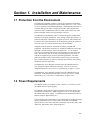
INSTALLATION AND MAINTENANCE
Protection from the Environment ........................................................................................... 1-1
Power Requirements ............................................................................................................. 1-1
CR5000 Power Supplies........................................................................................................ 1-2
Solar Panels........................................................................................................................... 1-4
Direct Battery Connection to the CR5000 Wiring Panel ........................................................ 1-4
Vehicle Power Supply Connections....................................................................................... 1-4
CR5000 Grounding ................................................................................................................ 1-6
Powering Sensors and Peripherals ....................................................................................... 1-9
Controlling Power to Sensors and Peripherals.................................................................... 1-10
Maintenance ........................................................................................................................ 1-12
DATA STORAGE AND RETRIEVAL
Data Storage in CR5000........................................................................................................ 2-1
Internal Data Format .............................................................................................................. 2-2
Data Collection....................................................................................................................... 2-3
Data Format on Computer ................................................................................................... 2-10
i
CR5000 TABLE OF CONTENTS
3.
3.1
3.2
3.3
3.4
3.5
3.6
3.7
3.8
4.
4.1
4.2
4.3
4.4
4.5
4.6
4.7
4.8
CR5000 MEASUREMENT DETAILS
Analog Voltage Measurement Sequence .............................................................................. 3-1
Single Ended and Differential Voltage Measurements .......................................................... 3-4
Signal Settling Time ............................................................................................................... 3-5
Thermocouple Measurements ............................................................................................... 3-7
Bridge Resistance Measurements....................................................................................... 3-17
Measurements Requiring AC Excitation .............................................................................. 3-19
Pulse Count Measurements................................................................................................. 3-20
Self Calibration..................................................................................................................... 3-21
CRBASIC - NATIVE LANGUAGE PROGRAMMING
Format Introduction................................................................................................................ 4-1
Programming Sequence ........................................................................................................ 4-2
Example Program .................................................................................................................. 4-4
Numerical Entries................................................................................................................... 4-7
Logical Expression Evaluation ............................................................................................... 4-7
Flags ...................................................................................................................................... 4-8
Parameter Types ................................................................................................................... 4-9
Program Access to Data Tables .......................................................................................... 4-10
5.
PROGRAM DECLARATIONS ........................................................................................... 5-1
6.
DATA TABLE DECLARATIONS AND OUTPUT PROCESSING INSTRUCTIONS
6.1
6.2
6.3
6.4
7.
7.1
7.2
7.3
7.4
7.5
7.6
7.7
7.8
7.9
Data Table Declaration .......................................................................................................... 6-1
Trigger Modifiers .................................................................................................................... 6-2
Export Data Instructions......................................................................................................... 6-8
Output Processing Instructions............................................................................................ 6-11
MEASUREMENT INSTRUCTIONS
Voltage Measurements .......................................................................................................... 7-3
Thermocouple Measurements ............................................................................................... 7-3
Half Bridges............................................................................................................................ 7-5
Full Bridges ............................................................................................................................ 7-8
Current Excitation ................................................................................................................ 7-11
Excitation/Continuous Analog Output .................................................................................. 7-13
Self Measurements .............................................................................................................. 7-15
Digital I/O ............................................................................................................................. 7-19
Peripheral Devices............................................................................................................... 7-29
8.
PROCESSING AND MATH INSTRUCTIONS ............................................................... 8-1
9.
PROGRAM CONTROL INSTRUCTIONS ....................................................................... 9-1
APPENDIX
A.
CR5000 STATUS TABLE .................................................................................................... A-1
INDEX ......................................................................................................................................... INDEX-1
ii
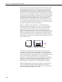
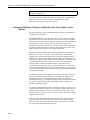
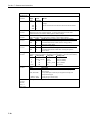
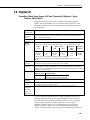
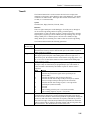
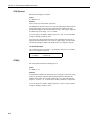
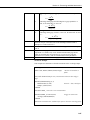
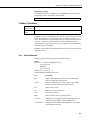
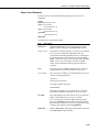
CR5000 Overview
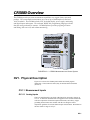
The CR5000 provides precision measurement capabilities in a rugged, battery-operated
package. The system makes measurements at a rate of up to 5,000 samples/second with
16-bit resolution. The CR5000 includes CPU, keyboard display, power supply, and analog
and digital inputs and outputs. The on-board, BASIC-like programming language includes
data processing and analysis routines. PC9000 Software provides program generation
and editing, data retrieval, and realtime monitoring.
1
H
1
2
3
L
H
2
4
5
L
H
3
6
7
L
H
8
4
L
H
9 10
5
L
11 12
6
H L
13 14
7
H L
15 16
8
H L
17 18
9
H L
19 20
10
H L
29 30
15
H L
31 32
16
H L
33 34
17
H L
35 36
18
H L
37 38
19
H L
39 40
20
H L
27 28
14
H L
C2
C3
G
C1
C4
G
12V
SW-12
SW-12
P1
P1
SDM-C3
G
IXR
12V
G
SDM-C1
SDM-C2
IX1
IX4
IX2
IX3
<0.8V
5V
5V
G
CONTROL I/O
SDI-12
CAO2
VX4
CAO1
C8
>2.0V
VX3
G
VX1
VX2
G
G
25 26
13
H L
23 24
12
H L
C5
C6
21 22
11
H L
C7
SE
DIFF
COMPUTER
RS-232
(OPTICALLY ISOLATED)
CS I/O
SE
DIFF
CAUTION
G 12V DC ONLY
CONTROL I/O
POWER
UP
POWER OUT
G 12V
POWER IN
11 - 16 VDC
GROUND
LUG
pc card
status
Logan, Utah
, ' _
A B C
Hm
2
J K L
4
P R S
Graph/
char
5
T U V
- + (
Del
6
W X Y
PgDn
7
OGGER
3
CURSOR
ALPHA
M N O
End
CR5000 MICROL
D E F
PgUp
1
G H I
8
* / )
9
< = >
Ins
0
ESC
SHIFT
Spc Cap
BKSPC
$ Q Z
ENTER
SN:
MADE IN USA
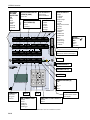
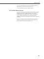
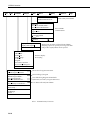
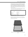
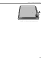
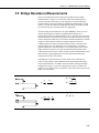
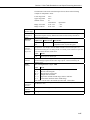
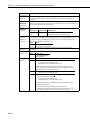
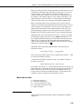
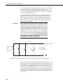
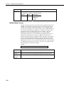
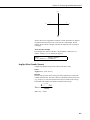
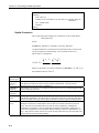
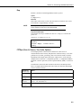
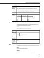
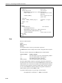
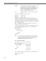
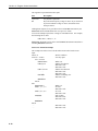
FIGURE OV1-1. CR5000 Measurement and Control System
OV1. Physical Description
Figure OV1-2 shows the CR5000 panel and the associated program
instructions. Unless otherwise noted, they are measurement instructions
(Section 7).
OV1.1 Measurement Inputs
OV1.1.1 Analog Inputs
There are 20 differential or 40 single-ended inputs for measuring voltages up
to ±5 V. A thermistor installed in the wiring panel can be used to measure the
reference temperature for thermocouple measurements, and a heavy copper
grounding bar and connectors combine with the case design to reduce
temperature gradients for accurate thermocouple measurements. Resolution on
the most sensitive range is 0.67 µV
OV-1
CR5000 Overview
1
H
SE
21
DIFF
H
1
11
2
3
L
H
22
23
L
H
2
12
SWITCHED CURRENT
EXCITATION (IX)
ExciteI
Resistance
4
5
L
H
3
24
25
L
H
13
6
7
L
H
26
27
L
H
4
14
8
9
L
H
28
29
L
H
5
15
10
11
L
H
30
31
L
H
6
16
12
13
L
H
32
33
L
H
7
17
14
15
L
H
34
35
L
H
8
18
CONTROL I/O
PortGet
PortSet
ReadIO
TimerIO
WriteIO
16
17
L
H
36
37
L
H
9
19
18
19
L
H
38
39
L
H
10
20
20
L
40
L
COMPUTER RS-232
(OPTICALLY ISOLATED)
SE
DIFF
PULSE INPUTS
PulseCount
PulseCountReset
CONTINUOUS ANALOG
OUTPUTS (CAO)
ExciteCAO
POWER
UP
C4
C3
SIGNAL
GROUND (
FOR
Analog
Pulse
Excitation
CS I/O
DSP4 (Data Tables and Output)
CAUTION
DC ONLY
CONTROL I/O
ANALOG INPUTS
Voltage
VoltDiff
VoltSE
Thermocouple
TCDiff
TCSE
Bridge measurements
(use VX)
BrFull
BrFull6W
BrHalf
BrHalf3W
BrHalf4W
Others
Resistance
PanelTemp
PeriodAvg
AM25T
G
SW-12
C1
C2
SW-12
G
12V
P2
G
SDM-C3
P1
SDM-C2
SDM-C1
IX4
IX3
IX2
IX1
IXR
G
12V
SDI-12
G
5V
5V
CAO1
CAO2
>0.8V
G
>2.0V
VX3
VX4
G
C8
C7
VX2
C6
C5
VX1
CONTROL I/O
G
CS I/O
SWITCHED
VOLTAGE
EXCITATION
(VX)
Excite
BrFull
BrFull6w
BrHalf
BrHalf3W
BrHalf4W
G 12V
POWER IN
11 - 16 VDC
POWER OUT
RS-232
GROUND
LUG
pc card
status
CHARGER INPUT
Logan, Utah
GROUND LUG
, ' _
A B C
PgUp
Hm
2
1
G H I
4
P R S
3
6
5
T U V
- + (
* / )
Del
Ins
POWER IN
0
SHIFT
W X Y
Spc Cap
PgDn
BKSPC
9
8
7
CURSOR
ALPHA
M N O
J K L
Graph/
char
End
CR5000 MICROLOGGER
D E F
< = >
$ Q Z
ESC
ENTER
SN:
MADE IN USA
POWER UP
PowerOff
(program
control)
SDI-12
SDM CONNECTIONS
CS7500
CSAT3
SDMINT8
SDMSpeed
SDMTrigger
POWER GROUND (G),
FOR
5V
SW-12
12V
SDM
PCMCIA PC CARD
CardOut (Data Tables
and Output)
12 V
SWITCHED 12 VOLTS SW-12
PortSet
SW12
FIGURE OV1-2. CR5000 Panel and Associated Instructions.
OV-2
),
CR5000 Overview
OV1.1.2 Signal Grounds (
)
The Signal Grounds ( ) should be used as the reference for Single-ended
Analog inputs, Excitation returns, and sensor shield wires.
Signal returns from the CAO and Pulse channels should use the
terminals
located on the CAO and Pulse terminal strip to minimize current flow through
grounds on the analog terminal strips.
the
OV1.1.3 Power Grounds (G)
The Power Grounds (G) should be used as the returns for the 5V, SW12, 12V,
and C1-C8 outputs. Use of the G grounds for these outputs with potentially
large currents will minimize current flow through the analog section, which
can cause Single-ended voltage measurement errors.
OV1.1.4 Ground Lug
The large ground lug is used to connect a heavy gage wire to earth ground. A
good earth connection is necessary fix the ground potential of the datalogger
terminals or
and to send to earth transients that come in on either the G or
are shunted to ground via the spark gaps protecting other inputs.
OV1.1.5 Power In
The G and 12V terminals on the unplugable Power In connector are for
connecting power from an external battery to the CR5000. These are the only
terminals that can be used to input battery power; the other 12V and SW-12V
terminals are out only. Power from this input will not charge internal CR5000
batteries. Power to charge the internal batteries (17-28 VDC or 18 VRMS AC)
must be connected to the charger input on the side of the LA battery back.
OV1.1.6 Switched 12 Volts SW-12
The SW-12 terminals provide an unregulated 12 volts that can be switched on
and off under program control.
OV1.1.7 Switched Voltage Excitation (VX)
Four switched excitation channels provide precision programmable voltages
within the ±5 Volt range for bridge measurements. Each analog output will
provide up to 50 mA between ±5 V.
OV1.1.8 Switched Current Excitation (IX)
Four Switched Current Excitation channels provide precision current
excitations programmable within ±2.5 mA for resistance or bridge
measurements.
OV1.1.9 Continuous Analog Outputs (CAO)
Two Continuous Analog Outputs (CAO) with individual outputs under
program control for proportional control (e.g., PID algorithm) and waveform
generation. Each analog output will provide up to 15 mA between ±5 V.
OV-3
CR5000 Overview
OV1.1.10 Control I/O
There are 8 digital Input/Output channels (0 V low, 5 V high) for frequency
measurement, digital control, and triggering.
OV1.1.11 Pulse Inputs
Two Pulse input channels can count pulses from high-level (5 V square wave),
switch closure, or low-level A/C signals.
OV1.1.12 Power Up
The CR5000 allows shutting off power under program control. The Power Up
inputs allow an external signal to awaken the CR5000 from a powered down
state (PowerOff, Section 9). When the CR5000 is in this power off state the
ON Off switch is in the on position but the CR5000 is off. If the "<0.5 " input
is switched to ground or if the ">2" input has a voltage greater than 2 volts
applied, the CR5000 will awake, load and run the “run on power-up” program.
If the "< 0.5" input continues to be held at ground while the CR5000 is
powered on and goes through its 2-5 second initialization sequence, the
CR5000 will not run “run on power-up” program.
OV1.1.13 SDM Connections
The Synchronous Device for Measurement (SDM) connections C1,C2, and C3
along with the adjacent 12 volts and ground terminals are used to connect
SDM sensors and peripherals.
OV1.2 Communication and Data Storage
OV1.2.1 PCMCIA PC Card
One slot for a Type I/II/III PCMCIA card. The keyboard display is used to
check card status. The card must be powered down before removing it. The
card will be reactivated if not removed.
CAUTION
Removing a card while it is active can cause garbled data
and can actually damage the card. Do not switch off the
CR5000 power while the card is present and active.
OV1.2.2 CS I/O
A 9-pin serial I/O port supports CSI peripherals.
OV1.2.3 Computer RS-232
RS-232 Port
OV-4
CR5000 Overview
OV1.3 Power Supply and AC Adapter
The CR5000 has two base options the low profile without any power supply
and the lead acid battery power supply base. The low profile base requires an
external DC power source connected to the Power In terminal on the panel.
The battery base has a 7 amp hour battery with built in charging regulator and
includes an AC adapter for use where 120 VAC is available (18 VAC RMS
output). Charging power can also come from a 17-28 VDC input such as a
solar panel. The DCDC18R is available for stepping the voltage up from a
nominal 12 volt source (e.g., vehicle power supply) to the DC voltage required
for charging the internal battery.
OV2. Memory and Programming Concepts
OV2.1 Memory
The CR5000 has 2MB SRAM and 1MB Flash EEPROM. The operating
system and user programs are stored in the flash EEPROM. The memory that
is not used by the operating system and program is available for data storage.
The size of available memory may be seen in the status file. Additional data
storage is available by using a PCMCIA card in the built in card slot.
OV2.2 Measurements, Processing, Data Storage
The CR5000 divides a program into two tasks. The measurement task
manipulates the measurement and control hardware on a rigidly timed
sequence. The processing task processes and stores the resulting
measurements and makes the decisions to actuate controls.
The measurement task stores raw Analog to Digital Converter (ADC) data
directly into memory. As soon as the data from a scan is in memory, the
processing task starts. There are at least two buffers allocated for this raw
ADC data (more under program control), thus the buffer from one scan can be
processed while the measurement task is filling another.
When a program is compiled, the measurement tasks are separated from the
processing tasks. When the program runs, the measurement tasks are
performed at a precise rate, ensuring that the measurement timing is exact and
invariant.
Processing Task:
Digital I/O task
Read and writes to digital I/O ports
(ReadI/O, WriteI/O)
Processes measurements
Determines controls (port states) to set next scan
Stores data
Measurement Task:
Analog measurement and excitation sequence and
timing
Reads Pulse Counters
Reads Control Ports (GetPort)
Sets control ports (SetPort)
OV-5
CR5000 Overview
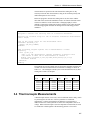
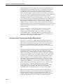
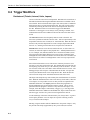
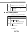
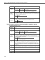
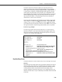
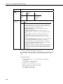
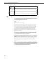
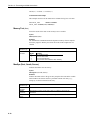
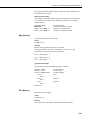
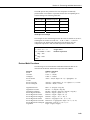
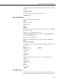
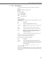
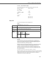
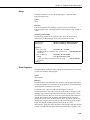
OV2.3 Data Tables
The CR5000 can store individual measurements or it may use its extensive
processing capabilities to calculate averages, maxima, minima, histogams,
FFTs, etc., on periodic or conditional intervals. Data are stored in tables such
as listed in Table OV2-1. The values to output are selected when running the
program generator or when writing a datalogger program directly.
Table OV2-1. Typical Data Table
TOA4
TIMESTAMP
TS
1995-02-16 15:15:04.61
1995-02-16 15:15:04.62
1995-02-16 15:15:04.63
1995-02-16 15:15:04.64
StnName Temp
RECORD RefTemp_Avg
RN
degC
Avg
278822 31.08
278823 31.07
278824 31.07
278825 31.07
TC_Avg(1)
degC
Avg
24.23
24.23
24.2
24.21
TC_Avg(2)
degC
Avg
25.12
25.13
25.09
25.1
TC_Avg(3)
degC
Avg
26.8
26.82
26.8
26.77
TC_Avg(4)
degC
Avg
24.14
24.15
24.11
24.13
TC_Avg(5)
degC
Avg
24.47
24.45
24.45
24.39
TC_Avg(6)
degC
Avg
23.76
23.8
23.75
23.76
OV3. PC9000 Application Software
PC9000 is a Windows™ application for use with the CR5000. The software
supports CR5000 program generation, real-time display of datalogger
measurements, graphing, and retrieval of data files.
OV3.1 Hardware and Software Requirements
The following computer resources are necessary:
•
•
•
•
•
•
•
IBM PC, Portable or Desktop
8 Meg of Ram
VGA Monitor
Windows 95 or newer
30 Meg of Hard Drive Space for software
40 Meg of Hard Drive Space for data
RS232 Serial Port
The following computer resources are recommended:
•
•
•
16 Meg of Ram
33 MHz 486 or faster
Mouse
OV3.2 PC9000 Installation
To install the PC9000 Software:
•
•
•
•
•
OV-6
Start Microsoft Windows
Insert diskette 1 (marked 1 of 2) in a disk drive.
From the Program Manager, select File menu and choose Run
Type (disk drive):\setup and press Enter e.g. a:\setup<Enter>
The setup routine will prompt for disk 2.
CR5000 Overview
You may use the default directory of PC9000 or install the software in a
different directory. The directory will be created for you.
To abort the installation, type Ctrl-C or Break at any time.
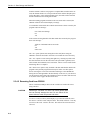
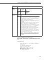
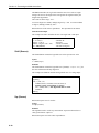
OV3.3 PC9000 Software Overview
This overview points out the main PC9000 functions and where to find them.
PC9000 has extensive on-line help to guide the user in its operation, run
PC9000 to get the details. A CR5000 is not necessary to try out the
programming and real time display options; a demo uses canned data for
viewing. Without a CR5000, there are no communications with the
datalogger; operations such as downloading programs and retrieving data will
not function.
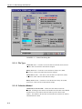
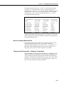
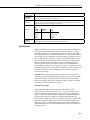
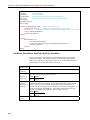
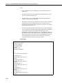
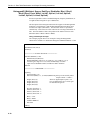
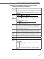
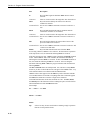
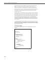
Figures OV3-1 and OV3-2 show the main PC9000 menus. The primary
functions of PC9000 are accessed from the File, Comm, Realtime, and
Analysis selections on the main menu (Figure OV3-1).
OV-7
CR5000 Overview
File
Edit Realtime
Analysis
Tools
Collect
Display
Data Retrieval . . .
Scheduled Data Retrieval . . .
CommLink
Select Series Linked Station . . .
Select Parallel Linked Station . . .
Logger Clock . . .
Logger Status . . .
Download . . .
Save and Download
Logger Files . . .
Diagnostics
Display Data Graph 1 . . .
Display Data Graph 2 . . .
ID2000 . . .
Ctrl + I
Alarms List . . .
Field Monitor . . .
Virtual Meter . . .
Virtual O'Scope . . .
X-Y Plotter . . .
Histogram . . .
Fast Fourier Transform . . .
Level Crossing Histogram . . .
Get/Set Variable . . .
CR9000 Program Generator
CR5000 Program Generator
CR9000 Program Editor . . .
CR5000 Program Editor . . .
Open Wiring Diagram . . .
Open Data Table Info File . . .
Open Data File . . .
Convert Binary to ASCII File . . .
Print . . .
Printer Setup . . .
DOS Shell . . .
File Manager . . .
Explorer . . .
Exit PC9000
Help
Collect data from CR5000
PC to CR5000
communications.
Display Data in Tables Collected From CR5000.
Graphing requires no special processing of the data
and provides rapid feedback to the operator.
Realtime Display
& Graphing
Menu-driven Program Generation.
Direct Editing of Program
View/Edit Wiring Diagram & DataTable
Information (Created by Program Generator)
View Data Collected from CR5000
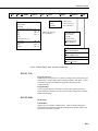
OV3-1. PC9000 Primary Functions
OV-8
Windows
CR5000 Overview
File
Edit Realtime
Analysis
Undo
Date & Time
Select All
Strip Remarks and Spaces
Cut
Copy
Paste
Delete
Delete Line Ctrl + Y
Wrap Text
Go To Line . . .
Find
Replace
Tools
Collect
Colors . . .
Fonts . . .
Defaults . . .
Ctrl + Z
Ctrl + S
Ctrl + X
Ctrl + C
Ctrl + V
Editing Options for
Active Windows
Ctrl + W
Display
Windows
Help
Change fonts
and/or Colors for
Active Windows.
Tile Horizontal . . .
Tile Vertical . . .
Cascade . . .
Arrange Icons . . .
Work Area Setup . . .
List of Windows
Ctrl + F
Ctrl + R
PC9000 Help Contents . . .
Search PC9000 Help . . .
CRBasic Help Contents . . .
Search CRBasic Help . . .
Obtaining Technical Support . . .
About PC9000 . . .
Software Versions . . .
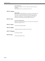
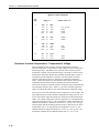
OV3-2. PC9000 Editing, Help, and User Preferences
OV3.3.1 File
Program Generator
Guides the user through a series of menus to configure the measurement types:
thermocouple, voltage, bridge, pulse counting, frequency, and others. Creates
a CR5000 program, wiring diagram, output table, description, and
configuration file.
Program Editor
Create programs directly or edit those created by the program generator or
retrieved from the CR5000. Provides context-sensitive help for the CR5000's
BASIC-like language.
OV3.3.2 Edit
REALTIME
Virtual Meter
Updates up to five displays simultaneously. Choices include analog meter,
horizontal and vertical bars, independent scaling/offset, multiple alarms, and
rapid on-site calibration of sensors
OV-9
CR5000 Overview
Virtual Oscilloscope
Displays up to six channels. Time base variable from milliseconds to hours.
X-Y Plotter
Allows comparison of any two measurements in real time.
OV3.3.3 Analysis
Data Graphing
Displays up to 16 fields simultaneously as strip charts or two multi-charts with
up to 8 traces each. Includes 2D/3D bars, line, log/linear, area, and scatter.
Line statistics available for max/min, best fit, mean, and standard deviation.
Handles files of unlimited size. Historical graphing requires no special
processing of the data and provides rapid feedback to the operator.
OV3.3.4 Tools
Control and Communications
Supports PC to CR5000 communications: clock read/set, status read, program
download, and program retrieval.
OV3.3.5 Collect
Collect data from CR5000 data tables
OV3.3.6 Display
Configure the font and color scheme in an active window.
OV3.3.7 Windows
Size and arrange windows.
OV3.3.8 Help
On-line help for PC9000 software.
OV-10
CR5000 Overview
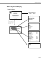
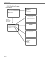
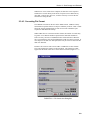
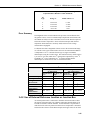
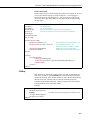
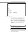
OV4. Keyboard Display
Power Up Screen
CAMPBELL
SCIENTIFIC
CR5000 Datalogger
06/18/2000, 18:24:35
CPU: TRIG.CR5
Running.
Press any key
for Main Menu
(except < >)
Data
Run/Stop Program
File
Status
Configure, Settings
Adjust contrast with < >
< lighter
darker >
Real Time Tables
Real Time Custom
Final Storage Data
Reset Data Tables
Graph Setup
New
Edit
Copy
Delete
Run Options
Directory
Format
ROM Version
OS Version
OS Date
OS Signature
Serial Number
Rev Board
Station Name
Program Name
StartTime
Run Signature
DLD Signature
Battery
:
:
:
xxxx
xxxx
xxxx
:
:
:
xxxx
xxxxx
xxxxx
:
xxxx
Set Time/Date
Settings
Display
OV-11
CR5000 Overview
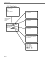
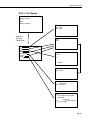
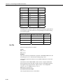
OV4.1 Data Display
Data
Run/Stop Program
File
Status
Configure, Settings
Cursor to Data
and Press
Enter
Real Time Tables
Real Time Custom
Final Storage Data
Reset Data Table
Graph Setup
List of Data Tables created by
active program
List of Data Tables created by
active program
List of Data Tables created by
active program
All Tables
List of Data Tables created by
active program
Graph Type: Scope
Scaler: Manual
Upper: 0.000000
Lower: 0.000000
Display Val
Off
Display Max
Off
Display Min
Off
OV-12
CR5000 Overview
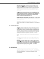
OV4.1.1 Real Time Tables
List of Data Tables created by
active program. For Example,
Table1
Temps
Public
Cursor to desired
Table and press
Enter
Tref
TCTemp(1)
TCTemp(2)
TCTemp(3)
Flag(1)
Flag(2)
Flag(3)
Flag(4)
: 23.0234
: 19.6243
: 19.3429
: 21.2003
: -1.0000
: 0.00000
: 0.00000
: 0.00000
Public Table values
can be changed.
Cursor to value and
press Enter to edit
value.
Press Graph/ Char
for Graph of
selected field
30.0
22.35
Press Ins for
Graph Setup
_____
___
____
__
20.00
Tref
TCTemp(1)
TCTemp(2)
TCTemp(3)
TCTemp(3)
Flag(1)
Flag(2)
Flag(3)
Flag(4)
Fl (3)
: 23.0234
: 19.6243
: 19.3429
: 221.2003
: -1.0000
: 0.00000
: 0.00000
: 0.00000
Scaler Manual
Upper: 30.000000
Lower: 20.000000
Display Val
On
Display Max
On
Display Min
On
Graph Type
Roll
New values are displayed as they
are stored.
OV-13
CR5000 Overview
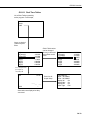
OV4.1.2 Setting up Real Time Custom Display
List of Data Tables created by
active program. For Example,
Table1
Temps
Public
Cursor to desired
Table and Press
Enter
Cursor to position for next value
and Press Enter
Tref
TCTemp(1)
TCTemp(2)
TCTemp(3)
Flag(1)
Flag(2)
Flag(3)
Flag(4)
Cursor to desired
Field and Press
Enter
TCTemp(3)
: 24.9496
:
:
:
:
:
:
:
New values are displayed as they
are stored.
OV-14
CR5000 Overview
OV4.1.3 Final Storage Tables
List of Data Tables created by
active program. For Example:
Table1
Temps
Cursor to desired
Table and Press
Enter
TimeStamp
"2000-01-03 00:12:38"
"2000-01-03 00:12:39"
"2000-01-03 00:12:40"
"2000-01-03 00:12:41"
"2000-01-03 00:12:42"
"2000-01-03 00:12:43"
"2000-01-03 00:12:44"
"2000-01-03 00:12:45"
"2000-01-03 00:12:46"
"2000-01-03 00:12:47"
"2000-01-03 00:12:48"
"2000-01-03 00:12:49"
Record
0
1
2
3
4
5
6
7
8
9
10
11
Use Hm (oldest), End (newest),
PgUp (older), PgDn (newer),
←, →, ↑, and ↓ to move around
in data table.
Tref
5
24.1242
Tref
24.1242
24.1242
24.1242
24.1242
24.1242
24.1242
24.1242
24.1242
24.1242
24.1242
TC(1)
:
:
:
:
:
:
21.8619
TC(1)
21.8786
21.8786
21.8786
21.8675
21.8675
21.8675
21.8398
21.8176
21.8342
21.8453
Go to Record:
5
press Ins to edit
Press Graph/ Char for
Graph of selected field.
Use ←, →, PgUp, PgDn
to move cursor and
window of data graphed.
30.0
Table Size:
1000
Current Record:
759
21.87
_______
______
_______
____
20.00
TC(2)
TC(3)
21.934
22.8419
21.9173
22.8364
21.9229
22.8364
21.9173
22.8419
21.9173
22.8253
21.9118
22.8364
21.9173
22.8087
21.9173
22.8142
21.9395
22.8253
21.9118
22.8308
21.945
22.8364
21.9506
22.8364
Press Ins for Jump To screen.
:2000-01-03 00:12:43
___
____
__
Press Ins for
Graph Setup
Scaler Manual
Upper: 30.000000
Lower: 20.000000
Display Val
On
Display Max
On
Display Min
On
Graph Type
Roll
OV-15
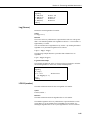
CR5000 Overview
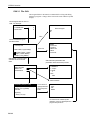
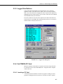
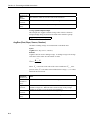
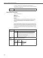
OV4.2 Run/Stop Program
PCCard Display
Data
Run/Stop Program
File
Status
Configure, Settings
CPU:
List of Programs
No Program
CRD:
List of Programs
You may now
remove the Card.
CR5000 closes tables first.
Cursor to
PCCard and
Press Enter
Remove Card
Format Card
Table Status
Card Status
All Card Data
Will be Lost!
Proceed?
Yes
No
List of Data Tables on card
created by active program
PC Card Status:
Battery OK
5Volt Card
WP Disabled
OV-16
CR5000 Overview
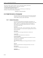
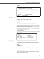
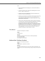
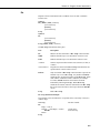
OV4.3 File Display
Data
Run/Stop Program
File
Status
Configure, Settings
New File Name:
CPU: .CR5
CRD: .CR5
Cursor to
File and
Press Enter
New
Edit
Copy
Delete
Run Options
Directory
Format
CPU:
CRD:
Copy
From
To
Execute
List of files on
CPU or Card.
CPU: Program
No Program
CRD: Program
CPU:
All programs and other files
will be lost!
Proceed?
Yes
List of Programs
No
OV-17
CR5000 Overview
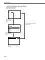
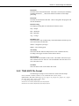
OV4.3.1 File: Edit
The Program Editor in PC9000 is recommended for writing and editing
datalogger programs. Changes in the field can be made with the keyboard
display.
List of Program files on CPU: or
CRD: For Example:
CPU:
TCTEMP.CR5
RACE.CR5
0
0
Save Changes?
Yes
No
ESC
Cursor to desired Program
and Press Enter
INSERT
Instruction
Function
Blank Line
Block
Insert Off
CR5000
' TCTemp.CR5
Public TREF,TC(3),FLAG(8)
D
D ataTable (Temps,1,1000)
Sample (1,TREF,IEEE4)
Sample (3,TC(),IEEE4)
E dT bl
Edit Directly or Cursor to first
character of line and Press
Enter
Press Ins
Edit Instruction parameters with
parameter names and some pick lists:
DataTable
TableName
> Temps
TrigVar
1
Size
1000
ENTER
Edit Instruction
Blank Line
Create Block
Insert blank line
DataTable
DataTable(Temps,1,1000)
(Temps,1,1000)
Sample (1,TREF,IEEE4)
Sample (3,TC(),IEEE4)
EndTable
Cursor down to
highlight desired
block and press
Enter
Block Commands
Copy
Cut
Delete
BeginProg
Scan(1,sec,3,0)
To insert a block created by this
operation, cursor to desired place in
program and press Ins.
OV-18
CR5000 Overview
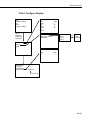
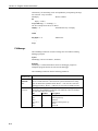
OV4.4 Configure Display
05/24/2000, 15:10:40
Year
Month
Day
Hour
Minute
Set
Cancel
Data
Run/Stop Program
File
Status
Configure, Settings
Cursor to
Configure,
Settings and
Press Enter
2000
5
24
15
10
Security Enable
RS-232 Time Out: No
CR5000 Off
Enter Passwords:
Level 1:
Level 2:
Level 3:
click
Enter
Num
Password
Set Time/Date
Settings
Display
Light
<-
*
Dark
->
Turn off display
Back Light
Contrast Adjust
Display Time Out: No, Yes (if yes)
Time out (min) 1
OV-19
CR5000 Overview
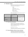
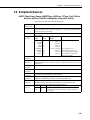
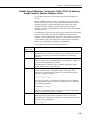
OV5. Specifications
Electrical specifications are valid over a -25° to +50°C range unless otherwise specified; testing over -40° to +85°C available as
an option, excludes batteries. Non-condensing environment required. Yearly calibrations are recommended to maintain electrical specifications.
PROGRAM EXECUTION RATE
RESISTANCE MEASUREMENTS
EMI and ESD PROTECTION
The CR5000 can measure one channel and store the
result in 500 µs; all 40 SE* channels can be measured
in 8 ms (5 kHz aggregate rate).
Provides voltage ratio measurements of 4- and 6-wire
full bridges, and 2-, 3-, 4-wire half bridges. Direct
resistance measurements available with current excitation. Dual-polarity excitation is recommended.
The CR5000 is encased in metal and incorporates
EMI filtering on all inputs and outputs. Gas discharge
tubes provide robust ESD protection on all terminal
block inputs and outputs. The following European
standards apply.
ANALOG INPUTS
DESCRIPTION: 20 DF* or 40 SE, individually
configured. Channel expansion provided through
AM16/32, AM416, and AM25T Multiplexers.
RANGES, RESOLUTION, AND TYPICAL INPUT
NOISE: Basic Resolution (Basic Res) is the A/D
resolution of a single conversion. Resolution of
DFM* with input reversal is half the Basic Res.
Noise values are for DFM with input reversal; noise
is greater with SEM.*
Input
Basic
0 Int.
Rng (mV) Res (µV) (µV RMS)
±5000
±1000
±200
±50
±20
167
33.3
6.67
1.67
0.67
250 µs Int. 20/16.7 ms Int.
(µV RMS)
(µV RMS)
70
30
8
3.0
1.8
60
12
2.4
0.8
0.5
30
6
1.2
0.3
0.2
ACCURACY†:
±(0.05% of Reading + Offset)
0° to 40°C
±(0.075% of Reading + Offset)
-25° to 50°C
±(0.10% of Reading + Offset)
-40° to 85°C
Offset for DFM w/input reversal =
Basic Res +1 µV
Offset for DFM w/o input reversal =
2Basic Res + 2 µV
Offset for SEM = 2Basic Res + 10 µV
MINIMUM TIME BETWEEN MEASUREMENTS:
Zero Integration:
250 µs Integration:
16.7 ms Integration:
20 ms Integration:
125 µs
475 µs
19.9 ms
23.2 ms
VOLTAGE RATIO ACCURACY†: Assumes input and
excitation reversal and an excitation voltage of at
least 2000 mV.
±(0.04% Reading + Basic Res/4)
0° to 40°C
±(0.05% Reading + Basic Res/4) -25° to 50°C
±(0.06% Reading + Basic Res/4) -40° to 85°C
ACCURACY† WITH CURRENT EXCITATION:
Assumes input and excitation reversal, and an
excitation current, Ix, of at least 1 mA.
±(0.075% Reading + Basic Res/2Ix) 0° to 40°C
±(0.10% Reading + Basic Res/2Ix) -25° to 50°C
±(0.12% Reading + Basic Res/2Ix) -40° to 85°C
PERIOD AVERAGING MEASUREMENTS
DESCRIPTION: The average period for a single
cycle is determined by measuring the duration of a
specified number of cycles. Any of the 40 SE
analog inputs can be used; signal attenuation and
ac coupling may be required.
INPUT FREQUENCY RANGE:
Input
Rng (mV)
±5000
±1000
±200
Signal (peak to peak)
Min.
Max.1
600 mV
100 mV
4 mV
10 V
2.0 V
2.0 V
Min.
Pulse W.
Max.
Freq
2.5 µs
5.0 µs
25 µs
200 kHz
100 kHz
20 kHz
1
Maximum signals must be centered around
datalogger ground.
RESOLUTION: 70 ns/number of cycles measured
ACCURACY: ±(0.03% of Reading + Resolution)
COMMON MODE RANGE: ±5 V
PULSE COUNTERS
DC COMMON MODE REJECTION: >100 dB with
input reversal (>80 dB without input reversal)
DESCRIPTION: Two 16-bit inputs selectable for switch
closure, high frequency pulse, or low-level ac.
NORMAL MODE REJECTION: 70 dB @ 60 Hz
when using 60 Hz rejection
SUSTAINED INPUT VOLTAGE WITHOUT DAMAGE:
±16 Vdc
INPUT CURRENT: ±2 nA typ., ±10 nA max. @ 50°C
INPUT RESISTANCE: 20 GΩ typical
ACCURACY OF INTERNAL THERMOCOUPLE
REFERENCE JUNCTION:
±0.25°C, 0° to 40°C
±0.5°C, -25° to 50°C
±0.7°C, -40° to 85°C
ANALOG OUTPUTS
DESCRIPTION: 4 switched voltage; 4 switched current; 2 continuous voltage; switched outputs active
only during measurements, one at a time.
RANGE: Voltage (current) outputs programmable
between ±5 V (±2.5 mA)
RESOLUTION: 1.2 mV (0.6 µA) for voltage (current)
outputs
ACCURACY: ±10 mV (±10 µA) for voltage (current)
outputs
CURRENT SOURCING: 50 mA for switched voltage;
15 mA for continuous
CURRENT SINKING: 50 mA for switched voltage;
5 mA for continuous (15 mA w/selectable option)
COMPLIANCE VOLTAGE: ±5 V for switched current
excitation
MAXIMUM COUNT: 4 x 109 counts per scan
SWITCH CLOSURE MODE:
Minimum Switch Closed Time: 5 ms
Minimum Switch Open Time: 6 ms
Maximum Bounce Time: 1 ms open without
being counted.
HIGH FREQUENCY PULSE MODE:
Maximum Input Frequency: 400 kHz
Maximum Input Voltage: ±20 V
Voltage Thresholds: Count upon transition
from below 1.5 V to above 3.5 V at low frequencies. Larger input transitions are required at high
frequencies because of 1.2 µs time constant filter.
Details of performance criteria applied are available
upon request.
Warning: This is a Class A product. In a domestic
environment this product may cause radio interference
in which case the user may be required to correct the
interference at the user’s own expense.
CPU AND INTERFACE
PROCESSOR: Hitachi SH7034
MEMORY: Battery-backed SRAM provides 2 Mbytes
for data and operating system use with
128 kbytes reserved for program storage.
Expanded data storage with PCMCIA type I,
type II, or type III card.
DISPLAY: 8-line-by-21 character alphanumeric or
128 x 64 pixel graphic LCD display w/backlight.
SERIAL INTERFACES: Optically isolated RS-232
9-pin interface for computer or modem. CSI/O
9-pin interface for peripherals such as CSI
modems.
BAUD RATES: Selectable from 1,200 to 115,200 bps.
ASCII protocol is eight data bits, one start bit, one
stop bit, no parity.
CLOCK ACCURACY: ±1 minute per month
SYSTEM POWER REQUIREMENTS
VOLTAGE: 11 to 16 Vdc
TYPICAL CURRENT DRAIN: 400 µA software power
off; 1.5 mA sleep mode; 4.5 mA at 1 Hz (200 mA
at 5 kHz) sample rate.
INTERNAL BATTERIES: 7 Ahr rechargeable base
(optional); 1650 mAhr lithium battery for clock and
SRAM backup, 10 years of service typical, less at
high temperatures.
EXTERNAL BATTERIES: 11 to 16 Vdc; reverse
polarity protected.
PHYSICAL SPECIFICATIONS
SIZE: 9.8” x 8.3” x 4.5” (24.7 cm x 21.0 cm x 11.4 cm)
Terminal strips extend 0.4” (1.0 cm).
WEIGHT: 4.5 lbs (2.0 kg) with low-profile base;
12.2 lbs (5.5 kg) with rechargeable base
WARRANTY
Three years against defects in materials and
workmanship.
LOW LEVEL AC MODE:
Internal ac coupling removes dc offsets up to
±0.5 V.
Input Hysteresis: 15 mV
Maximum ac Input Voltage: ±20 V
Minimum ac Input Voltage (sine wave):
(mV RMS)
Range (Hz)
20
1.0 to 1000
200
0.5 to 10,000
1000
0.3 to 16,000
DIGITAL I/O PORTS
*SE(M): Single-Ended (Measurement)
DESCRIPTION: 8 ports selectable as binary inputs or
control outputs.
*DF(M): Differential (Measurement)
OUTPUT VOLTAGES (no load): high 5.0 V ±0.1 V;
low < 0.1 V
†
Sensor and measurement noise not included.
OUTPUT RESISTANCE: 330 Ω
INPUT STATE: high 3.0 to 5.3 V; low -0.3 to 0.8 V
INPUT RESISTANCE: 100 kΩ
OV-20
EMC tested and conforms to BS EN61326:1998.
We recommend that you confirm system
configuration and critical specifications with
Campbell Scientific before purchase.
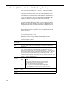
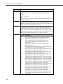
Section 1. Installation and Maintenance
1.1 Protection from the Environment
The normal environmental variables of concern are temperature and moisture.
The standard CR5000 is designed to operate reliably from -25 to +50°C (-40°C
to +85°C, optional) in noncondensing humidity. When humidity tolerances are
exceeded, damage to IC chips, microprocessor failure, and/or measurement
inaccuracies due to condensation on the various PC board runners may result.
Effective humidity control is the responsibility of the user.
The CR5000 is not hermetically sealed. Two half unit packets of DESI PAK
desiccant are located by the batteries. A dry package weighs approximately 19
grams and will absorb a maximum of six grams of water at 40% humidity and
11 grams at 80%. Desiccant packets can be dried out by placing the packets in
an oven at 120°C for 16 hours (desiccant only, not the CR5000).
Campbell Scientific offers two enclosures for housing a CR5000 and
peripherals. The fiberglass enclosures are classified as NEMA 4X (water-tight,
dust-tight, corrosion-resistant, indoor and outdoor use). A 1.25" diameter
entry/exit port is located at the bottom of the enclosure for routing cables and
wires. The enclosure door can be fastened with the hasp for easy access, or
with the two supplied screws for more permanent applications. The white
plastic inserts at the corners of the enclosure must be removed to insert the
screws. Both enclosures are white for reflecting solar radiation, thus reducing
the internal enclosure temperature.
The Model ENC 12/14 fiberglass enclosure houses the CR5000 and one or
more peripherals. Inside dimensions of the ENC 12/14 are 14"x12"x5.5",
outside dimensions are 18"x13.5"x8.13" (with brackets); weight is 11.16 lbs.
The Model ENC 16/18 fiberglass enclosure houses the CR5000 and several
peripherals. Inside dimensions of the ENC 16/18 are 18"x16"x8¾", outside
dimensions are 18½"x18¾"x10½" (with brackets); weight is 18 lbs.
1.2 Power Requirements
The CR5000 operates at a nominal 12 VDC. Below 11.0 V or above 16 volts
the CR5000 does not operate properly.
The CR5000 is diode protected against accidental reversal of the positive and
ground leads from the battery. Input voltages in excess of 18 V may damage
the CR5000 and/or power supply. A transzorb provides transient protection by
limiting voltage at approximately 20 V.
System operating time for the batteries can be determined by dividing the battery
capacity (amp-hours) by the average system current drain. The CR5000
typically draws 1.5 mA in the sleep state (with display off), 4.5 mA with a 1 Hz
sample rate, and 200 mA with a 5 kHz sample rate.
1-1
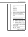
Section 1. Installation and Maintenance
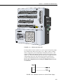
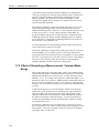
1.3 CR5000 Power Supplies
The CR5000 may be purchased with either a rechargeable lead acid battery or
with a low profile case without a battery.
While the CR5000 has a wide operating temperature range (-40 to +85°C
optional), the lead acid battery base is limited to -40 to +60°C. Exceeding this
range will degrade battery capacity and lifetime and could also cause
permanent damage.
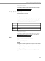
1.3.1 CR5000 Lead Acid Battery BASE
Temperature range:
Charging voltage:
NOTE
-40° to +60°C
17 to 24 VDC or 18 V RMS AC
In normal operation a charging source should be connected to
the base at all times. The CR5000 stops measuring at ~11 V.
Battery life is shortened when discharged below 10.5 V.
The CR5000 includes a 12 V, 7.0 amp-hour lead acid battery, an AC
transformer (18 V RMS AC), and a temperature compensated charging circuit
with a charge indicating LED (Light Emitting Diode). An AC transformer or
solar panel should be connected to the base at all times. The charging source
powers the CR5000 while float charging the lead acid batteries. The internal
lead acid battery powers the datalogger if the charging source is interrupted.
The lead acid battery specifications are given in Table 1.3-1.
The leads from the charging source connect to a wiring terminal plug on the
side of the base. Polarity of the leads to the connector does not matter. A
transzorb provides transient protection to the charging circuit. A sustained
input voltage in excess of 40V will cause the transzorb to limit voltage.
The red light (LED) on the base is on during charging with 17 to 24 VDC or
18 V RMS AC. The switch turns power to the CR5000 on or off. Battery
charging still occurs when the switch is off.
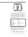
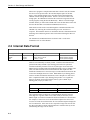
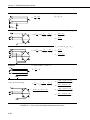
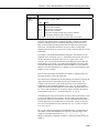
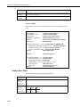
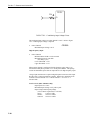
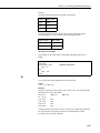
Should the lead acid batteries require replacement, consult Figure 1.3-1 for
wiring.
1-2
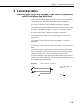
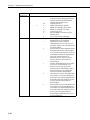
Section 1. Installation and Maintenance
LEAD ACID BATTERY REPLACEMENT
6V 7AH
LEAD ACID
BATTERY
+
+
6V 7AH
LEAD ACID
BATTERY
RED
WHITE
BLACK
-
-
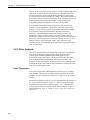
FIGURE 1.3-1. Lead Acid Battery Wiring
Monitor the power supply using datalogger Instruction “ Battery” . Incorporate
this instruction into data acquisition programs to keep track of the state of the
power supply. If the system voltage level consistently decreases through time,
some element(s) of the charging system has failed. Battery measures the
voltage at the CR5000 electronics, not the voltage of the lead acid battery. The
measured voltage will normally be about 0.3 V less than the voltage at the
internal or external 12 V input. This voltage drop is on account of a Schottkey
diode. External power sources must be disconnected from the CR5000 to
measure the actual lead acid battery voltage.
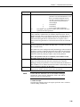
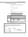
TABLE 1.3-1. CR5000 Rechargeable Battery and AC Transformer
Specifications
Lead Acid Battery
Battery Type
Float Life @ 25oC
Capacity
Shelf Life, full charge
Charge Time (AC Source)
Operating temperature
AC Transformer
Input:
Isolated Output:
Yuasa NP7-6
3 years minimum
7.0 amp-hour
6 months
40 hr full charge, 20 hr 95% charge
-40°C to 60°C
120 VAC, 60 Hz
18 VAC 1.2 Amp
There are inherent hazards associated with the use of sealed lead acid batteries.
Under normal operation, lead acid batteries generate a small amount of
hydrogen gas. This gaseous by-product is generally insignificant because the
hydrogen dissipates naturally before build-up to an explosive level (4%)
occurs. However, if the batteries are shorted or overcharging takes place,
hydrogen gas may be generated at a rate sufficient to create a hazard.
Campbell Scientific recommends:
1.
A CR5000 equipped with standard lead acid batteries should NEVER be
used in applications requiring INTRINSICALLY SAFE equipment.
2.
A lead acid battery should not be housed in a gas-tight enclosure.
1-3
Section 1. Installation and Maintenance
1.3.2 Low Profile CR5000
The low profile CR5000 option is not supplied with a battery base. See
Section 1.5 and 1.6 for external power connection considerations.
1.4 Solar Panels
Auxiliary photovoltaic power sources may be used to maintain charge on lead
acid batteries.
When selecting a solar panel, a rule-of-thumb is that on a stormy overcast day
the panel should provide enough charge to meet the system current drain
(assume 10% of average annual global radiation, kW/m2). Specific site
information, if available, could strongly influence the solar panel selection.
For example, local effects such as mountain shadows, fog from valley
inversion, snow, ice, leaves, birds, etc. shading the panel should be considered.
Guidelines are available from the Solarex Corporation for solar panel selection
called "DESIGN AIDS FOR SMALL PV POWER SYSTEMS". It provides a
method for calculating solar panel size based on general site location and
system power requirements. If you need help in determining your system
power requirements contact Campbell Scientific's Marketing Department.
1.5 Direct Battery Connection to the CR5000 Wiring
Panel
Any clean, battery backed 11 to 16 VDC supply may be connected to the 12 V
and G connector terminals on the front panel. When connecting external
power to the CR5000, first, remove the green power connector from the
CR5000 front panel. Insert the positive 12 V lead into the right-most terminal
of the green connector. Insert the ground lead in the left terminal. Double
check polarity before plugging the green connector into the panel.
Diode protection exists so that an external battery can be connected to the green
G and 12 V power input connector, without loading or charging the internal
batteries. The CR5000 will draw current from the source with the largest
voltage. When power is connected through the front panel, switch control on
the standard CR5000 power supplies is by-passed (Figure 1.7-1).
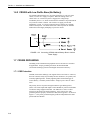
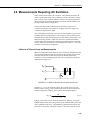
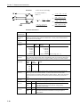
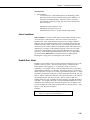
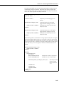
1.6 Vehicle Power Supply Connections
1.6.1 CR5000 with Battery Base
The best way to power a CR5000 with battery base from a vehicle’s 12 V
power system is to use the DCDC18R to input the power to the CR5000’s
charger input (Figure 1.6-1). With this configuration the CR5000’s batteries
are charged when the vehicle power is available. When the vehicle’s voltage is
too low or off, the CR5000 is powered from its internal batteries.
1-4
Section 1. Installation and Maintenance
1
H
1
2
3
L
H
2
4
5
L
H
3
6
7
L
H
8
4
L
H
9 10
5
L
11 12
6
H L
13 14
7
H L
15 16
8
H L
17 18
9
H L
19 20
10
H L
29 30
15
H L
31 32
16
H L
33 34
17
H L
35 36
18
H L
37 38
19
H L
39 40
20
H L
DCDC1R
BOOST REG
ULATOR
G
C3
C2
C1
C4
SW-12
SW-12
G
12V
G
P1
IXR
P1
SDM-C3
SDM-C2
SDM-C1
IX4
SDI-12
12V
G
IX1
IX2
CAO2
CAO1
IX3
G
5V
5V
G
>2.0V
CONTROL I/O
<0.8V
VX4
VX3
C7
C8
27 28
14
H L
25 26
13
H L
23 24
12
H L
G
VX1
G
VX2
21 22
11
H L
C5
C6
SE
DIFF
COPTER
RS-232
(OPTICALLY ISOLATED)
CS I/O
SE
DIFF
V in
(11-16)V
CATON
CONTROL I/O
POWER
UP
POWER OUT
12V
POWER N
11 - 16 VDC
G
V out
18V G
MADE IN
USA
12V DC ONL
ROND
L
pc card
status
Logan tah
A B C
m
2
L
4
P R S
easurement and
Control
3
raph
char
5
T
CRSOR
ALPA
N O
V
6
W
End
CR5000
D E
Pgp
1
PgDn
ST
Spc Cap
BSPC
-
System
Del
ns
0
ESC
ENTER
SN
ADE N SA
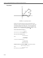
FIGURE 1.6-1. CR5000 with DCDC18R
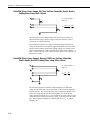
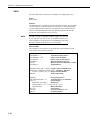
It is also possible to use the vehicle's 12 V power system as the primary supply
for a CR5000 with a battery base (Figure 1.6-2). When a vehicle’s starting
motor is engaged, the system voltage drops considerably below the 11 volts
needed for uninterrupted datalogger function. Diodes in the CR5000 in series
with the 12 V Power In connector allow the battery base to supply the needed
voltage during motor start. The diodes also prevent the separate power
systems of the CR5000 and vehicle from attempting to charge each other.
Because this configuration does not charge the CR5000 batteries, it is not
recommended.
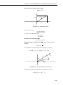
CR5000
Panel
+12V
G
FIGURE 1.6-2. Alternate Connect on to Vehicle Power Supply
1-5
Section 1. Installation and Maintenance
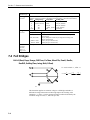
1.6.2 CR5000 with Low Profile Base (No Battery)
If a CR5000 without batteries is to be powered from the 12 Volts of a motor
vehicle, a second 12 V supply is required. When the starting motor of a
vehicle with a 12 V electrical system is engaged, the voltage drops
considerably below 11 V, which would cause the CR5000 to stop measurement
every time the vehicle is started. The second 12 V supply prevents this
malfunction. Figure 1.6-3 shows connecting the two supplies to a CR5000
without a battery base. The diodes allows the vehicle to power the CR5000
without the second supply attempting to power the vehicle.
CR5000
Panel
+12V
G
FIGURE 1.6-3. Connecting CR5000 without Battery Base to Vehicle
Power Supply
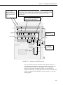
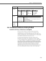
1.7 CR5000 GROUNDING
Grounding of the CR5000 and its peripheral devices and sensors is critical in
all applications. Proper grounding will ensure the maximum ESD
(electrostatic discharge) protection and higher measurement accuracy.
1.7.1 ESD Protection
An ESD (electrostatic discharge) can originate from several sources. However,
the most common, and by far potentially the most destructive, are primary and
secondary lightning strikes. Primary lightning strikes hit the datalogger or
sensors directly. Secondary strikes induce a voltage in power lines or sensor
wires.
The primary devices for protection against ESD are gas-discharge tubes
(GDT). All critical inputs and outputs on the CR5000 are protected with GDTs
or transient voltage suppression diodes. The GDTs fire at 150 V to allow
current to be diverted to the earth ground lug. To be effective, the earth
ground lug must be properly connected to earth (chassis) ground. As shown in
Figure 1.7-1, the power ground and signal ground are independent lines until
joined inside the CR5000.
1-6
Section 1. Installation and Maintenance
Tie analog signal
shields and returns to
grounds ( ) located in
analog input terminal
strips.
Tie CAO and pulse-counter returns into grounds ( ) in CAO and pulse-counter
terminal strip. Large excitation return currents may also be tied into this ground
in order to minimize induced single-ended offset voltages in half bridge
measurements.
Tie 5 V, SW-12, 12 V and C1-C8
returns into power grounds (G).
1
H
1
2
3
L
H
22
23
L
H
Analog Grounds
2
4
5
L
H
3
6
7
L
H
4
8
9
L
H
28
29
L
H
5
10
11
L
H
30
31
L
H
6
12
13
L
H
32
33
L
H
7
14
15
L
H
34
35
L
H
8
16
17
L
H
36
37
L
H
9
18
19
L
H
38
39
L
H
10
20
L
CS IO
SE
DIFF
Ground Plane
24
25
L
H
13
26
27
L
H
14
15
16
17
18
19
20
40
L
COPUTER RS-232
(OPTICALL ISOLATED)
12
C2
C3
C4
SW-12
SW-12
Star Ground at
Ground Lug
1.85A
Thermal fuse
G
C1
G
P2
12V
G
G
IXR
P1
IX4
12V
SDM-C3
IX3
SDI-12
SDM-C2
IX2
G
>0.8V
G
C6
Power Grounds (G)
SDM-C1
IX1
5V
CAO2
5V
CAO1
G
VX4
>2.0V
VX3
C8
CONTROL I/O
C7
)
VX2
Excitation, CAO,
Pulse Counter Grounds (
11
VX1
H
C5
21
G
SE
DIFF
CAUTION
DC ONL
CONTROL I/O
POWER
UP
G 12V
POWER IN
11 - 16 VDC
POWER UP
0.9A
Thermal
fuse
SW12
Control
GROUND
LUG
Batteriespc card
status
On/Off
Logan Utah
1.85A
Thermal fuse
A B C
D E
PgUp
m
2
1
G
5A Thermal fuse
I
To CR5000
Electronics
4
Graph
char
6
5
10µf
T U V
End
(
Del
SIT
1.5k E20A
W
Spc Cap
PgDn
BSPC
7
-
CR5000 ICROLOGGER
External
Power Input
N O
L
P R S
3
CURSOR
ALPA
)
Ins
0
ESC
ENTER
SN
ADE IN USA
FIGURE 1.7-1. Schematic of CR5000 Grounds
The 9-pin serial I/O ports on the CR5000 are another path for transients to
enter and damage the CR5000. Communications devices such a telephone or
short-haul modem lines should have spark gap protection. Spark gap
protection is often an option with these products, so it should always be
requested when ordering. The spark gaps for these devices must be connected
to either the CR5000 earth ground lug, the enclosure ground, or to the earth
(chassis) ground.
1-7
Section 1. Installation and Maintenance
A good earth (chassis) ground will minimize damage to the datalogger and
sensors by providing a low resistance path around the system to a point of low
potential. Campbell Scientific recommends that all dataloggers be earth
(chassis) grounded. All components of the system (dataloggers, sensors,
external power supplies, mounts, housings, etc.) should be referenced to one
common earth (chassis) ground.
In the field, at a minimum, a proper earth ground will consist of a 6 to 8 foot
copper sheathed grounding rod driven into the earth and connected to the
CR5000 Ground Lug with a 12 AWG wire. In low conductive substrates, such
as sand, very dry soil, ice, or rock, a single ground rod will probably not
provide an adequate earth ground. For these situations, consult the literature
on lightning protection or contact a qualified lightning protection consultant.
An excellent source of information on lightning protection can be located via
the web at http://www.polyphaser.com.
In vehicle applications, the earth ground lug should be firmly attached to the
vehicle chassis with 12 AWG wire or larger.
In laboratory applications, locating a stable earth ground is not always obvious.
In older buildings, new cover plates on old AC sockets may indicate that a
safety ground exists when in fact the socket is not grounded. If a safety ground
does exist, it is good practice to verify that it carries no current. If the integrity
of the AC power ground is in doubt, also ground the system through the
buildings, plumbing or another connection to earth ground.
1.7.2 Effect of Grounding on Measurements: Common Mode
Range
The common mode range is the voltage range, relative to the CR5000 ground,
within which both inputs of a differential measurement must lie in order for the
differential measurement to be made correctly. Common mode range for the
CR5000 is ±5.0 V. For example, if the high side of a differential input is at 2 V
and the low side is at 0.5 V relative to CR5000 ground, a measurement made on
the ±5.0 V range would indicate a signal of 1.5 V. However, if the high input
changed to 6 V, the common mode range is exceeded and the measurement may
be in error.
Common mode range may be exceeded when the CR5000 is measuring the
output from a sensor which has its own grounded power supply and the low
side of the signal is referenced to the sensors power supply ground. If the
CR5000 ground and the sensor ground are at sufficiently different potentials,
the signal will exceed the common mode range. To solve this problem, the
sensor power ground and the CR5000 ground should be connected, creating
one ground for the system.
In a laboratory application, where more than one AC socket may be used to
power various sensors, it is not safe to assume that the power grounds are at the
same potential. To be safe, the ground of all the AC sockets in use should be
tied together with a 12 AWG wire.
1-8
Section 1. Installation and Maintenance
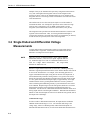
1.7.3 Effect of Grounding on Single-Ended Measurements
Low-level single-ended voltage measurements can be problematic because of
ground potential fluctuations. The grounding scheme in the CR5000 has been
designed to eliminate ground potential fluctuations due to changing return
currents from 12 V, SW-12, 5 V, and the control ports. This is accomplished
by utilizing separate signal grounds ( ) and power grounds (G). To take
advantage of this design, observe the following grounding rule:
NOTE
Always connect a device’s ground next to the active terminal
associated with that ground.
Examples:
1.
Connect 5 Volt, 12 Volt, and control grounds to G terminals.
2.
Connect excitation grounds to the closest
terminal block.
3.
Connect the low side of single-ended sensors to the nearest
the analog input terminal blocks.
4.
Connect shield wires to the nearest
terminal blocks.
terminal on the excitation
terminal on
terminal on the analog input
If offset problems occur because of shield or ground leads with large current
terminals next to the excitation, CAO,
flow, tying the problem leads into the
and pulse-counter channels should help. Problem leads can also be tied
directly to the ground lug to minimize induced single-ended offset voltages.
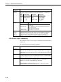
1.8 Powering Sensors and Peripherals
The CR5000 is a convenient source of power for sensors and peripherals
requiring a continuous or semi-continuous 5 VDC or 12 VDC source. The
CR5000 has 2 continuous 12 Volt (12V) supply terminals, 2 switched 12 Volt
(SW-12) supply terminals, and 2 continuous 5 Volt (5V) supply terminals.
Voltage on the 12V and SW-12 terminals will change with the CR5000 supply
voltage. The 5V terminal is regulated and will always remain near 5 Volts
(±4%)so long as the CR5000 supply voltage remains above 11 Volts. The 5V
terminal is not suitable for resistive bridge sensor excitation. Table 1.8-1
shows the current limits of the 12 Volt and 5 Volt ports. Table 1.8-2 shows
current requirements for several CSI peripherals. Other devices normally have
current requirements listed in their specifications. Current drain of all
peripherals and sensors combined should not exceed current sourcing limits of
the CR5000.
1-9
Section 1. Installation and Maintenance
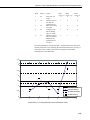
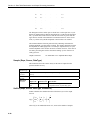
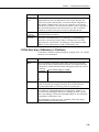
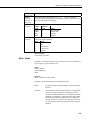
Table 1.8-1 Current Sourcing Limits
Terminals
Current Source Limit
SW12
< 900 mA @ 20°C
< 729 mA @ 40°C
< 630 mA @ 50°C
< 567 mA @ 60°C
< 400 mA @ 80°C
12V + SW12
< 1.85 A @ 20°C
< 1.50 A @ 40°C
< 1.30 A @ 50°C
< 1.17 A @ 60°C
< 0.85 A @ 80°C
5V + CSI/O
< 200 mA
Make certain that the primary source of power for the CR5000 can sustain the
current drain for the period of time required. Contact a CSI applications
engineer for help in determining a power budget for applications that approach
the limits of a given power supply’s capabilities. Be particularly cautious
about any application using solar panels and cellular telephone or radio,
applications requiring long periods of time between site visits, or applications
at extreme temperatures.
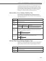
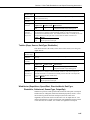
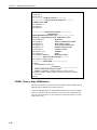
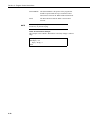
TABLE 1.8-2. Typical Current Drain for Some CR5000 Peripherals
Peripheral
AM25T
COM100
COM200 Phone Modem
SDM-INT8
Typical Current Drain (mA)
Quiescent
.5
.5
0.0012
0.4
Active
1
1.8
140
6.5
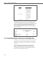
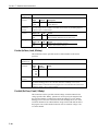
1.9 Controlling Power to Sensors and Peripherals
Controlling power to an external device is a common function of the CR5000.
Many devices can conveniently be controlled with the SW-12 (Switched 12
Volt) terminals on the CR5000. Table 1.8-1 shows the current available from
SW-12 port.
Applications requiring more control channels or greater power sourcing
capacity can usually be satisfied with the use of Campbell Scientific’s
A21REL-12 Four Channel Relay Driver, A6REL-12 Six Channel Relay
Driver, SDM-CD16AC 16 Channel AC/DC Relay Module, or by using the
control (C1-C8) ports as described in Section 1.9.1
1-10
Section 1. Installation and Maintenance
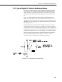
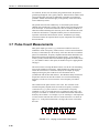
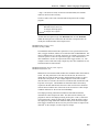
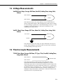
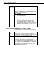
1.9.1 Use of Digital I/O Ports for Switching Relays
Each of the eight digital I/O ports can be configured as an output port and set
low or high (0 V low, 5 V high) using the PortSet or WriteIO instructions. A
digital output port is normally used to operate an external relay driver circuit
because the port itself has a limited drive capability (2.0 mA minimum at 3.5
V).
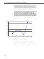
Figure 1.9-1 shows a typical relay driver circuit in conjunction with a coil
driven relay which may be used to switch external power to some device. In
this example, when the control port is set high, 12 V from the datalogger passes
through the relay coil, closing the relay which completes the power circuit to a
fan, turning the fan on.
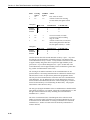
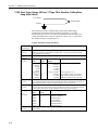
In other applications it may be desirable to simply switch power to a device
without going through a relay. Figure 1.9-2 illustrates a circuit for switching
external power to a device without going through a relay. If the peripheral to be
powered draws in excess of 75 mA at room temperature (limit of the 2N2907A
medium power transistor), the use of a relay (Figure 1.9-1) would be required.
Other control port activated circuits are possible for applications with greater
current/voltage demands than shown in Figures 1.9-1 and 2. For more
information contact a Campbell Scientific applications engineer.
FIGURE 1.9-1. Relay Driver Circuit with Relay
1-11
Section 1. Installation and Maintenance
FIGURE 1.9-2. Power Switching without Relay
1.10 Maintenance
The CR5000 power supplies require a minimum of routine maintenance.
When not in use, the rechargeable supply should be stored in a cool, dry
environment with the AC charger active.
1.10.1 Desiccant
The CR5000 is shipped with desiccant to reduce humidity. Desiccant should
be changed periodically. To prevent corrosion in uncontrolled or condensing
atmospheres, the CR5000 must be placed inside a weather tight instrument
enclosure with desiccant. Do not completely seal the enclosure if lead acid
batteries are present. Hydrogen gas generated by the batteries may build up to
an explosive concentration.
1.10.2 Replacing the Internal Battery
CAUTION
Misuse of the lithium battery or installing it improperly can
cause severe injury. Fire, explosion, and severe burn
hazard! Do not recharge, disassemble, heat above 100°C
(212°F), solder directly to the cell, incinerate, nor expose
contents to water.
The CR5000 contains a lithium battery that operates the clock and SRAM
when the CR5000 is not powered. The CR5000 does not draw any power from
the lithium battery while it is powered by a 12 VDC supply. In a CR5000
stored at room temperature, the lithium battery should last approximately 10
years (less at temperature extremes). Where the CR5000 is powered most or
all of the time the lithium cell should last much longer.
1-12
Section 1. Installation and Maintenance
While powered from an external source, the CR5000 measures the voltage of
the lithium battery daily. This voltage is displayed in the status table (Section
1.6) A new battery will have approximately 3.6 volts. The CR5000 Status
Table has a “ Lithium Battery” field. This field is either “ True” (battery is
good) or “ False” (replace battery). If the lithium cell is removed or allowed to
discharge below the safe level, the CR5000 will still operate correctly while
powered. Without the lithium battery, the clock will reset and data will be lost
when power is removed.
A replacement lithium battery can be purchased from Campbell (part number
13497). Table 1.10-1 lists the specifications of the battery.
Table 1.10-1 CR5000 Lithium Battery Specifications
Model
Tadiran
Capacity
self discharge rate
Diameter
Length
Operating temperature range
TL-5955 (3.6 V)
1650 mAh
1%/year @ 20°C
14.5 mm
33.5 mm
-55°C to 85°C
The CR5000 must be partially disassembled to replace the lithium cell.
O
Y
N
A
S
The battery is replaced as shown in Figures 1.10-4 to 1.10-6. The battery is
held in place by a band clamp. It can be removed by gently prying the band
from the sides of the battery holder.
FIGURE 1.10-4. Removal of CR5000 back plate and lithium battery
location.
1-13
Section 1. Installation and Maintenance
O
Y
N
A
S
The new cell is placed into the battery holder, observing the polarity markings
on the holder. Replace the band clamp, ensuring that both ends snap securely
into the battery holder.
2
Y
R
E
T
A
B
(datalogger/cr5
000)
FIGURE 1.10-5. Loosening of band clamp.
1-14
O
Y
N
A
S
Section 1. Installation and Maintenance
FIGURE 1.11-6. Removal of band clamp and battery.
1-15
Section 1. Installation and Maintenance
This is a blank page.
1-16
Section 2. Data Storage and Retrieval
The CR5000 can store individual measurements or it may use its extensive processing
capabilities to calculate averages, maxima, minima, histograms, FFTs, etc., on periodic or
conditional intervals. Data are stored in tables. For simplicity, the PC9000 program
generator allows a maximum of three data tables (in the native language up to 30 data
tables can be created). The number of tables and the values to output in each table are
selected when running the program generator (Overview) or when writing a datalogger
program directly (Sections 4 – 9).
2.1 Data Storage in CR5000
There are two areas for data storage on the CR5000:
Internal Static RAM
PCMCIA PC Card
Internal RAM is used as either the sole storage area for a data table or as a
buffer area when data are sent to PC card.
When the CR5000 gets a request for data that is stored on a PC card, the
CR5000 only looks for the data in the PC card when the oldest data are
requested or if the data are not available in internal RAM.
In the CRBASIC program, the DataTable instruction sets the size of the data
table or buffer area. A data table can be stored in a PC card by including the
CardOut instruction within the data table declaration. A maximum of 30
tables can be created by the program.
2.1.1 Internal Static RAM
Internal RAM is used as either the sole storage area for a data table or as a
buffer area when data are sent to a PC card. The only limit on the number of
tables is the available memory. Internal RAM is battery backed. Data remain in
memory when the CR5000 is powered down under program control. Data in
RAM are erased when a different program is loaded and run.
There are 2 Mbytes of SRAM. Some of this is used by the operating system
and for program storage. The rest is available for data storage. When a new
program is compiled, the CR5000 checks that there is adequate space in SRAM
for the data tables; a program that requests more space than is available will
not run.
2.1.2 PCMCIA PC Card
The CR5000 has a built in PC card slot for a Type I, Type II, or Type III
PCMCIA card. PCMCIA PC Cards allows expanding the CR5000’s storage
capacity. SRAM and ATA cards are supported. A program can send a
maximum of 30 data tables to PC cards.
2-1
Section 2. Data Storage and Retrieval
When a new program is compiled that sends data to the PC card, the CR5000
checks if a card is present and if the card has adequate space for the data
tables. If the card has adequate space, the tables will be allocated and the
CR5000 will start storing data to them. If there is no card or if there is not
enough space, the CR5000 will warn that the card is not being used and will
run the program, storing the data in SRAM only. When a card with enough
available memory is inserted the CR5000 will create the data tables on the card
and store the data that is accumulated in SRAM (Section 2.3.4).
Data stored on cards can be retrieved through the communication link to the
CR5000 or by removing the card and inserting it in a PC card slot in a
computer. The PCMCIA interface is much faster than the communication link.
With large files transferring the PC card is faster than collecting the data over
the link.
The CR5000 uses an MS DOS format for the PC cards. Cards can be
formatted in a PC or in the CR5000.
2.2 Internal Data Format
TABLE 2.2-1 CR5000 DATA TYPES
Data Type
LONG
IEEE4
FP2
Size
4 bytes
4 bytes
2 bytes
Range
-2,147,483,648 to +2,147,483,647
1.8 E -38 to 1.7 E 38
-7999 to +7999
Resolution
1 bit (1)
24 bits (about 7 digits)
13 bits (about 4 digits)
Data are stored internally in a binary format. Variables and calculations are
performed internally in IEEE 4 byte floating point with some operations
calculated in double precision. There are two data types used to store data:
IEEE4 four byte floating point and Campbell Scientific two byte floating point
(FP2). The data format is selected in the instruction that outputs the data.
Within the CR5000, time is stored as integer seconds and nanoseconds into the
second since midnight, the start of 1990. While IEEE 4 byte floating point is
used for variables and internal calculations, FP2 is adequate for most stored
data. Campbell Scientific 2 byte floating point provides 3 or 4 significant
digits of resolution, and requires half the memory space as IEEE 4 byte
floating point (2 bytes per value vs 4).
TABLE 2.2-2. Resolution and Range Limits of FP2 Data
Zero
0.000
Minimum Magnitude
±0.001
Maximum Magnitude
±7999.
The resolution of FP2 is reduced to 3 significant digits when the first (left
most) digit is 8 or greater (Table 2.2-2). Thus, it may be necessary to use
IEEE4 output or an offset to maintain the desired resolution of a measurement.
For example, if water level is to be measured and output to the nearest 0.01
foot, the level must be less than 80 feet for low resolution output to display the
0.01 foot increment. If the water level is expected to range from 50 to 90 feet
the data could either be output in high resolution or could be offset by 20 feet
(transforming the range to 30 to 70 feet).
2-2
Section 2. Data Storage and Retrieval
TABLE 2.2-3 FP2 Decimal Location
Absolute Value
0 7.999
8 79.99
80 - 799.9
800 - 7999.
Decimal Location
X.XXX
XX.XX
XXX.X
XXXX.
2.3 Data Collection
Data can be transferred into a computer using PC9000 via a communications
link or by transferring a PC card from the PC9000 to the computer. There are
three ways to collect data via a link to the CR5000 using the PC9000 software.
The collect menu is used to collect any or all stored data and is used for most
archival purposes.
On each of the RealTime screens, there is a "write file" check box. Data
stored to the table while the box is checked are also stored in a file on the
PC.Logger Files under the Tools menu has the option of retrieving a file from a
PC card. This can be used to retrieve a data file.
When the CR5000 is used without a computer in the field, or large data files
are collected on a PC card, the PC card can be transported to the computer
with the data on it.
The format of the data files on the PC card is different than the data file
formats created by PC9000 when the collect or write file options are used.
Data files retrieved from the Logger Files screen or read directly from the PC
card generally need to be converted into another format to be used (Section
2.3.4.2).
2.3.1 The Collect Menu
When Retrieve Data is selected in the Collect menu, PC9000 displays the
Collect Data dialog box (Figure 2.3.1). The station name (may be entered by
the user when a program is downloaded) is retrieved from the connected
CR5000 and shown at the top.
2-3
Section 2. Data Storage and Retrieval
FIGURE 2.3.1. Collect Data Dialog Box
2.3.1.1 File Type
ASCII With Time – Click here to store the data as an ASCII (TOA5, Section
2.4) file. Each record will be date and time stamped.
Binary With Time – Click here to store the data as a binary file (TOB1,
Section 2.4). Each record will be date and time stamped.
ASCII Without Time – Click here to store the data as an ASCII file (TOA5,
Section 2.4). There will be no date and time stamps.
Binary Without Time – Click here to store the data as a binary file (TOB1,
Section 2.4). There will be no date and time stamps.
2.3.1.2 Collection Method
All Records, Create New File – Collects the entire table stored in the
CR5000. PC9000 gets the current record number from the table in the CR5000
and then retrieves the oldest record in the table up to the current record
number. The number in the file name is incremented to create the file name in
which the data are stored.
2-4
Section 2. Data Storage and Retrieval
Since Last, Create New File – Click here to save new data in a new file.
PC9000 searches for the last file with the Root name, gets the last record
number from that file, then the current record from the table in the CR5000,
and requests all records in between those numbers from the CR5000. The
number in the file name is incremented to create the file name in which the
data are stored.
Since Last, Append To File – Click here to append retrieved data to the end
of the named file. PC9000 searches for the last file with the Root name, gets
the last record number from that file, then the current record from the table in
the CR5000, and requests all records in between those numbers from the
CR5000. The data are appended to the existing file.
Number of Records, Create New File Collects the number of records entered
in Num of Recs box. Retrieves that many records back from the current record
number. The number in the file name is incremented to create the file name in
which the data are stored.
Num of Recs – Enabled when Number of Records, Create New File is
checked. Enter the number of records back from the current record number to
retrieve.
2.3.1.3 Table Selection
All Tables – When the All Tables box is checked, all data tables except the
Public and Status tables are collected when collection is executed. The data
from each table are stored in a file with the table name and increment number
(see Table naming). This is a convenient method of collecting all data from
the CR5000. The first time data are collected, all data is checked and the file
type and collection method are selected. PC9000 remembers the settings, and
on subsequent collections the operator only needs to click on execute.
Stream – acts the same as Write file for the selected Table Name (Section
2.3.2).
Table Name – When "All tables" is not checked, a single data table can be
selected for collection. The Table Name box is used to select the table to be
retrieved.
Reset Table – Resetting a data table erases all data in the table and sets the
record number back to 0. Unless the table is configured as fill and stop by the
CR5000 program, it is not necessary to reset the table because the "Since Last"
collection option can be used to get only the new data. If the table is
configured as fill and stop, it stops collecting data once full and must be reset
before more data can be collected. Use with caution.
2.3.1.4 File Control
The default naming for a file stored to disk is to use the data table name
appended with a 2 digit number and the extension .DAT. If the table name is
longer than 6 characters, it is truncated. For example, the table name EVENTS
is stored as EVENTS00.DAT. A table named CYLTEMP is stored as
CYLTEM00.DAT.
2-5
Section 2. Data Storage and Retrieval
When the file collection options that create a new file are used, each time a
table is collected, the 2 digit number is incremented (e.g., EVENTS00.DAT,
EVENTS01.DAT, EVENTS03.DAT ...). PC9000 searches the selected
directory and adds 1 to the number of the highest numbered file of the
matching name to create the new name.
When the new data are to be appended to the existing file, PC9000 searches the
selected directory for the highest numbered file of the matching name, and
appends the data to that file.
Change File – Press the Change File button to change the name of the file to
be stored on disk. This is not possible when "All Tables" is selected.
Set Path – Press here to select a different disk or directory to write the files to.
EXECUTE – Press here to begin collecting data.
2.3.1.5 Status Messages
TABLE SIZE – Shows the size (in records) of the table highlighted in the
Table Name box above.
COLLECTION RANGE – Displays the range of records to be collected.
More records than the last number in this range may actually be retrieved.
LOGGER MESSAGE – Displays messages from the CR5000.
2.3.2 RealTime Write File
This feature is provided to allow the user to start and stop collecting data for
some event without leaving the real-time window. Check this box to write the
current table to a file in the computer. Writing begins with the current record
and continues until the Write File box is unchecked or until the window is
closed.
This collection method requires that the PC is connected to the CR5000 while
the data are collected. Because the beginning and end points of the data file
are roughly determined by when the box is checked, this is best suited to
collecting data when the user rather than the measurements determine when
data should be collected.
The bottom line of the screen will periodically display the current record being
written. The name of the file written will be the first six characters of the table
name plus 2 digits and an extension of .DAT. If the table name is MAIN then
the first file created will be named MAIN00.DAT. The next file will be named
MAIN01.DAT and so on. It takes a little time to open the file so be sure it is
opened in advance of the event you want to store.
The file is written to every 1 second so it is important the table size be large
enough to store sufficient data between writes. During each write operation,
the data may not be updated on the screen but this will not effect the stored
data.
2-6
Section 2. Data Storage and Retrieval
2.3.3 Logger Files Retrieve
Logger Files under the PC9000 tools menu allows the user to check the
programs stored in CPU Flash memory and the files stored on the PCMCIA
cards. Any of the files shown in logger files can be copied to the computer by
highlighting the file and pressing the retrieve button. Data files in the CR5000
CPU and Flash memory are not shown.
The retrieved data file is stored on the computer in the same form that it was
stored on the PC card (TOB2). This format generally needs to be converted to
another format for analysis (Section 2.3.4)
FIGURE 2.3-2. Logger Files Dialog Box
2.3.4 Via PCMCIA PC Card
When the CR5000 is used without a computer in the field, or large data files
are collected on a PC card, the PC card can be transported to the computer
with the data on it.
2.3.4.1 Inserting a PC Card
A card inserted in the PCMCIA slot when no program is running or when a
program is running that does not use the PC card does not cause a response
2-7
Section 2. Data Storage and Retrieval
from the CR5000. When a new program is compiled that sends data to the PC
card, the CR5000 checks if a card is present and if the card has adequate space
for the data tables. If the card has adequate space, the tables will be allocated
and the CR5000 will start storing data to them.
When the running program sends data to the card, and a card is inserted, the
CR5000 will detect the card and display a message.
A card that has no data tables files with the same names as those created by the
program causes the message:
New Card. Start Storing?
No
Yes
If the card has existing data table files that match those created by the program
there is the message:
Tables on Card Must be Reset. Proceed?
No
Yes
Same Card
The “ No” option [do not start storing data to the card] allows using the
CR5000 to check the card and to erase files or to format the card if necessary.
The “ Yes” option is to start storing data right away, resetting any tables with
the same name that exist on the card. This is the option that is generally used
when a blank (but formatted) card is inserted or when a card is reinserted after
transferring data to a computer.
The “ Same Card” option is only available if the data table header matches the
program exactly and the program has already run with a card. This option
allows removing the card to read it and then returning it to the CR5000 and
having the new data appended to the data already on the card. If you choose to
use this option be aware that if the CR5000 overwrites its buffer while the card
is out, there will be a gap in the data on the card.
2.3.4.2 Removing Card from CR5000
The PC Card Status LED just above the PC card door is lit when the card is
being written to.
CAUTION
Removing a card while it is active can cause garbled data
and can actually damage the card. Do not switch off the
power while the cards are present and active.
To remove a card, use the keyboard display to go to the PcCard menu; move
the cursor to “ Remove Card: and press Enter. The Status will show “ You may
now remove the card” . Remove the card. The card will be reactivated if not
removed.
2-8
Section 2. Data Storage and Retrieval
When the PC card is inserted in a computer, the data files can be copied to
another drive or used directly from the PC card just as one would from any
other disk. In most cases, however, it will be necessary to convert the file
format before using the data.
2.3.4.3 Converting File Format
The CR5000 stores data on the PC card in TOB2 Format. TOB2 is a binary
format that incorporates features to improve reliability of the PC Cards. TOB2
allows the accurate determination of each record’s time without the space
required for individual time stamps.
When TOB2 files are converted to another format, the number of records may
be greater or less than the number requested in the data table declaration.
There are always at least two additional frames of data allocated. When the
file is converted these will result in additional records if no lapses occurred. If
more lapses occur than were anticipated, there may be fewer records in the file
than were allocated.
PC9000’s file converter will convert TOB1 or TOB2 files to other formats.
The Convert Data Files option is in the File Menu. The options for TOB2
appear after the name of the file to convert has been selected (Figure 2.3-3.)
FIGURE 2.3-3 File Conversion Dialog Box
2-9
Section 2. Data Storage and Retrieval
"File Format","Station","Logger","Serial No.","OS Ver","DLD File","DLD Sig","Table Name"
"TIMESTAMP","RECORD","Field Name","Field Name","Field Name"
"TS","RN","Field Units","Field Units","Field Units"
"","","Processing","Processing","Processing"
"Field Data Type","Field Data Type","Field Data Type","Field Data Type","Field Data Type"
timestamp,record number,field data,field data,field data,
FIGURE 2.4.1 Header Information
2.4 Data Format on Computer
The format of the file stored on disk can be either ASCII or Binary depending
on the file type selected in the collect data dialog box. Files collected from a
real time window are always stored in ASCII format.
2.4.1. Header Information
Every data file stored on disk has an ASCII header at the beginning. The
header gives information on the format, datalogger and program used to collect
the data. Figure 2.4.1 is a sample header where the text in the header is a
generic name for the information contained in the header. The entries are
described following the figure.
File Format
The format of the file on disk. TOA5 is an ASCII format. TOB1 is a Binary
format. This information is used by the historical graphing and file conversion
functions of PC9000.
Station Name
The station name set in the logger that the data was collected from.
Logger Model
The datalogger model that the data was collected from.
Logger Serial Number
The serial number of the logger that the data was collected from. This is the
serial number of the CR5000 CPU.
Operating System Version
The version of the operating system in the logger that the data was collected
from.
DLD File
The name of the DLD file that was running when the data were created.
DLD Signature
The signature of the DLD file that created the data.
Table Name
The data table name.
2-10
Section 2. Data Storage and Retrieval
Field Name
The name of the field in the data table. This name is created by the CR5000 by
appending underscore ( _ ) and a three character mnemonic for the output
processing.
Field Units
The units for the field in the data table. Units are assigned in the program with
the units declaration.
Field Processing
The output processing that was used when the field was stored.
Smp = Sample
Max = Maximum
Min = Minimum
Avg = Average
Field Data Type
This header line is only in TOB1 binary format and identifies the data type for
each of the fields in the data table.
UINT4 = Unsigned 4 byte integer
IEEE4 = 4 byte floating point
Time Stamp
This field is the date and time stamp for this record. It indicates the time,
according to the logger clock, that each record was stored.
Record Number
This field is the record number of this record. The number will increase up to
2E32 and then start over with zero. The record number will also start over at
zero if the table is reset.
Field Data
This is the data for each of the fields in the record.
2.4.2 TOA5 ASCII File Format
The following is a sample of a file collected as ASCII with time stamps.
"TOA5","Bob's9K","CR5000","1048575","1.00","EXPLDAT.DLD","4339","Temp"
"TIMESTAMP","RECORD","RefTemp_Avg","TC_Avg(1)","TC_Avg(2)","TC_Avg(3)","TC_Avg(4)"
"TS","RN","degC","degC","degC","degC","degC"
"","","Avg","Avg","Avg","Avg","Avg"
"1995-09-19 14:31:43.84",458,29.94,25.6,25.36,25.48,25.4
"1995-09-19 14:31:43.85",459,29.93,25.6,25.36,25.41,25.35
2-11
Section 2. Data Storage and Retrieval
The following is an example of how the above data might look when imported
into a spread sheet.
TOA5
Bob's9K
TIMESTAMP
TS
RECORD
RN
1995-09-19 14:31:43.84
1995-09-19 14:31:43.85
458
459
CR5000
1048575
1.00
EXPLDAT. 4339
Temp
DLD
RefTemp_Avg TC_Avg(1) TC_Avg(2) TC_Avg(3) TC_Avg(4)
degC
degC
degC
degC
degC
Avg
Avg
Avg
Avg
Avg
29.94
25.6
25.36
25.48
25.4
29.93
25.6
25.36
25.41
25.35
This is the same data table collected as ASCII without time stamps
"TOA5","Bob's9K","CR5000","1048575","1.00","EXPLDAT.DLD","4339","Temp"
"RefTemp_Avg","TC_Avg(1)","TC_Avg(2)","TC_Avg(3)","TC_Avg(4)"
"degC","degC","degC","degC","degC"
"Avg","Avg","Avg","Avg","Avg"
29.94,25.6,25.36,25.48,25.4
29.93,25.6,25.36,25.41,25.35
And again, an example of how the above data might look when imported into a
spread sheet.
TOA5
Bob's9K
CR5000
1048575
1.00
RefTemp_Avg
degC
Avg
29.94
29.93
TC_Avg(1)
degC
Avg
25.6
25.6
TC_Avg(2)
degC
Avg
25.36
25.36
TC_Avg(3)
degC
Avg
25.48
25.41
TC_Avg(4)
degC
Avg
25.4
25.35
EXPLDAT. 4339
DLD
Temp
2.4.2 TOB1 Binary File Format
This is a sample of a file collected as Binary with time stamps.
TOB1,Bob's9K,CR5000,1048575,1.00,EXPLDAT.DLD,4339,Temp
SECONDS,NANOSECONDS,RECORD,RefTemp_Avg,TC_Avg(1),TC_Avg(2),TC_Avg(3),TC_Avg(4)
SECONDS,NANOSECONDS,RN,degC,degC,degC,degC,degC
,,,Avg,Avg,Avg,Avg,Avg
UINT4,UINT4,UINT4,IEEE4,IEEE4,IEEE4,IEEE4,IEEE4
(data lines are binary and not directly readable )
This is an example of binary without time stamps.
TOB1,Bob's9K,CR5000,1048575,1.00,EXPLDAT.DLD,4339,Temp
RefTemp_Avg,TC_Avg(1),TC_Avg(2),TC_Avg(3),TC_Avg(4)
degC,degC,degC,degC,degC
Avg,Avg,Avg,Avg,Avg
IEEE4,IEEE4,IEEE4,IEEE4,IEEE4
(data lines are binary and not directly readable )
2.4.3 TOB2 Binary File Format
The TOB2 binary format has a header similar to the other formats. TOB2 data
is stored in fixed size “ frames” that generally contain a number of records.
The size of the frames is a function of the record size. The frames are time
2-12
Section 2. Data Storage and Retrieval
stamped, allowing the calculation of time stamps for their records. If there is a
lapse in periodic interval records that does not occur on a frame boundary, an
additional time stamp is written within the frame and its occurrence noted in
the frame boundary. This additional time stamp takes up space that would
otherwise hold data.
When TOB2 files are converted to another format, the number of records may
be greater or less than the number requested in the data table declaration.
There are always at least two additional frames of data allocated. When the
file is converted these will result in additional records if no lapses occurred. If
more lapses occur than were anticipated, there may be fewer records in the file
than were allocated.
2-13
Section 2. Data Storage and Retrieval
This is a blank page.
2-14
Section 3. CR5000 Measurement Details
3.1 Analog Voltage Measurement Sequence
The CR5000 measures analog voltages with either an integrate and hold or a
sample and hold analog to digital (A/D) conversion. The A/D conversion is
made with a 16 bit successive approximation technique which resolves the
signal voltage to approximately one part in 60,000 of the full scale range. The
maximum conversion rate is 5000 per second or one measurement every 200
µs (10,000 measurements per second on a single channel).
The timing of CR5000 measurements is precisely controlled. The measurement
schedule is determined at compile time and loaded into memory. This schedule
sets interrupts that drive the measurement task.
Using two different voltage measurement instructions with the same
voltage range takes the same measurement time as using one instruction
with two repetitions. (This is not the case in the CR10X, 21X, CR23X and
CR7 dataloggers where there is always a setup time for each instruction.)
There are four parameters in the measurement instructions that may vary the
sequence and timing of the measurement. These are options to measure and
correct the ground offset on single-ended measurements each time
measurements are made (MeasOfs), reverse the high and low differential
inputs (RevDiff), to set the time to allow the signal to settle between switching
to a channel and making a measurement (SettlingTime), and the length of time
to integrate a measurement (Integ), and to reverse the polarity of excitation
voltage (RevEx).
3.1.1 Voltage Range
The CR5000 has 5 fixed voltage ranges and autorange. The 16 bit A/D has a
16
resolution of 1 part in 2 (65,536). To allow for some overrange capabilities
the A/D is applied to a range approximately 9% greater than the Full Scale
Range resulting in the 1 part in 60,000 resolution over the FSR. For example,
on the ±20 mV range the full scale range is 40 mV [20 - (-20)] and the
resolution is two thirds of a microvolt; 0.04 / 0.000000667 = 60,000. The
smaller the voltage range, the better the absolute resolution. In general, a
measurement should use the smallest fixed voltage range that will
accommodate the full scale output of the sensor being measured. If the voltage
exceeds the range, the CR5000 indicates the overrange by returning Not-ANumber (NAN) for the measurement.
For signals that do not fluctuate too rapidly, AutoRange allows the CR5000 to
automatically choose the voltage range to use. AutoRange causes the CR5000
to make two measurements. The first measurement determines the range to
use. It is made with no integration on the ±5000 mV range. The second
measurement is made on the appropriate range using the integration specified
in the instruction. Both measurements use the settling time programmed in the
instruction. AutoRange optimizes resolution but takes longer than a
measurement on a fixed range, because of the two measurements required.
3-1
Section 3. CR5000 Measurement Details
An AutoRange measurement will return Not-A-Number if the voltage exceeds
the range picked by the first measurement. To avoid problems with a signal on
the edge of a range, AutoRange selects the next larger range when the signal
exceeds 90% of a range.
AutoRange is very good for a signal that occasionally exceeds a particular
range, for example, a Type J thermocouple that most of the time will be less
than 360 °C (±20 mV range) but will occasionally see temperatures as high as
400 °C (±50 mV range, Table 3.4-2). AutoRange should not be used for
rapidly fluctuating signals, particularly those whose signal traverses several
voltage ranges rapidly because of the possibility that the signal could change
ranges between the range check and the actual measurement.
3.1.2 Reversing Excitation or the Differential Input
Reversing the excitation polarity or the differential input are techniques to
cancel voltage offsets that are not part of the signal. For example, if there is a
+5 µV offset in the measurement circuitry, a 5 mV signal will be measured as
5.005 mV. When the input is reversed, the measurement will be
-4.995 mV. Subtracting the second measurement from the first and dividing
by 2 gives the correct answer: 5.005-(-4.995)=10, 10/2=5. Most offsets are
thermocouple effects caused by temperature gradients in the measurement
circuitry or wiring.
Reversing the excitation polarity cancels voltage offsets in the sensor, wiring,
and measurement circuitry. One measurement is made with the excitation
voltage with the polarity programmed and a second measurement is made with
the polarity reversed. The excitation "on time" for each polarity is exactly the
same to ensure that ionic sensors do not polarize with repetitive measurements.
Reversing the inputs of a differential measurement cancels offsets in the
CR5000 measurement circuitry and improves common-mode rejection. One
measurement is made with the high input referenced to the low input and a
second with the low referenced to the high.
3.1.3 Measuring Single-Ended Offset
The single-ended offset is a voltage offset on a single-ended input. It is
measured by internally switching the input to ground and measuring the
voltage. When a single-ended measurement is made this offset is corrected for
in the calibration. The offset can either be measured automatically as part of
the background calibration or as part of the measurement sequence each time
the measurement is made (adding to the time to make the measurement).
When the offset is measured in the measurement sequence, the offset is
measured once prior to completing all of the instruction reps.
The MeasOfs parameter in instructions that make single-ended voltage
measurements is used to force the offset measurement. In most cases the
background calibration is adequate. Additional accuracy can be gained by
making the offset measurement with each measurement instruction when the
offset is changing rapidly as it would during when the CR5000 is undergoing
rapid temperature swings.
3-2
Section 3. CR5000 Measurement Details
3.1.4 SettlingTime
When the CR5000 switches to a new channel or switches on the excitation for
a bridge measurement, there is a finite amount of time required for the signal to
reach its true value. Delaying between setting up a measurement (switching to
the channel, setting the excitation) and making the measurement allows the
signal to settle to the correct value. The default settling times are the
minimum required for the CR5000 to settle to within its accuracy
specifications. Additional time is necessary when working with high sensor
resistances or long lead lengths (higher capacitance). Using a longer settling
time increases the time required for each measurement. Section 3.3 goes into
more detail on determining an adequate settling time.
When the CR5000 Reverses the differential input or the excitation polarity it
delays the same settling time after the reversal as it does before the first
measurement. Thus there are two delays per channel when either RevDiff or
RevEx is used. If both RevDiff and RevEx are selected, there are four
measurement segments, positive and negative excitations with the inputs one
way and positive and negative excitations with the inputs reversed. The
CR5000 switches to the channel:
sets the excitation, delays, measures,
reverses the excitation, delays, measures,
reverses the excitation, reverses the inputs, delays, measures,
reverses the excitation, delays, measures.
Thus there are four delays per channel measured. The CR5000 processes the
measurement segments into the single value it returns for the measurement.
3.1.5 Integration
Integration is used to reduce the noise included in a measurement. The CR5000
may use a combination of analog and digital integration.
For the fastest measurements, there is a zero integration measurement. This
measurement does not integrate. The signal at a precise instant is sampled and
this voltage is held for A/D conversion.
With analog integration, the input signal is integrated for a precise period of
time. The integrated value is held for the A/D conversion. There are three
possible analog integration times 20 ms, 16.67 ms and 250 µs. The 20 ms
(1/50 second) and 16.667 ms (1/60 second) are available to integrate out the
effects of noise from 50 or 60 Hz AC power sources.
An integration time in microseconds is specified as part of the measurement
instruction. An integration time of 0 selects the sample-and-hold, 250 selects
the 250 µs integration, 16667 or “ _60 Hz” selects the 60 Hz rejection
(16667 µs), and 20000 or “ _50 Hz” selects 50 Hz rejection (20000 µs).
In addition to the analog integrations, it is possible to average a number of the
sample-and-hold or 250 µs integration measurements. The A/D conversions
are made as rapidly as possible: every 100 µs for the samples and every 500 µs
for the 250 µs integrations. If the integration time specified is 250 µs or a
3-3
Section 3. CR5000 Measurement Details
multiple of 500 µs, the CR5000 will repeat 250 µs integration measurements
every 500 µs throughout the integration interval. If the integration time
specified is 100 µs or 200 µs, the CR5000 makes one or two samples in the
integration interval. The average of these measurements is stored as the result
of the measurement.
The random noise level is decreased by the square root of the number of
measurements made. For example, the input noise on the ±5000 mV range
with one 250 µs integration is 120 µV RMS; entering 2000 µs for the
integration (four measurements) will cut this noise in half (120/(√4)=60).
The integration time specified in the measurement instruction is used for each
segment of the measurement. Thus, if reversing the differential input or
reversing the excitation is specified, there will be two integrations per channel;
if both reversals are specified, there will be four integrations.
3.2 Single Ended and Differential Voltage
Measurements
A single-ended voltage measurement is made on a single input which is
measured relative to ground. A differential measurement measures the
difference in voltage between two inputs.
NOTE
There are two sets of channel numbers on the analog channels.
Differential channels (1-20) have two inputs: high (H) and low
(L). Either the high or low side of a differential channel can be
used for a single ended measurement. The single-ended
channels are numbered 1-40.
Because a single ended measurement is referenced to CR5000 ground, any
difference in ground potential between the sensor and the CR5000 will result in
an error in the measurement. For example, if the measuring junction of a
copper-constantan thermocouple, being used to measure soil temperature, is
not insulated and the potential of earth ground is 1 mV greater at the sensor
than at the point where the CR5000 is grounded, the measured voltage would
be 1 mV greater than the thermocouple output, or approximately 25 oC high.
Another instance where a ground potential difference creates a problem is
where external signal conditioning circuitry is powered from the same source
as the CR5000. Despite being tied to the same ground, differences in current
drain and lead resistance result in different ground potential at the two
instruments. For this reason, a differential measurement should be made on an
analog output from the external signal conditioner. Differential measurements
MUST be used when the inputs are known to be different from ground, such as
the output from a full bridge.
Common mode range
In order to make a differential measurement, the inputs must be within the
CR5000 common mode range of ±5 V. The common mode range is the
voltage range, relative to CR5000 ground, within which both inputs of a
differential measurement must lie, in order for the differential measurement to
3-4
Section 3. CR5000 Measurement Details
be made. For example, if the high side of a differential input is at 4 V and the
low side is at 3 V relative to CR5000 ground, there is no problem. A
measurement made on the ±5000 mV range will return 1000 mV. However, if
the high input is at 5.8 V and the low input is at 4.8 V, the measurement can
not be made because the high input is outside of the ±5 V common mode
range (the CR5000 will indicate the overrange by returning not-a-number
(NAN)).
Sensors that have a floating output or are not referenced to ground through a
separate connection may need to have one side of the differential input
connected to ground to ensure the signal remains within the common mode
range.
Problems with exceeding common mode range may be encountered when the
CR5000 is used to read the output of external signal conditioning circuitry if a
good ground connection does not exist between the external circuitry and the
CR5000. When operating where AC power is available, it is not always safe to
assume that a good ground connection exists through the AC wiring. If a
CR5000 is used to measure the output from a laboratory instrument (both
plugged into AC power and referencing ground to outlet ground), it is best to
run a ground wire between the CR5000 and the external circuitry. Even with
this ground connection, the ground potential of the two instruments may not be
at exactly the same level, which is why a differential measurement is desired.
A differential measurement has the option of reversing the inputs to cancel
offsets as described above.
NOTE
Sustained voltages in excess of ±16 V will damage the CR5000
circuitry.
3.3 Signal Settling Time
Whenever an analog input is switched into the CR5000 measurement circuitry
prior to making a measurement, a finite amount of time is required for the
signal to stabilize at it's correct value. The rate at which the signal settles is
determined by the input settling time constant which is a function of both the
source resistance and input capacitance.
The CR5000 delays after switching to a channel to allow the input to settle
before initiating the measurement. The default delays used by the CR5000
depend on the integration used and the voltage range. For the sample-andhold, the default delay is 100 µs on the ±5000, ±1000, ±200, and ±50 mV
ranges and 200 µs on the ±20 mV range. The default delay is 200 µs for 250
µs integrations and 3 ms for 50 Hz or 60 Hz rejection integrations. This
settling time is the minimum required to allow the input to settle to the
resolution specification.
Additional wire capacitance associated with long sensor leads can increase the
settling time constant to the point that measurement errors may occur. There
are three potential sources of error which must settle before the measurement is
made:
3-5
Section 3. CR5000 Measurement Details
1.
The signal must rise to its correct value.
2.
A small transient caused by switching the analog input into the
measurement circuitry must settle.
3.
When a resistive bridge measurement is made using a switched excitation
channel, a larger transient caused when the excitation is switched must
settle.
3.3.1 Minimizing Settling Errors
When long lead lengths are mandatory, the following general practices can be
used to minimize or measure settling errors:
1.
DO NOT USE WIRE WITH PVC INSULATED CONDUCTORS. PVC
has a high dielectric which extends input settling time.
2.
Where possible run excitation leads and signal leads in separate shields to
minimize transients.
3.
When measurement speed is not a prime consideration, additional time
can be used to ensure ample settling time. The settling time required can
be measured with the CR5000.
3.3.2 Measuring the Necessary Settling Time
The CR5000 can measure the time required for a particular sensor/cable
configuration to settle. This is done by allowing the signal to settle the
minimum amount of time and then making zero integration measurements
every 100 µs. Looking at the series of measurements it is possible to see the
settling of the sensor signal. By counting the number of measurements before
the signal settles the correct settling time can be determined (100 µs per
measurement plus an extra 100 µs if the measurement is made on the 20 mV
range where the default settling time is 200 µs).
NOTE
This technique for measuring settling time can only be used with
instructions that measure only one voltage per repetition. The
settling time to use with instructions that make more than one
measurement can be determined with an instruction that uses
only one measurement. For example, for the BrFull6W
determine the settling time with BrFull; for BrHalf3W use
BrHalf.
The following example demonstrates measuring the settling time for a
differential voltage measurement. If you are not yet familiar with CR5000
programming, you may want to read Section 4 before trying to follow the
example.
The series of measurements on the sensor is made with one instruction.
Measurement instructions have a repetitions parameter that allow one
instruction to repeat the measurement on a number of channels. There is also
the capability to repeat measurements on the same channel. When
3-6
Section 3. CR5000 Measurement Details
measurements are repeated on the same channel the settling time is only
necessary before the first measurement (as long as the excitation polarity and
differential inputs are not reversed).
Before the program to measure the settling time is run, the sensor with the
cable that will be used in the installation needs to be connected and the sensor
needs to be stabilized. If the sensed value is changing rapidly it will be
difficult to separate the settling time from true changes in the value measured.
The following program measures the settling time on a full bridge pressure
transducer.
'CR5000
'Program to measure the settling time on a Pressure Transducer
'Declare the variable array for the 20 Pressure Transducer measurements:
public PT(20)
'Set up the output table for the measurement data:
DataTable (SetlDat,1,5)
Sample (20,PT(),IEEE4)
EndTable
'The following program repeats the 20 measurements 5 times:
BeginProg
Scan (1,Sec,3,5)
'The -1 in the differential channel parameter of BrFull tells
'the CR5000 to make the 20 measurements on channel 1:
BrFull (PT(),20,mV50,-1,Vx1,20,5000,False,False,0,0,1.0,0)
CallTable SetlDat
NextScan
EndProg
The program was run on a Druck water level pressure transducer with 200 feet
of cable. The first six measurements of each of the 5 readings are shown in
Table 3.3-1. The reading has settled by the second measurement, PT(2), thus a
settling time of 200 µs is adequate.
Table 3.3-1. First Six Values of Settling Time Data
PT(1)
PT(2)
PT(3)
PT(4)
PT(5)
PT(6)
0.291257 0.052925 0.053937 0.054274 0.057645 0.056296
0.292269 0.052925 0.053262 0.054948 0.055622 0.056633
0.286538 0.053937 0.054274 0.055959 0.053599 0.054948
0.284515 0.052925 0.052925 0.053599 0.057645 0.055285
0.286875 0.052925 0.052925 0.054611 0.056296 0.057308
3.4 Thermocouple Measurements
A thermocouple consists of two wires, each of a different metal or alloy, which
are joined together at each end. If the two junctions are at different
temperatures, a voltage proportional to the difference in temperatures is
induced in the wires. If the junctions are at the same temperature, there is no
voltage. When a thermocouple is used for temperature measurement, the wires
are soldered or welded together at the measuring junction. The second
3-7
Section 3. CR5000 Measurement Details
junction, which becomes the reference junction, is formed where the other ends
of the wires are connected to the measuring device. (With the connectors at
the same temperature, the chemical dissimilarity between the thermocouple
wire and the connector does not induce any voltage.) When the temperature of
the reference junction is known, the temperature of the measuring junction can
be determined by measuring the thermocouple voltage and adding the
corresponding temperature difference to the reference temperature.
The CR5000 determines thermocouple temperatures using the following
sequence. First the temperature of the reference junction is measured and
stored in °C. If the reference junction is the CR5000 analog input terminals,
the temperature is measured with the built in thermistor (PanelTemp
instruction). The thermocouple measurement instruction measures the
thermocouple voltage (TCDiff or TCSE). The thermocouple instruction
calculates the voltage that a thermocouple of the type specified would output at
the reference junction temperature if its reference junction were at 0 oC, and
adds this voltage to the thermocouple voltage. The temperature of the
measuring junction is then calculated from a polynomial approximation of the
NIST TC calibrations
3.4.1 Error Analysis
The error in the measurement of a thermocouple temperature is the sum of the
errors in the reference junction temperature, the thermocouple output
(deviation from standards published in NIST Monograph 175), the
thermocouple voltage measurement, and the linearization error (difference
between NIST standard and CR5000 polynomial approximations). The
discussion of errors which follows is limited to these errors in calibration and
measurement and does not include errors in installation or matching the sensor
to the environment being measured.
Panel Temperature
A brass bar is just under the CR5000 panel between the two rows of analog
input terminals. This bar helps to reduce temperature gradients between the
terminals. The panel temperature thermistor is in a depression in the center of
this bar.
The thermistor (Betatherm 10K3A1A) has an interchangability specification of
0.1 °C for temperatures between 0 and 70 °C. Below freezing and at higher
temperatures this specification is degraded (Figure 3.4.1). Combined with
possible errors in completion resistors and the measurement, the accuracy of
panel temperature is ±0.25 °C 0 to 40 °C, ±0.5 °C -25 to 50 °C, and ±0.7 °C
-40 to 85 °C.
3-8
Section 3. CR5000 Measurement Details
0.3
0.25
Thermistor Tolerance ºC
0.2
0.15
0.1
0.05
0
-60
-50
-40
-30
-20
-10
0
10
20
30
40
50
60
70
80
90
100
Temperature ºC
FIGURE 3.4-1. Thermistor Tolerance
The error in the reference temperature measurement is a combination of the
error in the thermistor temperature and the difference in temperature between
the panel thermistor and the terminals the thermocouple is connected to. The
terminal strip cover should always be used when making thermocouple
measurements. It insulates the terminals from drafts and rapid fluctuations in
temperature as well as conducting heat to reduce temperature gradients. In a
typical installation where the CR5000 is in a weather proof enclosure not
subject to violent swings in temperature or lopsided solar radiation loading, the
temperature difference between the terminals and the thermistor is likely to be
less than 0.2 °C.
With an external driving gradient, the temperature gradients on the input panel
can be much worse. For example, the CR5000 with the rechargeable battery
back was placed in a controlled temperature chamber. Thermocouples in
channels at the ends and middle of each analog terminal strip measured the
temperature of an insulated aluminum bar outside the chamber. The
temperature of this bar was also measured by another datalogger. Differences
between the temperature measured by one of the thermocouples and the actual
temperature of the bar are due to the temperature difference between the
terminals the thermocouple is connected to and the thermistor reference (the
figures have been corrected for thermistor errors). Figure 3.4-2 shows the
errors when the chamber was changed from -55 to 80 °C in approximately 15
minutes. Figure 3.4-3 shows the results when going from 80 to 25 °C in
approximately 45 minutes, a less dramatic change but still greater than would
be seen in most natural circumstances. During these rapid changes in
temperature, the temperature of panel thermistor will tend to lag behind the
terminals because it is buried a bit deeper in the CR5000 and is closer to the
3-9
Section 3. CR5000 Measurement Details
thermal mass of the batteries. Note that the smallest errors are on channels 5
and 16 in the middle of the terminal strips closest to the thermistor.
Reference Temperature Errors Due to Panel Gradient
Chamber changed from -55 to 80 °C at maximum rate
80
2
1
0
40
Measured - Actual (°C)
-1
20
-2
-3
0
Chanel 1
Chanel 5
Chanel 10
Chanel 11
Chanel 16
Chanel 20
Panel
Chamber
-4
-5
-6
-20
Chamber and CR5000 Panel Temperature (°C)
60
-40
95
90
85
80
75
70
65
60
55
50
45
40
35
30
25
20
15
5
10
0
-60
-5
-7
Time (minutes)
FIGURE 4.3-2. Panel Temperature Gradients During -55 to 80 °C change
3-10
Section 3. CR5000 Measurement Details
Reference Temperature Errors Due to Panel Gradient
Chamber Changed From 80 to 25 °C at 1.3 °C/Minute
80
1.4
Channel 1
Channel 5
Channel 10
Channel 11
Channel 16
Channel 20
Panel
Chamber
1
Measured - Actual (°C)
0.8
70
60
0.6
50
0.4
40
0.2
0
Chamber and CR5000 Panel Temperature (°C)
1.2
30
-0.2
95
90
85
80
75
70
65
60
55
50
45
40
35
30
25
20
15
10
5
0
20
-5
-0.4
Time (minutes)
FIGURE 4.3-3. Panel Temperature Gradients During 80 to 25 °C change
Thermocouple Limits of Error
The standard reference which lists thermocouple output voltage as a function
of temperature (reference junction at 0oC) is the National Institute of Standards
and Technology Monograph 175 (1993). The American National Standards
Institute has established limits of error on thermocouple wire which is accepted
as an industry standard (ANSI MC 96.1, 1975). Table 3.4-1 gives the ANSI
limits of error for standard and special grade thermocouple wire of the types
accommodated by the CR5000.
TABLE 3.4-1. Limits of Error for Thermocouple Wire (Reference Junction at 0oC)
Thermocouple
Type
Temperature
Range oC
Limits of Error
(Whichever is greater)
Standard
Special
-200 to 0
0 to 350
± 1.0oC or 1.5%
± 1.0oC or 0.75%
± 0.5oC or 0.4%
J
0 to 750
± 2.2oC or 0.75%
± 1.1oC or 0.4%
E
-200 to 0
0 to 900
± 1.7oC or 1.0%
± 1.7oC or 0.5%
± 1.0oC or 0.4%
-200 to 0
0 to 1250
± 2.2oC or 2.0%
± 2.2oC or 0.75%
± 1.1oC or 0.4%
0 to 1450
± 1.5oC or 0.25%
± 0.5%
T
K
R or S
B
800 to 1700
± 0.6oC or 0.1%
Not Estab.
3-11
Section 3. CR5000 Measurement Details
When both junctions of a thermocouple are at the same temperature there is no
voltage produced (law of intermediate metals). A consequence of this is that a
thermocouple can not have an offset error; any deviation from a standard
(assuming the wires are each homogeneous and no secondary junctions exist) is
due to a deviation in slope. In light of this, the fixed temperature limits of error
(e.g., ±1.0 °C for type T as opposed to the slope error of 0.75% of the temperature)
in the table above are probably greater than one would experience when
considering temperatures in the environmental range (i.e., the reference junction, at
0 °C, is relatively close to the temperature being measured, so the absolute error the product of the temperature difference and the slope error - should be closer to
the percentage error than the fixed error). Likewise, because thermocouple
calibration error is a slope error, accuracy can be increased when the reference
junction temperature is close to the measurement temperature. For the same reason
differential temperature measurements, over a small temperature gradient, can be
extremely accurate.
In order to quantitatively evaluate thermocouple error when the reference
junction is not fixed at 0 oC, one needs limits of error for the Seebeck
coefficient (slope of thermocouple voltage vs. temperature curve) for the
various thermocouples. Lacking this information, a reasonable approach is to
apply the percentage errors, with perhaps 0.25% added on, to the difference in
temperature being measured by the thermocouple.
Accuracy of the Thermocouple Voltage Measurement
The -25 to 50 °C accuracy of a CR5000 differential voltage measurement is
specified as ± (0.075% of the measured voltage plus the input offset error of 2
times the basic resolution of the range being used to make the measurement
plus 2 µV). The input offset error reduces to the basic resolution if the
differential measurement is made utilizing the option to reverse the differential
input.
For optimum resolution, the ±20 mV range is used for all but high temperature
measurements (Table 3.4-2). The input offset error dominates the voltage
measurement error for environmental measurements. A temperature difference
of 45 to 65 °C between the measurement and reference junctions is required for
a thermocouple to output 2.67 mV, the voltage at which 0.075% of the reading
is equal to 2 µV. For example, assume that a type T thermocouple is used to
measure a temperature of 45 °C and that the reference temperature is 25 °C.
The voltage output by the thermocouple is 830.7 µV. At 45 degrees a type T
thermocouple outputs 42.4 µV per oC. The possible slope error in the voltage
measurement is 0.00075x830.7 µV = 0.62 µV or 0.014 oC (0.62/42.4). The
basic resolution on the ±20 mV range is 0.67 µV or 0.01 oC. The 2 µV offset
is an error of 0.047 oC. Thus, the possible error due to the voltage
measurement is 0.081 oC on a non-reversing differential, or 0.024 oC with a
reversing differential measurement. The value of using a differential
measurement with reversing input to improve accuracy is readily apparent.
The error in the temperature due to inaccuracy in the measurement of the
thermocouple voltage is worst at temperature extremes, particularly when the
temperature and thermocouple type require using the 200 mV range. For
example, assume type K (chromel-alumel) thermocouples are used to measure
temperatures around 1300 oC. The TC output is on the order of 52 mV,
3-12
Section 3. CR5000 Measurement Details
requiring the ±200 mV input range. At 1300 oC, a K thermocouple outputs
34.9 µV per oC. The possible slope error in the voltage measurement is
0.00075x52 mV = 39 µV or 1.12 oC (39/34.9). The basic resolution on the 200
mV range is 6.67 µV or 0.19 oC. Thus, the possible error due to the voltage
measurement is 1.56 oC on a non-reversing differential, or 1.31 oC with a
reversing differential measurement.
TABLE 3.4-2. Voltage Range for maximum Thermocouple resolution
TC Type and temp.
range oC
Temp. range for
±20 mV range
Temp. range for
±50 mV range
Temp. range for
±200 mV range
T -270 to 400
E -270 to 1000
K --270 to 1372
J -210 to 1200
B 0 to 1820
R -50 to 1768
S -50 to 1768
N -270 to 1300
-270 to 400
-270 to 280
-270 to 610
-210 to 360
0 to 1820
-50 to 1680
-50 to 1768
-270 to 580
not used
-270 to 660
-270 to 1230
-210 to 870
not used
-50 to 1768
not used
-270 to 1300
not used
>660
>1230
> 870
not used
not used
not used
not used
When the thermocouple measurement junction is in electrical contact with the
object being measured (or has the possibility of making contact) a differential
measurement should be made.
Noise on Voltage Measurement
The typical input noise on the ±20 mV range for a differential measurement
with no integration and input reversal is 1.8 µV RMS. On a type T
thermocouple (approximately 40 µV/oC) this is 0.05 oC. Note that this is an
RMS value, some individual readings will vary by greater than this. By
integrating for 250 µs the noise level is reduced to 0.6 µV RMS.
Thermocouple Polynomial: Voltage to Temperature
NIST Monograph 175 gives high order polynomials for computing the output
voltage of a given thermocouple type over a broad range of temperatures. In
order to speed processing and accommodate the CR5000's math and storage
capabilities, 4 separate 6th order polynomials are used to convert from volts to
temperature over the range covered by each thermocouple type. Table 3.4-3
gives error limits for the thermocouple polynomials.
3-13
Section 3. CR5000 Measurement Details
TABLE 3.4-3. Limits of Error on CR5000 Thermocouple Polynomials
(Relative to NIST Standards)
TC
Type
T
Range oC
Limits of Error oC
-270
-270
-200
-100
100
to
to
to
to
to
400
-200
-100
100
400
+
±
±
±
J
-150
-100
to
to
760
300
± 0.008
± 0.002
E
-240
-240
-130
200
to
to
to
to
1000
-130
200
1000
± 0.4
± 0.005
± 0.02
-50
-50
950
to
to
to
1372
950
1372
± 0.01
± 0.04
K
18 @ -270
0.08
0.001
0.015
Reference Junction Compensation: Temperature to Voltage
The polynomials used for reference junction compensation (converting
reference temperature to equivalent TC output voltage) do not cover the entire
thermocouple range. Substantial errors will result if the reference junction
temperature is outside of the linearization range. The ranges covered by these
linearizations include the CR5000 environmental operating range, so there is
no problem when the CR5000 is used as the reference junction. External
reference junction boxes however, must also be within these temperature
ranges. Temperature difference measurements made outside of the reference
temperature range should be made by obtaining the actual temperatures
referenced to a junction within the reference temperature range and subtracting
one temperature from the other. Table 3.4-3 gives the reference temperature
ranges covered and the limits of error in the linearizations within these ranges.
Two sources of error arise when the reference temperature is out of range. The
most significant error is in the calculated compensation voltage, however error
is also created in the temperature difference calculated from the thermocouple
output. For example, suppose the reference temperature for a measurement on
a type T thermocouple is 300 oC. The compensation voltage calculated by the
CR5000 corresponds to a temperature of 272.6 oC, a -27.4 oC error. The type
T thermocouple with the measuring junction at 290 oC and reference at 300 oC
would output -578.7 µV; using the reference temperature of 272.6 oC, the
CR5000 calculates a temperature difference of -10.2 oC, a -0.2 oC error. The
temperature calculated by the CR5000 would be 262.4 oC, 27.6 oC low.
3-14
Section 3. CR5000 Measurement Details
TABLE 3.4-4. Reference Temperature Compensation Range and
Polynomial Error Relative to NIST Standards
TC
Type
Range oC
Limits of Error oC
T
J
E
K
-100 to 100
-150 to 296
-150 to 206
-50 to 100
± 0.001
± 0.005
± 0.005
± 0.01
Error Summary
The magnitude of the errors described in the previous sections illustrate that
the greatest sources of error in a thermocouple temperature measurement with
the CR5000 are likely to be due to the limits of error on the thermocouple wire
and in the reference temperature. Errors in the thermocouple and reference
temperature linearizations are extremely small, and error in the voltage
measurement is negligible.
To illustrate the relative magnitude of these errors in the environmental range,
we will take a worst case situation where all errors are maximum and additive.
A temperature of 45 oC is measured with a type T (copper-constantan)
thermocouple, using the ±20 mV range. The nominal accuracy on this range is
1 µV (0.01% of 10 mV) which at 45 oC changes the temperature by 0.012 oC.
The RTD is 25 oC but is indicating 25.1 oC, and the terminal that the
thermocouple is connected to is 0.05 oC cooler than the RTD.
TABLE 3.4-5. Example of Errors in Thermocouple Temperature
Source
Reference Temp.
TC Output
Voltage
Measurement
Noise
Reference
Linearization
Output
Linearization
Total Error
Error: oC : % of Total Error
Single Differential
Reversing Differential
No Integration
250 µs Integration
ANSI TC Error TC Error 1% ANSI TC
TC Error 1%
(1oC)
Slope
Error (1oC)
Slope
0.15o:11.5%
0.15o:29.8%
0.15o:12.6%
0.15o:38.4%
o
o
o
1.0 :76.7%
0.2 :39.8%
1.0 :84%
0.2o:51.2%
o
o
o
0.081 :6.2%
0.081 :16.1%
0.024 :2%
0.024o:6.1%
0.07o:5.4%
0.001o:0.1%
0.07o:13.9%
0.001o:0.2%
0.015o:1.2%
0.001o:0.1%
0.015o:3.8%
0.001o:0.25%
0.001o:0.1%
0.001o:0.2%
0.001o:0.1%
0.001o:0.25%
1.303o:100%
0.503o:100%
1.191o:100%
0.391o:100%
3.4.2 Use of External Reference Junction or Junction Box
An external junction box is often used to facilitate connections and to reduce
the expense of thermocouple wire when the temperature measurements are to
be made at a distance from the CR5000. In most situations it is preferable to
make the box the reference junction in which case its temperature is measured
and used as the reference for the thermocouples and copper wires are run from
3-15
Section 3. CR5000 Measurement Details
the box to the CR5000. Alternatively, the junction box can be used to couple
extension grade thermocouple wire to the thermocouples, and the CR5000
panel temperature used as the reference. Extension grade thermocouple wire
has a smaller temperature range than standard thermocouple wire, but meets
the same limits of error within that range. The only situation where it would be
necessary to use extension grade wire instead of a external measuring junction
is where the junction box temperature is outside the range of reference junction
compensation provided by the CR5000. This is only a factor when using type
K thermocouples, where the upper limit of the reference compensation
linearization is 100 oC and the upper limit of the extension grade wire is 200
oC. With the other types of thermocouples the reference compensation range
equals or is greater than the extension wire range. In any case, errors can arise
if temperature gradients exist within the junction box.
Figure 3.4-1 illustrates a typical junction box. Terminal strips will be a
different metal than the thermocouple wire. Thus, if a temperature gradient
exists between A and A' or B and B', the junction box will act as another
thermocouple in series, creating an error in the voltage measured by the
CR5000. This thermoelectric offset voltage is a factor whether or not the
junction box is used for the reference. This offset can be minimized by making
the thermal conduction between the two points large and the distance small.
The best solution in the case where extension grade wire is being connected to
thermocouple wire would be to use connectors which clamped the two wires in
contact with each other.
CR9000
CR5000
Junction Box
Junction
Box
A'
A
B'
B
TC
H
L
FIGURE 3.4-1. Diagram of Junction Box
An external reference junction box must be constructed so that the entire
terminal area is very close to the same temperature. This is necessary so that a
valid reference temperature can be measured and to avoid a thermoelectric
offset voltage which will be induced if the terminals at which the thermocouple
leads are connected (points A and B in Figure 3.4-1) are at different
temperatures. The box should contain elements of high thermal conductivity,
which will act to rapidly equilibrate any thermal gradients to which the box is
subjected. It is not necessary to design a constant temperature box, it is
desirable that the box respond slowly to external temperature fluctuations.
Radiation shielding must be provided when a junction box is installed in the
field. Care must also be taken that a thermal gradient is not induced by
conduction through the incoming wires. The CR5000 can be used to measure
the temperature gradients within the junction box.
3-16
Section 3. CR5000 Measurement Details
3.5 Bridge Resistance Measurements
There are six bridge measurement instructions included in the standard
CR5000 software. Figure 3.5-1 shows the circuits that would typically be
measured with these instructions. In the diagrams, the resistors labeled Rs
would normally be the sensors and those labeled Rf would normally be fixed
resistors. Circuits other than those diagrammed could be measured, provided
the excitation and type of measurements were appropriate.
All of the bridge measurements have the option (RevEx) to make one set of
measurements with the excitation as programmed and another set of
measurements with the excitation polarity reversed. The offset error in the two
measurements due to thermal emfs can then be accounted for in the processing
of the measurement instruction. The excitation channel maintains the excitation
voltage or current until the hold for the analog to digital conversion is
completed. When more than one measurement per sensor is necessary (four
wire half bridge, three wire half bridge, six wire full bridge), excitation is
applied separately for each measurement. For example, in the four wire half
bridge when the excitation is reversed, the differential measurement of the
voltage drop across the sensor is made with the excitation at both polarities and
then excitation is again applied and reversed for the measurement of the
voltage drop across the fixed resistor.
Calculating the actual resistance of a sensor which is one of the legs of a
resistive bridge usually requires additional processing following the bridge
measurement instruction. In addition to the schematics of the typical bridge
configurations, Figure 3.5-1 lists the calculations necessary to compute the
resistance of any single resistor, provided the values of the other resistors in the
bridge circuit are known.
BrHalf
X = result w/mult = 1, offset = 0
X=
BrHalf3W
V1
Vx
=
Rs
Rs + R f
X = result w/mult = 1, offset = 0
X=
2 V2 − V1
VX − V1
=
Rs
X
1− X
Rs (1 − X )
Rs = Rf
Rf =
X
Rs = R f X
Rf = R s / X
Rf
3-17
Section 3. CR5000 Measurement Details
X = result w/mult = 1, offset = 0
BrHalf4W
X=
H
L
H
V2
V1
=
Rs
Rs = R f X
Rf = R s / X
Rf
L
X = result w/mult = 1, offset = 0
BrFull
X = 1000
H
L

 R3
V
R
1
2 
= 1000
−

Vx
 R3 + R4 R1 + R2 
X1 = − X / 1000 + R 3 / ( R 3 + R 4 )
R1 =
R 2 (1 − X1 )
X1
R X
R2 = 1 1
1 − X1
X = result w/mult = 1, offset = 0
BrFull6W
X = 1000
H
L
H
L
V2
V1
 R
R2 
3

= 1000
−
 R3 + R4 R1 + R2 
X 2 = X / 1000 + R 2 / ( R 1 + R 2 )
R3 =
R4 =
R4 X2
1 − X2
R 3 (1 − X 2 )
X2
X = result w/mult = 1, offset = 0
Resistance
I
X=
H
L
H
V
= Rs
Ix
IXR
X = result w/mult = 1, offset = 0
Resistance
used to measure full bridge
X=
=
H
L
 R3
V1
R2 

= Rbridge 
−
Ix
 R3 + R4 R1 + R2 
R3 ( R1 + R2 ) − R2 ( R3 + R4 )
R1 + R2 + R3 + R4
− R2 R4 − X ( R2 + R3 + R4 )
X − R3
R R − X ( R1 + R3 + R4 )
R2 = 1 3
X + R4
− R2 R4 − X ( R1 + R2 + R4 )
R3 =
X − R1
R R − X ( R1 + R2 + R3 )
R4 = 1 3
X + R2
R1 =
IXR
FIGURE 3.5-1. Circuits Used with Bridge Measurement Instructions
3-18
Section 3. CR5000 Measurement Details
3.6 Measurements Requiring AC Excitation
Some resistive sensors require AC excitation. These include electrolytic tilt
sensors, soil moisture blocks, water conductivity sensors and wetness sensing
grids. The use of DC excitation with these sensors can result in polarization,
which will cause an erroneous measurement, and may shift the calibration of
the sensor and/or lead to its rapid decay.
Other sensors like LVDTs (without built in electronics) require an AC
excitation because they rely on inductive coupling to provide a signal. DC
excitation would provide no output.
Any of the bridge measurements can reverse excitation polarity to provide AC
excitation and avoid ion polarization. The frequency of the excitation can be
determined by the delay and integration time used with the measurement. The
highest frequency possible is 5 kHz, the excitation is switched on and then
reversed 100 µs later when the first measurement is held and then is switched
off after another 100 µs when the second measurement is held (i.e., reverse the
excitation, 100 µs delay, no integration).
Influence of Ground Loop on Measurements
When measuring soil moisture blocks or water conductivity the potential exists
for a ground loop which can adversely affect the measurement. This ground
loop arises because the soil and water provide an alternate path for the
excitation to return to CR5000 ground, and can be represented by the model
diagrammed in Figure 3.6-1.
FIGURE 3.6-1. Model of Resistive Sensor with Ground Loop
In Figure 3.6-1, Vx is the excitation voltage, Rf is a fixed resistor, Rs is the
sensor resistance, and RG is the resistance between the excited electrode and
CR5000 earth ground. With RG in the network, the measured signal is:
V1 = Vx
Rs
(Rs + Rf ) + RsRf / RG
[3.6-1]
RsRf/RG is the source of error due to the ground loop. When RG is large the
equation reduces to the ideal. The geometry of the electrodes has a great effect
on the magnitude of this error. The Delmhorst gypsum block used in the 227
probe has two concentric cylindrical electrodes. The center electrode is used
3-19
Section 3. CR5000 Measurement Details
for excitation; because it is encircled by the ground electrode, the path for a
ground loop through the soil is greatly reduced. Moisture blocks which consist
of two parallel plate electrodes are particularly susceptible to ground loop
problems. Similar considerations apply to the geometry of the electrodes in
water conductivity sensors.
The ground electrode of the conductivity or soil moisture probe and the
CR5000 earth ground form a galvanic cell, with the water/soil solution acting
as the electrolyte. If current was allowed to flow, the resulting oxidation or
reduction would soon damage the electrode, just as if DC excitation was used
to make the measurement. Campbell Scientific probes are built with series
capacitors in the leads to block this DC current. In addition to preventing
sensor deterioration, the capacitors block any DC component from affecting
the measurement.
3.7 Pulse Count Measurements
Many pulse output type sensors (e.g., anemometers and flow-meters) are
calibrated in terms of frequency (counts/second). For these measurements the
accuracy is related directly to the accuracy of the time interval over which the
pulses are accumulated. Frequency dependent measurements should have the
PulseCount instruction programmed to return frequency. If the number of
counts is primary interest, PulseCount should be programmed to return counts
(i.e., the number of times a door opens, the number of tips of a tipping bucket
rain gage).
The interval of the scan loop that PulseCount is in is not the sole determining
factor in the calculation of frequency. While normally the counters will be
read on the scan interval, if execution is delayed, for example by lengthy
output processing, the pulse counters are not read until the scan is
synchronized with real time and restarted. The CR5000 actually measures the
elapsed time since the last time the counters were read when determining
frequency so in the case of an overrun, the correct frequency will still be
output.
The resolution of the pulse counters is one count. The resolution of the
calculated frequency depends on the scan interval: frequency resolution =
1/scan interval (e.g., a pulse count in a 1 second scan has a frequency
resolution of 1 Hz, a 0.5 second scan gives a resolution of 2 Hz, and a 1 ms
scan gives a resolution of 1000 Hz). The resultant measurement will bounce
around by the resolution. For example, if you are scanning a 2.5 Hz input once
a second, in some intervals there will be 2 counts and in some 3 as shown in
figure 3.7-1. If the pulse measurement is averaged, the correct value will be
the result.
3
2
3
2
FIGURE 3.7-1. Varying counts within Pulse interval.
3-20
Section 3. CR5000 Measurement Details
The resolution gets much worse with the shorter intervals used with higher
speed measurements. As an example, assume that engine RPM is being
measured from a signal that outputs 30 pulses per revolution. At 2000 RPM,
the signal has a frequency of 100 Hz (2000 RPMx(1 min/60 s)x30=1000). The
multiplier to convert from frequency to RPM is 2 RPM/Hz (1 RPM/(30
pulses/60s) = 2). At a 1 second scan interval, the resolution is 2 RPM.
However, if the scan interval were 1 ms, the resolution would be 2000 RPM.
At the 1 ms scan, if every thing was perfect, each interval there would be 1
count. However, a slight variation in the frequency might cause 2 counts
within one interval and none in the next, causing the result to vary between 0
and 4000 RPM!
3.8 Self Calibration
The CR5000 performs a self-calibration of the analog voltage measurements
and excitation voltages. The range gains and offsets and the excitation voltage
output will vary with temperature. The self calibration allows the CR5000 to
maintain its specifications over the temperature range.
Rather than make all of the measurements required to calibrate all
range/integration type combinations possible in the CR5000, the calibration
only measures the range/integration type combinations that occur in the
running CR5000 program. The calibration may occur in three different modes.
1.
Compile time calibration. This occurs prior to running the program and
calibrates all integration/range combinations needed. For the 250 usc and
zero integrations multiple measurements are made and averaged to come
up with gain values to use in the measurements. Ten measurements are
made on the zero integration ranges and five measurements for the 250
usec integrations. When this calibration is performed the values in the
calibration table are completely replaced (i.e., no filtering is used).
2.
System background calibration. This automatically takes place in the
background while the user program is running. Multiple measurements
are not averaged, but a filter is applied to the new gain/offset values
obtained. The filter is used so that the calibration values change slowly.
The filter combines the newly measured value multiplied by 0.1 with the
previous calibration value by 0.9 to arrive at the new calibration value. A
piece of the background calibration is added to each fast scan in the user
program. The background calibration measurements will be repeated
every 4 seconds or the time it takes to complete them, whichever is
longer. If there is not enough time to do the background calibration, the
CR5000 will display: “ Warning when Fast Scan X is running
background calibration will be disabled.” (X is the number of the fast
scan where the first scan entered in the program is 1, the next scan is 2,
etc.)
3.
Calibration under program control. When the calibrate instruction is
included in a program, the calibration is identical to the compile time
calibration. The calibration table values are replaced with those
calculated. The fast integrations have averaging as in the compile
calibrate. When a calibrate instruction is found in any scan the
3-21
Section 3. CR5000 Measurement Details
background calibration will be disabled (even if the scan is not executed).
The calibrate instruction is described in Section 7.
The self calibration does not take place if there is not enough time to run it or if
the calibrate instruction is in the CR5000 program and never executed.
Without the self calibration the drift in accuracy with temperature is about a
factor of 10 worse. For example, over the extended temperature range (-40 to
85°C) the accuracy specification is approximately 0.1% of reading. If the self
calibration is disabled, the accuracy over the range is approximately 1% of
reading. Temperature is the main factor causing a calibration shift and the
need for the self calibration. If the temperature of the CR5000 remains the
same there will be little calibration drift with the self calibration disabled.
The time constant for the background calibration (at the 4 second rate) is
approximately 36 seconds. This allows the CR5000 to remain calibrated
during fairly rapid temperature changes. In cases of extreme temperature
change, such as bringing a vehicle from equilibrium in a chamber at -30°C out
into a hot Arizona day, it may be worthwhile to override the background
calibration by running the calibration instruction in the scan with the
measurements.
Another case where using the calibration instruction makes sense is where
there is not time for the background calibration in the normal scan but the
program can periodically stop making measurements and run the calibration
instruction in a separate scan.
3-22
Section 4. CRBasic - Native Language
Programming
The CR5000 is programmed in a language that has some similarities to a structured basic.
There are special instructions for making measurements and for creating tables of output
data. The results of all measurements are assigned variables (given names).
Mathematical operations are written out much as they would be algebraically. This
section describes a program, its syntax, structure, and sequence.
4.1 Format Introduction
4.1.1 Mathematical Operations
Mathematical operations are written out much as they would be algebraically.
For example, to convert a temperature in Celsius to Fahrenheit one might
write:
TempF = TempC * 1.8 + 32
With the CR5000 there may be 2 or 20 temperature (or other) measurements.
Rather than have 20 different names, a variable array with one name and 20
elements may be used. A thermocouple temperature might be called TCTemp.
With an array of 20 elements the names of the individual temperatures are
TCTemp(1), TCTemp(2), TCTemp(3), ... TCTemp(20). The array notation
allows compact code to perform operations on all the variables. For example,
to convert ten temperatures in a variable array from C to F:
For I=1 to 10
TCTemp(I)=TCTemp(I)*1.8+32
Next I
4.1.2 Measurement and Output Processing Instructions
Measurement instructions are procedures that set up the measurement
hardware to make a measurement and place the results in a variable or a
variable array. Output processing instructions are procedures that store the
results of measurements or calculated values. Output processing includes
averaging, saving maximum or minimum, standard deviation, FFT, etc.
The instructions for making measurements and outputting data are not found in
a standard basic language. The instructions Campbell Scientific has created for
these operations are in the form of procedures. The procedure has a keyword
name and a series of parameters that contain the information needed to
complete the procedure. For example, the instruction for measuring the
temperature of the CR5000 input panel is:
PanelTemp (Dest, Integ)
4-1
Section 4. CRBasic - Native Language Programming
PanelTemp is the keyword name of the instruction. The two parameters
associated with PanelTemp are: Destination, the name of the variable in which
to put the temperature; and Integration, the length of time to integrate the
measurement. To place the panel temperature in the variable RefTemp (using
a 250 microsecond measurement integration time) the code is:
PanelTemp(RefTemp, 250)
The use of these instructions should become clearer as we go through an
introductory example.
4.1.3 Inserting Comments Into Program
Comments can be inserted into a program by preceding the comment with a
single quote ('). Comments can be entered either as independent lines or
following CR5000 code. When the CR5000 compiler sees the ' it ignores the
rest of the line.
' The declaration of variables starts here.
Public Start(6)
'Declare the start time array
4.2 Programming Sequence
The following table describes the structure of a typical CR5000 program:
Declarations
4-2
Make a list of what to measure and calculate.
Declare constants
Within this list, include the fixed constants used,
Declare Public variables
indicate the values that the user is able to view
while the program is running,
Dimension variables
the number of each measurement that will be
made,
Define Aliases
and specific names for any of the measurements.
Define data tables.
Describe, in detail, tables of data that will be
saved from the experiment.
Process/store trigger
Set when the data should be stored. Are they
stored when some condition is met? Are data
stored on a fixed interval? Are they stored on
a fixed interval only while some condition is
met?
Table size
Set the size of the table in CR5000 RAM
Other on-line storage
devices
Should the data also be sent to the PC card?
Processing of Data
What data are to be output (current value,
average, maximum, minimum, etc.)
Section 4. CRBasic - Native Language Programming
Define Subroutines
Program
Set scan interval
If there is a process or series of calculations
that need to be repeated several times in the
program, it can be packaged in a subroutine
and called when needed rather than repeating
all the code each time.
The program section defines the action of
datalogging
The scan sets the interval for a series of
measurements
Measurements
Enter the measurements to make
Processing
Enter any additional processing with the
measurements
Call Data Table(s)
The Data Table must be called to process output
data
Initiate controls
Check measurements and Initiate controls if
necessary
NextScan
Loop back (and wait if necessary) for the next
scan
End Program
4-3
Section 4. CRBasic - Native Language Programming
4.3 Example Program
Const RevDiff=1
Const Del=0 'default
Const Integ=250
Const Mult=1
Const Offset=0
Declare constants
Public RefTemp
Public TC(6)
Units RefTemp=degC
Units TC=DegC
Declare public variables ,
dimension array, and
declare units.
DataTable (Temp,1,2000)
DataInterval (0,100,mSec,10)
Average (1,RefTemp,FP2,0)
Average (6,TC(),FP2,0)
EndTable
Declarations
Define Data Table
BeginProg
Scan (10,mSec,3,0)
PanelTemp (RefTemp, 250)
Measure
TCDiff (TC(),6,mV20C ,1,TypeT,RefTemp,RevDiff,Del,Integ,Mult,Offset)
CallTable Temp
Call Data Table
NextScan
EndProg
Scan loop
4.3.1 Data Tables
Data storage follows a fixed structure in the CR5000 in order to optimize the
time and space required. Data are stored in tables such as:
TOA4
TIMESTAMP
TS
1995-02-16 15:15:04.61
1995-02-16 15:15:04.62
1995-02-16 15:15:04.63
1995-02-16 15:15:04.64
StnName Temp
RECORD RefTemp_Avg
RN
degC
Avg
278822 31.08
278823 31.07
278824 31.07
278825 31.07
TC_Avg(1)
degC
Avg
24.23
24.23
24.2
24.21
TC_Avg(2)
degC
Avg
25.12
25.13
25.09
25.1
TC_Avg(3)
degC
Avg
26.8
26.82
26.8
26.77
TC_Avg(4)
degC
Avg
24.14
24.15
24.11
24.13
TC_Avg(5)
degC
Avg
24.47
24.45
24.45
24.39
TC_Avg(6)
degC
Avg
23.76
23.8
23.75
23.76
The user's program determines the values that are output and their sequence.
The CR5000 automatically assigns names to each field in the data table. In the
above table, TIMESTAMP, RECORD, RefTemp_Avg, and TC_Avg(1) are
fieldnames. The fieldnames are a combination of the variable name (or alias if
one exists) and a three letter mnemonic for the processing instruction that
outputs the data. Alternatively, the FieldNames instruction can be used to
override the default names.
The data table header also has a row that lists units for the output values. The
units must be declared for the CR5000 to fill this row out (e.g., Units RefTemp
4-4
Section 4. CRBasic - Native Language Programming
= degC). The units are strictly for the user's documentation; the CR5000
makes no checks on their accuracy.
The above table is the result of the data table description in the example
program:
DataTable (Temp,1,2000)
DataInterval(0,10,msec,10)
Average(1,RefTemp,fp2,0)
Average(6,TC(1),fp2,0)
EndTable
All data table descriptions begin with DataTable and end with EndTable.
Within the description are instructions that tell what to output and that can
modify the conditions under which output occurs.
DataTable(Name, Trigger, Size)
DataTable (Temp,1,2000)
The DataTable instruction has three parameters: a user specified name for the
table, a trigger condition, and the size to make the table in CR5000 RAM. The
trigger condition may be a variable, expression, or constant. The trigger is true
if it is not equal to 0. Data are output if the trigger is true and there are no
other conditions to be met. No output occurs if the trigger is false (=0). The
example creates a table name Temp, outputs any time other conditions are met,
and retains 2000 records in RAM.
DataInterval(TintoInt, Interval, Units, Lapses)
DataInterval(0,10,msec,10)
DataInterval is an instruction that modifies the conditions under which data are
stored. The four parameters are the time into the interval, the interval on
which data are stored, the units for time, and the number of lapses or gaps in
the interval to keep track of. The example outputs at 0 time into (on) the
interval relative to real time, the interval is 10 milliseconds, and the table will
keep track of 10 lapses. The DataInterval instruction reduces the memory
required for the data table because the time of each record can be calculated
from the interval and the time of the most recent record stored. Other output
condition modifiers are: Worst Case and FillandStop.
The output processing instructions included in a data table declaration
determine the values output in the table. The table must be called by the
program in order for the output processing to take place. That is, each time a
new measurement is made, the data table is called. When the table is called,
the output processing instructions within the table process the current inputs.
If the trigger conditions for the are true, the processed values are output to the
data table. In the example, several averages are output.
4-5
Section 4. CRBasic - Native Language Programming
Average(Reps, Source, DataType, DisableVar)
Average(1,RefTemp,fp2,0)
Average(6,TC(1),fp2,0)
Average is an output processing instruction that will output the average of a
variable over the output interval. The parameters are repetitions - the number
of elements in an array to calculate averages for, the Source variable or array to
average, the data format to store the result in (Table 4.3-1), and a disable
variable that allows excluding readings from the average if conditions are not
met. A reading will not be included in the average if the disable variable is not
equal to 0; the example has 0 entered for the disable variable so all readings are
included in the average.
TABLE 4.3-1 Formats for Output Data
Code
Data Format
Size
Range
Resolution
FP2
Campbell Scientific floating point
2 bytes
±7999
13 bits (about 4 digits)
IEEE4
IEEE four byte floating point
4 bytes
1.8 E -38 to 1.7 E 38
24 bits (about 7 digits)
LONG
4 byte Signed Integer
4 bytes
-2,147,483,648 to
+2,147,483,647
1 bit (1)
4.3.2 The Scan -- Measurement Timing and Processing
Once you know what you want, the measurements and calculations have been
listed and the output tables defined, the program itself may be relatively short.
The executable program begins with BeginProg and ends with EndProg. The
measurements, processing, and calls to output tables bracketed by the Scan and
NextScan instructions determine the sequence and timing of the datalogging.
BeginProg
Scan(1,MSEC,3,0)
ModuleTemp(RefTemp, 250)
TCDiff(TC(),6,mV50,4,1,TypeT,RefTemp,RevDiff,Del,Integ,Mult,Offset)
CallTable Temp
NextScan
EndProg
The Scan instruction determines how frequently the measurements within the
scan are made:
Scan(Interval, Units, BufferSize, Count)
Scan(1,MSEC,3,0)
The Scan instruction has four parameters. The Interval is the interval between
scans. Units are the time units for the interval. The maximum scan interval is
one minute. The BufferSize is the size (in the number of scans) of a buffer in
RAM that holds the raw results of measurements. Using a buffer allows the
processing in the scan to at times lag behind the measurements without
affecting the measurement timing (see the scan instruction in Section 9 for
more details). Count is the number of scans to make before proceeding to the
instruction following NextScan. A count of 0 means to continue looping
4-6
Section 4. CRBasic - Native Language Programming
forever (or until ExitScan). In the example the scan is 1 millisecond, three
scans are buffered, and the measurements and output continue indefinitely.
4.4 Numerical Entries
In addition to entering regular base 10 numbers there are 3 additional ways to
represent numbers in a program: scientific notation, binary, and hexadecimal
(Table 4.4-1).
TABLE 4.4-1 Formats for Entering Numbers in CRBasic
Format
Example
Value
Standard
6.832
6.832
Scientific notation
5.67E-8
5.67X10
Binary:
&B1101
13
Hexadecimal
&HFF
255
-8
The binary format makes it easy to visualize operations where the ones and
zeros translate into specific commands. For example, a block of ports can be
set with a number, the binary form of which represents the status of the ports
(1= high, 0=low). To set ports 1, 3, 4, and 6 high and 2, 5, 7, and 8 low; the
number is &B00101101. The least significant bit is on the right and represents
port 1. This is much easier to visualize than entering 72, the decimal
equivalent.
4.5 Logical Expression Evaluation
4.5.1 What is True?
Several different words get used to describe a condition or the result of a test.
The expression, X>5, is either true or false. However, when describing the
state of a port or flag, on or off or high or low sounds better. In CRBasic there
are a number of conditional tests or instruction parameters the result of which
may be described with one of the words in Table 4.5-1. The CR5000 evaluates
the test or parameter as a number; 0 is false, not equal to 0 is true.
TABLE 4.5-1. Synonyms for True and False
Predefined Constant
True (-1)
False (0)
Synonym
High
Low
Synonym
On
Off
Synonym
Yes
No
Synonym
Trigger
Do Not Trigger
Number
≠0
0
Digital port
5 Volts
0 Volts
4-7
Section 4. CRBasic - Native Language Programming
4.5.2 Expression Evaluation
Conditional tests require the CR5000 to evaluate an expression and take one
path if the expression is true and another if the expression is false. For
example:
If X>=5 then Y=0
will set the variable Y to 0 if X is greater than or equal to 5.
The CR5000 will also evaluate multiple expressions linked with and or or.
For example:
If X>=5 and Z=2 then Y=0
will only set Y=0 if both X>=5 and Z=2 are true.
If X>=5 or Z=2 then Y=0
will set Y=0 if either X>=5 or Z=2 is true (see And and Or in Section 9). A
condition can include multiple and and or links.
4.5.3 Numeric Results of Expression Evaluation
The CR5000 expression evaluator evaluates an expression and returns a
number. A conditional statement uses the number to decide which way to
branch. The conditional statement is false if the number is 0 and true if the
number is not 0. For example:
If 6 then Y=0,
is always true, Y will be set to 0 any time the conditional statement is executed.
If 0 then Y=0
is always false, Y will never be set to 0 by this conditional statement.
The CR5000 expression evaluator evaluates the expression, X>=5, and returns
-1, if the expression is true, and 0, if the expression is false.
W=(X>Y)
will set W equal to -1 if X>Y or will set W equal to 0 if X<=Y.
The CR5000 uses -1 rather than some other non-zero number because the and
and or operators are the same for logical statements and binary bitwise
comparisons (see and and or in Section 8). The number -1 is expressed in
binary with all bits equal to 1, the number 0 has all bits equal to 0. When -1 is
anded with any other number the result is the other number, ensuring that if the
other number is non-zero (true), the result will be non-zero
4.6 Flags
Any variable can be used as a flag as far as logical tests in CRBasic are
concerned. If the value of the variable is non-zero the flag is high. If the value
of the variable is 0 the flag is low (Section 4.5). PC9000 looks for the variable
array with the name Flag when the option to display flag status is used in one
of the real time screens.
4-8
Section 4. CRBasic - Native Language Programming
4.7 Parameter Types
Instructions parameters allow different types of inputs these types are listed
below and specifically identified in the description of the parameter in the
following sections or in PC9000 CRBasic help.
Constant
Variable
Variable or Array
Constant, Variable, or Expression
Constant, Variable, Array, or Expression
Name
Name or list of Names
Variable, or Expression
Variable, Array, or Expression
Table 4.7-1 list the maximum length and allowed characters for the names for
Variables, Arrays, Constants, etc.
TABLE 4.7-1. Rules for Names
Name for
Maximum Length (number of
characters)
Allowed characters
Variable or Array
16
Letters A-Z, upper or lower.
Constant
16
case, underscore “ _” , and
Alias
16
numbers 0-9. The name must
Data Table Name
8
start with a letter. CRBasic is
Field name
16
not case sensitive
4.7.1 Expressions in Parameters
Many parameters allow the entry of expressions. If an expression is a
comparison, it will return -1 if the comparison is true and 0 if it is false
(Section 4.5.3). An example of the use of this is in the DataTable instruction
where the trigger condition can be entered as an expression. Suppose the
variable TC(1) is a thermocouple temperature:
DataTable(Name, TrigVar, Size)
DataTable(Temp, TC(1)>100, 5000)
Entering the trigger as the expression, TC(1)>100, will cause the trigger to be
true and data to be stored whenever the temperature TC(1) is greater than 100.
4.7.2 Arrays of Multipliers Offsets for Sensor Calibration
If variable arrays are used as the multiplier and offset parameters in
measurements that use repetitions, the instruction will automatically step
through the multiplier and offset arrays as it steps through the channels. This
allows a single measurement instruction to measure a series of individually
4-9
Section 4. CRBasic - Native Language Programming
calibrated sensors, applying the correct calibration to each sensor. If the
multiplier and offset are not arrays, the same multiplier and offset are used for
each repetition.
VoltSE(Dest,Reps,Range,ASlot,SEChan,Delay,
Integ,Mult,Offset)
'Calibration factors:
Mult(1)=0.123 : Offset(1)= 0.23
Mult(2)=0.115 : Offset(2)= 0.234
Mult(3)=0.114 : Offset(3)= 0.224
VoltSE(Pressure(),3,mV1000,6,1,1,100,Mult(),Offset()
4.8 Program Access to Data Tables
Data stored in a table can be accessed from within the program. The format
used is:
Tablename.Fieldname(fieldname index,records back)
Where Tablename is the name of the table in which the desired value is stored.
Fieldname is the name of the field in the table. The fieldname is always an
array even if it consists of only one variable; the fieldname index must always
be specified. Records back is the number of records back in the data table
from the current time (1 is the most recent record stored, 2 is the record stored
prior to the most recent). For example, the expression:
Tdiff=Temp.TC_Avg(1,1)–Temp.TC_Avg(1,101)
could be used in the example program (Section 4.3) to calculate the change in
the 10 ms average temperature of the first thermocouple between the most
recent average and the one that occurred a second (100 x 10 ms) earlier.
In addition to accessing the data actually output in a table, there are some
pseudo fields related to the data table that can be retrieved:
Tablename.record(1,n) = the record number of the record output n records ago.
Tablename.output(1,1) = 1 if data were output to the table the last time the
table was called, = 0 if data were not output.
Tablename.timestamp(m,n) = element m of the timestamp output n records ago
where:
timestamp(1,n) = microseconds since 1990
timestamp(2,n) = microseconds into the current year
timestamp(3,n) = microseconds into the current month
timestamp(4,n) = microseconds into the current day
timestamp(5,n) = microseconds into the current hour
timestamp(6,n) = microseconds into the current minute
timestamp(7,n) = microseconds into the current second
4-10
Section 4. CRBasic - Native Language Programming
Tablename.eventend(1,1) is only valid for a data table using the DataEvent
instruction, Tablename.eventend(1,1) = 1 if the last record of an event occurred
the last time the table was called, = 0 if the data table did not store a record or
if it is in the middle of an event.
NOTE
The values of Tablename.output(1,1) and Tablename.eventend
(1,1) are only updated when the tables are called.
The WorstCase example in Section 6.2 illustrates the use of this syntax.
4-11
Section 4. CRBasic - Native Language Programming
This is a blank page.
4-12
Section 5. Program Declarations
Alias
Used to assign a second name to a variable.
Syntax
Alias VariableA = VariableB
Remarks
Alias allows assigning a second name to a variable. Within the datalogger
program, either name can be used. Only the alias is available for Public variables.
The alias is also used as the root name for data table fieldnames.
With aliases the program can have the efficiency of arrays for measurement and
processing yet still have individually named measurements.
Alias Declaration Example
The example shows how to use the Alias declaration.
Dim TCTemp(4)
Alias TCTemp(1) = CoolantT
Alias TCTemp(2) = ManifoldT
Alias TCTemp(3) = ExhaustT
Alias TCTemp(4) = CatConvT
Const
Declares symbolic constants for use in place of numeric entries.
Syntax
Const constantname = expression
Remarks
The Const statement has these parts:
Part
constantname
expression
Description
Name of the constant.
Expression assigned to the constant. It can consist of literals
(such as 1.0), other constants, or any of the arithmetic or
logical operators.
Tip
Constants can make your programs self-documenting and easier to
modify. Unlike variables, constants can't be changed while your
program is running.
Caution
Constants must be defined before referring to them.
Tip
Use all uppercase letters for constant names to make them easy to
recognize in your program listings.
5-1
Section 5. Program Declarations
Const Declaration Example
The example uses Const to define the symbolic constant PI.
Const PI = 3.141592654
Dim Area, Circum, Radius
Radius = Volt( 1 )
Circum = 2 * PI * Radius
Area = PI * ( Radius ^ 2 )
'Define constant.
'Declare variables.
'Get measurement.
'Calculate circumference.
'Calculate area.
Dim
Declares variables and allocates storage space. In CRBasic, ALL variables MUST
be declared.
Syntax
Dim varname[([subscripts]) [, varname[([subscripts])]]
Remarks
The Dim statement has these parts:
Part
varname
subscripts
Description
Name of a variable.
Dimensions of an array variable. You can declare multiple
dimensions.
The argument subscripts has the following syntax:
size [size, size]
In CRBasic the Option Base is always 1. This means the lowest number in a
dimension is 1 and not 0.
Dim A( 8, 3 )
The maximum number of array dimensions allowed in a Dim statement is 3. If a
program uses a subscript that is greater than the dimensioned value, a subscript out
of bounds error is recorded.
When variables are initialized, they are initialized to 0
Tip
Put Dim statements at the beginning of the program.
Public
Dimensions a variable as public and available in the Public table of the CR5000.
Syntax
Public(list of [dimensioned] variables that make up the Public Table)
Remarks
More than one Public statement can be made.
5-2
Section 5. Program Declarations
Public Declaration Example
The example shows the use of the Public declaration.
Dim x( 3 ), y, z( 2, 3, 4 )
Public x, y, z
Public Dim x( 3 ), y, z( 2, 3, 4 )
Public x( 3 ),y, z( 2, 3, 4 )
Public w
'Dim is optional
Station Name
Sets the station name.
Syntax
StationName StaName
Remarks
StationName is used to set the datalogger station name with the program. The
station name is displayed by PC9000 and stored in the data table headers
(Section 2.4).
Units
Used to assign a unit name to a field associated with a variable.
Syntax
Units Variable = UnitName
Remarks
Units allows assigning a unit name to a field. Units are displayed on demand
in the real-time windows of PC9000. The unit name also appears in the header
of the output files and in the Data Table Info file of PC9000. The unit name is
a text field that allows the user to label data. When the user modifies the units,
the text entered is not checked by PC9000 or the CR5000.
Example
Dim TCTemp( 1 )
Units TCTemp( 1 ) = Deg_C
Sub, Exit Sub, End Sub
Declares the name, variables, and code that form a Subroutine.
Syntax
Sub SubName [(VariableList )]
[ statementblock ]
[ Exit Sub ]
[ statementblock ]
End Sub
5-3
Section 5. Program Declarations
The Sub statement has these parts:
Part
Description
Sub
Marks the beginning of a Subroutine.
SubName
Name of the Subroutine. Because Subroutine names are
recognized by all procedures in all modules, subname cannot
be the same as any other globally recognized name in the
program.
VariableList
List of variables that are passed to the Subroutine when it is
called. The variable names used in this list should not be the
same names as variables, aliases, or constants declared
elsewhere. The variable names in this list can only be used
within the Subroutine. Multiple variables are separated by
commas. When the Subroutine is called, the call statement
must list the program variables or values to pass into the
subroutine variable. The number and sequence of the
program variables/values in the call statement must match the
number and sequence of the variable list in the sub
declaration. Changing the value of one of the variables in this
list inside the Subroutine changes the value of the variable
passed into it in the calling procedure.
The call may pass constants or expressions that evaluate to
constants (i.e., do not contain a variable) into some of the
variables. If a constant is passed, the “ variable” it is passed
to becomes a constant and cannot be changed by the
subroutine. If constants will be passed, the subroutine should
be written to not try to change the value of the “ variables”
they will be passed into.
statementblock
Any group of statements that are executed within the body of
the Subroutine.
Exit Sub
Causes an immediate exit from a Subroutine. Program
execution continues with the statement following the
statement that called the Subroutine. Any number of Exit
Sub statements can appear anywhere in a Subroutine.
End Sub
Marks the end of a Subroutine.
A Subroutine is a procedure that can take variables, perform a series of statements,
and change the value of the variables. However, a Subroutine can't be used in an
expression. You can call a Subroutine using the name followed by the variable list.
See the Call statement for specific information on how to call Subroutines.
The list of Subroutine variables to pass is optional. Subroutines can operate on the
global program variables declared by the Public or Dim statements. The advantage
of passing variables is that the subroutine can be used to operate on whatever
program variable is passed (see example).
Caution
5-4
Subroutines can be recursive; that is, they can call themselves to
perform a given task. However, recursion can lead to strange results.
Section 5. Program Declarations
Subroutine Example
'CR5000
'Declare Variables used in Program:
Public RefT, TC(4),PRTresist,PRTtemp,I
'Data output in deg C:
DataTable (TempsC,1,-1)
DataInterval (0,5,Min,10)
Average (1,RefT,FP2,0)
Average (4,TC(),FP2,0)
Average (1,PRTtemp,FP2,0)
EndTable
'Same Data output in F:
DataTable (TempsF,1,-1)
DataInterval (0,5,Min,10)
Average (1,RefT,FP2,0)
Average (4,TC(),FP2,0)
Average (1,PRTtemp,FP2,0)
EndTable
'Subroutine to convert temperature in degrees C to degrees F
Sub ConvertCtoF (Tmp)
Tmp = Tmp*1.8 +32
EndSub
BeginProg
Scan (1,Sec,3,0)
'Measure Temperatures (panel, 4 thermocouples, and 100 ohm PRT) in deg C
PanelTemp (RefT,250)
TCDiff (TC(),4,mV20C ,1,TypeT,RefT,True ,0,250,1.0,0)
Resistance (PRTresist,1,mV50,7,Ix1,1,500,True ,True ,0,250,0.01,0)
PRT (PRTtemp,1,PRTresist,1.0,0)
'Call Output Table for C
CallTable TempsC
'Convert Temperatures to F using Subroutine:
Call ConvertCtoF(RefT)
'Subroutine call using Call statement
For I = 1 to 4
ConvertCtoF(TC(I))
'Subroutine call without Call statement
Next I
ConvertCtoF(PRTtemp)
'Subroutine call without Call statement
'Call Output Table for F:
CallTable TempsF
NextScan
EndProg
5-5
Section 5. Program Declarations
This is a blank page.
5-6
Section 6. Data Table Declarations and
Output Processing Instructions
6.1 Data Table Declaration
DataTable (Name, TrigVar, Size)
output trigger modifier
export data destinations
output processing instructions
EndTable
DataTable is used to declare/define a data table. The name of the table, output
trigger and size of the table in RAM are set with DataTable. The Table
declaration must be at the beginning of the code prior to BeginProg. The table
declaration starts with DataTable and ends with EndTable. Within the
declaration are output trigger modifiers (optional, e.g., DataInterval, DataEvent
or WorstCase), the on-line storage devices to send the data to (optional, e.g.,
CardOut, DSP4), and the output processing instructions describing the data set
in the table.
Parameter
& Data Type
Name
Enter
The name for the data table. The table name is limited to eight characters.
Name
TrigVar
Constant
Variable, or
Expression
Size
Constant
The name of the variable to test for the trigger. Trigger modifiers add additional
conditions.
Value
Result
0
Do not trigger
≠0
Trigger
The size to make the data table. The number of data sets (records) to allocate memory for
in static RAM. Each time a variable or interval trigger occurs, a line (or row) of data is
output with the number of values determined by the output Instructions within the table.
This data is called a record. The total number of records stored equals the size..
Enter a negative number and all remaining memory
Note
(after creating fixed size data tables) will be
allocated to the table or partitioned between all
tables with a negative value for size. The
partitioning algorithm attempts to have the tables fill
at the same time.
DataTable Example - see native language Section 4.
EndTable
Used to mark the end of a data table.
See DataTable
6-1
Section 6. Data Table Declarations and Output Processing Instructions
6.2 Trigger Modifiers
DataInterval (TintoInt, Interval, Units, Lapses)
Used to set the time interval for an output table. DataInterval is inserted into a
data table declaration following the DataTable instruction to establish a fixed
interval table. The fixed interval table requires less memory than a conditional
table because time is not stored with each record. The time of each record is
calculated by knowing the time of the most recent output and the interval of
the data. DataInterval does not override the Trigger in the DataTable
instruction. If the trigger is not set always true by entering a constant, it is a
condition that must be met in addition to the time interval before data will be
stored.
The Interval determines how frequently data are stored to the table. The
interval is synchronized with the real time clock. Time is kept internally as the
elapsed time since the start of 1990 (01-01-1990 00:00:00). When the interval
divides evenly into this elapsed time it is time to output (elapsed time MOD
interval = 0). Entering 0 for the Interval sets it equal to the scan Interval.
TintoInt allows the user to set the time into the Interval, or offset relative to
real time, at which the output occurs([elapsed time + TintoInt] MOD interval =
0). For example, 360 (TintoInt) minutes into a 720 (Interval) minute (Units)
interval specifies that output should occur at 6:00 (6 AM, 360 minutes from
midnight) and 18:00 (6 PM, 360 minutes from noon) where the 720 minute (12
hour) interval is set relative to midnight 00:00. Enter 0 to keep output on the
even interval.
Interval driven data allows a more efficient use of memory because it is not
necessary to store time with each record. The CR5000 still stores time but on a
fixed spacing, only about once per 1 K of memory used for the table. As each
new record is stored, time is checked to ensure that the interval is correct. The
datalogger keeps track of lapses or discontinuities in the data. If a lapse has
occurred, the CR5000 inserts a time stamp into the data. When the data are
retrieved a time stamp can be calculated and stored with each record.
This lapse time stamp takes up some memory that would otherwise be used for
data. While the CR5000 allocates some extra memory for the table, if there are
a lot of lapses, it is not possible to store as many records as requested in the
DataTable declaration. The Lapses parameter allows the programmer to
allocate additional space for the number of lapses entered. This is used in
particular when the program is written in a way that will create lapses. For
example, if the data output is controlled by a trigger (e.g., a user flag) in the
DataTable instruction in addition to the DataInterval, lapses would occur each
time the trigger was false for a period of time longer than the interval.
To take advantage of the more efficient memory use, always enter 1 or greater
for the lapses parameter even if no lapses are expected. Entering 0 causes
every record to be time stamped.
Entering a negative number tells the CR5000 not to keep track of lapses. Only
the periodic time stamps (approximately once per K of data) are inserted.
6-2
Section 6. Data Table Declarations and Output Processing Instructions
Parameter
& Data Type
TintoInt
Constant
Interval
Constant
Units
Constant
Lapses
Constant
Enter
The time into the interval (offset to the interval) at which the table is to be output. The
units for time are the same as for the interval.
Enter the time interval on which the data in the table is to be recorded. The interval may
be in µs, ms, s, or minutes, whichever is selected with the Units parameter. Enter 0 to
make the data interval the same as the scan interval.
The units for the time parameters, PowerOff is the only instruction that uses hours or
days.
Alpha
Numeric
Code
Code
Units
USEC
0
microseconds
MSEC
1
milliseconds
SEC
2
seconds
MIN
3
minutes
As each new record is stored, time is checked to ensure that the interval is correct. The
datalogger keeps track of lapses or discontinuities in the data.
OpenInterval
When the DataInterval instruction is included in a data table, the CR5000 uses
only values from within an interval for time series processing (e.g., average,
maximum, minimum, etc.). When data are output every interval, the output
processing instructions reset each time output occurs. To ensure that data from
previous intervals is not included in a processed output, processing is reset any
time an output interval is skipped. (An interval could be skipped because the
table was not called or another trigger condition was not met.) The CR5000
resets the processing the next time that the table is called after an output
interval is skipped. If this next call to the table is on a scheduled interval, it
will not output. Output will resume on the next interval. (If Sample is the only
output processing instruction in the table, data will be output any time the table
is called on the interval because sampling uses only the current value and
involves no processing.)
OpenInterval is used to modify an interval driven table so that time series
processing in the table will include all values input since the last time the table
output data. Data will be output whenever the table is called on the output
interval (provided the other trigger conditions are met), regardless of whether
or not output occurred on the previous interval.
OpenInterval Example:
In the following example, 5 thermocouples are measured every 500
milliseconds. Every 10 seconds, while Flag(1) is true, the averages of the
reference and thermocouple temperatures are output. The user can toggle
Flag(1) to enable or disable the output. Without the OpenInterval Instruction,
the first averages output after Flag(1) is set high would include only the
measurements within the previous 10 second interval. This is the default and is
what most users desire. With the Open interval in the program (remove the
initial single quote (‘) to uncomment the instruction) all the measurements
made while the flag was low will be included in the first averages output after
the flag is set high.
6-3
Section 6. Data Table Declarations and Output Processing Instructions
Const RevDiff 1
'Reverse input to cancel offsets
Const Del 0
'Use default delay
Const Integ 0
'Use no integration
Public RefTemp
'Declare the variable used for reference temperature
Public TC(5)
'Declare the variable used for thermocouple measurements
Public Flag(8)
Units RefTemp=degC
'
Units TC=degC
DataTable (AvgTemp,Flag(1),1000)
'Output when Flag(1)=true
DataInterval(0,10,sec,10)
'Output every 10 seconds(while Flag(1)=true)
'OpenInterval
'When Not Commented, include data while Flag(1)=false in next average
Average(1,RefTemp,IEEE4,0)
Average(5,TC,IEEE4,0)
EndTable
BeginProg
Scan(500,mSec,0,0)
PanelTemp (RefTemp,250)
TCDiff (TC(),5,mV50C,9,TypeT,RefTemp,RevDiff,Del,Integ,1,0)
CallTable AvgTemp
NextScan
EndProg
DataEvent (RecsBefore, StartTrig, StopTrig, RecsAfter)
Used to set a trigger to start storing records and another trigger to stop storing
records within a table. The number of records before the start trigger and the
number of records after the stop trigger can also be set. A filemark (Section 8) is
automatically stored in the table between each event.
Parameter
& Data Type
RecsBefore
Constant
StartTrig
Enter
Variable, or
Expression
Value
0
≠0
StopTrig
Variable,
Expression or
Constant
The variable, expression or constant to test to stop storing to the data table. The
CR5000 does not start checking for the stop trigger until after the Start Trigger
occurs. A non-zero (true) constant may be used to store a fixed number of
records when the start trigger occurs (total number of records = PreTrigRecs+ 1
record for the trigger +PostTrigRecs.). Zero (false) could be entered if it was
desired to continuously store data once the start trigger occurred.
The number of records to store before the Start Trigger.
The variable or expression test to Trigger copying the pre trigger records into the
data table and start storing each new record..
Value
0
≠0
RecsAfter
Constant
6-4
Result
Do not trigger
Trigger
Result
Do not trigger
Trigger
The number of records to store after the Stop Trigger occurs.
Section 6. Data Table Declarations and Output Processing Instructions
DataEvent Example:
In this example, 5 type T thermocouples are measured. The trigger for the start
of an event is when TCTemp(1) exceeds 30 degrees C. The stop trigger is
when TCTemp(1) less than 29 degrees C. The event consists of 20 records
prior to the start trigger and continues to store data until 10 records following
the stop trigger.
Const RevDiff 1
Const Del 0
Const Integ 0
Public RefTemp
Public TC(5)
Public Flag(8)
Units RefTemp=degC
Units TC=degC
'Reverse input to cancel offsets
'Use default delay
'Use no integration
‘Declare the variable used for reference temperature
'Declare the variable used for thermocouple measurements
'
DataTable (Event,1,1000)
DataInterval(0,00,msec,10)
DataEvent(20,TC(1)>30,TC(1)<29,10)
Sample(1,RefTemp,IEEE4)
Sample(5,TC,IEEE4)
EndTable
'Set the sample interval equal to the scan
'20 records before TC(1)>30,
'after TC(1)<29 store 10 more records
'Sample the reference temperature
'Sample the 5 thermocouple temperatures
BeginProg
Scan(500,mSec,0,0)
PanelTemp (RefTemp,250)
TCDiff (TC(),5,mV50C,1,TypeT,RefTemp,RevDiff,Del,Integ,1,0)
CallTable Event
NextScan
EndProg
FillStop
Data Tables are by default ring memory where, once full, the newest data are
written over the oldest. Entering FillStop into a data table declaration makes
the table fill and stop. Once the table is filled, no more data are stored until the
table has been reset. The table can be reset from within the program by
executing the ResetTable instruction. Tables can also be reset from PC9000
real time windows or the collect data window.
Example:
DataTable (Temp,1,2000)
DataInterval(0,10,msec,10)
FillStop
Average(1,RefTemp,fp2,0)
Average(6,TC(1),fp2,0)
EndTable
' the table will stop collecting data after 2000 records.
6-5
Section 6. Data Table Declarations and Output Processing Instructions
WorstCase (TableName, NumCases, MaxMin, Change, RankVar)
Allows saving the most significant or “ worst-case” events in separate data
tables.
A data table is created that is sized to hold one event. This table acts as the
event buffer. Each event that occurs is stored to this table. This table may use
the DataEvent instruction or some other condition to determine when an event
is stored. The significance of an event is determined by an algorithm in the
program and a numerical ranking of the event is stored in a variable.
WorstCase creates as many clones of the specified table as the number of cases
for which to keep data. When WorstCase is executed, it checks the ranking
variable; if the value of the variable is a new worst case, the data in the event
table replace the data in the cloned table that holds the least significant event
currently stored.
An additional data table, nameWC (e.g., EvntWC) is created that holds the
values of the rank variables for each of the worst case tables and the time that
that table was stored.
WorstCase must be used with data tables sent to the CPU. It will not work if
the event table is sent to the PC card.
While WorstCase acts as Trigger Modifier and a data table declaration
(creating the cloned data tables), it is entered within the program to call the
worst case tables (see example).
Parameter
& Data Type
TableName
name
NumCases
MaxMin
Constant
Change
Constant
RankVar
Variable
6-6
Enter
The name of the data table to clone. The length of this name should be 4 characters or
less so the complete names of the worst case tables are retained when collected (see
NumCases).
The number of “ worst” cases to store. This is the number of clones of the data table to
create. The cloned tables use the name of the table being cloned (up to the first 6
characters) plus a 2 digit number (e.g., Evnt01, Evnt02, Evnt03, …). The numbers give
the tables unique names, they have no relationship to the ranking of the events. PC9000
uses this same name modification when creating a new data file for a table. To avoid
confusion and ambiguous names when collecting data with PC9000, keep the base name
four characters or less (4character base name + 2 digit case identifier + 2 digit collection
identifier = 8 character maximum length).
A code specifying whether the maximum or minimum events should be saved.
Value
Result
0
Min, save the events associated with the minimum ranking; i.e.,
Keep track of the RankVar associated with each event stored.
If a new RankVar is less than previous maximum, copy the
event over the event with previous maximum)
1
Max, save the events associated with the maximum ranking;
i.e., copy if RankVar is greater than previous lowest (over event
with previous minimum)
The minimum change that must occur in the RankVariable before a new worst case is
stored.
The Variable to rank the events by.
Section 6. Data Table Declarations and Output Processing Instructions
WorstCase Example
This program demonstrates the Worst Case Instruction. Five type T
thermocouples are measured. The event is similar to that in the example for
the DataEvent instruction; the trigger for the start of a data event is when
TC(1) exceeds 30 degrees C. However in this example, the stop trigger is set
immediately true. This is done to set a fixed size for the event which can be
duplicated in the worst case tables. To use the worst case instruction with
events of varying duration, the event table size must be selected to
accommodate the maximum duration expected (or needed). The event consists
of 20 records prior to the start trigger and continues until 100 records
following the start trigger.
The ranking criteria is the number of readings following the trigger that TC(1)
stays above 30 degrees C. The greater the number the “ worse” the event.
Const RevDiff 1
Const Del 0
Const Integ 0
Const NumCases 5
Const Max 1
Public RefTemp
Public TC(5)
Public I, NumAbove30
Units RefTemp=degC
Units TC=degC
'Reverse input to cancel offsets
'Use default delay
'Use default Integration
'Number of Worst Cases to save
'Declare the variable used for reference temperature
'Declare the variable used for thermocouple measurements
‘Declare index and the ranking variable
'
DataTable (Evnt,1,125)
DataInterval(0,00,msec,10)
DataEvent(20,TC(1)>30,-1,100)
Sample(1,RefTemp,IEEE4)
Sample(5,TC,IEEE4)
EndTable
'Set the sample interval equal to the scan
'20 records before TC(1)>30,
‘100 records after TC(1)>30
'Sample the reference temperature
'Sample the 5 thermocouple temperatures
BeginProg
Scan(500,mSec,3,0)
ModuleTemp(RefTemp,1,5,30)
TCDiff(TC(),5,mV50C,5,9,TypeT,RefTemp,RevDiff,Del,Integ,1,0)
CallTable Evnt
If Evnt.EventEnd(1,1)
Check if an Event just Ended
I=100
‘Initialize Index
NumAbove30=0
‘Zero Ranking Variable
Do
‘Loop through the Event table
NumAbove30=NumAbove30+1
‘Counting the # of times TC(1)>30
I=I-1
Loop While I>0 and Evnt.TC(1,I)>=30
‘Quit looping when at end or TC(1)<30
WorstCase(Evnt,NumCases,Max,0,NumAbove30)
‘Check for worst case
End If
NextScan
EndProg
6-7
Section 6. Data Table Declarations and Output Processing Instructions
6.3 Export Data Instructions
CardOut (StopRing, Size)
Used to send output data to the PCMCIA card. This instruction creates a data
table on the PCMCIA card. CardOut must be entered within each data table
declaration that is to store data on a PCMCIA card.
Parameter
& Data Type
StopRing
Constant
Size
Constant
Enter
A code to specify if the Data Table on the PCMCIA card is fill and stop or ring (newest
data overwrites oldest).
Value Result
0
Ring
1
Fill and Stop
The size to make the data table. The number of data sets (records) to allocate memory for
in the PCMCIA card. Each time a variable or interval trigger occurs, a line (or row) of
data is output with the number of values determined by the output Instructions within the
table. This data is called a record.
Enter a negative number and all remaining memory (after creating fixed size
Note
data tables) will be allocated to the table or partitioned between all tables with a
negative value for size. The partitioning algorithm attempts to have the tables
fill at the same time.
DSP4 (FlagVar, Rate)
Send data to the DSP4. If this instruction appears inside a DataTable, the
DSP4 can display the fields of this Table, otherwise, the Public Variables are
used by the DSP4. The Instruction can only be used once in a program; hence,
only the public variables or a single data table can be viewed.
Parameter
& Data Type
FlagVar
Array
Rate
Enter
The variable array to use for the 8 flags that can be displayed and toggled by the DSP4.
A value of 0 = low; ≠0 = high. If the array is dimensioned to less than 8, the DSP4 will
only work with the flags up to the dimension. The array used for flags in the Real Time
displays of PC9000 is Flag ().
How frequently to send new values to the DSP4 in milliseconds.
Constant
Example
DSP4 (Flag( ), 200)
Use Flag( ) to work with the buttons, update the DSP4 display every 200 msec.
(5 times a second).
GOESData (Dest, Table, TableOption, BufferControl, DataFormat)
The GOESData instruction is used to transmit data to the SAT HDR GOES
satellite data transmitter. The GOESData instruction is not inserted within the
Data Table declaration, it is inserted within the program, typically within the
scan.
6-8
Section 6. Data Table Declarations and Output Processing Instructions
Data transfer to the transmitter can occur via the datalogger's CS I/O port only.
The GOESData instruction has the following parameters:
NOTE
Parameter
& Data Type
Dest
Variable or
Array
Table
Table Name
TableOption
Constant
BufferControl
Constant
When the datalogger sends a command, further processing tasks
will be performed only after a response has been received from
the HDR GOES Transmitter.
Enter
The variable that holds a result code for the transmission. The result codes are:
Code
Description
0
Command executed successfully
2
Timed out waiting for STX character from transmitter after SDC
addressing
3
Wrong character received after SDC addressing.
4
Something other than ACK returned when select data buffer command
was executed
5
Timed out waiting for ACK
6
CS I/O port not available
7
Random message transmit failure (could be no data in buffer)
The data table from which record(s) should be transmitted.
The TableOption indicates which records should be sent from the data table.
Code
Description
0
send all records since last execution
1
send only the most recent record stored in the table
The BufferControl parameter specifies which buffer should be used (random or
self-timed) and whether data should be overwritten or appended to the existing
data. Data stored in the self-timed buffer is transmitted only during a
predetermined time frame. Data is erased from the transmitter's buffer after each
transmission. Data in the random buffer is transmitted immediately after a
threshold has been exceeded. The transmission is randomly repeated to insure it
is received.
Code
Description
0
Append to self-timed buffer
1
Overwrite self-timed buffer
2
Append to random buffer
3
Overwrite random buffer
9
Clear random buffer
6-9
Section 6. Data Table Declarations and Output Processing Instructions
Parameter
& Data Type
DataFormat
Constant
Enter
The DataFormat parameter specifies the format of the data sent to the transmitter
Code
Description
0
CSI FP2 data; 3 bytes per data point
1
Floating point ASCII; 7 bytes per data point
2
18-bit binary integer; 3 bytes per data point, numbers to the right of
the decimal are truncated
3
RAWS7; 7 data points:
Data Point
Description
1
total rainfall in inches, format = xx.xxx
2
wind speed MPH, format = xxx
3
vector average wind direction in degrees, format = xxx
4
air temperature in degrees F, format = xxx
5
RH percentage, format = xxx
6
fuel stick temperature in degrees F, format = xxx
7
battery voltage in VDC, format = xx.x
4
Fixed decimal ASCII xxx.x
5
Fixed decimal ASCII xx.xx
6
Fixed decimal ASCII x.xxx
7
Fixed decimal ASCII xxx
8
Fixed decimal ASCII xxxxx
GOESStatus (Dest, StatusCommand)
The GOESStatus instruction is used to request status and diagnostic
information from the SAT HDR GOES satellite transmitter.
NOTE
Parameter
& Data Type
Dest
Array
6-10
When the datalogger sends a command, further processing tasks
will be performed only after a response has been received from
the HDR GOES Transmitter.
Enter
An array that will hold the result codes returned from the transmitter. The size of
the array is determined by the option chosen in the StatusCommand.
Code
Description
0
Command executed successfully
1
Checksum failure in response
2
Timeout waiting for STX character after SDC addressing
3
Wrong character (not STX) received after SDC addressing
4
Received a NAK
5
Timed out waiting for ACK
6
CS I/O port not available
7
Transmit random message failure, could be no data
9
Invalid command
Section 6. Data Table Declarations and Output Processing Instructions
Parameter
& Data Type
Enter
StatusComma
nd
The StatusCommand specifies the type of information requested from the
transmitter.
Constant
Code
0
1
2
3
4
5
6
Description
Read time
Status
Last message status
Transmit random message
Read error register
Reset error register
Return transmitter to online mode
Array Dim Required
4
13
14
1
10
1
1
6.4 Output Processing Instructions
Average (Reps, Source, DataType, DisableVar)
This instruction stores the average value over the output interval for the source
variable or each element of the array specified.
Parameter
& Data Type
Reps
Constant
Source
Enter
The number of averages to calculate. When Reps is greater than one, the source must be
an array.
The name of the Variable that is to be averaged.
Variable
DataType
Constant
DisableVar
Constant,
Variable, or
Expression
A code to select the data storage format.
Alpha Code
Numeric Code
Data Format
IEEE4
24
IEEE 4 byte floating point
FP2
7
Campbell Scientific 2 byte floating point
A non-zero value will disable intermediate processing. Normally 0 is entered so all inputs
are processed. For example, in the Average instruction, when the disable variable is ≠0
the current input is not included in the average. The average that is eventually stored is
the average of the inputs that occurred while the disable variable was 0.
Value
Result
0
Process current input
≠0
Do not process current input
Covariance (NumVals, Source, DataType, DisableVar, NumCov)
Calculates the covariance of values in an array over time. The Covariance of
X and Y is calculated as:
∑ ( X ⋅ Y ) ∑ X ⋅∑ Y
Cov ( X , Y ) =
n
n
n
i
i =1
n
i
−
i =1
i
i =1
i
n2
6-11
Section 6. Data Table Declarations and Output Processing Instructions
n is the number of values processed over the output interval and X i
and Yi are the individual values of X and Y .
where
Parameter&
Data Type
NumVals
Constant
Source
Variable
Array
Enter
DataType
A code to select the data storage format.
Alpha Code
Numeric Code
Data Format
IEEE4
24
IEEE 4 byte floating point
FP2
7
Campbell Scientific 2 byte floating point
A non-zero value will disable intermediate processing. When the disable variable is ≠0
the current input is not included in the Covariance.
Value
Result
0
Process current input
≠0
Do not process current input
Constant
DisableVar
Constant,
Variable, or
Expression
NumCov
Constant
The number of elements in the array to include in the covariance calculations
The variable array that contains the values from which to calculate the
covariances. If the covariance calculations are to start at some element of the
array later than the first, be sure to include the element number in the source
(e.g., X(3)).
The number of covariances to calculate. The maximum number of covariances is
Z/2*(Z+1). Where Z= NumVals. If X(1) is the first specified element of the
source array, the covariances are calculated and output in the following
sequence: X_Cov(1)…X_Cov(Z/2*(Z+1)) = Cov[X(1),X(1)], Cov[X(1),X(2)],
Cov[X(1),X(3)], … Cov[X(1),X(Z)], Cov[X(2),X(2)], Cov[X(2),X(3)], …
Cov[X(2),X(Z)], … Cov[X(Z),X(Z)]. The first “ NumCov” of these possible
covariances are output.
FFT (Source, DataType, N, Tau, Units, Option)
The FFT performs a Fast Fourier Transform on a time series of measurements
stored in an array. It can also perform an inverse FFT, generating a time series
from the results of an FFT. Depending on the output option chosen, the output
can be: 0) The real and imaginary parts of the FFT; 1) Amplitude spectrum.
2) Amplitude and Phase Spectrum; 3) Power Spectrum; 4) Power Spectral
Density (PSD); or 5) Inverse FFT.
Parameter
& Data Type
Source
Enter
The name of the Variable array that contains the input data for the FFT.
Variable
DataType
Constant
N
Constant
Tau
Constant
6-12
A code to select the data storage format.
Alpha Code
Numeric Code
Data Format
IEEE4
24
IEEE 4 byte floating point
FP2
7
Campbell Scientific 2 byte floating point
Number of points in the original time series. The number of points must be a power of 2
(i.e., 512, 1024, 2048, etc.).
The sampling interval of the time series.
Section 6. Data Table Declarations and Output Processing Instructions
Parameter
& Data Type
Units
Constant
Options
Constant
Enter
The units for Tau.
Alpha
Numeric
Code
Code
Units
USEC
0
microseconds
MSEC
1
milliseconds
SEC
2
seconds
MIN
3
minutes
A code to indicate what values to calculate and output.
Code
Result
0
FFT. The output is N/2 complex data points, i.e., the real and
imaginary parts of the FFT. The first pair is the DC component and
the Niquist component. This first pair is an exception because the DC
and niquist components have no imaginary part.
1
Amplitude spectrum. The output is N/2 magnitudes. With Acos(wt);
A is magnitude.
2
Amplitude and Phase Spectrum. The output is N/2 pairs of magnitude
and phase; with Acos(wt - φ); A is amplitude, φ is phase (-π,π).
3
Power Spectrum. The output is N/2 values normalized to give a power
2
spectrum. With Acos(wt - φ), the power is A / 2. The summation of
the N/2 values yields the total power in the time series signal.
4
Power Spectral Density (PSD). The output is N/2 values normalized
to give a power spectral density (power per herz). The Power
Spectrum multiplied by T = N*tau yields the PSD. The integral of the
PSD over a given bandwidth yields the total power in that band. Note
that the bandwidth of each value is 1/T hertz.
5
Inverse FFT. The input is N/2 complex numbers, organized as in the
output of option 0, which is assumed to be the transform of some real
time series. The output is the time series whose FFT would result in
the input array.
T = N*tau: the length, in seconds, of the time series.
Processing field: “ FFT,N,tau,option” . Tick marks on the x axis are 1/(N*tau)
Hertz. N/2 values, or pairs of values, are output, depending upon the option
code.
Normalization details:
Complex FFT result i, i = 1 .. N/2: ai*cos(wi*t) + bi*sin(wi*t).
wi = 2π(i-1)/T.
φi = atan2(bi,ai) (4 quadrant arctan)
2
2
2
Power(1) = (a1 + b1 )/N (DC)
2
2
2
Power(i) = 2*( ai + bi )/N (i = 2..N/2, AC)
PSD(i) = Power(i) * T = Power(i) * N * tau
2
2
A1 = sqrt(a1 + b1 )/N (DC)
2
2
Ai = 2*sqrt(ai + bi )/N (AC)
6-13
Section 6. Data Table Declarations and Output Processing Instructions
Notes:
•
Power is independent of the sampling rate (1/tau) and of the number of
samples (N).
•
The PSD is proportional to the length of the sampling period (T=N*tau),
since the “ width” of each bin is 1/T.
•
The sum of the AC bins (excluding DC) of the Power Spectrum is the
Variance (AC Power) of the time series.
•
The factor of 2 in the Power(i) calculation is due to the power series being
mirrored about the Niquist frequency N/(2*T); only half the power is
represented in the FFT bins below N/2, with the exception of DC. Hence,
DC does not have the factor of 2.
•
The Inverse FFT option assumes that the data array input is the transform
of a real time series. Filtering is performed by taking an FFT on a data set,
zeroing certain frequency bins, and then taking the Inverse FFT.
Interpolation is performed by taking an FFT, zero padding the result, and
then taking the Inverse FFT of the larger array. The resolution in the time
domain is increased by the ratio of the size of the padded FFT to the size
of the unpadded FFT. This can be used to increase the resolution of a
maximum or minimum, as long as aliasing is avoided.
FFT Example
Const SIZE_FFT 16
CONST PI 3.141592654
Const CYCLESperT 2
Const AMPLITUDE 3
Const DC 7
Const OPT_FFT 0
CONST PI 3.141592654
dim i
public x(SIZE_FFT),y(SIZE_FFT)
DataTable(Amp,1,1)
fft(x,fp2,SIZE_FFT,10 msec,1)
EndTable
DataTable(AmpPhase,1,1)
fft(x,fp2,SIZE_FFT,10 msec,2)
EndTable
DataTable(power,1,1)
fft(x,fp2,SIZE_FFT,10 msec,3)
EndTable
DataTable(PSD,1,1)
fft(x,fp2,SIZE_FFT,10 msec,4)
EndTable
DataTable(FFT,1,1)
fft(x,IEEE4,SIZE_FFT,10 msec,0)
EndTable
6-14
Section 6. Data Table Declarations and Output Processing Instructions
DataTable(IFFT,1,1)
'inverse FFT
fft(y,IEEE4,SIZE_FFT,10 msec,5)
EndTable
BeginProg
Scan(10, msec,0,SIZE_FFT)
i=i+1
X(i) = DC + Sin(PI/8+2*PI*CYCLESperT*i/SIZE_FFT) * AMPLITUDE + Sin(PI/2+PI*i)
Next Scan
CallTable(Amp)
CallTable(AmpPhase)
CallTable(Power)
CallTable(PSD)
CallTable(FFT)
for i = 1 to SIZE_FFT
y(i) = FFT.x_fft(i,1)
next
CallTable(IFFT)
' get result back into y()
' inverse, result is the same as x()
EndProg
FieldNames “list of fieldnames”
The FieldNames instructions may be used to override the fieldnames that the
CR5000 generates for results sent to the data table. Fieldnames must
immediately follow the output instruction creating the data fields. Field names
are limited to 19 characters. Individual names may be entered for each result
generated by the previous output instruction or an array may be used to name
multiple fields. When the program is compiled, the CR5000 will determine
how many fields are created. If the list of names is greater than the number of
fields the extra names are ignored. If the number of fields is greater than the
number names in the list of fieldnames, the default names are used for the
remaining fields.
Example
Sample(4, Temp(1), IEEE4)
FieldNames “ IntakeT, CoolerT, PlenumT, ExhaustT”
The 4 values from the variable array temp are stored in the output table with
the names IntakeT, CoolerT, PlenumT, and ExhaustT.
Sample(4, Temp(1), IEEE4)
FieldNames “ IntakeT, CoolerT”
The 4 values from the variable array Temp are stored in the output table with 2
individual names and the remainder of the default array Temp:
IntakeT, CoolerT, Temp(3), and Temp(4),
6-15
Section 6. Data Table Declarations and Output Processing Instructions
Sample(4, Temp(1), IEEE4)
FieldNames “ IntakeT(2)”
The 4 values from the variable array Temp are stored in the output table with
IntakeT,an array of 2, and the remainder of the default array Temp:
IntakeT(1), IntakeT(2), Temp(3), and Temp(4),
Histogram (BinSelect, DataType, DisableVar, Bins, Form, WtVal, LoLim,
UpLim)
Processes input data as either a standard histogram (frequency distribution) or
a weighted value histogram.
The standard histogram counts the time that the bin select variable is within a
particular sub-range of its specified range. The count in a bin is incremented
whenever the bin select input falls within the sub-range associated with the bin.
The value that is output to the data table for each bin can either be the
accumulated total count for each bin or a relative fraction of time computed by
dividing the accumulated total in each bin by the total number of scans. This
form of output is also referred to as a frequency distribution.
The weighted value histogram does not add a constant to the bin but instead
adds the current value of a variable. That variable name is entered as the
weighted value. Each time the instruction is executed, the weighted value is
added to a bin. The sub-range that the bin select value is in determines the bin
to which the weighted value is added. When the histogram is output, the value
accumulated in each bin can be output or the totals can be divided by the
TOTAL number of input scans and then output. These values are the
contributions of the sub-ranges to the overall weighted value. A common use
of a closed form weighted value histogram is the wind speed rose. Wind speed
values (the weighted value input) are accumulated into corresponding direction
sectors (bin select input).
To obtain the average of the weighted values that occurred while the bin select
value was within a particular sub-range, the weighted value output must be
divided by the fraction of time that the bin select value was within that
particular sub-range (i.e., a standard histogram of the bin select value must also
be output; for each bin the weighted value output must be divided by the
frequency distribution output).
The frequency distribution histogram is specified by entering a constant in the
weighted value parameter. Enter 1 to have frequency output as the fraction of
the total time that the bin select value was within the bin range. Enter 100 to
have the frequency output as the percent of time. Enter a variable name for the
weighted value histogram.
At the user's option, the histogram may be either closed or open. The open
form includes all values below the lower range limit in the first bin and all
values above the upper range limit in the last bin. The closed form excludes
any values falling outside the histogram range.
6-16
Section 6. Data Table Declarations and Output Processing Instructions
The difference between the closed and open form is shown in the following
example for temperature values:
Lower range limit
Upper range limit
Number of bins
Range of first bin
Range of last bin
Parameter
& Data Type
BinSelect
Variable or
Array
DataType
Constant
DisableVar
Constant,
Variable, or
Expression
Bins
Constant
Form
10° C
30° C
10
Closed Form
10 to <12°
28 to <30°
Open Form
< 12°
> 28°
Enter
The variable that is tested to determine which bin is selected. The histogram 4D
instruction requires an array dimensioned with at least as many elements as
histogram dimensions.
A code to select the data storage format.
Alpha Code
Numeric Code Data Format
IEEE4
24
IEEE 4 byte floating point
FP2
7
Campbell Scientific 2 byte floating point
A non-zero value will disable intermediate processing. Normally 0 is entered so all inputs
are processed. For example, when the disable variable is ≠0 the current input is not
included in the histogram. The histogram that is eventually stored includes the inputs that
occurred while the disable variable was 0.
Value
Result
0
Process current input
≠0
Do not process current input
The number of bins or subranges to include in the histogram bin select range. The width
of each subrange is equal to the bin select range (UpLim - LowLim) divided by the
number of bins.
The Form argument is 3 digits - ABC
Constant
Code
Form
A=0
Reset histogram after each output.
A=1
Do not reset histogram.
B=0
Divide bins by total count.
B=1
Output total in each bin.
C=0
Open form. Include outside range values in end bins.
C=1
Closed form. Exclude values outside range.
101 means: Do not reset. Divide bins by total count. Closed form.
WtVal
Constant or
Variable
LoLim
The variable name of the weighted value. Enter a constant for a frequency distribution of
the BinSelect value.
The lower limit of the range covered by the bin select value.
Constant
UpLim
The upper limit of the range of the bin select value.
Constant
6-17
Section 6. Data Table Declarations and Output Processing Instructions
Histogram4D (BinSelect, Source, DataType, DisableVar, Bins1, Bins2,
Bins3, Bins4, Form, WtVal, LoLim1, UpLim1, LoLim2, UpLim2,
LoLim3, UpLim3, LoLim4, UpLim4)
Processes input data as either a standard histogram (frequency distribution) or
a weighted value histogram of up to 4 dimensions.
The description of the Histogram instruction also applies to the Histogram4D
instruction. The difference is that the Histogram4D instruction allows up to
four bin select inputs (dimensions). The bin select values are specified as
variable array. Each of the bin select values has its own range and number of
bins. The total number of bins is the product of the number of bins in each
dimension (Bins1 x Bins2 x Bins3 x Bins4).
Histogram4D Output Example
'The example program below is an example of using the Histogram4D
'instruction to calculate a 2 dimensional histogram of RPM distribution vs Gear
'\\\\\\\\\\\\\\\\\\\\ VARIABLES and CONSTANTS ////////////////////
Public RPM, Gear, Port(4)
Dim Bin(2)
'\\\\\\\\\\\\\\\\\\\\\\\\ OUTPUT SECTION ////////////////////////
DataTable (RPMvsG,1,100)
DataInterval(0,60,Min,100)
Histogram4D(Bin(), FP2, 0,4,8, 0, 0,000,1,0.5, 4.5, 0,8000, 0, 0, 0, 0)
'4 bins for gear, range 0.5 to 4.5; 8 bins for RPM range 0 to 8000
'Open form so that RPM >8000 is included in 7000 to 8000 bin
EndTable
'\\\\\\\\\\\\\\\\\\\\\\\\\\\ PROGRAM ///////////////////////////
BeginProg
Scan (100,mSec,3,0)
PulseCount (RPM,1,1 ,1,1,0.4225,0)'RPM from pick up on 142 tooth fly wheel
'60 rpm/142 Hz = 0.42253 ...
Portget (Port(1),1)
'There are digital inputs to ports 1 to 4
Portget (Port(2),2)
'If C1 is high then the care is in first gear
Portget (Port(3),3)
'C2 indicates 2nd gear etc.
Portget (Port(4),4)
IF Port(1) then Gear = 1
If Port(2) Then Gear = 2
If Port(3) Then Gear = 3
If Port(4) Then Gear = 4
Bin(1) = Gear
Bin(2) = RPM
CallTable RPMvsG
Next Scan
EndProg
6-18
Section 6. Data Table Declarations and Output Processing Instructions
LevelCrossing (Source, DataType, DisableVar, NumLevels, 2ndDim,
CrossingArray, 2ndArray, Hysteresis, Option)
Parameter
& Data Type
Source
Variable or
Array
Enter
DataType
A code to select the data storage format.
Alpha Code
Numeric Code Data Format
IEEE4
24
IEEE 4 byte floating point
FP2
7
Campbell Scientific 2 byte floating point
A non-zero value will disable intermediate processing. Normally 0 is entered so all inputs
are processed. For example, when the disable variable is ≠0 the current input is not
included in the histogram. The histogram that is eventually stored includes the inputs that
occurred while the disable variable was 0.
Value
Result
0
Process current input
≠0
Do not process current input
The number levels on which to count crossings. This is the number of bins in which to
store the number of crossings for the associated level. The actual levels are input in the
Crossing Array. A count is added to a bin when the Source goes from less than the
associated level to greater than the associated level (Rising edge or positive polarity). Or
if Falling edge or negative polarity is selected, a count occurs if the source goes from
greater than the level to less than the level.
The second dimension of the histogram. The total number of bins output =
NumLevels*2ndDim. Enter 1 for a one dimensional histogram consisting only of the
number of level crossings. If 2ndDim is greater than 1, the element of the source array
following the one tested for level crossing is used to determine the second dimension.
The name of the Array that contains the Crossing levels to check. Because it does not
make sense to change the levels while the program is running, the program should be
written to load the values into the array once before entering the scan.
Constant
DisableVar
Constant,
Variable, or
Expression
NumLevels
Constant
2ndDim
Constant
Crossing
Array
Array
2ndArray
Array
Hysteresis
The variable that is tested to determine if it crosses the specified levels. If a two
dimensional level crossing is selected, the source must be an array. The second
element of the array (or the next element beyond the one specified for the
source) is the variable that is tested to determine the second dimension of the
histogram.
The name of the Array that contains the levels that determine the second dimension.
Because it does not make sense to change the levels while the program is running, the
program should be written to load the values into the array once before entering the scan.
The minimum change in the source that must occur for a crossing to be counted.
Constant
Option
The Option code is 3 digits - ABC
Constant
Code
Form
Count on falling edge (source goes form > level to <level)
A=0
Count on rising edge (source goes from < level to >level)
A=1
B=0
Reset histogram counts to 0 after each output.
B=1
Do not reset histogram; continue to accumulate counts.
C=0
Divide count in each bin by total number of counts in all bins.
C=1
Output total counts in each bin.
101 means: Count on rising edge, reset count to 0 after each output, output
counts.
6-19
Section 6. Data Table Declarations and Output Processing Instructions
Processes data with the Level Crossing counting algorithm. The output is a
two dimensional Level Crossing Histogram. One dimension is the levels
crossed; the second dimension, if used, is the value of a second input at the
time the crossings were detected. The total number of bins output =
NumLevels*2ndDim. For a one dimensional level crossing histogram, enter 1 for
2ndDim.
The source value may be the result of a measurement or calculation. Each time
the data table with the Level Crossing instruction is called, the source is
checked to see if its value has changed from the previous value and if in any
change it has crossed any of the specified crossing levels. The instruction can
be programmed to count crossings on either the rising edge (source changes
from less than the level to greater than the level) or on the falling edge (source
changes from greater than the level to less than the level).
3.5
3
2.5
2
1.5
1
0.5
0
0
1
2
3
4
5
6
FIGURE 6.4-1. Example Crossing Data
As an example of the level crossing algorithm, assume we have a one
dimension 3 bin level crossing histogram (the second dimension =1) and are
counting crossings on the rising edge. The crossing levels are 1, 1.5, and 3.
Figure 6.4-1 shows some example data. Going through the data point by point:
6-20
Section 6. Data Table Declarations and Output Processing Instructions
Point
Source
Action
1
0.5
2
1.2
3
1.4
4
0.3
5
3.3
First value, no
counts
Add one count to
first bin, the
signal crossed 1
No levels crossed,
no counts
Crossed a level
but was falling
edge, no counts
Add one count to
first, second, and
third bins, the
signal crossed 1,
1.5 and 3.
Bin 1
(level=1)
0
Bin 2
(level=1.5)
0
Bin 3
(level=3)
0
1
0
0
1
0
0
1
0
0
2
1
1
The second dimension, when greater than 1, is determined by the value of the
element in the source array following the element checked for the crossing. It
is the value of this variable at the time the crossings are detected that
determines the second dimension.
3.5
3
2.5
2
1.5
1
Crossing Levels
Crossing Source
2nd Dim Boundary
2ndDim Source
0.5
0
0
1
2
3
4
5
6
FIGURE 6.4-2. Crossing Data with Second Dimension Value
6-21
Section 6. Data Table Declarations and Output Processing Instructions
Point
1
2
Crossing
Source
0.5
1.2
2nd Dim
Source
.7
1.8
Action
First value, no counts
Add one count to first crossing,
second 2D bin, the signal crossed
1
Histogram:
Cross 1
Cross 1.5
Cross 3
2D < 1.25
0
0
0
3
4
1.4
0.3
.7
.7
5
3.3
2.7
1.25<2D<2.25
1
0
0
2.25<2D<3.25
0
0
0
No levels crossed, no counts
Crossed a level but was falling
edge, no counts
Add one count to first, second, and
third crossing bins in the third 2D
bin, the signal crossed 1, 1.5 and 3.
Histogram:
Cross 1
Cross 1.5
Cross 3
2D < 1.25
0
0
0
1.25<2D<2.25
1
0
0
2.25<2D<3.25
1
1
1
Note that the first bin of the second dimension is always “ open” . Any value
less than the specified boundary is included in this bin. The last bin of the
second dimension is always “ closed” . It only includes values that are less than
its upper boundary and greater than or equal to the upper boundary of the
previous bin. If you want the histogram to be “ open” on both ends of the
second dimension, enter an upper boundary for the last bin that is greater than
any possible second dimension source value.
The crossing levels and the boundaries for the second dimension are not
specified in the LevelCrossing instruction but are contained in variable arrays.
This allows the levels to be spaced in any manner the programmer desires.
The arrays need to be dimensioned to at least the same size as the dimensions
of the histogram. If a one dimension level crossing histogram is selected (1
entered for the second dimension) the name of the Crossing Array can also be
entered for the 2nd Array to avoid declaring an unused array. The program
must load the values into these arrays.
The array specifying the boundaries of the second dimension is loaded with the
upper limits for each bin. For example, assume the second dimension is 3, and
the upper limits loaded into the array containing the second dimension
boundaries are 1, 3, and 6.
The value of each element (bin) of the histogram can be either the actual
number of times the signal crossed the level associated with that bin or it can
be the fraction of the total number of crossings counted that were associated
with that bin (i.e., number of counts in the bin divided by total number of
counts in all bins).
6-22
Section 6. Data Table Declarations and Output Processing Instructions
The hysteresis determines the minimum change in the input that must occur
before a crossing is counted. If the value is too small, “ crossings” could be
counted which are in reality just noise. For example, suppose 5 is a crossing
level. If the input is not really changing but is varying from 4.999 to 5.001, a
hysteresis of 0 would allow all these crossings to be counted. Setting the
hysteresis to 0.1 would prevent this noise from causing counts.
Maximum (Reps, Source, DataType, DisableVar, Time)
This instruction stores the MAXIMUM value that occurs in the specified
Source variable over the output interval. Time of maximum value(s) is
OPTIONAL output information, which is selected by entering the appropriate
code in the time parameter.
Parameter
& Data Type
Reps
Constant
Source
Enter
The number of maximum values to determine. When repetitions are greater than 1, the
source must be an array..
The name of the Variable that is the input for the instruction.
Variable
DataType
Constant
DisableVar
Constant,
Variable, or
Expression
Time
Constant
A code to select the data storage format.
Alpha Code
Numeric Code
Data Format
IEEE4
24
IEEE 4 byte floating point
FP2
7
Campbell Scientific 2 byte floating point
A non-zero value will disable intermediate processing. Normally 0 is entered so all inputs
are processed. For example, when the disable variable is ≠0 the current input is not
checked for a new maximum. The maximum that is eventually stored is the maximum
that occurred while the disable variable was 0.
Value
Result
0
Process current input
≠0
Do not process current input
Option to store time of Maximum. When time is output, the maximums for all reps are
output first followed by the respective times at which they occurred.
Value Result
0
Do not store time
1
Store time
Minimum (Reps, Source, DataType, DisableVar, Time)
This instruction stores the MINIMUM value that occurs in the specified Source
variable over the output interval. Time of minimum value(s) is OPTIONAL
output information, which is selected by entering the appropriate code for
Parameter
& Data Type
Reps
Constant
Source
Enter
The number of minimum values to determine. When repetitions are greater than 1, the
source must be an array..
The name of the Variable that is the input for the instruction.
Variable
6-23
Section 6. Data Table Declarations and Output Processing Instructions
Parameter
& Data Type
DataType
Constant
DisableVar
Constant,
Variable, or
Expression
Time
Constant
Enter
A code to select the data storage format.
Alpha Code
Numeric Code
Data Format
IEEE4
24
IEEE 4 byte floating point
FP2
7
Campbell Scientific 2 byte floating point
A non-zero value will disable intermediate processing. Normally 0 is entered so all inputs
are processed. For example, when the disable variable is ≠0 the current input is not
checked for a new minimum. The minimum that is eventually stored is the minimum that
occurred while the disable variable was 0.
Value
Result
0
Process current input
≠0
Do not process current input
Option to store time of Minimum. When time is output, the minimum values for all
repetitions are output first followed by the times at which they occurred.
Value Result
0
Do not store time
1
Store time
RainFlow (Source, DataType, DisableVar, MeanBins, AmpBins, Lowlimit,
Highlimit, MinAmp, Form)
Parameter
& Data Type
Source
Variable
DataType
Constant
DisableVar
Constant,
Variable, or
Expression
MeanBins
Constant
AmpBins
Constant
LowLim
Enter
The variable that is tested to determine which bin is selected
A code to select the data storage format.
Alpha Code
Numeric Code Data Format
IEEE4
24
IEEE 4 byte floating point
FP2
7
Campbell Scientific 2 byte floating point
A non-zero value will disable intermediate processing. Normally 0 is entered so all inputs
are processed. For example, when the disable variable is ≠0 the current input is not
included in the histogram. The histogram that is eventually stored includes the inputs that
occurred while the disable variable was 0.
Value
Result
0
Process current input
≠0
Do not process current input
This parameter allows sorting by the mean value of the signal during a stress strain cycle.
The number entered is the number of bins or subranges to sort the mean values into.
Enter 1 to disregard the signal value and only sort by the amplitude of the signal. The
width of each subrange is equal to the HiLimit - LowLimit divided by the number of bins.
The lowest bin’s minimum value is the low limit and the highest bin’s maximum value is
the High limit
The number of bins or subranges to sort the amplitude of a stress strain cycle into. The
width of each subrange is equal to the HiLimit - LowLimit divided by the number of bins.
The lower limit of the input signal and the Mean Bins.
Constant
UpLim
The upper limit of the input signal and the Mean Bins.
Constant
MinAmp
Constant
6-24
The minimum amplitude that a stress strain cycle must have to be counted.
Section 6. Data Table Declarations and Output Processing Instructions
Parameter
& Data Type
Form
Enter
The Form code is 3 digits - ABC
Constant
Code
Form
A=0
Reset histogram after each output.
A=1
Do not reset histogram.
B=0
Divide bins by total count.
B=1
Output total in each bin.
C=0
Open form. Include outside range values in end bins.
C=1
Closed form. Exclude values outside range.
101 means: Do not reset. Divide bins by total count. Closed form.
Processes data with the rainflow counting algorithm, essential to estimating
cumulative damage fatigue to components undergoing stress/strain cycles.
Data can be provided by making measurements in either the standard or the
burst mode. The Rainflow Instruction can process either a swath of data
following the burst mode, or it can process "on line" similar to other processing
instructions.
The output is a two dimensional Rainflow Histogram. One dimension is the
amplitude of the closed loop cycle (i.e., the distance between peak and valley);
the other dimension is the mean of the cycle (i.e., [peak value + valley
value]/2). The value of each element (bin) of the histogram can be either the
actual number of closed loop cycles that had the amplitude and average value
associated with that bin or the fraction of the total number of cycles counted
that were associated with that bin (i.e., number of cycles in bin divided by total
number of cycles counted).
The user enters the number of mean bins, the number of amplitude bins, and
the upper and lower limits of the input data.
The values for the amplitude bins are determined by the difference between the
upper and lower limits on the input data and by the number of bins. For
example, if the lower limit is 100 and the upper limit is 150, and there are 5
amplitude bins, the maximum amplitude is 150 - 100 = 50. The amplitude
change between bins and the upper limit of the smallest amplitude bin is 50/5 =
10. Cycles with an amplitude, A, less than 10 will be counted in the first bin.
The second bin is for 10 ≤ A < 20, the third for 20 ≤ A < 30, etc.
In determining the ranges for mean bins, the actual values of the limits are used
as well as the difference between them. The lower limit of the input data is
also the lower limit of the first mean bin. Assume again that the lower limit is
100, the upper limit 150, and that there are 5 mean bins. In this case the first
bin is for cycles which have a mean value M, 100 ≤ M < 110, the second bin
110 ≤ M < 120, etc.
If Cm,a is the count for mean range m and amplitude range a, and M and N are
the number of mean and amplitude bins respectively, then the output of one
repetition is arranged sequentially as (C1,1, C1,2, ... C1,N, C2,1, C2,2, ... CM,N).
Multiple repetitions are sequential in memory. Shown in two dimensions, the
output is:
6-25
Section 6. Data Table Declarations and Output Processing Instructions
C1,1
C1,2
.
.
.
C1,N
C2,1
C2,2
.
.
.
C2,N
.
.
.
.
.
.
.
CM,1
CM,2
.
.
.
.
.
.
.
.
CM,N
The histogram can have either open or closed form. In the open form, a cycle
that has an amplitude larger than the maximum bin is counted in the maximum
bin; a cycle that has a mean value less than the lower limit or greater than the
upper limit is counted in the minimum or maximum mean bin. In the closed
form, a cycle that is beyond the amplitude or mean limits is not counted.
The minimum distance between peak and valley, MinAmp, determines the
smallest amplitude cycle that will be counted. The distance should be less than
the amplitude bin width ([high limit - low limit]/no. amplitude bins) or cycles
with the amplitude of the first bin will not be counted. However, if the value is
too small, processing time will be consumed counting "cycles" which are in
reality just noise.
Outputs Generated:
No. Mean Bins x No. Amplitude Bins x Reps
Sample (Reps, Source, DataType)
This instruction stores the current value(s) at the time of output from the
specified variable or array.
Parameter
& Data Type
Reps
Constant
Source
Enter
The number of values to sample. When repetitions are greater than 1, the source must be
an array.
The name of the Variable to sample.
Variable
DataType
Constant
A code to select the data storage format.
Alpha Code
Numeric Code
Data Format
IEEE4
24
IEEE 4 byte floating point
FP2
7
Campbell Scientific 2 byte floating point
StdDev (Reps, Source, DataType, DisableVar)
StdDev calculates the standard deviation of the Source(s) over the output
interval.
1
 i = N
 i =N 2   2

2 
 
δ( x) = 
xi −  xi  / N / N

 
 i=1
 i =1 
 

∑
∑
where δ( x) is the standard deviation of x, and N is the number of samples
6-26
Section 6. Data Table Declarations and Output Processing Instructions
Parameter
& Data Type
Reps
Constant
Source
Enter
The number of standard deviations to calculate. When repetitions are greater than 1, the
source must be an array.
The name of the Variable that is the input for the instruction.
Variable
DataType
Constant
DisableVar
Constant,
Variable, or
Expression
A code to select the data storage format.
Alpha Code
Numeric Code
Data Format
IEEE4
24
IEEE 4 byte floating point
FP2
7
Campbell Scientific 2 byte floating point
A non-zero value will disable intermediate processing. Normally 0 is entered so all inputs
are processed. For example, when the disable variable is ≠0 the current input is not
included in the standard deviation. The standard deviation that is eventually stored is the
standard deviation of the inputs that occurred while the disable variable was 0.
Value
Result
0
Process current input
≠0
Do not process current input
Totalize (Reps, Source, DataType, DisableVar)
This instruction stores the total(s) of the values of the source(s) over the given
output interval.
Parameter
& Data Type
Reps
Constant
Source
Enter
The number of totals to calculate. When repetitions are greater than 1, the source must be
an array.
The name of the Variable that is the input for the instruction.
Variable
DataType
Constant
DisableVar
Constant,
Variable, or
Expression
A code to select the data storage format.
Alpha Code
Numeric Code
Data Format
IEEE4
24
IEEE 4 byte floating point
FP2
7
Campbell Scientific 2 byte floating point
A non-zero value will disable intermediate processing. Normally 0 is entered so all inputs
are processed. For example, when the disable variable is ≠0 the current input is not
included in the total. The total that is eventually stored is the total of the inputs that
occurred while the disable variable was 0.
Value
Result
0
Process current input
≠0
Do not process current input
WindVector (Repetitions, Speed/East, Direction/North, DataType,
DisableVar, Subinterval, SensorType, OutputOpt)
WindVector processes wind speed and direction from either polar (wind speed
and direction) or orthogonal (fixed East and North propellers) sensors. It uses
the raw data to generate the mean wind speed, the mean wind vector
magnitude, and the mean wind vector direction over an output interval. Two
different calculations of wind vector direction (and standard deviation of wind
vector direction) are available, one of which is weighted for wind speed.
6-27
Section 6. Data Table Declarations and Output Processing Instructions
Parameter
& Data Type
Repetitions
Constant
Speed/East
Dir/North
Variables or
Arrays
DataType
Constant
DisableVar
Constant,
Variable, or
Expression
Subinterval
Constant
SensorType
Constant
OutputOpt
Constant
Enter
The name of the data table to clone. The length of this name should be 4 characters or
less so the complete names of the worst case tables are retained when collected (see
NumCases).
The source variables for wind speed and direction or, in the case of orthogonal sensors,
East and North wind speeds. If repetitions are greater than 1 the source variables must be
arrays containing elements for all repetitions.
A code to select the data storage format.
Alpha Code Numeric Code Data Format
IEEE4
24
IEEE 4 byte floating point
FP2
7
Campbell Scientific 2 byte floating point
A non-zero value will disable intermediate processing. Normally 0 is entered so all inputs
are processed. For example, when the disable variable is ≠0 the current input is not
included in the total. The total that is eventually stored is the total of the inputs that
occurred while the disable variable was 0.
Value
Result
0
Process current input
≠0
Do not process current input
The number of samples per sub-interval calculation. Enter 0 for no sub-interval
calculations.
The type of wind sensors
Value
Sensor Type
0
Speed and Direction
1
East and North
Value
Outputs (for each rep)
0
1. Mean horizontal wind speed, S.
2. Unit vector mean wind direction, Θ1.
3. Standard deviation of wind direction, σ(Θ1).
1
2
Standard deviation is calculated using the Yamartino algorithm. This
option complies with EPA guidelines for use with straight-line Gaussian
dispersion models to model plume transport.
1. Mean horizontal wind speed, S.
2. Unit vector mean wind direction, Θ1.
1. Mean horizontal wind speed, S.
2. Resultant mean wind speed, U .
3. Resultant mean wind direction, Θu.
4. Standard deviation of wind direction, σ(Θu).
This standard deviation is calculated using Campbell Scientific's wind
speed weighted algorithm.
Use of the Resultant mean horizontal wind direction is not
recommended for straight-line Gaussian dispersion models, but may be
used to model transport direction in a variable-trajectory model.
6-28
Section 6. Data Table Declarations and Output Processing Instructions
When used with polar sensors, the instruction does a modulo divide by 360 on
wind direction, which allows the wind direction (in degrees) to be 0 to 360, 0
to 540, less than 0, or greater than 540. The ability to handle a negative
reading is useful where a difficult to reach wind vane is improperly oriented.
For example, a vane outputs 0 degrees at a true reading of 340 degrees. The
simplest solution is to enter an offset of -20 in the instruction measuring the
wind vane, which results in 0 to 360 degrees following the modulo divide.
When a wind speed sample is 0, the instruction uses 0 to process scalar or
resultant vector wind speed and standard deviation, but the sample is not used
in the computation of wind direction. The user may not want a sample less
than the sensor threshold used in the standard deviation. If this is the case,
Write the datalogger program to check wind speed, and if it is less than the
threshold set the wind speed variable equal to 0 prior to calling the data table.
Standard deviation can be processed one of two ways: 1) using every sample
taken during the output period (enter 0 for the Subinterval parameter), or 2)
by averaging standard deviations processed from shorter sub-intervals of the
output period. Averaging sub-interval standard deviations minimizes the
effects of meander under light wind conditions, and it provides more complete
1
information for periods of transition .
Standard deviation of horizontal wind fluctuations from sub-intervals is
calculated as follows:
σ(Θ)=[((σΘ1)2+(σΘ2)2 ...+( σΘM)2)/M]1/2
where σ(Θ) is the standard deviation over the output interval, and σΘ1 ... σΘM
are sub-interval standard deviations.
A sub-interval is specified as a number of scans. The number of scans for a
sub-interval is given by:
Desired sub-interval (secs) / scan rate (secs)
For example if the scan rate is 1 second and the Data Interval is 60 minutes, the
standard deviation is calculated from all 3600 scans when the sub-interval is 0.
With a sub-interval of 900 scans (15 minutes) the standard deviation is the
average of the four sub-interval standard deviations. The last sub-interval is
weighted if it does not contain the specified number of scans.
Measured raw data:
Si = horizontal wind speed
Θi = horizontal wind direction
Uei = east-west component of wind
Uni = north-south component of wind
N = number of samples
1
EPA On-site Meteorological Program Guidance for Regulatory Modeling
Applications.
6-29
Section 6. Data Table Declarations and Output Processing Instructions
Calculations:
North
sn
U
Θu
s4
s1
s2
s3
East
FIGURE 6.4-2. Input Sample Vectors
In Figure 6.4-2, the short, head-to-tail vectors are the input sample vectors
described by si and Θ i , the sample speed and direction, or by Uei and Uni, the
east and north components of the sample vector. At the end of output interval
T, the sum of the sample vectors is described by a vector of magnitude U and
direction Θu. If the input sample interval is t, the number of samples in output
interval T is N = T / t . The mean vector magnitude is U = U / N .
Scalar mean horizontal wind speed, S:
S=(Σsi)/N
where in the case of orthogonal sensors:
2
2 1/2
Si=(Uei +Uni )
Unit vector mean wind direction, Θ1:
Θ1=Arctan (Ux/Uy)
where
Ux=(Σsin Θi)/N
Uy=(Σcos Θi)/N
or, in the case of orthogonal sensors
Ux=(Σ(Uei/Ui))/N
Uy=(Σ(Uni/Ui))/N
2
2 1/2
where Ui=(Uei +Uni )
Standard deviation of wind direction, σ(Θ
Θ1), using Yamartino algorithm:
σ(Θ1)=arc sin(ε)[1+0.1547 ε ]
3
where,
ε=[1-((Ux) +(Uy) )]
and Ux and Uy are as defined above.
2
6-30
2
1/2
Section 6. Data Table Declarations and Output Processing Instructions
Resultant mean horizontal wind speed, U :
2
2 1/2
U =(Ue +Un )
Un
U
Ue
FIGURE 6.4-3. Mean Wind Vector
where for polar sensors:
Ue=(ΣSi Sin Θi)/N
Un=(ΣSi Cos Θi)/N
or, in the case of orthogonal sensors:
Ue=(ΣUei)/N
Un=(ΣUni)/N
Resultant mean wind direction, Θu:
Θu=Arctan (Ue/Un)
Standard deviation of wind direction, σ(Θ
Θu), using Campbell Scientific
algorithm:
σ(Θu)=81(1- U /S)
1/2
The algorithm for σ(θu) is developed by noting (Figure 6.4-4) that
Cos (Θi ') = U i / si ; where Θi ' = Θ i − Θu
U
Ui
Θu
Θ'i
si
FIGURE 6.2-3. Standard Deviation of Direction
The Taylor Series for the Cosine function, truncated after 2 terms is:
Cos (Θi ') ≅ 1 − (Θi ') 2 / 2
6-31
Section 6. Data Table Declarations and Output Processing Instructions
For deviations less than 40 degrees, the error in this approximation is less than
1%. At deviations of 60 degrees, the error is 10%.
The speed sample may be expressed as the deviation about the mean speed,
si = s'i + S
Equating the two expressions for Cos (θ‘) and using the previous equation for
si ;
1 − (Θi ') 2 / 2 = U i / ( si '+ S )
(Θi ') 2 , one obtains;
Solving for
(Θi ') 2 = 2 − 2U i / S − (Θi ') 2 si '/ S + 2 si '/ S
Summing (Θ i ') over N samples and dividing by N yields the variance of Θu.
Note that the sum of the last term equals 0.
2
N
N
(σ (Θu)) = ∑ (Θi ' ) / N = 2(1 − U / S ) − ∑ ((Θi ') 2 si ') / NS
2
2
i =1
The term,
i =1
∑ ((Θ ')
i
2
si ' ) / NS , is 0 if the deviations in speed are not
correlated with the deviation in direction. This assumption has been verified in
tests on wind data by CSI; the Air Resources Laboratory, NOAA, Idaho Falls,
ID; and MERDI, Butte, MT. In these tests, the maximum differences in
σ (Θu) = ( ∑ (Θ i ') 2 / N )1/ 2 and σ (Θu) = (2(1 − U / S ))1/ 2
have never been greater tan a few degrees.
The final form is arrived at by converting from radians to degrees (57.296
degrees/radian).
σ (Θu) = (2(1 − U / S ))1/ 2 = 81(1 − U / S )1/ 2
6-32
Section 7. Measurement Instructions
7.1 Voltage Measurements
VoltDiff – Differential Voltage Measurement............................................. 7-3
VoltSE – Single-ended Voltage Measurement ............................................ 7-3
7.2 Thermocouple Measurements
Measure the Output of Thermocouples and Convert to Temperature.
TCDiff – Differential Voltage Measurement of Thermocouple .................. 7-3
TCSE – Single-ended Voltage Measurement of Thermocouple.................. 7-4
Resistance Bridge Measurements
Bridge measurements combine an excitation with voltage measurements and
are used to measure sensors that change resistance in response to the
phenomenon being measured. These sensors include RTDS, thermistors,
potentiometers, strain gages, and pressure and force transducers.
7.3 Half Bridges
BrHalf – Half Bridge ................................................................................... 7-5
BrHalf3W – Three Wire Half Bridge .......................................................... 7-6
BrHalf4W – Four Wire Half Bridge............................................................ 7-6
7.4 Full Bridges
BrFull – Four Wire Full Bridge ................................................................... 7-8
BrFull6W – Six Wire Full Bridge ............................................................... 7-9
7.5 Current Excitation
Resistance - Measures Resistance or Full Bridge with Current
Excitation........................................................................................... 7-11
7.6 Excitation / Continuous Analog Output
ExciteCAO - Sets the voltage of a Continuous Analog Output channel ... 7-13
ExciteI - Sets the specified current excitation channel to the current
specified............................................................................................. 7-14
ExciteV - Sets the specified switched voltage excitation channel to the
voltage specified ................................................................................ 7-14
7.7 Self Measurements
Battery – Measures Battery Voltage or Current ........................................ 7-15
PanelTemp – (Used as a Reference for Thermocouple Measurements) .... 7-15
Calibrate – Adjusts the Calibration for Analog Measurements ................. 7-16
7-1
Section 7. Measurement Instructions
7.8 Digital I/O
PeriodAvg - Measures the period or the frequency of a signal on a
single-ended channel.......................................................................... 7-19
PortGet - Reads the status of one of the eight control ports....................... 7-21
PortSet – Sets Digital Ports........................................................................ 7-22
PulseCount – Pulse/Frequency Measurement............................................ 7-23
PulseCountReset - Resets Pulse Counters and Running Averages
Used in Pulse Count Instruction ........................................................ 7-25
ReadIO – Reads State of Digital I/O Ports................................................. 7-25
SW12 – Sets a switched 12 Volt supply high or low................................. 7-26
TimerIO – Measures the time between edges or frequency on the
digital I/O ports of the datalogger ...................................................... 7-27
WriteIO – Sets Digital Outputs.................................................................. 7-28
7.9 Peripheral Devices
AM25T - Controls the AM25T multiplexer............................................... 7-29
AO4 – Sets the voltage to an SDM-AO4 output device ............................ 7-30
CANBUS – Measures and controls the SDM-CAN interface ................... 7-31
CD16AC – Controls an SDM-CD16AC, SDMCD16, or SDM-CD16D
16 channel relay/control port device.................................................. 7-36
CS7500 - Communicates with the CS7500 open path CO2 sensor ............ 7-37
CSAT3 - Communicates with the CSAT3 sonic anemometer ................... 7-38
INT8 – Allows the use of the SDM-INT8, 8 channel interval timer,
with the CR5000 ................................................................................ 7-39
SDMSpeed - Changes the rate that the CR5000 uses to clock the SDM
data..................................................................................................... 7-42
SDMTrigger - Allows the CR5000 to synchronize when measurements
are made ............................................................................................. 7-42
SIO4 – Controls and transmits/retrieves data from a CSI SIO4 interface.. 7-42
SW8A – Controls the SDM-SW8A 8-channel switch closure module...... 7-44
7-2
Section 7. Measurement Instructions
7.1 Voltage Measurements
VoltDiff (Dest, Reps, Range, DiffChan, RevDiff, SettlingTime, Integ, Mult,
Offset)
Diff. Chanel H
Sensor
Diff. Chanel L.
This instruction measures the voltage difference between the HI and Low
inputs of a differential channel. Both the high and low inputs must be within ±
5V of the datalogger's ground (See Common Mode Range, Section 3.2). With
a multiplier of one and an offset of 0, the result is in millivolts or volts
depending on the range selected.
VoltSE (Dest, Reps, Range, SEChan, MeasOfs, SettlingTime, Integ, Mult,
Offset)
S.E. Chanel
Sensor
Ground
This instruction measures the voltage at a single ended input with respect to
ground. With a multiplier of one and an offset of 0, the result is in millivolts
or volts depending on the range selected.
7.2 Thermocouple Measurements
TCDiff (Dest, Reps, Range, DiffChan, TCType, TRef, RevDiff, SettlingTime,
Integ, Mult, Offset)
Diff. Chanel H
Thermocouple
Diff. Chanel L
This instruction measures a thermocouple with a differential voltage
measurement and calculates the thermocouple temperature (°C) for the
thermocouple type selected. The instruction adds the measured voltage to the
voltage calculated for the reference temperature relative to 0° C, and converts
the combined voltage to temperature in °C. The mV50C and mV200C ranges
briefly (10 µs) connect the differential input to reference voltages prior to
making the voltage measurement to insure that it is within the common mode
range and to test for an open thermocouple.
7-3
Section 7. Measurement Instructions
TCSE (Dest, Reps, Range, SEChan, TCType, TRef, MeasOfs, SettlingTime,
Integ, Mult, Offset)
S.E. Chanel
Ground
Thermocouple
This instruction measures a thermocouple with a single-ended voltage
measurement and calculates the thermocouple temperature (°C) for the
thermocouple type selected. The instruction adds the measured voltage to the
voltage calculated for the reference temperature relative to 0° C, and converts
the combined voltage to temperature in °C.
Voltage and Thermocouple Parameters
Parameter
& Data Type
Dest Variable
or Array
Reps
Enter
The Variable in which to store the results of the instruction. When Reps are used the
results are stored in an array with the variable name. An array must be dimensioned to
have elements for all the Reps.
The number of repetitions for the measurement or instruction.
Constant
Range
Constant
DiffChan
Constant
SEChan
Constant
TCType
Constant
TRef
Variable
7-4
Numeric Voltage
Alpha
Code
Range
Code
± 5000 mV
mV5000 0
± 1000 mV
mV1000 1
± 200 mV
mV200 2
± 50 mV
mV50 3
± 20 mV
mV20 4
mV20 - mV5000 Selects range (Sect. 3.1)
AutoRange 5
± 200 mV The mV200C, mV50C, and mV20C
mV200C 20
± 50 mV ranges pull the channel into common
mV50C 30
± 20 mV mode range and check for open input
mV20C 40
The differential channel number on which to make the first measurement. When Reps are
used, subsequent measurements will be automatically made on the following channels. If
the channel is entered as a negative number, all reps occur on that channel.
The single-ended channel number on which to make the first measurement. When Reps
are used, subsequent measurements will be automatically made on the following channels.
If the channel is entered as a negative number, all reps occur on that channel.
Numeric
Thermocouple Type
Alpha
Code
Code
0
Copper Constantan
TypeT
1
Chromel Constantan
TypeE
2
Chromel Alumel
TypeK
3
Iron Constantan
TypeJ
4
Platinum Rhodium
TypeB
5
Platinum Rhodium
TypeR
6
Platinum Rhodium
TypeS
The name of the variable that is the reference temperature for the thermocouple
measurements.
Section 7. Measurement Instructions
Parameter
& Data Type
RevDiff
Constant
MeasOfs
Constant
SettlingTime
Constant
Integ
Constant
Mult, Offset
Constant,
Variable,
Array, or
Expression
Enter
Result (Reversing requires twice as much time to complete)
Signal is measured with the high side referenced to the low
A second measurement is made after reversing the inputs to cancel
offsets
Code
Value Result the Ground offset voltage is subtracted from single
ended measurements.
Offset voltage is corrected from background calibration
False
0
Offset voltage is measured each scan
True
≠0
The time in microseconds to delay between setting up a measurement (switching to the
channel, setting the excitation) and making the measurement. (1 microsecond resolution)
Voltage Range
Integration
Settling Time
Entry
±
20
mV
Flash
200 µS (default)
0
All but ± 20 mV,
Flash
100 µS (default)
0
All
250 µS
200 µS (default)
0
All
_50Hz, _60 Hz 3 mS (default)
0
All
All
µS entered
>=100
The time spent on integration in microseconds for each of the channels measured.
Integration
Entry
Flash Conversion; 200 = 2 flash conversions 100 µS apart
0, 200
and averaged
250 µS; multiples of 500: 250 µS integrations starting each
250; 500-16000
500 µS and averaged
16,667 µS (reject 60 Hz noise)
_60Hz or 16667
20,000 µS (reject 50 Hz noise)
_50 Hz or 20000
A multiplier and offset by which to scale the raw results of the measurement. See the
measurement description for the units of the raw result; a multiplier of one and an offset
of 0 are necessary to output in the raw units. For example, the TCDiff instruction
measures a thermocouple and outputs temperature in degrees C. A multiplier of 1.8 and
an offset of 32 will convert the temperature to degrees F.
Code
False
True
Value
0
≠0
7.3 Half Bridges
BrHalf (Dest, Reps, Range, SEChan, ExChan, MeasPEx, ExmV, RevEx,
SettlingTime, Integ, Mult, Offset)
X = result w/mult = 1,
offset = 0
X=
V1
Rs
=
Vx Rs + Rf
This Instruction applies an excitation voltage, delays a specified time and then makes a
single ended voltage measurement. The result with a multiplier of 1 and an offset of 0 is
the ratio of the measured voltage divided by the excitation voltage.
7-5
Section 7. Measurement Instructions
BrHalf3W (Dest, Reps, Range, SEChan, ExChan, MeasPEx, ExmV, RevEx,
SettlingTime, Integ, Mult, Offset)
X = result w/mult = 1,
offset = 0
X=
2V2 − V1 Rs
=
Vx − V1
Rf
This Instruction is used to determine the ratio of the sensor resistance to a
known resistance using a separate voltage sensing wire from the sensor to
compensate for lead wire resistance.
The measurement sequence is to apply an excitation voltage and make two
voltage measurements on two adjacent single-ended channels: the first on the
reference resistor and the second on the voltage sensing wire from the sensor.
The two measurements are used to calculate the resulting value (multiplier = 1,
offset = 0) that is the ratio of the voltage across the sensor to the voltage across
the reference resistor.
BrHalf4W (Dest, Reps, Range1, Range2, DiffChan, ExChan, MeasPEx,
ExmV, RevEx, RevDiff, SettlingTime, Integ, Mult, Offset)
X = result w/mult = 1,
offset = 0
X=
V2 Rs
=
V1 Rf
This Instruction applies an excitation voltage and makes two differential
voltage measurements, then reverses the polarity of the excitation and repeats
the measurements. The measurements are made on sequential channels. The
result is the voltage measured on the second channel (V2) divided by the
voltage measured on the first (V1). The connections are made so that V1 is the
voltage drop across the fixed resistor (Rf), and V2 is the drop across the sensor
(Rs). The result with a multiplier of 1 and an offset of 0 is V2 / V1 which
equals Rs / Rf.
7-6
Section 7. Measurement Instructions
Half Bridge Parameters
Parameter
& Data Type
Dest
Variable or
Array
Reps
Enter
The Variable in which to store the results of the instruction. When Reps are used the
results are stored in an array with the variable name. An array must be dimensioned to
have elements for all the Reps.
The number of repetitions for the measurement or instruction.
Constant
Range
Constant
SEChan
Constant
ExChan
Constan
MeasPEx
Constant
ExmV
Constant
RevEx
Constant
RevDiff
Constant
Numeric
Voltage
Code
Range
± 5000 mV
mV5000 0
± 1000 mV
mV1000 1
± 200 mV
mV200 2
± 50 mV
mV50 3
± 20 mV
mV20 4
mV20 - mV5000 Selects range (Sect. 3.1)
AutoRange 5
± 200 mV The mV200C, mV50C, and mV20C
mV200C 20
± 50 mV ranges pull the channel into common
mV50C 30
± 20 mV mode range and check for open input
mV20C 40
The single-ended channel number on which to make the first measurement. When Reps
are used, subsequent measurements will be automatically made on the following singleended channels. If the channel is entered as a negative number, all reps occur on that
channel.
Enter the excitation channel number to excite the first measurement.
Alpha
Code/
Result
Code
Channel
VX1 1
Switched excitation channels, are switched to the excitation
voltage.
VX2 2
for the measurement and switched off between measurements.
VX3 3
VX4 4
The number of sensors to excite with the same excitation channel before automatically
advancing to the next excitation channel. To excite all the sensors with the same
excitation channel, the number should equal the number of Reps.
The excitation voltage in millivolts. Allowable range ± 5000 mV. RevEx may be used to
excite with both a positive and negative polarity to cancel offset voltages.
Code
Value
Result (Reversing requires twice as much time to complete)
False
0
Excite only with the excitation voltage entered
True
A second measurement is made with the voltage polarity
≠0
reversed to cancel offsets
Code
Value
Result (Reversing requires twice as much time to complete)
False
0
Signal is measured with the high side referenced to the low
True
A second measurement is made after reversing the inputs to cancel
≠0
offsets
Alpha Code
7-7
Section 7. Measurement Instructions
Parameter
& Data Type
SettlingTime
Constant
Integ
Constant
Mult, Offset
Enter
The time in microseconds to delay between setting up a measurement (switching to the
channel, setting the excitation) and making the measurement. (1 microsecond resolution)
Entry Voltage Range
Integration
Settling Time
0
± 20 mV
Flash
200 µS (default)
0
All but ± 20 mV,
Flash
100 µS (default)
0
All
250 µS
200 µS (default)
0
All
_50Hz, _60 Hz 3 mS (default)
>=100
All
All
µS entered
The time spent on integration in microseconds for each of the channels measured.
Integration
Entry
Flash Conversion; 200 = 2 flash conversions 100 µS apart
0, 200
and averaged
250 µS; multiples of 500: 250 µS integrations starting each
250; 500-16000
500 µS and averaged
16,667 µS (reject 60 Hz noise)
_60Hz or 16667
20,000 µS (reject 50 Hz noise)
_50 Hz or 20000
A multiplier and offset by which to scale the raw results of the measurement.
Constant,
Variable,
Array, or
Expression
7.4 Full Bridges
BrFull (Dest, Reps, Range, DiffChan, ExChan, MeasPEx, ExmV, RevEx,
RevDiff, SettlingTime, Integ, Mult, Offset)
X = result w/mult = 1, offset = 0
X = 1000
⎛ R3
V1
R2 ⎞
= 1000⎜
−
⎟
Vx
⎝ R3 + R4 R1 + R2 ⎠
This Instruction applies an excitation voltage to a full bridge and makes a
differential voltage measurement of the bridge output. The resulting value
(multiplier = 1, offset = 0) is the measured voltage in millivolts divided by the
excitation voltage in volts (i.e., millivolts per volt).
7-8
Section 7. Measurement Instructions
BrFull6W (Dest, Reps, Range1, Range2, DiffChan, ExChan, MeasPEx,
ExmV, RevEx, RevDiff, SettlingTime, Integ, Mult, Offset)
X = result w/mult = 1, offset = 0
X = 1000
⎛ R3
V2
R2 ⎞
= 1000⎜
−
⎟
V1
⎝ R3 + R4 R1 + R2 ⎠
This Instruction applies an excitation voltage and makes two differential
voltage measurements. The measurements are made on sequential channels.
The result is the voltage measured on the second channel (V2) divided by the
voltage measured on the first (V1). The result is 1000 times V2 / V1 or
millivolts output per volt of excitation. The connections are made so that V1 is
the measurement of the voltage drop across the full bridge, and V2 is the
measurement of the bridge output.
Full Bridge Parameters
Parameter
& Data Type
Dest
Variable or
Array
Reps
Enter
The Variable in which to store the results of the instruction. When Reps are used the
results are stored in an array with the variable name. An array must be dimensioned to
have elements for all the Reps.
The number of repetitions for the measurement or instruction.
Constant
Range
Constant
DiffChan
Constant
Numeric Voltage
Code
Range
± 5000 mV
mV5000 0
± 1000 mV
mV1000 1
± 200 mV
mV200 2
± 50 mV
mV50 3
± 20 mV
mV20 4
mV20 - mV5000 Selects range (Sect. 3.1)
AutoRange 5
± 200 mV The mV200C, mV50C, and mV20C
mV200C 20
± 50 mV ranges pull the channel into common
mV50C 30
± 20 mV mode range and check for open input
mV20C 40
The differential channel number on which to make the first measurement. When Reps are
used, subsequent measurements will be automatically made on the following differential
channels. If the channel is entered as a negative number, all reps occur on that channel.
Alpha Code
7-9
Section 7. Measurement Instructions
Parameter
& Data Type
ExChan
Constan
MeasPEx
Constant
ExmV
Constant
RevEx
Constant
RevDiff
Constant
SettlingTime
Constant
Integ
Constant
Mult, Offset
Constant,
Variable,
Array, or
Expression
7-10
Enter
Enter the excitation channel number to excite the first measurement.
Alpha
Code/
Result
Code
Channel
VX1 1
Switched excitation channels, are switched to the excitation
voltage.
VX2 2
for the measurement and switched off between measurements.
VX3 3
VX4 4
The number of sensors to excite with the same excitation channel before automatically
advancing to the next excitation channel. To excite all the sensors with the same
excitation channel, the number should equal the number of Reps.
The excitation voltage in millivolts. Allowable range ± 5000 mV. RevEx may be used to
excite with both a positive and negative polarity to cancel offset voltages.
Code
Value
Result (Reversing requires twice as much time to complete)
False
0
Excite only with the excitation voltage entered
True
A second measurement is made with the voltage polarity
≠0
reversed to cancel offsets
Result (Reversing requires twice as much time to complete)
Code
Value
Signal is measured with the high side referenced to the low
False
0
A second measurement is made after reversing the inputs to
True
≠0
cancel offsets
The time in microseconds to delay between setting up a measurement (switching to the
channel, setting the excitation) and making the measurement. (1 microsecond resolution)
Voltage Range
Integration
Settling Time
Entry
± 20 mV
Flash
200 µS (default)
0
All but ± 20 mV,
Flash
100 µS (default)
0
All
250 µS
200 µS (default)
0
All
_50Hz, _60 Hz 3 mS (default)
0
All
All
µS entered
>=100
The time spent on integration in microseconds for each of the channels measured.
Integration
Entry
Flash Conversion; 200 = 2 flash conversions 100 µS apart
0, 200
and averaged
250 µS; multiples of 500: 250 µS integrations starting each
250; 500-16000
500 µS and averaged
16,667 µS (reject 60 Hz noise)
_60Hz or 16667
20,000 µS (reject 50 Hz noise)
_50 Hz or 20000
A multiplier and offset by which to scale the raw results of the measurement.
Section 7. Measurement Instructions
7.5 Current Excitation
Resistance (Dest, Reps, Range, DiffChan, IxChan, MeasPEx, ExuA, RevEx,
RevDiff, SettlingTime, Integ, Mult,Offset)
The Resistance instruction applies a precision current excitation and measures
a differential voltage. The result is the measured voltage divided by the
excitation current. The measurement can be used to measure resistance or, with
some sensors, to provide a current excitation for measuring a full bridge.
The excitation current is set in the instruction with a maximum current of 2500
microamps. The compliance voltage is ± 5 volts. The compliance voltage is
the maximum or minimum voltage to which the excitation can go in order to
drive the current specified. Some of the consequences of this are:
The maximum resistance that can be excited with 2500 µA= 5V/0.0025A =
2000 Ohms.
The maximum resistance that can be excited with 1000 µA = 5V/0.001A =
5000 Ohms.
The minimum resistance required to fill the 20 mV range = 0.02V/0.0025A = 8
Ohms.
The resistance instruction can be used for full bridge measurements were the
sensor is calibrated for current excitation or the resistance across the bridge is
constant (or assumed to be). The 2.5 mA maximum current excitation
provides for reasonable output from the full bridge when the bridge resistance
is in the range of 2000 to 5000 ohms. For lower resistance bridges such as 120
ohm or 350 ohm, measuring with the voltage excitation full bridge BrFull will
allow a higher output from the bridge.
Resistance
used to measure resistance
I
X = result w/mult = 1,
offset = 0
H
L
H
IXR
L
X=
V
= Rs
Ix
7-11
Section 7. Measurement Instructions
Resistance
used to measure full bridge
X = result w/mult = 1,
offset = 0
IX
H
L
X=
IXR
=
⎛ R3
V1
R2 ⎞
⎟
= Rbridge ⎜
−
Ix
⎝ R3 + R4 R1 + R2 ⎠
R3 ( R1 + R2 ) − R2 ( R3 + R4 )
R1 + R2 + R3 + R4
− R2 R4 − X ( R2 + R3 + R4 )
X − R3
R1 R3 − X ( R1 + R3 + R4 )
R2 =
X + R4
− R2 R4 − X ( R1 + R2 + R4 )
R3 =
X − R1
R1 R3 − X ( R1 + R2 + R3 )
R4 =
X + R2
R1 =
Resistance Parameters
Parameter
& Data Type
Dest
Variable or
Array
Reps
Enter
The Variable in which to store the results of the instruction. When Reps are used the
results are stored in an array with the variable name. An array must be dimensioned to
have elements for all the Reps.
The number of repetitions for the measurement or instruction.
Constant
Range
Constant
DiffChan
Constant
IxChan
Constant
MeasPEx
Constant
ExuA
Constant
RevEx
Constant
RevDiff
Constant
7-12
Numeric Voltage
Code
Range
± 5000 mV
mV5000 0
± 1000 mV
mV1000 1
± 200 mV
mV200 2
± 50 mV
mV50 3
± 20 mV
mV20 4
mV20 - mV5000 Selects range (Sect. 3.1)
AutoRange 5
The differential channel number on which to make the first measurement. When Reps are
used, subsequent measurements will be automatically made on the following differential
channels. If the channel is entered as a negative number, all reps occur on that channel.
Enter the current excitation channel number to use to excite the first measurement.
Alpha
Code/
Result
Code
Channel
IX1 1
Current Excitation Channels
IX2 2
IX3 3
IX4 4
The number of sensors to excite with the same excitation channel before automatically
advancing to the next excitation channel. To excite all the sensors with the same
excitation channel, the number should equal the number of Reps. With current excitation,
the sensors must be wired in series when more than one measurement per excitation is
made.
The excitation current in microamps. The allowable range is ±2500 µA. RevEx may be
used to excite with both a positive and negative polarity to cancel offset voltages.
Code
Value
Result (Reversing requires twice as much time to complete)
False
0
Excite only with the current polarity entered
True
A second measurement is made with the voltage polarity
≠0
reversed to cancel offsets
Code
Value Result (Reversing requires twice as much time to complete)
Signal is measured with the high side referenced to the low
False
0
A second measurement is made after reversing the inputs to
True
≠0
cancel offsets
Alpha Code
Section 7. Measurement Instructions
Parameter
& Data Type
SettlingTime
Constant
Integ
Constant
Mult, Offset
Enter
The time in microseconds to delay between setting up a measurement (switching to the
channel, setting the excitation) and making the measurement. (1 microsecond resolution)
Voltage Range
Integration
Settling Time
Entry
± 20 mV
Flash
200 µS (default)
0
All but ± 20 mV,
Flash
100 µS (default)
0
All
250 µS
200 µS (default)
0
All
_50Hz, _60 Hz
3 mS (default)
0
All
All
µS entered
>=100
The time spent on integration in microseconds for each of the channels measured.
Integration
Entry
Flash Conversion; 200 = 2 flash conversions 100 µS apart
0, 200
and averaged
250 µS; multiples of 500: 250 µS integrations starting each
250; 500-16000
500 µS and averaged
16,667 µS (reject 60 Hz noise)
_60Hz or 16667
20,000 µS (reject 50 Hz noise)
_50 Hz or 20000
A multiplier and offset by which to scale the raw results of the measurement.
Constant,
Variable,
Array, or
Expression
7.6 Excitation/Continuous Analog Output
ExciteCAO (CAOChan, CAOmV, Boost, FastUpdate)
ExciteCAO sets the voltage of a Continuous Analog Output channel.
The datalogger has two continuous analog out (CAO) channels. These
channels are used to provide a continuous analog output. The output may be
used for proportional control. The CAO channels can source 15 mA and sink
5 mA. If Boost is enabled, sink is increased to 15 mA.
To ensure the CAO voltage settles to with in the ±10 mV accuracy
specification of the CAOmV value, a settling time of ten time constants
(~2.6 ms) is required. This time is required for the worst case voltage changes
(e.g., -5000 to +5000 mV). In instances where the change in CAO voltage
from one scan to the next is small and the time required for measurements is
approaching the scan time, the FastScan parameter can be used to shorten the
execution time. When FastScan is true the settling time is shortened to
approximately one time constant and the time required to execute the
instruction to approximately 300 µs. In one time constant the signal settles to
63% of the step change which will not be within ±10 mV for large steps.
7-13
Section 7. Measurement Instructions
Parameter
& Data Type
CAOChan
Constant
CAOmV
Constant or
Variable
Boost
Constant
FastUpdate
Enter
The CAO channel to set.
Alpha
Numeric
Description
CAO1
1
CAO channel 1
CAO2
2
CAO channel 2
The voltage, in millivolts, to apply to the CAO Channel. The allowable range is ±5000
mV. The voltage can be constant or a variable can be used to vary the analog output in
response to time or measurements.
Sets the current that the CAO can sink (The CAO can always source up to 15 mA.)
Alpha Code Value
Result
False
0
Boost off: Maximum current sink 5 mA
True
Boost Enabled: Maximum current sink 15 mA
≠0
Shortens the execution time of the instruction and the settling time for the excitation.
Alpha Code Value
Result
False
0
Settle 10 time constants (~2.6 ms)
True
≠0
Settle 1 time constant (~300 µs)
ExciteI (IxChan, IxuA, XDelay)
This instruction sets the specified current excitation channel to the current
specified.
Parameter
& Data Type
IxChan
Constant
ExuA
Enter
Enter the current excitation channel number to use to excite the first measurement.
Alpha
Code/
Result
Code
Channel
IX1 1
Current Excitation Channels (IxChan)
IX2 2
IX3 3
IX4 4
The excitation current in microamps. The allowable range is ±2500 µA.
Constant
XDelay
Specifies the length of time the current channel is enabled, after which, the channel is set
low and the datalogger moves on to the next instruction. If XDelay is set to 0, the
excitation will be on until the end of the program scan or until another instruction sets an
excitation voltage, CAO, or current channel.
ExciteV (ExChan, ExmV, XDelay)
This instruction sets the specified switched voltage excitation channel to the
voltage specified. The XDelay parameter is used to specify the length of time
the excitation channel is enabled, after which, the channel is set low and the
datalogger moves on to the next instruction. If the SettlingTime is set to 0, the
excitation channel will be enabled and the voltage will be held until the end of
the program scan or until another instruction sets an excitation voltage, CAO,
or current channel.
7-14
Section 7. Measurement Instructions
Parameter
& Data Type
ExChan
Constan
ExmV
Constant
XDelay
Enter
Enter the excitation channel number to excite the first measurement.
Alpha
Code/
Result
Code
Channel
VX1 1
Switched excitation channels, are switched to the excitation
voltage.
VX2 2
for the measurement and switched off between measurements.
VX3 3
VX4 4
The excitation voltage in millivolts. Allowable range ± 5000 mV.
Specifies the length of time the excitation is enabled, after which, the channel is
set low and the datalogger moves on to the next instruction. If XDelay is set to 0,
the excitation will be on until the end of the program scan or until another
instruction sets an excitation voltage, CAO, or current channel.
7.7 Self Measurements
Battery (Dest)
This instruction reads the battery voltage and stores it in the destination
variable. The units for battery voltage are volts.
PanelTemp (Dest, Integ)
This instruction measures the panel temperature in °C.
Parameter
& Data Type
Dest
Variable or
Array
Integ
Constant
Enter
The Variable in which to store the results of the instruction. When Reps are used the
results are stored in an array with the variable name. An array must be dimensioned to
have elements for all the Reps.
The time spent on integration in microseconds for each of the channels measured.
Integration
Entry
Flash Conversion; 200 = 2 flash conversions 100 µS apart
0, 200
and averaged
250 µS; multiples of 500: 250 µS integrations starting each
250; 500-16000
500 µS
16,667 µS (reject 60 Hz noise)
_60Hz or 16667
20,000 µS (reject 50 Hz noise)
_50 Hz or 20000
7-15
Section 7. Measurement Instructions
Calibrate (Dest, AllRanges)
The Calibrate instruction places the CR5000 self calibration under program
control. Placing the Calibrate instruction in the program disables the automatic
self calibration that is normally run in the background (Section 3.8).
The Calibrate parameters are optional and are only used to place the results of
the calibration in a variable array. With no parameters the Calibrate instruction
does not return data.
Parameter
& Data Type
Dest
Array
AllRanges
Constant
NOTE
Enter
If present the array must contain at least 60 elements (more if excitation is used in the
program. With no parameters no data are returned.
Option to calibrate ranges not being used. Dest must be entered before AllRanges
parameter
Alpha Code Value
Result
False
=0
Calibrate only Voltage ranges used in program
True
Calibrate all Voltage ranges
≠0
In most cases the background calibration is adequate and the
calibrate instruction should not be used in the program.
There are three valid situations for using the Calibrate instruction:
1) With the normal set of measurements there is not time for the Calibration
to run in the background but the program can periodically stop making
measurements and run the calibration in a separate scan.
2) The CR5000 will experience extremely rapid temperature change and the
Calibration instruction is run to update the calibration before each set of
measurements.
3) The program is run by a repair technician specifically to get the results of
the calibration. (Calibration values are also available in the status table
without running a special program.)
If there is not enough time leftover in a fast scan for the background calibration
to run, the message: “Warning when Fast Scan x is running background
calibration will be disabled.” will be returned when the program is compiled (x
is the number of the fast scan where the first fast scan entered in the program is
1, the next scan is 2, etc.) If you see this message you have the options of
letting the scan run without any calibration (if the temperature remains
constant there will be little shift, Section 3.8), reducing the number of
measurements or the time it takes to make them (e.g., shorten the integration),
or periodically changing to a different scan to run the calibration.
In cases of rapid temperature change, such as bringing a vehicle from
equilibrium at -30°C to a hot Arizona day, running the Calibration instruction
in the program can improve the accuracy of the measurements. It has to be a
rapid change to require this; the background calibration filters new readings
and has a time constant (63% response to a step change) of approximately 36
seconds. When the calibration instruction is run in the program the calibration
is completely updated each time the instruction is run.
7-16
Section 7. Measurement Instructions
Unless the AllRanges option is selected, the calibrate instruction only measures
the range and integration combinations that occur in the measurements in the
program. For the 250 µs and zero integration calibrations multiple
measurements are averaged for the calibration values. The 250 µs integration
calibration averages five measurements and the zero integration calibration
averages ten measurements.
The Calibration instruction can occur in a fast scan or in a slow sequence scan.
In a fast scan the entire calibration is completed at once. In a slow sequence
scan the calibration measurements are separated into sections that can be
spliced on to the end of fast sequence scans.
If it is necessary to update the calibration more rapidly than is done by the
background calibration, try running the Calibrate instruction in the fast scan
with the measurements. If there isn’t time for it to run there it can be placed in
a slow sequence scan, but remember, unless the slow scan is faster than about
40 seconds the calibration isn’t being updated any faster than with the
background calibration.
Running Calibrate in a slow sequence scan is not an option when there is not
time for the automatic background calibration. The instruction requires more
time because of the multiple measurements for the 250 µs and zero
integrations.
When the results of the calibration are placed in an array, the array must have
at least 60 elements, more if the program contains instructions which use
excitations. The calibration values will be in the following order, followed by
the calibrations of the excitations if any. If a range is not calibrated, 0 will be
returned for the gain and offset.
Table 7.7-1. Calibrate Return Value Decode
Array Element
1
2
3
4
5
6
7
8
9
10
11
12
13
14
15
16
17
18
19
Description
zero integrate 5000 mV single ended offset
zero integrate 5000 mV differential offset
zero integrate 5000 mV gain
zero integrate 1000 mV single ended offset
zero integrate 1000 mV differential offset
zero integrate 1000 mV gain
zero integrate 200 mV single ended offset
zero integrate 200 mV differential offset
zero integrate 200 mV gain
zero integrate 50 mV single ended offset
zero integrate 50 mV differential offset
zero integrate 50 mV gain
zero integrate 20 mV single ended offset
zero integrate 20 mV differential offset
zero integrate 20 mV gain
250 µSec integrate 5000 mV single ended offset
250 µSec integrate 5000 mV differential offset
250 µSec integrate 5000 mV gain
250 µSec integrate 1000 mV single ended offset
7-17
Section 7. Measurement Instructions
20
21
22
23
24
25
26
27
28
29
30
31
32
33
34
35
36
37
38
39
40
41
42
43
44
45
46
47
48
49
50
51
52
53
54
55
56
57
58
59
60
7-18
250 µSec integrate 1000 mV differential offset
250 µSec integrate 1000 mV gain
250 µSec integrate 200 mV single ended offset
250 µSec integrate 200 mV differential offset
250 µSec integrate 200 mV gain
250 µSec integrate 50 mV single ended offset
250 µSec integrate 50 mV differential offset
250 µSec integrate 50 mV gain
250 µSec integrate 20 mV single ended offset
250 µSec integrate 20 mV differential offset
250 µSec scriptsizeintegrate 20 mV gain
60 Hz rejection 5000 mV single ended offset
60 Hz rejection 5000 mV differential offset
60 Hz rejection 5000 mV gain
60 Hz rejection 1000 mV single ended offset
60 Hz rejection 1000 mV differential offset
60 Hz rejection 1000 mV gain
60 Hz rejection 200 mV single ended offset
60 Hz rejection 200 mV differential offset
60 Hz rejection 200 mV gain
60 Hz rejection 50 mV single ended offset
60 Hz rejection 50 mV differential offset
60 Hz rejection 50 mV gain
60 Hz rejection 20 mV single ended offset
60 Hz rejection 20 mV differential offset
60 Hz rejection 20 mV gain
50 Hz rejection 5000 mV single ended offset
50 Hz rejection 5000 mV differential offset
50 Hz rejection 5000 mV gain
50 Hz rejection 1000 mV single ended offset
50 Hz rejection 1000 mV differential offset
50 Hz rejection 1000 mV gain
50 Hz rejection 200 mV single ended offset
50 Hz rejection 200 mV differential offset
50 Hz rejection 200 mV gain
50 Hz rejection 50 mV single ended offset
50 Hz rejection 50 mV differential offset
50 Hz rejection 50 mV gain
50 Hz rejection 20 mV single ended offset
50 Hz rejection 20 mV differential offset
50 Hz rejection 20 mV gain
Section 7. Measurement Instructions
7.8 Digital I/O
PeriodAvg (Dest, Reps, Range, SEChan, Threshold, PAOption, Cycles,
Timeout, Mult, Offset)
This instruction measures the period of a signal on any single-ended input
channel. The specified number of Cycles are timed with a resolution of 70 ns,
making the resolution of the period measurement 70 ns divided by the number
of Cycles chosen.
Parameter
& Data Type
Dest
Variable or
Array
Reps
Enter
The Variable in which to store the results of the instruction. When Reps are used the
results are stored in an array with the variable name. An array must be dimensioned to
have elements for all the Reps.
The number of repetitions for the instruction on adjacent channels.
Constant
Range
Constant
SEChan
Constant
Threshold
Constant
PAoption
The voltage range for the measurement, which determines the gain applied to the signal
prior to a zero-crossing detector. Maximum frequency decreases with increasing gain.
Range
Gain
Signal (pk-pk)1
Minimum
Maximum
Code
Min
Max
Pulse
Frequency2
Width
mV5000
0.8
600 mV
10.0 V
200 kHz
2.5 µs
mV1000
4.0
100 mV
2.0 V
100 kHz
5.0 µs
mV200
20
4 mV
2.0 V
20 kHz
25 µs
1
Signals must cross threshold to trigger the voltage comparator.
2
Maximum frequency equals 1/(Twice Minimum Pulse Width) for 50% duty cycle
signals.
The single-ended channel number on which to make the first measurement. If the channel
is entered as a negative number, all reps occur on that channel.
The voltage in millivolts that the input must cross for a count to occur. For a signal
centered around CR5000 ground (Figure 7.8-1) the threshold should be 0. If the input
signal is a 0 to 5 V CMOS signal then a threshold of 2500 mV would result in the voltage
comparator switching at 2.5 V.
Specifies whether to output the period in µs or the frequency in Hz.
Numeric Code
0
1
Cycles
Voltage Range
Period of the signal is returned
Frequency of the signal is returned
The number of cycles to be measured for the average calculation.
Constant
Timeout
Constant
Mult, Offset
Constant,
Variable,
Array, or
Expression
The maximum time duration (in msec) that the logger will wait for the number of Cycles
to be measured for the average calculation.
A multiplier and offset by which to scale the raw results of the measurement.
Low-level signals are amplified prior to a voltage comparator for the period
averaging measurement. The internal voltage comparator is referenced to the
user entered threshold. The threshold parameter allows a user to reference the
internal voltage comparator to voltages other than 0 V. For example, a
threshold of 2500 mV allows a 0 to 5 V digital signal to be sensed by the
internal comparator without the need of any additional input conditioning
circuitry. The threshold allows direct connection of standard digital signals, but
7-19
Section 7. Measurement Instructions
is not recommended for small amplitude sensor signals. For sensor amplitudes
less than 20 mV pk-pk a dc blocking capacitor, see Figure 7.8-1, is
recommended to center the signal at CR5000 ground (threshold = 0) because
of offset voltage drift along with limited accuracy (± 10 mV) and resolution
(1.2 mV) of a threshold other than 0.
The minimum pulse width requirements increase (maximum frequency
decreases) with increasing gain as shown in range parameter. Signals larger
than the specified maximum for a range will saturate the gain stages and
prevent operation up to the maximum specified frequency. Back-to-back
diodes, Figure 7.8-1, are recommended to limit large amplitude signals to
within the input signal ranges.
CAUTION
Noisy signals with slow transitions through the voltage
threshold have the potential for extra counts around the
comparator switch point. A voltage comparator with 20 mV
of hysteresis follows the voltage gain stages. The effective
input referred hysteresis equals 20 mV divided by the
selected voltage gain. The effective input referred
hysteresis on the ± 200 mV range is 1 mV. Consequently,
1 mV of noise on the input signal could cause extraneous
counts on the ± 200 mV range. For best results, select
the largest input range (smallest gain) that will meet
the minimum input signal requirements.
c
1µF
To single - ended
input
Sensor
with
DC
V
offset o s
D1
D2
R
10k
Silicon diodes
such as 1N4001
FIGURE 7.8-1. Input conditioning circuit for low-level and high level period averaging.
Figure 7.8-1 shows a circuit that capacitively couples an input signal to center
it around ground and also limits the amplitude of the input to allowable levels.
The capacitor C is a dc blocking capacitor for offset voltage removal. Resistor
R1 is used to bias the datalogger side of the input circuit to ground. The
reactance of the dc blocking capacitor (Xc = (2⋅π⋅f⋅C)-1) and resistor R1 form
a voltage divider at low frequencies (R1/(R1 + Xc)) that attenuates the applied
input signal. This attenuation sets a lower limit on low-frequency operation
and the minimum size of R1. The circuit attenuates the input signal by a factor
of 2 at 16 Hz.
7-20
Section 7. Measurement Instructions
The back-to-back silicon diodes D1 and D2 provide ESD protection of
capacitor C and the sensor, and also limit the amplitude of large amplitude
sensor signals. These diodes clip large amplitude signals to approximately 1.4
V pk-pk which is within the recommended input signal ranges for all range
codes. Diodes D1 and D2 along with resistor R1 are recommended to limit
large amplitude sensor signals, even when dc blocking capacitor C is not used.
Sensors outputting large voltages may cause large currents to flow through
these back-to-back diodes. A current limiting resistor may be desirable to
minimize these currents in some situations.
The current flow through these clipping diodes may also induce single-ended
offset voltages if it returns into the ground terminals. Single-ended offset
voltages of up to 2 µV/mA of current that flows into the ground terminals
can be induced across the front panel. The back-to-back diodes can be tied into
the G ground terminals, rather than ground terminals, if this is a problem.
Period Average Example
The following program instructions demonstrate the use of the PeriodAvg
function to measure a water content reflectometer that outputs a square wave
that can be measured by the datalogger. The measured period is converted to
volumetric water content using a polynomial.
Dim Time1(9)
Public H20period
Const H20percent=0
Public H20percent
'array for the realtime instruction
'declaration
'set value
'declaration
BeginProg
Scan (5,Sec,3,0)
'set 5 second scan rate
If Time5=0 Then
'if the time is the top of the hour Then DO
Portset (1 ,1 )
'Turn on Sensor by setting port 1 high
PeriodAvg(H20period,1,0,1,0,10,0.05,.001,0)
Portset (1 ,0)
'Turn off sensor by setting port 1 low
'Run through a polynomial to calculate percent
H20percent=(-0.187)+(0.037*H20period)+((0.335*H20period)^2)
EndIf Time5<>0
'if the time is not the top of the hour, End
NextScan
EndProg
PortGet (Dest, Port)
The PortGet function is used to read the status of one of the eight control ports.
Remarks
This instruction will read the status of the specified port and place the result in
the Dest variable. This instruction is controlled by the task sequencer, which
sets up the measurement order. This results in the PortGet instruction always
occurring directly after the measurement instruction preceding it in the
program, regardless if the PortGet instruction is in a conditional block. If it is
desired to read the status of a port conditionally, the ReadIO instruction should
be utilized.
7-21
Section 7. Measurement Instructions
Parameter
& Data Type
Dest
Variable
Port
Constant
Enter
The variable in which to store the result of the instruction. A 1 is stored if the port is high;
0 is stored if the port is low.
The control port number (1-8) for which the status should be obtained.
PortGet Example
This example uses PortGet to read the status of port 1 at the beginning of each
scan.
Const RATE = 500
Const RUNITS = 1
Const TBLINT1 = 200
Const UNITS1 = 1
Dim Tblk1( 1 ),PortStatus
Dim Tref
Public Flag( 8 )
'Scan interval number
'Scan interval units (mSecs)
'Table 1 interval number
'Table 1 interval units (mSecs)
'Block #1 dimensioned source
'Declare reference temperature variable
'Flag dimension
DataTable( TEST, Flag( 1 ), 1000 ) 'Trigger, buffer of 1000 Records
DataInterval( 0, TBLINT1, UNITS1, 100 )
'200 mSecs, 100 lapses
Average( 1, Tblk1(), FP2, 0 ) 'Reps,Source,Res,Disable
Sample ( 1, PortStatus, FP2 ) 'Reps,Source,Res,Disable
EndTable
'End of table TEST
BeginProg
'Program begins here
Scan( RATE, RUNITS, 3, 0 ) 'Scan 500 (mSecs)
PortGet( PortStatus, 1)
'Set port 1 high
PanelTemp( Tref. Integ ) 'PanelTemp
TCDiff( Tblk1(), 1, 1, 1, 1, Tref, 0, 20, 40, 1.8, 32 )
CallTable TEST
'Run Table TEST
Next Scan
'Loop up for the next scan
EndProg
'Program ends here
PortSet (Port, State)
This Instruction will set the specified port high or low.
Parameter
& Data Type
Port
Enter
The number of the port (1-8) to set with the instruction.
Constant,
Variable, or
Expression
State
Constant,
Variable, or
Expression
7-22
The state (high or low) to set the port to.
Code
Value
State
True
0
Low
False
High
≠0
Section 7. Measurement Instructions
PulseCount (Dest, Reps, PChan, PConfig, POption, Mult, Offset)
Pulse Channel
Sensor
Ground
Parameter
& Data Type
Dest
Variable or
Array
Reps
Enter
The Variable in which to store the results of the instruction. When Reps are used the
results are stored in an array with the variable name. An array must be dimensioned
to have elements for all the Reps.
The number of repetitions for the measurement or instruction.
Constant
PChan
The number of the pulse channel (1 or 2) for the measurement.
Constant
PConfig
Constant
POption
Constant
Mult, Offset
Constant,
Variable,
Array, or
Expression
A code specifying the type of pulse input to measure.
Code
Input Configuration
0
High Frequency
1
Low Level AC
2
Switch Closure
A code that determines if the raw result (multiplier = 1, offset = 0) is returned as
counts or frequency. The running average can be used to smooth out readings when
a low frequency relative to the scan rate causes large fluctuations in the measured
frequency from scan to another.
Code
Result
0
Counts
1
Frequency (Hz) counts/scan interval in seconds
>1
Running average of frequency. The number entered is the time
period over which the frequency is averaged in milliseconds.
A multiplier and offset by which to scale the raw results of the measurement. See the
measurement description for the units of the raw result; a multiplier of one and an
offset of 0 are necessary to output in the raw units. For example, the TCDiff
instruction measures a thermocouple and outputs temperature in degrees C. A
multiplier of 1.8 and an offset of 32 will convert the temperature to degrees F.
The PulseCount instruction is used to measure counts or frequency on one of
the pulse channels.
NOTE
The PulseCount instruction can not be used in a Slow Sequence
scan.
7-23
Section 7. Measurement Instructions
CR23X
20k
Pi
FIGURE 7.8-1. Conditioning Large Voltage Pulses
The maximum input voltage on a pulse channel is ±20 V. Refer to Figure
7.8-1 if reducing input voltage is required.
•
Pulse Channels
Maximum Input Voltage: ±20 V
CR5000
High Frequency Input
•
Pulse Channels
Minimum Pulse Width: 1.2 microsecond
Maximum Frequency: 400 kHz
(50% Duty Cycle)
Lower Threshold: 1.5 V*
Upper Threshold: 3.5 V*
When a pulse channel is configured for high-frequency pulse, there is an
internal 100 kohm pull-up resistor to 5 V on the pulse channel. This pull-up
resistor accommodates open-collector output devices for high-frequency input.
*Larger input transitions are required at high frequencies because of the input
RC filter with 1.2 microsecond time constant. Signals up to 400 kHz will be
counted if centered around +2.5 V with deviations ≥ ± 2.5 V for ≥ 1.2
microseconds.
Low Level AC (Pulse Channels Only)
Input Hysteresis: 15 mV
Maximum Input Voltage: 20 V peak-to-peak
Input Voltage and Frequency Range
(16 bit counter required above 2.56 kHz)
20 mV
1.0 Hz to 1 kHz
200 mV
0.5 Hz to 10 kHz
1000 mV
0.3 Hz to 16 kHz
7-24
Section 7. Measurement Instructions
Switch Closure
•
Pulse Channels
A switch closure is connected between P1..P4 and analog ground.
When the switch is open, the CR23X pulls the pulse channel to 5 V
through a 100 kOhm impedance. When the switch is closed, the
pulse channel is pulled to ground. The count is incremented when
the switch opens.
Minimum Switch Closed Time: 5 ms
Minimum Switch Open Time: 6 ms
Maximum Bounce Time: 1 ms open without being counted
PulseCountReset
PulseCountReset is used to reset the pulse counters and the running averages
used in the pulse count instruction. The 16 bit counters can count up to
decimal 65535. More counts than 65535 result in an over-range condition.
With each scan, the CR5000 reads the counts accumulated since the last scan
and then resets the counter. If the scans stop, as in a program with more that
one Scan loop, the counter continues to accumulate counts until another scan is
initiated or it over-ranges. If the running averaging is in use, the over-range
value will be included in the average until for the duration of the averaging
period (e.g., with a 1000 millisecond running average, the over-range will be
the value from the PulseCount(...) instruction until 1 second has passed.
Resetting the average prior to (re)starting the scan avoids this.
ReadIO (Dest, Mask)
ReadIO is used to read the status of selected control I/O channels (ports) on the
CR5000. There are 8 ports. The status of these ports is considered to be a
binary number with a high port (+5 V) signifying 1 and a low port (0 V)
signifying 0. For example, if ports 1 and 3 are high and the rest low, the binary
representation is 00000101, or 5 decimal. The mask parameter is used to select
which of the ports to read, it too is a binary representation of the ports, a 1 means
pay attention to the status of the port, a 0 means ignore the status of the port (the
mask is "anded" with the port status; the "and" operation returns a 1 for a digit if
the mask digit and the port status are both 1 and a 0 if either or both is 0).
CRBasic allows the entry of numbers in binary format by preceding the number
with "&B". For example if the mask is entered as &B100 (leading zeros can be
omitted in binary format just as in decimal) and ports 3 and 1 are high as in the
previous example, the result of the instruction will be 4 (decimal, binary = 100);
if port 3 is low, the result would be 0.
Examples
ReadIO(Port3, &B100) ' read port 3 if port 3 is high then
Port3 = 4, if port 3 is low then Port3 = 0
7-25
Section 7. Measurement Instructions
SW12
The SW12 instruction is used to set a Switched 12 volt supply high or low.
Syntax
SW12( State )
Remarks
The datalogger has a switched 12 volt output with two terminals. This switched
12 volts is used to provide a continuous 12 volt supply to external peripherals.
At room temperature the switched 12 volt supply can source 900 mA between
the SW-12 terminal and Ground. The State parameter indicates whether the
switched 12 volts is High (non-zero) or low (0).
NOTE
The SW-12 supply is unregulated and can supply up to 900 mA
at 20C and up to 630 mA at 50C. A resettable polymeric fuse
protects against over-current. Reset is accomplished by removing
the load or turning off the SW-12 for several seconds.
SW12 Example
This example sets the switched 12 volt supply high at the beginning of each
scan, and low at the end of the program.
Const RATE = 500
Const RUNITS = 1
Const TBLINT1 = 200
Const UNITS1 = 1
Dim Tblk1( 1 )
Dim Tref
Public Flag( 8 )
'Scan interval number
'Scan interval units (mSecs)
'Table 1 interval number
'Table 1 interval units (mSecs)
'Block #1 dimensioned source
'Declare reference temperature variable
'Flag dimension
DataTable( TEST, Flag( 1 ), 1000 ) 'Trigger, buffer of 1000 Records
DataInterval( 0, TBLINT1, UNITS1, 100 ) '200 mSecs, 100 lapses
Average( 1, Tblk1(), FP2, 0 ) 'Reps,Source,Res,Disable
EndTable
'End of table TEST
BeginProg
'Program begins here
Scan( RATE, RUNITS, 1, 0 )
'Scan 500 (mSecs), no fast buffer
SW12( 1 )
'Set SW12 high
PanelTemp( Tref., Integ )
'PanelTemp
TCDiff( Tblk1(), 1, 1, 1, 1, Tref, 0, 20, 40, 1.8, 32 )
CallTable TEST
'Run Table TEST
SW12 ( 0 )
'Set SW12 log
Next Scan
'Loop up for the next scan
EndProg
'Program ends here
7-26
Section 7. Measurement Instructions
TimerIO
The TimerIO instruction is used to measure the time between edges (state
transitions) or frequency on the digital I/O ports of the datalogger. The timing
resolution is 50 nanoseconds. The longest interval that can be timed is 214.7
seconds (232 x 50 nanoseconds).
Syntax
TimerIO( Dest, Edges, Function, Timeout, Units)
Remarks
There are eight control ports on the datalogger. Six of the ports (1 through 6)
can be used for edge timing and low frequency period/frequency
measurements (<1 kHz). The other two ports (7 and 8) can be used to measure
high frequency signals (up to about 5 MHz) with edge counting only (no edge
timing). When port 7 is enabled, ports 3 and 4 are not available for edge
timing. When port 8 is enabled, ports 5 and 6 cannot be used for edge timing.
The TimerIO instruction has the following parameters:
Parameter
& Data Type
Dest
Edges
Function
Timeout
Enter
The Dest parameter is a variable array in which to store the results of the
measurement. The array must be dimensioned equal to the number of ports for
which results are requested.
The Edge parameter consists of 8 digits used to configure each of the 8 ports.
The digits represent the ports in descending order from left to right. If a 1 is
entered for a port, the transition will be counted on the rising edge (from <1.5V
to >3.5V). If a 0 is entered, the transition will be counted on the falling edge
(from >3.5V to <1.5V).
The Function parameter has 8 digits. Each digit is used to program the results for
each port. Only one function may be programmed per port. The number of
values returned is determined by the number of ports for which a result is
requested.
Results
Digit
0
The associated port is not used.
1
Calculate the period of the signal on the specified port (in
microseconds).
2
Calculate the frequency (Hz) for the specified port.
3
Calculate the time from an edge on the previous port (1 number
lower) to an edge on the specified port (in microseconds).
4
Calculate the time from an edge on port 1 to an edge on the
specified port (in microseconds).
5
Not used.
6
Not used.
7
Pulse counting period on port 7 or 8 (in microseconds).
8
Pulse counting frequency on port 7 or 8 (in Hz).
A constant is entered for the Timeout parameter to determine the results to be
returned when no changes have occurred in the specified ports since the last
execution of the instruction. If the timeout period has expired and no change has
occurred, a null value will be returned (0 for frequency and NaN for period or
time since last edge). If the timeout period has not expired the last valid result
will be returned. This is useful for measuring signals with periods greater than
the scan interval. The maximum time out is 232 x the scan.
7-27
Section 7. Measurement Instructions
Parameter
& Data Type
Units
Enter
The Units parameter is used to specify the unit of measure for the timeout period.
An alphabetical or numeric code can be entered.
Alpha
Description
Numeric
0
usec
microseconds
1
msec
milliseconds
2
sec
seconds
3
min
minutes
WriteIO (Mask, Source)
WriteIO is used to set the status of selected control I/O channels (ports) on the
CR5000. (See Also PortSet.) There are 8 ports. The status of these ports is
considered to be a binary number with a high port (+5 V) signifying 1 and a
low port (0 V) signifying 0. For example, if ports 1 and 3 are high and the rest
low, the binary representation is 00000101, or 5 decimal. The source value is
interpreted as a binary number and the ports set accordingly. The mask
parameter is used to select which of the ports to set, it too is a binary
representation of the ports, a 1 means set the port according to the source, a 0
means do not change the status of the port. CRBasic allows the entry of
numbers in binary format by preceding the number with "&B". For example if
the mask is entered as &B110 (leading zeros can be omitted in binary format
just as in decimal) and the source is 5 decimal (binary 101) port 3 will be set
high and port 2 will be set low. The mask indicates that only 3 and 2 should be
set. While the value of the source also has a 1 for port 1, it is ignored because
the mask indicates 1 should not be changed.
Example
WriteIO (&B100, &B100)
Parameter
& Data Type
Mask
Constant
Source
Constant
Variable
7-28
' Set port 3 high.
Enter
The Mask allows the read or write to only act on certain ports. The Mask is ANDed
with the value obtained when reading and ANDed with the source before writing.
The Variable or number that is to be written to the I/O ports.
Section 7. Measurement Instructions
7.9 Peripheral Devices
AM25T (Dest, Reps, Range, AM25TChan, DiffChan, TCType, Tref, ClkPort,
ResPort, VxChan, RevDiff, SettlingTime, Integ, Mult, Offset)
This Instruction controls the AM25T Multiplexer.
Parameter
& Data Type
Dest Variable
or Array
Enter
The Variable in which to store the results of the instruction. When Reps are used the
results are stored in an array with the variable name. An array must be dimensioned
to have elements for all the Reps.
Reps
The number of channels to measure on the AM25T. Enter 0 to just measure
Temperature.
Range
Alpha
Code
mV5000
mV1000
mV200
mV50
mV20
AutoRange
mV200C
mV50C
mV20C
Constant
Am25tChan
Constant
DiffChan
Constant
Numeric
Code
0
1
2
3
4
5
20
30
40
Voltage
Range
± 5000 mV
± 1000 mV
± 200 mV
± 50 mV
± 20 mV
mV20 - mV5000
± 200 mV
± 50 mV
± 20 mV
Selects range (Sect. 3.1)
The mV200C, mV50C, and
mV20C ranges pull the channel
into common mode range and
check for open input
The starting input channel on the multiplexer.
The Differential channel that will be used to make the actual measurements
from the AM25T. If the channel is entered as a negative number, all reps occur on
that channel.
TCType
Constant
Tref
Variable
ClkPort
Constant
ResPort
Constant
VxChan
Constant
RevDiff
Constant
The Thermocouple Type Code. Enter -1 to return voltage measurements.
The variable in which to store/read the AM25T reference temperature.
The Digital Output port number that will be used to clock the AM25T. One
clock port may be used with several AM25Ts.
The Digital Output port number that will be used to enable and reset the
AM25T. Each AM25T must have it's own unique Reset line
The Excitation Channel number that will be used to provide excitation for
the PRT reference temperature measurement. If 0 is entered for the
excitation channel, the temperature is not measured.
Code
False
True
Value
0
≠0
Result (Reversing requires twice as much time to complete)
Signal is measured with the high side referenced to the low
A second measurement is made after reversing the inputs to
cancel offsets
7-29
Section 7. Measurement Instructions
Parameter
& Data Type
SettlingTime
Constant
Integ
Constant
Mult, Offset
Constant,
Variable,
Array, or
Expression
Enter
The time in microseconds to delay between setting up a measurement (switching to
the channel, setting the excitation) and making the measurement. (1 microsecond
resolution)
Voltage Range
Integration
Settling Time
Entry
± 20 mV
Flash
200 µS (default)
0
All but ± 20 mV,
Flash
100 µS (default)
0
All
250 µS
200 µS (default)
0
All
_50Hz, _60 Hz
3 mS (default)
0
All
All
µS entered
>=100
The time spent on integration in microseconds for each of the channels measured.
Integration
Entry
Flash Conversion; 200 = 2 flash conversions 100 µS apart
0, 200
and averaged
250 µS; multiples of 500: 250 µS integrations starting each
250; 500-16000
500 µS and averaged
16,667 µS (reject 60 Hz noise)
_60Hz or 16667
20,000 µS (reject 50 Hz noise)
_50 Hz or 20000
A multiplier and offset by which to scale the raw results of the measurement. See the
measurement description for the units of the raw result; a multiplier of one and an
offset of 0 are necessary to output in the raw units. For example, the TCDiff
instruction measures a thermocouple and outputs temperature in degrees C. A
multiplier of 1.8 and an offset of 32 will convert the temperature to degrees F.
AO4 (Source, Reps, SDMAdress)
This instruction is used to set the voltage to an SDM-AO4 four channel analog
output device.
The AO4 instruction has the following parameters:
Parameter
& Data Type
Source
Reps
SDMAddress
Enter
The Source parameter is the variable that hold the voltage, in millivolts, that
should be sent to the SDM-AO4. If multiple SDM-AO4s are to be triggered
with one instruction, this parameter must be an array dimensioned to the size
of the Reps.
The Reps parameter determines the number of SDM-AO4 devices to supply
a voltage using this instruction. The SDM-A04s must have sequential SDM
addresses if the Reps parameter is greater than 1.
The SDMAddress parameter defines the address of the SDM-AO4 to which
a voltage should be applied. Valid SDM addresses are 0 through 14.
Address 15 is reserved for the SDMTrigger instruction.
The SDM address is entered as a base 10 number, unlike older, jumpersettable SDM instruments that used base 4.
7-30
Section 7. Measurement Instructions
CANBUS (Dest, SDMAddress, TimeQuanta, TSEG1, TSEG2, ID, DataType,
StartBit, NumBits, NumVals, Multiplier, Offset)
The CANBUS instruction is used to measure and control the SDM-CAN
interface.
Multiple CANBUS instructions may be used within a program. The initial
function of the instruction is to configure the SDM-CAN interface when the
datalogger program is compiled. Subsequent instructions can be used to
determine what data is passed between the CAN-bus network and the
datalogger, set and/or read the SDM-CAN's internal switches, and read and/or
reset detected errors.
The SDMTrigger instructioncan be used to trigger simultaneous measurements
from one or more SDM-CANs and other SDM devices connected to the
datalogger. When the SDMTrigger instruction is encountered in a program, it
broadcasts a special SDM message which causes all the SDM-CAN devices to
copy the last data values captured from the CAN-bus into the working data
buffers. Refer to the SDM-CAN manual for additional help.
The CANBUS instruction has the following parameters:
Parameter
& Data Type
Dest
SDMAddress
TimeQuanta
Enter
The Dest parameter is a variable array in which to store the results of the
measurement. It must be an array of sufficient size to hold all of the values
that will be returned by the function chosen (defined by the DataType
parameter).
The SDMAddress parameter defines the address of the SDM-CAN with
which to communicate. Valid SDM addresses are 0 through 14. Address 15
is reserved for the SDMTrigger instruction.
The SDM address is entered as a base 10 number, unlike older, jumpersettable SDM instruments that used base 4.
Three time segments are used to set the bit rate and other timing parameters
for the CAN-bus network, TimeQuanta, TSEG1, and TSEG2. These
parameters are entered as integer numbers. The relationship between the
three time segments is defined as:
t bit = t q + t TSEG1 + t TSEG 2
The first time segment, the synchronization segment (S-SG), is defined by
the TimeQuanta parameter. To calculate a suitable value for TiimeQuanta,
use the following equation:
TimeQuanta = t q * 8 * 10 6
TSEG1
where tq = the TimeQuanta. There are between 8 and 25 time quanta in the
bit time. The bit time is defined as 1/baud rate.
The second time segment, TSEG1, is actually two time segments known as
the propagation segment and phase segment one. The value entered is
determined by the characteristics of the network and the other devices on the
network. It can be calculated as:
TSEG1 = t TSEG1 / t q
7-31
Section 7. Measurement Instructions
Parameter
& Data Type
TSEG2
Enter
The third time segment, TSEG2 (the phase segment two), is defined by the
TSEG2 parameter. The value of TSEG2 can be calculated using the
equation:
TSEG 2 = t TSEG 2 / t q
ID
DataType
The relative values of TSEG1 and TSEG2 determine when the SDM-CAN
samples the data bit.
Each device on a CAN-bus network prefaces its data frames with an 11 or
29 bit identifier. The ID parameter is used to set this address. The ID is
entered as a single decimal equivalent. Enter a positive value to signify a 29
bit ID or a negative value to signify an 11 bit ID.
The DataType parameter defines what function the CANBUS instruction
will perform. This instruction can be used to collect data, buffer data for
transmission to the CAN-bus, transmit data to the CAN-bus, read or reset
error counters, read the status of the SDM-CAN, read the SDM-CAN's OS
signature and version, send a remote frame, or read or set the SDM-CAN's
internal switches. Enter the numeric value for the desired option:
Value
1
2
3
4
5
6
7
8
9
10
11
12
13
14
15
16
17
7-32
Description
Retrieve data; unsigned integer, most significant byte first
Retrieve data; unsigned integer, least significant byte first
Retrieve data; signed integer, most significant byte first
Retrieve data; signed integer, least significant byte first
Retrieve data; 4-byte IEEE floating point number; most
significant byte first
Retrieve data; 4-byte IEEE floating point number; least
significant byte first
Build data frame in SDM-CAN memory; unsigned integer, most
significant byte first. Overwrite existing data.
Build data frame in SDM-CAN memory; unsigned integer, least
significant byte first. Overwrite existing data.
Build data frame in SDM-CAN memory; signed integer, most
significant byte first. Overwrite existing data.
Build data frame in SDM-CAN memory; signed integer, least
significant byte first. Overwrite existing data.
Build data frame in SDM-CAN memory; 4-byte IEEE floating
point number; most significant byte first. Overwrite existing data.
Build data frame in SDM-CAN memory; 4-byte IEEE floating
point number; least significant byte first. Overwrite existing data.
Build data frame in SDM-CAN memory; unsigned integer, most
significant byte first. Logical "OR" with existing data.
Build data frame in SDM-CAN memory; unsigned integer, least
significant byte first. Logical "OR" with existing data.
Build data frame in SDM-CAN memory; signed integer, most
significant byte first. Logical "OR" with existing data.
Build data frame in SDM-CAN memory; signed integer, least
significant byte first. Logical "OR" with existing data.
Build data frame in SDM-CAN memory; 4-byte IEEE floating
point number; most significant byte first. Logical "OR" with
existing data.
Section 7. Measurement Instructions
Parameter
& Data Type
Enter
18
19
20
21
22
23
24
25
26
27
28
29
30
31
32
Build data frame in SDM-CAN memory; 4-byte IEEE floating
point number; least significant byte first. Logical "OR" with
existing data.
Transmit data value to the CAN-bus; unsigned integer, most
significant byte first.
Transmit data value to the CAN-bus; unsigned integer, least
significant byte first.
Transmit data value to the CAN-bus; signed integer, most
significant byte first.
Transmit data value to the CAN-bus; signed integer, least
significant byte first.
Transmit data value to the CAN-bus; 4-byte IEEE floating point
number; most significant byte first.
Transmit data value to the CAN-bus; 4-byte IEEE floating point
number; least significant byte first.
Transmit previously built data frame to the CAN-bus.
Set up previously built data frame as a Remote Frame Response.
Read Transmit, Receive, Overrun, and Watchdog errors. The
errors are placed consecutively in the array specified by the Dest
parameter.
Read Transmit, Receive, Overrun, and Watchdog errors. The
errors are placed consecutively in the array specified by the Dest
parameter. Reset error counters to 0 after reading.
Read SDM-CAN status; result is placed into the array specified
in the Dest parameter. The result codes are as follows:
Status
Description
0000
The SDM-CAN is involved in bus activities; error
counters are less than 96.
0001
The SDM-CAN is involved in bus activities; one or
more error counters is greater than or equal to 96.
0002
The SDM-CAN is not involved in bus activities;
error counters are less than 96.
0003
The SDM-CAN is not involved in bus activities; one
or more error counters is greater than or equal to 96.
Read SDM-CAN operating system and version number; results
are placed in two consecutive array variables beginning with the
variable specified in the Dest parameter.
Send Remote Frame Request.
Set SDM-CAN's internal switches. The code is stored in the
array specified in the Dest parameter and is entered in the form
of ABCD.
Switch
Code
Description
A
0
Currently not used; set to 0.
B
0
SDM-CAN returns the last value captured
from the network, even if that value has
been read before (default).
7-33
Section 7. Measurement Instructions
Parameter
& Data Type
Enter
1
C
D
2-9
0
1
2
3-7
8
9
0
1
2
3
4
5
7-34
SDM-CAN returns -99999 if a data value
is requested by the datalogger and a new
value has not been captured from the
network since the last request.
Currently not used.
Disable I/O interrupts (default).
Enable I/O interrupts, pulsed mode.
Enable I/O interrupts, fast mode.
Currently not used.
Place the SDM-CAN into low power
stand-by mode
Leave switch setting unchanged.
Listen only (error passive) mode. CAN
transmissions are not confirmed.
Transmit once. Data will not be
retransmitted in case of error or loss of
arbitration. Frames received without error
are acknowledged.
Self-reception. A frame transmitted from
the SDM-CAN that was acknowledged
by an external node will also be received
by the SDM-CAN but no retransmission
will occur in the event of loss of
arbitration or error. Frames received
correctly from an external node are
acknowledged.
Normal, retransmission will occur in the
event of loss of arbitration or error.
Frames received correctly from an
external node are acknowledged. This is
the typical setting to use if the SDMCAN is to be used to transmit data.
Transmit once; self-test. The SDM-CAN
will perform a successful transmission
even if there is no acknowledgment from
an external CAN node. Frames received
correctly from an external node are
acknowledged.
Self-reception; self -test. The SDM-CAN
will perform a successful transmission
even if there is no acknowledgment from
an external CAN node. Frames received
correctly from an external node are
acknowledged. SDM-CAN will receive
its own transmission.
Section 7. Measurement Instructions
Parameter
& Data Type
Enter
6
StartBit
NumBits
Normal; self-test. The SDM-CAN will
perform a successful transmission even if
there is no acknowledgment from an
external CAN node. Frames received
correctly from an external node are
acknowledged.
7
Not defined.
8
Not defined.
9
Leave switch setting unchanged.
33
Read SDM-CAN's internal switches. Place results in the array
specified in the Dest parameter.
The StartBit parameter is used to identify the least significant bit of the data
value within the CAN data frame to which the instruction relates. The bit
number can range from 1 to 64 (there are 64 bits in a CAN data frame). The
SDM-CAN adheres to the ISO standard where the least significant bit is
referenced to the right most bit of the data frame. If a negative value is
entered, the least significant bit is referenced to the left most bit of the data
frame.
The NumBits parameter is used to specify the number of bits that will be
used in a transaction. The number can range from 1 to 64 (there are 64 bits
in a CAN data frame).
The SDM-CAN can be configured to notify the datalogger when new data is
available by setting a control port high. This allows data to be stored in the
datalogger tables faster than the program execution interval. This interrupt
function is enabled by entering a negative value for this parameter.
NumVals
Mult, Offset
NOTE
Note: This parameter may be overridden by a fixed number of bits,
depending upon the data type selected.
The NumVals parameter defines the number of values (beginning with the
value stored in the Dest array) that will be transferred to or from the
datalogger during one operation. For each value transferred, the Number of
Bits (NumBits) will be added to the Start Bit number so that multiple values
can be read from or stored to one data frame.
The Mult and Offset parameters are each a constant, variable, array, or
expression by which to scale the results of the measurement.
If more than one Instruction 118 is used within a datalogger
program, the values used for TimeQuanta, TSEG1 and TSEG2
must be the same for each instruction.
CANBUS Example
The following example reads a 16-bit engine speed value from a CAN-bus
network running at 250K baud.
7-35
Section 7. Measurement Instructions
'Set Scan Rate
Const Period=1
Const P_Units=2
' \ \ \ \ \ \ \ \ \ \ \ \ CANBUS Constants / / / / / / / / / / / /
'------------------------- Physical Network Parameters -----------'Set SDM-CAN to 250K
Const TQUANT=4
Const TSEG1=5
Const TSEB2=2
'------------------------ Data Frame Parameters ------------------'___________________ Canbus Block1_____________________
'Collect and retrieve 16-bit data value
'Data Type 1, unsigned integer, most significant byte first
Const CANREP1=1
'Repetitions
Const ADDR1=0
'Address of SDM-CAN module
Const DTYPE1=1
'Data values to collect
Const STBIT1=33
'Start position in data frame
Const NBITS1=16
'Number of bits per value
Const NVALS1=1
'Number of values
Const CMULT1=0.4
'Multiplier
Const COSET1=0
'Offset
Dim CANBlk1(CANREP1)
'Dimensioned Dest
' \ \ \ \ \ \ \ \ \ \ \ \ Aliases and other Variables / / / / / / / /
Alias Canblk1(1)=Engine_Speed
' \ \ \ \ \ \ \ \ \ \ \ \ \ PROGRAM / / / / / / / / / / / / / / / / /
BeginProg
Scan(PERIOD,P_UNITS,0,0)
'____________________ CAN Blocks_______________________
'Retrieve Data from CAN-bus network
Canbus (CANBLK1(), ADDR1, TQUANT, TSEG1, TSEG2,
217056256, DTYPE1, STBIT1, NBITS1, NVALS2, CMJLT1, COSET1)
Next Scan
EndProg
CD16AC (Source, Reps, SDMAddress)
The CD16AC instruction is used to control an SDM-CD16AC, SDM-CD16, or
SDM-CD16D 16 channel relay/control port device.
A port on an SDM-CD16xx is enabled/disabled (turned on or off) by sending a
value to it using the CD16AC instruction. A non-zero value will turn the port
on; a zero value will turn it off. The values to be sent to the CD16AC are held
in the Source array.
7-36
Section 7. Measurement Instructions
Parameter
& Data Type
Source
Array
Reps
Constant
SDMAddress
Constant
Enter
The array which holds the values that will be sent to the SDM-CD16AC to
enable/disable its ports. An SDM-CD16AC has 16 ports; therefore, the
source array must be dimensioned to 16 times the number of Repetitions
(the number of SDM-CD16AC devices to be controlled). As an example,
with the array CDCtrl(32), the value held in CDCtrl(1) will be sent to port 1,
the value held in CDCtrl(2) will be sent to port 2, etc. The value held in
CDCtrl(32) would be sent to port 16 on the second SDM-CD16AC..
The Reps parameter is the number of SDM-CD16AC devices to be
controlled with this instruction.
The address of the first CD16AC that will be controlled with this
instruction. Valid SDM addresses are 0 through 15. If the SDMTrigger
instruction is used in the program, address 15 should not be used. If the
Reps parameter is greater than 1, the datalogger will increment the SDM
address for each subsequent device that it communicates with.
CS7500 (Dest, Reps, SDMAddress, CS7500Cmd)
Communicates with the CS7500 open path CO2 and H2O sensor. See CS7500
manual for more information.
Parameter
& Data Type
Dest
Enter
The Dest parameter is the input variable name in which to store the data
from each CS7500 associated with this instruction. The length of the input
variable array will depend on the number of Repetitions and on the selected
Command.
Command
Reps
SDMAddress
Input Variable Length per CS7500
0 and 1
2
2
4
3
3
4
11
5
3
The Reps parameter determines the number of CS7500 gas analyzers with
which to communicate using this instruction. The CS7500s must have
sequential SDM addresses if the Reps parameter is greater than 1
The SDMAddress parameter defines the address of the CS7500 with which
to communicate. Valid SDM addresses are 0 through 14. Address 15 is
reserved for the SDMTrigger instruction. If the Reps parameter is greater
than 1, the datalogger will increment the SDM address for each subsequent
CS7500 that it communicates with.
The SDM address is entered as a base 10 number, unlike older, jumpersettable SDM instruments that used base 4.
7-37
Section 7. Measurement Instructions
Parameter
& Data Type
CS7500Cmd
Enter
The CS7500Cmd parameter requests the data to be retrieved from the
sensor. The command is sent first to the device specified by the
SDMAddress parameter. If the Reps parameter is greater than 1, subsequent
CS7500s will be issued the command with each rep. The results for the
command will be returned in the array specified by the Dest parameter. A
numeric code is entered to request the data:
Code Description
0
Get CO2 & H2O molar density (mmol/m3)
1
Get CO2 & H2O absorptance
2
Get internal pressure estimate (kPa), auxiliary measurement A,
auxiliary measurement B, and cooler voltage (V)
3
Get cell diagnostic value, output bandwidth (Hz), and
programmed delay [230 + (delay * 6.579)] (msec)
4
Get all data (CO2 molar density (mmol/m3), H2O molar density
(mmol/m3), CO2 absorptance, H2O absorptance, internal
pressure estimate (kPa), auxiliary measurement A, auxiliary
measurement B, cooler voltage (V), cell diagnostic value, output
bandwidth (Hz), and programmed delay [230 + (delay * 6.579)]
(msec))
5
Get CO2 & H2O molar density (mmol/m3) and internal
pressure estimate (kPa)
CSAT3 (Dest, Reps, SDMAddress, CSAT3Cmd, CSAT3Opt)
Communicates with the CSAT3 three dimensional sonic anemometer. See
CSAT3 manual for more information.
Parameter
& Data Type
Dest
Reps
SDMAddress
Enter
The Dest parameter is a variable in which to store the results of the
measurement. This variable must be dimensioned to a length of five to hold
the CSAT3 Ux, Uy, Uz, speed of sound, and diagnostic data.
The Reps parameter is the number of times the measurement should be
made. Measurements are made on consecutive channels. If the Reps
parameter is greater than 1, the Dest parameter must be a variable array.
The SDMAddress parameter defines the address of the CSAT3 with which
to communicate. Valid SDM addresses are 0 through 14. Address 15 is
reserved for the SDMTrigger instruction. If the Reps parameter is greater
than 1, the datalogger will increment the SDM address for each subsequent
CSAT3 that it communicates with.
The SDM address is entered as a base 10 number, unlike older, jumpersettable SDM instruments that used base 4.
7-38
Section 7. Measurement Instructions
Parameter
& Data Type
Command
Rate
Enter
Commands 90 - 92 send a measurement trigger to the CSAT3 with the SDM
address specified by the SDMAddress argument. The CSAT3 also sends
data to the datalogger. Options 97 - 99 get data after a group trigger,
SDMTrigger(), from the CSAT3 specified by the SDMAddress parameter
without triggering a new CSAT3 measurements. The CSAT() instruction
must be preceded by the SDMTrigger() instruction in order to used Options
97 - 99.
Code Description
90
Trigger and Get wind & speed of sound data
91
Trigger and Get wind & sonic temperature data
92
Trigger and Get wind & speed of sound data minus 340 m/s
97
Get wind & speed of sound data minus 340 m/s after a Group
Trigger
98
Get wind & sonic temperature data after a Group Trigger
99
Get wind & speed of sound data after a Group Trigger
The Rate argument sets the CSAT3’s execution parameter. This parameter
tells the CSAT3 which measurement parameters to use and what frequency
to expect the measurement trigger from the datalogger. See the table below
for a brief description of each of the parameter and the CSAT3 manual for a
detailed description.
Code Description
1
Set Execution Parameter to 1 Hz
2
Set Execution Parameter to 2 Hz
3
Set Execution Parameter to 3 Hz
5
Set Execution Parameter to 5 Hz
6
Set Execution Parameter to 6 Hz
10
Set Execution Parameter to 10 Hz
12
Set Execution Parameter to 12 Hz
20
Set Execution Parameter to 20 Hz
30
Set Execution Parameter to 30 Hz
60
Set Execution Parameter to 60 Hz
61
Set Execution Parameter to 60 Hz to 10 Hz Oversample Mode
62
Set Execution Parameter to 60 Hz to 20 Hz Oversample Mode
INT8 (Dest, Address, Config8_5, Config4_1, Funct8_5, Funct4_1,
OutputOpt, CaptureTrig, Mult, Offset )
This Instruction allows the use of the SDM-INT8, 8 Channel Interval Timer,
with the CR5000. The INT8 is a (S)ynchronous (D)evice for the
(M)easurement of intervals, counts between events, frequencies, periods,
and/or time since an event. See the INT8 manual for more information about
its capabilities.
7-39
Section 7. Measurement Instructions
Parameter
& Data Type
Dest
Variable or
Array
Address
Constant
Config8_5
Config4_1
Constants
Funct8_5
Funct4_1
Constants
Enter
The array where the results of the instruction are stored. For all output
options except Capture All Events, the Dest argument should be a one
dimensional array with as many elements as there are programmed INT8
channels. If the "Capture All Events" OutputOption is selected, then the
Dest array must be two dimensional. The magnitude of first dimension
should be set to the number of functions (up to 8), and the magnitude of the
second dimension should be set to at least the number of events to be
captured. The values will be loaded into the array in the sequence of all of
the time ordered events captured from the lowest programmed channel to the
time ordered events of the highest programmed channel.
The address is entered as a base 10 number. Valid addresses are 0 to 15.
The INT8 is addressable using internal jumpers. The jumpers are set at the
factory for address 00. See Appendix A of the INT8 manual for details on
changing the INT8 address.
Each of the 8 input channels can be configured for either high or low level
voltage inputs, and for rising or falling edges. Config8_5 is a four digit code
to configure the INT8's channels 5 through 8. Config4_1 is a four digit code
to configure the INT8's channels 1 through 4. The digits represent the
channels in descending order left to right. For example, the code entered for
Config8_5 to program channels 8 and 6 to capture the rising edge of a high
level voltage, and channels 5 and 7 to capture the falling edge of a low level
voltage would be "0303". See section 2 of the INT8 manual for information
about the specification requirements of high and low level voltage signals.
Digit Edge
0
High level, rising edge
1
High level, falling edge
2
Low level, rising edge
3
Low level falling edge
Each of the 8 input channels can be independently programmed for one of
eight different timing functions. Funct8_5 is a four digit code to program
the timing functions of INT8 channels 5 through 8. Funct4_1 is a four digit
code to program the timing functions of INT8 channels 1 through 4. See
section 5.3 of the INT8 manual for further details about these functions.
Digit Results
0
None
1
Period (msec) between edges on this channel
2
Frequency (kHz) of edges on the channel
3
Time between an edge on the previous channel and the edge on
this channel (msec)
4
time between an edge on channel 1 and the edge on this channel
(msec)
5
Number of edges on channel 2 between the last edge on channel
1 and the edge on this channel using linear interpolation
6
Low resolution frequency (kHz) of edges on this channel
7
8
7-40
Total number of edges on this channel since last interrogation
Integer number of edges on channel 2 between the last edge on
channel 1 and the edge on this channel.
Section 7. Measurement Instructions
Parameter
& Data Type
Enter
For example, 4301 in the second function parameter means to return 3
values: the period for channel 1, (nothing for channel 2) the time between an
edge on channel 2 and an edge on channel 3, and the time between an edge
on channel 1 and an edge on channel 4. The values are returned in the
sequence of the channels, 1 to 16.
OutputOpt
Note: the destination array must be dimensioned large enough to hold
all the functions requested.
Code to select one of the five different output options. The Output Option
that is selected will be applied to the data collection for all of the INT8
channels. The numeric code for each option is listed below with a brief
explanation of each. See the INT8 manual for detailed explanations of each
option.
Code
0:
32768
nnnn
-nnnn
-9999
Result
Average of the event data since the last time that the INT8 was
interrogated by the datalogger. If no edges were detected, 0 will
be returned for frequency and count functions, and 99999 will
be returned for the other functions. The INT8 ceases to capture
events during communications with the logger, thus some edges
may be lost.
Continuous averaging, which is utilized when input frequencies
have a slower period than the execution interval of the
datalogger. If an edge was not detected for a channel since the
last time that the INT8 was polled, then the datalogger will not
update the input location for that channel. The INT8 will
capture events even during communications with the datalogger.
Averages the input values over "nnnn" milliseconds. The
datalogger program is delayed by this instruction while the
INT8 captures and processes the edges for the specified time
duration and sends the results back to the logger. If no edges
were detected, 0 will be returned for frequency and count
functions, and 99999 will be returned for the other functions.
Instructs the INT8 to capture all events until "nnnn" edges have
occurred on channel 1, or until the logger addresses the INT8
with the CaptureTrig argument true, or until 8000 (storage space
limitation) events have been captured. When the CaptureTrig
argument is true, the INT8 will return up to the last nnnn events
for each of the programmed INT8 channels, reset its memory
and begin capturing the next nnnn events. The Dest array must
be dimensioned large enough to receive the captured events.
Causes the INT8 to perform a self memory test. The signature
of the INT8's PROM is returned to the datalogger.
RESULT CODE
DEFINITION
0
Bad ROM
-0
Bad ROM, & bad RAM
positive integer
ROM signature, good RAM
negative integer
ROM signature, bad RAM
7-41
Section 7. Measurement Instructions
Parameter
& Data Type
CaptureTrig
Constant,
Variable, or
Expression
Mult, Offset
Constant,
Variable,
Array, or
Expression
Enter
This argument is used when the "Capture All Events" output option is used.
When CaptureTrig is true, the INT8 will return the last nnnn events.
A multiplier and offset by which to scale the raw results of the
measurement. See the measurement description for the units of the raw
result; a multiplier of one and an offset of 0 are necessary to output in the
raw units. For example, the TCDiff instruction measures a thermocouple
and outputs temperature in degrees C. A multiplier of 1.8 and an offset of
32 will convert the temperature to degrees F.
SDMSpeed (BitPeriod)
Changes the rate that the CR5000 uses to clock the SDM data. Slowing down
the clock rate may be necessary when long cables lengths are used to connect
the CR5000 and SDM devices.
Parameter
& Data Type
BitPeriod
Constant or
variable
Enter
The time per bit, in microseconds.
Initial Setting (default): 30.0 µS
Resolution: 50 µS
Min Setting: 8 µS
Max Setting 3 mS
SDMSpeed(30) gives: 30.0 µS
SDMSpeed(k) gives: bit_rate = INT(k*20) * Resolution
When calculating SDMSpeed(k), the loggers round down to the next higher
bit rate.
SDMTrigger
When SDMTrigger is executed, the CR5000 sends a "measure now" group
trigger to all connected SDM devices. SDM stands for Synchronous Device
for Measurement. SDM devices make measurements independently and send
the results back to the datalogger serially. The SDMTrigger instruction allows
the CR5000 to synchronize when the measurements are made. Subsequent
Instructions communicate with the SDM devices to collect the measurement
results. Not all SDM devices support the group trigger; check the manual on
the device for more information.
SIO4 (Dest, Reps, SDMAddress, Mode, Command, Param1, Param2,
ValuesPerRep, Multiplier, Offset)
The SIO4 instruction is used to control and transmit/retrieve data from a
Campbell Scientific SIO4 Interface (4 Channel Serial Input/Output device).
See the SDM-SIO4 Serial Input Interface manual for operation details.
7-42
Section 7. Measurement Instructions
Parameter
& Data Type
Dest
Reps
SDMAddress
Mode
Command
Enter
The Dest parameter is the variable in which to store the results of the
instruction when retrieving data from the SIO4. If data is being sent to the
SIO4, then Dest becomes the source array for the data to be sent. The Dest
array must be at least as large as the Reps parameter value multiplied by the
ValuesPerRep parameter value.
The Reps parameter defines the number of sequential SIO4s that will be
called by the instruction. The datalogger will poll the SIO4 with the address
set by the Address parameter first, receive or send the number of values set
by the ValuesPerRep parameter next, and then poll the SIO4 with the next
sequential address. If the Reps parameter is 2, the ValuesPerRep is 3, and
the Command parameter is set to receive, then three values from the first
SIO4 would be sent to the first three elements of the Dest array, and three
values from the second SIO4 would be received and written to the forth
through sixth elements of the Dest array.
The SDMAddress parameter defines the address of the CSAT3 with which
to communicate. Valid SDM addresses are 0 through 14. Address 15 is
reserved for the SDMTrigger instruction. If the Reps parameter is greater
than 1, the datalogger will increment the SDM address for each subsequent
CSAT3 that it communicates with.
The SDM address is entered as a base 10 number, unlike older, jumpersettable SDM instruments that used base 4.
The mode parameter defines which port the instruction will affect.
Code
Description
1
Send/Receive Port 1
2
Send/Receive Port 2
3
Send/Receive Port 3
4
Send/Receive Port 4
5
Send to all Ports (global)
The Command parameter is used to configure the SIO4. The commands are
listed briefly below. See the SDM-SIO4 manual for details.
Code
Description
1
Poll of available data.
2
Get EPROM and memory signatures.
3
Flush all receive buffers.
4
Send data to datalogger.
5
Return number of watchdog errors, invalid command
executed, and lithium battery voltage.
6
Flush transmit buffer.
7
Activate command line.
8
Poll TX buffers for data.
9
Flush converted data buffer.
66
Send single-byte data to datalogger.
67
Get return code.
320
Send byte data to SDM-SIO4.
321
Execute command line command.
1024
Send string to SIO4.
1025
Transmit a byte.
1026
Serial port status.
1027
Manual handshake mode.
7-43
Section 7. Measurement Instructions
Parameter
& Data Type
Param1
Param2
ValuesPerRep
Mult, Offset
Enter
2049
Communication parameters.
2054
Set up receive filter.
2304
Transmit string and/or data to device (formatter/filter).
2305
Transmit bytes.
Param1 is the first parameter that should be passed on to the SIO4 for the
selected Command. Refer to the SDM-SIO4 manual for details.
Param2 is the second parameter that should be passed on to the SIO4 for the
selected Command. Refer to the SDM-SIO4 manual for details.
The ValuesPerRep parameter is the number of values to be sent or received
from each SIO4 each time this instruction is performed.
These parameters are the multiplier and offset with which to scale the values
received by the datalogger from the SIO4.
SW8A (Dest, Reps, SDMAddress, FunctOp, SW8AStartChan, Mult, Offset)
The SW8A instruction is used to control the SDM-SW8A Eight-Channel
Switch Closure module, and store the results of its measurements to a variable
array.
Parameter
& Data Type
Dest
Variable or
Array
Reps
Constant
SDMAddress
Constant
FunctOp
Constant
7-44
Enter
The variable in which to store the results of the SW8A measurement. The
variable array for this parameter must be dimensioned to the number of
Reps.
The number of channels that will be read on the SW8A. If (StartChan +Reps
–1) is greater than 8, measurement will continue on the next sequential
SW8A. In this instance, the addresses of the SDM devices must be
consecutive.
The address of the first SW8A with which to communicate. Valid SDM
addresses are 0 through 15. If the SDMTrigger instruction is used in the
program, address 15 should not be used. If the Reps parameter used more
channels than are available on the first SW8A, the datalogger will increment
the SDM address for each subsequent device that it communicates with.
The FunctOp is used to determine the result that will be returned by the
SW8A.
Numeric Function
Code
0
Returns the state of the signal at the time the instruction is
executed. A 0 is stored for low and a 1 is stored for high.
1
Returns the duty cycle of the signal. The result is the percentage
of time the signal is high during the scan interval.
2
Returns a count of the number of positive transitions of the
signal.
3
Returns a value indicating the condition of the module:
ROM and RAM are good
positive integer:
RAM is bad
negative value:
ROM is bad
Zero:
Section 7. Measurement Instructions
Parameter
& Data Type
StartChan
Constant
Mult, Offset
Constant,
Variable,
Array, or
Expression
Enter
The first channel that should be read on the SW8A. If the Reps parameter is
greater than 1, measurements will be made on sequential channels.
A multiplier and offset by which to scale the raw results of the measurement. See the
measurement description for the units of the raw result; a multiplier of one and an
offset of 0 are necessary to output in the raw units. For example, the TCDiff
instruction measures a thermocouple and outputs temperature in degrees C. A
multiplier of 1.8 and an offset of 32 will convert the temperature to degrees F.
7-45
Section 7. Measurement Instructions
This is a blank page.
7-46
Section 8. Processing and Math
Instructions
Operators
^
*
/
+
=
<>
>
<
>=
<=
Raise to Power
Multiply
Divide
Add
Subtract
Equals
Not Equal
Greater Than
Less Than
Greater Than or Equal
Less Than or Equal
ABS (Source)
Returns the absolute value of a number.
Syntax
x = ABS (source)
Remarks
Source can be any valid numeric expression. The absolute value of a number
is its unsigned magnitude. For example, ABS(-1) and ABS(1) both return 1.
ABS Function Example
The example finds the approximate value for a cube root. It uses Abs to
determine the absolute difference between two numbers.
Dim Precision, Value, X, X1, X2
'Declare variables.
Precision = .00000000000001
Value = Volt(3)
'Volt(3) will be evaluated.
X1 = 0: X2 = Value
'Make first two guesses.
'Loop until difference between guesses is less than precision.
Do Until Abs(X1 - X2) < Precision
X = (X1 + X2) / 2
If X * X * X - Value < 0 Then
'Adjust guesses.
X1 = X
Else
X2 = X
End If
Loop
'X is now the cube root of Volt(3).
8-1
Section 8. Processing and Math Instructions
ACOS (Source)
The ACOS function returns the arc cosine of a number.
Syntax
x = ACOS (source)
Remarks
The source can be any valid numeric expression that has a value between -1
and 1 inclusive.
The ACOS function takes the ratio of two sides of a right triangle and returns
the corresponding angle. The ratio is the length of the side adjacent to the angle
divided by the length of the hypotenuse. The result is expressed in radians and
is in the range -π/2 to π/2 radians.
To convert degrees to radians, multiply degrees by π/180. To convert radians
to degrees, multiply radians by 180/π.
ACOS is the inverse trigonometric function of COSINE, which takes an angle
as its argument and returns the length ratio of the side adjacent to the angle to
the hypotenuse.
ACOS Function Example
The example uses ACOS to calculate π. By definition, a full circle is 2π
radians. ACOS(0) is π/2 radians (90 degrees).
Public Pi
Pi = 2 * ACOS( 0 )
'Declare variables.
'Calculate Pi.
AND
Used to perform a logical conjunction on two expressions.
Syntax
result = expr1 And expr2
Remarks
If, and only if, both expressions evaluate True, result is True. If either
expression evaluates False, result is False. The following table illustrates how
result is determined:
If expr1 And expr2
The result
is
is
is
True
True
True
True
False
False
False
True
False
False
False
False
The And operator also performs a bit-wise comparison of identically
positioned bits in two numeric expressions and sets the corresponding bit in
result according to the following truth table:
8-2
Section 8. Processing and Math Instructions
If bit in
expr1 is
0
0
1
1
And bit in
expr2 is is
0
0
1
0
0
0
1
1
The result
And Operator Example
The example assigns a value to Msg that depends on the value of variables A,
B, and C, assuming that no variable is a Null. If A = 10, B = 8, and C = 6, both
expressions evaluate True. Because both expressions are True, the And
expression is also True.
Dim A, B, C, Msg
A = 10: B = 8: C = 6
If A > B And B > C Then
Msg = True
Else
Msg = False
End If
'Declare variables.
'Assign values.
'Evaluate expressions.
ASIN (Source)
The ASIN function returns the arc sin of a number.
Syntax
x = ASIN (source)
Remarks
Source can be any valid numeric expression that has a value between -1 and 1
inclusive.
The ASIN function takes the ratio of two sides of a right triangle and returns
the corresponding angle. The ratio is the length of the side opposite to the
angle divided by the length of the hypotenuse. The result is expressed in
radians and is in the range -π/2 to π/2 radians.
To convert degrees to radians, multiply degrees by π/180. To convert radians
to degrees, multiply radians by 180/π.
ASIN is the inverse trigonometric function of Sin, which takes an angle as its
argument and returns the length ratio of the side opposite the angle to the
hypotenuse.
ASIN Function Example
The example uses ASIN to calculate π. By definition, a full circle is 2π radians.
ASIN(1) is π/2 radians (90 degrees).
Public Pi
Pi = 2 * ASin( 1 )
'Declare variables.
'Calculate Pi.
8-3
Section 8. Processing and Math Instructions
ATN (Source)
Returns the arctangent of a number.
Syntax
x = ATN (source)
Remarks
Source can be any valid numeric expression.
The Atn function takes the ratio of two sides of a right triangle and returns the
corresponding angle. The ratio is the length of the side opposite the angle
divided by the length of the side adjacent to the angle. The result is expressed
in radians and is in the range -π/2 to π/2 radians.
To convert degrees to radians, multiply degrees by π/180. To convert radians
to degrees, multiply radians by 180/π.
Atn is the inverse trigonometric function of Tan, which takes an angle as its
argument and returns the ratio of two sides of a right triangle. Do not confuse
Atn with the cotangent, which is the simple inverse of a tangent (1/tangent).
Atn FunctionExample
The example uses Atn to calculate π. By definition, a full circle is 2π radians.
Atn(1) is π/4 radians (45 degrees).
Dim Pi
Pi = 4 * Atn(1)
'Declare variables.
'Calculate Pi.
ATN2()
The ATN2 function returns the arctangent of y/x.
Syntax
x = ATN2 ( Y, X )
Remarks
ATN2 function calculates the arctangent of Y/X returning a value in the range
from Pi to -Pi radians, using the signs of both parameters to determine the
quadrant of the return value. ATN2 is defined for every point other than the
origin (X = 0 and Y = 0). Y and X can be variables, constants, or expressions.
To convert degrees to radians, multiply degrees by π/180. To convert radians
to degrees, multiply radians by 180/π.
8-4
Section 8. Processing and Math Instructions
Pi/2
+y
+x
-x
0
Pi
-y
-Pi/2
ATN2 is the inverse trigonometric function of TAN, which takes an angle as
its argument and returns the ratio of two sides of a right triangle. Do not
confuse ATN2 with the cotangent, which is the simple inverse of a tangent
(1/tangent).
ATN2 Function Example
The example uses ATN2 to calculate π. By definition, a full circle is 2π
radians. ATN2(1,1) is π/4 radians (90 degrees).
Dim Pi
'Declare variables.
Pi = 4 * ATN2( 5, 5 ) 'Calculate Pi.
AvgSpa (Dest, Swath, Source)
Computes the spatial average of the values in the source array.
Syntax
AvgSpa (Dest, Swath, Source)
Remarks
Find the average of the values in the given array and place the result in the
variable named in Dest. The Source must be a particular element in an array
(e.g., Temp(1)); it is the first element in the array to include in the average.
The Swath is the number of elements to include in the average.
∑
i = j + swath
Dest =
i= j
X (i )
swath
Where X(j) = Source
8-5
Section 8. Processing and Math Instructions
Parameter
& Data Type
Dest
Variable
Swath
Constant
Source
Array
Enter
The variable in which to store the results of the instruction.
The number of values of the source array to average.
The name of the variable array that is the input for the instruction.
Average Spatial Output Example
This example uses AvgSpa to find the average value of the five elements
Temp(6) through Temp(10) and store the result in the variable AvgTemp.
AvgSpa(AvgTemp, 5, Temp(6))
AvgRun (Dest, Reps, Source, Number)
Calculates a running average of a measurement or calculated value.
Syntax
AvgRun (Dest, Reps, Source, Number)
Remarks
AvgRun is used to create a running average. A running average is the average
of the last N values where N is the number of values.
∑
Dest =
i= N
i =1
Xi
N
X N is the most recent value of the source variable and X N −1 is the
previous value ( X 1 is the oldest value included in the average, i.e., N-1 values
Where
back from the most recent).
Parameter
& Data Type
Dest
Variable or
Array
Reps
Constant
Number
Constant
Source
Array
8-6
Enter
The variable or array in which to store the average(s).
When the source is an array, this is the number of variables in the array to
calculate averages for. When the source is not an array or only a single
variable of the array is to be averaged, reps should be 1.
The number of values to include in the running average..
The name of the variable or array that is to be averaged.
Section 8. Processing and Math Instructions
Example
BeginProg
'Program begins here
Scan( RATE, RUNITS, 0, 0 ) 'Scan 1(mSecs),
'______________________ Volt Blocks ______________________
VoltDiff(HiVolts, VREP1, VRNG1, 5, 1, 0, VDLY1, VINT1, VMULT1,
VOSET1)
AvgRun(AvgOut,1,HiVolts,100 ) 'Put the average of 100 HiVolts in
AvgOut
CallTable MAIN
'Go up and run Table MAIN
Next Scan
'Loop up for the next scan
EndProg
'Program ends here
Cos (Source)
Returns the cosine of an angle specified in radians.
Syntax
x = Cos (source)
Remarks
Source can be any valid numeric expression measured in radians.
The Cos function takes an angle and returns the ratio of two sides of a right
triangle. The ratio is the length of the side adjacent to the angle divided by the
length of the hypotenuse. The result lies in the range -1 to 1.
To convert degrees to radians, multiply degrees by π/180. To convert radians
to degrees, multiply radians by 180/π.
Cos FunctionExample
The example uses Cos to calculate the cosine of an angle with a user-specified
number of degrees.
Dim Degrees, Pi, Radians, Ans
BeginProg
Pi = 4 * Atn(1)
Degrees = Volts(1)
Radians = Degrees * (Pi / 180)
Ans = Cos(Radians)
EndProg
'Declare variables.
'Calculate Pi.
'Get value to convert.
'Convert to radians.
‘The Cosine of Degrees.
CosH (Source)
The COSH function returns the hyperbolic cosine of an expression or value.
Syntax
x = COSH (source)
Remarks
The COSH function takes a value and returns the hyperbolic cosine [COSH(x)
= 0.5(ex + e-x)] for that value.
COSH Function Example
The example uses COSH to calculate the hyperbolic cosine of a voltage input
and store the result in the Ans variable.
8-7
Section 8. Processing and Math Instructions
Public Volt1, Ans
'Declare variables.
BeginProg
Scan (1,Sec,3,0)
VoltDiff (Volt1,1,mV5000,1,True ,200,500,1.0,0) 'Return voltage on
DiffChan1
Ans = COSH( Volt1 )
NextScan
EndProg
Spatial Covariance
The CovSpa instruction computes the covariance(s) of sets of data that are
loaded into arrays.
Syntax
CovSpa(Dest, NumOfCov, SizeOfSets, CoreArray; DatArray)
CovSpa calculates the covariance(s) between the data in the CoreArray and
one or more data sets in the DatArray. The covariance of the sets of
data X and Y is calculated as:
n
Cov( X , Y ) =
∑ X i ⋅ Yi
i =1
n
−
n
n
i =1
i =1
2
∑ X i ∑ Yi
n
Where n is the number of values in each data set (SizeofSets).
the individual values of X and
Parameter
& Data Type
Dest
Variable or
Array
NumOfCov
Constant
SizeOfSets
Constant
CoreArray
Array
DatArray
Array
8-8
X i and Yi are
Y.
Enter
The Variable in which to store the results of the instruction. When multiple covariances are
calculated, the results are stored in an array with the variable name. An array must be
dimensioned to at least the value of NumOfCov.
The number of covariances to be calculated. If four data sets are to be compared against a fifth
set, this would be set to four.
The number of values in the data sets for the covariance calculations.
The array that holds the core data set. The covariance of core data with each of the other sets is
calculated independently. The data need to be consecutive in the array. If the first data value is
not the first point of the array, the first point of the data set must be specified in this parameter.
The array that contains the data set(s) for calculating the covariance with the CoreSet. When
multiple covariances are calculated, the data sets have to be loaded consecutively into one
array. The array must be dimensioned to at least the value of NumOfCov multiplied by
SizeOfSets. For example, if each set of data has 100 elements (SizeOfSets), and there are 4
covariances (NumOfCov) to be calculated, then the DatArray needs to be dimensioned to 4 x
100 = 400. If the first value of the first set is not the first point of the array, the first point of the
data set must be specified in this parameter.
Section 8. Processing and Math Instructions
Exp
Returns e (the base of natural logarithms) raised to a power.
Syntax
x = Exp (source)
Remarks
If the value of the source exceeds 709.782712893, an Overflow error occurs.
The constant e is approximately 2.718282.
NOTE
The Exp function complements the action of the Log function
and is sometimes referred to as the antilogarithm.
Exp FunctionExample
The example uses Exp to calculate the value of e. Exp(1) is e raised to the
power of 1.
'Exp(x) is e ^x so Exp(1) is e ^1 or e.
Dim ValueOfE
BeginProg
ValueOfE = Exp(1)
EndProg
'Declare variables.
'Calculate value of e.
FFTSpa (Dest, N, Source, Tau, Units, Option)
The FFTSpa performs a Fast Fourier Transform on a time series of
measurements stored in an array and places the results in an array. It can also
perform an inverse FFT, generating a time series from the results of an FFT.
Depending on the output option chosen, the output can be: 0) The real and
imaginary parts of the FFT; 1) Amplitude spectrum. 2) Amplitude and Phase
Spectrum; 3) Power Spectrum; 4) Power Spectral Density (PSD); or 5) Inverse
FFT.
The difference between the FFT instruction (Section 6) and FFTSpa is that
FFT is an output instruction that stores the results in a data table and FFTSpa
stores its results in an array.
Parameter
& Data Type
Dest
Enter
The array in which to store the results of FFT.
Array
Source
The name of the Variable array that contains the input data for the FFT.
Variable
N
Constant
Tau
Number of points in the original time series. The number of points must be a power
of 2 (i.e., 512, 1024, 2048, etc.).
The sampling interval of the time series.
Constant
8-9
Section 8. Processing and Math Instructions
Parameter
& Data Type
Units
Constant
Options
Constant
Enter
The units for Tau.
Alpha
Numeric
Code
Code
Units
USEC
0
microseconds
MSEC
1
milliseconds
SEC
2
seconds
MIN
3
minutes
A code to indicate what values to calculate and output.
Code
Result
0
FFT. The output is N/2 complex data points, i.e., the real and
imaginary parts of the FFT. The first pair is the DC component and
the Niquist component. This first pair is an exception because the DC
and niquist components have no imaginary part.
1
Amplitude spectrum. The output is N/2 magnitudes. With
Acos(wt); A is magnitude.
2
Amplitude and Phase Spectrum. The output is N/2 pairs of
magnitude and phase; with Acos(wt - φ); A is amplitude, φ is phase (π,π).
3
Power Spectrum. The output is N/2 values normalized to give a
2
power spectrum. With Acos(wt - φ), the power is A / 2. The
summation of the N/2 values yields the total power in the time series
signal.
4
Power Spectral Density (PSD). The output is N/2 values normalized
to give a power spectral density (power per herz). The Power
Spectrum multiplied by T = N*tau yields the PSD. The integral of
the PSD over a given bandwidth yields the total power in that band.
Note that the bandwidth of each value is 1/T herz.
5
Inverse FFT. The input is N/2 complex numbers, organized as in the
output of option 0, which is assumed to be the transform of some real
time series. The output is the time series whose FFT would result in
the input array.
T = N*tau: the length, in seconds, of the time series.
Processing field: “ FFT,N,tau,option” . Tick marks on the x axis are 1/(N*tau)
Herz. N/2 values, or pairs of values, are output, depending upon the option
code.
Normalization details:
Complex FFT result i, i = 1 .. N/2: ai*cos(wi*t) + bi*sin(wi*t).
wi = 2π(i-1)/T.
φi = atan2(bi,ai) (4 quadrant arctan)
2
2
2
Power(1) = (a1 + b1 )/N (DC)
2
2
2
Power(i) = 2*( ai + bi )/N (i = 2..N/2, AC)
PSD(i) = Power(i) * T = Power(i) * N * tau
2
2
A1 = sqrt(a1 + b1 )/N (DC)
2
2
Ai = 2*sqrt(ai + bi )/N (AC)
8-10
Section 8. Processing and Math Instructions
Notes:
•
Power is independent of the sampling rate (1/tau) and of the number of
samples (N).
•
The PSD is proportional to the length of the sampling period (T=N*tau),
since the “ width” of each bin is 1/T.
•
The sum of the AC bins (excluding DC) of the Power Spectrum is the
Variance (AC Power) of the time series.
•
The factor of 2 in the Power(i) calculation is due to the power series being
mirrored about the Niquist frequency N/(2*T); only half the power is
represented in the FFT bins below N/2, with the exception of DC. Hence,
DC does not have the factor of 2.
•
The Inverse FFT option assumes that the data array input is the transform
of a real time series. Filtering is performed by taking an FFT on a data set,
zeroing certain frequency bins, and then taking the Inverse FFT.
Interpolation is performed by taking an FFT, zero padding the result, and
then taking the Inverse FFT of the larger array. The resolution in the time
domain is increased by the ratio of the size of the padded FFT to the size
of the unpadded FFT. This can be used to increase the resolution of a
maximum or minimum, as long as aliasing is avoided.
Frac (Source)
Returns the fractional part of a number.
Syntax
x = Frac (source)
Remarks
Returns the fractional portion of the number within the parentheses.
Frac FunctionExample
The example uses Frac function.
GetRecord (Dest, TableName, RecsBack)
Retrieves one record from a data table.
Syntax
GetRecord (Dest, TableName, RecsBack)
Remarks
The GetRecord instruction retrieves one entire record from a data table. The
destination array must be dimensioned large enough to hold all the fields in the
record.
8-11
Section 8. Processing and Math Instructions
Parameter
& Data Type
Dest
Array
Enter
TableName
name
RecsBack
Const. Or
variable
The name of the data table to retrieve the record from.
The destination variable array in which to store the fields of the record. The
array must be dimensioned large enough to hold all the fields in the record.
The number of records back from the most recent record stored to go to
retrieve the record (1 record back is the most recent).
IfTime
The IfTime instruction is used to return a number indicating True (-1) or False
(0) based on the datalogger's real-time clock.
Syntax
IfTime (TintoInt, Interval, Units)
The IfTime function returns True (-1) or False (0) based on the scan clock.
Time is kept internally by the datalogger as the elapsed time since January 1,
1990, at 00:00:00 hours. The interval is synchronized with this elapsed time
(i.e., the interval is true when the Interval divides evenly into this elapsed
time). The time into interval allows an offset to the interval. The IfTime
instruction can be used to set the value of a variable or it can be used as an
expression for a condition.
The scan clock that the IfTime function checks has the time resolution of the
scan interval (i.e., it remains fixed for an entire scan and increments for the
next scan). IfTime must be within a scan to function.
The window of time in which the IfTime instruction is true is 1 of its specified
Units. For example, if IfTime specifies 0 into a 10 minute interval, it could be
true when the scan clock specified any time within the first minute of the ten
minute interval. With 0 into a 600 second interval, the interval is still 10
minutes but it could only be true during the first 1 second of that interval.
IfTime will only return true once per interval. For example, a program with a
1 second scan that tests IfTime(0,10, min) -- 0 minutes into a 10 minute
interval – each scan will execute the instruction 60 times during the minute that
it could be true. It will only return true the first time that it is executed, it will
not return true again until another interval has elapsed.
8-12
Section 8. Processing and Math Instructions
Parameter
& Data Type
TintoInt
constant
Interval
constant
Units
Constant
Enter
The time into interval sets an offset from the datalogger’s clock to the
interval at which the IfTime will be true. For example, if the Interval is set at
60 minutes, and TintoInt is set to 5, IfTime will be True at 5 minutes into the
hour, every hour, based on the datalogger's real-time clock. If the TintoInt is
set to 0, the IfTime statement is True at the top of the hour.
The Interval is how often IfTime will be True.
The time units for TintoInt and Interval
Alpha Code
Numeric Code
Units
Usec
0
microseconds
Msec
1
milliseconds
Sec
2
seconds
Min
3
minutes
Hr
4
hours
Day
5
days
IIF
The IIF function evaluates a variable or expression and returns one of two
results based on the outcome of that evaluation.
Syntax
Result = IIF(Expression, TrueValue, FalseValue)
Parameter
& Data Type
Expression
Expression or
Variable
TrueValue
Constant
Variable or
Expression
FalseValue
Constant
Variable or
Expression
Enter
The Variable or expression to test.
Value
Result
≠0
True: return TrueValue
0
False: return FalseValue
The Value (or expression determining the value) to return if the test condition is true
The Value (or expression determining the value) to return if the test condition is
False
IMP
The IMP function is used to perform a logical implication on two expressions.
Syntax
result = expression1 IMP expression2
Remarks
The following table illustrates how Result is determined:
8-13
Section 8. Processing and Math Instructions
If expression1 is
And expression2 is
The result is
True
True
True
True
False
False
True
Null
Null
False
True
True
False
False
True
False
Null
True
Null
True
True
Null
False
Null
Null
Null
Null
The IMP operator performs a bitwise comparison of identically positioned bits
in two numeric expressions and sets the corresponding bit in result according
to the following table:
If bit in expression1 is
And bit in expression2 is
The result is
0
0
1
0
1
1
1
0
0
1
1
1
Int, Fix
Return the integer portion of a number.
Syntax
Int (source)
Fix (source)
Remarks
The source can be any valid numeric expression. Both Int and Fix remove the
fractional part of source and return the resulting integer value.
If the numeric expression results in a Not-a-Number, Int and Fix return a Nota-Number.
The difference between Int and Fix is that if number is negative, Int returns
the first negative integer less than or equal to number, whereas Fix returns the
first negative integer greater than or equal to number. For example, Int
converts -8.4 to -9, and Fix converts -8.4 to -8.
Fix(number) is equivalent to:
Int and Fix Function Example
This example illustrates the use of Int and Fix.
8-14
Section 8. Processing and Math Instructions
Dim A, B, C, D
BeginProg
A = Int(-99.8)
B = Fix(-99.8)
C = Int(99.8)
D = Fix(99.8)
EndProg
'Declare variables.
'Returns -100
'Returns -99
'Returns 99
'Returns 99
Log (Source)
Returns the natural logarithm of a number.
Syntax
x = Log (source)
Remarks
The source can be any valid numeric expression that results in a value greater
than 0. The natural logarithm is the logarithm to the base e. The constant e is
approximately 2.718282.
You can calculate base-n logarithms for any number x by dividing the natural
logarithm of x by the natural logarithm of n as follows:
Logn(x) = Log(x) / Log(n)
The following example illustrates a procedure that calculates base-10
logarithms:
Log10 = Log(X) / Log(10)
Log Function Example
The example calculates the value of e, then uses the Log function to calculate
the natural logarithm of e to the first, second, and third powers.
Dim I, M
'Declare variables.
BeginProg
M = Exp(1)
For I = 1 To 3
'Do three times.
M =Log(Exp(1) ^ I)
Next I
EndProg
LOG10 (number)
The LOG10 function returns the base 10 logarithm of a number.
Syntax
LOG10( number )
Remarks
The LOG10 function returns the logarithm base 10 of a number.
The Number argument can be any valid numeric expression that has a value
greater than 0. You can calculate base-n logarithms for any number x by
dividing the logarithm base 10 of x by the logarithm base 10 of n as follows:
8-15
Section 8. Processing and Math Instructions
LOGN( x ) = LOG10( x ) / LOG10( n )
LOG10 Function Example
This example uses the LOG10 instruction to calculate the log base 2 of 1000.
Dim LOG2_1000
'Declare variables.
LOG2_1000 = LOG10(1000)/ LOG10(2)
MemoryTest (Dest)
Stores the results of the most recent memory test in a variable.
Syntax
MemoryTest (Dest)
Remarks
The CR5000 tests CPU RAM and Task Sequencer memory when it compiles
and runs a program. MemoryTest stores the results of this compile test in a
variable
Parameter
& Data Type
Dest
Variable
Enter
The variable in which to store the results of the memory test
Result
Meaning
0
No problems found
1
Error in CPU RAM
2
Error in Task Memory
3
Error in both CPU RAM and Task Memory
MaxSpa (Dest, Swath, Source)
Finds the maximum value in an array.
Syntax
MaxSpa(Dest, Swath, Source)
Remarks
Find the maximum value in the given array and place the result in the variable
named in Dest. The Source must be a particular element in an array (e.g.,
Temp(1)); it is the first element in the array
Parameter
& Data Type
Dest
Variable
Swath
Constant
Source
Array
8-16
Enter
The variable in which to store the maximum.
The number of values of the source array in which to search for the
maximum.
The name of the variable array that is the input for the instruction.
Section 8. Processing and Math Instructions
MaxSpa Function Example
This example uses MaxSpa to find the maximum value of the five elements
Temp(6) through Temp(10) and store the result in the variable MaxTemp.
MaxSpa(MaxTemp, 5, Temp(6))
MinSpa (Dest, Swath, Source)
Finds the minimum value in an array.
Syntax
MinSpa(Dest, Swath, Source)
Remarks
Find the minimum value in the given array and place the result in the variable
named in Dest. The Source must be a particular element in an array (e.g.,
Temp(1)); it is the first element in the array to check for the minimum. The
Swath is the number of elements to compare for the minimum.
Parameter
& Data Type
Dest
Variable
Swath
Constant
Source
Array
Enter
The variable in which to store the results of the instruction.
The number of values of the source array in which to search of the
minimum.
The name of the variable array that is the input for the instruction.
MinSpa Function Example
This example uses MinSpa to find the minimum value of the five elements
Temp(6) through Temp(10) and store the result in the variable MinTemp.
MinSpa(MinTemp, 5, Temp(6))
Mod
Divides two numbers and returns only the remainder.
Syntax
result = operand1 Mod operand2
Remarks
The modulus, or remainder, operator divides operand1 by operand2 (rounding
floating-point numbers to integers) and returns only the remainder as result.
For example, in the expression A = 19 Mod 6.7, A (which is result) equals 5.
The operands can be any numeric expression.
Mod Operator Example
The example uses the Mod operator to determine if a 4-digit year is a leap
year.
8-17
Section 8. Processing and Math Instructions
Dim TestYr, LeapStatus
TestYr = 1995
If TestYr Mod 4 = 0 And TestYr Mod 100 = 0 Then
If TestYr Mod 400 = 0 Then
LeapStatus = True
Else
LeapStatus = False
End If
ElseIf TestYr Mod 4 = 0 Then
LeapStatus = True
Else
LeapStatus = False
End If
'Declare variables.
'Divisible by 4?
'Divisible by 400?
Move (Dest, Swath, Source)
Moves a block or fills an array.
Syntax
Move(Dest, Reps, Source, Reps)
Remarks
Block Move or fill array.
Parameters: Dest array, destination reps; Source array or expression; Source
reps. If source reps is less than destination reps, the remainder of destination is
filled with that last value of source.
Parameter
& Data Type
Dest
Variable or
Array
Reps
Constant
Source
Array
Reps
Constant
Enter
The variable in which to store the results of the instruction.
The number of repetitions for the measurement or instruction.
The name of the variable array that is the input for the instruction.
The number of repetitions for the measurement or instruction.
Move Function Example
The example uses the Move function.
Move(x, 20, y, 20)
Move(x, 20, 0.0, 1)
'move array y into array x
'fill x with 0.0.
NOT
The NOT function is used to perform a logical negation on an expression.
Syntax
result = NOT expression
8-18
Section 8. Processing and Math Instructions
Remarks
The following table illustrates how Result is determined:
If expr is
The result is
True
False
False
True
Null
Null
The NOT operator also inverts the bit values of any variable and sets the
corresponding bit in result according to the following truth table:
If bit in expr1 is
The result is
0
1
1
0
NOT Operator Example
The example sets the value of the variable Msg depending on the state of
Flag(1).
Dim A, B, C, Flag(8)
Public Msg
If NOT Flag(1) Then
Msg = 10
Else
Msg = 100.
End If
'Declare variables.
'Evaluate expressions.
Or
Used to perform a logical disjunction on two expressions.
Syntax
result = expr1 Or expr2
Remarks
If either or both expressions evaluate True, result is True. The following table
illustrates how result is determined:
If expr1 is
is
is is
True True
True False
False True
False False
And expr2
The result
True
True
True
False
The Or operator also performs a bit-wise comparison of identically positioned
bits in two numeric expressions and sets the corresponding bit in result
according to the following truth table:
8-19
Section 8. Processing and Math Instructions
If bit in
expr1 is
0
0
1
1
And bit in
expr2 is
0
1
0
1
The result
is
0
1
1
1
Or Operator Example
The example sets Msg that depends on the value of variables A, B, and C,
assuming that no variable is a Null. If A = 10, B = 8, and C = 11, the left
expression is True and the right expression is False. Because at least one
comparison expression is True, the Or expression evaluates True
Dim A, B, C
A = 10: B = 8: C = 11
If A > B Or B > C Then
Msg = True
Else
Msg = False.
End If
'Declare variables.
'Assign values.
'Evaluate expressions.
PeakValley (DestPV, DestChange, Reps, Source, Hysteresis)
PeakValley is used to detect peaks and valleys (local maxima and minima) in a
signal. When a new peak or valley is detected, the new peak or valley and the
change from the previous peak or valley are stored in variables.
Parameter
& Data Type
DestPV
Variable or
array
DestChange
Variable or
array
Reps
Constant
Source
Variable or
Array
Hysteresis
Constant
Variable or
expression
8-20
Enter
Variable or array in which to store the new peak or valley. When a new
peak or valley is detected, the value of the peak or valley is loaded in the
destination. PeakValley will continue to load the previous peak or valley
until the next peak or valley is detected.
Variable or array in which to store the change from the previous peak or
valley. When a new peak or valley is detected, the change from the previous
peak or valley is loaded in the destination. When a new peak or valley has
not yet been reached, 0 is stored in the destination. When Reps are greater
than 1, the array must be dimensioned to Reps+1. The additional element is
used to flag when a new peak or valley is detected in any of the source
inputs. The flag element is stored after the changes [e.g.,
changevar(Reps+1)] and is set to -1 (true) when a new peak or valley is
detected and set to 0 (false) when none are detected.
The number inputs to track the peaks and valleys for. Each input is tracked
independently. When reps are greater than 1 the source and DestPV arrays
must be dimensioned to at least the number of repetitions; DestChange must
be dimensioned to Reps+1.
The variable or array containing the inputs to check for peaks and valleys.
The minimum amount the input has to change to be considered a new peak
or valley. This would usually be entered as a constant.
Section 8. Processing and Math Instructions
The following example uses sine and cosine signal inputs to illustrate the use
of PeakValley with two repetitions. Data Table PV1 stores the peaks and
valleys from the cosine wave. PV2 stores the peaks and valleys from the sine
wave. PV3 stores the peaks and valleys from both.
Public PeakV(2), Change(3),Deg
Public Dim XY(2)
Const Pi=4*ATN(1)
‘Define Pi for converting degrees to
radians
DataTable(PV1,Change(1),500)
‘Peaks and valleys for first signal,
triggered when ‘Change(1) is not 0.
‘DataTable PV1 holds the peaks and
valleys for XY(1)
Sample(1,PeakV(1),IEEE4)
EndTable
DataTable(PV2,Change(2),500)
Sample(1,PeakV(2),IEEE4)
‘Peaks and valleys for second signal,
triggered when ‘Change(2) is not 0.
‘DataTable PV2 holds the peaks and
valleys for XY(2)
EndTable
‘The Following table is an alternative to using separate tables for each signal.
‘It stores both signals whenever there is a new peak or valley in either signal.
‘The value stored for the signal that does not have a new peak will be a repeat
‘of its last peak or valley. Normally a program would not have a table storing
‘peaks and valleys for several signals, it would use individual tables for the
‘signals.
DataTable(PVBoth,Change(3),500)
Sample(2,PeakV(1),IEEE4)
EndTable
BeginProg
Scan(500,mSec,0,0)
Deg=Deg+5
XY(1)=Cos(Deg*Pi/180)
XY(2)=Sin(Deg*Pi/180)
‘Compute the cosine as input XY(1)
‘Compute the sine as input XY(2)
PeakValley(PeakV(1),Change(1),2,XY(1),0.1)
‘Find the peaks and
‘valleys for both
‘inputs. Hysteresis
‘= 0.1
CallTable PV1
CallTable PV2
CallTable PVBoth
Next Scan
EndProg
8-21
Section 8. Processing and Math Instructions
PRT (Dest, Reps, Source, Mult, Offset)
Used to calculate temperature from the resistance of an RTD.
Syntax
PRT (Dest, Reps, Source, Mult, Offset)
Remarks
This instruction uses the result of a previous RTD bridge measurement to
calculate the temperature. The input (Source) must be the ratio Rs/R0, where
Rs is the RTD resistance and R0 the resistance of the RTD at 0° C.
The temperature is calculated according to the DIN 43760 specification
adjusted (1980) to the International Electrotechnical Commission standard.
The range of linearization is -200° C to 850° C. The error in the linearization is
less than 0.001° C between -200 and +300° C, and is less than 0.003° C
between -180 and +830° C. The error (T calculated - T standard) is +0.006° at
-200° C and -0.006° at +850° C.
Parameter
& Data Type
Dest
Variable or
Array
Reps
Constant
Source
Variable or
Array
Mult, Offset
Constant,
Variable,
Array, or
Expression
Enter
The variable in which to store the temperature in degrees C.
The number of repetitions for the measurement or instruction.
The name of the variable or array that contains the Rs/RO value(s).
A multiplier and offset by which to scale the raw results of the
measurement. See the measurement description for the units of the raw
result; a multiplier of one and an offset of 0 are necessary to output in the
raw units. For example, the TCDiff instruction measures a thermocouple
and outputs temperature in degrees C. A multiplier of 1.8 and an offset of
32 will convert the temperature to degrees F.
Randomize (Source)
Initializes the random-number generator.
Syntax
Randomize (source)
Remarks
The argument number can be any valid numeric expression. Number is used to
initialize the random-number generator by giving it a new seed value. If you
omit number, the value returned by the Timer function is used as the new seed
value.
If Randomize is not used, the Rnd function returns the same sequence of
random numbers every time the program is run. To have the sequence of
random numbers change each time the program is run, place a Randomize
statement with no argument at the beginning of the program.
8-22
Section 8. Processing and Math Instructions
RealTime
Used to pick out year, month, day, hour, minute, second, usecond, day of
week, and/or day of year from the CR5000 clock.
Syntax
RealTime(Dest)
Remarks
RealTime Example
This example uses RealTime to place all time segments in the Destination array. If
the remark (‘) is removed from the first 8 Sample statements and the last Sample
statement is remarked, the results will be exactly the same.
Public rTime(9)
Alias rTime(1) = Year
Alias rTime(2) = Month
Alias rTime(3) = Day
Alias rTime(4) = Hour
Alias rTime(5) = Minute
Alias rTime(6) = Second
Alias rTime(7) = uSecond
Alias rTime(8) = WeekDay
Alias rTime(9) = Day_of_Year
'declare as public and dimension rTime to 9
'assign the alias Year to rTime(1)
'assign the alias Month to rTime(2)
'assign the alias Day to rTime(3)
'assign the alias Hour to rTime(4)
'assign the alias Minute to rTime(5)
'assign the alias Second to rTime(6)
'assign the alias uSecond to rTime(7)
'assign the alias WeekDay to rTime(8)
'assign the alias Day_of_Year to rTime(9)
DataTable (VALUES, 1, 100)
DataInterval(0, 1, mSec, 0)
' Sample(1, Year, IEEE4)
' Sample(1, Month, IEEE4)
' Sample(1, Day, IEEE4)
' Sample(1, Hour, IEEE4)
' Sample(1, Minute, IEEE4)
' Sample(1, Second, IEEE4)
' Sample(1, uSecond, IEEE4)
' Sample(1, WeekDay, IEEE4)
' Sample(1, Day_of_Year, IEEE4)
Sample(9, rTime(), IEEE4)
EndTable
'set up data table
'set up data table
'place Year in VALUES table
'place Month in VALUES table
'place Day in VALUES table
'place Hour in VALUES table
'place Minute in VALUES table
'place Second in VALUES table
'place uSecond in VALUES table
'place WeekDay in VALUES table
'place Day_of_Year in VALUES table
'place all 9 segments in VALUES table
BeginProg
Scan (1, mSec, 0, 0)
RealTime(rTime())
CallTable VALUES
Next Scan
EndProg
8-23
Section 8. Processing and Math Instructions
RectPolar (Dest, Source)
Converts from rectangular to polar coordinates.
Parameter
& Data Type
Dest
Variable
array
Source
Variable
Array
Enter
Variable array in which to store the 2 resultant values. The length of the
vector is stored in the specified destination element and the angle, in
radians(± π), in the next element of the array
The variable array containing the X and Y coordinates to convert to Polar
coordinates. The X value must be in the specified array element and the Y
value in the next element of the array.
Example: In the following example, a counter (Deg) is incremented from 0 to
360 degrees. The cosine and sine of the angle are taken to get X and Y in
rectangular coordinates. RectPolar is then used to convert to polar coordinates.
Dim XY(2),Polar(2),Deg,AnglDeg
Const Pi=4*ATN(1)
Alias XY(1)=X
Alias XY(2)=Y
Alias Polar(1)=Length
Alias Polar(2)=AnglRad
DataTable(RtoP,1,500)
Sample(1,Deg,IEEE4)
Sample(2,XY,IEEE4)
Sample(2,Polar,IEEE4)
Sample(1,AnglDeg,IEEE4)
EndTable
BeginProg
For Deg=0 to 360
XY(1)=Cos(Deg*Pi/180)
XY(2)=Sin(Deg*Pi/180)
RectPolar(Polar,XY)
AnglDeg=Polar(2)*180/Pi
CallTable RtoP
Next Deg
EndProg
8-24
‘Cos and Sin operate on radians
‘Convert angle to degrees for
comparison w/Deg
Section 8. Processing and Math Instructions
RMSSpa (Dest, Swath, Source)
Used to compute the RMS value of an array.
Syntax
RMSSpa(Dest, Swath, Source)
Remarks
Spatial RMS, Calculate the root mean square of values in an array.
i = j + swath
Dest =
∑ ( X (i))
2
i= j
swath
Where X(j) = Source
Parameter
& Data Type
Dest
Variable
Swath
Constant
Source
Array
Enter
The variable in which to store the RMS value.
The number of values of the array to include in the RMS calculation.
The name of the variable array that is the input for the instruction.
RmsSpa Function Example
The example uses the RmsSpa function to
RND (Source)
The RND function is used to generate a random number.
Syntax
RND( source )
Remarks
The RND function returns a single value less than 1 but greater than or equal to
0.
The same random-number sequence is generated each time the instruction is
encountered because each successive call to the RND function uses the
previous random number as a seed for the next number in the random-number
sequence.
The value of the Number argument determines how the random number will be
generated:
Value
<0
>0
=0
Number omitted
Description
The same number each time, as determined by Number
The next random number in the sequence
The number most recently generated
The next random number in the sequence
8-25
Section 8. Processing and Math Instructions
To have the program generate a different random-number sequence each time
it is run, use the Randomize statement with no Number argument to initialize
the random-number generator before RND is called.
To produce random integers in a given range, use this formula:
INT( ( upperbound - lowerbound + 1 ) * RND + lowerbound )
Here, upperbound is the highest number in the range, and lowerbound is the
lowest number in the range.
StrainCalc (Dest, Reps, Source, BrZero, BrConfig, GF, v)
Converts the output of a bridge measurement instruction to microstrain.
Syntax
StrainCalc (Dest, Reps, Source, BrZero, BrConfig, GF, v)
Remarks
Calculates microstrain, µ∈, from the appropriate formula for the bridge
configuration. All are electrically full bridges , the quarter bridge, half bridge
and full bridge strain gages refer to the number of active elements (i.e., strain
gages), 1,2, or 4 respectively.
Parameter
& Data Type
Dest
Reps
BrConfig
Enter
Variable to store strain in.
Number of strains to calculate, Destination, source, and zero variables must
be dimensioned accordingly.
Bridge configuration code for strain gages The bridge configuration code
can be entered as a positive or negative number:
+ code: Vr = 0.001( Source − Zero) ; bridge configured so its output
decreases with increasing strain.
- code: Vr = −0.001( Source − Zero) ; bridge configured so output
increases with strain. This is the configuration for a quarter bridge using
CSI’s 4WFB350 Terminal Input Module (i.e., enter the bridge configuration
code as -1 for 1/4 bridge with TIM.)
Code Configuration
6
1
−4 ⋅ 10 Vr
Quarter bridge strain gaugeµε =
GF(1 + 2 Vr )
2
Half bridge strain gauge, one gage parallel to strain, the other at 90°
to strain:
6
µε =
3
−4 ⋅ 10 Vr
GF[(1 + ν) − 2 Vr (ν − 1)]
Half bridge strain gauge, one gage parallel to +ε , the other parallel
to −ε:
6
µε =
8-26
−2 ⋅ 10 Vr
GF
Section 8. Processing and Math Instructions
Full bridge strain gage, 2 gages parallel to +ε , the other 2 parallel to
−ε:
4
6
µε =
−10 Vr
GF
Full bridge strain gage, half the bridge has 2 gages parallel to +ε
and −ε: the other half +νε and −νε:
5
6
µε =
Code
6
−2 ⋅ 10 Vr
GF(ν + 1)
Configuration
Full bridge strain gage, one half +ε and
+ε .:
−νε, the other half −νε and
6
µε =
−2 ⋅ 10 Vr
GF[(ν + 1) − Vr (ν − 1)]
The source variable array for the measurement(s), the input is expected as
millivolts out per volt in (the result of the full bridge instruction with a
multiplier of 1 and an offset of 0.
The variable array that holds the unstrained reading(s) in millivolts out per
volt in.
Gage Factor. The gage factor can be entered as a constant used for all
repetitions or a variable array can be loaded with individual gage factors
which are automatically used with each rep. To use an array enter the
parameter as arrayname(), with no element number in the parentheses.
Poisson ratio, enter 0 if it does not apply to configuration.
Source
BrZero
GF
v
StrainCalc Example
This example uses StrainCalc to find the microstrain value of a bridge output.
'
Program name: STRAIN.DLD
Public Count, ZStrain, StMeas, Strain, Flag(8)
' Declare all variables as
public
'Data Table STRAINS samples every measurement when user Sets Flag(1)
High
DataTable(STRAINS,Flag(1),-1)
DataInterval(0,0,0,100)
Sample (1,Strain,Ieee4)
EndTable
'Interval = Scan, 100 lapses
'DataTable ZERO_1 stores the "zero" measurements
DataTable(ZERO_1,Count>99,100)
Average(1,ZStrain,IEEE4,0)
EndTable
'Trigger on Count 100
'Subroutine to measure Zero, Called on first pass or when user sets Flag(2)low
8-27
Section 8. Processing and Math Instructions
Sub Zero
Count = 0
'Reset Count
Scan(10,mSec,0,100)
'Scan 100 times
BrFull(ZStrain,1,mV50,5,1,6,7,1,5000,1,0,0,100,1,0)
Count = Count + 1
'Increment Counter used By
DataTable
CallTable ZERO_1
'Zero_1 outputs on last scan
(Count=100)
Next Scan
ZStrain = ZERO_1.ZStrain_Avg(1,1)
'Set ZStrain = averaged
value
Flag(2) = True
End Sub
BeginProg
Scan(10,mSec,0,0)
'Scan 10(mSecs)
If Not Flag(2) Then Zero
BrFull(StMeas,1,mV50,5,1,6,7,1,5000,1,0,0,100,1,0)
StrainCalc(Strain,1,StMeas,ZStrain,-1,2,0)
CallTable STRAINS
'Strains outputs only when
Flag(1)=True
Next Scan
EndProg
Rnd
Returns a random number.
Syntax
Rnd [(number)]
Remarks
The argument number can be any valid numeric expression.
The Rnd function returns a Single value less than 1 but greater than or equal to
0.
The value of number determines how Rnd generates a random number:
Value of number
<0
>0
=0
number omitted
Number returned
The same number every time, as determined by number.
The next random number in the sequence.
The number most recently generated.
The next random number in the sequence.
The same random-number sequence is generated each time the instruction is
encountered because each successive call to the Rnd function uses the previous
random number as a seed for the next number in the random-number sequence.
To have the program generate a different random-number sequence each time
it is run, use the Randomize statement without an argument to initialize the
random-number generator before Rnd is called.
To produce random integers in a given range, use this formula:
Int((upperbound - lowerbound + 1) * Rnd + lowerbound)
8-28
Section 8. Processing and Math Instructions
Here, upperbound is the highest number in the range, and lowerbound is the
lowest number in the range.
Rnd Function Example
The example uses the Rnd function to generate random integer values from 1
to 9. Each time this program is run, Randomize generates a new randomnumber sequence.
Dim Wild1, Wild2
Randomize
Wild1 = Int(9 * Rnd + 1)
Wild2 = Int(9 * Rnd + 1)
'Declare variables.
'Seed random number generator.
'Generate first random value.
'Generate second random value.
Sgn (Source)
Used to find the sign value of a number.
Syntax
x = Sgn (source)
Remarks
Returns an integer indicating the sign of a number.
The argument number can be any valid numeric expression. Its sign
determines the value returned by the Sgn function:
If X > 0, then Sgn(X) = 1.
If X = 0, then Sgn(X) = 0.
If X < 0, then Sgn(X) = -1.
Sgn Function Example
The example uses Sgn to determine the sign of a number.
Dim Msg, Number
Number = Volt(1)
Select Case Sgn(Number)
Case 0
Msg = 0
Case 1
Msg = 1
Case -1
Msg = -1
End Select
'Declare variables.
'Get user input.
'Evaluate Number.
'Zero.
'Positive.
'Negative.
Sin (Source)
Returns the sine of an angle.
Syntax
x = Sin (source)
Remarks
Source can be any valid numeric expression measured in radians.
8-29
Section 8. Processing and Math Instructions
The Sin function takes an angle and returns the ratio of two sides of a right
triangle. The ratio is the length of the side opposite the angle divided by the
length of the hypotenuse.
The result lies in the range -1 to 1.
To convert degrees to radians, multiply degrees by π/180. To convert radians
to degrees, multiply radians by 180/π.
Returns the sine of the value in parentheses. The input must be in radians.
Sin Function Example
The example uses Sin to calculate the sine of an angle from a Volt input.
Dim Degrees, Pi, Radians, Ans
Pi = 4 * Atn(1)
Degrees = Volt(1)
Radians = Degrees * (Pi / 180)
Ans = Sin(Radians)
'Declare variables.
'Calculate Pi.
'Get input.
'Convert to radians.
‘The Sine of Degrees.
SinH (Source)
The SINH function returns the hyperbolic sine of an expression or value.
Syntax
x = SINH( Expr )
Remarks
The SINH function returns the hyperbolic sine [ SINH(x) = 0.5( ex - e-x ) ] for
the value contained in the Expr argument.
The example uses SINH to calculate the hyperbolic sine of a voltage input.
Public Volt1, Ans
'Declare variables.
BeginProg
Scan ( 1, min, 3, 0)
VoltDiff(Volt1,1,mV5000,1,True,100,500,1,0)
'Returns voltage on Channel(1) to Volt(1)
Ans = SINH( Volt1 ) 'The Hyperbolic Sine of Volt1.
NextScan
EndProg
Sqr (Source)
Returns the square root of a number.
Syntax
x = Sqr (number)
Remarks
The argument number can be any valid numeric expression that results in a
value greater than or equal to 0.
Returns the square root of the value in parentheses.
8-30
Section 8. Processing and Math Instructions
Sqr Function Example
The example uses Sqr to calculate the square root of Volt(1) value.
Dim Msg, Number
Number = Volt(1)
If Number < 0 Then
Msg = 0
'Declare variables.
'Get input.
‘Cannot determine the square root of a
negative number.
Else
Msg = Sqr(Number)
End If
StdDevSpa
Used to find the standard deviation of an array.
Syntax
StdDevSpa(Dest, Swath, Source)
Remarks
Spatial standard deviation.
1
2
i = j + swath
i= j + swath
2



2
Dest =  ∑ X (i ) −  ∑ X (i )  / swath / swath
 i= j


 i = j

Where X(j) = Source
Parameter
& Data Type
Dest
Variable or
Array
Swath
Constant
Source
Array
Enter
The variable in which to store the results of the instruction.
The number of values of the array over which to perform the specified
operation.
The name of the variable array that is the input for the instruction.
Tan (Source)
Returns the tangent of an angle.
Syntax
x = Tan (source)
Remarks
Source can be any valid numeric expression measured in radians.
Tan takes an angle and returns the ratio of two sides of a right triangle. The
ratio is the length of the side opposite an angle divided by the length of the side
adjacent to the angle.
To convert degrees to radians, multiply degrees by π/180. To convert radians
to degrees, multiply radians by 180/π.
8-31
Section 8. Processing and Math Instructions
Tan Function Example
The example uses Tan to calculate the tangent of an angle from a Volt(1) input.
Dim Degrees, Pi, Radians, Ans
Pi = 4 * Atn(1)
Degrees = Volt(1)
Radians = Degrees * (Pi / 180)
Ans = Tan(Radians)
'Declare variables.
'Calculate Pi.
'Get user input.
'Convert to radians.
‘The Tangent of Degrees.
TANH (Source)
The TANH function returns the hyperbolic tangent of an expression or value.
Syntax
x = TANH (Source)
Remarks
The TANH function returns the hyperbolic tangent [ tanh(x) = sinh(x)/cosh(h) ]
for the value defined in Source.
TANH Function Example
The example uses TANH to calculate the hyperbolic tangent of a voltage input.
Public Volt1, Ans
'Declare variables.
VoltDiff(Volt1,1,mV5000,1,True,100,500,1,0)
'Returns voltage on Channel(1) to Volt(1)
Ans = TANH( Volt1 )
'The Hyperbolic Tangent of Volt1.
XOR
The XOR function is used to perform a logical exclusion on two expressions.
Syntax
result = expr1 XOR expr2
Remarks
If only one of the expressions evaluates True, result is True. If either
expression is a Null, result is also a Null. When neither expression is a Null,
result is determined according to the following table:
8-32
If expr1 is
And expr2 is
The result is
True
True
False
True
False
True
False
True
True
False
False
False
Section 8. Processing and Math Instructions
The XOR operator also performs a bit-wise comparison of identically
positioned bits in two numeric expressions and sets the corresponding bit in
result according to the following truth table:
If bit in expr1 is
And bit in expr2 is
The result is
0
0
0
0
1
1
1
0
1
1
1
0
XOR Operator Example
The example sets the variable Msg based on the value of variables A, B, and C,
assuming that no variable is a Null. If A = 10, B = 8, and C = 11, the left
expression is True and the right expression is False. Because only one
comparison expression is True, the XOR expression evaluates True.
Dim A, B, C
A = 10: B = 8: C = 11
If A > B XOR B > C Then
Msg = True
Else
Msg = False.
End If
'Declare variables.
'Assign values.
'Evaluate expressions.
Derived Math Functions
The following is a list of nonintrinsic mathematical functions that can be
derived from the intrinsic math functions provided with CRBasic:
Function
Secant
Cosecant
Cotangent
Inverse Secant
1.5708
Inverse Cosecant
Inverse Cotangent
CRBasic equivalent
Sec = 1 / Cos(X)
Cosec = 1 / Sin(X)
Cotan = 1 / Tan(X)
Arcsec = Atn(X / Sqr(X * X - 1)) + Sgn(Sgn(X) -1) *
Hyperbolic Secant
Hyperbolic Cosecant
Hyperbolic Cotangent
Inverse Hyperbolic Sine
Inverse Hyperbolic Cosine
Inverse Hyperbolic Tangent
Inverse Hyperbolic Secant
Inverse Hyperbolic Cosecant
Inverse Hyperbolic Cotangent
Logarithm
HSec = 2 / (Exp(X) + Exp(-X))
HCosec = 2 / (Exp(X) - Exp(-X))
HCotan = (Exp(X) + Exp(-X)) / (Exp(X) - Exp(-X))
HArcsin = Log(X + Sqr(X * X + 1))
HArccos = Log(X + Sqr(X * X - 1))
HArctan = Log((1 + X) / (1 - X)) / 2
HArcsec = Log((Sqr(-X * X + 1) + 1) / X)
HArccosec = Log((Sgn(X) * Sqr(X * X + 1) +1) / X)
HArccotan = Log((X + 1) / (X - 1)) / 2
LogN = Log(X) / Log(N)
Arccosec = Atn(X/Sqr(X * X - 1)) + (Sgn(X) - 1) * 1.5708
Arccotan = Atn(X) + 1.5708
8-33
Section 9. Program Control
Instructions
BeginProg, EndProg
The BeginProg instruction is used to mark the beginning of a program.
EndProg marks the end of a program.
Syntax
BeginProg
...
...
EndProg
Remarks
All of the instructions for the main program fall between the BeginProg and
EndProg statements. Program Variables, DataTables, and Subroutines must be
defined before the main program. The BeginProg/EndProg statements are not
necessary if there are no subroutines or DataTables.
BeginProg Example
The following code shows the layout of a typical datalogger program and the
use of the BeginProg/EndProg statements. Program variables and the
DataTable are defined, followed by the code for the main program.
'Define Variables for WindSpeed and Rain
'Dimension the RealTime array
PUBLIC WINDSP
PUBLIC RAIN
DIM TIME(9)
ALIAS TIME(1)=YEAR
ALIAS TIME(2)=MONTH
ALIAS TIME(3)=DAY
ALIAS TIME(4)=HOUR
ALIAS TIME(5)=MINUTES
ALIAS TIME(6)=SECONDS
ALIAS TIME(7)=mSECONDS
ALIAS TIME(8)=DAY_OF_WEEK
ALIAS TIME(9)=DAY_OF_YEAR
'Define the DataTable, METDATA
DataTable (METDATA,1,1000)
DataInterval (0,1,Min,10)
Sample (1,WINDSP,FP2)
Totalize (1,RAIN,FP2,False )
EndTable
'Main program - Read datalogger real-time clock
'Measure 2 pulse count channels and Call DataTable
BeginProg
9-1
Section 9. Program Control Instructions
Scan (1,Sec,3,0)
RealTime (TIME)
PulseCount (WINDSP,1,1 ,1,1,1.0,0)
PulseCount (RAIN,1,2,2,0,1.0,0)
CallTable METDATA
NextScan
EndProg
Call
The Call statement is used to transfer program control from the main program
to a subroutine.
Syntax
Call Name(list of variables)
Remarks
Use of the Call keyword when calling a subroutine is optional.
The Call statement has these parts:
Call
Call is an optional keyword used to transfer
program control to a subroutine.
Name
The Name parameter is the name of the
subroutine to call.
List of Variables or Constants The list may contain variables, constants, or
expressions that evaluate to a constant (i.e., do
not contain a variable) that should be passed
into the variables declared in the subroutine.
Values of variables passed can be altered by
the subroutine. If the subroutine changes the
value of the subroutine declared variable, it
changes the value in the variable that was
passed in. If a constant is passed to one of the
subroutine declared “ variables” , that
“ variable” becomes a constant and its value
cannot be changed by the subroutine.
Call Statement Example
See Sub description in Section 5.
CallTable
Used to call a data table.
Syntax
CallTable Name
Remarks
CallTable is used in the main program to call a DataTable. DataTables are
listed in the declaration section of the program prior to BeginProg. When the
9-2
Section 9. Program Control Instructions
DataTable is called, it will process data as programmed and check the output
condition.
CallTable Example
This example uses CallTable to call the ACCEL table.
CallTable ACCEL
Data, Read, Restore
Used to mark the beginning of a data list.
Syntax
Data list of constants
Read [VarExpr]
Restore
Remarks
Data function: A list of floating point constants that can be read (using Read)
into an Array Variable.
Parameter: A list of floating point constants.
Reads Data from Data declaration into an array. Subsequent Read picks up
where current Read leaves off.
Parameter: Variable destination.
Restore pointer to Data to beginning. Used in conjunction with Data and
Read.
Data Statement Example
This example uses Data to hold the data values and Read to transfer the values
to variables.
Data 1, 2, 3, 4, 5
'data for x
Data 6, 7, 8, 9, 10
'data for y
For I = 1 To 5
Read x( I )
Next I
For I = 1 To 5
Read y( I )
Next I
This next example uses Restore to read 1, 2, 3, 4 into both X( ) and Y( )
variables.
Data 1, 2, 3, 4
For I = 1 To 4
Read X( I )
Next I
Restore
For I = 1 To 4
Read Y( I )
Next I
ClockSet (Source)
Sets the CR5000 clock from the values in an array. The most likely use for
this is where the CR5000 can input the time from a more accurate clock than
9-3
Section 9. Program Control Instructions
its own (e.g., a GPS receiver). The input time would periodically or
conditionally be converted into the required variable array and ClockSet would
be used to set the CR5000 clock.
Source
Array
The source must be a seven element array . array(1)..array(7) should hold
respectively year, month, day, hours, minutes, seconds, and microseconds..
Delay (Option, Delay, Units)
Used to delay the program.
Syntax
Delay Option
Delay(Delay, Units)
Remarks
The Delay instruction is used to delay the measurement task sequence or the
processing instructions for the time period specified by the Delay and Units
arguments, before progressing to the next measurement or processing
instruction.
The Scan Interval should be sufficiently long to process all measurements plus
the delay period. If the delay is applied to the measurement task sequence and
the scan interval is not long enough to process all measurements plus the delay,
the program will not compile when downloaded to the datalogger. If the delay
is applied to the processing task sequence, the program will compile but scans
will be skipped.
Parameter
& Data Type
DelayOption
Constant
Delay
Constant
Units
Constant
9-4
Enter
Result
Delay will affect the measurement task sequence. Processing
will continue to take place as needed in the background.
When this option is chosen, the Delay instruction must not
be placed in a conditional statement.
1
Delay will affect processing. Measurements will continue as
called for by the task sequencer.
The numeric value for the time delay.
Code
0
The units for the delay.
Alpha
Numeric
Code
Code
USEC
0
MSEC
1
SEC
2
MIN
3
Units
microseconds
milliseconds
seconds
minutes
Section 9. Program Control Instructions
Do
Repeats a block of statements while a condition is true or until a condition
becomes true.
Syntax 1
Do [{While | Until} condition]
[statementblock]
[Exit Do]
[statementblock]
Loop
Syntax 2
Do
[statementblock]
[Exit Do]
[statementblock]
Loop [{While | Until} condition]
The Do...Loop statement has these parts:
Part
Description
Do
Must be the first statement in a Do...Loop control structure.
While
Indicates that the loop is executed while condition is true.
Until
Indicates that the loop is executed until condition is true.
condition
Numeric expression that evaluates true (nonzero) or false (0
or Null).
statementblock
Program lines between the Do and Loop statements that are
repeated while or until condition is true.
Exit Do
Only used within a Do...Loop control structure to provide an
alternate way to exit a Do...Loop. Any number of Exit Do
statements may be placed anywhere in the Do...Loop. Often
used with the evaluation of some condition (for example,
If...Then), Exit Do transfers control to the statement
immediately following the Loop. When Do...Loop
statements are nested, control is transferred to the Do...Loop
that is one nested level above the loop in which the Exit Do
occurs.
Loop
Ends a Do...Loop.
Do...Loop Statement Example
The example creates an infinite Do...Loop that can be exited only if Volt(1) is
within a range.
Dim Reply
Do
Reply = Volt(1)
If Reply > 1 And Reply < 9 Then
Exit Do
End If
Loop
'Declare variable.
'Check range.
'Exit Do Loop.
9-5
Section 9. Program Control Instructions
Alternatively, the same thing can be accomplished by incorporating the range
test in the Do...Loop as follows:
Dim Reply
'Declare variable.
Do
Reply = Volt(1)
Loop Until Reply > 1 And Reply < 9
The next example show the use of Wend.
While X > Y
'Old fashioned way of looping.
.........
.........
Wend
Do While X > Y
.........
.........
Loop
'Much better
FileManage
The FileManage instruction is used to manage files from within a running
datalogger program.
Syntax
FileManage( "Device: FileName", Attribute )
Remarks
FileManage is a function that allows the active datalogger program to
manipulate program files that are stored in the datalogger.
The FileManage instruction has the following parameters:
Parameter
& Data Type
Device;
Filename
Text
Attribute
Constant
9-6
Enter
The "Device:Filename" argument is the file that should be manipulated. The
Device on which the file is stored must be specified and the entire string
must be enclosed in quotation marks. Device = CPU, the file is stored in
datalogger memory. Device = CRD, the file is stored on a PCMCIA card..
The Attribute is a numeric code to determine what should happen to the file
affected by the FileManage instruction. The Attribute codes are actually a
bit field. The codes are as follows:
Bit
Decimal
Description
bit 0
1
Program not active
bit 1
2
Run on power up
bit 2
4
Run now
bits 1 & 2
6
Run now and on power up
bit 3
8
Delete
bit 4
16
Delete all
Section 9. Program Control Instructions
FileManage Example
The statement below uses FileManage to run TEMPS.CR5, which is stored on
the datalogger's CPU, when Flag(2) becomes high.
If Flag(2) then FileManage( "CPU:TEMPS.CR5" 4 ) '4 means Run Now
FileMark (TableName)
Parameter
& Data Type
TableName
name
Enter
The name of the data table in which to insert the filemark..
FileMark is used to insert a filemark into a data file. The filemark can be used
by the decoding software to indicate that a new file should be started at the
mark. This capability to create multiple files only exists in the binary to ASCII
converter. To make use of it files must be stored to a PCMCIA card and
retrieved from the logger files screen or by removing the card and transferring
the file directly to the computer.
FileMark is placed within a conditional statement in order to write the filemark
at the desired time.
For ... Next Statement
Repeats a group of instructions a specified number of times.
Syntax
For counter = start To end [ Step increment ]
[statementblock]
[Exit For]
[statementblock]
Next [counter [, counter][, ...]]
The For...Next statement has these parts:
Part
Description
For
Begins a For...Next loop control structure. Must appear
before any other part of the structure.
counter
Numeric variable used as the loop counter. The variable
cannot be an array element or a record element.
start
Initial value of counter.
To
Separates start and end values.
end
Final value of counter.
Step
Indicates that increment is explicitly stated.
increment
Amount counter is changed each time through the loop. If
you do not specify Step, increment defaults to one.
statementblock
Program lines between For and Next that are executed the
specified number of times.
9-7
Section 9. Program Control Instructions
Exit For
Only used within a For...Next control structure to provide
an alternate way to exit. Any number of Exit For
statements may be placed anywhere in the For...Next loop.
Often used with the evaluation of some condition (for
example, If...Then), Exit For transfers control to the
statement immediately following the Next.
Next
Ends a For...Next loop. Causes increment to be added to
counter.
The Step value controls loop execution as follows:
When Step is
Loop executes if
Positive or 0
counter <= end
Negative
counter >= end
Once the loop has been entered and all the statements in the loop have
executed, Step is added to counter. At this point, either the statements in the
loop execute again (based on the same test that caused the loop to execute in
the first place), or the loop is exited and execution continues with the statement
following the Next statement.
Tip
Changing the value of counter while inside a loop can make the
program more difficult to read and debug.
You can nest For...Next loops by placing one For...Next loop within another.
Give each loop a unique variable name as its counter. The following
construction is correct:
For I = 1 To 10
For J = 1 To 10
For K = 1 To 10
...
Next K
Next J
Next I
Note
If you omit the variable in a Next statement, the value of Step
increment is added to the variable associated with the most recent
For statement. If a Next statement is encountered before its
corresponding For statement, an error occurs.
For...Next Statement Example
The example runs one For..Next loop inside another.
Dim I, J 'Declare variables.
For J = 5 To 1 Step -1
'Loop 5 times backwards.
For I = 1 To 12
'Loop 12 times.
....
'Run some code.
Next I
....
'Run some code.
Next J
....
'Run some code.
This next example fills odd elements of X up to 40 * Y with odd numbers.
For I = 1 To 40 * Y Step 2
X( I ) = I
Next I
9-8
Section 9. Program Control Instructions
If ... Then ... Else Statement
Allows conditional execution, based on the evaluation of an expression.
Syntax 1
If condition Then thenpart [Else elsepart]
Syntax 2
If condition1 Then
[statementblock-1]
[ElseIf condition2 Then
[statementblock-2] ]
[Else
[statementblock-n] ]
End If
Syntax 1 Description
The single-line form is often useful for short, simple conditional tests. Syntax
1 has these parts:
Part
Description
If
Begins the simple If...Then control structure.
condition
An expression that evaluates true (nonzero) or false (0 and
Null).
Then
Identifies actions to be taken if condition is satisfied.
thenpart
Statements or branches performed when condition is true.
Else
Identifies actions taken if condition is not satisfied. If the
Else clause is not present, control passes to the next
statement in the program.
elsepart
Statements or branches performed when condition is false.
The thenpart and the elsepart fields both have this syntax:
{statements | [GoTo] linenumber | GoTo linelabel }
The thenpart and elsepart syntax has these parts:
Part
Description
statements
One or more CRBasic statements, separated by colons.
Note
You can have multiple statements with a condition, but they
must be on the same line and separated by colons, as in the
following statement:
If A > 10 Then A = A + 1 : B = B + A : C = C + B
Syntax 2 Description
The block form of If...Then...Else provides more structure and flexibility than
the single-line form and is usually easier to read, maintain, and debug. Syntax
2 has these parts:
9-9
Section 9. Program Control Instructions
Part
Description
If
Keyword that begins the block If...Then decision control
structure.
condition1
Same as condition used in the single-line form shown above.
Then
Keyword used to identify the actions to be taken if a
condition is satisfied.
statementblock-1 One or more CRBasic statements executed if condition1 is
true.
ElseIf
Keyword indicating that alternative conditions must be
evaluated if condition1 is not satisfied.
condition2
Same as condition used in the single-line form shown above.
statementblock-2 One or more CRBasic statements executed if condition2 is
true.
Else
Keyword used to identify the actions taken if none of the
previous conditions are satisfied.
statementblock-n One or more CRBasic statements executed if condition1 and
condition2 are both false.
End If
Keyword that ends the block form of the If...Then.
In executing a block If, CRBasic tests condition1, the first numeric expression.
If the expression is true, the statements following Then are executed.
If the first expression is false, CRBasic begins evaluating each ElseIf condition
in turn. When CRBasic finds a true condition, the statements immediately
following the associated Then are executed. If none of the ElseIf conditions is
true, the statements following the Else are executed. After executing the
statements following Then or Else, the program continues with the statement
following End If.
The Else and ElseIf clauses are both optional. You can have as many ElseIf
clauses as you like in a block If, but none can appear after an Else clause. Any
of the statement blocks can contain nested block If statements.
CRBasic looks at what appears after the Then keyword to determine whether
or not an If statement is a block If. If anything other than a comment appears
after Then, the statement is treated as a single-line If statement.
A block If statement must be the first statement on a line. The Else, ElseIf,
and End If parts of the statement can have nothing but spaces in front of them.
The block If must end with an End If statement.
For Example
If a > 1 And a <= 100 Then
...
ElseIf a = 200 Then
...
End If
Tip
9-10
Select Case may be more useful when evaluating a single expression
that has several possible actions.
Section 9. Program Control Instructions
If...Then ... Else Statement Example
The example illustrates the various forms of the If...Then...Else syntax.
Dim X, Y, Temp( 5 )
X = Temp( 1 )
If X < 10 Then
Y=1
ElseIf X < 100 Then
Y=2
Else
Y=3
End If
....
....
'Declare variables.
'1 digit.
'2 digits.
'3 digits.
'Run some code
'Run some code
Power Off
Used to turn the CR5000 off until a designated time.
Syntax
PowerOff(StartTime, Interval, Units)
Parameter
& Data Type
Start Time
Array
Interval
Constant
Units
Constant
Enter
The name of a six element array that contains the start time: Year, month,
day, hour, minutes, and seconds, respectively.
Enter the time interval on which the CR5000 is to be powered up.
The units for the time parameters.
Alpha
Numeric
Code
Code
Units
SEC
2
seconds
MIN
3
minutes
HR
4
hours
DAY
5
days
Remarks
This instruction sets a time to power up and then shuts off CR5000 power.
Only the clock continues running while the CR5000 is powered down. When
the time to power up arrives, the power is restored, the CR5000 reloads its
program from Flash memory and begins running.
The interval allows the CR5000 to periodically power up and execute a program.
StartTime is a time value. If StartTime is in the future when PowerOff is
executed, it is the time the CR5000 will be programmed to power up. If
StartTime is in the past when PowerOff is executed, The CR5000 will set the
time to power up to the next occurrence of the interval (using StartTime as the
start of the first interval)
The units for the interval are days, hours, minutes, or seconds.
When the CR5000 is in this power off state the ON Off switch is in the on position
just like when the CR5000 is turned off from the keyboard’s configure menu. The
CR5000 will wake up if a key is pressed on the keyboard or in response to
communication on the CSI/O or RS232 ports.
9-11
Section 9. Program Control Instructions
Power off can also be used in conjunction with the power-up digital inputs to set up
the CR5000 to power up in response to external trigger, make a series of
measurements, and then power off.
If the "<0.5 " input is switched to ground or if the ">2" input has a voltage
greater than 2 volts applied, the CR5000 will awake, load the program in
memory and run. If the "< 0.5" input is held at ground and off/on switch
turned off then on, the CR5000 will not run the program in memory. This is
extremely useful if the program executes the PowerOff instruction immediately
or after a short measurement period.
The following example is a good one to play with to become familiar with the
PowerOff instruction. The CR5000 "scans" once a second for two minutes.
At the end of that time it powers down. It is programmed to wake up on a 4
minute interval. After the first PowerOff, it will wake up every four minutes,
count for 2 minutes and turn itself off. You can load this program and use the
Power On inputs to wake the CR5000 before the interval is up. A program for
an actual application would have measurements within the scan.
Public Start(6), count
'Declare the start time array and count
'Start() is initialized to 0 at compile time. 0 time is Midnight the start of 1990
'count is initialized to 0 at compile time
BeginProg
Scan(1,SEC,0,120)
'Scan once per second for 2 minutes
Count=count+1
'Increment counter
NextScan
PowerOff(Start,4,min) 'Power off, wake up on 4 minute interval
EndProg
Print list of variables or quoted text
Print is used as a tool in debugging a program to print text or the value of
variables at different points in the program. “ Printing” occurs over the active
link and can be observed from Tools | Diagnostics | Terminal Mode in PC9000.
RunDLDFile
The RunDLDFile instruction is used to run a datalogger program file from the
active program file.
Syntax
RunDLDFile( "Device:FileName", Attrib )
Remarks
The RunDLDFile has the following parameters:
9-12
"Device:FileName"
The "Device:Filename" argument is the file that should
be executed. The Device on which the file is stored
must be specified and the entire string must be enclosed
in quotation marks. Device = CPU, the file is stored in
datalogger memory. Device = CRD, the file is stored on
a PCMCIA card.
Attribute
The Attribute is a numeric code to determine what
should happen to the file called by the RunDLDFile
Section 9. Program Control Instructions
instruction. The Attribute codes are actually a bit field.
The codes are as follows:
Bit
Decimal
Description
bit 1
2
Run on power up
bit 2
4
Run now
RunDLDFile Example
The statement below uses RunDLDFile to run TEMPS.DLD, which is stored
on the datalogger's CPU, when Flag(2) becomes high.
If Flag(2) then RunDLDFile( "CPU:TEMPS.DLD" 4 )
'4 means Run Now
Reset Table
Used to reset a data table under program control.
Syntax
ResetTable( TableName )
Remarks
ResetTable is a function that allows a running program to erase and restart a
data table. TableName is the name of the table to reset.
ResetTable Example
The example program line uses ResetTable to reset table MAIN when Flag(2)
is high.
If Flag(2) then ResetTable( MAIN )
'resets table MAIN
Scan
Used to establish the program scan rate.
Syntax
Scan(Interval, Units, Option, Count)
...
...[Exit Scan]
...
Next Scan
The measurements, processing, and calls to output tables bracketed by the
Scan…NextScan instructions determine the sequence and timing of the
datalogger program.
The Scan instruction determines how frequently the measurements within the
Scan…NextScan structure are made, controls the buffering capabilities, and
sets the number of times to loop through the scan.
9-13
Section 9. Program Control Instructions
Parameter
& Data Type
Interval
Constant
Units
Constant
Option
Constant
Enter
Enter the time interval at which the scan is to be executed. The interval may
be in µs, ms, s, or minutes, whichever is selected with the Units parameter.
The maximum scan interval is one minute.
The units for the time parameters.
Alpha
Numeric
Code
Code
Units
USEC
0
microseconds
MSEC
1
milliseconds
SEC
2
seconds
MIN
3
minutes
The Option parameter determines how data will be buffered during the
Scan…NextScan process. The options are:
Option
0, 1, or 2
>3
Result
The datalogger uses two buffers when processing
measurements. When a measurement begins on a scan,
the values of the previous scan are loaded into a buffer.
This allows processing to finish on the previous scan
during measurement of the current scan.
The datalogger uses three or more buffers when
processing measurements, based on the number of scans
defined by this Constant.
Larger buffers can be used for a Scan that has occasional large processing
requirements such as FFTs or Histograms, and/or when processing may be
interrupted by communications. If a value of 1000 is inserted into the
BufferSize argument of a scan having 10 thermocouple measurements,
40,000 bytes of SRAM will be allocated for the buffer [(4 bytes) /
(measurement) x (10 measurements)/(buffered scan) x 1000 buffered
scans)]. The buffer size plus the size of any Output Tables stored in SRAM
should not exceed 2 megabytes.
If the processing ever lags behind by more than the buffer allocated, the
datalogger will discard the buffered values and synchronize back up to the
current measurement
Count
Integer
9-14
The SlowSequence instruction does not allow for this buffering scheme even
though Scan is used to signify the start of a scan in a slow sequence. In
SlowSequence, the measurements are stored in a single buffer. Processing of
this buffer is completed before the NextScan measurements are made.
The number of times to execute the Scan/NextScan loop. Enter 0 for infinite
looping.
Section 9. Program Control Instructions
Select Case Statement
Executes one of several statement blocks depending on the value of an
expression.
Syntax
Select Case testexpression
[Case expressionlist1
[statementblock-1] ]
[Case expressionlist2
[statementblock-2] ]
[Case Else
[statementblock-n] ]
End Select
The Select Case syntax has these parts:
Part
Description
Select Case
Begins the Select Case decision control structure. Must
appear before any other part of the Select Case structure.
testexpression
Any numeric or string expression. If testexpression matches
the expressionlist associated with a Case clause, the
statementblock following that Case clause is executed up to
the next Case clause, or for the final one, up to the End
Select. Control then passes to the statement following End
Select. If testexpression matches more than one Case
clause, only the statements following the first match are
executed.
Case
Sets apart a group of CRBasic statements to be executed if
an expression in expressionlist matches testexpression.
expressionlist
The expressionlist consists of a comma-delimited list of one
or more of the following forms.
expression
expression To expression
Is compare-operator expression
statementblock
Elements statementblock-1 to statementblock-n consist of
any number of CRBasic statements on one or more lines.
Case Else
Keyword indicating the statementblock to be executed if no
match is found between the testexpression and an
expressionlist in any of the other Case selections. When
there is no Case Else statement and no expression listed in
the Case clauses matches testexpression, program execution
continues at the statement following End Select.
End Select
Ends the Select Case. Must appear after all other statements
in the Select Case control structure.
9-15
Section 9. Program Control Instructions
The argument expressionlist has these parts:
Part
Description
expression
Any numeric expression.
To
Keyword used to specify a range of values. If you use the To
keyword to indicate a range of values, the smaller value
must precede To.
Although not required, it is a good idea to have a Case Else statement in your
Select Case block to handle unforeseen testexpression values.
You can use multiple expressions or ranges in each Case clause. For example,
the following line is valid:
Case 1 To 4, 7 To 9, 11, 13
Select Case statements can be nested. Each Select Case statement must have a
matching End Select statement.
Select Case Statement Example
The example uses Select Case to decide what action to take based on user
input.
Dim X, Y
If Not X = Y Then
If X > Y Then
Select Case X
Case 0 To 9
....
....
Case 10 To 99
....
....
Case Else
....
End Select
End If
Else
Select Case Y
Case 1, 3, 5, 7, 9
....
Case 0, 2, 4, 6, 8
....
Case Else
....
....
End Select
End If
....
....
9-16
'Declare variables.
'Are they equal
'What is X.
'Must be less than 10.
'Run some code.
'Run some code.
'Must be less than 100.
'Run some code.
'Run some code.
'Must be something else.
'Run some code.
'What is Y.
'It's odd.
'Run some code.
'It's even.
'Run some code.
'Out of range.
'Run some code.
'Run some code.
'Run some code.
'Run some code.
Section 9. Program Control Instructions
Sleep
The Sleep instruction is used to put the datalogger in a quiescent mode
between program scans.
Syntax
Sleep
Remarks
This instruction allows the datalogger to go into its lowest current state
between program scans. The Sleep instruction affects only the scan in which it
resides.
Sleep Program Example
The following program has two separate scans. One scan uses the Sleep
instruction to put the datalogger in low power mode between scans.
DIM DiffVolt1
DIM SeVolt2
'Declare variable for diff measurement
'Declare variable for se measurement
BeginProg
Scan (1,Sec,3,0)
'Scan interval = 1 second
VoltDiff (DiffVolt1,1,mV5000,1,True ,100,250,1.0,0)
'Scan diff channel
NextScan
Scan (10,Min,3,0)
'Scan interval = 10 minutes
Sleep
'Low power between scans
VoltSe (SeVolt2,1,mV5000,1,1,100,250,1.0,0)
'Scan se channel
NextScan
EndProg
Slow Sequence
The SlowSequence instruction allows a group of measurements to be executed
at a rate slower than the main program.
Syntax
SlowSequence
Remarks
The SlowSequence statement marks the end of the main program and begins a
low priority program. The instructions for this program are executed when the
main program is not running as time allows.
It is possible to have up to four different SlowSequence scans for
measurements that are not needed at the rate of the primary scan interval. The
datalogger tags on measurement instructions from the SlowSequence scans to
the normal scan as time allows. At least one rep of a measurement instruction
from the SlowSequence scan is added to each normal scan (the requested
settling time occurs before the measurement). Thus, the primary scan interval
must be long enough to make the primary scan measurements plus the longest
single measurement (including settling time) from the scan in the
SlowSequence. In the case where the primary scan interval is only long enough
to allow one measurement fragment from the SlowSequence per primary scan,
9-17
Section 9. Program Control Instructions
the minimum time for the SlowSequence scan interval is the product of the
number of SlowSequence measurement segments and the primary scan
interval. One function of a SlowSequence is to update the calibration table.
The measurements in a single "scan" of the SlowSequence may be spread out
over a longer time period because the measurements can be parceled into
multiple primary scans.
When more than one SlowSequence is used in a program, certain combinations
of the main program scan rate and the SlowSequence scan rates may result in a
lower priority SlowSequence never being executed. If the interval for a higher
priority SlowSequence arrives before the lower priority SlowSequence can be
sliced in, the lower priority SlowSequence will never be performed. Each
combination of main program and SlowSequence program segments must be
evaluated to determine if there is sufficient time to allow lower priority scans
to be executed.
Low priority DataTables can be included in the SlowSequence scan by listing
them after the SlowSequence instruction. It should be noted that time stamped
data written to SlowSequence DataTables will be stamped with the start time of
the last SlowSequence scan.
SlowSequence Example
The example uses SlowSequence to calibrate the datalogger every sixty
seconds.
'Calibrate
Public Temp1
Public Calib1(60)
DataTable(Table1,1,600)
DataInterval(0,1,sec,1)
Sample(1,Temp1,FP2)
EndTable
BeginProg
Scan(20,mSec,0,0)
PanelTemp (Temp1,250)
CallTable Table1
Next scan
SlowSequence
Scan (60,Sec,0,0)
Calibrate(Calib1)
Next scan
EndProg
9-18
Section 9. Program Control Instructions
SubScan (SubInterval, Units, SubRatio)
The SubScan instruction is used to control an AM16/32 multiplexer or to
measure some analog inputs at a faster rate than the program scan.
Syntax
SubScan (SubInterval, Units, SubRatio)
Measurements and processing
Next SubScan
Remarks
The SubScan/NextSubScan instructions are placed within the Scan/NextScan
instructions of a program.
NOTE
Parameter
& Data Type
SubInterval
Constant
Units
Constant
SubRatio
Constant
SubScans cannot be nested or placed in a SlowSequence. Pulse
Count or SDM measurements cannot be used within a SubScan.
Enter
The time interval between subscans. Enter 0 for no delay between subscans.
The unit of time for the SubInterval.
Alpha Code
Numeric Code
Units
usec
0
microseconds
msec
1
milliseconds
sec
2
Seconds
The number of times to loop through the subscan each time the scan runs.
The maximum number is 65,535.
Example program:
‘CR5000
'Example Program showing the use of the SubScan instruction to measure
'16 100 ohm Platinum Resistance Thermometers connected to an AM16/32 multiplexer
' used in the 4x16 configuration. The program also measures 6 copper constantan
'thermocouples.
'Wiring:
'CR5000
AM16/32
'
Control/Common
'C1 ------------------------- Reset
'C2 ------------------------- Clock
'IX1 ------------------------- COM 1H
'IXR ------------------------- COM 1L
'7H ------------------------- COM 2H
'7L ------------------------- COM2L
PRT(4 Wires)
Sensor Terminals
1H -----------------Excitation
1L ---------------- Excitation Return
2H ---------------- Sense wire excitation side
2L -----------------Sense wire return side
9-19
Section 9. Program Control Instructions
'The Thermocouples are connected to differential channels 1-6.
'Declare Variables:
Public TRef, TCTemp(6), PRTResist(16), PRTTemp(16)
Dim I 'Counter for setting Array element to correct value for mux measurement
'Declare Output Table for 15 minute averages:
DataTable (Avg15Min,1,-1)
DataInterval (0,5,Min,10)
Average (1,TRef,IEEE4,0)
Average (6,TCTemp(),IEEE4,0)
Average (16,PRTTemp(),IEEE4,0)
EndTable
BeginProg
Scan (1,Sec,3,0)
PanelTemp (TRef,250)
TCDiff (TCTemp(),6,mV20C ,1,TypeT,TRef,True ,0,250,1.0,0)
Portset (1 ,1 ) 'Enable Multiplexer
I=0
SubScan(0,sec,16)
'Pulse port (Set High, Delay, Set Low) to clock multiplexer
Portset (2,1 )
Delay (0,20,mSec)
Portset (2,0)
I=I+1
'The Resistance measurement measures the PRT resistance:
Resistance (PRTResist(I),1,mV50,7,Ix1,1,500,True ,True ,0,250,0.01,0)
'With a multiplier of 0.01 (1/100) the value returned is the Resistance/Resistance @ 0 deg,
'the required input for the PRT temperature calculation instruction.
NextSubScan
PRT (PRTTemp(1),16,PRTResist(1),1.0,0)
CallTable Avg15Min
NextScan
EndProg
Timer
Used to return the value of a timer.
Remarks
Timer is a function that returns the value of a timer. TimOpt is used to start,
stop, reset and start, stop and reset, or read without altering the state (running
or stopped). Multiple timers, each identified by a different number (TimNo),
may be active at the same time.
Syntax
variable = Timer(1,usec,2)
9-20
Section 9. Program Control Instructions
Parameter
& Data Type
TimNo
Constant,
Variable, or
Expression
Units
Constant
TimOpt
Constant
Enter
An integer number for the timer (e.g., 0, 1, 2, . . .) Use low numbers to
conserve memory; using TimNo 100 will allocate space for 100 timers even
if it is the only timer in the program.
The units in which to return the timer value.
Alpha
Numeric
Code
Code
Units
USEC
0
microseconds
MSEC
1
milliseconds
SEC
2
seconds
MIN
3
minutes
The action on the timer. The timer function returns the value of the timer
after the action is performed
Code Result
0
start
1
stop
2
reset and start
3
stop and reset
4
read only
Timer Example
The example uses Timer.
While…Wend
The While…Wend instructions are used to executes a series of statements in a
loop as long as a given condition is true.
Syntax
While Condition
[StatementBlock]
Wend
Remarks
While…Wend loops can be nested.
The While...Wend statement has the following parameters:
While
The While statement begins the While...Wend loop control
structure.
Condition
The Condition is any expression that can be evaluated True
(nonzero) or False (0 and Null). If Condition is true, all
statements in StatementBlock are executed until the Wend
statement is encountered. Control then returns to the While
statement and Condition is again checked. If Condition is
still true, the process is repeated. If Condition it is not True,
execution resumes with the statement following the Wend
statement.
9-21
Section 9. Program Control Instructions
NOTE
StatementBlock
The StatementBlock is the portion of the program that
should be repeated until the loop is terminated. These
instructions lie between the While and Wend statements.
Wend
The Wend statement ends the While...Wend control
structure.
The Do...Loop statement provides more structure and a more
flexible way to perform looping.
While...Wend Statement Example
This example creates a While...Wend that is exited only if Reply is within a
range.
Dim Reply
While Reply < 90
Reply = Reply + 1
Wend
9-22
'Declare variable.
Appendix A. CR5000 Status Table
The CR5000 status table contains current system operating status information
that can be accessed from the running CR5000 program or monitored by PC
software. There is also a way to view the status information from the
keyboard. Table 1 shows the variables in the status table and a brief
explanation of each follows.
Table 1. CR5000 Status Table
Name
ROMVersion
OSVersion
OSItem
OSDate
StationName
ProgName
StartTime
Battery
PanelTemp
LithiumBattery
CPUSignature
DLDSignature
ProgSignature
PC-CardBytesFree
MemoryFree
DLDBytesFree
ProcessTime
MaxProcTime
MeasureTime
SkippedScan
SlowProcTime
MaxSlowProcTime
LastSlowScan
SkippedSlowScan
MeasureOps
WatchdogErrors
Low12VCount
StartUpCode
CommActive
ProgErrors
ErrorCalib
VarOutOfBound
SkippedRecord
SecsPerRecord
SrlNbr
Rev
CalVolts
CalGain
Type
String
String
Float
String
String
String
Time
Float
Float
Integer(Boolean)
Integer
Integer
Integer
Integer
Integer
Integer
Integer
Integer
Integer
Integer
Integer(array)
Integer(array)
Integer(array)
Integer(array)
Integer
Integer
Integer
Integer
Integer(Boolean)
Integer
Integer
Integer
Integer(array)
Integer(array)
integer
integer
Float(array)
Float(array)
A-1
Appendix A. CR5000 Status Table
CalSeOffset
CalDiffOffset
CardStatus
CompileResults
Integer(array)
Integer(array)
string
string
ROMVersion - Version of the ROM code. This value is stored in the ROM
and read by the OS at compile time.
OSVersion - Current version of the operating system.
OSItem - The CSI item number for the operating system.
OSDate - Date that the Operating System was compiled.
StationName - String stored as the Station Name of the CR5000.
ProgName - The Name of the currently running program.
StartTime - Time that the program began running.
Battery - Current value of the battery voltage. This measurement is made in
the background calibration.
PanelTemp - Current Panel temperature measurement. This measurement is
made in the background to temp compensate the display contrast. The
measurement is made with a zero integration conversion and minimal settling
time and therefore should not be used as a reference temperature for
thermocouple measurements.
LithiumBattery - A Boolean variable signaling ” True” (-1) if the lithium
battery is OK and ” False” (0) if not. The lithium battery is loaded and a
comparator checked every 4 seconds to verify that the battery is charged.
CPUSignature - The Operating System signature. The value should match the
value obtained by running the CSI sig program on the name.obj operating
system file.
DLDSignature - Signature of the current running program file.
ProgSignature - Signature of the compiled binary data structure for the
current program. This value is independent of comments added or nonfunctional changes to the program file.
PC-CardBytesFree - Gives the number of bytes free on the PC-Card.
MemoryFree - Amount (in bytes) of unallocated memory on the CPU
(SRAM). The user may not be able to allocate all of free memory for data
tables as final storage must be contiguous. As memory is allocated and freed
there may be holes that are unusable for final storage, but that will show up as
free bytes.
A-2
Appendix A. CR5000 Status Table
DLDBytesFree - Amount of free space in the CPU RAM disk that is used to
store program files.
ProcessTime - Time in microseconds that it took to run through processing on
the last scan. Time is measured from the end of the EndScan instruction (after
the measurement event is set) to the beginning of the EndScan (before the wait
for the measurement event begins) for the subsequent scan.
MaxProcTime - The maximum time required to run through processing for
the current scan. This value is reset when the scan exits.
MeasureTime - The time required by the hardware to make the measurements
in this scan. The sum of all integration times and settling times. Processing will
occur concurrent with this time so the sum of measure time and process time is
not the time required in the scan instruction.
SkippedScan - Number of scans that have occurred while running the current
program.
SlowProcTime - Time required to process the current slow scan. If the user
has slow scans then this variable becomes an array with a value for the system
slow scan and each of the users scans.
MaxSlowProcTime - The maximum Time required to process the current slow
scan. If the user has slow scans then this variable becomes an array with a
value for the system slow scan and each of the users scans.
LastSlowScan - The last time that this slow scan executed. If the user has slow
scans then this variable becomes an array with a value for the system slow scan
and each of the users scans.
SkippedSlowScan - The number of scans that have been skipped in this slow
sequence. If the user has slow scans then this variable becomes an array with a
value for the system slow scan and each of the users scans.
MeasureOps - This is the number of task sequencer opcodes required to do all
measurements in the system. This value includes the Calibration opcodes
(compile time) and the system slow sequence opcodes.
WatchdogErrors - The number of Watchdog errors that have occurred while
running this program. This value can be reset from the keyboard by going to
status and scrolling down to the variable and pressing the DEL key. It is also
reset upon compiling a new program.
Low12VCount - Keeps a running count of the number of occurrences of the
12VLow signal being asserted. When this condition is detected the logger
ceases making measurements and goes into a low power mode until the system
voltage is up to a safe level. This value can be reset from the keyboard by
going to status and scrolling down to the variable and pressing the DEL key. It
is also reset upon compiling a new program.
StartUpCode - A code variable that allows the user to know how the system
woke up from poweroff.
A-3
Appendix A. CR5000 Status Table
CommActive - A variable signaling whether or not communications is
currently active (increments each time the autobaud detect code is executed).
ProgErrors - The number of compile (or runtime) errors for the current program.
ErrorCalib - A counter that is incremented each time a bad calibration value is
measured. The value is discarded (not included in the filter update) and this var
is incremented.
VarOutOfBound - Flags whether an array was accessed out of bounds.
SkippedRecord - Variable that tells how many records have been shipped for
a given table. Each table has its own entry in this array.
SecsPerRecord - Output interval for a given table. Each table has its own
entry in this array.
SrlNbr - Machine specific serial number. Stored in FLASH memory.
Rev - Hardware revision number. Stored in FLASH memory.
CalVolts - Factory calibration numbers. This array contains twenty values
corresponding to the 20 integration / range combinations. These numbers are
loaded by the Factory Calibration and are stored in FLASH.
CalGain - Calibration table Gain values. Each integration / range combination
has a gain associated with it. These numbers are updated by the background
slow sequence if the running program uses the integration / range.
CalSeOffset - Calibration table single ended offset values. Each integration /
range combination has a single ended offset associated with it. These numbers
are updated by the background slow sequence if the running program uses the
integration / range.
CalDiffOffset - Calibration table differential offset values. Each integration /
range combination has a differential offset associated with it. These numbers
are updated by the background slow sequence if the running program uses the
integration / range.
CardStatus - Contains a string with the most recent card status information.
CompileResults - Contains any error messages that were generated by
compilation or during run time.
A-4
Index
A
D
ABS 8-1
ACOS 6-13, 8-2
Alias 4-2, 4-4, 4-9, 5-1, 6-14, 8-23, 8-24, 9-1
AM25T OV2, 1-10, 7-29
AND 7-28, 8-2
ASIN 8-3
ATN 8-4, 8-7, 8-21, 8-24, 8-30, 8-32, 8-33
ATN2 8-4, 8-5
Average 4-6, 6-11
AvgRun 8-6, 8-7
AvgSpa 8-5, 8-6
Data, Read, Restore 9-3
DataEvent 4-11, 6-1, 6-4, 6-5, 6-6, 6-7
DataInterval 4-4, 4-5, 6-1, 6-2, 6-3, 6-4, 6-5, 6-7,
6-18, 7-22, 7-26, 8-23, 8-27, 9-1, 9-18
DataTable EndTable OV-8, 2-1, 3-7, 4-4, 4-5, 4-9,
6-1, 6-2, 6-4, 6-5, 6-7, 6-8, 6-14, 6-15, 6-18,
7-22, 7-26, 8-21, 8-23, 8-24, 8-27, 8-28, 9-1,
9-2, 9-3, 9-18
Delay 3-3, 3-5, 3-19, 3-20, 4-10, 6-4, 6-5, 6-7, 7-5,
7-8, 7-10, 7-13, 7-30, 7-38, 9-4
Dim 5-1, 5-2, 5-3, 6-14, 6-17, 7-21, 7-22, 7-26, 8-1,
8-3, 8-4, 8-5, 8-7, 8-9, 8-15, 8-16, 8-18, 8-19,
8-20, 8-21, 8-24, 8-29, 8-30, 8-31, 8-32, 8-33,
9-1, 9-2, 9-5, 9-6, 9-8, 9-10, 9-16, 9-17, 9-20
Do 9-5, 9-6
DSP4 OV-2, 6-1, 6-8
B
Battery OV-1, OV-3, OV-9, 1-1, 1-2, 1-3, 1-4, 1-5,
1-6, 1-12, 1-13, 1-14, 1-15, 2-1, 3-9, 7-15, A-1,
A-2
BeginProg, EndProg 3-7, 4-4, 4-6, 6-1, 6-4, 6-5,
6-7, 6-15, 6-18, 7-21, 7-22, 7-26, 8-7, 8-9, 8-15,
8-21, 8-23, 8-24, 8-28, 8-30, 9-1, 9-2, 9-12,
9-17, 9-18
BrFull OV-2, 3-6, 3-7, 3-18, 7-8, 7-11, 8-28
BrFull6W OV-2, 3-6, 3-18, 7-9
BrHalf OV-2, 3-6, 3-17, 7-5
BrHalf3W OV-2, 3-6, 3-17, 7-6
BrHalf4W OV-2, 3-18, 7-6
C
Calibrate 3-20, 3-21, 3-22, 4-10, 7-11, 7-16, 7-17,
9-18
Call 9-2
CallTable 3-7, 4-4, 4-6, 6-4, 6-5, 6-7, 6-15, 6-18,
7-22, 7-26, 8-7, 8-21, 8-23, 8-24, 8-28, 9-2, 9-3,
9-18
CardOut OV-2, 2-1, 6-1, 6-8
ClockSet 9-4
Const 4-4, 5-1, 5-2, 6-4, 6-5, 6-7, 6-13, 7-21, 7-22,
7-26, 8-21, 8-24
Cos 6-1, 8-7, 8-10, 8-21, 8-24, 8-33
CosH 8-7, 8-8, 8-32
Covariance 6-11, 6-12
CS7500 OV-2, 7-37
CSAT3 OV-2, 7-38
E
ExciteCAO OV-2, 7-13
ExciteI OV-2, 7-14
ExciteV 7-14
Exp 8-9, 8-15, 8-33
F
FFT OV-6, 2-1, 4-1, 6-12, 6-13, 6-14, 6-15, 9-14
FieldNames 4-4, 4-10, 5-1, 6-14
FileManage 9-6, 9-7
FileMark 6-4, 9-7
FillStop 6-5
For ... Next Statement 9-7, 9-8, 9-9
Frac 8-8
G
GetRecord 8-11
H
Histogram 2-1, 6-16, 6-17, 6-18, 6-19, 6-20, 6-22,
6-24, 6-25, 6-26, 9-14
Histogram4D 6-18
Index-1
Index
I
If ... Then ... Else Statement 9-9, 9-10, 9-11
IMP 8-13
Int, Fix 8-14
INT8 Interval Timer 7-39, 7-40, 7-41
L
LevelCrossing 6-19, 6-22
Log 8-9, 8-15, 8-16, 8-33
M
Maximum 2-11, 4-1, 4-2, 6-3, 6-12, 6-23
MaxSpa 8-16, 8-17
MemoryTest 8-11
Minimum 2-11, 4-1, 4-2, 6-3, 6-14, 6-19, 6-23,
6-24
MinSpa 8-17
Mod 6-2, 8-17, 8-18
Move 8-18
N
NOT 8-18
O
OpenInterval 6-3, 6-4
Or 4-8, 8-19, 8-20
P
PanelTemp 3-8, 4-1, 4-2, 4-4, 6-4, 6-5, 7-15, 7-22,
7-26, 9-18, A-1, A-2
PeakValley 8-20, 8-21
PeriodAvg 7-19, 7-21
PortGet 6-18, 7-21, 7-22
PortSet 1-11, 7-21, 7-22, 7-28
Power Off OV-4, 6-3, 9-11, 9-12, A-3
Print 9-12
PRT 7-29, 8-22
Public 2-5, 3-7, 4-2, 4-4, 5-1, 5-2, 5-3, 6-4, 6-5,
6-7, 6-8, 6-14, 6-18, 7-21, 7-22, 7-26, 8-2, 8-3,
8-8, 8-19, 8-21, 8-23, 8-27, 8-30, 8-32, 9-1,
9-12, 9-18
PulseCount 3-20, 6-18, 7-23, 9-2
PulseCountReset 7-25
Index-2
R
RainFlow 6-24, 6-25
Randomize 8-22, 8-29
ReadIO OV-2, 7-21, 7-25
RealTime OV-1, OV-7, OV-8, OV-9, 2-3, 2-6,
7-21, 8-23, 9-1, 9-2
RectPolar 8-24
Reset Table 2-5, 6-5, 7-26, 9-13
Resistance OV-2, OV-3, 3-17, 3-18, 3-19, 7-6,
7-11, 7-12, 8-22
RMSSpa 8-25
Rnd 8-22, 8-25, 8-26, 8-28, 8-29
RunDLDFile 9-12, 9-13
S
Sample 2-11, 3-7, 6-3, 6-5, 6-7, 6-14, 6-26, 7-22,
8-21, 8-23, 8-24, 8-27, 9-1, 9-18
Scan OV-5, 3-7, 3-20, 3-21, 3-22, 4-3, 4-4, 4-6,
4-7, 6-2, 6-4, 6-5, 6-7, 6-15, 6-16, 6-18, 7-13,
7-14, 7-16, 7-17, 7-21, 7-22, 7-23, 7-25, 7-26,
8-7, 8-8, 8-12, 8-21, 8-23, 8-27, 8-28, 8-30, 9-2,
9-4, 9-12, 9-13, 9-14, 9-17, 9-18, 9-19, A-1,
A-3
SDMSpeed OV-2, 7-34
SDMTrigger OV-2, 7-30, 7-31, 7-37
Select Case Statement 9-15, 9-16
Sgn 8-29, 8-33
Sin 6-13, 6-15, 8-3, 8-10, 8-21, 8-24, 8-29,
8-30, 8-33
SinH 8-30, 8-32
Sleep 1-1, 9-16, 9-17
Slow Sequence 7-17, 7-23, 9-14, 9-17, A-3, A-4
Sqr 8-30, 8-31, 8-33
Station Name 2-4, 2-10, 5-3, A-1, 1-2
StdDev 6-26
StdDevSpa 8-31
StrainCalc 8-26, 8-27, 8-28
Sub, Exit Sub, End Sub 5-3, 5-4, 8-23
SW12 OV-2, OV-3, 1-9, 1-10, 7-26
T
Tan 8-4, 8-5, 8-31, 8-32, 8-33
TANH 8-27
TCDiff OV-2, 3-8, 4-4, 4-6, 6-4, 6-5, 6-7, 7-3, 7-5,
7-22, 7-23, 7-26, 7-30, 7-42, 7-45, 8-22
TCSE OV-2, 3-8, 7-4
Timer 8-22, 9-20, 9-21
Index
TimerIO OV-2, 7-27
Totalize 6-27, 9-1
U
Units 2-10, 2-11, 4-4, 4-5, 4-6, 5-3, 6-2, 6-3, 6-4,
6-5, 6-7, 6-12, 6-13, 7-5, 7-15, 7-22, 7-26, 7-27,
7-28, 7-30, 7-36, 7-42, 9-4, 9-11, 9-13,
9-14, 9-19
V
VoltDiff OV-2, 7-3, 8-7, 8-8, 8-30, 8-32, 9-17
VoltSE OV-2, 4-10, 7-3, 9-17
W
While…Wend 9-6, 9-21, 9-22
WorstCase 4-11, 6-1, 6-6, 6-7
WriteIO OV-2, 1-11, 7-28
Index-3
Index
This is a blank
page.
Index-4
This is a blank page.
Campbell Scientific Companies
Campbell Scientific, Inc. (CSI)
815 West 1800 North
Logan, Utah 84321
UNITED STATES
www.campbellsci.com
[email protected]
Campbell Scientific Africa Pty. Ltd. (CSAf)
PO Box 2450
Somerset West 7129
SOUTH AFRICA
www.csafrica.co.za
[email protected]
Campbell Scientific Australia Pty. Ltd. (CSA)
PO Box 444
Thuringowa Central
QLD 4812 AUSTRALIA
www.campbellsci.com.au
[email protected]
Campbell Scientific do Brazil Ltda. (CSB)
Rua Luisa Crapsi Orsi, 15 Butantã
CEP: 005543-000 São Paulo SP BRAZIL
www.campbellsci.com.br
[email protected]
Campbell Scientific Canada Corp. (CSC)
11564 - 149th Street NW
Edmonton, Alberta T5M 1W7
CANADA
www.campbellsci.ca
[email protected]
Campbell Scientific Ltd. (CSL)
Campbell Park
80 Hathern Road
Shepshed, Loughborough LE12 9GX
UNITED KINGDOM
www.campbellsci.co.uk
[email protected]
Campbell Scientific Ltd. (France)
Miniparc du Verger - Bat. H
1, rue de Terre Neuve - Les Ulis
91967 COURTABOEUF CEDEX
FRANCE
www.campbellsci.fr
[email protected]
Campbell Scientific Spain, S. L.
Psg. Font 14, local 8
08013 Barcelona
SPAIN
www.campbellsci.es
[email protected]
Please visit www.campbellsci.com to obtain contact information for your local US or International representative.