Download Agilent Technologies PN 8510-16 Programming instructions

Introduction to New Features
Agilent Technologies 8510C Network Analyzer
Revision 7.XX (7.00 and Greater)
Part Number 11575-90024
Printed in USA
Edition 1
March 1995
Certification
Hewlett-Packard Company certies that this product met its published specications at the
time of shipment from the factory. Hewlett-Packard further certies that its calibration
measurements are traceable to the United States National Institute of Standards and Technology
(NIST, formerly NBS), to the extent allowed by the Institute's calibration facility, and to the
calibration facilities of other International Standards Organization members.
Warranty
This Hewlett-Packard instrument product is warranted against defects in material and
workmanship for a period of one year from date of delivery. During the warranty period,
Hewlett-Packard Company will, at its option, either repair or replace products which prove to
be defective.
Warranty service for products installed by HP and certain other products designated by HP
will be performed at Buyer's facility at no charge within HP service travel areas. Outside HP
service travel areas, warranty service will be performed at Buyer's facility only upon HP's
prior agreement and Buyer shall pay HP's round trip travel expenses. In all other areas,
products must be returned to a service facility designated by HP.
For products returned to HP for warranty service, Buyer shall prepay shipping charges to HP
and HP shall pay shipping charges to return the product to Buyer. However, Buyer shall pay
all shipping charges, duties, and taxes for products returned to HP from another country.
HP warrants that its software and rmware designated by HP for use with an instrument
will execute its programming instructions when properly installed on that instrument. HP
does not warrant that the operation of the instrument, or software, or rmware will be
uninterrupted or error free.
Limitation of Warranty
The foregoing warranty shall not apply to defects resulting from improper or inadequate
maintenance by Buyer, Buyer-supplied software or interfacing, unauthorized modication or
misuse, operation outside of the environmental specications for the product, or improper site
preparation or maintenance.
NO OTHER WARRANTY IS EXPRESSED OR IMPLIED. HP SPECIFICALLY DISCLAIMS THE IMPLIED
WARRANTIES OF MERCHANTABILITY AND FITNESS FOR A PARTICULAR PURPOSE.
EXCLUSIVE REMEDIES
THE REMEDIES PROVIDED HEREIN ARE BUYER'S SOLE AND EXCLUSIVE REMEDIES. HP SHALL NOT
BE LIABLE FOR ANY DIRECT, INDIRECT, SPECIAL, INCIDENTAL, OR CONSEQUENTIAL DAMAGES,
WHETHER BASED ON CONTRACT, TORT, OR ANY OTHER LEGAL THEORY.
c Copyright 1994 Hewlett-Packard Company.
All Rights Reserved.Reproduction, adaptation,
or translation without prior written permission is prohibited, except as allowed under the
copyright laws.
Santa Rosa Systems Division, 1400 Fountaingrove Pkwy, Santa Rosa, CA 95403-1799
Assistance
Product maintenance agreements and other customer assistance agreements are available for
Hewlett-Packard products. For any assistance, contact your nearest Hewlett-Packard Sales and
Service Oce. Addresses are provided at the back of this manual.
General Safety Considerations
WARNING
Before you turn on this instrument, make sure it has been properly grounded
through the protective conductor of the ac power cable to a socket outlet
provided with protective earth contact.
Any interruption of the protective (grounding) conductor, inside or outside
the instrument, or disconnection of the protective earth terminal can result in
personal injury.
Typeface Conventions
The following conventions are used in the HP 8510 series documentation:
Italics
Italic type is used for emphasis, and for titles of manuals and other publications. It is also
used to designate a variable entry value.
Computer
Computer type is used for information displayed on the instrument and to designate a
programming command or series of commands.
4Hardkeys5
Instrument keys are represented in \key cap." You are instructed to press a hardkey.
WWWWWWWWWWWWWWWWWWWWWWWWWWWW
Softkeys
Softkeys are located along side of the display, and their functions depend on the current
display. These keys are represented in \softkey." You are instructed to select a softkey.
iii
1
General Information
Introduction to this Document
This Introduction to New Features of the HP 8510C is designed to provide you with a quick
introduction to the new features and operating details of rmware revision 7.0 or greater of
the HP 8510C Network Analyzer.
Note
A working knowledge of the HP 8510, and basic familiarity with front-panel
operation is assumed, and only new features are explained. Demonstration
sequences assume that your are using an HP 8510C (color display), executing
rmware revision C.07.00, or higher.
For more comprehensive information, see the HP 8510 Operating and Programming Manual .
A companion volume, the HP 8510 Keyword Dictionary expands upon the Operating and
Programming Manual by providing a complete alphabetical list of HP 8510 front{panel
hardkeys, menu softkeys, and programming mnemonics. Each entry also includes information
about how to use the function in programmed operation.
Turn Power On
There are now two line power switches. First turn on all other system instruments, then
switch the LINE rocker switch on the bottom box to ON, then press the latching pushbutton
LINE switch on the top box to ON. The self{test will execute, the HP 8510C issues a device
preset to instruments on the HO 8510 System Bus, the the HP 8510 internal user{dened
Instrument State 8 is recalled.
Introduction to Limit Lines and Limit Points Measurements
On the HP 8510C network analyzer, you can dene limits that are displayed on the screen,
while the trace is displayed. These limits allow you to visually compare the trace values with
the limits that are dened.
In addition to the limits display on the screen, you can select to have the HP 8510C perform a
numeric PASS/FAIL comparison with the dened limits. The comparison will indicate whether
the current trace meets the user-dened limits. PASS appears if the trace meets the dened
limits, or FAIL appears if the trace exceeds the dened limits.
General Information
1-1
Types of Limits
There are two limit types:
This type of limit consists of two end points with a line drawn
between the end points. The end points of the line are dened by
a stimulus value, usually a frequency, and a limit value. The limit
line drawn between the two end points may be either at or sloping,
depending upon the end point settings. Make certain that you enter
an end-point value that is greater than the begin-point value.
This type of limit consists of a single point, having a single stimulus
value and limit value. a limit point is drawn on the display as v;
symbol. The sharp point in the v; indicates the position of the limit
point.
Limit Lines
Limit Points
Limit Testing
For the purpose of limit PASS/FAIL testing, limit lines and points may be dened as being
either \upper" (maximum) limits, or \lower" (minimum) limits. When limit PASS/FAIL
testing is turned on, the measurement points that are on-screen, and fall within any dened
limits, are tested. Either a PASS or FAIL message is displayed relating to the results of the
test.
For limit lines, keep in mind that only data points that are actually measured are tested
against the limits. For example, a limit line could end between two measurement points. If
this happens, the end point of the limit line is not tested.
Note
For limit lines, only the measurement points that fall between the limit line
end points are tested.
For limit points, if the limit point does not fall exactly on a measurement point, then the
nearest actual measurement point is used for the limit PASS/FAIL test. In addition, any limit
point that is not in the measurement range (o the edge of the display), of course, is not
tested.
When no limits are dened, turning limit testing ON displays a PASS message. Any limits
that are dened, but are not in the current measurement range (they are o the edge of the
display) are also not tested.
If desired, limit PASS/FAIL may be turned on without limits being displayed.
Limit Tables
Each limit table can consist of from 0 to 12 limits, in any combination of limit lines and limit
points.
An instrument state in the HP 8510C can contain eight limit tables. There are four tables
for each channel. One table for each of the four \primary" parameters (one each for S11,
S21, S12, and S22, but the same limit table is used for S11 and User 1.) By having multiple
limit tables, separate tables of limits may be dened for each parameter while in 4-parameter
display mode.
1-2
General Information
After a limit table has been created for one parameter on one channel, that table may be
copied to any other parameter on either of the channels, using the COPY LIMITS function.
NNNNNNNNNNNNNNNNNNNNNNNNNNNNNNNNNNN
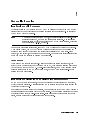
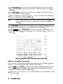
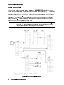
Figure 1-1. Example of a Limit Test using Limit Lines
Creating a Limit Test
Use the following example to set up an example limit test for an RF lter.
Note
This procedure assumes a device response is displayed on the network analyzer
screen.
To Set Up the Measurement
1. Connect the RF lter between the network analyzer RF OUT and RF IN ports.
2. Press 4PRESET5, 4FREQ5, then 4CENTER5. Enter the center frequency of the RF lter being
tested.
For this example, enter 175 MHz for the center frequency.
3. Press 4SPAN5 and enter a frequency span that simplies viewing the passband of the RF
lter.
Use a 200 MHz span, as an example.
4. Press 4SCALE5 then AUTOSCALE to view the entire measurement trace.
NNNNNNNNNNNNNNNNNNNNNNNNNNNNN
General Information
1-3
To Set the Limit Test Values
Limits create boundaries between which an active trace must remain for the measurement to
pass. To develop the limits, you select an appropriate softkey and adjust its position (value)
with the RPG, the step keys, or by entering the numeric value via the key pad.
5. Press 4DISPLAY5 then LIMITS . The network analyzer display splits into two sections. One
section displays the limit table and the other shows the selected limits on the display.
6. Press ADD LIMIT to display the Add Limit Menu.
NNNNNNNNNNNNNNNNNNNN
NNNNNNNNNNNNNNNNNNNNNNNNNNNNN
To Define the Maximum Limit
In the following example, the response of the lter is measured against three maximum limit
lines. The values are determined from the displayed trace, then limit parameters are entered
for a limit test. The values used for determining the limits are as follows:
Location
The low side of the cut-o
frequency portion
The bandpass portion
The high-side of the cut-o
frequency portion
Frequency of Interest
125 MHz to 150 MHz
155 MHz to 195 MHz
200 MHz to 225 MHz
There are two ways to dene the test limits:
1. Use a marker to determine the frequencies of the trace you plan to limit test:
NNNNNNNNNNNNNNNNNNNN
Press MARKER .
NNNNNNNNNNNNNNNNNNNNNNNNNN
Use the RPG knob to move the marker along the trace, or use the = MARKER key to
enter values directly.
2. Or, use the softkeys and the RPG, step keys, or numeric keys in any combination to
visually adjust the limits in real-time, about the displayed measurement trace.
a. Press ADD MAX LINE to set a limit above the device's response trace.
NNNNNNNNNNNNNNNNNNNNNNNNNNNNNNNNNNNNNN
b. Press BEGIN STIMULUS , then enter 125 MHz. This is the beginning frequency value of
the rst, maximum limit line.
NNNNNNNNNNNNNNNNNNNNNNNNNNNNNNNNNNNNNNNNNNNN
Note
Correct a mistake by using the following technique:
If your incorrect value is entered and you have not pressed 4MHz5, back space
over the error, then enter the correct value.
NNNNNNNNNNNNNNNNNNNNNNNNNNNNNNNNNNNNNNNNNNNN
If you have pressed 4MHz5 for the incorrect value, press BEGIN STIMULUS
and enter the corrected value.
NNNNNNNNNNNNNNNNNNNNNNNNNNNNNNNNNNNNNN
c. Press END STIMULUS . Enter 150 MHz, the ending frequency of the rst maximum limit
line. A limit line is drawn between the two frequency values you entered, at a zero (0.0)
unit level.
1-4
General Information
NNNNNNNNNNNNNNNNNNNNNNNNNNNNNNNNNNN
d. Press BEGIN LIMIT and watch the limit segment and measurement trace as you rotate
the RPG knob to adjust the beginning of the limit segment.
e. Place the beginning of the limit line at 025 dB, which is the device's maximum
allowable output power level, for the beginning frequency.
Note
Notice that the power level and frequency value appear in the limit-test table.
You can iterate between setting the beginning and ending of the limit line
position.
NNNNNNNNNNNNNNNNNNNNNNNNNNNNN
f. Press END LIMIT , and watch the traces on the display as you rotate the RPG to adjust
the end of the limit segment.
g. Place the end of the limit line at 0.0 dB, which is the device's maximum allowable
output power level, for the ending frequency.
3. Press 4PRIOR MENU5, then ADD MAX LINE . Repeat the above steps for the frequencies of the
second and third maximum limit lines. For this example:
NNNNNNNNNNNNNNNNNNNNNNNNNNNNNNNNNNNNNN
1) 155 MHz to 195 MHz, and 2) 200 MHz to 225 MHz
To Define Minimum Limit Lines
If desired, use the RPG, step keys, or numeric keypad to dene minimum limits. Minimum
limits may be at frequencies that are dierent from the maximum limit frequencies. It is
acceptable to enter minimum limits before or after entering maximum limits.
For this example, the frequencies used for maximum and minimum limit lines are slightly
dierent. Refer to the table below:
Location
The low side of the cut-o
frequency portion
The bandpass portion
The high-side of the cut-o
frequency portion
Frequency of Interest
125 MHz to 150 MHz
155 MHz to 195 MHz
200 MHz to 225 MHz
NNNNNNNNNNNNNNNNNNNNNNNNNNNNNNNNNNNNNN
1. Press 4PRIOR MENU5, then ADD MIN LINE to set up the limit line for the device's lower level
response.
2. Press BEGIN STIMULUS and enter 125 MHz, the beginning frequency of the rst minimum
limit line.
NNNNNNNNNNNNNNNNNNNNNNNNNNNNNNNNNNNNNNNNNNNN
Note
Correct a mistake by using the following technique:
If your incorrect value is entered and you have not pressed 4MHz5, back space
over the error, then enter the correct value.
If you have pressed 4MHz5 for the incorrect value, press BEGIN STIMULUS
and enter the corrected value.
NNNNNNNNNNNNNNNNNNNNNNNNNNNNNNNNNNNNNNNNNNNN
General Information
1-5
NNNNNNNNNNNNNNNNNNNNNNNNNNNNNNNNNNNNNN
3. Press END STIMULUS . Enter 150 MHz, the ending frequency of the rst minimum limit
line. A limit line is drawn between the two frequency values you entered, at a zero (0.0)
unit level.
4. Press BEGIN LIMIT and watch the limit segment and measurement trace as you rotate the
RPG knob to adjust the limit segment.
5. Place the beginning of the limit line at 050 dB, which is the device's minimum allowable
output power level for the beginning frequency.
NNNNNNNNNNNNNNNNNNNNNNNNNNNNNNNNNNN
Note
Notice that the power level and frequency value appear in the limit-test table.
You can iterate between setting the beginning and ending of the limit line
position.
6. Press END LIMIT and rotate the RPG to position the end of the limit line at 010 dB, the
device's minimum allowable output power level for the ending frequency.
7. Press 4PRIOR MENU5, then ADD MIN LINE and repeat the steps above for the second and
third minimum limit lines. For this example, 1) 155 MHz to 195 MHz, and 2) 200 MHz to
225 MHz.
NNNNNNNNNNNNNNNNNNNNNNNNNNNNN
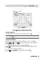
NNNNNNNNNNNNNNNNNNNNNNNNNNNNNNNNNNNNNN
Figure 1-2. Limit Test Example Using Limit Lines and Limit Points
Editing the Limits in the Limits Table
You may edit any individual frequency, limit, or limit line after you have created it. Become
familiar with the information below about modifying a limit value:
1. Press 4DISPLAY5, then LIMITS . The display shows the test device response with limit lines
and the tabular listing of the limits set. The highlighted box surrounding one segment
indicates the currently selected limit for editing.
2. Press the arrow keys or use the RPG to move the highlighted box to the portion of the test
parameter to edit.
NNNNNNNNNNNNNNNNNNNN
1-6
General Information
3. Press EDIT LIMITS , then press the keys that correspond to the portions of the limit you
want to edit (begin frequency, end frequency, begin limit, or end limit, as an example.
4. Enter new limit values.
5. Press 4PRIOR MENU5 to return to the limits menu.
6. Press LIMIT TEST ON to activate the limit test with the new limits. Test results are
displayed on the screen as PASS or FAIL.
NNNNNNNNNNNNNNNNNNNNNNNNNNNNNNNNNNN
NNNNNNNNNNNNNNNNNNNNNNNNNNNNNNNNNNNNNNNNN
General Information
1-7
2
Changing the Calibration Type
Introduction
You can create new calibration sets from an active two-port calibration set. The two-port set
can be a full two-port, a one-path two-port or a TRL two-port calibration set.
NNNNNNNNNNNNNNNNNNNNNNNNNNNNNNNNNNNNNNNNNNNNNNNNNNNNNNNNNNNNNNN
2-PORT to: S11 1-PORT creates an S11 1-port calibration from the currently active 2-port
calibration set.
NNNNNNNNNNNNNNNNNNNNNNNNNNNNNNNNNNNNNNNNNNNNNNNNNNNNNNNNNNNNNNN
2-PORT to: S22 1-PORT creates an S22 1-port calibration from the currently active 2-port
calibration set. Use the following key sequenceto create the new calibration set.
1. 4CAL5 MORE
2.
MODIFY CAL SET
3.
CHANGE CAL TYPE
4.
2-PORT to: S11 1-PORT
5.
CHANGE & SAVE
6.
CAL SET n (and select a new cal set,
dierent from the existing cal set. If the same cal set is used,
its original contents are overwritten.)
NNNNNNNNNNNNNN
NNNNNNNNNNNNNNNNNNNNNNNNNNNNNNNNNNNNNNNNNNNN
NNNNNNNNNNNNNNNNNNNNNNNNNNNNNNNNNNNNNNNNNNNNNNN
NNNNNNNNNNNNNNNNNNNNNNNNNNNNNNNNNNNNNNNNNNNNNNNNNNNNNNNNNNNNNNN
NNNNNNNNNNNNNNNNNNNNNNNNNNNNNNNNNNNNNNNNN
NNNNNNNNNNNNNNNNNNNNNNNNNNNNN
Changing the Calibration Type
2-1
Modifying a Cal Set with Connector Compensation
Connector compensation is a feature that provides for compensation of the discontinuity
found at the interface between the test port and a connector. The connector here, although
mechanically compatible, is not the same as the connector used for the calibration. There are
several connector families that have the same characteristic impedance, but use a dierent
geometry. Examples of such pairs include:
3.5 mm
3.5 mm
SMA
2.4 mm
/ 2.92 mm
/ SMA
/ 2.92 mm
/ 1.85 mm
The interface discontinuity is modeled as a lumped, shunt-susceptance at the test port
reference plane. The susceptance is generated from a capacitance model of the form:
C=C0 + C1 2F + C2 2F2 + C3 2F3
where F is the frequency. The coecients are provided in the default Cal Kits for a number
of typically used connector-pair combinations. To add models for other connector types, or
to change the coecients for the pairs already dened in a Cal Kit, use the \Modifying a
Calibration Kit" procedure on the previous pages. Note that the denitions in the default Cal
Kits are additions to the Standard Class ADAPTER, and are Standards of type \OPEN."
2-2
Changing the Calibration Type
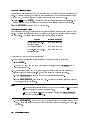
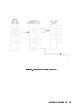
Figure 2-1. Connector Compensation Menu Keys
Changing the Calibration Type
2-3
Using Connector Compensation
1. Press 4CAL5, then press MORE .
NNNNNNNNNNNNNN
2. Press MODIFY CAL SET , then press CONNECTOR COMPENSATE .
NNNNNNNNNNNNNNNNNNNNNNNNNNNNNNNNNNNNNNNNNNNN
Note
NNNNNNNNNNNNNNNNNNNNNNNNNNNNNNNNNNNNNNNNNNNNNNNNNNNNNNNNNNNNNN
Connector compensation requires that the active Cal Set be a 1-Port or 2-Port
calibration. If a Cal Set of any other type is selected, the message ACTIVE
CALSET WRONG TYPE appears.
NNNNNNNNNNNNNNNNNNNNNNNNNNNNNNNNNNNNNNNNNNNNNNNNNNNNN
NNNNNNNNNNNNNNNNNNNNNNNNNNNNNNNNNNNNNNNNNNNNNNNNNNNNN
3. Choose the connector pair at either PORT 1 connectors or PORT 2 connectors to apply
connector compensation.
4. From the standards menu, choose the correct pair of connectors.
Note
If the connector pairs listed do not include the connector pairs you you
are using, return to the prior menu to choose the alternate Cal Kit before
repeating the procedure.
If the connector pairs you are using are not listed in either Cal Kit 1 or Cal
Kit 2, then you need to modify the calibration kit. Use the MODIFY 1 or
MODIFY 2 functions to enter an appropriate set of coecients. Refer to the
previous section, \Modifying a Calibration Kit."
NNNNNNNNNNNNNNNNNNNNNNNNNN
NNNNNNNNNNNNNNNNNNNNNNNNNN
After selecting a connector pair, the previous menu re-appears with the
selected Port selection underlined.
5. To apply connector compensation to the other port, repeat Step 3 for the other port.
6. Press COMPENSATE & SAVE to compute the modied Cal Set.
NNNNNNNNNNNNNNNNNNNNNNNNNNNNNNNNNNNNNNNNNNNNNNNNNNNNN
7. Select a Cal Set to store the modied calibration terms.
Other than the changes to the error coecients, all other properties of the Cal Set remain
unchanged.
Note that you do not need to overwrite the original (uncompensated) Cal Set. You may
also compare the compensated Cal Set with the uncompensated Cal Set and view the eect
of compensation.
2-4
Changing the Calibration Type
3
Power Domain Measurements
Introduction
This chapter explains the function and use of power domain in the HP 8510C network
analyzer, with rmware revision 7.0, or higher. The following sections explain the concept of
power domain, how to set up the HP 8510C to use power domain, the calibration implications,
and limitations, as well as detailed measurement examples.
This chapter also includes a description of Receiver Cal function, which is required to allow
calibrated measurements in power domain mode.
What is Power Domain?
Power domain allows measurements of a device under test, over a power range of interest, at
a constant frequency. In contrast, a frequency domain mode measurement measures power
over a frequency range of interest. A typical application for power domain is measuring the
compression of ampliers. In power domain, the independent variable (STIMULUS) swept
or stepped by the network analyzer system (normally frequency) is changed to power. The
STIMULUS block keys (4START5, 4STOP5, 4CENTER5, and 4SPAN5 ) refer to power and aect the
horizontal axis of a rectangular display. A frequency point must be selected, and is displayed
beside the range of power.
NNNNNNNNNNNNNNNNNNNNNNNNNNNNNNNNNNNNNN
Without a calibrated receiver ( RECEIVER CAL ) and source atness calibration
( FLATNESS CAL ), the test port absolute power cannot be known. The power is varied by
controlling the HP 8360 synthesized source.
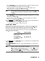
NNNNNNNNNNNNNNNNNNNNNNNNNNNNNNNNNNNNNN
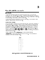
Figure 3-1. Domain Menu With Power Domain Function Keys
Power Domain Measurements
3-1
Power Domain Measurements
What is Receiver Cal?
NNNNNNNNNNNNNNNNNNNNNNNNNNNNNNNNNNNNNN
The HP 8510C network analyzer receiver calibration ( RECEIVER CAL ) feature provides a
display of unratioed receiver inputs, calibrated in absolute power (usually dBm). The feature
is normally used in association with power domain since the power levels displayed are
otherwise those determined by the source and do not account for losses in the path between
the source and the test ports. Receiver calibration is performed after calibrating the HP 8360
Series source with a power meter and ensuring that it remains leveled across the frequency
range of operation. A receiver calibration is stored as a Cal Set and corrects Port 1 (a1)
output power and Port 2 (b2) input power, only.
Note
There are a number of assumptions associated with receiver calibration.
Specically, the feature relies on the linearity of the detectors and does not
make any correction for mismatches at the test ports.
Figure 3-2. Receiver Calibration Menu
3-2
Power Domain Measurements
Power Domain Measurements
Making a Power Domain Measurement
The HP 8510C must already be calibrated in the frequency range of choice, or the user should
perform the calibration at the beginning of this power domain procedure.
It is recommended that you choose a frequency range that gives frequency steps of a
convenient size. Doing so allows the measurement frequencies to be easily recalled later. For
example, setting 4START5 to 50 MHz, and 4STOP5 to 5050 MHz, with the number of points set
to 101, gives measurement frequencies in even 50 MHz increments.
1. In frequency domain, set the HP 8510C to the frequency range of interest. Press the
appropriate STIMULUS block keys to enter the values. (4START5 and 4STOP5, or 4CENTER5,
and 4SPAN5.)
2. Press the STIMULUS block 4MENU5 key, then press STEP to underline step mode.
NNNNNNNNNNNNNN
Note
Step mode is required while using the power domain function. If you
calibrate or use a previously stored Cal Set, the power domain frequency of
measurement must be a point in the original (frequency domain) calibration.
3. Either calibrate the system at this point, or recall a previously stored Cal Set to use.
4. Activate a marker and set the marker to the frequency at which you wish to make a power
sweep. If the marker is not used, the power domain is entered at 2 GHz.
Note
If multiple markers are ON, the active marker is used for the power domain
frequency of measurement.
NNNNNNNNNNNNNNNNN
5. Press 4DOMAIN5, POWER , then press the appropriate STIMULUS block keys to set the power
levels of interest.
Note
The default power level values are START equals 010 dBm, STOP equals
0 dBm. The POWER SOURCE 1 softkey in the STIMULUS POWER MENU has no
eect in power domain mode. Pressing the key and entering a value displays
an error message. When you enter frequency domain mode again, source 1
power is reset to its original value.
NNNNNNNNNNNNNNNNNNNNNNNNNNNNNNNNNNNNNNNNNNNN
NNNNNNNNNNNNNNNNNNNNNNNNNNNNNNNN
6. With the power level set, you may change frequency setting using the
FREQ. of MEASUREMENT key.
NNNNNNNNNNNNNNNNNNNNNNNNNNNNNNNNNNNNNNNNNNNNNNNNNNNNNNNNNNNNNN
a. To choose a calibrated frequency point, use the NEXT PT HIGHER or NEXT PT LOWER
keys.
b. Select a valid (calibrated) frequency value. Notice that as you change frequencies, the
trace changes as the calibration is rst turned OFF , then back ON again.
NNNNNNNNNNNNNNNNNNNNNNNNNNNNNNNNNNNNNNNNNNNN
NNNNNNNNNNNNNNNNNNNNNNNNNNNNNNNNNNNNNNNNN
Power Domain Measurements
3-3
Power Domain Measurements
Note
When in power domain mode, you may use only one Cal Set for 4-parameter
display. If power domain is selected with more than one Cal Set applied, then
the active parameter calibration is converted to power domain and applied to
the measurements. All others are reset. Dual channel display may be used to
view power domain data and frequency domain data simultaneously, however,
UNCOUPLED CHANNELS must rst be selected.
NNNNNNNNNNNNNNNNNNNNNNNNNNNNNNNNNNNNNNNNNNNNNNNNNNNNNNNN
Performing a Receiver Calibration
1. Set the HP 8510C system to Frequency Domain and set the frequency range of interest.
2. Select the desired number of points to measure. If you plan to use power domain, STEP
sweep mode must be selected.
3. Set the source power level.
a. Press the HP 8510C STIMULUS block 4MENU5 key.
b. Press POWER MENU , then press POWER SOURCE 1 .
NNNNNNNNNNNNNN
NNNNNNNNNNNNNNNNNNNNNNNNNNNNNNNN
NNNNNNNNNNNNNNNNNNNNNNNNNNNNNNNNNNNNNNNNNNNN
c. Adjust the source power to a value appropriate for the device under test.
If you have carried out a power atness calibration since cycling the system power, skip to
Step 5, otherwise, continue with the atness calibration at Step 4.
The Flatness Calibration Must be Completed
Flatness calibration must be completed before beginning the receiver calibration. Data
obtained during the atness calibration is used during the receiver calibration.
4. Connect the power sensor from a zeroed power meter to Port 1 of the test set.
a. Press the STIMULUS block 4MENU5 key, then press the following keys:
NNNNNNNNNNNNNNNNNNNNNNNNNNNNNNNN
POWER MENU
NNNNNNNNNNNNNNNNNNNNNNNNNNNNNNNNNNNNNNNNNNNN
POWER FLATNESS
NNNNNNNNNNNNNNNNNNNNNNNNNNNNNNNNNNNNNNNNNNNNNNNNNNNNNNNN
CALIBRATE FLATNESS
NNNNNNNNNNNNNNNNNNNNNNNNNNNNNNNNNNNNNNNNNNNNNNNNNNNNNNNN
FLATNESS CAL START
b. Wait until the completion message is displayed before continuing.
Note
The source must remain leveled during the atness calibration process.
Calibration fails and displays an error message if the source is unleveled at any
frequency. Refer to Product Note 8510-16 for a complete description of the
atness correction feature.
c. Remove the power sensor from Port 1 of the test set.
5. Perform the receiver calibration. If valid power atness data is not available, the system
requires that a atness calibration be completed. Return to Step 4, above.
3-4
Power Domain Measurements
Power Domain Measurements
6. Connect a thru between Port 1 and Port 2 of the HP 8510C. It is not necessary for the
thru to be zero length or lossless, but should be appropriately dened in the selected Cal
Kit.
7. In the MENUS block, press 4CAL5, then press RECEIVER CAL .
NNNNNNNNNNNNNNNNNNNNNNNNNNNNNNNNNNNNNN
a. Press INPUT PWR to measure power at Port 1. The softkey label is underlined after the
measurement is completed.
b. Press OUTPUT PWR to measure power at Port 2. If several THRUs have been dened in
the Cal Kit, a further menu appears to allow selection of the appropriate standard. At
the completion of the measurement, the OUTPUT PWR key is underlined.
NNNNNNNNNNNNNNNNNNNNNNNNNNNNN
NNNNNNNNNNNNNNNNNNNNNNNNNNNNNNNN
NNNNNNNNNNNNNNNNNNNNNNNNNNNNNNNN
c. Press SAVE RCVR CAL then select a Cal Set number and store the receiver cal data.
NNNNNNNNNNNNNNNNNNNNNNNNNNNNNNNNNNNNNNNNN
Note
Unless both input and output power have been measured, pressing
SAVE RCVR CAL generates an error message.
NNNNNNNNNNNNNNNNNNNNNNNNNNNNNNNNNNNNNNNNN
When Receiver Cal is turned on, parameter User 1 a1 displays input power (Pin) in dBm and
User 2 b2 displays output power (Pout). Note that once calibrated, the measurements are
valid even if the source power level is changed and whether atness is turned ON or OFF.
Swept-Frequency Gain Compression Measurement Exercise
Making a swept-frequency gain compression measurement requires the receiver calibration
feature to obtain the output power at the desired compression level, in absolute power units.
1. Set the HP 8510C to the frequency range of interest.
2. Set the power to a value low enough to avoid driving the device under test (DUT) into
compression.
3. Perform a receiver calibration as appropriate. Then connect the (DUT).
4. Display S21 and perform an S21 Response Cal (Thru) with the DUT in place.
5. Press 4SCALE5 415 4x15 for convenient viewing.
6. Select split channel display mode.
a. Press 4DISPLAY5, then DISPLAY MODE .
NNNNNNNNNNNNNNNNNNNNNNNNNNNNNNNNNNNNNN
b. Select either DUAL CHAN SPLIT or DUAL CHAN OVERLAY .
NNNNNNNNNNNNNNNNNNNNNNNNNNNNNNNNNNNNNNNNNNNNNNN
NNNNNNNNNNNNNNNNNNNNNNNNNNNNNNNNNNNNNNNNNNNNNNNNNNNNN
c. Press CHANNEL 2 , PARAMETER 4MENU5, then USER 2 b2 .
NNNNNNNNNNNNNNNNNNNNNNNNNNNNN
NNNNNNNNNNNNNNNNNNNNNNNNNNNNN
d. Conrm that the display on Channel 2 reads Pout in units of dBm.
7. Press 4CHANNEL 15, and increase the source power until the gain (S21 ) decreases to 01 dB at
any frequency point.
8. Press MARKER and set the marker to the frequency point at which S21 is 01 dB.
NNNNNNNNNNNNNNNNNNNN
Power Domain Measurements
3-5
Power Domain Measurements
Note
NNNNNNNNNNNNNN
NNNNNNNNNNNNNNNNNNNNNNN
Marker search may be used by pressing 4MARKER5, MORE , and MINIMUM .
9. Read the absolute power at the output from the marker readout for Channel 2.
Swept-Power Gain Compression Measurement Exercise
Making a swept-power gain compression measurement requires using the power domain and
receiver calibration features.
1. Set up the HP 8510C for this measurement as for the \Swept-Frequency Gain
Compression Measurement Exercise" above.
2. Ensure that a receiver calibration has been completed, and an appropriate calibration for
S21 is done (a response cal is usually adequate for well-matched ampliers).
3. Connect the DUT and display S21 on Channel 1 with calibration turned ON.
4. Display a1 (Pin) or b2 (Pout) on Channel 2. Turn on the previously stored Cal Set
having a receiver calibration.
Note
Channels 1 and 2 must be in uncoupled mode.
5. Set a marker to the desired frequency of measurement for Power Domain.
6. Select Power Domain. Press 4DOMAIN5, then POWER .
NNNNNNNNNNNNNNNNN
7. Set the start- and stop-power points to values that drive the amplier into compression
during the trace.
8. Use the marker search function to locate a gain drop of 1 dB on the S21 trace.
9. Read the marker value for Channel 2 to determine the absolute input power (Pin) or
output power (Pout) at the 1 dB compression point.
a. Press 4CHANNEL 25, then 4MENU5 in the PARAMETER block.
b. Press USER 1 a1 or USER 2 b2 .
NNNNNNNNNNNNNNNNNNNNNNNNNNNNN
NNNNNNNNNNNNNNNNNNNNNNNNNNNNN
10. To make calibrated compression measurements at other frequencies of interest, use the
steps that follow:
a. Press DOMAIN , POWER , then NEXT PT HIGHER or NEXT PT LOWER to select the next
point from the original frequency domain calibrations.
b. OR
c. Enter a valid frequency of measurement using the numeric keypad. This method
may be used provided the exact frequency point entered is contained in the original
frequency domain calibration. Press DOMAIN , POWER , then FREQUENCY OF MEAS. and
enter the valid frequency.
NNNNNNNNNNNNNNNNNNNN
NNNNNNNNNNNNNNNNN
NNNNNNNNNNNNNNNNNNNNNNNNNNNNNNNNNNNNNNNNNNNN
NNNNNNNNNNNNNNNNNNNN
3-6
Power Domain Measurements
NNNNNNNNNNNNNNNNNNNNNNNNNNNNNNNNNNNNNNNNN
NNNNNNNNNNNNNNNNN
NNNNNNNNNNNNNNNNNNNNNNNNNNNNNNNNNNNNNNNNNNNNNNNNNNNNNNNN
Power Domain Measurements
Note
Entering a frequency of measurement not contained in the original frequency
domain calibration causes the calibrations to be turned OFF.
11. Repeat steps 8 and 9 above for the new frequency of measurement.
Power Domain Measurements
3-7