Download Agilent Technologies 54503A User`s guide

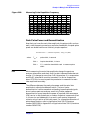
User’s Guide
Agilent Technologies 8560 E-Series and EC-Series
Spectrum Analyzers
Manufacturing Part Number: 08560-90158
Printed in USA
November 2000
© Copyright 1990 − 2000 Agilent Technologies
Notice
Agilent Technologies makes no warranty of any kind with regard to
this material, including but not limited to, the implied warranties of
merchantability and fitness for a particular purpose. Agilent
Technologies shall not be liable for errors contained herein or for
incidental or consequential damages in connection with the furnishing,
performance, or use of this material.
All Rights Reserved. Reproduction, adaptation, or translation without
prior written permission is prohibited, except as allowed under the
copyright laws.
The information contained in this document is subject to change
without notice.
Certification
Agilent Technologies certifies that this product met its published
specifications at the time of shipment from the factory. Agilent
Technologies further certifies that its calibration measurements are
traceable to the United States National Institute of Standards and
Technology, to the extent allowed by the Institute's calibration facility,
and to the calibration facilities of other International Standards
Organization members.
General Safety Considerations
The following safety notes are used throughout this manual.
Familiarize yourself with these notes before operating this instrument.
WARNING
Warning denotes a hazard. It calls attention to a procedure
which, if not correctly performed or adhered to, could result in
injury or loss of life. Do not proceed beyond a warning note
until the indicated conditions are fully understood and met.
CAUTION
Always use the three-prong AC power cord supplied with this product.
Failure to ensure adequate grounding may cause product damage.
2
CAUTION
Caution denotes a hazard. It calls attention to a procedure that, if not
correctly performed or adhered to, could result in damage to or
destruction of the instrument. Do not proceed beyond a caution sign
until the indicated conditions are fully understood and met.
WARNING
This is a Safety Class 1 Product (provided with a protective
earth ground incorporated in the power cord). The mains plug
shall be inserted only in a socket outlet provided with a
protected earth contact. Any interruption of the protective
conductor inside or outside of the product is likely to make the
product dangerous. Intentional interruption is prohibited.
WARNING
No operator serviceable parts inside. Refer servicing to
qualified personnel. To prevent electrical shock do not remove
covers.
WARNING
Before this instrument is switched on, make sure it has been
properly grounded through the protective conductor of the ac
power cable to a socket outlet provided with protective earth
contact.
WARNING
There are many points in the instrument which can, if
contacted, cause personal injury. Be extremely careful. Any
adjustments or service procedures that require operation of the
instrument with protective covers removed should be
performed only by trained service personnel
WARNING
Any interruption of the protective (grounding) conductor,
inside or outside the instrument, or disconnection of the
protective earth terminal can result in personal injury.
WARNING
If this instrument is used in a manner not specified by Agilent
Technologies, the protection provided by the instrument may
be impaired.
CAUTION
Before this instrument is turned on, make sure its primary power
circuitry has been adapted to the voltage of the ac power source. Failure
to set the ac power input to the correct voltage could cause damage to
the instrument when the ac power cable is plugged in.
This product conforms to Enclosure Protection IP 2 0 according to
IEC-529. The enclosure protects against finger access to hazardous
parts within the enclosure; the enclosure does not protect against the
entrance of water.
3
Warranty
This Agilent Technologies instrument product is warranted against
defects in material and workmanship for a period of one year from date
of shipment. During the warranty period, Agilent Technologies will, at
its option, either repair or replace products that prove to be defective.
For warranty service or repair, this product must be returned to a
service facility designated by Agilent Technologies. Buyer shall prepay
shipping charges to Agilent Technologies and Agilent Technologies
shall pay shipping charges to return the product to Buyer. However,
Buyer shall pay all shipping charges, duties, and taxes for products
returned to Agilent Technologies from another country.
Agilent Technologies warrants that its software and firmware
designated by Agilent Technologies for use with an instrument will
execute its programming instructions when properly installed on that
instrument. Agilent Technologies does not warrant that the operation
of the instrument, or software, or firmware will be uninterrupted or
error-free.
LIMITATION OF WARRANTY
The foregoing warranty shall not apply to defects resulting from
improper or inadequate maintenance by Buyer, Buyer-supplied
software or interfacing, unauthorized modification or misuse, operation
outside of the environmental specifications for the product, or improper
site preparation or maintenance.
NO OTHER WARRANTY IS EXPRESSED OR IMPLIED. AGILENT
TECHNOLOGIES SPECIFICALLY DISCLAIMS THE IMPLIED
WARRANTIES OF MERCHANTABILITY AND FITNESS FOR A
PARTICULAR PURPOSE.
EXCLUSIVE REMEDIES
THE REMEDIES PROVIDED HEREIN ARE BUYER’S SOLE AND
EXCLUSIVE REMEDIES. AGILENT TECHNOLOGIES SHALL NOT
BE LIABLE FOR ANY DIRECT, INDIRECT, SPECIAL, INCIDENTAL,
OR CONSEQUENTIAL DAMAGES, WHETHER BASED ON
CONTRACT, TORT, OR ANY OTHER LEGAL THEORY.
4
Contents
1. Quick Start Guide
What You'll Find in This Chapter . . . . . . . . . . . . . . . . . . . . . . . . . . . . . . . . . . . . . . . . . . . . . .
Initial Inspection . . . . . . . . . . . . . . . . . . . . . . . . . . . . . . . . . . . . . . . . . . . . . . . . . . . . . . . . . . . .
Turning the Spectrum Analyzer On for the First Time . . . . . . . . . . . . . . . . . . . . . . . . . . . . .
Making a Basic Measurement . . . . . . . . . . . . . . . . . . . . . . . . . . . . . . . . . . . . . . . . . . . . . . . . .
Reference Level Calibration . . . . . . . . . . . . . . . . . . . . . . . . . . . . . . . . . . . . . . . . . . . . . . . . . . .
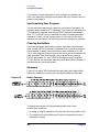
Front Panel Overview . . . . . . . . . . . . . . . . . . . . . . . . . . . . . . . . . . . . . . . . . . . . . . . . . . . . . . . .
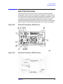
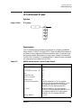
Rear Panel Overview . . . . . . . . . . . . . . . . . . . . . . . . . . . . . . . . . . . . . . . . . . . . . . . . . . . . . . . . .
Assistance . . . . . . . . . . . . . . . . . . . . . . . . . . . . . . . . . . . . . . . . . . . . . . . . . . . . . . . . . . . . . . . . . .
General Safety Considerations . . . . . . . . . . . . . . . . . . . . . . . . . . . . . . . . . . . . . . . . . . . . . . . . .
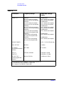
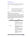
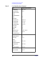
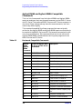
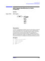
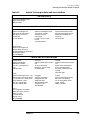
8560 E-Series and EC-Series Spectrum Analyzer Documentation Description . . . . . . . . . . .
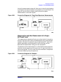
Manuals Available Separately. . . . . . . . . . . . . . . . . . . . . . . . . . . . . . . . . . . . . . . . . . . . . . . . . .
22
25
28
30
35
36
41
44
45
46
47
2. Making Measurements
Making Measurements . . . . . . . . . . . . . . . . . . . . . . . . . . . . . . . . . . . . . . . . . . . . . . . . . . . . . . . 50
Example 1: Resolving Closely Spaced Signals (with Resolution Bandwidth) . . . . . . . . . . . . 51
Example 2: Improving Amplitude Measurements with Ampcor . . . . . . . . . . . . . . . . . . . . . . 56
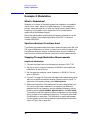
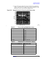
Example 3: Modulation . . . . . . . . . . . . . . . . . . . . . . . . . . . . . . . . . . . . . . . . . . . . . . . . . . . . . . . 60
Example 4: Harmonic Distortion . . . . . . . . . . . . . . . . . . . . . . . . . . . . . . . . . . . . . . . . . . . . . . . 67
Example 5: Third-Order Intermodulation Distortion . . . . . . . . . . . . . . . . . . . . . . . . . . . . . . . 75
Example 6: AM and FM Demodulation . . . . . . . . . . . . . . . . . . . . . . . . . . . . . . . . . . . . . . . . . . 81
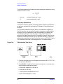
Example 7: Stimulus-Response Measurements . . . . . . . . . . . . . . . . . . . . . . . . . . . . . . . . . . . . 84
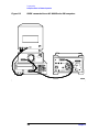
Example 8: External Millimeter Mixers (Unpreselected) . . . . . . . . . . . . . . . . . . . . . . . . . . . . 98
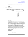
Example 9: Adjacent Channel Power Measurement . . . . . . . . . . . . . . . . . . . . . . . . . . . . . . . 108
Example 10: Power Measurement Functions . . . . . . . . . . . . . . . . . . . . . . . . . . . . . . . . . . . . 125
Example 11: Time-Gated Measurement . . . . . . . . . . . . . . . . . . . . . . . . . . . . . . . . . . . . . . . . 129
Example 12: Making Time-Domain Measurements with Sweep Delay . . . . . . . . . . . . . . . . 154
Example 13: Making Pulsed RF Measurements . . . . . . . . . . . . . . . . . . . . . . . . . . . . . . . . . . 158
3. Softkey Menus
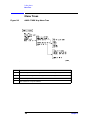
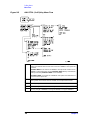
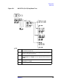
Menu Trees . . . . . . . . . . . . . . . . . . . . . . . . . . . . . . . . . . . . . . . . . . . . . . . . . . . . . . . . . . . . . . . 166
4. Key Function Descriptions
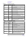
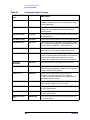
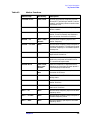
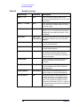
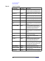
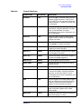
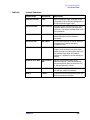
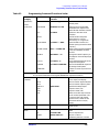
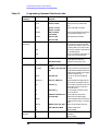
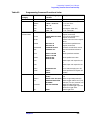
Key Function Tables . . . . . . . . . . . . . . . . . . . . . . . . . . . . . . . . . . . . . . . . . . . . . . . . . . . . . . . . 184
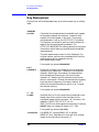
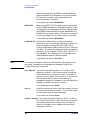
Key Descriptions . . . . . . . . . . . . . . . . . . . . . . . . . . . . . . . . . . . . . . . . . . . . . . . . . . . . . . . . . . . 204
5. Programming
Programming Features . . . . . . . . . . . . . . . . . . . . . . . . . . . . . . . . . . . . . . . . . . . . . . . . . . . . . .
Setup Procedure for Remote Operation . . . . . . . . . . . . . . . . . . . . . . . . . . . . . . . . . . . . . . . . .
Communication with the System . . . . . . . . . . . . . . . . . . . . . . . . . . . . . . . . . . . . . . . . . . . . . .
Initial Program Considerations . . . . . . . . . . . . . . . . . . . . . . . . . . . . . . . . . . . . . . . . . . . . . . .
Program Timing . . . . . . . . . . . . . . . . . . . . . . . . . . . . . . . . . . . . . . . . . . . . . . . . . . . . . . . . . . .
Data Transfer to Computer . . . . . . . . . . . . . . . . . . . . . . . . . . . . . . . . . . . . . . . . . . . . . . . . . .
Input and Output Buffers . . . . . . . . . . . . . . . . . . . . . . . . . . . . . . . . . . . . . . . . . . . . . . . . . . . .
Math Functions . . . . . . . . . . . . . . . . . . . . . . . . . . . . . . . . . . . . . . . . . . . . . . . . . . . . . . . . . . . .
Creating Screen Titles . . . . . . . . . . . . . . . . . . . . . . . . . . . . . . . . . . . . . . . . . . . . . . . . . . . . . .
Generating Plots and Prints Remotely . . . . . . . . . . . . . . . . . . . . . . . . . . . . . . . . . . . . . . . . .
Monitoring System Operation . . . . . . . . . . . . . . . . . . . . . . . . . . . . . . . . . . . . . . . . . . . . . . . .
290
291
293
297
298
303
316
319
324
327
332
5
Contents
6. Programming Command Cross Reference
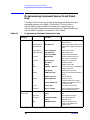
Programming Command Cross Reference Features . . . . . . . . . . . . . . . . . . . . . . . . . . . . . . . .340
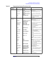
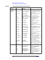
Front Panel Key Versus Command . . . . . . . . . . . . . . . . . . . . . . . . . . . . . . . . . . . . . . . . . . . . .341
Programming Command Versus Front Panel Key . . . . . . . . . . . . . . . . . . . . . . . . . . . . . . . . .352
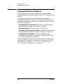
7. Language Reference
Language Reference Features. . . . . . . . . . . . . . . . . . . . . . . . . . . . . . . . . . . . . . . . . . . . . . . . . .370
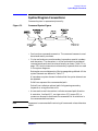
Syntax Diagram Conventions . . . . . . . . . . . . . . . . . . . . . . . . . . . . . . . . . . . . . . . . . . . . . . . . .371
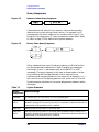
Programming Commands . . . . . . . . . . . . . . . . . . . . . . . . . . . . . . . . . . . . . . . . . . . . . . . . . . . .377
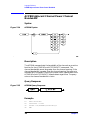
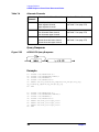
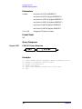
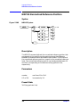
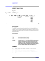
ACPACCL Accelerate Adjacent Channel Power Measurement . . . . . . . . . . . . . . . . . . . . . . .378
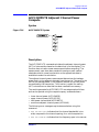
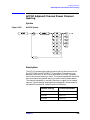
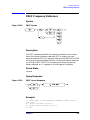
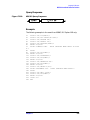
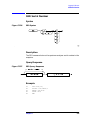
ACPALPHA Adjacent Channel Power Alpha Weighting . . . . . . . . . . . . . . . . . . . . . . . . . . . .380
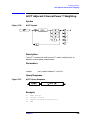
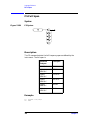
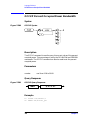
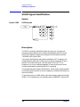
ACPALTCH Adjacent Channel Power Alternate Channels . . . . . . . . . . . . . . . . . . . . . . . . . .381
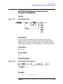
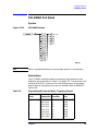
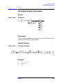
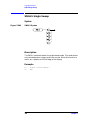
ACPBRPER Adjacent Channel Power Burst Period . . . . . . . . . . . . . . . . . . . . . . . . . . . . . . . .382
ACPBRWID Adjacent Channel Power Burst Width . . . . . . . . . . . . . . . . . . . . . . . . . . . . . . . .383
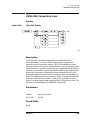
ACPBW Adjacent Channel Power Channel Bandwidth . . . . . . . . . . . . . . . . . . . . . . . . . . . . .384
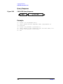
ACPCOMPUTE Adjacent Channel Power Compute . . . . . . . . . . . . . . . . . . . . . . . . . . . . . . .385
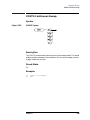
ACPFRQWT Adjacent Channel Power Frequency Weighting . . . . . . . . . . . . . . . . . . . . . . . .387
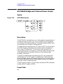
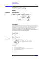
ACPGRAPH Adjacent Channel Power Graph . . . . . . . . . . . . . . . . . . . . . . . . . . . . . . . . . . . .388
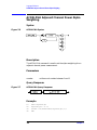
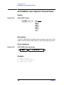
ACPLOWER Lower Adjacent Channel Power . . . . . . . . . . . . . . . . . . . . . . . . . . . . . . . . . . . .390
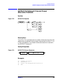
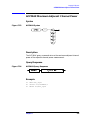
ACPMAX Maximum Adjacent Channel Power . . . . . . . . . . . . . . . . . . . . . . . . . . . . . . . . . . . .391
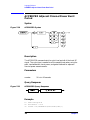
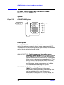
ACPMEAS Measure Adjacent Channel Power . . . . . . . . . . . . . . . . . . . . . . . . . . . . . . . . . . . .392
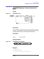
ACPMETHOD Adjacent Channel Power Measurement Method . . . . . . . . . . . . . . . . . . . . . .394
ACPMSTATE Adjacent Channel Power Measurement State . . . . . . . . . . . . . . . . . . . . . . . .397
ACPPWRTX Total Power Transmitted . . . . . . . . . . . . . . . . . . . . . . . . . . . . . . . . . . . . . . . . . .399
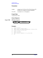
ACPRSLTS Adjacent Channel Power Measurement Results . . . . . . . . . . . . . . . . . . . . . . . .400
ACPSP Adjacent Channel Power Channel Spacing . . . . . . . . . . . . . . . . . . . . . . . . . . . . . . . .403
ACPT Adjacent Channel Power T Weighting . . . . . . . . . . . . . . . . . . . . . . . . . . . . . . . . . . . . .405
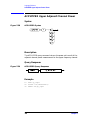
ACPUPPER Upper Adjacent Channel Power . . . . . . . . . . . . . . . . . . . . . . . . . . . . . . . . . . . . .406
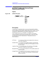
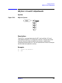
ADJALL LO and IF Adjustments . . . . . . . . . . . . . . . . . . . . . . . . . . . . . . . . . . . . . . . . . . . . . .407
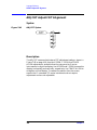
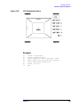
ADJCRT Adjust CRT Alignment . . . . . . . . . . . . . . . . . . . . . . . . . . . . . . . . . . . . . . . . . . . . . . .408
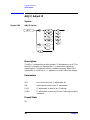
ADJIF Adjust IF . . . . . . . . . . . . . . . . . . . . . . . . . . . . . . . . . . . . . . . . . . . . . . . . . . . . . . . . . . . .410
AMB Trace A Minus Trace B . . . . . . . . . . . . . . . . . . . . . . . . . . . . . . . . . . . . . . . . . . . . . . . . . .412
AMBPL Trace A Minus Trace B Plus Display Line . . . . . . . . . . . . . . . . . . . . . . . . . . . . . . . .414
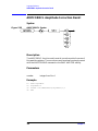
AMPCOR Amplitude Correction . . . . . . . . . . . . . . . . . . . . . . . . . . . . . . . . . . . . . . . . . . . . . . .416
AMPCORDATA Amplitude Correction Data . . . . . . . . . . . . . . . . . . . . . . . . . . . . . . . . . . . . .417
AMPCORSIZE Amplitude Correction Data Array Size . . . . . . . . . . . . . . . . . . . . . . . . . . . . .419
AMPCORRCL Amplitude Correction Recall . . . . . . . . . . . . . . . . . . . . . . . . . . . . . . . . . . . . . .420
AMPCORSAVE Amplitude Correction Save . . . . . . . . . . . . . . . . . . . . . . . . . . . . . . . . . . . . . .421
ANNOT Annotation On/Off . . . . . . . . . . . . . . . . . . . . . . . . . . . . . . . . . . . . . . . . . . . . . . . . . . .422
APB Trace A Plus Trace B . . . . . . . . . . . . . . . . . . . . . . . . . . . . . . . . . . . . . . . . . . . . . . . . . . . .423
AT Input Attenuation . . . . . . . . . . . . . . . . . . . . . . . . . . . . . . . . . . . . . . . . . . . . . . . . . . . . . . . .424
AUNITS Absolute Amplitude Units . . . . . . . . . . . . . . . . . . . . . . . . . . . . . . . . . . . . . . . . . . . .426
AUTOCPL Auto Coupled . . . . . . . . . . . . . . . . . . . . . . . . . . . . . . . . . . . . . . . . . . . . . . . . . . . . .428
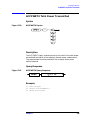
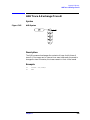
AXB Trace A Exchange Trace B . . . . . . . . . . . . . . . . . . . . . . . . . . . . . . . . . . . . . . . . . . . . . . .429
BLANK Blank Trace . . . . . . . . . . . . . . . . . . . . . . . . . . . . . . . . . . . . . . . . . . . . . . . . . . . . . . . .430
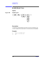
BML Trace B Minus Display Line . . . . . . . . . . . . . . . . . . . . . . . . . . . . . . . . . . . . . . . . . . . . . .431
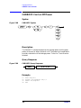
CARROFF Carrier Off Power . . . . . . . . . . . . . . . . . . . . . . . . . . . . . . . . . . . . . . . . . . . . . . . . .432
CARRON Carrier On Power . . . . . . . . . . . . . . . . . . . . . . . . . . . . . . . . . . . . . . . . . . . . . . . . . . .433
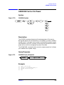
CF Center Frequency . . . . . . . . . . . . . . . . . . . . . . . . . . . . . . . . . . . . . . . . . . . . . . . . . . . . . . . .434
6
Contents
CHANPWR Channel Power . . . . . . . . . . . . . . . . . . . . . . . . . . . . . . . . . . . . . . . . . . . . . . . . . .
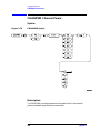
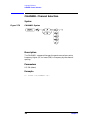
CHANNEL Channel Selection . . . . . . . . . . . . . . . . . . . . . . . . . . . . . . . . . . . . . . . . . . . . . . . .
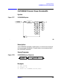
CHPWRBW Channel Power Bandwidth . . . . . . . . . . . . . . . . . . . . . . . . . . . . . . . . . . . . . . . .
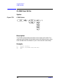
CLRW Clear Write . . . . . . . . . . . . . . . . . . . . . . . . . . . . . . . . . . . . . . . . . . . . . . . . . . . . . . . . .
CNVLOSS Conversion Loss . . . . . . . . . . . . . . . . . . . . . . . . . . . . . . . . . . . . . . . . . . . . . . . . . .
CONTS Continuous Sweep . . . . . . . . . . . . . . . . . . . . . . . . . . . . . . . . . . . . . . . . . . . . . . . . . . .
COUPLE Input Coupling . . . . . . . . . . . . . . . . . . . . . . . . . . . . . . . . . . . . . . . . . . . . . . . . . . . .
DELMKBW Occupied Power Bandwidth Within Delta Marker . . . . . . . . . . . . . . . . . . . . . .
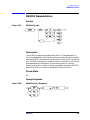
DEMOD Demodulation . . . . . . . . . . . . . . . . . . . . . . . . . . . . . . . . . . . . . . . . . . . . . . . . . . . . . .
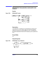
DEMODAGC Demodulation Automatic Gain Control . . . . . . . . . . . . . . . . . . . . . . . . . . . . .
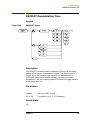
DEMODT Demodulation Time . . . . . . . . . . . . . . . . . . . . . . . . . . . . . . . . . . . . . . . . . . . . . . . .
DET Detection Modes . . . . . . . . . . . . . . . . . . . . . . . . . . . . . . . . . . . . . . . . . . . . . . . . . . . . . . .
DL Display Line . . . . . . . . . . . . . . . . . . . . . . . . . . . . . . . . . . . . . . . . . . . . . . . . . . . . . . . . . . . .
DLYSWP Delay Sweep . . . . . . . . . . . . . . . . . . . . . . . . . . . . . . . . . . . . . . . . . . . . . . . . . . . . . .
DONE Done . . . . . . . . . . . . . . . . . . . . . . . . . . . . . . . . . . . . . . . . . . . . . . . . . . . . . . . . . . . . . . .
ERR Error . . . . . . . . . . . . . . . . . . . . . . . . . . . . . . . . . . . . . . . . . . . . . . . . . . . . . . . . . . . . . . . .
ET Elapsed Time . . . . . . . . . . . . . . . . . . . . . . . . . . . . . . . . . . . . . . . . . . . . . . . . . . . . . . . . . . .
EXTMXR External Mixer Mode . . . . . . . . . . . . . . . . . . . . . . . . . . . . . . . . . . . . . . . . . . . . . . .
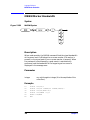
FA Start Frequency . . . . . . . . . . . . . . . . . . . . . . . . . . . . . . . . . . . . . . . . . . . . . . . . . . . . . . . . .
FB Stop Frequency . . . . . . . . . . . . . . . . . . . . . . . . . . . . . . . . . . . . . . . . . . . . . . . . . . . . . . . . .
FDIAG Frequency Diagnostics . . . . . . . . . . . . . . . . . . . . . . . . . . . . . . . . . . . . . . . . . . . . . . . .
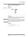
FDSP Frequency Display Off . . . . . . . . . . . . . . . . . . . . . . . . . . . . . . . . . . . . . . . . . . . . . . . . .
FFT Fast Fourier Transform . . . . . . . . . . . . . . . . . . . . . . . . . . . . . . . . . . . . . . . . . . . . . . . . . .
FOFFSET Frequency Offset . . . . . . . . . . . . . . . . . . . . . . . . . . . . . . . . . . . . . . . . . . . . . . . . . .
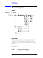
FREF Frequency Reference . . . . . . . . . . . . . . . . . . . . . . . . . . . . . . . . . . . . . . . . . . . . . . . . . .
FS Full Span . . . . . . . . . . . . . . . . . . . . . . . . . . . . . . . . . . . . . . . . . . . . . . . . . . . . . . . . . . . . . .
FULBAND Full Band . . . . . . . . . . . . . . . . . . . . . . . . . . . . . . . . . . . . . . . . . . . . . . . . . . . . . . .
GATE Gate . . . . . . . . . . . . . . . . . . . . . . . . . . . . . . . . . . . . . . . . . . . . . . . . . . . . . . . . . . . . . . . .
GATECTL Gate Control . . . . . . . . . . . . . . . . . . . . . . . . . . . . . . . . . . . . . . . . . . . . . . . . . . . . .
GD Gate Delay . . . . . . . . . . . . . . . . . . . . . . . . . . . . . . . . . . . . . . . . . . . . . . . . . . . . . . . . . . . . .
GL Gate Length . . . . . . . . . . . . . . . . . . . . . . . . . . . . . . . . . . . . . . . . . . . . . . . . . . . . . . . . . . . .
GP Gate Polarity . . . . . . . . . . . . . . . . . . . . . . . . . . . . . . . . . . . . . . . . . . . . . . . . . . . . . . . . . . .
GRAT Graticule On/Off . . . . . . . . . . . . . . . . . . . . . . . . . . . . . . . . . . . . . . . . . . . . . . . . . . . . . .
HD Hold . . . . . . . . . . . . . . . . . . . . . . . . . . . . . . . . . . . . . . . . . . . . . . . . . . . . . . . . . . . . . . . . . .
HNLOCK Harmonic Number Lock . . . . . . . . . . . . . . . . . . . . . . . . . . . . . . . . . . . . . . . . . . . .
HNUNLK Unlock Harmonic Number . . . . . . . . . . . . . . . . . . . . . . . . . . . . . . . . . . . . . . . . . .
ID Output Identification . . . . . . . . . . . . . . . . . . . . . . . . . . . . . . . . . . . . . . . . . . . . . . . . . . . . .
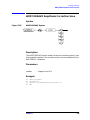
IDCF Signal Identification to Center Frequency . . . . . . . . . . . . . . . . . . . . . . . . . . . . . . . . . .
IDFREQ Signal Identified Frequency . . . . . . . . . . . . . . . . . . . . . . . . . . . . . . . . . . . . . . . . . .
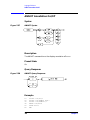
IP Instrument Preset . . . . . . . . . . . . . . . . . . . . . . . . . . . . . . . . . . . . . . . . . . . . . . . . . . . . . . .
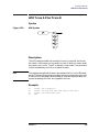
LG Logarithmic Scale . . . . . . . . . . . . . . . . . . . . . . . . . . . . . . . . . . . . . . . . . . . . . . . . . . . . . . .
LN Linear Scale . . . . . . . . . . . . . . . . . . . . . . . . . . . . . . . . . . . . . . . . . . . . . . . . . . . . . . . . . . . .
MBIAS Mixer Bias . . . . . . . . . . . . . . . . . . . . . . . . . . . . . . . . . . . . . . . . . . . . . . . . . . . . . . . . .
MEANPWR Mean Power Measurement . . . . . . . . . . . . . . . . . . . . . . . . . . . . . . . . . . . . . . . .
MEAS Measurement Status . . . . . . . . . . . . . . . . . . . . . . . . . . . . . . . . . . . . . . . . . . . . . . . . . .
MINH Minimum Hold . . . . . . . . . . . . . . . . . . . . . . . . . . . . . . . . . . . . . . . . . . . . . . . . . . . . . . .
MKA Marker Amplitude . . . . . . . . . . . . . . . . . . . . . . . . . . . . . . . . . . . . . . . . . . . . . . . . . . . . .
MKBW Marker Bandwidth . . . . . . . . . . . . . . . . . . . . . . . . . . . . . . . . . . . . . . . . . . . . . . . . . . .
MKCF Marker to Center Frequency . . . . . . . . . . . . . . . . . . . . . . . . . . . . . . . . . . . . . . . . . . .
436
438
439
440
441
443
444
445
447
449
451
453
455
457
459
460
462
463
464
466
468
470
472
475
477
478
479
481
483
484
485
486
487
488
489
491
492
493
494
495
498
500
501
503
505
506
507
508
509
7
Contents
MKCHEDGE Marker to Channel Edges . . . . . . . . . . . . . . . . . . . . . . . . . . . . . . . . . . . . . . . . .510
MKD Marker Delta . . . . . . . . . . . . . . . . . . . . . . . . . . . . . . . . . . . . . . . . . . . . . . . . . . . . . . . . . .511
MKDELCHBW Delta Markers to Channel Power Bandwidth . . . . . . . . . . . . . . . . . . . . . . .513
MKDR Reciprocal of Marker Delta . . . . . . . . . . . . . . . . . . . . . . . . . . . . . . . . . . . . . . . . . . . . .514
MKF Marker Frequency . . . . . . . . . . . . . . . . . . . . . . . . . . . . . . . . . . . . . . . . . . . . . . . . . . . . . .516
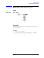
MKFC Frequency Counter . . . . . . . . . . . . . . . . . . . . . . . . . . . . . . . . . . . . . . . . . . . . . . . . . . . .518
MKFCR Frequency Counter Resolution . . . . . . . . . . . . . . . . . . . . . . . . . . . . . . . . . . . . . . . . .519
MKMCF Marker Mean to the Center Frequency . . . . . . . . . . . . . . . . . . . . . . . . . . . . . . . . . .521
MKMIN Marker to Minimum . . . . . . . . . . . . . . . . . . . . . . . . . . . . . . . . . . . . . . . . . . . . . . . . .522
MKN Marker Normal . . . . . . . . . . . . . . . . . . . . . . . . . . . . . . . . . . . . . . . . . . . . . . . . . . . . . . . .523
MKNOISE Marker Noise . . . . . . . . . . . . . . . . . . . . . . . . . . . . . . . . . . . . . . . . . . . . . . . . . . . . .525
MKOFF Marker Off . . . . . . . . . . . . . . . . . . . . . . . . . . . . . . . . . . . . . . . . . . . . . . . . . . . . . . . . .527
MKPK Peak Search . . . . . . . . . . . . . . . . . . . . . . . . . . . . . . . . . . . . . . . . . . . . . . . . . . . . . . . . .528
MKPT Marker Threshold . . . . . . . . . . . . . . . . . . . . . . . . . . . . . . . . . . . . . . . . . . . . . . . . . . . . .530
MKPX Peak Excursion . . . . . . . . . . . . . . . . . . . . . . . . . . . . . . . . . . . . . . . . . . . . . . . . . . . . . . .532
MKRL Marker to Reference Level . . . . . . . . . . . . . . . . . . . . . . . . . . . . . . . . . . . . . . . . . . . . . .535
MKSP Marker Delta to Span . . . . . . . . . . . . . . . . . . . . . . . . . . . . . . . . . . . . . . . . . . . . . . . . . .536
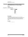
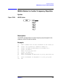
MKSS Marker to Center Frequency Step-Size . . . . . . . . . . . . . . . . . . . . . . . . . . . . . . . . . . . .537
MKT Marker Time . . . . . . . . . . . . . . . . . . . . . . . . . . . . . . . . . . . . . . . . . . . . . . . . . . . . . . . . . .538
MKTRACK Signal Track . . . . . . . . . . . . . . . . . . . . . . . . . . . . . . . . . . . . . . . . . . . . . . . . . . . . .539
ML Mixer Level . . . . . . . . . . . . . . . . . . . . . . . . . . . . . . . . . . . . . . . . . . . . . . . . . . . . . . . . . . . .541
MXMH Maximum Hold . . . . . . . . . . . . . . . . . . . . . . . . . . . . . . . . . . . . . . . . . . . . . . . . . . . . . .543
MXRMODE Mixer Mode . . . . . . . . . . . . . . . . . . . . . . . . . . . . . . . . . . . . . . . . . . . . . . . . . . . . .544
NORMLIZE Normalize Trace Data . . . . . . . . . . . . . . . . . . . . . . . . . . . . . . . . . . . . . . . . . . . . .545
NRL Normalized Reference Level . . . . . . . . . . . . . . . . . . . . . . . . . . . . . . . . . . . . . . . . . . . . . .547
NRPOS Normalized Reference Position . . . . . . . . . . . . . . . . . . . . . . . . . . . . . . . . . . . . . . . . .550
OCCUP Percent Occupied Power Bandwidth . . . . . . . . . . . . . . . . . . . . . . . . . . . . . . . . . . . . .552
OP Output Display Parameters . . . . . . . . . . . . . . . . . . . . . . . . . . . . . . . . . . . . . . . . . . . . . . . .553
PLOT Plot Display . . . . . . . . . . . . . . . . . . . . . . . . . . . . . . . . . . . . . . . . . . . . . . . . . . . . . . . . . .554
PLOTORG Display Origins . . . . . . . . . . . . . . . . . . . . . . . . . . . . . . . . . . . . . . . . . . . . . . . . . . .556
PLOTSRC Plot Source . . . . . . . . . . . . . . . . . . . . . . . . . . . . . . . . . . . . . . . . . . . . . . . . . . . . . . .558
PP Preselector Peak . . . . . . . . . . . . . . . . . . . . . . . . . . . . . . . . . . . . . . . . . . . . . . . . . . . . . . . . .560
PRINT Print . . . . . . . . . . . . . . . . . . . . . . . . . . . . . . . . . . . . . . . . . . . . . . . . . . . . . . . . . . . . . . .561
PSDAC Preselector DAC Number . . . . . . . . . . . . . . . . . . . . . . . . . . . . . . . . . . . . . . . . . . . . . .563
PSTATE Protect State . . . . . . . . . . . . . . . . . . . . . . . . . . . . . . . . . . . . . . . . . . . . . . . . . . . . . . .565
PWRBW Power Bandwidth (Full Trace) . . . . . . . . . . . . . . . . . . . . . . . . . . . . . . . . . . . . . . . . .567
RB Resolution Bandwidth . . . . . . . . . . . . . . . . . . . . . . . . . . . . . . . . . . . . . . . . . . . . . . . . . . . .569
RBR Resolution Bandwidth to Span Ratio . . . . . . . . . . . . . . . . . . . . . . . . . . . . . . . . . . . . . . .571
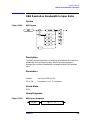
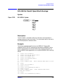
RCLOSCAL Recall Open/Short Average . . . . . . . . . . . . . . . . . . . . . . . . . . . . . . . . . . . . . . . . .573
RCLS Recall State . . . . . . . . . . . . . . . . . . . . . . . . . . . . . . . . . . . . . . . . . . . . . . . . . . . . . . . . . .575
RCLT Recall Trace . . . . . . . . . . . . . . . . . . . . . . . . . . . . . . . . . . . . . . . . . . . . . . . . . . . . . . . . . .576
RCLTHRU Recall Thru . . . . . . . . . . . . . . . . . . . . . . . . . . . . . . . . . . . . . . . . . . . . . . . . . . . . . .577
REV Revision Number . . . . . . . . . . . . . . . . . . . . . . . . . . . . . . . . . . . . . . . . . . . . . . . . . . . . . . .579
RL Reference/Range Level . . . . . . . . . . . . . . . . . . . . . . . . . . . . . . . . . . . . . . . . . . . . . . . . . . . .580
RLCAL Reference Level Calibration . . . . . . . . . . . . . . . . . . . . . . . . . . . . . . . . . . . . . . . . . . . .583
ROFFSET Amplitude Reference Offset . . . . . . . . . . . . . . . . . . . . . . . . . . . . . . . . . . . . . . . . . .585
RQS Request Service Conditions . . . . . . . . . . . . . . . . . . . . . . . . . . . . . . . . . . . . . . . . . . . . . . .587
SAVES Save State . . . . . . . . . . . . . . . . . . . . . . . . . . . . . . . . . . . . . . . . . . . . . . . . . . . . . . . . . .589
SAVET Save Trace . . . . . . . . . . . . . . . . . . . . . . . . . . . . . . . . . . . . . . . . . . . . . . . . . . . . . . . . . .590
8
Contents
SER Serial Number . . . . . . . . . . . . . . . . . . . . . . . . . . . . . . . . . . . . . . . . . . . . . . . . . . . . . . . . .
SIGID Signal Identification . . . . . . . . . . . . . . . . . . . . . . . . . . . . . . . . . . . . . . . . . . . . . . . . . .
SNGLS Single Sweep . . . . . . . . . . . . . . . . . . . . . . . . . . . . . . . . . . . . . . . . . . . . . . . . . . . . . . .
SP Frequency Span . . . . . . . . . . . . . . . . . . . . . . . . . . . . . . . . . . . . . . . . . . . . . . . . . . . . . . . . .
SQUELCH Squelch . . . . . . . . . . . . . . . . . . . . . . . . . . . . . . . . . . . . . . . . . . . . . . . . . . . . . . . . .
SRCALC Source Leveling Control . . . . . . . . . . . . . . . . . . . . . . . . . . . . . . . . . . . . . . . . . . . . .
SRCCRSTK Coarse Tracking Adjust . . . . . . . . . . . . . . . . . . . . . . . . . . . . . . . . . . . . . . . . . . .
SRCFINTK Fine Tracking Adjust . . . . . . . . . . . . . . . . . . . . . . . . . . . . . . . . . . . . . . . . . . . . .
SRCPOFS Source Power Offset . . . . . . . . . . . . . . . . . . . . . . . . . . . . . . . . . . . . . . . . . . . . . . .
SRCPSTP Source Power Step . . . . . . . . . . . . . . . . . . . . . . . . . . . . . . . . . . . . . . . . . . . . . . . . .
SRCPSWP Source Power Sweep . . . . . . . . . . . . . . . . . . . . . . . . . . . . . . . . . . . . . . . . . . . . . . .
SRCPWR Source Power . . . . . . . . . . . . . . . . . . . . . . . . . . . . . . . . . . . . . . . . . . . . . . . . . . . . .
SRCTKPK Source Tracking Peak . . . . . . . . . . . . . . . . . . . . . . . . . . . . . . . . . . . . . . . . . . . . . .
SRQ Service Request . . . . . . . . . . . . . . . . . . . . . . . . . . . . . . . . . . . . . . . . . . . . . . . . . . . . . . . .
SS Center Frequency Step-Size . . . . . . . . . . . . . . . . . . . . . . . . . . . . . . . . . . . . . . . . . . . . . . .
ST Sweep Time . . . . . . . . . . . . . . . . . . . . . . . . . . . . . . . . . . . . . . . . . . . . . . . . . . . . . . . . . . . .
STB Status Byte Query . . . . . . . . . . . . . . . . . . . . . . . . . . . . . . . . . . . . . . . . . . . . . . . . . . . . . .
STOREOPEN Store Open . . . . . . . . . . . . . . . . . . . . . . . . . . . . . . . . . . . . . . . . . . . . . . . . . . . .
STORESHORT Store Short . . . . . . . . . . . . . . . . . . . . . . . . . . . . . . . . . . . . . . . . . . . . . . . . . .
STORETHRU Store Thru . . . . . . . . . . . . . . . . . . . . . . . . . . . . . . . . . . . . . . . . . . . . . . . . . . . .
SWPCPL Sweep Couple . . . . . . . . . . . . . . . . . . . . . . . . . . . . . . . . . . . . . . . . . . . . . . . . . . . . .
SWPOUT Sweep Output . . . . . . . . . . . . . . . . . . . . . . . . . . . . . . . . . . . . . . . . . . . . . . . . . . . . .
TDF Trace Data Format . . . . . . . . . . . . . . . . . . . . . . . . . . . . . . . . . . . . . . . . . . . . . . . . . . . . .
TH Threshold . . . . . . . . . . . . . . . . . . . . . . . . . . . . . . . . . . . . . . . . . . . . . . . . . . . . . . . . . . . . . .
TITLE Title Entry . . . . . . . . . . . . . . . . . . . . . . . . . . . . . . . . . . . . . . . . . . . . . . . . . . . . . . . . . .
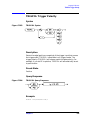
TM Trigger Mode . . . . . . . . . . . . . . . . . . . . . . . . . . . . . . . . . . . . . . . . . . . . . . . . . . . . . . . . . . .
TRA/TRB Trace Data Input/Output . . . . . . . . . . . . . . . . . . . . . . . . . . . . . . . . . . . . . . . . . . . .
TRIGPOL Trigger Polarity . . . . . . . . . . . . . . . . . . . . . . . . . . . . . . . . . . . . . . . . . . . . . . . . . . .
TS Take Sweep . . . . . . . . . . . . . . . . . . . . . . . . . . . . . . . . . . . . . . . . . . . . . . . . . . . . . . . . . . . .
TWNDOW Trace Window . . . . . . . . . . . . . . . . . . . . . . . . . . . . . . . . . . . . . . . . . . . . . . . . . . . .
VAVG Video Average . . . . . . . . . . . . . . . . . . . . . . . . . . . . . . . . . . . . . . . . . . . . . . . . . . . . . . . .
VB Video Bandwidth . . . . . . . . . . . . . . . . . . . . . . . . . . . . . . . . . . . . . . . . . . . . . . . . . . . . . . . .
VBR Video Bandwidth to Resolution Bandwidth Ratio . . . . . . . . . . . . . . . . . . . . . . . . . . . .
VIEW View Trace . . . . . . . . . . . . . . . . . . . . . . . . . . . . . . . . . . . . . . . . . . . . . . . . . . . . . . . . . .
VTL Video Trigger Level . . . . . . . . . . . . . . . . . . . . . . . . . . . . . . . . . . . . . . . . . . . . . . . . . . . . .
591
592
594
595
597
599
600
602
604
606
608
610
612
613
614
616
618
620
622
624
626
628
630
632
634
636
638
641
642
643
645
647
649
651
652
8. Options and Accessories
Options . . . . . . . . . . . . . . . . . . . . . . . . . . . . . . . . . . . . . . . . . . . . . . . . . . . . . . . . . . . . . . . . . . . 656
Accessories Available . . . . . . . . . . . . . . . . . . . . . . . . . . . . . . . . . . . . . . . . . . . . . . . . . . . . . . . 659
9. If You Have a Problem
What You'll Find in This Chapter . . . . . . . . . . . . . . . . . . . . . . . . . . . . . . . . . . . . . . . . . . . . .
Spectrum Analyzer Problems . . . . . . . . . . . . . . . . . . . . . . . . . . . . . . . . . . . . . . . . . . . . . . . . .
Agilent 85629B Test and Adjustment Module . . . . . . . . . . . . . . . . . . . . . . . . . . . . . . . . . . . .
Agilent 85620A Mass Memory Module . . . . . . . . . . . . . . . . . . . . . . . . . . . . . . . . . . . . . . . . .
Replacing the Battery . . . . . . . . . . . . . . . . . . . . . . . . . . . . . . . . . . . . . . . . . . . . . . . . . . . . . . .
Power Requirements . . . . . . . . . . . . . . . . . . . . . . . . . . . . . . . . . . . . . . . . . . . . . . . . . . . . . . . .
Procedures . . . . . . . . . . . . . . . . . . . . . . . . . . . . . . . . . . . . . . . . . . . . . . . . . . . . . . . . . . . . . . . .
666
667
669
670
671
672
675
9
Contents
Servicing the Spectrum Analyzer Yourself . . . . . . . . . . . . . . . . . . . . . . . . . . . . . . . . . . . . . . .678
Calling Agilent Technologies Sales and Service Offices . . . . . . . . . . . . . . . . . . . . . . . . . . . . .679
Returning Your Spectrum Analyzer for Service . . . . . . . . . . . . . . . . . . . . . . . . . . . . . . . . . . .680
Serial Numbers . . . . . . . . . . . . . . . . . . . . . . . . . . . . . . . . . . . . . . . . . . . . . . . . . . . . . . . . . . . . .684
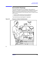
Electrostatic Discharge . . . . . . . . . . . . . . . . . . . . . . . . . . . . . . . . . . . . . . . . . . . . . . . . . . . . . .685
Error Messages . . . . . . . . . . . . . . . . . . . . . . . . . . . . . . . . . . . . . . . . . . . . . . . . . . . . . . . . . . . . .688
10
Figures
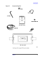
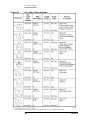
Figure 1-1 . Accessories Supplied . . . . . . . . . . . . . . . . . . . . . . . . . . . . . . . . . . . . . . . . . . . . . . 27
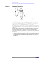
Figure 1-2 . Selecting the Correct Line Voltage . . . . . . . . . . . . . . . . . . . . . . . . . . . . . . . . . . . . 28
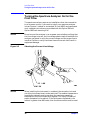
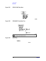
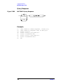
Figure 1-3 . 300 MHz Calibration Signal Connection . . . . . . . . . . . . . . . . . . . . . . . . . . . . . . . 30
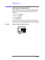
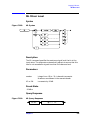
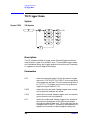
Figure 1-4 . Softkey Menu . . . . . . . . . . . . . . . . . . . . . . . . . . . . . . . . . . . . . . . . . . . . . . . . . . . . 31
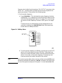
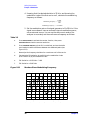
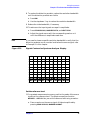
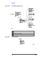
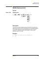
Figure 1-5 . 300 MHz Center Frequency . . . . . . . . . . . . . . . . . . . . . . . . . . . . . . . . . . . . . . . . . 32
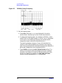
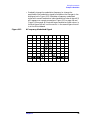
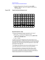
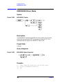
Figure 1-6 . 20 MHz Frequency Span . . . . . . . . . . . . . . . . . . . . . . . . . . . . . . . . . . . . . . . . . . . . 33
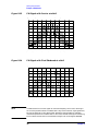
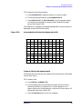
Figure 1-7 . Activated Normal Marker . . . . . . . . . . . . . . . . . . . . . . . . . . . . . . . . . . . . . . . . . . . 33
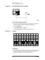
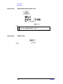
Figure 1-8 . −10 dBm Reference Level . . . . . . . . . . . . . . . . . . . . . . . . . . . . . . . . . . . . . . . . . . 34
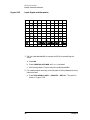
Figure 1-9 . Peaked Signal to Reference Level . . . . . . . . . . . . . . . . . . . . . . . . . . . . . . . . . . . . . 35
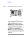
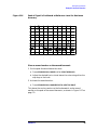
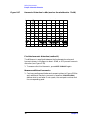
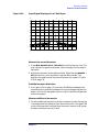
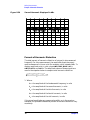
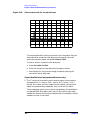
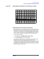
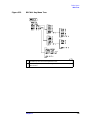
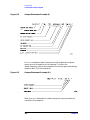
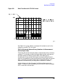
Figure 1-10 . Front Panel of an 8560 E-Series or EC- Series Spectrum Analyzer . . . . . . . . . . 36
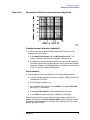
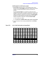
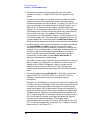
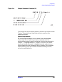
Figure 1-11 . Display Annotation . . . . . . . . . . . . . . . . . . . . . . . . . . . . . . . . . . . . . . . . . . . . . . . 39
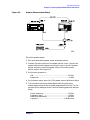
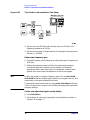
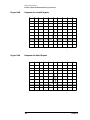
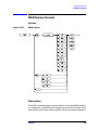
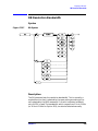
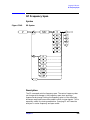
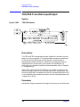
Figure 1-12 . Rear Panel Functions - 8560 E-series . . . . . . . . . . . . . . . . . . . . . . . . . . . . . . . . . 41
Figure 1-13 . Rear Panel Functions - 8560 EC-series . . . . . . . . . . . . . . . . . . . . . . . . . . . . . . . . 41
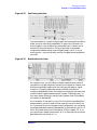
Figure 2-1 . 1 kHz Signal Separation . . . . . . . . . . . . . . . . . . . . . . . . . . . . . . . . . . . . . . . . . . . . 52
Figure 2-2 . 2 kHz Signal Separation . . . . . . . . . . . . . . . . . . . . . . . . . . . . . . . . . . . . . . . . . . . . 52
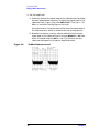
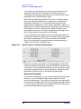
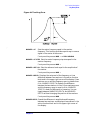
Figure 2-3 . Bandwidth Shape Factor . . . . . . . . . . . . . . . . . . . . . . . . . . . . . . . . . . . . . . . . . . . . 54
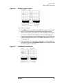
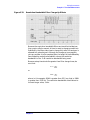
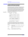
Figure 2-4 . 100 kHz Bandwidth Resolution . . . . . . . . . . . . . . . . . . . . . . . . . . . . . . . . . . . . . . 55
Figure 2-5 . 300 kHz Bandwidth Resolution . . . . . . . . . . . . . . . . . . . . . . . . . . . . . . . . . . . . . . 55
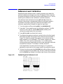
Figure 2-6 . Ampcor Measurement Setup . . . . . . . . . . . . . . . . . . . . . . . . . . . . . . . . . . . . . . . . . 57
Figure 2-7 . An Amplitude-Modulated Signal . . . . . . . . . . . . . . . . . . . . . . . . . . . . . . . . . . . . . 61
Figure 2-8 . Percentage of Modulation . . . . . . . . . . . . . . . . . . . . . . . . . . . . . . . . . . . . . . . . . . . 61
Figure 2-9 . FM Deviation Test Setup . . . . . . . . . . . . . . . . . . . . . . . . . . . . . . . . . . . . . . . . . . . 62
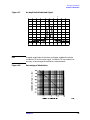
Figure 2-10 . Bessel Functions for Determining Modulation Index . . . . . . . . . . . . . . . . . . . . . 63
Figure 2-11 . Markers Show Modulating Frequency . . . . . . . . . . . . . . . . . . . . . . . . . . . . . . . . 64
Figure 2-12 . A Frequency-Modulated Signal . . . . . . . . . . . . . . . . . . . . . . . . . . . . . . . . . . . . . 65
Figure 2-13 . FM Signal with Carrier at a Null . . . . . . . . . . . . . . . . . . . . . . . . . . . . . . . . . . . . . 66
Figure 2-14 . FM Signal with First Sidebands at a Null . . . . . . . . . . . . . . . . . . . . . . . . . . . . . . 66
Figure 2-15 . Input Signal and Harmonics . . . . . . . . . . . . . . . . . . . . . . . . . . . . . . . . . . . . . . . . 68
Figure 2-16 . Peak of Signal is Positioned at Reference Level for Maximum Accuracy . . . . . 69
Figure 2-17 . Harmonic Distortion in dBc (marker threshold set to −70 dB) . . . . . . . . . . . . . . 70
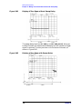
Figure 2-18 . Percentage of Distortion versus Harmonic Amplitude . . . . . . . . . . . . . . . . . . . . 71
Figure 2-19 . Input Signal Displayed in a 1 MHz Span . . . . . . . . . . . . . . . . . . . . . . . . . . . . . . 73
Figure 2-20 . Second Harmonic Displayed in dBc . . . . . . . . . . . . . . . . . . . . . . . . . . . . . . . . . . 74
Figure 2-21 . Third-Order Intermodulation Test Setup . . . . . . . . . . . . . . . . . . . . . . . . . . . . . . 76
Figure 2-22 . Signals Centered on Spectrum Analyzer Display . . . . . . . . . . . . . . . . . . . . . . . . 77
Figure 2-23 . Signal Peak Set to Reference Level . . . . . . . . . . . . . . . . . . . . . . . . . . . . . . . . . . 78
Figure 2-24 . Intermodulation Distortion Measured in dBc . . . . . . . . . . . . . . . . . . . . . . . . . . . 79
Figure 2-25 . Display with Title . . . . . . . . . . . . . . . . . . . . . . . . . . . . . . . . . . . . . . . . . . . . . . . . 80
Figure 2-26 . AM and FM Demodulation Test Setup . . . . . . . . . . . . . . . . . . . . . . . . . . . . . . . . 82
Figure 2-27 . FM Band . . . . . . . . . . . . . . . . . . . . . . . . . . . . . . . . . . . . . . . . . . . . . . . . . . . . . . . 82
Figure 2-28 . Place a marker on the signal of interest, then demodulate. . . . . . . . . . . . . . . . . . 83
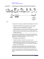
Figure 2-29 . Block Diagram of a Spectrum Analyzer and Tracking Generator System . . . . . 84
Figure 2-30 . Transmission Measurement Test Setup . . . . . . . . . . . . . . . . . . . . . . . . . . . . . . . 85
Figure 2-31 . Tracking-Generator Output Power Activated . . . . . . . . . . . . . . . . . . . . . . . . . . . 86
Figure 2-32 . Adjust analyzer settings according to the measurement requirement. . . . . . . . . 87
11
Figures
Figure 2-33 . Decrease the resolution bandwidth to improve sensitivity. . . . . . . . . . . . . . . . . 88
Figure 2-34 . Manual tracking adjustment compensates for tracking error. . . . . . . . . . . . . . . 89
Figure 2-35 . Guided calibration routines prompt the user. . . . . . . . . . . . . . . . . . . . . . . . . . . . 90
Figure 2-36 . The thru trace is displayed in trace B. . . . . . . . . . . . . . . . . . . . . . . . . . . . . . . . . 90
Figure 2-37 . Normalized Trace . . . . . . . . . . . . . . . . . . . . . . . . . . . . . . . . . . . . . . . . . . . . . . . . 91
Figure 2-38 . Measure the rejection range with delta markers. . . . . . . . . . . . . . . . . . . . . . . . . 92
Figure 2-39 . NORM REF LVL adjusts the trace without changing analyzer settings. . . . . . 93
Figure 2-40 . Increase the dynamic measurement range by using RANGE LVL. . . . . . . . . . 94
Figure 2-41 . Normalized Frequency Response Trace of a Preamplifier . . . . . . . . . . . . . . . . 95
Figure 2-42 . NORM REF LVL is a trace function. . . . . . . . . . . . . . . . . . . . . . . . . . . . . . . . . 96
Figure 2-43 . RANGE LVL adjusts analyzer for compression-free measurements. . . . . . . . . 96
Figure 2-44 . External Mixer Setup (a) without Bias; (b) with Bias . . . . . . . . . . . . . . . . . . . . 99
Figure 2-45 . Select the band of interest. . . . . . . . . . . . . . . . . . . . . . . . . . . . . . . . . . . . . . . . . 101
Figure 2-46 . Store and correct for conversion loss. . . . . . . . . . . . . . . . . . . . . . . . . . . . . . . . 102
Figure 2-47 . Signal Responses Produced by a 50 GHz Signal in U Band . . . . . . . . . . . . . . 103
Figure 2-48 . Response for Invalid Signals . . . . . . . . . . . . . . . . . . . . . . . . . . . . . . . . . . . . . . 104
Figure 2-49 . Response for Valid Signals . . . . . . . . . . . . . . . . . . . . . . . . . . . . . . . . . . . . . . . 104
Figure 2-50 . SIG ID AT MKR Performed on an Image Signal . . . . . . . . . . . . . . . . . . . . . . 105
Figure 2-51 . SIG ID AT MKR Performed on a True Signal . . . . . . . . . . . . . . . . . . . . . . . . 106
Figure 2-52 . Adjacent Channel Power Measurement Test Setup . . . . . . . . . . . . . . . . . . . . . 109
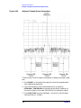
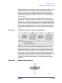
Figure 2-53 . Adjacent Channel Power Parameters . . . . . . . . . . . . . . . . . . . . . . . . . . . . . . . . 110
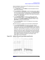
Figure 2-54 . Adjacent Channel Power Measurement Results . . . . . . . . . . . . . . . . . . . . . . . 111
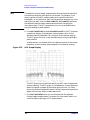
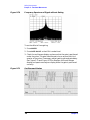
Figure 2-55 . ACP Graph Display . . . . . . . . . . . . . . . . . . . . . . . . . . . . . . . . . . . . . . . . . . . . . 112
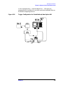
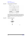
Figure 2-56 . Trigger Configuration for Gated Method, Non-Option 001 . . . . . . . . . . . . . . 123
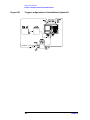
Figure 2-57 . Trigger Configuration for Gated Method, Option 001 . . . . . . . . . . . . . . . . . . . 124
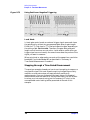
Figure 2-58 . Simplified Digital Mobile-Radio Signal in Time Domain . . . . . . . . . . . . . . . . 129
Figure 2-59 . Frequency of the Combined Signals of the Radios . . . . . . . . . . . . . . . . . . . . . 130
Figure 2-60 . Time-Gated Spectrum of Signal Number 1 . . . . . . . . . . . . . . . . . . . . . . . . . . . 130
Figure 2-61 . Time-Gated Spectrum of Signal Number 2 . . . . . . . . . . . . . . . . . . . . . . . . . . . 131
Figure 2-62 . Block Diagram of the Spectrum Analyzer with Time Gate . . . . . . . . . . . . . . . 132
Figure 2-63 . Timing Relationship of Signals During Gating . . . . . . . . . . . . . . . . . . . . . . . . 133
Figure 2-64 . Spectrum within pulse #1 . . . . . . . . . . . . . . . . . . . . . . . . . . . . . . . . . . . . . . . . . 133
Figure 2-65 . Using Time-Gating to View Signal 1 . . . . . . . . . . . . . . . . . . . . . . . . . . . . . . . . 134
Figure 2-66 . Spectrum within pulse #2 . . . . . . . . . . . . . . . . . . . . . . . . . . . . . . . . . . . . . . . . . 134
Figure 2-67 . Using Time-Gating to View Signal 2 . . . . . . . . . . . . . . . . . . . . . . . . . . . . . . . . 135
Figure 2-68 . Connection Diagram for Time-Gated Spectrum Measurements . . . . . . . . . . . 137
Figure 2-69 . Connection Diagram for Example . . . . . . . . . . . . . . . . . . . . . . . . . . . . . . . . . . 137
Figure 2-70 . Frequency Spectrum of Signal without Gating . . . . . . . . . . . . . . . . . . . . . . . . 140
Figure 2-71 . Oscilloscope Display . . . . . . . . . . . . . . . . . . . . . . . . . . . . . . . . . . . . . . . . . . . . 140
Figure 2-72 . Spectrum Analyzer Display . . . . . . . . . . . . . . . . . . . . . . . . . . . . . . . . . . . . . . . 141
Figure 2-73 . Using Positive or Negative Triggering . . . . . . . . . . . . . . . . . . . . . . . . . . . . . . 142
Figure 2-74 . Time-domain Parameters . . . . . . . . . . . . . . . . . . . . . . . . . . . . . . . . . . . . . . . . . 143
Figure 2-75 . Positioning the Gate . . . . . . . . . . . . . . . . . . . . . . . . . . . . . . . . . . . . . . . . . . . . . 145
Figure 2-76 . Best Position for Gate . . . . . . . . . . . . . . . . . . . . . . . . . . . . . . . . . . . . . . . . . . . 145
Figure 2-77 . Setup Time for Interpulse Measurement . . . . . . . . . . . . . . . . . . . . . . . . . . . . . 146
12
Figures
Figure 2-78 . Resolution Bandwidth Filter Charge-Up Effects . . . . . . . . . . . . . . . . . . . . . . . 147
Figure 2-79 . Gate Positioning Parameters . . . . . . . . . . . . . . . . . . . . . . . . . . . . . . . . . . . . . . . 151
Figure 2-80 . Pulsed-RF Signal in Time Domain . . . . . . . . . . . . . . . . . . . . . . . . . . . . . . . . . . 154
Figure 2-81 . Display of Zero-Span without Sweep Delay . . . . . . . . . . . . . . . . . . . . . . . . . . . 156
Figure 2-82 . Display of Zero-Span with Sweep Delay . . . . . . . . . . . . . . . . . . . . . . . . . . . . . 156
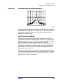
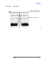
Figure 2-83 . Main Lobe and Side Lobes . . . . . . . . . . . . . . . . . . . . . . . . . . . . . . . . . . . . . . . . 159
Figure 2-84 . Trace Displayed as a Solid Line . . . . . . . . . . . . . . . . . . . . . . . . . . . . . . . . . . . . 160
Figure 2-85 . Center Frequency at Center of Main Lobe . . . . . . . . . . . . . . . . . . . . . . . . . . . . 160
Figure 2-86 . Markers Show Sidelobe Ratio . . . . . . . . . . . . . . . . . . . . . . . . . . . . . . . . . . . . . . 161
Figure 2-87 . Markers Show Pulse Width . . . . . . . . . . . . . . . . . . . . . . . . . . . . . . . . . . . . . . . . 162
Figure 2-88 . Measuring Pulse Repetition Frequency . . . . . . . . . . . . . . . . . . . . . . . . . . . . . . 163
Figure 3-1 . AMPLITUDE Key Menu Tree . . . . . . . . . . . . . . . . . . . . . . . . . . . . . . . . . . . . . . 166
Figure 3-2 . AUTO COUPLE Menu Tree . . . . . . . . . . . . . . . . . . . . . . . . . . . . . . . . . . . . . . . . 167
Figure 3-3 . AUX CTRL (1 of 3) Key Menu Tree. . . . . . . . . . . . . . . . . . . . . . . . . . . . . . . . . . 168
Figure 3-4 . AUX CTRL (2 of 3) Key Menu Tree. . . . . . . . . . . . . . . . . . . . . . . . . . . . . . . . . . 169
Figure 3-5 . AUX CTRL (3 of 3) Key Menu Tree. . . . . . . . . . . . . . . . . . . . . . . . . . . . . . . . . . 170
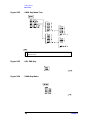
Figure 3-6 . BW Key Menu . . . . . . . . . . . . . . . . . . . . . . . . . . . . . . . . . . . . . . . . . . . . . . . . . . 170
Figure 3-7 . CAL Key Menu Tree . . . . . . . . . . . . . . . . . . . . . . . . . . . . . . . . . . . . . . . . . . . . . . 171
Figure 3-8 . CONFIG Key Menu Tree. . . . . . . . . . . . . . . . . . . . . . . . . . . . . . . . . . . . . . . . . . . 172
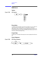
Figure 3-9 . COPY Key . . . . . . . . . . . . . . . . . . . . . . . . . . . . . . . . . . . . . . . . . . . . . . . . . . . . . . 173
Figure 3-10 . DISPLAY Key Menu Tree. . . . . . . . . . . . . . . . . . . . . . . . . . . . . . . . . . . . . . . . . 173
Figure 3-11 . FREQ COUNT Key Menu. . . . . . . . . . . . . . . . . . . . . . . . . . . . . . . . . . . . . . . . . 174
Figure 3-12 . FREQUENCY Key Menu Tree . . . . . . . . . . . . . . . . . . . . . . . . . . . . . . . . . . . . . 174
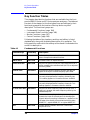
Figure 3-13 . HOLD Key . . . . . . . . . . . . . . . . . . . . . . . . . . . . . . . . . . . . . . . . . . . . . . . . . . . . . 174
Figure 3-14 . MEAS/USER Key Menu Tree . . . . . . . . . . . . . . . . . . . . . . . . . . . . . . . . . . . . . . 175
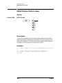
Figure 3-15 . ACP MENU Key Menu Tree. . . . . . . . . . . . . . . . . . . . . . . . . . . . . . . . . . . . . . . 176
Figure 3-16 . MKR Key Menu. . . . . . . . . . . . . . . . . . . . . . . . . . . . . . . . . . . . . . . . . . . . . . . . . 176
Figure 3-17 . MKR-> Key Menu . . . . . . . . . . . . . . . . . . . . . . . . . . . . . . . . . . . . . . . . . . . . . . . 177
Figure 3-18 . MODULE Key Menus . . . . . . . . . . . . . . . . . . . . . . . . . . . . . . . . . . . . . . . . . . . . 177
Figure 3-19 . PEAK SEARCH Key Menu Tree . . . . . . . . . . . . . . . . . . . . . . . . . . . . . . . . . . . 178
Figure 3-20 . PRESET Key . . . . . . . . . . . . . . . . . . . . . . . . . . . . . . . . . . . . . . . . . . . . . . . . . . . 178
Figure 3-21 . RECALL Key Menu Tree . . . . . . . . . . . . . . . . . . . . . . . . . . . . . . . . . . . . . . . . . 179
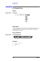
Figure 3-22 . SAVE Key Menu Tree . . . . . . . . . . . . . . . . . . . . . . . . . . . . . . . . . . . . . . . . . . . . 180
Figure 3-23 . SGL SWP Key . . . . . . . . . . . . . . . . . . . . . . . . . . . . . . . . . . . . . . . . . . . . . . . . . . 180
Figure 3-24 . SPAN Key Menu . . . . . . . . . . . . . . . . . . . . . . . . . . . . . . . . . . . . . . . . . . . . . . . . 180
Figure 3-25 . SWEEP Key Menu Tree . . . . . . . . . . . . . . . . . . . . . . . . . . . . . . . . . . . . . . . . . . 181
Figure 3-26 . TRACE Key Menu Tree . . . . . . . . . . . . . . . . . . . . . . . . . . . . . . . . . . . . . . . . . . 181
Figure 3-27 . TRIG Key Menu . . . . . . . . . . . . . . . . . . . . . . . . . . . . . . . . . . . . . . . . . . . . . . . . 181
Figure 4-1 . Channel Bandwidth Parameters . . . . . . . . . . . . . . . . . . . . . . . . . . . . . . . . . . . . . 210
Figure 4-2 . ACP Graph Display . . . . . . . . . . . . . . . . . . . . . . . . . . . . . . . . . . . . . . . . . . . . . . . 213
Figure 4-3 . CRT Alignment Pattern . . . . . . . . . . . . . . . . . . . . . . . . . . . . . . . . . . . . . . . . . . . . 228
Figure 4-4 . Tracking Error . . . . . . . . . . . . . . . . . . . . . . . . . . . . . . . . . . . . . . . . . . . . . . . . . . . 247
Figure 4-5 . PEAK EXCURSN defines the peaks on a trace. . . . . . . . . . . . . . . . . . . . . . . . . . 258
Figure 5-1 . 8560E connected to an HP 9000 Series 300 computer. . . . . . . . . . . . . . . . . . . . 292
Figure 5-2 . Output Statement Example (I) . . . . . . . . . . . . . . . . . . . . . . . . . . . . . . . . . . . . . . . 294
13
Figures
Figure 5-3 . Output Statement Example (II) . . . . . . . . . . . . . . . . . . . . . . . . . . . . . . . . . . . . . .
Figure 5-4 . Output Statement Example (III) . . . . . . . . . . . . . . . . . . . . . . . . . . . . . . . . . . . . .
Figure 5-5 . Invalid Trace Information . . . . . . . . . . . . . . . . . . . . . . . . . . . . . . . . . . . . . . . . .
Figure 5-6 . Updated Trace Information . . . . . . . . . . . . . . . . . . . . . . . . . . . . . . . . . . . . . . . .
Figure 5-7 . Update trace with TS before executing marker commands. . . . . . . . . . . . . . . .
Figure 5-8 . Data Transferred in TDF M Format . . . . . . . . . . . . . . . . . . . . . . . . . . . . . . . . . .
Figure 5-9 . Buffer Summary . . . . . . . . . . . . . . . . . . . . . . . . . . . . . . . . . . . . . . . . . . . . . . . . .
Figure 5-10 . Display Units . . . . . . . . . . . . . . . . . . . . . . . . . . . . . . . . . . . . . . . . . . . . . . . . . .
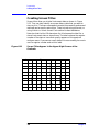
Figure 5-11 . Screen Titles Appear in the Upper-Right Corner of the Graticule . . . . . . . . . .
Figure 5-12 . P1 and P2 Coordinates . . . . . . . . . . . . . . . . . . . . . . . . . . . . . . . . . . . . . . . . . . .
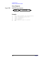
Figure 7-1 . Command Syntax Figure . . . . . . . . . . . . . . . . . . . . . . . . . . . . . . . . . . . . . . . . . .
Figure 7-2 . Numeric Value Query Response . . . . . . . . . . . . . . . . . . . . . . . . . . . . . . . . . . . .
Figure 7-3 . Binary State Query Response . . . . . . . . . . . . . . . . . . . . . . . . . . . . . . . . . . . . . . .
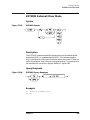
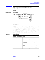
Figure 7-4 . ACPACCL Syntax . . . . . . . . . . . . . . . . . . . . . . . . . . . . . . . . . . . . . . . . . . . . . . .
Figure 7-5 . ACPACCL Query Response . . . . . . . . . . . . . . . . . . . . . . . . . . . . . . . . . . . . . . . .
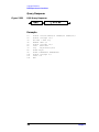
Figure 7-6 . ACPALPHA Syntax . . . . . . . . . . . . . . . . . . . . . . . . . . . . . . . . . . . . . . . . . . . . . .
Figure 7-7 . ACPALPHA Query Response . . . . . . . . . . . . . . . . . . . . . . . . . . . . . . . . . . . . . .
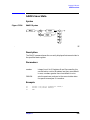
Figure 7-8 . ACPALTCH Syntax . . . . . . . . . . . . . . . . . . . . . . . . . . . . . . . . . . . . . . . . . . . . . .
Figure 7-9 . ACPALTCH Query Response . . . . . . . . . . . . . . . . . . . . . . . . . . . . . . . . . . . . . .
Figure 7-10 . ACPBRPER Syntax . . . . . . . . . . . . . . . . . . . . . . . . . . . . . . . . . . . . . . . . . . . . .
Figure 7-11 . ACPBRPER Query Response . . . . . . . . . . . . . . . . . . . . . . . . . . . . . . . . . . . . . .
Figure 7-12 . ACPBRWID Syntax . . . . . . . . . . . . . . . . . . . . . . . . . . . . . . . . . . . . . . . . . . . . .
Figure 7-13 . ACPBRWID Query Response . . . . . . . . . . . . . . . . . . . . . . . . . . . . . . . . . . . . .
Figure 7-14 . ACPBW Syntax . . . . . . . . . . . . . . . . . . . . . . . . . . . . . . . . . . . . . . . . . . . . . . . .
Figure 7-15 . ACPBW Query Response . . . . . . . . . . . . . . . . . . . . . . . . . . . . . . . . . . . . . . . . .
Figure 7-16 . ACPCOMPUTE Syntax . . . . . . . . . . . . . . . . . . . . . . . . . . . . . . . . . . . . . . . . . .
Figure 7-17 . ACPFRQWT Syntax. . . . . . . . . . . . . . . . . . . . . . . . . . . . . . . . . . . . . . . . . . . . .
Figure 7-18 . ACPFRQWT Query Response . . . . . . . . . . . . . . . . . . . . . . . . . . . . . . . . . . . . .
Figure 7-19 . ACPGRAPH Syntax . . . . . . . . . . . . . . . . . . . . . . . . . . . . . . . . . . . . . . . . . . . . .
Figure 7-20 . ACPGRAPH Query Response . . . . . . . . . . . . . . . . . . . . . . . . . . . . . . . . . . . . .
Figure 7-21 . ACPLOWER Syntax. . . . . . . . . . . . . . . . . . . . . . . . . . . . . . . . . . . . . . . . . . . . .
Figure 7-22 . ACPLOWER Query Response . . . . . . . . . . . . . . . . . . . . . . . . . . . . . . . . . . . . .
Figure 7-23 . ACPMAX Syntax . . . . . . . . . . . . . . . . . . . . . . . . . . . . . . . . . . . . . . . . . . . . . . .
Figure 7-24 . ACPMAX Query Response . . . . . . . . . . . . . . . . . . . . . . . . . . . . . . . . . . . . . . .
Figure 7-25 . ACPMEAS Syntax . . . . . . . . . . . . . . . . . . . . . . . . . . . . . . . . . . . . . . . . . . . . . .
Figure 7-26 . ACPMETHOD Syntax . . . . . . . . . . . . . . . . . . . . . . . . . . . . . . . . . . . . . . . . . . .
Figure 7-27 . ACPMETHOD Query Response. . . . . . . . . . . . . . . . . . . . . . . . . . . . . . . . . . . .
Figure 7-28 . ACPMSTATE Syntax. . . . . . . . . . . . . . . . . . . . . . . . . . . . . . . . . . . . . . . . . . . .
Figure 7-29 . ACPMSTATE Query Response . . . . . . . . . . . . . . . . . . . . . . . . . . . . . . . . . . . .
Figure 7-30 . ACPPWRTX Syntax. . . . . . . . . . . . . . . . . . . . . . . . . . . . . . . . . . . . . . . . . . . . .
Figure 7-31 . ACPPWRTX Query Response . . . . . . . . . . . . . . . . . . . . . . . . . . . . . . . . . . . . .
Figure 7-32 . ACPRSLTS Syntax. . . . . . . . . . . . . . . . . . . . . . . . . . . . . . . . . . . . . . . . . . . . . .
Figure 7-33 . ACPRSLTS Query Response . . . . . . . . . . . . . . . . . . . . . . . . . . . . . . . . . . . . . .
Figure 7-34 . ACPSP Syntax . . . . . . . . . . . . . . . . . . . . . . . . . . . . . . . . . . . . . . . . . . . . . . . . .
Figure 7-35 . ACPSP Query Response . . . . . . . . . . . . . . . . . . . . . . . . . . . . . . . . . . . . . . . . . .
14
294
295
299
300
302
309
318
323
324
328
371
372
372
378
379
380
380
381
381
382
382
383
383
384
384
385
387
387
388
389
390
390
391
391
392
394
396
397
398
399
399
400
402
403
404
Figures
Figure 7-36 . ACPT Syntax . . . . . . . . . . . . . . . . . . . . . . . . . . . . . . . . . . . . . . . . . . . . . . . . . . . 405
Figure 7-37 . ACPT Query Response . . . . . . . . . . . . . . . . . . . . . . . . . . . . . . . . . . . . . . . . . . . 405
Figure 7-38 . ACPUPPER Syntax . . . . . . . . . . . . . . . . . . . . . . . . . . . . . . . . . . . . . . . . . . . . . . 406
Figure 7-39 . ACPUPPER Query Response . . . . . . . . . . . . . . . . . . . . . . . . . . . . . . . . . . . . . . 406
Figure 7-40 . ADJALL Syntax. . . . . . . . . . . . . . . . . . . . . . . . . . . . . . . . . . . . . . . . . . . . . . . . . 407
Figure 7-41 . ADJCRT Syntax. . . . . . . . . . . . . . . . . . . . . . . . . . . . . . . . . . . . . . . . . . . . . . . . . 408
Figure 7-42 . CRT Alignment Pattern . . . . . . . . . . . . . . . . . . . . . . . . . . . . . . . . . . . . . . . . . . . 409
Figure 7-43 . ADJIF Syntax. . . . . . . . . . . . . . . . . . . . . . . . . . . . . . . . . . . . . . . . . . . . . . . . . . . 410
Figure 7-44 . ADJIF Query Response . . . . . . . . . . . . . . . . . . . . . . . . . . . . . . . . . . . . . . . . . . . 411
Figure 7-45 . AMB Syntax. . . . . . . . . . . . . . . . . . . . . . . . . . . . . . . . . . . . . . . . . . . . . . . . . . . . 412
Figure 7-46 . AMB Query Response . . . . . . . . . . . . . . . . . . . . . . . . . . . . . . . . . . . . . . . . . . . . 413
Figure 7-47 . AMBPL Syntax . . . . . . . . . . . . . . . . . . . . . . . . . . . . . . . . . . . . . . . . . . . . . . . . . 414
Figure 7-48 . AMBPL Query Response. . . . . . . . . . . . . . . . . . . . . . . . . . . . . . . . . . . . . . . . . . 415
Figure 7-49 . AMPCOR Syntax. . . . . . . . . . . . . . . . . . . . . . . . . . . . . . . . . . . . . . . . . . . . . . . . 416
Figure 7-50 . AMPCOR Query Response . . . . . . . . . . . . . . . . . . . . . . . . . . . . . . . . . . . . . . . . 416
Figure 7-51 . AMPCORDATA Syntax . . . . . . . . . . . . . . . . . . . . . . . . . . . . . . . . . . . . . . . . . . 417
Figure 7-52 . AMPCORDATA Query Response . . . . . . . . . . . . . . . . . . . . . . . . . . . . . . . . . . 418
Figure 7-53 . AMPCORSIZE Syntax . . . . . . . . . . . . . . . . . . . . . . . . . . . . . . . . . . . . . . . . . . . 419
Figure 7-54 . AMPCORSIZE Query Response . . . . . . . . . . . . . . . . . . . . . . . . . . . . . . . . . . . . 419
Figure 7-55 . AMPCORRCL Syntax . . . . . . . . . . . . . . . . . . . . . . . . . . . . . . . . . . . . . . . . . . . . 420
Figure 7-56 . AMPCORSAVE Syntax . . . . . . . . . . . . . . . . . . . . . . . . . . . . . . . . . . . . . . . . . . 421
Figure 7-57 . ANNOT Syntax . . . . . . . . . . . . . . . . . . . . . . . . . . . . . . . . . . . . . . . . . . . . . . . . . 422
Figure 7-58 . ANNOT Query Response . . . . . . . . . . . . . . . . . . . . . . . . . . . . . . . . . . . . . . . . . 422
Figure 7-59 . APB Syntax . . . . . . . . . . . . . . . . . . . . . . . . . . . . . . . . . . . . . . . . . . . . . . . . . . . . 423
Figure 7-60 . AT Syntax . . . . . . . . . . . . . . . . . . . . . . . . . . . . . . . . . . . . . . . . . . . . . . . . . . . . . 424
Figure 7-61 . AT Query Response . . . . . . . . . . . . . . . . . . . . . . . . . . . . . . . . . . . . . . . . . . . . . . 425
Figure 7-62 . AUNITS Syntax . . . . . . . . . . . . . . . . . . . . . . . . . . . . . . . . . . . . . . . . . . . . . . . . . 426
Figure 7-63 . AUNITS Query Response . . . . . . . . . . . . . . . . . . . . . . . . . . . . . . . . . . . . . . . . . 427
Figure 7-64 . AUTOCPL Syntax . . . . . . . . . . . . . . . . . . . . . . . . . . . . . . . . . . . . . . . . . . . . . . . 428
Figure 7-65 . AXB Syntax . . . . . . . . . . . . . . . . . . . . . . . . . . . . . . . . . . . . . . . . . . . . . . . . . . . . 429
Figure 7-66 . BLANK Syntax . . . . . . . . . . . . . . . . . . . . . . . . . . . . . . . . . . . . . . . . . . . . . . . . . 430
Figure 7-67 . BML Syntax . . . . . . . . . . . . . . . . . . . . . . . . . . . . . . . . . . . . . . . . . . . . . . . . . . . . 431
Figure 7-68 . CARROFF Syntax . . . . . . . . . . . . . . . . . . . . . . . . . . . . . . . . . . . . . . . . . . . . . . . 432
Figure 7-69 . CARROFF Query Response . . . . . . . . . . . . . . . . . . . . . . . . . . . . . . . . . . . . . . . 432
Figure 7-70 . CARRON Syntax . . . . . . . . . . . . . . . . . . . . . . . . . . . . . . . . . . . . . . . . . . . . . . . . 433
Figure 7-71 . CARRON Query Response . . . . . . . . . . . . . . . . . . . . . . . . . . . . . . . . . . . . . . . . 433
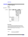
Figure 7-72 . CF Syntax. . . . . . . . . . . . . . . . . . . . . . . . . . . . . . . . . . . . . . . . . . . . . . . . . . . . . . 434
Figure 7-73 . CF Query Response . . . . . . . . . . . . . . . . . . . . . . . . . . . . . . . . . . . . . . . . . . . . . . 435
Figure 7-74 . CHANPWR Syntax . . . . . . . . . . . . . . . . . . . . . . . . . . . . . . . . . . . . . . . . . . . . . . 436
Figure 7-75 . CHANPWR Query Response . . . . . . . . . . . . . . . . . . . . . . . . . . . . . . . . . . . . . . 437
Figure 7-76 . CHANNEL Syntax. . . . . . . . . . . . . . . . . . . . . . . . . . . . . . . . . . . . . . . . . . . . . . . 438
Figure 7-77 . CHPWRBW Syntax . . . . . . . . . . . . . . . . . . . . . . . . . . . . . . . . . . . . . . . . . . . . . . 439
Figure 7-78 . CHPWRBW Query Response . . . . . . . . . . . . . . . . . . . . . . . . . . . . . . . . . . . . . . 439
Figure 7-79 . CLRW Syntax . . . . . . . . . . . . . . . . . . . . . . . . . . . . . . . . . . . . . . . . . . . . . . . . . . 440
Figure 7-80 . CNVLOSS Syntax . . . . . . . . . . . . . . . . . . . . . . . . . . . . . . . . . . . . . . . . . . . . . . . 441
15
Figures
Figure 7-81 . CNVLOSS Query Response . . . . . . . . . . . . . . . . . . . . . . . . . . . . . . . . . . . . . . .
Figure 7-82 . CONTS Syntax . . . . . . . . . . . . . . . . . . . . . . . . . . . . . . . . . . . . . . . . . . . . . . . . .
Figure 7-83 . COUPLE Syntax . . . . . . . . . . . . . . . . . . . . . . . . . . . . . . . . . . . . . . . . . . . . . . . .
Figure 7-84 . COUPLE Query Response . . . . . . . . . . . . . . . . . . . . . . . . . . . . . . . . . . . . . . . .
Figure 7-85 . DELMKBW Syntax . . . . . . . . . . . . . . . . . . . . . . . . . . . . . . . . . . . . . . . . . . . . .
Figure 7-86 . DELMKBW Query Response. . . . . . . . . . . . . . . . . . . . . . . . . . . . . . . . . . . . . .
Figure 7-87 . DEMOD Syntax . . . . . . . . . . . . . . . . . . . . . . . . . . . . . . . . . . . . . . . . . . . . . . . .
Figure 7-88 . DEMOD Query Response. . . . . . . . . . . . . . . . . . . . . . . . . . . . . . . . . . . . . . . . .
Figure 7-89 . DEMODAGC Syntax . . . . . . . . . . . . . . . . . . . . . . . . . . . . . . . . . . . . . . . . . . . .
Figure 7-90 . DEMODAGC Query Response . . . . . . . . . . . . . . . . . . . . . . . . . . . . . . . . . . . .
Figure 7-91 . DEMODT Syntax . . . . . . . . . . . . . . . . . . . . . . . . . . . . . . . . . . . . . . . . . . . . . . .
Figure 7-92 . DEMODT Query Response . . . . . . . . . . . . . . . . . . . . . . . . . . . . . . . . . . . . . . .
Figure 7-93 . DET Syntax. . . . . . . . . . . . . . . . . . . . . . . . . . . . . . . . . . . . . . . . . . . . . . . . . . . .
Figure 7-94 . DET Query Response . . . . . . . . . . . . . . . . . . . . . . . . . . . . . . . . . . . . . . . . . . . .
Figure 7-95 . DL Syntax . . . . . . . . . . . . . . . . . . . . . . . . . . . . . . . . . . . . . . . . . . . . . . . . . . . . .
Figure 7-96 . DT Query Response . . . . . . . . . . . . . . . . . . . . . . . . . . . . . . . . . . . . . . . . . . . . .
Figure 7-97 . DLYSWP Syntax . . . . . . . . . . . . . . . . . . . . . . . . . . . . . . . . . . . . . . . . . . . . . . .
Figure 7-98 . DLYSWP Query Response . . . . . . . . . . . . . . . . . . . . . . . . . . . . . . . . . . . . . . . .
Figure 7-99 . DONE Syntax . . . . . . . . . . . . . . . . . . . . . . . . . . . . . . . . . . . . . . . . . . . . . . . . . .
Figure 7-100 . DONE Query Response . . . . . . . . . . . . . . . . . . . . . . . . . . . . . . . . . . . . . . . . .
Figure 7-101 . ERR Syntax. . . . . . . . . . . . . . . . . . . . . . . . . . . . . . . . . . . . . . . . . . . . . . . . . . .
Figure 7-102 . ERR Query Response . . . . . . . . . . . . . . . . . . . . . . . . . . . . . . . . . . . . . . . . . . .
Figure 7-103 . ET Syntax . . . . . . . . . . . . . . . . . . . . . . . . . . . . . . . . . . . . . . . . . . . . . . . . . . . .
Figure 7-104 . ET Query Response. . . . . . . . . . . . . . . . . . . . . . . . . . . . . . . . . . . . . . . . . . . . .
Figure 7-105 . EXTMXR Syntax . . . . . . . . . . . . . . . . . . . . . . . . . . . . . . . . . . . . . . . . . . . . . .
Figure 7-106 . EXTMXR Query Response. . . . . . . . . . . . . . . . . . . . . . . . . . . . . . . . . . . . . . .
Figure 7-107 . FA Syntax . . . . . . . . . . . . . . . . . . . . . . . . . . . . . . . . . . . . . . . . . . . . . . . . . . . .
Figure 7-108 . FA Query Response . . . . . . . . . . . . . . . . . . . . . . . . . . . . . . . . . . . . . . . . . . . .
Figure 7-109 . FB Syntax . . . . . . . . . . . . . . . . . . . . . . . . . . . . . . . . . . . . . . . . . . . . . . . . . . . .
Figure 7-110 . FB Query Response. . . . . . . . . . . . . . . . . . . . . . . . . . . . . . . . . . . . . . . . . . . . .
Figure 7-111 . FDIAG Syntax . . . . . . . . . . . . . . . . . . . . . . . . . . . . . . . . . . . . . . . . . . . . . . . .
Figure 7-112 . FDIAG Query Response . . . . . . . . . . . . . . . . . . . . . . . . . . . . . . . . . . . . . . . . .
Figure 7-113 . FDSP Syntax . . . . . . . . . . . . . . . . . . . . . . . . . . . . . . . . . . . . . . . . . . . . . . . . . .
Figure 7-114 . FDSP Query Response . . . . . . . . . . . . . . . . . . . . . . . . . . . . . . . . . . . . . . . . . .
Figure 7-115 . FFT Syntax . . . . . . . . . . . . . . . . . . . . . . . . . . . . . . . . . . . . . . . . . . . . . . . . . . .
Figure 7-116 . FOFFSET Syntax . . . . . . . . . . . . . . . . . . . . . . . . . . . . . . . . . . . . . . . . . . . . . .
Figure 7-117 . FOFFSET Query Response. . . . . . . . . . . . . . . . . . . . . . . . . . . . . . . . . . . . . . .
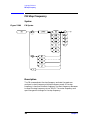
Figure 7-118 . FREF Syntax . . . . . . . . . . . . . . . . . . . . . . . . . . . . . . . . . . . . . . . . . . . . . . . . . .
Figure 7-119 . FREF Query Response . . . . . . . . . . . . . . . . . . . . . . . . . . . . . . . . . . . . . . . . . .
Figure 7-120 . FS Syntax . . . . . . . . . . . . . . . . . . . . . . . . . . . . . . . . . . . . . . . . . . . . . . . . . . . .
Figure 7-121 . FULBAND Syntax . . . . . . . . . . . . . . . . . . . . . . . . . . . . . . . . . . . . . . . . . . . . .
Figure 7-122 . GATE Syntax . . . . . . . . . . . . . . . . . . . . . . . . . . . . . . . . . . . . . . . . . . . . . . . . .
Figure 7-123 . GATE Query Response. . . . . . . . . . . . . . . . . . . . . . . . . . . . . . . . . . . . . . . . . .
Figure 7-124 . GATECTL Syntax . . . . . . . . . . . . . . . . . . . . . . . . . . . . . . . . . . . . . . . . . . . . .
Figure 7-125 . GATECTL Query Response . . . . . . . . . . . . . . . . . . . . . . . . . . . . . . . . . . . . . .
16
442
443
444
444
445
446
447
447
449
449
451
452
453
454
455
456
457
458
459
459
460
460
462
462
463
463
464
465
466
467
468
469
470
470
472
475
476
477
477
478
479
481
482
483
483
Figures
Figure 7-126 . GD Syntax . . . . . . . . . . . . . . . . . . . . . . . . . . . . . . . . . . . . . . . . . . . . . . . . . . . . 484
Figure 7-127 . GD Query Response. . . . . . . . . . . . . . . . . . . . . . . . . . . . . . . . . . . . . . . . . . . . . 484
Figure 7-128 . GL Syntax . . . . . . . . . . . . . . . . . . . . . . . . . . . . . . . . . . . . . . . . . . . . . . . . . . . . 485
Figure 7-129 . GL Query Response . . . . . . . . . . . . . . . . . . . . . . . . . . . . . . . . . . . . . . . . . . . . . 485
Figure 7-130 . GP Syntax. . . . . . . . . . . . . . . . . . . . . . . . . . . . . . . . . . . . . . . . . . . . . . . . . . . . . 486
Figure 7-131 . GP Query Response . . . . . . . . . . . . . . . . . . . . . . . . . . . . . . . . . . . . . . . . . . . . . 486
Figure 7-132 . GRAT Syntax. . . . . . . . . . . . . . . . . . . . . . . . . . . . . . . . . . . . . . . . . . . . . . . . . . 487
Figure 7-133 . GRAT Query Response . . . . . . . . . . . . . . . . . . . . . . . . . . . . . . . . . . . . . . . . . . 487
Figure 7-134 . HD Syntax . . . . . . . . . . . . . . . . . . . . . . . . . . . . . . . . . . . . . . . . . . . . . . . . . . . . 488
Figure 7-135 . HNLOCK Syntax . . . . . . . . . . . . . . . . . . . . . . . . . . . . . . . . . . . . . . . . . . . . . . . 489
Figure 7-136 . HNLOCK Query Response . . . . . . . . . . . . . . . . . . . . . . . . . . . . . . . . . . . . . . . 490
Figure 7-137 . HNUNLK Syntax. . . . . . . . . . . . . . . . . . . . . . . . . . . . . . . . . . . . . . . . . . . . . . . 491
Figure 7-138 . ID Syntax . . . . . . . . . . . . . . . . . . . . . . . . . . . . . . . . . . . . . . . . . . . . . . . . . . . . . 492
Figure 7-139 . ID Query Response . . . . . . . . . . . . . . . . . . . . . . . . . . . . . . . . . . . . . . . . . . . . . 492
Figure 7-140 . IDCF Syntax. . . . . . . . . . . . . . . . . . . . . . . . . . . . . . . . . . . . . . . . . . . . . . . . . . . 493
Figure 7-141 . IDFREQ Syntax . . . . . . . . . . . . . . . . . . . . . . . . . . . . . . . . . . . . . . . . . . . . . . . . 494
Figure 7-142 . IDFREQ Query Response . . . . . . . . . . . . . . . . . . . . . . . . . . . . . . . . . . . . . . . . 494
Figure 7-143 . IP Syntax . . . . . . . . . . . . . . . . . . . . . . . . . . . . . . . . . . . . . . . . . . . . . . . . . . . . . 495
Figure 7-144 . LG Syntax . . . . . . . . . . . . . . . . . . . . . . . . . . . . . . . . . . . . . . . . . . . . . . . . . . . . 498
Figure 7-145 . LG Query Response . . . . . . . . . . . . . . . . . . . . . . . . . . . . . . . . . . . . . . . . . . . . . 498
Figure 7-146 . LN Syntax . . . . . . . . . . . . . . . . . . . . . . . . . . . . . . . . . . . . . . . . . . . . . . . . . . . . 500
Figure 7-147 . MBIAS Syntax . . . . . . . . . . . . . . . . . . . . . . . . . . . . . . . . . . . . . . . . . . . . . . . . . 501
Figure 7-148 . MBIAS Query Response . . . . . . . . . . . . . . . . . . . . . . . . . . . . . . . . . . . . . . . . . 502
Figure 7-149 . MEANPWR Syntax . . . . . . . . . . . . . . . . . . . . . . . . . . . . . . . . . . . . . . . . . . . . . 503
Figure 7-150 . MEANPWR Query Response . . . . . . . . . . . . . . . . . . . . . . . . . . . . . . . . . . . . . 504
Figure 7-151 . MEAS Syntax. . . . . . . . . . . . . . . . . . . . . . . . . . . . . . . . . . . . . . . . . . . . . . . . . . 505
Figure 7-152 . MEAS Query Response . . . . . . . . . . . . . . . . . . . . . . . . . . . . . . . . . . . . . . . . . . 505
Figure 7-153 . MINH Syntax . . . . . . . . . . . . . . . . . . . . . . . . . . . . . . . . . . . . . . . . . . . . . . . . . . 506
Figure 7-154 . MKA Syntax . . . . . . . . . . . . . . . . . . . . . . . . . . . . . . . . . . . . . . . . . . . . . . . . . . 507
Figure 7-155 . MKA Query Response . . . . . . . . . . . . . . . . . . . . . . . . . . . . . . . . . . . . . . . . . . . 507
Figure 7-156 . MKBW Syntax. . . . . . . . . . . . . . . . . . . . . . . . . . . . . . . . . . . . . . . . . . . . . . . . . 508
Figure 7-157 . MKCF Syntax . . . . . . . . . . . . . . . . . . . . . . . . . . . . . . . . . . . . . . . . . . . . . . . . . 509
Figure 7-158 . MKCHEDGE Syntax . . . . . . . . . . . . . . . . . . . . . . . . . . . . . . . . . . . . . . . . . . . . 510
Figure 7-159 . MKD Syntax . . . . . . . . . . . . . . . . . . . . . . . . . . . . . . . . . . . . . . . . . . . . . . . . . . 511
Figure 7-160 . MKD Query Response . . . . . . . . . . . . . . . . . . . . . . . . . . . . . . . . . . . . . . . . . . . 512
Figure 7-161 . MKDELCHBW Syntax . . . . . . . . . . . . . . . . . . . . . . . . . . . . . . . . . . . . . . . . . . 513
Figure 7-162 . MKDR Syntax . . . . . . . . . . . . . . . . . . . . . . . . . . . . . . . . . . . . . . . . . . . . . . . . . 514
Figure 7-163 . MKDR Query Response . . . . . . . . . . . . . . . . . . . . . . . . . . . . . . . . . . . . . . . . . 515
Figure 7-164 . MKF Syntax . . . . . . . . . . . . . . . . . . . . . . . . . . . . . . . . . . . . . . . . . . . . . . . . . . . 516
Figure 7-165 . MKF Query Response . . . . . . . . . . . . . . . . . . . . . . . . . . . . . . . . . . . . . . . . . . . 517
Figure 7-166 . MKFC Syntax . . . . . . . . . . . . . . . . . . . . . . . . . . . . . . . . . . . . . . . . . . . . . . . . . 518
Figure 7-167 . MKFCR Syntax . . . . . . . . . . . . . . . . . . . . . . . . . . . . . . . . . . . . . . . . . . . . . . . . 519
Figure 7-168 . MKFCR Query Response . . . . . . . . . . . . . . . . . . . . . . . . . . . . . . . . . . . . . . . . 519
Figure 7-169 . MKMCF Syntax. . . . . . . . . . . . . . . . . . . . . . . . . . . . . . . . . . . . . . . . . . . . . . . . 521
Figure 7-170 . MKMIN Syntax . . . . . . . . . . . . . . . . . . . . . . . . . . . . . . . . . . . . . . . . . . . . . . . . 522
17
Figures
Figure 7-171 . MKN Syntax . . . . . . . . . . . . . . . . . . . . . . . . . . . . . . . . . . . . . . . . . . . . . . . . . .
Figure 7-172 . MKN Query Response . . . . . . . . . . . . . . . . . . . . . . . . . . . . . . . . . . . . . . . . . .
Figure 7-173 . MKNOISE Syntax . . . . . . . . . . . . . . . . . . . . . . . . . . . . . . . . . . . . . . . . . . . . .
Figure 7-174 . MKNOISE Query Response . . . . . . . . . . . . . . . . . . . . . . . . . . . . . . . . . . . . . .
Figure 7-175 . MKOFF Syntax. . . . . . . . . . . . . . . . . . . . . . . . . . . . . . . . . . . . . . . . . . . . . . . .
Figure 7-176 . MKPK Syntax . . . . . . . . . . . . . . . . . . . . . . . . . . . . . . . . . . . . . . . . . . . . . . . . .
Figure 7-177 . MKPT Syntax . . . . . . . . . . . . . . . . . . . . . . . . . . . . . . . . . . . . . . . . . . . . . . . . .
Figure 7-178 . MKPT Query Response . . . . . . . . . . . . . . . . . . . . . . . . . . . . . . . . . . . . . . . . .
Figure 7-179 . MKPX Syntax . . . . . . . . . . . . . . . . . . . . . . . . . . . . . . . . . . . . . . . . . . . . . . . . .
Figure 7-180 . MKPX Determines Which Signals are Considered Peaks . . . . . . . . . . . . . . .
Figure 7-181 . MKPX Query Response . . . . . . . . . . . . . . . . . . . . . . . . . . . . . . . . . . . . . . . . .
Figure 7-182 . MKRL Syntax . . . . . . . . . . . . . . . . . . . . . . . . . . . . . . . . . . . . . . . . . . . . . . . . .
Figure 7-183 . MKSP Syntax . . . . . . . . . . . . . . . . . . . . . . . . . . . . . . . . . . . . . . . . . . . . . . . . .
Figure 7-184 . MKSS Syntax . . . . . . . . . . . . . . . . . . . . . . . . . . . . . . . . . . . . . . . . . . . . . . . . .
Figure 7-185 . MKT Syntax . . . . . . . . . . . . . . . . . . . . . . . . . . . . . . . . . . . . . . . . . . . . . . . . . .
Figure 7-186 . MKT Query Response. . . . . . . . . . . . . . . . . . . . . . . . . . . . . . . . . . . . . . . . . . .
Figure 7-187 . MKTRACK Syntax. . . . . . . . . . . . . . . . . . . . . . . . . . . . . . . . . . . . . . . . . . . . .
Figure 7-188 . MKTRACK Query Response . . . . . . . . . . . . . . . . . . . . . . . . . . . . . . . . . . . . .
Figure 7-189 . ML Syntax. . . . . . . . . . . . . . . . . . . . . . . . . . . . . . . . . . . . . . . . . . . . . . . . . . . .
Figure 7-190 . ML Query Response . . . . . . . . . . . . . . . . . . . . . . . . . . . . . . . . . . . . . . . . . . . .
Figure 7-191 . MXMH Syntax . . . . . . . . . . . . . . . . . . . . . . . . . . . . . . . . . . . . . . . . . . . . . . . .
Figure 7-192 . MXRMODE Syntax . . . . . . . . . . . . . . . . . . . . . . . . . . . . . . . . . . . . . . . . . . . .
Figure 7-193 . MXRMODE Query Response. . . . . . . . . . . . . . . . . . . . . . . . . . . . . . . . . . . . .
Figure 7-194 . NORMALIZE Syntax . . . . . . . . . . . . . . . . . . . . . . . . . . . . . . . . . . . . . . . . . . .
Figure 7-195 . NORMALIZE Query Response . . . . . . . . . . . . . . . . . . . . . . . . . . . . . . . . . . .
Figure 7-196 . NRL Syntax. . . . . . . . . . . . . . . . . . . . . . . . . . . . . . . . . . . . . . . . . . . . . . . . . . .
Figure 7-197 . NRL Query Response . . . . . . . . . . . . . . . . . . . . . . . . . . . . . . . . . . . . . . . . . . .
Figure 7-198 . NRPOS Syntax . . . . . . . . . . . . . . . . . . . . . . . . . . . . . . . . . . . . . . . . . . . . . . . .
Figure 7-199 . NRPOS Query Response. . . . . . . . . . . . . . . . . . . . . . . . . . . . . . . . . . . . . . . . .
Figure 7-200 . OCCUP Syntax . . . . . . . . . . . . . . . . . . . . . . . . . . . . . . . . . . . . . . . . . . . . . . . .
Figure 7-201 . OCCUP Query Response . . . . . . . . . . . . . . . . . . . . . . . . . . . . . . . . . . . . . . . .
Figure 7-202 . OP Syntax . . . . . . . . . . . . . . . . . . . . . . . . . . . . . . . . . . . . . . . . . . . . . . . . . . . .
Figure 7-203 . OP Query Response . . . . . . . . . . . . . . . . . . . . . . . . . . . . . . . . . . . . . . . . . . . .
Figure 7-204 . PLOT Syntax. . . . . . . . . . . . . . . . . . . . . . . . . . . . . . . . . . . . . . . . . . . . . . . . . .
Figure 7-205 . PLOTORG Syntax . . . . . . . . . . . . . . . . . . . . . . . . . . . . . . . . . . . . . . . . . . . . .
Figure 7-206 . PLOTORG Query Response . . . . . . . . . . . . . . . . . . . . . . . . . . . . . . . . . . . . . .
Figure 7-207 . PLOTSRC Syntax . . . . . . . . . . . . . . . . . . . . . . . . . . . . . . . . . . . . . . . . . . . . . .
Figure 7-208 . PLOT SRC Query Response. . . . . . . . . . . . . . . . . . . . . . . . . . . . . . . . . . . . . .
Figure 7-209 . PP Syntax . . . . . . . . . . . . . . . . . . . . . . . . . . . . . . . . . . . . . . . . . . . . . . . . . . . .
Figure 7-210 . PRINT Syntax . . . . . . . . . . . . . . . . . . . . . . . . . . . . . . . . . . . . . . . . . . . . . . . . .
Figure 7-211 . PSDAC Syntax . . . . . . . . . . . . . . . . . . . . . . . . . . . . . . . . . . . . . . . . . . . . . . . .
Figure 7-212 . PSDAC Query Response. . . . . . . . . . . . . . . . . . . . . . . . . . . . . . . . . . . . . . . . .
Figure 7-213 . PSTATE Syntax . . . . . . . . . . . . . . . . . . . . . . . . . . . . . . . . . . . . . . . . . . . . . . .
Figure 7-214 . PSTATE Query Response. . . . . . . . . . . . . . . . . . . . . . . . . . . . . . . . . . . . . . . .
Figure 7-215 . PWRBW Syntax . . . . . . . . . . . . . . . . . . . . . . . . . . . . . . . . . . . . . . . . . . . . . . .
18
523
524
525
525
527
528
530
530
532
533
533
535
536
537
538
538
539
540
541
541
543
544
544
545
546
547
548
550
551
552
552
553
553
554
556
556
558
559
560
561
563
563
565
565
567
Figures
Figure 7-216 . PWRBW Query Response . . . . . . . . . . . . . . . . . . . . . . . . . . . . . . . . . . . . . . . . 567
Figure 7-217 . RB Syntax . . . . . . . . . . . . . . . . . . . . . . . . . . . . . . . . . . . . . . . . . . . . . . . . . . . . 569
Figure 7-218 . RB Query Response . . . . . . . . . . . . . . . . . . . . . . . . . . . . . . . . . . . . . . . . . . . . . 570
Figure 7-219 . RBR Syntax . . . . . . . . . . . . . . . . . . . . . . . . . . . . . . . . . . . . . . . . . . . . . . . . . . . 571
Figure 7-220 . RBR Query Response . . . . . . . . . . . . . . . . . . . . . . . . . . . . . . . . . . . . . . . . . . . 571
Figure 7-221 . RCLOSCAL Syntax. . . . . . . . . . . . . . . . . . . . . . . . . . . . . . . . . . . . . . . . . . . . . 573
Figure 7-222 . RCLS Syntax . . . . . . . . . . . . . . . . . . . . . . . . . . . . . . . . . . . . . . . . . . . . . . . . . . 575
Figure 7-223 . RCLT Syntax . . . . . . . . . . . . . . . . . . . . . . . . . . . . . . . . . . . . . . . . . . . . . . . . . . 576
Figure 7-224 . RCLTHRU Syntax . . . . . . . . . . . . . . . . . . . . . . . . . . . . . . . . . . . . . . . . . . . . . . 577
Figure 7-225 . REV Syntax . . . . . . . . . . . . . . . . . . . . . . . . . . . . . . . . . . . . . . . . . . . . . . . . . . . 579
Figure 7-226 . REV Query Response . . . . . . . . . . . . . . . . . . . . . . . . . . . . . . . . . . . . . . . . . . . 579
Figure 7-227 . RL Syntax. . . . . . . . . . . . . . . . . . . . . . . . . . . . . . . . . . . . . . . . . . . . . . . . . . . . . 580
Figure 7-228 . RL Query Response . . . . . . . . . . . . . . . . . . . . . . . . . . . . . . . . . . . . . . . . . . . . . 582
Figure 7-229 . RLCAL Syntax. . . . . . . . . . . . . . . . . . . . . . . . . . . . . . . . . . . . . . . . . . . . . . . . . 583
Figure 7-230 . ROFFSET Syntax . . . . . . . . . . . . . . . . . . . . . . . . . . . . . . . . . . . . . . . . . . . . . . 585
Figure 7-231 . ROFFSET Query Response . . . . . . . . . . . . . . . . . . . . . . . . . . . . . . . . . . . . . . . 586
Figure 7-232 . RQS Syntax . . . . . . . . . . . . . . . . . . . . . . . . . . . . . . . . . . . . . . . . . . . . . . . . . . . 587
Figure 7-233 . RQS Query Response. . . . . . . . . . . . . . . . . . . . . . . . . . . . . . . . . . . . . . . . . . . . 588
Figure 7-234 . SAVES Syntax . . . . . . . . . . . . . . . . . . . . . . . . . . . . . . . . . . . . . . . . . . . . . . . . . 589
Figure 7-235 . SAVET Syntax. . . . . . . . . . . . . . . . . . . . . . . . . . . . . . . . . . . . . . . . . . . . . . . . . 590
Figure 7-236 . SER Syntax . . . . . . . . . . . . . . . . . . . . . . . . . . . . . . . . . . . . . . . . . . . . . . . . . . . 591
Figure 7-237 . SER Query Response . . . . . . . . . . . . . . . . . . . . . . . . . . . . . . . . . . . . . . . . . . . . 591
Figure 7-238 . SIGID Syntax . . . . . . . . . . . . . . . . . . . . . . . . . . . . . . . . . . . . . . . . . . . . . . . . . . 592
Figure 7-239 . SIGID Query Response . . . . . . . . . . . . . . . . . . . . . . . . . . . . . . . . . . . . . . . . . . 593
Figure 7-240 . SNGLS Syntax . . . . . . . . . . . . . . . . . . . . . . . . . . . . . . . . . . . . . . . . . . . . . . . . . 594
Figure 7-241 . SP Syntax . . . . . . . . . . . . . . . . . . . . . . . . . . . . . . . . . . . . . . . . . . . . . . . . . . . . . 595
Figure 7-242 . SP Query Response . . . . . . . . . . . . . . . . . . . . . . . . . . . . . . . . . . . . . . . . . . . . . 596
Figure 7-243 . SQUELCH Syntax . . . . . . . . . . . . . . . . . . . . . . . . . . . . . . . . . . . . . . . . . . . . . . 597
Figure 7-244 . SQUELCH Query Response . . . . . . . . . . . . . . . . . . . . . . . . . . . . . . . . . . . . . . 598
Figure 7-245 . SRCALC Syntax . . . . . . . . . . . . . . . . . . . . . . . . . . . . . . . . . . . . . . . . . . . . . . . 599
Figure 7-246 . SRCALC Query Response. . . . . . . . . . . . . . . . . . . . . . . . . . . . . . . . . . . . . . . . 599
Figure 7-247 . SRCCRSTK Syntax . . . . . . . . . . . . . . . . . . . . . . . . . . . . . . . . . . . . . . . . . . . . . 600
Figure 7-248 . SRCCRSTK Query Response . . . . . . . . . . . . . . . . . . . . . . . . . . . . . . . . . . . . . 600
Figure 7-249 . SRCFINTK Syntax . . . . . . . . . . . . . . . . . . . . . . . . . . . . . . . . . . . . . . . . . . . . . 602
Figure 7-250 . SRCFINTK Query Response . . . . . . . . . . . . . . . . . . . . . . . . . . . . . . . . . . . . . . 603
Figure 7-251 . SRCPOFS Syntax . . . . . . . . . . . . . . . . . . . . . . . . . . . . . . . . . . . . . . . . . . . . . . 604
Figure 7-252 . SRCPOFS Query Response . . . . . . . . . . . . . . . . . . . . . . . . . . . . . . . . . . . . . . . 605
Figure 7-253 . SRCPSTP Syntax . . . . . . . . . . . . . . . . . . . . . . . . . . . . . . . . . . . . . . . . . . . . . . . 606
Figure 7-254 . SRCPSTP Query Response . . . . . . . . . . . . . . . . . . . . . . . . . . . . . . . . . . . . . . . 606
Figure 7-255 . SRCPSWP Syntax . . . . . . . . . . . . . . . . . . . . . . . . . . . . . . . . . . . . . . . . . . . . . . 608
Figure 7-256 . SRCPSWP Query Response . . . . . . . . . . . . . . . . . . . . . . . . . . . . . . . . . . . . . . 609
Figure 7-257 . SRCPWR Syntax . . . . . . . . . . . . . . . . . . . . . . . . . . . . . . . . . . . . . . . . . . . . . . . 610
Figure 7-258 . SRCPWR Query Response . . . . . . . . . . . . . . . . . . . . . . . . . . . . . . . . . . . . . . . 611
Figure 7-259 . SRCTKPK Syntax . . . . . . . . . . . . . . . . . . . . . . . . . . . . . . . . . . . . . . . . . . . . . . 612
Figure 7-260 . SRQ Syntax . . . . . . . . . . . . . . . . . . . . . . . . . . . . . . . . . . . . . . . . . . . . . . . . . . . 613
19
Figures
Figure 7-261 . SS Syntax . . . . . . . . . . . . . . . . . . . . . . . . . . . . . . . . . . . . . . . . . . . . . . . . . . . .
Figure 7-262 . SS Query Response . . . . . . . . . . . . . . . . . . . . . . . . . . . . . . . . . . . . . . . . . . . . .
Figure 7-263 . ST Syntax . . . . . . . . . . . . . . . . . . . . . . . . . . . . . . . . . . . . . . . . . . . . . . . . . . . .
Figure 7-264 . ST Query Response. . . . . . . . . . . . . . . . . . . . . . . . . . . . . . . . . . . . . . . . . . . . .
Figure 7-265 . STB Syntax . . . . . . . . . . . . . . . . . . . . . . . . . . . . . . . . . . . . . . . . . . . . . . . . . . .
Figure 7-266 . STB Query Response . . . . . . . . . . . . . . . . . . . . . . . . . . . . . . . . . . . . . . . . . . .
Figure 7-267 . STOREOPEN Syntax . . . . . . . . . . . . . . . . . . . . . . . . . . . . . . . . . . . . . . . . . . .
Figure 7-268 . STORESHORT Syntax. . . . . . . . . . . . . . . . . . . . . . . . . . . . . . . . . . . . . . . . . .
Figure 7-269 . STORETHRU Syntax . . . . . . . . . . . . . . . . . . . . . . . . . . . . . . . . . . . . . . . . . . .
Figure 7-270 . SWPCPL Syntax . . . . . . . . . . . . . . . . . . . . . . . . . . . . . . . . . . . . . . . . . . . . . . .
Figure 7-271 . SWPCPL Query Response . . . . . . . . . . . . . . . . . . . . . . . . . . . . . . . . . . . . . . .
Figure 7-272 . SWPOUT Syntax . . . . . . . . . . . . . . . . . . . . . . . . . . . . . . . . . . . . . . . . . . . . . .
Figure 7-273 . SWPOUT Query Response . . . . . . . . . . . . . . . . . . . . . . . . . . . . . . . . . . . . . . .
Figure 7-274 . TDF Syntax . . . . . . . . . . . . . . . . . . . . . . . . . . . . . . . . . . . . . . . . . . . . . . . . . . .
Figure 7-275 . TDF Query Response . . . . . . . . . . . . . . . . . . . . . . . . . . . . . . . . . . . . . . . . . . .
Figure 7-276 . TH Syntax . . . . . . . . . . . . . . . . . . . . . . . . . . . . . . . . . . . . . . . . . . . . . . . . . . . .
Figure 7-277 . TH Query Response . . . . . . . . . . . . . . . . . . . . . . . . . . . . . . . . . . . . . . . . . . . .
Figure 7-278 . TITLE Syntax . . . . . . . . . . . . . . . . . . . . . . . . . . . . . . . . . . . . . . . . . . . . . . . . .
Figure 7-279 . TM Syntax . . . . . . . . . . . . . . . . . . . . . . . . . . . . . . . . . . . . . . . . . . . . . . . . . . .
Figure 7-280 . TM Query Response . . . . . . . . . . . . . . . . . . . . . . . . . . . . . . . . . . . . . . . . . . . .
Figure 7-281 . TRA/TRB Syntax . . . . . . . . . . . . . . . . . . . . . . . . . . . . . . . . . . . . . . . . . . . . . .
Figure 7-282 . TRA/TRB Query Response. . . . . . . . . . . . . . . . . . . . . . . . . . . . . . . . . . . . . . .
Figure 7-283 . TRIGPOL Syntax . . . . . . . . . . . . . . . . . . . . . . . . . . . . . . . . . . . . . . . . . . . . . .
Figure 7-284 . TRIGPOL Query Response. . . . . . . . . . . . . . . . . . . . . . . . . . . . . . . . . . . . . . .
Figure 7-285 . TS Syntax . . . . . . . . . . . . . . . . . . . . . . . . . . . . . . . . . . . . . . . . . . . . . . . . . . . .
Figure 7-286 . TWNDOW Syntax . . . . . . . . . . . . . . . . . . . . . . . . . . . . . . . . . . . . . . . . . . . . .
Figure 7-287 . VAVG Syntax . . . . . . . . . . . . . . . . . . . . . . . . . . . . . . . . . . . . . . . . . . . . . . . . .
Figure 7-288 . VAVG Query Response . . . . . . . . . . . . . . . . . . . . . . . . . . . . . . . . . . . . . . . . .
Figure 7-289 . VB Syntax . . . . . . . . . . . . . . . . . . . . . . . . . . . . . . . . . . . . . . . . . . . . . . . . . . . .
Figure 7-290 . VB Query Response . . . . . . . . . . . . . . . . . . . . . . . . . . . . . . . . . . . . . . . . . . . .
Figure 7-291 . VBR Syntax . . . . . . . . . . . . . . . . . . . . . . . . . . . . . . . . . . . . . . . . . . . . . . . . . .
Figure 7-292 . VBR Query Response . . . . . . . . . . . . . . . . . . . . . . . . . . . . . . . . . . . . . . . . . . .
Figure 7-293 . VIEW Syntax . . . . . . . . . . . . . . . . . . . . . . . . . . . . . . . . . . . . . . . . . . . . . . . . .
Figure 7-294 . VTL Syntax. . . . . . . . . . . . . . . . . . . . . . . . . . . . . . . . . . . . . . . . . . . . . . . . . . .
Figure 7-295 . VTL Query Response . . . . . . . . . . . . . . . . . . . . . . . . . . . . . . . . . . . . . . . . . . .
Figure 9-1 . Voltage Selection Switch and Line Fuse Locations . . . . . . . . . . . . . . . . . . . . . .
Figure 9-2 . AC Power Cables Available . . . . . . . . . . . . . . . . . . . . . . . . . . . . . . . . . . . . . . . .
Figure 9-3 . CRT Adjustment Pattern . . . . . . . . . . . . . . . . . . . . . . . . . . . . . . . . . . . . . . . . . .
Figure 9-4 . Shipping Container and Cushioning Materials . . . . . . . . . . . . . . . . . . . . . . . . .
Figure 9-5 . Serial Number Label Example . . . . . . . . . . . . . . . . . . . . . . . . . . . . . . . . . . . . . .
Figure 9-6 . Example of a Static-Safe Workstation . . . . . . . . . . . . . . . . . . . . . . . . . . . . . . . .
20
614
615
616
617
618
619
620
622
624
626
626
628
629
630
631
632
633
634
636
637
638
639
641
641
642
643
645
646
647
648
649
650
651
652
653
672
674
675
681
684
685
1
Quick Start Guide
21
Quick Start Guide
What You'll Find in This Chapter
What You'll Find in This Chapter
• How to Use This Guide
• Differences between 8560 E-Series and EC-Series Instruments
• Initial Inspection
• Turning the Spectrum Analyzer On for the First Time
• Making a Basic Measurement
• Setting Reference Level Calibration
• Front Panel Overview
• Rear Panel Overview
• Cleaning the Instrument
• Safety Considerations
• Documentation Description
How to Use This Guide
Where to Start
If you are familiar with spectrum analyzers:
• Briefly review the front and rear panel overview sections in Chapter
1 for a short introduction to the 8560E/EC, 8561E/EC, 8563E/EC,
8564E/EC, and 8565E/EC spectrum analyzers.
• If you want more information about a particular spectrum analyzer
function, refer to Chapter 4.
If you are not familiar with spectrum analyzers:
• Read Chapter 1, "Quick Start Guide," which introduces you to the
spectrum analyzer.
• Continue on to Chapter 2, "Making Measurements," to gain
experience with spectrum analyzer measurements.
22
Chapter 1
Quick Start Guide
What You'll Find in This Chapter
This manual uses the following conventions:
Front-Panel Key
This font represents either a hard key, which is physically
located on the instrument, or a softkey, whose label is
determined by the instrument’s firmware.
Screen Text
This font indicates text displayed on the instrument's
screen.
Differences between 8560 EC-Series and
E-Series Spectrum Analyzers
Features
8560 EC-Series
8560 E-Series
Display
—
—
—
—
LCD display
color
display not adjustable
backlight bulbs are
replacable (replace both
bulbs when display is dim)
— requires A17 LCD driver
board
— CRT display
— monochrome
— display adjustable for
focus, intensity, and
quadrature
— requires high voltage
module (HVM), which is
located in the A6 power
supply
— requires A17 CRT driver
board
Fast ADC
sweep times
(FADC)
enables sweep
times of 30 ms
to 50 µs
— FADC is standard
— FADC is available as an
option (Option 007)
— separate A16 FADC board
required
VGA port
— located on rear panel
— always active
— does not require user
interface
— FADC circuitry integrated
into A2 controller board
Not available
In all other operational respects the EC-series and E-series are
identical. Unless otherwise noted, the information in this manual
applies to all EC-series and E-series instruments.
Chapter 1
23
Quick Start Guide
What You'll Find in This Chapter
Introducing Your New Spectrum Analyzer
Table 1-1
Spectrum Analyzer Operating Range
Spectrum
Analyzer
Amplitude Range
Frequency Range
8560E/EC
−145 dBm to +30 dBm
30 Hz to 2.9 GHz
8561E/EC
−145 dBm to +30 dBm
30 Hz to 6.5 GHz
8562E/EC
−148 dBm to +30 dBm
30 Hz to 13.2 GHz
8563E/EC
−148 dBm to +30 dBm
9 kHz to 26.5 GHz
30 Hz to 26.5 GHz
(with Option 006)
8564E/EC
−147 dBm to +30 dBm
9 kHz to 40 GHz
30 Hz to 40 GHz
(with Option 006)
8565E/EC
−147 dBm to +30 dBm
9 kHz to 50 GHz
30 Hz to 50 GHz
(with Option 006)
24
Chapter 1
Quick Start Guide
Initial Inspection
Initial Inspection
Inspect the shipping container upon receipt. Retain it and the
cushioning materials. If the container or cushioning material is
damaged, verify that the contents are complete and that the analyzer
functions correctly mechanically and electrically.
If the contents are incomplete or the analyzer fails the verification tests
in the calibration guide, notify one of the Agilent Technologies Sales
and Service Offices listed in Table 9-2 on page 672. Show any container
or cushioning materials damages to the carrier. The Sales and Service
Office will arrange for repair or replacement without waiting for a claim
settlement.
The shipping container and cushioning materials are shown in the "If
You Have A Problem" chapter, Figure 9-4 on page 679. Instructions for
repackaging the analyzer are included in that chapter.
Chapter 1
25
Quick Start Guide
Initial Inspection
Part Numbers of Accessories Supplied
Item
Part Number
Front cover
5063-0274
Mass memory module
85620A
(not included with Option 104)
BNC cable, 23 cm (9 in.)
10502A
4 mm hex (Allen) wrench
8710-1755
Power cord
see Figure 9-2 on page 672
Fuse: 5 A, 250 V (supplied in fuse holder)
2110-0709
Adapter, Type-N (m) to SMA (f) (8563E/EC only)
1250-1250
Adapter, Type-N (m) to BNC (f)
1250-0780
(not included with Option 026)
(2 per Option 002)
Adapter, SMA (m) to BNC (f)
1250-1200
(Option 026, 8564E/EC or 8565E/EC only)
Adapter, APC 3.5 (f) to APC 3.5 (f)
5061-5311
(Option 026 only)
Adapter, K (f) to 2.4 mm (f)
1250-2187
(8564E/EC or 8565E/EC only)
Adapter, 2.4 mm (f) to 2.4 mm (f)
1250-2188
(8564E/EC or 8565E/EC only)
Termination, 50 Ω SMA (m)
1810-0118
Power holes will occur when using adapters and cables beyond their specified range.
26
Chapter 1
Quick Start Guide
Initial Inspection
Figure 1-1
Accessories Supplied
* See Figure 9-2 on page 672 for part numbers.
Chapter 1
27
Quick Start Guide
Turning the Spectrum Analyzer On for the First Time
Turning the Spectrum Analyzer On for the
First Time
The spectrum analyzer requires no installation other than connection
to an ac power source. If you want to install your spectrum analyzer
into an System II cabinet or a standard 19 inch (486.2 mm) equipment
rack, complete instructions are provided with the Option 908 and
Option 909 Rack mounting Kits.
CAUTION
Do not connect the analyzer to an ac power source before verifying that
the line voltage is correct, the line-voltage selector switch located on the
analyzer rear panel is set to the correct voltage, and the proper fuse is
installed. Failure to verify that these items are correct could result in
equipment damage.
Figure 1-2
Selecting the Correct Line Voltage
CAUTION
When installing the instrument in a cabinet, the convection into and
out of the instrument must not be restricted. The ambient temperature
(outside the cabinet) must be less than the maximum operating
temperature of the instrument by 4 degrees C for every 100 watts of
power dissipated in the cabinet. If the total power dissipated in the
cabinet is greater than 800 watts, then forced convection must be used.
28
Chapter 1
Quick Start Guide
Turning the Spectrum Analyzer On for the First Time
1. Press LINE to turn the analyzer on.
2. The analyzer takes about half a minute to perform a series of
self-diagnostic and adjustment routines. At completion, the screen
displays the analyzer model number and the firmware date (for
example, 890802 indicates August 2, 1989). If you should ever need
to call Agilent Technologies for service or have any questions
regarding your analyzer, it is helpful to know the firmware date to
get the most accurate information.
3. Allow the analyzer a 5-minute warmup. Refer to the warmup
specification in the calibration guide.
4. The reference level calibration adjustment procedure in this chapter
should be performed before checking the specifications.
5. The trace alignment procedure can be performed to optimize the
display location.
6. The GPIB address may need to be changed for remote operation.
Chapter 1
29
Quick Start Guide
Making a Basic Measurement
Making a Basic Measurement
A basic measurement involves tuning the spectrum analyzer to place a
signal on the screen, then measuring the frequency and amplitude of
the signal with a marker. We can measure an input signal in four
simple steps.
1. Set the center frequency.
2. Set the frequency span.
3. Activate the marker.
4. Set the amplitude.
As an example, we will measure the front panel 300 MHz calibration
signal. First, switch on the spectrum analyzer. (For maximum accuracy,
if the analyzer has just been powered up, allow for a 5-minute warmup.)
Figure 1-3
300 MHz Calibration Signal Connection
30
Chapter 1
Quick Start Guide
Making a Basic Measurement
Connect a short cable from the analyzer CAL OUTPUT connector to the
INPUT 50 Ω connector (both connectors are on the front panel of the
spectrum analyzer). Then perform the following steps:
1. Set the center frequency.
a. Press FREQUENCY. This activates the center frequency function,
indicated by CENTER appearing in the active function block on the
left side of the display (see Figure 1-5 on page 32). It also brings
up a menu of other frequency functions. See Figure 1-4 on page
31.
These functions are called softkeys and are designated in the
manual by shading. (e.g. CENTER FREQ) Most front panel keys
access menus of softkey functions.
Figure 1-4 Softkey Menu
b. To set the center frequency to 300 MHz, use the keys in the DATA
section of the front panel and enter 300 MHz. These data keys
allow you to select the exact numeric value of the active function,
which, in this case, is the center frequency. The step keys and
knob also allow you to select values for the function.
NOTE
When entering some data values, such as unitless entries, ENTER must
be used to terminate the data entry. ENTER is located in the lower right
corner of the spectrum analyzer front panel. It is also labeled Hz/µV/µs.
Chapter 1
31
Quick Start Guide
Making a Basic Measurement
Figure 1-5
300 MHz Center Frequency
2. Set the frequency span.
a. Press SPAN. Note that SPAN is now displayed in the active
function block, identifying it as the current active function.
b. To reduce the frequency span—for example, to 20 MHz—either
press 20 MHz on the data keypad, or use the ⇓ key to "step down"
to this value. (Like data keys, step keys can also be used to
change the numeric value of the active function.)
The resulting display is shown in Figure 1-6. Note that the
resolution and video bandwidths are coupled to the frequency
span; they are automatically adjusted to appropriate values for a
given span. Sweeptime is also a coupled function.
c. Press SWEEP and notice the SWP TIME AUTO MAN softkey. The
softkey can be used to make the sweeptime be auto-coupled or
manually controlled; the underline indicates which part of the
function is enabled. For example, the SWP TIME AUTO MAN
function is auto-coupled when AUTO is underlined.
32
Chapter 1
Quick Start Guide
Making a Basic Measurement
Figure 1-6
20 MHz Frequency Span
3. Activate the marker.
a. Press MKR, which is located in the MARKER section of the front
panel. This activates the normal marker and places it at the
center of the trace (in this case, at or near the peak of the signal).
The marker reads both the frequency and the amplitude, and
displays these values in the active function block. In this case, the
marker reads 300.00 MHz and −10.00 dBm, as shown in Figure
1-7 on page 33.
b. If the marker is not on the peak of the signal, it can be placed on
the highest point by pressing PEAK SEARCH, or by using the knob
to move the marker manually.
Figure 1-7
Activated Normal Marker
Chapter 1
33
Quick Start Guide
Making a Basic Measurement
4. Set the amplitude.
a. Generally, placing the signal peak at the reference level provides
the best measurement accuracy. To adjust the signal peak to the
reference level ( Figure 1-8), press AMPLITUDE. Then key in −10
dBm, or use either the step keys or the knob.
Using the knob is the easiest way to fine-tune the signal peak to
the reference level, which is located at the top of the graticule.
b. Because the marker is active, a faster method to fine-tune the
signal peak to the reference level is to press MARKER → REF LVL,
which is located under the MKR → key. This function sets the
reference level equal to the marker amplitude value.
Figure 1-8
−10 dBm Reference Level
34
Chapter 1
Quick Start Guide
Reference Level Calibration
Reference Level Calibration
Recalibrating the reference level is usually necessary only when the
ambient temperature changes more than 10 degrees Celsius. Because
the spectrum analyzer continually monitors and reduces any IF errors,
executing the reference-level calibration is seldom necessary.
The reference-level calibration function REF LVL ADJ allows the
analyzer internal gain to be adjusted. When the calibrator signal is
connected to the input, selecting a reference level equal to the
calibrator amplitude will display the signal at top-screen.
1. Turn the markers off by pressing MKR, then MARKERS OFF.
2. Press CAL. This accesses a menu of calibration routines. The fifth
function on this new list, labeled REF LVL ADJ, allows you to
calibrate the amplitude of the instrument.
3. Press REF LVL ADJ to activate the function.
4. To calibrate the spectrum analyzer, use the knob on the front panel
and adjust the peak of the signal to the reference level as shown in
Figure 1-9. Note the number that appears in the active function
block (number 0 in this example). This number ranges from −528 to
+528 (−33 to +33 in earlier instruments). It is a relative value
indicating how much amplitude correction was required to calibrate
the spectrum analyzer. The number is usually around 0.
If the amplitude is at either end of the range, or if it cannot be
adjusted to a value within this range, consult the calibration guide.
5. To store the value, press the STORE REF LVL softkey. When entering
or storing a value using the data keys, the entry must be terminated
with the ENTER key, located in the lower-right corner of the analyzer.
Figure 1-9
Peaked Signal to Reference Level
Chapter 1
35
Quick Start Guide
Front Panel Overview
Front Panel Overview
Figure 1-10
Front Panel of an 8560 E-Series or EC- Series Spectrum
Analyzer
1. FREQUENCY, SPAN, and AMPLITUDE are the fundamental
functions for most measurements. The HOLD key freezes the active
function and holds it at the current value until a function key is
pressed.
2. INSTRUMENT STATE functions affect the state of the entire
spectrum analyzer, not just the state of a single function.
3. MARKER functions read out frequencies and amplitudes on the
spectrum analyzer trace, let you make relative measurements,
automatically locate the signal of highest amplitude on a trace, and
tune the spectrum analyzer to track a signal automatically.
4. CONTROL functions allow you to adjust the resolution and video
bandwidths, the sweep time, the display, and other functions that
control spectrum analyzer measurement capabilities.
5. DATA keys, STEP keys, and the knob allow you to change the
numeric value of the active function. Use the data keys to enter an
exact value or to move quickly from one value to another. The step
keys vary a value in predefined increments or, for some functions, in
increments that you choose. The knob allows you to fine-tune most
numeric values.
36
Chapter 1
Quick Start Guide
Front Panel Overview
6. The front-panel connectors include an RF input, an active-probe
power, a 300 MHz calibrator signal, a 310.7 MHz IF input, and a
first LO output. Table 1-2 has a short specification summary of these
connectors. The IF input is not available with the 8560E/EC, Option
002. A volume knob is provided for making adjustments to the
volume of the built-in speaker. The LINE button turns the spectrum
analyzer on and off.
CAUTION
The maximum input level to the INPUT 50 Ω is +30 dBm with a
minimum of 10 dB input attenuation.
For the 8560E/EC, 8561E/EC, or 8562E/EC only: When ac coupled,
the maximum dc voltage to the RF input is ±50 V. When dc coupled, the
maximum dc voltage is ±0.2 V. Default power-up mode is ac coupled. It
is best to leave the analyzer in ac coupled mode for maximum
protection. Exceeding the maximum safe input levels can damage the
input attenuator and the input mixer.
For the 8563E/EC, 8564E/EC, or 8565E/EC only: The maximum dc
voltage to the RF input is ±0.2 V. Exceeding this voltage can damage
the input attenuator and the input mixer. Option 006 extends the
frequency range down to 30 Hz and is more susceptible to damage from
dc voltages.
Chapter 1
37
Quick Start Guide
Front Panel Overview
Table 1-2
Connector
Frequency Range
Amplitude/ Voltage
Limits
INPUT 50 Ω
8560E/EC:
30 Hz–2.9 GHz (dc coupled)
100 kHz–2.9 GHz (ac coupled)
8561E/EC:
30 Hz–6.5 GHz (dc coupled)
100 kHz–6.5 GHz (ac coupled)
8562E/EC:
30 Hz–13.2 GHz (dc coupled)
100 kHz–13.2 GHz (ac coupled)
8563E/EC:
9 kHz–26.5 GHz (dc coupled)
30 Hz–26.5 GHz (Option 006)
8564E/EC:
9 kHz–40 GHz (dc coupled)
30 Hz–40 GHz (Option 006)
8565E/EC:
9 kHz–50 GHz (dc coupled)
30 Hz–50 GHz (Option 006)
+30 dBm Max
±0.2 V dc Max (dc coupled)
±50 V dc Max (ac coupled)
+30 dBm Max
±0.2 V dc Max (dc coupled)
±50 V dc Max (ac coupled)
+30 dBm Max
±0.2 V dc Max (dc coupled)
±50 V dc Max (ac coupled)
+30 dBm Max
±0.2 V dc Max (dc coupled)
PROBE POWER
——
+15 V, −12.6 V (150 mA max)
CAL OUTPUT
300 MHz
−10 dBm
IF INPUT*
(for use with external
mixers)
310.7 MHz
0 V dc Max
1ST LO
OUTPUT
3.00 GHz–6.81 GHz
+16.5 dBm ±2.0 dB
+14.5 dBm ± 3.0 dB‡
RF OUT 50 Ω†
(tracking generator
output)
300 kHz–2.9 GHz
−10 dBm to +1 dBm
+30 dBm Max
±0.2 V dc Max (dc coupled)
+30 dBm Max
±0.2 V dc Max (dc coupled)
* Not available with an 8560E/EC Option 002 or Option 327.
† Available only with an 8560E/EC Option 002.
‡ LO output of an 8560E/EC Option 002.
38
Chapter 1
Quick Start Guide
Front Panel Overview
Display Annotation
Figure 1-11
Display Annotation
1. Number of video averages.
2. Logarithmic or linear amplitude scale per division.
3. Marker amplitude and frequency.
4. Title area.
5. Data invalid indicator, displayed when analyzer settings are
changed before completion of a full sweep.
6. Menu title and softkey menu.
7. Error message area.
8. Frequency span or stop frequency.
9. Sweep time.
10.Indicator of uncoupled function for sweep time, resolution
bandwidth, video bandwidth, or input attenuation.
11.Video bandwidth.
12.Resolution bandwidth.
13.Center or start frequency.
Chapter 1
39
Quick Start Guide
Front Panel Overview
14.Active special functions: the following characters appear in a
vertical line alongside the graticule. This information is also
available by pressing DISPLAY, then ANNOT HELP.
Table 1-3
A=
IF adjust turned OFF
C=
DC coupling selected (The 8563E/EC, 8564E/EC, and 8565E/EC
are always dc coupled. AC coupling is available only for an
8560E/EC, 8561E/EC or 8562E/EC spectrum analyzers. The
default setting for an 8560E/EC, 8561E/EC or 8562E/EC is ac
coupling.)
D=
Detector mode set to sample, negative peak, or positive peak
E=
Special sweep-time equations in use (refer to tracking generator
menus)
F=
Frequency offset is less than or greater than 0 Hz
G=
Internal tracking generator is ON
K=
Signal track is ON
M=
Trace math is ON
N=
Normalization is ON
R=
Reference level offset is less than or greater than 0 dB
S=
Single-sweep mode
T=
Trigger mode set to line, video, or external
W=
Amplitude correction (ampcor) is on
X=
10 MHz reference is external
+=
External mixer bias is greater than 0 mA
−=
External mixer bias is less than 0 mA
15.Active function area
16.Message area (for example, messages such as MEAS UNCAL, PEAKING,
and Sampling are displayed in the message area)
17.Marker indicator
18.Indicator of reference-level position when in normalized mode
19.Reference level
20.Input attenuator value (internal mixing) or conversion loss (external
mixing)
40
Chapter 1
Quick Start Guide
Rear Panel Overview
Rear Panel Overview
The rear panels of the E-series and EC-series are identical except
the earjack on the E-series instruments is located at J1 (see 2, Figure
1-12) while on EC-series instruments, the earjack is located at J7 (see
15, Figure 1-13). EC-series instruments have a VGA port at J1, while
E-series instruments do not have a VGA port. Three CRT display
adjustment pots are accessed through the rear of E-series instruments
(see 7, Figure 1-12), which are not present on EC-series instruments.
Figure 1-12
Rear Panel Functions - 8560 E-series
Figure 1-13
Rear Panel Functions - 8560 EC-series
Chapter 1
41
Quick Start Guide
Rear Panel Overview
CAUTION
To prevent damage to the instrument, be sure to set the voltage selector
to the appropriate value for your local line-voltage output. For more
information, refer to the "If You Have A Problem" chapter.
1. J4 VIDEO OUTPUT provides a detected video signal that is
proportional to the vertical deflection of the trace on the display. The
output range is 0 V to 1 V when terminated in 50 Ω. It can be used
when the display is in 10 dB/div or LINEAR mode. For resolution
bandwidth settings less than 300 Hz, a 4.8 kHz IF signal with a dc
offset is present at J4. The VIDEO OUTPUT connector is not
available with Option 327.
2. J1 on 8560 E-series instruments (see 14 for information on J1 in
EC-series instruments) EARPHONE provides a 4 Ω impedance
earphone jack .
3. J5 EXT/GATE TRIG INPUT accepts a TTL signal as an external
trigger, or as a trigger for gated video. The input signal range is 0 V
to 5 V (TTL). For external triggering, the instrument sweep triggers
on the rising or falling edge (as determined by TRIG POL POS NEG) of
the signal (about +1.5 V).
For gated video triggering, the instrument sweep trigger depends upon
the setting of GATE CTL EDGE LVL. If GATE CTL EDGE LVL is set to
EDGE, either the positive or negative edge of the trigger input
signal initiates the gate delay. (Set EDGE POL POS NEG.) If
GATE CTL EDGE LVL is set to level (LVL), either the TTL high level or
TTL low level opens the gate. (Set LVL POL POS NEG.) The gate
control functions can be accessed by pressing SWEEP.
4. J6 BLKG/GATE OUTPUT provides either a blanking output or a
gate output.
The blanking output is a 0 V to 5 V (TTL) signal that is low (0 V)
during spectrum analyzer sweeps. The output is high (5 V) during
retrace and when the instrument is between bands in multiband
sweeps. Use this output for pen lift when plotting with nondigital
plotters. It is also useful for synchronizing instruments.
The gate output provides a TTL signal that indicates the status of
the gate when the gate is in edge trigger mode. A high TTL signal
indicates the gate is on; a low TTL signal indicates the gate is off.
The gate output is not active in level mode.
5. J2 GPIB is the General Purpose Interface Bus connector.
6. J3 OPTION MODULE allows connection of option modules such as
the 85620A mass memory module or the 85629B test and
adjustment module.
42
Chapter 1
Quick Start Guide
Rear Panel Overview
7. X POSN, Y POSN, and TRACE ALIGN on 8560 E-series
instruments allow you to align the spectrum analyzer display of
using a special CRT pattern. Refer to the softkey CRT ADJ PATTERN
under the CAL menu, or consult the service guide for your model of
spectrum analyzer. 8560 EC-Series instruments are not adjustable.
8. J11 ALC EXT INPUT provides either an external leveling input or
an alternate sweep output that corresponds to the sweep ramp that
tunes the local oscillator.
For an 8560E/EC, Option 002 (which has a built-in tracking
generator), J11 provides an external leveling input. For an Option
005, J11 provides a 0 V to 10 V ramp that corresponds to the sweep
ramp that tunes the local oscillator (the same local oscillator sweep
ramp that J8 provides).
9. VOLTAGE SELECTOR switch adapts the spectrum analyzer to the
power source: either 115 V or 230 V.
10. J10 2ND IF OUT is the Option 001, 310.7 MHz IF output.
11. J9 10 MHz REF IN/OUT provides a 10 MHz, 0 dBm minimum,
time-base reference signal. This connector can be switched to an
input, to use an external reference. An external reference must be 10
MHz at a minimum of −2 dBm. To select the external reference
mode, press AUX CTRL, REAR PANEL, 10 MHZ EXT INT.
12. J8 LO SWP|FAV OUTPUT provides different signals at connector
J8: a 0 V to 10 V ramp corresponding to the local oscillator tune
ramp, or a sweeping dc output of 0.5 V per GHz of tuned frequency
(and 0.25 V for the 8564E/EC and 8565E/EC). The voltage range of
the sweeping dc output depends on the spectrum analyzer frequency
range. Select the output with the softkeys that are accessed when
you press AUX CTRL, REAR PANEL.
The 0.25 V/GHz output is needed for frequency ranges above 26
GHz. External tracking generators, such as the 85640A, 85644A, or
85645A use the 0.5 V/GHz output. When you have selected
preselected external mixers, the 0.5 V/GHz output provides
approximately 1.5 V per GHz of LO frequency, to control the
preselected mixer.
13.The LINE input operates at nominally 115 V (47 to 440 Hz) or at
nominally 230 V (47 to 66 Hz).
14.J1 VGA OUT port on 8560 EC-series instruments provides a VGA
port. The VGA port is always active and does not require user
interface.
15. J7 EARPHONE provides a 4 Ω impedance earphone jack on 8560
EC-series instruments.
Chapter 1
43
Quick Start Guide
Assistance
Assistance
Product maintenance agreements and other customer assistance
agreements are available for Agilent Technologies products.
For any assistance, contact your nearest Agilent Technologies Sales and
Service Office.
Cleaning
The instrument front and rear panels should be cleaned using a soft
cloth with water or a mild soap and water mixture.
Safety Symbols
The following safety symbols are used throughout this manual.
Familiarize yourself with each of the symbols and its meaning before
operating this instrument.
CAUTION
The caution sign denotes a hazard. It calls attention to a procedure
which, if not correctly performed or adhered to, could result in damage
to or destruction of the instrument. Do not proceed beyond a caution
until the indicated conditions are fully understood and met.
WARNING
The warning sign denotes a hazard. It calls attention to a
procedure which, if not correctly performed or adhered to,
could result in injury or loss of life. Do not proceed beyond a
warning until the indicated conditions are fully understood
and met.
Instruction
Documentation
44
The product is marked with this symbol when it is
necessary for you to refer to the instructions in the
documentation.
Chapter 1
Quick Start Guide
General Safety Considerations
General Safety Considerations
WARNING
Before this instrument is switched on, make sure it has been
properly grounded through the protective conductor of the ac
power cable to a socket outlet provided with protective earth
contact.
Any interruption of the protective (grounding) conductor,
inside or outside the instrument, or disconnection of the
protective earth terminal can result in personal injury.
If this instrument is used in a manner not specified by Agilent
Technologies, the protection provided by the instrument may
be impaired.
There are many points in the instrument which can, if
contacted, cause personal injury. Be extremely careful. Any
adjustments or service procedures that require operation of the
instrument with protective covers removed should be
performed only by trained service personnel.
CAUTION
Before this instrument is switched on, make sure its primary power
circuitry has been adapted to the voltage of the ac power source.
Failure to set the ac power input to the correct voltage could cause
damage to the instrument when the ac power cable is plugged in.
This product conforms to Enclosure Protection IP 2 0 according to
IEC-529. The enclosure protects against finger access to hazardous
parts within the enclosure; the enclosure does not protect against the
entrance of water.
Chapter 1
45
Quick Start Guide
8560 E-Series and EC-Series Spectrum Analyzer Documentation Description
8560 E-Series and EC-Series Spectrum
Analyzer Documentation Description
User's Guide
The 8560 E-Series and EC-Series User's Guide applies to the 8560E/EC,
8561E/EC, 8562E/EC, 8563E/EC, 8564E/EC, and 8565E/EC spectrum
analyzers. The 8560 E-Series and EC-Series User's Guide includes
information about preparing the spectrum analyzer for use, spectrum
analyzer functions, common spectrum analyzer measurements,
programming fundamentals, and definitions for remote programming
commands.
In addition to the user's guide, the following manuals are shipped with
your spectrum analyzer:
Calibration Guide
The Agilent Technologies 8560 E-Series and EC-Series Calibration
Guide includes the specifications and characteristics, and information
about how to test your spectrum analyzer to determine if the spectrum
analyzer meets its specifications.
Quick Reference Guide
The Agilent Technologies 8560 E-Series and EC-Series Quick Reference
Guide applies to the 8560E/EC, 8561E/EC, 8562E/EC, 8563E/EC,
8564E/EC, and 8565E/EC spectrum analyzers. The 8560 E-Series and
EC-Series Quick Reference Guide includes information about how to
make a simple measurement with your spectrum analyzer, briefly
describes the spectrum analyzer functions, and lists all the
programming commands.
46
Chapter 1
Quick Start Guide
Manuals Available Separately
Manuals Available Separately
Service Guide
The service guide provides information for servicing an instrument to
the assembly level. The manual includes instrument adjustments,
troubleshooting, major assembly replaceable parts lists, and
replacement procedures. For ordering information, contact a Agilent
Technologies Sales and Service Office. This manual is not always
immediately available for new products.
Component-Level Information
The component-level information manual provides component level
information for the assemblies used in the instrument. Schematic
drawings, component locators and assembly parts list are provided for
the current vintage of assemblies. Component-level information is not
always immediately available for new assemblies.
How to Order Manuals
Each of the manuals listed above can be ordered individually. To order,
contact your local Agilent Technologies Sales and Service Office. See
Table 9-3 on page 681 for a listing of Agilent Technologies sales and
service offices.
Chapter 1
47
Quick Start Guide
Manuals Available Separately
48
Chapter 1
2
Making Measurements
49
Making Measurements
Making Measurements
Making Measurements
This chapter demonstrates spectrum analyzer measurement
techniques with examples of typical applications. Each application
focuses on different features of the Agilent 8560 E-Series and EC-Series
spectrum analyzers. The measurement application and procedures
covered in this chapter are:
• Resolving Closely Spaced Signals (with Resolution Bandwidth)
• Improving Amplitude Measurements with Ampcor
• Modulation
• Harmonic Distortion
• Third-Order Intermodulation Distortion
• AM and FM Demodulation
• Stimulus-Response Measurements
• External Millimeter Mixers
• Adjacent Channel Power Measurement
• Power Measurements Functions
• Time-gated Measurement
• Making Time-Domain Measurements Using Sweep Delay
• Making Pulsed RF Measurements
50
Chapter 2
Making Measurements
Example 1: Resolving Closely Spaced Signals (with Resolution Bandwidth)
Example 1: Resolving Closely Spaced Signals
(with Resolution Bandwidth)
What Is Resolution Bandwidth?
Signal resolution is determined by the intermediate frequency (IF)
filter bandwidth. The spectrum analyzer traces the shape of its IF filter
as it tunes past a signal. Thus, if two equal-amplitude signals are close
enough in frequency, the filter shapes for the two signals can fall on top
of one another and appear as a single response. If two signals are not
equal in amplitude but are still close together, the smaller signal can be
hidden under the response of the larger one.
Spectrum Analyzer Function Used
The resolution bandwidth function (RES BW) selects the appropriate IF
bandwidth for a measurement. (Agilent Technologies specifies
resolution bandwidth as the 3 dB bandwidth of a filter.) The following
guidelines can help you determine the appropriate resolution
bandwidth to choose.
Stepping Through a Measurement of Two Equal
Amplitude Signals
Generally, to resolve two signals of equal amplitude, the resolution
bandwidth must be less than or equal to the frequency separation of the
two signals. For example, to resolve two signals of equal amplitude with
a frequency separation of 1 kHz, a resolution bandwidth of 1 kHz or less
should be used.
1. Connect two signal sources to the spectrum analyzer INPUT 50 Ω.
Set the frequency of one source to 499.5 kHz and the other source to
500.5 kHz. Set both sources to the same amplitude.
2. Press PRESET on the spectrum analyzer to start the procedure from
a preset state, and set the spectrum analyzer center frequency to 500
kHz.
3. Set the span to 10 kHz.
4. Set the resolution bandwidth to 1 kHz. See Figure 2-1.
5. Change the resolution bandwidth to a wider value and notice that
you can no longer see that there are two signals present.
6. Change the two source frequencies to 499 kHz and 501 kHz.
Chapter 2
51
Making Measurements
Example 1: Resolving Closely Spaced Signals (with Resolution Bandwidth)
To resolve two signals with a frequency separation of 2 kHz, a 1 kHz
resolution bandwidth again must be used (see Figure 2-2). Since the
spectrum analyzer uses bandwidths in a 1, 3, 10 sequence, the next
larger filter, 3 kHz, would exceed the 2 kHz separation and thus would
not resolve the signals.
Keep in mind that noise sidebands (phase noise) can also affect
resolution.
Figure 2-1
1 kHz Signal Separation
Figure 2-2
2 kHz Signal Separation
52
Chapter 2
Making Measurements
Example 1: Resolving Closely Spaced Signals (with Resolution Bandwidth)
Stepping Through a Measurement of Two Signals of
Unequal Amplitude
This example resolves a third-order intermodulation distortion product
with a frequency separation of 700 kHz and an amplitude separation of
about 60 dB.
1. Connect two signal sources to the spectrum analyzer INPUT 50 Ω.
Set the frequency of one source to 10 MHz and the other source to
10.7 MHz. Set both sources to an amplitude of about −10 dBm.
2. Press PRESET on the spectrum analyzer to start the procedure from
a preset state and set the spectrum analyzer center frequency to
10.35 MHz.
3. Set the span to 5 MHz.
4. Set the resolution bandwidth to 100 kHz and the video bandwidth to
1 kHz. See Figure 2-4 on page 55.
To resolve two signals of unequal amplitude, the resolution bandwidth
must be less than or equal to the frequency separation of the two
signals (the same as resolving two equal amplitude signals). However,
in this case the largest resolution bandwidth that will resolve the two
unequal signals is determined primarily by the shape factor of the IF
filter, rather than by the 3 dB bandwidth. Shape factor is defined as the
ratio of the 60 dB bandwidth to the 3 dB bandwidth of the IF filter, as in
Figure 2-3.
The wider IF filters in this spectrum analyzer have shape factors of
15:1 or better. The IF filters less than or equal to 100 Hz have a better
shape factor of 5:1 or better. Therefore, to resolve two signals of unequal
amplitude, the half-bandwidth of a filter at the point equal to the
amplitude separation of the two signals must be less than the frequency
separation of the two signals.
Chapter 2
53
Making Measurements
Example 1: Resolving Closely Spaced Signals (with Resolution Bandwidth)
Figure 2-3
Bandwidth Shape Factor
Use a 100 kHz resolution bandwidth filter to resolve this third-order
intermodulation distortion product. The 100 kHz filter has a typical
shape factor of 12:1, a 60 dB bandwidth of 1.2 MHz, and a
half-bandwidth value of 600 kHz. This half-bandwidth is narrower than
the frequency separation, so the two input signals will be resolved. See
Figure 2-4.
However, using a 300 kHz filter, the 60 dB bandwidth is 3.6 MHz and
the half-bandwidth value is 1.8 MHz. Since this half-bandwidth is
wider than the frequency separation, the signals most likely would not
be resolved
• Change the resolution bandwidth to 300 kHz and notice that you can
no longer see that the distortion product is present. See Figure 2-5
on page 55.
54
Chapter 2
Making Measurements
Example 1: Resolving Closely Spaced Signals (with Resolution Bandwidth)
Figure 2-4
100 kHz Bandwidth Resolution
Figure 2-5
300 kHz Bandwidth Resolution
NOTE
Spectrum analyzer sweep time is inversely proportional to the square of
the resolution bandwidth, for bandwidths greater than or equal 300 Hz.
So, if the resolution bandwidth is reduced by a factor of ten, the sweep
time is increased by a factor of 100. For fastest measurement times, use
the widest resolution bandwidth that still permits resolution of all
desired signals.
Chapter 2
55
Making Measurements
Example 2: Improving Amplitude Measurements with Ampcor
Example 2: Improving Amplitude
Measurements with Ampcor
What Is Ampcor?
The amplitude correction function is used to improve the amplitude
accuracy of your measurement system. System flatness is often
degraded by many things including cable and adapter losses. Additional
systematic amplitude errors such as IF gain uncertainty, resolution
bandwidth switching uncertainty, and attenuator switching
uncertainty can also be corrected. These system effects can be
normalized out of the displayed measurement results using the ampcor
function. Pairs of frequency/amplitude correction points are entered
into the spectrum analyzer. Turning on the ampcor function causes
real-time correction of the measurement data using these points. This
real-time correction is updated as the frequency and amplitude
parameters of the spectrum analyzer are changed.
Spectrum Analyzer Functions Used
This example uses the amplitude correction function, ampcor. It
illustrates the use of some of the ampcor data entry and editing
functions that help with the entry of the frequency-amplitude
correction pairs. Once you have entered a set of correction values, they
can be saved and recalled for later use.
Stepping Through an Ampcor Measurement
The ampcor function will be used to correct for variations in the flatness
of a measurement system. Suppose we want to make measurements on
a personal digital cellular system (PDC). The PDC frequency range is 1
GHz to 1.6 GHz, and in this frequency range the spectrum analyzer
frequency response has a small amount of ripple. The ampcor function
will be used to correct for this and for some cable losses.
Substitute a source and power meter for the PDC signal and set up the
measurement with the system cable. The flatness correction values are
identified, and then entered and saved.
56
Chapter 2
Making Measurements
Example 2: Improving Amplitude Measurements with Ampcor
Figure 2-6
Ampcor Measurement Setup
Set up the measurement.
1. Zero and calibrate the power meter and power sensor.
2. Connect the source output to the power splitter input. Connect the
system cable from the spectrum analyzer input to one of the power
splitter outputs. Connect the power sensor to the other power
splitter output. See Figure 2-6.
3. Set the source output to:
CW ............................................................................1.0 GHz
Amplitude ................................................................... 0 dBm
4. On the power meter, enter the 1 GHz power sensor calibration factor.
5. The correction values should be determined using the same
measurement setup as the intended measurement will use. For the
purpose of this example, we will use the following spectrum analyzer
setup:
Center frequency ......................................................1.0 GHz
Frequency span ......................................................... 5 MHz
Resolution bandwidth ............................................ 300 kHz
Log scale .......................................................... 1 dB/division
Chapter 2
57
Making Measurements
Example 2: Improving Amplitude Measurements with Ampcor
6. On the spectrum analyzer, press CAL, MORE 1 OF 2, AMPCOR MENU,
and EDIT AMPCOR. If there is a correction already loaded, purge it by
pressing MORE 1 OF 2, DONE EDIT, PURGE CORR, PURGE DATA. (Or
you can save the correction first and then purge it. Refer to the
procedures that follow.) If data was purged, press EDIT AMPCOR
again before continuing.
Enter the correction points.
1. On the spectrum analyzer, press MORE 1 OF 2, PEAK SEARCH, MORE
2 OF 2.
2. Enter the marker frequency.
3. Use the knob to adjust AMPL until the marker amplitude reads the
same as the power meter. The ampcor function will be automatically
turned on after the first point is entered. Note the "W" along the left
edge of the display.
4. Set the source CW frequency to the next frequency to be corrected.
5. Enter the power sensor calibration factor for this frequency into the
power meter.
6. On the spectrum analyzer, press FREQUENCY and enter the next
frequency to be corrected.
7. Press CAL, MORE 1 OF 2, AMPCOR MENU, EDIT AMPCOR, MORE 1 OF
2, PEAK SEARCH, MORE 2 OF 2, NEW CORR PT.
8. Use the knob to adjust AMPL until the marker amplitude reads the
same as the power meter.
9. Repeat steps 4 through 8 for each additional correction point.
Storing the ampcor data.
1. Press MORE 1 OF 2, DONE EDIT, SAVE AMPCOR. Select a convenient
register number.
2. If you would like to create a softkey label under which the correction
data will be saved, press DISPLAY and enter a screen title. Return to
the ampcor menu, press SAVE AMPCOR and select a correction
register number. The first 16 characters of the screen title will be
used as a softkey label.
You have now completed the process for entering amplitude correction
points. At this point you can disconnect the source from the spectrum
analyzer input and connect the test signal, using the same system
cable. You can recall the correction points and begin to make
measurements.
58
Chapter 2
Making Measurements
Example 2: Improving Amplitude Measurements with Ampcor
Using the ampcor data.
1. With ampcor on, the amplitude measured by the analyzer at the
correction-point frequencies should agree with the power meter
reading ±0.2 dB. This error is due primarily to the spectrum
analyzer marker amplitude resolution, which ranges from 0.017 dB
to 0.17 dB, depending upon the log scale selected.
2. If you want to turn off ampcor, press AMPCOR ON OFF so that OFF is
selected. The correction to the trace is now turned off, but the
correction values remain in memory.
3. If you want to purge the ampcor correction data, press PURGE CORR
and purge the correction data. The correction values are now gone
from active memory.
Ampcor Limitations
When using the ampcor function consider the following:
Trace data above or below the graticule
If any of the uncorrected trace data is above or below
the graticule, the ampcor function will not properly
correct it. The spectrum analyzer amplitude accuracy is
not specified above or below the graticule. Anytime
ampcor applies a correction such that data outside the
graticule is moved to within the graticule, an error
(error number 921 or 922) is generated. In order to
avoid these errors, make sure that the trace data which
is being corrected is within the graticule before the
correction is applied.
Measurements near the bottom of the graticule
If you are using 10 dB/division and the measurements
occur in the bottom division of the display, imperfect log
fidelity will cause errors in the correction.
Flatness correction and temperature drift
If the factors that contribute to poor flatness are
temperature dependent, the corrections will not be as
effective.
Chapter 2
59
Making Measurements
Example 3: Modulation
Example 3: Modulation
What Is Modulation?
Modulation is the act of translating some low frequency or baseband
signal (voice, music, data) to a higher frequency. In the modulation
process, some characteristic of a carrier signal (usually amplitude or
frequency) is changed in direct proportion to the instantaneous
amplitude of the baseband signal.
More information about amplitude and frequency modulation can be
found in Agilent Technologies Application Note 150-1, literature
number 5954-9130.
Spectrum Analyzer Functions Used
The following procedure describes how to measure signals with AM and
FM types of modulation on them. It shows how to tune the signal onto
the spectrum analyzer display. It demonstrates using the frequency
count function and several marker functions to make measurements.
Stepping Through Modulation Measurements
Amplitude Modulation
1. Connect the signal source to the spectrum analyzer INPUT 50Ω.
2. Set the source to a carrier frequency of 100 MHz with amplitude
modulation of about 34 kHz.
3. Set the spectrum analyzer center frequency to 100 MHz. Set the
span to 500 kHz.
4. Figure 2-7 on page 61 illustrates the amplitude-modulated signal as
seen on the spectrum analyzer display. Note the carrier signal. To
determine its frequency, simply press PEAK SEARCH.
5. Additional modulation information can be easily determined from
the carrier signal and a sideband. For example, the difference
between the carrier frequency and the sideband frequency can be
found by pressing PEAK SEARCH, MARKER DELTA, and NEXT PEAK.
The markers read the frequency difference between the two signals,
which is equal to the modulating frequency. The marker also reads
the difference in amplitude. This difference in amplitude between
the two signals can be used to determine percentage of modulation
(refer to Figure 2-8 on page 61).
60
Chapter 2
Making Measurements
Example 3: Modulation
Figure 2-7
An Amplitude-Modulated Signal
NOTE
Unequal amplitudes of the lower and upper sidebands indicate
incidental FM on the input signal. Incidental FM can reduce the
accuracy of percentage-of-modulation measurements.
Figure 2-8
Percentage of Modulation
Chapter 2
61
Making Measurements
Example 3: Modulation
The following equation also determines percentage of modulation using
amplitude units in volts:
2 A s × 100
M = ----------------------Ac
where As
= sideband amplitude, in volts
Ac
= carrier amplitude, in volts
Frequency Modulation
This section contains general information about frequency modulation,
as well as a procedure for calculating FM deviation using a spectrum
analyzer.
For sinusoidal modulation where either the modulation frequency or
the FM deviation can be varied, the spectrum analyzer can be used to
accurately set up a modulation index corresponding to a Bessel null.
The following example illustrates how to verify the FM deviation
accuracy of a signal generator with FM capability. We will use a carrier
frequency of 100 MHz and test for FM deviation accuracy at a 25 kHz
rate using the modulation index for the first carrier null (2.401). Figure
2-9 illustrates how to set up the equipment for this measurement.
Figure 2-9
FM Deviation Test Setup
1. Connect the signal source to the spectrum analyzer INPUT 50Ω. Set
the source to 100 MHz.
2. Press PRESET to begin with the spectrum analyzer in a preset state
and change the settings as follows:
a. Set center frequency to 100 MHz.
b. Set span to 100 kHz.
c. Set resolution bandwidth to 1 kHz.
d. Set video bandwidth to 1 kHz.
62
Chapter 2
Making Measurements
Example 3: Modulation
3. Figure 2-10 contains Bessel functions for determining modulation.
(Table 2-1 and Table 2-2 on page 63 also contain modulation index
numbers for carrier nulls and first sideband nulls.)
Figure 2-10
Bessel Functions for Determining Modulation Index
Table 2-1
Carrier Nulls and Modulation Indexes
Order of Carrier Null
Modulation Index
1
2.401
2
5.520
3
8.653
4
11.791
5
14.931
6
18.071
n (n > 6)
18.071 + π(n − 6)
Table 2-2
Sideband Nulls and Modulation Indexes
Order of First Sideband Null
Modulation Index
1
3.83
2
7.02
3
10.17
4
13.32
5
16.47
6
19.62
Chapter 2
63
Making Measurements
Example 3: Modulation
4. Knowing that the desired deviation is 25 kHz, and choosing the
modulation index of the first carrier null, calculate the modulating
frequency as follows:
25kHz
Modulating Frequency = ---------------2.401
Modulating Frequency = 10.412kHz
5. Set the modulation rate on the signal generator to 10.412 kHz. If the
signal source doesn't have an accurate internal modulation source,
use an external source. You can use the delta count mode of the
analyzer to accurately set the audio source frequency as follows:
Table 2-3
a.
Press FREQ COUNT to activate the counter function, then press
COUNTER RES and set the counter resolution.
b.
Press COUNTER ON OFF so that ON is underlined, and use the delta
count mode to read the difference between two sideband peaks (see
Figure 2-11).
c.
Now adjust the frequency deviation for a maximum null of the carrier.
d.
Calculate the FM deviation by multiplying the modulation index
(from Table 2-10) by the modulation rate:
e.
FM Deviation = 10.39 kHz × 2.401
f.
FM Deviation = 24.95 kHz
Figure 2-11
Markers Show Modulating Frequency
64
Chapter 2
Making Measurements
Example 3: Modulation
• Gradually change the modulation frequency (or change the
amplitude of the modulation signal) and observe the changes in the
displayed nulls. Figure 2-12 illustrates a frequency-modulated
signal with a small modulation index (modulation index of about 0.2)
as it appears on a spectrum analyzer. Figure 2-13 on page 66 and
Figure 2-14 on page 66 illustrate larger modulation index values. In
the first figure the null is at the carrier. In the second figure the null
is at the first sideband.
Figure 2-12
A Frequency-Modulated Signal
Chapter 2
65
Making Measurements
Example 3: Modulation
Figure 2-13
FM Signal with Carrier at a Null
Figure 2-14
FM Signal with First Sidebands at a Null
NOTE
Incidental AM from a source signal can cause the frequency null to shift, resulting in
errors to the procedure above. Incidental AM is very low for most RF signal generators,
but can be significant in microwave signal generators. Nonsymmetrical side lobes
indicate the presence of incidental AM. In such cases, the best technique for measuring
FM is to down-convert and use a modulation analyzer such as the Agilent 8901A/B.
66
Chapter 2
Making Measurements
Example 4: Harmonic Distortion
Example 4: Harmonic Distortion
What Is Harmonic Distortion?
Most transmitting devices and signal sources contain harmonics.
Measuring the harmonic content of such sources is frequently required.
In fact, measuring harmonic distortion is one of the most common uses
of a spectrum analyzer. Harmonic distortion can be checked very
quickly by using the measurement routine described below. This
measurement routine measures harmonic amplitudes relative to the
source frequency.
Spectrum Analyzer Functions Used
The following harmonic distortion measurement applies an important
group of spectrum analyzer operating skills: setting the frequency span
using start and stop frequencies; setting the video bandwidth; and
making relative measurements using two markers. It also
demonstrates setting a signal to center frequency using a marker, and
setting the frequency step size to the value of the center frequency.
There are two common ways to measure harmonic distortion using a
spectrum analyzer. Procedure A illustrates the faster method, which
permits a simultaneous display of the fundamental and its harmonics.
Procedure B takes longer to perform but provides a better
measurement of harmonics closer to the noise floor.
Stepping through the Fast Harmonic Measurements:
Procedure A
This example measures the harmonic content of a 1 MHz signal
provided by a signal generator. You may use the 300 MHz calibrator
signal of the spectrum analyzer, but be sure to adjust the spectrum
analyzer start and stop frequencies to accommodate the source
frequency and its harmonics.
1. Connect the signal source to the spectrum analyzer INPUT 50 Ω.
Press PRESET to start the procedure from a preset state.
Measure the 1 MHz fundamental and its first two harmonics
1. Set the start frequency to 450 kHz.
2. Set the stop frequency to 3.5 MHz.
This displays the fundamental frequency and the second and third
harmonics as shown in Figure 2-15 on page 68.
Chapter 2
67
Making Measurements
Example 4: Harmonic Distortion
Figure 2-15
Input Signal and Harmonics
1. Set the video bandwidth to improve visibility by smoothing the
noise:
a. Press BW.
b. Press VIDEO BW AUTO MAN until MAN is selected.
c. Use the step down ⇓ key to select the video bandwidth.
2. For measurement accuracy, raise the peak of the fundamental to the
reference level:
a. Press PEAK SEARCH, MKR →, MARKER → REF LVL. The result is
shown in Figure 2-16.
68
Chapter 2
Making Measurements
Example 4: Harmonic Distortion
Figure 2-16
Peak of Signal is Positioned at Reference Level for Maximum
Accuracy
Place a second marker on the second harmonic
1. Set the peak threshold above the noise:
a. Press PEAK SEARCH, MORE 1 OF 2, PEAK THRESHLD.
b. Adjust the dashed line to a level above the noise using either the
step keys or the knob.
2. Activate the second marker:
a. Press PEAK SEARCH, MARKER DELTA, NEXT PK RIGHT.
This places the anchor marker on the fundamental, and a second
marker on the peak of the second harmonic, as shown in Figure 2-17 on
page 70.
Chapter 2
69
Making Measurements
Example 4: Harmonic Distortion
Figure 2-17
Harmonic Distortion in dBc (marker threshold set to −70 dB)
Find the harmonic distortion (method 1)
The difference in amplitude between the fundamental and second
harmonic shown in the figure is about −50 dB, or 0.33 percent harmonic
distortion (see Figure 2-18).
1. To measure the third harmonic, press NEXT PK RIGHT again.
Measure additional harmonics
1. Continue reading amplitudes and comparing them to Figure 2-18 for
each additional harmonic you want to measure. PEAK EXCURSN
defines what is and what is not a peak; the next-peak routines find
the corresponding peak.
70
Chapter 2
Making Measurements
Example 4: Harmonic Distortion
Figure 2-18
Percentage of Distortion versus Harmonic Amplitude
Find the harmonic distortion (method 2)
1. Another easy way of determining the percent of distortion is to
change the units to volts:
a. Press AMPLITUDE, MORE 1 OF 3, AMPTD UNITS, VOLTS. The
marker readout automatically changes to voltage units.
b. To determine the percentage of distortion, use the ratio given by
the marker and move the decimal point of this value two places to
the right. However, the displayed ratio is limited to a minimum of
0.01, or 1 percent, before reaching zero.
Plot the display
1. You may want to plot the display for hard-copy documentation:
a. Connect a graphics plotter (such as an Agilent 7440A ColorPro) to
the analyzer via GPIB.
b. Set the plotter address to 5.
c. On the spectrum analyzer, press CONFIG, then COPY DEV PRNT
PLT until PLT is selected.
d. Press PLOTTER CONFIG to view available plot functions.
e. Press COPY to transfer the entire display to the plotter.
Other plotter functions let you select certain traces or parts of the
display for plotting. The PLOT ORG DSP GRAT function lets you choose
the plotter reference points to correlate to the display (DSP) or to the
display graticule (GRAT).
Chapter 2
71
Making Measurements
Example 4: Harmonic Distortion
An Alternative Harmonic Measurement Method:
Procedure B
This method is somewhat longer, but because each signal is measured
in a narrower span and resolution bandwidth, the signal-to-noise ratio
is improved, making the results more accurate.
1. Using the present setup, clear the markers from the screen by
pressing MKR, MARKERS OFF. Notice that when MARKERS OFF or
HOLD is pressed, the display expands to the full size of the screen, for
easier viewing.
Measure the 1 MHz fundamental
1. Reduce the frequency span:
a. Press PEAK SEARCH, which activates a marker on the
highest-level signal on-screen.
b. Reduce the frequency span to 1 MHz by pressing SPAN, SPAN
ZOOM.
c. Enter 1 MHz. The span zoom function lets you quickly "zoom" to a
narrower frequency span without losing the signal from the
screen (because signal track is activated).
d. After the frequency span is reduced, turn off the signal-track
function by pressing MKR, and setting SIG TRK ON OFF to OFF.
2. Set the center-frequency step-size to the frequency of the
fundamental:
a. Press MKR →, MARKER → CF STEP
3. For better amplitude accuracy, move the signal to the top of the
graticule:
a. Press MARKER → REF LVL. The resulting display should resemble
Figure 2-19 on page 73.
72
Chapter 2
Making Measurements
Example 4: Harmonic Distortion
Figure 2-19
Input Signal Displayed in a 1 MHz Span
Measure the second harmonic
1. Press MKR, MARKER DELTA, FREQUENCY, and the step up › key. This
step retunes the spectrum analyzer center frequency to the second
harmonic.
2. Adjust the harmonic to the reference level. (Note that the MARKER →
REF LVL function is not available in marker-delta mode.) This
displays the amplitude of the second harmonic as shown in Figure
2-20 on page 74.
Find the harmonic distortion
1. Use Figure 2-18 on page 71 to convert the difference between the
second harmonic and the fundamental to a percentage of distortion.
Again, units can be changed to volts in order to read the voltage ratio
of the two signals.
Measure additional harmonics
1. For each additional harmonic you wish to measure, press the step up
› key and adjust the reference level. Note the arrow in the upper-left
corner of the graticule indicates that the anchor marker is off-screen.
However, the results are still valid.
Chapter 2
73
Making Measurements
Example 4: Harmonic Distortion
Figure 2-20
Second Harmonic Displayed in dBc
Percent of Harmonic Distortion
The total percent of harmonic distortion of a signal is also measured
frequently. For this measurement, the amplitude of each harmonic
must be measured in linear units (for example, volts) instead of dBc. To
display amplitude units in volts, press AMPLITUDE, MORE 1 OF 3,
AMPTD UNITS, and VOLTS. The amplitude values of these signals are
used in the equation below to compute total harmonic distortion:
2
2
2
2
( A 2 ) + ( A 3 ) + ( A 4 ) .... + ( A n ) × 100
---------------------------------------------------------------------------------------------------A1
1. Where:
A1 = the amplitude of the fundamental frequency, in volts
A2 = the amplitude of the second harmonic, in volts
A3 = the amplitude of the third harmonic, in volts
A4 = the amplitude of the fourth harmonic, in volts
An = the amplitude of the nth harmonic, in volts
If the signal amplitudes are measured carefully, as in the previous
example, this procedure measures percent-of-harmonic distortion very
accurately.
74
Chapter 2
Making Measurements
Example 5: Third-Order Intermodulation Distortion
Example 5: Third-Order Intermodulation
Distortion
What Is Intermodulation Distortion?
In crowded communication systems, signal interference of one device
with another is a common problem. For example, two-tone, third-order
intermodulation often is a problem in narrow-band systems. When two
signals (F1 and F2) are present in a system, they can mix with the
second-order harmonics that are generated (2F1 and 2F2), creating
third-order intermodulation distortion products, which are located close
to the original signals at 2F2−F1 and 2F1−F2. Higher order
intermodulation distortion can also occur. These distortion products are
generated by such system components as amplifiers and mixers.
Spectrum Analyzer Functions Used
The following procedure describes how to measure third-order
intermodulation distortion. It shows how to tune two signals onto the
spectrum analyzer display and demonstrates setting the resolution
bandwidth, mixer level, and reference level. It also incorporates several
marker functions.
Stepping through the Measurement
Set up the test
1. To test a device for third-order intermodulation, connect the
equipment as shown in Figure 2-21 on page 76. This example uses a
6 dB directional coupler, and two sources set to 20 MHz and 21 MHz.
You may substitute other source frequencies, but for this example,
maintain a frequency separation of about 1 MHz. The device under
test is a 26 dB preamplifier. The low-pass filters are required to stop
the signal from the two sources from causing distortion due to
reflecting the signal. If you are performing this procedure only for
practice using the instrument, you don't need the low-pass filters.
Chapter 2
75
Making Measurements
Example 5: Third-Order Intermodulation Distortion
Figure 2-21
Third-Order Intermodulation Test Setup
2. Set one source to 20 MHz and the other source to 21 MHz, for a
frequency separation of 1 MHz.
3. Set the sources equal in amplitude (for this example, we have set the
sources to −30 dBm).
Reduce the frequency span
4. Tune both signals onto the display by setting the center frequency to
20.5 MHz.
5. Reduce the frequency span to 5 MHz for a span wide enough to
include the distortion products on the display. For frequency
separations other than those used in this example, choose a span
greater than three times the separation of the source signals.
NOTE
A quick way to get to a smaller frequency span is to use SPAN ZOOM.
SPAN ZOOM activates a highest-peak marker, turns signal track on, and
zooms down to the span selected by the user.
To activate the span zoom function, press SPAN, SPAN ZOOM, and enter
5 MHz. Be sure to turn signal track off before changing other spectrum
analyzer settings.
Center and adjust the signals on the display
6. Press FREQUENCY.
7. Using the knob, center the two signals on the display, as shown in
Figure 2-22 on page 77.
76
Chapter 2
Making Measurements
Example 5: Third-Order Intermodulation Distortion
8. To resolve the distortion products, reduce the resolution bandwidth
until the distortion products are visible:
a. Press BW.
b. Use the step down ⇓ key to reduce the resolution bandwidth.
9. Reduce the video bandwidth, if necessary.
10.To make sure the input signals are equal in amplitude:
a. Press PEAK SEARCH, MARKER DELTA, and NEXT PEAK.
b. Adjust the signal source with the corresponding marker on it
until the difference in amplitude reads zero.
NOTE
If you need to choose a specific resolution bandwidth to verify that the
distortion products are at a certain level below the source signal, refer
to Example 1 in this chapter.
Figure 2-22
Signals Centered on Spectrum Analyzer Display
Set the reference level
11.For greatest measurement accuracy, position the peaks of the source
signals at the reference level. The spectrum analyzer function
MARKER → REF LVL lets you set the reference level using a marker:
a. Place a marker on the source signal of highest amplitude by
pressing PEAK SEARCH, MARKER NORMAL.
Chapter 2
77
Making Measurements
Example 5: Third-Order Intermodulation Distortion
b. Set the reference level to this value by pressing MKR →,
MARKER → REF LVL. Figure 2-23 on page 78 illustrates the
resulting display.
Figure 2-23
Signal Peak Set to Reference Level
Maximize dynamic range
12.Distortion-free dynamic range is important for this type of
measurement. To maximize such dynamic range:
a. Set the mixer input level to −30 dBm by pressing AMPLITUDE,
MORE 1 OF 3, MAX MXR LEVEL.
b. Enter −30 dBm.
The spectrum analyzer automatically sets the attenuation so the
maximum signal level is −30 dBm at the input mixer when the signal is
at or below the reference level (see Example 1). You will hear the input
attenuator click; notice that the value of the attenuator is now 20 dB
(see Figure 2-24 on page 79).
This change to the maximum mixer level can affect the noise, so you
may need to adjustment the resolution and video bandwidths.
Set a second marker and measure the distortion product
Once a marker is activated, the marker delta function activates a
second marker and displays the difference between the two markers.
Relative measurements can then be performed easily.
78
Chapter 2
Making Measurements
Example 5: Third-Order Intermodulation Distortion
13.To measure a distortion product:
a. Press PEAK SEARCH to place a marker on a source signal.
b. To activate a second marker, press MARKER DELTA.
c. Press NEXT PK LEFT or NEXT PK RIGHT to set the second marker
on the peak of the distortion product that is beside the signal
source (see Figure 2-24).
The difference in frequency and amplitude between the two markers is
displayed in the active function block.
Figure 2-24
Intermodulation Distortion Measured in dBc
Create a title for the measurement
The screen title function lets you create a title on the screen, and a label
for the recall menu.
14.To create a title:
a. Press DISPLAY, SCREEN TITLE.
b. Use the softkeys from the screen-title menu and the knob (to
choose the letters) to create a title. The title appears in the
upper-right corner of the graticule; it can be up to two rows of 16
characters each (see Figure 2-25).
c. Press TITLE DONE when the title is complete.
Chapter 2
79
Making Measurements
Example 5: Third-Order Intermodulation Distortion
Figure 2-25
Display with Title
Save the measurement information
The save and recall functions allow you to store data for later viewing.
15.To save the instrument state:
a. Press SAVE, SAVE STATE.
b. Press a softkey to enter the instrument state data into the
register (0 to 9) you select. The first 16 characters of the title are
used to label the register on the recall menu.
16.To view this menu, press RECALL, RECALL STATE. If a stored state
has not been titled, the menu reads STATE followed by the register
number chosen.
80
Chapter 2
Making Measurements
Example 6: AM and FM Demodulation
Example 6: AM and FM Demodulation
What is AM and FM Demodulation?
Amplitude modulation (AM) and frequency modulation (FM) are
common modulation techniques used to broadcast information. In the
United States and Canada, the AM broadcast band is 535 kHz to 1605
kHz, while the FM broadcast band covers 88 MHz to 108 MHz.
Demodulation of AM and FM signals can be done with any spectrum
analyzer with zero span capability and with a wide enough bandwidth
to fully encompass the modulated signal. An easier method of
examining a demodulated signal is to use the built-in AM and FM
demodulator and speaker in the 8560 E-Series and EC-Series spectrum
analyzers.
For simplicity, in our example we will demodulate only an FM signal. To
demodulate and listen to an AM signal, repeat the same steps, but
activate AM DEMOD ON OFF instead of FM DEMOD ON OFF.
Spectrum Analyzer Functions Used
The following procedure illustrates the use of the built-in AM and FM
demodulator and speaker. The example includes tuning the spectrum
analyzer to a band of interest, activating and moving a marker to the
signal that is to be demodulated, and demodulating and listening to the
signal with the built-in demodulator and speaker.
Stepping through the Measurement
Set up the test
1. Provide a signal to the spectrum analyzer by connecting an antenna
to the input port of the spectrum analyzer.
Chapter 2
81
Making Measurements
Example 6: AM and FM Demodulation
Figure 2-26
AM and FM Demodulation Test Setup
Set the start and stop frequencies
2. Tune to the FM band by setting the start frequency of the spectrum
analyzer to 88 MHz, and the stop frequency to 108 MHz:
a. Press FREQUENCY.
b. Press START FREQ; enter 88 MHz.
c. Press STOP FREQ; enter 108 MHz (see Figure 2-27).
Figure 2-27
FM Band
Set a marker
3. To demodulate an FM signal, you must activate a marker before you
turn on the demodulator. For your convenience, the AM and FM
demodulation menu contains the marker functions.
82
Chapter 2
Making Measurements
Example 6: AM and FM Demodulation
a. Press AUX CTRL AM/FM DEMOD to access the demodulation menu.
b. Activate a marker by pressing MARKER NORMAL.
c. Position the marker on the signal of interest. If the signal of
interest is the highest in amplitude, press PEAK SEARCH directly,
as in Figure 2-28 on page 83.
Figure 2-28
Place a marker on the signal of interest, then demodulate.
Set the time
4. For this example, before demodulating the signal, set the
demodulation time to 30 seconds:
a. pressing MORE 1 OF 2, DEMOD TIME.
b. Enter 30 seconds. This sets the actual time that the built-in
demodulator will demodulate the signals so you may listen to it.
Demodulate the signal
5. Press MORE 2 OF 2, then set FM DEMOD ON OFF to ON. You may have
to adjust the volume of the speaker using the volume knob located on
the front panel, under the display.
NOTE
You also can use AM or FM demodulation when the frequency span of
the spectrum analyzer is zero. To obtain continuous demodulation in
zero span, set the trigger mode to external by pressing TRIG,
EXTERNAL. Setting the spectrum analyzer to the external trigger mode
(without actually supplying a trigger) gives you an uninterrupted
signal. Otherwise, demodulation will occur only during the spectrum
analyzer sweep.
Chapter 2
83
Making Measurements
Example 7: Stimulus-Response Measurements
Example 7: Stimulus-Response Measurements
What Are Stimulus-Response Measurements?
Stimulus-response measurements require a source to stimulate a
device under test (DUT), and a receiver to analyze the
frequency-response characteristics of the DUT. Characterization of a
DUT can be made in terms of its transmission or reflection parameters.
Ripple, flatness, and rejection are examples of transmission
measurements. A typical reflection measurement is return loss.
A spectrum analyzer combined with a tracking generator forms a
stimulus-response measurement system. With the tracking generator
as the swept source and the spectrum analyzer as the receiver,
operation is analogous to a single-channel scalar network analyzer.
Because the tracking generator is a narrow-band system, its output
frequency must be made to track the spectrum analyzer input
frequency precisely, resulting in a wide dynamic range. This wide
dynamic range will be illustrated in the following example.
Figure 2-29
Block Diagram of a Spectrum Analyzer and Tracking Generator
System
Spectrum Analyzer Functions Used
The following procedure describes how to use the 8560E/EC Option 002
spectrum analyzer with built-in tracking generator system to measure
the rejection range of a bandpass filter, which is a type of transmission
measurement.
84
Chapter 2
Making Measurements
Example 7: Stimulus-Response Measurements
The same measurement can be made using an 8560E/EC (without
Option 002), Agilent 8561E/EC, Agilent 8562E/EC, Agilent 8563E/EC,
Agilent 8564E/EC or Agilent 8565E/EC spectrum analyzer with an
Agilent 85640A, Agilent 85644A, or Agilent 85645A tracking generator.
This example illustrates several functions in the 8560E/EC Option 002
tracking-generator menu: adjusting the tracking-generator output
power, source calibration, and normalization.
Because the procedure for conducting a reflection measurement is
similar, use this example as your guide. You may also refer to the
Agilent Technologies Spectrum Analyzer Seminar, Application Note
150-7, or Applicaton Note 1212 for more information about reflection
measurements.
Stepping through the Measurement
There are four basic steps for performing any stimulus-response
measurement (either transmission or reflection):
1. Set up the spectrum analyzer settings
2. Calibrate
3. Normalize
4. Measure
Set up the test
1. To measure the rejection of a bandpass filter, connect the equipment
as shown in Figure 2-30. This example uses a bandpass filter with a
center frequency of 321.4 MHz and a specified rejection of −85 dB, as
the device under test (DUT).
Figure 2-30
Transmission Measurement Test Setup
Chapter 2
85
Making Measurements
Example 7: Stimulus-Response Measurements
Set the spectrum analyzer
2. To activate the tracking generator menu, press AUX CTRL,
TRACKING GENRATOR. The tracking-generator output power is
displayed in the active function block. Because the filter (DUT) is not
particularly sensitive, an output power of −10 dBm should not
damage it.
3. Activate the tracking-generator power level by pressing SRC PWR ON
OFF until ON is selected.
If ERR 901 TGFrqLmt appears in the error message area, set the
start frequency to 300 kHz. (Stimulus-response measurements using
an 8560E/EC Option 002 are specified from 300 kHz to 2.9 Ghz.) Due
to the current resolution of the annotation, changing the start
frequency to 300 kHz will be denoted only in smaller spans.
4. Put the sweep time of the analyzer into stimulus-response
auto-coupled mode by pressing MORE 1 OF 3, then SWP CPL SR SA
until SR is selected. In stimulus-response mode, the auto-coupled
sweep times usually are much faster for swept-response
measurements (see Figure 2-31).
Figure 2-31
Tracking-Generator Output Power Activated
5. Because we are interested only in bandpass-filter rejection, tune the
center frequency so the filter roll off takes up most of the trace on the
display (see Figure 2-32).
86
Chapter 2
Making Measurements
Example 7: Stimulus-Response Measurements
Figure 2-32
Adjust analyzer settings according to the measurement
requirement.
6. Decrease the resolution bandwidth to increase sensitivity, and
narrow the video bandwidth to smooth the noise. In Figure 2-33, the
resolution bandwidth has been decreased to 3 kHz.
NOTE
The minimum resolution bandwidth supported in stimulus-response
measurements is 300 Hz.
Chapter 2
87
Making Measurements
Example 7: Stimulus-Response Measurements
Figure 2-33
Decrease the resolution bandwidth to improve sensitivity.
NOTE
Tracking Error
Adjusting the resolution bandwidth may result in a decrease in
amplitude of the signal. This is known as a tracking error. Tracking
errors occur when the tracking generator output frequency does not
exactly match the input frequency of the spectrum analyzer. The
resulting product from the spectrum analyzer input mixer is not at the
center of the IF bandwidth. Tracking errors are most notable when
using narrow resolution bandwidths.
Compensate for the tracking error, by using either the manual or the
automatic tracking adjustment. These keys are on the second softkey
menu page of TRACKING GENRATOR under the AUX CTRL key.
Automatic Tracking
Once the automatic tracking routine is activated in a wide resolution
bandwidth, it is not necessary to use the tracking adjust again when
decreasing the resolution bandwidth. The automatic tracking routine
uses the 300 Hz resolution bandwidth to perform the tracking
adjustment.
To activate the automatic tracking routine, press TRACKING PEAK, then
press MAN TRK ADJ to display the DAC values of the coarse- and
fine-tracking adjustments. In this example, the automatic tracking
routine was performed, and the resolution bandwidth was decreased to
300 Hz, without encountering any tracking error (see Figure 2-34).
88
Chapter 2
Making Measurements
Example 7: Stimulus-Response Measurements
Figure 2-34
Manual tracking adjustment compensates for tracking error.
Calibrate
Calibration in a transmission measurement is done using a through
(thru). A thru essentially is a conductor that is connected in place of the
device under test.
7. To calibrate using a thru:
a. Press AUX CTRL, TRACKING GENRATOR, SOURCE CAL MENU, CAL
THRU.
b. The guided calibration routine prompts you to connect the thru,
as illustrated in Figure 2-35. Connect the thru, then press STORE
THRU to store the thru trace in trace B and in an internal memory
location in the analyzer.
The state information of the thru-calibration trace is stored in
state register number 9. This trace can be recalled for future use.
Figure 2-36 shows what appears on-screen after the thru trace is
stored.
Chapter 2
89
Making Measurements
Example 7: Stimulus-Response Measurements
Figure 2-35
Guided calibration routines prompt the user.
Figure 2-36
The thru trace is displayed in trace B.
Normalize
Normalization eliminates the frequency response error in the test
setup. When normalization is on, trace math is performed on the active
trace:
A − B + NRP → A
1. where:
A is the active trace.
B is the stored thru calibration trace.
NRP is the normalized reference position.
90
Chapter 2
Making Measurements
Example 7: Stimulus-Response Measurements
The units of the reference level, dB, reflect this relative measurement
(see Figure 2-37).
• To normalize, press NORMLIZE ON OFF until ON is selected. (This
softkey is located on the first page of the tracking-generator menu.)
An arrow appears on each side of the graticule when normalization is
activated. These two arrows mark the normalized reference position, or
the position where 0 dB insertion loss (transmission measurements) or
0 dB return loss (reflection measurements) will normally reside.
You can set the dB value of the normalized reference position using the
NORM REF LVL adjustment under the AMPLITUDE key. Changing
NORM REF POSN changes the position of the normalized trace, within
the range of the graticule.
Figure 2-37
Normalized Trace
Measure
Measure the range using the delta markers:
1. Press PEAK SEARCH, MARKER DELTA.
2. Use the knob to position the second marker in the rejection area of
the bandpass filter as shown in Figure 2-38.
Chapter 2
91
Making Measurements
Example 7: Stimulus-Response Measurements
Figure 2-38
Measure the rejection range with delta markers.
Activating normalization changes the softkeys that appear in the
amplitude menu: RANGE LVL appears, and REF LVL is replaced by NORM
REF LVL. Although both these functions reposition the trace on the
display, RANGE LVL adjusts attenuation and gain, while NORM REF LVL
does not change the spectrum analyzer settings.
NORM REF LVL, like NORM REF POSN, is a trace math function that lets
you change the position of the normalized trace within the range of the
graticule, without changing spectrum analyzer settings. See Figure
2-39. As a result, your measurement remains calibrated. However,
using these two trace math functions may mean that the top of the
screen does not represent the gain-compression limit.
92
Chapter 2
Making Measurements
Example 7: Stimulus-Response Measurements
Figure 2-39
NORM REF LVL adjusts the trace without changing analyzer
settings.
RANGE LVL increases the dynamic range of the measurement by
changing the input attenuator and IF gain. It is equivalent to REF LVL
used in signal analysis measurements. Both RANGE LVL and REF LVL
ensure that the input signal is not in gain compression.
To increase the dynamic range of the measurement, press RANGE LVL.
Note that while increasing the dynamic range, more errors are
introduced into the measurement, such as attenuator switching.
However, as Figure 2-40 shows, the dynamic range level has increased
by 18 dB, when using RANGE LVL.
Chapter 2
93
Making Measurements
Example 7: Stimulus-Response Measurements
Figure 2-40
Increase the dynamic measurement range by using RANGE LVL.
If the actual measured signal is beyond the gain-compression limit, or
below the bottom graticule of the display, an error message will appear
in the lower right corner of the display. In the case shown here, the
passband information is adjusted off-screen in order to view the
rejection range with better resolution. Changing the analyzer settings
to raise the passband information above the top of the screen results in
an ERR 903
A>DLMT.
In normalized mode, ERR 904 B>DLMT also may appear if:
• The calibration trace is off-screen, or
• No calibration has been performed after a preset, or
• Trace B is blank.
To clear this error and ensure a calibrated measurement, recalibrate
and perform a store-thru operation.
94
Chapter 2
Making Measurements
Example 7: Stimulus-Response Measurements
Using Range Level versus Using Normalized Reference Level
The following example illustrates the difference between RANGE LVL
and NORM REF LVL. The normalized frequency response of a
preamplifier is shown in Figure 2-41. The normalized trace is cut off at
the top of the graticule. This is confirmed by the step up ⇓ key when a
marker is activated, and the ERR 903 A>DLMT error message appears in
the error message block.
Figure 2-41
Normalized Frequency Response Trace of a Preamplifier
By increasing NORM REF LVL to 30 dB, as shown in Figure 2-42, the
trace moves down on the screen. Note that (1) the input attenuator
value remains at 10 dB, (2) the marker-amplitude readout displays 13.2
dB, and (3) the ERR 903 A>DLMT error message is still displayed, even
though the signal appears to be fully within the graticule.
Chapter 2
95
Making Measurements
Example 7: Stimulus-Response Measurements
Figure 2-42
NORM REF LVL is a trace function.
After returning NORM REF LVL to 0 dB, increase RANGE LVL to 30 dB. As
shown in Figure 2-43, the trace moves fully within the graticule.
Compare the settings: (1) input attenuator value has changed to 40 dB,
(2) the marker-amplitude readout displays −6.3 dB, and (3) the ERR 903
A>DLMT error message no longer appears.
Figure 2-43
RANGE LVL adjusts analyzer for compression-free measurements.
96
Chapter 2
Making Measurements
Example 7: Stimulus-Response Measurements
Figure 2-42 shows that NORM REF LVL is a trace function that can
position the active trace without changing analyzer settings. The ERR
903 A>DLMT error message is an indicator that the actual measured
trace may fall outside of the analyzer measurement range with the
current settings. Compression-free measurements are assured by
adjusting RANGE LVL and changing the input attenuator and IF gain.
Chapter 2
97
Making Measurements
Example 8: External Millimeter Mixers (Unpreselected)
Example 8: External Millimeter Mixers
(Unpreselected)
External millimeter mixers can be used to extend the frequency
coverage of the 8560 E-Series and EC-Series spectrum analyzers. (The
8560E/EC Option 002 and Option 327 do not have external mixing
capability.) Agilent Technologies manufactures external mixers that do
not require biasing and cover frequency ranges from 18 GHz to 110
GHz. Other manufacturers sell mixers that extend the range to 325
GHz, but may require biasing. The 8560 E-Series and EC-Series
spectrum analyzers support both types of mixers.
Spectrum Analyzer Functions Used
The 8560 E-Series and EC-Series spectrum analyzers contain an
extensive menu of functions that help with millimeter measurements.
This example explains how to connect external mixers to the spectrum
analyzer, how to choose the band of interest, how to store
conversion-loss factors, and how to use the optional automatic
signal-identification functions.
Stepping through the Measurement
Set up the equipment
1. Figure 2-44 illustrates how to connect an external harmonic mixer to
the spectrum analyzer.
CAUTION
The spectrum analyzer local-oscillator output power is +16.5 dBm. Be
sure that your external harmonic mixer can accommodate this power
level before connecting it to the analyzer.
98
Chapter 2
Making Measurements
Example 8: External Millimeter Mixers (Unpreselected)
Figure 2-44
External Mixer Setup (a) without Bias; (b) with Bias
NOTE
Good-quality shielded SMA-type cables should be used to connect the
mixer to the spectrum analyzer to ensure that no signal attenuation
occurs. Agilent 5061-5458 SMA-type cables may be used. Do not
over-tighten the cables; the maximum torque should not exceed 112
N-cm (10 in-lb).
Select the Frequency Band
2. Specify unpreselected external mixing by pressing CONFIG, then EXT
MXR PRE UNPR until UNPR is selected.
3. To select a frequency above 18 GHz:
a. Press AUX CTRL, EXTERNAL MIXER to set the analyzer to external
mixer mode.
b. Enter the desired frequency directly using the center-frequency
function.
c. Notice in Table that some frequencies overlap and fall into two
bands. To be sure that the desired band is selected, refer to Table
and select the desired frequency band, then use the full band
function to enter this band.
Chapter 2
99
Making Measurements
Example 8: External Millimeter Mixers (Unpreselected)
d. In the external mixer menu, press FULL BAND, then press the
step up › key until the letter preceding BAND in the active function
area corresponds to the desired frequency band.
In this example, we'll look at U-band, which ranges from 40 GHz to 60
GHz, as shown in Figure 2-45. The LOCK HARMONIC function "locks"
the spectrum analyzer in that band, ensuring that the spectrum
analyzer sweeps only the chosen band. LOCK ON OFF is automatically
set to ON when FULL BAND is pressed.
Table 2-4
Frequency
Band
100
External Mixer Frequency Ranges
Frequency
Range (GHz)
Mixing
Harmonic
Conversion
Loss
K
18.0 to 26.5
6−
30 dB
A
26.5 to 40.0
8−
30 dB
Q
33.0 to 50.0
10−
30 dB
U
40.0 to 60.0
10−
30 dB
V
50.0 to 75.0
14−
30 dB
E
60.0 to 90.0
16−
30 dB
W
75.0 to 110.0
18−
30 dB
F
90.0 to 140.0
24−
30 dB
D
110.0 to 170.0
30−
30 dB
G
140.0 to 220.0
36−
30 dB
Y
170.0 to 260.0
44−
30 dB
J
220.0 to 325.0
54−
30 dB
Chapter 2
Making Measurements
Example 8: External Millimeter Mixers (Unpreselected)
Figure 2-45
Select the band of interest.
Save the average conversion-loss value
4. Table lists default conversion-loss values that are stored in the
analyzer for each frequency band. These values approximate the
values for the Agilent 11970 series mixers. Other conversion-loss
values may be entered into the spectrum analyzer in two ways. The
first method lets you to save the average conversion-loss value for
the entire band using AVERAGE CNV LOSS. To activate this function:
a. Press AUX CTRL, EXTERNAL MIXER, AMPTD CORRECT, AVERAGE
CNV LOSS.
b. Enter the appropriate average conversion-loss value. On Agilent
11970 Series harmonic mixers, these values are charted on the
mixer. The U-band mixer used for this example had an average
conversion loss of 23.5 dB, as shown in Figure 2-46.
Chapter 2
101
Making Measurements
Example 8: External Millimeter Mixers (Unpreselected)
Figure 2-46
Store and correct for conversion loss.
The second method for storing conversion-loss information lets you
save individual conversion-loss data points at specific intervals
across the harmonic band, using CNV LOSS VS FREQ.
To view or enter a conversion-loss data point:
a. Press CNV LOSS VS FREQ.
b. Enter the conversion-loss data at the frequency shown.
c. Use the step up › key to step through the band, entering the
conversion loss at each step.
Signal Identification (unpreselected mixers only)
5. The IF output of a harmonic mixer contains many mixer products
(frequencies of LO ± source, 2LO ± source, 3LO ± source…nLO ±
source). As a result, within a single harmonic band, a single input
signal can produce many responses, only one of which is valid.
These responses come in pairs, where the members of the valid pair
are spaced 621.4 MHz apart (see Figure 2-47) and the right-most
member for the pair is the correct response (for this analyzer, the left
member of a pair is not valid).
102
Chapter 2
Making Measurements
Example 8: External Millimeter Mixers (Unpreselected)
Figure 2-47
Signal Responses Produced by a 50 GHz Signal in U Band
Identify signals with the frequency-shift method
6. Signal-identification routines that identify the signal and images are
available on instruments with firmware revisions ≤920528, or with
Option 008. The frequency-shift method of identifying valid signals
uses the spectrum-analyzer function SIG ID ON OFF. When using this
function, smaller spans will yield more accurate measurements.
a. Span down to 50 MHz.
b. Press AUX CTRL, EXTERNAL MIXER, SIGNAL IDENT.
c. Press SIG ID ON OFF until ON is selected.
Any signal not produced by the currently selected harmonic will be
shifted horizontally on alternate sweeps (see Figure 2-48).
Therefore, when viewing the display, on alternate sweeps the signal
will appear, then not appear, at the frequency of interest. The correct
signal produced by the selected harmonic will be shifted in a vertical
direction only, as in Figure 2-49.
Chapter 2
103
Making Measurements
Example 8: External Millimeter Mixers (Unpreselected)
Figure 2-48
Response for Invalid Signals
Figure 2-49
Response for Valid Signals
104
Chapter 2
Making Measurements
Example 8: External Millimeter Mixers (Unpreselected)
Identify signals in wide frequency spans
7. SIG ID AT MKR identifies signals in wide frequency spans, using
harmonic search. SIG ID AT MKR automatically determines the proper
frequency of a signal and displays its value on the spectrum
analyzer.
Activating SIG ID AT MKR on an image of the signal will yield a
reading in the active block, as shown in Figure 2-50. The true signal
frequency is given with an identifier that the marker resides on an
image. If the marker is placed on a true signal, and SIG ID AT MKR is
activated, the signal frequency will appear without the IMAGE
notation, as shown in Figure 2-51. To activate SIG ID AT MKR:
a. Place a marker on a signal.
b. Press AUX CTRL, EXTERNAL MIXER, SIGNAL IDENT, SIG ID AT MKR.
8. To exit the external mixer mode, press AUX CTRL, then INTERNAL
MIXER.
Figure 2-50
SIG ID AT MKR Performed on an Image Signal
Chapter 2
105
Making Measurements
Example 8: External Millimeter Mixers (Unpreselected)
Figure 2-51
SIG ID AT MKR Performed on a True Signal
Bias
The Agilent 11970A Series harmonic mixers mentioned in the previous
section do not require bias. Mixers requiring bias can also be used with
the 8560 E-Series and EC-Series. Bias minimizes the conversion loss of
these mixers; however, the bias must be adjusted for every frequency
where a measurement is made. Mixers requiring bias are connected as
shown in Figure 2-44 (with mixer bias supplied via the IF line).
To measure a signal, access a band as described above.
To activate the bias:
1. Press AUX CTRL, EXTERNAL MIXER, BIAS.
2. Press the softkey corresponding to the bias polarity (positive or
negative) that your mixer requires.
3. Use the knob on the spectrum analyzer to adjust the bias and to
peak the signal for maximum amplitude.
4. If your spectrum analyzer has Option 008 or a firmware revision
≤920528, activate the signal identification method that you desire.
5. On most mixers, the optimum bias varies with frequency, so the bias
should be adjusted for every signal measured.
106
Chapter 2
Making Measurements
Example 8: External Millimeter Mixers (Unpreselected)
WARNING
The open-circuit bias voltage can be as great as +3.5 V through
a source resistance of 300 ohms. Such voltage levels may appear
when recalling an instrument state in which an active bias has
been stored.
NOTE
The bias value that appears on the spectrum analyzer display is
expressed in terms of short-circuit current (that is, the amount of
current that would flow if the IF line were shorted to ground). The
actual amount of current flowing into the mixer will be less.
Chapter 2
107
Making Measurements
Example 9: Adjacent Channel Power Measurement
Example 9: Adjacent Channel Power
Measurement
What Is Adjacent Channel Power (ACP)?
Adjacent channel power measures the modulation that leaks from the
intended channel of a communication device, such as a cellular radio,
into an adjacent channel. That leakage may degrade communication
among users of the adjacent channels. Therefore, regulatory bodies
specify the amount of power that is allowed to leak into the adjacent
channels. (Regulations can also specify the leakage into the first and
second alternate channels.)
Adjacent channel power may be measured directly for continuously
modulated carriers, as in the many analog FM systems. There are
many complex standards for measuring ACP in systems that use burst
carriers like TDMA (time-division multiple access) cordless phones and
cellular systems. These signals can also be measured with a spectrum
analyzer.
Spectrum Analyzer Functions Used
The ACP examples are applicable to spectrum analyzers with firmware
revisions >930809. Earlier firmware revisions do include a limited
amount of ACP functionality. Its operation is similar to the
ACP AUTO MEASURE function which is documented in "Stepping
Through a Basic ACP Measurement".
Two examples of adjacent channel power measurements are shown, a
basic measurement using the analog measurement method and a
measurement of a burst signal using the two-bandwidth method.
Calculations are made for measurements such as the ACP leakage ratio
and the total transmitted power. The channel spacing and channel
bandwidth with which the measurement was made are also displayed.
The following topics are covered in this example:
• Stepping Through a Basic ACP Measurement
• ACP Analog Method Information
• Stepping Through a Burst Signal ACP Measurement
• PDC Measurements of Mobiles According to the RCR-27B Standard
• PHS Measurements of Mobiles According to the RCR-28 Standard
• NADC Measurements of Mobiles According to the IS-54 Standard
108
Chapter 2
Making Measurements
Example 9: Adjacent Channel Power Measurement
Stepping Through a Basic ACP Measurement
In this example, we will be using a transmitter with a carrier frequency
of 300 MHz. We will define the signal that we examine has having a
channel bandwidth of 14.0 kHz and a channel spacing requirement of
20.0 kHz, as shown in Figure 2-53. For this example we will use the
calibrator as the signal source. You would normally provide a signal to
the spectrum analyzer either by connecting a radio directly, or by
coupling a signal from the radio via an antenna.
CAUTION
The maximum input to the spectrum analyzer should not exceed +30
dBm (1 W) with greater than or equal to 10 dB attenuation.
Figure 2-52
Adjacent Channel Power Measurement Test Setup
Chapter 2
109
Making Measurements
Example 9: Adjacent Channel Power Measurement
Figure 2-53
Adjacent Channel Power Parameters
The first step is to set the spectrum analyzer to display the signal under
test.
1. Press PRESET on the spectrum analyzer to start the measurement
from a defined preset state.
2. Input the frequency of the transmitted carrier by pressing
FREQUENCY, CENTER FREQ, and entering the center frequency of
the carrier signal (in this case, 300 MHz for the calibrator signal).
3. Press AMPLITUDE, then the step down ⇓ key once to set the signal
reference level to −10 dBm.
110
Chapter 2
Making Measurements
Example 9: Adjacent Channel Power Measurement
Access the adjacent channel power (ACP) softkey functions and set up
the measurement parameters.
1. Press MEAS/USER, then ACP MENU to access the adjacent channel
power menu of softkeys.
2. Press ACP SETUP and METHODS to select the measurement method
that will be used to make the measurement. Press ANALOG METHOD
if it is not already selected. The analog method is the most common
measurement method and is described in more detail following this
example. Press PREV MENU.
3. Press SPACING/BANDWDTH to access the channel spacing and
channel bandwidth softkeys. Press CHANNEL SPACING and enter
20.0 kHz. Press CHANNEL BANDWDTH and enter 14.0 kHz. Press
PREV MENU to return to the setup menu.
4. Then press PREV MENU to return to the adjacent channel power
menu of functions.
Now that the setup is complete, you can activate the measurement.
5. Press ACP AUTO MEASURE to activate the automatic adjacent
channel power measurement. ACP AUTO MEASURE reconfigures the
measurement parameters, optimizing the frequency span, resolution
bandwidth, video bandwidth, and detector of the spectrum analyzer.
Numerical results for the ACP leakage ratio in the upper and lower
adjacent channels are listed in the active function area, along with
the channel spacing and channel bandwidth. The total transmitted
power measured, and the maximum ACP ratio (of the upper and
lower adjacent channels) are listed in the title area in the
upper-right corner of the display.
Figure 2-54
Adjacent Channel Power Measurement Results
Chapter 2
111
Making Measurements
Example 9: Adjacent Channel Power Measurement
NOTE
The adjacent channel power measurement also can be performed with
the spectrum analyzer settings that you choose. For example, if you
want to perform the ACP measurement with a specific resolution
bandwidth, or in a particular span, set the spectrum analyzer up in the
state that you want, then use ACP COMPUTE. ACP COMPUTE performs
the adjacent channel power measurement without changing the
instrument state. The ACP compute function is only available when
using the analog or peak method.
6. Press EXIT & RESTORE and set ACPGRAPH ON OFF to ON. This shows
a graphical display of the adjacent channel power ratio, for the
selected channel bandwidth, as a function of the channel spacing.
The ACP graph function is only available when using the analog or
peak method.
A delta marker is activated, with the reference marker at the center
frequency, and the marker spacing equal to the channel spacing.
Figure 2-55
ACP Graph Display
The ACP graph lets you see how rapidly the ACP ratio changes with
channel spacing. The ACP graph is not defined for channel spacings
where the graph is drawn at the bottom graticule line. For these
points, the channel bandwidth would include frequencies beyond the
edges of the screen, where no data was taken.
7. Press EXIT ACP MENU when you are finished with the adjacent
channel power measurement, to restore the instrument state to its
condition before making an ACP measurement.
112
Chapter 2
Making Measurements
Example 9: Adjacent Channel Power Measurement
ACP Analog Method Definition
When using the analog method and the ACP auto measurement
function for making adjacent channel power measurements, the
spectrum analyzer center frequency should be set to the transmitter
intended center frequency. The reference level should be set to optimize
the displayed range to minimize the number of data points above the
top or below the bottom of the range of the chosen display scale. The
display scale should be set to LOG 10 dB/division. The input attenuator
should be set to optimize the tradeoff between analyzer-induced
third-order intermodulation distortions and noise.
When ACP AUTO MEASURE is used with the analog method selected and
the number of alternate channel pairs is set to zero, the display reflects
the following:
• ACP ratio results in the lower channel (LOW) and upper channel
(UP), located in the active function area,
• channel spacing (CSP) and channel bandwidth (CBW) parameters,
located in the active function area, and
• total power transmitted (PWR Tx) and maximum adjacent channel
power (MAX ACP), located in the display title area.
Figure 2-53 illustrates how the channel bandwidth and channel spacing
parameters are defined. For more detailed information regarding how
an ACP measurement is determined, refer to "Adjacent Channel Power
(ACP) Computations" below.
The adjacent channel power measurement, as performed by the
spectrum analyzer using the analog method from the ACP AUTO
MEASURE softkey, responds to signals in an rms fashion. This means
that the total power transmitted and adjacent channel power ratios are
accurately reported, whether or not the transmitted signal contains
tones, noise, or both. If the instrument state violates any of the
following constraints, the response of ACP COMPUTE to signals is no
longer rms, and errors of up to −2.51 dB can occur for noise-like signals:
• Video bandwidth is at least 10 times the resolution bandwidth.
• Detector mode is SAMPLE.
• Resolution bandwidth is less than or equal to 100 kHz.
• Video averaging is OFF.
• Neither MAX HOLD nor MIN HOLD trace mode is selected.
When ACP AUTO MEASURE is pressed and the measurement setup is
suitable for rms detection, the following adjacent channel power
message is briefly displayed in the active function area immediately
before the measurement is made.
Chapter 2
113
Making Measurements
Example 9: Adjacent Channel Power Measurement
DETECTION:
RMS VOLTAGE
(POWER DETECTOR)
NOTE
Power detection is invoked during adjacent channel power calculations
but is not available as a detector mode.
In addition to the warning message, the instrument-state parameter
that is causing the warning will be displayed. The instrument-state
messages that may be displayed are:
• RBW ≥ 300 kHz
• VBW < 10 × RBW
• DETECTOR MODE
• MIN HOLD
• MAX HOLD
• VIDEO AVERAGE
Even though a warning message with an invalid instrument-state
parameter was indicated, the measurement is still made and the
results are displayed in the active function area. If an invalid
instrument-state parameter is suspected, the warning message can be
viewed briefly by pressing ACP COMPUTE repeatedly. Computation
results without rms detection can be accurate if the signals in the
adjacent channels are similar to continuous wave (CW) signals, but not
if the signals are noise-like. Also, some international standards for ACP
measurements require the video bandwidth to be equal to the
resolution bandwidth, which prohibits rms detection, while requiring
the measurement to respond to the rms sum of all signals in the
passband. If the video bandwidth is set according to this standard, the
warning message will be displayed.
In addition to the warning messages for invalid instrument-state
parameters listed above, the following three error messages may be
observed in the lower right corner of the display:
• ERR 908 BW>>SPCG indicates that the channel bandwidth is too
wide, compared to the channel spacing, for a valid computation.
• ERR 909 SPAN<ACP indicates that the frequency span is too narrow
to obtain a valid measurement.
• ERR 910 SPAN>ACP indicates that the frequency span is too wide,
compared to the channel bandwidth, to obtain an accurate
measurement.
If any of the three errors occur, the measurement is not completed. To
correct the measurement, adjust your instrument state settings
depending on the error that has occurred.
114
Chapter 2
Making Measurements
Example 9: Adjacent Channel Power Measurement
Adjacent Channel Power (ACP) Instrument Setup
Settings of the reference level, input attenuation, and display scale are
not changed by the ACP auto measurement function. They must be set
for optimum dynamic range to optimize accuracy.
Although linear and other logarithmic scales are supported, only the
log 10 dB per division scale has adequate dynamic range for ACP
measurements; thus, it should always be used. The reference level (RL)
should be chosen so that the signal exceeds neither the top nor the
bottom of the fidelity-specified range of the chosen (10 dB per division)
scale. When the signals in the channel are CW-like, the optimum RL is
that for which the largest signal is at the RL.
When the signals in the channel are noise-like, as is the case for most
digital modulations, the optimum RL depends on the range of the
logarithmic amplifier and other parameters. The difference between the
transmitter power and the optimum reference level is given by:
1.85RBW
RL
( 10dB )log --------- = ( 10dB )log ------------------------ + 0.439 ( logrange + ACP range )
ChBW
P TX
1. where:
PTX is the total transmitted power.
RBW is the spectrum analyzer resolution bandwidth.
ChBW is the channel bandwidth.
RL is the reference level power (note that the units must be
power units, for example, mW, and match those of PTX).
logrange is the specified range of the log amplifier, a positive
number (100 dB for the 8560 Series and EC-Series Spectrum
Analyzers).
ACPratio is the ratio of the adjacent channel power to the
transmitter power, expressed in dB, and is always a negative
number.
The setting of the input attenuator of the spectrum analyzer
determines the tradeoff between the distortion errors and noise errors.
The following equation expresses the optimum choice of input
attenuation for a spectrum analyzer.
Chapter 2
115
Making Measurements
Example 9: Adjacent Channel Power Measurement
1
ATT N opt = PdB TX – ( 3.84dB ) – ---  DAN L Ref + 2M L Ref + TODdB Ref
3
ChBW
ChSpacing 
+ ( 10dB )log --------------------- – ( 20dB ) log 2 – ----------------------------- 
NBW Ref
ChBW

where:
ATTNopt is the optimum choice of attenuation.
ATTN is the attenuator setting chosen within 10 dB increments.
PdBTX is the transmitter power in units of dBm.
DANLRef is the displayed average noise level specification for the
analyzer, in dBm, with no input attenuation.
MLRef is the mixer level for which third-order distortion is
specified in the spectrum analyzer.
TODdBRef is the ratio of the signal power to the distortion
component power for the third-order distortion specification, in
dB, a positive number.
ChBW and ChSpacing are the channel bandwidth and channel
spacing parameters NBWRef is the noise bandwidth for the
resolution bandwidth in which DANL is specified; the NBW is
1.055 times the resolution bandwidth for RBW less than or equal
to 100 Hz.
Given this optimum attenuation, and a 10 dB step-size in the input
attenuator, choose the input attenuator in the range:
ATTN < ATT N opt + 5.80dB
ATTN > ATT N opt – 4.20dB
Adjacent Channel Power (ACP) Computations
The analog method calculates ratios for the upper and lower adjacent
channels of the power within these channels to the total transmitter
power. The total transmitter power is computed as follows:
 SPAN
---------------
 600 
- + RL
∑ P ( x ) -------------------NBW
x4
PWRT x = ( 10dB )log 10
x1
where:
x1 and x4 are positions of the trace data points at the left edge of
the lower adjacent channel and the right edge of the upper
adjacent channel, respectively.
116
Chapter 2
Making Measurements
Example 9: Adjacent Channel Power Measurement
P(x) is the power ratio of the indicated trace data at point x to the
reference level. For example, if the trace data is −60 dB, P(x) is
0.000001.
SPAN/600 is the spacing of trace data points.
NBW is the effective noise bandwidth of the resolution bandwidth
used for the measurement. It depends on the shape of the
resolution bandwidth filter, the scale, and the detector mode. For
the ACP function, for most resolution bandwidths, the noise
bandwidth is approximately:
1.128 × 3 dB BW for RBW ≥ 300 Hz
1.055 × 3 dB BW for RBW ≤ 100 Hz
RL is the reference level in dB units.
The power in the lower adjacent channel is given by the same
expression, except that the upper summation limit is x2, the right edge
of the lower channel, instead of x4. Likewise, the power in the upper
channel includes summation limits from x3, the left edge of the upper
channel, to x4.
The ACP leakage ratio displayed as LOW (lower channel) is given in
decibels as the dB difference between the total power transmitted
(PWR Tx) and the power in the lower channel. UP is computed
similarly for the upper channel.
The edges of the adjacent channels, x1 through x4, are given by:
1
1
1
x1 = F c – ChSp –   --- ChBW  + 0.307RBW +   ---  --------- SPAN 
  2  600
  2


1
1
1
x2 = F c – ChSp +   --- ChBW  – 0.307RBW –   ---  --------- SPAN 
  2  600

  2

1
1
1
x3 = F c + ChSp –   --- ChBW  + 0.307RBW +   ---  --------- SPAN 
  2  600

  2

1
1
1
x4 = F c + ChSp +   --- ChBW  – 0.307RBW –   ---  --------- SPAN 
  2  600

  2

where:
Fc is the center frequency.
ChSp and ChBW are channel spacing and channel bandwidth.
RBW is the resolution bandwidth.
1/2 × 1/600 × SPAN is one-half of the spacing of trace data.
0.307 × RBW is a term that changes the effective passband shape
for the power measurement to a shape with a response that is −6
dB at the channel edges compared to the channel center.
Chapter 2
117
Making Measurements
Example 9: Adjacent Channel Power Measurement
This correction to x1 through x4 will help the spectrum analyzer
results agree with measuring receiver results, because a
measuring receiver is specified to have a −6 dB response at the
channel edges.
The ACP leakage ratio displayed as MAX ACP is for either the lower or
upper adjacent channel, whichever has the higher power. In other
words, MAX ACP is the least negative of the dB numbers displayed as
LOW and UP.
Stepping Through a Burst Signal ACP Measurement
In this example, we will be making a measurement on a PDC (personal
digital cellular) mobile transmitter. You will need to provide a signal to
the spectrum analyzer either by connecting a radio directly, or by
coupling a signal from the radio via an antenna. The MKK method is
one of the standards used for PDC radios, the two bandwidth method
(specified in the RCR-27 document) is another. We will use the two
bandwidth method in this example.
Signal transmission formats are measured using different standards
and parameter settings. Table shows the relationship between some of
the formats and their measurement requirements.
Table 2-5
Format
Specification
Meas Method
Mobile
Base
Channel
Spacing
Channel
Bandwidth
# Alt
Chnls
Burst Burst
Period Width
Weighting
NADC
IS-54
Gated
Analog
30 kHz
33 kHz
2
20 ms
6.43 ms
√COS*
PDC
RCR-27B 2 BW‡
Analog
50 kHz
21 kHz
1
20 ms
6.52 ms
OFF†
PDC
MKK
Analog
50 kHz
21 kHz
1
20 ms
6.52 ms
OFF†
PHS
RCR-28** Peak
Peak
300 kHz
192 kHz
2§
5 ms
625 µs
OFF†
Analog
FM/25
kHz
Analog
Analog
25 kHz
16 kHz
0
n/a
n/a
OFF†
Analog
FM/12.5
kHz
Analog
Analog
12.5 kHz
8.5 kHz
0
n/a
n/a
OFF†
Peak
When making NADC measurements, use root-raised-cosine frequency weighting with T=41 µs and α=0.35. T=42 µs is
specified for NADC measurements, but 41 µs is used due to number rounding limitations of the spectrum analyzer.
*
†
The weighting function is turned off, therefore T and α are not applicable.
‡
The 2BW method is described in the following section about PDC measurements.
§
The 8560 E-Series and EC-Series documentation refers to the channels that are offset by 300 kHz,600 kHz, and 900 kHz
as the adjacent channels, first alternate channels and second alternate channels. The RCR-28 standard does not have a
name for the channels at 300 kHz offset, and it calls the 600 kHz and 900 kHz offsets the adjacent channels and the first
alternate channels, respectively.
**
The RCR-28 standard is discussed further in the following section about PHS measurements.
CAUTION
The maximum input to the spectrum analyzer should not exceed +30
dBm (1 W) with greater than or equal to 10 dB attenuation.
118
Chapter 2
Making Measurements
Example 9: Adjacent Channel Power Measurement
Set up the spectrum analyzer to display the signal before going to the
adjacent channel power softkeys.
1. Press PRESET on the spectrum analyzer to start the measurement
from a defined preset state.
2. Press AMPLITUDE and set the reference level to the value of the
transmitter power that is being input to the spectrum analyzer. (You
may need to use an external attenuator.)
3. Press FREQUENCY and set the center frequency to the center
frequency of the transmission channel that you want to measure.
Now the signal is displayed. Set up the ACP measurement before
executing it.
1. Press MEAS/USER, ACP MENU and SETUP ACP to access the ACP
setup functions.
2. Press METHODS and 2BW METHOD to select the two bandwidth
measurement method. Press PREV MENU.
3. Press ACCELERAT. Check that the ACCELERAT NORMAL function is
selected. The normal setting is required to measure to the standard.
You can use faster measurement methods, but the results would not
agree completely with the standards. Press PREV MENU.
4. Press SPACING/BANDWDTH and CHANNEL SPACING, and set the
spacing to 50 kHz. ( Table 2-5 on page 118 shows the settings for
some other formats.)
5. Press CHANNEL BANDWDTH and set the bandwidth to 21 kHz.
6. Press # ALT CHANNELS and set it to 1. This will give you
measurement results for the adjacent channels and for the first
alternate channel pair. Press PREV MENU.
7. Press the BURST/WEIGHTNG softkey. Press BURST PERIOD and set
the period to 20 ms. Press BURST WIDTH and set the width to 6.43
ms.
8. Press WEIGHTNG √COS OFF so that off is selected. This turns off the
root-raised-cosine weighting function. Press PREV MENU.
9. Press ACPSTATE DFL CURR so that the default state (DFL) is
selected. This allows the spectrum analyzer to default to the
parameters considered best for the measurement. In this example,
and any in the table, the defaults are compatible with the standard.
Press PREV MENU.
Chapter 2
119
Making Measurements
Example 9: Adjacent Channel Power Measurement
Now that the parameters are set, you can activate the measurement.
1. Press AUTO ACP MEASURE to activate the measurement. The
measured values are displayed in the upper left part of the graticule.
2. Press VIEW TBL TRAC so that table (TBL) is selected. The display will
change from showing the signal trace to showing a table of the ACP
measurements.
PDC Measurements of Mobiles According to the
RCR-27B Standard
The following information is applicable as of September 1993. The
two-bandwidth method, as described in standard RCR-27B, was not
strictly followed by Agilent Technologies in the development of the
built-in adjacent channel power functions (ACP). We believe that
following the standard exactly as written will not make the intended
measurements. If you are not familiar with the standard, you may want
to skip over the following paragraph and proceed to the final paragraph
in this section.
One example of the differences between the standard and the Agilent
Technologies implementation is that the standard calls for 10 kHz/3
kHz resolution bandwidths and the implementation uses 3 kHz/1 kHz
resolution bandwidths. This is because a 10 kHz resolution bandwidth
is not adequately selective for measurements. Another difference is that
the ratio Mr in the implementation is compensated to account for the
fact that the peak response to noise exceeds the average response to
noise by an amount that depends on the product of the noise bandwidth
and the observation time (the burst width). Without this compensation,
the two-bandwidth method did not effectively separate impulsive from
noise-like power. There are other minor differences between the
standard and the implementation as well.
The most significant difference is the way that the standard calls for
measuring the ratio of the power in the adjacent channels to the main
channel. The standard measures the power in the adjacent channels
using a peak detector, and computes its ratio to the average power in
the main channel when "on," measured with a power meter. The Agilent
Technologies implementation takes the ratio with the power in the
main channel measured in the same way as the power in the adjacent
channels. We believe that this latter method provides a more
meaningful ratio and meets the intention of the standard. However, the
Agilent Technologies implementation results in an ACP ratio that is
7.25 dB more negative than the standard method. This is due to the
difference between measuring power of a noise-like signal with a peak
detector versus using a true averaging power detector.
120
Chapter 2
Making Measurements
Example 9: Adjacent Channel Power Measurement
The user may want to add +7.25 dB to the (negative) ACP ratios
measured, to compensate for the difference between the standard and
the Agilent Technologies interpretation of its intent. The 8560 E-Series
and EC-Series implementation is consistent with that used in the
Agilent 85720A JDC/TDMA Measurement Personality.
PHS Measurements of Mobiles According to the
RCR-28 Standard
The following information is applicable as of September 1993. The
RCR-28 standard does not specify a ratio for adjacent channel power,
but rather an absolute power. The standard specifies that the power be
computed as follows:
P adj
P adjS = -------------- × P xmit
P main
where:
PadjS
is the (absolute) adjacent channel power according to
the definition of standard RCR-28.
Padj
is the power measured in the adjacent channel using
the peak method.
Pmain
is the power measured in the main channel, within the
channel bandwidth, using the peak method.
Pxmit
is the total power measured in the transmitted burst.
That is the average power measured in a wide
bandwidth, while the burst is "on."
Because the transmitter is specified to have at least 99% of its power
within a 288 kHz bandwidth, Pmain, being measured in a 192 kHz
bandwidth, must be accurately measured.
To find PadjS according to the standard, we can make the following
measurements and computations:
P wide
P adjS = ACP adj × ----------------- × P carr
P center
where:
ACPadj
is the ACP ratio in the adjacent channel (or alternate
channel). This result should be in decimal form,
converted from decibels by the equation:
ACP adj = 10
0.1 × ACP dB
where ACPdB is the ACP ratio in decibels (it is
always negative).
Chapter 2
121
Making Measurements
Example 9: Adjacent Channel Power Measurement
Pwide
is measured with the channel power function, using the
same trace data as was used by the ACP measurement.
That means with the channel power bandwidth set to
(2×channel spacing + channel bandwidth), or 792 kHz.
The units should be W, mW, or a similar unit.
Pcenter
is the same as Pwide except the channel power
bandwidth should be equal to the channel bandwidth.
Use the same units as Pwide.
Pcarr
is measured in zero span with:
Resolution bandwidth........................ ≥300 kHz
Video bandwidth ...................................... 3 MHz
Sweep time ............................................... 30 ms
Use the units you would like for the final answer, such
as nW.
For many users, the built-in ACP function without all the computations
gives useful information. To measure according to the standard
requires the computations shown above.
NADC Measurements of Mobiles According to the
IS-54 Standard
The following information is applicable as of February 1995. The IS-54
standard requires a measurement method that we call the gated
method. In order to make time-selective measurements, an external
TTL-type trigger input is required when using the gated method. If the
device under test does not have a trigger output, you can use the
Agilent 85902A burst trigger adapter to provide a trigger. This
accessory is connected to the signal directly (see Figure 2-56); it may be
more convenient for some users to connect the Agilent 85902A to the
second IF output (310.7 MHz) of a spectrum analyzer equipped with
Option 001. See Figure 2-57.
The IS-54 standard also requires that the received spectrum be
weighted in the same manner as it would be in a receiver. The
weighting function used is the root-raised-cosine weighting, with
parameters T and α. W is the weighting in dB. It is a function of ∆f, the
offset of the frequency of the spectral component from the center of the
channel. The relationship is as follows:
1–α
for ∆f ≤ ------------ , W( ∆f ) = 0dB
2T
1+α
for ∆f ≥ ------------- , W( ∆f ) = – ∞ dB
2T
1
π ( 2 ∆f T – 1 )
for all other ∆f , W( ∆f ) = 10dB × log 10  --- 1 – sin  ----------------------------------
 2


2α
122
Chapter 2
Making Measurements
Example 9: Adjacent Channel Power Measurement
In this implementation , α and the edge of the −∞ dB region are
compensated for the effects of a non-zero resolution bandwidth filter on
the effective weighting function.
Figure 2-56
Trigger Configuration for Gated Method, Non-Option 001
Chapter 2
123
Making Measurements
Example 9: Adjacent Channel Power Measurement
Figure 2-57
Trigger Configuration for Gated Method, Option 001
124
Chapter 2
Making Measurements
Example 10: Power Measurement Functions
Example 10: Power Measurement Functions
What are the Power Measurement Functions?
The spectrum analyzer can make several different types of power
measurements on complex communication signals. These are in
addition to the adjacent channel power measurements discussed in
Example 9. These measurements are available as built-in functions in
the spectrum analyzer MEAS/USER menu. These measurements include
the following:
• The occupied bandwidth of a modulated signal is the bandwidth that
contains the specified (usually 99.00%) portion of the total
transmitted power.
• The channel power within a frequency range, such as a
communications channel, is a calculation of the total power of the
signal from its spectrum.
• The carrier power of a burst communications signal can be computed
while the burst is on and the carrier leakage can be computed while
the burst is off. The measurement is made in zero span with a wide
resolution bandwidth (compared to the modulation, when on).
Using Power Measurement Functions
RMS Detection
For most power measurements, it is desireable to respond to signals in
an RMS fasion. This means that the power measured is accurately
reported, whether the signal contains tones, noise, or other signals. If
the spectrum analyzer is not configured for RMS detection (also known
as power detection), CW-like signals (tones) will be measured correctly,
but noise-like signals (including most digitally-modulated signals) will
not be correctly measured.
The power measurement functions compute the RMS of all the
applicable measurement cells (display buckets). If the data in those
cells is unbiased, RMS detection occurs. To keep the data unbiased
requires:
• The detection mode must be SAMPLE. Other modes, such as
POSitive PEAK, are biased differently for noise-like signals than for
CW-like signals.
• The video bandwidth (VBW) should be at least 10 times the
resolution bandwidth (RBW). If it is not, video filtering of a
noise-like signal on a logarithmic (dB) display scale biases the
measurement.
Chapter 2
125
Making Measurements
Example 10: Power Measurement Functions
• The resolution bandwidth may not exceed 100 kHz in the 8560
E-Series and EC-Series spectrum analyzers. A wider resolution
bandwidth would cause the video filtering problem mentioned above
because the internal video bandwidth in the SAMPLE detection
mode is limited by the analyzer hardware to about 450 kHz. At 4.5
times the resolution bandwidth, noise power is underestimated by
0.02 dB.
• Video averaging and other display functions such as MAX HOLD
must be turned off. Video averaging, like video bandwidth filtering,
averages the log of the signal before RMS detection, biasing
noise-like signals.
It is not necessary to be concerned about power detection in all cases. In
occupied bandwidth measurements, which are ratiometric, power
detection is only necessary if the signals beyond the edge of the
occupied bandwidth have different statistical parameters from those in
the center (ie. for those with tones in the center and noise at the edges).
In channel power measurements, power detection is only necessary if
significant amounts of the power are noise-like signals; if all signals are
CW-like, power detection is unnecessary. In carrier power
measurements, the "On" power usually acts like a constant power
because the phase is modulated, not the amplitude. So power detection
is not required. But if the "On" power shows considerable modulation,
such as with a QAM signal, power detection is necessary. The "Off"
power is usually noise-like, thus requiring power detection.
Making Carrier "On" Power Measurements
The carrier power measurement computes the average power during
the time that a burst is on. The result will be accurate if the power
indicated is accurate, and if the time over which it is averaged is
representative.
In order for the indicated power to be accurate, the resolution
bandwidth must be much wider than the spectrum of the signal while
the burst is on. The spectrum for most burst signals is about as wide as
the symbol rate; a resolution bandwidth greater than 3 times this rate
is recommended. The recommended video bandwidth is at least twice
the symbol rate.
The time over which the power is averaged depends on the time
between the rising and falling transitions. The threshold is 20 dB below
the peak level. The averaging zone is moved in from these thresholds by
1% of the sweep time plus the reciprocal of the resolution bandwidth
(1/RBW).
If this automatic choice of the averaging zone is undesirable, it may be
possible to fill in the screen with the section of the burst of interest. Use
the desired averaging time as the sweep time, and set up the desired
video trigger (or other trigger) source and delay.
126
Chapter 2
Making Measurements
Example 10: Power Measurement Functions
Making Carrier "Off" Power Measurements
Carrier "Off" power measurements are usually made under the same
conditions as are the "On" power measurements. Power-indicated
accuracy and time-averaged representativeness issues apply here also.
RMS detection is usually very important for carrier "Off"
measurements because the power tends to be noise-like. The ideal
resolution bandwidth for "Off" power measurements may be only about
the width of the spectrum of the signal to minimise the addition of noise
from the spectrum analyzer or other system noise generators. If noise is
not a consideration, a wide resolution bandwidth, such as that used for
the "On" power measurement, is preferred.
The averaging zone is like that of the "On" power measurement
averaging zone, dependent on the time between threshold crossings.
The starting point after the falling edge is delayed by 1% of the sweep
time plus about 1.2/RBW. The ending point preceeds the threshold by
1% of the sweep time plus about 0.6/RBW.
Unlike the "On" power measurement case, changing the averaging zone
using triggering is not practical. Some control may be exercised by
changing the sweep time or resolution bandwidth.
Making CHAN PWR OVER BW Measurements
The channel power function cumputes the sum of the power across the
bandwidth (centered at the center frequency) specified by the CHPWR
BW parameter. RMS detection is usually important, as previously
discussed.
The CHPWR BW parameter is the 6 dB bandwidth. This means that a
sine wave at the edge of the band (for example, a frequency given by the
center frequency plus half of the CHPWR BW) will cause a response in
the channel power measured 6 dB below the response to a sine wave at
the center frequency. Sine waves outside the CHPWR BW are rejected
by the selectivity of the chosen resolution bandwidth.
The 3 dB bandwidth of the channel power function is narrower than the
CHPWR BW by 0.6 times the resolution bandwidth. The user can
compute the desired CHPWR BW to program by adding 0.6 RBW to the
desired 3 dB bandwidth.
Spectrum Analyzer Functions Used
The carrier power measurement functions, including the on-power and
the off-power (carrier leakage), will be used to measure a burst RF
signal.
Chapter 2
127
Making Measurements
Example 10: Power Measurement Functions
Stepping through a Carrier Power Measurement
A carrier power measurement will be made on a typical cellular radio
signal. The signal should be a burst RF signal with about a 20 ms burst
period.
1. Connect the burst RF signal to the input of the spectrum analyzer.
2. Press FREQUENCY and set the spectrum analyzer center frequency
to the carrier frequency of the signal.
3. Press AMPLITUDE and set the reference level a few dB higher than
the expected carrier level.
4. On the spectrum analyzer, set:
Resolution bandwidth ............................................... 100 kHz
Video bandwidth........................................................... 3 MHz
Span ..................................................................................0 Hz
Sweep time ................ 40 ms (for typical 20 ms burst period)
5. Press MEAS/USER, CARRIER PWR MENU and AVG "ON" POWER.
Notice the carrier power value on the display. Press PREV MENU.
6. Press AVG "OFF" POWER and notice the carrier power value on the
display. This is the leakage power present when the burst is off.
128
Chapter 2
Making Measurements
Example 11: Time-Gated Measurement
Example 11: Time-Gated Measurement
What Is Time-Gating?
Traditional frequency-domain spectrum analysis provides only limited
information for certain signals. Examples of these difficult-to-analyze
signal include the following signal types:
•
•
•
•
•
Pulsed RF
Time multiplexed
Time domain multiple access (TDMA)
Interleaved or intermittent
Burst modulated
In some cases, time-gating capability enables you to perform
measurements that would otherwise be very difficult, if not impossible.
For example, consider Figure 2-58, which shows a simplified digital
mobile-radio signal in which two radios, number 1 and number 2, are
time-sharing a single frequency channel. Each radio transmits for 1 ms.
Figure 2-58
Simplified Digital Mobile-Radio Signal in Time Domain
What if you wanted to measure the unique frequency spectrum of each
transmitter? Unfortunately, a traditional spectrum analyzer cannot
perform that measurement. By the time the spectrum analyzer has
completed its measurement sweep, which lasts about 50 ms, the radio
transmissions will have switched back and forth 25 times. Because the
radios are both transmitting at the same frequency, their frequency
spectra will overlap, as shown in Figure 2-59. The spectrum analyzer
shows the combined spectrum; you will not be able to tell which part of
the spectrum results from which signal.
Chapter 2
129
Making Measurements
Example 11: Time-Gated Measurement
Figure 2-59
Frequency of the Combined Signals of the Radios
Using the time-gate capability and an external trigger signal, you can
see the separate spectrum of radio number one (or radio number 2 if
you wish) and identify it as the source of the spurious signal shown as
in Figure 2-60 and Figure 2-61.
Figure 2-60
Time-Gated Spectrum of Signal Number 1
130
Chapter 2
Making Measurements
Example 11: Time-Gated Measurement
Figure 2-61
Time-Gated Spectrum of Signal Number 2
Time-gating lets you define a time window, or time gate, during which a
measurement will be performed. This permits you to specify the part of
a signal that you want to measure, and exclude or mask out other
signals that might interfere.
How Time-Gating Works
Time-gating is achieved because the spectrum analyzer selectively
interrupts the path of the detected signal, as shown in Figure 2-62. By
opening and closing a switch relative to an externally supplied trigger
signal, the analyzer controls the times at which it captures
measurement data. Under the right conditions, the only signals that
the analyzer measures are those present at the input to the analyzer
when the gate is on. With the correct spectrum analyzer settings, all
other signals are masked out.
The RF section of the spectrum analyzer is responding to the full signal.
The selective gating occurs only before the video processing. This means
that there are some limitations on the gate settings because of signal
response times in the RF signal path.
Chapter 2
131
Making Measurements
Example 11: Time-Gated Measurement
Figure 2-62
Block Diagram of the Spectrum Analyzer with Time Gate
The gate within the analyzer is opened and closed based on four factors:
• An externally supplied transistor-transistor logic (TTL) signal.
• The gate control, or trigger mode (positive or negative edge
triggering, or positive or negative level triggering).
• The gate delay setting, which determines how long after the trigger
signal the gate actually becomes active for the edge trigger mode.
• The gate length setting, which determines how long the gate is on for
the edge trigger mode.
To understand time-gating better, consider a spectrum measurement
performed on two pulsed-RF signals. You need to consider the timing
interaction of three key signals that are present during this
measurement. The three signals are:
• The pulsed-RF signal under test.
• The gate trigger signal, supplied from the signal source.
• The gate output signal, available from a BNC connector on the rear
panel of the spectrum analyzer. This transistor-transistor logic
(TTL) signal is low when the gate is "off" (masking) and high when
the gate is "on" (measuring).
The timing interactions between the three key signals are best
understood if you observe them first on a oscilloscope. Figure 2-63
shows each of the signals as the would appear on the oscilloscope.
Keep in mind the main goal: to measure the spectrum of pulse train
number 1 and determine if it has any low-level modulation or spurious
signals.
132
Chapter 2
Making Measurements
Example 11: Time-Gated Measurement
Because the pulse trains of signal number 1 and signal number 2 have
almost the same carrier frequency, their frequency-domain spectra
overlap. Further, the spectrum of pulse train number 2 dominates
because signal number 2 has greater amplitude. Without gating, you
won't see the spectrum of pulse train number 1; it is masked by pulse
train number 2.
To measure pulse train number 1, the gate must be on only during
those pulses. The gate will be off at all other times, thus excluding all
other signals. To position the gate, set the gate delay and gate length,
as shown in Figure 2-63, so that the gate is on only during some central
part of the pulse. Carefully avoid positioning the gate over the rising or
falling pulse edges. When gating is activated, the gate output signal
will indicate actual gate position in time, as shown in the line labeled
"Gate."
Figure 2-63
Timing Relationship of Signals During Gating
Now that you've set up the spectrum analyzer to perform the gate
measurement, you'll see, as shown if Figure 2-65, the spectrum within
the pulses of pulse train number 1 only; the spectrum of pulse train
number 2 is excluded. In addition, when viewing pulse train number 1,
you also will have eliminated the pulse spectrum generated from the
pulse edges. Gating has allowed you to view spectral components that
otherwise would be hidden. (See the following section, “Stepping
through a Time-Gated Measurement” for the detailed measurement
procedure.)
Figure 2-64
Spectrum within pulse #1
Chapter 2
133
Making Measurements
Example 11: Time-Gated Measurement
Figure 2-65
Using Time-Gating to View Signal 1
Moving the gate so that it is positioned over the middle of pulse train
number 2 produces a result such as that shown in Figure 2-67. Here,
you see only the spectrum within the pulses of signal number 2; both
signal number 1 and the pulse spectrum of signal number 2 are
excluded.
Figure 2-66
Spectrum within pulse #2
134
Chapter 2
Making Measurements
Example 11: Time-Gated Measurement
Figure 2-67
Using Time-Gating to View Signal 2
Time-gating serves as a useful measurement tool for many different
types of signals. However, the signal must be repetitive and have a TTL
timing trigger signal available to synchronize the gate.
Making Noise Measurements Noise measurements made using a
gated measurement technique will vary from the value measured
without gating. A typical measurement made without gating uses
sample detection mode and has some errors caused by the
instrumentation. The errors come from the differences between the
filter shape of the resolution bandwidth filters compared with ideal
filters, and from the spectrum analyzer internal block diagram which
takes the logarithm of the noise first and than averages it.
A gated measurement is also affected by these considerations, and it
uses peak detection rather than sample detection. This adds additional
inaccuracy because the peak value of the noise during some time
interval will give a higher result than the average power (using sample
detection). The resulting value increases as the time interval increases,
because the probability of finding the statistically rarer larger peaks
increases. For very accurate noise measurements using the gated
function, the impact of these considerations must be calculated based
on the current spectrum analyzer settings.
Chapter 2
135
Making Measurements
Example 11: Time-Gated Measurement
The equation below can be used to calculate a correction value for the
measured noise. Subtract the correction from the measured value.
Correction = 10db log 10 [ ln ( 2πγBW i + e ) ]
where:
BWi
is the impulse bandwidth which is 1.62 × resolution
bandwidth, for resolution bandwidths ≥300 Hz.
τ
is the time interval over which the peak detection
occurs and is equal to the sweeptime/600.
Refer to Agilent Technologies Application Note 1303, page 18, for more
details.
Test Setup and Connection Diagram
Figure 2-68 shows a block diagram of the test setup. In Figure 2-68, the
signal source is treated as one block. The source produces a signal
RF-pulse train from one port and a TTL trigger signal from the other
port. The other blocks represent a spectrum analyzer with time-gating
capability and a multi-channel oscilloscope. As shown in the previous
section, the oscilloscope is very useful for illustrating the timing
interactions of the signals.
Instrument
Spectrum analyzer
Connections
RF input (the RF-pulse train from
the signal source)
Gate trigger input (the TTL timing
trigger signal from the signal source)
Gate output (the TTL voltage output
indicating whether the gate is on or
off)
Oscilloscope
Gate trigger input (the TTL timing
trigger signal from the signal source;
this is same signal as the analyzer
gate trigger input.)
Gate output (This is the signal from
the spectrum analyzer BLKG/GATE
OUTPUT connector. The gate output
graphically shows the gate status
versus time.)
RF signal under test (the same
signal that is input to the spectrum
analyzer input)
136
Chapter 2
Making Measurements
Example 11: Time-Gated Measurement
Using this measurement setup will allow you to view all signal spectra
on the spectrum analyzer and all timing signals on the oscilloscope. The
setup will prove to be very helpful when you perform gated
measurements on unknown signals.
Figure 2-68
Connection Diagram for Time-Gated Spectrum Measurements
Stepping through the Measurement of a Single
RF-Pulse Train
This measurement example will give you a closer look at time-gating
and will show even more clearly the advantages of this measurement
capability. Because the example uses a simple pulsed-RF signal with
specific parameters and shows specific control settings, you can
duplicate the measurement using your own equipment.
The objective of this measurement is to eliminate the pulse spectrum
and then view the spectrum of the carrier as if it were continually on,
rather than pulsed. This will reveal low-level modulation components
that were hidden by the pulse spectrum.
Figure 2-69
Connection Diagram for Example
Chapter 2
137
Making Measurements
Example 11: Time-Gated Measurement
Instrument configurations for the measurement are:
Pulse Generator: Agilent 8112A or equivalent
Instrument Connections
Pulse period
5 ms (or pulse frequency equal to 200 Hz)
Mode
norm
Pulse width
4 ms
High level (HIL)
5V
Waveform
pulse
Low level (LOL)
0V
Delay
0 or minimum
Amplitude
5V
Offset
2.5 V
Signal Generator: Agilent 8642A or equivalent
Instrument Connections
Frequency
40 MHz
Amplitude
0 dBm
AM
OFF
PULSE
ON, modulation source set to EXT DC
FM
ON, 1 kHz deviation
FM MOD SOURCE
INT
MOD
FREQUENCY
100 kHz
RF
ON
Spectrum Analyzer Settings
Instrument Connections
Center frequency
40 MHz
Span
500 kHz
Reference level
0 dBm
Sweep time
3.1 s
Resolution
bandwidth
3 kHz
138
Chapter 2
Making Measurements
Example 11: Time-Gated Measurement
Video bandwidth
3 kHz
Gate
OFF (Press SWEEP, then GATE ON OFF so that OFF is
underlined.)
Gate delay
2 ms (Press GATE DLY [ ], use the data keys to enter in
a 2, then press ms.)
Gate length
1ms (Press GATED VIDEO, GATE LEN [ ], use the data
keys to enter in a 1, then press ms.)
Gate control
EDGE (Press GATE CTL EDGE LVL so that EDGE is
underlined.)
Gate polarity
POS (Press EDGE POL POS NEG so that POS is
underlined.)
Oscilloscope: Agilent 54503A or equivalent with 3 or more input
channels
Instrument Connections
Timebase
1 ms/div
Display
Normal
Number of screens
4
Persistence
Minimum
Channel 1
ON, 4 V/div, OFFSET = 2 V, DC coupled, 1 M Ω input,
connect to external trigger signal. Adjust channel 1
settings as necessary.
Channel 2
ON, 400 mV/div, OFFSET = 0 V, DC coupled, 50 Ω
input, connect to the pulsed-RF signal. Adjust
channel 2 settings as necessary.
Channel 3
ON, 4 V/div, OFFSET = 2 V, DC coupled, 1 M Ω input,
connect to the BLKG/GATE OUTPUT connector on
the spectrum analyzer. Adjust channel 3 settings as
needed when gate is active.
Channel 4
OFF
Trigger
TRIG'D, channel 1, level = 3.5 V, or as needed
System control
running
Measurement Results
Without time-gating, the signals appear as shown in Figure 2-70.
Chapter 2
139
Making Measurements
Example 11: Time-Gated Measurement
Figure 2-70
Frequency Spectrum of Signal without Gating
To see the effect of time-gating:
1. Press SWEEP.
2. Press GATE ON OFF so that ON is underlined.
3. Check the oscilloscope display and ensure that the gate is positioned
under the pulse. The gate should be set to be on around the third
quarter of the pulse. If necessary, adjust gate length and gate delay.
See Figure 2-71 and Figure 2-72 for displays of the oscilloscope
display and spectrum analyzer display when the gate is positioned
correctly.
Figure 2-71
Oscilloscope Display
140
Chapter 2
Making Measurements
Example 11: Time-Gated Measurement
Figure 2-72
Spectrum Analyzer Display
Notice that the gated spectrum is much cleaner than the ungated
spectrum. The spectrum you see is the same as would be seen if the
signal were on continually. To prove this, turn off the pulse modulation
in the signal generator by pressing SHIFT PULSE OFF; the spectrum
does not change. In both cases, you can see the two low-level
modulation sidebands caused by the narrow-band FM. Without gating,
these sidebands had been obscured by the pulse spectrum.
Using the Edge Mode and the Level Mode for
Triggering
Depending on the trigger signal that you are working with, you can
trigger the gate in one of two separate modes: edge or level. This
gate-trigger function is separate from the normal external trigger
capability of the spectrum analyzer, which initiates a sweep of a
measurement trace based on an external TTL signal.
Edge Mode
Edge mode lets you position the gate relative to either the rising or
falling edge of a TTL trigger signal. To trigger on the rising edge, press
SWEEP, GATED VIDEO, GATE CTL LVL EDGE so that EDGE is underlined,
EDGE POL POS NEG so that POS is underlined. With the equipment set
up as in the previous example, the oscilloscope screen should appear as
shown in Figure 2-73. By activating EDGE POL POS NEG so that NEG is
underlined and decreasing the gate delay, the oscilloscope should
appear as shown in Figure 2-73, where the falling edge initiates the
gate delay.
Chapter 2
141
Making Measurements
Example 11: Time-Gated Measurement
Figure 2-73
Using Positive or Negative Triggering
Level Mode
In level gate-control mode, an external trigger signal opens and closes
the gate directly, without any programmed gate delay or gate length.
Either the TTL high level or TTL low level opens the gate, depending on
the setting of LVL POL POS NEG. Therefore, the gate delay and gate
length control functions are not active. Level mode is useful when you
trigger signal occurs at exactly the same time as does the portion of the
signal you want to measure.
When using level or edge mode, you must set the sweep time, resolution
bandwidth, and video bandwidth as described in “Summary of
Time-Gated Measurement Procedure”.
Stepping through a Time-Gated Measurement
The previous example showed you how to use time-gating to measure a
very specific signal. But most signals requiring time-gating are fairly
complex, so some extra steps are required when performing
measurements. Once you understand the basic steps of time-gated
measurements and the reasons for taking these steps, you will be able
to set up your instruments using just the summary of "rules" or the
recommended control setting tables presented at the end of this
example.
142
Chapter 2
Making Measurements
Example 11: Time-Gated Measurement
To make a time-gated measurement:
1. Determine how your signal under test appears in the time domain
and how it is synchronized to the trigger signal.
You need to do this to position the time gate by setting the delay
relative to the trigger signal. To set the delay, you need to know the
timing relationship between the trigger and the signal under test.
Unless you already have a good idea of how the two signals look in
the time domain, you will want to examine the signals with an
oscilloscope to determine the following parameters:
• Trigger type (positive or negative edge of a TTL signal).
• Pulse repetition interval (PRI), which is the length of time
between trigger events.
• Pulse width, or τ. If your signal is not pulsed as in this example, τ
could be as large as the PRI.
• Signal delay (SD), which is the length of time occurring between
the trigger event and when the signal is present and stable. If
your trigger occurs at the same time as the signal, signal delay
will be zero.
Figure 2-74
Time-domain Parameters
In Figure 2-75, the parameters are:
• PRI is 5 ms long.
• Pulse width (τ) is 3 ms long.
• If EDGE POL POS NEG is set to POS, the signal delay is 1 ms
long. (If EDGE POL POS NEG is set to NEG, the signal delay is
0.8 ms long.)
• Gate delay is 2.5 ms long.
• Setup time is 1.5 ms long.
Chapter 2
143
Making Measurements
Example 11: Time-Gated Measurement
2. Set analyzer sweep time greater than 601 times PRI (pulse
repetition interval), or longer if MEAS UNCAL appears on the
screen.
To ensure that the gate is on at least once during each of the 601
digital trace points on the spectrum analyzer, you may need to
increase the sweep time of the analyzer. In Figure 2-74, the PRI is 5
ms, so you should set the sweep time to at least 601 times 5 ms, or
3005 ms (3.1 s). Because the next-higher available sweep time
setting is 3.1 s, the sweep time should be set to 3.1 s in this example.
If the sweep time is too fast, some trace points may show values of
zero or other incorrectly low readings. If the signal has an
intermittent or variable repetition interval, use the longest PRI for
calculating sweep time. If the trace seems incomplete or erratic, try
a longer sweep time. You should leave the SWEEP AUTO MAN set to
MAN, so that the sweep time that you have selected will be retained.
3. Locate the signal under test on the display of the spectrum analyzer.
Set CENTER FREQ and SPAN so that you can view the signal
characteristics that you are interested in measuring. Although the
analyzer is not yet configured for correct gated measurements, you
will want to determine the approximate frequency and span in
which to display the signal of interest. If the signal is erratic or
intermittent, you may want to press TRACE, MAX HOLD A to
determine the frequency of peak energy.
Set SPAN narrow enough to show the signal characteristics that you
want to measure. For example, if you wanted to look for spurious
signals within a 200 kHz frequency range, you might set the
frequency span to just over 200 kHz, or if you just wanted to
measure peak amplitude during the gate, you could leave the span
wider.
4. Turn on the gate pressing GATE ON OFF so that ON is underlined.
Adjust EDGE POL POS NEG, GATE DLY, and GATE LEN as
necessary. Determine the setup time and signal delay for
time-gating.
Generally, you should position the gate over a part of the signal that
is stable, not over a pulse edge or other transition that might disturb
the spectrum. Starting the gate at the center of the pulse gives a
setup time of about half the pulse width. Setup time describes the
length of time during which that signal is present and stable before
the gate comes on. Generally, you should maximize the setup time
(SUT). Signal delay (SD) is the delay inherent in the signal; that is,
SD is the length of time after the trigger, but before the signal of
interest occurs and becomes stable. If the trigger occurs
simultaneously with the signal of interest, SD is equal to zero, and
SUT is equal to the gate delay. Otherwise, SUT is equal to the gate
delay minus SD. See Figure 2-75.
144
Chapter 2
Making Measurements
Example 11: Time-Gated Measurement
Figure 2-75
Positioning the Gate
You have flexibility in positioning the gate, but some positions offer a
wider choice of resolution bandwidths. A good rule of thumb is to
start the gate in the middle of the pulse and have it remain on for
one-fourth the pulse duration. Doing so provides a reasonable
compromise between setup time and gate length, but it is only a
starting point—you can actually position the gate almost anywhere
you wish.
Figure 2-76
Best Position for Gate
As a general rule, you will obtain the best measurement results if
you position the gate relatively late within the signal of interest, but
without extending the gate over the trailing pulse edge or signal
transition. Doing so maximizes setup time and provides the
resolution bandwidth filters of the spectrum analyzer the most time
to settle before a gated measurement is made. "Relatively late," in
this case, means allowing a setup time of greater than 2 divided by
the resolution bandwidth.
As an example, if you want to use a 1 kHz resolution bandwidth for
measurements, you will need to allow a setup time of at least 2 ms.
Or, if you want to turn on the gate as early as possible, you could use
the widest specified resolution bandwidth in the analyzer, which is 2
MHz. Minimum setup time (2 divided by 2 MHz), equals 1.0 µs, so
you could have a setup time as short as 1 µs, although the minimum
gate delay that can be set is 3 µs.
Chapter 2
145
Making Measurements
Example 11: Time-Gated Measurement
You can set the gate length to any value you desire that lets you
select the proper portion of the signal of interest to measure.
Choosing a narrower gate length forces you to select a wider video
bandwidth, as will be discussed in step 5.
Note that the signal need not be an RF pulse. It could be simply a
particular period of modulation in a signal that is continuously
operating at full power, or it could even be during the off time
between pulses. Depending on your specific application, adjust the
gate position to allow for progressively longer setup times (ensuring
that the gate is not left on over another signal change such as a
pulse edge or transient), and select the gate delay and length that
offer the best signal-to-noise ratio on the display.
If you were measuring the spectrum occurring between pulses, you
should use the same (or longer) setup time after the pulse goes away,
but before the gate goes on. This lets the resolution-bandwidth
filters fully discharge the large pulse before the measurement is
made on the low-level interpulse signal.
Figure 2-77
Setup Time for Interpulse Measurement
5. Adjust the resolution bandwidth and video bandwidth. Adjust the
resolution bandwidth to greater than two divided by the setup time.
If you want to use a narrower bandwidth, you can increase the setup
time. See the previous step for more information. Adjust the video
bandwidth to greater than one divided by the gate length.
Resolution Bandwidth
The resolution bandwidth you can choose is determined by the gate
position, so you can trade off longer setup times for narrower
resolution bandwidths. This trade-off is due to the time required for
the resolution-bandwidth filters to fully charge before the gate comes
on. Setup time, as mentioned, is the length of time that the signal is
present and stable before the gate comes on.
146
Chapter 2
Making Measurements
Example 11: Time-Gated Measurement
Figure 2-78
Resolution Bandwidth Filter Charge-Up Effects
Because the resolution-bandwidth filters are band-limited devices,
they require a finite amount of time to react to changing conditions.
Specifically, the filters take time to charge fully after the analyzer is
exposed to a pulsed signal. Although the charge-up is asymptotic,
you can consider it to be complete after the length of time defined by
two divided by resolution bandwidth, where the resolution
bandwidth is the −3 dB resolution bandwidth being used.
Because setup time should be greater than filter charge times, be
sure that:
2
SUT > ------------RBW
or
2
RBW > ----------SUT
where, in this example, RBW is greater than 2/1.5 ms; that is, RBW
is greater than 1333 Hz. The resolution bandwidth should be set to
the next larger value, 3 kHz.
Chapter 2
147
Making Measurements
Example 11: Time-Gated Measurement
Video Bandwidth
Just as the resolution-bandwidth filter needs a finite amount of time
to charge and discharge, so does the video filter, which is a
post-detection filter used mainly to smooth the measurement trace.
Regardless of the length of the real RF pulse, the video filter sees a
pulse no longer than the gate length, and the filter will spend part of
that time charging up. To ensure that a true peak value is obtained
before the gate goes off, the video filter must have a charge time of
less than the gate length. For this purpose, you can approximate the
charge time of the video filter as 1/VBW, where VBW is the −3 dB
bandwidth of the video filter. Therefore, you will want to be sure
that:
1
gate length e> ------------VBW
or
1
VBW > -------------------------gate length
For example, if you use a 1 kHz video bandwidth for noise
smoothing, you need a gate length greater than 1 ms. Alternatively,
if you use a gate as narrow as 1 µs, you should use a video filter of 1
MHz.
Reducing the video-bandwidth filter too fast causes the signal to
appear to drop in amplitude on the screen.
If you are in doubt about the proper video bandwidth to choose, set it
to 1 MHz and reduce it gradually until the detected signal level
drops slightly. Then reset it to the value it was at just before the
signal dropped.
Leave both RBW and VBW in MANUAL mode, not AUTO; this is
important so that they will not change if SPAN is changed. Press the
BW front-panel key, then press RES BW or VID BW once or twice
until MAN is underlined. The setting readout on the bottom line of
the analyzer screen should show a "" sign next to the function names
(for example, RES BW, VBW, and SWP), indicating that they have been
set manually.
6. Adjust span as necessary, and perform your measurement.
Now your spectrum analyzer is set up to perform accurate
measurements. Freeze the trace data by either activating single
sweep (press SGL SWP), or by placing you active trace in view mode
(press TRACE, VIEW A). Use the markers to measure the signal
parameters you chose in step 1. If necessary, adjust SPAN, but do not
decrease resolution bandwidth, video bandwidth, or sweeptime. IF
MEAS UNCAL is displayed after increasing span, you must increase
the sweeptime further. Most normal trace functions are still
available with time-gating. Most marker functions are also
available, except marker noise.
148
Chapter 2
Making Measurements
Example 11: Time-Gated Measurement
Summary of Time-Gated Measurement Procedure
The following is a description of the steps required to perform a
time-gated spectrum measurement.
1. Determine how your signal under test appears in the time domain
and how it is synchronized to the trigger signal. You need to
determine the following:
• Trigger type (positive or negative)
• Pulse repetition interval (PRI)
• Pulse width (τ)
• Signal delay (SD)
• The parameters of the signal that you want to measurement and
the resolution bandwidth required to measure those parameters.
2. Set the analyzer sweep time to greater than 601 times PRI (pulse
repetition interval), or longer if MEAS UNCAL appears on the
screen. Leave sweep time in the manual mode (not autocoupled).
3. Locate the signal under test on the display of the spectrum analyzer.
Set the center frequency and span so that you can view the signal
characteristics in which you are interested.
4. Activate the gate (turn the gate on), and position the gate over the
part of the signal that you want to measure by adjusting gate
control, gate delay, gate length, and sweep delay. Determine the
setup time (SUT). (You will need to use an oscilloscope to view and
position the gate.) Do not read the measurement results yet; you
must adjust the resolution bandwidth for the gate settings.
5. Adjust the spectrum analyzer settings:
Resolution bandwidth: Adjust to greater than 2 divided by the
setup time. If you want to use a narrower bandwidth, you can
increase the setup time. See the previous step for more information.
Video bandwidth: Adjust to greater than 1 divided by the gate
length. Leave both resolution bandwidth and video bandwidth in
manual mode, not autocoupled.
6. Adjust the span and reference level as necessary, and perform your
measurement.
Chapter 2
149
Making Measurements
Example 11: Time-Gated Measurement
"Rules" for Making a Time-Gated Spectrum
Measurement
This section summarizes the rules described in the previous sections.
Table 2-6
Determining Spectrum Analyzer Settings for Viewing a Pulsed
RF Signal
Spectrum
Analyzer
Function
Spectrum Analyzer Setting
Comments
Sweep
Time
Set the sweep time to be 601
times greater than the pulse
repetition interval (PRI):
Because the gate must be on at least
once per trace point, the sweep time has
to be set to the pulse repetition interval
times for every point of the trace. (Each
trace has 601 points.)
Sweep time > 601 × PRI
Gate Delay
The gate delay is equal to the
signal delay plus half of the
pulse width:
Gate Delay = Signal Delay + τ/2
Gate
Length
The gate length is equal to
one-fourth the pulse width:
Gate Length = τ/4
Video
Bandwidth
Resolution
Bandwidth
Set the video bandwidth to a
value greater than 1 divided by
the gate length:
The gate delay must be set so that the
gating captures the pulse. If the gate
delay is too short or too long, the gating
can miss the pulse or include resolution
bandwidth transient responses.
If the gate length is too long, the signal
display can include transients caused by
the spectrum analyzer filters.
Video Bandwidth >1/gate length
The video bandwidth must be wide
enough so that the rise times of the video
bandwidth do not attenuate the signal.
The maximum video bandwidth for
time-gate measurements is 1 MHz.
Set the resolution bandwidth to
a value greater than 2 divided
by the gate delay minus the
signal delay:
The resolution bandwidth must be wide
enough so that the charging time for the
resolution bandwidth filters is less than
the pulse width of the signal.
Resolution Bandwidth >
2/(Gate Delay - Signal Delay)
150
Chapter 2
Making Measurements
Example 11: Time-Gated Measurement
Figure 2-79
Gate Positioning Parameters
Most control settings are determined by two key parameters of the
signal under test: the pulse repetition interval (PRI) and the pulse
width (τ). If you know these parameters, you can begin by picking some
standard settings. Table and Table summarize the parameters for a
signal whose trigger event occurs at the same time as the beginning of
the pulse (for example, SD is 0). If your signal has a non-zero delay, just
add it to the recommended gate delay.
Table 2-7
Suggested Initial Settings for Known Pulse Width (τ) and Zero
Signal Delay
Pulse width (τ)
Gate Delay
(SD + τ/2)
Resolution
Bandwidth
(2>SUT)
Gate Length
(τ/4)
Video Bandwidth
(1/gate length)
4 µs
3 µs
1 MHz
1 µs
1 MHz
10 µs
5 µs
1 MHz
3 µs
1 MHz
50 µs
25 µs
100 kHz
13 µs
100 kHz
63.5 µs
32 µs
100 kHz
16 µs
100 kHz
100 µs
50 µs
100 kHz
25 µs
100 kHz
500 µs
250 µs
10 kHz
125 µs
10 kHz
1 ms
500 µs
10 kHz
250 µs
10 kHz
5 ms
2.5 ms
1 kHz
1.25 ms
1 kHz
10 ms
5 ms
1 kHz
2.5 ms
1 kHz
16.6 ms
8.3 ms
1 kHz
4 ms
1 kHz
33 ms
16.5 ms
1 kHz
8 ms
1 kHz
50 ms
25 ms
1 kHz
13 ms
1 kHz
100 ms
50 ms
1 kHz
25 ms
1 kHz
≥130 ms
65 ms
1 kHz
33 ms
1 kHz
When using the short gate delays, you may notice the gate delay time jitter by ±1 µs. This jitter is due to the
spectrum analyzer 1 MHz gate clock, and it does not indicate a problem.
Chapter 2
151
Making Measurements
Example 11: Time-Gated Measurement
Table 2-8
Suggested Sweep Times for a Known Pulse Repetition Interval
(PRI) or Pulse Repetition Frequency (PRF)
Pulse Repetition
Interval (PRI)
Pulse Repetition
Frequency (PRF)
Sweep Time (minimum)
≤50 µs
≥20 kHz
50 ms
100 µs
10 kHz
61 ms
500 µs
2 kHz
301 ms
1 ms
1 kHz
601 ms
5 ms
200 Hz
3.01 s
10 ms
100 Hz
6.01 s
16.7 ms
60 Hz
20 s
33.3 ms
30 Hz
30 s
50 ms
20 Hz
40 s
100 ms
10 Hz
60 s
>170 ms
Use the MAX HOLD trace function and take several measurement sweeps.
Table 2-9
If You Have a Problem with the Time-Gated Measurement
Symptom
Possible Cause
Suggested Solution
Erratic analyzer trace with
random vertical lines or
dropouts extending below
the peak trace amplitude.
Sweep rate too fast to
ensure at least one gate
occurrence per trace point.
Increase sweep time until
dropouts disappear.
Erratic analyzer trace with
dropouts that are not
removed by increasing
analyzer sweep time;
oscilloscope view of gate
output signal jumps
erratically in time domain.
GATE DLY may be greater
than trigger repetition
interval.
Reduce GATE DLY until it
is less than trigger interval.
Gate does not trigger.
Gate trigger voltage may be
too low, or gate may not be
activated.
Ensure gate trigger reaches
5.0 volts. Check to see if
other connections to trigger
signal may be reducing
voltage. If using
oscilloscope, check that all
inputs are high impedance,
not 50 Ω.
Display spectrum does not
change when the gate is
turned on.
Insufficient setup time.
Increase setup time for the
current resolution
bandwidth, or increase
resolution bandwidth.
152
Chapter 2
Making Measurements
Example 11: Time-Gated Measurement
Table 2-9
If You Have a Problem with the Time-Gated Measurement
Symptom
Possible Cause
Suggested Solution
Displayed spectrum too low
in amplitude.
Resolution bandwidth or
video bandwidth filters not
charging fully.
Widen resolution
bandwidth or video
bandwidth, or both.
Display changed drastically
during operation.
Gate functions have been
turned off by changing
detector path. For example,
activating the marker noise
function (MKRNOISE ON
OFF) changes the detector
path.
Do not change the detector
path during the
measurement.
Chapter 2
153
Making Measurements
Example 12: Making Time-Domain Measurements with Sweep Delay
Example 12: Making Time-Domain
Measurements with Sweep Delay
Although spectrum analyzers are primarily frequency-domain devices,
they can also show signals in the time domain. The simplest way to do
this is to set the SPAN of the analyzer to 0 Hz so that it becomes a
fixed-tuned receiver. The display of the analyzer then shows received
power versus time, which lets you determine the shape of the envelope
of an RF or microwave signal, as shown in Figure 2-80. The zero-span
display represents the power detected at the center frequency of the
analyzer, within the bandwidth of the resolution-bandwidth filter.
Figure 2-80
Pulsed-RF Signal in Time Domain
In both the time and frequency domains, the measurement sweep is
initiated following a valid sweep-trigger condition. The sweep trigger
can be set by pressing TRIG, and the selecting between the following
choices:
FREE RUN
Sweep initiated as soon as the analyzer is ready to start
another sweep.
VIDEO
Sweep initiated when the signal reaches a variable
level.
LINE
Sweep initiated by the AC power cycle.
EXTERNAL
Sweep initiated by an external TTL signal.
154
Chapter 2
Making Measurements
Example 12: Making Time-Domain Measurements with Sweep Delay
Unless the delay sweep function is used, the sweep starts immediately
after a valid trigger and lasts as long as the sweep time setting
indicates, and the only adjustment that can be made is to increase or
decrease the length of the sweep. A spectrum analyzer can show a
zero-span display, but if the spectrum analyzer is not using a sweep
delay, the amount of detail that can be seen for events that do not occur
immediately after the trigger event is limited. See Figure 2-81 for an
example of a zero-span display of an RF pulse that occurs 48 ms after
the external sweep trigger signal.
Chapter 2
155
Making Measurements
Example 12: Making Time-Domain Measurements with Sweep Delay
Figure 2-81
Display of Zero-Span without Sweep Delay
The sweep delay functions DLY SWP [ ] and DLY SWP ON OFF allow you
to delay the start of a measurement sweep by up to 65 ms after a trigger
signal is received. This lets you zoom in on the event of interest, as
shown in Figure 2-82.
Figure 2-82
Display of Zero-Span with Sweep Delay
156
Chapter 2
Making Measurements
Example 12: Making Time-Domain Measurements with Sweep Delay
The following procedure shows how you can use the sweep delay
functions in zero span.
1. Set the center frequency of the spectrum analyzer to the signal of
interest.
2. Set the resolution bandwidth and video bandwidth wider than the
spectral width of the signal of interest. If possible, choose a value
wide enough so that the resolution bandwidth filter is fairly flat over
the width of you signal. (The resolution bandwidth setting indicates
the −3 dB width of the filter.)
3. Set the frequency span to 0 Hz.
4. Connect the TTL trigger signal from the device under test to the
BNC connector labeled EXT/GATE TRIG INPUT.
5. Press TRIG, and then press EXTERNAL.
6. Press SWEEP.
7. Press DLY SWP [ ], and then use the data keys or knob to enter the
sweep delay.
8. Press DLY SWP ON OFF so that ON is underlined.
9. Set the sweep time so that the duration of the signal is less than the
sweep time.
The sweep delay functions allow you to see the full pulse width. See
Figure 2-82. The sweep delay functions can be used for non-zero spans,
as well as time-gated measurements. When the sweep delay is used
during a time-gated measurement, the sweep delay and the gate delay
are not summed together. For example, if the pulse occurred 60 ms after
the trigger signal, you would set the sweep delay to 58 ms and the gate
delay to 60 ms.
Chapter 2
157
Making Measurements
Example 13: Making Pulsed RF Measurements
Example 13: Making Pulsed RF Measurements
What Is Pulsed RF?
A pulsed RF signal is a train of RF pulses with a constant repetition
rate, constant pulse width and shape, and constant amplitude. Several
procedures for measuring characteristics of a pulsed-RF signal are
included in this example. The procedures explain how to measure
center frequency, pulse width, and pulse repetition frequency. Peak
pulse power and desensitization are also discussed.
Spectrum Analyzer Functions Used
The resolution bandwidth used to measure a pulsed RF signal greatly
affects the measurement. The relationship between the resolution
bandwidth and the pulse repetition frequency must be understood.
When the resolution bandwidth is narrow compared to the pulse
repetition frequency, the display will show the individual frequency
components making up the pulsed RF signal. This is called the narrow
band mode. When the resolution bandwidth is wide compared to the
pulse repetition frequency, it is the broadband mode. The envelope of
the spectrum can be seen traced out by pulse lines which are separated
by the pulse repetition frequency.
Stepping Through Pulsed RF Measurements
Broadband Mode
1. Connect a signal source to the spectrum analyzer INPUT 50 Ω and
input a pulse modulated signal.
a. Set the carrier frequency to 1 GHz.
b. Set the pulse repetition frequency to 1 kHz.
c. Set the pulse width to 900 nsec.
2. Press PRESET on the spectrum analyzer to start the procedure from
a preset state.
3. Pulsed RF measurements are generally made in the broadband
mode. To set the spectrum analyzer for pulse-mode measurements,
begin by setting the video bandwidth to 3 MHz.
4. Activate the positive peak detector by pressing TRACE, MORE,
DETECTOR MODES, and DETECTOR POS PEAK.
5. Select the center frequency function, then adjust the span until the
center lobe and at least one pair of side lobes appear on the display.
See Figure 2-83.
158
Chapter 2
Making Measurements
Example 13: Making Pulsed RF Measurements
6. Increase the sweep time (that is, the sweep becomes slower) until the
display fills in and becomes a solid line (see Figure 2-84). If this line
does not fill in, the instrument is not in broadband mode, in which
case the following procedures for side lobe ratio, pulse width, and
peak pulse power do not apply. For further reference, consult Agilent
Technologies Application Note 150-2, entitled "Pulsed RF"
(literature number 5954-2705).
Figure 2-83
Main Lobe and Side Lobes
Chapter 2
159
Making Measurements
Example 13: Making Pulsed RF Measurements
Figure 2-84
Trace Displayed as a Solid Line
Center Frequency, Sidelobe Ratio, and Pulse Width
1. For a pulsed RF signal, the center frequency is at the center of the
main lobe (see Figure 2-85). To identify this frequency, simply use
the spectrum analyzer peak search function. The marker also reads
the main lobe amplitude.
Figure 2-85
Center Frequency at Center of Main Lobe
160
Chapter 2
Making Measurements
Example 13: Making Pulsed RF Measurements
2. To measure the side lobe ratio, with the marker still at the center
frequency of the main lobe, press PEAK SEARCH, MARKER DELTA and
NEXT PEAK. See Figure 2-86. The difference between the amplitude
of the main lobe and the side lobe is the side lobe ratio.
Figure 2-86
Markers Show Sidelobe Ratio
3. The pulse width is also easy to identify. The pulse width is the
reciprocal of the frequency difference between two envelope peaks.
To determine this difference, continuing from the last procedure,
press MARKER DELTA, and NEXT PK RIGHT; then press MKR, and
MARKER 1/DELTA.
4. The pulse width is equal to the time value displayed in the active
function block on the spectrum analyzer screen, as in Figure 2-87.
For best pulse-width accuracy, measure the distance between two
adjacent lobe nulls by manually adjusting the marker positions. If
desired, first reduce the resolution bandwidth for sharper nulls.
Chapter 2
161
Making Measurements
Example 13: Making Pulsed RF Measurements
Figure 2-87
Markers Show Pulse Width
Pulse Repetition Frequency (PRF)
Pulse repetition interval (PRI) is the spacing in time between any two
adjacent pulse responses, shown in Figure 2-83. Using the
MARKER 1/DELTA function, PRI can easily be inverted to read PRF
instead.
1. To measure PRI, set the span to 0 Hz and adjust amplitude of the
main lobe to the reference level.
2. Set the amplitude scale to linear and readjust the signal so that it is
on screen.
3. Decrease the sweep time (that is, the sweep becomes faster) until the
display resembles Figure 2-88.
4. Select the single trigger mode by pressing SGL SWP.
5. Press PEAK SEARCH, MARKER DELTA, and NEXT PK RIGHT or NEXT
PK LEFT. The difference displayed between the two markers is equal
to the PRI.
6. Press MKR and MARKER 1/DELTA to display the PRF, as shown in
Figure 2-88.
162
Chapter 2
Making Measurements
Example 13: Making Pulsed RF Measurements
Figure 2-88
Measuring Pulse Repetition Frequency
Peak Pulse Power and Desensitization
Now that you know the main lobe amplitude, the pulse width, and can
easily note the spectrum analyzer resolution bandwidth, the peak pulse
power can be derived from a relatively simple equation:
Peak Pulse Power = ( Mainlobe Amplitude ) – 20log ( T eff ) ( BW i )
where
NOTE
Teff =
pulse width, in seconds
BWi =
impulse bandwidth, in Hertz
BWi =
1.5 × resolution bandwidth used to measure pulse
width.
While measuring the main lobe amplitude, change the spectrum
analyzer attenuation and check that the main lobe amplitude does not
change. If it changes by more than 1 dB, the analyzer is in compression
and the RF attenuation must be increased. For carrier frequencies
above 2.75 GHz, be sure to peak the preselector to measure the main
lobe amplitude accurately.
The difference between the peak pulse power and the main lobe
amplitude is called pulse desensitization. The term "pulse
desensitization" can be somewhat misleading, because pulsed signals
do not reduce spectrum analyzer sensitivity. Rather, apparent
desensitization occurs because the power of a pulsed continuous wave
(CW) carrier is distributed over a number of spectral components (that
is, the carrier and sidebands). As a result, each spectral component
contains only a fraction of the total power. For a complete discussion of
pulse desensitization, refer to Application Note 150-2 (literature
number 5952-1039) or Appendix A of Application Note 330-1 (literature
number 5954-2705).
Chapter 2
163
Making Measurements
Example 13: Making Pulsed RF Measurements
164
Chapter 2
3
Softkey Menus
165
Softkey Menus
Menu Trees
Menu Trees
Figure 3-1
AMPLITUDE Key Menu Tree
*
Becomes NORM REF LVL when NORMLIZE ON OFF is set to ON.
†
Available only with internal mixing (when set to external mixing, this key is not available).
‡
Not available for an Agilent 8563E/EC, Agilent 8564E/EC, or Agilent 8565E/EC.
§
Available only when NORMLIZE ON OFF is set to ON.
||
Not available for an Agilent 8560E/EC.
166
Chapter 3
Softkey Menus
Menu Trees
Figure 3-2
AUTO COUPLE Menu Tree
*
Available only with internal mixing.
Chapter 3
167
Softkey Menus
Menu Trees
Figure 3-3
AUX CTRL (1 of 3) Key Menu Tree
*
The TRACKING GENRATOR menu shown here is for spectrum analyzers without
Option 002 installed. See AUX CTRL menu 3 of 3 for an 8560E/EC with Option 002
installed.
INTERNAL MIXER is not shown for an 8560E/EC with Option 002 installed. For an
8560E/EC without Option 002, only the INTERNAL MIXER softkey is available (the
softkeys accessed by INTERNAL MIXER are not available).
EXTERNAL MIXER is not shown for an 8560E/EC with Option 002 installed and is
non-functional for Option 327.
†
Signal identification functions are only available in non-preselected external
mixing mode, with firmware revisions ≤920528, or with Option 008 installed.
‡
This key changes to MARKER DELTA if the marker delta function is active.
§
This key changes to V/GHz .25 .50 for the Agilent 8564E/EC and Agilent 8565E/EC.
||
This key changes to .25V/GHz for the Agilent 8564E/EC and Agilent 8565E/EC.
168
Chapter 3
Softkey Menus
Menu Trees
Figure 3-4
AUX CTRL (2 of 3) Key Menu Tree
*
This key is not shown for an 8560E/EC with Option 002 installed and is
non-functional for Option 327.
†
This signal identification function is only available with firmware revisions
≤920528 or with Option 008 installed.
‡
This key is displayed only if unpreselected external mixing is selected (EXT
MXR PRE UNPR is set to UNPR), and is not displayed if external mixing is set
to PRE.
§
This key is displayed only if preselected external mixing is selected (EXT MXR
PRE UNPR is set to PRE).
||
This key changes to MARKER DELTA if the marker delta function is active.
Chapter 3
169
Softkey Menus
Menu Trees
Figure 3-5
AUX CTRL (3 of 3) Key Menu Tree
Figure 3-6
BW Key Menu
170
Chapter 3
Softkey Menus
Menu Trees
Figure 3-7
CAL Key Menu Tree
*
Changes to STOP ADJUST if FULL IF ADJ is pressed.
†
Changes to STORE REF LVL if REF LVL ADJ is pressed.
‡
These functions are only available with firmware revisions >930809.
§
The CRT ADJ PATTERN key activates a pattern on the screen which is used
for adjusting the quadrature of the display. This pattern will appear in both
E-series and EC-series instruments. However, EC-series instruments do not
require adjustment and are not adjustable.
Chapter 3
171
Softkey Menus
Menu Trees
Figure 3-8
CONFIG Key Menu Tree
*
Changes to STORE HPIB ADR if pressed.
†
Not available for an 8560E/EC with Option 002 installed in it and
non-functional for instruments with Option 327.
‡
Both E-series and EC-series instruments appear as E-series in the instrument
display when the DATECODE&OPTIONS key is pressed. EC-series
instruments also appear as Option 007 instruments (Option 007 is the FADC
option, which is standard in EC-series instruments).
172
Chapter 3
Softkey Menus
Menu Trees
Figure 3-9
COPY Key
Figure 3-10
DISPLAY Key Menu Tree
*
Changes to STORE INTENSTY if INTENSTY is pressed. E-series instruments
are adjustable. However, EC-series instruments do not require adjustment
and are not adjustable.
†
Changes to STORE FOCUS if FOCUS is pressed. E-Series instruments are
adjustable. However, EC-series instruments do not require adjustment and
are not adjustable
Chapter 3
173
Softkey Menus
Menu Trees
Figure 3-11
FREQ COUNT Key Menu
Figure 3-12
FREQUENCY Key Menu Tree
*
Figure 3-13
MORE 1 OF 2 is displayed under FREQUENCY only on spectrum analyzers
with firmware revision 960401 and later.
HOLD Key
174
Chapter 3
Softkey Menus
Menu Trees
Figure 3-14
MEAS/USER Key Menu Tree
*
Spectrum analyzers with firmware revisions ≤930809 have fewer power and
adjacent channel power (ACP) functions.
†
See the following figure for ACP setup menus.
‡
The SPAN softkey is displayed if the markers are not active.
§
Present only when this menu is accessed from the occupied power menu.
Chapter 3
175
Softkey Menus
Menu Trees
Figure 3-15
Figure 3-16
ACP MENU Key Menu Tree
*
The ACP MENU softkey is under the MEAS/USER key. See the preceding
figure.
†
For firmware revisions ≤930809.
‡
For firmware revisions >930809.
MKR Key Menu
176
Chapter 3
Softkey Menus
Menu Trees
Figure 3-17
MKR-> Key Menu
Figure 3-18
MODULE Key Menus
NOTE
*
MODULE accesses these additional softkeys if the Agilent 85620A mass
memory module is attached to the spectrum analyzer. See the Agilent 85620A
documentation for more information about these softkeys.
†
MODULE accesses these additional softkeys if the Agilent 85629B test and
adjustment module (TAM) is attached to the spectrum analyzer. See the
Agilent 85629B documentation for more information about these softkeys. The
Agilent 85629B is not compatible with the Agilent 8564E/EC or Agilent
8565E/EC.
The Agilent 8562E/TAM Interface Software is required when using the
TAM with the Agilent 8562E/EC spectrum analyzer.
Chapter 3
177
Softkey Menus
Menu Trees
Figure 3-19
PEAK SEARCH Key Menu Tree
*
Figure 3-20
Changes to MARKER NORMAL if the spectrum analyzer is in
zero span or MARKER DELTA is active.
PRESET Key
178
Chapter 3
Softkey Menus
Menu Trees
Figure 3-21
RECALL Key Menu Tree
*
Available only with internal mixing above 2.9 GHz.
†
Available with preselected external mixing. Available with internal mixing
above 2.9 GHz.
Chapter 3
179
Softkey Menus
Menu Trees
Figure 3-22
SAVE Key Menu Tree
*
Available with preselected external mixing. Available with internal mixing
above 2.9 GHz.
Figure 3-23
SGL SWP Key
Figure 3-24
SPAN Key Menu
180
Chapter 3
Softkey Menus
Menu Trees
Figure 3-25
SWEEP Key Menu Tree
*
This softkey is blanked if GATE CTL EDGE LVL is set to level (LVL).
†
This softkey becomes LVL POL POS NEG if GATE CTL EDGE LVL is set to
level (LVL).
Figure 3-26
TRACE Key Menu Tree
Figure 3-27
TRIG Key Menu
Chapter 3
181
Softkey Menus
Menu Trees
182
Chapter 3
4
Key Function Descriptions
183
Key Function Descriptions
Key Function Tables
Key Function Tables
This chapter describes the functions that are available from the front
panel of 8560 E-Series and EC-Series spectrum analyzers. The tables at
the start of the chapter list the front-panel keys and softkeys by their
functional groups with the location of the key and a very brief
description. The functional groups are:
•
•
•
•
Fundamental Functions ( page 184)
Instrument State Functions ( page 186)
Marker Functions ( page 197)
Control Functions ( page 199)
Following the tables of key locations, each key and softkey is listed
alphabetically along with a detailed description of its operation. The
front-panel key under which the softkey can be found is indicated at the
end of this description.
Table 4-1
Fundamental Functions
Function Keys
Access Key
Description
AMPLITUDE
—
Activates the reference level function and accesses a
menu of amplitude related functions.
AMPTD UNITS
AMPLITUDE
Accesses a menu of amplitude units.
ATTEN AUTO MAN
AMPLITUDE
Adjusts the spectrum analyzer input attenuator that is
either coupled to the reference level (AUTO) or adjusted
manually (MAN).
CENTER FREQ
FREQUENCY
Activates the center frequency function and sets the
spectrum analyzer to center-frequency span mode.
CF/2→CF
FREQUENCY
Sets the center frequency of the spectrum analyzer to the
currently-displayed center frequency divided by two.
This softkey appears in firmware revisions >941028.
CF*2→CF
FREQUENCY
Sets the center frequency of the spectrum analyzer to the
currently-displayed center frequency times two. This
softkey appears in firmware revisions >941028.
CF STEP AUTO MAN
FREQUENCY
Adjusts the center frequency step size so that when a
step key is pressed, the center frequency shifts by the
selected step size.
COUPLING AC DC
AMPLITUDE
Selects ac or dc coupling to the input; ac coupling
protects the input of the analyzer from damaging dc
signals. When dc coupling is selected, a C appears on the
left edge of the display. Not available with an Agilent
8563E/EC,, Agilent 8564E/EC or Agilent 8565E/EC.
dBm
AMPLITUDE
Selects absolute decibels relative to 1 mW as the
amplitude units.
184
Chapter 4
Key Function Descriptions
Key Function Tables
Table 4-1
Fundamental Functions
Function Keys
Access Key
Description
dBµV
AMPLITUDE
Selects absolute decibels relative to 1 µV as the
amplitude units.
dBmV
AMPLITUDE
Selects absolute decibels relative to 1 mV as the
amplitude units.
FREQ OFFSET
FREQUENCY
Adds an offset value to displayed frequency values,
including marker frequency values. The range of the
sweep (that is, the span) is not affected. When this
function is active an F appears on the left edge of the
display.
FREQUENCY
—
Activates the center frequency (or the start frequency)
and accesses a menu of frequency functions.
FULL SPAN
SPAN
Sets the spectrum analyzer span to its maximum
frequency range.
HOLD
—
Holds the active function to its present value, blanks the
softkeys and active function area from the display, and
expands the remaining graticule and annotation.
LAST SPAN
SPAN
Sets the spectrum analyzer to the previously selected
span.
LINEAR
AMPLITUDE
Selects the linear amplitude scale.
LOG dB/DIV
AMPLITUDE
Selects a 1, 2, 5, or 10 dB logarithmic amplitude scale.
MAX MXR LEVEL
AMPLITUDE
Selects the maximum mixer level seen at the input mixer
for signals at or below the reference level.
NORM REF LVL
AMPLITUDE
Activates the normalized reference level, permitting an
offset to be introduced to the displayed trace.
NORM REF POSN
AMPLITUDE
Adjusts the normalized reference position.
PRESEL AUTO PK
AMPLITUDE
Automatically peaks the preselector for the desired
signal on a trace.
PRESEL MAN ADJ
AMPLITUDE
Permits manual adjustment of the preselector. Peak the
preselector using the data keys, the step keys, or the
knob.
RANGE LVL
AMPLITUDE
Activates the dynamic range level function and ensures
the displayed range is compression free.
REF LVL
AMPLITUDE
Activates the reference level function.
REF LVL OFFSET
AMPLITUDE
Introduces an offset to all amplitude readouts, but does
not change the position of the on-screen trace. When this
function is active, an R appears on the left side of the
display.
Chapter 4
185
Key Function Descriptions
Key Function Tables
Table 4-1
Fundamental Functions
Function Keys
Access Key
Description
SPAN
—
Activates the frequency span, sets the spectrum analyzer
to center-frequency span mode, and accesses a menu of
span related functions.
SPAN
SPAN
Activates the span width function and sets the spectrum
analyzer to center-frequency span mode.
SPAN ZOOM
SPAN
Tracks a marked signal and activates the span function
so that the span may be reduced quickly without losing
the signal from the display.
START FREQ
FREQUENCY
Activates the start frequency and sets the spectrum
analyzer to start stop mode.
STOP FREQ
FREQUENCY
Activates the stop frequency and sets the spectrum
analyzer to start stop mode.
UNITS AUTO MAN
AMPLITUDE
Accesses a menu of amplitude units. AUTO indicates
default units for the amplitude scale are in use. MAN
indicates other units have been selected.
VOLTS
AMPLITUDE
Selects volts as the display amplitude units.
WATTS
AMPLITUDE
Selects watts as the display amplitude units.
ZERO SPAN
SPAN
Sets the span to 0 Hz. This displays the input signal in
an amplitude versus time mode which is especially
useful for viewing modulation.
Table 4-2
Instrument State Functions
Instrument State
Keys
Access Key
Description
# ALT CHANNELS
MEAS/USER
Selects the number of pairs of alternate channels for
an ACP measurement.
∆MARKER OCC BW
MEAS/USER
Calculates the occupied power bandwidth with respect
to the power between the markers.
2BW METHOD
MEAS/USER
Makes ACP measurement using two different
resolution bandwidths.
0→10V LO SWP
AUX CTRL
Selects the 0 V to 10 V ramp for J8 on the rear panel.
The 0 V to 10 V ramp corresponds to the sweep ramp.
0.5 V/GHz (FAV)
AUX CTRL
Selects a 0.5 V per GHz sweep output for J8 on the
rear panel. This is the frequency-analog voltage (FAV).
It is primarily used with external tracking generators.
10MHz EXT INT
AUX CTRL
Selects an external (EXT) or internal (INT) frequency
reference. When external mode is selected, an X
appears on the left side of the display.
186
Chapter 4
Key Function Descriptions
Key Function Tables
Table 4-2
Instrument State Functions
Instrument State
Keys
Access Key
Description
3dB POINTS
MEAS/USER
A peak search is performed, and the 3 dB bandwidth of
the largest signal on-screen is displayed in the
message area.
6dB POINTS
MEAS/USER
A peak search is performed, and the 6 dB bandwidth of
the largest signal on-screen is displayed in the
message area.
ACCELRAT
MEAS/USER
Accelerates the adjacent channel power measurement.
ACCELRAT FASTER
MEAS/USER
Accelerates the ACP measurement with minimal
affects on accuracy.
ACCELRAT FASTEST
MEAS/USER
Accelerates the ACP measurement, but affects the
accuracy by as much as 2 dB.
ACCELRAT NORMAL
MEAS/USER
Makes the ACP measurement as specified by the
standards.
ACP AUTO MEASURE
MEAS/USER
Measures the power that "leaks" from the transmitter
output into the channels that are adjacent to the
carrier.
ACP COMPUTE
MEAS/USER
Performs an adjacent channel power (ACP)
computation on the current trace data without
changing the instrument state settings.
ACP MENU
MEAS/USER
Accesses the adjacent channel power (ACP) menu of
softkeys that measure the adjacent channel power
ratio of a transmitter.
ACP GRAPH ON OFF
MEAS/USER
Displays a graphical representation of the adjacent
channel power (ACP) ratio, for the selected channel
bandwidth, as a function of the channel spacing.
ACP STATE DFL CURR
MEAS/USER
Selects the default state for measuring adjacent
channel power, or allows you to create a current state.
ADJ CURR IF STATE
CAL
Adjusts various parameters in the IF for the
bandwidth currently in use, producing optimum
amplitude accuracy.
AGC ON OFF
AUX CTRL
Switches automatic gain control on or off and keeps
the volume relatively constant during AM
demodulation.
ALC INT EXT
AUX CTRL
Selects internal or external leveling which improves
the amplitude accuracy of tracking generator
measurements.
AM DEMOD ON OFF
AUX CTRL
Turns AM demodulation on and off.
AM/FM DEMOD
AUX CTRL
Accesses functions for AM or FM demodulation.
Chapter 4
187
Key Function Descriptions
Key Function Tables
Table 4-2
Instrument State Functions
Instrument State
Keys
Access Key
Description
AMPCOR MENU
CAL
Accesses functions that allow you to enter amplitude
correction (ampcor) factors to correct system flatness.
AMPCOR ON OFF
CAL
Turns the amplitude correction factors on and off.
When this mode is selected, a W appears on the left side
of the display.
AMPTD CORRECT
AUX CTRL
Accesses functions that set conversion loss and
flatness data for external mixer measurements.
ANALOG METHOD
MEAS/USER
Makes adjacent channel power (ACP) measurements
by measuring continuous power integration versus
frequency.
ANALYZER ADDRESS
CONFIG
Displays the current GPIB address of the spectrum
analyzer.
AUX CTRL
—
Accesses a menu of tracking generator, internal mixer,
external mixer, demodulation, and rear-panel
functions.
AVERAGE CNV LOSS
AUX CTRL
Displays the mean conversion loss for the current
harmonic and allows you to enter new conversion loss
data.
AVG "OFF" POWER
MEAS/USER
Measures the power of the carrier when the burst is
off.
AVG "ON" POWER
MEAS/USER
Measures the power of the carrier when the burst is
on.
BW
CONFIG
Selects a monochromatic printer configuration for use
with COPY.
BIAS
AUX CTRL
Displays a menu of functions for selecting
external-mixer bias for unpreselected external mixers.
BIAS OFF
AUX CTRL
Turns external mixer bias off.
BURST/WEIGHTNG
MEAS/USER
Accesses functions that allow you to change the burst
width and period for ACP measurements.
BURST PERIOD
MEAS/USER
Sets the burst period for ACP measurements.
BURST WIDTH
MEAS/USER
Sets the burst width for ACP measurements.
BURST PWR METHOD
MEAS/USER
Makes adjacent channel power (ACP) measurements
on burst signals.
CAL
—
Accesses a menu of calibration functions.
CAL OPN/SHRT
AUX CTRL
Measures and computes the average of an open- and a
shorted-input calibration, then stores the data in trace
B and in instrument state register 8.
188
Chapter 4
Key Function Descriptions
Key Function Tables
Table 4-2
Instrument State Functions
Instrument State
Keys
Access Key
Description
CAL THR
AUX CTRL
Stores thru calibration in trace B and in instrument
state register 9.
CARRIER PWR MENU
MEAS/USER
Accesses carrier power measurement functions.
CH EDGES → ∆MKR
MEAS/USER
Moves the marker locations to the channel edges, for
an occupied power measurement.
CHAN DN
MEAS/USER
Moves the center frequency down (lower) by one
channel spacing.
CHAN PWR OVER BW
MEAS/USER
Calculates the power in the channel power bandwidth.
CHAN UP
MEAS/USER
Moves the center frequency up (higher) by one channel
spacing.
CHANNEL
BANDWDTH
MEAS/USER
Sets the channel bandwidth for an adjacent channel
power (ACP) measurement.
CHANNEL PWR MENU
MEAS/USER
Accesses the channel power measurement functions.
CHANNEL SPACING
MEAS/USER
Sets the spacing between channels for an adjacent
channel power (ACP) measurement.
CHPWR BW [ ]
MEAS/USER
Sets the channel power bandwidth for adjacent
channel power (ACP) measurements.
CNV LOSS VS FREQ
AUX CTRL
Displays the conversion loss for a specific frequency in
the current band.
COLOR
CONFIG
Selects the HP PaintJet or compatible color printer
configuration for use with COPY.
CONFIG
—
Accesses a menu of functions used to configure a
plotter and a printer as hard-copy devices, sets the
spectrum analyzer GPIB address, and views the
instrument datecode and options.
CONT MEASURE
MEAS/USER
Sets the measurements so that they run continuously.
COPY
—
Copies the display contents onto a plotter or a printer.
COPY DEV PRNT PLT
CONFIG
Selects a printer or a plotter as the hard-copy device
used with COPY.
CRT ADJ PATTERN
CAL
Displays an alignment pattern which is used in
conjunction with X POSN, Y POSN, and TRACE
ALIGN adjustments on E-series instruments.
EC-series instruments do not require adjustment and
are not adjustable.
Chapter 4
189
Key Function Descriptions
Key Function Tables
Table 4-2
Instrument State Functions
Instrument State
Keys
Access Key
Description
DATECODE OPTIONS
CONFIG
Displays the analyzer firmware datecode, its
instrument serial number, its model number, and any
options present. EC-series instruments also appear as
Option 007 instruments (Option 007 is the FADC
option, which is standard in EC-series instruments).
DELETE CORR PT
CAL
Ampcor function which deletes a single correction
point.
DEMOD TIME
AUX CTRL
Selects the duration of demodulation between
successive sweeps.
DONE EDIT
CAL
Exits the ampcor menu that is used for editing
correction points.
EDIT AMPCOR
CAL
Allows you to edit the amplitude correction points.
EDIT AMPL
CAL
Allows you to edit the amplitude of an ampcor
correction point.
EDIT FREQ
CAL
Allows you to edit the frequency of an ampcor
correction point.
ELAPSED TIME
RECALL
Displays the cumulative operating time of the
analyzer.
EXIT RESTORE
MEAS/USER
Exits the ACP menu turning off the function and
restoring the previous spectrum analyzer state.
EXIT ACP
MEAS/USER
Exits the adjacent channel power measurement menu.
EXIT AMPCOR
CAL
Exits the amplitude correction menu.
EXT MXR PRE UNPR
CONFIG
Selects either preselected or unpreselected external
mixing mode. (Non-functional in Option 327.)
EXTERNAL MIXER
AUX CTRL
Accesses a menu of external-mixer functions.
(Non-functional in Option 327.)
FACTORY PRSEL PK
RECALL
Restores the factory preselector-peaking data as the
current preselector data.
FFT MEAS
MEAS/USER
Performs a discrete Fourier transform on the input
signal, converting zero-span information into the
frequency domain.
FM DEMOD ON OFF
AUX CTRL
Switches FM demodulation on and off.
FRAC N FREQ
CAL
Displays the fractional N frequency corresponding to
the current start frequency.
FREQ DIAGNOSE
CAL
Accesses a menu of diagnostic functions which allow
the value of various internal parameters to be
retrieved.
190
Chapter 4
Key Function Descriptions
Key Function Tables
Table 4-2
Instrument State Functions
Instrument State
Keys
Access Key
Description
FULL BAND
AUX CTRL
Selects commonly used frequency bands above 18 GHz
and activates the harmonic lock function.
FULL IF ADJ
CAL
Executes a complete adjustment of the IF system for
optimum measurement accuracy.
GATED METHOD
MEAS/USER
Makes adjacent channel power (ACP) measurements
using time gating techniques.
IF ADJ ON OFF
CAL
Switches the automatic IF adjustment on and off.
When it is on, various IF parameters are adjusted
during retrace to ensure amplitude accuracy within
specifications. If this function is turned off, an A
appears on the left side of the display.
INTERNAL MIXER
AUX CTRL
Accesses a menu of signal identification functions or
returns the spectrum analyzer from external mixer
mode to its internal frequency coverage.
LAST STATE
PRESET,
RECALL
Recalls the state that existed before preset was
pressed or power was turned off.
LO FREQ
CAL
Displays the first local oscillator frequency
corresponding to the current start frequency.
LOCK HARMONIC
AUX CTRL
Displays the number of the harmonic currently used to
sweep the selected frequency band. Only frequencies
and spans that fall within the frequency band of the
current harmonic may be entered.
LOCK ON OFF
AUX CTRL
Turns the harmonic lock on and off. When it is on, it
performs the same function as LOCK HARMONIC.
MAN TRK ADJ
AUX CTRL
Permits manual adjustment of the tracking generator
oscillator using the data keys, the step keys or the
knob.
MARKER DELTA
AUX CTRL
Reads the difference in amplitude and in frequency (or
time when the span equals 0 Hz) and displays these
values.
MARKER NORMAL
AUX CTRL,
CAL
Activates a single marker and places it at the center of
the trace.
MEAS/USER
—
Accesses softkeys for automatic functions and user
defined functions like, power measurements, adjacent
channel power, bandwidth measurements, and FFT
measurements.
METHODS
MEAS/USER
Selects the measurement method that will be used to
make the adjacent channel power measurement.
Chapter 4
191
Key Function Descriptions
Key Function Tables
Table 4-2
Instrument State Functions
Instrument State
Keys
Access Key
Description
MKR∆ → CH PWR BW
MEAS/USER
Sets the channel power bandwidth parameter to the
value of the difference between the two markers.
MKR MEAN → CF
MEAS/USER
Moves the midpoint of the two displayed markers to
the center frequency.
MODULE
—
Accesses the functions of an optional rear panel
module, when it is present.
NEGATIVE BIAS
AUX CTRL
Selects negative bias for an external mixer. When this
function is selected, a "-" appears on the left side of the
display. Not available with an 8560E/EC Option 002.
NEW CORR PT
CAL
Allows you to create a new ampcor correction point.
NEXT PEAK
AUX CTRL
Moves the active marker to the next-highest trace
peak relative to the current marker position.
NORM REF POSN
AUX CTRL
Adjusts the normalized reference position. For use
with NORMLIZE ON OFF.
NORMLIZE ON OFF
AUX CTRL
Switches the normalization routine, for
stimulus-response measurements, on and off. An N
appears on the left side of the display when this
function is active.
OCCUPIED [ %]
MEAS/USER
Enters the desired percentage of occupied power for an
occupied bandwidth measurement.
OCCUPIED
BANDWDTH
MEAS/USER
Integrates the power displayed and returns the
bandwidth containing the selected percent of the total
displayed power.
OCCUPIED PWR
MENU
MEAS/USER
Accesses the occupied power bandwidth functions.
PEAK METHOD
MEAS/USER
Makes adjacent channel power (ACP) measurements
using peak power integration.
PEAK SEARCH
AUX CTRL,
CAL
Places a marker on the highest point on a trace and
displays the marker frequency and amplitude.
PLOT ANNOT
CONFIG
Plots only the display annotation. To halt plotting
before it is complete, press STOP ANNOT.
PLOT GRATICUL
CONFIG
Plots only the graticule. To halt plotting before it is
complete, press STOP GRATICUL.
PLOT ORG DSP GRAT
CONFIG
Selects either the display or the graticule area for
plotting. In either case, the plot fills the entire area
defined by the P1 and P2 plot parameters.
192
Chapter 4
Key Function Descriptions
Key Function Tables
Table 4-2
Instrument State Functions
Instrument State
Keys
Access Key
Description
PLOT TRACE A
CONFIG
Plots only the contents of trace A and any markers
associated with the trace. To halt plotting before it is
complete, press STOP TRACE A.
PLOT TRACE B
CONFIG
Plots only the contents of trace B and any markers
associated with the trace. To halt plotting before it is
complete, press STOP TRACE B.
PLOTTER ADDRESS
CONFIG
Displays the GPIB address of the plotter. After
changing and entering the address, press STORE
GPIB ADR.
PLOTTER CONFIG
CONFIG
Accesses a menu for configuring a plotter as a
hard-copy device.
POSITIVE BIAS
AUX CTRL
Selects positive mixer bias for an external mixer. When
this function is selected, a "+" appears on the left side
of the display. Not available with an 8560E/EC Option
002.
POSTSCLR
CAL
Displays the value of the post scaler divider within the
fractional N assembly.
POWER MENU
MEAS/USER
Accesses the power measurements including occupied
power bandwidth, channel power and carrier power.
POWER ON
RECALL
Sets the instrument state to the state stored in the
power-on register.
PRESEL AUTO PK
AUX CTRL
Automatically peaks the preselector for the selected
signal on a trace.
PRESEL MAN ADJ
AUX CTRL
Permits manual adjustment of the preselector. Peak
the preselector using the data keys, the step keys, or
the knob.
PRESEL PEAK
AUX CTRL
Displays a menu of functions for preselected external
mixers.
PRESET
—
Sets the spectrum analyzer to the preset state.
PRINTER ADDRESS
CONFIG
Displays the GPIB address of the printer. After
changing the address, press STORE HPIB ADR.
PRINTER CONFIG
CONFIG
Accesses a menu for configuring a printer as a
hard-copy device.
PURGE CORR
CAL
Allows you to purge all of the ampcor correction points
that are in active memory.
PWR MENU HELP
MEAS/USER
Includes measurement information for making
occupied power bandwidth, channel power, carrier
power, and adjacent channel power measurements.
Chapter 4
193
Key Function Descriptions
Key Function Tables
Table 4-2
Instrument State Functions
Instrument State
Keys
Access Key
Description
PWR ON STATE
SAVE
Saves the current state in the power-on register. The
spectrum analyzer is set to this state whenever LINE is
turned on or when POWER ON is pressed.
PWR SWP ON OFF
AUX CTRL
Switches the power-sweep function on and off. The
tracking generator output power sweeps over the
chosen amplitude range.
RANGE LVL
AUX CTRL
Activates the dynamic range level function and
ensures there is no signal compression in the displayed
range. For use with NORMLIZE ON OFF.
RAW OSC FREQ
CAL
Displays the value of the oscillator frequency, which is
used to generate the fractional N frequency.
REALIGN LO IF
CAL
Activates the LO and IF alignment routines for a
complete LO and IF alignment.
REAR PANEL
AUX CTRL
Accesses a menu for selecting the signals available at
connectors J8 (LO SWP|FAV OUTPUT) and J9 (10
MHz REF IN/OUT).
RECALL
—
Accesses a menu of functions that recall instrument
data.
RECALL AMPCOR
CAL
Recalls a previously stored table of amplitude
correction (ampcor) points.
RECALL ERRORS
RECALL
Displays the last error that has occurred. Use the step
keys to cycle through accumulated errors.
RECALL OPN/SHRT
AUX CTRL
Recalls the stored, averaged open/short calibration
data into trace B and sets the instrument to the
calibration state.
RECALL PRSEL PK
RECALL
Recalls the preselector data initially stored in the user
table using SAVE PRSEL PK.
RECALL STATE
RECALL
Displays a menu of ten registers from which
instrument states can be recalled and displayed.
RECALL THRU
AUX CTRL
Recalls stored thru calibration data into trace B and
sets the instrument to the calibration state.
RECALL TO TR A
RECALL
Displays a menu of eight registers from which data can
be recalled and placed in trace A.
RECALL TO TR B
RECALL
Displays a menu of eight registers from which data can
be recalled and placed in trace B.
194
Chapter 4
Key Function Descriptions
Key Function Tables
Table 4-2
Instrument State Functions
Instrument State
Keys
Access Key
Description
REF LVL ADJ
CAL
Permits adjusting the spectrum analyzer internal gain
so that when the calibrator signal is connected to the
input, the reference level at top screen equals the
calibrator amplitude.
SAMPLER FREQ
CAL
Displays the sampling oscillator frequency and loop
bandwidth compensation value corresponding to the
current start frequency.
SAMPLER HARMONIC
CAL
Displays the sampler harmonic number corresponding
to the current start frequency.
SAVE
—
Accesses a menu for storing instrument data.
SAVE AMPCOR
CAL
Saves the current table of amplitude correction
(ampcor) points.
SAVE PRSEL PK
SAVE
Saves the current preselector peak data in a data
table.
SAVE STATE
SAVE
Displays a menu of ten registers for storing the current
instrument state.
SAVE TRACE A
SAVE
Displays a menu of eight registers for storing trace
contents.
SAVE TRACE B
SAVE
Displays a menu of eight registers for storing trace
contents.
SAVELOCK ON OFF
SAVE
When this function is on, the data in the state and
trace registers cannot be erased or overwritten. No
new data may be entered into the registers until this
function is turned off.
SCROLL CORR PTS
CAL
Allows you to scroll through the list of ampcor
amplitude correction points.
SGL SWP
—
Initiates one sweep and activates single sweep mode.
SIG ID −> CF
AUX CTRL
Sets the center frequency to the frequency obtained
from executing SIG ID AT MKR.
SIG ID AT MKR
AUX CTRL
Locates the frequency and harmonic number of the
mixer response where a marker has been positioned.
SIG ID ON OFF
AUX CTRL
Switches manual signal identification on and off.
Signals that are correct for the selected band are
identified by being shifted less than 50 kHz.
SIGNAL IDENT
AUX CTRL
Accesses a menu of signal identification functions.
SINGLE MEASURE
MEAS/USER
Puts the spectrum analyzer in single sweep mode,
completing the current measurement.
Chapter 4
195
Key Function Descriptions
Key Function Tables
Table 4-2
Instrument State Functions
Instrument State
Keys
Access Key
Description
SOURCE CAL MENU
AUX CTRL
Accesses a menu of functions used to calibrate
frequency response errors in test setups when using a
tracking generator.
SPACING/BANDWDTH
MEAS/USER
Accesses the channel spacing and channel bandwidth
softkeys for use in adjacent channel power (ACP)
measurements.
SQUELCH ON OFF
AUX CTRL
Turns squelch on and off and adjusts the squelch level
for demodulation.
SRC PWR OFFSET
AUX CTRL
Offsets the displayed power of the tracking generator.
SRC PWR ON OFF
AUX CTRL
Switches the tracking generator output power on and
off. A G appears on the left side of the display when this
function is active. 8560E/EC Option 002 only.
SRC PWR STP SIZE
AUX CTRL
Sets the step size of the source power level, the source
power offset, and the power sweep range function.
SWP CPL SR SA
AUX CTRL
Selects an auto-coupled sweep time equation for
stimulus-response (SR) measurements or for spectrum
analyzer (SA) measurements. When SR mode is
selected, an E appears on the left side of the display.
TRACKING
GENRATOR
AUX CTRL
Accesses a menu of tracking generator functions.
TRACKING PEAK
AUX CTRL
Adjusts the coarse and fine tracking adjustments to
peak the tracking generator response on the spectrum
analyzer display automatically.
V/GHz .25 .50
AUX CTRL
Selects a 0.25 V/GHz or 0.5 V/GHz output for
connector J8 on the rear panel. This output is
primarily used with external tracking generators or
preselected external mixers.
VIEW TBL TRAC
MEAS/USER
Sets the display to show a table of the ACP
measurement results or to show a trace.
WEIGHT α
MEAS/USER
Enters the α factor for root-raised-cosine weighting on
an ACP measurement.
WEIGHT T
MEAS/USER
Enters the T factor for root-raised-cosine weighting on
an ACP measurement.
WEIGHTING √COS
OFF
MEAS/USER
Turns on and off root-raised-cosine weighting for an
ACP measurement.
196
Chapter 4
Key Function Descriptions
Key Function Tables
Table 4-3
Marker Functions
Marker Keys
Access Key
Description
COUNTER ON OFF
FREQ COUNT
Switches the precision frequency counter
ON and OFF (activating a marker if none is
present), and displays counter results when
the counter is on.
COUNTER RES
FREQ COUNT
Adjusts the resolution of the frequency
counter readout.
FREQ COUNT
—
Turns the frequency counter on (activates a
marker if none is present) and accesses a
menu of counter and marker functions.
MARKER → CF
MKR→, PEAK
SEARCH
Sets the center frequency equal to the
marker frequency.
MARKER → CF STEP
MKR→
Sets the center frequency step size equal to
the marker frequency. The step keys change
the center frequency in increments equal to
the step size.
MARKER → REF LVL
MKR→
Sets the reference level equal to the
amplitude of the marker.
MARKER 1/DELTA
MKR
Sets the marker readout to a frequency
equal to the reciprocal of the delta value.
For use with zero span mode.
MARKER DELTA
FREQ COUNT,
MKR, PEAK
SEARCH
Reads the difference in amplitude and in
frequency (or time when the span equals 0
Hz) and displays these values.
MARKER NORMAL
FREQ COUNT,
MKR
Activates a single marker and places it at
the center of the trace.
MARKERS OFF
MKR
Turns all markers off and blanks the
softkey menu.
MKR
—
Activates a marker and accesses a menu of
marker functions.
MKR→
—
Activates a marker and accesses a menu of
"marker-to" functions.
MKR ∆ → CF
MKR→
Sets the center frequency equal to the delta
frequency value.
MKR ∆ → CF STEP
MKR→
Sets the center frequency step size equal to
the delta frequency value.
MKR ∆ → SPAN
MKR→
Sets the frequency span equal to the delta
frequency value.
Chapter 4
197
Key Function Descriptions
Key Function Tables
Table 4-3
Marker Functions
Marker Keys
Access Key
Description
MKR 1/∆ → CF
MKR→
Sets the center frequency equal to the
reciprocal of the delta value. For use in zero
span mode.
MKR 1/∆ → CF STEP
MKR→
Sets the center frequency step size equal to
the reciprocal of the delta value. For use in
zero span mode.
MKR NOISE ON OFF
MKR
Turns the marker noise function on or off.
When it is on, it normalizes the equivalent
amplitude of the measured noise to a 1 Hz
bandwidth.
NEXT PEAK
FREQ COUNT,
PEAK SEARCH
Moves the active marker to the next-highest
trace peak relative to the current marker
position.
NEXT PK LEFT
PEAK SEARCH
Finds the next peak to the left of the
current marker position.
NEXT PK RIGHT
PEAK SEARCH
Finds the next peak to the right of the
current marker position.
PEAK EXCURSN
PEAK SEARCH
Defines what constitutes a peak on a trace.
The selected value specifies the amount
that a trace must increase then decrease in
order to be a peak.
PEAK SEARCH
—
Places a marker at the highest point on a
trace and accesses a menu of marker
functions.
PEAK SEARCH
FREQ COUNT
Places a marker on the highest point on a
trace and displays the marker frequency
and amplitude.
PEAK THRESHLD
PEAK SEARCH
Sets the minimum amplitude level from
which a peak on a trace can be detected.
SIG TRK ON OFF
MKR
Switches the signal tracking function on
and off. When it is on, it keeps the active
marker on the peak of the signal where it
was initially placed and keeps the center
frequency at the marker value. A K appears
on the left side of the display to indicate this
function is active.
198
Chapter 4
Key Function Descriptions
Key Function Tables
Table 4-4
Control Functions
Control Keys
Access Key
Description
A+B→A
TRACE
Adds the contents of trace A with those of
trace B and places the result in trace A.
A-B→A ON OFF
TRACE
When on, this function continuously
subtracts the contents of trace B from those
of trace A and places the result in trace A.
An M appears on the left side of the display
when this function is on.
A-B+DL→A ON OFF
TRACE
When on, this function continuously
subtracts the contents of trace B from those
of trace A, adds the display line to the
result, then places the final result in trace
A. An M appears on the left side of the
display when this function is on.
A EXCH B
TRACE
Exchanges the contents of trace A with
those of trace B, then places traces A and B
in the view mode.
ALL
AUTO COUPLE
Couples all "AUTO" functions; resolution
bandwidth, video bandwidth, sweep time,
input attenuation, center frequency
step-size, and amplitude units.
ANNOT HELP
DISPLAY
Displays descriptions of the annunciators
that appear on the left-hand side of the
screen indicating which functions are
turned on or off.
ANNOT ON OFF
DISPLAY
Switches the display annotation on or off.
ATTEN AUTO MAN
AUTO COUPLE
Sets the spectrum analyzer input
attenuator, so it is either coupled to the
reference level (AUTO) or manually
adjustable (MAN).
AUTO COUPLE
—
Accesses a menu of coupled-mode functions.
B-DL→B
TRACE
Subtracts the display-line value from the
contents of trace B, then places the result in
trace B.
BACK SPACE
DISPLAY
Deletes the last character placed in the
current title.
BLANK A
TRACE
Blanks the contents of trace A from the
display.
BLANK B
TRACE
Blanks the contents of trace B from the
display.
BW
—
Accesses the bandwidth functions menu.
Chapter 4
199
Key Function Descriptions
Key Function Tables
Table 4-4
Control Functions
Control Keys
Access Key
Description
CF STEP AUTO MAN
AUTO COUPLE
Adjusts the center frequency step size so
that when a step key is pressed, the center
frequency shifts by the selected step size.
CHAR SET 1 2
DISPLAY
Accesses character sets used for creating
titles.
CLEAR WRITE A
TRACE
Clears trace A and sets it to accept and
display new input-signal data continuously.
CLEAR WRITE B
TRACE
Clears trace B and sets it to accept and
display new input-signal data continuously.
DETECTOR MODES
TRACE
Accesses a menu of detector modes.
DETECTOR NEG
PEAK
TRACE
Selects negative-peak detection of the video
signal and places a D on the left side of the
display.
DETECTOR NORMAL
TRACE
The normal-detector mode alternately
displays positive and negative-peaks when
the presence of noise is detected, and
displays positive peaks otherwise.
DETECTOR POS PEAK
TRACE
Selects positive-peak detection of the video
signal and places a D on the left side of the
display.
DETECTOR SAMPLE
TRACE
Samples the video signal and places a D on
the left side of the display.
DISPLAY
—
Accesses a menu of display related
functions.
DLY SWP [ ]
SWEEP
Delays the start of the sweep until the
specified time elapses after the trigger
event (or before with Option 007.)
DLY SWP ON OFF
SWEEP
Turns on and off the function which delays
the start of the sweep until after the trigger
event. With Option 007 the sweep can be
started before the trigger event.
DSPL LIN ON OFF
DISPLAY
Switches the display line on and off.
EDGE POL POS NEG
SWEEP
Selects the polarity for edge triggering of a
gated measurement.
ERASE TITLE
DISPLAY
Erases the current title from the display.
200
Chapter 4
Key Function Descriptions
Key Function Tables
Table 4-4
Control Functions
Control Keys
Access Key
Description
EXTERNAL
TRIG
Sets the trigger to external mode. Connect
external trigger source to J5 (EXT/GATE
TRIG INPUT) on the rear panel. When this
mode is selected, a T appears on the left side
of the display.
FOCUS
DISPLAY
Permits focusing of the display on E-series
instruments, using the data keys, the step
keys, or the knob.Note: EC-series
instruments do not require adjustment and
are not adjustable.
FREE RUN
TRIG
Sets the trigger to free-run mode; sweep
triggers occur as rapidly as the spectrum
analyzer will allow.
FREQ DSP ON OFF
DISPLAY
Turns off all frequency related annotation.
Press PRESET to restore annotation.
GATE CTL EDGE LVL
SWEEP
Selects the use of edge triggering or level
triggering to control the gate.
GATE DLY [ ]
SWEEP
Controls the length of time from the trigger
until the gate is turned on.
GATE LEN [ ]
SWEEP
Controls the length of time that the gate is
on when using edge triggering.
GATE ON OFF
SWEEP
Turns the gate function on and off.
GATED VIDEO
SWEEP
Accesses the menu of functions for setting
gate parameters.
GRAT ON OFF
DISPLAY
Turns the display graticule on and off.
INTENSITY
DISPLAY
Permits changing the display intensity on
E-series instruments, using the data keys,
step keys, or the knob. Note: EC-series
instruments do not require adjustment and
are not adjustable.
LINE
TRIG
Sets the trigger to line mode; sweep triggers
occur at intervals synchronized to the line
frequency. When this mode is selected, a T
appears on the left side of the display.
LVL POL POS NEG
SWEEP
Selects the polarity for turning the gate on
when using level triggering for a gated
measurement.
MAX HOLD A
TRACE
Displays and holds the maximum responses
of the input signal in trace A.
Chapter 4
201
Key Function Descriptions
Key Function Tables
Table 4-4
Control Functions
Control Keys
Access Key
Description
MAX HOLD B
TRACE
Displays and holds the maximum responses
of the input signal in trace B.
NORM REF POSN
TRACE
Adjusts the normalized reference position.
For use with NORMLIZE ON OFF.
NORMLIZE ON OFF
TRACE
Switches the normalization routine, for
stimulus-response measurements, on and
off.
RBW/SPAN RATIO
BW
Displays the current coupling ratio between
the resolution bandwidth and the frequency
span.
RES BW AUTO MAN
AUTO COUPLE,
BW
Adjusts the resolution bandwidth of the
spectrum analyzer. The resolution
bandwidth may be coupled to other
functions (AUTO) or adjusted manually
(MAN).
SCREEN TITLE
DISPLAY
Accesses a menu of functions for creating
on-screen titles.
SELECT CHAR
DISPLAY
Causes the currently selected character in
the active block to appear in the next
available position of the title.
SPACE
DISPLAY
Places a blank space in the next available
character position in the title.
SWEEP
—
Activates the sweep time function and
accesses a menu of sweep related function.
SWEEP CONT SGL
SWEEP, TRIG
Allows you to select continuous sweep or
single sweep mode.
SWP TIME AUTO MAN
AUTO COUPLE,
SWEEP
Adjusts the sweep time of the spectrum
analyzer. The sweep time may be coupled to
bandwidth and span settings (AUTO) or
adjusted manually (MAN).
THRESHLD ON OFF
DISPLAY
Sets a threshold that determines the lower
limit of an active trace. Adjust the threshold
using the data keys, the step keys, or the
knob.
TITLE DONE
DISPLAY
Ends editing of the current title.
TRACE
—
Accesses a menu of trace functions.
TRACE A B
TRACE
Accesses trace related functions for trace A
or B.
TRIG
—
Accesses a menu of trigger functions.
202
Chapter 4
Key Function Descriptions
Key Function Tables
Table 4-4
Control Functions
Control Keys
Access Key
Description
TRIG POL POS NEG
TRIG
Sets the external trigger to trigger on the
rising edge (POS) or the falling edge (NEG)
of the rear panel trigger input.
UNITS AUTO MAN
AUTO COUPLE
Accesses a menu of amplitude units. AUTO
indicates default units for the amplitude
scale are in use. MAN indicates other units
can be selected.
VBW/RBW RATIO
BW
Displays the coupling ratio between the
video bandwidth and the resolution
bandwidth.
VID AVG ON OFF
BW, TRACE
Turns video averaging on and off. When on,
it smoothes the trace by averaging
successive traces.
VIDEO
TRIG
Sets the trigger to video mode. Sweep
triggers occur whenever the input signal
passes through the video trigger level, with
the selected slope. When this mode is
selected, a T appears on the left side of the
display.
VIDEO BW AUTO MAN
AUTO COUPLE,
BW
Adjusts the video bandwidth of the
spectrum analyzer. The video bandwidth
may be coupled to other functions (AUTO)
or adjusted manually (MAN).
VIEW A
TRACE
Displays the current contents of trace A,
but does not update the contents.
VIEW B
TRACE
Displays the current contents of trace B, but
does not update the contents.
Chapter 4
203
Key Function Descriptions
Key Descriptions
Key Descriptions
Descriptions are listed alphabetically by the front-panel key or softkey
label.
∆MARKER
OCC BW
Calculates the occupied power bandwidth with respect
to the power between the markers, instead of with
respect to the total power in the span. The percent
occupied power is set by the OCCUPIED [ %] softkey.
The markers are moved to positions that indicate the
edges of the occupied power bandwidth. The
OCCUPIED BANDWDTH softkey description has more
information about making occupied power bandwidth
measurements.
The post-measurement menu is then displayed. The
original marker positions are remembered so that the
measurement can be repeated from the
post-measurement menu.
Front-panel key access: MEAS/USER
# ALT
CHANNELS
Allows you to select the number of pairs of alternate
channels to be measured, in addition to the adjacent
channels. Selecting a zero makes the measurement
with the adjacent channel pair, but no alternate
channels. A 1 selects the first alternate channel pair
which is centered at ±2 times the channel spacing away
from the center frequency of the main channel. A 2
selects the second alternate pair which is at ±3 times
the channel spacing.
Front-panel key access: MEAS/USER
0 → 10V
LO SWP
Specifies the 0 to 10 volt ramp that corresponds to the
sweep ramp that tunes the local oscillator at the
rear-panel sweep output connector, J8. Connector J8 is
labeled LO SWP|FAV OUTPUT, (or LO
SWP|0.5V/GHz on older spectrum analyzers). Pressing
PRESET does not change J8 output of 0 → 10V.
Front-panel key access: AUX CTRL
.5 V/GHz(FAV)
204
For 8560E/EC, Agilent 8561E/EC or Agilent
8563E/EC only. Specifies a 0.5 volts per GHz voltage
output at the rear-panel connector J8.
Chapter 4
Key Function Descriptions
Key Descriptions
This is also referred to as the frequency analog voltage
(FAV). Connector J8 is labeled LO SWP|FAV OUTPUT,
(or LO SWP 0.5 V/GHz on older spectrum analyzers).
When using an 8560 E-Series or EC-Series with a
tracking generator such as an Agilent 85640A, this
softkey must be activated. Pressing PRESET does not
change the selection of FAV as the output for J8.
If the preselected external mixer mode is selected,
rear-panel output J8 is automatically switched to the
0.5 V/GHz (FAV) mode. The actual output at J8
becomes 1.5 V/GHz, referenced to the LO frequency.
The 1.5 V/GHz of the LO frequency is required for the
Agilent 11974 Series preselected external mixers.
Front-panel key access: AUX CTRL
2BWMETHOD
Makes adjacent channel power (ACP) measurements
using two different resolution bandwidths and
measuring transient and random peak power. This
method is meant for use with burst signals. The sweep
time is set to 600 times the burst period. Two sweeps
are made, one in each of the two resolution bandwidths,
and positive peak detection is used. This method
supports 1993 RCR standards for PDC systems.
The algorithm used for this method assumes that the
power in the adjacent channels consists of two types of
power: impulsive power (transients due to enabling and
disabling the carrier power) and random power
(noise-like signals due to the intermodulation of
noise-like modulation in the main channel). The
characteristics of these two types of power change
differently with resolution bandwidth changes, so they
can be computed algebraically from measurements in
two bandwidths.
The impulsive powers for all frequencies within each
adjacent channel are converted to an equivalent
voltage. These voltages are assumed to be in phase so
they are added to compute a peak voltage in the
channel and a peak power is computed. The random
powers are all added within a channel to give a peak
random power. The peak random power is added to the
peak impulsive power to give a peak weighted power.
Front-panel key access: MEAS/USER
3dBPOINTS
Chapter 4
When using 3dB POINTS, a peak search is performed
and the 3 dB bandwidth of the largest on-screen signal
is displayed in the message area.
205
Key Function Descriptions
Key Descriptions
When used remotely, the MKBW command finds the
signal bandwidth at 3 dB below the on-screen marker
(if a marker is present) or the signal peak (if no
on-screen marker is present).
Front-panel key access: MEAS/USER
6dBPOINTS
When using 6dB POINTS, a peak search is performed
and the 6 dB bandwidth of the largest signal on-screen
is displayed in the message area. When used remotely,
the MKBW command finds the signal bandwidth at 6
dB below the on-screen marker (if a marker is present)
or the signal peak (if no on-screen marker is present).
Front-panel key access: MEAS/USER
10 MHzEXT INT Allows you to select either an internal frequency
reference or your own external frequency reference. An
external reference must be 10 MHz ±100 Hz at a
nominal amplitude of 0 dBm (limits are from −2 dBm to
+10 dBm). The external reference must be connected to
connector J9 (J9 is labeled "10 MHz REF IN/OUT"), on
the rear panel. An X displayed on the left edge of the
display denotes external reference mode.
Front-panel key access: AUX CTRL
NOTE
If an external frequency reference is selected but not supplied to the
rear panel, hardware error messages are displayed. Refer to the
Chapter 8 for more information.
A-B→AON OFF Turns the trace math function A−B→A ON or OFF.
When this function is ON, the contents of trace B are
subtracted from the contents of trace A; the result is
placed in trace A. When this function is on, the trace A
minus trace B math function is executed on all
subsequent sweeps. An M appears on the left edge of the
display to indicate the function is active.
Front-panel key access: TRACE
A+B→A
Sums the contents of trace A with the contents of trace
B, and places the result in trace A. This function is done
only once and not on a continuous basis.
Front-panel key access: TRACE
A-B+DL→AON OFF Turns the trace math function A−B+DL→A ON or
OFF. When this function is ON, the contents of trace B
are subtracted from the contents of trace A and the
value of the display line is added to the result then
displayed in trace A.
206
Chapter 4
Key Function Descriptions
Key Descriptions
The trace math function is executed on all subsequent
sweeps until it is turned off. An M appears on the left
edge of the display to indicate the function is active.
The display line is activated as a result of this function;
however, it can only be turned off by DSPL LIN ON
OFF. (DSPL LIN ON OFF can be accessed with
DISPLAY.)
Front-panel key access: TRACE
A EXCH B
Exchanges the contents of trace A with the contents of
trace B, and places both trace A and trace B in view
mode.
Front-panel key access: TRACE
ACCELRAT
Allows you to change the speed (acceleration) at which
different ACP measurements are made. Changing the
measurement speed affects each measurement method
in different ways.
ANALOG METHOD The sweep rate is increased by a
factor of two (faster acceleration) or
four (fastest acceleration) above that
used in normal analog measurements.
The center frequency of the spectrum
analyzer is shifted to compensate for
the expected shift in effective center
frequency from the faster sweep rate.
The amplitude of the transmitted
power result is modified to compensate
for its expected variation with sweep
rate.
Compensation is not done to the ACP
ratios because the compensation needs
for the adjacent and main channels
cancel in the ratio. The compensation is
not needed for noise-like signals, so
errors will occur in the transmitted
power result if the modulation is
noise-like. Errors will also occur in the
ACP ratio if the modulation is not
noise-like but the adjacent channel
power has significant noise-like power
components. Typical values for the
amplitude errors due to acceleration
are less than 0.02 dB for faster
acceleration and less than 0.10 dB for
fastest acceleration.
Chapter 4
207
Key Function Descriptions
Key Descriptions
PEAK METHOD The sweep is changed from one
sweep, to cover the range of all
alternate and adjacent channels, to one
sweep for each channel under test. In
the faster acceleration, the sweep time
is controlled to allow the same number
of burst RF cycles in each sweep as
would occur in the normal sweep if the
spectrum analyzer had 400
measurement cells in its display; the
peak is measured over time intervals
equivalent to the burst period. The
results should be equivalent to those of
a spectrum analyzer with 400 display
points. International standards (MKK
method) are written around this so the
faster mode has no errors due to
acceleration.
In the fastest acceleration mode, the
sweep time is further decreased by a
factor of two.
2BW METHOD The faster acceleration mode is not
available. The fastest acceleration
changes the two bandwidth method to
the burst power method. The burst
power method is much faster and it
provides results that are equivalent
with less than 0.10 dB difference.
BURSTPWR METHOD No acceleration is available.
GATED METHOD The faster acceleration mode is not
available. In the fastest acceleration,
the sweep is changed from one sweep to
cover the range of all alternate and
adjacent channels, to one sweep for
each channel under test. The sweep
time is controlled to allow the same
number of burst RF cycles in each
sweep as would occur in the normal
sweep if the spectrum analyzer had 400
measurement cells in its display; the
peak is measured over time intervals
equivalent to the burst period. The
results should be equivalent to those of
a spectrum analyzer with 400 display
points.
208
Chapter 4
Key Function Descriptions
Key Descriptions
International standards (MKK method)
are written around this so the fastest
mode has minimal errors due to
acceleration.
Front-panel key access: MEAS/USER
ACCELRAT FASTER Speeds up the ACP measurement with a minimal
affect on the accuracy or repeatability. Sweep speeds or
measurement techniques are changed to allow faster
measurements than those described by the standards.
The techniques used to speed up the measurement
depend on the method being used. These techniques
may allow a small difference in the measured ACP ratio
(1 dB error in amplitude).
Front-panel key access: MEAS/USER
ACCELRAT FASTEST Speeds up the ACP measurement significantly at
the expense of up to 2 dB of difference from using the
normal speed. The techniques used to speed up the
measurement depend on the measurement method
selected.
Front-panel key access: MEAS/USER
ACCELRAT NORMAL Selects the normal measurement speed. The
measurement speed is limited by the requirements of
the standard. The technique for making the
measurement is in accordance with the applicable
standards committee documents for the chosen method.
No speed-up techniques are used, therefore, there is no
additional measurement error due to the use of
speed-up techniques.
Front-panel key access: MEAS/USER
ACP AUTOMEASURE Measures the power that "leaks" from the
transmitter output into the channels that are adjacent
to the carrier. ACP AUTO MEASURE performs an
automatic measurement which calculates the ratio of
the "leakage" power in the adjacent channel to the total
power transmitted by a transmitter. ACP AUTO
MEASURE uses the measurement method that you
have selected and changes the instrument state to
ensure that a valid measurement is made. The
instrument state parameters that can be affected are
frequency span, resolution bandwidth, video
bandwidth, and detection mode. Center frequency and
reference level, are not affected.
Chapter 4
209
Key Function Descriptions
Key Descriptions
ACP AUTO MEASURE turns off the following
functions if they are on:
•
•
•
•
•
Trace Math
Video Averaging Functions
Frequency Count
Signal Tracking
AM/FM Demodulation
The spectrum analyzer center frequency should be set
to the transmitter intended center frequency. The
reference level should be set to optimize the displayed
range to minimize the number of data points above the
top or below the bottom of the range of the chosen
display scale. The display scale should be set to LOG 10
dB/division. The input attenuator should be set to
optimize the tradeoff between analyzer-induced
third-order intermodulation distortion products and
noise.
Front-panel key access: MEAS/USER
Figure 4-1 Channel Bandwidth Parameters
210
Chapter 4
Key Function Descriptions
Key Descriptions
ACP COMPUTE Performs an adjacent channel power (ACP)
computation on the current trace data without
changing the instrument state settings. This
computation operates exactly the same as that of ACP
AUTO MEASURE, but ACP COMPUTE allows you to
control the instrument state settings. The peak method
or analog method must be selected to use this function.
When ACP COMPUTE is pressed and the
measurement setup is suitable for rms detection, the
same rms voltage detection message displayed when
using ACP AUTO MEASURE is displayed in the active
function area. However, if the instrument state is
unsuitable for rms detection, the following warning
message is displayed.
****WARNING****
NOT RMS DETECTOR
In addition to the warning message, the
instrument-state parameter that is causing the
warning will also be displayed. The instrument-state
messages that may be displayed are:
• RBW ≥ 300 kHz
• VBW < 10 × RBW
• DETECTOR MODE
• MIN HOLD
• MAX HOLD
• VIDEO AVERAGE
Even though a warning message with an invalid
instrument-state parameter was indicated, the
measurement is still made and the results are
displayed in the active function area. If an invalid
instrument-state parameter is suspected, the warning
message can be viewed briefly by pressing ACP
COMPUTE repeatedly. Computation results without
rms detection can be accurate if the signals in the
adjacent channels are similar to continuous wave (CW)
signals, but not if the signals are noise-like. Also, some
international standards for ACP measurements require
the video bandwidth to be equal to the resolution
bandwidth, which prohibits rms detection, while
requiring the measurement to respond to the rms sum
of all signals in the passband. If the video bandwidth is
set according to this standard, the warning message
will be displayed.
Chapter 4
211
Key Function Descriptions
Key Descriptions
In addition to the warning messages for invalid
instrument-state parameters listed above, the following
three error messages may be observed in the lower
right corner of the display:
• ERR 908 BW>>SPCG indicates that the channel
bandwidth is too wide, compared to the channel
spacing, for a valid computation.
• ERR 909 SPAN<ACP indicates that the frequency
span is too narrow to obtain a valid measurement.
• ERR 910 SPAN>ACP indicates that the frequency
span is too wide, compared to the channel
bandwidth, to obtain an accurate measurement.
If any of the three errors occurs, the measurement is
not completed. To correct the measurement, adjust your
instrument state settings depending on the error that
has occurred.
Front-panel key access: MEAS/USER
ACP MENU
Accesses the adjacent channel power (ACP) menu of
softkeys that measures the adjacent channel power
ratio of a transmitter. The softkeys that are accessed by
ACP MENU are ACP AUTO MEASURE, ACP
COMPUTE, ACPGRAPH ON OFF, and ACP SETUP.
Front-panel key access: MEAS/USER
ACP SETUP
Accesses the ACP setup functions. Many different
measurement parameters can be set from this menu.
Some of the parameters are interactive. Changing one
parameter can change other parameters, or add and
delete parameters. There are different measurement
methods for measuring adjacent channel power and
each method has several different parameters
associated with it.
Different measurement methods are required by the
different standards. Table 2-10 on page 63, included in
chapter 2, relates the measurement methods to the
various communications standards and formats.
Front-panel key access: MEAS/USER
ACP GRAPH ON OFF Displays a graphical representation of the
adjacent channel power (ACP) ratio for the selected
channel bandwidth, as a function of the channel
spacing, using power integration (refer to the ANALOG
METHOD softkey description.)
212
Chapter 4
Key Function Descriptions
Key Descriptions
The graph can demonstrate how rapidly the ACP ratio
changes with channel spacing. The peak method or
analog method must be selected since the graph
function requires data that is only available with these
methods.
The upper graticule represents an ACP ratio of 0 dB.
The vertical scale for the ACP graph is the same as the
vertical scale for the spectrum trace, usually 10
dB/division. The horizontal scale represents the
channel spacing, with 0 Hz spacing in the center and a
scale factor that is the same as that for the spectrum
trace, or the frequency span divided by 10 divisions.
The ACP graph is not defined for channel spacings
where the graph is drawn at the bottom graticule line.
For these points, the channel bandwidth would include
frequencies beyond the edges of the screen, where no
data was taken.
Front-panel key access: MEAS/USER
Figure 4-2 ACP Graph Display
ACPSTATE DFL CURR Allows you to select between using the default
state for measuring adjacent channel power, or using
the current state. In the default state the ACP function
will alter parameters as needed to make the
measurement. Using a current state allows you to
specify some of the measurement parameters so they do
not change while the measurement is being made.
Chapter 4
213
Key Function Descriptions
Key Descriptions
The measurement state parameters that may be
changed include:
• resolution bandwidth
• video bandwidth
• span
• sweep time
• detector mode
• gating parameters
• trigger parameter
• video averaging
Front-panel key access: MEAS/USER
ADJ CURRIF STATE Executes a routine that adjusts only the current
bandwidth state. During this adjustment, the message
IF ADJUST STATUS: <text> appears in the active
function area. Depending on which portion of the IF
system is being adjusted, either AMPLITUDE or a specific
resolution bandwidth (for example, 1 MHz) is displayed
in the message.
Front-panel key access: CAL
AGC
ON OFF
Switches automatic gain control (AGC) ON or OFF.
AGC keeps the volume relatively constant during AM
demodulation. AGC operates only during AM
demodulation and when the frequency span is greater
than 0 Hz.
Front-panel key access: AUX CTRL
ALC
INT EXT
For Option 002 only: Activates internal (INT) leveling
or external (EXT) leveling. The external leveling input
is located on the rear panel of the analyzer.
Negative-polarity detectors are supported. External
leveling increases the amplitude accuracy by improving
the effective source match.
Front-panel key access: AUX CTRL
ALL
Sets the following functions to coupled mode: resolution
bandwidth, video bandwidth, sweep time, input
attenuator, center-frequency step-size, and units.
214
Chapter 4
Key Function Descriptions
Key Descriptions
The spectrum analyzer chooses appropriate values for
these functions depending on the selected frequency
and span (or start and stop frequencies). These values
are set according to the coupled ratios stored under
VBW/RBW RATIO or RBW/SPAN RATIO. If no ratios
are stored, default ratios are used instead.
Front-panel key access: AUTO COUPLE
AM DEMOD
ON OFF
Not available in normalized mode.
Turns AM demodulation ON or OFF. If no marker is
active and the frequency span is greater than 0 Hz,
pressing AM DEMOD ON OFF automatically places a
marker at the center of the trace and demodulates the
signal at that marker position. Activating AM
demodulation turns off FM demodulation, if it is on.
When the frequency span is greater than 0 Hz, a 10
kHz resolution bandwidth is used during
demodulation, regardless of the bandwidth annotated
on the screen. When the span is equal to 0 Hz, the
displayed bandwidth is used. In either case the video
bandwidth is not applied to the demodulation.
Front-panel key access: AUX CTRL
AM/FM DEMOD Accesses a menu of demodulation functions, which are
as follows: AM DEMOD ON OFF, FM DEMOD ON
OFF, MARKER NORMAL or MARKER DELTA, PEAK
SEARCH, and NEXT PEAK. When AM or FM
demodulation is activated, the demodulated signal is
output to the both the spectrum analyzer internal
speaker, and the earphone jack connector. The
earphone jack connector is located on the rear panel of
the spectrum analyzer.
Front-panel key access: AUX CTRL
AMPCOR MENU Accesses functions that allow you to specify a
correction to, or normalization of, the spectrum
analyzer measurement. The corrections are entered as
frequency-amplitude pairs and can be used to correct
for variations in the flatness of the measurement
system.
Front-panel key access: CAL
AMPCOR ON OFF Allows you to turn the amplitude correction function
on and off. Correction points can be used to specify a
correction to, or normalization of, the spectrum
analyzer measurement.
Chapter 4
215
Key Function Descriptions
Key Descriptions
A W appears on the left edge of the display to indicate
the function is active. If you have not previously edited
or recalled correction data, then the ampcor function is
not activated and the message No Correction Loaded
appears in the active annunciator area of the display.
Each correction point consists of a frequency at which
the correction should be applied and an amplitude, in
dB, of the correction. For frequencies between
correction points, the ampcor function linearly
interpolates the correction data you have entered.
Frequencies outside the range over which you have
specified correction are corrected by the amplitude
values at the nearest (in frequency) end of the list of
correction data. The correction is automatically
recalculated for any span or vertical scale, including
linear.
If any of the trace data is above or below the graticule,
the ampcor function may not properly correct it. The
spectrum analyzer amplitude accuracy is not specified
above or below the graticule. Anytime ampcor applies a
correction such that data outside the graticule is moved
to within the graticule, an error (error number 921 or
922) is generated. In order to avoid these errors, make
sure that the trace data which is being corrected is
within the graticule before the correction is applied.
Front-panel key access: CAL
AMPLITUDE
Accesses the amplitude functions, which are as follows:
REF LVL, NORM REF LVL, ATTEN AUTO MAN, LOG
dB/DIV, LINEAR, RANGE LVL, REF LVL OFFSET,
MAX MXR LEVEL, AMPTD UNITS, COUPLING AC
DC, NORM REF POSN, PRESEL AUTO PK, and
PRESEL MAN ADJ. AMPLITUDE also activates the
reference-level function.
Front-panel key access: AMPLITUDE
AMPTD CORRECT Displays a menu of functions that set conversion
losses and flatness data.
Front-panel key access: AUX CTRL
AMPTD UNITS
Accesses the softkeys that allow you to change the
amplitude units of the spectrum analyzer. AMPTD
UNITS accesses following softkeys: UNITS AUTO
MAN, dBm, dBµV, dBmV, VOLTS, and WATTS.
Front-panel key access: AMPLITUDE
216
Chapter 4
Key Function Descriptions
Key Descriptions
NOTE
Amplitude units are not available in normalized mode.
ANALOG METHOD Makes adjacent channel power (ACP) measurements
by measuring continuous power integration versus
frequency. Uses an analog method that measures the
power in the main and adjacent channels assuming a
continuous carrier. The rms power of that carrier is
detected using power detection. This is done by using a
video bandwidth that is much wider than the resolution
bandwidth. Then the power, not the log of the power, of
each measurement cell is added. This method is used
for measuring analog FM systems.
Front-panel key access: MEAS/USER
ANALYZER ADDRESS Displays the current GPIB address of the
spectrum analyzer. A new address can be entered by
using the data keys (and pressing ENTER), the step
keys, or the knob. You should press STORE HPIB ADR
once the GPIB address has been entered. If you do not
press STORE HPIB ADR, the redefined GPIB address
is retained if PRESET is pressed, but not if the power to
the spectrum analyzer is turned off.
Front-panel key access: CONFIG
ANNOT HELP
Defines the annunciators that appear in the special
functions area at the left side of the display screen. The
annunciators are:
A
IF adjust turned OFF
C
DC coupling selected (ac coupling is default)
D
Detector mode set to sample, negative peak, or positive peak
E
Special sweep-time equations in use (Refer to tracking
generator SWP CPL SR SA key for more information.)
F
Frequency offset is less than or greater than 0 Hz
G
Internal tracking generator is on
K
Signal track is on
M
Trace math is on
N
Normalization is on
R
Reference level offset is less than or greater than 0 dB
S
Single-sweep mode
Trigger mode set to line, video, or external
T
Chapter 4
217
Key Function Descriptions
Key Descriptions
W
Amplitude correction (ampcor) is on
X
10 MHz reference is external
+
External mixer bias is greater than 0 mA
−
External mixer bias is less than 0 mA
Front-panel key access: DISPLAY
ANNOT ON OFF Blanks the annotation from the display (OFF) or
reactivates it (ON).
Front-panel key access: DISPLAY
ATTEN AUTO MAN Available with internal mixing only.
Adjusts the spectrum analyzer input attenuator. In
AUTO mode, the input attenuator is coupled to the
reference level. In manual (MAN) mode, the input
attenuation can be adjusted using the data keys, the
step keys, or the knob. The attenuator ranges from 0 dB
to 70 dB in 10 dB increments (0 dB to 60 dB range for
the Agilent 8564E/EC and Agilent 8565E/EC). 0 dB
attenuation can only be selected using the data keys.
Attenuation is normally a coupled function and is
automatically adjusted when the reference level
changes. The reference level generally does not change
when the attenuation changes. The attenuator is
adjusted so that the maximum signal amplitude at the
input mixer is −10 dBm or less. For example, if the
reference level is +23 dBm, the attenuation is 40 dB for
an input of −17 dBm at the mixer (23 − 40 = −17). This
prevents signal compression. To adjust the input
attenuator set ATTEN AUTO MAN to MAN. A line
under AUTO or MAN indicates whether the attenuator
is coupled (AUTO) or in manual mode (MAN). When
the input attenuator is in manual mode, pressing
ATTEN AUTO MAN again recouples the attenuator to
the reference level.
Front-panel key access: AMPLITUDE or AUTO COUPLE
CAUTION
Maximum input signal amplitude is +30 dBm with at least 10 dB of
input attenuation. Higher amplitude signals can result in damage to
the input attenuator or to the input mixer.
AUTO COUPLE Accesses a menu of coupled-mode functions, as follows:
ALL, RES BW AUTO MAN, VIDEO BW AUTO MAN,
SWP TIME AUTO MAN, ATTEN AUTO MAN, CF
STEP AUTO MAN, and UNITS AUTO MAN.
218
Chapter 4
Key Function Descriptions
Key Descriptions
Front-panel key access: AUTO COUPLE
AUX CTRL
Accesses the softkeys that control auxiliary functions,
for example, the tracking generator and AM or FM
demodulation. AUX CTRL accesses TRACKING
GENRATOR, INTERNAL MIXER, EXTERNAL
MIXER, AM/FM DEMOD, and REAR PANEL.
Front-panel key access: AUX CTRL
AVERAGE CNV LOSS Displays the mean conversion loss for the current
harmonic and allows you to enter new conversion loss
data. In a full frequency band (such as K band), the
mean conversion loss is defined as the minimum loss
plus the maximum loss for that band divided by two. To
change the maximum and minimum values, use CNV
LOSS VS FREQ. Any change to the average conversion
loss also affects the flatness data, which is described in
Table 4-1 on page 184.
The default conversion loss value for each band is 30
dB.
Front-panel key access: AUX CTRL
AVG "OFF"POWER Measures the average power of a burst carrier
during the time that the carrier is off. The
measurement should be made in zero span. The
resolution bandwidth should be nearly as wide as (or
wider than) the modulation bandwidth, during the
on-time of the pulse.
The off-time is determined by the transitions through a
power level 20 dB below the peak level. Trace data
following a trailing edge or preceding a leading edge is
used, except when it is close enough to the edge to
possibly be due to resolution bandwidth and video
bandwidth response times.
If the rising or falling performance of the burst signal to
be tested is slow compared to the resolution
bandwidth/video bandwidth responses, the transition
power will be measured as part of the average off
power. In this case, reducing the resolution bandwidth
is recommended.
Front-panel key access: MEAS/USER
AVG "ON"POWER Measures the average power of the carrier during
that portion of the time when the burst is on (within 20
dB of its peak level). The true mean carrier power is
calculated. This is done by measuring the time
waveform of the RF envelope, converting the trace data
from dB to power units, and then averaging the power
trace data.
Chapter 4
219
Key Function Descriptions
Key Descriptions
Front-panel key access: MEAS/USER
BW
Selects operation with a monochrome printer, such as
an HP ThinkJet, for use by the COPY key.
Front-panel key access: CONFIG
B-DL→B
Subtracts the value of the display line from the
contents of trace B and places the result in trace B.
This function is executed only once; to execute it again,
press B-DL→B again. The display line is activated as a
result of this function.
Front-panel key access: TRACE
BACKSPACE
Deletes the last character placed in the title.
Front-panel key access: DISPLAY
BIAS
Available only with unpreselected external
mixers.Displays a menu of functions that allow you to
select external-mixer bias. The external-mixer bias is
provided on the center conductor of the IF INPUT
connector on the front panel. The functions that are
accessed by BIAS are BIAS OFF, POSITIVE BIAS, and
NEGATIVE BIAS.
Front-panel key access: AUX CTRL
CAUTION
External mixers that require bias may be damaged by the open-circuit
bias voltage that can be as great as ±3.5 V through a source resistance
of 300 ohms. Such voltage may appear when recalling an instrument
state in which an active bias has been stored.
NOTE
The bias value that appears on the spectrum analyzer display is
expressed in terms of short-circuit current (that is, the amount of
current that would flow if the center conductor of the IF INPUT were
shorted to ground). The actual amount of current flowing into the mixer
will be less.
BIAS OFF
Turns off the external-mixer bias.
Front-panel key access: AUX CTRL
BLANK A
Blanks trace A from the screen. The contents of trace A
are retained, but not updated.
Front-panel key access: TRACE
BURST/WEIGHTNG Accesses a menu of functions that allow you to
change the burst width and period when making
adjacent channel power (ACP) measurements on burst
signals and to select different weighting factors for ACP
measurements.
220
Chapter 4
Key Function Descriptions
Key Descriptions
Front-panel key access: MEAS/USER
BURST PERIOD Allows you to enter the period (cycle time) of the burst
RF signal. The cycle time is needed to set sweep times.
Front-panel key access: MEAS/USER
BURST WIDTH
Allows you to enter the pulse width ("on" time) of the
burst RF signal. The pulse width is needed in the gated
method to set gating times. It is also needed in the
burst power method.
Front-panel key access: MEAS/USER
BURST PWR METHOD Makes adjacent channel power (ACP)
measurements measuring peak transient, peak
random, and average power. This method performs a
measurement and computation to find the impulsive
and random powers similar to the two-bandwidth
method (2BW METHOD), but using a different and
faster technique.
It also uses an rms-responding technique to compute a
true power ratio between the main and adjacent
channels, without peak weighting or assumptions
about phase relationships.
Front-panel key access: MEAS/USER
BW
Accesses the bandwidth functions menu: RES BW
AUTO MAN, VIDEO BW AUTO MAN, VBW/RBW
RATIO, RBW/SPAN RATIO, and VID AVG ON OFF.
BW also activates the resolution-bandwidth function.
Front-panel key access: BW
CAL
Displays all menus related to calibration and diagnostic
routines.
Front-panel key access: CAL
CAL OPN/SHRT Activates a procedure to store the average of an open
and a short calibration into trace B and into the
nonvolatile memory of the spectrum analyzer (this
average is stored in spectrum analyzer memory for
future reference). When activated, the message
Connect OPEN. Store when ready. appears in the
active function block. Once the open is connected, press
STORE OPEN. Connect SHORT. Average with open
when
ready. will then appear in the active function block.
Connect the short, then press AVERAGE SHORT. The
state of the open/short average trace is stored in state
register number 8.
Chapter 4
221
Key Function Descriptions
Key Descriptions
The SAVELOCK ON OFF function must be off. If this
procedure needs to be interrupted at any time, press
ABORT.
Front-panel key access: AUX CTRL
CAL THRU
Activates a procedure to store a thru calibration trace
into trace B and into the nonvolatile memory of the
spectrum analyzer (for future reference). When
activated, the message Connect THRU. Store when
ready. appears in the active function block. Once the
thru is connected, press STORE THRU. The state of the
thru information is stored in state register number 9.
The SAVELOCK ON OFF function must be off. If the
procedure needs to be interrupted at any time, press
ABORT.
Front-panel key access: AUX CTRL
Accesses the carrier power menu of functions which
includes AVG "ON" POWER and AVG "OFF" POWER.
Front-panel key access: MEAS/USER
CENTER FREQ Activates the center frequency and sets the spectrum
analyzer to the center-frequency/span mode. CENTER
FREQ can be adjusted using the data keys, the step
keys, or the knob. If a selected center frequency is not
compatible with the current span, the span is adjusted
to the nearest value that will accommodate the desired
frequency.
Front-panel key access: FREQUENCY
CF/2→CF
Sets the center frequency of the spectrum analyzer to
the currently-displayed center frequency divided by
two. The displayed center frequency is divided by two
each time this key is pressed until the lower center
frequency limit is reached. This allows quick and easy
measurement of sub-harmonics. This softkey is
available only in spectrum analyzers with firmware
revisions >941028.
Front-panel key access: FREQUENCY
CF*2→CF
222
Sets the center frequency of the spectrum analyzer to
the currently-displayed center frequency times two.
The displayed center frequency is multiplied by two
each time this key is pressed until the upper center
frequency limit is reached. This allows quick and easy
measurement of harmonics. This softkey is available
only in spectrum analyzers with firmware revisions
>941028.
Chapter 4
Key Function Descriptions
Key Descriptions
Front-panel key access: FREQUENCY
CF STEP AUTO MAN Adjusts the center-frequency step-size. When this
function is in coupled (AUTO) mode and center
frequency is the active function, pressing a step key
yields a one-division shift (10 percent of span) in the
center frequency for spans greater than 0 Hz. For zero
span, pressing a step key when center frequency is the
active function yields a center-frequency shift equal to
25 percent of the resolution bandwidth. For manual
(MAN) mode, the step size can be adjusted using the
data keys, the step keys, or the knob. After entering a
step size and changing the active function to CENTER
FREQ, use the step keys to adjust the center frequency
by the step size selected. This function is useful for
quickly tuning to the harmonics of an input signal. For
example, to tune to the harmonics of a 300 MHz signal,
set CF STEP AUTO MAN to MAN and enter 300 MHz.
If the center frequency is at 300 MHz, pressing the step
key increases the center frequency to 600 MHz, which
is equal to the second harmonic. Pressing the STEP key
again increases the center frequency by another 300
MHz, to 900 MHz. CF STEP AUTO MAN indicates
whether the step size is in a coupled (AUTO) or manual
(MAN) mode. When the step size is in manual mode,
pressing CF STEP AUTO MAN returns the function to
coupled mode.
Front-panel key access: AUTO COUPLE or FREQUENCY
CH EDGES→ ∆MKR Moves the marker locations to ±0.5 channel
spacings from the center frequency. This allows power
measurements within a channel with the ∆MARKER
OCC BW softkey while multiple channels are shown in
the displayed frequency span.
Front-panel key access: MEAS/USER
CHAN PWR OVER BW Calculates the power and power spectral density
in the channel power bandwidth specified by the
CHPWR BW [ ] softkey, and centered around the
spectrum analyzer center frequency. The center
frequency, reference level, and channel power
bandwidth must be set by the user.
Front-panel key access: MEAS/USER
CHAN DN
Moves the center frequency of the spectrum analyzer
lower in frequency by one channel spacing.
Front-panel key access: MEAS/USER
Chapter 4
223
Key Function Descriptions
Key Descriptions
CHAN UP
Moves the center frequency of the spectrum analyzer
higher in frequency by one channel spacing.
Front-panel key access: MEAS/USER
CHANNEL BANDWDTH Allows you to set the channel bandwidth for an
adjacent channel power (ACP) measurement. Changing
the channel bandwidth will affect the channel power
bandwidth setting (CHPWR BW [ ]). The channel
bandwidth can be adjusted using the data keys, the
step keys, or the knob.
Front-panel key access: MEAS/USER
CHANNEL PWR MENU Accesses the channel power menu of functions
which includes CHANNEL POWER, MKR MEAN
→CF, MKR∆ →CHPWR BW, and CHPWR BW [ ].
Front-panel key access: MEAS/USER
CHANNEL SPACING Allows you to set the spacing between transmitted
signals for an adjacent channel power (ACP)
measurement. CHANNEL SPACING can be adjusted
using the data keys, the step keys, or the knob.
Front-panel key access: MEAS/USER
CHPWR BW[ ]
Allows you to set the channel power bandwidth. This is
the frequency span over which the channel power is
computed. It can be adjusted using the data keys, the
step keys, or the knob. The CHAN PWR OVER BW
softkey uses this bandwidth for its calculation of
channel power.
Changing this parameter does not change the channel
bandwidth parameter in the ACP setup menu.
However, if the channel bandwidth is changed, this
parameter is also updated.
Front-panel key access: MEAS/USER
CHAR SET 1 2
Selects one of two character sets. Character set 1
contains uppercase letters, numbers, and miscellaneous
characters. Character set 2 contains lowercase letters
and miscellaneous characters.
Front-panel key access: DISPLAY
CLEAR WRITE A Clears trace A and sets it to accept and display new
input-signal data continuously.
Front-panel key access: TRACE
CNV LOSS VS FREQ Displays the stored conversion loss for a specific
frequency in the current external mixing band.
224
Chapter 4
Key Function Descriptions
Key Descriptions
This allows amplitude correction to be entered to
compensate for changes in conversion loss with
frequency. To enter a new value, use the data keys. To
change the displayed frequency, use the step keys. Any
changes to the data also affect the mean conversion loss
stored under AVERAGE CNV LOSS. <Undefined
Cross-Reference> shows the number of flatness points
for each band and the default flatness values. To view
the correction, connect a 310.7 MHz signal of a known
amplitude (approximately −30 dBm) to the IF input and
set the analyzer to sweep the associated band.
Front-panel key access: AUX CTRL
Table 4-5
Flatness Points and Conversion Losses for External Mixing
Bands
Frequency
Band
Frequency
Range (GHz)
Number of
Flatness
Points
Point
Spacing
Conversion
Loss
K
18.0 to 26.5
6
2 GHz
30 dB
A
26.5 to 40.0
8
2 GHz
30 dB
Q
33.0 to 50.0
7
3 GHz
30 dB
U
40.0 to 60.0
6
4 GHz
30 dB
V
50.0 to 75.0
6
5 GHz
30 dB
E
60.0 to 90.0
7
5 GHz
30 dB
W
75.0 to 110.0
8
5 GHz
30 dB
F
90.0 to 140.0
6
10 GHz
30 dB
D
110.0 to 170.0
7
10 GHz
30 dB
G
140.0 to 220.0
9
10 GHz
30 dB
Y
170.0 to 260.0
7
15 GHz
30 dB
J
220.0 to 325.0
8
15 GHz
30 dB
COLOR
Selects the HP PaintJet color printer (or compatible
device) for use by the COPY key.
Front-panel key access: CONFIG
CONFIG
Chapter 4
Accesses a menu of settings that allow information
shown on the instrument’s display to be copied to an
external GPIB printer or plotter. Under this menu, the
analyzer GPIB address can be changed and external
mixing set to preselected or unpreselected.
225
Key Function Descriptions
Key Descriptions
Front-panel key access: CONFIG
CONT
MEASURE
Sets the measurements, available under the front panel
MEAS/USER key, so that they run continuously. The
selected measurement is repeated unless interrupted
by another front panel key. The COPY key does not stop
the measurement.
Front-panel key access: MEAS/USER
COPY
Transfers display data to a GPIB device (either a
printer or a plotter) that has been selected with COPY
DEV PRNT PLT.
COPY allows either a black and white or color print of
the entire display screen, or a plot of the entire display
screen. Softkeys cannot be printed or plotted.
See also COPY DEV PRNT PLT, PRINTER CONFIG,
and PLOTTER CONFIG for more information on how
to plot or print the spectrum analyzer display.
Front-panel key access: COPY
NOTE
If the message CONNECT PLOTTER appears briefly in the active function
area of the display when executing any plot function, and there are no
other errors, the plotter is not connected to the GPIB. Check that the
GPIB cable between the spectrum analyzer and plotter is functional
and that the plotter is turned on.
If the CONNECT PLOTTER message appears, and either ERR 109
CtrlFail or ERR 110 NOT CTRL are displayed, the spectrum analyzer is
not able to take control of the GPIB. Disconnect any other controller
from the bus.
If the message CHECK PLOTTER appears briefly in the active function
area of the display when executing any plot function, the plotter is not
responding to a query for its P1 and P2 coordinates. Check that the
plotter is not set to listen-only.
COPY DEV
PRNT PLT
Designates the hardcopy device (printer or plotter) that
is used when the COPY key is pressed. The current copy
selection (PRNT for a printer, PLT for a plotter) is
underlined.
Front-panel key access: CONFIG
COUNTER
ON OFF
226
Activates (ON) or deactivates (OFF) the counter mode.
This softkey is not available when a tracking generator
is active.
Chapter 4
Key Function Descriptions
Key Descriptions
The counted value appears in the upper right corner of
the display.
Front-panel key access: FREQ COUNT
COUNTER
RES
Adjusts the resolution of the frequency-count
measurement. The resolution ranges from 1 Hz to 1
MHz in decade increments. The default value is 10
kHz. The counter measurement occurs over a time
interval of twice the reciprocal of the counter resolution
for resolution bandwidths greater than or equal to 300
Hz.
Front-panel key access: FREQ COUNT
COUPLING
AC DC
Not available with an Agilent 8563E/EC, Agilent
8564E/EC, or Agilent 8565E/EC. Toggles the input
between ac and dc coupling. The preset state of the
analyzer is ac-coupled. This protects the input of the
analyzer from damaging dc signals. It also limits the
lower frequency-range response to 100 kHz (although
the analyzer will tune down to 0 Hz with signal
attenuation).
Front-panel key access: AMPLITUDE
CRT ADJ
PATTERN
Displays a fixed pattern of lines and characters on the
screen, each of which is used in setting the various
adjustments in display hardware (such as vertical gain,
focus, and so on) that are available in E-series
instruments. Three of these adjustments—X POSN, Y
POSN, and TRACE ALIGN—are available from the
rear panel. Use the CRT alignment pattern and the
above three adjustments to align the display. Refer to
Figure 4-3. When this function is active, all front-panel
keys are inactive except PRESET. Press EXIT to remove
the pattern and return the analyzer to its previous
state. For other display adjustments, refer to the
Chapter 8. EC-series instruments do not require
adjustment and are not adjustable.
Front-panel key access: CAL
Chapter 4
227
Key Function Descriptions
Key Descriptions
Figure 4-3 CRT Alignment Pattern
228
Chapter 4
Key Function Descriptions
Key Descriptions
DATE CODE OPTIONS Displays the analyzer firmware datecode, the
instrument serial number, the model number, and the
number of options that are installed in the spectrum
analyzer. Note that both E-series and EC-series
instruments will appear as E-series instruments in the
display when the DATECODE&OPTION key is
pressed. EC-series and E-series instruments with
Option 007 will both appear as Option 007 instruments.
For the 8560E/EC, valid options are:
•
Option 001
Second IF output
•
Option 002
Built-in tracking generator
•
Option 005
Alternate sweep output
•
Option 008
Signal Identification
•
Option 103
Delete precision frequency reference
•
Option 104
Delete Agilent 85620A
•
Option 327
Delete IF input and video output
•
Option 007
Fast time domain sweeps (E-series only)
For the Agilent 8561E/EC and Agilent 8562E/EC, valid
options are:
Chapter 4
•
Option 001
Second IF output
•
Option 005
Alternate sweep output
•
Option 008
Signal Identification
•
Option 103
Delete precision frequency reference
•
Option 104
Delete Agilent 85620A
•
Option 327
Delete IF input and video output
•
Option 007
Fast time domain sweeps (E-series only)
229
Key Function Descriptions
Key Descriptions
For the Agilent 8563E/EC, valid options are:
•
Option 001
Second IF output
•
Option 005
Alternate sweep output
•
Option 007
Fast time domain sweeps (E-series only)
•
Option 008
Signal Identification
•
Option 026
APC 3.5 front panel RF connector
•
Option 103
Delete precision frequency reference
•
Option 104
Delete Agilent 85620A
•
Option 007
Fast time domain sweeps (E-series only)
For the Agilent 8564E/EC, valid options are:
•
Option 001
Second IF output
•
Option 005
Alternate sweep output
•
Option 006
Frequency extension down to 30 Hz
•
Option 008
Signal Identification
•
Option 103
Delete precision frequency reference
•
Option 104
Delete Agilent 85620A
•
Option 007
Fast time domain sweeps (E-series only)
For the Agilent 8565E/EC, valid options are:
•
Option 001
Second IF output
•
Option 005
Alternate sweep output
•
Option 006
Frequency extension down to 30 Hz
•
Option 008
Signal Identification
•
Option 103
Delete precision frequency reference
•
Option 104
Delete Agilent 85620A
•
Option 007
Fast time domain sweeps (E-series only)
Front-panel key access: CONFIG
230
Chapter 4
Key Function Descriptions
Key Descriptions
dBm
Selects absolute decibels relative to 1 milliwatt as the
amplitude units.
Front-panel key access: AMPLITUDE
dBµV
Selects absolute decibels relative to 1 µvolt as the
amplitude units.
Front-panel key access: AMPLITUDE
dBmV
Selects absolute decibels relative to 1 millivolt as the
amplitude units.
Front-panel key access: AMPLITUDE
DELETE
CORR PT
Deletes the currently selected frequency-amplitude
correction pair from the list of correction points. The
display of correction point data and the applied
correction is updated as soon as the key is pressed. If
there are no correction points in the list, or if the
currently selected point is a new point past the end of
the list, no action is taken.
Front-panel key access: CAL
DEMOD
TIME
Adjusts the duration of demodulation between
successive sweeps when the span is greater than 0 Hz.
The time ranges from 0.1 seconds to 60 seconds; the
default value is 1 second. When the frequency span
equals 0 Hz, demodulation is continuous, except for
transients during retrace. To avoid these transients, set
the analyzer to external trigger mode, but do not supply
a trigger input.
Front-panel key access: AUX CTRL
DETECTOR
MODES
Accesses a menu of detector modes, which include
normal, sample, and positive or negative peak
detection. When any detector mode other than
NORMAL is active, a D appears on the left edge of the
display.
Front-panel key access: TRACE
Chapter 4
231
Key Function Descriptions
Key Descriptions
Detector
Mode
Typical Measurement
Positive
Peak
Good for making sure you do not miss any fast signal
peaks. Good for seeing signals that are very close to the
noise floor. Shows a noise floor that is slightly higher than
the actual noise floor.
Negative
Peak
Mostly used for troubleshooting the spectrum analyzer
and not for making measurements. Gives a good
representation of the modulation envelope for an AM
modulated signal.
Normal
Used for most normal operation. Good for viewing signals
and the noise floor at the same time. Does not miss any
signal peaks. May display signal peaks with a slight shift
in frequency. (Delayed by one display sample interval,
1/600 of the span.)
Sample
Good for making noise measurements. It's a more realistic
representation of noise than normal detection.
DETECTOR
NEG PEAK
Selects the negative-peak detector mode. Used to detect
the negative-peak noise level of a trace.
Front-panel key access: TRACE
DETECTOR
NORMAL
Sets the detector to normal mode; this is also the
default mode. In normal mode, the display simulates an
analog display by alternately displaying positive and
negative peaks when the presence of noise is detected,
and displaying positive peaks otherwise.
Front-panel key access: TRACE
232
Chapter 4
Key Function Descriptions
Key Descriptions
DETECTOR
POS PEAK
Selects the positive-peak detector mode. Used to detect
the positive-peak noise level of a trace. This is the
detector selected by MAX HOLD.
Front-panel key access: TRACE
DETECTOR
SAMPLE
Sets the detector to sample mode. This mode is used
with the video averaging and marker noise functions,
as well as for the combination of resolution bandwidths
greater than or equal to 300 Hz and video bandwidths
less than or equal to 100 Hz. Note that when the
resolution bandwidth is not much greater than the
display resolution, the peak responses can be missed
when the video signal is sampled.
Front-panel key access: TRACE
DISPLAY
Accesses the keys that control the display including
setting the intensity and focus, turning the display line
and threshold line on and off, turning the graticule and
annotation on and off, and entering a screen title.
Front-panel key access: DISPLAY
DLY SWP[ ]
Delays the start of the sweep until the specified time
elapses after the trigger event. With Option 007 the
delay can be set to start the sweep before the trigger
event, when using sweep times <30 ms. The second line
of the softkey indicates the current setting of the sweep
delay. This function is useful when making gated
measurements.
Front-panel key access: SWEEP
DLY SWP
ON OFF
Turns on and off the function that delays the start of
the sweep until after the trigger event. With Option 007
the sweep can be started before the trigger event.
Useful when making gated measurements.
Front-panel key access: SWEEP
DONE
EDIT
Exits the ampcor edit menu and returns to the ampcor
menu.
Front-panel key access: CAL
Chapter 4
233
Key Function Descriptions
Key Descriptions
DSPL LIN
ON OFF
Activates a display line that can be adjusted with the
data keys, the step keys, or the knob. When the display
line is ON, pressing DSPL LIN ON OFF again turns
the display line OFF.
Front-panel key access: DISPLAY
EDGE POL
POS NEG
NOTE
Selects the polarity for edge triggering of a gated
measurement. The gate can be triggered on either a
positive or negative going edge of the rear panel input
EXT/GATE TRIG INPUT.
When the polarity of the gate trigger is set, the instrument normal
sweep trigger will always be set to the same polarity.
Front-panel key access: SWEEP
EDIT
AMPCOR
Accesses a menu of functions for editing the
frequency-amplitude pairs which define the desired
measurement correction. The SCROLL CORR PTS
softkey is automatically activated and highlighted upon
entering the new menu. Current correction data is
displayed. The knob and the step-keys can be used to
scroll through the correction points.
If correction data is available when the edit ampcor
function is activated, amplitude correction is turned on,
the correction is applied to the displayed trace, and the
data is available for editing. If there are no current
correction points, the function is not turned on until
you have entered a point.
Each correction point consists of a frequency at which
the correction should be applied, and the amplitude of
the correction in decibels. The spectrum analyzer
accepts, stores and corrects frequencies with 1 Hertz
resolution. The amplitude resolution is in hundredths
of a dB, although the displayed resolution may be less.
The list of correction points is sorted in order by
frequency.
Front-panel key access: CAL
EDIT
AMPL
234
Allows you to modify the amplitude information
associated with the currently selected correction point.
After pressing this softkey, the amplitude can be edited
using the knob, step-keys, or numeric keypad.
Chapter 4
Key Function Descriptions
Key Descriptions
Data entry is simplified if you are entering new
correction pairs in frequency order. After using the
EDIT FREQ softkey and entering the frequency data, a
default amplitude is provided and the EDIT AMPL
softkey is activated.
This default corresponds to the previous amplitude
correction value in the list, if one exists, or 0 dB if the
new point is the first correction on the list. If you use
the numeric keypad and one of the terminator keys to
enter the amplitude value, the correction list
automatically moves to the end of the list and activates
the EDIT FREQ softkey, allowing you to enter a new
correction point.
Front-panel key access: CAL
EDIT
FREQ
Allows you to modify the frequency information
associated with the currently selected correction point.
After pressing this softkey, the numeric keypad can be
used to enter a frequency. This may be the frequency for
a new correction point or a new frequency for a point
that already exists. The knob and step-keys are
inactive during "edit frequency".
The list of frequency-amplitude correction pairs is
sorted according to frequency as soon as a frequency
entry has been terminated. The currently selected
correction point remains as the frequency which has
just been entered. A maximum of 200 correction points
can be entered.
You may have a frequency point that must be corrected
with different values when it is approached from a
lower frequency, than when it is approached from a
higher frequency. This discontinuous correction can be
created by entering the same frequency more than once
with different correction amplitudes. Corrections
specified for the same frequency remain on the list in
the order in which they were entered. The ampcor
function interpolates the correction. At measurement
frequencies below the duplicate frequency, it uses the
amplitude value corresponding to the first correction
pair entered. Corrections applied above the duplicate
frequency are interpolated using the last amplitude
entered at the duplicate frequency. Once entered, the
amplitudes at the duplicate frequency can be edited to
obtain the desired correction behavior.
Front-panel key access: CAL
Chapter 4
235
Key Function Descriptions
Key Descriptions
ELAPSED
TIME
Displays the cumulative operating time of the spectrum
analyzer. The value, which is expressed in hours,
appears in the active function block.
Front-panel key access: RECALL
ERASE
TITLE
Erases the current title from the display.
Front-panel key access: DISPLAY
EXIT &
RESTORE
Leaves the ACP menus, turns off the current function,
and restores the spectrum analyzer state to the
previous state. Exiting the ACP menus by pressing
other front panel keys terminates the measurement but
does not restore the spectrum analyzer state.
Front-panel key access: MEAS/USER
EXIT
ACP
Returns to the measure/user menu.
Front-panel key access: MEAS/USER
EXIT AMPCOR
Exits the ampcor menu and returns to the calibration
menu.
Front-panel key access: CAL
EXT MXR PRE UNPR Not available with an 8560E/EC Option 002 and
non-functional in instruments with Option 327. Selects
either preselected external mixing mode or
unpreselected external mixing mode. This softkey sets
the external mixer type, but does not select external
mixing. Select external mixing with the EXTERNAL
MIXER softkey under AUX
CTRL.
If the preselected external mixer mode is selected,
rear-panel output J8 of the analyzer is automatically
switched to the 0.5 V/GHz (FAV) mode with an output
of 1.5 V/GHz of the LO frequency. The 1.5 V/GHz of the
LO frequency definition is required for the Agilent
11974 Series preselected external mixers.
Front-panel key access: CONFIG
NOTE
There are two different types of external mixers available, preselected
and unpreselected. The EXT MXR PRE UNPR softkey function applies
only to the selection of the type of external mixer to be used. It does not
switch the analyzer from internal to external mixing.
236
Chapter 4
Key Function Descriptions
Key Descriptions
EXTERNAL
Sets the trigger to external mode. Connect an external
trigger source to J5 EXT/GATE TRIG INPUT on the
rear panel of the spectrum analyzer. The source must
range from 0 V to 5 V dc (TTL). The trigger occurs on
the rising or falling edge of the signal (about 1.5 V) as
selected by the TRIG POL POS NEG softkey function.
Front-panel key access: TRIG
EXTERNAL MIXER Not available with Option 002 and non-functional in
instruments with Option 327. Accesses a menu of
functions that allow you to extend the spectrum
analyzer frequency range using external mixers. These
functions include band and harmonic selection,
amplitude correction, signal identification (if available),
and setting the external mixer bias.
Front-panel key access: AUX CTRL
NOTE
No external mixing capabilities are available with an 8560E/EC Option
002.
Resolution bandwidths less than 300 Hz are not available with external
mixers.
FACTORY PRSEL PK Available only with internal mixing of signals >2.9
GHz. Restores the factory preselector-peaking data and
makes this data the current preselector data. This data
is stored in the factory data table and can only be
changed by service personnel. For more information on
the preselector data tables, refer to the RECALL
PRSEL PK softkey.
Front-panel key access: RECALL
FFT MEAS
NOTE
Performs a discrete Fourier transform on the input
signal. It is intended to convert zero-span information
into the frequency domain, allowing the demodulated
signal to be viewed as spectral data relative to the
frequency of the modulation. However, performing a
fast Fourier transform (FFT) on a frequency sweep will
not provide time-domain results. When FFT MEAS is
pressed, the function sets the analyzer to
sample-detection mode and takes a sweep to obtain a
sample of the input signal. Then the spectrum analyzer
executes a series of computations on the time-domain
data to produce the frequency-domain results.
Pressing FFT MEAS sets the analyzer into single-sweep mode. To leave
the FFT measure mode, set the sweep to continuous by pressing
SWEEP CONT SGL (CONT) under either the SWEEP or TRIG key.
Chapter 4
237
Key Function Descriptions
Key Descriptions
The FFT results are displayed on the spectrum
analyzer in a 10 dB per division logarithmic scale. For
the horizontal dimension, the frequency at the left side
of the graph is 0 Hz, and at the right side is 300 divided
by the sweep time. Also, peak search marker is
activated.
The FFT function is commonly used to measure AM in
the presence of incidental FM. In this case, performing
an FFT on the demodulated, zero-span AM signal, will
result in a component (shown at 0 Hz) that depicts the
power in the carrier of an AM signal. Other components
are shown at the power level of the AM sidebands, with
FM sidebands rejected. The amplitude accuracy of
these sidebands is affected by the effective filtering of
the resolution bandwidth filter (equivalent to a
low-pass filter with a cutoff frequency equal to half the
resolution bandwidth) and the video filter.
Aliasing can occur when modulation rates on the
carrier are higher than one-half the sample rate for the
zero-span signal, or 300 divided by the sweep time. The
aliasing can be reduced by using a narrower resolution
or video bandwidth.
Front-panel key access: MEAS/USER
FM DEMOD ON OFF Not available in normalized mode. Turns FM
demodulation ON or OFF. If no marker is active and
the frequency span is greater than 0 Hz, pressing FM
DEMOD ON OFF automatically places a marker at the
center of the trace and demodulates the frequency at
that marker position. Turning FM demodulation on
turns off AM demodulation, if it is active. When the
frequency span is greater than 0 Hz, a 100 kHz
bandwidth is used during the demodulation, regardless
of the bandwidth annotated on the screen. When the
span is equal to 0 Hz, the displayed bandwidth is used.
In either case, the video bandwidth is not applied to the
demodulation.
Front-panel key access: AUX CTRL
FOCUS
238
Changes the focus of the display on E-series
instruments. Press FOCUS, then use the data keys, the
step keys, or the knob to adjust the focus. The focus
ranges from 0 to 255; the current value appears in the
active function block. When FOCUS is pressed, STORE
FOCUS appears on the menu. Press STORE FOCUS to
store the new focus value. The overall display focus can
only be affected a small amount. EC-series instruments
do not require adjustment and are not adjustable.
Chapter 4
Key Function Descriptions
Key Descriptions
Front-panel key access: DISPLAY
FRAC N FREQ
Displays the fractional N frequency corresponding to
the start frequency. This oscillator is used for
fine-tuning the local oscillator.
Front-panel key access: CAL
FREE RUN
Sets the trigger to free-run mode. Sweep triggers occur
as rapidly as the spectrum analyzer will allow.
Front-panel key access: TRIG
FREQ COUNT
Activates the frequency counter and displays its results
in the upper-right corner of the screen. This replaces
any current marker readout in that area. If MARKER
NORMAL or MARKER DELTA is already active, FREQ
COUNT uses that marker mode to read the frequency or
the difference in frequency between two markers,
respectively. If no marker mode is active, pressing FREQ
COUNT automatically activates MARKER NORMAL.
The counter will only count signals that are displayed
on the screen. Thus, counter accuracy is lost when
using MARKER DELTA when the anchor marker is off
the screen or when either marker is not on a signal. All
signal-counting is done during the retrace time of the
sweep. FREQ COUNT uses the same marker priority as
described under the MARKER NORMAL softkey. FREQ
COUNT cannot be used on traces that are being viewed,
in stimulus-response (tracking generator)
measurements, or in video trigger.
FREQ COUNT also accesses a menu of additional counter
functions, which are as follows: COUNTER ON OFF,
COUNTER RES, MARKER NORMAL, MARKER
DELTA, PEAK SEARCH, and NEXT PEAK.
Front-panel key access: FREQ COUNT
FREQ DIAGNOSE Displays a menu of diagnostic functions, which allow
various internal parameters of the analyzer to be
retrieved. Refer to the CAL menu tree for a list of all of
the frequency diagnostic softkeys.
Front-panel key access: CAL
NOTE
In multiband sweeps, the frequency displayed corresponds to the
local-oscillator start frequency of the band that was being swept when
the key was pressed.
Chapter 4
239
Key Function Descriptions
Key Descriptions
FREQ DSP OFF Turns off all frequency annotation. This includes the
start and stop frequencies, center frequency, frequency
span, marker readouts, center-frequency step size, and
signal identification to center frequency. Once this key
is pressed, there is no way to display the frequency
data. To reactivate the annotation, press PRESET.
Front-panel key access: DISPLAY
FREQ OFFSET
Adds an offset to the displayed frequency values,
including marker frequency values. It does not affect
the frequency range of the sweep. Enter the value using
the data keys, the step keys, or the knob. When this
function is active (that is, when the frequency offset is
not equal to 0 Hz), an F appears on the left edge of the
display.
Front-panel key access: FREQUENCY
FREQUENCY
Accesses CENTER FREQ, START FREQ, STOP FREQ,
CF STEP AUTO MAN, and FREQ OFFSET.
FREQUENCY also activates the center frequency
function when the spectrum analyzer is in the
center-frequency span mode. If the analyzer is in
start-frequency stop-frequency mode, the start
frequency is activated.
Front-panel key access: FREQUENCY
FULL BAND
Allows you to select a commonly used external mixing
frequency band above 18 GHz. These bands are shown
in <Undefined Cross-Reference>. Use the step keys or
the knob to select a desired frequency band. The
selected band appears in the active function block.
Activating FULL BAND also activates the
harmonic-lock function. See the LOCK HARMONIC
softkey for more information.
Front-panel key access: AUX CTRL
FULL IF ADJ
Executes a complete adjustment of the IF system. Once
activated, the softkey changes to STOP ADJUST
which, if pressed, stops the IF adjustment and returns
the analyzer to its previous state. During this
adjustment, the message IF ADJUST STATUS: <text>
appears in the active function area. Depending on
which portion of the IF system is being adjusted, either
AMPLITUDE or the specific resolution bandwidth (for
example, 300 Hz) is displayed in the message.
Front-panel key access: CAL
240
Chapter 4
Key Function Descriptions
Key Descriptions
FULL SPAN
Sets the spectrum analyzer to the center-frequency
span mode and sets the span to the maximum range.
Full span is:
Spectrum Analyzer
Frequency Span
8560E/EC
2.9 GHz
Agilent 8561E/EC
6.5 GHz
Agilent 8562E/EC
13.2 GHz
Agilent 8563E/EC
26.5 GHz
Agilent 8564E/EC
40 GHz
Agilent 8565E/EC
50 GHz
Front-panel key access: SPAN
GRAT ON OFF
Blanks the graticule from the display (OFF) or
reactivates it (ON).
Front-panel key access: DISPLAY
GATE CTL EDGE LVL Selects the use of edge triggering or level
triggering to control the gate. In edge mode the gate
delay starts from the specified trigger edge. The gate is
then on for the time specified by the gate length
function.
In level mode the gate is controlled by the level of the
input trigger signal, so gate delay and gate length are
not functional.
Front-panel key access: SWEEP
GATE DLY[ ]
Controls the length of time from the trigger until the
gate is turned on. The second line of the softkey
indicates the current setting of the gate delay.
Front-panel key access: SWEEP
GATE LEN[ ]
Controls the length of time that the gate is on when
using edge triggering to control the gate. The second
line of the softkey indicates the current setting of the
gate length.
Front-panel key access: SWEEP
GATE ON OFF
Chapter 4
Turns the gate function on and off. When set ON, the
analyzer activates the gate circuitry to function
according to the parameters controlled by gate length,
gate delay, and the gate trigger input.
241
Key Function Descriptions
Key Descriptions
The gate function requires a gate trigger signal be
connected to the rear panel. If the gate is turned on
without a signal present, operating other functions like
signal tracking, signal identification, frequency count,
or preselector peaking may cause the spectrum
analyzer to stop functioning until it is powered on
again.
Front-panel key access: SWEEP
GATED METHOD Makes adjacent channel power (ACP) measurements
of transient and random peak power using
time-selective gating techniques. A TTL-type trigger
signal must be applied to the spectrum analyzer when
using this method. This method is the same as the two
bandwidth method (2BW METHOD) except that the
random and impulsive powers are separated using a
different technique. Gated video techniques are used to
allow a response to just the peak of the random part of
the adjacent channel power. The impulsive part of the
power is found by the power difference between an
ungated measurement and a gated measurement. This
method supports TIA/EIA IS-54 NADC-TDMA
measurements.
Front-panel key access: MEAS/USER
GATED VIDEO
Accesses the menu of functions for setting gate
parameters.
Front-panel key access: SWEEP
HOLD
Clears the active function area and the current softkey
menu from the display, and expands the display
horizontally to the full width of the screen. The width of
the trace and graticule increase to occupy the resulting
blank space. The current active function is held at a
constant setting until another function is activated.
Front-panel key access: HOLD
IF ADJ ON OFF Allows you to turn the automatic IF adjustment ON or
OFF. This function is normally ON. When IF ADJ ON
OFF is ON, various parameters in the IF are adjusted
during the retrace time of the sweep. Several minutes
and several sweeps may be required to complete a cycle
of all the adjustments. In single sweep mode, a small
portion of the IF adjustment will be done at the end of
each sweep and approximately every two seconds
afterward while the spectrum analyzer waits for a
trigger.
242
Chapter 4
Key Function Descriptions
Key Descriptions
This function is automatically deactivated when the
spectrum analyzer is set to zero span, with a sweep
time less than 30 ms. It is automatically reactivated
when either the spectrum analyzer is set to a span
greater than 0 Hz, or the sweep time is set greater than
or equal to 30 ms with a resolution bandwidth greater
than or equal to 300 Hz. When reactivated, several
sweeps may need to be taken before automatic
adjustment is completed. When reactivated after being
inactive for several minutes, the delay between sweeps
will be longer than usual as the spectrum analyzer does
a complete IF adjustment as quickly as possible. The IF
adjust is also temporarily deactivated while waiting for
an EXTERNAL or VIDEO trigger event.
When IF ADJ ON OFF is off, an A appears in the special
functions area at the left side of the display screen.
Front-panel key access: CAL
INTENSTY
Changes the intensity of the display on E-series
instruments. Press INTENSTY, then use the data keys,
the step keys, or the knob to adjust the intensity. The
intensity ranges from 1 to 255; the current value
appears in the active function block. When INTENSTY is
pressed, STORE INTEN appears on the menu. Press
STORE INTEN to store the new intensity value in
nonvolatile memory. EC-series instruments do not
require adjustment and are not adjustable.
For indoor use, keep the intensity around 80. For
outdoor use, increase the intensity as necessary,
keeping in mind that excessive brightness shortens the
life of the CRT.
Front-panel key access: DISPLAY
INTERNAL MIXER Displays the internal mixer softkey menu with signal
identification and preselector peaking. When using
external mixers, this softkey returns the spectrum
analyzer to its internal mixing mode.
Front-panel key access: AUX CTRL
NOTE
The INTERNAL MIXER softkey and its lower-level softkeys are not
available with an 8560E/EC Option 002. However, the INTERNAL MIXER
softkey is available with a standard 8560E/EC; its softkey menus are
not.
Chapter 4
243
Key Function Descriptions
Key Descriptions
LAST SPAN
Sets the spectrum analyzer to the previously selected
span, allowing you to toggle between two settings. For
example, you can toggle between zero span and a larger
span to view modulation in both the frequency and time
domains.
Front-panel key access: SPAN
LAST STATE
Recalls the instrument state that existed before the last
time that PRESET was pressed.If the spectrum analyzer
has just been turned on, the recalled state will be the
state that the instrument was in when power was
turned off.
Front-panel key access: PRESET or RECALL
LINE
Sets the trigger to line mode. Sweep triggers occur at
intervals synchronized to the line frequency.
Front-panel key access: TRIG
LINEAR
Selects a linear amplitude scale. Measurements using a
linear scale are normally read in millivolts, but other
units can be selected. See the UNITS softkey
description.
Front-panel key access: AMPLITUDE
LOCK HARMONIC Displays and locks to the current harmonic number.
A harmonic number refers to the local-oscillator
harmonic that is used to sweep a specific external
mixing frequency band. These numbers are shown in
Table on page 244. When locked, only center
frequencies and spans that fall within the frequency
band of the current harmonic may be entered. When
FULL SPAN under SPAN is activated, the span is limited
to the frequency band of the selected harmonic.
Front-panel key access: AUX CTRL
Table 4-6
Mixing Harmonics for Unpreselected External Mixing
Frequency
Band
Frequency
Range
(GHz)
Mixing
Harmonic
Conversion
Loss
(Default)
K
18.0 to 26.5
6−
30 dB
A
26.5 to 40.0
8−
30 dB
Q
33.0 to 50.0
10−
30 dB
U
40.0 to 60.0
10−
30 dB
V
50.0 to 75.0
14−
30 dB
E
60.0 to 90.0
16−
30 dB
244
Chapter 4
Key Function Descriptions
Key Descriptions
Table 4-6
Mixing Harmonics for Unpreselected External Mixing
Frequency
Band
Frequency
Range
(GHz)
Mixing
Harmonic
Conversion
Loss
(Default)
W
75.0 to 110.0
18−
30 dB
F
90.0 to 140.0
24−
30 dB
D
110.0 to 170.0
30−
30 dB
G
140.0 to 220.0
36−
30 dB
Y
170.0 to 260.0
44−
30 dB
J
220.0 to 325.0
54−
30 dB
LOCK ON OFF
Displays the current external mixing harmonic
number. When LOCK ON OFF is ON, only center
frequencies and spans that fall within the frequency
band of the current harmonic may be entered. When
FULL SPAN under SPAN is activated, the span is
limited to the frequency band of the selected harmonic.
When LOCK ON OFF is OFF, more than one harmonic
can be used to sweep across a desired span. For
example, sweep a span from 26.5 GHz to 60 GHz. In
this case, the spectrum analyzer will automatically
sweep first using the 8− mixing harmonic and then
using the 10− mixing harmonic. When FULL SPAN is
active and LOCK ON OFF is OFF, the entire range of
external mixing for the selected band appears on the
display.
Front-panel key access: AUX CTRL
LO FREQ
Displays the first local-oscillator frequency
corresponding to the current start-frequency.
Front-panel key access: CAL
LOGdB/DIV
Selects a 1, 2, 5, or 10 dB logarithmic amplitude scale.
The default value is 10 dB division. 1 dB per division
and 5 dB per division scales are not available in fast
zero span (sweep times less than 30 ms). Any activated
markers read out in dBm, and delta markers read the
difference between the markers in dB. If desired, it is
possible to select other units while in a log-scale mode.
See the UNITS softkey description.
Front-panel key access: AMPLITUDE
Chapter 4
245
Key Function Descriptions
Key Descriptions
LVL POL POS NEG Selects the polarity for turning the gate on when
using level triggering for a gated measurement. If
(POS) is underlined, the gate will be on while the rear
panel trigger input is high. The gate will be on while
the trigger input is low if (NEG) is selected. The gate
delay and gate length functions are not available when
level triggering is used.
NOTE
When the polarity of the gate trigger is set, the instrument normal
sweep trigger will always be set to the same polarity.
Front-panel key access: SWEEP
MAN TRK ADJ
Allows you to adjust the frequency of the
tracking-generator oscillator manually using the step
keys or knob. The tracking adjust is tuned to maximize
the amplitude of the trace.
Once activated, either the coarse or fine adjustment can
be made. COARSE TRACK ADJ can be adjusted in
digital-to-analog-converter (DAC) values from 0 to 255
using the step keys or data keys. FINE TRACK ADJ can
be adjusted from 0 to 255 (DAC values) using the knob.
Tracking error occurs when the output frequency of the
tracking generator is not exactly matched to the input
frequency of the spectrum analyzer. The resulting
mixing product from the spectrum analyzer input
mixer is not at the center of the IF bandwidth. Any
tracking errors may be compensated for through
manual adjustments of the tracking generator
oscillator, or through an automatic tracking routine,
TRACKING PEAK.
Front-panel key access: AUX CTRL
246
Chapter 4
Key Function Descriptions
Key Descriptions
Figure 4-4 Tracking Error
MARKER→CF
Sets the center frequency equal to the marker
frequency. This function provides a quick way to move a
signal to the center of the screen.
Front-panel key access: MKR → or PEAK SEARCH
MARKER→CF STEP Sets the center frequency step-size equal to the
marker frequency.
Front-panel key access: MKR →
MARKER→REF LVL Sets the reference level equal to the amplitude of
the marker.
Front-panel key access: MKR →
MARKER 1/DELTA Displays the reciprocal of the frequency or time
difference between two markers in the active function
block and in the upper-right corner of the display. If two
markers are on and the frequency span is greater than
0 Hz, MARKER 1/DELTA displays the difference
between the two markers in time. If two markers are on
and the frequency span is equal to 0 Hz, MARKER
1/DELTA reads the difference in frequency. You can
toggle between MARKER 1/DELTA and MARKER
DELTA without changing the position of the markers.
Front-panel key access: MKR
MARKER DELTA Reads the difference in amplitude and frequency
between two markers, and displays these values in the
active function block and in the upper-right corner of
the display.
Chapter 4
247
Key Function Descriptions
Key Descriptions
If a single marker is already on, MARKER DELTA
places both an anchor marker and an active (movable)
marker at the position of the original, single marker. To
move the active marker, use either the knob, the step
keys, or the data keys. If two markers are already on,
pressing MARKER DELTA once makes it the active
function. However, if MARKER DELTA is already the
active function, pressing MARKER DELTA places the
anchor marker at the same position as the active
marker. The delta amplitude is displayed in dB, or as a
ratio when linear units are selected.
Front-panel key access: AUX CTRL, FREQ COUNT, MKR,
or PEAK SEARCH
MARKER NORMAL Activates a single marker and places it at the center
of the trace. This softkey location is changed to the
MARKER DELTA function, if delta-marker mode has
been previously activated by the MARKER DELTA
softkey under the MKR menus.
If one marker is already on, no operation takes place. If
two markers are on (as in MARKER DELTA mode),
MARKER NORMAL deletes the anchor marker and
makes the active one the new, single marker. The
marker reads the amplitude and the frequency (or the
relative time, when the frequency span equals 0 Hz),
and displays these values in the active function block
and in the upper-right corner of the display. To move
the marker, use either the knob, the step keys, or the
data keys.
The marker reads data from the currently active trace.
(An active trace is one in either the clear-write or
max-hold mode; this may be either trace A or trace B.)
If both traces are active, or if both traces are in view
mode, the marker reads data from trace A.
Front-panel key access: AUX CTRL, FREQ COUNT, CAL,
or MKR
MARKERS OFF Turns off all markers, blanks the softkey menu, and
expands the display screen. This softkey turns off all
marker-related functions such as SIG TRK ON OFF
and MKRNOISE ON OFF, if they are on.
Front-panel key access: MKR
MAX HOLD A
Displays and holds the maximum responses of the
input signal in trace A. In this mode, the trace accepts
data from subsequent sweeps and selects the
positive-peak detector mode.
Front-panel key access: TRACE
248
Chapter 4
Key Function Descriptions
Key Descriptions
MAX HOLD B
Displays and holds the maximum responses of the
input signal in trace B. In this mode, the trace accepts
data from subsequent sweeps and selects the
positive-peak detector mode.
Front-panel key access: TRACE
MAX MXR LEVEL Available with internal mixing only. Selects the
maximum signal amplitude seen at the input mixer.
This value is always in dBm, regardless of the selected
scale or units. MAX MIXER LEVEL is especially useful
when distortion-free dynamic range is an important
consideration. The following procedure explains how to
check for signal compression quickly. Press MAX MXR
LEVEL and increase the attenuation using the step
key. If the signal peak shifts more than 1 dB, the signal
is in compression. In this case, continue to increase the
attenuation until the peak moves less than 1 dB
between steps; then decrease the attenuation one step.
Front-panel key access: AMPLITUDE
MEAS/USER
Accesses the softkey functions that perform automatic
measurements and user defined function: fast Fourier
transform (FFT), occupied power bandwidth, carrier
power, channel power, the bandwidth at 3dB or 6 dB,
and the adjacent channel power (ACP) measurement.
Front-panel key access: MEAS/USER
METHODS
Chapter 4
Allows you to select the measurement method that will
be used to make the adjacent channel power
measurement. These measurement methods have
different settable parameters. The different methods
are required for the various communications formats.
There are currently five different measurement
methods and these are described on the following
pages.
249
Key Function Descriptions
Key Descriptions
ANALOG METHOD Continuous power
integration versus frequency
measurement Selects the analog
method which measures the power in
the main and adjacent channels
assuming a continuous carrier. The rms
power of that carrier is detected using
power detection. This is done by using a
video bandwidth that is much wider
than the resolution bandwidth. Then
the power, not the log of the power, of
each measurement cell is added. This
method measures analog FM systems.
PEAK METHOD Peak power integration
measurement for TDMA This
method is similar to the analog
measurement used by the analog
method except that positive peak
detection is used, allowing the
measurement of burst carriers. For this
method, the sweep time is set to 600
times the burst period. There are 600
measurement cells per sweep, so this
sets one burst RF cycle per
measurement cell. This method
supports 1993 MKK standard for PDC
systems and the 1993 RCR standards
for PHP systems.
2BW METHOD Two bandwidth, transient and
random peak measurement for
TDMA This method is meant for use
with burst signals. The sweep time is
set to 600 times the burst period. Two
sweeps are made, one in each of two
resolution bandwidths and positive
peak detection is used. This method
supports 1993 RCR standard for PDC
systems.
The algorithm used for this method
assumes that the power in the adjacent
channels consists of two types of power:
impulsive power (transients due to
enabling and disabling the carrier
power) and random power (noise-like
signals due to the intermodulation of
noise-like modulation in the main
channel).
250
Chapter 4
Key Function Descriptions
Key Descriptions
The characteristics of these two types
of power change differently with
resolution bandwidth changes, so they
can be computed algebraically from
measurements in two bandwidths.
The impulsive powers for all
frequencies within each adjacent
channel are converted to an equivalent
voltage. These voltages are assumed to
be in phase so they are added to
compute a peak voltage in the channel
and a peak power is computed. The
random powers are all added within a
channel to give a peak random power.
The peak random power is added to the
peak impulsive power to give a peak
weighted power.
BURSTPWR METHOD Burst power, transient and
random peak average power
measurement This method performs
a measurement and computation to
find the impulsive and random powers
similar to the two-bandwidth method,
but using a different and faster
technique.
It also uses an rms-responding
technique to compute a true power
ratio between the main and adjacent
channels, without peak weighting or
assumptions about phase relationships.
GATED METHOD Transient and random peak
measurement for TDMA This
method is the same as the
two-bandwidth method except that the
random and impulsive powers are
separated using a different technique.
Gated video techniques are used to
measure the response of just the peak
of the random part of the adjacent
channel power. A TTL-type trigger
signal must be connected to the
spectrum analyzer to do this
time-selective gating.
Chapter 4
251
Key Function Descriptions
Key Descriptions
The impulsive part of the power is
found by the power difference between
an ungated measurement and the
gated measurement. This method
supports TIA/EIA IS-54 NADC-TDMA
measurements.
Front-panel key access: MEAS/USER
MKR
Accesses a menu of softkeys: MARKER NORMAL,
MARKER DELTA, MARKER 1/DELTA, MKRNOISE
ON OFF, SIG TRK ON OFF, and MARKERS OFF. MKR
also activates the current marker mode (such as
MARKER DELTA); if no mode is active, MKR activates
MARKER NORMAL.
Front-panel key access: MKR
MKR→
Accesses four different menus of marker functions. The
menu that is accessed depends on the frequency span of
the spectrum analyzer and if the marker is in the
normal mode or the delta mode.
Span > 0 Hz
Zero Span
Normal Marker Mode
MARKER → CF
—
MARKER → REF LVL
MARKER → REF LVL
MARKER → CF STEP
—
Delta Marker Mode
MKR ∆ → CF
MKR 1/∆ → CF
—
—
MKR ∆ → CF STEP
MKR 1/∆ → CF STEP
MKR ∆ → SPAN
—
These marker functions allow the user to use the
marker as a reference for changing analyzer settings.
Front-panel key access: MKR→
MKR ∆ →CF
252
Sets the center frequency of the spectrum analyzer
equal to the delta frequency value. Once activated, both
the anchor marker and the active marker are
positioned at the new center frequency.
Chapter 4
Key Function Descriptions
Key Descriptions
This function is useful in harmonic distortion
measurements, where the delta marker can be used to
mark the difference between harmonics, and MKR ∆ ->
CF can be used to tune to the frequency of the
fundamental.
Front-panel key access:MKR →
MKR ∆ →CF STEP Sets the center-frequency step-size to the delta
frequency value so that, when the center frequency
function is active, using the step key will result in
changes to the center frequency equivalent to the delta
value. This can be used to step from one harmonic to
another which is useful in harmonic distortion
measurements.
Front-panel key access:MKR →
MKR∆ →CH PWR BW Sets the channel power bandwidth parameter to
the value of the difference between the two markers.
This key is useful when using the occupied bandwidth
function to measure power in a channel. The MKR∆ →
CHPWR BW softkey can be used to change the desired
channel power bandwidth to the frequency difference
between the two markers that are currently on the
signal. The MKR MEAN → CF is then used to center
this bandwidth on the display.
Front-panel key access: MEAS/USER
MKR ∆ →SPAN Sets the frequency span to the delta frequency value,
allowing you to span down quickly to the spectrum of
interest.
Front-panel key access: MKR→
MKR 1/∆ →CF
Sets the center frequency equal to the reciprocal of the
delta value. In zero span, the delta-marker frequency
readout units are seconds. Therefore, the units for the
reciprocal of the delta value will be in Hz.
Front-panel key access: MKR →
MKR 1/∆ →CF STEP Sets the center-frequency step-size equal to the
reciprocal of the delta value.
Front-panel key access: MKR→
MKR MEAN→ CF Moves the midpoint of the two displayed markers to
the spectrum analyzer center frequency. This key is
useful when using the occupied bandwidth function to
measure power in a channel.
Chapter 4
253
Key Function Descriptions
Key Descriptions
The MKR∆ → CHPWR BW softkey can be used to
change the desired channel power bandwidth to the
frequency difference between the two markers that are
currently on the signal. The MKR MEAN → CF is then
used to center this bandwidth on the display.
Front-panel key access: MEAS/USER
MKR NOISE ON OFF Not available when a tracking generator is
active.Turns the marker noise function ON or OFF.
When ON, this function normalizes the equivalent
amplitude of the measured noise to a 1 Hz bandwidth.
To do this, it sets the detector mode to sample and
displays the average of 33 data points (16 data points to
the left of the marker, the marker itself, and 16 data
points to the right of the marker).
This average is corrected for effects of the log amplifier,
bandwidth shape factor, RF detector, and resolution
bandwidth. If two markers are on, MKRNOISE ON
OFF works on the active marker and not on the anchor
marker.
When MKR NOISE ON OFF is ON, the sample detector
mode is initiated. This is the most appropriate detector
mode for making noise measurements. Turning off the
active marker also turns off MKRNOISE ON OFF, and
returns the detector mode to its previous setting.
Front-panel key access: MKR
MODULE
Gives access to additional functions of an option
module, such as the Agilent 85629B test and
adjustment module or the Agilent 85620A mass
memory module, when the module is connected to J3,
OPTION MODULE, on the rear of the spectrum
analyzer. If an option module is not connected when the
MODULE key is pressed, the MODULE NOT FOUND
message appears. For specific information on operating
an option module, refer to the operating manual for
that module.
Front-panel key access: MODULE
NEGATIVE BIAS Selects negative mixer bias for an external mixer. This
value, which can be entered using the data keys, the
step keys, or the knob, appears in the active function
block and is expressed in milliamps. When the bias is
less than 0 mA, a "−" appears on the left edge of the
display.
Front-panel key access: AUX CTRL
254
Chapter 4
Key Function Descriptions
Key Descriptions
NEW CORR PT Moves you to a new point at the end of the list of
frequency-amplitude correction points and activates
the EDIT FREQ softkey. This is a convenient way to
enter a new correction point when you are not currently
at the end of the list of corrections.
Front-panel key access: CAL
NEXT PEAK
Moves the active marker to the next highest trace point
relative to the current marker position. Finds
successively lower peaks when pressed repeatedly. The
next trace peak must meet the current peak excursion
and peak threshold criteria in order to be considered a
peak.
Front-panel key access: AUX CTRL, FREQ COUNT, or
PEAK
SEARCH
NEXT PK LEFT Finds the next peak to the left of the current marker
position. The next trace peak must meet the current
peak excursion and peak threshold criteria in order to
be considered a peak.
Front-panel key access: PEAK SEARCH
NEXT PK RIGHT Finds the next peak to the right of the current marker
position. The next trace peak must meet the current
peak excursion and peak threshold criteria in order to
be considered a peak.
Front-panel key access: PEAK SEARCH
NORM REF LVL Available only when NORMLIZE ON OFF is ON.
Activates the normalized reference level. Adjustments
may be made using the data keys, step keys, or knob.
The units for the normalized reference level is dB.
NORM REF LVL is not equivalent to REF LVL. When
NORM REF LVL is adjusted, the input attenuator and
IF step gains are not affected. This function is a
trace-offset function, enabling the user to offset the
displayed trace without introducing errors into the
stimulus-response measurement.
Front-panel key access: AMPLITUDE
NORM REF POSN Allows the user to adjust the normalized reference
position that corresponds to the position on the
graticule where the difference between the measured
and calibrated traces resides. The dB value of
normalized reference position is equal to the
normalized reference level.
Chapter 4
255
Key Function Descriptions
Key Descriptions
The normalized reference position may be adjusted
between 0.0 and 10.0 (corresponding to the bottom and
top graticule lines, respectively) using the data keys,
step keys, or knob.
The normalized-reference-position adjustment allows
measured data to be compared to a reference position,
where the difference between the measured data and
the reference position represents the gain or loss of the
device under test.
When normalization is on, two indicators (→ and ←)
appear on-screen to mark the location of the normalized
reference position.
Front-panel key access: AMPLITUDE, AUX CTRL, or
TRACE
NORMLIZE ON OFF Activates (ON) or deactivates (OFF) the
normalization routine for stimulus-response
measurements. The routine subtracts the calibration
trace stored in trace B from the active trace, trace A.
The result is then offset by the normalized reference
position. Results are displayed in trace A. The reference
level value is displayed in dB when normalization is
active.
When normalization is activated, an N appears in the
special functions area at the left side of the display
screen. The REF LVL softkey under AMPLITUDE is
replaced by NORM REF LVL in addition to RANGE
LVL now being available.
NOTE
If a trace math function has been previously activated, turning
normalize mode on can deactivate the trace math function.
If a thru or open/short calibration state does not
correspond to the current state when normalization is
activated (that is, have the same center frequency, start
frequency, stop frequency, frequency span, or amplitude
scale), the error message ERR 902 BAD NORM appears.
This can happen when several open/short or thru
calibrations are performed. The NORMLIZE ON OFF
function recalls the last calibration run. If one of the
earlier short or thru states has been recalled just before
turning the normalization function on, then the current
and recalled states don't match and the error occurs.
256
Chapter 4
Key Function Descriptions
Key Descriptions
To avoid this error, update the CAL THRU or CAL
OPN/SHRT state register with the current state before
turning NORMLIZE ON OFF on. The CAL THRU state
register is state register 9. The CAL OPN/SHRT state
register is state register 8. Make sure the trace is
updated before saving the state.
Front-panel key access: AUX CTRL or TRACE
OCCUPIED[ %] Allows you to enter the desired percentage of occupied
power for the OCCUPIED BANDWDTH and ∆MKR →
OCC % functions. The settability is 0.01% and the
current percentage is displayed on the softkey label.
Front-panel key access: MEAS/USER
OCCUPIED BANDWDTH Integrates the power displayed and places the
delta markers at the points containing the desired
percent of the power. The occupied power bandwidth
can be read directly from the delta markers. The
OCCUPIED [ %] softkey is used to select the desired
percentage of power to be measured.
The power-bandwidth routine first computes the
combined power of all signal responses contained in the
trace. It then puts markers at the frequencies for which
1/2 of (100 − occupied %) of the power lies to the right of
the right marker and to the left of the left marker.
Thus, the selected percent of the power lies between the
markers. The difference between the marker
frequencies is the occupied power bandwidth for the
selected occupied percentage, and is displayed
on-screen.
Front-panel key access: MEAS/USER
OCCUPIED PWR MENU Accesses the occupied power bandwidth menu
including the OCCUPIED BANDWDTH, OCCUPIED [
%], ∆MARKER OCC BW and CH EDGES → ∆MKR
softkeys.
Front-panel key access: MEAS/USER
PEAK EXCURSN Defines what constitutes a peak on a trace. To enter a
value, use the data keys, step keys, or the knob and
terminate the entry with dB. The value specifies the
amount that a trace must increase monotonically and
then decrease monotonically in order to be a peak. For
example, if the peak excursion is 5 dB, the amplitude of
the sides of a candidate peak must descend at least 5
dB in order to be considered a peak (see <Undefined
Cross-Reference>).
Chapter 4
257
Key Function Descriptions
Key Descriptions
The excursion values range from 0 dB to 30 dB in log
mode, and 0.1 to 10.0 divisions in linear mode. The
default value is 6 dB.
Any portion of a peak that falls below the peak
threshold is also used to satisfy the peak excursion
criteria. For example, when the peak excursion is equal
to 6 dB, a peak that is equal to 3 dB above the peak
threshold will be found if the peak extends an
additional 3 dB or more below the threshold.
Front-panel key access: PEAK SEARCH
Figure 4-5 PEAK EXCURSN defines the peaks on a trace.
PEAK METHOD Makes adjacent channel power (ACP) measurements
using peak power integration. This is a method that
measures the power in the main and adjacent channels.
It differs from the analog method because it uses
positive peak detection, allowing the measurement of
burst carriers. The power, not the log of the power, of
each measurement cell is added. For this method, the
sweep time is set to 600 times the burst period. There
are 600 measurement cells per sweep, so this sets one
burst RF cycle per measurement cell. This method
supports 1993 MKK standards for PDC systems and
1993 RCR standards for PHP systems.
Front-panel key access: MEAS/USER
258
Chapter 4
Key Function Descriptions
Key Descriptions
PEAK SEARCH and PEAKSEARCH Places a marker on the highest
point on a trace. The frequency and amplitude of the
marker are displayed in the upper-right corner of the
screen; PEAK SEARCH does not alter the active
function.
The trace must meet the criterion set by the marker
threshold function in order for a peak to be found. If no
peak is found and no marker is active, the marker will
be placed on the trace at center screen. If no peak is
found and a marker is active, the marker position will
not change.
Front-panel key access: AUX CTRL, FREQ COUNT, CAL,
or PEAK SEARCH
PEAK THRESHLD Sets the minimum amplitude level from which a peak
on the trace can be detected. This function places a
dashed line across the graticule to denote the selected
level. To enter a value, use the data keys, the step keys,
or the knob and terminate the entry with +dBm or
−dBm. The default is −130 dBm.
Any portion of a peak that falls below the peak
threshold is also used to satisfy the peak excursion
criteria. For example, when the peak excursion is equal
to 6 dB, a peak that is equal to 3 dB above the threshold
will be found if the peak extends an additional 3 dB or
more below the threshold.
Front-panel key access: PEAK SEARCH
PLOT ANNOT
Plots only the annotation (excluding the menu, trace
markers, and error codes). When PLOT ANNOT is
active, STOP ANNOT appears in its place, allowing you
to stop the plot before it is finished. If the annotation is
turned off, no output will be plotted.
Front-panel key access: CONFIG
PLOT GRATICUL Plots only the graticule. When PLOT GRATICUL is
active, STOP GRATICUL appears in its place, allowing
you to stop the plot before it is finished. If the graticule
is turned off, no output will be plotted.
Front-panel key access: CONFIG
PLOT ORG DSP GRAT Selects either the display (DSP) or the graticule
(GRAT) origin mode. Agilent Technologies plotters
allow the user to define the size of the plot using P1 and
P2 parameters. P1 defines the lower-left corner of the
plot, while P2 defines the upper-right corner.
Chapter 4
259
Key Function Descriptions
Key Descriptions
When DSP is selected, the analyzer scales the full
display (excluding the softkey area), so that the
corresponding hardcopy plot resides completely within
the user-defined P1 and P2 limits.
When GRAT is selected, P1 and P2 correspond to the
lower-left and upper-right corners of the graticule. If a
full plot is activated using COPY, the graticule will be
scaled according to the P1 and P2 parameters; however,
the annotation will be plotted outside the defined
range. GRAT allows you to position the desired plot
information on a preprinted graticule to save plotting
time.
This softkey function is locked out when any plot is in
progress or pending.
Front-panel key access: CONFIG
PLOT TRACE A Plots only the contents of trace A and any markers
associated with trace A. When PLOT TRACE A is
active, STOP TRACE A appears in its place, allowing
you to stop the plot before it is finished. If trace A is
blanked, the message TRACE IS BLANKED will
momentarily appear in the active function area, and no
plotting will occur.
Front-panel key access: CONFIG
PLOT TRACE B Plots only the contents of trace B and any markers
associated with trace B. When PLOT TRACE B is
active, STOP TRACE B appears in its place, allowing
you to stop the plot before it is finished. If trace B is
blanked, the message TRACE IS BLANKED will
momentarily appear in the active function area, and no
plotting will occur.
Front-panel key access: CONFIG
PLOTTER ADDRESS Displays the current GPIB address of the plotter. A
new address can be entered by using the data keys (and
pressing ENTER), the step keys, or the knob, and
pressing STORE HPIB ADR. The new address is stored
in nonvolatile memory and is recalled when the power
is cycled. If the plotter address is redefined without
saving it with STORE HPIB ADR, the new address will
still be valid after PRESET is pressed, but will be lost if
the power is turned off. The PLOTTER ADDRESS
softkey is not displayed whenever a plot is pending or
in progress.
Front-panel key access: CONFIG
260
Chapter 4
Key Function Descriptions
Key Descriptions
PLOTTER CONFIG Accesses plotter configuration options to set the
plotter address, to assign the origin, and to plot trace A,
trace B, the graticule, or the frequency annotation.
Front-panel key access: CONFIG
NOTE
If the message CONNECT PLOTTER appears briefly in the active function
area of the display when executing any plot function, and there are no
other errors, the plotter is not connected to the GPIB. Check that the
GPIB cable between the spectrum analyzer and plotter is functional
and that the plotter is turned on.
If the CONNECT PLOTTER message appears, and either ERR 109
CtrlFail or ERR 110 NOT CTRL are displayed, the spectrum analyzer is
not able to take control of the GPIB. Disconnect any other controller
from the bus.
If the message CHECK PLOTTER appears briefly in the active function
area of the display when executing any plot function, the plotter is not
responding to a query for its P1 and P2 coordinates. Check that the
plotter is not set to listen-only.
POSITIVE BIAS Selects positive mixer bias for an external mixer. This
value, which can be entered using the data keys, the
step keys, or the knob, appears in the active function
block and is expressed in milliamps. When the bias is
greater than 0 mA, a "+" appears on the left edge of the
display.
Front-panel key access: AUX CTRL
POST SCLR
Displays the value of the post-scaler divider within the
fractional N assembly. This value is used to divide down
the raw oscillator frequency to the required fractional
N frequency.
Front-panel key access: CAL
POWER MENU
Accesses the menu of power measurements including
occupied power bandwidth, channel power and carrier
power. Adjacent channel power measurements are
found under the ACP MENU softkey.
Front-panel key access: MEAS/USER
POWER ON
Sets the instrument state to the state stored in the
power-on register, which is the same state that occurs
when LINE is switched on. This state must be saved
initially under the SAVE key.
Front-panel key access: RECALL
PRESEL AUTO PK Automatically peaks the preselector on the desired
signal on a trace.
Chapter 4
261
Key Function Descriptions
Key Descriptions
For internal mixing the marker must be positioned
above band 0. Set the trace to clear-write mode, place a
marker on the desired point, then press PRESEL
AUTO PEAK. The peaking routine zooms to zero span,
peaks the preselector tracking, then returns to the
original span. To read the new preselector peaking
number, press PRESEL MAN ADJ. Preselector peaking
is available only with resolution bandwidths greater
than 100 Hz.
The automatic preselector peaking routine is not
designed to work when an Agilent 85644A or Agilent
85645A tracking source is used with the spectrum
analyzer.
Front-panel key access: AMPLITUDE or AUX CTRL
NOTE
For internal mixing, when PRESET is pressed, the preselector data
stored by the user does not change. However, the factory settings now
become active.
Factory preselector data always takes precedence over user-activated
preselected data, unless the user data is explicitly recalled using
RECALL PRSEL PK. For more information on storing and recalling
preselector data, refer to the SAVE PRSEL PK and RECALL PRSEL
PK softkeys.
PRESEL MAN ADJ Allows you to adjust the preselector tracking to
maximize amplitude response with either internal or
external mixers. Preselector peaking is only available
with resolution bandwidths greater than 100 Hz.
When the PRESEL MAN ADJ softkey appears under
the menus AMPLITUDE or INTERNAL MIXER, and the
start frequency is set equal to or above 2.9 GHz, then
the preselector tracking can be adjusted for internal
mixing.
262
Spectrum
Analyzer
Preselected Range
Agilent 8561E/EC
2.75 GHz to 6.5 GHz
Agilent 8562E/EC
2.75 GHz to 13.2 GHz
Agilent 8563E/EC
2.75 GHz to 26.5 GHz
Agilent 8564E/EC
2.75 GHz to 40 GHz
Agilent 8565E/EC
2.75 GHz to 50 GHz
Chapter 4
Key Function Descriptions
Key Descriptions
Place a marker on the desired signal on a trace, then
press PRESEL MAN ADJ. The current preselector
tracking number, which is displayed in the active
function block, can be changed using the data keys, the
step keys, or the knob. The value ranges from 0 to 255.
If no marker is active, pressing PRESEL MAN ADJ
automatically activates a marker at the peak.
Executing the function affects data in the current data
table (which may be data from either the user or the
factory data tables). To save this data, use SAVE
PRSEL PK found under SAVE.
When the PRESEL MAN ADJ softkey appears under
the EXTERNAL MIXER menu, preselector tracking of
external mixers can be adjusted. Pressing PRESEL
MAN ADJ causes the preselector tracking number that
applies to the marker frequency to be displayed in the
active function block. If no marker is active, pressing
PRESEL MAN ADJ automatically activates a marker
at the peak. When the tracking number is displayed in
the active function block, it can be changed using the
data keys, the step keys, or the knob. This tracking
number ranges from 0 to 255. It is initialized to 128
when entering the external mixer mode of operation or
whenever the band number is changed. Changing the
tracking number affects the data in the current data
table which may be a previously saved user data table.
The resulting value after changing this function is only
valid for the current band. To save this data, use the
SAVE PRSEL PK softkey found under SAVE. This
overwrites any previously saved preselector data
regardless of whether that data was generated while
using internal or external preselectors.
Front-panel key access: AMPLITUDE or AUX CTRL
PRESEL PEAK
Available only with preselected external
mixing.Displays the preselected external mixer softkey
menu. This softkey menu is available only when the
EXT MXR PRE UNPR softkey under CONFIG is set to
preselected (PRE) mode.
Front-panel key access: AUX CTRL
NOTE
The PRESEL PEAK softkey and its lower-level softkeys are for use only
with preselected external mixers. The preselected configuration must
initially be set up using the EXT MXR PRE UNPR softkey under CONFIG.
Chapter 4
263
Key Function Descriptions
Key Descriptions
PRESET
Sets the spectrum analyzer to a known, predefined
state. PRESET does not affect the spectrum analyzer
GPIB address, the contents of any data or trace
registers, stored preselector data, or any state and trace
registers that are locked (SAVELOCK). PRESET also
accesses the LAST STATE softkey. Refer to Table 4-7 on
page 264 for a description of each analyzer predefined
state which is stored in memory and cannot be
changed.
Front-panel key access: PRESET
NOTE
When PRESET is pressed, the preselector data stored by the user does
not change. However, the factory settings now become active.
Table 4-7
Instrument State after PRESET Is Executed
Function
State
10 MHz REF
INTERNAL
A−B→A
OFF
A−B+DISPLAY LINE→A
OFF
AGC
OFF
ANNOTATION
ON
AUTO IF ADJUST
ON
BAND LOCK
OFF
CENTER FREQUENCY
1.45 GHz (8560E/EC) 3.25 GHz
(Agilent 8561E/EC) 6.6 GHz (Agilent
8562E/EC) 13.25 GHz (Agilent
8563E/EC) 20 GHz (Agilent 8564E/EC)
25 GHz (Agilent 8565E/EC)
CF STEP
290 MHz (8560E/EC) 650 MHz
(Agilent 8561E/EC) 1.32 GHz (Agilent
8562E/EC) 2.65 GHz (Agilent 8563E/EC)
4.0 GHz (Agilent 8564E/EC) 5.0 GHz
(Agilent 8565E/EC)
DELAY SWEEP
2µs, OFF
DEMODULATION
FM OFF; AM OFF
DEMODULATION TIME
1 second
DETECTOR
NORMAL
DISPLAY LINE
0 dBm, OFF
EXT MIXER BIAS
0 mA, OFF
EXT MIXER LO HARMONIC
6
264
Chapter 4
Key Function Descriptions
Key Descriptions
Table 4-7
Instrument State after PRESET Is Executed
Function
State
FREQUENCY COUNTER
OFF
FREQUENCY COUNTER
RESOLUTION
10 kHz
FREQUENCY DISPLAY
ON
FREQUENCY MODE
CENTER FREQUENCY, SPAN
FREQUENCY OFFSET
0 Hz
GATE
OFF
GATE CONTROL
EDGE
GATE DELAY
3µs
GATE LENGTH
1µs
GATE POLARITY
POSITIVE
GRATICULE
ON
INPUT ATTENUATION
10 dB, AUTO
MARKER MODE
OFF
MAX MIXER LEVEL
−10 dBm
MIXER
INT
MIXER CONV LOSS
30.0 dB, OFF
NOISE MARKER
OFF
PEAK EXCURSION
6 dB
PEAK THRESHOLD
−130 dBm
PRESELECTOR PEAK
TABLE
factory data (for Agilent 8561E/EC,
Agilent 8562E/EC, Agilent 8563E/EC,
Agilent 8564E/EC, Agilent 8565E/EC)
RBW/SPAN RATIO
0.011
REFERENCE LEVEL
0 dBm
REFERENCE LEVEL
OFFSET
0 dB, OFF
RESOLUTION BW
1 MHz, AUTO
SIGNAL IDENTIFICATION
OFF
SIGNAL TRACK
OFF
Chapter 4
265
Key Function Descriptions
Key Descriptions
Table 4-7
Instrument State after PRESET Is Executed
Function
State
SPAN
2.9 GHz, AUTO (8560E/EC) 6.5 GHz,
AUTO (Agilent 8561E/EC) 13.2 GHz,
AUTO (Agilent 8562E/EC) 26.5 GHz,
AUTO (Agilent 8563E/EC) 40 GHz,
AUTO (Agilent 8564E/EC) 50 GHz,
AUTO (Agilent 8565E/EC)
SQUELCH
OFF
SQUELCH LEVEL
−120 dBm
SWEEP TIME
60 ms, AUTO (8560E/EC) 200 ms,
AUTO (Agilent 8561E/EC) 264 ms,
AUTO (Agilent 8562E/EC) 530 ms,
AUTO (Agilent 8563E/EC) 800 ms,
AUTO (Agilent 8564E/EC) 1 s, AUTO
(Agilent 8565E/EC)
THRESHOLD
−90 dBm, OFF
TRACE A
CLEAR-WRITE
TRACE B
BLANK
TRACE-DATA FORMAT
P
TRIGGER MODE
CONTINUOUS
TRIGGER POLARITY
POSITIVE
TRIGGER SOURCE
FREE-RUN
UNITS
dBm, AUTO
VERTICAL SCALE
10 dB/DIV
VBW/RBW RATIO
1
VIDEO BW
1 MHz, AUTO
VIDEO AVERAGE
100, OFF
VIDEO TRIG LEVEL
0 dBm
PRINTER ADDRESS Displays the current GPIB address of the
designated printer. A new address can be entered by
using the data keys (and pressing ENTER), the step
keys, or the knob, and pressing STORE HPIB ADR.
The new address is stored in nonvolatile memory and is
recalled when the power is cycled. If the printer
address is redefined without saving it with STORE
HPIB ADR, the redefined address is valid after PRESET
is pressed, but not through a power cycle.
266
Chapter 4
Key Function Descriptions
Key Descriptions
Front-panel key access: CONFIG
PRINTER CONFIG Accesses printer configuration options to set the
printer address and to select a black-and-white or color
printer.
Front-panel key access: CONFIG
NOTE
If the printer is not connected when any of the print functions are
executed, then the message CONNECT PRINTER appears in the active
function block.
PURGE CORR
Allows you to delete the entire table of
frequency-amplitude correction points currently being
edited.
Front-panel key access: CAL
PWR MENU HELP Includes measurement information for making
occupied power bandwidth, channel power, carrier
power, and adjacent channel power measurements.
Front-panel key access: MEAS/USER
PWR ON STATE Saves the current instrument state in the power-on
register. The spectrum analyzer is then set to this state
whenever LINE is switched on. The same state can be
retrieved with POWER ON, available from the RECALL
menu.
Front-panel key access: SAVE
PWR SWP ON OFF For 8560E/EC Option 002. Activates (ON) or
deactivates (OFF) the power-sweep function, where the
output power of the tracking generator is swept over
the power-sweep range chosen. The value of the
power-sweep range is displayed in the active function
block, when PWR SWP ON OFF is turned on. The
power-sweep range can be set from 0 to 12.8 dB;
however, the power-sweep range specified under
warranty is 10 dB. It can be adjusted using the data
keys, step keys, or knob.
The output power of the tracking generator is swept
according to the sweep rate of the spectrum analyzer.
Power-sweep measurements are particularly useful in
making gain compression or output power versus
frequency measurements.
Front-panel key access: AUX CTRL
Chapter 4
267
Key Function Descriptions
Key Descriptions
RANGE LVL
Appears only when NORMLIZE ON OFF is set to
ON.Activates the dynamic-range-level function, which
corresponds to the top of the display in dBm. RANGE
LVL ensures that the displayed range is
compression-free by adjusting the input attenuator and
IF gain accordingly. RANGE LVL is equivalent to REF
LVL, which is commonly used in signal-analysis
measurements.
When in normalized mode, NORM REF LVL and
NORM REF POSN affect the value of the top of the
display (that is, the top of screen does not necessarily
represent the gain compression limit). If the actual
measured signal is beyond the gain compression limit,
or below the bottom line of the graticule, the error
message ERR 903 A > DLMT will appear. Adjusting
RANGE LVL until the error message disappears,
assures the user that the measured signal level is no
longer beyond the measurement limits of the
instrument. If the signal of interest is both above the
gain compression limit and below the bottom line of the
graticule, changing RANGE LVL does not clear the
error message. Refer to Chapter 2 for a measurement
example using RANGE LVL.
ERR 904 B > DLMT appears in normalized mode only if
any one of the following conditions occur:
• Any data point of the calibration trace is off-screen.
• No calibration has been performed after a preset.
• Trace B is blank.
To ensure valid calibration trace data, readjust
analyzer settings, turn normalize off, and perform a
CAL THRU or CAL OPN/SHRT operation.
RANGE LVL can be adjusted from +30 dBm to −120
dBm using the data keys, step keys, or the knob.
Front-panel key access: AMPLITUDE or AUX CTRL
RAW OSC FREQ Displays the value of the oscillator frequency which is
used to generate the fractional N frequency. The
fractional N frequency is one-half of the raw oscillator
frequency divided by the post scaler. See the
POSTSCLR softkey.
Front-panel key access: CAL
268
Chapter 4
Key Function Descriptions
Key Descriptions
RBW/SPAN RATIO Displays the current coupling ratio between the
resolution bandwidth and the frequency span. The ratio
is displayed in the active function block, and it is used
when resolution bandwidth is in coupled mode. The
ratio ranges from 0.002 to 0.10, in a 1, 2, 5 sequence.
The default ratio is 0.011.
Front-panel key access: BW
REALIGN LO & IF Activates the automatic local oscillator (LO) and
intermediate frequency (IF) alignment routines. These
are the same routines that occur when LINE is switched
on. When REALIGN LO &IF is active, STOP REALIGN
appears and all other softkeys are blank during this
time. STOP REALIGN allows you to stop the IF
adjustment routine before it is finished; however the
routine is not stopped immediately. If STOP REALIGN
is activated, the amplitude accuracy of measurements
made by the instrument may not meet published
specifications.
Front-panel key access: CAL
REAR PANEL
Accesses the softkeys that allow you to select the
signals at the rear-panel connectors. The 10 MHz EXT
INT softkey controls the J9 connector output. The
softkeys 0 → 10V LO SWP and .5 V/GHz (FAV) ( or
V/GHz .25 .50) select the signal that is present at J8.
Selections are not changed when PRESET is pressed.
If the preselected external mixer mode is selected,
rear-panel output J8 is automatically switched to the
0.5 V/GHz (FAV) mode. The actual output at J8
becomes 1.5 V/GHz, referenced to the LO frequency.
The 1.5 V/GHz of the LO frequency is required for the
Agilent 11974 Series preselected external mixers.
Front-panel key access: AUX CTRL
The VGA output port on the rear panel is always active
and does not require user interaction.
RECALL
Accesses softkeys that allow you to recall stored
instrument-state and trace data. The softkeys are:
POWER ON, LAST STATE, RECALL STATE, RECALL
TO TR A, and RECALL TO TR B.
Front-panel key access: RECALL
Chapter 4
269
Key Function Descriptions
Key Descriptions
RECALL AMPCOR Recalls a table of frequency-amplitude correction
points that was previously saved.
Front-panel key access: CAL
RECALL ERRORS Displays the last error that has occurred. Use the
step keys to cycle through accumulated errors. For a list
of all error codes and additional error information, refer
to Appendix C, "Error Messages", or to the installation
and verification manual.
Front-panel key access: RECALL
NOTE
When PRESET is pressed, the preselector data stored by the user does
not change. However, the factory settings now become active.
Factory preselector data always takes precedence over user-activated
preselected data, unless the user data is explicitly recalled using
RECALL PRSEL PK. For more information on storing and recalling
preselector data, refer to the SAVE PRSEL PK and RECALL PRSEL
PK softkeys.
RECALL OPN/SHRT Recalls the internally-stored open/short average
calibration trace into trace B. The instrument state is
also set to the state of the stored open/short calibration.
Front-panel key access: AUX CTRL
RECALL PRSEL PK Only for use with internal mixing or for preselected
external mixing. Recalls the preselector data that is
stored by the user in the user data table. This data can
be saved using SAVE PRSEL PK, found under the SAVE
menu. The three available tables of preselector data are
described below.
1. Current Data Table contains the data used to tune
the preselector. The data is obtained from either the
user data table or the factory data table. Use either
the PRESEL MAN ADJ or PRESEL AUTO PK
softkey (located under AMPLITUDE or AUX CTRL) to
modify the data in the current table. To save the
data, use SAVE PRSEL PK. If the current data is
not saved, it is lost when the instrument is preset,
turned off, or whenever bands are changed in the
case of external mixing.
2. Factory Data Table is the default data table for
internal mixing. This data is set at the factory and
can be changed only by service personnel. This data
is copied to the current data table when PRESET is
pressed.
270
Chapter 4
Key Function Descriptions
Key Descriptions
The data in this table is sufficient for virtually all
applications, because this is the table that allows the
spectrum analyzer to meet its published
specifications.
3. User Data Table is the current data table that was
saved last and is recalled using the RECALL PRSEL
PK softkey. The same user data table is used to store
either internal or external preselector data. The
preselector data saved depends on the current mode
(internal or external). Therefore, when in external
mixer mode and internal preselector data was
previously saved, recalling the user data table will
cause an ERR 704 PRESELCT error message. ERR 704
also occurs if internal mixer mode and external
preselector data is recalled.
Front-panel key access: RECALL
RECALL STATE Displays a menu of 10 registers from which the stored
instrument states can be recalled and displayed on the
spectrum analyzer screen. The recall-state registers
appear on two menus: STATE 0 through STATE 4 on
the first page, and STATE 5 through STATE 9 on the
second page. To recall the data, press the softkey next
to the desired register number, or enter the number
using the data keys. Terminate the entry with any
units (Hz, kHz, and so on). If a recall-state register does
not contain a previously-saved instrument state, the
NOT SAVED! message appears.
If a stored state has a title, the first sixteen characters
of the title are used as the softkey annotation for that
register. The register annotation appears in two rows of
eight characters each. For example, if the data
previously stored in register 0 has the title "Harmonic
Test," the softkey annotation STATE 0 is replaced with
the text Harmonic Test.
Front-panel key access: RECALL
NOTE
State registers 8 and 9 are used to store normalization traces. Refer to
tracking-generator calibration softkey descriptions in this chapter for
more information.
RECALL THRU
Recalls the internally stored thru calibration trace into
trace B. The instrument state is also set to the stored
thru state.
Front-panel key access: AUX CTRL
Chapter 4
271
Key Function Descriptions
Key Descriptions
RECALL TO TR A Displays a menu of eight registers from which trace
data can be recalled and placed in trace A. The
recall-trace registers appear on two menus: TRACE 0
through TRACE 4 on the first page, and TRACE 5
through TRACE 7 on the second page. To recall trace
data from a desired register into trace A, press the
softkey next to the register number, or enter the
number using the data keys. Terminate the entry with
any units key (Hz, kHz, and so on). If a recall-trace
register does not contain previously-saved trace data,
the NOT SAVED! message appears.
Front-panel key access: RECALL
RECALL TO TR B Displays a menu of eight registers from which trace
data can be recalled and placed in trace B. The
recall-trace registers appear on two menus: TRACE 0
through TRACE 4 on the first page, and TRACE 5
through TRACE 7 on the second page. To recall trace
data from a desired register into trace B, press the
softkey next to the register number, or enter the
number using the data keys. Terminate the entry with
any units key (Hz, kHz, and so on). If a recall-trace
register does not contain previously-saved trace data,
the NOT SAVED! message appears.
Front-panel key access: RECALL
REF LVL
Activates the reference-level function. The reference
level can be adjusted using the data keys, the step keys,
or the knob. The reference level is the top line of the
graticule. For best measurement accuracy, place the
peak of the signal of interest on the reference-level line.
The spectrum analyzer input attenuator is coupled to
the reference level and is automatically adjusted to
avoid compression of the input signal.
The minimum reference level, with 0 dB of attenuation,
is −120 dBm when using a logarithmic scale. It is 2.2
µV with the linear scale.
Front-panel key access: AMPLITUDE
REF LVL ADJ
272
Allows the analyzer internal gain to be adjusted so that
when the calibrator signal is connected to the input, a
reference level equal to the calibrator amplitude
displays the signal at top-screen. When REF LVL ADJ
is pressed, the STORE REF LVL softkey appears in its
place and a number without units appears in the active
function area. The reference-level value can be changed
by using the data keys, the step keys, or the knob.
Chapter 4
Key Function Descriptions
Key Descriptions
When the desired calibration level is reached, STORE
REF LVL may be pressed to store the new value in
nonvolatile memory. If STORE REF LVL is not pressed,
the new value remains in use until a power-on occurs.
Front-panel key access: CAL
REF LVL OFFSET Introduces an offset to all amplitude readouts (for
example, reference level and marker amplitude). It
does not change the position of the trace on-screen. The
offset is in dB, regardless of the selected scale and
units. The offset can be useful to account for gains or
losses in accessories connected to the input of the
analyzer. To enter an offset value, use the data keys,
the step keys, or the knob. When this function is active,
an R appears on the left edge of the display.
Front-panel key access: AMPLITUDE
RES BW AUTO MAN Adjusts the resolution bandwidth. The bandwidth,
which appears in the active function block, ranges from
1 Hz to 2 MHz in a 1, 3, 10 sequence. The value can be
changed using the data keys, the step keys, or the knob.
A line under AUTO or MAN indicates whether the
bandwidth is coupled (AUTO) or is in manual mode
(MAN). When the resolution bandwidth is in manual
mode, press RES BW AUTO MAN until AUTO is
underlined to return the bandwidth to coupled mode.
Front-panel key access: AUTO COUPLE
SAMPLER FREQ Displays the sampling-oscillator frequency
corresponding to the current start frequency. It also
displays the loop bandwidth compensation value
(established during local oscillator calibration) for the
sampler frequency. This value is displayed below the
sampler frequency and is preceded by a "#" sign.
Front-panel key access: CAL
SAMPLER HARMONIC Displays the sampler harmonic number
corresponding to the current start frequency.
Front-panel key access: CAL
SAVE
Accesses a menu of softkeys that allow you to save
instrument-state data and trace data. These softkeys
are as follows: SAVE STATE, PWR ON STATE, SAVE
TRACE A, SAVE TRACE B, SAVELOCK ON OFF, and
SAVE PRSEL PK.
Front-panel key access: SAVE
Chapter 4
273
Key Function Descriptions
Key Descriptions
SAVE AMPCOR Saves the current table of frequency-amplitude
correction points. Front-panel key access: CAL
SAVE PRSEL PK For use only with internal mixing or preselected
external mixing. Saves the current preselector-peak
data in the user data table. This does not affect the
preselector data that is set at the factory or by service
personnel. To recall saved data to the current data
table, use either FACTORY PRSEL PK to recall the
factory data table, or RECALL PRSEL PK to recall the
user data table. Both of these softkeys are located
under RECALL. The three available tables of preselector
data are described below.
1. Current Data Table contains the data used to tune
the preselector. The data is obtained from either the
user data table or the factory data table. Use either
the PRESEL MAN ADJ or PRESEL AUTO PK
softkey (located under AMPLITUDE or AUX CTRL) to
modify the data in the current table. To save the
data, use SAVE PRSEL PK. If the current data is
not saved, it is lost when the instrument is preset,
turned off, or whenever bands are changed in the
case of external mixing.
2. Factory Data Table is the default data table for
internal mixing. This data is set at the factory and
can be changed only by service personnel. This data
is copied to the current data table when PRESET is
pressed. The data in this table is sufficient for
virtually all applications, because this is the table
that allows the spectrum analyzer to meet its
published specifications.
3. User Data Table is the current data table that was
saved last and is recalled using the RECALL PRSEL
PK softkey. The same user data table is used to store
either internal or external preselector data. The
preselector data saved depends on the current mode
(internal or external). Therefore, when in external
mixer mode and internal preselector data was
previously saved, recalling the user data table will
cause an ERR 704 PRESELCT error message. ERR 704
also occurs if internal mixer mode and external
preselector data is recalled.
Front-panel key access: SAVE
274
Chapter 4
Key Function Descriptions
Key Descriptions
NOTE
When PRESET is pressed, the preselector data stored by the user does
not change. However, the factory settings now become active.
Factory preselector data always takes precedence over user-activated
preselected data, unless the user data is explicitly recalled using
RECALL PRSEL PK. For more information on storing and recalling
preselector data, refer to the SAVE PRSEL PK and RECALL PRSEL
PK softkeys.
SAVE STATE
Displays a menu of 10 registers in which the current
instrument state can be stored. The save-state registers
appear on two menus: STATE 0 through STATE 4 on
the first page, and STATE 5 through STATE 9 on the
second page. To store the current instrument state in a
desired register, press the softkey next to the register
number, or enter the number using the data keys.
Terminate the entry with any units key (Hz, kHz, and so
on). The SAVELOCK ON OFF function must be OFF to
save a state.
If a stored state has a title, the first 16 characters of the
title are used as the softkey annotation for that
register. The register annotation appears in two rows of
eight characters each. For example, if the data stored in
register 0 has the title "Harmonic Test," the softkey
annotation STATE 0 is replaced with the text Harmonic
Test.
Front-panel key access: SAVE
NOTE
State registers 8 and 9 are used to store normalization traces. Refer to
tracking-generator calibration softkey descriptions in this chapter for
more information.
SAVE TRACE A Displays a menu of eight registers in which the current
contents of trace A can be stored. The save-trace
registers appear on two menus: TRACE 0 through
TRACE 4 on the first page, and TRACE 5 through
TRACE 7 on the second page. To store current trace A
data in a desired register, press the softkey next to the
register number, or enter the number using the data
keys. Terminate the entry with any units key (Hz, kHz,
and so on).
Chapter 4
275
Key Function Descriptions
Key Descriptions
NOTE
SAVE TRACE A and SAVE TRACE B use exactly the same eight save-trace
registers in which to store trace data. Be careful not to overwrite
previously saved trace data.
Trace-registers 5, 6, and 7 should not be used when using an Agilent
85620A mass memory module. These registers are used by the module
and may be overwritten if data has been previously stored in them.
Front-panel key access: SAVE
SAVE TRACE B Displays a menu of eight registers in which the current
contents of trace B can be stored. The save-trace
registers appear on two menus: TRACE 0 through
TRACE 4 on the first page, and TRACE 5 through
TRACE 7 on the second page. To store current trace B
data in a desired register, press the softkey next to the
register number, or enter the number using the data
keys. Terminate the entry with any units key (Hz, kHz,
and so on).
Front-panel key access: SAVE
SAVE LOCK ON OFF Prevents storing any new data in the state or trace
registers. When SAVELOCK ON OFF is ON, the
registers are "locked"; the data in them cannot be
erased or overwritten, although the data can be
recalled. To "unlock" the registers and store new data,
switch SAVELOCK ON OFF to OFF.
Front-panel key access: SAVE
SCREEN TITLE Displays a menu of functions that allow you to create a
title on the screen or to erase an existing title. SCREEN
TITLE also displays a set of characters in the active
function block. Use the step keys or the knob to select
the desired characters for your title. After selecting the
desired character, press SELECT CHAR to place it in
the title area, which is in the upper-right corner of the
graticule. The title can be up to two lines of 16
characters each.
Front-panel key access: DISPLAY
276
Chapter 4
Key Function Descriptions
Key Descriptions
SCROLL CORR PTS Activates a 3 line display of the current
frequency-amplitude correction data. Each correction
point consists of a frequency at which the correction
should be applied and an amplitude, in dB, of the
correction. The list of correction points is sorted in
order by frequency and is numbered.
The currently selected frequency-amplitude correction
pair is marked with an *. You can scroll through the list
of correction pairs by using the knob, or by using the
step-keys. You can go directly to the point that you wish
to edit by entering its number using the numeric
keypad and pressing one of the terminator keys.
Front-panel key access: CAL
SELECT CHAR Causes the currently selected character in the active
function block to appear in the next available character
position of the title, which is indicated by a blinking
dot. This key may be held down for repeated characters.
Front-panel key access: DISPLAY
SGL SWP
Selects the single sweep mode and triggers a sweep if
the spectrum analyzer is in continuous sweep mode. If
the analyzer is in the single sweep mode, pressing SGL
SWP triggers another sweep.
Front-panel key access: SGL SWP
SIG ID→ CF
For firmware revisions ≤920528 or for Option 008 only.
Sets the center frequency to the frequency obtained
from the softkey SIG ID AT MKR. If the frequency is
outside the range of the analyzer, no action takes place.
If no signal identification has previously been
performed, the message DO: SIG ID AT MKR
momentarily appears in the active function block, and
no other action takes place. Use this function only after
executing SIG ID AT MKR.
Front-panel key access: AUX CTRL
Chapter 4
277
Key Function Descriptions
Key Descriptions
SIG ID AT MKR
For firmware revisions ≤920528 or for Option 008 only.
Activates a signal-identification function that locates
the frequency and harmonic number of the mixer
response. Place a marker on the desired signal, then
activate SIG ID AT MKR. The frequency of the signal
and the LO harmonic mixing number appear in the
active function block. If the function cannot identify the
signal, either one of two messages, NOT FOUND or LOST
SIGNAL, is displayed in the active function block.
If the analyzer traces are in states other than
clear-write, then no action takes place and the message
ACTIVATE TRACE appears.
Front-panel key access: AUX CTRL
SIG ID ON OFF
For firmware revisions ≤920528 or for Option 008 only.
Switches the manual signal-identification function ON
and OFF. When ON, this function employs a
frequency-shift method of identifying signals.
Displayed signals are shifted horizontally and
vertically on alternate sweeps. Signals that are correct
for the selected harmonic band are shifted less than 50
kHz. In addition, all signals are shifted downward in
amplitude by approximately one division, regardless of
scale. This routine is only effective for signal
identification in certain spans; the user must ensure
that a proper span is selected. (To ensure accuracy,
limit the frequency span to less than 20 MHz.)
Front-panel key access: AUX CTRL
SIG TRK ON OFF Not available when a tracking generator is
active.Turns the signal-tracking function ON or OFF.
The signal-track function keeps the active marker on
the peak of the signal where it has been initially placed,
and sets the center frequency to its value. This is done
after every sweep, thus maintaining the marked signal
at the center frequency. This allows you to "zoom in"
quickly from a wide span to a narrow one without
losing the signal from the screen. Or, use SIG TRK ON
OFF to keep a slowly drifting signal centered on the
display. When this function is active, a K appears on the
left edge of the display.
Front-panel key access: MKR
SIGNAL ID ENT For firmware revisions ≤920528 or for Option 008 only.
Displays a menu of signal-identification functions for
use with unpreselected external mixers.
Front-panel key access: AUX CTRL
278
Chapter 4
Key Function Descriptions
Key Descriptions
SINGLE MEASURE Puts the spectrum analyzer in single sweep.
Completes the current measurement and stops further
measurements from occurring. If the measurement is
already stopped, it is re-started and one measurement
is completed.
Front-panel key access: MEAS/USER
SOURCE CAL MENU Accesses a menu of softkeys that allow you to
calibrate for frequency-response errors in test setups.
Thru calibration is used when making transmission
measurements, and open/short average calibration is
used when making reflection measurements.
Front-panel key access: AUX CTRL
SPACE
Places a blank space in the next available character
position in the title.
Front-panel key access: DISPLAY
SPACING/BANDWDTH Accesses the functions that allow you to change
channel spacing and channel bandwidth when making
adjacent channel power measurements.
Front-panel key access: MEAS/USER
SPAN
Activates the span function and sets the spectrum
analyzer to center-frequency span mode. A span hard
key and a span softkey are available. The SPAN hard
key also accesses SPAN, SPAN ZOOM, FULL SPAN,
ZERO SPAN, and LAST SPAN. The span setting can be
changed using the data keys, the step keys, or the knob.
The span can be set to 0 Hz using either the data keys
or ZERO SPAN.
Front-panel key access: SPAN
SPAN ZOOM
Tracks a marked signal and activates the span
function. If no marker is active, an active marker is
positioned at the highest peak, signal track is turned
on, and SPAN is made the active function. Once the
span is entered and the new span is reached, the
marker and signal track both remain on with SPAN as
the active function. Therefore, keying in consecutive
frequency span values continues to activate the
span-zoom function. To deactivate the span-zoom
function, press MKR, and then press MARKERS OFF, or
set SIG TRK ON OFF to OFF.
Front-panel key access: SPAN
Chapter 4
279
Key Function Descriptions
Key Descriptions
SQUELCH ON OFF Adjusts the squelch level. The value is displayed in
the active function block, in dBm. The squelch level is
also indicated by a dashed line across the display. A
marker must be active and located above the squelch
line for demodulation to occur when squelch is on. Note
that in zero span, squelch for AM is inactive.
Front-panel key access: AUX CTRL
SRC PWR OFFSET For 8560E/EC Option 002. Allows you to offset the
displayed power of the tracking generator. Offset values
may range from −100 dB to +100 dB.
Using the source-power-offset capability of the tracking
generator allows you to take system losses into account,
thereby displaying the actual power delivered to the
device under test.
Front-panel key access: AUX CTRL
SRC PWR ON OFF For 8560E/EC Option 002. Activates (ON) or
deactivates (OFF) the output power of the tracking
generator. The power level can then be adjusted using
the data keys, step keys, or knob. The output power
level can be varied from −10 dBm to +2.8 dBm, with 0.1
dB resolution.
When source power is on, a G appears in the special
functions area at the left side of the display screen.
Front-panel key access: AUX CTRL
NOTE
The tracking generator warmup period begins when the source power is
set to ON and the G is displayed in the special functions area. The
tracking generator is not turned on automatically when the analyzer is
turned on, unless the power-on state is specified as having the source
power set to ON.
SRC PWR STP SIZE For 8560E/EC Option 002. Allows the user to set
the step size of the source power level, source power
offset, and power-sweep range functions. The step size
may be values from 0.1 dB to 12.8 dB.
Front-panel key access: AUX CTRL
START FREQ
280
Activates the start frequency and sets the spectrum
analyzer to the start-frequency stop-frequency mode.
START FREQ can be adjusted using the data keys, the
step keys, or the knob. When adjusting START FREQ,
if the selected start frequency exceeds the stop
frequency, the stop frequency increases to equal the
start frequency plus the minimum swept span (100 Hz
x N, where N is the local oscillator harmonic).
Chapter 4
Key Function Descriptions
Key Descriptions
Front-panel key access: FREQUENCY
STATE 0 through STATE 9 Allows you to select which state register to
recall or save instrument state information.
NOTE
State registers 8 and 9 are used to store normalization traces. Refer to
tracking-generator calibration softkey descriptions in this chapter for
more information.
Recalling from a state register You can recall
previously saved state information from 10 state
registers (STATE 0 through STATE 9). When state
information is recalled, the state of the spectrum
analyzer changes to the state of the recalled
information. To recall state information, press the
softkey next to the desired register number, or enter the
number using the data keys. Terminate the entry with
any units (Hz, kHz, and so on). If a recall-state register
does not contain a previously saved instrument state,
the NOT SAVED! message appears.
If a stored state has a title, the first 16 characters of the
title are used as the softkey annotation for that
register. The register annotation appears in two rows of
eight characters each. For example, if the data
previously stored in register 0 has the title "Harmonic
Test," the softkey annotation STATE 0 is replaced with
the text Harmonic Test.
Saving to a state register You can save instrument
state information in 10 state registers (STATE 0
through STATE 9). If there is a title on the spectrum
analyzer display when the state data is saved, the first
16 characters of the title are used as the softkey
annotation for that register. The register annotation
appears in two rows of eight characters each. For
example, if the data is saved in register 0 has the title
"Harmonic Test," the softkey annotation STATE 0 is
replaced with the text Harmonic Test.
Front-panel key access: RECALL or SAVE
STOP FREQ
Activates the stop frequency and sets the spectrum
analyzer to the start-frequency stop-frequency mode.
STOP FREQ can be adjusted using the data keys, the
step keys, or the knob. When adjusting STOP FREQ, if
the selected stop frequency is less than the start
frequency, the start frequency decreases to equal the
stop frequency minus the minimum swept span (100 Hz
x N, where N is the local oscillator harmonic).
Front-panel key access: FREQUENCY
Chapter 4
281
Key Function Descriptions
Key Descriptions
SWEEP
Activates the sweep time function and accesses a menu
of sweep-related functions, which are as follows: SWP
TIME AUTO MAN, SWEEP CONT SGL, GATE ON
OFF, GATED VIDEO, DLY SWP [ ], DLY SWP ON OFF,
GATE DLY [ ], GATE LEN [ ], EDGE POL POS NEG,
and GATE CTL EDGE LVL. SWEEP also activates the
sweep-time function.
Front-panel key access: SWEEP
SWEEP CONT SGL Allows you to select continuous sweep or single
sweep mode. Pressing SWEEP CONT SGL so that CONT
is underlined, activates the continuous-sweep mode.
Continuous sweep mode is the default mode. Pressing
SWEEP CONT SGL so that SGL is underlined,
activates the single-sweep mode. Press SGL SWP to
restart the sweep at the next trigger. When the
single-sweep mode is active, an S appears at the left
edge of the display.
Front-panel key access: SWEEP or TRIG
SWP CPL SR SA Allows the user to choose a stimulus-response (SR) or
spectrum-analyzer (SA) auto-coupled sweep time. In
spectrum analyzer mode, the sweep times are coupled
so that the measurement remains calibrated. In
stimulus-response mode, auto-coupled sweep times are
usually faster for swept-response measurements.
Stimulus-response auto-coupled sweep times are
typically valid in stimulus-response measurements
when the system frequency span is less than 20 times
the bandwidth of the device under test. When a
stimulus-response sweep time is chosen, an E appears
in the special functions area at the left side of the
display screen.
Front-panel key access: AUX CTRL
SWP TIME AUTO MAN Adjusts the sweep time of the spectrum analyzer.
To change the sweep time, use the data keys, the step
keys, or the knob. A line under MAN indicates that the
sweep time can be manually set. A line under AUTO,
indicates a coupled sweep time based on the resolution
bandwidth, span, and video bandwidth settings. When
the sweep time is in manual mode, press SWP TIME
AUTO MAN until AUTO is underlined to return the
sweep time to coupled mode.
In stimulus response, auto-coupled sweep-time mode
(SR), sweeps are usually much faster than spectrum
analyzer, auto-coupled sweep time mode (SA).
282
Chapter 4
Key Function Descriptions
Key Descriptions
An E appears in the special functions area at the left
side of the display screen when the stimulus response
mode is selected. Manual sweep mode only applies to
SA mode. If SWP TIME AUTO MAN is set to MAN, the
analyzer sweep time coupling defaults to SA mode. The
SWP CPL SR SA softkey is located under the
TRACKING GENRATOR menu.
Front-panel key access: AUTO COUPLE or SWEEP
THRESHLD ON OFF Sets a threshold that determines the lower limit of
the active traces. To change the threshold, use the data
keys, the step keys, or the knob. The selected level is
indicated by a dashed line across the screen. When the
trace is in max-hold mode, once the threshold is raised,
any data below the new threshold is permanently lost.
Front-panel key access: DISPLAY
TITLE DONE
Ends editing of the current title and returns to the
previous softkey menu.
Front-panel key access: DISPLAY
TRACE
Accesses a menu of trace-related functions, which are
as follows: CLEAR WRITE A, MAX HOLD A, VIEW A,
BLANK A, TRACE A B, VID AVG ON OFF,
DETECTOR MODES, A EXCH B, NORMLIZE ON
OFF, NORM REF POSN, A−B→A ON OFF, A+B→A,
B−DL→B, and A−B+DL→A ON OFF. Trace A is
brighter than trace B, to distinguish between the two
traces.
Front-panel key access: TRACE
TRACE 0 through TRACE 7 Allows you to select a trace register to recall
or save trace information.
Front-panel key access: RECALL or SAVE
NOTE
SAVE TRACE A and SAVE TRACE B use exactly the same eight save-trace
registers in which to store trace data. Be careful not to overwrite
previously saved trace data.
Trace-registers 5, 6, and 7 should not be used when using an Agilent
85620A mass memory module. These trace registers are used by the
module and may be overwritten if trace data has been previously stored
in them.
TRACE A B
Toggles the trace softkey functions between traces A
and B.
Front-panel key access: TRACE
Chapter 4
283
Key Function Descriptions
Key Descriptions
TRACKING GENRATOR For an 8560E/EC Option 002 see the alternate
softkey description below. Displays softkey menus only
for use with an external tracking generator. The
minimum resolution bandwidth that is supported for
stimulus-response measurements is 300 Hz.
Front-panel key access: AUX CTRL
NOTE
Before making a stimulus-response measurement, maximize the
tracking adjustment of the tracking generator to ensure amplitude
accuracy.
TRACKING GENRATOR 8560E/EC Option 002 only. Displays softkey
menus only for use with a built-in tracking generator.
When selected, TRACKING GENRATOR also displays
the RF power level of the tracking generator in the
active function block. The tracking generator warmup
period begins when the source power is set to ON and
the G is displayed in the special functions area. The
tracking generator is not turned on automatically when
the analyzer is turned on, unless the power-on state is
specified as having the source power set to ON.
The minimum resolution bandwidth that is supported
for stimulus-response measurements is 300 Hz. If a
tracking generator is active and a resolution bandwidth
less than 300 Hz is selected, then the error message
TG/RBW
INCOMPATIBLE will flash in the message area.
Front-panel key access: AUX CTRL
NOTE
Before making a stimulus-response measurement, maximize the
tracking adjustment of the tracking generator to ensure amplitude
accuracy.
TRACKING PEAK Activates a routine that automatically adjusts both
the coarse- and fine-tracking adjustments to obtain the
peak response of the tracking generator on the
spectrum-analyzer display. The routine uses a 300 Hz
resolution bandwidth for peaking; therefore, narrowing
the resolution bandwidth after a tracking peak has
been done results in no tracking adjustment. Tracking
peak is not needed for resolution bandwidths greater
than or equal to 300 kHz.
Front-panel key access: AUX CTRL
NOTE
The tracking generator must be connected to the spectrum analyzer in
order for tracking peak to function properly.
284
Chapter 4
Key Function Descriptions
Key Descriptions
TRIG
Accesses a menu of trigger functions: SWEEP CONT
SGL, FREE RUN, VIDEO, LINE, EXTERNAL, and
TRIG POL POS NEG. When any mode other than
FREE RUN is selected, a T appears in the special
functions area at the left side of the display screen.
Front-panel key access: TRIG
TRIG POL POS NEG Sets the sweep to trigger on the rising edge (POS)
or the falling edge (NEG) of the trigger signal.
Front-panel key access: TRIG
UNITS AUTO MAN Selects amplitude units automatically (AUTO) or
manually (MAN). When in AUTO mode, the default
units are dBm (in log scale) or VOLTS (in linear scale).
The units available from this menu are: dBm, dBµV,
dBmV, VOLTS, WATTS.
Front-panel key access: AMPLITUDE or AUTO COUPLE
VBW/RBW RATIO Displays the current coupling ratio between the video
bandwidth and the resolution bandwidth. The ratio is
displayed in the active function block, and is used when
the two bandwidths are in coupled mode. The ratio
ranges from 0.003 to 3, in a 1, 3, 10 sequence. The
default value is 1.
Front-panel key access: BW
V/GHz .25 .50
For Agilent 8564E/EC and Agilent 8565E/EC only.
Specifies a 0.25 or 0.5 volts per GHz sweep output at
the rear-panel connector J8. This is also referred to as
the frequency analog voltage (FAV). Connector J8 is
labeled LO SWP|FAV OUTPUT. When using a 8560
E-Series or EC-Series with a tracking generator such as
an Agilent 85640A, this softkey must be activated and
set to 0.5 V/GHz. Pressing PRESET does not change the
selection of FAV as the output for J8.
If the preselected external mixer mode is selected,
rear-panel output J8 is automatically switched to the
0.5 V/GHz (FAV) mode. The actual output at J8
becomes 1.5 V/GHz, referenced to the LO frequency.
The 1.5 V/GHz of the LO frequency is required for the
Agilent 11974 Series preselected external mixers.
Front-panel key access: AUX CTRL
Chapter 4
285
Key Function Descriptions
Key Descriptions
VID AVG ON OFF Turns the video averaging ON or OFF. Video
averaging smooths the displayed trace without using a
narrow video bandwidth. The function sets the detector
mode to sample mode and smoothes the trace by
averaging successive traces with each other.
Front-panel key access: BW or TRACE
VIDEO
Sets the trigger to video mode. Sweep triggers occur
whenever the input signal passes through the video
trigger level with a slope determined by the TRIG POL
POS NEG function. This trigger level can be changed
using the data keys, the step keys, or the knob. A
dashed line appears on the screen to denote the
selected level. Note that in 1 dB per division, the error
in this line can be up to three divisions.
Front-panel key access: TRIG
VIDEO BW AUTO MAN Adjusts the video bandwidth, which appears in
the active function block, and ranges from 1 Hz to 3
MHz in a 1, 3, 10 sequence. The value can be changed
using the data keys, the step keys, or the knob. A line
under AUTO or MAN indicates whether the bandwidth
is coupled (AUTO) or is in manual mode (MAN). When
the video bandwidth is in manual mode, press VIDEO
BW AUTO MAN until AUTO is underlined to return
the bandwidth to coupled mode. When the video
bandwidth is less than or equal to 100 Hz and the
resolution bandwidth is greater than or equal to 300
Hz, the detector mode automatically changes to sample
mode.
Front-panel key access: AUTO COUPLE or BW
VIEW A
Displays the current contents of trace A, but does not
update the contents.
Front-panel key access: TRACE
VIEW B
Displays the current contents of trace B, but does not
update the contents.
Front-panel key access: TRACE
286
Chapter 4
Key Function Descriptions
Key Descriptions
VIEW TBL TRCE Sets the display mode for an adjacent channel power
measurement to show a table (TBL) of the
measurement results or to show a representative
spectrum trace (TRCE). The trace option is not
available when using the burst power measurement
method. The trace option is also not available when
using acceleration with any of the methods except the
analog method.
Front-panel key access: MEAS/USER
VOLTS
Selects volts as the display amplitude units.
Front-panel key access: AMPLITUDE
WATTS
Selects watts as the display amplitude units.
Front-panel key access: AMPLITUDE
WEIGHT α
Allows you to enter the "alpha" factor of the
root-raised-cosine weighting function. The current
value is displayed on the softkey.
Front-panel key access: MEAS/USER
WEIGHT T
Allows you to enter the "T" factor of the
root-raised-cosine filter function. The current value is
displayed on the softkey.
Front-panel key access: MEAS/USER
Chapter 4
287
Key Function Descriptions
Key Descriptions
WEIGHTNG √ COS OFF Turns on or off the function that does
root-raised-cosine weighting of the spectrum data for
an ACP measurement. This weighting simulates the
filtering expected in the radio receiver to be used.
Front-panel key access: MEAS/USER
The root-raised-cosine weighting function is described
by the following equations:

1–α
∆f ≤  ------------ → W ( ∆f ) = 0dB

 2T 


 –α
1
1–α
π ( 2 ∆f T – 1 ) 
W ( ∆f ) =   1----------- < [ ∆f ] <  ------------ → [ ∆f ] = ( 10dB )log  --- 1 – sin  ---------------------------------- 
10 2
 2T 


2α
  2T 




1–α
------------ ≤ ∆f → ∆f = – ∞dB

2T

The resolution bandwidth of the spectrum analyzer is
of a finite width. Therefore, we compensate slightly for
α and for the threshold of the zero response:
1–α
-----------2T
ZERO SPAN
Sets the span to 0 Hz. This effectively allows an
amplitude versus time mode in which to view signals.
This is especially useful for viewing modulation.
Front-panel key access: SPAN
288
Chapter 4
5
Programming
289
Programming
Programming Features
Programming Features
This chapter describes how to operate an 8560 E-Series or EC-Series
spectrum analyzer by remote (computer) control.
• Setup Procedure for Remote Operation
• Communication with the System
• Initial Program Considerations
• Program Timing
• Data Transfer to Computer
• Input and Output Buffers
• Math Functions
• Creating Screen Titles
• Generating Plots and Prints Remotely
• Monitoring System Operation (service requests)
290
Chapter 5
Programming
Setup Procedure for Remote Operation
Setup Procedure for Remote Operation
The following procedure describes how to connect your equipment for
remote operation of the 8560 E-Series or EC-Series spectrum analyzers.
NOTE
Refer to the Chapter 1 for more information on installing, configuring,
and addressing the system.
1. Connect computer, spectrum analyzer system, and other peripherals
with GPIB cables. The Agilent 85620A mass memory module can be
attached for downloadable programming (DLP) capabilities. Turn off
the analyzer before installing or removing any option module.
2. After the GPIB cables are installed, reset all instruments connected
to the bus. (If you are not sure how to reset a device, switch off the
line power to the device, and then switch the line power back on to
reset it.)
3. Check the GPIB address of the spectrum analyzer by pressing
CONFIG, then ANALYZER ADDRESS. Note that examples in this
section, use GPIB address 18.
Chapter 5
291
Programming
Setup Procedure for Remote Operation
Figure 5-1
8560E connected to an HP 9000 Series 300 computer.
292
Chapter 5
Programming
Communication with the System
Communication with the System
This section develops some fundamental techniques for controlling the
spectrum analyzer and obtaining reliable measurement results. The
spectrum analyzer is remotely controlled with commands that
correspond to front-panel softkey functions.
It is important to understand how messages are communicated to the
spectrum analyzer; therefore, enter and output statements and
command syntax discussed in this chapter should be understood before
proceeding. HP BASIC is used for all examples in this manual.
Executing Remote Commands
The computer communicates with the spectrum analyzer system on the
General Purpose Interface Bus (GPIB), using HP BASIC OUTPUT and
ENTER statements.
An OUTPUT statement tells the computer to send a message to the
spectrum analyzer. For example, executing the statement below sets
the center frequency to 300 MHz and the frequency span to 1 MHz.
Chapter 5
293
Programming
Communication with the System
Figure 5-2
Output Statement Example (I)
GPIB
An ENTER statement used in conjunction with a spectrum analyzer
query returns information to the computer. To return the
center-frequency value to the computer, first form a query by adding a
question mark (?) to the command:
Figure 5-3
Output Statement Example (II)
Next, the ENTER statement is used to assign the returned value to a
variable in the computer:
294
Chapter 5
Programming
Communication with the System
Figure 5-4
Output Statement Example (III)
GPIB
The value of the center frequency above is placed in the variable named
"Center." The variable can be printed, stored, or used for other
computer functions.
Syntax Requirements
All of the program examples in this manual show recommended
command syntax. All spectrum analyzer commands must be
constructed according to specific syntactical rules that are outlined in
Chapter 7, "Language Reference." Chapter 7 lists all of the remote
spectrum analyzer commands in alphabetical order, and contains a
syntax diagram for each command. Refer to Chapter 6 for a complete
command listing of all valid remote commands sorted by function,
rather than alphabetically.
Chapter 5
295
Programming
Communication with the System
Local and Remote Control
Whenever the spectrum analyzer is remotely addressed, all front-panel
keys and softkeys are disabled, except for the one GPIB related softkey
RMT LCL. When the analyzer is remotely addressed, the remote mode
(RMT) is selected. Pressing RMT LCL until "LCL" is underlined
returns the analyzer to local mode, clears the softkey menu, and
reactivates front-panel operation. Executing the HP BASIC statement
LOCAL achieves the same result.
You can also use the HP BASIC LOCAL LOCKOUT command to
disable the spectrum analyzer keys. If you use LOCAL LOCKOUT, you
must either use the LOCAL command to reenable the spectrum
analyzer keys, or turn the spectrum analyzer off and then back on.
NOTE
Local mode should not be activated, via the RMT LCL softkey, until
other processes are complete (for example, instrument preset, recall
state, fast Fourier transform, and so on). Using the LOCAL command
via GPIB may require the HP BASIC command WAIT to precede it.
Executing a WAIT statement before the LOCAL command ensures that
sufficient time has been allocated for full execution of other commands
before local mode is activated.
Program timing can be affected when using the LOCAL command at
the end of a command string or at the end of a program without
preceding it with a WAIT command. In this case, all commands in the
program cannot be executed, and errors that are generated cannot be
reported due to the fact that the analyzer has exited remote mode as
soon as the LOCAL command is received.
296
Chapter 5
Programming
Initial Program Considerations
Initial Program Considerations
Programs should begin with a series of HP BASIC statements and
signal analyzer commands that form a good starting point for
measurements. Some initial program considerations are discussed
below.
CLEAR is an HP BASIC statement that puts a GPIB instrument (for
example, 8560E) in a known state (the preset state) by clearing the
input buffer, the output buffer, and the command parser of the specified
instrument so that it is ready for operation. This command can be used
to clear devices on the bus singly or in unison. It is often desirable to
clear only one instrument so that other instruments on the bus are not
affected. Refer to the "Program Timing" section, in this chapter, for
more information.
To clear only the spectrum analyzer, CLEAR 718 should be used.
To clear all devices at select code 7, CLEAR 7 must be used.
IP, the instrument preset command, presets all parameters of the
spectrum analyzer for the current mode of operation, and provides a
good starting point for all measurement processes. Executing IP is
actually the same as executing a number of commands that set the
spectrum analyzer to a known state (the preset state). Refer to Table
4-8 for more information about the preset state.
Chapter 5
297
Programming
Program Timing
Program Timing
Most remotely controlled measurements require control of the sweep.
The TS (take sweep) command initiates a sweep when the trigger
conditions are met. When TS is executed as part of a command
sequence, the analyzer starts and completes one full sweep before the
next analyzer command is executed.
Use the SNGLS (single sweep) command to maintain absolute control
over the sweep and to reduce execution time. Once SNGLS activates
the single-sweep mode, TS can be used to initiate a sweep only when
necessary.
NOTE
If a TS command is executed, but the trigger conditions are not met, the
spectrum analyzer will not respond on GPIB. The analyzer continues to
take commands into its input buffer, however the commands are not
processed at this time. This can also appear to happen if the sweep time
is very long. If this occurs, the HP BASIC CLEAR (that is, CLEAR 718)
statement can be used to abort the TS command. (CLEAR also causes
an instrument preset.)
Because many remote commands process trace information, updating
trace information with TS becomes important whenever the input
signal or analyzer settings change. Use TS to update the trace after the
analyzer settings or input signals change, but before the trace
information is returned to the computer or processed by other
commands, like trace math or marker commands.
When developing measurement algorithms with the front-panel
controls, use the single-sweep function to simulate the effect of the TS
command updating the trace. Pressing either SGL SWP or SWEEP CONT
SGL (so that SGL is underlined), and waiting until the end of the sweep,
is the same as executing TS via remote control during the single-sweep
mode.
The following examples demonstrate the importance of updating trace
information with the TS command.
EXAMPLE: Change the measurement range but do not update trace
information.
298
Chapter 5
Programming
Program Timing
Connect the calibrator signal to the analyzer 50Ω INPUT before
performing this example.
10
CLEAR 718
20 OUTPUT 718;"IP;SNGLS;TS;"
Initialize analyzer.
30 OUTPUT 718;"CF 300MHZ;SP 1MHZ;"
Change measurement
range.
40
Figure 5-5
END
Invalid Trace Information
Chapter 5
299
Programming
Program Timing
The previous program example does not measure with the new
analyzer settings as depicted by the data-invalid indicator "*" in the
upper right corner. To obtain valid trace information, the trace must be
updated with the TS command. Here is the program again, corrected to
include the TS command. EXAMPLE. Change the measurement range,
then update trace information.
Connect the calibrator signal to the analyzer 50Ω INPUT before
performing this example.
10
CLEAR 718
20 OUTPUT 718;"IP;SNGLS;"
Initialize analyzer.
30 OUTPUT 718;"SP 1MHZ;CF 300MHZ;"
Change measurement
range.
40 OUTPUT 718;"TS;"
Measure with trace A.
50
Figure 5-6
END
Updated Trace Information
300
Chapter 5
Programming
Program Timing
The next example processes trace information with a marker command,
MKPK HI (marker peak highest), which selects the highest amplitude
level in the trace. Because the program changes the measurement
range, the trace information must be updated with TS before MKPK HI
is executed. EXAMPLE. Use TS to update trace information before using
the marker commands.
Connect the calibrator signal to the analyzer INPUT 50Ω before
performing this example.
10
CLEAR 718
20 OUTPUT 718;"IP;SNGLS;"
Initialize analyzer.
30 OUTPUT 718;"SP 1MHZ;CF 300MHZ;RL -5DBM;"
Change
measurement
range.
40 OUTPUT 718;"TS;"
Update trace.
50 OUTPUT 718;"MKPK HI;"
Place marker on highest signal
level.
60
END
Chapter 5
301
Programming
Program Timing
Figure 5-7
Update trace with TS before executing marker commands.
As the example shows, TS is executed after analyzer settings are
changed, but before trace information is processed.
There are two commands that change the measurement range
indirectly: MKCF (marker to center frequency) and MKRL (marker to
reference level). They set the center frequency and reference level equal
to the marker frequency and amplitude, respectively. If valid trace
information is needed, a TS command must be executed after these
commands are executed.
The TS command invokes at least one entire sweep. It invokes more
than one sweep when certain commands are active, such as SP
(frequency span) when MKTRACK (marker tracking) is turned on.
NOTE
To ensure that all processes have been completed (for example, MKFC),
take a sweep and then query the data.
302
Chapter 5
Programming
Data Transfer to Computer
Data Transfer to Computer
An important part of spectrum-analyzer remote operation is sending
and receiving trace data to and from a computer via GPIB. Three
requirements apply to all trace data transfers:
1. Determine the trace length.
The traces are composed of 601 data points, or trace elements. This
is the length of all traces and cannot be changed. When transferring
trace data to or from a computer, trace-data array dimensions must
be set to 601 elements.
2. Determine the trace conditions.
Trace data is of little value if you do not also know the trace
conditions from which the data was taken. The five conditions that
you must store in addition to the trace data are the start and stop
frequencies, the reference level, the amplitude scaling, and the
absolute amplitude units. You may want to store additional
conditions such as the resolution bandwidth, attenuation, or sweep
time. Example 1 below queries the spectrum analyzer for the trace
conditions shown on the display and stores them. Example 2 shows
how to return this data to the analyzer. These procedures, which you
may find useful and are referred to by subroutine name, are used
throughout the programming examples in this chapter.
EXAMPLE 1
10
20
30
40
SUB Get_settings(Fa,Fb,Rl,Rb,Vb,St,Lg,Aunits$)
OUTPUT 718;"FA?;FB?;RL?;RB?;VB?;ST?;LG?;AUNITS?;"
ENTER 718 USING "K";Fa,Fb,Rl,Rb,Vb,St,Lg,Aunits$
SUBEND
EXAMPLE 2
10
20
30
40
50
60
70
80
90
100
110
120
130
140
SUB Setup_analyzer(Fa,Fb,Rl,Rb,Vb,St,Lg,Aunits$)
OUTPUT 718;"FA ";Fa;"HZ;"
OUTPUT 718;"FB ";Fb;"HZ;"
OUTPUT 718;"RL ";Rl;"DBM;"
OUTPUT 718;"AUNITS ";Aunits$;";"
OUTPUT 718;"RB ";Rb;"HZ;"
OUTPUT 718;"VB ";Vb;"HZ;"
OUTPUT 718;"ST ";St;"SEC;"
If Lg=0 THEN
OUTPUT 718;"LN;"
ELSE
OUTPUT 718;"LG ";Lg;" dB;"
END IF
SUBEND
3. Specify the data format before transferring data.
Chapter 5
303
Programming
Data Transfer to Computer
Use the TDF (trace data format) command to specify the format
before sending data from the spectrum analyzer to the computer.
The examples in this section illustrate how to use this command.
The examples in this section use the ] (trace A) command. This
command transfers data to and from trace A. The TRB (trace B)
command is also available for transferring trace B data. It is possible
to read data from trace A and then send it to trace B, and also to
read data from trace B and send it to trace A. For simplicity, this
capability is not reflected in the programming examples in this
section.
The analyzer returns information as decimal values in fundamental
units shown in Table 5-1. The analyzer does not automatically apply
these units to data received from the computer; the user must specify
the units.
Table 5-1
Units for Returned Data
Measured
Data
Fundamental Unit
Frequency
Hz
Power
dBm, dBmV, dBµV, W
Amplitude
dBm, dBmV, dBµV, W, V
Ratio
dB, unitless (voltage ratio)
Voltage
V
Time
s
As indicated in Table 5-1, power and amplitude information can be
returned in several different units. The AUNITS (amplitude units)
command is used to select the desired unit. The AUNITS command can
either specify a single unit to be used for all power and amplitude
information, or it can be set to automatically select the units, based on
certain measurement settings. Refer to the description of the AUNITS
command in Chapter 7 of this manual for more information.
Parameter Units versus Measurement Units
All units referred to above are parameter units, which are standard
scientific units. Trace data can optionally be sent to and received from
the analyzer in non-standard units, measurement units, which are
used internally by the analyzer. The main advantage to communicating
with the analyzer in measurement units is speed; when the analyzer
communicates in parameter units, it must convert between internal
measurement units and parameter units.
304
Chapter 5
Programming
Data Transfer to Computer
The TDF (trace data format) command is used to select measurement
or parameter units. Traces are stored internally as integers in the
range from 0 to 600, where 0 represents the bottom graticule line and
600 represents the top graticule line. Because there are 10 graticule
divisions vertically, there will be 60 measurement units per graticule.
There is a small over-range area above the top graticule line (up to 610),
so traces can contain numbers slightly larger than 600.
To convert from measurement units to parameter units or from
parameter units to measurement units, you must have the following
information at the time that the trace data is measured: log-scale
setting (dB/division or linear), reference level, and the amplitude units
in which the reference level is expressed. For log scales where the
reference level is expressed in a dB-related unit, the following formulas
can be used:
Measurement Units – 600
Parameter Units = Reference Level + Log Scale × -------------------------------------------------------------60
Parameter Units – Reference Level
Measurement Units = ------------------------------------------------------------------------------------ × 60 + 600
Log Scale
If reference level is not expressed in a dB-related unit, it must first be
converted to such a unit before using the formulas.
When using a linear display scale, the following formulas can be used
with the reference level expressed in volts. If the reference level is not
expressed in volts, it must be converted to volts before these formulas
are used.
Measurement Units
Parameter Units = Reference Level × ----------------------------------------------600
Parameter Units
Measurement Units = --------------------------------------- × 600
Reference Level
Notice that the interpretation of measurement units always depends on
the reference level and amplitude scaling of the display at the time that
the trace data was measured.
Position Units and Trace Elements
Traces are comprised of a fixed number of elements (601). Each
element has a fixed position on the horizontal axis of the trace. An
element is identified by specifying its horizontal position in position
units. Position units are integers, ranging from 1 to 601. The element
at the left end of a trace is always identified by a position value of 1.
The element at the right end of a trace has a position value of 601.
Chapter 5
305
Programming
Data Transfer to Computer
The left edge of the trace corresponds to the start frequency and the
right edge corresponds to the stop frequency. You will need to know
start and stop frequencies under which the trace data was measured if
you plan to convert from position units to frequency.
Trace-Data Formatting
The TDF (trace-data format) command controls the formatting of
trace-amplitude data. There are five format modes: real-number
parameter units (P) format, binary (B) format, A-block format, I-block
format, and measurement units (M) format. All the format modes
return amplitude information in measurement units except for TDF P,
which returns parameter units.
The output format, and how to transfer data to and from a computer
with each format, is described in the following section. TDF P: Return
Decimal Numbers in Parameter Units
The real number, or "P" format allows you to receive or send data as
ASCII decimal values in real-number (parameter) units. This is the
default format when the instrument is turned on, and when instrument
preset (IP) is activated. Numbers are in dBm, dBmV, dBµV, volts, or
watts, as determined using the amplitude units (AUNITS) command.
Default units are volts for linear trace information, and dBm for
logarithmic trace information.
A line feed (ASCII code 10) follows data output. The end-or-identify
message (EOI) is sent with a line feed.
NOTE
When using the P-format, be sure to include amplitude units with the
trace data using the AUNITS command.
Real-number data can be an advantage if you wish to use the data later
in a program. However, data transfers using P-format tend to be slow
and require more storage memory (approximately 1200 bytes for binary
and 4800 bytes for real numbers). In some cases, P-format can take up
to four times the amount of controller memory compared to binary
format.
Example 3 below illustrates how to send trace data to a computer.
EXAMPLE 3
10
20
30
40
50
60
70
80
90
100
306
REAL A(1:601)
OUTPUT 718;"IP;CF 300MHZ;SP 20MHZ;SNGLS;TS;"
CALL Get_settings(Fa,Fb,Rl,Rb,Vb,St,Lg,Aunits$)
OUTPUT 718;"TDF P;TRA?"
ENTER 718;A(*)
END
SUB Get_settings(Fa,Fb,Rl,Rb,Vb,St,Lg,Aunits$)
OUTPUT 718;"FA?;FB?;RL?;RB?;VB?;ST?;LG?;AUNITS?;"
ENTER 718 USING "K";Fa,Fb,Rl,Rb,Vb,St,Lg,Aunits$
SUBEND
Chapter 5
Programming
Data Transfer to Computer
Line 10 dimensions array A to 601 elements (one element for each
point of trace data). The array is dimensioned using the REAL
statement, allowing each array element to accept real-number data.
Line 20 sets the analyzer to a desired state.
Line 30 calls the subprogram that queries the spectrum analyzer for
the required state data.
Line 40 specifies P-format (TDF P), then queries the analyzer for data
in trace A (TRA?).
Line 50 enters the data into the array.
Example 4 illustrates how to return data from a computer to the
spectrum analyzer.
EXAMPLE 4
10
20
30
40
50
60
70
80
90
100
110
120
130
140
150
REAL A(1:601)
OUTPUT 718;"IP;CF 300MHZ;SP 20MHZ;SNGLS;TS;"
CALL Get_settings(Fa,Fb,Rl,Rb,Vb,St,Lg,Aunits$)
OUTPUT 718;"TDF P;TRA?"
ENTER 718;A(*)
PRINT "PRESS CONTINUE TO RETURN DATA TO THE ANALYZER"
PAUSE
OUTPUT 718;"IP;TDF P;VIEW TRA;"
CALL Setup_analyzer(Fa,Fb,Rl,Rb,Vb,St,Lg,Aunits$)
OUTPUT 718;"TRA ";
FOR I=1 TO 600
OUTPUT 718;A(I);"DBM,";
NEXT I
OUTPUT 718;A(601);"DBM;"
END
Lines 10 to 50 are the same as in Example 3.
Line 80 begins to send trace data by presetting the analyzer, preparing
the spectrum analyzer to accept data into trace A, and selecting the
P-format.
Line 90 sets the analyzer to the stored trace conditions per the
subroutine in Example 2.
Lines 100 to 140 enter the stored trace data into trace A. When
sending trace data into the analyzer using P-format, the data points
must be entered into the analyzer one point at a time. Note that in line
120, each data point value of the trace array is followed by the
amplitude units (in this case, dBm).
See Table 5-2 on page 315 for an example of how data is sent to the
computer using the TDF P format.
Chapter 5
307
Programming
Data Transfer to Computer
TDF M (M-format): Return Decimal Numbers in Measurement
Units (output only)
The measurement units (M) format transfers trace data as ASCII
integer values in measurement units, which is the internal format used
by the spectrum analyzer. See Figure 5-8 on page 309. The displayed
amplitude of each element falls on one of 601 vertical points (with the
601st equal to the reference level). For example, the peak of the signal
in Figure 5-8 on page 309 is equal to −10 dBm, or one division below
the reference level. This is equal to 540 measurement units (600
measurement units at the reference level, less 60 measurement units
for one division down, equals 540 measurement units). There are also
ten additional points of overrange. Measurement units range from 0 to
610.
A line feed (ASCII code 10) follows data output. The end-or-identify
message (EOI) is sent with a line feed.
The M-format is faster than the P-format, but most applications will
require computer conversion to parameter units. Also, because the
M-format transfers data as ASCII characters, the data can be viewed
directly.
To send trace data to the computer, see Example 5.
EXAMPLE 5
10
20
30
40
50
60
70
308
INTEGER A(1:601)
OUTPUT 718;"IP;CF 300MHZ;SP 20MHZ;SNGLS;TS;"
CALL Get_settings(Fa,Fb,Rl,Rb,Vb,St,Lg,Aunits$)
OUTPUT 718;"TDF M;TRA?;"
ENTER 718;A(*)
PRINT A(*)
END
Chapter 5
Programming
Data Transfer to Computer
Figure 5-8
Data Transferred in TDF M Format
See Table 5-1 on page 304 for an example of how data is sent to the
computer using the TDF M format.
TDF B (B-Format): Return Binary Numbers in Measurement
Units (output only)
The binary (B) format transmits data in measurement units, as binary
numbers. This format provides the fastest data transfer and requires
the least amount of memory to store data. Each data point is
transferred in binary as two 8-bit bytes; the most significant byte is
sent first, followed by the least significant byte. Binary data can also be
easily converted into measurement data. If speed and memory are
important considerations, you may prefer B-format to P-format.
Unlike A-block and I-block formats, the B-format does not send a
header. The data is sent immediately, and the end-or-identify message
(EOI) is sent with the last byte.
Chapter 5
309
Programming
Data Transfer to Computer
Example 6 shows how to transfer data in B-format from the spectrum
analyzer to a computer.
EXAMPLE 6
10
20
30
40
50
60
70
INTEGER Tra_binary(1:601)
ASSIGN @Sa_bin TO 718;FORMAT OFF
OUTPUT 718;"IP;CF 300MHZ;SP 20MHZ;SNGLS;TS;"
CALL Get_settings(Fa,Fb,Rl,Rb,Vb,St,Lg,Aunits$)
OUTPUT 718;"TDF B;TRA?"
ENTER @Sa_bin;Tra_binary(*)
END
Line 10 dimensions the array Tra_binary to 601 elements. Here the
INTEGER statement dimensions each array element as two bytes
(remember, each data point transferred in B-format is sent as two 8-bit
bytes).
Line 20 assigns the spectrum analyzer address to "@Sa_bin". Format is
set to off because the trace data is transferred in the format of two 8-bit
bytes and this format is also the internal format of the computer.
Line 40 enters the instrument state conditions.
Line 50 selects B-format, then queries the spectrum analyzer for trace
A data.
Line 60 enters the data into the array Tra_binary.
To convert a trace-data point from binary to a real, logarithmic number
(for example, dBm), use the equation below:
x
n = RL – 10 divisions × Log Scale + Log Scale ×  ------------------------------------------
 600 ⁄ 10 divisions
x
= RL + Log Scale ×  ------------------------------------------ – 10 divisions
 600 ⁄ 10 divisions

where:
x = binary data in an array element
RL = reference level in dBm, dBmV, or dBµV
Log Scale = the log scale in units of dB per division selected on
the spectrum analyzer.
n = real, log data
310
Chapter 5
Programming
Data Transfer to Computer
Example 7 converts binary values to measurement data and prints
them on the computer display.
EXAMPLE 7
10
20
30
40
50
60
70
80
90
100
110
INTEGER Trace_a(1:601)
DIM Real_num(1:601)
Ref_lvl=0
!0 dBm reference level
Log_scale=10
!10dB/division log scale
OUTPUT 718;"TDF B;TRA?;"
ENTER 718 USING "#,W";Trace_a(*)
MAT Real_num= Trace_a
FOR X=1 TO 601
Real_num(X)=Ref_level+Log_scale*(Real_num(X)/60-10)
NEXT X
END
For converting linear data, use this equation:
x
n = RL ×  ---------
 600
where:
x = binary data in an array element.
RL = reference level. When RL is in volts, n will be in volts.
These equations are useful when you are interested in viewing only a
few points of data, rather than an entire trace. B-format saves time and
memory, and these equations provide a means to view the data, if
necessary.
NOTE
It is not possible to return data to the analyzer using binary format.
You must use either A-block or I-block format. These two formats are
described below.
See Table 5-2 on page 315 for an example of how data is sent to the
computer using the TDF B format.
TDF A (A-block format): Return Absolute Block-Data Fields in
Measurement Units
The A-block format transmits data in measurement units as binary
numbers in an absolute block-data field, or field of a known size, similar
to the binary format. Each data point is sent as two 8-bit bytes; the
most significant byte is sent first, followed by the least significant byte.
The A-block format also transfers a four-byte header before the 601
points of trace data. The bytes are the ASCII characters "#", "A", and a
two-byte length field specifying the number of data bytes in the block
that follows (that is, 1202).
Chapter 5
311
Programming
Data Transfer to Computer
The first two characters indicate that the transferred data is in A-block
format. "1202" indicates the length of the trace data, expressed in bytes.
As previously mentioned, trace data is composed of 601 trace elements.
Each trace element is transferred as one word that is composed of two
8-bit bytes. Thus, 601 words contain 1202 bytes. 1202 is the trace
length sent. You may want to keep this format and trace length
information separate from the actual trace data, as in Example 8.
The end-or-identify message (EOI) is sent with a line feed.
IP (instrument preset) and device clear select words as the default data
size. Block data formats are the fastest method of transferring trace
data.
Example 8 illustrates how to keep the format and trace length
information separate from the actual trace data.
EXAMPLE 8
10
20
30
40
50
60
70
INTEGER Tra_binary(1:601)
DIM Header$[4]
OUTPUT 718;"IP;CF 300MHZ;SP 20MHZ;SNGLS;TS;"
CALL Get_settings(Fa,Fb,Rl,Rb,Vb,St,Lg,Aunits$)
OUTPUT 718;"TDF A;TRA?;"
ENTER 718 USING "#,4A,601(W)";Header$,Tra_binary(*)
END
Line 10 creates the array Tra_binary using the INTEGER statement.
Line 20 creates a string, Header$. The header will be placed in this
string, separate from the trace data.
Line 50 specifies the data format, then queries for the contents of trace
A.
Line 60 places the header in "Header$" and places 601 points of trace
data in "Tra_binary". Header$ will contain the #A and two non-printing
characters that represent in binary the integer 1202. The first
non-printing character is CHR$(4), and the second non-printing
character is CHR$(178). Because this string does not contain desired
trace data, you can discard it. The USING statement specifies that four
header characters will be transferred, followed by 601 16-bit words,
which are the actual trace data. The "#" sign within the USING
statement suppresses any end-of-line signals that can occur before the
last trace-data byte is sent.
312
Chapter 5
Programming
Data Transfer to Computer
To send trace data from the computer to the analyzer, refer to Example
9.
EXAMPLE 9
10
INTEGER Tra_binary(1:601)
20
DIM Header$[4]
30
OUTPUT 718;"IP;CF 300MHZ;SP 20MHZ;SNGLS;TS;"
40
CALL Get_settings(Fa,Fb,Rl,Rb,Vb,St,Lg,Aunits$)
50
OUTPUT 718;"TDF A;TRA?;"
60
ENTER 718 USING "#,4A,601(W)";Header$,Tra_binary(*)
70
PRINT "PRESS CONTINUE TO RETURN DATA TO THE ANALYZER"
80
PAUSE
90
OUTPUT 718;"IP;TS;VIEW TRA;"
100 CALL Setup_analyzer(Fa,Fb,Rl,Rb,Vb,St,Lg,Aunits$)
110 OUTPUT 718;"TDF A;"
120 OUTPUT 718 USING
"#,K,W,601(W)";"TRA#A",1202,Tra_binary(*),";"
130 END
Line 90 presets the analyzer and sets trace A to view mode.
Line 100 returns the state data to the analyzer.
Line 110 sets the data format to A-block.
Line 120 sends the TRA command, the format information, and the
trace data. The USING statement specifies that the data "TRA#A" will
be sent as characters, followed by a word (1202) and 601 16-bit words
(the actual trace data). Remember, you must send #A to indicate the
format and 1202 to indicate the length of the trace, in bytes. The "#"
sign within the USING statement suppresses any end-of-line signal
characters.
See Table 5-2 on page 315 for an example of how data is sent to the
computer using the TDF A format.
TDF I (I-block format): Return Indefinite Block-Data Fields in
Measurement Units
Very similar to A-block format, the I-block format transmits data in
measurement units as binary numbers in an indefinite block-data field
of unknown size. Each data point is sent as two 8-bit bytes; the most
significant byte is sent first, followed by the least significant byte. The
I-block format also transfers a header before the trace data. The header
is comprised of ASCII characters "#", and "I". These characters indicate
that the trace data is in I-block format. Like the A-block format
examples, when sending the trace data to the computer, you may want
to keep these two characters separate from the trace data, as in
Example 10.
I-format sends an end-or-identify message (EOI) with the last byte of
data. IP (instrument preset) and device clear select words as the default
data size. Block data formats are the fastest method of transferring
trace data.
Chapter 5
313
Programming
Data Transfer to Computer
Example 10 uses the I-block format to separate the # and I characters
from the trace data.
EXAMPLE 10
10
20
30
40
50
60
70
INTEGER Tra_binary(1:601)
DIM Header$[2]
OUTPUT 718;"IP;CF 300MHZ;SP 20MHZ;SNGLS;TS;"
CALL Get_settings(Fa,Fb,Rl,Rb,Vb,St,Lg,Aunits$)
OUTPUT 718;"TDF I;TRA?;"
ENTER 718 USING "#,2A,601(W)";Header$,Tra_binary(*)
END
Like the examples for the A-block format, you store format information
in a string (Header$) and store the desired trace data in an integer
array (Tra_binary).
Returning the trace data to the analyzer requires an important
instruction. The "I" in the term I-block refers to the ability of the
spectrum analyzer to accept data of "indefinite" length when using
I-block format. Even though the analyzer uses only 601 points of trace
data, the I-block format lets you send any number of data points. The
spectrum analyzer will continue to accept data until an
end-of-instruction (EOI) signal is sent to it. HP 9000 Series 200/300
BASIC allows you to send an EOI with the last data byte using the
END command. Refer to Example 11.
EXAMPLE 11
10
20
30
40
50
60
70
80
90
100
110
120
130
INTEGER Tra_binary(1:601)
DIM Header$[2]
OUTPUT 718;"IP;CF 300MHZ;SP 20MHZ;SNGLS;TS;"
CALL Get_settings(Fa,Fb,Rl,Rb,Vb,St,Lg,Aunits$)
OUTPUT 718;"TDF I;TRA?;"
ENTER 718 USING "#,2A,601(W)";Header$,Tra_binary(*)
PRINT "PRESS CONTINUE TO RETURN DATA TO THE ANALYZER"
PAUSE
OUTPUT 718;"IP;TS;VIEW TRA;"
CALL Setup_analyzer(Fa,Fb,Rl,Rb,Vb,St,Lg,Aunits$)
OUTPUT 718;"TDF I;"
OUTPUT 718 USING "#,K,601(W)";"TRA#I",Tra_binary(*) END
END
By now most of this program should look familiar. Line 120 requires
some explanation, however. The END statement appearing after the
array Tra_binary sends (to the spectrum analyzer) the last data byte
stored in the array, with the GPIB EOI line set "true," as required by
I-block format.
See Table 5-2 on page 315 for an example of how data is sent to the
computer using the TDF I format.
314
Chapter 5
Programming
Data Transfer to Computer
Transmission Sequence of Data on GPIB
Table 5-2 on page 315 shows a GPIB transmission sequence for each
format mode. Each one transmits the +10 dBm amplitude level of a
one-element trace with the amplitude equal to the reference level. In
each case, the HP 9000 Series 200 or 300 computer must be instructed
how to interpret the data received correctly. The parenthetical numbers
in the table are decimal values representing binary 8-bit numbers.
Table 5-2
GPIB Transmission Sequence for Different Trace-Data Formats
(TDF)
Byte 1
Byte 2
Byte 3
Byte 4
Byte 5
Byte 6
TDF P
1
0
.
0
0
(10-EOI)
TDF M
6
0
0
(10-EOI)
TDF A
#
A
(0)
(2)
(2)
(88-EOI)
TDF I
#
I
(2)
(88-EOI)
TDF B
(2)
(88-EOI)
Chapter 5
315
Programming
Input and Output Buffers
Input and Output Buffers
Features of the 8560 E-Series and EC-Series include the input and
output data buffers. This section describes how to take advantage of the
buffers and how to avoid potential programming pitfalls.
Benefits of an Output Buffer
The 64-character input buffer allows you to send several data queries to
the spectrum analyzer using only one HP BASIC OUTPUT statement.
The 64-character output-data buffer holds queried values so that you
can read them into variables using only one ENTER statement. This is
a more efficient method than using one OUTPUT statement per query
and one ENTER statement per value read. See Example 1.
EXAMPLE 1
10 OUTPUT 718;"IP;SNGLS;MKPX 6DB;MKPT -65DB;FA 270MHZ;FB
1200MHZ;TS;"
20 OUTPUT 718;"MKPK HI;MKD;MKPK NR;MKF?;MKA?;"
30 ENTER 718 USING "K";Mkf,Mka
40 PRINT Mkf,Mka
50 END
Example 1 reads the difference in frequency and amplitude between
two peaks, then enters the values into variables. Note the order of the
queries and entries. The first query is the first value to come out of the
output-data buffer; you read the values into variables in the same order
that you query the spectrum analyzer.
Whenever you execute a query, be sure to read that value out. If you do
not read it out, you will get that value returned for your next query. See
Example 2.
EXAMPLE 2
10
20
30
40
50
OUTPUT 718;"CF?;"
OUTPUT 718;"AT UP;RL?;"
ENTER 718;Rl
PRINT Rl
END
In Example 2, even though you wanted to read the reference level, the
printed value is equal to the center frequency. The center frequency had
been left in the output-data buffer and was the first value to come out of
the buffer.
316
Chapter 5
Programming
Input and Output Buffers
If you are entering multiple values into multiple variables with one
ENTER statement, use a "K" format with the ENTER statement. The
spectrum analyzer separates queried values by a line feed with an
end-or-identify (EOI) asserted; "K" format recognizes that a new value
starts after each line feed with EOI. If you omit the USING statement,
the ENTER statement will terminate on the first EOI encountered and
generate an error.
Buffer Space
The maximum number of characters that the output-data buffer can
hold is 64. In Example 1, the query MKD? filled seven character spaces
in the output-data buffer. The returned value, −33.34, fills six spaces;
the line feed that separates this value from the next one fills the
seventh space. This method is used to enter all queries into the
output-data buffer. You can continue to query the analyzer until the
queries fill all 64 spaces. The input buffer fills similarly. The query AT?
fills four spaces in the input data buffer. The input buffer can hold as
many commands as will fill its 64-character capacity. The returned
frequency value is not dependent on the current resolution bandwidth.
Preventing Timeouts
A program can pause unexpectedly when the output data buffer is
completely filled with query values, the input buffer is completely filled
with commands, and the spectrum analyzer is currently executing a
query. Under this set of conditions, the program will pause indefinitely.
The spectrum analyzer is trying to complete the query, but there is
simply no more room in the output-data buffer for any more query data
and no place to hold the query in the input buffer. If you have a timeout
statement in the program, a timeout will occur. To prevent this
situation, do not allow query values or commands to stack up in the
buffers. Query for only a few values, then read them into variables
before you send more queries. If you must leave the output buffer full,
do not send more than 64 characters of commands with one OUTPUT
statement.
A program can also pause unexpectedly while the spectrum analyzer is
executing a command that takes a long time to complete. Consider
executing the take-sweep (TS) command when the selected sweep time
is equal to 100 seconds. In this case, the TS command requires 100
seconds before it is completed. While this command is executing, the
input-data buffer fills with 64 characters of commands. When the buffer
is full, if there are any remaining commands in that OUTPUT
statement, the program will pause. It will start again when the TS
command is complete; the spectrum analyzer can then begin processing
the commands in the buffer, and the remaining commands in the
OUTPUT statement will move into the input data buffer.
Chapter 5
317
Programming
Input and Output Buffers
If you have a timeout statement in your program, the timeout can
occur; this depends on whether the timeout setting is shorter than the
pause in the program.
Synchronizing Your Program
You can use spectrum analyzer queries to synchronize a program. For
example, when executing a TS command, if you want to know when the
TS command is complete, execute the DONE command immediately
after TS. The DONE query is satisfied only after the sweep has been
completed. In fact, you can use any query in this manner. No query
operation can take place until after the previous command is complete.
Clearing the Buffers
If you use the output-data buffer correctly, the buffer should be clear
after the last ENTER statement is executed. But if you want to ensure
that the buffer is empty, execute the device clear statement CLEAR
718. If your program is returning incorrect values, use this statement to
clear the buffer; then look through your program for any missing
ENTER statements. Or, use CLEAR at the beginning of a program.
CLEAR flushes out the output-data and input-data buffers; however, it
also executes an instrument preset.
Summary
Figure 5-9 on page 318 illustrates the input and output data buffers.
Below, the causes for the analyzer not accepting data are described.
Figure 5-9
Buffer Summary
The spectrum analyzer will stop accepting data under these
nonexclusive conditions:
1. A sweep or lengthy command is not done and the input buffer is full.
2. The output and input buffers are full and the command currently
executed is a query.
318
Chapter 5
Programming
Math Functions
Math Functions
The analyzer processes and stores measurement results that can be
displayed or manipulated arithmetically.
This section describes the internal processing of traces and tells how to
manipulate data correctly with the math commands.
Variables and Traces
The analyzer processes all information as variables and trace arrays.
For example, the analyzer reserves an area in memory for trace A
information. Whenever trace A is swept, the analyzer updates that
memory area with new data. The analyzer also has space in memory for
variables. Whenever a marker is placed on a trace, the analyzer assigns
the amplitude value to the variable, MKA (marker amplitude).
Variables
Variables exist permanently in the analyzer memory. The CF (center
frequency) command and SP (frequency span) command are examples
of variables.
Traces
Traces consist of a series of data points that contain amplitude
information. Two separate traces can be swept: trace A or B. These are
the predefined traces that exist permanently in the analyzer memory.
Traces A and B each have preset lengths of 601 data points.
Math Commands
Math commands are data-manipulating functions that modify traces or
return modified data to the computer.
Two Rules for Trace Math
Special consideration must be exercised when using math commands
with traces. Otherwise, these data-manipulating commands can yield
inaccurate results. Follow these two rules to obtain accurate results:
1. Avoid truncation of data. Be sure that the destination length is equal
to or greater than the source length.
2. Remember that the analyzer limits numbers greater than 600 (610
with overrange) and less than 0 (slightly above the top and at the
bottom graticule, respectively), when operating with trace elements.
Math operations are restricted to the legal range of measurement units
when trace arrays form the destination or source.
Chapter 5
319
Programming
Math Functions
Adding and Subtracting in dBm
Trace-math functions allow easy addition and subtraction of correction
values in dBm units. For example, to correct for 3 dB of loss in trace A
data values, you can add or subtract trace B, which has been preloaded
with +3 dBm or −3 dBm as its data values. The two traces can then be
added or subtracted using APB (trace A plus trace B) or AMB (trace A
minus trace B) and thus eliminate the effects of the loss.
Note that in the example above, the result is an addition or subtraction
of dBm and not an addition or subtraction of power. Consider a
trace-data value of −50 dBm and a second trace-data value of −50 dBm.
When the two values are added using the APB command, the result is
−50 dBm + −50 dBm = −100 dBm. However, if two −50 dBm power
sources at two different frequencies (but close enough in frequency to be
within the resolution bandwidth passband) are physically summed, the
result is a power of −47 dBm. To illustrate this point further, if trace A
is at 3.0 dBm and trace B is at 7.0 dBm, performing APB; moves trace A
to 10.0 dBm (that is, trace A would move up on the screen). On the
other hand, if trace A is at −10 dBm and trace B is at −6.0 dBm,
performing APB; drops trace A data to −16 dB, even though trace B is
4.0 dBm higher in power in both cases. As you can see, the spectrum
analyzer is not adding and subtracting physical values, but rather
providing an efficient method for calculations in dBm units.
Use AMBPL to Correct Data
The AMBPL (trace A minus trace B plus display line) command
provides the most versatile method for applying correction data to a
trace. AMBPL subtracts the contents of trace B from the contents of
trace A and adds the result to the display line. Consider characterizing
the response of a device under test in a swept-measurement system.
Enter the response of the system in trace B. Insert the device into the
system, then enter this response into trace A. Use AMBPL to subtract
the system response from the response with the device under test; the
result is the response of the device under test, which is centered about
the display line. So, to correct data, use trace B to store a copy of the
uncorrected response and subtract this from new data in trace A; the
result is a corrected response.
If the two traces are identical, as in the following example, the result of
subtracting these two traces will equal 0 dBm. Note, however, that if
the reference level is less than 0 dBm, the results will be off the screen,
or even clipped (clipping is described under "Trace Data Limits" below).
The display line is added to return the result to the screen, with no
clipping occurring. Because you can specify the position of the display
line, you can move the corrected data to any on-screen position.
Example 1 illustrates how to correct data remotely. Before running this
example, connect the calibration signal to the INPUT 50Ω.
320
Chapter 5
Programming
Math Functions
EXAMPLE 1
10
OUTPUT 718;"IP;SNGLS;CF 300MHZ;SP 20KHZ;RB 10KHZ;RL
−10DBM;LG 5DB;TS;"
20
OUTPUT 718;"CLRW TRA; CLRW TRB;TS;"
30
OUTPUT 718;"VIEW TRB;DL −16DBM;"
40
OUTPUT 718;"AMBPL ON;"
50
END
Line 10 executes an instrument preset, then uses the calibration signal
to simulate uncorrected data. The program sets the reference level to
−10 dBm, the span to 20 kHz, the center frequency to 300 MHz, the
resolution bandwidth to 10 kHz, the log scale to 5 dB, and the sweep to
single mode.
Line 20 sets traces A and B to clear-write mode and takes data into
both traces.
Line 30 sets trace B to view mode in order to freeze the data in this
trace. Use the display line to indicate where you want the corrected
data to appear on the screen; for this example, the display line is set to
−16 dBm.
Line 40 executes the function AMBPL. Trace B is subtracted from
trace A; because the traces are identical, the result is a flat response
equal to 0 dBm. Note, however, that the reference level is at −10 dBm; if
this were the end of the calculation, you would not be able to see the
result. The display line is added to move the response to −16 dBm and
onto the screen where you can view the result.
Adding and Subtracting in Volts
In linear mode, all trace math is executed in positive-voltage units. This
means that the APB command moves trace A data up the screen, while
the AMB command moves trace A data down the screen (assuming
trace B contains non-zero data).
To illustrate the difference between trace math in log mode and in
linear mode, see Example 2. Here, both trace A and trace B are set to
mid-screen values. When in log mode, the result of executing "AMB
ON" appears at the top of the screen. When in linear mode, the result
appears at the bottom of the screen.
Chapter 5
321
Programming
Math Functions
EXAMPLE 2
10
! PUT TRACES ON SCREEN
20
INTEGER Atrace(1:601)
30
FOR I=1 TO 601
40
Atrace(I)=300
50
NEXT I
60
OUTPUT 718;"IP;LG 10DB;SNGLS;TS;"
70
OUTPUT 718 USING "#,K,W,601(W) ,K";"TDF
A;TRA#A",1202,Atrace(*),";"
80
OUTPUT 718 USING "#,K,W,601(W) ,K";"TDF
A;TRB#A",1202,Atrace(*),";"
90
OUTPUT 718;"AMB ON;"
100 PRINT "PRESS CONTINUE"
110 PAUSE
120 OUTPUT 718;"LN;SNGLS;TS;"
130 OUTPUT 718 USING "#,K,W,601(W) ,K";"TDF
A;TRA#A",1202,Atrace(*),";"
140 OUTPUT 718 USING "#,K,W,601(W) ,K";"TDF
A;TRB#A",1202,Atrace(*),";"
150 OUTPUT 718;"AMB ON;"
160 PAUSE
170 END
Trace Data Limits
The displayed amplitude of each trace element falls in one of 601
vertical data points. See Figure 5-10. There are an additional 10 points
of overrange. The spectrum analyzer clips results that exceed these
limits. The overrange is equal to one-sixth of a division above the
reference level. Also, the same clipping algorithm is applied to
correction data in a trace (for example, correction data that you enter
into trace B). For example, if the reference level is 0 dBm, the scale is
equal to 10 dB per division; therefore, the correction values must be
within the range of +1.66 dBm to −100.00 dBm (one-sixth of 10 dB is
equal to 1.66 dB).
322
Chapter 5
Programming
Math Functions
Figure 5-10
Display Units
Chapter 5
323
Programming
Creating Screen Titles
Creating Screen Titles
Screen titles allow you to label instrument data as shown in Figure
5-11. They can help identify on-screen data or data that you want to
store or print. There are commands to create titles remotely and several
methods can be used to make titles. These include using no format, or
using A-block or I-block format. Each method is described below.
Note also that the first 16 characters of a title become the label for a
stored instrument state or stored trace. The label replaces the register
number of the state or trace that usually appears on the spectrum
analyzer menu. If you save or recall states or traces remotely, be sure to
use the register number and not this label.
Figure 5-11
Screen Titles Appear in the Upper-Right Corner of the
Graticule
324
Chapter 5
Programming
Creating Screen Titles
No-Format Method
This is the simplest method for creating a title. No format is used; you
simply enclose the title within string delimiters. A list of delimiters
appears below. Refer to Example 1.
EXAMPLE 1
10
20
OUTPUT 718;"TITLE@This is a title@;"
END
In this example, the "@" symbols are the string delimiters. Inside the
delimiters is the title. A title can be up to 32 characters in length. On
the spectrum analyzer display, a title appears on up to two lines of 16
characters each. The title can be made up of any valid, printing ASCII
characters (line feed and carriage return are not recommended).
The string delimiters are: ! $ % &' / : = @ \ | < > {}
Format Methods
The method described above allows you to enter a title directly. Using
formats provides greater flexibility. You can use data that has been
previously stored in a string as the title. This data can be in ASCII
characters, or even in binary or decimal equivalents. The two formats,
A-block and I-block, are described below.
Making a Title in A-Block Format
A-block format allows you to use a string of data as a title. A-block
format also requires that this string be of a known length; the length is
sent to the spectrum analyzer. To place the title in a string, see
Example 2.
EXAMPLE 2
10
20
DIM A$[15]
A$="THIS IS A TITLE"
A-block format also requires that you send the length of the title, in
bytes. When using Hewlett-Packard BASIC (HPBASIC), this task is
easily accomplished. See Example 3.
EXAMPLE 3
10
20
30
40
DIM A$[15]
A$="THIS IS A TITLE"
OUTPUT 718 USING "#,K,W,K";"TITLE#A",LEN(A$),A$,";"
END
Chapter 5
325
Programming
Creating Screen Titles
Line 30 sends the TITLE command to the analyzer: the #A to specify
that the title is in A-block format; the string length; and the contents of
the string, which is the actual title. The # sign in the USING statement
suppresses any end-of-line characters. The USING statement specifies
that some of the data will be sent as characters (K) and some as a 16-bit
word (W). The character data is the spectrum analyzer command
(TITLE #A) and the title (in A$). The length of the trace (LEN(A$)) is
sent as one 16-bit word that is made up of two 8-bit bytes.
Making a Title in I-Block Format
I-block format, like A-block format, also allows you to use string data as
a title. With I-block, however, you can send a string of indefinite length.
The spectrum analyzer will continue to accept data (up to 32
characters) until an end-or-identify (EOI) signal is sent to the spectrum
analyzer. See Example 4.
EXAMPLE 4
10
20
30
40
DIM A$[15]
A$="THIS IS A TITLE"
OUTPUT 718 USING "#,K";"TITLE#I",A$,END
END
This example is much like the previous one. For I-block format, you
must place the title in a string. However, you do not send the title
length. Line 30 sends all character data; thus, the USING statement
specifies K format only. Again, the # sign in the USING statement
suppresses any end-of-line characters. TITLE #I activates the analyzer
TITLE function and specifies that the title is in I-block format. A$
sends the title, and the END statement, which is sent with the last byte
of title data, activates the end-or-identify control line.
326
Chapter 5
Programming
Generating Plots and Prints Remotely
Generating Plots and Prints Remotely
In addition to the plot and print functions available from the spectrum
analyzer front panel, you can also generate plots and prints remotely.
This section describes how to combine plot commands to generate plots,
as well as the print command to generate a color or monochrome print.
Plotter Requirements
Be sure your plotter satisfies the following requirements to execute the
programming examples in this section successfully.
1. The following plotters are supported: the Agilent 7470A, Agilent
7475A, Agilent 7550A and the Agilent 7440A ColorPro. Be sure that
the Agilent 7550A plotter is in "standard" mode.
2. Set the plotter to address 5 and cycle the power. To change the
address on the plotter, refer to the plotter operation manual. If you
want to use a different plotter address for remote operation, be sure
to modify the examples accordingly. Remember, to generate plots
from the spectrum analyzer front panel, you must reset the address
to 5.
NOTE
The plotter should not be set to LISTEN ALWAYS mode.
The plotter address of 5 corresponds to the default plotter address that
the analyzer uses. This default can be changed via PLOTTER ADDRESS
under the CONFIG key.
3. Know how to select the scaling points on your plotter. The scaling
points (referred to as the P1 and P2 plotter coordinates) define the
lower-left and upper-right corners of the plot. See Figure 5-12 on
page 328. These coordinates define the size of the plot. Table 5-3 on
page 328 shows the scaling points for two Agilent Technologies
plotters.
Chapter 5
327
Programming
Generating Plots and Prints Remotely
Figure 5-12
P1 and P2 Coordinates
Table 5-3
Scaling Points for Various Plotters
Typical Scaling Points
Plotting Range
Plotter
P1x,P1y
P2x,P2y
X-Axis
Y-Axis
Agilent
7440
250,279
10250,7479
0 to 10900
0 to 7650
Agilent
7470A
250,279
10250,7479
0 to 10900
0 to 7650
Agilent
7475A
250,596
10250,7796
0 to 10365
0 to 7962
Making a Basic Plot
To make a basic plot, choose P1 and P2 coordinates for the plot size you
desire and set the plotter to these values. The typical coordinates
shown in Table 5-1 on page 304 create a plot with approximately 1 in
margins on an 8-1/2 in by 11 in sheet of paper. (Many plotters have
default values for this size of paper.) You can enter coordinates in a
program directly, or query the plotter for the values. The latter method
is used in the example program below. To generate a plot, connect the
plotter via GPIB to the computer and execute Example 1.
EXAMPLE 1
10
20
30
40
50
328
OUTPUT 705;"OP;"
ENTER 705; P1x,P1y,P2x,P2y
OUTPUT 718;"PLOT ";P1x;",";P1y;",";P2x;",";P2y;";"
SEND 7;UNL LISTEN 5 TALK 18 DATA
END
Chapter 5
Programming
Generating Plots and Prints Remotely
Line 10 queries the plotter for its P1 and P2 coordinates.
Line 20 enters the P1 and P2 coordinate values into variables.
Line 30 sends the spectrum analyzer PLOT command and the plotter
coordinates.
Line 40 sends the following statements over the GPIB interface: UNL
sets all instruments on the GPIB to unlisten mode; LISTEN 5 sets only
the plotter to listen mode; TALK 18 specifies the spectrum analyzer as
the talker, which can then send its display contents to the plotter.
Because the controller GPIB interface must not interfere with the plot,
the DATA statement puts the controller GPIB interface on standby and
sets the attention line low. Example 1 illustrates the statements
required to generate a plot. However, there is no provision to indicate to
the controller when the plot is finished. Example 2 uses a spectrum
analyzer "command complete" service request to indicate when the plot
is done. (Service requests are discussed later in this chapter.) When the
spectrum analyzer PLOT command is finished, a "command complete"
service request is triggered and signals that the plot is done. EXAMPLE 2
10
20
30
40
50
60
70
80
90
100
110
120
OUTPUT 705;"OP;"
ENTER 705;P1x,P1y,P2x,P2y
ON INTR 7 GOTO Done
ENABLE INTR 7;2
OUTPUT 718;"RQS 16;"
OUTPUT 718;"PLOT ";P1x;",";P1y;",";P2x;",";P2y;";"
SEND 7;UNL LISTEN 5 TALK 18 DATA
Idle: GOTO Idle
Done: S_poll=SPOLL(718)
OUTPUT 718;"RQS 0;"
PRINT "COMMAND IS COMPLETE"
END
Lines 10 and 20 obtain the P1 and P2 coordinates, as in the previous
example.
Line 30 commands the controller to go to the subroutine Done when an
interrupt occurs.
Line 40 enables the controller to receive service request interrupts.
Line 50 The RQS command specifies that a "command complete"
condition will generate a service request.
Lines 60 and 70 plot the display contents.
Line 80 keeps the controller on Line 80 of the program until the plot is
finished and the PLOT command satisfies the "command complete"
condition. When the plot is finished, the controller continues to the
subroutine Done. Done performs a serial poll on the spectrum analyzer
and reads the generated service request. This also clears the analyzer
of this request.
Chapter 5
329
Programming
Generating Plots and Prints Remotely
Line 100 returns the spectrum analyzer service requests to their initial
condition.
Line 110 prints on the computer screen that the plot is done.
Plotting Options
Perhaps you do not want the entire display contents transferred to the
plotter. You may want to plot only a trace, or only a trace and the screen
annotation. The spectrum analyzer PLOTSRC (plot source) command
specifies the display contents you want to plot. Choose to plot the entire
display, trace A, trace B, the annotation, or the graticule. Example 3
illustrates how to plot trace A and the annotation. EXAMPLE 3
10
20
30
40
50
60
70
80
90
100
110
120
130
140
150
OUTPUT 705;"OP;"
ENTER 705;P1x,P1y,P2x,P2y
OUTPUT 718;"PLOTSRC TRA;RQS 16;PLOT
";P1x;",";P1y;",";P2x;",";P2y;";RQS 0;"
GOSUB Wait_plot
OUTPUT 718;"PLOTSRC ANNT;RQS 16;PLOT
";P1x;",";P1y;",";P2x;",";P2y;";RQS 0;"
GOSUB Wait_plot
PRINT "COMMAND IS COMPLETE"
STOP
Wait_plot:
ON INTR 7 GOTO Go_back
ENABLE INTR 7;2
SEND 7;UNL LISTEN 5 TALK 18 DATA
Idle:
GOTO Idle
Go_back:
S_poll=SPOLL(718)
RETURN
END
Another available plot function, the PLOTORG (display origins)
command, specifies whether the plotter P1 and P2 coordinates are the
origins for the entire analyzer display or for its graticule. If you choose
the graticule as the origin and plot only the graticule, you can, in effect,
create graph paper especially for analyzer plots. Using paper with
preprinted graticule lines can save plotting time. When you use this
paper, be sure to set the PLOTORG command in reference to the
graticule ("PLOTORG GRT") and use the P1 and P2 coordinates that
you used to create the graticule lines.
Printer Requirements
Be sure your printer satisfies the following requirements to execute the
programming examples in this section successfully.
1. GPIB printers with graphics capability are supported (for example,
the HP 2225A ThinkJet and the HP 3630A PaintJet).
330
Chapter 5
Programming
Generating Plots and Prints Remotely
2. Set the printer to address 1, turn the printer off, and then turn the
printer back on. If you cannot locate the address switch on the
printer, refer to the printer operation manual. If you want to use a
different printer address for remote operation, be sure to modify the
examples accordingly. Remember, to generate prints from the
spectrum analyzer front panel, you must reset the address to 1.
NOTE
The printer address of 1 corresponds to the default printer address that
the analyzer uses. This default can be changed via PRINTER ADDRESS
under the CONFIG key.
Making a Basic Print
To make a basic print, use any GPIB printer with graphics capability. If
using a color printer, the color format (PRINT 1) can be selected;
otherwise, a monochrome output is the default output selected. The
example program shown below demonstrates how to generate a print.
NOTE
The color format output cannot be selected for use with a monochrome
printer (for example, an HP ThinkJet).
10
20
30
40
50
60
70
80
90
100
110
120
OUTPUT 718;"IP;"
OUTPUT 718;"CF 300MHZ;SP 1MHZ;TS;DONE?;"
ENTER 718;Done
ON INTR 7 GOTO Finish
ENABLE INTR 7;2
OUTPUT 718;"PRINT 0;RQS 16;"
SEND 7;UNT UNL LISTEN 1 TALK 18 DATA
Idle: GOTO Idle
Finish: S_poll=SPOLL(718)
OUTPUT 718;"RQS 0;"
PRINT "PRINT IS COMPLETE"
END
Chapter 5
331
Programming
Monitoring System Operation
Monitoring System Operation
The programming techniques discussed so far describe communication
between the analyzer and the computer, where the sequence of all data
transfer is controlled by a computer program. This section describes
how the analyzer can interrupt computer operation when the analyzer
has attained a particular state.
The interrupting process is called a service request. Service requests
have many applications. They facilitate economical use of
computer-processing time when the analyzer is part of a large
measurement system. For example, after the computer initiates an
analyzer measurement, the computer can make calculations or control
other devices via GPIB while the analyzer is measuring. When the
analyzer is through, it signals the computer with a service request. The
computer service-request subprogram then determines what the
computer will do next. Service requests can also be used to report
analyzer errors and other analyzer events, such as end-of-sweep.
Interrupt Process
The interrupt process begins when the analyzer "requests" attention by
setting the GPIB service-request line (SRQ) true. The computer must
be programmed to respond to this event. Typically, the computer is
programmed to interrupt normal program execution and call a
user-specified subroutine when the service request occurs. If multiple
instruments are being controlled remotely, this subroutine determines
which instrument or instruments on GPIB caused the service request.
Then, it may be necessary to call another subroutine that determines
why a particular instrument requested service (because there can be
more than one possible cause). Finally, one or more subroutines will be
called to respond to the indicated events. Note that more than one
instrument can request service simultaneously, and each instrument
can have more than one event to report. These steps are summarized
below.
1. Computer monitors GPIB service request line (SRQ).
2. Analyzer requests service by setting the SRQ line true.
3. Computer branches to routine that determines the instrument or
instruments that caused the SRQ.
4. Computer branches to routine that determines why a particular
instrument is requesting service.
5. Computer branches to routine to process a specific event in a
particular instrument.
332
Chapter 5
Programming
Monitoring System Operation
Some of the routines (that are shown above) can be omitted, if only one
instrument has been instructed to use the SRQ line, or if a particular
instrument has been instructed to use the SRQ line for only one event.
Several system-level statements are required to make the computer
respond to service requests. The HP BASIC statement, ENABLE INTR
(enable interrupt), tells the computer to monitor the service-request
line. The on-interrupt statement, ON INTR, specifies where the
computer program will branch when a service request occurs. If more
than one instrument could cause the service request, or if an
instrument can cause a service request for more than one reason, the
serial-poll statement, SPOLL, is used. The serial-poll statement is
always required to clear the service request being generated by the
instrument.
Analyzer Status Byte
The analyzer status byte indicates the status or occurrence of certain
analyzer functions. The status byte contains eight bits, numbered 0 to
7, with bit 0 being the least significant bit.
Bits 0, 1, 2, 3, 4, 5, and 7 represent specific conditions or events. These
bits are referred to as condition bits and event bits. Condition bits
reflect a condition in the analyzer that can be present or absent at any
given moment. Event bits reflect the occurrence of a transition or event
within the analyzer.
Bit 6 is set by the analyzer to indicate whether or not it is requesting
service.
When the analyzer is instructed not to use the service request line on
GPIB, the status bits always reflect the current condition of the
analyzer. In this situation, the event bits in the status byte should not
be used. Event bits are only true at the exact instant of a transition in
the analyzer and as such are not reliable when service requests are
disabled.
When the analyzer is instructed to generate service requests for one or
more conditions or events, the status bits reflect the current condition
of the analyzer until a service request is generated. Then, the bits that
are generating the service request are held true until the status byte is
read out of the analyzer (by the HP BASIC SPOLL system-level
statement), by the STB? command, or until a GPIB DEVICE CLEAR
(HP BASIC CLEAR system-level statement) is received. These actions
clear the status byte to once again reflect the current conditions and
events within the analyzer.
Chapter 5
333
Programming
Monitoring System Operation
The Service-Request Mask
The service-request mode is enabled and controlled by the
request-service-condition command, RQS. It defines a service-request
mask that specifies which of the status-byte bits can generate a service
request. Below, RQS specifies the ERROR-PRESENT and
COMMAND-COMPLETE states (bits 5 and 4, respectively) for service
requests.
OUTPUT 718;"RQS ";DVAL("00110000",2)
Selects bit 5 and 4
(32+16) to enable
service request mode for ERROR-PRESENT and COMMAND-COMPLETE.
OUTPUT 718;"RQS 48;"
Also selects bits 5
and 4 as above, but is somewhat easier to read.
Once RQS is executed, the analyzer requests service by setting the SRQ
line true when the desired conditions or events occur.
Table 5-4
Status Register
Bit Number
Decimal
Equivalent
Analyzer
State
7
6
5
128
64
32
4
16
3
2
8
4
1
2
END OF
SWEEP
MESSAGE
0
1
TRIGGER
RQS
ERROR
PRESENT
COMMAND
COMPLETE
Description
Not used
Requests service
Set when error present
Any command is completed
Not used
Set when any sweep is
completed
Set when display message
appears
Trigger is activated
Computer Interrupt Statements
Now that the spectrum analyzer is prepared to trigger service requests,
you must prepare the computer to accept this type of interrupt. Use the
BASIC statements ON INTR…GOTO or CALL or GOSUB and
ENABLE INTR. ON INTR…GOTO causes the computer to branch to a
subroutine or some other part of the program when an interrupt is
generated. ENABLE INTR enables the computer to accept an interrupt.
These two commands appear below.
10
20
30
334
OUTPUT 718;"RQS 16;"
ON INTR 7 GOSUB Srq
ENABLE INTR 7;2
Chapter 5
Programming
Monitoring System Operation
In this example, Line 20 indicates that if an interrupt appears (ON
INTR 7), the computer is to go to the subroutine Srq (GOSUB Srq). The
7 specifies the interface select code; in this case, it refers to the General
Purpose Interface Bus (GPIB). Line 30 enables the computer to accept
an interrupt. Here, the 7 again specifies the GPIB select code. The
semicolon is part of the BASIC statement ENABLE INTR. The 2
indicates that the interrupt is specifically a service request interrupt,
which is asserted from the SRQ line of the GPIB. From Line 10, you
know the interrupt will be a service request triggered from a "command
complete" condition.
Now that the spectrum analyzer and computer can assert and accept
service-request interrupts, choose an event that will trigger the service
request and create a subroutine to handle the interrupt. In the example
below, the take sweep command (TS) is used to trigger a command
complete signal. (Because 10 video-averaging sweeps are desired, this
signal does not occur until after the selected number of averages is
complete.) This service request will cause the computer to go to the
subroutine Srq. The subroutine identifies the type of service request
and prints it on the computer screen. See Example 1.
EXAMPLE 1
10
20
30
40
50
60
70
80
90
100
110
OUTPUT 718;"IP;SNGLS;CF 300MHZ;SP 20MHZ;TS;"
OUTPUT 718;"VAVG 10;RQS 16;"
ON INTR 7 GOTO Srq
ENABLE INTR 7;2
OUTPUT 718;"TS;"
Idle: GOTO Idle
Srq: Sbyte=SPOLL(718)
PRINT Sbyte
PRINT "VIDEO AVERAGING IS COMPLETE"
OUTPUT 718;"RQS 0;"
END
Line 10 sets the desired instrument state. Note that the instrument is
set to single-sweep mode. This allows the video averages to happen only
when the take-sweep command is sent.
Line 20 selects the number of video averages desired. It is not until
after the VAVG (video average) command is sent that the RQS
command is sent. This ensures that no previous commands can
accidentally generate an SRQ.
Line 30 directs that the computer should execute the Srq routine when
an interrupt occurs.
Line 40 enables the computer to accept the interrupt.
Chapter 5
335
Programming
Monitoring System Operation
Lines 50 and 60 sends the take-sweep command; during the 10 video
averages that will now occur, the computer remains on line 60. When
the video averaging is complete, TS is complete and the "command
complete" condition is satisfied. The computer then branches to the
subroutine Srq.
Lines 70 and 80 causes the computer to read the decimal equivalent of
the generated service request into the variable Sbyte. The computer
then prints the value, alerting you that the interrupt has occurred.
Line 100 returns the status register to its initial state (that is, no
conditions are masked).
Reading Service Request Data
In the above example, you used the serial-poll statement (SPOLL) to
read the service request data into a variable. The STB (status byte
query) command also reads service request data. Example 2 shows how.
EXAMPLE 2
10
20
30
40
50
60
70
80
90
100
110
120
130
140
150
160
OUTPUT 718;"IP;SNGLS;CF 300MHZ;SP 20MHZ;TS;"
OUTPUT 718;"VAVG 10;RQS 16;"
ON INTR 7 GOSUB Srq
ENABLE INTR 7;2
Done=0
OUTPUT 718;"TS;"
Idle: IF Done=0 GOTO Idle
STOP
Srq:OUTPUT 718;"STB?;";
ENTER 718;Sbyte
PRINT Sbyte
PRINT "VIDEO AVERAGING IS COMPLETE"
OUTPUT 718;"RQS 0;"
Done=1
RETURN
END
Line 20 sets the bit mask so that only the "command complete"
condition is set. On Line 70, once the "command complete" condition is
satisfied (in this case, after ten video averages), the STB command
queries the spectrum analyzer for the service-request data. The data is
then entered into variable Sbyte and printed. The value returned is the
decimal equivalent of the generated service request.
Reading Service Requests From More Than One Instrument
Most instruments that can be controlled remotely have service request
capability similar to that in the 8560 E-Series and EC-Series. You may
want to take advantage of this capability in other instruments as well
as in the spectrum analyzer. If you have more than one instrument on a
bus that can generate a service request, you need to modify the above
program to look for interrupts from more than one instrument.
336
Chapter 5
Programming
Monitoring System Operation
See Example 3.
EXAMPLE 3
10
20
30
40
50
60
70
80
90
100
110
120
"
130
140
150
160
170
180
190
200
210
220
OUTPUT 718;"IP;SNGLS;CF 300MHZ;SP 20MHZ;TS;"
OUTPUT 718;"VAVG 10;RQS 16;"
ON INTR 7 GOSUB Srq
ENABLE INTR 7;2
Done=0
OUTPUT 718;"TS;"
Idle: IF Done=0 GOTO Idle
STOP
Srq: Sbyte_1=SPOLL(718)
Sbyte_2=SPOLL(705)
IF BIT (Sbyte_1,6)=1 THEN
PRINT "SERVICE REQUEST",Sbyte_1,"ON ADDRESS 18
OUTPUT 718;"RQS 0;"
STOP
END IF
IF BIT(Sbyte_2,6)=1 THEN
PRINT "SERVICE REQUEST",Sbyte_2,"ON ADDRESS 5"
END IF
ENABLE INTR 7;2
Done=1
RETURN
END
In this example, you execute the SPOLL command for each instrument
that can cause a service request interrupt; in this case, the analyzer or
an instrument that is set to address 5. Once the instruments are
queried for interrupts, the IF…THEN statements provide a way to
branch to the appropriate routine.
Testing Service Request Routines
In the previous programming examples, you knew that a service
request would be generated when the VAVG command was completed.
You could easily test the program and make sure that it worked.
However, service requests may not always be so predictable; this can
make a program difficult to test. The spectrum analyzer SRQ command
automatically triggers any service request you choose. Of course, as
with other service requests, you must set the bit mask before executing
the SRQ command. See Example 4.
Chapter 5
337
Programming
Monitoring System Operation
EXAMPLE 4
10
20
30
40
50
60
70
80
90
100
110
120
130
140
150
OUTPUT 718;"IP;SNGLS;CF 300MHZ;SP 20MHZ;TS;"
OUTPUT 718;"RQS 16;"
ON INTR 7 GOSUB Srq
ENABLE INTR 7;2
Done=0
OUTPUT 718;"SRQ 16;"
Idle: IF Done=0 GOTO Idle
STOP
Srq:
Sbyte=SPOLL(718)
PRINT Sbyte
PRINT "INTERRUPT GENERATED"
OUTPUT 718;"RQS 0;"
Done=1
RETURN
END
Here, on Line 50, a "command complete" service request is immediately
generated, and you can be sure that the routine will work.
Summary
The main points to using service requests are highlighted below.
1. Choose the conditions for generating service requests.
2. Set a bit mask that enables only these chosen conditions.
3. Prepare the computer to accept service requests. Use the ON
INTR…GOSUB and ENABLE INTR statements.
4. Once an interrupt is triggered, use the analyzer STB command or
the SPOLL statement to read the interrupt.
338
Chapter 5
6
Programming Command Cross
Reference
339
Programming Command Cross Reference
Programming Command Cross Reference Features
Programming Command Cross Reference
Features
• Front Panel Key Versus Command lists the front panel keys
alphabetically and indicates the corresponding programming
command, if any.
• Programming Command Versus Front Panel Key lists the
programming commands by functional groups and indicates the
corresponding front panel key.
• Agilent 8566A and Agilent 8568A Compatible Commands lists
the commands that are the same in the Agilent 8566A and Agilent
8568A spectrum analyzers, and in the Agilent 8560 E-Series and
EC-Series.
• Mass Memory Module Commands lists the commands that are
available through the Agilent 85620A mass memory module, when it
is used with the spectrum analyzer.
340
Chapter 6
Programming Command Cross Reference
Front Panel Key Versus Command
Front Panel Key Versus Command
Table 6-1
Front Panel Key Versus Command
Key
Programming Command
# ALT CHANNELS
ACPALTCH
∆MARKER OCC BW
DELMKBW
0→10V LO SWP
SWPOUT
.5 V/GHz (FAV)
SWPOUT
2BW METHOD
ACPMETHOD
3dB POINTS
MKBW
6dB POINTS
MKBW
10 MHz EXT INT
FREF
A
A+B→A
APB
A−B→A ON OFF
AMB
A−B+DL→A ON OFF
AMBPL
ACCELERAT
ACPACCL
ACCELERAT FASTER
ACPACCL
ACCELERAT FASTEST
ACPACCL
ACCELERAT NORMAL
ACPACCL
ACP AUTO MEASURE
ACPMEAS
ACP COMPUTE
ACPCOMPUTE
ACPGRAPH ON OFF
ACPGRAPH
ACP MENU
—
ACP SETUP
—
ACP STATE DFL CURR
ACPMSTATE
A EXCH B
AXB
ADJ CURR IF STATE
ADJIF
AGC ON OFF
DEMODAGC
ALC INT EXT
SRCALC
ALL
AUTOCPL
Chapter 6
341
Programming Command Cross Reference
Front Panel Key Versus Command
Table 6-1
Front Panel Key Versus Command
Key
Programming Command
AM DEMOD ON OFF
DEMOD
AM/FM DEMOD
—
AMP COR MENU
—
AMP COR ON OFF
AMPCOR
AMPLITUDE
RL
AMPTD CORRECT
—
AMPTD UNITS
AUNITS
ANALOG METHOD
ACPMETHOD
ANALYZER ADDRESS
—
ANNOT HELP
—
ANNOT ON OFF
ANNOT
ATTEN AUTO MAN
AT
AUTO ACP MEASURE
ACPMEAS
AUTO COUPLE
—
AUX CTRL
—
AVERAGE CNV LOSS
CNVLOSS
AVG "OFF" POWER
CARROFF
AVG "ON" POWER
CARRON
B
B−DL→B
BML
B &W
PRINT
BACK SPACE
—
BIAS
MBIAS
BIAS OFF
MBIAS
BLANK A
BLANK
BLANK B
BLANK
BURST/WEIGHTNG
—
BURST PERIOD
ACPBRPER
BURST WIDTH
ACPBRWID
342
Chapter 6
Programming Command Cross Reference
Front Panel Key Versus Command
Table 6-1
Front Panel Key Versus Command
Key
Programming Command
BURST PWR METHOD
ACPMETHOD
BW
RB
C
CAL
—
CAL OPN/SHRT
STOREOPEN, STORESHORT
CAL THRU
STORETHRU
CARRIER PWR MENU
—
CENTER FREQ
CF
CF STEP AUTO MAN
SS
CF/2→CF
—
CF*2→CF
—
CH EDGES → ∆MKR
MKCHEDGE
CHAN DN
CHANNEL
CHAN PWR OVER BW
CHPWRBW
CHAN UP
CHANNEL
CHANNEL BANDWDTH
ACPBW
CHANNEL PWR MENU
—
CHANNEL SPACING
ACPSP
CHPWR BW [ ]
CHPWRBW
CHAR SET 1 2
—
CLEAR WRITE A
CLRW
CLEAR WRITE B
CLRW
CNV LOSS VS FREQ
—
COLOR
PRINT
CONFIG
—
CONT MEASURE
MEAS
COPY
PLOT, PRINT
COPY DEV PRNT PLT
—
COUNTER ON OFF
MKFC
Chapter 6
343
Programming Command Cross Reference
Front Panel Key Versus Command
Table 6-1
Front Panel Key Versus Command
Key
Programming Command
COUNTER RES
MKFCR
COUPLING AC DC
COUPLE
CRT ADJ PATTERN
ADJCRT
D
DATECODE & OPTIONS
ID, REV, SER
dBµV
AUNITS
dBm
AUNITS
dBmV
AUNITS
DELETE CORR PT
AMPCORDATA
DEMOD TIME
DEMODT
DETECTOR MODES
—
DETECTOR NEG PEAK
DET
DETECTOR NORMAL
DET
DETECTOR POS PEAK
DET
DETECTOR SAMPLE
DET
DISPLAY
—
DLY SWEEP [ ]
DLYSWP
DLY SWP ON OFF
DLYSWP
DONE EDIT
—
DSPL LIN ON OFF
DL
E
EDGE POL POS NEG
GP
EDIT AMPCOR
AMPCORDATA
EDIT AMPL
AMPCORDATA
EDIT FREQ
AMPCORDATA
ELAPSED TIME
ET
ERASE TITLE
—
EXIT ACP
—
EXIT AMPCOR
—
344
Chapter 6
Programming Command Cross Reference
Front Panel Key Versus Command
Table 6-1
Front Panel Key Versus Command
Key
Programming Command
EXTERNAL
TM
EXTERNAL MIXER
MXRMODE
EXT MXR PRE UNPR
EXTMXR
F
FACTORY PRSEL PK
—
FFT MEAS
FFT
FM DEMOD ON OFF
DEMOD
FOCUS
—
FRAC N FREQ
FDIAG
FREE RUN
TM
FREQ COUNT
MKFC
FREQ DIAGNOSE
FDIAG
FREQ DSP OFF
FDSP
FREQ OFFSET
FOFFSET
FREQUENCY
CF
FULL BAND
FULBAND
FULL IF ADJ
ADJIF
FULL SPAN
FS
G
GATE CTL EDGE LVL
GATECTL
GATE DLY [ ]
GD
GATE LEN [ ]
GL
GATE ON OFF
GATE
GATED METHOD
ACPMETHOD
GATED VIDEO
—
GRAT ON OFF
GRAT
H
HOLD
Chapter 6
HD
345
Programming Command Cross Reference
Front Panel Key Versus Command
Table 6-1
Front Panel Key Versus Command
Key
Programming Command
I
IF ADJ ON OFF
ADJIF
INTENSTY
—
INTERNAL MIXER
MXRMODE
L
LAST SPAN
SP
LAST STATE
RCLS
LINE
TM
LINEAR
LN
LOCK HARMONIC
HNLOCK
LOCK ON OFF
HNLOCK, HNUNLK
LO FREQ
FDIAG
LOG dB/DIV
LG
LVL POL POS NEG
GP
M
MAN TRK ADJ
SRCCRSTK, SRCFINTK
MARKER →CF
MKCF
MARKER →CF STEP
MKSS
MARKER →REF LVL
MKRL
MARKER DELTA
MKD
MARKER 1/DELTA
MKDR
MARKER NORMAL
MKN
MARKERS OFF
MKOFF
MAX HOLD A
MXMH
MAX HOLD B
MXMH
MAX MXR LEVEL
ML
MEAS/USER
—
METHODS
ACPMETHOD
MKR
MKN
346
Chapter 6
Programming Command Cross Reference
Front Panel Key Versus Command
Table 6-1
Front Panel Key Versus Command
Key
Programming Command
MKR→
MKN
MKR ∆→CF
MKCF
MKR ∆→CF STEP
MKSS
MKR ∆ →CHPWR BW
MKDELCHBW
MKR ∆ →SPAN
MKSP
MKR 1/∆→CF
—
MKR 1/∆->CF STEP
—
MKR MEAN → CF
MKMCF
MKRNOISE ON OFF
MKNOISE
MODULE
—
N
NEGATIVE BIAS
MBIAS
NEW CORR PT
AMPCORDATA
NEXT PEAK
MKPK
NEXT PK LEFT
MKPK
NEXT PK RIGHT
MKPK
NORMLIZE ON OFF
NORMLIZE
NORM REF LVL
NRL
NORM REF POSN
NRPOS
O
OCCUPIED [ %]
OCCUP
OCCUPIED BANDWIDTH
PWRBW
OCCUPIED PWR MENU
—
P
PEAK EXCURSN
MKPX
PEAK METHOD
ACPMETHOD
PEAK SEARCH
MKPK
PEAK SEARCH
MKPK
PEAK THRSHLD
MKPT
Chapter 6
347
Programming Command Cross Reference
Front Panel Key Versus Command
Table 6-1
Front Panel Key Versus Command
Key
Programming Command
PLOT ANNOT
PLOTSRC
PLOT GRATICUL
PLOTSRC
PLOT ORG DSP GRAT
PLOTORG
PLOT TRACE A
PLOTSRC
PLOT TRACE B
PLOTSRC
PLOTTER ADDRESS
—
PLOTTER CONFIG
PLOTSRC
POSITIVE BIAS
MBIAS
POSTSCLR
FDIAG
POWER MENU
—
POWER ON
RCLS
PRESEL AUTO PK
PP
PRESEL MAN ADJ
PSDAC
PRESEL PEAK
—
PRESET
IP
PRINTER ADDRESS
—
PRINTER CONFIG
—
PURGE CORR
AMPCORDATA
PWR MENU HELP
—
PWR ON STATE
SAVES
PWR SWP ON OFF
SRCPSWP
R
RANGE LVL
RL
RAW OSC FREQ
FDIAG
RBW/SPAN RATIO
RBR
REALIGN LO & IF
ADJALL
REAR PANEL
—
RECALL
—
RECALL AMPCOR
AMPCORRCL
348
Chapter 6
Programming Command Cross Reference
Front Panel Key Versus Command
Table 6-1
Front Panel Key Versus Command
Key
Programming Command
RECALL ERRORS
ERR
RECALL OPN/SHRT
RCLOSCAL
RECALL PRSEL PK
—
RECALL STATE
RCLS
RECALL THRU
RCLTHRU
RECALL TO TR A
RCLT
RECALL TO TR B
RCLT
REF LVL
RL
REF LVL ADJ
RLCAL
REF LVL OFFSET
ROFFSET
RES BW AUTO MAN
RB
S
SAMPLER FREQ
FDIAG
SAMPLER HARMONIC
FDIAG
SAVE
—
SAVE AMPCOR
AMPCORSAVE
SAVE PRSEL PK
—
SAVE STATE
SAVES
SAVE TRACE A
SAVET
SAVE TRACE B
SAVET
SAVELOCK ON OFF
PSTATE
SCREEN TITLE
TITLE
SCROLL CORR PTS
AMPCORSIZE
SELECT CHAR
—
SGL SWP
SNGLS
SIG ID AT MKR
SIGID
SID ID ON OFF
SIGID
SIG ID→CF
IDCF
SIGNAL IDENT
—
Chapter 6
349
Programming Command Cross Reference
Front Panel Key Versus Command
Table 6-1
Front Panel Key Versus Command
Key
Programming Command
SIG TRK ON OFF
MKTRACK
SINGLE MEASURE
MEAS
SOURCE CAL MENU
—
SPACE
—
SPACING/BANDWDTH
—
SPAN
SP
SPAN ZOOM
—
SQUELCH ON OFF
SQUELCH
SRC PWR OFFSET
SRCPOFS
SRC PWR ON OFF
SRCPWR
SRC PWR STP SIZE
SRCPSTP
START FREQ
FA
STOP FREQ
FB
SWEEP
ST
SWEEP CONT SGL
CONTS, SNGLS
SWP CPL SR SA
SWPCPL
SWP TIME AUTO MAN
ST
T
THRESHLD ON OFF
TH
TITLE DONE
TITLE
TRACE
—
TRACE A B
TRA, TRB
TRACKING GENRATOR
—
TRACKING PEAK
SRCTKPK
TRIG
—
TRIG POL POS NEG
TRIGPOL
U
UNITS AUTO MAN
350
AUNITS
Chapter 6
Programming Command Cross Reference
Front Panel Key Versus Command
Table 6-1
Front Panel Key Versus Command
Key
Programming Command
V
VBW/RBW RATIO
VBR
V/GHz .25 .50
SWPOUT
VID AVG ON OFF
VAVG
VIDEO
TM, VTL
VIDEO BW AUTO MAN
VB
VIEW A
VIEW
VIEW B
VIEW
VIEW TBL TRCE
ACPRSLTS
VOLTS
AUNITS
W
WATTS
AUNITS
WEIGHT α
ACPALPHA
WEIGHT T
ACPT
WEIGHTNG √COS OFF
ACPFRQWT
Z
ZERO SPAN
Chapter 6
SP
351
Programming Command Cross Reference
Programming Command Versus Front Panel Key
Programming Command Versus Front Panel
Key
This table is a functional sort of the programming commands. Alternate
commands common to the 8560 E-Series and EC-Series, and the
Agilent 8566 and Agilent 8568, are shown within parentheses. For
further information about alternate commands, see "Agilent 8566A and
Agilent 8568A Compatible Commands" in this chapter.
Table 6-2
Programming Command Functional Index
Function
Category
Command
Corresponding Key
Function
Description
AMPLITUDE
AMPCOR
AMPCOR ON OFF
Turns on and off the correction for
system flatness.
AMPCORDATA
EDIT AMPCOR
Enters amplitude correction data.
AMPCORSIZE
AUTO
COUPLING
352
Indicates the number of correction
points.
AMPCORRCL
RECALL AMPCOR
Recalls ampcor data.
AMPCORSAVE
SAVE AMPCOR
Saves ampcor data.
AT
ATTEN AUTO MAN
Specifies input attenuation.
AUNITS
AMPTD UNITS
Specifies amplitude units for
input, output, and display.
COUPLE
COUPLE AC DC
Selects dc or ac coupling.
LG
LOG dB/DIV
Specifies log scale.
LN
LINEAR
Specifies linear scale.
MKRL
MARKER → REF LVL
Moves active marker amplitude to
reference level (E4).
ML
MAX MXR LVL
Specifies the mixer level.
NRPOS
NORM REF POSN
Adjusts the normalized reference
position.
PP
PRESEL AUTO PK
Peaks preselector.
PSDAC
PRESEL MAN ADJ
Adjusts or returns
preselector-peak DAC number.
RL
REF LVL RANGE LVL
Specifies the amplitude value of
the reference level.
RLCAL
REF LVL ADJ
Calibrates reference level.
ROFFSET
REF LVL OFFSET
Offsets all amplitude readouts
without affecting the trace.
AT AUTO
ATTEN AUTO MAN
(AUTO)
Auto-couples the RF attenuator
(CA).
AUTOCPL
ALL
Auto-couples all controls.
RB AUTO
RES BW AUTO MAN
(AUTO)
Auto-couples resolution
bandwidth (CR).
RBR
RBW/SPAN RATIO
Specifies coupling ratio of
resolution bandwidth and
frequency span.
Chapter 6
Programming Command Cross Reference
Programming Command Versus Front Panel Key
Table 6-2
Programming Command Functional Index
Function
Category
AUXILIARY
CONTROL
Command
Corresponding Key
Function
Description
SS AUTO
CF STEP AUTO MAN
(AUTO)
Auto-couples center-frequency
step-size (CS).
ST AUTO
SWP TIME AUTO MAN
(AUTO)
Auto-couples sweep time (CT).
VB AUTO
VIDEO BW AUTO MAN
(AUTO)
Auto-couples video bandwidth
(CV).
VBR
VBW/RBW RATIO
Specifies coupling ratio of video
bandwidth and resolution
bandwidth.
CNVLOSS
AVERAGE CNV LOSS
Sets reference-level offset to
compensate for external mixer
conversion loss.
DEMOD
AM DEMOD ON OFF FM
DEMOD ON OFF
Turns demodulation on or off.
DEMODAGC
AGC ON OFF
Demodulation auto gain control.
DEMODT
DEMOD TIME
Demodulation time.
EXTMXR
EXT MXR PRE UNPR
Specifies the external mixing mode
as either preselected or
unpreselected.
FREF
10 MHz EXT INT
Specifies the frequency reference
source.
FULBAND
FULL BAND
Sets start and stop frequencies for
full waveguide bands.
HNLOCK
LOCK HARMONIC
Locks to specified harmonic
number.
HNUNLK
LOCK ON OFF
Unlocks the specified harmonic
number.
IDCF
SIG ID → CF
Sets center frequency to frequency
of SIGID.
IDFREQ
Returns frequency of identified
signal.
MBIAS
BIAS
Specifies the bias level for external
mixers.
MKN
MARKER NORMAL
Activates marker and moves
marker to specified frequency or
center screen (M2).
MKPX
PEAK EXCURSN
Specifies minimum excursion for
peak identification.
MXRMODE
EXTERNAL MIXER
Specifies either internal or
external mixing.
INTERNAL MIXER
Chapter 6
NORMLIZE
NORMLIZE ON OFF
Activates normalization routine.
NRL
NORM REF LVL
Sets the normalized reference
level.
NRPOS
NORM REF POSN
Adjusts the normalized reference
position.
PP
PRESEL AUTO PK
Peaks preselector.
353
Programming Command Cross Reference
Programming Command Versus Front Panel Key
Table 6-2
Programming Command Functional Index
Function
Category
Command
Corresponding Key
Function
Description
AUXILIARY
CONTROL
PSDAC
PRESEL MAN ADJ
Adjusts or returns
preselector-peak DAC number.
(continued)
RCLOSCAL
RECALL OPN/SHRT
Recalls stored open/short trace
calibration data.
RCLTHRU
RECALL THRU
Recalls stored thru calibration
data.
RL
REF LVL RANGE LVL
Adjusts the range level.
SIGID
SIG ID AT MKR SIG ID ON Identifies signals for external
OFF
mixing frequency bands.
SQUELCH
SQUELCH ON OFF
Controls the squelch for
demodulation.
SRCALC
ALC INT EXT
Selects internal or external
leveling.
SRCCRSTK
MAN TRK ADJ
Course-tunes the tracking
generator oscillator.
SRCFINTK
MAN TRK ADJ
Fine-tunes the tracking generator
oscillator.
SRCPOFS
SRC PWR OFFSET
Offsets the displayed
tracking-generator source power.
SRCPSTP
SRC PWR STP SIZE
Sets the step size of the source
power level.
SRCPSWP
PWR SWP ON OFF
Controls the power-sweep
function.
SRCPWR
SRC PWR ON OFF
Controls the output power of the
tracking generator.
SRCTKPK
TRACKING PEAK
Peaks the tracking generator
response.
STOREOPEN
CAL OPN/SHRT
Saves open-input calibration data
for use with STORESHORT.
STORESHORT
CAL OPN/SHRT
Averages shorted-input and
open-input calibration data and
saves the average.
STORETHRU
CAL THRU
Stores thru-calibration data.
SWP CPL
SWP CPL SR SA
Selects a stimulus response or
spectrum analyzer coupled sweep
time.
SWP OUT
BANDWIDTH
354
Specifies the sweep output.
RB
RES BW AUTO MAN
Specifies resolution bandwidth.
RBR
RBW/SPAN RATIO
Specifies the coupling ratio of
resolution bandwidth and
frequency span.
VAVG
VID AVG ON OFF
Turns video averaging on or off.
VB
VIDEO BW AUTO MAN
Specifies video bandwidth.
VBR
VID/RBW RATIO
Specifies coupling ratio of video
bandwidth and resolution
bandwidth.
Chapter 6
Programming Command Cross Reference
Programming Command Versus Front Panel Key
Table 6-2
Programming Command Functional Index
Function
Category
Command
Corresponding Key
Function
Description
CALIBRA TION
ADJALL
REALIGN LO &IF
Initiates power-on adjustment
sequence.
ADJCRT
CRT ADJ PATTERN
Initiates CRT adjustment
patterns.
ADJIF
IF ADJ ON OFF ADJ
CURR IF STATE
Initiates IF adjustment sequence.
AMPCOR
AMPCOR ON OFF
Turns on and off the correction for
system flatness.
AMPCORDATA
EDIT AMPCOR
Enters amplitude correction data.
FULL IF ADJ
AMPCOR SIZE
Indicates the number of correction
points.
AMPCOR RCL
RECALL AMPCOR
Recalls ampcor data.
AMPCOR SAVE
SAVE AMPCOR
Saves ampcor data.
FDIAG
FREQ DIAG LO FREQ
SAMPLER FREQ
SAMPLER HARMONIC,
FRAC N FREQ,
POSTSCLR, RAW OSC
FREQ
Returns frequency of specified
oscillator.
RLCAL
REF LVL ADJ
Calibrates reference level.
EXT MXR PRE UNPR
Selects either preselected or
unpreselected external mixing
mode.
DATECODE OPTIONS
Returns the model number of
analyzer used.
CONFIGURATION EXT MXR
ID
OP
COPY
Chapter 6
Returns the display lower-left and
upper-right coordinates.
PLOT
COPY
Sends analyzer display to a
plotter.
PLOTORG
PLOT ORG DSP GRT
Selects scaling points for plot.
PLOTSRC
PLOT ANNOT
PLOT GRATICUL
PLOT ORG DSP GRAT
PLOT TRACE A
PLOT TRACE B
Specifies plot source.
PRINT
COPY
Sends analyzer display to a
printer.
REV
DATECODE &OPTIONS
Returns analyzer firmware
revision date.
SER
DATECODE &OPTIONS
Returns analyzer serial number.
PLOT
COPY with COPY DEV
PRNT PLT
Sends analyzer display to a
plotter.
PRINT
COPY with COPY DEV
PRNT PLT
Sends analyzer display to a
printer.
355
Programming Command Cross Reference
Programming Command Versus Front Panel Key
Table 6-2
Programming Command Functional Index
Function
Category
DISPLAY
Command
Corresponding Key
Function
Description
ANNOT
ANNOT ON OFF
Turns annotation on or off.
BLANK
BLANK A BLANK B
Stores and blanks specified trace
register (A4 and B4).
DL
DSPL LIN ON OFF
Specifies display-line level in dBm,
and turns the display line on or off.
(L0)
FDSP
FREQ DSP OFF
Turns all frequency display
annotation off.
GRAT
GRAT ON OFF
Turns graticule on or off.
TH
THRESHLD ON OFF
Specifies display threshold value.
TITLE
SCREEN TITLE
Writes specified ASCII characters
in title block area of display.
CF
CENTER FREQ
Specifies center frequency.
FA
START FREQ
Specifies start frequency.
FB
STOP FREQ
Specifies stop frequency.
FOFFSET
FREQ OFFSET
Specifies frequency offset.
SS
CF STEP AUTO MAN
Specifies center-frequency
step-size.
MKFC
COUNTER ON OFF
Turns the frequency counter on or
off.
MKFCR
COUNTER RES
Specifies resolution of the
frequency counter.
MKD
MARKER DELTA
Moves delta marker to specified
frequency (M3).
MKN
MARKER NORMAL
Moves marker to specified
frequency or center screen (M2).
MKPX
PEAK EXCURSN
Specifies minimum excursion for
peak identification.
HOLD
HD
HOLD
Holds or disables data entry and
blanks active function display
readout.
INFORMATION
AND SERVICE
DIAGNOSTICS
ADJALL
REALIGN LO &IF
Initiates power-on adjustment
sequence.
ADJCRT
CRT ADJ PATTERN
Initiates CRT adjustment
patterns.
ADJIF
FULL IF ADJ
Initiates IF adjustment sequence.
FREQUENCY
FREQUENCY
COUNT
DONE
356
Returns a 1 when task has been
completed.
ERR
RECALL ERRORS
Returns list of instrument error
codes.
ET
ELAPSED TIME
Returns elapsed time.
FDIAG
FREQ DIAGNOSE
Returns frequency of specified
oscillator.
ID
DATECODE &OPTIONS
Returns the model number of
analyzer used.
Chapter 6
Programming Command Cross Reference
Programming Command Versus Front Panel Key
Table 6-2
Programming Command Functional Index
Function
Category
MARKER
Command
Corresponding Key
Function
Description
PSDAC
PRESEL MAN ADJ
Adjusts or returns
preselector-peak DAC number.
REV
DATECODE &OPTIONS
Returns analyzer firmware
revision date.
RLCAL
REF LVL ADJ
Calibrates reference level.
SER
DATECODE &OPTIONS
Returns analyzer serial number.
MKA
Amplitude of active marker (MA).
MKBW
3 dB POINTS 6 dB
POINTS
Finds the signal's bandwidth at
the specified power level.
MKCF
MARKER → CF
Enters marker frequency into
center frequency (E2).
MKD
MARKER DELTA
Moves delta marker to specified
frequency (M3).
MKDR
MARKER 1/DELTA
Marker delta reciprocal, readout
in time.
MKF
Frequency of active marker (MF).
MKMIN
Moves marker to minimum signal
detected.
MKN
MARKER NORMAL
Moves marker to specified
frequency or center screen (M2).
MKNOISE
MKRNOISE ON OFF
Average noise value at marker and
normalize to 1 Hz bandwidth.
MKPK
NEXT PEAK
NEXT PK RIGHT
NEXT PK LEFT
Moves marker to signal peak (E1).
MKPT
PEAK THRESHLD
Specifies marker peak threshold.
MKPX
PEAK EXCURSN
Specifies minimum excursion for
peak identification.
MKRL
MARKER → REF LVL
Moves active marker to reference
level (E4).
MKSP
MKR ∆ → SPAN
Moves marker delta frequency into
span.
MKSS
MARKER → CF STEP
Moves marker frequency to
center-frequency step-size (E3).
MKT
MARKER NORMAL (Span Positions marker at point
set to 0)
corresponding to the time from
beginning of sweep.
MKTRACK
SIG TRK ON OFF
Turns marker signal track on
(MT1) or off (MT0).
ACPACCL
ACCELRAT
Changes the speed of the
measurement.
ACPALPHA
WEIGHT α
Sets the ACP alpha weighting.
ACPALTCH
# ALT CHANNELS
Sets the number of alternate
channels for the adjacent channel
power measurement.
MKOFF
MEASURE/USER
Chapter 6
Turns the active marker off (M1).
357
Programming Command Cross Reference
Programming Command Versus Front Panel Key
Table 6-2
Programming Command Functional Index
Function
Category
Command
Corresponding Key
Function
Description
ACPBRPER
BURST PERIOD
Sets the burst period for an
adjacent channel power
measurement.
ACPBRWID
BURST WIDTH
Sets the burst width for an
adjacent channel power
measurement.
ACPBW
CHANNEL BANDWDTH
Sets the channel bandwidth for an
adjacent channel power
measurement.
ACPCOMPUTE
ACP COMPUTE
Performs an adjacent channel
power computation with current
instrument settings.
ACPFRQWT
WEIGHTNG √COS OFF
Sets the adjacent channel power
frequency weighting.
ACPGRAPH
ACPGRAPH ON OFF
Turns on or off the adjacent
channel power graph mode.
ACPLOWER
Returns the lower adjacent
channel power result.
ACPMAX
Returns the maximum adjacent
channel power result.
ACPMEAS
AUTO ACP MEASURE
Performs an automatic adjacent
channel power measurement.
ACPMETHOD
METHODS
Changes the adjacent channel
power measurement algorithm.
ACPMSTATE
ACPSTATE DFL CURR
Selects default or current for the
measurement state of an adjacent
channel power measurement.
ACPPWRTX
Returns the total power
transmitted in an adjacent
channel power measurement.
ACPRSLTS
Returns an array of the results of
the adjacent channel power
measurement.
ACPSP
CHANNEL SPACING
Sets the channel spacing for an
adjacent channel power
measurement.
ACPT
WEIGHT T
Sets the adjacent channel power
tau weighting.
ACPUPPER
358
Returns the upper adjacent
channel power result.
CARROFF
AVG”OFF”POWER
Measures the average carrier
power when the burst is off.
CARRON
AVG "ON" POWER
Measures the average carrier
power when the burst is on.
CHANPWR
CHAN PWR OVER BW
Measures the power in the
channel bandwidth.
CHANNEL
CHAN UP CHAN DOWN
Changes the center frequency by
one channel width.
Chapter 6
Programming Command Cross Reference
Programming Command Versus Front Panel Key
Table 6-2
Programming Command Functional Index
Function
Category
Command
Corresponding Key
Function
Description
MEASURE/
CHPWRBW
CHPWR BW [ ]
Sets the bandwidth for the desired
channel power.
DELMKBW
∆MARKER OCC BW
Measures the occupied power
bandwidth with respect to the
power between the delta markers.
FFT
FFT MEAS
Performs a discrete Fourier
transform.
USER
(continued)
MEAS
Queries whether the power
measurement is running
continuously, or a single time.
MKCHEDGE
CH EDGES → ∆MKR
Moves the delta markers to a
channel spacing around the center
frequency.
MKDELCHBW
MKR∆ → CHPWR BW
Sets the channel power bandwidth
to the value between the delta
markers.
MKMCF
MKR MEAN → CF
Changes the center frequency to
the midpoint of the two displayed
markers.
OCCUP
OCCUPIED [ %]
Enters the desired percent of the
occupied channel power.
PWRBW
OCCUPIED POWER BW
Returns the bandwidth equal to a
percentage of total power.
TWNDOW
Creates a trace array for the FFT
function.
MODULE—A list of the Agilent 85620A mass memory module commands follows this table. (There
are no remote commands for the Agilent 85629B test adjustment module.)
OUTPUT
FORMAT
AUNITS
AMPTD UNITS
MKA
Returns marker amplitude (MA).
MKF
SWPOUT
Specifies amplitude units for
input, output, and display.
Returns marker frequency (MF).
REAR PANEL
Specifies the sweep output.
TRA
Outputs trace A (TA).
TRB
Outputs trace B (TB).
TDF
Selects trace data output format
as real number parameter units
(P) format, binary (B) format,
A-block format, I-block format,
and measurement units (M)
format.
PRESET
IP
PRESET
Sets instrument parameters to
preset values.
RECALL AND
SAVE
ERR
RECALL ERRORS
Returns list of instrument error
codes.
ET
ELAPSED TIME
Returns elapsed time.
PSDAC
PRESEL MAN ADJ
Adjusts or returns
preselector-peak DAC number.
Chapter 6
359
Programming Command Cross Reference
Programming Command Versus Front Panel Key
Table 6-2
Programming Command Functional Index
Function
Category
Command
Corresponding Key
Function
Description
PSTATE
SAVELOCK ON OFF
Protects saved states (save lock).
RCLS
RECALL STATE
Recalls previously saved state
(RC).
RCLT
RECALL TO TRA
RECALL TO TRB
Recalls specified trace data.
SAVES
PWR ON STATE
Saves current state of the analyzer
in the specified register (SV).
SAVE STATE
SAVET
SAVE TO TRA
Saves specified trace data.
SAVE TO TRB
SERVICE
REQUEST
SPAN
SWEEP
RQS
Specifies the decimal weighing of
status byte bits that are allowed
during service request. RQS is set
to 0 with power-up or device clear.
SRQ
Sets service request if operand bits
are allowed by RQS.
STB
Returns the decimal equivalent of
the bits set in the status byte.
FS
FULL SPAN
Specifies the full frequency span
for the spectrum analyzer.
SP
SPAN ZERO SPAN
Specifies the frequency span.
CONTS
SWEEP CONT SGL
(CONT)
Selects continuous sweep mode
(S1).
DLYSWP
DLY SWP [ ] DLY SWP ON Delays the start of the sweep until
OFF
the specified time elapses after the
trigger event (or before the trigger
event with Option 007).
GATE
GATE ON OFF
Turns on or off the time-gating
function.
GATECTL
GATE CTL EDGE LVL
Selects between the edge and the
level mode for time-gate function.
GD
GATE DLY [ ]
Sets the delay time from when the
gate trigger occurs to when the
gate is turned on.
GL
GATE LEN [ ]
Sets the length of time the time
gate is turned on.
GP
EDGE POL POS NEG LVL Sets the polarity (positive or
POL POS NEG
negative) for the gate trigger.
MEAS
SYNCHRONIZATION
360
Queries whether the instrument is
sweeping continuously, or a single
time.
SNGLS
SWEEP CONT SGL (SGL) Selects single sweep mode (S2).
ST
SWP TIME AUTO MAN
Specifies sweep time.
TS
Takes a sweep.
DONE
Returns a 1 when task has been
completed.
TS
Takes a sweep.
Chapter 6
Programming Command Cross Reference
Programming Command Versus Front Panel Key
Table 6-2
Programming Command Functional Index
Function
Category
Command
Corresponding Key
Function
Description
TRACE
DET
DETECTOR MODES
Specifies video detector type.
TRACE MATH
AMB
A−B→A ON OFF
A − B into A (C1 and C2).
AMBPL
A−B+DL→A ON OFF
A − B + DL into A.
APB
A+B → A
A + B into A.
AXB
A EXCH B
Exchanges A and B (EX).
BML
B−DL → B
B − DL into B (BL).
BLANK
BLANK A BLANK B
Stores and blanks specified trace
register (A4 and B4).
CLRW
CLEAR WRITE A CLEAR
WRITE B
Clear-writes specified trace
register (A1 and B1).
TRACE
PROCESSING
MINH
TRIGGER
Chapter 6
Holds the minimum trace register
values.
MXMH
MAX HOLD A
MAX HOLD B
Max-holds the specified trace
register (A2 and B2).
NORMLIZE
NORMLIZE ON OFF
Activates normalization routine.
NRL
NORM REF LVL
Sets the normalized reference
level.
RCLT
RECALL TO TRA
RECALL TO TRB
Recalls specified trace data.
SAVET
SAVE TO TRA
SAVE TO TRB
Saves specified trace data.
TRA
Selects input and output of trace
A.
TRB
Selects input and output of trace
B.
VAVG
VID AVG ON OFF
Turns video averaging on or off.
VIEW
VIEW A
VIEW B
Views specified trace register (A3
and B3).
CONTS
SWEEP CONT SGL
(CONT)
Selects continuous sweep mode
(S1).
SNGLS
SWEEP CONT SGL (SGL) Selects single sweep mode (S2).
TM
FREE RUN VIDEO LINE
EXTERNAL
Selects trigger mode: free run (T1),
video (T4), line (T2), external (T3).
TRIGPOL
TRIG POL POS NEG
Selects the edge (positive or
negative) of the trigger input that
causes the trigger event.
VTL
VIDEO
Video trigger level.
361
Programming Command Cross Reference
Programming Command Versus Front Panel Key
Agilent 8566A and Agilent 8568A Compatible
Commands
This is a list of commands from the Agilent 8566A and Agilent 8568A
spectrum analyzers that use the same mnemonic as the 8560 E- Series
and EC-Series. The preferred 8560 E-Series and EC-Series mnemonic is
also listed. Other commands may have the same mnemonic, but their
results may differ slightly.
This command compatibility allows programs that were originally
written for the Agilent 8566A and Agilent 8568A spectrum analyzers to
be used with the 8560 E-Series and EC-Series spectrum analyzers, with
only minor modifications. We recommend that you do not use the old
Agilent 8566A/8568A commands when writing new programs for the
8560 E-Series and EC-Series.
Table 6-3
Backward-Compatible Commands
Agilent
8566A
Agilent
8568A
Command
Preferred Agilent 8560
E-Series and EC-Series
Command
Description
A1
CLRW TRA
Clear-Write Trace A
A2
MXMH TRA
Maximum Hold Trace A
A3
VIEW TRA
Store-View Trace A
A4
BLANK TRA
Blank Trace A
B1
CLRW TRB
Clear-Write Trace B
B2
MXMH TRB
Maximum Hold Trace B
B3
VIEW TRB
Store-View Trace B
B4
BLANK TRB
Blank Trace B
BL
BML
Trace B minus Display Line
C1
AMB OFF
Trace A minus Trace B off
C2
AMB ON
Trace A minus Trace B on
CA
AT AUTO
Couples the RF attenuator
CR
RB AUTO
Couples the resolution bandwidth
CS
SS AUTO
Couples the center frequency step
size
CT
ST AUTO
Couples the sweep time
CV
VB AUTO
Couples the video bandwidth
362
Chapter 6
Programming Command Cross Reference
Programming Command Versus Front Panel Key
Table 6-3
Backward-Compatible Commands
Agilent
8566A
Agilent
8568A
Command
Preferred Agilent 8560
E-Series and EC-Series
Command
Description
E1
MKPK HI
Marker to highest peak
E2
MKCF
Marker to Center Frequency
E3
MKSS
Marker Frequency to Center
Frequency Step Size
E4
MKRL
Marker to Reference Level
EX
AXB
Exchange Trace A and Trace B
GZ
GHZ
Gigahertz (unit)
KZ
KHZ
Kilohertz (unit)
L0
DL OFF
Display Line off
LB
TEXT
Write text to display
M1
MKOFF
Marker off
M2
MKN
Marker Normal on
M3
MKD
Marker Delta on
MA
MKA?
Query Marker Amplitude
MF
MKF?
Query Marker Frequency
MZ
MHZ
Megahertz (unit)
MT0
MKTRACK OFF
Marker Track off
MT1
MKTRACK ON
Marker Track on
PRSDAC
PSDAC
Query Preselector DAC number
RC
RCLS
Recall Instrument State
S1
CONTS
Continuous Sweep
S2
SNGLS
Single Sweep
SV
SAVES
Save Instrument State
T1
TM
Trigger Mode Free Run
T2
TM LIN
Trigger Mode Line
T3
TM EXT
Trigger Mode External
T4
TM VID
Trigger Mode Video
TA
TRA?
Trace A Data
Chapter 6
363
Programming Command Cross Reference
Programming Command Versus Front Panel Key
Table 6-3
Backward-Compatible Commands
Agilent
8566A
Agilent
8568A
Command
Preferred Agilent 8560
E-Series and EC-Series
Command
Description
TB
TRB?
Trace B Data
364
Chapter 6
Programming Command Cross Reference
Programming Command Versus Front Panel Key
Mass Memory Module Commands
The following commands are available when the Agilent 85620A mass
memory module is being used with the spectrum analyzer. See the
documentation for the Agilent 85620A for more information.
Table 6-4
Mass Memory Module Commands
ABORT
ABS
ACTVFUNC
ADD
ARRAYDEF
AUTOEXEC
AUTOFUNC
AUTOSAVE
AVG
CARDLOAD
CARDSTORE
CATALOG
CLRDSP
CLRSCHED
CNTLA
CNTLB
CNTLC
CNTLD
CNTLI
CTRLHPIB
DATEMODE
DISPOSE
DIV
DSPLY
EDITDONE
EDITLIML
EM
ENTER
EXP
FORMAT
FUNCDEF
Chapter 6
Controls flow of your program.
Places the absolute value of the source values in the
destination.
Creates a user-defined active function.
Adds the sources and sends the sum to the destination.
Defines an array.
Turns on or off the function that was defined with the
AUTOFUNC command.
Defines a function for automatic execution.
Automatically saves traces.
Averages the source and the destination.
Copies data from the memory card to module memory.
Copies data to a memory card.
Catalogs the files in the mass memory module or memory card.
Clears the display.
Clears the Autosave and Autoexec Schedule buffer.
Controls auxiliary control line A.
Controls auxiliary control line B.
Controls auxiliary control line C.
Controls auxiliary control line D.
Reads auxiliary control line I.
Allows the spectrum analyzer to control the GPIB.
Allows you to set the format for displaying the real-time clock.
Deletes user-defined functions.
Divides source 1 by source 2 and places the result in the
destination.
Displays the value of a variable on the spectrum analyzer
screen.
Indicates that the limit-line editing is complete.
Allows you to edit the current limit line.
Erases user display memory.
Allows the spectrum analyzer to receive data from other devices
on the GPIB.
Places the exponential of the source in the destination.
Formats a memory card using default parameters.
Defines a routine consisting of spectrum analyzer commands,
assigns the routine a label, and stores the routine and its label
in the user memory.
365
Programming Command Cross Reference
Programming Command Versus Front Panel Key
Table 6-4
Mass Memory Module Commands
IF
INT
KEYCLR
KEYDEF
LCLVAR
LIMD
LIMF
LIMIFAIL
LIMIPURGE
LIMIRCL
LIMIREL
LIMISAV
LIMITEST
LIML
LIMM
LIMTFL
LIMTSL
LIMU
LOG
MEAN
MEM
MENU
MIN
MOD
MODRCLT
MODSAVT
MOV
MPY
MSDEV
MXM
ONEOS
366
IF THEN ELSE ENDIF forms a decision and branching
construct.
Places the greatest integer that is less than or equal to the
source value into the destination.
Clears softkeys 1 through 6.
Assigns a label and user-defined function to a softkey.
Defines a local variable for use within a downloadable program.
Enters the delta amplitude value for a limit-line segment.
Enters the frequency value for a limit-line segment.
Returns a "0" if the last measurement sweep of trace A is equal
to or within the limit-line bounds.
Disposes of the current limit line, but not the limit-line table.
Recalls a limit line table from module memory.
Specifies a relative limit line.
Saves the current limit-line table in module memory.
Compares trace A with the current limit-line data.
Assigns an amplitude value to a limit-line segment in the lower
limit line.
Assigns a middle amplitude value to a limit-line segment.
Specifies a flat limit-line segment.
Specifies a sloped limit-line segment.
Assigns an amplitude value to a limit-line segment in the upper
limit line.
Takes the logarithm (base 10) of the source, multiplies the
result by the scaling factor, then stores it in the destination.
Returns the mean value of the given trace in measurement
units.
Returns the amount of spectrum analyzer memory available.
Selects and displays the softkey menus on the spectrum
analyzer screen.
Compares source 1 and 2, point by point, and stores the lesser
of the two in the destination.
Stores the remainder from the division of source 1 by source 2
in the destination.
Recalls the trace from module memory.
Saves the trace in module memory.
Copies the source values into the destination.
Multiplies the sources, point by point, and places the results in
the destination.
Specifies the mass storage device.
Compares source 1 and source 2, point by point, sending the
greater value of each comparison to the destination.
Executes the list of analyzer commands after the end of the
sweep.
Chapter 6
Programming Command Cross Reference
Programming Command Versus Front Panel Key
Table 6-4
Mass Memory Module Commands
OR
OUTPUT
PA
PD
PDA
PDF
PEAKS
PR
PU
RELHPIB
REPEAT
UNTIL
RETURN
RMS
SADD
SDEL
SDON
SEDI
SENTER
SETDATE
SETTIME
SHOWMENU
SKYCLR
SKYDEF
SMOOTH
SQR
STDEV
SUB
Chapter 6
Sets the origin.
Allows the spectrum analyzer to send data to other devices on
the GPIB.
Moves the pen to a vector location on the spectrum analyzer
screen relative to the reference coordinates (0,0).
Instructs the spectrum analyzer to plot vectors on the spectrum
analyzer screen until a PU command is received.
Sums the probability distribution of amplitude in the
destination trace with the amplitude distribution function of
the source trace.
Increments an element of the destination trace whenever the
corresponding element of the source trace exceeds a threshold.
Sorts signal peaks by frequency or amplitude, stores the results
in the destination trace, and returns the number of peaks
found.
Moves the pen to a new plot location on the spectrum analyzer
screen relative to the current coordinates in display units.
Instructs the spectrum analyzer not to plot vectors on the
spectrum analyzer screen until a PD command is received.
Releases spectrum analyzer control of the GPIB.
Forms a looping construct.
Stops the operation of a user-defined command and returns
program operation to the point where the user-defined function
was called.
Returns the root mean square value of the trace in
measurement units.
Adds a limit-line segment.
Deletes the limit-line segment.
Indicates that the limit-line segment is done.
Edits the limit-line segment.
Enters the limit-line segment into the limit-line table.
Sets the date of the real-time clock.
Sets the time of the real-time clock.
Shows menu.
Clears user softkey.
Defines user softkey.
Smooths the trace according to the number of points specified
for the running average.
Places the square root of the source into the destination.
Returns the standard deviation of the trace amplitude in
measurement units.
Subtracts source 2 from source 1, point by point, and sends the
difference to the destination.
367
Programming Command Cross Reference
Programming Command Versus Front Panel Key
Table 6-4
Mass Memory Module Commands
SUM
SUMSQR
TEXT
TIMEDATE
TRDEF
VARDEF
VARIANCE
368
Returns the sum of the amplitudes of the trace elements in
measurement units.
Returns the sum of the squares of the amplitude of each trace
element.
Writes text on the analyzer screen at the current pen position.
Sets the time and date of the real-time clock.
Declares a user-defined trace.
Creates a user-defined variable and assigns it a value.
Returns the amplitude variance of the specified trace, in
measurement units.
Chapter 6
7
Language Reference
369
Language Reference
Language Reference Features
Language Reference Features
This chapter contains complete information for the programming
commands available to operate an 8560 E-Series or EC-Series spectrum
analyzer.
Cross-reference information for the softkeys and programming
commands are supplied in Chapter 6. The commands available when
using the mass memory module with the spectrum analyzer are listed
in Table 6-4 on page 365.
• Syntax Diagram Conventions describes the pictorial notation
that represents the proper syntax for each command.
• Syntax Elements are listed in Table 7-1 on page 372.
• Secondary Keywords and Characters (Reserved Words) used by
the programming commands are listed in Table 7-1 on page 372.
• Programming commands are listed in alphabetical order
according to their mnemonic, followed by a complete description of
their syntax, parameters, and function.
If using languages other than Rocky Mountain Basic (HP Basic), the
information within quotes in the examples can be used with IBREAD
and IBWRITE. For example, 718;”ACPWRTX?;” can be written as
IBWRITE (address, command string, error string).
370
Chapter 7
Language Reference
Syntax Diagram Conventions
Syntax Diagram Conventions
Command syntax is represented pictorially.
Figure 7-1
Command Syntax Figure
• Ovals enclose command mnemonics. The command mnemonic must
be entered exactly as shown.
• Circles and ovals surround secondary keywords or special numbers
and characters. The characters in circles and ovals are considered
reserved words and must be entered exactly as shown. Table 7-1 on
page 372 lists the characters and secondary keywords that are used
in the syntax diagrams.
Rectangles surround elements of the language being defined. All the
syntax elements are defined in Table 7-1.
A loop above a syntax element indicates that the syntax element can
be repeated.
Solid lines represent the recommended path.
Dotted lines indicate a optional path for bypassing secondary
keywords or using alternate units.
• Arrows and curved intersections indicate command path direction.
A semicolon, line feed (LF), carriage return (CR), space (SP), or
comma can be used to terminate the command line. A semicolon is
the recommended terminator.
NOTE
Uppercase is recommended for entering all commands unless otherwise
noted.
Chapter 7
371
Language Reference
Syntax Diagram Conventions
Query Responses
Figure 7-2
Numeric Value Query Response
Commands that set a function to a numeric value can be queried to
determine the current setting of that function. For example, the CF
command sets the center frequency to a numeric value in hertz. The
format for the response to a CF query command is shown above. Refer
to Table on page 372 for definitions of syntax elements.
Figure 7-3
Binary State Query Response
Other commands that control the binary state (on or off) of a function
can also be queried to determine its state. Examples are commands
that accept ON and OFF parameters such as the ANNOT or GRAT
commands. The query response in this case, as shown above, is either
zero (indicating that the queried state is off or inactive) or one
(indicating that the queried state is on or active). As an example, GRAT?
will return a zero if the display graticule is off, and a one if it is on.&&
Syntax elements are shown in the syntax diagrams as elements within
rectangles.
Table 7-1
Syntax Elements
Syntax
Component
Definition/Range
character
SP a b c d e f g h i j k l m n o p q r s t u v w x y z data byte.
character
&EOI
8-bit byte containing only character data and followed by end-or-identify (EOI)
condition, where the EOI control line on GPIB is asserted to indicate the end of the
transmission. END signifies the EOI condition.
data byte
8-bit byte containing numeric or character data.
data byte
&EOI
8-bit byte containing numeric or character data followed by end-or-identify (EOI)
condition, where the EOI control line on GPIB is asserted to indicate the end of the
transmission. END signifies the EOI condition.
372
Chapter 7
Language Reference
Syntax Diagram Conventions
Table 7-1
Syntax Elements
Syntax
Component
Definition/Range
delimiter
! $ % & ' / : = \ @ &^ ` | ~ A character, chosen from the above list, marks the
beginning and end of a string of characters. For simplified use, choose delimiters
that are not the same as any character within the string they delimit. Otherwise,
every occurrence of the delimiter character inside the string being delimited must
be replaced with a pair of delimiters when forming the delimited string.
digit
0123456789
LF with EOI
Line feed (LF) with end-or-identify (EOI). ASCII code 10 (line feed) is sent with EOI
control line.
lsb length
Represents the least significant byte of a two-byte word that describes the number
of bytes returned or transmitted. See msb length.
msb length
Represents the most significant byte of a two-byte word that describes the number
of bytes returned or transmitted. See lsb length.
number
Expressed as integer, decimal, or in exponential (E) form. Range: −10+100 through
+10+100. The smallest positive fractional number that can be represented is
+10−100. This is the range of numbers that can be used in commands. This range is
further restricted when numbers are attached to specific types of units:
• frequency values are limited to ±1000 GHz.
• amplitude values are limited to ±300 dBm or ±300 dB.
• power values are limited to ±300 dBm or ±300 dB.
The above ranges can be further limited by hardware. These limitations are
identified under the individual command descriptions. Precision: approximately 15
decimal digits, unless otherwise limited by hardware. Length: the complete
number must be less than 25 characters.
Chapter 7
373
Language Reference
Syntax Diagram Conventions
In the syntax diagrams, characters and secondary keywords are shown
within circles or ovals. Characters and secondary keywords must be
entered exactly as shown.
Table 7-2
Characters and Secondary Keywords (Reserved Words)
Element
Description
A
AC
ALL
AM
ANNT
AUTO
B
CURR
D
DB
DBM
DBMV
DBUV
DC
DM
DN
DSP
E
EDGE
EP
EXT
F
FAV
FAVA
FLATTOP
FM
FREE
FULL
G
GHZ
GRT
GZ
HANNING
HARM
HI
HZ
I
ampere (unit); A-block data format; external mixer frequency band
alternating current (coupling)
all (marker off, plot screen)
amplitude modulation (DEMOD)
annotation
automatic operation
8-bit byte output format
current (IF adjustment)
external mixer frequency band
relative decibel (unit)
absolute decibel milliwatt (unit)
absolute decibel millivolt (unit)
absolute decibel microvolt (unit)
direct current (coupling)
absolute decibel milliwatt (unit)
decrement the parameter
display
external mixer frequency band
trigger edge
enable parameter for front panel operator entry (see note below)
external (reference, mixer mode)
external mixer frequency band
frequency analog voltage (0.5 V/GHz)
frequency analog voltage attenuated (0.25 V/GHz)
FFT window format
frequency modulation (DEMOD)
free run
full band span width
external mixer frequency band
gigahertz (unit)
graticule
gigahertz (unit)
FFT window format
harmonic number (frequency diagnostic)
highest
hertz
I-block data format
374
Chapter 7
Language Reference
Syntax Diagram Conventions
Table 7-2
Characters and Secondary Keywords (Reserved Words)
Element
Description
INT
J
K
KHZ
KZ
LAST
LEVEL
LINE
LO
M
MA
MAN
MHZ
MROLL
MS
MSEC
MV
MW
MZ
NEG
NH
NL
NR
NRM
OA
OFF
ON
P
POS
POSTSC
PRE
PWRON
Q
RAMP
RAWOSC
S
SA
SC
SEC
SMP
internal (reference, mixer mode)
external mixer frequency band
external mixer frequency band
kilohertz (unit)
kilohertz (unit)
previous state before a change or previous span before a change
trigger level
line, as in line trigger
local oscillator (frequency diagnostic)
ASCII display data output format
milliamp (unit)
manual operation
megahertz (unit)
fractional N frequency (frequency diagnostic)
millisecond (unit)
millisecond (unit)
millivolt (unit)
milliwatt (unit)
megahertz (unit)
negative peak detection or negative polarity
next highest
next left
next right
normal rosenfell detection
function query (same as "?")
turn function off
turn function on
real number output format
positive peak detection or positive polarity
postscaler value
preselected external mixer mode
sets same state as turning power on
external mixer frequency band
sweep ramp voltage (LO SWP)
raw oscillator frequency
second (unit)
spectrum analyzer (sweep time coupling)
second (unit)
second (unit)
sample detection, sampling oscillator (frequency diagnostic)
Chapter 7
375
Language Reference
Syntax Diagram Conventions
Table 7-2
NOTE
Characters and Secondary Keywords (Reserved Words)
Element
Description
SR
TRA
TRB
U
UA
UNIFORM
UNPR
UP
UV
US
V
VID
W
Y
ZERO
0
1
?
stimulus response (sweep time coupling)
trace A
trace B
external mixer frequency band
microamp (unit)
FFT window format
unpreselected external mixer mode
increment the parameter
microvolt (unit)
microsecond (unit)
volt (unit); external mixer frequency band
video
watt (unit); external mixer frequency band
external mixer frequency band
zero span
off
on
returns a query response containing the value or state of the
associated parameter (same as OA)
After executing a command with EP as a secondary keyword, select a
numeric value using the spectrum analyzer DATA keys, STEP keys, or
knob. When using the data keys, be sure to terminate the value with a
units key (such as Hz, dBm, and so on.). When using the step keys or the
knob, terminate the value with HOLD.
376
Chapter 7
Language Reference
Programming Commands
Programming Commands
This chapter contains the programming commands. Each spectrum
analyzer command is described in this section. Before using this part of
the manual, you may want to refer to Chapter 5 of this manual.
Chapter 7
377
Language Reference
ACPACCL Accelerate Adjacent Channel Power Measurement
ACPACCL Accelerate Adjacent Channel Power
Measurement
Syntax
Figure 7-4
ACPACCL Syntax
Description
The ACPACCL command sets the acceleration of the adjacent channel
power measurement to normal (NRM), faster (FASTR), or fastest
(FASTS). The ACP measurement techniques are changed when faster
and fastest are selected to speed up the measurement process. This
results in a degradation in the amplitude accuracy of 1 dB for faster
and as much as 2 dB for fastest. Refer to the softkey description of
ACCELERAT for more information.
Parameters
NRM, FASTR, FASTS
Preset State
NRM (normal)
378
Chapter 7
Language Reference
ACPACCL Accelerate Adjacent Channel Power Measurement
Query Response
Figure 7-5
ACPACCL Query Response
Example
10
OUTPUT 718;"ACPACCL FASTR;"
Chapter 7
379
Language Reference
ACPALPHA Adjacent Channel Power Alpha Weighting
ACPALPHA Adjacent Channel Power Alpha
Weighting
Syntax
Figure 7-6
ACPALPHA Syntax
Description
The ACPALPHA command is used to set the alpha weighting for an
adjacent channel power measurement.
Parameters
number
unitless real number between 0 and 1
Query Response
Figure 7-7
ACPALPHA Query Response
Example
10
20
30
40
380
REAL Alphaweight
Alphaweight = 0.13
OUTPUT 718;"ACPALPHA";Alphaweight;";"
END
Chapter 7
Language Reference
ACPALTCH Adjacent Channel Power Alternate Channels
ACPALTCH Adjacent Channel Power
Alternate Channels
Syntax
Figure 7-8
ACPALTCH Syntax
Description
The ACPALTCH command sets the number of alternate channels to be
measured by an adjacent channel power measurement to either 0, 1, or
2. Zero is the default. The number of alternate channels is used with
the ACPRSLTS command.
Query Response
Figure 7-9
ACPALTCH Query Response
Example
10
20
30
40
INTEGER Altchannel
Altchannel = 2
OUTPUT 718;"ACPALTCH";Altchannel;";"
END
Chapter 7
381
Language Reference
ACPBRPER Adjacent Channel Power Burst Period
ACPBRPER Adjacent Channel Power Burst
Period
Syntax
Figure 7-10
ACPBRPER Syntax
Description
The ACPBRPER command sets the cycle time (period) of the burst RF
signal. The cycle time is needed to set the sweep times when using the
peak, two bandwidth, burst power, and gated methods for adjacent
channel power measurements.
Parameters
number
50 µs to 10 seconds
Query Response
Figure 7-11
ACPBRPER Query Response
Example
10
20
30
382
REAL Burstperiod
Burstwidth = 20.0
OUTPUT 718;"ACPBRWID";Burstwidth;"MS;";
Chapter 7
Language Reference
ACPBRWID Adjacent Channel Power Burst Width
ACPBRWID Adjacent Channel Power Burst
Width
Syntax
Figure 7-12
ACPBRWID Syntax
Description
The ACPBRWID command sets the on-time (pulse width) of the burst
RF signal. The pulse width is needed to set the gating times when using
the gated method for adjacent channel power measurements.
Parameters
number
5 µs to 9.5 seconds
Query Response
Figure 7-13
ACPBRWID Query Response
Example
10
20
30
REAL Burstwidth
Burstwidth = 6.53
OUTPUT 718;"ACPBRWID";Burstwidth;"MS;";
Chapter 7
383
Language Reference
ACPBW Adjacent Channel Power Channel Bandwidth
ACPBW Adjacent Channel Power Channel
Bandwidth
Syntax
Figure 7-14
ACPBW Syntax
Description
The ACPBW command sets the bandwidth of the channels as an active
function for the ACPMEAS and ACPCOMPUTE commands. The
channel bandwidth cannot be greater than the channel spacing. If the
channel bandwidth is greater than the channel spacing, the spacing is
automatically increased. Checking for proper limits is performed in the
ACPMEAS and ACPCOMPUTE measurement algorithms. The query
returns the channel bandwidth in hertz.
Query Response
Figure 7-15
ACPBW Query Response
Example
10
20
30
40
384
REAL Channelbw
Channelbw = 8.5E3
OUTPUT 718;"ACPBW";Channelbw;";"
END
Chapter 7
Language Reference
ACPCOMPUTE Adjacent Channel Power Compute
ACPCOMPUTE Adjacent Channel Power
Compute
Syntax
Figure 7-16
ACPCOMPUTE Syntax
Description
The ACPCOMPUTE command calculates the adjacent channel power
(ACP) of a transmitter based on the data that is on the display. This
function does not make a new measurement before computing. The
measurement must have been made with analog or peak method
selected and with normal acceleration so the appropriate data is
available to make the calculation.
The adjacent channel power measurement determines the leakage
power that is in the adjacent channels from the carrier. The result is the
ratio of the leakage power in the adjacent channel to the total power
transmitted by the transmitter. This function is useful for making
(ACP) calculations on data that has been recalled from memory.
The results generated by ACPCOMPUTE are categorized as follows
and can be queried using the respective query command shown:
•
•
•
•
lower channel power (ACPLOWER)
upper channel power (ACPUPPER)
total power transmitted (ACPPWRTX)
maximum adjacent channel power (ACPMAX)
The following error messages may be observed when using this
command:
• ERR 908 BW>>SPCG indicates that the channel bandwidth is too
wide, compared to the channel spacing, for a valid computation.
• ERR 909 SPAN<ACP indicates that the frequency span is too narrow
Chapter 7
385
Language Reference
ACPCOMPUTE Adjacent Channel Power Compute
to obtain a valid measurement.
• ERR 910 SPAN>ACP indicates that the frequency span is too wide,
compared to the channel bandwidth, to obtain an accurate
measurement.
If any of these errors occurs, the measurement is not completed. To
make a measurement, adjust your instrument state settings depending
on the error that has occurred.
Example
10
386
OUTPUT 718;"ACPCOMPUTE;"
Chapter 7
Language Reference
ACPFRQWT Adjacent Channel Power Frequency Weighting
ACPFRQWT Adjacent Channel Power
Frequency Weighting
Syntax
Figure 7-17
ACPFRQWT Syntax
Description
The ACPFRQWT command can be used to effect the frequency
weighting when making an adjacent channel power measurement.
Weighting is not used in the measurement if OFF has been selected.
Root-raised-cosine weighting is selected with the RRCOS parameter.
Parameters
RRCOS, OFF
Preset State
Off
Query Response
Figure 7-18
ACPFRQWT Query Response
Example
10
OUTPUT 718;"ACPFRQWT OFF;"
Chapter 7
387
Language Reference
ACPGRAPH Adjacent Channel Power Graph
ACPGRAPH Adjacent Channel Power Graph
Syntax
Figure 7-19
ACPGRAPH Syntax
Description
The ACPGRAPH command turns on or off a graphical representation of
the adjacent channel power ratio, for the selected channel bandwidth,
as a function of the channel spacing. The command requires data that is
only available with the peak or analog method.
The upper graticule represents an ACP ratio of 0 dB. The vertical scale
for the ACP graph is the same as the vertical scale for the spectrum
trace, usually 10 dB/division. The horizontal scale represents the
channel spacing, with 0 Hz spacing in the center and a scale factor that
is the same as that for the spectrum trace, or the frequency span
divided by 10 divisions.
The graph can demonstrate how rapidly the ACP ratio changes with
channel spacing. The ACP graph is not defined for channel spacings
where the graph is drawn at the bottom graticule line. For these points,
the channel bandwidth would include frequencies beyond the edges of
the screen, where no data was taken.
The ACP graph is drawn in trace B. Query trace B (see TRB command)
to obtain the ACP graph via GPIB.
Preset State
Off
388
Chapter 7
Language Reference
ACPGRAPH Adjacent Channel Power Graph
Query Response
Figure 7-20
ACPGRAPH Query Response
Example
10
OUTPUT 718;"ACPGRAPH ON;"
Chapter 7
389
Language Reference
ACPLOWER Lower Adjacent Channel Power
ACPLOWER Lower Adjacent Channel Power
Syntax
Figure 7-21
ACPLOWER Syntax
Description
The ACPLOWER query command returns the power ratio result of the
adjacent channel power measurement for the lower frequency channel.
Query Response
Figure 7-22
ACPLOWER Query Response
Example
10
20
30
390
REAL Low_chpwr
OUTPUT 718;"ACPLOWER?;"
ENTER 718;Low_chpwr
Chapter 7
Language Reference
ACPMAX Maximum Adjacent Channel Power
ACPMAX Maximum Adjacent Channel Power
Syntax
Figure 7-23
ACPMAX Syntax
Description
The ACPMAX query command returns the maximum adjacent channel
power of the adjacent channel power measurement.
Query Response
Figure 7-24
ACPMAX Query Response
Example
10
20
30
REAL Max_chpwr
OUTPUT 718;"ACPMAX?;"
ENTER 718;Max_chpwr
Chapter 7
391
Language Reference
ACPMEAS Measure Adjacent Channel Power
ACPMEAS Measure Adjacent Channel Power
Syntax
Figure 7-25
ACPMEAS Syntax
Description
The ACPMEAS command makes a measurement and calculates the
adjacent channel power (ACP) of a transmitter. The measurement
determines the leakage power that is in the adjacent channels from the
carrier. The result is the ratio of the leakage power in the adjacent
channel to the total power transmitted by the transmitter.
The instrument state is evaluated to determine if the ACP
measurement can be made with the current parameter settings. If the
ACP state is set to default, the best settings for the measurement
parameters will be used. If the ACP state is set to current, the
measurement will be made with the current settings even though the
results may not be optimum.
The instrument state parameters that can be affected by the
ACPMEAS command are frequency span, resolution bandwidth, video
bandwidth, and detection mode. If trace math or video averaging are
currently on, they will be turned off.
The optional command SNGLS or CONTS can be used to make a single
measurement, or to measure continuously. If no parameter is specified,
the measurement is only made once. The results generated by
ACPMEAS are categorized as follows and can be queried using the
respective query command shown:
•
•
•
•
lower channel power (ACPLOWER)
upper channel power (ACPUPPER)
total power transmitted (ACPPWRTX)
maximum adjacent channel power (ACPMAX)
392
Chapter 7
Language Reference
ACPMEAS Measure Adjacent Channel Power
The current channel spacing and channel bandwidth values are also
displayed as follows:
• channel spacing (ACPSP)
• channel bandwidth (ACPBW)
Example
10
20
30
40
50
60
70
80
90
100
110
120
130
140
150
REAL Lower,Upper,Total_pwr,Max_acp
OUTPUT 718;"ACPMEAS;"
OUTPUT 718;"ACPLOWER?;"
ENTER 718;Lower
OUTPUT 718;"ACPUPPER?;"
ENTER 718;Upper
OUTPUT 718;"ACPPWRTX?;"
ENTER 718;Total_pwr
OUTPUT 718;"ACPMAX?;"
ENTER 718;Max_acp
PRINT USING "K,K";"ACPUPPER= ",Upper
PRINT USING "K,K";"ACPLOWER= ",Lower
PRINT USING "K,K";"ACPPWRTX= ",Total_pwr
PRINT USING "K,K";"ACPMAX= ",Max_acp
END
Chapter 7
393
Language Reference
ACPMETHOD Adjacent Channel Power Measurement Method
ACPMETHOD Adjacent Channel Power
Measurement Method
Syntax
Figure 7-26
ACPMETHOD Syntax
Description
The ACPMETHOD command is used to select the measurement
method for making an adjacent channel power measurement (ACP).
The selections include the analog method, peak method, two bandwidth
method, burst method and gated method.
ANALOG METHOD Continuous power integration versus
frequency measurement Selects the analog method
which measures the power in the main and adjacent
channels assuming a continuous carrier. The rms power
of that carrier is detected using power detection. This is
done by using a video bandwidth that is much wider
than the resolution bandwidth. Then the power, not the
log of the power, of each measurement cell is added.
This method measures analog FM systems.
PEAK METHOD Peak power integration measurement for
TDMA This method is similar to the analog
measurement used by the analog method except that
positive peak detection is used, allowing the
measurement of burst carriers. For this method, the
sweep time is set to 600 times the burst period.
394
Chapter 7
Language Reference
ACPMETHOD Adjacent Channel Power Measurement Method
There are 600 measurement cells per sweep, so this
sets one burst RF cycle per measurement cell. This
method supports 1993 MKK standard for PDC systems
and the 1993 RCR standards for PHP systems.
2BW METHOD Two bandwidth, transient and random peak
measurement for TDMA This method is meant for
use with burst signals. The sweep time is set to 600
times the burst period. Two sweeps are made, one in
each of two resolution bandwidths and positive peak
detection is used. This method supports 1993 RCR
standard for PDC systems.
The algorithm used for this method assumes that the
power in the adjacent channels consists of two types of
power: impulsive power (transients due to enabling and
disabling the carrier power) and random power
(noise-like signals due to the intermodulation of
noise-like modulation in the main channel). The
characteristics of these two types of power change
differently with resolution bandwidth changes, so they
can be estimated algebraically from measurements in
two bandwidths.
The impulsive powers for all frequencies within each
adjacent channel are converted to an equivalent
voltage. These voltages are assumed to be in phase so
they are added to estimate a peak voltage in the
channel and a peak power is computed. The random
powers are all added within a channel to give a peak
random power. The peak random power is added to the
peak impulsive power to give a peak weighted power.
BURSTPWR METHOD Burst power, transient and random peak
average power measurement This method performs
a measurement and computation to find the impulsive
and random powers similar to the two-bandwidth
method, but using a different and faster technique. It
also computes the true power ratio between the main
and adjacent channels, without peak weighting or
assumptions about phase relationships, using an
rms-responding technique.
GATED METHOD Transient and random peak measurement for
TDMA This method is the same as the two-bandwidth
method except that the random and impulsive powers
are separated using a different technique. Gated video
techniques are used to allow a response to just the peak
of the random part of the adjacent channel power.
Chapter 7
395
Language Reference
ACPMETHOD Adjacent Channel Power Measurement Method
The impulsive part of the power is found by the power
difference between an ungated measurement and the
gated measurement. This method supports the
TIA/EIA IS-54 NADC/TDMA measurements.
Parameters
ANALOG, PEAK, TWOBW, BURST, GATED
Preset State
Analog
Query Response
Figure 7-27
ACPMETHOD Query Response
Example
10
396
OUTPUT 718;"ACPMETHOD TWOBW;"
Chapter 7
Language Reference
ACPMSTATE Adjacent Channel Power Measurement State
ACPMSTATE Adjacent Channel Power
Measurement State
Syntax
Figure 7-28
ACPMSTATE Syntax
Description
The ACPMSTATE command sets the parameters of the measurement
state to either the default state (determined by the rest of the setup) or
the current state. Using the current state allows you to select unusual
conditions, such as testing to emerging standards that did not exist at
the time this function was created.
The state parameters that could change between the default state and a
current state include:
•
•
•
•
•
•
•
•
Resolution bandwidth
Video bandwidth
Span
Sweep time
Detector mode
Gating parameters
Trigger parameters
Video averaging
The center frequency for the measurement is always determined by the
current state. The reference level, input attenuation, and scale are also
determined by the current state.
Preset State
default
Chapter 7
397
Language Reference
ACPMSTATE Adjacent Channel Power Measurement State
Parameters
CURR (current), DFLT (default)
Query Response
Figure 7-29
ACPMSTATE Query Response
Example
10
398
OUTPUT 718;"ACPMSTATE CURR;"
Chapter 7
Language Reference
ACPPWRTX Total Power Transmitted
ACPPWRTX Total Power Transmitted
Syntax
Figure 7-30
ACPPWRTX Syntax
Description
The ACPPWRTX query command returns the result of the total power
transmitted calculation of the adjacent channel power measurement.
The measurement must be made with the analog or burst power
method selected.
Query Response
Figure 7-31
ACPPWRTX Query Response
Example
10
20
30
REAL Totalpwr
OUTPUT 718;"ACPPWRTX?;"
ENTER 718;Totalpwr
Chapter 7
399
Language Reference
ACPRSLTS Adjacent Channel Power Measurement Results
ACPRSLTS Adjacent Channel Power
Measurement Results
Syntax
Figure 7-32
ACPRSLTS Syntax
Description
The ACPRSLTS command returns an array of power data resulting
from an adjacent channel power measurement of an RF signal. The size
of the array is determined by the number of alternate channel pairs
selected by the ACPALTCH command. (The default is 0.)
Power measurements and calculations are made for the selected
channels. Different measurement methods (that is, ANALOG, 2BW)
provide different power measurements. These power ratios are
described below:
ACP Ratio
It is a measure of the channel power that is done as a
continuous integration.
Random Power It is a measure of the power (usually noise-like) that
exists between the leading and falling edge transients
of a burst signal.
Impulsive Power It is the peak power of the leading or falling edge
(whichever is higher) of a burst signal.
Weighted Power It is a summed combination of the random power and
impulsive power.
Average Power It is a measure of all the power in the pulse of a burst
signal. This value is only available if the burst power
method is selected.
400
Chapter 7
Language Reference
ACPRSLTS Adjacent Channel Power Measurement Results
The measurement method and the number of alternate channels you
have selected determine the size of the data array that will be returned
by the ACPRSLTS command. Table 7-1 indicates the values that will be
returned for each method. The values are returned in the order
indicated in the table. One set of values is returned if the number of
alternate channels is set to zero. Each additional alternate channel pair
selected will return another set of values. See Table 7-4 on page 402.
Table 7-3
ACP Methods Versus Results (with 0 Alternate Channels)
Method
Number of
Results/Set
Analog
2
ACP ratio (lower channel)
ACP ratio (upper channel)
Peak
2
ACP ratio (lower channel)
ACP ratio (upper channel)
2BW
6
Random power (lower channel)
Impulsive power (lower channel)
Weighted power (lower channel)
Random power (upper channel)
Impulsive power (upper channel)
Weighted power (upper channel)
Gated
6
Random (lower channel)
Impulsive power (lower channel)
Weighted power (lower channel)
Random (upper channel)
Impulsive power (upper channel)
Weighted power (upper channel)
Burstpwr
8
Random power (lower channel)
Impulsive power (lower channel)
Weighted power (lower channel)
Average power (lower channel)
Random power (upper channel)
Impulsive power (upper channel)
Weighted power (upper channel)
Average power (upper channel)
Chapter 7
Results (in order of output)
401
Language Reference
ACPRSLTS Adjacent Channel Power Measurement Results
Table 7-4
Alternate Channels
Alternate
Channels
Channels Used For Calculation
Number of Values Returned
0
main channel
lower adjacent channel
upper adjacent channel
above channels plus:
first alternate lower channel
first alternate upper channel
above channels plus:
second alternate lower channel
second alternate upper channel
1 set
(see Table 7-1 on page 372)
1
2
2 sets
(see Table 7-1 on page 372)
3 sets
(see Table 7-1 on page 372)
Query Response
Figure 7-33
ACPRSLTS Query Response
Example
10 OUTPUT 718;"ACPALTCH 0;"
20 OUTPUT 718;"ACPMETHOD BURST;"
30 OUTPUT 718;"ACPMEAS;"
40 OUTPUT 718;"ACPRSLTS?;"
50 ENTER 718;Low_random;Low_impulse;Low_weight;Low_avg;
Up_random;Up_impulse;Up_weight;Up_avg
60 END
10
20
30
40
50
60
70
80
402
OUTPUT 718;"ACPALTCH 2;"
OUTPUT 718;"ACPMETHOD ANALOG;"
OUTPUT 718;"ACPMEAS;"
OUTPUT 718;"ACPRSLTS?;"
ENTER 718;Low0_ratio;Up0_ratio
ENTER 718;Low1_ratio;Up1_ratio
ENTER 718;Low2_ratio;Up2_ratio
END
Chapter 7
Language Reference
ACPSP Adjacent Channel Power Channel Spacing
ACPSP Adjacent Channel Power Channel
Spacing
Syntax
Figure 7-34
ACPSP Syntax
Description
The ACPSP command sets channel spacing as the active function for
the ACPMEAS and ACPCOMPUTE commands. The spacing is set
between a minimum of 100 Hz to a maximum of 50 GHz. The query
returns the channel spacing in hertz. The channel bandwidth cannot be
more than twice the channel spacing, to make a valid measurement.
The channel bandwidth is normally less than or equal to the channel
spacing. Typical channel spacing/channel bandwidth values used for
standards for analog FM radios include the following:
Chapter 7
Channel Spacing
Channel Bandwidth
12.5 kHz
8.5 kHz
20.0 kHz
14.0 kHz
25.0 kHz
16.0 kHz
403
Language Reference
ACPSP Adjacent Channel Power Channel Spacing
Query Response
Figure 7-35
ACPSP Query Response
Example
10
20
30
40
404
REAL Channelsp
Channelsp = 12.5E3
OUTPUT 718;"ACPSP ";Channelsp;"HZ;"
END
Chapter 7
Language Reference
ACPT Adjacent Channel Power T Weighting
ACPT Adjacent Channel Power T Weighting
Syntax
Figure 7-36
ACPT Syntax
Description
The ACPT command is used to set the T used in weighting for an
adjacent channel power measurement.
Parameters
number
real number between 1 µs and 1 s
Query Response
Figure 7-37
ACPT Query Response
Example
10
20
30
40
REAL Tweight
Tweight = 41E-6
OUTPUT 718;"ACPT ";Tweight;"S;"
END
Chapter 7
405
Language Reference
ACPUPPER Upper Adjacent Channel Power
ACPUPPER Upper Adjacent Channel Power
Syntax
Figure 7-38
ACPUPPER Syntax
Description
The ACPUPPER query command returns the power ratio result of the
adjacent channel power measurement for the upper frequency channel.
Query Response
Figure 7-39
ACPUPPER Query Response
Example
10
20
30
406
REAL Up_chpwr
OUTPUT 718;"ACPUPPER?;"
ENTER 718;Up_chpwr
Chapter 7
Language Reference
ADJALL LO and IF Adjustments
ADJALL LO and IF Adjustments
Syntax
Figure 7-40
ADJALL Syntax
Description
The ADJALL command activates the RF local oscillator (LO) and
intermediate frequency (IF) alignment routines. These are the same
routines that occur when the spectrum analyzer is switched on.
Commands following ADJALL are not executed until after the analyzer
has finished the alignment routines.
Example
10
20
OUTPUT 718;"ADJALL;"
END
Chapter 7
407
Language Reference
ADJCRT Adjust CRT Alignment
ADJCRT Adjust CRT Alignment
Syntax
Figure 7-41
ADJCRT Syntax
Description
The ADJCRT command activates a CRT adjustment pattern, shown in
Figure 7-42 on page 409. Use the X POSN, Y POSN, and TRACE
ALIGN adjustments, available from the rear panel on E-series
instruments, to align the display. Use X POSN and Y POSN to move the
display horizontally and vertically, respectively. Use TRACE ALIGN to
straighten a tilted display. To remove the pattern from the screen,
execute the IP command. EC-series instruments do not require
adjustment and are not adjustable.
408
Chapter 7
Language Reference
ADJCRT Adjust CRT Alignment
Figure 7-42
CRT Alignment Pattern
Example
10
20
30
40
50
60
70
OUTPUT 718;"ADJCRT;"
OUTPUT 2;CHR$(255)&"K";
PRINT TABXY(0,1);"USE X POSN AND Y POSN"
PRINT TABXY(0,3);"TO ADJUST THE DISPLAY"
INPUT "THEN PRESS ENTER",Ans$
OUTPUT 718;"IP;"
END
Chapter 7
409
Language Reference
ADJIF Adjust IF
ADJIF Adjust IF
Syntax
Figure 7-43
ADJIF Syntax
Description
The ADJIF command turns the automatic IF adjustment on or off. This
function is normally on. Because the IF is continuously adjusting,
executing the IF alignment routine is seldom necessary. When the IF
adjustment is not active, an "A" appears on the left side of the display.
Parameters
OFF
turns the continuous IF adjustment off.
ON
reactivates the continuous IF adjustment.
FULL
IF adjustment is done for all IF settings.
CURR
IF adjustment is done only for the IF settings currently
displayed.
Preset State
On
410
Chapter 7
Language Reference
ADJIF Adjust IF
Query Response
Figure 7-44
ADJIF Query Response
Example
10
20
30
40
50
OUTPUT 718;"ADJIF OFF;"
OUTPUT 718;"ADJIF?;"
ENTER 718;Adjif
PRINT Adjif
END
Chapter 7
411
Language Reference
AMB Trace A Minus Trace B
AMB Trace A Minus Trace B
Syntax
Figure 7-45
AMB Syntax
Description
The AMB command subtracts the contents of trace B from trace A and
places the result in dBm (when in log mode) in trace A. When in linear
mode, the result is in volts. If trace A is in clear-write or max-hold
mode, this function is continuous. When AMB is active, an "M" appears
on the left side of the display. The command AMBPL overrides AMB.
For more information on trace math, refer to Chapter 5.
NOTE
The displayed amplitude of each trace element falls in one of 600 data
points. There are 10 points of overrange, which corresponds to one-sixth
of a division of overrange. When adding or subtracting trace data, any
results exceeding this limit are clipped at the limit.
Preset State
Off
412
Chapter 7
Language Reference
AMB Trace A Minus Trace B
Query Response
Figure 7-46
AMB Query Response
Example
10
20
30
40
50
60
OUTPUT 718;"IP;"
OUTPUT 718;"CLRW TRB;TS;VIEW TRB;AMB ON;"
OUTPUT 718;"AMB?;"
ENTER 718;Amb
PRINT Amb
END
Chapter 7
413
Language Reference
AMBPL Trace A Minus Trace B Plus Display Line
AMBPL Trace A Minus Trace B Plus Display
Line
Syntax
Figure 7-47
AMBPL Syntax
Description
The AMBPL command subtracts the contents of trace B from trace A,
adds the display line to this value, and stores the result in dBm (when
in log mode) in trace A. When in linear mode, the result is in volts. If
trace A is in clear-write or max-hold mode, this function is continuous.
When this function is active, an "M" appears on the left side of the
display. AMBPL overrides the AMB command.
NOTE
The displayed amplitude of each trace element falls in one of 600 data
points. There are 10 points of overrange, which corresponds to one-sixth
of a division of overrange. When adding or subtracting trace data, any
results exceeding this limit are clipped at the limit.
Preset State
Off
414
Chapter 7
Language Reference
AMBPL Trace A Minus Trace B Plus Display Line
Query Response
Figure 7-48
AMBPL Query Response
Example
10
20
30
40
50
60
70
OUTPUT 718;"IP;"
OUTPUT 718;"CLRW TRB;TS;VIEW TRB;DL -50DBM;"
OUTPUT 718;"AMBPL ON;"
OUTPUT 718;"AMBPL?;"
ENTER 718;Ambpl
PRINT Ambpl
END
Chapter 7
415
Language Reference
AMPCOR Amplitude Correction
AMPCOR Amplitude Correction
Syntax
Figure 7-49
AMPCOR Syntax
Description
Use AMPCOR to turn the amplitude correction function on and off. The
ampcor function is used to compensate for frequency-dependent
amplitude variations. When ampcor is on, the current correction values
are added to all measurement results. Turning ampcor off does not
erase the current frequency-amplitude correction factors. Performing
an instrument preset (IP) or turning off the spectrum analyzer will turn
off ampcor.
Preset State
Off
Query Response
Figure 7-50
AMPCOR Query Response
Example
10
416
OUTPUT 718;"AMPCOR ON;"
Chapter 7
Language Reference
AMPCORDATA Amplitude Correction Data
AMPCORDATA Amplitude Correction Data
Syntax
Figure 7-51
AMPCORDATA Syntax
Description
The AMPCORDATA function allows you to enter or query the
frequency-amplitude correction points that are used to normalize the
spectrum analyzer measurement. Up to 200 pairs of frequencyamplitude correction points can be entered.
Whenever ampcor is on, the correction values are added to all
measurement results. Setting ampcor off, performing an instrument
preset, (IP) or turning off the spectrum analyzer turns off the amplitude
correction. Turning ampcor off does not erase the current
frequency-amplitude correction factors.
Chapter 7
417
Language Reference
AMPCORDATA Amplitude Correction Data
The values of the correction points are applied across the active
measurement range. Between points, the correction values are
interpolated. When measuring at frequencies outside the first and last
correction points, these values are used as the correction value. If you
do not want any amplitude correction outside of the first and last
correction points, set the amplitude correction to 0 at the frequencies
that are outside of the first and last correction values.
If any of the trace data is above or below the graticule, the ampcor
function may not properly correct it. The spectrum analyzer amplitude
accuracy is not specified above or below the graticule. Anytime ampcor
applies a correction such that data outside the graticule is moved to
within the graticule, an error (error number 921 or 922) is generated. In
order to avoid these errors, make sure that the trace data which is
being corrected is within the graticule before the correction is applied.
Query Response
Figure 7-52
AMPCORDATA Query Response
Example
10
418
OUTPUT 718;"AMPCORDATA 1GHZ, -1.56DB, 10MHZ, 10DB;"
Chapter 7
Language Reference
AMPCORSIZE Amplitude Correction Data Array Size
AMPCORSIZE Amplitude Correction Data
Array Size
Syntax
Figure 7-53
AMPCORSIZE Syntax
Description
The AMPCORSIZE query tells you how many frequency-amplitude
correction points are in the current correction table.
Parameters
number
integer from 0 to 200
Query Response
Figure 7-54
AMPCORSIZE Query Response
Example
10
20
30
40
REAL Ampcorpts
OUTPUT 718;"AMPCORSIZE?;"
ENTER 718;Ampcorpts
END
Chapter 7
419
Language Reference
AMPCORRCL Amplitude Correction Recall
AMPCORRCL Amplitude Correction Recall
Syntax
Figure 7-55
AMPCORRCL Syntax
Description
The AMPCORRCL function recalls a set of correction points from one of
five possible registers. The corrections must have been previously saved
with the AMPCORSAVE command or the SAVE AMPCOR softkey.
Parameters
number
integer from 0 to 4
Example
10
20
30
40
420
REAL Regnumber
Regnumber=2
OUTPUT 718;"AMPCORRCL";Regnumber;";"
END
Chapter 7
Language Reference
AMPCORSAVE Amplitude Correction Save
AMPCORSAVE Amplitude Correction Save
Syntax
Figure 7-56
AMPCORSAVE Syntax
Description
The AMPCORSAVE function saves the current correction points in one
of ten possible registers. The correction points can be recalled with the
AMPCORRCL command.
Parameters
number
integer from 0 to 5
Example
10
20
30
40
REAL Regnumber
Regnumber=2
OUTPUT 718;"AMPCORSAVE";Regnumber;";"
END
Chapter 7
421
Language Reference
ANNOT Annotation On/Off
ANNOT Annotation On/Off
Syntax
Figure 7-57
ANNOT Syntax
Description
The ANNOT command turns the display annotation off or on.
Preset State
On
Query Response
Figure 7-58
ANNOT Query Response
Example
10
20
30
40
50
60
422
OUTPUT 718;"IP;"
OUTPUT 718;"ANNOT OFF;"
OUTPUT 718;"ANNOT?;"
ENTER 718;Annot
PRINT Annot
END
Chapter 7
Language Reference
APB Trace A Plus Trace B
APB Trace A Plus Trace B
Syntax
Figure 7-59
APB Syntax
Description
The APB command adds the contents of trace A to trace B and stores
the result in dBm (when in log mode), in trace A. When in linear mode,
the results are in volts. Trace A is placed in view mode. This command
is done immediately and not on a repetitive basis.
NOTE
The displayed amplitude of each trace element falls in one of 600 data
points. There are 10 points of overrange, which corresponds to one-sixth
of a division of overrange. When adding or subtracting trace data, any
results exceeding this limit are clipped at the limit.
Example
10
20
30
40
OUTPUT 718;"IP;SNGLS;"
OUTPUT 718;"TS;VIEW TRA;CLRW TRB;TS;VIEW TRB;"
OUTPUT 718;"APB;BLANK TRB;"
END
Chapter 7
423
Language Reference
AT Input Attenuation
AT Input Attenuation
Syntax
Figure 7-60
AT Syntax
Description
The AT command sets the amount of attenuation between the input
and the first mixer. The attenuation can be set to 0 dB only by numeric
data entry, and not by using the knob or step keys.
Parameters
number
integer from 0 to 70, in decade increments. Numbers
are rounded up to the nearest decade. (integer from 0 to
60 for the Agilent 8564E/EC and Agilent 8565E/EC)
AUTO
sets the attenuation to coupled mode.
MAN
sets the attenuation to manual mode.
UP or DN
changes the attenuation by 10 dB (but cannot set
attenuation to 0 dB).
Preset State
Coupled mode, 10 dB
424
Chapter 7
Language Reference
AT Input Attenuation
Query Response
Figure 7-61
AT Query Response
Example
10
20
30
40
50
OUTPUT 718;"AT UP;"
OUTPUT 718;"AT?;"
ENTER 718;At
PRINT At
END
Chapter 7
425
Language Reference
AUNITS Absolute Amplitude Units
AUNITS Absolute Amplitude Units
Syntax
Figure 7-62
AUNITS Syntax
Description
The AUNITS command sets the absolute amplitude units for the input
signal and the display. AUNITS will affect the query responses of the
following commands: MKA, TRA and TRB (when in trace data format
P-format), DL, RL, SQUELCH, TH, and VTL. AUNITS is disabled
when the 8560E/EC Option 002 tracking generator is in use.
Parameters
AUTO
sets amplitude units to coupled mode. For a log scale,
the units default to dBm; for a linear scale, units
default to volts.
MAN
sets amplitude units to manual mode.
Preset State
Coupled mode, dBm
426
Chapter 7
Language Reference
AUNITS Absolute Amplitude Units
Query Response
Figure 7-63
AUNITS Query Response
Example
10
20
30
40
OUTPUT 718;"AUNITS DBUV;"
OUTPUT 718;"AUNITS?;"
ENTER 718;Aunits$
END
Chapter 7
427
Language Reference
AUTOCPL Auto Coupled
AUTOCPL Auto Coupled
Syntax
Figure 7-64
AUTOCPL Syntax
Description
The AUTOCPL command sets video bandwidth, resolution bandwidth,
input attenuation, sweep time, and center frequency step-size to
coupled mode. These functions can be recoupled individually or all at
once. The spectrum analyzer chooses appropriate values for these
functions. The video bandwidth and resolution bandwidth are set
according to the coupled ratios stored with VBW/RBW RATIO or
RBW/SPAN RATIO, or the ratios selected using the VBR or RBR
commands. If no ratios are chosen, default ratios (1.0 and 0.011,
respectively) are used instead.
Example
10
20
428
OUTPUT 718;"AUTOCPL;"
END
Chapter 7
Language Reference
AXB Trace A Exchange Trace B
AXB Trace A Exchange Trace B
Syntax
Figure 7-65
AXB Syntax
Description
The AXB command exchanges the contents of trace A with those of
trace B. If the traces are in clear-write or max-hold mode, the mode is
changed to view. Otherwise, the traces remain in their initial mode.
Example
10
20
OUTPUT 718;"AXB;"
END
Chapter 7
429
Language Reference
BLANK Blank Trace
BLANK Blank Trace
Syntax
Figure 7-66
BLANK Syntax
Description
The BLANK command blanks the chosen trace from the display. The
current contents of the trace remain in the trace but are not updated.
Example
10
20
20
430
OUTPUT 718;"BLANK TRA;"
OUTPUT 718;"CLRW TRB;"
END
Chapter 7
Language Reference
BML Trace B Minus Display Line
BML Trace B Minus Display Line
Syntax
Figure 7-67
BML Syntax
Description
The BML command subtracts the display line from trace B and places
the result in dBm (when in log mode) in trace B, which is then set to
view mode. In linear mode, the results are in volts.
NOTE
The displayed amplitude of each trace element falls into one of 600 data
points. There are 10 additional points of overrange, which corresponds
to one-sixth of a division. When adding or subtracting trace data, any
results exceeding the limits are clipped at that limit.
Example
10
20
30
40
50
OUTPUT
OUTPUT
OUTPUT
OUTPUT
END
Chapter 7
718;"IP;"
718;"BLANK TRA;"
718;"CLRW TRB;TS;DL -50DBM;"
718;"BML;"
431
Language Reference
CARROFF Carrier Off Power
CARROFF Carrier Off Power
Syntax
Figure 7-68
CARROFF Syntax
Description
The CARROFF command measures the average power and the peak
power of the carrier when the burst is off. The powers are combined to
provide a calculation of the leakage power. Trace A or Trace B can be
selected.
Query Response
Figure 7-69
CARROFF Query Response
Example
10
20
30
40
432
REAL Offpower
OUTPUT 718;"CARROFF TRA,?;"
ENTER 718;Offpower
END
Chapter 7
Language Reference
CARRON Carrier On Power
CARRON Carrier On Power
Syntax
Figure 7-70
CARRON Syntax
Description
The CARRON command measures the average power of the carrier
during that portion of the time when it is on (when it is within 20 dB of
its peak level). True mean carrier power is calculated by measuring the
time waveform of the RF envelope, converting the trace data from dB to
power units, and then averaging the power trace data.
The MEANPWR command makes a similar measurement but it allows
you to define the on power range.
Query Response
Figure 7-71
CARRON Query Response
Example
10
20
30
40
REAL Carron_pwr
OUTPUT 718;"CARRON TRB,?;"
ENTER 718;Carron_pwr
END
Chapter 7
433
Language Reference
CF Center Frequency
CF Center Frequency
Syntax
Figure 7-72
CF Syntax
Description
The CF command sets the center frequency and sets the spectrum
analyzer to center frequency and span mode. The span remains
constant, unless it is limited by the spectrum analyzers frequency
range. The start and stop frequencies change as the center frequency
changes.
Parameters
number
real from 0 to 2.9E+9 (8560E/EC)
0 to 6.5E+9 (Agilent 8561E//EC)
434
Chapter 7
Language Reference
CF Center Frequency
0 to 13.2E+9 (Agilent 8562E/EC)
0 to 26.5E+9 (Agilent 8563E/EC)
0 to 40E+9 (Agilent 8564E/EC)
0 to 50E+9 (Agilent 8565E/EC)
from 18E+9 to 325E+9 in external mixer mode.
UP or DN
10 percent of the frequency span or the amount set by
the SS command.
Preset State
•
•
•
•
•
•
1.45 GHz (8560E/EC)
3.25 GHz (Agilent 8561E/EC)
6.6 GHz (Agilent 8562E/EC)
13.25 GHz (Agilent 8563E/EC)
20 GHz (Agilent 8564E/EC)
50 GHz (Agilent 8565E/EC)
Query Response
Figure 7-73
CF Query Response
Example
10
20
30
40
50
60
OUTPUT 718;"IP;"
OUTPUT 718;"CF 300MHZ;SP 20MHZ;TS;"
OUTPUT 718;"CF?;"
ENTER 718;Cf
PRINT Cf
END
Chapter 7
435
Language Reference
CHANPWR Channel Power
CHANPWR Channel Power
Syntax
Figure 7-74
CHANPWR Syntax
Description
The CHANPWR command measures the power within the channel
power bandwidth specified by the command.
436
Chapter 7
Language Reference
CHANPWR Channel Power
Query Response
Figure 7-75
CHANPWR Query Response
Example
10
20
30
40
REAL Chanbw, Chan_pwr
Chanbw = 12.8
OUTPUT 718; "CHANPWR TRA,";Chanbw;"KHZ,?;"
ENTER 718; Chan_pwr
Chapter 7
437
Language Reference
CHANNEL Channel Selection
CHANNEL Channel Selection
Syntax
Figure 7-76
CHANNEL Syntax
Description
The CHANNEL command changes the spectrum analyzer center
frequency higher (UP) or lower (DN) in frequency by one channel
spacing.
Parameters
UP, DN (down)
Example
10
438
OUTPUT 718;"CHANNEL UP;"
Chapter 7
Language Reference
CHPWRBW Channel Power Bandwidth
CHPWRBW Channel Power Bandwidth
Syntax
Figure 7-77
CHPWRBW Syntax
Description
The CHPWRBW command is used to query or set the current value of
the channel power bandwidth. Channel power can be measured with
the CHANPWR command.
Query Response
Figure 7-78
CHPWRBW Query Response
Example
10
20
30
REAL Powerbw
Powerbw = 30
OUTPUT 718; "CHPWRBW";Powerbw;"KHZ;"
Chapter 7
439
Language Reference
CLRW Clear Write
CLRW Clear Write
Syntax
Figure 7-79
CLRW Syntax
Description
The CLRW command sets the chosen trace to clear-write mode. This
mode sets each element of the chosen trace to the bottom-screen value;
then new data from the detector is put in the trace with each sweep.
Example
10
20
30
440
OUTPUT 718;"IP;"
OUTPUT 718;"BLANK TRA;CLRW TRB;"
END
Chapter 7
Language Reference
CNVLOSS Conversion Loss
CNVLOSS Conversion Loss
Syntax
Figure 7-80
CNVLOSS Syntax
Description
The CNVLOSS command compensates for losses outside the
instrument when in external mixer mode (such as losses within
external mixers or connector cables). CNVLOSS specifies the mean
conversion loss for the current harmonic band. In a full frequency band
(such as band K), the mean conversion loss is defined as the minimum
loss plus the maximum loss for that band divided by two. Adjusting for
conversion loss allows the system to remain calibrated (that is, the
displayed amplitude values have the conversion loss incorporated into
them). The default value for any band is 30 dB. The spectrum analyzer
must be in external-mixer mode in order for this command to work.
When in internal-mixer mode, querying CNVLOSS returns a zero. This
function is not available for an 8560E/EC Option 002.
Parameters
number
real from 15 to 60.
UP or DN
0.1 dB.
Preset State
30 dB
Chapter 7
441
Language Reference
CNVLOSS Conversion Loss
Query Response
Figure 7-81
CNVLOSS Query Response
Example
10 OUTPUT 718;"IP;MXRMODE EXT;"
20 INPUT "ENTER DESIRED FREQUENCY BAND (KAQUVEWFDGY OR
J)",Fulband$
30 OUTPUT 718;"FULBAND ";Fulband$;";"
40 INPUT "ENTER IN THE CONVERSION LOSS FOR THAT BAND",Loss
50 OUTPUT 718;"CNVLOSS ";Loss;"DB;"
60 END
442
Chapter 7
Language Reference
CONTS Continuous Sweep
CONTS Continuous Sweep
Syntax
Figure 7-82
CONTS Syntax
Description
The CONTS command activates the continuous-sweep mode. This mode
enables another sweep at the completion of the current sweep once the
trigger conditions are met.
Preset State
On
Example
10
20
OUTPUT 718;"CONTS;"
END
Chapter 7
443
Language Reference
COUPLE Input Coupling
COUPLE Input Coupling
Syntax
Figure 7-83
COUPLE Syntax
Description
The COUPLE command sets the input coupling to ac or dc coupling. AC
coupling protects the input of the analyzer from damaging dc signals,
while limiting the lower frequency-range to 100 kHz (although the
analyzer will tune down to 0 Hz with signal attenuation). This
command is not available in an Agilent 8563E/EC, Agilent 8564E/EC or
Agilent 8565E/EC; they are always dc coupled.
Preset State
AC
Query Response
Figure 7-84
COUPLE Query Response
Example
10
20
30
40
50
60
70
444
OUTPUT 718;"COUPLE DC;"
PRINT "CAUTION: ANALYZER IS NOW DC-COUPLED."
OUTPUT 718;"COUPLE?;"
ENTER 718;C$
PRINT C$
LOCAL 718
END
Chapter 7
Language Reference
DELMKBW Occupied Power Bandwidth Within Delta Marker
DELMKBW Occupied Power Bandwidth
Within Delta Marker
Syntax
Figure 7-85
DELMKBW Syntax
Description
The DELMKBW command calculates the occupied power bandwidth
with respect to the power between the displayed delta markers. The
desired percent occupied power is specified with the DELMKBW
command. The power between the displayed markers is then used as
the reference rather than using the total power in the frequency span,
as is done with the PWRBW command.
The current selected percent of the occupied power can be queried with
the OCCUP command.
Parameters
number
Chapter 7
real number from 1.00 to 99.99
445
Language Reference
DELMKBW Occupied Power Bandwidth Within Delta Marker
Query Response
Figure 7-86
DELMKBW Query Response
Example
10
20
30
40
446
REAL Percentocc
Percentocc = 90
OUTPUT 718; "DELMKBW TRA";Percentocc;",?;"
END
Chapter 7
Language Reference
DEMOD Demodulation
DEMOD Demodulation
Syntax
Figure 7-87
DEMOD Syntax
Description
The DEMOD command activates either AM or FM demodulation, or
turns the demodulation off. Place a marker on a desired signal and then
activate DEMOD; demodulation takes place on this signal. If no marker
is on, DEMOD automatically places a marker at the center of the trace
and demodulates the frequency at that marker position. Use the
volume and squelch controls to adjust the speaker and listen. DEMOD
does not function for resolution bandwidths less than 300 Hz.
Preset State
Off
Query Response
Figure 7-88
DEMOD Query Response
Chapter 7
447
Language Reference
DEMOD Demodulation
Example
10
OUTPUT 718;"IP;"
20
OUTPUT 718;"FA 88MHZ;FB 108MHZ;"
30
OUTPUT 718;"MKN EP;"
40
PRINT "MOVE MARKER TO SIGNAL TO BE DEMODULATED; PRESS
HOLD."
50
PRINT "THEN PRESS CONTINUE"
60
PAUSE
70
INPUT "ENTER DEMODULATION TIME (.1 SEC - 60 SEC)",Dtim
e
80
OUTPUT 718;"DEMODT ";Dtime;"S;"
90
OUTPUT 718;"DEMOD FM;"
100
LOCAL 718
110
PRINT "ADJUST VOLUME AND SQUELCH AS NECESSARY."
120
END
448
Chapter 7
Language Reference
DEMODAGC Demodulation Automatic Gain Control
DEMODAGC Demodulation Automatic Gain
Control
Syntax
Figure 7-89
DEMODAGC Syntax
Description
The DEMODAGC command turns the demodulation automatic gain
control (AGC) on or off. The AGC keeps the volume of the speaker
relatively constant during AM demodulation. AGC is available only
during AM demodulation and when the frequency span is greater than
0 Hz.
Preset State
Off
Query Response
Figure 7-90
DEMODAGC Query Response
Chapter 7
449
Language Reference
DEMODAGC Demodulation Automatic Gain Control
Example
OUTPUT 718;"IP;"
OUTPUT 718;"FA 550KHZ;FB 1600KHZ;"
OUTPUT 718;"MKN EP;"
PRINT "MOVE MARKER TO SIGNAL TO BE DEMODULATED; PRESS HOLD."
PRINT "THEN PRESS CONTINUE"
PAUSE
INPUT "ENTER DEMODULATION TIME (.1 - 60 SEC)",Dtime
OUTPUT 718;"DEMODT ";Dtime;"S;"
OUTPUT 718;"DEMOD AM;DEMODAGC ON;"
LOCAL 718
PRINT "ADJUST VOLUME AND SQUELCH AS NECESSARY."
450
Chapter 7
Language Reference
DEMODT Demodulation Time
DEMODT Demodulation Time
Syntax
Figure 7-91
DEMODT Syntax
Description
The DEMODT command selects the amount of time that the sweep
pauses at the marker to demodulate a signal. The default value is 1
second. When the frequency span equals 0 Hz, demodulation is
continuous, except when between sweeps. For truly continuous
demodulation, set the frequency span to 0 Hz and the trigger mode to
single sweep (see TM).
Parameters
number
real from 100E−3 to 60.
UP or DN
increments in a 1, 2, 5, 10 sequence.
Preset State
Off
Chapter 7
451
Language Reference
DEMODT Demodulation Time
Query Response
Figure 7-92
DEMODT Query Response
Example
10
OUTPUT 718;"IP;"
20
OUTPUT 718;"FA 88MHZ;FB 108MHZ;"
30
OUTPUT 718;"MKN EP;"
40
PRINT "MOVE MARKER TO SIGNAL TO BE DEMODULATED; PRESS H
OLD."
50
PRINT "THEN PRESS CONTINUE"
60
PAUSE
70
INPUT "ENTER DEMODULATION TIME (.1 SEC - 60 SEC)",Dtime
80
OUTPUT 718;"DEMODT ";Dtime;"S;"
90
OUTPUT 718;"DEMOD FM;"
100 LOCAL 718
110 PRINT "ADJUST VOLUME AND SQUELCH AS NECESSARY."
120 END
452
Chapter 7
Language Reference
DET Detection Modes
DET Detection Modes
Syntax
Figure 7-93
DET Syntax
Description
The DET command specifies the IF detector used for acquiring
measurement data. This is normally a coupled function, in which the
spectrum analyzer selects the appropriate detector mode. Four modes
are available: normal, positive, negative, and sample. The modes are
described below. When a mode other than normal is chosen, a "D"
appears on the left side of the display.
Parameters
NEG
selects the negative peak detector. The minimum signal
values are displayed.
NRM
selects the normal peak detector, which displays both
positive and negative peak values. The noise floor
displayed by alternately selecting positive and negative
peaks. When a signal is encountered, the positive peak
detector is used.
POS
selects the positive peak detector. The maximum signal
values are displayed.
SMP
selects the sample mode, which places the
instantaneous signal value of the analog-to-digital
conversion in memory.
Chapter 7
453
Language Reference
DET Detection Modes
If no detector mode is specified, the following rules determine the
chosen detector.
1. If video averaging or marker noise functions are on, or if the
resolution bandwidth is greater than or equal to 300 Hz and the
video bandwidth is less than 300 Hz, the detector is set to sample
mode.
2. If the sweeptime is less than 30 ms, the detector is set to sample
mode. Positive and negative peak detection are available with
sweeptimes less than 30 ms if Option 007 is installed. (Sweeptimes
of less than 50 ms are available only if the spectrum analyzer
frequency span is set to zero.)
3. If the maximum-hold trace mode is on, the positive peak detector is
used.
4. If the minimum-hold trace mode is on, the negative peak detector is
used.
5. If none of the above rules apply, the normal detector is used.
6. If more than one of the above rules applies, the first rule listed
determines the detector used.
Preset State
Coupled mode, normal detector
Query Response
Figure 7-94
DET Query Response
Example
10
Det$
20
30
40
454
INPUT "SELECT A DETECTOR MODE (NEG, NRM, POS, OR SMP)",
OUTPUT 718;"DET ";Det$;";"
PRINT "CHOSEN DETECTOR MODE IS ",Det$
END
Chapter 7
Language Reference
DL Display Line
DL Display Line
Syntax
Figure 7-95
DL Syntax
Description
The DL command activates a horizontal display line for use as a visual
aid or for computational purposes. The default value is 0 dBm.
Chapter 7
455
Language Reference
DL Display Line
Parameters
number
real. Dependent on the selected amplitude units.
UP or DN
changes the display line by one vertical division.
Preset State
Off
Query Response
Figure 7-96
DT Query Response
Example
10
20
30
40
50
60
70
456
INPUT "ENTER START FREQUENCY, IN MHZ",Fa
INPUT "ENTER STOP FREQUENCY, IN MHZ",Fb
OUTPUT 718;"AUNITS DBUV;"
OUTPUT 718;"FA ";Fa;"MHZ;"
OUTPUT 718;"FB ";Fb;"MHZ;"
OUTPUT 718;"DL 48DBUV;"
END
Chapter 7
Language Reference
DLYSWP Delay Sweep
DLYSWP Delay Sweep
Syntax
Figure 7-97
DLYSWP Syntax
Description
DLYSWP delays the start of the sweep until the specified time elapses
after the trigger event. With Option 007, and when using sweep times
<30 ms, the delay function can make the sweep start before the trigger
event. Executing "DLYSWP n;", where n is a non-zero number, is the
same as executing "DLYSWP ON;". Executing "DLYSWP 0;" is the same
as executing "DLYSWP OFF;". A positive DLYSWP value causes a
delayed sweep and a negative DLYSWP value causes the sweep to
pre-trigger. Querying DLYSWP either returns the value of sweep delay
length in seconds, or a "0" indicating the delay sweep is turned off.
Chapter 7
457
Language Reference
DLYSWP Delay Sweep
Parameters
number
real from 2 µs to 65,535 ms
non-zero
Turns on DLYSWP.
0
Turns off DLYSWP.
Range with Option 007
sweep time <100 µs −2.5 ms to 65,535 ms
sweep time <150 µs −5.0 ms to 65,535 ms
sweep time <200 µs −7.5 ms to 65,535 ms
sweep time <30 ms −9.999 ms to 65,535 ms
Preset State
Off
Query Response
Figure 7-98
DLYSWP Query Response
Example
OUTPUT 718;"DLYSWP 10US;"
Sets the sweep delay to 10
µs.
458
Chapter 7
Language Reference
DONE Done
DONE Done
Syntax
Figure 7-99
DONE Syntax
Description
The DONE command sends a "1" to the controller when all commands
in a command string entered before DONE have been completed.
Sending a TS command before DONE ensures that the spectrum
analyzer will complete a full sweep before continuing on in a program.
Query Response
Figure 7-100
DONE Query Response
Example
10
20
30
40
OUTPUT 718;"IP;CF 1GHZ;SP 2GHZ;TS;DONE?;"
ENTER 718;Done
PRINT "COMMAND STRING IS DONE"
END
Chapter 7
459
Language Reference
ERR Error
ERR Error
Syntax
Figure 7-101
ERR Syntax
Description
The ERR command outputs a list of errors present. An error code of "0"
means there are no errors present. For a list of error codes and
descriptions, refer to Chapter 9. Executing ERR clears all GPIB errors.
For best results, enter error data immediately after querying for errors.
Each error code is three digits long.
Preset State
Remote error list cleared. Persistent errors are reentered into the error
list.
Query Response
Figure 7-102
ERR Query Response
460
Chapter 7
Language Reference
ERR Error
Example
10
DIM Err$[200]
20
OUTPUT 718;"ERR?;"
30
ENTER 718;Err$
40
PRINT Err$
50
!the following routine removes the comma between error
s in
a string
60
Position_comma=POS(Err$,",")
70
IF Position_comma>0 THEN
80
!multiple errors
90
First_error=VAL(Err$)
100
PRINT First_error
110
Err$=Err$[POS(Err$,",")+1]
120
REPEAT
130
Position_comma=POS(Err$,",")
140
Next_error=VAL(Err$)
150
PRINT Next_error
160
IF Position_comma THEN Err$=Err$[POS(Err$,",")+1]
170
UNTIL Position_comma=0
180
ELSE
190
Err=VAL(Err$)
200
IF Err<0 THEN
210
PRINT Err
220
ELSE
230
PRINT "NO ERRORS"
240
END IF
250
END IF
260
!end routine
270
END
Chapter 7
461
Language Reference
ET Elapsed Time
ET Elapsed Time
Syntax
Figure 7-103
ET Syntax
Description
The ET command returns to the controller the elapsed time (in hours)
of analyzer operation. This value can be reset only by a HAgilent
Technologies service center.
Query Response
Figure 7-104
ET Query Response
Example
10
20
30
40
462
OUTPUT 718;"ET?;"
ENTER 718;Et
PRINT Et
END
Chapter 7
Language Reference
EXTMXR External Mixer Mode
EXTMXR External Mixer Mode
Syntax
Figure 7-105
EXTMXR Syntax
Description
The EXTMXR command specifies the external mixing mode as either
preselected (PRE) or unpreselected (UNPR). This command applies
only to the selection of the type of external mixer to be used. It does not
switch the analyzer from internal to external mixing. This command is
not available for use with an Agilent 8560E/EC Option 002.
Query Response
Figure 7-106
EXTMXR Query Response
Example
10
20
OUTPUT 718;"EXTMXR PRE;"
END
Chapter 7
463
Language Reference
FA Start Frequency
FA Start Frequency
Syntax
Figure 7-107
FA Syntax
Description
The FA command sets the start frequency and sets the spectrum
analyzer to start-frequency and stop-frequency mode. If the start
frequency exceeds the stop frequency, the stop frequency increases to
equal the start frequency plus the minimum span. The center frequency
and span change with changes in the start frequency.
Parameters
number
real from 0 to 2.9E+9 (8560E/EC)
0 to 6.5E+9 (Agilent 8561E/EC)
464
Chapter 7
Language Reference
FA Start Frequency
0 to 13.2E+9 (Agilent 8562E/EC)
0 to 26.5E+9 (Agilent 8563E/EC)
0 to 40E+9 (Agilent 8564E/EC)
0 to 50E+9 (Agilent 8565E/EC)
from 18E+9 to 325E+9 in external mixer mode.
UP or DN
increments in 10 percent of span.
Preset State
• 0 Hz
Query Response
Figure 7-108
FA Query Response
Example
10
20
30
40
50
OUTPUT 718;"FA 88MHZ;FB 108MHZ;"
OUTPUT 718;"FA?;"
ENTER 718;Fa
PRINT Fa
END
Chapter 7
465
Language Reference
FB Stop Frequency
FB Stop Frequency
Syntax
Figure 7-109
FB Syntax
Description
The FB command sets the stop frequency and sets the spectrum
analyzer to start-frequency and stop-frequency mode. If the stop
frequency is less than the start frequency, the start frequency decreases
to equal the stop frequency minus 100 Hz. The center frequency and
span change with changes in the stop frequency.
466
Chapter 7
Language Reference
FB Stop Frequency
Parameters
number
real from 0 to 2.9E+9 (8560E/EC)
0 to 6.5E+9 (Agilent 8561E/EC)
0 to 13.2E+9 (Agilent 8562E/EC)
0 to 26.5E+9 (Agilent 8563E/EC)
0 to 40E+9 (Agilent 8564E/EC)
0 to 50E+9 (Agilent 8565E/EC)
from 18E+9 to 325E+9 in external mixer mode.
UP or DN
increments in 10 percent of span.
Preset State
•
•
•
•
•
•
2.9 GHz (8560E/EC)
6.5 GHz (Agilent 8561E/EC)
13.2 GHz (Agilent 8562E/EC)
26.5 GHz (Agilent 8563E/EC)
40 GHz (Agilent 8564E/EC)
50 GHz (Agilent 8565E/EC)
Query Response
Figure 7-110
FB Query Response
Example
10
20
30
40
50
OUTPUT 718;"FA 88MHZ;FB 108MHZ;"
OUTPUT 718;"FB?;"
ENTER 718;Fb
PRINT Fb
END
Chapter 7
467
Language Reference
FDIAG Frequency Diagnostics
FDIAG Frequency Diagnostics
Syntax
Figure 7-111
FDIAG Syntax
Description
The FDIAG command activates the frequency diagnostic routine, which
returns the frequency of the specified oscillator.
Parameters
NOTE
LO
returns the first local oscillator frequency
corresponding to the current start frequency.
SMP
returns the sampling oscillator frequency
corresponding to the current start frequency.
HARM
returns the sampler harmonic number corresponding to
the current start frequency.
MROLL
returns the frequency corresponding to the current
setting of the fractional N phase locked loop.
POSTSC
returns the value of the postscaler, either 5, 6, or 7.
RAWOSC
returns the fractional N VCO frequency
In multiband sweeps, the above frequencies correspond to the band
being swept when the command is executed.
468
Chapter 7
Language Reference
FDIAG Frequency Diagnostics
RAWOSC
MROLL = -------------------------------2 × POSTSC
Query Response
Figure 7-112
FDIAG Query Response
Example
10
20
30
40
OUTPUT 718;"FDIAG SMP,?;"
ENTER 718;Fdiag
PRINT "DIAGNOSTIC FREQUENCY IS ",Fdiag
END
Chapter 7
469
Language Reference
FDSP Frequency Display Off
FDSP Frequency Display Off
Syntax
Figure 7-113
FDSP Syntax
Description
The FDSP command turns off all annotation that describes the
spectrum analyzer frequency setting. This includes start and stop
frequencies, center frequency, frequency span, marker readouts, center
frequency step-size, and signal identification to center frequency. To
retrieve the frequency data, query the spectrum analyzer. To reactivate
the annotation, execute the IP command.
Preset State
On
Query Response
Figure 7-114
FDSP Query Response
470
Chapter 7
Language Reference
FDSP Frequency Display Off
Example
10
20
30
40
50
OUTPUT 718;"FDSP OFF;"
OUTPUT 718;"FDSP?;"
ENTER 718;Fdsp
PRINT Fdsp
END
Chapter 7
471
Language Reference
FFT Fast Fourier Transform
FFT Fast Fourier Transform
Syntax
Figure 7-115
FFT Syntax
Description
The FFT command performs a discrete Fourier transform on the source
trace array and stores the logarithms of the magnitudes of the results
in the destination array. The maximum length of any of the traces is
601 points.
FFT is designed to be used in transforming zero-span
amplitude-modulation information into the frequency domain.
Performing an FFT on a frequency sweep will not provide time-domain
results and is not recommended.
The FFT results are displayed on the spectrum analyzer in a
logarithmic amplitude scale. For the horizontal dimension, the
frequency at the left side of the graticule is 0 Hz, and at the right side is
Fmax. Fmax is equal to 300 divided by sweep time.
As an example, if the sweep time of the analyzer is 60 ms, Fmax equals 5
kHz.
472
Chapter 7
Language Reference
FFT Fast Fourier Transform
The FFT algorithm assumes that the sampled signal is periodic with an
integral number of periods within the time-record length (that is, the
sweep time of the analyzer). Given this assumption, the transform
computed is that of a time waveform of infinite duration, formed of
concatenated time records. In actual measurements, the number of
periods of the sampled signal within the time record may not be
integral. In this case, there is a step discontinuity at the intersections of
the concatenated time records in the assumed time waveform of infinite
duration. This step discontinuity causes measurement errors, both
amplitude uncertainty (where the signal level appears to vary with
small changes in frequency) and frequency resolution (due to filter
shape factor and sidelobes). Windows are weighing functions that are
applied to the input data to force the ends of that data smoothly to zero,
thus reducing the step discontinuity and reducing measurement errors.
Three types of windows are available, using the TWNDOW command.
FLATTOP
provides optimum amplitude accuracy.
HANNING
provides an amplitude accuracy and frequency
resolution compromise, which is useful for general
purpose measurements, as well as noise
measurements.
UNIFORM
provides equal weighing of the time record for
measuring transients.
Some important parameters of the three available windows are shown
in the table below. In the bandwidth entries, multiply the entry by
one-divided-by-sweeptime (1/sweeptime).
FLATTOP
HANNING
UNIFORM
Noise equivalent bandwidth
3.63×
1.5×
1×
3 dB bandwidth
3.60×
1.48×
1×
Sidelobe height
<−90 dB
−32 dB
−13 dB
Amplitude uncertainty
0.10 dB
1.42 dB
3.92 dB
Shape factor (60 dB BW/3 dB BW)
2.6
9.1
>300
Chapter 7
473
Language Reference
FFT Fast Fourier Transform
Example
10
20
30
40
50
60
70
80
90
100
474
OUTPUT
OUTPUT
OUTPUT
OUTPUT
OUTPUT
OUTPUT
OUTPUT
OUTPUT
OUTPUT
END
718;"IP;"
718;"CF 300 MHZ;"
718;"SP 0HZ;ST 50MS;"
718;"TWNDOW TRA, UNIFORM;"
718;"CLRW TRB;"
718;"SNGLS;TS;TS;"
718;"FFT TRA,TRB,TRA;"
718;"BLANK TRB;"
718;"VIEW TRA;"
Chapter 7
Language Reference
FOFFSET Frequency Offset
FOFFSET Frequency Offset
Syntax
Figure 7-116
FOFFSET Syntax
Description
The FOFFSET command adds a specified offset to the displayed
absolute-frequency values, including marker-frequency values. It does
not affect the frequency range of the sweep, nor does it affect relative
frequency readouts. When this function is active, an "F" appears on the
left side of the display.
Chapter 7
475
Language Reference
FOFFSET Frequency Offset
Parameters
number
real from 0 to 2.9E+9 (8560E/EC)
real from 0 to 6.5E+9 (Agilent 8561E/EC)
real from 0 to 13.2E+9 (Agilent 8562E/EC).
real from 0 to 26.5E+9 (Agilent 8563E/EC).
real from 0 to 40E+9 (Agilent 8564E/EC).
real from 0 to 50E+9 (Agilent 8565E/EC).
UP or DN
changes by 10 percent of span.
Preset State
Off
Query Response
Figure 7-117
FOFFSET Query Response
Example
10
20
30
40
50
60
476
INPUT "ENTER DESIRED FREQUENCY OFFSET IN HERTZ",Foffset
OUTPUT 718;"FOFFSET ";Foffset;"HZ;"
OUTPUT 718;"FOFFSET?;"
ENTER 718;Foffset
PRINT "THE FREQUENCY OFFSET IS",Foffset,"HZ"
END
Chapter 7
Language Reference
FREF Frequency Reference
FREF Frequency Reference
Syntax
Figure 7-118
FREF Syntax
Description
The FREF command specifies the frequency reference source. Select
either the internal frequency reference (INT) or supply your own
external reference (EXT). An external reference must be 10 MHz (±100
Hz) at a minimum amplitude of 0 dBm. Connect the external reference
to J9 (10 MHz REF IN/OUT) on the rear panel. When the external
mode is selected, an "X" appears on the left edge of the display.
Preset State
Internal
Query Response
Figure 7-119
FREF Query Response
Example
10 INPUT "WHAT IS THE FREQUENCY REFERENCE SOURCE (INT OR
EXT)",Src$
20 OUTPUT 718;"FREF ";Src$;";"
30 PRINT "SOURCE SELECTED IS",Src$
40 END
Chapter 7
477
Language Reference
FS Full Span
FS Full Span
Syntax
Figure 7-120
FS Syntax
Description
The FS command selects the full frequency span as defined by the
instrument. The full span is:
Spectrum
Analyzer
Full Span
8560E/EC
2.9 GHz
Agilent
8561E/EC
6.5 GHz
Agilent
8562E/EC
13.2 GHz
Agilent
8563E/EC
26.5 GHz
Agilent
8564E/EC
40 GHz
Agilent
8565E/EC
50 GHz
Example
10
20
478
OUTPUT 718;"FS;"
END
Chapter 7
Language Reference
FULBAND Full Band
FULBAND Full Band
Syntax
Figure 7-121
FULBAND Syntax
NOTE
When in preselected external mixing mode, band K is not available.
Description
The FULBAND command selects a commonly-used, external-mixer
frequency band, as shown in Table 7-1 on page 372. The harmonic lock
function (HNLOCK) is also set; this locks the harmonic of the chosen
band. External-mixing functions are not available with an 8560E/EC
Option 002.
Table 7-5
Unpreselected External-Mixer Frequency Bands
Frequency
Band
Frequency
Mixing
Range (GHz) Harmonic
Conversion
Loss
K
A
Q
U
V
E
W
F
18.0 to 26.5
26.5 to 40.0
33.0 to 50.0
40.0 to 60.0
50.0 to 75.0
60.0 to 90.0
75.0 to 110.0
90.0 to 140.0
30 dB
30 dB
30 dB
30 dB
30 dB
30 dB
30 dB
30 dB
Chapter 7
6−
8−
10−
10−
14−
16−
18−
24−
479
Language Reference
FULBAND Full Band
Table 7-5
Unpreselected External-Mixer Frequency Bands
Frequency
Band
Frequency
Mixing
Range (GHz) Harmonic
Conversion
Loss
D
G
Y
J
110.0 to 170.0
140.0 to 220.0
170.0 to 260.0
220.0 to 325.0
30 dB
30 dB
30 dB
30 dB
30−
36−
44−
54−
Example
Lines 40 through 160 are only applicable with firmware revisions
≤920528 or with Option 008.
10
OUTPUT 718;"IP;MXRMODE EXT;"
20
INPUT "ENTER DESIRED FREQUENCY BAND (KAQUVEWFDGY OR
J)",Fulband$
30
OUTPUT 718;"FULBAND ";Fulband$;";"
40
OUTPUT 718;"MKN EP;"
50
PRINT "POSITION THE MARKER ON THE DESIRED SIGNAL."
60
PRINT "PRESS THE ANALYZER HOLD KEY, THEN PRESS CONTINUE
."
70
PAUSE
80
OUTPUT 718;"SNGLS;TS;SIGID AUTO;DONE?;"
90
ENTER 718;Done
100 OUTPUT 718;"IDFREQ?;"
110 ENTER 718;Idfreq
120
IF Idfreq<0 THEN
130
PRINT Idfreq
140
ELSE
150
PRINT "NO SIGNAL FOUND"
160
END IF
170 OUTPUT 718;"CONTS;"
180 LOCAL 718
190 END
480
Chapter 7
Language Reference
GATE Gate
GATE Gate
Syntax
Figure 7-122
GATE Syntax
Description
The GATE command turns on or off the time-gating function. When the
time-gating function is turned on, the spectrum analyzer activates the
time gate circuitry according to the parameters controlled by gate
length (GL), gate delay (GD), and the gate trigger input.
Preset State
Off
Query Response
A "0" is returned if the time-gate function is off, a "1" is returned if the
time-gate function is on.
Chapter 7
481
Language Reference
GATE Gate
Figure 7-123
GATE Query Response
Example
OUTPUT 718;"GATE ON;"
Turns on the gating.
482
Chapter 7
Language Reference
GATECTL Gate Control
GATECTL Gate Control
Syntax
Figure 7-124
GATECTL Syntax
Description
The GATECTL command selects between the edge and the level mode
for time-gate function. In the edge mode, a specified trigger edge starts
the gate delay timer that in turn starts the gate length timer. In the
level mode, the gate follows the trigger input level. The gate polarity
(GP), gate delay time (GD), and gate time length (GL) are operational
in the edge mode, but not in the level mode.
Preset State
Edge
Query Response
Figure 7-125
GATECTL Query Response
Example
OUTPUT 718;"GATECTL LEVEL;"
Chapter 7
483
Language Reference
GD Gate Delay
GD Gate Delay
Syntax
Figure 7-126
GD Syntax
Description
The GD command sets the delay time from when the gate trigger occurs
to when the gate is turned on. GD applies only if GATECTL is set to
EDGE.
Parameters
number
real from 3 µs to 65.535 ms
Preset State
3 µs
Query Response
Figure 7-127
GD Query Response
Example
OUTPUT 718;"GD 20US;"
Sets the gate delay to 20 µs.
484
Chapter 7
Language Reference
GL Gate Length
GL Gate Length
Syntax
Figure 7-128
GL Syntax
Description
The GL command sets the length of time the time gate is turned on. GL
applies only if GATECTL is set to EDGE.
Parameters
number
real from 1 µs to 65.535 ms
Preset State
1 µs
Query Response
Figure 7-129
GL Query Response
Example
OUTPUT 718;"GL 15US;"
Sets the gate length to 15 µs.
Chapter 7
485
Language Reference
GP Gate Polarity
GP Gate Polarity
Syntax
Figure 7-130
GP Syntax
Description
The GP command sets the polarity (positive or negative) for the gate
trigger. If the gate control (GATECTL) is in the edge mode, the gate
delay timer can be triggered on either a positive or negative edge of the
trigger input. If the gate control is in level mode and positive is chosen,
the gate will be on when the trigger input is high. If the gate control is
in level mode and negative is chosen, the gate will be on when the
trigger input is low.
Preset State
Positive
Query Response
Figure 7-131
GP Query Response
Example
OUTPUT 718;"GP POS;"
486
Chapter 7
Language Reference
GRAT Graticule On/Off
GRAT Graticule On/Off
Syntax
Figure 7-132
GRAT Syntax
Description
The GRAT command turns the display graticule on or off.
Preset State
On
Query Response
Figure 7-133
GRAT Query Response
Example
10
20
30
40
50
OUTPUT 718;"GRAT OFF;"
OUTPUT 718;"GRAT?;"
ENTER 718;Grat
PRINT Grat
END
Chapter 7
487
Language Reference
HD Hold
HD Hold
Syntax
Figure 7-134
HD Syntax
Description
The HD command freezes the active function at its current value. If no
function is active, no operation takes place.
Example
10
20
488
OUTPUT 718;"IP;CF 300MHZ;SP 20MHZ;HD;"
END
Chapter 7
Language Reference
HNLOCK Harmonic Number Lock
HNLOCK Harmonic Number Lock
Syntax
Figure 7-135
HNLOCK Syntax
Description
The HNLOCK command locks a chosen harmonic so only that harmonic
is used to sweep an external frequency band. To select a frequency
band, use the FULBAND command; it selects an appropriate harmonic
for the desired band. To change the harmonic number, use HNLOCK.
Table 7-6 on page 490 shows the frequency bands and the harmonics
that sweep each band. Note that HNLOCK also works in
internal-mixing modes.
Once FULBAND or HNLOCK are set, only center frequencies and
spans that fall within the frequency band of the current harmonic can
be entered. When the FS command is activated, the span is limited to
the frequency band of the selected harmonic. This command is not
available with an 8560E/EC Option 002.
Chapter 7
489
Language Reference
HNLOCK Harmonic Number Lock
Table 7-6
Frequency Bands and the Corresponding LO
Harmonic For Unpreselected Mixers
Frequency Range Mixing
(GHz)
Harmonic
18.00 to 26.50
26.50 to 40.00
33.00 to 50.00
40.00 to 60.00
50.00 to 75.00
60.00 to 90.00
75.00 to 110.00
40.00 to 140.00
110.00 to 170.00
140.00 to 220.00
170.00 to 260.00
220.00 to 325.00
6−
8−
10−
10−
14−
16−
18−
24−
30−
36−
44−
54−
Parameters
number
integer from 1 to 54 (for best results, choose from
harmonic numbers shown in Table 7-1 on page 372).
UP or DN
increments of 1.
Preset State
Off
Query Response
Figure 7-136
HNLOCK Query Response
Example
10
20
30
40
50
60
70
80
490
OUTPUT 718;"IP;MXRMODE EXT;"
INPUT "SELECT THE START FREQUENCY, IN GHZ",Fa
INPUT "SELECT THE STOP FREQUENCY, IN GHZ",Fb
INPUT "ENTER HARMONIC DESIRED TO SWEEP RANGE",Harm
OUTPUT 718;"FA ";Fa;"GHZ;"
OUTPUT 718;"FB ";Fb;"GHZ;"
OUTPUT 718;"HNLOCK ";Harm;";"
END
Chapter 7
Language Reference
HNUNLK Unlock Harmonic Number
HNUNLK Unlock Harmonic Number
Syntax
Figure 7-137
HNUNLK Syntax
Description
The HNUNLK command unlocks the harmonic number, allowing you to
select frequencies and spans outside the range of the locked harmonic
number. Also, when HNUNLK is executed, more than one harmonic can
then be used to sweep across a desired span. For example, sweep a span
from 18 GHz to 40 GHz. In this case, the analyzer will automatically
sweep first using 6− mixing harmonic, then using 8− mixing harmonic.
This command is not available with an 8560E/EC Option 002.
Example
10
20
30
40
OUTPUT 718;"IP;MXRMODE EXT;FULBAND Q;"
OUTPUT 718;"FA 18GHZ;FB 40GHZ;"
OUTPUT 718;"HNUNLK;"
END
Chapter 7
491
Language Reference
ID Output Identification
ID Output Identification
Syntax
Figure 7-138
ID Syntax
Description
The ID command returns the model number of the spectrum analyzer
(for example, HP8563E/EC) and any options installed.
Query Response
Figure 7-139
ID Query Response
Example
10
20
30
40
50
492
DIM Id$[80]
OUTPUT 718;"ID?;"
ENTER 718;Id$
PRINT Id$
END
Chapter 7
Language Reference
IDCF Signal Identification to Center Frequency
IDCF Signal Identification to Center
Frequency
Syntax
Figure 7-140
IDCF Syntax
Description
The IDCF command sets the center frequency to the frequency obtained
from the command SIGID. SIGID must be in AUTO mode and have
found a valid result for this command to execute properly. Use SIGID
on signals when in external mixing mode. IDCF only applies to
spectrum analyzers with firmware revisions ≤920528 or with Option
008. The command does not apply to an 8560E/EC Option 002 or when
the spectrum analyzer is configured to use preselected external mixers.
Example
10
20
30
40
50
60
OUTPUT 718;"SIGID AUTO;"
OUTPUT 718;"IDCF;"
OUTPUT 718;"CF?;"
ENTER 718;Cf
PRINT Cf
END
Chapter 7
493
Language Reference
IDFREQ Signal Identified Frequency
IDFREQ Signal Identified Frequency
Syntax
Figure 7-141
IDFREQ Syntax
Description
The IDFREQ command returns the frequency of the last identified
signal. After an instrument preset or an invalid signal identification,
IDFREQ returns a "0." IDFREQ only applies to spectrum analyzers
with firmware revisions ≤920528 or with Option 008. The command
does not apply to an 8560E/EC Option 002 or when the spectrum
analyzer is configured to use preselected external mixers.
Query Response
Figure 7-142
IDFREQ Query Response
Example
10
20
30
40
494
OUTPUT 718;"IDFREQ?;"
ENTER 718;Idfreq
PRINT Idfreq
END
Chapter 7
Language Reference
IP Instrument Preset
IP Instrument Preset
Syntax
Figure 7-143
IP Syntax
Description
The IP command sets the spectrum analyzer to a known, predefined
state, shown in Table 7-1 on page 372. IP does not affect the contents of
any data or trace registers or stored preselector data. IP does not clear
the input or output data buffers; to clear these, execute the statement
CLEAR 718. Include the TS command after IP when the next command
will operate on trace data (such as TRA).
Table 7-7
8560 E-Series and EC-Series Preset States
Function
State
10 MHz REF
A−B → A
A−B+DISPLAY LINE → A
AGC
ANNOTATION
AUTO IF ADJUST
BAND LOCK
CENTER FREQUENCY
INTERNAL
OFF
OFF
OFF
ON
ON
OFF
1.45 GHz (8560E/EC) 3.25 GHz (Agilent
8561E/EC) 6.6 GHz (Agilent 8562E/EC) 13.25
GHz (Agilent 8563E/EC) 20 GHz (Agilent
8564E/EC) 25 GHz (Agilent 8565E/EC)
290 MHz (8560E/EC) 650 MHz (Agilent
8561E/EC) 1.32 GHz (Agilent 8562E/EC) 2.65
GHz (Agilent 8563E/EC) 4.0 GHz (Agilent
8564E/EC) 5.0 GHz (Agilent 8565E/EC)
2 µs, OFF
CF STEP
DELAY SWEEP
Chapter 7
495
Language Reference
IP Instrument Preset
Table 7-7
8560 E-Series and EC-Series Preset States
Function
State
DEMODULATION
DEMODULATION TIME
DETECTOR
DISPLAY LINE
EXT MIXER BIAS
EXT MIXER LO
HARMONIC
FREQUENCY COUNTER
FREQUENCY COUNTER
RESOLUTION
FREQUENCY DISPLAY
FREQUENCY MODE
FREQUENCY OFFSET
GATE
GATE CONTROL
GATE DELAY
GATE LENGTH
GATE POLARITY
GRATICULE
INPUT ATTENUATION
MARKER MODE
MAX MIXER LEVEL
MIXER
MIXER CONV LOSS
NOISE MARKER
PEAK EXCURSION
PEAK THRESHOLD
PRESELECTOR PEAK
TABLE
RBW to SPAN RATIO
REFERENCE LEVEL
REFERENCE LEVEL
OFFSET
RESOLUTION BW
SIGNAL
IDENTIFICATION
FM OFF; AM OFF
1 second
NORMAL
0 dBm, OFF
0 mA, OFF
6
SIGNAL TRACK
SPAN
496
OFF
10 kHz
ON
CENTER-SPAN
0 Hz
OFF
EDGE
3 µS
1 µS
Positive
ON
10 dB, AUTO
OFF
−10 dBm
INT
30.0 dBm, OFF
OFF
6 dB
−130 dBm
FACTORY DATA (not for 8560E/EC)
0.011
0 dBm
0 dB, OFF
1 MHz, AUTO
OFF
OFF
2.9 GHz (8560E/EC) 6.5 GHz (Agilent
8561E/EC) 13.2 GHz (Agilent 8562E/EC) 26.5
GHz (Agilent 8563E/EC) 40 GHz (Agilent
8564E/EC) 50 GHz (Agilent 8565E/EC)
Chapter 7
Language Reference
IP Instrument Preset
Table 7-7
8560 E-Series and EC-Series Preset States
Function
State
SQUELCH
SQUELCH LEVEL
SWEEP TIME
OFF
−120 dBm
60 ms, AUTO (8560E/EC) 200 ms, AUTO
(Agilent 8561E/EC) 264 ms, AUTO (Agilent
8562E/EC) 530 ms, AUTO (Agilent 8563E/EC)
800 ms, AUTO (Agilent 8564E/EC) 1 s, AUTO
(Agilent 8565E/EC)
−90 dBm, OFF
CLEAR-WRITE
BLANK
FORMAT P
CONTINUOUS
Positive
FREE-RUN
dBm, AUTO
10 dB per DIV
1
1 MHz, AUTO
100, OFF
0 dBm
THRESHOLD
TRACE A
TRACE B
TRACE-DATA
TRIGGER MODE
TRIGGER POLARITY
TRIGGER SOURCE
UNITS
VERTICAL SCALE
VBW to RBW RATIO
VIDEO BW
VIDEO AVERAGE
VIDEO TRIG LEVEL
Example
10
20
OUTPUT 718;"IP;SNGLS;"
END
Chapter 7
497
Language Reference
LG Logarithmic Scale
LG Logarithmic Scale
Syntax
Figure 7-144
LG Syntax
Description
The LG command selects a 1, 2, 5, or 10 dB logarithmic amplitude scale.
When in linear mode, querying LG returns a "0". The 1 dB per division
and 5 dB per division scales are not available for sweep times less than
30 ms.
Parameters
number
1, 2, 5, or 10.
UP or DN
increments in a 1, 2, 5, 10 sequence.
Preset State
10 dB per division
Query Response
Figure 7-145
LG Query Response
498
Chapter 7
Language Reference
LG Logarithmic Scale
Example
10
20
30
40
50
OUTPUT
OUTPUT
OUTPUT
OUTPUT
END
Chapter 7
718;"LG 10DB;"
718;"AUNITS DBMV;"
718;"TS;MKPK HI;MKRL;"
718;"LG 2DB;"
499
Language Reference
LN Linear Scale
LN Linear Scale
Syntax
Figure 7-146
LN Syntax
Description
The LN command selects a linear amplitude scale. Measurements made
on a linear scale can be read out in any amplitude units.
Example
10
20
500
OUTPUT 718;"LN;"
END
Chapter 7
Language Reference
MBIAS Mixer Bias
MBIAS Mixer Bias
Syntax
Figure 7-147
MBIAS Syntax
Description
The MBIAS command sets the bias for an external mixer that requires
diode bias for efficient mixer operation. The bias, which is provided on
the center conductor of the IF input, is activated when MBIAS is
executed. A + or − appears on the left edge of the spectrum analyzer
display, indicating that positive or negative bias is on. When the bias is
turned off, MBIAS is set to 0. Default units are in milliamps. This
function does not apply to an 8560E/EC Option 002.
CAUTION
The open-circuit voltage can be as great as ±3.5 V through a source
resistance of 300 ohms. Such voltage may appear when recalling an
instrument state in which an active bias has been stored.
NOTE
The bias value that appears on the spectrum analyzer display is
expressed in terms of short-circuit current (the amount of current that
would flow if the IF line were shorted to ground). The actual amount of
current flowing into the mixer will be less.
Chapter 7
501
Language Reference
MBIAS Mixer Bias
Parameters
number
real from 0.01 mA to −0.01 mA.
UP or DN
increments of 0.1 mA.
Preset State
Off
Query Response
Figure 7-148
MBIAS Query Response
Example
10
20
30
40
50
60
70
80
90
100
110
120
130
140
150
502
OUTPUT 718;"IP;MXRMODE EXT;FULBAND U;"
OUTPUT 718;"MKN EP;"
PRINT "MOVE THE MARKER TO THE DESIRED SIGNAL"
PRINT "PRESS HOLD THEN PRESS CONTINUE"
PAUSE
INPUT "ENTER THE BIAS VALUE, IN MA",Bias
OUTPUT 718;"MBIAS ";Bias;"MA;"
OUTPUT 718;"MBIAS EP;"
PRINT "ADJUST BIAS IF NECESSARY"
PRINT "PRESS HOLD THEN PRESS CONTINUE"
PAUSE
OUTPUT 718;"SIGID AUTO;TS;DONE?;"
ENTER 718;Done
PRINT Done
END
Chapter 7
Language Reference
MEANPWR Mean Power Measurement
MEANPWR Mean Power Measurement
Syntax
Figure 7-149
MEANPWR Syntax
Description
The MEANPWR command measures the average power of the carrier
during that portion of the time when it is on. The on state is defined as
the time when the signal is within a selected number of dB of its peak
level. The range of amplitudes that is defined as the on state can be set
with the command. The amplitude range is set relative to the peak
value of the signal. The CARRON command is similar except that it
doesn't allow definition the range of powers that are the on state.
The reference level and input attenuation are set automatically based
on the measured power level of the carrier. Several sweeps are used to
measure the true mean carrier power. True mean carrier power is
calculated by measuring the time waveform of the RF envelope,
converting the trace data from dB to power units, and then averaging
the power trace data.
Parameters
number
Chapter 7
0.01 dB to 100 dB
503
Language Reference
MEANPWR Mean Power Measurement
Query Response
Figure 7-150
MEANPWR Query Response
Example
10
20
30
504
REAL Onrange
Onrange = 10
OUTPUT 718;"MEANPWR TRB,";Onrange;"DB,?;"
Chapter 7
Language Reference
MEAS Measurement Status
MEAS Measurement Status
Syntax
Figure 7-151
MEAS Syntax
Description
The MEAS command query returns the current sweep status. If the
spectrum analyzer is set to sweep and make measurements
continuously, the command returns CONTS. If it is set to make a single
sweep with a single measurement, it returns SNGLS.
The spectrum analyzer can be set to single sweep and continuous sweep
using the SNGLS and CONTS commands.
Parameters
SNGLS, CONTS
Example
FILLER TEXT
Query Response
Figure 7-152
MEAS Query Response
10
20
OUTPUT 718;"MEAS?;"
ENTER 718;Sweepstat$
Chapter 7
505
Language Reference
MINH Minimum Hold
MINH Minimum Hold
Syntax
Figure 7-153
MINH Syntax
Description
The MINH command updates the chosen trace with the minimum
signal level detected at each trace-data point from subsequent sweeps.
This function employs the negative peak detector (refer to the DET
command).
Example
10
20
30
40
50
60
70
80
90
100
110
120
506
OUTPUT 718;"IP;SNGLS;"
INPUT "ENTER START FREQUENCY, IN MHZ",Fa
INPUT "ENTER STOP FREQUENCY, IN MHZ",Fb
OUTPUT 718;"FA ";Fa;"MHZ;"
OUTPUT 718;"FB ";Fb;"MHZ;"
OUTPUT 718;"TS;MINH TRA;"
OUTPUT 718;"TS;MKPK HI;MKD;"
OUTPUT 718;"TS;MKPK NH;MKA?;AUNITS?;"
ENTER 718 USING "K";Difference,Aunits$
PRINT "DIFFERENCE IN AMPLITUDE IS ",Difference,Aunits$
LOCAL 718
END
Chapter 7
Language Reference
MKA Marker Amplitude
MKA Marker Amplitude
Syntax
Figure 7-154
MKA Syntax
Description
The MKA command returns the amplitude of the active marker. If no
marker is active, MKA places a marker at the center of the trace and
returns that amplitude value.
Query Response
Figure 7-155
MKA Query Response
Example
10
20
30
40
50
60
70
80
90
100
OUTPUT 718;"IP;SNGLS;"
INPUT "ENTER IN DESIRED CENTER FREQUENCY, IN MHZ",Cf
INPUT "ENTER IN DESIRED FREQUENCY SPAN, IN MHZ",Sp
OUTPUT 718;"CF ";Cf;"MHZ;"
OUTPUT 718;"SP ";Sp;"MHZ;"
OUTPUT 718;"TS;MKPK HI;"
OUTPUT 718;"MKA?;AUNITS?;"
ENTER 718 USING "K";Mka,Aunits$
PRINT "HIGHEST PEAK IS",Mka,Aunits$
END
Chapter 7
507
Language Reference
MKBW Marker Bandwidth
MKBW Marker Bandwidth
Syntax
Figure 7-156
MKBW Syntax
Description
When used remotely, the MKBW command finds the signal bandwidth
at the power level in dB below the on-screen marker (if a marker is
present) or the signal peak (if no on-screen marker is present). When
the command is used manually, a peak search is automatically
performed, and the bandwidth of the largest signal on-screen is
displayed in the message area.
Parameter
integer
any valid negative integer (0 to the amplitude of the
noise floor).
Example
10
20
30
40
50
60
508
OUTPUT 718;"IP;"
OUTPUT 718;"CF 300MHZ;SP 100MHZ;SNGLS;"
OUTPUT 718;"TS;MKPK HI;"
OUTPUT 718;"MKBW -3,?;"
ENTER 718;Mkbw
END
Chapter 7
Language Reference
MKCF Marker to Center Frequency
MKCF Marker to Center Frequency
Syntax
Figure 7-157
MKCF Syntax
Description
The MKCF command sets the center frequency to the frequency value
of an active marker.
Example
10
20
30
40
50
60
70
OUTPUT 718;"IP;SNGLS;"
INPUT "ENTER IN DESIRED START FREQUENCY, IN MHZ",Fa
INPUT "ENTER IN DESIRED STOP FREQUENCY, IN MHZ",Fb
OUTPUT 718;"FA ";Fa;"MHZ;"
OUTPUT 718;"FB ";Fb;"MHZ;"
OUTPUT 718;"TS;MKPK HI;MKCF;TS;"
END
Chapter 7
509
Language Reference
MKCHEDGE Marker to Channel Edges
MKCHEDGE Marker to Channel Edges
Syntax
Figure 7-158
MKCHEDGE Syntax
Description
The MKCHEDGE command moves the markers to ±0.5 channel
spacings from the current center frequency. This command can be used
with the MKDELCHBW command to make power measurements
within a channel while multiple channels are being shown on the
display.
Example
10
510
OUTPUT 718;"MKCHEDGE;"
Chapter 7
Language Reference
MKD Marker Delta
MKD Marker Delta
Syntax
Figure 7-159
MKD Syntax
Description
The MKD command places a second marker on the trace. The number
specifies the distance in frequency or time (when the spectrum analyzer
is in zero span) between the two markers. When using zero span, data
entered or output is always interpreted as microseconds (US).
Parameters
number
dependent upon the chosen span.
UP or DN
increments in 10 percent of span.
Chapter 7
511
Language Reference
MKD Marker Delta
Query Response
Figure 7-160
MKD Query Response
Example
10
20
30
40
50
60
512
OUTPUT 718;"IP;CF 450MHZ;SP 400MHZ;"
OUTPUT 718;"TS;MKPK HI;MKD 300MHZ;"
OUTPUT 718;"MKPK HI;MKD;MKPK NH;MKD?;"
ENTER 718;Mkd
PRINT Mkd
END
Chapter 7
Language Reference
MKDELCHBW Delta Markers to Channel Power Bandwidth
MKDELCHBW Delta Markers to Channel
Power Bandwidth
Syntax
Figure 7-161
MKDELCHBW Syntax
Description
The MKDELCHBW command sets the channel power bandwidth to the
value of the frequency difference between the current delta markers.
This command is useful when making the occupied channel power
measurements. Use the MKDELCHBW command to change the desired
channel power to the power between the current delta markers. The
MKMCF command can then be used to center this bandwidth on the
display for making further measurements.
Example
10
OUTPUT 718; "MKDELCHBW TRA;"
Chapter 7
513
Language Reference
MKDR Reciprocal of Marker Delta
MKDR Reciprocal of Marker Delta
Syntax
Figure 7-162
MKDR Syntax
Description
The MKDR command displays the reciprocal of the frequency or time
(when in zero span) difference between two markers.
Parameter
number
514
from 10E−12 to 20E+3.
Chapter 7
Language Reference
MKDR Reciprocal of Marker Delta
Query Response
Figure 7-163
MKDR Query Response
Example
10
20
30
40
50
OUTPUT 718;"CF 300MHZ;SP 200MHZ;"
OUTPUT 718;"TS;MKPK HI;MKD;MKPK NH;MKDR?;"
ENTER 718;Period
PRINT "THE TIME PERIOD IS ",Period
END
Chapter 7
515
Language Reference
MKF Marker Frequency
MKF Marker Frequency
Syntax
Figure 7-164
MKF Syntax
Description
The MKF command places an active marker on the chosen frequency or
can be queried to return the frequency of the active marker. Default
units are in hertz.
Parameter
number
real from 0 to 2.9E+9 (8560E/EC)
0 to 6.5E+9 (Agilent 8561E/EC)
0 to 13.2E+9 (Agilent 8562E/EC)
0 to 26.5E+9 (Agilent 8563E/EC)
0 to 40E+9 (Agilent 8564E/EC)
0 to 50E+9 (Agilent 8565E/EC)
516
Chapter 7
Language Reference
MKF Marker Frequency
from 18E+9 to 325E+9 in external mixer mode.
Query Response
Figure 7-165
MKF Query Response
Example
10
20
30
40
50
OUTPUT 718;"CF 300MHZ;SP 20MHZ;MKF 290MHZ;"
OUTPUT 718;"TS;MKPK HI;MKF?;"
ENTER 718;Marker_freq
PRINT Marker_freq
END
Chapter 7
517
Language Reference
MKFC Frequency Counter
MKFC Frequency Counter
Syntax
Figure 7-166
MKFC Syntax
Description
The MKFC command activates a frequency counter that counts the
frequency of the active marker or the difference in frequency between
two markers. If no marker is active, MKFC places a marker at the
center of the trace and counts that marker frequency. The frequency
counter provides a more accurate frequency reading; it completes a
sweep, zooms in on the marked signal, goes into zero span, counts the
value, and then starts a new sweep. To adjust the frequency counter
resolution, use the MKFCR command. To return the counter value, use
the MKF command.
Preset State
Offf
Example
10
INPUT "ENTER IN THE DESIRED CENTER FREQUENCY, IN MHZ",F
req
20
INPUT "ENTER IN THE DESIRED FREQUENCY SPAN,IN MHZ",Span
30
OUTPUT 718;"IP;CF ";Freq;"MHZ;"
40
OUTPUT 718;"SP ";Span;"MHZ;"
50
INPUT "ENTER DESIRED FREQUENCY-COUNTER RESOLUTION, IN
HZ",Resolution
60
OUTPUT 718;"MKFCR ";Resolution;"HZ;",
70
OUTPUT 718;"MKN EP;"
80
PRINT "PLACE THE MARKER ON THE DESIRED SIGNAL."
90
PRINT "PRESS HOLD ON THE ANALYZER, THEN PRESS CONTINUE.
"
100 PAUSE
110 OUTPUT 718;"MKFC ON;"
120 END
518
Chapter 7
Language Reference
MKFCR Frequency Counter Resolution
MKFCR Frequency Counter Resolution
Syntax
Figure 7-167
MKFCR Syntax
Description
The MKFCR command specifies the resolution of the frequency counter.
Refer to the MKFC command. The default value is 10 kHz.
Parameter
number
1 Hz to 1 MHz, in powers of ten.
Query Response
Figure 7-168
MKFCR Query Response
Chapter 7
519
Language Reference
MKFCR Frequency Counter Resolution
Example
10
INPUT "ENTER IN THE DESIRED CENTER FREQUENCY, IN MHZ",F
req
20
INPUT "ENTER IN THE DESIRED FREQUENCY SPAN, IN MHZ",Spa
n
30
OUTPUT 718;"IP;CF ";Freq;"MHZ;"
40
OUTPUT 718;"SP ";Span;"MHZ;"
50
INPUT "ENTER DESIRED FREQUENCY-COUNTER RESOLUTION, IN
HZ",Resolution
60
OUTPUT 718;"MKFCR ";Resolution;"HZ;",
70
OUTPUT 718;"MKN EP;"
80
PRINT "PLACE THE MARKER ON THE DESIRED SIGNAL."
90
PRINT "PRESS HOLD ON THE ANALYZER, THEN PRESS CONTINUE.
"
100 PAUSE
110 OUTPUT 718;"MKFC ON;"
120 OUTPUT 718;"MKF?;"
130 ENTER 718;Freq_count
140 PRINT "FREQUENCY IS",Freq_count,"HZ"
150 END
520
Chapter 7
Language Reference
MKMCF Marker Mean to the Center Frequency
MKMCF Marker Mean to the Center
Frequency
Syntax
Figure 7-169
MKMCF Syntax
Description
The MKMCF command moves the midpoint of the two displayed
markers to the spectrum analyzer center frequency. This command is
useful when making occupied channel power measurements. Use the
MKDELCHBW command to change the desired channel power to the
power between the current delta markers. The MKMCF command can
then be used to center this bandwidth on the display for making further
measurements.
Example
10
OUTPUT 718;"MKMCF;"
Chapter 7
521
Language Reference
MKMIN Marker to Minimum
MKMIN Marker to Minimum
Syntax
Figure 7-170
MKMIN Syntax
Description
The MKMIN command places an active marker on the minimum signal
detected on a trace.
Example
10
20
30
40
50
60
70
80
90
100
110
120
OUTPUT 718;"IP;SNGLS;"
INPUT "ENTER IN THE START FREQUENCY, IN MHZ",Start_freq
INPUT "ENTER IN THE STOP FREQUENCY, IN MHZ",Stop_freq
OUTPUT 718;"FA ";Start_freq;"MHZ"
OUTPUT 718;"FB ";Stop_freq;"MHZ"
OUTPUT 718;"TS;MKPK HI;MKD;MKMIN;MKF?;"
ENTER 718;Delta_freq
OUTPUT 718;"MKA?;"
ENTER 718;Delta_amp
PRINT "DIFFERENCE IN FREQUENCY IS ",Delta_freq,"HZ"
PRINT "DIFFERENCE IN AMPLITUDE IS",Delta_amp,"DB"
END
522
Chapter 7
Language Reference
MKN Marker Normal
MKN Marker Normal
Syntax
Figure 7-171
MKN Syntax
Description
The MKN command places an active marker on the specified frequency.
If no frequency is specified, MKN places the marker at the center of the
trace. When in zero span, querying MKN returns the center frequency.
Chapter 7
523
Language Reference
MKN Marker Normal
Parameters
number
real from 0 to 2.9E+9 (8560E/EC)
0 to 6.5E+9 (Agilent 8561E/EC)
0 to 13.2E+9 (Agilent 8562E/EC)
0 to 26.5E+9 (Agilent 8563E/EC)
0 to 40E+9 (Agilent 8564E/EC)
0 to 50E+9 (Agilent 8565E/EC)
from 18E+9 to 325E+9 in external mixer mode.
UP or DN
increments in 10 percent of span.
Query Response
Figure 7-172
MKN Query Response
Example
10
q
20
30
40
50
60
70
80
90
100
110
120
INPUT "ENTER IN THE START FREQUENCY, IN MHZ",Start_fre
524
Chapter 7
INPUT "ENTER IN THE STOP FREQUENCY, IN MHZ",Stop_freq
OUTPUT 718;"IP;FA ";Start_freq;"MHZ"
OUTPUT 718;"FB ";Stop_freq;"MHZ;"
OUTPUT 718;"MKN EP;"
PRINT "PLACE THE MARKER ON THE DESIRED SIGNAL."
PRINT "PRESS HOLD, THEN PRESS CONTINUE."
PAUSE
OUTPUT 718;"MKN?;"
ENTER 718;Mkn
PRINT "MARKER FREQUENCY IS ",Mkn,"HZ"
END
Language Reference
MKNOISE Marker Noise
MKNOISE Marker Noise
Syntax
Figure 7-173
MKNOISE Syntax
Description
The MKNOISE command sets the detector mode to sample and
computes the average of 33 data points (16 points to the left of the
marker, the marker itself, and 16 points to the right of the marker).
This average is corrected for effects of the log or linear amplifier,
bandwidth shape, IF detector, and resolution bandwidth. If two
markers are on (whether in marker delta mode or 1/marker delta
mode), MKNOISE works on the active marker and not on the anchor
marker. This allows you to measure signal-to-noise density directly. To
query the value, use the MKA command.
Query Response
Figure 7-174
MKNOISE Query Response
Example
10
OUTPUT 718;"CF 300MZ;SP 10MZ;DET SMP;TS;MKPK HI;MKA?;"
Chapter 7
525
Language Reference
MKNOISE Marker Noise
20
ENTER 718;Amp_1
30
OUTPUT 718;"MKD UP UP;MKNOISE ON;MKA?;MKNOISE OFF;"
40
ENTER 718;Amp_2
50
DISP Amp_2
60
C_to_n=Amp_1-Amp_2
70
PRINT "CARRIER TO NOISE RATIO IN 1 HZ BANDWIDTH IS
";C_to_n;" DB"
80
END
526
Chapter 7
Language Reference
MKOFF Marker Off
MKOFF Marker Off
Syntax
Figure 7-175
MKOFF Syntax
Description
The MKOFF command turns off the active marker. Executing MKOFF
ALL; turns off all markers.
Example
10
20
OUTPUT 718;"MKOFF ALL;"
END
Chapter 7
527
Language Reference
MKPK Peak Search
MKPK Peak Search
Syntax
Figure 7-176
MKPK Syntax
Description
The MKPK command places a marker on the highest point on a trace,
the next-highest point, the next-left peak, or the next-right peak. The
default is HI (highest point). If the NH, NR, or NL parameter is
specified, the trace peaks must meet the criteria of the marker
threshold and peak excursion functions in order for a peak to be found.
If no parameter (or the HI parameter) is specified, only the peak
threshold criteria must be met for a peak to be found. If no peak is
found, the marker will appear on the trace at the center of the display.
See also the MKPT and MKPX commands.
Parameters
HI
finds the highest point on a trace.
NH
finds the next-highest point on a trace.
NR
finds the next-right peak.
NL
finds the next-left peak.
Example
10
20
30
40
50
528
OUTPUT 718;"IP;SNGLS;"
INPUT "ENTER START FREQUENCY, IN MHZ",Start_freq
INPUT "ENTER STOP FREQUENCY, IN MHZ",Stop_freq
OUTPUT 718;"FA ";Start_freq;"MHZ;"
OUTPUT 718;"FB ";Stop_freq;"MHZ;"
Chapter 7
Language Reference
MKPK Peak Search
60
70
80
90
100
110
120
"
130
OUTPUT 718;"TS;MKPK HI;MKD;MKPK NH;"
OUTPUT 718;"MKA?;"
ENTER 718;Delta_amplitude
OUTPUT 718;"MKF?;"
ENTER 718;Delta_freq
PRINT "DIFFERENCE IN FREQUENCY IS ",Delta_freq,"HZ"
PRINT "DIFFERENCE IN AMPLITUDE IS ",Delta_amplitude,"DB
END
Chapter 7
529
Language Reference
MKPT Marker Threshold
MKPT Marker Threshold
Syntax
Figure 7-177
MKPT Syntax
Description
The MKPT command sets the minimum amplitude level from which a
peak on the trace can be detected. The default value is −130 dBm. See
also the MKPX command.
Any portion of a peak that falls below the peak threshold is used to
satisfy the peak excursion criteria. For example, a peak that is equal to
3 dB above the threshold when the peak excursion is equal to 6 dB will
be found if the peak extends an additional 3 dB or more below the
threshold level.
Parameters
number
real from −200 to 30.
UP or DN
increments of 10 dB.
Query Response
Figure 7-178
MKPT Query Response
530
Chapter 7
Language Reference
MKPT Marker Threshold
Example
10
20
30
40
50
60
70
80
90
OUTPUT 718;"IP;SNGLS;"
INPUT "ENTER START FREQUENCY, IN MHZ",Start_freq
INPUT "ENTER STOP FREQUENCY, IN MHZ",Stop_freq
INPUT "ENTER IN MARKER THRESHOLD, IN DB",Thresh
OUTPUT 718;"FA ";Start_freq;"MHZ;"
OUTPUT 718;"FB ";Stop_freq;"MHZ;"
OUTPUT 718;"MKPT ";Thresh;"DBM;"
OUTPUT 718;"TS;MKPK HI;"
END
Chapter 7
531
Language Reference
MKPX Peak Excursion
MKPX Peak Excursion
Syntax
Figure 7-179
MKPX Syntax
Description
The MKPX command defines what constitutes a peak on a trace. The
chosen value specifies the amount that a trace must increase
monotonically, then decrease monotonically, in order to be a peak. For
example, if the peak excursion is 10 dB, the amplitude of the sides of a
candidate peak must descend at least 10 dB in order to be considered a
peak. See Figure 7-180 on page 533. The default value is 6 dB. In linear
mode, enter the marker peak excursion as a unitless number of
divisions.
Any portion of a peak that falls below the peak threshold is also used to
satisfy the peak excursion criteria. For example, a peak that is equal to
3 dB above the threshold when the peak excursion is equal to 6 dB will
be found if the peak extends an additional 3 dB or more below the
threshold level.
532
Chapter 7
Language Reference
MKPX Peak Excursion
Figure 7-180
MKPX Determines Which Signals are Considered Peaks
Parameters
number
real from 0.1 to 10 in linear mode; 0 to 30 in log mode.
UP or DN
1 vertical division of the display.
Query Response
Figure 7-181
MKPX Query Response
Chapter 7
533
Language Reference
MKPX Peak Excursion
Example
10
20
30
40
50
60
70
80
90
100
534
OUTPUT 718;"IP;FA 250MHZ;FB 1300MHZ;"
INPUT "ENTER IN PEAK EXCURSION, IN DB ",Excursion
OUTPUT 718;"MKPX ";Excursion;"DB;"
OUTPUT 718;"TS;MKPK HI;MKA?;"
ENTER 718;Mka
OUTPUT 718;"MKF?;"
ENTER 718;Mkf
PRINT "PEAK FOUND AT ",Mkf
PRINT "PEAK AMPLITUDE IS",Mka
END
Chapter 7
Language Reference
MKRL Marker to Reference Level
MKRL Marker to Reference Level
Syntax
Figure 7-182
MKRL Syntax
Description
The MKRL command sets the reference level to the amplitude of an
active marker. If no marker is active, MKRL places a marker at the
center of the trace and uses that marker amplitude to set the reference
level. This command is not available when in delta marker mode.
Example
10
20
30
40
50
60
OUTPUT 718;"IP;SNGLS;CF 300MHZ;SP 20MHZ;"
OUTPUT 718;"TS;MKPK HI;MKRL;TS;"
OUTPUT 718;"RL?;AUNITS?;"
ENTER 718 USING "K";Ref_level,Aunits$
PRINT "REFERENCE LEVEL IS",Ref_level,Aunits$
END
Chapter 7
535
Language Reference
MKSP Marker Delta to Span
MKSP Marker Delta to Span
Syntax
Figure 7-183
MKSP Syntax
Description
The MKSP command sets the frequency span equal to the frequency
difference between two markers on a trace. The start frequency is set
equal to the frequency of the left-most marker and the stop frequency is
set equal to the frequency of the right-most marker.
Example
10
$
20
30
40
536
INPUT "CONNECT THE 300 MHZ CALIBRATOR TO THE INPUT",Ans
OUTPUT 718;"IP;SNGLS;FA 270MHZ;FB 1275MHZ;TS;"
OUTPUT 718;"MKPK HI;MKD;MKPK NH;TS;MKSP;TS;"
END
Chapter 7
Language Reference
MKSS Marker to Center Frequency Step-Size
MKSS Marker to Center Frequency Step-Size
Syntax
Figure 7-184
MKSS Syntax
Description
The MKSS command sets the center frequency step-size equal to the
frequency value of the active marker.
Example
10
s$
20
30
40
50
60
70
80
"
90
100
INPUT "CONNECT THE 300 MHZ CALIBRATOR TO THE INPUT",An
OUTPUT 718;"IP;SNGLS;CF 300MHZ;SP 20MHZ;TS;"
OUTPUT 718;"MKPK HI;MKSS;MKD;CF UP;TS;MKPK HI;"
OUTPUT 718;"MKA?;"
ENTER 718;Delta_amplitude
OUTPUT 718;"MKF?;"
ENTER 718;Delta_freq
PRINT "DIFFERENCE IN AMPLITUDE IS",Delta_amplitude,"DB
PRINT "DIFFERENCE IN FREQUENCY IS ",Delta_freq,"HZ"
END
Chapter 7
537
Language Reference
MKT Marker Time
MKT Marker Time
Syntax
Figure 7-185
MKT Syntax
Description
The MKT command places a marker at a position that corresponds to a
specified point in time during the sweep. Default units are seconds.
Parameter
number
real from 0 to the current sweep time.
Preset State
Off
Query Response
Figure 7-186
MKT Query Response
Example
10
20
538
OUTPUT 718;"ST 2S;MKT 1.6S;"
END
Chapter 7
Language Reference
MKTRACK Signal Track
MKTRACK Signal Track
Syntax
Figure 7-187
MKTRACK Syntax
Description
The MKTRACK command locates the active marker and sets the center
frequency to the marker value. After every successive sweep,
MKTRACK performs a peak search (MKPK), and then changes the
center frequency of the spectrum analyzer to the frequency of the peak,
thus maintaining the marker value at the center frequency. This allows
you to "zoom in" quickly from a wide span to a narrow one, without
losing the signal from the screen. Or, use MKTRACK to keep a slowly
drifting signal centered on the display. When this function is active, a K
appears on the left edge of the display.
Preset State
Off
Chapter 7
539
Language Reference
MKTRACK Signal Track
Query Response
Figure 7-188
MKTRACK Query Response
Example
10
20
30
40
50
60
70
80
540
INPUT "ENTER IN CENTER FREQUENCY, IN MHZ",Freq
INPUT "ENTER IN FREQUENCY SPAN, IN MHZ",Span
OUTPUT 718;"IP;"
OUTPUT 718;"CF ";Freq;"MHZ;TS;"
OUTPUT 718;"MKTRACK ON;"
OUTPUT 718;"SP ";Span;"MHZ;TS;"
OUTPUT 718;"MKTRACK OFF;"
END
Chapter 7
Language Reference
ML Mixer Level
ML Mixer Level
Syntax
Figure 7-189
ML Syntax
Description
The ML command specifies the maximum signal level that is at the
input mixer. The attenuator automatically adjusts to ensure that this
level is not exceeded for signals less than the reference level.
Parameters
number
integer from −80 to −10, in decade increments.
Numbers round down to the nearest decade.
UP or DN
increments by 10 dB.
Preset State
−10 dBm
Query Response
Figure 7-190
ML Query Response
Chapter 7
541
Language Reference
ML Mixer Level
Example
10
20
30
40
50
542
OUTPUT 718;"ML −40DBM;"
OUTPUT 718;"ML?;"
ENTER 718;Ml
PRINT Ml
END
Chapter 7
Language Reference
MXMH Maximum Hold
MXMH Maximum Hold
Syntax
Figure 7-191
MXMH Syntax
Description
The MXMH command updates the chosen trace with the maximum
signal level detected at each trace-data point from subsequent sweeps.
This function employs the positive peak detector (refer to the DET
command). The detector mode can be changed, if desired, after
maximum hold is initialized.
Example
10
20
OUTPUT 718;"BLANK TRA;CLRW TRB;MXMH TRB;"
END
Chapter 7
543
Language Reference
MXRMODE Mixer Mode
MXRMODE Mixer Mode
Syntax
Figure 7-192
MXRMODE Syntax
Description
The MXRMODE command specifies the mixer mode. You can select
either the internal mixer (INT) or an external mixer (EXT). This
command does not apply to an 8560E/EC Option 002.
Preset State
Internal
Query Response
Figure 7-193
MXRMODE Query Response
Example
10
20
30
544
INPUT "ENTER THE MIXER MODE (INT OR EXT)",Mode$
OUTPUT 718;"MXRMODE ";Mode$;";"
END
Chapter 7
Language Reference
NORMLIZE Normalize Trace Data
NORMLIZE Normalize Trace Data
Syntax
Figure 7-194
NORMALIZE Syntax
Description
The NORMLIZE command activates or deactivates the normalization
routine for stimulus-response measurements. This function subtracts
trace B from trace A, offsets the result by the value of the normalized
reference position (NRL), and displays the result in trace A.
NORMLIZE is intended for use with the STOREOPEN and
STORESHORT or STORETHRU commands. These functions are used
to store a reference trace into trace B. Refer to the respective command
descriptions for more information.
Normalization is not available when using linear mode. Accurate
normalization occurs only if the reference trace and the measured trace
are on-screen. If any of these traces are off-screen, an error message
will be displayed. If the error message ERR 903 A > DLMT is displayed,
the range level (RL) can be adjusted to move the measured response
within the displayed measurement range of the analyzer. If ERR
904 B > DLMT is displayed, the calibration is invalid and a thru or
open/short calibration must be performed.
If active (ON), the NORMLIZE command is automatically turned off
with an instrument preset (IP) or at power on.
Preset State
Off
Chapter 7
545
Language Reference
NORMLIZE Normalize Trace Data
Query Response
Figure 7-195
NORMALIZE Query Response
Example
The following example is for use with an 8560E/EC Option 002 only.
10
20
30
40
50
60
70
80
."
90
100
110
120
130
140
150
160
170
180
190
OUTPUT 718;"IP;SNGLS;"
OUTPUT 718;"FA 300KHZ;FB 1GHZ;"
OUTPUT 718;"SRCPWR ON;"
OUTPUT 718;"SWPCPL SR;"
OUTPUT 718;"RB 100KHZ;"
OUTPUT 718;"SRCTKPK;DONE?;"
ENTER 718;Done
PRINT "CONNECT THRU. PRESS CONTINUE WHEN READY TO STORE
546
Chapter 7
PAUSE
OUTPUT 718;"TS;DONE?;"
ENTER 718;Done
OUTPUT 718;"STORETHRU;"
OUTPUT 718;"TS;DONE?;"
ENTER 718;Done
OUTPUT 718;"NORMLIZE ON;"
OUTPUT 718;"TS;DONE?;"
ENTER 718;Done
LOCAL 718
END
Language Reference
NRL Normalized Reference Level
NRL Normalized Reference Level
Syntax
Figure 7-196
NRL Syntax
Description
The NRL command sets the normalized reference level. It is intended to
be used with the NORMLIZE command. When using NRL, the input
attenuator and IF step gains are not affected. This function is a
trace-offset function enabling the user to offset the displayed trace
without introducing hardware-switching errors into the
stimulus-response measurement. The unit of measure for NRL is dB.
In absolute power mode (dBm), reference level (RL) affects the gain and
RF attenuation settings of the instrument, which affects the
measurement or dynamic range. In normalized mode (relative power or
dB-measurement mode), NRL offsets the trace data on-screen and does
not affect the instrument gain or attenuation settings. This allows the
displayed normalized trace to be moved without decreasing the
measurement accuracy due to changes in gain or RF attenuation. If the
measurement range must be changed to bring trace data on-screen,
then the range level (see RL) should be adjusted. Adjusting the
range-level in normalized mode has the same effect on the instrument
settings as does reference level in absolute power mode (normalize off).
A normalization error will occur when the NRL command is executed if
the current spectrum analyzer state is not the same as the state stored
by the last execution of the STORETHRU or STORESHORT command.
This can happen when several open/short or thru calibrations are
performed.
Chapter 7
547
Language Reference
NRL Normalized Reference Level
The NRL command recalls the last calibration run. If one of the earlier
short or thru states has been recalled just before executing the NRL
command then the current and recalled states don't match and the
error occurs. To avoid this error, update the STORETHRU or
STORESHORT state register with the current state before turning
NRL on. The STORETHRU state register is state register 9. The
STORESHORT state register is state register 8. It is a good idea to take
a sweep (TS command) prior to saving the state using the SAVES 8 or
SAVES 9 command.
Parameters
number
real from −100 to +100.
Preset State
0 dB
Query Response
Figure 7-197
NRL Query Response
Example
The following example is for use with an 8560E/EC Option 002.
10
20
30
40
50
60
70
E."
80
90
100
110
120
130
140
150
160
170
180
190
200
OUTPUT 718;"IP;SNGLS;"
OUTPUT 718;"FA 300KHZ;FB 1GHZ;"
OUTPUT 718;"SRCPWR ON;"
OUTPUT 718;"SWPCPL SR;"
OUTPUT 718;"SRCTKPK;DONE?;"
ENTER 718;Done
PRINT "CONNECT THRU. PRESS CONTINUE WHEN READY TO STOR
548
Chapter 7
PAUSE
OUTPUT 718;"TS;DONE?;"
ENTER 718;Done
OUTPUT 718;"STORETHRU;"
OUTPUT 718;"TS;DONE?;"
ENTER 718;Done
OUTPUT 718;"NORMLIZE ON;"
OUTPUT 718;"TS;DONE?;"
ENTER 718;Done
OUTPUT 718;"NRPOS 5;TS;"
PRINT "RECONNECT DUT. PRESS CONTINUE WHEN READY."
PAUSE
OUTPUT 718;"NRL -10DB;"
Language Reference
NRL Normalized Reference Level
210
220
230
240
OUTPUT 718;"TS;DONE?;"
ENTER 718;Done
LOCAL 718
END
Chapter 7
549
Language Reference
NRPOS Normalized Reference Position
NRPOS Normalized Reference Position
Syntax
Figure 7-198
NRPOS Syntax
Description
The NRPOS command adjusts the normalized reference-position that
corresponds to the position on the graticule where the difference
between the measured and calibrated traces resides. The dB value of
the normalized reference-position is equal to the normalized reference
level. The normalized reference-position can be adjusted between 0.0
and 10.0, corresponding to the bottom and top graticule lines,
respectively.
Parameters
number
real from 0.0 to 10.0.
UP or DN
increments by 1.0.
Preset State
10.0 (top graticule line)
550
Chapter 7
Language Reference
NRPOS Normalized Reference Position
Query Response
Figure 7-199
NRPOS Query Response
Example
The following example is for use with an 8560E/EC Option 002 only.
10
20
30
40
50
60
70
E."
80
90
100
110
120
130
140
150
160
170
180
190
200
210
220
230
240
OUTPUT 718;"IP;SNGLS;"
OUTPUT 718;"FA 300KHZ;FB 1GHZ;"
OUTPUT 718;"SRCPWR ON;"
OUTPUT 718;"SWPCPL SR;"
OUTPUT 718;"SRCTKPK;DONE?;"
ENTER 718;Done
PRINT "CONNECT THRU. PRESS CONTINUE WHEN READY TO STOR
PAUSE
OUTPUT 718;"TS;DONE?;"
ENTER 718;Done
OUTPUT 718;"STORETHRU;"
OUTPUT 718;"TS;DONE?;"
ENTER 718;Done
OUTPUT 718;"NORMLIZE ON;"
OUTPUT 718;"TS;DONE?;"
ENTER 718;Done
OUTPUT 718;"NRPOS 5;TS;"
PRINT "RECONNECT DUT. PRESS CONTINUE WHEN READY."
PAUSE
OUTPUT 718;"NRL -10DB;"
OUTPUT 718;"TS;DONE?;"
ENTER 718;Done
LOCAL 718
END
Chapter 7
551
Language Reference
OCCUP Percent Occupied Power Bandwidth
OCCUP Percent Occupied Power Bandwidth
Syntax
Figure 7-200
OCCUP Syntax
Description
The OCCUP command is used to query the current value of the percent
occupied power. This percentage is set by the DELMKBW and PWRBW
commands. The OCCUP command can also be used to set the percent
occupied power.
Parameters
number
real from 1.00 to 99.99
Query Response
Figure 7-201
OCCUP Query Response
Example
10
20
552
OUTPUT 718;"OCCUP?;"
ENTER 718;Percent_pwr
Chapter 7
Language Reference
OP Output Display Parameters
OP Output Display Parameters
Syntax
Figure 7-202
OP Syntax
Description
The OP command requests the location of the lower left (P1) and upper
right (P2) vertices of the display window.
Query Response
Figure 7-203
OP Query Response
Example
10
20
30
40
OUTPUT 718;"OP?;"
ENTER 718;X$
PRINT X$
END
Chapter 7
553
Language Reference
PLOT Plot Display
PLOT Plot Display
Syntax
Figure 7-204
PLOT Syntax
Description
The PLOT command copies the specified display contents onto any
HP-GL plotter. Set the plotter address to 5, select the P1 and P2
positions, and then execute the plot command. P1 and P2 correspond to
the lower-left and upper-right plotter positions, respectively. If P1 and
P2 are not specified, default values (either preloaded from power-up or
sent in via a previous plot command) are used. Once PLOT is executed,
no subsequent commands are executed until PLOT is done. For more
information, refer to Chapter 5.
Parameters
P1X, P1Y
plotter-dependent values that specify the lower-left
plotter position.
P2X, P2Y
plotter-dependent values that specify the upper-right
plotter position.
554
Chapter 7
Language Reference
PLOT Plot Display
Example
10
20
30
40
50
60
70
80
90
100
110
120
OUTPUT 705;"OP;"
ENTER 705;P1x,P1y,P2x,P2y
ON INTR 7 GOTO Done
ENABLE INTR 7;2
OUTPUT 718;"PLOT ";P1x;",";P1y;",";P2x;",";P2y;";"
OUTPUT 718;"RQS 16;"
SEND 7;UNL LISTEN 5 TALK 18 DATA
Idle: GOTO Idle
Done: S_poll=SPOLL(718)
OUTPUT 718;"RQS 0;"
PRINT "COMMAND IS COMPLETE"
END
Chapter 7
555
Language Reference
PLOTORG Display Origins
PLOTORG Display Origins
Syntax
Figure 7-205
PLOTORG Syntax
Description
The PLOTORG command specifies whether the P1 and P2 plotter
settings are the origin for the display graticule or for the entire display.
GRT allows you to position the output plot, such as trace A, on a
preprinted graticule (obtained from the PLOTSRC command) and to
save plotting time. For more information on P1 and P2 settings, see the
PLOT command, or refer to Chapter 5.
Parameters
DSP
references P1 and P2 to the corners of the entire
display.
GRT
references P2 and P2 to the corners of the graticule.
Query Response
Figure 7-206
PLOTORG Query Response
556
Chapter 7
Language Reference
PLOTORG Display Origins
Example
10
20
30
40
50
60
OUTPUT 705;"OP;"
ENTER 705;P1x,P1y,P2x,P2y
OUTPUT 718;"PLOTORG GRT;"
OUTPUT 718;"PLOT ";P1x;",";P1y;",";P2x;",";P2y;";"
SEND 7;UNL LISTEN 5 TALK 18 DATA
END
Chapter 7
557
Language Reference
PLOTSRC Plot Source
PLOTSRC Plot Source
Syntax
Figure 7-207
PLOTSRC Syntax
Description
The PLOTSRC command specifies the source for the PLOT command.
Parameters
ANNT
plots only the annotation.
GRT
plots only the graticule.
TRA
plots only trace A.
TRB
plots only trace B.
ALL
plots the entire display.
Preset State
All
558
Chapter 7
Language Reference
PLOTSRC Plot Source
Query Response
Figure 7-208
PLOT SRC Query Response
Example
10
OUTPUT 705;"OP;"
20
ENTER 705;P1x,P1y,P2x,P2y
30
OUTPUT 718;"PLOTSRC TRA;RQS 16;PLOT
";P1x;",";P1y;",";P2x;",";P2y;";RQS 0;"
40
Done=0
50
IF Done=0 THEN GOSUB Wait_plot
60
Done=0
70
OUTPUT 718;"PLOTSRC ANNT;RQS 16;PLOT
";P1x;",";P1y;",";P2x;",";P2y;";RQS 0;"
80
IF Done=0 THEN GOSUB Wait_plot
90
PRINT "COMMAND IS COMPLETE"
100
STOP
110 Wait_plot: Done=1
120
ON INTR 7 GOTO Go_back
130
ENABLE INTR 7;2
140
SEND 7;UNL LISTEN 5 TALK 18 DATA
150 Idle:
GOTO Idle
160 Go_back: S_poll=SPOLL(718)
170
RETURN
180 END
Chapter 7
559
Language Reference
PP Preselector Peak
PP Preselector Peak
Syntax
Figure 7-209
PP Syntax
Description
The PP command peaks the preselector in the Agilent 8561E/EC,
Agilent 8562E/EC, Agilent 8563E/EC, Agilent 8564E/EC and Agilent
8565E/EC or when using the spectrum analyzer with a preselected
external mixer. Make sure the entire frequency span is in high band
(greater than 2.9 GHz), set the desired trace to clear-write mode, place
a marker on a desired signal, then execute PP. The peaking routine
zooms to zero span, peaks the preselector tracking, then returns to the
original position. To read the new preselector peaking number, use the
PSDAC command. Commands following PP are not executed until after
the analyzer has finished peaking the preselector.
NOTE
Preselector peaking is not available if the spectrum analyzer resolution
bandwidth is less than or equal to 100 Hz.
Example
10
20
30
560
OUTPUT 718;"CF 3GHZ;SP 500KHZ;"
OUTPUT 718;"TS;MKPK HI;MKCF;TS;PP;"
END
Chapter 7
Language Reference
PRINT Print
PRINT Print
Syntax
Figure 7-210
PRINT Syntax
Description
The PRINT command initiates an output of the screen data to the
remote interface. With appropriate GPIB commands, the GPIB can be
configured to route the data to an external printer. The data is output in
HP raster graphics format. PRINT or PRINT 0 produces a monochrome
printout. PRINT 1 produces a "color format" output, if an HP PaintJet
printer (or a compatible printer) is used.
The PRINT command must be followed by the program line listed below
with the correct values added in place of the variables:
SEND Sel_code; UNT UNL LISTEN Prt_addr TALK Sa_addr DATA
where:
Sel_code is the interface select code
Prt_addr is the printer address on that select code
Sa_addr is the analyzer address on that select code
Parameters
• 0: monochrome output
• 1: color format output
Chapter 7
561
Language Reference
PRINT Print
Example
10
20
30
40
50
60
70
80
90
100
110
120
562
OUTPUT 718;"IP;"
OUTPUT 718;"CF 300MHZ;SP 1MHZ;TS;DONE?;"
ENTER 718;Done
ON INTR 7 GOTO Finish
ENABLE INTR 7;2
OUTPUT 718;"PRINT 0;RQS 16;"
SEND 7;UNT UNL LISTEN 1 TALK 18 DATA
Idle: GOTO Idle
Finish: S_poll=SPOLL(718)
OUTPUT 718;"RQS 0;"
PRINT "PRINT IS COMPLETE"
END
Chapter 7
Language Reference
PSDAC Preselector DAC Number
PSDAC Preselector DAC Number
Syntax
Figure 7-211
PSDAC Syntax
Description
The PSDAC command adjusts or returns the preselector peak DAC
number. For use with Agilent 8561E/EC, Agilent 8562E/EC, Agilent
8563E/EC, Agilent 8564E/EC and Agilent 8565E/EC spectrum
analyzers and when using preselected external mixers.
When setting PSDAC to a given value, the hardware is not set until the
end of the sweep. Therefore, trace data does not reflect the current
instrument hardware settings until another TS command is done.
Parameters
number
integer from 0 to 255.
UP or DN
increments of 1.
Query Response
Figure 7-212
PSDAC Query Response
Chapter 7
563
Language Reference
PSDAC Preselector DAC Number
Example
10
20
30
40
50
60
564
OUTPUT 718;"CF 3GHZ;SP 500KHZ;"
OUTPUT 718;"TS;MKPK HI;MKCF;TS;PP;"
OUTPUT 718;"PSDAC?;"
ENTER 718;Dac_number
PRINT "PRESELECTOR DAC NUMBER IS",Dac_number
END
Chapter 7
Language Reference
PSTATE Protect State
PSTATE Protect State
Syntax
Figure 7-213
PSTATE Syntax
Description
The PSTATE command prevents storing any new data in the state or
trace registers. When PSTATE is on, the registers are "locked"; the data
in them cannot be erased or overwritten, although the data can be
recalled. To "unlock" the registers, and store new data, set PSTATE to
off by selecting 0 or OFF as the parameter.
Preset State
Off
Query Response
Figure 7-214
PSTATE Query Response
Chapter 7
565
Language Reference
PSTATE Protect State
Example
10
20
30
40
50
60
566
OUTPUT 718;"PSTATE ON;"
OUTPUT 718;"PSTATE?;"
ENTER 718;State
PRINT State
OUTPUT 718;"PSTATE OFF;"
END
Chapter 7
Language Reference
PWRBW Power Bandwidth (Full Trace)
PWRBW Power Bandwidth (Full Trace)
Syntax
Figure 7-215
PWRBW Syntax
Description
The PWRBW command first computes the combined power of all signal
responses contained in a trace array. The command then computes the
bandwidth equal to a percentage of the total power.
For example, if 100 percent is specified, the power bandwidth equals
the current frequency span. If 50 percent is specified, trace elements
are eliminated from either end of the array, until the combined power of
the remaining trace elements equals half of the total power computed.
The frequency span of these remaining trace elements is the power
bandwidth output to the controller.
Parameter
number
real from 0.00 to 100.00.
Query Response
Figure 7-216
PWRBW Query Response
Chapter 7
567
Language Reference
PWRBW Power Bandwidth (Full Trace)
Example
10
20
30
40
50
60
70
80
Hz"
90
DISP "CONNECT CAL OUT TO INPUT"
OUTPUT 718;"IP;"
OUTPUT 718;"SNGLS;"
OUTPUT 718;"CF 300MHZ;SP 1MHZ;RB 300KHZ;"
OUTPUT 718;"MXMH TRA;TS;TS;TS;TS;"
OUTPUT 718;"PWRBW TRA, 99.0,?;"
ENTER 718;P
DISP "THE POWER BANDWIDTH AT 99 PERCENT IS";P/1.0E+3;"k
568
Chapter 7
END
Language Reference
RB Resolution Bandwidth
RB Resolution Bandwidth
Syntax
Figure 7-217
RB Syntax
Description
The RB command sets the resolution bandwidth. This is normally a
coupled function that is selected by the span setting according to the
ratio selected by the RBR command. If no ratio is selected, a default
ratio (0.011) is used. The bandwidth, which ranges from 1 Hz to 2 MHz
(or 10 Hz to 2 MHz for Option 103), can also be selected manually.
Chapter 7
569
Language Reference
RB Resolution Bandwidth
Parameters
number
integer from 1 to 2E+6, or 10 to 2E+6 for Option 103.
Numbers are rounded to the nearest bandwidth.
UP or DN
increments in a 1, 3, 10 sequence.
Preset State
Coupled mode, 1 MHz
Query Response
Figure 7-218
RB Query Response
Example
10
20
30
40
50
60
70
80
570
OUTPUT 718;"IP;"
OUTPUT 718;"CF 1.2GHZ;SP 2GHZ;"
INPUT "SELECT THE RESOLUTION BANDWIDTH, IN KHZ",B_width
OUTPUT 718;"RB ";B_width;"KHZ;"
OUTPUT 718;"RB?;"
ENTER 718;B_width
PRINT "SELECTED BANDWIDTH IS ",B_width,"KHZ"
END
Chapter 7
Language Reference
RBR Resolution Bandwidth to Span Ratio
RBR Resolution Bandwidth to Span Ratio
Syntax
Figure 7-219
RBR Syntax
Description
The RBR command specifies the coupling ratio between the resolution
bandwidth and the frequency span. When the frequency span is
changed, the resolution bandwidth is changed to satisfy the selected
ratio.
Parameters
number
real from 0.002 to 0.10.
UP or DN
increments in a 1, 2, 5 sequence.
Preset State
0.011
Query Response
Figure 7-220
RBR Query Response
Chapter 7
571
Language Reference
RBR Resolution Bandwidth to Span Ratio
Example
10
OUTPUT 718;"IP;"
20
OUTPUT 718;"CF 1.2GHZ;SP 200MHZ;"
30
INPUT "SELECT THE RESOLUTION BANDWIDTH TO SPAN
RATIO",B_ratio
40
OUTPUT 718;"RBR ";B_ratio;";"
50
OUTPUT 718;"RB?;"
60
ENTER 718;B_width
70
PRINT "SELECTED BANDWIDTH IS ",B_width,"KHZ"
80
END
572
Chapter 7
Language Reference
RCLOSCAL Recall Open/Short Average
RCLOSCAL Recall Open/Short Average
Syntax
Figure 7-221
RCLOSCAL Syntax
Description
The RCLOSCAL command recalls the internally stored open/short
average reference trace into trace B. The instrument state is also set to
the stored open/short reference state.
Example
The following example applies only to an 8560E/EC Option 002.
However, the RCLOSCAL command can be used on the 8560 E-Series
and EC-Series spectrum analyzers when they are being used with an
Agilent 85640A tracking generator, or an Agilent 85644A/645A tracking
source.
10
OUTPUT 718;"IP;SNGLS;"
20
OUTPUT 718;"FA 300 KHZ;FB 1GHZ;"
30
OUTPUT 718;"SRCPWR ON;"
40
OUTPUT 718;"SWPCPL SR;"
50
OUTPUT 718;"SRCTKPK;DONE?;"
60
ENTER 718;Done
70
PRINT "CONNECT OPEN. PRESS CONTINUE WHEN READY TO STOR
E."
80
PAUSE
90
OUTPUT 718;"TS;DONE?;"
100 ENTER 718;Done
110 OUTPUT 718;"STOREOPEN;TS;DONE?;"
120 ENTER 718;Done
130 PRINT "CONNECT SHORT. PRESS CONTINUE WHEN READY
TO STORE AND AVERAGE."
140 PAUSE
150 OUTPUT 718;"STORESHORT;TS;DONE?;"
Chapter 7
573
Language Reference
RCLOSCAL Recall Open/Short Average
160
170
180
190
200
210
220
230
240
250
260
270
280
290
300
310
320
330
340
350
574
ENTER 718;Done
PRINT "RECONNECT DUT. PRESS CONTINUE WHEN READY."
PAUSE
OUTPUT 718;"NORMLIZE ON;"
OUTPUT 718;"TS;DONE?;"
ENTER 718;Done
OUTPUT 718;"NRPOS 8;TS;"
!demonstrate recall of open/short average trace
OUTPUT 718;"IP;"
OUTPUT 718;"RCLOSCAL;TS;DONE?;"
ENTER 718;Done
!instrument state is returned to calibrated state
OUTPUT 718;"NORMLIZE ON;"
OUTPUT 718;"TS;DONE?;"
ENTER 718;Done
OUTPUT 718;"NRPOS 8;"
OUTPUT 718;"TS;DONE?;"
!end recall
LOCAL 718
END
Chapter 7
Language Reference
RCLS Recall State
RCLS Recall State
Syntax
Figure 7-222
RCLS Syntax
Description
The RCLS command recalls to the display a previously saved
instrument state. See SAVES.
Parameters
number
integer from 0 to 9. Registers 8 and 9 are used by the
normalization routine. Numbers less than zero default
to zero; numbers greater than nine default to nine.
LAST
recalls the instrument state that existed previous to
executing the IP command or switching the spectrum
analyzer off.
PWRON
sets the instrument state to the same state that
occurred when the spectrum analyzer was switched on.
This state was originally saved using the SAVES
command.
Example
10
20
30
40
OUTPUT 718;"SAVES 7;"
OUTPUT 718;"IP;"
OUTPUT 718;"RCLS 7;"
END
Chapter 7
575
Language Reference
RCLT Recall Trace
RCLT Recall Trace
Syntax
Figure 7-223
RCLT Syntax
Description
The RCLT command recalls previously saved trace data to the display.
See SAVET.
Parameters
TRA
recalls the trace data to trace A.
TRB
recalls the trace data to trace B.
number
integer from 0 to 7. If a Agilent 85620A mass memory
module is attached to the spectrum analyzer, trace
registers 5, 6, and 7 are used by the Agilent 85620A
mass memory module. Numbers less than zero default
to zero; numbers greater than seven default to seven.
Example
10
20
30
40
50
576
OUTPUT
OUTPUT
OUTPUT
OUTPUT
END
718;"IP;CF 300MHZ;SP 20MHZ;"
718;"SAVET TRA,7;"
718;"IP;"
718;"RCLT TRB,7;"
Chapter 7
Language Reference
RCLTHRU Recall Thru
RCLTHRU Recall Thru
Syntax
Figure 7-224
RCLTHRU Syntax
Description
The RCLTHRU command recalls the internally stored thru-reference
trace into trace B. The instrument state is also set to the stored
thru-reference state.
Example
The following example applies only to an 8560E/EC Option 002.
However, the RCLTHRU command can be used on the 8560 E-Series and
EC-Series spectrum analyzers when they are being used with an Agilent
85640A tracking generator, an Agilent 85644A tracking source, or
Agilent 85645A tracking source.
10
20
30
40
50
60
70
RE."
80
90
100
110
120
130
140
150
160
OUTPUT 718;"IP;SNGLS;"
OUTPUT 718;"FA 300 KHZ;FB 1GHZ;"
OUTPUT 718;"SRCPWR ON;"
OUTPUT 718;"SWPCPL SR;"
OUTPUT 718;"SRCTKPK;DONE?;"
OUTPUT 718;"ENTER 718;Done
PRINT "CONNECT THRU. PRESS CONTINUE WHEN READY TO STO
PAUSE
OUTPUT 718;"TS;DONE?;"
ENTER 718;Done
OUTPUT 718;"STORETHRU;TS;DONE?;"
ENTER 718;Done
PRINT "RECONNECT DUT. PRESS CONTINUE WHEN READY."
PAUSE
OUTPUT 718;"NORMLIZE ON;"
OUTPUT 718;"TS;DONE?;"
Chapter 7
577
Language Reference
RCLTHRU Recall Thru
170
180
190
200
210
220
230
240
250
260
270
280
290
300
310
320
330
578
ENTER 718;Done
OUTPUT 718;"NRPOS 8;TS;"
PAUSE
!demonstrate recall of thru trace
OUTPUT 718;"IP;"
OUTPUT 718;"RCLTHRU;TS;DONE?;"
ENTER 718;Done
!instrument state is returned to calibrated state
OUTPUT 718;"NORMLIZE ON;"
OUTPUT 718;"TS;DONE?;"
ENTER 718;Done
OUTPUT 718;"NRPOS 8;"
OUTPUT 718;"TS;DONE?;"
ENTER 718;Done
!end recall
LOCAL 718
END
Chapter 7
Language Reference
REV Revision Number
REV Revision Number
Syntax
Figure 7-225
REV Syntax
Description
The REV command sends to the computer the revision date code of the
spectrum analyzer firmware.
Query Response
Figure 7-226
REV Query Response
Example
10
20
30
40
50
DIM A$[6]
OUTPUT 718;"REV?;"
ENTER 718;A$
PRINT A$
END
Chapter 7
579
Language Reference
RL Reference/Range Level
RL Reference/Range Level
Syntax
Figure 7-227
RL Syntax
Description
The RL command sets the reference level, or range level when in
normalized mode. (Range level functions the same as reference level.)
The reference level is the top horizontal line on the graticule. For best
measurement accuracy, place the peak of a signal of interest on the
reference-level line. The spectrum analyzer input attenuator is coupled
to the reference level and automatically adjusts to avoid compression of
the input signal. Table 7-1 on page 372 shows the minimum reference
level for each band and amplitude scale. Refer also to AUNITS.
580
Chapter 7
Language Reference
RL Reference/Range Level
Table 7-8
Frequency Ranges and Minimum Reference Level (0 dB Input
Attenuation)
Minimum Reference Level
Band
8560E/EC:
30 Hz to 2.9 GHz
Agilent 8561E/EC:
30 Hz to 2.9 GHz
2.9 GHz to 6.5 GHz
Agilent 8562E/EC:
30 Hz to 2.9 GHz
2.9 GHz to 6.46 GHz
6.76 GHz to 13.2 GHz
Agilent 8563E/EC:
30 Hz to 2.9 GHz
2.9 GHz to 6.46 GHz
6.46 GHz to 13.2 GHz
13.2 GHz to 26.5 GHz
Agilent 8564E/EC:
30 Hz to 2.9 GHz
2.9 GHz to 6.46 GHz
6.46 GHz to 13.2 GHz
13.2 GHz to 26.8 GHz
26.8 GHz to 31.15 GHz
31.15 GHz to 40 GHz
Agilent 8565E/EC:
30 Hz to 2.9 GHz
2.9 GHz to 6.46 GHz
6.46 GHz to 13.2 GHz
13.2 GHz to 26.8 GHz
26.8 GHz to 31.15 GHz
31.15 GHz to 40 GHz
40 GHz to 50 GHz
Chapter 7
Log Scale
Linear Scale
−120.0 dBm
2.2 µV
−120.0 dBm
−120.0 dBm
2.2 µV
2.2 µV
−120.0 dBm
−120.0 dBm
−120.0 dBm
2.2 µV
2.2 µV
2.2 µV
−120.0 dBm
−120.0 dBm
−120.0 dBm
−120.0 dBm
2.2 µV
2.2 µV
2.2 µV
2.2 µV
−120.0 dBm
−120.0 dBm
−120.0 dBm
−120.0 dBm
−120.0 dBm
−115.0 dBm
2.2 µV
2.2 µV
2.2 µV
2.2 µV
3.98 µV
3.98 µV
−120.0 dBm
−120.0 dBm
−120.0 dBm
−120.0 dBm
−120.0 dBm
−115.0 dBm
−115.0 dBm
2.2 µV
2.2 µV
2.2 µV
2.2 µV
2.2 µV
3.98 µV
3.98 µV
581
Language Reference
RL Reference/Range Level
Parameters
number
dependent on the chosen amplitude units.
UP or DN
increments by one vertical division in log mode, and in
a 1, 2, 5, 10 sequence in linear mode.
Query Response
Figure 7-228
RL Query Response
Preset State
0 dBm
Example
10
20
30
40
50
60
582
OUTPUT 718;"IP;SNGLS;CF 300MHZ;SP 20MHZ;"
OUTPUT 718;"TS;MKPK HI;MKRL;TS;"
OUTPUT 718;"RL?;"
ENTER 718;Ref_level
PRINT "REFERENCE LEVEL IS",Ref_level,"DB"
END
Chapter 7
Language Reference
RLCAL Reference Level Calibration
RLCAL Reference Level Calibration
Syntax
Figure 7-229
RLCAL Syntax
Description
The RLCAL command allows you to calibrate the reference level
remotely or check the current calibration. To calibrate the reference
level, connect the 300 MHz calibration signal to the RF input. Set the
center frequency to 300 MHz, the frequency span to 20 MHz, and the
reference level to −10 dBm. Use the RLCAL command to move the input
signal to the reference level. When the signal peak falls directly on the
reference-level line, the reference level is calibrated. Storing this value
in the analyzer in EEROM can be done only from the front panel. The
RLCAL command, when queried, returns the current value.
Parameter
number
integer from −528 to 528.
(−33 to +33 for firmware revisions ≤920528)
Chapter 7
583
Language Reference
RLCAL Reference Level Calibration
Example
10
INTEGER Rlcal,Fw_rev
20
DIM Model$[80]
30
OUTPUT 718;"Revision?;"
40
ENTER 718;Fw_rev
50
OUTPUT 718;"ID string?;"
40
ENTER 718;Model$
50
INPUT "CONNECT CAL SIGNAL TO RF INPUT AND PRESS CONTINU
E",A$
60
OUTPUT 718;"IP;TS;CF 300MHZ;SP 100KHZ;RL 0DBM;TS;"
70
OUTPUT 718;"MKPK HI;MKA?;"
80
ENTER 718;Mkamptd
90
OUTPUT 718;"RLCAL?;"
100 ENTER 718;Rlcal
110 IF POS(Model$,"E")=7 AND Fw_rev>=930226 THEN
! 8560E/
EC-Series
with newer firmware
120
Dac_sens=0.01
! Dac sensitivity is 0.01 dB/step
130 ELSE
! Non-8560 E-Series and older E-Serie
s
140
Dac_sens=0.17
! Dac sensitivity is 0.17 dB/step
150 END IF
160 Rlcal=Rlcal-INT((Mkamptd+10)/Dac_sens)
170 OUTPUT 718;"RLCAL ";Rlcal;";"
180 END
For firmware revisions ≤920528, use .17 rather than .01. See below:
80
584
Rlcal=Rlcal-INT((Mkamptd+10)/.17)
Chapter 7
Language Reference
ROFFSET Amplitude Reference Offset
ROFFSET Amplitude Reference Offset
Syntax
Figure 7-230
ROFFSET Syntax
Description
The ROFFSET command introduces an offset to all amplitude readouts
(for example, the reference level and marker amplitude). The offset is in
dB, regardless of the selected scale and units. The offset can be useful to
account for gains or losses in accessories connected to the input of the
analyzer. When this function is active, an R appears on the left edge of
the display.
Parameters
number
real from −100 to 100.
UP or DN
increments of one vertical division.
Preset State
0
Chapter 7
585
Language Reference
ROFFSET Amplitude Reference Offset
Query Response
Figure 7-231
ROFFSET Query Response
Example
10
20
30
40
50
60
586
INPUT "ENTER REFERENCE LEVEL OFFSET",Roffset
OUTPUT 718;"ROFFSET ";Roffset;"DB;"
OUTPUT 718;"ROFFSET?;"
ENTER 718;Roffset
PRINT "AMPLITUDE OFFSET IS ",Roffset
END
Chapter 7
Language Reference
RQS Request Service Conditions
RQS Request Service Conditions
Syntax
Figure 7-232
RQS Syntax
Description
The RQS command sets a bit mask that specifies which service requests
can interrupt a program sequence. Each service request has a
corresponding bit number and decimal equivalent of that bit number, as
shown in Table 7-1 on page 372. Use the decimal equivalents to set the
bit mask. For example, to set a mask for bits 4 and 5, add the decimal
equivalents (16 + 32 = 48), then send the command RQS 48. For more
service request information, refer to Chapter 5.
Table 7-9
Status Register
BIT
NUMBER
DECIMAL
EQUIVALENT
7
128
6
64
RQS
Request service
5
32
ERROR
PRESENT
Set when error present
4
16
COMMAND
COMPLETE
Any command is completed
3
8
2
4
END OF
SWEEP
Set when any sweep is completed
1
2
MESSAGE
Set when display message appears
0
1
TRIGGER
Trigger is activated
Chapter 7
ANALYZER
STATE
DESCRIPTION
Not used
Not used
587
Language Reference
RQS Request Service Conditions
Query Response
Figure 7-233
RQS Query Response
Example
10
20
30
40
50
60
70
80
90
100
110
120
588
OUTPUT 718;"IP;SNGLS;CF 300MHZ;SP 20MHZ;TS;"
OUTPUT 718;"RQS 16;"
ON INTR 7 GOTO Srq
ENABLE INTR 7;2
OUTPUT 718;"SRQ 16;"
Idle: GOTO Idle
Srq:
Sbyte=SPOLL(718)
PRINT Sbyte
PRINT "INTERRUPT GENERATED"
OUTPUT 718;"RQS 0;"
LOCAL 718
END
Chapter 7
Language Reference
SAVES Save State
SAVES Save State
Syntax
Figure 7-234
SAVES Syntax
Description
The SAVES command saves the currently displayed instrument state in
the specified state register.
Parameters
number
integer from 0 to 9. Registers 8 and 9 are used by the
normalization routine. Numbers less than zero default
to zero; numbers greater than nine default to nine.
PWRON
sets the spectrum analyzer to the current state when
the spectrum analyzer is turned on.
Example
10
20
30
OUTPUT 718;"IP;CF 300MHZ;SP 20MHZ;"
OUTPUT 718;"SAVES PWRON;"
END
Chapter 7
589
Language Reference
SAVET Save Trace
SAVET Save Trace
Syntax
Figure 7-235
SAVET Syntax
Description
The SAVET command saves the selected trace in the specified trace
register. There is a total of eight save-trace registers in which to store
trace data from traces A and B. Be careful not to overwrite previously
saved trace data.
Parameters
TRA
stores the contents of trace A.
TRB
stores the contents of trace B.
number
integer from 0 to 7. If a Agilent 85620A mass memory
module is attached to the spectrum analyzer, trace
registers 5, 6, and 7 are used by the Agilent 85620A
mass memory module. Numbers less than zero default
to zero; numbers greater than seven default to 7.
Example
10
INPUT "SELECT THE TRACE YOU WISH TO SAVE (TRA OR
TRB)",Save_trace$
20
INPUT "SELECT THE REGISTER NUMBER",Reg_number
30
OUTPUT 718;"SAVET ";Save_trace$;", ";Reg_number;";"
40
END
590
Chapter 7
Language Reference
SER Serial Number
SER Serial Number
Syntax
Figure 7-236
SER Syntax
Description
The SER command returns the spectrum analyzer serial number to the
computer.
Query Response
Figure 7-237
SER Query Response
Example
10
20
30
40
50
DIM Ser$[10]
OUTPUT 718;"SER?;"
ENTER 718;Ser$
PRINT Ser$
END
Chapter 7
591
Language Reference
SIGID Signal Identification
SIGID Signal Identification
Syntax
Figure 7-238
SIGID Syntax
Description
The SIGID command identifies signals primarily for the external
mixing frequency bands, when using unpreselected external mixers.
SIGID only applies to spectrum analyzers with firmware revisions
≤920528 or with Option 008.
Two signal identification methods are available. AUTO employs the
image response method for locating correct mixer responses. Place a
marker on the desired signal, then activate SIGID AUTO. The
frequency of a correct response appears in the active function block.
Use this mode before executing the IDCF command.
The second method of signal identification, MAN, shifts responses both
horizontally and vertically. A correct response is shifted horizontally by
less than 80 kHz.
To ensure accuracy in MAN mode, limit the frequency span to less than
20 MHz. This command is not available with an 8560E/EC Option 002.
592
Chapter 7
Language Reference
SIGID Signal Identification
Query Response
Figure 7-239
SIGID Query Response
where 1 = manual mode is active and 0 = auto mode is active or SIGID
is off.
Example
10
20
30
40
50
60
OUTPUT 718;"SIGID AUTO;"
OUTPUT 718;"IDCF;"
OUTPUT 718;"CF?;"
ENTER 718;Cf
PRINT Cf
END
Chapter 7
593
Language Reference
SNGLS Single Sweep
SNGLS Single Sweep
Syntax
Figure 7-240
SNGLS Syntax
Description
The SNGLS command selects the single-sweep mode. This mode allows
only one sweep when trigger conditions are met. When this function is
active, an S appears on the left edge of the display.
Example
10
20
594
OUTPUT 718;"IP;SNGLS;"
END
Chapter 7
Language Reference
SP Frequency Span
SP Frequency Span
Syntax
Figure 7-241
SP Syntax
Description
The SP command sets the frequency span. The center frequency does
not change with changes in the frequency span; start and stop
frequencies do change. Setting the frequency span to 0 Hz effectively
allows an amplitude-versus-time mode in which to view signals. This is
especially useful for viewing modulation. Querying SP will leave the
analyzer in center frequency and span mode.
Chapter 7
595
Language Reference
SP Frequency Span
Parameters
number
real from 0 to 2.9E+9 (8560E/EC)
0 to 6.5E+9 (Agilent 8561E/EC)
0 to 13.2E+9 (Agilent 8562E/EC)
0 to 26.5E+9 (Agilent 8563E/EC)
0 to 40E+9 (Agilent 8564E/EC)
0 to 50E+9 (Agilent 8565E/EC)
0 to 307E+9 in external mixer mode.
UP or DN
increments in a 1, 2, 5 sequence.
Preset State
•
•
•
•
•
•
Full span, 2.9 GHz (8560E/EC)
Full span, 6.5 GHz (Agilent 8561E/EC)
Full span, 13.2 GHz (Agilent 8562E/EC)
Full span, 26.5 GHz (Agilent 8563E/EC)
Full span, 40 GHz (Agilent 8564E/EC)
Full span, 50 GHz (Agilent 8565E/EC)
Query Response
Figure 7-242
SP Query Response
Example
10
20
30
40
50
596
OUTPUT 718;"IP;CF 300MHZ;SP 20MHZ;"
OUTPUT 718;"SP UP;SP?;"
ENTER 718;Span
PRINT Span
END
Chapter 7
Language Reference
SQUELCH Squelch
SQUELCH Squelch
Syntax
Figure 7-243
SQUELCH Syntax
Description
The SQUELCH command adjusts the squelch level for demodulation.
When this function is on, a dashed line indicating the squelch level
appears on the display. A marker must be active and above the squelch
line for demodulation to occur. Refer to the DEMOD command. The
default value is −120 dBm.
Chapter 7
597
Language Reference
SQUELCH Squelch
Parameters
number
real from −220 to 30.
UP or DN
increments by 1 vertical division.
Preset State
Off
Query Response
Figure 7-244
SQUELCH Query Response
Example
10
OUTPUT 718;"IP;"
20
OUTPUT 718;"FA 88MHZ;FB 108MHZ;"
30
OUTPUT 718;"MKN EP;"
40
PRINT "MOVE MARKER TO SIGNAL TO BE DEMODULATED"
50
PRINT "PRESS HOLD; THEN PRESS CONTINUE"
60
PAUSE
70
INPUT "ENTER DEMODULATION TIME (.1 SEC - 60 SEC)",Dtim
e
80
OUTPUT 718;"DEMODT ";Dtime;"S;"
90
OUTPUT 718;"SQUELCH EP;"
100
INPUT "ADJUST SQUELCH AS NECESSARY; PRESS HOLD, THEN
ENTER",A$
110
OUTPUT 718;"DEMOD FM;"
120
LOCAL 718
130
END
598
Chapter 7
Language Reference
SRCALC Source Leveling Control
SRCALC Source Leveling Control
Syntax
Figure 7-245
SRCALC Syntax
Description
The SRCALC command selects internal (INT) or external (EXT)
leveling for use with the built-in tracking generator. This function is
available only with an 8560E/EC Option 002.
Query Response
Figure 7-246
SRCALC Query Response
Example
10
OUTPUT 718;"IP;SNGLS;TS;CF 300 MHZ;SP 1MHZ;"
20
OUTPUT 718;"SRCPWR ON;SRCPWR -5DBM;TS;"
30
PRINT "CONNECT EXTERNAL LEVELING LOOP. PRESS CONTINUE
WHEN
READY."
40
PAUSE
50
OUTPUT 718;"SRCALC EXT;TS;"
60
WAIT 1
70
OUTPUT 718;"ERR?;"
80
ENTER 718;Err
90
IF Err=900 THEN
100
PRINT "UNLEVELED CONDITION. CHECK LEVELING LOOP."
110
END IF
120
LOCAL 718
130
END
Chapter 7
599
Language Reference
SRCCRSTK Coarse Tracking Adjust
SRCCRSTK Coarse Tracking Adjust
Syntax
Figure 7-247
SRCCRSTK Syntax
Description
The SRCCRSTK command controls the coarse adjustment to the
frequency of the built-in tracking-generator oscillator. Once enabled,
this adjustment is made in digital-to-analog-converter (DAC) values
from 0 to 255. For fine adjustment, refer to the SRCFINTK command
description.
SRCCRSTK is available only with an 8560E/EC Option 002.
Parameters
number
integer from 0 to 255.
UP or DN
increments by 1.
Preset State
32
Query Response
Figure 7-248
SRCCRSTK Query Response
600
Chapter 7
Language Reference
SRCCRSTK Coarse Tracking Adjust
Example
10
20
30
40
50
60
70
80
90
100
110
120
130
140
150
160
170
180
190
RE."
200
210
220
230
240
250
260
270
280
290
300
310
OUTPUT 718;"IP;"
OUTPUT 718;"FA 300KHZ;FB 1GHZ;"
OUTPUT 718;"SRCPWR ON;"
OUTPUT 718;"SWPCPL SR;RB 10KHZ;"
OUTPUT 718;"TS;DONE?;"
ENTER 718;Done
OUTPUT 718;"SRCCRSTK EP;"
PRINT "ADJUST TRACKING (coarse adjust) USING KNOB ON
ANALYZER."
PRINT "PRESS [HOLD], THEN CONTINUE WHEN READY."
PAUSE
OUTPUT 718;"TS;DONE?;"
ENTER 718;Done
OUTPUT 718;"SRCFINTK EP;"
PRINT "ADJUST TRACKING (fine adjust) USING KNOB ON
ANALYZER."
PRINT "PRESS [HOLD], THEN CONTINUE WHEN READY."
PAUSE
OUTPUT 718;"TS;DONE?;"
ENTER 718;Done
PRINT "CONNECT THRU. PRESS CONTINUE WHEN READ TO STO
PAUSE
OUTPUT 718;"STORETHRU;"
OUTPUT 718;"TS;DONE?;"
ENTER 718;Done
OUTPUT 718;"NORMLIZE ON;"
OUTPUT 718;"TS;DONE?;"
ENTER 718;Done
OUTPUT 718;"NRPOS 8;TS;"
PRINT "RECONNECT DUT. PRESS CONTINUE WHEN READY."
PAUSE
LOCAL 718
END
Chapter 7
601
Language Reference
SRCFINTK Fine Tracking Adjust
SRCFINTK Fine Tracking Adjust
Syntax
Figure 7-249
SRCFINTK Syntax
Description
The SRCFINTK command controls the fine adjustment of the frequency
of the built-in tracking-generator oscillator. Once enabled, this
adjustment is made in digital-to-analog-converter (DAC) values from 0
to 255. For coarse adjustment, refer to the SRCCRSTK command
description. SRCFINTK is available only with an 8560E/EC Option
002.
Parameters
number
integer from 0 to 255.
UP or DN
increments by 1.
Preset State
128
602
Chapter 7
Language Reference
SRCFINTK Fine Tracking Adjust
Query Response
Figure 7-250
SRCFINTK Query Response
Example
10
20
30
40
50
60
70
80
90
100
110
120
130
140
150
160
170
180
190
RE."
200
210
220
230
240
250
260
270
280
290
300
310
OUTPUT 718;"IP;"
OUTPUT 718;"FA 300KHZ;FB 1GHZ;"
OUTPUT 718;"SRCPWR ON;"
OUTPUT 718;"SWPCPL SR;RB 10KHZ;"
OUTPUT 718;"TS;DONE?;"
ENTER 718;Done
OUTPUT 718;"SRCCRSTK EP;"
PRINT "ADJUST TRACKING (coarse adjust) USING KNOB ON
ANALYZER."
PRINT "PRESS [HOLD], THEN CONTINUE WHEN READY."
PAUSE
OUTPUT 718;"TS;DONE?;"
ENTER 718;Done
OUTPUT 718;"SRCFINTK EP;"
PRINT "ADJUST TRACKING (fine adjust) USING KNOB ON
ANALYZER."
PRINT "PRESS [HOLD], THEN CONTINUE WHEN READY."
PAUSE
OUTPUT 718;"TS;DONE?;"
ENTER 718;Done
PRINT "CONNECT THRU. PRESS CONTINUE WHEN READ TO STO
PAUSE
OUTPUT 718;"STORETHRU;"
OUTPUT 718;"TS;DONE?;"
ENTER 718;Done
OUTPUT 718;"NORMLIZE ON;"
OUTPUT 718;"TS;DONE?;"
ENTER 718;Done
OUTPUT 718;"NRPOS 8;TS;"
PRINT "RECONNECT DUT. PRESS CONTINUE WHEN READY."
PAUSE
LOCAL 718
END
Chapter 7
603
Language Reference
SRCPOFS Source Power Offset
SRCPOFS Source Power Offset
Syntax
Figure 7-251
SRCPOFS Syntax
Description
The SRCPOFS command offsets the displayed power of the built-in
tracking generator. This function can be used to take into account
system losses (for example, cable loss) or gains (for example,
preamplifier gain) reflecting the actual power delivered to the device
under test. SRCPOFS is available only with an 8560E/EC Option 002.
Parameters
number
real from −100 dB to +100 dB.
UP or DN
increments in steps equal to the value set by SRCPSTP.
Preset State
0.0 dB
604
Chapter 7
Language Reference
SRCPOFS Source Power Offset
Query Response
Figure 7-252
SRCPOFS Query Response
Example
OUTPUT 718;"IP;SNGLS;"
OUTPUT 718;"CF 300MHZ;SP 0HZ;TS;"
OUTPUT 718;"SRCPWR ON;SRCPWR -10DBM;"
OUTPUT 718;"SRCPSWP ON;SRCPSWP 10DB;TS;"
INPUT "ENTER GAIN OF PREAMPLIFIER UNDER TEST",Gain
OUTPUT 718;"SRCPOFS ";Gain;"DB;"
OUTPUT 718;"TS;MKPK HI;MKD;MKMIN;"
Chapter 7
605
Language Reference
SRCPSTP Source Power Step
SRCPSTP Source Power Step
Syntax
Figure 7-253
SRCPSTP Syntax
Description
The SRCPSTP command sets the step size of the source power level,
source power offset, and power-sweep range functions. This function is
available only with an 8560E/EC Option 002.
Parameters
number
real from 0.1 dB to 12.75 dB; 0.05 dB resolution via
GPIB.
UP or DN
0.1 dB steps.
Preset State
1.0 dB
Query Response
Figure 7-254
SRCPSTP Query Response
606
Chapter 7
Language Reference
SRCPSTP Source Power Step
Example
10
20
30
40
50
60
70
80
OUTPUT 718;"IP;SNGLS;"
OUTPUT 718;"CF 300MHZ;SP 0HZ;TS;"
OUTPUT 718;"SRCPWR ON;SRCPWR -10DBM;"
OUTPUT 718;"SRCPSTP 1.0DB;"
OUTPUT 718;"SRCPWR UP;"
OUTPUT 718;"SRCPWR?;"
ENTER 718;Pwr
END
Chapter 7
607
Language Reference
SRCPSWP Source Power Sweep
SRCPSWP Source Power Sweep
Syntax
Figure 7-255
SRCPSWP Syntax
Description
The SRCPSWP command activates and deactivates the power-sweep
function, where the output power of the tracking generator is swept
over the power-sweep range chosen. The starting source power level is
set using the SRCPWR command. The output power of the tracking
generator is swept according to the sweep rate of the spectrum
analyzer.
SRCPSWP is available only with an 8560E/EC Option 002.
Parameters
number
real from 0 dB to 12.75 dB; 0.05 dB resolution via
GPIB.
UP or DN
increments in steps equal to the value set by SRCPSTP.
Preset State
10 dB
608
Chapter 7
Language Reference
SRCPSWP Source Power Sweep
Query Response
Figure 7-256
SRCPSWP Query Response
Example
10
20
30
40
50
60
OUTPUT
OUTPUT
OUTPUT
OUTPUT
OUTPUT
END
Chapter 7
718;"IP;SNGLS;"
718;"CF 300MHZ;SP 0HZ;TS;"
718;"SRCPWR ON;SRCPWR -10DBM;"
718;"SRCPSWP ON;SRCPSWP 10DB;TS;"
718;"MKPK HI;MKD;MKMIN;TS;"
609
Language Reference
SRCPWR Source Power
SRCPWR Source Power
Syntax
Figure 7-257
SRCPWR Syntax
Description
The SRCPWR command turns the built-in tracking generator on and
off and adjusts the output power. This function is available only with an
8560E/EC Option 002.
610
Chapter 7
Language Reference
SRCPWR Source Power
Parameters
number
real from −10 dBm to +2.8 dBm; 0.05 dB resolution via
GPIB.
UP or DN
increments in steps equal to the value set by SRCPSTP.
Preset State
−10 dBm
Query Response
Figure 7-258
SRCPWR Query Response
Example
10
20
30
40
50
RE."
60
70
80
90
100
110
120
130
140
150
160
170
180
190
200
210
220
230
240
OUTPUT 718;"IP;SNGLS;"
OUTPUT 718;"FA 300KHZ;FB 1GHZ;"
OUTPUT 718;"SRCPWR ON;"
OUTPUT 718;"SWPCPL SR;"
PRINT "CONNECT THRU. PRESS CONTINUE WHEN READY TO STO
PAUSE
OUTPUT 718;"SRCTKPK;DONE?;"
ENTER 718;Done
OUTPUT 718;"TS;DONE?;"
ENTER 718;Done
OUTPUT 718;"STORETHRU;"
OUTPUT 718;"TS;DONE?;"
ENTER 718;Done
OUTPUT 718;"NORMLIZE ON;"
OUTPUT 718;"TS;DONE?;"
ENTER 718;Done
OUTPUT 718;"NRPOS 5;TS;"
PRINT "RECONNECT DUT. PRESS CONTINUE WHEN READY."
PAUSE
OUTPUT 718;"NRL -10DB;"
OUTPUT 718;"TS;DONE?;"
ENTER 718;Done
LOCAL 718
END
Chapter 7
611
Language Reference
SRCTKPK Source Tracking Peak
SRCTKPK Source Tracking Peak
Syntax
Figure 7-259
SRCTKPK Syntax
Description
The SRCTKPK command activates a routine that automatically adjusts
both the coarse- and fine-tracking adjustments to obtain the peak
response of the tracking generator on the spectrum-analyzer display.
Tracking peak is not necessary for resolution bandwidths greater than
or equal to 300 kHz. A thru connection should be made prior to peaking
in order to ensure accuracy.
SRCTKPK is available only with an 8560E/EC Option 002.
Example
10
20
30
40
50
50
60
70
80
612
OUTPUT 718;"IP;SNGLS;"
OUTPUT 718;"FA 300KHZ;FB 1GHZ;"
OUTPUT 718;"SRCPWR ON;"
OUTPUT 718;"SWPCPL SR;"
OUTPUT 718;"RB 100KHZ;"
OUTPUT 718;"SRCTKPK;DONE?;"
ENTER 718;Done
LOCAL 718
END
Chapter 7
Language Reference
SRQ Service Request
SRQ Service Request
Syntax
Figure 7-260
SRQ Syntax
Description
The SRQ command triggers a service request. This command allows
you to force a service request and test a program designed to handle
service requests. However, the service request can be triggered only if it
is first masked using the RQS command. For more service request
information, refer to "Monitoring System Operation" in Chapter 5,
"Programming."
Example
10
20
30
40
50
60
70
80
90
100
110
120
OUTPUT 718;"IP;SNGLS;CF 300MHZ;TS;"
OUTPUT 718;"RQS 16;"
ON INTR 7 GOTO Srq
ENABLE INTR 7;2
OUTPUT 718;"SRQ 16;"
Idle: GOTO Idle
Srq:
Sbyte=SPOLL(718)
PRINT Sbyte
PRINT "INTERRUPT GENERATED"
OUTPUT 718;"RQS 0;"
LOCAL 718
END
Chapter 7
613
Language Reference
SS Center Frequency Step-Size
SS Center Frequency Step-Size
Syntax
Figure 7-261
SS Syntax
Description
The SS command sets the center frequency step-size. This is normally a
coupled function. After entering a step size, execute the CF command
using the UP or DN parameter. The center frequency is adjusted by the
selected step size. This function is useful for quickly tuning to the
harmonics of an input signal. The default value is 10 percent of span.
When the span is 0 Hz, the default value is one-fourth of the resolution
bandwidth.
614
Chapter 7
Language Reference
SS Center Frequency Step-Size
Parameters
number
real from 25 to 26.50E+9 (hardware dependent).
UP or DN
increments in a 1, 2, 5, 10 sequence.
Preset State
•
•
•
•
•
•
290 MHz, AUTO (8560E/EC)
650 MHz, AUTO (Agilent 8561E/EC)
1.32 GHz, AUTO (Agilent 8562E/EC)
2.65 GHz, AUTO (Agilent 8563E/EC)
4.0 GHz, AUTO (Agilent 8564E/EC)
5.0 GHz, AUTO (Agilent 8565E/EC)
Query Response
Figure 7-262
SS Query Response
Example
10
CLEAR 718
20
OUTPUT 718;"IP;SNGLS;CF300MHZ;SP 20MZ;TS;"
30
OUTPUT 718;"MKPK HI;MKRL;TS;MKF?;MKA?;"
40
ENTER 718 USING "K";Mk_freq,Mk_amp
50
OUTPUT 718;"SS ";Mk_freq;"HZ"
60
OUTPUT 718;"CF UP;TS;MKPK HI;MKA?;"
70
ENTER 718;Mk_ampl
80
PRINT "The fundamental is ";Mk_amp-MK_ampl;" db above t
he
first harmonic."
90
END
Chapter 7
615
Language Reference
ST Sweep Time
ST Sweep Time
Syntax
Figure 7-263
ST Syntax
Description
The ST command sets the sweep time. This is normally a coupled
function that is automatically set to the optimum value allowed by the
current instrument settings. Alternatively, you can specify the sweep
time. Note that when the specified sweep time is too fast for the current
instrument settings, the instrument is no longer calibrated and the
message MEAS UNCAL appears on the display.
616
Chapter 7
Language Reference
ST Sweep Time
Parameters
number
real from 50 ms to 100s with spans greater than 0 Hz
(50 ms to 2000s for Agilent 8562E/EC, Agilent
8564E/EC, Agilent 8565E/EC; and Agilent 8560E/EC,
Agilent 8561E/EC, and Agilent 8563E/EC with serial
number prefix ≥3424A).
real from 50 µs to 6000s when the span equals 0 Hz (50
µs to 100 s for firmware revision 920528).
UP or DN
increments in a 1, 2, 5, 10 sequence.
Preset State
• AUTO
Query Response
Figure 7-264
ST Query Response
Example
10
20
30
40
50
60
OUTPUT 718;"ST 500MS;"
OUTPUT 718;"ST DN;"
OUTPUT 718;"ST?;"
ENTER 718;St
PRINT St
END
Chapter 7
617
Language Reference
STB Status Byte Query
STB Status Byte Query
Syntax
Figure 7-265
STB Syntax
Description
The STB command returns to the controller the decimal equivalent of
the bits set in the status byte (see the RQS and SRQ commands). STB is
equivalent to a serial poll command. The RQS and associated bits are
cleared in the same way that a serial poll command would clear them.
For more information, refer to Chapter 5.
618
Bit
Decimal
Definition
7
—
Not used
6
64
Request service
5
32
Error present in error register
4
16
Command complete
3
—
Not used
2
4
End of sweep
1
2
Message occurred
0
0
Cleared
Chapter 7
Language Reference
STB Status Byte Query
Query Response
Figure 7-266
STB Query Response
Example
10
20
30
40
50
60
70
80
90
100
110
120
130
OUTPUT 718;"IP;SNGLS;CF 300MHZ;SP 20MHZ;TS;"
OUTPUT 718;"VAVG 10;RQS 16;"
ON INTR 7 GOTO Srq
ENABLE INTR 7;2
OUTPUT 718;"TS;"
Idle: GOTO Idle
Srq:
OUTPUT 718;"STB?;"
ENTER 718;Sbyte
PRINT Sbyte
PRINT "VIDEO AVERAGING IS COMPLETE"
OUTPUT 718;"RQS 0;"
LOCAL 718
END
Chapter 7
619
Language Reference
STOREOPEN Store Open
STOREOPEN Store Open
Syntax
Figure 7-267
STOREOPEN Syntax
Description
The STOREOPEN command saves the current instrument state and
trace A into nonvolatile memory. This command must be used in
conjunction with the STORESHORT command and must precede the
STORESHORT command. The data obtained during the STOREOPEN
procedure is averaged with the data obtained during the
STORESHORT procedure to provide an open/short calibration. The
instrument state (that is, instrument settings) must not change
between the STOREOPEN and STORESHORT operations in order for
the open/short calibration to be valid. Refer to the STORESHORT
command description for more information.
NOTE
The STOREOPEN command is intended primarily for use with a
tracking generator.
620
Chapter 7
Language Reference
STOREOPEN Store Open
Example
10
OUTPUT 718;"IP;SNGLS;"
20
OUTPUT 718;"FA 300KHZ;FB 1GHZ;"
30
OUTPUT 718;"SRCPWR ON;"
!8560E Option 002 only.
40
OUTPUT 718;"SWPCPL SR;"
50
PRINT "CONNECT OPEN. PRESS CONTINUE WHEN READY TO STO
RE."
60
PAUSE
70
OUTPUT 718;"TS;DONE?;"
80
ENTER 718;Done
90
OUTPUT 718;"STOREOPEN;"
100
PRINT "CONNECT SHORT. PRESS CONTINUE WHEN READY
TO STORE AND AVERAGE."
110
PAUSE
120
OUTPUT 718;"TS;DONE?;"
130
ENTER 718;Done
140
OUTPUT 718;"STORESHORT;"
150
OUTPUT 718;"TS;DONE?;"
160
ENTER 718;Done
170
OUTPUT 718;"NORMLIZE ON;"
180
OUTPUT 718;"TS;DONE?;"
190
ENTER 718;Done
200
LOCAL 718
210
END
Chapter 7
621
Language Reference
STORESHORT Store Short
STORESHORT Store Short
Syntax
Figure 7-268
STORESHORT Syntax
Description
The STORESHORT command takes currently displayed trace A data
and averages this data with previously stored open data, and stores it
in trace B. This command is used in conjunction with the STOREOPEN
command and must be preceded by it for proper operation. Refer to the
STOREOPEN command description for more information. The state of
the open/short average trace is stored in state register number 8.
NOTE
The STORESHORT command is primarily intended for use with a
tracking generator.
A normalization error will occur when the NRL command is executed if
the current spectrum analyzer state is not the same as the state stored
by the last execution of the STORETHRU or STORESHORT command.
This can happen when several open/short or thru calibrations are
performed.
The NRL command recalls the last calibration run. If one of the earlier
short or thru states has been recalled just before executing the NRL
command, then the current and recalled states don't match and the
error occurs. To avoid this error, update the STORETHRU or
STORESHORT state register with the current state before turning
NRL on. The STORETHRU state register is state register 9. The
STORESHORT state register is state register 8. It is a good idea to take
a sweep (TS command) prior to saving the state using the SAVES 8 or
SAVES 9 command.
622
Chapter 7
Language Reference
STORESHORT Store Short
Example
10
OUTPUT 718;"IP;SNGLS;"
20
OUTPUT 718;"FA 300KHZ;FB 1GHZ;"
30
OUTPUT 718;"SRCPWR ON;"
!8560E/EC Option 002 only
.
40
OUTPUT 718;"SWPCPL SR;"
50
PRINT "CONNECT OPEN. PRESS CONTINUE WHEN READY TO STO
RE."
60
PAUSE
70
OUTPUT 718;"TS;DONE?;"
80
ENTER 718;Done
90
OUTPUT 718;"STOREOPEN;"
100
PRINT "CONNECT SHORT. PRESS CONTINUE WHEN READY
TO STORE AND AVERAGE."
110
PAUSE
120
OUTPUT 718;"TS;DONE?;"
130
ENTER 718;Done
140
OUTPUT 718;"STORESHORT;"
150
OUTPUT 718;"TS;DONE?;"
160
ENTER 718;Done
170
OUTPUT 718;"NORMLIZE ON;"
180
OUTPUT 718;"TS;DONE?;"
190
ENTER 718;Done
200
LOCAL 718
210
END
Chapter 7
623
Language Reference
STORETHRU Store Thru
STORETHRU Store Thru
Syntax
Figure 7-269
STORETHRU Syntax
Description
The STORETHRU command stores a thru-calibration trace into trace B
and into the nonvolatile memory of the spectrum analyzer.
The state of the thru information is stored in state register number 9.
NOTE
The STORETHRU command is primarily intended for use with a
tracking generator.
A normalization error will occur when the NRL command is executed if
the current spectrum analyzer state is not the same as the state stored
by the last execution of the STORETHRU or STORESHORT command.
This can happen when several open/short or thru calibrations are
performed.
The NRL command recalls the last calibration run. If one of the earlier
short or thru states has been recalled just before executing the NRL
command, then the current and recalled states don't match and the
error occurs. To avoid this error, update the STORETHRU or
STORESHORT state register with the current state before turning
NRL on. The STORETHRU state register is state register 9. The
STORESHORT state register is state register 8. It is a good idea to take
a sweep (TS command) prior to saving the state using the SAVES 8 or
SAVES 9 command.
624
Chapter 7
Language Reference
STORETHRU Store Thru
Example
10
20
30
40
50
60
."
70
80
90
100
110
120
130
140
150
160
170
180
190
OUTPUT 718;"IP;SNGLS;"
OUTPUT 718;"FA 300KHZ;FB 1GHZ;"
OUTPUT 718;"SRCPWR ON;"
!8560E Option 002 only.
OUTPUT 718;"SWPCPL SR;"
OUTPUT 718;"RB 300KHZ;TS;"
PRINT "CONNECT THRU. PRESS CONTINUE WHEN READY TO STORE
PAUSE
OUTPUT 718;"SRCTKPK;DONE?;"
ENTER 718;Done
OUTPUT 718;"TS;DONE?;"
ENTER 718;Done
OUTPUT 718;"STORETHRU;"
OUTPUT 718;"TS;DONE?;"
ENTER 718;Done
OUTPUT 718;"NORMLIZE ON;"
OUTPUT 718;"TS;DONE?;"
ENTER 718;Done
LOCAL 718
END
Chapter 7
625
Language Reference
SWPCPL Sweep Couple
SWPCPL Sweep Couple
Syntax
Figure 7-270
SWPCPL Syntax
Description
The SWPCPL command selects either a stimulus-response (SR) or
spectrum-analyzer (SA) auto-coupled sweep time. In stimulus-response
mode, auto-coupled sweep times are usually much faster for
swept-response measurements. Stimulus-response auto-coupled sweep
times are typically valid in stimulus-response measurements when the
system frequency span is less than 20 times the bandwidth of the
device under test.
Preset State
SA (spectrum analyzer mode)
Query Response
Figure 7-271
SWPCPL Query Response
626
Chapter 7
Language Reference
SWPCPL Sweep Couple
Example
10
20
30
40
50
60
70
80
OUTPUT 718;"IP;SNGLS;"
OUTPUT 718;"FA 300KHZ;FB 1GHZ;"
OUTPUT 718;"SRCPWR ON;"
!8560E Option 002 only.
OUTPUT 718;"SWPCPL SR;"
OUTPUT 718;"SRCTKPK;DONE?;" !8560E Option 002 only.
ENTER 718;Done
LOCAL 718
END
Chapter 7
627
Language Reference
SWPOUT Sweep Output
SWPOUT Sweep Output
Syntax
Figure 7-272
SWPOUT Syntax
Description
The SWPOUT command selects the sweep-related signal that is
available from connector J8 (labeled LO SWP|FAV OUTPUT) on the
rear panel.
FAV
(frequency analog voltage) provides a voltage nominally
equal to 0.5 V/GHz of the tuned frequency when in
internal mixing.
FAVA
(frequency analog voltage attenuated) provides a
voltage nominally equal to 0.25 V/GHz of the tuned
frequency when in internal mixing. For Agilent
8564E/EC and Agilent 8565E/EC only.
RAMP
provides a 0 to 10 V ramp corresponding to the sweep
ramp that tunes the first local oscillator (LO). In
multiband sweeps, one sweep ramp is provided for each
frequency band.
When configured to use preselected external mixers, the 0.5 V/GHz
signal is automatically selected. The 0.5 V/GHz signal is increased to
1.5 V/GHz and the external mixer preselector DAC value is summed
with it before it is output. This means that with preselected external
mixers, the 0.5 V/GHz output provides a signal of approximately 1.5
V/GHz of LO frequency to control the mixer.
628
Chapter 7
Language Reference
SWPOUT Sweep Output
Query Response
Figure 7-273
SWPOUT Query Response
Example
10
INPUT "SELECT THE SIGNAL OUTPUT OF J8 (RAMP OR
FAV)",Sig_out$
20
OUTPUT 718;"SWPOUT ";Sig_out$;";"
30
OUTPUT 718;"SWPOUT?;"
40
ENTER 718;Sig_out$
50
PRINT "SELECTED SIGNAL OUTPUT IS ",Sig_out$
60
END
Chapter 7
629
Language Reference
TDF Trace Data Format
TDF Trace Data Format
Syntax
Figure 7-274
TDF Syntax
Description
The TDF command selects the format used to input and output trace
data (see the TRA/TRB command or refer to Chapter 5 for more
information about trace data formats). You must specify the desired
format when transferring data from the spectrum analyzer to a
computer; this is optional when transferring data to the analyzer.
Parameters
A
specifies A-block data format.
B
specifies binary data format.
I
specifies I-block data format.
M
specifies ASCII data format.
P
specifies parameter data format. Numbers are in Hz,
volts, watts, dBm, dBmV, dBµV, dBV, or seconds.
630
Chapter 7
Language Reference
TDF Trace Data Format
Query Response
Figure 7-275
TDF Query Response
Example
10
20
30
40
50
60
70
80
90
100
110
120
130
140
150
160
170
180
190
200
210
220
230
240
250
260
270
280
290
300
310
320
330
REAL A(1:601)
OUTPUT 718;"IP;CF 300MHZ;SP 20MHZ;SNGLS;TS;"
CALL Get_data(Fa,Fb,Rl,Rb,Vb,St,Lg,Aunits$)
OUTPUT 718;"TDF P;TRA?;"
ENTER 718;A(*)
PRINT "PRESS CONTINUE TO RETURN DATA TO THE ANALYZER."
PAUSE
OUTPUT 718;"IP;TDF P;TS;VIEW TRA;"
CALL Enter_data(Fa,Fb,Rl,Rb,Vb,St,Lg,Aunits$)
OUTPUT 718;"TRA ";
FOR I=1 TO 600
OUTPUT 718;A(I);"DBM,"
NEXT I
OUTPUT 718;A(601);"DBM;"
END
SUB Enter_data(Fa,Fb,Rl,Rb,Vb,St,Lg,Aunits$)
OUTPUT 718;"FA ";Fa;"HZ;"
OUTPUT 718;"FB ";Fb;"HZ;"
OUTPUT 718;"AUNITS ";Aunits$;";"
OUTPUT 718;"RB ";Rb;"HZ;"
OUTPUT 718;"VB ";Vb;"HZ;"
OUTPUT 718;"ST ";St;"S;"
IF Lg=0 THEN
OUTPUT 718;"LN;"
ELSE
OUTPUT 718;"LG ";Lg;"DB;"
END IF
SUBEND
SUB Get_data(Fa,Fb,Rl,Rb,Vb,St,Lg,Aunits$)
OUTPUT 718;"FA?;FB?;RL?;RB?;VB?;ST?;LG?;AUNITS?;"
ENTER 718 USING "K";Fa,Fb,Rl,Rb,Vb,St,Lg,Aunits$
PRINT Fa,Fb,Rl,Rb,Vb,St,Lg,Aunits$
SUBEND
Chapter 7
631
Language Reference
TH Threshold
TH Threshold
Syntax
Figure 7-276
TH Syntax
Description
The TH command sets the minimum amplitude level and clips data at
this value. Default value is −90 dBm. See also MKPT. MKPT does not
clip data below its threshold.
NOTE
When a trace is in max-hold mode, if the threshold is raised above any
of the trace data, the data below the threshold will be permanently lost.
632
Chapter 7
Language Reference
TH Threshold
Parameters
number
dependent upon the chosen amplitude units.
UP or DN
increments by one vertical division.
Preset State
Off
Query Response
Figure 7-277
TH Query Response
Example
10
20
30
40
50
OUTPUT 718;"TH EP;"
PRINT "SELECT THE THRESHOLD ON THE ANALYZER"
PRINT "PRESS HOLD THEN PRESS CONTINUE"
PAUSE
END
Chapter 7
633
Language Reference
TITLE Title Entry
TITLE Title Entry
Syntax
Figure 7-278
TITLE Syntax
Description
The TITLE command places character data in the title area of the
display, which is in the upper-right corner. A title can be up to two rows
of sixteen characters each and can include the special characters shown
in Table 7-1 on page 372. Carriage return and line feed characters are
not recommended. For more information on creating titles, refer to
Chapter 5 of this manual.
Special Characters
The characters shown in the following table can be included in a title.
To include the special characters within a title, you should:
1. End the title entry by inserting a quote mark and a semicolon.
2. After the semicolon, insert "CHR$", a left parenthesis, the code for
the special character, and then a right parenthesis.
3. Insert a semicolon and then a quote mark and then continue with
the title entry.
634
Chapter 7
Language Reference
TITLE Title Entry
See the programming example for an example of a title with a special
character in it.
Table 7-10
Special Printing Characters
Code
Character
60
62
168
169
225
226
237
240
241
242
243
244
247
249
<
>
←
→
α
β
µ
π
θ
ρ
σ
τ
ω
∆
Parameter
msb length and lsb length represent the length of the title as two 8-bit
bytes.
Example
10
OUTPUT 718;"TITLE@This is a title@;"
Displays "This is a
title" as the screen title.
20
OUTPUT 718;"TITLE@This is a ";
CHR$(249);" within a title@;"
Displays "This is a ∆
within a title" as the screen title.
30
END
Chapter 7
635
Language Reference
TM Trigger Mode
TM Trigger Mode
Syntax
Figure 7-279
TM Syntax
Description
The TM command selects a trigger mode. Selected trigger conditions
must be met in order for a sweep to occur. The available trigger modes
are listed below. When any trigger mode other than free run is selected,
a T appears on the left edge of the display.
Parameters
EXT
selects the external mode. Connect an external trigger
source to J5 EXT/GATE TRIG INPUT on the rear panel
of the spectrum analyzer. The source must range from 0
to 5 V (TTL). The trigger occurs on the rising, positive
edge of the signal (about 1.5 V).
FREE
selects the free-run mode. Sweep triggers occur as fast
as the spectrum analyzer will allow.
LINE
selects the line mode. Sweep triggers occur at intervals
synchronized to the line frequency.
VID
selects the video mode. Sweep triggers occur whenever
the positively-sloped part of the input signal passes
through the video trigger level. This trigger level can be
changed (refer to the VTL command), and a dashed line
appears on the screen to denote (approximately) the
636
Chapter 7
Language Reference
TM Trigger Mode
selected level. Video triggering is not available for
resolution bandwidths ≤100 Hz.
Preset State
Free-run mode
Query Response
Figure 7-280
TM Query Response
Example
10
20
30
OUTPUT 718;"TM VID;"
OUTPUT 718;"VTL −20DBM;"
END
Chapter 7
637
Language Reference
TRA/TRB Trace Data Input/Output
TRA/TRB Trace Data Input/Output
Syntax
Figure 7-281
TRA/TRB Syntax
Description
The TRA and TRB commands provide a method for transferring trace
data to or from a computer. The available data formats are parameter
(P) format, binary (B) format, A-block format, I-block format, or
measurement units (M) format. Transfers to the computer must be
completed within 30 seconds or the transfer will be aborted. For
instructions on transferring data and more examples, refer to Chapter
5, "Programming."
Option 007, Fast Digitized Time Domain, is necessary to obtain trace
data with sweep times <30 ms. Without Option 007, sweep times <30
ms are not digitized. If a sweep time <30 ms is selected and Option 007
is not installed, the trace data returned is the last trace data taken with
a sweep time ≥30 ms.
Parameter
msb and lsb length represents the length of the trace as two 8-bit bytes.
638
Chapter 7
Language Reference
TRA/TRB Trace Data Input/Output
Query Response
Figure 7-282
TRA/TRB Query Response
Example
10
20
30
40
50
60
70
80
90
100
110
120
130
140
150
160
170
180
190
200
210
220
230
240
250
260
REAL A(1:601)
OUTPUT 718;"IP;CF 300MHZ;SP 20MHZ;SNGLS;TS;"
CALL Get_data(Fa,Fb,Rl,Rb,Vb,St,Lg,Aunits$)
OUTPUT 718;"TDF P;TRA?;"
ENTER 718;A(*)
PRINT "PRESS CONTINUE TO RETURN DATA TO THE ANALYZER."
PAUSE
OUTPUT 718;"IP;TDF P;TS;VIEW TRA;"
CALL Enter_data(Fa,Fb,Rl,Rb,Vb,St,Lg,Aunits$)
OUTPUT 718;"TRA ";
FOR I=1 TO 600
OUTPUT 718;A(I);"DBM,"
NEXT I
OUTPUT 718;A(601);"DBM;"
END
SUB Enter_data(Fa,Fb,Rl,Rb,Vb,St,Lg,Aunits$)
OUTPUT 718;"FA ";Fa;"HZ;"
OUTPUT 718;"FB ";Fb;"HZ;"
OUTPUT 718;"AUNITS ";Aunits$;";"
OUTPUT 718;"RB ";Rb;"HZ;"
OUTPUT 718;"VB ";Vb;"HZ;"
OUTPUT 718;"ST ";St;"S;"
IF Lg=0 THEN
OUTPUT 718;"LN;"
ELSE
OUTPUT 718;"LG ";Lg;"DB;"
Chapter 7
639
Language Reference
TRA/TRB Trace Data Input/Output
270
280
290
300
310
320
330
640
END IF
SUBEND
SUB Get_data(Fa,Fb,Rl,Rb,Vb,St,Lg,Aunits$)
OUTPUT 718;"FA?;FB?;RL?;RB?;VB?;ST?;LG?;AUNITS?;"
ENTER 718 USING "K";Fa,Fb,Rl,Rb,Vb,St,Lg,Aunits$
PRINT Fa,Fb,Rl,Rb,Vb,St,Lg,Aunits$
SUBEND
Chapter 7
Language Reference
TRIGPOL Trigger Polarity
TRIGPOL Trigger Polarity
Syntax
Figure 7-283
TRIGPOL Syntax
Description
Selects the edge (positive or negative) of the trigger input that causes
the trigger event. TRIGPOL is available in all trigger modes. The
trigger polarity (TRIGPOL) will always match the gate polarity. For
example, if you set GP to positive, TRIGPOL will automatically be set
to positive also.
Preset State
Positive
Query Response
Figure 7-284
TRIGPOL Query Response
Example
OUTPUT 718;"TRIGPOL POS;"
Chapter 7
641
Language Reference
TS Take Sweep
TS Take Sweep
Syntax
Figure 7-285
TS Syntax
Description
TS commands the spectrum analyzer to take one full sweep across the
trace display. Commands following TS are not executed until after the
analyzer has finished the trace sweep. (This ensures that the
instrument is set to a known condition before subsequent commands
are executed.) For information on how to synchronize a program using
TS and the DONE command, refer to Chapter 5.
Example
10
20
30
40
50
642
OUTPUT 718;"IP;SNGLS;"
OUTPUT 718;"TS;DONE?;"
ENTER 718;Done
PRINT Done
END
Chapter 7
Language Reference
TWNDOW Trace Window
TWNDOW Trace Window
Syntax
Figure 7-286
TWNDOW Syntax
NOTE
The destination trace is not currently used, but it must be supplied for
future compatibility.
Description
The TWNDOW command creates a window trace array for the fast
Fourier transform (FFT) function. The trace-window function creates a
trace array according to three built-in algorithms: UNIFORM,
HANNING, and FLATTOP. When used with the FFT command, the
three algorithms give resultant passband shapes that represent a
compromise among amplitude uncertainty, sensitivity, and frequency
resolution. Refer to the FFT command description for more
information.
The three types of windows that are available when using the
TWNDOW command are:
FLATTOP
provides optimum amplitude accuracy.
HANNING
provides an amplitude accuracy and frequency
resolution compromise, which is useful for general
purpose measurements, as well as noise
measurements.
UNIFORM
provides equal weighing of the time record for
measuring transients.
Chapter 7
643
Language Reference
TWNDOW Trace Window
Preset State
HANNING
Example
10
20
30
40
50
60
70
80
90
100
644
OUTPUT
OUTPUT
OUTPUT
OUTPUT
OUTPUT
OUTPUT
OUTPUT
OUTPUT
OUTPUT
END
718;"IP;"
718;"CF 300 MHZ;"
718;"SP 0HZ;ST 50MS;"
718;"TWNDOW TRA, UNIFORM;"
718;"CLRW TRB;"
718;"SNGLS;TS;TS;"
718;"FFT TRA,TRB,TRA;"
718;"BLANK TRB;"
718;"VIEW TRA;"
Chapter 7
Language Reference
VAVG Video Average
VAVG Video Average
Syntax
Figure 7-287
VAVG Syntax
Description
The VAVG command activates the video averaging function. Video
averaging smooths the displayed trace without using a narrow
bandwidth. VAVG sets the IF detector to sample mode (see the DET
command) and smooths the trace by averaging successive traces with
each other. If desired, you can change the detector mode during video
averaging.
Video averaging is available only for trace A, and trace A must be in
clear-write mode for VAVG to operate. After VAVG is executed, the
number of sweeps that have been averaged appears at the top of the
analyzer screen.
Using video averaging allows you to view changes to the entire trace
much faster than using narrow video filters. Narrow video filters
require long sweep times, which may not be desired. Video averaging,
though requiring more sweeps, uses faster sweep times; in some cases,
it can produce a smooth trace as fast as a video filter.
Chapter 7
645
Language Reference
VAVG Video Average
Parameters
number
integer from 1 to 999.
UP or DN
increments by 1.
Preset State
100, off
Query Response
Figure 7-288
VAVG Query Response
Example
10
20
646
OUTPUT 718;"SNGLS;VAVG 20;TS;"
END
Chapter 7
Language Reference
VB Video Bandwidth
VB Video Bandwidth
Syntax
Figure 7-289
VB Syntax
Description
The VB command specifies the video bandwidth. Video bandwidths
filter (or smooth) post-detected video information. This is normally a
coupled function that is selected according to the ratio selected by the
VBR command. (If no ratio is selected, a default ratio of 1.0 is used.)
The bandwidths, which range from 1 Hz to 3 MHz, can also be selected
manually. If the specified video bandwidth is less than 300 Hz, and the
resolution bandwidth is greater than or equal to 300 Hz, the IF detector
is set to sample mode.
Chapter 7
647
Language Reference
VB Video Bandwidth
When the sweep time is <30 ms and the resolution bandwidth is ≥300
Hz, then the narrowest video bandwidth available is 300 Hz. If the
resolution bandwidth is ≤100 Hz and the span is zero, video filtering
does not occur.
Reducing the video bandwidth or increasing the number of video
averages will usually smooth the trace by about as much for the same
total measurement time. Reducing the video bandwidth to one-third or
less of the resolution bandwidth is desirable when the number of video
averages is above 25. For the case where the number of video averages
is very large, and the video bandwidth is equal to the resolution
bandwidth, internal mathematical limitations allow about 0.4 dB
overresponse to noise on the logarithmic scale. The overresponse is
negligible (less than 0.1 dB) for narrower video bandwidths.
Parameters
number
integer from 1 to 3E+6.
UP or DN
increments in a 1, 3, 10 sequence.
Preset State
Coupled mode, 1 MHz
Query Response
Figure 7-290
VB Query Response
Example
10
20
30
40
50
60
70
80
648
OUTPUT 718;"IP;"
OUTPUT 718;"CF 1.2GHZ;SP 2GHZ;"
INPUT "SELECT THE VIDEO BANDWIDTH, IN KHZ",B_width
OUTPUT 718;"VB ";B_width;"KHZ;"
OUTPUT 718;"VB?;"
ENTER 718;B_width
PRINT "SELECTED BANDWIDTH IS ",B_width,"HZ"
END
Chapter 7
Language Reference
VBR Video Bandwidth to Resolution Bandwidth Ratio
VBR Video Bandwidth to Resolution
Bandwidth Ratio
Syntax
Figure 7-291
VBR Syntax
Description
The VBR command specifies the coupling ratio between the video
bandwidth and the resolution bandwidth. Thus, when the resolution
bandwidth is changed, the video bandwidth changes to satisfy the ratio.
When a new ratio is selected, the video bandwidth changes to satisfy
the new ratio — the resolution bandwidth does not change value.
Parameters
number
real from 0.003 to 3.
UP or DN
increments in a 1, 3, 10 sequence.
Preset State
1
Chapter 7
649
Language Reference
VBR Video Bandwidth to Resolution Bandwidth Ratio
Query Response
Figure 7-292
VBR Query Response
Example
10
OUTPUT 718;"IP;"
20
OUTPUT 718;"CF 1.2GHZ;SP 200MHZ;"
30
INPUT "SELECT THE VIDEO BANDWIDTH TO RESOLUTION BANDWID
TH
RATIO",B_ratio
40
OUTPUT 718;"VBR ";B_ratio;";"
50
INPUT "SELECT THE RESOLUTION BANDWIDTH, IN KHZ",B_width
60
OUTPUT 718;"RB ";B_width;"KHZ;"
70
OUTPUT 718;"VB?;"
80
ENTER 718;B_width
90
PRINT "THE VIDEO BANDWIDTH IS ",B_width,"HZ"
100 END
650
Chapter 7
Language Reference
VIEW View Trace
VIEW View Trace
Syntax
Figure 7-293
VIEW Syntax
Description
The VIEW command displays the current contents of the selected trace,
but does not update the contents. View mode can be executed before a
sweep is complete when SNGLS and TS are not used. For more
information on using SNGLS and TS, refer to Chapter 5.
Example
10
20
OUTPUT 718;"CLRW TRA;TS;VIEW TRA;"
END
Chapter 7
651
Language Reference
VTL Video Trigger Level
VTL Video Trigger Level
Syntax
Figure 7-294
VTL Syntax
Description
The VTL commands sets the video trigger level when the trigger mode
is set to VIDEO (refer to the TM command). A dashed line appears on
the display to indicate the approximate level. The default value is 0
dBm.
Parameters
number
real from −220 to 30.
UP or DN
increments by 1 vertical division.
652
Chapter 7
Language Reference
VTL Video Trigger Level
Preset State
0 dBm
Query Response
Figure 7-295
VTL Query Response
Example
10
20
30
OUTPUT 718;"TM VID;"
OUTPUT 718;"VTL −20DBM;"
END
Chapter 7
653
Language Reference
VTL Video Trigger Level
654
Chapter 7
8
Options and Accessories
655
Options and Accessories
Options
Options
Options tailor the spectrum analyzer to your needs. Order options by
the option number when you order the analyzer. Some options are
available as kits, which may be ordered and installed after you receive
your instrument.
Second IF output (Option 001) provides an output for the second IF
(310.7 MHz) at rear-panel connector J10. Not available
with Option 327.
Tracking generator
(Option 002) provides a built-in 300 kHz to 2.9 GHz source that
tracks the spectrum analyzer sweep. Option 002 is only
available on the Agilent 8560E and the 8560EC. It is
not available with Option 005.
Alternate sweep output
(Option 005) provides a 0 V to 10 V sweep ramp with 0 V
corresponding to the left portion of the display and 10 V
corresponding to the right portion of the display. Option
005 is not available with Option 002 or Option 327.
Frequency coverage down to 30 Hz
(Option 006) extends the frequency range of the Agilent 8563E/EC,
Agilent 8564E/EC, and Agilent 8565E/EC from the
standard 9 kHz down to 30 Hz.
Fast time domain sweeps
(Option 007) allows digitized sweep times as fast as 50 µs in spans of
0 Hz. Not available with Option 327.
Signal identification (Option 008) provides signal identification
capability for use with unpreselected external mixers.
Not available with Option 327.
APC 3.5 mm input connector
(Option 026) provides an APC 3.5 mm input connector on the Agilent
8563E/EC.
Soft carrying case (Option 042) provides a soft carrying case with a
strap and a pouch for accessories. It is used to provide
additional protection during travel.
Delete precision frequency reference
(Option 103) deletes the ovenized oscillator used for improved
frequency accuracy and replaces it with a temperature
compensated crystal oscillator (TCXO). The minimum
resolution bandwidth is changed from 1 Hz to 10 Hz.
656
Chapter 8
Options and Accessories
Options
Delete mass memory module (Option 104) deletes the module
used to expand user memory which allows storage and
execution of downloadable programs (DLPs) and limit
lines.
Delete IF input and video output (Option 327) deletes the
front-panel IF input connector and the rear-panel video
output connector.
Refurbished 8560 E-Series (Option 8ZE) provides refurbished
spectrum analyzers at a reduced cost.
Rack-mount flange kit
(Option 908) provides the parts necessary to mount the analyzer in
an Agilent System II cabinet in a standard 19 inch
(482.6 mm) equipment rack. Option 908 is also
available as a kit (part number 5062-4841). The
instrument dimensions, without handles or flanges, are
222 mm (h) × 422 mm (d) × 425 mm (w).
Rack-mount flange kit with handles
(Option 909) is the same as Option 908 but includes front handles for
added convenience. Option 909 is also available as a kit
(part number 5062-4840). The instrument dimensions,
without handles or flanges, are 222 mm (h) × 422 mm
(d) × 425 mm (w).
Additional manual set (Option 910) provides an additional manual
set shipped with the analyzer. This option includes a
copy of the Installation and Verification Manual, the
Operating and Programming Manual, the Mass
Memory Module Manual, and the Quick Reference
Guide. To order additional manuals after initial
shipment, use manual part numbers that appear on the
title page.
Service documentation (Option 915) provides service guide and
component level information for troubleshooting and
repair of the analyzer.
Additional quick reference guide (Option 916) provides an
additional copy of the Quick Reference Guide. To obtain
a copy of the Quick Reference Guide after initial
shipment, order by the manual part number, which
appears on the title page.
MIL 45662A calibration (Option 1BN) spectrum analyzer ships
with a MIL STD 45662A calibration certificate.
MIL 45662A calibration with test data
(Option 1BP) spectrum analyzer is shipped with a MIL STD 45662A
calibration certificate that includes the calibration test
data.
Chapter 8
657
Options and Accessories
Options
Commercial calibration with test data
(Option UK6) spectrum analyzer is shipped with a commercial
calibration certificate and the calibration test data.
Three years return-to-Agilent service
(Option W30) extends the factory warranty for three years of
customer return repair service.
Three years return-to-Agilent calibration (Option W32) provides
three years of Agilent Technologies calibration service
at Agilent Technologies Customer Service Centers.
Five years return-to-Agilent service
(Option W50) extends the factory warranty for five years of customer
return repair service.
Five years return-to-Agilent calibration (Option W52) provides
five years of Agilent Technologies calibration service at
Agilent Technologies Customer Service Centers.
658
Chapter 8
Options and Accessories
Accessories Available
Accessories Available
A number of accessories are available from Agilent Technologies to help
you configure the spectrum analyzer for your specific needs.
Agilent 85629B test and adjustment module Not available for the
Agilent 8564E/EC or Agilent 8565E/EC. The Agilent
85629B adds four test and repair procedures to the
8560E/EC, Agilent 8561E/EC, Agilent 8562E/EC, and
Agilent 8563E/EC spectrum analyzers:
•
•
•
•
Functional Tests.
Adjustment Procedures.
Diagnostic (troubleshooting) Procedures.
Automatic Alignment Routines.
When connected to the rear panel of the spectrum
analyzer, the module displays menus, procedures, and
results on the display of the spectrum analyzer . While
testing with the module, the spectrum analyzer
controls other instruments over GPIB, reads data, and
formats that data for the user. In addition to a large
program stored in ROM, the module has the necessary
hardware for troubleshooting, including dc signal
injection and detection. The Agilent 8562E/TAM
Interface Software is required when using the TAM
with the Agilent 8562E or Agilent 8562EC spectrum
analyzer.
Agilent 85640A portable tracking generator adds scalar analysis
capability from 300 kHz to 2.9 GHz. Measure gain,
frequency response, compression, flatness, and return
loss on components and subsystems. A built-in
attenuator provides an output power range of −80 to 0
dBm.
Agilent 8721A directional bridge has a frequency range of 100 kHz
to 100 MHz. This bridge is used in return-loss
measurements. It has 6 dB insertion loss and is 6 dB
coupled to the auxiliary arm. Frequency response is
+0.5 dB (0.1 to 110 MHz); directivity is greater than 40
dB (1 to 110 MHz); load-port return loss is less than
0.03; maximum input power is +20 dBm.
Chapter 8
659
Options and Accessories
Accessories Available
Agilent 86205A RF bridge has a frequency range of 300 kHz to 6
GHz. This general-purpose, 50Ω bridge is used for
reflection measurements and signal leveling
applications. It has 1.5 dB + 0.1 dB/GHz of insertion
loss and approximately 3 dB coupling factor. The
directivity varies from 40 dB to 16 dB over the specified
operating range. The maximum input power is +25
dBm.
Agilent 11852B Option C04 50 to 75 ohm minimum-loss pad is a
low-VSWR device required for measurements on
75-ohm devices.
Agilent 11974A preselected millimeter mixer is a preselected
mixer from 26.5 GHz to 40 GHz. Preselection reduces
mixer overload from broadband signals and reduces
radiation of local oscillator harmonics back to the
device under test.
Agilent 11974Q preselected millimeter mixer is a preselected
mixer from 33 GHz to 50 GHz. Preselection reduces
mixer overload from broadband signals and reduces
radiation of local oscillator harmonics back to the
device under test.
Agilent 11974U preselected millimeter mixer is a preselected
mixer from 40 GHz to 60 GHz. Preselection reduces
mixer overload from broadband signals and reduces
radiation of local oscillator harmonics back to the
device under test.
Agilent 11974V preselected millimeter mixer is a preselected
mixer from 50 GHz to 75 GHz. Preselection reduces
mixer overload from broadband signals and reduces
radiation of local oscillator harmonics back to the
device under test.
Agilent 11970K millimeter harmonic mixer is a broadband
harmonic mixer used to extend the frequency range
from 18 GHz to 26.5 GHz.
Agilent 11970A millimeter harmonic mixer is a broadband
harmonic mixer used to extend the frequency range
from 26.5 GHz to 40 GHz.
Agilent 11970Q millimeter harmonic mixer is a broadband
harmonic mixer used to extend the frequency range
from 33 GHz to 50 GHz.
Agilent 11970U millimeter harmonic mixer is a broadband
harmonic mixer used to extend the frequency range
from 40 GHz to 60 GHz.
660
Chapter 8
Options and Accessories
Accessories Available
Agilent 11970V millimeter harmonic mixer is a broadband
harmonic mixer used to extend the frequency range
from 50 GHz to 77 GHz.
Agilent 11970W millimeter harmonic mixer is a broadband
harmonic mixer used to extend the frequency range
from 75 GHz to 110 GHz.
Agilent 83006A Amplifier provides 20 dB gain from 10 MHz to 26.5
GHz in a small package which fits easily into existing
systems.
Agilent 83017A Amplifier provides 25 dB gain from 500 MHz to 26.5
GHz in a small package which fits easily into existing
systems. It includes internal directional detectors for
external leveling applications.
Agilent 83018A Amplifier provides 27 dB gain from 2 GHz to 26.5
GHz in a small package which fits easily into existing
systems. It includes internal directional detectors for
external leveling applications.
Agilent 83020A Amplifier provides 30 dB gain from 2 GHz to 26.5
GHz in a small package which fits easily into existing
systems. It includes internal directional detectors for
external leveling applications.
Agilent 83050A Amplifier provides 23 dB gain from 2 GHz to 50 GHz
in a small package which fits easily into existing
systems.
Agilent 83051A Preamplifier provides 23 dB gain from 45 MHz to
50 GHz in a small package which fits easily into
existing systems.
Agilent 8447A preamplifier provides 20 dB gain from 100 kHz to
400 MHz to enhance measurements of very low-level
signals.
Agilent 8447D preamplifier provides a minimum of 26 dB gain from
100 kHz to 1.3 GHz to enhance measurements of very
low-level signals.
Agilent 8449B preamplifier provides a minimum of 28 dB gain from
1 to 26.5 GHz to enhance measurements of very
low-level signals.
Agilent 10855A preamplifier provides a minimum of 22 dB gain
from 2 MHz to 1.3 GHz to enhance measurements of
very low-level signals. It operates conveniently from the
PROBE POWER output of the spectrum analyzer.
Chapter 8
661
Options and Accessories
Accessories Available
Agilent 85671A Phase Noise Measurement Utility is a software
measurement utility that makes it easy to use the
spectrum analyzer to make phase noise measurements.
Agilent 85672A Spurious Response Measurements Utility is a
software measurement utility that makes it easy to use
the spectrum analyzer to make TOI/IMD, harmonics,
general spurious, sidebands, and mixer measurements.
Agilent 85700A RAM memory card provides 32 Kbytes of RAM
memory; the Agilent 85702A provides 128 Kbytes of
RAM memory.
Agilent 85710A Digital Radio Personality is a software
measurement personality that makes it easy to use the
spectrum analyzer to make measurements on digital
radio systems. It is simple to characterize spectral
occupancy on microwave terrestrial links, to do mask
comparisons, to measure frequency response, and to do
transient analysis.
Agilent 11940A and Agilent 11941A close field probes are small,
hand-held, electromagnetic-field sensors. The Agilent
11940A close-field probe provides repeatable, absolute,
magnetic-field measurements from 30 MHz to 1 GHz (9
kHz to 30 MHz with the Agilent 11941A). When
attached to a source, the probe generates a localized
magnetic field for electromagnetic interference (EMI)
susceptibility testing.
Agilent 11945A close field probe set includes both the Agilent
11940A and Agilent 11941A probes for full coverage
from 9 kHz to 1 GHz. Option E51 adds the Agilent
8447F Option H64 dual preamplifier, a 36 inch (914
mm) Type-N cable, and a carrying bag for storage and
protection of the entire set.
Agilent 11687A 75 to 50 ohm adapter allows you to make
measurements in 75-ohm systems. Amplitude
calibration is retained by using the reference level
offset to compensate for the loss through the pad. It is
effective over a frequency range of dc to 1.3 GHz.
Agilent 11693A microwave limiter protects the spectrum analyzer
input circuits from damage due to high power levels
and operates over a frequency range of 0.4 to 12.4 GHz.
Agilent 11742A dc blocking capacitor protects the spectrum
analyzer input circuits from damage due to the
presence of dc voltages on the input signal. It blocks up
to 50 Vdc at frequencies from 10 MHz to 26.5 GHz.
662
Chapter 8
Options and Accessories
Accessories Available
part number 8120-6164 50 GHz RF cable is used for connecting the
device under test to the RF input of the spectrum
analyzer. This 50 Ω cable has less than 5.7 dB of loss at
50 GHz. It is 1 meter long with 2.4 mm (male) and 2.4
mm (female) connectors.
Agilent 10833A/B/C/D GPIB cable is used for connecting GPIB
devices.
ITEL-45CHVUB (U.S. and CAN) and ITEL-45CHVEB
(International) GPIB to Centronics converters convert GPIB to
Centronics interface allowing a GPIB instrument or
computer to print data, text, and graphics to HP
Centronics parallel printers.
Controllers
The spectrum analyzer is fully GPIB programmable.
The preferred controllers are HP 9000 Series 300
computers. Consult your local Agilent Technologies
service representative for other recommended
controllers and available software.
HP ColorPro 7440A graphics plotter adds color printout capability
to the analyzer for permanent records of important
measurements. The eight-pen HP ColorPro produces
color plots with 0.025 mm (0.001 in) resolution on
either 8.5- by 11-inch paper or transparency film. Other
GPIB plotters are available from Agilent Technologies.
Printers
The HP 2225A ThinkJet or the HP 3630A PaintJet
printers may be used with the spectrum analyzer.
Agilent 85901A portable AC power source can be used as a
standalone battery for over one hour of operation at 100
W continuous load, or can be connected to an external
12 Vdc source for longer use. It can be recharged in six
hours or less.
Agilent 41800A active probe is a high-input impedance probe that
covers the frequency from 5 Hz to 500 MHz. It can be
used to perform signal analysis of circuits in audio,
video, HF, and VHF band.
Agilent 85024A high frequency probe permits high-frequency
probing from 300 kHz to 3 GHz without adverse loading
of the circuit under test.
Rack slide kit (p/n 1494-0060) provides the hardware to adapt rack
mount kits (Options 908 and 909) for mounting the
analyzer in an Agilent system II cabinet.
Agilent 1182A testmobile provides a sturdy, mobile platform for your
analyzer.
Chapter 8
663
Options and Accessories
Accessories Available
Transit case (p/n 9211-5604) provides extra protection for frequent
travel situations. The transit case protects your
instrument from hostile environments, shock,
vibration, moisture, and impact while providing a
secure enclosure for shipping.
Soft Carrying Bag (p/n 1540-1130) provides a soft carrying bag that
is used to provide additional protection when
transporting your instrument.
664
Chapter 8
9
If You Have a Problem
665
If You Have a Problem
What You'll Find in This Chapter
What You'll Find in This Chapter
This chapter provides information for troubleshooting and adjusting
the spectrum analyzer, and returning it to Agilent Technologies for
service.
• Spectrum Analyzer Problems
• Replacing the Battery
• Power Requirements
• Adjustment and Troubleshooting Procedures
• Servicing the Spectrum Analyzer Yourself
• Calling Agilent Technologies Sales and Service Offices
• Returning Your Spectrum Analyzer for Service
• Serial Numbers
• Electrostatic Discharge
• Error Messages
Read the Warranty
The warranty for your spectrum analyzer is printed at the front of this
manual. Please read it and become familiar with its terms. If your
analyzer is covered by a separate maintenance agreement, please be
familiar with its terms.
666
Chapter 9
If You Have a Problem
Spectrum Analyzer Problems
Spectrum Analyzer Problems
If you need additional information, or want to order parts, options,
accessories, or service documentation, contact your Agilent
Technologies sales and service office. See Table 9-3 on page 683.
There are different types of problems:
• Blank screen Refer to "Blank Display" following this section.
• Error message Refer to "Error Messages" at the end of this chapter.
You may also refer to "Check the Basics" to help eliminate an error
message.
• Unexpected behavior Continue with "Check the Basics".
• Memory loss Refer to "Replacing the Battery".
Blank Display
If your display is blank, before calling Agilent Technologies or returning
the analyzer for service, please make the checks listed below. The
"Power Requirements" section includes more detailed information
about making these checks.
• Is the analyzer plugged into the proper ac power source? Does the
line socket have power?
• Is the rear-panel voltage selector switch set correctly?
• Is the line fuse good?
• Is the analyzer turned on?
• Check that the LED over the power switch is lit and the fan is on. If
the spectrum analyzer has power applied but the display is still
blank, you may have a hardware failure. See "Servicing the
Spectrum Analyzer Yourself" in this chapter.
Check the Basics
Unexpected behavior can have many different causes. Perform the
checks below and then refer to the list of symptoms and suggestions.
These checks may eliminate the problem altogether, or may give a
clearer idea of its cause. If you determine that there is a hardware
problem refer to the "Hardware Problems" section.
• If other equipment, cables, and connectors are being used with the
spectrum analyzer, are they connected properly and operating
correctly?
• Often problems may be solved by repeating what was being done
when the problem occurred.
Chapter 9
667
If You Have a Problem
Spectrum Analyzer Problems
• Review the test procedure that was being used when the problem
occurred. Are all the settings correct?
• Are the measurements that are being performed and the expected
results within the specifications and capabilities of the spectrum
analyzer? Refer to the calibration guide for specifications.
Table 9-1
Problems and Possible Causes
Symptoms
Things to Check
GPIB doesn't work
• Check that GPIB cable is connected and cable is good.
• Check that GPIB address is set correctly. (See "GPIB
Address Selection")
• Disconnect equipment from GPIB one instrument at a
time and retry.
Doesn't plot/print
Refer to "Plotting and Printing Directly".
Can't find signal
• Check for the local oscillator signal at 0 Hz which
indicates that the hardware is probably good.
• Narrow the resolution bandwidth in case the signal is
being obscured.
Signal amplitude is
wrong
• Refer to "Reference Level Calibration".
• Increase input attenuation, since the signal may be in
compression.
Amplitude dropouts
Mating a K connector with APC 3.5 results in moding near
32 GHz. Power holes exist at other frequencies when using
adapters and cables beyond their specified range.
Hardware Problems
Some of the procedures in this chapter may clear hardware problems.
• Trace Alignment
• Reference Level Calibration
• Realigning the LO and IF
If the necessary test equipment is available, perform the verification
tests in the calibration guide. Record all results in the performance test
record.
If you have an Agilent 85629B Test and Adjustment Module, you can
use its automatic fault isolation routine to troubleshoot your Agilent
8560E/EC, Agilent 8561E/EC, or Agilent 8563E/EC. Refer to "Running
the Automatic Fault Isolation Routine" in this chapter.
If there is a hardware problem, you can repair it yourself or return the
analyzer to Agilent Technologies for repair. See "Returning Your
Spectrum Analyzer For Service" for more information.
668
Chapter 9
If You Have a Problem
Agilent 85629B Test and Adjustment Module
Agilent 85629B Test and Adjustment Module
The test and adjustment module (TAM) can be used with the 8560E/EC,
Agilent 8561E/EC and Agilent 8563E/EC. A powerful feature of the
TAM is the automatic fault isolation routine. If a problem with the
spectrum analyzer is suspected, in most cases automatic fault isolation
can determine whether or not a fault exists in the analyzer. There are
some problems, such as excessive residual FM, that automatic fault
isolation cannot detect. As a minimum, the display and keyboard must
be operational to execute automatic fault isolation.
Running the Automatic Fault Isolation Routine
To start the automatic fault isolation routine, press MODULE and
DIAGNOSE. Rotate the front-panel knob until the arrow points to
Automatic Fault Isolation. Press EXECUTE. The CAL OUTPUT must be
connected to the INPUT 50Ω. A BNC cable and Type N-to-BNC adapter
is shipped with each analyzer in the front cover. Press CONTINUE, and
the automatic fault isolation routine begins.
The automatic fault isolation routine performs checks of five sections of
the analyzer. Progress of the routine is displayed on the screen. The
routine stops as soon as it detects a failure. If no failures are detected,
the automatic fault isolation routine takes about 90 seconds to
complete.
If a failure is detected, either continue troubleshooting using the
service guide or return the analyzer to the nearest Agilent Technologies
service center as described in "Returning Your Analyzer for Service" in
this chapter. If a GPIB printer is properly connected and configured, a
hard-copy printout of the automatic fault isolation results can be
obtained by pressing PRINT PAGE. Include a copy of this printout with
the analyzer if it is being returned to an Agilent Technologies service
center for repair.
Chapter 9
669
If You Have a Problem
Agilent 85620A Mass Memory Module
Agilent 85620A Mass Memory Module
If the mass memory module functions are missing when you press the
MODULE key, check the rear panel of the spectrum analyzer. In this
case, the message MODULE NOT FOUND will appear on the display. The
mass memory module should be attached to the rear panel. When it is
attached, the spectrum analyzer has internal memory and a broader
range of commands available. The additional commands are
documented in the Agilent 85620A manual.
It is possible to get a different set of functions from a given mass
memory module, depending on the firmware revision of the host
spectrum analyzer. In spectrum analyzers with firmware revision
>941028, the firmware that controls the mass memory module actually
resides in the host spectrum analyzer and contains a more recent set of
features and functionality. If that same mass memory module is
installed on a host spectrum analyzer with firmware revision 941028 or
earlier, the firmware that resides in the mass memory module (revision
A, B, or C) will control the features and functionality of the module.
To check the mass memory module firmware version, press the MODULE
key. An earlier spectrum analyzer displays firmware revision 910116 or
earlier. A later spectrum analyzer displays firmware revision 950829 or
later.
670
Chapter 9
If You Have a Problem
Replacing the Battery
Replacing the Battery
If the battery that maintains the spectrum analyzer random access
memory is deteriorating, stored states and traces will only be retained
for a short time after the instrument is powered off. When the voltage
across the battery drops to +2.6 V, its life and use are limited and the
output voltage will deteriorate quickly. The battery for maintaining the
memory can be accessed through the rear panel.
There are two ways to avoid loss of the calibration constants.
• Remove and replace the battery in less than 10 minutes.
• Power on the spectrum analyzer before removing the battery.
Replace the battery using the following steps:
1. If an option module is attached to the rear panel, turn the spectrum
analyzer off and remove the module. Then, if necessary, turn the
spectrum analyzer on.
2. Remove the two screws securing the small panel labeled with a
battery. Do not remove the bottom screw.
3. Remove the battery and replace it, observing proper polarity. Use
the following Agilent Technologies battery, part number:
Battery Information
WARNING
Battery part number
1420-0341
Voltage
3V
Amps
1.2 A
Typical life
3 to 5 years
Type
non-rechargeable
The battery contains lithium polycarbon monofluoride. Do not
incinerate or puncture this battery. Dispose of discharged
battery in a safe manner.
Chapter 9
671
If You Have a Problem
Power Requirements
Power Requirements
The power requirements for the spectrum analyzer are listed in Table
9-2.
Table 9-2
Operating Power Requirements
Line Input
Power Requirements
115 V ac Operation
230 V ac Operation
Line Voltage
90 V to 140 V rms
180 V to 250 V rms
Current
3.2 A rms max
1.8 A rms max
Frequency
47 Hz to 440 Hz
47 Hz to 66 Hz
Setting the Line-Voltage Selector Switch
Set the instrument rear-panel voltage selector switch to the line voltage
range (115 V or 230 V) corresponding to the available ac voltage. See
Figure 9-1 on page 672. Insert a small screwdriver or similar tool in the
slot and slide the switch until the proper voltage label is visible.
Figure 9-1
Voltage Selection Switch and Line Fuse Locations
672
Chapter 9
If You Have a Problem
Power Requirements
Checking the Fuse
The type of ac line input fuse depends on the input line voltage. Use the
following fuses:
115 V operation:
5 A 125 V UL/CSA (part number 2110-0756)
230 V operation:
5 A 250 V IEC (part number 2110-0709)
The line fuse is housed in a small container located on the rear-panel
power connector. The container provides space for storing a spare fuse,
as shown in the Figure 9-1 on page 672.
To check the fuse, use the tip of a screwdriver inserted into the
container slot to gently pry the cover off. Verify that replacement fuses
are installed in the correct position as illustrated in the Figure 9-1 on
page 672.
WARNING
For continued protection against fire hazard, replace line fuse
only with same type and rating. The use of other fuses or
materials is prohibited.
Power Cable
The spectrum analyzer is equipped with a three-wire power cable, in
accordance with international safety standards. When connected to an
appropriate power source outlet, this cable grounds the instrument
cabinet.
WARNING
The spectrum analyzer is a safety Class 1 product. Failure to
ground the instrument properly can result in personal injury.
Before turning on the spectrum analyzer, you must connect its
protective earth terminals to the protective conductor of the
main power cable. Insert the main power cable plug only into a
socket outlet that has a protective earth contact.
DO NOT defeat the earth-grounding protection by using an
extension cable, power cable, or autotransformer without a
protective ground conductor. If you are using an
autotransformer, make sure its common terminal is connected
to the protective earth contact of the power source socket.
Various power cables are available for the power outlets unique to
specific geographic areas. The appropriate cable is included with the
instrument when it is shipped to an area requiring one of these cables.
You can order additional ac power cables listed in Figure 9-2 on page
674 for use in different areas. Figure 9-2 also illustrates the plug
configurations and identifies the geographic area in which each cable is
appropriate.
Chapter 9
673
If You Have a Problem
Power Requirements
Figure 9-2
AC Power Cables Available
674
Chapter 9
If You Have a Problem
Procedures
Procedures
The following adjustment and troubleshooting procedures are included
here.:
•
•
•
•
Trace Alignment - used for 8560 E-Series instruments only
Reference Level Calibration
GPIB Address Selection
Plotting And Printing Directly
Trace Alignment (8560 E-series)
1. Press PRESET CAL, MORE 1 OF 2, CRT ADJ PATTERN.
2. Adjust the rear-panel TRACE ALIGN until the leftmost line of the test
pattern is parallel with the CRT bezel. See Figure 9-3 on page 675.
3. Adjust the rear-panel X POSN until the leftmost @ characters and the
softkey labels appear just inside the left and right edges of the CRT
bezel.
4. Adjust the rear-panel Y POSN until the softkey labels align with the
appropriate softkeys.
5. Press PRESET to return the analyzer to normal operation.
Figure 9-3
CRT Adjustment Pattern
Chapter 9
675
If You Have a Problem
Procedures
Reference Level Calibration
1. Press PRESET.
2. Connect a 50Ω coaxial cable (such as Agilent 10503A) between the
front-panel CAL OUTPUT and INPUT 50Ω connectors.
3. Set the analyzer center frequency to 300 MHz by pressing
FREQUENCY 300 MHz.
4. Set the analyzer span to 20 MHz by pressing SPAN 20 MHz.
5. Press PEAK SEARCH.
6. Set the analyzer reference level to −10 dBm by pressing AMPLITUDE
10 −dBm.
7. Press CAL, REF LVL ADJ.
8. Rotate the analyzer front-panel knob until the MKR reading is −10.00
dBm ±0.17 dB. There is a slight delay in time between adjusting the
knob and the change in marker value. Notice that the displayed REF
LEVEL CAL value changes. The REF LVL CAL value should range
between −528 and +528 (−33 to +33 with firmware revisions
≤920528).
9. Press STORE REF LVL.
10.Press PRESET.
GPIB Address Selection
1. The GPIB address for the analyzer is preset at the factory to a
decimal value of 18. Valid addresses range from 0 to 30. To view the
GPIB address, press PRESET CONFIG, ANALYZER ADDRESS.
2. To change the address value, enter the new address number using
the front-panel data keys. Terminate the entry by pressing a units
key. For example, enter an address of 18 by pressing the PRESET
CONFIG, ANALYZER ADDRESS, 18 Hz.
3. Press STORE HPIB ADR.
4. Press PRESET.
With the GPIB address set and trace alignment and reference level
calibration procedures successfully completed, the analyzer is ready for
normal operation.
676
Chapter 9
If You Have a Problem
Procedures
Plotting and Printing Directly
1. The printer or plotter must be connected to the spectrum analyzer
GPIB bus.
2. No other controller can be on the bus when doing direct plotter or
printer dumps.
3. The printer or plotter cannot be set to a listen only mode, it must be
addressable.
4. Printing is selected by pressing CONFIG and COPY DEV PRNT PLT so
that PRNT is underlined. Plotting is selected by pressing the key so
that PLT is underlined.
5. The factory default GPIB address for a printer is 01. For a plotter, it
is 05. This address can be changed by pressing CONFIG and either
PRINTER CONFIG or PLOTTER CONFIG to access the address
functions.
Chapter 9
677
If You Have a Problem
Servicing the Spectrum Analyzer Yourself
Servicing the Spectrum Analyzer Yourself
If you want to service the spectrum analyzer yourself after warranty
expiration, a service guide and component-level information is
available. Full performance tests are included in the calibration guide
to identify problems and verify the repair. Contact your Agilent
Technologies Sales and Service Office to obtain the most current test
and maintenance information.
A Product Support Kit, part number 08562-60021, is available through
the sales and service office. The kit contains the following accessories:
•
•
•
•
•
•
•
PC board prop
power line switch assembly
power line assembly
SMB cable puller
option module extender cable
two test cables, BNC to SMB
contact extractor tool
678
Chapter 9
If You Have a Problem
Calling Agilent Technologies Sales and Service Offices
Calling Agilent Technologies Sales and Service
Offices
Agilent Technologies has sales and service offices around the world to
provide complete support for your spectrum analyzer. To obtain
servicing information or to order replacement parts, contact the nearest
Agilent Technologies Sales and Service Office listed in Table 9-3 on
page 683.
In any correspondence or telephone conversations, refer to the
spectrum analyzer by its model number, full serial number, and
firmware date. With this information, the Agilent Technologies
representative can quickly determine whether your unit is still within
its warranty period and can provide accurate service information.
• If the spectrum analyzer is still under warranty or covered by a
Agilent Technologies maintenance contract, it is repaired based on
the terms of the warranty or maintenance contract (the warranty is
printed in the front of this manual).
• If the spectrum analyzer is no longer under warranty, Agilent
Technologies offers several maintenance plans to service your
spectrum analyzer. Call your Agilent Technologies sales and service
office for full details.
• If the spectrum analyzer is no longer under warranty or covered by a
Agilent Technologies maintenance contract, Agilent Technologies
will notify you of the cost of the repair after examining the unit.
Chapter 9
679
If You Have a Problem
Returning Your Spectrum Analyzer for Service
Returning Your Spectrum Analyzer for Service
If you are returning the analyzer to Agilent Technologies for servicing,
fill in and attach a blue service tag. Several service tags are supplied at
the rear of this chapter.
Please be as specific as possible about the nature of the problem. Please
send a copy of any or all of the following information:
• any recorded error messages that appeared on the screen
• completed performance test record
• other specific data on the performance of the analyzer
Original Packaging
Before shipping, pack the unit in the original factory packaging
materials if they are available. If the original materials are
unavailable, identical packaging materials may be acquired through
any Agilent Technologies sales and service office. Descriptions of the
packaging materials are listed in Figure 9-4 on page 681.
680
Chapter 9
If You Have a Problem
Returning Your Spectrum Analyzer for Service
Figure 9-4
Shipping Container and Cushioning Materials
Item
Description
Part Number
1
9211-6969
Outer Carton
2
9220-5073
Pads (2)
3
9220-5072
Top Tray
Chapter 9
681
If You Have a Problem
Returning Your Spectrum Analyzer for Service
Other Packaging
CAUTION
Spectrum Analyzer damage can result from using packaging materials
other than those specified. Never use styrene pellets in any shape as
packaging materials. They do not adequately cushion the equipment or
prevent it from shifting in the carton. They cause equipment damage by
generating static electricity and by lodging in the analyzer fan.
Repackage the analyzer in the original packaging materials or with
commercially available materials described in steps 4 and 5, below.
1. Attach a completed service tag to the instrument.
2. Install the front-panel cover on the instrument.
3. Wrap the instrument in antistatic plastic to reduce the possibility of
damage caused by electrostatic discharge.
4. Use the original materials or a strong shipping container that is
double-walled, corrugated cardboard carton with 159 kg (350 lb)
bursting strength. The carton must be both large enough and strong
enough to accommodate the analyzer and allows at least 3 to 4
inches on all sides of the analyzer for packing material.
5. Surround the equipment with at least 3 to 4 inches of packing
material, or enough to prevent the equipment from moving in the
carton. If packing foam is unavailable, the best alternative is SD-240
Air Cap™ from Sealed Air Corporation (Commerce, CA 90001). Air
Cap looks like a plastic sheet covered with 1-1/4 inch air-filled
bubbles. Use the pink-colored Air Cap to reduce static electricity.
Wrap the equipment several times in this material to both protect
the equipment and prevent it from moving in the carton.
6. Seal the shipping container securely with strong nylon adhesive
tape.
7. Mark the shipping container "FRAGILE, HANDLE WITH CARE" to
assure careful handling.
8. Retain copies of all shipping papers.
682
Chapter 9
If You Have a Problem
Returning Your Spectrum Analyzer for Service
Table 9-3
Agilent Technologies Sales and Service Offices
UNITED STATES
Instrument Support Center
Agilent Technologies
(800) 403-0801
EUROPEAN FIELD OPERATIONS
France
Agilent Technologies France
1 Avenue Du Canada
Zone D’Activite De
Courtaboeuf
F-91947 Les Ulis Cedex
France
(33 1) 69 82 60 60
Headquarters
Agilent Technologies S.A.
150, Route du Nant-d’Avril
1217 Meyrin 2/ Geneva
Switzerland
(41 22) 780.8111
Germany
Agilent Technologies GmbH
Agilent Technologies Strasse
61352 Bad Homburg v.d.H
Germany
(49 6172) 16-0
Great Britain
Agilent Technologies Ltd.
Eskdale Road, Winnersh
Triangle Wokingham, Berkshire
RG41 5DZ England
(44 118) 9696622
INTERCON FIELD OPERATIONS
Headquarters
Agilent Technologies
3495 Deer Creek Rd.
Palo Alto, CA 94304-1316
USA
(415) 857-5027
Japan
Agilent Technologies Japan, Ltd.
Measurement Assistance Center
9-1, Takakura-Cho, Hachioji-Shi,
Tokyo 192-8510, Japan
TEL (81) -426-56-7832
FAX (81) -426-56-7840
Australia
Agilent Technologies Australia
Ltd.
31-41 Joseph Street
Blackburn, Victoria 3130
(61 3) 895-2895
Canada
Agilent Technologies (Canada)
Ltd.
17500 South Service Road
Trans-Canada Highway
Kirkland, Quebec H9J 2X8
Canada
(514) 697-4232
Singapore
Agilent Technologies
Singapore (Pte.) Ltd.
150 Beach Road
#29-00 Gateway West
Singapore 0718
(65) 291-9088
Taiwan
Agilent Technologies Taiwan
8th Floor, H-P Building
337 Fu Hsing North Road
Taipei, Taiwan
(886 2) 712-0404
China
China Agilent Technologies
38 Bei San Huan X1 Road
Shuang Yu Shu
Hai Dian District
Beijing, China
(86 1) 256-6888
Chapter 9
683
If You Have a Problem
Serial Numbers
Serial Numbers
Agilent Technologies makes frequent improvements to its products to
enhance their performance, usability, or reliability. Agilent
Technologies service personnel have access to complete records of
design changes to each type of equipment, based on the equipment
serial number. Whenever you contact Agilent Technologies about your
spectrum analyzer, have the complete serial number available to ensure
obtaining the most complete and accurate information possible.
The serial number label is attached to the rear of the spectrum
analyzer. The serial number has two parts: the prefix (the first four
numbers and a letter), and the suffix (the last five numbers). See Figure
9-5.
The first four numbers of the prefix are a code identifying the date of
the last major design change incorporated in your spectrum analyzer.
The letter identifies the country in which the unit was manufactured.
The five-digit suffix is a sequential number and is different for each
unit. Whenever you list the serial number or refer to it in obtaining
information about your spectrum analyzer, be sure to use the complete
number, including the full prefix and the suffix.
Figure 9-5
Serial Number Label Example
684
Chapter 9
If You Have a Problem
Electrostatic Discharge
Electrostatic Discharge
Electrostatic discharge (ESD) can damage or destroy electronic
components. Therefore, all work performed on assemblies consisting of
electronic components should be done at a static-free work station.
Figure 9-6 is an example of a static-safe work station using two kinds of
ESD protection:
• conductive table mat and wrist-strap combination
• conductive floor mat and heel-strap combination
These methods may be used together or separately.
Figure 9-6
Example of a Static-Safe Workstation
Chapter 9
685
If You Have a Problem
Electrostatic Discharge
Reducing Potential for ESD Damage
The suggestions that follow may help reduce ESD damage that occurs
during instrument testing and servicing.
• Before connecting any coaxial cable to an analyzer connector for the
first time each day, momentarily ground the center and outer
connectors of the cable.
• Personnel should be grounded with a resistor-isolated wrist strap
before touching the center in of any connector and before removing
any assembly from the unit.
• Be sure all instruments are properly earth-grounded to prevent
buildup of static discharge.
Static-Safe Accessories
Table 9-1 lists static-safe accessories that can be obtained from Agilent
Technologies by ordering the part numbers shown. Contact your
nearest Agilent Technologies Sales Office for more information on
ordering these accessories.
686
Chapter 9
If You Have a Problem
Electrostatic Discharge
Table 9-4
Static-Safe Accessories
Accessory
Description
Part
Number
Static-control mat and
ground wire
Set includes:
9300-0797
3M static-control mat, 0.6 m
× 1.2 m (2 ft × 4 ft)
ground wire, 4.6 m (15 ft)
(The wrist strap and
wrist-strap cord are not
included. They must be
ordered separately.)
Wrist-strap cord
1.5 m (5 ft)
9300-0980
Wrist strap
Black, stainless steel with
four adjustable links and
7-mm post-type connector
(The wrist-strap cord is not
included.)
9300-1367
ESD heel strap
Reusable 6 to 12 months
9300-1308
Chapter 9
687
If You Have a Problem
Error Messages
Error Messages
Error messages are displayed in the lower right-hand corner of the
analyzer display. These error codes are provided for service personnel
who troubleshoot the spectrum analyzer. However, they also alert the
user to errors in spectrum analyzer function or use. Error codes are set
up in these categories:
100 to 199
Programming errors
200 to 299
ADC failures
300 to 399
LO or RF failures
400 to 599
IF failures
600 to 699
Display failures
700 to 799
Digital failures
800 to 899
Option module failures
900 to 999
User generated errors
If returning the analyzer for repair is necessary, include a list of any
error codes and messages that appeared when the trouble began. These
codes and messages provide troubleshooting information for the service
person working on the spectrum analyzer.
Viewing Multiple Messages
The spectrum analyzer displays only one error message at a time. More
error messages may exist, since one problem can cause several errors.
Check for more error messages and find the one that is the most likely
cause.
1. Press RECALL, then MORE 1 OF 2.
2. Press RECALL ERRORS. An error message is displayed in the active
function block on the analyzer display.
3. Use the ⇓ and ⇓ keys to scroll through any other error messages
which might exist, making note of each error code.
688
Chapter 9
If You Have a Problem
Error Messages
Eliminating Error Messages
It might be possible to eliminate some error messages by running the
LO and IF realignment procedure below, or by running the procedures
described in "Hardware Problems". If an error message remains
displayed, the following actions are suggested:
Error
Action
100 to 199
Programming error detected. Refer to chapters 3 and 7
in the user's guide for information on programming the
spectrum analyzer.
200 to 799
The instrument is in need of service. Refer to this
chapter for information about calling Agilent
Technologies.
800 to 899
Option module failures detected. Refer to the
appropriate option-module for an explanation of these
errors.
900 to 999
User generated errors. Information entered incorrectly
or an attempt to use the spectrum analyzer
inappropriately.
Realigning the LO and IF
The LO and IF realignment procedure may eliminate error conditions.
1. Press SAVE, then SAVE STATE.
2. Store the current state in a convenient STATE register.
3. Press PRESET, CAL, then REALIGN LO &IF. Wait for the sequence to
finish.
4. Press RECALL, then RECALL STATE.
5. Recall the previously stored STATE.
Chapter 9
689
If You Have a Problem
Error Messages
Error Code Listing
Error codes and their associated messages are listed in numeric order
below. Error codes 100 to 199 relate to incorrect spectrum
analyzer programming
ERR 100
NO PWRON Power-on state is invalid; default state is
loaded.
ERR 101
NO STATE State to be RECALLed not valid or not SAVEd.
ERR 102
# ARGMTS Command does not have enough arguments.
ERR 103
# ARGMTS Command does not have enough arguments.
ERR 104
# ARGMTS Command does not have enough arguments.
ERR 105
# ARGMTS Command does not have enough arguments.
ERR 106
ABORTED! Current operation is aborted; GPIB parser
reset.
ERR 107
HELLO ?? No GPIB listener is present.
ERR 108
TIME OUT Analyzer timed out when acting as controller.
ERR 109
CtrlFail Analyzer unable to take control of the bus.
ERR 110
NOT CTRL Analyzer is not system controller.
ERR 111
# ARGMTS Command does not have enough arguments.
ERR 112
??CMD?? Unrecognized command.
ERR 113
FREQ NO! Command cannot have frequency units.
ERR 114
TIME NO! Command cannot have time units.
ERR 115
AMPL NO! Command cannot have amplitude units.
ERR 116
?UNITS?? Unrecognizable units.
ERR 117
NOP NUM Command cannot have numeric units.
ERR 118
NOP EP Enable parameter cannot be used.
ERR 119
NOP UPDN UP/DN are not valid arguments for this
command.
ERR 120
NOP ONOF ON/OFF are not valid arguments for this
command.
ERR 121
NOP ARG AUTO/MAN are not valid arguments for this
command.
ERR 122
NOP TRC Trace registers are not valid for this command.
ERR 123
NOP ABLK A-block format not valid here.
690
Chapter 9
If You Have a Problem
Error Messages
ERR 124
NOP IBLK I-block format not valid here.
ERR 125
NOP STRNG Strings are not valid for this command.
ERR 126
NO ? This command cannot be queried.
ERR 127
BAD DTMD Not a valid peak detector mode.
ERR 128
PK WHAT? Not a valid peak search parameter.
ERR 129
PRE TERM Premature A-block termination.
ERR 130
BAD TDF Arguments are only for TDF command.
ERR 131
?? AM/FM AM/FM are not valid arguments for this
command.
ERR 132
!FAV/RMP FAV/RAMP are not valid arguments for this
command.
ERR 133
!INT/EXT INT/EXT are not valid arguments for this
command.
ERR 134
??? ZERO ZERO is not a valid argument for this
command.
ERR 135
??? CURR CURR is not a valid argument for this
command.
ERR 136
??? FULL FULL is not a valid argument for this
command.
ERR 137
??? LAST LAST is not a valid argument for this
command.
ERR 138
!GRT/DSP GRT/DSP are not valid arguments for this
command.
ERR 139
PLOTONLY Argument can only be used with PLOT
command.
ERR 140
?? PWRON PWRON is not a valid argument for this
command.
ERR 141
BAD ARG Argument can only be used with FDIAG
command.
ERR 142
BAD ARG Query expected for FDIAG command.
ERR 143
NO PRESL No preselector hardware to use command with.
ERR 144
COUPL?? Invalid COUPLING argument, expected AC or
DC.
Chapter 9
691
If You Have a Problem
Error Messages
Error codes 200 through 299 relate to ADC hardware/firmware
failures. Instrument service is required.
ERR 200
SYSTEM ADC Driver/ADC hardware/firmware interaction;
check for other errors.
ERR 201
SYSTEM ADC Controller/ADC hardware/firmware
interaction; check for other errors.
ERR 202
FADC CAL Linear offset search failed.
This error applies applies only to EC-series analyzers
and E-series analyzers with fast ADC (Option 007)
ERR 203
FADC CAL Log offset search failed.
This error applies applies only to EC-series analyzers
and E-series analyzers with fast ADC (Option 007)
ERR 204
FADC CAL Log 2× expand offset search failed.
This error applies applies only to EC-series analyzers
and E-series analyzers with fast ADC (Option 007)
ERR 205
FADC CAL Linear slope calibration is out of range.
This error applies applies only to EC-series analyzers
and E-series analyzers with fast ADC (Option 007)
ERR 206
FADC CAL Log slope calibration is out of range.
This error applies applies only to EC-series analyzers
and E-series analyzers with fast ADC (Option 007)
ERR 207
FADC CAL Log 2× expand slope calibration is out of range.
This error applies applies only to EC-series analyzers
and E-series analyzers with fast ADC (Option 007)
ERR 250
OUTOF RG ADC input is outside of ADC range.
ERR 251
NO IRQ Microprocessor not receiving interrupt from ADC.
692
Chapter 9
If You Have a Problem
Error Messages
Error codes 300 through 399 relate to LO and RF
hardware/firmware failures. Instrument service is required.
ERR 300
YTO UNLK YTO (1ST LO) phase-locked loop (PLL) is
unlocked.
ERR 301
YTO UNLK YTO PLL is unlocked.
ERR 302
OFF UNLK Offset roller oscillator PLL is unlocked.
ERR 303
XFR UNLK Transfer roller oscillator PLL is unlocked.
ERR 304
ROL UNLK Main roller oscillator PLL is unlocked.
ERR 305
FREQ ACC Coarse adjust DAC cannot bring MAINSENSE
close to zero.
ERR 306
FREQ ACC Fine adjust DAC cannot bring MAINSENSE
close to zero.
ERR 307
FREQ ACC Transfer oscillator pretune DAC out of range.
ERR 308
FREQ ACC Offset oscillator pretune DAC not within
prescribed limits at low frequency.
ERR 309
FREQ ACC Offset oscillator pretune DAC not within
prescribed limits at high frequency.
ERR 310
FREQ ACC Main roller pretune DAC set to 255 before
MAINSENSE changes to negative polarity.
ERR 311
FREQ ACC Main roller pretune DAC set to 255 before
MAINSENSE changes to negative polarity.
ERR 312
FREQ ACC Fine adjust DAC cannot bring MAINSENSE
close to zero.
ERR 313
FREQ ACC The combination of sampler oscillator and
roller oscillator frequencies do not correspond to the
required YTO start frequency.
ERR 314
FREQ ACC Span calibration problems. An unlocked main
roller loop or lack of a sweep ramp.
ERR 315
FREQ ACC Span calibration problems. Roller span
attenuator DAC is out of range.
ERR 316
FREQ ACC Sensitivity of the main roller DAC is zero.
ERR 317
FREQ ACC Main coil coarse DAC at limits.
ERR 318
FREQ ACC Main coil fine DAC at limits.
ERR 319
WARN COA The YTO coarse tune DAC is near its limits.
ERR 320
WARN FIN The YTO fine tune DAC is near its limits.
Chapter 9
693
If You Have a Problem
Error Messages
ERR 321
FREQ ACC Main roller tuning sensitivity is not greater
than zero.
ERR 322
FREQ ACC Main roller pretune DAC value set greater
than 255.
ERR 324
FREQ ACC Coarse adjust DAC cannot bring MAINSENSE
close to zero.
ERR 325
FREQ ACC Fine adjust DAC cannot bring MAINSENSE
close to zero.
ERR 326
FREQ ACC Fine adjust DAC near the end of range.
ERR 327
OFF UNLK Offset roller oscillator PLL is unlocked.
ERR 328
FREQ ACC Roller fine adjust DAC sensitivity less than or
equal to zero.
ERR 329
FREQ ACC Roller coarse adjust DAC sensitivity less than
or equal to zero.
ERR 331
FREQ ACC Invalid YTO frequency.
ERR 333
600 UNLK 600 MHz reference oscillator PLL is unlocked.
ERR 334
LO AMPL 1st LO distribution amplifier is unleveled. The
front panel LO OUTPUT must be terminated in a 50Ω
load.
ERR 335
SMP UNLK Sampling oscillator PLL is unlocked.
ERR 336
10 MHz Ref Cal oscillator failed to lock when going to
internal 10 MHz reference.
ERR 337
FN UNLK Fractional N circuitry is unable to lock.
ERR 338
LOMA AGC The LOMA (local oscillator multiplier
amplifier) main loop AGC is unleveled.
ERR 339
SBTX AGC The LOMA SBTX (switched barium-tuned
mixer) loop AGC is unleveled.
ERR 340
SAMP AGC The LOMA (local oscillator multiplier
amplifier) sampler loop AGC is unleveled.
ERR 351
SETL FLD The YTO error voltage is not settling.
ERR 352
TWID FLD Unable to bring error voltage DACs to
quiescent point.
ERR 353
SRCH FLD No acceptable YTO DAC value found.
ERR 354
LK ITERS Cannot lock. Lock iteration routine
terminated.
ERR 355
SMP CAL Sampler unlock condition during calibration
routine. This error remains until a successful
recalibration is performed.
694
Chapter 9
If You Have a Problem
Error Messages
ERR 356
SPAC CAL Sweep data problem finding "bucket 1" of the
span accuracy calibration sweep.
ERR 357
SPAC CAL Cannot find the "x" intersection for "bucket 1"
of the span accuracy calibration sweep.
ERR 358
SPAC CAL Cannot find "bucket 2" of the span accuracy
calibration sweep.
ERR 359
SPAC CAL Cannot find the "x" intersection for "bucket 2"
of the span accuracy calibration sweep.
ERR 360
SPAC CAL The start bucket correction is out of range.
ERR 361
SPAC CAL The percent of span correction is out of range.
Error codes 400 through 599 relate to IF failures. Instrument
service is required These errors are generated when the automatic
IF adjustment routine detects a fault. These errors are designed to
assist service personnel in IF problem isolation, however, an
instrument will function if the suspect functional parameters are not
required. This routine adjusts amplitude parameters first, then
resolution bandwidths in this sequence: 300 kHz, 1 MHz, 2 MHz, 100
kHz, 30 kHz, 10 kHz, 3 kHz, 1 kHz, 300 Hz, 100 Hz, 30 Hz, 10 Hz, 3 Hz,
and 1 Hz. The routine restarts from the beginning if a fault is detected.
Resolution bandwidth filters adjusted after the routine begins and
before the fault is detected should be acceptable; resolution bandwidth
filters adjusted later in the sequence are suspect. If the fault is detected
before the first resolution bandwidth (300 kHz) is adjusted, all IF
performance is suspect.
ERR 400
AMPL<300 Unable to adjust less than 300 Hz RES BW
amplitude.
ERR 401
AMPL 300 Unable to adjust amplitude of 300 Hz RES BW.
ERR 402
AMPL 1K Unable to adjust amplitude of 1 kHz RES BW.
ERR 403
AMPL 3K Unable to adjust amplitude of 3 kHz RES BW.
ERR 404
AMPL 10K Unable to adjust amplitude of 10 kHz RES BW.
ERR 405
RBW 10K Unable to adjust 10 kHz RES BW pole 1.
ERR 406
RBW 10K Unable to adjust 10 kHz RES BW pole 2.
ERR 407
RBW 10K Unable to adjust 10 kHz RES BW pole 3.
ERR 408
RBW 10K Unable to adjust 10 kHz RES BW pole 4.
ERR 409
RBW 10K Unable to adjust 10 kHz RES BW pole 1.
ERR 410
RBW 10K Unable to adjust 10 kHz RES BW pole 2.
Chapter 9
695
If You Have a Problem
Error Messages
ERR 411
RBW 10K Unable to adjust 10 kHz RES BW pole 3.
ERR 412
RBW 10K Unable to adjust 10 kHz RES BW pole 4.
ERR 413
RBW 10K Unable to adjust 10 kHz RES BW pole 1.
ERR 414
RBW 10K Unable to adjust 10 kHz RES BW pole 2.
ERR 415
RBW 10K Unable to adjust 10 kHz RES BW pole 3.
ERR 416
RBW 10K Unable to adjust 10 kHz RES BW pole 4.
ERR 417
RBW 3K Unable to adjust 3 kHz RES BW pole 1.
ERR 418
RBW 3K Unable to adjust 3 kHz RES BW pole 2.
ERR 419
RBW 3K Unable to adjust 3 kHz RES BW pole 3.
ERR 420
RBW 3K Unable to adjust 3 kHz RES BW pole 4.
ERR 421
RBW 10K Unable to adjust 10 kHz RES BW pole 1.
ERR 422
RBW 10K Unable to adjust 10 kHz RES BW pole 2.
ERR 423
RBW 10K Unable to adjust 10 kHz RES BW pole 3.
ERR 424
RBW 10K Unable to adjust 10 kHz RES BW pole 4.
ERR 425
RBW 3K Unable to adjust 3 kHz RES BW pole 1.
ERR 426
RBW 3K Unable to adjust 3 kHz RES BW pole 2.
ERR 427
RBW 3K Unable to adjust 3 kHz RES BW pole 3.
ERR 428
RBW 3K Unable to adjust 3 kHz RES BW pole 4.
ERR 429
RBW <300 Unable to adjust less than 300 Hz RES BW.
ERR 430
RBW 300 Unable to adjust 300 Hz RES BW.
ERR 431
RBW 1K Unable to adjust 1 kHz RES BW.
ERR 432
RBW 3K Unable to adjust 3 kHz RES BW.
ERR 433
RBW 10K Unable to adjust 10 kHz RES BW.
ERR 434
RBW 300 Unable to adjust 300 Hz RES BW pole 1.
ERR 435
RBW 300 Unable to adjust 300 Hz RES BW pole 2.
ERR 436
RBW 300 Unable to adjust 300 Hz RES BW pole 3.
ERR 437
RBW 300 Unable to adjust 300 Hz RES BW pole 4.
ERR 438
RBW 1K Unable to adjust 1 kHz RES BW pole 1.
ERR 439
RBW 1K Unable to adjust 1 kHz RES BW pole 2.
ERR 440
RBW 1K Unable to adjust 1 kHz RES BW pole 3.
ERR 441
RBW 1K Unable to adjust 1 kHz RES BW pole 4.
ERR 442
RBW 3K Unable to adjust 3 kHz RES BW pole 1.
696
Chapter 9
If You Have a Problem
Error Messages
ERR 443
RBW 3K Unable to adjust 3 kHz RES BW pole 2.
ERR 444
RBW 3K Unable to adjust 3 kHz RES BW pole 3.
ERR 445
RBW 3K Unable to adjust 3 kHz RES BW pole 4.
ERR 446
RBW 10K Unable to adjust 10 kHz RES BW pole 1.
ERR 447
RBW 10K Unable to adjust 10 kHz RES BW pole 2.
ERR 448
RBW 10K Unable to adjust 10 kHz RES BW pole 3.
ERR 449
RBW 10K Unable to adjust 10 kHz RES BW pole 4.
ERR 450
IF SYSTM IF hardware failure. Check other error
messages.
ERR 451
IF SYSTM IF hardware failure. Check other error
messages.
ERR 452
IF SYSTM IF hardware failure. Check other error
messages.
ERR 454
AMPL Unable to adjust step gain amplifiers.
ERR 455
AMPL Unable to adjust step gain amplifiers.
ERR 456
AMPL Unable to adjust step gain amplifiers.
ERR 457
AMPL Unable to adjust step gain amplifiers.
ERR 458
AMPL Unable to adjust step gain amplifiers.
ERR 459
AMPL Unable to adjust step gain amplifiers.
ERR 460
AMPL Unable to adjust step gain amplifiers.
ERR 461
AMPL Unable to adjust step gain amplifiers.
ERR 462
AMPL Unable to adjust step gain amplifiers.
ERR 463
AMPL Unable to adjust step gain amplifiers.
ERR 464
AMPL Unable to adjust step gain amplifiers.
ERR 465
AMPL Unable to adjust step gain amplifiers.
ERR 466
LIN AMPL Unable to adjust linear amplitude scale.
ERR 467
LOG AMPL Unable to adjust log amplitude scale.
ERR 468
LOG AMPL Unable to adjust log amplitude scale.
ERR 469
LOG AMPL Unable to adjust log amplitude scale.
ERR 470
LOG AMPL Unable to adjust log amplitude scale.
ERR 471
RBW 30K Unable to adjust 30 kHz RES BW.
ERR 472
RBW 100K Unable to adjust 100 kHz RES BW.
ERR 473
RBW 300K Unable to adjust 300 kHz RES BW.
Chapter 9
697
If You Have a Problem
Error Messages
ERR 474
RBW 1M Unable to adjust 1 MHz RES BW.
ERR 475
RBW 30K Unable to adjust 30 kHz RES BW.
ERR 476
RBW 100K Unable to adjust 100 kHz RES BW.
ERR 477
RBW 300K Unable to adjust 300 kHz RES BW.
ERR 478
RBW 1M Unable to adjust 1 MHz RES BW.
ERR 483
RBW 10K Unable to adjust 10 kHz RES BW.
ERR 484
RBW 3K Unable to adjust 3 kHz RES BW.
ERR 485
RBW 1K Unable to adjust 1 kHz RES BW.
ERR 486
RBW 300 Unable to adjust 300 Hz RES BW.
ERR 487
RBW 100 Unable to adjust 100 Hz RES BW.
ERR 488
RBW 100 Unable to adjust 100 Hz RES BW.
ERR 489
RBW 100 Unable to adjust 100 Hz RES BW.
ERR 490
RBW 100 Unable to adjust 100 Hz RES BW.
ERR 491
RBW <300 Unable to adjust less than 300 Hz RES BW.
ERR 492
RBW 300 Unable to adjust 300 Hz RES BW.
ERR 493
RBW 1K Unable to adjust 1 kHz RES BW.
ERR 494
RBW 3K Unable to adjust 3 kHz RES BW.
ERR 495
RBW 10K Unable to adjust 10 kHz RES BW.
ERR 496
RBW 100 Unable to adjust 100 Hz RES BW.
ERR 497
RBW 100 Unable to adjust 100 Hz RES BW.
ERR 498
RBW 100 Unable to adjust 100 Hz RES BW.
ERR 499
CAL UNLK Cal oscillator is unlocked.
ERR 500
AMPL 30K Unable to adjust amplitude of 30 kHz RES BW.
ERR 501
AMPL .1M Unable to adjust amplitude of 100 kHz RES
BW.
ERR 502
AMPL .3M Unable to adjust amplitude of 300 kHz RES
BW.
ERR 503
AMPL 1M Unable to adjust amplitude of 1 MHz RES BW.
ERR 504
AMPL 30K Unable to adjust amplitude of 30 kHz RES BW.
ERR 505
AMPL .1M Unable to adjust amplitude of 100 kHz RES
BW.
ERR 506
AMPL .3M Unable to adjust amplitude of 300 kHz RES
BW.
698
Chapter 9
If You Have a Problem
Error Messages
ERR 507
AMPL 1M Unable to adjust amplitude of 1 MHz RES BW.
ERR 508
AMPL 30K Insufficient gain during LC BW Cal of 30 kHz
RES BW.
ERR 509
AMPL .1M Insufficient gain during LC BW Cal of 100 kHz
RES BW.
ERR 510
AMPL .3M Insufficient gain during LC BW Cal of 300 kHz
RES BW.
ERR 511
AMPL 1M Insufficient gain during LC BW Cal of 1 MHz
RES BW.
ERR 512
RBW <300 Insufficient gain during crystal BW Cal of less
than 300 Hz RES BW.
ERR 513
RBW 300 Insufficient gain during crystal BW Cal of 300
Hz RES BW.
ERR 514
RBW 1K Insufficient gain during crystal BW Cal of 1 kHz
RES BW.
ERR 515
RBW 3K Insufficient gain during crystal BW Cal of 3 kHz
RES BW.
ERR 516
RBW 10K Insufficient gain during crystal BW Cal of 10
kHz RES BW.
ERR 517
RBW 100 Unable to adjust 100 Hz RES BW.
ERR 518
RBW 300 Unable to adjust 300 Hz RES BW.
ERR 519
RBW 1K Unable to adjust 1 kHz RES BW.
ERR 520
RBW 3K Unable to adjust 3 kHz RES BW.
ERR 521
RBW 10K Unable to adjust 10 kHz RES BW.
ERR 522
RBW 10K Unable to adjust 10 kHz RES BW symmetry of
pole 1.
ERR 523
RBW 10K Unable to adjust 10 kHz RES BW symmetry of
pole 2.
ERR 524
RBW 10K Unable to adjust 10 kHz RES BW symmetry of
pole 3.
ERR 525
RBW 10K Unable to adjust 10 kHz RES BW symmetry of
pole 4.
ERR 526
RBW <300 Unable to adjust less than 300 Hz RES BWs.
Timeout during data sampling.
ERR 527
RBW <300 Step gain correction failed for less than 300 Hz
RES BW.
Chapter 9
699
If You Have a Problem
Error Messages
ERR 528
RBW <300 Unable to adjust less than 300 Hz RES BWs.
DC level at ADC cannot be calibrated.
ERR 529
RBW <300 Unable to adjust less than 300 Hz RES BWs.
Demod data for calibration is bad.
ERR 530
RBW <300 Unable to adjust less than 300 Hz RES BWs.
Narrow BW VCXO Calibration failed.
ERR 531
RBW <300 Flatness correction data not acceptable for less
than 300 Hz RES BWs.
ERR 532
RBW <300 Absolute gain data for less than 300 Hz RES
BWs not acceptable.
ERR 533
RBW <300 Unable to adjust less than 300 Hz RES BWs.
Timeout during data sampling narrow BW chunk.
ERR 534
RBW <300 Unable to adjust less than 300 Hz RES BWs.
Frequency count of CAL OSC using IF downconverter
failed.
ERR 535
RBW <300 Unable to adjust less than 300 Hz RES BWs.
Inadequate FM demod range for 500Hz IF filter
measurement.
ERR 536
RBW <300 Unable to adjust less than 300 Hz RES BWs.
Unable to autorange the chirp signal.
ERR 537
RBW <300 Unable to adjust less than 300 Hz RES BWs.
CW CAL OSC not autoranging.
ERR 538
RBW <300 Unable to adjust less than 300 Hz RES BWs.
Noisy shape of 500 Hz IF filter.
ERR 539
RBW <300 Unable to adjust less than 300 Hz RES BWs.
CW CAL OSC not autoranging.
ERR 540
RBW <300 Unable to adjust less than 300 Hz RES BWs.
No SIGLOCK on CW CAL OSC during pretune.
ERR 550
IDCALOSC CAL Oscillator ID. Indicates incompatible
hardware. Cal oscillator not expected.
ERR 551
ID LOGBD LOG Board ID. Indicates incompatible
hardware. Log board not expected.
ERR 552
LOG AMPL Unable to adjust amplitude of log scale.
ERR 553
LOG AMPL Unable to adjust amplitude of log scale.
ERR 554
LOG AMPL Unable to adjust amplitude of log scale.
ERR 555
LOG AMPL Unable to adjust amplitude in log scale.
ERR 556
LOG AMPL Unable to adjust amplitude in log scale.
ERR 557
LOG AMPL Unable to adjust amplitude in log scale.
700
Chapter 9
If You Have a Problem
Error Messages
ERR 558
LOG AMPL Unable to adjust amplitude in log scale.
ERR 559
LOG AMPL Unable to adjust amplitude in log scale.
ERR 560
LOG AMPL Unable to adjust amplitude in log scale.
ERR 561
LOG AMPL Unable to adjust amplitude in log scale.
ERR 562
LOG AMPL Unable to adjust amplitude in log scale.
ERR 563
LOG AMPL Unable to adjust amplitude in log scale. Third
Step Gain range problem.
ERR 564
LOG AMPL Unable to adjust amplitude in log scale.
ERR 565
LOG AMPL Unable to adjust amplitude in log scale.
ERR 566
LOG AMPL Unable to adjust amplitude in log scale.
ERR 567
LOG AMPL Unable to adjust amplitude in log scale.
ERR 568
LOG AMPL Unable to adjust amplitude in log scale.
ERR 569
LOG AMPL Unable to adjust amplitude in log scale.
ERR 570
LOG AMPL Unable to adjust amplitude in log scale.
ERR 571
AMPL Unable to adjust step gain amplifiers.
ERR 572
AMPL 1M Unable to adjust amplitude of 1 MHz RES BW.
ERR 573
LOG AMPL Unable to adjust amplitude in log scale.
ERR 574
LOG AMPL Unable to adjust amplitude in log scale.
ERR 575
LOG AMPL Unable to adjust amplitude in log scale.
ERR 576
LOG AMPL Unable to adjust amplitude in log scale.
ERR 577
LOG AMPL Unable to adjust amplitude in log scale.
ERR 578
LOG AMPL Limiter calibration error from DC logger
calibration.
ERR 579
LOG AMPL Attenuator CAL level error from DC logger
calibration.
ERR 580
LOG AMPL Calibration level error from DC logger fidelity
calibration.
ERR 581
AMPL Unable to adjust 100 kHz resolution bandwidth and
resolution bandwidths less than or equal to 10 kHz.
ERR 582
AMPL Unable to adjust 100 kHz resolution bandwidth and
resolution bandwidths less than or equal to 10 kHz.
Bad CALOSC calibration of sweep rate.
ERR 583
RBW 30K Unable to adjust 30 kHz RES BW.
ERR 584
RBW 100K Unable to adjust 100 kHz RES BW.
Chapter 9
701
If You Have a Problem
Error Messages
ERR 585
RBW 300K Unable to adjust 300 kHz RES BW.
ERR 586
RBW 1M Unable to adjust 1 MHz RES BW.
ERR 587
RBW 30K Unable to adjust 30 kHz RES BW.
ERR 588
RBW 100K Unable to adjust 100 kHz RES BW.
ERR 589
RBW 300K Unable to adjust 300 kHz RES BW.
ERR 590
RBW 1M Unable to adjust 1 MHz RES BW.
ERR 591
LOG AMPL Unable to adjust amplitude in log scale.
ERR 592
LOG AMPL Unable to adjust amplitude in log scale.
ERR 593
LOG TUNE LIMIT Cal tune error from DC logger
calibration.
ERR 594
LOG OFST Attenuator calibration offset error from DC
logger calibration.
ERR 595
LOG ATTN Attenuator calibration absolute error from DC
logger calibration.
ERR 596
LOG FID Fidelity error from DC logger calibration.
ERR 597
LOG OFST Fidelity offset error from DC logger
calibration.
ERR 598
LOG OFST Fidelity offset unstable from DC logger
calibration.
ERR 599
LOG GAIN Fidelity gain error from DC logger calibration.
Error codes 600 through 699 relate to system failures.
Instrument service is required.
ERR 600
SYSTEM Hardware/firmware interaction; check other
errors.
ERR 601
SYSTEM Hardware/firmware interaction; check other
errors.
ERR 650
OUTOF RG ADC input is outside of the ADC range.
ERR 651
NO IRQ Microprocessor is not receiving interrupt from
ADC.
702
Chapter 9
If You Have a Problem
Error Messages
Error codes 700 through 799 relate to digital and checksum
failures. Instrument service is required.
ERR 700
EEROM Checksum error of EEROM A2U501.
ERR 701
AMPL CAL Checksum error of frequency response
correction data.
ERR 702
ELAP TIM Checksum error of elapsed time data.
ERR 703
AMPL CAL Checksum error of frequency response
correction data.
ERR 704
PRESELCT Checksum error of customer preselector peak
data; external preselector data recalled in internal
mode; or internal preselector data recalled in external
mode.
ERR 705
ROM U306 Checksum error of program ROM A2U306.
ERR 706
ROM U307 Checksum error of program ROM A2U307.
ERR 707
ROM U308 Checksum error of program ROM A2U308.
ERR 708
ROM U309 Checksum error of program ROM A2U309.
ERR 709
ROM U310 Checksum error of program ROM A2U310.
ERR 710
ROM U311 Checksum error of program ROM A2U311.
ERR 711
RAM U303 Checksum error of system RAM A2U303.
ERR 712
RAM U302 Checksum error of system RAM A2U302.
ERR 713
RAM U301 Checksum error of system RAM A2U301.
ERR 714
RAM U300 Checksum error of system RAM A2U300.
ERR 715
RAM U305 Checksum error of system RAM A2U305.
ERR 716
RAM U304 Checksum error of system RAM A2U304.
ERR 717
BAD uP!! Microprocessor is not fully operational.
ERR 718
BATTERY? Nonvolatile RAM is not working; check
battery.
ERR 719
MODEL #? Cannot identify the model number.
ERR 720
OPTION #? Cannot identify an option number.
ERR 721
AMPC RAM Checksum error of the ampcor function
correction data.
ERR 750
SYSTEM Hardware/firmware interaction, zero divide;
check other errors.
Chapter 9
703
If You Have a Problem
Error Messages
ERR 751
SYSTEM Hardware/firmware interaction, floating
overflow; check other errors.
ERR 752
SYSTEM Hardware/firmware interaction, floating
underflow; check other errors.
ERR 753
SYSTEM Hardware/firmware interaction, LOG error;
check other errors.
ERR 754
SYSTEM Hardware/firmware interaction, Integer overflow;
check other errors.
ERR 755
SYSTEM Hardware/firmware interaction, squareroot error;
check other errors.
ERR 756
SYSTEM Hardware/firmware interaction, Triple overflow;
check other errors.
ERR 757
SYSTEM Hardware/firmware interaction, BCDL overflow;
check other errors.
ERR 758
SYSTEM Unknown system error.
ERR 759
SYSTEM Hardware/firmware interaction. Code invoked for
wrong instrument.
ERR 760
NO FADC The power-on read of the fast analog to digital
converter hardware is failing.
This error applies applies only to EC-series analyzers
and E-series analyzers with fast ADC (Option 007)
Error codes 800 through 899, MODULE, are reserved for option
modules, such as the Agilent 85629B test and adjustment module or
the Agilent 85620A mass memory module. Refer to the option module
manual for a list of product-specific error messages.
Error codes 900 to 910 relate to user-generated errors. These
errors occur if the operator has entered information incorrectly, or is
attempting to use the analyzer inappropriately.
ERR 900
TG UNLVL Tracking generator output is unleveled.
ERR 901
TGFrqLmt Tracking generator output unleveled because
START FREQ is set below tracking generator
frequency limit (300 kHz).
704
Chapter 9
If You Have a Problem
Error Messages
ERR 902
BAD NORM A normalization error will occur if the current
spectrum analyzer state is not the same as the state
stored by the last execution of the STORETHRU or
STORESHORT command.
This will happen when several open/short or thru
calibrations are performed. The NORMLIZE function
recalls the last calibration run. If one of the earlier
SHORT or THRU states has been recalled just before
turning the NORMLIZE function on, then the current
and recalled states don't match and the error occurs. To
avoid this error, update the STORETHRU or
STORESHORT state register with the current state
before turning NORMLIZE on. The STORETHRU state
register is state register 9. The STORESHORT state
register is state register 8. It is a good idea to take a
sweep (TS command) prior to saving the state using the
SAVES 8 or SAVES 9 command.
ERR 903
A > DLMT Unnormalized trace A is off screen with trace
math or normalization on.
ERR 904
B > DLMT Calibration trace (trace B) is off screen with
trace math or normalization on.
ERR 905
EXT REF Unable to lock cal oscillator when set to external
reference. Check that external reference is within
tolerance.
ERR 906
OVENCOLD The oven controlled crystal oscillator (OCXO)
oven is cold.
ERR 907
DO IFCAL Unit is still performing IF calibration, or is in
need of IF calibration which were not done due to an
OVENCOLD condition.
ERR 908
BW>>SPCG Channel bandwidth is too wide, compared to
the channel spacing, for a meaningful computation.
ERR 909
SPAN<ACP The frequency span is too small to obtain a
valid ACP measurement.
ERR 910
SPAN>ACP The frequency span is too wide, compared to
the channel bandwidth, to obtain a valid ACP
measurement.
ERR 911
ACP STATE The adjacent channel power measurement
has been compromised (invalid measurement
parameters).
ERR 919
SP <CHBW The channel spacing is too narrow, compared
to the channel bandwidth, to obtain a valid channel
power bandwidth measurement.
Chapter 9
705
If You Have a Problem
Error Messages
ERR 920
RBW>CHBW The resolution bandwidth is too wide,
compared to the channel bandwidth, to obtain a valid
channel power bandwidth measurement. The
resolution bandwidth should be much less than the
channel bandwidth (<0.1×channel BW).
ERR 921
↑AMPCOR↑ Measurement data which would normally be
displayed above the top graticule, and therefore has
unspecified accuracy, has been corrected by ampcor the
amplitude correction function (ampcor) to appear
between the top and bottom graticule.
ERR 922
↓AMPCOR↓ Measurement data which would normally be
displayed below the bottom graticule, and therefore has
unspecified accuracy, has been corrected by ampcor the
amplitude correction function (ampcor) to appear
between the top and bottom graticule.
706
Chapter 9
Index
Symbols
# ALT CHANNELS softkey, 204
OCCUPIED, 257
% occupied power, 257
.5 V/GHz (FAV) softkey, 204
Numerics
0 10V LO SWP softkey, 204
10 MHz EXT INT softkey, 206
2BW method, 120
2BW METHOD softkey, 205
3 dB POINTS softkey, 205
50 GHz cable, 663
6 dB POINTS softkey, 206
75 adapter, 662
75 minimum loss pad, 660
A
A EXCH B softkey, 207
A+BA softkey, 206
A-B+DLA ON OFF softkey, 206
A-BA ON OFF softkey, 206
A-block format, 311
ABORT command, 365
ABS command, 365
absolute amplitude units, 426
ac coupling, 227
ACCELRAT FASTER softkey,
209
ACCELRAT FASTEST softkey,
209
ACCELRAT NORMAL softkey,
209
ACCELRAT softkey, 207
accessories, 659
ACP analog method, 113
ACP AUTO MEASURE softkey,
209
ACP COMPUTE softkey, 112, 211
ACP formats, 249, 252
ACP measurement methods, 249
ACP MENU softkey, 212
ACP SETUP softkey, 212
ACPACCL command, 378
ACPALPHA command, 380
ACPALTCH command, 381
ACPBRPER command, 382
ACPBRWID command, 383
ACPBW command, 384
ACPCOMPUTE command, 385
ACPFRQWT command, 387
ACPGRAPH command, 388
ACPGRAPH ON OFF softkey,
112, 212
ACPLOWER command, 390
ACPMAX command, 391
Index
ACPMEAS command, 392
ACPMETHOD command, 394
ACPMSTATE command, 397
ACPPWRTX command, 399
ACPRSLTS command, 400
ACPSP command, 403
ACPSTATE DFL CURR softkey,
213
ACPT command, 405
ACPUPPER command, 406
active function area, 40
active probe, 663
active special functions, 40, 217
ACTVFUNC command, 365
adapter
75, 662
ADD command, 365
address of Agilent Technologies,
682
address selection, GPIB, 676
ADJ CURR IF STATE softkey,
214
adjacent channel power
acceleration, 378
bandwidth, 384
channel bandwidth, 224
channel spacing, 224
computations, 116
compute, 385
data format, 286
description, 108
example, 109, 118
frequency weighting, 387
graph, 388
instrument setup, 115
lower, 390
maximum, 391
measure, 392
measurement, 108, 209
measurement method, 394
softkeys, 212
spacing, 403
total power transmitted, 399
upper, 406
ADJALL command, 407
ADJCRT command, 408
ADJIF command, 410
adjust CRT alignment, 408
AGC ON OFF softkey, 214
Agilent 85620A, 670
Agilent 85620A programming
commands, 365
Agilent 85629B, 659, 669
Agilent 8566A compatible
commands, 362
Agilent 8568A compatible
commands, 362
Agilent Technologies address, 682
Agilent Technologies sales and
service, 679
ALC INT EXT softkey, 214
ALC/EXT input, 43
alignment
LO and IF, 269
trace, 675
alignment of CRT, 408
ALL softkey, 214
alternate sweep output, 43
AM DEMOD ON OFF softkey,
215
AM modulation, 60
AM/FM DEMOD softkey, 82, 215
AMB command, 412
AMBPL command, 414
AMPCOR command, 416
ampcor example, 56
ampcor limitations, 59
AMPCOR MENU softkey, 215
AMPCOR ON OFF softkey, 215
AMPCORDATA command, 417
AMPCORRCL command, 420
AMPCORSAVE command, 421
AMPCORSIZE command, 419
amplifier, 661
amplitude correction, 56, 224,
416
data, 417, 419
recall, 420
save, 421
amplitude function, 36, 216
amplitude functions
UNITS AUTO MAN, 285
AMPLITUDE key, 216
amplitude modulation, 60, 61, 81
amplitude readout offset, 273
amplitude reference offset, 585
amplitude scale, 498, 500
linear, 244
logarithmic, 245
amplitude units, 285, 426
dBm, 230
dBmV, 231
dBV, 231
VOLTS, 287
WATTS, 287
AMPTD CORRECT softkey, 101,
216
AMPTD UNITS softkey, 74, 216
analog method
ACP, 109, 111, 113
ANALOG METHOD softkey, 217
ANALYZER ADDRESS softkey,
217
analyzer command, 372
707
Index
analyzer status byte, 333
ANNOT command, 422
ANNOT HELP softkey, 217
ANNOT ON OFF softkey, 218
annotation on/off, 422
annotation plots, 259
APB command, 423
ARRAYDEF command, 365
asterisk on display, 39
AT command, 424
ATTEN AUTO MAN softkey, 218
attenuation, 424
AUNITS command, 304, 426
AUTO ACP MEASURE softkey,
111
AUTO COUPLE key, 218
auto-coupled functions, 428
AUTOCPL command, 428
AUTOEXEC command, 365
AUTOFUNC command, 365
automatic gain control, 214, 449
AUTOSAVE command, 365
AUX CTRL key, 219
AVERAGE CNV LOSS softkey,
101, 219
AVG "OFF" POWER softkey, 219
AVG "ON" POWER softkey, 219
AVG command, 365
AXB command, 429
B
B W softkey, 220
BACK SPACE softkey, 220
backward-compatible commands,
362
bandwidth state adjustment, 214
basic measurement, 30
battery, 663
battery replacement, 671
B-DLB softkey, 220
bias, 106
BIAS OFF softkey, 220
BIAS softkey, 106, 220
binary format, 309
BLANK A softkey, 220
BLANK command, 430
blank display, 667
blanking output, 42
blanking traces, 430
blocking capacitor, dc, 662
BML command, 431
broadband mode, 158
BURST PERIOD softkey, 221
BURST WIDTH softkey, 221
BURST/WEIGHTNG softkey, 220
BURSTPWR METHOD softkey,
221
708
BW key, 221
C
cable
50 GHz, 663
GPIB, 663
CAL key, 221
CAL OPN/SHRT softkey, 221
CAL THRU softkey, 89, 222
calibration
3 year, 658
5 year, 658
commercial, 657
MIL 45662A, 657
calibration guide, 46
description, 46
calibration, reference level, 35,
676
calibrator signal, 38
capacitor, dc blocking, 662
card, memory, 662
CARDLOAD command, 365
CARDSTORE command, 365
carrier power measurement, 125
CARRIER PWR MENU softkey,
222
CARROFF command, 432
CARRON command, 433
CATALOG command, 365
caution symbol, 45
CENTER FREQ softkey, 222
center frequency, 31, 39, 434, 537
center-frequency step-size, 223,
614
Centronix converter, 663
CF command, 434
CF STEP AUTO MAN softkey,
223
CF*2CF softkey, 222
CF/2CF softkey, 222
CH EDGES MKR softkey, 223
CHAN DN softkey, 223
CHAN PWR OVER BW softkey,
223
CHAN UP softkey, 224
CHANNEL BANDWDTH softkey,
111, 224
channel bandwidth, 279
CHANNEL command, 438
channel power measurement, 125
CHANNEL PWR MENU softkey,
224
channel spacing, 279
CHANNEL SPACING softkey,
111, 224
CHANPWR command, 436
CHAR SET 1 2 softkey, 224
character, 372
character EOI, 372
character on edge of display, 40
character sets, 224
characters and secondary
keywords, 372, 374
CHPWRBW command, 439
cleaning, 44
CLEAR statements, 297, 298
clear write, 440
CLEAR WRITE A softkey, 224
CLIP manual, 47
closely spaced signals, 51
CLRDSP command, 365
CLRSCHED command, 365
CLRW command, 440
CNV LOSS VS FREQ softkey,
102, 224
CNVLOSS command, 441
coarse tracking adjust, 600
COLOR softkey, 225
command mnemonic, 371
command terminators, 371
command to front panel key, 352
commands
Agilent 85620A, 365
backward compatible, 352, 362
from mass memory module, 365
commands changing, 670
compatibility of commands, 362
component-level information, 47
computation of adjacent channel
power, 116
compute adjacent channel power,
385
computer, 663
CONFIG key, 225
CONT MEASURE softkey, 226
continuous sweep mode, 443
continuous sweep query, 505
continuous sweep, single sweep
mode, 282
control functions, 36
controller, 663
CONTS command, 443
conversion loss, 40, 101, 219, 224,
225, 441
frequency bands, 225
COPY DEV PRNT PLT softkey,
71, 226
COPY key, 226
COUNTER ON OFF softkey, 226
COUNTER RES softkey, 227
COUPLE command, 444
coupled functions, 214, 428
COUPLING AC DC softkey, 227
CRT ADJ PATTERN softkey, 227
Index
Index
CRT adjustment
alignment, 227
TRACE ALIGN, 43
X POSN, 43
Y POSN, 43
CRT alignment, 408
CTRLA command, 365
CTRLB command, 365
CTRLC command, 365
CTRLD command, 365
CTRLHPIB command, 365
CTRLI command, 365
D
data byte, 372
data byte EOI, 372
data entry, 36
data invalid indicator, 39
data keys, 36
data transfer, 303
DATECODE OPTIONS softkey,
229
DATEMODE command, 365
dBm softkey, 230
dBmV softkey, 231
dBV softkey, 231
dc blocking capacitor, 662
dc coupling, 227
delay of gate, 241
delay sweep, 457
gated video, 233
on/off, 233
DELETE CORR PT softkey, 231
delimiter, 372
DELMKBW command, 445
DEMOD command, 447
DEMOD TIME softkey, 83, 231
DEMODAGC command, 449
DEMODT command, 451
demodulation, 215, 447, 449,
451, 597
AM, 215
duration, 231
FM, 238
demodulation time, 451
desensitization, 163
DET command, 453
detection modes, 453
detector mode, 506
negative peak, 232
positive peak, 232
detector modes
normal, 232
sample, 233
DETECTOR MODES softkey, 231
DETECTOR NEG PEAK softkey,
232
Index
DETECTOR NORMAL softkey,
232
DETECTOR POS PEAK softkey,
232
DETECTOR SAMPLE softkey,
233
diagnostic functions, 239
diagnostics, 468
digit, 372
digital radio measurements, 662
discrete Fourier transform, 237
display
adjustment, 227
aids, 470
annotation, 39, 218, 422
asterisk indicator, 39
blank, 667
focus, 238
graticule, 241, 487
intensity, 243
line, 234, 455
display character/indicator, 40
DISPLAY key, 233
display origin plots, 259
display origins for plotting, 556
DISPOSE command, 365
distortion
harmonic, 67
intermodulation, 75
DIV command, 365
DL command, 455
DLY SWP ON OFF softkey, 157,
233
DLYSWP command, 457
done, 459
DONE command, 459
DONE EDIT softkey, 233
dotted lines, 371
DSPL LIN ON OFF softkey, 234
DSPLY command, 365
dynamic range, 93
dynamic range level, 267
E
earphone jack, 42
edge mode, 141
EDGE POL POS NEG softkey,
234
edge polarity
positive or negative, 234
EDIT AMPCOR softkey, 234
EDIT AMPL softkey, 234
EDIT FREQ softkey, 235
EDITDONE command, 365
EDITLIML command, 365
elapsed time, 462
ELAPSED TIME softkey, 235
electrostatic discharge, 685
EM command, 365
ENTER command, 365
ENTER statements, 293
EOI, 372
ERASE TITLE softkey, 236
ERR command, 460
error, 460
error codes
100 to 199, 690
200 to 299, 692
300 to 399, 693
400 to 599, 695
600 to 699, 702
800 to 899, 704
900 to 910, 704
automatic IF adjust, 695
numeric listing, 690, 706
error message area, 39
error messages, 270, 688, 689,
690
eliminating, 689
viewing, 688
ESD, 685
ET command, 462
exchanging trace contents, 429
EXIT ACP softkey, 236
EXIT AMPCOR softkey, 236
EXIT RESTORE softkey, 236
EXP command, 365
EXT MXR PRE UNPR softkey,
236, 263
extended frequency range, 98
external frequency reference, 206
external leveling input, 43
external millimeter mixers, 98
external mixer, 98, 660
bands, 489
loss compensation, 441
mode, 463
preselected, 236
unpreselected, 236
external mixer bias, 220, 501
negative, 254
positive, 261
EXTERNAL MIXER softkey, 99,
103, 237
external mixing
bands, 479
external mixing bands, 491
external mixing functions, 592
EXTERNAL softkey, 236
external tracking generator
functions, 283
external trigger input, 42
EXTMXR command, 463
709
Index
F
FA command, 464
FACTORY PRSEL PK softkey,
237
fast Fourier transform, 237, 472
fault isolation routine, 669
FAV output, 43
FB command, 466
FDIAG command, 468
FDSP command, 470
FFT command, 472
FFT MEAS softkey, 237
fine tracking adjust, 602
firmware date code, 229, 579
first LO output, 38
flatness, 219, 224
flatness points, 225
FM DEMOD ON OFF softkey, 83,
238
FM modulation, 62
FM signal with AM, 66
FOCUS softkey, 238
FOFFSET command, 475
FORMAT command, 365
format TDF A, 311
format TDF B, 309
format TDF I, 313
format TDF M, 308
format TDF P, 306
formatting trace data, 306
FRAC N FREQ softkey, 239
FREE RUN softkey, 239
FREF command, 477
FREQ DIAGNOSE softkey, 239
FREQ DSP OFF softkey, 239
FREQ OFFSET softkey, 240
frequency analog voltage, 204,
285
frequency annotation, 239
frequency conversion loss, 225
frequency count resolution, 227
frequency counter, 518
frequency counter resolution, 519
frequency diagnostics, 468
frequency display off, 470
frequency function, 36
FREQUENCY key, 240
frequency modulation, 62, 81
Bessel null, 62
carrier nulls, 63
deviation, 64
FM with incidental AM, 66
measurement, 62
sideband nulls, 63
frequency offset, 240, 475
frequency reference, 206, 477
frequency response functions, 279
710
frequency span, 32, 39, 478, 595
front panel
connector data, 38
volume control, 37
front panel key versus command,
341
front-panel connectors, 38
active-probe power, 38
calibrator signal, 38
first LO output, 38
IF input, 38
RF input, 38
FS command, 478
FULBAND command, 479
full Band, 479
FULL BAND softkey, 240
FULL IF ADJ softkey, 240
full span, 478
FULL SPAN softkey, 241
FUNCDEF command, 365
functions disappearing, 670
fundamental functions, 36
fundamental units, 304
G
GATE command, 481
gate control, 483
edge level, 241
on/off, 241
GATE CTL EDGE LVL softkey,
241
gate delay, 241, 484
setting the gate delay, 145
gate delay and sweep delay, 157
gate length, 241
setting the gate length, 145
GATE ON OFF softkey, 144, 241
gate output, 42
gate polarity, 486
gate time length, 485
GATECTL command, 483
gated method, 122
GATED METHOD softkey, 242
gated video, 242
edge polarity, 234
gate delay, 241
gate length, 241
gate on/off, 241
gate trigger edge level, 241
level polarity, 246
sweep delay, 233
trigger input, 42
GATED VIDEO softkey, 242
GD command, 484
GL command, 485
GP command, 486
GPIB address, 291
analyzer, 217
plotter, 260
printer, 264
selection, 676
GPIB cable, 663
GPIB connector, 42
GPIB transmission data
sequence, 315
GRAT command, 487
GRAT ON OFF softkey, 241
graticule on/off, 487
graticule origin plots, 259
graticule plots, 259
H
hardcopy devices, 226
harmonic distortion, 67
alternative harmonic
measurement method, 72
harmonic distortion percentage,
74
harmonic lock, 240
harmonic number, 244
mixing, 244
harmonic number lock, 489
harmonic number unlock, 491
HD command, 488
help using this guide, 22
high frequency cable, 663
HNLOCK command, 489
HNUNLK command, 491
hold, 488
HOLD key, 36, 242
I
I-block format, 313
ID command, 492
IDCF command, 493
identification, 492
IDFREQ command, 494
IF
adjustment, 242, 410
command, 366
input, 38
output, 43
IF ADJ ON OFF softkey, 242
if you have a problem with the
time-gated measurement,
152
incidental AM on FM signal, 66
indicator, 39
initial program considerations,
297
initial setting for time-gating, 151
input attenuation, 424
input attenuator, 218
input attenuator value, 40
Index
Index
input connectors
alternate sweep output, 43
external leveling, 43
external trigger and gated
video, 42
IF, 38
RF, 38
input coupling, 444
input mixer, 541
input mixer level, 249
instrument calibration, 35
instrument errors, 460
instrument identification, 492
instrument options, 229
instrument preset, 495
state, 264
instrument state functions, 36
INT command, 366
integer number range, 372
INTENSTY softkey, 243
intermodulation distortion, 75
internal frequency reference, 206
INTERNAL MIXER softkey, 243
interrupt process, 332
IP command, 495
IP state, 264
IS-54 measurement standard,
122
J
J1 connector, 42
J10 connector, 43
J11 connector, 43
J2 connector, 42
J3 connector, 42
J4 connector, 42
J5 connector, 42
J6 connector, 42
J8 connector, 43
J9 connector, 43
K
key to programming command,
341
KEYCLR command, 366
KEYDEF command, 366
L
LAST SPAN softkey, 243
LAST STATE softkey, 244
LCLVAR command, 366
length of gate, 241
letter on edge of display, 40
level mode, 142
level polarity positive or negative,
246
Index
LG command, 498
LIMD command, 366
LIMF command, 366
LIMIFAIL command, 366
LIMIPURGE command, 366
LIMIRCL command, 366
LIMIREL command, 366
LIMISAV command, 366
limiter, 662
LIMITEST command, 366
LIML command, 366
LIMM command, 366
LIMTFL command, 366
LIMTSL command, 366
LIMU command, 366
LINE input, 43
LINE softkey, 244
linear amplitude scale, 244
linear scale, 500
LINEAR softkey, 244
LN command, 500
LO and IF adjustments, 407
LO and IF alignment routines,
269
LO FREQ softkey, 245
LO output, first, 38
local control, 296
local oscillator frequency, 245
LOCK HARMONIC softkey, 100,
244
LOCK ON OFF softkey, 244
LOG command, 366
LOG dB/DIV softkey, 245
logarithmic amplitude scale, 245
logarithmic scale, 498
lower adjacent channel power,
390
lsb length, 372
LVL POL POS NEG softkey, 246
M
making measurements, 50
MAN TRK ADJ softkey, 246
manuals
descriptions of, 46
marker
activation of, 33
amplitude, 507
bandwidth, 508
frequency, 516
indicator, 40
normal, 523
threshold, 530
time, 538
turning off, 527
MARKER 1/DELTA softkey, 247
MARKER CF softkey, 247
MARKER CF STEP softkey, 247
MARKER DELTA, 247
marker delta, 511
MARKER DELTA softkey, 68, 73,
77, 78, 91, 247
marker delta to span, 536
marker functions, 36
amplitude, 507
center frequency, 509
center frequency step size, 537
delta, 511
delta to span, 536
frequency, 516
frequency counter, 518
frequency-counter resolution,
519
marker to minimum, 522
noise, 525
normal, 523
off, 527
peak excursion, 532
peak search, 528
reciprocal of marker delta, 514
reference level, 535
signal track, 539
threshold, 530
time, 538
marker noise, 525
MARKER NORMAL softkey, 82,
248
MARKER OCC BW softkey, 204
MARKER REF LVL softkey, 68,
73, 77, 247
marker to center frequency, 509
marker to center frequency step
size, 537
marker to minimum, 522
marker to reference level, 535
marker, asterisk, 39
MARKERS OFF softkey, 248
mass memory module, 670
mass memory module commands,
365
math commands, 319
math functions, 319
math commands, 319
traces, 319
variables, 319
MAX HOLD A softkey, 248
MAX HOLD B softkey, 248
MAX MXR LEVEL softkey, 78,
249
maximum adjacent channel
power, 391
maximum hold, 543
maximum signal amplitude, 249
MBIAS command, 501
711
Index
MEAN command, 366
MEANPWR command, 503
MEAS command, 505
MEAS/USER key, 249
measure adjacent channel power,
392
measurement techniques, 50
measurement units, 304
measurement units format, 308
measurements
adjacent channel power
measurement, 108
AM and FM demodulation, 81
ampcor, 56, 59
external millimeter mixers, 98,
107
harmonic distortion, 67, 74
modulation, 60, 66
power measurement, 125, 128
pulsed RF, 158, 163
resolving closely spaced signals,
51, 55
stimulus-response, 84–??
stimulus-response<$endrage,
97
third-order intermodulation
distortion, 75, 81
time-domain measurement with
sweep delay, 154, 157
time-gated measurement, 129,
152
measuring harmonics, 72
MEM command, 366
memory card, 662
memory losses, 671
MENU command, 366
menu title, 39
message area, 40
METHODS softkey, 249
MIN command, 366
MINH command, 506
minimum hold, 506
mixer
external, 660
preselected external, 660
mixer bias, 501
mixer level, 541
mixer mode, 544
mixing harmonic number, 244
MKA command, 507
MKBW command, 508
MKCF command, 509
MKCHEDGE command, 510
MKD command, 511
MKDELCHBW command, 513
MKDR command, 514
MKF command, 516
712
MKFC command, 518
MKFCR command, 519
MKMCF command, 521
MKMIN command, 522
MKN command, 523
MKNOISE command, 525
MKOFF command, 527
MKPK command, 528
MKPT command, 530
MKPX command, 532
MKR 1/ CF softkey, 253
MKR 1/ CF STEP softkey, 253
MKR CF softkey, 252
MKR CF STEP softkey, 72, 253
MKR CHPWR BW softkey, 253
MKR key, 252
MKR MEAN CF, 253
MKR SPAN softkey, 253
MKRL command, 535
MKRNOISE ON OFF softkey,
254
MKSP command, 536
MKSS command, 537
MKT command, 538
MKTRACK command, 539
ML command, 541
mnemonics, 371
MOD command, 366
MODRCLT command, 366
MODSAVT command, 366
modulation measurement, 60
module commands, 365
module connector, 42
MODULE key, 254
monitoring system operation, 332
MOV command, 366
MPY command, 366
msb length, 372
MSDEV command, 366
MXM command, 366
MXMH command, 543
MXRMODE command, 544
N
NADC measurements, 122
NEGATIVE BIAS softkey, 254
negative triggering, 142
negative-peak detector mode, 232
NEW CORR PT softkey, 255
NEXT PEAK softkey, 77, 255
NEXT PK LEFT softkey, 78, 255
NEXT PK RIGHT softkey, 68, 78,
255
NORM REF LVL softkey, 91, 92,
95, 255
NORM REF POSN softkey, 91,
92, 255
normal detector mode, 232
normalization, 91
normalization routine, 256
normalize system flatness, 416
normalize trace data, 545
normalized reference level, 255,
547
normalized reference position, 90,
255, 550
NORMLIZE command, 545
NORMLIZE ON OFF softkey, 91,
256
NRL command, 547
NRPOS command, 550
number, 372
O
OCCUP command, 552
OCCUPIED BANDWDTH
softkey, 257
occupied bandwidth percentage,
257
occupied channel power
measurement, 125
OCCUPIED PWR MENU softkey,
257
ONEOS command, 366
OP command, 553
open/short average calibration
trace, 221, 270
operation time, 462
option module connector, 42
option modules, 254
OR command, 367
OUTPUT command, 367
output connectors
blanking or gate output, 42
IF, 43
sweep ramp, 43
video, 42
output display parameters, 553
output identification, 492
output power, 280
OUTPUT statements, 293
output termination, 372
P
PA command, 367
packaging, 680, 682
pad
minimum loss, 660
parameter format, 306
parameter units, 304
PD command, 367
PDA command, 367
PDC measurements, 120
PDF command, 367
Index
Index
peak excursion, 532
PEAK EXCURSN softkey, 70,
257
peak method, 121
PEAK METHOD softkey, 258
peak pulse power, 163
peak response routine, 284
peak search, 528
PEAK SEARCH softkey, 82, 258
PEAK THRESHLD softkey, 259
PEAKS command, 367
percent occupied power
bandwidth, 257
percent of harmonic distortion, 74
phase noise measurement, 662
PHS measurements, 121
PLOT ANNOT softkey, 259
PLOT command, 554
PLOT GRATICUL softkey, 259
PLOT ORG DSP GRAT softkey,
71, 259
plot source, 558
PLOT TRACE A softkey, 260
PLOT TRACE B softkey, 260
PLOTORG command, 556
PLOTSRC command, 558
plotter, 663
PLOTTER ADDRESS softkey,
260
PLOTTER CONFIG softkey, 71,
260
plotter configuration options, 260
plotting the display, 226, 554,
556, 558, 677
polarity
gated video trigger, 234, 246
position units, 305
positioning the gate, 145
POSITIVE BIAS softkey, 261
positive triggering, 142
positive-peak detector mode, 232
POSTSCLR softkey, 261
power
percent bandwidth occupied,
257
power density, 254, 525
power measurement, 125
POWER MENU softkey, 261
POWER ON softkey, 261
power requirements
line fuse, 673
line voltage range, 672
power cables, 673
power source, portable, 663
power transmitted, total, 399
power-on register, 267
PP command, 560
Index
PR command, 367
preamplifier, 661
predefined function, 372
PRESEL AUTO PK softkey, 261
PRESEL MAN ADJ softkey, 262
PRESEL PEAK softkey, 263
preselected external mixer, 660
preselected external mixing, 236
preselected mixer control, 43
preselector DAC number, 563
preselector peak, 560
current data, 270, 274
factory data, 237, 270, 274
user data, 270, 271, 274
preselector peaking, 261
preselector tracking, 262
PRESET key, 263
PRESET state, 264
print, 561
PRINT command, 561
PRINT CONFIG softkey, 267
printer, 663
PRINTER ADDRESS, 264
printer configuration options, 267
printer options
color printer, 225
monochrome printer, 220
printing the display, 226, 677
probe
active, 663
close field, 662
high frequency, 663
probe power, 38
problems, 667
program timing, 298, 302, 459,
642
SINGLE (sweep) softkey, 298
single-sweep mode, 298
TS command, 298
programming command, 376
functional index, 352, 362
versus front panel key, 352
programming commands
changing, 670
programming techniques, 297
protect stored state data, 565
PSDAC command, 563
PSTATE command, 565
PU command, 367
pulse mode, 158
pulse power, 163
pulse width, 161
pulsed RF
broadband mode, 158
center frequency, 160
desensitization, 163
measurement, 158
peak pulse power, 163
pulse mode, 158
pulse repetition interval, 162
pulse width, 161
side lobe ratio, 160
PURGE CORR softkey, 267
PWR MENU HELP softkey, 267
PWR ON STATE softkey, 267
PWR SWP ON OFF softkey, 267
PWRBW command, 567
Q
query response
binary state value, 372
numeric value, 372
quick reference guide, 46
R
rack mount kit, 657
rack slide kit, 663
range level, 580
RANGE LVL softkey, 92, 93, 96,
267
RAW OSC FREQ softkey, 268
RB command, 569
RBR command, 571
RBW/SPAN RATIO softkey, 268
RCLOSCAL command, 573
RCLS command, 575
RCLT command, 576
RCLTHRU command, 577
RCR-27B measurement standard,
120
RCR-28 measurement standard,
121
real number range, 372
REALIGN LO IF softkey, 269
realigning LO and IF, 689
rear panel, 41
REAR PANEL softkey, 269
rear-panel sweep output, 204, 285
RECALL AMPCOR softkey, 269
recall amplitude correction data,
420
RECALL ERRORS softkey, 270
recall instrument state, 575
RECALL key, 269
recall open/short average, 573
RECALL OPN/SHRT softkey, 270
RECALL PRSEL PK softkey, 270
RECALL STATE softkey, 80, 271
recall thru, 577
RECALL THRU softkey, 271
RECALL TO TR A softkey, 271
RECALL TO TR B softkey, 272
recall trace data, 576
reciprocal of marker delta, 514
713
Index
recommended path, 371
REF LVL ADJ softkey, 272
REF LVL OFFSET softkey, 273
REF LVL softkey, 92, 93, 272
reference frequency, 477
reference level, 40, 535, 580
amplitude, 34
function, 272
indicator, 40
reference level calibration, 35,
272, 583, 676
RELHPIB command, 367
remote commands
CLEAR statements, 297, 298
ENTER statements, 293
OUTPUT statements, 293
query, 294
syntax requirements, 295
remote control, 296
remote setup procedure, 291
repair information, 678
REPEAT UNTIL command, 367
repeating syntax element, 371
request service conditions, 587
RES BW AUTO MAN softkey, 273
reserved words, 371
resolution bandwidth, 39, 51,
273, 569, 649
shape factor, 53
sweep time, 55
resolution bandwidth to span
ratio, 571
resolving closely spaced signals,
51
RETURN command, 367
REV command, 579
reviewing error messages, 688
revision number, 579
RF input, 38
RL command, 580
RLCAL command, 583
RMS command, 367
ROFFSET command, 585
root-squared-cosine weighting,
287
RQS command, 587
rules for time-gating, 150
S
SADD command, 367
safety considerations, 45
safety symbols, 44
sales and service offices, 683
sample detector mode, 233
SAMPLER FREQ softkey, 273
sampler harmonic number, 273
714
SAMPLER HARMONIC softkey,
273
sampling oscillator frequency,
273
SAVE AMPCOR softkey, 273
save amplitude correction data,
421
save instrument state, 589
SAVE key, 273
SAVE PRSEL PK softkey, 274
SAVE STATE softkey, 80, 275
SAVE TRACE A softkey, 275
SAVE TRACE B softkey, 276
save trace data, 590
SAVELOCK ON OFF softkey, 276
SAVES command, 589
SAVET command, 590
screen functions, 233
SCREEN TITLE softkey, 79, 276
SCROLL CORR PTS softkey, 276
SDEL command, 367
SDON command, 367
secondary keywords, 371
SEDI command, 367
SELECT CHAR softkey, 277
SENTER command, 367
SER command, 591
serial number, 591
serial numbers, 684
service information, 47
service it yourself, 678
service kit, 678
service request, 332, 338, 613,
618
information, 587
mask, 334
service tag, 680
servicing, 667
servicing the spectrum analyzer,
680
SETDATE command, 367
SETTIME command, 367
setup, adjacent channel power
measurement, 115
SGL SWP key, 277
shipping the spectrum analyzer,
680
SHOWMENU command, 367
side lobe ratio, 160
SIG ID AT MKR softkey, 105, 277
SIG ID CF softkey, 277
SIG ID ON OFF softkey, 103, 278
SIG TRK ON OFF softkey, 72,
278
SIGID command, 592
signal compression, 163, 249
SIGNAL IDENT, 103
SIGNAL IDENT softkey, 278
signal identification, 102, 278,
592
frequency, 277
harmonic number, 277
signal identification to center
frequency, 493
signal identified frequency, 494
signal parameters for a
time-gated measurement,
143
signal to noise density, 525
signal track, 539
signal tracking, 278
SINGLE MEASURE softkey, 278
single sweep, 594
single sweep query, 505
SKYCLR command, 367
SKYDEF command, 367
SMOOTH command, 367
SNGLS command, 594
softkey, 144, 157, 224, 233, 241,
257
softkey cross reference, 341
softkey menu, 39
softkey, definition of, 23
SOURCE CAL MENU softkey,
89, 279
source leveling control, 599
source power, 610
offset, 604
step, 606
sweep, 608
source tracking peak, 612
SP command, 595
SPACE softkey, 279
SPACING/BANDWDTH softkey,
111, 279
span, 536
span function, 36
SPAN key, 279
span setting for a time-gated
measurement, 144
SPAN ZOOM softkey, 76, 279
special characters, 634
special function annunciators,
217
special functions, 40
special numbers and characters,
371
spectrum analyzer auto-coupled
sweep time, 282
spurious signals measurement,
662
SQR command, 367
squelch, 597
SQUELCH command, 597
Index
Index
SQUELCH ON OFF softkey, 279
SRC PWR OFFSET softkey, 280
SRC PWR ON OFF softkey, 86,
280
SRC PWR STP SIZE softkey, 280
SRCALC command, 599
SRCCRSTK command, 600
SRCFINTK command, 602
SRCPOFS command, 604
SRCPSTP command, 606
SRCPSWP command, 608
SRCPWR command, 610
SRCTKPK command, 612
SRQ command, 613
SS command, 614
ST command, 616
START FREQ softkey, 82, 280
start frequency, 39, 464
state registers, 275, 276
STATE softkeys, 281
static protection, 685
static-safe accessories, 686
status byte, 587
query of, 618
status register, 587
STB command, 618
STDEV command, 367
step keys, 36
stimulus response mode, 282
stimulus-response, 84
STOP FREQ softkey, 82, 281
stop frequency, 39, 466
store open, 620
store short, 622
store thru, 624
STORE THRU softkey, 89
stored instrument state registers,
271, 281
STOREOPEN command, 620
STORESHORT command, 622
STORETHRU command, 624
SUB command, 367
SUM command, 368
summary of the time-gated
measurement procedure, 149
SUMSQR command, 368
sweep
single sweep mode, 277
SWEEP CONT SGL softkey, 282
sweep couple, 626
sweep delay
example, 157
gated video, 233
on/off, 233
using DLY SWP, 154
SWEEP key, 281
sweep modes, 443
Index
sweep output, 628
sweep ramp output, 43
sweep status query, 505
sweep time, 39, 282, 616
sweep time for a time-gated
measurement, 144
sweep time versus bandwidth, 55
sweep times for PRI or PRF, 151
SWP CPL SR SA softkey, 86, 282
SWP TIME AUTO MAN softkey,
282
SWPCPL command, 626
SWPOUT command, 628
syntax conventions
query responses, 372
syntax elements, 371, 372
syntax requirements, 295
system communication
remotely, 293
system IF adjustment, 240
T
T weighting, 287
take sweep, 642
take sweep command, 298
TAM, 669
TDF
A-block format, 311
binary format (B), 309
I-block format (I), 313
measurement units format (M),
308
parameter format (P), 306
TDF command, 304, 306, 630
test and adjustment module, 659,
669
TEXT command, 368
TH command, 632
THRESHLD ON OFF softkey,
283
threshold, 632
thru calibration trace, 222, 271
time-base reference, 43
external, 43
internal, 43
TIMEDATE command, 368
time-domain measurement with
sweep delay, 154
time-gated measurement, 129,
142
time-gated measurement
procedure
summary, 149
time-gating
description, 129
example, 137
GATE command, 481
gate control command, 483
gate delay, 484
gate length, 485
gate polarity, 486
how time-gating works, 131
if you have a problem, 152
initial settings, 151
measurement results, 139
positioning the gate, 145
rules, 150
setting the resolution
bandwidth, 146, 147
setting the span, 148
setting the video bandwidth,
146, 148
signal parameters, 143
sweep time, 144
sweep times, 151
test setup and connection
diagram, 136
triggering, 141
title, 276
creating, 79
entry, 634
title area, 39
TITLE command, 634
TITLE DONE softkey, 79, 283
TM command, 636
tools
service kit, 678
total power transmitted, 399
TRA/TRB commands, 638
trace A
blank, 220
clear-write, 224
display, 286
maximum response, 248
selection, 283
TRACE A B softkey, 283
trace A exchange trace B, 429
trace A minus trace B, 412
trace A minus trace B plus display
line, 414
trace A plus trace B, 423
TRACE ALIGN adjustment, 43
trace alignment, 675
trace B, 283
display, 286
maximum response, 248
trace B minus display line, 431
trace data transfers, 630, 638
trace elements, 305
trace format, 306, 630
A-block, 311
binary, 309
I-block, 313
measurement units, 308
715
Index
parameter, 306
TRACE key, 283
trace math
A + B, 423
A B, 412
A B + DL, 414
A+BA, 206
A-B+DLA, 206
A-BA, 206
B DL, 431
B-DLB, 220
functions, 319
rules, 319
trace modes, 440, 543, 651
trace power bandwidth, 567
trace registers, 271, 272, 275,
276, 283
TRACE softkeys, 283
trace window, 643
tracking adjust
coarse, 600
fine, 602
tracking generator, 659
frequency adjustment, 246
internal/external leveling, 214
output power, 280
peak response, 284
power sweep, 267
power sweep range, 280
source power level step size, 280
source power offset, 280
tracking generator control, 43
TRACKING GENRATOR softkey,
86, 283, 284
TRACKING PEAK softkey, 88,
284
tracking source, 659
transit case, 663
TRDEF command, 368
TRIG key, 284
TRIG POL POS NEG softkey, 285
trigger
edge or level mode, 141
external mode, 236
free run mode, 239
line mode, 244
mode, 636
sweep delay, 233
using sweep delay, 154
video mode, 286
trigger polarity, 641
triggering gated measurements,
122
TRIGPOL command, 641
TS command, 642
TWNDOW command, 643
two bandwidth method
716
ACP, 118
U
uncoupled function indicator, 39
UNITS AUTO MAN softkey, 285
units of measure, 426
unpreselected external mixing,
236
updating trace information, 298
upper adjacent channel power,
406
X
X POSN adjustment, 42
Y
Y POSN adjustment, 42
Z
ZERO SPAN softkey, 288
V
V/GHz .25 .50 softkey, 285
VARDEF command, 368
variable math functions, 319
VARIANCE command, 368
VAVG command, 645
VB command, 647
VBR command, 649
VBW/RBW RATIO softkey, 285
VID AVG ON OFF softkey, 285
video averaging, 285, 645
video bandwidth, 39, 286, 647
video bandwidth to resolution
bandwidth ratio, 649
VIDEO BW AUTO MAN softkey,
68, 286
video output, 42
VIDEO softkey, 286
video trigger level, 636, 652
VIEW A softkey, 286
VIEW B softkey, 286
VIEW command, 651
VIEW TBL TRCE softkey, 286
view trace, 651
voltage selector, 43
VOLTS softkey, 287
volume control, 37
VTL command, 652
W
warning symbol, 45
warranty
3 year, 658
5 year, 658
WATTS softkey, 287
WEIGHT softkey, 287
WEIGHT T softkey, 287
weighting, 287
weighting factor, ACP, 220
weighting of adjacent channel
power, 380, 387, 405
WEIGHTNG COS OFF softkey,
287
Index