Download Agilent Technologies 346A Specifications

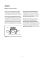
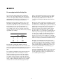
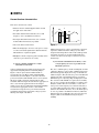
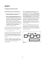
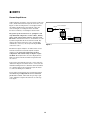
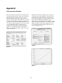
10 Hints for
Making Successful
Noise Figure Measurements
Application Note 57-3
Table of Contents
Introduction
● HINT 1: Select the appropriate noise source
● HINT 2: Minimize extraneous signals
● HINT 3: Minimize mismatch uncertainties
● HINT 4: Use averaging to minimize display jitter
● HINT 5: Avoid non-linearities
● HINT 6: Account for mixer characteristics
● HINT 7: Use proper measurement correction
● HINT 8: Choose the optimal measurement
bandwidth
● HINT 9: Account for path losses
● HINT 10: Account for the temperature of
the measurement components
Appendix A: Checklist
Appendix B: Total uncertainty calculations
Appendix C: References
Appendix D: Abbreviations
Appendix E: Glossary and definitions
Key web resources
3
4
5
6
7
8
9
11
12
13
14
15
16
18
18
19
20
2
Introduction
To achieve accurate and repeatable results at RF or
microwave frequencies, measurement uncertainties and
barriers to measurement repeatability must be minimized.
The performance of a device can be obscured if errors
are allowed to accumulate. For the most accurate
measurement, it is important to understand the nature
of the error contributors and identify which of these can be
influenced or changed to improve the quality of the results.
This application note provides useful tips that
will assist in making accurate noise figure measurements.
The checklist in Appendix A is a helpful tool to verify
that all hints have been considered for a particular
measurement.
A detailed explanation of the uncertainties in noise
figure measurements is provided in Agilent Technologies’
Application Note 57-2, Noise Figure Measurement
Accuracy (see reference 5). For a general understanding
of noise figure and its variety of measurement techniques,
refer to Agilent Technologies Application Note 57-1,
Fundamentals of Noise Figure Measurement (see
reference 2).
3
● HINT 1:
Select the appropriate noise source
ENR
Frequency range
The output of a noise source is defined in terms of its
frequency range and excess noise ratio (ENR). Nominal
ENR values of 15 dB and 6 dB are commonly available.
ENR values are calibrated at specific spot frequencies.
The uncertainties of these calibrations vary over the
frequency range of the noise source and add to the
uncertainty of the measurement. This uncertainty is
typically limited to approximately 0.1 dB using the
root-sum-of-squares method (RSS).
Commercial noise sources cover frequencies up to
50 GHz with choices of co-axial or waveguide connectors.
The frequency range of the noise source must include the
input frequency range of the DUT, of course. If the DUT
is a mixer or frequency translation device, the output
frequency range of the DUT must also be addressed.
If one source does not include both frequency ranges,
a second source will be required. A second noise source
may also be necessary when measuring a non-frequency
translating device with low noise and high gain. Low
ENR is best for the measurement, however, high ENR
is necessary to calibrate the full dynamic range of the
instrument. In either case, a full-featured noise figure
analyzer can account for the different ENR tables
required for calibration and measurement.
Use a 15 dB ENR noise source for:
• general-purpose applications to measure noise
figure up to 30 dB.
• user-calibrating the fullest dynamic range of an
instrument (before measuring high-gain devices)
Match
Use a 6 dB ENR noise source when:
If possible, use a noise source with the lowest
change in output impedance between its ON and
OFF states. The noise source’s output impedance
changes between its ON and OFF states, which varies
the match between the noise source and the DUT. This
variation changes the gain and noise figure of the DUT,
especially for active devices like GaAs FET amplifiers.
To minimize this effect, 6 dB ENR noise sources are
commercially available that limit their changes in
reflection coefficient between ON and OFF states to
better than 0.01 at frequencies to 18 GHz.
• measuring a device with gain that is especially
sensitive to changes in the source impedance
• the device under test (DUT) has a very low
noise figure
• the device’s noise figure does not exceed 15 dB
A low ENR noise source will minimize error due to
noise detector non-linearity. This error will be smaller
if the measurement is made over a smaller, and therefore
more linear, range of the instrument’s detector. A 6 dB
noise source uses a smaller detector range than a
15 dB source.
Adapters
A low ENR noise source will require the instrument to
use the least internal attenuation to cover the dynamic
range of the measurement, unless the gain of the DUT
is very high. Using less attenuators will lower the noise
figure of the measurement instrument, which will lower
the uncertainty of the measurement.
Use a noise source with the correct connector for the
DUT rather than use an adapter, particularly for devices
with gain. The ENR values for a noise source apply only at
its connector. An adapter adds losses to these ENR values.
The uncertainty of these losses increases the overall
uncertainty of the measurement. If an adapter must be
used, account for the adapter losses.
If ENR values must be entered into the instrument
manually, double-check them to ensure that the table in
the instrument is correct.
4
● HINT 2:
Minimize extraneous signals
A noise figure analyzer measures the noise power from
the noise source as affected by the DUT. It uses the power
ratio at two detected noise levels to measure the noise
figure of whatever is between the noise source and the
instrument’s detector. Any interference, airborne or
otherwise, is measured as noise power from the DUT
and can cause an error of any magnitude.
Follow these guidelines:
Figure 2-1 demonstrates the types of stray signals that
can get coupled into the signal path and affect the
measurement. Fluorescent lights, adjacent instruments,
computers, local TV and Radio stations, pocket pagers,
mobile phones and base stations are notorious for their
adverse effects on noise measurements. Random stray
signals can cause several tenths of a dB difference
between individual readings, and result in unstable
measurements (i.e. jitter that will not average to a
stable mean).
(b) Use threaded connectors in the signal path
whenever possible. (For example BNC connectors are
very susceptible to stray signals.)
(a) Ensure that mating connectors are clean and
not worn or damaged (see Reference 8 for further
information). If the measurement becomes unstable
when the cables and connectors are shaken lightly by
hand, try other cables or connectors.
(c) Use double shielded cables (common flexible
braided coaxial cable is too porous to RF).
(d) Use shielded GPIB cables.
(e) Move the measurement setup to a screened room.
If a transmitter that has any frequency content within the
measurement bandwidth is nearby and any covers are off
of the DUT, move the measurement setup to a screened
room. Test for such signals with a spectrum analyzer with
a simple wire antenna on the input. Attenuate these stray
signals by 70 to 80 dB.
Interference
Lights ( esp. fluorescent)
RF comms basestation
(f) Use shielding. This is especially important for
making measurements on an open PC breadboard. (See
Reference 5 for further information.)
DUT
Noise
Source
NF
Analyzer
FM
TV
Computers
(g) Use an analyzer with minimal electromagnetic
emissions. Devices may be susceptible to stray emissions
from some measurement instruments. Some modern
noise figure analyzers have electromagnetic emission
characteristics low enough to have negligible impact on
the measurement.
Double-shielded cables for IF (ordinary braid is too porous)
Shielded GPIB Cables
Enclose all circuits
Test connectors by shaking leads
Figure 2-1
5
● HINT 3:
Minimize mismatch uncertainties
Mismatch at connection planes will create multiple
reflections of the noise signal in the measurement and
calibration paths (as shown in Figure 3-1). Mismatch
uncertainties at these planes will combine vectorially
and will contribute to the total measurement uncertainty.
Alternately, insert a well matched attenuator
(pad) between the noise source and the DUT to
attenuate multiple reflections. As an example, with a
10 dB attenuator, the re-reflections are attenuated by
20 dB. The advantage of an attenuator vs. an isolator is
broadband response. The disadvantage is that the noise
source’s ENR values will be reduced by the attenuator’s
insertion loss (10 dB in this example).
One method to reduce the mismatch uncertainty is to
place an isolator in the RF path between the noise
source and the DUT. This isolator can prevent multiple
re-reflections from reaching the DUT and can suppress
the build-up of error vectors. Isolators, however, operate
over restricted frequency ranges. Several may be needed
for the frequency range of interest. Isolators also add to
path losses. As a result compensation is required. Fullfeatured noise figure analyzers have a loss compensation
feature to account for the insertion losses of any isolators.
If the DUT has a high output reflection coefficient
(S22) and low or no insertion gain (S21), then, in some
cases, place a low noise pre-amp between
the DUT and the measurement instrument to
reduce the total measurement uncertainty. The
pre-amp should have an input reflection coefficient (S11)
as low as possible. The effective bandwidth of a pre-amp
with very low S11 is usually narrow. More than one may
be required for the entire frequency range of interest. To
identify an appropriate pre-amp, see Agilent Technologies
Application Note 57-2 (Reference 5).
Mismatch
Uncertainty
ρ1
ρ2
Calibration
Noise
ρ3
ρ4
Measuring
DUT
Source
System
Measurement
ρ = reflection coefficient at a reference plane
Figure 3-1
6
● HINT 4:
Use averaging to minimize display jitter
Noise measurement inherently displays variability or
jitter because of the random nature of the noise being
measured. Averaging many readings can minimize
displayed jitter and bring the measurement closer to
the true mean of the noise’s gaussian distribution.
If time constraints limit the number of averages during
DUT measurement (e.g. in manufacturing), use more
averages during calibration. This will make the
correction for all subsequent DUT measurements more
accurate.
Modern noise figure analyzers enable the user to select
the number of readings that will be averaged for each
measurement. This will reduce jitter in the measurement
by the square root of N, where N is the number of
measurements in the average. The table below shows
some examples of the effect of averaging on jitter. For
example, jitter may be reduced by almost 70% by averaging
approximately 10 readings.
Modern noise figure analyzers have the ability to do point
averaging or trace averaging. Point averaging makes all
measurements for the first frequency point, calculates and
displays their average, then moves to the next frequency
point. The process is repeated until each frequency
has been measured and averaged the number of times
specified in the measurement setup. Trace averaging
measures only once at each frequency point through one
entire sweep of the frequency range. It then begins the
second sweep, averaging each individual measurement
at each frequency with the previous average for that
frequency, as it sweeps. It repeats this process until the
number of sweeps or “traces” averaged together equals the
number of averages specified in the measurement setup.
N
SQRT
(N)
% jitter
reduction
1
4
16
64
256
1
2
4
8
16
0
50
75
87.5
93.75
Both types of averaging give the same answer. Point
averaging is faster overall since the analyzer’s tuner has
to retune fewer times for all measurements to complete.
Trace averaging displays a rough measurement over the
entire frequency range faster. This enables a user to see
any obvious problems with the measurement (e.g. an
extraneous signal) sooner.
Increasing the averaging will add time to make the
measurement. This would affect the device test time and
total test throughput in manufacturing. There is a trade-off
between the speed of the measurement and the level of
jitter.
Use trace averaging first. Watch a few sweeps across
the display and look for indications of RF interference
such as a spike in the response at a single frequency, or
even a small step in the response.
Decreasing the bandwidth of the measurement increases
proportionately the number of readings necessary to
obtain the same level of jitter reduction. For example,
half the bandwidth requires twice as many readings of
noise figure averaged together to obtain the same jitter
reduction; one fourth requires four time as many readings,
and so on. These additional readings do not necessarily
extend the time for the measurement proportionately.
7
● HINT 5:
Avoid non-linearities
Avoid all predictable sources of nonlinearities:
A Y-Factor noise figure analyzer assumes a linear
change in the detected noise power as the noise source
is switched between Thot and Tcold. Any variations
from linearity in either the DUT or in the detector directly
produce an error in the Y value and hence in the noise
figure that is displayed. The instrumentation uncertainty
specification accounts for the linearity of the analyzer’s
detector. The linearity of the DUT, however, should be
carefully considered when making the measurement.
• circuits with phase lock loops (and any circuit
that relies on signal presence to set its operating
condition)
• circuits that oscillate (even if at a far-removed
frequency)
• amplifiers or mixers that are operating
near saturation
The measured noise figure is determined by the power in
the instrument’s resolution bandwidth. The instrument’s
attenuation settings, however, may be determined by
the power in the instrument’s overall frequency range
that reaches the range detector. The analyzer is therefore
susceptible to being overdriven by noise outside the
bandwidth of any one individual measurement, and
therefore vulnerable to non-linearity errors. In such
cases, attenuate any broadband power outside the
analyzer’s resolution bandwidth. Use a filter wider than
the measurement frequency range and before the DUT.
• AGC circuits or limiters (AGC circuits have been
known to contribute additional noise power at the
power levels near its operational point, even when
disabled.)
• High Gain DUT’s without in-line attenuation
(Attenuate the output of the DUT if necessary.
See Hint 7 for details)
• power supply drifts
Consider measuring a familiar “reference” or “gold
standard” device at the beginning of each day to assure
that the same result is obtained as prior days for the same
device, to add assurance that the measurement instrument
is warmed up sufficiently.
• DUTs or measurement systems that have not
warmed up
• logarithmic amplifiers (The standard Y-Factor
measurement is invalid for amplifiers in a logarithmic
mode.)
8
● HINT 6:
Account for mixer characteristics
If the device under test is a mixer:
• Measure the same sideband(s) that will be used in
the application of the mixer.
FLO
LSB
Noise Power
avera
• For double sideband measurements, select a LO
frequency close to the RF band of interest.
ge
USB
FIF
• For single sideband measurements, select a LO far
from the RF band of interest, if possible.
Freq
• Choose the LO to suit the mixer.
Figure 6-1
• Filter the RF signal (i.e. the noise source) if necessary
to remove unwanted signals that would mix with the
LO’s harmonics or spurious signals.
DSB measurements are easier to perform since they don’t
require the additional burden of image rejection filter
design and matching. When a mixer with a DSB specified
noise figure is going to be used in an SSB application,
careful correction is needed. (See reference 5 for more
information)
• Always document a frequency plan to identify which
of the above precautions are necessary.
b) For double sideband measurements, select
a LO frequency as close as possible to the
RF band of interest.
a) Select a double sideband or a single
sideband measurement.
A mixer will translate input signals and noise from the
upper sideband (USB) and lower sideband (LSB) as
Figure 6-1 shows. (Note that the LSB and USB are
separated by twice the IF.) A double sideband (DSB)
measurement, shown in Figure 6-2, measures the noise
powers for both the USB and LSB. Some receiver systems,
like those in radio astronomy, intentionally use both
sidebands. DSB noise figure measurement is appropriate in
these cases. In many applications the desired signal
will be seen in only one sideband. A single sideband (SSB)
measurement is appropriate in these cases. In SSB
measurement setups, the noise power in the unwanted
sideband is suppressed by appropriate “image rejection”
filtering at the input of the mixer.
The choice of LO frequency, and the resulting IF, can make
a dramatic difference in the results of DSB measurements.
Instruments typically display the average of the LSB and
USB noise figures. They measure the power in the IF band
(which is the sum of both sidebands after conversion),
diminish that power by half (3 dB), and display the result.
The closer the USB and LSB are together, the more likely
they are to be equal (as shown in Figure 6-1) and the more
likely the default 3 dB correction will be accurate. Since
noise power versus frequency for a mixer is rarely flat, if
too wide an IF is used the error and its correction will be
unknown. To minimize this error, choose the LO frequency
as close as possible to the RF band of interest, within the
limitation that the resulting IF cannot be below the lower
frequency limit of the instrument being used (often
10 MHz).
9
To determine if sideband-averaging error is a problem, set
up the noise figure measurement for a mixer with swept
LO and fixed IF (modern noise figure analyzers allow this).
Monitor the noise figure reading. If the noise figure values
change dramatically as the LO sweeps, then SSB
measurement is recommended (See reference 5 for
further information.)
Balanced and double-balanced mixers have more than
one diode to perform the frequency conversion. This
improves the LO to IF isolation (20 dB and better), but
usually requires more LO power or biasing. This higher
power may raise the LO’s noise output, produce spurs
away from the set frequency, or produce LO harmonics
inside the mixer. Any of these can mix additional, yet
unwanted, RF signal into the IF, or leak through to the IF.
This may raise the measured noise and possibly overdrive
the analyzer’s first stage to a non-linear state. Experiment
with the LO to see what improves performance and
produces the lowest noise figure.
Measurement System
IF Amplifier
(DUT)
Mixer
Noise source
fRF
f LO
f IF
LO
Noise
Figure
Analyzer
e) Filter the RF signal (i.e. the noise source)
if necessary.
Noise
Source
Drive
It may be necessary to filter the RF noise source to remove
frequencies that are outside the band of interest as shown
in Figure 6-4. This can remove unwanted signals that
would mix with the LO or its harmonics or spurious signals
and raise the measured noise figure.
Figure 6-2
c) For single sideband measurements, select
a LO far from the RF band of interest,
if possible.
The farther the LO is from the RF, the higher will be the
IF, and the less stringent will be the rolloff requirement
for the filter that suppresses the unwanted sideband as
shown in Figure 6-3.
d) Choose the LO to suit the mixer.
Choose the LO to avoid spurious output where the mixer is
sensitive and to avoid high broadband noise floor.
Filter the LO if necessary to diminish spurious signals
and broadband noise, since the IF pass band will include
noise power one IF away from the LO frequency and
one IF away from any spurious signals or harmonics of
the LO.
10
f) Filter the IF signal (ie, the DUT output)
if necessary.
FLO
LSB
USB
Noise Power
Keep the LO outside of the frequency range of the
instrument if possible. LO power will almost certainly
leak through to the IF port of the mixer. Assume that
LO to IF isolation will be insufficient. If this leakage is
within the band of the measurement, it will add to the
noise figure measured. If it is outside the band of the
measurement but within (or close to) the overall
frequency range of the instrument, it could cause the
instrument to autorange itself to use more attenuation,
which would increase the uncertainty of the measurement.
Filter the output of the mixer to remove this LO
leakage and any LO harmonics created in the mixer
without appreciably attenuating the wanted mixer
output signal.
filter response
FIF
Freq
FIG 6-3
Measurement System
g) Document a frequency plan to evaluate
which of the above precautions are
necessary.
(DUT)
IF Amplifier
Mixer
Noise source
f IF
fMEAS
A frequency plan will help identify which of the
precautions above are the most important before the
measurement is made.
f LO
LO
FIG 6-4
11
Noise
Figure
Analyzer
Noise
Source
Drive
● HINT 7:
Use proper measurement correction
Take the following steps to ensure the measurement
system itself does not add error to the measurement.
The cascade equation shows how F12 is very sensitive
to uncertainty margins in the second stage term
[(F2 - 1) / G1]. (To see how F12 would vary with marginal
changes in F2 or G1, see reference 6.) If the DUT has
insertion loss (e.g. a mixer, attenuator, etc.), use a low
noise pre-amplifier before the instrument to reduce
the uncertainty margin. Choose a pre-amp with the
lowest noise figure and a gain of more than 100 (20 dB +).
(See Agilent Technologies Application Note 57-2 for more
information on selecting the pre-amp.) Make the noise
figure of the second stage as low as practical and the
uncertainty of F12 (and hence F1), as low as possible.
Adding a pre-amp also gives the measurement some
resilience against noise figure variations versus frequency
of the second stage.
• Remove the noise figure of the measurement
system with regular user calibration.
• Avoid exceeding the maximum input power of
the measurement instrument. Modern instruments
can handle around 65 dB of device gain for narrow
band devices. For wider band devices with high gains
it is likely that an attenuator will be required after the
device to keep the overall power within the
instrument’s range. Use the analyzer’s compensation
feature to account for the losses of the attenuator.
Use appropriate filters/isolators/circulator to suppress
out-of-band responses that would otherwise
contribute noise power at the high gain level and
overpower the instrument’s input.
In the case of a high-gain DUT, there may not be a need
for a pre-amp. In order to make that decision, place the
DUT’s linear gain and the measurement system’s linear
noise figure (i.e. noise factor) into the Cascade Equation.
Notice the noise figure of the cascade will converge to the
noise figure of the DUT.
A Y-Factor noise figure analyzer measures the noise figure
of the measurement system and the DUT combined (see
Figure 7-1). Below is F12 in the cascade equation:
F12 = F1 + [(F2 - 1 ) / G1]
(7-1)
F1 and F2 are linear noise figure values for the DUT and
the measurement system, respectively, and G1 is the
gain of the DUT. User calibration (termed “second stage
correction”) determines F2; measurement determines
F12 and G1. The analyzer calculates F1 from the cascade
equation.
Calibration path
Noise
source
DUT
Gain, G
Measuring
system
Measurement
path
Perform user-calibration prior to the measurement to
remove the second stage contribution. Calibrate out the
second stage contribution at regular intervals depending
on how sensitive the noise figure and gain are to
temperature drifts.
F2 = noise figure of the measurement system
F1 = noise figure of the device under test (DUT)
Figure 7-1.
12
● HINT 8:
Choose the optimal measurement bandwidth
Select a measurement bandwidth no larger than the
pass band of the DUT. Modern noise figure analyzers
provide a selection of various measurement bandwidths
to enable measurements that are more relevant to current
practical applications (e.g. individual wireless GSM
channels). 4 MHz bandwidths were common in past
generations of noise figure instruments; modern analyzers
can measure down to at least 100 kHz bandwidth.
Analyzer's frequency instability
due to drift during time required
for all measurements to be made
and averaged
Lowest possible actual
measurement bandwidth due
to downward frequency drift
If the measurement bandwidth is similar to the DUT’s
operational pass band, then any instabilities between
the center frequency of the analyzer’s final IF and the
DUT’s operational bandwidth will lead to an error in the
displayed gain. The analyzer may recognize the noise
power outside of the DUT’s pass band during calibration
and inside during measurement. The extent of this effect
depends on the shape of the DUT’s pass band overlapping
with the shape of the analyzer’s final IF pass band. This
issue is less significant if the analyzer’s pass band is
narrower than the DUT’s pass band.
Highest possible actual
measurement bandwidth due
to upward frequency drift
Noise power detected during
calibration but not during
DUT measurement
understates DUT's noise figure
Noise
Power
Frequency
Measurement
Bandwidth Setting
Figure 8-1
Past generations of noise figure instruments required
additional time to obtain the same level of jitter reduction
in a narrower bandwidth. For the same jitter reduction,
half the bandwidth required twice the time, one fourth
required four times as long, etc. In modern full-featured
noise figure analyzers, this time penalty is mostly
eliminated due to digital signal processing (DSP)
techniques that measure a group of adjacent frequencies
simultaneously.
13
● HINT 9:
Account for path losses
Adapters must be used if the connectors between the noise
source, DUT, and measurement system do not mate, as in
Figure 9-1. It is most important to avoid adapters where
the signal is smallest in the measurement setup. For
devices with gain, avoid adapters before the DUT.
For devices with loss, avoid adapters after the DUT.
Connection Diagram
Cable C1
Noise
Source
Keep track of the insertion losses of adapters and
any additional components such as cables, baluns,
filters, pads, and isolators that are not part of the
DUT. These insertion losses have to be taken into account
by subtracting them from the measurement result. Any
adapters used between the noise source and the DUT
will introduce some loss, effectively reducing the ENR
of the noise source.
Coax/WG adapter
A
G1
DUT
Cable C 2
G2
B
Coax/WG adapter
Figure 9-1
Modern noise figure analyzers can subtract these losses
from the measurement automatically. The analyzer
will also need to know the temperature of these
components and whether they are before or after
the DUT. The analyzer will correct the displayed noise
figure for all loss elements and their temperatures that
are entered.
Losses in the measurement system are corrected by user
calibration. Adapters and cables that are connected to the
instrument during both user calibration and measurement
are considered part of the measurement system and are
accounted for during user calibration.
If a pre-amp is needed prior to the measurement system
then choose a pre-amp with the correct connector
for the noise source, and include the pre-amp as part
of the calibration setup that measures the second stage
noise figure.
14
Measurement
system
● HINT 10:
Account for the temperature of
the measurement components
Y-Factor noise figure analyzers assume that the surface
temperatures of all components in the measurement
(noise source, DUT, connectors, cables, etc.) are the
default value for Tcold, 290K (16.8°C, 62.2°F). If this is
not the case, enter the correct temperature of each
component into the analyzer and monitor them
regularly. Full featured noise figure analyzers allow the
entry of the temperatures of any components added before
and after the device.
If the actual local ambient temperature is not entered
into the analyzer, it will make its calculations with the
wrong temperature assumption. An extra error term in
the over-all uncertainty margin will be present. This can
be a significant value if the true noise figure of the DUT is
low. Figure 10-2 shows typical differences between the
displayed and actual noise figures for different ambient
temperatures.
NF(dB) = F mea - Factual
Figure 10-1 shows the measurement response curve
where the noise powers N1 and N2 are due to input noise
temperatures Tcold and Thot, respectively. The solid
line on this graph represents the response when T0 is
considered as the reference ambient temperature of 290K.
If the Tcold of the noise source (for a solid state noise
source, its surface temperature) is not equal to T0, then the
dotted line may become the response curve. The noise
power added by the DUT would then be Na´ and not Na.
0.24
T amb = 305K (=89 F)
0.20
0.16
+1K
0.12
0.04
0
0.4
0.8
1.2
NF(dB)
Pout
N2
Figure 10-2
N1
Na´
Na
To Tc
Th
Ts
Figure 10-1
15
T amb = 296.5K (=74 F)
0.08
1.4
1.8
Appendix A:
Checklist
❑ Account for mixer characteristics. See Hint # 6.
❑ Measure the same sideband(s) that will be used in
the application.
❑ For double-sideband measurements, select a LO
frequency close to the RF band of interest.
❑ For single-sideband measurements, select a LO far
from the RF band of interest, if possible.
❑ Choose the LO to suit the mixer.
❑ Filter the LO if necessary to diminish spurious signals
and broadband noise.
❑ Keep the LO outside of the measurement bandwidth
if possible.
❑ Filter the IF if necessary to remove LO harmonics
created inside the mixer.
❑ Filter the RF to prevent unwanted mixing.
❑ Test for DSB error by changing IF.
❑ Experiment with different LOs to get the most
accurate (i.e. lowest) noise figure.
❑ Document a frequency plan to evaluate which of the
above precautions are necessary.
Use this checklist to assist with locating the hint relating to
specific issues or considerations. Reading the 10 Hints
Application Note sequentially is not necessary.
❑ Select the appropriate noise source. See Hint # 1.
❑ Use a low ENR source whenever possible.
❑ Avoid adapters between the noise source and DUT.
❑ Double check manually entered ENR values.
❑ Reduce EMI influence. See Hint # 2.
❑ Use clean, undamaged connectors.
❑ Use threaded connectors.
❑ Use double shielded cables.
❑ Use shielded GPIB cables.
❑ Use a screened room.
❑ Use shielding.
❑ Use an analyzer with minimal electromagnetic
emissions.
❑ Minimize mismatch uncertainties. See Hint # 3.
❑ Use an attenuator or isolator if needed.
❑ Use a pre-amp if needed.
❑ Enter proper measurement correction.
See Hint # 7.
❑ Calibrate regularly.
❑ Keep overall gain below the instrument’s spec.
❑ Filter out-of-band power.
❑ If 2nd stage effect is large, add a low-noise pre-amp
(with proper connectors).
❑ Use averaging to minimize display jitter.
See Hint # 4.
❑ Select enough averages to stabilize the measurement.
❑ Use “trace averaging” first to spot measurement setup
problems soonest.
❑ Look for spikes or even small steps in the display that
indicate RF interference.
❑ If time constrained, use more averaging during
calibration than during DUT measurement.
❑ Choose the optimal bandwidth. See Hint # 8.
❑ Select a measurement bandwidth no larger than the
pass band of the DUT.
❑ Avoid non-linearities. See Hint # 5.
❑ Avoid the following:
❑ Circuits with phase lock loops
❑ Circuits that oscillate
❑ Amplifiers or mixers operating near saturation
❑ AGC circuits or limiters
❑ High-gain DUTs without in-line attenuation
❑ Power supply drifts
❑ DUTs or instruments that have not warmed up
❑ Logarithmic amplifiers
❑ Account for path losses. See Hint # 9.
❑ Avoid adapters as much as possible.
❑ If used, enter their losses into the instrument.
❑ Account for the temperature of measurement
components. See Hint # 10.
❑ Enter physical temperatures of the noise source and
the components of the measurement setup into the
instrument.
16
Appendix B:
Total uncertainty calculations
The error model in the spreadsheet shown in Figure B-1
is obtained from the derivative of the Cascade equation
(F1 = F12 - [(F2-1) / G1]). It takes into account the
individual mismatch uncertainty calculations at each
reference or incident plane of the DUT, noise source and
measurement system. This example represents the total
noise figure measurement uncertainty, RSS analysis, for
a microwave transistor with an S11 of 0.5, S22 of 0.8 and
S21 of 5 (14dB). Noise figure uncertainty, here is
calculated as ±0.48 dB. The uncertainty dramatically
improves to ±0.26dB, in this instance, if the gain is
improved to 20dB. The calculation for this error model
is derived in Reference 6.
Figure B-2 shows the typical display for the entry point
to this interactive model. Figures B-3, B-4 and B-5 show
simulated results for the uncertainty calculator. There
are a number of graphs that can be plotted. These figures
show examples of RSS uncertainty with respect to
instrument match, DUT input match and instrument noise
figure, respectively. This interactive uncertainty calculator
and the spreadsheet version shown in Figure B-1 can be
accessed via the Internet by using the URL on the back
page of this application note.
Figure B-2
Figure B-1
Figure B-3
17
Appendix C:
References
1. Agilent 346A, 346B, and 346C Noise Sources
(10 MHz to 26.5 GHz), Technical Specification Sheet,
literature number 5953-6452
2. Fundamentals of RF and Microwave Noise Figure
Measurements, Application Note 57-1,
literature number 5952-8255E
3. Noise Parameter Measurement Using the Agilent
8970B Noise Figure Meter and the ATN NP4 Noise
Parameter Test Set, Product Note 8970B/S-3,
literature number 5952-6639
4. Noise Parameter Measurement Accuracy and
Repeatability Considerations, ATN Application Note 001
Figure B-4
5. Noise Figure Measurement Accuracy,
Application Note 57-2, literature number 5952-3706
6. “Calculate the Uncertainty of NF Measurements”
Microwaves and RF, October 1999.
Also available at: http:\\www.mwrf.com
(select Editorial Archives; then October 1999).
7. Agilent R/Q 347B Solid-State Noise Sources at
Millimeter-Wave Frequencies, Technical Specifications,
literature number 5954-8888
8. Principles of microwave connector care
(for higher reliability and better measurements),
Application Note 326, literature number 5954-1566
Figure B-5
18
Appendix D:
Appendix E:
Abbreviations
Glossary and definitions
AGC
DUT
DSB
ENR
F
LSB
NF
RSS
SSB
Tc
Tcold
Th
Thot
USB
URL
WG
1. Excess Noise Ratio (ENR):
ENR is the measure of how much more noise power is
output from a noise source when “ON” (i.e. operating at
virtual temperature Thot) than is output when “OFF” (i.e.
operating at ambient temperature Tcold), normalized by its
output power at the standard temperature 290K.
Automatic Gain Control
Device Under Test
Double Sideband
Excess Noise Ratio
Noise Factor (linear expression of NF)
Lower Sideband
Noise Figure (noise factor [F] expressed in dB)
Root Sum of Squares
Single Sideband
Cold Temperature
Cold Temperature
Hot Temperature
Hot Temperature
Upper Sideband
Universal Reference Locator
Waveguide
ENR = 10 log (Th - Tc) / T0
For example, an ENR of 15 dB means that the noise source
output when ON is greater than when OFF by the antilog
of 15/10 times the noise power ouput at 290K. This is
equivalent to a resistor at 9171K, calculated as antilog
(15/10) x 290.
2. Second Stage Contribution:
During the measurement process the noise source is
connected to the input of the DUT and the DUT’s output is
connected to the measurement system. In this cascade, the
DUT is the first stage and the measurement system is the
second stage. The measurement system will measure the
noise figure of the cascade. Correction requires that the
noise figure (F1) value of the DUT has to be de-embedded”
from the cascade’s combined noise figure (F12) by
removing the contribution of the second stage in the
cascade or Friis equation:
F12 = F1 + [(F2 - 1) / G1]
The expression in the brackets is the second stage
contribution. G1 is the gain of the DUT.
3. Y-Factor:
This is the linear ratio of the noise power seen by the
measurement system when the noise source is turned ON,
to that when the noise source is turned OFF. This is the
basis of the calculation of noise figure. After the
instrument recognizes the ENR, the noise figure is derived
from the equation:
NF = ENR - 10 log (Y - 1)
19
Agilent Technologies’ Test and Measurement
Support, Services, and Assistance
Agilent Technologies aims to maximize
the value you receive, while minimizing
your risk and problems. We strive to ensure that
you get the test and measurement
capabilities you paid for and obtain the
support you need. Our extensive support
resources and services can help you
choose the right Agilent products for your
applications and apply them successfully. Every
instrument and system we sell has
a global warranty. Support is available for
at least five years beyond the production
life of the product. Two concepts underlie
Agilent’s overall support policy:
“Our Promise” and “Your Advantage.”
Our Promise
Our Promise means your Agilent test and
measurement equipment will meet its
advertised performance and functionality.
When you are choosing new equipment,
we will help you with product information,
including realistic performance specifications
and practical recommendations from
experienced test engineers. When you use
Agilent equipment, we can verify that it
works properly, help with product operation,
and provide basic measurement assistance
for the use of specified capabilities, at no
extra cost upon request. Many self-help
tools are available.
Your Advantage
Your Advantage means that Agilent offers
a wide range of additional expert test and
measurement services, which you can
purchase according to your unique technical
and business needs. Solve problems
efficiently and gain a competitive edge by
contracting with us for calibration, extra-cost
upgrades, out-of-warranty repairs, and
on-site education and training, as well as
design, system integration, project
management, and other professional
engineering services. Experienced Agilent
engineers and technicians worldwide
can help you maximize your productivity,
optimize the return on investment of your
Agilent instruments and systems, and obtain
dependable measurement accuracy for the
life of those products.
For more assistance with your test &
measurement needs go to
www.agilent.com/find/assist
Or contact the test and measurement experts
at Agilent Technologies
(During normal business hours)
United States:
(tel) 1 800 452 4844
Canada:
(tel) 1 877 894 4414
(fax) (905) 206 4120
Europe:
(tel) (31 20) 547 2000
Japan:
(tel) (81) 426 56 7832
(fax) (81) 426 56 7840
Latin America:
(tel) (305) 267 4245
(fax) (305) 267 4286
Australia:
(tel) 1 800 629 485
(fax) (61 3) 9272 0749
New Zealand:
(tel) 0 800 738 378
(fax) 64 4 495 8950
Asia Pacific:
(tel) (852) 3197 7777
(fax) (852) 2506 9284
Product specifications and descriptions in this
document subject to change without notice.
Copyright © 2000
Agilent Technologies
Printed in U.S.A. 11/21/00
5980-0288EN