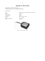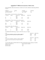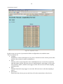
1
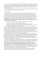
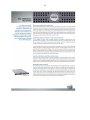
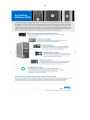
Specifications Seismic System as part of the LOFAR Project Report: GeoLOFAR-004 (DRAFT) Version: 5.0 Date of issue: May 2012 Contact person: Dr. Guy G. Drijkoningen Dept. of Geotechnology Stevinweg 1 2628 CN Delft The Netherlands Tel: + 31- 15 - 278 7846 Fax: + 31- 15 - 278 1189 Email: [email protected] 2 Contents 1 Introduction ............................................................................................................................... 3 2 Overview seismic system .......................................................................................................... 4 3 Local (sensor) fields .................................................................................................................. 6 3.1 Geometry of sensors ......................................................................................................... 6 3.2 Hardware .......................................................................................................................... 9 3.3 Local software components ............................................................................................ 12 3.4 Power consumption ........................................................................................................ 14 4 Central LOFAR network ......................................................................................................... 15 5 Central System (Rekencentrum Groningen) ........................................................................... 16 6 Data storage and retrieval sites (TNO, KNMI) ....................................................................... 19 7 Data access for users (e.g., TU Delft) ..................................................................................... 20 8 References ............................................................................................................................... 22 Appendix A: AD converters: The “GeoEel”................................................................................. 23 Appendix B: 220V AC to 48V DC converter ............................................................................... 26 Appendix C: Sensors and housing ................................................................................................ 28 C.1. Geophone: SM-6 geophone from Sensor b.v. ................................................................... 28 C.2. Hydrophone: Benthos PreSeis 2520 .................................................................................. 29 C.3. Holder ................................................................................................................................ 30 C.4. Housing of 3C geophone and hydrophone. ....................................................................... 32 C.5. Casting material................................................................................................................. 33 Appendix D: Cables ...................................................................................................................... 34 Appendix E: GPS antenna............................................................................................................. 36 Appendix F: Different scenarios of data rates .............................................................................. 37 Appendix G: GeoLOFAR Seismic Control software ................................................................... 38 Appendix H: Description of the GeoLOFAR-web site ................................................................. 46 H.1. Data-functionality of the GeoLOFAR-web site ................................................................ 49 H.2. Infrastructure of the GeoLOFAR website ......................................................................... 53 Appendix I: Failover and recovery ............................................................................................... 55 Appendix J: Computer Hardware ................................................................................................. 56 3 1 Introduction This document specifies the design and implementation of the seismic system within the LOFAR project. This document results from extensive testing at the Exloo test-site of LOFAR. From the “Project Plan of the Seismic Application in LOFAR” [1] this document refers to tasks 1.1 and 3.6. The structure of this document is as follows: first an overview of the total seismic infrastructure will be given, before zooming in into the different components. The different components may have a hardware and software component, and will then be described separately. All fine details and detailed specifications of hardware and software are given in appendices in order to keep the discussion at a general level and come up with a readable piece of text. 4 2 Overview seismic system In this section an overview of the total seismic system is given and described. It shows the different subsystems which are described in further detail in subsequent sections. This section describes in a general manner how the sensor network LOFAR is implemented for seismic applications. In Figure 2.1 a drawing is shown which gives the over-all structure. The data start to be sensed by the sensors in the field. Locally, the data is converted to digital signals before they are sent over the LOFAR network to a central unit at the “Rekencentrum” of Groningen. There, the data are collected, (automatically) analyzed and pre-processed if necessary. Then, based on the application, the data is sent via standard internet to TNO and/or KNMI for storage, further analysis and interpretation. These two institutes then allow these data to be retrieved via standard internet by other users, such as the TU Delft. Figure 2.1. Pictorial overview of seismic system of LOFAR The description so far dealt with the stream of data and not the control, such as parameter setting and testing. The control of the data and meta-data can be done locally on a sensor field, globally via the central server at Groningen or remotely via any place on the internet, although not all functionality is available at all locations. The functionality at each level will be described separately. For the description in the sections, the total system is divided into the following subsystems: - local (sensor) fields - central LOFAR network - central system (Groningen Rekencentrum, with TNO facilities) 5 - data-storage and retrieval sites (TNO, KNMI) - data access for users (e.g., TU Delft) This will be done in the following, noting that the discussion on the first item, the local sensor fields, will be the most extensive one. 6 3 Local (sensor) fields In this section the local sensor fields are further described in detail. First, the geometries as being used within the framework of LOFAR will be described. Next, the hardware will be discussed where its actual specifications are mostly given in appendices. Finally the software active on the local fields will be described. 3.1 Geometry of sensors Two seismic geometries are planned: 1. A province-scale geometry that is making use of the fields as used by the astronomers as part of the LOFAR project. From a geophysical perspective, this geometry is focussed on the lower frequencies (< 20 Hz) and sparse sampling of the wavefield. This geometry can be used for inferring information of the deeper subsurface, and can be used for lowfrequency interferometry. 2. A kilometre-scale geometry which is laid out on top of a seismically active field. This array will not be on one of the fields that the astronomers are using. Typically, this geometry will be similar to that being used by the hydrocarbon industry. A requirement for such geometry is that the wavefield needs to be properly sampled. This geometry focuses more on the higher frequency bands, up to 100 Hz. This geometry is most promising for the passive interferometric technique to work. Also for monitoring for the changes in the subsurface, this geometry is the proper way to do it. Although this set-up will not be on one of the LOFAR fields, the network does need somewhere linking up to the LOFAR network where the facilities of LOFAR are again available. For the province-scale geometry, most of the antenna fields of the outer core are used for installation of 3-component (3C) sensors. In one borehole, four 3C sensors will be placed at different depths: 30m, 60m, 90m and 120m. This geometry allows estimating the (apparent) velocity of different arrivals in the vertical direction, next to its polarization. In order to estimate the 3D direction certain events come from, three other boreholes are made in which one 3C sensor is placed at 60 meters depth. These three boreholes are put at maximal horizontal distance from the borehole with the four sensors, and at angles of 120o. The whole geometry is shown in Figure 3.1 7 Figure 3.1 Configuration of 4C sensors for province-scale network at each antenna field (3 shown here) For the local/km-scale geometry, the sensors will not be placed on any of the antenna fields but somewhere on top of a producing gas field where induced seismicity is occurring. In the horizontal direction, the total seismic wavefield needs to be properly spatially sampled, and this requires a horizontal spacing of 12 m (Drijkoningen [2]). The sensors are at a depth of 50 m, again to minimize effects of surface waves. For proper processing and interpretation of the data, 96 4C sensors are placed along one line. A line of 24 4C sensors are placed on a line perpendicular to it but with a spacing of 48m. In depth, one borehole in the middle houses 6 4C sensors, at depths of 5 m, 25 m, 50 m, 75 m, 100 m and 125 m. The whole configuration is shown in Figure 3.2. This network is linked to the LOFAR-internet connection 8 Figure 3.2 Configuration of 4C and 1C sensors for local/km-scale network. For the final systems, most of the electric and electronics is housed in one cabinet. The hardware components are described in subsection 3.2. From a software point of view the systems are approached in the same way, and are described in subsection 3.3. 9 3.2 Hardware Most of the electric and electronics is housed in one cabinet. An overview of a system is given in Figure 3.3. GPS-antenna output LAN (optical) control Local Seismic Controller AD controller 10 kHz HC control Analog-to-Digital signal converters control data 10 kHz HC 48 V = AC-to-DC converter 48 V = ( 220V~ to 48V= ) 220 V ~ 220 V ~ 380V separator 4-component seismic sensor 4-component seismic sensor Figure 3.3 Overview of the province-scale network. Blue is the cabinet in which the electric and electronic equipment is housed. The different components can be seen in this figure. The different components are briefly described in the following. AC Power Supplies The system is powered by a 380V coming from the local electric energy supplier (Essent). From one phase 220V is needed for local power. Earth Wiring Earth wiring is a very special issue since it is the most important noise source for the seismic monitoring. Separators and single earth-points are selected such that no undesired power runs over the earth-wires that pick up the 50-Hz signal from the central power supply. The central power supply is earthed, but separated by a separator from the earth of the cabinet itself. DC Power Supply The AD controller and AD converters use a DC voltage as energy source. In the case of the Exloo test-site these systems need 48 Volts. So a converter is included which converts the 220V AC-current to a 48V DC current. This system itself is using power from the local AC power supply (220V) 10 AD controller This is a local piece of electronics that is supplied by a vendor so it is off-the-shelf. In the case for the test-site at Exloo, this was supplied by Geometrics Inc. This controller controls the AD converters and makes sure the data is properly transported. A specific task of the AD controller is to use a GPS clock to time-synchronize all AD converters on a common time-base. Local Seismic Controller This is the computer system from TNO on which the local software runs. The reason that there is this second controller is that some functionality of this off-the-shelf AD controller is still needed since this functionality was too cumbersome to develop within LOFAR itself (such as the test functionality which includes a signal generator.) However, because of LOFAR, a separate communication had to be set up, which would be independent of the seismic manufacturer. It was developed by TNO such that the software can directly communicate with the AD-converters and with the LOFAR network. The software is further discussed in the section on the software (section 2.3). GPS antenna The AD controller needs to get its time from the GPS satellites. Therefore an antenna is placed on top of the cabinet to pick up the GPS signal and transfer it to the AD controller. The AD controller uses this signal to synchronize all recordings on a common time base. This has been implemented by the vendor (so it is not known how this is done exactly). The accuracy needed is 1/10th of a time-sample, so 1/10th of 0.5 ms which is 50 sec. The accuracy of the supplied system from the vendor is 10 sec so it satisfies the needs. AD converters The AD converters convert the signals from the seismic sensors from analogue to digital ones. The input voltages for seismic vary tremendously. It is difficult to quantify what would be required to have a system that could cope with passive as well active seismic sources. It can be said that the current 24-bit systems are sometimes not sufficient since sources can be nearby (some tens of meters) as well as kilometres away. Especially for the application of seismic interferometry, it is not known what is needed. So the choice was for the highest possible dynamic range in the market, and those are the 24-bit ones. Mostly, they are from the DeltaSigma type. High-cut filters Since the AD converters are conventionally of the Delta-Sigma type, they are operating in the MHz range. These types of frequencies are noise sources for the astronomy applications of LOFAR, working in the range of 10-240 MHz. Measurements at the test-site have shown that the AD converters radiate into the cables. In order to avoid these frequencies, high-cut filters are taken such that the high frequencies (above 10 kHz) are filtered out. This frequency is way below the minimum frequency of interest of the astronomers which is 10 MHz. At the same time this 10 kHz is 100 times higher than the highest frequency of interest for the seismic applications which is 100 Hz. At this moment the high-cut filters are called “10 kHz HC filters” but the actual cut-off frequency will be slightly different in practice; the 10 kHz indicates the order of frequency where the cut-off will be. Cables The analogue signals from the seismic sensors are transported over a cable to the cabinet. At this moment, the only special requirement for the cables is that they are able to work properly 11 over 10 years and that they need to be below the frost region which is often taken as 60cm below the surface. Also, a cable placed at the surface is prone to damage, e.g. due to farming, and also therefore it is desired to bury the cables. Still, one would like to be able to retrieve and/or repair any damaged cable, so the cable should not be too deep. Therefore, it was decided to bury the cables at 1 meter depth. In order to reduce cross-talk over the cable, especially the 50Hz and higher harmonics picked over the analogue wires, twisted-pair cables are chosen. 4C seismic sensors The requirements of the sensors is that they are able to pickup both P- and S-waves. This requires the use of 3-component sensors. Then, a soil as encountered near the surface also contains water and/or air in the pores of the soil and pressure-sensors are able to pick up the energy in water. In testing at the Exloo site it turned out that data from sensors sensitive to the fluid pressure showed, as expected, lower levels of surface waves and higher levels of P-wave information. Therefore the use of sensors sensitive to the fluid pressure is desired. Also, the combination of the 3-component sensors with fluid-pressure sensors allows better wavefield decomposition so has advantages from an interpretation point of view. Currently, work is under way to exploit such a combination. Next, a choice needed to be made with the type of sensor and its working range: - They need to be able to work in the range of 1-100 Hz; - They need to be able to have good sensitivity for passive and active data; - Although not a requirement, but a preference: because of power requirements would be for passive elements rather than active elements Based on these considerations, 3-C geophones do very well since they can be used in the range of 1-100 Hz although at the low frequencies they lose some dynamic range (12 dB/octave below resonance), have shown to be very good sensitivity for active seismic and good sensitivity for passive seismic, and are passive elements. For the fluid-pressure, passive transformercoupled hydrophones were chosen since they work also in the range 1-100 Hz with a bit of loss at low frequencies (6 dB/octave below resonance), have very good sensitivity for active seismic and good sensitivity for passive seismic, and are passive elements. One of the options was to bury sensors rather than placing at the surface. Especially fluidpressure measurements in water can only be done at depth and not at the surface. In the testing at Exloo (and also at Annerveen, see Drijkoningen [3]), it turned out that burying the sensor at depth makes the signal levels of undesired surface waves become (much) lower than at the surface. This means that the sensor need to be buried which meant under the water table. To this aim, a special housing needed to be designed. Because of the combination of two types of sensors and its use under the water table at depth, a special housing needed to be designed: it is desired to deploy as much at the same location as possible. At sea, such a combination is used on the sea floor, but in LOFAR it needs to be used in a borehole. In order to make sure the horizontal components of the geophone are well oriented, a special holder is designed which makes sure they are well oriented. A drawing is given in appendix C.3. Then this holder is used within a housing that can be used in an environmentally hostile area. A drawing/picture is given in appendix C.4. Finally, special casting material is used to permanently stick the two parts together. The specifications of the casting material are given in appendix C.5. So the 4C seismic sensors are especially designed for its use in LOFAR. The 4C sensors are placed at the field of Annerveen. On the other fields, 3C geophones are used. On those fields, 7 sensors are placed; 4 at different depths in a borehole, and 3 in three other boreholes, 1 sensor in each borehole. 12 3.3 Local software components Locally on a sensor field, the different software systems that are running are: - Local Control System - Local Data System - Local Meta-data System Local Control System (LCS) Each site has it own Local Control System (LCS). By means of the LCS the geophones at the site can be configured and monitored. The Local Seismic Controller presented in the hardware description performs all the functions of the LCS. It controls the AD converters and the transport of data and meta-data over the LOFAR network. It communicates with the local LOFAR server on each field, which in turn communicates with the servers at Groningen, with the Blue Gene Stella. Also in the hardware description, the AD controller was shown. This controller is supplied by the vendor, in this case Geometrics. The AD controller controls the AD converters and makes sure the data is properly handled. A specific task of the AD controller is to use a GPS clock to time-synchronize all AD converters on a common time-base. A web application is installed for control and configuration of the seismic data acquisition process. With this web application the user can: Enter structural information of the site such as the number of devices in the site and their IPaddress; Enter operational settings that are used during the acquisition such as the sample rate; Start and stop the acquisition process, if needed. Normal mode is continuously recording, but stopping the process may be needed for maintenance. In appendix G an overview of the web application is given, using screenshots. Finally, testing software runs locally. This software is supplied by the vendor, i.e., Geometrics. This software has the capability to test the hardware, i.e., the AD converters themselves. It tests the DC-offset, noise, gain accuracy, cross feed, harmonic distortion, filters, etc. This software is only available for Windows XP. It is not covered in the developed TNO LDS software because it is very specific. To avoid placing too many servers in each field for maintaining and collecting data there is chosen for a virtualization option on this server. This makes it possible to create multiple virtual operating systems on a server and makes it very useful for using the testing and calibration software from Geometrics. Local Data System (LDS) Each field has it own data collection server that polls the sensors in the field and creates files of a predefined time interval. These servers are placed in the field nearby the sensors that means that they are spread over a wide area. By choosing for Linux as the underlying operating system the robustness and accessibility will be covered. The Local Data System buffers the data from the AD converters temporarily before they are transported to the Central Data Storage system, the Blue Gene. The size of the disks is at this moment 500 GBytes. But this can be smaller depending on the reliability of the network or on the fact that there is no limitation on time/bandwidth for transport of large amounts of buffered data. On each field data collection server there is an image service that creates real-time an image of the data. A webserver can make a request to the field gateway for this real-time image initiated by a user request from for example the geolofar website. 13 Local Meta-data System (LMS) At every LOFAR field, meta-data about the local (specific) AD-converter configuration can be entered and queried from the internet by means of the Local Meta-data System (LMS). The LMS also provides meta-information to other local systems like LDS and LCS in a standardized and consistent way. 14 3.4 Power consumption In this section a summary of the power consumption for the two configurations is given. For one field of the province-scale network: Component PC (low-power) IP switch AD converters (24) DC Power Supply 6 4C sensors Cables Total Power breakdown (Watt) 10 80 15 10 115 For the km-scale network (Annerveen), more PC’s and AD converters are used: Component PC’s (8, low-power) IP switch AD converters (504) DC Power Supplies (8) 126 4C sensors 126 hydrophones Cables Total Power breakdown (Watt) 80 80 300 80 540 15 4 Central LOFAR network In this section, the bandwidth that is needed for the transportation over the LOFAR network is specified. To this end, a separation is made between two types of measurements: - time-lapse seismic measurements, requiring higher bandwidths temporarily, and - continuous monitoring for seismic interferometry and making use of events. For the time-lapse seismic measurements it is assumed active seismic sources are used (think about vibratory sources or dynamite), and only the km-scale network will be used for this purpose. With such sources some control exists over the frequencies, so this allows higher resolution (band extends to higher frequencies). Also, time-lapse changes are generally subtle and small and do require higher resolution than the other passive recordings. 4C sensors are used, namely the 126 4-component ones (3-component geophone + hydrophone). Each component is one channel for the AD converter, so the km-scale network comprises totally 504 channels. For time-lapse seismic, frequencies up to 500 Hz are needed. So this will require higher sampling rates, namely a sampling of 2000 Hz (= 0.5 ms). As common in seismic dataacquisition systems, the AD converters contain proper anti-alias filters. For such a sampling frequency we obtain the data rate: - 4.0 MBytes/sec ( = 504 (channels)* 2000 (samples/sec) * 4 bytes/sample) For the continuous monitoring with the province-scale network, 17 fields are equipped, each containing 7 3-component sensors. One acquisition system at a field comprises 24 AD converters. For the continuous monitoring, the maximum frequency of interest is defined as 100 Hz. Since this requirement is lower than for the time-lapse measurements, the choice of 2000 Hz is kept for sampling frequency in order to be consistent with the time-lapse measurements. For such a sampling frequency we obtain the data rate: - For one LOFAR site (province-scale network): 192 KBytes per second (= 24 signals/acquisition-system * 2000 samples/sec * 4 bytes/sample) - For all LOFAR sites of the province-scale network: 3.26 MBytes/sec (= 17 fields * 192 KBytes/field). 16 5 Central System (Rekencentrum Groningen) The central system where all data from all sensor fields come together is at the Rekencentrum at Groningen. At Groningen, TNO has installed its own servers with separate LINUX-based machines. An overview of the different components is given in Figure 5.1. At Groningen the following software systems will run: - Central Data Storage (TNO system) - Central Processing System (TNO system and Blue Gene) Below, each of these systems is described: Central Data Storage (CDS) The Central Data Storage system (CDS) is responsible for storing temporarily the data from the LOFAR sites, so that it can be transported to other systems for further processing like the CPS or the permanent storage. On the central system a Data Collection Server will run. This server hosts the two above systems. It retrieves the data from all the fields by making a connection to each field. The collected data is time stamped and registered in a local database. All the data files are stored on the Data Collection Server that acts as a disk manager that stores the data depending on the available storage space. A quota management on the server restricts the life time of each file before it will be overwritten by a new file. There are two types of fields: there is one local/km-scale network planned with 96 x 4 component sensors and 96 1-component sensors, resulting in 480 channels on this field. The second type is the province-scale geometry with 45 fields that have 6 4-component sensors, resulting in 24 channels per site. Different scenarios for the temporary data storage can be worked out; these are shown in appendix F. The scenario anticipated and taken as reference is shown in the table below. Temporary data storage on the CDS system # channels 45*24=1080 (province-scale network) 480 (local/km-scale) Total #Bytes/sample 4 4 #Samples/sec 2000 2000 Mbytes/sec 8.64 3.84 12.48 GBytes/day 746 332 1078 To store all the data of all the fields for 14 days a storage capacity of 15 TByte is needed. At this moment 14 TBytes of storage is available. It is used for storage of the retrieved data for processing and, secondly, it is used for storing the requested data for transport and permanent storage at TNO. In order to guarantee the up time of the servers and specially the Central Data Server a failover and recovery strategy is implemented. See Appendix I: Failover and Recovery for details. 17 Figure 5.1. Pictorial overview of the different components, centralized at Groningen. 18 Central Processing System (CPS) This system is responsible for processing the collected data from the sites. The following processes on this system can currently be identified. - Data reduction/Seismic Interferometry - Event detection Currently, no more processing steps are taken into account. However, because of the very little experience in interferometry, it might be needed, in future, to add extra processing steps to make the results better. Data reduction One of the steps that need to be taken is data reduction since storing all data over all times is not feasible. Two approaches can be taken, one via compression techniques, and the other via the step inherent in seismic Interferometry, namely correlations of the data themselves. After correlation, the output is only a limited time-window (some 30 seconds) and only this timewindow needs to be saved. Since in the LOFAR project the seismic-interferometric technique plays a central role, there is chosen for doing the data reduction by correlation only. During the data reduction process there must be searched for a correlation of the recordings from the field sites. As an example 24 channels (6 sensors with 4 components per sensor) with 30 seconds of data at 500 Hz will result in 3.61.105 measurements. By correlation this means 2 N*2Log(2 N) + N = 1.4 . 107 calculations. If 1 calculation is 20 Flops, this results in 0.29 GFlops. For the province-scale geometry, correlation of 17 LOFAR sites (408 channels) will result in 4.9 GFlops, while for the km-scale geometry (504 channels) 6.0 GFlops will be needed. [Also, for the correlation we correlate: P - P, Vx - Vx, Vy - Vy, Vz - Vz, Vx - Vy, Vx - Vz, and Vy - Vz, where P is the measurement from a hydrophone and Vi a component from the geophone. This means that for each position 10 correlations are necessary.] Event Detection The data that is collected on the Central Data Storage can be provided to the CPS as a stream. In order to detect real events on this stream, existing software of the KNMI will be used. The solution taken is to down-sample the data and send the data over to the KNMI. There the data will be analysed for events and separate events will be stored. 19 6 Data storage and retrieval sites (TNO, KNMI) The data are only temporarily stored on a storage server at the Rekencentrum Groningen. The ultimate storage will take place at TNO and the KNMI. On the system of TNO, the following software systems will run: - Global Data services System - Global Control System - Global Meta-data System Global Data services System (GDS) After processing the data on the Central Processing System the identified events can be stored permanently. The Global Data services System takes care of the permanent storage and all the retrieval functionality that allows for future processing of the data by retrieving parties. The standard LOFAR products are two-fold. First, seismic events will be detected and stored, where events are mainly the gas-induced earthquakes. Second, continuous data will be stored but then in a compressed way using cross-correlations type compression as used in seismic interferometric techniques. How well this last technique will perform for seismic purposes is an important issue within the LOFAR project. In the case of events, the data volume for storage is pretty restricted. Assuming 50 events per year and 10 minutes of data around an event, the data volume is in the order of 240 GBytes per year. (50 (events) * 10 (min/event) * 60 (sec/min) * 2000 (samples/sec) * 4 (bytes/sample)* 1080 (channels) = 260 GBytes.) [Numbers for interferometry also in previous sections ??] Global Control System (GCS) In order to monitor and control the entire LOFAR network there is one global system. A web application exists to control and configure the LOFAR-wide data acquisition process. With this web application the user can enter operational settings that are used during the acquisition such as the sample rate start and stop the acquisition process Global Meta-data System (GMS) The complete Geo-LOFAR network with its configurations can be queried from the internet by means of Global Meta-data System. This system can be used by other Global systems like GDS and GCS to get consistent meta-information quickly. 20 7 Data access for users (e.g., TU Delft) This section describes the data access from remote sites. Since a lot of seismic data is constantly measured and stored by the LOFAR-network and because many data consumers want to use these data again at any arbitrary moment in time, a graphical tool has been developed that allows the user to get easily certain selections of measured seismic data for further processing at the user’s own local site. The tool that has been developed for the purpose of getting data from the LOFAR-network is the GeoLOFAR-web site. The URL of the web site is: http://geolofar.nitg.tno.nl. In Figure 7.1 the home page is given: Figure 7.1 Home of website Geolofar.nitg.tno.nl The website has 3 functions: - Data-function: this function allows browsing through all stored data files. Millions of different data files are stored separately per field and per day. - View-function: the view function gives us a graphical overview of all recently measured data. The overview appears in a popup window and is being refreshed automatically every six seconds. In the overview all measurements of all available data channels are taken into account; 21 - Query data-function: the query data function helps us to find data files of a certain period in time. We have the possibility to formulate two types of queries: o All data files around a certain event in time or o All data files with a certain time interval. For the use of the website, the reader is referred to appendix H. 22 8 References [1] Drijkoningen, G.G. et al., 2007. Project Plan of the Seismic Applications in LOFAR. Report GeoLOFAR-002. [2] Drijkoningen, 2007. Design of Seismic network in LOFAR: Testing at Exloo test-site. Report GeoLOFAR-006 [3] Drijkoningen, G.G., J. Brouwer and H. Haak, 2003. Veldtest Meetnet nabij Annerveen, 2003: Metingen, Resultaten en Implicaties, pp.24. (in Dutch) Appendix A: AD converters: The “GeoEel” GeoEel: This system is the system supplied by the vendor Geometrics Inc. It is an off-the-shelf system which is designed for seismic monitoring and not specifically for GeoLOFAR. It contains digitizers, DC/DC power supplies, timing control mechanisms and output over Ethernet lines. It is designed as a field-deployed distributed system. As such it has internal power supplies and processors, and is packaged in a rugged housing, if needed. It is designed to store and forward Ethernet packets, daisy-chain fashion, along a continuous cable to identical systems further from the host computer and human operator. The GeoEel speaks standard TCP/IP, and it is easy to communicate with using sockets, HTPTP or telnet. Specifications: Max Sampling Rate High-frequency Cut-off Low-frequency Cut-off Available Gains Signal Input Voltage Distortion Noise CMR Dynamic Range Ethernet Link Power Consumption GeoEel 2 7 ≈1 1, 2, 8, 32, 128 +/- 2.25 0.0003 @ 2ms x 32 gain 0.20 @ 2ms x 32 gain > 100 110 @ 2ms, x 32 gain 100 Base-T 5W Units kHz kHz Hz Voltage Ratio V p-p differential % μV RMS dB dB From digital board Per 8-channel module Instrument constant 1.1809610-5 mV per LSB at 30dB gain Input impedance An equivalent circuitry describing the input impedance of the system is given in Figure A.1: Figure A.1. Equivalent circuitry for input impedance of the GeoEel. 24 Hardware Description The GeoEel system consists of 3 boards in a set, 8 channels per set. The GeoEel consists of the analogue board, the DSP board, and the Ethernet board. Analogue board: - Calibration and reference DAC - ADC converters, with integrated programmable gain pre-amplifiers - Output: serial data stream, each channel read through a MUX - Required input: many registers to be written to set up clock, sample rates, gains, inputs and so on. DSP board - DSP device - 5Vpower supply - Flash memory and clock circuitry - Memory for recorded data - Output: parallel data stream of buffered, de-multiplexed data - Input: Commands from the user to determine system parameters. System may store these in flash memory, to be automatically loaded on power up. Ethernet board - Coldfire embedded processor, running embedded Linux operating system - Three port Ethernet switch - 48V input, 3.3V output power supply - Output: TCP/IP socket communication, HTML, telnet. - Input: user commands setting gains, sample rates, record length, etc. Firmware: Function of DSP The DSP controls the setup of the ADC chips, setting internal; parameters such as gain setting and sampling rate. It could perform filtering of the data if desired. It gathers samples from the ADCs and stores them into shot records in memory. Function of Coldfire The Coldfire processor serves as the main interface to the outside world. It runs an embedded Linux operating system, and is thus capable of working at high-level interfaces with the outside world, including HTTP, telnet, and sockets. It receives commands from the host computer, and translates them for the DSP. It also sends recorded data out to the Ethernet switch. Function of Ethernet switch The Ethernet switch is used primarily to increase the distance between 8-channel modules to the full 100m Ethernet specification. Data from other GeoEels passes through this switch, and data from itself is sent out the switch to the host computer. TCP/IP is the protocol used in communicating throughout the system. 25 Figure A.2. Photo of GeoEel-boards, with 14 8-channel boards. (On the left (white): 48V power supply). 26 Appendix B: 220V AC to 48V DC converter The Xantrex HPD Series stands for “High Power Density”, providing 300W in a quarter-rack wide chassis. The HPD uses switch-mode technology combined with linear post regulation to provide performance comparable to an all-linear design. (Webpage: http://www.xantrex.com/web/id/84/p/1/pt/27/product.asp) Model: HPD 60-5 M2, with locking knob M13. Electric Specifications: Output Ratings Output Voltage Output Current Output Power 0-60V 0-5A 300W Line/Load Regulation Voltage (0.01% of Vmax + 2mV) Current (0.01% of Imax + 1mA) 8mV 1.5mA Meter Accuracy Voltage (1% of Vmax + 1 count) Current (1% of Imax + 1 count) 0.7V 0.06A Output Noise & Ripple rms p-p (0-20MHz) 5mV 100mV Drift (8 hours) Voltage (0.02% of Vmax) Current (0.03% of Imax) 12mV 1.5mA Temperature Coefficient Voltage (0.015% of Vmax/o C) Current (0.02% of Imax/o C) 9mV 1mA General Specifications: Operational AC Input Voltage Switching Frequency Voltage Mode Transient Response Time Operating Ambient Temperature Storage Temperature Range Humidity Range Front Panel Voltage and Current Control Front Panel Voltage Control Resolution AC Input Connector Type Weight Approvals 200-250 VAC (50/60 Hz) Nominal 100 kHz < 500 μs recovery to 50 mV band for ±50% load change in range of 25% to 100% of rated load 0 to 30o C for full rated output. Above 30o C, derate output linearly to zero at 70o C. -55o to +85o C 0 to 80% RH, non-condensing 10-turn voltage and 1-turn current potentiometers 0.02% of maximum voltage IEC 320 connector Approximately 3.5 kg CE-marked units meet standard: EN55011 (Group 1 Class A), 27 En500781-2, EN50082-1 and IEC 1010-1, NRTL/C, CSA certified Analog Programming: Remote On/Off and Interlock Remote Monitoring Over Voltage Protection Trip Range Tracking Accuracy 2-25V signal or TTL-compatible input, selectable logic 0-10VDC for 0-100% or rated vo9ltage or current ±1.0% 3V to full output + 10% ±1% for series operation Figure B.2 Photo of converter of 220V AC to 48V DC. 28 Appendix C: Sensors and housing C.1. Geophone: SM-6 geophone from Sensor b.v. Specifications SM-6/U-B 4.5Hz 375 Ω (B-coil) Frequency Natural Frequency fn Tolerance Maximum tilt angle for specified fn Typical Spurious Frequency 4.5 Hz ±0.5 Hz 0o 140 Hz Distortion Distortion with 0.7 ips p.p. coil-to-case velocity Distortion measurement frequency Maximum tilt angle for distortion specification < 0.3% 12 Hz 0o C Damping Open-circuit damping Open-circuit damping tolerance 0.56 ±5 % Resistance Standard Coil Resistance Tolerance 375 Ω ±5 % Sensitivity Open-circuit sensitivity Tolerance RtBc fn Moving mass Maximum Coil Excursion p.p. 28.8 V/m/s ±5 % 6000 Ω Hz 11.1g 4 mm Physical Diameter Height Weight Operating Temperature Range 25.4 mm 36 mm 81g -40o C to +100o C Figure C.1. Frequency response curves of Sensor SM-6 geophones 29 C.2. Hydrophone: Benthos PreSeis 2520 General Characteristics Impedance DC resistance Sensitivity Change vs. frequency Change vs. depth Change vs. temperature Natural frequency Distortion Mechanical Resonance Leads Polarity 1730 Ω nominal at 100 Hz 350 Ω ± 5% at 20o C -206.8 ± 1.5dB re 1V/μPa (4.58μV/μbar) Less than 3.0dB from 10Hz to 1000 Hz Less than 1dB fro 0.3m to 200m Less than 1.5dB from 0o to 50o C 10Hz ± 15 % at 5mV rms output (not specified) Greater than 2.0 kHz Two 16 AWGF stranded conductors, polypropylene insulation, polyurethane cable jacket A positive (increase in) acoustic pressure generates positive voltage on yellow conductor Temperature Operating Storage From 0o to 50o C From -10o to 55o C Depth Maximum operating Maximum survival 200m 275m Physical Length Diameter Weight Displacement 208.7 mm with protective cover, without lead and connector 61.7 mm 426 g without lead connector 221.7 cm3 without lead and connector 30 Figure C.2. Frequency response curves of PreSeis hydrophone C.3. Holder The 3C geophone is put in a special holder as shown in Figure C.3. 31 Figure C.3. Drawing of the holder for the 3 components of the SM-6 geophone. Photo of holder of 3C geophone, with two components of the geophone partly shown. 32 C.4. Housing of 3C geophone and hydrophone. In Figure C.4 the drawing of the 4C sensor (geophone + hydrophone) housing is shown. Figure C.4. Drawing of the housing for the 4C (geophone + hydrophone) sensor. 33 Figure C.5. Photo of housing of 4C sensor. C.5. Casting material As casting material for the housing, Scotch-cast® No.815 Resin is used. It is an unfilled solvent free two component Epoxy Resin for room temperature curing. It is one of a system of products available from 3M Electrical Specialties Division. This product has been used extensively for hydrophones deployed at sea. Its features are: - Good adhesion on metals and different plastics; - Highly flexible; - Low viscosity; - Re-enterable. Its specifications are given in the table below. Property Density Viscosity 23o C Gel-time Shore-D-Hardness Tensile Strength Elongation at Break Glass Transition Temperature Electrolytic Corrosion Dielectric Strength Dissipation factor: At 23o C, 50 Hz At 40o C, 50 Hz At 60o C, 50 Hz Dielectric Constant: At 23o C, 50 Hz At 40o C, 50 Hz At 60o C, 50 Hz Track Resistance (low voltage) Value 1.14 g/cm3 0.77 Pa 30 min. At 55 1.0 N/mm2 33 % 2o C AN 1.2 24 kV/mm Specification DIN 53479 / ISO 0061 DIN 16945 / ISO 3104 DIN 16945 procedure B DIN 53505 / ISO/R-868 DIN 53455 / ISO/R527 DIN 53455 / ISO/R527 DIN 53445 / ISO/DR 533 VDE 0303 / IEC 426 VDE 0303 / IEC 243 VDE 53479 / IEC 250 0.13 0.225 0.36 VDE 53479 / IEC 250 5.7 7.6 6.8 CTI 600 DIN / IEC 112 34 Appendix D: Cables The cables chosen needed to be waterproof for duration of 10 years. Poly-urethane (PUR) material is the material which is often used in the offshore industry so are well suited for land applications. The cable from Ehrbecker-Schiefelbusch was chosen: S 200 series. Its outstanding features are: - labs uncritical (labs = enamel moisturing interfering substances) - flexible at low temperatures - halogen-free - travel >10m is possible - high abrasion resistance - minimal bending radius - small outer diameter In the table below the properties are given Properties Conductor Insulation Colour code from 2 conductors Stranding Wrapping Sheath material Nominal voltage Testing Voltage Minimal bending radius (continuously flexible) Radiation resistance Temperature range: Fixed laying: Flexible application: Halogen-free Oil resistance Chemical Resistance Continuous Flexibility Weather Resistance Absence of harmful substances Value/Specification Bare copper strands acc. to IEC 60228, EN 60228, VDE 0295, class 6 TPE 510 Black cores with consecutive numbers acc. to EN 50334; Green-yellow earth wire from 3 cores Specially adjusted layering with non-woven tape over each layer Non-woven type PUR, TMPU acc. to DIN VDE 0282 part 10 + HD 22.10 with mat surface Uo/U 300/500 V 2000 V acc. to DIN VDE 0281 part 2 + HD 21.2 5xd 5 x 10⁶ cJ/kg 50o/+90o C 40o/+90o C Acc. to DIN VDE 0472 part 815 + IEC 60754-1 Very good – TMPU acc. to DIN VDE 0282 part 10 + HD 22.10 Good against acids, alkalines, solvents, hydraulic liquids, etc. Very good Very good Acc. to RoHS-guideline 2002/95/EG as well as GefStoffV appendix IV-no.24, see page N/14 Data cable characteristics: - Special data cable LiY11Y, 4 x 2 x 0,25 mm2 - PUR Data cable twisted-pair 35 - Characteristic acc. to DIN 47100 Outer diameter: ± 6,4 mm Temperature range o Moved: 5o/+70o C o Not moved: -30o/+70o C Bending radius o Fixed laid: 5 x d o Freely moved: 10 x d 36 Appendix E: GPS antenna GPS antenna, from D.D.S. Electronics. (Webpage: http://www.d-d-s.nl/gps-antenne.htm) Specifications Size Weight Cable Length Connector Type Mounting Power Current consumption Gain 48mm (width x 15 mm (height) x 58 mm (length) 65 grams 3 meter BNC-M Magnet or screws 3 mm 2.5 – 5.0 V DC 6 mA ± 15 % ± 27 dB Figure E.1. Photo of GPS antenna 37 Appendix F: Different scenarios of data rates In this appendix, different scenarios are worked out. For the continuous monitoring 2000 Hz is used. Field type 1 Province-scale field 2D cross (km-scale) # Fields 17 # sensors 6 * 4 component 126 * 4 comp. # channels 24 504 Data transport 1 site of province-scale geometry # channels #Bytes 24 24 3 4 Sample rate (Hz) 2000 2000 MBytes/sec GBytes/day 0.14 0.18 11.59 15.45 Data transport 17 sites of province-scale geometry # channels #Bytes 408 408 3 4 Sample rate (Hz) 2000 2000 Mbytes/sec GBytes/day 2.44 3.26 210 282 MBytes/sec GBytes/day 3.02 4.03 260.9 348.2 Data transport km-scale geometry #channels #Bytes 504 504 3 4 Sample rate (Hz) 2000 2000 Total Bandwidth and Storage capacity ordered by bytes per sample. Field 17 province-scale fields at 3 Bytes per sample at 2000 Hz 1 2D Cross (km-scale) 3 Bytes per sample at 2000 Hz Total Mbytes/sec 2.44 3.02 6.46 GBytes/day 210 261 471 Field 17 province-scale fields at 4 Bytes per sample at 2000 Hz 1 2D Cross (km-scale) 4 Bytes per sample at 2000 Hz Total Mbytes/sec 3.26 4.03 7.29 GBytes/day 282 348 630 To store all the data of all the fields for 14 days the following storage capacity is needed: Sample rate and Byte size 2000 Hz 3 Bytes 2000 Hz 4 Bytes Storage Capacity (TBytes) 6.59 8.82 38 Appendix G: GeoLOFAR Seismic Control software The following screenshots provide an overview of the web application. Figure 0.1 Main menu This is the main menu for the web Application. From here the user can navigate to the different parts of the application. 39 Acquisition control Figure 0.2 Acquisition control In this screen an overview is presented of all the configured devices and their state. There are buttons for Connect Establishes a socket connection to every device and activates the selector process that monitors the sockets for traffic and handles it. Start After the socket connections have been established the user can start the acquisition with this button. All the AD-converters are initialized and a start-trigger is sent to the AD-controller (SPSU) which in turn triggers all the AD-converters to start sampling simultaneously. Stop With this button the stop-trigger is sent to the AD-converters so that the sampling is ended. Disconnect Deactivates the selector process and closes all socket connections to the devices. 40 Operational settings Through the next 3 screens the user can respectively change general settings, AD-controller (SPSU) settings and AD-converters settings. Figure 0.3 General settings Nr of blocks per sample file: This is the number of sample blocks that are written to one sample file. When this number is reached the current sample file is closed and a new sample file is created. Length of SEGY trace in millisecond: On every site a SEGY file is generated on the fly for monitoring purposes. This parameter sets the length of the traces generated in this SEGY file. 41 Figure 0.4 AD-controller settings Internal trigger interval Input select Output select Not applicable Single Streamer on 42 Figure 0.5 AD-converter settings These settings apply to all the AD-converters of a site. Arm mode Calibrate Gain Channel length Coupling Sample rate Continuous or Triggered Not applicable Gain factor Nr of samples per block of data received from the AD-converter Selects AC or DC coupling Frequency with which samples are recorded. 2000Hz means that the device takes 2000 samples per second. 43 Structural information Figure 0.6 AD-controller structural information IP Address The IP address of the AD-controller device 44 Figure 0.7 Overview of structural data for the AD-converters Before an AD-converter can be used in the acquisition process on this site, its structural data has to be configured through this screen. This screen provides an overview of all the AD-converters of the site. It offers the following possibilities Edit opens the edit screen where the different attributes of the structural data of the can be changed. Add opens the add screen for addition of a AD-converter Delete checked removes the structural data for the AD-converters that are selected in the list. 45 Figure 0.8 Structural data for a AD-converter In this screen the structural attributes for AD-converters can be changed. This screen is also used for adding a new AD-converter. Identifier IP Address Port Nr X Y sourceDepth waterDepth enabled An identifier that is unique for this site. Together with the name of the site it is used to The IP Address of the AD-converter The port number of the AD-converter (default is 9221) A sequence number X-coordinate of the AD-converter Y-coordinate of the AD-converter Not applicable Not applicable Let’s the user select if this AD-converter is enabled or disabled for the acquisition process. Sampling will only be started for AD-converters that are enabled. 46 Appendix H: Description of the GeoLOFAR-web site Hereafter one can find a functional description of the GeoLOFAR -web site, a description of the data functionality that the web site offers and a brief description of the infrastructure that is used. The GeoLOFAR-web site can be used in a Microsoft Internet Explorer 7 web browser. Other web browser may function as well. The URL of the web site is: http://geolofar.nitg.tno.nl. By entering the URL mentioned above in the address bar of the web browser, the following screen appears: In this screen we activated the Legend tab and we can see the map of the Netherlands and find on it all the measuring geo-sensors (geophones) and all the LOFAR fields. By means of a number of tools we can have a closer look at the LOFAR fields on the map. Below a short description follows of the tools that we can use: Zoom-in, for zooming in to the map by means of a rubber box (mouse drag) or according to a fixed step size; 47 Zoom-out, for zooming out of the map by means of a rubber box (mouse drag) or according to a fixed step size; Pan, for moving the map to the right, to the left or up or down (mouse drag); Zoom-full-extent, for zooming to the full extent of the map; Zoom-Lofar-field, for zooming to a particular LOFAR field; Identify, for identifying Seismic sensors and LOFAR fields on the map by showing meta data of these objects and for applying data functions. In the next screen we zoomed to the LOFAR field in Exloo by means of the tools described above. Also we activated the contents tab in this screen. The contents tab allows us to set the visibility of the layers of the map. In the screen above the Seismic Sensors, the LOFAR fields, the Cities and the Netherlands (background map) are set to visible. By means of the layer activity combo box we made the Seismic Sensors layer the active layer. This means that we can use the Identify tool to select a Seismic Sensors on the map with our cursor. After 48 selecting the Geophone (mouse click), the corresponding Meta-data will appear in a Popup window. By activating other layers we can select elements of those layers at the map and Meta-data of the elements will appear in the popup window. When we further zoom in to the Exloo field and after we set the City layer to invisible, we get the following screen and we can see the exact position of the available Geophones in the Exloo field. Because we selected the “Lofar field” layer to be the active map layer, we can select (mouse click) any LOFAR field by means of the Identify tool and have a look at the Meta-data in a popup window. 49 As we can see in the popup window above, we selected the Exloo field, the status is test and we see that 48 Geophones are connected to the LOFAR network. The number attributes of the LOFAR field entity can be extended in the Meta-data database if desired. H.1. Data-functionality of the GeoLOFAR-web site By means of three buttons in the popup window that has been described in the previous paragraph, we are able to apply three data functions to allow us to get measured data from the selected LOFAR field. Data-function, this function allows browsing through all stored data files. Millions of different data files are stored separately per field and per day. 50 After pushing the data function button, the screen above appears which gives us an overview of all the data files of the selected LOFAR field. This screen allows us to look further for data files of a certain date, by selecting a day in the list (mouse click). Finally we can download the data files by selecting and downloading the files to our local work station. Also it is possible to look for data files in a Windows file explorer. By copying the FTP-URL in the screens and pasting this URL in the address bar of the file explorer, all the data files can be examined as if they were files on a local disk. Thus, copying more than one data file at the time or using data files directly in a desktop application is possible. 51 View-function, the view function gives us a graphical over view of all recently measured data. The overview appears in a popup window and is being refreshed automatically every six seconds. In the overview all measurements of all available data channels are taken into account. Query data-function, the query data function helps us to find data files of a certain period in time. By means of the Query window below we have the possibility to formulate two types of questions: All data files around a certain event in time or All data files with a certain time interval. 52 For the quick retrieval of the desired data file according to the given search criteria, a GeoLOFAR Meta-data database is has been developed. In this database all aspects of the measured data and all the attributes of each data file are being stored. An overview of the structure of the file meta-data-table that is being used to store the Meta-data is given in the next screen. Finally the file meta-data-table will contain many of millions of meta-data attributes of all stored data files. After applying the query to the database the result will appear in table layout. 53 In this table we can browse through all data files that are adopted in the result. Also it is possible to create an overview from this table with the layout like the one that is being used at the data-button functionality described earlier (Get data (FTP)). The result can also be transformed to a SEGY-format table (Get SEGY Data), so that the data can be used directly in PC-desktop applications that work with the SEGY format. H.2. Infrastructure of the GeoLOFAR website The infrastructure that is being used by the GeoLOFAR-web site is as follows: 54 CDS (Central Data Storage) Storage QueryServer Groningen.nitg.tno.nl LDS (Local Data System) Viewer GDS (Geo Data System) WebServer Geolofar.nitg.tno.nl Astronbuinen.nema.rug.nl http 80, ftp 21 internet MapServer Kochab.nitg.tno.nl We have the following infrastructure components: Web Server, a Jahia Content Management System with one iFrame that contains the Map of the Map Server; Map Server, a set of JSP files, JavaScript files and a link to an ArcIMS server that serves the GeoLOFAR Map. Query Server, an Apache2 web server that is PHP-enabled, a number of PHP-scripts and a link to the GeoLOFAR MySQL database engine; Viewer. A detailed description of the Viewer component can be found in a separate document: Geolofar_Viewer.doc. 55 Appendix I: Failover and recovery To create a reliable server infrastructure each server type has his own failover system that fits to his purpose. The following Raid options are implemented. Description: RAID 1 is usually implemented as mirroring; a drive has its data duplicated on two different drives using either a hardware RAID controller or software (generally via the operating system). If either drive fails, the other continues to function as a single drive until the failed drive is replaced. Conceptually simple, RAID 1 is popular for those who require fault tolerance and don't need top-notch read performance. A variant of RAID 1 is duplexing, which duplicates the controller card as well as the drive, providing tolerance against failures of either a drive or a controller. It is much less commonly seen than straight mirroring. Description: RAID 05 and 50 form large arrays by combining the block striping and parity of RAID 5 with the straight block striping of RAID 0. RAID 05 is a RAID 5 array comprised of a number of striped RAID 0 arrays; it is less commonly seen than RAID 50, which is a RAID 0 array striped across RAID 5 elements. RAID 50 and 05 improve upon the performance of RAID 5 through the addition of RAID 0, particularly during writes. It also provides better fault tolerance than the single RAID level does, especially if configured as RAID 50. For the complete server hardware description and the used failover and recovery see appendix J. 56 Appendix J: Computer Hardware In this network we identify two types of servers. Depending on the server task a system configuration, failover and recovery plan is made. In a later stadium we may have to reconsider the system configurations storage size depending on the life time of the data. The identified server types are: 1 2 Central servers for storing and providing data, like the CDS and GMS Field server, like the LDS The central servers (Dell PowerEdge 1850) placed in Groningen are critical in the process so extra actions have been taken to make those servers more reliable. The Storage attached to the CDS (Dell PowerVault MD1000) that stores the data is capable of storing 6 TBytes of data. This Storage can be extended to 22.5 TBytes by simple adding new Storage cabinets to the CDS. Each server has minimal a mirrored disk for the operating System and the hardware for all the servers is the same, except for the Field Gateways. The Central Data Storage has a raid 50 with hot spare so that disks can be replaced online. There are no backup facilities because there is no time to recover the lost data. See appendix I “Failover and recovery”. A LDS is a regular PC (Dell Optiplex GX620 ) as non-critical parts of the network. In the network there are 45 LDS systems so a simple and cost efficient solution is preferred. The only non standard thing is the amount of memory of 4GBytes. This is done to install Vmware. This Vmware makes it possible to create virtual PCs on one PC. We use a virtual Microsoft Windows Professional XP for using test and calibration software for the AD converters. Each LDS system has a power switch that is accessible by the internet for resetting the complete system. This power switch makes it possible to restart the LDS and all the AD converters as the last chance to solve a problem in the communication. The size of the hard disk in the LDS is Operating System Local Data System (LDS) Central Data Storage (CDS) Redundant power supply Linux/VMware No Virtual Windows Professional XP Linux Yes Memory Disk Raid Disksize Example type 4 GBytes 0 500 GB Dell Optiplex GX620 4 GBytes - Server: RAID 1 - Storage (Raid 50 + hot spare ) - server 147 GBytes - Storage 15 * 500 GBytes Dell PowerEdge 1950 + Dell PowerVault MD100 57 58 59 60 61 62