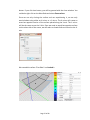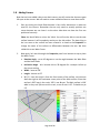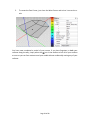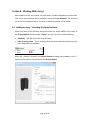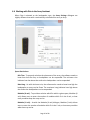
1
Updated 12/16/2014 Table of Contents 1. Introduction 2. Menu Features 2.1. File Menu 2.2. Edit Menu 2.3. View Menu 2.4. Network Menu 2.5. Options Menu 2.6. Tools Menu 2.7. Help Menu 3. Getting Around Resolution 3.1. Array View Window 3.2. Venue View Window 3.3. Project Explorer Window 3.4. Properties Window 3.5. Surfaces 3.6. Frequency Response Window 4. Network Configuration View 4.1. Adaptive Systems Network 4.1.1. The Private Network 4.1.2. The DHCP Network 4.1.3. The Dante Controller 4.2. Going Online 4.3. Assigning Physical Arrays/Modules to Modeled Arrays/Modules 4.4. Managing Arrays 4.5. Assigning Inputs 4.6. Selecting Analog or AES Input 4.7. Selecting the Net or Net Aux Input 4.8. Adaptive Systems Diagnostic Window 4.8.1. Overview Tab Page 2 of 89 4.8.2. Meters Tab 4.8.3. Maintenance Tab 4.8.4. Temp Log Tab 4.8.5. Impedance Log Tab 4.8.6. Error Log Tab 4.8.7. Acoustic Measurements Tab 4.8.8. Adaptive Healing 5. Entering 3D Audience Areas 5.1. Modeling Basics 5.2. Surfaces 5.3. Options for Adding a New Surface 5.4. Adding a Balcony 5.5. Front of House Position 5.6. Adding a Stage 5.7. Adding Sides 5.8. Adding Corners 6. Working with Arrays 6.1. Adding an Array - Launching the Array Assistant 6.1.1. Array Settings 6.1.2. Coverage Goals 6.2. Differences between Line Arrays and Anya Arrays in the Assistant 6.3. Modifying An Array 6.4. Working with Otto in the Array Assistant 6.5. Working with Otto in the Properties Window 6.6. Working with Otto in the Array View Window 6.7. Going online with Otto 6.8. Find Me (Trilateration) Page 3 of 89 7. Appendix 7.1. Anya Voicing’s 7.2. Exporting from Resolution into EASE 7.3. Upgrading Firmware on Adaptive Modules 7.4. Further Resolution Support Resources Page 4 of 89 Section 1 - Introduction EAW Resolution™ 2 is a tool to assist sound system designers and engineers to select, configure, and implement EAW loudspeaker products. Resolution™ 2 predicts direct sound pressure level (SPL) in a ‘virtual’ venue. Signal processing can be applied in software, and the resulting frequency response calculated for ‘virtual microphones’ throughout the model. Additionally, Resolution™ 2 performs mechanical calculations for a given array or loudspeaker configuration to assist the user in correctly rigging their sound system. As compared to previous versions of Resolution™, version 2.0 (and higher) adds threedimensional visualization capabilities, as well as design and control capabilities for EAW Adaptive Systems™. A Note about Compatibility with Resolution™ 1 Models Though Resolution 1.x models are displayed in two dimensions, Resolution 2 will accept and open these files without issue. Users should expect the same acoustical results in both software versions, but may also gain additional insight into a Resolution 1 model viewed in Resolution 2 due to the enhanced three-dimensional viewing options available. Due to the significantly more complex audience area data in Resolution 2, however, these files will not open successfully in Resolution 1. If users wish to maintain Resolution 1 compatibility for a given file, they should not save it in Resolution 2, or should maintain a separate copy of the original file. System Requirements Resolution 2 is designed to run under Windows 7, 8 and 8.1. Though processor speed and memory size primarily impact only calculation time, the following specifications are recommended for useful operation: Processor Memory Operating System Storage Resolution MINIMUM REQUIREMENTS RECOMMENDED SPECIFICATIONS 2.2 GHz Dual Core Processor 2.8 GHz Quad Core Processor 2 GB RAM 4 GB RAM Windows 7 / Windows 8 / Windows 8.1 1 GB available HD space 1024 x 768 minimum display resolution Page 5 of 89 Section 2 - Menu Features 2.1 File Menu A Resolution File contains venue and loudspeaker information. The following options are available from the ‘File’ drop-down menu: New - Creates a new Resolution File (clears all data in the current model). Open - Opens a Resolution (.eawresolution format) File. Save - Saves the current settings to currently open Resolution File. Save As… - Saves the current settings to a Resolution File under a new name. Import - Used to place previously-saved .eawvenue or .eawarray files into the default Resolution file folders. Once imported, the files can be found using the “Load Preset” button for either venue or array. Export EASE File - Exports the current design as a file that is compatible with EASE software (for more detail about this, see our EASE Export Tech Note) Create PDF - Outputs information for each loudspeaker array utilized in a Resolution file Create CSV - Creates a spreadsheet (readable via Excel) with all pertinent data of the design. Recent Files - Recall recently-used Resolution Files. Exit - Quits the Resolution software. 2.2 Edit Menu Undo - Undoes your last action. Redo - Re-does your last “undone” action. 2.3 View Menu Venue Configuration - Opens the “Venue Configuration” window, which displays the venue and array geometry in 2D and 3D views. Network Configuration - Opens the “Network Configuration” window, which allows access to loudspeaker control and configuration parameters, both ‘virtual’ (offline) and online. Page 6 of 89 Free View - Changes the Venue View screen to 3D view that can be rotated with the mouse. Side View - Changes the Venue View screen to show X and Z axis view. Top View - Changes the Venue View screen to show X and Y axis view Array View Window - Toggles visibility of “Array View” window, which displays physical configuration of array in section view. Project Explorer Window - Toggles visibility of “Project Explorer” window, which catalogs all loudspeaker and venue elements within the file. Properties Window - Toggles visibility of “Properties” window, which displays all available parameters for loudspeaker and venue objects, selected either in Project Explorer or directly in graphical Venue Configuration window. Array Names - Toggles visibility of array names. Aiming Lines - Toggles visibility of green aiming lines, which extend from the central axis of each loudspeaker until intersecting a venue surface. Aiming Coverage Lines - Toggles visibility of red coverage lines, which indicate ‘soft edges’ of system coverage (6dB down point). SPL - Toggles visibility of sound pressure levels. SPL (mic only) - Toggles visibility of sound pressure levels for microphones only. SPL Map - Toggles visibility of sound pressure levels in free space. Note: With SPL map disabled but SPL enabled, sound pressure levels will continue to be mapped to venue surfaces. Contour Lines - Toggles visibility of user selectable SPL dB down points (selected in Options menu) Frequency Response - Opens a secondary window showing the direct SPL response of your system based on the virtual microphones placed within the model Main Toolbar - Toggles the main toolbar on or off File Toolbar - Toggles the file toolbar on or off Edit Toolbar - Toggles the Edit toolbar on or off Page 7 of 89 2.4 Network Menu Connect - Poll network for all available devices. Refresh Network - Refreshes network connection on all available devices Disconnect - Discontinue network polling and disconnect from any connected network devices. 2.5 Options Menu Temperature and Humidity - Set the Temperature and Humidity of your venue. Changing these values will modify air absorption characteristics, and therefore resultant SPL on venue surfaces. These parameters are also used in calculating air loss compensation processing for products that support this feature. Without Air Absorption - Toggle between an SPL calculation with and without air absorption based on the user defined temperature and humidity values. Auto-Adjust SPL Range - Automatically determines the difference between highest and lowest SPL within a given file, and sets limits of SPL color scale to these values. SPL Interpolation - Affects how quickly an SPL map is created. Available settings are: Fastest SPL mapping is rendered in the shortest amount of time. To accomplish this, the resolution (detail) of audience area mapping is decreased. Normal Standard SPL resolution is used. This offers the best balance of resolution and calculation speed. Best SPL mapping is divided into multiple steps, beginning at low resolution and increasing as more time elapses. This provides the user with initial data in the shortest amount of time, but also provides higher-resolution information if given more time. Side View Contour Lines - Defines side view contour line SPL increments. In the side view, contour lines are positive (increasing) increments starting with the highest SPL value on the venue surface. Selectable in 1, 2 and 3 dB increments. Top View Contour Lines - Defines top view contour line SPL increments. IN the top view, contour lines are negative (decreasing) increments starting with the highest SPL value on the venue surface. Selectable in 1, 2 and 3 dB increments. Design Factor - Selects the design factor as it relates to the working load limits of a design. Resolution uses this selection to alert the user when stresses on loudspeaker rigging components have exceeded the selected design factor. Page 8 of 89 Note: ALWAYS READ AND ABIDE BY ALL RIGGING-RELATED WARNINGS AND INDICATIONS, INCLUDING USER MANUAL(S) AND PRODUCT-RELATED INSTRUCTIONS AND LABELS. FAILURE TO DO SO MAY RESULT IN INJURY OR DEATH. SI Units - All measurements are shown using the metric system US Units - All measurements are shown using the US system. Max SPL - SPL is measured as a maximum output per passband of a loudspeaker. Note: This may result in an unusual tonal response, since each passband is driven to its maximum output independently (i.e. if low-frequency components in a bi-amp system are capable of 6 dB more output than high-frequency components, the LF passband will display as 6 dB higher). Flat SPL - SPL is measured as the greatest output of a loudspeaker while maintaining a consistent broadband tonal response. 2.6 Tools Menu Recalculate - Recalculates the SPL map on the defined audience plane. Find Me (Trilateration) - Trilateration provides users with the ability to “map” a venue in 3D utilizing only two Anya arrays, a computer running both Resolution and Smaart, and a measurement microphone. Inventory Manager - Defines which EAW products are included in available loudspeaker models under the Array Assistant. This is particularly useful for rental firms, as it allows the product list to be narrowed to match their inventory. Under this window, users can also view the release notes for a product and access web-based data (requires an internet connection) via a hyperlink. Select from the list of Resolution-supported products available in your inventory. Unselected products will not appear in the property pane for use when building arrays. Firmware Manager - When online, polls devices on the network for their firmware options and provides means to update firmware when necessary. Automatically Check For Updates - When selected, Resolution automatically checks for updates every time the software is started. The computer must have internet access for updates to be downloaded. To ensure that Resolution is automatically kept as up-to-date as possible, it is recommended that users enable this setting. Check for Updates - Regardless of status of “Automatically Check For Updates” option, Resolution will immediately check for updates when this is selected. Page 9 of 89 Keyboard Shortcuts - Allows user to confirm and/or modify keyboard shortcuts, or restore defaults. 2.7 Help Menu Help - Displays this help file. About - Displays the version of the software. Page 10 of 89 Section 3 - Getting Around Resolution Resolution is segmented into four major sections or “panes”: Array View Venue View Project Explorer Properties Note: The relative size of each pane can be easily adjusted by dragging the borders between panes. 3.1 The Array View Window Pane Overview The Array View is located on the left side of the main Resolution window. This section of the software displays a side view of the currently-selected array, and includes information about suspension points and stresses on each critical point within an array’s rigging. At the bottom of this window, users can also find information about the array height, depth, vertical aim angle, and overall weight (including flybars). The information in this pane corresponds to the array selected from the tabs in the Property Pane. This Pane also displays the Design Factor used for the Resolution file, displays the array on a dimensioned grid, and allows access to an Auto Design feature for quick generation of a basic array. Arrays are displayed in profile (side view). If a specific array element is currently selected, it is highlighted in blue. The gray and blue lined grid in the background is a reference for real-world distances in the venue. An array is displayed with X and Y axis origins at (0,0) defined by the pick point at the fly bar. Line arrays are built from 1 or more items selectable and manipulated from the Properties Pane. Mechanical Loads For each array element (flybars, adapter bars, or loudspeakers), mechanical loads are calculated for each connection point to determine if the configuration is safe for suspension. Acceptable loads (within the user-specified Design Factor) are highlighted in green. Loads which approach stress limits are highlighted in yellow. Loads which exceed stress limits are highlighted in red. The actual load (in pounds or kilograms, Page 11 of 89 depending on which unit system is selected) can be viewed by hovering the mouse over it. NOTE: It is the user’s responsibility to ensure that rigging above the flybar (also referred to as “above the hook”) is suitable for suspension of the stated loads. Several other features of the Array View are called out in the image below. Connection point load status Flybar suspension point position Front pin assignments Rear pin assignments Currentlyselected loudspeaker Pullback (if used) Array Mechanical Summary Note: For clarification on the labeling of pin assignments for your specific product, consult your product’s Owner’s Manual. Page 12 of 89 3.2 The Venue View Window The Venue View provides a visual representation of the loudspeaker arrays, venue geometry, and sound pressure level (SPL) mapping for a given system. Resolution can display this information in three different ways. Top View SPL is mapped onto each surface as viewed from directly above (“in plan”). In this mode, it is possible to zoom in or out, as well as scroll horizontally (in both the X- and Y-axis) by simply clicking and dragging. Take care not to click and drag an audience area or loudspeaker while navigating. Side View SPL is mapped onto a cross-sectional ‘slice’ through the venue, as seen from the side (“in section”). The location (y-coordinate) of the ‘slice’ is defined by a field in the top-right corner of the window. In this mode, it is possible to zoom in or out, as well as to scroll horizontally and vertically (in the X- and Z-axis, respectively) by simply clicking and dragging. While in this view, users can select which Y-axis “slice” to view by manipulating the “Y:” value in the upper right-hand corner. Surfaces currently intersecting the Y-axis “slice” will be displayed with a thick blue outline, while those that do not are displayed with a thin blue outline. Page 13 of 89 Free View SPL is mapped onto each surface area, viewed in 3D. Users can manipulate the exact vantage point by using the mouse in combination with keyboard. In this mode, it is possible to zoom in or out, as well as to ‘orbit’ a center point in 3D by clicking and dragging. By holding the “Shift” key while clicking and dragging, this point can be shifted around the X-Y (horizontal) plane. In all three views, the user can zoom in or out by using the toolbar buttons or the scroll wheel on the mouse (if the computer is so equipped). Additionally, the X, Y, and Z axes are color-coded (X is red, Y is green, Z blue) and labeled with text in all three views for easy identification. SPL Scale On the right side of all three view modes, the SPL scale is displayed. Values range from low (bottom, dark blue) to high (top, bright red). The limits of the scale and therefore the resolution (dB of change per color change) are variable, however. To automatically set the range of the scale to the range of SPL in the current prediction, the user may use the “Auto-Adjust SPL Range” function (under the “Options” menu, or by pressing “A” with default keyboard shortcuts). For manual control, single-click on the SPL scale. Page 14 of 89 Main Toolbar A toolbar is also provided at the top of the window, allowing a number of Venue Window functions to be quickly accessed: Switch to Design View (currently selected) Toggle SPL On/Off Switch to Network View SPL (mic only) Add an Array Select Free View mode Clear All Mics Select Side View mode Unsolo All Arrays Select Top View mode Hide All Surfaces Zoom Out Lock Floors & Arrays Zoom In Reset View File and Edit Toolbar Two optional toolbars are available allowing access to additional quick access functions: File Toolbar Edit Toolbar Create New Project Save Project Open an existing Project Page 15 of 89 Undo Redo 3.3 The Project Explorer Window The Project Explorer Window provides a summary of all audience areas and EAW loudspeakers in the current model. Project Explorer Window Hierarchy This pane utilizes a tree organizational structure to allow the user to select which details are visible at any given time. The hierarchy of objects within ‘Arrays’ and ‘Venue’ are as follows: Arrays Array 1 [Example: Line Array] Array 1, Module 1 Array 1, Module 2 Array 1, Module 3 … Array 2 [Example: Anya Array] Column 1 Column 1, Module 1 Column 1, Module 2 Column 1, Module 3 … Column 2 Column 2, Module 1 Column 2, Module 2 Column 2, Module 3 … Notice that when users employ an Anya array, Resolution provides an additional subcategory of information, since each array can include multiple columns with each column containing a flybar and number of modules. Mechanically-articulated line arrays, on the other hand, only ever employ one column per array. Page 16 of 89 ‘Pop Out’ Window Project Explorer Window Buttons Close Window Surface/ Venue List Loudspeaker/ Array List When the window is ‘popped out’, it can be placed anywhere on the screen. In addition to clicking on the button, users can also simply drag the window to a different location on the screen. The window can be ‘popped in’ or docked by dropping it into the ribbon on either side of the Venue window. Venue Magnified View of “Venue” Heading and Sub-headings in Project Explorer Window Add Surface Load a Venue Preset Save Venue Preset Delete Surface Clone Surface Add Surface - Allows the user to input a completely new surface to the model. New surfaces will be displayed in a “tree” format under the venue. When a new surface is added to the model, the following options are available for that new surface in the project explorer window. Clone Surface - This allows you to make a complete duplicate of any surface in the venue tree and helps to speed up the process of building complex venues and listening environments. Remove Surface - This allows the user to remove the currently selected surface. You will be prompted before final removal of the surface. Page 17 of 89 Load a Venue Preset - Allows the user to drop a preconfigured and saved venue preset into the model. Useful for when the venue remains the same but arrays will differ from show to show. Files are identified as .eawvenue extensions Save Venue Preset - If the current model is a venue that the user will frequent, the room can be saved independently as a venue file in the software and recalled at any time. Venue files do not include any array data. Arrays Magnified View of “Arrays” Heading and Sub-headings in Project Explorer Window Delete Array Load Array Preset Clone Array Add Array Edit Array Save Array Preset Delete Array Item Launch Array Processing Launch Module Processing Upon initial start of the software, there will not be any arrays added to the model. In the project explorer window under Arrays the user can do one of the following: Add array - Launches the array assistant. Save an Array Preset - Stores the array as an array file. Load an Array Preset - Loads a previously-saved array file. Stored arrays are useful when the system design is basically fixed but the venue will change from show to show. Edit Array - Launches the array assistant as with Add Array, but already contains the current settings of the array. Page 18 of 89 Clone Arrays - Duplicate the current array and mirror or offset it. Launch Processing - Opens the processing window for the current array or module (depending on which Launch Processor button is selected). Allows access to Greyboxes, rear switch settings, parametric equalization, delay, gain, and highpass/low-pass parameters. If online with an Adaptive System, these functions are implemented in real time. Delete Array/Item - Deletes the array, column or module/item (depending on which Delete button is selected). Project Explorer Window Right-Click Functions A number of functions are available by right-clicking in various locations within the Project Explorer window. When an array is selected, the following options are available: When a module is selected, the following options are available: Page 19 of 89 In almost all cases, these functions duplicate those provided by the icons directly to the right of Project Explorer items. The exception to this is as follows: Insert item above/below - Adds an item above or below the currently-selected array item. This may be a flybar, adapter bar, subwoofer, or line array module depending on the type of item currently selected. 3.4 The Properties Window The Properties area is divided into two columns. On the left is the property and on the right is the value. The property column is fixed and cannot be altered. The value area is where adjustments are made and access to the value is achieved by clicking in the associated box on the right. Front of House (FOH) a. Select on which surface FOH will be placed. b. X - Select the distance along the X-axis where the FOH location will be placed. c. Y - Select the distance along the Y-axis where the FOH location will be placed. Temperature and Humidity This area allows the user to define the current temperature and state of humidity within the venue. This is extremely important when taking advantage of the air-loss compensation feature available in EAW, DSP driven products. Temperature - Enter the current temperature within the venue. This value can be updated at any time. Humidity - Enter the current humidity within the venue. This value can be updated at any time. SPL Options The user has the option to let the software automatically adjust the SPL range for selected loudspeakers in the design or else manually set the upper and lower extremities of the measurement. The user can also select specific frequencies to map in the model. Min SPL - Select the minimum amount of SPL that will be displayed in the SPL map Max SPL - Select the maximum amount of SPL that will be displayed in the SPL map. Page 20 of 89 Display Mode - Select the range of frequencies that will be plotted within the SPL map. Frequency - If 1/3 octave, 1 octave, or 3 octave range is selected, the user must select an appropriate frequency to be mapped. 3.5 Surfaces Once surfaces have been added to the venue, the actual dimensions and conditions of the surface will be adjusted in the properties pane. Clicking in the value column on the right side of the window will allow editing of the surface parameters. Name - Naming your surfaces is highly recommended as it is easy to lose track of the running order of surfaces in complex designs. Click on the current name of the surface to edit. Start - Each surface must have an origin to determine where it will lay in the model. The origin of the surface can be anywhere you like. The (X,Y,Z) coordinate for each surface is defined as the front, center point. All movement and rotation is relative to this point. X - Where along the X-axis the surface is centered. Y - Where along the Y-axis the surface is centered. Z - Where along the Z-axis the surface is centered. Length - The total length of the surface from the defined origin. Width - The total width of the surface along the Y-axis (y-axis measurements will expand equally in both directions from the origin). Inclination Angle - If the surface has a rake such as can be found in a theatre or balcony, enter the inclination here. Rotation Angle - If there is a rotation required for the surface (such as in large arena designs), enter the rotation angle here. Ear Height - The vertical offset from the defined surface to the audience ear height. This surface is used for acoustic model calculation (i.e. as the target coverage area for the Array Wizard), the insertion height for virtual microphones, and the mapping surface for SPL. This can be defined for each surface independently, and chosen from four possible options: Floor - The audience ear height is on the floor surface. Page 21 of 89 Seated - The audience ear height is defined as 3.5 feet (approx. 1 meter) above the surface. Standing - The audience ear height is defined as 5 feet (1.5 meters) above the floor surface. Custom - Any custom value can be entered into the field. Hidden - Checking the “hidden” box will make the surface opaque and remove it from the SPL calculations. The surface will still be included in Array Wizard calculations -- if you wish to remove it from these calculations, delete it from the model. Locked - Surfaces cannot be accidentally moved or altered in the model. Once you have completed a surface, it is highly recommended that you lock it to prevent accidental changes. Page 22 of 89 3.6 The Frequency Response Window Resolution offers the capability of displaying the calculated frequency response at one or more locations in a venue - called ‘virtual microphones’ - representing the direct sound (without the effect of room acoustics) at that location. Additionally, it is possible to store these measurements, modify the model, and then compare to new measurements. Accessed from the View menu, or from the shortcut key “f”, the window appears as follows: Vertical Zoom (in/out) Average Response Virtual microphone responses Snapshot Enable/ Disable Microphone selection/ visibility The average response is always displayed in white, and each virtual microphone response is displayed in the color with which the microphone is highlighted in the Venue view. Single-clicking a microphone color in the lower right-hand corner highlights that measurement. Double-clicking toggles the visibility of that measurement. Note that the average response is calculated from all virtual microphones in the model, regardless of whether they are visible or not. Note that in addition to the +/- zoom buttons, the mouse scroll wheel also functions to adjust vertical zoom. Clicking and dragging within the frequency response window also slides the vertical scale up and down. Page 23 of 89 When “Show Snapshots” is selected, an additional pane is displayed: This pane adds the ability to store each microphone, give it a label and toggle visibility. To store a snapshot, single-click the lower right-hand corner microphone you wish to store, and then click Capture. Alternately, simply click Capture All to store all virtual microphones. The default label for each will then be “mic @”, followed by the (X,Y,Z) coordinate of the virtual microphone. Note that the average response cannot be stored as a snapshot. To delete a virtual microphone snapshot, select that snapshot from the Snapshots list and click Delete. Note that users can delete more than one snapshot at a time by shiftselecting (to select the range of snapshots between the first and last snapshot clicked) or control-selecting (to select only the snapshots that were clicked), followed by the “Delete” button. Page 24 of 89 To export a CSV file containing the frequency response data, right click on the Frequency Response window and select Export to CSV. This will copy all frequency response data into a .CSV file which can be saves for analysis in third party programs such as excel. Page 25 of 89 Section 4 - The Network Configuration View The Network Configuration window provides control and monitoring of all Adaptive loudspeakers in the currently loaded Venue. All other loudspeakers (self-powered and passive) will be represented, but the current version of Resolution only supports control and monitoring of Adaptive products. This mode can also display the Array View, Project Explorer and Properties windows in addition to the list of Online Devices and the Arrays and Loudspeakers area. To switch to the Network Configuration View, either select View>Network Configuration from the Menu bar or click the Network Configuration view button on the Tool Bar. This will change the Tool Bar to display the Design View and Network Configuration View buttons along with buttons for Auto Identify, Upload Array Parameters and Add Array. Switch to Design View Add Array Switch to Network View (Currently Selected) Auto Identify Toggle On/Off Upload Array Parameters Page 26 of 89 Auto Identify Enabling the Auto Identify button will trigger the white LED indicator on an Adaptive Module or modules in an array to turn on when selected in the Online Devices list or in the currently assigned Anya/Otto arrays in the Venue window. Selecting a single Adaptive Module will turn the LED on that one module, selecting an array will turn on all the LEDS in that array. This is especially helpful when assigning the physical arrays displayed in the Online Devices list to the arrays in the Venue model. Upload Array Parameters Clicking the Upload Array Parameters button will send all signal processing including Adaptive Performance processing and user signal processing to the appropriate Anya/Otto Modules. The status screen will indicate if this process completes successfully. If an error occurs, exit the status screen and select Upload Array parameters again. This button will be greyed out if adaptive performance calculations are incomplete. If calculations are complete but modules are not assigned, the button will remain clickable but will present an error, “Please make sure loudspeakers are connected to the network and assigned”. Add Array Clicking the Add Array button allows you to add more arrays to your design and works as described in the Design View section. 4.1 Adaptive Systems Network There are two typical Network scenarios depending on how you set up your Network IP addresses: A default Private Network (using automatic private IP addressing) A DHCP Network (using an additional network switch with internal DHCP server) *Refer to Audinate and Netgear documentation for additional information on implementation of Ethernet and their products. Support for the Netgear® Prosafe® 16-Port Network Data Switches [GS716T-200] can be found at: http://support.netgear.com/search/GS716T-200 Support for the Dante http://www.audinate.com digital audio network can be found at: 4.1.1 The Private Network Each Adaptive System includes some number of Netgear switches depending on the Page 27 of 89 number of modules included in the system. These switches do not include a DHCP server. Each Anya module includes an Audinate Dante Network Interface Card (NIC). If the module does not detect a DHCP server on the network, then all modules will default to the Private Network range of IP addresses and each module will select a unique IP address from the following ranges: Primary Network (in redundant networks) and non-redundant networks o IP Address Range: 169.254.###.### o Subnet Mask: 255.255.0.0 Secondary Network (in redundant networks only) o IP Address Range 172.31.###.### o Subnet Mask: 255.255.0.0 The computer running Resolution 2 connected to the network can automatically select an IP address in the primary network range if no DHCP server is detected on the network, but it generally is a best practice to manually assign your computer IP address and Subnet Mask in the Private Network range to speed up the discovery process. A computer on the Secondary network must be manually assigned an IP address in the range 172.31.###.###. *Note: All Adaptive modules and the control computer must be connected to the same network! All Primary Ethernet ports on every Adaptive module must be connected to the same Primary network on the switches and Secondary ports to Secondary network on the switches. All switches must be linked Primary to Primary, Secondary to Secondary. Any Dante source device such as mixing consoles must also be connected to the same Primary and Secondary networks. Page 28 of 89 4.1.2 The DHCP Network You may find it useful to add a network switch to your FOH position (two switches or a switch with redundancy for redundant networks) to connect your Dante enabled mixing console or outboard Dante on-ramp and your control and monitoring computer running Resolution 2. This can be particularly useful if it has an 802.11n wireless router allowing you to use a remote desktop app on a tablet or another notebook computer to make system adjustments from anywhere in the venue. *Note: The Dante protocol does not permit wireless adapters to be used for control or audio streaming. *Note: Careful consideration should be given to leaving your system connected to any WiFi enabled network. EAW recommends disabling any wireless access during a show to prevent any unauthorized access to your system. You should enable extremely robust security measures as a minimum. Be sure any network switch you connect meets all of the minimum requirements required for a Dante network. EAW strongly recommends a Gigabit switch as a minimum. Gigabit switches are required if audio is sent over the Dante network. When redundancy is used, all locations in the network require redundant connection, so two switches (with DHCP) must be used. When Anya detects the DHCP server, then all modules will receive their IP addresses from the server. You can also set your computer’s networking settings to “Obtain IP Address automatically” in Windows, further simplifying the network setup process. 4.1.3 Dante Controller EAW recommends installing the Dante Controller application on your computer to give you better visibility and control over the entire Dante network. This is especially true when other non-EAW Dante devices (such as a mixing console with Dante network connections) are connected to your network. The Dante Controller software can be downloaded from the Audinate website. *Refer to Audinate documentation for additional information on implementation of Ethernet and their products. http://www.audinate.com 4.2 Going Online (Applies to Adaptive systems only) Before going online, be sure your computer is connected to the same Ethernet network as the Adaptive loudspeaker system. Communications is established by Page 29 of 89 clicking Network on the Menu bar and selecting Connect. Resolution 2 will then search for any Anya devices on the network and displays them in the Online Devices list. This list will include your computer running Resolution 2. Anya Module Green indicates module assigned to modeled array and properly connected. Anya Module Orange indicates module out of sync with the Resolution model. Anya Module Black indicates module appears on the network but has not been assigned to any array in the model. The Anya devices with be grouped according to how they are physically arrayed, so if you have assembled an array of two Anya modules in a single vertical column, those will be listed as: Array # Column 1 EAW-ANYA-##### EAW-ANYA-##### ……. Column 2 EAW-ANYA-##### EAW-ANYA-##### ……. ..and so on. If an array does not automatically group; right click Online Devices select Refresh Neighbor List The names of the individual modules in that Column will be listed in the order they are physically arranged. Stand-alone modules will be listed individually. Page 30 of 89 4.3 Assigning Physical Arrays/Modules to Modeled Arrays/Modules **EAW’s recommended best practice for Adaptive systems is to create your venue in the Design View and determine the optimum arrays needed to provide the coverage you will need prior to assembling, flying, energizing and connecting to the system. This will ensure you know how the Arrays will need to be configured. However, this is not required and you can simply fly the arrays and connect Resolution 2 to your system with a blank Venue loaded if needed. Note that the Adaptive Performance processing for Adaptive Systems will be calculated for any venue surfaces (or areas of coverage) in the model. It is best to at least enter a simple representation of the area you intend the Adaptive System to cover. Adding arrays in the appropriate positions prior to going online will speed connection time allowing you to upload settings as soon as you associate a modeled Array with its physical Array. If you have not defined any Arrays in your Venue, then you can simply click on each Array in the Online Devices list and drag them over to the Network Configuration desktop. This will open the Array Assistant dialog. Once you enter the settings and click finish, Resolution 2 will create an icon with the name of the Array, the list of arrayed modules in each Column in the Array, an Array Mute button, Input Level and Gain Reduction meters. Array Name Adaptive Module Module Status Indicator Module Status Array Mute You can edit the X,Y,Z physical location, Min Trim, Max Hang and Aim Angle in the Properties pane while that Array is selected. If you have created a venue and arrays in Resolution, then “virtual” Arrays and Modules in your model will be displayed in the Network Configuration View as grey boxes. Each module in the array will have a small indicator square that reports each module’s status. Page 31 of 89 A question mark indicates that no physical module has been associated with the module in the model. A Yellow box indicates a module that has gone offline. A Red box indicates a module previously assigned that was not found upon reconnecting to the Network. A box that occasionally flashes Green indicates the module is successfully communicating with Resolution. Unassigned modeled Arrays will have the list of modules or loudspeakers included in the Array while non-arrayed loudspeakers will be shown as individual boxes with only one device listed. Adaptive Arrays will be shown with the modules in Columns and the meters. A physical Adaptive Array in the Online Devices list can be assigned or associated with a modeled Adaptive Array in the model by simply clicking on the Array in the list and dragging it on to the appropriate modeled Array. Note: the physical Array and modeled Array must include the same quantity and arrangement of Anya modules). For example, assume your model includes two Anya Arrays and you’ve named them as “Left Array” and “Right Array”. You have assembled two, two-module arrays on-site and physically mounted them in the corresponding positions in your model. Click on an Array in the Online Devices list, observe which physical array has LED lights turned on (be sure Auto Identify is enabled) and drag the Array over and on top of the corresponding Array in the model, i.e., the left physical Array on the “Left Array” in the model. Proceed with assigning any remaining physical Arrays to modeled Arrays until all Arrays have been assigned. *Note: While we may think the LEDs are very pretty and cool, it is probably a good idea to remember to turn Auto Identify off before the show starts!! Page 32 of 89 4.4 Managing Arrays Once a physical Array has been associated with a modeled Array, the individual modules listed in the Array will be graphically arranged in Columns and a small square “indicator light” for each module. These indicators will periodically flash green to confirm that Resolution 2 has established active communications with each Anya module. Clicking an Array in the Network Configuration Desktop will display it’s properties in the Properties View window (if you have the Properties View window opened) and can be edited as explained in the Properties View chapter. Array Processing can be displayed and edited in real-time by double-clicking the EQ graph at the top of the Properties View window. Right clicking an Adaptive Array will open a menu with options to open Array Processing, Unassign All, Edit the array (which will launch the Array Assistant), Clone the array, Save Array Preset, Lock array movement, or Remove array. These mirror functions available in the Project Explorer and Properties panes. Double clicking the name of an Array will open the Array Configuration dialog. Page 33 of 89 Right clicking an Adaptive module in an Array will open a menu with options to Insert Item Above, Insert Item Below, Unassign, or Remove Array Item. Double clicking an Anya module will open the Diagnostics Window for that module: Page 34 of 89 4.5 Assigning Inputs Inputs may be assigned by double-clicking the name of an Array. This opens the Input Configuration dialog box where you can select how you will feed audio to the Anya System. Following are the available options based on the Mode you select Mode Master Dante Source Dante Channel None N/A N/A N/A Analog Select which physical Module is receiving the analog audio signal N/A N/A AES L Select which physical Module is receiving the AES/EBU audio signal (left AES channel). N/A N/A AES R Select which physical Module is receiving the AES/EBU audio signal (right AES channel). N/A N/A Net N/A Select which device, typically the house console or Dante onramp device Select either the Main or Aux Channel Net Aux N/A Select which device, typically the house console or Dante onramp device Select either the Main or Aux Channel *Note: You may receive a yellow banner with a warning that “Network settings out of sync: one or more input modes out of sync.” with Dismiss and Select Inputs buttons, or Dismiss and Sync Now buttons (depending on which parameters are out of sync). Clicking Select Inputs opens the Input Configuration dialog box, allowing this parameter to be confirmed for all modules. Clicking Sync Now synchronizes the EQ and processing parameters for all modules with the Resolution model. WARNING: IT IS CRITICAL THAT ALL PARAMETERS ARE SYNCHRONIZED FOR ANYA TO FUNCTION PROPERLY. LISTENING TO ANYA ARRAYS WITHOUT FULLY SYNCHRONIZED PARAMETERS OR WITH NETWORK ERRORS MAY PRODUCE UNEXPECTED ACOUSTICAL RESULTS AND IS NOT RECOMMENDED. Page 35 of 89 4.6 Selecting Analog or AES Input Checking the On-ramp box tells the Adaptive Module to transmit the incoming analog or AES-EBU audio signal over the Dante network. Select which input you wish to use, Analog, AES L or AES R, then select which physical Adaptive module will receive the signal. All other modules in the Array will be automatically configured to receive the Dante audio signal from the transmitting module. No further input assignments are required for that Array. WARNING: Users should not loop than two modules with AES/EBU. Doing so will degrade the AES signal resulting in unpredictable behavior. Page 36 of 89 4.7 Selecting the Net or Net Aux Input Un-check the On-ramp checkbox and select which Dante Network you want to use, Net Main or Net Aux, then select which Dante channel you want the Array to receive. This may be an Adaptive module transmitting an Analog or AES input or other Dante on-ramp source such as your Dante equipped digital mixing console. All other Adaptive modules in that Array will automatically be configured to receive the Dante audio signal from that source. Repeat the Input Source assignment for the remaining Arrays in the system. If the remaining Arrays in the system are to receive the same signal as the first Array, then select Net, then the Dante Source transmitting device such as the Anya module receiving the Analog or AES audio Input. Page 37 of 89 4.8 Adaptive Systems Diagnostics Window Any connected Adaptive module may be monitored and managed by doubleclicking the individual modules in each Array. This opens the Diagnostics window for the selected module shown below: 4.8.1 The Overview Tab The Diagnostics window opens to the Overview tab. This displays information about that specific module’s electronics unit including: The module’s Network Name The Product Name The currently installed Software Version The currently installed Firmware Version The currently assigned IP Address The unique MAC Address of the module The available RX channels The RX latency The available TX channels The X axis Tilt angle The Y axis Tilt angle A field for entering any relevant information you wish to record about the module such as the S/N of the loudspeaker the module is installed on, dates any transducers that have been replaced, dates of service and service performed, date of the last maintenance performed, etc. Page 38 of 89 4.8.2 The Meters Tab The Meters tab displays the levels of each amplifier channel in real-time along with a Gain Reduction meter to indicate any system limiting. The meter is scaled in a “VU” format to emulate traditional analog metering. 4.8.3 The Maintenance Tab The Maintenance tab displays the current Amplifier Temperature (in SI or US units based on the settings in Resolution 2 Options), calculated Impedance, Amp Protect status and Amp Status for each amplifier channel in the module. Page 39 of 89 4.8.4 The Temp Log Tab The Temp Log tab displays a log of operating temperature of each amplifier channel over the previous 24 hours of run time with a Timestamp for each entry in the log. Temperature will be displayed in C even when US units is selected. This tab includes Fetch button to refresh the log Export button to export the log to a text file Import button to allow an exported file to be read. The Export and Import buttons are provided primarily to help EAW Support, Service and Engineering troubleshoot problems should they arise in the future. 4.8.5 The Impedance Log Tab The Impedance Log tab displays a log of calculated impedance of the load on each amplifier channel over the previous 24 hours of run time with a Timestamp for each entry in the log. This tab includes Fetch button to refresh the log Export button to export the log to a text file Import button to allow an exported file to be read. The Export and Import buttons are provided primarily to help EAW Support, Service and Engineering troubleshoot problems should they arise in the future. Page 40 of 89 4.8.6 The Error Log Tab The Error Log tab displays a log of any errors reported over the previous 24 hours of run time with a Timestamp for each entry in the log. This tab includes Fetch button to refresh the log Export button to export the log to a text file Import button to allow an exported file to be read. The Export and Import buttons are provided primarily to help EAW Support, Service and Engineering troubleshoot problems should they arise in the future. Page 41 of 89 4.8.7 The Acoustic Measurements Tab The Acoustic Measurements tab provides the Adaptive self-diagnostics functions. The window lists all the transducers with Solo, Sweep select box and Progress status for each transducer along with Calibrate, Measure and Cancel buttons. As with any dual FFT measurement system, performing Calibration and diagnostic Measurements should only be performed in a relatively quiet space. Excessive ambient noise can cause measurement errors and inconsistencies. Calibrate Calibrate allows you to create new reference impedance and response measurements for use by Adaptive products for diagnostics. This should be used whenever a transducer has been replaced. Select which transducer you need to calibrate and click the Calibrate button. Anya will generate a very short noise burst (about 6ms) and capture impedance and frequency response measurements with the internal microphone. It will perform the measurements three times for each transducer and verify the measurements are consistent. This is to ensure the measurements are valid and have not been contaminated by excessive external noise. If the measurements are not consistent, then the measurements will be repeated. Once a valid measurement has been made, Anya will store the averaged results as the reference for that transducer. This will be the reference used to compare to diagnostic Page 42 of 89 measurements in the future. Total time to complete the process for all transducers in an Anya module will be about 5 minutes. *Note: The noise burst stimulus will sound like a “popping” noise due to the extremely short duration. This is normal and should not be interpreted as any fault in the system. Measure Measure allows you to perform diagnostics to check the health of the Anya module. To start the diagnostics function, check the Sweep box for each transducer you wish to measure, click the Measure button. Anya will perform the same measurements as the Calibrate function and compare the average of the three measurements with the reference stored in the internal memory. Resolution 2 will then display a Pass or Fail result for each transducer. Cancel Clicking Cancel during a Calibrate or Measurement routine will stop the measurement. 4.8.8 Adaptive Healing In the event that an Adaptive Module which is part of an array is unassigned, or goes offline, Resolution gives the user the ability to heal around those missing modules when the Upload Array Parameters box is selected. When the user opts to ‘exclude these modules and recalculate’, Resolution will generate a new acoustical model, taking into account the missing module and optimizing the sound system given the available online modules. Once an option is chosen and the network is refreshed, the dialogue will not appear until the modules in the system unassigned, then reassigned accordingly. Page 43 of 89 In the event that a fault is detected within a specific module due to either an amplifier or transducer failure, Resolution gives the user the ability to exclude the faulty cells from the parameter calculation, optimizing the system for this condition. To heal around the failures, select Yes, exclude and recalculate, or select Ignore to proceed without adaptive healing. Page 44 of 89 Section 5 - Entering 3D Audience Areas Familiarize yourself with Resolution’s features by going over Section 3 - Getting Around Resolution before starting to model your venue. 5.1 Modeling Basics When you first open Resolution, you will be met with a very basic venue setup. This is a starting reference which will show a single, small surface and the Front of House mix position. Because we are working in 3D, it will be important to understand and remember the axis you will be working with. X = Depth (red line) Y = Width (green line) Z = Height (blue line) As you free rotate around the model, these references will track along with your moves to remind you of your viewing perspective to the model. You will also notice that the entire model is set up on a grid. When working with Imperial units of measurement, these grids are setup in 10’ x 10’ divisions. When working with the metric system, the divisions of the grid spacing are 5m x 5m. Zoom - You have the option of using the mouse wheel to roll in and roll out on your model, or you can hold down the CNTRL key while depressing the + or - keys on your keyboard. Plus will zoom in and minus will zoom out. Pan - First hold down the SHFT key on your keyboard and then left click and hold your mouse in any free area of the model not already containing room or array model images. Now simply move your mouse left, right, up or down to pan around your model. Rotate - When in three dimensional view of your model, global rotation is achieved by again finding a free area within the model, left clicking on your mouse and moving your mouse around to allow for global movement around your model. Front of House - The Front of House (FOH) mix position will always be part of your model and cannot be removed. It is important to be able to see what the engineer will hear and where they will be placed as this will have an impact on the overall result of your design. Placing the Front of House position seems basic but it is very important to Page 45 of 89 your overall design result. Left-click and hold on the Front of House position to freely position it around the listening surface. Editing Surfaces As you hover your mouse over a surface, you will notice rectangular blocks that become visible on each side of the surface and squares that become visible on each corner. These blocks allow you to grab and alter the dimension of the surface. This is a coarse way of adjusting a surface but once roughed in, editing the dimensions is easy using the Properties pane. Once a rectangle on a surface has been selected by left-clicking and holding on it, you are able to pull on that surface from the rectangles location. Raising or lowering your mouse while holding the rectangle will adjust the inclination of the surface on that particular side. Left-clicking and holding a square on each corner of the surface adjusts all sides together allowing you to increase or decrease the entire size of the surface while also allowing transformation from square to rectangular surfaces. Inclination changes are not available with the corner squares. 5.2 Surfaces Beginning with a new file, Resolution 2 opens with a surface already in the Venue View that has starting coordinates of (0, 0, 0). When you select this surface, you can see all of its values in the Properties pane, including a default value for the length and width of the surface. The selected surface is highlighted in blue in the Venue View. Page 46 of 89 The origin of the model is important to understand as it will have an effect on the flow of work. The direction you choose to take will impact where the origin lies. If you are only concerned with what’s happening in front of the arrays, you can simplify the build by starting your model at the origin. You may also use the origin to show the center of the room and build around that origin 360 degrees OR you can leave the origin with the arrays and still build behind it. There are no restrictions so choose the best way to model your venue go get the best results. For our first example, we will leave the origin with the arrays representing the downstage edge of the stage. We will work through the Properties pane setting the values for our surface. It is best practice to enter a Name for the surface to keep track of each surface as you move along creating your venue. 1. Enter the Start values. The Start coordinates refer to the front center of the selected surface. From the desired room origin of your venue, determine the values of the starting coordinates (X, Y, and Z) of your first surface and enter them into the values side of X, Y, and Z in the Properties pane. Since we are doing a simple model, we will leave the X and Y origins at zero. This means that the surface will be centered with the Y dimension and it will begin right at the X origin line. What we will change about the origin is the origin on the Z axis which determines the overall height of the surface. Page 47 of 89 There are two options to choose from to determine what your surface is representing: The actual structure of the building (concrete or wood surfacing) The heads of the people in the audience (listening area). This option is much more advisable because the structure is not what we are concerned about when focusing loudspeakers. Our concerns lie with the impact to the listeners in the audience. For quick reference, a seated audience is roughly 3.5’ (1.1m) above the surface while a standing audience is typically 5.5’ (1.7m) above the surface. For our simple model, we will say that the audience is seated and will therefore enter 3.5’ (1.1m) into the Z value for surface origin. 2. Enter the Length and Width values of the surface. Measure the length (distance along x-axis) and width (distance along y-axis) of just this surface, and enter the values into the Properties pane while making sure the surface is still selected. Let’s enter 200’ as the Length of the surface and 100’ as the Width of the surface. You will notice that all the changes are reflected in your model in the Venue View. Remember: the Width measurement expands equally in both directions from the starting point of the surface, so your surface is still centered along the x-axis. 3. The next cell down is the Inclination Angle. This is to set a rake of the surface. The surface will begin an inclination beginning at the origin, and will incline on an angle that you determine. Inclination angles can be determined from room drawings but may also be determined on-site using an inclinometer tool. For our simple example, we have chosen 2 degrees as the Inclination Angle. Page 48 of 89 4. The next cell down is the Rotation Angle. In our simple model we will not need to rotate the surface, but in complex models this can be very handy especially when designing curved areas like the back of an arena. 5. Finally, there are two boxes that can either be checked or unchecked: Hidden - This is used when you want to omit the surface from SPL calculations. As an example, maybe you are only interested in viewing the main surface of a venue and there is a balcony in the way. By hiding the balcony, it will be disregarded in the SPL calculations even though it is still there and visible as an opaque surface. Simply uncheck the box to bring the surface back into the model for calculation. Locked - Many times during the creation of a model, the user may inadvertently move parts of the model while creating or viewing other items. By checking the “Locked” button, the user can be assured that the current surface cannot be moved accidentally or altered without unlocking it first. Now that the main surface is completed, go ahead and free rotate around the model to get used to viewing things from different angles. You can also snap to a section or plan view using the snap buttons located on the toolbar at the top of the screen. 5.3 Options For Adding A New Surface There are two options for adding a new surface to your venue. Let’s get an understanding of the difference between them before moving along in modeling our venue. Page 49 of 89 1. To add a surface from scratch, select the icon to the right of Venue in the Project Explorer pane. This will add a surface with the stating coordinates (0,0,0) in your Venue View. To save time, you could also right-click anywhere in the Venue View and select Add Surface. This will create a surface with the starting point located at where you right-clicked. You can then alter the properties of this new surface in the Properties pane, as we have done for the previous surface. 2. To Clone a surface, switch to the Project Explorer pane and click the the right of the surface you wish to clone. icon to Once clicked, a pane will come up on the screen for you to modify the conditions of the cloned surface. By just accepting it “as-is” the new surface will simply overlay the old surface and will not be visible. Making changes to the new surface using the cloning pane is as follows: NAME - select a name for the new surface MIRROR - There are two ways to mirror a surface o X - Mirror the surface against its X axis o Y - Mirror the surface against its Y axis OFFSET - You can preset new coordinates for the surface prior to it being cloned. These coordinates can be set on all three axis’ (X,Y,Z) Once you have set the parameters and coordinates for the cloned surface, simply click OK and the new surface will be created in the model. Most often, this will only be a rough placement that we will have to adjust, but it can be a little quicker than starting from scratch each time. 5.4 Adding A Balcony We want to add a balcony above the Main Surface in our model. Using the clone feature we can copy the width of the venue to the new surface even though all the other parameters will need to be entered manually. 1. To the right of “Main Surface” in the Project Explorer pane, click the Clone button, which will open up the cloning pane for us to set new parameters and coordinates for the cloned surface. Define a new name for the surface “Balcony” If you already know the coordinates of the balcony, you can enter some of them under Offset. Page 50 of 89 X - Where will the balcony face begin along the X Axis? (enter 100’) Y - Where will the balcony face center along the Y-Axis? (leave at 0) Z - How high will the balcony be at its front edge on the Z-Axis? (enter 25’). Note that the offset in the Z axis is based on height of the previous surface. Since we raised our main surface on the Z axis by 3.5’, the cloned surface will also be increased by a further 3.5 feet to whatever value we enter. If we enter 25’, the balcony will raise 28.5’. Hit the OK button and the Balcony will be added to the model. 2. Define the Properties of the cloned surface. You will notice in the model that the Length of the balcony is still 200’ which is not what we want. Select the new surface in the Project Explorer window which will reveal all the data of that surface in the Properties pane. We should be happy with the name and origin of the surface because we defined these when we made the balcony, but you are able to alter them if needed. Length - Reduce the length of the balcony to 100’ Width - The width can remain the same. Inclination Angle - Set the inclination angle to 10 degrees. You can now choose to Hide and / or Lock the balcony. Page 51 of 89 Now we can see a relatively basic venue setup comprised of two surfaces: a main surface and a balcony. These surfaces are representing the heads of the people so when we focus loudspeakers in the area, we know how the audience will receive the acoustical information. 5.5 Front of House Position One item that we should also consider altering is the position of the Front of House. It is extremely important to know what the engineer will hear when the audio is playing so placing the front of house accurately within the model is important. 1. 2. In the Project Explorer select “Venue” and the Front of House properties will appear in the Properties pane. For our model, let’s leave the Front of House position on the Main Surface but let’s move it to a little bit better location than where it currently is in our venue. Let’s start by changing its X location to 75’ Let’s put in 10’ in the Y location which will move the Front of House position 10’ to the right. A negative value would have moved it to the left. Page 52 of 89 5.6 Adding a Stage 1. Start by adding a new surface to the model. This time to add a surface we will use the Add surface option in the Project Explorer window next to Venue. Simply hit the + button a new, generic surface will be added to the model. We will have to manually enter in the data for this surface and since we are using it to build a stage, some negative values will be used. 2. 3. 4. Once the surface is created, it automatically highlights and its parameters are shown in the Properties pane. As we did earlier, begin by giving the surface a name. This one will be called Stage. Now we need to set the origin of the surface. Since the stage will be behind our origin marks, we will enter in an X-axis origin that is equivalent to the depth of the stage. This value will be entered as a negative value because we are going backwards. Our stage is 30’ deep so the value entered for the X-axis origin will be -30’ Our Y-axis origin can remain at 0 keeping the stage centered on the origin. The Z-axis origin can either be equivalent to the height of the stage or to the height of the artists on the stage. Since the artists are not part of the model in reality, we can simply put the Z-axis origin to the height of the stage. Enter 4’ as the Z-axis origin. Now the depth of the stage should match the negative offset that we put in for the X-axis origin. This will place the downstage lip precisely back to where the audience begins. Since our X-axis origin was placed at -30’ for this venue, we simply enter in 30’ for its Length and it will come back to the audience line. Page 53 of 89 A typical stage Width is usually around 40’ in width so let’s enter that as our width. Hiding the stage from the SPL calculations is optional but locking the stage once it has been properly defined is a very good idea to prevent accidental changes to it. If all of the surfaces that you have created are locked, you can now freely rotate the model without any fear of accidentally dragging surfaces out of position or changing their dimensions. 5.7 Adding Sides Let’s begin again with a new model so that we can create something more similar to an arena type design. Create a new Resolution file and the default layout will be presented. 1. Select the surface in the Venue View, or go to Venue in the Project Explorer pane and expand it to show the surface that is visible. It will be default labeled as “new surface”. Before going further, let’s give the surface a proper name. We are going to call it North Main. X, Y, Z origin of the surface - Since we are going to leave our position at the origin of the software, we will leave X and Y as it is but we are going to set the Z origin to 5.5’ representing a standing audience in this model. Length and Width - to keep things simple, let’s work in full numbers. Set the length of the surface to 200’ and the width of the surface to 100’ Our main surface is finished so let’s use the Locked feature so the surface cannot be accidentally adjusted. Page 54 of 89 2. Next, we want to include a raked seating area at the back of the house to represent bleachers. In the Project Explorer in the venue area click on the green + button to create a new surface. The new surface will be displayed with the default name so we want to change the name to North Rake in the Properties Pane. X, Y, Z - Since the first surface was 200’ in length, set the X origin of the raked surface to 200’. The Y origin can remain at 0 since we are going to remain centered. As I did with the main surface, set the Z origin of the raked surface to 5.5’ just to keep the model consistent. Length and Width - Set the length of the raked surface to 75’ and the width to match that of the main surface at 100’ wide. Inclination angle - let’s put in 20 degrees as the inclination angle. Now you can see the model taking shape. This completes the raked section of the model so like we did for the main floor surface, let’s lock it. Page 55 of 89 3. Next create a new surface in the Project Explorer pane. To keep track of the surfaces in our model, let’s call this surface the “West Rake”. To simplify a few things, we are going to work this surface in the Properties pane from the bottom up. This is because the Rotation Angle is taken from the center point of the surface, so when adding a Rotation Angle, the starting coordinates change. It is best practice to add the Rotation Angle first so you do not have to enter the starting coordinates twice. 4. Rotation Angle - rotate the surface 90 degrees. This will place the orientation of this surface at a 90 degree relationship to the main floor surface. If you look at the origin of this surface now you will see that it is not all zeros anymore. It is displaced due to the rotation of the surface. Inclination Angle - set to 20 degrees just like the rake at the back of the venue. Width - The width of the surface should match the length of the original surface so that they line up. Enter in 200’ for the width of the surface Length - translates into the “depth” of the surface when the orientation has been shifted to expand along the Y-Axis over the X-axis. Set the length of the surface to match the length of the North Rake, which is 75’ X, Y, Z - Since this surface starts halfway through the width of the main floor surface and the main floor surface is 100’ wide, it is simple to figure out that placing the surface along the Y-axis should be 50’. Since the surface Start point is halfway down the length of the main surface, it is easy to determine that to place the X-axis we would say 100’ To create the rake on the other side is exceptionally easy using the cloning feature. Simply select the raked surface that we just created up in the Project Explorer window named West Rake. Next to that title you will find the “clone” Page 56 of 89 button. If you click that button, you will be greeted with the clone window. You could also right-click on the West Rake and select Clone surface Since we are only cloning the surface and not repositioning it, we are only worried about using either an X mirror or a Y mirror. The X mirror will create an exact but opposite version of the surface placed along the X axis. The Y mirror will do the same across the Y-Axis. Since we need an equal but opposite surface on the other side of the venue, we will select a cloned surface mirrored to the Xaxis. We named this surface “East Rake” and Locked it. Page 57 of 89 5.8 Adding Corners Now that we have added rakes to our basic venue, you will notice that there are gaps left open at the corners. We will need to create rotated surfaces to cover these areas. 1. Start by cloning the North Rake because it has similar dimensions to what we need for the corners. Remember that we only need to actually position one corner because we can clone it to the other side when we have the first one positioned correctly. Clone the North Rake to mirror the X-Axis. You will not be able to see the new surface because it will completely overlay on the old surface. The best thing to do is as soon as the surface has been created is to head to the Properties to change the name of the surface to differentiate between the two. We have called this corner West Corner. 2. Now again, let’s work through the Properties pane from bottom to top to place the West Corner. Rotation Angle - set to 45 degrees to cut the angle between the West Rake and the North Rake. Inclination Angle - let’s increase this to 28 degrees for a steeper incline up the corner seating. Width - leave at 100’ Length - shorten to 55’ X, Y, Z - since the origin is from the front center of the surface, we know we want that right at the northwest corner point of the Main surface. Since that surface is 200’ long in the x-axis, 200’ is our X start. The Main surface is 100’ wide in the y-axis split across the x-axis, so our Y start is 50’. Z should stay at 5.5’ Page 58 of 89 3. To create the East Corner, just clone the West Corner and mirror it across the xaxis. You have now completed a model of your venue. If you have forgotten to Lock your surfaces along the way, simply select the icon in the toolbar to lock all of your surfaces at once so you can free rotate around your model without accidentally moving any of your surfaces. Page 59 of 89 Section 6 - Working With Arrays After audience areas are entered, the next step is to add loudspeakers to the model. This can be accomplished quickly and easily using the Array Assistant. The Assistant can be used to add point-source, line array or Adaptive systems to the model. 6.1 Adding an Array - Launching the Array Assistant Upon initial start of the software, there will not be any arrays added to the model. In the Project Explorer window under “Arrays” the user can do one of the following: Add Array - This will launch the Array Assistant. Load an array preset - This is assuming that you have previously saved array files contained within the software. When the + button is clicked in the Project Explorer window next to Array, or the “+” button on the tool bar, this will launch the Array Assistant. Page 60 of 89 6.1.1 Array Settings Page The purpose of the Array Assistant is to allow the complex software in Resolution to determine the proper placement and aiming of the selected loudspeaker(s) based on data inputted by the user. Before launching the Array Assistant, a complete model of the venue should have already been designed. The first page of the Array Assistant allows you to give the Array a name, define the compliment of loudspeakers you intend to use and information about its physical location. Array Name Enter any name you wish for the array such as “Left Main”, “Center Main”, etc. Page 61 of 89 Loudspeakers Determine if the array or loudspeaker will be ground stacked or flown. Select the product that will be used at the top of your array from the dropdown menu labeled Top. Only products that have been selected in the Inventory Manager will be visible in this dropdown menu. Select how many elements of that product are available to form an Array. This is a number that the software will draw from. It is not guaranteed that the exact number will be used but the software will not use more than what you say is available. Select the EAW Greybox that you wish to use with this product. Some products have multiple Greyboxes available while others may have only a single selection. If you are building an Array with a different model loudspeaker for the lower section, then select that model from the dropdown menu labeled Bottom. For example, you may want to build an array with KF740s on top with KF730s on the bottom. Select the EAW Greybox that you wish to use with this product. Some products have multiple Greyboxes available while others may have only a single selection. Flybar Some EAW products have more than one flybar available. A case for this is the KF760 which has two generations of flybars. This feature allows the user to select the flybar that they have in inventory. This is important as each flybar will produce a different set of mechanical data. EAW Flybars will also have a choice of hanging options. Some may have more than 3 so it is important to select what method you will use to hang your flybar. Array Location One final step on the first page of the array assistant will allow you to place the array within the model. Hang Point X - This allows you to place the loudspeaker or array along the Xaxis of the model. Normally this value would be set to zero but not always, especially when you are building a room model that is designed in a full 360 degrees. Hang Point Y - This allows you to place the loudspeaker or array along the Yaxis of the model. When left at zero, the array will present itself in the center Page 62 of 89 of the model representing a center cluster. Plus and minus measurements are used to place the array at its real separated distance. Aim Direction - If there will be a predetermined azimuth for the loudspeaker or array, enter that value here and the model will consider the aim angle when deploying the loudspeaker or array. Space Restrictions Min Trim - To properly calculate the placement of the array, the software needs to know how low the array or loudspeaker can be suspended. The minimum trim indicates how low above the surface the loudspeakers can be suspended. Max Hang - As with minimum trim, the software also needs to know how high the loudspeaker or array can be flown. The maximum trim indicates how high above the surface the loudspeakers can be suspended. 6.1.2 Coverage Goals page On this page, you will define what performance criteria you want Resolution 2 to calculate the Array configuration. Page 63 of 89 Array Options Allow Non-Incremental Splays - You can select or deselect the use of “NonIncremental Splays”. Some designers adhere strictly to a “spiral-array” approach of deploying line arrays. This means that the angles between enclosures will always increase from top to bottom. Others will allow the angles of the array to adapt to match the contour of the audience. If you choose to create spiral arrays, you would deselect this feature. Allow Front Splays - Front splays may also be selected. By default, the software has this feature turned off. Opening the fronts of EAW line array enclosures is possible but not recommended. Best results are obtained when the fronts are tight together but there are occasions when “audio triage” is necessary either to cover the entire audience due to an insufficient number of enclosures on hand or to try and split an array to miss reflections from a balcony face, etc. Coverage By default, Resolution uses the extremities of the listening area to determine coverage. However, there may be occasions when the entire venue may not need to be covered. Using the Coverage section, you may create a new listening area within the model without having to redesign the surfaces. Coverage is indicated within the model as a blue arc drawn on the X-Y plane. Modify Coverage Check the Modify Coverage box to open the feature. Enter in the closest distance to the origin that you are trying to achieve coverage. The software will cover as closely as possible to your desired coverage request. Enter in the farthest distance from the origin that you are trying to cover. Allow Upper Overshoot - By default, Resolution uses the extremities of the enclosure coverage to determine the end of coverage. These are also known as the “soft edges” of the coverage angle and although frequency response is still nominal in this region, the SPL will have dropped on average 6dB. Allowing the software to overshoot means the top of coverage is biased towards more “on-axis” response from the loudspeaker and the loudspeaker or array will point higher than the top of its coverage limit. The advantage to this is more SPL delivered to the back of the venue. Page 64 of 89 Coverage Goal The first slider named Coverage Goal effectively controls the trim height of the loudspeaker or array. By flying higher and tilting down more, we can provide a more even coverage of the SPL front to back of the venue. This is not always desirable as it does raise the array away from the front of the audience. Certain types of music such as heavy metal may actually prefer to have the array quite loud at the front. This feature is limited by the available height in the venue. SPL Requirement - The SPL Requirement slider can be used to define how many enclosures the software will pull to create an array (no more than what you entered as the max available). With the slider all the way left to “spoken word”, the software will pull the fewest modules possible to cover the audience area. If the slider is pulled full right to maximum, the software will pull all available enclosures as you had defined on the previous panel, maximizing SPL for that particular audience configuration. At this point, you can click the Finish button and allow Resolution to calculate the best possible placement and deployment of your loudspeaker or arrays. You may also click back arrow button in the top left corner to make edits to your arrays or click the Cancel button to abort the process and begin again. 6.2 Modifying An Array via the Array Assistant The process for modifying an array is identical to that of adding a new array, except that the Assistant auto-populates with the current settings of the array you are editing. Page 65 of 89 6.3 Differences between Line Arrays and Anya Arrays in the Assistant When Anya is selected as the loudspeaker type, the Coverage Goals dialogue is slightly different than with a mechanically-articulated line array. Array Options and Coverage are replaced with just Coverage. The user is able to define a horizontal coverage angle requirement, as well as “coverage start” and “coverage stop” distances (along the X-Y plane) for each Anya column individually. Options Columns driven uniformly - Selecting Columns driven uniformly will configure the system to provide the maximum output from all columns. This option should be selected if maximum SPL is desired at the cost of consistency over the audience surfaces. Columns driven Adaptively - Selecting Columns driven Adaptively will adjust the relative level between columns in the arrays in order to provide the most consistent SPL levels at the audience surface. This option should be used by default and will provide the most consistent SPL over the audience area. The Coverage Goal and SPL Requirement sliders function as they do with all other arrays. Page 66 of 89 6.4 Working with Otto in the Array Assistant When Otto is selected as the loudspeaker type, the Array Settings dialogues are slightly different than with a mechanically-articulated line array or Anya. Space Restrictions Min Trim - To properly calculate the placement of the array, the software needs to know how low the array or loudspeaker can be suspended. The minimum trim indicates how low above the surface the loudspeakers can be suspended. Max Hang - As with minimum trim, the software also needs to know how high the loudspeaker or array can be flown. The maximum hang indicates how high above the surface the loudspeakers can be suspended. Modules (X axis) - To provide a solution which fits within a given space, Modules (X axis) allows users to enter the number of modules which fit in the X axis, or how many modules deep the array can be. Modules (Y axis) – As with the Modules (X axis) dialogue, Modules (Y axis) allows users to enter the number of modules which fit in the Y axis, or how many modules wide the array can be. Page 67 of 89 Rejection Goal - On the second page of the Array Assistant for Otto, the ‘Coverage Goal’ and ‘SPL Requirement’ sliders function as they do with all other arrays. A third slider has been added which allows the user to input a desired ‘Rejection Goal’. The ‘Rejection Goal’ slider allows the user to choose ‘Max SPL’, ‘Max Rejection’ or points in between to achieve an appropriate balance between rejection and SPL depending on the application. Max SPL - Selecting ‘Max SPL’ will configure Otto to provide the maximum possible SPL over the user defined audience surfaces, or defined coverage areas in the Resolution model. Max Rejection - Selecting ‘Max Rejection’ will configure Otto to reject energy outside of the user defined audience surfaces, or defined coverage areas in the Resolution model. Maximum Rejection by default is opposite the primary coverage areas. Page 68 of 89 6.5 Working with Otto in the Properties Window The properties window for Otto is unique in that it includes a ‘Rejection Goal’ drop down menu. The Rejection Goal percentage mirrors the functionality of the rejection goal slider found on the Array Assistant page. Max SPL corresponds to a rejection goal of 0% whereas Max Rejection corresponds to a rejection goal of 100%. Selecting values of 25% and 50% and 75% allow the user to select a balance between Max SPL and Max Rejection according to the needs of the given application. Orientation - Selecting an individual Otto module in the ‘Project Explorer’ will open a ‘Properties’ menu unique to the module selected. From this properties menu the orientation of individual Otto modules can be rotated 90°. This allows the user to prevent driver apertures from being blocked in certain array configurations. Page 69 of 89 6.6 Working with Otto in the Array View Window The Array View window for Otto allows the placement of additional columns by right clicking on a module and using the Insert Column dialogue box. Ground Stacked Otto Arrays Flown Otto Arrays Insert column - As with other arrays, items can be inserted above and below existing array items by right clicking on them in the Array View, or in the perspective view. Unique to Otto is the ability to add elements to the right or left of the array when using a flown array. When Otto is being ground stacked, additional modules can be added in front or behind of the selected array. Page 70 of 89 6.7 Going Online With Otto When going online with Otto, Resolution presents the user with an Array Orientation promt. This window asks the necessary questions to determine how the Otto array is physically oriented with respect to the audience surfaces defined in the Resolution model. Choose Orientation – Select the orientation based on how the arrays are positioned, either Ground Stack or Flown. Select The Bottom, Front, House Left Module - From the perspective of the audience, Resolution requires that the bottom (-z), front (+x), house left (-y) model is selected. The LED’s on the modules will illmuniate when selected in this dialogue to make the easier to recognize. Page 71 of 89 Orientation Details – The orientation details dialogue will determine how the array as a whole is oriented, using the bottom, front, house left module as a reference. Has modules to the right will orient the array such that other modules in the array placed to the right of the bottom, front, house left module, or along the (y) axis. Has modules behind will orient the array such that other modules in the array are placed behind the bottom, front, house left module, or along the (x) axis. Page 72 of 89 6.8 Find Me (Trilateration) Trilateration provides users with the ability to “map” a venue in 3D utilizing only two Anya arrays, a computer running both Resolution and Smaart, and a measurement microphone. To utilize this feature, the following is needed: Two Anya arrays (i.e. stage-left and stage-right). At least one array must have two or more modules. The relative locations of the arrays (height and width) relative to one another must be known. A computer running both Resolution 2 and Smaart 7.2 or later (within one operating system; this cannot be split across multiple OSs via virtualization). An audio interface and measurement microphone. At least one transfer function must be configured in Smaart (a two-channel measurement). A stimulus (noise) source, either in Smaart or external, fed to both the Anya system and the reference channel in Smaart. A reasonable working knowledge of Smaart 7 and measurement best practices. Initial Setup To configure Smaart to work with Resolution, several configuration steps are necessary: Under the “Options” menu, select “General…”. Ensure that under “API”, “Enabled” is checked, and that the Port is set to 26000. Under the “Delay” tab (also under the “Options” dialog), select an FFT size that results in a time constant that is significantly longer than the longest time-of-flight from the array to the microphone. For more help in selecting an appropriate FFT size, consult the Smaart 7 Help File. For most applications, a 32k FFT with 3 averages will be sufficient with 44.1 kHz or 48 kHz sampling rates. This corresponds to a flight-time of approximately 700-800 feet. Go online and assign all Anya arrays. Step 1 Open the Find Me dialog, which can be found in the Tools menu. The following dialog box will be displayed: Page 73 of 89 Enter the exact name corresponding to the transfer function (TF) configured in Smaart: For “Column 1” and “Column 2”, define the two columns to be used for the measurement. These should not be columns within the same array. For the best accuracy, using widely-spaced columns is suggested (i.e. Column 1 is stage-left and Column 2 is stage-right). It is also recommended that the user select columns that are horizontally aimed at the microphone position. After this is complete, click “OK”. Page 74 of 89 Step 2 The following dialog will be displayed: This indicates that the entire Anya system has muted. The user should verify this by applying the stimulus source (noise) to the system. No noise should be audible from the system. This confirms communication with all modules. Click “OK”. Step 3 The following dialog will be displayed: This indicates that a single cell from one column has been unmuted. The user should then increase the noise output level (via the audio interface, mixer, or both) until a suitable balance between measurement and reference channels is achieved. The criteria for trilateration to function correctly are the same as for achieving a good transfer function measurement. For more help on this, please consult the Smaart 7 Help File. Once “OK” is selected, Resolution will begin the Find Me routine. The stimulus signal will continue to be audible, and will move between several devices in both arrays. Do not modify any system parameters while this process is underway. If successful, a virtual microphone will be placed within the model at the coordinate of the actual microphone. This microphone will be labeled “Find Me Result”. The following dialog will then be displayed: Page 75 of 89 The user should now turn off the noise source and restore the original mixer levels. Once “OK” is clicked, the entire Anya system will unmute and return to its state prior to using the Find Me function. To define an entire venue, the user may wish to repeat this process several times, moving the microphone to a new location within the audience area and repeating these steps. Audience areas may then be drawn connecting these virtual microphones to form coverage areas. If Find Me is unsuccessful, the following dialog will appear: This could occur for several reasons, including: The incorrect name is entered under “Smaart Measurement Name” in the initial Find Me dialog. The API is not enabled in Smaart, or the correct port number is not set. The signal-to-noise ratio is insufficient to capture accurate delay times, or the measurement system is not properly configured. The arrays are not near their indicated positions. To resolve these issues, the user should first ensure that they are able to obtain a valid transfer function measurement in Smaart. Find Me works by using the API to run the Smaart Delay Finder multiple times and capture the results. If the Smaart Delay Finder is not able to produce accurate results, Find Me will fail. Page 76 of 89 Section 7 - Appendix 7.1 Anya Voicing’s Just as multiple “voicings” or tonalities (in the form of color-coded Greyboxes) are offered with EAW Microwedge loudspeakers, Anya offers users the choice of a variety of different tunings to suit different musical styles and engineer tastes. Below, the target response and a brief explanation are provided for each voicing. Please note that to change from voicing to another, the acoustical model must be recalculated (this is necessary to optimize internal gain-staging). All voicings are optimized to achieve the best possible gain-staging and coverage with Anya systems. White This represents a nominally flat voicing (prior to addition of air loss compensation, which is automatic for Anya). The White voicing should be used when the most neutral, uncolored system response is desired. Page 77 of 89 Grey Compared to White, the Grey voicing provides a 1 dB low-frequency boost with a gradual high-frequency roll-off, reaching 4 dB at 10 kHz. Blue The Blue voicing provides a more significant 2 dB low-frequency boost, coupled with the same high-frequency roll-off as Grey, but with 2 dB more mid-frequency attenuation from 700 Hz to 8,000 Hz. This voicing is most suitable for high-SPL performances with significant upper-mid content. The more extensive mid- and high-frequency attenuation is sometimes useful to combat fatigue with midrange-heavy instruments, as the ear is most sensitive to this range of frequencies. Page 78 of 89 Sapphire The Sapphire voicing combines the low-frequency boost and high-frequency attenuation of Blue, but with the addition of additional very high-frequency emphasis above 10 kHz for additional “air” and clarity. This voicing is especially suitable for high-quality audio playback (without the need for supplemental equalization), and was the result of feedback from a number of touring audio engineers. Summary The following figure illustrates all four previously-discussed voicings. The black response is the “white” voicing. Blue, grey and sapphire are as they appear. Page 79 of 89 7.2 Exporting from Resolution into EASE In Resolution, select the tab of the array you wish to export in the ‘Project Explorer’ window. Select ‘Export EASE file’ from the ‘File’ menu. Note that if more than one array exists in the Resolution model, it is critical to select the specific array you would like to export. If the ‘Venue’ tab is selected in the ‘Project Explorer’ window, the ‘Export EASE file’ option will be unavailable (greyed out). After the user designates a location to save the file, Resolution will calculate a complete three-dimensional balloon for the selected array, which will be centered on the array’s pick point. The calculated balloon will include any vertical tilt in the array, but will set the horizontal aim angle to zero. In other words, you will not need to re-tilt the array vertically, but it will be necessary to re-apply any horizontal rotation once you have imported the data to EASE. Page 80 of 89 Next, the user must import the .XHN file created by Resolution into EASE Speaker Base. Open Speaker Base, and select ‘Import ASCII’ from the ‘File’ menu. Next, select a location to save the new loudspeaker files. Speaker Base will select a default project folder, so it is suggested that the user select a more familiar location for the new loudspeaker data. To do this, click on ‘Change Destination Path For All Files’ and indicate the desired location. EASE will place a number of files in this directory. After a suitable path has been selected, select ‘Save All’. Next, select ‘Speaker Model from the ‘Edit’ menu. Page 81 of 89 In the dialogue box, select ‘Check Speaker’ so that the ‘Checked’ field indicates ‘Yes’. You may also enter a name for the loudspeaker model. Click ‘OK’. Next, EASE requires you to run calculations on the data. These are accessed via the ‘Speaker Data’ function in the ‘Edit’ menu. This dialogue box can also be accessed quickly by pressing the ‘F4’ keyboard key. Page 82 of 89 In the ‘Speaker Data’ dialogue box, perform the following functions in order: 1. Compute Cone 2. Compute Directivity a. You may be asked if you wish to do this for all bands. Click ‘Ok’. 3. Compute Efficiency a. You may again be asked if you wish to do this for all bands. Click ‘Ok’. 4. Apply, and click ‘Ok’. These functions ensure that the correct directivity and output data is included in the loudspeaker model. Page 83 of 89 Once done with this, the final step is to save the correctly formatted and calculated loudspeaker. Simply select ‘Save’ from the ‘File’ menu. Speaker Base will save the data as a .SPK file, and will also include several other files sharing the name but using different extensions (.spk, .fed, .ffc, .frd, .fvt, .fwm, and .lob). It is critical that all of these files are kept together. You can now utilize the exported model in any EASE simulation, just as you would any Page 84 of 89 other loudspeaker. Remember that the loudspeaker (representing your array) should be positioned in the model at the pick point, as indicated in Resolution. While any tilt will be included in the data exported from Resolution (the EASE object should be left at 0 degrees vertical), it will be necessary to horizontally aim the array within EASE as appropriate. Page 85 of 89 7.3 Upgrading Firmware on Adaptive Modules Select Tools>Firmware Manager: Or, open any diagnostic window and select Update Firmware: Page 86 of 89 Select the firmware file (.eawfw) in C:\ProgramData\EAW Resolution: Page 87 of 89 Select the Anya modules you wish to upgrade (or select all): Select Upgrade Firmware: The upgrade is complete when the status indicates ‘Finished’. The status will return to ‘Ready’ about 30 seconds after it has finished. Page 88 of 89 7.4 Further Resolution Support Resources For further assistance in using Resolution 2, please contact the Application Support Group: Application Support Group Eastern Acoustic Works One Street Whitinsville, MA 01588 Tel: 508-234-6158 or 800-992-5013 http://www.eaw.com/contact [email protected] Page 89 of 89