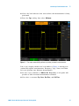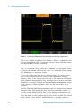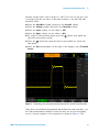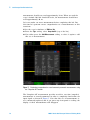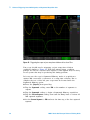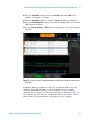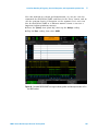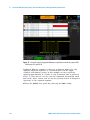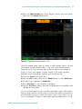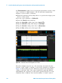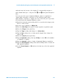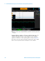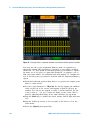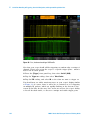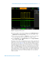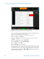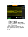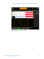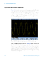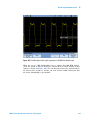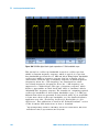
1
Agilent 4000 X-Series
Oscilloscopes
Advanced Training Guide
Lab guide and tutorial for making advanced
oscilloscope measurements using an Agilent
4000 X- Series oscilloscope with the DSOXEDK
training kit.
s1
Notices
© Agilent Technologies, Inc. 2008-2012
Manual Part Number
The copyright on this instructional material
grants you permission to reprint, modify,
and distribute in whole or in part the document for the purpose of training on Agilent
test equipment.
54702-97011
Edition
November, 2012
Available in electronic format only
Trademarks
Microsoft®, MS-DOS®, Windows®, Windows 2000®, and Windows XP® are U.S.
registered trademarks of Microsoft Corporation.
Adobe®, Acrobat®, and the Acrobat
Logo® are trademarks of Adobe Systems
Incorporated.
Agilent Technologies, Inc.
1900 Garden of the Gods Road
Colorado Springs, CO 80907 USA
agency regulation or contract clause. Use,
duplication or disclosure of Software is
subject to Agilent Technologies’ standard
commercial license terms, and non-DOD
Departments and Agencies of the U.S. Government will receive no greater than
Restricted Rights as defined in FAR
52.227-19(c)(1-2) (June 1987). U.S. Government users will receive no greater than
Limited Rights as defined in FAR 52.227-14
(June 1987) or DFAR 252.227-7015 (b)(2)
(November 1995), as applicable in any
technical data.
Warranty
The material contained in this document is provided “as is,” and is subject to being changed, without notice,
in future editions. Further, to the maximum extent permitted by applicable
law, Agilent disclaims all warranties,
either express or implied, with regard
to this manual and any information
contained herein, including but not
limited to the implied warranties of
merchantability and fitness for a particular purpose. Agilent shall not be
liable for errors or for incidental or
consequential damages in connection
with the furnishing, use, or performance of this document or of any
information contained herein. Should
Agilent and the user have a separate
written agreement with warranty
terms covering the material in this
document that conflict with these
terms, the warranty terms in the separate agreement shall control.
Technology Licenses
The hardware and/or software described in
this document are furnished under a
license and may be used or copied only in
accordance with the terms of such license.
Restricted Rights Legend
If software is for use in the performance of
a U.S. Government prime contract or subcontract, Software is delivered and
licensed as “Commercial computer software” as defined in DFAR 252.227-7014
(June 1995), or as a “commercial item” as
defined in FAR 2.101(a) or as “Restricted
computer software” as defined in FAR
52.227-19 (June 1987) or any equivalent
Safety Notices
CAUTION
A CAUTION notice denotes a hazard. It calls attention to an operating procedure, practice, or the like
that, if not correctly performed or
adhered to, could result in damage
to the product or loss of important
data. Do not proceed beyond a
CAUTION notice until the indicated
conditions are fully understood and
met.
WA R N I N G
A WARNING notice denotes a
hazard. It calls attention to an
operating procedure, practice, or
the like that, if not correctly performed or adhered to, could result
in personal injury or death. Do not
proceed beyond a WARNING
notice until the indicated conditions are fully understood and met.
Contents
1 Getting Started
Lab Guide—At a Glance
5
Front Panel Overview 6
Run Control 7
Waveform Controls 7
Horizontal Controls 8
Vertical Controls 9
Trigger Controls 9
Tools Controls 10
2 Oscilloscope Familiarization Labs
Lab #1: Using Cursors and Automatic Parametric Measurements
Lab #2: Using Zoom Display to Perform Gated Measurements
Lab #3: Using Waveform Math
19
23
Lab #4: Using Peak Detect Acquisition Mode
27
Lab #5: Using Segmented Memory Acquisition Mode
Lab #6: Using Mask Test
12
31
37
3 Advanced Triggering, Search & Navigation, and Segmented Acquisition Labs
Lab #7: Triggering on a Digital Burst using Trigger Holdoff
42
Lab #8: Triggering on Unique Pulses and Glitches using “Pulse-width” Trigger
46
Lab #9: Triggering on the Nth Pulse within a Burst using “Nth Edge Burst” Trigger
Lab #10: Triggering on and Searching for Edge Speed Violations
Lab #11: Triggering on and Searching for Runt Pulses
Lab #12: Triggering on Setup & Hold Time Violations
51
53
60
66
Lab #13: Triggering on a Qualified Burst using “Edge then Edge” Trigger
70
Lab #14: Triggering on Logic Patterns using the MSO’s Digital Channels
73
4 Serial Bus Decoding & Triggering, Search & Navigation, and Segmented Acquisition Labs
Lab #15: Decoding, Triggering, and Searching on I2C Serial Bus Signals
4000 X-Series Oscilloscopes Advanced Training Guide
80
3
Lab #16: Decoding, Triggering, and Searching on SPI Serial Bus Signals
87
Lab #17: Decoding, Triggering, and Searching on RS232/UART Serial Bus Signals
Lab #18: Decoding, Triggering, and Searching on CAN Serial Bus Signals
102
Lab #19: Decoding, Triggering, and Searching on LIN Serial Bus Signals
110
Lab #20: Decoding, Triggering, and Searching on I2S Serial Bus Signals
118
Lab #21: Decoding, Triggering, and Searching on FlexRay Serial Bus Signals
125
Lab #22: Decoding, Triggering, and Searching on Universal Serial Bus (USB) Signals
Lab #23: Decoding, Triggering, and Searching on ARINC 429 Signals
94
132
139
Lab #24: Decoding, Triggering, and Searching on MIL-STD-1553 Signals
144
A Oscilloscope Block Diagram and Theory of Operation
DSO Block Diagram
ADC Block
152
152
Attenuator Block
153
DC Offset Block
153
Amplifier Block
153
Trigger Comparator and Trigger Logic Blocks
154
Timebase and Acquisition Memory Blocks
Display DSP Block
154
155
B Oscilloscope Bandwidth Tutorial
Defining Oscilloscope Bandwidth
157
Required Bandwidth for Analog Applications
158
Required Bandwidth for Digital Applications 159
Rule of Thumb 159
Step 1: Determine fastest actual edge speeds 160
Step 2: Calculate fknee 160
Step 3: Calculate scope bandwidth
Example 161
160
Digital Clock Measurement Comparisons
162
C Related Agilent Literature
Index
4
4000 X-Series Oscilloscopes Advanced Training Guide
Agilent 4000 X-Series Oscilloscopes
Advanced Training Guide
1
Getting Started
Lab Guide—At a Glance 5
Front Panel Overview 6
Lab Guide—At a Glance
This advanced oscilloscope training guide and tutorial is intended to be
used with Agilent Technologies InfiniiVision 4000 X- Series oscilloscopes
(DSO and MSO models) that are licensed with the Oscilloscope Education
Training Kit (DSOXEDK). When licensed with this training kit,
4000 X- Series oscilloscopes are able to generate a broad range of built- in
training signals.
The built- in training signals can be probed by simply connecting a
standard 10:1 passive probe between channel- 1’s input BNC and the front
panel terminal labeled “Demo 1”, and another probe between channel- 2’s
input BNC and the terminal labeled “Demo 2” as shown on the next page.
To turn on specific training signals for each of the labs documented in this
training guide, simply:
1 Press the scope’s front panel [Help] key.
2 Press the Training Signals sofkey.
3 Turn the
Entry knob to select the appropriate training signal, or
use the all new touchscreen interface to select a signal directly.
4 Press the Output softkey to enable the training signal output on the
Demo terminal(s). The signal will also begin output when double
pressed in the menu.
s1
5
1
Getting Started
If you not familiar with the Agilent InfiniiVision 4000 X- Series
oscilloscope, first look over the main sections of the front panel as
illustrated on the following pages, and then begin with Chapter 2,
“Oscilloscope Familiarization Labs,” starting on page 11.
Once you have become familiar with using the basic functions of the
oscilloscope, you can then skip to particular labs of interest. Each
hands- on lab can be considered as a standalone lab exercise because each
begins with a default setup. In other words, successive labs do not build
on the previous lab. They can be completed in any order of preference.
Front Panel Overview
For instant help on any topic, press and hold any key, softkey, or knob.
6
4000 X-Series Oscilloscopes Advanced Training Guide
Getting Started
1
Run Control
When the oscilloscope is turned on, or if [Auto Scale] is pressed, the
acquisition will be set to [Run]. At any time you may [Stop] the acquisition
process to examine a signal in detail or to save it.
• The [Default Setup] key on the front panel sets the oscilloscope to the
default configuration.
Because the oscilloscope may have been used in a variety of
applications by a variety of people, it is a good measurement procedure
to put the oscilloscope in a known starting mode (Default Setup). This
makes it easy to duplicate measurements because no special conditions
are set.
• The [Auto Scale] key on the front panel automatically configures the
oscilloscope by analyzing all active channels, turning them on and
setting the timebase, V/div, and trigger conditions for an initial display.
• Press the [Single] key to make a single acquisition and stop the
acquisition process.
Waveform Controls
• The [Analyze] key sets trigger levels, measurement threshold levels, video
trigger auto setup and display, or the mask testing application options.
• The [Acquire] key on the front panel lets you set the oscilloscope data
acquisition modes.
• The [Display] key on the front panel lets you set the waveform
persistence options and the grid type and grid intensity.
4000 X-Series Oscilloscopes Advanced Training Guide
7
1
Getting Started
• The [Intensity] key and the
signal brightness.
Entry knob lets you set the desired
Horizontal Controls
a Turn the large knob in the Horizontal control section clockwise and
counter- clockwise to control the time/div setting of the horizontal
axis.
Observe the changes in the displayed signal. The current timebase
setting is displayed at the top of the display on the status line.
b Turn the small knob in the horizontal control section to move the
trigger point (solid orange triangle) from the reference point (hollow
orange triangle).
c Press the [Horiz] key to display the Horizontal menu. Note the various
Time Modes of Normal, Roll, and XY. Also notice the Zoom mode
softkey.
d Press the
(zoom) key to quickly turn on the zoom mode. This
split- screen mode shows the big picture on top and an expanded
view on the bottom. Turn the large timebase knob counter- clockwise
to make the window on top larger.
8
4000 X-Series Oscilloscopes Advanced Training Guide
Getting Started
1
Vertical Controls
• Turn the large knobs in the Vertical section to control the V/div setting
for each analog channel. The V/div setting is displayed in the upper left
hand corner of the status line at the top of the display.
Color coding matches analog channel inputs, vertical control knobs, and
waveform colors.
• Press the [1] key to display the channel 1 menu. Press again to turn the
channel on and off.
• Turn the small knobs to control the vertical offset position of the
waveform, moving the ground level up or down.
Trigger Controls
• Turn the Trigger Level knob to move the trigger level up and down. The
trigger level is displayed while it is adjusted. If the trigger level is above
or below the signal and the oscilloscope is in Auto trigger mode, the
oscilloscope will force a trigger and display an acquisition (waveform).
Auto trigger mode is useful when unsure of the exact waveform because
forced acquisitions are displayed, making it easy to better configure the
oscilloscope’s settings and trigger level.
4000 X-Series Oscilloscopes Advanced Training Guide
9
1
Getting Started
• Press the [Mode/Coupling] key in the Trigger controls section to view the
Trigger Mode and Coupling Menu selections and to set trigger holdoff.
• Press and hold the Mode softkey to read the built- in help about the
Auto and Normal trigger modes.
Tools Controls
• Press the [Utility] key to access the I/O ports, file explorer, options,
service information, and the “Quick Action” key function settings.
• Press the [Quick Action] key to perform one of the quick action functions
that can be mapped to this key.
• Press [WaveGen1] or [WaveGen2] to use the Arbitrary Waveform
Generators.
10
4000 X-Series Oscilloscopes Advanced Training Guide
Agilent 4000 X-Series Oscilloscopes
Advanced Training Guide
2
Oscilloscope Familiarization Labs
Lab #1: Using Cursors and Automatic Parametric Measurements 12
Lab #2: Using Zoom Display to Perform Gated Measurements 19
Lab #3: Using Waveform Math 23
Lab #4: Using Peak Detect Acquisition Mode 27
Lab #5: Using Segmented Memory Acquisition Mode 31
Lab #6: Using Mask Test 37
s1
11
2
Oscilloscope Familiarization Labs
Lab #1: Using Cursors and Automatic Parametric Measurements
During this first hands- on lab, you will learn how to make simple voltage
and timing measurements using the scope’s manually positioned
measurement cursors, as well as perform similar measurements using the
scope’s automatic parametric measurement capability.
1 Connect the channel- 1 probe to the Demo 1 terminal and ground.
2 Press [Default Setup] on the scope’s front panel.
3 Press [Help]; then press the Training Signals softkey.
4 Using the touch screen Training Signals menu, select the Repetitive Pulse
with Ringing signal; press the Output softkey to turn it on.
5 Set channel- 1’s V/div setting to 500 mV/div.
6 Set channel- 1’s position/offset to 1.40 V.
7 Push the trigger level knob to automatically set the trigger level at
approximately 50%.
8 Set the scope’s timebase to 500.0 ns/div.
Figure 1 Oscilloscope setup to capture and display a repetitive digital pulse with ringing
and overshoot.
12
4000 X-Series Oscilloscopes Advanced Training Guide
Oscilloscope Familiarization Labs
2
At this point, you should see a repetitive digital pulse with overshoot and
ringing similar to what is shown in Figure 1. Note that all front panel
knobs are pushable. If you push the V/div knob or time/div knob, you can
toggle between course adjustment and fine adjustment (vernier control).
When other knobs are pushed, the scope will pre- set conditions associated
with that particular knob. For instance, if you push one of the vertical
position/offset knobs, offset will be set to 0.0 V for that input channel. If
you push the horizontal position/delay knob, delay relative to trigger will
be set to 0.0 seconds. If you push the trigger level knob, the scope will
automatically set the trigger level to approximately 50%.
Figure 2
Measurement Cursors knob.
Let’s now use the scope’s “cursors” function to measure the positive pulse
width and peak- to- peak voltage of this waveform. First, visually locate the
“Cursors” button in the Measure section of the front panel as shown in
Figure 2.
9 Push the Cursors button; then select "X1" on the right side of the
display. A pop up appears where you can increment its value (arrows)
or explicitly assign its value (press the value to make the keyboard
appear). You may also choose to drag the orange X1 flag on the bottom
edge of the screen to move the cursor to your desired position. The
cursors knob can also be used for fine tuning and adjustments.
10 Move the X1 cursor (#1 timing marker) so it intersects with a rising
edge of the pulse.
11 Select X2 on the right of the display (#2 timing marker) and position it
on the falling edge of the same pulse.
12 Select Y1 on the right of the display (#1 voltage marker) and move it
vertically such that it intersects with the negative peak of the pulse.
13 Select Y2 on the right of the display (#2 voltage marker) and move it
vertically such that it intersects with the positive peak of the pulse.
4000 X-Series Oscilloscopes Advanced Training Guide
13
2
Oscilloscope Familiarization Labs
Figure 3
Using the scope’s cursor measurements.
Delta readouts are displayed on the right- hand side of the display. If you
the press the [Cursors] front panel key, you can see absolute voltage and
time readouts for each cursor near the bottom of the display. Your screen
should now look similar to Figure 3.
In addition to using the scope’s default “manual” placement of time and
voltage cursors independently, you can also select the Track Waveform cursor
mode by pressing the [Cursors] front panel key, and then change from
“manual” to “tracking”. In the “tracking” cursor mode, you have the ability
to control the time placement of the cursors, and then the scope will
automatically position the voltage cursors on the waveform where the time
cursors intersect the waveform.
Let’s now perform some automatic parametric measurements on this
waveform.
14 Press the [Meas] front panel key (next to the Cursors knob).
If beginning with a default setup (as we have done), when the [Meas] key
is pressed the scope will turn on an automatic frequency and Vp- p
measurement. Because this scope is able to show up to four continuously
updated measurements, let’s add more measurements.
15 Press the Type softkey; then select Maximum.
14
4000 X-Series Oscilloscopes Advanced Training Guide
2
Oscilloscope Familiarization Labs
16 Notice the level indicator that shows where this measurement is being
performed.
17 Press the Type softkey; then select Minimum.
Figure 4
The scope automatically performs up to four parametric measurements.
Your scope’s display should now look similar to Figure 4 showing four
continuously update measurements; Frequency, Vp- p, Vmax, and Vmin.
Let’s now perform four different measurements.
18 Set the scope’s timebase to 200.0 ns/div. Expanding on the pulse will
provide us with increased measurement resolution.
19 Now select to measure Top, Base, Rise Time, and Fall Time.
4000 X-Series Oscilloscopes Advanced Training Guide
15
2
Oscilloscope Familiarization Labs
Figure 5
Performing additional pulse parameter measurements on a digital pulse.
Your scope’s display should now look similar to Figure 5. If Fall Time was
the last measurement that you selected, then the cursors will show where
this measurement is being performed.
At this point, you may be wondering what the difference is between the
“top” of a waveform (Vtop) versus the “maximum” of a waveform (Vmax),
as well as the difference between the “base” of a waveform (Vbase) versus
the “minimum” of a waveform (Vmin).
Vtop is the steady- state high level of the waveform. This is the voltage
level of the waveform after the overshoot and ringing have settled.
Likewise, Vbase is the steady- state low level of the waveform. For digital
pulse parameter measurements, Vtop and Vbase are often more important
parameters to measure than the absolute maximum and minimum voltages
of the waveform (Vmax and Vmin), which are the peak values of the
overshoot.
The Rise Time and Fall Time measurements that we performed are relative
transition times. This means that they have been performed relative to
specific voltage threshold levels. The scope’s default threshold levels for
these measurements are the 10% and 90% levels relative to Vbase and
Vtop. But many of today’s higher speed devices have specified rise and fall
times relative to 20% and 80% threshold levels, or perhaps relative to
16
4000 X-Series Oscilloscopes Advanced Training Guide
Oscilloscope Familiarization Labs
2
absolute voltage levels, such as from/to ± 1.0 V. Let’s now set up our scope
to measure just the rise time of this pulse relative to the 20% and 80%
threshold levels.
20 Press the Clear Meas softkey; then press the Clear All softkey.
21 Press the Settings softkey; then press the Thresholds softkey.
22 Press the Lower softkey; set the value to 20%.
23 Press the Upper softkey; set the value to 80%.
24 To return to the previous menu, press the
Back
(Back) front panel key
(just above the power switch).
25 Press the
Back
(Back) key again because we descended two levels into
this menu.
26 Press the Rise measurement on the right of the display; select Track with
Cursors.
Figure 6
Performing a rise time measurement relative to 20% and 80% threshold levels.
Using these user- defined measurement threshold levels (20% and 80%), our
rise time measurement should be faster because we are now measuring
across a shorter segment of the waveform as shown in Figure 6. The
4000 X-Series Oscilloscopes Advanced Training Guide
17
2
Oscilloscope Familiarization Labs
measurement should now read approximately 30 ns. When we used the
scope’s default 10%/90% threshold levels, the measurement should have
read approximately 40 ns.
Let’s now make one more measurement before completing this lab. But
this time let’s perform a more comprehensive set of measurements on this
waveform.
27 Set the scope’s timebase to 500.0 ns/div.
28 Press the Type softkey; select Snapshot All (top of the list).
29 Now either press the Add Measurement softkey, or select it again to add
this set of measurements.
Figure 7 Performing a comprehensive set of automatic parametric measurements using
the “Snapshot All” function.
The “Snapshot- All” measurement provides us with a one- time (snapshot)
measurement of several parameters in order to completely characterize our
input signal as shown in Figure 7. Note that this set of measurements is
not continuously updated, and if you press any front panel or softkey, the
display of these measurements will disappear.
18
4000 X-Series Oscilloscopes Advanced Training Guide
Oscilloscope Familiarization Labs
2
Lab #2: Using Zoom Display to Perform Gated Measurements
When performing automatic parametric measurements, such as positive
pulse width measurements, on an exactly repetitive input signal, such as a
simple sine wave or square wave, it really doesn’t matter which particular
pulse the scope chooses to make the measurement on; each pulse is the
same. But what if the input signal you are probing is more complex; where
each pulse has unique parametric characteristics? In this case, you would
first need to set up the scope to trigger at a unique point in time on the
complex signal, and then you would need to set up the scope’s
measurements in such a way that the scope would be more selective as to
which pulse it chooses to perform measurements on. In this lab you will
learn how to perform selective, or “gated”, measurements on specific
pulses using the scope’s Zoom display mode.
1 Connect the channel- 1 probe to the Demo 1 terminal and ground.
2 Press the [Default Setup] key on the scope’s front panel.
3 Press [Help]; then press the Training Signals softkey.
4 Select the Digital Burst with Infrequent Glitch signal; then press the Output
softkey to turn it on.
5 Set channel- 1’s V/div setting to 1.0 V/div.
6 Set channel- 1’s position/offset setting to approximately 2.0 V in order to
center the waveform on- screen.
7 Push the trigger level knob in order to automatically set the trigger
level at approximately 50% (~1.7 V).
8 Set the scope’s timebase to 1.000 µs/div.
9 Press the [Mode/Coupling] front panel key near the trigger level knob.
10 Press the Holdoff softkey; set the trigger holdoff value to 4.000 µs.
With the scope’s trigger holdoff feature turned on and set to 4.0 µs, the
scope now triggers on the 1st rising edge of the burst, disarms triggering
for 4.0 µs, and then re- arms triggering after the last pulse in the burst so
that the scope will again trigger on the 1st pulse during the next
repetition of the burst. We have now established a stable and unique
trigger point on this complex digital signal using Trigger Holdoff. You can
learn more about Trigger Holdoff during "Lab #7: Triggering on a Digital
Burst using Trigger Holdoff" on page 42.
4000 X-Series Oscilloscopes Advanced Training Guide
19
2
Oscilloscope Familiarization Labs
Figure 8 Setting up the oscilloscope to capture a burst of digital pulses with different
pulse widths.
You should now observe 6 positive pulses with varying widths, plus an
infrequent glitch occurring after the 6th pulse as shown in Figure 8. Let’s
now turn on a “+ Width” measurement.
11 Press the [Meas] front panel key (next to the Cursors knob).
12 Press the Clear Meas softkey; then press the Clear All softkey.
13 Press the Type softkey; then press the + Width measurement.
14 Either press it again or press the Add Measurement softkey to select this
measurement.
20
4000 X-Series Oscilloscopes Advanced Training Guide
2
Oscilloscope Familiarization Labs
Figure 9
Measuring the positive pulse width of the 1st pulse in the burst.
The scope always performs measurements on the pulse located closest to
center- screen. In this case, the scope measures the positive pulse width of
the 1st pulse in this digital burst as shown in Figure 9. But what if we
want to know the widths of the 2nd, 3rd, 4th, etc., pulses?
15 Press the
button in the Horizontal section of the front panel to turn
on the scope’s “zoom” display mode.
16 Set the Zoom timebase to 50.00 ns/div by turning the large timebase
knob.
17 Set the horizontal position/delay to 950.0 ns in order to window- in on
the 3rd pulse.
When the “zoom” display is turned on, the horizontal controls (s/div and
position) control the zoomed (or expanded) timebase settings.
4000 X-Series Oscilloscopes Advanced Training Guide
21
2
Oscilloscope Familiarization Labs
Figure 10 Using the scope’s Zoom timebase mode to perform “gated” measurements.
You should now see on your scope’s display an expansion of just the 3rd
pulse in this burst in the lower portion of the display as should in
Figure 10. And the + Width measurement should be measuring the positive
pulse width of just the 3rd pulse.
22
4000 X-Series Oscilloscopes Advanced Training Guide
Oscilloscope Familiarization Labs
2
Lab #3: Using Waveform Math
In addition to performing automatic parametric measurements on
waveform data, the oscilloscope can also perform math operations on an
entire waveform or pair of waveforms. One very common waveform math
function that you may want the scope to perform is to subtract one
waveform from another. For instance, if you were using standard 10:1
passive probes to capture waveforms on your circuit, you would be limited
to capturing these waveforms relative to ground only. But what if you
wanted to see what a waveform looks like across a particular component
where neither end of the component is connected to ground? In this case,
you could capture waveforms at both ends of the component relative to
ground, and then subtract one waveform from the other. Let’s try it.
1 Connect the channel- 1 probe to the Demo 1 terminal and ground.
2 Connect the channel- 2 probe to the Demo 2 terminal and ground.
3 Press [Default Setup] on the scope’s front panel.
4 Press the [2] front panel key to turn on Channel- 2.
5 Press [Help]; then press the Training Signals softkey.
6 Select the Phase Shifted Sine signal; then press the Output softkey to turn
it on.
7 Set channel- 1’s V/div setting to 500 mV/div.
8 Set channel- 2’s V/div setting to 500 mV/div.
9 Set the scope’s timebase to 200.0 µs/div.
10 Press the [Math] front panel key (right- hand side of front panel).
11 Press the Operator softkey and select "- ". Change the Math voltage scale
to 500mV/div using the knob above the [Math] front panel key.
4000 X-Series Oscilloscopes Advanced Training Guide
23
2
Oscilloscope Familiarization Labs
Figure 11 Using waveform math to subtract channel-2 from channel-1.
You should now see three waveforms on your scope’s display as shown in
Figure 11. The purple waveform is the result of the scope’s math function
of subtracting the channel- 2 waveform from the channel- 1 waveform.
Note that to change the scaling of the math waveform, you can use the
knobs on the right- hand side of the scope’s front panel near the [Math]
key.
Let’s now vary the phase shift of the two sine waves and observe the
results.
12 Press the [Help] front panel key; the press the Training Signals softkey.
13 Press the Phase softkey; then turn the Entry knob to vary the phase
shift. You can also tap the angle value to set it yourself.
When the phase shift is exactly 180 degrees, the resultant math waveform
will be at its highest amplitude as expected. When the phase shift is
exactly 0 or 360 degrees, the resultant math waveform flat- lines (0.0 V).
Let’s now perform a more complex math function; FFT (Fast Fourier
Transform).
14 Press [Default Setup].
15 Press [Help]; then press the Training Signals softkey.
24
4000 X-Series Oscilloscopes Advanced Training Guide
Oscilloscope Familiarization Labs
2
16 Select the Clock with Infrequent Glitch signal and press the Output softkey to
turn it on.
17 Set channel- 1’s V/div setting to 500 mV/div.
18 Set channel- 1’s offset to approximately 1.00 V in order to center the
waveform on- screen.
19 Push the trigger level knob to set the trigger level at approximately 50%.
20 Set the timebase to 20.0 µs/div. At this timebase setting there will be
many cycles of the clock signal on- screen, which is typically required
when performing a precision FFT math function.
21 Press the [Math] front panel key; then press the Operator softkey.
22 Select the FFT math function. Select the softkey Span and set to
100 MHz; then set Center to 50 MHz.
Figure 12 Performing an FFT math function on a repetitive digital clock.
You should now see a display similar to Figure 12. The scope is now
displaying both a time domain waveform (Voltage versus Time) as well as
a frequency domain waveform (Power in units of dB versus Frequency).
An FFT math function breaks signals down into their individual sine wave
frequency components. All electrical signals, including digital signals, are
composed of multiple sine waves of different frequencies. An ideal clock
4000 X-Series Oscilloscopes Advanced Training Guide
25
2
Oscilloscope Familiarization Labs
signal that has a 50% duty cycle should consist of a fundamental sine
wave frequency component (signal’s repetitive frequency), plus its odd
harmonics (3rd, 5th, 7th, etc.). Note that non- ideal square waves will also
include lower- level even harmonics. Let’s now verify the frequencies of the
fundamental and odd harmonics.
23 Press the [Cursors] front panel key (near the Cursors knob).
24 Press the Source softkey and change the Source from channel- 1 to Math:
f(t)
25 Push the Cursors knob and select the X1 cursor.
26 Move the X1 cursor so that it is on top of the highest frequency peak
(near the left side of the display).
27 On the right of the screen, select the X2 cursor.
28 Move the X2 cursor until it is on top of the 2nd highest frequency peak.
The frequencies at the X1 and X2 cursor locations are displayed near the
bottom of the scope’s display.
Let’s now verify the fundamental frequency of this signal using the scope’s
“counter” measurement.
29 Press the [Meas] front panel key.
30 Press the Type softkey and select Counter.
The “counter” measurement measures the average frequency over a fixed
gate time to provide a very high resolution (5 digits) measure of frequency,
similar to a standalone counter. But the measurement requires that the
input signal be repetitive.
The “frequency” measurement measures the period of just one cycle of the
signal, and then computes the frequency by taking the reciprocal.
26
4000 X-Series Oscilloscopes Advanced Training Guide
Oscilloscope Familiarization Labs
2
Lab #4: Using Peak Detect Acquisition Mode
All DSOs and MSOs have a fixed amount of acquisition memory. This is
the number of samples that the oscilloscope can digitize for each
acquisition cycle. If the scope’s timebase is set to a relatively fast time/div
setting, such as 20 ns/div, then the scope will always have a sufficient
amount of memory to capture a waveform at that setting using the scope’s
maximum specified sample rate. For example, if a scope’s maximum
specified sample rate is 4 GSa/s (250 ps between samples), and if the
scope’s timebase is set to 20 ns/div, then an acquisition memory depth of
800 points is all that is required to capture and display a complete
waveform. At 20 ns/div, a complete waveform across the scope’s screen
would consist of 200 ns of time (20 ns/div x 10 horizontal divisions). The
required memory depth to fill this time while still sampling at 4 GSa/s is
then just 800 points (200ns/250ps = 800).
If you set the scope’s timebase to a much slower time/div setting in order
to capture slower waveforms and longer time, then the scope may need to
automatically reduce its sampling rate in order to fill the required
waveform time. All DSOs and MSOs do this. For example, let’s assume that
you want to capture a relatively slow signal and need to set the scope’s
timebase to 10 ms/div (100 ms across screen). If the scope’s maximum
memory depth is 2 M points, then the scope will need to reduce its
sample rate to 20 MSa/s (100 ms/2 M = 50 ns sample period).
Although in most cases this is not a problem, because capturing slower
waveforms doesn’t require fast sample rates, what if the input signal
consisted of a combination of low- speed and high- speed characteristics?
For example, what if the input signal that you want to capture is a 30 Hz
sine wave with very narrow glitches riding on it? Capturing the 30 Hz sine
wave doesn’t require a fast sample rate, but capturing the narrow glitches
may require a very fast sample rate. Let’s set up a test to capture a signal
such as this.
1 Connect the channel- 1 probe to the Demo 1 terminal and ground.
2 Press [Default Setup] on the scope’s front panel.
3 Press [Help]; then press the Training Signals softkey.
4 Select the Sine with Glitch signal; then press the Output softkey to turn it
on.
5 Set channel- 1’s V/div setting to 500.0 mV/div.
6 Set the scope’s timebase to 10.00 ms/div.
7 Press the [Intensity] button (under the Entry knob); then set the
waveform trace intensity to 100% using the Entry knob or on- screen
slider.
4000 X-Series Oscilloscopes Advanced Training Guide
27
2
Oscilloscope Familiarization Labs
Figure 13 The scope’s automatically-reduced sample rate under-samples the repetitive
glitch.
At this point, you should see a sine wave similar to Figure 13. But if you
look closely you should also see some glitches (narrow pulses) near the
peaks of this sine wave. And the amplitude of these glitches may appear
to vary (bouncing up and down). The amplitude of these glitches is
actually very stable. The problem is that the scope has reduced its sample
rate (note the sample rate shown under the Agilent logo on the scope’s
display) and the scope is now intermittently capturing the narrow glitches.
The scope is under- sampling the narrow glitches. Sometimes the scope
captures a single point on the peak of a glitch. Sometimes it captures a
point on a transition of the glitch. And sometimes it captures nothing at
all on the glitch (the glitch width is narrower than the sample interval).
This scope has a special acquisition mode called “Peak Detect” that will
resolve this problem. Let’s turn it on.
8 Press the [Acquire] front panel key (below the Cursors knob).
9 Press the Acq Mode softkey and select Peak Detect.
28
4000 X-Series Oscilloscopes Advanced Training Guide
2
Oscilloscope Familiarization Labs
Figure 14 The Peak Detect acquisition mode reliably captures the narrow glitches riding
on the slow sine wave.
The height of the glitches should now appear much more stable as shown
in Figure 14. When the Peak Detect acquisition mode has been selected,
rather than sampling waveforms at a reduced rate, the scope intelligently
decimates acquired data at a higher sample rate. For example, let’s assume
that the scope needs to run at a sample rate that is 1/100th of its
maximum sample rate. This would be equivalent to running the scope at
its maximum sample rate, but only storing every 1/100th point, which is
“unintelligent” decimation. In the Peak Detect mode, the scope would
analyze a group of 200 consecutive samples in real- time (sampled at a
high rate), and then store just the maximum and minimum digitized values
for this group of 200 points, which is just 2 points. This would be a
decimation factor of 100.
So you may ask why not always use the Peak Detect mode? There are some
tradeoffs when using this mode of acquisition. First of all, the scope’s
absolute maximum sample rate is reduced. Secondly, stored points will
NOT be evenly spaced. And this is an important criterion of the Nyquist
Sampling theorem. So for this particular measurement application, using
the Peak Detect mode is a good choice. But for other measurement
applications, Peak Detect may not be the appropriate acquisition mode.
4000 X-Series Oscilloscopes Advanced Training Guide
29
2
Oscilloscope Familiarization Labs
To learn more about oscilloscope real- time sampling, refer to Agilent’s
Application Note titled, “Evaluating Oscilloscope Sample Rates vs
Sampling Fidelity” listed in "Related Agilent Literature" on page 165.
30
4000 X-Series Oscilloscopes Advanced Training Guide
Oscilloscope Familiarization Labs
2
Lab #5: Using Segmented Memory Acquisition Mode
All oscilloscopes have a limited amount of acquisition memory. The
amount of acquisition memory that your scope has will determine the
length of time it can capture while still using a fast sampling rate. You can
always capture a long time span by simply setting the timebase to a long
time/div setting. But the scope may automatically reduce its sample rate in
order to capture the long time- span which will reduce acquired waveform
detail and measurement resolution. Using this scope’s Segmented Memory
acquisition mode is another solution to optimize memory depth and
sample rate; especially when attempting to capture multiple low duty cycle
type signals. Agilent 4000 X- Series Oscilloscopes come with segmented
memory as a standard option. Let’s now attempt to capture and display a
simulated low duty cycle radar burst.
1 Connect the channel- 1 probe to the Demo 1 terminal and ground.
2 Press [Default Setup] on the scope’s front panel.
3 Press [Help]; then press the Training Signals softkey.
4 Select the RF Burst signal.
5 Set channel- 1’s V/div setting to 500.0 mV/div.
6 Set the scope’s timebase to 200.00 ns/div.
7 Set the scope’s trigger level to approximately +900 mV (~2.0 divisions
above center- screen).
8 Press the [Intensity] button (under the Entry knob); then set the
waveform trace intensity to 100% using the Entry knob.
4000 X-Series Oscilloscopes Advanced Training Guide
31
2
Oscilloscope Familiarization Labs
Figure 15 Capturing and displaying an RF burst at 200.0 ns/div.
You should see a single burst of sine waves similar to what is shown in
Figure 15. Let’s now rescale the timebase in an attempt to capture several
of these bursts.
9 Set the scope’s timebase to 10.000 ms/div.
32
4000 X-Series Oscilloscopes Advanced Training Guide
Oscilloscope Familiarization Labs
2
Figure 16 Capturing multiple RF burst waveforms at a slower timebase setting.
When we attempt to capture multiple RF bursts that are separated by
4.0 ms, the scope under- samples and shows varying amplitudes of the
signal as shown in Figure 16. Again, this is because the scope
automatically reduced its sample rate in order to capture a longer
time- span with its limited amount of acquisition memory. Let’s now
zoom- in and take a closer look at this under- sampled data.
10 Press [Run/Stop] to stop repetitive acquisitions ([Run/Stop] key will turn
red).
11 Now set the scope’s timebase to 200.0 ns/div.
4000 X-Series Oscilloscopes Advanced Training Guide
33
2
Oscilloscope Familiarization Labs
Figure 17 Zooming in reveals an under-sampled waveform.
After acquiring the waveform at the slower timebase setting, and then
zooming in, we can clearly see that our waveform was under- sampled as
evidenced by the triangular shaped waveforms shown in Figure 17.
Remember, this should be a burst of sine waves.
Although using the scope’s Peak Detect mode would provide us with a
more accurate measure of the peak amplitudes of each burst when
captured at the slower timebase setting (Figure 16), we would see that the
waveform would still be under- sampled after zooming in on a stored trace.
Another solution would be to purchase a scope with much deeper
memory. Let’s now use the scope’s Segmented Memory acquisition mode to
capture multiple bursts with high resolution.
12 Press [Run/Stop] to begin repetitive acquisitions again with the timebase
still set at 200.0 ns/div ([Run/Stop] should turn green).
13 Press the [Acquire] front panel key (near the Cursors knob); then press
the Segmented softkey to open the Segmented Memory settings.
14 Set # of Segs = 500.
15 Now press the Segmented softkey to turn on this mode of acquisition.
The scope should have just captured 500 consecutive occurrences of this
burst. Let’s review them.
34
4000 X-Series Oscilloscopes Advanced Training Guide
Oscilloscope Familiarization Labs
2
16 Press the Current Seg softkey; then turn the Entry knob to review all 500
waveforms.
17 Now set the Current Seg = 500 using the Entry knob (last captured
segment/waveform).
Figure 18 Using Segmented Memory Acquisition to capture more waveforms with high
resolution.
Along with capturing consecutive low duty cycle signal bursts, the scope
also “time- tags” each segment/waveform so that you know the time of each
capture segment/waveform relative to the first captured
segment/waveform. Time- tags are shown in the lower left- hand corner of
the display. Segment #500 should have a time- tag of approximately 2
seconds along with a time- of- day stamp as shown in Figure 18. The
captured waveform should also have very high resolution because the
scope used a high sample rate to capture each waveform. If you attempted
to capture ~2 s (200 ms/div) of time- span using the scope’s Normal
acquisition mode, the scope would have significantly reduced its sample
rate and thereby would have provided extremely poor sample resolution on
each burst.
Segmented Memory acquisition optimizes oscilloscope acquisition memory
by only capturing waveform data around small portions (or segments) of a
signal (a short sine wave burst in this case). The scope does not capture
4000 X-Series Oscilloscopes Advanced Training Guide
35
2
Oscilloscope Familiarization Labs
unimportant signal idle- time between each burst. Segmented Memory
acquisition can also be a very useful tool for capturing multiple serial
packets of digital data, which will be demonstrated in Chapter 4, “Serial
Bus Decoding & Triggering, Search & Navigation, and Segmented
Acquisition Labs,” starting on page 79.
36
4000 X-Series Oscilloscopes Advanced Training Guide
Oscilloscope Familiarization Labs
2
Lab #6: Using Mask Test
With mask testing you can set up a pass/fail test criteria for automatically
testing waveforms to see if they conform to specific wave shapes. In this
lab we will test a digital signal that includes an infrequent glitch. With
InfiniiVision’s hardware- based mask testing capability, we will be able to
test over 200,000 waveforms per second and gain insight into the
statistical occurrences of this particular glitch. To enable Mask Testing,
your oscilloscope must have the mask test option installed (Option
DSOX4MASK). You can verify the installed options on your oscilloscope at
[Help] > About Oscilloscope.
1 Connect the channel- 1 probe to the Demo 1 terminal and ground.
2 Press [Default Setup] on the scope’s front panel.
3 Press [Help]; then press the Training Signals softkey.
4 Turn on Clock with Infrequent Glitch signal.
5 Set channel- 1 to 500 mV/div and position/offset to 1.0 V.
6 Push the Trigger Level knob to set the trigger level at 50%.
7 Set the timebase to 20 ns/div.
8 Set the waveform intensity to 100% by first pressing the [Intensity]
button; then turn the Entry knob.
4000 X-Series Oscilloscopes Advanced Training Guide
37
2
Oscilloscope Familiarization Labs
Figure 19 The scope’s fast waveform update rate easily captures an infrequent glitch.
At this point, you should be able to see that the scope is capturing an
infrequent glitch as shown in Figure 19. This particular glitch occurs just
once every 1,000,000 cycles of the clock signal that we are triggering on.
Because this scope can update waveforms as fast as 1,000,000
waveforms/sec, the scope can capture the glitch on average once per
second. Let’s now use the scope’s Mask Test capability to analyze this
glitch.
9 Press [Analyze].
10 Press Features Mask two times to turn on mask testing.
11 Press Automask.
12 Press Create Mask to automatically create a pass/fail mask around this
waveform.
38
4000 X-Series Oscilloscopes Advanced Training Guide
Oscilloscope Familiarization Labs
2
Figure 20 Mask Testing provides us within detailed statistics about the rate of occurrence
of the infrequent glitch.
Because the InfiniiVision oscilloscope’s mask testing capability is
hardware- based, it can test over 200,000 waveforms/sec and provide
detailed pass/fail statistics including failure rate in terms of both percent
and a Sigma quality factor as shown in Figure 20. A Sigma quality factor
of 6σ relates to approximately three or fewer defects per million tested.
Because this particular glitch occurs 1/1,000,000, we have a Sigma quality
factor that exceeds 6σ. Let’s now set up the oscilloscope to stop on the
first detected failure.
13 Press [Run/Stop] to stop acquisitions.
14 Press the
Back
(Back) key.
15 Press Statistics.
16 Press Reset Statistics to clear the statistics from the previous test.
17 Press the
Back
(Back) key.
18 Press Setup.
19 Press On Error – Stop two times.
20 Press [Run/Stop] to begin a new “Stop- on- Error” test.
4000 X-Series Oscilloscopes Advanced Training Guide
39
2
Oscilloscope Familiarization Labs
Figure 21 Establishing specific test criteria.
In addition to stopping acquisitions when an error is detected as shown in
Figure 21, you can also save a waveform, save an image, print, or perform
specific measurements when an error is detected. Using the “Run Until”
selection, you can also set up mask testing to run for a specific number of
tests, minimum time, or minimum Sigma test criteria. Note that in
addition to creating a pass/fail mask using the auto- mask creation feature
as demonstrated in this lab, you can also import a mask based on industry
specifications, such as an eye- diagram mask, from a USB memory device.
These types of imported masks can be easily created within a standard
text editor, such as Notepad on your PC.
40
4000 X-Series Oscilloscopes Advanced Training Guide
Agilent 4000 X-Series Oscilloscopes
Advanced Training Guide
3
Advanced Triggering, Search &
Navigation, and Segmented Acquisition
Labs
Lab #7: Triggering on a Digital Burst using Trigger Holdoff 42
Lab #8: Triggering on Unique Pulses and Glitches using “Pulse-width”
Trigger 46
Lab #9: Triggering on the Nth Pulse within a Burst using “Nth Edge Burst”
Trigger 51
Lab #10: Triggering on and Searching for Edge Speed Violations 53
Lab #11: Triggering on and Searching for Runt Pulses 60
Lab #12: Triggering on Setup & Hold Time Violations 66
Lab #13: Triggering on a Qualified Burst using “Edge then Edge”
Trigger 70
Lab #14: Triggering on Logic Patterns using the MSO’s Digital
Channels 73
s1
41
3
Advanced Triggering, Search & Navigation, and Segmented Acquisition Labs
Lab #7: Triggering on a Digital Burst using Trigger Holdoff
Signals in the real world of electronics are rarely as simple as repetitive
sine waves and square waves. Establishing unique trigger points on more
complex signals sometimes requires using trigger “hold- off”. In this lab you
will learn how to use the scope’s trigger hold- off capability in order to
trigger on a burst of digital pulses.
1 Connect the channel- 1 probe to the Demo 1 terminal and ground.
2 Press [Default Setup] on the scope’s front panel.
3 Press [Help]; then tap the Training Signals softkey.
4 Tap the Digital Burst signal from the Training Signals menu.
5 Set channel- 1’s V/div setting to 1.00 V/div.
6 Set channel- 1’s offset/position to approximately +1.7 V in order to
center this waveform on the scope’s display.
7 Push the Trigger Level knob to automatically set the trigger level to
approximately 50%.
8 Set the scope’s timebase to 20.00 µs/div.
Figure 22 Attempting to view a burst of pulses while using the scope’s default trigger
setup conditions.
42
4000 X-Series Oscilloscopes Advanced Training Guide
Advanced Triggering, Search & Navigation, and Segmented Acquisition Labs
3
You should see on your scope’s display what may appear to be an
un- triggered display of a series of digital pulses similar to Figure 22. The
scope is actually triggering on random rising edge crossings of this
complex digital data stream, which is actually a “burst” of pulses.
Unfortunately we can’t “see” the burst activity because we haven’t yet set
up the scope to establish a unique trigger point on this complex signal. So
let’s now “stop” repetitive acquisitions so that we can see a single- shot
acquisition of the bursts, and then make some measurements. We will then
use these measurements to enter a specific trigger holdoff time in order to
synchronize triggering on the 1st pulse of each burst.
9 Press the [Run/Stop] front panel key to stop repetitive acquisitions.
Figure 23 Single-shot acquisition reveals digital burst activity.
With repetitive acquisitions stopped, you should now be able to see digital
burst activity as shown in Figure 23. In other words, there are a series of
negative pulses followed by a short idle- time (high level), and then it
repeats. If you press [Single] several times, you should observe that the
trigger event (rising edge closest to center- screen) for each acquisition is
almost always a different pulse within the burst.
4000 X-Series Oscilloscopes Advanced Training Guide
43
3
Advanced Triggering, Search & Navigation, and Segmented Acquisition Labs
Estimate or use the scope’s timing cursors (X1 & X2) to measure the
width of one of the burst of pulses, and also measure the time from the
beginning of one burst of pulses to the beginning of the next burst of
pulses. You should find that the width of each burst is approximately
40 µs, and the time between bursts is approximately 50 µs.
When we use the scope’s default triggering condition, the scope triggers on
“any” random edge of this signal. In other words, sometimes the scope
triggers on the 1st edge of the burst, sometimes the 11th edge of the burst,
sometimes the 5th edge, etc. An ideal synchronization point would be to
set up the scope so that it always triggers on just the 1st edge of each
burst, rather than a random edge. We can do this using the scope’s
“trigger holdoff” capability.
With trigger holdoff, we can instruct the scope to always arm triggering
during the signal idle- time between each burst of pulses. This way the
scope will always trigger on the next rising edge after arming, which will
always be the 1st edge in each burst. And ideal holdoff time to achieve
this would be a trigger holdoff time somewhere between 40 µs (width of
burst) and 50 µs (time between bursts). This may sound confusing, so let’s
just do it and see what happens.
10 Press the [Run/Stop] front panel key to begin repetitive acquisitions
again.
11 Press the [Mode/Coupling] key in the Trigger section of the front panel.
12 Tap the Holdoff softkey twice to bring up the keypad; set to 45.000 µs.
44
4000 X-Series Oscilloscopes Advanced Training Guide
Advanced Triggering, Search & Navigation, and Segmented Acquisition Labs
Trigger Point
3
Holdoff Time
Next Valid Trigger Event
Figure 24 Using the scope’s trigger holdoff feature to synchronize on a burst of pulses.
You should now see a synchronized display as shown in Figure 24. The
scope triggers on the 1st edge of a burst of pulses (center- screen) and
then disables triggering for 45.00 µs (holdoff time). During this holdoff
time, the scope ignores the 2nd, 3rd, 4th, etc., crossings, and then re- arms
triggering after the end of the burst, but before the beginning of the next
burst, which is during the signal’s “idle- time”. The next valid trigger event
will again be the 1st edge crossing on the next burst.
4000 X-Series Oscilloscopes Advanced Training Guide
45
3
Advanced Triggering, Search & Navigation, and Segmented Acquisition Labs
Lab #8: Triggering on Unique Pulses and Glitches using “Pulse-width”
Trigger
In this lab you will learn how to use the scope’s Pulse Width triggering
mode to trigger on pulses within a digital data stream that have unique
pulse widths, including an infrequently occurring glitch.
1 Connect the channel- 1 probe to the Demo 1 terminal and ground.
2 Press [Default Setup] on the scope’s front panel.
3 Press [Help]; then press the Training Signals softkey.
4 Tap the Digital Burst with Infrequent Glitch signal from the Training Signals
menu.
5 Set channel- 1’s vertical scaling to 1.00 V/div.
6 Set channel- 1’s offset/position to approximately +1.7 V in center the
waveform on- screen.
7 Set the trigger level to +1.00 V (~1 division above bottom of waveform).
8 Set the scope’s timebase to 2.000 µs/div.
Figure 25 Capturing a digital burst using the scope’s default Edge triggering mode.
46
4000 X-Series Oscilloscopes Advanced Training Guide
3
Advanced Triggering, Search & Navigation, and Segmented Acquisition Labs
You should now see on your scope’s display a digital burst waveform
consisting of six pulses of various widths, followed by an infrequent glitch
similar to Figure 25. Using the scope’s default Edge triggering mode, the
scope usually triggers on the 1st pulse of this burst. But if you increase
the scope’s waveform intensity to 100%, you will see that the scope
sometimes triggers on later pulses within this burst. We could further
stabilize triggering on the 1st pulse in this burst if we used the scope’s
trigger holdoff capability. But what if we wanted to trigger on a specific
pulse (other than the 1st pulse)? We could accomplish this by using the
“Nth Edge Burst” triggering mode, assuming that the input signal is a
repetitive burst. We will show how to use the “Nth Edge Burst” triggering
mode in the next lab (Lab #9). Another option would be to use the scope’s
“Pulse Width” triggering mode, which can be used on a continuous data
stream of digital pulses; the data stream does not need to come in bursts.
But the pulses must have a unique pulse width for this triggering mode to
be effective. Note that the 5th pulse within this burst has a positive pulse
width of approximately 300 ns. This is a unique pulse width within this
burst of pulses. Let’s now set up the scope to trigger specifically on this
pulse.
9 Press the [Trigger] front panel key; then tap the Pulse Width trigger type
from the Trigger Type menu.
10 Tap the “ < > >< ” softkey until the “><” time qualifier has a check
below it.
11 Tap the “ < 30 ns ” softkey; then set the time to < 350 ns using the
keypad.
12 Tap the “ > 20 ns ” softkey; then set the time to > 250 ns using the
keypad.
13 Set the scope’s timebase to 500.0 ns/div.
4000 X-Series Oscilloscopes Advanced Training Guide
47
3
Advanced Triggering, Search & Navigation, and Segmented Acquisition Labs
Figure 26 Triggering on a 300 ns wide pulse using the scope’s Pulse Width triggering
mode.
Your scope should now be triggering at the end of the 5th pulse of the
burst as shown in Figure 26. This particular pulse uniquely meets the
pulse width time qualification of > 250 ns, but < 350 ns. You can select
the +Width measurement if you would like to verify that this pulse has an
approximate width of 300 ns.
Now take note of the narrow infrequent glitch that occurs after the end of
this burst of six pulses. In addition to using the scope’s Pulse Width
trigger type to trigger on “known” pulses that have unique widths, such as
this 300 ns wide pulse, we can also use the Pulse Width triggering mode
to trigger on “unknown” or “unwanted” glitches. Let’s do it.
14 Tap the “ < > >< ” softkey; then select the “<” time qualifier.
15 Tap the < 30 ns softkey; then set the time to < 50 ns.
48
4000 X-Series Oscilloscopes Advanced Training Guide
Advanced Triggering, Search & Navigation, and Segmented Acquisition Labs
3
Figure 27 Triggering on a narrow infrequent glitch using the scope’s Pulse Width
triggering mode.
Your scope should now be triggering on the narrow infrequent glitch that
follows the repetitive burst of six pulses as shown in Figure 27. Note that
if this glitch was more infrequent, you would also need to select the
Normal trigger mode to avoid auto triggering.
Let’s now use the scope’s Segmented Memory mode of acquisition to
capture 500 consecutive occurrences of this burst of pulses to see if we
can determine how often the glitch occurs relative to the occurrence of
each burst. But before beginning a Segmented Memory acquisition, we will
change the trigger condition to trigger on the 300 ns wide pulse again so
that we can capture every occurrence of the burst. To complete the rest of
this lab your scope must be licensed with the Segmented Memory option.
16 Tap the “ < > >< ” softkey; then select the “><” time qualifier.
17 Press the [Acquire] front panel key.
18 Tap the Segmented softkey twice and enter 500 as the number of
segments to capture.
19 Tap the Segmented softkey to begin a Segmented Memory acquisition.
20 Tap the Current Segment softkey; then turn the Entry knob to review all
500 captured segments. Or, tap it a second time to set a specific value.
4000 X-Series Oscilloscopes Advanced Training Guide
49
3
Advanced Triggering, Search & Navigation, and Segmented Acquisition Labs
21 Set the Current Segment to 500 and note the time- tag of the last captured
segment.
Figure 28 Using the scope’s Segmented Memory acquisition to selectively capture 500
consecutive occurrences of a burst of pulses.
Segmented Memory optimizes oscilloscope acquisition memory by only
capturing important segments of a waveform based on the trigger
condition and timebase setting. In this example, we have selectively
captured 500 consecutive occurrences of this burst for a total acquisition
time of than 40 ms as shown in Figure 28. The scope did not waste
valuable acquisition memory capturing signal idle time between each burst.
But the scope does provide us with timing information about the time of
each segment relative to the first captured segment. As you were reviewing
each captured segment, you should have determined the glitch occurs
every on 40th occurrence of the burst.
50
4000 X-Series Oscilloscopes Advanced Training Guide
3
Advanced Triggering, Search & Navigation, and Segmented Acquisition Labs
Lab #9: Triggering on the Nth Pulse within a Burst using “Nth Edge Burst”
Trigger
In this lab you will learn how to use the scope’s “Nth Edge Burst”
triggering mode to trigger on pulses within a burst based on pulse count.
Note that we will be using the same training signal that we used in the
previous lab.
1 Connect the channel- 1 probe to the Demo 1 terminal and ground.
2 Press [Default Setup] on the scope’s front panel.
3 Press [Help]; then press the Training Signals softkey.
4 Open the Training Signals: Sine menu and double- tap the Digital Burst with
Infrequent Glitch signal.
5 Set channel- 1’s vertical scaling to 1.00 V/div.
6 Set channel- 1’s offset/position to approximately +1.7 V in center the
waveform on- screen.
7 Set the trigger level to +1.00 V (~1 division above bottom of waveform).
8 Set the scope’s timebase to 500 ns/div.
Figure 29 Capturing a digital burst using the scope’s default Edge triggering mode.
4000 X-Series Oscilloscopes Advanced Training Guide
51
3
Advanced Triggering, Search & Navigation, and Segmented Acquisition Labs
You should now see on your scope’s display a digital burst waveform
consisting of six pulses of various widths, followed by an infrequent glitch
similar to Figure 29. Using the scope’s default Edge triggering mode, the
scope usually triggers on the 1st pulse of this burst. Let’s now set up the
scope to trigger on the 3rd pulse in this burst using the “Nth Edge Burst”
triggering mode.
9 Press the [Trigger] front panel key; then tap Nth Edge Burst using the
Trigger Type menu.
10 Tap the Idle softkey; then set the minimum signal idle time to 2.00 µs.
11 Tap the Edge softkey; then set the edge count to 3.
Figure 30 Triggering on the 3rd pulse in the burst using the “Nth Edge Burst” triggering
mode.
Your scope should now be triggering on the 3rd rising edge in this burst
as shown in Figure 30. Note that the idle time setting of 2.00 µs defines
when a burst ends and begins. This setting must be set to a value that is
greater that the longest legitimate pulse width within the burst, but less
than signal idle time between each occurrence of the burst. To trigger on
other edges within this burst, vary the Edge count setting between 1 and
7.
52
4000 X-Series Oscilloscopes Advanced Training Guide
Advanced Triggering, Search & Navigation, and Segmented Acquisition Labs
3
Lab #10: Triggering on and Searching for Edge Speed Violations
In this lab you will learn how to set up the scope to trigger on edge speed
violation conditions using the scope’s “Rise/Fall Time” trigger mode. We
will also be using the scope’s Search & Navigation capability to
automatically find, mark, and then navigate to edge speed violations, as
well as using the scope’s Segmented Memory acquisition to capture
multiple and consecutive occurrences of edge speed violations.
1 Connect the channel- 1 probe to the Demo 1 terminal and ground.
2 Press [Default Setup] on the scope’s front panel.
3 Press [Help]; then tap the Training Signals softkey.
4 From the Training Signals menu, double- tap the Edge Transition Violation
Signal.
5 Set channel- 1 to 500 mV/div.
6 Set channel- 1 offset/position to approximately 1.6 V to center the
waveform on- screen.
7 Push the trigger level knob to automatically set the trigger level to
approximately 50%.
8 Set the scope’s timebase to 100.0 ns/div.
4000 X-Series Oscilloscopes Advanced Training Guide
53
3
Advanced Triggering, Search & Navigation, and Segmented Acquisition Labs
Figure 31 Scope display reveals two different rising edge speeds when triggering on any
rising edge.
Your scope’s display should now look similar to Figure 31. Using the
scope’s default rising edge type trigger, we can see two distinctly different
rising edge speeds on this waveform. Also notice that the slower
transitioning edge appears dimmer. This is because the slower
transitioning edges occur less often than the faster transitioning edges.
Perhaps these slower transitioning edges are in violation of meeting
minimum required specifications. Let’s first set up the scope to measure
the rise times of this signal, and then we will set up the scope to uniquely
trigger on the violation edges.
9 Press [Meas]; then tap the Type softkey.
10 Select the Rise Time measurement; Once on, tap Statistics and then
Display On.
54
4000 X-Series Oscilloscopes Advanced Training Guide
Advanced Triggering, Search & Navigation, and Segmented Acquisition Labs
3
Figure 32 The scope’s measurement statistics shows the range of rising edge speeds on
this signal.
Looking at the on- screen Rise Time measurement statistics, we can see
that the scope is measuring a minimum Rise Time in the range of 50 ns,
while also measuring a maximum Rise Time in the range of 125 ns as
shown in Figure 32. If we assume that our system specification requires
that signal edge speeds (based on 10% to 90% threshold levels) must be
faster than 100 ns, then we have just detected a signal integrity problem
with our design. To further troubleshoot this issue we should set up our
scope to uniquely trigger on just the edges that are in violation. This might
help us isolate what the root cause might be that is causing these
occasional violations. Uniquely triggering on edge speed violation signals
can be accomplished on Agilent’s 4000 X- Series oscilloscopes using the
Rise/Fall Time triggering mode.
11 Press the [Trigger] front panel key and select the Rise/Fall Time trigger
type.
12 Press the Level Select softkey to select Low.
13 Turn the Trigger Level knob to set the lower trigger threshold level to the
approximate 10% level. Note that you can also drag the TL marker on
the left edge of the display.
4000 X-Series Oscilloscopes Advanced Training Guide
55
3
Advanced Triggering, Search & Navigation, and Segmented Acquisition Labs
14 Press the Level Select softkey until it indicates High; then turn the Trigger
Level knob to set the upper (high) trigger threshold level to the
approximate 90% level. Note that you can also drag the TH marker on
the left side of the display.
15 Tap the “< >” softkey to select “>”.
16 Tap the Time softkey twice, which opens the keypad. Set the violation
time to > 100 ns.
Figure 33 Using Rise/Fall Time triggering to trigger on violation edge speeds.
Your scope should now be triggering on just rising edges of the input
signal that have rise times in excess of 100 ns as shown in Figure 33. In
addition to triggering on Rise/Fall Time violation edges, the Agilent
4000 X- Series oscilloscopes can also perform Search & Navigation to find
multiple edge speed violation conditions, regardless of the specific trigger
setup condition.
17 Set the scope’s timebase to 200.0 µs/div.
18 Press [Run/Stop] to stop repetitive acquisitions (the [Run/Stop] key
should turn red).
19 Press the [Search] front panel key.
20 Tap the Search Edge softkey and select the Rise/Fall Time search mode.
56
4000 X-Series Oscilloscopes Advanced Training Guide
Advanced Triggering, Search & Navigation, and Segmented Acquisition Labs
3
21 Tap the Settings softkey.
22 Tap the “< >” softkey; the select “>”.
23 Press the Time softkey; enter in > 100 ns.
Figure 34 The scope automatically finds several rise time violation edges.
At this timebase setting (200 µs/div), the scope captured over a thousand
edges of this signal. And using the search conditions we entered (rising
edges that exceed 100 ns), the scope should have just found approximately
10 violation edges as shown in Figure 34. The white triangle marks at the
top of the display indicate the location of each “found” violation. Let’s now
“navigate” to each of these detected violations.
24 Press the
(zoom) front panel key.
25 Press the
and
edge violation.
navigation keys to navigate to each discovered
Let’s now use the scope’s Segmented Memory mode of acquisition to
capture 500 consecutive occurrences of this edge transition violation. But
to complete the rest of this lab your scope must be licensed with the
Segmented Memory option.
4000 X-Series Oscilloscopes Advanced Training Guide
57
3
Advanced Triggering, Search & Navigation, and Segmented Acquisition Labs
Press the
mode.
(zoom) front key to turn off the scope’s horizontal zoom
26 Push the horizontal position/delay knob to re- position the trigger point
back to center- screen.
27 Set the scope’s timebase to 100.0 ns/div.
28 Press the [Run/Stop] front panel to begin repetitive acquisition again.
29 Press the [Acquire] front panel key.
30 Tap the Segmented softkey; set 500 as the number of segments to
capture.
31 Tap the Segmented softkey to begin a Segmented Memory acquisition.
32 Tap the Current Segment softkey; then turn the Entry knob to review all
500 captured segments.
33 Set the Current Segment to 500 and note the time- tag of the last captured
segment.
Figure 35 Using the scope’s Segmented Memory acquisition to selectively capture 500
edge violations.
58
4000 X-Series Oscilloscopes Advanced Training Guide
Advanced Triggering, Search & Navigation, and Segmented Acquisition Labs
3
Segmented Memory optimizes oscilloscope acquisition memory by only
capturing important segments of a waveform based on the trigger
condition and timebase setting. In this example, we have selectively
captured 500 occurrences of this signal that has a rise time violation for a
total acquisition time of nearly 100 ms.
4000 X-Series Oscilloscopes Advanced Training Guide
59
3
Advanced Triggering, Search & Navigation, and Segmented Acquisition Labs
Lab #11: Triggering on and Searching for Runt Pulses
A “runt” pulse is defined as either a positive or negative digital pulse that
fails to meet a minimum required amplitude. In this lab you will learn
how to set up the scope to trigger on runt pulse conditions. In addition,
we will be using the scope’s Search & Navigation capability to
automatically find, mark, and then navigate to runt pulses, as well as use
the scope’s segmented memory acquisition to capture multiple and
consecutive occurrences of runt conditions.
1 Connect the channel- 1 probe to the Demo 1 terminal and ground.
2 Press [Default Setup] on the scope’s front panel.
3 Press [Help]; then tap the Training Signals softkey.
4 Select the Runt Pulses signal.
5 Set channel- 1 to 500 mV/div.
6 Set channel- 1 offset/position to approximately 1.6 V to center the
waveform on- screen.
7 Push the trigger level knob to automatically set the trigger level to
approximately 50%.
8 Set the scope’s timebase to 100.0 ns/div.
60
4000 X-Series Oscilloscopes Advanced Training Guide
Advanced Triggering, Search & Navigation, and Segmented Acquisition Labs
3
Figure 36 Scope display reveals various amplitude pulses while triggering on any rising
edge.
Your scope’s display should now look similar to Figure 36. Using the
scope’s default rising edge type trigger, we can see pulses that have
various amplitudes. The pulses that have the lower amplitudes are “runt”
pulses. This particular data stream includes both positive runts (pulses
that fail to meet a minimum high level) and negative runts (pulses that fail
to meet a minimum low level). Let’s now set up the scope to trigger on
just positive runt conditions.
9 Press the [Trigger] front panel key and select Runt type triggering.
10 Tap the Level Select softkey to select Low.
11 Turn the trigger level knob to set the lower trigger level threshold to be
approximately 1 division above the bottom of the waveform.
12 Tap the Level Select softkey to select High; then turn the Trigger Level
knob to set the upper trigger level threshold to be approximately 1
division below the top of the waveform.
4000 X-Series Oscilloscopes Advanced Training Guide
61
3
Advanced Triggering, Search & Navigation, and Segmented Acquisition Labs
Figure 37 Triggering on positive runts.
Your scope should now be triggering on positive runt pulses of two
different widths as shown in Figure 37. Note that as shown in previous
labs, the high and low trigger levels can be set using the touchscreen with
the TL and TH markers to the left of the display. You can also change the
polarity of the runt triggering to either “positive runts only”, “negative
runts only”, or “either polarity runts” using the appropriate softkey
selection. Note that the Agilent 4000 X- Series oscilloscopes can also trigger
on runt pulses that meet a specific time qualification. Based on the
scope’s current timebase setting (100.0 ns/div), we can estimate that the
width of these two positive runt pulses shown in Figure 37 are
approximately 300 ns and 100 ns wide. Let’s set up the scope to uniquely
trigger on the positive runts that are < 200 ns wide. In other words, let’s
isolate the smaller of these two runts.
13 Tap the Qualifier softkey; and then select “<”.
14 Double- tap the Time softkey and enter 200.0 ns.
62
4000 X-Series Oscilloscopes Advanced Training Guide
Advanced Triggering, Search & Navigation, and Segmented Acquisition Labs
3
Figure 38 Triggering on a positive runt pulse that is < 200 ns wide.
Your scope’s display should look similar to Figure 38 showing a positive
runt pulse that is approximately 100 ns wide near center- screen. In
addition to triggering on runt pulse conditions, the Agilent 4000 X- Series
oscilloscopes can also perform Search & Navigation to find multiple runt
pulse conditions, regardless of the specific trigger setup condition. Let’s
now capture a longer stream of pulses and perform an automatic search
operation to find all runts.
15 Set the scope’s timebase to 100.0 µs/div.
16 Press [Run/Stop] to stop repetitive acquisitions.
17 Press the [Search] front panel key.
18 Tap the Search Edge softkey; double- tap on Runt.
19 Tap the Settings softkey to observe the default runt search conditions.
4000 X-Series Oscilloscopes Advanced Training Guide
63
3
Advanced Triggering, Search & Navigation, and Segmented Acquisition Labs
Figure 39 Automatic “Search” finds and marks multiple runt pulses.
Your scope’s display should now look similar to Figure 39. The white
triangle marks at the top of the display indicate the location of each
positive runt pulse that the scope found. Let’s now set up the scope to
automatically navigate to each “found” runt.
20 Press the
(zoom) front panel key to turn on the scope’s horizontal
zoom mode.
21 Press the
and
positive runt pulse.
navigation keys to navigate to each discovered
Let’s now use the scope’s Segmented Memory mode of acquisition to
capture 500 consecutive occurrences of runt pulses of either polarity and
with no specific time qualification. But to complete the rest of this lab
your scope must be licensed with the Segmented Memory option.
22 Press the
(zoom) front panel key to turn off the scope’s horizontal
zoom mode.
23 Push the horizontal position/delay knob to re- position the trigger point
back to center- screen.
24 Set the scope’s timebase to 100.0 ns/div.
25 Press the [Run/Stop] front panel to begin repetitive acquisition again.
64
4000 X-Series Oscilloscopes Advanced Training Guide
Advanced Triggering, Search & Navigation, and Segmented Acquisition Labs
3
26 Press the [Trigger] front panel key.
27 Press the “runt polarity” softkey and select the “either polarity” (third)
icon.
28 Tap the Qualifier softkey to select None.
29 Press the [Acquire] front panel key.
30 Tap the Segmented softkey; then double- tap # of Segs to enter 500 as the
number of segments to capture.
31 Tap the Segmented softkey to begin a Segmented Memory acquisition.
32 Tap the Current Segment softkey; then turn the Entry knob to review all
500 captured segments.
33 Set the Current Segment to 500 and note the time- tag of the last captured
segment.
Figure 40 Using the scope’s Segmented Memory acquisition to selectively capture 500
consecutive runt pulses.
Segmented Memory optimizes oscilloscope acquisition memory by only
capturing important segments of a waveform based on the trigger
condition and timebase setting. In this example, we have selectively
captured 500 occurrences of positive and negative runts of any width for a
total acquisition time of more than 20 ms as shown in Figure 40.
4000 X-Series Oscilloscopes Advanced Training Guide
65
3
Advanced Triggering, Search & Navigation, and Segmented Acquisition Labs
Lab #12: Triggering on Setup & Hold Time Violations
In this lab we will set up the scope to trigger on a Setup & Hold time
violation. We will also use the scope’s Segmented Memory acquisition to
capture multiple and consecutive occurrences of Setup & Hold time
violations.
1 Connect the channel- 1 probe to the Demo 1 terminal and ground.
2 Connect the channel- 2 probe to the Demo 2 terminal and ground.
3 Press [Default Setup] on the scope’s front panel.
4 Press [Help]; then tap the Training Signals softkey.
5 Using the Entry knob, select the Setup & Hold Violation Signals signal; then
press the Output softkey to turn it on.
6 Press [Auto Scale], which should set each signal to 1.00V/ and timescale
to 50.00ns/.
Figure 41 Display of a clock signal (yellow trace) and data signal (green trace) in the form
of an eye-diagram.
You should now see on your scope’s display waveforms similar to
Figure 41. The channel- 1 waveform (yellow trace) is a clock signal, while
the channel- 2 waveform (green trace) represents a random data signal
66
4000 X-Series Oscilloscopes Advanced Training Guide
Advanced Triggering, Search & Navigation, and Segmented Acquisition Labs
3
presented in an eye- diagram format. When clocking data into a memory
device, if the data signal is going to change polarity (high- to- low or
low- to- high), then it must switch polarities a minimum amount of time
before the occurrence of the clocking signal. This is commonly referred to
as the device’s minimum specified “setup” time. And then the data signal
must remain stable (“hold” high or low) for a minimum amount of time
after the occurrence of the clocking signal before switching to the opposite
polarity. This is commonly referred to as the device’s minimum specified
“hold” time.
Let’s assume that data is being clocked into a device on the rising edge of
our clock signal (yellow trace). To determine the setup time of our signals
we could use the scope’s timing cursors to measure the time from the
rising/falling edges of the data signal to the rising edge of the clock signal.
If you make this measurement based on the brighter green traces, then
you should measure a setup time in the range of 37 ns. But notice the
fainter green traces. It appears that our data signal is occasionally shifting
closer to the clock signal. If you make the setup time measurement based
on the fainter green traces you should measure a setup time in the range
of just 17 ns. Let’s now assume that our device has a minimum specified
setup time of 25 ns. This would mean that the timing of our signals
usually meet specification, but sometimes they are in violation of the
specification. Rather than triggering on any rising edge of the clock
(current trigger condition), triggering on clock signals that are preceded by
a data setup time violation might help us to debug this timing problem.
Let’s do it.
7 Press the [Trigger] front panel key.
8 Select the Setup & Hold trigger type.
9 Double- tap the < Setup softkey and enter 25 ns.
4000 X-Series Oscilloscopes Advanced Training Guide
67
3
Advanced Triggering, Search & Navigation, and Segmented Acquisition Labs
Figure 42 Triggering the scope on just setup time violations of less than 25 ns.
Your scope should now be triggering on just setup time violation
conditions similar to Figure 42. With this unique trigger condition,
perhaps we can now correlate these signals to other signals and/or activity
in our system that may be producing this timing problem.
Let’s now use the scope’s Segmented Memory mode of acquisition to
capture 500 consecutive occurrences of a setup time violation. But to
complete the rest of this lab your scope must be licensed with the
Segmented Memory option.
10 Press the [Acquire] front panel key.
11 Tap the Segmented softkey; enter 500 as the number of segments to
capture.
12 Tap the Segmented softkey to begin a Segmented Memory acquisition.
13 Tap the Current Segment softkey; then turn the Entry knob to review all
500 captured segments.
14 Set the Current Segment to 500 and note the time- tag of the last captured
segment.
68
4000 X-Series Oscilloscopes Advanced Training Guide
Advanced Triggering, Search & Navigation, and Segmented Acquisition Labs
3
Figure 43 Using the scope’s Segmented Memory acquisition to selectively capture 500
consecutive occurrences of a setup time violationrunt pulses.
Segmented Memory optimizes oscilloscope acquisition memory by only
capturing important segments of a waveform based on the trigger
condition and timebase setting. In this example, we have selectively
captured 500 consecutive occurrences of a setup time violation for a total
acquisition time of approximately 20 ms as shown in Figure 43.
4000 X-Series Oscilloscopes Advanced Training Guide
69
3
Advanced Triggering, Search & Navigation, and Segmented Acquisition Labs
Lab #13: Triggering on a Qualified Burst using “Edge then Edge” Trigger
In this lab you will learn how to use the scope’s “Edge then Edge” trigger
mode. This trigger mode is sometimes referred to as “qualified A then B”
triggering. “Edge then Edge” triggering allows you to qualify triggering on
an edge of any channel, then delay arming of the final trigger condition by
both time and event count of an edge of any channel.
1 Connect the channel- 1 probe to the Demo 1 terminal and ground.
2 Connect the channel- 2 probe to the Demo 2 terminal and ground.
3 Press [Default Setup] on the scope’s front panel.
4 Press [Help]; then press the Training Signals softkey.
5 Select the Edge then Edge signal.
6 Set channel- 1 to 1.0 V/div; set the channel- 1 offset to -1.0 V
7 Press the [2] front panel key to turn on channel- 2.
8 Set channel- 2 to 1.0 V/div.
9 Set channel- 2 offset/position to approximately 2.0 V.
10 Push the trigger level knob to automatically set the trigger level on both
channels to approximately 50%.
11 Set the scope’s timebase to 1.0 µs/div.
70
4000 X-Series Oscilloscopes Advanced Training Guide
3
Advanced Triggering, Search & Navigation, and Segmented Acquisition Labs
Figure 44 Capturing a complex burst signal while triggering on a synchronization signal.
Your scope’s display should now look similar to Figure 44 while using the
scope’s default trigger condition (rising edge of channel- 1). Let’s now set
up the scope to trigger on one of the wider digital pulses on channel- 2. To
do this we will qualify triggering on the channel- 1 pulse, then delay
arming of the trigger past the 5 MHz analog burst, and then finally trigger
on the Nth occurrence of one of the wider digital pulses.
12 Press the [Trigger] front panel key; then select Edge then Edge.
13 Double- tap the Delay softkey; then enter 2.0 µs.
14 Double- tap the Nth Edge B softkey and enter 3.
4000 X-Series Oscilloscopes Advanced Training Guide
71
3
Advanced Triggering, Search & Navigation, and Segmented Acquisition Labs
Figure 45 Using Edge then Edge triggering to synchronize acquisitions on the 3rd digital
pulse of channel-2.
Your scope’s triggering should now be synchronized on the 3rd digital
pulse on channel- 2 after qualifying on the channel- 1 pulse, and after
delaying past the higher frequency analog burst as shown in Figure 45.
72
4000 X-Series Oscilloscopes Advanced Training Guide
3
Advanced Triggering, Search & Navigation, and Segmented Acquisition Labs
Lab #14: Triggering on Logic Patterns using the MSO’s Digital Channels
In this lab you will learn how to use the scope’s digital channels of
acquisition (MSO), and then set up the scope to trigger on a specific
Boolean pattern combination. Note that to complete this lab your scope
must either be an MSO model, or a DSO model that has been upgraded
with the MSO option (Option MSO). You can verify the installed options on
your oscilloscope at [Help] > About Oscilloscope.
1 Connect the channel- 1 probe to the Demo 1 terminal and ground.
2 Press [Default Setup] on the scope’s front panel.
3 Press [Help]; then tap the Training Signals softkey.
4 Select Analog & Digital Signals signal.
5 Set channel- 1 to 500 mV/div.
6 Push the trigger level knob to set the trigger level to approximately 50%.
7 Set the scope’s timebase to 50.00 µs/div.
8 Press the [Digital] front panel key (right side of scope) to turn on the
digital channels of acquisition.
9 Tap the Turn off D15-D8 softkey to turn off the upper 8 digital channels.
Figure 46 Capturing multiple analog and digital signals with an MSO.
4000 X-Series Oscilloscopes Advanced Training Guide
73
3
Advanced Triggering, Search & Navigation, and Segmented Acquisition Labs
You should now see on your scope’s display a stair- step sine wave on
channel- 1 plus eight digital waveforms captured by the D0 through D7
digital channels of acquisition similar to Figure 46. D0 through D7 are the
input signals to an digital- to- analog converter (DAC), while the stair- step
sine wave is the output of the DAC. At this point, you may be wondering
where these digital signals are coming from. Are they real or just
simulated? They are real signals generated by an internal pattern
generator inside the scope. They are then internally routed directly to
eight digital/logic acquisition channels of the scope (D7- D0); bypassing the
parallel logic probe. In a real measurement application such as this, you
would use the logic probe that is supplied with the scope to probe signals
such as these.
The scope is currently triggering on the output of the DAC (channel- 1)
using the scope’s default Edge triggering mode. We can also set up the
scope to trigger on Boolean pattern conditions based on the input of the
DAC (D7- D0), which might be necessary if the output signal were more
complex than a repetitive sine wave. Let’s now set up the scope to trigger
on an input pattern condition = 1110 0110 (binary D7 – D0), which is
equivalent to E6 (HEX). Note that this input logic pattern condition will be
coincident with the highest output level of the DAC (positive peak of the
stair- step sine wave).
10 Press the [Trigger] front panel key; then select Pattern.
11 Tap the Channel softkey; then select D7.
12 Tap the Pattern softkey; then select 1 as the pattern condition for D7.
13 Double- tap the Channel softkey to select D6.
14 Tap the Pattern softkey; then select 1 as the pattern condition for D6.
15 Repeat the above process until:
Pattern = 1 XXXX 4 D15 XXXX XXXX 1110 0110 D0
74
4000 X-Series Oscilloscopes Advanced Training Guide
Advanced Triggering, Search & Navigation, and Segmented Acquisition Labs
3
Figure 47 Triggering on Pattern = 1110 0110.
Your scope should now be triggering on logic pattern 1110 0110 (D7- D0),
and the top of the sine wave should be centered on- screen as shown in
Figure 47. In addition to displaying individual digital channels, this scope
can also display all of the digital channels of acquisition in an overlaid
bus display mode while displaying the HEX value of the bus. Let’s now set
up the scope to show the bus display mode.
16 Press the [Digital] front panel key; then tap the Bus softkey.
17 Double- tap the Bus softkey to enable the Bus1 bus display mode.
18 Set the scope’s timebase to 20.00 µs/div.
4000 X-Series Oscilloscopes Advanced Training Guide
75
3
Advanced Triggering, Search & Navigation, and Segmented Acquisition Labs
Figure 48 Displaying digital channels in a “bus” display mode.
You should now see a “bus” display mode showing HEX values of the
D7- D0 bus at the bottom of the scope’s display similar to Figure 48. Note
that it addition to specifying a pattern trigger condition in a binary
format, we can also specify to trigger on a pattern condition as a HEX
value. The HEX value of the input to the DAC when the output is at its
lowest amplitude is 1AHEX. Let’s now specify to trigger on 1AHEX.
19 Press the [Trigger] front panel key.
20 Tap the Channel softkey; then select Bus1.
21 Tap the Digit softkey; then select 1 using the Entry knob.
22 Tap the Hex softkey; then select 1 using the Entry knob.
23 Tap the Digit softkey; then select 0 using the Entry knob.
24 Tap the Hex softkey; then select A using the Entry knob.
76
4000 X-Series Oscilloscopes Advanced Training Guide
3
Advanced Triggering, Search & Navigation, and Segmented Acquisition Labs
Figure 49 Triggering on pattern = 1AHEX.
Your scope should now be triggering on 1AHEX, which is coincident with
the lowest output level of DAC, as shown in Figure 49.
4000 X-Series Oscilloscopes Advanced Training Guide
77
3
78
Advanced Triggering, Search & Navigation, and Segmented Acquisition Labs
4000 X-Series Oscilloscopes Advanced Training Guide
Agilent 4000 X-Series Oscilloscopes
Advanced Training Guide
4
Serial Bus Decoding & Triggering,
Search & Navigation, and Segmented
Acquisition Labs
Lab #15: Decoding, Triggering, and Searching on I2C Serial Bus
Signals 80
Lab #16: Decoding, Triggering, and Searching on SPI Serial Bus
Signals 87
Lab #17: Decoding, Triggering, and Searching on RS232/UART Serial Bus
Signals 94
Lab #18: Decoding, Triggering, and Searching on CAN Serial Bus
Signals 102
Lab #19: Decoding, Triggering, and Searching on LIN Serial Bus
Signals 110
Lab #20: Decoding, Triggering, and Searching on I2S Serial Bus
Signals 118
Lab #21: Decoding, Triggering, and Searching on FlexRay Serial Bus
Signals 125
Lab #22: Decoding, Triggering, and Searching on Universal Serial Bus
(USB) Signals 132
Lab #23: Decoding, Triggering, and Searching on ARINC 429 Signals 139
Lab #24: Decoding, Triggering, and Searching on MIL-STD-1553
Signals 144
s1
79
4
Serial Bus Decoding & Triggering, Search & Navigation, and Segmented Acquisition Labs
Lab #15: Decoding, Triggering, and Searching on I2C Serial Bus Signals
In this lab you will learn how to set up the scope to decode and trigger on
I2C serial bus traffic. In addition, you will learn how to use the scope’s
automatic I2C Search & Navigation capability, as well as use Segmented
Memory acquisition to capture multiple and consecutive occurrences of a
particular Read operation. This lab does not provide a tutorial on the I2C
protocol and signaling. To complete this lab, your scope must be licensed
with the I2C trigger and decode option (Option EMBD). You can verify the
installed options on your oscilloscope at [Help] > About Oscilloscope.
1 Connect the channel- 1 probe to the Demo 1 terminal and ground.
2 Connect the channel- 2 probe to the Demo 2 terminal and ground.
3 Press [Default Setup] on the scope’s front panel.
4 Press [Help]; then tap the Training Signals softkey.
5 Select and enable the I2C signal.
6 Set channel- 1 to 1.00 V/div.
7 Press the [2] front panel key to turn on channel- 2.
8 Set channel- 2 to 1.00 V/div.
9 Set channel- 2’s offset/position to +3.50 V.
10 Push the trigger level knob to set the trigger level to approximately 50%.
11 Set the scope’s timebase to 500.0 µs/div.
80
4000 X-Series Oscilloscopes Advanced Training Guide
Serial Bus Decoding & Triggering, Search & Navigation, and Segmented Acquisition Labs
4
Figure 50 Capturing I2C clock and data while triggering on an edge of the clock
(channel-1).
You should see on your scope’s display what appears to be an un- triggered
display of two digital signals similar to Figure 50. Your scope is actually
triggering on random rising edges of channel- 1, which is the scope’s
default trigger condition. But these signals are too complex to establish a
unique trigger point using simple edge triggering. The signal being
captured by channel- 1 is an I2C serial clock signal (SCL), and the signal
being captured by channel- 2 is an I2C serial data signal (SDA). Let’s first
set up the scope to intelligently decode this data stream based on the I2C
protocol, and then we will establish a more unique trigger point using I2C
triggering.
12 Press the [Serial] front key.
13 Tap the Mode softkey; then select the I2C serial decode mode.
14 Tap the Signals softkey and verity that SCL is defined as channel- 1, and
that SDA is defined as channel- 2 (default conditions). Set each
Threshold level to ~1.3 V if not set already.
15 Press the
(Back) front panel button (above power switch) to return
to the previous menu.
Back
16 Tap the Addr Size softkey and verify that 7 Bit is selected.
4000 X-Series Oscilloscopes Advanced Training Guide
81
4
Serial Bus Decoding & Triggering, Search & Navigation, and Segmented Acquisition Labs
17 Tap the Lister softkey; then select Window and tap Half-Screen to show a
list of Serial 1 (I2C).
Figure 51 Decoding I2C serial bus traffic.
Your scope should now be decoding I2C serial bus traffic as shown in
Figure 51. We can see automatic decoding of this I2C bus in two formats.
The blue trace at the bottom of the display shows time- aligned decoding of
the serial bus traffic, while the lister table at the top of the display shows
I2C decoding in a tabular format.
I2C addresses can be decoded in either an 8- bit or 7- bit format. The MSB
of an 8- bit address byte is the READ/WRITE bit, while the lower seven
bits define the address. The scope already detects the MSB of the address
byte and symbolically decodes it as to whether the address byte is a Read
or Write instruction. So the typical address decoding format most
engineers prefer is the 7- bit format, which is what we have selected. But
you also have the option of seeing the address byte in an 8- bit format,
which will include the MSB Read/Write bit.
82
4000 X-Series Oscilloscopes Advanced Training Guide
Serial Bus Decoding & Triggering, Search & Navigation, and Segmented Acquisition Labs
4
Note that your scope should still be triggering on random edge crossings of
channel- 1. Let’s now set up the scope to trigger when it detects a Read
operation from address = 29HEX, following by an “acknowledge”, followed
by any data content (don’t care).
18 Press the [Trigger] front panel key; then select Serial 1 (I2C) using the
Entry knob.
19 Tap the Trigger: Start softkey; then select Frame(Start:Addr 7:Read:Ack:Data).
20 Tap the Address softkey; then set to 0x29 using the Entry knob.
21 Set the scope’s timebase to 200.0 µs/div.
Figure 52 Triggering on I2C traffic.
You should now see stable waveform traces on your scope’s display similar
to Figure 52. The I2C frame that is near the center of the scope’s display,
which is the frame that the scope is triggering on, should be decoded as:
< 29RA FFA 80~A > or < 29RA FFA C0~A >
4000 X-Series Oscilloscopes Advanced Training Guide
83
4
Serial Bus Decoding & Triggering, Search & Navigation, and Segmented Acquisition Labs
This particular frame should be interpreted as a Read (R) operation from
address 29 with an acknowledge (A), followed by a data byte equal to FF
with an acknowledge (A), following by a data byte equal to either 80 or C0
without an acknowledge (~A). Let’s now capture a very long stream of I2C
data and then manually search through the captured and decoded record.
22 Set the scope’s timebase to 20.00 ms/div.
23 Press the [Serial] front panel key; then tap the Lister softkey.
24 Press [Run/Stop] to stop repetitive acquisitions.
25 Tap the Scroll Lister softkey; then turn the Entry knob to manually scroll
through the lister table. You can also use the scroll bar to the right of
the lister.
As you scroll through the data, note that waveforms “track”. This means
that the frame that the arrow points to in the lister table corresponds to
the waveforms that are positioned at center- screen. If you want to zoom
in on a particular I2C frame, either push the Entry knob, or tap the Zoom
to Selection softkey. Let’s now perform an automatic search to find every
occurrence of a “Missing Acknowledge”. We will then automatically
navigate to each of these occurrences.
26 Push the horizontal position/delay knob to re- position the trigger point
back to center- screen.
27 Set the scope’s timebase to 20.00 ms/div.
28 Press the [Search] front panel key.
29 Tap the Search Edge softkey; then select Serial 1 (I2C).
30 Tap the Search for softkey; then select Missing Acknowledge as our search
criteria.
84
4000 X-Series Oscilloscopes Advanced Training Guide
Serial Bus Decoding & Triggering, Search & Navigation, and Segmented Acquisition Labs
4
Figure 53 Automatic Search & Navigation.
The white triangles near the top of the waveform area mark the time
location of each “found” occurrence of our search operation as shown in
Figure 53. These frames are also marked in orange in the first/pointer
column of the lister table. Your scope should have found and marked
approximately 25 occurrences of this search operation based on a total
acquisition time of 200 ms. Note that the number of “found” events is
indicated near the bottom of the display. To automatically navigate to each
frame with a “Missing Acknowledge”, press the
navigation keys near the timebase controls.
and
front panel
Let’s now use the scope’s Segmented Memory mode of acquisition to
selectively capture 500 consecutive occurrences of our trigger condition
(Read from address 29HEX). But to complete the rest of this lab your scope
must be licensed with the Segmented Memory option.
31 Push the horizontal position/delay knob to re- position the trigger point
back to center- screen.
32 Set the scope’s timebase to 100.0 µs/div.
33 Press the [Run/Stop] front panel key to begin repetitive acquisitions
again.
34 Press the [Acquire] front panel key.
4000 X-Series Oscilloscopes Advanced Training Guide
85
4
Serial Bus Decoding & Triggering, Search & Navigation, and Segmented Acquisition Labs
35 Tap the Segmented softkey; double- tap on # of Segs and set the value to
500.
36 Press the Segmented softkey to begin a Segmented Memory acquisition.
37 Tap the Current Segment softkey; then turn the Entry knob to review all
500 captured segments.
38 Set the Current Segment to 500 and note the time- tag of the last captured
segment.
Figure 54 Using the scope’s Segmented Memory acquisition to selectively capture more
I2C traffic.
Segmented Memory optimizes oscilloscope acquisition memory by only
capturing important segments of a waveform based on the trigger
condition and timebase setting. In this example, we have selectively
captured approximately 20 seconds of total acquisition time as shown in
Figure 54. Note that we can also view the decoded I2C data in the “lister”
format, and we can also perform Search & Navigation on the segments.
86
4000 X-Series Oscilloscopes Advanced Training Guide
4
Serial Bus Decoding & Triggering, Search & Navigation, and Segmented Acquisition Labs
Lab #16: Decoding, Triggering, and Searching on SPI Serial Bus Signals
In this lab you will learn how to set up the scope to decode and trigger on
4- wire SPI serial bus traffic. In addition, you will learn how to use the
scope’s automatic SPI Search & Navigation capability, as well as use
Segmented Memory acquisition to capture multiple and consecutive
occurrences of a particular serial byte. This lab does not provide a tutorial
on the SPI protocol and signaling. To complete this lab, your scope must
be licensed with the SPI trigger and decode option (Option EMBD), as well
as the MSO option. You can verify the installed options on your
oscilloscope at [Help] > About Oscilloscope.
1 Press [Default Setup] on the scope’s front panel.
2 Press [Help]; then tap the Training Signals softkey.
3 Select and enable the SPI signal.
4 Press the [1] front panel key two times to turn off channel- 1.
5 Press the [Digital] front panel key to turn on the digital channels of
acquisition.
6 Tap the Turn off D7-D0 softkey to turn off the lower 8 digital channels.
7 Tap the Turn off D15-D9 softkey to turn off the upper 8 digital channels.
8 Tap the Channel softkey.
9 Double tap on D9 to enable digital channel 9.
10 Repeat Step #9 to also turn on D8, D7, and D6.
11 Set the scope’s timebase to 200.0 µs/div.
4000 X-Series Oscilloscopes Advanced Training Guide
87
4
Serial Bus Decoding & Triggering, Search & Navigation, and Segmented Acquisition Labs
Figure 55 Capturing 4-wire SPI signals using the scope’s digital channels of acquisition
(MSO).
You should now see four digital waveforms captured by the scope’s digital
channels of acquisition similar to Figure 55. These SPI training signals are
being generated by the scope’s built- in pattern generator and routed
directly to the scope’s digital acquisition system; bypassing the logic probe.
Note that in a real measurement application such as this, you would use
the scope’s analog input channels and/or logic probe to capture these
signals from your system.
D9 is the MOSI data signal (Master- out, Slave- in), and D8 is the MISO
data signal (Master- in, Slave- out). You can also think of these signals as
serial data- out and serial data- in relative to the Master. D7 is the SPI
clock signal (CLK), and D6 is the chip select low- enable signal (~CS). This
signal is sometimes referred to as Slave- select (SS). Note that the “~”
symbol simply means “not” or “low- enable”. Let’s now set up the scope to
decode these SPI signals.
12 Press the [Serial] front panel key.
13 Tap the Mode I2C softkey; then double- tap SPI to enable.
14 Tap the Signals softkey.
88
4000 X-Series Oscilloscopes Advanced Training Guide
4
Serial Bus Decoding & Triggering, Search & Navigation, and Segmented Acquisition Labs
15 Tap the Clock softkey twice to open the menu; then double- tap D7 to set
it as as the clock source.
16 Press the
Back
(Back) front panel button to return to the previous menu.
17 Tap the MOSI softkey; then select D9.
18 Press the
Back
(Back) front panel button to return to the previous menu.
19 Tap the MISO softkey; then select D8.
20 Press the
Back
(Back) front panel button to return to the previous menu.
21 Tap the CS softkey; then tap the ~CS softkey; then select D6 using the
Entry knob.
22 Press the [Label] front panel key to turn on the scope’s default labels.
Figure 56 Decoding a 4-wire SPI serial bus.
Your scope should now be decoding the MOSI and MISO serial data lines
similar to Figure 56. However, the scope is not yet triggering on these
signals. The scope should be randomly auto triggering because the default
trigger condition is to trigger on a rising edge of channel- 1. But there are
no signals present on the channel- 1 input. Let’s now set up the scope to
trigger on a MOSI data byte equal to 0000 0011 (03HEX).
23 Press the [Trigger] front panel key; then select Serial 1 (SPI).
4000 X-Series Oscilloscopes Advanced Training Guide
89
4
Serial Bus Decoding & Triggering, Search & Navigation, and Segmented Acquisition Labs
24 Tap the Trigger Setup softkey.
25 Tap the Bit softkey and enter 0 in the keypad.
26 Tap the 0 1 X softkey to select 0 as the trigger logic condition for Bit 0
(MSB).
27 Tap the Bit softkey and enter 1 in the keypad.
28 Tap the 0 1 X softkey to select 0 for Bit 1.
29 Repeat Steps #27 and #28 until MOSI Data = 0000 0011.
Figure 57 Triggering on MOSI data = 03HEX.
Your scope should now be triggering on MOSI data = 03HEX with this byte
shown at center- screen similar to Figure 57. Let’s now capture a very long
stream of SPI traffic and then manually search through the captured and
decoded record.
30 Press the [Serial] front panel key.
31 Tap the Lister softkey; then set the Window menu to select Half-Screen.
32 Set the scope’s timebase to 20.00 ms/div.
33 Press [Run/Stop] to stop repetitive acquisitions.
90
4000 X-Series Oscilloscopes Advanced Training Guide
Serial Bus Decoding & Triggering, Search & Navigation, and Segmented Acquisition Labs
4
34 Tap the Scroll Lister softkey; then turn the Entry knob to manually scroll
through the lister table. You can also scroll using the scroll bar on the
right of the lister window.
As you scroll through the data, note that waveforms “track”. This means
that the frame that the arrow points to in the lister table corresponds to
the waveforms that are positioned at center- screen. If you want to zoom
in on a particular SPI frame of data, tap the Zoom to Selection softkey. Let’s
now perform an automatic search to find every occurrence of MOSI data =
03HEX. We will then automatically navigate to each of these occurrences.
35 Push the horizontal position/delay knob to re- position the trigger point
back to center- screen.
36 Set the scope’s timebase to 20.00 ms/div.
37 Press the [Search] front panel key.
38 Tap the Search Edge softkey; then select Serial 1 (SPI).
39 Tap the Bits softkey.
40 Tap the Select Digit softkey; then select the upper nibble (Digit 0).
41 Tap the Hex softkey; then turn the Entry knob to select 0.
42 Tap the Select Digit softkey; then turn the Entry knob to select lower
nibble (Digit 1).
43 Tap the Hex softkey; then turn the Entry knob to select 3.
4000 X-Series Oscilloscopes Advanced Training Guide
91
4
Serial Bus Decoding & Triggering, Search & Navigation, and Segmented Acquisition Labs
Figure 58 Automatic Search & Navigation on SPI traffic.
The white triangles near the top of the waveform area mark the time
location of each “found” occurrence of our search operation as shown in
Figure 58. These frames are also marked in orange in the first/pointer
column of the lister table. Your scope should have found and marked
approximately 20 occurrences of this search operation based on a total
acquisition time of 200 ms. Note that the number of “found” events is
indicated near the bottom of the display. To automatically navigate to each
MOSI byte = 03HEX, press the
and
front panel navigation keys.
Let’s now use the scope’s Segmented Memory mode of acquisition to
capture 500 consecutive occurrences of SPI serial bus traffic when MOSI =
03HEX. But to complete the rest of this lab your scope must be licensed
with the Segmented Memory option.
44 Push the horizontal position/delay knob to re- position the trigger point
back to center- screen.
45 Set the scope’s timebase to 200.0 µs/div.
46 Press the [Run/Stop] front panel to begin repetitive acquisition again.
47 Press the [Acquire] front panel key.
92
4000 X-Series Oscilloscopes Advanced Training Guide
4
Serial Bus Decoding & Triggering, Search & Navigation, and Segmented Acquisition Labs
48 Tap the Segmented softkey; then tap # of Segs and enter 500 as the
number of segments to capture.
49 Tap the Segmented softkey to begin a Segmented Memory acquisition.
50 Tap the Current Segment softkey; then turn the Entry knob to review all
500 captured segments.
51 Set the Current Segment to 500 and note the time- tag of the last captured
segment.
Figure 59 Using the scope’s Segmented Memory acquisition to selectively capture more
SPI traffic.
Segmented Memory optimizes oscilloscope acquisition memory by only
capturing important segments of a waveform based on the trigger
condition and timebase setting. In this example, we have selectively
captured over 4 seconds of total acquisition time as shown in Figure 59.
Note that we can also view the decoded SPI data in the “lister” format,
and we can also perform Search & Navigation on the segments.
4000 X-Series Oscilloscopes Advanced Training Guide
93
4
Serial Bus Decoding & Triggering, Search & Navigation, and Segmented Acquisition Labs
Lab #17: Decoding, Triggering, and Searching on RS232/UART Serial Bus
Signals
In this lab you will learn how to set up the scope to decode and trigger on
transmit and receive RS232/UART serial bus traffic. In addition, you will
learn how to use the scope’s automatic RS232/UART Search & Navigation
capability, as well as Segmented Memory acquisition. This lab does not
provide a tutorial on the RS232/UART protocols and signaling. To complete
this lab, your scope must be licensed with the RS232/UART trigger and
decode option (Option COMP). You can verify the installed options on your
oscilloscope at [Help] > About Oscilloscope.
1 Connect the channel- 1 probe to the Demo 1 terminal and ground.
2 Connect the channel- 2 probe to the Demo 2 terminal and ground.
3 Press [Default Setup] on the scope’s front panel.
4 Press [Help]; then tap the Training Signals softkey.
5 Using the Entry knob, select the RS232/UART signal; then tap the Output
softkey to turn it on.
6 Set channel- 1 to 1.00 V/div.
7 Set channel- 1’s offset/position to -1 V.
8 Press the [2] front panel key to turn on channel- 2.
9 Set channel- 2 to 1.00 V/div.
10 Set channel- 2’s offset/position to +2.3 V.
11 Push the trigger level knob to automatically set the trigger level to
approximately 50%.
12 Set the scope’s timebase to 2.00 ms/div.
94
4000 X-Series Oscilloscopes Advanced Training Guide
Serial Bus Decoding & Triggering, Search & Navigation, and Segmented Acquisition Labs
4
Figure 60 Capturing RS232/UART transmit and receive data signals using the scope’s
Edge triggering mode.
You should now see on your scope’s display what appears to be an
un- triggered display of two digital signals similar to Figure 60. Your scope
is actually triggering on random rising edges of channel- 1, which is the
scope’s default trigger condition. But these signals are too complex to
establish a unique trigger point using simple edge triggering. The signal
captured by channel- 1 is an RS232 serial receive data signal (RX), and the
signal captured by channel- 2 is an RS232 serial transmit data signal (TX).
Let’s first set up the scope to intelligently decode this data stream based
on the RS232/UART protocol, and then we will establish a more unique
trigger point using RS232/UART triggering.
13 Press the [Serial] front panel key.
14 Tap the Mode I2C softkey; then select the UART/RS232 serial decode mode
using the Entry knob.
15 Tap the Signals softkey and verify that Rx is defined as channel- 1, and
that Tx is defined as channel- 2 (default conditions).
16 Press the
(Back) front panel button (above power switch) to return
to the previous menu.
Back
17 Tap the Bus Config softkey.
4000 X-Series Oscilloscopes Advanced Training Guide
95
4
Serial Bus Decoding & Triggering, Search & Navigation, and Segmented Acquisition Labs
18 Tap the Parity softkey; then select Odd.
19 While this menu is active, also verity that the # of Bits is set to 8, the
Baud Rate is set to 19.2 kb/s, Polarity is set to Idle Low, and Bit Order is
set to LSB first.
20 Press the [Label] front panel key (between channel- 1 and channel- 2
controls) to turn on the scope’s default labels.
Figure 61 Decoding the RS232/UART serial bus.
You should now see RS232/UART decoding of these signals on your scope’s
display similar to Figure 61, but we still haven’t established stable
triggering. The scope is still triggering on any rising edge of channel- 1
(default trigger condition). Let’s now set up the scope to trigger when the
transmit data signal (TX) is equal to 4DHEX.
21 Press the [Trigger] front panel key; then select Serial 1 (UART/RS232).
22 Tap the Trigger Setup softkey; then select Tx Data from the Trigger menu.
23 Tap the Data softkey; then select 0x4D using the Entry knob.
24 Set the scope’s timebase to 1.000 ms/div.
96
4000 X-Series Oscilloscopes Advanced Training Guide
Serial Bus Decoding & Triggering, Search & Navigation, and Segmented Acquisition Labs
4
Figure 62 Triggering on Tx = 4DHEX.
Your scope should now be triggering on Tx = 4DHEX while displaying this
byte at center- screen similar to Figure 62. Let’s now set up the scope to
capture a longer record of time (2 seconds) and review our data in a
“lister” format.
25 Set the scope’s timebase to 200.0 ms/div.
26 Press [Run/Stop] to stop repetitive acquisitions.
27 Press the [Serial] front panel key.
28 Tap the Lister softkey; then select Half-Screen from the Window menu.
29 Tap the Scroll Lister softkey; then turn the Entry knob to scroll through
the decoded data.
As you scroll through the data, note that waveforms “track”. This means
that the frame that the arrow points to in the lister table corresponds to
the waveforms that are positioned at center- screen. If you want to zoom
in on a particular RS232/UART byte of data, tap the Zoom to Selection
softkey. This particular stream of RS232/UART data includes some
infrequent parity errors (marked in red). But locating the occasional parity
bit error conditions can be difficult using the manual scrolling method if
the parity bit errors are very infrequent. So let’s now perform an
4000 X-Series Oscilloscopes Advanced Training Guide
97
4
Serial Bus Decoding & Triggering, Search & Navigation, and Segmented Acquisition Labs
automatic search to find every occurrence of parity bit errors on both the
Tx and Rx data lines. We will then automatically navigate to each of these
occurrences.
30 Push the horizontal position/delay knob to re- position the trigger point
back to center- screen.
31 Set the scope’s timebase to 200.0 ms/div.
32 Press the [Search] front panel key.
33 Tap the Search Edge softkey; then select Serial 1 (UART/RS232).
34 Tap the Search for softkey; then select Rx or Tx Parity Error.
Figure 63 Using the scope’s automatic Search & Navigation capability to find all
occurrences of parity bit errors over a 2 second time span.
The white triangles near the top of the waveform area mark the time
location of each “found” occurrence of our search operation as shown in
Figure 63. These frames are also marked in orange in the first/pointer
column of the lister table. Your scope should have found and marked 4 or
5 occurrences of this search operation based on a total acquisition time of
2 seconds. Note that the number of “found” events is indicated near the
bottom of the display. To automatically navigate to each parity bit error,
press the
98
and
front panel navigation keys.
4000 X-Series Oscilloscopes Advanced Training Guide
4
Serial Bus Decoding & Triggering, Search & Navigation, and Segmented Acquisition Labs
Let’s now set up the scope to trigger exclusively on parity errors. But
because these errors occur so infrequently, we will need to change the
trigger mode from Auto to Normal to prevent auto triggering.
35 Push the horizontal position/delay knob to re- position the trigger point
back to center- screen.
36 Set the scope’s timebase to 1.00 ms/div.
37 Press the [Run/Stop] front panel to begin repetitive acquisitions again.
38 Press the [Trigger] front panel key; then tap the Trigger Setup softkey.
39 Tap the Trigger Tx Data softkey; then select Rx or Tx Parity Error.
40 Press the [Mode/Coupling] front panel key near the trigger level knob.
41 Tap the Mode Auto softkey; then select Normal. The parity error is
infrequent, so the scope will auto trigger on an asynchronous interval
unless we force the normal mode of triggering.
42 Set the horizontal position/delay to approximately -4.7 ms.
Figure 64 Triggering on Parity Errors.
We now have the scope triggering exclusively on parity errors (note that
“31” is displayed in red) as shown in Figure 64. Let’s now use the scope’s
Segmented Memory acquisition to capture 50 consecutive occurrences of
4000 X-Series Oscilloscopes Advanced Training Guide
99
4
Serial Bus Decoding & Triggering, Search & Navigation, and Segmented Acquisition Labs
parity errors. We will then review the captured errors to determine how
often they occur. But to complete the rest of this lab your scope must be
licensed with the Segmented Memory option.
43 Press the [Acquire] front panel key.
44 Tap the Segmented softkey; then enter 50 on the keypad as the number
of segments to capture.
45 Tap the Segmented softkey to begin a Segmented Memory acquisition (be
patient… these errors occur very infrequently).
46 When the scope finishes capturing 50 segments, tap the Current Segment
softkey; then turn the Entry knob to review all 50 captured segments
and note the time between each event.
Figure 65 Using the scope’s Segmented Memory acquisition to selectively capture 50
occurrences of Parity Errors.
Segmented Memory optimizes oscilloscope acquisition memory by only
capturing important segments of a waveform based on the trigger
condition and timebase setting. In this example, we have selectively
captured just bursts of data that include a parity error over a time- span
exceeding 20 seconds as shown in Figure 65.
100
4000 X-Series Oscilloscopes Advanced Training Guide
Serial Bus Decoding & Triggering, Search & Navigation, and Segmented Acquisition Labs
4
Note that although not shown and demonstrated, we can also view the
segmented decoded RS232/UART serial data in the “lister” format, and we
can also perform Search & Navigation on the segments. Let’s now view
this decoded RS232/UART in a different numeric format to uncover a
important Agilent marketing message.
47 Press the [Serial] front panel key; then tap the Settings softkey
48 Tap the Base softkey; then select ASCII.
Figure 66 Decoded RS232/UART message indicating which oscilloscope vendor is #1 in
the MSO market.
4000 X-Series Oscilloscopes Advanced Training Guide
101
4
Serial Bus Decoding & Triggering, Search & Navigation, and Segmented Acquisition Labs
Lab #18: Decoding, Triggering, and Searching on CAN Serial Bus Signals
In this lab you will learn how to set up the scope to decode and trigger on
a CAN serial bus signal. In addition, you will learn how to use the scope’s
automatic CAN Search & Navigation capability, as well as Segmented
Memory acquisition. This lab does not provide a tutorial on the CAN
protocol and signaling. To complete this lab, your scope must be licensed
with the CAN/LIN trigger and decode option (Option AUTO). You can
verify the installed options on your oscilloscope at [Help] > About
Oscilloscope.
1 Connect the channel- 1 probe to the Demo 1 terminal and ground.
2 Press [Default Setup] on the scope’s front panel.
3 Press [Help]; then tap the Training Signals softkey.
4 Select and enable the CAN signal from the Training Signals menu.
5 Set channel- 1 to 500.0 mV/div.
6 Set channel- 1’s offset/position to +1.4 V.
7 Push the trigger level knob to automatically set the trigger level to
approximately 50%.
8 Set the scope’s timebase to 100.0 µs/div.
102
4000 X-Series Oscilloscopes Advanced Training Guide
Serial Bus Decoding & Triggering, Search & Navigation, and Segmented Acquisition Labs
4
Figure 67 Capturing a CAN frame using the scope’s Edge triggering mode.
You should now see on your scope’s display what appears to be an
un- triggered display of a digital burst signal similar to Figure 67. Your
scope is actually triggering on random rising edges of channel- 1, which is
the scope’s default trigger condition. But this signal is too complex to
establish a unique trigger point using simple edge triggering. This signal is
a packet/frame of CAN serial bus traffic. Let’s first set up the scope to
intelligently decode this data stream based on the CAN protocol, and then
we will establish a more unique trigger point using CAN triggering.
9 Press the [Serial] front panel key.
10 Tap the Mode I2C softkey; then select the CAN serial decode.
11 Tap the Signals softkey; then from the Signal menu, select CAN_L.
12 With the Signals menu active, also verify that the input Source is
defined as channel- 1 and the baud rate is set to 125 kb/s (default
conditions).
4000 X-Series Oscilloscopes Advanced Training Guide
103
4
Serial Bus Decoding & Triggering, Search & Navigation, and Segmented Acquisition Labs
Figure 68 Decoding a CAN bus while triggering on any rising edge of the input signal.
You should now see CAN decoding of this signal on your scope’s display
similar to Figure 68, but we still haven’t established stable triggering. The
scope is still triggering on any rising edge of channel- 1 (default trigger
condition). Let’s now set up the scope to trigger on a CAN data frame
with the ID = 07FHEX.
13 Press the [Trigger] front panel key.
14 Select Serial 1 (CAN) from the Trigger Type menu.
15 Tap Trigger on: SOF; then select Data Frame ID (~RTR).
16 Tap the Bits softkey.
17 Tap the Hex softkey; then select F using the Entry knob.
104
4000 X-Series Oscilloscopes Advanced Training Guide
4
Serial Bus Decoding & Triggering, Search & Navigation, and Segmented Acquisition Labs
Figure 69 While triggering on CAN data frame = 07FHEX, the scope’s hardware-based
decoding reveals infrequent error conditions.
Your scope should now be triggering on CAN data frame = 07FHEX as
shown in Figure 69. With this scope’s very fast hardware- based decoding,
you should also see some decoded red “flashing” near the end of this
packet/frame of data. This is an indication that the scope is capturing and
quickly decoding infrequent Error Frames. Let’s now capture a very long
stream of CAN traffic (1 second of acquisition time) and then manually
search through the captured and decoded record.
18 Press the [Serial] front panel key.
19 Tap the Lister softkey; then use the Window menu to select Half-Screen.
20 Set the scope’s timebase to 100.00 ms/div.
21 Press [Run/Stop] to stop repetitive acquisitions.
22 Tap the Scroll Lister softkey; then turn the Entry knob to manually scroll
through the lister table.
As you scroll through the data, note that waveforms “track”. This means
that the frame that the arrow points to in the lister table corresponds to
the waveforms that are positioned at center- screen. If you want to zoom
in on a particular CAN frame of data, either push the Entry knob, or tap
the Zoom to Selection softkey. Looking for infrequent errors in this long
4000 X-Series Oscilloscopes Advanced Training Guide
105
4
Serial Bus Decoding & Triggering, Search & Navigation, and Segmented Acquisition Labs
decoded record can be difficult. So let’s now perform an automatic search
to find all occurrences of Error Frames and “form” errors (non- flagged
error conditions). We will then automatically navigate to each of these
error conditions.
23 Push the horizontal position/delay knob to re- position the trigger point
back to center- screen.
24 Set the scope’s timebase to 100.0 ms/div.
25 Press the [Search] front panel key.
26 Tap the Search Edge softkey; then select Serial 1 (CAN).
27 Tap the Search for softkey; then select All Errors.
Figure 70 Using the scope’s automatic Search & Navigation capability to find all
occurrences of CAN errors over a 1 second time span.
The white triangles near the top of the waveform area mark the time
location of each “found” occurrence of our search operation as shown in
Figure 70. These frames are also marked in orange in the first/pointer
column of the lister table. Your scope should have found and marked more
than 10 occurrences of this search operation based on a total acquisition
106
4000 X-Series Oscilloscopes Advanced Training Guide
Serial Bus Decoding & Triggering, Search & Navigation, and Segmented Acquisition Labs
4
time of 1 second. Note that the number of “found” events is indicated near
the bottom of the display. To automatically navigate to each CAN error,
press the
and
front panel navigation keys.
Let’s now use the scope’s Segmented Memory mode of acquisition to
capture 100 consecutive occurrences of CAN error conditions. But to
complete the rest of this lab your scope must be licensed with the
Segmented Memory option.
28 Push the horizontal position/delay knob to re- position the trigger point
back to center- screen.
29 Set the scope’s timebase to 200.0 µs/div.
30 Press the [Run/Stop] front panel to begin repetitive acquisition again.
31 Press the [Trigger] front panel key.
32 Tap the Trigger: ID & ~RTR softkey; then select All Errors.
33 Press the [Mode/Coupling] key in the Trigger section of the front panel;
then select the Normal trigger mode.
34 Press the [Acquire] front panel key.
35 Tap the Segmented softkey; then enter 100 as the number of segments to
capture.
36 Tap the Segmented softkey to begin a Segmented Memory acquisition.
37 Tap the Current Segment softkey; then turn the Entry knob to review all
100 captured segments.
38 Set the Current Segment to 100 and note the time- tag of the last captured
segment. This can be done with the Entry knob, or double- tapping
Current Seg and tapping Max on the keypad.
4000 X-Series Oscilloscopes Advanced Training Guide
107
4
Serial Bus Decoding & Triggering, Search & Navigation, and Segmented Acquisition Labs
Figure 71 Using the scope’s Segmented Memory acquisition to selectively capture 100
CAN error conditions.
Segmented Memory optimizes oscilloscope acquisition memory by only
capturing important segments of a waveform based on the trigger
condition and timebase setting. In this example, we have selectively
captured approximately 10 seconds of total acquisition time as shown in
Figure 71. Note that we can also view the segmented decoded CAN serial
data in the “lister” format, and we can also perform Search & Navigation
operations on the captured segments.
39 Press the [Serial] front panel key; then tap the Lister softkey.
108
4000 X-Series Oscilloscopes Advanced Training Guide
4
Serial Bus Decoding & Triggering, Search & Navigation, and Segmented Acquisition Labs
Figure 72 Lister display shows errors in every frame from a Segmented Memory
acquisition based on triggering on “All Errors”.
Because we performed the Segmented Memory acquisition based on
triggering on any “form” or flagged “error frame” condition (All Errors),
our Lister display now shows that every captured frame contains some
type of error as shown in Figure 72.
4000 X-Series Oscilloscopes Advanced Training Guide
109
4
Serial Bus Decoding & Triggering, Search & Navigation, and Segmented Acquisition Labs
Lab #19: Decoding, Triggering, and Searching on LIN Serial Bus Signals
In this lab you will learn how to set up the scope to decode and trigger on
a LIN serial bus signal. In addition, you will learn how to use the scope’s
automatic LIN Search & Navigation capability, as well as Segmented
Memory acquisition. This lab does not provide a tutorial on the LIN
protocol and signaling, which is primarily used in automotive applications.
To complete this lab, your scope must be licensed with the CAN/LIN
trigger and decode option (Option AUTO). You can verify the installed
options on your oscilloscope at [Help] > About Oscilloscope.
1 Connect the channel- 1 probe to the Demo 1 terminal and ground.
2 Press [Default Setup] on the scope’s front panel.
3 Press [Help]; then tap the Training Signals softkey.
4 Using the Training Signals menu, select and enable the LIN signal.
5 Set channel- 1 to 500.0 mV/div.
6 Set channel- 1’s offset/position to +1.4 V.
7 Push the trigger level knob to automatically set the trigger level to
approximately 50%.
8 Set the scope’s timebase to 1.00 ms/div.
110
4000 X-Series Oscilloscopes Advanced Training Guide
4
Serial Bus Decoding & Triggering, Search & Navigation, and Segmented Acquisition Labs
Figure 73 Capturing a LIN frame using the scope’s Edge triggering mode.
You should now see on your scope’s display what appears to be an
un- triggered display of a digital burst signal similar to Figure 73. Your
scope is actually triggering on random rising edges of channel- 1, which is
the scope’s default trigger condition. But this signal is too complex to
establish a unique trigger point using simple edge triggering. This signal is
a packet/frame of LIN serial bus traffic. Let’s first set up the scope to
intelligently decode this serial data stream based on the LIN protocol, and
then we will establish a more unique trigger point using LIN triggering.
9 Press the [Serial] front key.
10 Tap the Mode I2C softkey; then select the LIN serial decode mode.
11 Tap the Signals softkey and then the Baud Rate softkey and verify that
the Baud Rate is set to 19.2 kb/s.
4000 X-Series Oscilloscopes Advanced Training Guide
111
4
Serial Bus Decoding & Triggering, Search & Navigation, and Segmented Acquisition Labs
Figure 74 Decoding a LIN bus while triggering on any rising edge of the input signal.
You should now see LIN protocol decoding of this signal on your scope’s
display similar to Figure 74, but we still haven’t established stable
triggering. The scope is still triggering on any rising edge of channel- 1
(default trigger condition). Let’s now set up the scope to trigger on a LIN
frame with the ID = 21HEX.
12 Press the [Trigger] front panel key.
13 Select Serial 1 (LIN) using the Trigger Type menu.
14 Tap Trigger on: Sync; then select ID – Frame ID.
15 Tap the Frame ID softkey; then set ID = 0x21 using the Entry knob.
112
4000 X-Series Oscilloscopes Advanced Training Guide
4
Serial Bus Decoding & Triggering, Search & Navigation, and Segmented Acquisition Labs
Figure 75 While triggering on LIN frame = 21HEX, the scope’s hardware-based decoding
reveals parity bit errors in the frame ID field.
Your scope should now be triggering on LIN frame = 21HEX as shown in
Figure 75. With this scope’s very fast hardware- based decoding, you
should also see that the frame ID field (left- most decoded byte) is
sometimes displayed in red. This is an indication that the scope is
capturing and quickly decoding infrequent parity bit errors. If the scope
detects a checksum error, the last byte in the serial string (checksum byte)
will be displayed in red. Note that Frame ID = 12HEX contains an
occasional checksum error. If you change to the trigger condition to trigger
on ID = 0x12, you can observe this particular type of error. Let’s now
capture a very long stream of LIN traffic (2 seconds of acquisition time)
and then manually search through the captured and decoded record.
16 Press the [Serial] front panel key.
17 Tap the Lister softkey; then select Half-Screen from the Window menu.
18 Set the scope’s timebase to 200.00 ms/div.
19 Press [Run/Stop] to stop repetitive acquisitions.
20 Tap the Scroll Lister softkey; then turn the Entry knob to manually scroll
through the lister table.
4000 X-Series Oscilloscopes Advanced Training Guide
113
4
Serial Bus Decoding & Triggering, Search & Navigation, and Segmented Acquisition Labs
As you scroll through the data, note that waveforms “track”. This means
that the frame that the arrow points to in the lister table corresponds to
the waveforms that are positioned at center- screen. If you want to zoom
in on a particular LIN frame of data, tap the Zoom to Selection softkey.
Looking for infrequent errors in this long decoded record can be difficult.
So let’s now perform an automatic search to find all occurrences of errors.
We will then automatically navigate to each of these error conditions.
21 Push the horizontal position/delay knob to re- position the trigger point
back to center- screen.
22 Set the scope’s timebase to 200.0 ms/div.
23 Press the [Search] front panel key.
24 Tap the Search Edge softkey; then select Serial 1 (LIN).
25 Tap the Search for softkey; then select Errors.
Figure 76 Using the scope’s automatic Search & Navigation capability to find all
occurrences of LIN errors over a 2 second time span.
The white triangles near the top of the waveform area mark the time
location of each “found” occurrence of our search operation as shown in
Figure 76. These frames are also marked in orange in the first/pointer
column of the lister table. Your scope should have found and marked more
than 15 occurrences of this search operation based on a total acquisition
114
4000 X-Series Oscilloscopes Advanced Training Guide
4
Serial Bus Decoding & Triggering, Search & Navigation, and Segmented Acquisition Labs
time of 2 seconds. Note that the number of “found” events is indicated
near the bottom of the display. To automatically navigate to each LIN
error, press the
and
front panel navigation keys.
Let’s now use the scope’s Segmented Memory mode of acquisition to
capture 500 consecutive occurrences of the LIN frame that the scope is
currently set up to trigger on (either ID = 21HEX or ID = 12HEX). But to
complete the rest of this lab your scope must be licensed with the
Segmented Memory option.
26 Push the horizontal position/delay knob to re- position the trigger point
back to center- screen.
27 Set the scope’s timebase to 1.00 ms/div.
28 Press the [Run/Stop] front panel to begin repetitive acquisition again.
29 Press the [Acquire] front panel key.
30 Tap the Segmented softkey; then tap # of Segs to set 500 as the number
of segments to capture.
31 Tap the Segmented softkey to begin a Segmented Memory acquisition.
Note that capturing this many consecutive occurrences of this particular
frame will take about 30 seconds.
32 Tap the Current Segment softkey; then turn the Entry knob to review all
500 captured segments. Tap it again to pull up the keypad to manually
enter a segment number.
33 Set the Current Segment to 500 and note the time- tag of the last captured
segment.
4000 X-Series Oscilloscopes Advanced Training Guide
115
4
Serial Bus Decoding & Triggering, Search & Navigation, and Segmented Acquisition Labs
Figure 77 Using the scope’s Segmented Memory acquisition to selectively capture 500
LIN frames of a specific ID.
Segmented Memory optimizes oscilloscope acquisition memory by only
capturing important segments of a waveform based on the trigger
condition and timebase setting. In this example, we have selectively
captured approximately 15 seconds of total acquisition time as shown in
Figure 77. Note that we can also view the segmented decoded LIN serial
data in the “lister” format, and we can also perform Search & Navigation
operations on the captured segments.
34 Press the [Serial] front panel key; then tap the Lister softkey.
116
4000 X-Series Oscilloscopes Advanced Training Guide
Serial Bus Decoding & Triggering, Search & Navigation, and Segmented Acquisition Labs
4
Figure 78 Lister display shows 500 consecutive occurrences of one particular LIN frame.
Because we performed the Segmented Memory acquisition based on
triggering on LIN frame ID = 21HEX (or perhaps you changed the trigger
condition to trigger on ID = 12HEX), our Lister display now shows a list of
consecutive occurrences of just this particular frame ID as shown in
Figure 78. To find out how often the parity bit or checksum errors occur
during this particular frame, you could manually scroll through the list, or
you could use the scope’s Search & Navigation capability to locate all
occurrences of errors.
4000 X-Series Oscilloscopes Advanced Training Guide
117
4
Serial Bus Decoding & Triggering, Search & Navigation, and Segmented Acquisition Labs
Lab #20: Decoding, Triggering, and Searching on I2S Serial Bus Signals
In this lab you will learn how to set up the scope to decode and trigger on
the I2S (audio) serial bus traffic. In addition, you will learn how to use the
scope’s automatic I2S Search & Navigation capability, as well as Segmented
Memory acquisition. This lab does not provide a tutorial on the I2S
protocol and signaling. To complete this lab, your scope must be licensed
with the I2S trigger and decode option (Option AUDIO), as well as the
MSO option. You can verify the installed options on your oscilloscope at
[Help] > About Oscilloscope.
1 Press [Default Setup] on the scope’s front panel.
2 Press [Help]; then tap the Training Signals softkey.
3 From the Training Signals menu, select and enable the I2S signal.
4 Press the [1] front panel key two times to turn off channel- 1.
5 Press the [Digital] front panel key to turn on the digital channels of
acquisition.
6 Tap the Turn off D7-D0 softkey to turn off the lower 8 digital channels.
7 Tap the Turn off D15-D9 softkey to turn off the upper 8 digital channels.
8 Tap the Channel softkey.
9 Double- tap D9 to turn on D9.
10 Repeat Step #9 to also turn on D8 and D7.
11 Set the scope’s timebase to 500.0 µs/div.
118
4000 X-Series Oscilloscopes Advanced Training Guide
4
Serial Bus Decoding & Triggering, Search & Navigation, and Segmented Acquisition Labs
Figure 79 Capturing I2S signals using the scope’s digital channels of acquisition (MSO).
You should now see three digital waveforms captured by the scope’s digital
channels of acquisition similar to Figure 79. These I2S training signals are
being generated by the scope’s built- in pattern generator and routed
directly to the scope’s digital acquisition system; bypassing the logic probe.
Note that in a real measurement application such as this, you would use
the scope’s analog inputs and/or logic probe to capture these signals from
your system.
D9 is the audio serially encoded data signal (SDATA), D8 is the serial
clock signal (SCLK), and D7 is the Word Select signal (WS). Let’s now set
up the scope to decode these I2S signals.
12 Press the [Serial] front panel key.
13 Tap the Mode I2C softkey; then select I2S.
14 Tap the Signals softkey.
15 Tap the SCLK softkey; then select D8 as the clock source by
double- tapping it in the menu.
16 Tap the WS softkey; then select D7.
17 Tap the SDATA softkey; then select D9.
18 Press the
Back
(Back) front panel button to return to the previous menu.
4000 X-Series Oscilloscopes Advanced Training Guide
119
4
Serial Bus Decoding & Triggering, Search & Navigation, and Segmented Acquisition Labs
19 Tap the Bus Config softkey; then verify that Word Size is set to “8”,
Receiver is set to “8”, Alignment is set to “Standard I2S”, WS Low is set to
“Left channel”, SCLK Slope is set “rising edge”.
20 Use your finger to drag the data signals to match the order on the
screen's help image by dragging the digital channel identifiers on the far
left of the display.
Figure 80 Decoding I2S signals.
Your scope should now be decoding the left- channel and right- channel
audio data similar to Figure 80. However, the scope is not yet triggering
on these signals. The scope should be randomly auto triggering because
the default trigger condition is to trigger on a rising edge of channel- 1.
But there are no signals present on the channel- 1 input. Let’s now set up
the scope to trigger on I2S right- channel audio data as the value of the
data increases from ≤ - 10 to ≥ +10 (signed decimal format).
21 Press the [Trigger] front panel key; then select Serial 1 (I2S) using the
Trigger Type menu.
22 Tap the Audio Left softkey; then change to Right.
23 Tap the Trigger = softkey; then set it to Increasing value.
120
4000 X-Series Oscilloscopes Advanced Training Guide
4
Serial Bus Decoding & Triggering, Search & Navigation, and Segmented Acquisition Labs
24 Press the [Mode/Coupling] key in the Trigger section of the front panel;
then select the Normal trigger mode.
Figure 81 Triggering on I2S right-channel = +20.
Using the default trigger value of arming on right- channel value ≤ - 10 and
then trigger on right- channel value ≥ +10, your scope should now be
triggering on “R: +20” with this byte shown at center- screen similar to
Figure 81. Let’s now capture a longer stream of I2S traffic and then
manually search through the captured and decoded record.
25 Press the [Serial] front panel key.
26 Tap the Lister softkey; then use the Window menu to select Half-Screen.
27 Set the scope’s timebase to 10.00 ms/div.
28 Press [Run/Stop] to stop repetitive acquisitions.
29 Tap the Scroll Lister softkey; then turn the Entry knob to manually scroll
through the lister table.
As you scroll through the data, note that waveforms “track”. This means
that the frame that the arrow points to in the lister table corresponds to
the waveforms that are positioned at center- screen. If you want to zoom
in on a particular I2S frame of data, either push the Entry knob, or tap
4000 X-Series Oscilloscopes Advanced Training Guide
121
4
Serial Bus Decoding & Triggering, Search & Navigation, and Segmented Acquisition Labs
the Zoom to Selection softkey. Let’s now perform an automatic search to find
every occurrence of Right- channel > +10. We will then automatically
navigate to each of these occurrences.
30 Push the horizontal position/delay knob to re- position the trigger point
back to center- screen.
31 Set the scope’s timebase to 10.00 ms/div.
32 Press the [Search] front panel key.
33 Tap the Search Edge softkey; then select Serial 1 (I2S).
34 Tap the Audio Left softkey and change to Audio Right.
35 Tap the Search for softkey; then select > (Greater than).
36 Tap the Data softkey twice; then type in 10.
Figure 82 Automatic Search & Navigation on I2S data.
The white triangles near the top of the waveform area mark the time
location of each “found” occurrence of our search operation as shown in
Figure 82. These frames are also marked in orange in the first/pointer
column of the lister table. Your scope should have found and marked
approximately 20 occurrences of this search operation based on a total
acquisition time of 100 ms. Note that the number of “found” events is
122
4000 X-Series Oscilloscopes Advanced Training Guide
Serial Bus Decoding & Triggering, Search & Navigation, and Segmented Acquisition Labs
4
indicated near the bottom of the display. To automatically navigate to
right- channel data byte > +10, press the
keys.
and
front panel navigation
Let’s now use the scope’s Segmented Memory mode of acquisition to
capture 100 consecutive occurrences of I2S serial bus traffic when
right- channel > +10. But to complete the rest of this lab your scope must
be licensed with the Segmented Memory option.
37 Push the horizontal position/delay knob to re- position the trigger point
back to center- screen.
38 Set the scope’s timebase to 200.0 µs/div.
39 Press the [Run/Stop] front panel to begin repetitive acquisition again.
40 Press the [Trigger] front panel key.
41 Tap the Trigger softkey and change to > (Greater than).
42 Tap the Data softkey twice to bring up the keypad; then change the
value to 10.
43 Press the [Acquire] front panel key.
44 Tap the Segmented softkey; then tap # of Segs to enter 100 as the number
of segments to capture.
45 Tap the Segmented softkey to begin a Segmented Memory acquisition.
46 Tap the Current Segment softkey; then turn the Entry knob to review all
100 captured segments.
47 Set the Current Segment to 100 and note the time- tag of the last captured
segment.
4000 X-Series Oscilloscopes Advanced Training Guide
123
4
Serial Bus Decoding & Triggering, Search & Navigation, and Segmented Acquisition Labs
Figure 83 Using the scope’s Segmented Memory acquisition to selectively capture more
I2S traffic.
Segmented Memory optimizes oscilloscope acquisition memory by only
capturing important segments of a waveform based on the trigger
condition and timebase setting. In this example, we have selectively
captured over 700 ms of total acquisition time as shown in Figure 83.
Note that we can also view the decoded I2S data in the “lister” format,
and we can also perform Search & Navigation on the segments.
124
4000 X-Series Oscilloscopes Advanced Training Guide
4
Serial Bus Decoding & Triggering, Search & Navigation, and Segmented Acquisition Labs
Lab #21: Decoding, Triggering, and Searching on FlexRay Serial Bus
Signals
In this lab you will learn how to set up the scope to decode and trigger on
FlexRay serial bus traffic. In addition, you will learn how to use the
scope's automatic FlexRay Search & Navigation capability, as well as use
Segmented Memory acquisition to capture multiple and consecutive
occurrences of a particular operation. This lab does not provide a tutorial
on the FlexRay protocol and signaling. Also, the FlexRay signal provided is
not a complex representation of true FlexRay traffic; while most FlexRay
implementations may have dozens of static slots and dozens of cycles, our
training signal will consist of two slots and two cycles, for simplicity. To
complete this lab, your scope must be licensed with the FlexRay trigger
and analysis option (Option FLX). You can verify the installed options on
your oscilloscope at [Help] > About Oscilloscope.
1 Connect the channel- 1 probe to the Demo 1 terminal and ground.
2 Press [Default Setup] on the scope's front panel.
3 Press [Help]; then tap the Training Signals softkey.
4 Select and enable the FlexRay signal.
5 Set channel- 1 to 500 mV/div.
6 Rotate the trigger level knob to set the trigger level to approximately
-300 mV. This is the standard trigger level for FlexRay signals.
7 Set the scope's timebase to 2.0 µs/div.
You should see on your scope's display what appears to be an un- triggered
display similar to Figure 84. Your scope is actually triggering on random
rising edges of channel- 1, which is the scope's default trigger condition.
But these signals are too complex to establish a unique trigger point using
simple edge triggering. Let's first set up the scope to intelligently decode
this data stream based on the FlexRay protocol, and then we will establish
a more unique trigger point using FlexRay triggering.
4000 X-Series Oscilloscopes Advanced Training Guide
125
4
Serial Bus Decoding & Triggering, Search & Navigation, and Segmented Acquisition Labs
Figure 84 Random edge triggering on a FlexRay signal.
8 Press the [Serial] front key.
9 Tap the Mode softkey; then select the FlexRay serial decode mode.
10 Tap the Signals softkey and verity that Source is defined as channel- 1,
and that Baud is defined as 10 Mb/s (default conditions).
11 Press the
(Back) front panel button (above power switch) to return
to the previous menu.
Back
Your scope should now be decoding FlexRay serial bus traffic as shown in
Figure 85. We can see automatic decoding of this FlexRay bus on the blue
trace at the bottom of the display, which shows time- aligned decoding of
the serial bus traffic. Note the high update rate, one advantage of having
hardware based serial decoding.
126
4000 X-Series Oscilloscopes Advanced Training Guide
4
Serial Bus Decoding & Triggering, Search & Navigation, and Segmented Acquisition Labs
Figure 85 Fast, hardware decoding of FlexRay frames.
Note that your scope should still be triggering on random edge crossings of
channel- 1. Let's now set up the scope to trigger when it detects a frame
with ID=1.
12 Press the [Trigger] front panel key; then select Serial 1 (FlexRay).
13 Tap the Trigger on: softkey; then select Frame.
14 Tap the Frames softkey.
15 Set Frame ID to 1.
We are now triggering on Frame ID=1, all cycles. Note how the Cycle count
(yellow, two digit number) flips quickly from 00 to 01, in sync with the
corresponding data (white) and FCRC (blue).
To provide more insight on the Rep and Bas settings, imagine a more
complex FlexRay implementation with 64 static frames and 64 cycles.
Setting rep to 8 and Bas to 0 would allow you to trigger on Frame ID 1,
cycles 0, 8, 16, 24… If you set rep to 8 and Bas to 2, you will trigger on
Frame ID 1, cycles 2, 10, 18, 26… Many topology designers utilize this
method to multiplex signals that do not require updates on each cycle,
allowing Frame ID to be utilized for many different systems. This is why
4000 X-Series Oscilloscopes Advanced Training Guide
127
4
Serial Bus Decoding & Triggering, Search & Navigation, and Segmented Acquisition Labs
there is not an explicit Cycle count trigger. If you wish to trigger on the
same cycle count, set Rep to 64, and use the Bas setting to scroll to a
specific cycle count.
You should now see stable waveform traces on your scope's display similar
to Figure 86. This frame represents Frame ID 1 on all cycles (this signal
only uses two cycles). Let's now capture a very long stream of FlexRay
data and then manually search through the captured and decoded record.
Figure 86 Triggering on a specific FlexRay frame.
16 Tap the Lister tab on the upper right of the waveform display. This will
show a list of decoded FlexRay data, with timestamps relative to the
trigger.
17 Set the scope's timebase to 20.00 µs/div.
18 Press [Run/Stop] to stop repetitive acquisitions.
19 You can now scroll through available data in the list by using the scroll
bar to the right of the list.
As you scroll through the data, tap on a few of the rows. Note that
waveforms "track". This means that the frame that the arrow points to in
the lister table corresponds to the waveforms that are positioned at
center- screen. If you want to zoom in on a particular FlexRay frame, tap
128
4000 X-Series Oscilloscopes Advanced Training Guide
4
Serial Bus Decoding & Triggering, Search & Navigation, and Segmented Acquisition Labs
Lister Menu on the top right of the signal list, and tap the Zoom to Selection
softkey. Let's now perform an automatic search to find every occurrence of
a particular Frame ID. We will then automatically navigate to each of
these occurrences.
20 Push the horizontal position/delay knob to re- position the trigger point
back to center- screen.
21 Set the scope's timebase to 100.00 µs/div.
22 Press [Run/Stop] to restart repetitive acquisitions.
23 Press the [Search] front panel key.
24 Tap the Search Edge softkey; then select Serial 1: FlexRay.
25 Tap the Search for softkey; then select Frame ID as our search criteria.
26 Tap the Frame ID softkey; enter 1 as our search criteria.
The white triangles near the top of the waveform area mark the time
location of each "found" occurrence of our search operation as shown in
Figure 87. These frames are also marked in orange in the first column of
the lister table. Your scope should have found and marked approximately
20 occurrences of this search operation based on a total acquisition time
of 1 ms. Note that the number of "found" events is indicated near the
bottom of the display. If you want to automatically navigate to each frame
with ID of 1, press the
timebase controls).
4000 X-Series Oscilloscopes Advanced Training Guide
and
front panel navigation keys (near the
129
4
Serial Bus Decoding & Triggering, Search & Navigation, and Segmented Acquisition Labs
Figure 87 Using the lister in conjuction with the search feature to find specific Frame IDs.
Let's now use the scope's Segmented Memory mode of acquisition to
selectively capture 500 consecutive occurrences of our trigger condition
(Frame ID = 1). This would be extremely useful if you wished to capture
an entire set of 64 cycles of a particular Frame ID, or perhaps a set of
640 consecutive frames, for troubleshooting and analysis. To complete the
rest of this lab your scope must be licensed with the Segmented Memory
option.
27 Push the horizontal position/delay knob to re- position the trigger point
back to center- screen.
28 Set the scope's timebase to 1.30 µs/div. Do this by tapping the timebase
value on the top of the screen, and tapping it again in the pop up
window. You can use the keypad to enter a custom timebase. Set the
scope's offset to ~- 1.2 µs to center the frame on the screen. This is
done by adjusting Main Delay in the same timebase pop up menu.
29 Tap the Search key to disable the search feature (button light will turn
off).
30 Tap the double- up arrows to the top right of the lister to close the
lister menu,
31 Press the [Acquire] front panel key.
130
4000 X-Series Oscilloscopes Advanced Training Guide
4
Serial Bus Decoding & Triggering, Search & Navigation, and Segmented Acquisition Labs
32 Tap the Segmented softkey; double- tap on # of Segs and set the value to
500.
33 Tap the Segmented softkey to begin a Segmented Memory acquisition.
34 Tap the Current Segment softkey; then turn the Entry knob to review all
500 captured segments.
35 Set the Current Segment to 500 and note the time- tag of the last captured
segment.
Segmented Memory optimizes oscilloscope acquisition memory by only
capturing important segments of a waveform based on the trigger
condition and timebase setting. In this example, we have selectively
captured approximately 25 ms of total acquisition time as shown in
Figure 88. Note that we can also view the decoded FlexRay data in the
"lister" format, and we can also perform Search & Navigation on the
segments. This particular example is limited since there are only four
unique frames in the entire signal to analyze, but the exercise should
provide insight on how segmented memory can be advantageous to
debugging FlexRay signals.
Figure 88 Using the scope’s Segmented Memory acquisition to selectively capture more
FlexRay traffic.
4000 X-Series Oscilloscopes Advanced Training Guide
131
4
Serial Bus Decoding & Triggering, Search & Navigation, and Segmented Acquisition Labs
Lab #22: Decoding, Triggering, and Searching on Universal Serial Bus
(USB) Signals
In this lab you will learn how to set up the scope to decode and trigger on
USB traffic. In addition, you will learn how to use the scope's automatic
Search & Navigation capability, as well as use Segmented Memory
acquisition to capture multiple and consecutive occurrences of a particular
operation. This lab does not provide a tutorial on the USB protocol. Also,
the USB signal provided is not a complex representation of true USB
traffic; our training signal will consist of four IN transactions, using
low- speed (USB 1.1) for simplicity. To complete this lab, your scope must
be licensed with the USB 2.0 Full/Low Speed serial decode and triggering
option (Option USF). You can verify the installed options on your
oscilloscope at [Help] > About Oscilloscope.
1 Connect the channel- 1 probe to the Demo 1 terminal and ground.
2 Connect the channel- 2 probe to the Demo 2 terminal and ground.
3 Press [Default Setup] on the scope's front panel.
4 Press [Help]; then tap the Training Signals softkey.
5 Select and enable the USB signal.
6 Set channel- 1 to 1.00 V/div.
7 Tap the channel 2 button to enable channel 2 output.
8 Set channel- 2 to 1.00 V/div.
9 Set channel- 2 offset to 3.50 V.
10 Push the trigger level knob to set the trigger level to approximately 50%.
11 Set the scope's timebase to 20.0 µs/div.
You should see on your scope's display what appears to be an un- triggered
display of two digital signals similar to Figure 89. Your scope is actually
triggering on random rising edges of channel- 1, which is the scope's
default trigger condition. But these signals are too complex to establish a
unique trigger point using simple edge triggering. Let's first set up the
scope to intelligently decode this data stream based on the USB protocol,
and then we will establish a more unique trigger point using USB
triggering.
132
4000 X-Series Oscilloscopes Advanced Training Guide
Serial Bus Decoding & Triggering, Search & Navigation, and Segmented Acquisition Labs
4
Figure 89 Random edge triggering on USB traffic.
12 Press the [Serial] front key.
13 Tap the Mode softkey; then select the USB serial decode mode.
14 Tap the Speed softkey and select Low.
15 Tap the Signals softkey and verity that D+ Source is defined as
channel- 1, and that D- Source is defined as channel- 2 (default
conditions). Set each Threshold levels to ~1.4 V if not set already.
16 Press the
(Back) front panel button (above power switch) to return
to the previous menu.
Back
Your scope should now be decoding USB traffic as shown in Figure 90. We
can see automatic decoding of this USB bus via the blue trace at the
bottom of the display, which shows time- aligned decoding of the serial bus
traffic.
4000 X-Series Oscilloscopes Advanced Training Guide
133
4
Serial Bus Decoding & Triggering, Search & Navigation, and Segmented Acquisition Labs
Figure 90 Fast, hardware decoding of USB traffic.
Note that your scope should still be triggering on random edge crossings of
channel- 1. Let's now set up the scope to a specific trigger point - when it
detects an IN token packet.
17 Press the [Trigger] front panel key; then select Serial 1 (USB).
18 Tap the Trigger on: softkey; then select Token Packet.
19 Tap the PID softkey, and select IN as the token we want to trigger on.
You should now see stable waveform traces on your scope's display similar
to Figure 91. Of course, there is still a bit of confusion as it is triggering
on multiple IN packets, which are rapidly flashing on the bottom of the
screen in the blue decode area. Let's zoom out and see the scope's ability
to list all decoded traffic, to discover a unique and stable trigger point.
134
4000 X-Series Oscilloscopes Advanced Training Guide
4
Serial Bus Decoding & Triggering, Search & Navigation, and Segmented Acquisition Labs
Figure 91 Triggering on IN Token packets.
20 On the top right of the waveform display, tap the double down arrows to
expand the lister to half screen mode. The lister will display a time
organized list of all decoded traffic.
21 Zoom out the scope's timebase to 100 µs/div. As the lister scrolls data,
notice the NAK packet that is appearing. Let's trigger on that.
22 In the Trigger Menu, select Handshake Packet from the Trigger: Data Packet
menu. Change the PID to NAK.
The trigger is now stable, and displaying the entire training signal. Tap the
double down arrows at the top right of the display to expand the lister to
full screen, as seen in Figure 92. The eleven decoded messages represent
four transactions (you may see more than eleven rows, as the training
signal has repeated over the course of 1 ms). The first is a successful IN
packet, then DATA0, with an ACK. The second transaction has a packet
with a corrupt PID (MDATA is only used in full- speed applications), but
follows with packets of DATA1 and an ACK, so an engineer debugging the
circuit might assume it was originally an IN packet with a bit flip in the
PID check. Next is an IN with a NAK, and finally a last successful IN,
DATA1, and ACK.
4000 X-Series Oscilloscopes Advanced Training Guide
135
4
Serial Bus Decoding & Triggering, Search & Navigation, and Segmented Acquisition Labs
Figure 92 Using the full screen lister to view decoded information.
Next, let's explore the Search and Navigate feature of the 4000 X- Series
and see how it can help you identify errors.
23 Use the double up arrows to set the lister to half screen.
24 Set the timebase to 1.0 ms/div.
25 Press the [Search] key in the Horizontal control portion of the front
panel.
26 Under the Search menu, Select Serial 1: USB.
27 In the Search for field, select Handshake Packet.
28 Set the PID to find as NAK.
29 Press [Run/Stop] to halt acquisitions.
Above the waveform, you will see white arrows that represent the location
of NAK packets on the screen. They are also listed on the top half of the
screen in the lister. If you want to automatically navigate to each NAK
packet that was found, press the
(near the timebase controls).
136
and
front panel navigation keys
4000 X-Series Oscilloscopes Advanced Training Guide
4
Serial Bus Decoding & Triggering, Search & Navigation, and Segmented Acquisition Labs
Next, let's explore how the scope can save and decode hundreds of errors
at once using segmented memory.
30 Press [Trigger], and from the Trigger softkey, and select All Errors.
31 Set the timebase to 20.00 µs/div. Press the horizontal control knob to
reset the timebase.
32 Press the [Acquire] front panel key.
33 Tap the Segmented softkey; double- tap on # of Segs and set the value to
500.
34 Press [Run/Stop] to restart signal acquisition.
35 Tap the Segmented softkey to begin a Segmented Memory acquisition.
This may take a moment as the scope is processing and analyzing 500
packets and associated screen space.
36 Tap the Current Segment softkey; then turn the Entry knob to review all
500 captured segments.
37 Set the Current Segment to 500 and note the time- tag of the last captured
segment.
Segmented Memory optimizes oscilloscope acquisition memory by only
capturing important segments of a waveform based on the trigger
condition and timebase setting. In this example, we have selectively
captured approximately 400 ms of total acquisition time as shown in
Figure 93. Note that we can also view the decoded USB data in the "lister"
format, and we can also perform Search & Navigation on the segments.
This particular example is limited since all the frames are identical, but
the exercise should provide insight on how segmented memory can be
advantageous to debugging USB signals.
4000 X-Series Oscilloscopes Advanced Training Guide
137
4
Serial Bus Decoding & Triggering, Search & Navigation, and Segmented Acquisition Labs
Figure 93 Using the scope’s Segmented Memory acquisition to selectively capture more
USB traffic.
138
4000 X-Series Oscilloscopes Advanced Training Guide
Serial Bus Decoding & Triggering, Search & Navigation, and Segmented Acquisition Labs
4
Lab #23: Decoding, Triggering, and Searching on ARINC 429 Signals
In this lab you will learn how to set up the scope to decode and trigger on
ARINC 429 traffic. In addition, you will learn how to use the scope's
automatic Search & Navigation capability, as well as use Segmented
Memory acquisition to capture multiple and consecutive occurrences of a
particular operation. This lab does not provide a tutorial on the
ARINC 429 protocol. Also, the ARINC 429 signal provided is not a complex
representation of true ARINC 429 traffic; our training signal will consist of
five words, using low- speed (12.5kbps) for simplicity. To complete this lab,
your scope must be licensed with the MIL- STD 1553 & ARINC 429 serial
triggering & analysis option (Option AER). You can verify the installed
options on your oscilloscope at [Help] > About Oscilloscope.
1 Connect the channel- 1 probe to the Demo 1 terminal and ground.
2 Press [Default Setup] on the scope's front panel.
3 Press [Help]; then tap the Training Signals softkey.
4 Select and enable the ARINC 429 signal.
5 Change channel- 1 to 1.00 V/div.
6 Change the timebase to 100 µs/div.
You should now see what appears to be an untriggered display, as seen in
Figure 94. This is because the scope is triggering on random rising edges,
but the signal we are trying to view is too complex for this trigger type.
Our next steps will be to setup and enable serial decoding of the signal,
and determining a stable trigger point.
4000 X-Series Oscilloscopes Advanced Training Guide
139
4
Serial Bus Decoding & Triggering, Search & Navigation, and Segmented Acquisition Labs
Figure 94 Random edge triggering on ARINC-429 traffic.
7 Press [Serial] on the front panel of the scope.
8 In the Mode menu, select ARINC 429.
9 In the Signals menu, set High Threshold to +1.0 V and Low Threshold to
-1.0 V. These determine how high or low a signal needs to go to qualify
for logic levels. In a true ARINC 429 signal, the signal voltages are set
to +10 V, but for this example signal, they are only +2.5 V. ARINC 429
protocol suggests a range of 3- 6 V. Set your thresholds on true signals
accordingly.
You should now see ARINC 429 serial information being actively decoded
on the bottom of the waveform. Agilent's hardware based decoding allows
for extremely fast update and decode rates, allowing you to read the
information as it passes along the screen. Next, let's set up a trigger point,
as we are still triggering on random rising edges.
10 Press [Trigger] on the front panel, and in the Trigger Type menu, select
Serial 1: ARINC 429.
11 There are many different options in the Trigger menu for you to choose
from; for this example, select Word Start. This will trigger on all legal
words. You should now have a stable trigger, as in Figure 95.
140
4000 X-Series Oscilloscopes Advanced Training Guide
Serial Bus Decoding & Triggering, Search & Navigation, and Segmented Acquisition Labs
4
Figure 95 Fast hardware decoding of ARINC-429 traffic.
12 Switch the Trigger from Word Start to Label. Tap the Label softkey and
rotate the Entry knob to select a value of 076.
You should now see a stable trigger, as a word with label 076 only occurs
once in the repetitive training signal built into the machine. Reference
Figure 96. Next, let's widen the scope's timebase and look how the search
tool works.
4000 X-Series Oscilloscopes Advanced Training Guide
141
4
Serial Bus Decoding & Triggering, Search & Navigation, and Segmented Acquisition Labs
Figure 96 Triggering on a frame with label 076.
13 Set the scope timebase to 2.000 ms/div.
14 Press the [Search] feature in the Horizontal area of the front panel.
15 You will notice a display pop up telling you to enable the Lister feature
in order to search. Do this by tapping the double down arrows in the
top right corner of the waveform display, which brings up a half screen
Lister window. This is a list of all decoded words and errors.
16 Ensure that Search for is set to Label, and then tap the Label softkey. Use
the Entry knob to set a value of 076.
White arrows should appear on the top of the waveform, below the Lister
window. These represent the locations of all hits from the search
parameters, namely all words with a label of 076. There should be 10- 11
on the display. They are also marked in the Lister window with orange
tabs on the left column.
17 Press [Run/Stop] to halt all acquisitions.
18 Use the
and
front panel navigation keys to automatically scroll
through all search results. The lower screen will automatically zoom
into the word in the search list, and point to it in the lister window.
See Figure 97.
142
4000 X-Series Oscilloscopes Advanced Training Guide
4
Serial Bus Decoding & Triggering, Search & Navigation, and Segmented Acquisition Labs
Figure 97 Using the lister to view decoded information.
Next, we will explore how you can utilize Segmented Memory to capture
large amounts of waveforms with high fidelity. It works by capturing and
saving the data you want, and skipping everything between. What you get
is high resolution waveforms in high quantity (up to 1000). Note that you
can also use search and navigate features, as well as the lister, for
segmented acquisitions.
19 At this point, you should still be zoomed into a word with a label of
076. Press the [Acquire] front panel key, and go into the Segmented
menu.
20 Tap # of Segs, and when the keypad appears, tap Max. This will set it to
a value of 1000.
21 Press [Run/Stop] to restart acquisitions.
22 Tap the Segmented softkey to begin acquisition and analysis of 1000
words. This can take around a minute due to the large amount of
analysis; the result being nearly 2 seconds of acquisition.
23 When complete, tap Current Seg, open the keypad, and tap Max. Note the
timestamp of the final segment; it should be roughly 1.8 s.
4000 X-Series Oscilloscopes Advanced Training Guide
143
4
Serial Bus Decoding & Triggering, Search & Navigation, and Segmented Acquisition Labs
Lab #24: Decoding, Triggering, and Searching on MIL-STD-1553 Signals
In this lab you will learn how to set up the scope to decode and trigger on
MIL- STD- 1553 traffic. In addition, you will learn how to use the scope's
automatic Search & Navigation capability, as well as use Segmented
Memory acquisition to capture multiple and consecutive occurrences of a
particular operation. This lab does not provide a tutorial on the
MIL- STD- 1553 protocol. Also, the MIL- STD- 1553 signal provided is not a
complex representation of true MIL- STD- 1553 traffic; our training signal
will consist of five words, using low- speed (12.5 kbps) for simplicity. To
complete this lab, your scope must be licensed with the MIL- STD 1553 &
ARINC 429 serial triggering & analysis option (Option AER). You can
verify the installed options on your oscilloscope at [Help] > About
Oscilloscope.
1 Connect the channel- 1 probe to the Demo 1 terminal and ground.
2 Press [Default Setup] on the scope's front panel.
3 Press [Help]; then tap the Training Signals softkey.
4 Select and enable the MIL-STD-1553 signal.
5 Change channel- 1 to 700 mV/div.
6 Change the timebase to 20 µs/div.
You should now see what appears to be an untriggered display, as seen in
Figure 98. This is because the scope is triggering on random rising edges,
but the signal we are trying to view is too complex for this trigger type.
Our next steps will be to setup and enable serial decoding of the signal,
and determining a stable trigger point.
144
4000 X-Series Oscilloscopes Advanced Training Guide
4
Serial Bus Decoding & Triggering, Search & Navigation, and Segmented Acquisition Labs
Figure 98 Random edge triggering on MIL-STD-1553 traffic.
7 Press [Serial] on the front panel of the scope.
8 In the Mode menu, select MIL-STD-1553.
9 In the Signals menu, set High Threshold to +1.0 V and Low Threshold to
-1.0 V. These determine how high or low a signal needs to go to qualify
for logic levels. In a true MIL- STD- 1553 signal, the signal voltages are
set between +9 V and +14 V, but for this example signal, they are only
+2.5 V. MIL- STD- 1553 protocol suggests a range of 3- 6 V. Set your
thresholds on true signals accordingly.
You should now see MIL- STD- 1553 serial information being actively
decoded on the bottom of the waveform, as in Figure 99. Agilent's
hardware based decoding allows for extremely fast update and decode
rates, allowing you to read the information as it passes along the screen.
Next, let's set up a trigger point, as we are still triggering on random
rising edges.
4000 X-Series Oscilloscopes Advanced Training Guide
145
4
Serial Bus Decoding & Triggering, Search & Navigation, and Segmented Acquisition Labs
Figure 99 Fast hardware decoding of serial traffic while triggering on Framed Data.
10 Press [Trigger] on the front panel, and in the Trigger Type menu, select
Serial 1: MIL-STD-1553.
11 There are many different options in the Trigger menu for you to choose
from; for this example, select Sync Error.
You should now see a stable trigger, as a word with a sync error only
occurs once in the repetitive training signal built into the machine.
Reference Figure 100. Next, let's widen the scope's timebase and look how
the search tool works.
146
4000 X-Series Oscilloscopes Advanced Training Guide
4
Serial Bus Decoding & Triggering, Search & Navigation, and Segmented Acquisition Labs
Figure 100 Triggering on a unique sync error.
12 Set the scope timebase to 200.0 µs/div.
13 Press the [Search] feature in the Horizontal area of the front panel.
14 Tap the Search Edge softkey and change the mode to Serial 1:
MIL-STD-1553.
15 Open the Lister by tapping the double down arrows to the upper right of
the waveform display.
White arrows should appear on the top of the waveform, below the Lister
window. These represent the locations of all hits from the search
parameters, namely all command and segment status word starts. There
should be 10- 11 on the display. They are also marked in the Lister
window with orange tabs on the left column.
16 Tap Search for C/S Start and change it to Sync Error.
17 Press [Run/Stop] to halt all acquisitions.
18 Use the
and
front panel navigation keys to automatically scroll
through all search results. The lower screen will automatically zoom
into the sync error in the search list, and point to it in the lister
window. See Figure 101.
4000 X-Series Oscilloscopes Advanced Training Guide
147
4
Serial Bus Decoding & Triggering, Search & Navigation, and Segmented Acquisition Labs
Figure 101 Using the lister in conjunction with the search feature to find sync errors.
Next, we will explore how you can utilize Segmented Memory to capture
large amounts of waveforms with high fidelity. It works by capturing and
saving the data you want, and skipping everything between. What you get
is high resolution waveforms in high quantity (up to 1000). Note that you
can also use search and navigate features, as well as the lister, for
segmented acquisitions.
19 At this point, you should still be zoomed into a word with a sync error.
Press the [Acquire] front panel key, and go into the Segmented menu.
20 Tap # of Segs, and when the keypad appears, tap Max. This will set it to
a value of 1000.
21 Press [Run/Stop] to restart acquisitions.
22 Tap the Segmented softkey to begin acquisition and analysis of 1000
words. This can take around a minute due to the large amount of
analysis; the result being nearly 700 milliseconds of acquisition.
23 When complete, tap Current Seg, open the keypad, and tap Max. Note the
timestamp of the final segment; it should be roughly 1.8 s. see
Figure 102.
148
4000 X-Series Oscilloscopes Advanced Training Guide
Serial Bus Decoding & Triggering, Search & Navigation, and Segmented Acquisition Labs
4
Figure 102 Zoomed in on a frame with a sync error.
4000 X-Series Oscilloscopes Advanced Training Guide
149
4
150
Serial Bus Decoding & Triggering, Search & Navigation, and Segmented Acquisition Labs
4000 X-Series Oscilloscopes Advanced Training Guide
Agilent 4000 X-Series Oscilloscopes
Advanced Training Guide
A
Oscilloscope Block Diagram and
Theory of Operation
DSO Block Diagram 152
ADC Block 152
Attenuator Block 153
DC Offset Block 153
Amplifier Block 153
Trigger Comparator and Trigger Logic Blocks 154
Timebase and Acquisition Memory Blocks 154
Display DSP Block 155
s1
151
A
Oscilloscope Block Diagram and Theory of Operation
DSO Block Diagram
Acquistion
Memory
8-bit
ADC
Amplifier
Attenuator
Input
BNC
DC
Offset
Scope Display
Display
DSP
Trigger
Coupling
Timebase
System
Trig Comp
Trigger
Logic
DC Trigger
Level
CPU
System
Figure 103 DSO block diagram
Figure 103 shows the block diagram of one channel of acquisition of a
typical digital storage oscilloscope (DSO). The yellow- shaded blocks
represent system components unique to a single channel of acquisition,
such as Channel- 1 or Channel- 2. The blue- shaded blocks represent system
components that are common among all channels of acquisition, such as
the scope’s common timebase and CPU system.
ADC Block
Shown near the middle of this block diagram is the analog- to- digital
convertor (ADC). The ADC block is the core/central component of all
DSOs. The function of this block is to convert the analog input into a
series of digital words. Most of today’s DSOs utilize 8- bit ADCs which will
provide 256 unique digital output levels/codes. These digital binary codes
are stored in the scope’s acquisition memory, which will be discussed
later. If the analog input level to the ADC is equal to or less than –V, then
the output of the ADC will be 00000000 (0 decimal). If the analog input
level to the ADC is equal to or greater than +V, then the output of the
152
4000 X-Series Oscilloscopes Advanced Training Guide
Oscilloscope Block Diagram and Theory of Operation
A
ADC will be 11111111 (255 decimal). If the analog input level to the ADC
is equal to 0.0 V, then the output of the ADC will be 10000000 (128
decimal).
To obtain the highest resolution and accurate measurements, the input to
the ADC must be scaled within its dynamic range, which is ± V. Although
the ADC has a limited and fixed input dynamic range based on the ADC’s
reference voltages (± V), scopes must be able to capture a broad dynamic
range of signals including both high level and low level input signals.
Scaling the ADCs analog input to be within the ADC’s dynamic range is
the combined function of the attenuator, DC offset, and amplifier blocks,
which are discussed next.
Attenuator Block
The attenuator block is basically a network of resistor dividers used to
scale the input signal to be within the dynamic range of the scope’s
variable gain analog amplifier and ADC. When inputting a high level input
signal such as 40 Vpp, the signal level must be reduced (attenuated). If
inputting a low level input signal such as 10 mVpp, then the input signal
is passed through to the amplifier with no attenuation (1:1). When you
change the scope’s V/div setting, you may hear audible clicking sounds.
The clicking that you hear are mechanical relays switching- in different
resistor divider networks. Note that the attenuator block also includes
switching of the user- selectable input impedance (1 MΩ or 50 Ω), as well
as AC or DC input coupling.
DC Offset Block
When inputting a signal with DC offset such as a digital signal that swings
between 0V to 5V, if we want to display this signal centered on the scope’s
display, then an internal DC offset of the opposite polarity must to added
to the signal in order to shift the input signal to be within the ADC’s
dynamic range. Alternatively, AC coupling can be selected to eliminate the
DC component of the input signal.
Amplifier Block
The final analog processing stage to scale the input signal to be within the
dynamic range of the ADC system is the scope’s variable gain amplifier. If
inputting a very low level input signal, you would typically set the V/div
setting to a relatively low setting. With a low V/div setting the attenuator
stage would then pass this signal straight through to the amplifier with no
attenuation (gain =1), and then the amplifier would boost (gain >1) the
amplitude the signal in order to take advantage of the full dynamic range
4000 X-Series Oscilloscopes Advanced Training Guide
153
A
Oscilloscope Block Diagram and Theory of Operation
of the ADC. If inputting a very high level input signal, you would typically
set the V/div setting to a relatively high setting. Using a high V/div setting,
the attenuator stage would first attenuate the input signal (gain < 1) to get
it within the dynamic range of the amplifier, and then the amplifier may
further attenuate the signal (gain <1) to get it within the dynamic range of
the ADC.
Note that when you select a specific V/div setting, the scope automatically
determines the required amount of attenuation in the attenuator block and
the required amount of gain (or possibly additional attenuation) in the
amplifier block. You can think of the attenuator block, DC Offset block,
and amplifier block as a single block of analog input signal conditioning
that linearly conditions a signal that is representative of the input signal
to be within the dynamic range of the ADC block based on the V/div and
offset setting of that particular channel of the scope.
Trigger Comparator and Trigger Logic Blocks
The purpose of the trigger comparator and trigger logic blocks are to
establish a unique point in time on the input signal (or combination of
multiple input signals) upon which to establish a synchronized acquisition.
Let’s assume that your input signal is a sine wave and that you want to
trigger acquisitions on the rising edge of the sine wave at the 50% level. In
this case, the non- inverted output of the trigger comparator would be a
square wave with a 50% duty cycle. If you set the trigger level above the
50% level, then the non- inverted output of the trigger comparator would
be less than 50%. Alternatively, if you set the trigger level below the 50%
level, then the non- inverted output would be greater than 50%. Assuming
that triggering is to be based on just a positive edge crossing of a single
channel, the trigger logic block would pass the non- inverted output of the
trigger comparator to the timebase block. If you have selected to trigger on
a negative edge crossing of a single channel, then the trigger logic block
would pass the inverted output of the trigger comparator to the timebase
block. The timebase block then uses the rising edge of the trigger signal as
the unique synchronization point in time. Also note that triggering can be
based on many other variables including time- qualification, as well as a
combination of input signals from multiple input channels.
Timebase and Acquisition Memory Blocks
The timebase block controls when ADC sampling is started and stopped
relative to the trigger event. In addition, the timebase block controls the
ADCs sample rate based on the scope’s available acquisition memory
depth and the timebase setting. For example, let’s assume that the scope
has been set up to trigger at exactly center screen (default setting) using a
154
4000 X-Series Oscilloscopes Advanced Training Guide
A
Oscilloscope Block Diagram and Theory of Operation
timebase setting of 1 ms/div. Let also assume for simplicity that the
scope’s acquisition memory depth is just 1000 points. Using these
assumptions, the scope should acquire 500 points before the trigger event
followed by acquiring 500 points after the trigger event. At this timebase
setting, the scope will acquire 1000 points across a 10 ms time span
(1 ms/div x 10 divisions). Even though the scope’s maximum specified
sample rate may be 2 GSa/s, at this timebase setting the timebase block
will reduce the scope’s continuous sample rate to 100 k samples/sec
(Sample Rate = Memory/Time- span = 1000 samples/10ms = 100 kSa/s).
When the Run key is pressed, the timebase block enables continuous
storing of digitized data into the scope’s “circular” acquisition memory at
the appropriate sample rate (100 kSa/s). While the timebase block
increments addressing of the circular acquisition memory buffer after each
sample, it also counts the number of samples taken up to 500 (assuming a
memory depth of 1000 and also assuming triggering at center screen).
After the timebase block determines that a minimum of 500 samples have
been stored (meaning that at least half of the acquisition memory is full),
the timebase block then enables triggering and begins to look for the first
rising edge of the output trigger comparator (assuming simple edge
triggering mode). While looking for the trigger event, acquisitions continue
to be stored in the scope’s circular acquisition memory buffer. If the
trigger event is very infrequent, stored samples can actually be overwritten
while waiting on the trigger event. But this is okay. Once the trigger event
is detected, the timebase block then begins counting up to 500 again.
When an additional 500 samples have been stored, the timebase block then
disables (shuts down) sampling. This means that the last 500 stored
samples represent sequential points on the waveform that occurred after
the trigger event, while the previous 500 points represent sequential points
on the waveform that occurred before the trigger event. At this point,
operation is turned over to the Display DSP block.
Although we used an example of triggering at center- screen, using the
horizontal delay/position control you can position the trigger point at any
point. For example, if you adjust the delay such that the trigger point
should occur at the 75% point along the horizontal axis (relative to the left
side of the screen), then the timebase block would set the counter to
initially store 750 points (assuming a memory depth of 1000 points) before
enabling the trigger, and then capture an additional 250 points after
detection of the trigger event.
Display DSP Block
Once an acquisition is completed, the Display DSP block then backs out
the stored data from the acquisition memory block in a last- in- first- out
sequence. Not only can the Display DSP block quickly perform digital
signal processing on the stored data such as running a Sin(x)/x digital
4000 X-Series Oscilloscopes Advanced Training Guide
155
A
Oscilloscope Block Diagram and Theory of Operation
reconstruction filter, but it can also “pipeline” the stored and/or processed
data into the scope’s pixel display memory. After the data has been
“backed out” of acquisition memory, the DSP block then signals the
timebase block that it can begin another acquisition.
Note that early generations of DSOs did not include an explicit Display
DSP block. This function was traditionally handled by the scope’s CPU
system, but with much lower efficiency that produced much slower
waveform update rates. With custom display DSP processing, some of
today’s DSOs can update waveforms as fast as 1,000,000
waveforms/second.
TIP
156
To learn more about the fundamentals of oscilloscopes, download Agilent’s application
note titled Evaluating Oscilloscope Fundamentals. This publication is listed in "Related
Agilent Literature" on page 165 with instructions on how to download.
4000 X-Series Oscilloscopes Advanced Training Guide
Agilent 4000 X-Series Oscilloscopes
Advanced Training Guide
B
Oscilloscope Bandwidth Tutorial
Defining Oscilloscope Bandwidth 157
Required Bandwidth for Analog Applications 158
Required Bandwidth for Digital Applications 159
Digital Clock Measurement Comparisons 162
Oscilloscopes have many different specifications that determine the
accuracy that signals can be captured and measured. But the primary
specification of an oscilloscope is its bandwidth. This tutorial on
oscilloscope bandwidth will provide you some helpful hints on how to
select an oscilloscope with the appropriate bandwidth for your digital and
analog applications. But first, let’s define oscilloscope bandwidth.
Defining Oscilloscope Bandwidth
All oscilloscopes exhibit a low- pass frequency response that rolls- off at
higher frequencies as shown in Figure 104. Most scopes with bandwidth
specifications of 1 GHz and below typically have what is called a Gaussian
frequency response. An oscilloscope Gaussian frequency response
approximates a single- pole low- pass filter.
s1
157
B
Oscilloscope Bandwidth Tutorial
Figure 104 Oscilloscope Gaussian frequency response
The lowest frequency at which the input signal is attenuated by 3 dB is
considered the scope’s bandwidth (fBW). Signal attenuation at the - 3 dB
frequency translates into approximately - 30% amplitude error. In other
words, if you input a 1 Vp- p, 100 MHz sine wave into a 100 MHz
bandwidth oscilloscope, the measured peak- to- peak voltage using this
scope would be in the range of approximately 700 mVp- p (- 3 dB = 20 Log
[0.707/1.0]). So you can’t expect to make accurate measurements on
signals that have significant frequencies near your scope’s bandwidth.
Closely related to an oscilloscope’s bandwidth specification is its rise time
specification. Scopes with a Gaussian- type frequency response will have an
approximate rise time of 0.35/fBW based on a 10% to 90% criterion. But
you need to remember that a scope’s rise time is not the fastest edge
speed that the oscilloscope can accurately measure. It is the fastest edge
speed the scope can possibly produce if the input signal has a theoretical
infinitely fast rise time (0 ps). Although this theoretical specification is
impossible to test — because pulse generators don’t have infinitely fast
edges — from a practical perspective, you can test your oscilloscope’s rise
time by inputting a pulse that has edge speeds that are 5 to 10 times
faster than the scope’s rise time specification.
Required Bandwidth for Analog Applications
Years ago, most oscilloscope vendors recommended that your scope’s
bandwidth should be at least three times higher than the maximum input
signal frequency. Although this “3X” multiplying factor would not apply to
158
4000 X-Series Oscilloscopes Advanced Training Guide
Oscilloscope Bandwidth Tutorial
B
digital applications based on clock rates or edge speeds, it still applies to
analog applications, such as modulated RF. To understand where this
3- to- 1 multiplying factor comes from, let’s look at an actual frequency
response of a 1 GHz bandwidth scope.
Figure 105 shows a measured frequency response test (1 MHz to 2 GHz)
on an Agilent 1 GHz bandwidth oscilloscope. As you can see, at exactly
1 GHz the measured output (waveform on oscilloscope display) is
attenuated by slightly less than 3 dB (Vo/Vi > 0.7). To make accurate
measurements on analog signals, you would need to use the scope in the
portion of the frequency band where it is still relatively flat with minimal
attenuation. At approximately one- third the scope’s 1 GHz bandwidth, this
scope exhibits very little attenuation (- 0.2 dB).
Figure 105 Actual frequency response of an Agilent 1 GHz bandwidth oscilloscope
Required Bandwidth for Digital Applications
Rule of Thumb
As a rule of thumb, your scope’s bandwidth should be at least five times
higher than the fastest digital clock rate in your system under test. If your
scope meets this criterion, then it will be able to capture up to the fifth
harmonic with minimum signal attenuation. This component of the signal
is very important in determining the overall shape of your digital signals.
fBW >= 5 x fclk
4000 X-Series Oscilloscopes Advanced Training Guide
159
B
Oscilloscope Bandwidth Tutorial
But if you need to make accurate measurements on high- speed edges, this
simple formula does not take into account the actual highest- frequency
components embedded in fast rising and falling edges.
Step 1: Determine fastest actual edge speeds
A more accurate method to determine required oscilloscope bandwidth is
to ascertain the maximum frequency present in your digital signals, which
is not the maximum clock rate. The maximum frequency will be based on
the fastest edge speeds in your designs. So the first thing you need to do
is determine the rise and fall times of your fastest signals. You can usually
obtain this information from published specifications for devices used in
your designs.
Step 2: Calculate fknee
You can then use a simple formula to compute the maximum “practical”
frequency component. Dr. Howard W. Johnson has written a book on this
topic, “High- speed Digital Design – A Handbook of Black Magic.” 1 He
refers to this frequency component as the “knee” frequency (fknee). All fast
edges have an infinite spectrum of frequency components. However, there
is an inflection (or “knee”) in the frequency spectrum of fast edges where
frequency components higher than fknee are insignificant in determining
the shape of the signal.
fknee = 0.5/RT (10% 90%)
fknee = 0.4/RT (20% 80%)
For signals with rise time characteristics based on 10% to 90% thresholds,
fknee is equal to 0.5 divided by the rise time of the signal. For signals with
rise time characteristics based on 20% to 80% thresholds, which is very
common in many of today’s device specifications, fknee is equal to 0.4
divided by the rise time of the signal. Now don’t confuse these rise times
with a scope’s specified rise time. We are talking about actual signal edge
speeds.
Step 3: Calculate scope bandwidth
The third step is to determine the oscilloscope bandwidth required to
measure this signal, based on your desired degree of accuracy when
measuring rise times and fall times. Table 1 shows multiplying factors for
various degrees of accuracy for scopes with a Gaussian frequency
response.
160
4000 X-Series Oscilloscopes Advanced Training Guide
Oscilloscope Bandwidth Tutorial
B
Table 1 Multiplying factors to calculate required scope bandwidth based
on desired accuracy
Required Accuracy
Require Bandwidth
20%
fBW = 1.0 x fknee
10%
fBW = 1.3 x fknee
3%
fBW = 1.9 x fknee
Example
Let’s now walk through this simple example:
Determine the minimum required bandwidth of an
oscilloscope with an approximate Gaussian frequency
response to measure a 1 ns rise time (10-90%)
If the signal has an approximate rise/fall time of 1 ns (based on a 10% to
90% criteria), then the maximum practical frequency component (fknee) in
the signal would be approximately 500 MHz.
fknee = 0.5/1 ns = 500 MHz
If you are able tolerate up to 20% timing errors when making parametric
rise time and fall time measurements on your signals, then you could use
a 500 MHz bandwidth oscilloscope for your digital measurement
applications. But if you need timing accuracy in the range of 3%, then a
scope with 1 GHz bandwidth would be the better choice.
20% timing accuracy:
Scope bandwidth = 1.0 x 500 MHz = 500 MHz
3% timing accuracy:
Scope bandwidth = 1.9 x 500 MHz = 950 MHz
Let’s now make some measurements on a digital clock signal with
characteristics similar to this example, using various bandwidth scopes....
4000 X-Series Oscilloscopes Advanced Training Guide
161
B
Oscilloscope Bandwidth Tutorial
Digital Clock Measurement Comparisons
Figure 106 shows the waveform results when measuring a 100 MHz digital
clock signal with fast edge speeds using a 100 MHz bandwidth
oscilloscope. As you can see, this scope primarily just passes through the
100 MHz fundamental of this clock signal, thus representing our clock
signal as an approximate sine wave. A 100 MHz scope may be a good
solution for many 8- bit, MCU- based designs with clock rates in the
10 MHz to 20 MHz range, but 100 MHz bandwidth is clearly insufficient
for this 100 MHz digital clock signal.
Figure 106 100 MHz digital clock signal captured on a 100 MHz bandwidth scope
Using a 500 MHz bandwidth oscilloscope, Figure 107 shows that this scope
is able to capture up to the fifth harmonic, which was our first rule of
thumb recommendation. But when we measure the rise time, we see that
the scope measures approximately 750 ps. In this case, the scope is not
making a very accurate measurement on the rise time of this signal. The
scope is actually measuring something closer to its own rise time (700 ps),
not the input signal’s rise time, which is closer to 500 ps. We need a
higher- bandwidth scope for this digital measurement application if timing
measurements are important.
162
4000 X-Series Oscilloscopes Advanced Training Guide
Oscilloscope Bandwidth Tutorial
B
Figure 107 100 MHz digital clock signal captured on a 500 MHz bandwidth scope
When we use a 1 GHz bandwidth scope to capture this 100 MHz digital
clock, the result is that we now have a much more accurate picture of this
signal, as shown in Figure 108. We can measure faster rise and fall times,
we observe less overshoot, and we can even observe subtle reflections that
the lower bandwidth scope masked.
4000 X-Series Oscilloscopes Advanced Training Guide
163
B
Oscilloscope Bandwidth Tutorial
Figure 108 100 MHz digital clock signal captured on a 1 GHz bandwidth scope
This tutorial on oscilloscope bandwidth focused on oscilloscopes that
exhibit a Gaussian frequency response, which is typical of scopes that
have bandwidth specifications of 1 GHz and below. Many higher bandwidth
oscilloscopes exhibit a frequency response that has a sharper roll- off
characteristic. With this type of frequency response, in- band frequencies
(frequencies below the - 3 dB frequency) are attenuated less, while
out- of- band frequencies (frequencies above the - 3 dB frequency) are
suppressed to a higher degree. This type of frequency response, which
begins to approximate an ideal “brick- wall” filter, is sometimes called a
“maximally- flat” frequency response. The formulas for computing required
oscilloscope bandwidth on these higher bandwidth scopes (> 1 GHz) are
different than what was presented in this tutorial guide. If you would like
to learn more about oscilloscope bandwidth, you can download Agilent’s
application note title, “Evaluating Oscilloscope Bandwidths for your
Application”. This publication is listed in the “Related Literature” section
of this document with instructions on how to download.
1
High-Speed Digital Design, A Handbook of Black Magic, Howard Johnson, Martin Graham, 1993, Prentice
Hall PTD, Prentice-Hall, Inc, Upper Saddle River, New Jersey 07458
164
4000 X-Series Oscilloscopes Advanced Training Guide
Agilent 4000 X-Series Oscilloscopes
Advanced Training Guide
C
Related Agilent Literature
Table 2
Related Agilent literature
Publication title
Publication type
Publication
number
Evaluating Oscilloscope Fundamentals
Application note
5989-8064EN
Evaluating Oscilloscope Bandwidths for your Application
Application note
5989-5733EN
Evaluating Oscilloscope Sample Rates vs. Sampling Fidelity
Application note
5989-5732EN
Evaluating Oscilloscopes for Best Waveform Update Rates
Application note
5989-7885EN
Evaluating Oscilloscope Vertical Noise Characteristics
Application note
5989-3020EN
Evaluating Oscilloscopes for Best Display Quality
Application note
5989-2003EN
Evaluating Oscilloscopes to Debug Mixed-signal Designs
Application note
5989-3702EN
Evaluating Oscilloscope Segmented Memory for Serial Bus
Applications
Application note
5990-5817EN
To download these documents, insert the publication number in the URL:
http://cp.literature.agilent.com/litweb/pdf/xxxx- xxxxEN.pdf
s1
165
C
166
Related Agilent Literature
4000 X-Series Oscilloscopes Advanced Training Guide
Index
Symbols
+Width measurement, 48
A
Acquire key, 7
Analyze key, 7
ARINC 429 serial bus
trigger/decode/search, 139
Auto Scale key, 7
automatic parametric measurements, 12, 14
C
CAN serial bus trigger/decode/search, 102
counter measurement, 26
cursors, 12
D
default setup, 6
Default Setup key, 7
Display key, 7
DSOXEDK, 5
E
Edge then Edge trigger mode, 70
Edge triggering mode, 52
Entry knob, 5
F
Fall Time measurement, 16
FFT (Fast Fourier Transform), 24
FlexRay serial bus trigger/decode/search, 125
frequency measurement, 14, 26
front panel, 6
H
help on any topic, 6
hold-off, trigger, 42
Horiz key, 8
Horizontal Controls, 8
I
I2C serial bus trigger/decode/search, 80
I2S (audio) serial bus
trigger/decode/search, 118
import a mask, 40
Intensity key, 8
L
LIN serial bus trigger/decode/search, 110
literature, related Agilent, 165
M
manual cursors, 14
mask testing, 37
math operations, 23
MIL-STD-1553 serial bus
trigger/decode/search, 144
Mode/Coupling key, 10
MSO (mixed-signal oscilloscope), 73
N
notices, 2
Nth Edge Burst triggering mode, 47, 51
Setup & Hold time violation trigger, 66
Sigma quality factor, 39
Single key, 7
Snapshot-All measurement, 18
SPI serial bus trigger/decode/search, 87
subtract waveform, 23
T
Tools Controls, 10
tracking cursor mode, 14
trademarks, 2
training signals, 5
Trigger Controls, 9
trigger hold-off, 42
Trigger Level knob, 9
U
USB serial bus trigger/decode/search, 132
Utility key, 10
V
pattern trigger, 74
Peak Detect acquisition mode, 28
Pulse Width triggering mode, 46
Vbase measurement, 16
Vertical Controls, 9
Vmax measurement, 15, 16
Vmin measurement, 15, 16
Vp-p measurement, 14
Vtop measurement, 16
Q
W
Quick Action key, 10
Waveform Controls, 7
waveform math function, 23
WaveGen1 key, 10
WaveGen2 key, 10
P
R
real-time sampling, 30
Rise Time measurement, 16
Rise Time measurement statistics, 55
Rise/Fall Time trigger mode, 53
RS232/UART serial bus
trigger/decode/search, 94
Run Control, 7
runt pulse, 60
Z
Zoom display mode, 19
zoom key, 8
S
sample rate, 27
sampling, 30
Segmented Memory acquisition mode, 31
4000 X-Series Oscilloscopes Advanced Training Guide
167
Index
168
4000 X-Series Oscilloscopes Advanced Training Guide