Download RHealthCare SP100 Specifications

This page intentionally left blank
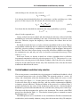
Reliable Communications for Short-range Wireless Systems
Ensuring reliable communication is an important concern in short-range wireless communication systems with stringent quality of service requirements. Key characteristics
of these systems, including data rate, communication range, channel profiles, network
topologies, and power efficiency, are different from those in long-range systems. This
comprehensive book classifies short-range wireless technologies as high and low data
rate systems. It addresses major factors affecting reliability at different layers of the
protocol stack, detailing the best ways to enhance the capacity and performance of shortrange wireless systems. Particular emphasis is placed on reliable channel estimation,
state-of-the-art interference mitigation techniques, and cooperative communications for
improved reliability. The book also provides detailed coverage of related international
standards including UWB, ZigBee, and 60 GHz communications. With a balanced treatment of theoretical and practical aspects of short-range wireless communications, and
with a focus on reliability, this is an ideal resource for practitioners and researchers in
wireless communications.
Ismail Guvenc is a Research Engineer with DOCOMO USA Laboratories, where his
research interests include UWB communications and position estimation, femtocell
networks, relay networks, LTE systems, and cognitive radio. He has published several
standardization contributions for IEEE 802.15 and IEEE 802.16 standards, and holds
four US patents, with another 15 US patent applications pending.
Sinan Gezici is an Assistant Professor in the Department of Electrical and Electronics
Engineering at Bilkent University, Turkey. His research interests are in the areas of signal
detection, estimation and optimization theory, and their applications to wireless communications and localization systems. Among his publications in these areas is the recent
book Ultra-wideband Positioning Systems: Theoretical Limits, Ranging Algorithms, and
Protocols.
Zafer Sahinoglu is a Senior Principal Member of Technical Staff at Mitsubishi Electric
Research Laboratories, where his current research interests include UWB localization,
high efficiency wireless power transfer, low complexity space-time adaptive processing,
and game-theoretic dynamic energy pricing. He has contributed significantly to MPEG21, ZigBee, IEEE 802.15.4a, and IEEE 802.15.4e standards and holds two European
and 25 US patents, with 26 patents pending.
Ulas C. Kozat is the Project Manager for the Network Architecture team at DOCOMO
USA Laboratories. He has conducted research in the broad areas of wireless communications and communications networks, and has published mainly in cross-layer optimization, network modeling and performance analysis, and algorithm/protocol design.
Reliable Communications for
Short-range Wireless Systems
Edited by
ISMAIL GUVENC
DOCOMO Communications Laboratories USA, Inc.
SINAN GEZICI
Bilkent University, Turkey
ZAFER SAHINOGLU
Mitsubishi Electric Research Laboratories
ULAS C. KOZAT
DOCOMO Communications Laboratories USA, Inc.
CAMBRIDGE UNIVERSITY PRESS
Cambridge, New York, Melbourne, Madrid, Cape Town,
Singapore, S˜ao Paulo, Delhi, Tokyo, Mexico City
Cambridge University Press
The Edinburgh Building, Cambridge CB2 8RU, UK
Published in the United States of America by Cambridge University Press, New York
www.cambridge.org
Information on this title: www.cambridge.org/9780521763172
C
Cambridge University Press 2011
This publication is in copyright. Subject to statutory exception
and to the provisions of relevant collective licensing agreements,
no reproduction of any part may take place without the written
permission of Cambridge University Press.
First published 2011
Printed in the United Kingdom at the University Press, Cambridge
A catalog record for this publication is available from the British Library
Library of Congress Cataloging in Publication data
Reliable communications for short-range wireless systems / edited by
Ismail Guvenc . . . [et al.].
p. cm.
Includes bibliographical references and index.
ISBN 978-0-521-76317-2 (hardback)
1. Wireless communication systems – Reliability. I. G¨uvenc¸, Ismail.
TK5103.2.R376 2011
621.384 – dc22
2010049116
ISBN 978-0-521-76317-2 Hardback
Cambridge University Press has no responsibility for the persistence or
accuracy of URLs for external or third-party internet websites referred to
in this publication, and does not guarantee that any content on such
websites is, or will remain, accurate or appropriate.
Contents
List of contributors
1
Short-range wireless communications and reliability
page xi
1
Ismail Guvenc, Sinan Gezici, Zafer Sahinoglu, and Ulas C. Kozat
1.1 Short-range wireless communications
1.1.1 Enabling factors
1.1.2 Short-range versus medium/long-range communications
1.1.3 High-rate versus low-rate communications
1.1.4 Review of frequency regulations and available frequency bands
1.2 Definition of reliability
1.2.1 Reliability at the PHY layer
1.2.2 Reliability at the MAC layer
1.2.3 Reliability at the routing layer
1.3 Review of related wireless standards
1.3.1 Bluetooth
1.3.2 IEEE 802.15.5 (mesh networking)
1.3.3 IEEE 802.15 TG6 (body area networks (BANs))
1.3.4 IEEE 802.15 TG7 (visible light communication)
1.3.5 ISA SP100.11a (process control and monitoring)
Part I High-rate systems
2
High-rate UWB and 60 GHz communications
l2
2
3
4
6
7
8
12
12
13
16
17
20
22
23
29
31
Sinan Gezici and Ismail Guvenc
2.1 Overview and application scenarios
2.2 ECMA-368 high-rate UWB standard
2.2.1 Transmitter structure
2.2.2 Signal model
2.2.3 System parameters
2.3 ECMA-387 millimeter-wave radio standard
2.3.1 Transmitter structure
2.3.2 Signal models
2.3.3 System parameters
31
35
36
37
39
40
43
47
50
vi
3
Contents
2.4 IEEE 802.15.3c millimeter-wave radio standard
2.4.1 Single-carrier PHY
2.4.2 High-speed interface PHY
2.4.3 Audio/visual PHY
53
55
56
57
Channel estimation for high-rate systems
61
Zhongjun Wang, Yan Xin, and Xiaodong Wang
4
3.1 Channel models for high-rate systems
3.1.1 Large-scale propagation effects
3.1.2 Small-scale propagation effects
3.1.3 Discrete-time model
3.2 Review of channel estimation techniques
3.2.1 Signal model for channel frequency response estimation
3.2.2 LS channel frequency response estimator
3.2.3 LMMSE channel frequency response estimator
3.2.4 ML channel frequency response estimator
3.2.5 Multistage channel frequency response estimator
3.2.6 Complexity comparison
3.3 Impact of channel estimation error on performance
3.3.1 Average uncoded SER
3.3.2 FER performance
61
62
63
68
70
72
75
76
78
80
84
85
86
88
Adaptive modulation and coding for high-rate systems
93
Ruonan Zhang and Lin Cai
4.1 Adaptive modulation and coding (AMC)
4.2 AMC in MB-OFDM systems
4.3 WPAN link architecture in ECMA-368
4.3.1 Superframe structure and DRP
4.3.2 Block-acknowledgment mechanism
4.4 Packet-level model for UWB channels with shadowing
4.4.1 Body shadowing effect on UWB channels
4.4.2 Definition of channel states in the channel model
4.4.3 Channel state transitions
4.5 WPAN link performance analysis
4.5.1 System model
4.5.2 Markovian analysis
4.5.3 Packet drop rate and throughput
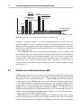
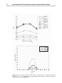
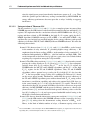
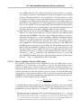
4.6 Simulation results
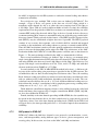
4.7 AMC in 60 GHz millimeter-wave radio systems
4.7.1 AMC mechanism in ECMA-387
4.7.2 MAC protocol in ECMA-387
4.8 Summary
94
95
97
97
98
99
99
101
101
102
102
102
105
106
108
108
109
110
Contents
5
MIMO techniques for high-rate communications
vii
113
Wasim Q. Malik and Andr´e Pollok
5.1 Principles of MIMO systems
5.2 MIMO for ultrawideband systems
5.2.1 Channel model
5.2.2 Spatial correlation
5.2.3 Channel capacity
5.2.4 The role of multipath
5.2.5 Time-reversal prefiltering
5.2.6 Summary
5.3 MIMO for 60 GHz systems
5.3.1 MIMO channel model
5.3.2 Spatial correlation
5.3.3 Beamforming
5.3.4 Receiver performance
5.3.5 Summary
5.4 Conclusion
Part II Low-rate systems
6
ZigBee networks and low-rate UWB communications
113
115
115
116
118
119
120
123
123
124
124
126
129
132
132
137
139
Zafer Sahinoglu and Ismail Guvenc
7
6.1 Overview and application examples
6.2 ZigBee
6.2.1 Channel allocations in ZigBee and IEEE 802.15.4
6.2.2 Data transmission methods in ZigBee and IEEE 802.15.4
6.2.3 Network channel managing for interference resolution
6.3 Impulse-radio based UWB (IEEE 802.15.4a)
6.3.1 Channel allocations
6.3.2 Transmitter structure and signal model
6.3.3 Frame structure and system parameters
6.3.4 Ranging and location awareness
6.4 Low latency MAC for WPANs (IEEE 802.15.4e)
6.4.1 EGTS
6.4.2 Low latency protocol (LLP)
6.4.3 Time synchronized channel hopping (TSCH)
6.5 IEEE 802.15.4f (active RFID)
6.6 IEEE 802.15.4g (smart utility networks)
139
142
142
143
148
149
149
151
154
156
158
158
161
162
163
164
Impact of channel estimation on reliability
168
Hongsan Sheng
7.1 Introduction
168
viii
8
Contents
7.2 Signal and channel models with channel estimation errors
7.2.1 Signal and channel model
7.2.2 Estimation errors of channel parameters
7.3 Reliability with channel estimation errors
7.3.1 SNR analysis
7.3.2 BER analysis
7.4 System optimization with channel estimation errors
7.4.1 Allocations of power to pilot symbols
7.4.2 Signal bandwidth
7.4.3 Design of rake receivers
7.5 Concluding remarks
170
170
171
173
174
176
180
180
181
184
186
Interference mitigation and awareness for improved reliability
190
Huseyin Arslan, Serhan Yarkan, Mustafa E. Sahin, and Sinan Gezici
9
8.1 Mitigation of multiple-access interference (MAI)
8.1.1 Receiver design for MAI mitigation
8.1.2 Coding design for MAI mitigation
8.2 Mitigation of narrowband interference (NBI)
8.2.1 UWB and narrowband system models
8.2.2 NBI avoidance
8.2.3 NBI cancelation
8.3 Interference awareness
8.4 Summary
190
190
208
212
213
215
219
222
226
Characterization of Wi-Fi interference for dynamic channel allocation
in WPANs
234
Federico Penna, Claudio Pastrone, Hussein Khaleel, Maurizio A. Spirito, and Roberto Garello
9.1 Towards adaptive wireless personal area networks (WPANs)
9.1.1 Introduction and motivation
9.1.2 Spectrum sensing for cognitive radio networks
9.2 WPANs under Wi-Fi interference
9.2.1 Detecting the interference: spectrum sensing in WPANs
9.2.2 Test-bed configuration and scenarios
9.2.3 Wi-Fi interference model
9.2.4 Duration of the sensing window
9.2.5 Sensing duty cycle
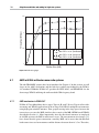
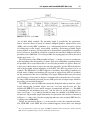
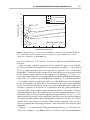
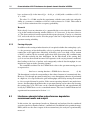
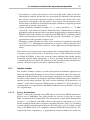
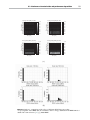
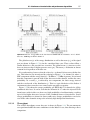
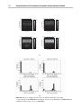
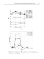
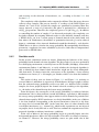
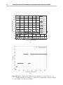
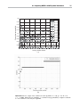
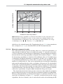
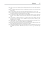
9.3 Interference characterization and performance degradation:
measurement results and analysis
9.3.1 Anechoic chamber
9.3.2 Indoor 1
9.3.3 Indoor 2
9.3.4 Analyzing the different spectrum evaluation metrics
234
234
235
236
236
237
241
241
244
244
245
250
255
260
Contents
9.4
9.5
10
Improving WPAN’s reliability under interference:
dynamic channel selection
9.4.1 Algorithm description
9.4.2 Simulation results
Conclusion
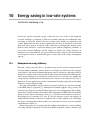
Energy saving in low-rate systems
ix
261
261
263
267
270
Tae Rim Park and Myung J. Lee
10.1 Background on energy efficiency
10.1.1 Measure of energy consumption
10.2 Energy saving MACs
10.2.1 Asymmetric single-hop MACs
10.2.2 Symmetric multihop MACs
10.3 Summary
270
275
276
277
282
289
Part II Selected topics for improved reliability
291
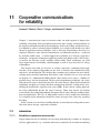
11
293
Cooperative communications for reliability
Andreas F. Molisch, Stark C. Draper, and Neelesh B. Mehta
12
11.1 Introduction
11.1.1 Reliability via cooperative communication
11.1.2 Overview of methods
11.2 Cooperative communication using virtual beamforming
11.2.1 Basic principles
11.2.2 Basic “building block” network and protocol
11.2.3 Basic network: analysis and results
11.2.4 Routing
11.3 Cooperative communication using rateless codes
11.3.1 Basic principles
11.3.2 Basic “building block” network and protocols
11.3.3 Basic network: analysis and results
11.3.4 Routing
293
293
295
297
297
298
301
304
308
308
310
311
318
Reliability through relay selection in cooperative networks
326
Ramy Abdallah Tannious and Aria Nosratinia
12.1
12.2
12.3
12.4
Introduction
Signaling in multiple-relay networks
Motivations for relay selection
Overview of relay selection
12.4.1 System model and mathematical background
12.4.2 Relay selection strategies
326
327
328
330
331
333
x
13
Contents
12.5 Limited feedback centralized relay selection
12.5.1 Outage probability and effective rate
12.5.2 DMT analysis
12.6 Summary
337
339
341
343
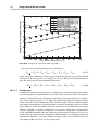
Fundamental performance limits in wideband relay architectures
347
¨ ur Oyman
Ozg¨
14
13.1 Introduction
13.2 Power–bandwidth tradeoff in serial relay architectures
13.2.1 Network model and definitions
13.2.2 Power–bandwidth tradeoff characterization
13.2.3 Section summary
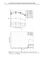
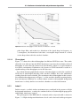
13.3 Power–bandwidth tradeoff in parallel relay architectures
13.3.1 Network model and definitions
13.3.2 Upper-limit on MRN power–bandwidth tradeoff
13.3.3 MRN power–bandwidth tradeoff with practical LDMRB
techniques
13.3.4 Numerical results
13.3.5 Section summary
347
352
352
357
362
362
362
367
Reliable MAC layer and packet scheduling
386
369
378
382
Ulas C. Kozat
14.1 Introduction
14.2 Opportunistic scheduling/multiuser diversity
14.2.1 Unicast case
14.2.2 Multicast case
14.3 Coding and scheduling
14.3.1 Unicast case
14.3.2 Multicast case
14.4 Media quality driven scheduling
14.5 Summary
386
388
389
391
394
394
397
401
404
Index
407
Contributors
Huseyin Arslan
University of South Florida, Florida, USA
Lin Cai
University of Victoria, Canada
Stark C. Draper
University of Wisconsin-Madison, Wisconsin, USA
Roberto Garello
Politecnico di Torino, Torino, Italy
Sinan Gezici
Bilkent University, Turkey
Ismail Guvenc
DOCOMO Communications Laboratories USA, Inc., California, USA
Hussein Khaleel
Politecnico di Torino, Torino, Italy
Ulas C. Kozat
DOCOMO Communications Laboratories USA, Inc., California, USA
Myung J. Lee
City University of New York, City College, New York, USA
Wasim Q. Malik
Massachusetts Institute of Technology, Massachusetts, USA
Neelesh B. Mehta
Indian Institute of Science (IISc), Bangalore, India
xii
List of contributors
Andreas F. Molisch
University of Southern California, California, USA
Aria Nosratinia
University of Texas at Dallas, Texas, USA
¨ ur
¨ Oyman
Ozg
Intel Corporation, California, USA
Tae Rim Park
Samsung Advanced Institute of Technology, Republic of Korea
Claudio Pastrone
Istituto Superiore Mario Boella (ISMB), Torino, Italy
Federico Penna
Istituto Superiore Mario Boella (ISMB), Torino, Italy
Andre´ Pollok
Institute for Telecommunications Research, University of South Australia, Australia
Mustafa E. Sahin
University of South Florida, Florida, USA
Zafer Sahinoglu
Mitsubishi Electric Research Laboratories, Massachusetts, USA
Hongsan Sheng
InterDigital Communications, LLC., Pennsylvania, USA
Maurizio A. Spirito
Istituto Superiore Mario Boella (ISMB), Torino, Italy
Ramy Abdallah Tannious
University of California, Davis, California, USA
Xiaodong Wang
Columbia University, New York, USA
Zhongjun Wang
Wipro Techno Centre, Singapore
Yan Xin
NEC Laboratories America Inc., New Jersey, USA
List of contributors
Serhan Yarkan
Texas A&M University, Texas, USA
Ruonan Zhang
University of Victoria, Canada
xiii
1
Short-range wireless
communications and reliability
Ismail Guvenc, Sinan Gezici, Zafer Sahinoglu, and Ulas C. Kozat
Even though there is no universally accepted definition, short-range wireless communications typically refers to a wide variety of technologies with communication ranges
from a few centimeters to several hundreds of meters. While the last three decades of the
wireless industry have been mostly dominated by cellular systems, short-range wireless
devices have gradually become a more integrated part of our everyday lives over the
last decade. The Wireless World Research Forum (WWRF) envisions that this trend
will accelerate in the upcoming years: by the year 2017, it is expected that seven billion
people in the world will be using seven trillion wireless devices [1]. The majority of
these devices will be short-range wireless devices that interconnect people with each
other and their environments.
While the reliability of wireless communication systems has been studied in detail in
the past, a comprehensive study of different factors affecting reliability for short-range
wireless systems and how they can be handled is not available in the literature, to date.
The present book intends to fill this gap by covering important reliability problems for
short-range wireless communication systems. The scope of the contributions in the book
is mostly within the domain of wireless personal area networks (WPANs) and wireless
sensor networks (WSNs), and issues related to wireless local area networks (WLANs)
are not specifically treated.
Due to the differences in application scenarios, quality of service (QoS) requirements,
signaling models, and different error sources and mitigation approaches, the high-rate
and low-rate systems will be addressed in separate parts of the book. For the highrate systems covered in Part I, multiband orthogonal frequency division multiplexing
(OFDM) and millimeter wave communication systems will be the main focus owing
to their significant potential for achieving high throughputs. On the other hand, Part II
of the book will be focusing mostly on ZigBee and pulse-based ultrawideband (UWB)
communications owing to their benefits for low-rate, low-power, and low-complexity
operation. In addition, a third set of chapters within Part III will be addressing some
selected topics related to the reliability of short-range wireless communication systems,
where the chapters are written from a broader perspective without specifying a certain
technology or standard.
The rest of this chapter is organized as follows. First, in Section 1.1, enabling
factors for short-range wireless communications are discussed, and differences from
long-range wireless systems are summarized. In addition, a comparison of low-rate
and high-rate systems in terms of application scenarios, typical transmitter/receiver
2
Short-range wireless communications and reliability
characteristics, and reliability requirements is provided, and globally available frequency
bands for short-range wireless systems are reviewed. In Section 1.2, reliability problems
observed at different layers of the protocol stack are defined, and possible solutions
to address these are discussed along with references to different chapters in the book.
Section 1.3 provides a brief review of certain short-range wireless communications
standards, leaving the detailed treatment of more established standards to Chapter 2 and
Chapter 6.
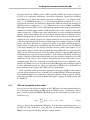
1.1
Short-range wireless communications
1.1.1
Enabling factors
There are three significant factors that play an important role for the widespread use and
adoption of short-range wireless communications devices in today’s world: (i) advancements in the solid-state devices, (ii) developments in the digital communication and
modulation techniques, and (iii) developments in related standardization activities.
Advances in the solid-state technology have been an important factor enabling the
widespread use of short-range wireless technologies. First, the mass production of
devices became possible, decreasing the production cost per unit device. Second, with
the new developments, higher center frequencies have become operational for shortrange devices. This implies access to the previously inaccessible frequency bands such
as the 2.4 GHz, 5 GHz, and 60 GHz bands of the industrial, scientific, and medical
(ISM) bands that will be discussed in more detail in Section 1.1.4. Using higher center
frequencies also enables the use of very small antenna elements, of which multiple
may easily be embedded within the same device [2]. Today, circuit miniaturization and
small-size antennas make it possible to manufacture extremely small radio frequency
integrated circuits (RFICs) on chips that contain all the essential system components.
For example, CMOS RFIC-on-chip antennas are available for short-range wireless technologies utilizing central frequencies as high as 60 GHz and having chip sizes of less
than 1 mm2 [3, 4].
Another enabling factor that has an important role in the success of short-range wireless communication systems is the recent developments in digital modulation techniques
and transceiver algorithms. For example, direct sequence spread spectrum (DSSS) technology has been used successfully in systems such as the IEEE 802.15.4 WPANs and
the IEEE 802.11 WLANs. Through spreading the frequency content of a transmitted
signal, DSSS provides advantages such as interference resilience, low-power spectral
density, resistance to jamming, and mitigation of multipath effects [5]. Frequencyhopping spread spectrum (FHSS) is another spread spectrum transmission technology
that has commonly been used in short-range wireless devices due to its interference
resilience. Because of its important advantages in multipath environments, OFDM has
recently been a key technology for achieving higher throughputs in short-range wireless
communication systems [6, 7]. Advantages of OFDM over other relevant competitive
technologies include the following: (i) there is no need for time-domain equalization, and
1.1 Short-range wireless communications
3
much simpler frequency-domain equalization techniques can be utilized efficiently,1 (ii)
it is robust in frequency selective channels owing to the use of a cyclic prefix (CP), and
(iii) multiple-input multiple-output (MIMO) is easily implementable with OFDM due to
frequency-flat fading at each tone. Due to such advantages, OFDM has been adopted by
recent standards such as ECMA-368 (high-rate UWB PHY and MAC [6]) and ECMA387 (high-rate 60 GHz PHY, MAC, and HDMI PAL [7]). Other recent developments
that may impact the future of short-range wireless communications include the advances
in MIMO techniques for achieving higher data rates and better reliability [9–13], and
cognitive radio methods for more efficient and reliable utilization of the wireless spectrum [14–17].
The critical role of standardization bodies in the widespread use of short-range wireless devices should also be emphasized here. Through standardization, related companies and research organizations actively work towards obtaining a well-defined technical
specification for a given wireless technology. This brings with it a high potential for
the realizability and interoperability of the technology; a better understanding of the
application scenarios, potentials, and limitations is achieved, and a consensus is reached
on how to implement it in a good way. Several successful short-range wireless devices
that we use in our everyday lives today such as WiFi, Bluetooth headsets, wireless keyboards, and ZigBee devices are all the result of long years of standardization. Probably
the most important standardization group working on short-range wireless communication technologies is the IEEE 802.15 Working Group for WPANs. As well as the already
standardized short-range wireless technologies discussed before, IEEE 802.15 is also
working on the standardization of some recent technologies such as wireless body area
networks (WBANs), radio frequency identification (RFID) systems, mesh networks,
and visible light communications (VLCs). Other standard bodies related to short-range
wireless communications include ISA-100 and ECMA standards. A more detailed discussion on related short-range wireless communication standards will be presented in
Section 1.3 as well as in other chapters of the book.
1.1.2
Short-range versus medium/long-range communications
While short-range wireless technologies span a wide range of application scenarios,
they typically have some common characteristics that are significantly different from
medium and long-range wireless technologies, such as WLANs, cellular systems, wireless metropolitan area networks, and satellite communication systems. Some of the
common features of short-range wireless devices include low-power operation, communication ranges from several centimeters up to a hundred meters, principally indoor
operation, omnidirectional built-in antennas, low-complexity and low-price devices,
battery operated transmitter/receiver, and unlicensed operation [18].
Short-range wireless devices typically have very low or no mobility, which implies
simple and low-complexity receiver architectures compared, for example, to cellular
1
Note that frequency domain equalization is also possible for single-carrier frequency domain multiple access
(SC-FDMA) systems [8].
4
Short-range wireless communications and reliability
systems. On the other hand, multihop and cooperative communications may be considered as important operational modes for certain short-range wireless communications
scenarios (e.g., as in WSNs). This is primarily due to dense deployment scenarios of
wireless sensors that collect local information, aggregate it, and communicate to the
intended receiver. Such wireless networks should have very low-power operation for
extended network life, and overall power consumption may be decreased by transmitting
the packets over multiple shorter distance hops rather than over a direct link with longer
transmitter–receiver separation. Due to their critical importance for short-range wireless
communication systems, multihop and cooperative communication techniques will be
treated in detail in Part III of this book.
The QoS requirements (e.g., packet error rate, data rate, and latency) for short-range
wireless systems are also quite different from long-range communication technologies
and are closely coupled with the application scenarios. In reference [19], the top 10
design rules for short-range communications, which are different from the design rules
of long-range networks, have been listed as follows: communication architecture (both
point-to-point and point-to-multipoint communications capability), energy awareness,
signaling and traffic channels, scalability and connectivity, medium access control and
channel access methods, self organization, service discovery, security and privacy issues,
flexible spectrum usage, and software-defined radio design.
1.1.3
High-rate versus low-rate communications
It is possible to have different sets of taxonomies and classifications for short-range
wireless communication technologies. Among some other possible classifications, they
may be classified with respect to their communication ranges, mobility characteristics, network topology, QoS requirements, indoor versus outdoor operation, operating
frequency/bandwidth, and data rates. Communication ranges of short-range wireless
systems may be on the order of several centimeters (e.g., for near field communications
(NFCs)), fractions of a meter (e.g., for WBANs), several meters (e.g., WPANs), or from
a few meters up to hundreds of meters (WSNs) [20]. The range of passive RFIDs are
on the order of tens of centimeters, while active RFIDs may have ranges as large as a
hundred meters. Even though short-range wireless technologies typically operate with
no mobility or very low mobility, there may be scenarios in which the mobility may be
a concern. For example, body movements in WBANs, or movement of the transmitter
and/or the receiver in certain WSN applications may introduce mobility related problems
that should be taken into account in receiver design. Centralized network topology or
distributed network architectures are two common topologies for short-range wireless
communication systems.
Despite the aforementioned classifications and several other possible taxonomies,
it is difficult to classify different short-range technologies within different groups.
The large diversity of application scenarios and requirements, differences in the air
interface, and variations in operational ranges even for the same wireless technology
are only a few of the factors preventing well-defined taxonomies. In this book, since
it provides a relatively uniform and well-defined classification, we choose to study
1.1 Short-range wireless communications
5
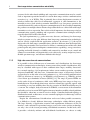
Table 1.1 Example applications for short-range wireless communications.
Low-rate systems
High-rate systems
Tele-control for home and building
Wireless microphones and headphones
Wireless mouse, keyboard, etc.
Remote keyless entry, gate openers, etc.
Wireless bar-code readers
Wireless sensor networks
Emergency medical alarms
Wireless billing
Wireless USB
Internet access and multimedia services
Uncompressed high-definition video
Patient monitoring in hospitals
Wireless surveillance cameras
Wireless video conferencing
Wireless ad-hoc communications
Wireless peripheral interfaces
short-range wireless communications systems by grouping them into two categories:
high-rate systems and low-rate systems.
While a clear-cut separation does not exist, high-rate systems are considered for
data rates higher than 10 Mbps (up to several Gbps), and they have communication ranges smaller than 10 m. Example application scenarios for high-rate systems include wireless video streaming, wireless file transfer (e.g., wireless USB),
wireless video conferencing, and wireless surveillance cameras. Also, as discussed
in reference [1], high-rate technologies considered for short-range wireless communication applications are based on multiband UWB [21] and millimeter wave
technologies [22, 23], and related wireless standards will be discussed in detail in
Chapter 2.
Low-rate systems, on the other hand, are considered for low-power and low-complexity
applications that do not have significant data rate requirements. While they do not necessarily have long communication ranges, the maximum ranges of low-rate systems may
be significantly larger than those of the high-rate systems. Apart from application related
requirements, two important reasons for this are as follows: (i) larger communication
ranges mean lower levels of received power, which inherently prevent high data rates,
and (ii) high-rate systems require a significantly large bandwidth, which is commonly
available at higher central frequencies (e.g., 60 GHz spectrum) that are subject to a larger
path-loss. WSNs are probably the most common applications for short-range low-rate
wireless communication systems. Two important recent wireless technologies that are
suitable for low-rate systems are ZigBee and low-rate UWB, and the wireless standards
related to these technologies will be reviewed in detail in Chapter 6. Some examples for
short-range wireless communications applications for high-rate and low-rate systems
are summarized in Table 1.1, and more detailed discussions of the related applications
are left to Chapter 2 and Chapter 6.
The QoS requirements as well as possible techniques and protocols for improving
the reliability of low-rate and high-rate systems are considerably different. For example,
primarily due to application scenarios and requirements, low-power operation becomes
more relevant to WSNs, e.g., for environmental sensing applications, where the sensor
nodes should operate with the same battery for extended durations. Power efficient routing techniques and cooperative communication methods may also gain more importance
6
Short-range wireless communications and reliability
in such scenarios. While such techniques may also be applied to certain high-rate communication scenarios, one of the most common applications for high-rate systems is
the wireless USB, which by definition is point-to-point, and routing and cooperative
communications techniques become irrelevant. Due to multiple-antenna capabilities
enabled by high-frequency operation of high-rate systems (e.g., for millimeter wave
communications), beamforming techniques and protocols may be very important for
certain scenarios in order to minimize the interference and improve reliability.
Signaling models utilized by low-rate and high-rate systems may vary greatly. For
example, the high-rate ECMA-368 standard has adopted an MB-OFDM based physical
(PHY) layer, which facilitates a simple equalization process in the frequency domain.
On the other hand, the low-rate IEEE 802.15.4a standard uses pulse-based signal transmissions. It is an ideal signaling scheme, for example, for low-rate WSN applications,
in which low-complexity transmitter/receiver architectures may be designed and highly
accurate ranging/positioning is supported. Low-complexity transceiver architectures
such as the energy detector and the transmitted-reference schemes become possible with
pulse-based signaling, whereas FFT/IFFT operations in OFDM-based transmission may
increase the transceiver complexity.
1.1.4
Review of frequency regulations and available frequency bands
The choice of the central frequency and communication bandwidth is critical for shortrange wireless communication systems. As discussed earlier, high central frequencies
may be preferable in many cases, because they facilitate small form-factors owing to
small antenna sizes, and enable access to several license-free frequency bands at high
frequencies (typically having fewer interference sources). On the other hand, since signal
attenuation is directly proportional to the central frequency, wireless devices employing
high central frequencies may not communicate reliably over relatively long distances
owing to severe signal attenuation. Based on the application requirements of a certain
short-range wireless system, before deciding on an operational center frequency, such
trade-offs should be evaluated carefully by system designers.
The frequency bands in which short-range wireless devices may operate are in most
cases limited to license-free bands. While certain license-free bands are globally available, there are also some license-free bands that are available in only certain regions
of the world. The frequency bands that are globally available for short-range wireless
devices are the 13.56 MHz band (typically considered for near-field communications),
40 MHz band, 433 MHz band, 2.4 GHz band, and the 5.8 MHz band [5]. Among these,
the 2.4 GHz band is the most popular global license-free band, which is commonly used
by WLANs and microwave ovens. Another band that is available and commonly used for
short-range communications in Europe, the USA, Canada, Australia, and New Zealand
is the 868 MHz/915 MHz band.
A part of the spectrum that can be used without a license in most countries is the
ISM band [24], which also includes some of the frequency bands discussed above. For
example, in the USA, popular ISM bands include the 902–928 MHz, 2.4 GHz, and 5.7–
5.8 GHz bands. Similar to several other frequency bands for unlicensed transmissions,
1.2 Definition of reliability
7
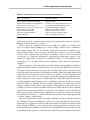
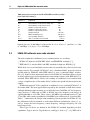
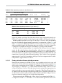
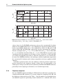
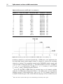
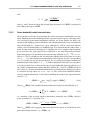
Table 1.2 Review of the ISM/U-NII bands, and the spectrum used for UWB and 60 GHz systems in
the USA.
ISM bands
Power limit
U-NII 5 GHz bands
Power limit
902–928 MHz
Cordless phones
Microwave ovens
Industrial heaters
Military radar
1W
750 W
100 kW
1000 kW
WiFi (802.11a/n)
5.15–5.25 GHz
5.25–5.35 GHz
5.47–5.725 GHz
5.725–5.825 GHz
200 mW
1W
1W
4W
2.4–2.4835 GHz
Wi-Fi (802.11b/g)
Microwave ovens
1W
900 W
60 GHz band
57–64 GHz
Ultra–wideband
0.5 W
3.1–10.6 GHz
−41.3 dBm/Mhz
5 GHz
5.725–5.825 GHz
Wi-Fi (802.11a/n)
4W
the ISM bands are defined under the Part 15 rules of the Federal Communications
Commission (FCC). Until 1985, the industrial, scientific, and medical (ISM) bands were
not allowed to be used for radio communications in the USA. Together with the FCC
Part 15.247 rules in 1985, the ISM bands have been opened for use by WLANs and
mobile communications [24]. The Unlicensed National Information Infrastructure (UNII) bands introduced by Part 15.401 to Part 15.407 of the FCC in 1997 added additional
license-free frequency bands in the 5 GHz range.
In 2002, the FCC released the Subpart-F of its Part 15 rules, which defines the
scope and operation of UWB devices (including communications, imaging systems, and
ground-penetrating radar) under Part 15.501 to Part 15.525. Based on this new ruling,
UWB devices can transmit at power levels up to −41.3 dBm/MHz in the frequency
spectrum between 3.1 GHz and 10.6 GHz. This opens up a large amount of spectrum
available for use by short-range UWB wireless devices. Another large spectrum that can
be utilized by short-range wireless devices is defined by the Part 15.255 rules of the
FCC, which allow transmission powers up to 500 mW within the frequency range 57–
63 GHz. This spectrum is commonly referred to as the millimeter wave or the 60 GHz
spectrum, and is another popular band for future short-range high-rate communication
systems. The frequency bands and transmit power limits for the ISM/U-NII bands,
UWB, and 60 GHz systems in the USA are summarized in Table 1.2. More details
on the unlicensed frequency bands of the FCC can be found in reference [25], while
further discussions about the sub-GHz frequency bands around the world for short-range
wireless communication systems can be found in reference [5].
1.2
Definition of reliability
The focus of the current book is on reliability aspects of short-range wireless
communication systems. Ultimately, reliability should be defined by the application
8
Short-range wireless communications and reliability
itself. For some applications (e.g., data transfer), reliability is about data integrity and
all the information sent by the transmitter must be accurately received at the receiver.
For other applications such as audio and video, it is less about data integrity and more
about tolerable distortion at the application layer which is a convoluted function of
error rates, error burstiness, delay, error concealment techniques, etc. Traditionally,
each layer of the communication stack addresses reliability at different timescales to
fix errors that are not correctable, observable, or too costly to correct at the lower
layers. In wireless systems, however, independent decisions at each layer often lead
to an unreliable or inefficient communication environment. Therefore, some degree of
cross-layer coordination/optimization has been proposed by numerous research papers
and adopted in some systems (especially between the PHY and medium access control (MAC) layers). In different chapters, examples of such cross-layer optimization
and coordination will be treated in their special contexts. In the rest of this section,
we briefly overview how reliability is impacted by the decisions at different layers
of the communication stack and discuss error sources from the perspective of each
layer.
1.2.1
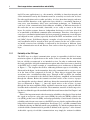
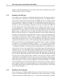
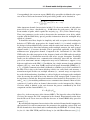
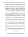
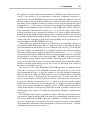
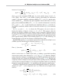
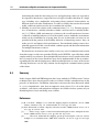
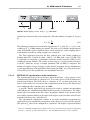
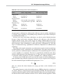
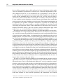
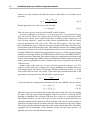
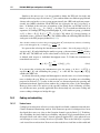
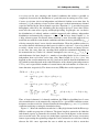
Reliability at the PHY layer
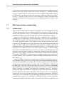
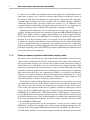
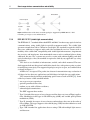
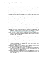
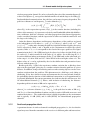
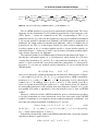
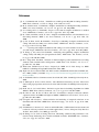
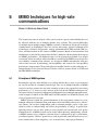
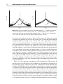
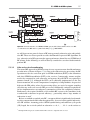
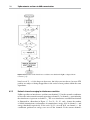
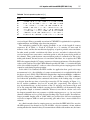
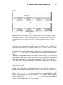
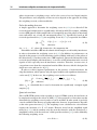
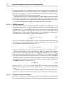
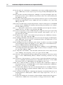
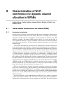
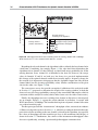
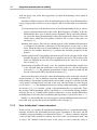
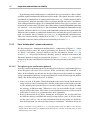
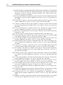
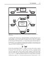
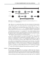
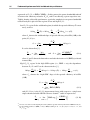
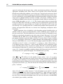
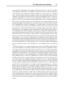
The PHY layer in a digital communication system is responsible for bit-level transmission/reception of signals between the nodes. It has to ensure that the transmitted
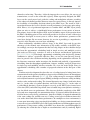
bits are reliably reconstructed at an intended receiver. In order to understand better
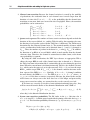
the basic principles of digital transmission/reception and related error sources involved
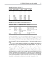
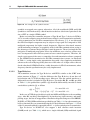
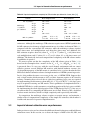
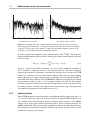
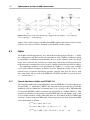
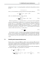
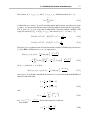
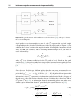
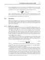
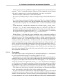
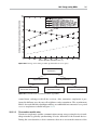
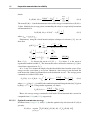
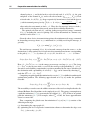
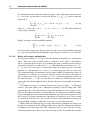
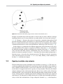
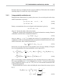
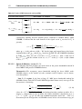
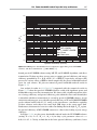
at the PHY layer, a simple example of a transmitter/receiver architecture is illustrated
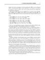
in Figure 1.1. The chapters that will be addressing different aspects of reliability are
illustrated in the figure. At the transmitter, data to be communicated to a target receiver
is in the form of bits, composed of 0’s and 1’s. These bits are mapped onto signal
waveforms after a modulation/coding stage. Through an RF oscillator, the transmit
waveform is up-converted to the desired central frequency, amplified, and transmitted
through the antenna. Before the transmit waveform arrives at the receiver, it propagates through the wireless channel, which may distort the transmitted signal in different
ways as illustrated in Figure 1.1. Once the signal arrives at the receiver, it passes
through the low-noise amplifier (LNA) and down-conversion stages, and gets demodulated/decoded to obtain the received bits. The transmitter structure of short-range wireless devices defined in specific standards will be discussed in more detail in Chapter 2 and
Chapter 6.
Some of the important metrics that characterize reliability at the physical layer include
the signal to interference plus noise ratio (SINR), bit error rate (BER), symbol error
rate (SER), packet error rate (PER), and outage probability. Certain issues related to the
reliability and relevant error sources at the PHY layer may also be explained through the
help of basic channel capacity formulations. In reference [26], a reliable communication
is defined as having an arbitrarily small error probability Pb , and the maximum data rate
at which reliable communication is possible is defined as the capacity C of the channel.
Achievable capacity for reliable communications may simply be written for additive
1.2 Definition of reliability
Transmitter Antenna
Ch. 4
Transmitter
Modulation
and Coding
Data
Amplifier
011…100
Cognitive
Engine
RF Oscillator
Ch. 8, Ch. 9
Receiver
Channel
Estimation
Wireless Channel
• Attenuation
• Multipath
• Fading
• Interference
• Noise
Scheduler
Ch. 14
Ch. 5
Ch. 3, Ch. 7
Down
Conversion
LNA
Demodulation
and Decoding
Interference
Cancellation
Receiver
Antenna
Ch. 3, Ch. 7
Estimated
Data
011…101
9
Ch. 8
Bit Error
Figure 1.1 An example block diagram of a wireless transmitter/receiver and related error sources.
white Gaussian noise (AWGN) channels as2
Cawgn = B log 1 +
Prec
2
σI + σn2
,
(1.1)
where B is the communication bandwidth, Prec is the received power of the signal, σI2
captures the variance of different error/interference terms (which are assumed to be white
Gaussian processes independent from the noise term), σn2 = B N0 is the noise variance,
rec
N0 is the noise spectral density, and σ 2P+σ
2 is referred to as the SINR. Note that while
n
I
the interference is assumed to be Gaussian in (1.1), this holds only with a sufficiently
large number of interferers, which may not always be the case for short-range systems.
As the channel capacity in (1.1) increases, reliable communications become possible at
higher data rates. In order to increase the capacity, the bandwidth B can be increased
(e.g., through scheduling algorithms), average interference power (σI2 ) can be decreased
(e.g., through interference cancellation techniques), or the received power Prec can be
increased (e.g., through power control algorithms).
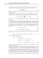
In the rest of this subsection, Figure 1.1 and equation (1.1) will be used to discuss the
major error sources that may impact the reliability at the PHY layer. Possible techniques
that may be used in order to mitigate the undesired effects of these error sources will
2
This may be easily extended to include different types of MIMO techniques, impact of multipath channels,
cooperative communications, etc. [26].
10
Short-range wireless communications and reliability
also be explained, along with referrals to the related chapters in the book for a more
complete treatment.
1.2.1.1
Attenuation
The received power Prec in (1.1) should be sufficiently larger than the combination of
noise and interference powers for the reliable detection of received bits. Due to path loss,
the received power is less than the transmitted power. In free space, the Friis formula
relates the transmitted and received powers as follows:
Prec = Pt
λ2 G t G r
,
(4π d)2
(1.2)
where Pt denotes the transmit power, λ = c/ f c is the wavelength, c is the speed of light,
f c is the central frequency, and G t and G r are the antenna gains at the transmitter and the
receiver, respectively. Since free-space propagation may not describe most environments
accurately, a better approach is to use the empirical path loss formula
α
do
χsh ,
(1.3)
Prec = Pt Po
d
where Po is the measured path loss at a reference distance do (typically well approximated
by (4π/λ)2 for do = 1 [27]) and α is the path loss exponent. The path loss is also subject
to shadowing effect due to several obstacles between the transmitter and receiver, that
is captured by the multiplicative term χsh in (1.3). The shadowing is typically modeled
using a log-normal random variable, where 10 log10 χsh ∼ N (0, σs2 ), with σs2 denoting
the variance of χsh in the logarithmic scale.
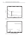
It is obvious from both (1.2) and (1.3) that the path loss is directly proportional to
the central frequency. Therefore, wireless communication systems operating at higher
central frequencies (e.g., operating in the millimeter wave spectrum) may have significantly shorter communication distances than wireless devices operating at lower central
frequencies. Similarly, the path loss is also directly proportional to the propagation distance. Therefore, the receivers that are closer to the transmitter will have larger received
powers while far-away receivers will have lower received powers, implying lower reliability based on (1.1). A method to tackle this problem is to use adaptive modulation and
coding (AMC) schemes, which adaptively select the modulation/coding scheme based
on the received signal quality. When the received signal quality is good, higher order
modulation schemes such as 64-QAM can be utilized to achieve higher data rates. If the
receiver moves away from the transmitter, the received signal quality degrades and the
receiver is no longer able reliably to demodulate the received bits with 64-QAM. Hence,
a lower order modulation such as binary phase shift keying (BPSK) can be used, where
the distance between the constellation points is larger, enabling reliable demodulation
of the bits at the expense of lower data rates. The AMC schemes for high-rate systems
will be discussed in more detail in Chapter 4.
Another possible way to improve the system performance in the presence of variations
in the received signal power is to employ power control techniques. For users far away
from the transmitter, a larger transmit power may be used to ensure sufficiently large
1.2 Definition of reliability
11
received powers at the receiver. The power may also be focused along a certain beam
direction using beamforming techniques, which will be discussed in detail in Chapter 5.
In order to improve network lifetime, energy saving approaches at the MAC layer are
also commonly considered, which will be discussed in detail in Chapter 10.
1.2.1.2
Multipath propagation
Apart from path-loss and shadowing, the received signal power is also subject to variations (selectivity) in time, frequency, and space. These three characteristics of the channel
have critical impacts on receiver design and the reliability of communications. In particular, the channel should accurately be estimated for reliable detection of transmitted
symbols. Channel models for short-range wireless systems will be reviewed in Chapter 3
and Chapter 7 along with the related channel estimation techniques for high-rate and
low-rate systems, respectively.
While accurate channel estimation is critical for reliable communications, different
multiple antenna techniques may also be used in order to improve reliability by utilizing
the selectivity of the wireless channel in time, frequency, and space. The data rate of a
multiple antenna system may be improved using spatial multiplexing techniques, where
the achievable capacity scales with min{Ntx , Nrx }, with Ntx and Nrx denoting the number
of transmitter and receiver antennas, respectively [26]. On the other hand, multiple
antennas may also be used to increase the reliability through diversity techniques. For
example, through transmit diversity techniques, identical information is transmitted over
multiple antennas, each of which goes through independently fading channels. Receiver
diversity techniques, on the other hand, utilize multiple receiver antennas, which again
observe independently faded replicas of the transmitted signal. Through intelligent
combining of the multiple and independently faded replicas of the transmitted signal
at the receiver, a more reliable demodulation of the received signal can be obtained.
This tradeoff between the capacity and the reliability of a wireless system with multiple
antennas is commonly referred to as the diversity–multiplexing tradeoff [28]. Several
variations of MIMO and smart antenna techniques for short-range high-rate wireless
communications will be discussed in detail in Chapter 5.
1.2.1.3
Interference sources
Interference factors such as multiuser interference and narrowband interference may
make the σI2 term in (1.1) larger, and hence degrade the SINR and the reliability
of the received signals. Short-range wireless communication systems typically have to
coexist with various technologies utilizing the frequency bands summarized in Table 1.2.
Therefore, they may receive interference from (and cause interference to) other wireless
technologies such as the WLANs that operate within the unlicensed bands.
There may be several approaches for improving the reliability in the presence of
interference from other wireless devices. For example, cognitive radio techniques can be
utilized to sense the interference sources and try to avoid them [14]. Along these lines, in
Chapter 9, spectrum sensing techniques and some related experimental results for lowrate systems will be presented. In some cases, however, it may not be possible to avoid
interference, necessitating the use of interference cancellation methods. Cancellation of
12
Short-range wireless communications and reliability
multiuser and narrowband interference for short-range wireless communication systems
will be discussed in detail in Chapter 8.
1.2.2
Reliability at the MAC layer
At the MAC layer, reliability is traditionally defined from the data integrity point of
view and packets erroneously received from the physical layer are dropped. Thus, a
critical metric at this layer is the packet drop rate (PDR) and at least for point-to-point
unicast transmissions MAC layer designs aim at marginalizing the packet drops due to
link/channel errors. Collision-free channel access and coded or uncoded packet retransmissions are the main mechanisms employed at this layer to improve the PDR. On
the other hand, many wireless MAC designs do not attempt to fix packet errors for
point-to-multipoint (i.e., multicast/broadcast) wireless transmissions. Instead, low-rate
transmissions for such sessions are used for increased reliability in terms of PERs.
More recently, a combination of erasure coding at the MAC layer and rate control at the
PHY layer has been proposed as a promising technique for various multicast/broadcast
scenarios [52]. Since in short-range radio there are fewer receivers (with possibly more
correlations in their channel conditions) to be served in comparison to broadcasting
in terrestrial or satellite-type services, feedback might be a plausible option even for
multicast/broadcast-type services. Cross-layer optimization and cooperative communications have been other recent areas of focus that require tight coordination between the
MAC layer and other layers including physical and routing layers to improve reliability
in multiple access and multicast channels. Chapters 11 to 14 provide an interesting
spectrum of research results with an in-depth treatment of particularly important ones.
Limiting the reliability to data integrity and/or packet drop rates at the MAC layer is
quite a narrow view once the requirements of several short-range radio applications are
considered. In one set of applications such as multimedia and interactive applications,
forcing low packet error rates indiscriminately might induce excessive delays due to
retransmissions rendering the received packets useless at the application layer. Delay and
jitter are directly impacted by the MAC layer decisions. The scheduling problem might
be quite hard even under fixed channel conditions and error-prone wireless channels
coupled with such scheduling decisions lead to an even greater challenge. In this respect,
many efforts are dedicated to cross-layer optimization both in single-hop and multihop
wireless networks [51]. Some of those techniques are presented in Chapter 14. Another
critical reliability measure that mainly the MAC layer decisions govern is the network or
device lifetime, which is of paramount importance for battery-powered environments.
Several MAC design choices and the design tradeoffs for energy efficiency are discussed
in more detail in Chapter 10.
1.2.3
Reliability at the routing layer
At the routing layer, reliability traditionally targets end-to-end connectivity and maintenance of sufficiently high-quality communication paths under dynamic network
conditions. Network conditions might vary as a result of node or link failures, mobility,
1.3 Review of related wireless standards
13
changes in wireless channel quality, changes in traffic demand, etc. Depending on the
particular scenario, few of these network dynamics become the dominant characteristics
and routing protocols can be customized accordingly with various notions of reliability.
For instance, many works on routing in wireless networks in the context of mobile adhoc networks (MANET) have mainly focused on developing protocols that can work in
high-mobility scenarios. With links forming and tearing up quite fast, route discovery
and packet losses due to lack of connectivity are the main reliability issues that have
been investigated. Therefore, routing protocols in MANET scenarios have been evaluated principally with respect to their overhead versus packet delivery ratios, mainly
under deterministic coverage models [54, 55].
When wireless nodes are quasi-stationary or stationary, other aspects, such as losses
due to unreliable wireless channel conditions and to congestion, network stability, delay,
and network capacity, surface as critical objectives moving away from connectivityoriented routing layer reliability. In the context of wireless mesh networks and sensor
networks, these different angles of reliability have been tackled to a degree. Some of
the notable developments to increase the reliability of the routing layer range from
the devising of new routing metrics [56] to developing better protocols that utilize
techniques such as multipath diversity, opportunistic routing, back-pressure algorithms,
cooperative communications, erasure and network coding. Many of these methods take
full advantage of the broadcast medium and cross-layer optimization with the PHY and
MAC layers being important aspects. Some of these techniques are treated in Chapters 11
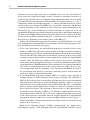
to 13. In particular, Chapter 11 investigates cooperative communication techniques with
emphasis on virtual beamforming and rateless coding. Authors construct a building block
network and protocols over a simpler relay channel model. Authors also investigate how
to perform routing and resource allocation in large networks based on these building
blocks. Chapter 12, in contrast, focuses on the relay selection problem in block fading
channels to boost the communication reliability against channel outages. Chapter 13
focuses on power-limited low SNR wideband communication scenarios. End-to-end
scaling performance limits of various relaying and multihop routing algorithms and
architectures in large-scale distributed wireless networks are investigated in depth. The
analysis formalizes multihop communication as another form of diversity.
Going beyond communications, in some more specialized areas such as in certain sensor network applications, routing also facilitates and maintains high-quality (distributed)
computation, generates data compression opportunities, and/or forms a network-wide
storage. Routing plays an important role also in terms of network and node lifetimes,
since it ultimately determines the load of each relay node in the system [53].
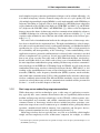
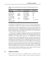
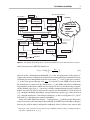
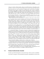
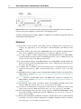
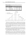
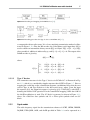
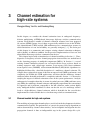
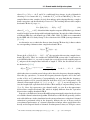
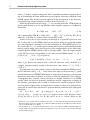
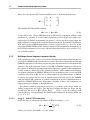
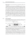
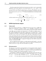
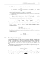
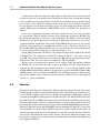
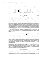
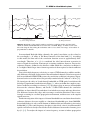
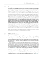
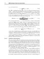
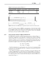
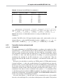
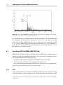
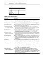
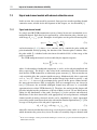
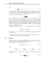
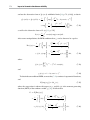
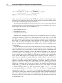
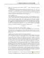
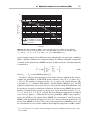
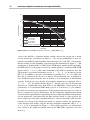
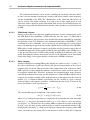
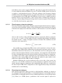
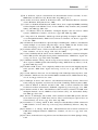
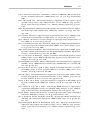
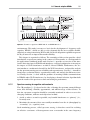
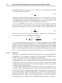
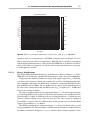
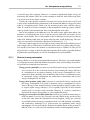
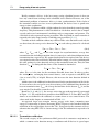
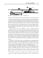
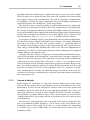
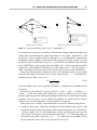
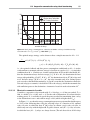
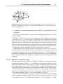
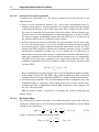
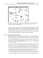
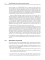
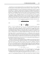
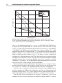
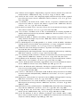
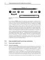
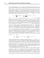
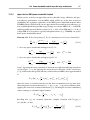
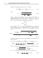
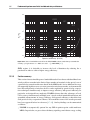
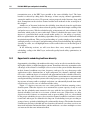
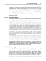
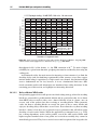
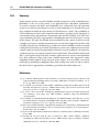
A summary of how different error sources are handled in MAC and routing layers and
respective chapters in which they are handled is illustrated in Figure 1.2.
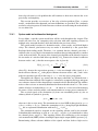
1.3
Review of related wireless standards
In order to provide harmonization of various short-range wireless systems, standardization efforts are in progress. The main body that organizes standardization activities is the
14
Short-range wireless communications and reliability
Relays
Ch. 12
1
Source A
Destination A
Ch. 13
14
1
(a)
X
Source B
Destination B
X
Ch. 11
12
1
(b)
Coded Data
Source C
Destination C
Coded Data
Coded Data
Erasure Coding
Network Coding
(c)
Source D
Destination D
Ch. 10
Power Savings
Through Sleep Mode
(d)
Coded Data
Destination E1
Source E
Destination E2
Ch. 14
12
1
Destination En
(e)
Figure 1.2 Different techniques for achieving reliability at the MAC/routing layers; (a) relay
selection, (b) cooperative communications, (c) error/erasure correction codes, (d) routing and
power saving mechanisms, (e) coded opportunistic scheduling.
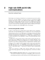
IEEE, which formed the IEEE 802.15 Working Group for WPAN for the development
of consensus standards for short-range wireless networks [29].
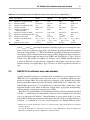
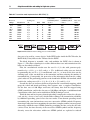
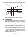
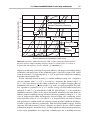
In Table 1.3, the task groups (TGs) under the IEEE 802.15 Working Group are listed.
TG1 focused on Bluetooth devices and provided a standard for the initial versions of
Bluetooth. However, the main activities on the standardization of Bluetooth have been
undertaken by the Bluetooth Special Interest Group (SIG) [30], and the later versions
of Bluetooth have not been ratified as IEEE standards (see Section 1.3.1). TG2 was
formed to develop coexistence mechanisms for the coexistence of WPANs and WLANs,
1.3 Review of related wireless standards
15
Table 1.3 Task groups (TGs) in IEEE 802.15 Working Group for WPAN [29].
Name
Description
IEEE standard
TG1
TG2
TG3
TG3a
TG3b
TG3c
TG4
TG4a
TG4b
TG4c
TG4d
TG4e
TG4f
TG4g
TG5
TG6
TG7
Bluetooth
Coexistence of WPAN (802.15) and WLAN (802.11)
High-rate WPAN
High-rate alternative PHY
MAC amendment to IEEE 802.15.3-2003
Millimeter wave alternative PHY
Low-rate WPAN
Low-rate alternative PHY with UWB and CSS
Enhancements to IEEE 802.15.4-2003
PHY amendment to IEEE 802.15.4-2006 and IEEE 802.15.4a-2007
Amendment to IEEE 802.15.4-2006
MAC amendment to IEEE 802.15.4-2006
Active RFID system
Smart utility networks
Mesh networking
Body area networks (BANs)
Visible Light Communications (VLC)
IEEE 802.15.1-2002
IEEE 802.15.2-2003
IEEE 802.15.3-2003
None
IEEE 802.15.3b-2005
IEEE 802.15.3c-2009
IEEE 802.15.4-2003
IEEE 802.15.4a-2007
IEEE 802.15.4-2006
IEEE 802.15.4c-2009
IEEE 802.15.4d-2009
In progress
In progress
In progress
IEEE 802.15.5-2009
In progress
In progress
and published the IEEE 802.15.2-2003 standard that focuses on the coexistence of
Bluetooth devices based on the IEEE 802.15.1-2002 standard and WLANs based on the
IEEE 802.11b-1999 standard [31]. Since the ongoing efforts on new WPAN and WLAN
standards affect the coexistence mechanisms between the networks, TG2 decided to stop
its activities and is now in hibernation until further notice [32].
TG3 is the high-rate task group for WPANs and it aims for high-rate (above 20 Mbps),
low-power and low-cost solutions for portable consumer digital imaging and multimedia
applications [33]. After TG3 published the IEEE 802.15.3-2003 standard for high-rate
WPANs, a new task group TG3b provided an amendment, IEEE 802.15.3b-2005, to the
standard for MAC layer enhancements. IEEE 802.15.3-2003 and IEEE 802.15.3b-2005
are studied in Section 1.3.2.2 in more detail. In 2005, TG3c was formed to provide an
amendment to the IEEE 802.15.3-2003 standard for an alternative PHY based on the
millimeter wave technology. The activities of TG3c and the millimeter wave technology
are discussed in Section 2.4 of Chapter 2. Another attempt to provide an alternative PHY
was taken by TG3a, which aimed for a PHY based on UWB technology. However, TG3a
was not able to choose between the two PHY proposals and had to stop its activities
without a standard. High-rate WPANs based on the UWB technology were standardized
by ECMA [34, 35]; this is discussed in detail in Section 2.2 of Chapter 2.
TG4 is the low-rate task group for WPANs, and published the IEEE 802.15.4-2003
standard. The standard aims to provide low-cost, low-rate, and ubiquitous communication between wireless devices. Low-rate WPANs and related standards are discussed
in Chapter 6. The activities of TG5, TG6, and TG7 are studied within this chapter in
Sections 1.3.2, 1.3.3, and 1.3.4, respectively.
In addition to the IEEE standards mentioned above, there are also standards on
short-range wireless systems developed by other standardization bodies, such as ECMA
16
Short-range wireless communications and reliability
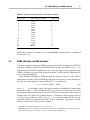
Table 1.4 Different classes for Bluetooth devices.
Class
Maximum power (mW)
Range (m)
Class 1
Class 2
Class 3
100
2.5
1
100
10
1
International [36] and ISA [37]. Also, a large number of proprietary systems are available
in the market. A brief discussion on the ISA SP-100 standard for process control and
monitoring is provided in Section 1.3.5, while a detailed review of ECMA standards for
UWB and millimeter wave communication systems will be provided in Chapter 2.
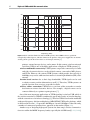
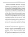
1.3.1
Bluetooth
Bluetooth is a WPAN standard for exchanging data over short distances. It is employed
in many personal devices today, such as mobile phones and laptops. Bluetooth was
originally developed by Ericsson in 1994. Then, the Bluetooth SIG was formed in 1998
with five companies, and the Bluetooth 1.0 specification was released in 1999 [30]. The
next versions, Bluetooth 1.1 and Bluetooth 1.2, were also IEEE standards, namely, IEEE
Standard 802.15.1-2002 and IEEE Standard 802.15.1-2005, respectively [38, 39]. The
first versions of Bluetooth employ Gaussian frequency shift keying (GFSK) and provide
data rates up to 721 kbps.
The second versions of Bluetooth, Bluetooth 2.0 and Bluetooth 2.1, provide an
enhanced data rate (EDR) feature and can reach data rates of 2.1 Mbps. EDR uses GFSK
for the packet header and the access code,3 and π/4 differential quaternary phase-shift
keying (π/4-DQPSK) or eight-phase differential phase-shift keying (8-DPSK) for the
payload [40]. The use of PSK in the payload provides the increase in the data rate.
The Bluetooth devices operate in the 2.4 GHz unlicensed ISM band, that is from
2.4 GHz to 2.4835 GHz. A Bluetooth system uses 79 channels in this band, that are
indexed as 2402 + k MHz for k = 0, 1, . . . , 78. Since each channel is 1 MHz, the
operating frequency range is given by [2.4015, 2.4805] GHz. Each channel is divided
into time slots for time-division duplexing (TDD), and FHSS is used to combat the
adverse effects of wireless channels, such as fading and interference. Frequency hoppings
can take place between 79 or fewer channels and a standard hop rate of 1600 hop/s is
employed [39]. In addition, the Bluetooth standard provides three classes with different
power-range tradeoffs as shown in Table 1.4.
The Bluetooth system supports point-to-point and point-to-multipoint connections.
Two or more devices with the same PHY form an ad-hoc network (piconet). One device
is designated as the master, and up to seven other devices can join the piconet as slaves.
All the devices in a piconet are synchronized to a common clock reference and frequency
hop pattern, which is determined by the master device [40, 41].
3
The access code is used by the receiver to recognize incoming transmissions.
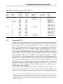
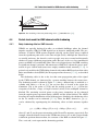
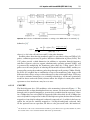
1.3 Review of related wireless standards
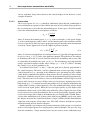
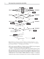
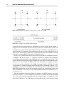
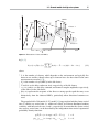
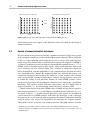
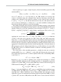
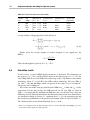
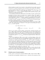
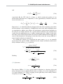
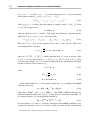
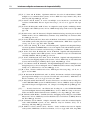
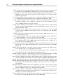
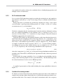
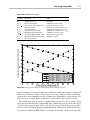
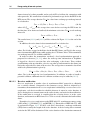
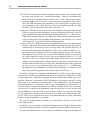
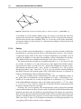
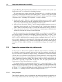
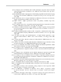
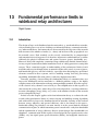
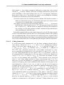
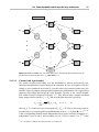
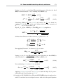
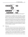
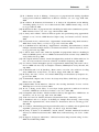
17
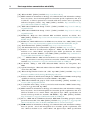
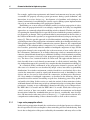
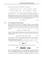
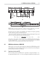
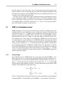
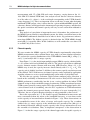
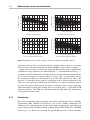
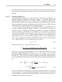
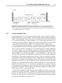
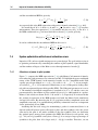
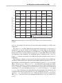
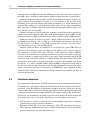
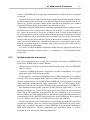
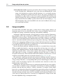
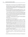
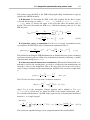
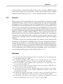
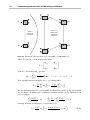
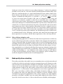
Figure 1.3 (a) Full mesh topology (b) partial mesh topology.
Recently, Bluetooth 3.0 specification has been announced by the Bluetooth SIG,
which integrates the previous Bluetooth technology with 802.11. Bluetooth 3.0 has the
Alternate MAC/PHY (AMP) feature, which facilitates the use of alternative MAC and
PHY layers to transfer Bluetooth profile data. By this method, transmission of large
amounts of data can be performed much faster than the previous versions of Bluetooth.
However, the conventional Bluetooth techniques are still employed for device discovery,
initial connection, and profile configuration, which provide an overall system with low
power consumption [42].
1.3.2
IEEE 802.15.5 (mesh networking)
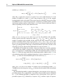
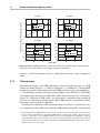
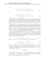
The IEEE 802.15.5 standard specifies the necessary mechanisms that must be present
in the PHY and MAC layers of WPANs to facilitate wireless mesh networking (WMN)
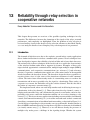
[43, 44]. WMN enables dynamic self-organization and self-configuration, meaning that
the nodes in the network can automatically form an ad-hoc network and maintain mesh
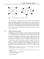
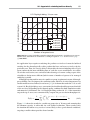
connectivity [45]. A WMN is a fully connected network if each node is connected
directly to each of the other nodes, and is also called the full mesh topology. However,
in the partial mesh topology, some nodes are connected to all the others, but some
are connected only to those other nodes with which they exchange the most data [44].
In Figure 1.3, examples of full and partial mesh topologies are illustrated. The main
advantages of the full mesh topology are improved reliability and efficiency. However,
these advantages are accompanied by high cost, since a large number of links are needed.
Specifically, for a fully connected network with N nodes, N (N − 1)/2 links need to be
formed.
The IEEE 802.15.5 standard aims to optimize wireless mesh topologies for WPANs
in order to provide the following features [43]:
r extension of network coverage without increasing the transmit power or the receiver
sensitivity;
r enhanced reliability via route redundancy;
r easier network configuration;
r improved battery life.
18
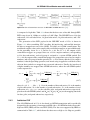
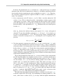
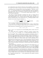
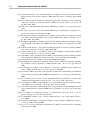
Short-range wireless communications and reliability
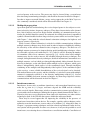
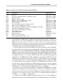
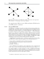
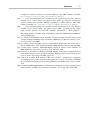
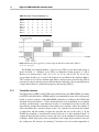
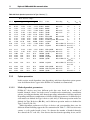
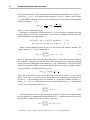
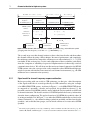
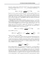
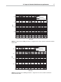
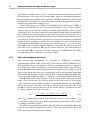
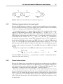
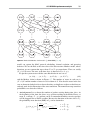
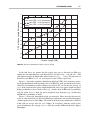
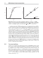
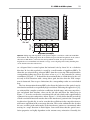
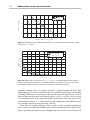
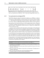
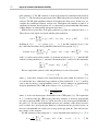
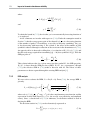
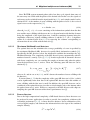
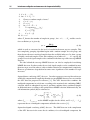
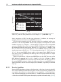
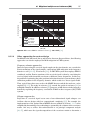
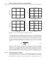
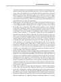
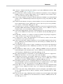
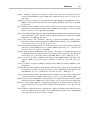
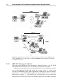
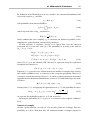
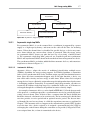
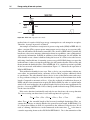
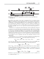
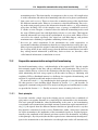
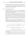
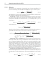
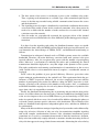
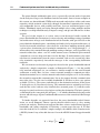
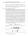
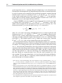
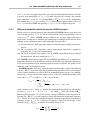
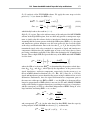
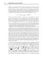
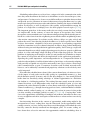
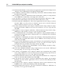
Figure 1.4 Network topologies in the IEEE 802.15.4-2006 standard, where circles represent the
PAN coordinators: (a) star topology; (b) peer-to-peer topology.
The standard describes WMN for low-rate WPANs and high-rate WPANs based on
related IEEE standards, as studied next.
1.3.2.1
Low-rate WPAN mesh
The IEEE 802.15.5 standard [43] provides an architectural framework to facilitate interoperable, stable, and scalable wireless mesh topologies for low-rate WPANs based on
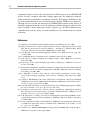
the IEEE 802.15.4-2006 standard [46].4 Originally, IEEE 802.15.4-2006 supported the
star topology and the peer-to-peer topology, as shown in Figure 1.4. In the star topology,
the devices are connected to a single central controller, called the personal area network
(PAN) coordinator. However, in the peer-to-peer topology, a device can form a connection
with any other device as long as they are in range of each other. Although the peer-to-peer
topology allows mesh networking to be realized in WPANs, the IEEE 802.15.4-2006
standard does not specify how mesh networking should be implemented.
The IEEE 802.15.5 standard describes a standard way of performing mesh networking
over IEEE 802.15.4-2006, and provides supports for the following features [43]:
r
r
r
r
unicast, multicast, and reliable broadcast mesh data forwarding;
synchronous and asynchronous power saving for mesh devices;
trace route function;
portability of end devices.
Low-rate WPAN mesh networks have various applications, such as automation and
control, safety, security, environment monitoring, and automatic meter reading [43, 47].
As a specific example, it is stated in reference [43] that, via WPAN mesh networks,
wireless light switches in a commercial building (e.g., in a department store) can control
the lights of an entire floor, with the ability to group lights in different ways in a dynamic
manner and turn them on/off with a single push of a button.
4
The IEEE 802.15.4-2006 standard is studied in detail in Section 6.2 of Chapter 6.
1.3 Review of related wireless standards
19
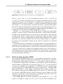
Table 1.5 Different modulation and coding types in IEEE
802.15.3, where TCM refers to trellis coded modulation [48].
1.3.2.2
Modulation
Coding
Data rate (Mbps)
QPSK
DQPSK
16-QAM
32-QAM
64-QAM
8-state TCM
None
8-state TCM
8-state TCM
8-state TCM
11
22
33
44
55
High-rate WPAN mesh
The high-rate WPAN mesh provides network range extension, reliable communication,
and efficient bandwidth reuse in high-rate multimedia applications based on the IEEE
802.15.3 standard [43]. As stated in reference [48], IEEE 802.15.3 defines a protocol
for the compatible interconnection of data and multimedia communication equipment
via 2.4 GHz radio transmissions in a WPAN. The main purpose of IEEE 802.15.3 is to
meet the requirements of portable consumer imaging and multimedia applications by
low-power and low-cost systems. In the IEEE 802.15.3 standard, various modulation and
coding types are employed in order to support scalable data rates, as shown in Table 1.5.
The MAC layer of the standard supports both isochronous and asynchronous data types,
and provides the following features [48]:
r
r
r
r
ad-hoc peer-to-peer networking;
fast connections;
data transport with QoS;
security.
In order to provide corrections and enhancements to the IEEE 802.15.3 standard,
the IEEE 802.15.3b amendment was published in 2005 [49]. IEEE 802.15.3b aims to
improve the MAC sublayer by introducing a new definition for the MAC layer management entity (MLME) service access point, and a new acknowledgment policy that
allows polling and a more efficient use of channel time. Interested readers are referred
to reference [49] for other important additions in IEEE 802.15.3b.
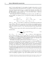
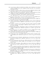
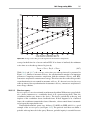
A number of IEEE 802.15.3 devices form a piconet, which is a wireless ad-hoc network that facilitates independent data devices to communicate with each other. One of the
devices in a piconet becomes the piconet coordinator (PNC) and provides timing information to the other devices via transmission of beacon signals, as shown in Figure 1.5.
In addition, the PNC manages the power-saving modes and the QoS requirements, and
controls access to the piconet [48].
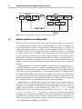
The main purpose of the IEEE 802.15.5 standard is to provide an architectural framework to facilitate PNCs in an IEEE 802.15.3 piconet to form a mesh network. In this
way, the advantages of mesh networking, listed at the beginning of Section 1.3.2, can be
realized. This facilitates various applications, such as coverage extension for multimedia
home networking, and improved capacity for interconnection between computers and
20
Short-range wireless communications and reliability
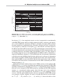
Figure 1.5 Illustration of a piconet, where the circle represents the PNC. The dashed lines
indicate beacons sent from the PNC, whereas the solid lines denote data communications.
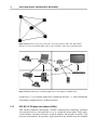
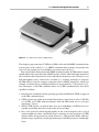
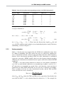
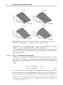
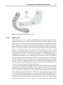
Figure 1.6 Multimedia home networking application of the high-rate WPAN mesh.
peripherals [47]. An example application is illustrated in Figure 1.6, where multimedia
networking is implemented in a multiroom house.
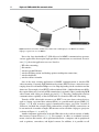
1.3.3
IEEE 802.15 TG6 (body area networks (BANs))
This ongoing standard is developing a reliable communication technology optimized
for low-power devices and operation on, in, or around the human body. Target applications include consumer electronics, medical implants and portable electronics, and
personal entertainment. In particular, applications that may benefit from this standard
1.3 Review of related wireless standards
21
include the wireless monitoring of electroencephalogram (EEG), electrocardiogram
(ECG), electromyography (EMG), and the monitoring of vital signals. In customizing
the technology solution, regulatory issues such as specific absorption rate (SAR) limits
are taken into consideration.
The frequency bands supported in the IEEE 802.15.6 standard are 402–405 MHz,
420–450 MHz, 863–870 MHz, 902–928 MHz, 950–956 MHz, 2360–2400 MHz, and
2400–2483.5 MHz. Information data rates provided for these frequency bands are given
below.
r
r
r
r
r
r
r
402–405 MHz: {57.5, 75.9, 151.8, 303.6, 455.4} Kbps.
420–450 MHz: {57.5, 75.9, 151.8, 187.5} Kbps.
863–870 MHz: {76.6, 101.2, 202.4, 404.8, 607.1} Kbps.
902–928 MHz: {91.9, 121.4, 242.9, 485.7, 728.6} Kbps.
950–956 MHz: {76.6, 101.2, 202.4, 404.8, 607.1} Kbps.
2360–2400 MHz: {91.9, 121.4, 242.9, 485.7, 971.4} Kbps.
2400–2483.5 MHz: {91.9, 121.4, 242.9, 485.7, 971.4} Kbps.
There are several mechanisms to improve communication reliability in BANs including relaying, hybrid ARQ, channel hopping, and interference mitigation.
The BAN supports a star network in which frames are communicated between a
coordinator and its end nodes directly. End nodes synchronize their transmissions to a
beacon that is periodically transmitted by the body area network (BAN) coordinator.
The standard also provides an option for an end node to relay data to the coordinator on
behalf of another end node. In this case, an end node is responsible for discovering a
secure relay in its range. Overhearing an ACK destined for another end node is used as
an indication that the link between the coordinator and that end node is fairly reliable.
Therefore, the overhearing node initiates link establishment with the discovered relay
end node.
To improve reliability, a hybrid automatic repeat request (HARQ) is adopted. Another
reliability improvement comes with channel-hopping. A coordinator may switch to a
different channel by including in its beacon the channel-hopping state and the next
channel hop fields. It is important that the new channel-hopping sequence is not being
used by a different BAN. Switching to a different channel-hopping sequence does not
take effect immediately. The coordinator and its end nodes should reside in the current
channel for a certain number of beacon periods.
A prospective coordinator can use an interference mitigation mode, in which the
coordinator selects a logical channel for network operation while minimizing the impact
on the existing BANs. Performing a passive scan on all logical channels in all frequency
bands can help the prospective coordinator to estimate other BAN information such as
the number of devices on other BANs, their traffic estimates, the data rate used by devices
in the other BANs, etc. At the end of the passive scan, the prospective coordinator makes
a decision about which logical channel and frequency band to use.
This standard is currently going through a letter ballot and comment resolution. It is
expected to be completed in the first half of 2011.
22
Short-range wireless communications and reliability
Star
Broadcast
Peer-to-peer
master
slave
Figure 1.7 Illustration of the three network topologies supported by IEEE 802.15.7 VLC
networks: peer-to-peer, star, and broadcast.
1.3.4
IEEE 802.15 TG7 (visible light communication)
The IEEE 802.15.7 standard defines both PHY and MAC for short-range optical wireless
communications, using visible light in optically transparent media. The visible light
spectrum extends from 380 to 780 nm in wavelength. The standard is required to deliver
data rates sufficient to support audio and video multimedia services. Issues such as
mobility of the visible link, compatibility with visible light infrastructures, impairments
due to noise, and interference from unintended sources such as ambient light are being
addressed, because VLC systems may need to coexist with ambient lighting and other
optical technologies. Also, the standard is required to abide by any applicable eye safety
regulations.
VLC devices are classified as infrastructure, mobile, and vehicle-mounted. The standard supports both uni-directional and bi-directional data, with point-to-point or pointto-multipoint connectivity. The supported topologies are peer-to-peer, star, and broadcast
as shown in Figure 1.7.
A PER of 8% is targeted. The packet size chosen for transmission range evaluation is
256 bytes for low data rate applications and 1024 bytes for high data rate applications.
VLC transmits data by intensity modulating optical sources such as LEDs [50]. Some
of the key features of this standard include
r star or peer-to-peer operation;
r optional guaranteed time slots;
r random access with collision avoidance;
r acknowledged transmissions.
The PHY supports three modes:
r Type-I: intended for ranges of tens of meters and low data rate (tens of Kbps) applications. Modulation in this type is ON/OFF keying (OOK) and variable pulse position
modulation (VPM).
r Type-II: intended for ranges of tens of meters and moderate data rates in the order of
tens of Mbps. This type supports color shift keying (CSK)-based modulation as well
as OOK and VPM.
r Type CSK: intended for applications that are using CSK with multiple light sources
and detectors.
23
I/O device
Gateway,
System manager
Security manager
control
system
plant network
1.3 Review of related wireless standards
Routing device
Figure 1.8 Illustration of the SP100.11a supported network topologies for I/O devices and routers.
The standard provides channel hopping to avoid adjacent cell and adjacent coordinator interference. For instance, two coordinators can adopt the following hopping patterns to avoid interference with each other: {R, B, G, G, G, R, G, B, R} and
{G, G, R, B, R, G, B, R, G}, where R, G, and B denote the red, green, and blue colors,
respectively.
This standard is also currently going through a letter ballot and comment resolution.
It is expected to be completed in the first half of 2011.
1.3.5
ISA SP100.11a (process control and monitoring)
Target applications of SP100.11a are periodic monitoring and process control, where
tolerable latency is less than 100 ms. The standard supports simple star topology for
portable and I/O devices, mesh topology for routing devices, and a combination of the
two, as illustrated in Figure 1.8. Path diversity is envisioned to improve reliability.
SP100.11a uses the 2.4 GHz option of the IEEE 802.15.4-2006 as the default PHY. At
least 15 frequency channels are supported. A raw PHY data rate is 250 Kbps per channel.
Unlike the IEEE 802.15.4 MAC, carrier sense multiple access (CSMA)-based medium
access control is made optional, because it may delay transmission of a packet due to
random backoff. Instead, the superframe structure is divided into time slots the same as
in the time slotted channel hopping (TSCH) configuration of the IEEE 802.15.4e. Each
time slot is dedicated to communication between a particular source and destination
pair over a prespecified frequency channel hopping pattern. This is referred to as slot
hopping in the standard. Channel hopping can be also on a superframe basis. Then, it is
called slow hopping. A combination of slot hopping and slow hopping (see Figure 1.9)
is also supported.
The ISA SP100.11a standardization was completed in 2009 as being the first industrial
wireless networking standard in the ISA100 family of standards. This wireless mesh
Short-range wireless communications and reliability
Slotted
hopping
Slow
hopping
Channels
24
time
Figure 1.9 Illustration of the hybrid channel hopping operation in SP100.11a, where a number of
timeslots using slotted hopping is followed by a slow-hopping period.
network standard protocol helps supplier companies to build inter-operable wireless
automation control products.
References
[1] R. Kraemer and M. D. Katz, Short-Range Wireless Communications: Emerging Technologies and Applications, 1st ed. West Sussex, United Kingdom: John Wiley & Sons,
2009.
[2] F. F. Dai, Y. Shi, J. Yan, and X. Hu, “MIMO RFIC transceiver designs for WLAN applications,” in Proc. IEEE International Conference on ASIC, Oct. 2007, pp. 348–351.
[3] C. C. Lin, S. S. Hsu, C. Y. Hsu, and H. R. Chuang, “A 60-GHz millimeter-wave CMOS RFICon-chip triangular monopole antenna for WPAN applications,” in Proc. IEEE Antennas and
Propag. Soc. Int. Symp., June 2007, pp. 2522–2525.
[4] P. J. Guo and H. R. Chuang, “A 60-GHz millimeter-wave CMOS RFIC-on-chip meander-line
planar inverted-F antenna for WPAN applications,” in Proc. IEEE Antennas and Propag. Soc.
Int. Symp., July 2008, pp. 1–4.
[5] A. Harney and C. O. Mahony, “Wireless short-range devices: Designing global license-free
system for frequencies < 1 GHz,” Analog Dialogue Mag., vol. 40, no. 3, pp. 18–22, Mar.
2006.
[6] ECMA International, “High rate ultra wideband PHY and MAC,” ECMA-368 Standard, Dec.
2008. [Online]. Available: http://www.ecma-international.org/publications/files/ECMA-ST/
ECMA-368.pdf
[7] ——, “High rate 60 GHz PHY, MAC, and HDMI PAL,” ECMA-387 Standard, Dec.
2008. [Online]. Available: http://www.ecma-international.org/publications/files/ECMA-ST/
ECMA-387.pdf
[8] H. G. Myung, J. Lim, and D. J. Goodman, “Single carrier FDMA for uplink wireless transmission,” IEEE Veh. Technol. Mag., vol. 1, no. 3, pp. 30–38, Sep. 2006.
[9] G. Fettweis, E. Zimmermann, V. Jungnickel, and E. Jorswieck, “Challenges in future short
range wireless systems,” IEEE Veh. Technol. Mag., vol. 1, no. 2, pp. 24–31, June 2006.
[10] W. P. Siriwongpairat, W. Su, M. Olfat, and K. J. R. Liu, “Multiband-OFDM MIMO coding
framework for UWB communication systems,” IEEE Trans. Sig. Processing, vol. 54, no. 1,
pp. 214–224, Jan. 2006.
[11] H. Yang, P. F. M. Smulders, and M. H. A. J. Herben, “Channel characteristics and transmission
performance for various channel configurations at 60 GHz,” EURASIP J. Wireless Commun.
Networking, pp. 1–15, Jan. 2007, article ID: 19613.
References
25
[12] A. M. Kuzminsky and H. R. Karimi, “Multiple-antenna interference cancellation for WLAN
with MAC interference avoidance in open access networks,” EURASIP J. Wireless Commun.
Networking, pp. 1–11, Sep. 2007, article ID: 51358.
[13] B. W. Koo, M. S. Baek, Y. H. You, and H. K. Song, “High-speed MB-OFDM system
with multiple antennas for multimedia communication and home network,” IEEE Trans.
Consumer Electronics, vol. 52, no. 3, pp. 844–849, Aug. 2006.
[14] S. M. Mishra, R. W. Brodersen, S. T. Brink, and R. Mahadevappa, “Detect and avoid:
An ultrawideband/WiMAX coexistence mechanism,” IEEE Commun. Mag., vol. 45, no. 6,
pp. 68–75, June 2007.
[15] H. Zhang, X. Zhou, K. Y. Yazdandoost, and I. Chlamtac, “Multiple signal waveforms adaptation in cognitive ultrawideband radio evolution,” IEEE J. Select. Areas in Commun., vol. 24,
no. 4, pp. 878–884, Apr. 2006.
[16] O. Bakr, M. Johnson, R. Mudumbai, and K. Ramchandran, “Multi-antenna interference
cancellation techniques for cognitive radio applications,” in Proc. IEEE Wireless Commun.
Networking Conf. (WCNC), Budapest, Hungary, Apr. 2009, pp. 1–6.
[17] J. Misic and V. B. Misic, “Performance of cooperative sensing at the MAC level: Error minimization through differential sensing,” IEEE Trans. Veh. Technol., vol. 58, no. 5, pp. 2457–
2470, June 2009.
[18] A. Bensky, Short-Range Wireless Communication: Fundamentals of RF System Design and
Application, 2nd ed. Elsevier, 2003.
[19] F. H. P. Fitzek and M. D. Katz, Short-Range Wireless Communications – Emerging
Technologies and Applications, 1st ed. West Sussex, UK: John Wiley, 2009, ch. 2,
pp. 16–23.
[20] R. Kraemer and M. D. Katz, Short-Range Wireless Communications – Emerging Technologies
and Applications, 1st ed. West Sussex, UK: John Wiley, 2009, ch. 1, p. 5.
[21] B. Allen, T. Brown, K. Schwieger, E. Zimmermann, W. Malik, D. Edwards, L. Ouvry, and
I. Oppermann, “Ultra wideband: Applications, technology and future perspectives,” in Proc.
Int. Workshop on Convergent Technol. (IWCT), Oulu, Finland, June 2005.
[22] H. Singh, S. K. Yong, J. Oh, and C. Ngo, “Principles of IEEE 802.15.3c: Multi-gigabit
millimeter-wave wireless PAN,” in Proc. IEEE Int. Conf. Computer Commun. Networks
(ICCCN), San Francisco, CA, Aug. 2009, pp. 1–6.
[23] S. K. Yong and C. C. Chong, “An overview of multigigabit wireless through millimeter wave
technology: Potentials and technical challenges,” EURASIP J. Wireless Commun. Networking,
pp. 1–10, Jan. 2007, article ID: 78907.
[24] C. D. Encyclopedia, “ISM band,” The Computer Language Company Inc., Jul. 2009.
[Online]. Available: http://encyclopedia2.thefreedictionary.com/ISM+band
[25] FCC, “Part 15 – radio frequency devices,” ch. I, Title 47 of the Code of Federal
Regulations (CFR). [Online]. Available: http://www.access.gpo.gov/nara/cfr/waisidx 05/
47cfr15 05.html
[26] D. Tse and P. Viswanath, Fundamentals of Wireless Communication. Cambridge, UK: Cambridge University Press, 2005.
[27] J. G. Andrews, A. Ghosh, and R. Muhamed, Fundamentals of WiMAX, 1st ed. Upper Saddle
River, NJ: Prentice Hall, 2007.
[28] L. Zheng and D. N. C. Tse, “Diversity and multiplexing: A fundamental tradeoff in
multiple-antenna channels,” IEEE Trans. Inf. Theory, vol. 49, no. 5, pp. 1073–1096, May
2003.
[29] “IEEE 802.15 Working Group for WPAN.” [Online]. Available: http://www.ieee802.org/15
26
Short-range wireless communications and reliability
[30] “Bluetooth SIG.” [Online]. Available: http://www.bluetooth.org
[31] IEEE standard for information technology, telecommunications and information exchange
between systems, “Local and metropolitan area networks specific requirements, Part 15.2:
Coexistence of wireless personal area networks with other wireless devices operating in
unlicensed frequency bands,” Aug. 2003. [Online]. Available: http://standards.ieee.org/
getieee802/download/802.15.2-2003.pdf
[32] “IEEE 802.15 WPAN Task Group 2 (TG2).” [Online]. Available: http://www.ieee802.org/
15/pub/TG2.html
[33] “IEEE 802.15 WPAN Task Group 3 (TG3).” [Online]. Available: http://www.ieee802.org/
15/pub/TG3.html
[34] ECMA-368, “High rate ultra wideband PHY and MAC standard, 1st edition,” Dec.
2005. [Online]. Available: http://www.ecma-international.org/publications/files/ECMA-ST/
ECMA-368.pdf
[35] ECMA-369, “MAC-PHY interface for ECMA-368, 1st edition,” Dec. 2005. [Online]. Available: http://www.ecma-international.org/publications/files/ECMA-ST/ECMA-369.pdf
[36] “Ecma International.” [Online]. Available: http://www.ecma-international.org
[37] “The International Society of Automation.” [Online]. Available: http://www.isa.org
[38] Institute of Electrical and Electronics Engineers, “IEEE Std 802.15.1-2001, wireless
medium access control (MAC) and physical layer (PHY) specifications for wireless
personal area networks (WPANs),” June 2002. [Online]. Available: http://standards.ieee.
org/getieee802/download/802.15.1-2002.pdf
[39] ——, “IEEE Std 802.15.1-2005, wireless medium access control (MAC) and physical layer
(PHY) specifications for wireless personal area networks (WPANs),” June 2005. [Online].
Available: http://standards.ieee.org/getieee802/download/802.15.1-2005.pdf
[40] D. McCall, “Taking a walk inside Bluetooth EDR,” Wireless Net DesignLine, Dec.
2004.
[41] Agilent Technologies, “Bluetooth enhanced data rate (EDR): The wireless evolution,” Application Note, May 2006.
[42] “Bluetooth Specification Version 3.0 + HS,” Apr. 2009. [Online]. Available: http://www.
bluetooth.com/Bluetooth/Technology/Building/Specifications
[43] Institute of Electrical and Electronics Engineers, “IEEE Std 802.15.5-2009, mesh topology
capability in wireless personal area networks (WPANs),” May 2009.
[44] “IEEE 802.15 WPAN task group 5 (TG5) mesh networking.” [Online]. Available: http://
www.ieee802.org/15/pub/TG5.html
[45] I. F. Akyildiz and X. Wang, “A survey on wireless mesh networks,” IEEE Commun. Mag.,
vol. 43, no. 9, pp. S23–S30, Sep. 2005.
[46] IEEE standard for information technology, telecommunications and information exchange
between systems, “Local and metropolitan area networks specific requirements, Part 15.4:
Wireless medium access control (MAC) and physical layer (PHY) specifications for
low-rate wireless personal area networks (LR-WPANs),” Sep. 2006. [Online]. Available:
http://standards.ieee.org/getieee802/download/802.15.4-2006.pdf
[47] M. Lee, “IEEE 802.15.5 WPAN mesh tutorial, IEEE P802.15 working group for wireless
personal area networks,” Nov. 2006. [Online]. Available: http://grouper.ieee.org/groups/802/
802 tutorials/06-November/15-06-0464-00-0005-802-15-5-mesh-tutorial.pdf
[48] IEEE standard for information technology, telecommunications and information exchange
between systems, “Local and metropolitan area networks specific requirements, Part
15.3: Wireless medium access control (MAC) and physical layer (PHY) specifications
References
[49]
[50]
[51]
[52]
[53]
[54]
[55]
[56]
27
for high-rate wireless personal area networks (WPANs),” Sep. 2003. [Online]. Available:
http://standards.ieee.org/getieee802/download/802.15.3-2003.pdf
——, “Local and metropolitan area networks specific requirements, Part 15.3: Wireless
medium access control (MAC) and physical layer (PHY) specifications for high-rate
wireless personal area networks (WPANs: Amendment 1: MAC sublayer),” May 2006.
[Online]. Available: http://standards.ieee.org/getieee802/download/802.15.3b-2005.pdf
——, “Local and metropolitan area networks specific requirements, Part 15.7: Wireless
medium access control (MAC) and physical layer (PHY) specifications for Visible
Light wireless personal area networks (WPANs: Amendment 1: MAC sublayer),”
May 2010. [Online]. Available: http://standards.ieee.org/getieee802/download/d1P802-157-Draft-Standard.pdf
U. C. Kozat, I. Koutsopoulos, and L. Tassiulas, “Cross-layer design for power efficiency and
QoS provisioning in multihop wireless networks,” IEEE Trans. on Wireless Commun., vol. 5,
no. 11, pp. 3306–3315, 2006.
U. C. Kozat, “On the throughput capacity of opportunistic multicasting with erasure codes,”
in Proc. IEEE 27th Int. Conf. Computer Commun. (IEEE Infocom 2008), Phoenix, AZ, 2008.
J. Chang and L. Tassiulas, “Maximum lifetime routing in wireless sensor networks,” in
IEEE/ACM Trans. Networking, vol. 12, no. 4, pp. 609–619, 2004.
S. R. Das, C. E. Perkins, E. M. Royer and M K. Marina, “Performance comparison of two
on-demand routing protocols for ad hoc networks,” IEEE Personal Commun. Mag. special
issue on Ad hoc Networking, Feb. 2001, pp. 16–28.
J. Broch, D. A. Maltz, D. B. Johnson, Y. Hu, and J. Jetcheva, “A performance comparison
of multihop wireless ad hoc network routing protocols,” in Proc. 4th Annual ACM/IEEE
Int. Conf. Mobile Computing and Networking (MobiCom’98), Dallas, Texas, October 25–30,
1998.
C. E. Koksal and Hari Balakrishnan, “Quality-aware routing metrics for time-varying wireless
mesh networks,” in IEEE J. Selected Areas in Commun., vol. 24, pp. 1984–1994, 2006.
Part I
High-rate systems
2
High-rate UWB and 60 GHz
communications
Sinan Gezici and Ismail Guvenc
In this chapter, two technologies for high data-rate communications systems for wireless
personal area networks (WPANs) are discussed. Namely, the ultrawideband (UWB)
technology that operates in the 3.1–10.6 GHz band and the millimeter wave (MMW)
technology (also called 60 GHz radio) that can use the 57–64 GHz band in most parts
of the world are considered. First, a generic overview is given and various application
scenarios are discussed. Then, the ECMA standard for high-rate UWB systems is studied.
Finally, two standards for the 60 GHz MMW radio are investigated.
2.1
Overview and application scenarios
In order to realize high-speed communications systems with low power consumption,
signals with very large bandwidths need to be employed. One way of designing such
communications systems is to use UWB signals as an underlay technology by utilizing
all or part of the frequency spectrum between 3.1 and 10.6 GHz [1–3]. According to the
US Federal Communications Commission (FCC), a UWB signal is defined as having
an absolute bandwidth of at least 500 MHz or a relative (fractional) bandwidth of larger
than 20% [3, 4].
In order not to cause any adverse effects on other wireless systems in the same frequency band, such as IEEE 802.11a wireless local area networks (WLANs), certain
power emission limits are imposed on UWB devices by regulatory authorities, such
as the FCC in the USA [3] and the Electronic Communications Committee (ECC)
in Europe [5]. For example, the FCC requires that the average power spectral density (PSD) must not exceed −41.3 dBm/MHz over the frequency band from 3.1 to
10.6 GHz, and it must be even lower outside this band, depending on the specific application [3]. Specifically, Figure 2.1 shows the FCC limits for indoor communications
systems.
Due to the regulations on UWB systems, high-rate UWB systems can only be
used for short-range applications. Some typical applications can be listed as follows
[6, 7]:
wireless peripheral connectivity UWB systems can provide high data rates of the
order of several hundreds of megabits per second (Mbps), which can be used to
provide high-speed wireless connectivity between PCs and PC peripherals, such as
High-rate UWB and 60 GHz communications
−40
−45
EIRP Emission Level (dBm)
32
−50
1.99
−55
3.1
10.6
−60
−65
−70
−75
−80
0 96
1.61
0
1
10
10
Frequency (GHz)
Figure 2.1 FCC emission limits for indoor UWB systems, where EIRP refers to equivalent
isotropically radiated power, which is defined as the product of the power supplied to an antenna
and its gain in a given direction relative to an isotropic antenna [2].
printers, external storage devices, and scanners. In this context, wireless universal
serial bus (USB) is one of the killer applications of high-rate UWB systems [8].
wireless multimedia connectivity UWB systems can provide connectivity for audio
and video electronics devices, such as digital cameras, camcorders, MP3 players,
and DVDs. However, the current UWB systems, which provide data rates up to
480 Mbps, may not be sufficient for transfer of certain high-definition (HD) video
streams.
location based services due to their large bandwidths, UWB signals can be used
to obtain accurate position information as well [2]. Therefore, UWB systems can
provide location aware services at specific locations.
wireless ad-hoc connections UWB devices can form ad-hoc networks to transfer
data between various electronics devices. For example, a digital camera can be
connected directly to a printer to print pictures [7].
One of the most important applications of UWB signaling is wireless USB, which is
the wireless extension to USB that combines the speed and security of wired technology
with the convenience of wireless technology [8]. Wireless USB is based on the multiband
orthogonal frequency division multiplexing (MB-OFDM) UWB radio platform, which
is discussed in Section 2.2. It provides 480 Mbps at 3 m and 110 Mbps at 10 m. Recently,
a number of commercial products have appeared on the market (Figure 2.2).
Another way of designing high-speed systems for short-range wireless communications is to utilize the MMW frequency bands, especially the 60 GHz band [9–13,19–28].
2.1 Overview and application scenarios
33
Figure 2.2 A commercial wireless USB product.
The frequency spectrum from 57 GHz to 64 GHz is allocated for MMW communications
in most parts of the world [10–12]. MMW communications systems can provide data
rates of a few gigabits per second (Gbps) over ranges up to 10 m [9].
Due to high signal attenuation in the MMW frequency bands, 60 GHz radios transmit
significantly more power than other WPAN systems. On the other hand, high attenuation
also results in reduced interference levels and efficient frequency reuse. Therefore, very
high throughputs can be achieved in a network [11]. Another advantage of using the
60 GHz radio is related to compact component sizes at MMW frequencies, which, for
example, facilitates the use of multiple antennas at user terminals [11]. In reference [13],
four advantages of 60 GHz communications over UWB communications have been
specified as follows:
1. International coordination for the operating spectrum is difficult for UWB, as opposed
to 60 GHz communications.
2. UWB systems may suffer from in-band interference from devices such as WLANs
at 2.4 GHz and 5 GHz unlicensed bands, while 60 GHz bands are free of major
interference sources.
3. While UWB systems can provide data rates up to 480 Mbps, 60 GHz devices are
capable of providing data rates on the order of several Gbps.
4. Due to the path loss which depends tightly on the central frequency, the received
signal strength may show considerably larger variations over the spectrum of UWB
signals (where the spectrum may range between 3.1 GHz and 10.6 GHz), while the
dynamic range of path loss over the spectrum range of 60 GHz systems is considerably
lower.
34
High-rate UWB and 60 GHz communications
Figure 2.3 Wireless transfer of HD video/audio from a DVD player to an HDTV, and from a
laptop to a projector or to an HDTV.
Due to the large bandwidth of 7 GHz allocated to MMW communications systems,
various applications that require high-speed data transmission are envisioned. In reference [12], the main application areas are listed as:
r
r
r
r
r
r
HD video streaming;
file transfer;
wireless gigabit Ethernet;
wireless docking station and desktop point-to-multipoint connections;
wireless backhaul;
wireless ad-hoc networks.
One of the most exciting applications of MMW communications is wireless HD
video streaming. Currently, high-definition televisions (HDTVs) have various data rates
ranging from several hundred Mbps to a few Gbps depending on the resolution and the
frame rate. For example, for an HDTV with resolution 1920 × 1080 and frame rate 60 Hz,
the required data rate for wireless HD transmission is around 3 Gbps (considering RGB
video format with 8 bits per channel per pixel) [11]. Therefore, multigigabit wireless
communications capability of the 60 GHz radio is essential in HD video streaming.
Transfer of HD video/audio streams to an HDTV can come from various devices,
such as a laptop, a personal data assistant (PDA), or a portable media player (PMP) [12]
(Figure 2.3). In such scenarios, typical communication ranges vary from 3 meters to
10 meters, and both line-of-sight (LOS) and non-line-of-sight (NLOS) connections can
be encountered. As another example, HD streams can be sent from a laptop to a projector
as shown in Figure 2.3 as well [12].
Another important application of the 60 GHz radio is the wireless transfer of bulky
files between various devices [11, 12]. For example, in office or residential environments, wireless file transfer can be performed between a computer and its peripherals
such as printers, camcorders, and digital cameras. In addition, it is possible to sell
2.2 ECMA-368 high-rate UWB standard
35
Table 2.1 Allocation of frequency bands in the ECMA-368 standard.
Band index
Center frequency (GHz)
Band group
1
2
3
4
5
6
7
8
9
10
11
12
13
14
3.432
3.960
4.488
5.016
5.544
6.072
6.600
7.128
7.656
8.184
8.712
9.240
9.768
10.296
1
1
1
2
2
2
3
3
3
4
4
4
5
5
audio/video contents in a kiosk in a store using MMW communications, as mentioned
in reference [12].
2.2
ECMA-368 high-rate UWB standard1
The main standards for high-rate UWB systems are the ECMA-368 high-rate UWB PHY
and MAC standards and the ECMA-369 MAC-PHY interface for ECMA-368 [14, 15].2
In particular, these ECMA standards specify a basis for high data rate and short-range
WPANs, utilizing all or part of the spectrum between 3.1 GHz and 10.6 GHz with data
rates of up to 480 Mbps [2].
In the ECMA-368 high-rate UWB standard, the frequency band 3.1–10.6 GHz is
divided into 14 bands, with a 528 MHz spacing between consecutive center frequencies.
Namely, the center frequency for the nth band, f c(n) , is calculated as
f c(n) = 2.904 + 0.528n
(GHz),
(2.1)
for n = 1, . . . , 14. In addition, these 14 frequency bands are classified into 5 band groups
as shown in Table 2.1. The transmitted signal at a given time occupies only one of the
14 frequency bands, and time-frequency codes (TFCs) are used to specify the frequency
band used by each symbol. For example, Figure 2.4 illustrates a time-frequency plot for
six consecutive symbols for a TFC of {1, 2, 3, 1, 2, 3}. In other words, the first, second,
and third symbols are transmitted in band 1, band 2, and band 3, respectively; and this
structure is repeated for the next three symbols.
1
2
This section is adopted from Section 2.3.1 of reference [2].
ECMA International is an industry association that works on the standardization of information and communication technology and consumer electronics (www.ecma-international.org).
36
High-rate UWB and 60 GHz communications
Table 2.2 Seven TFCs for band group 1 [2].
TFC-1
TFC-2
TFC-3
TFC-4
TFC-5
TFC-6
TFC-7
1
1
1
1
1
2
3
2
3
1
1
1
2
3
3
2
2
3
1
2
3
1
1
2
3
1
2
3
2
3
3
2
1
2
3
3
2
3
2
1
2
3
Figure 2.4 Time-frequency plot for a system using the first three bands with a TFC of
{1, 2, 3, 1, 2, 3} [2].
The ECMA-368 standard defines a total of seven TFCs for the first band group as
shown in Table 2.2. Similarly, seven TFCs are defined for band groups 2, 3, and 4.
However, for band group 5, only {13, 13, 13, 13, 13, 13} and {14, 14, 14, 14, 14, 14},
are specified. In this way, a total of 30 channels are specified in the standard. When a
TFC consists of at least two distinct band indices, time-frequency interleaving (TFI) is
performed as data is interleaved over different bands. Otherwise, data is transmitted over
a single band, which is called fixed-frequency interleaving (FFI) [2].
2.2.1
Transmitter structure
The physical layer (PHY) of the ECMA-368 standard is based on MB-OFDM. According
to the TFCs described above, OFDM symbols are transmitted in some of the 14 frequency
bands. A generic structure of the MB-OFDM transmitter according to the ECMA-368
standard is shown in Figure 2.5. First, information bits to be transmitted are scrambled,
and then encoded using a convolutional encoder. A convolutional encoder encodes the
input bits by passing them through a linear finite state machine, where the number of
states determines the constraint length of the code, and the ratio between the number
of output bits and the number of input bits specifies the rate of the code [2]. In the
ECMA-368 standard, a convolutional encoder with rate 1/3 and constraint length 7 is
employed. By using this encoder, various code rates can be obtained via the puncturing
technique, which omits some of the encoded bits at the output of the encoder to increase
the coding rate. For instance, by omitting 7 bits from each 15 encoded output bits of
37
2.2 ECMA-368 high-rate UWB standard
Figure 2.5 Basic blocks of an MB-OFDM UWB transmitter according to the ECMA-368 [2].
the rate 1/3 convolutional encoder, the rate can be increased to 5/8. In the standard, a
coding rate of 1/3, 1/2, 5/8, or 3/4 can be used in the system corresponding to various
data-rate options [2].
After convolutional encoding, the encoded bits are interleaved, which is a process
that spreads bits over a series of symbols in order to provide robustness against burst
errors. The ECMA-368 standard defines both inter-symbol and intra-symbol interleaving. For the inter-symbol interleaving, bits are permuted over six symbols, whereas the
arrangements of bits inside symbols are changed according to certain structures for the
intra-symbol interleaving [2].
After the interleaving operation, the bits are mapped onto a complex constellation.
For data rates of 53.3, 80, 106.7, 160, and 200 Mbps, the binary data is mapped to a
quadrature phase-shift keying (QPSK) constellation, whereas for data rates of 320, 400,
and 480 Mbps, the binary data is mapped to a multidimensional constellation using the
dual-carrier modulation (DCM) approach [2]. For QPSK, each pair of binary bits, b2i
and b2i+1 , is mapped to a complex number given by √12 (2b2i − 1 + j(2b2i+1 − 1)) for
i = 0, 1, . . . For DCM, all 200 bits are converted into 100 complex numbers by grouping
200 bits into 50 groups of 4 bits, and then by mapping each 4-bit group onto 2 complex
numbers according to a specific pattern, as defined in reference [14].
The complex numbers obtained via constellation mapping are then input to the OFDM
modulator in Figure 2.5, and zero padding is applied to the output of the OFDM modulator [2]. Next, the discrete signal is converted into a continuous-time waveform by a
digital-to-analog converter (DAC) and an anti-aliasing filter. Finally, depending on the
TFC, a local oscillator is employed to set the center frequency of the signal, which is
then transmitted through the antenna as shown in Figure 2.5.
2.2.2
Signal model
The mathematical expression for the transmitted packet is given by
N
s
(q(i))
stx (t) = Re
si (t − i Ts ) exp j2π f c t
,
i=0
(2.2)
38
High-rate UWB and 60 GHz communications
where Ts is the symbol length, Ns is the number of symbols in the packet, si (t) is the
complex baseband signal representation for the ith symbol, f c(n) is the center frequency
for the nth frequency band, and q(i) is a function that maps the ith symbol to the
appropriate frequency band according to the TFC at the transmitter. For example, for
the TFC in Figure 2.4, q(i) = mod{i, 3} + 1 can be used, where mod{x, y} represents
the remainder of the division of x by y [2].
Since each packet consists of a synchronization preamble, a header, and a PHY service
data unit (PSDU),3 the symbol si (t) in (2.2) is expressed according to the symbol index
as follows:
⎧
⎪
0 ≤ i < Nsync
⎪
⎨ssync,i (t),
si (t) = shdr,i−Nsync (t),
(2.3)
Nsync ≤ i < Nsync + Nhdr ,
⎪
⎪
⎩s
(t), N
+N ≤i <N
frame,i−Nsync −Nhdr
sync
hdr
s
where Nsync and Nhdr are the number of symbols in the synchronization preamble and
header sections of the packet, respectively. In the following, the detailed descriptions
of the signal structures are provided only for the header and the PSDU. Interested
readers are referred to reference [14] for a detailed investigation of the synchronization
signals.
Consider the discrete signal si [k], which is obtained by taking the IDFT of the complex
modulated data:
61
1
bi,l exp ( j2πlk/NFFT ) ,
si [k] = √
NFFT l=−61
(2.4)
for i = Nsync , . . . , Ns − 1 and k = 0, 1, . . . , NFFT − 1, where bi,l is the complex information at the lth subcarrier of the ith symbol, and NFFT is the size of the IDFT. Note
that si [k] in (2.4) is an OFDM symbol, which effectively divides the frequency spectrum
of 528 MHz into overlapping but orthogonal subbands by using NFFT subcarriers and
transmits information symbols (bi,l ) at each subcarrier [2, 16].
The ECMA-368 standard specifies that the total number of subcarriers NFFT is 128,
and out of 128 subcarriers 122 are used in the system, as can be noted from (2.4)
(the subcarrier corresponding to the DC component is set to zero; i.e., bi,0 = 0). The
subcarriers are classified as data subcarriers, pilot subcarriers, and guard subcarriers.
According to the standard, there are 100 data subcarriers that are used to carry information, whereas there exist 12 pilot subcarriers that transmit known data for the purpose
of signal parameter estimation at the receiver. Also, there are 10 guard subcarriers, 5 on
each side of the OFDM symbol, that carry the same information as the outermost data
subcarriers [2, 14].
In order to mitigate the effects of multipath propagation and to provide a time window
to allow the transmitter and the receiver sufficient time to switch between the different
bands, zero-padding is applied to si [k] after the IDFT operation, and sframe,i [k] and
3
The PSDU is formed by concatenating the frame payload with the frame check sequence, tail bits, and pad
bits, which are inserted in order to align the data stream on the boundary of the symbol interleaver [14].
39
2.2 ECMA-368 high-rate UWB standard
Table 2.3 Various data rate options and corresponding parameters in the ECMA-368 standard [2].
Data rate (Mbps)
Modulation
Coding rate
FDS factor
TDS factor
53.3
80
106.7
160
200
320
400
480
QPSK
QPSK
QPSK
QPSK
QPSK
DCM
DCM
DCM
1/3
1/2
1/3
1/2
5/8
1/2
5/8
3/4
2
2
1
1
1
1
1
1
2
2
2
2
2
1
1
1
shdr,i [k] are obtained as
shdr,i [k] =
si [k],
k = 0, 1, . . . , NFFT − 1,
0,
k = NFFT , . . . , Ns − 1,
for i = Nsync , . . . , Nsync + Nhdr − 1, and
si [k], k = 0, 1, . . . , NFFT − 1,
sframe,i [k] =
0,
k = NFFT , . . . , Ns − 1,
(2.5)
(2.6)
for i = Nsync + Nhdr , . . . , Ns − 1. Then, from the discrete-time signals shdr,i [k] and
sframe,i [k], the continuous-time symbols si (t) are obtained by digital-to-analog conversion
and filtering, as shown in Figure 2.5.
2.2.3
System parameters
Table 2.3 lists the data rates supported by the ECMA-368 standard that range from
53.3 Mbps to 480 Mbps. Note that various data rates are achieved by adjusting the
rate of convolutional encoder, and/or by using spreading in the time and/or frequency
domain. In the time-domain spreading (TDS), the same information is transmitted
across two consecutive OFDM symbols, whereas in the frequency-domain spreading
(FDS) the same information is transmitted on two separate subcarriers within an OFDM
symbol [2].
In Table 2.4, the main system parameters are listed. As each symbol is transmitted
over 312.5 ns and 100 data subcarriers are transmitted per symbol, a total of 3.2 ×
108 subcarriers are transmitted per second. Since each subcarrier carries two bits of
information (for both QPSK and DCM), the raw data rate is obtained as 640 Mbps.
Then, according to the rate R of the convolutional encoder, and the TDS and FDS
factors, the data rate can be calculated as
Data rate =
Raw data rate × R
,
NTDS × NFDS
(2.7)
where NTDS and NFDS denote the TDS and FDS factors, respectively. Note that the data
rates listed in Table 2.3 can be obtained from the relation in (2.7). For example, the
40
High-rate UWB and 60 GHz communications
Table 2.4 Systems parameters for the MB-OFDM UWB transmitter according
to the ECMA-368 standard [2].
Parameter
Definition
Value
NFFT
NT
ND
NP
NG
Ts
TFFT
TZP
Tswitch
Total number of subcarriers (FFT size)
Total number of subcarriers used
Number of data subcarriers
Number of pilot subcarriers
Number of guard subcarriers
Symbol interval
IFFT and FFT period
Zero-padding duration
Time to switch between bands
128
122
100
12
10
312.5 ns
242.42 ns
70.08 ns
9.47 ns
highest data rate of 480 Mbps is achieved for R = 3/4, NTDS = 1, and NFDS = 1; that
is, 640 Mbps × (3/4)/(1 × 1) = 480 Mbps.
2.3
ECMA-387 millimeter-wave radio standard
The main standards for millimeter wave communications are as follows:
r ECMA-387 high rate 60 GHz PHY, MAC, and HDMI PAL standard [17];
r IEEE 802.15.3c wireless MAC and PHY standard for high rate WPANs [18].
While there are several similarities between the two standards, they also have their own
unique features. For example, ECMA-387 uses a distributed MAC protocol based on
specifications by WiMedia, while IEEE 802.15.3c uses a centralized MAC architecture [19]. In this section, important features of the ECMA-387 standard will be reviewed
in detail, and the next section will summarize some unique features of the IEEE 802.15.3c
standard. While IEEE 802.11 TGad is also working on a millimeter wave standard with
a target completion date of December 2012, it will not be specifically discussed in this
chapter.
ECMA International TC48 completed its millimeter wave standard ECMA-387 in
December 2008. The main applications targeted by the standard are bulk data transfer
and high-definition video streaming at very high data rates. In ECMA 387, the frequency
range between 57 GHz and 66 GHz is divided into four channels each having an
equal bandwidth of 2.16 GHz. There exists a 240 MHz of guardband between 57 and
57.24 GHz, while another guardband of 120 MHz is placed between 65.88 and 66 GHz.
Table 2.5 summarizes the unique band numbering system specified in ECMA-387 for
the utilization of all four channels as well as their different combinations, where f L , f C ,
and f U , denote the lower frequency, central frequency, and upper frequency for each
band, respectively.
Three types of device are defined in the ECMA-387 standard depending on their
capabilities: Type A devices, Type B devices, and Type C devices [17, 20]. While all of
2.3 ECMA-387 millimeter-wave radio standard
41
Table 2.5 Band allocation in ECMA 387 [17].
Band ID
Channel bonding
f L (GHz)
f C (GHz)
f U (GHz)
1
2
3
4
5
6
7
8
9
10
No
No
No
No
1 and 2
2 and 3
3 and 4
1, 2, and 3
2, 3, and 4
1, 2, 3, and 4
57.24
59.40
61.56
63.72
57.24
59.40
61.56
57.24
59.40
57.24
58.32
60.48
62.64
64.80
59.40
61.56
63.72
60.48
62.64
61.56
59.40
61.56
63.72
65.88
61.56
63.72
65.88
63.72
65.88
65.88
Table 2.6 Device types in ECMA-387 and corresponding data rates [17].
Device type
Mode
Transmission scheme
Data rate
Type A
Mandatory
Optional
Optional
SCBT (A0)
SCBT
OFDM
0.397 Gbps
0.794 to 6.350 Gbps (no CB)
1.008 to 4.032 Gbps
Type B
Mandatory
Optional
DBPSK
DQPSK, UEP-QPSK,
Dual-AMI
0.794 to 1.588 Gbps (no CB)
3.175 Gbps
Type C
Mandatory
Optional
OOK
4ASK
0.8 Gbps and 1.6 Gbps
3.2 Gbps
the four bands in Table 2.5 may be used individually, Type A and Type B devices may
also use channel bonding (CB) to combine multiple of these bands in order to achieve
higher data rates. All three devices can operate independently; moreover, they can also
coexist and inter-operate with each other. Some of the important characteristics of these
three different device types are summarized in Table 2.6, which will be further discussed
below.
Type A devices can be considered as high-end devices which may typically be used
for video/data services over LOS/NLOS links with trainable antennas. They have significant baseband DSP capabilities, which enable the implementation of sophisticated
equalization and FEC techniques. Type A devices have two main transmission schemes:
single carrier block transmission (SCBT) and orthogonal frequency division multiplexing (OFDM). The cyclic prefix (CP) size may be selected among four different options
for SCBT (0, 32, 64, or 96 symbols), while a fixed CP size of 64 symbols is considered
for OFDM. Having a variable CP size in SCBT allows good performance in varying
multipath environments. As specified in Table 2.6, using Type A devices with SCBT and
no CB, ECMA-387 is capable of achieving data rates up to 6.35 Gbps. On the other hand,
SCBT with channel bonding is capable of achieving data rates as large as 25.402 Gbps
when all the available bands are utilized (see Section 10.2.1 in reference [17]).
42
High-rate UWB and 60 GHz communications
Table 2.7 Transmit spectral mask requirements in ECMA-387 for Type A, Type B, and
Type C devices (in MHz) [17].
Device type
Channel bonding
f0
f1
f2
f3
f4
A and B
C
A and B
A and B
A and B
Single channel
Single channel
Two bonded channels
Three bonded channels
Four bonded channels
N/A
4
N/A
N/A
N/A
1050
1050
2100
3150
4200
1080
1080
2160
3240
4320
1500
1500
3000
4500
6000
2000
2000
4000
6000
8000
Figure 2.6 Transmit spectrum mask for Type A, Type B, and Type C devices in ECMA-387 [17].
Type B devices specified in ECMA-387 use a simplified single-carrier transmission
scheme. They can be considered as economy devices that may be used for video and data
services over LOS links with non-trainable antennas. Cyclic prefix is not supported by
Type B devices, and there is no discovery mode for antenna training. In the mandatory
mode, differential BPSK (DBPSK) is utilized, which is capable of achieving data rates
on the order of 0.8 Gbps. On the other hand, up to 3.2 Gbps data rates can be achieved
with the optional mode.
Finally, Type C devices are the bottom-end devices with an extremely short range of
operation (less than 1 m), inexpensive PHY implementation, and nontrainable antennas.
Both coherent and noncoherent detection is possible with Type C devices, thanks to the
use of amplitude shift keying (ASK) modulation. As opposed to Type A and Type B
devices, channel bonding is not supported for Type C devices.
The PSD masks for Type A, Type B, and Type C devices are shown in Figure 2.6,
where the parameters, f 0 , f 1 , f 2 , f 3 , and f 4 are specified in Table 2.7. Note that since
channel bonding is not possible for Type C devices, the spectral mask applies only to
single channel transmissions. On the other hand, spectral masks for Type A and Type B
devices are applicable to single channel transmission, as well as channel bonding with
two, three, or four bonded channels. Since Type C devices generate a single line spectrum
2.3 ECMA-387 millimeter-wave radio standard
43
Figure 2.7 Block diagram of the SCBT PHY baseband of Type A devices in ECMA-387 (with
EEP) [17].
at the center frequency f c , the PSD mask for Type C devices allows an extra 35 dBr
transmission power over the PSD of Type A and Type B devices in the frequency range
from −4 MHz to 4 MHz.4
2.3.1
Transmitter structure
As discussed, both single-carrier and OFDM-based transmissions are possible in the
ECMA-387 standard. In this section, the transmitter structures for Type A (both for SCBT
and OFDM), Type B, and Type C devices will be reviewed based on the specifications
in reference [17].
2.3.1.1
Type A devices
A general view of the encoding procedure for Type A SCBT with equal error protection
(EEP) is illustrated in Figure 2.7. First, the payload data to be transmitted is scrambled,
followed by inclusion of pad bits. Then, a systematic Reed–Solomon (RS) encoder
RS(255, 239) defined over Galois field GF(28 ) and having primitive polynomial p(z) =
z 8 + z 4 + z 2 + 1 is used to encode the output bit stream from the output of bit padding.
The RS encoded bits are then demultiplexed to obtain four bit streams, and each bit
stream is interleaved by a bit interleaver of length 48. After the inclusion of tail bits,
each bit stream goes through a convolutional encoder using an appropriate coding rate
of R = 4/7, 2/3, 4/5, 5/6, 6/7. In particular for non-square 8QAM (NS8QAM) and
16QAM modulation schemes, trellis coded modulation (TCM) is utilized. Then, the
4
dBr denotes the relative power difference in decibels.
44
High-rate UWB and 60 GHz communications
Figure 2.8 Constellation of QPSK modulation with (a) EEP, and (b) UEP.
Figure 2.9 An example of the SCBT symbol structure.
coded bits from the four streams are multiplexed to obtain a single stream, which is
mapped to the constellations based on the targeted data rate. Obtained data symbols are
repeated consecutively by NTDS times at the TDS stage, and fed into a symbol interleaver
after inclusion of pad symbols. The symbol interleaver uses a 21 by 24 dual helical scan
interleaver to obtain output symbols to be transmitted, where the data symbols are written
and read in a memory block with a helical scan pattern [17].
For the case of SCBT with unequal error protection (UEP), the transmitter structure
is similar to the one in Figure 2.7, with the exception of splitting least significant
bits (LSBs) and most significant bits (MSBs) before scrambling the payload data. This
ensures that the bits that require higher reliability are more robust to demodulation errors
at the receiver. For example, the MSBs of the color pixel have more significant impact
on the video quality compared to the LSBs, and require higher reliability. Example
constellations for QPSK modulation with EEP and UEP are illustrated in Figure 2.8(a)
and Figure 2.8(b), respectively. While the constellation points are uniformly spaced for
EEP-QPSK modulation, the Euclidean distance between the constellation points with
different MSB bits is scaled by α for the UEP-QPSK modulation. In ECMA-387 [17],
α is taken as 1.25.
After the multiplexed transmit symbols are obtained, the SCBT symbol is generated
as shown in Figure 2.9. The transmit data symbols are divided into blocks of length
ND = 252, each of which is appended with a pilot symbol sequence of length NP = 4 to
obtain the SCBT block. The SCBT block is then prefixed with a cyclic prefix of length
2.3 ECMA-387 millimeter-wave radio standard
45
Figure 2.10 Block diagram of the OFDM PHY baseband of Type A devices in ECMA-387 [17].
NCP ∈ {0, 32, 64, 96} symbols that is composed of the last NCP symbols of the SCBT
symbol.
Apart from SCBT, OFDM transmission is also specified in ECMA-387 and is summarized in the block diagram in Figure 2.10. For the UEP case, the information bits
are split into two streams, and they are passed through data scrambler, bit padding, and
RS encoder, respectively, as discussed for the case of SCBT. This is followed by an
additional outer interleaver step for OFDM PHY before demultiplexing of the bits. The
demultiplexing stages yield four bit streams for the MSBs and another four bit streams
for the LSBs, which are then processed by eight parallel convolutional encoders, labeled
A–H, as shown in Figure 2.10. Each of the eight parallel convolutional encoders uses a
constraint length K = 7, a mother code rate of 1/3, delay memory of 6, and a generator
polynomial g0 = 133 O , g1 = 171 O , and g2 = 165 O and g2 = 165 O , where subscript O
denotes octet representation.5 This is followed by a puncturing stage where the puncturing yields one of the code rates 4/7, 2/3, or 4/5. The multiplexing and bit-interleaving
stages combine and interleave the eight different bit streams, and a mapping stage maps
the bits onto the symbol constellations based on the desired data rate and the UEP/EEP
specification. After symbol padding where the resulting data symbols are appended
with Npadsym,OFDM zero symbols, the symbols are mapped to the subcarriers through
OFDM PHY modulation. The subcarriers are numbered from −256 to 255, where
the null subcarriers are given by the subcarriers within the range [−256, . . . , −190]
and [190, . . . , 255], the pilot subcarriers are given by the subcarriers ±[14, 39, 64, 89,
114, 139, 164, 189], and the DC subcarriers are given by the subcarriers [−1, 0, 1]. All
the remaining subcarriers are used for carrying data. The generated complex symbols
are sequentially mapped to data subcarriers. In order to guarantee that neighboring data
5
For example, 165 O is 001110101 in its binary form and it corresponds to generating polynomial g2 =
X 6 + X 5 + X 4 + X 2 + 1.
46
High-rate UWB and 60 GHz communications
Figure 2.11 An example for SC symbol structure.
symbols are mapped onto separate subcarriers, all of the modulated QPSK and QAM
symbols are also interleaved by a block interleaver that has a block size equivalent to the
size of FFT in a single OFDM symbol.
Before reviewing the transmitter structure of Type B and Type C devices in ECMA387, it is worth comparing some tradeoffs between single-carrier transmission and multicarrier transmission for 60 GHz communications. In reference [13], it was discussed
that NLOS multipath components may be subject to larger path loss compared to LOS
multipath components for higher central frequencies. Moreover, directional antennas
and beamforming techniques are popularly used for 60 GHz communications owing to
the advantages of antenna design at higher central frequencies. These facts imply that the
mitigation of multipath propagation effects for millimeter wave wireless systems may
have less importance than wireless systems at lower central frequencies. Therefore, the
single-carrier approach becomes a competitive low-end transmission scheme compared
to the OFDM-based transmission for 60 GHz communication systems. As illustrated
in Table 2.6, using single-carrier transmission along with a low-complexity modulation
scheme such as on-off keying (OOK), data rates of the order of 1.6 Gbps can be achieved.
On the other hand, OFDM still offers a viable alternative for NLOS environments, where
frequency domain equalization may be easily implemented.
2.3.1.2
Type B devices
The transmitter structure for Type B devices with EEP is similar to the SCBT transmitter structure in Figure 2.7, with the difference that Type B devices do not have tail
bit inclusion and CC/TCM encoding stages. Moreover, after the symbol interleaver, a
differential encoder is included in Type B devices. For modes B0, B1, and B2 specified
in Table 2.10, the padded data symbols v[n] should be differentially encoded to obtain
encoded data symbols t[n] as follows
v[n]
if n mod ND = 0
(2.8)
t[n] =
t[n − 1]v[n]/ v[n − 1] if n mod ND > 0 .
In the case of UEP, the payload data is split into MSB and LSB prior to the scrambling
stage. After RS encoding, demultiplexing, bit interleaving (eight streams), and multiplexing stages, the bits are mapped into constellation diagrams using one of the DBPSK,
DQPSK, or UEP-QPSK modulations specified later in Table 2.10. Once the transmit symbols are obtained, they are transmitted using the SC block illustrated in Figure 2.11. Each
of the ND transmit symbols is appended with NP = 4 pilot symbols prior to transmission.
Type B devices in ECMA-387 also support a dual alternate mark inversion
(DAMI) mode (see Table 2.10), which uses a single sideband (SSB) modulated signal
2.3 ECMA-387 millimeter-wave radio standard
47
Figure 2.12 Encoding and mapping for DAMI devices [17].
Figure 2.13 Encoding procedure for Type C devices in ECMA-387 [17].
accompanied with two pilot tones. It is a low-complexity transmission method as illustrated in Figure 2.12. After the RS encoder, the coded binary serial input data b[k] is
ˆ
ˆ = b[k
ˆ − 2] ⊕ b[k],
used to obtain an intermediate binary stream b[k]
as follows: b[k]
ˆ
ˆ
where modulo-2 addition is indicated by ⊕, and b[−2]
= b[−1]
= 0. The output of the
DAMI encoder is given by
√
(2.9)
d[k] = 2 I [k] ,
where
2.3.1.3
⎧
⎪
0,
⎪
⎪
⎪
⎨1 ,
I [k] =
⎪
−1 ,
⎪
⎪
⎪
⎩
0,
ˆ − 2] = 0 ,
if b[k
ˆ − 2] = 0 ,
if b[k
ˆ =0
b[k]
ˆ =1
b[k]
ˆ − 2] = 1 , b[k]
ˆ =0
if b[k
ˆ − 2] = 1 , b[k]
ˆ =1
if b[k
.
(2.10)
Type C devices
The transmitter structure for the Type C devices in ECMA-387 is illustrated in Figure 2.13, which is a considerably simpler structure than SCBT in Figure 2.7. Prior to
mapping the coded bits on the constellation diagrams, an additional stage that does not
exist in Type A and Type B devices is the bit reversal stage, where, given the input
bit sequence b[n], the output bit sequence is given by g[n] = NOT(b[n]), with NOT(.)
denoting the bitwise NOT operation. For the constellation mapping, either the OOK or
the 4ASK modulations is used. The SC block is generated as shown in Figure 2.11,
where ND = 508NTDS data symbols and NP = 4NTDS pilot symbols form one SC
block.
2.3.2
Signal models
The radio frequency signal for the transmission schemes of SCBT, OFDM, DBPSK,
DQPSK, UEP-QPSK, OOK, and 4ASK specified in Table 2.6 can be expressed in a
48
High-rate UWB and 60 GHz communications
unified way as follows [17]
N −1
f
sRF (t) = Re
sn t − nTsym exp( j2π f c t) ,
(2.11)
n=0
where Re{.} captures the real part of a signal, Tsym is the symbol duration, Nf is the
number of symbols in a frame, f c is the center frequency, and sn (t) is the complex
baseband signal for the nth symbol. The general format for the PHY layer protocol data
unit (PPDU) may be composed of four major components: preamble, header, payload,
and antenna training sequence (ATS). Hence, sn (t) can be written in different forms as
follows depending on its location within the frame:
⎧
⎪
0 ≤ n < Nprm
⎪
⎪sprm,n (t) ,
⎪
⎪
⎪
s
(t)
,
Nprm ≤ n ≤ Nprm + Nhdr
⎪
⎨ hdr,n−Nprm
sn (t) = spyl,n−Nprm −Nhdr (t) ,
Nprm + Nhdr ≤ n ≤ Nprm + Nhdr + Npyl , (2.12)
⎪
⎪
⎪
⎪
sATS,n−Nprm −Nhdr −Npyl (t) , Nprm + Nhdr + Npyl ≤ n ≤ Nprm + Nhdr
⎪
⎪
⎪
⎩
+N + N
pyl
ATS
where sprm,n (t), shdr,n (t), spyl,n (t), and sATS,n (t) are the nth symbols of the preamble,
header, payload, and ATS, respectively, while Nprm , Nhdr , Npyl , and NATS denote the
number of symbols in the preamble, header, payload, and ATS, respectively. The total
number of symbols within a frame is given by Nf = Nprm + Nhdr + Npyl + NATS . Note
that sn (t) is created by passing the real and imaginary components of the discrete-time
signal sn [k] through DACs and using reconstruction filters after DACs. Details on the
generation of sn [k] are discussed for different device types in Section 2.3.1.
The ECMA-387 standard also includes a discovery mode that is used for communications before the training of antenna arrays. During the discovery mode, ECMA-387
uses a concatenation of a wideband preamble and a narrowband preamble as shown in
Figure 2.14. While the signal model for the wideband preamble complies with (2.12), the
narrowband preamble shall be modulated using three carriers at frequencies f c , f c + f 0 ,
and f c − f 0 , where the transmitted RF signal can be written as [17]
N −1
NB
sRF (t) = Re
sNB,n (t − nTsym ) exp( j2π f c t)
n=0
+ exp j2π [ f c − f 0 ]t + exp j2π [ f c + f 0 ]t
,
(2.13)
where NNB = 163 839 is the number of symbols in the narrowband preamble, f 0 =
720 MHz is the offset frequency, and sNB,n (t) denotes the nth symbol of the narrowband
preamble.
The narrowband preamble is obtained through the concatenation of four copies of a
preamble sequence P0 [.], appended by a copy of the same preamble sequence multiplied
by −1. The wideband preamble is composed of the concatenation of six copies of a
preamble sequence P1 [.], followed by a sequence P1h [.], and three copies of sequence
2.3 ECMA-387 millimeter-wave radio standard
49
Table 2.8 Discovery modes with different data rates [17].
Mode
NDISCREP
Data rate (Mbps)
D0
D1
D2
D3
D4
D5
D6
D7
128
64
32
16
8
4
2
1
2.255
4.510
9.020
18.041
36.082
72.164
144.327
288.655
Figure 2.14 Discovery mode preamble structure in ECMA-387 [17].
P2 [.]. Since there is no array gain prior to training, the discovery mode increases the SINR
through repetition. As shown in Table 2.8, eight different modes (D0-D7) are specified in
the standard with different repetition factors NDISCREP , and the data rate for the discovery
mode may vary between 2.255 Mbps and 288.655 Mbps. Among 10 different channels
specified in Table 2.5, the channel with the BAND ID = 3 shall be used specifically as
the discovery channel.
Finally, Type B devices in ECMA-387 support a dual alternate mark inversion (DAMI)
mode (see Table 2.10), which uses a single sideband (SSB) modulated signal accompanied by two pilot tones. The SSB signal can be written as [17]
sSSB (t) = s(t) cos(2π f c t) + sˆ (t) sin(2π f c t) ,
(2.14)
where sˆ (t) is the Hilbert transform of s(t), and the baseband signal s(t) can be represented
by
s(t) =
N
f −1
d[k]g(t − kTsym ) ,
(2.15)
k=0
where d[k] ∈ {−1, 0, 1} is the kth symbol of the modulated data and g(t) is the baseband
pulse shape. How d[k] is generated in preamble, header, and payload is specified further
in reference [17].
50
High-rate UWB and 60 GHz communications
Table 2.9 Mode dependent parameters for Type A devices [17].
Base data rate (Gbps)
Mode NB = 1 NB = 2 NB = 3 NB = 4 Mod.
Const.
Encoding
A0
A1
A2
A3
A4
A5
A6
A7
A8
A9
A10
A11
0.397
0.794
1.588
1.588
2.722
3.175
4.234
4.763
4.763
6.350
1.588
4.234
0.794
1.588
3.175
3.175
5.443
6.350
8.467
9.526
9.526
12.70
3.175
8.467
1.191
2.381
4.763
4.763
8.165
9.526
13.70
14.29
14.29
19.05
4.763
12.70
1.588
3.175
6.350
6.350
10.88
12.70
16.94
19.05
19.05
25.40
6.350
16.93
SCBT
SCBT
SCBT
SCBT
SCBT
SCBT
SCBT
SCBT
SCBT
SCBT
SCBT
SCBT
BPSK
BPSK
BPSK
QPSK
QPSK
QPSK
NS8QAM
NS8QAM
TCM-16QAM
16QAM
QPSK
16QAM
RS & CC
RS & CC
RS
RS & CC
RS & CC
RS
RS & TCM
RS
RS & TCM
RS
RS & UEP-CC
RS & UEP-CC
A12
A13
A14
A15
A16
A17
2.117
4.234
1.008
2.016
4.032
2.016
4.234
8.467
N/A
N/A
N/A
N/A
6.350
12.70
N/A
N/A
N/A
N/A
8.467
16.93
N/A
N/A
N/A
N/A
SCBT
SCBT
OFDM
OFDM
OFDM
OFDM
UEP-QPSK
UEP-16QAM
QPSK
QPSK
16QAM
QPSK
A18
4.032
N/A
N/A
N/A
OFDM 16QAM
A19
A20
A21
2.016
4.032
2.016
N/A
N/A
N/A
N/A
N/A
N/A
N/A
N/A
N/A
OFDM UEP-QPSK
OFDM UEP-16QAM
OFDM QPSK
2.3.3
RCC
1/2
1/2
1
1/2
6/7
1
5/6
1
2/3
1
RMSB :1/2
RMSB :4/7
RLSB :4/5
RS & CC
2/3
RS & CC
2/3
RS & CC
1/3
RS & CC
2/3
RS & CC
2/3
RS & UEP-CC RMSB :4/7
RLSB :4/5
RS & UEP-CC RMSB :4/7
RLSB :4/5
RS & CC
2/3
RS & CC
2/3
RS & CC
RMSB :2/3
NTDS Ntl
2
1
1
1
1
1
1
1
1
1
1
1
4
4
0
4
6
0
8
0
6
0
4
4
1
1
1
1
1
1
4
4
6
6
6
6
1
6
1
1
1
6
6
6
System parameters
In this section, mode-dependent, time-dependent, and frame-dependent system parameters for different device types in the ECMA-387 standard are summarized.
2.3.3.1
Mode-dependent parameters
ECMA-387 devices may have different peak data rates based on the number of
bonded channels, choice for single-carrier or multicarrier transmission, constellation
scheme, encoding mechanism, time-domain spreading, and number of tail bits employed.
Depending on different combinations of all these different parameters, 22 different operation modes are defined for Type A devices (A0–A21), 5 different operation modes are
defined for Type B devices (B0–B4), and 3 different operation modes are defined for
Type C devices (C0–C2).
Mode-dependent parameters for Type A devices and corresponding data rates for
different channel-bonding approaches are summarized in Table 2.9. The base data rates
assume a cyclic prefix length of zero, NB denotes the number of bonded channels,
RCC denotes the CC code rate, NTDS denotes the time domain spreading factor, and Ntl
2.3 ECMA-387 millimeter-wave radio standard
51
Table 2.10 Mode-dependent parameters for Type B devices [17].
Base data rate (Gbps)
Mode
NB = 1
NB = 2
NB = 3
NB = 4
Modul.
Const.
Encoding
NTDS
B0
B1
B2
B3
B4
0.794
1.588
3.175
3.175
3.175
1.588
3.175
6.350
6.350
6.350
2.381
4.763
9.526
9.526
9.526
3.175
6.350
12.70
12.70
12.70
SC
SC
SC
SC
DAMI
DBPSK
DBPSK
DQPSK
UEP-QPSK
N/A
RS & Diff
RS & Diff
RS & Diff
RS
RS
2
1
1
1
1
Table 2.11 Mode-dependent parameters for Type C devices [17].
Mode
Base data rate (Gbps)
Modul.
Const.
Encoding
NTDS
C0
C1
C2
0.800
1.600
3.200
SC
SC
SC
OOK
OOK
4ASK
RS
RS
RS
2
1
1
denotes the number of tail bits. The table shows that by using four bonded channels, the
ECMA-387 standard is capable of achieving data rates as high as 25 Gbps with mode A9.
Mode-dependent parameters for Type B and Type C devices and corresponding
data rates for different channel bonding approaches are summarized in Table 2.10 and
Table 2.11, respectively. While Type B devices can achieve data rates as high as 12.7 Gbps
with four bonded channels, the maximum data rate with Type C devices is limited to
3.2 Gbps due to simplified architecture and inability to perform channel bonding.
In order to achieve interoperability, it is mandatory that all Type A devices support
modes A0, B0, and C0 without channel bonding, while they may optionally support
modes A0–A21 and B0–B3 with channel bonding, or modes C1–C2. All Type B devices,
on the other hand, are required to support mode B0 with channel bonding, mode C0, and
transmission of mode A0 (without channel bonding). Type B devices may optionally
support modes C1 and C2. It is mandatory for Type C devices to support mode C0, while
it is optional to support modes C1 and C2.
2.3.3.2
Timing-related and frame-related parameters
Timing-related parameters in ECMA-387 may vary depending on the device type and
single-carrier versus multicarrier transmission method. Timing-related parameters for
single-carrier transmissions in the ECMA-387 standard are summarized in Table 2.12
(see also Figure 2.9 and Figure 2.11), which include the SCBT of Type A devices, as well
as Type B and Type C devices. The table shows that the timing-related parameters for
single-carrier device types are mostly similar. Compared to Type B and Type C devices,
an additional CP duration with four different possible sizes is included with SCBTs. On
the other hand, a number of pilot and data symbols within an SC block of Type C devices
may show variations owing to the use of time domain spreading.
The parameters for the OFDM mode of Type A devices are summarized in Table 2.13.
A comparison of Table 2.13 with Table 2.12 reveals that while parameters such as the
52
High-rate UWB and 60 GHz communications
Table 2.12 Timing-related parameters for SCBTs of Type A devices, and SC transmissions of Type B and
Type C devices [17].
Param.
Description
f sym
Tsym
NB
Symbol frequency
Symbol duration
Number of symbols per
SCBT (or SC) block
SCBT block interval
Number of data symbols per
SCBT (or SC) block
Number of pilot symbols per
SCBT (or SC) block
Number of symbols in the CP
CP duration
TSCBTB
ND
NP
NCP
TCP
NSCBTS
TSCBTS
Number of symbols per one
SCBT symbol
SCBT symbol interval
SCBT
(Type A)
SC
(Type B)
SC
(Type C)
1.728 Gsps
0.5787 ns
256
1.728 Gsps
0.5787 ns
256
1.728 Gsps
0.5787 ns
512NTDS
148.148 ns
252
N/A
252
N/A
508NTDS
4
4
4NTDS
0, 32, 64, 96
0 ns, 18.51 ns,
37.03 ns, 55.55 ns
256, 288, 320, 352
0
0
N/A
N/A
N/A
N/A
148.148 ns, 166.667 ns,
185.185 ns, 203.707 ns
N/A
N/A
Table 2.13 Timing-related parameters for OFDM transmissions
of Type A devices [17].
Param.
Description
OFDM
f sym
Tsym
NFFT
TFFT
ND
NDC
NP
NN
NCP
TCP
Tsym,OFDM
Symbol rate
Symbol time
Number of subcarriers
FFT Period
Number of data carriers
Number of DC carriers
Number of pilot carriers
Number of null carriers
Cyclic prefix length
CP duration
OFDM symbol duration
2.592 Gsps
0.386 ns
512
197.53 ns
360
3
16
133
64
24.70 ns
222.23 ns
symbol duration and the CP size show variations compared to the single carrier transmissions, there are also several other parameters specified for multicarrier transmissions,
such as the FFT size and the number of DC/null carriers.
Frame-related parameters for SCBT and OFDM transmissions of Type A devices,
Type B devices, and Type C devices are compared in Table 2.14, where the number of
symbols in the ATS of Type A devices is given by
(A)
NATS = 256(NTXTS + NRXTS )NDISCREP ,
(2.16)
2.4 IEEE 802.15.3c millimeter-wave radio standard
53
Table 2.14 Frame-related parameters for ECMA-387 transmissions (all time units in nanoseconds) [17].
Param. Description
SCBT
OFDM
SC (Type B)
SC (Type C)
Nsync
Tsync
NCE
TCE
Nprm
2048
1185.19 ns
768
444.444 ns
2816
1792
691.7 ns
1088
419.97 ns
2880
2048
1185.19 ns
768
444.444 ns
2816
4096
2370.37 ns
1536
888.89 ns
5632
1629.63 ns
(A)
NATS
NATS Tsym
Nsync + Nhdr +
Npyl + NATS
Nfrm Tsym
1111.68 ns
(A)
NATS
NATS Tsym
Nprm + Nhdr +
Npyl + NATS
Nfrm Tsym
1629.63 ns
256NRXTS
NATS Tsym
Nsync + Nhdr +
Npyl + NATS
Nfrm Tsym
3259.26 ns
N/A
N/A
Nprm + Nhdr +
Npyl
Nfrm Tsym
Tprm
NATS
TATS
Nfrm
Tfrm
Number of symbols in FSS
Duration of FSS
Number of symbols in CES
Duration of CES
Number of symbols in
PLCP preamble
Duration of frame preamble
Number of symbols in the ATS
Duration of the ATS
Number of symbols in the
frame
Duration of the frame
with NTXTS and NRXTS denoting the numbers of training sequences for training the transmitter and receiver antennas, respectively, and NDISCREP denoting the different repetition
factors specified in Table 2.8.6 While the numbers of symbols in the frame synchronization sequence (FSS), channel estimation sequence (CES), and physical layer convergence
protocol (PLCP) preamble are identical for SCBTs and Type B devices, Type C devices
include twice the number of symbols for all these cases. OFDM transmissions have
a relatively different set of parameters compared to other single-carrier devices. Since
antenna training is not applicable to Type C devices, no ATS is specified for this device
type.
2.4
IEEE 802.15.3c millimeter-wave radio standard
Another standard for high-rate communications at millimeter wave frequencies is the
IEEE 802.15.3c standard (hereafter referred to as the 15.3c standard), which was completed in October 2009. The main application examples of the standard are portable
point-to-point file transfer and video streaming. Unlike ECMA-387, which uses a distributed MAC protocol, the 15.3c standard uses a centralized MAC architecture.7 Some
important features of the MAC architecture include frame aggregation, beamforming,
channel probing, and unequal error protection (UEP).
Both the 15.3c and the ECMA-387 standards use the first of the four channels specified
in Table 2.5, which makes the harmonized coexistence of the standards with each other
easier. As opposed to ECMA-387, channel bonding is not an option in the 15.3c standard. While a similar spectral mask as in the spectral mask of Type A and Type B devices
in Figure 2.6 is utilized in 15.3c, the cut-off frequencies are slightly different, where
6
7
ECMA-387 uses Frank–Zadoff (FZ) sequences for antenna training, frame synchronization, and channel
estimation purposes.
Note that the IEEE 802.15.3c standard is based on the former IEEE 802.15.3 (high-rate WPAN) and
IEEE 802.15.3b (MAC amendment to IEEE 802.15.3-2003) standards.
54
High-rate UWB and 60 GHz communications
f 1 = 0.94 GHz, f 2 = 1.1 GHz, f 3 = 1.6 GHz, and f 4 = 2.2 GHz. For OOK transmissions, up to 40 dB transmission power is allowed between ± f 0 , where f 0 = 6 MHz.
Two of the important and unique features in the 15.3c standard are the device discovery
process and the aggregation of the MAC service data units (MSDUs) [19]. Due to
directional beamformed transmissions, new protocols are required for beam discovery.
Consider that a piconet controller (PNC) has AT,PNC and AR,PNC transmit and receive
antennas, respectively, while a device has AT,DEV and AR,DEV transmit and receive
antennas, respectively. Note that the number of transmit/receive antennas also specify
the number of directions that a PNC or a device may transmit/receive. Then, for beam
discovery purposes, the PNC transmits identical copies of beacons in AT,PNC different
directions. This enables devices in different locations to discover and join a certain
piconet. Each device listens to the beacons of the PNC from AR,DEV different directions.
After comparing at least AT,PNC and AA,DEV pairs of transmit/receive directions, the
device selects the pairs having the best and the second best link qualities and informs the
PNC about these pairs. While a coarse beam is selected through this process, a second
stage involves selection of a fine beam direction. Using a similar procedure as in the
coarse beam selection, the best transmit/receive fine beam direction between the PNC
and the device is determined, which is then used for data communications. Since the
beam discovery process has a large overhead in terms of used packets that may otherwise
be employed for communications, beam tracking can be utilized in slow fading channels.
Beam tracking consumes considerably less time compared with beam discovery, because
it selects the best beam pair within the already discovered coarse beam pair [19].
Another important feature of the 15.3c standard is the aggregation of the MSDUs and
the block ACK procedure. The basic motivation for aggregation of the frames in the
15.3c standard is to improve the throughput using larger payload sizes. Two aggregation
types are specified in the standard: (i) standard aggregation for high-speed data/video
transmissions, and (ii) aggregation for low-latency bi-directional data transmission.
Block ACKs are used only with aggregated frames; once the destination node receives
the aggregated frames, it checks whether all the subframes are successfully received.
For those subframes that are not correctly received, the corresponding bits in the block
ACK bitmap field are set to zero, and a retransmission of those subframes is requested
from the transmitter. The control of retransmission is different for the two different
aggregation types, and the reader is referred to Section 8.8 of the 15.3c standard for
further details [18].
The 15.3c standard defines a total of three PHY modes:
r single-carrier PHY (SC PHY);
r high-speed interface PHY (HSI PHY);
r audio/visual PHY (AV PHY).
As discussed in the previous section, the single-carrier transmission modes are more
suitable for LOS scenarios, while the OFDM transmission is more appropriate for NLOS
scenarios. At least one of the above three PHY modes is required to be implemented for
each device complying with the standard. In the following sections, parameters related
to modulation and coding schemes and transmitter architecture for these different PHY
modes will be briefly reviewed.
2.4 IEEE 802.15.3c millimeter-wave radio standard
55
Table 2.15 MCS dependent parameters for SC PHY MCS [18].
MCS
class
Class 1
MCS
index
0 (CMS)
1
2
3 (MPR)
4
5
6
Data rate
(Mbps),
Lp = 0
Data rate
(Mbps),
L p = 64
25.8
412
825
1650
1320
440
880
Modulation
scheme
Spreading
factor (L sf )
FEC
type
–
361
722
1440
1160
385
770
π/2 BPSK/
(G)MSK
64
4
2
1
1
1
1
RS(255,239)
RS(255,239)
RS(255,239)
RS(255,239)
LDPC(672,504)
LDPC(672,336)
LDPC(672,336)
Class 2
7
8
9
10
11
1760
2640
3080
3290
3300
1540
2310
2700
2870
2890
π/2 QPSK
1
1
1
1
1
LDPC(672,336))
LDPC(672,504)
LDPC(672,588)
LDPC(1440,1344)
RS(255,239)
Class 3
12
13
3960
5280
3470
4620
π/2 8-PSK
π/2 16-QAM
1
1
LDPC(672,504)
LDPC(672,504)
2.4.1
Single-carrier PHY
SC-PHY in 15.3c is based on low-complexity single-carrier transmissions and it supports
operation in both LOS and NLOS scenarios. It specifies three classes of modulation and
coding schemes (MCSs) as illustrated in Table 2.15. Class 1 can achieve data rates as
high as 1.5 Gbps and targets the low-power and low-cost mobile market with high data
rate requirements [18]. Class 2 is capable of achieving twice the peak rate of Class 1,
while Class 3 can achieve data rates above 5 Gbps. All the SC-PHY devices (except
for the optional OOK/DAMI modes, which will not be discussed here) are required
to implement the common mode signaling (CMS) MCS (mode 0) and the mandatory
PHY rate (MPR) MCS (mode 3).8 SC-PHY in 15.3c supports π/2 BPSK, π/2 QPSK,
π/2 8-PSK, and π/2 16-QAM modulations, as well as the RS codes (mandatory) and
LDPC block codes (optional) with several coding rates. The pilot word length is denoted
by L p , and the standard supports L p = 0, 8, 64. In order to improve robustness, encoded
bit sequences can be spread by different factors before mapping them onto different
constellation diagrams. SC-PHY supports spreading factors of L sf = 64, 4, 2, 1; for
CMS mode, L sf = 64 is employed to have reliable communications, which results in a
peak data rate of only 25.8 Mbps.
Construction of the SC PHY payload in the 15.3c standard is shown in Figure 2.15.
After scrambling of the MAC frame body and FEC encoding using RS or LDPC codes,
stuff bits (i.e., bits carrying no information) are included in the scrambled and encoded
8
Moreover, it is mandatory for all HSI-PHY and AV-PHY PNC capable devices to transmit a CMS interference
mitigation sync frame in every superframe, and they should also be capable of receiving and decoding a
CMS sync frame and other CMS command frames. This ensures that each PNC capable device is required to
transmit a CMS sync frame within each superframe that is utilized for the mitigation of potential interference
from other piconets.
56
High-rate UWB and 60 GHz communications
Figure 2.15 General transmitter structure for SC PHY in IEEE 802.15.3c [18].
Table 2.16 MCS-dependent parameters for HSI PHY [18].
MCS
index
Data rate
(Mbps)
Modulation
scheme
Spreading
factor (L sf )
Coding
mode
0
1
2
3
4
5
6
7
8
9
10
11
32.1
1540
2310
2695
3080
4620
5390
5775
1925
2503
3850
5005
QPSK
QPSK
QPSK
QPSK
16-QAM
16-QAM
16-QAM
64-QAM
QPSK
QPSK
16-QAM
16-QAM
48
1
1
1
1
1
1
1
1
1
1
1
EEP
EEP
EEP
EEP
EEP
EEP
EEP
EEP
UEP
UEP
UEP
UEP
FEC rate
msb 8b
lsb 8b
1/2
1/2
3/4
7/8
1/2
3/4
7/8
5/8
1/2
3/4
1/2
3/4
3/4
7/8
3/4
7/8
MAC frame body. The reason for inclusion of stuff bits is that the length of the encoded
data bits is typically not an integer multiple of the length of the data portion in a
subblock. Then, Golay sequences with length 64 are used for spreading the intermediate
bit sequence, thus improving the robustness of the frame header and the MAC frame body.
The resulting bit sequences are then mapped to the desired constellation. Using pilot
words that facilitate timing tracking, compensation for clock drift, and compensation
for frequency offsets, subblocks are generated from constellation mappings. Frequency
domain equalization also becomes possible through the use of pilot words, which act as
a known cyclic prefix. As an optional stage, a pilot channel estimation sequence (PCES)
can be inserted in the end in order for the receiver to reacquire the channel periodically.
2.4.2
High-speed interface PHY
HSI-PHY in 15.3c is based on the OFDM technology and is appropriate for low-latency
bi-directional communications at high data rates, e.g., for an ad-hoc system which
connects computers/devices in a conference room. As illustrated in Table 2.16, HSIPHY supports QPSK, 16-QAM, and 64-QAM modulations, LDPC codes at different
rates, and both EEP and UEP constellations (64-QAM is used with EEP only). When
UEP is used, different coding rates are applied to the MSBs and LSBs, each of which
2.4 IEEE 802.15.3c millimeter-wave radio standard
57
Figure 2.16 General transmitter structure for HSI PHY in IEEE 802.15.3c [18].
is composed of eight bits. Table 2.16 shows that the data rates achievable through HSIPHY range from 32.1 Mbps to as high as 5.005 Gbps. The HSI-PHY uses 336 data
subcarriers, 141 null subcarriers, 16 guard subcarriers, 16 pilot subcarriers, and 3 DC
subcarriers.
The generation of the PHY payload in the HSI-PHY mode of 15.3c is shown in
Figure 2.16. After scrambling, FEC encoding, bit interleaving, and stuff bit insertion,
the bits are mapped onto one of the QPSK, 16-QAM, or 64-QAM constellations. The
modulated complex values at the output of the constellation mapper are spread differently
for the spreading factor L sf = 1, and for L sf = 48. For L sf = 1, the outputs of the
constellation mapper are grouped into sets of 336 complex numbers (corresponding
to 336 data subcarriers), and each group is assigned to a certain OFDM symbol. For
L sf = 48, the outputs of the constellation mapper are grouped into sets of seven complex
numbers, and each group is further spread by L sf = 48 to obtain a block of 336 complex
numbers. After the spreading operation, tone interleaving is applied to each block so that
adjacent data symbols are mapped onto separated subcarriers. Finally, the interleaved
complex numbers are mapped onto OFDM subcarriers, where the nth OFDM symbol
can be expressed as
N −1
N
D
P −1
1
k MD (m)
k MP (m)
dm,n exp j2π
pm,n exp j2π
+ xn
sk,n = √
Nsc
Nsc
Nsc m=0
m=0
N
G −1
k MG (m)
+
gm,n exp j2π
(2.17)
Nsc
m=0
where k ∈ {0, 1, . . . , NFFT − 1}, ND is the number of data subcarriers, NP is the number
of pilot subcarriers, NG is the number of guard subcarriers, Nsc is the number of total
subcarriers, dm,n , pm,n , gm,n are the mth data, pilot, and guard subcarriers, respectively,
placed on the nth OFDM symbol, and MD (m), MP (m), MG (m) are the mapping functions
for data, pilot, and guard subcarriers, respectively.
2.4.3
Audio/visual PHY
The AV-OFDM mode in 15.3c is also based on OFDM transmission and is specifically
designed for the streaming of uncompressed HD video. AV-OFDM includes two modes:
high-rate PHY (HRP) and low-rate PHY (LRP). The data rates supported by HRP are
summarized in Table 2.17, which shows that data rates as high as 3.8 Gbps are possible
58
High-rate UWB and 60 GHz communications
Table 2.17 MCS-dependent parameters for AV PHY (HRP) [18].
MCS
index
Data rate
(Gbps)
Modulation
0
1
2
3
4
5
6
0.952
1.904
3.807
1.904
3.807
0.952
1.904
QPSK
QPSK
16-QAM
QPSK
16-QAM
QPSK
QPSK
Inner code rate
Coding
MSB
LSB
Mode
1/3
2/3
2/3
4/7
4/7
1/3
2/3
1/3
2/3
2/3
4/5
4/5
N/A
N/A
EEP
EEP
EEP
UEP
UEP
MSB-only
MSB-only
Table 2.18 MCS-dependent parameters for AV PHY (LRP) [18].
MCS index
Data rate (Mbps)
Modulation
FEC
Repetition
0
1
2
3
2.5
3.8
5.1
10.2
BPSK
BPSK
BPSK
BPSK
1/3
1/2
2/3
4/3
8
8
8
4
Figure 2.17 General transmitter structure for AV PHY in IEEE 802.15.3c (HRP) [18].
with AV-PHY. The HRP mode supports both EEP and UEP, and the modulation schemes
of QPSK and 16-QAM. It also includes a transmission mode, where only the four MSBs
are transmitted while the remaining four LSBs are discarded. The LRP mode, on the
other hand, has a simpler architecture and it only supports considerably lower data rates.
Table 2.18 shows that achievable data rates through LRP range between 2.5 Mbps and
10.2 Mbps. Only the BPSK modulation, FEC rates of 1/2, 1/3, and 2/3, and repetition
rates of 4 and 8 are supported in the LRP mode.
HRP and LRP reference implementation block diagrams are shown in Figure 2.17
and Figure 2.18, respectively. For the HRP, the input data bits are scrambled and split
into two bit streams. Then, RS codes with parameters (224, 216, t = 4) are used for the
outer encoding of each stream, followed by the outer interleaver. After convolutional
encoding and puncturing, multiple bit streams are multiplexed into a single stream and
References
59
Figure 2.18 General transmitter structure for AV PHY in IEEE 802.15.3c (LRP) [18].
bit interleaving is applied. The output bit sequence is mapped onto one of the QPSK
or 16-QAM constellations, and onto OFDM subcarriers after the insertion of pilot, DC,
and null subcarriers, and tone interleaving. The LRP architecture in Figure 2.18 does
not involve RS encoding, splitting/multiplexing, and UEP stages, and therefore has a
considerably simpler architecture than the HRP, at the expense of limited capabilities.
References
[1] H. Arslan, Z. N. Chen, and M.-G. D. Benedetto (editors), Ultra Wideband Wireless Communications. Hoboken: Wiley-Interscience, 2006.
[2] Z. Sahinoglu, S. Gezici, and I. Guvenc, Ultra-Wideband Positioning Systems: Theoretical Limits, Ranging Algorihtm, and Protocols. New York: Cambridge University Press,
2008.
[3] Federal Communications Commission, “First Report and Order 02-48,” Feb. 2002.
[4] S. Gezici and H. V. Poor, “Position estimation via ultrawideband signals,” Proc. IEEE (Special
Issue on UWB Technology and Emerging Applications), vol. 97, no. 2, pp. 386–403, Feb.
2009.
[5] The Commission of the European Communities, “Commission Decision of 21 February
2007 on allowing the use of the radio spectrum for equipment using ultrawideband
technology in a harmonised manner in the Community,” Official Journal of the
European Union, 2007/131/EC, Feb. 23, 2007. [Online]. Available: http://eur-lex.europa.eu/
LexUriServ/site/en/oj/2007/l 055/l 05520070223en00330036.pdf
[6] B. Allen, T. Brown, K. Schwieger, E. Zimmermann, W. Malik, D. Edwards, L. Ouvry, and
I. Oppermann, “Ultra wideband: Applications, technology and future perspectives,” in Proc.
IEEE Int. Workshop on Convergent Technologies (IWCT), Oulu, Finland, June 2005.
[7] “Ultrawideband (UWB) technology: Enabling high-speed wireless personal area networks,”
2005, White Paper, Intel. [Online]. Available: http://www.intel.com/technology/comms/
uwb/download/ultrawideband.pdf
[8] “USB.org, Wireless USB.” [Online]. Available: http://www.usb.org/developers/wusb
[9] R. Kraemer and M. D. Katz (Editors), Short-Range Wireless Communications. West Sussex,
UK: Wiley, 2009.
[10] Federal Communications Commission, “Part 15 – Radio Frequency Devices, cfr 15.255:
Operation within the band 57–64 GHz,” Oct. 2006. [Online]. Available: http://www.access.
gpo.gov/nara/cfr/waisidx 06/47cfr15 06.html
[11] S. K. Yong and C.-C. Chong, “An overview of multigigabit wireless through millimeter
wave technology: Potentials and technical challenges,” EURASIP J. Wireless Commun. and
Networking, vol. 2007, article ID 78907, 10 pages.
60
High-rate UWB and 60 GHz communications
[12] N. Guo, R. C. Qiu, S. S. Mo, and K. Takahashi, “60-GHz millimeter-wave radio: Principle,
technology, and new results,” EURASIP J. Wireless Commun. Networking, vol. 2007, article
ID 68253, 8 pages.
[13] S. K. Yong, P. Xia, and A. V. Garcia, 60 GHz Technology for Gbps WLAN and WPAN: From
Theory to Practice, 1st edition, Wiley, 2011.
[14] ECMA-368, “High rate ultra wideband PHY and MAC standard, 1st edition,” Dec.
2005. [Online]. Available: http://www.ecma-international.org/publications/files/ECMA-ST/
ECMA-368.pdf
[15] ECMA-369, “MAC-PHY interface for ECMA-368, 1st edition,” Dec. 2005. [Online]. Available: http://www.ecma-international.org/publications/files/ECMA-ST/ECMA-369.pdf
[16] A. R. S. Bahai, B. R. Saltzberg, and M. Ergen, Multi-carrier Digital Communications:
Theory and Applications of OFDM, 2nd ed. Springer, 2004.
[17] ECMA International, “High rate 60 GHz PHY, MAC, and HDMI PAL,” ECMA-387
Standard, Dec. 2008. [Online]. Available: http://www.ecma-international.org/publications/
files/ECMA-ST/ECMA-387.pdf
[18] IEEE standard for information technology, telecommunications and information exchange
between systems, “Local and metropolitan area networks specific requirements, Part 15.3:
Wireless medium access control (MAC) and physical layer (PHY) specifications for
high-rate wireless personal area networks (WPANs),” Sep. 2003. [Online]. Available: http://
standards.ieee.org/getieee802/download/802.15.3-2003.pdf
[19] H. Singh, S. K. Yong, J. Oh, and C. Ngo, “Principles of IEEE 802.15.3c: Multi-gigabit
millimeter-wave wireless PAN,” in Proc. IEEE Int. Conf. Computer Commun. Networks
(ICCCN), San Francisco, CA, Aug. 2009, pp. 1–6.
[20] ECMA International, “ECMA-387/ISO/IEC/13156: High rate 60 GHz PHY, MAC, and
HDMI PAL,” ECMA-387 website (presentation slides), Mar. 2008. [Online]. Available:
http://www.ecma-international.org/activities/Communications/tc48-2009-006.ppt
[21] S. K. Yong and C. C. Chong, “An overview of multigigabit wireless through millimeter wave
technology: Potentials and technical challenges,” EURASIP J. Wireless Commun. Networking,
pp. 1–10, Jan. 2007, article ID: 78907.
[22] C. Park and T. S. Rappaport, “Short-range wireless communications for next-generation
networks: UWB, 60 GHz millimeter-wave WPAN, and ZigBee,” IEEE Wireless Commun.,
vol. 14, no. 4, pp. 70–78, Aug. 2007.
[23] P. Smulders, “Exploiting the 60 GHz band for local wireless multimedia access: Prospects
and future directions,” IEEE Commun. Mag., vol. 40, no. 1, pp. 140–147, Jan. 2002.
[24] ——, “60 GHz radio: Prospects and future directions,” in Proc. IEEE Int. Symp. Commun.
and Vehic. Technol. (ISCVT), Benelux, Nov. 2003, pp. 1–8.
[25] M. Piz, M. Krstic, M. Ehrig, and E. Grass, “An OFDM baseband receiver for short-range
communication at 60 GHz,” in Proc. IEEE Int. Symp. Circuits and Syst. (ISCAS), Taipei,
Taiwan, May 2009, pp. 409–412.
[26] K. Kornegay, “60 GHz radio design challenges,” in Proc. IEEE Symp. Gallium Arsenide
Integrated Circuit (GaAsIC), San Diego, CA, Nov. 2003, pp. 89–92.
[27] C. C. Lin, S. S. Hsu, C. Y. Hsu, and H. R. Chuang, “A 60-GHz millimeter-wave CMOS RFICon-chip triangular monopole antenna for WPAN applications,” in Proc. IEEE Antennas and
Propag. Soc. Int. Symp., June 2007, pp. 2522–2525.
[28] P. J. Guo and H. R. Chuang, “A 60-GHz millimeter-wave CMOS RFIC-on-chip meander-line
planar inverted-F antenna for WPAN applications,” in Proc. IEEE Int. Symp. Antennas and
Propag., July 2008, pp. 1–4.
3
Channel estimation for
high-rate systems
Zhongjun Wang, Yan Xin, and Xiaodong Wang
In this chapter, we consider the channel estimation issue in orthogonal frequencydivision multiplexing (OFDM)-based short-range high-rate wireless communication
systems. Even though a number of channel estimation schemes have been proposed
for various OFDM systems, few of them are practically suitable for use in the ECMA368 ultrawideband (UWB) and 60 GHz millimeter-wave communication systems in
which limitations on cost and reliability are generally stringent [1, 2]. The main goal
of this chapter is to summarize and compare existing channel estimation techniques
and to identify an efficient candidate for the practical implementation of low-cost and
ultrareliable short-range wireless communication devices.
This chapter begins with an introduction of channel modelling in Section 3.1. Timedispersive or frequency selective channel propagation characteristics are studied based
on the clustering property of multipath components (MPCs). In Section 3.2, several
existing channel estimation schemes are reviewed with the focus on those based on
training sequences with a block-type structure. Least-squares (LS), linear minimum
mean-squared error (LMMSE) and maximum-likelihood (ML)-based algorithms are
highlighted followed by a detailed description of a multistage channel estimator. We
compare these estimators in terms of their mean-squared error (MSE) performance and
complexity for ECMA-368 UWB applications, and show that the multistage channel
estimator strikes desirable performance–complexity tradeoffs. Section 3.3 is devoted to
studying the impact of channel estimation errors on the system performance. Analysis
and numerical examples show that, in terms of symbol error rate (SER) and frame error
rate (FER), the multistage channel estimator substantially outperforms the conventional
LS approach and it performs comparably to the ML estimator, under various highly
noisy multipath channel conditions. It turns out that the use of a multistage scheme
leads to a high-efficiency channel estimator, which is desirable for the cost-effective
implementation of ultra-reliable devices for short-range wireless communications.
3.1
Channel models for high-rate systems
The modeling of propagation channels plays a crucial role in the development of wireless
communication systems. The performance of a practical system is largely dependent on
and/or determined by channel characteristics, and an insightful investigation into the
propagation channels is thus an indispensable step in the system design life cycle.
62
Channel estimation for high-rate systems
For example, application requirements and channel environments may become equally
accountable for properly selecting system parameters during system definition, and
innovations in receiver design (e.g., development of algorithms and techniques for
channel estimation) for maximizing the system capacity during system implementation
also rely on our understanding of the propagation channels.
Establishing an accurate universal channel model for wireless propagation is infeasible, since the propagation itself is exceedingly complicated. In reality, two simplified
approaches are commonly adopted for modeling wireless channels. The first one focuses
on capturing the channel behavior in a specific location of which the geometry and dielectric properties are known. This is performed either by measurements in that location, or
the solution of Maxwell’s equation (or an approximation thereof) using ray-tracing techniques [3]. This site-specific approach is called deterministic modeling, which leads to a
good interpretation of the propagation environment and has been found particularly useful in planning prevalent cellular communication systems. However, the computational
complexity of this solution makes it impractical as a modeling tool for most application scenarios, particularly when the number of multipath components is large and the
propagation channel varies temporally due to the movement of users and/or objects in
the environment. Furthermore, in an indoor short-range wireless communication environment, ultrawideband channels pose additional challenges for deterministic modeling
owing to the frequency selectivity of the propagation processes (reflection, diffraction,
etc.). For these cases, statistical models are often used. The approach that derives statistical models from actual channel measurements is called statistical modeling. This
site-independent approach is generally less complex than the deterministic modeling [4].
In a statistical model, randomness of the propagation channel is present, and variable states of a channel are not described by unique values, but rather, by probability
distributions. In an indoor environment, statistical models are used statistically to characterize the attenuation caused by signal path obstructions such as furnishings or other
objects and are also used to characterize the constructive and destructive interference
for a large number of multipath components, as described in the following. Often, the
parameters used for statistical modeling are path loss, shadowing, power delay profile,
and small-scale fading. In this section, we study the statistical characterization of ultrawideband channels for short-range wireless communications by reviewing these channel
parameters, focusing on two standardized channel models that are in widespread use:
the IEEE 802.15.3a model and the IEEE 802.15.3c model. While this section gives
a brief overview of these two models, extensive channel measurements and in-depth
investigations behind the standardization process deserve considerably more description, and interested readers may refer to references [3, 5–7] and references therein for a
comprehensive understanding of these channel models as well as their variations.
3.1.1
Large-scale propagation effects
In the wireless propagation channel, the variation in received signal power over a distance
that is larger than several wavelengths is characterized by path loss and shadowing. Path
loss is due to dissipation of the power radiated by the transmitter and many effects of the
3.1 Channel models for high-rate systems
63
wireless propagation channel. It can be evaluated by the ratio of the transmitted power Pt
to the received power Pr , averaged over both the small-scale and the large-scale fading [4].
In ultrawideband communications, the path loss can become frequency-dependent. The
path loss at distance d and frequency f can be defined as [8]
f + f /2
H (d, f˜)2 d f˜
f
(3.1)
ζ P (d, f ) = E
f − f /2
where E{·} is the expectation operator, H (d, f ) is the transfer function (including the
effects of the antennas), f represents a relatively small bandwidth within which diffraction coefficients, dielectric constants, and other propagation related material properties
can be considered invariant, and the expectation is taken over both the small-scale and
the large-scale fading [3].
Often the distance-dependence and frequency-dependence of the path loss are found
to be independent of each other, i.e., ζ P (d, f ) = ζ P (d)ζ P ( f ), where ζ P (d) ∝ d −n and
ζ P ( f ) ∝ f −2κ , with n and κ denoting the path-loss exponent and the frequency decaying
factor, respectively. Both n and κ depend on the environment in which the system
operates, and n = 2, κ = 1 corresponds to the classical free-space path loss. For signal
transmission in the 3.1–10.6 GHz band, typical values of n for line-of-sight (LOS) are of
the order of 1.5, and for non-LOS of the order of 3–4, while κ lies in the range 0.5–1.5
in various different indoor environments. In the 57–66 GHz band, on the other hand, n is
in the range 1.2–2.0 for LOS and 1.97–10 for NLOS with even higher values of κ. The
higher values of κ can be explained by the fact that diffraction and penetration losses
increase with frequency [3].
Besides path loss, a signal also experiences random variation due to blockage from
objects in the signal path, giving rise to a random variation about the path loss at a given
distance. In addition, changes in reflecting surfaces and scattering objects can also cause
random variation about the path loss. This phenomenon is called large-scale fading or
shadowing. It has been shown in many measurements that for narrow-band channels,
the probability density function of this additional attenuation is well approximated by
log-normal distribution. Recent measurements also indicate that this remains true also
for ultrawideband channels [5, 6]. Hence, with inclusion of shadowing, the distancedependent path loss in units of dB can be expressed as
ζ P (d) = ζ P0 + 10n log10 (d/d0 ) + X d B , d > d0
(3.2)
where d0 is a reference distance (e.g., 1 m), ζ P0 is the path loss in units of dB at d0 ,
and X d B is a Gaussian-distributed random variable in units of dB with mean zero and
standard deviation σx . The standard deviation is highly dependent on the environment
and is typically 1–2 dB (LOS) and 2–6 dB (NLOS) for ultrawideband propagation
channels.
3.1.2
Small-scale propagation effects
A prominent feature of wireless channels is multipath propagation, i.e., the fact that the
signal may travel from the transmitter to the receiver via different paths and interactions.
64
Channel estimation for high-rate systems
Variation in received signal power due to multipath occurs over very short distances,
on the order of the signal wavelength, so these variations are sometimes referred to as
small-scale propagation effects or multipath fading. Multipath fading can be modeled
by interpreting the electromagnetic field emitted by the transmit antenna as a sum of
components, which can take different paths, i.e., interact with different objects, before
arriving at the receive antenna. Each MPC has a certain delay, attenuation, and direction
of arrival, depending on the path that it takes. Given the channel bandwidth B, the
time (delay) axis can be divided into resolvable delay bins of length 1/B, where all
contributions falling into one such bin cannot be resolved and are thus simply superposed.
The interaction of MPCs falling into the same delay bin gives rise to small-scale fading.
In other words, the MPCs sometimes add up in a constructive way, and sometimes in a
destructive way, depending on the relative phases of the MPCs [3].
Studies and measurement campaigns have shown a significant difference in smallscale fading between ultrawideband and conventional narrow-band propagation channels. The difference has mainly two aspects.
1. In the same environment, the ultrawideband propagation typically involves fewer
numbers of MPCs that fall into one delay bin due to the high temporal resolution of
ultrawideband systems. Hence, the Rayleigh distribution (based on the Central Limit
Theorem) that has been widely used to describe the variations of the received signal
envolope in narrow-band wireless systems might not be suitable for ultrawideband
systems, where the small-scale fading becomes relatively less extreme. Depending
on the environment and application scenario, an alternative distribution such as Nakagami distribution, Weibull distribution, Rice distribution, or log-normal distribution
may lead to a better interpretation of the related small-scale fading. In fact, extensive measurements show the suitability of the log-normal distribution for most of
the environments and, therefore, it has been commonly used for characterizing the
small-scale fading in ultrawideband systems.
2. In an ultrawideband propagation channel, MPCs are found to arrive typically in
multiple clusters at various attenuation levels, delays, and angles. The clustering of
MPCs is due to the fact that, in most indoor environments, objects are not distributed
uniformly in space but rather, are clustered. Roughly speaking, a cluster is a group of
objects that are close together and are separated from other objects by a considerable
distance. Chairs around a dining table, or books on a shelf, are examples for objects
that are present in clusters. The clustering of objects can be, to a first approximation,
translated into the clustering of MPCs [3]. It should be emphasized that the clustering phenomenon could not only occur in the temporal domain but also present
in the angular domain, particularly when the angular dispersion of ultrawideband
propagation channels is taken into account in multiple-antenna systems. Figure 3.1
illustrates the MPCs clustered with similar mean values of time-of-arrival (ToA) and
angle-of-arrival (AoA) [6].
Based on the clustering property of MPCs, mathematically, the complex baseband impulse response of the multipath model for ultrawideband channels is given
3.1 Channel models for high-rate systems
65
Relative Power of MPCs
MPCs
AoA
¯
0
Cluster 1
σθ
Cluster L
Cluster 0
ToA
1/
Figure 3.1 Illustration of clustered MPCs.
by [6, 9]
¯
h(t, θ ) = βδ(t,
θ) +
L−1 K
l −1
βk,l δ(t − Tl − τk,l )δ(θ − l − ϑk,l )
(3.3)
l=0 k=0
where
r L is the number of clusters, which depends on the environment and typically lies
between one and five, though values up to fourteen have also been observed in some
measurement scenarios [3, 6];
r K is the number of rays (MPCs) in the lth cluster;
l
r T and are the delay and mean AoA, respectively, of the lth cluster;
l
l
r τ , ϑ and β are the delay, azimuth, and channel complex amplitude, respectively,
k,l
k,l
k,l
of the kth ray in the lth cluster;
r βδ(t,
¯
θ ) represents the response of the direct or strong specular path that may occur
distinctively from the clustered MPCs, particularly when directional antennas are
used.
The popular Saleh–Valenzuela (S–V) model [10] suggests that both the cluster arrival
time Tl and the ray arrival time τk,l within one cluster are Poisson distributed random
variables, with inter-arrival rates and λ, respectively. It means that the cluster arrival
time and ray arrival time can be described by the independent inter-arrival exponential
probability density functions
p(Tl |Tl−1 ) = exp(−(Tl − Tl−1 )),
l>0
p(τk,l |τk−1,l ) = λ exp(−λ(τk,l − τk−1,l )),
k > 0.
66
Channel estimation for high-rate systems
In the angular domain, on the other hand, the conditional distribution of l given l−1
(or p(l |l−1 ) for l > 0) is approximately uniform on [0, 2π ), and the arrival angles
ϑk,l of the MPCs within one cluster can be modeled by zero-mean Laplacian distributed
random variables [6, 11], i.e.,
√ 2 ϑk,l
1
exp −
p(ϑk,l ) = √
σθ
2σθ
where σθ is the standard deviation.
It should be noted that the channel model in (3.3) is based on the assumption that the
cluster and ray statistics are independent, as well as the assumption that the time and
angle distributions are independent, i.e.,
p(Tl , l |Tl−1 , l−1 ) = p(Tl |Tl−1 )p(l |l−1 ), l > 0
p(τk,l , ϑk,l |τk−1,l ) = p(τk,l |τk−1,l )p(ϑk,l ),
k > 0.
When an ultrawideband system involves no directional and multiple antennas, the
channel model in (3.3) can be simplified as1
h(t) = X
L−1 K
l −1
αk,l δ(t − Tl − τk,l )
(3.4)
l=0 k=0
where X represents the log-normal shadowing and αk,l is the channel gain coefficient
(real-valued) of the kth ray in the lth cluster. This model has been commonly adopted
for the high-rate UWB applications using the 3.1–10.6 GHz band [9]. The power delay
profile is exponential within each cluster, and also the mean energy of clusters follows
an exponential decay. Mathematically, we have
τk,l
Tl
E |αk,l |2 = 0 e− e− γ
where 0 is the mean energy of the first path of the first cluster, is the cluster
decay factor, and γ is the ray decay factor. Moreover, following the discussion in
Section 3.1.1, the shadowing term X is modeled as a log-normal random variable, i.e.,
20 log10 X ∼ N (0, σx2 ), while the total energy contained in the terms {αk,l } is normalized
to unity for each channel realization, i.e.,
L−1 K
l −1
|αk,l |2 = 1.
(3.5)
l=0 k=0
Several parameters related to the power delay profile are important for characterizing
the time dispersion of multipath channels. Based on (3.5), the first moment of the power
delay profile, called the mean excess delay, is given by
τm =
L−1 K
l −1
|αk,l |2 (Tl + τk,l ).
l=0 k=0
1
Note that (3.3) gives a complex baseband model whereas (3.4) is a real passband model.
3.1 Channel models for high-rate systems
67
Correspondingly, the root-mean-square (RMS) delay spread that is defined as the square
root of the second central moment of the power delay profile can be obtained as
L−1 Kl −1
|αk,l |2 (Tl + τk,l − τm )2 .
τrms = l=0 k=0
Other important channel characteristics include N P1 , the mean number of paths whose
power levels are above a threshold (e.g., 10 dB below the peak power), and N P2 , the
mean number of paths, which capture the majority (e.g., 85%) of the channel energy.
These two parameters can be used to characterize the maximum excess delay, which,
together with the RMS delay spread, provides information about the multipath delay
spread of a channel.
It should be noted that, despite its simplicity and wide acceptance in describing the
behavior of UWB radio propagation, the channel model (3.4) is mainly suitable for
the design of ultrawideband radio systems with the omni-omni antenna setup. When a
radio system involves directional antennas and/or multiple antennas, the more general
channel model (3.3) becomes desirable. This is particularly applicable to the 60 GHz
millimeter-wave propagation channel. Compared to the conventional 3.1–10.6 GHz
UWB radio, the radio propagation in the frequency band of 60 GHz suffers from high
penetration loss of construction materials and severe oxygen absorption. Feasibility
studies on the millimeter-wave communication technology show that the achievable
gain of an omni-omni antenna configuration may not be sufficient to support a very
high-rate application at 60 GHz [12]. In addition, for a single antenna element with high
antenna gain (e.g., more than 30 dBi) and low half power beamwidth (HPBW) (e.g.,
6.5◦ ), a reliable communication link is difficult to establish even in LOS conditions at
60 GHz. This is due to the human blockage which can easily block and attenuate a
narrowbeam signal. In this case, multiple antennas (i.e., antenna array) are expected to
be used with beamforming algorithms to achieve high gain and suppress the multipath
effect by steering the main beam to the direction of the strongest path. It turns out to
¯ l
be important to include the directional-antenna-related statistical characteristics β,
and ϑk,l in (3.3) for modeling millimeter-wave communication channels. Moreover, the
variation of β¯ and its effect on channel characteristics can be interpreted by a Rician
K -factor, which is defined as the ratio between the powers contributed by the LOS
component and the clustered MPCs, i.e.,
¯ 2 }/Pmpc
K = E{|β|
where Pmpc is the mean power of the clustered MPCs. The larger the value of the Rician
K -factor, the stronger the LOS component in the channel. Experimental results show
that the Ricean K -factor increases with the decrease of channel RMS delay spread in
general [7, 13].
By matching the important characteristics of the statistical channel model output to the
characteristics of actual measurements, the parameters for modeling various LOS and
NLOS channels have been found and recommended by the IEEE 802.15.3 Study Group
3a (for 3.1–10.6 GHz UWB) and Task Group 3c (for 60 GHz millimeter-wave) [5, 6].
68
Channel estimation for high-rate systems
Table 3.1 Multipath characteristics for UWB channel modeling provided
by the IEEE 802.15.3 Study Group 3a [5].
CM1
CM2
CM3
CM4
Parameters and
characteristics
LOS,
0–4 m
NLOS,
0–4 m
NLOS,
4–10 m
NLOS, strong
delay dispersion
(1/ns)
λ (1/ns)
γ
σx (dB)
τm (ns)
τrms (ns)
N P1 (10 dB)
N P2 (85%)
0.0233
2.5
7.1
4.3
3
5.0
5
12.5
20.8
0.4
0.5
5.5
6.7
3
9.9
8
15.3
33.9
0.0667
2.1
14.0
7.9
3
15.9
15
24.9
64.7
0.0667
2.1
24.0
12
3
30.1
25
41.2
123.3
Table 3.1 summarizes some important characteristics of the statistical channel models
used for the design of 3.1–10.6 GHz UWB systems, which, as exemplified here, become
our stepping stone to the further exploration of channel estimation in this chapter.
Readers interested in viewing channel modeling details for 60 GHz millimeter-wave
communications can find them in reference [6].
3.1.3
Discrete-time model
The investigation of the statistical characteristics of ultrawideband propagation channels
suggests a continuous-time multipath model with continuous time arrivals and amplitude
values. In fact, the impulse response of the multipath model for ultrawideband channels
shown in (3.4) can be generalized as
h(t) =
Q−1
αq δ(t − tq )
(3.6)
q=0
where Q is the number of paths, and αq and tq = τq Ts (τ0 < τ1 < · · · < τ Q−1 ) are the
gain coefficient and time delay of the qth path, respectively. Here, Ts is the sampling
interval of the received signals and, for example, we have Ts ≈ 1.894 ns for the UWB
system defined in reference [1] and Ts ≈ 0.386 ns for the 60 GHz millimeter-wave
system defined in reference [2].
To obtain the discrete-time domain channel impulse response (CIR), one may first
convert h(t) to oversampled discrete-time samples as2
h d (m) =
h(τq Ts ), m = 0, 1, . . . , NG − 1
(3.7)
0≤q<Q
m−0.5<Gτq ≤m+0.5
2
Note that notations x(t) and x[m] (x[m] = x(mT ) at sampling interval T ) are commonly used to denote
continuous-time and discrete-time signals, respectively. In this chapter, by a slight abuse of notation convention, we also use x(m) (x(m) = x(mT )) to denote discrete-time signals.
3.1 Channel models for high-rate systems
69
where NG = Gτ Q−1 + 0.5 and G is a sufficiently large integer. A rule of thumb for
choosing G is to ensure that G ≥ 1 and that G/Ts is at least 100 GHz [5]. The oversampled discrete-time samples {h d (m)} then undergo pulse shaping filtering, complex
down-conversion, and decimation by a factor of G. The resulting discrete-time complex
baseband CIR has N Q taps, i.e.,
¯
¯
¯ Q − 1)]T
h¯ = [h(0),
h(1),
. . . , h(N
(3.8)
where N Q = τ Q−1 + 0.5. Often this finite-impulse-response (FIR) filter type channel
model is used for system design with baseband simulations. In particular, 100 realizations
of different FIRs for each channel type (CM1, CM2, CM3, or CM4) are recommended
by the IEEE 802.15.3 Study Group 3a for evaluation of the UWB system performance
[5, 9, 14].
An alternative way to obtain the discrete-time domain CIR from h(t) is first to obtain
its corresponding continuous-time complex baseband CIR as
˜ =
h(t)
Q−1
α˜ q δ(t − tq ).
(3.9)
q=0
˜
˜
˜ − 1)]T the equivalent discrete-time complex baseDenote by h˜ = [h(0),
h(1),
. . . , h(N
˜
band CIR of h(t). Here, we consider the OFDM-UWB system with N subcarriers in
each OFDM symbol, i.e., we need to sample the received signal with sampling interval
Ts and process the sampled data in blocks of length N . Then, the lth element of h˜ can
be obtained as [15, 16]
˜ =
h(l)
q
α˜ q e− jπ[l+(N −1)τq ]/N
sin(π τq )
, l = 0, 1, . . . , N − 1
sin(π (τq − l)/N )
(3.10)
which takes into account the power leakage effect due to the frequency-domain sampling.
Note that, by equivalence, we mean the frequency-domain response of h˜ is the same
˜ on N subcarriers. Correspondingly, one may find that the frequencyas that of h(t)
˜ on N subcarriers, if the
domain response of h¯ is generally different from that of h(t)
channel is non-sample-spaced, i.e., {τq }, q = 0, 1, . . . , Q − 1, are not all integers.3 In
fact, the length of the equivalent discrete-time CIR is usually N and, most likely, we have
˜ represents a true channel model, we view h¯ as the approximate
N N Q . Since h(t)
discrete-time complex baseband CIR, which is slightly different from the equivalent
˜
discrete-time complex baseband CIR h.
¯
In practice, the difference between h and h˜ has important implications for the selection
of a suitable channel estimation algorithm. While the use of h¯ or h˜ will generally yield no
noticeable difference in the simulation-based system performance evaluation if channel
estimation is performed solely in the frequency domain, the use of h¯ may result in
overestimated performance of a channel estimation technique whose application relies
heavily on the temporal details of channels. In subsequent sections, we will give a more
3
The channel is usually called sample-spaced if {τq }, q = 0, 1, . . . , Q − 1, are all integers.
70
Channel estimation for high-rate systems
Block-type Pilot Arrangement
Comb-type Pilot Arrangement
Pilot
Frequency
Frequency
Data
Time
Time
Figure 3.2 Block-type and comb-type pilot arrangements in OFDM systems.
detailed discussion of the impact of the difference between h¯ and h˜ on the design of
channel estimators.
3.2
Review of channel estimation techniques
We have shown in the previous section that a significant amount of signal energy exists
in the multipath components of ultrawideband propagation channels. This is partly due
to the very wide bandwidth, which helps the receiver to resolve many paths that have
useful energy. This further helps to explain the increasingly wide adoption of OFDM as
an effective modulation scheme for high-rate ultrawideband communications [9,17,18].
OFDM systems transform high-rate data signals, which would otherwise suffer from
severe frequency selective channel fading, into a number of orthogonal components
before transmission, with the bandwidth of each component being less than the coherence bandwidth of the channel. By modulating them onto different subcarriers, each
component experiences only frequency flat fading. As a result, together with a forward
error correction (FEC) channel coding scheme, a simple one-tap equalizer can be used
to combat the fading at each subcarrier. Further, in coded OFDM systems,4 coherent detection is preferred for providing the channel decoder with proper constellation
knowledge. This requires channel estimation and tracking, and it is usually done in
frequency-domain,5 i.e., by estimating the channel frequency response (CFR).
Channel estimators developed for OFDM can be classified into two main categories:
pilot-assisted estimation [19–22] and blind or semi-blind channel estimation [23–28].
As shown in Figure 3.2, in pilot-assisted approaches, pilot signals are embedded in
certain subcarriers of OFDM symbols, with either the block-type or the comb-type
arrangement. In case of comb-type pilot arrangement, the channel components estimated
using the pilots at the receiver are interpolated for estimating the complete channel.
These pilots can also be used to track channel variations. The blind schemes avoid the
4
5
OFDM systems with FEC coding are usually called coded OFDM (COFDM) systems in the literature.
Channel estimation for OFDM is seldom performed in time-domain owing to the multicarrier nature of
OFDM systems.
3.2 Review of channel estimation techniques
71
use of pilots, for achieving high spectral efficiency. This is achieved at the cost of higher
implementation complexity and some amount of performance loss. The performance
loss can be recovered to some extent by resorting to semi-blind approaches, which use a
few pilots to eliminate the phase ambiguity problem that exists in blind approaches and to
provide initial channel estimation. The actual channel estimation is performed with the
virtual block-type pilots obtained using the well-known decision-directed (DD) coherent
detection for closely tracking the time variation of channels [29]. The pilot density in
semi-blind approaches is much more sparse, compared to pilot-assisted methods, thereby
maintaining the feature of high spectral efficiency.
The OFDM-based short-range and high-rate wireless communication systems usually employ frame-based transmission [1, 2]. Typically, the ultrawideband channel can
be assumed to be invariant over the transmission period of one OFDM frame, and
the estimation of CFR can be accomplished using the channel training sequence (i.e.,
block-type pilots) included in the frame preamble. Consequently, our discussion in this
chapter focuses on the channel estimation techniques using block-type pilots. Generally
speaking, any of the existing schemes, such as the LS, ML, or MMSE-based algorithms,
can be adopted for CFR estimation [19, 29–34]. Among these, the LS estimator has
the lowest complexity but it cannot achieve acceptable estimation accuracy in the low
signal-to-noise ratio (SNR) regime [35], and hence more sophisticated channel estimation algorithms are required in ultrawideband receiver design. Although ML and MMSE
estimators can achieve sufficient estimation accuracy, they generally are not suitable
for low-cost and low-power applications, since they require either high computational
complexity or knowledge of channel statistics and SNR.
There exist several modified MMSE and LS estimators with low complexity and/or
improved performance for OFDM applications (see [32] and references therein). A singular value decomposition (SVD)-based frequency-domain LMMSE estimator using a
low-rank approximation approach was proposed by Edfors et al. [33]. Another SVDbased channel estimator that is simplified by making use of the discrete Fourier transform
(DFT) was proposed by Li et al. [30]. Both of these approaches require knowledge of
the frequency-domain channel correlation and SNR. Deneire et al. [34] introduced
an ML estimation scheme that links the finite delay spread of the channel to the
frequency-domain channel correlation and achieves similar noise reduction capability as the LMMSE estimator. Aiming to achieve low-complexity channel estimation
in multiband (MB)-OFDM UWB applications, a time-domain LS estimator was proposed recently by Li and Minn [31]. This estimator also exploits the finite delay spread
property of the channel and thus can be interpreted as a time-domain version of the ML
estimator with equivalent noise reduction performance. However, as in conventional ML
estimation, it requires either pre-storing a large matrix or performing a real-time matrix
inversion. This requirement, in general, is prohibitive for the practical implementation
of low-power and low-cost portable devices.
Recently, Wang et al. [36] introduced a practical multistage channel estimation scheme
tailored to MB-OFDM UWB applications. The multistage CFR estimator consists of two
stages. The first stage employs a simple LS method together with a frequency-domain
smoothing operation that estimates the channel using the available training sequence.
72
Channel estimation for high-rate systems
Preamble: 30 × 0.3125 = 9.375 μs
Frame Sync
Sequence
Channel Training
Sequence
Frame Header
24 OFDM Symbols
6 OFDM Symbols
12 OFDM Symbols
OFDM Symbol
Index n:
Index Set:
0
1
2
3
4
5 6
7
C = {0, 1, · · · , 5}
Index Set on
Subband 1:
8
Frame Payload
M OFDM Symbols
9 10 11 12 13 14 15 16 17
F = {6, 7, · · · , 17}
F1 = {6, 9, 12, 15}
C1 = {0, 3}
Used for obtaining
ˆ2
ˆ 1 and H
H
OFDM Symbol
on Subband 1
M × 0.3125 μs
12 × 0.3125 = 3.75 μs
Used for obtaining
ˆ4
ˆ 3 and H
H
OFDM Symbol
on Subband 2
OFDM Symbol
on Subband 3
Figure 3.3 MB-OFDM UWB frame structure, OFDM symbol indexing, and multiband symbol
c 2010 IEEE) [36].
grouping with time-frequency code TFC = 1 (
The second stage uses this channel estimate to detect the frame header and then refines
the channel estimate by using a DD technique. In terms of performance and complexity,
the multistage estimator has competitive advantages over other solutions [30,31,34]. The
remainder of this section gives a review and comparison of these solutions, particularly
from the viewpoint of suitability for practical implementation of short-range wireless
communication devices. We will focus our discussion on channel estimation for OFDMUWB systems, since the concept can be easily extended to other OFDM-based high-rate
wireless systems with similar frame structures and channel environments (e.g., 60 GHz
millimeter-wave communication systems).
3.2.1
Signal model for channel frequency response estimation
Before proceeding with our revisit to CFR estimators, we first give a brief description
of the signal model that is created specifically for CFR estimation, using the example
of an MB-OFDM UWB system. As shown in Figure 3.3, each MB-OFDM UWB frame
is composed of a preamble, a header, and a payload. As specified in reference [1], the
preamble consists of 30 OFDM symbols, among which the last six symbols are dedicated
to channel estimation. The header consists of 12 OFDM symbols that convey information
about the frame configuration. The payload consists of M OFDM data symbols, where M
is an integer multiple of 6. In Figure 3.3 we index the OFDM symbols that are involved in
channel estimation, i.e., the channel training symbols in preamble and the frame header
symbols,6 and are divided into groups, each of which consists of six consecutive OFDM
symbols.
6
The frame header symbols are used by a multistage channel estimator described in reference [36]. The
estimates Hˆ 1 , Hˆ 2 , Hˆ 3 , and Hˆ 4 in Figure 3.3 are also referred to this estimator as will be shown in Section 3.2.5.
73
3.2 Review of channel estimation techniques
Subcarrier
Index
Data Tones
DC
0
1
2
...
D1
Guard Tones
56 57 58
...
G1
Null
61 62 63
...
Guard Tones
66 67 68
Z
...
G2
Data Tones
71 72 73
...
127
D2
c 2010 IEEE) [36].
Figure 3.4 Subcarrier indexing of OFDM symbols (
The six OFDM symbols in a group may be transmitted in multiple bands. The center
frequency for the transmission of each symbol is prescribed by a time-frequency code
(TFC). Figure 3.3 shows one realization of the TFC (corresponding to TFC = 1 as
defined in reference [1]), where the first symbol of each group is transmitted on Subband
1, the second symbol is transmitted on Subband 2, the third symbol is transmitted on
Subband 3, the fourth symbol is transmitted on Subband 1, and so on. Without loss of
generality, we use TFC = 1 in this chapter. In this case, there are three subbands, each
of which consists of M1 = 2 training symbols and M2 = 4 frame header symbols. As
indicated in Figure 3.3, index sets C1 and F1 specify indexes of training symbols and the
frame header, respectively, for Subband 1.
The subcarrier profile of an OFDM symbol is illustrated and annotated in Figure 3.4.
Specifically, each symbol employs N = 128 subcarriers, which include R = 112 tones
carrying data (denoted by D1 and D2 ), R1 = 10 guard tones (denoted by G1 and G2 ),
and R2 = 6 direct current (DC) and virtual (null) tones (denoted by Z). Among the R
data tones, P = 12 tones are assigned as pilots (denoted by P). Let us consider the nth
OFDM symbol
Sn = [Sn (0), Sn (1), . . . , Sn (N − 1)]T
(3.11)
where Sn (k) denotes the symbol modulating the kth subcarrier. With reference to Figure
3.4, the symbols Sn (k) for k ∈√{D1 , D2 , G1 , G√2 } are drawn from a QPSK constellation,
denoted as ±c ± jc with j = −1 and c = 2/2. In particular, Sn (k) is a known pilot
symbol if k ∈ P. In addition, Sn (k) = 0 if k = 0 or k ∈ Z. The symbol vector Sn is
fed to an N -point inverse DFT that yields an N × 1 time-domain vector. To eliminate
the intersymbol interference (ISI) resulting from time-dispersive channels, an N g -point
zero-padded (ZP) suffix is appended to each time-domain vector to form an OFDM
symbol.
Moreover, within the header’s OFDM modulation process, time-domain spreading
is used by transmitting the same information across two consecutive header OFDM
symbols. Considering as an example the header symbols transmitted on Subband 1 and
their adjacent symbols transmitted on Subband 2 or 3, we have
Sn (k) = Sn (k), n ∈ F1 , n ∈ F1 , |n − n | = 1
(3.12)
for k ∈ {0, 1, . . . , N − 1}, where F1 = {6, 9, 12, 15} and F1 = {7, 8, 13, 14} (see Figure 3.3 for the relation between F1 and F1 ).
It should also be noted that, within each OFDM symbol in header, a frequency-domain
spreading technique is applied; that is,
Sn (k) = [Sn (N − k)]∗ , k ∈ D1 , n ∈ F
(3.13)
74
Channel estimation for high-rate systems
where [·]∗ denotes complex conjugation. Such a spreading maximizes frequency diversity by transmitting the same information on two separate subcarriers within the same
OFDM symbol. This feature has been exploited in the development of the aforementioned multistage channel estimator as will be shown in Section 3.2.5.
Following the discussion in Section 3.1.3, we generally model the UWB channel in
discrete-time domain as an Nh -tap FIR filter whose impulse response on a subband is
denoted by7
h = [h(0), h(1), . . . , h(Nh − 1)]T .
(3.14)
The corresponding CFR H = [H (0), H (1), . . . , H (N − 1)]T is given by H = FNh h,
where FNh is the first Nh columns of the N -point DFT matrix.
At the receiver, the received samples pass through an N -point DFT processor after
the N g ZP points of each OFDM symbol are removed by using an overlap-add method
(for converting linear convolution to circular convolution in a ZP-OFDM system [37]).
We assume that Nh ≤ N g and that perfect timing and frequency synchronization (frame
timing, symbol timing, and carrier frequency offset compensation) can be achieved by
using the first 24 OFDM symbols of the received preamble.8 Thus, the output samples
of the DFT processor corresponding to the nth received OFDM symbol, i.e., Yn =
[Yn (0), Yn (1), . . . , Yn (N − 1)], are given by
Yn (k) = Sn (k)H (k) + Vn (k), k ∈ {0, 1, . . . , N − 1}
(3.15)
where Vn (k) denotes the channel noise at the kth subcarrier and is modelled as a
complex Gaussian random variable with mean zero and variance σ 2 , i.e., Vn (k) ∼
CN (0, σ 2 ).
It is important to note that, similar to those in all other standardized OFDM systems,
the DC subcarrier and R1 + R2 − 1 subcarriers at the edges of the spectrum (i.e., guard
and null subcarriers) of OFDM-UWB signals are used to provide frequency guard against
interference from adjacent channels or systems as well as to simplify the receiver design.
Consequently, they generally cannot participate in channel estimation in an OFDM
system. Often, the need for frequency guard-zeros and DC suppression is ignored in
the literature, particularly when a study is conducted for analytical purposes. With a
focus on practical applications, we emphasize the existence of those zero subcarriers by
using only R nonzero data subcarriers to perform channel estimation in the subsequent
discussion.
and
Sˇn = diag{Sn (N − R0 ), Sn (N − R0 + 1), . . . , Sn (N −
Let
R0 = R/2
1), Sn (1), Sn (2), . . . , Sn (R0 )} be an R × R diagonal matrix with diagonal entries
ˇ and Vˇn be R × 1 vectors, which are the
{Sn (k)} for all k ∈ {D2 , D1 }. Let Yˇn , H,
7
8
Without loss of generality and for notational convenience, we have not used different notations to denote
different impulse responses (including Nh ) on different subbands. Moreover, the CIR here includes also the
effects of transmit and receive filters.
The assumption Nh ≤ N g may not always be strictly correct, especially when CM4 is considered. However,
the ISI in this case basically has no significant impairment to the effectiveness of the channel estimators
described in this chapter.
75
3.2 Review of channel estimation techniques
data-subcarrier-related subsets of Yn , H, and Vn , respectively, i.e.,
Yˇn = [Yn (N − R0 ), Yn (N − R0 +1), . . ., Yn (N −1), Yn (1), Yn (2), . . ., Yn (R0 )]T
Hˇ = [H (N − R0 ), H (N − R0 +1), . . ., H (N −1), H (1), H (2), . . ., H (R0 )]T
Vˇn = [Vn (N − R0 ), Vn (N − R0 +1), . . ., Vn (N −1), Vn (1), Vn (2), . . ., Vn (R0 )]T .
Denote by Dˇ = {0, 1, . . . , R − 1}, an alternative index set for data subcarriers. Let Sˇn (k)
be the kth diagonal entry of Sˇn and let Yˇn (k), Hˇ (k), and Vˇn (k) be the kth elements of
Yˇn , Hˇ and Vˇn , respectively. It turns out that Sˇn (k) = Sn (m), Yˇn (k) = Yn (m), Hˇ (k) =
H (m) and Vˇn (k) = Vn (m) following a one-to-one mapping between elements k ∈ Dˇ and
m ∈ {D2 , D1 }. Hence, from (3.15), we can rewrite the signal model as
Yˇn = Sˇn Hˇ + Vˇn .
3.2.2
(3.16)
LS channel frequency response estimator
ˇ The LS approach obtains the estimate of Hˇ that
Denote by Hˆ the estimate of H.
ˆ which is a deterministic
minimizes the squared error between the assumed data, Sˇn H,
ˇ
but unknown vector, and the given data, Yn , which is the observation vector of the
ˆ is
assumed data corrupted by noise and modeling inaccuracy. The squared error JLS ( H)
given by
ˆ H (Yˇn − Sˇn H)
ˆ
ˆ = (Yˇn − Sˇn H)
JLS ( H)
(3.17)
where (·)H denotes the Hermitian transpose. Setting to zero the partial derivative of
ˆ with respect to H,
ˆ we obtain the LS estimate of Hˇ based on a single training
JLS ( H)
OFDM symbol as
Hˆ LS = ( SˇnH Sˇn )−1 SˇnH Yˇn = Sˇn−1 Yˇn = SˇnH Yˇn
(3.18)
where the equivalence between the pseudoinverse ( SˇnH Sˇn )−1 SˇnH and the inverse Sˇn−1 is
obtained with the fact that Sˇn is a diagonal matrix, and the last equality is valid due to
the finite alphabet property of QPSK.
Averaging M1 estimates obtained from the same subband C1 using (3.18), we have
1 ˇH ˇ
Hˆ LS =
S Yn .
M1 n∈C n
(3.19)
1
The normalized mean-squared error (NMSE) of this estimator is given by [38]
MSELS =
ˇ 2}
E{ Hˆ LS − H
β
=
2
ˇ
M
·
E{ H }
1 SNR
(3.20)
where β = E{| Sˇn (k)|2 }E{| Sˇn (k)|−2 } is a constant depending on the signal constellation
with β = 1 for QPSK, and SNR is the average SNR over all data subcarriers at the
receiver. If the UWB propagation channel is modeled by CM1, CM2, CM3, or CM4, we
have SNR = E 0 /σ 2 with E 0 = E{| Hˇ (k)|2 } = exp(0.0265σx2 ), for all k ∈ Dˇ [39, Eq. (8)].
76
Channel estimation for high-rate systems
3.2.3
LMMSE channel frequency response estimator
The LMMSE is based on the Bayesian approach to statistical estimation, in which Hˇ is
modeled as a random vector. The LMMSE estimate of Hˇ that minimizes the MSE
ˆ = E{ Hˆ − H
ˇ 2}
JMMSE ( H)
(3.21)
ˇ
Hˆ MMSE = RHˇ Yˇ RY−1
ˇ Yˇ Yn
(3.22)
is given by [15]
where RHˇ Yˇ is the cross-covariance matrix between Hˇ and Yˇn , and RYˇ Yˇ is the autocovariance matrix of Yˇn . Denote by RHˇ Hˇ = E{ Hˇ Hˇ H } the CFR covariance matrix. Then,
from (3.16), we have
RHˇ Yˇ = E{ Hˇ Yˇ H } = RHˇ Hˇ SˇnH
RYˇ Yˇ =
E{Yˇn YˇnH }
=
Sˇn RHˇ Hˇ SˇnH
(3.23)
+ σ IR
2
(3.24)
where IR is an R × R identity matrix. Next, using Sˇn SˇnH = IR for QPSK constellations
or, more generally, approximating Sˇn SˇnH with its expectation E{ Sˇn SˇnH } in case multiamplitude constellations are used, from (3.22)–(3.24) and (3.19), we obtain the LMMSE
estimate of Hˇ as
−1
β
ˆ
Hˆ LS
(3.25)
HMMSE = RHˇ Hˇ RHˇ Hˇ +
IR
M1 · SNR
where β = 1 for an OFDM-UWB system with QPSK constellations.
It should be pointed out that the LMMSE estimator (3.25) is obtained based on the
assumption that the CFR vector Hˇ is Gaussian and uncorrelated with the channel noise
vector Vˇn . If Hˇ is not Gaussian, which happens to be the case for UWB communications,
Hˆ MMSE given by (3.25) may not necessarily be the estimate of Hˇ with the minimum
mean-squared error. However, even in a system with non-Gaussian channel conditions,
(3.25) is known to be the best linear estimator in the sense of the resulting mean-squared
estimation error [15].
From (3.25), it is clear that the LMMSE and LS CFR estimators are related by a linear
transformation, which is given by
−1
β
IR
.
(3.26)
Q MMSE = RHˇ Hˇ RHˇ Hˇ +
M1 · SNR
The transformation matrix Q MMSE , which constitutes the knowledge of the channel
frequency correlation and the operating SNR, transforms Hˆ LS to Hˆ MMSE with improved
NMSE performance at the expense of considerably increased computational complexity,
particularly for obtaining the transformation matrix itself with matrix inversion.
The high complexity involved in (3.25) can be reduced with a low-rank approximation
to the LMMSE estimator using an SVD-based approach. Applying SVD to RHˇ Hˇ , we
obtain
RHˇ Hˇ = U ΛU H
(3.27)
3.2 Review of channel estimation techniques
77
where U is a unitary matrix containing the singular vectors, and Λ is a diagonal matrix
containing the singular values λ0 ≥ λ1 ≥ · · · ≥ λ R−1 on its diagonal. Substituting (3.27)
into (3.25), we obtain
−1
β
IR
U H Hˆ LS .
(3.28)
Hˆ MMSE = U Λ Λ +
M1 · SNR
In practice, the true channel correlation and SNR are generally unknown. However, one
may design an estimator that is robust to channel correlation and/or SNR mismatch by
considering the worst channel correlation, i.e., the channel with a uniform power-delay
profile, and by choosing a relatively high SNR such that the channel estimation error
can be effectively suppressed at a high SNR for which the estimation error becomes
dominant against the channel noise.
Apparently, when compared with the LMMSE estimator present in (3.25), the SVDbased LMMSE estimator has much reduced computational complexity, since it only
requires computing the inverse of a diagonal matrix. To further reduce the complexity
of the SVD-based LMMSE estimator, we next consider only the largest Ns (Ns < R)
¯ be the Ns × Ns submatrix in
singular values. Let U¯ be the first Ns columns of U , Λ
the upper left corner of Λ, and INs be an Ns × Ns identity matrix. The optimal rank-Ns
SVD-based LMMSE estimator can be obtained as [33]
−1
β
¯ Λ
¯ +
IN s
Hˆ MMSE−SVD = U¯ Λ
U¯ H Hˆ LS
(3.29)
M1 · SNR
whose NMSE is given by
Ns −1 R−1
1 βδk2
1 2
MSESVD (Ns ) =
λk
λk (1 − δk ) +
+
R k=0
M1 · SNR
R M1 k=N
(3.30)
s
where δk = λk /[λk + β/(M1 · SNR)].
The rank-Ns estimator can be viewed as first projecting the R-dimensional LS estimate onto an Ns -dimensional subspace by the transform U¯ H , then performing the
Ns -dimensional estimation, and finally transforming back the resulting Ns -dimensional
estimate to the R-dimensional estimate by the transform U¯ . If the Ns -dimensional subspace cannot describe the channel well, i.e., λk = 0 does not hold for all k ≥ Ns , there
exists an NMSE error floor given by
MSESVD (Ns ) =
R−1
1 λk .
R M1 k=N
(3.31)
s
This error floor holds for a non-sample-spaced channel when Ns < R is selected due to
the power leakage effect mentioned in Section 3.1.3 and the fact that the singular values
are related to the channel power [33]. The NMSE error floor will cause an irreducible
error floor in the SER performance in the high-SNR regime. In practice, by selecting a
sufficiently large rank Ns , the system performance loss caused by the NMSE error floor
can be limited within an acceptable level. Since the complexity of the low-rank estimator
is also rank-dependent, a good compromise between the system performance and the
78
Channel estimation for high-rate systems
required complexity becomes necessary in the actual implementation of a low-rank
LMMSE estimator.
3.2.4
ML channel frequency response estimator
Let Nm be an integer in the range Nh ≤ Nm ≤ N g . Define an Nm × 1 vector, h Nm , whose
first Nh elements are the same as the h defined in (3.14) and the rest are all zeros, i.e.,
h Nm = [hT , 0, 0, . . . , 0]T
and, an R × Nm matrix, D Nm , with entries
− j2πk(m−R )/N
0
e
,
m ∈ {0, 1, . . . , R0 − 1}
[D Nm ]m,k =
− j2πk(m−R0 +1)/N
, m ∈ {R0 , R0 + 1, . . . , R − 1}
e
(3.32)
(3.33)
for k ∈ {0, 1, . . . , Nm − 1}. It follows that Hˇ = D Nm h Nm . The ML estimate of Hˇ can be
obtained from the linear model (3.16) as [34]
−1 H ˆ
Hˆ ML = D Nm (D H
Nm D Nm ) D Nm HLS .
(3.34)
Similar to the LMMSE estimator, the ML estimator relates itself to the LS estimators
by a linear transformation given by
−1 H
Q ML = D Nm (D H
Nm D Nm ) D Nm .
(3.35)
Clearly, the R × R matrix Q ML first converts the LS estimate into the time-domain,
then performs a linear transformation on the resulting CIR for noise reduction, and
finally converts it back to the frequency domain. For this reason, this type of estimator is
sometimes also referred to as the DFT-based channel estimator and the transformation
Q ML is called a noise reduction matrix in the literature. The subtle difference between
the ML estimator and the DFT-based estimator lies mainly in the fact that the latter
requires the assumption that all subcarriers are available for channel estimation, which,
as we have pointed out in Section 3.2.1, is not the case in practice, and in that sense one
may view the DFT-based channel estimation as a special case of the ML estimation.
Similar to the LS estimator, the ML estimator is based on the assumption that Hˇ is
a deterministic but unknown vector. By exploiting the fact that Q ML is Hermitian and
2
idempotent, i.e., Q ML = Q H
ML and (Q ML ) = Q ML , it can be found that the NMSE of
the ML estimator with the assumed effective length of CIR, Nm , is given by
MSEML (Nm ) =
β
Nm
·
.
R M1 · SNR
(3.36)
A comparison between (3.36) and (3.20) shows that the MSE performance of the ML
estimator is better than that of the LS estimator by a factor of Nm /R. The reduction of
MSE in the ML estimator is achieved based on the following consideration: since an
indoor wireless multipath channel typically experiences a finite delay spread which is
−1
far less than N in practice, the use of the linear transformation, (D H
Nm D Nm ) , forces the
purely noisy tail portion (from Nm to N ) of the estimated CIR to be zero. Using this, the
3.2 Review of channel estimation techniques
79
residual error in the initial LS estimate can be further reduced in time-domain as long
as Nm is selected to satisfy Nh ≤ Nm < N or, more precisely, Nh ≤ Nm < R.
Slightly different from the low-rank LMMSE estimator that requires the detailed
knowledge of frequency domain channel correlation for achieving the best MSE performance, the ML estimator just has to know the effective length of CIR, Nh , such that we
may set Nm = Nh . For a sample-spaced channel, the effective length of CIR depends
on the channel delay spread as well as the timing error in case of nonperfect timing
synchronization.9 Since Nh is usually not perfectly known, a common practice is to set
Nm = N g .
For a non-sample-spaced channel, on the other hand, the selection of the optimum
value of Nm turns out to be somewhat tricky. Following (3.10), we have Nh = N in this
case. Hence, setting Nm < R yields an irreducible MSE floor, which may degrade the
system performance, particularly in the high SNR regime. However, since most of the
channel energy is kept in the neighborhood of the original pulse locations [15, 41],
the channel power leakage effect can be reduced to an acceptable level by selecting a
sufficiently large Nm provided that Nm < R. The actual selection of Nm is applicationdependent. For most OFDM applications with non-sample-spaced channel conditions,
setting Nm = N g , for example, is still one of the practical yet suitable choices for the
design of ML estimators.
One way to lessen the effect of channel power leakage impairment on the DFTbased ML channel estimation is to employ a discrete cosine transform (DCT)-based
noise reduction scheme. DCT was initially introduced to improve the performance of
a channel estimator that uses the DFT-based interpolation with comb-type pilots [42].
The use of DCT instead of DFT is motivated by the fact that, given a sequence of
N -point data, DFT conceptually treats it as a periodic signal with a period of N points
and, thus, there exist high-frequency components in the transform domain if the two
ends of the N -point data are discontinuous. The resulting high-frequency components
become harmful to the interpolation process, since it involves large aliasing errors in this
case [43]. On the other hand, however, the operation of an N -point DCT is equivalent to
extending the original N -point data to 2N points by mirror extension, followed by a 2N point DFT of the extended data with some magnitude and phase compensations. Since
the discontinuous edge effect can generally be eliminated by the mirror extension of a
signal, the DCT-based interpolation will lead to lower aliasing errors and less channel
power leakage, particularly for a non-sample-spaced channel, when compared with the
DFT-based interpolation.
For the non-interpolation-based channel estimation that relies on block-type pilots,
DCT has also been found to be preferable over DFT [44]. By exploiting the excellent
energy compaction property of DCT, one may form a new noise reduction matrix given
by
Q DCT = C R WR C RH
9
(3.37)
The effective length of CIR is found to be also SNR-dependent when it is used as the optimum value of Nm
in ML estimation [40].
80
Channel estimation for high-rate systems
where C R is the R-point DCT matrix and WR is an R × R matrix with the form
⎛
⎞
IN m 0 · · · 0
⎜ 0 0 ··· 0⎟
⎜
⎟
WR = ⎜ .
.. . .
.. ⎟ .
⎝ ..
. .⎠
.
0
0
···
0
The resulting DCT-based ML estimator
Hˆ ML−DCT = Q DCT Hˆ LS
(3.38)
is expected to have a lower MSE floor than its DFT-based counterpart with the same
parameter Nm and, thus, it is more robust against the power leakage effect under nonsample-spaced channel environments. In practice, concern has been raised about the
high complexity required by this estimator for performing the R-point DCT and inverse
DCT since, for most OFDM applications, R is not a power of two (e.g., R = 112, in the
case of the OFDM-UWB system). Further reduction of the computational complexity of
the DCT-based estimator is necessary, and interested readers may refer to reference [45]
for a possible solution.
3.2.5
Multistage channel frequency response estimator
In the previous sections, we have reviewed several important channel estimators that are
prevalent in OFDM-based communication systems. It has been shown that the ML and
LMMSE estimators as well as their variants are generally much more accurate than the LS
estimator. The high estimation accuracy of the ML or LMMSE estimator is achieved at
the expense of much increased implementation complexity required for the manipulation
of large matrices. This leads to the following dilemma: while sophisticated solutions
for channel estimation in OFDM-UWB devices are desirable because of very low SNR
conditions (less than 0 dB), the use of high-complexity algorithms makes it difficult
to achieve low power and low cost in implementation. For this reason, the LMMSE
estimator and the ML estimator are seldom considered for practical implementation of
small-size OFDM-UWB devices. This makes it desirable to have a low-complexity yet
high-performance estimator, as described below.
The channel estimator proposed in reference [36] consists of five steps, which are
further grouped into two stages. The first stage includes the first two steps and the
second stage the rest. Let Hˆ q = [ Hˆ q (0), Hˆ q (1), . . . , Hˆ q (R − 1)] be the estimate of Hˇ
after the qth step. Correspondingly, the NMSE of this estimator is denoted by MSEq for
q = 1, 2, 3, 4, 5.
3.2.5.1
Stage 1 – initial CFR estimation
In the first step, we obtain the LS estimate of Hˇ by rewriting (3.19) as
1 ˇH ˇ
S Yn .
Hˆ 1 = Hˆ LS =
M1 n∈C n
1
In this case, we have that MSE1 = 1/(M1 · SNR).
(3.39)
3.2 Review of channel estimation techniques
81
In the second step, we apply a simple frequency domain smoothing operation to Hˆ 1
and obtain Hˆ 2 as
%
&
Hˆ 2 (k) = αh Hˆ 1 (k − 1) + Hˆ 1 (k + 1) + (1 − 2αh ) Hˆ 1 (k)
(3.40)
ˇ where 0 < αh < 0.5. By doing so, the CFR estimate on each data subfor k ∈ D,
carrier is smoothed using the estimates from adjacent subcarriers such that the
residual error contained in the initial LS estimate can be reduced. Note that when
k ∈ {0, R0 − 1, R0 , R − 1}, the kth data subcarrier has only one valid adjacent subcarrier as can be seen from Figure 3.4. In this case, (3.40) can be modified accordingly such
that only one adjacent subcarrier is used for smoothing.
The validity of using the above frequency domain smoothing technique can be justified
by examining the relationship between the channel’s coherence bandwidth and subcarrier
spacing. Denote by ρ(k) the normalized cross-correlation of H (k), i.e., ρ(k) =
E{ Hˇ (k + k)[ Hˇ (k)]∗ }/E{| Hˇ (k)|2 }, with k being a small integer. Then, we have [39]
1 + N Ts 1 + λγ N Ts N Ts + j2πkγ N Ts + j2πk (3.41)
|ρ(k)| ≈ .
1 + 1 + λγ
Applying the actual values of , λ, , and γ (see Table 3.1) to (3.41), we find that
|ρ(k)| = 0.99, 0.98, 0.94, and 0.84 for CM1, CM2, CM3, and CM4, respectively,
when |k| = 1. Since the UWB channel’s coherence bandwidth is much larger than the
subcarrier spacing, the CFRs for adjacent subcarriers are approximately identical [46].
Therefore, the use of frequency domain smoothing for channel estimation in this case is
appropriate. It should be pointed out that, strictly speaking, Hˆ 2 is a biased estimate of
Hˇ in a frequency selective fading channel unless αh = 0. Nevertheless, it is conceivable
that Hˆ 2 will be close to an unbiased estimate of Hˇ if the smoothing parameter αh is
sufficiently small.
The actual choice of the smoothing parameter αh should also take into account the
resulting MSE2 . Let η = 6 − 2[4ρ(1) − ρ(2)], where [X ] denotes the real part of X .
The closed-form expression for αh , which is optimal in the sense of minimizing MSE2 ,
is given by [36]
αh = (3 + 0.5ηM1 · SNR)−1 .
opt
(3.42)
Replacing αh in (3.40) with its optimum value requires the knowledge of channel
statistics and SNR, which may not be available in practice. A suboptimal yet practical
solution is to evaluate MSE2 over the entire SNR range of interest for the four types of
1,2
:= MSE1 /MSE2 , we have
UWB channel. Defining Rmse
1,2
= (ηαh2 M1 · SNR + 6αh2 − 4αh + 1)−1 .
Rmse
(3.43)
1,2
, versus αh and SNR for the four different types
Figure 3.5 shows the NMSE ratio, Rmse
of UWB channel. The SNR range is chosen to be −5 dB to 20 dB in the case of CM1
and CM2 and −5 dB to 9 dB in the case of CM3 and CM4, since the latter are only
applicable to lower rate transmissions with lower high-end operational SNRs [9]. Since
1,2
(in units of dB) indicates that Hˆ 2 is more accurate than the initial LS
a positive Rmse
82
Channel estimation for high-rate systems
(b) CM2
Rmse (dB)
1
1
1,2
R1,2
(dB)
mse
(a) CM1
0
0.1
0
0.1
0
0.05
αh
0 20
10
SNR (dB)
0.05
Rmse (dB)
1
1
1,2
R1,2
(dB)
mse
0 20
(d) CM4
(c) CM3
0
0.1
αh
0
10
SNR (dB)
0.05
αh
0 10
5
0
−5
0
0.1
SNR (dB)
0.05
αh
0 10
5
0
−5
SNR (dB)
1,2
Figure 3.5 NMSE ratio, Rmse
, versus smoothing parameter αh and SNR under various channel
c 2010 IEEE) [36]. (a) CM1, (b) CM2, (c) CM3, and (d) CM4.
environments (
estimate Hˆ 1 , we can conclude from Figure 3.5 that a good smoothing factor should
1,2
> 0 dB in all scenarios.10
satisfy 0 < αh ≤ 0.1 so that we have Rmse
The channel estimate Hˆ 2 obtained from the second step will be used to process the
frame header. Header processing, in turn, leads to the second stage of channel estimation,
which is described next.
3.2.5.2
Stage 2 – enhanced CFR estimation
In this stage, we first detect the OFDM symbols within the frame header, i.e., those
with indices n ∈ F in Figure 3.3, using the channel estimate Hˆ 2 obtained from Stage 1.
Then, by using these detected header symbols in a DD manner, we obtain a refined CFR
estimate.
Let
Z n (k) = Yˇn (k)[ Hˆ 2 (k)]∗ ,
n ∈ F1
Z n (k) = Yˇn (k)[ Hˆ 2 (k)]∗ ,
n ∈ F1 (3.44)
ˇ where Hˆ (k), corresponding to its counterpart on Subband 1, Hˆ 2 (k), denotes
for k ∈ D,
2
ˇ the detected
the channel estimate associated with Subband 2 or 3. Denote by Sˆn (k), k ∈ D,
data corresponding to Sˇn (k). Recall that each Sˆn (k) belongs to a QPSK constellation, i.e.,
10
Note that the actual propagation environments of UWB may be different from those described by CM1 to
CM4. However, as long as the ranges of ρ(1), ρ(2), and SNR are roughly available, a desirable choice of
αh can be easily made using (3.43).
3.2 Review of channel estimation techniques
83
√
Sˆn (k) = c[uˆ n (k) + j vˆn (k)], where c = 2/2 and uˆ n (k), vˆn (k) ∈ {+1, −1}. Thus, from
(3.12) and (3.13), uˆ n (k) and vˆn (k) can be obtained as
uˆ n (k) = sgn [Z n (k) + Z n (R −1−k) + Z n (k) + Z n (R −1−k)]
vˆn (k) = sgn [Z n (k) − Z n (R −1−k) + Z n (k) − Z n (R −1−k)]
(3.45)
ˇ n ∈ F1 , n ∈ F1 , and |n − n | = 1, where [X ] denotes the imaginary part
for k ∈ D,
of X . In fact, one may find that the header symbol detection given by (3.44) and (3.45)
has actually incorporated an efficient CFR-weighting process, leading to much reduced
detection errors [36].
Using the detected header symbols, we now obtain a DD channel estimate Hˆ 3 in the
third step as11
c ˇ
Hˆ 3 (k) =
Yn (k)[uˆ n (k) − j vˆn (k)].
(3.46)
M2 n∈F
1
In the fourth step, we apply the frequency domain smoothing introduced in the second
step to Hˆ 3 . The resulting CFR estimate Hˆ 4 is given by
Hˆ 4 (k) = βh [ Hˆ 3 (k − 1) + Hˆ 3 (k + 1)] + (1 − 2βh ) Hˆ 3 (k)
(3.47)
ˇ where βh is a smoothing factor whose value can be determined following a
for k ∈ D,
procedure similar to that for choosing αh .
Finally, in the fifth step, we obtain Hˆ as a weighted average of Hˆ 2 and Hˆ 4 as
Hˆ = Hˆ 5 = (M1 Hˆ 2 + M2 Hˆ 4 )/(M1 + M2 ).
(3.48)
The final CFR estimate Hˆ is more accurate than Hˆ 2 obtained in the first stage and will
be used for processing the payload OFDM symbols in the current frame.
3.2.5.3
MSE performance
The NMSE of the multistage CFR estimator is approximately upper bounded by [36]
1
MSEMul ≈ 4 P˜e + (M1 +M
η(M1 αh + M2 βh )2
2
2)
+ [M1 (6αh2 − 4αh + 1) + M2 (6βh2 − 4βh + 1)]/SNR
(3.49)
where P˜e is related to the average bit error probability (BEP) of the header OFDM
symbol detector used in the third step and is approximately given by
)
∞ ' (
2
− x2
(
+
1)SNR
1
x
P˜e ≈ √
Q 4
· 10 20 e 2σx d x
(3.50)
[(4SNR + 1) + 1]E 0
2π σx −∞
where = ηαh2 + (6αh2 − 4αh + 1)/(4M1 · SNR), and Q(·) denotes the complementary
cumulative distribution function of the standard Gaussian distribution.
Let Rmse = MSELS /MSEMul . Figure 3.6 shows Rmse versus SNR under different
channel environments with αh = 0.1 and βh = 0.05. It can be seen from Figure 3.6 that
the multistage CFR estimator using 18 OFDM symbols (M1 + M2 = 6 per subband) can
11
Note that, for a pilot-related subcarrier, uˆ n (k) and vˆn (k) are not necessarily obtained from the DD detection,
since they are known at the receiver end.
84
Channel estimation for high-rate systems
CM1
CM2
5.5
5
R
mse
(dB)
6
4.5
4
0
5
10
15
20
SNR (dB)
CM3
CM4
5.5
5
R
mse
(dB)
6
4.5
4
−4
−2
0
2
SNR (dB)
4
6
8
Figure 3.6 Analytical NMSE ratio of the multistage estimator, Rmse , under various channel
c 2010 IEEE) [36].
environments with αh = 0.1 and βh = 0.05 (
achieve about 4.1–5.9 dB NMSE performance gain over the conventional LS solution
which uses six OFDM symbols (M1 = 2 per subband). In comparison, the ML estimator
based on six OFDM symbols (M1 = 2 per subband) has about 4.81 dB and 2.43 dB
gain for CM1/CM2 and CM3/CM4, respectively, over the conventional LS estimator,
with the assumption that Nm = N g = 37 for CM1/CM2 and Nm = 64 for CM3/CM4
in (3.36). It should be noted that setting Nm > N g for CM3/CM4 here is based on the
consideration that the maximum excess delays of some realizations of CM3 and CM4
are actually non-negligibly larger than N g . From the comparison, we can conclude that,
in terms of the NMSE performance, the multistage estimator significantly outperforms
the conventional LS estimator and is almost comparable to the more sophisticated ML
estimator.
It should be pointed out that, since the multistage estimator performs channel estimation exclusively in the frequency domain, it turns out to be insusceptible to the
channel power leakage issue that has been suffered by both ML and LMMSE estimators,
particularly in non-sample-spaced channels, as we mentioned previously.
3.2.6
Complexity comparison
Since the LMMSE estimator including its SVD-based low-rank form is generally more
complicated than the ML estimator [34], we only compare the complexity of LS, ML, and
the multistage solution in this section. Table 3.2 lists the number of real multiplications
and additions required for performing channel estimation on a subband with various
3.3 Impact of channel estimation error on performance
85
Table 3.2 Required computational complexity for CFR estimation per subband in a frame (after [36]).
Scheme
LS (2 symbols)
Multistage
(6 symbols
per subband)
Step 1
Step 2
Step 3
Step 4
Step 5
Total
ML (2 symbols)
Real multiplications
Real additions
2R(= 224)
6R(= 672)
2R(= 224)
2R
2R
2R
0
6R(= 672)
4R
20R − 6P
4R
2R
8R(= 896)
*
6508,
if Nm = 37;
17 416, if Nm = 64.
36R − 6P(= 3960)
*
10 690, if Nm = 37;
21 544, if Nm = 64.
estimators. Although the multistage CFR estimator requires more OFDM symbols than
the ML estimator, its advantage of implementation ease is evident. As shown in Table 3.2,
compared with the conventional LS estimator, while the multistage scheme requires
three times more real multiplications and about five times more real additions, the
ML estimator requires about 28 (when Nm = 37) or 77 (when Nm = 64) times more
real multiplications and 15 (when Nm = 37) or 31 (when Nm = 64) times more real
additions. The drastically increased computational complexity of the ML scheme makes
it prohibitive in practice.
We want to point out that the complexity of the ML scheme given in Table 3.2 is
−1
in (3.34),
based on the assumption that a matrix of size Nm × Nm , i.e., (D H
Nm D Nm )
is prestored. Since Nm may vary with the actual channel environment and one cannot
afford to prestore several different ML matrices with limited hardware resource, the
Nm -dependent property of the ML matrix is considered to be a serious drawback of the
ML-based channel estimation scheme for implementation of OFDM systems in practice.
In fact, this problem becomes even worse in the case of OFDM-UWB. Suppose that
only a single matrix which amounts to 2Nm2 real data elements requires to be stored in
memory. Assuming that each real data is 8 bits long and three logic gates are required
for implementing one bit memory, about 66K (Nm = 37) to 197K (Nm = 64) logic gates
may be required for storing one ML matrix. This is prohibitive for implementation in a
handheld UWB device as this amounts to a significant portion of the logic gates available
for implementing the whole digital portion of the UWB physical layer [9]. One way to
circumvent this is by computing the ML matrix in real-time. However, this calculation
involves matrix inversion, which is of high complexity and is practically infeasible.
In comparison, the multistage scheme requires no matrix storage and maintains a
similar order of computational complexity as the simple LS estimator, which makes it
feasible and attractive for practical implementation.
3.3
Impact of channel estimation error on performance
In the previous section, we have shown that different channel estimators result in different
estimation errors. In this section, we evaluate the impact of MSE of the LS, ML, and
86
Channel estimation for high-rate systems
multistage estimators on the system performance by comparing their resulting average
SERs and FERs.
The performance evaluation is based on an OFDM-UWB system with a data rate of
53.3 Mbps. The selection of the lowest data rate specified in reference [1], as exemplified here, is to take note of the fact that a channel estimator for ultrareliable short-range
wireless communications should be effective under very low SNR conditions. In this
case, the frame payload is encoded using a convolutional encoder with rate 1/3 and
constraint length 7, modulated with QPSK and spread in time and frequency domains
in a way similar to that described in (3.12) and (3.13) for processing the frame header.
We assume that TFC = 1 and the frame payload is 1024 octets long with perfect timing and frequency synchronization. We use the UWB channel models CM1, CM2,
CM3, and CM4, each of which has 100 realizations [9]. Following the convention
of OFDM-UWB system design, the worst 10 realizations of each channel model are
ignored for all the SER- and FER-related performance evaluation [9, 39]. This is due
to the fact that the maximum excess delays of some channel realizations, particularly
those of CM3 and CM4, are nonnegligibly longer than N g , as mentioned in Section
3.2.5. In addition, we set αh = 0.1 and βh = 0.05 for the multistage estimator, and set
Nm = N g = 37 and Nm = 64 for CM1/CM2 and CM3/CM4, respectively, for the ML
estimator.
3.3.1
Average uncoded SER
The uncoded SER is defined as the error rate at the output of the symbol detector with
hard decision. Denoting by MSE the NMSE of a CFR estimator and referring to the
discussion in reference [36, Appendix B], we obtain
SERuc = 1 − (1 − Pe )2
where Pe is approximately upper bounded by Peub , which is given by
)
∞ ' (
2
− x2
(MSE + 1)SNR/E 0
1
x
ub
· 10 20 e 2σx d x.
Q 2
Pe ≈ √
(SNR + 1)MSE + 1
2π σx −∞
(3.51)
(3.52)
Let SERuc = 1 − (1 − Peub )2 be the approximation of SERuc . Figure 3.7 shows SERuc
versus SNR for different channel estimation schemes. As expected, both the multistage
and ML estimators outperform the LS estimator by about 1.0 dB gain at SER = 10−3
and have about 0.5 dB loss from the case of perfect channel knowledge under CM1.
This is also confirmed via simulations, as shown in Figure 3.8.
(Mul)
be the SER performance gain of the multiFurthermore, let Rser = SER(LS)
uc /SERuc
stage estimator over the LS estimator. Figure 3.9 shows Rser and Rmse versus SNR
obtained from simulations under different channel environments. It is clear from Figure
3.9 that SER performance is generally improved along with a decrease in channel
estimation error. In particular, we observe that the SER performance gain Rser is less
sensitive to the MSE performance gain Rmse in the low SNR regime than that in the
high SNR regime. This is attributed to the fact that, when SNR is low, the channel noise
3.3 Impact of channel estimation error on performance
87
LS
ML
Multistage
Known channel
−1
10
−2
SER
10
−3
10
−4
10
−4
−2
0
2
4
6
SNR (dB)
8
10
12
14
16
Figure 3.7 Analysis-based SER performance comparison for various channel-estimation methods
under CM1.
LS
ML
Multistage
Known channel
−1
10
−2
SER
10
−3
10
−4
10
−4
−2
0
2
4
6
SNR (dB)
8
10
12
14
16
Figure 3.8 Simulation-based SER performance comparison for various channel estimation
methods under CM1.
88
Channel estimation for high-rate systems
(a) CM1
(b) CM2
Performance Gain (Multistage versus LS)
4
4
3
3
SER
MSE
2
1
−5
2
0
5
10
15
1
−5
(c) CM3
3.5
3
3
2.5
SER
MSE
2
0
5
10
15
(d) CM4
3.5
1.5
1
−5
SER
MSE
2.5
SER
MSE
2
1.5
0
5
1
−5
SNR (dB)
0
5
Figure 3.9 MSE and SER performance gains (note: both are not in units of dB) of the multistage
estimator over the LS estimator under various channel environments.
becomes a relatively dominant source of symbol detection errors, when compared to
others.
3.3.2
FER performance
The numerical results of the FER performance for the four different types of UWB
channel are shown in Figure 3.10. Observe from Figure 3.10 and Figure 3.6 that the MSE
performance gain has been translated into the FER performance gain correspondingly,12
i.e., the multistage channel estimator performs slightly worse than ML for CM1/CM2
and slightly better than ML for CM3/CM4, while outperforming the LS estimator by
about 1.0–1.2 dB gain (at FER = 0.08 – the performance comparison point specified in
reference [1]) and with much reduced loss (about 2 dB) from the case of perfect channel
knowledge, under all channel conditions.
In summary, the multistage CFR estimation scheme can achieve an estimation accuracy comparable to that of the more complicated ML estimator but with a computational
12
Strictly speaking, the NMSE differences between the multistage estimator and the ML (or LS) estimator
do not correlate well with their corresponding FER differences among four channels. This is due to the
existence of ISI in the received OFDM symbols and the fact that the MSE of the multistage estimator
results from both channel noise and header detection errors whereas the MSE of the ML or LS estimator is
only related to channel noise. The detailed explanation for this MSE/FER mismatch phenomenon may be
found in reference [36, Section V].
3.3 Impact of channel estimation error on performance
(a) CM1 and CM2
0
10
FER
LS (2 Symbols)
Multistage (6 Symbols)
ML (2 Symbols)
Known channel
−1
10
Solid:
CM1
Dashdot: CM2
−2
10
−4.5
−4
−3.5
−3
−2.5
SNR (dB)
−2
−1.5
−1
−0.5
(b) CM3 and CM4
0
10
FER
LS (2 Symbols)
Multistage (6 Symbols)
ML (2 Symbols)
Known channel
−1
10
Solid:
CM3
Dashdot: CM4
−2
10
−4.5
−4
−3.5
−3
−2.5
−2
SNR (dB)
−1.5
−1
−0.5
0
Figure 3.10 FER performance comparison for various channel estimation methods under (a)
c 2010 IEEE) [36].
CM1 and CM2 and (b) CM3 and CM4 (
89
90
Channel estimation for high-rate systems
complexity similar to that of the conventional LS CFR estimator in an OFDM-UWB
system. Overall, compared with other existing approaches, the multistage estimator
strikes much better performance–complexity tradeoffs. This makes it desirable for the
practical implementation of low-cost and low-power wireless UWB devices. Moreover,
although we have focused our discussion on OFDM-UWB systems in this chapter, it
should be emphasized that the use of the multistage channel estimation scheme can be
easily extended to other short-range wireless systems (e.g., 60 GHz millimeter-wave
communication systems) where cost and reliability are key considerations for system
realization.
References
[1] High Rate Ultra Wideband PHY and MAC Standard, Std. ECMA-368, Dec. 2005.
[2] Wireless Medium Access Control (MAC) and Physical Layer (PHY) Specifications for High
Rate Wireless Personal Area Networks (WPANs) – Amendment 2: Millimeter-Wave Based
Alternative Physical Layer Extension, IEEE P802.15.3c/D05, 2009.
[3] A. F. Molisch, “Ultra-wide-band propagation channels,” Proc. IEEE, vol. 97, no. 2, pp. 353–
371, Feb. 2009.
[4] A. Goldsmith, Wireless Communications. Cambridge University Press, 2005.
[5] J. R. Foerster, “Channel modeling sub-committee report – final,” IEEE 802.15-02/490r1SG3a, Feb. 2003.
[6] S.-K. Yong, “TG3c channel modeling sub-committee final report,” IEEE 802.15-07/058401-003c, Jun. 2009.
[7] H. Yang, P. F. M. Smulders, and M. H. A. J. Herben, “Channel characteristics and transmission
performance for various channel configurations at 60 GHz,” EURASIP J. Wireless Commun.
Networking, vol. 2007, 2007.
[8] Z. Sahinoglu, S. Gezici and I. Guvenc, Ultra-wideband Positioning Systems: Theoretical Limits, Ranging Algorithms, and Protocols. Cambridge University Press, 2008,
Ch. 3.
[9] A. Batra, J. Balakrishnan, G. R. Aiello, J. R. Foerster, and A. Dabak, “Design of a multiband
OFDM system for realistic UWB channel environments,” IEEE Trans. Microw. Theory Tech.,
vol. 52, no. 9, pp. 2123–2138, Sep. 2004.
[10] A. Saleh and R. Valenzuela, “A statistical model for indoor multipath propagation,” IEEE J.
Sel. Areas Commun., vol. 5, no. 2, pp. 128–137, Feb. 1987.
[11] Q. H. Spencer, B. D. Jeffs, M. A. Jensen, and A. L. Swindlehurst, “Modeling the statistical
time and angle of arrival characteristics of an indoor multipath channel,” IEEE J. Sel. Areas
Commun., vol. 18, no. 3, pp. 347–360, Mar. 2000.
[12] S. K. Yong and C.-C. Chong, “An overview of multigigabit wireless through millimeter wave
technology: Potentials and technical challenges,” EURASIP J. Wireless Commun. Networking,
vol. 2007, 2007.
[13] S. Geng, J. Kivinen, X. Zhao, and P. Vainikainen, “Millimeter-wave propagation channel characterization for short-range wireless communications,” IEEE Trans. Veh. Technol., vol. 58,
no. 1, pp. 3–13, Jan. 2009.
[14] A. Batra et al., “Multiband OFDM physical layer proposal for IEEE 802.15 Task Group 3a,”
IEEE P802.15-04/0493r1-TG3a, Sep. 2004.
References
91
[15] J. van de Beek, O. Edfors, M. Sandell, S. K. Wilson, and P. O. B¨orjesson, “On channel
estimation in OFDM system,” in Proc. IEEE Veh. Technol. Conf. (VTC), vol. 2, Chicago, IL,
Jul. 1995, pp. 815–819.
[16] J. Liu and J. Li, “Parameter estimation and error reduction for OFDM-based WLANs,” IEEE
Trans. Mobile. Comput., vol. 3, no. 2, pp. 152–163, Apr.–Jun. 2004.
[17] “Wireless universal serial bus specification,” Universal Serial Bus Implementers Forum
(USBIF), Rev. 1.0, May 12, 2005. [Online]. Available: http://www.usb.org
[18] L. Yang and G. B. Giannakis, “Ultra-wideband communications: An idea whose time has
come,” IEEE Signal Process. Mag., vol. 21, no. 6, pp. 26–54, Nov. 2004.
[19] R. Negi and J. Cioffi, “Pilot tone selection for channel estimation in a mobile OFDM system,”
IEEE Trans. Consum. Electron., vol. 44, no. 3, pp. 1122–1128, Aug. 1998.
[20] Y. Li, “Pilot-symbol-aided channel estimation for OFDM in wireless systems,” IEEE Trans.
Veh. Technol., vol. 49, no. 4, pp. 1207–1215, Jul. 2000.
[21] J. Rinne and M. Renfors, “Pilot spacing in orthogonal frequency division multiplexing
systems on practical channels,” IEEE Trans. Consum. Electron., vol. 42, no. 4, pp. 959–962,
Nov. 1996.
[22] O. Simeone, Y. Bar-Ness, and U. Spagnolini, “Pilot-based channel estimation for OFDM
systems by tracking the delay-subspace,” IEEE Trans. Wireless Commun., vol. 3, no. 1,
pp. 315–325, Jan. 2004.
[23] B. Muquet, M. de Courville, and P. Duhamel, “Subspace-based blind and semi-blind channel
estimation for OFDM systems,” IEEE Trans. Signal Process., vol. 50, no. 7, pp. 1699–1712,
Jul. 2002.
[24] M.-X. Chang and Y. T. Su, “Blind and semiblind detections of OFDM signals in fading
channels,” IEEE Trans. Commun., vol. 52, no. 5, pp. 744–754, May 2004.
[25] G. B. Giannakis, “Filterbanks for blind channel identification and equalization,” IEEE Signal
Process. Lett., vol. 4, no. 6, pp. 184–187, Jun. 1997.
[26] Y. Zeng and T. S. Ng, “A semi-blind channel estimation method for multiuser multiantenna OFDM systems,” IEEE Trans. Signal Process., vol. 52, no. 5, pp. 1419–1429, May
2004.
[27] R. W. Heath and G. B. Giannakis, “Exploiting input cyclostationarity for blind channel
identification in OFDM systems,” IEEE Trans. Signal Process., vol. 47, no. 3, pp. 848–856,
Mar. 1999.
[28] M. Luise, R. Reggiannini, and G. M. Vitetta, “Blind equalization/detection for OFDM signals
over frequency-selective channels,” IEEE J. Sel. Areas Commun., vol. 16, no. 8, pp. 1568–
1578, Oct. 1998.
[29] S. Zhou and G. B. Giannakis, “Finite-Alphabet based channel estimation for OFDM and
related multicarrier systems,” IEEE Trans. Commun., vol. 49, no. 8, pp. 1402–1414, Aug.
2001.
[30] Y. Li, A. F. Molisch, and J. Zhang, “Practical approaches to channel estimation and interference suppression for OFDM-based UWB communications,” IEEE Trans. Wireless Commun.,
vol. 5, no. 9, pp. 2317–2320, Sep. 2006.
[31] Y. Li and H. Minn, “Channel estimation and equalization in the presence of timing offset in
MB-OFDM systems,” in Proc. IEEE Global Commun. Conf. (GLOBECOM), Washington,
DC, Nov. 26–30, 2007, pp. 3389–3394.
[32] M. Morelli and U. Mengali, “A comparison of pilot-aided channel estimation methods
for OFDM systems,” IEEE Trans. Signal Process., vol. 49, no. 12, pp. 3065–3073, Dec.
2001.
92
Channel estimation for high-rate systems
[33] O. Edfors, M. Sandell, J. van de Beek, S. K. Wilson, and P. O. B¨orjesson, “OFDM channel
estimation by singular value decomposition,” IEEE Trans. Commun., vol. 46, no. 7, pp. 931–
939, Jul. 1998.
[34] L. Deneire, P. Vandenameele, L. V. d. Perre, B. Gyselinckx, and M. Engels, “A low complexity
ML channel estimator for OFDM,” IEEE Trans. Commun., vol. 51, no. 2, pp. 135–140, Feb.
2003.
[35] J. Kim, J. Park, and D. Hong, “Performance analysis of channel estimation in OFDM systems,”
IEEE Signal Process. Lett., vol. 12, no. 1, pp. 60–62, Jan. 2005.
[36] Z. Wang, Y. Xin, G. Mathew, and X. Wang, “A low complexity and efficient channel estimator
for multiband OFDM-UWB systems,” IEEE Trans. Veh. Technol., vol. 59, no. 3, pp. 1355–
1366, Mar. 2010.
[37] B. Muquet, Z. Wang, G. B. Giannakis, M. de Courville, and P. Duhamel, “Cyclic prefixing
or zero padding for wireless multicarrier transmissions?,” IEEE Trans. Commun., vol. 50,
no. 12, pp. 2136–2148, Dec. 2002.
[38] O. Edfors, M. Sandell, J. van de Beek, S. K. Wilson, and P. O. B¨orjesson, “Analysis of DFTbased channel estimators for OFDM,” Wireless Personal Commun., vol. 12, no. 1, pp. 55–70,
Jan. 2000.
[39] Q. Zou, A. Tarighat, and A. H. Sayed, “Performance analysis of multiband OFDM UWB
communications with application to range improvement,” IEEE Trans. Veh. Technol., vol. 56,
no. 6, pp. 3864–3878, Nov. 2007.
[40] Z. Wang, G. Mathew, Y. Xin, and M. Tomisawa, “An iterative channel estimator for indoor
wireless OFDM systems,” in Proc. IEEE Int. Conf. Commun. Syst. (ICCS), Singapore, Oct.
30 – Nov. 1, 2006.
[41] Y. Li, L. J. Cimini, and N. R. Sollenberger, “Robust channel estimation for OFDM systems
with rapid dispersive fading channels,” IEEE Trans. Commun., vol. 46, no. 7, pp. 902–915,
July 1998.
[42] Y.-H. Yeh and S.-G. Chen, “Efficient channel estimation based on discrete cosine transform,”
Proc. IEEE Int. Conf. Acoust., Speech, Signal Process. (ICASSP), vol. 4, Hongkong, Apr.
6–10, 2003, pp. IV-676–679.
[43] B. Yang, Z. Cao, and K. Letaief, “Analysis of low-complexity windowed DFT-based MMSE
channel estimator for OFDM systems,” IEEE Trans. Commun., vol. 49, no. 11, pp. 1977–
1987, Nov. 2001.
[44] A. Troya, K. Maharatna, M. Krsti´c, E. Grass, U. Jagdhold, and R. Kraemer, “Efficient inner
receiver design for OFDM-based WLAN systems: Algorithm and architecture,” IEEE Trans.
Wireless Commun., vol. 6, no. 4, pp. 1374–1385, Apr. 2007.
[45] D. Takeda, Y. Tanabe, and K. Sato, “Channel estimation scheme with low complexity discrete
cosine transformation in MIMO-OFDM system,” in Proc. IEEE Veh. Technol. Conf. (VTC),
Dublin, Ireland, Apr. 22–25, 2007, pp. 486–490.
[46] H. Xu and L. Yang, “Differential UWB communications with digital multicarrier modulation,” IEEE Trans. Signal Process., vol. 56, no. 1, pp. 284–295, Jan. 2008.
4
Adaptive modulation and coding for
high-rate systems
Ruonan Zhang and Lin Cai
As wireless channels are fading and error-prone in nature, the adaptive modulation
and coding (AMC) scheme is important in wireless communication systems to enhance
reliability and spectral efficiency. By adapting transmission schemes to time-varying
channels conditions, AMC can provide attractive rate and error performance characteristics. AMC has been widely adopted in the wireless standards, such as GSM
and CDMA cellular systems, IEEE 802.11 WLANs, IEEE 802.16 WMANs and also
the WPANs based on the short-range ultra-wideband (UWB) systems like the multiband orthogonal frequency division multiplexing (MB-OFDM) and millimeter wave
(MMW).
On the other hand, the automated repeat request (ARQ) scheme is typically used as
the link-layer error-control mechanism. By retransmitting the corrupted packets, ARQ
can further improve the reliability of wireless systems. The interaction of the queueing
and ARQ in the link layer with AMC in the PHY layer provides interesting cross-layer
design problems.
The AMC adopted in the conventional narrowband systems over flat-fading channels
(e.g., Rayleigh and Nakagami-m fading) has been studied extensively in the literature
[1–4]. There has also been considerable interest in the design and analysis of joint AMC
and ARQ transmission systems [5–8]. However, the performance of AMC in shortrange high-rate systems, considering the UWB channel characteristics and media access
control (MAC) protocols, is much less explored. This chapter is intended to fill this gap
by presenting a detailed study of the error-control mechanisms employed in high-rate
WPANs.
This chapter is organized as follows. In Section 4.1, we first briefly overview the
general architecture of the error-control mechanisms in wireless communication links,
including AMC in the PHY layer and ARQ in the link layer. In Section 4.2, we will
discuss in detail the AMC technologies implemented in MB-OFDM [9, 10]. Then the
WPAN link model defined in ECMA-368 [10] will be described in Section 4.3. In
Section 4.4, since the objective of AMC is to adapt to and mitigate the channel fading,
we will introduce the model of the indoor UWB fading channels and the body shadowing
effect (BSE). In Section 4.5, we will analyze the performance of the link using MBOFDM, AMC, and ARQ over the UWB fading channels. The simulation results and
performance evaluations will be presented in Section 4.6. Finally, in Section 4.7, we will
take a look at the AMC in 60 GHz MMW-based UWB communication systems and its
performance analysis method.
94
Adaptive modulation and coding for high-rate systems
Figure 4.1 Wireless transmission system with joint AMC and ARQ.
4.1
Adaptive modulation and coding (AMC)
Because wireless channels typically suffer from time-varying fading, the performance
of a fixed transmission scheme varies significantly, which can result in unreliable communications and also a waste of channel resources. The major objective of AMC is to
adapt the transmission scheme according to channel conditions. The basic principle is
to transmit at higher data rates when the channel condition is favorable, e.g., when the
received signal-to-noise ratio (SNR) is high, and at lower data rates otherwise. It has
also been shown that under the average power constraint, the spectral efficiency can be
maximized by holding the transmission if the SNR is lower than a certain threshold [11].
With these transmission mode (TM) selection strategies, AMC can provide much more
reliable communications and also higher channel utilization than a fixed transmission
strategy.
The general system associated with adaptive transmission is described in Figure 4.1
(as discussed later, we assume a constant transmission power). The AMC selector is
implemented at the receiver, which determines the TM based on the channel estimate
and feeds back the TM information to the transmitter through a feedback channel.
The TMs of MB-OFDM will be discussed in detail in the next section. The physical
layer deals with frame-by-frame transmissions, where each frame contains one or more
packets from the link layer. To provide reliable delivery, the ARQ is usually adopted and
the corrupted packets are retransmitted for negative acknowledgments.
Multiple TMs are available with each mode representing a set of transmission parameters such as the constellation scheme and forward error correction (FEC) coding. Let
K denote the total number of TMs and partition the entire SNR range into K nonoverlapping consecutive intervals, with boundaries of k for k = 1, 2, . . . , K − 1. The kth
TM, denoted as Mk , is chosen when the received SNR γ is between k−1 and k ; that is,
γ ∈ [k−1 , k ), for k = 1, 2, . . . , K . In practical systems, the objective of the AMC is
to maximize the average link throughput given the transmission power constraint while
maintaining the prescribed (target) average or instantaneous bit error probability ε0 .
AMC is particularly suitable and favorable for short-range high-rate communications,
such as MB-OFDM and MMW used in WPANs.
4.2 AMC in MB-OFDM systems
95
First, the premier requirement for AMC is the feedback path, which can be used
by the receiver to inform the transmitter of the channel state information (CSI) or the
optimal data rate to increase the throughput and/or to reduce the frame error rate (FER).
In WPANs, the devices usually need to broadcast beacon frames periodically in order to
maintain the organization and timing of the network. The beacon frames may contain
the information element (IE) about the CSI or the TM the device suggests to use to
receive data. Alternatively, in WPAN links, the ARQ in the link layer is typically used,
and the receiver needs to send an acknowledgment (ACK) for every data frame (using
Immediate-ACK) or for a burst of several frames (using Block-ACK). Thus, the ACK
frames can piggyback the CSI and the transmitter can adjust the TM accordingly in the
next (burst) transmission. It is very natural to combine the ARQ and AMC by cross-layer
design for WPANs.
Second, the AMC is applicable for slow-fading channels owing to the delay in estimate
and feedback of the CSI. If the channel characteristics are changing too rapidly, the
AMC can no longer adapt to the current channel state and its performance gain will
degrade significantly. For example, fast fading caused by multipath in narrowband mobile
communications can change very quickly and other technologies such as coding and
diversity should be used to mitigate the effects of fast fading. However, in short-range
communications, the transceivers are typically stationary and the channel variations
are mainly caused by the shadowing of moving obstacles, such as persons. Such slow
variations can be tracked to use AMC effectively.
Third, in long-distance large-area wireless networks, such as cellular systems, the
transmission power control is also important to improve spectral efficiency and to avoid
near-far effects. However, the transmission power of UWB systems has been strictly
regulated by emission masks [12]. It has been shown that the network throughput
improvement resulting from power control is very limited [13], and the AMC is much
more effective for the communication reliability and performance for such short-range
communications.
4.2
AMC in MB-OFDM systems
MB-OFDM has been described in general in Chapter 2. In this section, we focus on
the AMC implemented in MB-OFDM. In ECMA-368 MAC, packets are encapsulated
and transmitted in the physical layer convergence protocol (PLCP) frame. The MAC
beacon frames are intended to be received and interpreted by all devices and hence their
frame payloads are transmitted at pBeaconTransmitRate (53.3 Mbps). For the data or
command frames, the PLCP header is always sent at a data rate of 39.4 Mbps, and the
payload (the PHY service data unit, PSDU) may be sent at the desired rate as listed in
Table 4.1.
ECMA-368 [10] specifies the supported data rates of 53.3, 80, 106.7, 160, 200, 320,
400, and 480 Mbps. The type of constellation, the FEC coding, and the time/frequency
domain spreading are used to vary the data rates and the transmission reliability, as listed
in Table 4.1. A recipient device may use the Link Feedback IE to suggest the optimal
96
Adaptive modulation and coding for high-rate systems
Table 4.1 Transmission mode implementation in MB-OFDM [10].
Data rate
(Mbps)
53.3
80
106.7
160
200
320
400
480
Modulation
Coding rate
(R)
FDS
QPSK
QPSK
QPSK
QPSK
QPSK
DCM
DCM
DCM
1/3
1/2
1/3
1/2
5/8
1/2
5/8
3/4
Y
Y
N
N
N
N
N
N
TDS
Coded bits /
6 OFDM symbol
(NCBP6S )
Information bits /
6 OFDM symbol
(NIBP6S )
Date rate
field
Y
Y
Y
Y
Y
N
N
N
300
300
600
600
600
1200
1200
1200
100
150
200
300
375
600
750
900
00000
00001
00010
00011
00100
00101
00110
00111
Figure 4.2 Modulation and encoding process for the PSDU.
data rate to be used by a source device. In the PHY header inside the PLCP header, the
RATE field (5 bits) indicates the TM used for the PSDU.
The block diagram to scramble, code, and modulate the PSDU data is shown in
Figure 4.2. The three technologies to realize different data rates and transmission reliability are described as follows.
First, the convolutional encoder uses the rate R = 1/3 code with generator polynomials of g0 = 1338 , g1 = 1658 , and g2 = 1718 . Additional coding rates are derived
by puncturing the rate R = 1/3 convolutional code, i.e., to increase the data rate by
omitting some of the encoded bits at the transmitter and thus reducing the number of
transmitted bits. Consequently, the protection of the information bits from the coding
gain is reduced. The puncturing patterns can be found in the ECMA-368 standard, which
result in the coding rates of R = 1/3, R = 1/2, R = 5/8, and R = 3/4.
Second, the data rate and error resilience depend on the constellation mapping, which
maps the coded and interleaved binary data sequence onto a complex constellation.
For the data rates of 200 Mbps and lower, the binary data shall be mapped using
QPSK constellation, and for the data rates of 320 Mbps and higher, a multidimensional
constellation with a dual-carrier modulation (DCM) technique is used.
Third, the time and/or frequency domain spreading is employed to reduce the effective
code rate by a factor of two each, which further enhances the transmission reliability
by additional spreading gain for low data rate modes. Time-domain spreading means
transmitting the same information across two consecutive OFDM symbols. Frequency
domain spreading involves transmitting the same data (complex number) on two separate
subcarriers within the same OFDM symbol by permuting the bits across the data subcarriers. Thus, the time diversity of the successive OFDM symbols and the frequency
diversity across the subcarriers within one OFDM symbol are exploited to tradeoff
4.3 WPAN link architecture in ECMA-368
97
Figure 4.3 MAS reservation in a superframe: (a) MAS reservation in a superframe; (b) the timing
c 2010 IEEE) [19, 20].
of burst transmission of B-ACK in one reservation block. (
between the data rate and the error probability. For example, the frequency spreading
provides robustness against narrowband interferers.
Based on the AMC technologies described above, if the payload length is L bytes and
TM Mk is used, the transmission time of the PLCP frame is
+
,
8L + 38
(4.1)
TF (L , Mk ) = 6 ×
× Ts + Tpre + Thdr ,
NIBP6S (Mk )
where NIBP6S is the number of information bits per six OFDM symbols (determined by
the TM as listed in Table 4.1), Ts , Tpre , and Thdr are the transmission time of one OFDM
symbol, the PLCP frame preamble, and the frame header, respectively.
4.3
WPAN link architecture in ECMA-368
In this section, we overview the system architecture and models for WPAN links specified
in the ECMA-368 standard, including the MAC protocol and the block-acknowledgment
(B-ACK) ARQ mechanism in the link layer.
4.3.1
Superframe structure and DRP
The basic timing structure for ECMA-368 is a superframe. As depicted in Figure 4.3(a),
the superframe duration of TSF = 65, 536 μs in length is divided into 256 media access
98
Adaptive modulation and coding for high-rate systems
slots (MASs). An MAS lasts for 256 μs and is the minimum time unit for reservation.
Each superframe starts with a beacon period (BP), where the Availability IE indicates
the current utilization of MASs in the superframe. The BP is followed by a data transfer
period (DTP), in which the users communicate with each other through either contentionbased or reservation-based channel access.
For the MAC protocols in WPANs, the distributed reservation protocol (DRP) is
proposed in the ECMA-368 for reservation-based media access. A node negotiates
with its target to reserve MASs according to its traffic load and quality-of-service (QoS)
requirement. They also need to observe the Availability IE to find out the available MASs
they could reserve to transmit traffic. To reduce the delay variation, it is desired to reserve
evenly spaced time blocks (the interval between two reservations and the duration of each
reservation are constant). However, because the reservation is performed in a distributed
manner without a centralized controller, the reserved MASs of a source–destination pair
can be arbitrarily distributed in one superframe, as shown in Figure 4.3(a). A reservation
block (RB) is one or multiple continuous MAS(s) reserved by the same user. A user is
said to be in service during its RBs, and on vacation otherwise. The duration between
two consecutive RBs of the user is called the vacation time. Each RB and the preceding
vacation time together is named a reservation slot (RS).
4.3.2
Block-acknowledgment mechanism
Two error-recovery mechanisms are specified in ECMA-368: immediateacknowledgment (Imm-ACK) and B-ACK (called Delayed-ACK in IEEE802.15.3).
With Imm-ACK, the receiver sends one ACK frame immediately upon the reception of
every data frame to indicate that frame’s reception status (failed or successful). However,
with the B-ACK, the transmitter sends a burst of frames and the receiver replies one ACK
frame for the whole burst. Because of reducing the ACK overhead and the turnaround
time between transmitting/receiving modes, B-ACK can provide higher bandwidth efficiency, especially in high-rate links [14]. Therefore, we consider B-ACK in this chapter.
In the B-ACK scheme shown in Figure 4.3(b), we call the B data frames plus the ACK
frame a burst transmission. The last data frame and the ACK frame are separated by
a short interframe spacing (SIFS), and there is a minimum interframe spacing (MIFS)
interval between two consecutive data frames. Given the allocated channel time in the
nth RB n , the data frame payload size L bytes, and the TM Mk , the number of frames
in a burst, called the burst size, is given by
.
n − TACK − 2 × S I F S − GT + M I F S
Bn,k =
,
(4.2)
TF (L , Mk ) + M I F S
where TACK is the transmission time of the ACK frame and GT is the guard time. TACK
is constant because the payload of ACK is approximately fixed and the TM is always
53.3 Mbps for reliable reception.
The ACK frame piggybacks the link Feedback IE which recommends the adjustment
to the data rate and the transmission power level. Then, the transmitter may change the
TM in the next burst transmission accordingly.
4.4 Packet-level model for UWB channels with shadowing
r
y
Rx
θ1
99
obstructing
position
θ2
θ4
x
θ3
Tx
D
c 2010 Elsevier) [17].
Figure 4.4 The modeling of the body shadowing effect (
4.4
Packet-level model for UWB channels with shadowing
4.4.1
Body shadowing effect on UWB channels
WPANs are typically deployed in office or residential buildings where the channel
impulse response (CIR) for UWB signals has an intensive multipath profile. The performance of indoor UWB systems depends critically on the signal energy captured
from the significant paths such as the line-of-sight (LOS). Although the transceivers
are usually stationary, the obstacles, such as people, may move around and frequently
shadow off some significant propagation paths. Because of the very low transmission
power, such BSE can considerably reduce the received signal power and SNR, resulting
in significant channel variations. Measurements of BSE have shown the power attenuation of up to 8 dB if both transceivers employ omnidirectional antennas [15, 16]. A
packet-level model for the UWB fading channels with random BSE based on a first-order
finite-state Markov chain (FSMC) has been proposed in references [17,18], as described
below.
The shadowing effect is due to the fact that some propagation paths of the signal
in the UWB channel are obstructed by a person standing between the transceivers.
The shadowing model is shown in Figure 4.4, where a human body is modeled as a
cylinder with radius r = 30 cm [21], the receiver (Rx) is located at the origin, the
transmitter (Tx) at the point of (D, 0) and the moving person at (x, y). From the
viewpoint of the Rx, a range of angle-of-arrival (AOA) of the multipath channel is
blocked. The remaining received power or the power attenuation can be estimated
from the angular power spectrum density (APSD) and the AOAs blocked. The APSD
describes the angular distribution of the incident power. Similarly, the shadowing effect
on the Tx antenna can be estimated [17, 18]. Thus, the BSE, denoted as χ (x, y),
can be obtained by superimposing the shadowing effect on both antennas together
as
χ (x, y) (dB) = 10log10 [Er (θ1 , θ2 )] + 10log10 [E t (θ3 , θ4 )] .
(4.3)
where Er and E t are the power attenuation on the Rx and Tx antennas, respectively. For
example, when the distance between the UWB transceivers is 4.5 m and a person stands
at different positions between them, the contours of the BSE are shown in Figure 4.5.
The x-axis and y-axis represent the obstructing position.
Adaptive modulation and coding for high-rate systems
100
80
−2.5
60
Y coordinate of the person
100
−2
40
−2
−2
−3
20 −4.5
−3
−3.5
−4.5
−3.5
0
−3
−3
−3
−3.5
−20 −4.5
−3.5−3
−2
−2
−40
−4.5
−3
−3.5
−2
−60
−4
−80
−100
50
100
150
200
250
300
350
400
X coordinate of the person
Figure 4.5 The contours of the BSE (in dB) with a person standing on the two-dimensional plane
c 2010 Elsevier) [17].
(D = 4.5 m) (
The average SNR when the distance between the UWB transceivers is D and there is
no shadowing is given by the link budget as [9, 22]1
0 (D) (dB) = PT − L(D) − N − N F − I ,
(4.4)
where PT , L(D), N , N F , and I are the transmission power, path loss, thermal noise
per bit, system noise figure, and implementation loss, respectively. Their definitions and
values can be found in references [9, 22].
The BSE imposes attenuation on the total received power which can be regarded as
large-scale fading of the indoor UWB channels (similar to the shadowing effect for
narrowband channels). The average received SNR when a person is standing at (x, y)
can be obtained by
γ (D, x, y) (dB) = 0 (D) + χ (x, y) ,
(4.5)
where χ (x, y) is from (4.3). The FER with received SNR of γ is denoted by ε(γ ) which
can be determined according to the MB-OFDM transmission performance [9, 18].
1
Due to the frequency selective fading, the instantaneous received bit-energy and SNR of different subcarriers
in MB-OFDM systems are random. The received SNR, E b /N0 , is averaged over the small-scale fading,
which is determined by the transmitted power, path loss, implementation loss, antenna gain, and shadowing.
4.4 Packet-level model for UWB channels with shadowing
λ1
S1
λK −1
λ2
....
S2
μ2
μ3
101
SK
μK
Figure 4.6 FSMC model for UWB channels with shadowing process.
4.4.2
Definition of channel states in the channel model
Because the BSE depends on obstacles’ angular locations and distances from the antennas, the random movements of a person result in slow variations of the received SNR in
a range, i.e., the large-scale fading of the UWB channels.
As presented in Section 4.2, suppose that the AMC in the communications system
supports K TMs which operate in the K SNR intervals [k−1 , k ) for k = 1, 2, . . . , K ,
respectively. Thus, we define each interval as a channel state, Sk . Because the received
SNR depends on the obstruction position, the state Sk corresponds to the kth spatial zone
enclosed by the two contours of γ = k−1 and γ = k . The state SK corresponds to
the zones that are closest to the antenna of the transmitter or the receiver, and therefore
has the lowest SNR due to the most severe BSE. The state S1 , with the SNR interval
of [0 , 1 ), corresponds to the zones outside the most exterior contour of γ = 1 , and
therefore represents the channel condition in which there is no shadowing (no person
standing in the vicinity of the system). 0 is the SNR when there is no BSE, as defined
in (4.4).
Finally, the average bit error rate (BER) of channel state Sk can be obtained as
k=1
ε [//0 (D)] ,
,
(4.6)
ε¯ n =
1
(D,
[γ
d
x
d
y
,
k = 2, 3, . . . , K
ε
x,
y)]
(x,y)∈Ak
Ak
where the SNR 0 (D) and γ (D, x, y) are given by (4.4) and (4.5), respectively, and Ak
is the area of the zone of state Sk .
4.4.3
Channel state transitions
Because the channel states correspond to the spatial zones and the person can walk into
the adjacent zones from the current one, the shadowing process is a birth–death process
with state transitions only to adjacent states. Thus, the shadowed UWB channels can be
presented by a continuous-time first-order FSMC, as shown in Figure 4.6.
First, the contour line of 1 is the boundary of the shadowing region. An arriving
person (entering the boundary) results in the onset of shadowing and the state transition
from S1 to S2 . We assume that the person’s arrival is a Poisson process with the arrival
rate λ P , which increases with higher density and activity of the people inside the home or
office. When the person moves out of the boundary, he (or another person) may re-enter
the region later.
102
Adaptive modulation and coding for high-rate systems
Second, we approximate that the time the person stays inside a zone is exponentially
distributed. The average duration to stay in the kth zone is t¯k = Ak τ , where τ is the
average duration for which the person stays in a unit area. The departure rate from
state Sk is vk = 1/t¯k = 1/(Ak τ ). Suppose that the probability of moving to the inner
zone (from Sk to Sk+1 ) is α, 0 < α < 1. Thus, the transition rates to the adjacent inner
zone are
k=1
λP ,
(4.7)
λk =
αvk = Aαk τ , k = 2, 3, . . . , K − 1
and the transition rates to the adjacent exterior zone (from Sk to Sk−1 ) are
(1 − α)vk = 1−α
, k = 2, 3, . . . , K − 1
Ak τ
.
μk =
1
vk = Ak τ ,
k=K
4.5
WPAN link performance analysis
4.5.1
System model
(4.8)
The system under investigation is a UWB link where the users reserve N RBs using
DRP in one superframe, as shown in Figure 4.3(a). The RBs are indexed by n for
n = 1, 2, . . . , N . Since the MAS reservation is arbitrary, the duration (number of MASs)
of the RBs may be variable and is denoted by n . The RSs (as defined earlier, an
RS contains the RB and the proceeding vacation time) are denoted by Tn . A burst
transmission of B-ACK is conducted in one RB, where the delayed ACK is returned
from the receiver at the end of each block. The ACK frame acknowledges the frames
in the current burst and at the same time piggybacks the channel information, which is
obtained by performing channel estimation in the reception of the burst. The ongoing link
may be frequently shadowed off by a moving person, resulting in large-scale channel
fading. The MB-OFDM AMC is employed to adaptively select TM to maintain the
average or instantaneous FER.
For easy exploration in the analysis, we assume that the packet length, i.e., the frame
payload, is fixed as L bytes, and the packet arrivals are assumed as a Poisson process
with an arrival rate of λ pps. The size of the buffer is F packets.
4.5.2
Markovian analysis
The objective is to model the queueing behavior at the transmitter’s buffer and derive
the distribution of the queue length. Because it is very difficult, if not impossible, to
apply the traditional queueing analysis, we model the system based on the RSs in the
superframes and build a three-dimensional FSMC as follows [19, 20].
A superframe is divided into N RSs from the viewpoint of the tagged node. We
define the system state at the beginning of each RS as the triplet of (n, k, q), where
n ∈ {1, 2, . . . , N } is the index of the RS, k ∈ {1, 2, . . . , K } is the channel state, and
q ∈ {0, 1, . . . , F} is the number of packets in the buffer. The three-dimensional FSMC
4.5 WPAN link performance analysis
103
c 2010 IEEE) [19, 20].
Figure 4.7 Embedded Markov chain model (
model can capture the MAC protocol scheduling, channel evolution, and queueing
behavior. We use the RSs as the time slots of the discrete-time Markov model, whose
durations are not constant but repeat from T1 to TN per superframe. There are totally
(F + 1)N K states. The state at the time slot t is denoted as (n t , kt , qt ) .
We put the system states with the same block index in one row as
(n, 1, 0), . . . , (n, 1, F), . . . , (n, K , 0), . . . , (n, K , F) ,
(4.9)
and the Markov chain is shown in Figure 4.7. The number of states in each row is
(F + 1)K and the number of states in each column is N . Note that the states in the last
row are drawn in dashed circles to denote that they are duplicates to those on the first row
and only used for the illustration of the state transitions. The nonnull one-step transition
probabilities are derived as follows.
1. Arrival process Let at denote the number of packets arriving during time slot t. At
the beginning of the time slot, there are qt packets residing in the buffer. Hence, at
most, bt = min{at , F − qt } packets can be accommodated and the excessive packets
will be dropped due to buffer overflow. Because the duration of the time slot is Tn t ,
the probability mass function (PMF) of bt can be obtained as
⎧ (λT )x
nt
−λTn t
⎪
,
x < F − qt
⎨ x! e
0 M−qt −1 (λTnt ) y e−λTnt
f bt (x|n t , qt ) = 1 − y=0
(4.10)
, x = F − qt .
y!
⎪
⎩
0,
x > F − qt
104
Adaptive modulation and coding for high-rate systems
2. Channel state transition Because the channel variation is caused by the mobility
of pedestrians, the residential time in each channel state is much larger than the
duration of a time slot Tn (n = 1, . . . , N ), so the probability that the channel state
transition occurs more than once in one time slot is negligible. Hence, the transition
probabilities can be estimated as
⎧
h k,k+1 = λk Tn t ,
k = 1, 2, . . . , K − 1
⎪
⎪
⎪
⎪
=
μ
T
,
k = 2, 3, . . . , K
h
⎨ k,k−1
k nt
.
k=1
h k,k = 1 − h k,k+1 ,
⎪
⎪
⎪ h k,k = 1 − h k,k−1 ,
k=K
⎪
⎩
h k,k = 1 − h k,k+1 − h k,k−1 , k = 2, 3, . . . , K − 1
3. Queue service process The number of frames sent in one burst depends on both the
duration of the reserved block, n , and the TM selected by the transmitter, because
the duration of each packet varies with the TM (NIBP6S is different). The TM in turn is
determined by the estimated channel state, kt . The maximal number of frames which
can be accommodated in the burst can be obtained from (4.1) and (4.2), denoted as
Bn t ,kt . Thus, the number of packets in the burst is vt = min{qt , Bn t ,kt }. In addition,
the duration of an RB is of several MASs which is much smaller than the channel
coherence time. Therefore, the channel is assumed static within a burst, so the frame
error probability is constant.
By using the AMC mechanism, the PHY layer chooses an appropriate TM to
adhere the target BER in each of the channel states that is denoted as ε0 . However,
the TM of one burst is determined by kt estimated by the receiver during the previous
burst. When the current burst is in transmission using TM Mkt , the channel is in state
kt+1 , which can be the same as kt or its adjacent states. If kt+1 = kt , we have the target
BER ε0 and the target FER. If kt+1 = kt + 1, the channel condition becomes worse
than expected, the BER is εw > ε0 . Similarly, if kt+1 = kt − 1 (channel condition
becomes better), the BER is εb < ε0 . The FER is ηkt ,kt+1 = 1 − (1 − ε) L where ε is
ε0 , εw , or εb for the three scenarios, respectively. Because the frame header and the
ACK frames are always sent at the base data rate of 39.4 Mbps and protected by
strong error-correction coding, we assume that they can be correctly received.
If dt frames are correctly received in a burst transmission during time slot t, they
will be removed from the buffer. dt has binomial distribution with a PMF of
x −x
vt 1 − ηkt ,kt+1 ηkvtt ,k
= x, vt , 1 − ηkt ,kt+1 , (4.11)
f dt (x|vt , kt , kt+1 ) =
t+1
x
where (·) is the binomial distribution function.
4. System state transition probabilities The RS index in the (t + 1)th time slot is
n t+1 = (n t mod N ) + 1 and the queue length at the beginning of the time slot is qt+1 =
qt + bt − dt . The transition probability from state (n t , qt , kt ) to state (n t+1 , qt+1 , kt+1 )
is
Pr{(n t+1 , qt+1 , kt+1 )|(n t , qt , kt )}
= Pr{kt+1 |kt , n t }Pr{bt − dt = qt+1 − qt |n t , kt , qt , kt+1 } .
(4.12)
4.5 WPAN link performance analysis
105
The PMF of the random variable bt − dt can be obtained as
F−qt
f bt −dt (x|n t , kt , kt+1 , qt ) =
f bt (y|n t , qt ) f dt (y − x|bt , qt , kt , kt+1 ) ,
(4.13)
y=0
where f bt and f dt are given in (4.10) and (4.11), respectively.
We organize the transition probabilities from state (n, k, q) to all the system states
in a column vector as
P(n,k,q) = [Pr{(1, 1, 0)|(n, k, q)} · · · Pr{(N , K , F)|(n, k, q)}]T .
(4.14)
Then, the state transition probability matrix can be obtained as
%
&
P = P(1,1,0) · · · P(1,K,F) · · · P(N,1,0) · · · P(N,K,F) .
(4.15)
5. Stationary distribution Let π(n,k,q) denote the steady-state probability of
%(n, k, q) and define the column vector of&T the steady-state distribution as Π =
π(1,1,0) · · · π(1,K ,F) · · · π(N ,1,0) · · · π(N ,K ,F) , which can be solved by the following linear equations:
Π = PΠ ,
0N 0K 0F
n=1
k=1
q=0 π(n,c,q) = 1 .
Finally, denote by Q the queue length at the beginning of an RS. Then, the stationary
distribution of Q is
f Q (q) =
N K
π(n,k,q) .
(4.16)
n=1 k=1
4.5.3
Packet drop rate and throughput
Considering that AMC in the PHY layer can bound the BER, the probability that
a frame is discarded due to excessive retransmissions is negligible and therefore
we only consider the packet drop caused by buffer overflow. Because of the arbitrary length of the vacation time, we evaluate the packet drop rate (PDR) for each
RS.
Denote the queue length at the beginning of the nth RS in the superframe as Q n . First,
the stationary distribution of Q n is
f Q n (q) =
K
πn,k,q .
(4.17)
k=1
Let Dn denote the number of dropped packets during the nth RS. Thus, an = F − Q n +
Dn is the total number of packets arrived during the slot. The conditional probability of
F−y+x
n)
e−λTn = (F − y + x, λTn ). The
Dn is f Dn (x|Q n = y) = f an (F − y + x) = (λT
(F−y+x)!
106
Adaptive modulation and coding for high-rate systems
Table 4.2 Transmission modes and channel model
Channel
state
TM
(Mbps)
SNR interval
[k−1 , k )
Transition rate
λk (/s)
Transition rate
μk (/s)
Steady-state
probability
S1
S2
S3
S4
200
160
106.7
80
[7.74
[6.77
[5.01
[0
0.023
0.027
0.259
—
—
0.027
0.259
2.023
0.514
0.435
0.046
0.006
8.62)
7.74)
6.77)
5.01)
average number of dropped packets in the nth slot is
D¯ n =
F ∞
x f Dn (x|Q n = y) f Q n (y)
y=0 x=1
=
F ∞
%
&
x(F − y + x, λTn ) f Q n (y) .
(4.18)
y=0 x=1
Finally, given the average number of packets dropped in one superframe, the
PDR is
0N
D¯ n
¯
D = n=1
.
(4.19)
λ TS F
¯ .
Then, the throughput is given by H = (1 − D)λ
4.6
Simulation results
In this section, a typical WPAN deployed indoors is simulated. The dimensions of
the room are 7.5 × 8 m2 and the distance between the transceivers is D = 7.5 m. For
106.7 Mbps TM, the received SNR varies in the range of [0, 8.62] dB due to the random
shadowing, where 0 = 8.62 dB is the SNR without shadowing. The four TMs of
80, 106.7, 160, and 200 Mbps which can operate in this range [10] are considered.2
The packet size is 1500 bytes.
We evaluate two AMC strategies with maximal FERs of η M = 0.02 and η M = 0.08,
respectively. For the first strategy, the SNR intervals for the four TMs are listed in
Table 4.2 to ensure that the instantaneous FER does not exceed 0.02. Then, using the
SNR range of each TM as the boundaries, the obstructing zones of the four channel states
are obtained according to Section 4.4. Assuming that α = 1/2, the transition rates and
the steady-state probabilities of the packet-level channel model are listed in Table 4.2.
The channel model can be obtained similarly for η M = 0.08.
2
If the received SNR is larger, the TMs with higher data rates, such as 320, 400, and 480 Mbps [10] can be
used, and the analysis approach is still applicable.
107
4.6 Simulation results
1.1
Max FER = 0.02 (Analytical)
CDF of Queue Length Distribution
1
Max FER = 0.02 (Simulation)
Max FER = 0.08 (Analytical)
0.9
Max FER = 0.08 (Simulation)
0.8
0.7
0.6
0.5
0.4
0.3
0.2
0.1
0
10
20
30
40
50
60
70
80
90
Queue Length (KB)
Figure 4.8 Stationary distribution (CDF) of queue length.
In the link layer, we assume that the tagged user pair is allocated two RBs per
superframe and eight MASs in each block that are located at 129 ∼ 136 and 193 ∼ 200
(the numbers denote the MAS index which resides in {1, 2, . . . , 256}). The burst size of
B-ACK in each RB is 22, 15, 12, and 8 frames for the 4 TMs, respectively.
Figure 4.8 shows the cumulative distribution function (CDF) of the stationary queueing length distribution with the buffer size of 90 KB. The good agreement between the
analytical and simulation results validates our analysis. We can see that the strategy of
η M = 0.08 results in better queue length distribution; that is, the queue length has much
higher probability to have small values (e.g., smaller than 20 KB with a probability
of 0.55), while for η M = 0.02, the queue length has large dynamics (e.g., smaller than
20 KB with a probability of 0.30).
Figure 4.9 shows the throughputs of the two strategies. Please note that because the
users are allocated totally 16 out of 256 MASs per superframe, the maximal throughput
(without packet loss) is 8.06 Mbps. The traffic load used in the simulations is Poisson
traffic with an average data rate of 5.5 Mbps. In accordance with the results of the
queue distribution, the strategy of η M = 0.08 has smaller PDR and therefore higher
throughput.
108
Adaptive modulation and coding for high-rate systems
Throughput (Mbps)
5.5
5
4.5
Max FER = 0.02 (Analytical)
Max FER = 0.02 (Simulation)
Max FER = 0.08 (Analytical)
Max FER = 0.08 (Simulation)
4
20
30
40
50
60
70
80
90
Buffer Size (KB)
Figure 4.9 Link throughput.
4.7
AMC in 60 GHz millimeter-wave radio systems
The 60 GHz MMW systems have been introduced in Chapter 2. In this section, we will
focus on the AMC mechanism and the link-layer architecture defined in the ECMA387 standard. WiMedia ECMA-387 specifies the PHY, MAC, and HDMI PAL for the
short-range WPANs utilizing the unlicensed 60 GHz frequency band.
4.7.1
AMC mechanism in ECMA-387
ECMA-387 has defined three device types: Types A, B, and C. Device Type A offers video
streaming and WPAN applications in 10 m range LOS/NLOS multipath environments,
using high-gain trainable antennas. Thus, people moving in the large space between the
transceivers can cause the BSE, similar to the scenario of the MB-OFDM-based WPANs
described in Section 4.4. More importantly, since the directional antennas are employed
in 60 GHz systems, the BSE is much more severe. The measurements in reference [21]
have shown that the power attenuation caused by BSE can be more than 20 dB when
both transceivers use horn antennas and the distance between them is 3.5 m. Therefore,
4.7 AMC in 60 GHz millimeter-wave radio systems
109
the AMC is important for 60 GHz systems to combat the channel fading and enhance
transmission reliability.
For each device type, multiple TMs or data rates are defined in ECMA-387. For
example, a Type A device can operate at the data rate of 0.397 Gbps, which is a
mandatory mode denoted by A0, or at other data rates ranging from 0.794 Gbps to
6.350 Gbps. These TMs are used for different kinds of frame to satisfy the reliability
requirements. First, the payloads of MAC beacon frames are transmitted using one of the
common PHY modes, like the mode A0 for Type A devices. Second, in device discovery
or antenna training, MAC frames are transmitted using one of the discovery modes in the
discovery channel. Third, payloads of other frames, called PHY-layer PLCP protocol date
unit (PPDU), may be transmitted at higher data rates if possible. The PPDU payload
consists of one or more data segments, each of which shall be encoded and mapped
according to the modulation and coding scheme to generate a transmit symbol block.
Thus, the AMC mechanism is used to select the optimal combination of transmit rate and
power to increase the throughput and/or reduce the FER. The architecture of the AMC
mechanism defined in ECMA-387 for 60 GHz systems is still the same as that shown in
Figure 4.1. The main techniques utilized in the AMC are summarized as follows.
First, several modulation schemes are defined. Type A devices can transmit using
single carrier block transmission (SCBT) at the data rates from 0.397 Gbps to 6.350 Gbps,
and using OFDM at the data rates from 1.008 Gbps to 4.032 Gbps. Type B devices can
operate with single carrier modulation at 0.794, 1.588, and 3.175 Gbps, and with dual
alternate mark inversion (DAMI) at 3.175 Gbps.
Second, similarly to the FEC in MB-OFDM described in Section 4.2, different coding rates with certain coding gain protection are provided in the 60 GHz systems. The
scrambled data bits are first encoded using Reed–Solomon codes. Then, the resulting
Reed–Solomon coded payload bits are interleaved and coded using convolutional codes
with (or without) trellis coded modulation, depending on the data-rate mode. The convolutional encoder shall use the rate R = 1/2 code and then additional coding rates are
derived from the “mother” convolutional code by employing puncturing, resulting in the
coding rates of R = 4/7, 2/3, 4/5, 5/6, and 6/7.
Third, different constellation mapping schemes can be utilized to map the coded and
interleaved binary data sequence onto a complex constellation. BPSK, QPSK, 16QAM,
etc. have been defined in ECMA-387.
Fourth, similarly to the time-domain spreading in MB-OFDM, the data symbols may
be spread in the time domain; that is, the data symbols may be consecutively repeated
NTDS times, where NTDS is the time domain spreading factor (TDSF). In the TM of A0
of Type A device, the time spreading with NTDS = 2 is used to improve the transmission
reliability.
4.7.2
MAC protocol in ECMA-387
ECMA-387 defines the link-layer channel access protocols, synchronization, coexistence, and interoperability among different types of device, power management, and
security policy. In this section, we focus on the MAC and ARQ mechanisms.
110
Adaptive modulation and coding for high-rate systems
Coordination of devices within the radio range is achieved by the transmission and
reception of beacon and control frames. During device discovery and antenna training,
devices send beacon and control frames in the discovery channel using contention-based
access. Once a device finds its communication partner and selects a channel, it transmits
the data by the reservation-based channel access, using the similar superframe structure
and the DRP protocol defined for MB-OFDM systems in ECMA-368, described as
follows.
In the data transmission procedure, the basic timing structure for frame exchange
is a superframe. With the similar structure of the superframe specified in ECMA-368,
the superframe duration of 16 384 μs is also divided into 256 MASs, where each MAS
duration is 64 μs. Each superframe is composed of a BP, which extends over one or more
contiguous MASs, and then the data period. Using DRP, the devices reserve one or more
MASs in each superframe to communicate with the targets. Therefore, the devices in
the 60 GHz WPAN specified by ECMA-387 use the same reservation-based mechanism
to access channel and exchange data, as shown in Figure 4.3(a).
For the ARQ mechanisms, ECMA-387 also defines the Imm-ACK and B-ACK, similar
to ECMA-368. The architecture of B-ACK is shown in Figure 4.3(b), and is used in
each RB. The delayed ACK is sent at the end of the RB and can piggyback the channel
information. Then, the source device can adjust the TM accordingly.
Because the reservation-based channel access and the ARQ mechanisms defined
in ECMA-387 are basically the same as those in ECMA-368, the analytical framework for the link performance presented in Section 4.5 can be directly applied to the
60 GHz MMW-based WPANs. Besides, the approach to evaluate the BSE for indoor MBOFDM systems can be extended for the BSE on the 60 GHz propagation channels with
directional antennas and a packet-level channel model, similar to the one described in
Section 4.4, can be established.
4.8
Summary
In summary, this chapter has studied the AMC mechanism employed in the short-range
UWB systems to improve transmission reliability. Rate adaptiveness is an attractive feature for UWB communications. We have briefly investigated the UWB fading channels
caused by random BSE and the packet-level channel model. The WPAN link model using
the AMC, B-ACK, and DRP protocols has been described and the Markovian queueing
model to analytically evaluate the link performance over the fading channels has been
presented. The analytical framework can be used for both the MB-OFDM systems specified by ECMA-368 and the 60 GHz MMW systems defined by ECMA-387, because the
two standards have similar ARQ and MAC protocols. AMC combined with ARQ can
effectively support high data-rate transmissions over time-varying wireless channels.
The analysis and simulation results in this chapter can provide important guidance into
the design of optimal error-control strategies to improve the transmission reliability and
QoS support in WPANs.
References
111
References
[1] A. J. Goldsmith and S. Chua, “Variable-rate variable-power MQAM for fading channels,”
IEEE Trans. Commun., vol. 45, no. 10, pp. 1218–1230, Oct. 1997.
[2] M. S. Alouini and A. J. Goldsmith, “Adaptive modulation over Nakagami fading channels,”
IEEE J. Sel. Areas Commun., vol. 13, nos. 1–2, pp. 119–143, May 2000.
[3] S. T. Chung and A. J. Goldsmith, “Degrees of freedom in adaptive modulation: A unified
view,” IEEE Trans. Commun., vol. 49, no. 9, pp. 1561–1571, Sep. 2001.
[4] K. J. Hole, H. Holm, and G. E. Oien, “Adaptive multidimensional coded modulation over
flat fading channels,” IEEE J. Sel. Areas Commun., vol. 18, no. 7, pp. 1153–1158, Jul.
2000.
[5] Q. Liu, S. Zhou, and G. B. Giannakis, “Cross-layer combining of adaptive modulation and
coding with truncated ARQ over wireless links,” IEEE Trans. Wireless Commun., vol. 2,
no. 5, pp. 1746–1775, Sep. 2004.
[6] ——, “Queuing with adaptive modulation and coding over wireless links: Cross-layer analysis and design,” IEEE Trans. Wireless Commun., vol. 4, no. 3, pp. 1142–1153, May 2005.
[7] X. Wang, Q. Liu, and G. B. Giannakis, “Analyzing and optimizing adaptive modulation
coding jointly with ARQ for QoS-guaranteed traffic,” IEEE Trans. Veh. Technol., vol. 56,
no. 2, pp. 710–720, Mar. 2007.
[8] H.-C. Yang and S. Sasankan, “Analysis of channel-adaptive packet transmission over fading
channels with transmit buffer management,” IEEE Trans. Veh. Technol., vol. 57, no. 1,
pp. 404–413, Jan. 2008.
[9] Multi-band OFDM Physical Layer Proposal for IEEE 802.15 Task Group 3a, IEEE
P802.15.3a Working Group, P802.15-03/268r3, Mar. 2004.
[10] High rate ultra wideband PHY and MAC standard, ECMA International Std. ECMA-368,
Dec. 2005. [Online]. Available: http://www.ecma-international.org/publications/standards/
Ecma-368.htm
[11] A. Goldsmith, Wireless Communications. New York, NY, USA: Cambridge University Press,
2005.
[12] Z. Sahinoglu, S. Gezici, and I. Guvenc, Ultra-Wideband Positioning Systems: Theoretical
Limits, Ranging Algorihtm, and Protocols. New York, NY, USA: Cambridge University Press,
2008.
[13] K.-H. Liu, L. Cai, and X. Shen, “Exclusive-region based scheduling algorithms for UWB
WPAN,” IEEE Trans. Wireless Commun., vol. 7, no. 3, pp. 933–942, Mar. 2008.
[14] H. Chen, Z. Guo, R. Yao, X. Shen, and Y. Li, “Performance analysis of delayed acknowledgement scheme in UWB based high rate WPAN,” IEEE Trans. Veh. Technol., vol. 55, no. 2,
pp. 606–621, Mar. 2006.
[15] P. Pagani and P. Pajusco, “Characterization and modeling of temporal variations on an
ultrawideband radio link,” IEEE Trans. Antennas Propag., vol. 54, no. 11, pp. 3198–3206,
Nov. 2006.
[16] Z. Irahhauten, J. Dacuna, G. J. Janssen, and H. Nikookar, “UWB channel measurements and
results for wireless personal area networks applications,” in Proc. European Conf. Wireless
Technol., Paris, France, Oct. 2005, pp. 189–192.
[17] R. Zhang, L. Cai, S. He, X. Dong and J. Pan, “Modeling, validation and performance evaluation of body shadowing effect in ultra-wideband networks,” ELSEVIER Phys. Commun.,
vol. 2, no. 4, pp. 237–247, Dec. 2009.
112
Adaptive modulation and coding for high-rate systems
[18] R. Zhang and L. Cai, “A packet-level model for UWB Channel with people shadowing
process based on angular spectrum analysis,” IEEE Trans. Wireless Commun., vol. 8, no. 8,
pp. 4048–4055, Aug. 2009.
[19] R. Zhang and L. Cai, “Joint AMC and packet fragmentation for error-control over fading
channels,” IEEE Trans. Veh. Technol., vol. 59, no. 6, pp. 3070–3080, Jul. 2010.
[20] R. Zhang and L. Cai, “Optimizing throughput of UWB networks with AMC, DRP, and
Dly-ACK,” in Proc. IEEE Global Commun. Conf. (GLOBECOM), New Orleans, LA, Nov.
2008.
[21] M. Ghaddar, L. Talbi, and T. Denidni, “A conducting cylinder for modeling human body
presence in indoor propagation channel,” IEEE Trans. Antennas Propag., vol. 55, no. 11,
pp. 3099–3103, Nov. 2007.
[22] J. Foerster et al., “Channel modeling sub-committee report final,” IEEE 802.15-02/490, Tech.
Rep., Feb. 2003.
5
MIMO techniques for high-rate
communications
Wasim Q. Malik and Andre´ Pollok
This chapter presents an analysis of the gain in system capacity and reliability that can
be achieved with the use of multiple-antenna array systems. The general philosophy
of multiple-input multiple-output (MIMO) systems is introduced and practical design
considerations are highlighted. We focus on two short-range wireless communication
technologies of interest and promise, namely ultrawideband (UWB) and 60 GHz systems, and discuss them in the context of MIMO systems. Based on measurements and
simulations, we discuss the propagation channel conditions and investigate their impact
on MIMO performance. An important aspect of the propagation channel is its spatial
correlation, which we analyze in detail and draw conclusions for MIMO array design. For
our candidate communication schemes, we investigate MIMO transmission strategies
such as time-reversal, beamforming, and waterfilling, and evaluate the corresponding
performance improvement. We provide physical insights into the results and make recommendations for the practical design of future wireless systems based on UWB and
60 GHz MIMO techniques.
5.1
Principles of MIMO systems
Boosting the capacity and reliability of a wireless link has been a topic of great interest
for several decades in communications design. The use of multiple-antenna or MIMO
arrays in wireless systems has attracted attention owing to the potential for increasing
performance [1–4]. After excessive interest in the last decade, MIMO techniques now
form part of many current narrowband and wideband wireless standards and applications,
some examples of which are the IEEE 802.11n WiFi and 802.16e WiMAX systems, and
a host of proposed 4G systems.
MIMO systems exploit the spatial dimension of the propagation channel to create
multiple orthogonal communication paths between the transmitter and receiver. A diversity scheme can use these independent paths to transmit multiple copies of the same
signal in order to combat fading and reduce the probability of outage. A spatial multiplexing scheme can use these paths to create parallel data streams and scale up the
information rate. A MIMO system can be used to obtain diversity, multiplexing, or both.
A MIMO antenna array comprises elements that are orthogonal in space, polarization,
or radiation pattern. Of these, spatial arrays, and, in particular, uniform linear arrays, are
most common due to their simplicity, ease of manufacture, and good performance.
114
MIMO techniques for high-rate communications
For a conventional narrowband N T × N R MIMO system, the received signal is given
by
⎤
⎡
h 1,1
y1
7
ρ ⎢ .
⎢ .. ⎥
⎣ ..
⎣ . ⎦=
NT
yN R
h N R ,1
⎡
...
..
.
...
⎤⎡
⎤ ⎡
⎤
h 1,NT
x1
w1
.. ⎥ ⎢ .. ⎥ + ⎢ .. ⎥
. ⎦⎣ . ⎦ ⎣ . ⎦
h N R ,NT
x NT
wNR
which can be written compactly in matrix form as
7
ρ
Hx + w,
y=
NT
(5.1)
(5.2)
where ρ is the average receive signal-to-noise ratio (SNR), x is the transmitted signal,
w ∼ N (0, I) is the additive white Gaussian noise, and H is the MIMO channel matrix
with flat-fading coefficients. This narrowband MIMO channel model is the basis of the
analyses widely undertaken in the literature.
In the rest of this chapter, we investigate the feasibility and promise of MIMO techniques for two candidate schemes for future high-performance wireless technologies,
namely UWB and 60 GHz systems. Our theoretical and experimental analysis explores
various aspects related to propagation channel characteristics and system architectures,
with recommendations for practical system design. However, before embarking on these
specific technologies, we first review the concept of channel capacity for narrowband
and wideband MIMO systems.
Under perfect channel state information (CSI) at the receiver, we can evaluate the
capacity of a given realization of the narrowband MIMO channel H in bps per Hertz
(bps/Hz) as [2, 5, 6]
ρ †
HH ,
(5.3)
INB = log2 det I N R +
NT
where I N R is the N R × N R identity matrix, (.)† is the Hermitian transpose, and we have
assumed that N R ≥ N T . Note that this expression inherently assumes the entries of the
transmitted signal vector x to be mutually uncorrelated zero-mean circularly symmetric
complex Gaussian, which is known to maximize the input-output mutual information
of H [7]. The capacity is also sometimes referred to as the spectral efficiency, and
correspondingly the maximum achievable rate is given by R = W INB , where W is the
channel bandwidth.
Let us now consider a frequency selective MIMO channel with frequency domain
transfer function H( f ). Taking into account that H( f ) at a single frequency f is a
narrowband channel, we can compute the associated capacity INB ( f ) from (5.3). The
capacity of the wideband channel, which can be considered as a collection of such
narrowband channels, can therefore be obtained as [2]
IWB = E f ∈W {INB ( f )} .
(5.4)
In the general case, the expectation in (5.4) requires integration over the capacity contributions of infinitesimally narrow channels. However, both UWB and 60 GHz channels
can be regarded as a collection of narrowband channels each with bandwidth f , and
5.2 MIMO for ultrawideband systems
115
thus the integral can be replaced by a sum. Conceptually, this treatment can be easily
understood in the context of orthogonal frequency division multiplexing (OFDM), which
decomposes the frequency selective MIMO channel into M orthogonal subcarriers, each
of which can be considered frequency flat.
The above capacity expressions assume a uniform allocation of transmit power across
space and frequency, which is reasonable in the absence of CSI at the transmitter. Under
perfect transmit-side CSI, power allocation across antennas can be optimized by means
of waterfilling (WF) [2]. The WF counterparts of (5.3) and (5.4) are not presented here,
but can be found, for example, in reference [2].
5.2
MIMO for ultrawideband systems
MIMO techniques offer the potential to boost the performance of UWB systems substantially and solve some of their key issues, as shown by a number of theoretical and
experimental studies [8–13]. MIMO spatial multiplexing and beamforming schemes
hold great importance for UWB systems. The data rates of UWB MIMO systems,
demonstrated to be well over 1 Gbps, are among the highest achievable by any wireless technology over a short range. Via beamforming, a MIMO array can also be used
to combat the severe range limitation of a UWB link without increasing the transmit
power. As UWB channels do not suffer from severe spatial or temporal fading under
usual operating conditions [8, 14, 15], antenna diversity is generally not considered the
most important application of MIMO for UWB systems. One application of antenna
diversity in UWB, which can be useful in some practical receiver designs, is in replacing
some of the required rake fingers with antenna elements at the receiver [16, 17]. In this
section, we take an in-depth look at some of the key aspects of UWB MIMO propagation
channels and system design.
5.2.1
Channel model
The bandwidth, W , of a UWB channel may range from a few hundred MHz to a few
GHz, with current FCC specifications permitting UWB transmission within the 3.1–
10.6 GHz band [18]. Such a large bandwidth and the resulting frequency selectivity (see
Figure 5.1) lead to fine temporal resolution and small time-bins, τ = 1/W . The UWB
channel thus has high multipath resolution. A single-input single-output (SISO) UWB
channel can be modeled as a tapped delay line,
h(τ ) =
L
αl e jφl δ(τ − τl )
l=1
=
n
T −1
αn e jφn δ(τ − nτ ),
(5.5)
n=0
where τ is the time delay with respect to the time-of-arrival of the first resolved multipath
component (MPC), L is the number of resolved MPCs, n T is the number of time-bins, αl ,
116
MIMO techniques for high-rate communications
−10
0
−20
Magnitude, dB
Magnitude, dB
−30
−40
−50
−60
−70
3.1
4.6
6.1
7.6
Frequency, GHz
9.1
10.6
−80
0
50
100
150
Time delay, ns
(b) Channel impulse response
(a) Channel transfer function
Figure 5.1 An example of the line-of-sight UWB channel obtained from measurements in an
indoor propagation environment. (a) The power-normalized transfer function shows the highly
frequency selective nature of the channel. (b) The power-normalized impulse response of the
channel in (a) shows high temporal and multipath resolution.
φl , and τl represent the amplitude, phase, and time delay of the l th MPC. The frequency
domain channel transfer function forms a Fourier pair with the channel impulse response
and is given by
n f −1
H ( f ) = F {h(τ )} =
Ak e jθk δ( f − k f ),
(5.6)
k=0
where F {.} denotes the Fourier transform, Ak and θk are the amplitude and phase at
the k th frequency component, and f is the frequency bin size. The above frequency
domain representation is sometimes convenient for analysis, since it models the UWB
channel as a collection of several narrowband channels with adjacent, nonoverlapping
bands, allowing us to apply existing analysis techniques for narrowband channels. It
also enables the direct analysis of the UWB MIMO channel based on frequency domain
measurements conducted with a vector network analyzer. We will use this channel
model in conjunction with measurement-based channel data to arrive at the results in the
upcoming sections. A detailed description of the measurement setup and propagation
environments considered can be found in reference [8].
5.2.2
Spatial correlation
Indoor UWB channels are characterized by rich multipath and large angular spreads [14],
as a result of which we expect the spatial correlation in typical UWB channels to be
low. Another factor that determines spatial correlation is the geometry of the MIMO
antenna array: larger inter-element separation leads to lower correlation between the
MIMO subchannels. Thus, the amount of multipath correlation is jointly determined by
the propagation environment (multipath richness and angular spread) and the system
architecture (antenna array design).
117
1
1
0.75
0.75
Correlation coefficient
Correlation coefficient
5.2 MIMO for ultrawideband systems
0.5
0.5
0.25
0.25
25 MHz
100 MHz
7.5 GHz
0
−50
−25
0
Cross-range offset, cm
25
(a) Cross range direction.
50
0
−50
−25
0
Range offset, cm
25
50
(b) Range direction.
Figure 5.2 Magnitude of the spatial complex correlation coefficient in line-of-sight (LOS)
channels with the bandwidth indicated, centered at 6.85 GHz. Range (or inline) refers to the
direction along the line joining the transmitter and receiver, while cross-range (or broadside) is
perpendicular to that line.
In narrowband Rayleigh-fading channels, the spatial correlation can be related to
the wavelength, λ, in terms of the Bessel function of the first kind [19]. According
to this model, the first null of the correlation function occurs at approximately halfwavelength. Therefore, d = λ/2 is considered the ideal inter-element separation in
terms of signal decorrelation. Nonisotropic scattering conditions, however, increase the
coherence distance, defined as the distance within which the correlation coefficient is
0.5 or higher. Much larger inter-element separation is then required to obtain sufficient
decorrelation.
Due to their high frequency selectivity, we expect UWB channels to exhibit considerably different correlation characteristics than narrowband channels. It has been reported
that in a multiband-OFDM UWB system, the correlation coefficient is frequency dependent and varies across subcarriers, but generally remains below 0.5 when d = 10 cm [12].
We investigate the effect of d and channel bandwidth on UWB spatial correlation with
the help of experimental results shown in Figure 5.2, where we define the complex correlation coefficient according to reference [20]. We observe that an increase in bandwidth
decreases the coherence distance, and for the 7.5 GHz UWB channel, the correlation
sidelobes are lower than 0.5 beyond about 4 cm in both cross-range and range directions.
The difference between the range and cross-range correlation functions is due to nonisotropic scattering in a realistic propagation environment, and decreases as the angular
spread increases.
Further investigation of the impact of channel bandwidth on correlation shows that the
coherence distance decreases rapidly as a function of bandwidth up to about 500 MHz,
beyond which there is only a small amount of additional decorrelation due to increasing
bandwidth [20]. The center frequency also plays a critical role, since it is well known that
spatial correlation is closely related to the electrical distance between the elements, given
by d/λ [14]. To analyze the impact of center frequency, we turn to indoor propagation
118
MIMO techniques for high-rate communications
measurements with W = 500 GHz and center frequency varying between the 3.1–
10.6 GHz FCC-defined UWB band. Our analysis reveals that the coherence distance
is of the order of λc , where λc is the wavelength corresponding to the UWB channel’s
center frequency [20]. This is an important factor to take into account when designing
multiband-UWB systems, since it shows that for a given multiband MIMO system, the
coherence distance will depend on the instantaneous operating frequency, and therefore
the spatial correlation and channel capacity will vary to some extent from subband to
subband.
This analysis of correlation is important because it determines the performance of
the MIMO system. Similar to narrowband systems, the fading correlation between the
UWB MIMO subchannels should be low in order to derive any performance enhancement from MIMO. The highest capacity is obtained when the UWB MIMO channel
matrix, H( f ), is spatially white. In this condition, we will consider the case where CSI
is available only at the receiver.
5.2.3
Channel capacity
We now examine the MIMO capacity of UWB channels experimentally using indoor
MIMO measurements with a uniform linear array with 6 cm inter-element separation.
We evaluate the capacity distributions of the UWB MIMO channel, H( f ), using (5.3)
and (5.4) and analyze the 1% outage capacity.
From Figure 5.3(a), the single-input multiple-output (SIMO) capacity, obtained with a
1 × N R system, increases logarithmically with N R . The gain in capacity due to additional
receive antennas remains constant with increasing SNR. However, when a N T × N R
MIMO array is used, the capacity increases almost linearly with N = N T = N R . The
capacity gain is slightly less than N -fold due to the nonzero spatial correlation present
in the channel. The N -fold increase in channel capacity can be exploited by appropriate
signaling schemes to create a spatial multiplexing system with very high data-rates.
We note that our capacity evaluation, which assumes uniform power allocation, is
based on the availability of instantaneous CSI at the receiver. Delayed CSI can degrade
MIMO performance considerably, but this is not a serious problem for indoor UWB
channels owing to their remarkable temporal stationarity. Unlike narrowband systems,
UWB systems generally cannot exploit CSI at the transmitter with optimal power allocation schemes such as waterfilling, since the FCC regulations on UWB transmission
require the transmit power spectral density constraints to be met isotropically [18].
Therefore, the use of spatial shaping techniques is only permissible at the receiver.
Due to the expectation in (5.4), the channel capacity distribution becomes more and
more concentrated about the mean as the bandwidth increases, as seen from results
on the capacity of measured indoor channels in Figure 5.3(b). These observations can
be quantified in terms of the values of outage and ergodic capacity. For a random
channel, the q% outage capacity is the information rate guaranteed for (100-q)% of
the channel realizations, while the ergodic capacity is the average information rate over
the ensemble of realizations. Thus, an important consequence of the observations in
Figure 5.3 is that the outage capacity of the channel approaches its ergodic capacity as
5.2 MIMO for ultrawideband systems
119
1
12
1 Hz
4 GHz
10
CDF
Capacity, bps/Hz
0.75
8
6
0.5
2x2
1x1
3x3
4
0
0.25
1x1
1x2
1x3
2x2
3x3
2
0
3
6
9
12
Signal-to-noise ratio, dB
(a)
15
18
0
0
3
6
9
Capacity, bps/Hz
(b)
Figure 5.3 MIMO capacity of measured indoor LOS channels in the 3.1–10.6 GHz band.
(a) Capacity of N T × N R MIMO at 1% outage with UWB channel bandwidth W = 7.5 GHz.
(b) Capacity of N × N MIMO with W = 1 Hz (narrowband) and W = 4 GHz (UWB)
centered at f c = 8.5 GHz.
the channel bandwidth or MIMO array size increases, as reported in references [21, 22].
In other words, the UWB MIMO channel has high reliability and stability, and the
availability of a large capacity is guaranteed in almost all of the channel realizations.
To further analyze the variance of capacity as a function of system dimensionality, we
introduce the coefficient of variation (CV) of channel capacity. The CV is a normalized
measure of dispersion of a distribution, evaluated as the ratio of the standard deviation
to the mean of a nonzero mean random variable. The CV is a useful measure in this
context because it is also the square-root of the amount of fading (AF) in the capacity of
the channel, which differentiates nonfading AWGN channels (AF → 0) from Rayleigh
fading channels (AF → 1). We find that the capacity CV of a narrowband LOS indoor
channel falls from 50% for a 1 × 1 system to 20% for a 3 × 3 system, and similarly, it
decreases from 50% for the narrowband channel to 4% for the 7.5 GHz UWB channel
under a SISO or 1 × 1 system [21].
5.2.4
The role of multipath
We can make some interesting observations on the basis of the channel representations
in Section 5.2.1. In a narrowband Rayleigh fading channel, the capacity gain of an
N T × N R MIMO spatial multiplexing system is min {N T , N R } [2]. On the other hand,
in a multipath UWB channel with L resolvable MPCs, the gain is upper-bounded by
min {N T , N R , L} [2, 4, 23]. For a UWB system operating in a multipath-rich indoor
channel with a realistic MIMO array size, L N T , N R . Thus, the MIMO capacity of
a UWB channel is limited only by the array configuration (N T and N R ) and will scale
well with the array size. Also, the diversity gain of the UWB channel is bounded by
N T N R L [2], suggesting that the MIMO diversity gain can be significant only when N T
and N R are comparable to L, which is typically very large in UWB channels.
120
MIMO techniques for high-rate communications
1
9
N = 1, 2, 3
N=3
Capacity, bps/Hz
CDF
0.75
0.5
6
N=2
N=1
3
0.25
Measurement
Regression
Ideal
0
7
8
9
√L / N
10
(a)
11
0
0
5
10
15
√L
20
25
30
35
(b)
Figure 5.4 Relation between the number of multipath components, L, and the N × N MIMO
capacity for the measured indoor LOS UWB channels with 7.5 GHz
√ bandwidth. (a) The number
L/N remains approximately
of MPCs, L, increases as the square of N and the expectation
of
√
constant. (b) The MIMO capacity scales linearly with L when an N × N array is used.
Considering that indoor UWB channels experience rich multipath with tens of MPCs,
the above discussion suggests that the MIMO spatial multiplexing gain would increase
with N T and N R for practical array sizes smaller than L. Further information theoretic
analysis shows that in order for an N × N wideband MIMO system to sustain linear
capacity growth, L should increase quadratically with N [24]. The measurement-based
analysis in reference [25] demonstrates that typical indoor UWB MIMO channels do
meet this condition. We note from the experimental results in Figure 5.4 that due to the
stochastic nature of the UWB channel, the number of MPCs varies from realization to
realization,
√ but the distribution of L stabilizes as the array size N increases. The expected
value of L/N remains approximately constant for N = 1, 2, 3, which implies that the
number of MPCs grows as the square of the array size. This effect refers to the increased
number of transmitter–receiver propagation
paths as the array size increases. As a result,
√
the capacity grows linearly with L. We note that, as a consequence, the MIMO spatial
multiplexing gain in these measured UWB channels is linear with N owing to the
presence of sufficiently dense multipath.
5.2.5
Time-reversal prefiltering
Another way of exploiting rich multipath propagation in UWB MIMO channels is with
time-reversal (or phase-conjugation) prefiltering, with potential for improved reliability, simplified receiver design, interference mitigation, high-resolution imaging, and
physical layer wireless security [26–30]. With origins in acoustics and oceanography,
time-reversal (TR) techniques can be used to achieve four-dimensional (4D) space-time
localization of the signal in a channel with a large bandwidth – delay-spread product [31–33]. This condition is met by UWB channels, making it possible to use TR
schemes effectively [34, 35].
5.2 MIMO for ultrawideband systems
121
Theoretically, TR arises as a consequence of the wave equation that describes the
propagation of an electromagnetic wave ψ with velocity v through a medium as
1 δ2ψ
= 0.
v 2 δt 2
Due to the second-order derivative, the wave equation is invariant with sign(t), leading
to the possibility of focusing the radiated wavefield back at the source at a single timeinstant with TR. The constructive interference of the wavefield at the target space-time
and destructive interference elsewhere provides the focusing gain.
TR fundamentally depends on the property of reciprocity in a UWB channel, which
states that the forward and reverse channels share the same transfer functions [35]. A TR
prefilter acts as a space-time matched filter and predistorts the transmitted signal with
a time-reversed copy of the forward channel impulse response. The transmitted signal
consequently converges within a small region around the receiver and within a timespan
that is significantly shorter than the channel delay spread. Consider a UWB multipleinput single-output (MISO) system with N transmit antennas. The nth subchannel is
given by
2 ψ −
h n (τ ) =
Ln
αn,l e jφn,l δ(τ − τn,l ).
(5.7)
l=1
Now assuming perfect CSI at the transmitter, we can apply an adaptive transmit filter,
gn , before the nth antenna. In a TR scheme, we have gn = h ∗n (t0 − τ ), where t0 is a fixed
time-delay introduced to satisfy causality and (.)∗ denotes complex conjugation. If E n
is the power allocated to the nth antenna and signal x(t) is transmitted, subject to the
0N
E n = 1, the received signal is
constraint n=1
y(t) =
N 8
E n rhh (τ − t0 ) ∗ x(t) + w(t),
(5.8)
n=1
where w(t) is zero-mean additive white Gaussian noise. Here,
rhh (τ − t0 ) = h n (τ ) ∗ h ∗n (t0 − τ )
(5.9)
is the autocorrelation function of the channel, h n (τ ), and now serves as the effective
downlink channel due to the TR scheme.
The results in Figure 5.5(a), obtained with indoor propagation measurements, show
that the impulse response of a TR UWB channel is substantially localized within a small
temporal support. While the 25 MHz wideband channel also experiences a temporal
focus due to TR, the 7.5 GHz UWB channel measured in the same environment (and
thus, with the same delay spread) has a much more pronounced peak at the intended
time-instant. The energy of the TR channel, which is an even function of τ (Figure 5.5),
is concentrated in the tap corresponding to the time-instant t0 . The time-instant of focus
can be determined on the basis of the delay spread of h n (τ ) as a design strategy.
TR relies heavily on dense multipath, which creates virtual sources in the environment
that act like a sparse, distributed virtual antenna array. With appropriate phase weighting
achieved by coherent TR transmission, the signals from this virtual array converge at
122
MIMO techniques for high-rate communications
0
Magnitude, dB
Magnitude, dB
0
−25
−25
N=1
N=3
W = 25 MHz
W = 7.5 GHz
−50
−100
−50
0
Time, ns
(a)
50
100
−50
−50
−25
0
Time, ns
25
50
(b)
Figure 5.5 The power-normalized time-reversed downlink channel, rhh (τ ), which is the temporal
autocorrelation function of the standard channel, h(τ ), with bandwidth W and N transmit
antennas, obtained from the measured LOS channel in Figure 5.1. The effect of (a) bandwidth
and (b) array size on the time-reversed channel impulse response is shown.
the desired focal point in space-time. Thus, for TR systems, the higher the random
scattering in the medium, the greater is the focusing gain. We note that under sufficient
multipath, significant focusing can be achieved even with a single physical transmit
antenna, as demonstrated in Figure 5.5(a). The focusing is perfect if all of the numerous
waves propagating from the source are captured by a time reversal mirror that encloses
the source, such as in a chaotic cavity, leading to a focal point of infinitesimal radius
with TR. Otherwise, the focusing is diffraction-limited and the point-spread function
is not concentrated at the source but spread around it [36]. In a realistic propagation
environment, only a fraction of the transmitted energy reaches the receiver after scattering. In such a situation, a multiple-antenna array at the transmitter can be used to
create a TR mirror and increase the focusing [37], but the improvement is not expected
to be significant in UWB channels with large delay spread and angular spread [33, 35].
Our results in Figure 5.5(b) show that an N -antenna transmitter increases the energy
focusing capability due to the array gain and off-focus signal suppression, but the effect
is not very dramatic.
There are several important consequences of TR signalling for UWB systems. It
provides power gain and diversity gain in addition to spatiotemporal concentration of
received signal energy. The power gain can be consequential toward improving the
reliability of UWB links that are typically power-limited due to regulatory constraints
on emission levels. By shortening the effective channel impulse response through TR,
we can use a much smaller number of receiver taps and reduce receiver complexity. The
space-time focusing of energy ensures that it would reach only the intended receiver,
lowering the probability of interception by unintended receivers and providing a wireless
link with security at the physical layer level. Another aspect of spatiotemporal focusing
is the reduction in interference caused to other radio devices sharing the medium, which
is also important for the coexistence of multiple radio links within the same environment.
5.3 MIMO for 60 GHz systems
5.2.6
123
Summary
The analysis of UWB MIMO systems in this section has highlighted some of its key
potential applications and promise for future wireless communications. The large frequency selectivity and dense multipath in indoor UWB propagation channels leads to
sufficient spatial decorrelation at a small distance, typically of the order of 4 cm. As a
result, it is possible to design compact MIMO arrays and use MIMO spatial multiplexing
and diversity schemes effectively. Our results show that the amount of fading correlation at a given distance does not vary appreciably with the UWB channel bandwidth,
but decreases as the center frequency increases. The antenna array for a multiband
UWB system must therefore be designed according to the worst-case antenna separation
requirements that correspond to the lowest operating subband. Our information theoretic
and experimental analysis shows that MIMO spatial multiplexing can provide virtually
unlimited capacity scaling in a UWB channel. A significant effect of bandwidth on
MIMO capacity is that the capacity variance falls rapidly with the channel bandwidth,
with the result that the outage capacity of a UWB channel approaches its ergodic capacity. Our analysis of time-reversal prefiltering reveals that UWB channels are particularly
well suited to such a transmission scheme, and remarkable spatiotemporal focusing is
obtained with applications in secure communications, imaging, and localization. However, the improvement in the time-reversal focusing gain with MISO array size is only
marginal, since the large number of scatterers in the channel already act as a considerably
dense time-reversal mirror. Our analysis thus shows that MIMO is an effective strategy
for boosting the performance of UWB communication systems.
5.3
MIMO for 60 GHz systems
We now consider MIMO techniques for 60 GHz systems, another promising area in highrate wireless communications. Triggered by the international release of up to 7 GHz of
unlicensed spectrum in this frequency band, 60 GHz communications have attracted
enormous attention over the last few years. With potential data rates of multiple Gbps,
the 60 GHz band is one of the strongest competitors for next-generation short-range
wireless services.
On the downside, the potential of 60 GHz communications is to some degree hampered by channel characteristics that impose tremendous challenges for system design
and operation. In addition to high free-space path loss, the signal attenuation caused
by oxygen absorption and reflections from, or penetration through objects, has been
reported to be substantially higher at 60 GHz than, say, in the 2.4 or 5 GHz WiFi bands
(see references [38–42] and therein). Coupled with weak diffraction [39], these propagation characteristics imply a high sensitivity of 60 GHz communications to shadowing
or LOS obstruction. For example, human body blockage can lead to a dramatic drop
of more than 20 dB in received signal power [43]. Adaptive antenna array solutions,
offering high antenna gain coupled with the flexibility of steerable beams, are generally
considered essential to overcome these adverse channel conditions (e.g., see [40–42]).
124
MIMO techniques for high-rate communications
Small form factors of 60 GHz RF components and antennas open up the possibility to
integrate multiple 60 GHz antennas even into small devices.
In the following sections, we review the characteristic properties of 60 GHz channels
and discuss some important implications for transceiver design.
5.3.1
MIMO channel model
Despite several standardization efforts for 60 GHz communications (e.g. [44–46]), a
generic MIMO channel model for this frequency band is not yet available. However,
recently there has been considerable activity within the IEEE Task Group TGad towards
developing such a model for next-generation 802.11ad WiFi systems [46]. The TGad
model captures the space-time characteristics of 60 GHz channels, including azimuth
and elevation information at transmitter and receiver [47]. This model is therefore
suitable for MIMO communications and overcomes some of the limitations of earlier
60 GHz channel models such as the IEEE 802.15.3c model [42,48], which is restricted to
single-antenna transmitters and azimuth characteristics. TGad has adopted a statistical
approach with clustering in the time and angular domains to describe the channel, where
the cluster statistics are extracted from measured and ray-tracing data [47, 49]. At the
time of writing, TGad’s channel modelling efforts were making good progress. Please
check the IEEE 802.11ad website [46] for updates.
For the 60 GHz results presented in this chapter, we have adopted a coherent 3D
ray-tracing approach, some details of which can be found in references [50,51]. Channel
ensembles were obtained for the propagation environment described in reference [51],
assuming a link budget ρ = 8.3 dB at a reference distance of 3 m with parameters
described in reference [50]. For the sake of generality, ideal half-wavelength dipole
antennas with vertical alignment were used instead of application-specific 60 GHz
antennas. Furthermore, we assume OFDM with M = 64 subcarriers.
5.3.2
Spatial correlation
Unlike UWB channels (see Section 5.2.2), 60 GHz channels are characterized by nonrich multipath and thus, the spatial correlation can be expected to be comparably high.
As already pointed out in Section 5.2.2, spatial correlation is known to reduce the
capacity of MIMO channels [52, 53] and is therefore a critical factor for the system
performance. Numerical results in this section will quantify the correlation as a function
of antenna separation. To this end, ray-tracing simulations were carried out between a
single-antenna transmitter at a fixed location and a single-antenna receiver placed on
all points of a squared grid with regular grid point spacing. The grid was aligned such
that its rows are parallel (range direction) and its columns are orthogonal (cross-range
direction) to the LOS path or, in case of obstruction, the virtual LOS path.
Figure 5.6 shows the normalized squared channel magnitude for a 10λc × 10λc grid
of receiver positions with λc /8 grid point spacing and LOS conditions. Interestingly, the
plot exhibits a fairly regular interference pattern with two main components: one set of
peaks and troughs is almost aligned with the vertical axis, whereas the second set occurs
5.3 MIMO for 60 GHz systems
125
Figure 5.6 Fading map and magnitude of the spatial complex correlation coefficient in 60 GHz
LOS channel. The fading map shows the normalized squared channel magnitude on the central
subcarrier in dB. Before conversion into the logarithmic domain, the squared channel
magnitudes were normalized such that the average across all grid points is unity. Similar plots
can be obtained for other subcarriers.
on a diagonal that is rotated against the horizontal axis by about 30◦ in a clockwise
direction. In fact, this regularity is caused by a small number of significant MPCs. To
show this, we extracted the p strongest MPCs from the ray-tracing CIRs and plotted the
corresponding fading map. Even for values as low as p = 3, the pattern bears a strong
resemblance to Figure 5.6. It should also be mentioned that we found this to be the case
not only in LOS situations with a strong direct path, but also when the LOS component is obstructed. Due to space limitations, the corresponding results are not included
here.
The few aforementioned strong MPCs also dictate the behavior of the spatial correlation function and lead to exceptionally high correlation. Following the approach of [20],
we estimated the complex correlation coefficients for both range and cross-range direction and plotted their absolute values on the left side and below the fading map in
Figure 5.6. It can be seen that the correlation falls off only slowly and is approximately
symmetric for negative and positive offsets. Figure 5.6 clearly shows that the periodicity
of both correlation functions matches that of the interference pattern in the corresponding direction. Specifically, it can be seen that the oscillations in the range direction are
much more rapid than in the cross-range direction. This can be attributed to the fact that
the rate at which peaks and troughs of the interference pattern are encountered when
moving in a range direction is much higher. Our results show that the spatial correlation properties are highly dependent on the antenna array orientation. Generally, the
126
MIMO techniques for high-rate communications
1
Correlation coefficient
Correlation coefficient
1
0.8
0.6
0.4
0.2
0
0
2
4
6
8
10
12
14
16
18
0.8
0.6
0.4
0.2
0
20
0
2
4
Range offset [cm]
12
14
16
18
20
18
20
1
Correlation coefficient
Correlation coefficient
10
(b) Range direction, NLOS
1
0.8
0.6
0.4
0.2
0
8
Range offset [cm]
(a) Range direction, LOS
0
6
2
4
6
8
10
12
14
16
Cross-range offset [cm]
(c) Cross range direction, LOS
18
20
0.8
0.6
0.4
0.2
0
0
2
4
6
8
10
12
14
16
Cross-range offset [cm]
(d) Cross range direction, NLOS
Figure 5.7 Magnitude of the spatial complex correlation coefficient in 60 GHz channels.
orientation with the lowest correlation will not coincide with the range or cross-range
direction, but is rather determined by the dominant MPCs at the location of interest.
Range and cross-range correlation for typical 60 GHz channels with or without LOS
conditions over larger distances are shown in Figure 5.7. As mentioned in Section 5.2.2,
a channel is usually considered decorrelated once the correlation function remains below
0.5. It can be seen that even at large distances of up to 40λc , or equivalently, 20 cm,
the correlation coefficient is still around, or even above this critical value. Due to the
presence of a dominant direct path, the oscillations of the correlation function in the
LOS case are less pronounced than those in the NLOS case, where local minima tend to
be lower. In contrast to these results, the spatial correlation at lower carrier frequencies
falls off much more quickly. For example, we have seen in Section 5.2.2 that in the UWB
frequency band 3.1–10.6 GHz, the correlation typically drops below 0.5 within about
4 cm from the reference point.
5.3.3
Beamforming
Due to the exceptionally high propagation, penetration, and reflection losses at 60 GHz,
beamforming (BF) solutions are foreseen as one of the enabling technologies for
millimeter-wave communications. In fact, smart antenna technology is a prerequisite in
current and upcoming 60 GHz standards including WirelessHD, ECMA-387, and IEEE
802.11ad [44–46]. Instead of reviewing the specific BF protocols of these standards,
5.3 MIMO for 60 GHz systems
127
Figure 5.8 General structure of a MIMO-OFDM system with joint transmit and receive BF:
c 2009 IEEE).
(a) subcarrier-wise BF and (b) symbol-wise BF [54] (
we will focus on two general classes of BF strategy, namely subcarrier-wise and symbolwise BF. These two classes provide us with a benchmark for practical BF algorithms. In
fact, subcarrier-wise BF represents the upper performance bound for any OFDM-based
BF scheme. In the following, we will exclusively consider the case where both terminals
perform BF.
5.3.3.1
Subcarrier-wise beamforming
The natural BF approach in OFDM systems is to use separate narrow-band beamformers
per subcarrier as shown in Figure 5.8(a). Due to the subcarrier-wise processing, the BF
operations need to be carried out prior to OFDM modulation (IDFT) at the transmitter
and after OFDM demodulation (DFT) at the receiver. Consequently, antenna weights
need to be computed for each subcarrier and separate M-point DFTs are required per
antenna element [54]. Although the DFT can be efficiently implemented via the fast
Fourier transform, the overall computational complexity is still prohibitive for practical
high-rate 60 GHz radios, where low processing delays are crucial to support sampling
rates that may well reach several GHz per second. Additionally, stringent requirements
for low implementation cost and power consumption call for low-complexity solutions.
Furthermore, the required feedback of M transmit BF vectors to the transmitter leads
to undesirable reductions in spectral efficiency – particularly when a large number of
subcarriers is used.1
Before we embark on symbol-wise BF – an approach that is significantly less demanding in its computational and feedback requirements – let us review the optimal subcarrierwise BF solution. Assuming perfect OFDM symbol timing and sufficient cyclic prefix
(CP) length, the received symbol on subcarrier n = 0, 1, . . . , M−1 can be written as
1
Throughout this chapter, we assume that the BF vectors are computed at the receiver.
128
MIMO techniques for high-rate communications
(e.g., see reference [54])
yn =
√ †
ρ un Hn vn xn + u†n wn ,
(5.10)
where Hn is a shorthand notation for H ( f = n f ), f denotes the subcarrier spacing,
and wn ∼ N (0, I). We assume that the zero-mean data symbols xn ∈ C have average
0 M−1
μn ≤ M ensures that the available transmit power
power μn , where the constraint n=0
per OFDM symbol is not exceeded. Furthermore, vn ∈ C NT ×1 and un ∈ C N R ×1 denote
the unit-norm transmit and receive BF vectors on subcarrier n. From (5.10), the post-BF
average received SNR on the n th subcarrier is found as [55]
*√
2 9
Exn ρ u†n Hn vn xn 2
*
SNRn (un , vn , μn ) =
(5.11)
= ρμn u†n Hn vn .
2 9
†
Ew un wn n
For a given power allocation μn , (5.11) is maximized when vn is chosen as the dominant
eigenvector of H†n Hn and un = αHn vn , where α is a normalizing constant [55]. Computation of the optimal vectors un and vn is highly complex, requiring a separate eigendecomposition per subcarrier. The resulting SNRn is given by SNRn (μn ) = ρμn λmax,n ,
where λmax,n denotes the largest eigenvalue of H†n Hn . Note that this solution also maximizes the mutual information (MI) of the (beamformed) OFDM channel [7]
IBF (un , vn , μn ) =
M−1
1 log2 (1 + SNRn (un , vn , μn ))
M n=0
(5.12)
over un and vn . This BF solution will henceforth be referred to as maxMIsc BF, but is
also known as dominant eigenmode transmission or maximum ratio transmission and
combining [2]. Note that in the case of an equal power (EP) allocation μn = 1, (5.12)
can also be obtained by combining (5.3) and (5.4), evaluated for the effective SISO
channels u†n Hn vn . Under perfect CSI at the transmitter, the optimal μn are given by the
WF power allocation (see Section 5.1).
5.3.3.2
Symbol-wise beamforming
Due to their simplicity, BF in the analog domain and in particular phased-array BF [56]
are much better suited for low-complexity implementations than subcarrier-wise BF. In
the context of OFDM systems, these BF approaches fall into the class of symbol-wise
BF [54]. This name highlights the fact that the transmit and receive weight vectors u and v
are kept fixed for the entire OFDM symbol, or equivalently, across all M subcarriers [54].
Mathematically, symbol-wise BF can be regarded as a special case of subcarrier-wise
BF, corresponding to un = u and vn = v for all n [54]. With this substitution, (5.10) to
(5.12) are therefore still valid for symbol-wise BF.
A major advantage of symbol-wise BF is that only a single OFDM (de)modulator
is required per terminal [54] as shown in Figure 5.8(b). In terms of the number of
DFTs, this scheme is therefore on a par with OFDM-based single-antenna systems. In
addition to the computational savings, the feedback is reduced significantly: only one
vector v rather than M vectors vn needs to be sent back to the transmitter [54]. On
the downside, symbol-wise BF incurs a performance loss due to its reduced degree of
5.3 MIMO for 60 GHz systems
129
freedom (compared to subcarrier-wise BF) [54]. However, our computer simulations
in Section 5.3.4 demonstrate that this loss is comparably small in typical 60 GHz
channels.
The optimization of symbol-wise BF is a highly challenging task. The joint optimization of u and v was first tackled in reference [57], where the maximization of the
average pair-wise code word distance leads to an iterative algorithm that relies on alternatively solving a pair of coupled eigenproblems. In reference [54], symbol-wise BF
was later extended to the case with co-channel interference by maximizing the signal-tointerference-plus-noise ratio at the input of the OFDM demodulator. In fact, the resulting
iterative solution maxSINRsym contains the algorithm of reference [57] as a special case.
The authors of reference [58] adopted a maximum mutual information criterion, leading
to the algorithm maxMIsym. While the more involved nature of this metric rules out a
solution as simple as maxSINRsym, reference [58] proposes a gradient-based update of
u and v. It should be stressed that all three algorithms have been reported to converge
rapidly [54, 57, 58]. Also note that, regardless of the optimization metric, the aforementioned reduced degree of freedom is responsible for non-convex optimization problems
that are analytically intractable. Furthermore, the joint optimization of BF vectors and
power allocation is intractable – unlike in the subcarrier-wise BF case, where these
optimization problems decouple.
5.3.4
Receiver performance
This section aims to assess the ultimate capabilities of different antenna-array-based
techniques for 60 GHz communications. We will shed some light on what amount of
multiplexing gain is typically available in 60 GHz channels and address the question of
whether practical antenna spacings are sufficient to exploit this gain. Furthermore, we
will explore the potential of subcarrier-wise and symbol-wise BF. Performance will be
assessed in terms of mutual information.
Figure 5.9 shows the complementary cumulative distribution functions of the mutual
information for an ensemble of 2 × 2 channels with mixed LOS and NLOS conditions
and 20λc antenna spacing. The curves correspond to the MIMO channel capacity (see
Section 5.1) and the mutual information for subcarrier-wise BF according to (5.12), both
obtained for the optimal WF power allocation. Furthermore, the performance of a SISO
system using an EP allocation is shown as a reference. Interestingly, Figure 5.9 reveals
that maxMIsc BF almost achieves the capacity of the considered 60 GHz MIMO channel,
indicating that only little multiplexing gain is available. Particularly for probabilities
greater than 0.7, the maxMIsc and MIMO WF curves virtually coincide. Note that
this high-probability region corresponds to data rates that can be supported with high
reliability or, equivalently, few outages. Our results demonstrate that MIMO techniques
can greatly boost the reliability of 60 GHz communications.
The observed small multiplexing gain is in line with the exceptionally high spatial
correlation reported in the previous section and can be attributed to the eigenvalue profile
of the channel. To further illuminate this behavior, Figure 5.10 shows the histogram of
the ratio λn,2 /λn,1 , where λn,1 and λn,2 denote the largest and the second eigenvalues on
MIMO techniques for high-rate communications
1
MIMO WF
maxMIsc WF
SISO EP
Pr(I > Abscissa)
0.8
0.6
0.4
0.2
0
0
0.5
1
1.5
2
2.5
3
3.5
4
4.5
5
Spectral Efficiency [bps/Hz]
Figure 5.9 Distribution of the mutual information for 2 × 2 60 GHz channels with 20λc antenna
spacing at ρ0 = 8.3 dB.
18
1 λc spacing
10 λc spacing
20 λc spacing
16
14
hist λn,2 /λn,1
130
12
10
8
6
Antenna spacing
4
2
0
0
0.1
0.2
0.3
0.4
0.5
0.6
0.7
0.8
0.9
1
λn,2 /λn,1
Figure 5.10 Histogram of eigenvalue ratio λn,2 /λn,1 for 2 × 2 60 GHz channels with different
antenna spacings. The histograms were obtained from the eigenvalue ratios for all subcarriers
and channel realizations. The area under the histograms is normalized to unity.
subcarrier n. Ratios close to one imply eigenmodes of similar strength and hence, high
multiplexing gain. It can be seen that the ratio stays well below unity for the vast majority
of channels, indicating a considerably weaker second eigenmode. Furthermore, it can be
observed that increasing the antenna spacing from 1 to 10 or even 20λc does not result
in any significant shift of the eigenvalue profile towards unity. Analogous observations
can be made from Figure 5.11, which shows that the distributions of the MIMO capacity
for 1 and 20λc antenna spacing practically coincide.
Given that even antenna spacings as large as 20λc provide negligible multiplexing
gain, it can be concluded that 60 GHz devices with reasonable/practical antenna spacings are generally unsuitable for spatial multiplexing. Note, however, that in the special
5.3 MIMO for 60 GHz systems
131
1
20 λc spacing
1 λc spacing
Pr(I > Abscissa)
0.8
0.6
0.4
0.2
0
0
0.5
1
1.5
2
2.5
3
3.5
4
4.5
5
Spectral Efficiency [bps/Hz]
Figure 5.11 Distribution of the MIMO WF capacity for 2 × 2 60 GHz channels with 1 and 20λc
antenna spacing at ρ0 = 8.3 dB.
1
MIMO WF
maxMIsc EP
maxMIsym EP
SISO EP
Pr(I > Abscissa)
0.8
5×5
0.6
0.4
3×3
0.2
0
0
1
2
3
4
5
6
Spectral Efficiency [bps/Hz]
Figure 5.12 Distribution of the mutual information for 60 GHz channels and different array sizes.
case, where transmission occurs over short distances with LOS conditions, spatial multiplexing in conjunction with polarization diversity can still give good performance [59].
Rather than relying on rich multipath propagation, this approach takes advantage of the
multipath sparsity and weak polarization mixing. The interested reader is referred to
reference [59].
To investigate the potential of symbol-wise BF for 60 GHz communications,
Figure 5.12 compares the performance of maxMIsym and maxMIsc BF, using three
or five antennas at each link end. Since the optimal power allocation is not known in the
symbol-wise BF case (see Section 5.3.3), all BF results in Figure 5.12 were obtained for
a uniform power allocation.2 The algorithm maxMIsym was initialized as proposed in
2
Note, however, that simulation results for subcarrier-wise BF have shown that the gain due to the optimal
WF allocation is typically minor, which can be attributed to high SNR of the beamformed channels.
132
MIMO techniques for high-rate communications
reference [58]. For reference, the distribution of the MIMO WF capacity is also shown.
As noted earlier, maxMIsc performs very close to this upper performance limit, indicating the availability of only little multiplexing gain. It can also be seen from Figure 5.12
that, despite its considerably lower complexity, the performance loss of maxMIsym relative to maxMIsc is only small. For probabilities larger than 0.8, i.e. in the high-reliability
region, the gap is less than 0.35 bps/Hz in the 3 × 3 case, and less than 0.5 bps/Hz in
the 5 × 5 case. It should also be mentioned that the curves for maxSINRsym have been
omitted, as they practically coincide with the maxMIsym curves.
5.3.5
Summary
Our results have revealed that 60 GHz MIMO channels typically offer only small multiplexing gain. However, we have also found that BF approaches promise significant
performance and reliability improvements over single-antenna systems and in fact, have
the potential to almost achieve the capacity of the MIMO channel. Unfortunately, the
computational complexity arising from the subcarrier-wise processing of the optimal
BF scheme maxMIsc is prohibitive for practical 60 GHz transceivers. A much better
tradeoff between complexity and performance is achieved by symbol-wise BF, rendering this approach ideal for 60 GHz communications. Compared to subcarrier-wise BF,
the performance degradation of the algorithms maxMIsym and its lower-complexity
counterpart maxSINRsym was found to be only small.
In practice, a simple search over finite codebooks of transmit and receive BF vectors often replaces the joint and explicit computation of the optimal vectors. This
approach is particularly useful for the (periodic) antenna weight training and has,
for example, been adopted in WirelessHD and ECMA-387 [44, 45]. Tracking of the
BF vectors (e.g., by means of adaptive algorithms [56]) can then achieve fine adjustments and provides resilience against small channel perturbations. Both WirelessHD and
ECMA-387 include tracking protocols [44, 45]. Assessing the performance of such BF
protocols/codebooks/algorithms against the upper bounds obtained with maxMIsym or
maxSINRsym can greatly assist the design and evaluation process.
5.4
Conclusion
We have analyzed the feasibility of MIMO techniques for UWB and 60 GHz systems.
Armed with the MIMO technology, these systems have the potential to offer some of
the highest possible wireless data-rates. By experimentally investigating the propagation
characteristics and information theoretic capacity gains of UWB and 60 GHz MIMO
channels, we have determined the utility of MIMO techniques for these specialized
systems. Our analysis shows that the coherence distance in indoor UWB channels
(3.1–10.6 GHz band) is only a few centimeters, and the spatial correlation decays
rapidly with distance due to rich multipath. However, the same is not true for 60 GHz
channels with quasi-optical propagation characteristics and large, oscillatory spatial
correlation functions. As a consequence, MIMO spatial multiplexing can provide a large
References
133
multiplexing gain and boost the achievable data-rates in UWB systems, but not in 60 GHz
systems. On the other hand, beamforming is more advantageous in 60 GHz systems and
can almost achieve the MIMO channel capacity. The lack of significant spatial fading in
UWB and 60 GHz channels suggests that polarized MIMO antenna arrays can be used
effectively in both types of system. These theoretical and practical insights will assist
in the development of algorithms and devices for future high-performance UWB and
60 GHz systems.
References
[1] E. Biglieri, R. Calderbank, A. Constantinides, A. Goldsmith, A. Paulraj, and H. V.
Poor, MIMO Wireless Communications. Cambridge, UK: Cambridge University Press,
2007.
[2] A. J. Paulraj, R. Nabar, and D. Gore, Introduction to Space-Time Wireless Communications.
Cambridge, UK: Cambridge University Press, 2003.
[3] C. Oestges and B. Clerckx, MIMO Wireless Communications. Orlando, FL, USA: Academic
Press, 2007.
[4] S. N. Diggavi, N. Al-Dhahir, A. Stamoulis, and A. R. Calderbank, “Great expectations: The
value of spatial diversity in wireless networks,” Proc. IEEE, vol. 92, no. 2, pp. 219–270, Feb.
2004.
[5] G. J. Foschini and M. J. Gans, “On limits of wireless communications in a fading environment
when using multiple antennas,” Wireless Personal Commun., vol. 6, Mar. 1998.
[6] I. E. Telatar, “Capacity of multi-antenna Gaussian channels,” Eur. Trans. Telecommun.,
vol. 10, no. 6, pp. 585–595, Nov./Dec. 1999.
[7] A. Goldsmith, Wireless Communications. Cambridge, UK: Cambridge University Press,
2005.
[8] W. Q. Malik and D. J. Edwards, “Measured MIMO capacity and diversity gain with spatial and
polar arrays in ultrawideband channels,” IEEE Trans. Commun., vol. 55, no. 12, pp. 2361–
2370, Dec. 2007.
[9] L. Yang and G. B. Giannakis, “Analog space-time coding for multiantenna ultrawideband
transmissions,” IEEE Trans. Commun., vol. 52, no. 3, pp. 507–517, Mar. 2004.
[10] H. Liu, R. C. Qiu, and Z. Tian, “Error performance of pulse-based ultrawideband MIMO
systems over indoor wireless channels,” IEEE Trans. Wireless Commun., vol. 4, no. 6,
pp. 2939–2944, Nov. 2005.
[11] L.-C. Wang, W.-C. Liu, and K.-J. Shieh, “On the performance of using multiple transmit and
receive antennas in pulse-based ultrawideband systems,” IEEE Trans. Wireless Commun.,
vol. 4, no. 6, pp. 2738–2750, Nov. 2005.
[12] T. Kaiser, F. Zheng, and E. Dimitrov, “An overview of ultrawide-band systems with MIMO,”
Proc. IEEE, vol. 97, no. 2, pp. 285–312, Feb. 2009.
[13] T. Kaiser and F. Zheng, Ultra Wideband Systems with MIMO. Chichester, UK, John Wiley,
2010.
[14] A. Molisch, “Ultra-wide-band propagation channels,” Proc. IEEE, vol. 97, no. 2, pp. 353–
371, Feb. 2009.
[15] W. Q. Malik, B. Allen, and D. J. Edwards, “Bandwidth-dependent modelling of smallscale fade depth in wireless channels,” IET Microwave Antennas Propagat., vol. 2, no. 6,
pp. 519–528, Sep. 2008.
134
MIMO techniques for high-rate communications
[16] J. Keignart, C. Abou-Rjeily, C. Delaveaud, and N. Daniele, “UWB SIMO channel measurements and simulations,” IEEE Trans. Microwave Theory Tech., vol. 54, no. 4, pp. 1812–1819,
Apr. 2006.
[17] W. Q. Malik and D. J. Edwards, “UWB impulse radio with triple-polarization SIMO,” in
Proc. IEEE Global Commun. Conf. (Globecom), Washington, DC, USA, Nov. 2007.
[18] B. Allen, M. Dohler, E. E. Okon, W. Q. Malik, A. K. Brown, and D. J. Edwards, Eds., UltraWideband Antennas and Propagation for Communications, Radar and Imaging. London,
UK: John Wiley, 2006.
[19] G. L. St¨uber, Principles of Mobile Communications, 2nd ed. Norwell, MA, USA: Kluwer,
2001.
[20] W. Q. Malik, “Spatial correlation in ultrawideband channels,” IEEE Trans. Wireless Commun.,
vol. 7, no. 2, pp. 604–610, Feb. 2008.
[21] ——, “MIMO capacity convergence in frequency selective channels,” IEEE Trans. Commun.,
May 2008.
[22] A. F. Molisch, M. Steinbauer, M. Toeltsch, E. Bonek, and R. S. Thom, “Capacity of MIMO
systems based on measured wireless channels,” IEEE J. Select. Areas Commun., vol. 20,
no. 3, pp. 561–569, Apr. 2002.
[23] G. G. Raleigh and J. M. Cioffi, “Spatio-temporal coding for wireless communication,” IEEE
Trans. Commun., vol. 46, no. 3, pp. 357–366, Mar. 1998.
[24] K. Liu, V. Raghavan, and A. M. Sayeed, “Capacity scaling and spectral efficiency in wideband correlated MIMO channels,” IEEE Trans. Inf. Theory, vol. 49, no. 10, Oct. 2003.
[25] W. Q. Malik, “MIMO capacity and multipath scaling in ultrawideband channels,” IET Electron. Lett., vol. 44, no. 6, pp. 427–428, Mar. 2008.
[26] H. T. Nguyen, J. B. Andersen, G. F. Pedersen, P. Kyritsi, and P. C. F. Eggers, “Time reversal
in wireless communications: A measurement-based investigation,” IEEE Trans. Wire, vol. 5,
no. 8, pp. 2242–2252, Aug. 2006.
[27] Y. Jin, J. M. F. Moura, and N. O’Donoughue, “Time reversal in multiple-input multiple-output
radar,” IEEE J. Select. Areas Sig. Proc., vol. 4, no. 1, pp. 210–225, Feb. 2010.
[28] M. E. Yavuz and F. L. Teixeira, “Space-frequency ultrawideband time-reversal imaging,”
IEEE Trans. Geosci. Remote Sensing, vol. 46, no. 4, pp. 1115–1124, Apr. 2008.
[29] P. Kosmas and C. M. Rappaport, “A matched-filter FDTD-based time reversal approach
for microwave breast cancer detection,” IEEE Trans. Antennas Propagat., vol. 54, no. 4,
pp. 1257–1264, Apr. 2006.
[30] R. Wilson, D. Tse, and R. A. Scholtz, “Channel identification: secret sharing using reciprocity
in ultrawideband channels,” IEEE Trans. Inf. Forensics Security, vol. 2, no. 3, pp. 364–375,
Sep. 2007.
[31] G. Lerosey, J. de Rosny, A. Tourin, and M. Fink, “Focusing beyond the diffraction limit with
far-field time reversal,” Science, vol. 315, no. 5815, pp. 1120–1122, Feb. 2007.
[32] M. Fink, “Time-reversed acoustics,” Sci. Am., Nov. 1999.
[33] C. Oestges, A. D. Kim, G. Papanicolaou, and A. J. Paulraj, “Characterization of space-time
focusing in time-reversed random fields,” IEEE Trans. Antennas Propagat., vol. 53, no. 1,
pp. 283–293, Jan. 2005.
[34] G. Lerosey, J. de Rosny, A. Tourin, A. Derode, G. Montaldo, and M. Fink, “Time reversal of
electromagnetic waves,” Phys. Rev. Lett., vol. 92, no. 19, May 2004.
[35] R. C. Qiu, C. Zhou, N. Guo, and J. Q. Zhang, “Time reversal with MISO for ultrawideband communications: Experimental results,” IEEE Antennas Propagat. Lett., vol. 5, no. 1,
pp. 269–273, Dec. 2006.
References
135
[36] L. Borcea, G. Papanicolaou, C. Tsogka, and J. Berryman, “Imaging and time reversal in
random media,” Inverse Problems, vol. 18, no. 5, pp. 1247–1279, Jun. 2002.
[37] Y. Jin and J. M. F. Moura, “Time-reversal detection using antenna arrays,” IEEE Trans. Sig.,
vol. 57, no. 4, pp. 1396–1414, Apr. 2009.
[38] J. Sch¨onthier, “The 60 GHz channel and its modelling,” WP3-Study, BROADWAY
IST-2001-32686, Version V1.0, May 2003. [Online]. Available: http://www.ist-broadway.
org/public.html
[39] P. Smulders, “Exploiting the 60 GHz band for local wireless multimedia access: Prospects
and future directions,” IEEE Commun. Mag., vol. 40, no. 1, pp. 140–147, Jan. 2002.
[40] S. K. Yong and C.-C. Chong, “An overview of multigigabit wireless through millimeter
wave technology: Potentials and technical challenges,” EURASIP J. Wireless Commun. and
Networking, vol. 2007, 2007, 10 pages, article ID 78907.
[41] N. Guo, R. C. Qiu, S. S. Mo, and K. Takahashi, “60-GHz millimeter-wave radio: Principle,
technology, and new results,” EURASIP J. Wireless Commun. and Networking, vol. 2007,
2007, 8 pages, article ID 68253.
[42] S. Kato, H. Harada, R. Funada, T. Baykas, C. S. Sum, J. Wang, and M. A. Rahman, “Single
carrier transmission for multi-gigabit 60-GHz WPAN systems,” IEEE J. Sel. Areas Commun.,
vol. 27, no. 8, pp. 1466–1478, Oct. 2009.
[43] S. Collonge, G. Zaharia, and G. Zein, “Influence of the human activity on wide-band characteristics of the 60 GHz indoor radio channel,” IEEE Trans. Wireless Commun., vol. 3, no. 6,
pp. 2396–2406, Nov. 2004.
[44] “WirelessHD specification version 1.0a overview,” Overview, Aug. 2009.
[Online]. Available: http://www.wirelesshd.org/pdfs/WirelessHD-Specification-Overviewv1%200%%204%20Aug09.pdf
[45] “Standard ECMA-387 – High rate 60 GHz PHY, MAC and HDMI PAL,” ECMA,
Standard, Dec. 2008. [Online]. Available: http://www.ecma-international.org/publications/
files/ECMA-ST/Ecma-387.pdf
[46] IEEE 802.11ad Very High Throughput in 60 GHz, http://www.ieee802.org/11/Reports/tgad
update.htm.
[47] A. Maltsev, “Channel models for 60 GHz WLAN systems,” Document IEEE 802.1109/0334r2, May 2009. [Online]. Available: https://mentor.ieee.org/802.11/dcn/09/11-090334-02-00ad-channel-models%-for-60-ghz-wlan-systems.doc
[48] IEEE P802.15 Working Group for Wireless Personal Area Networks (WPANs), “TG3c
channel modeling sub-committee final report,” Document IEEE 15-07-0584-01-003c, Mar.
2007. [Online]. Available: https://mentor.ieee.org/802.15/file/07/15-07-0584-01-003c-tg3cchannel-%modeling-sub-committee-final-report.doc
[49] M. Jacob, “Deterministic channel modeling for 60 GHz WLAN,” Document IEEE 802.1109/0302r0, Mar. 2009. [Online]. Available: https://mentor.ieee.org/802.11/dcn/09/11-090302-00-00ad-deterministic-%channel-modeling-for-60-ghz-wlan.pdf
[50] I. D. Holland, A. Pollok, and W. G. Cowley, “Design and simulation of NLOS high data
rate mm-wave WLANs,” in Proc. NEWCOM-ACoRN Joint Workshop, Vienna, Austria, Sep.
2006.
[51] I. Holland and W. Cowley, “Physical layer design for mm-wave WPANs using adaptive
coded OFDM,” in Proc. Australian Commun. Theory Workshop (AusCTW), Christchurch,
New Zealand, Jan. 2008, pp. 107–112.
[52] H. B¨olcskei, D. Gesbert, and A. J. Paulraj, “On the capacity of OFDM-based spatial multiplexing systems,” IEEE Trans. Commun., vol. 50, no. 2, pp. 225–234, Feb. 2002.
136
MIMO techniques for high-rate communications
[53] D.-S. Shiu, G. Foschini, M. Gans, and J. Kahn, “Fading correlation and its effect on the
capacity of multielement antenna systems,” IEEE Trans. Commun., vol. 48, no. 3, pp. 502–
513, Mar. 2000.
[54] A. Pollok, W. G. Cowley, and N. Letzepis, “Symbol-wise beamforming for MIMO-OFDM
transceivers in the presence of co-hhannel interference and spatial correlation,” IEEE Trans.
Wireless Commun., vol. 8, no. 12, pp. 5755–5760, Dec. 2009.
[55] K. Wong, R. Cheng, K. Letaief, and R. Murch, “Adaptive antennas at the mobile and base
stations in an OFDM/TDMA system,” IEEE Trans. Commun., vol. 49, no. 1, pp. 195–206,
Jan. 2001.
[56] L. Godara, “Application of antenna arrays to mobile communications. II. Beam-forming and
direction-of-arrival considerations,” Proc. IEEE, vol. 85, no. 8, pp. 1195–1245, Aug. 1997.
[57] D. Huang and K. B. Letaief, “Symbol-based space diversity for coded OFDM systems,”
IEEE Trans. Wireless Commun., vol. 3, no. 1, pp. 117–127, Jan. 2004.
[58] J. Via, V. Elvira, I. Santamaria, and R. Eickhoff, “Analog antenna combining for maximum
capacity under OFDM transmissions,” in Proc. 2009 IEEE Int. Conf. Commun., Dresden,
Germany, Jun. 2009, pp. 1–5.
[59] A. Pollok, W. G. Cowley, and I. D. Holland, “Multiple-input multiple-output options for
60 GHz line-of-sight channels,” in Proc. Australian Commun. Theory Workshop (AusCTW),
Christchurch, New Zealand, Jan. 2008, pp. 101–106.
Part II
Low-rate systems
6
ZigBee networks and low-rate UWB
communications
Zafer Sahinoglu and Ismail Guvenc
In this chapter, technologies and standards for low data rate communication systems
for wireless personal area networks (WPANs) and wireless sensor networks (WSNs)
are discussed. First, ZigBee technology based on the IEEE 802.15.4 standard, and then
low-rate UWB technology based on the IEEE 802.15.4a standard are reviewed. Finally,
some of the related standards that are being developed by IEEE 802.15 working groups
(WGs) are summarized.
6.1
Overview and application examples
Together with the recent advances in radio frequency (RF) and MEMS integrated circuit technologies, wireless sensors are becoming cheaper, smaller, and more capable.
Through WSNs, a wealth of new applications are becoming possible, including surveillance, building control, factory automation, and in-vehicle sensing [1]. In the near
future, we will observe that buildings, furniture, cars, streets, highways, etc. will all
comprise WSNs. The Wireless World Research Forum (WWRF) envisions that by the
year 2017 about 7 billion people in the world are expected to be using 7 trillion wireless
devices, and the majority of these devices will be short-range wireless devices including
small-size, low-power, low-complexity WSNs [2]. In order to provide a better picture
of potential WSN applications, recent example applications in the literature are listed in
Table 6.8 towards the end of the chapter.
WSNs may be typically deployed in large numbers and the network may need to
operate for an extensive duration on the same battery. Therefore, key requirements for
WSN transceivers include low-cost sensor nodes, small form factors, and low energy
consumption. Moreover, resilience to interference and multipath fading effects, support
for variable data rates, and highly accurate geolocation capability are three other attractive features for WSNs [1]. Two of the recent candidates carrying these characteristics
are ZigBee and IEEE 802.15.4a.
The ZigBee standard was completed in 2004, and it has numerous features to enable
reliable communications in harsh channel environments and interference conditions,
including [3]:
r self-healing: dynamically updates connections between different devices in order to
prevent route failures;
140
ZigBee networks and low-rate UWB communications
r self configuration: detects addition of a new device into the network, and continuously
updates and optimizes the best paths in the network; the network hence can handle
tasks with minimal human intervention;
r low-power operation: reduces interference from other nodes; enables longer battery
life and hence longer network time;
r mesh networking: offers flexibility and scalability by allowing path formation between
nodes in the network;
r redundancy: due to the availability of a large number of devices in the network that
can interconnect to each other, less downtime is guaranteed.
Availability of multiple channels, frequency agility, and robust modulation options
help ZigBee networks to cope with interference and harsh channel conditions. A narrowband direct sequence spread spectrum (DSSS) PHY is utilized in the IEEE 802.15.4
standard, which provides resilience against interference via spreading a transmitted
waveform over a spreading sequence.
ZigBee has gained popularity for use in numerous personal, commercial, industrial,
and military applications. A short list of some of the applications is as follows [3–5]:
r home networking and control: controlling TV, VCR, DVD, mouse, keyboard, etc.;
r building automation/control: lighting control, access control, and security;
r industrial plant monitoring: asset management, process control, environmental energy
management;
r interactive toys;
r automated remote meter reading: fast/accurate gathering of meter readings;
r healthcare: through in-home patient monitoring, patients receive high-quality and
low-cost care in comfort of their homes.
ZigBee Alliance [6], which is a non-profit association of more than 300 member companies promoting the worldwide adoption and development of the ZigBee technology,
currently specifies six different public profiles for ZigBee networks: (i) ZigBee Smart
Energy, (ii) ZigBee Remote Control, (iii) ZigBee Home Automation, (iv) ZigBee Personal Healthcare, (v) ZigBee Building Automation, and (vi) ZigBee Telecommunication
Services. These public profiles are used by manufacturers for implementing devices that
can communicate with devices from other vendors (e.g., a switch from one manufacturer
can work with the light fixture from another manufacturer), and the resulting products
are tested and certified for conformance to a certain profile.
As an amendment to the IEEE 802.15.4 standard, low-rate ultrawideband (UWB) was
standardized in 2007 under the IEEE 802.15.4a. Compared to the ZigBee technology,
which uses a narrowband DSSS based PHY, UWB offers important advantages due
to the utilization of extremely large bandwidths, such as robustness against multipath,
lower transmission powers in a given frequency band (mandated by a spectral mask, e.g.,
by FCC in the USA), and highly accurate localization capability.
Unlike ZigBee networks, the localization capability of impulse radio ultrawideband
(IR-UWB) systems enable applications where high-accuracy position estimation is
6.1 Overview and application examples
141
Table 6.1 Key real-time localization systems (RTLS) applications, ranges, and accuracy requirements [7].
Core RTLS applications
Range (m)
High-value inventory items (warehouses, ports, motor pools, manufacturing
plants)
Sports tracking (NASCAR, horse races, soccer)
Cargo tracking at large depots
Automobile dealerships and heavy equipment rental establishments
Key personnel in office/plant facility
Children in large amusement parks
Pet/cattle/wildlife tracking
100–300
30–300
100–300
300
100–300
100–300
300
300
10–30
300
300
15
300
15–150
Niche commercial markets
Robotic mowing and farming
Supermarket carts (matching customers with advertised products)
Vehicle caravan/personal radios/family radio service
300
100–300
300
30
30
300
300
300
30
300
300
30
300
300
300
300
300
300
300
300
30
30
30
30
30
30
30
300
Military applications
Military training facilities
Military search and rescue: lost pilot, man-overboard, Coast Guard rescue
operations
Army small tactical unit friendly forces situational awareness
Civil government / safety applications
Tracking guards and prisoners
Tracking firefighters and emergency responders
Anti-collision system: aircraft/ground vehicles
Tracking miners
Aircraft landing systems
Detecting avalanche victims
Locating RF noise and interference sources
Extension to LoJack vehicle theft recovery system
Accuracy (cm)
required. Some of the key high-precision localization applications using UWB have
been documented during the progress of the IEEE 802.15.4a standard, and these are
summarized in Table 6.1 along with their operational ranges and accuracy requirements [7].
In recent years, IEEE have launched new task groups for low data rate applications,
namely IEEE 802.15.4e, IEEE 802.15.4g, and IEEE 802.15.4f. The IEEE 802.15.4e task
group (TG) is developing a MAC layer amendment to the IEEE 802.15.4-2006 standard,
and it intends to support factory automation and control applications with stringent
latency and reliability requirements. The IEEE 802.15.4g TG is developing a physical
(PHY) layer technology to support utility applications. Typically, each IEEE 802.15.4g
device will be integrated into a smart meter, and be capable of forwarding at least 40 KB
data per day from a meter to a utility backbone [8]. The IEEE 802.15.4f TG is defining
a new physical layer, and also enhancements to the IEEE 802.15.4-2006 MAC layer to
142
ZigBee networks and low-rate UWB communications
Figure 6.1 Illustration of the network topologies supported by the ZigBee: (a) star topology;
(b) tree topology; (c) mesh topology.
support active radio frequency identification (RFID) applications and real-time-location
systems. An overview of these standards is provided later in this chapter.
6.2
ZigBee
The ZigBee network supports star, tree, and mesh network topologies (Figure 6.1). In the
star configuration, end devices directly communicate with a ZigBee coordinator, which
is responsible for initiating and maintaining devices on the network. In the tree-based
setup, data is routed in the network via routers using a hierarchical routing strategy. In
mesh networks, communication is peer-to-peer, and not restricted to hierarchical routing.
The underlying medium access mechanism for ZigBee is a carrier sense multiple
access with collision avoidance (CSMA-CA). Even though the media access is contention based, an optional superframe structure provides time slots for devices with
time-critical data. An overview of the IEEE 802.15.4 PHY and MAC is given in Section
6.2.1 and Section 6.2.2.
6.2.1
Channel allocations in ZigBee and IEEE 802.15.4
The frequency bands and corresponding data rates the IEEE 802.15.4 radio supports are
given in Table 6.2. 2400–2483.5 MHz is the only unlicensed spectrum that is available
worldwide with no limitations on transmit duty cycle, as long as the 6 dB bandwidth
is larger than 500 KHz and the maximum spectral density is +8 dBm/3 KHz [9]. This
spectrum is considered as the primary band for IEEE 802.15.4 and ZigBee, with a total
of 16 available channels. On the other hand, there are 10 channels in the 915 MHz band
and only 1 channel in the 868 MHz band. Center frequencies for these channels in MHz
can be determined as follows:
Fc(868) (k) = 868.3, for k = 0,
Fc(902) (k) = 906 + 2(k − 1), for k = 1, 2, . . . , 10,
Fc(2400) (k) = 2405 + 5(k − 11), for k = 11, 12, . . . , 26,
(6.1)
143
6.2 ZigBee
Table 6.2 Available frequency bands for IEEE 802.15.4.
Frequency band (MHz)
Modulation
Bit rate (Kbps)
Number of channels
Regions
868–868.6
902–928
2400–2483.5
BPSK
BPSK
O-QPSK
20
40
250
1
10
16
Europe
USA
Global
Figure 6.2 Illustration of the IEEE 802.15.4 superframe structure for the beacon-enabled mode.
where Fc(i) (k) denotes in units of MHz the center frequency of the kth channel within
the ith frequency band. The 868 MHz and 915 MHz bands employ binary phase shift
keying (BPSK) with differential encoding for data modulation, whereas the 2400 MHz
band employs orthogonal QPSK (O-QPSK) modulation.
6.2.2
Data transmission methods in ZigBee and IEEE 802.15.4
The IEEE 802.15.4 specifies an optional superframe structure as shown in Figure 6.2.
A particular configuration of the superframe is defined by the network coordinator,
and then announced to the network devices via a periodically broadcast beacon. The
superframe comprises an active period that is called superframe duration (SD) and an
inactive period. Two parameters, namely, beacon order (BO) and superframe order (SO),
determine the lengths of a beacon interval (BI ) and the SD, where
BI = 960 × 2BO symbols
S D = 960 × 2SO symbols
(6.2)
The SD is divided into 16 equal-length time slots. The beacon is transmitted within
the first time slot. The remaining slots form a contention access period (CAP) and a
contention free period (CFP).
The CSMA-CA algorithm is used before transmitting a data frame within the CAP
according to IEEE 802.15.4. If the personal area network (PAN) is operating in a
beacon-enabled mode, then CSMA-CA is employed within the CAP of the superframe.
In a nonbeacon mode, devices transmit their data using the unslotted CSMA-CA as
summarized in Figure 6.3.
144
ZigBee networks and low-rate UWB communications
Figure 6.3 Flowchart of the slotted CSMA-CA and unslotted CSMA-CA channel access
mechanisms in the IEEE 802.15.4 (adapted from reference [10]).
Since CFP is for applications requiring deterministic channel access, the coordinator
may dedicate up to seven slots during CFP, referred to as guaranteed time slots (GTSs).
The CFP always appears after the CAP.
A coordinator that does not wish to use a superframe structure (referred to as the
nonbeacon-enabled network) sets the BO and SO parameters to 15. In this case, no
beacon is transmitted, and devices in the network use an unslotted CSMA-CA channel
access mechanism.
Each device maintains three variables for each transmission attempt according to the
CSMA-CA algorithm in general. Let NB, CW, and BE denote the number of times to
backoff per each transmission, contention window length, and the backoff exponent,
respectively. The CW is only used for slotted CSMA-CA, and it defines the number
6.2 ZigBee
145
of backoff periods that need to be clear of channel activity prior to transmission. The
BE is related to the number of backoff periods a device must wait before assessing a
channel.
6.2.2.1
Unslotted CSMA-CA
The backoff period boundaries are aligned with the superframe slot boundaries. An
unslotted CSMA-CA algorithm is illustrated in Figure 6.3. The MAC sublayer first
initializes NB and BE and waits for a random number of complete backoff periods.
Then, the PHY performs clear channel assessment (CCA). If the channel is assessed as
idle, the transmission commences. Otherwise, the NB is increased by one, BE is adjusted,
and then the CCA is repeated after another random wait time.
We now look into the performance of unslotted CSMA-CA-based IEEE 802.15.4
networks. Assume that fixed-size packets of length Ttx are generated at each device in
a network of size N according to a Poisson process with rate λ. A packet is transmitted
upon its generation, if the channel is free. Otherwise, it is relegated to a queue. Let
α denote the probability that the channel is busy at the CCA. An analytical method
is developed in reference [11] to analyze unslotted CSMA-CA by modeling device
behavior by the busy cycle of the M/G/1 queuing system [12] with assumptions that
service time is independent and identically distributed. When a packet is discarded after
M + 1 failed attempts at CCA, the packet loss rate is given by
Ploss = α M+1 .
(6.3)
Indeed, in reference [11], α is given in terms of Ploss as
α=
ˆ CCA + Ttx + 2Tturn + Tack )
(N − 1)(1 − Ploss )(T
,
1/λ + ˆ Dˆ HoL
(6.4)
where TCCA is the interval for performing CCA, Tturn is the turnaround time, Tack is the
length of the acknowledgment frame, and ˆ = 1/(1 − λ(Ttx + 2Tturn + Tack + Dˆ HoL )) is
the expected number of packets served in the busy period of the M/G/1 queuing system.
The term Dˆ HoL is the expected waiting time defined as the duration from the time the
packet arrives at the head of the queue to the time before its transmission, which is given
by
Dˆ HoL =
M
α v (1 − v)
v
v=0
+ α M+1
i=0
M
i=0
Wi − 1
b + (v + 1)TCCA
2
Wi − 1
b + (M + 1)TCCA
2
,
(6.5)
where b is the length of a backoff slot and Wi the contention window size for the ith
retry given by Wi = min{2j macMinBE, macMaxBE}. The default value of macMinBE
is five for ZigBee to provide better joining performance at times when many devices are
responding to the same beacon request.
146
ZigBee networks and low-rate UWB communications
6.2.2.2
Slotted CSMA-CA
The backoff period boundaries of different devices are not related in time to one another.
The MAC sublayer initializes NB and BE, and then waits for a random number of
complete backoff periods. The initial value of BE depends on whether battery life
extension is required. The MAC sublayer is responsible for ensuring that the remaining
CSMA-CA operations can be undertaken after random backoff. If the channel is assessed
as busy, both NB and BE are increased by one, and CW is reset to two. If the channel
is considered to be idle, CW is decreased by one to test that the contention window has
expired before the transmission takes place.
Performance analysis of slotted CSMA-CA for the IEEE 802.15.4 is conducted in
reference [13]. The transmission failure probability Ploss is given by
Ploss = b0,0 (α − βα + β) N B+1 ,
(6.6)
where α is the probability that CCA fails the first time, and β the probability that CCA
fails the second time given that the channel was idle in the first CCA. The parameter
b0,0 satisfies the equality [13]:
NB 1 − cα,β
b0,0 1=
3 + 2(1 − α) − 2cα,β Ntx
2
1 − cα,β
d+1
NB
cα,β − cα,β
1 − (2cα,β )d+1
d
+ 2 W0
+ W0
,
(6.7)
1 − cα,β
1 − 2cα,β
where cα,β = α − αβ + β, d = macMaxBE − macMinBE, and Ntx is the packet transmission duration measured in slots.
6.2.2.3
Contention free period
In this section, we look into the average transmission delay and packet drop rate for GTS
transmissions. Assume that a GTS is used by the same slave device across superframes,
once assigned. Then, the time between two successive guaranteed time slots of the device
becomes BI . The average transmission delay, , can be expressed as
=
∞
f
Pi ( + i BI ) ,
(6.8)
i=0
f
where Pi , 0 ≤ i ≤ ∞, is the probability that a GTS frame is successfully transmitted
in the ith superframe after its generation at a device, and is the round trip delay. In
f
reference [14], Pi is given by
Pi = (1 − Pe e−λ BI )(Pe e−λ BI )i ,
f
(6.9)
where Pe is the packet error rate over the given channel, and λ is the arrival rate of
GTS packets for a device according to a Poisson process. Then, the average transmission
delay is given by
=+
Pe e−λ BI
BI .
1 − Pe e−λ BI
(6.10)
147
6.2 ZigBee
Figure 6.4 GTS packet drop rate versus Pe for an IEEE 802.15.4 beacon-enabled network at
various GTS packet arrival rates λ (adapted from reference [14]).
As for the packet drop rate, a packet is dropped after either it fails the maximum
number of transmission attempts or a new frame arrives at the device while the subject
packet is still waiting for its transmission. The packet drop rate is a function of λ and
the beacon interval BI .
Let a random variable Z represent the interarrival duration of GTS frames, and assume
that Z is exponentially distributed with mean 1/λ. To calculate Pdrop , one needs to first
calculate the probability, Pdi , that a frame is dropped in the ith superframe after its
arrival. Summing Pdi over 0 ≤ i < ∞ gives the closed-form expression for Pdrop . In
reference [14], Pdi and Pdrop are given by
Pdi = (1 − Pd0 )Pei (1 − e−λ BI )e−(i−1)λ BI
Pdrop = Pd0 + (1 − Pd0 )
∞
Pdi
(6.11)
(6.12)
i=1
where e−(i−1)λ BI represents no arrivals in the previous i − 1 superframes and 1 − e−λ BI
represents at least one arrival in superframe i. Also, (1 − Pd0 ) is the probability that the
packet is not dropped in the first superframe, and is given by
Pd0 = 1 −
λ BI e−λ BI
.
1 − e−λ BI
(6.13)
In Figure 6.4, changes in the GTS packet drop rate as Pe varies are shown for different
λ. Intuitively, a higher packet arrival rate causes the drop rate to increase. On the other
148
ZigBee networks and low-rate UWB communications
Figure 6.5 Illustration of the interference avoidance mechanism in ZigBee (adapted from
reference [15]).
hand, even if Pe → 0, the drop rate decreases, but it does not reach zero, because GTS
packets are subject to being dropped due to the arrival of new packets within the same
superframe.
6.2.3
Network channel managing for interference resolution
ZigBee specifies an interference avoidance mechanism [15] for the network coordinator
to move the entire network currently operating at channel c j to channel ci∗ , upon inferring
that interference is present on channel c j . The exact interference resolution mechanism
is illustrated in a flowchart in Figure 6.5. Let Nf , Ntx , E i , and γ denote the number
of failed transmissions, total number of transmissions, energy level in channel ci , and
energy threshold, respectively. If the ratio Nf /Ntx exceeds 0.25 on channel c j , the
coordinator performs an energy scan over all the channels. If the current channel’s
6.3 Impulse-radio based UWB (IEEE 802.15.4a)
149
energy is higher than the other channels, the channel with the minimum energy level,
channel ci∗ , is considered as the candidate channel to switch the network on to avoid
interference. If E ci ∗ is less than an energy threshold γ , the coordinator broadcasts ci∗
as the new channel and resets Nf and Ntx . Otherwise, channel switching does not
occur.
6.3
Impulse-radio based UWB (IEEE 802.15.4a)
In addition to high-rate WPAN applications discussed in Chapter 2, UWB signals have
also been considered for low-rate WPANs that focus on low-power and low-complexity
devices. The IEEE formed the task group 4a (TG4a) in March 2004 for an amendment to the already existing IEEE 802.15.4 standard [17] for an alternative PHY. The
main purpose of the TG4a was to provide reliable/robust communications and highprecision ranging with low-power and low-cost devices. The TG4a’s efforts resulted in
the IEEE 802.15.4a standard in 2007. With additional features provided by the 15.4a
amendment, the IEEE 802.15.4 standard now facilitates new applications and market
opportunities.
The IEEE 802.15.4a specifies two optional signaling formats based on impulse radio
UWB (IR-UWB) and chirp spread spectrum (CSS).1 The IR-UWB option can use
250−750 MHz, 3.244−4.742 GHz, or 5.944−10.234 GHz bands, whereas the CSS
uses the 2.4−2.4835 GHz band. In other words, while the UWB PHY utilizes the
spectrum being made available for UWB devices around the world, CSS PHY makes
use of the global deployability in the ISM band. For the IR-UWB there is an optional
ranging capability, whereas the CSS signals can only be used for communications
purposes. In this section, channel allocation, transmitter structure, signal model, and
system parameters of both PHY options will be reviewed.
6.3.1
Channel allocations
As specified above, a UWB device can transmit in one or more of the following bands
according to the IEEE 802.15.4a standard:
r sub-GHz: 250−750 MHz
r low band: 3.244−4.742 GHz
r high band: 5.944−10.234 GHz
Over these three bands, 16 channels are supported for the UWB PHY: 1 in the subGHz band, 4 in the low band and 11 in the high band. These channels and their center
frequencies and bandwidths are listed in Table 6.3, along with the specification of
1
The UWB option in the IEEE 802.15.4a standard does not employ a conventional IR-UWB signal. Instead,
bursts of pulses are transmitted in different burst intervals and information is carried by the positions and
the polarities of the bursts, as will be investigated in Section 6.3.2.
150
ZigBee networks and low-rate UWB communications
Table 6.3 UWB channels for the IEEE 802.15.4a standard [16].
Channel no.
Center freq. (MHz)
Bandwidth (MHz)
UWB band
Mandatory
0
1
2
3
4
5
6
7
8
9
10
11
12
13
14
15
499.2
3494.4
3993.6
4492.8
3993.6
6489.6
6988.8
6489.6
7488.0
7987.2
8486.4
7987.2
8985.6
9484.8
9984.0
9484.8
499.2
499.2
499.2
499.2
1331.2
499.2
499.2
1081.6
499.2
499.2
499.2
1331.2
499.2
499.2
499.2
1354.97
Sub-GHz
Low band
Low band
Low band
Low band
High band
High band
High band
High band
High band
High band
High band
High band
High band
High band
High band
Yes
No
No
Yes
No
No
No
No
No
Yes
No
No
No
No
No
No
Figure 6.6 Transmit spectrum mask for UWB PHY in IEEE 802.15.4a standard [18].
mandatory channels in each band. Specifically, a UWB device that implements the
low band (high band) should support channel 3 (channel 9), whereas the remaining
channels are optional. The transmitted signals in the UWB PHY should comply with
a spectral mask as illustrated in Figure 6.6. The PSD should be less than −10 dBr for
f 1 < | f − f c | < f 2 , and less than −18 dBr for | f − f c | > f 2 , where f 1 = 0.65/Tp and
f 2 = 0.8/Tp , with Tp denoting the pulse duration.2
As for the CSS PHY of IEEE 802.15.4a standard, there are 14 channels available
within the 2.4 GHz band as illustrated in Table 6.4. In addition, there are four different
subchirp sequences, which implies that a total of 14 × 4 = 56 complex channels are
available. In different parts of the world, different subgroups of these channels may be
2
dBr is the relative decibels with respect to the maximum spectral density of the signal.
6.3 Impulse-radio based UWB (IEEE 802.15.4a)
151
Table 6.4 CSS channels for the IEEE 802.15.4a standard [18].
Channel no.
Center freq. (MHz)
Channel no.
Center freq. (MHz)
0
1
2
3
4
5
6
2412
2417
2422
2427
2432
2437
2442
7
8
9
10
11
12
13
2447
2452
2457
2462
2467
2472
2484
Figure 6.7 Basic blocks of an IR-UWB transmitter according to the IEEE 802.15.4a
standard [18].
available. The PSD of the CSS signal should comply with a mask similar to the one
shown in Figure 6.6, where the PSD should be less than −30 dBr for f 1 < | f − f c | < f 2 ,
and less than −50 dBr for | f − f c | > f 2 , where f 1 = 11 MHz and f 2 = 22 MHz.
6.3.2
6.3.2.1
Transmitter structure and signal model
UWB PHY
The main components of an IR-UWB transmitter according to the standard are illustrated in Figure 6.7. The information bits are first encoded by a Reed–Solomon encoder,
which is a type of block error-correcting code that works by oversampling a generator polynomial constructed from the input data [19]. The RS encoder takes a block
of 330 bits at a time, and adds 48 parity bits according to a generator polynomial
specified in the standard. So, the RS encoder has a rate of around 0.87. Then, the
encoded bits from the RS encoder are encoded by a convolutional encoder with a rate
of 1/2.
Each pair of encoded bits is carried by one UWB symbol. A UWB symbol structure
is shown in Figure 6.8, where the symbol duration Tsym is divided into two intervals,
denoted as TBPM . At each symbol interval, one burst of UWB pulses is transmitted, and
the location of the burst in either the first or the second interval indicates one bit of
information. In other words, if the burst resides in the first half of the symbol, a “0” is
transmitted; if the burst is in the second half of the symbol, a “1” is transmitted. This
is called burst position modulation (BPM). In addition, the polarity of the burst carries
another bit of information, corresponding to BPSK. Overall, BPM-BPSK modulation is
used to carry two bits of information per symbol.
Also note from Figure 6.8 that the burst can be transmitted in one of the possible
intervals, each with length Tburst , in the first or third quarter of the symbol. The position
152
ZigBee networks and low-rate UWB communications
Figure 6.8 UWB symbol structure according to the IEEE 802.15.4a standard.
of the burst can be determined by a burst hopping sequence, which provides robustness
against multiuser interference.
After the symbol mapper in Figure 6.7, a preamble is added prior to the header of
each packet, that is used for timing acquisition, coarse and fine frequency recovery,
packet and frame synchronization, channel estimation, and leading edge signal tracking
for ranging. After that, bits are transmitted by means of UWB pulses, using the pulse
shaper, the RF components, and the antenna, as shown in Figure 6.7.
The transmitted signal for the ith symbol can be mathematically expressed as
Ncpb −1
si (t) = (1 − 2bi,1 )
1 − 2sn+i Ncpb ω t − bi,0 TBPM − h˜ i Tburst − nTc ,
(6.14)
n=0
where Ncpb is the number of chips per burst, i.e., Tburst = Ncpb Tc , with Tc denoting the
Ncpb −1
chip interval, ω(t) is the UWB pulse waveform, {sn+i Ncpb }n=0
is the binary spreading sequence, and h˜ i ∈ {0, 1, . . . , Nburst /4 − 1} is the burst hopping position for the
ith symbol, where Nburst = Tsym /Tburst . Note that the limitation of the burst hopping
position to a quarter of the number of bursts per symbol provides a guard interval in
the symbol as shown in Figure 6.8. The information bits carried by the ith symbol
are denoted by bi,0 and bi,1 , where bi,0 ∈ {0, 1} is the BPM information determining
the position of the burst, and bi,1 ∈ {0, 1} is encoded into the burst polarity for BPSK
modulation.
The UWB PHY in IEEE 802.15.4a has some unique features that improve the robustness of low-rate WPANs in harsh channel conditions [18]:
r ultra wide bandwidths: provide reliable communications even at very harsh multipath
and interference settings;
r concatenated FEC: the coding rate can be adapted to have reliable communications
even at very unfavorable multipath scenarios;
r optional UWB pulse features: while the standard requires a mandatory pulse type, it
also offers the capability of transmitting three optional pulse types.
The mandatory pulse shape for UWB PHY should be constrained by the
shape of the cross-correlation function of a root raised cosine pulse, which is
6.3 Impulse-radio based UWB (IEEE 802.15.4a)
153
Figure 6.9 Basic blocks of CSS PHY transmitter according to the IEEE 802.15.4a standard [18].
defined as [18]3
r (t) =
4β
8
π Tp
cos (1 + β)π t/Tp +
sin (1−β)πt/Tp
4βt/Tp
(4βt/Tp )2 − 1
,
(6.15)
where β = 0.6 is the roll-off factor and Tp is the pulse duration.
Possible pulses other than the mandatory pulse are specified as chirp on UWB (CoU)
pulses, continuous spectrum (CS) pulses, and linear combination of pulses (LCPs). The
CoU pulses provide a third dimension (in addition to separation through frequency
and direct sequence codes) to support simultaneously operating piconets (SOPs), and
is generated by multiplying the mandatory pulse shape by a chirp signal. The CS
pulses serve the same purpose of reducing the interference between SOPs, and they are
generated by passing the mandatory pulse shape through an all-passing CS filter. Finally,
the LCPs are weighted linear combination of up to four mandatory pulse shapes with
different relative delays as large as 4 ns with respect to the earliest pulse shape. LCPs may
be used to minimize interference to coexisting technologies, and become particularly
useful for detect-and-avoid (DAA) schemes where the weight of certain pulses whose
spectrum receives interference may be set to zero.
6.3.2.2
CSS PHY
The block diagram for a CSS modulator at the transmitter is shown in Figure 6.9. The
information bits are first demultiplexed into two streams. Each stream is further passed
through serial-to-parallel mapping to generate data symbols from bit sequences, where
for a 1 Mbps data rate each symbol is composed of three bits while for a 0.25 Mbps data
rate each symbol is composed of six bits. For the high-rate option, the three bits are further
mapped to a four-chip bi-orthogonal codeword (composed of ±1), while for the low-rate
option, the six bits are similarly mapped to a 32-chip bi-orthogonal codeword. Only
for the optional low-rate operation, the bits are also processed with a bit interleaver,
3
The main lobe of the cross-correlation function shall be greater than 0.8 for a specified duration Tw , while
the sidelobe of the cross-correlation function shall not be greater than 0.3.
154
ZigBee networks and low-rate UWB communications
Figure 6.10 Illustration of the IEEE 802.15.4a packet structure. The data part is BPM-BPSK
modulated.
which provides robustness to double intra-symbol errors caused by the differential
detector. After parallel-to-serial mapping, the codewords are mapped onto a QPSK
symbol, which is followed by differential QPSK (DQPSK) encoding. Finally, DQPSK
symbols are modulated onto subchirps to obtain the differential quadrature chirp-shift
keying (DQCSK) outputs. The subchirps are generated by the chirp-shift keying (CSK)
generator, which periodically produces one of the four subchirp sequences.
The time-domain baseband chirp symbol in IEEE 802.15.4a standard is defined as
follows
∞
∞ 4
s˜ m (t, n) =
c˜n,k exp j 2π f k,m
s˜ m (t) =
n=0
n=0 k=1
μ
+ ξk,m (t − Tn,k,m ) (t − Tn,k,m ) PRC (t − Tn,k,m ) ,
2
(6.16)
where n is the sequence number of chirp symbols, k ∈ {1, 2, 3, 4} is the subchirp index,
m ∈ {1, 2, 3, 4} is the index for four different possible subchirp sequences, c˜n,k = an,k +
jbn,k is the complex data generated through DQPSK coding (an,k , bn,k ∈ {±1}), f k,m
are the center frequencies of the subchirp signals, Tn,k,m is the starting time of the
actual subchirp signal to be generated, μ = 2π × 7.3158 × 1012 [rad/s] is a constant
that defines the characteristics of the subchirp signal, and PRC (.) is a raised-cosine
windowing function for chirp pulse shaping.
The CSS PHY in IEEE 802.15.4a offers an alternative to UWB PHY for supporting
extended-range links or supporting links to devices with relatively higher mobility. Due
to their unique properties of the CSS PHY, the CSS devices are also immune to multipath
fading, and can operate with minimal energy consumption.
6.3.3
6.3.3.1
Frame structure and system parameters
UWB PHY
Every UWB PHY device communicates using the packet format illustrated in Figure 6.10. The UWB PHY packet consists of a synchronization header (SHR) preamble,
a physical layer header (PHR), and a data field.
The SHR preamble is composed of a ranging preamble and a start of frame delimiter (SFD). The preamble is used for acquisition, channel sounding, and leading edge
detection. According to the standard, the ranging preamble may consist of one of
6.3 Impulse-radio based UWB (IEEE 802.15.4a)
155
Figure 6.11 Structure of the PHR.
{16, 64, 1024, 4096} symbols. The preamble length is specified by the application,
and its selection criteria is based on channel multipath profiles, signal-to-noise ratio
(SNR), and receiving PHY capabilities (e.g., coherent/noncoherent reception, quality
of leading-edge search engine, and tracking capability). Shortening preamble length
lowers channel occupancy, and it provides more transmission opportunities for neighbor
devices. However, it should be noted that acquisition becomes more difficult with short
preambles at low SNR links. Use of the preamble for ranging purposes will be discussed
further in Section 6.3.4.
The SFD portion of the SHR preamble in Figure 6.10 helps a receiver to synchronize
to the beginning of the data portion of a frame. Only after establishing acquisition during
the preamble, the receiver knows that it is receiving the preamble of a packet. However,
it does not yet know when to expect the end of the preamble. It is the SFD that flags the
end of the preamble and the beginning of the PSDU. The SFD can consist of 8 or 64
symbols. The IEEE 802.15.4a PHY supports a mandatory short SFD (8 symbols) for
default mode (1 Mbps) and medium data rate and an optional long SFD (64 symbols)
for the nominal low data rate of 106 Kbps. The longer SFD provides more processing
gain. Therefore, if one wants to design a communication system that has a long range,
the longer SFD should be preferred, because SNR gets lower at longer ranges and more
processing gain would be beneficial.
The PHR comes after the SHR and contains the fields that indicate data rate, frame
length, ranging flag, preamble length, and error correction and detection bits. The
length of the PHR is 19 octets and its structure is summarized in Figure 6.11. The PHR
is transmitted at the mandatory data rate,4 and the data rate for the data field of the
frame (see Figure 6.10) is indicated within the data rate subfield of the PHR. Each of
the data rate and preamble length information is represented with two bits as illustrated
in Figure 6.11, and a value 1 for the ranging flag indicates to the recipient PHY that it is
a ranging frame (RFRAME).
Finally, the data field in Figure 6.10 is the part that carries the communication data.
The UWB PHY of the IEEE 802.15.4a standard supports various data rates through
4
As an exception for the low data rate option, the PHR is transmitted at the low data rate, and the extended
SFD, which is 64 symbols long, is used as an indicator for the low rate.
156
ZigBee networks and low-rate UWB communications
Table 6.5 System parameters for UWB PHY of the IEEE 802.15.4a standard for a
mean PRF of 62.4 MHz, where CC refers to convolutional coding.
RS rate
CC rate
Nburst
Ncpb
Nc
Bit rate (Mbps)
0.87
0.87
0.87
0.87
0.5
0.5
0.5
0.5
8
8
8
8
512
64
8
2
4096
512
64
16
0.11
0.85
6.81
27.24
the use of variable-length bursts. The bit rates supported by a given channel are
{0.11, 0.85, 1.7, 6.81, 27.24} Mbps. Also, the channels can transmit pulses with various
mean pulse repetition frequency (PRF) options, which are 3.90, 15.6, and 62.4 MHz.
As an example, in Table 6.5, the parameters are listed for a mean PRF of 62.4 MHz.
Note that by changing the number of chips per burst (Ncpb ), and keeping the number of
bursts per symbol (Nburst ) fixed, various symbol lengths (in terms of number of chips
per symbol (Nc ) in Table 6.5), and therefore various data rates are obtained.
6.3.3.2
CSS PHY
The packet format for the CSS PHY also consists of a preamble, SFD, PHR, and data
parts. The preamble includes 8 chirp symbols (32 bits) for the 1 Mbps mode, and 20 chirp
symbols (80 bits) for the 0.25 Mbps option. The preamble sequence for the CSS PHY
is composed of all ones for both modes. The SFD field consists of a 16-bit sequence
(4 symbols), which is different for the high-rate and low-rate modes. The first 7 bits
include the information about the length of the payload, while the remaining bits are not
used or reserved.
6.3.4
Ranging and location awareness
In the IEEE 802.15.4a standard, ranging is optional and it is only enabled for the UWB
PHY option. The main ranging protocol that the standard adopts is the two-way time of
arrival (TW-TOA) protocol. However, it also enables the use of time difference of arrival
(TDOA) and symmetric double sided (SDS) ranging protocols [16]. To make decoding
of ranging waveforms difficult for malicious devices and protect range information,
the standard also describes a so-called private ranging protocol, which is optional. It
enhances the integrity of ranging traffic in the case of a hostile attack.
The goal for the ranging algorithm is to detect accurately the leading edge multipath
component among a large number of multipath components. If the leading edge path
corresponds to the line-of-sight (LOS) multipath component, it yields a reliable estimate
for the distance between the transmitter and the receiver. If the leading edge is a nonLOS (NLOS) multipath component, still, it provides a reasonably good estimate for the
distance between the transmitter and the receiver. Therefore, it is crucial that the system
is designed in such a way as to enable accurate detection of the leading edge of the
6.3 Impulse-radio based UWB (IEEE 802.15.4a)
157
Table 6.6 The basis preamble symbol set [16].
Index
S1
S2
S3
S4
S5
S6
S7
S8
Symbol
- 0 0 0 0 +0 - 0 +++0 +- 0 0 0 +- +++0 0 - +0 - 0 0
0 +0 +- 0 +0 +0 0 0 - ++0 - +- - - 0 0 +0 0 ++0 0 0
- +0 ++0 0 0 - +- ++0 0 ++0 +0 0 - 0 0 0 0 - 0 +0 0 0 0 0 +- 0 0 - 0 0 - ++++0 +- +0 0 0 +0 - 0 ++0 - 0 +- 0 0 +++- +0 0 0 - +0 +++0 - 0 +0 0 0 0 - 0 0
++0 0 +0 0 - - - +- 0 ++- 0 0 0 +0 +0 - +0 +0 0 0 0
+0 0 0 0 +- 0 +0 +0 0 +0 0 0 +0 ++- - - 0 - +0 0 - +
0 +0 0 - 0 - 0 ++0 0 0 0 - - +0 0 - +0 ++- ++0 +0 0
received signal. Hence, preamble waveform in UWB PHY is optimized for acquisition,
synchronization, and leading edge detection purposes.
The underlying symbol in the ranging preamble is one of the length-31 ternary
sequences, Si , in Table 6.6. Each Si of length L ts = 31 contains 15 zeros and 16
nonzero codes, and has the much desired property of perfect periodic autocorrelation.
In other words, periodic correlation side lobes are zero, and what is observed at the
receiver between two consecutive correlation peaks is only the power delay profile of
the channel. Thus, paths between autocorrelation peaks are ensured to be due to the
multi-path channel, but not because of correlation side-lobes. As an option, the UWB
PHY also supports length-127 ternary sequences for better performance. Note that which
codes can be used in each of the UWB channels specified in Table 6.3 is restricted. Eight
of the 24 available length-127 codes are also reserved for private ranging protocol and
cannot be used during regular operation.
In the 802.15.4a standard, the PHY notifies its application how good each range
measurement is (i.e., the reliability of a range measurement) via an eight-bit field called
the figure of merit (FoM). The FoM field contains three important subfields: confidence
interval scaling factor, confidence interval (CI), and confidence level. The confidence
level shows the probability of the estimated arrival time of the leading edge of a signal
to deviate from the true time of arrival by at most the CI. For example, in Figure 6.12,
the CI and the confidence level are 25 ns and 90%, respectively. The effective CI
may be obtained from a scaled versions of the CI, and may vary between 50 ps and
12 ns. By using this FoM feedback, ranging devices (RDEVs) can dynamically adapt
the preamble length to channel conditions. However, note that in certain cases even
the longest preamble does not guarantee a reliable ranging process, e.g., for very harsh
channel conditions or for a poorly designed leading-edge search engine. Nevertheless,
longer preamble lengths such as {1024, 4096} are preferred for low-rate noncoherent
receivers to improve SNR via more processing gain and to have a more reliable ToA
estimate.
As a final remark related to ranging process, note that the IEEE 802.15.4a uses the
ALOHA protocol for channel access. In ALOHA, a device transmits a frame without
sensing whether the channel is busy. If a transmission collides with another one, the frame
158
ZigBee networks and low-rate UWB communications
Figure 6.12 A received UWB PHY waveform, and representation of the confidence interval with
respect to the true arrival of the signal leading edge [16].
is retransmitted after a random backoff. Achievable throughput, η,
˜ for the ALOHA with
the assumption of a Poisson frame arrival rate λ is η˜ = λ e−2λ [20]. Since the ranging
frames are very long in IEEE 802.15.4a,5 even a single frame may occupy the channel
in the order of milliseconds, and retransmissions become very costly. Therefore, a
sparse network in which RDEVs perform ranging very often might experience as low
throughput as a very dense network.
6.4
Low latency MAC for WPANs (IEEE 802.15.4e)
IEEE 802.15.4 standard specifies an amendment to the IEEE 802.15.4-2006 standard to
enhance its latency and reliability performances. It is expected to be completed by 2011.
The standard comprises the following options:
r extended guaranteed time slot (EGTS) for scheduled services networks;
r low latency protocol (LLP) for factory automation applications;
r time synchronized channel hopping (TSCH) protocol for process control applications.
In this section we provide an overview of these options.
6.4.1
EGTS
Typical applications that can benefit from EGTS include water/waste treatment plants,
oil and gas industry, chemical production, etc. The EGTS option specifies the so-called
5
Especially in the low rate option, where the preamble and the SFD consist of 4096 and 64 symbols,
respectively.
6.4 Low latency MAC for WPANs (IEEE 802.15.4e)
159
beacon
superframe
CAP
CAP
CAP
CAP
CAP
CAP
(a)
CAP
CAP
Multi superframe
(b)
Figure 6.13 Illustration of the IEEE 802.15.4e multisuperframe structure for EGTS: (a) without
channel diversity during the CFP, (b) with channel diversity as channel hopping per time slot
during the CFP. Vertical slots indicate different frequency channels at a given time slot.
Transmission that occurs in a particular frequency channel and time slot is shown as a dark
square.
multisuperframe structure illustrated in Figure 6.13. Multisuperframe is a sequence of
superframes, and each superframe consists of a beacon interval, CAP, and CFP. The
CFP immediately follows the CAP, and comprises a set of GTSs. The CFP can be
extended towards the end of the superframe in a case where retransmission of any
GTS transmission is needed. The number of superframes in a multisuperframe is given
by Ns = 2MO–SO , where MO is the multisuperframe order and SO is the superframe
order.
Multipath fading and RF interference may degrade channel quality. To overcome poor
signal reception, IEEE 802.15.4e MAC provides two types of channel diversity method
called channel adaptation and channel hopping during the CFP of each superframe.
The IEEE 802.15.4e channel adaptation mechanism is adopted only in the EGTS
option to switch to a different channel from the one in use when the received signal
quality drops below a given threshold value. Otherwise, the communication continues
on the current channel.
The channel-hopping mechanism can be run in both beacon-enabled and nonbeaconenabled modes; it switches to a different channel for each time slot according to a
predefined channel-hopping pattern, which is set by a layer above the MAC. Let L j
denote a logical channel number, which is mapped onto a channel-hopping sequence of
length i as L j = {c j1 , c j2 , . . . , c ji }, where c ji denotes the channel index. If the PHY
employs channel hopping with logical channels {L j , L k }, then the resulting hopping
sequence would be {c j1 , c j2 , . . . , c ji , ck1 , ck2 , . . . , cki }. Actual logical channel number
assignment for the IEEE 802.15.4e is given in Table 6.7.
160
ZigBee networks and low-rate UWB communications
Table 6.7 Logical channel numbering in IEEE 802.15.4e.
PHY hopping sequence
Logical channel index
{1, 3, 5, 7}
{2, 4, 6, 8}
{9, 11, 13, 15}
{10, 12, 14, 16}
L1
L2
L3
L4
Table 6.8 Example applications for WSNs.
Application
Description
Great Duck Island Project
150 sensing nodes are deployed through an island, which relay data such as
temperature, pressure, humidity, etc. to a central device. Data are made
available through Internet using a satellite link [25].
WSNs are used to study the behavior of Zebras, where special GPS-equipped
collar devices are attached to the Zebras [26].
In order to monitor the volcano activity in Ecuador, WSNs are used in the areas
where human presence is discouraged [27].
Data are collected using WSNs and processed to make decisions, such as
detecting parasites to automatically choose the right insecticide, or watering
and fertilization only wherever and whenever necessary [28, 29].
Avalanche victims can be rescued with the help of WSNs [30]. The people at
risk (skiers, hikers, etc.) carry wireless sensors with an oximeter, oxygen
sensor, and accelerometers (to detect orientation of victim), which are
communicated to the PDAs of a rescue team.
A prototype network of sensors has been deployed in Yosemite National Park to
monitor natural climate fluctuations, global warming, and the growing needs
of water consumers [31].
WSNs were used to monitor 44 days in the life of a 70 m-tall redwood tree, at a
density of every 5 min in time and every 2 m in space. Each sensor reported
the air temperature, relative humidity, and photosynthetically active solar
radiation [32].
An acoustic stimulus is given to animals which cross a virtual fence line. It can
be dynamically shifted based on the movement data of the animals,
improving the utilization of feed-lots and reducing overheads for installing
and moving physical fences [33].
Counter-sniper systems (detect and locate shooters as well as the trajectory of
bullets) [34], self-healing landmines (ensure that a certain geographical area
remains covered with landmines; if an enemy tampers with a mine, an intact
mine hops into the breach using a rocket thruster) [35, 36], tracking of
military vehicles (e.g., tanks) using sensors dropped from an unmanned aerial
vehicle (UAV) [35], and UAV flock control [37].
Damage detection in civil structures (such as smart structures actively
responding to earthquakes and making buildings safer [28]), continuous
medical monitoring [38], care for the elderly [39], the aware home [40], smart
kindergarten [41], condition-based maintenance of equipment [28], and
active visitor guidance system [42].
ZebraNet project
Monitoring volcanoes
Agricultural monitoring
(e.g., wireless vineyard)
Emergency rescue
Meteorological and
hydrological monitoring
Wildlife monitoring
Virtual fence
Military applications
Other medical and
commercial applications
6.4 Low latency MAC for WPANs (IEEE 802.15.4e)
161
beacon
Actuator
time slots
Sensor time slots
DL UL S1 S2
SM GACK R1 R2
RN A1
AK
time
Management
time slots
Group
ACK
Retransmission
time slots
Figure 6.14 Illustration of the IEEE 802.15.4e superframe structure for low latency protocol
(LLP). DL: downlink transmission, UL: uplink transmission, Si : transmission time slot for
sensor i, GACK: group acknowledgment, Ri : retransmission time slot for the ith failed sensor,
Ai : transmission time slot for actuator i.
6.4.2
Low latency protocol (LLP)
Typical applications that can benefit from LLP include factory automation, robotics,
portable machineries, airport logistics, and the packaging industry. These applications
require a high reliability and low latency that is less than 10 ms. The LLP is designed
for a star network topology as shown in Figure 6.1(a). Sensor and actuator devices are
connected to a single coordinator, which is also called a gateway. Wireless access to/from
sensors/actuators eliminates the cabling issue and makes mobility support easier.
The LLP superframe shown in Figure 6.14 is divided into a beacon slot and M number
of equal length time slots for sensors and K number of equal length time slots for actuator
devices. Since one device is assigned to a slot deterministically, no explicit addressing
is necessary. The first time slot following the beacon is dedicated to downlink and the
one after for uplink management communications. During management time slots, a
slotted CSMA-CA is used with macMinBE = 3 and macMaxBE = 5. These two slots
are followed by M time slots for original slave transmissions, one group acknowledgment
(GACK) and N sensor data retransmissions. The last K slots are allocated to actuators.
The GACK contains an M-bit bitmap to indicate failed and successful original sensor
transmissions according to their transmission order. For instance, setting the third and
fifth bits of the bitmap to 1 and all others to 0 in the bitmap indicates that the third
and fifth slave transmissions failed, and the third and fifth slaves are allocated the first
and the second time slots (i.e., R1 and R2 ) for retransmission, respectively. There is
no retransmission mechanism for actuators. If more than N slaves fail their original
transmissions, the first N will be using the corresponding available retransmission slots,
but the others will have to drop their packets.
The networks configured for LLP employ a slotted CSMA-CA channel access mechanism for slaves if they are sharing a given time slot. A field in the beacon announces the
direction of communication for each actuator and sensor time slot. Therefore, once the
direction for a time slot is set to downlink, the coordinator transmits its packet without
using the slotted CSMA-CA in that time slot.
162
ZigBee networks and low-rate UWB communications
Figure 6.15 Illustration of the TSCH slotframe structure with five time slots. The Ti indicates
time slot i. The direction of communication and the allocated frequency channel between two
devices in a given time slot are shown by → and ci , respectively (modified from reference [21]).
6.4.3
Time synchronized channel hopping (TSCH)
The TSCH configuration adopts the time division multiple access (TDMA). A collection
of time slots is called a slotframe. A slotframe repeats itself in time as shown in Figure
6.15. Directed communication between two devices for a given time slot is referred
to as a link. Links are assigned by a network coordinator. Shorter slotframes result in
lower latency and increased bandwidth. The number of time slots in a given superframe
determines how often each time slot repeats. A link is defined as the pairwise assignment
of a directed communication between devices in a given time slot on a given channel
offset. The choice of slot duration and how the slots are assigned for communication
sets the performance limits.
In general, shorter slotframes lead to lower latency at the expense of increased power
consumption. For conservative power consumption, longer slotframes are chosen. Multiple slotframes can be used to offer nonconflicting communication schedules to multiple
groups of nodes. A device may be assigned to multiple time slots and multiple slotframes, and may skip some slotframes. There are two components of network formation
in the TSCH network: advertising and joining. Network devices that are already part
of the network may send command frames advertising the presence of the network.
Since the TSCH relies on fine time synchronization, these advertisement command
frames include time synchronization information and the PAN ID. One way to achieve
synchronization is to use timing information when exchanging data and acknowledgment frames. In the TSCH configuration of the IEEE 802.15.4e standard, the following
synchronization algorithm has been adopted.
Algorithm 6.1 Acknowledgment-based synchronization algorithm [21]
1: Transmitter sets the transmission timestamp of the first symbol with respect to the
frame beginning, TsTxOFF.
2: Receiver records the reception timestamp of the first symbol with respect to the frame
beginning, TsRxActual.
3: Receiver calculates the difference between the two timestamps, TimeAdjustment =
TsTxOFF-TsRxActual.
4: Receiver reports TimeAdjustment in the acknowledgment packet.
5: Transmitter adjusts its network clock by TimeAdjustment.
6.5 IEEE 802.15.4f (active RFID)
163
If a device wishing to join the network receives a valid advertisement command frame,
the new device can attempt to join the network. The CCA is used to promote coexistence
with other users of the radio channel. A TSCH device also performs frequency channel
hopping, so there is no backoff period in the case that the CCA prevents a transmission.
When a device has a packet to transmit, it has to wait for availability of a link on which it
can transmit, as shown in Figure 6.15. The TSCH protocol is suitable for process control
applications with tolerable time budgets over multihop links. Recovery from network
failures is slow, because the network is centrally managed.
6.5
IEEE 802.15.4f (active RFID)
RFID is used to identify and locate various objects. An RFID tag attached to an object
communicates with an RFID reader for the purposes of identification and information
exchange. RFID tags are commonly classified into active and passive RFID tags as
follows:
r Active RFID An active RFID tag has its own source of power, which is commonly an
integrated battery unit.6 In other words, the tag produces its own radio signal without
deriving it from an external radio signal [22].
r Passive RFID A passive RFID tag does not have an internal battery unit and uses the
RF energy transferred from the RFID reader to power its circuitry [23].
Passive RFID tags require high signal powers from an RFID reader so that they can
power their circuitry and transmit a signal back to the reader. The signal power from
a passive RFID tag to the RFID reader is considerably lower than that from an active
RFID tag to the RFID reader. Therefore, the communications range of passive RFID (up
to 3 m) is significantly shorter than that of active RFID (of the order of 100 m) [23].
Hence, active RFID facilitates various applications in wireless sensor telemetry, control,
position estimation, and area monitoring [22]. On the other hand, the main advantage of
passive RFID is its low cost.
Recently, IEEE 802.15 WPAN Task Group 4f (TG4f) was formed to define a new
PHY and related modifications to the MAC layer of the IEEE 802.15.4-2006 standard
to support the new PHY for active RFID tags and readers [22]. The group aims to
provide a standard for ultra-low energy consumption, low-cost, flexible, and highly
reliable communication means and air interface protocol for active RFID and sensor
applications [24]. The IEEE 802.15.4f Project Authorization Request document lists the
following features to be included in the standard [24]:
r ultra-low energy consumption (low duty cycle);
r low PHY transmitter power;
r both simplex and duplex communications;
6
In some cases, an active RFID tag can also use ambient energy from the surrounding environment [22].
164
ZigBee networks and low-rate UWB communications
802 15 4g
Utility Network Backbone
.4g
802.15
AP to Backhaul
6)
.1
802 15 4g
g
802.15.4
et
(
LAN
(802.11))
rn
e
nt
I
Broadband Pipe
(80 HAN
2.1
5.4
)
AN
W
2
80
Bluetooth
(802.15.1)
Other
(Hi-speed)
Figure 6.16 Illustration of a typical IEEE 802.15.4g network to convey smart meter readings to a
utility network backbone via multihop communication (adopted from [8]).
r
r
r
r
r
r
r
r
r
high tag density;
reader-to-tag and tag-to-tag communication (unicast);
one-to-many communication (multicast);
authentication;
sensor integration;
accurate position estimation capability;
100 m read range;
narrow bandwidth PHY channels less than 3 MHz wide;
robustness to interference.
The IEEE 802.15.4f amendment for active RFID is expected to be completed in 2010.
6.6
IEEE 802.15.4g (smart utility networks)
Control and management of energy generation, transmission, distribution, and consumption have become crucial in today’s economically challenging world. Information
technologies can be leveraged to make future energy savings and smart utility networks
a reality. The smart utility network is a critical system to balance supply and demand
of electricity. It may comprise billions of smart devices that need to communicate with
References
165
each other (see, e.g., Figure 6.16). Such devices include meters, display systems, controllers, and various other infrastructure components. New service-based opportunities
are expected to emerge in the smart energy space within the next 10–15 years.
Currently, the most important issue seems to be the “standards”, regarding information
format, communication, and demand response (DR) signaling. Development of new
standards and adoption of existing ones into the utility network domain is a major
topic of interest in energy commissioning bodies, utilities, and National Institute of
Standards and Technology (NIST). Whether the standards should be open, partially
open, or proprietary is still up for debate.
Options for communications between smart meters and utility centers include cellular
networks, GPRS, and Internet, whereas within loads (buildings, homes, etc.), ZigBee
and power line communication-based technologies are becoming widely adopted. Also,
the IEEE 802 standards body launched the task group IEEE 802.15.4g in 2009 as an
amendment to IEEE 802.15.4-2006 MAC and PHY specifications to support reliable
utility communication infrastructure, and to promote evolution of smart grid networks.
IEEE 802.15.4g addresses mainly outdoor low data-rate wireless smart metering utility
network requirements. To reach every utility node in the network, a capability to communicate over links from a few meters to 5 km (LOS) is targeted. Operation will be in
license exempt frequency bands including 700 MHz to 1 GHz, and 2.4 GHz, and the
data rate will be at least 40 Kbps. Mesh network topology is outside the scope of this
standard. Currently, orthogonal frequency division multiplexing (OFDM) and frequency
shift keying (FSK)-based PHY designs are being considered. The standard is expected
to be completed in late 2011.
References
[1] J. Zhang, P. P. Orlik, Z. Sahinoglu, A. F. Molisch, and P. Kinney, “UWB systems for wireless
sensor networks,” Proc. IEEE, vol. 97, no. 2, pp. 313–331, Feb. 2009.
[2] R. Kraemer and M. D. Katz, Short-Range Wireless Communications: Emerging Technologies
and Applications, 1st ed. Chichester, UK: John Wiley, 2009.
[3] Daintree Networks, “What’s so good about mesh networks?” Jan. 2007, white paper.
[4] ZigBee Alliance, “ZigBee wireless sensor applications for health, wellness, and fitness,”
Mar. 2009, white paper.
[5] B. Heile, “Wireless sensors and control networks: Enabling new opportunities with ZigBee,”
San Jose, CA, Apr. 2006, ZigBee Alliance Tutorial.
[6] “ZigBee Alliance.” [Online]. Available: http://www.zigbee.org
[7] K. Siwiak and J. Gabig, “IEEE 802.15.4IGa informal call for application response,
contribution#11,” Doc.: IEEE 802.15-04/266r0, July, 2003. [Online]. Available: http://www.
ieee802.org/15/pub/TG4a.html
[8] B. Rolfe, “IEEE 802.15.4g application characteristics – summary,” Doc.: IEEE
802.15-09/0026r0-004g, January, 2009. [Online]. Available: http://www.ieee802.org/15/
pub/TG4g.html
[9] S. Farahani, ZigBee Wireless Networks and Transceivers, 1st ed. MA: Newnes, 2008.
[10] IEEE standard for information technology, telecommunications and information exchange
between systems, “Local and metropolitan area networks specific requirements, Part 15.4:
166
ZigBee networks and low-rate UWB communications
[11]
[12]
[13]
[14]
[15]
[16]
[17]
[18]
[19]
[20]
[21]
[22]
[23]
[24]
[25]
[26]
[27]
Wireless medium access control (MAC) and physical layer (PHY) specifications for
low-rate wireless personal area networks (LR-WPANs),” Sep. 2006. [Online]. Available:
http://standards.ieee.org/getieee802/download/802.15.4-2006.pdf
T. O. Kim, J. S. Park, H. K. Chong, K. J. Kim, and B. D. Choi, “Performance analysis of
IEEE 802.15.4 non-beacon mode with unslotted CSMA-CA,” IEEE Commun. Lett., vol. 12,
no. 4, pp. 238–240, Apr. 2008.
S. Ross, Stochastic Processes, 2nd ed. New York: John Wiley, 1996.
S. Pollin, M. Ergen, S. C. Ergen, and B. Bougard, “Performance analysis of slotted carrier
sense IEEE 802.15.4 medium access layer,” IEEE Trans. Wireless Commun., vol. 7, no. 9,
pp. 3359–3371, Sep. 2008.
A. Mehta, G. Bhatti, Z. Sahinoglu, R. Viswanathan, and J. Zhang, “Performance analysis of
beacon-enabled IEEE 802.15.4 MAC for emergency response applications,” in Proc. IEEE
Conf. Advanced Networks and Telecom. Systems (ANTS), New Delhi, India, Dec. 2009,
pp. 1–5.
Z. Alliance, “053474r18zb-csg-zigbee-specification,” June 2009.
Z. Sahinoglu, S. Gezici, and I. Guvenc, Ultra-Wideband Positioning Systems: Theoretical
Limits, Ranging Algorihtm, and Protocols. New York: Cambridge University Press, 2008.
IEEE standard for information technology, telecommunications and information exchange
between systems, “Local and metropolitan area networks specific requirements, Part 15.4:
Wireless medium access control (MAC) and physical layer (PHY) specifications for
low-rate wireless personal area networks (LR-WPANs),” May 2003. [Online]. Available:
http://standards.ieee.org/getieee802/download/802.15.4-2003.pdf
IEEE P802.15.4a/D4 (amendment of IEEE Std 802.15.4), “Part 15.4: Wireless medium
access control (MAC) and physical layer (PHY) specifications for low-rate wireless personal
area networks (LRWPANs),” July 2006.
S. B. Wicker and V. K. B. Eds., Reed–Solomon Codes and Their Applications, 1st ed.
Wiley-IEEE Press, 1999.
D. Bertsekas and R. Gallager, Data Networks, 2nd ed. Upper Saddle River, NJ: Prentice Hall,
1992.
L. L. Ludwig Winkel and Z. Sahinoglu, “IEEE 802.15.4e 1st draft specification,” Doc.:
IEEE 802.15-09-0604-04-004e, Jan. 2010. [Online]. Available: http://www.ieee802.org/15/
pub/TG4e.html
“IEEE 802.15 WPAN Task Group 4f (TG4f) Active RFID System.” [Online]. Available:
http://www.ieee802.org/15/pub/TG4f.html
Savi Technologies, “Active and passive RFID: Two distinct, but complementary, technologies
for real-time supply chain visibility,” Jan. 2002.
“IEEE 802.15.4f Project Authorization Request (PAR).” [Online]. Available: http://www.
ieee802.org/15/pub/TG4f.html
“Habitat monitoring on Great Duck Island.” [Online]. Available: http://www.greatduckisland.
net/
P. Juang, H. Oki, Y. Wong, M. Martonosi, L. S. Peh, and D. Rubenstein, “Energy-efficient
computing for wildlife tracking: Design tradeoffs and early experiences with ZebraNet,”
in Proc. Int. Conf. Architectural Support for Programming Languages and Operating Syst.
(ASPLOS-X), San Jose, CA, Oct. 2002, pp. 96–107.
G. W. Allen, K. Lorincz, M. Ruiz, O. Marcillo, J. Johnson, J. Lees, and M. Welsh, “Deploying
a wireless sensor network on an active volcano,” IEEE Internet Computing, Special Issue on
Data-Driven Applications in Sensor Networks, vol. 10, no. 2, pp. 18–25, March/April 2006.
References
167
[28] N. Patwari, J. N. Ash, S. Kyperountas, A. O. Hero, R. L. Moses, and N. S. Correal, “Locating
the nodes: Cooperative localization in wireless sensor networks,” IEEE Sig. Processing Mag.,
vol. 22, no. 4, pp. 54–69, July 2005.
[29] A. Baggio, “Wireless sensor networks in precision agriculture,” in ACM Workshop on RealWorld Wireless Sensor Networks (REALWSN), Stockholm, Sweden, June 2005.
[30] F. Michahelles, P. Matter, A. Schmidt, and B. Schiele, “Applying wearable sensors to
avalanche rescue,” Computers and Graphics, vol. 27, no. 6, pp. 839–847, 2003.
[31] J. D. Lundquist, D. R. Cayan, and M. D. Dettinger, “Meteorology and hydrology in Yosemite
national park: A sensor network application,” Lecture Notes in Computer Science, vol. 2634,
pp. 518–528, Apr. 2003.
[32] G. Tolle, J. Polastre, R. Szewczyk, N. Turner, K. Tu, P. Buonadonna, S. Burgess, D. Gay,
W. Hong, T. Dawson, and D. Culler, “A macroscope in the redwoods,” in Proc. ACM Conf.
on Embedded Networked Sensor Syst. (SenSys), San Diego, CA, Nov. 2005, pp. 51–63.
[33] Z. Butler, P. Corke, R. Peterson, and D. Rus, “Networked cows: Virtual fences for controlling
cows,” in Proc. Workshop on Applications of Mobile Embedded Syst. (WAMES), Boston,
MA, June 2004.
[34] G. Simon, A. Ledeczi, and M. Maroti, “Sensor network-based countersniper system,” in
Proc. ACM Conf. on Embedded Networked Sensor Syst. (SenSys), Baltimore, MD, Nov.
2004, pp. 1–12.
[35] K. Romer and F. Mattern, “The design space of wireless sensor networks,” IEEE Wireless
Commun. Mag., vol. 11, no. 6, pp. 54–61, Dec. 2004.
[36] W. Merrill, L. Girod, B. Schiffer, D. McIntire, G. Rava, K. Sohrabi, F. Newberg, J. Elson,
and W. Kaiser, “Defense Systems: Self Healing Land Mines”, in Wireless Sensor Networks:
A Systems Perspective, eds N. Bulusu and S. Jha, Artech House Publishers., Aug. 2005.
[37] D. A. Lawrance, R. E. Donahue, K. Mohseni, and R. Han, “Information energy for sensorreactive UAV flock control,” in Proc. AIAA Unmanned Unlimited Tech. Conf., Workshop and
Exhibit, Chicago, IL, Sep. 2004.
[38] G. Virone, A. Wood, L. Selavo, Q. Cao, L. Fang, T. Doan, Z. He, R. Stoleru, S. Lin, and
J. A. Stankovic, “An advanced wireless sensor network for health monitoring,” in Transdisciplinary Conf. on Distributed Diagnosis and Home Healthcare (D2H2), Arlington, VA, Apr.
2006.
[39] S. Consolvo, P. Roessler, B. Shelton, A. LaMarca, B. Schilit, and S. Bly, “Computer-supported
coordinated care: Using technology to help care for elders,” in Intel Res. Int. Report, IR-TR2003-131, Dec. 2003.
[40] C. Kidd, R. J. Orr, G. D. Abowd, C. G. Atkeson, I. A. Essa, B. MacIntyre, E. Mynatt, T. E.
Starner, and W. Newstetter, “The aware home: A living laboratory for ubiquitous computing
research,” in Proc. Int. Workshop on Cooperative Buildings, Mar. 1999, pp. 191–198.
[Online]. Available: http://www.awarehome.gatech.edu
[41] M. Srivastava, R. Muntz, and M. Potkonjak, “Smart kindergarten: Sensor-based wireless networks for smart developmental problem-solving environments,” in Proc. ACM SIGMOBILE
Int. Conf. on Mobile Computing and Networking, Rome, Italy, July 2001, pp. 166–179.
[42] X. Wang, F. Silva, and J. Heidemann, “Follow-me application–active visitor guidance system,” in Proc. ACM Int. Conf. Embedded Networked Sensor Syst. (SenSys), Baltimore, MD,
Nov. 2004, p. 316.
7
Impact of channel estimation
on reliability
Hongsan Sheng
This chapter discusses the impacts of channel estimation on the reliability of ultrawideband (UWB) systems when path delays and path amplitudes are jointly estimated [1].
The Cram´er–Rao bound (CRB) for the path delay estimates is presented as a function of
the signal-to-noise ratio (SNR) and signal bandwidth. The performance of a UWB system employing a Rake receiver and maximal ratio combining (MRC) is analyzed taking
into account estimation errors as predicted by the CRB. Expressions for the bit error
rate (BER) are obtained displaying the effects of the number of pilot symbols and the
number of multipath components on the overall system performance. Transceiver design
issues, such as allocation of power resources to pilot symbols, signal bandwidth, and
the number of diversity paths (fingers) used at the receiver, are discussed in the context
of the effects of estimation errors. Allocations of power resources to pilot symbols are
determined to optimize the BER. Finally, the estimation errors are taken into account to
optimize the signal bandwidth and the number of fingers of the Rake receiver in UWB
systems.
7.1
Introduction
One of the most attractive features of UWB is its ability to resolve multipath. Numerous
investigations have confirmed that the UWB channel can be resolved into a significant
number of distinct multipath components [2–4]. A Rake receiver with MRC can be
employed in UWB systems to exploit the multipath diversity. However, Rake receivers
require knowledge of multipath delays and amplitudes. In practice, that is obtained
through pilot-aided channel estimation [5, 6], producing imperfect channel state information (CSI), which leads to degraded performance.
The effects of errors in the estimation of path amplitudes in diversity combining
systems have been investigated extensively in the literature [6–12]. In some of those
works, the estimation error of each path amplitude is characterized by a correlation
coefficient between the true path amplitude and its estimate, and that correlation coefficient is assumed to be independent of the SNR. This model does not reflect the fact that
as the SNR increases, the quality of the estimator improves. The problem of channel
estimation and diversity combining is particularly relevant to UWB communications.
7.1 Introduction
169
The application of pilot-aided channel estimation to UWB systems is discussed in reference [6]. In reference [13], the performance of diversity combining is reported as a
function of the signal bandwidth in the presence of path amplitude estimation errors. In
all those studies, perfect path delay information is assumed. Some works have reported
that timing errors as small as fractions of a nanosecond can seriously degrade the system
performance [14,15]. The effects of estimation errors of path delays and path amplitudes
on BER are evaluated numerically in reference [5]. The CRB on the variance of the time
delay estimation is investigated in references [16, 17]. A general analysis on the effects
of delay estimation errors is performed in reference [18], where a simple uniform independent identically distributed (iid) channel model is assumed, and the results are based
on an infinite bandwidth assumption. Finally, reference [1] presents accurate analytical
results with joint estimation of path delays and amplitudes on the performance of a
practical impulse radio (IR) UWB Rake receiver.
In this chapter, we analyze the impacts of nonideal delay and amplitude estimates on
the reliability of IR-UWB systems. Also, we apply this analysis to determine the optimal
signal bandwidth and which paths are to be combined at the receiver [1]. Towards this
goal, pilot symbols are transmitted over a multipath channel with a diversity of paths.
This study extends from the analytical approaches in references [6, 9, 13, 18–21]. Using
error levels predicted by the CRB on the variances of the parameter estimates, we analyze
the performance of a Rake receiver employing MRC. The BER is expressed in terms
of the number of pilot symbols and the number of diversity paths. Transceiver design
issues, such as allocation of power resources to pilot symbols, signal bandwidth, and the
number of diversity paths (fingers) used at the receiver, are discussed in the context of
the effects of estimation errors [1].
The selection of the signal bandwidth in IR-UWB represents a significant design
choice due to its impact on the multipath resolution achieved by the receiver. As the
signal bandwidth increases, so does the number of resolved multipath components.
Moreover, due to the ability of UWB signals to resolve multipath down to individual
scatterers, the effects of fading become less pronounced [22]. At the same time, an
increase in the number of resolved paths also means a reduction in the average power
per path for a fixed total signal power [20, 21], which in turn leads to higher channel
estimation errors. Thus, in fact, we are in the presence of a tradeoff, leading to an optimal
choice of the signal bandwidth that should be used in a UWB communication link. It
can be shown that due to both practical limitations as well as channel estimation error
considerations, only a subset of available diversity branches should be combined at the
receiver [1].
The remainder of the chapter is organized as follows. The next section introduces the
system model, and presents the CRB of the path delay and amplitude estimation errors.
The average SNR and the BER of diversity combining are analyzed in Section 7.3.
Transceiver design issues, in particular, allocation of power resources to pilot symbols,
signal bandwidth, and number of diversity branches, are discussed in Section 7.4. Finally,
concluding remarks are made in Section 7.5.
170
Impact of channel estimation on reliability
7.2
Signal and channel models with channel estimation errors
In this section, the system model is presented. Some previous results regarding channel
estimation errors, needed for the development of this chapter, are also described [1].
7.2.1
Signal and channel model
In a single user IR-UWB transmission system, a binary bit stream is transmitted over a
multipath channel./Each data bit is represented by a short duration pulse, denoted q(t),
∞
with energy E p = −∞ q 2 (t)dt. Examples of such pulses are the general Gaussian pulse,
t2
c1
exp − 2 ,
(7.1)
q(t) = √
2σp
2π σp
and its derivatives [4, 23], where c1 is a constant, and σp controls the pulse width and
pulse bandwidth. Strictly speaking, the duration of the Gaussian pulse is infinite. Here,
the pulse width, Tp , is defined as the time interval in which 99.99% of the energy of the
pulse is contained.
The UWB multipath channel can be modeled by the impulse response
h (t) =
L−1
α δ (t − τ ) ,
(7.2)
=0
where L is the number of multipath components, α and τ are the th path amplitude and
delay, respectively.1 The delays τ take values in the continuum of time. Measurements
show that the UWB channel has an inherently sparse structure [2]. This means that not
each resolvable
delay
; bin contains significant energy. Mathematically, this is expressed
:
as L τmax /T p , where x denotes the smallest integer larger than or equal to x, and
τmax = τ L−1 − τ0 serves as the maximum delay spread. In the sparse channel model,
the inter-path interference (IPI) is negligible. Such an assumption may not always be
true [25]. However, the resolvable multipath channel may still serve as a reasonable
approximation to realistic UWB channels [2]. Therefore, the analysis in this chapter still
provides insights into the performance of practical Rake receivers. We use Nakagami-m
fading for the distribution of the paths’ envelopes [26] in the analysis and numerical
illustrations. It has been shown that, with appropriately selected parameters, multipath
channel models featuring clustered arrivals can be simplified by a single exponential
power delay profile (nonclustered arrivals) with similar simulated performance [27]. The
average received power of the th path is expressed as
% &
¯ exp {− (τ /τ L−1 ) δ0 } ,
(7.3)
= E α2 = ¯ is chosen such that the total average received power is unity, and δ0 is a constant,
where which determines the power decay factor. In order to reasonably compare channels with
1
Please refer to Chapter 3 of the present book and Chapter 3 of reference [24] for a detailed investigation of
UWB channel models.
7.2 Signal and channel models with channel estimation errors
171
different numbers of paths L, the constant δ0 is determined by the procedure suggested
in reference [28] and reviewed below for the convenience of the reader. The constant δ0
is chosen such that channel observations have a prescribed dynamic range, say x = 30
dB, independent of L. Thus, δ0 can be found from exp{δ0 (1 − τ0 /τ L−1 )} = 10x/10 . It
follows that δ0 = (τ L−1 /τmax )((x/10) ln 10). Implicitly, this formulation neglects paths
outside the prescribed dynamic range.
It is of interest to discuss the relation between the number of paths L and the signal
bandwidth. In all these studies, the signal power
constant. The number of
;
: is assumed
resolvable delay bins in the channel is L res ≈ τmax /Tp ≈ τmax W , where W is the
signal bandwidth (according to an arbitrary definition of bandwidth). Even though the
actual number of paths L L res , increasing the bandwidth still entails an increase in
the number of paths L. Similarly, since the average received power is assumed constant,
increasing the bandwidth leads to a reduction of the path amplitude.
Let the transmitted pulses be biphase modulated with each pulse representing a UWB
symbol. The symbol interval is denoted Ts . The signal received during the interval
0 ≤ t ≤ Ts can be expressed
y(t) = d q (t) ∗ h (t) + n (t)
=d
L−1
α q (t − τ ) + n (t) ,
0 ≤ t ≤ Ts ,
(7.4)
=0
where d ∈ {±1} denotes a binary symbol, ∗ represents the convolution operation, and
n(t) is additive white Gaussian noise (AWGN) with zero-mean and two-sided power
spectral density (PSD) N0 /2. The effects of mismatch between the transmitted and
received pulse are ignored. The symbol duration is assumed to be much longer than the
maximum delay spread, i.e., Ts τmax , such that inter-symbol interference (ISI) can be
neglected.
The receiver implements a Rake receiver with L correlators (fingers), where each
finger can extract the signal from one of the multipath components. The outputs of the
correlators are combined coherently using MRC. The combiner requires knowledge of
the paths’ delays and amplitudes. In practice, the parameters {α } and {τ } are not known
a priori and must be estimated. In this study, it is assumed that the estimation is aided
by a preamble of M pilot symbols. The full packet consists of Q symbols. In addition,
it is assumed that the energy per pulse, E p , is fixed for pilot symbols and data symbols.
To transmit (Q − M) data symbols, the total energy required is E p Q . Then the total
energy required per data symbols, E b , is E p Q/ (Q − M).
The channel estimates computed from the pilot symbols are used to detect the subsequent data symbols. Block fading is assumed, where α and τ are invariant over the
duration of one packet, and change independently from packet to packet.
7.2.2
Estimation errors of channel parameters
In this section, we describe the maximum likelihood (ML) estimate and the CRB on
the path delay and amplitude estimation errors as a function of the parameters of the
172
Impact of channel estimation on reliability
pilot symbols [1]. The ML estimate is used in the numerical simulations discussed in
Section 7.4. The closed-form expression of the CRB of the path is used in the theoretical
analysis. The ML path amplitude estimate is biased by the delay errors. In this case, we
compute the conditional estimate and its error. Throughout, the number of paths L is
assumed to be known. Investigations of L as a function of system bandwidth and number
of Rake fingers are subsequently discussed in Section 7.4.
Without loss of generality, all M pilot symbols in a packet are assumed to be d = 1.
Then, the received signal associated with the pilot symbols is
y (t) =
M−1
L−1
α q (t − mTs − τ ) + n(t) ,
0 ≤ t ≤ M Ts .
(7.5)
m=0 =0
Defining ␣ = [α0 , . . . , α L−1 ] and ␶ = [τ0 , . . . , τ L−1 ], the ML estimates of {␣, ␶ } are
the values that maximize the log-likelihood function of the pair {␣,
˜ ␶˜ } [1]
ln [(␣,
˜ ␶˜ )] = 2
M−1
L−1
M Ts
α˜ y(t)q(t − mTs − τ˜ )dt − M E p
0
m=0 =0
L−1
α˜ 2
(7.6)
=0
with x˜ as a trial version of the variable x. It is shown in references [5,16,17] that the ML
estimates of the path delays, τˆ , amount to determining the L values of τ˜ that maximize
M−1 2
M Ts
y(t)q(t − mTs − τ˜ )dt .
(7.7)
m=0
0
We now express the estimate of the th path delay as a sum of two terms
τˆ = τ + Tp ,
(7.8)
where is the delay estimate error normalized by the pulse width. In reference [29],
it is shown that for a sufficiently large number of pilot symbols M, τˆ in (7.8) will be
close to the true delay τ with probability close to 1 and according to an approximately
Gaussian distribution. The CRB of the variance of is given by [16, 17]
σ2 ≥
1
2E p
N0
Mρ 2 Tp2
,
(7.9)
where ρ is the root-mean-square bandwidth of the UWB pulse [30]. The expression
in (7.9) indicates that the CRB of the path delay estimate is inversely proportional
not only to the path SNR, 2E p /N0 M, but also to the mean-square bandwidth of
the pulse (ρ 2 ). As the signal bandwidth increases, the estimate of the delays becomes
more accurate for a given path gain. However, as discussed in the previous section, an
increase in bandwidth also reduces the average power per path . That will increase
the variance of the estimate.
The ML estimates of the path gains, αˆ , can be obtained from references [5,16,17] as
αˆ =
M−1 1 M Ts
y(t)q(t − mTs − τˆ )dt ,
M E p m=0 0
= 0, . . . , L − 1 .
(7.10)
7.3 Reliability with channel estimation errors
173
Substituting (7.5) into (7.10), the path amplitudes conditioned on the path delay estimates
become
αˆ = α μ + e ,
where μ is the normalized correlation function for the th path, defined as
∞
1
μ q (t − τ ) q(t − τˆ )dt ,
E p −∞
(7.11)
(7.12)
and e ’s are estimation errors due to noise, given by
M Ts
M−1 1 e n(t)q(t − mTs − τˆ )dt .
M E p m=0
(7.13)
0
When the path delays τ are perfectly known, it can be proven that the amplitude
estimates are both unbiased and efficient [30, p. 32]. However, when the path delays are
in error, since μ < 1, the estimates αˆ become biased. It is noted that e contain the
product of two uncorrelated random processes, n(t) and q(t − mTs − τˆ ). The central
limit theorem asserts that e will be approximately Gaussian as a consequence of the
integration and summation [6]. Therefore, e in (7.13) can be modeled as real, Gaussian
random variables with mean E [e ] = 0 and variance
σe2 =
1
2E p
N0
M
.
(7.14)
It is seen from (7.9) and (7.14) that the weaker the path power, the larger the normalized
variance of the estimation error, for both path amplitudes and path delays. Similarly,
the errors increase with the signal bandwidth due to reduced power per path. This
characterization affects the system reliability and the system design as discussed in the
sequel.
7.3
Reliability with channel estimation errors
In this section, we derive the BER for a Rake receiver employing MRC when the
estimation errors for path delays and amplitudes are taken into account [1]. The expressions directly exhibit the effects of the number of pilot symbols and the number of
multipath components on the overall system performance.
For the model in (7.4), and the estimated channel parameters (delay and amplitude),
the output of the MRC for received signal y(t) is given by
Ts
L−1
1
y (t)
αˆ q (t − τˆ ) dt
D=
Ep 0
=0
=d
Ts
L−1
L−1 L−1
1 αk αˆ q (t − τk ) q (t − τˆ ) dt +
αˆ w ,
E p k=0 =0
0
=0
(7.15)
174
Impact of channel estimation on reliability
where
1
w =
Ep
∞
−∞
n(t)q (t − τˆ ) dt ,
= 0, . . . , L − 1
(7.16)
is the noise term in the corresponding branch of the Rake receiver. Note that the terms
w contain the product of two uncorrelated random processes. Applying the central limit
theorem (CLT) due to integration and summation, the estimation errors w in (7.16) are
assumed to be Gaussian with mean zero and variance
1
σw2 =
.
(7.17)
2E p /N0
It is noted that IPI may not always be negligible. Due to path overlapping, noise components w , may not be mutually independent. In this case, optimum combining should
be used [31]. In reference [32], it is shown that the Rake receiver with MRC, which
ignores IPI caused by pulse overlapping and noise correlation, performs the same as the
minimum mean-squared error receiver, conditioned on perfect knowledge of channel
estimates. A channel model with negligible IPI may still serve as a reasonable approximation to realistic UWB channels.
Applying the definition of μ in (7.12) to (7.15), a decision statistic D can be expressed
as
D=d
L−1
αˆ α μ +
=0
L−1
αˆ w .
(7.18)
=0
The significance of (7.18) is that the channel estimation errors impact the decision
statistic in two ways:
r an effective loss in the signal gain due to the timing error, as manifested by μ ≤ 1 ;
r a mismatch of the path gains used with the MRC, αˆ α .
7.3.1
SNR analysis
Without loss of generality, let the data symbol be set to one; that is, d = +1. Then, an
error will occur if D < 0. Substituting the path amplitude estimate (7.11) in (7.18), after
some manipulations, the decision statistic becomes
D=
L−1
α2 μ2 + η1 + η2 + η3 ,
(7.19)
=0
where
η1 L−1
α μ e ,
η2 =0
L−1
α μ w ,
=0
η3 L−1
e w .
(7.20)
=0
L−1
, η1 and η2 are Gaussian with zero means,
Conditioned on the set of values {α μ }=0
and variances
% &
E η12 =
L−1
N0 2 2
α μ
2M E p =0 (7.21)
7.3 Reliability with channel estimation errors
175
and
L−1
% &
N0 2 2
E η22 =
α μ ,
2E p =0 (7.22)
respectively. By the CLT, when L is large, η3 , which contains the product of two
uncorrelated Gaussian noise components, is also approximately Gaussian with zero
mean and variance [6]
L−1
% & % &
% & E e2 E w2 = L ×
E η32 =
N0
N0
×
.
2M E p
2E p
=0
(7.23)
Expression (7.19) affords the following interpretation: the effects of timing errors on the
decision statistic can be modeled as a multiplicative noise term, while amplitude errors
are manifested as additive noise. Hence, the performance analysis bears similarities to
the analysis over fading channels. For a given channel realization, the communication
can be viewed as taking place over a “fading” channel, where the “fading” is due to the
time delay errors. In the analysis below, the effective SNR conditioned on the time delay
errors is first determined. Averaging over the time delay errors, the average SNR for a
given channel realization is obtained [1].
To continue the analysis, it is noted that the noise terms η1 , η2 , η3 are mutually
uncorrelated. The effective SNR, conditioned on the channel realization and the time
delay estimation errors {α μ }, is given by
2
0
L−1 2 2
=0 α μ
% &
% &
γeff = % 2 &
E η1 + E η22 + E η32
=
L−1
2E p N0 =0
α2 μ2
1+
1
M
1+
0L−1
.
(7.24)
L
2E p
N0
=0
α2 μ2
Defining
L−1
2E p 2 2
γt α μ ,
N0 =0 (7.25)
(7.24) becomes
γeff =
1+
1
M
γ
t
1+
L
γt
.
(7.26)
The effective SNR in (7.24) for a given channel realization is a function of the path
delay estimation errors as embodied in the terms μ within γt . It can be verified that γeff
is a convex function of γt . Then, averaging over the path delay errors and by Jensen’s
inequality, we have for γ eff E [γeff ],
1+
1
M
γ
t
1+
L
γt
≤ γ eff ≤
1+
1
M
γ
0
1+
L
γ0
,
(7.27)
176
Impact of channel estimation on reliability
where
γ t E [γt ] =
L−1
2E p 2 % 2 &
α E μ ,
N0 =0 (7.28)
and
γ0 L−1
2E p 2
α .
N0 =0 (7.29)
To obtain the bound in (7.27), the fact that γeff is a monotonically increasing function of
γt is employed.
A few comments are in order with respect to (7.26). Under the assumption stated in
Section 7.2 that the average power gain of the channel is 1, γ eff is a decreasing function
of the number of paths L. Nevertheless, as an effect of diversity combining, Var (γeff )
is also decreasing with increasing L. For a fixed L, the effect of the number of pilot
symbols is observed through a reduction of the error term in the denominator of (7.26).
An opposite effect is observed recalling that γt is a function of E p /N0 (cf. (7.25)), and
that the total energy required for transmitting (Q − M) data symbols is E p Q. Then the
SNR per pulse is
Ep
M Eb
= 1−
.
(7.30)
N0
Q N0
This relation indicates that, for a given energy per data symbol E b , the SNR per pulse,
E p /N0 , is lower than the SNR per data symbol, E b /N0 . As a consequence, through
(7.25), the effective SNR in (7.26) tends to decrease with M. The effects of these
parameters are better captured through the ensuing BER analysis [1].
7.3.2
BER analysis
We now seek to evaluate the BER, Pe = Pr(D < 0). From (7.26), the average BER is
given by
⎧
⎞⎫
⎛
⎪
⎪
⎨1
⎬
γt
⎟
⎜ ⎠ ,
erfc ⎝
Pe = E [Pr(e|γt )] = E
(7.31)
⎪
⎪
⎩2
⎭
2 1+ 1 1+ L
M
γt
√ /∞
where erfc (z) (2/ π ) z exp −t 2 dt is the complementary error function, and the
expectation is taken with respect to γt (i.e., the average over path delay and amplitude
errors). Since a closed form of (7.31) is unknown, an alternative method is used in
deriving the BER.
The decision statistic in (7.19) can be alternatively expressed as
D=
L−1
=0
(α μ + e ) (α μ + w ) .
(7.32)
7.3 Reliability with channel estimation errors
177
Now, denote X α μ + e and Y α μ + w . Substituting back in (7.32),
D=
L−1
X Y .
(7.33)
=0
Conditioned on α and μ , X and Y are independent and Gaussian, since the noise terms
e and w are measured at different times (training and data transmission, respectively).
The L pairs {X , Y } are real-valued, independent Gaussian random variables with
respective means E [X ] = E [Y ] = α μ , and variances (cf. (7.14) and (7.17))
&
%
Var (X ) = E (X − E [X ])2 = σe2 =
1
2E p
N0
M
,
&
%
1
Var (Y ) = E (Y − E [Y ])2 = σw2 = 2E p .
(7.34)
(7.35)
N0
Therefore, D is a quadratic form of Gaussian random variables. With the help of reference
[33], the BER conditioned on {α μ } is expressed as
2
1
a + b2
Pr(e|γt ) = Q 1 (a, b) − I0 (ab) exp −
2
2
2
L−1
b n a n
a + b2
1
In (ab)
−
Cn exp −
+
(7.36)
2 n=1
a
b
2
for L ≥ 2, and for L = 1, we have
Pr (e|{α μ }) = Q 1 (a, b) −
2
1
a + b2
I0 (ab) exp −
,
2
2
(7.37)
where Q 1 (a, b) is the first-order Marcum function, In (z) is the nth order modified Bessel
function of the first kind,
1 √ √
γt M − 1 ,
a=
2
1 √ √
b=
(7.38)
γt M + 1 ,
2
and
Cn =
=
In (7.39), 2L−1
k
Now, define
(2L−1)!
(2L−1−k)!k!
1
22L−2
L−1−n
k=0
2L − 1
.
k
(7.39)
denotes the binomial coefficient.
√
M − 1
a
ζ = √
,
b M + 1
(7.40)
178
Impact of channel estimation on reliability
and use the alternative form of Q 1 (a, b) with finite limits [34, p. 79, (4.28)], to obtain
2
π
b 1
1 − 2ζ cos θ + ζ 2
Q 1 (a, b) = Q 1 (ζ b, b) =
exp −
2π 0
2
)
'
2
1 − ζ2
b2
dθ ,
(7.41)
+ exp −
2 1 − 2ζ cos θ + ζ 2
as well as the alternative form of In (z) [35, p. 376]
1 π
cos (nθ ) exp{z cos θ}dθ .
In (z) =
π 0
After some manipulations, the BER conditioned on γt can be shown to be equal to
⎧
⎫
⎧
√
2
⎬
⎪
π⎪
⎨
⎨
2 2⎪
M
+
1
1−ζ
1
exp −γt
Pr (e|γt ) =
⎪
2π 0 ⎪
8
g (θ, ζ ) ⎪
⎩
⎭
⎩
⎧
⎫⎫
√
2
⎪
⎪
⎨
⎬⎪
⎬
M +1
+ f (θ, ζ ) exp −γt
g (θ, ζ )
dθ ,
⎪
⎪
8
⎩
⎭⎪
⎭
(7.42)
where
f (θ, ζ ) =
L−1
ζ −n − ζ n Cn cos (nθ ) ,
(7.43)
n=1
and
g (θ, ζ ) = 1 − 2ζ cos θ + ζ 2 .
(7.44)
To obtain the unconditional BER, we note that (7.42) consists of exponential functions,
and
E [exp {sγt }] = Mγt (s) ,
(7.45)
where the expectation is taken with respect to γt , and Mγt (s) is the moment generating
function (MGF) of the random variable γt [34]. It follows that
Pe = E [Pr (e|γt )]
⎧
⎞
⎛ √
2
π ⎪
⎨
2 2
M
+
1
1−ζ
1
⎟
⎜
=
Mγt ⎝−
⎠
⎪
(θ,
)
2π
8
g
ζ
⎩
0
⎞⎫
⎛ √
2
⎪
⎬
M
+
1
⎟
⎜
+ f (θ, ζ ) Mγt ⎝−
g (θ, ζ )⎠ dθ .
⎪
8
⎭
(7.46)
7.3 Reliability with channel estimation errors
179
Using (7.25) in (7.45), we have
Mγt (s) =
L−1
?
M (s) ,
(7.47)
=0
where
2E p 2 2
α μ
M (s) = E exp s
,
N0
(7.48)
and the expectation is taken with respect to both α and μ . In deriving (7.47), we assume
that no pulse overlapping occurs; that is, | | ≤ ξ . Assuming that the path amplitude α
has a Nakagami-m distribution with parameters and m , where has been defined
earlier, it follows that α2 has a Gamma distribution. Turning now to the random variable
μ , for the Gaussian pulse in (7.1), it can be shown that
T p2 2
2
μ = exp − 2 ,
(7.49)
2σ p
where was defined in (7.8). Taking the expectation, we have
−m +∞ T p2 2
2E p M (s) =
1−s
exp − 2 p ( ) d .
N0 m 2σ p
−∞
(7.50)
In reference [30], it is shown that the ML estimate of the channel path delay τ has an
error , which, asymptotically, has a Gaussian distribution with zero mean and variance
equal to the CRB (7.9). Using this information in (7.50), and after some algebraic
manipulations, (7.50) can be computed by the Hermite formula [35]
N¯
2 Hx f s (xi ) ,
M (s) = √
π i=1 i
(7.51)
where N¯ is the order of the Hermite polynomial, xi and Hxi are respectively, the zeros
and weight factors of the ith order Hermite polynomial tabulated in reference [35,
Table 25.10], and
−m xi2
2E p exp − E p
.
(7.52)
f s (xi ) = 1 − s
N0 m M
N0
Upon completing the evaluation of (7.50), the results are substituted in (7.47), and finally
in (7.46). Typically, N¯ = 10 is sufficient for good accuracy.
As a check, when the SNR allocated to the pilot is very large, i.e., M → ∞,
while E p /N0 is constant, we have f (θ, ζ ) → 0, g (θ, ζ ) = 2(1 − cos θ ), and γt =
0 L−1 2
α . After some manipulations, we obtain
(2E p /N0 ) =0
*
1 π/2
γt 9
Pr(e|γt ) =
exp −
dθ ,
(7.53)
π 0
2 sin2 θ
180
Impact of channel estimation on reliability
and the unconditional BER is given by
1 π/2
1
Pe =
Mγt −
dx .
π 0
2 sin2 θ
(7.54)
As expected, this is the BER expression with perfect channel estimation [34, p. 268].
√
It is noted that if M = 1, then a = 0 and b = γt . In such a case, (7.36) becomes
indeterminate. Thus, the expression (7.46) is suitable only for cases M ≥ 2. For M = 1,
the BER conditioned on γt has been derived in reference [36] and is given by
* γ 9
1 γ t n
1
t
.
Cn
exp −
2 n=0 n! 2
2
L−1
Pr(e|γt ) =
(7.55)
It can be verified that the unconditional BER in this case is
1 dn
1
Cn
Mγt (0.5s)|s=−1 .
2 n=0 n! ds n
L−1
Pe = E γt [Pr(e|γt )] =
7.4
(7.56)
System optimization with channel estimation errors
Imperfect CSI can have significant impacts on system design. The goal in this section is
to optimize performance by controlling the number of pilot symbols, signal bandwidth,
and the number of fingers of the Rake receiver through numerical results [1].
7.4.1
Allocations of power to pilot symbols
Figure 7.1 compares the BER expression in (7.46) with Monte-Carlo numerical simulations when the path parameters are estimated via ML. To highlight the sparse multipath
nature of the UWB channel, in the numerical results, we use a simplified model with
equally spaced taps defined as τ = (L r es /L) with = 0, . . . , L − 1. As an example,
we assume L r es /L = 2. For numerical illustrations, we use a Nakagami-m fading channel with an exponential power delay profile (PDP). The Nakagami parameter m is set to
1. The number of multipath components is assumed to be L = 35, and the curves are
parameterized by the number of pilot symbols M out of Q = 800 symbols in a packet.
Monte-Carlo results are shown for M = 10 and M = 5, respectively. It is observed that
the analytical expression of the BER matches well with the Monte-Carlo simulations
for larger M values. By observing the E b /N0 gap between delay+amplitude errors and
amplitude errors only, it is concluded that path delay estimation errors are an important
factor, particularly at low SNRs.
Assuming that the total energy for transmitting a packet is constrained, there is an
obvious tradeoff between power allocated to pilot and data symbols, since the power
allocated to the pilot is not made available to the data symbols. Next, we determine
the optimal power strategy that optimizes the BER. Recall that for each packet, only
(Q − M) out of Q symbols convey data. Given Q, if we assign a larger percentage of
symbols to the pilot, then M is larger and (1 − M/Q) is smaller. Therefore, on one
7.4 System optimization with channel estimation errors
181
0
10
Simulation, M = 5
Simulation, M = 10
−1
10
M=5
−2
BER
10
Perfect Delay
−3
10
M = 10
−4
10
−5
10
Perfect Estimates
−6
10
0
2
4
6
8
10
12
14
Eb /N 0 (dB)
Figure 7.1 BER as a function of E b /N0 parameterized by the number of pilot symbols M
c 2010 IEEE) [1].
(
hand, the effective SNR γeff in (7.26) increases through a reduction of the term in the
denominator, and the BER in (7.31) decreases. On the other hand, the effective SNR
γeff in (7.26) reduces, and the BER increases due to fewer symbols available for data
transmission. This can be seen through (7.30). For a fixed energy per data symbol E b ,
the SNR per pulse E p /N0 is lower, and γt in (7.25) and γeff in (7.26) are lower. In
Figure 7.2, the BER is plotted versus the percent of symbols allocated to the pilot, M/Q,
and parameterized by values of E b /N0 . For comparison, the BER without path delay
estimation errors is also plotted by substituting the upper bound (7.27) into (7.26), then in
(7.31). It is assumed that the number of multipath components is L = 100. It is observed
that the optimal fraction of symbols allocated to the pilot at high E b /N0 is smaller than
that for low E b /N0 . This reflects the fact that the accuracy of the channel estimator
is proportional to E b /N0 . It is also observed that the optimal percentage of symbols
allocated to the pilot in the presence of both path delay and amplitude estimation errors
is larger than that with only amplitude estimation errors. This means that extra pilot
symbols are required to compensate for the penalty of delay estimation errors. Further
insight into the effect of the channel estimation can be obtained from the gap between
the BER curves with and without path delay estimation errors. The gap narrows with
the increase in E b /N0 . This further strengthens the conclusion that the impact of delay
estimation errors has to be taken into account, especially at low SNRs.
7.4.2
Signal bandwidth
We now investigate the effects of channel estimation errors on the performance as a
function of the signal bandwidth [1]. It is noted that previously reference [19] has
Impact of channel estimation on reliability
0
10
E /N =3 dB
b
−1
0
10
−2
E /N =8 dB
10
b
0
BER
182
−3
10
E /N =10 dB
b
0
−4
10
0
10
20
30
40
50
60
70
80
Percent of symbols allocated to the pilot
Figure 7.2 BER as a function of the fraction of symbols allocated to the pilot parameterized by
E b /N0 , for Q = 800 symbols in a packet. Solid lines are without delay estimation errors; dash
c 2010 IEEE) [1].
lines are in the presence of both path delay and amplitude estimation errors (
exploited this topic in the presence of only amplitude estimation errors. By the FCC
regulations, IR-UWB is allowed to operate over a maximum bandwidth of 7.5 GHz [24].
It is of interest to find how much bandwidth one should use for optimal performance.
As pointed out in references [21,22], the number of multipath components, L, increases
linearly with the signal bandwidth. In short-range indoor environments, L can be large
but significantly less than W τmax due to insufficient scattering [2, 4]. In the limit, when
the channel has been resolved into nonfading paths, an increase in bandwidth will not
add any more paths. We will assume that the latter regime has not been reached yet, and
that the linear relation number of paths to bandwidth holds. We have
L = κ τmax W ,
(7.57)
where κ is a scalar depending on the scattering in the channel and the pulse waveform.
In particular, for the general Gaussian pulse in (7.1), and with L/L res = 0.5, it can be
verified that κ ≈ 0.7. Substituting (7.57) into the BER expressions, such as (7.46), links
the receiver performance to the signal bandwidth, W .
In our model, it is assumed that the sum of the channel gains is fixed, independent of
L. Hence, for perfect CSI, and if the Rake receiver uses all available paths, increasing the
signal bandwidth will initially lead to better performance due to higher diversity. This
advantage will quickly level off, as it is well known that diversity has diminishing returns
as the number of paths increases. As the bandwidth increases, the resolution advances
towards single path with no fading. Based on this scenario, one may be tempted to
conclude that the signal bandwidth should be as large as possible. This conclusion,
however, does not hold when the effects of channel estimation are thrown into the
7.4 System optimization with channel estimation errors
16
M=5
M = 5, perfect delay
M = 10
M = 10, perfect delay
15
14
Required E /N (dB)
b 0
183
−4
13
BER =10
12
11
10
9
8
No estimation errors
−3
7 BER =10
0.5
1
1.5
2
2.5
3
3.5
Signal bandwidth W (GHz)
Figure 7.3 Required E b /N0 to achieve a specified BER as a function of the signal bandwidth W
for a fixed number of pilot symbols M. Curves with perfect delays at BER = 10−3 are also
c 2010 IEEE) [1].
shown for a comparison (
mix. In the latter case, as W increases, L increases, while the average SNR per path
decreases.
Since no simple analytical expressions for the optimal W appear to be available,
its value is determined through numerical computations. In Figure 7.3, the required
E b /N0 to achieve specified error rates is plotted as a function of the −10 dB signal
bandwidth W . The delay spread is assumed to be 50 ns and the curves are parameterized
by the number of pilot symbols M. Our approach is to substitute (7.57) into (7.46),
and compare the performance of systems using different bandwidths by determining the
required E p /N0 to achieve a specified BER. The required E b /N0 is then obtained from
(7.30) with the number of symbols per packet Q = 800. Estimation errors of both path
delays and amplitudes are taken into account. Optimal values of the signal bandwidth
can be evaluated from the curves. Using a very large bandwidth leads to higher error
rates due to imperfect CSI. For the set of parameters used, the optimal bandwidth is
less than 1 GHz. As the number of pilot symbols M increases, the quality of channel
estimators improves, hence the optimal W increases. For comparison purposes, curves
with perfect delay are also plotted by applying the upper bound (7.27) to (7.31). It is
observed that in the presence of only amplitude estimation errors, the calculated optimal
W is larger than that with both delay and amplitude estimation errors. The case of ideal
channel CSI is also plotted for reference. When channel estimation errors are not a
factor, it is apparent that improved performance can be achieved by increasing the signal
bandwidth.
In Figure 7.3, we assume that the Nakagami fading parameter m = 1. To observe the
effect of m , in Figure 7.4, the BER is shown as a function of the signal bandwidth for
184
Impact of channel estimation on reliability
−1
10
−2
10
BER
ml = 0.5
ml = 1
−3
10
m =2
l
−4
10
0
0.5
1
1.5
2
Signal bandwidth W (GHz)
Figure 7.4 BER versus the signal bandwidth W as a function of Nakagami fading parameters m c 2010 IEEE) [1].
with E b /N0 = 10 dB and the number of pilot symbols M = 5 (
several values of m . Here, E b /N0 = 10 dB and M = 5. In general, a large m value is
associated with less fading and a strong line-of-sight (LOS) path. It is observed that as
m increases, the BER decreases and the optimal signal bandwidth is smaller.
7.4.3
Design of rake receivers
The foregoing analysis of the performance for a given bandwidth assumes the capture
of all available multipath components. In practice, Rake receivers often process only
a subset of the resolved multipath components. Such a Rake receiver is referred to as
selective. One possibility is to process the best L c paths out of the L available multipath
components, and then combine them using MRC. This is usually motivated by a reduction
in the receiver complexity. Here, we argue that selective Rake makes sense also from the
point of view of performance in the presence of imperfect CSI [9]. On one hand, as L c
increases, more energy of the signal is captured. However, in reality, the weaker paths
contribute less energy to the combiner and are more susceptible to estimation errors.
Thus, it is anticipated that an optimal number of paths exists, depending on the specific
delay spread.
The performance of selective Rake is a function of the number of combined paths L c .
Replacing L in (7.46) with L c , we obtain the BER for the selective-Rake receiver in the
presence of estimation errors of both path delays and amplitudes. The optimal value of
7.4 System optimization with channel estimation errors
185
−1
10
Eb /N0 = 10 dB
−2
10
BER
W = 0.5 GHz
W = 2 GHz
−3
10
Perfect delay
−4
10
E /N = 12 dB
b
0
−5
10
0
10
20
30
40
50
60
70
Number of rake fingers
Figure 7.5 BER as a function of the number of Rake fingers, for different signal bandwidths W
and E b /N0 . The number of pilot symbols M = 5. Curves with perfect delays at W = 2 GHz are
c 2010 IEEE) [1].
also shown for a comparison (
L c is obtained by minimizing Pe . Since no simple analytical expressions are available,
we rely on numerical computations.
In Figure 7.5, we plot the BER in (7.46) versus the number of fingers used at the
Rake receiver. Various values of E b /N0 are obtained from (7.30), where the number
of symbols per packet is Q = 800. It is clearly shown that due to imperfect CSI, the
performance does not improve after collecting approximately 20 paths for W = 2 GHz,
while 8 paths are sufficient for W = 0.5 GHz. It is also observed that the optimal number
of Rake fingers for W = 2 GHz changes to 28 paths when only the estimation errors of
amplitudes are taken into account. When E b /N0 increases, the BER is reduced and the
optimal number of Rake fingers increases.
Further insight into the optimal number of Rake fingers can be attained by observing
the E b /N0 required to attain a specified BER. This is shown in Figure 7.6. The number
of pilot symbols is M = 5. We compare the cases of two values of the signal bandwidth,
W = 0.5 GHz and W = 2 GHz. The optimal L c is obtained when the required E b /N0
is minimum. For a required BER of 10−4 , when the signal bandwidth W increases from
0.5 GHz to 2 GHz, the optimal L c increases from 8 to 20 approximately. As the specified
BER is lowered, such as from 10−3 to 10−4 , the optimal L c increases, for any value of
W . As a check, it is of interest to compare the result with that over a realistic UWB
channel, IEEE 802.15.3a CM1 [37]. For a desired BER of 10−4 and the signal bandwidth
of W = 1.75 GHz, it is shown that the optimal L c is approximately 12. This is consistent
with our result. Furthermore, as expected, the required E b /N0 over CM1 is lower than
that over the channel with m = 1 (Rayleigh fading) [26].
186
Impact of channel estimation on reliability
16
W = 0.5 GHz
W = 2 GHz
15
−4
Required Eb /N0 (dB)
14
BER = 10
13
12
BER = 10−3
11
10
BER = 10−4, W = 1.75 GHz, CM1
9
No estimation errors
8
7
5
10
15
20
25
30
35
40
45
50
Number of rake fingers
Figure 7.6 Required E b /N0 to attain a specified BER as a function of the number of Rake
fingers. Simulation results over CM1 in reference [37] is also plotted with signal bandwidth
c 2010 IEEE) [1].
W = 1.75 GHz. The number of pilot symbols M = 5 (
7.5
Concluding remarks
The effects of imperfect estimates on UWB system performance have been investigated
when path delays and path amplitudes are jointly estimated. It has been shown that, due
to delay estimation errors, estimates of the path amplitudes are biased. Also, it has been
observed that the CRBs of path delay estimates are functions of the bandwidth. As the
signal bandwidth increases, a delay estimate becomes more accurate for a given path
gain. At the same time, an increase in bandwidth reduces the average power per path,
increasing the variance of the estimate. These observations provide important guidelines
for the design of reliable UWB communications systems.
Using the errors obtained from the CRBs, the system performance has been analyzed
for a Rake receiver employing MRC, when estimation errors of both path delays and path
amplitudes are taken into account. The expressions for the BER, as well as the average
SNR at the output of the MRC, have been presented, and they have been expressed as
functions of the number of pilot symbols and the number of multipath components.
Subsequently, the optimum fraction of symbols allocated to the pilot signal has been
determined to minimize the BER. The gap between the BER curves with and without
path delay errors indicates that path delay estimation errors are an important factor,
particularly at low SNRs.
Finally, the estimation errors of both path delays and amplitudes have been taken into
account for determining the optimal signal bandwidth and the number of paths to be
combined. With a small number of pilot symbols (<10 in a packet of 800 symbols), the
optimal bandwidth is smaller than 1 GHz. For a given bandwidth, the optimum number
References
187
of paths to be processed by the Rake receiver is determined to attain minimum error rate
in the presence of imperfect CSI. For the 2 GHz signal bandwidth, the optimal number
of paths processed by Rake receivers is approximately 20.
References
[1] H. Sheng and A. M. Haimovich, “Impact of channel estimation on ultrawideband system
design,” IEEE J. Selected Topics in Signal Process., vol. 1, no. 3, pp. 498–507, Oct. 2007.
[2] A. F. Molisch, “Ultrawideband propagation channels-theory, measurement, and modeling,”
IEEE Trans. Veh. Technol., vol. 54, no. 5, pp. 1528–1545, Sep. 2005.
[3] J. Karedral, S. Wyne, P. Almers, F. Tufvesson, and A. F. Molisch, “A measurement-based
statistical model for industrial ultrawideband channels,” IEEE Trans. Wireless Commun.,
vol. 6, no. 8, pp. 3028–3037, Aug. 2007.
[4] M. Z. Win and R. A. Scholtz, “Characterization of ultrawide bandwidth wireless indoor
communications channel: A communication theoretic view,” IEEE J. Select. Areas Commun.,
vol. 20, no. 9, pp. 1613–1627, Dec. 2002.
[5] V. Lottici, A. D’Andrea, and U. Mengali, “Channel estimation for ultrawideband communications,” IEEE J. Select. Areas Commun., vol. 20, no. 9, pp. 1638–1645, Dec. 2002.
[6] L. Yang and G. B. Giannakis, “Optimal pilot waveform assisted modulation for ultrawideband
communications,” IEEE Trans. Wireless Commun., vol. 3, no. 4, pp. 1236–1249, July 2004.
[7] M. J. Gans, “The effect of Gaussian error in maximal ratio combiners,” IEEE Trans. Commun.
Technol., vol. COM-19, no. 4, pp. 492–500, Aug. 1971.
[8] B. M. Sadler and A. Swami, “On the performance of episodic UWB and direct-sequence
communication systems,” IEEE Trans. Wireless Commun., vol. 3, no. 6, pp. 2246–2255, Nov.
2004.
[9] C. R. C. M. da Silva and L. B. Milstein, “The effects of narrowband interference on UWB
communication systems with imperfect channel estimation,” IEEE J. Select. Areas Commun.,
vol. 24, no. 4, pp. 717–723, Apr. 2006.
[10] W. M. Gifford, M. Z. Win, and M. Chiani, “Diversity with pilot symbol assisted channel
estimation,” in Proc. 38th Annual Conf. Inf. Sci. Syst. (CISS’04), Princeton, NJ, Mar. 2004,
pp. 101–105.
[11] H. Niu, J. A. Ritcey, and H. Liu, “Performance of UWB Rake receivers with imperfect tap
weights,” in Proc. IEEE Conf. Acoustics, Speech, and Signal Processing (ICASSP’03), vol. 4,
Apr. 2003, pp. 125–128.
[12] J. Wang and J. Chen, “Performance of wideband CDMA systems with complex spreading and
imperfect channel estimation,” IEEE J. Select. Areas Commun., vol. 19, no. 1, pp. 152–163,
Jan. 2001.
[13] J. D. Choi and W. E. Stark, “Performance of UWB communications with imperfect channel estimation,” in Proc. IEEE Military Commun. Conf. (MILCOM’03), vol. 2, Oct. 2003,
pp. 915–920.
[14] L. Wu, X. Wu, and Z. Tian, “Asymptotically optimal UWB receivers with noisy templates:
Design and comparison with RAKE,” IEEE J. Select. Areas Commun., vol. 24, no. 4, pp. 808–
814, Apr. 2006.
[15] W. Lovelace and J. K. Townsend, “The effects of timing jitter and tracking on the performance
of impulse radio,” IEEE J. Select. Areas Commun., vol. 20, no. 9, pp. 1646–1651, Dec.
2002.
188
Impact of channel estimation on reliability
[16] L. Huang and C. C. Ko, “Performance of maximum-likelihood channel estimator for UWB
communications,” IEEE Commun. Lett., vol. 8, no. 6, pp. 356–358, June 2004.
[17] J. Zhang, R. A. Kennedy, and T. D. Abhayapala, “Cram´er-Rao lower bounds for the time
delay estimation of UWB signals,” in Proc. IEEE Int. Conf. Commun. (ICC’04), vol. 6, June
2004, pp. 3424–3428.
[18] I. E. Telatar and D. N. C. Tse, “Capacity and mutual information of wideband multipath
fading channels,” IEEE Trans. Inf. Theory, vol. 46, no. 4, pp. 1384–1400, July 2000.
[19] M. S. W. Chen and R. W. Brodersen, “The impact of a wideband channel on UWB system
design,” in Proc. IEEE Military Commun. Conf. (MILCOM’04), vol. 1, Oct. 2004, pp. 163–
168.
[20] D. Cassioli, M. Z. Win, F. Vatalaro, and A. F. Molisch, “Effects of spreading bandwidth
on the performance of UWB Rake receivers,” in Proc. IEEE Int. Conf. Commun. (ICC’03),
vol. 5, Anchorage, AK, May 2003, pp. 3545–3549.
[21] W. C. Lau, M.-S. Alouini, and M. K. Simon, “Optimum spreading bandwidth for selective
RAKE reception over Rayleigh fading channels,” IEEE J. Select. Areas Commun., vol. 19,
no. 6, pp. 1080–1089, June 2001.
[22] M. Z. Win, G. Chrisikos, and N. R. Sollenberger, “Performance of Rake reception in dense
multipath channels: Implications of spreading bandwidth and selection diversity order,” IEEE
J. Select. Areas Commun., vol. 18, no. 8, pp. 1516–1525, Aug. 2000.
[23] H. Sheng, P. Orlik, A. M. Haimovich, L. Cimini, and J. Zhang, “On the spectral and power
requirements for ultrawideband transmission,” in Proc. IEEE Int. Conf. Commun. (ICC’03),
vol. 1, Anchorage, AK, May 2003, pp. 738–742.
[24] Z. Sahinoglu, S. Gezici, and I. Guvenc, Ultrawideband Positioning Systems: Theoretical Limits, Ranging Algorithms, and Protocols, New York: Cambridge University Press,
2008.
[25] J. Kunish and J. Pamp, “An ultrawideband space-variant multipath indoor radio channel
model,” in Proc. IEEE Conf. Ultra Wideband Syst. Technol. (UWBST’03), Reston, Virginia,
Nov. 2003.
[26] D. Cassioli, M. Z. Win, and A. F. Molisch, “The ultra-wide bandwidth indoor channel: From
statistical model to simulations,” IEEE J. Select. Areas Commun., vol. 20, no. 6, pp. 1247–
1257, Aug. 2002.
[27] R. D. Wilson and R. A. Scholtz, “On the dependence of UWB impulse radio link performance
on channel statistics,” in Proc. IEEE Int. Conf. Commun. (ICC’04), vol. 6, June 2004,
pp. 3566–3570.
[28] J. R. Foerster, “The effects of multipath interference on the performance of UWB systems
in an indoor wireless channel,” in Proc. IEEE 53rd Veh. Technol. Conf. (VTC Spring’01),
vol. 2, May 2001, pp. 1176–1180.
[29] J. P. Ianniello, “Large and small error performance limits for multipath time delay estimation,”
IEEE Trans. Acous., Speech, and Signal Processing, vol. ASSP-34, no. 2, pp. 245–251, Apr.
1986.
[30] S. M. Kay, Fundamentals of Statistical Signal Processing: Estimation Theory. Upper Saddle
River, NJ: Prentice-Hall, 1993.
[31] H. Sheng, “Transceiver design and system optimization for ultrawideband communications,”
PhD dissertation, Electrical and Computer Engineering, New Jersey Institute of Technology,
Newark, NJ, May 2005.
[32] S. Zhao and H. Liu, “On the optimum linear receiver for impulse radio systems in the
presence of pulse overlapping,” IEEE Commun. Lett., vol. 9, no. 4, pp. 340–342, Apr. 2005.
References
189
[33] J. G. Proakis, “Probabilities of error for adaptive reception of M-phase signals,” IEEE Trans.
Commun. Technol., vol. COM-16, no. 1, pp. 71–81, Feb. 1968.
[34] M. K. Simon and M.-S. Alouini, Digital Communication over Fading Channels: A Unified
Approach to Performance Analysis. John Wiley & Sons, Inc., 2000.
[35] M. Abramowitz and I. A. Stegun, Eds., Handbook of Mathematical Functions with Formulas,
Graphs, and Mathematical Tables, 10th ed. Government Printing Office, 1972.
[36] R. Price, “Error probabilities for adaptive multichannel reception of binary signals,” IRE
Trans. Inform. Theory, vol. 8, no. 6, pp. 387–389, Oct. 1962.
[37] IEEE P802.15 Working group for wireless personal area networks (WPANs). Feb. 2003.
Channel modeling sub-committee report final.
8
Interference mitigation and
awareness for improved reliability
Huseyin Arslan, Serhan Yarkan, Mustafa E. Sahin, and Sinan Gezici
Wireless systems are commonly affected by interference from various sources. For
example, a number of users that operate in the same wireless network can result in
multiple-access interference (MAI). In addition, for ultrawideband (UWB) systems,
which operate at very low power spectral densities, strong narrowband interference
(NBI) can have significant effects on the communications reliability. Therefore, interference mitigation and awareness are crucial in order to realize reliable communications
systems. In this chapter, pulse-based UWB systems are considered, and the mitigation
of MAI is investigated first. Then, NBI avoidance and cancelation are studied for UWB
systems. Finally, interference awareness is discussed for short-rate communications,
next-generation wireless networks, and cognitive radios.
8.1
Mitigation of multiple-access interference (MAI)
In an impulse radio ultrawideband (IR-UWB) communications system, pulses with very
short durations, commonly less than one nanosecond, are transmitted with a low-duty
cycle, and information is carried by the positions or the polarities of pulses [1–5]. Each
pulse resides in an interval called “frame”, and the positions of pulses within frames are
determined according to time-hopping (TH) sequences specific to each user. The lowduty cycle structure together with TH sequences provide a multiple-access capability
for IR-UWB systems [6].
Although IR-UWB systems can theoretically accommodate a large number of users
in a multiple-access environment [2, 4], advanced signal processing techniques are
necessary in practice in order to mitigate the effects of interfering users on the detection
of information symbols efficiently [6]. In this section, various MAI mitigating receiver
structures are studied first. Then, the effects of coding design on the mitigation of MAI
are investigated.
8.1.1
Receiver design for MAI mitigation
In this section, optimal and suboptimal detector structures with various levels of computational complexity are investigated in order to mitigate the effects of MAI [6]. A
synchronous IR-UWB system with K users is considered, and the transmitted signal
8.1 Mitigation of multiple-access interference (MAI)
from user k is expressed as
(
∞
E k (k) (k)
(k)
(k)
(k)
stx (t) =
d j b j/N f ptx t − j T f − c j Tc − a j/N f δ ,
N f j=−∞
191
(8.1)
where ptx (t) is the transmitted UWB pulse, E k is the symbol energy of user k, T f
is the “frame” time, and N f is the number of pulses representing one information
(k)
symbol [7]. For pulse amplitude modulation (PAM), a j/N f = 0, ∀ j, k, and the infor(k)
mation symbol b j/N f determines the pulse amplitude. On the other hand, for M-ary
(k)
pulse position modulation (PPM), b j/N f = 1, ∀ j, k, and the information is carried by
(k)
a j/N f ∈ {0, 1, . . . , M − 1} with δ denoting the modulation index [4, 6, 8]. In this section, PAM is considered, and the readers are referred to references [6, 9] for extensions
to PPM.
(k)
In (8.1), c j ∈ {0, 1, . . . , Nc − 1} denotes the TH sequence for user k, where Nc
denotes the number of chips in a frame; i.e., Nc = T f /Tc . TH sequences allow the
channel to be shared by multiple users without causing catastrophic collisions between
the pulses from different users. In order to further reduce the effects of MAI, the polarity
(k)
codes, d j ∈ {−1, 1}, can be employed, which also help reduce the spectral lines in the
power spectral density (PSD) of the transmitted signal [10–12]. In the following, it is
assumed that the receiver for user k knows its TH and polarity codes.
The IR-UWB signal in (8.1) can also be expressed as a code division multiple access
(CDMA) signal by introducing the following sequence [9, 11]:
(k)
(k)
d j/Nc , if j − Nc j/Nc = c j/Nc (k)
.
(8.2)
sj =
0,
otherwise
Then, (8.1) becomes
(k)
stx (t)
(
=
∞
E k (k) (k)
s b
ptx (t − j Tc ) ,
N f j=−∞ j j/(N f Nc )
(k)
(8.3)
which is in the form of a CDMA signal with s j defining a generalized spreading
sequence that can take values from the set {−1, 0, +1} [6,9,11,13]. Therefore, multipleaccess mitigation techniques or multiuser detection (MUD) algorithms developed for
CDMA systems can be adopted for IR-UWB systems as well [8, 13–16]. However, the
complexity of those techniques is often quite high, and the signaling structure of IR-UWB
systems allows for simpler multiple-access mitigation algorithms which are specifically
designed to exploit that structure [6, 14], and which are the main focus of this section.
Assuming a tapped-delay-line channel model with multipath resolution Tc , the discrete
(k)
(k)
channel α(k) = [α1 · · · α L ] is adopted for user k [7]. Then, the received signal can be
stated as
(
K
L
∞
E k (k) (k) (k)
r (t) =
α d b
N f j=−∞ l=1 l j j/N f k=1
(k)
× prx t − j T f − c j Tc − (l − 1)Tc + σn n(t) ,
(8.4)
192
Interference mitigation and awareness for improved reliability
r (t)
prx (–t )
Detector
bˆ (1)
Figure 8.1 A receiver structure with chip-rate sampling.
where prx (t) is the received unit-energy UWB pulse, which is usually modeled as the
derivative of ptx (t) due to the effects of the antenna, and n(t) is zero-mean additive white
Gaussian noise (AWGN) with unit spectral density.
After filtering and amplification, the front-end of the receiver can perform different
operations on the received analog signal with varying levels of complexity and accuracy.
In that respect, the receivers can be classified as [17]:
r direct sampling receivers;
r matched filter receivers;
r energy detection receivers.
Although direct sampling can facilitate perfect reconstruction of the received signal from its samples, it requires very high sampling rates on the order of a few GHz
for UWB systems, which results in increased power consumption and complexity for
the receiver [18]. On the other hand, energy detection receivers provide a design alternative with low power consumption and complexity [19–22]. However, those benefits are accompanied by performance loss, which can be critical in multiple-access
environments.
A matched filter receiver provides a tradeoff between the direct sampling and energy
detection approaches in the sense that it can both achieve better performance than
energy detection receivers and facilitate designs with lower power consumption and
complexity than direct sampling receivers. In addition, depending on the design of
the matched filter, various sampling rate options can be obtained. For example, the
receiver analog signal can be applied to a filter that is matched to the received pulse
shape and the filter output can be sampled at the chip-rate, as shown in Figure 8.1.
Since chip-rate sampling can require high-speed analog-to-digital conversion on the
order of a few Gbps, a low-cost and low-power alternative is to employ frame-rate
sampling via multiple matched filter (equivalently, correlator) branches as shown in
Figure 8.2. In that case, each branch collects signals from one of the multipaths. More
specifically, considering user 1 as the user of interest, the template signal matches the
UWB pulse prx (t) and the TH and polarity codes of user 1, and samples are taken
at instants when the paths l ∈ L arrive
in each frame, where
L = {l1 , . . . , l M } with
(1)
(1)
(1)
M ≤ L. Namely, stemp,l (t) = d j prx t − c j Tc − (l − 1)Tc for l ∈ L , and the samples
are taken at t = (i N f )T f , . . . , ((i + 1)N f − 1)T f for the ith symbol. In other words, M
correlators are used to collect frame-rate samples from M of the L multipath components.
Since there can be collisions among various multipath components due to inter-frame
interference (IFI), the actual number N of distinct samples per information symbol can
be smaller than N f M.
8.1 Mitigation of multiple-access interference (MAI)
(1)
s temp,1 (–t )
r (t )
(1)
s temp,2 (–t )
(1)
s temp,M (–t )
193
rl 1,j
rl 2,j
bˆ (1)
Detector
rl M,j
Figure 8.2 A receiver structure with M branches, where frame-rate sampling is employed at each
branch.
Based on the receiver front-end in Figure 8.2, the discrete signal at the lth path of the
jth frame can be expressed, for the ith information bit, as [7]
rl, j = sl,T j Abi + n l, j ,
(8.5)
(1)
(K )
for l = l1 , . . . , l M and j = i N f , . . . , (i + 1)N f − 1, where bi = [bi · · · bi ]T , n l, j ∼
N (0 , σn2 ), and
⎡@
⎤
E1
0 ···
0
Nf
⎢
⎥
⎢
.. ⎥
..
..
⎢ 0
.
.
. ⎥
⎥.
(8.6)
A=⎢
⎢ ..
⎥
..
..
⎢ .
⎥
.
.
0
⎣
@ ⎦
EK
0
··· 0
Nf
In addition, sl, j is a K × 1 vector that is equal to the sum of the desired signal part (SP),
IFI, and MAI terms:
(SP)
(IFI)
(MAI)
sl, j = sl, j + sl, j + sl, j
where the kth elements can be expressed as
(1)
αl , k = 1
(SP)
sl, j
=
,
k
0,
k = 2, . . . , K
(1) 0
(1) (1)
dj
(IFI)
(n,m)∈Al, j dm αn ,
sl, j
=
k
0,
0,
(MAI)
=
sl, j
(1) 0
(k) (k)
k
(k)
dj
(n,m)∈B dm αn ,
l, j
,
(8.7)
(8.8)
k=1
k = 2, . . . , K
k=1
k = 2, . . . , K
,
(8.9)
,
(8.10)
194
Interference mitigation and awareness for improved reliability
with
Al, j = {(n, m) : n ∈ {1, . . . , L}, m ∈ Fi , m = j,
(1)
mT f + cm(1) Tc + nTc = j T f + c j Tc + lTc }
(8.11)
and
(k)
Bl, j = {(n, m) : n ∈ {1, . . . , L}, m ∈ Fi ,
(1)
mT f + cm(k) Tc + nTc = j T f + c j Tc + lTc } ,
(8.12)
where Fi = {i N f , . . . , (i + 1)N f − 1} [7].
It is observed from (8.11) that Al, j represents the set of frame and multipath indices
of pulses from user 1 that originate from a frame different from the jth one and collide
(k)
with the lth path of the jth pulse of user 1. Similarly, Bl, j denotes the set of frame and
path indices of pulses from user k that collide with the lth path of the jth pulse of user
1 [7].
In the following, it is assumed that there exists a guard interval between adjacent
symbols that is equal to the length of the channel impulse response (CIR) so that no
inter-symbol interference (ISI) occurs. Therefore, for bit i, only the interference from
the pulses in the frames of the current symbol i; namely, from the pulses in frames
i N f , . . . , (i + 1)N f − 1, are taken into account [7]. In addition, a binary modulation
(k)
with bi ∈ {−1, 1} is considered in the remainder of the section.
In order to provide intuitive explanations for some of the multiple-access mitigation
algorithms below, the special case of the signal model in (8.5) for single-path channels
(k)
(k)
can be useful. In that case, α1 = 1 and αl = 0 for l > 1 and ∀k are considered.
Therefore, one sample is collected from each frame, resulting in the following received
signal vector for the 0th symbol of user 1 [6]:
r = [r1,0 r1,1 · · · r1,N f −1 ]T ,
(8.13)
where r1, j is as given in (8.5), with the kth element of s1, j being expressed as
1,
k=1
% &
s1, j k =
.
(1) (k)
d j d j I{c(k) =c(1) } , k = 2, . . . , K
j
(8.14)
j
(k)
(1)
Here, I{c(k) =c(1) } denotes an indicator function that is equal to one if c j = c j , and zero
j
j
otherwise. It is noted from (8.14) that, for single-path channels, no IFI exists, and the
main source of interference becomes the MAI. The received signal in (8.13) can be
expressed in the vector form as
r = SAb + n ,
(1)
(K )
where b = b0 · · · b0
T
(8.15)
, n is a K × 1 vector of independent and identically distributed
(i.i.d.) Gaussian noise components, n ∼ N (0 , σn2 I), and S is the N f × K signature
T
matrix, the jth row of which is given by s1,
j in (8.14) [6].
8.1 Mitigation of multiple-access interference (MAI)
195
Since IR-UWB systems transmit pulses with a low duty cycle, signals from some of
the users may not collide with the pulses of the desired user. In that case, the signals of
such users can be excluded from the signal model in (8.15), and a simpler model can be
obtained. If K 1 is the number of users colliding with the pulses of user 1, the received
signal vector can be expressed as [14]
r = S1 A1 b1 + n ,
(8.16)
where b1 is a (K 1 + 1) × 1 vector consisting of the information symbols from the first
user and the users colliding with that user, A1 is a diagonal matrix with the first element
being the amplitude of the signal from user 1 and the remaining elements being the
amplitudes of the users’ signals colliding with user 1, and the N f × (K 1 + 1) signature
matrix S1 is obtained from S in (8.15) by removing the columns corresponding to
elements that do not collide with the first user [6].
8.1.1.1
Maximum likelihood based detectors
The optimal detector that minimizes the average probability of error is specified by
the maximum likelihood (ML) detector for equally likely information symbols [23].
Specifically, the ML detector selects the information symbols that maximize the loglikelihood function. The complexity of the ML detector grows exponentially with the
number of users K ; namely, O(2 K ) [6,15,24]. In order to provide an alternative detector
with lower complexity, one can consider the samples at instants only when the pulses
from the desired user, user 1, arrives. Then, the following quasi-ML detector can be
obtained [14]:
A
%
&T A
A
A2
(8.17)
bˆ (1) = arg max
Ar − S1 A1 b(1) b˜ A ,
b(1) ∈{−1,1}
K1
˜
b∈{−1,1}
where r, S1 , and A1 are as in (8.16), and K 1 denotes the number of users colliding with
the first user.
It is noted from (8.17) that the complexity of the quasi-ML detector is O(2 K 1 ), which
can be significantly lower than that of the optimal ML detector when the number of
users colliding with the first user is small. In addition, the quasi-ML detector can be
considered as the optimal detector given the received samples only at the instants when
the pulses from user 1 arrive. However, compared to the ML detector with chip-rate
sampling, the quasi-ML detector suffers from a performance loss [6].
8.1.1.2
Linear detectors
Due to the high computational complexity of ML-based detectors, linear detectors can
be preferred in some applications in order to provide low-complexity solutions with
reasonable performance [6, 25]. A linear detector obtains a linear combination of the
received signal samples, and estimates the information bit as the sign of the combined
samples. Namely,
(8.18)
bˆ (1) = sign θT r ,
196
Interference mitigation and awareness for improved reliability
where θ represents a weighting vector, and r is the vector of received signal samples.
The performance and complexity of linear receivers depend on the approach for setting
the weighting vector θ, as discussed below.
Pulse discarding detectors
A simple approach to determine the weighting vector in (8.18) is to discard all the
received signal samples that are (significantly) affected by MAI. For example, a blinking
receiver (BR) ignores all the samples that are corrupted by any of the pulses of interfering
users and makes use of only the uncorrupted pulses [14]. Specifically, based on the
received signal model in (8.13), the weighting vector in (8.18) is expressed for a BR as
1 , if [s1, j ]2 = · · · = [s1, j ] K = 0
(8.19)
[θ] j =
0 , otherwise
for j = 1, . . . , N f , where [θ] j denotes the jth component of θ.
It should be noted that a BR needs to know which samples are affected by interference
in order to determine the weighting vector in (8.19). In addition, its performance can
degrade in the presence of weak interfering signals colliding with many of the pulses of
the desired user [6]. In other words, since a BR completely ignores the information in the
received signal samples with interference, it can lose useful information in the received
signals as well, especially in weak interference scenarios. Therefore, in some cases, it
can perform worse than the conventional matched filter detector, which is designed for
single user cases and sets θ = 1 [26].
In order to achieve improved performance in the presence of weak interferers, the
chip discriminator, which ignores only the signal samples with significant interference,
can be used [27]. In that case, the weighting vector can be set as follows:
√ √
1 , if max
E 2 [s1, j ]2 , . . . , E K [s1, j ] K < τcd
,
(8.20)
[θ] j =
0 , otherwise
where τcd is a threshold that is used to determine the significantly corrupted signal
samples [25].
Quasi-decorrelator
Since an IR-UWB system can be regarded as a type of CDMA system, decorrelators can
be employed to mitigate the effects of MAI [14]. A decorrelator is a linear detector that
determines its weighting vector in order to cancel out MAI. In other words, it perfectly
cancels out MAI in the absence of background noise; however, its performance degrades
as the noise power increases [15]. The weighting vector calculation for a decorrelator
requires the inversion of a K × K matrix. However, based on the simplified signal
model in (8.16), which considers only the users that interfere with the desired user, a
simplified version of the decorrelator, called quasi-decorrelator [14], can be defined by
the following weighting vector
θ = S1 s˜decor ,
(8.21)
8.1 Mitigation of multiple-access interference (MAI)
197
−1
where s˜decor represents the first column of S1T S1
with S1 denoting the signature
matrix in (8.16).
It is noted that the quasi-decorrelator requires the inversion of a (K 1 + 1) × (K 1 + 1)
matrix, where K 1 is the number of users interfering with the desired user. As studied
in reference [14], the quasi-decorrelator can provide significant complexity reduction in
some cases. However, its performance is practically equivalent to that of the BR, and
degrades significantly when the number of users is large [6].
Quasi-MMSE detector
A decorrelator determines the weighting vector in order to cancel out MAI in the absence
of noise. On the other hand, the conventional matched filter detector equally combines
the received signal samples, which is the optimal approach in the absence of MAI.
In the presence of both MAI and noise, the minimum mean-squared error (MMSE)
detector provides an efficient mitigation of both effects [15]. Similar to the decorrelator,
the MMSE detector requires the inversion of a K × K matrix. However, for IR-UWB
systems, the simplified signal model in (8.16) can be used to obtain the quasi-MMSE
detector [14], which is specified by the following weighting vector:
θ = S1 s˜mmse ,
(8.22)
−1
where s˜mmse represents the first column of S1T S1 + σn2 (A1 )−2 .
When the main source of error is MAI, the quasi-MMSE detector and the quasidecorrelator have similar performance. On the other hand, when the noise is the main
source of error, the quasi-MMSE detector performs similarly to the conventional matched
filter detector.
Optimal and suboptimal schemes for multipath channels
Although the linear detectors above are explained based on the simplified signal model
in (8.16), high time resolution of UWB signals results in a large number of multipath
components in practice. Therefore, IR-UWB receivers need to combine not only the
signals in different frames but also the multipath components in each frame efficiently
in order to achieve low error rates. To that aim, a Rake receiver as shown in Figure 8.2
can be employed to collect signal samples from M multipath components in each frame.
It should be noted that since there are a large number L of multipath components in
typical UWB channels, M is commonly smaller than L due to complexity constraints.
Such Rake receivers that combine only a subset of the multipath components are called
selective Rake receivers [28]. In a selective Rake receiver, it is important to optimally
select M of the multipath components that are used at the receiver branches in Figure 8.2;
this is called the finger selection problem [29]. After selecting the multipath components,
it is also important to combine the signal samples optimally. In this part, it is assumed
that finger selection has already been performed, and the aim is to obtain various linear
detector structures with various performance and complexity.
Optimal linear MMSE detector First, the optimal linear detector for user 1 is obtained
according to the MMSE criterion. Consider the received signal samples rl, j in (8.5) for
198
Interference mitigation and awareness for improved reliability
l ∈ L = {l1 , . . . , l M } and j ∈ {1, . . . , N f }, and let r represent an N × 1 vector consisting
of the distinct samples rl, j for (l, j) ∈ L × {1, . . . , N f }:
T
r = rl1 , j (1) · · · rl1 , jm(1) · · · rl M , j (M) · · · rl M , jm(M) ,
(8.23)
0M
1
1
1
M
where i=1 m i = N denotes the total number of samples, with N ≤ M N f [7]. From
(8.5), r can be expressed as1
r = SAb + n ,
(8.24)
where A and b are as in (8.5) and n ∼ N (0 , σn2 I). Also, S denotes a signature matrix,
which has sl,T j in (8.7) for (l, j) ∈ C as its rows, where
*
9
(1)
(M)
C=
l1 , j1 , . . . , l1 , jm(1)1 , . . . , l M , j1
, . . . , l M , jm(M)
.
(8.25)
M
Based on (8.7)–(8.10), S can be expressed as S = S(SP) + S(IFI) + S(MAI) . Then, after
some manipulation, r becomes
(
E1
(1)
(α + e) + S(MAI) Ab + n ,
(8.26)
r=b
Nf
T
(1)
(1)
where α = αl1 1mT 1 · · · αl M 1mT M , with 1m denoting an m × 1 vector of all ones, and e
(1) 0
(1) (1)
is an N × 1 vector with elements el, j = d j
(n,m)∈Al, j dm αn for (l, j) ∈ C [7]. The
received signal samples in (8.26) can also be expressed as the summation of the signal
and the total noise terms as follows [7]:
r = b(1) β + w,
where
(
(8.27)
E1
(α + e) ,
Nf
(8.28)
w = S(MAI) Ab + n .
(8.29)
β=
For the signal model in (8.27), the optimal weights in (8.18) according to the MMSE
criterion are given by
−1
θ = ββT + Rw
β = c Rw−1 β ,
(8.30)
where Rw = E{wwT } and c = (1 + SINR)−1 , with SINR = βT Rw−1 β denoting the
signal-to-interference-plus-noise ratio [15]. Note that the correlation matrix Rw can
be calculated from (8.29) for equiprobable symbols as
T
(8.31)
Rw = S(MAI) A2 S(MAI) + σn2 I .
It is noted from (8.30) and (8.31) that the calculation of the MMSE weighting vector
requires the inversion of an N × N matrix, which can result in high computational
1
The symbol index i is dropped from bi for notational convenience.
8.1 Mitigation of multiple-access interference (MAI)
199
complexity when the number of frames and/or the number of receiver branches (Rake
fingers) is large [30].
Two-step MMSE detector In order to reduce the complexity of the linear MMSE
detector specified by (8.18) and (8.30), a two-step MMSE combining approach can be
considered [7]. In that case, the received signal samples r in (8.23) are first grouped into
N1 vectors as
rn = b(1) βn + wn ,
(8.32)
for n = 1, . . . , N1 . Then, the samples in each group are combined according to the
MMSE criterion via the following weighting vectors [30]:
−1
βn = cn Rw−1n βn ,
(8.33)
θn = βn βnT + Rwn
where cn = (1 + βnT Rw−1n βn )−1 and Rwn = E{wn wnT } . In the second step, the combined
samples, θ1T r1 , . . . , θTN1 r N1 , are combined again according to the MMSE criterion. In
order to formulate the second step, let rˆ denote the set of combined samples at the end
of the first step; that is,
&T
%
(8.34)
rˆ = θ1T r1 · · · θTN1 r N1 ,
which can be expressed as
ˆ ,
rˆ = b(1) βˆ + w
(8.35)
ˆ = [θ1T w1 · · · θTN1 w N1 ]T . Then, the symbol estimate
with βˆ = [θ1T β1 · · · θTN1 β N1 ]T and w
is obtained as
bˆ (1) = sgn γT rˆ ,
(8.36)
where γ is the MMSE weighting vector for the samples in rˆ , which is calculated as
−1
T
ˆ
βˆ = cˆ Rw−1
(8.37)
γ = βˆ βˆ + Rwˆ
ˆ β,
ˆw
ˆ T } [7]. It is noted from (8.33)–(8.37) that the two-step MMSE comwith Rwˆ = E{w
bining approach results in computational complexity reduction compared to the MMSE
detector specified by (8.18) and (8.30). Specifically, it can be shown that the complexity
of the former is O(N 1.8 ) whereas it is O(N 3 ) for the latter [30]. This complexity reduction is accompanied by performance degradation in general, since each group ignores
the information about the other groups in the first step of the two-step MMSE detector.
However, whenever the noise samples in w1 , . . . , w N1 of (8.32) are mutually uncorrelated, the two-step MMSE detector becomes the optimal linear detector, as discussed in
reference [7]. In other words, the two-step MMSE detector is optimal when the correlation matrix Rw in (8.31) has a block diagonal structure. When the correlation matrix
does not have such a structure, grouping the highly correlated samples into the same
group to obtain a “near block diagonal” structure can increase the performance of the
two-step MMSE detector. To that aim, the following grouping algorithm is proposed in
reference [7]:
200
Interference mitigation and awareness for improved reliability
1. S = {1, . . . , N }
2. for i = 1 : N1 − 1
3.
Choose a random sample s from S
4.
S = S − {s}
5.
S˜i = {s}
6.
for j = 1 : Nˆ i − 1
0
7.
l˜ = arg max k∈S˜i |ρlk |
l∈S
˜
8.
S˜i = S˜i ∪ {l}
˜
9.
S = S − {l}
10. S˜N1 = S
where Nˆ i denotes the number of samples in group i, for i = 1, . . . , N1 , and the correlation coefficient ρlk is given by
[Rw ]lk
,
ρlk = √
[Rw ]ll [Rw ]kk
(8.38)
which is used as a measure for the level of correlation between any two samples. This
low-complexity grouping algorithm begins with a random sample for each group, and
then chooses the most correlated samples from the available index set S to form a group
of highly correlated samples. Then, the resulting sets of indices S˜1 , . . . , S˜N1 specify the
groups of received signal samples to be combined in the first step of the two-step MMSE
detector.
The idea behind the two-step MMSE detector can also be employed for multistep
MMSE detectors. In other words, the received signal samples can be combined in more
than two steps as well in order to achieve further reduction in computational complexity.
However, performance degradation becomes more significant as the number of steps
increases.
Optimal frame combining (OFC) detector In order to propose a two-step linear detector
with lower computational complexity than the two-step MMSE detector, one can consider
the OFC detector proposed in reference [31]. The OFC detector first combines the
multipath components in each frame according to the maximal ratio combining (MRC)
criterion, which is suboptimal in general, and then combines those combined samples
in different frames according to the optimal linear MMSE criterion. Mathematically, the
ith information symbol (bit) is estimated as
⎧
⎫
⎨(i+1)N
f −1 (1) ⎬
θˆ j
αl rl, j ,
(8.39)
bˆ (1) = sign
⎩
⎭
j=i N f
l∈L
where θˆi N f , . . . , θˆ(i+1)N f −1 are the MMSE weights for the ith bit, and L = {l1 , . . . , l M }
represents the set of multipath components utilized at the receiver [31].
Optimal multipath combining (OMC) detector The OMC detector is the complement
of the OFC detector in the sense that it combines, for each multipath component, the
8.1 Mitigation of multiple-access interference (MAI)
201
0
10
−1
Bit Error Probability
10
−2
10
−3
10
Optimal Combining
2−step MMSE w/ Grouping
2−step MMSE w/o Grouping
Conventional
−4
10
−5
10
6
8
10
12
SNR (dB)
14
16
Figure 8.3 Bit error probability (BEP) versus signal-to-noise ratio (SNR) for the optimal,
conventional, and two-step algorithms in a 5-user IR-UWB system over the channel, where
c 2006 IEEE) [30].
Nc = 10, N f = 8, L = {1, 2, 3, 4}, and E k = 1 ∀k (
received signal samples from different frames suboptimally via equal gain combining
(EGC), and then combines the combined samples for different multipath components
according to the optimal linear MMSE criterion. In other words, the ith information bit
is estimated as
⎧
⎫
⎨ (i+1)N
f −1 ⎬
rl, j ,
θ˜l
(8.40)
bˆ (1) = sign
⎩
⎭
l∈L
j=i N f
where θ˜l1 , . . . , θ˜l M are the MMSE weights [31].
In order to compare the performance of the linear detectors studied in this section,
consider the downlink of an IR-UWB system with five users (K = 5), where E k =
1 ∀k [30]. The number of chips per frame, Nc , is equal to 10 and the discrete CIR
is given by α(k) = [−0.4019 0.5403 0.1069 − 0.0479 0.0608 0.0005] ∀k [32]. The TH
sequences and polarity codes of the users are selected from uniform distributions, and
the results are averaged over different realizations. For the two-step MMSE detector, the
numbers of samples in the groups are chosen to be equal. In the first scenario, N1 = 2,
N f = 8, and L = {1, 2, 3, 4}; i.e., only the first four multipath components are utilized
at the receiver. Figure 8.3 illustrates the bit error probability (BEP) versus signal-tonoise ratio (SNR) for the optimal linear MMSE, the conventional,2 and the two-step
MMSE (with and without grouping) receivers. It is observed that the performance of
the two-step MMSE receiver is close to that of the optimal linear MMSE receiver, and
the conventional receiver, which combines the multipath components via MRC and the
2
The conventional detector combines different multipath components via MRC and different frame components via EGC.
202
Interference mitigation and awareness for improved reliability
0
10
−1
Bit Error Probability
10
−2
10
−3
Optimal Combining
2−step, N =2
10
1
2−step, N1=4
−4
2−step, N =8
10
1
2−step, N1=16
Conventional
−5
10
6
8
10
12
SNR (dB)
14
16
Figure 8.4 BEP versus SNR for the optimal, conventional, and two-step algorithms for various
c 2006 IEEE) [30].
values of N1 , where the same parameters are used as in Figure 8.3 (
frame components via EGC, has the worst performance. In addition, the advantage of
grouping is observed for the two-step MMSE detector [30].
Next, the same parameters as in the previous scenario are considered, and the performance of the two-step MMSE detector with grouping is investigated for various
numbers of groups, N1 , in Figure 8.4. As the number of groups increases, the algorithm
gets more suboptimal due to the fact that the MMSE combining in each group ignores
the information about the other groups. However, as N1 gets close to N , which is 32 in
this case, the detector starts performing better, since the MMSE combining in the second
step becomes more effective (e.g., N1 = 16 performs better than N1 = 8). In fact, for
N1 = N , the two-step MMSE detector reduces to the optimal linear MMSE detector,
since there occurs no combining in the first step since each group consists of a single
sample in that case [7].
Finally, the performance of the two-step MMSE detector, the OMC detector, and the
OFC detector is compared for N f = N1 = 5 and L = {1, 2, 3, 4, 5}. Figure 8.5 shows
that the two-step MMSE detector performs better than the OMC and OFC detectors as
the optimal MMSE criterion is employed in both steps of the two-step MMSE detector
whereas the OMC and OFC detectors employ EGC and MRC, respectively, in their first
steps [7].
8.1.1.3
Iterative algorithms
Iterative MUD algorithms exchange soft information, in the form of posterior probabilities, between MUD and channel decoding units in order to provide low-complexity and
near-optimal demodulation in coded multiple-access channels [6, 33]. This turbo principle of iteration among the two decision units, i.e., soft MUD and soft channel decoding,
can also be used for IR-UWB systems that employ any kind of channel coding [34–38].
8.1 Mitigation of multiple-access interference (MAI)
203
0
10
−1
Bit Error Probability
10
−2
10
−3
10
Optimal Combining
Optimal Multipath Combining
Optimal Frame Combining
Conventional RAKE
2-Step MMSE
−4
10
−5
10
0
5
10
SNR (dB)
15
20
Figure 8.5 BEP versus SNR for the optimal, conventional, OMC, OFC, and two-step MMSE
receivers, where N f = N1 = 5, L = {1, 2, 3, 4, 5}, and all the other parameters are the same as
c 2006 IEEE) [30].
in Figure 8.4 (
In reference [35], a low-complexity iterative receiver is proposed for convolutionally
coded IR-UWB systems, which is mainly composed of pulse correlators, soft interference canceler-likelihood calculators (SICLCs), soft-input soft-output (SISO) channel
decoders, interleavers, and deinterleavers. The pulse correlator for user k correlates the
received signal r (t) with the received pulse prx (t), and sends the correlation outputs to
the SICLC unit. In the SICLC unit for user k, the total interference from all other users
is calculated based on the soft information provided by the SISO channel decoders, and
is subtracted from the correlation output corresponding to user k [6]. Then, based on
the resulting output for user k, the log-likelihood ratio (LLR) for bit k is obtained by a
single-user likelihood calculator [35]. That LLR forms the soft (extrinsic) information
to be delivered to the kth SISO channel decoder, which uses it as the a priori information
and calculates an update of LLRs for the coded bits based on the code constraint. Then,
those updated LLRs are sent to the SICLC block for the next iteration. After a number
of iterations, the bit decisions are obtained based on the LLRs calculated by the SISO
channel decoders [6, 35].
Although the iterative multiuser detectors for CDMA systems can be applied to IRUWB systems [34–38], iterative algorithms that exploit the special structure of IR-UWB
signaling can result in low-complexity receivers [14,39]. Specifically, iterative multiuser
detectors can be designed for IR-UWB systems by regarding the IR-UWB signaling
structure as a concatenated coding system, where the inner code is the modulation
and the outer code is the repetition code. In reference [39], a low-complexity iterative
receiver, called the pulse-symbol iterative detector, is proposed for IR-UWB systems
over frequency selective channels. In order to describe this detector in more detail,
k
}, with lmk ∈ {1, 2, . . . , L} and M ≤ L, denote the indices of the
let Lk = {l1k , . . . , l M
204
Interference mitigation and awareness for improved reliability
(1)
(1)
r l 1 ,j ,…,r l 1 ,j
M
1
p rx (–t)
(2)
(2)
r l 2 ,j ,…, r l 2 ,j
p rx (–t )
M
1
Multiuser
Detector
(K )
(K )
r l K,j ,…, r l K ,j
p rx (–t )
M
1
Figure 8.6 The general structure of the multiuser receiver in reference [39], where prx (t) denotes
the received UWB pulse.
(k)
signal paths the receiver samples for user k, and rl, j represent the received sample
corresponding to the jth pulse of the kth user via the lth signal path (see Figure 8.6). In
addition, the receiver combines the samples from the M multipath components in each
frame via MRC for each user, and the resulting combined sample in the jth frame of
user k is denoted by
(k)
r˜ j =
M
(k) (k)
αl k rm, j ,
m
(8.41)
m=1
(k)
where αl k is the channel coefficient for the lmk th path of user k. Based on the signal
m
samples in (8.41), the pulse-symbol detector performs iterations between pulse detector
and symbol detector stages in order to estimates the information symbols of the users
[39].
Pulse detector In this stage, different pulses from the same user are assumed to correspond to independent information symbols. In other words, although it is known a
(k)
(k)
priori that b(i−1)N f +1 = · · · = bi N f for all k ∈ {1, . . . , K }, the pulse detector ignores this
(k)
information, where b j represents the information symbol carried by the jth pulse of
the kth user. At the nth iteration, the pulse detector calculates the a posteriori LLR of
(k)
(k)
b j , given r˜ j in (8.41), the information about the transmitted pulses from other users,
(k)
and the a priori information about b j provided by the symbol detector, as [14]
(k)
(k)
˜
Pr
b
=
1|
r
j
j
(k) L n1 b j = log (8.42)
(k)
(k)
Pr b j = −1| r˜ j
(k) (k)
(k)
f r˜ j | b j = 1
Pr b j = 1
+ log = log (8.43)
(k) (k)
(k)
f r˜ j | b j = −1
Pr b j = −1
205
8.1 Mitigation of multiple-access interference (MAI)
(k) (k)
for j = 1, . . . , N f and k = 1, . . . , K , where f r˜ j | b j = i is the likelihood of the
jth combined sample for the kth user given that the transmitted symbol is equal to i. It
is observed that the a posteriori LLR is the sum of the a priori LLR of the transmitted
symbol,
(k)
Pr b j = 1
(k)
= λn−1
bj
,
(8.44)
log 2
(k)
Pr b j = −1
and the extrinsic information provided by the pulse detector about the transmitted
symbol,
(k) (k)
f r˜ j | b j = 1
= λn1 b(k)
.
(8.45)
log j
(k) (k)
f r˜ j | b j = −1
Explicit expressions are provided in reference [39] for calculating the a posteriori LLR
in (8.43).
Symbol detector
(k)
(k)
The symbol detector utilizes the fact that b(i−1)N f +1 = · · · = bi N f
(k)
for all k ∈ {1, . . . , K }. Therefore, it calculates the a posteriori LLR of b j given the
(k)
b(i−1)N f +1
(k)
extrinsic information from the pulse detector, and given
= · · · = bi N f for all
k ∈ {1, . . . , K }, which results in the following expression [14]:
* 9 N f ,K
(k)
(k)
n
; constraints on pulses
Pr b j = 1| λ1 b j
j=1,k=1
(k) L n2 b j = log * 9 N f ,K
(k)
(k)
Pr b j = −1| λn1 b j
; constraints on pulses
j=1,k=1
N f ( j−1)/N f +N f
=
i=N f ( j−1)/N f +1,i= j
B
CD
(k) (k)
(k)
,
λn1 bi +λn1 b j
(8.46)
E
λn2 b j
(k)
(k)
where the constraints are b(i−1)N f +1 = · · · = bi N f for every k ∈ {1, . . . , K }. It is
observed from (8.46) that the a posteriori LLR at the output of the
symbol detector
(k) is the sum of the prior information from the pulse detector, λn1 b j , and the extrinsic
(k) (k)
information about b j , denoted by λn2 b j , which is obtained from the information
about all the pulses except for the jth pulse of the kth user. In the next iteration, this
information is fed back to the pulse detector as a priori information on the jth pulse of
the kth user [39].
The complexity of the pulse-symbol detector described above depends considerably
on the number of pulses per information symbol, N f . In some cases, an increase in N f
can increase the computational complexity significantly. Therefore, two low-complexity
implementations are proposed in reference [39]. The first one is based on approximating
Interference mitigation and awareness for improved reliability
0
10
−1
10
Bit Error Probability
206
−2
10
−3
10
LC 1st iter.
LC 2nd iter.
SIC 1st iter.
SIC 2nd iter.
MRC Rake
Single−User Bound
−4
10
−5
10
0
2
4
6
SNR (dB)
8
10
12
c 2008 IEEE) [39].
Figure 8.7 BEP versus SNR for various receivers (
a part of the MAI by a Gaussian random variable, whereas the second one is based
on soft interference cancelation. In Figure 8.7, the average probabilities of error are
plotted versus SNR for both algorithms, where the labels “LC” and “SIC” correspond to
the first and the second algorithms, respectively. In the simulations for Figure 8.7, 100
realizations of channel model 1 (CM-1) in the UWB indoor channel model reported by
the IEEE 802.15.3a task group are used [40], and the uplink of a synchronous IR-UWB
system with N f = 5, Nc = 250, and a bandwidth of 0.5 GHz is considered. Also, the
TH sequences are generated uniformly over {0, 1, . . . , Nc − L − 1} in order to prevent
IFI [39]. In addition, a five-user environment is considered (i.e., K = 5), where the
first user is assumed to be the user of interest. Each interfering user is modeled to
have 10 dB more power than the user of interest so as to investigate an MAI-limited
scenario. In all the receivers, the first 25 multipath components are employed; that is,
L1 = {1, . . . , 25}. It is observed from Figure 8.7 that the error rates of the proposed
detectors are considerably lower than those of the MRC-Rake, which refers to the
performance of a conventional MRC-Rake receiver as in reference [41]. In addition,
just after two iterations, the performance of the proposed detectors gets very close to
that of a single-user system. Furthermore, the low-complexity implementation based
on the Gaussian approximation outperforms the low-complexity implementation based
on soft interference cancelation after the first iteration, which is a price paid for the
lower complexity of the latter algorithm. However, after two iterations, both detectors
perform very closely to the single-user bound. As another example, the performance
of the detectors that employ only the first five multipath components (that is, L1 =
{1, 2, 3, 4, 5}) is investigated in Figure 8.8. The iterative detectors can still perform
very closely to the single-user bound, whereas the MRC-Rake experiences an error
floor [39].
8.1 Mitigation of multiple-access interference (MAI)
207
0
10
−1
Bit Error Probability
10
−2
10
LC 1st iter.
LC 2nd iter.
SIC 1st iter.
SIC 2nd iter.
MRC Rake
Single−User Bound
−3
10
−4
10
0
2
4
6
8
SNR (dB)
10
12
14
16
c 2008 IEEE) [39].
Figure 8.8 BEP versus SNR for various receivers (
8.1.1.4
Other approaches for receiver design
In addition to the ML based, linear, and iterative detectors discussed above, the following
approaches can also be employed for MAI mitigation in UWB systems:
Frequency domain approaches
Instead of processing the received signal samples in the time domain, one can take the
Fourier transform of the signal samples, and perform MAI mitigation in the frequency
domain as well [42–45]. In reference [42], an IR-UWB system that employs PPM is
considered, and the Fourier transform of the received signal is taken by correlating the
received signal with sinusoidal waveforms at different center frequencies. In this way,
the problem of estimating the pulse positions in the time domain is converted into a phase
estimation problem in the frequency domain, which results in a linear signal model.
Then, typical linear detectors, such as the MMSE detector and the decorrelator, can be
employed [6, 25]. The study in reference [43] extends the results in reference [42] to
multipath channels. In addition, reference [45] proposes an ML detector in the frequency
domain by exploiting the frequency correlation of MAI in direct sequence (DS) UWB
systems.
Subspace approaches
Projection of a received signal vector onto a lower dimensional signal subspace can
facilitate detector design with low computational complexity [25]. For example, the
implementation of the optimal linear MMSE detector studied in Section 8.1.1.2 can be
simplified by determining a low-rank subspace spanned by the columns of the covariance
matrix. One way to achieve this rank-reduction is via principal component analysis
[46, 47], which uses the eigen-decomposition of the covariance matrix to determine a
208
Interference mitigation and awareness for improved reliability
signal subspace spanned by the eigenvectors associated with the largest eigenvalues and
a noise subspace spanned by the eigenvectors associated with the remaining eigenvalues.
Then, the received signal vector is projected onto this signal subspace [6]. The application
of this subspace approach to IR-UWB systems is studied in reference [48]. Another
technique for rank-reduction is the multistage Wiener filter (MSWF) approach [49, 50],
which does not require any eigen-decomposition, and commonly outperforms the other
rank-reduction approaches [51].
Subtractive interference cancelation
In this approach, the aim is to estimate the MAI and to subtract it from the received
signal [15, 16, 52]. One way of implementing this approach is to use successive interference cancelation, which estimates the interference due to each user and subtracts it from
the received signal sequentially. In reference [53], successive interference cancelation
is employed for UWB systems, by ranking the users according to their post-detection
SNRs, and subtracting signal estimates sequentially (starting from the strongest user)
from the received signal. Also, a partial Rake receiver is used to collect the energy of
different multipath components [25]. Another study on subtractive interference cancelation for UWB system can be found in reference [54], which regenerates the interfering
signals via a low-complexity partial Rake receiver. In addition to successive interference
cancelation, the parallel interference cancelation approach detects all the signals in parallel and subtracts the interference estimate for each user (sum of all the signal estimates
except for the desired user’s) from the received signal. This procedure can be repeated a
number of times in order to achieve improved performance, by using the results of the
previous step to regenerate the interference [6]. Finally, the multistage detection and the
decision feedback approaches can also be employed for MAI mitigation [15].
Blind approaches
For detectors that assume the knowledge of received signal parameters, such as the
correlation matrix in (8.31), training sequences need to be used in practice in order to
estimate those parameters before the detector can be implemented. On the other hand,
blind detectors do not assume the knowledge of received signal parameters except for
the signature vector and the timing of only the desired user and do not employ any
training sequences [25, 55]. An example of the blind interference cancelation approach
is the minimum variance (MV) detector, which aims to minimize the output variance
with respect to a certain code-based constraint in order to estimate the desired user’s
signal while canceling the multiuser interference [56]. As another example, the power
of R (POR) technique can be considered, which takes the power of the data covariance
matrix to virtually increase the SNR [57]. In fact, the MV detector can be regarded as a
special case of the POR detector [25].
8.1.2
Coding design for MAI mitigation
In the previous sections, MAI mitigation is achieved via various signal processing
algorithms at the receiver. In this section, the effects of coding design on the mitigation
8.1 Mitigation of multiple-access interference (MAI)
209
of MAI are investigated. In particular, the design of TH sequences and/or polarity codes
in (8.1) is studied from a perspective of MAI mitigation.
8.1.2.1
Time-hopping sequence design
For synchronous IR-UWB systems over flat fading channels, it is possible to design Nc
orthogonal TH sequences and to perform MAI-free communications, where Nc is the
number of chips per frame in (8.1). Specifically, TH sequences can be chosen to satisfy
(k )
(k )
c j 1 = c j 2 for k1 = k2 and for all j. One way of designing orthogonal TH sequences
is based on the use of congruence equations [25, 58, 59]. In particular, linear, quadratic,
cubic, and hyperbolic congruence codes (LCC, QCC, CCC, and HCC) can be used for
TH sequences in IR-IWB systems. For instance, a variant of linear congruence codes
can be expressed as [58]
(k)
c j = (k + j − 1) mod (Nc ) ,
(8.47)
for j ∈ {0, 1, . . . , N f − 1} and k ∈ {1, . . . , Nc }, where mod denotes the modulo operator. Based on the code construction technique in (8.47), it becomes possible to accommodate Nc orthogonal users in a synchronous IR-UWB system for flat fading channels [6].
Due to the high time resolution of UWB signals, IR-UWB systems commonly operate
over frequency selective channels. Therefore, the TH sequence design techniques, such as
that in (8.47), need to be generalized by considering the multipath characteristics of UWB
channel channels. In references [60, 61], the following TH sequence design approach is
proposed for synchronous IR-UWB systems over frequency selective environments:
.
k−1
(k)
(8.48)
mod (Nc ) ,
c j = (k − 1)D + j +
Nf
for j = 0, 1, . . . , N f − 1 and k = 1, 2, . . . , Nc , where D = τd /Tc + 1, with τd being
the maximum excess delay, and . and . denoting the integer floor and integer ceiling
operations, respectively. In addition, the number of pulses per symbol is selected as N f =
Nc /D so that the multipath components do not destroy the orthogonal construction, and
it is possible to perform MAI-free communications for K ≤ N f [6].
In some applications, IR-UWB systems can have users with different numbers of
pulses per information symbol in order to satisfy certain quality of service (QoS)
requirements [62]. In other words, N f in (8.1) can vary from user to user. In those
scenarios, in order to facilitate the design of orthogonal TH sequences, one can consider
a more general IR-UWB signaling structure, where the constraint of inserting pulses
(k)
into certain frame intervals is removed [6, 60]. If N f denotes the number of pulses per
information symbol of the kth user, a common symbol duration can be defined in terms
0K
(k)
N f . Then, the following TH sequence construction
of the chip duration as Nc = k=1
algorithm can be employed [60]:
1. for k = 1 : K
(k)
2.
c(k) = rand(S, N f )
(k)
3.
S =S −c
4. end
210
Interference mitigation and awareness for improved reliability
Figure 8.9 Block diagram of the transmitter for user k in a PCTH system.
(k)
(k)
where S = {1, . . . , Nc }, c(k) = rand(S, N f ) chooses N f random elements from the
set S and inserts them into the vector c(k) , and S − c(k) denotes the exclusion of the
elements of c(k) from the set S.
For scenarios in which the users’ signals are not synchronized, it may not be possible to
design orthogonal TH sequences. Then, the aim becomes designing TH sequences with
good autocorrelation and cross-correlation properties. Due to the similarity between
the design of time-hopping and frequency hopping codes, LCC, QCC, CCC, and HCC
can be employed for IR-UWB systems [63]. The analysis in reference [60] indicates
that QCC have reasonably good cross-correlation and autocorrelation characteristics
compared to the other options [6].
8.1.2.2
Pseudo-chaotic time-hopping
Another approach for MAI mitigation via code design is the pseudo-chaotic timehopping (PCTH) for IR-UWB systems [64]. In this approach, a pseudo-chaotic encoder
driven by i.i.d. binary information symbols determines the frame (also called “slot”)
in which the pulses of a given user are transmitted. In addition, signature sequences
specific to users are employed in order to mitigate the effects of MAI. A simplified
block diagram of the transmitter for user k is illustrated in Figure 8.9. Specifically, the
transmitted signal of user k for the ith information symbol is expressed as [65]
(k)
s˜i (t) =
N
c −1
(k)
(k)
d˜l ptx t − lTc − c˜i T f ,
t ∈ [0, Ts ) ,
(8.49)
l=0
where Ts is the symbol interval, which is divided into N f frames each with duration
(k)
T f , the frame duration T f consists of Nc chips (i.e., T f = Nc Tc ), d˜l ∈ {0, 1} is the
(k)
signature for user k, and c˜i ∈ {0, 1, . . . , N f − 1} is the output of the pseudo-chaotic
encoder that is determined by the incoming sequence of information bits. It is noted
(k)
that each user transmits its pulses in one frame depending on the value of c˜i , which
is different from the conventional IR-UWB scheme in which each user transmits one
pulse per frame. In a PCTH system, if two users transmit their pulses in different frames,
there occurs no interference; however, if they send their pulses in the same frame, the
pulses can overlap, but the effects of this overlap can be reduced by a careful design of
(k)
the users’ signature sequences d˜l , for l ∈ {0, 1, . . . , Nc − 1}, and k = 1, . . . , K [6].
In a typical PCTH system, the i.i.d. information bits are stored in an M-bit shift
register, and the state of the system is represented by
x = 0.b1 b2 . . . b M =
M
i=1
2−i bi ,
(8.50)
8.1 Mitigation of multiple-access interference (MAI)
211
Figure 8.10 Block diagram of the receiver for user k in a PCTH system.
where bi ∈ {0, 1}, and x ∈ I = [0, 1]. Dividing the interval I into I0 = [0, 0.5) and
I1 = [0.5, 1], the binary information bits are assigned to different intervals, which
implies that if a pulse is in the first half of a symbol interval, information 0 is being
transmitted and if it is in the second half, a 1 is being transmitted. Dividing the symbol
interval into N f = 2 M slots, the pulse can reside in any of the N f positions in the symbol
interval. For each new information bit, the binary bits in the representation of state x
in (8.50) are shifted leftwards by discarding the old most significant bit (MSB), b1 , and
assigning the new bit as the least significant bit (LSB), b M [6, 64].
In Figure 8.10, a block diagram of the PCTH receiver is illustrated, which mainly
consists of a pulse correlator, transversal matched filter, a pulse-position demodulator (PPD), and a threshold detector [66]. First, the received signal is correlated with
the pulse shape and the correlator output is sampled at the chip rate. Then, the chip
rate samples are fed into a digital transversal matched filter implemented by a tapped
delay line [65]. After that, the PPD selects the largest sample among N f samples at
the output of the matched filter. Finally, the bit estimate is obtained via a threshold
detector [66].
One of the advantages of IR-UWB systems with PCTH is the random distribution of
inter-pulse intervals, which results in a smooth PSD of the transmitted signal. On the
other hand, the main disadvantage is related to the self interference from the pulses of
a given user, which can be significant in multipath channels, since all the pulses are
transmitted in the same frame interval. In addition, the synchronization can be difficult
since PCTH results in aperiodic TH sequences as the pulse positions depend on the
incoming information symbols [6].
8.1.2.3
Multistage block-spreading (MSBS)
In a conventional IR-UWB system as in (8.1), each symbol is transmitted via N f pulses,
where each pulse resides in a frame interval of duration T f that consists of Nc chips. For
the TH sequence design studies in Section 8.1.2.1, the number of chips per frame, Nc ,
is considered as the upper limit on the number of users that can operate over flat fading
(k)
channels without any MAI. However, the polarity codes, d j in (8.1) can also be utilized
to increase the multiple-access capability of an IR-UWB system. In particular, the
total processing gain of an IR-UWB system can be expressed N f Nc , assuming UWB
pulses with duration Tc , which implies a significantly larger multiuser capacity [67].
The multistage block-spreading (MSBS) approach in reference [9] utilizes this large
user capacity of IR-UWB systems by means of polarity codes in addition to the TH
sequences [6]. Therefore, it has the advantage of supporting many more active users
compared to the approaches in the previous sections.
In the MSBS approach, when the total number of users satisfies K ≤ N f Nc , a TH
sequence is assigned to a group of K /Nc (or K /Nc ) users. Then, the polarity codes
212
Interference mitigation and awareness for improved reliability
ISM Band
Fixed
IEEE 802.11b Satellite UNII-ISM Band
Bluetooth
HiperLAN
PCS IEEE 802.11g
IEEE 802.11a
Home RF
Cordless Phones
GPS
FCC Part 15 Limit
(-41 dBm/MHz)
UWB
1.6
1.9
2.4
3.1
4
5
10.6
Frequency (GHz)
Figure 8.11 Spectrum crossover between narrowband and UWB systems.
(forming a “multiuser address”) are used to distinguish among the users in the same
group. In addition, the users in different groups are separated by their TH sequences.
Therefore, the same polarity codes can be assigned to the users in different groups. By
this joint use of the TH sequence and the polarity codes, N f Nc orthogonal user signals
can be constructed [6, 9].
In an MSBS IR-UWB system, the transmitter first spreads a block of symbols, and
then performs chip-interleaving. In this way, the mutual orthogonality between different
users can be preserved even for multipath channels. At the receiver, the received signal
is despread by a linear filtering stage, which essentially reduces the multiple-access
channel into a set of single-user ISI channels. Then, an equalizer can be used for a
given user before the symbol detection without any need for additional multiuser signal
processing [6, 9].
8.2
Mitigation of narrowband interference (NBI)
UWB systems operate at a very low power over extremely wide frequency bands (wider
than 500 MHz), where various narrowband (NB) technologies also operate with much
higher power levels, as illustrated in Figure 8.11. Although NB signals interfere with only
a small fraction of the UWB spectrum, due to their relatively high power with respect
to the UWB signal, they might affect the performance and capacity of UWB systems
considerably [68]. The recent studies show that the bit-error-rate (BER) performance of
UWB receivers is greatly degraded due to the impact of NBI [69–74]. Therefore, either
UWB transmitters should avoid transmission over the spectra of strong NB interferers, or
UWB receivers should employ NBI suppression techniques to preserve the performance,
capacity, and range of UWB communications.
NBI mitigation has been studied extensively for wideband systems such as direct
sequence spread spectrum (DSSS)-based CDMA communications, and for broadband
orthogonal frequency division multiplexing (OFDM) systems that operate in unlicensed
8.2 Mitigation of narrowband interference (NBI)
213
frequency bands. In CDMA systems, NBI is partially handled by the processing gain
as well as by employing interference cancelation techniques. Approaches including
notch filtering [75], linear and nonlinear predictive techniques [76–80], adaptive methods [81–84], MMSE detectors [85, 86], and transform domain techniques [87–91] are
investigated extensively for interference suppression. NBI cancelation and avoidance in
OFDM systems are studied in [92–95]. Compared to the cases of CDMA and OFDM,
NBI suppression in UWB is a more challenging problem because of the restricted power
transmission and the higher number of NB interferers due to the extremely wide bandwidth occupied by a UWB system. More significantly, in carrier modulated wideband
systems, before demodulating the received signal both the desired wideband and the
NB interfering signals are down-converted to the baseband, and the baseband signal is
sampled at least with the Nyquist rate, which enables the use of various efficient NBI
cancelation algorithms based on advanced digital signal processing techniques. In UWB,
on the other hand, this kind of an approach requires a very high sampling frequency,
which results in high power consumption and increases the receiver cost. In addition
to the high sampling rate, the analog-to-digital-converter (ADC) must support a very
large dynamic range to resolve the signal from the strong NB interferers. Currently, such
ADCs are far from being practical. An alternative method to suppress NBI applied in
wideband systems is to use analog notch filters. To be employed in UWB, this method
requires a number of NB analog filter banks, since the frequency and power of the NB
interferers can be various. Also, adaptive implementation of the analog filters is not
straightforward. Therefore, employing analog filtering increases the complexity, cost,
and size of UWB receivers. As a result, many of the NBI suppression techniques applied
to other wideband systems are either not applicable to UWB, or the complexities of
those methods are too high for the UWB receiver requirements.
In the remainder of this section, first, appropriate models for UWB and narrowband
systems will be introduced. Later, techniques for avoiding NBI in UWB systems including multiband/multicarrier transmission and pulse shaping will be reviewed. Finally,
some important NBI cancelation methods that might be applied to UWB systems will
be addressed.
8.2.1
UWB and narrowband system models
It is necessary to investigate the models of the UWB signal and narrowband interferers
for a thorough understanding of NBI effects on UWB systems. Considering a binary
pulse position modulated (BPPM) IR-UWB signal, the transmitted waveform can be
modeled as [96]
s(t) =
∞
ptx (t − j Tf − c j Tc − a δ) ,
(8.51)
j=−∞
where ptx denotes the transmitted UWB pulse, Tf is the pulse repetition duration, c j is
the TH code in the jth frame, Tc is the chip time, δ is the pulse position offset regarding
BPPM, and a represents the data, which is a binary number.
214
Interference mitigation and awareness for improved reliability
Depending on its type, the NBI can be modeled in various ways. For example, it can
be considered to consist of a single tone interferer, which can be modeled as
√
(8.52)
i(t) = γ 2Pcos(2π f c t + φi ) ,
where γ is the channel gain, P is the average power, f c is the frequency of the sinusoid,
and φ is the phase.
NBI can also be thought of as the effect of a band limited interferer, then the corresponding model is a zero-mean Gaussian random process, and its PSD is as follows:
Pint , f c − B2 ≤ | f | ≤ f c + B2
,
(8.53)
Si ( f ) =
0,
otherwise
where B, f c , and Pint are the bandwidth, center frequency, and PSD of the interferer,
respectively.
Since the NB signal has a bandwidth much smaller than the coherence bandwidth
of the channel, the time domain samples of the NBI are highly correlated with each
other. Therefore, for the investigation of the NB interferers, the correlation functions
are of primary interest, rather than the time- or frequency domain representations. The
correlation functions corresponding to the single tone and band-limited cases can be
written as
Ri (τ ) = Pi |γ |2 cos(2π f c τ ) ,
(8.54)
Ri (τ ) = 2Pint B cos(2π f c τ ) sinc(Bτ ) ,
(8.55)
respectively. The resulting correlation matrices for the kth and lth interference samples
are [97]
%
&2
[Ri ]k,l = 4Ns Pi |γ |2 |Wr ( f c )|2 sin(π f c δ) cos 2π f c (τk − τl )
(8.56)
for the single tone interferer, and
[Ri ]k,l = 2Ns Pint B|Wr ( f c )|2
× 2 cos 2π f c (τk − τl ) sinc B(τk − τl )
− cos 2π f c (τk − τl − δ) sinc B(τk − τl − δ)
− cos 2π f c (τk − τl + δ) sinc B(τk − τl + δ)
(8.57)
for the case of band-limited interference, where |Wr ( f c )|2 is the PSD of the received
signal at the frequency f c .
Another strong candidate for UWB communications besides the impulse radio is the
multicarrier approach, which can be implemented using OFDM. OFDM has become a
very popular technology for wireless communications due to its special features such
as robustness against multipath interference, ability to allow frequency diversity with
the use of efficient forward error correction (FEC) coding, and ability to provide high
bandwidth efficiency. A strong motivation for employing OFDM in UWB applications
is its resistance to NBI, and its ability to turn the transmission on and off on separate
8.2 Mitigation of narrowband interference (NBI)
215
subcarriers depending on the level of interference. The NBI models that can be considered for OFDM include one or more tone interferers, as well as a zero-mean Gaussian
random process that occupies certain subcarriers along with white noise as
Ni +Nw
, if κ1 < κ < κ2
,
(8.58)
Sn (κ) = Nw 2
,
otherwise
2
where κ is the subcarrier index, κ1 is the index of the first occupied subcarrier, κ2 is the
index of the last occupied subcarrier, and Ni /2 and Nw /2 are the spectral densities of
the narrowband interferer and white noise, respectively.
8.2.2
NBI avoidance
NBI can be avoided at the receiver by properly designing the transmitted UWB waveform.
If the statistics of NBI are known, the transmitter can adjust the transmission parameters
appropriately. NBI avoidance can be achieved in various ways, and it depends on the
type of access technology.
8.2.2.1
Multi-carrier approach
The multi-carrier approach can be one way of avoiding NBI. OFDM, which was mentioned in the previous section, is a well-known example for multi-carrier techniques. In
OFDM-based UWB, NBI can be avoided easily by an adaptive OFDM system design.
Since NBI will corrupt only some subcarriers in the OFDM spectrum, only the information transmitted over those frequencies will be affected from the interference. If
the interfered subcarriers can be identified, transmission over those subcarriers can be
avoided. In addition, by sufficient FEC and frequency interleaving, jamming resistance
against NBI can also be obtained.
At the OFDM receiver, the signal is received along with noise and interference. After
synchronization and removal of the cyclic prefix, FFT is applied to convert the timedomain received samples to the frequency domain signal. The received signal at the κth
subcarrier of the mth OFDM symbol can then be written as
Ym,κ = Sm,κ Hm,κ + Im,κ + Wm,κ ,
B
CD
E
(8.59)
NBI+AWGN
where Sm,κ is the transmitted symbol which is obtained from a finite set (e.g., QPSK or
QAM), Hm,κ is the value of the channel frequency response, Im,κ is the NBI, and Wm,κ
denotes the uncorrelated Gaussian noise samples.
In OFDM, in order to identify the interfered subcarriers, the transmitter requires a
feedback from the receiver. The receiver should have the ability to identify those interfered subcarriers. Once the receiver estimates those subcarriers, the relevant information
will be sent back to the transmitter. The transmitter will then adjust the transmission
accordingly. Note that in such a scenario, the interference statistics need to be constant
for a certain period of time. If the interference statistics change rapidly, by the time
the transmitter receives feedback, and adjusts the transmission parameters, the receiver
might observe different interference characteristics.
216
Interference mitigation and awareness for improved reliability
The feedback information can be various, including the interfered subcarrier index,
in some cases the amount of interference on these subcarriers, and the center frequency
and the bandwidth of the NBI. The identification of the interfered subcarriers can
also be various. One simple technique is to look at the average signal power in each
subcarrier, and to compare it against a threshold. If the average received signal power of a
subcarrier is larger than the threshold, that channel can be regarded as severely interfered
by NBI.
8.2.2.2
Multiband schemes
Similar to the multicarrier approach, multiband schemes are also considered for avoiding NBI. Rather than employing a UWB radio that uses the entire 7.5 GHz band to
transmit information, the spectrum can be divided into smaller subbands by exploiting
the flexibility of the FCC definition of the minimum bandwidth of 500 MHz [17]. The
combination of these subbands can be used freely for optimizing the system performance. By splitting the spectrum into smaller chunks that are still larger than 500 MHz,
NBI can be avoided, and better coexistence with other wireless systems can be achieved.
A multiband approach will also enable worldwide inter-operability of the UWB devices,
as the spectral allocation for UWB could possibly be different in different parts of the
world. In multiband systems, information on each of the subbands can be transmitted
using either single-carrier (pulse-based) or multicarrier (OFDM) techniques.
8.2.2.3
Pulse shaping
Another technique for avoiding NBI is pulse shaping. As can be seen in (8.56) and (8.57),
the effect of interference is directly related to the spectral characteristics of the receiver
template pulse waveform. That means that, if the transmission at the frequencies where
NBI is present can be avoided, the influence of interference on the received signal can
be mitigated significantly. Therefore, designing the transmitted pulse shape properly,
such that the transmission at some specific frequencies is omitted, NBI avoidance can be
realized. An excellent example for the implementation of this approach is the Gaussian
doublet [98]. A Gaussian doublet, representing one bit, consists of a pair of narrow
Gaussian pulses with opposite polarities. Considering the time delay Td between the
pulses, the doublet can be represented as
1 sd (t) = √ s(t) − s(t − Td ) .
2
(8.60)
The corresponding spectral amplitude of the doublet is then
|Sd ( f )|2 = 2|S( f )|2 sin2 (π f Td ) ,
(8.61)
where |S( f )|2 is the power spectrum of a single pulse. It is noted that due to the sinusoidal
term in (8.61), the power spectrum has nulls at f = n/Td , where n can be any integer
(see Figure 8.12). The basic idea for avoiding NBI is to adjust the location of these nulls
in such a way that they overlap with the peaks created by narrowband interferers. By
modifying the time delay Td , a null can be obtained at the specific frequency where NBI
exists, and in this way the strong effect of the interferer can be avoided. If Td is adjusted
217
8.2 Mitigation of narrowband interference (NBI)
10
0
Normalized Spectrum Magnitude (dB)
−10
−20
−30
−40
−50
−60
−70
Spectrum of the single Gaussian pulse
Spectrum of the Gaussian doublet with Td = 0.5 ns
Spectrum of the Gaussian doublet with T = 1 ns
d
−80
−90
3
4
5
6
7
Frequency (GHz)
8
9
10
Figure 8.12 Normalized spectra for the single Gaussian pulse and two different Gaussian
doublets.
to 0.5 ns, for example, the interferers located at the integer multiples of 2 GHz can be
suppressed.
The purpose of avoiding NBI through abstaining transmission at frequencies of
interference can also be carried out by making use of notch filters in the transmitter. To accomplish this, the parameters of the filters have to be adjusted such that the
notches they create overlap with the frequencies of strong NBI. When notch filters
are employed in the transmitter, the transmitted pulse is shaped in such a way (see
Figure 8.13) that the correlation of the NBI with the pulse template in the receiver is
minimized.
Pulse-shaping techniques are not limited to the Gaussian doublet and notch filtering.
Another feasible method is the adjustment of the PPM modulation parameter δ in (8.51).
Revisiting the correlation matrix for a single tone interferer given in (8.56), it is seen that
[Ri ]k,l = 0 for δ = n/ f c , where n = 1, 2, . . . , M, with M being the number of possible
pulse positions. Therefore, an effective interference avoidance can be attained by setting
δ to n/ f c . Similarly, considering the correlation matrix corresponding to the band-limited
interference (8.57), it is seen that cos (2π f c (τk − τl ± δ)) = cos (2π f c (τk − τl )) , when
δ = n/ f c . Also, in the light of the knowledge that the bandwidth of the interference (B)
is much smaller than its center frequency ( f c ), the assumption sinc (B(τk − τl ± δ)) sinc(B(τk − τl )) can be made for δ = n/ f c . These two facts lead to the conclusion that
[Ri ]k,l in (8.57) becomes zero for the band-limited interference case, too, when δ is set
to n/ f c .
218
Interference mitigation and awareness for improved reliability
Spectrum of 6th order Gaussian pulse
0
6th order Gaussian pulse
0.5
−5
10
Amplitude
Magnitude (dB)
10
−10
10
0
−0.5
−15
10
0
0
5
10
15
4.5
5
5.5
Frequency (GHz)
Time (ns)
Spectrum of notch-filtered pulse
Notch-filtered pulse
0.5
−5
10
Amplitude
Magnitude (dB)
10
−10
10
0
−0.5
−15
10
0
5
10
15
4.5
Frequency (GHz)
5
5.5
Time (ns)
Figure 8.13 The effect of notch filtering on the transmitted pulse shape.
Although the adjustment of the PPM modulation parameter δ is a straightforward way
of avoiding NBI, it has an important drawback. The correlation output is also dependent
on δ, and for a certain value of it a maximum signal correlation can be obtained. However,
this value of δ does not necessarily have to be equal to 1/ f c . For the AWGN case (without
considering the NBI), the BER function from which the optimum δ can be determined
is [99]
)
'(
Ns AE p
Ropt ,
(8.62)
Q
N0
where Ropt = R(0) − R(δopt ), Ns is the number of pulses per symbol, A is the pulse
amplitude, N0 /2 is the double sided PSD of AWGN, and R(t) is the autocorrelation
function of the received pulse. Therefore, there is an obvious tradeoff between maximizing Ropt and avoiding NBI, when determining the δ parameter. Depending on the level
of NBI and AWGN, this parameter can be adjusted to provide an optimal performance.
8.2.2.4
Other NBI avoidance methods
For the IR-UWB systems, it is possible to avoid NBI by placing notches in the spectrum
via adjusting the TH code [100]. In reference [101], a PAM UWB signal is considered.
Each symbol has a duration of Ts and is composed of N f pulses, giving rise to N f
8.2 Mitigation of narrowband interference (NBI)
219
frames, which last for T f = Ts /N f and are divided into chips with a duration of Tc .
The pseudo-random TH code determines the position of the pulse inside the frame by
selecting the chip where to place the pulse. In short, a PAM UWB signal over a symbol
duration can be written as
N f −1
u(t) = A
ptx (t − cn Tc − nT f − Ts ) ,
(8.63)
n=0
where A ∈ {−1, 1} denotes the amplitude of the pulse, and cn is the TH code. In
reference [100], the spectrum shape for the multisymbol case is given by
Pu ( f ) = |W ( f )|2
N
b −1
|Tm ( f )|2 ,
(8.64)
m=0
where W ( f ) is the Fourier transform of the transmitted pulse ptx (t), Nb is the total
number of different TH codes used, m is the symbol index, and
N f −1
Tm ( f ) =
exp − j2π f (cn,m Tc + nT f + mTs ) .
(8.65)
n=0
From (8.65), it is observed that changing the TH code causes the spectrum of the
transmitted signal to vary. This means that by employing various methods, the TH code
can be adjusted in such a way that spectral notches are created at the frequencies of
strong NB interferers, allowing the system to avoid NBI.
In addition to the methods mentioned above, physical solutions can also be considered
for avoiding NBI. In reference [102], an NBI avoidance technique based on antenna
design is proposed. The main idea is to generate frequency notches by intentionally
adding a narrowband resonant structure to the antenna, and thus, make it insensitive to
some particular frequencies. This technique is more economical than the explicit notchfiltering method, since it does not require additional notch filters. In reference [102], a
frequency notched UWB antenna suitable for avoiding NBI is realized and explained
in detail. This special-purpose antenna is obtained by employing planar elliptical dipole
antennas and incorporating a half-wave resonant structure, which is obtained by implementing triangular and elliptical notches. It is important to note that the performance of
the antenna is reduced as the number of notches increases. This fact leads to the idea
that the frequency notched antenna may not be successful enough in avoiding numerous
simultaneously existing NB interferers.
8.2.3
NBI cancelation
Although most of the avoidance methods mentioned seem to have high feasibility, they
may not be implemented under all circumstances. The main limitation on those methods
is their dependency on the exact knowledge about NB interferers. Without having the
accurate information about the center frequency of the interference, suppressing NBI
is not possible by means of any of the avoidance techniques explained. Even if the
complete knowledge about the NBI is available, if there is an abundant number of
220
Interference mitigation and awareness for improved reliability
interferers, methods such as employing notch filters or changing the parameters of the
transmitted pulse may lose their practicality. If it is not possible to avoid NBI at the
transmission stage for any reason, one should make an effort at the receiver side for
extracting and eliminating it from the received signal.
Throughout the previous section, the methods for avoiding NBI were discussed and the
limitations on their realization were mentioned. In practice, UWB systems that employ
only avoidance techniques are not totally successful in eliminating NBI. In this section,
an overview of different types of NBI cancelation method will be provided.
8.2.3.1
MMSE combining
One of the popular receivers considered for UWB is the Rake receiver. Rake receivers are
designed to collect the energy of strong multipath components, and with this purpose they
employ fingers [28,29]. At each Rake finger, there is a correlation receiver synchronized
with one of the multipath components. The correlation receiver is followed by a linear
combiner whose weight is determined depending on the combination algorithm used.
The output of the receiver for the ith pulse can be denoted as [103]
L f −1
yi =
(ai θl ψβl + θl n l ) ,
(8.66)
l=0
where L f is the number of Rake fingers, ai is the data bit transmitted on the ith pulse,
θl , βl , and n l are the weight used by the combiner, the channel gain, and the noise for
the lth multipath component, respectively, and
∞
prx (t)v(t)dt ,
(8.67)
ψ=
−∞
with prx (t) denoting the received waveform, and v(t) being the correlating function.
In the traditional Rake receiver, which employs MRC, the weight of the combiner
is the conjugate of the gain of the particular multipath component (θl = βl∗ ). Such a
selection maximizes the SNR in the absence of NBI. However, when NBI exists, MRC
is no longer the optimum method as the interference samples are correlated. The MMSE
combining, which is an alternative approach, depends on varying these weights in such
a way that the mean-squared error between the required and actual outputs is minimized.
The MMSE weights are calculated as [104]
θ = kRn−1 β ,
(8.68)
where θ = [θ1 θ2 · · · θ M ]T , k is a scaling constant, Rn−1 is the inverse of the correlation
matrix of the noise-plus-interference term, and β = [β1 β2 · · · β M ]T is the channel gain
vector.
The NBI cancelation methods other than MMSE combining can be grouped into three
categories as frequency domain, time-frequency domain, and time-domain approaches.
8.2.3.2
Frequency domain techniques
Cancelation techniques in the frequency domain can be exemplified by notch filtering in
the receiver side. Having an estimate of the frequencies of the powerful NB interferers,
8.2 Mitigation of narrowband interference (NBI)
221
notch filters can be used to suppress NBI. The appealing fact about this method is that
it can be utilized in almost all kinds of receiver, so that the UWB system is not forced
to employ a correlation-based receiver. The main weakness of the frequency domain
methods, on the other hand, is that they are useful only when the received signal, which
is a superposition of the UWB signal and NBI from various sources, exhibits stationary
behavior. If the received signal has a time-varying nature, methods that analyze the
frequency content taking the temporal changes into account are required. These methods
are called the time-frequency approaches.
8.2.3.3
Time-frequency domain techniques
The most commonly employed time-frequency domain method for interference suppression is the wavelet transform. Similar to the well-known Fourier transform, the wavelet
transform also employs basis functions, which are called wavelets. A wavelet is defined
as
t −b
1
,
(8.69)
ψa,b (t) = √ ψ
| a|
a
where a and b are the scaling and shifting parameters, respectively. If these parameters
are set as a = 1 and b = 0, the mother wavelet is obtained. By dilating and shifting
the mother wavelet, a family of daughter wavelets is formed. The continuous wavelet
transform can be expressed as
+∞
f (t)ψa,b (t)dt .
(8.70)
W (a, b) =
−∞
One possible way of suppressing NBI via the wavelet transform is to have the transmitter part of the UWB system estimate the electromagnetic spectrum, and set a proper
threshold for interference detection [105]. The interference level at each frequency component is then determined with the wavelet transform, and compared to this threshold
in order to distinguish between the interfered and not interfered frequency components.
According to the results of this comparison step, the transmitter does not transmit at
frequencies where strong NBI exists. Obviously, this method is quite similar to the
multicarrier approach in the NBI avoidance techniques.
Methods employing the wavelet transform in the receiver side of the system also
exist [106, 107]. In these methods, the wavelet transform is applied to the received
signal, and the frequency components with considerably high energy are considered to
be affected by the NBI. These components are then suppressed by using conventional
methods such as notch filtering.
8.2.3.4
Time-domain techniques
Time-domain approaches, which can also be called predictive methods, are based on
the assumption that the predictability of narrowband signals is much higher than the
predictability of wideband signals, because wideband signals have a nearly flat spectrum
[108]. Hence, in a UWB system, a prediction of the received signal is expected to
222
Interference mitigation and awareness for improved reliability
primarily reflect the NBI rather than the UWB signal. This fact leads to the consequence
that NBI can be canceled by subtracting the predicted signal from the received signal.
Predictive methods can be classified as linear and nonlinear techniques. Linear techniques employ transversal filters in order to get an estimate of the received signal
depending on the previous samples and model assumptions [79]. If one-sided taps are
used, the filter employed is a linear prediction filter, whereas it is a linear interpolation
filter if the taps are double-sided. It is worth noting that interpolation filters prove to be
more effective in canceling NBI.
Common examples for linear predictive methods are the Kalman–Bucy prediction,
which is based on the Kalman–Bucy filter with infinite impulse response (IIR), and the
least-mean-squares (LMS) algorithm based on a finite impulse response (FIR) structure.
Nonlinear methods are found to provide a better solution than linear ones for DS
systems because they are able to make use of the highly non-Gaussian structure of
the DS signals [108]. However, for UWB systems, this is not the case since such a
non-Gaussianity does not exist in UWB signals.
Adaptive prediction filters are considered as a powerful tool against NBI. When an
interferer is detected in the system, the adaptation algorithm creates a notch to suppress
the interference caused by this source. However, if the interferer vanishes suddenly,
since there is no mechanism to respond immediately to remove the notch created, the
receiver continues to suppress the portion of the wanted signal around the notch. If NB
interferers enter and exit the system in a random manner, this shortcoming reduces the
performance of the adaptive system dramatically. A more useful algorithm is proposed
in reference [79], where a hidden Markov model (HMM) is employed to keep track of
the interferers entering and exiting the system. In this algorithm, the frequency locations
where an interferer is present are detected by an HMM filter, and a suppression filter
is inserted there. When the system detects that the interferer has vanished, the filter is
removed automatically.
8.3
Interference awareness
Up until this point, interference in UWB systems has been investigated from the mitigation perspective, especially in a multiuser environment. In order to focus on interference
awareness, a broader definition of interference might be necessary. In this way, the discussion outlined here can also be related to other wireless communications domains such
as next generation wireless networks (NGWNs) and cognitive radios (CRs). In this sense,
interference can be defined as any kind of signal received besides the desired signal and
noise. Interference may occur in the following two ways depending on its source:
1. Self-interference, which is caused by the own transmitted signal due to improper
system design or adverse channel conditions.
Examples include ISI, inter-carrier interference (ICI), IFI, inter-pulse interference
(IPI), and cross-modulation interference (CMI). Self-interference can be handled by
properly designing the system and transceivers.
8.3 Interference awareness
223
2. Interference from other users, which can be further categorized as
– Multiuser interference, which is the interference from users using the same system
or a similar technology. Co-channel interference (CCI) and adjacent channel interference (ACI) belong to this category. It can be overcome by proper multiaccess
design and/or employing multiuser detection techniques.
– Interference from other types of technology, a sort of interference that mostly
requires interference avoidance or cancelation. It is more difficult to handle compared to multiuser interference and often it cannot be suppressed completely. NBI
is a well-known example of this type of interference.
Among the two types of interference listed above, the latter one (and especially CCI)
draws more attention especially with the increasing demand and services in wireless
communications. Note that, by being slightly different from UWB systems, NGWNs
focus on frequency reuse of one (FRO) scheme in order to avoid arduous and expensive
systemwise planning step due to the underutilization concern of the electromagnetic
spectrum. However, FRO comes at the expense of dramatic CCI levels, especially for
the user equipments (UEs) in the vicinity of cell borders. This fact obligates nodes
in NGWNs and CR systems to be aware of many factors influencing interference to
perform better under such conditions.
In order to establish a framework for interference awareness, factors affecting CCI
can be investigated from the perspective of the traditional protocol stack. Yet, there
are some factors that affect CCI but cannot be populated in any of the layers, since
they cannot be measured (therefore, controlled) in real-time in an adaptive manner.
Weather and seasonal variations would be one of the most interesting “non-layer factors”
influencing interference and falling into this category. Due to the presence of highpressure air, signals can sometimes be reflected to the distances to which they are not
intended [109, 110] (for related models such as two-ray ground reflection model, see
reference [110, Section 3]). Since the signal over the same channel is able to reach the
other terminal, CCI inevitably occurs. Especially for UWB systems, one of the most
interesting instances of such a nonlayered factor is the impact of extreme humidity, other
gaseous media, or even water in liquid form (such as in an office where a fire alarm
goes off and sprinklers spray water) present in the propagation environment. As can be
predicted, the attenuation characteristics of UWB signals change drastically depending
on the environmental properties which imply different interference behaviors [111].
Since wireless propagation is governed by the physical environment, namely by topographical and even by demographical characteristics (and by the traffic distribution
which depends also on the same two factors [112, 113] indirectly), it can be concluded
that CCI is affected by the physical environment as well. However, it is very difficult
to model those effects, since they are mathematically intractable. Statistically speaking,
one can still observe more severe interference levels in urban areas due to the large
number of base stations and mobiles [114, and references therein]. In indoor environments, depending on the use of devices, CCI is more likely to occur, since there are
many devices (e.g., microwave ovens and telephone handsets) operating in the similar bands. Especially in indoor environments, in conjunction with propagation channel
224
Interference mitigation and awareness for improved reliability
properties, interference conditions change depending on the propagation characteristics
since non-line-of-sight (NLOS) cases experience more severe interference compared
to line-of-sight (LOS) cases [115]. This is also valid in the interference scenarios for
UWB [116]. Many possible combinations of the propagation effects of several environmental characteristics with respect to interference conditions are investigated in detail
in reference [117, and therein].
In contrast to nonlayer parameters, there are many parameters that can be populated
in the protocol stack. Interference power is one of the fundamental measurement items
falling into the physical layer. With the emergence of CR, the term interference power
gains additional concepts which have not existed before in previous communication systems such as “interference temperature” and “primary user.” Interference temperature is
a sort of measure of radio frequency (RF) power that includes power of ambient noise
and other interfering signals per unit bandwidth for a receiver antenna. Primary users
can be defined as the users who have the higher priority or legacy rights on the usage of
a specific part of the spectrum. On the other hand, secondary users are defined as those
who (have lower priority) exploit this spectrum in such a way that they do not cause
interference to the primary users. Therefore, secondary users need to have the capabilities of CRs, such as sensing the spectrum reliably to check whether it is being used by a
primary user and to change the radio parameters to exploit the unused part of the spectrum.3 Sensing the spectrum for the opportunity is, therefore, one of the most important
attributes of CR. Although spectrum sensing is traditionally understood as measuring
the spectral content or the interference temperature over the spectrum, when the ultimate
CR is considered, it refers to a general term that also involves obtaining the spectrum
usage characteristics in multiple dimensions (including time, space, and frequency).
When multihop systems are considered, all of these dimensions merge on transmission
paths of routing, which is also very important from the network layer standpoint.4 In
such scenarios, some routes might observe more interference than others [118]. Therefore, beside the lower layers, upper layer awareness gains more importance in dealing
with interference. Apart from these, determining a comprehensive list of characteristics
of signals present in the spectrum (including the modulation, waveform, bandwidth,
carrier frequency, duty cycle, application, and so on) is desired for interference awareness in any type of communications system. However, this requires more powerful
signal analysis techniques with additional computational complexity. Some of the current challenges in acquiring further information for interference awareness include the
following:
1. Difficulty and complexity of wideband sensing, which requires high sampling rate
and high-resolution ADC or multiple analog front-end circuitry, high-speed signal
processors, and so on. Estimating the noise variance or interference temperature
over the transmission of narrowband desired signals is not new. Such noise variance
3
4
In Chapter 9, a case study and experimental results for a CR system will be presented, where ZigBee devices
can efficiently utilize the available spectrum in the presence of co-channel wireless local area network
(WLAN) devices.
Note that single-hop systems do not need to be concerned about such sorts of awareness.
8.3 Interference awareness
225
estimation techniques have been popularly used for optimal receiver designs (such as
channel estimation and soft information generation), as well as for improved hand-off,
power control, and channel allocation techniques. The noise/interference estimation
problem is easier for these purposes as the receiver is tuned to receive the signal
that is transmitted over the desired bandwidth anyway. Also, the receiver is capable
of processing the narrowband baseband signal with reasonably low-complexity and
low-power processors. However, CRs are required to process the transmission over a
much wider band for sensing any opportunity.
2. Hidden primary user problems (such as the hidden node/terminal problem in carrier
sense multiple accessing (CSMA), which can be caused by many reasons including
severe multipath fading or shadowing that the secondary user observes in scanning
the primary user’s transmission. The hidden terminal problem can be avoided by
incorporating distributed sensing, where the information sensed between multiple
terminals is shared, rather than each terminal making the decision based on its local
measurement. One of the examples of distributed sensing is known as spectrum
pooling. In this technique [119], cooperative sensing decreases the probability of
miss-detections and false alarms considerably. The rental users who are the users
that, in case of having spectral opportunities, rent the licensed band temporarily until
the licensed user emerges, send their results to a base, which makes a decision and
sends the final decision back to the rental users. In this type of scheme, throughout
exchanging the sensing information between the base station, the mobile units may
create interference to the primary users around. However, this can be overcome
by a special signaling scheme which attains a reliable result very fast so that the
interference to the primary users can be neglected [119]. Besides, it is again reported
in reference [119] that, since this special signaling scheme is not involved with the
medium access control (MAC) layer and directly operates on the physical layer, the
overhead problem on the network is minimized.
3. Primary users that employ frequency hopping (FH) and spread spectrum signaling,
where the power of the primary user signal is distributed over a wider frequency even
though the actual information bandwidth is much narrower. Especially, FH-based
signaling creates significant problems regarding spectrum sensing. If one knows the
hopping pattern, and also perfect synchronization to the signal is achieved, then
the problem can be avoided. However, in reality, this is not practical. Approaches
based on exploiting the cyclostationarity of the signal have recently been studied to
avoid these requirements. The cyclostationary-based techniques exploit the features
of the received signal caused by the periodicity in the signal or in its statistics (mean,
autocorrelation, and so on).
4. Traffic type is another factor that affects the interference. Statistical characteristics
of the traffic type determine the evolution of interference in several dimensions
such as time and frequency and help in determining crucial QoS parameters such as
link capacity and buffer size and in predicting bandwidth requirements. It is known
that different types of traffic exhibit different statistical characteristics. Having the
knowledge about the traffic type helps nodes avoid/cancel/minimize interference by
different methods such as employing intelligent scheduling. However, it is worth
226
Interference mitigation and awareness for improved reliability
mentioning that with the increasing services and applications, nodes are expected to
be exposed to interference composed of several types of traffic rather than of a single
type, including voice, multimedia, and gaming whose statistical characteristics are
different from each other. Furthermore, in order to reliably characterize the network
traffic, sufficient statistics need to be accumulated in real time.
5. Mobility is crucial for wireless radio communications [120, 121]. From the perspective of interference, mobility introduces further concerns such as mobility behavior [122]. When a MAI environment is of interest, the overall interference becomes
a function of mobility behavior of all of the mobile sources within the environment,
which can be of individual or of group form. In case victim nodes can extract or are
provided with the pattern of the mobility behavior of interfering sources, they can
make use of it and improve their performances. Decentralized sensing seems to be a
plausible approach for this concern which combines speed and direction information
for multiple interference sources.
The interference awareness term actually covers every sort of communications system
from short-range to wide area networks (WANs) and to NGWNs, especially those which
employ multi-access schemes. Even though fully interference-aware systems which take
into account all of the factors listed here may not be implementable in the near future,
expanding this list and developing more efficient techniques that are aware of the factors
affecting interference are the only solution for the improved communications systems
of the future.
8.4
Summary
In this chapter, MAI and NBI mitigation have been studied for UWB systems. Various
techniques have been investigated in order to facilitate reliable communications in the
presence of interference. In addition, interference awareness has been discussed, which
is a very comprehensive term that encompasses many factors. It is clear that better
avoidance, cancelation, and mitigation techniques for reliable wireless systems rely on
identifying these factors and being aware of them.
References
[1] R. A. Scholtz, “Multiple access with time-hopping impulse modulation,” in Proc. IEEE
Military Commun. Conf., vol. 2, Bedford, MA, Oct. 1993, pp. 447–450.
[2] M. Z. Win and R. A. Scholtz, “Impulse radio: How it works,” IEEE Commun. Letters, vol. 2,
no. 2, pp. 36–38, Feb. 1998.
[3] ——, “On the energy capture of ultra-wide bandwidth signals in dense multipath environments,” IEEE Commun. Letters, vol. 2, pp. 245–247, Sep. 1998.
[4] ——, “Ultra-wide bandwidth time-hopping spread-spectrum impulse radio for wireless
multiple-access communications,” IEEE Trans. Commun., vol. 48, no. 4, pp. 679–691, Apr.
2000.
References
227
[5] M. L. Welborn, “System considerations for ultrawideband wireless networks,” in Proc.
IEEE Radio and Wireless Conf., Boston, MA, Aug. 2001, pp. 5–8.
[6] H. Arslan, Z. N. Chen, and M.-G. D. Benedetto, Eds., Ultra Wideband Wireless Communications. Hoboken: Wiley-Interscience, 2006.
[7] S. Gezici, A. F. Molisch, H. Kobayashi, and H. V. Poor, “Low-complexity MMSE combining
for linear impulse radio UWB receivers,” in Proc. IEEE Int. Conf. Commun. (ICC), Istanbul,
Turkey, June 2006, pp. 4706–4711.
[8] C. J. Le-Martret and G. B. Giannakis, “All-digital impulse radio for wireless cellular
systems,” IEEE Trans. Commun., vol. 50, no. 9, pp. 1440–1450, Sep. 2002.
[9] L. Yang and G. B. Giannakis, “Multi-stage block-spreading for impulse radio multiple
access through ISI channels,” IEEE J. Selected Areas in Commun., vol. 20, no. 9, pp. 1767–
1777, Dec. 2002.
[10] Y.-P. Nakache and A. F. Molisch, “Spectral shape of UWB signals – influence of modulation
format, multiple access scheme and pulse shape,” in Proc. IEEE 57th Veh. Technol. Conf.
(VTC 2003-Spring), vol. 4, Jeju, Korea, Apr. 2003, pp. 2510–2514.
[11] E. Fishler and H. V. Poor, “On the tradeoff between two types of processing gain,” IEEE
Trans. Commun., vol. 53, no. 10, pp. 1744–1753, Oct. 2005.
[12] S. Gezici, H. Kobayashi, H. V. Poor, and A. F. Molisch, “Performance evaluation of impulse
radio UWB systems with pulse-based polarity randomization,” IEEE Trans. Signal Processing, vol. 53, no. 7, pp. 2537–2549, July 2005.
[13] U. Madhow and M. L. Honig, “On the average near-far resistance for MMSE detection for
direct sequence CDMA signals with random spreading,” IEEE Trans. Inf. Theory, vol. 45,
pp. 2039–2045, Sep. 1999.
[14] E. Fishler and H. V. Poor, “Low-complexity multiuser detectors for time-hopping impulseradio systems,” IEEE Trans. Signal Processing, vol. 52, no. 9, pp. 2561–2571, Sep.
2004.
[15] S. Verdu, Multiuser Detection. 1st ed. Cambridge, UK: Cambridge University Press, 1998.
[16] S. Moshavi, “Multi-user detection for DS-CDMA communications,” IEEE Commun. Mag.,
vol. 34, no. 10, pp. 124–136, Oct. 1996.
[17] Z. Sahinoglu, S. Gezici, and I. Guvenc, Ultra-Wideband Positioning Systems: Theoretical
Limits, Ranging Algorihtm, and Protocols. New York: Cambridge University Press, 2008.
[18] C. Falsi, D. Dardari, L. Mucchi, and M. Z. Win, “Time of arrival estimation for UWB
localizers in realistic environments,” EURASIP J. Applied Sig. Processing, pp. 1–13, 2006.
[19] D. Dardari and M. Z. Win, “Threshold-based time-of-arrival estimators in UWB dense
multipath channels,” in Proc. IEEE Int. Conf. Commun. (ICC), vol. 10, Istanbul, Turkey,
June 2006, pp. 4723–4728.
[20] I. Guvenc, Z. Sahinoglu, and P. Orlik, “TOA estimation for IR-UWB systems with different transceiver types,” IEEE Trans. Microw. Theory and Techniques (Special Issue on
Ultrawideband), vol. 54, no. 4, pp. 1876–1886, Apr. 2006.
[21] D. Dardari, C. C. Chong, and M. Z. Win, “Analysis of threshold-based TOA estimator in
UWB channels,” in Proc. Euro. Sig. Processing Conf. (EUSIPCO), Florence, Italy, Sep.
2006.
[22] D. Dardari, C. C. Chong, and M. Win, “Threshold-based time-of-arrival estimators in
UWB dense multipath channels,” IEEE Trans. Commun., vol. 56, no. 8, pp. 1366–1378,
Aug. 2008.
[23] H. V. Poor, An Introduction to Signal Detection and Estimation. New York: Springer-Verlag,
1994.
228
Interference mitigation and awareness for improved reliability
[24] Y. C. Yoon and R. Kohno, “Optimum multi-user detection in ultrawideband (UWB)
multiple-access communication systems,” in Proc. IEEE Int. Conf. Commun. (ICC), New
York City, NY, Apr. 2002, pp. 812–816.
[25] I. Guvenc and H. Arslan, “A review on multiple access interference cancellation and
avoidance for IR-UWB,” Elsevier Signal Processing J., vol. 87, no. 4, pp. 623–653, Apr.
2007.
[26] S. Gezici, H. Kobayashi, and H. V. Poor, “A comparative study of pulse combining schemes
for impulse radio UWB systems,” in Proc. IEEE Sarnoff Symp., Princeton, NJ, Apr. 2004,
pp. 7–10.
[27] W. M. Lovelace and J. K. Townsend, “Chip discrimination for large near-far power ratios in
UWB networks,” in Proc. IEEE Military Commun. Conf. (MILCOM), vol. 2, Boston, MA,
Oct. 2003, pp. 868–873.
[28] S. Gezici, H. Kobayashi, H. V. Poor, and A. F. Molisch, “Performance evaluation of impulse
radio UWB systems with pulse-based polarity randomization,” IEEE Trans. Signal Processing, vol. 53, no. 7, pp. 2537–2549, July 2005.
[29] S. Gezici, M. Chiang, H. V. Poor, and H. Kobayashi, “Optimal and suboptimal finger
selection algorithms for MMSE Rake receivers in impulse radio ultrawideband systems,”
EURASIP J. Wireless Commun. and Networking, vol. 2006, no. 7, 2006, article ID 84249.
[30] S. Gezici, H. V. Poor, H. Kobayashi, and A. F. Molisch, “Optimal and suboptimal linear
receivers for impulse radio UWB systems,” in Proc. IEEE Int. Conf. on Ultra-Wideband
(ICUWB), Waltham, MA, Sep. 2006, pp. 161–166.
[31] S. Gezici, H. Kobayashi, H. V. Poor, and A. F. Molisch, “Optimal and suboptimal linear
receivers for time-hopping impulse radio systems,” in Proc. IEEE Conf. on Ultra Wideband
Systems and Technologies (UWBST), Kyoto, Japan, May 2004, pp. 11–15.
[32] C. J. Le-Martret and G. B. Giannakis, “All-digital PAM impulse radio for multiple-access
through frequency-selective multipath,” in Proc. IEEE Global Telecommun. Conf. (GLOBECOM), vol. 1, San Francisco, CA, Nov. 2000, pp. 77–81.
[33] H. V. Poor, “Iterative multiuser detection,” IEEE Signal Processing Mag., vol. 21, no. 1,
pp. 81–88, Jan. 2004.
[34] A. R. Forouzan, M. Nasiri-Kenari, and J. A. Salehi, “Performance analysis of time-hopping
spread-spectrum multiple-access systems: Uncoded and coded schemes,” IEEE Trans. on
Wireless Commun., vol. 1, no. 4, pp. 671–681, Oct. 2002.
[35] A. Bayesteh and M. Nasiri-Kenari, “Iterative interference cancellation and decoding for a
coded UWB-TH-CDMA system in AWGN channel,” in Proc. IEEE Int. Symp. on Spread
Spectrum Techniques and Applications, vol. 1, Prague, Czech Republic, Sep. 2002, pp. 263–
267.
[36] ——, “Iterative interference cancellation and decoding for a coded UWB-TH-CDMA
system in multipath channels using MMSE filters,” in Proc. IEEE Int. Symp. on Personal,
Indoor and Mobile Radio Communications (PIMRC), vol. 2, Sep. 2003, pp. 1555–1559.
[37] K. Takizawa and R. Kohno, “Combined iterative demapping and decoding for coded UWBIR systems,” in Proc. IEEE Conf. on Ultra Wideband Syst. and Technol. (UWBST), Reston,
VA, Nov. 2003, pp. 423–427.
[38] N. Yamamoto and T. Ohtsuki, “Adaptive internally turbo-coded ultra wideband-impulse
radio (AITC-UWB-IR) system,” in Proc. IEEE Int. Conf. on Commun. (ICC), vol. 5,
Anchorage, AK, May 2003, pp. 3535–3539.
[39] E. Fishler, S. Gezici, and H. V. Poor, “Iterative (“turbo”) multiuser detectors for impulse
radio systems,” IEEE Trans. on Wireless Commun., vol. 7, no. 8, pp. 2964–2974, Aug. 2008.
References
229
[40] J. Foerster, “Channel modeling sub-committee report final, IEEE802.15-02/490,” 2002.
[Online]. Available: http://ieee802.org/15
[41] D. Cassioli, M. Z. Win, F. Vatalaro, and A. F. Molisch, “Performance of low-complexity
RAKE reception in a realistic UWB channel,” in Proc. IEEE Int. Conf. Commun. (ICC),
vol. 2, New York City, NY, Apr. 2002, pp. 763–767.
[42] Z. Xu, J. Tang, and P. Liu, “Frequency-domain estimation of multiple access ultrawideband
signals,” in Proc. IEEE Workshop on Statistical Signal Processing, Louis, MO, Sep. 2003,
pp. 74–77.
[43] S. Morosi and T. Bianchi, “Frequency domain multiuser detectors for ultrawideband shortrange communications,” in Proc. IEEE Conf. on Acoust., Speech, Sig. Processing (ICASSP),
vol. 3, Quebec, Canada, Mar. 2004, pp. 637–640.
[44] Y. Tang, B. Vucetic, and Y. Li, “An FFT-based multiuser detection for asynchronous blockspreading CDMA ultrawideband communication systems,” in Proc. IEEE Int. Conf. on
Commun. (ICC), vol. 5, Seoul, Korea, 2005, pp. 2872–2876.
[45] A. M. Tonello and R. Rinaldo, “Frequency domain multiuser detection for impulse radio systems,” in Proc. IEEE Veh. Technol. Conf., vol. 2, Stockholm, Sweden, May 2005, pp. 1381–
1385.
[46] H. Hotelling, “Analysis of a complex of statistical variables into principal component,”
J. Educ. Psychol., vol. 24, pp. 417–441, 498–520, 1933.
[47] C. Eckart and G. Young, “The approximation of one matrix by another of lower rank,”
Psychometrica, vol. 1, pp. 211–218, 1936.
[48] P. Liu, Z. Xu, and J. Tang, “Subspace multiuser receivers for UWB communication systems,”
in Proc. IEEE Conf. on Ultra Wideband Systems and Technologies (UWBST), Reston, VA,
Nov. 2003, pp. 16–19.
[49] J. S. Goldstein, I. S. Reed, and L. L. Scharf, “A multistage representation of the Wiener filter
based on orthogonal projections,” IEEE Trans. Inf. Theory, vol. 44, no. 7, pp. 2943–2959,
Nov. 1998.
[50] W. Sau-Hsuan, U. Mitra, and C.-C. J. Kuo, “Multistage MMSE receivers for ultra-wide
bandwidth impulse radio communications,” in Proc. IEEE Conf. on Ultra Wideband Systems
and Technologies (UWBST), Kyoto, Japan, May 2004, pp. 16–20.
[51] M. L. Honig and W. Xiao, “Performance of reduced-rank linear interference suppression,”
IEEE Trans. Inf. Theory, vol. 47, no. 5, pp. 1928–1946, July 2001.
[52] A. Muqaibel, B. Woerner, and S. Riad, “Application of multiuser detection techniques
to impulse radio time hopping multiple access systems,” in Proc. IEEE Conf. on Ultra
Wideband Syst. Technol. (UWBST), Baltimore, MD, May 2002, pp. 169–173.
[53] N. Boubaker and K. B. Letaief, “Combined multiuser successive interference cancellation
and partial RAKE reception for ultrawideband wireless communications,” in Proc. IEEE
Veh. Technol. Conf., vol. 2, Los Angeles, CA, Sep. 2004, pp. 1209–1212.
[54] D. H. S. Han, C.C. Woo, “UWB interference cancellation receiver in dense multipath fading
channel,” in Proc. IEEE Veh. Technol. Conf., vol. 2, Milan, Italy, May 2004, pp. 1233–
1236.
[55] Z. Xu, P. Liu, and J. Tang, “Blind multiuser detection for impulse radio UWB systems,”
in Proc. IEEE Topical Conf. on Wireless Commun. Technol., Honolulu, HI, Oct. 2003,
pp. 453–454.
[56] P. Liu, Z. Xu, and J. Tang, “Minimum variance multiuser detection for impulse radio UWB
systems,” in Proc. IEEE Conf. on Ultra Wideband Syst. Technol. (UWBST), Reston, VA,
Nov. 2003, pp. 111–115.
230
Interference mitigation and awareness for improved reliability
[57] P. Liu and Z. Xu, “Performance of POR multiuser detection for UWB communications,”
in Proc. IEEE Conf. on Acoust., Speech, Sig. Processing (ICASSP), Philadelphia, PA, Mar.
2005.
[58] M. S. Iacobucci and M. G. D. Benedetto, “Multiple access design for impulse radio communication systems,” in Proc. IEEE Int. Conf. Commun. (ICC), vol. 2, New York City, NY,
Apr. 2002, pp. 817–820.
[59] T. Erseghe, “Time-hopping patterns derived from permutation sequences for ultrawideband
impulse-radio applications,” in Proc. WSEAS Int. Conf. on Commun., vol. 1, Crete, July
2002, pp. 109–115.
[60] I. Guvenc and H. Arslan, “Design and performance analysis of TH sequences for UWB-IR
systems,” in Proc. IEEE Wireless Commun. and Networking Conf. (WCNC), vol. 2, Atlanta,
GA, Mar. 2004, pp. 914–919.
[61] ——, “TH sequence construction for centralised UWB-IR systems in dispersive channels,”
IEE Electron. Lett., vol. 40, no. 8, pp. 491–492, Apr. 2004.
[62] I. Guvenc, H. Arslan, S. Gezici, and H. Kobayashi, “Adaptation of two types of processing
gains for UWB impulse radio wireless sensor networks,” IET Commun., vol. 1, no. 6,
pp. 1280–1288, Dec. 2007.
[63] O. Moreno and S. V. Maric, “A new family of frequency-hop codes,” IEEE Trans. Commun.,
vol. 48, no. 8, pp. 1241–1244, Aug. 2000.
[64] G. M. Maggio, N. Rulkov, and L. Reggiani, “Pseudo-chaotic time hopping for UWB impulse
radio,” IEEE Trans. Circuits and Syst. I: Fundamental Theory and Applications, vol. 48,
no. 12, pp. 1424–1435, Dec. 2001.
[65] G. M. Maggio, D. Laney, F. Lehmann, and L. Larson, “A multi-access scheme for UWB
radio using pseudo-chaotic time hopping,” in Proc. IEEE Conf. on Ultra Wideband Syst.
Technol. (UWBST), Baltimore, MD, May 2002, pp. 225–229.
[66] D. C. Laney, G. M. Maggio, F. Lehmann, and L. Larson, “Multiple access for UWB impulse
radio with pseudochaotic time hopping,” IEEE J. on Selected Areas in Commun., vol. 20,
no. 9, pp. 1692–1700, Dec. 2002.
[67] L. Yang and G. B. Giannakis, “Ultra-wideband communications: An idea whose time has
come,” IEEE Sig. Processing Mag., vol. 21, no. 6, pp. 26–54, Nov. 2004.
[68] J. Foerster, “Ultra-wideband technology enabling low-power, high-rate connectivity (invited
paper),” in Proc. IEEE Workshop Wireless Commun. Networking, Pasadena, CA, Sep.
2002.
[69] J. R. Foerster, “The performance of a direct-sequence spread ultrawideband system in the
presence of multipath, narrowband interference, and multiuser interference,” in Proc. IEEE
Veh. Technol. Conf., vol. 4, Birmingham, AL, May 2002, pp. 1931–1935.
[70] K. Shi, Y. Zhou, B. Kelleci, T. Fischer, E. Serpedin, and A. Karsilayan, “Impacts of
narrowband interference on OFDM-UWB receivers: Analysis and mitigation,” IEEE Trans.
Signal Proc., vol. 55, no. 3, p. 1118, 2007.
[71] C. da Silva and L. Milstein, “The effects of narrowband interference on UWB communication systems with imperfect channel estimation,” IEEE J. Select. Areas Commun., vol. 24,
no. 4, pp. 717–723, 2006.
[72] Y. Alemseged and K. Witrisal, “Modeling and mitigation of narrowband interference for
transmitted-reference UWB systems,” IEEE J. Select. Topics Signal Proc., vol. 1, no. 3,
p. 456, 2007.
[73] L. Zhao and A. Haimovich, “Performance of ultrawideband communications in the presence
of interference,” IEEE J. Select. Areas Commun., vol. 20, pp. 1684–1691, Dec. 2002.
References
231
[74] G. Durisi and S. Benedetto, “Performance evaluation of TH-PPM UWB systems in the
presence of multiuser interference,” IEEE Commun. Lett., vol. 7, no. 5, pp. 224–226, May
2003.
[75] J. Choi and N. Cho, “Narrow-band interference suppression in direct sequence spread
spectrum systems using a lattice IIR notch filter,” in Proc. IEEE Int. Conf. Acoustics,
Speech, Signal Processing (ICASSP), vol. 3, Munich, Germany, April 1997, pp. 1881–
1884.
[76] L. Rusch and H. Poor, “Multiuser detection techniques for narrowband interference suppression in spread spectrum communications,” IEEE Trans. Commun., vol. 42, pp. 1727–1737,
Apr. 1995.
[77] J. Proakis, “Interference suppression in spread spectrum systems,” in Proc. IEEE Int. Symp.
on Spread Spectrum Techniques and Applications, vol. 1, Sep. 1996, pp. 259–266.
[78] L. Milstein, “Interference rejection techniques in spread spectrum communications,” in
Proc. IEEE, vol. 76, June 1988, pp. 657–671.
[79] C. Carlemalm, H. V. Poor, and A. Logothetis, “Suppression of multiple narrowband interferers in a spread-spectrum communication system,” IEEE J. Select. Areas Commun., vol. 18,
no. 8, pp. 1365–1374, Aug. 2000.
[80] P. Azmi and M. Nasiri-Kenari, “Narrow-band interference suppression in CDMA spreadspectrum communication systems based on sub-optimum unitary transforms,” IEICE Trans.
Commun., vol. E85-B, No.1, pp. 239–246, Jan. 2002.
[81] T. J. Lim and L. K. Rasmussen, “Adaptive cancellation of narrowband signals in overlaid
CDMA systems,” in Proc. IEEE Int. Workshop Intel. Signal Processing and Commun. Syst.,
Singapore, Nov. 1996, pp. 1648–1652.
[82] H. Fathallah and L. Rusch, “Enhanced blind adaptive narrowband interference suppression
in DSSS,” in Proc. IEEE Global Telecommun. Conf. (GLOBECOM), vol. 1, London, UK,
Nov. 1996, pp. 545–549.
[83] W.-S. Hou, L.-M. Chen, and B.-S. Chen, “Adaptive narrowband interference rejection in
DS-CDMA systems: A scheme of parallel interference cancellers,” IEEE J. Select. Areas
Commun., vol. 20, pp. 1103–1114, June 2001.
[84] P.-R. Chang, “Narrowband interference suppression in spread spectrum CDMA communications using pipelined recurrent neural networks,” in Proc. IEEE Int. Conf. Universal
Personal Commun. (ICUPC), vol. 2, Oct. 1998, pp. 1299–1303.
[85] H. V. Poor and X. Wang, “Code-aided interference suppression in DS/CDMA spread
spectrum communications,” IEEE Trans. Commun., vol. 45, no. 9, pp. 1101–1111, Sept.
1997.
[86] S. Buzzi, M. Lops, and A. Tulino, “Time-varying MMSE interference suppression in
asynchronous DS/CDMA systems over multipath fading channels,” in Proc. IEEE Int.
Symp. on Personal, Indoor and Mobile Radio Commun., Sep. 1998, pp. 518–522.
[87] M. Medley, “Narrow-band interference excision in spread spectrum systems using lapped
transforms,” IEEE Trans. Commun., vol. 45, pp. 1444–1455, Nov. 1997.
[88] A. Akansu, M. Tazebay, M. Medley, and P. Das, “Wavelet and subband transforms: Fundamentals and communication applications,” IEEE Commun. Mag., vol. 35, pp. 104–115,
Dec. 1997.
[89] B. Krongold, M. Kramer, K. Ramchandran, and D. Jones, “Spread spectrum interference
suppression using adaptive time-frequency tilings,” in Proc. IEEE Int. Conf. Acoustics,
Speech, Signal Processing (ICASSP), vol. 3, Munich, Germany, April 1997, pp. 1881–
1884.
232
Interference mitigation and awareness for improved reliability
[90] Y. Zhang and J. Dill, “An anti-jamming algorithm using wavelet packet modulated spread
spectrum,” in Proc. IEEE Military Commun. Conf., vol. 2, Nov 1999, pp. 846–850.
[91] T. Kasparis, “Frequency independent sinusoidal suppression using median filters,” in Proc.
IEEE Int. Conf. Acoustics, Speech, Signal Processing (ICASSP), vol. 3, Toronto, Canada,
April 1991, pp. 612–615.
[92] D. Zhang, P. Fan, and Z. Cao, “Interference cancellation for OFDM systems in presence of
overlapped narrow band transmission system,” IEEE Consum. Electron., 2004.
[93] R. Lowdermilk and F. Harris, “Interference mitigation in orthogonal frequency division
multiplexing (OFDM),” in Proc. IEEE Int. Conf. Universal Personal Commun. (ICUPC),
vol. 2, Cambridge, MA, Sep. 1996, pp. 623–627.
[94] R. Nilsson, F. Sjoberg, and J. LeBlanc, “A rank-reduced lmmse canceller for narrowband
interference suppression in OFDM-based systems,” IEEE Trans. Commun., vol. 51, no. 12,
pp. 2126–2140, Dec. 2003.
[95] M. Ghosh and V. Gadam, “Bluetooth interference cancellation for 802.11g WLAN
receivers,” in Proc. IEEE Int. Conf. Commun. (ICC), vol. 2, Anchorage, AK, May 2003,
pp. 1169–1173.
[96] M. Z. Win and R. A. Scholtz, “Impulse radio: How it works,” IEEE Commun. Lett., vol. 2,
no. 2, pp. 36–38, Feb. 1998.
[97] X. Chu and R. Murch, “The effect of NBI on UWB time-hopping systems,” IEEE Trans.
on Wireless Commun., vol. 3, no. 5, pp. 1431–1436, Sep. 2004.
[98] A. Taha and K. Chugg, “A theoretical study on the effects of interference on UWB multiple
access impulse radio,” in Proc. IEEE Asilomar Conf. on Signals, Syst., Comput., vol. 1,
Pacific Grove, CA, Nov 2002, pp. 728–732.
[99] I. Guvenc and H. Arslan, “Performance evaluation of UWB systems in the presence of
timing jitter,” in Proc. IEEE Ultra Wideband Syst. Technol. Conf., Reston, VA, Nov 2003,
pp. 136–141.
[100] L. Piazzo and J. Romme, “Spectrum control by means of the TH code in UWB systems,”
in Veh. Technol. Conf., vol. 3, Apr. 2003, pp. 1649–1653.
[101] ——, “On the power spectral density of time-hopping impulse radio,” in IEEE Conf.
Ultrawideband Syst. Technol. (UWBST), May 2002, pp. 241–244.
[102] H. Schantz, G. Wolenec, and E. Myszka, “Frequency notched UWB antennas,” in IEEE
Conf. Ultrawideband Syst. Technol. (UWBST), vol. 3, Nov. 2003, pp. 214–218.
[103] I. Bergel, E. Fishler, and H. Messer, “Narrowband interference suppression in impulse radio
systems,” in IEEE Conf. on UWB Syst. Technol., Baltimore, MD, May 2002, pp. 303–307.
[104] S. Verdu, Multiuser Detection. 1st ed. Cambridge, UK: Cambridge University Press, 1998.
[105] R. Klein, M. Temple, R. Raines, and R. Claypoole, “Interference avoidance communications
using wavelet domain transformation techniques,” Electron. Lett., vol. 37, no. 15, pp. 987–
989, July 2001.
[106] M. Medley, G. Saulnier, and P. Das, “Radiometric detection of direct-sequence spread
spectrum signals with interference excision using the wavelet transform,” in IEEE Int.
Conf. on Commun. (ICC 94), vol. 3, May 1994, pp. 1648–1652.
[107] J. Patti, S. Roberts, and M. Amin, “Adaptive and block excisions in spread spectrum
communication systems using the wavelet transform,” in Asilomar Conf. on Signals, Syst.,
Computers, vol. 1, Nov. 1994, pp. 293–297.
[108] X. Wang and H. V. Poor, Wireless Communication Systems: Advanced Techniques for Signal
Reception. 1st ed., Upper Saddle River, NJ: Prentice Hall, 2004.
References
233
[109] C. W. Rhodes, “Reduction of NTSC co–channel interference by referencing carrier frequencies to the LORAN–C signal,” IEEE Trans. on Broadcasting, vol. 41, no. 2, pp. 37–43,
June 1995.
[110] B. L. Cragin, “Prediction of seasonal trends in cellular dropped call probability,” in Proc.
IEEE Int. Conf. on Electro/Inf. Technol., East Lansing, Michigan, USA, May 7–10, 2006,
pp. 613–618.
[111] Y. Pinhasi and A. Yahalom, “Spectral characteristics of gaseous media and their effects on
propagation of ultrawideband radiation in the millimeter wavelengths,” J. Non-Crystalline
Solids, vol. 351, no. 33–36, pp. 2925–2928, 2005.
[112] A. R. S. Bahai and H. Aghvami, “Network planning and optimization in the third generation
wireless networks,” in Proc. First Int. Conf. on 3G Mobile Commun. Technologies, London,
UK, Mar. 27–29, 2000, pp. 441–445.
[113] V. M. Jovanovic and J. Gazzola, “Capacity of present narrowband cellular systems:
Interference-limited or blocking-limited?” IEEE Personal Commun. [see also IEEE Wireless Commun.], vol. 4, no. 6, pp. 42–51, Dec. 1997.
[114] S. Farahvash and M. Kavehrad, “Co-channel interference assessment for line-of-sight and
nearly line-of-sight millimeter-waves cellular LMDS architecture,” Int. J. Wireless Inf.
Networks, vol. 7, no. 4, pp. 197–210, 2000.
[115] M. Yang, D. Kaffes, D. Mavrakis, and S. Stavrou, “The impact of environment variation on
co-channel interference in WLAN,” in Proc. Twelfth Int. Conf. on Antennas and Propagation
(ICAP 2003), vol. 1. University of Exeter, UK: IEE, Mar. 31– Apr. 3, 2003, pp. 71–75.
[116] Q. Li and L. A. Rusch, “Multiuser detection for DS–CDMA UWB in the home environment,” IEEE J. on Selected Areas in Commun., vol. 20, no. 9, pp. 1701–1711, Dec.
2002.
[117] G. L. St¨uber, Principles of Mobile Communications. Kluwer Academic Publishers, 1996,
4th printing.
[118] R. Menon, A. B. MacKenzie, R. M. Buehrer, and J. H. Reed, “A game–theoretic framework
for interference avoidance in ad hoc networks,” in Proc. IEEE Global Telecommun. Conf.
(GLOBECOM ’06), vol. 1, San Francisco, CA, Nov. 27– Dec. 1, 2006, pp. 1–6.
[119] T. Weiss and F. K. Jondral, “Spectrum pooling: An innovative strategy for the enhancement
of spectrum efficiency,” IEEE Commun. Mag., vol. 42, no. 3, pp. S8–14, Mar. 2004.
[120] Y.-D. Yao and A. U. H. Sheikh, “Investigations into co-channel interference in microcellular
mobile radio systems,” IEEE Trans. on Veh. Technol., vol. 41, no. 2, pp. 114–123, May 1992.
[121] B. C. Jones and D. J. Skellern, “An integrated propagation–mobility interference model for
microcell network coverage prediction,” Wireless Personal Commun., vol. 5, pp. 223–258,
1997.
[122] S. Yarkan, A. Maaref, K. H. Teo, and H. Arslan, “Impact of mobility on the behavior of interference in cellular wireless networks,” in Proc. IEEE Global Commun. Conf. (GLOBECOM
2008), New Orleans, LA, Nov. 30–Dec. 4, 2008.
9
Characterization of Wi-Fi
interference for dynamic channel
allocation in WPANs
Federico Penna, Claudio Pastrone, Hussein Khaleel, Maurizio A. Spirito, and
Roberto Garello
9.1
Towards adaptive wireless personal area networks (WPANs)
9.1.1
Introduction and motivation
Recent years have witnessed a growing demand on wireless technologies, thanks to their
convenience and the variety of services offered. This success is leading to an increasing
adoption of wireless systems, especially the ones operating in the unlicensed 2.4 GHz
industrial, scientific, and medical (ISM) frequency band. As a result, the spectrum is
overcrowded and shared by a variety of standards, causing serious coexistence problems
due to their cross-interference: this may lead to performance degradation or even network
malfunctioning.
To overcome the problem of spectrum scarcity, and allow the network to maintain its
level of performance and reliability, a cognitive radio (CR) approach can be applied. As
will be discussed here, this emerging wireless communication paradigm aims at providing a more effective and flexible spectrum usage by observing the radio environment and
adapting transmission parameters consequently. According to the CR approach, instead
of a fixed frequency assignment, smart nodes are envisioned to constantly perform
“spectrum sensing” and dynamically allocate themselves to the best available channel,
thus achieving reliable and spectrally efficient communication. The first step towards
the implementation of a CR system is the characterization of interference between coexisting systems. This chapter in particular focuses on wireless personal area networks
(WPANs), based on the IEEE 802.15.4 standard, operating in the presence of IEEE
802.11b Wi-Fi traffic. As is evident in Figure 9.1, there is an almost complete overlap
between the channels allocated for these two systems [1, 2].
However, the interference situation is strongly asymmetric, because of the higher
power level of 802.11 devices and the difference in the listen-before-talk mechanisms
used by the two standards. IEEE 802.15.4 technology is characterized by poor computational resources and low RF output power, as well as limited available bandwidth and
data rate. As a result, WPAN nodes suffer mainly from coexistence problems with the
Wi-Fi technology.
In order to provide a better understanding of IEEE 802.15.4 channel occupation
patterns under different Wi-Fi traffic rates and to evaluate performance degradation,
experimental measurements have been performed in both ideal and realistic indoor
9.1 Towards adaptive WPANs
235
Figure 9.1 Channel occupation of IEEE 802.11 and IEEE 802.15.4.
environments. This study is meant as a basis for the development of “frequency-agile
cognitive WPANs”, which are able to select dynamically the best available channel,
adaptively reacting to interfering Wi-Fi traffic. Such self-adaptation capabilities represent
the key features for an improved network reliability.
This chapter is organized as follows. The remainder of this section provides a brief
introduction on spectrum sensing in the context of CR networks, as a background for
the applications considered in this work. Section 9.2 provides an overview of the interference detection issue in WPANs and introduces a test-bed configuration to investigate
the impact of Wi-Fi interference on 802.15.4 based WPANs. Furthermore, the section introduces a mathematical model for the Wi-Fi interference, and provides analysis
for the spectrum sensing process reliability and responsiveness. Section 9.3 introduces
interference evaluation metrics, experimental results, and analysis for different scenarios. Finally, Section 9.4 deals with the problem of ensuring reliable communications
in WPANs under Wi-Fi interference, by developing a channel selection algorithm built
upon the results of the previous sections and testing its performance.
9.1.2
Spectrum sensing for cognitive radio networks
The CR paradigm [3, 4] is based on the idea of sharing the spectrum among different
users, thus allowing a flexible, opportunistic, and efficient usage of this resource. To
this aim, spectrum occupation should be constantly monitored in order to react to the
changing conditions, with two main objectives in mind:
1. Avoid, or reduce as much as possible, any harmful interference to “primary” (i.e.,
licensed) users.
2. Maximize the amount of data successfully transmitted over the air (throughput) by
“secondary” (i.e., cognitive) users.
Such monitoring process, called spectrum sensing, is therefore crucial for realizing
an effective coexistence of heterogeneous users or networks in the same frequency
236
Characterization of Wi-Fi interference for dynamic channel allocation in WPANs
bands. Being a key aspect for the implementation of CR systems, spectrum sensing has
been one of the hottest research areas in recent years. Comprehensive reviews of the
challenges related to this problem and of the main state-of-the-art solutions can be found
in references [5–7].
A large number of different methods have been proposed for spectrum sensing. Among
them:
Matched filter detection (MFD) [8], applying the well-known principles of matched
filtering. Although theoretically optimal, this method is not practical as it would
require perfect knowledge of the transmitted signal.
Energy detection (ED) [9,10], probably the most popular method, using as test statistic
the average energy of received signal samples. The main disadvantage of ED is
that it requires knowledge of the noise level to set the decision threshold properly.
Cyclostationary feature detection (CFD) [11, 12], based on the idea that signal can
be distinguished from noise thanks to cyclostationarity properties in the time
or frequency domain. This method provides good performance, but has some
drawbacks as well: it involves long observation times, is more complex than ED,
and assumes some prior knowledge of both signal and noise.
Covariance- and eigenvalue-based detection (EBD) [13–16]: this class includes
a number of methods, exploiting some (usually asymptotic) properties of the
received signal’s covariance matrix. These methods are “blind” (i.e., do not require
any prior knowledge of signal or noise level) and are able to outperform ED, especially in case of noise uncertainty; however, their complexity is higher and a
multisensor detection setting is required.
On top of these techniques, several MAC-layer strategies and protocols have been
proposed to organize efficiently the task of spectrum sensing in multiuser cognitive
networks: for instance, references [17] and [18] relate sensing and channel access using
stochastic control, whereas references [19] and [20] propose both optimal and approximate algorithms for multiuser, multichannel opportunistic access in CR networks.
9.2
WPANs under Wi-Fi interference
9.2.1
Detecting the interference: spectrum sensing in WPANs
With regard to WPAN technology (where limited complexity is available at each node),
ED is currently considered the most suitable solution for implementation of spectrum
sensing features. In spite of the nonoptimality of ED and of the need for knowing
(or estimating) the noise variance, its limited complexity and possibility of hardware
implementation make it preferable to other more sophisticated techniques. In addition,
estimating the noise level is quite easy in a scenario characterized by bursty signals.
In the present work, an energy detector was developed for a specific WPAN platform
and used to perform experimental measurements. In particular, measurements of the
received signal strength indicator (RSSI) were collected by leveraging on physical-layer
9.2 WPANs under Wi-Fi interference
237
features of the IEEE 802.15.4 radio chips and then used to estimate the level of channel
occupation.
Compared to previous studies on CR, the present spectrum sensing method considers
the bursty nature of the interference to be detected. This fact was targeted in the development of a specific spectrum sensing model, and different parameters were defined
accordingly. Further details are provided in the following sections.
Spectrum sensing has different and contrasting requirements that have impacts on the
measurements accuracy and spectrum efficiency. In principle, at a given ED sampling
rate, longer observations are necessary to obtain a more accurate characterization of
the actual spectrum occupancy. On the other hand, the spectrum-sensing process should
enable a rapid detection of interference sources within the radio coverage of the network,
which in turn requires short and more frequent observations, resulting in an increased
system reactivity. Furthermore, when ED measurements are performed, normal transmissions are usually stopped. Accordingly, longer observation periods could result in a
reduced network data throughput.
As a result, a tradeoff should be considered to define the most appropriate observation
time, number of samples, and rate. Section 9.2.4 and Section 9.2.5 provide further details
on this issue.
9.2.2
Test-bed configuration and scenarios
Two sets of experiments were carried out to investigate the impact of IEEE 802.11b
interference on IEEE 802.15.4-based WPANs:
r characterization of statistics of interfering Wi-Fi signal energy on the 2.4 GHz IEEE
802.15.4 system;
r evaluation of WPAN performance degradation, in terms of throughput, of a typical
application under Wi-Fi interfering traffic.
For this purpose, a test-bed was defined based on a WPAN using 802.15.4-compliant
Crossbow Telos motes equipped with Chipcon CC2420 transceiver [21]. The interfering
signal is originated from a 3Com OfficeConnect IEEE 802.11a/b/g wireless access point
(AP) transmitting pseudo-internet traffic, generated by a PC, to a Wi-Fi laptop. In particular, the 3Com AP was set in 802.11b mode, with a transmit power of 18.8 dBm [22].
The distributed internet traffic generator (D-ITG) freeware application [23, 24] was
installed on both the PC and the Wi-Fi laptop and used to obtain the pseudo-internet
traffic. The D-ITG application operating on the PC was configured to act as a constant
bit rate (CBR) source at the application layer and transmit such traffic using transmission
control protocol (TCP). The D-ITG application active on the Wi-Fi laptop was configured
to act as a TCP receiver. The size of each packet was set to be 1500 byte.
In order to perform the two considered sets of experiments, two different setups of the
test-bed were defined: a first one, aimed at characterizing IEEE 802.11b energy distribution and a second one, designed to evaluate IEEE 802.15.4 performance degradation
under Wi-Fi interference. The two configurations are depicted in Figure 9.2 and are
described in more detail in the following subsections.
238
Characterization of Wi-Fi interference for dynamic channel allocation in WPANs
(a)
(b)
Figure 9.2 Configuration of the test-beds: (a) first setup, used to characterize the IEEE 802.11b
energy distribution; (b) second setup, to evaluate the IEEE 802.15.4 performance degradation
under Wi-Fi interference.
9.2.2.1
IEEE 802.11b energy distribution
The setup used for the first set of measurements is depicted in Figure 9.2(a). The Wi-Fi
AP+laptop and the Telos mote were at a distance of 3.35 m from each other.
A spectrum sensing application, developed in TinyOS [25], was installed on the Telos
device. This application periodically samples the received energy, i.e., reads a value
from the CC2420 RSSI register, while sequentially scanning the 16 physical channels.
Given Figure 9.3, let TS be the RSSI sampling time (the period between two consecutive
RSSI-register readings), TW be the duration of a sensing window on one channel (the
time before the detector moves to the next channel), and NW be the number of sensing
9.2 WPANs under Wi-Fi interference
239
c 2009 IEEE).
Figure 9.3 RSSI sampling scheme (from [27], windows per channel in the total sensing time. Then the number of samples N is given
by
N = NW
TW
.
TS
(9.1)
The following parameters were used in the experiments: TS = 4 ms, TW = 1 s, NW = 60,
resulting in N = 15 000 samples per channel. The choice of TS should consider that the
value in the RSSI register is updated with a certain refresh rate; if the sampling time is
lower than the refresh rate, energy samples are correlated.1
The Telos application processes the data gathered after each sensing window by
dividing them into 15 intervals (from −100 to −25 dBm with a step of 5 dB). This
is equivalent to computing a (quantized) cumulative density function (CDF) for the
considered sensing window. The results are then sent via a serial forwarder interface
to the PC, where the average N -sample quantized CDF (or PDF) is computed. The
number of samples is large enough to assume that the measured average distribution is
a good approximation of the probability density function (PDF) f W (x) (the main source
of inaccuracy left is the quantization over logarithmic intervals).
9.2.2.2
IEEE 802.15.4 performance under interference
The experimental setup of the second test, depicted in Figure 9.2(b), consists of two
communicating Telos nodes at a distance of 3.35 m, with a source of Wi-Fi interference
placed between them. The Wi-Fi AP is at a distance of 171 cm from each of the two
motes, with a shift of 35 cm from the line of sight between the motes. The Telos motes
were configured with a transmit power of 0 dBm.
A specific TinyOS application was developed in order to estimate the throughput
achievable by two communicating WPAN nodes in presence of interference. The experiments take as measured metric the relative throughput, defined as the amount of data
successfully transferred between the nodes with respect to the total data offered to the
network for delivery (the “offered load”).
The experimental configuration consists of one node (transmitter) programmed at
application level to continuously send packets to the other one (receiver) with a specific
time period (T p ) that can be configured as a parameter. The length l (expressed in bits)
1
In the case of CC2420, the RSSI-register is updated every 16 μs, each value being averaged over eight symbol
periods, i.e., 128 μs [21]. This means that for TS > 128 μs the RSSI values have no cross-correlation.
240
Characterization of Wi-Fi interference for dynamic channel allocation in WPANs
of the PHY payload to be sent over the air is a parameter as well. Then the offered load
L (bits per second) is calculated by
L=
l
.
Tp
(9.2)
In the experiments the following values were chosen: T p = 9.766 ms and l = 37 bytes,
determining an offered load of 30310 bps. This value was set so as to be consistent with
a reasonable amount of traffic for WPAN applications and, at the same time, to be
achievable without particular issues in a situation with no interference.
The receiver WPAN node counts the received packets and sends to the connected
PC the measure TR X,i of the time necessary to receive a bunch of 500 packets. The
“instantaneous throughput” Ri , referred to as the ith bunch, is thus computed by the PC
as
Ri =
500 l
.
TR X,i
(9.3)
Then, for the calculation of the average throughput, a sequence of Nb observations of
Ri is considered. The average throughput is computed as
R=
Nb
1 500 l Nb
Ri = 0 N b
.
Nb i=1
i=1 TR X,i
(9.4)
It is worth mentioning that at TinyOS level, a lightweight implementation of IEEE
802.15.4 is provided, basically including the carrier sense multiple access with collision
avoidance (CSMA-CA) unslotted mechanism and not performing MAC retransmissions.
However, the mentioned differences with a full-standard implementation of the IEEE
802.15.4 stack do not affect the validity of the obtained results relating to the final goal,
that is, to assess the WPAN performance degradation in presence of Wi-Fi interference.
9.2.2.3
Scenarios
The two types of experiment described in the previous sections were repeated in different
configurations, so as to investigate the impact of Wi-Fi interference on IEEE 802.15.4
networks for various of traffic rates and propagation environments.
First, four traffic scenarios were considered: 250, 90, 45, and 9 packets per second,
corresponding to data rates of 3000, 1080, 540, and 108 kbps, respectively. The first
scenario represents a heavy interference, occurring, for instance, when two 802.11 nodes
transfer large streams of data, whereas the last one corresponds to realistic average traffic
conditions for typical internet usage.
Second, a further distinction was introduced between ideal and realistic indoor environments. A first set of measurements was carried out in an anechoic chamber, in order
to eliminate the effects of multipath propagation and any undesired source of interference that might alter the signal stationarity. Then, a second set of measurements was
performed in a realistic indoor environment. In particular, a scenario with negligible
background interference (Indoor 1) was considered, in order to observe the effects of
multipath propagations. Another scenario with high background interference (Indoor 2)
9.2 WPANs under Wi-Fi interference
241
was considered, in order to observe the combined effects of multipath propagations and
multiple sources of interference.
9.2.3
Wi-Fi interference model
Let y(n) be the Wi-Fi interfering signal received by the sensing device and sampled at
time instant n and let W (n) = |y(n)|2 be its energy. W (n) is a random variable having a
PDF f W (x).
Energy detection is performed by periodically sampling the energy of the signal
received within a given spectrum sensing period. As a result, a vector of N energy
measurements, w N (y), can be defined:
w N (y) = [W (1) . . . W (N )] .
(9.5)
Under the assumption that the interfering signal remains stationary during the sensing
time, the empirical distribution of the elements in w N (y) converges to f W (x) as N
increases. In what follows, N is assumed to be large enough so that the measured
distribution approximates the statistical one.
Typically, Wi-Fi signals are discontinuous (bursty), with a burst duration that may be
much lower than the sampling period of the energy detector. As a consequence, even
when present, these signals do not occupy the channel at every sampling instant. For
this reason, a discontinuous signal model [26] may be adopted: let N1 be the number
of samples in which the signal is present, and N0 = N − N1 the remaining samples.
Accordingly, the presence rate and the absence rate are defined as p1 = N1 /N and
p0 = N0 /N , respectively. The overall energy distribution can be expressed as
f W (x) = p0 f 0 (x) + p1 f 1 (x) ,
(9.6)
where the components f 0 (x) and f 1 (x) are the partial energy distributions under the two
possible events. The model is validated by the experimental results, which are presented
in Section 9.3.
In this model, the outage probability Pout (γ ) is defined as the probability that the
energy of the interfering signal exceeds a given threshold γ . The threshold represents
the critical interference level for correct WPAN operation:
+∞
f W (x)d x
(9.7)
Pout (γ ) =
γ
A graphical representation of the model including the outage probability is shown in
Figure 9.4.
9.2.4
Duration of the sensing window
To obtain an accurate observation of the interfering signal, the choice of the number of
samples in the sensing window should take into account the discontinuous channel occupation described above. For example, if the signal is intermittent with a low occupancy
242
Characterization of Wi-Fi interference for dynamic channel allocation in WPANs
Figure 9.4 Probability distribution of the received energy f W (x) and outage probability (shaded
c 2009 IEEE).
part in the figure) (from reference [28], rate, a short sensing time may result in inaccurate statistics for the characterization of
the interference.
In this section, a simple statistical analysis is provided, that aims at determining the
number of samples necessary to collect “sufficiently accurate” statistics of the interfering
traffic. The following assumptions are made:
1. The interfering signal is a stationary random process within the sensing duration,
modeled according to (9.6).
2. Packet arrival times from the interfering (Wi-Fi) source, and the sampling times of
the ED are independent and asynchronous.
The second assumption is justified by the fact that the sensing device and the primary
source of interference are not aware of each other, and therefore they are by no means
synchronized. In addition, the sampling times of the ED are uniformly spaced, whereas
the Wi-Fi packets arrival times are a random process (because of the TCP and the random
delays introduced by the channel).
Under these assumptions, the sensing process can be regarded as a sequence of N
Bernoulli trials, where N is the number of samples collected. At each trial, the probability
of detecting a Wi-Fi packet is equal to p1 . Let k be the number of detections (number of
successful Bernoulli trials) in the sensing window. Then, the observed occupation rate
pˆ 1 relative to the considered sensing window is expressed as
pˆ 1 =
k
.
N
(9.8)
9.2 WPANs under Wi-Fi interference
243
By definition of the Bernoulli process, the variable k has a binomial distribution with
success rate equal to p1 , such that
k ∼ B(N , p1 ) .
with probability mass function (PMF) as
N k
f k (k) =
p1 (1 − p1 ) N −k ,
k
(9.9)
(9.10)
and an expected value of N p1 , and therefore
E [ pˆ 1 ] =
1
E [k] = p1 ,
N
(9.11)
which confirms that, after sampling, pˆ 1 is consistent and unbiased regardless of the
sampling rate, packet duration, and any other parameters.
We now introduce a confidence interval to express how close the observed
occupation rate is to the true value ( p1 ). The probability of pˆ 1 being in the interval
[ p1 − , p1 + ] is
Pr ( p1 − ≤ pˆ 1 ≤ p1 + ) =
Pr N ( p1 − ) ≤ kˆ ≤ N ( p1 + ) =
F (N ( p1 + ); N , p1 ) − F (N ( p1 − ); N , p1 ) ,
(9.12)
where F(k; N , p) is the binomial CDF, that may be expressed using the regularized
incomplete beta function as
F(k; N , p) = I1− p (N − k, 1 + k) .
(9.13)
Equation (9.12) gives the exact relation between the number of samples in the sensing
time and the confidence level, as a function of the occupation probability. However, it
can only be treated numerically to derive N . To obtain a simpler expression, the normal
approximation for the binomial distribution (accurate if N is sufficiently large) was used,
as follows
B(N , p) ≈ N (N p, N p(1 − p)) .
(9.14)
Starting from (9.12), and applying the approximation in (9.14), the probability becomes
)
'
√
N
.
(9.15)
Pr ( p1 − ≤ pˆ 1 ≤ p1 + ) erf √
2 p1 (1 − p1 )
As expected, the probability tends to 1 as N and increase.
Inverting the probability in (9.15) gives N as a function of the required confidence
level.
Numerical example
Assume a packet duration “over the air” of 2 ms and a packet rate of 90 pps. Thus, the
probability p1 is 0.18. With these data, the minimum number of samples required to
244
Characterization of Wi-Fi interference for dynamic channel allocation in WPANs
have an observed pˆ 1 in the interval [ p1 − 0.02, p1 + 0.02] with a confidence of 95% is
N = 1418.
The value N = 15 000, used in the experiments, with the same packet rate and probability p1 , guarantees a confidence of 99.86% with an interval = 0.01. This results in
a very accurate estimation of the occupancy probability.
Remark
Notice that pˆ 1 is not an estimation of p1 computed by the receiver, but it is the realization
of p1 in the considered sensing window. However, as N increases, pˆ 1 becomes closer to
p1 . The above analytical results express the discrepancy between pˆ 1 and p1 as a function
of N , and can be used as a tool to select the proper value for N depending on the required
spectrum sensing reliability.
9.2.5
Sensing duty cycle
In addition to the sensing window duration, it is required to define the sensing duty cycle,
i.e., the percentage of time dedicated by a device to perform spectrum sensing, other than
running the actual application. Obviously, if the duty cycle is too high, a large amount
of delay is suffered by the network application while processing and communicating
data, and thus reducing the data throughput. On the other hand, if the sensing duty
cycle is too low, the network becomes less responsive to the varying channel conditions,
thus leading to the loss of packets and consequently reduced data throughput in case
interference appears in the operating channel.
The communicated data loss for a WPAN device due to the spectrum sensing process
is expressed as:
data loss = sensing duration × WPAN device data rate .
(9.16)
The throughput is reduced corresponding to the reduced amount of communicated data.
However, even though spectrum sensing may cause throughput reduction if performed
in a high rate, it is expected that the gain in throughput achieved by moving the network
to a less occupied channel is positive. If the current operating channel is not under interference, the throughput degradation due to spectrum sensing can be reduced by lowering
the sensing duty cycle. The latter can be controlled dynamically and opportunistically
locally by a WPAN device or in a centralized manner. This issue is further illustrated via
experimental measurements in Section 9.4.2.
9.3
Interference characterization and performance degradation:
measurement results and analysis
In this section, the experimental results are illustrated and analyzed for the considered
scenarios (anechoic chamber, Indoor 1, and Indoor 2). In addition to the quantized energy
PDFs (which are the direct output of the measurements), the analysis is performed by
means of:
9.3 Interference characterization and performance degradation
245
r Spectrograms, to observe the behavior of the interfering traffic jointly in the time
and frequency domains. For this aim, in a spectrogram, the horizontal axis represents
time and the vertical axis represents frequency, such that each vertical slice of the
spectrogram corresponds to the spectrum at a time instant. The spectrogram can be
used to observe the behavior of the interfering signal, whether it occupies the spectrum
continuously or for just a short period.
r Outage probabilities defined according to (9.7), with a threshold γ = −75 dBm
(close to the “clear channel assessment” threshold of the CC2420 transceiver). Outage
probability graphs incorporate in the same figure the probability of misfunctioning of
WPANs versus all the channels (16 channels for the IEEE 802.15.4 standard), and for
all the tested interference data rates. Thus, they provide a meaningful “at a glance”
representation of the spectrum occupancy state.
r Throughput graphs, showing the results of the second set of experiments (described
in Section 9.2.2). Throughput measurements are meant to link the physical layer
characterization of the previous sections to a more application-oriented performance
metric.
These metrics are used to provide a representation and an understanding of the spectrum
occupancy pattern in the presence of interfering sources. Such information can then
be utilized by WPANs to detect the spectrum status efficiently and reliably, thereby
identifying channels under interference, as well as providing information about less
occupied channels in the band. The utilization of the spectrum-sensing information to
perform a dynamic frequency selection is explained in Section 9.4.
9.3.1
Anechoic chamber
The anechoic chamber is chosen as an ideal propagation environment, appropriate for
observing unaltered Wi-Fi signals as well as characterizing their impact on energy distributions at the ED. Thanks to the electromagnetic properties of the anechoic chamber,
the choice of the channels to perform the experiment is indifferent, as the conditions are
uniform over the whole spectrum. The choice was the following: Wi-Fi interference on
channel 7 of the 802.11 spectrum, WPAN sensing on channels 17–20 of the 802.15.4
spectrum (first set of experiments), and WPAN communication on channel 19 (second
set of experiments).
9.3.1.1
Energy distributions
Figure 9.5 shows the estimated energy PDF observed on the four WPAN channels for
the data rate of 3000 kbps. The graph provides an overview of the type of energy
PDFs encountered in the experiments. The discontinuous signal model introduced in
Section 9.2.3 is validated, as the PDFs consist of two separate components: p0 f 0 (x) on
the left, resulting from the subset of samples containing only noise, and p1 f 1 (x), resulting
from the samples containing signal plus noise. The noise part ( p0 f 0 (x)) occupies a small
range of the RSSI values (it is completely contained within the lowest interval). The
weight of the noise component, p0 , is approximately constant around 0.5 for all the four
246
Characterization of Wi-Fi interference for dynamic channel allocation in WPANs
Figure 9.5 Anechoic chamber: energy PDFs of the four interfered IEEE 802.15.4 channels
(17–20). Wi-Fi data rate: 3000 kbps on Wi-Fi channel 7.
considered channels. The signal part ( p1 f 1 (x)) shows higher RSSI values in the two
central channels (18 and 19); this is a consequence of the shape of the Wi-Fi signal lobe.
Figure 9.6 provides a comparison of the impact of different Wi-Fi data rates, by means
of spectrograms (a) and energy PDFs (b). Spectrograms provide a global representation
of the spectrum occupation. As expected, in the anechoic chamber, all the channels are
vacant except the ones where the Wi-Fi interference is deliberately injected. By varying
the Wi-Fi data rate, the interference intensity becomes more and more evident as the
data rate increases. As mentioned before, the central channels where the interference
is present are more intense than the side channels, this behavior can be seen in the
spectrograms, and it is clearly evident for the interference rate at 3000 kb/s (lower-right
spectrogram). The same behavior is confirmed by the PDFs in Figure 9.6(b), that focus
on the single IEEE 802.15.4 channel 19, in order to illustrate further the effects of
different data rates.
A different analysis of the obtained distribution is provided by Figure 9.7(a), showing
the impact of different Wi-Fi data rates on the variation of the following two parameters:
1. the mean μ of the global PDF f W (x), defined as
μ = E [ f w (x)] = E [ p0 f 0 (x) + p1 f 1 (x)]
(9.17)
2. the mean μ1 of the signal component:
μ1 E [ f 1 (x)]
(9.18)
9.3 Interference characterization and performance degradation
11
12
13
14
15
16
17
18
19
20
21
22
23
24
25
26
2 4 6 8 101214161820
Time [min]
Average RSSI [dBm],540 kb/s
>−55
−60
−65
−70
−75
−80
−85
−90
−inf
Channel number
Channel number
Average RSSI [dBm],108 kb/s
2 4 6 8 101214161820
Time [min]
2 4 6 8 101214161820
Time [min]
>−55
−60
−65
−70
−75
−80
−85
−90
−inf
Average RSSI [dBm],3000 kb/s
>−55
−60
−65
−70
−75
−80
−85
−90
−inf
Channel number
Channel number
Average RSSI [dBm],1080 kb/s
11
12
13
14
15
16
17
18
19
20
21
22
23
24
25
26
11
12
13
14
15
16
17
18
19
20
21
22
23
24
25
26
11
12
13
14
15
16
17
18
19
20
21
22
23
24
25
26
2 4 6 8 101214161820
Time [min]
>−55
−60
−65
−70
−75
−80
−85
−90
−inf
(a)
(b)
Figure 9.6 Comparison of the effect of different Wi-Fi data rates using (a) spectrograms of the
IEEE 802.15.4 channels, and (b) energy distribution for IEEE 802.15.4 channel 19 (from
c 2009 IEEE).
reference [28], 247
248
Characterization of Wi-Fi interference for dynamic channel allocation in WPANs
kbps)
kbps)
kbps)
kbps)
kbps)
kbps)
kbps)
kbps)
(a)
kbps
kbps
kbps
kbps
(b)
Figure 9.7 Anechoic chamber: analysis of the results, (a) global mean (μ) and mean of the signal
component (μ1 ) versus channels; (b) outage probability versus channels, for different data rates
c 2009 IEEE).
(from reference [28], 9.3 Interference characterization and performance degradation
249
In this expression, the mean definition is indeed an approximation, since the distinction
between f 0 and f 1 is somewhat arbitrary. However, in the considered case the domain
of the noise component is so narrow that identifying f 1 becomes very intuitive.
From the analysis of the means, it can be observed that:
r the curves of μ and especially μ reflect accurately the shape of the Wi-Fi interference
1
lobe;
r μ remains almost unchanged for different data rates. This fact confirms that higher
1
data rates affect the occupancy rates, but not the RSSI values (notice that μ1 does not
account for the occupancy rate, as its definition in (9.18) does not include the weight
p1 );
r on the other hand, μ includes the combined effect of both weights p and p , hence,
0
1
in Figure 9.7(a), it can be observed that the values of μ decrease as the data rate
decreases. For data rates lower than 540 kb/s the lobe shape is not visible anymore,
because the dominant component becomes p0 f 0 , i.e., the component p1 f 1 containing
the signal becomes negligible compared to p0 f 0 for low data rates;
Finally, Figure 9.7(b) shows the outage probability values, computed according to
(9.7) from the measured quantized PDFs, as a function of the channel number and for
different data rates. The outage probability provides a reliable representation of the
channel occupancy state, as it links the physical energy measurements to applicationrelated parameters (the threshold γ ); for this reason, it can be used in the context of
dynamic channel allocation as a metric to detect the interference level per channel, and
then to decide the most suitable channel (this will be discussed in detail in Section 9.4).
In the specific case of the anechoic chamber, the outage probability values of central
channels (18 and 19) of the Wi-Fi interference lobe, for all data rates, are higher than
those of the other channels. The growth of the outage probability values is approximately
linear versus the Wi-Fi data rate.
9.3.1.2
Throughput
The results of the second set of experiments are summarized by Figure 9.8, which shows
the achievable WPAN throughput versus different Wi-Fi data rates.
The graph shows, for each of the considered Wi-Fi data rates, the measured maximum,
minimum, and average values of the achieved throughput. The dashed horizontal line on
the upper part of the figure is the maximum theoretical throughput, i.e., the “offered load”
sent by the transmitter. As explained in Section 9.2.2.2, the “instantaneous” throughputs
are calculated on a time window equivalent to 500 received packets (packets are sent by
the transmitter every 9.766 ms), and the duration of each experiment is around 15 min.
This produces a sufficiently accurate statistic to determine the margin of the throughput.
The shaded area in the figure, bounded by the maximum and minimum throughput
curves, represents the “achievable region” in the considered scenario.
It can be seen from the results that the achieved throughput is equal to the offered
load when no interference is present, owing to the ideal environment inside the anechoic
chamber. As the interference data rate increases, the throughput drops correspondingly
in a linear manner. It can be seen also that the difference between the maximum and the
250
Characterization of Wi-Fi interference for dynamic channel allocation in WPANs
Figure 9.8 Relative throughput versus data rate in the anechoic chamber.
minimum throughput is small at low interference data rates, while a relatively higher
difference can be observed at higher Wi-Fi rates.
The results obtained from the throughput tests are consistent with those from the
energy-based analysis previously presented, and therefore presenting a motivation for
frequency agility mechanisms, to improve the performance of WPANs.
9.3.2
Indoor 1
In this section, the same set of experiments is performed in a realistic indoor environment,
to study the effect of multipath propagation, as it typically occurs in the environments
where WPANs are deployed. In this part, the goal is to isolate the effects of wave
propagation only, and not to consider the background Wi-Fi interference which may be
present as well (it is taken into account in the next scenario, “Indoor 2”).
For this purpose, a preliminary measurement has been carried out to observe the
spectrum conditions per se, without any deliberately injected interference. Results are
shown in Figure 9.9. The spectrogram reveals a background interference concentrated
in three Wi-Fi subbands, that are visible as the “stripes” in the graph. The presence
of these stripes depends on the current usage of the Wi-Fi networks available in the
considered environment. In this graph, they correspond to Wi-Fi channels 1, 6, and 11
of the 802.11b spectrum. Interference looks more intense on Wi-Fi channel 6 and lighter
on Wi-Fi channel 11. It can be seen that no traffic is present on IEEE 802.15.4 channels
25 and 26.
Given these conditions, the choice of channels to be used for the experiments was
the following: Wi-Fi interference on channel 13 of the 802.11b spectrum (overlapping
with IEEE 802.15.4 channels 23–26), WPAN sensing on channels 23–26 of the 802.15.4
9.3 Interference characterization and performance degradation
251
Average RSSI [dBm]
>−55
11
12
−60
13
14
−65
Channel number
15
16
−70
17
18
−75
19
20
−80
21
22
−85
23
24
−90
25
26
2
4
6
8
10
12
Time [min]
14
16
18
−inf
c 2009 IEEE).
Figure 9.9 Indoor 1: spectrogram without injected interference (from [28], spectrum (first set of experiments), and WPAN communication on channel 25 of the
802.15.4 spectrum (second set of experiments). With this choice, an indoor environment
with no background interference at all is attained on IEEE 802.15.4 channels 25 and 26,
while on the other two channels, 23 and 24, some background interference is present,
even though not very high.
9.3.2.1
Energy distributions
The energy PDFs obtained in the Indoor 1 environment are shown in Figure 9.10, for the
IEEE 802.15.4 channels 23–26 under Wi-Fi interference with a data rate of 3000 kbps.
Compared to the anechoic chamber, the shape of the signal component f 1 is different,
as it shows more symmetry; this may be explained as an effect of multipath propagation,
where multiple components are summed up, resulting in a lognormal distribution (note
that the RSSI scale is in dBm). The occupancy rates p0 and p1 remain approximately of
the same order. On the other hand, the RSSI values of f 1 are higher (by ∼ 10 dB) than
those in the anechoic chamber.
The impact of different data rates is compared in Figure 9.11, in terms of spectrograms
(a) and energy PDFs for the channel-25 (b). In the spectrograms, the contribution of the
injected traffic is visible, in addition to the pre-existing interference. Compared to the
anechoic chamber, higher energy values are observed. The same results are confirmed
by the PDF: occupancy rates are similar to those of the previous scenario, but the RSSI
values corresponding to f 1 are higher.
The PDF measurements are analyzed in Figure 9.12, in terms of mean values (a) and
outage probabilities (b). The trend observed in the anechoic chamber is confirmed also in
the indoor environment. In Figure 9.12(a), μ1 remains almost constant regardless of the
252
Characterization of Wi-Fi interference for dynamic channel allocation in WPANs
Figure 9.10 Indoor 1: energy PDFs of the four interfered IEEE 802.15.4 channels (23–26). Wi-Fi
data rate: 3000 kbps on Wi-Fi channel 13.
data rate (especially on channels 25 and 26 which are free from background interference),
whereas the global mean μ increases as the data rate increases. However, the behavior is
less “ideal” than in the previous case, because of reflections and a potentially changing
propagation environment (moving people, objects, etc.). Furthermore, compared to the
anechoic chamber test, both μ1 and μ are higher for corresponding data rates. This
phenomenon occurs also in channels 25 and 26, which are not affected by background
interference. This leads to the conclusion that the presence of multipath reflections
causes constructive signal interference, and thereby increases the RSSI values.
The outage probability plot in Figure 9.12(b) provides again a meaningful representation of the channel occupation. The values calculated for IEEE 802.15.4 channels 11–21
are nearly zero, hence the background interference present in this case can be considered
negligible. On the contrary, the channels where the injected Wi-Fi interference is present
can be clearly distinguished. Comparing these results with those in ideal conditions
(Figure 9.7), for corresponding data rates, it can be concluded that:
1. On the “central” channels (i.e., channel 25 for Indoor 1 versus channel 19 in the
anechoic chamber), the outage probability values are slightly higher in the Indoor 1
environment. Due to the availability of more instances of the signal reflected back to
the ED, the increase is observed to be insignificant.
2. On “side” channels (i.e. channel 26 for Indoor 1 versus channel 20 for the anechoic chamber), outage probabilities in the Indoor 1 scenario are definitely higher,
and become comparable to the central ones. This observation can be interpreted as
follows: in the indoor scenario, multipath propagation alters the effect of the Wi-Fi
9.3 Interference characterization and performance degradation
Average RSSI [dBm],540 kb/s
>−55
−60
Channel number
Channel number
Average RSSI [dBm],108 kb/s
11
12
13
14
15
16
17
18
19
20
21
22
23
24
25
26
−65
−70
−75
−80
−85
−90
2 4 6 8 1012141618
Time [min]
−inf
−60
Channel number
Channel number
−60
−65
−70
−75
−80
−85
−90
−inf
Average RSSI [dBm],3000 kb/s
>−55
−65
−70
−75
−80
−85
−90
2 4 6 8 1012141618
Time [min]
>−55
11
12
13
14
15
16
17
18
19
20
21
22
23
24
25
26
2 4 6 8 1012141618
Time [min]
Average RSSI [dBm],1080 kb/s
11
12
13
14
15
16
17
18
19
20
21
22
23
24
25
26
253
−inf
>−55
11
12
13
14
15
16
17
18
19
20
21
22
23
24
25
26
−60
−65
−70
−75
−80
−85
−90
2 4 6 8 1012141618
Time [min]
−inf
(a)
(b)
Figure 9.11 Indoor 1: comparison of the effect of different Wi-Fi data rates using
(a) spectrograms of the IEEE 802.15.4 channels, and (b) energy distribution for IEEE 802.15.4
c 2009 IEEE).
channel 25 (from reference [28], 254
Characterization of Wi-Fi interference for dynamic channel allocation in WPANs
Figure 9.12 Indoor 1: analysis of the results, (a) global mean (μ) and mean of the signal
component (μ1 ) versus channels; (b) outage probability versus channels, for different data rates
c 2009 IEEE).
(from reference [28], 9.3 Interference characterization and performance degradation
255
Figure 9.13 Relative throughput versus data rate for Indoor 1 scenario.
pulse shape filter, and results in a distortion of the signal shape in frequency; as
a consequence, the interference lobe takes a rectangular shape instead of a raised
cosine shape observed in the anechoic chamber.
9.3.2.2
Throughput
Figure 9.13 shows the achieved throughput for different Wi-Fi data rates. The results
show that even when no injected Wi-Fi interference is present, the maximum achieved
throughput is lower than the offered load (30 310 bit/s), which is a typical behavior
in realistic environments. Furthermore, the presence of Wi-Fi interference results in a
significant drop of the throughput even at low data rates.
It is evident from the graph that the variance of the throughput at each of the considered
Wi-Fi rates is much higher than that of the anechoic chamber, due to the randomness
resulting from the increased traffic. The maximum achieved throughput in this scenario
lies within the throughput range of Figure 9.8 of the anechoic chamber, meaning that the
best environment conditions in a realistic indoor scenario with negligible background
interference is closely similar to an anechoic chamber or an ideal environment.
9.3.3
Indoor 2
In this scenario, a realistic indoor environment was considered in the presence of high
background interference, to study the combined effects of both multipath propagation
and multiple interference sources.
The spectrogram of the IEEE 802.15.4 channels with no injected traffic is shown in
Figure 9.14. Higher background interference levels can be observed in this spectrogram
256
Characterization of Wi-Fi interference for dynamic channel allocation in WPANs
Average RSSI [dBm]
>−55
11
12
−60
13
14
−65
Channel number
15
16
−70
17
18
−75
19
20
−80
21
22
−85
23
24
−90
25
26
2
4
6
8
10
12
Time [min]
14
16
18
20
−inf
c 2009
Figure 9.14 Indoor 2: spectrogram without injected interference (from reference [28], IEEE).
compared to those in Figure 9.9. The AP was set to transmit interference on Wi-Fi
channel 4 (overlapping with IEEE 802.15.4 channels 14–17) where high background
interference is present, ensuring the consideration of multiple interference sources.
9.3.3.1
Energy distributions
Figure 9.15 shows the energy PDFs for the IEEE 802.15.4 channels 14–17 under the
Wi-Fi interference, with data rate 3000 kbps. It can be seen that the levels of μ1 are
similar to those in the Indoor 1 scenario, which leads to the conclusion that the increase
in the level of μ1 in realistic indoor environments compared to the anechoic chamber
is due to multipath propagations. Furthermore, f 1 maintains a shape similar to that in
the Indoor 1 scenario, while the presence rate p1 has a much higher value compared
to those in both scenarios (the anechoic chamber and the Indoor 1), as a result of high
background interference.
Figure 9.16(a) shows spectrograms of the IEEE 802.15.4 channels, for each of the
considered Wi-Fi interference data rates. Multiple sources of interference are visible in
addition to the injected traffic. Energy PDFs of IEEE 802.15.4 channel 15 for the
considered Wi-Fi interference data rates can be seen in Figure 9.16(b). Again, the value
of μ1 is independent of the data rate, while the presence rate p1 increases as the data
rate increases. The values of p1 at low interference data rates (108 kb/s, 540 kb/s) are
similar to those in both the anechoic chamber and the Indoor 1 scenarios, but they
become significantly larger at higher data rates (1080 kb/s, 3000 kb/s) owing to the
highly increased level of the total interference.
9.3 Interference characterization and performance degradation
257
Figure 9.15 Indoor 2: energy PDFs of the four interfered IEEE 802.15.4 channels (14–17). Wi-Fi
data rate: 3000 kbps on Wi-Fi channel 4.
The global mean (μ) of the energy distribution as well as the mean (μ1 ) of the signal
part are shown in Figure 9.17(a) for the considered data rates. These values follow a
similar behavior to the previous two scenarios. The global mean (μ) increases as the
data rate increases due to higher presence rates ( p1 ). The mean μ1 maintains an almost
constant level regardless of the data rate.
It is worth noticing, however, that the value of μ1 at channel 16 increases with the data
rate. This behavior was investigated by referring to Figure 9.15 at channel 16, where a
PDF component with the energy interval −70 dBm to −75 dBm is present. It was found
that this component is present with all the data rates in this channel, and has the same
probability. As a result, μ1 is affected by two components, the latter energy interval
and the actual mode of the distribution f 1 . This is a typical behavior of the Indoor 2
environment, where users have no control on the spectrum occupation.
Figure 9.17(b) shows the outage probability per IEEE 802.15.4 channels for all the
considered data rates. It can be seen that the channels 14–17 under the injected Wi-Fi
interference suffer in this case from very high probability of malfunctioning, reaching
up to 0.9 for higher data rates, because of the combined sources of interference. Lower
outage probabilities are shown for lower traffic rates. Outage probabilities can also be
seen in the other channels owing to the relatively high background interference.
9.3.3.2
Throughput
The relative throughput versus data rate is shown in Figure 9.18. The measurements
were performed under the same conditions as in the Indoor 1 case, thus allowing a direct
comparison.
Characterization of Wi-Fi interference for dynamic channel allocation in WPANs
Average RSSI [dBm],540 kb/s
>−55
−60
−65
−70
11
12
13
14
15
16
17
18
19
20
21
22
23
24
25
26
Channel number
Channel number
Average RSSI [dBm],108 kb/s
−75
−80
−85
−90
2 4 6 8 101214161820
Time [min]
−inf
Channel number
−60
−65
−70
−75
−80
−85
−90
2 4 6 8 101214161820
Time [min]
−75
−80
−85
−90
−inf
Average RSSI [dBm],3000 kb/s
>−55
11
12
13
14
15
16
17
18
19
20
21
22
23
24
25
26
>−55
−60
−65
−70
11
12
13
14
15
16
17
18
19
20
21
22
23
24
25
26
2 4 6 8 101214161820
Time [min]
Average RSSI [dBm],1080 kb/s
Channel number
258
−inf
>−55
11
12
13
14
15
16
17
18
19
20
21
22
23
24
25
26
−60
−65
−70
−75
−80
−85
−90
2 4 6 8 101214161820
Time [min]
−inf
(a)
(b)
Figure 9.16 Indoor 2: comparison of the effect of different Wi-Fi data rates using
(a) spectrograms of the IEEE 802.15.4 channels, and (b) energy distribution for IEEE 802.15.4
c 2009 IEEE).
channel 15 (from reference [28], 9.3 Interference characterization and performance degradation
259
Figure 9.17 Indoor 2: analysis of the results; (a) global mean (μ) and mean of the signal
component (μ1 ) versus channels; (b) outage probability versus channels, for different data rates
c 2009 IEEE).
(from reference [28], 260
Characterization of Wi-Fi interference for dynamic channel allocation in WPANs
Figure 9.18 Relative throughput versus data rate for Indoor 2 scenario.
In general, the range of the throughput in this scenario has a lower level: for example,
in the case of 3000 kbps the maximum value obtained was less than 2 kbps (compared
to 7.5 kbps in the Indoor 1 scenario). The severe reduction of achievable throughput
is in agreement with the higher outage probabilities observed in this scenario, that, as
expected, is the most challenging for the WPAN communication.
It is important to notice that even when no traffic is injected in this environment,
the throughput does not reach the offered load, owing to the presence of background
interference.
9.3.4
Analyzing the different spectrum evaluation metrics
The various spectrum evaluation metrics were introduced in order to identify a pattern
for the spectrum occupation, such that WPAN devices can detect interference efficiently
and reliably and use the best available channel in the band. These metrics were able to
determine the spectrum occupancy state from different aspects. The significance of each
of the metrics is discussed in the following.
Energy probability distributions (PDFs) are the direct output of the spectrum-sensing
process; they clearly show the signal part p1 f 1 (x) and the noise part p0 f 0 (x) of the
distribution, and how they scale for different data rates. Energy PDFs are the basis for
all the other evaluation metrics.
The average RSSI values μ and μ1 per channel were able to detect the presence of
interference, but they do not indicate whether or not the interference is harmful to WPAN
communications.
9.4 Improving WPAN’s reliability under interference
261
Spectrograms provide a temporal visualization of the spectrum occupancy state, they
are obtained by plotting the average RSSI values μ over time, and therefore they are able
to determine whether the present interference source is persistent or just a temporary
one.
The outage probability per channel graphs were able to offer an accurate detection of
the interference, as they consider the part of the energy PDF that is deemed harmful for
WPANs. In addition, outage probability values scale smoothly and meaningfully with
the interference data rate. It is also possible to introduce the time dimension to the outage
probability.
For the dynamic channel allocation algorithm, the outage probability per channel is
suggested as the spectrum evaluation metric.
9.4
Improving WPAN’s reliability under interference:
dynamic channel selection
From the results of the previous section, it is evident that the Wi-Fi interference has a
significant impact on the efficient operation of WPANs, like the one considered in the
testbed. It has been observed that, as expected, such impact becomes more harmful as the
Wi-Fi data rate increases and, also, that indoor environments introduce additional issues
due to multipath propagation and to the possible presence of background interference.
In order to improve the reliability of WPAN communication, it is desirable that the
network devices are capable of recognizing critical situations (e.g., the presence of colocated Wi-Fi networks) in an autonomous and reactive way, so as to enable frequency
agility mechanisms.
9.4.1
Algorithm description
The outage probability values introduced in the previous sections proved to reflect accurately the channel occupancy level, as they show significant changes among different data
rates as well as different propagation environments. For this reason, outage probabilities
computed in real time by WPAN nodes from the collected energy measurements will be
adopted as the metric for the evaluation of channel occupancy condition, and therefore,
the selection of the most suitable channel in a frequency agile network protocol.
Algorithm 9.1 explains in detail how the proposed frequency selection method
works.The pseudo-code refers to a single time slot, composed of a number of sensing windows equal to the number of channels, M, potentially available in the considered
band (as an example, M = 16 for the 802.15.4 WPANs considered in the experiments).
In addition, the algorithm takes as inputs the number of quantization intervals Q, the
number of samples gathered during the sensing window, the edges of the quantization
interval (a vector of length Q), and the outage probability threshold γ (−75 dBm for the
hardware used in the experiments), to which the algorithm associates the corresponding
edge index θ . In this way, the outage probability is computed simply as a sum of the
number of samples contained in the intervals from θ to Q.
262
Characterization of Wi-Fi interference for dynamic channel allocation in WPANs
Algorithm 9.1 Channel selection based on outage probability.
1: M: number of potentially available channels
2: N : number of energy samples per channel
3: Q: number of energy quantization intervals
4: γ : outage probability threshold
5: edges[Q + 1]: vector of limits of quantization intervals
6: θ ← arg mini∈{1,...,Q+1} |edges(i) − γ |
7: for c = 1 to M do
8:
Initialize: pdf(i) = 0, i = 1 to Q
9:
for n = 1 to N do
10:
W (n) ← read energy value from RSSI register
11:
choose i ∈ {1, . . . , Q} such that:
edges(i) < W (n) ≤ edges(i + 1)
12:
increment pdf(i)
13:
end for
0Q
pdf(i)
14:
Pout (c) ← N1 i=θ
15: end for
16: Best channel: c∗ ← arg minc∈{1,...,M} Pout (c)
The output of the algorithm, at each time slot, is the index of the “best channel”
chosen according to the outage probability. Such information is then forwarded to
the upper network layers, and used every time a frequency change is needed. The
algorithm, by acting as a background task, makes possible a “proactive” spectrum
management, such that a device is ready at any time to allocate itself to a new channel, if
required.
The procedure of frequency change may be initiated by a single node or in a distributed
manner based on a collaborative protocol. Frequency change can take place in response
to critical and persisting conditions, such as throughput drop, high packet loss rate,
or also outage probability remaining above a maximum value for a certain time. In
general, the decision of changing frequency should not be made every time a better
channel is identified, because it involves an additional “cost” for the network in terms
of exchange of messages (to inform all nodes about the new channel number) and of
resynchronization. For this reason, it should be limited to cases where it is essential for
the network functioning.
The selection of the best channel is updated every time a new spectrum-sensing phase
is performed, and it could be more reliable if based on a certain number of previous
measurements instead of only the latest one. In this case the network is able to detect
persistent interference sources, and not just temporary ones.
The task of deciding the number of nodes involved in the sensing operation, and
scheduling the sensing process (in terms of sensing window duration, number of samples
per window, and sensing duty cycle) is devolved upon the upper layers, and should
take into account the tradeoff between sensing accuracy, time left for communication,
9.4 Improving WPAN’s reliability under interference
263
and reactivity in the detection of interference, etc., according to Section 9.2.4 and
Section 9.2.5.
The complexity of the algorithm can be computed as follows. First, the energy detector
collects energy samples: this process involves N readings of the RSSI register per
channel for a total of M. Second, the samples are quantized by inserting them into
energy intervals (a total of Q intervals): this phase is performed
in a maximum
of
O(log2 Q) operations. Therefore, the complexity grows as O M N log2 Q . In addition
to controlling the number of samples N (as discussed previously), the complexity can
be further adjusted by assigning different nodes to sense different channels such that
a WPAN device can scan a certain group of channels instead of the whole band, and
thus reduce M. Furthermore, the number of quantization intervals Q can be reduced
down to a minimum of two intervals distributed around the threshold γ , such that the
WPAN device is able to calculate the outage probability. By manipulating the different
parameters, complexity becomes affordable by devices with reduced computational
power such as WPAN nodes.
9.4.2
Simulation results
In this section, simulation results are shown, illustrating the behavior of the outage
probability-based channel selection algorithm. The first couple of tests were performed
in a challenging environment: a relatively low-rate Wi-Fi traffic (108 kbps), in non-ideal
environments (Indoor 1 and Indoor 2), to verify whether the developed algorithm is
able to identify the best channel when interference might not be clearly distinguishable from noise. To observe better the convergence of the algorithm, a coarse sensing
resolution was chosen (N = 10 samples per window, which is far from the hardware
limits).
The results of these tests are shown in Figure 9.19 and Figure 9.20, referring to
scenario Indoor 1 and Indoor 2, respectively. In both figures, the upper graph (a) shows
how the estimated outage probability evolves over time, as a function of the available
samples; the lower graph (b) depicts the channel selected according to the algorithm,
i.e., the index of the channel having the lowest outage probability.
From the figures, the convergence of the outage probability is evident in both the
environments: after a short transient (around 40 windows, equivalent to 400 samples)
the average outage probability values appear stable for all 16 channels. In particular, the
channels intercepted by Wi-Fi interference are clearly identifiable: in the case of Indoor
1, the four channels corresponding to the injected interference (from 23 to 26) show
an outage level of around 0.04–0.05. At the same time, there are other channels with
even higher interference (e.g., channel 18), which in this experiment was not injected
on purpose, but is clearly detected as well. This fact confirms the responsiveness of the
proposed algorithm to arbitrary interference conditions.
In the case of Indoor 2, the outage probability levels are generally higher, since the
background interference adds to the injected traffic. This effect is evident, for instance,
on channel 17. However, the outage probability curves are quite stable also in this
case.
Characterization of Wi-Fi interference for dynamic channel allocation in WPANs
0.2
ch. 11
ch. 12
ch. 13
ch. 14
ch. 15
ch. 16
ch. 17
ch. 18
ch. 19
ch. 20
ch. 21
ch. 22
ch. 23
ch. 24
ch. 25
ch. 26
0.18
Resolution: 10 samples per sensing window
0.16
Estimated outage probability
264
0.14
0.12
0.1
0.08
0.06
0.04
0.02
0
20
40
60
80
100
Sensing window number
120
140
(a)
(b)
Figure 9.19 Indoor 1: output of the channel selection algorithm, N = 10, Q = 15, M = 16,
γ = −75 dBm, Wi-Fi data rate 108 kbps: (a) estimated outage probability (temporal evolution);
(b) “best channel” selected by the algorithm.
9.4 Improving WPAN’s reliability under interference
265
0.2
ch. 11
ch. 12
ch. 13
ch. 14
ch. 15
ch. 16
ch. 17
ch. 18
ch. 19
ch. 20
ch. 21
ch. 22
ch. 23
ch. 24
ch. 25
ch. 26
0.18
Resolution: 10 samples per sensing window
Estimated outage probability
0.16
0.14
0.12
0.1
0.08
0.06
0.04
0.02
0
20
40
60
80
100
Sensing window number
120
140
(a)
(b)
Figure 9.20 Indoor 2: output of the channel selection algorithm, N = 10, Q = 15, M = 16,
γ = −75 dBm, Wi-Fi data rate 108 kbps: (a) estimated outage probability (temporal evolution).
(b) “best channel” selected by the algorithm.
Characterization of Wi-Fi interference for dynamic channel allocation in WPANs
30
25
Instantaneous throughput (kb/s)
266
20
15
Channel selected
according to the algorithm
10
Starting channel
(540kb/s interference)
5
0
50
100
150
Sample number
Throughput range (starting ch.)
Throughput range (selected ch.)
Instantaneous throughput
Max.
Avg.
Min.
200
250
Figure 9.21 Throughput transition after switching from the starting channel under 540 kbps
Wi-Fi interference to a free channel in the Indoor 1 scenario.
Regarding the selected channels, the algorithm is able to identify the best channel after
a short time. Considering, for example, Figure 9.19(b), after fewer than 20 windows the
algorithm selects channel 15, that will keep an almost null outage probability for all the
sensing duration. Later, channel 21 is identified as the best one; however, the outage
value of channels 15 and 21 are both very low, hence in a practical implementation
this change of the optimal channel would not necessarily imply a frequency change for
the network (it is important to this purpose that the algorithm outputs not only the best
channel index, but also its outage probability value). Similar consideration can be given
also for the other case, Figure 9.20(b).
The convergence curves also provide an empirical validation of the analytical model
in Section 9.2.4 proposed to determine the length of the sensing window: in both the
observed cases, the outage probability converges after around 300–400 samples, which is
consistent with the analytical results (which, indeed, turn out to be rather conservative).
Finally, the throughput increase resulting from channel reallocation is investigated.
As an example, Figure 9.21 reports the results obtained in an Indoor 1 scenario with
Wi-Fi interference at 540 kbps. The benefits deriving from a dynamic channel allocation
are evident from this graph.
The first part represents the “instantaneous” throughput values, measured on windows
of 500 received packets (refer to Section 9.2.2), while the second part shows the throughputs achieved after switching to the new channel, selected by the algorithm. As expected,
the values of throughput after the transition get close to the maximum (30 310 bps), as
shown in Section 9.3. Furthermore, the variance of the instantaneous throughput values
decreases significantly, ensuring a persistent high throughput communication.
9.5 Conclusion
267
In order to discuss further the issue of the throughput reduction due to spectrum
sensing as described in Section 9.2.5, it can be seen that the average throughput in the
starting channel is approximately 19 kbps, and if the sensing duty cycle is set to 10%
with a sensing window of 1 s, the throughout loss corresponds to 19 kb of reduced
communicated data according to (9.16). By allocating the WPAN to the new channel,
the new throughput is approximately 29 kbps, achieving a throughput gain of 10 kbps,
i.e., 90 kb data gain for the 90% of the time when the WPAN is communicating data.
The throughput gain can be even higher if the starting channel or the current operating
channel is under higher interference. On the other hand, if the current operating channel
is not under interference, the throughput reduction is not compensated. In this case, the
sensing duty cycle can be reduced to minimize the data loss.
9.5
Conclusion
Dynamic frequency allocation is believed to be one of the most promising solutions
to improve reliability and efficiency of low-power, short-range networks. Following the
Cognitive Radio paradigm, efficient coexistence among heterogeneous users can be
achieved by smart spectrum-sensing and sharing mechanisms. The envisioned outcome
of this approach is a safe and reliable operation of a large number of devices even in
overcrowded portions of the spectrum, such as the 2.4 GHz ISM band.
In this chapter, the potential of frequency agility in low-power networks has been
thoroughly investigated by implementing spectrum-sensing features in a WPAN testbed –
based on the IEEE 802.15.4 standard – operating in the presence of coexisting IEEE
802.11 Wi-Fi networks. In designing a WPAN-specific spectrum-sensing methodology,
two main aspects have been taken into account: (a) the need for low complexity, due
to the limited computational power of this type of device, and (b) the bursty nature of
interference, which is typical of Wi-Fi traffic or similar sources of interference.
The experiments carried out and analyzed in the previous pages illustrate that nodes
equipped with spectrum-sensing capabilities are able to detect the presence of Wi-Fi
interfering traffic with a satisfying degree of reliability in all considered scenarios.
Several evaluation metrics have been introduced in order to characterize the spectrum
occupancy state from different points of view. In particular, the outage probability has
been chosen as the reference metric for implementing a dynamic frequency allocating
WPAN. Experimental results have revealed a substantial throughput improvement thanks
to the implementation of such reallocation procedures, thus confirming the potential of
spectrum-sensing and frequency agility features in WPANs and, more generally, shortrange communication systems.
Acknowledgments
The measurements in the anechoic chamber were performed in the laboratories of LACE,
Politecnico di Torino, Vercelli (Italy).
268
Characterization of Wi-Fi interference for dynamic channel allocation in WPANs
This work was partially supported by the European Commission in the framework of
the FP7 Network of Excellence in Wireless Communications Newcom++ (contract no.
216715).
References
[1] IEEE Standard 802.15.4-2006, “Wireless medium access control (MAC) and physical layer
(PHY) specifications for low-rate wireless personal area networks (WPANs)”, [Online].
Available: http://standards.ieee.org/getieee802/802.15.html
[2] IEEE Standard 802.11-1999, “Wireless LAN medium access control (MAC) and
physical layer (PHY) specifications”, [Online]. Available: http://standards.ieee.org/
getieee802/802.11.html
[3] J. Mitola and G. Q. Maguire, “Cognitive radios: Making software radios more personal”,
IEEE Personal Commun., vol. 6, no. 4, pp. 13–18, 1999.
[4] S. Haykin, “Cognitive radio: Brain-empowered wireless communications”, IEEE Trans.
Commun., vol. 23, no. 2, pp. 201–220, 2005.
[5] A. Sahai and D. Cabric, “Spectrum sensing: fundamental limits and practical challenges”,
Proc. IEEE Int. Symp. on Dynamic Spectrum Access Networks (DySPAN), Baltimore, MD,
Nov. 2005.
[6] A. Ghasemi and E. S. Sousa, “Spectrum sensing in cognitive radio networks: Requirements,
challenges and design tradeoffs”, IEEE Commun. Mag., Apr. 2008, pp. 32–39.
[7] Y. Zeng, Y.-C. Liang, A. T. Hoang, and R. Zhang, “A review on spectrum sensing for cognitive
radio: Challenges and solutions”, EURASIP J. Advances in Signal Processing, vol. 2010,
pp. 1–15, Jan. 2010.
[8] H. S. Chen, W. Gao, and D. G. Daut, “Signature based spectrum sensing algorithms for
IEEE 802.22 WRAN”, IEEE Int. Conf. on Commun. (ICC 07), pp. 6487–6492, June
2007.
[9] H. Urkowitz, “Energy detection of unknown deterministic signals”, Proc. IEEE, vol. 55,
no. 4, pp. 523–531, Apr. 1967.
[10] J. Ma, G. Zhao, Y. Li, “Soft combination and detection for cooperative spectrum sensing in
cognitive radio networks”, IEEE Trans. Wireless Commun., vol. 7, no. 11, pp. 4502–4507,
Nov. 2008.
[11] S. Enserink and D. Cochran, “A cyclostationary feature detector”, Proc. 28th Asilomar Conf.
on Signals, Systs and Computers, pp. 806–810, Oct. 1994.
[12] H. Sadeghi and P. Azmi, “Cyclostationarity-based cooperative spectrum sensing for cognitive
radio networks”, Int. Symp. on Telecommun. (IST), pp. 429–434, Aug. 2008.
[13] Y. H. Zeng and Y.-C. Liang, “Eigenvalue based spectrum sensing algorithms for cognitive
radio”, IEEE Trans. Commun., vol. 57, no. 6, pp. 1784–1793, June 2009.
[14] P. Bianchi, J. Najim, G. Alfano, and M. Debbah, “Asymptotics of eigenbased collaborative
sensing”, IEEE Inf. Theory Workshop (ITW 09), Oct. 2009.
[15] F. Penna, R. Garello, and M. A. Spirito, “Cooperative spectrum sensing based on the limiting
eigenvalue ratio distribution in Wishart matrices”, IEEE Commun. Lett., vol. 13, no. 7,
pp. 507–509, July 2009.
[16] Y. H. Zeng and Y.-C. Liang, “Spectrum-sensing algorithms for cognitive radio based
on statistical covariances”, IEEE Trans. Veh. Technol., vol. 58, no. 4, pp. 1804–1815,
2009.
References
269
[17] Q. Zhao, L. Tong, A. Swami, and Y. Chen, “Decentralized cognitive MAC for opportunistic
spectrum access in ad hoc networks: A POMDP framework”, IEEE J. Selected Areas in
Commun., vol. 25, pp. 589–600, Apr. 2007.
[18] L. Lai, H. El Gamal, H. Jiang, and H. V. Poor, “Optimal medium access protocols for cognitive
radio networks” , The 6th Int. Symp. on Modeling and Optimization in Mobile, Ad Hoc, and
Wireless Networks (WiOPT), pp. 328–334, Apr. 2008.
[19] Q. Zhao, B. Krishnamachari, and K. Liu “On myopic sensing for multichannel opportunistic
access”, IEEE Trans. on Inf. Theory, vol. 55, no. 9, pp. 4040–4050, Sep. 2009.
[20] S. Guha, K. Munagala, and S. Sarkar, “Jointly optimal transmission and probing strategies for
multichannel wireless systems”, The 40th Annual Conf. on Inf. Sci. and Systs, pp. 955–960,
22–24 Mar. 2006.
[21] Texas Instruments, Chipcon CC2420 radio transceiver datasheet. [Online]. Available:
http://inst.eecs.berkeley.edu/˜cs150/Documents/CC2420.pdf
[22] 3Com, “3Comfi OfficeConnectfi Wireless 11a/b/g Access Point” datasheet, [Online]. Available at: http://www.3com.com/other/pdfs/products/en US/400825.pdf
[23] “Distributed Internet Traffic Generator (D-ITG)” software and documentation. [Online].
Available: http://www.grid.unina.it/software/ITG/index.php
[24] A. Botta, A. Dainotti, and A. Pescape, “Multi-protocol and multi-platform traffic generation
and measurement”, The 26th IEEE Conf. on Computer Commun. (INFOCOM 2007) DEMO
Session, Anchorage, Alaska, USA, 6–12 May 2007.
[25] P. Levis, “TinyOS Programming”, 2006. [Online]. Available: http://csl.stanford.edu/˜pal/
pubs/tinyos-programming.pdf
[26] F. Penna, C. Pastrone, M. A. Spirito, and R. Garello, “Energy detection spectrum sensing
with discontinuous primary user signal”, Proc. IEEE Int. Conf. on Communic. (ICC 2009),
Dresden, Germany, 14–18 June 2009.
[27] F. Penna, C. Pastrone, M. A. Spirito, and R. Garello, “Measurement-based analysis of spectrum sensing in adaptive WSNs under Wi-Fi and Bluetooth interference”, Proc. IEEE 69th
Veh. Technol. Conf. (VTC), Barcelona, Spain, April 26–29, 2009.
[28] H. Khaleel, C. Pastrone, F. Penna, M. A. Spirito, and R. Garello, “Impact of Wi-Fi traffic on the
IEEE 802.15.4 channels occupation in indoor environments”, Int. Conf. on Electromagnetics
in Advanced Applications (ICEAA ’09), Turin, Italy, 14–18 Sep. 2009.
10
Energy saving in low-rate systems
Tae Rim Park and Myung J. Lee
In low-rate wireless networks, energy saving has been one of the recent important
research challenges. Compared to high-rate networks designed for multimedia data
streaming or large file transfer, low-rate systems focus mainly on monitoring and
control applications. In most of these applications, devices are expected to have low
data rates and to operate on battery. Since replacing or recharging the battery is difficult in many situations, conserving battery power without comprising reliability is
one of the essential challenges. In this chapter, we discuss the energy efficiency of
medium access control (MAC) layer protocols because they control actual transmission
and reception of devices, and therefore play a critical role in the energy consumption
aspects.
10.1
Background on energy efficiency
Recently, saving energy has been a prominent topic in the wireless communications
and networking community. Almost all devices changing our lifestyle such as laptops,
smart phones, and small environmental sensors operate on battery, and equip wireless
interfaces to connect to the outside world. Trouble comes mainly from the following fact:
while most technologies for portable electronic devices are evolving very rapidly, the
energy density of batteries has crawled by merely a factor of 3 over the past 15 years [1].
Moreover, in many applications, such as environmental sensing, replacing or recharging
batteries is costly and not feasible.
The only standard MAC protocol for the low-power and low-rate wireless networks
is the IEEE 802.15.4 protocol [2]. Although the standard supports energy saving, the
actual energy saving is not realized without proper use of certain functions. For example,
transceiver cc2420, currently the market leader supporting the IEEE 802.15.4 standard,
drains 17.4 mA when it transmits a frame [3]. A greedier current drainer is, however,
idle listening as it consumes 19.7 mA. If a device operates on two AA batteries of
1600 mAh, the lifetime of the device might be only 3.4 days without even considering
the energy consumptions in other modules of a sensor device such as a micro-controller
and numerous sensors [4].
Energy harvesting or scavenging from the ambient environment is a good candidate
for energy efficiency. Recently, research in the fields of thermal, motion, vibration, and
10.1 Background on energy efficiency
271
Table 10.1 Ambient energy sources and harvested power [1].
Source
Source energy density
Harvested energy density
Ambient light
Indoor
Outdoor
0.1 mW/cm2
100 mW/cm2
10 μW/cm2
10 mW/cm2
Vibration/motion
Human
Industrial
0.5 m @ 1Hz 1 m/s2 @ 50 Hz
1 m @ 5 Hz 10 m/s2 @ 1 kHz
4 μW/cm2
100 μW/cm2
Thermal energy
Human
Industrial
20 mW/cm2
100 mW/cm2
30 μW/cm2
1–10 mW/cm2
RF
Cell phone
0.3 μW/cm2
0.1 μW/cm2
electromagnetic radiation have addressed the efficiency issue in smaller embodiments
[1]. Energy sources and their corresponding energy densities of up-to-date technologies
are summarized in Table 10.1.
In most cases, these harvesting technologies can only be used in limited situations
because of time and location constraints. Moreover, the efficiency of the harvesting
modules and the energy source itself (except for outdoor ambient light) may not be
sufficient for the current wireless devices. Thus, one possible approach may lean towards
ultra low-power circuit technologies to reduce the energy consumption [5]. The first
step is to understand energy expenditures in different components of communication
technology.
The energy of the signal consumed to carry information over the air is the essential step
to understand the energy consumption for communication. The signal energy depends
on two parameters: transmission power and duration. The transmission power is set for
a power amplifier of a transmitter. The latter is controlled by modulation and coding
schemes, which determine the information rate, R. Thus, the energy to transmit a frame
is a function of three parameters: R, power of amplifier Pamp , and frame length L.
If a frame is successfully detected at a receiver, the energy of each bit composing the
frame should be larger than the required level at the receiver. In general, the energy per
bit in the transmitted signal is defined with signal power, P0 as
Eb =
P0
.
R
(10.1)
Also, if t0 denotes the frame duration, the energy per frame can be obtained as in
Figure 10.1.
The required power to attain a desired bit error rate (BER) is derived as a function of
E b and N0 , where N0 is the noise power spectral density in W/Hz. The attenuation of the
transmitted signal through the wireless media depends mainly on the operating frequency,
the distance between the transmitter and the receiver, and the antenna properties. When
272
Energy saving in low-rate systems
Figure 10.1 Energy per frame.
Figure 10.2 Comparision of two energy control methods: transmission power control (P0 → P1 )
versus transmission time control (t0 → t1 ).
the transmitted power is Ptx , the dissipated power Pamp at the amplifier is
Pamp = αamp + βamp Ptx ,
(10.2)
where αamp and βamp are constants, and their values depend on the process technology
and the amplifier architecture [6]. An example is presented in reference [6], where αamp
and βamp are 174 mW and 5 mW, respectively. Thus, the efficiency of the amplifier when
Ptx = 1 mW (0 dBm) is given by
Ptx
1
≈ 0.55% .
=
Pamp
174 + 5 × 1
(10.3)
If Pamp is expected to have a large margin at the receiver, reducing the transmitter
power is essential in order to achieve energy savings. Furthermore, modulation and
coding schemes can be adopted to control the energy consumption as well. Figure 10.2
compares two power control methods.
Although the consumed energies (areas) of two control methods are equal, controlling
modulation and coding must match ensuing bit error performance as well. In Figure 10.3,
we compare the BERs of four modulation techniques.
10.1 Background on energy efficiency
273
Figure 10.3 Bit error probability curves for four different modulation options.
Assume that the required BER is 10−5 and E b /N0 of a received signal using QPSK is
25 dB and also that adaptive modulation is available and the transmission power is fixed.
If the transmitter changes the modulation to 16QAM, then E b /N0 would be reduced
to 22 dB, still meeting the BER requirement (see Figure 10.3). Adopting 64QAM
requires E b /N0 larger than 25 dB, so it cannot fulfill the BER requirement. Thus, using
16QAM is the most energy efficient option in this example. However, if the transmission
power can be controlled, the situation permits different solutions. In that case, using
BPSK is the most efficient method if we disregard the energy consumption of other
components. Unfortunately, in many simple devices, adaptive modulation and coding
are not supported [2, 3, 7, 8].
In practice, power control is used only in limited cases, since it may require changes
in the network topology, which in turn has an impact on higher layer performances such
as routing and transport. A concern is also on the reduction of the signal margin, which
may hamper the signal quality in dynamic noisy wireless environments.
Besides the issue of efficient channel utilization, transmit and receive circuitries spend
energy for modulation/demodulation and coding/decoding. An internal architecture of a
network device is presented in references [6,9], which shows that the power consumption
of the modulation and coding block is 151 mW and that of the demodulation and decoding
block is 279 mW.
The models we have discussed so far focus on the energy consumption during transmission and reception. However, in reality, a wireless channel is shared by multiple
274
Energy saving in low-rate systems
Figure 10.4 Example time line of channel activity in view of energy consumption.
network devices. Exact transmission times are hard to predict. Therefore, energy spent
for sensing and contending the channel becomes critical.
Based on this understanding, the energy consumption pattern is analyzed in reference [10] to identify the exact sources of inefficient energy expenditure for communications. The authors presented four sources of power consumption, namely, collision,
overhearing, control packet overhearing, and idle listening. Among those, they reported
that idle listening is a major power drainer. As shown in reference [11], 90% of time is
used for idle listening in many applications (see Figure 10.4). The power level for idle
listening is the same as that of frame reception [3, 7, 8].
One possible way to resolve the idle listening issue is to define a role for a network
device. For example, a small sensor may transmit frames to a coordinator located within
one hop range without receiving any frame after joining the network. In this case, the
device does not need to spend energy for channel monitoring (idle listening) for possible
incoming frames. IEEE 802.15.4 supports such a device, and calls it a reduced function
device (RFD) [2]. The RFD joins the network as a member but does not support the
functions of the network coordinator. It can communicate only with a full function device
(FFD). Thus, it can be implemented with minimal processing capability and memory.
Even for transmission, the device can monitor the channel minimally. Since the carriersense multiple-access with collision avoidance (CSMA-CA) in IEEE 802.15.4 requires
monitoring the channel only at the last slot of chosen back-off slots, the RFD can
decrease a backoff counter without monitoring the channel before the last slot. In order
to transmit a frame to an RFD, the coordinator has to follow a specific protocol, named
indirect transmission. We discuss this method in the next subsection.
However, this type of approach is hardly generalized. Even small sensor devices are
required to have the receiving function to reconfigure control parameters or to request
on-demand data transmission. Moreover, in multihop sensor networks, frame reception
is an essential function for relaying frames.
Another interesting approach to deal with idle listening is to use low-power radio
only for monitoring the communication channel [5, 11–13]. A method, usually called a
wake-up radio, reasons that the high-quality signal and high-power processing are not
required to detect incoming frames. Thus, the system consists of two radios: low-power
wake-up radio and high-power main radio. The main radio supports high-speed data
transmission and reception. It is more energy efficient than the wake-up radio when it
10.1 Background on energy efficiency
275
is used for large data exchange. However, it consumes significantly higher energy for
monitoring the channel. Thus, the system attempts to make the main radio sleep while
it is not involved in any frame exchange.
Usually, the wake-up radio consumes extremely low energy (in the order of μW) and
is only used to transmit binary information or the destination address to trigger the main
radio of a designating node. Nodes wait for incoming frames only with the wake-up
radio. If a node has a frame to transmit, it first transmits the wake-up request with the
wake-up channel, then transmits the data frame through the main radio.
One of the problems is the additional cost. For many sensor applications where low
hardware cost and small form factor are the key success indicators, increased cost can
become a main hurdle. The second problem is the technology for low-power wake-up
radio itself. Making stable ultra low-power wake-up radio is still challenging. The state
of the art researches in this field are introduced in references [5, 12].
The most common approach is to design an energy saving function in a MAC protocol
with a single radio to control times at which the device turns on or off the radio circuitry.
It is usually located above the channel access function such as CSMA-CA. The goal of
the protocol is to assign as much sleeping time (turning off the radio) as possible without
degrading the required quality of services including latency and reliability.
10.1.1
Measure of energy consumption
Energy efficiency can be discussed from different aspects. Therefore, it is useful to define
a set of proper measures with which different systems can be evaluated objectively. Here,
we present four commonly used measures.
Energy per bit (joule/bit) a measure to present how much energy is used to transmit
or receive data. It is one of the best measures for presenting the energy efficiency
of a transmission or reception technology. If the energy consumption of a communication chain consisting of the transmitter and receiver is considered, because
of asymmetric energy consumption, the summation of transmitter and receiver
energy consumption is also used.
Energy delay product (joule-s/bit) a measure to consider the latency together with
the energy consumption. It is useful to optimize energy consumption as well as
latency. Because of the tradeoff relation, system designers usually sacrifice delay
to acquire higher energy efficiency. It is acceptable especially in delay-tolerant
systems such as wireless sensor networks. However, if a latency constraint is
requested, the energy delay product is a more applicable metric.
Energy per correctly received bit (joule/bit) a measure to count how much energy is
used to transmit or receive data correctly over time. While energy per bit focuses
on the time only when the transmission activity happens, energy per correctly
received bit includes all energy consumption such as for idle listening, contending,
and overhearing. Although it is a good measure for optimizing entire energy
consumption over the network, the analytical modelling based on the measure is
difficult. Thus, it is often used for simulation results or undersimplified models.
276
Energy saving in low-rate systems
Active time/active ratio a measure to present the effects of energy saving algorithms
on the sleeping time. Although the active time does not distinguish the actual
energy for transmission, reception, and idle listening, it is a reasonable measure
of energy consumption. In many low-power devices, the energy consumption for
transmission is quite similar to that for reception (including idle listening and
channel sensing). The energy consumption for transmission or reception is much
larger than that for the standby or power down mode used for sleeping [3, 7, 8].
When designing a duty cycle-based MAC, the active ratio is defined as the average
active period per unit time.
10.2
Energy saving MACs
As noted earlier, the MAC layer plays a critical role in energy saving, which is an
important aspect in low-rate networks. We classify energy saving MAC protocols into
two high-level groups: asymmetric single-hop and symmetric multihop.
Asymmetric single-hop networks are basic forms of wireless networks. Representative examples of this type of network are IEEE 802.11 power-saving mode [14] and
IEEE 802.15.4 beacon mode. Usually, these types of network consist of a coordinator
and devices located within one hop communication range of the coordinator. The coordinator is a network controller having more processing power and energy. Although WiFi
Alliance has a task group working on energy saving for the battery-powered coordinator
(access point in IEEE 802) itself [20], most protocols so far have been focusing on how
to provide low-power reception for general devices.
On the other hand, symmetric multihop networks are an extended form of networks.
When an application requires a coverage greater than one hop range of a node, it is
natural to use a multihop network. The first candidate may be to use multiple asymmetric
single-hop networks and to connect those clusters with wireless or wired links. The
other approach is to design a symmetric multihop network. The latter is common in
low-power and low-rate sensor networks with small symmetric sensor devices. Several
examples of such MAC protocols are found in references [10, 11, 16–19, 24].
For asymmetric single-hop networks and symmetric multihop networks, turning on
the radio circuitry only when it involves frame transaction activity is the best policy for
energy savings. Therefore, a corresponding MAC protocol should support a function to
buffer a frame for sleeping recipients at the transmitter and a function to retrieve the
buffered frame at the receiver.
Although the retrieving function may be performed aperiodically for some applications in order to minimize energy consumption, this function is usually performed at
periodic wake-up intervals owing to a latency constraint. To compare various MAC
protocols, we assume that all protocols maintain the same wake-up interval and that the
data rate is low. Also, the low-rate assumption is helpful to separate energy saving issues
from idle listening and other issues such as contending and overhearing. Finally, we use
active time per wake-up interval as a measure for comprehensive analysis in the time
line with simplified energy consumption model.
10.2 Energy saving MACs
277
Asymmetric
Synchronous
Automatic delivery
Transmitter notification
Asynchronous
Receiver query
Figure 10.5 Asymmetric single-hop MAC classification.
10.2.1
Asymmetric single-hop MACs
For asymmetric MACs, it can be assumed that a coordinator is supported by a power
supply or a high-capacity battery, and turns on the radio all the time for incoming
frames. Unless the channel time is scheduled for specific devices, a device may transmit a frame without any concern when a frame is generated. Thus, the energy saving
for asymmetric MACs focuses on what the best way of receiving a buffered frame
is. The asymmetric single-hop MAC protocols are classified again into synchronous
MACs and asynchronous MACs based on the methods of timer management in a device.
The synchronous MACs are further subdivided into automatic delivery and transmitter
notification as shown in Figure 10.5.
10.2.1.1
Automatic delivery
Automatic delivery adopts the merits of traditional time-division multiple-access
(TDMA) algorithms for energy-saving purposes. In TDMA algorithms, a transmitter
and a receiver synchronize their clocks, and then assign a specific time duration between
them. Since the frame transmission happens only in this time duration, a device can
turn off the radio circuitry and save energy at other times. When a time slot is assigned
among devices, how to efficiently assign and manage the independent time slots becomes
a challenging problem. Fortunately, in asymmetric single-hop networks, all nodes are
assumed to be within a single-hop range of a coordinator. In this case, if all frames are
exchanged through the coordinator, the problem becomes relatively simple.
An example of automatic delivery can be found in IEEE 802.15.4. In the beacon mode
of the protocol, a coordinator provides a synchronization service by periodically broadcasting a beacon frame. Thus, all devices have a common time line that is divided into
fixed time intervals, also known as beacon intervals. The beacon interval is divided into
two time periods: an active period and an optional inactive period. The beacon interval bounded by two beacon frames is called the superframe structure as explained in
Chapter 7. The automatic delivery happens at the contention free period (CFP). In order
to use the time slot, a device requests or is assigned a guaranteed time slot (GTS) by
exchanging the control frames during the contention access period (CAP) period. Then,
at an assigned time slot, a frame is transmitted to the device.
278
Energy saving in low-rate systems
Ideally, automatic delivery is the best energy-saving algorithm because it does not
have any control frame exchange in the scheduled active duration. However, one of the
fundamental problems of automatic delivery is time synchronization. If the clocks of
the transmitter and the receiver are not synchronized, the devices have to spend extra
energy to time synchronize.
In practice, oscillators exhibit a slight random deviation from their normal operating
frequency. This phenomenon is called clock drift or clock skew, and it is due to impure
crystals and several environmental conditions such as temperature and pressure. The
clock drift is often expressed in parts per million. The clock drift in sensor networks is
reported to be in the range between 1 and 100 parts per million [22, 23].
Consider an ideal condition without any collision. If the active duration is used only for
one data frame, the average active duration TAD S at each wake-up interval is calculated
as
TAD S = TSM + TData + TACK ,
(10.4)
where TSM , TData , and TACK are the time margin for resynchronization, average data
transmission time including transition time of a transceiver, and acknowledgment frame
transmission time, respectively. We assume that backoff is not required, since the devices
are assigned to time slots exclusively. When the buffer is empty, a receiver can distinguish
this after waiting for a time duration as long as the maximum frame size. Thus, the time
duration T AD M to distinguish the silence of the channel is obtained as
T AD
M
= TSM + TData max ,
(10.5)
where TData max is the time for the maximum allowable frame size. In order to reduce
the waiting time, exchanging short control frames, such as request to send (RTS) and
clear to send (CTS), is helpful. However, this increases the time duration defined in
(10.4).
Another issue is the additional overhead incurred for the synchronization of the clocks.
If a beacon has to be received at every beacon interval, the additional time duration for
beacon transmission time TBCN , the average backoff time for the beacon TBO /2, and the
sync margin TSM should be counted as well.
Based on (10.4) and (10.5), the average active time per wake-up interval is presented
in Figure 10.6. We used the basic parameters from IEEE 802.15.4. Since RTS and CTS
frames are not defined in the standard, we assume them as new control frames. The
values used in this chapter are summarized in Table 10.2.
As expected, larger sync margins increase average active time, consuming more
energy. It is interesting to observe that using RTS/CTS proves to be beneficial until the
utilization of the assigned time slot reaches 70%. It suggests for the automatic delivery
schemes that using RTS/CTS is a better strategy if the slot utilization is expected to be
low.
10.2.1.2
Transmitter notification
The second category of the synchronous MAC protocols is transmitter notification, in
which a common active duration among a coordinator and all devices is agreed upon.
10.2 Energy saving MACs
279
Table 10.2 Parameters for analysis.
Symbol
Parameter
Value
TTR
TBCN
TBCN e
TRTS
TCTS
TData
TData max
TACK
TBO
TWI
Turnaround time
Beacon frame time
Extended beacon frame time
RTS frame time
CTS frame time
Average data frame time
Maximum data frame time
Acknowledgment frame time
Maximum initial backoff time
Wake-up interval
0.192 ms
0.608 ms (19 bytes time)
0.928 ms (29 bytes time)
0.672 ms (15 bytes time + TTR )
0.672 ms (15 bytes time + TTR )
2.300 ms (66.5 bytes time + TTR )
4.300 ms (133 bytes time)
0.352 ms (11 bytes time)
2.240 ms (7 slots)
Figure 10.6 Average active time per wake-up interval in automatic delivery.
At the beginning of each active time, the coordinator notifies the existence of buffered
frames for all devices. Then a device, upon receiving a buffered frame notification,
requests the frame transmission to the coordinator by transmitting a request frame. If a
device receives an empty buffer notification, it turns off the radio and saves energy.
This notification may be used in a slightly different way. If a device wants a long
sleep, the time drift becomes considerably large, and the device may not be able to get
a beacon in the expected time. In this case, the device may turn on the receiver until it
receives a beacon without keeping synchronized time information. Although this type
of operation is defined in IEEE 802.15.4 as nonbeacon tracking, we do not consider this
280
Energy saving in low-rate systems
AP
STA A
Figure 10.7 IEEE 802.11 power save mode.
method, since it requires fairly large energy consumption at each attempt for reception.
Therefore, its usage in practice is limited.
An example of transmitter notification is power saving mode (PSM) in IEEE 802.11,
where a station (STA) requests power management service from an access point (AP).
Then, the AP buffers all the frames toward the STA. An AP of IEEE 802.11 periodically
broadcasts a beacon to announce information about its capabilities, some configuration,
and security information. In PSM, in addition to that information, the AP notifies the
STA whether or not a frame is buffered using the beacon. If a STA receives the beacon,
indicating a buffered frame, it transmits a power-save-poll (PS-Poll) frame to request the
buffered frame. After receiving the poll frame, the AP assumes that the STA is ready, and
then transmits the buffered frame. Also in IEEE 802.15.4, a similar operation is possible
in the beacon mode with indirect transmission. Figure 10.7 illustrates the operation of
PSM in IEEE 802.11.
This notification benefits in two ways. First, a device can resynchronize without any
extra effort. As mentioned before, automatic delivery MAC requires additional efforts
to synchronize. The other benefit is that a device is sure of the buffer status and can go
to sleep without waiting for a time duration that is equal to the maximum data frame
length. Compared to automatic delivery, it has the overhead of notification (beacon in
PSM) and the frame transmission request (PS-Poll in PSM). In order to contain buffer
status of all associated nodes, the required length of the beacon becomes problematic. In
practice, a beacon in IEEE 802.11 has a bitmap (traffic indication map (TIM) element)
for the associated STAs.
If the active duration is minimally used only for one data frame, the average duration
TTN S for receiving one data frame at each wake-up interval is given by
TTN S = TSM + TBO + TBCN e + TRTS + TData + TACK ,
(10.6)
where TBCN e is the extended length of the beacon for multiple destinations. Here, we
assume that 10 bytes are simply added to the general beacon length. In IEEE 802.15.4,
if a 2 byte-short address is used, it is equivalent to the addresses of five devices. If it is
used as a bitmap, 1024 devices can be announced at the same time. TRTS is the time to
count the requesting frame such as PS-Poll in IEEE 802.11. TBO is the summation of the
10.2 Energy saving MACs
281
Figure 10.8 Average active time per wake-up interval in transmitter notification.
average backoff time for a beacon and an RTS. If no frame is buffered, the minimum
active time at each wake-up interval is given by
TTN M = TSM + TBO /2 + TBCN e .
(10.7)
With (10.6) and (10.7), the average active time per wake-up interval is presented in
Figure 10.8. Similar to automatic delivery, the synchronization margin is an important
parameter. Comparing transmitter notification with the automatic delivery with RTS,
transmitter notification consumes more energy. This is because the overhead for periodic
resynchronization is not counted in automatic delivery. If a beacon is received at every
wake-up interval for resynchronization in automatic delivery, transmitter notification is
more energy efficient.
10.2.1.3
Receiver query
Receiver query is a receiver-oriented asynchronous algorithm. Without any agreed schedule, a device announces to a coordinator that it is in a power-saving mode. Then, the
coordinator buffers any frame to the device. The device periodically wakes up and
inquires of the coordinator about a buffered frame. If there happens to be a buffered
frame, the coordinator transmits the frame. Otherwise, a short control frame is transmitted to report the empty buffer state.
Unscheduled-automatic power save delivery (U-APSD) in IEEE 802.11 is a good
example of the receiver query (see Figure 10.9). The protocol itself does not define a
periodic wake-up interval for the query. However, periodic inquiry is essential because
282
Energy saving in low-rate systems
Beacon
AP
Figure 10.9 Example time line of unscheduled-automatic power save delivery.
of latency constraints. The trigger frame is used to query the buffered frame. Any uplink
data frame can be utilized for the query. If no data fame exists, a device uses a null frame
as a trigger frame. If queried, the AP transmits a buffered frame if any frame is buffered.
Otherwise, a null data frame is transmitted.
The best merit of receiver notification is that no agreed schedule is required. This
results in no time margin for synchronization. In addition, every device can optimize
its own wake-up interval based on traffic characteristics and latency constraints. On the
other hand, receiver notification requires active participation of devices.
If we use RTS and CTS frames as a query frame and a control frame to announce an
empty buffer, the average time TRQ S and the minimum duration without a buffered data
TRQ M are given by
TRQ S = TBO /2 + TRTS + TData + TACK
(10.8)
TRQ M = TBO /2 + TRTS + TCTS ,
(10.9)
and
respectively. The results are compared with the previous two algorithms in Figure 10.10.
The energy efficiency of receiver query is the best because it does not have any overhead
for synchronization.
10.2.2
Symmetric multihop MACs
In symmetric multihop networks, all devices are assumed to operate on battery power.
Thus, all devices repeat waking-up and sleeping to save energy. Here, designing efficient
receiving methods becomes important, since all devices participate in relaying frames for
one another. Another important issue is how to transmit a frame to the device that wakes
up and sleeps repetitively. Similar to the asymmetric single-hop MACs, the symmetric multihop MAC protocols are classified into synchronous MACs and asynchronous
MACs based on the clock management method of a device. However, in multihop networks, automatic delivery is not considered because it is impractical for a transmitter to
synchronize with all the receivers’ different active durations without counting explicit
10.2 Energy saving MACs
283
Active duration utilization rate (%)
Figure 10.10 Average active time per wake-up interval in receiver query.
Symmetric
Synchronous
Transmitter notification
Asynchronous
Transmitter sweep
Receiver notification
Figure 10.11 Classification of symmetric MAC algorithms.
control frame exchanges with all the receivers. Also, transmitter notification is performed in different ways because all neighbors can be transmitters. The asynchronous
MACs also need different algorithms and they are subdivided into transmitter sweep and
receiver notification as shown in Figure 10.11.
10.2.2.1
Transmitter notification
Transmitter notification enables communications among energy-saving devices in multihop networks by globally synchronizing all active durations of the network devices.
During the active duration, a device transmits a beacon to ascertain the existence of the
284
Energy saving in low-rate systems
active duration and to resynchronize the active durations. A device having a frame to
transmit notifies this by transmitting a control frame such as an RTS. The device receiving the RTS replies with a CTS, and the data frame is transmitted right after the CTS
or at the time duration dedicated to data frame transmission. Every node can contend to
transmit a beacon at the beginning of a common active duration, unlike the transmitter
notification classified in the asymmetric single-hop network. Also, an additional frame
such as an RTS is required to notify the existence of data to a destination.
Sensor MAC (SMAC) is a widely known sensor network protocol adopting transmitter
notification [10]. In the initialization stage of a network, all devices are in the active
mode. A device having the shortest value for synchronization broadcasts its own schedule
periodically in a sync frame. This divides time into periodic blocks, each of a short active
duration and a long inactive duration. A device that has received a sync frame follows
the received schedule. After copying the received schedule, it also broadcasts its sync
frame at the beginning of the active duration. This schedule is propagated to the whole
network. The active duration is subdivided into three subdurations for sync, RTS/CTS,
and data. In the duration for sync, a device broadcasts and receives a sync frame. The
transmission is probabilistic to reduce the collision rate. If a device has data to transmit, it
first exchanges RTS/CTS frames, which enables the devices involved in this transaction
to stay on to exchange data. On the other hand, other devices turn off their radio to save
energy.
A merit of transmitter notification is that the active duration can be used in the
same way as nonpower-saving mode. If the active duration is extended, frames can be
relayed to several hops within one active duration. Also, broadcast can be implemented
very easily. However, it is difficult to have a common schedule among all network
devices. In reference [10], if more than one device starts transmitting a sync frame in the
initialization stage, border nodes of different schedules should have two periodic active
durations.
The active duration of transmitter notification can be derived similarly to that for
asymmetric single-hop networks. In the ideal condition, the average duration TTN S for
a data frame at each wake-up interval is expressed as
TTN S = TSM + TBO + TBCN + TRTS + TCTS + TData + TACK ,
(10.10)
where TBO is the summation of the average backoff time for a beacon and an RTS. If no
frame is buffered, the minimum active duration TTN M at each wake-up interval is
TTN M = TSM + 1.5TBO + TBCN + TRTS
(10.11)
where 1.5TBO is the summation of the average backoff time for a beacon and the
maximum backoff time for an RTS. Comparison results with other symmetric multihop
networks will be presented in Figure 10.14.
10.2.2.2
Transmitter sweep
MAC protocols classified into transmitter sweep enable communications among network
devices having energy-saving algorithms without synchronization. The main motivation
for this class of protocols is the considerable overhead for synchronization and the low
10.2 Energy saving MACs
285
c 2008 IEEE) [4].
Figure 10.12 Example timeline of the X-MAC (
traffic rate. In other words, if the number of transmissions is very small compared to
the number of periodic wake-ups, it will be more efficient to spend more resources
(i.e., overhead) for transmission than on periodic waking-up and channel probing. In
transmitter sweep, devices periodically wake up and check whether or not there is any
transmission activity on the channel. If any activity is sensed, a device stays awake until
data is received. On the other hand, when a device has a frame to transmit, it announces
this with a long preamble or a stream of control frames to wake up the destination node.
If the announcement occupies the channel longer than one wake-up interval, all the
devices within one hop transmission range wake up and stay ready to receive a frame
from the transmitter.
The first protocol in this category is BMAC [16], where a transmitter broadcasts
a preamble longer than one wake-up interval, and the data transmission follows the
broadcast. To receive the data, devices periodically wake up and check whether or not
there is ongoing preamble. If the preamble is detected, devices keep receiving until
the transmission is completed with data. This ensures that devices have the minimum
periodic active duration. In this way, the lifetime of devices becomes maximized when
the traffic is very low. This approach too has some drawbacks. The preamble wakes
up all neighbors even if they are not the intended destination. In addition, although
the destination already recognizes the beginning of a preamble, the transmitter and
the receiver have to transmit and receive the long preamble for the entire wake-up
interval.
In X-MAC [17], short control frames, or short preambles, are transmitted until the
destination replies with an early acknowledgment (ACK). If the early ACK is received,
a data frame is transmitted. Since the short preamble has the destination address, other
devices can turn off the radio circuitry. However, the time duration to detect a short
preamble is longer than that of BMAC. We illustrate the X-MAC in Figure 10.12.
By minimizing the active duration, transmitter sweep maintains better energy efficiency than transmitter notification when the data rate is low. Interestingly, energy
efficiency of the BMAC proves to be the best if the traffic rate is extremely low [4].
However, by the asynchronous nature of transmitter notification, the energy consumption for transmission is considerably large. Also, the channel occupancy time is rather
long.
For performance comparison, we use X-MAC instead of BMAC, since many packet
radios are not capable of generating long preambles [2]. Also, we use RTS and CTS
286
Energy saving in low-rate systems
frames instead of a short preamble and an early ACK to facilitate the comparison with
other protocols. We assume that no backoff is performed except for the first RTS in the
RTS stream. The average duration TTS S for a data frame exchange per wake-up interval
is calculated as
TTS S = 1.5 (TRTS + TCTS ) + TData + TACK ,
(10.12)
where 0.5(TRTS + TCTS ) is the average time waste before receiving the RTS frame for
the first time. If no frames are buffered, the minimum active time TTS M at each wake-up
interval is
TTS M = 2TRTS + TCTS .
(10.13)
The results from (10.12) and (10.13) will be evaluated in Figure 10.14 at the end of the
section.
In addition, the active time for data transmission TTS T is derived as
TTS T = TBO /2 + TWI /2 + TRTS + TCTS + TData + TACK ,
(10.14)
where TBO /2 is the average backoff time for the first RTS frame, and TWI /2 is the average
time for transmitting RTS frames while waiting for a CTS frame. If no CTS is transmitted,
one wake-up interval TWI is filled with RTSs.
In order to reduce the transmission overhead, a local synchronization approach is
proposed in references [19, 21], where the wake-up time information of neighbors
is logged in a device’s own time line after exchanging a data frame. Then, without
synchronizing wake-up schedules, a device can wake up and transmit its data frame just
before the expected active time of the receiver. The average time to transmit a data frame
with local synchronization is given by
TTS TL = TSM + TBO /2 + TRTS + TCTS + TData + TACK ,
(10.15)
where TSM is the margin for local synchronization. In addition, in order to handle a
potential collision, additional time for collision avoidance may be added in (10.15).
10.2.2.3
Receiver notification
Receiver notification is another class of asynchronous MAC protocols to efficiently
use a wireless channel. Compared to the transmitter sweep, which is initiated by a
transmitter, the transmission of receiver notification is initiated by a receiver. In receiver
notification, each device notifies its schedule whenever it enters its active duration. A
device having data to transmit turns on the radio circuitry and waits for the notification.
If the notification is received, it considers that the receiving device is in the active
duration, and transmits an RTS frame. If a CTS is received, it transmits the buffered data
frame.
Examples of receiver notification are the IEEE 802.15.5 asynchronous energy saving
(AES) mode [15], RI-MAC [25], and RICER [18]. Illustration of IEEE 802.15.5 AES
is presented in Figure 10.13. In AES, each device broadcasts a wake-up notification
(WN) frame to notify the length of the active duration. A device having data to transmit
waits for the WN of the destination. If the active duration of the destination announced
287
10.2 Energy saving MACs
Figure 10.13 Example time line of IEEE 802.15.5 asynchronous energy saving (AES) mode
c 2008 IEEE) [4].
(
by the WN is long enough, a data frame is transmitted. If not, an extension request
(EREQ) is transmitted to request an extension of the active duration. If the request is
confirmed by an extension reply (EREP), the device transmits the data. Similar to the
local synchronization explained in transmitter sweep, the schedules of neighbors can
be logged to estimate the receivers’ schedule. However, the protocol does not explicitly
present the algorithm, since it is not a protocol issue but an internal operation of a
transmitter.
A merit of receiver notification is that channel time can be used efficiently. Compared
to transmitter sweep, the other nodes can transmit data frames while a device is waiting
for a beacon of a destination. In addition, the active duration can be extended flexibly
to accommodate any traffic burst. However, a problem is that the contention happens
within the active duration of a receiver. Note that in transmitter sweep, the contention is
resolved before the active duration of a receiver. Another issue is that the broadcasting
is not possible in receiver notification, since the active durations of devices are not
synchronized.
The performance of receiver notification can be derived similarly to that of the previous
protocols. The average duration TRN S at each wake-up interval is given by
TRN S = TBO + TBCN + TRTS + TCTS + TData + TACK ,
(10.16)
where TBO is the summation of the average backoff time for a beacon and an RTS. If no
frame is buffered, the minimum active time TRS M at each wake-up interval is
TRN M = 1.5TBO + TBCN + TRTS ,
(10.17)
where 1.5TBO is the summation of the average backoff time for a beacon and the
maximum backoff time for an RTS. Note that (10.16) and (10.17) are the same as (10.10)
and (10.11) when sync margin TSM is considered. When a data frame is transmitted
without RTS/CTS, (10.17) becomes
TRN MD = 1.5TBO + TBCN + TData Max .
(10.18)
Note that (10.18) is very similar to (10.5). The results from (10.16), (10.17), and (10.18)
are compared in Figure 10.14.
288
Energy saving in low-rate systems
Active duration utilization rate (%)
Figure 10.14 Comparison of symmetric MAC algorithms.
The active time for data transmission is calculated as
TRN T = TWI /2 + TBO + TBCN + TRTS + TCTS + TData + TACK ,
(10.19)
where TBO is the summation of the average backoff time for the beacon and the RTS,
and TWI /2 is the average time for waiting for a beacon. When local synchronization is
used, the active time for data transmission becomes
TRN TL = TSM + TBO + TBCN + TRTS + TCTS + TData + TACK .
10.2.2.4
(10.20)
Comparison
Compared to transmitter sweep and receiver notification, transmitter notification requires
some time margin for synchronization. If an ideal clock or external device for synchronization is assumed, the active durations of transmitter notification and receiver notification are the same (see Figure 10.14). However, transmitter notification does not require
undue overhead for data transmission. Thus, when the traffic increases and the transmission energy consumption are counted together, transmitter notification becomes the best
choice. However, when the traffic is very low, transmitter sweep will be the most energy
efficient algorithm. A detailed comparison of transmitter notification and transmitter
sweep with different traffic and wake-up intervals is presented in reference [4]. Receiver
notification has a higher energy consumption than transmitter sweep because of beacon
transmission. However, it can save channel occupancy time. Also, if RTS/CTS are not
used, higher traffic rates favor receiver notification.
References
10.3
289
Summary
In this chapter, we have presented issues for saving energy in low-rate networks and
explained how MAC protocols play a critical role in energy saving without compromising reliability. In order to evaluate the subject protocols, we have classified the MAC
protocols into two categories: asymmetric single-hop MAC and symmetric multihop
MAC. The asymmetric single-hop MAC is subdivided into automatic delivery, transmitter notification, and receiver query, while the symmetric multihop MAC is further
classified into transmitter notification, transmitter sweep, and receiver notification. The
characteristics, merits, and demerits of each subcategory are discussed. All protocols
are designed to achieve energy efficiency, and there is no clear all-round winner protocol. Different MACs have different strengths and characteristics. Therefore, it is recommended to select a proper approach based on application requirements and traffic
characteristics.
References
[1] R. J. M. Vullers, R. van Schaijk, I. Doms, C. Van Hoof, and R. Mertens, “Micropower energy
harvesting”, Solid-State Electronics, vol. 53, no.7, pp. 684–693, 2009.
[2] IEEE802.15.4-2006, Part 15.4: Wireless LAN medium access control (MAC) and physical layer (PHY) specifications for low-rate wireless personal area networks (LR-WPANs),
2006.
[3] Chipcon, 2.4GHz IEEE802.15.4/ZigBee-ready RF transceiver datasheet (rev1.2), Chipcon
AS, Oslo, Norway, 2004.
[4] T. R. Park and M. J. Lee, “Power saving algorithms for wireless sensor networks on IEEE
802.15.4,” IEEE Commun. Mag., vol. 46, no. 6, pp. 148–155, June 2008.
[5] J. Rabaey, J. Ammer, B. Otis, F. Burghardt, Y.H. Chee, N. Pletcher, M. Sheets, and H. Qin,
“Ultra-low-power design,” IEEE Circuits and Devices Mag., vol. 22, no. 4, pp. 23–29, July–
Aug. 2006.
[6] R. Min and A. Chandrakasan, “A framework for energy-scalable communication in highdensity wireless networks,” in Proc. Int. Symp. on Low Power Electronics and Des. (ISLPED
2002), pp. 36–41, Monterey, CA, Aug. 2002.
[7] Texas Instruments, cc2430 preliminary datasheet (rev2.01), Texas Instruments, Dallas, 2006.
[8] Freescale, MC13192/MC13193 2.4 GHz low power transceiver for the IEEE 802.15.4 standard (rev 2.9), Freescale Semiconductor, 2005.
[9] E. Shih, S.-H. Cho, N. Ickes, R. Min, A. Sinha, A. Wang, and A. Chandrakasan, “Physical
layer driven protocol and algorithm design for energy-efficient wireless sensor networks,”
in Proc. Int. Conf. on Mobile Computing and Networking (MOBICOM 2001), Rome, Italy,
pp. 272–287, July 2001.
[10] W. Ye, J. Heidemann, and D. Estrin, “An energy-efficient MAC protocol for wireless sensor
networks,” in Proc. IEEE Int. Conf. on Computer Commun. (INFOCOM 2002), vol. 3,
pp. 1567–1576, New York, NY, June 2002.
[11] C. Guo, L. C. Zhong, and J. M. Rabaey, “Low power distributed MAC for Ad hoc sensor radio
networks,” in IEEE Global Telecommun. Conf. (GLOBECOM 2001), vol. 5, pp. 2944–2948,
S. Antonio, TX, Nov. 2001.
290
Energy saving in low-rate systems
[12] N. M. Pletcher, S. Gambini, and J. Rabaey, “A 52 W wake-up receiver with 72 dBm sensitivity
using an uncertain-if architecture,” IEEE J. of Solid-State Circuits, vol. 44, no. 1, pp. 269–280,
Jan. 2009.
[13] T. Stathopoulos, D. McIntire, and W. J. Kaiser, “The energy endoscope: Real-time detailed
energy accounting for wireless sensor nodes,” in Proc. 7th Int. Conf. on Inf. Processing in
Sensor Networks, Washington, DC, pp. 383–394, April 2008.
[14] IEEE 802.11, “Part 11: Wireless LAN medium access control (MAC) and physical layer
(PHY) specifications – Revision of IEEE Std 802.11-1999,” 2007.
[15] IEEE 802.15.5, “Part 15.5: Mesh topology capability in wireless personal area networks
(WPANs)”, 2009.
[16] J. Polastre, J. Hill, and D. Culler, “Versatile low power media access for wireless sensor
networks,” in Proc. ACM Conf. on Embedded Networked Sensor Systems (ACM SenSys
2004), pp. 95–107, Baltimore, MD, Nov. 2004.
[17] M. Buettner, G. V. Yee, E. Anderson, and R. Han, “X-MAC: A short preamble MAC protocol
for duty-cycled wireless sensor networks,” in Proc. 4th ACM Conf. on Embedded Networked
Sensor Systs (ACM SenSys 2006), pp. 307–320, Boulder, Colorado, Nov. 2006.
[18] E.-Y. A. Lin, J. M. Rabaey, and A. Wolisz. “Power-efficient rendezvous schemes for dense
wireless sensor networks,” in Proc. IEEE Int. Conf. on Commun. (ICC 2004), Paris, France,
pp. 3769–3776, June 2004.
[19] C. C. Enz et al., “WiseNET: An ultralow-power wireless sensor network solution,” IEEE
Computer, vol. 37, no. 8, Aug. 2004.
[20] [Online.] Available: www.wi-fi.org
[21] W. Ye, F. Silva, and J. Heidemann, “Ultra-low duty cycle MAC with scheduled channel
polling,” in Proc. 4th ACM Conf. on Embedded Networked Sensor Systs (ACM SenSys 2006),
pp. 321–333, Boulder, Colorado, Nov. 2006.
[22] J. Elson, L. Girod, and D. Estrin, “Fine-grained time synchronization using reference broadcasts”, Proc. 5th Symp. on Operating Systs Des. and Implementation (OSDI 2002), Boston,
MA, Dec. 2002.
[23] F. Sivrikaya and B. Yener, “Time synchronization in sensor networks: A survey,” IEEE
Network, vol. 18, pp. 45–50, July-Aug. 2004.
[24] T. R. Park, M. J. Lee, J. Park, and J. Park, “FG-MAC: Fine-grained wakeup request MAC
for wireless sensor networks,” IEEE Commun. Letters, vol. 11, no. 12, pp. 1022–1024, Dec.
2007.
[25] Y. Sun, O. Gurewitz, and D. B. Johnson, “RI-MAC: A receiver-initiated asynchronous duty
cycle MAC protocol for dynamic traffic loads in wireless sensor networks,” in Proc. 6th ACM
Conf. on Embedded Networked Sensor Systs (ACM SenSys 2008), Raleigh, NC, pp. 1–14,
Nov. 2008.
Part III
Selected topics for
improved reliability
11
Cooperative communications
for reliability
Andreas F. Molisch, Stark C. Draper, and Neelesh B. Mehta
Chapter 11 describes how teams of wireless nodes can work together to improve the
reliability of signaling. Due to the inherent uncertain, time-varying, and shared nature of
the wireless environment (reflected in shadowing, small-scale fading, and interference),
it is difficult to achieve extremely high reliability over a single wireless link even when
advanced signal-processing techniques such as diversity and multiuser detection are
employed. However, since wireless transmissions are inherently broadcast – overheard
by all nodes within range – a natural approach to reliability is to develop cooperative
techniques. Cooperative techniques exploit in parallel many helper nodes, called relays,
to increase the diversity of the available wireless links. These techniques can yield
large improvements in reliability and throughput as well as large decreases in energy
consumption.
The chapter starts with an overview of various cooperative communications methods that can be employed depending on the level of channel state information (CSI)
and device synchronization. The chapter then considers two techniques in more detail:
relaying using virtual beamforming and rateless codes. In both cases, we start out with
an analysis of a “fundamental building block” that consists of one source, a number of
parallel relays, and one destination. In the virtual beamforming technique, the relays
rebroadcast the source signal that they have decoded. Relays adjust their transmission
amplitudes and phases to ensure that their transmissions interfere constructively, maximizing the destination’s signal-to-noise ratio (SNR). In the rateless coding approach,
the relays individually decode the source message. Those that decode successfully
re-encode the data using independently designed rateless codes, thereby avoiding redundant retransmissions. The use of independent rateless codes enables the destination
to accumulate novel information about the source message from each relay, speeding
decoding.
In the context of each of these building blocks, we then discuss routing and resource
allocation issues in large cooperative networks.
11.1
Introduction
11.1.1
Reliability via cooperative communication
Unprecedented levels of reliability are now being demanded by a number of emerging
wireless applications in, e.g., medicine and factory automation. It is worth remembering
294
Cooperative communications for reliability
that in cellular communications, which until now has been the dominant wireless application, the reliability requirements are relatively low: a blocked call probability of 10%
and a dropped call rate of 1% are considered to be a good quality of service. This is
in stark contrast to the requirements of industrial and medical applications, which often
require that the probability that a data packet fails to be received correctly within a
given latency time is below 0.001%. For example, for industry automation companies
to even consider wireless alternatives to their current wired systems, they require that
wireless achieves the same reliability as wired systems. The stringent requirements can
be explained by the possible catastrophic consequences of packets not reaching their
destination in time: take, as an example, an emergency shutdown of a machine to avoid
overheating and explosion. Failure of that command to be delivered in time can lead to
millions of dollars in damage, and even casualties. Similar considerations apply in the
medical area, e.g., in the surveillance of patients in intensive-care units.
Due to the characteristics of wireless channels, it is often impossible to reach such levels of reliability over a single wireless link.1 This is because, in contrast to, say, data storage, in wireless systems, the probability of transmission errors is not dominated by failure
of error-correction coding. Rather, it is dominated by the probability that the receiver
SNR drops below a critical level due to variations in the propagation channel termed “fading”. Increasing transmit power is an ineffectual method for combating fading [33, 43].
To appreciate the situation more fully, we need to distinguish between small-scale and
large-scale fading [33]. Small-scale fading (often described by a Rayleigh amplitude
distribution) arises from the interference among different multipath components. A
wealth of methods have been developed for combating small-scale fading, ranging from
wideband systems that exploit frequency diversity, to multi-antenna systems. Smallscale fading can, thus, be considered an issue that is solvable through clever transceiver
design. However, these techniques do not at all help in combating shadowing. Essentially,
shadowing arises from parts of the multipath energy being blocked by objects. Shadowing
impacts all frequencies (approximately) equally, so that wideband transmission does not
help. Similarly, the impact of fading is the same for (closely spaced) antenna elements;
in other words, if one antenna is shadowed, there is a high probability that the same is
true for other antennas on the same device.
The only way to attain the high reliability levels demanded by the emerging wireless
applications is, therefore, to spread the information across distinct links that are widely
separated in space. Just as “many hands make light work,” so too in cooperative communications, wireless nodes work together to realize behaviors and levels of performance
that are fundamentally different from those that can be obtained by nonnetworked systems. Improvements in robustness to fading and to failure of individual nodes result
from an increase in the number of available transmission paths that connect the source
and the destination, which reduces the probability of a loss in session connectivity. Furthermore, energy efficiency can be improved, since the distances over which individual
nodes must transmit are often reduced significantly, and transmission over channels
1
Unless the environment is deterministic and the location of the terminals is fixed and can be manually set
up in such a way that no deep fades will occur.
11.1 Introduction
295
with high attenuation, which requires a high transmit power to succeed, can be avoided.
These two aspects are actually two sides of the same coin: reliability can be increased by
increasing the energy spent on transmission. The goal of cooperative communications
for reliability is to reduce the energy consumption for a given reliability requirement, or
equivalently improve the reliability for a given energy budget.
The most basic form of relaying consists of routing information along a single path.
Data packets are passed from one node to the next in a manner akin to a bucket brigade.
For example, this approach underlies the widely used ZigBee standard [7] for low-rate,
low-power networking. More sophisticated methods that require tighter synchronization
among nodes at the physical and media access control (MAC) layer can lead to much
larger performance gains; see, e.g., [21, 24, 38, 39, 42] and the references therein.
At a high level, multihop relaying can be broken down into two distinct subproblems.
The first is the design of physical and MAC-layer techniques for relaying information
from one set of nodes to the next. The second is routing, i.e., identifying which of
the available nodes should participate in the transmission and what system resources
(time, energy, and bandwidth) should be allocated to each. These two subproblems are
connected. As we shall see in this chapter, the physical layer technique that is employed
strongly influences the optimum route.
Our approach to the vast topic of cooperative communications parallels this decomposition. In the remainder of the introduction, we present various cooperative strategies at
a high level. We discuss the type of CSI required by each strategy and the modifications
required in the receiver design. Then, in Sections 11.2 and 11.3 we concentrate on two
of the main physical layer techniques employed in cooperative networks. Respectively,
these are virtual beamforming and rateless coding. We first present the basic ideas and
discuss the situations where each is most appropriate. Next, we concentrate on smallscale “building block” networks, for which the strongest statements can be made. We
conclude each section by considering larger cooperative networks and the routing issues
that consequently arise.
11.1.2
Overview of methods
In this chapter we concentrate on cooperative schemes wherein relay nodes always
fully decode data packets before participating actively in forwarding the data to the
destination(s). In such “decode-and-forward” schemes nodes receive data packets and
demodulate and decode them. In the process, with high probability, they correct any
errors that might have occurred in transit. Finally, the nodes re-encode, remodulate,
and retransmit a (possibly different) signal. Thus, in this chapter we do not discuss
“amplify-and-forward” type settings wherein received signals are not cleaned up prior
to retransmission.
At some level, (re)transmissions from cooperating nodes must be coordinated. The
type of coordination possible depends, to a great extent, on the CSI available to the
transmitting and receiving nodes. In all cases we assume channel state information
is available at the receiver (CSIR). Thus, our current discussion focuses on the CSI
transmitter (CSIT).
296
Cooperative communications for reliability
Full CSIT The nodes know both the amplitude and the phase of the channel to the
receiving node. In this case, “virtual beamforming,” similar to maximum-ratio
transmission in a multiple-antenna system, can be used. This method ensures
maximum SNR at the receiver for a given sum power expenditure at the relays.
Since the SNR determines the probability of successful packet reception (for a
given modulation and coding scheme), virtual beamforming provides for high
reliability. This will be discussed in detail in Section 11.2.
Amplitude CSIT In this situation nodes know the amplitude (strength) of the channel
to the receiving node, but not the phase. In such settings the best strategy can be to
select a single relay that provides the best transmission quality [9,10]. The effective
SNR is then determined by the best SNR of the links from the transmitting nodes
to the receiving node, also providing high reliability. Note that this case, termed
“node selection,” is strongly related to multihop networks.
Average CSIT or no CSIT In this situation transmitting nodes have to provide transmit
diversity without knowing whether the different transmitted signals will interfere
constructively or destructively at the receiving nodes. The required diversity can
be achieved by employing distributed space-time codes, which are similar to, e.g.,
the Alamouti space-time block code for multiple antenna systems. The word distributed points to the fact that the antennas from which the signals are transmitted
are widely separated in space (in fact, they are on different nodes) [23–25]. An
alternative is the use of coded cooperation, where relaying and error correction
coding are integrated, leading to enhanced diversity. A data packet from a source is
encoded with a forward error correction code, and different parts of the codewords
are sent via two (or more) different paths in the network [21, 35, 38]. Enhancing
this approach is the transmission of incremental-redundancy encoded bits of the
same codeword. This approach is described in detail in Section 11.3.
It must be noted that the acquisition and distribution of CSI is a key problem particularly in larger reliable networks. Many theoretical investigations assume perfect CSIT
at some central node, which then can make decisions about routing and the type of cooperation. However, acquiring the CSIT for all links is a tremendous task (there can be
of the order of N ! channels in a network with N nodes). Furthermore, the transmission
of this information to a central node could use up a considerable part of the resources. It
is more realistic to assume that instantaneous CSIT is available only locally; even in that
case the cost of acquiring and distributing it must be taken into account. On the other
hand, distribution of average CSIT is more realistic. In this case only the mean channel gain and not the instantaneous realization is used. This case is interesting because
average CSIT can be acquired much more easily than instantaneous CSIT, particularly
in time-varying channels that vary quickly.
The type of transmission also determines, to a large degree, the type of receiver that
can be implemented:
r Standard receivers: For both virtual beamforming and node selection, the demodulation and decoding algorithms can operate without any special modification. In the case
of virtual beamforming, the receiver ends up accumulating energy from the different
11.2 Cooperative communication using virtual beamforming
297
transmitting nodes. This functionality is transparent to the receiver. All complication
is on the transmitter side where the transmitting nodes have to be phase-synchronized.
r Space-time code receivers: These receivers also accumulate energy of the signals from
the different transmit nodes. However, in contrast to virtual beamforming, the receiving nodes must properly process the information from the nodes, e.g., by performing
space-time decoding. One of the simplest cases of energy accumulation receivers
is a Rake receiver. Imagine a situation where the different transmitting nodes send
the same CDMA signal, but with slight delays relative to each other. This happens
naturally when nodes are not perfectly synchronized. A receiver with a Rake receiver
can receive the signals separately (one signal on each Rake finger), and perform
maximum-ratio combining or optimum combining of those signals.
r Receivers for coded cooperation: If the transmitters use coded cooperation, or
incremental-redundancy transmission, then the receiving nodes have to have the capability of piecing together the original codeword from the received signals. Effectively,
the receiving nodes do not add up energy from the different transmissions, but rather
they add up mutual information (coded bits). Such receivers are, therefore, often
called mutual information accumulation receivers.
11.2
Cooperative communication using virtual beamforming
In virtual beamforming, relays – with knowledge of the required CSI – linearly weight
their transmit signals so that they add up coherently at the destination. The goal is to
ensure reliable delivery of data to the destination with the help of intermediate relays
while minimizing the total energy spent by all the nodes in doing so. Obtaining and
exploiting CSI in a distributed manner is a challenge for cooperative beamforming, and
one that we explicitly model and analyze in this section.
We start in Section 11.2.1 by introducing the basic principle of virtual beamforming.
We then present a basic building block network in Section 11.2.2, and describe an
appropriate communication protocol. The analysis of this protocol and illustrative results
are provided in Section 11.2.3. Finally, we turn to issues of routing in Section 11.2.4.
11.2.1
Basic principles
Let us first consider a single step in the relaying process, namely, how a multitude of
relay nodes can together transmit (in a single hop) the information to the destination.
The basic principle behind the virtual beamforming is the same as for beamforming
or maximum ratio transmission in multiple-antenna systems that exploit transmit diversity [24]: the signals from the different antenna elements are phased in such a way that
they interfere constructively at the receiver. Furthermore, under a sum-power constraint
for all the transmitters, the amplitudes of the transmitted signals are weighted proportionally to the amplitude of the channel gain from a node to the destination. According
to this principle, any relay node (that has the required source information) should participate in the transmission to the destination even though some nodes will transmit only
298
Cooperative communications for reliability
with low power. One of the first suggestions of virtual beamforming can be found in
reference [22].
A number of different aspects of the beamforming process have been illuminated by a
variety of papers (the references are just examples, and are not intended as an exhaustive
list).
Synchronization One of the thorniest issues of virtual beamforming is how to achieve
proper synchronization between the nodes. Both frequency and phase of the distributed nodes have to be in almost perfect alignment. This is especially challenging given that virtual beamforming is often envisioned in the context of low-cost
sensor nodes, which have low-quality oscillators. For a review of this topic, see
reference [34].
Random beam pattern The effective antenna pattern of the distributed beamformer
is of interest, in particular, with respect to the interference it can create to other
users. When the nodes are located randomly in a certain area, the resulting beam
pattern is also random. Reference [36] analyzes the stochastic properties of that
pattern.
Amplify and forward Using amplify-and-forward (AF) for the relaying entails all the
possible advantages of AF with respect to simpler transceivers. The weights of the
nodes are different because the noise amplification by the relay has to be taken
into account [45].
Quantization of feedback In many cases, the optimum beamforming weights have
to be fed back from the destination to the relay nodes (see also the discussion
in Section 11.2.2). The optimum quantization of those weights for both AF and
decode-and-forward (DF) is discussed in reference [5].
An associated question is how the virtual beamforming can be used in the context of
larger networks, i.e., how to build up routes that make use of the possibility of virtual
beamforming. Conventional routing requires that we find a sequence of nodes such that
a data packet is handed from one node to the next, like the bucket in a fire brigade
(see Section 11.2.2). The fundamental trick for routing with beamforming, as outlined
in reference [22], is to consider a group of beamforming nodes as a supernode. Thus,
the routing with beamforming reduces essentially to a conventional routing problem,
only now the set of available nodes includes supernodes. A more detailed discussion,
including how to select the nodes constituting the supernodes, is given in Section 11.2.4.
Finally, it is noteworthy that several prototypes using distributed beamformers have
been built, thus, proving the practical feasibility of the concept [34].
11.2.2
Basic “building block” network and protocol
In this section, we consider the fundamental building blocks of a virtual-beamforming
network, and derive the relationship between power expenditure at the nodes and the
reliability (outage probability) of transmission. Figure 11.1 shows a schematic diagram
of the two-hop relay network. It contains one source node, one destination node, and
N relays. The channels from the source to the relays as well as from the relays to
299
11.2 Cooperative communication using virtual beamforming
1
1
g1
h1
h2
2
Pt
2
Source
Pt
Source
Transmission
Power PS
M
g2
Destination
M
gM
Destination
Pt
hN
N
Train
Broadcast
Relays
N
Relay selected for beamforming
Relays
Relay not selected for beamforming
Decode successfully
Unable to decode
CSI Feedback
Data Transmission
Unable to decode
(a) Broadcast and training
(b) CSI feedback and data transmission
c 2008 IEEE) [1].
Figure 11.1 Virtual beamforming scheme steps (
the destination are frequency nonselective channels that undergo independent Rayleigh
fading. Thus, the channel power gains from source to relay (S–R) i, denoted by h i , and
from relay i to the destination (R–D), denoted by gi , are independent, exponentially
¯ respectively. The general case with
distributed random variables with means h¯ and g,
unequal means is considered in reference [28]. At all nodes, the additive white Gaussian
noise (AWGN) has a power spectral density (PSD) of N0 . All the transmissions in the
system have a bandwidth of B Hz and occur with a fixed rate of r bits per symbol. A
node can reliably decode data only if the received signal power exceeds a threshold γ .
Each node that beamforms adjusts the phase of its transmit signal so that signals
from all nodes add up coherently at the receiver. And, if nodes 1, . . . , k beamform, the
transmit power of node i is set as [22]
gi
(11.1)
γ N 0 0
2
k
j=1 g j
so that the SNR at the receiver equals the threshold, γ , required for it to reliably decode
the signal.
We shall use the Shannon capacity relation to relate γ and r as follows: γ =
N0 B(2r − 1). We also assume that all links are reciprocal, which is the case in time
division duplexing systems with round-trip duplex times that are much shorter than the
channel’s coherence time [33]. For analytical tractability, we assume that the channel
from the source to the destination is weak enough to be neglected.
In the protocol we consider, data transmission occurs in the following four phases:
1. Broadcast: The source, which does not know the relay channel gains a priori, first
broadcasts the data to the relays using a fixed transmission power, PS , at a fixed rate,
r bits per symbol, for Td symbol durations. A node can decode the data correctly
only if the received power exceeds the threshold N0 B(2r − 1). Thus, depending on
the channel states, only a subset M ⊆ {1, . . . , N } of the relays successfully receives
the data from the source. We use M to denote the size of M.
300
Cooperative communications for reliability
2. Training: Only the M relays that receive data successfully from the source send
training sequences at a rate r and power Pt to the destination. This enables the
destination to estimate the instantaneous channel power gains, {gi , i ∈ M}, from the
relays to the destination. Pt is taken to be sufficient for the destination to accurately
estimate the gains of channels whenever they are used for data transmission. Also,
we assume that the training transmissions use Tt = M symbol durations, which is
the minimum possible value.
3. Relay selection and feedback of CSI: Based on the channel power gains, {gi , i ∈ M},
the destination either declares an outage with probability pout (M) (to save energy)
or it selects a subset of M, consisting of K (M) relays with the best channel power
gains to the destination, and feeds back to them the required CSI as per (11.1).
In our setup, the number of relays, K (M), selected for data transmission (when
outage is not declared) is only based on M and not on the instantaneous channel
states, {gi , i ∈ M}. Note, however, the actual set of relays (of size K (M)) used at
each step does depend on the instantaneous R–D channel power gains. Similarly,
outage is declared by the destination with a probability pout (M) that is a function of
M and is independent of the channel power gains.
Let [i] denote the index of the relay in M with the ith largest gain to the destination.
Since nodes [1], . . . , [K (M)] beamform, we see from (11.1) that the destination
needs to feed back:
0 K (M)
(i)
i=1 g[i] to all the selected K (M) nodes, and
(ii) g[i] and its phase only to selected relay [i].
The feedback, at a rate r , takes T f symbol durations. If c symbols are required to
feed back each channel power gain and phase, then T f (K (M)) = c(1 + K (M)).
The minimum feedback power required to reach relay i at rate r is N0 B(2r − 1)/g[i] .
The minimum feedback power to broadcast the sum of channel power gains to all the
K (M) relays is N0 B(2r − 1)/g[K (M)] and is determined by node [K (M)], which has
the worst channel among the selected relays.
The M = 1 case (when only one relay decodes the data) needs special attention
because the minimum power at which the relay needs to transmit to reach the destination is proportional to the inverse of the channel power gain. As is well known,
infinite average power is necessary for channel inversion with zero outage over a
Rayleigh fading channel [19]. Therefore, for this special case, the node is allowed to
transmit only if its channel power gain exceeds a threshold. Thus, it does not transmit,
with a probability of δ, even if the destination has not declared an outage. We will
assume that δ is a fixed system parameter.2
4. Cooperative beamforming: Having acquired the CSI, the optimal transmission power at each selected relay [i], as per (11.1), is given by
2 0
K (M)
N0 B(2r − 1). The K (M) selected nodes cooperate, i.e., transg[i] /
g
[ j]
j=1
mit coherently, to send data at a rate r bits per symbol to the destination for Td symbol
durations.
2
Another minor difference is that when the destination does allow only one relay to transmit, it has to feed
back to this relay only the gain of the channel from the relay to itself, which takes c, not 2c, symbol durations.
301
11.2 Cooperative communication using virtual beamforming
We model only the energy required for radio transmission and not the energy consumed
for reception. This is justifiable as the radio transmission is the dominant component of
energy consumption for long range transmissions [14]. Feedback quantization is taken
to be sufficiently fine to not affect beamforming performance. The relay transmissions
are assumed to be coherent and synchronized.
11.2.3
Basic network: analysis and results
Using symmetry arguments, we can show that there exists an optimal transmission
strategy for which pout (M) is the same for all sets M of the same cardinality, M.
Henceforth, we can, therefore, restrict ourselves to relay selection rules K (M) and
outage rules pout (M) that depend only on M.
Let p(M, PS ) denote the probability that exactly M relays successfully decode the
data broadcast by the source, when the source broadcast power is PS . For a given
relay selection rule K (.), let P f (K (M), M) denote the average power consumed in
feeding back the CSI to the selected relays, and Pd (K (M), M) denote the average
power consumed by the relays to coherently transmit data, both conditioned on the
events that M relays decode data from the source and the destination does not declare
outage. Note that for M = 1, these quantities also take into account the possibility that
the single relay does not transmit because its relay gain to the destination is below a
threshold.
Our aim is to determine PS , pout (M), and K (M) that minimize the average energy
consumption per message subject to an outage constraint. For this, we first derive
expressions for the average energy consumption, given the above parameters.
Accounting for all the possible outage events, the constraint that the destination
receives data from the source with a probability that exceeds (1 − Pout ) can be written
as
Pout ≥ p(0, PS ) + δp(1, PS )(1 − pout (1)) +
N
p(M, PS ) pout (M).
(11.2)
M=1
The total average energy consumed in all the four phases, E( pout , K , PS ), equals
E( pout , K , PS ) = Td PS +
N
M=1
p(M, PS )M Pt +
N
p(M, PS )(1 − pout (M))
M=1
× T f (K (M))P f (K (M), M) + Td Pd (K (M), M) .
(11.3)
We now derive expressions for P f (K (M), M) and Pd (K (M), M) that occur in (11.3).
The M > 1 and M = 1 cases are treated separately because, as we saw, their transmission
criteria differ slightly.
M > 1 case: Since the destination selects the K (M) best relays with indices
[1], . . . , [K (M)] and broadcasts the sum of their channel power gains to all of them,
and the individual channel power gains and phases only to the corresponding relays, we
302
Cooperative communications for reliability
obtain
K (M)
1
N0 B(2r − 1)
1
P f (K (M), M) =
+
.
E
K (M) + 1
g[K (M)]
g[i]
i=1
(11.4)
The term (K (M) + 1) in the denominator arises as the energy is consumed over (K (M) +
1) slots. Similarly, the average power consumed by the relays to cooperatively beamform
and transmit data is
1
,
(11.5)
Pd (K (M), M) = N0 B (2r − 1) E
gsum
0 K (M)
where gsum = i=1 g[i] .
Furthermore, using the virtual branch analysis technique of reference [44], we can
show that
γ M
γ j
r
r
N
e− h¯ − e− h¯
N! F
,
p(M, PS ) =
M! j=M+1 ( j − M) l≥M+1,l= j (l − j)
1
g¯
g¯
E
,...,
= E1+M−i
,
g[i]
i
M
¯ (M)
¯ (M)
gK
gK
1
¯ . . . , g,
¯
,...,
= E M g,
.
E
gsum
K (M) + 1
M
Here, En ( y¯1 , . . . , y¯n ) denotes the mean of 1/(Y1 + · · · Yn ), where y¯i is the mean of
exponential random variable Yi . The interested reader is referred to reference [28] for a
closed-form expression for En (.).
M = 1 case: Let i denote the single relay that decoded the data from the source. Now,
outage can also occur when gi is too low. Otherwise, when outage is not declared, the
node inverts the channel to transmit data to the destination at rate r . The average power
consumed to feed back CSI is then
∞
1 − gx¯
N0 B(2r − 1)
−α
r
e dx = −
Ei
, (11.6)
P f (K (1), 1) = N0 B(2 −1)
¯
g¯
g¯
αi gx
¯
where α = −
/ ug logxe (1 − δ) and Ei is the standard exponential integral function [20] given
by Ei(u) = −∞ ex d x. Using similar arguments, we obtain
−α
N0 B(2r − 1)
Ei
Pd (K (1), 1) = −
.
g¯
g¯
Hence, the average energy consumed to feed back CSI and transmit data can now be
computed from (11.4) and (11.5), respectively.
11.2.3.1
Optimal transmission strategy
It follows from (11.4), (11.5), and (11.6) that the optimal relay selection rule K ∗ (M) is
given by
K ∗ (M) = arg min T f (K (M))P f (K (M), M) + Td Pd (K (M), M) .
1≤K (M)≤M
11.2 Cooperative communication using virtual beamforming
18
optimal relay selection
single relay selection
M−1 relay selection
16
energy/message
303
14
12
10
8
6
2
4
6
8
10
12
14
16
number of relays
Figure 11.2 Total energy consumption as a function of number of relays for different relay
c 2008 IEEE) [1].
selection rules (h¯ = 6, g¯ = 0.5) (
The optimal outage strategy can be shown to have a simple structure for M > 1 if
1 c P f (K ∗ (1), 1) + Td Pd (K ∗ (1), 1)
(1 − δ)
≥ c(1 + K ∗ (M))P f (K ∗ (M), M) + Td Pd (K ∗ (M), M),
i.e., the optimal feedback and data power consumption conditioned on M > 1 (nodes
can beamform to transmit with zero outage) is less than or equal to 1/(1 − δ) times that
conditioned on M = 1. In this case, it turns out that when M is less than a threshold, M ∗ ,
then the destination always declares outage [28]. If M = M ∗ , the destination declares
∗
(M ∗ ). If M > M ∗ , the destination selects K ∗ (M) relays and
outage with probability pout
never declares outage. (If M = 1 > M ∗ , the relay transmits only if its channel power
gain exceeds a threshold determined by δ.) In the event that the destination allows the
selected relay(s) to transmit, it feeds back CSI to the relay(s), which then transmit data
with sufficient power to the destination. A numerical search is used to determine M ∗ .
11.2.3.2
Illustrative numerical results
Consider a cooperative relay network with N = 10 relays, r = 2 bits per symbol, Td =
100, δ = 0.005, Pout = 0.01, and c = 4. For the sake of illustration, we assume that the
training power, Pt , is such that it equals the power needed for transmitting from a relay
to the destination at rate r and with an outage of 0.1 (which is higher than Pout ).
In Figure 11.2, we show the energy consumption per message (normalized with respect
to N0 B) of the following three rules for selecting relays as a function of M: optimal
relay selection, in which the best K ∗ (M) relays are chosen, single relay selection, in
which only one relay with the highest R–D gain is chosen, and (M − 1) relay selection,
in which the best (M − 1) relays are always chosen. (The rule that selects all M relays
304
Cooperative communications for reliability
2
5
1
3
7
6
4
c 2008 IEEE) [2].
Figure 11.3 Illustration of wireless network graph, G, with seven nodes (
is not shown as it will consume infinite energy on average to feed back the CSI.) The
optimal relay selection rule consumes approximately 16% less energy than the other two
selection rules for the same reliability. Thus, we can clearly see the gains obtained by
varying the number of selected relays as a function of the number of relays that decode
the source’s packet.
11.2.4
Routing
We now consider virtual beamforming in a cooperative wireless network in which the
transmission of a message from the source to the destination occurs in a series of hops.
Cooperation among nodes in the form of virtual beamforming can possibly occur in
each hop. In addition, we also allow the possibility of direct transmission in each hop.
The channel models for each link in the network are the same as in Section 11.2.2.
The wireless network is modeled as an undirected graph G = (V, E), where E is the
set of links. An absence of an edge between two nodes implies that reliable communication between them can only occur for a statistically insignificant amount of time.
The channel gain between nodes i and j at time t is denoted by h i j (t). We say that a
link between nodes i and j exists if h¯ i j E {[} h i j (t)] is greater than a small predefined
threshold. Therefore, the network graph varies at the slower timescale of variations in
path loss and shadowing. This is illustrated in Figure 11.3.
A node can possibly decode transmissions only from its neighboring nodes in
the graph. The set of immediate one-hop neighbors of a node i is denoted by N1 (i),
and the set of nodes that are at most two hops from it is denoted by N2 (i). This also
leads to the definition of the hyper-edge set E 2 and the super-graph G 2 = (V, E 2 ), where
(i, j) ∈ E 2 if j ∈ N2 (i). Also, we assume that a node does not store observations from
previous receptions to decode a message.
As before, the cost of acquiring CSI, which helps the nodes to adjust their transmit
powers and determines who they cooperate with, is explicitly modeled in determining the
optimal cooperative route. We shall focus on beamforming as the scheme for cooperation.
Note, however, that the framework described in this section can model many other local
schemes, including those that cooperate over more than two hops for slower channels.
This can be done so long as CSI acquisition mechanisms can be designed, and the cost
of acquiring CSI for these schemes can be computed.
11.2 Cooperative communication using virtual beamforming
305
As before, all transmissions are at a constant rate, r , and each message is d symbol
durations long. Each local transmission is subject to a reliability requirement that the
data should reach the intended node with a probability of at least 1 − Pout . Therefore,
the cooperative and noncooperative options available to a node i to forward data to a
node j are as follows:
1. Direct transmission with CSI (when (i, j) ∈ E): Node i now first obtains the CSI
at time t, h i j (t). This is achieved by node j transmitting a training sequence with
a fixed power Pt to node i. Node i then forwards the data message with a transmit
power that depends on h i j (t) so that the received power at node j exactly equals the
power threshold γ with a probability of 1 − Pout . Mathematically, the transmit power
of node i is
γ
P(i, t) =
1[h (t)≥δi j ] ,
h i j (t) i j
where 1[x] denotes the indicator function that equals 1 if x is true, and equals 0
otherwise. To meet the reliability constraint, δi j = −h¯ i j loge (1 − Pout ) so that h i j (t)
exceeds δi j with probability (1 − Pout ). The total average energy consumed by this
scheme to forward a message from i to j, including the cost of acquiring CSI, is
given by
−δi j
dγ
Ei
.
Cd (i, j) = Pt +
h¯ i j
h¯ i j
2. Two-hop cooperative transmission with CSI ((i, j) ∈ E 2 ): As in Section 11.2.2, node
i uses a two-hop transmission to forward a message to node j, using a combination
of broadcast from i to its intermediate relays at time t and followed by beamforming
by the relays to j at time t + 1. Clearly, these relays must be common neighbors of
i and j, i.e., they belong to the set M2 (i, j) = N1 (i) ∩ N1 ( j). In order to make the
broadcast by node i more energy-efficient than the previous section, we allow it to
acquire CSI before transmission. This also serves to illustrate an interesting variation
of the model considered in Section 11.2.2.
The two-hop transmission from node i to j occurs as follows. Node i first obtains
the CSI about the links to its neighbors in the set M2 (i, j) and then broadcasts to
a subset of them. This is achieved by making the nodes in the set M2 (i, j) (which
can also include j if (i, j) ∈ E) send one training symbol each to node i, which
enables node i to estimate the channels to them. This incurs an energy cost of
|M2 (i, j)|Pt , where Pt is the training power. Node i then broadcasts the message
to a subset D(i, j) consisting of M relays with the highest channel gains at time
t among M2 (i, j). In order to meet the reliability constraint, node i broadcasts at
time t at a power P(i, t) = γ 1[h i[M] ≥δ] /(h i[M] (t)), where [M] is the index of the node
in M2 (i, j) with the Mth highest channel gain at time t and δ is chosen so that
Pr([h i[M] ≤ δ) = Pout . Other nodes do not transmit at this time t.
The nodes in the subset then beamform reliably to j as follows. As in Section 11.2.2,
each node acquires the CSI to node j by transmitting one training symbol to j. The
node j then selects a subset K(D(i, j)) of relays with the highest instantaneous
306
Cooperative communications for reliability
channel gains to j, and feeds back to each selected node, k ∈ K(D(i, j)), the gain
0
and phase of the channel h k j (t), and to all selected nodes m∈K(D(i, j)) h m j (t). Each
selected node, k ∈ K(D(i, j)), then
to
cooperatively beamforms to forward the data
j with its transmit power given by P(k, t + 1) = 1[D(i, j)] 0
γ h k j (t+1)
m∈K(D(i, j))
2 . All
h m j (t+1)
other nodes do not transmit at time t + 1. Thus, the data message arrives at node j
with a total received power that exactly meets the decodability threshold γ .
The optimal selection rule K(.) and the fading-averaged total energy consumed
Cb (i, j), including the cost of acquiring CSI, are then determined in a manner very
similar to in Section 11.2.2.
Given the above choice in transmission options, the minimum total energy consumed
in forwarding a message from i to j, conditioned on j reliably receiving the message, is
given by
C∗ (i, j) = min{Cd (i, j), Cb (i, j)}.
The total energy consumed, Ctot (s, d), to forward a message from the source, s, to the
destination, d, using optimal local cooperative data transmission schemes corresponding
to the path (s, v1 , . . . , vn , d), where (vk , vk+1 ) ∈ E 2 , for all k = 1, . . . , n − 1, is then
Ctot (s, d) = C∗ (s, v1 ) +
n−1
(1 − Pout )k C∗ (vk , vk+1 ) + (1 − Pout )n C∗ (vn , d).
(11.7)
k=1
Here, (1 − Pout )k C∗ (vk , vk+1 ) is the energy per message over hop (vk , vk+1 ). The factor
(1 − Pout )k occurs because node vk receives the message with probability (1 − Pout )k .
An end-to-end reliability constraint that a packet transmitted by the source should reach
rte
) can be ensured by choosing Pout
the destination with a probability of at least (1 − Pout
rte
n
such that Pout = 1 − (1 − Pout ) .
Computing an optimal path that minimizes the cost in (11.7) is a difficult combinatorial
optimization problem. The following upper bound on Ctot (s, d) makes the problem
tractable:
Ctot (s, d) ≤ C∗ (s, v1 ) +
n−1
C∗ (vk , vk+1 ) + C∗ (vn , d).
(11.8)
k=1
The tractability occurs because the additive structure of the total cost implies that the distributed Bellman–Ford algorithm can be employed over G 2 . The energy consumption on
rte
) of that of an optimal
a path that minimizes (11.8) is guaranteed to be within 1/(1 − Pout
rte
= 0.05, the above approximation
path that minimizes (11.7). For example, when Pout
factor is at most 1.05.
Thus, computing the global route that minimizes Ctot (s, d) in (11.8) consists of the
following main steps:
(a) determining the super-graph G 2 ,
(b) optimizing the local cooperative transmission schemes to determine the edge costs
C∗ (i, j) for each (i, j) ∈ E 2 ,
11.2 Cooperative communication using virtual beamforming
307
2
0.18
0.18
1
0.36
0.18
0.27
3
0.18
0.36
0.18
0.36
0.18
5
0.18
7
0.18
6
0.18
4
Figure 11.4 Computation of optimal scheme using supergraph G 2 . The solid edges are those in
G, while the dashed edges are those in G 2 but not in G. Optimal edge costs are shown for each
c 2008 IEEE) [2].
edge (
(c) computing in a distributed manner the shortest path on G 2 using the Bellman–Ford
algorithm.
The last step can be done in O(n 2 log(n)) time (assuming that the degree of G does
not grow with n).
The above route exhibits two layers of adaptation to the instantaneous and average
CSI. The costs, C∗ (i, j), for the graph G 2 , and, therefore, the optimum route, depend
only on the mean channel gains of the local links. Hence, the optimization of the local
transmission scheme and the Bellman–Ford algorithm need to be executed only once for
a given set of mean channel gains. At the same time, in each hop of the optimal route,
the relay subset selection and the transmit powers and phases of the transmitting nodes
are adjusted based on the instantaneous CSI, and, thus, change with time.
Additional results for the above model are discussed in reference [29]. The case
of slow fading, in which the CSI needs to be acquired less often, and its impact on
the optimal cooperative route is also considered in reference [29]. The possibility of
multipoint to multipoint transmission is not considered above given the significantly
more complicated multi-node symbol-level synchronization and training that will be
required.
11.2.4.1
Illustrative numerical results
We now illustrate the above steps by an example. Consider the wireless network represented by the graph G in Figure 11.3, in which node 1 is the source and node 7 is the
destination. The channels on all the links are assumed to undergo Rayleigh fading with
an average channel power gain of 1. The threshold, γ , for successful reception is such
that an instantaneous channel gain exceeds it with a probability of 0.95. The first step is
to form the supergraph G 2 , which is shown in Figure 11.4. For example, nodes 1 and 6,
which are not connected by an edge in G get connected by a dashed edge in G 2 because
their common neighbors, nodes 2, 3, and 4, can possibly act as relays.
The second step computes the costs associated with each of these edges. For example,
node 1 computes the minimum energy scheme to forward a message to nodes 2, 3, 4, and
6. The optimal cost, C∗ (i, j), is shown for each edge (i, j) ∈ G 2 in Figure 11.4. Then,
308
Cooperative communications for reliability
using the Bellman–Ford algorithm, the minimum cost route from the source (node 1) to
destination (node 7) is computed in a distributed manner.
The route turns out to consist of two hops. The first hop is (1, 6), in which a two-hop
cooperative transmission with CSI is used with nodes 2, 3, and 4 as relays. The second
hop is (6, 7), in which direct transmission with CSI is used. All the steps of the resulting
cooperative route – including CSI acquisition – are then as follows.
1. Broadcast by node 1: Nodes 2, 3, and 4 transmit training sequences to node 1, which
then broadcasts the message with the appropriate power to two nodes, say X and Y ,
in {2, 3, 4} to which it has the best instantaneous channel gains.
2. Relay selection by node 6: Nodes X and Y transmit training sequences to node 6,
which then selects one node, say Z , from among X and Y with the best channel to
node 6. Node 6 feeds back the CSI to Z , which then forwards the message to node 6.
3. Direct transmission by node 6: Node 6 acquires the channel gain to the destination
and directly forwards the message to the destination.
For direct transmission, since the outage probability on each hop is at most 0.05, the
total average energy consumed in forwarding a message from node 1 to node 7 over
the optimal path (1, 3), (3, 6), (6, 7) can be shown to be given by 0.18 × (1 + 0.95 +
0.952 ) = 0.513, while that for the cooperative scheme computed above is 0.27 + 0.95 ×
0.18 = 0.441, which is 14% less than 0.513. Note that in this example, we aim for an
overall outage probability of 10%, which is much higher than in most reliable applications; but, of course, higher reliability can be obtained by scaling up the energy at each
node.
11.3
Cooperative communication using rateless codes
In this section we discuss how significant additional improvements in reliability can
be realized in cooperative networks when rateless codes are employed at the physical
layer. In contrast to systems that employ energy accumulation, systems that employ
rateless codes can accumulate mutual information. The key difference is that independent
observations of the data are accumulated in the latter whereas energy accumulation, in
effect, implements repetition coding. This change makes for large improvements in
performance, especially at high SNRs. At the same time, the tight synchronization
requirements of virtual beamforming are avoided.
In a manner similar to our presentation in Section 11.2, we start in Section 11.3.1 by
introducing the basic principle of rateless coding and make clear the distinction from
energy accumulation. We then present a basic building block network and two protocols
in Section 11.3.2. Analysis and illustrative results for these two protocols are provided
in Section 11.3.3. Finally, we turn to issues of routing in Section 11.3.4.
11.3.1
Basic principles
The difference between energy accumulation and mutual information accumulation is
most easily understood from the following example. Consider binary signalling over a
11.3 Cooperative communication using rateless codes
309
pair of independent erasure channels each having erasure probability pe from two relays
to a single receiver. If the two relays use the same code, which corresponds to energy
accumulation, then each symbol will be erased with probability pe 2 . Therefore, on average 1 − pe 2 novel parity symbols are received per transmission of the two transmitters.
On the other hand, if the two transmitters use different codes, the transmissions are
independent and on average 2(1 − pe ) novel parity symbols (which exceeds 1 − pe 2 )
are received per transmission.
The impact of mutual information accumulation also takes on a simple form for
Gaussian fading channels with CSI at the decoder. Say that node i transmits at Pi
(joules/s/Hz) uniformly across a frequency-flat slow-fading channel. The power gain
between transmitting node i and receiving node k is h i,k . Following Shannon’s classic
formula [40] we express the spectral efficiency as
h i,k Pi Bi
h i,k Pi
Ci,k = log2 1+
= log2 1+
bits/s/Hz,
(11.9)
N0 Bi
N0
where N0 /2 denotes the PSD of the (white) noise process.
If a second node j transmits the same message to node k using an independently
generated code, along an orthogonal channel, then node k can decode as long as the
mutual information accumulated by node k exceeds the message size H , i.e.,
Ai Ci,k + A j C j,k ≥ H,
(11.10)
where Ai and A j are, respectively, the time-bandwidth products (s-Hz) allocated to
nodes i and j.
To contrast with energy accumulation, consider the symmetric situation where
Ai = A j = A, h i,k = h j,k = h, and Pi = P j = P. Then, the decoding constraint (11.10)
becomes 2A log2 [1 + h P] ≥ H while energy accumulation corresponds to A log2 [1 +
2h P] ≥ H . Hence, mutual information always dominates energy accumulation, i.e., a
smaller time-bandwidth product A satisfies the decoding constraint. One should note
that at low SNRs the two constraints converge as in that regime capacity is approximately linear in SNR. Next, consider systems where virtual beamforming can be
implemented. The coherent power gain of virtual beamforming yields the constraint
A log2 [1 + 4h P] ≥ H , which can dominate mutual information accumulation at low
SNRs. However, the detailed transmitter-side knowledge of channel gains and phases
required to phase-synchronize transmissions of different nodes limits the applicability
of such schemes.
Mutual information accumulation can be realized most easily through the use of
rateless codes of which Fountain and Raptor codes [11, 27, 41] are two prominent
examples. It can also be implemented using hybrid automatic repeat request (HARQ)
with incremental redundancy. The major difference between rateless coding and HARQ
is that HARQ transmits blocks of predetermined size, which have to be followed by
acknowledgements (ACK) or negative acknowledgements (NACK), the latter indicating
that the receiver has not received a sufficient amount of mutual information to decode the
codeword. HARQ with incremental redundancy thus exhibits higher feedback overhead,
and – depending on the block size – a coarser quantization of the number of bits that
can be transmitted.
310
Cooperative communications for reliability
In performing mutual information accumulation, the receiver must be able to distinguish the signals transmitted by different wireless nodes. The signals, therefore, must be
transmitted on channels that are orthogonal in some sense, e.g., at different times, different frequencies, different spreading codes, or perhaps through successive cancellation.
Such orthogonalization requires us to distinguish between two types of resource constraint in the current setting. The first is the setting where per-node bandwidth constraints
are enforced – each relay node has a fixed maximum transmission bandwidth. In this
situation, and in the absence of a system-wide bandwidth constraint, the requirement that
different nodes transmit on orthogonal channels does not limit the speed at which each
node can transmit. Such a situation can occur, e.g., in ultrawideband communications.
This is the situation mostly considered in Section 11.3.2. The second is a system-wide
bandwidth constraint, which will be discussed mainly in Section 11.3.4.
11.3.2
Basic “building block” network and protocols
We first analyze the “fundamental building block” configuration of Figure 11.1 when
it employs rateless codes. We start by presenting two protocols. In Section 11.3.2.1
we detail a “two-phase” protocol similar to the one described in Section 11.2.2, In
Section 11.3.2.2 we present an alternate “flooding” protocol. Analysis of the former and
illustrative numerical results are presented in Sections 11.3.3.1 to 11.3.3.4, respectively.
Analysis of the latter and illustrative numerical results are presented in Sections 11.3.3.5
to 11.3.3.7.
11.3.2.1
Two-phase quasi-synchronous protocol
As in the virtual beamforming protocol, the first protocol has two clearly defined phases.
In the first phase all relays act as receivers. In the second they either transmit or are
silent. In the following we describe the details of the protocol, the methods to compute
energy consumption and delay, and present illustrative results for Rayleigh and shadow
fading. The details of the protocol are as follows:
1. Source-to-relay (S–R) phase: During the first phase the source broadcasts the message
using a rateless code at constant power. All relay nodes listen to the broadcast stream.
As the channel gains from the source to each relay differ, the relays end up decoding
the message at different times. Whenever a relay can successfully decode, it feeds
back an ACK to the source. The source ceases transmission as soon as it has received
ACKs from L relays (L is a parameter that can be optimized).
2. Relay-to-destination (R–D) phase: During the second phase the L relays that have
decoded the message retransmit the message using rateless codes. If all relay nodes
use the same code (i.e., the streams transmitted from the relay nodes are identical),
then the destination can at best perform energy accumulation.3 If different relays use
3
Energy accumulation can be performed, e.g., in a spread-spectrum system by a Rake receiver when the
signals from the different relays are slightly delayed with respect to each other, or when the relays are using
distributed space-time coding.
11.3 Cooperative communication using rateless codes
311
different codes, then the destination can perform mutual information accumulation.
The second phase ends once the destination can decode the message.
The above protocol is reliable in the sense that every message will eventually be
decoded by the destination successfully, regardless of channel gains and source transmission power, and without the need for CSI at the transmitter. While this observation
says nothing about delay and and energy expenditure, we will show that with a suitable
choice of L, the scheme performs well with respect to these measures.
11.3.2.2
Network flooding
Network “flooding” is an asynchronous alternative to the two-phase protocol. Herein
each relay node starts to transmit as soon as it has received sufficient information to
decode. Due to the broadcast nature of wireless, these transmissions can also be heard
and exploited by relay nodes that are still trying to recover the message. Such nodes
have multiple sources of information (source and transmitting relays) which helps to
accelerate the propagation of information through the network. We can think of this
approach in one of two ways.
1. We can conceive of the approach as exploiting all N relays in parallel. Some relays
(those with the good channels) can now act as “helper” nodes for the other relays
in addition to helping the destination decode the message. Each successful recovery
now has a kind of avalanche effect. Once the first relay has recovered the message,
there are two sources of information for the remaining relays. This shortens the time
needed by the second relay to recover the message. After the second relay decodes,
three information sources become available, and so on.
2. We can think of the approach as flooding the network. Information propagates through
the network, each node adding to the flood as soon as it can. This approach leads to
the shortest possible total transmission time, though it may not be energy efficient.
Alternative signalling that trades off energy efficiency and transmission time will be
discussed in Section 11.3.4.
In contrast to the two-phase quasi-synchronous protocol, we shall assume that the
source node will continue to transmit until the destination successfully recovers the
message.
11.3.3
Basic network: analysis and results
We start by presenting a basic methodology for analysis of the two-phase protocol
in Section 11.3.3.1. We specialize the analysis to Rayleigh fading and shadowing in
Sections 11.3.3.2 and 11.3.3.3, respectively. We then present illustrative numerical results
in Section 11.3.3.4. Moving on to flooding, we discuss the general approach to analyzing
this protocol in Section 11.3.3.5. Since a closed-form analysis is analytically intractable,
we derive upper and lower bounds on the performance in Section 11.3.3.6. Finally, we
present numerical results in Section 11.3.3.7.
312
11.3.3.1
Cooperative communications for reliability
Analysis of two-phase protocol
Computing the performance (i.e., the energy consumed and delay) proceeds in the
following steps.
1. Source-to-relay transmission duration: For a given source transmission power Ps ,
number of relay nodes N , and relay parameter L, we shall compute the time required
to broadcast the message to the L best relay nodes. This is equal to the time it takes
the source to communicate the message to the relay with the Lth best channel gain.
Since the source-to-relay channel gains are random, this duration is a random variable.
We wish to compute its probability density function (PDF). As we are interested in
the Lth best channel, this is a problem of order statistics.
2. Relay-to-destination transmission duration: For a given number of active relay nodes
L, each with transmit power P, we need to calculate the transmission time required
for the destination to acquire sufficient information from them to decode. The transmission time PDF depends on whether the destination performs energy or mutual
information accumulation. In either case, we can compute the received energy (or
information) as the sum of the energies (or information) from the individual relays,
under the assumption that the relay-to-destination channel gains are independent.
The PDF of this sum can be computed via the characteristic functions (CF) of the
individual contributions. The CF of a random variable is the Fourier transform of the
variable’s PDF:
∞
fr (r )e− jωr dr.
M( jω) =
−∞
Basic probability theory tells us that the CF of a sum of independent random variables
is the product of their CFs. The PDF of the required transmission time can then be
computed from the energy (information) PDF via a simple variable transformation.
3. Total transmission duration: The overall transmission time is simply the sum of the
transmission time of each phase. If the fading on the source-to-relay and the relayto-destination links is independent, then the PDF of this sum can be computed via
the CF, as discussed above.
With this general outline, we proceed to calculating the results for Rayleigh and
shadow fading.
11.3.3.2
Rayleigh fading
Let y be the time at which relay node i can reliably decode the source data. Since we
assume the channel gains to be identically distributed, the distribution of this random
variable is not a function of i:
1
H
H
e H/y
exp
f SR (y) =
+
−
, for y ≥ 0
(11.11)
γ y2
γ
y
γ
and has a cumulative distribution function (CDF)
1
e H/y
FSR (y) = exp
−
,
γ
γ
for y ≥ 0.
11.3 Cooperative communication using rateless codes
313
This follows from the PDF of the SNR in Rayleigh fading and Shannon’s capacity
equation for AWGN channels.
S–R duration: To determine the PDF of the time required for the first L nodes
to decode the message we order y1 , . . . , y L , . . . , y N so that y(1) < y(2) < · · · < y(L) <
· · · < y(N ) , where (i) denotes the index of the relay that takes ith smallest time to
decode. We need to determine the PDF of y(L) . When the channel gains are i.i.d., this
PDF becomes
N
−L N!
e H/y
H
N−L
f SR(L) (y) =
(−1)k 2
γ (L − 1)!(N − L)! k=0
y
k
L +k 1 − e H/y , y ≥ 0.
× exp
γ
(11.12)
R–D duration, energy accumulation: For the case of energy accumulation in the
second phase, the PDF of the relay-to-destination transmission time is
H/z
L−1
H
1
H
H/z
+
e
−
1
exp
1
−
e
, z ≥ 0.
f RD−EA (z) =
L
z
λ
(L − 1)!λ z 2
This follows from taking the SNR-distribution in an Lbranch diversity system (assuming
equal mean channel gains for all the relay-to-destination channels), and using a variable
transformation analogous to (11.11).
R–D duration, mutual information accumulation: When mutual information accumulation is used in the second phase, we need to calculate the sum transmission rate
from the L relays to the destination. This is the sum of the rates from each of the L
relays. Using a standard variable transformation, the PDF of the rate from a single node
is
1
1
er
+r −
, for r ≥ 0.
f rate (r ) = exp
λ
λ
λ
The CF of the rate from a single node can thus be written as
jω
1
1
exp
(1 − jω, 1/λ)
M( jω) =
λ
λ
where
x) is the incomplete Gamma function and is defined as (α, x) =
/ ∞ −t (α,
α−1
e
t
dt
[6]. From this, we obtain the PDF of the mutual information, and –
x
via a variable transformation – the PDF of the required relay-to-destination transmission
duration, z, as a single integral
f RD−MI (z)
∞?
L jω
H
jωH 1
exp(1/λi ) 1/λi
=
(1 − jω, 1/λi ) exp
dω. (11.13)
2π −∞ i=1
z
z2
The total mean expended energy can be computed numerically from this PDF.
314
11.3.3.3
Cooperative communications for reliability
Shadowing
We now turn to the computation of transmission time and energy expenditure in the
presence of shadowing, where the PDF of the SNR between any two nodes is given as
[ln(x) − μ]2
1
exp −
.
(11.14)
f SNR (x) = √
2σ 2
2π σ x
This distribution can also be used to approximate a Suzuki distribution, which describes
the combination of Rayleigh fading and shadowing [32].
S–R duration: As before, we start by deriving the time required for the Lth best
relay node to decode the message from the source. Applying the appropriate variable
transformations the PDF of the transmission time, y, to an arbitrary node is given in
closed form as
%
&2 ln(e H/y − 1) − μ
1
1 H
exp −
(11.15)
f SR (y) = √
2σ 2
2π σ y 2 1 − e−H/y
and the CDF is then
FSR (y) = Q
ln(e H/y − 1) − μ
σ
where Q(x) is the Q-function as defined in reference [6]. Exploiting order statistics, we
get the PDF of the time it takes to reach at least L nodes in the S–R phase as
%
&2 ln(e H/y − 1) − μ
1
N!
1
H
exp −
f SR (L)(y) = √
2σ 2
2π σ (L − 1)!(N − L)! y 2 1 − e−H/y
×
N
−L
k=0
H/y
− 1) − μ
N−L
k L−1+k ln(e
.
(−1) Q
σ
k
R–D duration, energy accumulation: We next turn to the relay-to-destination transmission time. In the case of energy accumulation the effective channel consists of the
sum of L lognormal random variables, which can be accurately modeled by a single
lognormal random variable. The parameters μ and σ of the shadowing of this composite
channel can be obtained from a variety of methods, such as Fenton–Wilkinson [18],
Schwartz–Yeh [37], and Beaulieu and Xie [8]. A very flexible and accurate method,
based on matching characteristic functions at select values, was recently proposed in
reference [32]. Once the parameters of the equivalent channel have been determined, the
PDF of the relay-to-destination transmission time is obtained from (11.15).
R–D duration, mutual information accumulation: When the destination has accumulated mutual information, the CF of the composite rate is obtained as the Lth power of
the single-node CF of the transmission rate. After some manipulations, it can be written
as
L
∞
[z − μ]2
1
[e z + 1] jω exp −
(11.16)
dz
M( jω) = √
2σ 2
2π σ −∞
315
average energy expenditure
11.3 Cooperative communication using rateless codes
number of used relay nodes L
Figure 11.5 Mean energy expenditure as a function of the number of active relay nodes L for
different numbers of available relay nodes, N . Lines with crosses: multiple fountain codes
(mutual information accumulating receiver); lines with circles: single fountain code (energy
c 2008 IEEE) [3].
accumulating receiver), γ = λ = 10, Htarget = 1 (
which has to be evaluated numerically. Transforming the rate (11.16) into transmission
time, analogous to (11.13), we obtain the PDF of the R–D transmission time.
11.3.3.4
Illustrative numerical results
The results derived in the previous sections allow us to evaluate the performance of
relay networks for different values of available relay nodes, N , and active relay nodes,
L. These evaluations can form the basis of optimizing L, thus providing the best balance
between the time and energy expenditures assigned to the two phases. Figure 11.5 shows
the mean energy expenditure as a function of L for different values of N for both energy
accumulation and mutual information accumulation. In both cases, we find that there
is a pronounced minimum for L on the order of 3 (there is some dependence on the
number of available nodes N ). This can be explained by the fact that three transmitting
nodes provide sufficient diversity in the second phase of the protocol. We also find that
for the same L, mutual information accumulation requires less total energy than energy
accumulation. Note that in this example we assume perfect reliability, i.e., all messages
reach the destination. Also note that when L is chosen as 1, perfect reliability cannot be
achieved (or, equivalently, it requires infinite transmission energy on average).
The closed-form derivations in the previous section were done under the assumption
that the fading for the source-to-relay and relay-to-destination channels are independent.
However, using simulations, we investigate the impact of correlation, which can occur
especially for shadowing, in Figure 11.6. A positive correlation decreases the energy
expenditure; this fact is intuitive, since it means that the nodes selected during the SR
Cooperative communications for reliability
mean energy expenditure
316
correlation coefficient
Figure 11.6 Mean energy expenditure as a function of the correlation of the shadowing in uplink
and downlink with μ = 10, σ = 5, L = 3, and N = 20 (solid line), N = 10 (dashed line), or
c 2008 IEEE) [3].
N = 5 (dotted line) (
phase (i.e., the nodes that are the first to decode the source’s message) also have good
RD channels.
11.3.3.5
Flooding: performance computation
A completely closed-form solution of the performance of the asynchronous transmission
scheme is not possible. In the following, we first outline a solution for deterministic
channel states; from this the PDF of the transmission times and energy expenditures can
be obtained by Monte Carlo simulations (i.e., randomly generating channel states and
computing the transmission time for each of them). We subsequently derive upper and
lower bounds. We only consider mutual information accumulation; energy accumulation
can be computed in an analogous manner.
For deterministic channel states, the time until the first node has accumulated sufficient
information for decoding, denoted as τ1 , is the time until one relay node has gathered
sufficient information. Therefore,
τ1 =
H
&
%
log 1 + γk1
where k1 is the index of the relay node that finishes the decoding first, i.e., has the highest
channel gain to the source node. Next, we determine the time until a second relay node
has received sufficient information. The mutual information
that &has arrived at the ith
%
node by time Ti is Hi = Ti log [1 + γi ] + (Ti − τ1 ) log 1 + αk1 i , so that the time at
which a second node decodes the codeword is
&
%
&
%
1 + log 1 + αk1 i / log 1 + γk1
%
&
τG2 = H min
.
i=k1
log [1 + γi ] + log 1 + αk1 i
We denote the index of the node that achieves this minimum as k2 . The time during
which exactly two nodes (the source node plus the relay node k1 ) transmit the codeword
11.3 Cooperative communication using rateless codes
317
(using different fountain codes) is denoted as τ2 = τG2 − τ1 , and so on. Generally, the
time until i relay nodes have collected sufficient energy is denoted as τGi , and the time
that exactly i nodes (i.e., source plus (i − 1) relay nodes) are active is denoted as τi ; note
that τ1 = τG1 and τi = τGi − τGi−1 , for i > 1. Transmission stops at time t when
N
&
%
(t − τGi )H(t − τGi ) log 1 + λki = H
i=1
where H(x) is the Heaviside step function. Note that τi = 0 if the transmission to the
destination is complete before relay i has decoded the message. The total transmission
time can then be computed as τGN +1 , i.e., the time when the destination has decoded
N0
+1
iτi , as transmission during time τi
the message. The total transmission energy is
i=1
involves transmission from i relay nodes plus the source node.
11.3.3.6
Performance bounds
A lower bound on the transmission time can be obtained by considering a scenario with
extremely strong inter-relay channels. In this situation, all relays obtain the source information as soon as the relay with the strongest link can decode the source information;
due to the strong inter-relay links, the time required to forward the message from this
relay to the others is negligible. Thus, the transmission time is the S–R time (whose PDF
is given in (11.12), with L = 1) plus the R–D time (whose PDF is given in (11.13), with
L = N ).
An upper bound for the transmission time corresponds to the case of extremely weak
inter-relay channels, i.e., the relays do not help each other. However, we still allow that
each relay starts transmission as soon as it has received the message from the source.
Since the relays are decoupled, the accumulated mutual information that has arrived by
time T at the destination via the ith relay is
H
, for γ ≥ exp (H/T ) − 1
ln(1 + λ) T − ln(1+γ
)
H (T ) =
0, otherwise
since information arrives at the destination only after the relay has decoded the message.
The corresponding characteristic function can be shown to be
%
& '
H
∞
+
1,
1/λ
exp 1/λ − jω T − ln(1+γ
)
%
&
Monelink ( jω; T ) =
H
jω
T
−
exp(H/T )−1
ln(1+γ )
λ
)
1 − e H/T
exp(−γ /γ )
×
.
dγ + 1 − exp
γ
λ
N
The CF of the total information at the destination is simply Monelink
( jω; T ), from which
the PDF and CDF of the received information at time T can be obtained numerically by
the inverse Fourier transformation.
Cooperative communications for reliability
mean transmission time
mean transmission energy
318
number of relay nodes N
Figure 11.7 Mean transmission time and mean expended energy for the asynchronous protocol as
a function of the number of available relay nodes. Mean link gain between the relay nodes, α, is
c 2008 IEEE) [3].
0, 10, and 100, and γ = λ = 10 (
11.3.3.7
Illustrative numerical results
Figure 11.7 demonstrates that the mean energy expenditure of the flooding scheme
strongly depends on the channel gains between the relay nodes. This is intuitive, since
a strong inter-relay channel means that the relays can help each other more efficiently
in gathering the information. We see that the total energy expenditure decreases as the
number of available relay nodes N increases because more diversity is available, but this
effect quickly saturates.
Figure 11.8 shows the PDF of the total transmission energy for N = 10, for the
cases of weak and strong inter-relay links. These PDFs exhibit a small spread, which
decreases with increasing strength of the inter-relay links, and is also smaller than for
the quasi-synchronous protocol.
11.3.4
Routing
To our knowledge, there has been little prior work investigating routing in networks
consisting of nodes using mutual information accumulation. In reference [12] mutual
information accumulation is considered for a single-relay network. In references [30,31,
46] the routing problem is considered, but energy accumulation is assumed at the physical
layer. Another heuristic algorithm for routing with energy accumulation was proposed
in reference [13]. In reference [47] a heuristic algorithm for relaying information with
hybrid (automatic repeat request ARQ) with mutual information accumulation over time
is derived. However, in contrast with the work we present next, reference [47] assumed
that when relay nodes transmit simultaneously, they send out the same signal.
319
pdf of transmission energy
11.3 Cooperative communication using rateless codes
normalized transmission energy
Figure 11.8 PDF of transmission energy expenditure with N = 10 relay nodes for weak and
c 2008 IEEE) [3].
strong inter-relay links. γ = λ = 10 (
11.3.4.1
System model
We now present a system model of a unicast wireless ad-hoc network explored in depth
in references [15–17]. The network consists of N + 2 nodes: the source, the destination,
and N relay nodes. The network’s objective is to convey a data packet composed of H
bits from source to destination. Relay nodes can either transmit or receive, but cannot
do both simultaneously. Our channel and transmission model is specified by (11.9), i.e.,
when transmitting, each node transmits at a fixed PSD Pi (joules/s/Hz), uniform across
its transmission band. The network operates under bandwidth and energy constraints,
which we will introduce after introducing the routing problem.
The main question in routing is “who should transmit when?” This is, in effect,
a resource-allocation problem under the constraint that no node should start to expend
transmission resources until it has decoded. To make this problem tractable, our approach
is to break it into two subproblems and, alternately, to optimize each individually until
we find a locally optimum solution. We now state the details of our problem formulation
and then discuss their particular motivations.
Let Ti denote the time at which node i decodes the message where T0 = 0. (For
simplicity we label the ith node to decode as node i; for any decoding order we can
always relabel the node to make this identification.) Rather than work with the Ti , we find
it more useful to work with the inter-node decoding delays, i , where i = Ti − Ti−1
for 1 ≤ i ≤ L. There are L data transmission phases where the ith phase is of duration
i and is characterized by the fact that at the end of the phase the first i nodes have
all decoded the message. We refer to each phase as a “time slot.” Time slots are not of
preset or equal lengths, e.g., they can be of length zero. Rather, their lengths are solved
for in the optimization problem stated next.
A definition of reliability is the on-time delivery of packets. Thus, in the following
our objective is to minimize the source-to-destination transmission delay
TL =
L
i=1
i .
(11.17)
320
Cooperative communications for reliability
We minimize this linear objective function subject to the following constraints. First,
0i
l , a linear constraint
i ≥ 0 for all i. Second, node i must decode by time Ti = l=1
expressed as
k−1 k
Ai, j Ci,k ≥ H,
for all
k ∈ {1, 2, . . . , L},
(11.18)
i=0 j=i+1
where Ai, j ≥ 0 for all i ∈ {0, 1, . . . , L − 1}, j ∈ {1, 2, . . . , L}. The third constraint is
a sum-energy constraint
L−1 L
Ai, j Pi =
i=0 j=1
L−1 L
Ai, j Pi ≤ E T .
i=0 j=i+1
Finally, we impose a sum-bandwidth constraint
j−1
Ai, j ≤ j BT
for all
j ∈ {1, 2, . . . , L}.
(11.19)
i=0
Our framework accepts other objective functions and energy and bandwidth constraints
(e.g., per-node rather than sum-bandwidth or sum-energy), see reference [17] for details.
11.3.4.2
Route and resource optimization
As discussed regarding (11.17) above, the node labelling corresponds to a “transmission
order.” This is the order in which nodes are allowed to come online as transmitters.
Since a node must decode before it can transmit, this puts constraints on the resources
allocated to each node, as is reflected in (11.18). Through further examination of (11.17)–
(11.19), one can see that given a transmission order, the resulting resource allocation
problem (i.e., determination of i and Ai, j ) is a linear program (LP). Of course, the
LP is parametrized by the transmission order and the number of transmission orders is
exponential in L. However, for any given order the result of the LP provides hints on
how to improve the order. In particular, e.g., if i = 0 then swapping the position in
the order of nodes i − 1 and i can only decrease further the transmission time (after
running the LP with the updated order). Details and proofs are provided in references
[15–17].
Our solution strategy is to alternate between two types of update – an LP-based
resource allocation update and a subsequent updating of the decoding order. This
approach provides a very efficient way to explore the (possibly very large) space of solutions. As the numerical results we present illustrate, in comparison to traditional multihop, the resulting decrease in end-to-end transmission delay arises from two sources. The
first is the use of mutual information accumulation at the physical layer. This accounts
for about half of the decrease. The second is from the route-optimization strategy just
discussed. Both contribute significantly to the decrease in transmission time.
Finally, while our solution strategy is greedy and sometimes suboptimal, it makes clear
that the true complexity of the routing problem arises from the combinatorial problem
of finding the best decoding order. The complexity does not come from the resource
allocation problem (since that can be solved through an LP). For small-scale networks
11.3 Cooperative communication using rateless codes
321
Figure 11.9 Location of nodes in a 50-node network. The minimum-energy and minimum-delay
cooperative route is shown as a solid line and the minimum-delay non-cooperative route is
c 2008 IEEE) [4].
shown as a dotted line (
(up to about 15–20 nodes) for which we can exhaustively test all ordering to determine
the optimum problem solution, we observe empirically that our algorithm often yields
the global optimum. However, we have also developed examples that illustrate typical
situations in which the algorithm gets stuck in a local minimum; see reference [17] for an
example. As the high efficiency of the scheme allows us to attack large-scale networks,
we conclude by presenting results for a network consisting of 50 nodes.
11.3.4.3
Illustrative numerical results
Consider the two-dimensional 50-node network of Figure 11.9. The source node (0) and
destination node (49) are, respectively, located at [0.2, 0.2] and [0.8, 0.8]. Remaining
nodes are placed uniformly at random in the unit square. To give the reader a strong
sense of the relationship between geometry and channel strength we assume h i, j is
deterministically related to the Euclidean distance di, j as h i, j = (di, j )−2 . In the numerical
results we present, the sum-bandwidth constraint is BT = 1, Pi = P = 1 for all i, and
H = 28.9 bits (20 nats).
Using the solution strategy outlined in the preceding section, we find that
the subset of nodes that actually transmit in the final transmission order is
[0, 16, 33, 9, 47, 14, 43, 22, 38, 49], indicated in Figure 11.9 by the solid line. As can
be seen from inspection of the figure, the nodes that are active in the minimum delay
(and, therefore, minimum energy) solution are all quite close to the direct path between
source and destination. This is due to the fact that channel gain is inversely proportional
to distance squared. For this example network the destination decodes after 13 s.
To quantify the decrease in transmission time due to the use of cooperative routing and route optimization, we next develop results for noncooperative multihop as
a basis for comparison. In multihop only one node at a time transmits and the route
322
Cooperative communications for reliability
is selected using Dijkstra’s shortest-path algorithm. First, we consider the situation
where each node decodes based solely upon the transmission of the node that immediately precedes it. The incremental
delay accrued by the hop from node i to node j is
h P
H/BT Ci, j = H/BT log2 1 + i,Nj0 . The shortest path (Dijkstra) route is found to be
[0, 9, 49], indicated in the figure by the dotted line. The resulting source-to-destination
delay is 21.5 s. Interestingly, the set of nodes that transmit in the shortest path problem
is a proper subset of those that transmit in the cooperative protocol. Furthermore, the
only relay node participating in the optimal (shortest-path) route is node 9, which is the
closest node to the direct source-to-destination path.
Finally, we also calculate the transmission delay for a system that uses the Dijkstra route, but which consists of nodes that perform mutual information accumulation
(i.e., nodes listen to all preceding transmission instead of only the immediately prior
transmission). This provides a sense of the fractional performance improvement due
to the use of mutual information accumulation, and that due to using a route designed
specifically for cooperative communication. When using mutual information accumulation together with the Dijkstra route ([0, 9, 49]), the transmission delay is 16.5 s. Thus,
for this example, somewhat over half the decrease in transmission duration (from 21.5
to 16.5 s) is due to the use of mutual information accumulation. The balance of the
improvement (from 16.5 to 13 s) is due to the use of a route tuned to mutual information
accumulation.
To ensure that these results are not specific to the sample network of Figure 11.9,
we calculate the distribution of decoding delays over an ensemble of 500 independently
generated realizations of networks of the type depicted in Figure 11.9, keeping source
and destination locations constant at [0.2, 0.2] and [0.8, 0.8]. Full results are presented
in reference [17], but the average delays are quite close to those just discussed: 21.5 s for
multihop and 12.5 for our scheme. Thus, on average the conventional noncooperative
multihop approach incurs additional delay and energy usage on the order of 70% as
compared to cooperative transmission.4
References
[1] R. Madan, N. B. Mehta, and A. F. Molisch. “Energy-efficient cooperative relaying over
fading channels with simple relay selection.” IEEE Trans. on Wireless Commun., vol. 7,
no. 8, pp. 3013–3025, 2008.
[2] R. Madan, N. B. Mehta, A. F. Molisch, and J. Zhang. “Energy-efficient decentralized control
of cooperative wireless networks with fading.” IEEE Trans. on Automatic Control, vol. 54,
no. 3, pp. 512–517, Mar. 2009.
[3] A. F. Molisch, N. B. Mehta, J. Yedida, and J. Zhang. “Performance of fountain codes in
collaborative relay networks.” IEEE Trans. on Wireless Commun., vol. 6, no. 11, pp. 4108–
4119, Mar. 2007.
4
Since for this setting a sum-bandwidth constraint is imposed, energy usage is proportional to end-to-end
delay. Thus, a decrease in one is exactly reflected in a decrease in the other. Under per-node energy or
bandwidth constraints, this is not the case; see reference [17] for a full discussion.
References
323
[4] S. C. Draper, L. Liu, A. F. Molisch, and J. Yedida. “Routing in cooperative wireless networks
with mutual-information accumulation.” Proc. IEEE Int. Conf. Commun. (ICC), pp. 4272–
4277, May 2008.
[5] M. M. Abdallah and H. C. Papadopoulos. “Beamforming algorithms for information relaying
in wireless sensor networks.” IEEE Trans. on Signal Processing, vol. 56, no. 10, pp. 4772–
4784, 2008.
[6] M. Abramowitz and I. A. Stegun. Handbook of Mathematical Functions with Formulas,
Graphs, and Mathematical Tables. Dover, 9th ed., 1972.
[7] ZigBee Alliance. ZigBee specification version 1.0. [Online]. Available: http://www.
zigbee.org, 2004.
[8] N. C. Beaulieu and Q. Xie. “An optimal lognormal approximation to lognormal sum distributions.” IEEE Trans. Veh. Technol., vol. 53, pp. 479–489, 2004.
[9] A. Bletsas, A. Khisti, D. P. Reed, and A. Lippman. “A simple cooperative diversity method
based on network path selection.” IEEE J. on Selected Areas in Commun., vol. 24, no. 3,
pp. 659–672, 2006.
[10] A. Bletsas, Hyundong Shin, and M. Z. Win. “Cooperative communications with outageoptimal opportunistic relaying.” IEEE Trans. on Wireless Commun., vol. 6, no. 9, pp. 3450–
3460, 2007.
[11] J. W. Byers, M. Luby, and W. Mitzenmacher. “A digital fountain approach to asynchronous reliable multicast.” IEEE J. Select. Areas Commun., vol. 20, pp. 1528–1540,
2002.
[12] J. Castura and Y. Mao. “Rateless coding over fading channels.” IEEE Commun. Lett., vol.
10, pp. 46–48, 2006.
[13] J. Chen, L. Jia, X. Liu, G. Noubir, and R. Sundaram. “Minimum energy accumulative routing
in wireless networks.” Proc. IEEE INFOCOMM, pp. 1875–1886, 2005.
[14] S. Cui, A. J. Goldsmith, and A. Bahai. “Energy-constrained modulation optimization.” IEEE
Trans. Wireless Commun., vol. 4, pp. 2349–2360, 2005.
[15] S. C. Draper, L. Liu, A. F. Molisch, and J. S. Yedidia. “Iterative linear-programming-based
route optimization for cooperative networks.” In Proc. Int. Zurich Seminar Commun., Mar.
2008.
[16] S. C. Draper, L. Liu, A. F. Molisch, and J. S. Yedidia. “Routing in cooperative networks with
mutual-information accumulation.” In Proc. IEEE Int. Conf. Commun., May 2008.
[17] S. C. Draper, L. Liu, A. F. Molisch, and J. S. Yedidia. “Cooperative routing for wireless
networks using mutual-information accumulation.” Submitted to IEEE Trans. Inf. Theory,
March 2009. arXiv:0908.3886.
[18] L. F. Fenton. “The sum of lognormal probability distributions in scatter transmission systems.”
IRE Trans. Commun. Syst., vol. CS-8, pp. 57–67, 1960.
[19] A. J. Goldsmith. Wireless Communications. Cambridge University Press, 2005.
[20] L. S. Gradshteyn and L. M. Ryzhik. Tables of Integrals, Series and Products. Academic
Press, 2000.
[21] T. E. Hunter, S. Sanayei, and A. Nosratinia. “Outage analysis of coded cooperation.” IEEE
Trans. Inf. Theory, vol. 52, pp. 375–391, 2006.
[22] A. E. Khandani, J. Abounadi, E. Modiano, and L. Zheng. “Cooperative routing
in wireless networks.” In Proc. Allerton Conf. on Commun., Control and Comput.,
2003.
[23] G. Kramer, M. Gastpar, and P. Gupta. “Cooperative strategies and capacity theorems for
relay networks.” IEEE Trans. Inf. Theory, vol. 51, pp. 3037–3063, 2005.
324
Cooperative communications for reliability
[24] J. N. Laneman, D. N. C. Tse, and G. W. Wornell. “Cooperative diversity in wireless networks:
Efficient protocols and outage behavior.” IEEE Trans. Inf. Theory, vol. 50, pp. 3062–3080,
2004.
[25] J. N. Laneman and G. W. Wornell. “Distributed space-time-coded protocols for exploiting
cooperative diversity in wireless networks.” IEEE Trans. on Inf. Theory, vol. 49, no. 10,
pp. 2415–2426, 2003.
[26] T. K. Y. Lo. “Maximum ratio transmission.” IEEE Trans. Commun., vol. 47, pp. 1458–1461,
1999.
[27] M. Luby. “LT codes.” In the 43rd Annual IEEE Symp. on Foundations of Computer Sci.,
pp. 271–282, Vancouver, Canada, Nov. 2002.
[28] R. Madan, N. B. Mehta, A. F. Molisch, and J. Zhang. “Energy-efficient cooperative relaying
over fading channels with simple relay selection.” IEEE Trans. Wireless Commun., vol. 7,
pp. 3013–3025, Aug. 2008.
[29] R. Madan, N. B. Mehta, A. F. Molisch, and J. Zhang. “Energy-efficient decentralized cooperative routing in wireless networks.” IEEE Trans. Autom. Control, vol. 54, pp. 512–517, Mar.
2009.
[30] I. Maric and R. D. Yates. “Cooperative multihop broadcast for wireless networks.” IEEE J.
Select. Areas Commun., vol. 22, pp. 1080–1088, 2004.
[31] I. Maric and R. D. Yates. “Cooperative multicast for maximum network lifetime.” IEEE J.
Select. Areas Commun., vol. 23, pp. 127–135, 2005.
[32] N. B. Mehta, J. Wu, A. F. Molisch, and J. Zhang. “Approximating a sum of random variables
with a lognormal.” IEEE Trans. Wireless Commun., vol. 6, pp. 2690–2699, Jul. 2007.
[33] A. F. Molisch. Wireless Communications. Wiley-IEEE Press, 2005.
[34] R. Mudumbai, D. R. Brown, U. Madhow, and H. V. Poor. “Distributed transmit beamforming: Challenges and recent progress.” IEEE Commun. Mag., vol. 47, no. 2, pp. 102–110,
2009.
[35] A. Nosratinia, T. E. Hunter, and A. Hedayat. “Cooperative communication in wireless networks.” IEEE Communi. Mag., vol. 42, no. 10, pp. 74–80, 2004.
[36] H. Ochiai, P. Mitran, H. V. Poor, and V. Tarokh. “Collaborative beamforming for distributed
wireless ad hoc sensor networks.” IEEE Trans. Signal Process., vol. 24, pp. 4110–4124, Nov.
2005.
[37] S. C. Schwartz and Y. S. Yeh. “On the distribution function and moments of power sums
with lognormal components.” Bell Syst. Tech. J., vol. 61, pp. 1441–1462, 1982.
[38] A. Sendonaris, E. Erkip, and B. Aazhang. “User cooperation diversity Part I: System description.” IEEE Trans. on Commun., vol. 51, pp. 1927–1938, Nov. 2003.
[39] A. Sendonaris, E. Erkip, and B. Aazhang. “User cooperation diversity Part II: Implementation
aspects and performance analysis.” IEEE Trans. on Commun., vol. 51, pp. 1939–1948, Nov.
2003.
[40] C. E. Shannon. “A mathematical theory of communication.” Bell Syst. Tech. J., vol. 27,
pp. 379–423, pp. 623–656, July, October 1948.
[41] A. Shokrollahi. “Raptor codes.” “In Proc. IEEE Chicago, Il, Int. Symp. Inform. Theory,”
p. 36, 2004.
[42] A. Stefanov and E. Erkip. “Cooperative coding for wireless networks.” IEEE Trans. Commun.,
vol. 52, pp. 1470–1476, Sep. 2004.
[43] D. N. C. Tse and P. Viswanath. Fundamentals of Wireless Communication. Cambridge
University Press, 2005.
References
325
[44] M. Z. Win and J. H. Winters. “Analysis of hybrid selection/maximal-ratio combining in
Rayleigh fading.” IEEE Trans. Commun., vol. 47, pp. 1773–1776, 1999.
[45] A. Wittneben and B. Rankov. “Distributed antenna systems and linear relaying for gigabit
MIMO wireless.” In Proc. IEEE Veh. Technol. Conf. (Fall), pp. 3624–3630, Sep. 2004.
[46] R. Yim, N. B. Mehta, A. F. Molisch, and J. Zhang. “Progressive accumulative routing:
Fundamental concepts and protocol.” IEEE Trans. Wireless Commun., vol. 7, pp. 4142–
4154, Nov. 2008.
[47] B. Zhao and M. C. Valenti. “Practical relay networks: A generalization of hybrid-ARQ.”
IEEE J. Select. Areas Commun., vol. 23, pp. 7–18, 2005.
12
Reliability through relay selection in
cooperative networks
Ramy Abdallah Tannious and Aria Nosratinia
This chapter first presents an overview of the possible signaling techniques in relay
networks. The differences between the formation of the signals of the relays, network
performance, and complexity are highlighted. Then, the problem of relay selection is
reviewed and key factors in the design of relay selection schemes are described. Finally,
as a case study, the details of one exemplary relay selection protocol are presented.
12.1
Introduction
The demand of high data rates due to the explosive growth in data centric applications
drives further innovations in wireless communication systems. Novel techniques have
been developed to improve the reliability of wireless links and to boost their data rates.
The main novelty in those techniques in the last decade is to exploit the characteristics
of the wireless medium rather than to suppress its features. Examples of these techniques include opportunistic communications, multiple-input-multiple-output (MIMO)
communications, and cooperative communications (see reference [1] and references
therein). Cooperative communications exploit one of the main features of the unguided
wireless medium: the broadcast feature. The broadcast feature has been regarded as a
negative feature, since it is the source of the interference dilemma of radio communications. The same feature allows nearby nodes of a transmitting source to overhear the
transmission and in turn to possibly relay the signal to a destination. Thus, nodes can
cooperate to overcome the limitations set by the wireless channel. This idea has led to
the notion of cooperative communications [2].
The simplest network, where one node helps another node in delivering its message to
a destination, is the relay channel [3, 4]. Three nodes form the relay channel; a source, a
helping node named the relay, and a destination. In general, several nodes can be in close
proximity to the source and/or the destination and thus can act as relays forming a relay
network [5,6]. This is true in many applications including sensor networks (for industrial
control, environmental monitoring, etc.) or in ad-hoc networks such as those constructed
for military communications or broadband mesh networking, as depicted in Figure 12.1.
Careful design of signaling in relay networks can reap performance benefits similar to
those in MIMO communications by viewing these relay nodes as elements of a distributed
(or virtual) antenna array [7, 8]. However, as we will discuss shortly, the presence of
multiple relay nodes poses a challenge in the signaling design. Whether the system
12.2 Signaling in multiple-relay networks
327
Figure 12.1 Sensor network with a group of nodes clustered around the source.
designer recruits the help of all relay nodes or selects only one node, and how to design
signaling in both cases are issues that have recently stirred a lot of research activity [5,
6, 9–11]. Chapter 11 discusses the notion of cooperative communications in detail and
presents interesting models and schemes for cooperation between nodes. This chapter,
however, is dedicated to the idea of selecting only one relay out of multiple relays to assist
communications between a source and a destination, called single relay selection [11,12].
In this chapter, we summarize the different approaches in the literature for the relay
selection problem. The chapter is organized as follows. In Section 12.2 we summarize
the different signaling schemes in multiple-relay networks. In Section 12.3 we compare
relay selection with other schemes and illustrate why relay selection is a scheme of
interest in wireless networks. Section 12.4 describes the system model and presents a
literature survey of several relay selection protocols. We discuss in detail a promising
relay selection protocol in Section 12.5 as a case study. Finally, a brief summary in
Section 12.6 concludes the chapter.
12.2
Signaling in multiple-relay networks
The first study that focused on multiple-relay networks is reference [13]. The relay networks were studied under both discrete-memoryless channel and additive white Gaussian
noise (AWGN) channel models. A novel tool at that time, the cut-set bound [14], was
used to derive an upper bound on the capacity of relay networks. Therefore, the model
and the techniques had an information-theoretic flavor. It was in the work of Laneman
and Wornell that a relay network with a Rayleigh block-fading channel model was studied [5]. In that work, two signaling protocols for multiple-relay network were proposed
and analyzed. The first protocol simply divides the available time/bandwidth among the
relays so that their transmissions occupy orthogonal channels, e.g., a time/frequency
328
Reliability through relay selection in cooperative networks
division multiple access (TDMA/FDMA) system. To improve the spectral efficiency,
the second protocol views each relay node as an element of a distributed antenna array
and takes advantage of the flourishing field of space-time codes. Distributed space-time
codes (DSTC) were designed and analyzed, allowing all relays that decoded the source
message to transmit simultaneously in the same channel. Asymptotic high signal-tonoise ratio (SNR) analysis of this protocol established that a diversity order that is linear
in the number of participating relays in the network can be achieved.1
Another well-known signaling technique in relay networks is to allow the relays to
transmit simultaneously by adjusting their signal phases such that the destination can
coherently combine the signals from all the relays. This scheme is called distributed
beamforming and requires all relays to have instantaneous channel state information
(CSI) for their respective channels to the destination. The seminal work of Sendonaris
et al. on cooperative communications proposed a scheme where a relay and its partner
each beamforms the signals to the base station, which leads to a larger cooperative
multiple-access rate region than the non-cooperative capacity region [2]. The idea of
distributed beamforming generated a sizable literature very recently and the reader is
referred to reference [21] and the references therein for more details.
In reference [11], opportunistic relaying or relay selection was proposed to overcome
some shortcomings of the previous schemes and to simplify the signaling in large relay
networks. By selecting only a single node to relay the information of the source and
under certain selection criterion, the communication reliability is close to the reliability obtained using the previously mentioned signaling methods, with all the relays
used. Relay selection is named partner selection when pairs of users help each other
in delivering their information to a common destination, which has been proposed in
references [22, 23]. In the following we will compare in more detail the aforementioned signaling schemes in multiple-relay networks. This motivates relay selection as
a practical way of achieving high throughput and improved reliability in wireless relay
networks.
12.3
Motivations for relay selection
Orthogonal signaling schemes (TDMA/FDMA), DSTC, and distributed beamforming
in relay networks have several challenges in their implementation that motivate the use
of relay selection. We start by stating the problems in designing signaling protocols for
multiple-relay networks and emphasize the differences in the design from a scenario
with colocated antennas (MIMO).
1. The number of participating relay nodes in the range of the source node at any given
time is not known. This number depends on the average received SNR at each node
and the transmission rate used by the source.
1
A more rigorous definition of the diversity which is a high-SNR asymptotic reliability measure will be
defined in Section 12.4. Several papers appeared later that presented variations on DSTC and analyzed the
performance of their proposed protocols under various channel models and modulation schemes [15–20].
12.3 Motivations for relay selection
329
2. The data stream of the source is not known a priori at the candidate relay nodes.
Thus, acquiring such information or a reliable copy of the transmitted signal by the
source is the first step towards having reliable communications between the source
and the destination.
3. The signaling protocols require a distributed or centralized coordination between the
active nodes that would account for the overhead constraints. Also, these protocols
need to be scalable with the number of nodes and need to account for the channel
variations across the network.
4. Since the nodes are geographically separated, the aggregate effects of the channel
variations and circuit mismatches are more difficult to predict during practical implementation.
It is thus clear that signaling and coding for distributed antenna arrays are significantly different from coding for MIMO systems. Based on the previous discussions, one
can summarize the shortcomings of TDMA, DSTC, and distributed beamforming as
follows.
Transmission in orthogonal channels such as TDMA systems wastes the available
bandwidth. Therefore, the main deficiency associated with such systems is the poor
spectral efficiency. Also, the reception delay grows with the number of participating
nodes. Moreover, a mechanism for indexing the nodes and coordinating the slotted
transmissions should be deployed in a way that adapts to the dynamics of the system.
This tight coordination and ensuring synchronization of transmissions at the receiver
(with variable slots at each transmission interval) requires a considerable amount of
overhead.
DSTC solves the problem of poor spectral efficiency. However, space-time codes
require stringent synchronization at the symbol level. This requirement limits the performance of DSTC in practice. Moreover, the receiver complexity increases with the
number of participating relay nodes. In addition, coding for DSTC in practice is challenging, again due to the variation of the number of relay nodes. Also, a coordination
mechanism should be employed to let each relay know which pattern of symbols of the
space-time code it is responsible to transmit.
Finally, the distributed beamforming idea is promising and provides the best performance over all the schemes we discussed, since coherent combination of multiple signals
at the receiver improves the received SNR. However, precise knowledge of CSI at the
nodes is required, which can cause a lot of overhead. In addition, adjusting the phases at
each node cannot guarantee perfect coherence at the destination. The oscillators of the
nodes are distributed and experience independent phase noise, and thus are difficult to
be synchronized.
Many of the discussed shortcomings of signaling in relay networks can be addressed by
using relay selection. Selection of only one relay for transmission simplifies signaling
and avoids complex synchronization schemes. Also, oftentimes instantaneous power
constraints are set across a communication network to limit the interference footprint.
Relay selection would easily comply with such a constraint. Another interesting feature of
relay selection appears in energy-limited sensor networks. Alternating the selected relay
330
Reliability through relay selection in cooperative networks
Table 12.1 Comparison between signaling protocols for multiple-relay networks.
Protocol
Description
Pros
Slotted repetition Transmission in
Low-complexity receiver
orthogonal channels
Distributed STC Simultaneous transmission Spectrally efficient
using a space-time code
Beamforming
Relay selection
Cons
Spectrally inefficient
Strict synchronization
requirement
Challenging code design
Simultaneous transmission Best achieved rate
Requires transmit-side channel
with phase adjustment
knowledge at relays
of transmitted signals
Sensitive to mismatches in
carrier and timing
synchronization
Only the “best” relay
Simplifies signaling and
Design of selection mechanism
transmits
network synchronization
and associated overhead
Low-complexity receiver
at each transmission interval allows the network to extend its lifetime. Other signaling
schemes would drain the network resources much faster than relay selection. Finally,
transceiver complexity is an issue of utmost importance in sensor networks, and relay
selection requires a simple receiver architecture as in point-to-point communications.
Table 12.1 summarizes the comparison between the different signaling techniques for
multiple-relay networks. It is clear that relay selection has very appealing features making
it a viable candidate for implementation in current and future wireless communication
networks. However, there exist some challenging design issues to be addressed for relay
selection. The next section discusses in detail the design problems of relay selection and
the tradeoffs associated with it.
12.4
Overview of relay selection
Relay selection manifests itself as a challenging engineering problem. Given a group of
candidate relay nodes in the network, a designer is faced with the following questions:
1.
2.
3.
4.
Which node would assist the source?
How does this node help the source?
Under what criterion is the selection done?
How is the selection mechanism implemented?
Clearly each of the above questions has multiple valid answers and thus there are
several design combinations that appear in the literature, each forming a relay selection
protocol.2 Also, the channel model affects the selection process. We can then conclude
2
In fact, while we focus in this chapter on selecting a single relay out of a group of relays, recent papers have
discussed selecting more than one relay to enhance the performance while incurring increasing complexity.
12.4 Overview of relay selection
331
that relay selection is a rich problem that will continue to draw more interest due to its
practicality and simplicity.
This section provides an overview of the relay selection problem. First, a system
model, a mathematical background, and some definitions are provided. The commonly
used relay selection protocols in the literature are then reviewed stating the tradeoffs that
are accounted for.
12.4.1
System model and mathematical background
Let us define a specific system model that will be used throughout the chapter. This
model will also serve for comparing relay selection with other signaling schemes in
multiple-relay networks that have been described in the previous section.
The system model consists of a destination node, a source node, and M half-duplex
relays. The channel gain between any two nodes is described by a flat, quasi-static
Rayleigh block-fading model. Therefore, it is assumed that the channel gain takes a
random value at every block of transmission and then changes independently to another
value in the next block. The mean of the channel gain depends on the distance between
the two nodes of a wireless link. More specifically, if h i j denotes the channel coefficient
between nodes i and j, then the mean-square value is given by
λ2c
di, j −ν
,
(12.1)
E{|h i j |2 } = Di, j =
(4π do )2 do
where E{·} denotes the expectation operator, λc is the wavelength of the signal, do is a
fixed reference distance, di, j is the physical distance between nodes i and j, and ν is the
path loss exponent typically in the range 1 < ν < 4 for free space propagation.
Throughout the chapter, we assume that the input codewords are obtained from a
random Gaussian codebook. The length of a codeword is asymptotically large and spans
one coherence interval of the channel that is assumed to be the block length. The additive
noises at the receivers are normally distributed with mean 0 and variance σ 2 . The source
and the M relays are indexed by m; m = 0, . . . , M, where m = 0 is reserved for denoting
the source. Source and relay nodes each transmit under an average power constraint Pm .
The received signal at the destination (d) from one transmitting node (m) for an
arbitrary block of symbols is given by
8
(12.2)
yd = Pm h m,d xm + zd ,
where zd is the receiver noise. The instantaneous received SNR is thus given by γmd =
ρ|h m,d |2 , with ρ = Pm /σ 2 . Under the assumption of |h m,d | being Rayleigh distributed,
γm,d has an exponential distribution with mean γ¯m,d = ρ Dm,d .
The transmitted signal xm depends on the signaling scheme used by the network.
If distributed beamforming is used, xm = xo exp{− j arg(h m,d )} is transmitted to offset
the channel phase, arg(h m,d ). This signaling scheme has similarities to the maximal
ratio transmission (MRT) scheme in multiple-input-single-output (MISO) systems [24].
Beamforming allows coherent addition of the signals and thus leads to high receive
332
Reliability through relay selection in cooperative networks
SNR gains. If DSTC is used, xm will be transmitted based on a space-time code structure
which allows matched filter detection of concurrent transmissions from all relays.
We now introduce some performance measures used in the rest of the chapter. The first
measure is the outage probability [25], and the second one is the diversity-multiplexing
tradeoff (DMT) [26]. When the codeword length spans only one channel realization
whose value is unknown at the transmitter, there exists a nonzero probability of decoding
error that leads to outage. In this case, the Shannon capacity in its strict sense is zero.
One can instead define an outage probability Pout performance limit, which at high
SNR and for long enough block length was proven to tightly lower bound the error
probability [27]. For a given rate R, Pout is given by:
Pout = Pr{I (h, ρ) < R} ,
(12.3)
where Pr{·} denotes probability and I (h, ρ) is the mutual information of the channel. The
DMT provides a tradeoff between the reliability provided by a certain signaling scheme
versus the rate expressed as a fraction of the AWGN channel capacity at high SNR. Thus,
when communication occurs at a fixed rate, the maximum reliability of the channel is
achieved. This is because at high SNR any fixed rate R becomes vanishingly small with
respect to the channel capacity. Thus, one would be sacrificing the spectral efficiency of
the channel in order to attain the maximum diversity for the signal transmitted. A channel
is said to achieve multiplexing gain r and diversity gain d if there exists a sequence of
codes C(ρ) with rate R(ρ) and resulting outage probability Pout (ρ) such that:
lim
ρ→∞
R(ρ)
=r ,
log(ρ)
lim
ρ→∞
log Pout (ρ)
= −d .
log(ρ)
(12.4)
One can use the instantaneous receive SNR, γ , as a measure to compare the
performance of different signaling schemes. This measure can translate into either
BER/FER/outage performance and hence diversity,3 or rate/throughput and hence capacity characterization of the channel. For example, the expressions for γ for various
schemes assuming two relays are given by
2
γ BF = ρ |h 1,d | + |h 2,d | ,
γ DSTC = ρ(|h 1,d |2 + |h 2,d |2 ) ,
γ RS = ρ|h ∗ |2 ,
(12.5)
where h ∗ is the channel with the largest instantaneous gain, and BF and RS denote
the beamforming and relay selection, respectively. Figure 12.2 shows the receive SNR
versus the number of relays (M) for distributed BF, DSTC, and relay selection. The
transmit SNR (ρ) is set at 20 dB and the mean-square values of all channel gains are
assumed to be unity. The penalty paid by the simplicity of relay selection is the loss of
SNR gains at the receiver. This loss increases with the number of participating relay
nodes in the network.
3
BER: bit error rate, FER: frame error rate.
12.4 Overview of relay selection
333
38
Distributed beamforming
Distributed STC
Relay selection
36
34
Receive SNR (dB)
32
30
28
26
24
22
20
18
1
2
3
4
5
6
7
8
M
Figure 12.2 Received SNR versus the number of relays M for several signaling protocols.
12.4.2
Relay selection strategies
Relay selection has generated a sizable literature in very recent years. Here, we focus on
the most common relay selection strategies, and for each strategy, we state the criterion
used for relay selection, what relaying scheme is employed at the relays, and which node
decides the selection. As we shall explain shortly, different criteria can be used for relay
selection including instantaneous and average channel conditions, energy efficiency, or
a combination of these criteria. Also, the selection criterion is affected from the relaying
scheme (e.g., amplify-and-forward (AF) or decode-and-forward (DF)). The selection
process can be centralized, distributed, or semi-distributed, which leads to a tradeoff
between overhead and complexity.
The work of Bletsas et al. [11] (see also a practical implementation in reference [28])
is the first detailed study that proposed the use of relay selection in multiple-relay wireless networks to overcome some of the problems associated with previously proposed
signaling schemes.
In reference [11], the authors adopt a selection criterion based on the instantaneous
channel gains. Two policies were proposed, which take into account the balance of the
channel quality of source-to-relays and relays-to-destination links. One focuses on the
bottleneck of both links in the selection criterion,
h m = min |h o,m |2 , |h m,d |2 ,
(12.6)
334
Reliability through relay selection in cooperative networks
whereas the other smoothes the difference between both links via a harmonic mean
operation
hm =
2|h o,m |2 |h m,d |2
.
|h o,m |2 + |h m,d |2
(12.7)
In both approaches, the “best” relay is the one with
h ∗ = max{h m } .
(12.8)
This selection criterion can be used for both DF and AF schemes.
A major contribution of reference [11] is the proposal of a decentralized strategy
for relay selection. Each relay estimates its received signal strength based on a handshake process with the source and the destination. Assuming channel reciprocity, each
relay can then compute h m under any of the policies explained above, and sets a timer
inversely proportional to the value of h m . When the timer expires, each relay sends a
flag of transmission request. Then the best relay transmits its flag first, and other relays
remain silent upon hearing this flag signal. This method is similar to the random backoff
mechanism for channel access that is employed in wireless local area network (WLAN)
standards. While this work pioneered opportunistic relaying as a viable signaling scheme
and derived a thorough analysis of its DMT (shown to be the same as the DMT of DSTC),
it suffers from some limitations. The channel reciprocity assumption may not hold except
for time-division-duplexing (TDD) systems. In addition, the implementation of the timer
leads to nonzero probability of packet collisions and relays are required to hear the flag
of the best relay.
Another early work in the area of relay selection appears in reference [29]. The
objective of this work was to optimize the outage probability in a multiple-relay network employing the AF scheme and allowing different transmission powers Pm for the
source node and each of the relay nodes. Upon deriving the mutual information of AF
opportunistic relaying, the relay with the largest capacity metric,
Cm =
σ 2 αm
αm βm
,
+ σ 2 βm + σ 4
(12.9)
is selected under the assumption that all nodes have the same AWGN variances, where
αm = Po |h s,m |2 ,
(12.10)
βm = Pm |h m,d |2 .
(12.11)
This selection protocol maximizes the mutual information with only one relay helping
the source, thus the best network throughput with relay selection is achieved and the
signaling is simplified. The selection of the best relay is done in a centralized manner.
The channel estimates of each of the source-to-relay and relay-to-destination links are
required to be known at the destination. The knowledge of the source-to-relay channels is
needed for selecting the best relay and for detection at the destination as the relays employ
AF relaying and the destination experiences the end-to-end channel. The destination,
equipped with the knowledge of the channels and the received signal powers, can
optimally select the relay that minimizes outage.
12.4 Overview of relay selection
335
In reference [30], two relevant questions are posed about the relay selection problem.
The first question is about whether cooperation is needed or not, “when to cooperate.” The
second question targets the core issue in relay selection; which relay to select or, as posed
in reference [30], “whom to cooperate with.” The answer to the first question results in a
strategy where relaying is done only if the direct link does not satisfy a certain metric. If
this metric is not satisfied, only one relay out of the M relays is recruited to forward the
source message. The details of the relay selection strategy studied in reference [30] can
be explained as follows. M-PSK modulation is used for transmission. The relays employ
a demodulate-and-forward scheme, since no error correction coding across a block of
symbols is assumed. The metric used for relay selection and for evaluation of whether or
not relaying is preferred over direct link communications is a modified harmonic mean
function of the source-to-destination and relay-to-destination channels and is given by
Cm =
2q1 q2 |h m,d |2 |h s,m |2
,
q1 |h m,d |2 + q2 |h s,m |2
(12.12)
q1 =
A2
B
,
, q2 =
2
r
r (1 − r )
(12.13)
with
where r = Po /P is a power ratio, P = Po + Pm is the total transmission power from
the source and the selected relay, and A and B are constants that are functions of the
cardinality of the modulation alphabet used. The symbol error rate (SER) of this scheme
is elegantly derived in reference [30]. For this scheme, the selection is performed in a
semi-centralized fashion. Under the assumption that the channels are reciprocal, each
relay is assumed to know its channel strength with respect to the source and to the
destination and hence can calculate the metric in (12.12). The metric value is sent to the
source. The source, assumed to have the transmit-side CSI of the source-to-destination
link, determines whether or not cooperation is needed. It sends a control signal notifying
the relays and the destination with its decision and with the information about the relay
that should forward the message of the source in case cooperation is needed. This process
is repeated every time the channel gains vary.
In order to avoid some of the channel knowledge assumptions and to limit the overhead
of the relay selection protocol studied in reference [30], an open-loop architecture is
proposed in reference [31] that works as follows. The selection is completely centralized
and occurs at the destination. It is assumed that the destination can measure the quality of
the source-to-relay links and relay-to-destination links in addition to the direct link from
the source. The selection metric is given by the highest minimum of the source-to-relay
and relay-to-destination instantaneous SNR; that is,
C ∗ = max min{γo,m , γm,d } .
(12.14)
The destination will allow cooperation only if the selected relay has C ∗ greater than
the instantaneous SNR of the direct link, γo,d . A complete SER analysis for M-PSK
signaling is performed and comparisons with similar works are presented.
A different relay selection protocol is proposed in reference [32], where the selection
is done in a semi-distributed fashion for an AF relay network. This avoids the exchange
336
Reliability through relay selection in cooperative networks
of large overhead of CSI across the network. A relay node is feasible to participate in
relaying if its transmission leads to higher rate than the rate attained by the direct link
from the source to the destination. The best node is selected in a centralized fashion
based on the effective SNR from the set of feasible relays.
So far in the previous review of relay selection protocols, channel conditions have been
the only criterion used for relay selection. However, in wireless systems with constrained
power sources, energy efficiency is an important factor to include in signaling design.
We briefly summarize the findings of two works that consider the energy efficiency as
a factor in relay selection. Both works also generalize the relay selection problem to
selecting more than one relay. The first paper is the work of Madan et al. [33]. This work
takes into account the cost of acquiring CSI in the design of a DF relay selection protocol.
Moreover, the selection protocol allows for participation of more than one relay. Hence,
the proposed solution lies between the two extremes of selecting only one relay (which
is the focus of this chapter) and the participation of all candidate relay nodes. The goal
of minimizing the total energy consumption for data transmission and CSI acquisition
leads to a tradeoff between decreasing energy expenditure for data transmission by using
more relays and decreasing the overhead for CSI acquisition by using fewer relays. The
authors derive the optimum selection rule and corroborate their analysis with numerical
results. It is demonstrated that energy savings up to 16% are observed after CSI energy
overhead has been accounted for.
Another work that addresses the issue of energy consumption in the relay selection
problem is reference [34]. The authors elegantly cast the relay selection problem in
AF network with both energy and error performance constraints as a knapsack problem [35]. The knapsack problem is a well-studied problem in the field of combinatorial
optimization. Given a set of items, each with a weight and a profit (value), the goal is to
select a subset of these items such that the profit is maximized while the weight remains
bounded by a constant. In the relay selection problem, the items are the set of relays, the
weights are the energy expended by each relay, and the profit is a function of the error
performance. The selection is based on the average channel condition. It is assumed
that the destination acquires CSI of all channels through training and is responsible for
solving the knapsack problem. The destination sends the order of participation list to
the selected relays and then relays transmit orthogonally.
Another interesting relay selection algorithm is presented in reference [36]. The
algorithm is inspired by the well-known “stay and switch” combining technique that
has been studied in the context of achieving diversity from multiple branches at the
receiver [37]. It is assumed that only two relays are actively listening to the packets
transmitted by the source. The criterion for relay selection is again the instantaneous
SNR of both the source-to-relay and relay-to-destination channels. However, this effective
SNR is compared against a threshold T , and switching to a different relay occurs only
if the effective SNR is lower than T . The destination is responsible for computing such
a metric. In particular, if the relays use a demodulate-and-forward scheme (uncoded
transmission), the selection metric is the same as (12.6); that is,
h m = min |h o,m |2 , |h m,d |2 ,
(12.15)
12.5 Limited feedback centralized relay selection
337
and switching to the selected relay occurs if
h ∗m = max{h m } > T .
(12.16)
It is obvious that the threshold affects the performance and the switching rate of this
protocol. If the relays use the AF scheme, the selection metric is given by
hm =
|h o,m |2 |h m,d |2
.
|h o,m |2 + |h m,d |2
(12.17)
It is shown that the threshold that minimizes the outage probability is given by
T = 22R − 1 ,
(12.18)
where R is the requested rate.
Outage analysis has been studied and interestingly the diversity achieved with this
distributed stay and switch combining is the same as if the best relay is selected at each
time slot. Therefore, despite the simplicity of this scheme, the scheme does not lose
diversity.
We briefly mention the last set of relay selection algorithms in this section. This set
of algorithms combine the idea of collaborative hybrid automatic repeat request (ARQ)
with relay selection yielding a combination of simplicity, high throughput, and superior
diversity. The basic idea is that relaying occurs only if the direct link does not support
the transmission rate and only one relay is selected to retransmit the message of the
source [38–42].
In the next section, we discuss in detail one of these algorithms that is called the
incremental transmission with relay selection protocol of [38]. This protocol is a centralized relay selection protocol with limited feedback, where the best relay transmits
using the decode-and-forward scheme only if the destination fails to decode the initial
transmission block from the source.
12.5
Limited feedback centralized relay selection
This section presents a centralized relay selection protocol with limited feedback, called
incremental transmission relay selection (ITRS). The network consists of a source, M
relays, and a destination, where the destination has a fading link to the source as well
as the relays (see Figure 12.3). In this protocol, the limited feedback has a dual use:
It selects the best relay to improve diversity, and also enables retransmission (HARQ)
to improve spectral efficiency. The broad outline of the protocol is as follows. First, a
packet is broadcast by the source. If the destination cannot decode, a limited-feedback
handshake is performed that identifies the best available node (among source and relays).
This best node then retransmits the packet to the destination. The details of the ITRS
protocol are described in Table 12.2. Note that the channel gains are assumed to remain
fixed during steps 3, 4, and 5.
The ITRS protocol uses a maximum of one retransmission. Further retransmissions
would reduce (and eventually eliminate) outage, but also incur more delay. We study the
338
Reliability through relay selection in cooperative networks
c 2008 IEEE) [38].
Table 12.2 The incremental transmission with relay selection (ITRS) protocol (
1. The source transmits a packet.
2. If the destination correctly decodes the message, it broadcasts an ACK and system returns to Step 1.
Otherwise destination broadcasts a NACK.
3. Upon receiving the NACK, the relays that successfully decoded the packet will declare their status via a
one-bit packet (RTS – Request to Send) to the destination. The RTS packet includes a pilot.
4. The destination estimates channel gains, picks the best transmitter from among successful relays and the
source, and broadcasts the index of the best node.
5. The best node will retransmit the packet. The destination combines its two received packets and decodes.
If the decoding is unsuccessful, destination is in outage.
c 2008 IEEE) [38].
Figure 12.3 Wireless network with M relays (
case of one retransmission, which incurs modest delay and yet captures the biggest part
of the gains available through retransmissions.
The ITRS protocol uses type-I HARQ with packet combining; i.e., relays use the same
codebook as the source. Type-II HARQ, where the relays use non-identical codebooks,
has better mutual information but also increases complexity. The two methods achieve
the same DMT. In addition, the ITRS protocol includes the source in the competition
for the retransmission, thus improving the diversity as well as throughput, as seen in the
sequel.
In wireless networks, feedback often goes through a control channel. The medium
access layer for these channels can be either contention-based or slotted. In the former,
all relays contend in sending their RTS to the destination, in which case the relay address
(ID) must be attached to the RTS packet. In a time-slotted system, on the other hand, each
relay transmits an RTS in its designated mini-slot only. This avoids collisions between
relays, but some mini-slots may be unused depending on the number of available relays;
12.5 Limited feedback centralized relay selection
339
therefore, the usage of channel resources may be inefficient. The details of the feedback
signaling design are outside the scope of this chapter.
12.5.1
Outage probability and effective rate
During the first transmission of a packet by the source, the received signals at the relays
and the destination are given by
ym = h s,m xs + zm ,
m = 1, . . . , M ,
yd = h s,d xs + zd .
(12.19)
(12.20)
During a retransmission, the received signal at the destination is given by
yd = h m ∗ ,d xm ∗ + zd ,
(12.21)
where m ∗ denotes the index of the selected relay.
During the original packet transmission, the mutual information assuming Gaussian
codebooks across the source–destination channel is
I D = log(1 + ρgs,d ) ,
(12.22)
where we define gi, j = |h i, j |2 to simplify the notation. If a retransmission occurs, the
combination of the two transmissions forms an equivalent channel between the source
and the destination, whose mutual information is
∗
=
IITRS
%
&
1
log 1 + ρ(gs,d + gm ∗ ,d ) .
2
(12.23)
Denote the set of all relays that have decoded the source message with (s). Using the
law of total probability, the outage probability can be expressed as
M+1
Rv ∗
I
Pr IITRS
<
<
R
,
|(s)|
=
t
Pr I D < Rv Pr |(s)| = t
Pout =
D
v
2
t=1
=
M+1
t
Pr
∗
IITRS
Rv |(s)|
=
t
Pr |(s)| = t .
<
2
(12.24)
where t is the number of nodes (including the source) that know the message of the source.
The outage probability in (12.24) is computed for a rate Rv = R in case of successful
source transmission and for a rate Rv = Rv /2 in case of incremental transmission due
to information repetition.
The probability that exactly t nodes (including the source) know the message is given
by [5]
M
2 R − 1 t−1
Pr |(s)| =t =
exp −
Ds,m ρ
t −1
R
2 − 1 M−t+1
× 1 − exp −
.
(12.25)
Ds,m ρ
Reliability through relay selection in cooperative networks
0
10
3 bpcu
6 bpcu
−1
10
Outage Probability
340
−2
10
−3
10
HARQ−simulation
HARQ−analytical
Opportunistic
DSTC
ITRS−simulation
ITRS−analytical
−4
10
0
5
10
15
20
25
30
SNR (dB)
Figure 12.4 Outage performance of ITRS compared with distributed space-time coding,
opportunistic relaying, and HARQ noncooperative transmission for rates of 3 and 6 bits per
channel use (bpcu).
By substituting (12.25) into (12.24) and obtaining the cumulative distribution function
∗
, one can find a closed-form expression for the overall outage probability
(CDF) of IITRS
(M ≥ 1):
t−1 M−t+1
t=M+1
M
ψ
ψ
FW (ψ)
exp −
1 − exp −
Pout,ITRS =
t −1
Ds,m
Ds,m
t=1
(12.26)
where
t−1 t − 1 (−1)k
exp(−μ(k + 1)ψ) − 1
FW (ψ) = t
− exp(−μψ)
1+
k
(k + 1)
k
k=1
+ t (1 − (μψ + 1) exp(−μψ)) ,
(12.27)
ψ = (2 R − 1)/ρ, and for simplicity we let Ds,d = Dm ∗ ,d = 1/μ . The details of the
analysis are carried out in reference [38, Appendix A]. The outage expression gives an
upper bound on the FER subject to network parameters such as the number of active
relays, the power constraint, and the target data rate.
Figure 12.4 depicts the outage probability of several relaying schemes for a network
with two relays. The benchmark for direct transmission is a HARQ scheme with two
12.5 Limited feedback centralized relay selection
341
rounds of transmission for which the following outage expression can easily be derived:
Pout,HARQ = (2, μψ),
(12.28)
where (.) is the incomplete gamma function. ITRS performs better than the DSTC
and opportunistic relaying schemes as seen in Figure 12.4. Note that there is almost a
perfect match between the simulation results and the analytical expressions developed
for HARQ and ITRS protocols.
We now calculate the throughput (effective rate) η for the ITRS protocol. This value
has two contributing terms corresponding to the packets that are received in one try, or
two tries, as shown below:
2R − 1 R
2R − 1
(12.29)
+
1 − exp −
(1 − Pout ) .
η = R exp −
ρ Ds,d
2
ρ Ds,d
The first term in (12.29) is the average rate of the direct link and it occurs with the
associated success probability. The second term is the average rate of HARQ with relay
selection. Therefore, the rate is reduced to half, since two blocks are used to transmit the
same information. This second round of transmission is successful under the following
two conditions:
1. The first round transmission failed.
2. The second round transmission with relay selection is successful.
We note that a somewhat similar notion of expected spectral efficiency was developed
in reference [43] for a single-relay AF incremental relaying. The mapping R → η is
highly nonlinear and one may choose R to maximize the throughput η.
R
[1 − exp(− ρ2 D−1
)] bits of overhead per transThe ITRS protocol requires 1 + log(M+1)
M+1
s,d
mitting node. First, the destination broadcasts one bit of ACK/NACK. With probability
R
), the response is a NACK. The available relays and the source will
1 − exp(− 2ρλ−1
s,d
respond with one-bit (RTS). Finally, the destination will broadcast the index of the
best node using log(M + 1) bits. Asymptotically, this overhead is one bit per node per
packet.
The above overhead analysis only counts the information bits in the feedback/control
channels. It does not include the extra overhead that must be included in practice, for example a preamble. We also note that although we strive to design protocols with minimal overhead, this overhead will not affect the DMT results. In the
high SNR regime, any constant overhead will diminish with respect to the channel
capacity.
12.5.2
DMT analysis
The performance of ITRS can be described by its diversity-multiplexing tradeoff in the
the high-SNR regime. The ITRS protocol achieves the following diversity–multiplexing
tradeoff:
dITRS (r ) = (M + 2)(1 − r )+ ,
(12.30)
Reliability through relay selection in cooperative networks
6
Direct
DSTC, OR
DDF
ITRS
5
Diversity gain d(r)
342
4
3
2
1
0
0
0.2
0.4
0.6
Multiplexing gain r
0.8
1
Figure 12.5 DMT of ITRS compared with DSTC, opportunistic relaying (OR), dynamic
decode-and-forward and HARQ noncooperative transmission. There are eight relays and the
c 2008 IEEE) [38].
source destination link exists (
where r is the multiplexing gain and (·)+ = max{· , 0}. The DMT of the ITRS dITRS (r )
is equivalent to the optimal DMT of a system with one source node and M relay
nodes [9,26]. The reader interested in the proof can refer to reference [38, Appendix B].
The DMT of the ITRS protocol with eight relays is shown in Figure 12.5. Other
DF-based protocols that are shown in Figure 12.5 are the dynamic decode-and-forward
(DDF) of Azarian et al. [9, Theorem 6], and the DSTC of Laneman–Wornell [5],
which has DMT equivalent to Bletsas et al. [11]. For fairness, we have compared our
algorithm with a slight enhancement of DSTC by allowing its source to participate in the
second phase of transmission. For the noncooperative benchmark, the DMT of HARQ
signaling is shown, where a maximum diversity order of two is possible via packet
combining [44, Corollary 3]. We see that ITRS has improved performance over previous
protocols across all r , while requiring only limited feedback.
Protocol analysis corroborates the merits of allowing the source to compete for transmission in the relaying phase, which results in a higher effective rate and diversity order
M + 2 (since M + 1 nodes act as a distributed antenna array in the second phase).
Note that in the case where the destination node is limited to a type-I HARQ without
diversity combining, the ITRS protocol still works, and achieves a slightly diminished
maximum diversity order of M + 1. Thus, ITRS can also be used in networks with very
simple nodes without packet combining capabilities, e.g., wireless sensor networks.
When the SNR is low, retransmissions are frequent. If, furthermore, relays are not
abundant, the source may be called upon to retransmit frequently, which is a strain on
References
343
its power resources. Under these conditions, one may use a variation of ITRS, where the
source will retransmit only if all relays have failed to decode. This results in a slightly
diminished maximal diversity of M + 1, while extending the lifetime of the network.
12.6
Summary
In this chapter, we have presented the relay selection problem in cooperative networks
and discussed its key features. We have compared relay selection and other possible
signaling protocols in cooperative networks with multiple relays. We have explained the
key differences in terms of performance and complexity. We have then provided a brief
review of relay selection protocols in the literature and highlighted the factors used for
the selection process. More technical details about these protocols appear in the cited
references. We then discussed in detail a spectrally efficient relay selection scheme, the
ITRS, that achieves excellent reliability. ITRS is a relay selection protocol that uses
limited feedback for both relay selection and HARQ. In addition, the retransmission
is limited to one round, which makes it suitable for delay sensitive applications. The
analysis shows that ITRS achieves excellent throughput and diversity with minimal
overhead.
We believe that the relay selection problem will continue to draw attention in the
upcoming years. The presence of multiple relays to assist the communications between
a source and a destination is a scenario under study in emerging broadband networks [45,
46]. The challenge, however, is to assign each task in the relay selection protocol to the
relevant layers of the communication protocol stack and to avoid large modifications
to the transmission frame ensuring backward compatibility. Some recent efforts in
overcoming this challenge appear in the following works [47, 48].
References
[1] D. Tse and P. Viswanath, Fundamentals of Wireless Communication. New York, NY, USA:
Cambridge University Press, 2005.
[2] A. Sendonaris, E. Erkip, and B. Aazhang, “User cooperation diversity—Part I: System
description,” IEEE Trans. Commun., vol. 51, no. 11, pp. 1927–1938, Nov. 2003.
[3] E. C. van der Meulen, “Three-terminal communication channels,” Adv. Appl. Probab., vol. 3,
no. 1, pp. 120–154, Spring 1971.
[4] T. Cover and A. E. Gamal, “Capacity theorems for the relay channel,” IEEE Trans. Inf.
Theory, vol. 25, no. 5, pp. 572–584, Sep. 1979.
[5] J. N. Laneman and G. W. Wornell, “Distributed space-time-coded protocols for exploiting cooperative diversity in wireless networks,” IEEE Trans. Inf. Theory, vol. 49, no. 10,
pp. 2415–2425, Oct. 2003.
[6] G. Kramer, M. Gastpar, and P. Gupta, “Cooperative strategies and capacity theorems for
relay networks,” IEEE Trans. Inf. Theory, vol. 51, no. 9, pp. 3037–3063, Sep. 2005.
[7] A. Nostratinia, T. E. Hunter, and A. Hedayat, “Cooperative communication in wireless
networks,” IEEE Commun. Mag., vol. 42, no. 10, pp. 74–80, Oct. 2004.
344
Reliability through relay selection in cooperative networks
[8] R. Pabst, B. Walke, D. Schultz, P. Herhold, H. Yanikomeroglu, S. Mukherjee, H. Viswanathan,
M. Lott, W. Zirwas, M. Dohler, H. Aghvami, D. Falconer, and G. Fettweis, “Relay-based
deployment concepts for wireless and mobile broadband radio,” IEEE Commun. Mag.,
vol. 42, no. 9, pp. 80–89, Sep. 2004.
[9] K. Azarian, H. El Gamal, and P. Schniter, “On the achievable diversity-multiplexing tradeoff
in half-duplex cooperative channels,” IEEE Trans. Inf. Theory, vol. 51, no. 12, pp. 4152–4172,
Dec. 2005.
[10] S. Yang and J.-C. Belfiore, “Towards the optimal amplify-and-forward cooperative diversity
scheme,” IEEE Trans. Inf. Theory, vol. 53, no. 9, pp. 3114–3126, Sep. 2007.
[11] A. Bletsas, A. Khisti, D. P. Reed, and A. Lippman, “A simple cooperative diversity method
based on network path selection,” IEEE J. Select. Areas Commun., vol. 24, no. 3, pp. 659–672,
Mar. 2006.
[12] S. Cui, A. M. Haimovich, O. Somekh, and H. V. Poor, “Opportunistic relaying in wireless
networks,” IEEE Trans. Inf. Theory, vol. 55, no. 11, pp. 5121–5137, Nov. 2009.
[13] M. R. Aref, “Information flow in relay networks,” PhD dissertation, Stanford University,
Stanford, CA, 1980.
[14] T. M. Cover and J. A. Thomas, Elements of Information Theory. John Wiley, 1991.
[15] Y. Jing and B. Hassibi, “Distributed space-time coding in wireless relay networks,” IEEE
Trans. Wireless Commun., vol. 5, no. 12, pp. 3524–3536, Dec. 2006.
[16] Y. Jing and H. Jafarkhani, “Using orthogonal and quasi-orthogonal designs in wireless relay
networks,” IEEE Trans. Inf. Theory, vol. 53, no. 11, pp. 4106–4118, Nov. 2007.
[17] B. Sirkeci-Mergen and A. Scaglione, “Randomized space-time coding for distributed cooperative communication,” IEEE Trans. Signal Processing, vol. 55, no. 10, pp. 5003–5017,
Oct. 2007.
[18] S. Yang and J. C. Belfiore, “Optimal spacetime codes for the MIMO amplify-and-forward
cooperative channel,” IEEE Trans. Inf. Theory, vol. 53, no. 2, pp. 647–663, Feb. 2007.
[19] K. G. Seddik, A. K. Sadek, A. S. Ibrahim, and K. J. R. Liu, “Design criteria and performance analysis for distributed space-time coding,” IEEE Trans. Veh. Technol., vol. 57, no. 4,
pp. 2280–2292, July 2008.
[20] J. Harshan and B. S. Rajan, “High-rate, single-symbol ML decodable precoded DSTBCs
for cooperative networks,” IEEE Trans. Inf. Theory, vol. 55, no. 5, pp. 2004–2015, May
2009.
[21] Y. Jing and H. Jafarkhani, “Network beamforming using relays with perfect channel information,” IEEE Trans. Inf. Theory, vol. 55, no. 6, pp. 2499–2517, June 2009.
[22] A. Nosratinia and T. E. Hunter, “Grouping and partner selection in cooperative wireless
networks,” IEEE J. Select. Areas Commun., vol. 54, no. 4, pp. 369–378, Feb. 2006.
[23] Z. Lin, E. Erkip, and A. Stefanov, “Cooperative regions and partner choice in coded cooperative systems,” IEEE Trans. Commun., vol. 54, no. 7, pp. 1323–1334, July 2006.
[24] T. K. Y. Lo, “Maximum ratio transmission,” IEEE Trans. Commun., vol. 47, no. 10, pp. 1458–
1461, Oct. 1999.
[25] L. H. Ozarow, S. Shamai, and A. D. Wyner, “Information theoretic considerations for cellular
mobile radio,” IEEE Trans. Veh. Technol, vol. 43, no. 2, pp. 359–378, May 1994.
[26] L. Zheng and D. N. C. Tse, “Diversity and multiplexing: A fundamental tradeoff in
multiple-antenna channels,” IEEE Trans. Inf. Theory, vol. 49, no. 5, pp. 1073–1096, May
2003.
[27] E. Biglieri, J. Proakis, and S. Shamai, “Fading channels: Information-theoretic and communications aspects,” IEEE Trans. Inf. Theory, vol. 44, no. 6, pp. 2619–2692, Oct. 1998.
References
345
[28] A. Bletsas and A. Lippman, “Implementing cooperative diversity antenna arrays with commodity hardware,” IEEE Commun. Mag., vol. 44, no. 12, pp. 33–40, Dec. 2006.
[29] Y. Zhao, R. Adve, and T. J. Lim, “Improving amplify-and-forward relay networks: Optimal
power allocation versus selection,” IEEE Trans. Wireless Commun., vol. 6, no. 8, pp. 3114–
3123, Aug. 2007.
[30] A. S. Ibrahim, A. K. Sadek, W. Su, and K. J. R. Liu, “Cooperative communications with
relay-selection: When to cooperate and whom to cooperate with?” IEEE Trans. Wireless
Commun., vol. 7, no. 7, pp. 2814–2827, July 2008.
[31] M. M. Fareed and M. Uysal, “On relay selection for decode-and-forward relaying,” IEEE
Trans. Wireless Commun., vol. 8, no. 7, pp. 3341–3346, July 2009.
[32] J. Cai, X. Shen, J. W. Mark, and A. S. Alfa, “Semi-distributed user relaying algorithm for
amplify-and-forward wireless relay netwroks,” IEEE Trans. Wireless Commun., vol. 7, no. 4,
pp. 1348–1357, April 2008.
[33] R. Madan, N. Mehta, A. Molisch, and J. Zhang, “Energy-efficient cooperative relaying over
fading channels with simple relay selection,” IEEE Trans. Wireless Commun., vol. 7, no. 8,
pp. 3013–3025, Aug. 2008.
[34] D. S. Michalopoulos, G. K. Karagiannidis, T. A. Tsiftsis, and R. K. Mallik, “Distributed
transmit antenna selection (DTAS) under performance or energy consumption constraints,”
IEEE Trans. Wireless Commun., vol. 7, no. 4, pp. 1168–1173, April 2008.
[35] S. Martello and P. Toth, Knapsack Problems: Algorithms and Computer Implementations.
New York, NY, USA: John Wiley, 1990.
[36] D. Michalopoulos and G. Karagiannidis, “Two-relay distributed switch and stay combining,”
IEEE Trans. Commun., vol. 56, no. 11, pp. 1790–1794, Nov. 2008.
[37] A. A. Abu-Dayya and N. C. Beaulieu, “Analysis of switched diversity systems on generalizedfading channels,” IEEE Trans. Commun., vol. 42, no. 11, pp. 2959–2966, Nov. 1994.
[38] R. Tannious and A. Nosratinia, “Spectrally-efficient relay selection with limited feedback,”
IEEE J. Select. Areas Commun., vol. 26, no. 8, pp. 1419–1428, Oct. 2008.
[39] C. K. Lo, W. Heath, and S. Vishwanath, “Opportunistic relay selection with limited feedback,”
in Proc. IEEE Veh. Technol. Conf. (VTC), Dublin, Apr. 2007, pp. 135–139.
[40] C. K. Lo, R. W. Heath, and S. Vishwanath, “The impact of channel feedback on opportunistic
relay selection for hybrid-ARQ in wireless networks,” IEEE Trans. Veh. Technol., vol. 58,
no. 3, pp. 1255–1268, Mar. 2009.
[41] C. K. Lo, J. J. Hasenbein, S. Vishwanath, and R. W. Heath, “Relay-assisted user scheduling
in wireless networks with hybrid ARQ,” IEEE Trans. Veh. Technol., vol. 58, no. 9, pp. 5284–
5288, Nov. 2009.
[42] H. Boujemaa, “Delay analysis of cooperative truncated HARQ with opportunistic relaying,”
IEEE Trans. Veh. Technol., vol. 58, no. 9, pp. 4795–4804, Nov. 2009.
[43] J. N. Laneman, D. N. C. Tse, and G. W. Wornell, “Cooperative diversity in wireless networks:
Efficient protocols and outage behavior,” IEEE Trans. Inf. Theory, vol. 50, no. 12, pp. 3062–
3080, Dec. 2004.
[44] H. El Gamal, G. Caire, and M. O. Damen, “The MIMO ARQ channel: Diversity-multiplexingdelay tradeoff,” IEEE Trans. Inf. Theory, vol. 52, no. 8, pp. 3601–3621, Aug. 2006.
[45] Y. Yang, H. Hu, J. Xu, and G. Mao, “Relay technologies for Wimax and LTE-advanced
mobile systems,” IEEE Commun. Mag., vol. 47, no. 10, pp. 100–105, Oct. 2009.
[46] Z. Lin, M. Sammour, S. Sfar, G. Charlton, P. Chitrapu, and A. Reznik, “MAC v. PHY:
How to relay in cellular networks,” in Proc. IEEE Wireless Communcations and Networking
Conference (WCNC), Budapest, Apr. 2009, pp. 1262–1267.
346
Reliability through relay selection in cooperative networks
[47] Y. Ge, S. Wen, and Y.-H. Ang, “Analysis of optimal relay selection in IEEE 802.16 multihop
relay networks,” in Proc. IEEE Wireless Commun. and Networking Conf. (WCNC), Budapest,
Apr. 2009, pp. 2056–2061.
[48] S. Ann, K. G. Lee, and H. S. Kim, “A path selection method in IEEE 802.16j mobile
multihop relay networks,” in Proc. 2nd Int. Conf. on Sensor Technol. and Applications,
SENSORCOMM, Cap Esterel, Aug. 2008, pp. 808–812.
13
Fundamental performance limits in
wideband relay architectures
¨ ur
¨ Oyman
Ozg
13.1
Introduction
The design of large-scale distributed wireless networks (e.g., mesh and ad-hoc networks,
relay networks) poses a set of new challenges to information theory, communication theory, and network theory. Such networks are characterized by the large size of the network
both in terms of the number of nodes (i.e., dense) and in terms of the geographical area
the network covers. Each terminal can be severely constrained by its computational
and transmission/receiving power. It is therefore important to understand how to utilize
efficiently the physical infrastructure and system resources (power, bandwidth, etc.).
Moreover, delay and complexity constraints along with diversity-limited channel behavior may require transmissions under insufficient levels of coding protection causing link
outages. These constraints require an understanding of the performance limits of such
networks and associated implications on network architectures jointly in terms of power
and bandwidth efficiency and link reliability, especially when designing key operational
elements essential in these systems, such as multihop routing and relay processing
algorithms, bandwidth allocation policies, and relay deployment models.
Generally speaking, characterizing the fundamental limits of communication over
large-scale distributed wireless networks is a difficult problem, owing to the highly
complex nature of the information exchange among multiple terminals. Even the capacity
of the classical relay channel is not solved yet. One simplification in this regard is to
characterize the scaling laws, where the goal is to investigate how a certain performance
measure (throughput, energy, delay, etc.) scales as the number of nodes in the network
grows asymptotically large.
In that vein, this chapter applies tools from information theory to evaluate the endto-end scaling performance limits of various relaying and multihop routing algorithms
and architectures in large-scale distributed wireless networks focusing on the tradeoff
between energy efficiency and spectral efficiency; this is also known as the power–
bandwidth tradeoff. In particular, our main interest is in the power-limited wideband
communication regime, in which transmitter power is much more costly than bandwidth
and the optimization of energy efficiency dictates system design. Since bandwidth is in
abundance, communication in this regime is characterized by low signal-to-noise ratios
(SNRs), very low-signal power spectral densities (PSDs), and negligible interference
power.
348
Fundamental performance limits in wideband relay architectures
The power-limited wideband regime serves a practically relevant mode of operation
for the analysis of large-scale distributed wireless networks. Some relevant examples in
this context are ultrawideband (UWB) mesh networks and wireless ad-hoc and sensor
networks, which maintain connectivity through decentralized communication among
self-configurable devices with possibly small size, low-cost and limited power capabilities. Distributed signal processing through multiple relays along multiple-antenna
techniques can help simultaneously to improve energy and spectral efficiencies of these
systems.
The goal of this chapter is to review some recent theoretical studies toward the
power–bandwidth characterization of various relaying and multihop routing algorithms
and architectures in large-scale distributed wireless networks, with special focus on the
power-limited wideband regime, considering two kinds of relay network architecture: (i)
serial relay network architecture, also referred to as the linear multihop network, where
a given source–destination pair of terminals communicate over N hops through N − 1
intermediate relay terminals through multihop routing techniques, and (ii) parallel relay
network architecture, where a set of L multi-antenna source–destination pair terminals
communicate over two hops such that over the first hop, K multi-antenna relay terminals listen to transmissions from the source terminals, and over the second hop, these
relay terminals cooperatively forward the messages to the corresponding destination
terminals.
We can motivate our theoretical perspective based on the power–bandwidth tradeoff
analysis by a simple comparative example as illustrated in Figure 13.1 for the parallel
relay network architecture (we can construct a similar example for the serial network
architecture as well). Here, we have a source terminal wanting to communicate with a
destination terminal over a wireless network and a fixed total power of P is allocated by
the network to support this communication. Let us also suppose that the communication
must take place over the total available bandwidth B and that we have two options
available: (i) Direct: The source sends directly to the destination and uses all the power
P in the process, (ii) Distributed relaying: The communication is assisted by two relays
such that the source and two relay terminals have transmit power P/3 and the source
message is routed over the two relays before reaching the destination. The basic question,
as illustrated by the conceptual plot in Figure 13.2 is whether distributed relaying results
in more efficient usage of power and bandwidth resources of the network (for fixed target
data rate).
To further describe our approach based on the power–bandwidth tradeoff formulation, we recall Shannon’s famous capacity theorem which serves as a key starting
point in our analysis. This theorem suggests that there exists a tradeoff between power,
bandwidth, and coding complexity in achieving a certain target data rate R. To illustrate this tradeoff, let us consider a simple example; the additive white Gaussian noise
(AWGN) channel. Any achievable data rate R over the AWGN channel is upper bounded
by
P
,
R < B log2 1 +
N0 B
(13.1)
13.1 Introduction
349
P
TX
W
Option 1:
Direct
RX
ENC
DEC
Source
Destination
^
W
P/3
R1
P/3
TX
W
ENC
Option 2:
Distributed
Relays
RX
DEC
^
W
Destination
Source
P/3
R2
Figure 13.1 Power–bandwidth tradeoff comparison between distributed relaying and direct
transmissions.
as a function of the signal power P, channel bandwidth B, and single-sided noise power
spectral density N0 . Two measures determine the level of how efficiently the power
and bandwidth resources of the system are utilized: (i) Energy efficiency, quantified
by the energy per information bit E b = P/R (in Joules), and (ii) Spectral efficiency,
quantified by C = R/B (in bits per second per Hertz (b/s/Hz)). Re-expressing the terms
in (13.1) based on these definitions, we find that the achievable set of energy and spectral
efficiencies needs to satisfy the condition
2C − 1
Eb
>
.
N0
C
We plot this relationship in Figure 13.3. First, we note that there exists a tradeoff
between the efficiency measures E b /N0 and C known as the power–bandwidth tradeoff
in achieving a given target data rate. All points above the power–bandwidth tradeoff
curve are feasible with a certain amount of coding complexity. On the other hand,
in the region below the curve, reliable communication is not possible. We observe that
E b /N0 = ln 2 ≈ −1.6 dB is the minimum required level of energy efficiency for reliable
communication. When C 1, the system operates in the power-limited regime; i.e., the
Power (W)
Fundamental performance limits in wideband relay architectures
10
4
10
5
10
6
10
7
10
8
10
9
10
10
Direct
Distributed Relays?
4
5
10
10
6
7
10
8
10
Bandwidth (Hz)
10
Figure 13.2 Can distributed relaying enhance power and bandwidth efficiency over direct
transmissions?
12
10
Bandwidth-limited regime
(spectrally efficient)
8
Eb /N0 (dB)
350
6
4
2
Power-limited regime
(energy efficient)
Feasible
0
−2
10
Infeasible
4
10
3
10
2
10
1
Spectral efficiency (b/s/Hz)
Figure 13.3 Power–bandwidth tradeoff in the AWGN channel.
0
10
1
10
13.1 Introduction
351
bandwidth is large and the main concern is the limitation on power. Similarly, the case
of C 1 corresponds to the bandwidth-limited regime.
The analytical tools to study the power–bandwidth tradeoff in the power-limited regime
have been previously developed in the context of point-to-point single-user communications [1,2], and were extended to multi-user (point-to-multipoint and multipoint-to-point)
settings [3–5] and relay-assisted single-user and multi-user settings [6–8]. Similarly,
in the bandwidth-limited regime, the necessary tools to perform the power–bandwidth
tradeoff analysis were developed by reference [3] in the context of code-division multiple
access (CDMA) systems and were later used by references [9] and [10] to characterize
fundamental limits in multi-antenna channels [11–17] over point-to-point and broadcast communication, respectively. On the other hand, most of the previous work in the
literature addressing the fundamental limits over large ad-hoc wireless networks has
focused only on either the energy efficiency performance [18] or the spectral efficiency
performance [19–23]. Observing this gap, some recent works on linear multihop networks [24–26] and dense multi-antenna relay networks [27–30] have presented analysis
on the power–bandwidth tradeoffs of various relaying and multihop routing algorithms
and architectures in the distributed ad-hoc network setting. We will review the results
from these recent works in Sections 13.2 and 13.3.
Particularly, Section 13.2 will address power–bandwidth tradeoffs for multihop routing and spatial reuse over a serial relay network architecture. The goal of this analysis
is to establish which practical routing schemes for wireless networks are most suitable
for wideband systems in the power-limited regime, under the assumption that transmissions employ orthogonal frequency-division multiplexing (OFDM) modulation and are
affected by quasi-static, frequency selective fading. Considering open-loop (fixed-rate)
and closed-loop (rate-adaptive) multihop relaying techniques, we characterize the impact
of routing with spatial reuse on the statistical properties of the end-to-end conditional
mutual information (conditioned on the specific values of the channel-fading parameters
and therefore treated as a random variable [31]) and on the energy and spectral efficiency
measures of the wideband regime (computed from the conditional mutual information).
Our analysis particularly deals with the convergence of these end-to-end performance
measures in the case of large numbers of hops, i.e., the phenomenon first observed in
reference [25] and named as “multihop diversity.” We present analytical and empirical
results to demonstrate the realizability of the multihop diversity advantages in the cases
of fixed-rate and rate-adaptive routing with spatial reuse for wideband OFDM systems
under wireless channel effects such as path loss and quasi-static frequency selective
multipath fading.
Following this discussion, Section 13.3 will present a power–bandwidth tradeoff analysis for relay cooperation and distributed beamforming over a parallel relay network
architecture. Here, we consider a dense fading multiuser network with multiple active
multi-antenna source–destination pair terminals communicating simultaneously through
a large common set of K multi-antenna relay terminals in the full spatial multiplexing
mode. We use Shannon-theoretic tools to analyze the tradeoff between energy efficiency
and spectral efficiency (known as the power–bandwidth tradeoff) in meaningful asymptotic regimes of SNR and network size. We design linear distributed multi-antenna relay
352
Fundamental performance limits in wideband relay architectures
Range = D
1
2
D/N
N
N+1
Communicate in N hops
c 2008
Figure 13.4 Linear multihop network model for the serial relay network architecture. (
IEEE [26])
beamforming (LDMRB) schemes that exploit the spatial signature of multi-user interference and characterize their power–bandwidth tradeoff under a system-wide power
constraint on source and relay transmissions. The impact of multiple users, multiple
relays, and multiple antennas on the key performance measures of the high and low SNR
regimes is investigated in order to shed new light on the possible reduction in power
and bandwidth requirements through the usage of such practical relay cooperation techniques. Our results indicate that point-to-point coded multi-user networks supported by
distributed relay beamforming techniques yield enhanced energy efficiency and spectral
efficiency, and with appropriate signaling and sufficient antenna degrees of freedom, can
achieve asymptotically optimal power–bandwidth tradeoff with the best possible (i.e., as
in the cutset bound) energy scaling of K −1 and the best possible spectral efficiency slope
at any SNR for large number of relay terminals. Furthermore, our results help to identify
the role of interference cancellation capability at the relay terminals in realizing the
optimal power–bandwidth tradeoff; and show how relaying schemes that do not attempt
to mitigate multi-user interference, despite their optimal capacity scaling performance,
could yield a poor power–bandwidth tradeoff.
13.2
Power–bandwidth tradeoff in serial relay architectures
13.2.1
Network model and definitions
13.2.1.1
General assumptions
We model a linear multihop network (serial relay network architecture) as a network in
which a pair of source and destination terminals communicate with each other by routing
their data through multiple intermediate relay terminals, as depicted in Figure 13.4. If the
linear multihop network consists of N + 1 terminals; the source terminal is identified as
T1 , the destination terminal is identified as T N +1 , and the intermediate relay terminals are
identified as T2 -T N , where N is the number of hops along the transmission path. Because
terminals cannot transmit and receive at the same time in the same frequency band,
we only focus on time-division-based (half duplex) relaying, which orthogonalizes the
use of the time and frequency resources between the transmitter and receiver of a given
13.2 Power–bandwidth tradeoff in serial relay architectures
353
N=4
PHASE 1
1
Λ=2
PHASE 2
2
3
4
5
4
5
SIMULTANEOUS LINKS
1
2
3
Δ=2
Figure 13.5 Linear multihop network model with spatial reuse and time-sharing for N = 4,
c 2008 IEEE [26])
= 2, and = 2. (
radio. Moreover, we consider full decoding of the entire codeword at the intermediate
relay terminals, which is also called regeneration or decode-and-forward in various
contexts. In particular, for any given message to be conveyed from T1 to T N +1 , we
consider a simple N -hop decode-and-forward multihop routing protocol, in which, at
hop n, relay terminal Tn+1 , n = 1, . . . , N − 1, attempts to fully decode the intended
message based on its observation of the transmissions of terminal Tn and forwards its
re-encoded version over hop n + 1 to terminal Tn+1 . We consider multihop relaying
protocols with no interference across different hops, as well as those with spatial reuse,
for which we allow a certain number of terminals over the linear network to transmit
simultaneously over the same time slot and frequency band.
To facilitate parallel transmission of several packets through the linear multihop
network, the available bandwidth is reused between transmitters, with a minimum separation of terminals between simultaneously transmitting terminals (2 ≤ ≤ N );
such that N is divisible by and = N / simultaneous transmissions are allowed
at any time. Such spatial reuse schemes enable multiple nodes to transmit leading to
more efficient use of bandwidth, but introducing intra-route interference. An example
time-division based multihop routing protocol with spatial reuse and time-sharing is
depicted in Figure 13.5 for N = 4, = 2, and = 2. For the case of no spatial reuse,
we have = N and = 1. In decoding the message, terminals regard all interference
signals not originating from the preceding node as noise, i.e., the receiver at terminal
Tn+1 treats all received signal components other than that from terminal Tn as noise.
13.2.1.2
Channel and signal model
We consider the wideband channel over each hop to exhibit quasi-static frequency
selective fading with AWGN over the bandwidth of interest, and assume perfectly
synchronized transmission/reception between the terminals. Using OFDM modulation
turns the frequency selective fading channel into a set of W parallel frequency-flat fading
channels rendering multi-channel equalization particularly simple since for each OFDM
354
Fundamental performance limits in wideband relay architectures
tone a narrowband receiver can be employed. We assume that the length of the cyclic
prefix (CP) in the OFDM system is greater than the length of the discrete-time baseband
channel impulse response. This assumption guarantees that the frequency selective
fading channel decouples into a set of parallel frequency flat fading channels. Our
channel model accommodates multihop routing protocols with spatial reuse as well as
those without spatial reuse. At hop n and tone w, the discrete-time memoryless complex
baseband input–output channel relation is given by (n = 1, . . . , N and w = 1, . . . , W )
p/2
1 p/2
1
Hn,w sn,w +
G n,l,w i n,l,w + z n,w ,
yn,w =
dn
f n,l
l∈L
n
where yn,w ∈ C is the received signal at terminal Tn+1 , sn,w ∈ C is the temporally
independently identically distributed (i.i.d.) zero-mean circularly symmetric complex
Gaussian
&scalar transmit signal from Tn satisfying the average transmit power constraint
%
E |sn,w |2 = Ps , i n,l,w ∈ C is the temporally i.i.d. zero-mean circularly symmetric complex Gaussian scalar transmit signal from
interference source l satisfying the
&
% intra-route
average transmit power constraint E |i n,l,w |2 = Pi , z n,w ∈ C is the temporally white
zero-mean circularly symmetric complex Gaussian noise signal at Tn+1 , independent
across n and w and independent from the input signals {sn,w } and {i n,l,w }, with singlesided noise spectral density N0 , dn is the inter-terminal distance between terminals Tn
and Tn+1 , f n,l is the inter-terminal distance between interference source l and terminal
Tn+1 , set Ln contains the indices of the subset of terminals T1 -T N +1 over the linear multihop network contributing to the intra-route interference seen during the reception of
terminal Tn+1 and p is the path-loss exponent ( p ≥ 2). All of the discrete-time channels
are assumed to be frequency selective with V delay taps indexed by v = 0, . . . , V − 1,
under a certain power delay profile (PDP) such that their frequency responses sampled
at tones w = 1, . . . , W are
Hn,w =
V −1
v=0
h n,v e− j2πvw/W , G n,l,w =
V −1
gn,l,v e− j2πvw/W ,
v=0
for the signal and interference components, respectively, where h n,v ∈ C and gn,l,v ∈ C
are random variables of arbitrary continuous distributions representing the signal and
interference channel gains at receiving terminal Tn+1 , due to fading (including shadowing
and microscopic fading effects) over the wireless links. We assume that the linear
multihop network has a one-dimensional geometry such that the source terminal T1 and
destination terminal T N +1 are separated by a distance D and all intermediate terminals
T2 -T N (in that order) are equidistantly positioned on the line between T1 and T N +1 , i.e.,
the inter-terminal distance dn is chosen as dn = D/N .
The channel fading statistics over the linear multihop network (modeled by random
variables {h n,v } and {gn,l,v }) are assumed to be based on i.i.d. realizations across different
hops and taps (across n and v). Furthermore, our channel model concentrates on the
quasi-static regime, in which, once drawn, the channel variables {h n,v } and {gn,l,v } remain
fixed for the entire duration of the respective hop transmissions, i.e., each codeword spans
a single fading state, and that the channel coherence time is much larger than the coding
13.2 Power–bandwidth tradeoff in serial relay architectures
355
block length, i.e., slow fading assumption. Although we assume that each receiving
terminal Tn+1 accurately estimates and tracks its channel and therefore possesses the
V −1
and aggregate interference
perfect knowledge of the signal channel states {h n,v }v=0
powers due to sources in Ln , we consider two separate cases regarding the availability
of channel state information (CSI) at the transmitters:
Fixed-rate transmissions No terminal possesses transmit CSI which necessitates a
fixed-rate transmission strategy for all terminals, where the rate is chosen to meet
a certain level of reliability with a certain probability,
Rate-adaptive transmissions Each transmitting terminal Tn , n = 1, . . . , N possesses
V −1
and aggregate interference powers
the knowledge of the channel states {h n,v }v=0
due to sources in Ln , and this allows for adaptively choosing the transmission
rate over hop n in a way that guarantees reliable communication provided that the
coding blocklength is arbitrarily large.
It should be emphasized that we only assume the presence of local CSI at the terminals
so that each terminal knows perfectly the receive (and possibly transmit) CSI regarding
only its neighboring links, and our work does not assume the presence of global CSI at
the terminals. In general, due to slow fading, each terminal in the linear multihop network
may be able to obtain full CSI for its neighboring links through feedback mechanisms.
13.2.1.3
Coding framework
To model block-coded communication over the linear multihop network with reuse phases, indexed by k = 1, . . . , , and = N / simultaneous transmissions at each reuse phase, indexed by m = 1, . . . , , as depicted in Figure 13.5,
a ({{Mk,m }
k=1 }m=1 , {Q k }k=1 , Q) multihop code C Q is defined by a codebook of
0 0
m=1
k=1 Mk,m codewords such that Mk,m is the number of messages (i.e., number of codewords) for transmission m over reuse phase k at hop n = (m − 1) + k,
Q k is the coding blocklength over reuse phase k, Rk,m = (1/Q k ) ln(Mk,m ) is the rate
of communication for transmission m over reuse phase k (in nats per channel use)
0
at hop n = (m − 1) + k, and Q = k=1 Q k is the fixed total number of channel uses over the multihop link, representing a delay-constraint in the end-to-end
sense, i.e., the N -hop routing protocol to convey each message from T1 to T N +1
takes place over the total duration of Q symbol periods. Let Sm,Q k be the set of all
sequences of length Q k that can be transmitted on the channel over reuse phase k during transmission m at hop n = (m − 1) + k and Ym,Q k be the set of all sequences
of length Q k that can be received. The codebook for multihop transmissions is determined by the encoding functions φk,m , k = 1, . . . , , m = 1, . . . , , that map each
message wk,m ∈ Wk,m = {1, . . . , Mk,m } over transmission m and reuse phase k at
hop n = (m − 1) + k to a transmit codeword sk,m ∈ CW ×Q k , where sk,m,w [q] ∈ S1
is the transmitted symbol over transmission m, reuse phase k, and tone w during
channel use q, q = 1, . . . , Q k . Each receiving terminal employs a decoding function
ψk,m , k = 1, . . . , , m = 1, . . . , to perform the mapping CW ×Q k → wˆ k,m ∈ Wk,m
based on its observed signal yk,m ∈ CW ×Q k , where yk,m,w [q] ∈ Y1 is the received
symbol over transmission m, reuse phase k, and tone w during channel use q over
356
Fundamental performance limits in wideband relay architectures
hop n = (m − 1) + k. The codeword error probability for transmission m over the
kth reuse phase at hop n = (m − 1) + k is given by k,m = P(ψk,m (yk,m ) = wk,m ).
An N = -tuple of multihop rates {{Rk,m }
k=1 }m=1 is achievable if there exists a
sequence of ({{Mk,m }k=1 }m=1 , {Q k }k=1 , Q) multihop codes {C Q : Q = 1, 2, . . .} with
0
Q= k=1 Q k , Q k > 0, ∀k, and vanishing k,m , ∀k, m.
13.2.1.4
Power–bandwidth tradeoff measures
This section describes our methodology for evaluating power–bandwidth tradeoff over
the linear multihop network and accordingly introduces the key measures of energy and
spectral efficiency to be used in our performance characterization. We assume that the
linear multihop network is supplied with finite total average transmit power P (in watts
(W)) over unconstrained bandwidth B (in hertz (Hz)). The available transmit power is
shared equally among = N / simultaneous transmissions and W OFDM tones of
equal bandwidth B/W , leading to Ps = P/( W ) and Pi = P/( W ). If the transmitted
codewords over the linear multihop network are chosen to achieve the desired end-toend data rate per unit bandwidth (target spectral efficiency) R, reliable communication
requires that R ≤ I (E b /N0 ) as Q k → ∞, ∀k, where I denotes the conditional mutual
information (in bps/Hz) which is a random variable under quasi-static fading, and E b /N0
is the energy per information bit normalized by the background noise spectral level,
expressed as E b /N0 = SNR/I (SNR) for SNR = P/(N0 B) and I denoting the conditional mutual information as a function of SNR.1 The power–bandwidth tradeoff in this
context is between the efficiency measures E b /N0 and I in achieving a given target data
rate. Particular emphasis throughout our analysis is placed on this wideband regime, i.e.,
regions of low E b /N0 . Defining (E b /N0 )min as the minimum systemwide E b /N0 required
to convey any positive rate reliably, we have (E b /N0 )min = minSNR SNR/I (SNR). In
most scenarios, E b /N0 is minimized in the wideband regime when SNR is low and I is
near zero. We consider the first-order behavior of I as a function of E b /N0 when I → 0
by analyzing the affine function (in decibels)2,3
10 log10
Eb
Eb
I
a.s.
(I) =
10 log10
+ 10 log10 2 + o(I),
N0
N0 min S0
where S0 denotes the “wideband” slope of mutual information in bps/Hz/(3 dB) at the
point (E b /N0 )min ,
a.s
S0 =
Eb
N0
lim
E
↓ Nb
0 min
I( NEb0 )
10 log10
Eb
N0
− 10 log10
Eb
N0 min
10 log10 2.
It can be shown that [1]
Eb
a.s
=
N0 min
1
2
3
lim
SNR→0
ln 2
,
I˙(SNR)
(13.2)
The use of I and I avoids assigning the same symbol to conditional mutual information functions of SNR
and E b /N0 .
u(x) = o(v(x)), x → L stands for limx→L (u(x)/v(x)) = 0.
a.s.
=
denotes statistical equality with probability 1.
357
13.2 Power–bandwidth tradeoff in serial relay architectures
and
S0
%
&2
2 I˙(SNR)
= lim
,
SNR→0 − I¨(SNR)
a.s
(13.3)
where I˙ and I¨ denote the first and second order derivatives of I (SNR) (evaluated in
nats/s/Hz) with respect to SNR.
13.2.2
Power–bandwidth tradeoff characterization
We begin this section by characterizing the end-to-end mutual information over the
linear multihop network considering the use of point-to-point capacity achieving codes
over each hop. For the mutual information analysis, we do not impose any delay constraints on the multihop system and allow each coded transmission to have an arbitrarily
large blocklength (i.e. assume large {Q k }), although we will be concerned with the
relative sizes of blocklengths over multiple hops. It is assumed that the nodes share a
band of radio frequencies allowing for a signaling rate of B complex-valued symbols
per second. For any given spatial reuse separation , the time-division based multi0
hop routing protocol is specified by the time-sharing constants {λk }
k=1 ,
k=1 λk = 1,
where λk ∈ [0, 1] is defined as the fractional time during which reuse phase k is active
(k = 1, . . . , ), with simultaneous transmission and reception over the corresponding
= N / hops. For any given reuse phase k, the set of hops performing simultaneous
transmissions is indexed by m = 1, . . . , . If the transmitted codewords over reuse phase
k are chosen based on a common data rate per unit bandwidth (spectral efficiency) of
R˜ k , reliable communication requires that the condition R˜ k ≤ minm Ik,m (SNR) is met for
all k, where Ik,m denotes the mutual information over transmission m during reuse phase
k; such that the hop index is n = (m − 1) + k. The end-to-end conditional (instantaneous) mutual information I of the linear multihop network can be expressed in the
form [24, 25]
*
9
(13.4)
I (SNR) = 0max min λk min Ik,m (SNR) ,
m
k
k=1
λk =1
where Ik,m (SNR) is the conditional mutual information given (in nats/s/Hz) by [14]
Ik,m (SNR) =
W
1 ln 1 + SINR(m−1)+k,w (SNR) ,
W w=1
(13.5)
as a function of the received signal-to-interference-and-noise ratio (SINR), which is
given at terminal Tn+1 and tone w by
SINRn,w (SNR) =
N p−1 |Hn,w |2 SNR
(1 + ζn,w (SNR))−1 ,
Dp
where ζn,w (SNR) is the aggregate intra-route interference power scaled down by noise
power that satisfies limSNR→0 ζn,w (SNR) = 0.
358
13.2.2.1
Fundamental performance limits in wideband relay architectures
Fixed-rate multihop relaying
A suboptimal strategy that yields a lower bound to the conditional mutual information
in (13.4) is equal time-sharing (λk = 1/) and fixed-rate (open-loop) transmission over
all hops, i.e., the rate over reuse phase k and transmission m equals Rk,m = R, ∀k, m
for some fixed value of R. This strategy is applicable in the absence of rate adaptation
mechanisms if CSI is not available at the transmitters. In this setting, the end-to-end
conditional mutual information can be expressed as
I (SNR) =
=
W
1
ln 1 + SINR(m−1)+k,w (SNR)
min
k,m
W
w=1
W
1
min
ln (1 + SINRn,w (SNR)) .
W n w=1
(13.6)
Theorem 13.1 In the wideband regime, for time-division-based linear multihop networks employing the fixed-rate decode-and-forward relaying protocol (equal timesharing), the power–bandwidth tradeoff can be characterized as a function of the
channel-fading parameters through the following relationships:
Dp
Eb
ln 2
a.s.
=
,
0W
N0 min
minn (1/W ) w=1 |Hn,w |2 N p−1 and
a.s.
S0 =
2
.
In the limit of large N , (E b /N0 )min converges in distribution as follows:4
Dp
Eb
ln 2
d
−→
,
N0 min
a N + b N N p−1 where a N > 0, b N are sequences of constants and follows one of the three families of
extreme-value distributions μ:
(i) Type I, μ(x) = 1 − exp (−
exp(x)) ,−∞ < x < ∞,
(ii) Type II, μ(x) = 1 − exp −(−x)−γ , γ > 0 if x < 0 and μ(x) = 1 otherwise,
(iii) Type III, μ(x) = 1 − exp (−x γ ) , γ > 0 if x ≥ 0 and μ(x) = 0 otherwise.
Proof. We begin by applying (13.2)–(13.3) to (13.6), which yields the nonasymptotic
0W
|Hn,w |2 , if there exist
results of the theorem. Denoting β N = minn=1,...,N (1/W ) w=1
sequences of constants a N > 0, b N , and some nondegenerate distribution function μ
such that (β N − b N )/a N converges in distribution to μ as N → ∞, i.e.,
βN − bN
≤ x −→ μ(x) as N → ∞,
P
aN
4
d
−→
denotes convergence in distribution.
13.2 Power–bandwidth tradeoff in serial relay architectures
359
then μ belongs to one of the three families of extreme-value distributions above
[32]. The exact asymptotic limiting distribution is determined by the distribution
0W
|Hn,w |2 , and to which one of the three domains of attraction it
of (1/W ) w=1
d
a N + b N , which completes the proof of the
belongs. Consequently, we have β N −→
theorem.
In the presence of nonergodic, or even ergodic but slow fading channel variations, one
approach toward the information-theoretic characterization of the end-to-end performance under fixed-rate transmissions (in the absence of transmit CSI at all terminals)
involves the consideration of outage probability [31]. We define the end-to-end outage in
a linear multihop network as the event that the conditional mutual information based on
the instantaneous channel fading parameters {h n,v } and {gn,l,v } cannot support the considered data rate. Expressed mathematically, the end-to-end outage probability is given in
terms of end-to-end conditional mutual information I (SNR) as Pout = P (I (SNR) < R),
where R is the desired end-to-end data rate per unit bandwidth (spectral efficiency).
Following the results of Theorem 13.1, a similar outage characterization is applicable
to the power–bandwidth tradeoff in the wideband regime; in particular, we can write
(E b /N0 )min as
Dp
ln 2
Eb
=
.
N0 min,out
a N μ−1 (Pout ) + b N N p−1 13.2.2.2
Rate-adaptive multihop relaying
The conditional mutual information in (13.4) is achievable by the linear multihop network under optimal time-sharing and rate adaptation to instantaneous fading variations.
Because the transmission rate of each codeword over each hop is chosen so that reliable
decoding is always possible (the rate is changed on a codeword by codeword basis to
adapt to the instantaneous rate which depends on the channel fading conditions), the system is never in outage under this closed-loop strategy (assuming infinite blocklengths).
Although outage may be irrelevant on a per-hop basis (full reliability given infinite
blocklengths), investigating the statistical properties of end-to-end mutual information
over the linear multihop network still yields beneficial insights in applications sensitive
to certain quality of service (QoS) constraints (e.g., throughput, reliability, delay or
energy constraints). Applying Lemma 1 in reference [25], the end-to-end conditional
mutual information under the rate-adaptive multihop relaying strategy becomes
I (SNR) =
' k=1
1
minm Ik,m (SNR)
)−1
,
(13.7)
where Ik,m (SNR) was given earlier in (13.5).
Theorem 13.2 In the wideband regime, for time-division-based linear multihop networks employing the rate-adaptive decode-and-forward relaying protocol (optimal
time-sharing), the power–bandwidth tradeoff can be characterized as a function of
360
Fundamental performance limits in wideband relay architectures
the channel-fading parameters through the following relationships:5
Eb
ln 2
Dp
w.p.1
=
,
0W
N0 min
N p−1 k=1 minm (1/W ) w=1
|H(m−1)+k,w |2
and
2
.
In the limit of large N and for fixed = N /, (E b /N0 )min converges almost surely
(with probability 1) to the deterministic quantity
p D
1
Eb
w.p.1
−→
ln 2
χ
+
o
.
N0 min
N p−1
N p−1
w.p.1
S0 =
where the constant χ is given by
χ =E
13.2.2.3
1
minm=1,..., (1/W )
0W
w=1
|Hm,w |2
.
Remarks on Theorems 13.1 and 13.2
Theorems 13.1 and 13.2 suggest that the channel dependence of the power–bandwidth
tradeoff is reflected by the randomness of (E b /N0 )min for both fixed-rate and rate-adaptive
multihop relaying schemes in the presence of spatial reuse and frequency selectivity. We
observe under rate-adaptive relaying in the wideband regime that, as the number of hops
tends to infinity, (E b /N0 )min converges almost surely to a deterministic quantity independent of the fading channel realizations. Similarly, for fixed-rate relaying, we observe
a weaker convergence (in distribution) for (E b /N0 )min in the case of an asymptotically
large number of hops. This averaging effect achieved by fixed-rate and rate-adaptive
relaying schemes can be interpreted as multihop diversity, a phenomenon first observed
in reference [25] for routing with no spatial reuse in frequency-flat fading channels, and
now shown to be also realizable with spatial reuse and frequency selectivity. Although
fixed-rate relaying for asymptotically large N improves the outage performance, this
framework does not yield the fast averaging effect that leads to the strong convergence
of (E b /N0 )min , that is observed under rate-adaptive relaying. However, the variability
of (E b /N0 )min still reduces under fixed-rate relaying leading to weak convergence; i.e.,
as the number of hops grows, the min operation on the channel powers reduces both
the mean and variance of the end-to-end mutual information while the loss in the mean
is more than compensated by the reduction in path loss as per-hop distances become
shorter.
We note that in both fixed-rate and rate-adaptive multihop relaying, the enhancement
in energy efficiency and end-to-end link reliability comes at a cost in terms of loss in
spectral efficiency, as reflected through the wideband slope S0 , which decreases inversely
proportionally with spatial reuse separation (recall that 2 ≤ ≤ N ). However, it
should be emphasized that in comparison with no spatial reuse, the wideband slope
5 −→
w.p.1
denotes convergence with probability 1 (also known as almost sure convergence) [33].
13.2 Power–bandwidth tradeoff in serial relay architectures
361
1
Cumulative distribution function (CDF)
0.9
0.8
Solid: Frequency-Flat
Dashed: Frequency-Selective
0.7
0.6
N=1
0.5
N=8, Λ=4
N=8, Λ=8
0.4
Fixed-Rate
0.3
0.2
RateAdaptive
0.1
0
0
0.5
1
1.5
2
End-to-end mutual information (nats/s/Hz)
Figure 13.6 Cumulative distribution function (CDF) of end-to-end mutual information for
fixed-rate and rate-adaptive multihop relaying schemes for various values of N and in
c 2008 IEEE [26])
frequency flat and frequency selective channels. (
improves significantly; justifying the spectral efficiency advantages of multihop routing
techniques with spatial reuse in the wideband regime, especially in light of the earlier
result in reference [25] suggesting that S0 = 2/N in quasi-static fading linear multihop
networks with no spatial reuse.
For the following numerical study, we consider multihop routing over a frequency
selective channel with V = 2, W = 4 as well as a frequency-flat channel with V =
W = 1. For each channel √
tap, the fading realization has a complex Gaussian (Ricean)
distribution with mean 1/ 2 and variance 1/2, under an equal-power PDP. The pathloss exponent is assumed to be p = 4, and the average received SNR between the
terminals T1 and T N +1 is normalized to 0 dB. We plot in Figure 13.6 the cumulative
distribution function (CDF) of the end-to-end mutual information for both fixed-rate
and rate-adaptive multihop relaying schemes with varying number of hops N = 1, 8 in
cases of frequency-flat fading and frequency selective fading; also considering spatial
reuse separation values of = 4, 8 when N = 8. As predicted by our analysis, routing
with spatial reuse combined with rate-adaptive relaying provides significant advantages
in terms of spectral efficiency performance. With increasing number of hops, for both
frequency flat and frequency selective channels, we observe that the CDF of mutual
information sharpens around the mean, yielding significant enhancements particularly
at low outage probabilities over single-hop communication due to multihop diversity
362
Fundamental performance limits in wideband relay architectures
gains. In other words, our results show that multihop diversity gains remain viable
under frequency selective fading; and may be combined with the inherent frequency
diversity available in each link, to realize a higher overall diversity advantage. Finally,
consistent with our analysis, the numerical results show that the rate of end-to-end link
stabilization with multihopping is much faster with rate-adaptive relaying than with
fixed-rate relaying.
13.2.3
Section summary
Considering a serial relay network architecture based on the linear multihop network
model, this section presented analytical and empirical results to show the realizability
of the multihop diversity advantages in the cases of fixed-rate and rate-adaptive routing
with spatial reuse for wideband OFDM systems under wireless channel effects such
as path-loss and quasi-static frequency selective multipath fading. These contributions
demonstrate the applicability of the multihop diversity phenomenon for general channel
models and routing protocols beyond what was reported earlier in reference [25] and
show that this phenomenon can be exploited in designing multihop routing protocols to
enhance simultaneously the end-to-end link reliability, energy efficiency, and spectral
efficiency of OFDM-based wideband mesh networks.
13.3
Power–bandwidth tradeoff in parallel relay architectures
13.3.1
Network model and definitions
13.3.1.1
General assumptions
We assume that the parallel relay architecture is a multiuser multi-antenna relay network
(MRN) consisting of K + 2L terminals, with L active source–destination pairs and K
relay terminals located randomly and independently in a domain of fixed area. We denote
the lth source terminal by Sl , the lth destination terminal by Dl , where l = 1, . . . , L,
and the kth relay terminal by Rk , k = 1, 2, . . . , K . The source and destination terminals
{Sl } and {Dl } are equipped with Ms antennas each, while each of the relay terminals
Rk employs Mr transmit/receive antennas. We assume that there is a “dead zone” of
non-zero radius around {Sl } and {Dl } [20], which is free of relay terminals and that no
direct link exists between the source–destination pairs. The source terminal Sl is only
interested in sending data to the destination terminal Dl by employing point-to-point
coding techniques (without any cooperation across source–destination pairs) and the
communication of all L source–destination pairs is supported through the same set of
K relay terminals. As terminals can often not transmit and receive at the same time, we
consider time-division-based (half duplex) relaying schemes for which transmissions
take place in two hops over two separate time slots. In the first time slot, the relay
terminals receive the signals transmitted from the source terminals. After processing the
received signals, the relay terminals simultaneously transmit their data to the destination
terminals during the second time slot.
363
13.3 Power–bandwidth tradeoff in parallel relay architectures
Time Slot 1
Time Slot 2
t1
r1
S1
W1
R1
F1,l
Ek, 1
S1
Hk,1
Rk
tk
yl
Wl
Dl
Wl
DL
WL
^
GK,l
Hk,L
WL
^
D1
G1,l
rk
SL
y1
Ek,L
FK,l
SL
yL
^
tK
rK
RK
Figure 13.7 Multiuser MRN source-to-relay and relay-to-destination channel models for the
c 2007 IEEE [27])
parallel relay network architecture. (
13.3.1.2
Channel and signal model
We assume frequency-flat fading over the bandwidth of interest and perfectly synchronized transmission/reception between the terminals. In case of frequency selective
fading (as was considered in Section 13.2 for the serial relay network architecture), the
channel can be decomposed into parallel noninteracting subchannels each experiencing
frequency-flat fading and having the same Shannon capacity as the overall channel.
The channel model is depicted in Figure 13.7. The discrete-time complex baseband
input–output relation for the Sl → Rk link over the first time-slot is given by6
rk =
L
8
E k,l Hk,l sl + nk , k = 1, 2, . . . , K ,
l=1
where rk ∈ C Mr is the received vector signal at Rk , E k,l ∈ R is the scalar energy normalization factor to account for path loss and shadowing in the Sl → Rk link, Hk,l ∈ C Mr ×Ms
is the corresponding channel matrix independent across source and relay terminals (i.e.,
independent across k and l) and consisting of i.i.d. C N (0, 1) entries, sl ∈ C Ms is the
6
A → B signifies communication from terminal A to terminal B.
364
Fundamental performance limits in wideband relay architectures
spatio-temporally i.i.d. (i.e., assuming full spatial multiplexing [34] for all multiantenna
transmissions; which implies that Ms independent spatial streams are sent simultaneously
circularly
symmetric complex Gaussian
by each Ms -antenna source terminal) zero-mean
&
&
%
%
transmit signal vector for Sl satisfying E sl slH = (PSl /Ms ) I Ms (i.e. PSl = E sl 2
is the average transmit power for source terminal Sl ), and nk ∈ C Mr is the spatiotemporally white zero-mean circularly symmetric complex Gaussian noise vector at Rk ,
independent across k, with single-sided noise PSD N0 .
As part of LDMRB, each relay terminal Rk linearly processes its received vector signal
rk to produce the vector signal tk ∈ C Mr (i.e., ∃ Ak ∈ C Mr ×Mr such that tk = Ak rk , ∀k),
which is then transmitted to the destination terminals over the second time slot.7 The
destination terminal Dl receives the signal vector yl ∈ C Ms expressed as
yl =
K
8
Fk,l Gk,l tk + zl , l = 1, . . . , L ,
k=1
where Fk,l ∈ R is the scalar energy normalization factor to account for path loss and
shadowing in the Rk → Dl link, Gk,l ∈ C Ms ×Mr is the corresponding channel matrix
with i.i.d. C N (0, 1) entries, independent across k and l, and zl ∈ C Ms is the spatiotemporally white circularly symmetric complex Gaussian noise vector at Dl with single-sided
noise
& N0 . The transmit signal vector tk satisfies the average power constraint
% PSD
E tk 2 ≤ PRk (PRk is the average transmit power for relay terminal Rk ).8
As already mentioned above, the path-loss and shadowing statistics are captured by
{E k,l } (for the first hop) and {Fk,l } (for the second hop). We assume that these parameters
are random, i.i.d., strictly positive (due to the fact that the domain of interest has a fixed
area, i.e., dense network), bounded above (due to the dead zone requirement), and remain
constant over the entire time period of interest. Additionally, we assume an ergodic block
fading channel model such that the channel matrices {Hk,l } and {Gk,l } remain constant
over the entire duration of a time slot and change in an independent fashion across
time slots. Finally, we assume that there is no CSI at the source terminals {Sl }, each
relay terminal Rk has perfect knowledge of its local forward and backward channels,
L
L
and {E k,l , Hk,l }l=1
, respectively, and the destination terminals {Dl } have
{Fk,l , Gk,l }l=1
perfect knowledge of all channel variables.9
7
8
9
In the presence of linear beamforming at the relay terminals, the source–destination links Sl → Dl , l =
1, . . . , L can be viewed as a composite interference channel [35] where the properties of the resulting
conditional channel distribution function p({yl,m } | {sl,m }) rely upon the choice of the LDMRB matrices
K .
{Ak }k=1
Under a general frequency selective block-fading channel model, our assumptions imply that each relay
terminal transmits the same power over all frequency subchannels and fading blocks (equal power allocation),
while it should be noted that the availability of channel state information at the relays allows for designing
relay power allocation strategies across frequency subchannels and fading blocks. However, as the results of
reference [21] show, optimal power allocation at the relay terminals does not enhance the capacity scaling
achieved by equal power allocation, and therefore our asymptotic results on the power–bandwidth tradeoff
and the related scaling laws for the energy efficiency and spectral efficiency measures would remain the
same under optimal power allocation at the relays.
As we shall show later, the CSI knowledge at the destination terminals is not required for our results to hold
in the asymptotic regime where the number of relays tends to infinity.
13.3 Power–bandwidth tradeoff in parallel relay architectures
13.3.1.3
365
Coding framework
For any block length Q, a ({2 Q Rl,m : l = 1, . . . , L , m = 1, . . . , Ms } , Q) code C Q is
defined such that Rl,m is the rate of communication over the mth spatial stream of
the lth source–destination pair. In this setting, all multi-antenna transmissions employ
full spatial multiplexing and horizontal encoding/decoding [34]. The source codebook
0 L 0 Ms Q Rl,m
codewords) is determined by the
for the multi-user MRN (of size l=1
m=1 2
Q Rl,m
} of
encoding functions {φl,m } that map
% each message w&l,m ∈QWl,m = {1, . . . , 2
Sl to a transmit codeword sl,m = sl,m,1 , . . . , sl,m,Q ∈ C , where sl,m,q ∈ C is the
transmitted symbol from antenna m of Sl at time q = 1, . . . , Q (corresponding to the mth
spatial stream of Sl ). Under the two-hop relaying protocol, Q symbols are transmitted
over each hop for each of the L Ms spatial streams. For the reception of the mth spatial
stream of source–destination pair l, destination terminal Dl employs a decoding function
Q
ψ
% l,m to perform the& mapping C → wˆ l,m ∈ Wl,m based on its received signal yl,m =
yl,m,1 , . . . , yl,m,Q , where yl,m,q ∈ C is the received symbol at antenna m of Dl at time
q + 1, i.e., due to communication over two hops, symbols transmitted by the source
terminals at time q are received by the destination terminals at time q + 1. The error
probability for the mth spatial stream of the lth source–destination pair is given by
l,m = P(ψl,m (yl,m ) = wl,m ). The L Ms -tuple of rates {Rl,m } is achievable if there exists
a sequence of ({2 Q Rl,m }, Q) codes {C Q : Q = 1, 2, . . .} with vanishing l,m , ∀l, ∀m.
13.3.1.4
Power–bandwidth tradeoff measures
We assume that the network is supplied with fixed finite total power P over unconstrained
bandwidth B. We define the network signal-to-noise ratio (SNR) for the Sl → Dl , l =
1, . . . , L links as
0L
0K
PS + k=1
PRk
. P
= l=1 l
,
SNR network =
N0 B
2N0 B
where the factor of 1/2 comes from the half duplex nature of source and relay transmissions. Note that our definition of network SNR captures power consumption at the
relay as well as source terminals, ensuring a fair performance comparison between
distributed relaying and direct transmissions. To simplify notation, from now on we
refer to SNRnetwork as SNR. Due to the statistical symmetry of their channel distributions, we allow for equal power allocation among the source and relay terminals and set
PSl = PS , ∀l and PRk = PR , ∀k.
0 L 0 Ms
The multi-user MRN with desired sum rate R = l=1
m=1 Rl,m (the union of the
set of achievable rate L Ms -tuples {Rl,m } defines the capacity region) must respect the
fundamental limit R/B ≤ C (E b /N0 ), where C is the Shannon capacity (ergodic mutual
information10 ) (in b/s/Hz), which we will also refer as the spectral efficiency, and
E b /N0 is the energy per information bit normalized by background noise spectral level,
10
We emphasize that due to the ergodicity assumption on the channel statistics, a Shannon capacity exists
(this is obtained by averaging the total mutual information between the source and destination terminals
over the statistics of the channel processes) for the multi-user MRN. This is a key difference from the
analysis in Section II, which dealt with nonergodic channel models.
366
Fundamental performance limits in wideband relay architectures
expressed as E b /N0 = SNR/C(SNR).11 In this context, the power–bandwidth tradeoff
is between the efficiency measures E b /N0 and C in achieving a given target data rate.
Tightly framing achievable performance, particular emphasis in our power–bandwidth
tradeoff analysis is placed in the regions of low and high E b /N0 .
Low E b /N0 regime In the wideband regime (in which the spectral efficiency C is near
zero), we have
10 log10
Eb
Eb
C
(C) = 10 log10
+ 10 log10 2 + o(C),
N0
N0 min S0
where S0 denotes the wideband slope of spectral efficiency in b/s/Hz/(3 dB) at the
point (E b /N0 )min ,
S0 =
Eb
N0
C( NEb0 )
lim
E
↓ Nb
0 min
10 log10
− 10 log10
Eb
N0
Eb
N0 min
10 log10 2.
It can be shown that [1]
Eb
ln 2
,
= lim
˙
N0 min SNR→0 C(SNR)
and
%
&2
˙
2 C(SNR)
S0 = lim
,
¨
SNR→0 −C(SNR)
(13.8)
where C˙ and C¨ denote the first and second order derivatives of C(SNR) (evaluated
in nats/s/Hz).
High E b /N0 regime In the high SNR regime (i.e., SNR → ∞), the dependence
between E b /N0 and C can be characterized as [3]
10 log10
Eb
Eb
C
(C) =
10 log10 2 − 10 log10 (C) + 10 log10
+ o(1),
N0
S∞
N0 imp
where S∞ denotes the “high SNR” slope of the spectral efficiency in b/s/Hz/
(3 dB)
S∞ = lim
Eb
N0
=
→∞
C( NEb0 )
10 log10
Eb
N0
10 log10 2
˙
lim SNR C(SNR)
SNR→∞
(13.9)
and (E b /N0 )imp is the E b /N0 improvement factor with respect to a single-user
single-antenna unfaded AWGN reference channel12 and it is expressed as
Eb
C(SNR)
= lim
SNR exp −
.
(13.10)
N0 imp SNR→∞
S∞
11
12
The use of C and C avoids assigning the same symbol to spectral efficiency functions of SNR and E b /N0 .
For the AWGN channel; C(SNR) = ln(1 + SNR) resulting in S0 = 2, (E b /N0 )min = ln 2, S∞ = 1, and
(E b /N0 )imp = 1.
13.3 Power–bandwidth tradeoff in parallel relay architectures
13.3.2
367
Upper-limit on MRN power–bandwidth tradeoff
In this section, we derive an upper limit on the achievable energy efficiency and spectral efficiency performance over the MRN, which will be key in the next section for
establishing the asymptotic optimality of the MRN power–bandwidth tradeoff under
LDMRB schemes. Based on the cut-set upper bound on network spectral efficiency, we
now establish that the best possible energy scaling over a dense MRN is K −1 at all SNRs
and best possible spectral efficiency slopes are S0 = L Ms at low SNR and S∞ = L Ms /2
at high SNR. It is clear that no capacity-suboptimal scheme (e.g., LDMRB) can yield a
better power–bandwidth tradeoff.
Theorem 13.3 In the limit of large K , E b /N0 can almost surely be lower bounded by
−1
Eb
L Ms
22C(L Ms ) − 1
& +o
%
(C) ≥
N0
2C
K Mr E E k,l
1
K
.
(13.11)
1. Best-case power–bandwidth tradeoff at low E b /N0
E b best
ln 2
& +o
%
=
N0 min
K Mr E E k,l
1
K
and
S0best = L Ms ,
2. Best-case power–bandwidth tradeoff at high E b /N0
E b best
L Ms
& +o
%
=
N0 imp
2K Mr E E k,l
1
K
and
best
=
S∞
L Ms
.
2
Proof. Separating the source terminals {Sl } from the rest of the network using a broadcast
cut (see Figure 13.8), and applying the cut-set theorem (Theorem 14.10.1 of reference
[35]), it follows that the spectral efficiency of the multi-user MRN can be upper-bounded
as
1
L
K
L
K
I ({sl }l=1 ; {rk }k=1 , {yl }l=1 |{tk }k=1 ) ,
C ≤ E{Hk,l , Gk,l }
2
where the factor 1/2 results from the fact that data is transmitted over two time slots.
Observing that in our network model {sl } → {rk } → {tk } → {yl } forms a Markov chain,
applying the chain rule of mutual information [35], and using the fact that conditioning
reduces entropy, we extend the upper bound to
1
I (s1 , . . . , s L ; r1 , . . . , r K ) .
C ≤ E{Hk,l }
2
&
%
Recalling that {sl } are circularly symmetric complex Gaussian with E sl slH =
(PS /Ms ) I Ms , we have
PS
1
(13.12)
C ≤ E{Hk,l }
log2 I L Ms +
V ,
2
Ms N 0 B
368
Fundamental performance limits in wideband relay architectures
R1
W1
S1
W1
DL
WL
Relay and
destination
terminals
cooperate
Source
terminals
cooperate
WL
^
D1
SL
^
RK
c 2007 IEEE [27])
Figure 13.8 Illustration of the broadcast cut over the MRN. (
where V is an L Ms × L Ms matrix of the form
⎡
Q1,1 · · ·
⎢ ..
V=⎣ .
Q L ,1
···
⎤
Q1,L
.. ⎥ ,
. ⎦
Q L ,L
with Ms × Ms matrices Qi, j given by
Qi, j =
K
8
H
E k,i E k, j Hk,i
Hk, j ,
i = 1, . . . , L , j = 1, . . . , L
k=1
Now, applying Jensen’s inequality to (13.12) it follows that
'
)
L
K
Ms PS Mr C≤
log2 1 +
E k,l .
2 l=1
Ms N0 B k=1
By our assumption that {E k,l } are bounded, it follows that {var(E k,l )} are also bounded
∀k, ∀l. Hence, the Kolmogorov condition is satisfied and we can use Theorem 1.8.D
of [36] to obtain
&
%
∞
K
K
var(E k,l )
E k,l E E k,l w.p.1
−
−→ 0
<∞ →
k2
K
K
k=1
k=1
k=1
resulting in (based on Theorem 1.7 of reference [36])
)
'
&
%
PS K Mr E E k,l
L Ms
log2 1 +
+ o(K )
C≤
2
Ms N 0 B
(13.13)
13.3 Power–bandwidth tradeoff in parallel relay architectures
369
as K → ∞. Since our application of the cut-set theorem through the broadcast cut leads
to perfect relay-destination (i.e. Rk → Dl ) links, relays do not consume any transmit
power and hence, we set PR = 0 yielding SNR = C NEb0 = L PS /(2N0 B). Substituting
this relation into (13.13), we can show (13.11). Expressing the upper bound on C given
in (13.13) in terms of SNR and applying (13.8)–(13.10), we complete the proof.
13.3.3
MRN power–bandwidth tradeoff with practical LDMRB techniques
In this section, we present practical (but suboptimal) LDMRB schemes such that each
relay transmit vector tk ∈ C Mr is a linear transformation of the corresponding received
vector rk ∈ C Mr . These LDMRB schemes differ in the way they fight multi-stream
interference (arising due to simultaneous transmission of multiple spatial streams from
multiple source–destination pairs) and background Gaussian noise:
(i) The matched filter (MF) algorithm mitigates noise but ignores multi-stream interference.
(ii) The zero-forcing (ZF) algorithm cancels multi-stream interference completely
(requiring Mr ≥ L Ms ), but amplifies noise.
(iii) The linear minimum mean-square error (L-MMSE) algorithm is the best tradeoff
for interference and noise mitigation [34, 37].
The LDMRB schemes based on the ZF and L-MMSE algorithms have an interference
mitigation advantage over the MF-based scheme in that they can exploit the differences
in the spatial signatures of the interfering spatial streams to enhance the quality of the
estimates on the desired spatial stream.
LDMRB Schemes. Each relay terminal exploits its knowledge of the local backward
L
to perform input linear-beamforming operations on its received signal
CSI {E k,l , Hk,l }l=1
vector to obtain estimates for each of the L Ms transmitted spatial streams. Accordingly,
terminal Rk correlates its received signal vector rk with each of the beamforming (row)
vectors uk,l,m ∈ C Mr to yield sˆk,l,m = uk,l,m , rk such that
8
sˆk,l,m = E k,l uk,l,m hk,l,m sl,m
8
+
E k, p uk,l,m hk, p,q s p,q + uk,l,m nk ,
( p,q)=(l,m)
as the estimate for sl,m , where s p,q denotes the transmitted signal from the qth antenna
of source S p , p = 1, 2, . . . , L , q = 1, 2, . . . , Ms , and hk, p,q is the qth column of Hk, p .
Following this operation, Rk sets the average energy (conditional on the channel realL
) of each estimate to unity and obtains the normalized estimates
izations {E k,l , Hk,l }l=1
U
sˆk,l,m . Finally, Rk passes the normalized estimates through output linear-beamforming
(column) vectors vk,l,m ∈ C Mr (which are designed to exploit the knowledge of the
L
) to produce its transmit signal vector
forward CSI {Fk,l , Gk,l }l=1
√
tk =
L Ms
PR v
U
A k, p,q A sˆk,
,
A
L Ms p=1 q=1 vk, p,q A p,q
370
Fundamental performance limits in wideband relay architectures
Table 13.1 Practical LDMRB schemes for multi-user MRNs.
Relay link channel matrix
MF LDMRB ZF LDMRB
⎡8
T
E k,1 Hk,1
⎥
..
⎦
.
T
E k,L Hk,L
Uk = HkH
Uk = (HkH Hk )−1 HkH Uk = ( MsPNS0 B I + HkH Hk )−1 HkH
Fk,1 Gk,1
⎢
⎥
..
: Gk = ⎣
⎦
.
8
Fk,L Gk,L
Vk = GkH
Vk = GkH (Gk GkH )−1 Vk = GkH ( MrPNR0 B I + Gk GkH )−1
L
{Sl }l=1
→ Rk
⎢
: Hk = ⎣
links
8
⎡8
L
Rk → {Dl }l=1
links
L-MMSE LDMRB
⎤T
⎤
concurrently ensuring that the transmit power constraint is satisfied. Hence, under
LDMRB, it follows that the mth element of the signal vector yl received at Dl is
given by
K 8
L Ms
Fk,l PR gk,l,m vk, p,q U
A
A sˆ
+ zl,m ,
yl,m =
L Ms p=1 q=1 Avk, p,q A k, p,q
k=1
where gk, p,q is the qth row of Gk, p . We list the input and output linear relay beamK
K
and {Vk }k=1
based on the MF, ZF, and L-MMSE algorithms
forming matrices {Uk }k=1
in Table 13.1. Here, the row vector uk,l,m ∈ C Mr is the ((l − 1)Ms + m)th row of
Uk ∈ C L Ms ×Mr and the column vector vk,l,m ∈ C Mr is the ((l − 1)Ms + m)th column
of Vk ∈ C Mr ×L Ms .
13.3.3.1
Spectral efficiency versus E b /N0
The following theorem provides our main result on the power–bandwidth tradeoff in
dense MRNs with practical LDMRB schemes.
Theorem 13.4 The asymptotic power–bandwidth tradeoff for dense MRNs under
LDMRB schemes, as the number of relay terminals tends to infinity, can be characterized as follows:
Low E b /N0 regime. In the limit of large K , MRN power–bandwidth tradeoff for
LDMRB schemes under MF, ZF, and L-MMSE algorithms almost surely converges to the
deterministic relationship
(
1
L 3 Ms3 22C(L Ms )−1 − 1
Eb
√
(C) =
+
o
,
(13.14)
N0
C2
21 K
K
&
%8
E k,l Fk,l X k,l,m Yk,l,m and fading-dependent random variables X k,l,m
where 1 = E
and Yk,l,m (independent across k) follow the (Mr ) probability distribution p(γ ) =
(γ Mr −1 e−γ )/(Mr − 1)! for the MF and L-MMSE algorithms and (Mr − L Ms + 1)
distribution for the ZF algorithm. All LDMRB schemes achieve the minimum energy per
13.3 Power–bandwidth tradeoff in parallel relay architectures
bit at a finite spectral efficiency given by C∗ ≈ 1.15 L Ms and consequently
(
1
2.97L Ms
E b LDMRB
+o √
≈
, K → ∞.
N0 min
21 K
K
371
(13.15)
High E b /N0 regime. In the limit of large K , MRN power–bandwidth tradeoff for
LDMRB schemes under ZF and L-MMSE algorithms almost surely converges to the
deterministic relationship
−1
2
8
22C(L Ms ) L Ms 8
1
Eb
(C) =
+
L
M
+
o
,
(13.16)
2
s
2
N0
2C
K
K 3
&
%
&
%8
Fk,l X k,l,m and fading-dependent
where 2 = E (Fk,l X k,l,m )/(E k,l Yk,l,m ) , 3 = E
random variables X k,l,m and Yk,l,m (independent across k) follow the (Mr − L Ms + 1)
probability distribution. This power–bandwidth tradeoff leads to
2
8
1
L Ms 8
E b ZF,L−MMSE
=
+
L
M
+
o
2
s
N0 imp
K
2K 23
ZF,L−MMSE
S∞
=
L Ms
,
2
K → ∞.
(13.17)
The MRN operates in the interference-limited regime under MF-LDMRB and CMF
converges to a fixed constant (which scales like log(K )) as E b /N0 → ∞; leading to
MF
= 0.
S∞
Proof. In the presence of full spatial multiplexing and horizontal encoding/decoding as
discussed in Section 13.2, each spatial stream at the destination terminals is decoded
with no attempt to exploit the knowledge of the codebooks of the L Ms − 1 interfering streams (i.e., independent decoding); and instead, this interference is treated
as Gaussian noise. Consequently, the spectral efficiency of multi-user MRN can be
expressed as
CMRN =
L Ms
&
%
1 E{Hk,l ,Gk,l } log2 (1 + SIRl,m ) ,
2 l=1 m=1
(13.18)
where SIRl,m is the received SINR corresponding to spatial stream sl,m at terminal Dl .
The rest of the proof involves the analysis of low and high E b /N0 asymptotic behavior
of (13.18) as a function of SINRl,m in the limit of large K for LDMRB schemes under
the MF, ZF, and L-MMSE algorithms. Here, we present the detailed power–bandwidth
tradeoff analysis for the ZF-based and MF-based LDMRB schemes in the high and low
E b /N0 regimes. The LDMRB performance under the L-MMSE algorithm is identical
to that of the ZF algorithm in the high E b /N0 regime and to that of the MF algorithm in
the low E b /N0 regime.
A. Proof for the ZF-LDMRB Scheme It is easy to show that (see reference [38]) for
the ZF-LDMRB scheme, the signal received at the mth antenna of destination
372
Fundamental performance limits in wideband relay architectures
terminal Dl corresponding to spatial stream sl,m is given by
' K
)
K
ZF
dk,l,m sl,m +
dk,l,m nGk,l,m + zl,m ,
yl,m =
k=1
where
dk,l,m
(13.19)
k=1
=
P F X
R k,l k,l,m ,
−1
PS
L 2 Ms2 M
+ Ek,lNY0 k,l,m
B
s
(13.20)
Gk,l = (E k,l )−1/2 Dk,l nk and
and nGk,l,m denotes the mth element of the vector n
fading-dependent random variables X k,l,m and Yk,l,m follow the (Mr − L Ms + 1)
The matrices {Dk,l } are obtained by letting Fk =
%probability distribution.
&
†
Hk,1 · · · Hk,L , and setting Fk = (FkH Fk )−1 FkH , which leads to
⎤
⎡
Dk,1
⎥
⎢
†
Fk = ⎣ ... ⎦ ,
Dk,L
where each Dk,l ∈ C Ms ×Mr . As a result, the ZF-LDMRB scheme decouples the
L
into L Ms pareffective channels between source–destination pairs {Sl → Dl }l=1
allel spatial channels. From (13.19) and (13.20), we compute SIRl,m as given in
(13.21).
⎛
⎞2
(
−1−1
0
K
⎠
PS K 2 ⎝ 1 k=1
PR Fk,l X k,l,m L 2 Ms2 PS + Ek,l Yk,l,m
K
ZF
SIRl,m
=
Ms N 0 B 1 + K
Ms
1
K
0K
k=1
N0 B
−1
PR Fk,l X k,l,m L 2 Ms2 Ek,lMsPS Yk,l,m + N0 B
(13.21)
We shall now continue our analysis by investigating the low and high E b /N0
regimes separately:
ZF
in (13.21) simplifies to (13.22).
Low E b /N0 regime: If SNR 1, then SIRl,m
'
)2
K
K2
PS PR
1 8
ZF
E k,l Fk,l X k,l,m Yk,l,m
(13.22)
SIRl,m =
N0 B N0 B L 2 Ms3 K k=1
Under the assumption that {E k,l } and {Fk,l } are positive and bounded, we obtain
K 8
K
E k,l Fk,l X k,l,m Yk,l,m 1 w.p.1
−
−→ 0
K
K
k=1
k=1
as K → ∞, yielding (based on Theorems 1.8.D and 1.7 in reference [36])
ZF w.p.1
−→
SIRl,m
K2
PS PR
2 + o(K ).
N0 B N0 B L 2 Ms3 1
(13.23)
13.3 Power–bandwidth tradeoff in parallel relay architectures
373
Letting β = PR /PS , we find that SIR-maximizing power allocation (for fixed
SNR) is achieved with β ∗ = L/K resulting in (for SNR 1)
K 21
ZF w.p.1
SIRl,m
−→ SNR2
+
o(K
)
,
(13.24)
L 3 Ms3
L Ms
K 21
w.p.1
CZF −→
+
o(K
)
(13.25)
log2 1 + SNR2
2
L 3 Ms3
Substituting SNR = C NEb0 into (13.25) and solving for NEb0 , we obtain the
result in (13.14). The rest of the proof follows from the strict convexity of
−1
(22C(L Ms ) − 1)/C2 in C for all C ≥ 0.
ZF
in (13.21) simplifies to
High E b /N0 regime: If SNR 1, then SIRl,m
ZF
SIRl,m
0 @
2
PR Fk,l X k,l,m
K
PS K 2 K1 k=1
2
L Ms PS
.
=
1 0K
k,l,m
Ms N0 B 1 + K K k=1 L 2 PMRs FEk,lk,l YXk,l,m
PS
It follows from Theorem 1.8.D in reference [36] that as K → ∞
K
K
1 Fk,l X k,l,m 2 w.p.1
−
−→ 0.
K k=1 E k,l Yk,l,m
K
k=1
K
8
k=1
Fk,l X k,l,m 3 w.p.1
−
−→ 0,
K
K
k=1
K
Now applying Theorem 1.7 in reference [36], we obtain
ZF w.p.1
SIRl,m
−→
N0 B
K 2 23
L 2 Ms2
PR
+
K Ms
2
PS
+ o(K ).
Letting β = PR /PS ,8the SIR-maximizing power allocation (for fixed SNR) is
achieved with β ∗ = L 3 Ms /(K 2 2 ) resulting in (SNR 1)
ZF w.p.1
SIRl,m
−→
2K SNR
23
√
2 + o(K ).
√
L Ms
2 + L M s
Now substituting (13.26) into (13.18), we obtain
'
)
23
2K SNR
ZF w.p.1 L Ms
C −→
log2
√
2 + o(K ) .
√
2
L Ms
2 + L M s
(13.26)
(13.27)
Applying (13.9)–(13.10) to CZF in (13.27), we obtain the high E b /N0 power–
bandwidth tradeoff relationships in (13.17).
B. Proof for the MF-LDMRB Scheme When the MF-LDMRB scheme is employed, terminal Rk correlates its received signal vector rk with each of the spatial signature
374
Fundamental performance limits in wideband relay architectures
vectors hk,l,m (mth column of Hk,l ) to yield
8
8
A
A2
MF
H
H
sˆk,l,m
= E k,l Ahk,l,m A sl,m +
E k, p hk,l,m
hk, p,q s p,q + hk,l,m
nk ,
( p,q)=(l,m)
as the MF estimate for sl,m . After normalizing the average energy of the MF
L
) to unity, the
estimates (conditional on the channel realizations {E k,l , Hk,l }l=1
matched filter output is given by (13.28).
A
A2
8
8
0
H
H
E k,l Ahk,l,m A sl,m + ( p,q)=(l,m) E k, p hk,l,m
hk, p,q s p,q + hk,l,m
nk
U,MF
sˆk,l,m = @
A
A
A4 P
A
0
2
PS
H
E k,l Ahk,l,m A MSs + ( p,q)=(l,m) E k, p |hk,l,m
hk, p,q |2 M
+ Ahk,l,m A N0 B
s
(13.28)
Next, the relay terminal Rk prematches its forward channels to ensure that the
intended signal components add coherently at their corresponding destination
terminals, while satisfying its transmit power constraint, to produce the transmit
signal vector
√
L Ms
gH
PR U,MF
A k, p,q A sˆk,
,
tk =
L Ms p=1 q=1 Agk, p,q A p,q
where gk, p,q is the qth row of Gk, p and it follows that
K 8
L Ms
H
gk,l,m gk,
Fk,l PR MF
A
Ap,q U,MF
yl,m
=
Agk, p,q A sˆk, p,q + zl,m .
L Ms
k=1
(13.29)
p=1 q=1
We shall now continue our analysis by investigating low and high E b /N0 regimes
separately:
Low E b /N0 regime: Assuming that the system operates in the power-limited
low SNR (SNR 1) regime, the noise power dominates over the signal and
interference powers for the received signals at the relay and destination terminals.
Consequently, the loss in the SINR at each destination antenna due to the MFbased relays’ incapability of interference cancellation is negligible. Hence, in the
low E b /N0 regime, the expression for the received signal at the destination under
MF relaying in (13.29) can be simplified as
(
K
1
PR E k,l Fk,l
MF
||hk,l,m ||||gk,l,m ||sl,m + zl,m .
yl,m =
L Ms
N0 B
k=1
MF
over each stream is given by (13.30),
In this setting, SIRl,m
'
)2
K
K2
PS PR
1 8
MF
E k,l Fk,l X k,l,m Yk,l,m
SIRl,m =
N0 B N0 B L 2 Ms3 K k=1
(13.30)
where X k,l,m and Yk,l,m follow the (Mr ) distribution (note that the distribution
of X k,l,m and Yk,l,m is different from the ZF case). Observing the similarity of the
expression in (13.30) with (13.22), the rest of the proof is identical to the low
13.3 Power–bandwidth tradeoff in parallel relay architectures
375
E b /N0 analysis of the ZF-LDMRB scheme. We apply the same steps as in the
proof of (13.24) to obtain (for SNR 1)
K 21
MF w.p.1
SIRl,m
−→ SNR2
+
o(K
)
,
(13.31)
L 3 Ms3
K 21
L Ms
w.p.1
log2 1 + SNR2
CMF −→
+
o(K
)
,
(13.32)
2
L 3 Ms3
which finally leads to the result in (13.14).
High E b /N0 regime: Due to the tedious nature of the analysis of the MF-LDMRB
scheme in the high SNR regime, here we shall only provide a nonrigorous argument to justify why this scheme leads to interference-limited network behavior.
Assuming that the system operates in the high SNR regime (SNR 1), the signal
and interference powers dominate over the noise power for the received signals
at the relays and destination. Due to the fact that PS N0 B, the majority of the
transmitted signal at the relay terminals is composed of signal and interference
components and therefore the amplification of noise at the relays due to linear
processing contributes negligibly to the SIR at the destination for all multiplexed
streams. Thus, at high SNR, the spectral efficiency of the MRN under MF-LDMRB
is of the form
'
)
sig
P
L
M
R
s
l,m
E log2 1 +
,
CMF =
noise
int
2
PR l,m
+ N0 Bl,m
MF
, is determined by the positive-valued funcwhere the SIR of each stream, SIRl,m
sig
noise
int
, and l,m
, which specify the dependence of the powers of the
tions l,m , l,m
signal, interference, and noise components, respectively, (for the stream sl,m ) on
the set of MRN channel realizations {E k,l , Fk,l , Hk,l , Gk,l }. Since PR N0 B, the
signal and interference powers dominate the power owing to additive noise at each
destination. Furthermore, since the signal and interference components grow at
the same rate with respect to SNR, as SNR → ∞, the SIR of each stream will no
longer be proportional to SNR (which is not true for ZF and L-MMSE LDMRB
owing to their ability to suppress interference) resulting in interference-limitedness
and the convergence of CMF to a fixed limit independent of SNR. Fixing K to be
large but finite and letting SNR → ∞, we have
lim
SNR→∞
E b MF
=
N0
=
lim
SNR
C MF (SNR)
lim
SNR
→ ∞,
constant
SNR→∞
SNR→∞
and consequently
= 0. On the other hand, for fixed SNR, from the capacity
scaling analysis of MF-LDMRB in reference [23], we know that
MF
S∞
CMF =
L Ms
log2 (K + o(K )) ,
2
K → ∞,
376
Fundamental performance limits in wideband relay architectures
since the signal power grows faster than the interference power as K → ∞. Thus,
while the optimal spectral efficiency scaling is maintained by MF-LDMRB, the
energy efficiency performance becomes poor due to relays’ inability to suppress
interference.
13.3.3.2
Interpretation of Theorem 13.4
The key results in (13.24), (13.26), and (13.31) give a complete picture in terms of how
LDMRB impacts the SIR statistics at the destination terminal in the low and high E b /N0
regimes. We emphasize that the conclusions related to MF-LDMRB in the low E b /N0
regime and those related to ZF-LDMRB in the high E b /N0 regime apply for the LMMSE algorithm (L-MMSE converges to ZF as SNR → ∞ and to MF as SNR → 0),
and therefore our analysis has provided insights for the energy efficiency and spectral
efficiency of all three (MF, ZF, and L-MMSE) different LDMRB schemes. We make the
following observations:
Remark 1 We observe from (13.24), (13.26), and (13.31) that SIRl,m scales linearly
in the number of relay terminals, K , providing higher energy efficiency.13 We
emphasize that the linear scaling of SIRl,m in the number of relay terminals K , is
maintained independently of SNR (i.e., valid for both low and high SNR). This
can be interpreted as distributed energy efficiency gain, since it is realized without
requiring any cooperation among the relay terminals.
Remark 2 The SIR scaling results in (13.24), (13.26), and (13.31) have been key toward
proving the scaling results on E b /N0 given by (13.15)–(13.17). Our asymptotic
analysis shows that E b /N0 reduces like K −1/2 in the low E b /N0 regime for
LDMRB under the MF, ZF, and L-MMSE algorithms and like K −1 in the high
E b /N0 regime for the ZF and L-MMSE algorithms. Thus, ZF and L-MMSE
algorithms achieve optimal energy scaling (in K ) for high E b /N0 (the fact that
K −1 is the best possible energy scaling was established in Theorem 13.3 based
on the cut-set upper bound). Furthermore, unlike MF, the spectral efficiency of
the ZF and L-MMSE algorithms grows without bound with E b /N0 owing to their
interference cancellation capability and achieves the optimal high SNR slope (as
in the cutset bound) of S∞ = L Ms /2. In the high E b /N0 regime, Theorem 13.4
shows that for fixed K , the growth of SNR does not lead to an increase in spectral
efficiency for MF-LDMRB; and the spectral efficiency saturates to a fixed value
(from reference [23], we know that this fixed spectral efficiency value scales like
log2 (K )), leading to S∞ = 0 and a poor power–bandwidth tradeoff owing to the
interference-limited network behavior.
Remark 3 We observe from the almost sure convergence results in (13.24), (13.26), and
(13.31) on the SIR statistics that LDMRB schemes realize cooperative diversity
gain [39, 40] arising from the deterministic scaling behavior of SIRl,m in K .
Hence, in the limit of infinite number of relays, a Shannon capacity exists even
13
The fact that SIRl,m scales linearly in K for MF-LDMRB in the high E b /N0 regime has not been treated
rigorously here; a detailed analysis of this case can be found in reference [23].
13.3 Power–bandwidth tradeoff in parallel relay architectures
377
for an MRN under the slow fading (non-ergodic) channel model [31] and thus,
our asymptotic results are valid without the ergodicity assumption on the channel
statistics. This phenomenon of “relay ergodization” can be interpreted as a form
of statistical averaging (over the spatial dimension created due to the assistance
of multiple relay terminals) that ensures the convergence of the SIR statistics to a
deterministic scaling behavior even if the fading processes affecting the individual
relays are not ergodic. Even more importantly, the deterministic scaling behavior
also suggests that the lack of CSI knowledge at the destination terminals does not
degrade performance in the limit of infinite number of relay terminals.
Remark 4 Finally, we observe that all LDMRB schemes achieve the highest energy
efficiency at a finite spectral efficiency. In other words, the most efficient power
utilization under LDMRB is achieved at a finite bandwidth and there is no power–
bandwidth tradeoff above a certain bandwidth. Additional bandwidth requires
more power. A similar observation was made in references [41] and [42] in the
context of Gaussian parallel relay networks. The cause of this phenomenon is
noise amplification, which significantly degrades performance at low SNRs when
the MRN becomes noise-limited. We find that the ZF algorithm performs worse
than the MF and L-MMSE algorithms in the low E b /N0 regime because of its
inherent inability of noise suppression (the loss in SIR experienced by the ZF
algorithm in the low E b /N0 regime can be explained from our analysis; we have
seen that X k,l,m and Yk,l,m follow the (Mr ) distribution at low E b /N0 for the MF
and L-MMSE algorithms, while these fading-dependent random variables follow
the (Mr − L Ms + 1) distribution for the ZF algorithm).
13.3.3.3
Bursty signaling in the low SNR regime
One solution to the problem of noise amplification in the low SNR regime is bursty
transmission [43]. For the duty cycle parameter α ∈ [0, 1], this means that the sources
and relays transmit only α fraction of time over which they consume total power P/α
and remain silent otherwise, hence satisfying the average power constraints. The result
of bursty transmission is that the network is forced to operate in the high SNR regime
at the expense of lower spectral efficiency. This is achieved, for instance under the ZFLDMRB scheme, through the adjustment of signal burstiness by choosing the duty cycle
parameter α small enough so that the condition
α min
k,l,m
E k,l Yk,l,m PS
Ms N 0 B
(13.33)
is satisfied, which ensures that the linear beamforming operations at the relay terminals
are performed under high SNR conditions and thus the detrimental impact of noise
amplification on energy efficiency is minimized.14 With such bursty signaling, even
14
This implies that for block length Q, the number of symbol transmissions is given by Q bursty = α Q and
that for strictly positive α that satisfies (13.33), as Q → ∞, it is also true that Q bursty → ∞, provided
that Q grows much faster than K (since the growth of K necessitates the choice of a smaller α under
(13.33)). Thus, the degrees of freedom (per codeword) necessary to cope with fading and additive noise
are maintained and the Shannon capacity (ergodic mutual information) is achievable.
378
Fundamental performance limits in wideband relay architectures
though SNR 1, the SIR for each stream in (13.21) simplifies to (note the additional
α term in the denominator)
0 @
2
PR Fk,l X k,l,m
K
PS K 2 K1 k=1
2M P
L
s S
ZF,bursty
SIRl,m
=
PR Fk,l X k,l,m
1 0K
α Ms N0 B 1 + K K k=1 L 2 Ms Ek,l Yk,l,m PS
as in the high E b /N0 regime and the network spectral efficiency is computed as
CZF,bursty =
L Ms
α ZF,bursty
.
E log2 1 + SIRl,m
2 l=1 i=1
Hence, the results of Theorem 13.4 in (13.16) can immediately be applied, with slight
modifications, resulting in the power–bandwidth tradeoff relation
√
2
√
−1
2 + L M s
1
Eb
22C(αL Ms )
(C) =
+o
.
(13.34)
−1
2
N0
K
K 3
2C (αL Ms )
The energy efficiency and spectral efficiency performance can be quantified by applying
(13.9)–(13.10) to (13.34) yielding
2
8
1
L Ms 8
E b ZF,bursty
=
2 + L M s + o
2
N0 imp
K
2K 3
αL Ms
,
K → ∞.
2
As a result, we have shown that with sufficient amount of burstiness, the optimal energy
scaling of K −1 can be achieved with the ZF (as well as L-MMSE) LDMRB schemes,15
while the high SNR spectral efficiency slope scales down by the duty cycle factor α.
Thus, burstiness trades off spectral efficiency for higher energy efficiency. We remark
that our result establishes the asymptotic optimality of LDMRB schemes in the sense
that with proper signaling they can alternately achieve the best possible (i.e., as in the
cutset bound) energy efficiency scaling or the best possible spectral efficiency slope for
any SNR. We also emphasize that our results proving that the energy scaling of K −1 is
achievable with LDMRB schemes enhances the result of previous work in reference [18],
where the authors showed under an equivalent two-hop relay network model that linear
relaying can only yield the energy scaling of K −1/2 .
ZF,bursty
S∞
=
13.3.4
Numerical results
The goal of this section is to support the conclusions of our theoretical analysis with
numerical results. For the following examples, we set E k,l /(N0 B) = Fk,l /(N0 B) = 0 dB.
Example 13.1: SIR statistics. We consider an MRN with L = 2, Ms = 1, and Mr = 2
and analyze (based on Monte Carlo simulations) the SIR statistics for the LDMRB
15
The only necessary condition to achieve this optimal energy scaling is that Mr ≥ L Ms is satisfied so that
the system does not become interference-limited at high SNR, which, for instance, would also apply to a
single-user single-antenna relay network (where L = Ms = Mr = 1) under MF-LDMRB.
13.3 Power–bandwidth tradeoff in parallel relay architectures
379
scheme based on the ZF algorithm and compare with the performance under direct
transmissions. Direct transmission implies that the assistance from the relay terminals
is not possible (i.e., K = 0), necessitating the two source terminals to transmit simultaneously over a common time and frequency resource to their intended destination
terminals without the availability of relay interference cancelation mechanisms. For
direct transmission, we assume that two source terminals share the total fixed average
power P equally (since there are no relay terminals involved, and there is a single
time-slot for transmission) and thus we have PS = P/2 and the network SNR is again
given by SNR = P / ( N0 B ). In this setting, the communication takes place over a
fading interference channel [35] with single-user decoders at the destination terminals.
Note that the direct transmission does not suffer from the 1/2 capacity penalty that
the LDMRB scheme incurs under the half-duplex two-hop transmission protocol. The
channel distributions for the direct transmissions over the source–destination links are
assumed to be identical to those over the MRN source–relay and relay–destination links
(i.i.d. C N (0, 1) statistics over all links). For fair comparison with LDMRB schemes, no
transmit CSI is considered at the transmitters while the receivers possess perfect CSI.
Denoting the overall channel gain (including path loss, shadowing, and fading) between
source i ∈ {1, 2} and destination j ∈ {1, 2} by ξi, j , the SIR for the stream corresponding
to source–destination pair j under direct transmission is
SIRdirect
=
j
|ξ j, j |2 P2
N0 B + |ξi, j |2 P2
,
j ∈ {1, 2}, i = j.
We set SNR = 20 dB and plot the CDF of SIR for direct transmission and for
the LDMRB scheme based on the ZF algorithm, and varying K = 1, 2, 4, 8, 16 in
Figure 13.9. As predicted by (13.26), we observe that the mean of SIR for LDMRB
increases by 3 dB for every doubling of K due to the energy efficiency improvement
proportional in the number of relay terminals. This verifies our analytical results in
(13.24) and (13.26) indicating that the SIR of each multiplexed stream scales linearly in
K under ZF-LDMRB. We emphasize that these SIR scaling results have been key toward
proving the K −1/2 (at low SNR) and K −1 (at high SNR) scaling results on E b /N0 , and
therefore, this simulation result also serves toward verifying our energy scaling results
given by (13.15)–(13.17) in Theorem 13.4. Furthermore, we note the huge improvement
in SIR with respect to direct transmissions owing to increased interference cancellation
capability of the relay-assisted wireless network.
To illustrate the rate of convergence on the per-stream SIR statistics with respect
to the growing number of relays, we plot in Figure 13.10 the normalized SIR CDFs
(normalization is performed by scaling the set of SIR realizations by its median) for
the ZF-LDMRB scheme under the same assumptions for K = 1, 64. While the CDF
of normalized per-stream SIR is tightening with increasing K , we observe that the
convergence rate is slow and therefore we conclude that a large number of relay terminals
(i.e., large K ) is necessary to extract full merits of cooperative diversity gains.
Example 13.2: MRN power–bandwidth tradeoff. We consider an MRN with K =
10, L = 2, Ms = 1, and Mr = 2 and numerically compute (based on Monte Carlo
simulations) the average (i.e., ergodic) rates for the upper limit based on the cutset
1
0.9
Direct
LDMRB
0.8
0.7
CDF
0.6
0.5
Increasing K = 1,2,4,8,16
0.4
0.3
0.2
0.1
0
−2
10
−1
0
10
1
10
10
2
3
10
4
10
10
SIR per stream
Figure 13.9 CDF of SIR for direct transmission and (distributed) ZF-LDMRB for various values
c 2007 IEEE [27])
of K at SNR = 20 dB. (
1
0.9
0.8
K=1
K = 64
0.7
CDF
0.6
0.5
0.4
0.3
0.2
0.1
0
−2
10
−1
10
0
10
Normalized SIR per stream
1
10
2
10
Figure 13.10 CDF of normalized SIR (with respect to its median) per stream for ZF-LDMRB for
c 2007 IEEE [27])
K = 1, 64 at SNR = 20 dB. (
381
13.3 Power–bandwidth tradeoff in parallel relay architectures
5
10
4
10
3
10
2
Eb/N0
10
1
10
ZF LDMRB
MF LDMRB
L−MMSE LDMRB
Direct
Best case
0
10
−1
10
−2
10
0
2
4
6
8
10
12
14
16
18
Spectral efficiency (b/s/Hz)
Figure 13.11 MRN power–bandwidth tradeoff comparison: upper-limit, practical LDMRB
c 2007 IEEE [27])
schemes, and direct transmission. (
bound, practical LDMRB schemes using MF, ZF, and L-MMSE algorithms, and direct
transmission. We then use these average rates to compute spectral efficiency and energy
efficiency quantified by C = R/B and E b /N0 = SNR/C, respectively, and repeat this
process for various values of SNR to obtain empirically the power–bandwidth tradeoff
curve for each scheme. We plot our numerical power–bandwidth tradeoff results in
Figure 13.11.
Our analytical results in (13.15)–(13.17) supported with the numerical results in
Figure 13.11 show that practical LDMRB schemes could yield significant power and
bandwidth savings over direct transmissions. We observe that a significant portion of the
set of energy efficiency and spectral efficiency pairs within the cutset outer bound (that
is infeasible with direct transmission) is covered by practical LDMRB schemes. As our
analytical results suggest, we see that the spectral efficiency of ZF and L-MMSE LDMRB
grows without bound with E b /N0 owing to the interference cancellation capability
of these schemes and achieves the same high SNR slope as the cutset upper limit.
Furthermore, this numerical exercise verifies our finding that in the high E b /N0 regime,
the spectral efficiency of MF-LDMRB saturates to a fixed value leading to poor energy
efficiency.
In Figure 13.12, we plot power–bandwidth tradeoff under the ZF-LDMRB scheme
(setting K = 10, L = 2, Ms = 1, Mr = 2) for duty cycle parameter values of α =
0.02, 0.1, 0.5, 1. Clearly, we find that in the lower spectral efficiency (and hence, lower
382
Fundamental performance limits in wideband relay architectures
4
10
0.02
3
10
0.1
0.5
1
2
E /N
b
0
10
1
10
0
10
cutset bound
−1
10
−3
10
−2
10
−1
10
0
10
1
10
Spectral efficiency (b/s/Hz)
Figure 13.12 Power–bandwidth tradeoff for the ZF-LDMRB scheme under bursty transmission
c 2007 IEEE [27])
for duty cycle parameters α = 0.02, 0.1, 0.5, 1. (
SNR) regime, it is desirable to increase the level of burstiness by reducing the α
parameter in order to achieve higher energy efficiency.
13.3.5
Section summary
This section characterized the power–bandwidth tradeoff over dense wideband fixed-area
wireless ad-hoc networks in the limit of large number of terminals, in the special case of
a parallel relay network architecture based on the MRN model. As an additional leverage
for supporting high data rates over next-generation wireless networks, we demonstrated
how increasing density of wireless devices can be exploited by practical relay cooperation techniques simultaneously to improve energy efficiency and spectral efficiency. In
particular, we designed low-complexity LDMRB schemes that take advantage of local
CSI to convey simultaneously multiple users’ signals to their intended destinations and
quantified enhancements in energy efficiency and spectral efficiency achievable from
such practical relay cooperation schemes. We remark that some of the results presented
here have appeared before in references [27–30]. Our key findings can be summarized
as follows:
r LDMRB is asymptotically optimal for any SNR in point-to-point coded multi-user
MRNs. In particular, we prove that with bursty signaling, much better energy scaling
References
383
(K −1 rather than K −1/2 ) is achievable with LDMRB compared to previous work in
reference [18] and we verify the optimality of the K −1 energy scaling by analyzing
the cutset upper bound [35] on the multi-user MRN spectral efficiency in the limit of
large numbers of relay terminals. Furthermore, we show that LDMRB simultaneously
achieves the best possible spectral efficiency slope (i.e., as upper bounded by the
cutset theorem) at any SNR.
r Interference cancellation capability at the relay terminals plays a key role in achieving the optimal power–bandwidth tradeoff. Our results demonstrate how LDMRB
schemes that do not attempt to mitigate multi-user interference, despite their optimal
capacity scaling performance, could be energy inefficient; and yield a poor power–
bandwidth tradeoff in the high SNR regime owing to the interference-limited nature
of the multi-user MRN.
References
[1] S. Verd´u, “Spectral efficiency in the wideband regime,” IEEE Trans. Inf. Theory, vol. 48,
no. 6, pp. 1319–1343, June 2002.
[2] A. Lozano, A. Tulino, and S. Verd´u, “Multiple-antenna capacity in the low-power regime,”
IEEE Trans. Inf. Theory, vol. 49, no. 10, pp. 2527–2543, Oct. 2003.
[3] S. Shamai (Shitz) and S. Verd´u, “The impact of flat-fading on the spectral efficiency of
CDMA,” IEEE Trans. Inf. Theory, vol. 47, no. 5, pp. 1302–1327, May 2001.
[4] G. Caire, D. Tuninetti, and S. Verd´u, “Suboptimality of TDMA in the low-power regime,”
IEEE Trans. Inf. Theory, vol. 50, no. 4, pp. 608–620, Apr. 2004.
[5] T. Muharemovi´c and B. Aazhang, “Robust slope region for wideband CDMA with multiple
antennas,” in Proc. IEEE Inf. Theory Workshop, Paris, France, March 2003, pp. 26–29.
[6] A. El Gamal and S. Zahedi, “Minimum energy communication over a relay channel,” in
Proc. IEEE Int. Symp. on Inf. Theory (ISIT’03), Yokohama, Japan, June–July 2003, p. 344.
[7] X. Cai, Y. Yao, and G. Giannakis, “Achievable rates in low-power relay links over fading
channels,” IEEE Trans. Commun., vol. 53, no. 1, pp. 184–194, Jan. 2005.
¨ Oyman and M. Z. Win, “Power–bandwidth tradeoff in multiuser relay channels with
[8] O.
opportunistic scheduling,” in Proc. Allerton Conf. on Commun., Control and Computing,
Monticello, IL, Sep. 2008.
[9] A. Lozano, A. Tulino, and S. Verd´u, “High-SNR power offset in multiantenna communication,” IEEE Trans. Inf. Theory, vol. 51, no. 12, pp. 4134–4151, Dec. 2005.
[10] N. Jindal, “High SNR analysis of MIMO broadcast channels,” in Proc. 2005 IEEE Int. Symp.
on Inf. Theory (ISIT’05), Adelaide, Australia, Sep. 2005.
[11] A. J. Paulraj and T. Kailath, “Increasing capacity in wireless broadcast systems using distributed transmission/directional reception,” US Patent, no. 5,345,599, 1994.
[12] I. E. Telatar, “Capacity of multi-antenna Gaussian channels,” European Trans. Telecomm.,
vol. 10, no. 6, pp. 585–595, Nov.–Dec. 1999.
[13] G. J. Foschini and M. J. Gans, “On limits of wireless communications in a fading environment
when using multiple antennas,” Wireless Personal Commun., vol. 6, no. 3, pp. 311–335,
March 1998.
[14] H. B¨olcskei, D. Gesbert, and A. J. Paulraj, “On the capacity of OFDM-based spatial multiplexing systems,” IEEE Trans. Commun., vol. 50, no. 2, pp. 225–234, Feb. 2002.
384
Fundamental performance limits in wideband relay architectures
[15] G. Caire and S. Shamai, “On the achievable throughput of a multiantenna Gaussian broadcast
channel,” IEEE Trans. Inf. Theory, vol. 49, no. 7, pp. 1691–1706, July 2003.
[16] H. Weingarten, Y. Steinberg, and S. Shamai, “The capacity region of the Gaussian multipleinput multiple-output broadcast channel,” IEEE Trans. Inf. Theory, vol. 52, no. 9, pp. 3936–
3964, Sep. 2006.
[17] A. J. Goldsmith, S. Jafar, N. Jindal, and S. Vishwanath, “Capacity limits of MIMO channels,”
IEEE J. on Selected Areas in Commun., vol. 21, no. 5, pp. 684–702, June 2003.
[18] A. F. Dana and B. Hassibi, “On the power efficiency of sensory and ad-hoc wireless networks,”
IEEE Trans. Inf. Theory, vol. 52, no. 7, pp. 2890–2914, July 2006.
[19] P. Gupta and P. R. Kumar, “The capacity of wireless networks,” IEEE Trans. Inf. Theory,
vol. 46, no. 2, pp. 388–404, March 2000.
[20] M. Gastpar and M. Vetterli, “On the capacity of wireless networks: The relay case,” in Proc.
IEEE INFOCOM, vol. 3, pp. 1577–1586, New York, NY, June 2002.
[21] B. Wang, J. Zhang, and L. Zheng, “Achievable rates and scaling laws of power-constrained
wireless sensory relay networks,” IEEE Trans. Inf. Theory, vol. 52, no. 9, pp. 4084–4104,
Sep. 2006.
¨ ur, O. L´evˆeque, and D. Tse, “How does the information capacity of ad hoc networks
[22] A. Ozg¨
scale?,” in Proc. Allerton Conf. on Commun., Control and Computing, Monticello, IL, Sep.
2006.
¨ Oyman, and A. J. Paulraj, “Capacity scaling laws in MIMO
[23] H. B¨olcskei, R. U. Nabar, O.
relay networks,” IEEE Trans. Wireless Commun., vol. 5, no. 6, pp. 1433–1444, June 2006.
[24] M. Sikora, J. N. Laneman, M. Haenggi, D. J. Costello, and T. E. Fuja, “Bandwidth and
power efficient routing in linear wireless networks,” IEEE Trans. Inf. Theory, vol. 52, no. 6,
pp. 2624–2633, June 2006.
¨ Oyman and S. Sandhu, “Non-ergodic power–bandwidth tradeoff in linear multihop net[25] O.
works,” in Proc. IEEE Int. Symp. on Inf. Theory (ISIT’06), pp. 1514–1518, Seattle, WA, July
2006.
¨ Oyman and J. N. Laneman, “Multihop diversity in wideband OFDM systems: The impact
[26] O.
of spatial reuse and frequency selectivity,” in Proc. 2008 IEEE Int. Symp. on Spread Spectrum
Techniques and Applications (ISSSTA’08), Bologna, Italy, Aug. 2008.
¨ Oyman and A. J. Paulraj, “Power–bandwidth tradeoff in dense multi-antenna relay net[27] O.
works,” IEEE Trans. Wireless Commun., vol. 6, no. 6, pp. 2282–2293, June 2007.
¨ Oyman and A. J. Paulraj, “Energy efficiency in MIMO relay networks under processing
[28] O.
cost,” in Proc. Conf. on Inf. Sci. and Systs (CISS’05), Baltimore, MD, March 2005.
¨ Oyman and A. J. Paulraj, “Power–bandwidth tradeoff in linear multi-antenna interference
[29] O.
relay networks,” in Proc. Allerton Conf. on Commun., Control and Computing, Monticello,
IL, Sep. 2005.
¨ Oyman and A. J. Paulraj, “Leverages of distributed MIMO relaying: A Shannon-theoretic
[30] O.
perspective,” in 1st IEEE Workshop on Wireless Mesh Networks (WiMesh’05), Santa Clara,
CA, Sep. 2005.
[31] L. H. Ozarow, S. Shamai, and A. D. Wyner, “Information theoretic considerations for cellular
mobile radio,” IEEE Trans. Veh. Technol., vol. 43, no. 2, pp. 359–378, May 1994.
[32] M. R. Leadbetter, G. Lindgren, and H. Rootzen, Extremes and Related Properties of Random
Sequences and Processes, New York, NY, Springer-Verlag, 1983.
[33] P. Billingsley, Probability and Measure, New York, NY, Wiley, 3rd ed., 1995.
[34] A. Paulraj, R. Nabar, and D. Gore, Introduction to Space-Time Wireless Communications,
Cambridge, UK, Cambridge University Press, 1st ed., 2003.
References
385
[35] T. M. Cover and J. A. Thomas, Elements of Information Theory, New York, NY, John Wiley,
1991.
[36] R. J. Serfling, Approximation Theorems of Mathematical Statistics, New York, NY, John
Wiley, 1980.
[37] S. Verd´u, Multiuser Detection, New York, Cambridge University Press, 1st ed., 1998.
¨ Oyman, Fundamental limits and tradeoffs in distributed multi-antenna networks, PhD
[38] O.
dissertation, Stanford, CA, Stanford University, Dec. 2005.
[39] A. Sendonaris, E. Erkip, and B. Azhang, “Increasing uplink capacity via user cooperation
diversity,” in Proc. IEEE Int. Symp. on Inf. Theory (ISIT’98), p. 156, Cambridge, MA, Aug.
1998.
[40] J. N. Laneman, G. Wornell, and D. Tse, “An efficient protocol for realizing cooperative
diversity in wireless networks,” in Proc. of IEEE Int. Symp. on Inf. Theory (ISIT’01), p. 294,
Washington, D.C., June 2001.
[41] I. Maric and R. Yates, “Forwarding strategies for Gaussian parallel-relay networks,” in Proc.
Conf. on Inf. Sci. and Systs (CISS’04), Princeton, NJ, March 2004.
[42] B. Schein, Distributed coordination in network information theory, PhD dissertation, Cambridge, MA, Massachusetts Institute of Technology, Sep. 2001.
[43] A. El Gamal, M. Mohseni, and S. Zahedi, “Bounds on capacity and minimum energy-per-bit
for AWGN relay channels,” IEEE Trans. Inf. Theory, vol. 52, no. 4, pp. 1545–1561, Apr.
2006.
14
Reliable MAC layer and
packet scheduling
Ulas C. Kozat
Medium access control (MAC) is of paramount importance in wireless systems: it
orchestrates how the spectrum is shared across users and flows directly impacting the
system throughput, reliability, quality of service (QoS), and fairness. Numerous works
in the literature have challenged the classical layered view of protocol stacks in order
to improve the poor utilization of the scarce spectrum resources [1]. Both in the context
of random access and contention-free access, substantial gains have been demonstrated
by making the MAC layer more aware of channel conditions and applications. Another
classical view that has been challenged over the years is the tendency to emulate a pointto-point link view over inherently point-to-multipoint wireless medium. In the classical
approach, packets received by unintended users are simply discarded. Originally, in the
multihop routing domain, and more recently in the single-hop case, the notion of unintended user has become stale, especially in the contexts of cooperative communication,
network coding, and opportunistic routing [2–5, 22].
In this chapter we focus primarily on a specific network scenario, where there is
only one wireless transmitter serving many receivers. We assume a contention-free
MAC: a centralized scheduler dynamically allocates channels (e.g., spreading codes
and frequency subbands) to multiple users over time. We cover three key areas that
fundamentally alter the design principles and building blocks of MAC:
(i) multiuser diversity,
(ii) coded scheduling, and
(iii) media-aware scheduling.
Particular attention is paid towards multicast scenarios, a domain where short-range
radio communications shall be targeting more in the coming years.
14.1
Introduction
Cross-layer optimization has been one of the key areas in wireless communication to
provide better QoS, to increase system throughput, and to improve energy efficiency. In
terms of immediate impact on the wireless standards and actual technology deployment,
joint optimization of MAC and physical layers has been among the most prolific directions. The MAC layer is mainly responsible for controlling who has access to which
14.1 Introduction
387
channels at what time. Therefore, it directly impacts the access delays, the success of
transmissions, as well as the achievable capacity. When separately designed, the PHY
layer sets the actual power level, picks the coding and modulation schemes according
to the observed channel qualities between transceiver pairs. Hence, it directly impacts
the feasibility of scheduling decisions taken by the MAC layer. The result of such a
separation between the layers is that the overall performance can become quite suboptimal. Hence, it is of paramount importance to consider MAC and PHY layers jointly
when one tries to achieve a significantly better performance in any metric of interest.
The primary focus of this chapter will be on the reliability aspect of the question from
the MAC scheduling point of view and it will provide an overview of some of the major
techniques developed in recent years to achieve better performance guarantees with
cross-layer designs. By no means, however, do we aim at providing a comprehensive
overview of the literature on cross-layer scheduling.
More traditionally, schedulers observe losses at the MAC layer and do not take
advantage of the channel state information (CSI) readily available at the PHY layer.
Accordingly, one major development that has had a big impact on the scheduler design
has been the opportunistic scheduling both in single receiver and multiple receiver
(aka multi-user diversity) scenarios as well as in unicast and broadcast applications
[6, 8, 11, 15, 16, 21, 24]. Put simply, opportunistic scheduling waits for favoring channel
conditions to achieve a particular objective. Here, we use the term favoring loosely,
since in general it has a different meaning depending on the optimization criterion. In
the literature, numerous works investigate the benefits and tradeoffs of opportunistic
scheduling from the throughput optimization, fairness, stability, and QoS perspectives
in single hop and multihop wireless networks. We cover the main design issues in
opportunistic scheduling and a number of proposed solutions in the first part of this
chapter.
Another major development has been the use of coding instead of using brute-force
retransmissions at the packet schedulers to increase the reliability (hence the throughput)
of the system most efficiently [16, 27, 29]. The coding strategies encompass methods
such as hybrid automatic repeat request (HARQ) techniques and erasure coding including
rateless codes and network coding. The channel dynamics may change, both in the short
run (i.e., in the order of symbol duration) and in the long run (i.e., in the order of
a packet/block duration). System designers can rely on the PHY layer forward error
correction (FEC) and utilize large block sizes to handle long-term dynamics attaining a
very low block error rate performance. This increases both the complexity of the PHY
layer and, more importantly, the transmission delays. If, instead, shorter block sizes are
used for better average delay performance, then the reliability is impaired substantially
at the same coding rate and bit error rate. Coding at two layers in different timescales
can, on the other hand, deliver better performance. In a multiple-receiver environment, it
is even more interesting, since targeting high reliability as a design constraint uniformly
across all receivers at the PHY layer leads to quite inefficient overall throughput capacity
performance. Using erasure coding at the MAC layer boosts the overall throughput by
(i) reducing the overheads due to duplicate retransmissions and (ii) rendering higher
388
Reliable MAC layer and packet scheduling
transmission rates at the PHY layer possible at the same reliability level. The latter
benefit is achieved by taking better advantage of time-varying channel opportunities
among the multicast receivers. We present various proposals in the literature along with
their assumptions on the wireless channel and the main tradeoffs in the second part of
this chapter.
Another set of literature looks into the reliability issue directly from the application
point of view (i.e., ultimately observed media quality) rather than simple counting of bit
and packet error rates. Wireless schedulers play an important role, since ultimately they
determine which packet is sent at what time. When a scheduler becomes aware of the
impact of a particular block on the overall media quality (i.e., the utility of a packet),
then new optimization and scheduling algorithms emerge as a result of different utility
maximization problems. This goes beyond marking of a packet simply as low, medium,
and high priority at each source and performing priority-based scheduling. By explicitly
focusing on video, we will highlight more recent works in this area in the final part of
this chapter.
In the following sections, we will cover these three areas, namely, opportunistic
scheduling, coding at the MAC layer, and media quality based utility optimization, in
more detail.
14.2
Opportunistic scheduling/multiuser diversity
Opportunistic scheduling (aka multiuser diversity) can be an effective method in achieving highly reliable yet high-throughput systems. In multiuser diversity, transmitters take
advantage of the existence of multiple active receivers in the system and the fluctuations
in their channel conditions over time, frequency, and space. In very short-range radio
applications with a dominant line of sight component, the channel conditions might
not create a sufficient degree of variations and opportunism for the scheduler. However,
many short-range radio scenarios such as wireless home entertainment or environmental
sensing/monitoring/actuation systems with a single proxy/gateway/processing unit sending streams or bursty traffic to multiple end points can substantially benefit from multiuser diversity, as in the case of cellular networks, today.
Figure 14.1 depicts a two-user case over a time period of 100 slots assuming a timeslotted system. When the objective is to maximize the system capacity, clearly at each
time slot the scheduler must transmit to the user with the best achievable rate at the
desired reliability level that is set in terms of block error rates. When there are other
objectives such as fairness or constraints such as queue stability, QoS, etc., what should
be the proper scheduling is not as clear-cut unless channel conditions conform to certain
restrictions and targets are defined in the long-run. If scheduling is not per user but per
groups of users, again the scheduling policy substantially changes. The further discussion
of multi-user diversity is divided into two scenarios: the unicast case where receivers are
interested in distinct information flows and the multicast case where multiple receivers
are interested in the same information flow.
389
Rate (Kbps)
14.2 Opportunistic scheduling/multiuser diversity
Time (slot number)
Figure 14.1 Representation of how channel rates fluctuate over time, and the case for multiuser
diversity.
14.2.1
Unicast case
Probably the most popular scheduler in broadband wireless data networks is the proportional fair scheduler (PFS), different versions of which are employed in 3G and 4G
systems [6]. Consider a single-frequency band and time-slotted system. In current time
slot i, suppose that receiver k can receive at rate Rk [i] and it has already received an
average throughput Tk [i] until now. PFS transmits to the user k ∗ among all active users
[i]
. The time averaging follows an exponentially weighted
such that: k ∗ = arg maxk RTkk[i]
low-pass filter with a windowing length of w:
Tk [i + 1] =
(w − 1)
1
Tk [i] + Ik [i]Rk [i] ,
w
w
(14.1)
where Ik [i] is an indicator function (i.e., it is equal to one if k is scheduled in slot i,
zero otherwise). Under very general conditions on the channel statistics, it can be shown
0
that the PFS rule maximizes the long-term log-sum utility (i.e., limi→∞ k log(Tk [i]))
as w → ∞ [8]. The name proportional fair stems from the fact that the optimum
throughput values Tk∗ that maximize the log-sum utility satisfy the following condition
over any throughput values Tk achieved by any arbitrary feasible scheduling policy:
(Tk − T ∗ )
k
≤0
∗
T
k
k
(14.2)
Moving beyond proportional fairness, max min fairness that tries to maximize the
minimum flow throughput in the system as well as weighted proportional fairness that
differentiates flow priorities from each other have been widely used fairness objectives.
In many cases, similar to the PFS case, different long-term fairness objectives can be
reverse engineered to a sum-utility maximization problem, where fairness among flows
are captured by the per flow utility functions. Thus, one can also follow a top to bottom
390
Reliable MAC layer and packet scheduling
approach and instead, directly start from a utility maximization problem to find out the
appropriate scheduling rules. These efforts are not specific to the wireless networks,
though most challenging problems occur in this space. In the last decade many efforts
have been dedicated towards developing generalization of PFS and other fairness objectives by analyzing the corresponding utility-maximization problem in different network
setups such as multiple-channel scenarios, multiple cell systems, multihop wireless,
and multiuser MIMO systems that have been proposed under different constraints (e.g.,
power, SINR, throughput, etc.) [10, 13, 14]. The common point in those treatments that
lead to new PFS rules is that they are mainly based on gradient-based approaches that
greedily maximize the targeted utility over feasible rate allocation vectors in the next
slot. In many cases a problem turns into a combinatorial problem with exponential complexity, and approximate PFS rules are derived after simplifying assumptions and/or
relaxations.
Another important class of scheduler is the throughput optimal schedulers that can
stabilize all the user queues provided that there exists a stabilizing queue scheduler for
the given arrival rates. The term stability here refers to the existence of a bounded average
backlog or equivalently a bounded average delay (due to Little’s Theorem [32]). It is well
established that the PFS rule is not throughput optimal [24]. Examples of throughput optimal schedulers typically define a penalty on average delay or queue backlogs
[9, 24, 25]. For instance, in reference [9] authors introduce the modified largest weighted
delay first (M-LWDF) rule as one of the first throughput optimal schedulers. The rule
schedules receiver k ∗ at time i, if it satisfies k ∗ = arg maxk γk · Rk [i] · Wk [i], where γk
is an arbitrary positive constant (i.e., queue weight) and Wk [i] is the waiting time of the
head of the line packet at time i in receiver k’s queue. The rule can also be specified by
interchanging waiting times Wk with the queue backlogs Q k at each time epoch. In reference [24], a family of modified schedulers defined with exponential rule is presented
and also proved to be optimal throughput. The modified rule is given by
ai Wk [i]
∗
,
(14.3)
k = arg max γk · Rk [i] · exp
k
β + [W [i]]η
0
.
where W [i] = N1 k ak Wk [i], N is the number of users, and ai > 0, β > 0, η ∈ (0, 1)
are constants. The exponential rule results in better delay performance than M-LWDF
by taking greater advantage of good channel states. A more general treatment of the
problem that maximizes arbitrary (concave) network utility under the stability constraints
is presented in reference [25]. The rule dictates that among all the control decisions ψ,
pick ψ ∗ such that
∂ H (T [i])
Rk [i] −
β Q k [i]Q k [i] .
(14.4)
ψ ∗ = arg max
ψ
∂ Tk
k
k
Above H is the concave utility function, T is the throughput vector with Tk as the kth
element, and Q k [i] is the expected average increment (i.e., drift) of the queue length.
Tk ’s are updated in the same low-pass filtered fashion as in the PFS case. When utility is
the sum of log of individual throughput terms, the above rule becomes a modified PFS
rule with the queue stability constraints.
14.2 Opportunistic scheduling/multiuser diversity
WG
391
Z
A
B
Y
X
C
D
Figure 14.2 Scheduling multiple multicast groups.
14.2.2
Multicast case
Unlike in the unicast case, in multicasting multiple receivers are interested in the same
content. Depending on the scenario, there may be single or multiple multicast sessions.
For instance, in a streaming scenario where different screens are distributed in a home,
office, classroom, conference hall environments, depending on where the viewers are
located and what content they are streaming, different multicast groups can be realized.
Figure 14.2 depicts a situation where wireless gateway (WG) is delivering different
content to two distinct groups, one with four receivers (denoted as A, B, C, and D)
and the other with three receivers (denoted as X, Y, and Z). Suppose that we have a
time-slotted system and WG at each time slot must pick one multicast group and also set
a transmission rate from a set of available transmission rates. The traditional approach
would set the transmission rate for a multicast group with respect to the receiver who has
the worst channel conditions. This conservative strategy makes sure that once a multicast
group is scheduled over a set of wireless resources, everyone in that group successfully
receives it. However, targeting the worst user can dramatically reduce the transmission
rate and hence negatively impact both the short-term and long-term throughputs for each
receiver in the same group as well as in other groups.
Let us pay attention to the single multicast group case and see how rate selection in that
group leads to an intra-group scheduling decision. Suppose that the receivers A, B, C,
and D are in the same multicast group. At any given time slot i, each receiver can reliably
receive at rates R A [i], R B [i], RC [i], and R D [i]. When the transmitter sends at rate R[i]
for this multicast session, only the receivers that have rates larger than or equal to R[i]
can recover the payload sent during slot i at the targeted reliability level. Therefore, the
rate selection at the transmitter dictates who can and cannot receive, reliably leading to a
scheduling decision inside the multicast group. For instance, at time slot i, if the ordering
.
of rates is such that R D [i] > R A [i] > R B [i] > RC [i], the setting rate as R[i] = R B [i]
392
Reliable MAC layer and packet scheduling
R [1]
Block-1
R [2]
Block-2
Block-3
R[3]
Block-4
Slot-1
Slot-2
Slot-3
A, B, D
A, B, C
B, D
Block-5
Block-6
Figure 14.3 Intra-group scheduling via transmission rate control.
would result in A, B, D receiving the blocks sent during slot i and C not receiving the
same blocks. Figure 14.3 depicts an example in a time-slotted system on how different
receivers are implicitly scheduled over time via controlling the transmission rate. The
payload is divided into equal-length blocks and each rate choice can transmit an integer
number of such blocks in a single time slot.1 When the transmission rate in each
block is not set to the worst receiver, clearly not every information block is received by
everyone. Many works in the literature refrain from answering the question of measuring
the resulting goodput (i.e., keeping track of which user received which block and the
overall useful information delivered for the application) and instead focus on the system
throughput performance (i.e., the payload amount delivered to all receivers) as well as
fairness among the users. To make the distinction clear in our context, goodput measures
the rate at which the application layer receives the information at its desired reliability
level, whereas throughput measures the rate of information received successfully.
In reference [15], it is proven that for i.i.d. Rayleigh fading channels, setting the rate
according to the median user and in effect scheduling only the better half of the receivers
improves per-user throughput linearly in multicast group size in comparison with the
scheduler that transmits with respect to the worst receiver every time slot.2 Scheduling
with respect to the median user makes it possible to match the long-term throughput to
long-term goodput
N as follows. The transmitter has one buffer for storing the multicast
information and N transmit queues, each of which corresponds to a unique combination
2
of N /2 receivers. At each time slot, the scheduler checks which half of the receiver set
(say S) is targeted to identify the corresponding queue (Q S ). If there is a packet in that
queue, it will be scheduled and discarded from the transmit queue Q S . If there is no
packet in the transmission queue, first a new packet is removed from the storage queue
and a copy of it is placed both in Q S and Q S c (here S c is the complementary set of
S). Then, the transmission from Q S is resumed. Note that such a scheduling ensures
that no user receives a duplicate block and hence uses the system capacity efficiently
within its rate region. However, there is a delay penalty that increases as the multicast
size increases. Since the packets are delivered to receivers in an out-of-order manner, if
1
2
One can easily extend this scenario to a case where there exist transmission modes with very low rates. In
these modes, one block may not fit into a single slot and the transmission of one block is completed over
multiple slots.
To be exact, targeting the worst user leads to a per user throughput scaling of (1/N ) and targeting the
median user achieves (1) scaling. Here, N denotes the multicast group size. g(N ) = ( f (N )) is the order
notation simply to state that there exist constants c1 , c2 such that c1 f (N ) ≤ g(N ) ≤ c2 f (N ).
393
14.2 Opportunistic scheduling/multiuser diversity
I.I.D. Rayleigh fading, 10 user case
3
Normalized throughput
2.5
2
1.5
1
5 dB (sim)
10 dB (sim)
20 dB (sim)
5 dB (num)
10 dB (num)
20 dB (num)
0.5
0
1
2
3
4
5
6
7
8
9
10
Number of targeted users
Figure 14.4 Intra-group scheduling normalized throughput performance for different rate targets.
Markers show the numerical calculations according to equation (14.5) (from reference [16],
c 2008 IEEE).
the application layer requires reordering, the packets received so far must be buffered
awaiting for the chronologically earlier packets that have not been received yet by the
particular user. Thus, the average delay is dictated by the inter-scheduling time of each
queue and not by the inter-scheduling time of each user as one would desire. As will be
clear in the next section, one can instead take advantage of erasure coding as part of the
scheduler to design more efficient (both in terms of number of queues to be managed
and delay) systems.
Although targeting median users in a multicast group is optimum in terms of throughput scalability, one can improve the coefficient terms, which is of critical importance for
smaller multicast sizes. Indeed, in reference [16], it is shown that under the i.i.d. as well
as non-i.i.d. Rayleigh fading cases, a max-min fair scheduler should target more than half
of the receivers, depending on the channel quality confirmed by both simulation results
and numerical calculations. For i.i.d. Rayleigh fading with mean 1/λ, if the transmitter
targets the top L users, one can numerically compute the per user mean throughput via:
N ∞ −λx j
e
· (1 − e−λx )(N − j)
L N
dx
Tk (L) =
N ln 2 j=L j
1+x
0
(14.5)
Figure 14.4 shows the results for a multicast group size of 10 users and assuming that
the Shannon capacity is achievable for each channel realization. These results verify
the intuition that when every receiver is more likely to have good channel conditions,
targeting a smaller subset provides lesser benefits.
394
Reliable MAC layer and packet scheduling
Similar to the unicast case, it is also possible to define the PFS rule for single and
multiple multicast groups. In reference [7], the authors define two different proportional
fairness rules referred to as inter-group proportionally fair (IPF) and multicast proportionally fair (MPF) schedulers. In the IPF rule, the aggregate rate φg [i] of group g at
time i is defined as the sum rate of members of the group that can reliably receive at
0
time i, i.e., φg [i, R] = k∈g R · I {Rk [i] ≥ R}. Here, I {·} is an indicator function of its
argument. Accordingly the long-term throughput "g of the multicast group g is defined
. 0
as: "g = limi→∞ "g [i], "g [i] = 1i it=1 Ig [t]φg [t, R]}, where Ig [i] is one if group g is
scheduled at time i and zero otherwise. The authors define the following IPF rule that is
analogous to the PFS property defined in (14.2):
The scheduler is IPF if it results in long-term throughputs "g∗ such that for any arbitrary scheduling
policy with throughputs "g , it satisfies
0
g
("g −"g∗ )
"g∗
≤ 0.
It is proven that selecting the instantaneous rate at time i for each group as Rg∗ [i] =
φ [i,R ∗ ]
arg max R φg [i, R] and scheduling the multicast group g ∗ that maximizes g"g [i]g satisfies
the IPS rule. The MPF rule on the other hand is exactly the same as in (14.2), i.e., it
is defined with respect to individual throughput terms Tk . Define the instantaneous
normalized sum rate as
R
φ g [i, R] =
(14.6)
· I {Rk [i] ≥ R} .
T [i]
k∈g k
It is proven that selecting the instantaneous rate for group g in slot i as Rg∗ [i] =
arg max R φ g [i, R] and scheduling the group g ∗ at i that has the largest φ g [i, Rg∗ [i]]
satisfies the MPF rule.
As already discussed, goodput and throughput are not the same; it is of critical importance to bridge the gap. When we covered the special case of median user scheduling
proposed in reference [15] earlier in this section, we discussed purely the queuing and
retransmission-based approach that renders the goodput the same as the throughput.
However, this result is an artifact of the specific construct. In the following sections,
we will discuss more generally applicable ideas that mainly rely on erasure coding and
source-coding techniques to bridge this gap.
14.3
Coding and scheduling
14.3.1
Unicast case
Coding has been the most effective tool developed for reliable communication and since
Claude Shannon’s illuminating work in 1948, numerous practical techniques have been
developed that come very close to the Gaussian channel capacity limits [31]. Traditionally, scheduling decisions, link-layer reliability, and physical layer transmissions are all
decoupled from each other. Such a layered approach applies FEC at the physical layer
and attempts to correct as many bit errors as possible. Then at the link layer a separate
code is used for error detection. If an error is detected, the received bits are discarded and
14.3 Coding and scheduling
395
a repeat request is sent back to the sender using negative acknowledgement (NACK). If
no error is detected, a positive acknowledgment (ACK) is sent back instead. Typically,
senders keep a timer for automatic self-triggering of packet retransmission if an ACK
is not received for a predetermined time interval. These steps are used for unicast flows
almost universally in all modern communication systems including WiFi, WCDMA,
cdma2000, HSDPA, Bluetooth, IEEE 802.15.4, etc. Below, we cover two main trends
that couple the PHY layer and MAC layer closer in handling a more reliable radio
communication stack.
14.3.1.1
Hybrid ARQ (HARQ)
One of the areas where the physical layer and link layer have been cross-layered is the
use of HARQ with soft combining [29]. Among the approaches that are more relevant
for the discussion in this book is the technique commonly referred to as incremental
redundancy. The traditional layered strategy can be interpreted as using a repetition code
that has a poor coding gain. Incremental redundancy, on the other hand, can generate
a relatively large number of encoded bits from the same payload that corresponds to
a low rate but more reliable channel code. Instead of sending all the encoded bits, the
transmitter in its first attempt sends a fraction of the encoded bits that corresponds to a
high rate but less reliable transmission. If the channel conditions are sufficiently well and
decoding is successful, an ACK is generated and the transmitter tries to schedule the next
payload. If the NACK is received, then more encoding bits (different from the previously
transmitted ones) are sent in the second transmission attempt. The process continues
until ACK is received or all the encoded bits are consumed. In essence, the transmitter
uses a progressively lower rate code by implicitly learning the channel conditions via
ACKs and NACKs.
Another HARQ technique with soft combining is Chase combining where, unlike the
incremental redundancy, the same encoded bits (or a subset of them) of the original
transmission are retransmitted. Hence, there is no attempt to match the transmission
rate to the channel capacity. However, also different from the traditional approach, the
received bits from the previous failed transmissions are not discarded. Instead, they
are combined and decoded together. Thus, the attempt is to accumulate enough signal
strength over time. Clearly, this approach has better reliability than the traditional one,
but cannot beat the incremental redundancy in terms of reliable communication under a
given rate and power constraint unless poor codes are used.
14.3.1.2
Network coding
Unlike HARQ techniques, a separate body of work under the category network coding
combines MAC scheduling for multiple unicast sessions with linear coding across the
sessions to take advantage of the broadcast medium [27, 33–36]. Network coding in
general refers to the notion that an intermediate node can apply arbitrary encoding
operations on incoming payloads across multiple interfaces and/or flows to generate
outgoing packets. In the context of wireless networks, the AP/BS is an intermediate
node that can mix data from different flows destined for different users. Figure 14.5
pictorially shows a simple example of how network coding can assist in achieving
396
Reliable MAC layer and packet scheduling
WG
P:=XOR(P1,P2,P3)
P3
P2
A
P1
A
P
P3
P1
B
P2
B
P2
P1
P3
C
C
Figure 14.5 Coding and scheduling can be used together efficiently to improve the reliability of
multiple unicast sessions.
reliable communication with less overhead than classical retransmission strategies. In
this example, transmitter WG serves users A, B, and C over the same wireless channel.
WG has already transmitted packets P1 to A, P2 to B, and P3 to C once and they
are correctly received at all receivers but the intended ones owing to channel errors.
Since no ACKs are received back, these packets are still waiting in the corresponding
user buffers at the transmitter site. All users are tuned to the same channel, thus they
can listen in promiscuous mode and store the packets transmitted for other receivers,
e.g., A stores P2 and P3. Clearly, packets P1, P2, and P3 are to be retransmitted.
Traditionally, WG retransmits each packet separately. Instead, in network coding packets
from multiple flows are combined by simple linear XOR operations. In the example,
WG sends an encoding P which is generated by bit by bit XORing of three packets
P1, P2, and P3. Now, A already has P2 and P3. If it receives P correctly, then
it can recover P1 as a result of X O R(P, P2, P3). Similarly, B can decode P2 by
computing X O R(P, P1, P3) and C can decode P3 by X O R(P, P1, P2). With single
retransmission, all three packets that were lost in the original transmissions can be
recovered as opposed to three retranmissions without coding. To achieve such an efficient
coding, however, transmitters have to know which packets have been received at which
receiver, implying that users have to ACK or NACK all the received packets, including
those for which they are not the intended receivers. In the example, B must send ACKs
for P1 and P3 that belong to A and C’s unicast sessions, respectively. This feedback
requirement is not a trivial matter from the overhead and signaling requirements point of
view. The feedback overhead can be reduced substantially if proper feedback suppression
techniques are employed. One approach is to have a probabilistic model based on CSI
feedbacks and have an estimate of which packets might have been received correctly at
different users. Another approach is to have the ACK feedback not per packet basis but
per frame basis during which multiple packets are transmitted.
The idea of protecting multiple unicast flows using FEC itself is not a new technique
and predates approaches labeled under network coding. Especially for video broadcast and multicast systems, several standard solutions exist that make use of Raptor
14.3 Coding and scheduling
397
Original Source Blocks
Block-1
Block-2
Block-3
Block-l
Erasure
Encoder
Encoded Blocks
Encoding
Block-1
Encoding
Block-2
Slot-1
Encoding
Block-3
Slot-2
Encoding
Block-m
Slot-3
Slot-i
Figure 14.6 Opportunistic multicasting with erasure coding can be used together to boost up the
per user throughputs while achieving reliable delivery of the multicast source information.
codes, Reed–Solomon codes, or simple 1D, 2D interleaved parity FEC [17, 26] adopted
in standard bodies such as 3GPP, DVB, etc. These solutions, however, mainly target
application layer protection for a particular media type and are typically statically configured (e.g., coding overhead, number of sessions being supported, coding scheme).
In contrast, network coding penetrates the link scheduling decisions and is capable of
improving the reliability of the MAC layer across heterogeneous sets of flows by making
on-the-fly coding decisions based on physical layer and link layer feedbacks. Going
back to Figure 14.5, if A did not receive P3 and C did not receive P2, WG could send
X O R(P1 + P2) first followed by P3 so that A and B can decode P1 and P2, respectively, after the first retransmission and C can have P3 in the latter retransmission. This
optimization of what combination of packets shall be XORed and sent in what order
often turns out to be NP-complete [36]. Several heuristic techniques in the context of
rate-distortion optimization [33], minimum number of retransmissions [36], and Markov
decision process (MDP) [44] are proposed.
14.3.2
Multicast case
Coding introduces interesting gains and tradeoffs into the scheduler design for multicast
sessions as well. As already covered earlier in the chapter, targeting a subset of users
in a given multicast group based on channel opportunities substantially improves the
throughput of each user in the group. However, such a strategy creates an artificial
erasure channel that is controllable by the transmitter. Targeting a smaller subset of
receivers is equivalent to creating an erasure channel with a higher erasure rate.
Consider the case where multicast information is divided into frames of l equal-length
source blocks (see Figure 14.6). An (m, l) block code with rate r = l/m, produces m
encoding blocks from l original message blocks. If the code has the maximum distance
separable (MDS) property, then it is an efficient code in the sense that the decoder can
recover the original l blocks from any of the l blocks received out of the m encoding
398
Reliable MAC layer and packet scheduling
blocks [17]. As opposed to fixed-rate codes, a rateless code can generate as many
encoding blocks as needed (i.e., m is not fixed by construction) [18, 19]. However, the
down side is that the encoding blocks are generated in a probabilistic fashion with
very low probability of repetitions. Thus, recovering the original l blocks becomes a
probabilistic event. In reference [26], the authors provide a tight performance expression
on failure probability for Raptor codes that is valid for block lengths l > 200:
P f (m, l) =
1,
0.85 × 0.567m−l ,
if m < l
.
if m ≥ l
The above expression states that for l > 200 and m ≥ l, the performance is a function
of the coding overhead (m − l) and independent of the content size in number of blocks.
When m = l, unlike MDS codes, we are not guaranteed to recover the l original blocks.
On the contrary, we fail with a high probability of 0.85. The good news is that with
as few as 50 extra blocks, we can achieve P f < 10−12 , which as an overhead goes to
zero as l → ∞. In practice one can use a very low-rate erasure code such that targeting
even lower-rate scenarios is not acceptable due to service constraints. However, this
comes at the expense of decoding complexity. Rateless codes can also be used as a
computationally efficient non-MDS fixed-rate codes by enforcing a rate limit.
Regardless of which coding mechanism is employed, the transmitter can set the
transmission rate in each slot to maximize the minimum throughput in a given multicast
group (min-max fairness) and schedule the encoding blocks instead of the original source
blocks. Unlike the network coding case presented in the earlier section, the sender is not
required to know which user successfully received what particular blocks as long as each
user receives a sufficient number of encoding blocks. Each receiver can send back an
ACK when it has accumulated enough encoding blocks. Once the transmitter receives
ACKs from all the receivers, it can proceed with the encoding blocks generated from
the next frame. This mode of operation is elastic in the sense that the frame length in the
number of blocks is fixed, but the frame duration in seconds is variable to achieve full
reliability. This mode of operation can be feasible for video on demand type applications,
but not properly for the multicast content with rigid per frame delay requirements. In
such cases, the throughput gains should be accompanied by reliability performance, e.g.,
frame error rate per user.
Consider a general setup where the frame length is i slots as in the figure and reflects
the worst-case delay constraint. If the opportunistic scheduler targets best L users out
of N at each slot t resulting with rate decision R[t] (i.e., number of blocks per slot),
0
one can express the average system rate within a frame as R = 1i it=1 R[t]. Each
0
user k in return receives a long-term rate R k = 1i it=1 R[t] · I {Rk [t] ≥ R[t]}. If the
worst rate in the system is R min,L = mink R k , then applying an erasure code with rate
re = R min,L
and setting l = R min · i would guarantee that all the receivers can recover the
R
original frame in its entirety and deliver at rate R min,L . The goal is to find L = L ∗ such
that L ∗ = arg max L R min,L . Unless simplifying assumptions are done, this optimization
is a hard problem, since it requires the knowledge of many unknowns including the
future information on CSI and the scheduler decisions. One simplifying assumption
14.3 Coding and scheduling
399
is to focus on the user orderings and channel conditions that makes it possible to
completely characterize the distribution of a particular user becoming one of the “best”
L users at each time slot in an independent and identical fashion across time slots. In
reference [16], the ordering of users is done with respect to their instantaneous channel
capacities divided by the mean channel capacities. Equation (14.5) provides long-term
throughputs achieved by the scheduling rule that targets the top L users when all the
users have the same mean capacity and Rayleigh fading. In principle, one can derive
the distributions of ordered random variables supported with arbitrary independent
distributions and numerically compute re = R min,L /R for large frame lengths, i.e., in
a delay tolerant system. For shorter frame durations, a more reasonable approach is to
model the user with the worst channel conditions and characterize its probability ( pmin,L )
of being among the best L users after the normalization. Then, the problem reduces to
an erasure channel with bursty packet losses for which a code rate re has to be picked
to satisfy a frame error rate constraint. Note that the packet losses are bursty, because
in one time slot, more than one encoding block might be transmitted depending on
the transmission rate. Under i.i.d. channel assumptions, one can use pmin,L p L = NL
and furthermore the burst length (i.e., number of encoding blocks lost in a burst) are
independent from each other across time slots. Burst length b ∈ {1, bmax } in a slot
depends on the actual transmission rate R[i] and can be derived from the distribution of
R[i] which in return depends on the ordered statistics of the channel gains and parameter
L. Let η and e represent the number of erasure bursts and total number of erasures in a
frame duration, respectively. The frame error rate (FER) then can be expressed as:
F E R = 1 − Pr {e ≤ (m − l)}
= 1−
m−l
Pr {e ≤ (m − l)|η = j}Pr {η = j}
j=0
= 1−
m−)
j=0
= 1−
m
m− j
Pr {e ≤ (m − l)|η = j}
(1 − p L ) j p L
j
m−l m
j=0
j
m− j
(1 − p L ) j p L
0j
z=1
Pr {b = b1 } × · · · × Pr {b = b j }
bz ≤m−l
Thus, at least for known i.i.d. channel conditions, the FER for scheduling best L users
after normalization can be numerically computed. For a given FER constraint system,
designers can then search for L that maximizes the throughput (e.g., see (14.5)) over the
constraint satisfying set using the formulation above.
Figure 14.7 shows the simulation results for i.i.d. Rayleigh channel with 10 dB average
SNR for a multicast group size of 10 users. The frame length is assumed to be 100 slots
and channel capacity is assumed to be attained. The rates on the figures are the minmax
rates across the users. The average rate in the figure represents the average across many
frames (representing the optimum goodput that can be attained in an error-free fashion)
whereas the 99% curve represents the rate at which any user is able to attain that
400
Reliable MAC layer and packet scheduling
Normalized throughput
I.I.D. Rayleigh fading, 10 dB SNR, 100−slot, 10 user case
2
1.9
1.8
1.7
1.6
1.5
1.4
1.3
1.2
1.1
1
0.9
0.8
0.7
0.6
0.5
0.4
0.3
0.2
0.1
0
Average rate
(Average rate − STD)
Average rate at 99%
1
2
3
4
5
6
7
8
9
10
Number of targeted users
Figure 14.7 10 receivers in a multicast group with a frame duration of 100 slots. Targeting FER
c 2008 IEEE).
of 0.01 results in throughput losses (from reference [16], throughput for 99% of the frames, i.e., the FER constraint is 10−2 . To attain a higher
reliability for a given frame duration, goodput gains must be sacrificed by increasing the
coding gain.
As mentioned earlier, the main reason for imposing a frame structure is to limit the
decoding delay (and also buffering requirements) when erasures occur. Since opportunistic multicasting is equivalent to a high erasure rate channel, this limitation might
seem a fundamental one. In fact, however, it is not a fundamental limit once additional constraints and/or side information are introduced into coding decisions. In the
remaining part of this section, we highlight two interesting directions.
14.3.2.1
Delay efficient MDS codes
One promising approach is to still operate on a fixed coding strategy, where the encoding
blocks are generated in a predetermined fashion and in a particular order. As we know
from MDS codes or rateless codes, once a burst of blocks is lost in a frame, one can
recover each of the packets lost after receiving m encoding blocks. With systematic
codes, the first m encoding blocks are exactly the same as the m source blocks and
enjoy no decoding delays when there are no losses. Even when the very first encoding
block of a frame is lost, there are no partial recovery guarantees that will allow earlier
decoding of such source blocks. When the application or transport layer (e.g., TCP)
has a strong dependency on the earlier packets, even if the other source blocks with
higher sequence numbers than a lost packet are received successfully, they cannot be
immediately processed. They have to wait for successful reception of the lost packet for
14.4 Media quality driven scheduling
401
further processing. Some relatively recent coding techniques [17] achieve the minimum
possible recovery time for a lost source block by modifying Reed–Solomon (RS) codes
under the constraint that there is a single burst hitting the frame and the length of the
burst is known. Specifically, the authors in reference [17] prove that
a rate re encoder
re
to be able
requires a minimum decoding delay of τ such that τ ≥ b · max 1, (1−r
e)
to correct an erasure burst of length b. RS codes are suboptimal in this sense and
reference [17] constructs a family of codes that are maximally short codes (MSCs)
achieving this lower bound. Unfortunately, in opportunistic scheduling techniques that
order users with respect to normalized instantaneous capacities, these constraints are not
realized. For i.i.d. channels with relatively long delay constraints, RS codes do not suffer
much when losses due to delayed packets and packets lost due to channel errors are
combined. For more bursty channels and fewer i.i.d. characteristics, MSCs outperform
the regular RS codes. These observations make it plausible to develop techniques that
create a closed-loop system at the transmitter: the scheduler keeps track of which users
are scheduled based on the CSI during each frame and controls the burst lengths and
burst separations in accordance with the burst requirements of the code being utilized.
14.3.2.2
Delay efficient adaptive codes
Another promising approach is to eliminate the fixed frame length structure and directly
operate under the per packet delay constraints. Similar to the techniques developed in the
context of network coding, but mainly relying on the received CSI information and past
scheduling decision, the transmitter can keep track of who received which blocks and
dynamically update how the encoding is performed. When the delay targets are loose,
more opportunistic use of channels and when delay targets get stringent resorting to the
coding techniques may indeed strike a good balance. These issues of combining erasure
coding and scheduling (i.e., rate adaptation in the multicast setup) are still subjects
of open research problems and more mature, low-complexity, general techniques are
needed for adoption in standards and real-world deployments.
14.4
Media quality driven scheduling
The media, particularly video traffic, has seen a tremendous increase in data networks and
it will be one of the key payloads for wireless communication as well. Numerous works
in the literature have investigated the reliability for multimedia. Today there exists a very
effective set of tools developed as part of the source coding, channel coding, and joint
coding domains to improve the video quality against losses in end-to-end and per link
perspectives [41, 42]. Prevention of error propagation across frames, application layer
FEC, error concealment, scalable coding, and multiple description coding are among
the solutions that reflect the application layer methods to provide reliability. Given
such higher layer protection mechanisms on the content, targeting very tight reliability
guarantees at the MAC and PHY layers for media traffic might not be needed. This is
especially critical because there is a direct tradeoff between reliability and throughput.
402
Reliable MAC layer and packet scheduling
Scheduling and medium access layer have a unique role in the communication stacks
since they make the ultimate decisions as to which flows are to be favored in space, time,
and spectrum. Creating service classes across different flows to prioritize between them
and provide service guarantees in terms of short-term or long-term flow rates is a quite
mature topic that generates many results and solutions. Similarly, the impact of individual
packets on objective as well as subjective video quality and prioritization among the
packets of a single flow accordingly have also been popular research topics [37, 38].
The important point here is that many studies do not naively assume that lost packets
are irreplaceable. On the contrary, to assess the impact of lost packets, they actually
incorporate various standard error-concealment techniques that patch the missing macroblocks in a video frame from the neighboring macro-blocks and the neighboring frames
after motion compensation. In real-time media, delivery delays are quite critical and
packets that arrive later than the playback deadlines are as bad as packet losses. Based
on these observations, schedulers can be more preemptive in recognizing congestion
and delay constraints as well as channel situations in order to drop packets intelligently
without creating too much degradation in application quality. Such a strategy can provide
substantial benefits over widely employed queuing practices that are agnostic to different
packets in a flow and simply adopt tail-drop or head-of-line drop policies. The main
problem of employing such strategies is that it is not possible for schedulers to inspect
the content of each packet and derive the implications on the application performance.
Signaling the packet importance and inter-dependencies in a compressed fashion in
packet headers might be a feasible solution in theory, but in large-scale networks adopting
such generally acceptable sets of policies universally is not easy to achieve. Short-range
radio communications as part of consumer electronics and localized network needs,
however, can be arbitrarily customized and proprietary solutions can be relatively more
easily integrated.
Even when the scheduler knows about (i) the current channel state of various receivers,
(ii) the impact of each packet on the video quality in a quantifiable manner (e.g., how
much distortion penalty it incurs), and (iii) the delay budget (i.e., how much playback
buffer time has remained), taking advantage of channel opportunities in a distortion
fair fashion is a challenging problem. The existing literature mostly treats the wireless
channel decisions as an independent entity from the scheduler’s point of view and
optimizes the video distortion (within or across flows) under fully or partially observed
channel conditions (e.g., through observing past loss events, via known Markov or hidden
Markov models, online learning, etc.) to take one-step actions in terms of what packet
(or what encoding of multiple packets) to send [27, 33, 43, 44]. Carrying these works
over to the opportunistic scheduling for multiple unicast flows and multicast flow cases
is not a straightforward effort and requires solutions that are robust and not excessively
complex.
One interesting direction in the context of opportunistic multicasting might be the
incorporation of source coding ideas into the framework. In the opportunistic multicasting scenarios, we have already noted that several throughput fair methods do exist,
but they cannot be directly translated into throughput gains. Via erasure coding, we
have shown that at least for min-max fair opportunistic multicast scheduling, there is
14.4 Media quality driven scheduling
403
no gap between throughput and goodput. Nonetheless, when we operate over finite
frame lengths or under non-i.i.d. conditions, min-max fairness is not good enough due
to the fact that users with better channel conditions in a given frame are scheduled
more often than others observing different erasure rates. Especially under non-i.i.d.
conditions, the difference between the best and worst throughput gains in a multicast
group is substantial [16]. One key source coding idea is the successive refinement,
where every extra received information optimally follows the rate–distortion tradeoff.
Using such an encoder/decoder pair at the application layer naturally bridges the gap
between throughput and goodput. One can just send out source blocks at the scheduler
layer. Unfortunately, successive refinability [45] results apply to certain source types
(e.g., Gaussian source) under certain distortion measures (e.g., mean-square error) and
the treatment is vastly information theoretical. A bigger obstacle is, however, that by
definition, successive refinement requires availability of all the earlier packets. In practice, standards such as H.264 support scalable video coding (SVC) which provides a
more limited refinement where the video is divided into a base layer and one or more
enhancement layers. To decode the content with an acceptable quality, the base layer
must be received. As more enhancement layers are received, the content quality gradually improves. One can design an opportunistic multicasting scheme under non-i.i.d.
conditions that simply attempts to differentiate between the base layer and enhancement
layers by first focusing on pushing the enhancement layers when relatively bad users are
not in the scheduled list (e.g., the transmission rate is set relatively high) and pushing the
core layer when such users are also scheduled (e.g., the transmission rate is set relatively
low).
Another alternative is to employ multiple description codes (MDC) that divide the
source into multiple streams and any subset of these streams can be combined to achieve
a lower distortion than the individual streams would achieve [39, 40]. The main problem
with MDC in general is that a distortion penalty is paid up front and unless there are
substantial loss probabilities, such a penalty is not desirable. Fortunately, opportunistic
multicasting provides a scenario with high loss rates and indeed MDCs might be useful.
The problem, however, is that the scheduler has to make sure that some descriptions
are fully received, since many descriptions each partially received do not bring much
gains. This makes the scheduling job harder than the SVC case. Another important
criterion is that the opportunistic scheduling gains must compensate for the rate inefficiencies of MDC. Another problem with MDC is that they are not as commonly used
as SVC. More advanced ideas can combine unequal error protection (e.g., using the
PET scheme [30]) with SVC to realize the impact of MDC. The PET scheme takes
multiple blocks of different lengths and the desired performance guarantee (i.e., how
many packets are needed to recover a particular block) as inputs and generates a stream
of encoding blocks with minimum coding overhead to deliver the desired performance
guarantees. In other words, the scalable video combined with unequal error protection
at the scheduling layer can replace the equal error protection erasure coding described
in the previous section. Again, the system designer must make sure that the opportunistic multicasting gains in throughput are much higher than the overhead of the PET
scheme.
404
Reliable MAC layer and packet scheduling
14.5
Summary
In this chapter we have covered reliability from the perspective of the scheduling layer.
Reliability at the core of the matter is an application layer dependent requirement.
In wireless systems, the MAC and scheduling layer orchestrates how the spectrum
resources are allocated and shared. As such, it is not surprising to see that this layer gets
more sophisticated with decisions based on CSI and service classes. The availability of
CSI for different receivers at the transmitter side makes it possible to take advantage of
good channel states and push more information at the desired reliability level. This concept of multiuser diversity or opportunistic scheduling has been one major topic covered
in the chapter. The topic has broadly been treated both in the context of unicast as well
as multicast scenarios. Another important topic covered in the chapter has been the vital
role FEC played at the scheduling layer. In unicast scenarios, HARQ as well as network
coding have been briefly overviewed. In multicast scenarios, the emphasis has been more
on how coding is essential for opportunistic channel access for turning the rate gains into
goodput gains by recovering the original source information. The tradeoffs involved and
why a good system design for delay sensitive application is in general a hard problem
have been addressed along with some solution frameworks and suggestions under
simplified channel models. In the last part of the chapter, we have briefly overviewed
media-driven scheduling to highlight some of the existing state of the art and to connect
the ideas back to opportunistic scheduling, particularly the multicasting case.
References
[1] U. C. Kozat, I. Koutsopoulos, and L. Tassiulas, “Cross-layer design for power efficiency and
QoS provisioning in multihop wireless networks,” IEEE Trans. on Wireless Commun., vol. 5,
no. 11, pp. 3306–3315, 2006.
[2] O. Oyman, J. N. Laneman, and S. Sandhu, “Multihop relaying for broadband wireless mesh
networks: From theory to practice,” IEEE Commun. Mag., Special Issue on Wireless Mesh
Networks, vol. 45, no. 11, pp. 116–122, Nov. 2007.
[3] T. Cui, L. Chen, and T. Ho, “Distributed optimization in wireless networks using broadcast advantage,” Tech. Rep., June 2007. [Online]. Available: http://caltechcstr.library.
caltech.edu/567/
[4] G. Jakllari, S. V. Krishnamurthy, M. Faloutsos, P. V. Krishnamurthy, and O. Ercetin, “A cross
layer framework for exploiting virtual MISO links in mobile ad hoc networks,” IEEE Trans.
on Mobile Computing, vol. 6, no. 6, pp. 579–594, June 2007.
[5] M. J. Neely and R. Urgaonkar, “Opportunism, backpressure, and stochastic optimization with
the wireless broadcast advantage,” in Proc. Asilomar Conf. on Signals, Systs, and Computers,
Pacific Grove, CA, Oct. 2008.
[6] D. Tse and P. Viswanath, Fundamentals of Wireless Communications, Cambridge University
Press, 2005.
[7] H. Won, H. Cai, D. Y. Eun, K. Guo, A. Netraveli, I. Rhee, and K. Sabnani, “Multicast
scheduling in cellular data networks,” in Proc. IEEE 26th Int. Conf. on Computer Commun.
(IEEE Infocom 2007), Anchorage, AK, May 2007.
References
405
[8] H. J. Kushner and P. A. Whiting, “Convergence of proportional-fair sharing algorithms
under general conditions,” IEEE Trans. on Wireless Commun., vol. 3, no. 4, pp. 1250–1259,
2004.
[9] M. Andrews, K. Kumaran, K. Ramanan, A. L. Stolyar, R. Vijayakumar, and P. Whiting,
“Providing quality of service over a shared wireless link,” IEEE Commun. Mag., vol. 39,
no. 2, pp. 150–154, 2001.
[10] H. Kim and Y. Han, “A proportional fair scheduling for multicarrier transmission systems,”
IEEE Commun. Letters, vol. 9, no. 3, pp. 210–212, Mar. 2005.
[11] O. Sunay and A. Eksim, “Wireless multicast packet data provisioning using opportunistic
multiple access,” in Proc. IEEE Benelux Chapter Symp. on Commun. and Veh. Technol.,
2003.
[12] P. Viswanath, D. Tse, and R. Laroia, “Opportunistic beamforming using dumb antennas,”
IEEE Trans. on Inf. Theory, vol. 48, no. 6, pp. 1277–1294, June 2002.
[13] S. S. Kulkarni and C. Rosenberg, “Opportunistic scheduling: Generalizations to include
multiple constraints, multiple interfaces, and short term fairness,” Wireless Networks, vol. 11,
no. 5, pp. 557–569, Sep. 2005.
[14] C. Suh, S. Park, and Y. Cho, “Efficient algorithm for proportional fairness scheduling in
multicast OFDM systems,” in Proc. IEEE 62nd Semiannual Veh. Technol. Conf. (IEEE VTC
2005), Dallas, TX, Sep. 2005.
[15] P. K. Gopala and H. E. Gamal, “On the throughput-delay tradeoff in cellular multicast,” in
Proc. Int. Conf. on Wireless Networks, Commun. and Mobile Computing, June 2005.
[16] U. C. Kozat, “On the throughput capacity of opportunistic multicasting with erasure codes,”
in Proc. IEEE 27th Int. Conf. on Computer Commun. (IEEE Infocom 2008), Phoenix, AZ,
Apr. 2008.
[17] E. Martinian and C.-E. W. Sundberg, “Burst erasure correction codes with low decoding
delay,” IEEE Trans. on Inf. Theory, vol. 50, no. 10, pp. 2494–2502, Oct. 2004.
[18] M. Luby, “LT codes,” in Proc. 43rd Annual IEEE Symp. on Foundations of Computer Sci.,
pp. 271–282, 2002.
[19] A. Shokrollahi, “Raptor codes,” in Proc. Int. Symp. on Inf. Theory (ISIT 2004), p. 37, Chicago,
Illinois, June–July, 2004.
[20] P. Maymounkov and D. Mazieres, “Rateless codes and big downloads,” in Proc. 2nd Int.
Workshop on Peer-to-Peer Systems, 2003.
[21] W. Ge, J. Zhang, and S. Shen, “A cross-layer design approach to multicast in wireless
networks,” IEEE Trans. on Wireless Commun., vol. 6, no. 3, Mar. 2007.
[22] P. Chaporkar and S. Sarkar, “Wireless multicast: Theory and approaches,” IEEE Trans. on
Inf. Theory, vol. 51, no. 6, pp. 1954–1972, June 2005.
[23] T. M. Cover and J. A. Thomas, Elements of Information Theory, John Wiley, 1991.
[24] S. Shakkottai and A. L. Stolyar, “Scheduling for multiple flows sharing a time-varying
channel: The exponential rule,” in Am. Math. Soc. Translations, Series 2, vol. 207, pp. 185–
202, 2002.
[25] A. L. Stolyar, “Maximizing queueing network utility subject to stability: Greedy primal-dual
algorithm,” Queueing Syst. Theory Appl., vol. 50, no. 4, pp. 401–457, 2005.
[26] M. Luby, T. Gasiba, T. Stockhammer, and M. Watson, “Reliable multimedia download
delivery in cellular broadcast networks,” IEEE Trans. on Broadcasting, vol. 53, no. 1, Mar.
2007.
[27] D. Nguyen, T. Nguyen, and B. Bose, “Wireless broadcast using network coding,” in Proc.
IEEE NetCod Workshop, 2007.
406
Reliable MAC layer and packet scheduling
[28] M. Sharif and B. Hassibi, “A delay analysis for opportunistic transmission in fading broadcast
channels,” in Proc. IEEE Infocom 2005, Miami, FL, Mar. 2005.
[29] E. Dahlman, S. Parkvall, J. Skold, and P. Beming, 3G Evolution: HSPA and LTE for Mobile
Broadband, Elsevier, 2007.
[30] A. Albanese, J. Blomer, J. Edmonds, M. Luby, and M. Sudan, “Priority encoding transmission,” IEEE Trans. on Inf. Theory, vol. 42, pp. 1737–1744, 1994.
[31] S. Lin and D. J. Costella, Jr., Error Control Coding, Pearson Prentice Hall, 2nd ed., 2004.
[32] D. Bertsekas and R. Gallager, Data Networks, Prentice Hall, 2nd ed., 1992.
[33] H. Seferoglu and A. Markopoulou, “Video-aware opportunistic network coding over wireless
networks,” IEEE J. on Selected Areas in Commun., Special Issue on Network Coding for
Wireless Commun. Networks, vol. 27, no. 5, June 2009.
[34] T. Tran, T. Nguyen, B. Bose, and V. Gopal, “A hybrid network coding technique for singlehop wireless networks,” IEEE J. on Selected Areas in Commun., vol. 27, no. 5, pp. 685–698,
June 2009.
[35] D. Nguyen, T. Tran, T. Nguyen, and B. Bose, “Wireless broadcast using network coding,”
IEEE Trans. on Veh. Technol., vol. 58, no. 2, pp. 914–925, Feb. 2009.
[36] S. Y. El Rouayheb, M. A. R. Chaudhry, and A. Sprintson, “On the minimum number of
transmissions in single-hop wireless coding networks,” Proc. of IEEE Inf. Theory Workshop,
Lake Tahoe, CA, 2007.
[37] S. Kanumuri, S. Subramanian, P. Cosman, and A. Reibman, “Predicting H.264 packet loss
visibility using a generalized linear model,” in Proc. IEEE Int. Conf. on Image Processing
(ICIP 2006), Oct. 2006.
[38] T.-L. Lin, Y. Zhi, S. Kanumuri, P. Cosman, and A. Reibman, “Perceptual quality based packet
dropping for generalized video GOP structures,” in Proc. Int. Conf. on Acoustics, Speech,
and Signal Processing (ICASSP 2009), Taipei, Taiwan, Apr. 2009.
[39] P. A. Chou, H. J. Wang, and V. N. Padmanabhan, “Layered multiple description coding”,
Proc. Packet Video Workshop, 2003.
[40] V. K. Goyal, “Multiple description coding: Compression meets the network,” IEEE Signal
Processing Mag., vol. 18, no. 5, pp. 74–93, Sep. 2001.
[41] T. Schierl, T. Stockhammer, and T. Wiegand, “Mobile video transmission using scalable
video coding,” IEEE Trans. on Circuits and Systems for Video Technology, Special Issue on
Scalable Video Coding, vol. 17, no. 9, pp. 1204–1217, Sep. 2007.
[42] B. Girod and N. Farber, “Wireless video,” in M.-T. Sun and A. R. Reibman (eds.), Compressed
Video over Networks, Marcel Dekker: New York, 2000.
[43] F. Fu and M. van der Schaar, “Cross-layer optimization with complete and incomplete
knowledge for delay-sensitive applications,” in Proc. of Packet Video Workshop, Seattle,
WA, May 2009.
[44] D. Nguyen and T. Nguyen, “Network coding-based wireless media transmission using
POMDP,” in Proc. Packet Video Workshop, Seattle, WA, May 2009.
[45] W. H. R. Equitz and T. M. Cover, “Successive refinement of information,” IEEE Trans. on
Inf. Theory, vol. 37, pp. 269–274, Mar. 1991.
Index
60 GHz radio, 31
achievable region, 249
ACI, 223
ACK, 98, 110
active RFID, 163
adaptive modulation and coding, see AMC
additive white Gaussian noise (AWGN) channel, 9
Alamouti space-time block code, 296
ALOHA protocol, 157
AMC, 10, 93, 94
amplify-and-forward, 295, 298, 333–335, 337,
341
anechoic chamber, 244–246
angle-of-arrival (AoA), 64
angular spread, 116, 117, 122
anti-aliasing filter, 37
ARQ, 93, 97, 110
asymmetric single-hop MAC protocol, 277
asynchronous energy saving (AES), 286
audio/visual PHY, 54
automated remote meter reading, 140
automatic delivery, 277, 278, 280–282, 289
bandwidth-limited, 351
beamforming, 113, 126, 298, 304, 305,
351
Bellman–Ford algorithm, 306–308
BER, 176, 185
Bessel function, 117
binary phase shift keying, 151
binary phase shift keying (BPSK), 143
binomial distribution, 243
bit error rate, see BER
blinking receiver, 196
block-type pilot arrangement, 70, 79
Bluetooth, 14
body area networks (BAN), 20
body shadowing effect, see BSE
BPM-BPSK, 151
BSE, 99
building automation/control, 140
burst position modulation, 151
carrier sense multiple access with collision
avoidance (CSMA-CA), 142–144, 146, 161,
240
carrier-sense multiple-access with collision
avoidance (CSMA-CA), 274
CCI, 223
CDMA, 191
channel adaptation, 159
channel estimation, 168
channel frequency response (CFR), 70–72, 74, 76,
81–83, 85, 90
channel hopping, 159
channel selection, 262
channel state information (CSI), 114, 293, 296, 297,
300–308, 311, 328, 329, 335, 336, 355, 358,
359, 364, 369, 377, 382, 387, 396, 398, 401,
404
characteristic function (CF), 312
chirp spread spectrum (CSS), 149, 150, 154,
156
chirp-shift keying (CSK), 154
CIR, 99
clear channel assessment (CCA), 145, 146, 163
clear to send (CTS), 278, 282, 284–286, 288
co-channel interference, 129
cognitive radio, 234, 235, 237
coherence distance, 117, 132
comb-type pilot arrangement, 70, 79
complexity comparison, 84
conditional mutual information, 356
confidence interval, 243
constant bit rate (CBR), 237
contention access period (CAP), 143, 159
contention free period (CFP), 143, 159, 277
cooperative beamforming, 300
correlator, 192
CRB, 172
cross-layer optimization, 386
CSMA, 225
cutset bound, 352, 376, 378, 381
cyclic prefix (CP), 3
cyclostationary feature detection (CFD),
236
408
Index
DCM, 37, 96
decode-and-forward, 298, 333, 334, 336, 342
decorrelator, 196
deinterleaver, 203
differential QPSK (DQPSK), 154
differential quadrature chirp-shift keying (DQCSK),
154
Dijkstra route, 322
Dijkstra’s shortest path algorithm, 322
direct sequence spread spectrum (DSSS), 2, 140
direct transmission, 305, 308
discrete cosine transform (DCT), 79, 80
discrete Fourier transform (DFT), 71, 73, 74,
78–80
distributed beamforming, 328, 329, 331
distributed Internet traffic generator (D-ITG),
237
distributed reservation protocol, see DRP
distributed space-time codes, 328–330, 332, 340,
342
diversity, 318
diversity-multiplexing tradeoff, 11, 332, 341,
342
DRP, 98
dual-carrier modulation, see DCM
dynamic channel allocation, 261
Ecma International, 16
ECMA-368, 35, 95, 110
ECMA-387, 40, 108, 109
EEP, 43
effective SNR, 175
eigendecomposition, 128
eigenvalue-based detection (EBD), 236
empirical path loss formula, 10
energy awareness, 4
energy detection (ED), 192, 236
energy efficiency, 311, 347, 349, 351, 360, 362, 364,
367, 376–379, 381
energy harvesting, 270
equal error protection, see EEP
erasure probability, 309
ergodic capacity, 118, 123
ergodic mutual information, 365, 377
Euclidean distance, 321
exponential rule, 390
extended guaranteed time slot (EGTS), 158
extension reply (EREP), 287
extension request (EREQ), 287
FCC, 7
FDS, 39
FEC, 94, 387, 396
figure of merit, see FoM
finite-state Markov chain, see FSMC
flooding, 318
FoM, 157
forward error correction, see FEC
Fountain codes, 309
free-space propagation, 10
frequency agility, 140, 250, 261, 267
frequency hopping spread spectrum (FHSS),
16
frequency selection, 261
frequency selectivity, 115
frequency domain spreading, see FDS
frequency hopping spread spectrum (FHSS), 2
Friis formula, 10
FSMC, 99
full function device (FFD), 274
Gaussian pulse, 170
goodput, 392
group acknowledgment (GACK), 161
guaranteed time slot (GTS), 144, 146, 147,
277
HARQ, 309, 338, 343, 387, 395
harmonic mean, 334, 335
HD video streaming, 34
healthcare, 140
high-speed interface PHY, 54
home networking and control, 140
IDFT, 38
IEEE 802.11b, 234
IEEE 802.15.4, 142, 143, 145, 146, 149, 234, 270,
274, 276, 278–280
IEEE 802.15.4a, 139, 140, 149, 150, 152,
154–157
IEEE 802.15.4g, 141, 165
IEEE 802.15.3c, 40, 53
IFI, 192, 222
impulse radio, see IR
impulse radio ultrawideband, see IR-UWB
incremental redundancy, 309
incremental transmission relay selection (ITRS),
337, 338
industrial plant monitoring, 140
industrial, scientific, and medical (ISM), 234
inter-frame interference, see IFI
inter-group proportionally fair (IPF), 394
inter-symbol interference, see ISI
interference awareness, 222
interference cancellation, 9, 11, 352, 374, 376, 379,
381
interference resolution mechanism, 148
interleaver, 203
IPI, 222
IR, 169, 190
IR-UWB, 169, 202, 210
IR-UWB transmitter, 151
Index
ISA SP-100 standard, 16
ISI, 194, 222
ISM band, 6
iterative MUD, 202
knapsack problem, 336
Kolmogorov condition, 368
L-MMSE, 369
Laplacian distribution, 66
large-scale fading, 63
least-squares (LS) estimation, 61, 71, 75–78, 80, 84,
85, 88, 90
license free bands, 7
limited feedback, 337, 342, 343
linear detector, 195
linear distributed multiantenna relay beamforming
(LDMRB), 352, 364, 367, 369–373, 375, 376,
378, 379
linear minimum mean-squared error (LMMSE)
estimator, 61, 71, 76–80, 84
linear MMSE criterion, 197
linear network, 352
LLR, 203
log-likelihood ratio, see LLR
log-normal distribution, 63, 64, 66, 251
log-normal random variable, 10, 66
low latency protocol (LLP), 158, 161
MAC, 386
MAI, 190
MAI mitigation, 190, 207, 208
Markov chain, 367
Markov decision process (MDP), 397
matched filter, 192
matched filter detection (MFD), 236
max-min fairness, 389
maximally short codes (MSC), 401
maximum distance separable (MDS), 397
maximum likelihood, 171
maximum likelihood (ML) estimation, 61, 71,
78–80, 84–86, 88
maximum likelihood detector, 195
MB-OFDM, 36, 71, 72, 93, 108, 110
mesh networking, 18, 140
mesh topology, 142
MGF, 178
millimeter wave, see MMW
min-max fairness, 398, 402
MMSE combining, 220
MMSE detector, 197
MMW, 31
mobile ad-hoc networks (MANET), 13
mobility, 226
modified largest weighted delay first (M-LWDF),
390
409
MRC, 173, 174, 220
multiband OFDM, 6, 117
multicast, 388
multicast group, 391–394, 398, 399, 403
multicast proportionally fair (MPF), 394
multihop diversity, 351, 360
multihop relaying, 295
multipath channel, 170
multiple description codes (MDC), 403
multiple-access interference, see MAI
multiuser diversity, 387
multistage block-spreading, 211
mutual information, 128, 129, 309, 310, 314, 316,
332, 334, 338, 339
mutual information accumulation, 320
Nakagami distribution, 64
narrowband interference, see NBI
NBI, 212, 213
NBI avoidance, 215
NBI cancelation, 219
near-field communications (NFC), 4
network coding, 387, 395
network flooding, 311
OFDM, 41, 96, 351
opportunistic scheduling, 387, 388
outage capacity, 118, 123
outage probability, 8, 113, 257, 262, 263, 332, 334,
337, 339, 340, 359
packet drop rate, see PDR
packet error rate (PER), 8
passive RFID, 163
path diversity, 23
path loss, 62, 63
PDR, 12, 105
PHR, 154, 155
physical layer header, see PHR
piconet, 16
piconet coordinator (PNC), 19
pilot symbols, 171, 172, 180
Poisson distribution, 65
Poisson process, 145
polarity code, 192
power delay profile, 62, 66, 67
power saving mode (PSM), 280
power–bandwidth tradeoff, 347
power-limited, 349
power-limited wideband regime, 347
PRF, 156
mean, 156
proactive spectrum management, 262
process control and monitoring, 23
proportional fair scheduler (PFS), 389, 394
PSDU, 155
410
Index
pseudo-chaotic time-hopping, 210
pulse discarding detector, 196
pulse repetition frequency, see PRF
quantization of feedback, 298
quasi-decorrelator, 196
quasi-MMSE detector, 197
radio frequency integrated circuit (RFIC), 2
Rake receiver, 171, 184, 208, 220, 297
random beam pattern, 298
ranging frame (RFRAME), 155
Raptor codes, 309, 398
rateless code, 293, 308–310, 387
Rayleigh distribution, 64
Rayleigh fading, 307, 311
RB, 98
received signal strength indicator (RSSI), 236, 238,
239, 245, 249, 251, 252, 260, 262
receiver (CSIR), 295
receiver notification, 282, 283, 286–289
receiver oriented asynchronous algorithm, 281
reduced function device (RFD), 274
Reed–Solomon codes, 109, 397, 401
Reed–Solomon encoder, see RS encoder
relay network, 348
relay selection, 300–302, 308
request to send (RTS), 278, 281, 282, 284–288, 338,
341
reservation block, see RB
Rice distribution, 64
Ricean K-factor, 67
root-mean-square (RMS) delay spread, 67
route optimization, 320
RS encoder, 151
Saleh–Valenzuela (S–V) model, 65
scalable video coding (SVC), 403
SCBT, 41
scheduler, 386
self configuration, 140
self-healing, 139
sensing duty cycle, 244, 267
sensor MAC (SMAC), 284
SFD, 154
shadowing, 10, 62, 63, 66, 311
Shannon capacity, 9, 309, 313, 348, 351, 363, 365,
376, 377
SHR, 154
signal to interference plus noise ratio (SINR), 8
simultaneously operating piconets (SOPs), 153
single-carrier block transmission, see SCBT
single relay selection, 303, 327
single-carrier frequency domain multiple access
(SC-FDMA), 3
single-carrier PHY, 54
slotted CSMA-CA, 144, 146, 161
small-scale fading, 62–64
smart utility networks, 164
SNR, 155
space-time code receivers, 297
spatial correlation, 116–118, 124, 125, 129, 132
spatial multiplexing, 11
spectral efficiency, 347, 351, 356, 357, 359, 360,
364–367, 370, 371, 375–378, 381
spectrogram, 245, 246, 250, 251, 255, 256
spectrum sensing, 234–236
star topology, 142
start of frame delimiter, see SFD
subtractive interference cancelation, 208
successive cancellation, 310
symbol error rate (SER), 8
symmetric double sided (SDS) ranging protocol,
156
symmetric multihop MAC protocol, 282
synchronization header preamble, see SHR
TCM, 43
TDS, 39
TFC, 35
throughput optimal, 390
time difference of arrival (TDOA), 156
time slotted channel hopping (TSCH), 23
time synchronized channel hopping (TSCH), 158,
162, 163
time-division duplexing (TDD), 16
time-division multiple-access (TDMA), 277
time-domain spreading, see TDS
time-frequency code, see TFC
time-hopping, 190
time-hopping sequence, 209
time-of-arrival (ToA), 64
time-reversal, 113, 120, 121, 123
TinyOS, 238–240
transmission control protocol (TCP), 237, 242
transmitter CSI (CSIT), 295, 296
transmitter notification, 277, 278, 280, 281,
283–285, 288
transmitter sweep, 283–289
tree topology, 142
trellis coded modulation, see TCM
two-way time of arrival (TW-TOA), 156
U-NII band, 7
UEP, 44
ultrawideband, see UWB
unequal error protection, see UEP
unicast, 388
unscheduled-automatic power save delivery
(U-APSD), 281
unslotted CSMA-CA, 143, 145
UWB, 31, 35, 168, 190, 213, 348
Index
video, 401
virtual beamforming, 295–299, 304, 308–310
virtual branch analysis, 302
visible light communication (VLC), 22
wake-up interval, 276, 278–288
wake-up notification (WN), 286
waterfilling, 113, 115, 118
Weibull distribution, 64
411
Wi-Fi interference, 241
wideband, 351
wireless USB, 32
Wireless World Research Forum (WWRF), 1, 139
WPAN, 234
zero forcing, 369
ZigBee, 295
ZigBee Alliance, 140