1
Jpgfdraw User Manual
Version 0.5.6b
Nicola L.C. Talbot
http://www.dickimaw-books.com/
29th April, 2012
PGF
\parshape
\shapepar
flowframe
Java and all Java-based marks are trademarks or registered trademarks of Sun Microsystems, Inc.
Acorn is a trademark of Acorn Computers Limited.
Windows is a trademark of Microsoft Limited.
DOCUMENTATION IS PROVIDED “AS IS” AND ALL EXPRESS OR IMPLIED
CONDITIONS, REPRESENTATIONS AND WARRANTIES, INCLUDING ANY IMPLIED WARRANTY OF MERCHANTABILITY, FITNESS FOR A PARTICULAR
PURPOSE OR NON-INFRINGEMENT, ARE DISCLAIMED, EXCEPT TO THE EXTENT THAT SUCH DISCLAIMERS ARE HELD TO BE LEGALLY INVALID.
Jpgfdraw is subject to the GNU General Public License. See the file LICENSE for
details.
This is a beta release: it has known bugs and may be liable to change. It is strongly
recommended that you frequently save your work.
Please note that versions prior to 0.5b didn’t correctly render some text areas, so
images created in earlier versions may appear slightly different when you upgrade.
This document is a user manual for Jpgfdraw. For information about Jdrview or
jdrutils, see jdrview.pdf or jdrutils.pdf, respectively.
The latest version of Jpgfdraw can be downloaded from http://www.dickimaw-books.
com/apps/jpgfdraw/
Paragraphs starting with this icon indicate general TEX or LATEX related information. If you have no interest in using TEX or LATEX, you can ignore
these paragraphs.
Paragraphs starting with this icon indicate information related to using the
pgf package. If you have no interest in using this package, you can ignore
these paragraphs.
Paragraphs starting with this icon indicate information related to using the
flowfram package. If you have no interest in using this package, you can
ignore these paragraphs. Note that information about the pgf package is also
relevant as the style file that Jpgfdraw creates also uses the pgf package.
Contents
1
Introduction
1.1 Installation . . . . . . . . . . . . . . . . . . . . . . . . . . . . . . .
1.1.1 Windows Installation . . . . . . . . . . . . . . . . . . . . . .
1.1.2 Unix-Like Installation . . . . . . . . . . . . . . . . . . . . .
1
1
1
2
2
Accessibility
3
3
Settings
3.1 Command Line Arguments .
3.2 The Settings Menu . . . . .
3.2.1 Styles . . . . . . . .
3.2.2 Show Tools . . . . .
3.2.3 Show Rulers . . . .
3.2.4 Show Status Bar . .
3.2.5 Grid . . . . . . . . .
3.2.6 Zoom . . . . . . . .
3.2.7 Paper . . . . . . . .
3.2.8 Configuration Dialog
3.3 Configuration Directory . . .
.
.
.
.
.
.
.
.
.
.
.
.
.
.
.
.
.
.
.
.
.
.
.
.
.
.
.
.
.
.
.
.
.
.
.
.
.
.
.
.
.
.
.
.
.
.
.
.
.
.
.
.
.
.
.
.
.
.
.
.
.
.
.
.
.
.
.
.
.
.
.
.
.
.
.
.
.
.
.
.
.
.
.
.
.
.
.
.
.
.
.
.
.
.
.
.
.
.
.
.
.
.
.
.
.
.
.
.
.
.
.
.
.
.
.
.
.
.
.
.
.
.
.
.
.
.
.
.
.
.
.
.
.
.
.
.
.
.
.
.
.
.
.
.
.
.
.
.
.
.
.
.
.
.
.
.
.
.
.
.
.
.
.
.
.
.
.
.
.
.
.
.
.
.
.
.
.
.
.
.
.
.
.
.
.
.
.
.
.
.
.
.
.
.
.
.
.
.
.
.
.
.
.
.
.
.
.
.
.
.
.
.
.
.
.
.
.
.
.
.
.
.
.
.
.
.
.
.
.
.
.
.
.
.
.
.
.
.
.
.
.
.
7
7
8
8
8
10
10
10
10
11
11
14
The Basics
4.1 The Canvas . .
4.2 The Toolbars .
4.3 The Rulers . . .
4.4 The Status Bar .
4
5
6
.
.
.
.
.
.
.
.
.
.
.
.
.
.
.
.
.
.
.
.
.
.
.
.
.
.
.
.
.
.
.
.
.
.
.
.
.
.
.
.
.
.
.
.
.
.
.
.
.
.
.
.
.
.
.
.
.
.
.
.
.
.
.
.
.
.
.
.
.
.
.
.
.
.
.
.
.
.
.
.
.
.
.
.
.
.
.
.
.
.
.
.
.
.
.
.
.
.
.
.
.
.
.
.
.
.
.
.
.
.
.
.
15
15
16
16
16
The File Menu
5.1 New . . . . . . . .
5.2 Open . . . . . . . .
5.3 Recent Files . . . .
5.4 Image Description .
5.5 Save and Save As .
5.6 Export . . . . . . .
5.7 Import . . . . . . .
5.8 Print . . . . . . . .
5.9 Close . . . . . . .
5.10 Quit . . . . . . . .
.
.
.
.
.
.
.
.
.
.
.
.
.
.
.
.
.
.
.
.
.
.
.
.
.
.
.
.
.
.
.
.
.
.
.
.
.
.
.
.
.
.
.
.
.
.
.
.
.
.
.
.
.
.
.
.
.
.
.
.
.
.
.
.
.
.
.
.
.
.
.
.
.
.
.
.
.
.
.
.
.
.
.
.
.
.
.
.
.
.
.
.
.
.
.
.
.
.
.
.
.
.
.
.
.
.
.
.
.
.
.
.
.
.
.
.
.
.
.
.
.
.
.
.
.
.
.
.
.
.
.
.
.
.
.
.
.
.
.
.
.
.
.
.
.
.
.
.
.
.
.
.
.
.
.
.
.
.
.
.
.
.
.
.
.
.
.
.
.
.
.
.
.
.
.
.
.
.
.
.
.
.
.
.
.
.
.
.
.
.
.
.
.
.
.
.
.
.
.
.
.
.
.
.
.
.
.
.
.
.
.
.
.
.
.
.
.
.
.
.
.
.
.
.
.
.
.
.
.
.
.
.
.
.
.
.
.
.
.
.
.
.
.
.
.
.
.
.
.
.
.
.
.
.
.
.
.
.
.
.
.
.
.
.
.
.
.
.
.
.
17
17
17
17
17
17
18
19
19
19
19
Creating New Objects
6.1 Line Paths . . . .
6.2 Curve Paths . . .
6.3 Rectangles . . . .
6.4 Ellipses . . . . .
6.5 Text . . . . . . .
.
.
.
.
.
.
.
.
.
.
.
.
.
.
.
.
.
.
.
.
.
.
.
.
.
.
.
.
.
.
.
.
.
.
.
.
.
.
.
.
.
.
.
.
.
.
.
.
.
.
.
.
.
.
.
.
.
.
.
.
.
.
.
.
.
.
.
.
.
.
.
.
.
.
.
.
.
.
.
.
.
.
.
.
.
.
.
.
.
.
.
.
.
.
.
.
.
.
.
.
.
.
.
.
.
.
.
.
.
.
.
.
.
.
.
.
.
.
.
.
.
.
.
.
.
.
.
.
.
.
.
.
.
.
.
20
21
22
23
23
24
.
.
.
.
.
.
.
.
.
i
CONTENTS
ii
7
Bitmaps
7.1 Properties . . . . . . . . . . . . . . . . . . . . . . . . . . . . . . . .
7.2 Vectorizing a Bitmap . . . . . . . . . . . . . . . . . . . . . . . . . .
27
27
29
8
Selecting and Editing Objects
8.1 Moving an Object . . . . . . . . . . . . . . . . . . . . . . . .
8.2 Cut . . . . . . . . . . . . . . . . . . . . . . . . . . . . . . . .
8.3 Copy . . . . . . . . . . . . . . . . . . . . . . . . . . . . . . .
8.4 Paste . . . . . . . . . . . . . . . . . . . . . . . . . . . . . . .
8.5 Object Description . . . . . . . . . . . . . . . . . . . . . . .
8.6 Editing Control Points . . . . . . . . . . . . . . . . . . . . .
8.7 Symmetric Shapes . . . . . . . . . . . . . . . . . . . . . . .
8.8 Editing Text Areas . . . . . . . . . . . . . . . . . . . . . . .
8.9 Combining a Text Area and Path to Form a Text-Path . . . . .
8.10 Reducing to Grey Scale . . . . . . . . . . . . . . . . . . . . .
8.11 Fade . . . . . . . . . . . . . . . . . . . . . . . . . . . . . . .
8.12 Moving an Object to the Front . . . . . . . . . . . . . . . . .
8.13 Moving an Object to the Back . . . . . . . . . . . . . . . . .
8.14 Rotating Objects . . . . . . . . . . . . . . . . . . . . . . . .
8.15 Scaling Objects . . . . . . . . . . . . . . . . . . . . . . . . .
8.16 Shearing Objects . . . . . . . . . . . . . . . . . . . . . . . .
8.17 Grouping and Ungrouping Objects . . . . . . . . . . . . . . .
8.18 Aligning Objects . . . . . . . . . . . . . . . . . . . . . . . .
8.19 Reversing a Path’s Direction . . . . . . . . . . . . . . . . . .
8.20 Merging Paths . . . . . . . . . . . . . . . . . . . . . . . . . .
8.21 Path Union . . . . . . . . . . . . . . . . . . . . . . . . . . .
8.22 Exclusive Or Function . . . . . . . . . . . . . . . . . . . . .
8.23 Path Intersection . . . . . . . . . . . . . . . . . . . . . . . .
8.24 Path Subtraction . . . . . . . . . . . . . . . . . . . . . . . . .
8.25 Separating a Text-Path into a Text Area and Path . . . . . . .
8.26 Converting a Path or Text-Path into a Pattern . . . . . . . . . .
8.27 Converting to a Path . . . . . . . . . . . . . . . . . . . . . . .
8.27.1 Converting a Text Area, Text-Path or Pattern to a Path
8.27.2 Converting an Outline to a Path . . . . . . . . . . . .
8.28 Splitting Text Areas . . . . . . . . . . . . . . . . . . . . . . .
.
.
.
.
.
.
.
.
.
.
.
.
.
.
.
.
.
.
.
.
.
.
.
.
.
.
.
.
.
.
.
.
.
.
.
.
.
.
.
.
.
.
.
.
.
.
.
.
.
.
.
.
.
.
.
.
.
.
.
.
.
.
.
.
.
.
.
.
.
.
.
.
.
.
.
.
.
.
.
.
.
.
.
.
.
.
.
.
.
.
.
.
.
.
.
.
.
.
.
.
.
.
.
.
.
.
.
.
.
.
.
.
.
.
.
.
.
.
.
.
30
31
31
32
32
32
32
37
40
41
42
42
44
44
44
47
50
51
53
55
55
60
60
63
63
65
66
71
71
71
72
Path and Text Styles
9.1 Line Colour . . . . . . . . . . . . . .
9.2 Fill Colour . . . . . . . . . . . . . . .
9.3 Line Style . . . . . . . . . . . . . . .
9.3.1 Line Thickness (or Pen Width)
9.3.2 Dash Pattern . . . . . . . . .
9.3.3 Cap Style . . . . . . . . . . .
9.3.4 Join Style . . . . . . . . . . .
9.3.5 Markers . . . . . . . . . . . .
9.3.6 Winding Rule . . . . . . . . .
9.4 Text Colour . . . . . . . . . . . . . .
9.5 Text Style . . . . . . . . . . . . . . .
9.5.1 Font Family . . . . . . . . . .
9.5.2 Font Size . . . . . . . . . . .
.
.
.
.
.
.
.
.
.
.
.
.
.
.
.
.
.
.
.
.
.
.
.
.
.
.
.
.
.
.
.
.
.
.
.
.
.
.
.
.
.
.
.
.
.
.
.
.
.
.
.
.
74
74
75
76
76
76
76
78
78
87
87
88
88
89
9
.
.
.
.
.
.
.
.
.
.
.
.
.
.
.
.
.
.
.
.
.
.
.
.
.
.
.
.
.
.
.
.
.
.
.
.
.
.
.
.
.
.
.
.
.
.
.
.
.
.
.
.
.
.
.
.
.
.
.
.
.
.
.
.
.
.
.
.
.
.
.
.
.
.
.
.
.
.
.
.
.
.
.
.
.
.
.
.
.
.
.
.
.
.
.
.
.
.
.
.
.
.
.
.
.
.
.
.
.
.
.
.
.
.
.
.
.
.
.
.
.
.
.
.
.
.
.
.
.
.
.
.
.
.
.
.
.
.
.
.
.
.
.
.
.
.
.
.
.
.
.
.
.
.
.
.
.
.
.
.
.
.
.
.
.
.
.
.
.
CONTENTS
9.5.3
9.5.4
9.5.5
9.5.6
iii
Font Series . . . . . . . . .
Font Shape . . . . . . . . .
Text Transformation Matrix
Anchor . . . . . . . . . . .
.
.
.
.
.
.
.
.
.
.
.
.
.
.
.
.
.
.
.
.
.
.
.
.
.
.
.
.
10 TEX/LATEX
10.1 Settings . . . . . . . . . . . . . . . . . . . . . . . . . . .
10.1.1 Setting the Normal Font Size . . . . . . . . . . . .
10.1.2 Automatically Updating the Text Anchor . . . . .
10.1.3 Automatically Escaping TEX’s Special Characters .
10.2 Computing the Parameters for \parshape . . . . . . . .
10.3 Computing the Parameters for \shapepar . . . . . . . .
10.4 Creating Frames for Use with the flowfram Package . . . .
10.4.1 The flowfram Package: A Brief Summary . . . . .
10.4.2 Defining the Typeblock . . . . . . . . . . . . . . .
10.4.3 Defining a Frame . . . . . . . . . . . . . . . . . .
10.4.4 Only Displaying Objects Defined on a Given Page
.
.
.
.
.
.
.
.
.
.
.
.
.
.
.
.
.
.
.
.
.
.
.
.
.
.
.
.
.
.
.
.
.
.
.
.
.
.
.
.
.
.
.
.
.
.
.
.
.
.
.
.
.
.
.
97
. 97
. 97
. 97
.
98
. 98
. 100
. 101
. 101
. 103
. 103
. 107
11 Step-by-Step Examples
11.1 A House . . . . . . . . . . .
11.2 Lettuce on Toast . . . . . . .
11.3 Cheese and Lettuce on Toast
11.4 An Artificial Neuron . . . .
11.5 Bus . . . . . . . . . . . . .
11.6 A Poster . . . . . . . . . . .
11.7 A House With No Mouse . .
11.8 A Newspaper . . . . . . . .
11.9 A Lute Rose . . . . . . . . .
.
.
.
.
.
.
.
.
.
.
.
.
.
.
.
.
.
.
.
.
.
.
.
.
.
.
.
.
.
.
.
.
.
.
.
.
.
.
.
.
.
.
.
.
.
.
.
.
.
.
.
.
.
.
.
.
.
.
.
.
.
.
.
.
.
.
.
.
.
.
.
.
.
.
.
.
.
.
.
.
.
.
.
.
.
.
.
.
.
.
.
.
.
.
.
.
.
.
.
.
.
.
.
.
.
.
.
.
.
.
.
.
.
.
.
.
.
.
.
.
.
.
.
.
.
.
.
.
.
.
.
.
.
.
.
.
.
.
.
.
.
.
.
.
.
.
.
.
.
.
.
.
.
.
.
.
.
.
.
.
.
.
.
.
.
.
.
.
.
.
.
.
.
.
.
.
.
.
.
.
.
.
.
.
.
.
.
.
.
.
.
.
.
.
.
.
.
.
.
.
.
.
.
.
.
.
.
.
.
.
.
.
.
.
.
.
.
.
.
.
.
.
.
.
.
.
.
.
.
.
.
.
.
.
.
.
.
.
.
.
.
.
90
91
91
93
108
108
110
113
115
120
124
130
140
157
A JDR Binary Format
164
B AJR Format
203
C Multilingual Support
215
D Source Code
216
D.1 Java Source . . . . . . . . . . . . . . . . . . . . . . . . . . . . . . . 216
D.2 LATEXSource . . . . . . . . . . . . . . . . . . . . . . . . . . . . . . . 217
E Troubleshooting
219
E.1 Known Bugs . . . . . . . . . . . . . . . . . . . . . . . . . . . . . . 220
Glossary
222
Acronyms
226
List of Tables
2.1
2.2
Keyboard Accelerators and Menu Mnemonics . . . . . . . . . . .
JavaHelp Viewer Shortcut Keys . . . . . . . . . . . . . . . . . . .
3
5
3.1
Paper Size Identifiers . . . . . . . . . . . . . . . . . . . . . . . .
9
9.1
9.2
9.4
9.5
9.6
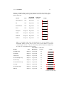
Available Marker Styles and Dependencies for Arrow Style Markers
Available Marker Styles and Dependencies for Partial Arrow Style
Markers . . . . . . . . . . . . . . . . . . . . . . . . . . . . . . .
Available Marker Styles and Dependencies for Data Point Style
Markers . . . . . . . . . . . . . . . . . . . . . . . . . . . . . . .
Available Marker Styles and Dependencies for Bracket Style Markers
Available Marker Styles and Dependencies for Cap Style Markers .
Available Marker Styles and Dependencies for Decorative Markers
10.1
Available Values for the Normal Font Size . . . . . . . . . . . . .
A.1
A.2
A.3
A.4
A.5
A.6
A.7
Tool Identifiers . . . . . . . . . . . . . . . . . . . . .
Paper Size Identifiers . . . . . . . . . . . . . . . . .
Additional Paper Size Identifiers (JDR v1.3 onwards)
Available Colour Types . . . . . . . . . . . . . . . .
Marker IDs . . . . . . . . . . . . . . . . . . . . . . .
Additional Marker IDs (JDR 1.4) . . . . . . . . . . .
Additional Marker IDs (JDR 1.6) . . . . . . . . . . .
9.3
iv
.
.
.
.
.
.
.
.
.
.
.
.
.
.
.
.
.
.
.
.
.
.
.
.
.
.
.
.
.
.
.
.
.
.
.
.
.
.
.
.
.
.
.
.
.
.
.
.
.
79
79
80
81
81
83
98
167
169
170
176
188
188
188
List of Figures
3.1
3.2
3.3
Available Grids . . . . . . . . . . . . . . . . . . . . . . . . . . .
Configuration Dialog Box . . . . . . . . . . . . . . . . . . . . . .
Hotspots . . . . . . . . . . . . . . . . . . . . . . . . . . . . . . .
11
12
13
4.1
The Main Window . . . . . . . . . . . . . . . . . . . . . . . . . .
15
6.1
6.2
6.3
6.4
Path Attributes Are Only Set Once the Path is Completed
Go To Co-ordinate Dialog Box . . . . . . . . . . . . . .
Text Area Popup Menu . . . . . . . . . . . . . . . . . .
Insert Symbol Dialog Box . . . . . . . . . . . . . . . . .
.
.
.
.
21
21
24
25
7.1
Bitmaps Are Displayed in Draft Mode When There Is Insufficient
Memory in the JRE . . . . . . . . . . . . . . . . . . . . . . . . .
28
Popup Menus in Select Mode Depend on What Objects Have Been
Selected . . . . . . . . . . . . . . . . . . . . . . . . . . . . . . .
Move Selected Objects Dialog Box . . . . . . . . . . . . . . . . .
Setting an Object’s Description . . . . . . . . . . . . . . . . . . .
Making the Join Between Segments Continuous . . . . . . . . . .
Opening a Path . . . . . . . . . . . . . . . . . . . . . . . . . . . .
Closing a Path . . . . . . . . . . . . . . . . . . . . . . . . . . . .
Adding Symmetry to a Path . . . . . . . . . . . . . . . . . . . . .
Closed Symmetric Path . . . . . . . . . . . . . . . . . . . . . . .
Edit Text Dialog Box . . . . . . . . . . . . . . . . . . . . . . . .
Combining a Text Area and Path to Form a Text-Path . . . . . . .
Symmetric Text-Paths . . . . . . . . . . . . . . . . . . . . . . . .
Three Selected Objects Rotated by 90 Degrees . . . . . . . . . . .
A Group Consisting of Three Objects Rotated by 90 Degrees . . .
Rotating a Text-Path . . . . . . . . . . . . . . . . . . . . . . . . .
Three Selected Objects Scaled by a Factor of 2 . . . . . . . . . . .
A Group Consisting of Three Objects Scaled by a Factor of 2 . . .
Scaling a Text-Path . . . . . . . . . . . . . . . . . . . . . . . . .
Two Selected Objects Sheared Horizontally . . . . . . . . . . . . .
A Group Consisting of Two Objects Sheared Horizontally . . . . .
Shearing a Text-Path . . . . . . . . . . . . . . . . . . . . . . . . .
Aligning a Group Consisting of Three Objects . . . . . . . . . . .
Aligning a Wider Object Relative to a Thinner Object . . . . . . .
Reversing the Direction of a Path . . . . . . . . . . . . . . . . . .
Reversing the Direction of a Text-Path . . . . . . . . . . . . . . .
Merging Two Paths . . . . . . . . . . . . . . . . . . . . . . . . .
Merging Two Text-Paths . . . . . . . . . . . . . . . . . . . . . . .
Paths Are Merged According to the Stacking Order . . . . . . . .
Path Union . . . . . . . . . . . . . . . . . . . . . . . . . . . . . .
Text-Path Union . . . . . . . . . . . . . . . . . . . . . . . . . . .
Exclusive OR Function . . . . . . . . . . . . . . . . . . . . . . .
Path Intersection Function . . . . . . . . . . . . . . . . . . . . . .
31
31
32
35
35
36
38
39
40
41
43
45
45
46
48
48
49
50
51
52
54
56
57
57
57
58
59
61
61
62
63
8.1
8.2
8.3
8.4
8.5
8.6
8.7
8.8
8.9
8.10
8.11
8.12
8.13
8.14
8.15
8.16
8.17
8.18
8.19
8.20
8.21
8.22
8.23
8.24
8.25
8.26
8.27
8.28
8.29
8.30
8.31
v
.
.
.
.
.
.
.
.
.
.
.
.
.
.
.
.
LIST OF FIGURES
vi
8.32
8.33
8.34
8.35
8.36
8.37
8.38
8.39
8.40
8.41
8.42
Path Subtraction Function . . . . . . . . . . .
Subtracting From a Text-Path . . . . . . . . .
Separating the Text and Path from a Text-Path
A Rotational Pattern . . . . . . . . . . . . . .
A Scaled Pattern . . . . . . . . . . . . . . . .
A Spiral Pattern . . . . . . . . . . . . . . . .
Patterns Can Either be Single or Multi-Mode .
Text-Path Patterns . . . . . . . . . . . . . . .
Converting a Text Area to a Path . . . . . . .
Converting an Outline to a Path . . . . . . . .
Splitting a Text Area . . . . . . . . . . . . . .
.
.
.
.
.
.
.
.
.
.
.
64
64
65
66
67
68
69
70
71
72
73
9.1
9.2
9.3
9.4
9.5
9.6
9.7
9.8
9.9
9.10
9.11
9.12
9.13
9.14
9.15
9.16
9.17
9.18
9.19
9.20
9.21
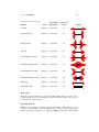
Example Dash Patterns . . . . . . . . . . . . . . . . . . . . . . .
Cap Styles . . . . . . . . . . . . . . . . . . . . . . . . . . . . . .
The Cap Style Is Affected by Whether the Path Is Open or Closed .
Join Styles . . . . . . . . . . . . . . . . . . . . . . . . . . . . . .
Repeat Markers . . . . . . . . . . . . . . . . . . . . . . . . . . .
Repeat Markers Are Placed Along the Gradient Vector . . . . . . .
Reversed Markers . . . . . . . . . . . . . . . . . . . . . . . . . .
Examples of Composite Markers . . . . . . . . . . . . . . . . . .
Disabling the Marker Auto Offset . . . . . . . . . . . . . . . . . .
Changing a Marker’s Offset Moves It Along the Gradient Vector .
Repeat Gap . . . . . . . . . . . . . . . . . . . . . . . . . . . . . .
Marker Colour May Be Independent of the Line Colour . . . . . .
Primary and Secondary Markers are Independent . . . . . . . . . .
Winding Rules . . . . . . . . . . . . . . . . . . . . . . . . . . . .
Setting the Font Family . . . . . . . . . . . . . . . . . . . . . . .
Setting the Font Size . . . . . . . . . . . . . . . . . . . . . . . . .
Setting the Font Series . . . . . . . . . . . . . . . . . . . . . . . .
Setting the Font Shape . . . . . . . . . . . . . . . . . . . . . . . .
Text-Path Transformation Matrix . . . . . . . . . . . . . . . . . .
The Effect of Converting from Java Fonts to TeX Fonts . . . . . .
The Font Used by the LaTeX Document may Result in Considerable
Differences from the Original Image . . . . . . . . . . . . . . . .
Text Area Containing Maths . . . . . . . . . . . . . . . . . . . . .
The Text Area’s Transformation Matrix Will Also Be Applied to the
Anchor . . . . . . . . . . . . . . . . . . . . . . . . . . . . . . . .
76
77
77
78
84
84
84
85
85
85
86
86
87
87
88
90
90
91
92
94
9.22
9.23
.
.
.
.
.
.
.
.
.
.
.
.
.
.
.
.
.
.
.
.
.
.
.
.
.
.
.
.
.
.
.
.
.
.
.
.
.
.
.
.
.
.
.
.
.
.
.
.
.
.
.
.
.
.
.
.
.
.
.
.
.
.
.
.
.
.
.
.
.
.
.
.
.
.
.
.
.
.
.
.
.
.
.
.
.
.
.
.
.
.
.
.
.
.
.
.
.
.
.
.
.
.
.
.
.
.
.
.
.
.
.
.
.
.
.
.
.
.
.
.
.
.
.
.
.
.
.
.
.
.
.
.
.
.
.
94
95
96
10.1
10.2
10.3
10.4
10.5
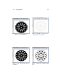
Parshape (Using Outline) . . . . . . . . . .
Parshape (Using Path) . . . . . . . . . . . .
Shapepar Example . . . . . . . . . . . . . .
Layout Containing Six Circles . . . . . . . .
The Effects of Too Much and Too Little Text
.
.
.
.
.
.
.
.
.
.
.
.
.
.
.
.
.
.
.
.
.
.
.
.
.
.
.
.
.
.
. 99
. 100
. 102
. 106
. 107
11.1
11.2
11.3
11.4
11.5
11.6
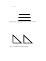
House Example—Creating a Rectangle . . . . . . . . .
House Example—Creating a Triangle . . . . . . . . . .
House Example — Completed Image . . . . . . . . . .
House Example — Saving the Image . . . . . . . . . .
House Example—Exporting the Image to a LaTeX File
Lettuce on Toast Example — Brown Rectangle . . . . .
.
.
.
.
.
.
.
.
.
.
.
.
.
.
.
.
.
.
.
.
.
.
.
.
.
.
.
.
.
.
. 109
. 109
. 110
. 110
. 110
. 111
LIST OF FIGURES
11.7
11.8
11.9
11.10
11.11
11.12
11.13
11.14
11.15
11.16
11.17
11.18
11.19
11.20
11.21
11.22
11.23
11.24
11.25
11.26
11.27
11.28
11.29
11.30
11.31
11.32
11.33
11.34
11.35
11.36
11.37
11.38
11.39
11.40
11.41
11.42
11.43
11.44
11.45
11.46
11.47
11.48
11.49
11.50
11.51
11.52
11.53
11.54
Lettuce on Toast Example—Editing the Rectangle . . . . . . . . .
Lettuce on Toast Example—Converting the Top Segment to a Curve
Lettuce on Toast Example—Finish Editing the Curve . . . . . . .
Lettuce on Toast Example — Adding a Closed Curve Path . . . . .
Lettuce on Toast Example — Completed Image . . . . . . . . . . .
Cheese and Lettuce on Toast Example — A Filled Rectangle . . . .
Cheese and Lettuce on Toast Example — Adding Ellipses . . . . .
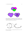
Cheese and Lettuce on Toast Example—Merging Paths . . . . . .
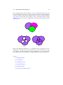
Cheese and Lettuce on Toast Example — Completed Image . . . .
Artificial Neuron Example — Adding a Rectangle . . . . . . . . .
Artificial Neuron Example — Adding a Circle . . . . . . . . . . .
Artificial Neuron Example—Creating a Sigmoidal Curve . . . . .
Artificial Neuron Example — Setting the Current Line Style . . . .
Artificial Neuron Example — End Marker Dialog Box . . . . . . .
Artificial Neuron Example — Adding Arrows . . . . . . . . . . . .
Artificial Neuron Example — Adding Text . . . . . . . . . . . . .
Artificial Neuron Example — Editing Text . . . . . . . . . . . . .
Artificial Neuron Example — Insert Symbol Dialog Box . . . . . .
Artificial Neuron Example — Setting the Font Style . . . . . . . .
Artificial Neuron Example—Setting the Equivalent LaTeX Symbol
Artificial Neuron Example — Justifying Objects . . . . . . . . . .
Artificial Neuron Example — Image as it Appears in a LATEX Document . . . . . . . . . . . . . . . . . . . . . . . . . . . . . . . . .
Bus Example — Setting the Normal Font Size . . . . . . . . . . .
Bus Example — Create a Circle . . . . . . . . . . . . . . . . . . .
Bus Example — Editing the Path . . . . . . . . . . . . . . . . . .
Bus Example — Break the Path . . . . . . . . . . . . . . . . . . .
Bus Example — Move and Rotate Top Semi-Circle . . . . . . . . .
Bus Example — Adding Lines . . . . . . . . . . . . . . . . . . . .
Bus Example — Convert Line Segment to a Curve . . . . . . . . .
Bus Example — Add Windows . . . . . . . . . . . . . . . . . . .
Bus Example — Subtract Windows from Bus Outline and Set Fill
Colour . . . . . . . . . . . . . . . . . . . . . . . . . . . . . . . .
Bus Example — Resulting Shaped Paragraph . . . . . . . . . . . .
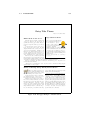
Poster Example — The Typeblock . . . . . . . . . . . . . . . . . .
Poster Example — Adding Rectangles . . . . . . . . . . . . . . .
Poster Example — Adding a Bitmap . . . . . . . . . . . . . . . .
Poster Example — Adding Some Colour . . . . . . . . . . . . . .
Poster Example—Assigning Frame Information . . . . . . . . . .
Poster Example — Frame Information Assigned . . . . . . . . . .
Poster Example — Export Frame Information to a LATEX Package .
Poster Example — Final Document . . . . . . . . . . . . . . . . .
No Mouse Example — Grid Settings Dialog Box . . . . . . . . . .
No Mouse Example — Go To Co-Ordinate Dialog Box . . . . . . .
No Mouse Example — Completed Rectangle . . . . . . . . . . . .
No Mouse Example — Set Fill Colour Dialog Box . . . . . . . . .
No Mouse Example — Fill Colour Set . . . . . . . . . . . . . . .
No Mouse Example — Completed Triangle . . . . . . . . . . . . .
No Mouse Example — Triangle Fill Colour Set to Red . . . . . . .
No Mouse Example — Windows Added . . . . . . . . . . . . . .
vii
111
112
112
113
113
114
114
114
115
115
115
116
116
117
117
117
118
118
119
119
120
120
121
121
121
122
122
122
123
123
123
124
125
126
126
127
127
128
128
130
130
131
131
132
133
133
134
135
LIST OF FIGURES
11.55
11.56
11.57
11.58
11.59
11.60
11.61
11.62
11.63
11.64
11.65
11.66
11.67
11.68
11.69
11.70
11.71
11.72
11.73
11.74
11.75
11.76
11.77
11.78
11.79
11.80
11.81
11.82
11.83
11.84
11.85
11.86
11.87
11.88
11.89
11.90
11.91
11.92
11.93
11.94
11.95
11.96
11.97
11.98
11.99
viii
No Mouse Example — Window Fill Colour Set . . . . . . . . . . . 135
No Mouse Example — Completed House . . . . . . . . . . . . . . 136
No Mouse Example — Move Dialog Box . . . . . . . . . . . . . . 136
No Mouse Example — Edit Mode . . . . . . . . . . . . . . . . . . 137
No Mouse Example — Edit Path Menu . . . . . . . . . . . . . . . 137
No Mouse Example — Control Point Co-Ordinates Dialog Box . . 138
No Mouse Example — Editing Finished . . . . . . . . . . . . . . . 138
No Mouse Example — Creating a New Text Area . . . . . . . . . 138
No Mouse Example — Editing Text Area . . . . . . . . . . . . . . 139
No Mouse Example — Text is Now Centred . . . . . . . . . . . . 140
Newspaper Example — Setting the LATEX Normal Font Size . . . . 141
Newspaper Example — Setting the Grid . . . . . . . . . . . . . . 141
Newspaper Example — Setting the Typeblock . . . . . . . . . . . 141
Newspaper Example — Title Frame . . . . . . . . . . . . . . . . . 142
Newspaper Example — Assigning Flowframe Data to Title Frame . 142
Newspaper Example — Left and Right Heading Frames Added . . 143
Newspaper Example — Assigning Flowframe Data to Left Heading
Frame . . . . . . . . . . . . . . . . . . . . . . . . . . . . . . . . 143
Newspaper Example — Added L Shaped Frame . . . . . . . . . . 144
Newspaper Example — Assigning Flowframe Data to L Shaped Frame144
Newspaper Example — Added Image . . . . . . . . . . . . . . . . 145
Newspaper Example — Assigning Flowframe Data to Bitmap . . . 146
Newspaper Example — Added Right Hand Polygon . . . . . . . . 146
Newspaper Example — Assigning Flowframe Data to Right Hand
Polygon . . . . . . . . . . . . . . . . . . . . . . . . . . . . . . . 147
Newspaper Example — Added L Shaped Divider . . . . . . . . . . 147
Newspaper Example — Assigning Flowframe Data to L Shaped Divider . . . . . . . . . . . . . . . . . . . . . . . . . . . . . . . . . 148
Newspaper Example — Added Horizontal Divider . . . . . . . . . 148
Newspaper Example — Assigning Flowframe Data to Horizontal Divider . . . . . . . . . . . . . . . . . . . . . . . . . . . . . . . . . 149
Newspaper Example — Added Lower Header . . . . . . . . . . . . 149
Newspaper Example — Assigning Flowframe Data to Lower Header 150
Newspaper Example — Added Lower Left and Right Rectangles . 151
Newspaper Example — Assigning Flowframe Data to Lower Left
Rectangle . . . . . . . . . . . . . . . . . . . . . . . . . . . . . . . 151
Newspaper Example — Added Sheep Bitmap . . . . . . . . . . . . 152
Newspaper Example — Assigning Flowframe Data to Sheep Bitmap 152
Newspaper Example — Added Polygon Defining Text Region . . . 153
Newspaper Example—Computing Parshape Parameters . . . . . . 153
Newspaper Example — Final Document . . . . . . . . . . . . . . 156
The Normal Font Size Setting Affects Paragraph Shapes . . . . . . 157
Selecting a Radial Grid . . . . . . . . . . . . . . . . . . . . . . . 157
The Underlying Path . . . . . . . . . . . . . . . . . . . . . . . . . 158
Give the Path Symmetry Using the Popup Menu . . . . . . . . . . 159
De-anchoring the End Control Using the Popup Menu . . . . . . . 159
Move the Line of Symmetry . . . . . . . . . . . . . . . . . . . . . 159
Add a Joining Curve Between the Underlying Path and its Reflection 159
Adjust the Curvature Control of the Join Segment . . . . . . . . . 160
Change the Path Style . . . . . . . . . . . . . . . . . . . . . . . . 161
LIST OF FIGURES
11.100
11.101
11.102
11.103
11.104
11.105
The Symmetric Path . . . . . . . . . . . . . . . . .
Setting the Pattern . . . . . . . . . . . . . . . . . .
The Pattern . . . . . . . . . . . . . . . . . . . . . .
Move the Control Governing the Rotational Anchor
Add a Circle Around the Pattern . . . . . . . . . . .
The Completed Lute Rose . . . . . . . . . . . . . .
ix
.
.
.
.
.
.
.
.
.
.
.
.
.
.
.
.
.
.
.
.
.
.
.
.
.
.
.
.
.
.
.
.
.
.
.
.
.
.
.
.
.
.
.
.
.
.
.
.
162
162
163
163
163
163
1
Introduction
Jpgfdraw is a vector graphics application written in JavaTM , with a graphical user in-
terface (GUI). In order to run the application you must have the JavaTM 2 Platform,
Standard Edition Runtime Environment (JRE) installed (at least version 1.5). Jpgfdraw
is based in part on Acorn’s !Draw application, but was tailored specifically to produce
files containing pgfpicture environments for use with Till Tantau’s pgf LATEX package.
In Jpgfdraw, you can:
• Construct shapes using line, move and cubic Bézier segments.
• Edit paths by modifying the defining control points.
• Incorporate text and bitmap images (for annotating and background effects).
• Text and paths can be combined to form a text along path effect.
• Extract the parameters for TEX’s \parshape command and for the \shapepar
command defined in Donald Arseneau’s shapepar package.
• Construct frames for use with the flowfram package.
• Pictures can be saved as or loaded from Jpgfdraw’s native JDR (binary) or AJR
(ascii) file formats.
• Pictures can be exported as:
– a LATEX file containing a pgfpicture environment for inclusion in a LATEX
document;
– a single-paged LATEX document containing the image;
– a LATEX 2ε package based on the flowfram package;
– an Encapsulated Postscript (EPS) file;
– a PNG file;
– a scalable vector graphics (SVG) file.
1.1
Installation
Ensure that you have the JRE installed. This can be downloaded from http://
java.sun.com/j2se/. You must ensure that you use at least Java 6, as Jpgfdraw
does not work with earlier versions.
1.1.1
Windows Installation
Download and run the file jpgfdraw-0.5.6b-setup.exe
1
1.1.2
UNIX-LIKE INSTALLATION
1.1.2
Unix-Like Installation
2
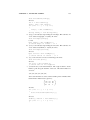
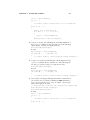
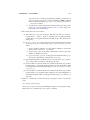
1. Unzip jpgfdraw-0.5.6b.zip, e.g.:
unzip jpgfdraw-0.5.6b -d /usr/share/
2. Add the bin sub-directory to your path, e.g.:
setenv PATH $PATH:/usr/share/jpgfdraw-0.5.6b/bin
or
export PATH=$PATH:/usr/share/jpgfdraw-0.5.6b/bin
or
declare -x PATH=$PATH:/usr/share/jpgfdraw-0.5.6b/bin
You can add this line to your login script. (The name varies, but it may be
˜/.cshrc, ˜/.bashrc, ˜/.login or ˜/.profile — check your system’s documentation.)
3. To run Jpgfdraw, type jpgfdraw at the command prompt.
2
Accessibility
As from version 0.3b Jpgfdraw has improved support for users who have difficulties
with or who are unable to use a mouse. (However please note known bug 5.) Almost
all Jpgfdraw’s mouse functions can be emulated using the keyboard, however it should
be noted that some systems do not permit applications to move the pointer, so keyboard
functions that move the pointer are not guaranteed to work on every system. Keyboard
accelerators and their menu mnemonic equivalents are listed in Table 2.1. Keyboard
accelerators for the JavaHelp system are listed in Table 2.2.
Within editable text fields, you can use Ctrl-A to select all the text, or Shift followed
by the left or right arrow key to select a portion of the text. If some of the text has been
selected, you can use Ctrl-C or Ctrl-X to copy or cut the text onto the clipboard, and you
can use Ctrl-V to paste text from the clipboard into the text field.
Table 2.1: Keyboard Accelerators and Menu Mnemonics
Accelerator
Function
Menu Mnemonic
Finish current path/text area or
Alt-O F
Select Okay button in dialog boxes
Alt-O
Escape
Abandon current path or
Alt-O A
Select Cancel button in dialog boxes
Alt-C
Delete
Delete selected control point
F3 Alt-D
Insert
Add control point or
F3 Alt-A
Display symbol dialog box
F3 Alt-I
Tab
Move focus to next focusable component
—
Space
Select component with current focus
—
PageUp
Scroll up by one screen full
—
PageDown
Scroll down by one screen full
—
Ctrl-PageDown If in a tabbed pane:
Move to the next tab
—
Otherwise:
Scroll right by one screen full
—
Ctrl-PageUp
If in a tabbed pane:
Move to the previous tab
—
Otherwise:
Scroll left by one screen full
—
Arrow Keys
If left mouse button pressed:
†
move mouse by one pixel in given direction —
Otherwise:
scroll by one tick mark in given direction
—
Home
Scroll to the top of the canvas
—
End
Scroll to the bottom of the canvas
—
Ctrl-Home
Scroll leftmost
—
Ctrl-End
Scroll rightmost
—
F1
Display Handbook
Alt-H H
F2
Show/hide grid
Alt-S G S
F3
Show popup menu (if available for current mode) —
†
Functions that move the pointer
Continued on next page
Enter
3
CHAPTER 2. ACCESSIBILITY
4
Table 2.1: Keyboard Accelerators and Menu Mnemonics (Continued)
Accelerator
Function
Mnemonics
Emulate single mouse click in construction mode —
†
Go to coordinate
Alt-N G
Select mode:
deselect the back-most selected object,
Alt-N K
and select next object in the stack
Edit mode:
select next control point
F3 Alt-N
F7
Select mode:
Move selected objects
Alt-E M
Edit mode:
Move selected control point
F3 Alt-R
F8
Undo
Alt-E U
F9
Redo
Alt-E R
F10
Writes log file in the configuration directory
F11
Saves all images to configuration directory
Shift-F2
Lock/unlock grid
Alt-S G L
Shift-F5
Select next object in the stack (from the front),
Alt-N S
and deselect all others
Shift-F6
Add next object in the stack (from the front) to
Alt-N A
selection
†
Shift-F7
Find selected objects
Alt-N F
Alt-F4
Quit
Alt-F Q
Ctrl-A
Select all objects
Alt-E A
Ctrl-B
Move selected objects to the back
Alt-E B
Ctrl-C
Copy selected objects to clipboard
Alt-E C
Ctrl-D
Convert outline to a path
Alt-T C
Ctrl-E
Switch to ellipse tool
Alt-O E
Ctrl-F
Move selected objects to the front
Alt-E F
Ctrl-G
Group selected objects
Alt-T G
Ctrl-H
Shear selected objects
Alt-T H
Ctrl-I
Edit selected path
Alt-E H E
Ctrl-J
Merge selected paths
Alt-T M
Ctrl-K
Switch to open curve tool
Alt-O C
Ctrl-L
Switch to open line tool
Alt-O L
Ctrl-M
Gap function
Alt-O G
Ctrl-N
New child window
Alt-F N
Ctrl-O
Open JDR or AJR file
Alt-F O
Ctrl-P
Switch to select tool
Alt-O S
Ctrl-Q
Quit
Alt-F Q
Ctrl-R
Switch to rectangle tool
Alt-O R
Ctrl-S
Save current image
Alt-F S
Ctrl-T
Switch to text tool
Alt-O T
Ctrl-U
Ungroup selected groups
Alt-T U
Ctrl-V
Paste objects from clipboard
Alt-E P
Ctrl-W
Rotate selected objects
Alt-T R
†
Functions that move the pointer
Continued on next page
F4
F5
F6
CHAPTER 2. ACCESSIBILITY
5
Table 2.1: Keyboard Accelerators and Menu Mnemonics (Continued)
Accelerator
Ctrl-X
Ctrl-Y
Ctrl-Z
Ctrl+Shift-A
Ctrl+Shift-I
Ctrl+Shift-K
Ctrl+Shift-L
Alt-1. . . Alt-8
Alt-1. . . Alt-9
Function
Cut selected objects
Edit the selected paths’ line styles
Scale selected objects
Deselect all
Edit selected text
Switch to closed curve tool
Switch to closed line tool
Linear gradient paint direction selectors
Radial gradient paint start location selectors
Mnemonics
Alt-E T
Alt-E H S A
Alt-T S
Alt-E D
Alt-E X E
Alt-O U
Alt-O I
Table 2.2: JavaHelp Viewer Shortcut Keys
Key
Ctrl-F1
F6
Tab
Shift-Tab
Space
Ctrl-Space
F8
Left/Right Arrow
Up/Down Arrow
Home
End
Ctrl-Home
Ctrl-End
Ctrl-T
Ctrl+Shift-T
Function
Displays alternative text for the toolbar button that currently has the
focus.
Moves the focus between the navigation pane and content pane.
Traverses through the viewer.
Traverses backwards through the viewer.
Activates the toolbar button with the current focus.
Follows a link in the content pane.
Selects the splitter bar between the navigator pane and the content
pane.
If the splitter bar is selected:
Moves the splitter bar to the left/right
If in the navigator pane:
Moves to another navigator tab
If in the viewer’s toolbar:
Moves the focus to the next toolbar button
If in the content pane:
Moves one character to the left/right.
If the splitter bar is selected:
Moves the splitter bar to the left/right
If in the navigator pane:
Selects the previous/next item in the list
If in the content pane:
Moves the focus to the previous/next line.
Selects the first item in the navigator list.
Selects the last item in the navigator list.
Selects the first line in the content pane.
Selects the last line in the content pane.
Shifts focus to the next link in the content pane.
Shifts the focus to the previous link in the content pane.
CHAPTER 2. ACCESSIBILITY
See also:
• §8 Selecting and Editing Objects
• §6 Creating New Objects
• §11.7 Step-by-Step Example: A House With No Mouse
6
3
Settings
You can customise the appearance of Jpgfdraw’s main window either using the command line arguments or using the settings menu.
3.1
Command Line Arguments
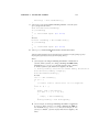
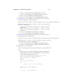
Jpgfdraw can be invoked from a command prompt using:
jpgfdraw hoption-listi hfilenamei
Note that hoption-listi and hfilenamei may be omitted. Only one filename is permitted,
and it must be either a JDR or an AJR file. This script uses the environment variable
JDR JVMOPTS to pass options to the Java Virtual Machine (JVM). For example, if
you want to run Jpgfdraw with a maximum size of 128Mb for the memory allocation
pool, you can set JDR JVMOPTS to -Xmx128m:
setenv JDR_JVMOPTS -Xmx128m
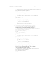
This script also uses the environment variable JPGFDRAW OPTS to pass options to
Jpgfdraw. For example, if you always want Jpgfdraw to start up with the grid showing,
you can set JPGFDRAW OPTS to -show grid:
setenv JPGFDRAW -show_grid
Note that these environment variables only have an effect if you use the jpgfdraw
script to run the JRE.
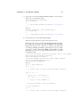
If you can’t use the jpgfdraw script, you can invoke Jpgfdraw from the command
line using (no line breaks):
java hjava optionsi -jar jpgfdraw.jar hjpgfdraw optionsi
hfilenamei
(You may need to include the full pathname to jpgfdraw.jar.)
The following options are provided:
-disable print Don’t request printer attributes on startup.
-show grid Show the grid.
-noshow grid Don’t show the grid.
-grid lock Set the grid lock on.
-nogrid lock Don’t set the grid lock.
-toolbar Show the toolbars.
-notoolbar Don’t show the toolbars.
-statusbar Show the status bar.
-nostatusbar Don’t show the status bar.
-rulers Show the rulers.
7
3.2
THE SETTINGS MENU
8
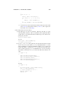
-norulers Don’t show the rulers.
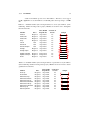
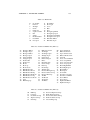
-paper Set the paper size. This option must be followed by a string identifying the
paper size. Known paper sizes are listed in Table 3.1. Custom sizes can be
specified using -paper user hwidthi hheighti, where hwidthi and hheighti
must be positive dimensions. Recognised units: pt, bp, in, mm, cm, pc, dd
and cc. If the unit is omitted, bp is assumed. Examples:
• -paper a4r
• -paper user 8.5in 12in
• -paper user 600 1000
-experimental Enables experimental functions. These functions may not work
properly.
-noexperimental Disables experimental functions. (Default.)
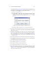
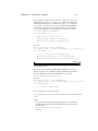
-debug Enables the debug menu. This menu provides the functions: Debug → Object
info (which displays diagnostic information about the currently selected objects),
Debug → Write Log (which writes diagnostic information for all currently open
images to a log file in the configuration directory) and Debug → Dump All (which
saves all current images to a subdirectory of the configuration directory).
-nodebug Disables the debug menu (default). However you can still use F10 and
F11 to do the same action as Debug → Write Log and Debug → Dump All, respectively.
-version Prints the current version to standard output.
-help Prints available command line options to standard output.
3.2
The Settings Menu
While Jpgfdraw is running, you can change the current settings using the Settings
menu. Most of the settings will be remembered next time you use Jpgfdraw, but may
be overridden either by command line arguments or by settings specified in any JDR
or AJR file that you load.
3.2.1
Styles
Settings → Styles. . . can be used to set the current path and text area attributes. New
paths and text areas will use these attributes when they are created. The attributes
for existing paths and text areas are changed using the Edit menu. These settings are
discussed in more detail in chapter 9.
3.2.2
Show Tools
Settings → Show Tools will toggle between showing and hiding the toolbars.
3.2.2
SHOW TOOLS
9
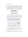
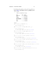
Table 3.1: Paper size identifiers for use with -paper command line switch.
a10
a9
a8
a7
a6
a5
a4
a3
a2
a1
a0
b10
b9
b8
b7
b6
b5
b4
b3
b2
b1
b0
c10
c9
c8
c7
c6
c5
c4
c3
c2
c1
c0
letter
legal
executive
A10 portrait
A9 portrait
A8 portrait
A7 portrait
A6 portrait
A5 portrait
A4 portrait
A3 portrait
A2 portrait
A1 portrait
A0 portrait
B10 portrait
B9 portrait
B8 portrait
B7 portrait
B6 portrait
B5 portrait
B4 portrait
B3 portrait
B2 portrait
B1 portrait
B0 portrait
C10 portrait
C9 portrait
C8 portrait
C7 portrait
C6 portrait
C5 portrait
C4 portrait
C3 portrait
C2 portrait
C1 portrait
C0 portrait
Letter portrait
Legal portrait
Executive portrait
a10r
a9r
a8r
a7r
a6r
a5r
a4r
a3r
a2r
a1r
a0r
b10r
b9r
b8r
b7r
b6r
b5r
b4r
b3r
b2r
b1r
b0r
c10r
c9r
c8r
c7r
c6r
c5r
c4r
c3r
c2r
c1r
c0r
letterr
legalr
executiver
A10 landscape
A9 landscape
A8 landscape
A7 landscape
A6 landscape
A5 landscape
A4 landscape
A3 landscape
A2 landscape
A1 landscape
A0 landscape
B10 landscape
B9 landscape
B8 landscape
B7 landscape
B6 landscape
B5 landscape
B4 landscape
B3 landscape
B2 landscape
B1 landscape
B0 landscape
C10 landscape
C9 landscape
C8 landscape
C7 landscape
C6 landscape
C5 landscape
C4 landscape
C3 landscape
C2 landscape
C1 landscape
C0 landscape
Letter landscape
Legal landscape
Executive landscape
3.2.3
3.2.3
SHOW RULERS
10
Show Rulers
Settings → Show Rulers will toggle between showing and hiding the rulers. The rulers
always show rectangular co-ordinates, even if a radial grid is in use.
3.2.4
Show Status Bar
Settings → Show Status Bar will toggle between showing and hiding the status bar.
3.2.5
Grid
The Settings → Grid submenu allows you to change the grid settings:
• Settings → Grid → Show Grid will toggle between displaying the grid on the canvas and hiding it. If there is enough memory available, the grid will be stored as
a bitmap in order to improve redraw speed.
• Settings → Grid → Lock Grid will toggle between locking and unlocking the grid.
If the grid is locked, mouse clicks will be translated to the nearest tick mark. This
means that if you use a mouse click to set the location of a control point when
constructing a path, the point will be placed at the nearest tick mark. This also
means that when you move a point while in edit mode, the point will be moved
in intervals of the gap between tick marks. Note that locking the grid does not
affect the keyboard or menu driven functions, such as Navigate → Go To. . . (F5)
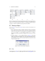
or emulate a mouse click (F4).
When the grid is locked, the status bar will show the image
will show the image
.
otherwise it
Warning: if you lock the grid, you will be unable to use the mouse to select
narrow paths that lie between tick marks as mouse clicks will be translated to
the nearest tick mark, unless you use the drag rectangle (which may select other
objects as well). Similarly, if the size of the control points is less than the gap
between the tick marks, you will not be able to select control points using the
mouse whilst in edit mode. (You will however be able to select them using the
Next Control (F6) popup menu item.)
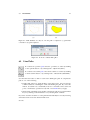
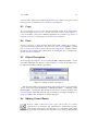
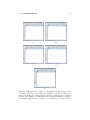
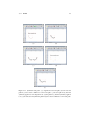
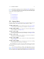
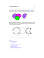
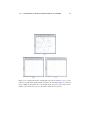
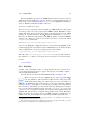
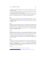
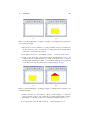
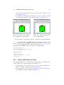
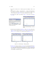
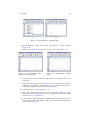
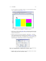
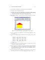
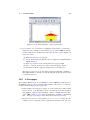
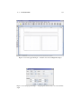
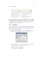
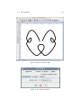
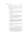
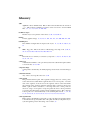
• Settings → Grid → Grid Settings. . . will produce a dialog box in which you can
specify the position of the tick marks and the units used. You can either use a
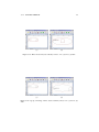
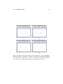
rectangular grid with the origin at the top left hand corner of the canvas (Figure 3.1(a)), or you can use a radial grid with the origin at the centre of the canvas
(Figure 3.1(b)).
3.2.6
Zoom
The Settings → Zoom submenu allows you to change the magnification. You can
choose one of the predefined settings or you can specify an arbitrary setting using
Settings → Zoom → User Defined. . .. This dialog box should have the actually magnification factor entered, not the percentage. For example, 300% magnification should
be entered as 3.
3.2.7
PAPER
11
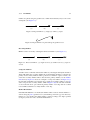
(a)
(b)
Figure 3.1: Available grids: (a) rectangular grid; (b) radial grid
3.2.7
Paper
The Settings → Paper submenu allows you to change the paper size and orientation. In
addition, Settings → Paper → Show Margins toggles between showing and hiding the
printer margins, but note that this facility is only available if Jpgfdraw detects a printer,
so you will need to ensure that the printer is switched on and connected to the computer
for this setting to have any effect.
The predefined paper sizes A0 to A5, letter, legal and executive can be selected from
the Settings → Paper menu. Other paper sizes can be selected from the dialog box displayed using Settings → Paper → Other. . .. Select the radio button labelled Predefined
to enable a list of additional known paper sizes or select the radio button labelled User
to enter a custom size.
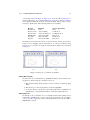
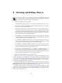
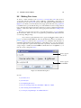
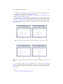
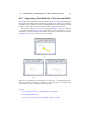
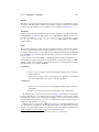
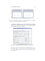
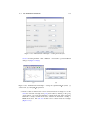
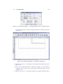
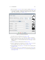
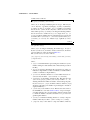
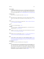
3.2.8
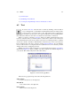
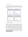
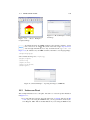
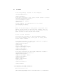
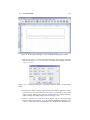
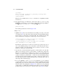
Configuration Dialog
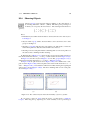
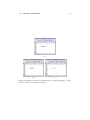
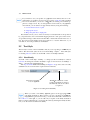
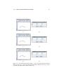
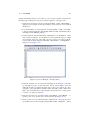
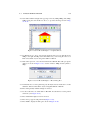
The menu item Settings → Configure. . . will open up a dialog box (Figure 3.2) in which
you can specify the following:
Graphics Tab
This tab allows you to:
•
•
•
•
Choose between using or not using anti-aliasing to display the graphics.
Choose between speed or quality in the rendering.
Set the size of the control points in the Control Size field.
Set the colour for the different types of control points.
Hotspots Tab
Choose between enabling and disabling hotspots along the bounding boxes. If
hotspots are enabled, you can scale, rotate or shear objects by dragging the appropriate hotspot. You may want to disable this option when you want to move
small objects, or you may end up transforming them instead of moving them.
When this option is enabled, the cursor will change shape1 when you move it
1 The actual cursor appearance depends on the look and feel of the platform you are using. On some
systems the South and North arrows may look the same, and similarly for the East and West arrows.
3.2.8
CONFIGURATION DIALOG
Use this tab to
Use this tab to
specify which settings
govern the settings
stored in JDR/AJR files. to apply on start up.
12
Use this tab to specify
which languages to use
for the manual and resources
Use this tab
to enable
the hotspots.
Use this tab to
specify which
directory to set
as the current
directory on
start up.
Use this tab to control
the graphics display.
Figure 3.2: Configuration Dialog Box
3.2.8
CONFIGURATION DIALOG
13
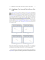
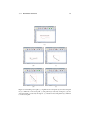
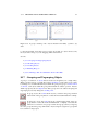
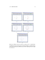
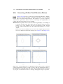
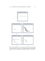
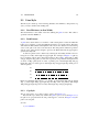
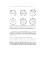
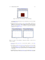
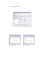
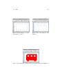
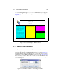
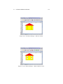
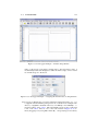
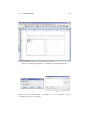
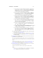
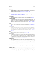
over the edge of the bounding box. Figure 3.3(a) shows how the bounding box is
displayed when hotspots are enabled and Figure 3.3(b) shows how the bounding
box is displayed when the hotspots have been disabled. Each hotspot is represented by a small square. The following functions are available:
Hotspot
Bottom left
Bottom centre
Bottom right
Middle right
Top right
Top left
Function
rotate
scale vertically
scale both directions
scale horizontally
shear vertically
shear horizontally
Cursor Appearance
hand
South arrow
South-East arrow
East arrow
North arrow
West arrow
Note that even if you have more than one object selected, only the object whose
hotspot you are dragging will be transformed. As may be predicted, using
hotspots is not as precise as using the transformation dialog boxes described
in chapter 8.
(a)
(b)
Figure 3.3: Hotspots: (a) enabled; (b) disabled.
Startup Directory Tab
Use this tab to choose which directory Jpgfdraw should use as the current working directory when it starts up. You have a choice of:
1. The current working directory that you were in when you started up Jpgfdraw.
2. The directory you were using when you last used Jpgfdraw.
3. A specific directory. In this case, type in the path in the box labelled Use
this directory: or use the Browse button to select the required directory.
JDR Settings tab
Use this tab to choose whether or not you want the current canvas settings stored
in the JDR or AJR file when you save your image. You can also choose whether
or not you want to apply any canvas settings information stored in any JDR or
AJR file that you load.
3.3
CONFIGURATION DIRECTORY
14
Startup Settings Tab
Use this tab to choose whether you want Jpgfdraw to start with its default settings, or whether to restore the settings from the last time you used Jpgfdraw, or
whether to use the settings that are currently in use.
Languages Tab
Use this tab to set which language to use for the application resources (menus,
messages etc) and which language to use for the manual. These settings will
not be applied until you quit and restart Jpgfdraw. Currently the only available
resource languages are: en-GB, en-US and zh, and the only available manual
languages are: en-GB and en-US.
3.3
Configuration Directory
When you quit Jpgfdraw, the current settings will be saved in Jpgfdraw’s configuration
directory.2 This directory is determined (and created if necessary) as follows:
• If the environment variable JDRSETTINGS exists and is a directory, that directory is used.
• If the directory hhomei/.jpgfdraw exists and is a directory, that directory is
used (where hhomei indicates the user’s home directory as given by the Java
user.home property).
• If the directory hhomei/jpgfdraw-settings exists and is a directory, that
directory is used (where hhomei indicates the user’s home directory as given by
the Java user.home property).
• If the operating system is a version of Windows and the directory hhomei/
jpgfdraw-settings can be created, that directory is used.
• For other operating systems, if the directory hhomei/.jpgfdraw can be created, that directory is used.
• If the directory settings/huseri or settings can be created in Jpgfdraw’s
installation directory, that directory will be used (where huseri is the current
user’s user name).
• If none of the above, an error will occur and you will need to set the environment
variable JDRSETTINGS to a sensible location with read/write permission.
The configuration directory may also contain the list of recent files (this file is
created by Jpgfdraw) as well as the LATEX font mappings (which you can create in any
text editor). For more information on the font mappings, see subsection 9.5.1.
In addition, the configuration directory is used to save the log file, jpgfdraw.log,
in the event that F10 is used (or Debug → Write Log if the command line option -debug
is used). The emergency save all function F11 (or Debug → Dump All if the command
line option -debug is used) will create a subdirectory (using the current date and time
to construct the name) and will save all open images to that directory with filenames of
the form imagehni.jdr.
2 unless you have selected the use current settings option in the Startup Settings panel, in which case it
will save the current settings at that point.
4
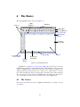
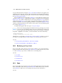
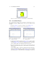
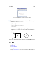
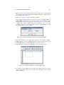
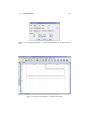
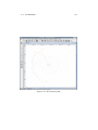
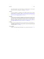
The Basics
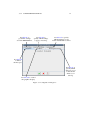
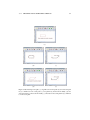
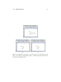
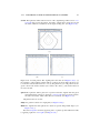
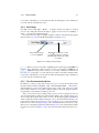
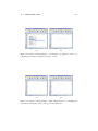
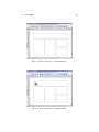
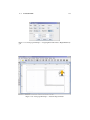
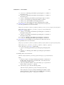
The main Jpgfdraw window is shown in Figure 4.1.
Child
Window
Toolbars
Title Bar
Menu Bar
Scroll Buttons
for Tool Bar
Horizontal
Ruler
Vertical
Scroll Bar
Status Bar
Scroll Buttons
for Tool Bar
Canvas
Horizontal
Scroll Bar
Vertical
Ruler
Figure 4.1: The Main Window
Jpgfdraw uses a multiple-document interface (MDI). This means that you can have
multiple images loaded in separate child windows, without having to start up new instances of Jpgfdraw. Most of the buttons and menu items will only be applied to the
child window that currently has the focus. If there are no child windows, or if they
have all been minimized, then the relevant buttons and menu items will be disabled.
The only exceptions are the items in the Window menu, the Help menu, and the new,
open, quit functions and the non-canvas specific items of the Settings menu.
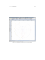
4.1
The Canvas
The canvas is the white area in each of Jpgfdraw’s child windows on which you create
your picture.
15
4.2
4.2
THE TOOLBARS
16
The Toolbars
There are two toolbars. The horizontal toolbar positioned at the top of the main window, which allows you to manipulate objects on the canvas (as well as the save, load
and new buttons) and the vertical toolbar positioned to the left of the main window,
which you can use to create new paths and text areas. If a toolbar is too wide, scroll
buttons will appear.
You can show or hide the toolbars using the menu item Settings → Show Tools.
4.3
The Rulers
There are two rulers. The horizontal ruler positioned above the canvas which marks
out the x-ticks, and the vertical ruler positioned to the left of the canvas which marks
out the y-ticks. Note that the origin starts at the top left of the canvas. The gap between
tick marks can be changed using the Settings → Grid → Grid Settings. . . menu item.
You can show or hide the rulers using the menu item Settings → Show Rulers.
4.4
The Status Bar
The status bar is positioned along the bottom of the main window. The left hand corner
shows the current position of the pointer (or the pointer’s last position before it was
moved away from the canvas). Next to that is the file status area. If the current picture
has been modified, it will display the word “Modified”, otherwise it will be blank. Next
or off
and next
to that is an image that indicates whether the grid lock is on
to that there is some brief information as to what you can do with the currently selected
tool.
You can show or hide the status bar using the menu item Settings → Show Status
Bar.
5
The File Menu
You can use the File menu to create a new picture, load a picture from a JDR or AJR
file, save the current picture, export the current picture to a supported format (such as
a LATEX file), assign a description to the current picture, print the current picture or quit
Jpgfdraw.
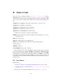
5.1
New
To start a new picture, select File → New. This will open a new child window. You can
switch between child windows using the Window menu.
5.2
Open
To load a JDR or AJR file, select File → Open. . .. If there is already a picture in the
current child window, a new child window will open to display the file. Note that
although Jpgfdraw can export to other formats, it can only load JDR and AJR files.1
If you load an image that contains a link to a bitmap and the bitmap is no longer in
the same location, you will be prompted for a new link or you can discard the link. Note
that if you select a new link, the LATEX link will also be updated to the full path name.
If you want a relative path name in the LATEX link, you will need to edit it using the
bitmap properties dialog. If there is insufficient memory in the JRE to load a bitmap,
Jpgfdraw will revert to draft mode for that bitmap.
5.3
Recent Files
To load a recently used JDR or AJR file, use the sub menu File → Recent Files. A
maximum of ten files, starting with the most recently used are listed. Note that loading
a file from this list will change the open file dialog box directory to that file’s directory.
5.4
Image Description
You can use the File → Image Description. . . dialog box to give the image a description.
The description is not visible in the image, but is saved when you export the image to
other formats: as a comment in a LATEX file, enclosed in a <desc> tag in an SVG file,
or a %%Title: DSC in an EPS file.
5.5
Save and Save As
You can save the current picture in Jpgfdraw’s native JDR or AJR format using either
File → Save (if it already has a name) or File → Save As. . . (if you want to specify the
1 The jdrutils suite comes with an application called eps2jdr which can convert some EPS files to JDR
files, but it is still in development and only works on fairly simple EPS files. See the jdrutils manual for
further details. (Jpgfdraw’s experimental mode will enable an import menu item, see §5.7 Import.)
17
5.6
EXPORT
18
filename). It is recommended that you save your work frequently, particularly given
that the current version of Jpgfdraw is still a beta release.
See also:
• §5.6 Export
5.6
Export
The File → Export. . . menu allows you to export your image as:
• A LATEX 2ε file containing a pgfpicture environment (limitations apply, see below).
• A single-paged LATEX document containing the image. (Note that you may need
to add addition packages or command definitions if you use commands in your
text area that aren’t part of the basic LATEX distribution. Again, the limitations
below apply.)
• A PNG file. (All colours are converted to RGB.)
• An encapsulated postscript (EPS) file. (Transparency is not implemented.)
• An SVG file. (CMYK colours are converted to RGB.)
• A LATEX 2ε package based on the flowfram package. The pgf package is also used
to create borders and backgrounds, so the limitations that apply to exporting to a
pgfpicture environment also apply (see below).
Note that Jpgfdraw can’t load the files that it can export, so it is recommended that you
first save the picture as a JDR file before exporting it, in case you wish to edit it later.
To save your picture as a pgfpicture environment, select the pgf environment
(*.tex, *.ltx) file filter. You can include the image into your LATEX document
using \input, but remember to specify the pgf package using:
\usepackage{pgf}
Alternatively, you can save the image (including paper dimensions) to a single-paged
LATEX document using the LaTeX document (*.tex, *.ltx) file filter.
Jpgfdraw was tested with version 1.10 of the pgf package. Files created by Jpgfdraw
may not work with earlier versions of the pgf package. Note that some DVI viewers
may not understand PGF specials. It is strongly recommended that you read the PGF
user manual.
Limitations: Gradient paint is not available for text areas and outlines — only the
start colour will be used. The gradient shading for fill colours has limited functionality
and the gradient paint transparency settings are ignored when exporting to a pgfpicture
environment. Text-paths only have limited support.
If you have used Jpgfdraw to create frames for use with the flowfram package, you can export the information to a LATEX package. To do this, select
the flowframe (*.sty) file filter, but note that only the objects that have been
5.7
IMPORT
19
identified as static, flow or dynamic frames will be saved. You must set the typeblock
before you can export the flowframe information.
See also:
• §10.4 Creating Frames for Use with the flowfram Package
• §11.1 Step-by-Step Example: A House
• §11.4 Step-by-Step Example: An Artificial Neuron
• §11.6 Step-by-Step Example: A Poster
• §11.8 Step-by-Step Example: A Newspaper
5.7
Import
This is an experimental function. The -experimental command line option must
be set for this function to available. Currently the import function only works with a
limited set of Encapsulated Postscript files.
See also:
• §5.6 Export
5.8
Print
You can print the current image using File → Print. . . which will open the printer dialog
box. If no printer is found, the error message “No printer services found” will be
displayed. If this happens, check that the printer is switched on and connected to the
computer.
5.9
Close
You can close the current child window, either by clicking on the child window’s close
icon or by selecting File → Close. If there is any unsaved data, Jpgfdraw will ask
for confirmation before discarding the window. An image will only be marked as
unmodified if it has been saved as a JDR or AJR file. If you have exported your image
to another file type, it is recommended that you also save it as a JDR file as well, in
case you want to edit it later.
Note that you must finish or discard any path that is under construction before you
can close an image.
5.10
Quit
To quit Jpgfdraw either use the menu item File → Quit or click on the close icon on the
main window. All child frames will be closed. If any child frame contains unsaved
data, you will be asked for confirmation before the window is discard.
6
Creating New Objects
New paths and text areas can be created using Jpgfdraw’s construction mode, which can
be obtained using any tool except the select tool. The tools can be selected using either
the vertical toolbar or the Tools menu. Once paths and text areas have been created they
can then be edited or transformed or combined to form a text-path object.
Whilst constructing a line path or curve path, you can:
Finish the path by pressing the Enter key or by double-clicking (instead of
single-clicking) on the final vertex or by selecting Tools → Finish or by clicking on the finish button. Note that transferring the focus to another Jpgfdraw
child window or selecting a new tool whilst you are constructing a path, will complete
the current path.
Cancel the current path by pressing the Escape key or by selecting Tools →
Abandon or by clicking on the cancel button.
Make a gap in the current path: once you have clicked on the vertex where
you want the gap to start, select Tools → Gap or click on the gap button or
press Ctrl-M, then click on the canvas where you want the gap to end.
The undo/redo mechanism is disabled while you are constructing a path, however while you are creating a line path or a curve path, you can delete the
previous segment using the Backspace key.
Note that Jpgfdraw won’t allow you to create a path whose total width and height
are both less than 1.002bp. This is to prevent accidentally creating a tiny path that can’t
be seen but contributes to the total image dimensions. This restriction only applies
when creating paths and does not apply to editing paths.
Note that the path attributes will only be set once the path has been completed.
Whilst the path is under construction you will only see a draft version (see Figure 6.1).
If you want a path with a mixture of line and curve segments, first construct a path with
only one type of segment (e.g. lines), and then use the edit path function to convert the
required segments.
If you are unable to use the mouse, you can move the pointer using Navigate →
Go To. . . which will display the dialog box shown in Figure 6.2. Enter the x and y
co-ordinates in the x and y fields if you are using a rectangular grid, or enter the angle
and radius in the Angle and Radius fields, if you are using a radial grid. The function
key F4 will emulate a single mouse click in construction mode.
See also:
• §8.6 Editing Control Points
• §8.7 Symmetric Shapes
• §8.26 Converting a Path or Text-Path into a Pattern
20
6.1
LINE PATHS
21
(a)
(b)
Figure 6.1: Path attributes are only set once the path is completed: (a) path under
construction; (b) path completed.
Figure 6.2: Go To Co-ordinate Dialog Box
6.1
Line Paths
To construct an open line path, select the open line tool, either by clicking
on the open line button or by selecting Tools → Open Line (Ctrl-L).
To construct a closed line path, select the closed line tool, either by clicking
on the closed line button or by selecting Tools → Closed Line (Ctrl+Shift-L).
Use the left mouse button to click on each vertex defining the path. To complete the
path, do one of the following:
• Double-click instead of single-clicking on the final vertex: this performs the
combined function of defining the vertex and finishing the path. If you use this
method, be careful not to accidentally create two coincident vertices at the end
point, or it will cause a problem for any mid or end marker that you apply.
• Single-click on the final vertex and then complete the path by pressing the Enter
key or by clicking on the finish button or by selecting Tools → Finish.
If you have used the closed line tool, the path will automatically be closed by inserting
a line between the end vertex and the initial vertex.
See also:
6.2
CURVE PATHS
22
• §6.3 Rectangles
• §9.1 Line Colour
• §9.2 Fill Colour
• §9.3 Line Style
• §8.6 Editing Control Points
• §11.1 Step-by-Step Example: A House
• §11.7 Step-by-Step Example: A House With No Mouse
6.2
Curve Paths
To construct an open curve path, select the open curve tool, either by clicking
on the open curve button or by selecting Tools → Open Curve (Ctrl-K).
To construct a closed curve path, select the closed curve tool, either by
clicking on the closed curve button or by selecting Tools → Closed Curve
(Ctrl+Shift-K).
Use the left mouse button to click on each vertex in the path. There is no way to specify
the location of the control points defining the curvature of the path whilst the path is
under construction, however, once the path has been completed, it is possible to move
these control points using the edit path function.
To complete the path, do one of the following:
• Double-click instead of single-clicking on the final vertex: this performs the
combined function of defining the vertex and finishing the path. If you use this
method, be careful not to accidentally1 create two coincident vertices at the end
point, or it will cause a problem for any mid or end marker that you apply.
• Single-click on the final vertex and then complete the path by pressing the Enter
key or by clicking on the finish button or by selecting Tools → Finish.
If you have used the closed curve tool, the path will automatically be closed by inserting
a curve between the end vertex and the initial vertex.
See also:
• §6.4 Ellipses
• §9.1 Line Colour
• §9.2 Fill Colour
• §9.3 Line Style
• §8.6 Editing Control Points
• §11.4 Step-by-Step Example: An Artificial Neuron
1 You
may, of course, want to do this intentionally, in which case ignore this caveat.
6.3
RECTANGLES
6.3
23
Rectangles
To construct a rectangle, select the rectangle tool either by clicking on the
rectangle button or by selecting Tools → Rectangle (Ctrl-R).
Use the left mouse button to click where you want the first corner to go, then move (not
drag) the mouse to the opposite corner, and click or press the Enter key to complete the
path.
Note that this function is just a shortcut to using the closed line function. Once the
rectangle is created, it is simply another closed path, and can be edited in exactly the
same way.
See also:
• §6.1 Line Paths
• §9.1 Line Colour
• §9.2 Fill Colour
• §9.3 Line Style
• §8.6 Editing Control Points
• §11.1 Step-by-Step Example: A House
• §11.4 Step-by-Step Example: An Artificial Neuron
6.4
Ellipses
To construct an ellipse, select the ellipse tool either by clicking on the ellipse
button or by selecting Tools → Ellipse (Ctrl-E).
Use the left button to click on the centre point of the ellipse, and then move (not drag)
the mouse until the ellipse has reached the desired dimension, and click or press the
Enter key to complete the path. If you want to create a circle, it is recommended that
you first lock the grid or use the Navigate → Go To. . . menu item.
Note that this function is just a shortcut to using the closed curve function. Once
the ellipse is created, it is simply another closed path, and can be edited in exactly the
same way.
See also:
• §6.2 Curve Paths
• §9.1 Line Colour
• §9.2 Fill Colour
6.5
TEXT
24
• §9.3 Line Style
• §8.6 Editing Control Points
• §11.3 Step-by-Step Example: Cheese and Lettuce on Toast
6.5
Text
To create a text area, select the text tool either by clicking on the text button
or by selecting Tools → Text (Ctrl-T). Click with the left mouse button at the
position where you want the text to start. This will produce a shaded area
with a cursor in which you can type no more than a single line of text. Clicking inside
this shaded area will move the cursor around the text area under construction.
When you want to complete a text area, either press Enter (which will start a new
text area on the line below) or click anywhere on the canvas outside of the current text
area (which will start a new text area at the new location). Selecting another tool whilst
a text area is under construction will finish the current text area. Once a text area has
been completed, the only way to edit it is via the edit text function. If you click the
mouse on the location of a completed text area (while the text tool is selected) you will
simply create a new overlapping text area.
Whilst a text area is under construction, you can activate the text area popup menu,
illustrated in Figure 6.3. (This is usually done with a right mouse click but depends on
your system. The function key F3 has the same effect.)
Figure 6.3: Text Area Popup Menu
The text area popup menu provides the following functions:
Copy (Ctrl-C)
Copies selected text to the clipboard.
Cut (Ctrl-X)
Cuts selected text to the clipboard.
Paste (Ctrl-V)
Pastes text from the clipboard.
6.5
TEXT
25
Select All (Ctrl-A)
Selects all the text.
Insert Symbol. . . (Insert)
Opens the Insert Symbol dialog box if you want to enter a symbol that doesn’t
appear on your keyboard.
The Insert Symbol dialog box (see Figure 6.4) has a field at the top which contains
the text currently in the text area. If you know the hexadecimal unicode value for the
character you want to insert, you can type the number into the Unicode box and press
the Select button to insert it into the text area. Alternatively, you can use the scroll box
on the left to select the character you want to insert in the text field. On the right hand
panel below the Unicode field there is an enlarged image of the selected character.
Contents of text area
Select required symbol
to insert into text area
Character’s unicode
(in hexadecimal)
Enlarged view of selected symbol
Figure 6.4: Insert Symbol Dialog Box
If you intend to save your picture as a pgfpicture environment, by default the
text will be placed in the file “as is”. This means you should take care using
TEX’s special characters, unless the auto escape special characters facility
is enabled. For example, $100 will cause a problem. However, you can specify an
alternative to appear in the LATEX file using the edit text dialog box. Similarly, if you
select a symbol from the Insert Symbol dialog box, you will most likely need to specify
alternative text to appear in the LATEX file that uses the relevant command to produce
6.5
TEXT
26
the required symbol. (For example, in Figure 6.4 the plus or minus symbol has been
selected, but this would need to be specified as \pm in the LATEX file, and the text would
need to be placed in maths mode.)
Note also that text in your pgfpicture environment may not look exactly the same as
in Jpgfdraw due to font differences as well as the translation of LATEX commands. See
subsection 9.5.6 for more details.
See also:
• §9.4 Text Colour
• §9.5 Text Style
• §8.8 Editing Text Areas
• §8.27.1 Converting a Text Area, Text-Path or Pattern to a Path
• §8.28 Splitting Text Areas
• §10.1.1 Setting the Normal Font Size
• §10.1.3 Automatically Escaping TEX’s Special Characters
• §11.4 Step-by-Step Example: An Artificial Neuron
• §11.7 Step-by-Step Example: A House With No Mouse
7
Bitmaps
Jpgfdraw is primarily a vector graphics application, however it is possible to insert a
raster graphics image (bitmap) into your picture for background effects or if you want
to annotate a bitmap (as was done in Figure 4.1). Note that Jpgfdraw does not save
the actual raster graphics data in either the JDR or the AJR file, but instead it creates
a link to the original file. You can’t edit the actual bitmap data in Jpgfdraw. However
you can scale, rotate or shear the link. If you change the location of the file containing
the bitmap, when Jpgfdraw reloads the JDR or AJR file it will prompt you for the new
location or discard the link.
If you use another application to edit the bitmap whilst you have a picture with a
link to it displayed in Jpgfdraw, you will need to select Bitmap → Refresh to update the
image.
To insert a bitmap into your picture, first make sure you are using the select tool,
and then select the menu item Bitmap → Insert Bitmap. . . and a dialog box will appear
in which you can choose the required bitmap. The bitmap will initially appear in the
top left hand corner of the canvas but can be moved to a new location.
If there is insufficient memory in the JRE to load a bitmap, Jpgfdraw will revert to
draft mode to display that bitmap. For example, in Figure 7.1 several photos have been
inserted into an image. Since photos tend to be quite large, there is insufficient memory
to load the final photo, so it is displayed in draft mode instead. Note that draft mode
will also be used when printing or exporting to PNG, and a bitmap in draft mode will
be ignored when exporting to EPS. Since LATEX and SVG files only contain a link to
the bitmap, draft mode should not affect exporting to those formats.
Note that the amount of memory available to any Java application is set at startup.
The default maximum value is usually around 64Mb but can be changed via the JRE
command line options. If you run Jpgfdraw from the shell script jpgfdraw, then you
can set the environment variable JDR JVMOPTS to change the default configuration.
See section 3.1 for further details. If you are running Jpgfdraw from Windows, you
will need to check the JRE documentation.
7.1
Properties
To change a bitmap’s properties, select the required bitmap and select the Bitmap →
Properties. . . menu item. This will open up a dialog box in which you can change the
path name to the bitmap file or the transformation matrix applied to the bitmap.
If you want to export your picture to a LATEX file, you can change the link
to the bitmap using the LaTeX image path field. The file extension will be
omitted when included in a LATEX file. (Note that if your operating system
uses a backslash \ as a directory divider, you must use a forward slash / in the LATEX
link name.) The bitmap will be included using the command specified in the LaTeX
Command field (for example \pgfimage) but remember to use a driver that can parse
the bitmap.
27
7.1
PROPERTIES
28
Figure 7.1: Bitmaps are displayed in draft mode when there is insufficient memory in
the JRE. The area taken up by the image is displayed as a semi-transparent light grey
rectangle with the bitmap’s file name in square brackets.
7.2
7.2
VECTORIZING A BITMAP
29
Vectorizing a Bitmap
This function is experimental. The -experimental command line must be set for
this function to available. This function attempts to generate a path that approximately
fits the outline of a given area of colour in the selected bitmap.
8
Selecting and Editing Objects
In order to edit an object, you must be in select mode. To do this either click
on the select button or use the menu item Tools → Select (Ctrl-P). An object
can be selected using any of the following methods:
• Click on it with the left mouse button.
• Double-click the left mouse button to select the object behind the current object.
• Use Control-click (i.e. click whilst holding down the control key) if you want to
add an object to the current selection.
• Click on an empty part of the canvas and drag. A dashed rectangle will appear. When you release the mouse button, any objects within that region will be
selected. (If you have the shift key depressed, only those objects which are completely inside the dashed rectangle will be selected, but make sure you release
the mouse button before releasing the shift key.)
• Use Navigate → Select (Shift-F5) to select the next object in the stack. (Starting
from the frontmost object and heading towards the back.) This will cycle back
to the start when it reaches the end of the stack.
• Use Navigate → Skip (F6) to deselect the selected object closest to the backmost
object, and select the next object in the stack (heading towards the back). This
will cycle back to the start when it reaches the end of the stack.
• Use Navigate → Add Next (Shift-F6) to add the next object in the stack to the
selection (starting from the front and heading towards the back). This will cycle
back to the start when it reaches the end of the stack.
• Use Navigate → Find By Description. . . or Navigate → Add By Description. . . to
select an object by its description. (If an object hasn’t been given a description, a
generic description will be supplied instead.) The former will deselect all other
objects, the latter will add the object to the current selection.
• Use Edit → Select All (Ctrl-A) to select all objects.
When an object is selected, a dashed red/grey rectangle will be displayed around
it. (This rectangle may optionally have hotspot regions.) Note that individual elements
of a group can not be selected independently of the group. When you select a group,
you will only see a dashed red/grey rectangle around the bounding box of the group,
not around the individual elements of the group.
To deselect an individual object, click on that object whilst depressing the shift key.
To deselect all objects, click on an empty part of the canvas, or use Edit → Deselect All
(Ctrl+Shift-A). Selecting another tool will also deselect all objects.
In select mode, you can also use the select popup menu. (This is usually done with
a right mouse click, but depends on your system. The function key F3 has the same
effect.) The contents of this menu vary according to what types of objects have been
selected, if any (see Figure 8.1).
30
8.1
MOVING AN OBJECT
31
(a)
(b)
(c)
(d)
(e)
(f )
Figure 8.1: Popup menus in select mode depend on what objects have been selected:
(a) no objects selected; (b) only text-paths have been selected; (c) only paths have been
selected; (d) only text areas have been selected; (e) only bitmaps have been selected;
(f ) groups or a selection of different object types have been selected.
8.1
Moving an Object
To move an object or objects, first select the objects you want to move and then do one
of the following:
• Depress the left mouse button somewhere inside the selection, and drag the
mouse. Release the mouse button when the objects have reached their required
location. If you only want to move the object by a very small amount, and your
mouse is very sensitive or you have difficulties with fine motor co-ordination,
depress the mouse button and instead of dragging use the arrow keys to move the
pointer.
• Use Edit → Move By. . . to show the Move By dialog box (Figure 8.2). In the field
marked x enter the horizontal displacement, and in the field marked y enter the
vertical displacement. For example, to move the selected objects 10 units to the
right and 20 units down, type 10 in the x field and 20 in the y field. To move left
or up, use a negative value.
Figure 8.2: Move Selected Objects Dialog Box
8.2
Cut
To cut a selection of objects to the clipboard, use Edit → Cut. Note that it will be stored
on the clipboard as a JDRGroup Java object, not as text or raster graphics, so you
8.3
COPY
32
won’t be able to paste it into a different application. If you want to cut a piece of text
from a text area, you will need to use the edit text area function.
8.3
Copy
To copy a selection of objects to the clipboard, use Edit → Copy. Note that it will be
stored on the clipboard as a JDRGroup Java object, not as text or raster graphics, so
you won’t be able to paste it into a different application. If you want to copy a piece of
text from a text area, you will need to use the edit text area function.
8.4
Paste
To paste a selection of objects from the clipboard, use Edit → Paste. If you want to
copy text from another application, and paste it into a text area in Jpgfdraw, you will
have to create a new text area, and use the text area popup menu to paste the text into
the text area. If you want to paste plain text into an existing text area, you will need to
use the edit text area function.
8.5
Object Description
You can assign a description to an object using the Edit → Object Description. . . menu
item. This will display the dialog box shown in Figure 8.3. Type the description into
the text field, and click on Okay or press Enter.
Figure 8.3: Setting an Object’s Description
The description will not appear in the image, but it can be used to locate and select
objects on the canvas using the Navigate → Find By Description. . . or Navigate → Add
By Description. . . menu items. The description may also be used as a comment when
exporting images, depending on the file type. Note that if you assign a description to a
group, you will lose the description if you later ungroup it.
8.6
Editing Control Points
To move, delete or add control points, open or close paths, or to convert
segments from one form (line, gap, cubic Bézier) to another, first select the
path, and then either click on the edit path icon or select Edit → Path → Edit
Path (Ctrl-I). (Note that you should not have any other objects selected.) The path will
8.6
EDITING CONTROL POINTS
33
then be displayed in draft format. The currently selected control point and the currently
selected segment will appear in red. The other control points will be orange.
A text-path object can have its underlying path edited in the same way as a normal
path, but in edit mode you will also see the text (without anti-aliasing).
Use one of the following methods to select a control point:
• Click on the control point. (If two or more points coincide with the location of
the mouse, the point with the lowest index will be selected.) Remember that if
the grid lock is on, mouse clicks will be translated to the nearest tick mark, so
even if the pointer is positioned over a control point, the nearest tick mark may
be outside the control point. In which case the required control point won’t be
selected, and you will either select a neighbouring point or exit edit mode.
• Press F6 until the required control point is selected. (You will need to use this
method if two or more control points are in the same location and you don’t want
the one with the lowest index. You will also need to use this method if the grid
lock is on and the control point’s bounding box doesn’t lie on a tick mark.)
Use one of the following methods to move a control point:
• Use the mouse to drag the point to its new location.
• Use the edit path popup menu (F3) and select Co-ordinates. . . (F7). Enter the
new co-ordinates in the dialog box. (You will need to use this method if two or
more control points are in the same location and you don’t want to move the one
with the lowest index. You will also need to use this method if the grid lock is
on and the control point’s bounding box doesn’t lie on a tick mark or if you want
to move the point by an interval that is not a multiple of the gap between tick
marks.)
• Use the edit path popup menu and select Snap To Grid to move the control point
to the nearest tick mark.
To exit edit mode either deselect the edit path tool (Ctrl-I) or click on the canvas
somewhere outside of the control points. Note that you can not edit a path if it belongs
to a group; you must first ungroup it.
Whilst a path is in edit mode, you can use the edit path popup menu which provides
functions to select or edit control points or the segments that they define. The following
functions are available:
Next Control (F6)
Select the next control point. This is an alternative to using the mouse to select
the point.
Previous Control (Shift-F6)
Select the previous control point.
Delete Point (Delete)
Delete the currently selected control point. (This function is not available for
control points that govern the curvature of Bézier segments.) If the control point
is the first or last point in an open path it will delete the corresponding segment,
otherwise it will replace two adjacent segments with a single segment. If the path
8.6
EDITING CONTROL POINTS
34
is open and only has one segment, or if the path is closed and has two segments,
deleting a control point will delete the path or the text-path object.1
Add Point (Insert)
Add a new control point in the middle of a segment (thus replacing a single segment with two segments). This will actually add three new points if the segment
is a Bézier curve as it will also create the required curvature control points.
Convert To Line
Convert a curve segment or a gap to a line segment.
Convert To Curve
Convert a line segment or a gap to a curve segment. The curvature control points
will be positioned so that the segment forms a straight line. These can then be
moved as required.
Convert To Move
Convert a line or curve segment to a gap.
Path Symmetry
This submenu can be used to add symmetry to the selected shape. (See §8.7
Symmetric Shapes for further details.)
Make Continuous
If the currently selected segment is a Bézier segment, this function will move the
curvature control point so that the gradient at the join is continuous. For example,
in Figure 8.4 the path was originally an open line path with three line segments.
The middle segment was selected and converted to a Bézier curve using the Convert To Curve function (Figure 8.4(a)). The Make Continuous function was then
used to change the starting gradient of the Bézier segment to make a smooth join
between the first two segments (Figure 8.4(b)). The Bézier curve’s third control
point, which governs the end curvature, was selected, and the Make Continuous
function was again used to change the end gradient of the Bézier segment to
make a smooth join between the last two segments (Figure 8.4(c)).
Open Path Menu
Open a closed path. There are two options available:
Remove Last Segment
Opens the path, removing the last segment (Figure 8.5(b)).
Keep Last Segment
Opens the path, but keeps the last segment (Figure 8.5(b)).
Close Path Menu
Close an open path. There are three options available:
Close With Line
Close the path with a line between the last and first control points of the
original path (Figure 8.6(a)).
1 The
text will also be lost.
8.6
EDITING CONTROL POINTS
35
(a)
(b)
(c)
Figure 8.4: Making the join between segments continuous: (a) the middle segment of
an open line path has been converted into a Bézier curve; (b) the gradient at the start
of the curve is now the same as the gradient at the end of the previous segment; (c) the
gradient at the end of the curve is now the same as the gradient at the start of the next
segment.
(a)
(b)
(c)
Figure 8.5: Opening a path: (a) the original closed path; (b) the path in (a) was opened,
removing the final segment; (c) the path in (a) was open, keeping the last segment.
8.6
EDITING CONTROL POINTS
36
Close With Curve
Close the path with a Bézier curve between the last and first control points
such that the curve is continuous at the join between the first and last segments of the original path (Figure 8.6(b)).
Merge Ends
Close the path, merging the last control point of the original path with the
first control point (Figure 8.6(c)).
(a)
(b)
(c)
(d)
Figure 8.6: Closing a path: (a) the original path; (b) the path in (a) was closed with a
line; (c) the path in (a) was closed with a curve continuous at the join between adjacent
segments; (d) the path in (a) was closed, merging the end points
Co-ordinates. . . (F7)
This menu item will display a dialog box in which you can set the control point’s
x and y values (instead of dragging the point to the required location).
Snap To Grid
Move the currently selected control point to the nearest tick mark.
Break path
Break the path into two separate paths at the end of the currently selected segment (not at the currently selected control point). If the object is a text-path,
the new text-paths will both have the same text (that is, the text is not broken
between them).
See also:
• §8.19 Reversing a Path’s Direction
• §8.20 Merging Paths
8.7
SYMMETRIC SHAPES
37
• §8.21 Path Union
• §8.22 Exclusive Or Function
• §8.23 Path Intersection
• §8.24 Path Subtraction
• §8.27 Converting to a Path
• §9.1 Line Colour
• §9.2 Fill Colour
• §9.3 Line Style
• §11.2 Step-by-Step Example: Lettuce on Toast
• §11.5 Step-by-Step Example: Bus
• §11.7 Step-by-Step Example: A House With No Mouse
8.7
Symmetric Shapes
A shape can have symmetry added to it using the Path Symmetry submenu. This provides the following menu items:
Has Symmetry
If this menu item is selected, symmetry will be added to the path. For example,
Figure 8.7(a) shows a path in edit mode, and Figure 8.7(b) shows the path with
symmetry applied to it. There are now two extra control points (coloured blue).
These points govern the line of symmetry2 . In Figure 8.7(c), these two controls
have been moved.
If you later decide to remove the symmetry, deselect Path Symmetry → Has Symmetry.
Adding symmetry to a closed shape may cause unexpected results as the shape
will be first opened (without removing the last segment), the symmetry will be
added, and then the symmetric shape will be closed, merging the end points.
Anchor End Control
When you add symmetry to a path, the final control point of the underlying path
is anchored to the line of symmetry. That is, it can only move along the line
defined by the two blue control points. To remove the constraint, deselect this
menu item. In Figure 8.7(d), the end anchor item has been deselected, and the
end control moved away from the line of symmetry.
Note that this function places a gap (move) segment between the end control and
its symmetric counterpart. This can be changed to a line or curve, using Convert
To Line or Convert To Curve, as described in §8.6 Editing Control Points. In
Figure 8.7(e), the join has been changed to a curve. Unlike the Bézier curves in
the non-symmetric paths, this curve only has one curvature control.
2 The line of symmetry extends infinitely though the two controls, but only the part of the line between
the two points is actually displayed in edit mode.
8.7
SYMMETRIC SHAPES
38
(a)
(b)
(c)
(d)
(e)
Figure 8.7: Adding Symmetry to a Path: (a) original path; (b) symmetry added to path
in (a) the two blue controls govern the line of symmetry; (c) the line of symmetry has
been moved, altering the overall appearance of the shape; (d) the end anchor constraint
has been removed and the end control has been moved away from the line of symmetry;
(e) the joining segment has been converted to a curve with only one curvature control.
8.7
SYMMETRIC SHAPES
39
Anchor Start Control
This menu item is only available for closed symmetric paths. A closed symmetric path by default has its first control point anchored to the line of symmetry.
Deselect this menu item to remove the constraint. For example, Figure 8.8(a)
shows a closed symmetric path (a closed version of Figure 8.7(e)). The anchor
on the first control was then removed and the control was moved to the left (Figure 8.8(b)). As with the join segment (above) the gap segment between the start
control and its reflect can be changed to a line or curve. As above, the curve only
has one curvature control (Figure 8.8(c)).
(a)
(b)
(c)
Figure 8.8: Closed symmetric path: (a) the symmetric path in Figure 8.7(e) has been
closed — the first control is now anchored to the line of symmetry; (b) deselecting
the close anchor constraint allows the start control to be moved away from the line of
symmetry; (c) the segment closing the symmetric path has been changed to a curve.
See also:
• §8.26 Converting a Path or Text-Path into a Pattern
• §11.9 Step-by-Step Example: A Lute Rose
8.8
EDITING TEXT AREAS
8.8
40
Editing Text Areas
To insert or delete characters from a text area or text-path first select the text area
or text-path, and then select Edit → Text → Edit text. . . (Ctrl+Shift-I). (Note that you
should not have any other objects selected.) This will display the Edit Text dialog box
(Figure 8.9) in which you can modify the text as appropriate. The text area popup menu
is available in the top text field allowing you to Select All the text, Cut or Copy selected
text to the clipboard, Paste text from the clipboard, or insert a symbol using the Insert
Symbol. . . menu item. This is the same as the popup menu used when creating a new
text area.
Note that you can not edit a text area or text-path if it belongs to a group. Deleting
all the characters within a text area or text-path isn’t permitted and will result in the
error message “Empty string”.
If you want to specify alternative text to appear in a LATEX document, click on
the button marked Different, and enter the alternative in the bottom field (see
Figure 8.9). The text area popup menu is not available in this field, but you
can still use Ctrl-A, Ctrl-C, Ctrl-X and Ctrl-V to select all the text, copy to the clipboard,
cut to the clipboard or paste from the clipboard, respectively. Note that the text may
occupy a larger or smaller area in the LATEX document than it does in Jpgfdraw, so you
may also need to change the anchor.
Text to appear
in text area
Text to appear
in LaTeX file
Figure 8.9: Edit Text Dialog Box
See also:
• §9.4 Text Colour
• §9.5 Text Style
• §8.28 Splitting Text Areas
• §8.27.1 Converting a Text Area, Text-Path or Pattern to a Path
• §10.1.1 Setting the Normal Font Size
• §11.4 Step-by-Step Example: An Artificial Neuron
8.9
8.9
COMBINING A TEXT AREA AND PATH TO FORM A TEXT-PATH
41
Combining a Text Area and Path to Form a TextPath
A text area and a path can be combined to form a text-path. The underlying
path will not be visible (except in path edit mode) and the text will run along
the path. The horizontal anchor determines whether the text should start at the
first control point of the underlying path or if it should be centred along the path or
if it should be right aligned at the end control point. The vertical anchor determines
whether the base, bottom, top or middle of the text should be aligned on the path. Note
that if the text is longer than the path, the text will be truncated to fit.
For example, the text area and path in Figure 8.10(a) are combined to form a textpath. The original text area’s horizontal anchor was set to left, so the text along the
path starts at the first control point in Figure 8.10(b). In Figure 8.10(c) the horizontal
anchor has been changed to centre, and in Figure 8.10(c) the horizontal anchor has
been changed to right.
(a)
(b)
(c)
(d)
Figure 8.10: Combining a text area and path to form a text-path: (a) the original text
area and path; (b) the resulting text-path with left horizontal anchor; (c) centred anchor;
(d) right anchor. (The text-paths are in edit mode to show the underlying path.)
Once a path has been combined with a text area, the path line style attributes are
lost as the path is only used as a guide to position the text. Most path functions, such
as path union, are applied to the underlying path and the text is adjusted to follow the
8.10
REDUCING TO GREY SCALE
42
new path. Transformations using the rotate, scale and shear functions are applied to the
underlying path not the text. You can either transform the text using the transformation
functions before combining it with a path or transform it after combining by changing
the text transformation matrix.
Note the difference between applying symmetry to a text-path and converting a text
area and symmetric shape to a text-path. For example, consider the text area and path in
Figure 8.11(a). If you first combine them to form a text-path (Figure 8.11(b)) and then
add symmetry (Figure 8.11(c)), the result is a text-path where the text is reflected across
the line of symmetry. Conversely, applying symmetry to the path first (Figure 8.11(d))
and then combining with the text area yields a text area where only the underlying path
has symmetry (Figure 8.11(e)).
A similar effect applies with other types of composite shapes.
Version 2.0 of the pgf package has limited text along a path support provided
by the decorations.text library. This only supports the (left, base) anchor and
doesn’t support the font transformation. If you export an image containing a
text-path to a pgfpicture environment, you must include the decorations.text library:
\usepackage{pgf}
\usepgflibrary{decorations.text}
Alternatively, you can either convert the text to a path or split the text before you export
the image. See the pgf manual for further details on text along a path decorations.
See also:
• §8.25 Separating a Text-Path into a Text Area and Path
• §8.26 Converting a Path or Text-Path into a Pattern
8.10
Reducing to Grey Scale
Line colours, fill colours and text colours can be reduced to grey scale using Edit →
Reduce to Grey Scale. Only selected paths and text areas will be affected. If you want
to reduce a bitmap to grey scale you will need to use a bitmap editor.
See also:
• §8.11 Fade
• §9.1 Line Colour
• §9.2 Fill Colour
• §9.4 Text Colour
8.11
Fade
Line colours, fill colours and text colours can be faded (transparency increased) using
Edit → Fade Alpha. Only selected paths and text areas will be affected. If you want to
fade a bitmap you will need to use a bitmap editor that provides that function.
See also:
8.11
FADE
43
(a)
(b)
(c)
(d)
(e)
Figure 8.11: Symmetric text-paths: (a) original text area and path; (b) text area and
path in (a) have been combined to form a text-path; (c) the text-path in (b) has had
symmetry applied to it in edit path mode; (d) the path in (a) has had symmetry applied
to it; (e) the text area and symmetric path in (d) have been combined to form a text-path.
8.12
MOVING AN OBJECT TO THE FRONT
44
• §8.10 Reducing to Grey Scale
• §9.1 Line Colour
• §9.2 Fill Colour
• §9.4 Text Colour
8.12
Moving an Object to the Front
Objects are painted on the page according to the stacking order. This means
that objects can partially or wholly obscure other objects in the same location. Each new object is automatically added to the front when it is created,
but objects can also be moved to the front either using the move to front button or by
selecting Edit → Move to Front (Ctrl-F).
See also:
• §8.13 Moving an Object to the Back.
8.13
Moving an Object to the Back
A selected object can be moved to the back of the stack (so that other objects
in the same location obscure it) either by clicking the move to back button
or by selecting Edit → Move to Back (Ctrl-B).
See also:
• §8.12 Moving an Object to the Front.
8.14
Rotating Objects
Selected objects can be rotated either by clicking on the rotate button or by
selecting Transform → Rotate. . . (Ctrl-W). This will display a dialog box in
which you can specify the angle of rotation.
Notes:
• Individual objects will be rotated relative to the centre of the object.
• Objects within a group will be rotated relative to the centre of the group.
• Rotating a text-path will rotate the path and the text will adjust to follow the
transformed path.
• Rotating a text area and path and then combining them to form a text-path is not
the same as first combining and then rotating.
8.14
ROTATING OBJECTS
45
To illustrate this, in Figure 8.12(a) there are three objects selected. The selection is
then rotated 90◦ . The result is shown in Figure 8.12(b).
In Figure 8.13, the three objects in Figure 8.12 were first grouped (Figure 8.13(a))
and then rotated 90◦ (Figure 8.13(b)).
In Figure 8.14, the path and text area in Figure 8.14(a) are combined into a textpath, shown in Figure 8.14(b). This text-path is then rotated by 90◦ resulting in Figure 8.14(c). Note that this is different from first rotating the original path and text
area, shown in Figure 8.14(d), and then combining them to form a text-path, shown in
Figure 8.14(e).
(a)
(b)
Figure 8.12: Three selected objects rotated by 90 degrees: (a) before, (b) after.
(a)
(b)
Figure 8.13: A group consisting of three objects rotated by 90 degrees: (a) before, (b)
after.
If you prefer to rotate an object using the mouse, you first need to enable the
hotspots. Then drag the bottom left hotspot to rotate. Note that even if you have
more than one object selected, only the object whose hotspot you are dragging will be
transformed.
See also:
• §8.17 Grouping and Ungrouping Objects
8.14
ROTATING OBJECTS
46
(a)
(b)
(c)
(d)
(e)
Figure 8.14: Rotating a text-path: (a) original text area and path; (b) text area and path
in (a) combined to form a text-path; (c) text-path in (b) rotated by 45 degrees; (d) text
area and path in (a) rotated by 45 degrees; (e) rotated text area and path in (d) combined
to form a text-path.
8.15
SCALING OBJECTS
47
• §8.15 Scaling Objects
• §8.16 Shearing Objects
• p11 Enabling Hotspots
• p41 Combining a Text Area and Path to Form a Text-Path
8.15
Scaling Objects
Selected objects can be scaled either by clicking on the scale button or by
selecting Transform → Scale. . . (Ctrl-Z). This will open up a dialog box in
which you can specify the scale factor. (There is a choice of scaling just the
x dimension, just the y dimension or both dimensions.)
Notes:
• Individual objects will be scaled relative to the top left corner of the object’s
bounding box.
• Objects within a group will be scaled relative to the top left corner of the group’s
bounding box.
• Scaling a text-path will scale the path and the text will adjust to follow the transformed path. Note that the text itself will not be scaled.
• Scaling a text area and path and then combining them to form a text-path is not
the same as first combining and then scaling.
To illustrate this, in Figure 8.15(a) there are three objects selected. The selection is
then scaled by a factor of 2. The result is shown in Figure 8.15(b).
In Figure 8.16, the three objects in Figure 8.15 were first grouped (Figure 8.16(a))
and then scaled by a factor of 2 (Figure 8.16(b)).
In Figure 8.17, the path and text area in Figure 8.17(a) are combined into a textpath, shown in Figure 8.17(b). This text-path is then scaled by a factor of 2 resulting
in Figure 8.17(c). Note that this is different from first scaling the original path and text
area, shown in Figure 8.17(d), and then combining them to form a text-path, shown in
Figure 8.17(e).
If you prefer to scale an object using the mouse, you first need to enable the
hotspots. Then drag the bottom centre hotspot to scale vertically, the bottom right
hotspot to scale in both directions or the middle right hotspot to scale horizontally.
Note that even if you have more than one object selected, only the object whose hotspot
you are dragging will be transformed.
See also:
• §8.17 Grouping and Ungrouping Objects
• §8.14 Rotating Objects
• §8.16 Shearing Objects
• p11 Enabling Hotspots
• §8.9 Combining a Text Area and Path to Form a Text-Path
8.15
SCALING OBJECTS
(a)
48
(b)
Figure 8.15: Three selected objects scaled by a factor of 2: (a) before, (b) after.
(a)
(b)
Figure 8.16: A group consisting of three objects scaled by a factor of 2: (a) before, (b)
after.
8.15
SCALING OBJECTS
49
(a)
(b)
(c)
(d)
(e)
Figure 8.17: Scaling a text-path: (a) original text area and path; (b) text area and path
in (a) combined to form a text-path; (c) text-path in (b) scaled by a factor of 2; (d) text
area and path in (a) scaled by a factor of 2; (e) scaled text area and path in (d) combined
to form a text-path.
8.16
SHEARING OBJECTS
8.16
50
Shearing Objects
Selected objects can be sheared either by clicking on the shear button or
by selecting Transform → Shear. . . (Ctrl-H). This will open up a dialog box
in which you can specify the shear factors. The shearing transformation is
given by:
1
sy
sx
1
x
y
=
x + sx y
y + sy x
Notes:
• Individual objects will be sheared relative to the bottom left corner of the object’s
bounding box.
• Objects within a group will be sheared relative to the bottom left corner of the
group’s bounding box.
• Shearing a text-path will shear the path and the text will adjust to follow the
transformed path. Note that the text itself will not be sheared.
• Shearing a text area and path and then combining them to form a text-path is not
the same as first combining and then shearing.
To illustrate this, in Figure 8.18(a) there are three objects selected. The selection is
then sheared with shear factors sx = 1 and sy = 0. The result is shown in Figure 8.18(b).
In Figure 8.19, the three objects in Figure 8.18 were first grouped (Figure 8.19(a))
and then sheared with shear factors sx = 1 and sy = 0 (Figure 8.19(b)).
In Figure 8.20, the path and text area in Figure 8.20(a) are combined into a textpath, shown in Figure 8.20(b). This text-path is then sheared with shear factors sx = 1
and sy = 0 Figure 8.20(c). Note that this is different from first shearing the original path
and text area, shown in Figure 8.20(d), and then combining them to form a text-path,
shown in Figure 8.20(e).
(a)
(b)
Figure 8.18: Two selected objects sheared horizontally: (a) before, (b) after.
If you prefer to shear an object using the mouse, you first need to enable the
hotspots. Then drag the top right hotspot to shear vertically or the top left hotspot
8.17
GROUPING AND UNGROUPING OBJECTS
(a)
51
(b)
Figure 8.19: A group consisting of two objects sheared horizontally: (a) before, (b)
after.
to shear horizontally. Note that even if you have more than one object selected, only
the object whose hotspot you are dragging will be transformed.
See also:
• §8.17 Grouping and Ungrouping Objects
• §8.14 Rotating Objects
• §8.15 Scaling Objects
• p11 Enabling Hotspots
• §8.9 Combining a Text Area and Path to Form a Text-Path
8.17
Grouping and Ungrouping Objects
A group is a collection of objects that are treated as though they are a single entity.
When you select a group, you will only see the bounding box of the entire group, not the
bounding boxes of each individual object within the group. If a group is rotated, scaled
or sheared, each object within the group will maintain its relative position. Objects
within a group may also be aligned. Note that a group can not be edited. Grouping and
ungrouping objects may change the stacking order.
To group objects, first select all the objects you want in the group, and then
either click on the group button or select the menu item Transform → Group.
To ungroup a group, first select the group, and then either click on the ungroup button or select the menu item Transform → Ungroup. Note that this
function is not recursive: if a group contains other groups when you ungroup
the outer group, the inner groups will remain. Any description assigned to a group will
be lost when it’s ungrouped.
8.17
GROUPING AND UNGROUPING OBJECTS
52
(a)
(b)
(c)
(d)
(e)
Figure 8.20: Shearing a text-path: (a) original text area and path; (b) text area and path
in (a) combined to form a text-path; (c) text-path in (b) sheared horizontally; (d) text
area and path in (a) sheared horizontally; (e) sheared text area and path in (d) combined
to form a text-path.
8.18
ALIGNING OBJECTS
53
Note that if you ungroup an object containing flowframe related data, the
flowframe information will be lost. If you group objects containing flowframe
data, and then assign that group flowframe data, any flowframe data assigned
to the contents of that group will be removed.
See also:
• §8.14 Rotating Objects
• §8.15 Scaling Objects
• §8.16 Shearing Objects
• §8.18 Aligning Objects
8.18
Aligning Objects
It is only possible to align objects that form part of a group. Objects within a group can
be aligned vertically or horizontally using the sub menu Transform → Justify.
Transform → Justify → Left
Move all objects within the group so that the left edge of each object’s bounding
box lies along the left edge of the group’s bounding box. (See Figure 8.21(b).)
Transform → Justify → Centre
Move all objects within the group so that they are centred horizontally within the
group’s bounding box. (See Figure 8.21(c).)
Transform → Justify → Right
Move all objects within the group so that the right edge of each object’s bounding
box lies along the right edge of the group’s bounding box. (See Figure 8.21(d).)
Transform → Justify → Top
Move all objects within the group so that the top of each object’s bounding box
lies along the top of the group’s bounding box.
Transform → Justify → Middle
Move all objects within the group so that they are centred vertically within the
group’s bounding box.
Transform → Justify → Bottom
Move all objects within the group so that the bottom of each object’s bounding
box lies along the bottom of the group’s bounding box.
Note that alignment is not recursive: if a group contains another group, the contents
of the sub group will not be aligned, each element in the sub group will be moved by
the same amount.
If the menu item TeX/LaTeX → Settings → Auto Adjust Anchor is selected,
any text areas that are contained in a group that is justified will automatically
have their anchors changed. For example, in Figure 8.21 one of the objects is
a text area. If the auto anchor update facility is enabled, the text area in Figure 8.21(b)
8.18
ALIGNING OBJECTS
54
will have its horizontal anchor changed to Left, in Figure 8.21(c) it will have its horizontal anchor changed to Centre and in Figure 8.21(d) it will have its horizontal anchor
changed to Right. Similarly, applying a vertical alignment will change the vertical anchor to one of: Top, Centre or Bottom. Note that there is no way of aligning text areas
along their baseline.3
(a)
(b)
(c)
(d)
Figure 8.21: Aligning a group consisting of three objects: (a) before; (b) left justified;
(c) centre justified; (d) right justified.
Tip: Sometimes you might want to centre an object relative to another thinner object. In this case it’s better to create a rectangle centred on the thin object that encompasses all the objects you want to justify. Include this rectangle in the group, justify,
ungroup and then delete the rectangle. For example, the image shown in Figure 8.22(a)
has a text area below the middle line. It would look better if the text was centred below
the line, so I grouped the middle line and text area and justified them using Transform
→ Justify → Centre. The result is shown in Figure 8.22(b). Although the text and line
are now centred relative to each other, the line was moved to the centre of the text area,
not the other way round. This was not what was intended. Instead, in Figure 8.22(c), I
created a new rectangle that is centred on the line. Since the line is on a tick mark and
the grid lock is on, it is relatively easy to create this rectangle (much easier than trying
to move the text area to manually align it). I then grouped the rectangle, the middle line
and the text area and justified them using Transform → Justify → Centre. The result is
3 However it is possible that the baseline may coincide with the bottom of the text area if the text area
doesn’t contain any characters with descenders.
8.19
REVERSING A PATH’S DIRECTION
55
shown in Figure 8.22(d). The justified objects were then ungrouped and the rectangle
was deleted to produced Figure 8.22(e).
See also:
• §8.17 Grouping and Ungrouping Objects
• §10.1.2 Automatically Updating the Text Anchor
• §11.4 Step-by-Step Example: An Artificial Neuron
8.19
Reversing a Path’s Direction
The direction of a path or text-path can be reversed using Transform → Reverse Path.
For example, the path in Figure 8.23 has a bar start marker, pointed arrow mid-markers
and a LATEX style arrow end marker. Figure 8.23(a) shows the original path, and Figure 8.23(b) shows the reversed path. Note that all the control points are in the same
place, but their ordering has changed.
In Figure 8.24, the text-path in Figure 8.24(a) is reversed to form Figure 8.24(b).
Note that the text now starts from the right instead of the left, since the first control
point is now on the right, and it is upside-down.
8.20
Merging Paths
Multiple paths can be merged into a single path using the menu item Transform →
Merge Paths. Note that this is not the same as grouping. Moves (gaps) will be placed
between the last control point of one path and the first control point of the next path.
Once the path has been merged, it can then be edited. If the paths had different styles,
the new path will retain the style of the first path (the lowest one in the stack). For
example, in Figure 8.25(a) there are two paths with different styles. Figure 8.25(b)
shows the single path created from merging the two original paths. Since the first path
used the even-odd winding rule, the new shape has a hole in it.
The same applies if one or more of the selected objects is a text-path. For example,
in Figure 8.26(a) there are two text-paths. These are merged to form a single textpath shown in Figure 8.26(b). Note that the text from the second text-path is lost.
The resulting path is shown in edit mode in Figure 8.26(c) to illustrate the underlying
path. A mixture of paths and text-paths can be merged. The resulting object will be a
text-path if the first object to be merged is a text-path, otherwise it will be a path.
Paths are merged according to their stacking order. For example, in Figure 8.27(a)
there are two paths, both with a bar start marker, and an arrow end marker. The path on
the right is further back in terms of the stacking order.4 Figure 8.27(b) shows the result
of merging the two paths — the left hand path has been appended to the right hand path.
Figure 8.27(c) shows the same two paths as in Figure 8.27(a) except that now the left
path is the backmost object. There is no visible difference between Figure 8.27(a) and
Figure 8.27(c), but the result of merging the paths in Figure 8.27(c) (see Figure 8.27(d))
is different to Figure 8.27(b) — the right hand path has been appended to the left hand
path.
4 i.e.
it gets painted on the canvas before the other path.
8.20
MERGING PATHS
56
(a)
(b)
(c)
(d)
(e)
Figure 8.22: Aligning a wider object relative to a thinner object: (a) original image;
(b) middle line and text area have been grouped and justified; (c) rectangle added to
original image centred on the middle line; (d) rectangle, middle line and text area have
been grouped and justified; (e) justified objects have been ungrouped and the rectangle
has been deleted.
8.20
MERGING PATHS
(a)
57
(b)
Figure 8.23: Reversing the direction of a path: (a) original path; (b) reversed path —
the vertices are in the same location, but the order has been reversed.
(a)
(b)
Figure 8.24: Reversing the direction of a text-path: (a) original text-path; (b) reversed
text-path — the vertices are in the same location, but the order has been reversed so the
text starts from the other end.
(a)
(b)
Figure 8.25: Merging two paths: (a) the first path has a solid line pattern, a green fill
colour and even-odd winding rule, and the second path has a dashed line pattern and
a yellow fill colour; (b) resulting merged path has a solid line pattern, green fill colour
and even-odd winding rule.
8.20
MERGING PATHS
58
(a)
(b)
(c)
Figure 8.26: Merging two text-paths: (a) the first path is on the left and the second
path is on the right; (b) resulting merged path; (c) resulting merged path in edit mode
to illustrate the underlying path.
8.20
MERGING PATHS
59
(a)
(b)
(c)
(d)
Figure 8.27: Paths are merged according to the stacking order: (a) two straight line
paths where the path on the right is at the back of the stack; (b) new single path resulting
from merging the two paths in (a); (c) same as (a) but the path on the left is at the back
of the stack; (d) new single path resulting from merging the two paths in (c).
8.21
PATH UNION
60
See also:
• §8.21 Path Union
• §8.22 Exclusive Or Function
• §8.23 Path Intersection
• §8.24 Path Subtraction
• p36 Breaking a Path
• §8.19 Reversing a Path’s Direction
• §11.3 Step-by-Step Example: Cheese and Lettuce on Toast
8.21
Path Union
Multiple paths or text-paths can be combined into a single path or text-path by performing a union on all the selected objects using the menu item Transform → Path Union. At
least two paths or text-paths must be selected to perform this function (or one of each).
As with the merge path function, the new path has the same styles as the backmost
path in the selection. For example, in Figure 8.28(a), there are three overlapping paths.
In Figure 8.28(b) the paths have been replaced by a single path created using the path
union function. For comparison, the same three paths in Figure 8.28(a) were replaced
using the merge function. The result is shown in Figure 8.28(c).
In Figure 8.29, a text-path and a path are combined: Figure 8.29(a) shows the
original objects and Figure 8.29(b) shows the resulting object. In this case, the resulting
object is a text-path since the backmost path in Figure 8.29(a) was the text-path object.
See also:
• §8.20 Merging Paths
• §8.22 Exclusive Or Function
• §8.23 Path Intersection
• §8.24 Path Subtraction
• p36 Breaking a Path
• §8.19 Reversing a Path’s Direction
• §11.5 Step-by-Step Example: Bus
8.22
Exclusive Or Function
Multiple paths or text-paths can be combined into a single path by performing an exclusive OR operation on all the selected objects using the menu item Transform → XOR
Paths. At least two paths or text-paths must be selected to perform this function (or
one of each). As with the merge path function, the new path or text-path has the same
styles as the backmost path in the selection. For example, in Figure 8.30(a), there are
8.22
EXCLUSIVE OR FUNCTION
61
(a)
(b)
(c)
Figure 8.28: Path union: (a) original paths (the rear path has an orchid fill colour, 2bp
line width and round join style); (b) the three paths in (a) have been replaced by a single
path using the path union function; (c) for comparison, the three paths in (a) have been
replaced by a single path using the merge paths function.
(a)
(b)
Figure 8.29: Text-path union: (a) original text-path and path; (b) objects in (a) have
been replaced with text-path.
8.22
EXCLUSIVE OR FUNCTION
62
three overlapping paths. The rear path has a non-zero winding rule. In Figure 8.30(b)
the paths have been replaced by a single path created using the exclusive OR function. For comparison, the same three paths in Figure 8.30(a) were replaced using the
merge function. The result is shown in Figure 8.30(c). Both paths in Figure 8.30(b)
and Figure 8.30(c) use a non-zero winding rule, since that was used by the rear path in
Figure 8.30(a).
(a)
(b)
(c)
Figure 8.30: Exclusive OR function: (a) original paths (the rear path has a non-zero
winding rule, orchid fill colour and round join style); (b) the three paths in (a) have
been replaced by a single path using the exclusive OR function; (c) for comparison, the
three paths in (a) have been replaced by a single path using the merge paths function.
See also:
• §8.20 Merging Paths
• §8.21 Path Union
• §8.23 Path Intersection
• §8.24 Path Subtraction
• p36 Breaking a Path
• §8.19 Reversing a Path’s Direction
8.23
PATH INTERSECTION
8.23
63
Path Intersection
Multiple paths or text-paths can be combined into a single path or text-path by performing an intersection on all the selected objects using the menu item Transform →
Path Intersect. At least two paths or text-paths must be selected to perform this function (or one of each), and at least two of the paths5 must overlap. As with the merge
path function, the new path has the same styles as the backmost path in the selection.
For example, in Figure 8.31(a), there are three overlapping paths. In Figure 8.31(b) the
paths have been replaced by a single path created using the path intersect function.
(a)
(b)
Figure 8.31: Path intersection function: (a) original paths (the rear path has an orchid
fill colour and round join style); (b) the three paths in (a) have been replaced by a single
path using the path intersect function.
See also:
• §8.20 Merging Paths
• §8.21 Path Union
• §8.22 Exclusive Or Function
• §8.24 Path Subtraction
• p36 Breaking a Path
• §8.19 Reversing a Path’s Direction
8.24
Path Subtraction
Multiple paths or text-paths can be combined into a single path by performing a subtraction on all the selected paths or text-paths using the menu item Transform → Subtract Paths. At least two paths or text-paths (or one of each) must be selected to perform
this function. The new path is the backmost selected path with the other selected paths
subtracted from it. For example, in Figure 8.32(a), there are three overlapping paths.
In Figure 8.32(b) the paths have been replaced by a single path created using the path
subtraction function.
5 or
underlying path in the case of a text-path
8.24
PATH SUBTRACTION
64
The new path will be a text-path if the backmost selected object was a text-path and
the text will adjust to fit the new underlying path. For example, in Figure 8.33(a), there
is a text-path and a path. The text-path is the backmost path. In Figure 8.33(b), the two
objects have been replaced by a single text-path using the path subtraction function.
(a)
(b)
Figure 8.32: Path subtraction function: (a) original paths (the rear path has an orchid
fill colour and round join style); (b) the three paths in (a) have been replaced by a single
path using the path subtraction function.
(a)
(b)
Figure 8.33: Subtracting from a text-path: (a) original text-path and path; (b) the path
has been subtracted from the underlying path of the text-path.
See also:
• §8.20 Merging Paths
• §8.21 Path Union
• §8.22 Exclusive Or Function
• §8.23 Path Intersection
• p36 Breaking a Path
• §8.19 Reversing a Path’s Direction
• §11.5 Step-by-Step Example: Bus
8.25
SEPARATING A TEXT-PATH INTO A TEXT AREA AND PATH
8.25
65
Separating a Text-Path into a Text Area and Path
A text-path can be separated into a group containing the text area and path that made up
the text-path. Note that any line styles that were applied to the path before combining
it with the text area will be lost, and the resulting path will use the default styles with
the line colour the same as the text colour from the text-path and no fill colour.
For example, in Figure 8.34 the text area and path in Figure 8.34(a) are combined
to form the text-path in Figure 8.34(b). The text-path is the separated into a group
containing a text area and a path. Note that the new path has lost the line style shown
in Figure 8.34(a) and is now the same colour as the text.
(a)
(b)
(c)
Figure 8.34: Separating the text and path from a text-path: (a) original path and text
area; (b) path and text area in (a) combined to form a text-path; (c) text-path in (b)
separated into a group containing a text area and a path.
See also:
• §8.9 Combining a Text Area and Path to Form a Text-Path
• §8.28 Splitting Text Areas
• §8.27.1 Converting a Text Area, Text-Path or Pattern to a Path
8.26
CONVERTING A PATH OR TEXT-PATH INTO A PATTERN
8.26
66
Converting a Path or Text-Path into a Pattern
A path or text-path can be converted into a pattern using Transform → Pattern.
You need to specify the number of replicates and whether or not the original
path or text-path should be displayed. For example, if you specify 4 replicates
and show the original, there will be 5 versions of the shape: the original and the 4
replicas. The following pattern types are available:
Rotational The replicates will be rotated around the original shape. For example, if
you specify an angle of 90◦ and 4 replicas, the first replicate with be created by
rotating a copy of the original by 90◦ , the second replicate by 180◦ , the third
by 270◦ and the fourth replicate by 360◦ , which will superimpose it over the
original.
The point of rotation is initially set to the centre of the original shape, but can be
moved to a different location when the shape is in edit mode. (See Figure 8.35.)
(a)
(b)
(c)
(d)
Figure 8.35: A rotational pattern: (a) original path; (b) the path in (a) has a rotational
pattern applied with 3 replicas, 90◦ angle of rotation, with the original path visible; (c)
the pattern in (b) in edit path mode: the green control indicates the point of rotation;
(d) the point of rotation has been move to the right, changing the shape of the pattern.
8.26
CONVERTING A PATH OR TEXT-PATH INTO A PATTERN
67
Scaled The replicates will be scaled versions of the original shape. There are two control points that govern the pattern: the anchor, which can be freely moved, and
the offset, which is constrained to lie along the scaling axis. (See Figure 8.36.)
(a)
(b)
(c)
Figure 8.36: A scaled pattern. The original path is the same as in Figure 8.35(a): (a)
the path has a scaled pattern applied with two replicas, the horizontal scale factor set
to 2 and the vertical scale factor set to 1.5; (b) the pattern in (a) in edit path mode: the
green control is the anchor and the cyan control is the offset; (c) the anchor has been
moved to the left.
Spiral The replicates will be placed in a spiral around the original with the given
incremental angle. There are again two control points that govern the pattern:
the anchor and offset, which can both be moved freely. (See Figure 8.37.)
All patterns have two modes:
Single the pattern is drawn as a single path (see Figure 8.38(b)).
Multi the original and each replicate are drawn as separate independent shapes (see
Figure 8.38(c)).
Note that text-paths created by applying text to a pattern produce different results
to applying a pattern to a text-path. (See Figure 8.39.)
8.26
CONVERTING A PATH OR TEXT-PATH INTO A PATTERN
68
(a)
(b)
(c)
Figure 8.37: A spiral pattern. The original path is the same as in Figure 8.35(a): (a) the
path has a spiral pattern applied with ten replicas, the increment angle set to 60◦ and
a gap of 50bp; (b) the pattern in (a) in edit path mode: the green control is the anchor
and the cyan control is the offset; (c) the anchor has been moved down.
8.26
CONVERTING A PATH OR TEXT-PATH INTO A PATTERN
69
(a)
(b)
(c)
Figure 8.38: Patterns can either be single or multi-mode: (a) original path has a bar
start marker, a triangle end-marker and a gradient fill paint; (b) the path in (a) has a
rotational pattern applied with single mode set; (c) the same pattern as (b) but with
multi-mode.
8.26
CONVERTING A PATH OR TEXT-PATH INTO A PATTERN
70
(a)
(b)
(c)
(d)
(e)
Figure 8.39: Text-path patterns: (a) original text area and path; (b) text area and path
in (a) combined to form a text-path; (c) a scaled pattern is applied to the text-path with
2 replicas and scale factors 2.0 and 1.5; (d) the path in (a) has the same scaled pattern
applied; (e) the text area and pattern in (d) have been combined to form a text-path.
8.27
CONVERTING TO A PATH
71
See also:
• §8.9 Combining a Text Area and Path to Form a Text-Path
• §11.9 Step-by-Step Example: A Lute Rose
8.27
Converting to a Path
It is possible to convert the outline of a shape, text area or text-path to a path using the
menu item Transform → Convert Outline To Path. Note that the convert to path function
can not be applied to groups or bitmaps.
8.27.1
Converting a Text Area, Text-Path or Pattern to a Path
To convert the outline of a text area, text-path or pattern to a path, first select the text
area, text-path or pattern and select the menu item Transform → Convert Outline To
Path. The text will then be converted to a group of paths where each path approximates
the shape of the corresponding character. Converting a text area or text-path to a path
allows you to:
• Apply a line/fill colour to the text (so that the text outline is a different colour to
the text’s interior.
• Include the image in LATEX document when you don’t have the equivalent LATEX
font.
• Make a \parshape or \shapepar from the text’s outline.
• Use a gradient text colour when you want to export to a format that doesn’t
support this.
Note that you will have to ungroup the paths before you can edit them. If you had a
gradient paint text colour, the gradient will be applied to each path. You can however,
merge the paths, which will apply a single gradient resembling the original text area
(see Figure 8.40).
(a)
(b)
(c)
Figure 8.40: Converting a text area to a path: (a) original text area; (b) converted to a
path; (c) ungroup and merge paths.
8.27.2
Converting an Outline to a Path
To convert the outline of a path to a path, first select the path and select the menu item
Transform → Convert Outline To Path. For example, consider the path in Figure 8.41(a).
This has a line width of 10bp, a circle start marker, a triangle end arrow, a gradient line
colour and a yellow fill colour. Figure 8.41(b) shows this path in edit mode to show the
8.28
SPLITTING TEXT AREAS
72
path’s defining control points. In Figure 8.41(c), the path’s outline has been converted
to a path. This new path now has a gradient fill colour with a line width of 1bp and no
start or end arrows. The new path’s defining control points are shown in Figure 8.41(d).
(a)
(b)
(c)
(d)
Figure 8.41: Converting an outline to a path: (a) the original path; (b) the original
path’s defining control points; (c) the new path; (d) the new path’s defining control
points.
8.28
Splitting Text Areas
A text area or text-path can be split into a group containing text areas each consisting
of a single character. For example, in Figure 8.42(a) there is a single text area containing the seven characters that make up the word “Rainbow”. This text area was then
converted into a group of seven text areas using Transform → Split Text. The group was
then ungrouped (see Figure 8.42(b)) and each text area was then given a different text
colour resulting in the image shown in Figure 8.42(c).
Note that if you split a text-path, you will lose the underlying path.
8.28
SPLITTING TEXT AREAS
73
(a)
(b)
(c)
Figure 8.42: Splitting a text area: (a) original text area; (b) split and ungroup; (c) apply
separate colours to each of the new text areas.
9
Path and Text Styles
The way a path is displayed is governed by the line colour, the fill colour, the line styles
(such as pen width and markers) and the winding rule. The way a text area is displayed
is governed by the text colour, font, transformation matrix and (if exporting to a LATEX
file) the anchor. The way a text-path is displayed is governed by the text colour, font,
anchor, transformation matrix and the underlying path.
The current path colours and styles can be set using the Settings → Styles. . . dialog
box. This dialog box has a tabbed pane with five tabs. The tabs for setting the current
path attributes are labelled: Line Colour, Fill Colour and Line Style. There is a sample
panel on the right hand side illustrating the effects of the path settings you choose. The
tabs for setting the current text area attributes are labelled: Text Colour and Font. There
is a sample panel along the top illustrating the effects of the text area attributes you
choose. Any subsequent new paths or text areas will be given the styles specified by the
Settings → Styles. . . dialog box. The current styles are saved when you exit Jpgfdraw,
and will be in effect next time you use Jpgfdraw, unless you change the startup settings
(see subsection 3.2.8). To restore the default settings, click on the Default button.
To change the style of an existing path, first select the path, and then use the Edit →
Path sub menu: the line colour can be changed using the Edit → Path → Line Colour. . .
dialog box. The fill colour can be changed using the Edit → Path → Fill Colour. . . dialog
box. The line style can be changed using the Edit → Path → Line Styles sub menu. If
you have more than one path selected, the chosen attributes will be applied to all the
paths in the selection. This is applied recursively through all paths within each selected
group. Note that the Edit → Path dialog boxes only affect selected paths and do not
affect new paths. You must use the Settings → Styles. . . dialog box to set the current
styles.
To change the style of an existing text area, first select the text area, and then use
the Edit → Text sub menu: the text colour can be changed using Edit → Text → Text
Colour. . . and the text attributes can be changed using the Edit → Text → Font Style
sub menu. If you have more than one text area selected, the chosen attributes will
be applied to all the text areas in the selection. This is applied recursively through
all text areas within each selected group. Note that the Edit → Text dialog boxes only
affect selected text areas and do not affect new text areas. You must use the Settings →
Styles. . . dialog box to set the current styles.
9.1
Line Colour
The line colour is the colour used to draw the path’s outline. You can specify one of
the following:
Transparent No colour (the outline is not drawn).
Colour A single colour is used for the outline. This can be specified as RGB (red green
blue), CMYK (cyan magenta yellow black), HSB (hue saturation brightness) or
grey scale. The alpha value changes the opacity (maximum value is solid, zero
is completely transparent and a value in between produces a semi-transparent
effect).
Gradient A two-tone gradient is used for the outline. This requires a start colour and
an end colour. The shading may be linear or radial: if linear, you need to specify
74
9.2
FILL COLOUR
75
a direction using one of the direction buttons; if radial, you need to specify the
starting location using one of the buttons provided.
Note that the colours you see on the screen may not exactly match colours produced
by your printer due to the non-invertible mapping between colour spaces. The colours
are specified as integer values between 0 and 100, or between 0 and 359 in the case of
hue. You can type in the number in the appropriate box or use the slider bars or you
can click on one of the predefined colour buttons.
When exporting your image, note that:
• Gradient paint line colour is not implemented when exporting to a LATEX file:
only the start colour will be used.
• The alpha value will be ignored if you export your image as an EPS file. Similarly, if you export your image as a pgfpicture environment, and then use LATEX
and dvips, the resulting PostScript file will not implement any semi-transparent
effects.
• All colours will be converted to RGB when exporting to a PNG file, and the
background will be set to white.
9.2
Fill Colour
The fill colour is the colour used to fill the path’s interior (the interior is defined by the
winding rule). You can specify one of the following:
Transparent No colour (the path is not filled).
Colour A single colour is used to fill the path. This can be specified as RGB (red green
blue), CMYK (cyan magenta yellow black), HSB (hue saturation brightness) or
grey scale. The alpha value changes the opacity (maximum value is solid, zero
is completely transparent and a value in between produces a semi-transparent
effect).
Gradient A two-tone gradient is used for the outline. This requires a start colour and
an end colour. The shading may be linear or radial: if linear, you need to specify
a direction using one of the direction buttons; if radial, you need to specify the
starting location using one of the buttons provided.
Note that the colours you see on the screen may not exactly match colours produced
by your printer due to the non-invertible mapping between colour spaces. The colours
are specified as integer values between 0 and 100, or between 0 and 359 in the case of
hue. You can type in the number in the appropriate box or use the slider bars or you
can click on one of the predefined colour buttons.
Note that the gradient paint fill colour has limitations if you export your
image as a pgfpicture environment. The alpha values will be ignored, and
there may be differences in the resulting shading. See the pgf user manual
for further details on the shading mechanism.
See also:
• §11.1 Step-by-Step Example: A House
9.3
LINE STYLE
9.3
76
Line Style
The line style is made up of the following attributes: line thickness, dash pattern, cap
style, join style, markers and winding rule.
9.3.1
Line Thickness (or Pen Width)
The line thickness is the width of the line defining the path’s border. This value is
specified in the Pen Width box.
9.3.2
Dash Pattern
A path can be drawn either as a solid line or with a dash pattern. Select the Solid Line
button for a solid line or select the Dashed Line button for a dash pattern. The latter
will enable the Offset, Dash and Gap fields. The offset is the distance from the starting
vertex of the path to the start of the first dash. The dash pattern will then repeat line
and gap pairs, where the line length is given by the Dash field and the gap length is
given by the Gap field.
A dash-dot pattern can be obtained by selecting the Secondary checkbox and entering the secondary dash length and gap length. For example, in Figure 9.1 path (a)
has a solid line; path (b) has a dash pattern with an offset of 0bp, dash length of 10bp
and gap length of 5bp; path (c) is the same as path (b) except that the dash pattern has
an offset of 10bp; path (d) has no offset, a primary pair of dash length 10bp and gap
length 5bp, and a secondary pair of dash length 1bp and gap length 5bp which gives a
dash-dot pattern.
(a)
(b)
(c)
(d)
Figure 9.1: Example dash patterns: (a) solid line; (b) dash length 10bp and gap length
5bp; (c) dash length 10bp, gap length 5bp and 10bp offset; (d) primary dash length
10bp with gap length 5bp and secondary dash length 1bp with gap length 5bp.
9.3.3
Cap Style
The cap style can be one of: butt, round or square. (See Figure 9.2.)
Note that the cap is affected by whether the path is open or closed. In Figure 9.3(a)
the path is an open path where the end points happen to coincide; in Figure 9.3(b) the
path is a closed path.
See also:
• §9.3.5 Markers
9.3.3
CAP STYLE
77
(a)
(b)
(c)
Figure 9.2: Cap styles: (a) butt, (b) round, (c) square. Note that the round and square
caps protude from the start and end vertices.
(a)
(b)
Figure 9.3: The cap style is affected by whether the path is open or closed: (a) butt cap
applied to an open path; (b) butt cap applied to a closed path.
9.3.4
9.3.4
JOIN STYLE
78
Join Style
The join style can be one of: mitre, round or bevel. (See Figure 9.4.) If a mitre join
style is selected, you can also specify the mitre limit, which must be a value greater
than or equal to 1.0.
(a)
(b)
(c)
Figure 9.4: Join styles: (a) mitre, (b) round, (c) bevel.
9.3.5
Markers
The start, mid and end markers are placed on the start, mid-point and end vertices,
respectively. Some of the markers require a size, some of them are dependent on the
line width and some of them require a size as well as being dependent on the line width.
Markers on existing paths can be set using the menu item Edit → Path → Line Styles
→ All Styles. . ., and clicking on the Select. . . button next to the appropriate marker
label. This will open up the marker dialog box. Alternatively, if the start, mid and
end markers all need to be the same, the menu item Edit → Path → Line Styles → All
Markers. . . can be used to set them all at the same time.
Enabling or Disabling a Marker
To enable a marker, select the Use Marker radio buttton, or to disable a marker, select
the No Marker radio button. Selecting the Use Marker radio button will enable the
marker type selector.
Marker Types
Marker types are divided into six categories: arrow style markers, partial arrow markers, data point style markers, bracket style markers, decorative markers and cap style
markers. Note that the cap style markers do not replace the line cap style, but are in
addition to the line cap style. However the cap style markers generally look best in
combination with the butt cap line style.
Available markers are listed in Table 9.1 (arrow style markers), Table 9.2 (partial
arrow markers), Table 9.3 (data point style markers), Table 9.4 (bracket style markers),
Table 9.5 (cap style markers) and Table 9.6 (decorative markers).
Jpgfdraw no longer uses the pgf arrow commands for the markers, as Jpgfdraw’s markers are too complicated, since they allow for user specific ori-
9.3.5
MARKERS
79
entation and include provision for mid-markers. Therefore, from version
0.4.0b, Jpgfdraw now sets all markers as individual paths when exporting to a LATEX
file.
Table 9.1: Available marker styles and dependencies for arrow style markers. (Line
width=2bp, marker size=8bp, butt cap style.) Markers are shown in red to distinguish
them from the line.
Marker
Pointed
Pointed 60
Pointed 45
Cusp
LaTeX
Alt LaTeX
Alt LaTeX Open
Triangle
Triangle Open
Equilateral Filled
Equilateral Open
Hooks
Size?
Required
Line Width
Dependent?
Dependent
Centred on
Vertex?
No
Required
Required
Required
N/A
Dependent
Dependent
Dependent
Dependent
No
No
No
No
N/A
N/A
Required
Required
Dependent
Dependent
Dependent
Dependent
No
No
No
No
Required
Required
Required
Independent
Independent
Dependent
No
No
No
Sample
Table 9.2: Available marker styles and dependencies for partial arrow style markers.
(Line width=2bp, marker size=8bp, butt cap style.) Markers are shown in red to distinguish them from the line.
Marker
Hook Up
Hook Down
Half Pointed Up
Half Pointed Down
Half Pointed 60 Up
Half Pointed 60 Down
Half Pointed 45 Up
Half Pointed 45 Down
Half Cusp Up
Half Cusp Down
Size?
Required
Required
Required
Required
Required
Required
Required
Required
Required
Required
Line Width
Dependent?
Dependent
Dependent
Dependent
Dependent
Dependent
Dependent
Dependent
Dependent
Dependent
Dependent
Centredon
Vertex?
No
No
No
No
No
No
No
No
No
No
Sample
9.3.5
MARKERS
80
Table 9.3: Available marker styles and dependencies for data point style markers. (Line
width=2bp, marker size=8bp, butt cap style.) Markers are shown in red to distinguish
them from the line.
Marker
Size?
Line Width
Dependent?
Centred on
Vertex?
Dot Filled
Required
Independent
Yes
Dot Open
Required
Independent
Yes
Box Filled
Required
Independent
Yes
Box Open
Required
Independent
Yes
Cross
Required
Independent
Yes
Plus
Required
Independent
Yes
Star
Required
Independent
Yes
Asterisk
Required
Independent
Yes
Open 5 Pointed Star
Required
Independent
Yes
Filled 5 Pointed Star
Required
Independent
Yes
Open 6 Pointed Star
Required
Independent
Yes
Filled 6 Pointed Star
Required
Independent
Yes
Triangle Up Filled
Required
Independent
Yes
Triangle Up Open
Required
Independent
Yes
Triangle Down Filled
Required
Independent
Yes
Triangle Down Open
Required
Independent
Yes
Rhombus Filled
Required
Independent
Yes
Rhombus Open
Required
Independent
Yes
Pentagon Filled
Required
Independent
Yes
Pentagon Open
Required
Independent
Yes
Hexagon Filled
Required
Independent
Yes
Hexagon Open
Required
Independent
Yes
Octagon Filled
Required
Independent
Yes
Octagon Open
Required
Independent
Yes
Filled Semicircle
Required
Independent
No
Open Semicircle
Required
Independent
No
Sample
9.3.5
MARKERS
81
Table 9.4: Available marker styles and dependencies for bracket style markers. (Line
width=2bp, marker size=8bp, butt cap style.) Markers are shown in red to distinguish
them from the line.
Marker
Size?
Line Width
Dependent?
Centred on
Vertex?
Square Bracket
N/A
Dependent
No
Bar
N/A
Dependent
Yes
Round Bracket
N/A
Dependent
No
Brace
N/A
Dependent
No
Alt Square
Required
Dependent
No
Alt Bar
Required
Dependent
Yes
Alt Round
Required
Dependent
No
Alt Brace
Required
Dependent
No
Sample
Table 9.5: Available marker styles and dependencies for cap style markers. (Line
width=10bp, marker size=5bp, butt cap style.) The cap style markers are designed
to be flush against the line, so they are only clearly visible for thick lines. Markers are
shown in red to distinguish them from the line.
Size?
Line Width
Dependent?
Centred on
Vertex?
Rectangle Cap
Required
Dependent
No
Round Cap
Required
Dependent
No
Triangle Cap
Required
Dependent
No
Inverted Triangle Cap
Required
Dependent
No
Chevron Cap
Required
Dependent
No
Inverted Chevron Cap
Required
Dependent
No
Fast Cap
Required
Dependent
No
Inverted Fast Cap
Required
Dependent
No
Ball Cap
Required
Dependent
No
Marker
Sample
Continued on Next Page
9.3.5
MARKERS
82
Continued from Previous Page
Marker
Size?
Line Width
Dependent?
Centred on
Vertex?
Leaf Cap
Required
Dependent
No
Double Leaf Cap
Required
Dependent
No
Triple Leaf Cap
Required
Dependent
No
Club Cap
Required
Dependent
No
Forward Triple Leaf Cap
Required
Dependent
No
Backwards Triple Leaf Cap
Required
Dependent
No
Forward Double Leaf Cap
Required
Dependent
No
Backwards Double Leaf Cap
Required
Dependent
No
Bulge Cap
Required
Dependent
No
Cutout Bulge Cap
Required
Dependent
No
Sample
Marker Size
The Size box will be enabled for only the resizeable markers. This box can be used to
vary the marker size, but some markers also depend on the line width, so the size box
is only meant as a general guide.
Repeating Markers
Markers can be doubled or tripled by selecting the Double or Triple radio boxes. To
go back to a single marker, select the Single radio box. Figure 9.5 illustrates single,
double and triple repeat markers for a path with a LATEX style end arrow. Note that the
9.3.5
MARKERS
83
Table 9.6: Available marker styles and dependencies for decorative markers. (Line
width=2bp, marker size=8bp, butt cap style.) Markers are shown in red to distinguish
them from the line.
Size?
Line Width
Dependent?
Centred on
Vertex?
Required
Dependent
No
N/A
Dependent
No
Required
Dependent
No
N/A
Dependent
No
Scissors Up Filled
Required
Dependent
No
Scissors Down Filled
Required
Dependent
No
Scissors Up Open
Required
Dependent
No
Scissors Down Open
Required
Dependent
No
Right Heart Filled
Required
Independent
No
Right Heart Open
Required
Independent
No
Heart Filled
Required
Independent
No
Heart Open
Required
Independent
No
Snowflake
Required
Independent
Yes
Star Chevron Open
Required
Independent
Yes
Star Chevron Filled
Required
Independent
Yes
Marker
Circle
Diamond
Circle Open
Diamond Open
Sample
9.3.5
MARKERS
84
markers are placed along the gradient vector which means that they may not lie on the
actual path. (See Figure 9.6.)
(a)
(b)
(c)
Figure 9.5: Repeat markers: (a) single, (b) double, (c) triple.
Figure 9.6: Repeat markers are placed along the gradient vector.
Reversing Markers
Markers can be reversed by selecting the Reversed checkbox. (See Figure 9.7.)
(a)
(b)
(c)
Figure 9.7: Reversed markers: (a) single reversed, (b) double reversed, (c) triple reversed.
Composite Markers
A marker can be combined with another marker by selecting the Composite checkbox
which will enable the secondary marker tab. If the Overlay checkbox is selected, the
primary and secondary markers will be positioned so that their origins coincide, otherwise the secondary marker will be offset from the primary marker (see also Marker
Offset below). Figure 9.8 shows two examples of composite markers: in Figure 9.8(a)
the start and end markers are formed from a pointed arrow primary marker of size 5bp
and a composite bar secondary marker, while in Figure 9.8(b) the start and end markers are formed from an open semicircle primary marker of size 5bp with an overlaid
reversed filled semicircle secondary marker of size 5bp.
Marker Orientation
If the Auto Orientation box is checked, the marker will be rotated so that the marker’s xaxis lies along the path’s gradient vector (start markers point in the opposite direction).
If this box is not checked, the marker will be rotated according to the angle specified
(in degrees) in the box next to the Auto Orientation box.
9.3.5
MARKERS
85
(a)
(b)
Figure 9.8: Examples of composite markers: (a) a bar primary marker with a pointed
secondary marker of size 5bp; (b) an open semicircle primary marker of size 5bp overlaid with a reversed filled semicircle secondary marker of size 5bp.
Marker Offset
If the Auto Offset box is checked, the marker’s offset from the vertex will be computed
automatically. (The primary marker will be placed with its origin coinciding with the
vertex, but the secondary marker will be offset from the primary marker according to
whether any duplicate markers have been specified and according to the line width.)
If this box is not checked, the marker will be offset according to the length specified
in the adjoining box. Examples: in Figure 9.9(a) both the start and end markers have
been set to the LATEX style marker with an offset of −10bp, and in Figure 9.9(b) both
the start and end markers are composite markers formed from a bar primary marker and
a pointed secondary marker, where the secondary marker’s offset has been set to 2bp.
Note that setting the secondary marker’s offset to 0 is equivalent to using the overlay
function.
Note that markers are placed along the path’s gradient vector, so the marker may
not necessarily lie on the path. For example, in Figure 9.10, a marker with offset 10bp
has been placed at the end of a Bézier curve. The marker’s offset has moved it along
the gradient vector, away from the curve.
(a)
(b)
Figure 9.9: Disabling the marker auto offset: (a) a negative offset makes the marker
protrude off the end of the line; (b) the secondary marker has an offset of 2bp so that it
is only slightly behind the primary marker.
Figure 9.10: Changing a marker’s offset moves it along the gradient vector.
Repeat Gap
If the Auto Repeat Gap box is checked, the gap between repeat markers is given by
7 times the line width. If this box is not selected, the gap will be given by the length
specified in the adjoining box. For example, in Figure 9.11(a) a line has an end marker
with a triple arrow with the auto repeat function selected. Since the line width is 1bp,
the gap between the markers is 7bp. In Figure 9.11(b) the line width is 2bp, so the gap
9.3.5
MARKERS
86
between the markers is 14bp. In Figure 9.11(c), the line width is 1bp and the repeat
gap has been set to 10bp and in Figure 9.11(d) the line width is 2bp again with a repeat
gap of 10bp.
(a)
(b)
(c)
(d)
Figure 9.11: Repeat gap: (a) line width of 1bp and auto repeat gap; (b) line width of
2bp and auto repeat gap; (c) line width of 1bp and repeat gap set to 10bp; (d) line width
of 2bp and repeat gap set to 10bp.
Marker Colour
If the Colour As Path box is checked, the marker will have the same colour as the path.
If you want the marker to have a specific colour, you should check the Specific Colour
box, which will enable the colour panel. Note that if the marker has been assigned
a specific colour, it will remain unchanged if you change the line colour of the path,
otherwise it will change with the path. For example, Figure 9.12 shows a path with a
transparent line colour and blue start, mid and end markers.
Figure 9.12: Marker colour may be independent of the line colour: this path has a
transparent line colour and blue start, mid and end markers.
Primary and secondary marker colour settings are independent of each other. For
example, in Figure 9.13 the start and end markers are composite markers formed from
a filled yellow pentagon primary marker and an open pentagon secondary marker. The
secondary marker colour is set to the line colour, so if the line colour is changed the
pentagon outline will change accordingly, but the filled pentagon will remain yellow.
9.3.6
WINDING RULE
87
Figure 9.13: Primary and Secondary Markers are Independent
9.3.6
Winding Rule
The winding rule describes how a path is filled (if it has a fill colour). The winding
rule can be either even-odd or non-zero. Figure 9.14 illustrates the difference between
the two winding rules. A path was constructed with a gap between the outer and inner
rectangles. Figure 9.14(a) shows the effect using the even-odd winding rule and Figure 9.14(b) shows the effect using the non-zero winding rule. The winding rule is also
used when extracting the parameters for \parshape and \shapepar.
(a)
(b)
Figure 9.14: Winding rules (arrows indicate direction of path): (a) even-odd, (b) nonzero.
See also:
• §11.3 Step-by-Step Example: Cheese and Lettuce on Toast
9.4
Text Colour
The text colour can be one of the following:
Transparent No colour. A transparent text area is not painted on the canvas, but it
does have a bounding box. When exporting to a LATEX document, transparent
text areas have their text set in the argument of \phantom.
Colour A single colour. This can be specified as RGB (red green blue), CMYK (cyan
magenta yellow black), HSB (hue saturation brightness) or grey scale. The alpha
value changes the opacity (maximum value is solid, zero is completely transparent, and a value in between produces a semi-transparent effect.
Gradient A two-tone gradient is used for the outline. This requires a start colourand
an end colour. The shading may be linear or radial: if linear, you need to specify
a direction using one of the direction buttons; if radial, you need to specify the
starting location using one of the buttons provided.
9.5
TEXT STYLE
88
If you intend to save your picture as a pgfpicture environment, there is no implementation of gradient colour for text. If you have a text area with a gradient
text colour, then when you save it to a LATEX file, the starting colour will be applied as a single colour. If you want gradient coloured text in your pgfpicture
environment, you can achieve an approximate effect by doing the following:
1. Convert the text area to a path
2. Ungroup the object
3. Merge the paths into a single path
Note that the colours you see on the screen may not exactly match colours produced
by your printer due to the non-invertible mapping between colour spaces. The colours
are specified as integer values between 0 and 100, or between 0 and 359 in the case of
hue. You can type in the number in the appropriate box, or use the slider bars, or you
can click on one of the predefined colour buttons.
9.5
Text Style
The text style consists of the font attributes and (if you are exporting to a LATEX file) an
anchor. The current text styles can be set via the Settings → Styles. . . menu. The style
for existing text areas can be set via the Edit → Text → Font Style submenu.
9.5.1
Font Family
Use Edit → Text → Font Style → Family. . . to change just the font family for selected
text areas. To change the current font family to apply to new text areas, use Settings →
Styles. . . and select the tab labelled Font.
The drop-down list labelled Font Family (see Figure 9.15) provides a list of locally
available fonts. You can select the required font from this list.
Select the font family
to use in Jpgfdraw
The LATEX command to set the
required font family is selected
automatically, but can be edited
as required
Figure 9.15: Setting the Font Family
When you select a font family, Jpgfdraw guesses at the appropriate LATEX
font family declaration. This is used if you save your image as a LATEX file.
If Jpgfdraw has guessed incorrectly, you can select a different command from
the combo box on the right, or you can edit it if you require a font family declaration
that is not listed. Alternatively you can clear the value (by deleting the family declaration) to use the current document font family.
9.5.2
FONT SIZE
89
Note that Jpgfdraw only guesses at a LATEX alternative when you select a new font
family from the Font Family drop-down list. If there is a particular mapping that you
always want, you can create a file called latexfontmap1 in Jpgfdraw’s configuration
directory. Each line in this file should be in the form:
hfont namei=hLaTeX declarationi
where hfont namei is the name of the font family (e.g. URW Chancery L) and hLaTeX
declarationi is the code2 used to set the font in a LATEX document. Blank lines or lines
starting with a hash (#) are ignored. For example, on my laptop I have the font “URW
Chancery L”. If I select this font, the LATEX equivalent will default to \rmfamily.
However, it would be more appropriate for the LATEX declaration to select the PSNFSS
chancery font. Therefore, I can use my favourite text editor to create a file called
latexfontmap with the line
URW Chancery L=\fontfamily{pzc}\selectfont
and save it in Jpgfdraw’s configuration directory. Next time I start Jpgfdraw, it will
load this mapping and use it whenever I select “URW Chancery L” from the font name
selector. Alternatively, you can use a regular expression. For example:
.*[Cc]hancery.*=\fontfamily{pzc}\selectfont
This will select \fontfamily{pzc}\selectfont for any font that contains either “Chancery” or “chancery” in its name. It is however faster to use the exact name.
See also:
• §9.5.6 Anchor
9.5.2
Font Size
Use Edit → Text → Font Style → Size. . . to change just the font size for selected text areas. To change the current font size to apply to new text areas, use Settings → Styles. . .
and select the tab labelled Font.
You can enter the font size in the field labelled Font Size (see Figure 9.16).
When you specify a font size, Jpgfdraw guesses at the appropriate LATEX
font size declaration. The normal size is taken from the value given in the
TeX/LaTeX Settings dialog box. This is used if you save your image as a
LATEX file. If Jpgfdraw has guessed incorrectly, you can select a different command
from the combo box on the right, or you can edit it if you require a font size declaration
that is not listed. Alternatively you can clear the value (by deleting the size declaration) to use the current document font size. Note that \veryHuge, \VeryHuge and
\VERYHuge are not standard commands, but are defined in the a0poster class file.
Jpgfdraw will only select these commands if the normal font size is 25pt. Remember
that if you want to use very large sizes in your LATEX document, you will need to use
scalable fonts, such as PostScript fonts, rather than the default Computer Modern.
1 Note that the file latexfontmap does not have an extension, so be careful if your text editor automatically appends an extension (such as .txt).
2 This code should be in the form of a declaration (sets the font “from this point onwards”) not a text
block command (a command that sets its argument in the given font).
9.5.3
FONT SERIES
90
Enter the font size
to use in Jpgfdraw
The LATEX command to set the
required font size is selected
automatically but can be edited
as required
Figure 9.16: Setting the Font Size
Note that if you change the \normalsize value, you will need to reselect the font
size for each of the text area’s already present unless the check box marked Update all
LaTeX font size declarations in current image is selected in the TeX/LaTeX Settings
dialog box.
See also:
• §9.5.6 Anchor
• §10.1.1 Setting the Normal Font Size
9.5.3
Font Series
Use Edit → Text → Font Style → Series. . . to change just the font series for selected
text areas. To change the current font series to apply to new text areas, use Settings →
Styles. . . and select the tab labelled Font.
You can set the font series to medium (normal) or bold by selecting the appropriate
item from the drop-down list labelled Font Series (see Figure 9.17).
Select the font series
to use in Jpgfdraw
The LATEX command to set the
required font series is selected
automatically, but can be edited
as required
Figure 9.17: Setting the Font Series
When you select a font series, Jpgfdraw guesses at the appropriate LATEX font
series declaration. This is used if you save your image as a LATEX file. If
Jpgfdraw has guessed incorrectly, you can select a different command from
the combo box on the right, or you can edit it if you require a font series declaration that
9.5.4
FONT SHAPE
91
is not listed. Alternatively you can clear the value (by deleting the series declaration)
to use the current document font series.
9.5.4
Font Shape
Use Edit → Text → Font Style → Shape. . . to change just the font shape for selected
text areas. To change the current font shape to apply to new text areas, use Settings →
Styles. . . and select the tab labelled Font.
You can set the font shape to upright (normal) or italic by selecting the appropriate
item from the drop-down list labelled Font Shape (see Figure 9.18).
Select the font shape
to use in Jpgfdraw
The LATEX command to set the
required font shape is selected
automatically, but can be edited
as required
Figure 9.18: Setting the Font Shape
When you select a font shape, Jpgfdraw guesses at the appropriate LATEX font
shape declaration. This is used if you save your image as a LATEX file. If
Jpgfdraw has guessed incorrectly, you can select a different command from
the combo box on the right, or you can edit it if you require a font shape declaration that
is not listed. Alternatively you can clear the value (by deleting the shape declaration)
to use the current document font shape.
9.5.5
Text Transformation Matrix
In addition to scaling, rotating and shearing a text area, you can also directly modify
the transformation matrix using Edit → Text → Transformation Matrix. . .. The transformation matrix for a text area is applied relative to the top left corner of the canvas. The
transformation matrix for a text-path is applied relative to the point along the underlying path where each character should be positioned.
Once a text area has been combined with a path to form a text-path, the text can
only be transformed by editing the transformation matrix. For example, Figure 9.19
shows a text-path in edit mode (so that you can see the underlying path) with different
values of the transformation matrix. In Figure 9.19(a), the transformation matrix is set
to the identity matrix, shown in Figure 9.19(b). In Figure 9.19(c), the transformation
matrix is set as shown in Figure 9.19(d), (the vertical translation has been set to 10).
The text is no longer flush against the path. In Figure 9.19(e), the transformation matrix
has been set as shown in Figure 9.19(f ), (the horizontal shear element has been set to
−1).
9.5.5
TEXT TRANSFORMATION MATRIX
92
(a)
(b)
(c)
(d)
(e)
(f )
Figure 9.19: Text-path transformation matrix: (a) the text-path with transformation
matrix shown in (b); (c) the text-path with transformation matrix shown in (d); (e) the
text-path with transformation matrix shown in (f ).
9.5.6
9.5.6
ANCHOR
93
Anchor
For a text-path, the anchor is used to determine where the text should be positioned
along the underlying path. Changing the anchor for a text-path will change the way it
is displayed in Jpgfdraw (as illustrated in Figure 8.10 on page 41). For a text area, the
anchor is only used when you export the image to a LATEX file and changing it will not
change the way the text area is displayed in Jpgfdraw.
If you export your image to a LATEX file, the font used in the document is unlikely
to completely match the font used in Jpgfdraw. As a result, text may appear wider or
narrower in the resulting LATEX document than in the image displayed in Jpgfdraw. This
may result in the text appearing as though it has shifted position. (Particularly when the
text area contains LATEX commands.) To reduce this effect, you can specify what part of
the text should be considered as the anchor. To illustrate this, consider the image shown
in Figure 9.20. An image was created in Jpgfdraw containing some text bordered by a
rectangle with an additional line along the text area’s baseline: Figure 9.20(a) shows
how the image appears in Jpgfdraw. The font used is the generic Java serif font and the
text takes up the entire box. The image was then exported to a LATEX file with various
anchor settings. The LATEX document set the Roman font via:
\usepackage{mathptmx}
This is a slightly narrower font than the Java font used in Jpgfdraw, so the text
no longer fills the box. In Figure 9.20(b), the anchor was set to (left, base); in Figure 9.20(c), the anchor was set to (centre, base); in Figure 9.20(d), the anchor was set
to (right, base). Notice that the base line for the text remains as it was in Jpgfdraw, but
the horizontal placement of the text varies.
In this example, the height of the text in the LATEX document is only slightly smaller
than that of the Java font, so the vertical anchor setting does not make that much difference, but there is still a slight shift: in Figure 9.20(e), the anchor was set to (left,
bottom); in Figure 9.20(f ), the anchor was set to (left, centre); in Figure 9.20(g), the
anchor was set to (left, top).
Note that in the above example, the LATEX document used a scalable font (via the
mathptmx package). The default Computer Modern font is not scalable. It is therefore
possible that the required size is not available, in which case TEX will substitute the
closest available font size. For example, in Figure 9.21, the image created in the previous example is again illustrated with anchor at (left, base). Figure 9.21(a) shows the
original image in Jpgfdraw using the Java generic serif font; Figure 9.21(b) shows the
image exported to a LATEX document that uses the mathptmx package; Figure 9.21(c)
shows the image exported to a LATEX document that uses the default Computer Modern font. The large font size (40) is not available in the Computer Modern font, so
the closest available font size is used instead, which in this example has resulted in a
significant change in size.
As mentioned earlier, if a text area contains LATEX commands, this may also result
in a horizontal or vertical shift. Consider an image that contains some maths. Figure 9.22(a) shows the image as it appears in Jpgfdraw. The red line path is aligned
along the left edge and along the baseline of the text. The text area has been assigned
the following alternative text to be used when exporting to a LATEX file:
$f(x) = \frac{(x-a_1)ˆ2}{a_2}$
Figure 9.22(b) shows how the image appears in a LATEX document when the anchor is
set to (left, base), and Figure 9.22(c) shows how the image appears in a LATEX document
when the anchor is set to (left, bottom).
9.5.6
ANCHOR
94
(a)
Sample
(b)
Sample
(c)
Sample
(d)
Sample Sample Sample
(e)
(f)
(g)
Figure 9.20: The effect of converting from Java fonts to TEX fonts: (a) image in Jpgfdraw using the generic Java serif font. The image was then exported to a LATEX document with the anchor set to: (b) left, base; (c) centre, base; (d) right, base; (e) left,
bottom; (f ) left, centre; (g) left, top.
Sample
(a)
(b)
Sample
(c)
Figure 9.21: The font used by the LATEX document may result in considerable differences from the original image: (a) image in Jpgfdraw; (b) image in LATEX document
using mathptmx package; (c) image in LATEX document using non-scalable Computer
Modern font.
9.5.6
ANCHOR
95
f (x) =
(a)
(x−a1 )2
a2
f (x) =
(b)
(x−a1 )2
a2
(c)
(d)
Figure 9.22: Text area containing maths: (a) image in Jpgfdraw; (b) image as it appears
in a LATEX document with anchor set to (left, base); (c) image as it appears in a LATEX
document with the anchor set to (left, bottom); (d) text area contents.
The default anchor is (left, base). This can be changed using the Edit → Text →
Font Style → Anchor menu. The sample panel will display a small red dot to indicate
the position of the anchor. If you enable the automatic anchor update facility, the
anchor will be changed when you align groups containing text areas.
Note that if the text area is transformed then the anchor will have the same transformation. See, for example, Figure 9.23.
See also:
• §10.1.2 Automatically Updating the Text Anchor
• §11.4 Step-by-Step Example: An Artificial Neuron
• §11.7 Step-by-Step Example: A House With No Mouse
9.5.6
ANCHOR
96
(a)
m
a
e
l
p
S
(b)
am
S
(c)
e
l
p
e
l
p
am
S
(d)
Figure 9.23: The text area’s transformation matrix will also be applied to the anchor:
(a) original image in Jpgfdraw. The image was then exported to a LATEX file with
anchor: (b) left, base; (c) centre, base; (d) right, base.
10
TEX/LATEX
This chapter covers functions that are specific to TEX or LATEX users. These functions
can be obtained via the TeX/LaTeX menu. The only functions that are relevant to Plain
TEX users are those relating to \parshape and \shapepar. The flowfram package
is a LATEX 2ε package. Although the pgf package is available for TEX formats other
than LATEX, Jpgfdraw currently only exports images using LATEX syntax.
10.1
Settings
The TeX/LaTeX → Settings menu allows you to control the settings that affect the
TEX/LATEX related functions available in Jpgfdraw.
10.1.1
Setting the Normal Font Size
Most of Jpgfdraw’s TEX/LATEX related functions (including the export function) require
a value corresponding to \normalsize (the LATEX command that sets the normal font
size). As mentioned in subsection 9.5.2, a text area needs to know the normal font size
to determine the appropriate font size declaration. In addition, both the parshape and
shapepar functions use the value of \baselineskip for the normal font size in order
to determine the location of the scan lines used to compute the required parameters.
This also means that any static or dynamic frames that use a non-standard paragraph
shape also require this information.
The normal font size can be set using the dialog box obtained via the TeX/LaTeX
→ Settings → Set Normal Size. . . menu item. Select the required value from the dropdown list and select Okay to set it. Note that you must remember to use this value in
your document. For example, if you set the normal size as 20, your document will
need to use one of the extsizes class files, e.g. extarticle, and specify 20pt as one of the
optional arguments:
\documentclass[20pt]{extarticle}
Note that the largest normal size available (25pt1 ) is for use with the a0poster class
file. Remember that for very large or very small fonts, you will need to use scalable
fonts in your document otherwise the required size may not be available. Available
values, along with the corresponding value of \baselineskip and the file in which
they are defined, are listed in Table 10.1.
If the check box labelled Update all LaTeX font size declarations in current image
is selected, changing the normal size setting will update the LATEX font size settings for
all the text areas in the current image.
10.1.2
Automatically Updating the Text Anchor
If the menu item TeX/LaTeX → Settings → Auto Adjust Anchor is selected, aligning
groups will automatically change the anchor of any text areas in the group. (This is
not applied recursively to subgroups.)
1 this
value is actually 24.88pt, but Jpgfdraw lists it as 25pt.
97
10.1.3
AUTOMATICALLY ESCAPING TEX’S SPECIAL CHARACTERS
98
Table 10.1: Available values for the normal font size, the corresponding value and the
file in which they are defined (relative to the TEXMF tree).
Normal size value
8
9
10
11
12
14
17
20
25
10.1.3
\baselineskip value
9.5
11
12
13.6
14.5
17
22
25
30
Relevant File
tex/latex/extsizes/size8.clo
tex/latex/extsizes/size9.clo
tex/latex/base/size10.clo
tex/latex/base/size11.clo
tex/latex/base/size12.clo
tex/latex/extsizes/size14.clo
tex/latex/extsizes/size17.clo
tex/latex/extsizes/size20.clo
tex/latex/a0poster/a0poster.sty
Automatically Escaping TEX’s Special Characters
If the menu item TeX/LaTeX → Settings → Auto Escape Special Characters is selected,
TEX’s 10 special characters (\ $ & % # { } ˆ ˜) will automatically be substituted with
appropriate commands in the LATEX text equivalent when you create new text areas.
Note that this facility only applies when creating text areas. It is not applied to existing
text areas (either in the current image or loaded from a file) or when editing a text area.
10.2
Computing the Parameters for \parshape
TEX’s \parshape command can be used to change a standard rectangular shaped
paragraph into a non-rectangular shape. The \parshape command has the following
format:
\parshape=hni hi1 i hl1 i . . . hin i hln i
where hi1 i is the indent for the first line and hl1 i is the length of the first line, etc. This
command should be placed at the start of the paragraph, and is only applied to that
paragraph. If there are more than hni lines in the paragraph, the specification for the
hnith line will be used until the end of the paragraph. If there are less than hni lines in
the paragraph, the shape will be truncated. See The TEXbook [1] for further details.
Since each line in the paragraph is constructed from only indent and line width
information, only certain types of shapes can be specified by a \parshape. If you
imagine horizontal scan lines passing through the shape, each scan line should not be
able to intersect the boundary of the shape more than twice.
Before you use Jpgfdraw to determine the parameters for \parshape, you must
first ensure that you have set the normal font size to the value used in your document.
See, for example, Figure 11.91 (in section 11.8) which illustrates what happens when
you fail to do this.
To determine the parameters for a \parshape, create your shape as a single path.
Select this path, and use the menu item TeX/LaTeX → Parshape. . .. This will open up
a dialog box in which you can specify whether you want to use the outline defined by
the actual path, or whether you want to use the outline defined by the line style.
10.2
COMPUTING THE PARAMETERS FOR \PARSHAPE
99
For example, Figure 10.1(a) shows a path which consists of a single line segment
(shown in Figure 10.1(b)), but with a line thickness of 52bp, butt cap and an equilateral
triangle start marker of size 80bp. If you select the Use Path option, Jpgfdraw will
attempt to construct the parameters from the actual path (ignoring the line style) which
it will not be able to do, as the path has no area. If you select the Use Outline option,
Jpgfdraw will construct the parameters from the outline as seen on the screen. These
parameters can be saved to a file, and used in a TEX or LATEX document to create a
shaped paragraph (Figure 10.1(c)).
An
example bit of
text shaped
like an arrow.
It’s too thin
for
long
words, but
gives
you
an idea of
what can be
done. It can
be tricky to
get just the
right amount
of text to get
the shape ok.
(a)
(b)
(c)
Figure 10.1: Parshape Use Outline: (a) path consisting of single line segment with 52bp
line width, butt cap and 80bp filled equilateral triangle start marker; (b) the actual path
defined in (a) without the line style applied; (c) \parshape parameters constructed
from the outline (a) used to create an arrow shaped paragraph in a LATEX document.
Another example is shown in Figure 10.2. In this example, the path was constructed
using the ellipse tool. If you select the Use Path option, Jpgfdraw will compute the
parameters used to create the paragraph shown in Figure 10.2(b). In this example, you
will not be able to use the Use Outline option as this will attempt to create an annulus
defined by the path’s border, which can’t be done by \parshape (but can be done by
\shapepar, although it is not recommended for such a narrow line width).
Whilst the parameters are being computed, the horizontal scan lines used by Jpgfdraw will appear on screen, and if successful, a dialog box will appear for you to save
the \parshape command to a file. You can then input this file at the start of the
appropriate paragraph in your TEX or LATEX document. For example, if you save the
\parshape command to a file called, say, myparshape.tex, then if you are using
plain TEX you would need to do:
\input myparshape
This is the start of the paragraph...
10.3
COMPUTING THE PARAMETERS FOR \SHAPEPAR
100
This example has
an elliptical shape. The
parameters were constructed
from the definition of the path,
not the outline defined by the
line style of the path. The paragraph indentation was suppressed at
the start using \noindent to help
keep the desired shape. Again it
needs to have just the right amount
of text to fill the entire shape, unlike paragraphs created using
\shapepar which expand or shrink to fit
the shape.
(a)
(b)
Figure 10.2: Parshape Use Path: (a) the path; (b) \parshape parameters constructed
from the path (a) used to create an elliptical shaped paragraph in a LATEX document.
or if you are using LATEX you would need to do:
\input{myparshape}%
This is the start of the paragraph...
You may want to suppress the paragraph indentation using \noindent:
\input{myparshape}%
\noindent This is the start of the paragraph...
The distance between the scanlines is given by the value of \baselineskip for
the normal font size. For example, if the normal font size is 10pt, \baselineskip
will be 12pt, and this will be the distance used between the scanlines. It is therefore
important that you set the value for the normal font size before using this function.
10.3
Computing the Parameters for \shapepar
The \parshape command is fairly limited. You need the right amount of text in
the paragraph to get the shape right, and you can’t have cut out sections. These two
things can be overcome using the \shapepar command defined in Donald Arseneau’s shapepar package. The syntax for \shapepar is complex; those interested
should read the shapepar documentation. As with \parshape, the shape is constructed using horizontal scan lines. If you want gaps to appear in your shape, make
sure to set the winding rule to even-odd. If in doubt, give the path a fill colour; the area
that is filled will contain the text of the paragraph, and the area that isn’t filled won’t.
To determine the parameters for a \shapepar, create your shape as a single
path. Select this path, and use the menu item TeX/LaTeX → Shapepar. . .. As with
10.4
CREATING FRAMES FOR USE WITH THE FLOWFRAM PACKAGE
101
\parshape, a dialog box will open allowing you to select whether you want to use
the path itself to define the shape or whether you want to use the path’s outline to define the shape. For example, Figure 10.3(a) shows a path with a 40bp line width. The
\shapepar parameters were constructed first from the path (Figure 10.3(b)) and then
from the outline (Figure 10.3(c)).
As with the parshape function, the horizontal scan lines used by Jpgfdraw will
appear on screen, and if successful, a dialog box will appear for you to save the
\shapepar command to a file. You can then input this file at the start of the appropriate paragraph in your TEX or LATEX document. For example, if you save the
\shapepar command to a file called, say, myshapepar.tex, then if you are using plain TEX you would need to do:
\input myshapepar
This is the start of the paragraph...
or if you are using LATEX you would need to do:
\input{myshapepar}%
This is the start of the paragraph...
Remember to include the shapepar package:
• \input shapepar.sty (plain TEX)
• \usepackage{shapepar} (LATEX)
See also:
• §11.5 Step-by-Step Example: Bus
• §10.4.3 Defining a Frame
10.4
Creating Frames for Use with the flowfram Package
Jpgfdraw can be used to help construct frames for use with the flowfram package.2 If
you are unfamiliar with this package, please ensure you read the user manual (ffuserguide.pdf).
10.4.1
The flowfram Package: A Brief Summary
The flowfram package is a LATEX 2ε package that allows the user to construct frames
in a document, such that the document text flows from one frame to the next in the
order that the frames were defined. The mechanism is much the same as that used to
create the columns when using the standard two column mode, but the columns are of
arbitrary width, height and position.
There are three types of frame: “flow” frames which are the main type of frame.
These are the frames in which the document text is placed. The other two types of
frame are “static” and “dynamic”. The contents of these frames has to be set explicitly
2 The
flowfram package can be downloaded from CTAN.
10.4.1
THE FLOWFRAM PACKAGE: A BRIEF SUMMARY
102
(a)
This
example has a circular shape and uses the
\shapepar command defined
in the shapepar package. The parameters were constructed from the
path. Since this uses \shapepar
rather than \parshape, the shape
will expand or shrink to fit the text.
The resulting paragraph will
therefore not necessarily be
the same size as the
original path.
Here is
a little bit of text as
an example. In this example, the
parameters
came
from
the
path
outline,
not the
path.
The
lines
are quite
thin
so TEX has some problems
finding good line
breaks.
(b)
(c)
Figure 10.3: Shapepar example: (a) the path; (b) parameters constructed from the
path and included in a LATEX document to produce a shaped paragraph; (c) parameters
constructed from the path’s outline and included in a LATEX document to produce a
shaped paragraph.
10.4.2
DEFINING THE TYPEBLOCK
103
using one of the commands or environments provided by the flowfram package. The
contents of the static frames are typeset once (when the contents are set) and it remains
unchanged until the user explicitly resets the contents. The contents of the dynamic
frames are re-typeset on each page for which the frame is defined. So, for example,
if on page 1 of your document, you set the contents of a static frame to contain the
command \thepage, the contents of that frame will always display a 1 (no matter
what page it appears on), since that was the value of \thepage when the contents
were set. If, on the other hand, you use a dynamic frame, the contents will be re-typeset
on every page, so it will display the relevant page number.
Each frame has an associated label which uniquely identifies it for a given frame
type, and it can optionally have a border. Frames also have an associated page list
indicating on which pages the frame should appear. The page list can be one of the
keywords all, odd, even or none, or it can be a comma separated list of pages or
page ranges (e.g. <4,7,9,10-14,>20).
The flowfram package stacks the frames on the page in the following order: static,
flow and dynamic, each in the order that they were defined. For example, if you define a
flow frame called left, then define a static frame called title, then a dynamic frame
called header and lastly a flow frame defined right, then the flowfram package will
stack the frames in the following order: title, left, right and header.
Note that Jpgfdraw defines the frames according to its own stacking order, and will
allow you to position, say, a static frame above a flow frame,3 but once the information
has been exported to a LATEX package, the frames will be displayed according to the
flowfram package’s stacking order.
To clear all data relating to the flowfram package, select the menu item TeX/LaTeX
→ Flow Frames → Clear All.
See also:
• §11.6 Step-by-Step Example: A Poster
• §11.8 Step-by-Step Example: A Newspaper
10.4.2
Defining the Typeblock
The typeblock is the main area of the page where the text goes. The dimensions of
the typeblock are given by the LATEX lengths \textwidth and \textheight.
In Jpgfdraw, you specify the typeblock using the TeX/LaTeX → Flow Frames → Set
Typeblock. . . menu item. This opens up a dialog box in which you should specify the
margins between the paper edge and the typeblock. You can specify the lengths as TEX
points (pt), PostScript points (bp), inches (in) or centimetres (cm).
Once you have set the typeblock, it will appear on the screen as a light grey rectangle, labelled typeblock.
10.4.3
Defining a Frame
An object can be identified as a flow, static or dynamic frame as follows: select the
object (it should be the only object selected) then select the TeX/LaTeX → Flow Frames
3 This
is because the only way to change the stacking order is to move objects to the front, to the back, or
by grouping and ungrouping
10.4.3
DEFINING A FRAME
104
→ Set Frame. . . menu item. This will open up a dialog box in which you can specify
the frame’s attributes.
Once an object has been identified as a frame, a grey rectangle will appear on the
screen indicating the area in which the contents of the frame will be typeset, along with
the frame’s type, identification label and page list.
Note that if the object is a group, the frame information will be applied to the
whole group. This means you can construct a frame border by grouping several objects,
however, if you later ungroup this object, you will lose the frame information.
Type
The frame’s type is specified using the drop-down list labelled Type. There is a choice
of: Flow, Static, Dynamic or None. None indicates that the object has no associated
flowframe data, which means that the object will not be saved if the image is exported
to a LATEX style file.
Label
Each frame is assigned a label so that it can be referenced in the document. Each
label must be unique for its given frame type. To assign a label to this frame, enter
the required label in the box marked Label. Note that if a dynamic frame is given the
label “header” or “footer”4 it will be converted into the header or footer frame. This is
analogous to the flowfram package’s \makedfheaderfooter command combined
with the relevant attribute commands.
Border
The Border drop-down list allows you to specify whether the frame has a border. If
the option As Shown is set, then the object will be drawn as the frame’s border. If the
option None is set, then the frame will not be given a border, and the object will be
used only as an indication of the frame’s size (or possibly shape) and location.
Note that all text areas are considered to be a part of the frame’s background, not
the frame’s contents, and will only appear if the border As Shown setting is applied.
Likewise for bitmaps.
Pages
You can specify the page list on which the frame is defined, using the Pages combo
box. Either select one of: All, None, Odd or Even, or you can type in a comma separated
list of pages or page ranges (e.g. 1-10,12,14,>20). Note that the page numbers
correspond to the LATEX page counter’s Arabic representation, not the way the page
number appears on the page (for example, pages i–iv must be indicated as 1-4). See
the flowfram user guide for further details.
See also:
• §10.4.4 Only Displaying Objects Defined on a Given Page
4 Note
that these labels are hard coded into the flowfram package and so should not be translated.
10.4.3
DEFINING A FRAME
105
Margins
The frame may have margins between the border and the area in which the contents
are typeset. The margins are usually only relevant if you have specified the As Shown
border option. The margins are not available for non-standard paragraph shapes.
Alignment
You can change the vertical alignment of the contents of a static or dynamic frame using
the Alignment drop-down list. This can be one of: Top, Middle or Bottom, which correspond to the settings valign=t, valign=c and valign=b, respectively, provided
by \setdynamicframe and \setstaticframe. This facility is not available
for flow frames.
Shape
The text in flow frames is typeset using the standard rectangular format, but the contents
of static or dynamic frames can be shaped using either \parshape or \shapepar.
If you have selected a path, you can enable this by selecting either Parshape or Shapepar
from the Shape drop-down list. Note that the shape option is not available for any other
type of object.
Note that if you use the Parshape or Shapepar options, it will only check if a set of
valid parameters can be extracted from the path when you export the image as a LATEX
package.5 Note, however, that the paragraph shape in your document may not exactly
match the shape you created in Jpgfdraw:
\parshape:
• If there are not enough words in the paragraph to fill the shape, the shape
will be truncated.
• If there are too many words in the paragraph, the dimensions of the final
line of the shape will be repeated for each subsequent line.
\shapepar:
• If there are not enough words in the paragraph to fill the shape, the shape
will shrink.
• If there are too many words in the paragraph, the shape will expand.
To illustrate this, consider the layout shown in Figure 10.4. There are six identical
circles arranged in two rows. Each circle has been identified as a static frame. Their
bounding boxes can be seen as light grey rectangles. The top three circles have all
been assigned a shape given by \parshape, while the bottom three circles have been
assigned a shape given by \shapepar.
This layout was exported as a LATEX package based on the flowfram package, and
was included into a document. Each of the static frames were filled with a varying
amount of text. The leftmost circles do not have enough text to fill the designated area,
while the rightmost circles have too much text. (See Figure 10.5.)
5 Otherwise
it would have to re-evaluate the parameters every time you edit the path.
10.4.3
DEFINING A FRAME
106
Figure 10.4: Layout containing six circles. All circles have been identified as static
frames. The top three circles have been assigned a shape given by \parshape. The
bottom three circles have been assigned a shape given by \shapepar.
10.4.4
ONLY DISPLAYING OBJECTS DEFINED ON A GIVEN PAGE
Some text. Some
more text. Some text.
Some more text. Some text.
Some more text.
Some text.
Some more text. Some text. Some
more text. Some text. Some more
text.
Some text.
Some more text.
Some text. Some more
text. Some text. Some
more text. Some text.
Some more text. Some
text. Some more text.
Some text. Some
more text.
Some text. Some
more text. Some text.
Some more text. Some text.
Some more text.
Some text.
Some more text. Some text. Some
more text. Some text. Some more
text. Some text. Some more text.
Some text. Some more text. Some
text. Some more text. Some text.
Some more text. Some text.
Some more text.
Some
text.
Some more
text.
Sample
text. Some more text.
Some text. Some more text.
Some text. Some more text.
Some text. Some more text. Some
text. Some more text. Some text.
Some more text. Some text. Some
more text. Some text. Some more
text. Some text. Some more text.
Some text. Some more text.
Some text. Some more text.
Some more text. Some
more
text.
107
Some text. Some
more text. Some text.
Some more text. Some text.
Some more text.
Some text.
Some more text. Some text. Some
more text. Some text. Some more
text. Some text. Some more text.
Some text. Some more text. Some
text. Some more text. Some text.
Some more text. Some text.
Some more text.
Some
text.
Some more
text.
Some
text.
Some
more
text.
Some
text.
Some more text. Some
text. Some more text. Some
text. Some more text. Some text.
Some more text. Some text. Some
more text. Some text. Some more
text. Some text. Some more text.
Some text. Some more text. Some
text. Some more text. Some text.
Some more text. Some text. Some
more text. Some text. Some more
text. Some text. Some more
text. Some text. Some
more
text.
Figure 10.5: The effects of too much and too little text. The top row uses \parshape:
(top left) too little text truncates the shape; (top right) too much text replicates the
dimension of the last line of the shape. The bottom row uses \shapepar: (bottom
left) too little text shrinks the shape; (bottom right) too much text expands the shape.
(The contents of the static frames were all set to a central vertical alignment.)
Note that when you use a non-standard paragraph shape, you can no longer specify
the margins. Since the paragraph shape is defined by the path, the margins don’t have
any meaning. If you want a border effect, you can make a slightly larger object behind, and set the border of the larger object to As Shown and the border of the smaller
object to None, but remember that the overall effect will depend on the amount of text
contained in the frame.
10.4.4
Only Displaying Objects Defined on a Given Page
It is possible to display only those frames that are defined on a given page using the
TeX/LaTeX → Flow Frames → Display Page. . . dialog box. You can select to display
those frames that are defined on all pages or just those that are defined on odd or even
pages or you can specify a particular page number by selecting the Page radio button
and entering the relevant page number in the text field. If you specify “0”, only those
frames that have the None page setting will be displayed. Note that objects that have
not been assigned flowframe data will always be displayed. The title bar will indicate
how many objects have been hidden.
11
Step-by-Step Examples
The examples in this section illustrate various aspects of Jpgfdraw.
§11.1 A House
Illustrates the basics: how to create filled rectangles and a closed line path.
§11.2 Lettuce on Toast
Illustrates editing paths.
§11.3 Cheese and Lettuce on Toast
Illustrates merging paths.
§11.4 An Artificial Neuron
Illustrates line styles, text areas and justifying. Also illustrates how to specify
different text to use when exporting to a LATEX file.
§11.5 Bus
Illustrates path functions, and using the shapepar function.
§11.6 A Poster
Illustrates how to use Jpgfdraw to create frames for use with the flowfram package.
§11.7 A House With No Mouse
Illustrates how to create and edit pictures without using the mouse.
§11.8 A Newspaper
Illustrates how to use Jpgfdraw to create non-standard shaped frames for use with
the flowfram package.
§11.9 A Lute Rose
Illustrates how to design a lute rose using a symmetric shape and rotational patterns.
11.1
A House
This example illustrates the basics. The aim is to create a simple image of a house
(shown in Figure 11.3).
1. The main part of the house will be constructed from a rectangle, so select the
rectangle tool.
2. Let’s make it a yellow brick house, so use Settings → Styles. . . to select a yellow
fill colour.
3. Click where you want the bottom left hand corner to go, and move (not drag)
the mouse to the opposite corner (Figure 11.1(a)). Click to complete the rectangle. You will only see the fill colour once the rectangle has been completed
(Figure 11.1(b)).
108
11.1
A HOUSE
109
(a)
(b)
Figure 11.1: House Example — creating a rectangle: (a) rectangle under construction,
(b) completed rectangle.
4. Next do the roof. Let’s make the roof using a triangle. For this you will need to
use the closed line path tool. Select this tool using either the closed line button
or the Tools → Closed Line menu item.
5. Let’s make it a red roof, so use Settings → Styles. . . to select a red fill colour.
6. Click on each of the three vertices that form the triangle (Figure 11.2(a)). To
complete the path, double click when you click on the third vertex, or click on
the third vertex and then press Enter, or use the finish path button. You will only
see the fill colour once the path has been completed (Figure 11.2(b)).
(a)
(b)
Figure 11.2: House Example — creating a triangle: (a) triangle under construction, (b)
completed triangle.
7. Lastly comes the door and windows. These are all rectangles, so follow the
same procedure as above. Let’s make the door black and the windows white.
Remember to set the fill colour before creating the rectangles (Figure 11.3).
To save the picture, select the File → Save As. . . menu item (Figure 11.4).
11.2
LETTUCE ON TOAST
Figure 11.3:
House Example —
Completed Image
110
Figure 11.4: House Example — Saving
the Image
To include the image in a LATEX document, select the File → Export. . . menu
item, and save it as a LATEX file (click on the File of Type drop-down list
and select pgf environment (*.tex, *.ltx), and name the file e.g. house.tex
Figure 11.5.) To include it in your LATEX document, remember to use the pgf package:
\usepackage{pgf}
and to include the image use \input, e.g.:
\begin{figure}
\centering
\input{house}
\caption{A House}
\end{figure}
Figure 11.5: House Example — exporting the image to a LATEX file.
11.2
Lettuce on Toast
This example illustrates how to edit paths. The aim is to create the picture illustrated
in Figure 11.11.
1. Let’s start with the toast first. To begin with create a rectangle with a brown fill
colour. (If you are using the CMYK model, you can get brown from 0% Cyan,
81% Magenta, 100% Yellow and 60% Black. If you are using the RGB model,
11.2
LETTUCE ON TOAST
111
Figure 11.6: Lettuce on Toast Example — Brown Rectangle
you can get brown from 40% Red, 8% Green and 0% Blue.) Create the rectangle
shown in Figure 11.6.
2. Bread quite often has a curved top, so let’s edit the rectangle so that the top is
slightly curved. To do this, select the rectangle, and then either click on the edit
path button or select the Edit → Path → Edit Path menu item. This will display
the path in edit mode (Figure 11.7(a).) Select the top segment, this will then be
highlighted in red (Figure 11.7(b)).
(a)
(b)
Figure 11.7: Lettuce on Toast Example — editing the rectangle: (a) edit mode; (b)
select top segment.
3. Use the edit path popup menu to convert the line segment to a curve (Figure 11.8).
4. The segment now has two extra control points, these need to be moved to change
the curvature (Figure 11.9(a)). Click anywhere outside the control points to exit
the edit path mode (Figure 11.9(b)). Note that if you have the grid lock enabled,
you may find it easier to temporarily disable it while you are editing the curvature
control points.
5. To make the lettuce, select the closed curve tool, and set the fill colour to green.
Make a rough outline of the lettuce leaf, clicking on each vertex, and double-
11.2
LETTUCE ON TOAST
(a)
112
(b)
Figure 11.8: Lettuce on Toast Example — converting the top segment to a curve: (a)
edit path popup menu; (b) segment converted to a curve.
(a)
(b)
Figure 11.9: Lettuce on Toast Example — finish editing the curve: (a) changing the
curvature by moving the control points; (b) exit edit path mode.
11.3
CHEESE AND LETTUCE ON TOAST
113
click to close the path. Then, if necessary, edit the path to modify the control
points (Figure 11.10).
6. Set the fill colour to transparent, and using the open curve tool, add in some paths
to give the lettuce leaf some creases and edit as appropriate (Figure 11.11).
Figure 11.10: Lettuce on Toast Example — Adding a Closed Curve Path
Figure 11.11: Lettuce on Toast Example — Completed Image
To save the picture, select the File → Save As. . . menu item, and enter the filename.
To include the image in a LATEX document, select the File → Export. . . menu
item, and save it as a LATEX file (click on the File of Type drop-down list and
select pgf environment (*.tex, *.ltx), and name the file e.g. lettuce.tex.
To include it in your LATEX document, remember to use the pgf package:
\usepackage{pgf}
and to include the image use \input, e.g.:
\begin{figure}
\centering
\input{lettuce}
\caption{Lettuce on Toast}
\end{figure}
11.3
Cheese and Lettuce on Toast
This example illustrates how to merge paths. It extends the previous example Lettuce
on Toast. The aim is to create the image shown in Figure 11.15.
1. Load the image you created in the lettuce on toast example, using the File →
Open. . . menu item, or clicking on the load image button.
2. To create the slice of cheese, select the rectangle tool, and set the fill colour to
yellow. Make a rectangle, as illustrated in Figure 11.12.
11.3
CHEESE AND LETTUCE ON TOAST
114
3. This slice of cheese is going to have holes in it, and we need to be able to see
the lettuce and toast through the holes. Since this is not a uniform colour, we
can’t just, say, put green ellipses on top of the cheese as this won’t look right.
Instead, we are going to create some ellipses, and then merge them into the
yellow rectangle. To do this, first select the ellipse tool, and create some ellipses
on top of the yellow rectangle (Figure 11.13).
Figure 11.12: Cheese and Lettuce on
Toast Example — A Filled Rectangle
Figure 11.13: Cheese and Lettuce on
Toast Example — Adding Ellipses
4. Now select all the ellipses you created in the previous step and the yellow rectangle (Figure 11.14(a)) and merge them using the Transform → Merge Paths menu
item (Figure 11.14(b)). If the ellipses remain filled, check to make sure you
have the winding rule set to even-odd. (Alternatively, you can use the Transform
→ Subtract Paths menu item, in which case you don’t need to worry about the
winding rule.)
(a)
(b)
Figure 11.14: Cheese and Lettuce on Toast Example — merging paths: (a) paths selected; (b) paths merged into a single path.
11.4
AN ARTIFICIAL NEURON
115
Figure 11.15: Cheese and Lettuce on Toast Example — Completed Image
11.4
An Artificial Neuron
This example illustrates setting line styles and adding text. The final image looks best
as a pgf picture included in a LATEX document, as then you can use maths fonts with
subscripts.
1. Select the rectangle tool, and create a rectangle, as shown in Figure 11.16.
2. Select the ellipse tool, and create a circle, as shown in Figure 11.17.
Figure 11.16: Artificial Neuron Example — Adding a Rectangle
Figure 11.17: Artificial Neuron Example — Adding a Circle
3. To make the logistic function symbol, select the open curve tool, and do a single
segment (Figure 11.18(a)). Then use the edit path tool to adjust the curvature,
as shown in Figure 11.18(b). (If you have enabled the grid lock, you may find it
easier to disable it while you are editing the curvature control points.)
4. Next set the current line style to have an end arrow. Note that lines with end
markers look best with a butt cap style, so this should also be set. This can be
done as follows:
Use the Settings → Styles. . . menu item to display the current styles dialog box.
Select the tab labelled Line Style to display the line style panel. Select Butt
from the drop-down list labelled Cap Style (see Figure 11.19). Next select the
button labelled Select. . . located on the same row as End Marker to open the end
11.4
AN ARTIFICIAL NEURON
(a)
116
(b)
Figure 11.18: Artificial Neuron Example — creating a sigmoidal curve: (a) adding an
open curve segment; (b) edit segment to adjust curvature.
marker dialog box (illustrated in Figure 11.20). Select the radio button labelled
Use Marker. This will enable the marker chooser panel. Select the tab labelled
Arrows and select Pointed 60. Select Okay to close the end marker dialog box
and select Okay to close the styles dialog box.
Figure 11.19: Artificial Neuron Example — Setting the Current Line Style
5. Select the open line tool, and add in the arrows as illustrated in Figure 11.21.
6. Use Settings → Styles. . . to open the current styles selector, and set the font family to “Serif” and press Okay. Select the text tool, and add in the text, as illustrated in Figure 11.22.
11.4
AN ARTIFICIAL NEURON
117
Figure 11.20: Artificial Neuron Example — End Marker Dialog Box
Figure 11.21: Artificial Neuron Example — Adding Arrows
Figure 11.22: Artificial Neuron Example — Adding Text
11.4
AN ARTIFICIAL NEURON
118
If you want to include your image into a LATEX document as a pgfpicture environment, it would look better if you put the text into maths mode, and use subscripts.
To do this first select the text area, and then select Edit → Text → Edit text. . .. This
will open up the edit text dialog box. Click on the Different button, and enter the
text as it should be in the LATEX file (Figure 11.23.) Do this for each text area. In
addition, select all of the text on the left (“x1”, “x2” and “xn”) and use the Edit
→ Text → Font Style → All Styles. . . dialog box to change the horizontal anchor
parameter to Right. (Note that you will not see any difference to the image in
Jpgfdraw.)
Figure 11.23: Artificial Neuron Example — Editing Text
7. Select the text tool and start a text area in the rectangle. I want to use a capital
sigma to indicate a summation, and as I don’t know the magic combination of
characters to access that symbol, I used the Insert Symbol dialog box. To do
this, either use the popup menu and select Insert Symbol. . ., or press the Ins key.
The required symbol can now be selected from the dialog box (illustrated in
Figure 11.24).
Figure 11.24: Artificial Neuron Example — Insert Symbol Dialog Box
8. Use the Edit → Text → Font Style → All Styles. . . to change the font size to 25 and
change both the anchor settings to Centre, see Figure 11.25. (You don’t need
to change the anchor settings if you have the automatic anchor update setting
enabled, as it will change when you justify the text area in step 9.)
If you want to export your image into a LATEX document, you will need to set
the LATEX equivalent text to $\Sigma$. As before, this is done by selecting the
11.4
AN ARTIFICIAL NEURON
119
Figure 11.25: Artificial Neuron Example — Setting the Font Style
text area and using the Edit → Text → Edit text. . . menu item to open the Edit Text
dialog box (Figure 11.26(b)).
(a)
(b)
Figure 11.26: Artificial Neuron Example — setting the equivalent LATEX symbol: (a)
selected text; (b) setting LATEX equivalent.
9. The Σ would look much better if it was centred inside the rectangle. To do this
select the Σ and the rectangle, then group them either by clicking on the group
objects button or by using the Transform → Group menu item. Then select the
Transform → Justify → Centre menu item, and then the Transform → Justify →
Middle menu item. The text area should now be centred inside the rectangle
(Figure 11.27).
11.5
BUS
120
Figure 11.27: Artificial Neuron Example — Justifying Objects
To include the image inside a LATEX document, save the image to a LATEX file
using the File → Export. . . menu item, and then include it in your document (assuming the file was called neuron.tex):
\begin{figure}
\centering
\input{neuron}
\caption{An Artificial Neuron}
\end{figure}
(Remember to use the pgf package.) The image will appear in the LATEX document as illustrated in Figure 11.28. (For best results use either PDFLATEX or
LATEX and dvips as some dvi viewers may not be able to interpret the pgf specials.)
x1
x2
Σ
y
xn
Figure 11.28: Artificial Neuron Example — Image as it Appears in a LATEX Document
11.5
Bus
This example illustrates how to:
• break a path
• create a path union
• subtract paths
• Use the shapepar function to create a shaped paragraph in a TEX or LATEX document.
11.5
BUS
121
1. If you have not already done so, enable the grid lock via Settings → Grid → Lock
Grid.
2. Use TeX/LaTeX → Settings → Set Normal Size. . . to display the TeX/LaTeX Settings dialog box and set the normal font size to the value that you will be using
in your document (see Figure 11.29). In my document, I have used 10pt.
3. To create the bus outline, start with the ellipse tool, and create a circle (Figure 11.30).
Figure 11.29: Bus Example — Setting
the Normal Font Size
Figure 11.30: Bus Example — Create a
Circle
4. Select the circle, and select the edit path tool. The control point at the start of
the path is always the first selected control point when you select the edit tool
(Figure 11.31(a)). Select the second segment in the path (Figure 11.31(b)).
(a)
(b)
Figure 11.31: Bus Example — Editing the Path
5. Break the path using the edit path popup menu and selecting Break path (Figure 11.32(a)). You should now have two separate semi-circles (Figure 11.32(b)).
If you find that the circle has been split unevenly (i.e. you have a quadrant and
a three-quarters of a circle) then you selected the wrong segment. Don’t panic,
just select Edit → Undo and try again.
11.5
BUS
122
(a)
(b)
Figure 11.32: Bus Example — Break the Path
6. Exit edit path mode. Move and rotate the top semi-circle so that it looks like
Figure 11.33.
7. Select the open line tool and add in the two lines as shown in Figure 11.34.
Figure 11.33: Bus Example — Move
and Rotate Top Semi-Circle
Figure 11.34: Bus Example — Adding
Lines
8. Select all paths and use Transform → Path Union. You should now have just a
single path.
9. Select this new path, and use the edit path tool to give the front end of the bus
a slightly curved outline, as shown in Figure 11.35. (You may find it easier to
temporarily disable the grid lock while you edit the path.)
10. Add the windows, as shown in Figure 11.36.
11. This next operation assumes that you haven’t changed the stacking order. The
main outline of the bus must be at the rear. To ensure this, select the bus outline
and use the move to back function.
12. Select all paths, and apply Transform → Subtract Paths. Set the fill colour to red
using the Edit → Path → Fill Colour. . . dialog box. The windows should appear
as holes. See Figure 11.37.
11.5
BUS
Figure 11.35: Bus Example — Convert
Line Segment to a Curve
123
Figure 11.36:
Windows
Bus Example — Add
Figure 11.37: Bus Example — Subtract Windows from Bus Outline and Set Fill Colour
11.6
A POSTER
124
13. Make sure that the bus is selected. Select the TeX/LaTeX → Shapepar. . . menu
item. A dialog box will appear: select the Use Path option and click Okay. Scan
lines will appear as Jpgfdraw works out the parameters. Once completed a file
dialog box will appear. Give the file a name, e.g. busshape.tex.
14. If you are using LATEX, create a document that looks something like:
\documentclass{article}
\usepackage{shapepar}
\begin{document}
\input{busshape}\frenchspacing
The wheels on the bus go round and round...
\end{document}
15. If you are using plain TEX, create a document that looks something like:
\input shapepar.sty
\input busshape.tex
\frenchspacing
The wheels on the bus go round and round...
\bye
16. The resulting shaped paragraph is shown in Figure 11.38.
The wheels on the bus go round and round, round and round, round
and round. The wheels on the bus go round and round all day long. The
wipers on the
bus
go swish swish swish,
swish
swish
swish, swish
swish swish.
The
wipers on
the bus go
swish swish
swish all
day long. The horn on the bus goes beep beep beep, beep beep beep, beep beep
beep. The horn on the bus goes beep beep beep all day long. The conductor on the bus says “any more fares?” “any more fares?” “any more fares?”
The conductor on the bus says “any more fares?” all day long. The mummies on the bus go natter natter natter, natter natter natter, natter natter
natter. The mummies on the bus go natter natter natter all day long. The
children on the bus make too much noise, too much noise, too much noise.
The children on the bus make too much noise all day long. The dogs on
the bus go woof woof woof, woof woof woof, woof woof woof. The dogs
on the bus go
woof
woof
woof all
day long.
Figure 11.38: Bus Example — Resulting Shaped Paragraph
11.6
A Poster
This example illustrates how to use Jpgfdraw to help construct frames for use with
the flowfram package. The aim is to create a LATEX 2ε package based on the flowfram
11.6
A POSTER
125
package that defines frames for use with a poster. For this example, I used the A4
landscape paper setting, but it can just as easily be applied to other paper sizes.
1. Set the grid to the unit of your choice using the Settings → Grid → Grid Settings. . .
dialog box. For example, I set the grid settings to major divisions of 1in, with 10
subdivisions.
2. I recommend that you set the grid lock on (using Settings → Grid → Lock Grid),
to help prevent having frames with slightly different widths, which will result in
warnings from the flowfram package.
3. Set the typeblock, using the TeX/LaTeX → Flow Frames → Set Typeblock. . . menu
item. I used 1in margins. You should now see the typeblock appear as a light
grey rectangle on the page. (Note that you can not select or move the typeblock,
you can only modify it using the TeX/LaTeX → Flow Frames → Set Typeblock. . .
dialog box.) See Figure 11.39.
Figure 11.39: Poster Example — The Typeblock
4. Select the rectangle tool, and create the rectangles shown in Figure 11.40. The
top rectangle is going to be the title frame, the two tall rectangles on the left
will be flow frames containing the main text for the poster, and the two short
rectangles on the right will be dynamic frames that will contain a table and a
figure. (To ensure that the two tall rectangles are the same size, you may prefer
to use the copy and paste function.)
5. Switch to the select tool, and add a bitmap using Bitmap → Insert Bitmap. . ., to
give the poster a logo, and move it to the location shown (Figure 11.41).
6. Garish posters are not recommended, but to illustrate how to liven up the poster,
set the fill colours for the rectangles using the Edit → Path → Fill Colour. . . dialog
11.6
A POSTER
Figure 11.40: Poster Example — Adding Rectangles
Figure 11.41: Poster Example — Adding a Bitmap
126
11.6
A POSTER
127
box. I also added two extra smaller rectangles on top of the right hand rectangles,
to give a double border effect (Figure 11.42).
Figure 11.42: Poster Example — Adding Some Colour
7. Select the top rectangle and the bitmap, and group them. Select the bottom right
hand rectangles (green) and group them. Select the middle right hand rectangles
(magenta) and group them.
8. Select the top group, and select the TeX/LaTeX → Flow Frames → Set Frame. . .
menu item. This will open up the dialog box shown in Figure 11.43. Set the
type to Static, and call it “title”. Set the margins as desired. (I used 10pt for all
the margins, but you may want to use different values to ensure that the logo is
inside the margins so that the frame’s text doesn’t overlap the image.)
Figure 11.43: Poster Example — assigning frame information. (Note that the shape
option is not available because the selected object is a group not a path.)
9. Similarly, make the left hand rectangle a flow frame with label “left” and the
middle rectangle a flow frame with label “middle”.
11.6
A POSTER
128
10. Make the two remaining groups dynamic frames with labels “figure” and “table”.
For these two, I used larger margins (20pt) to compensate for the double border
(Figure 11.44).
Figure 11.44: Poster Example — Frame Information Assigned
11. Use the menu item File → Export. . . to create a new LATEX package that defines
these frames. Remember to select the flowframe (*.sty) file filter. I called my file
poster.sty (Figure 11.45).
Figure 11.45: Poster Example — Export Frame Information to a LATEX Package
12. Create a LATEX document that uses this package. Since I used A4 landscape
paper, I’m going to use the article class file. If you use a larger size (e.g. A0), it
would be more appropriate to use the a0poster class file.
I created the following file called poster.tex:
\documentclass{article}
11.6
A POSTER
129
% use new package created in this example:
\usepackage{poster}
\begin{document}
% set the contents of the static frame called ‘‘title’’
\setstaticcontents*{title}{
\title{A Sample Poster}
\author{Nicola Talbot}
\maketitle
% page numbers not appropriate for a poster:
\thispagestyle{empty}
}
This is the main body of the poster. This text will
appear in the first of the two flow frames. Once it
has reached the end of the first flow frame, it will
then continue in the second flow frame.
% Lots of text omitted
% Now set the contents of the two dynamic frames
% For this example, they could just as easily have
% been static frames
% set the contents for the frame labelled ‘‘figure’’
\setdynamiccontents*{figure}{%
\begin{staticfigure}
\centering
Insert figure here!
\caption{A Sample Figure}
\label{fig:sample}
\end{staticfigure}}
% set the contents for the frame labelled ‘‘table’’
\setdynamiccontents*{table}{%
\begin{statictable}
\caption{A Sample Table}
\label{tab:sample}
\begin{center}
Insert table here!
\end{center}
\end{statictable}}
\end{document}
13. To make the poster a PDF document, do:
pdflatex poster.tex
(Note that the pgf package is used to create the borders, so you will need to
11.7
A HOUSE WITH NO MOUSE
130
use a driver that understands the \special commands used by the pgf package, such as PDFLATEX or LATEX and dvips.) The final document is illustrated in
Figure 11.46.
A Sample Poster
Nicola Talbot
July 22, 2008
This is the main body of the poster. This
text will appear in the first of the two flow
frames. Once it has reached the end of the
first flow frame, it will then continue in the
second flow frame.
The package, poster.sty, was created by
JpgfDraw, and uses the flowfram package. All
the package options defined by the flowfram
package are also available for this new package. If used, they are simply passed on to the
flowfram package, so you can do, say
Remember that you can’t use the normal
figure and table environments within a dynamic or static frame, instead use staticfigure
(see Figure 1) and statictable (see Table 1).
Insert figure here!
Figure 1: A Sample Figure
\usepackage[draft]{poster}
and you will see the outline of all the defined
frames.
The new package also uses the geometry
package to set the page layout, and the pgf
package to draw in the frame’s borders.
Note that JpgfDraw will only define the
frame, and set the frame’s border (and offset). It will not set any of the other keys, so
if, for example, you want to rotate the frame
contents, you will have to edit that in here.
The flowfram package isn’t perfect, and
will sometimes create an additional unwanted
page. It also conflicts with certain other packages that also change the output routine.
Table 1: A Sample Table
Insert table here!
Figure 11.46: Poster Example — Final Document
11.7
A House With No Mouse
This example illustrates how to create and edit pictures without using the mouse.
1. For this example I’m going to use bp units. To do this, use the menu mnemonics
Alt-S G G. This will open up the Grid Settings dialog box shown in Figure 11.47.
The Major Divisions field should already have the focus, but if not, you can do
Alt-M. Set this value to 100. Press the Tab key to move to the unit drop-down list.
Press the b key to select bp. Press Tab or Alt-S to select the Sub-Divisions field.
Set this value to 10. Then press either Enter or Alt-O to apply these settings and
close the dialog box.
Figure 11.47: No Mouse Example — Grid Settings Dialog Box
11.7
A HOUSE WITH NO MOUSE
131
2. Make sure that you don’t have the grid lock on as some of the co-ordinates that
this example uses lie between tick marks. Shift-F2 or Alt-S G L toggles between
setting the grid lock on and off.
3. Select the rectangle tool, using either Ctrl-R or Alt-O R.
4. The rectangle forming the main part of the house will go from (100bp, 100bp) to
(250bp, 200bp). To move the mouse either press F5 or use the menu mnemonic
Alt-N G. This will open up the dialog box shown in Figure 11.48. Set the x field
to 100bp and the y field to 100bp. (You can use the Tab key to move to the next
focusable component, or you can use Alt-X to select the x field and Alt-Y to select
the y field.) Then press Enter or Alt-O.
Figure 11.48: No Mouse Example — Go To Co-Ordinate Dialog Box
5. Press F4 to emulate a mouse click. This will anchor the rectangle at (100bp,
100bp). Then use either F5 or Alt-N G to display the Go To dialog box. Set the x
field to 250bp and the y field to 200bp. Then press Enter or Alt-O.
6. To complete the rectangle, press either Enter or F4. (See Figure 11.49.)
Figure 11.49: No Mouse Example — Completed Rectangle
7. Let’s make it a yellow brick house. To change the rectangle’s fill colour, we first
need to switch to the select tool. To do this either use Ctrl-P or use the menu
mnemonic Alt-O S.
11.7
A HOUSE WITH NO MOUSE
132
8. To select the rectangle, use either F6 or Alt-N K.1 Alternatively, you can use Alt-N
D which will show a dialog box with a drop-down list that you can use to select
an object.
9. To change the fill colour use the menu mnemonic Alt-E H F. This will open up
the dialog box shown in Figure 11.50.
Figure 11.50: No Mouse Example — Set Fill Colour Dialog Box
10. To select the Colour radio button, either do Alt-L or press Tab until the Colour
button has the focus, and then press Space.
11. The single colour selector will now be enabled. To change the colour to yellow,
you can do one of the following:
• Press Tab until the yellow swatch is selected, and then press Space.
• Press Alt-R to select the RGB panel and set the Red field to 100, the Green
field to 100, the Blue field to 0 and the Alpha field to 100.
• Press Alt-K to select the CMYK panel and set the Cyan field to 0, the Magenta field to 0, the Yellow field to 100, the Black field to 0 and the Alpha
field to 100.
Then press Enter or Alt-O to apply the fill colour and close the dialog box (see
Figure 11.51).
1 Since
there is only one object on the canvas, you could use any of the other select functions in the
Navigate menu, but F6 is easier to type.
11.7
A HOUSE WITH NO MOUSE
133
Figure 11.51: No Mouse Example — Fill Colour Set
12. Next we need to construct a triangle for the roof. The closed line path tool is
needed for this, so either use Ctrl+Shift-L or use the menu mnemonic Alt-O I.
13. The triangle vertices will be at (80bp, 100bp), (175bp, 50bp) and (270bp, 100bp).
Move to the first co-ordinate using either F5 or Alt-N G, and set the x field to 80bp
and the y field to 100bp in the Go To. . . dialog box. Press Enter or Alt-O to close
the dialog box and move the mouse to the required location, and press F4 to set
the first vertex.
14. Repeat the process for the second and third vertices, and press Enter to complete
the path. The path will automatically close. (See Figure 11.52.)
Figure 11.52: No Mouse Example — Completed Triangle
15. Let’s make the roof red. First switch to the select tool using either Ctrl-P or Alt-O
S.
16. Select the triangle using F6 or Alt-N K.
11.7
A HOUSE WITH NO MOUSE
134
17. Open the fill colour dialog box using the menu mnemonic Alt-E H F.
18. Use Alt-L to select the Colour radio button.
19. To set the colour to red either use the Tab key to move the focus to the red colour
swatch and press Space or use Alt-R to select the RGB tab and set the Red field
to 100, the Green and Blue fields to 0 and the Alpha field to 100.
20. Press Enter or Alt-O to set the fill colour and close the dialog box. (See Figure 11.53).
Figure 11.53: No Mouse Example — Triangle Fill Colour Set to Red
21. Now for the windows: press Ctrl-R or use the menu mnemonic Alt-O R to select
the rectangle tool.
22. Create four rectangles using the method described above with opposing vertices
at:
• Window 1: (120bp, 180bp), (145bp, 155bp)
• Window 2: (120bp, 135bp), (145bp, 110bp)
• Window 3: (205bp, 135bp), (230bp, 110bp)
• Window 4: (205bp, 180bp), (230bp, 155bp)
See Figure 11.54.
23. To change the fill colour of the window rectangles, you will first need to switch
to the select tool using either Ctrl-P or Alt-O S.
24. It’s more efficient to select all four of the window rectangles and change their fill
colour simultaneously, rather than setting the fill colour individually. Since the
four small rectangles are at the front of the stack, pressing Shift-F6 four times
will select these four rectangles.
25. Now use the menu mnemonic Alt-E H F to set the fill colour to white, following
the same process as before to produce the image shown in Figure 11.55.
11.7
A HOUSE WITH NO MOUSE
Figure 11.54: No Mouse Example — Windows Added
Figure 11.55: No Mouse Example — Window Fill Colour Set
135
11.7
A HOUSE WITH NO MOUSE
136
26. Now make a black rectangle with opposing corners at (160bp, 200bp) and (190bp,
160bp) using the same method as above, to produce the image shown in Figure 11.56.
Figure 11.56: No Mouse Example — Completed House
27. To illustrate how to move objects using the keyboard, let’s now shift the house
100bp to the right and 50bp down. First make sure you are using the select tool.
Then select all the objects using either Ctrl-A or Alt-E A.
28. Then either press F7 or use the menu mnemonic Alt-E M. This will open up the
dialog box shown in Figure 11.57. Set the x field to 100bp and the y field to
50bp.
Figure 11.57: No Mouse Example — Move Dialog Box
29. To illustrate how to edit a path using only the keyboard, let’s make the roof a bit
shallower. First deselect all the objects using Ctrl+Shift-A or Alt-E D.
30. Press F6 repeatedly until the triangle is selected.
31. To enter edit mode, use either Ctrl-I or Alt-E H E. You should now see the path in
edit mode. (See Figure 11.58.)
32. Press F6 until the highest vertex is selected.
33. Press F3 to popup the edit path menu (Figure 11.59).
34. Press Alt-R to display the dialog box shown in Figure 11.60.
11.7
A HOUSE WITH NO MOUSE
Figure 11.58: No Mouse Example — Edit Mode
Figure 11.59: No Mouse Example — Edit Path Menu
137
11.7
A HOUSE WITH NO MOUSE
138
35. Set the y field to 120bp, and press Enter.
36. Press Ctrl-I to exit edit path mode. The image should now look like Figure 11.61.
Figure 11.60: No Mouse Example —
Control Point Co-Ordinates Dialog
Box
Figure 11.61: No Mouse Example —
Editing Finished
37. To illustrate how to create a text area using the keyboard, let’s add a label. First
select the text tool using either Ctrl-T or Alt-O T.
38. Press F5 or Alt-N G to display the Go To. . . dialog box. Set the x field to 200bp
and the y field to 100bp.
39. Press F4 to start the text area. You should now see a small pale rectangle with a
cursor, as illustrated in Figure 11.62. Whilst this rectangle contains a cursor, you
can type in text or press F3 to display the text area popup menu.
Figure 11.62: No Mouse Example — Creating a New Text Area
40. Type in the text House #1, then switch to the select tool (using Ctrl-P or Alt-O
S.)
41. The text area contains one of TEX’s special characters, namely the hash (#) character. This will cause a problem if you want to save your image as a pgfpicture
11.7
A HOUSE WITH NO MOUSE
139
environment if the auto escape special characters facility is not enabled. If so,
you will need to modify the text area so that it has an alternative text to be used
if the image is saved in a LATEX file. You can do this as follows:
(a) Press F6 to select the text area.
(b) Press Ctrl+Shift-I or Alt-E X E to display the Edit Text dialog box. Select
the Different button (either Tab to it and press Space or use Alt-D.) This
will enable the alternate text field. Change the text to House \#1 (Figure 11.63).
Figure 11.63: No Mouse Example — Editing Text Area
(c) Press Enter or Alt-O to update the text area, and close the dialog box.
42. It would look better if the label was centred over the house. In order to use the
align function, it is necessary to group all the objects that make up the house.
This is done as follows:
43. Assuming you created all the objects in the same order as listing in this example,
the text area should be at the front of the stack, then the door, the four windows,
the roof and lastly the body of the house. You should still have the text area
selected, and nothing else. If not, deselect all objects (Ctrl+Shift-A) and press F6
to select the text area.
44. Press F6 to deselect the text area and select the next object in the stack (the door).
45. Press Shift-F6 to add the next object to the selection. Keep pressing Shift-F6 until
everything has been selected except the text area.
46. Press Ctrl-G or Alt-T G to group the selected objects.
47. Press Shift-F6 to add the text area to the selection.
48. Press Ctrl-G or Alt-T G to group the selected objects.
49. Use the menu mnemonic Alt-T J C to centre the objects.
50. Press Ctrl-U or Alt-T U to ungroup the objects. The image should now look like
Figure 11.64. Note that the house had to be grouped and that group then grouped
with the text area to ensure that the individual house components maintained
their position relative to each other.
11.8
A NEWSPAPER
140
Figure 11.64: No Mouse Example — Text is Now Centred
51. If you want to save your image as a pgfpicture environment, you will need to
change the anchor settings to ensure that the text area in the LATEX file remains
centred. (Otherwise font differences may cause the text to appear slightly off
centre.) To do this:
(a) Ensure that the text area is selected.
(b) Use the menu mnemonic Alt-E X F A H to display the Horizontal Anchor
Setting dialog box.
(c) If the drop-down list doesn’t already have the focus, press Alt-A.
(d) Press c or use the arrow keys to set the horizontal setting to Centre.
(e) Press Enter or Alt-O to apply the settings and close the dialog box.
(Note that you don’t need to do this if the menu item TeX/LaTeX → Settings →
Auto Adjust Anchor is selected as it will automatically update the anchor when
you align the text area.)
11.8
A Newspaper
This example illustrates how to use Jpgfdraw to create a LATEX 2ε package based on
the flowfram package, using non-standard shaped frames. The aim is to produce the
document shown in Figure 11.90 on page 156.
1. In this example, my newspaper is going to be on A4 portrait paper, with a normal
font size of 12pt, so the first thing to do is to select the paper size and orientation
using Settings → Paper → A4 and Settings → Paper → Portrait, and set the value
of the LATEX normal size font, using the TeX/LaTeX → Settings → Set Normal
Size. . . dialog box (see Figure 11.65). Select 12 from the drop-down list.
2. The 12pt font size has a corresponding \baselineskip of 14.5pt. For this
example, it is more practical to have a grid that has intervals of this size, as it
11.8
A NEWSPAPER
141
Figure 11.65: Newspaper Example — Setting the LATEX Normal Font Size
gives a guide as to how many lines there will be in each frame.2 Therefore I
set the grid to have 145pt major divisions with 10 subdivisions. This means that
each minor tick mark is at a distance of 14.5pt (one \baselineskip) from
its neighbour. To do this select Settings → Grid → Grid Settings. . ., and enter the
values as shown in Figure 11.66.
Figure 11.66: Newspaper Example — Setting the Grid
3. Next set the typeblock. This nominally defines the paper margins, although it is
possible to define frames outside this area. I used 58pt margins on all sides. To
do this, select TeX/LaTeX → Flow Frames → Set Typeblock. . . which will display
the dialog box shown in Figure 11.67. Enter the values shown and click on Okay
or press Enter to continue. You should now see a pale grey rectangle displayed
on the canvas denoting the typeblock.
Figure 11.67: Newspaper Example — Setting the Typeblock
4. The newspaper is going to have a static frame along the top of the typeblock
that will contain the title of the paper. This isn’t going to have a border, but
we will need to draw a rectangle to define the frame’s bounding box. So select
the rectangle tool and draw a rectangle with opposing corners at (58pt,58pt) and
(536.5pt,145pt). You should now see something like Figure 11.68.
2 This
is of course only an approximate guide, as larger or smaller font sizes may be used in a frame,
which will affect the total number of lines in the frame.
11.8
A NEWSPAPER
142
Figure 11.68: Newspaper Example — Title Frame
5. Switch to the select tool, and select this rectangle. Select TeX/LaTeX → Flow
Frames → Set Frame. . . and enter the values shown in Figure 11.69. Note that
the Border field has been set to None.
Figure 11.69: Newspaper Example — Assigning Flowframe Data to Title Frame
6. Below the title, there will be two columns each with its own heading. I am going
to make separate frames for the headings, and since the headings will be in a
larger font, I shall give their frames a height of twice the \baselineskip.
Select the rectangle tool, and make two rectangles with opposing corners at:
• (58pt, 159.5pt) and (290pt, 188.5pt)
• (304.5pt, 159.5pt) and (536.5pt, 188.5pt)
You should now see something like Figure 11.70.
11.8
A NEWSPAPER
143
Figure 11.70: Newspaper Example — Left and Right Heading Frames Added
7. Switch to the select tool, and select the left hand frame, and assign the flowframe
data shown in Figure 11.71. Do the same for the right hand rectangle, but call it
rightheading.
Figure 11.71: Newspaper Example — Assigning Flowframe Data to Left Heading
Frame
8. The left hand column is going to angle around underneath the right hand column,
as it will have more text in it. Select the closed line tool and make a polygon with
vertices at (58pt, 203pt), (58pt, 507.5pt), (536.5pt, 507.5pt), (536.5pt, 420.5pt),
(290pt, 420.5pt) and (290pt, 203pt) as shown in Figure 11.72.
9. Switch to the select tool, and select this L shaped polygon, and assigned the
flowframe data shown in Figure 11.73. Note that the Alignment field has been set
to Top to ensure that if there is insufficient text to fill the frame, all blank space
11.8
A NEWSPAPER
144
Figure 11.72: Newspaper Example — Added L Shaped Frame
will go at the bottom of the frame, and thus help to keep the frame’s shape. I
used Parshape rather than Shapepar to define the frame’s shape as I don’t want
it to shrink and grow to fit the text.
Figure 11.73: Newspaper Example — Assigning Flowframe Data to L Shaped Frame
10. I’m going to illustrate the story in the right hand column. The image egg.png
is supplied with the flowfram package but is also available in the examples subdirectory of Jpgfdraw’s installation directory. Use Bitmap → Insert Bitmap. . . to
insert the bitmap on the canvas. This will initially appear in the top left hand
corner of the canvas. Move it over to the location shown in Figure 11.74, either by dragging it or by using Edit → Move By. . . and specifying a horizontal (x)
11.8
A NEWSPAPER
145
displacement of 472.8pt and a vertical (y) displacement of 206pt.
Figure 11.74: Newspaper Example — Added Image
11. Set the flowframe data shown in Figure 11.75 to this bitmap. Note that you must
set the Border setting to As Shown, otherwise the bitmap will not appear in the
document.
12. Next comes the right hand frame. This is a polygon with a stepped area that
goes around the bitmap. Select the closed line tool, and construct a polygon with
vertices at: (304.5pt, 203pt), (304.5pt, 406pt), (536.5pt, 406pt), (536.5pt, 290pt),
(478.5pt, 290pt), (478.5pt, 261pt), (464pt, 261pt), (464pt, 232pt), (478.5pt, 232pt)
(478.5pt, 217.5pt), (493pt, 217.5pt) and (493pt, 203pt) as shown in Figure 11.76.
13. Switch to the select tool, select this polygon and assign the flowframe data shown
in Figure 11.77. Note that the Shape field has been set to Parshape and the
Alignment field has been set to Top.
14. I’m going to add an L-shaped segment between the left and right blocks to clearly
delineate them. Switch to the open line tool, and construct a path with vertices
at: (297.25pt, 159.5pt), (297.25pt, 413.25pt) and (536.5pt, 413.25pt) as shown
in Figure 11.78.
15. Switch to the select tool, select this new path and assign the flowframe data
shown in Figure 11.79. Make sure that you have set the Border field to As Shown.
16. Next comes a horizontal divider to separate the top two columns from the bottom
columns (which will be created later). Select the open line tool, and construct
11.8
A NEWSPAPER
Figure 11.75: Newspaper Example — Assigning Flowframe Data to Bitmap
Figure 11.76: Newspaper Example — Added Right Hand Polygon
146
11.8
A NEWSPAPER
147
Figure 11.77: Newspaper Example — Assigning Flowframe Data to Right Hand Polygon
Figure 11.78: Newspaper Example — Added L Shaped Divider
11.8
A NEWSPAPER
148
Figure 11.79: Newspaper Example — Assigning Flowframe Data to L Shaped Divider
a line with end points at: (58pt, 514.75pt) and (536.5pt, 514.75pt) as shown in
Figure 11.80.
Figure 11.80: Newspaper Example — Added Horizontal Divider
17. Switch to the select tool, select this line and assign the flowframe data shown in
Figure 11.81.
18. Next comes another header frame. Select the rectangle tool, and construct a
rectangle with opposing corners at: (58pt, 522pt) and (536.5pt, 551pt) as shown
in Figure 11.82.
19. Switch to the select tool, select this rectangle, and assign the flowframe data as
11.8
A NEWSPAPER
149
Figure 11.81: Newspaper Example — Assigning Flowframe Data to Horizontal Divider
Figure 11.82: Newspaper Example — Added Lower Header
11.8
A NEWSPAPER
150
shown in Figure 11.83.
Figure 11.83: Newspaper Example — Assigning Flowframe Data to Lower Header
20. At the bottom of the page, I want to have two columns, with the text flowing from
the left hand column into the right hand column. This means that these frames
need to be flow frames. Select the rectangle tool, and construct two rectangles
with opposing corners at:
• (58pt, 565.5pt) and (290pt, 783pt)
• (304.5pt, 565.5pt) and (536.5pt, 783pt)
as shown in Figure 11.84.
21. Switch to the select tool, select the left lower rectangle and assign the flowframe
data shown in Figure 11.85. Similarly for the right hand lower rectangle.
22. I also want to have an image in the lower left hand frame. This is going to be
slightly more complicated as flow frames can not be assigned a shape like the
static and dynamic frames. The image I’m going to use is called sheep.png
and is provided with the flowfram package, but it is also available in the examples
subdirectory of Jpgfdraw’s installation directory. Use Bitmap → Insert Bitmap. . .
to insert this image, and then either drag it with the mouse or use the Edit →
Move By. . . dialog box to move it by (50pt, 556pt) to the location shown in Figure 11.86.
23. Assign this bitmap the flowframe data shown in Figure 11.87.
24. As it stands, any text in the left flow frame will overlap the sheep image, so
I’m going to construct a new polygon to go around the sheep image. This polygon will not form a frame, but will be used to construct the parameters of the
\parshape command, which can then be input at the start of the flow frame.
To do this, select the closed line tool, and construct a polygon with vertices
at: (116pt, 565.5pt), (116pt, 580pt), (101.5pt, 580pt), (101.5pt, 609pt), (58pt,
609pt), (58pt, 783pt), (290pt, 783pt) and (290pt, 565.5pt) as shown in Figure 11.88.
25. Select this polygon, and select the TeX/LaTeX → Parshape. . . menu item. This
will open the dialog box shown in Figure 11.89(a). Select the Use Path option
and click Okay. Save to a file named sheepcutout.tex (Figure 11.89(b)).
11.8
A NEWSPAPER
151
Figure 11.84: Newspaper Example — Added Lower Left and Right Rectangles
Figure 11.85: Newspaper Example — Assigning Flowframe Data to Lower Left Rectangle
11.8
A NEWSPAPER
152
Figure 11.86: Newspaper Example — Added Sheep Bitmap
Figure 11.87: Newspaper Example — Assigning Flowframe Data to Sheep Bitmap
11.8
A NEWSPAPER
153
Figure 11.88: Newspaper Example — Added Polygon Defining Text Region
(a)
(b)
Figure 11.89: Newspaper Example — computing \parshape parameters: (a) select
“Use Path” option; (b) export dialog.
11.8
A NEWSPAPER
154
26. Save the image as newspaper.jdr and then select the File → Export. . . menu
item. Select the flowframe (*.sty) filter, and save as newspaper.sty.
27. Use your favourite text editor to create a file called news.tex that looks like:
\documentclass[12pt]{article}
\usepackage{newspaper}
% suppress section numbering
\setcounter{secnumdepth}{0}
% set the paragraph indentation for static
% and dynamic frames
\setlength{\sdfparindent}{\parindent}
\begin{document}
\begin{staticcontents*}{title}
\begin{center}
\bfseries\Huge
Fairy Tale Times
\end{center}
\hfill Issue 2. 7 December 2005.
\end{staticcontents*}
\begin{staticcontents*}{leftheading}
\section{Killer Wolf on the Loose}
\end{staticcontents*}
\begin{staticcontents*}{lefttext}
The authorites are warning of a killer wolf on the
% lots of text omitted
\end{staticcontents*}
\begin{staticcontents*}{rightheading}
\section{Tragic Wall Accident}
\end{staticcontents*}
\begin{staticcontents*}{righttext}
An egg person tragically fell from a six foot wall
% lots of text omitted
\end{staticcontents*}
\begin{staticcontents*}{bottomheading}
\section{Relief as Missing Sheep Finally Return Home}
\end{staticcontents*}
% set the paragraph shape
\input{sheepcutout}
% suppress paragraph indentation
11.8
A NEWSPAPER
155
\noindent
There was much celebration yesterday morning when
% lots of text omitted
\end{document}
This file is also available in the examples subdirectory of Jpgfdraw’s installation directory.
28. The included images are PNG files, which means that if you are not using
PDFLATEX you will have to convert them to Encapsulated Postscript (EPS) to
use LATEX and dvips. Run news.tex through LATEX, e.g.
pdflatex news
The resulting document is shown in Figure 11.90.
Things to note:
• Jpgfdraw uses bp units as its internal unit, and rounding errors may occur when
converting from pt to bp. This may result in warnings from the flowfram package
about moving to a flow frame of unequal width. For example, the two flow
frames defined in this example may end up being saved in the style file as:
\newflowframe[all]{232.571716bp}{217.523743bp}
{-0.599379bp}{3.620695bp}[left]
\newflowframe[all]{231.735718bp}{217.523743bp}
{245.184339bp}{3.620695bp}[right]
The difference between the two frames is less than 1bp, but from the point of
view of the flowfram package, the second frame is wider than the first, and so
warrants a warning. You may therefore want to edit these two lines to ensure
that the two frames have identical widths.
• You may have noticed that I had the page list for all my frames set to All. Naturally if you want more pages in your document, you will need to change this.
However on your final page you will need to specify an open ended range. For
example, if you have a 4 page document, then at least one flow frame defined
on page 4 should have a page list like >3. This is because the flowfram package
looks ahead for the next flow frame before it ships out the page. If there are no
more flow frames defined, it will automatically create a new flow frame, and you
will end up with an unwanted page.
• If you use Jpgfdraw to create \parshape’d paragraphs for your document,
you must make sure that the normal font size setting in Jpgfdraw’s TeX/LaTeX
Settings dialog box is the same as that used by your document, otherwise it will
affect the shape of the paragraph (see Figure 11.91). Likewise, if your paragraph
contains larger or smaller than normal lines this will also adversely affect the
paragraph shape, and you will need to adjust the shape of the path accordingly.
11.8
A NEWSPAPER
156
Fairy Tale Times
Issue 2. 7 December 2005.
Tragic Wall Accident
Killer Wolf on the Loose
The authorites are warning of a killer wolf
An egg person tragically fell from
on the loose. He has so far devoured an old a six foot wall yesterday afternoon
grandmother and two pig brothers. He is de- and was smashed to pieces.
scribed as being furry with big eyes and big The king’s cavalry rushed to
teeth.
the scene, but regretted that they
On Monday this week he broke into a were unable to help him.
house, and devoured an old lady. He then
Humpty Dumpty was believed to be sitdisguised himself as the old lady in order to ting on the wall when he fell. Police have ruled
deceive her granddaughter. Luckily for the out foul play, but are advising people not to
little girl a woodsman arrived in time to res- play on high walls, particularly those vulneracue her. Parents are being cautioned not to ble members of the population suffering from
let their children wander about on their own, eggshell syndrome.
Exclusive interview with one of the King’s
and to remind them not to talk to strangers.
The next day the wolf struck again, this men on page 6
time targeting two pig brothers who had most
incautiously made their dwellings on the cheap using inadequate materials. The wolf also made
an attempt on the third pig brother, but was unable to break into his house.
Police are appealing to the public for witnesses, and remind people to keep their doors
securely fastened at all times.
“Always ask to see identification,” said one police advisor, “and invest in improving the
general security of your property.”
Relief as Missing Sheep Finally Return Home
There was much celebration yesterday morning when Little Bo Peep’s
sheep finally returned home. They
had been missing for more than a week.
“I just didn’t know where to find them,”
the shepherdess stated, “but I was told to
leave them alone and they’d come home.”
Unusual advice perhaps, but it seems to
have worked as they did indeed come home.
Eye witnesses reported that their tails were
wagging behind them. “I’m just so happy
they’ve come home,” Little Bo Peep said in
a press conference yesterday afternoon. The
sheep themselves made no comment, and police are still trying to determine what hap-
pened to them. The big bad wolf is reportedly
helping them with their inquiries.
This is a sample document illustrating the
flowfram package. It uses TEX’s \parshape
command to create irregularly shaped paragraphs. This can be a complicated and somewhat tiresome task, but is made easier using
JpgfDraw. The paragraph breaks in the static
frames are actually simulated breaks to ensure
the \parshape stays in effect until the end of
the frame. This is done behind the scenes by
the flowfram package, but is something that
you need to be aware of in case it causes a
problem with other commands.
1
Figure 11.90: Newspaper Example — Final Document
11.9
A LUTE ROSE
157
(a)
(b)
Figure 11.91: The normal font size setting affects paragraph shapes: (a) both the LATEX
document and Jpgfdraw have been set to use a normal size font of 12pt — the paragraph
follows the correct shape; (b) the LATEX document used 12pt as the normal font size,
but Jpgfdraw had the normal font size set to 10pt — the paragraph has too many narrow
lines and spills over the bottom of the frame.
11.9
A Lute Rose
This example illustrates how to use symmetric shapes and patterns. The aim is to design
the lute rose (the decorative cover of a lute’s sound hole) shown in Figure 11.105. This
example uses a radial grid. All co-ordinates (r : θ ) are radial co-ordinates where r is
the radius (bp) and θ is the angle (degrees).
1. Use Settings → Grid → Grid Settings. . . to select a radial grid with 100bp major
division interval, 10 sub-divisions and 32 spokes. (See Figure 11.92.)
Figure 11.92: Selecting a Radial Grid
2. Create a path (using the open curve tool and the edit path tool) started at (20 :
−170) containing three Bézier segments with control points:
(a) (145 : −145), (215 : −145), (200 : −170)
(b) (200 : 135), (200 : −115), (200 : 170)
(c) (210 : 150), (255 : 115), (200 : 100)
11.9
A LUTE ROSE
158
Figure 11.93: The Underlying Path
11.9
A LUTE ROSE
159
(See Figure 11.93)
3. In edit path mode, use the popup menu and select Path Symmetry → Has Symmetry (see Figure 11.94).
4. Using the edit path popup menu again, deselect Path Symmetry → Anchor End
Control (see Figure 11.95).
Figure 11.94: Give the Path Symmetry
Using the Popup Menu
Figure 11.95: De-anchoring the End
Control Using the Popup Menu
5. Still in edit path mode, move the control points governing the line of symmetry
(coloured blue by default) to (85 : −90) and (215 : 90) (see Figure 11.96).
6. Select the last control point on the path (not including the line of symmetry) and
select the edit path popup menu item Convert To Curve. This should add a curve
segment that joins the underlying path with its reflection (see Figure 11.97). Note
that this joining segment only has one curvature control to enforce symmetry.
Figure 11.96: Move the Line of Symmetry
Figure 11.97: Add a Joining Curve Between the Underlying Path and its Reflection
11.9
A LUTE ROSE
Figure 11.98: Adjust the Curvature Control of the Join Segment
160
11.9
A LUTE ROSE
161
7. Move the curvature control point on the join segment to (200, 0) (see Figure 11.98).
8. Leave edit path mode and, ensuring the path is still selected, use the Edit → Path
→ Line Styles → All Styles. . . menu item to change the path style to: 10bp pen
width, round cap and round join (see Figure 11.99).
Figure 11.99: Change the Path Style
9. The path should now look like that shown in Figure 11.100.
10. Ensure that the path is selected. Use the Transform → Pattern → Set Pattern. . .
menu item. This should open the dialog box shown in Figure 11.101. Set the
number of replicas to 11. Select the Rotational tab, and set the angle of rotation
to 30 degrees.
11. The shape should now look like that shown in Figure 11.102.
12. Switch to edit path mode. You should now see an extra control point (coloured
green by default). Move this control to (0 : 0) (see Figure 11.103).
13. Leave path edit mode, select the ellipse tool and draw a circle around the pattern
(see Figure 11.104).
14. Select the circle, set its fill colour to black and move the circle to the back of the
stack. Select the pattern, and set its line colour to white. The image should now
look as Figure 11.105.
11.9
A LUTE ROSE
162
Figure 11.100: The Symmetric Path
Figure 11.101: Setting the Pattern
11.9
A LUTE ROSE
163
Figure 11.102: The Pattern
Figure 11.103: Move the Control Governing the Rotational Anchor
Figure 11.104: Add a Circle Around
the Pattern
Figure 11.105: The Completed Lute
Rose
A
JDR Binary Format
Jpgfdraw’s native JDR file format is a binary format written in the big-endian fash-
ion. Since all JavaTM binary data files are platform independent, there should be no
problems transferring the files between processors1 . Integers are stored as 32-bit integers, single precision numbers are stored as 32-bit floats, double precision numbers
are stored as 64-bit doubles and characters are stored as 16-bit Unicode characters.
(For more details see [2, Chapter 12] or http://java.sun.com/j2se/1.5.0/
docs/api/java/io/DataInput.html)
The current JDR file format version is 1.6.
If you use the uk.ac.uea.cmp.nlct.jdr package, you can load and save a
JDR file using the JDR.load() and JDR.save() methods, otherwise the JDR file
format is as follows:
1. To read a data stream in JavaTM (where filename is a string containing the file
name):
DataInputStream din =
new DataInputStream(new FileInputStream(filename));
or to write a data stream:
DataOutputStream dout =
new DataOutputStream(new FileOutputStream(filename));
2. At the start of the file, there must be the three characters JDR stored as 16-bit
Unicode characters. To write:
dout.writeChars("JDR");
To read:
char[] str = new char[3];
for (int i = 0; i < 3; i++) str[i] = din.readChar();
if (!(new String(str)).equals("JDR"))
{
// not a JDR file error code
}
3. The JDR file format version comes next. This may be 1.0, 1.1, 1.2, 1.3, 1.4, 1.5
or 1.6. The file version number is stored as a string not a number. First the length
of the string (fileVersion) is stored, then follows the string itself. To write:
dout.writeInt(fileVersion.length())
dout.writeChars(fileVersion)
To read:
1 although
some fonts may not be available, and links to bitmaps may be unresolved
164
APPENDIX A. JDR BINARY FORMAT
165
int n = din.readInt();
char[] version = new char[n];
for (int i = 0; i < n; i++) version[i] = din.readChar();
4. Next is a value indicating whether or not the Jpgfdraw settings are stored.
JDR1.3 onwards
In version 1.3 onwards, this value is a byte, and may take one of three values: 0
(no settings), 1 (all settings) or 2 (paper size only). To omit the settings information:
dout.writeByte((byte)0);
To save all the settings:
dout.writeByte((byte)1);
// code to save the settings (see below)
To save only the paper size:
dout.writeByte((byte)2);
// code to save the paper size (see below)
To read:
switch (din.readByte())
{
case 0:
// do nothing
break;
case 1:
// read settings (see below)
break;
case 2:
// read paper size (see below)
break;
default
// throw exception
}
JDR1.3 onwards
JDR1.0–1.2
In versions prior to 1.3, this value is a boolean value. To save the settings:
dout.writeBoolean(true);
// code to save the settings (see below)
To omit the settings information:
dout.writeBoolean(false);
APPENDIX A. JDR BINARY FORMAT
166
To read:
if (din.readBoolean())
{
// read settings (see below)
}
JDR1.0–1.2
5. The settings information is stored as follows:
(a) A boolean variable (grid) indicating whether or not to display the grid.
To write:
dout.writeBoolean(grid);
To read:
boolean grid = din.readBoolean();
(b) A boolean variable (gridLock) indicating whether or not to lock the grid.
To write:
dout.writeBoolean(gridLock);
To read:
boolean gridLock = din.readBoolean();
(c) A boolean variable (showRulers) indicating whether or not to show the
rulers. To write:
dout.writeBoolean(showRulers);
To read:
boolean showRulers = din.readBoolean();
(d) A 32-bit integer indicating which tool to select. This must be an integer
between 0 and 7 (inclusive). Table A.1 indicates the integer ID for each
tool. To write (where tool is an integer):
dout.writeInt(tool);
To read:
int tool = din.readInt();
if (tool < 0 || tool > 7)
{
// insert invalid tool id error
}
(e) A 32-bit integer indicating the normal font size. (This is used as the default
in the font settings dialog box, and as the normal size font for the LATEX
font size conversions.) To write:
dout.writeInt(normalSize);
To read:
APPENDIX A. JDR BINARY FORMAT
167
Table A.1: Tool Identifiers
ID
0
1
2
3
4
5
6
7
Tool
Select
Open Line Path
Closed Line Path
Open Curve Path
Closed Curve Path
Rectangle
Ellipse
Text
int normalSize = din.readInt();
(f) The paper size (see below).
(g) The grid style:
JDR1.0–1.5
i. An 8-bit byte representing the unit used for the rulers and grid. This
should be one of: 0 (TEX pt), 1 (inches), 2 (centimetres) or 3 (PostScript
points). To write:
dout.writeByte(unitType);
To read:
byte unitType = din.readByte();
ii. Two 32-bit integers representing the major grid divisions and the subdivisions, respectively. To write:
dout.writeInt(majorDivisions);
dout.writeInt(subdivisions);
To read:
int majorDivisions = din.readInt();
int subdivisions = din.readInt();
JDR1.0–1.5
JDR1.6 onwards
An 8-bit byte representing the grid style ID. This may be:
0 A rectangular grid. This is then followed by:
i. An 8-bit byte representing the unit ID (as above).
ii. A 64-bit double representing the major grid division.
iii. A 32-bit integer representing the grid subdivision.
1 A radial grid. This is then followed by:
i. An 8-bit byte representing the unit ID (as above).
ii. A 64-bit double representing the major grid division.
iii. A 32-bit integer representing the grid subdivision.
iv. A 32-bit integer representing the number of spokes.
JDR1.6 onwards
APPENDIX A. JDR BINARY FORMAT
168
6. The paper size is specified as an 8-bit byte. For versions before 1.3, this must be
an integer in the range 0 to 18 (inclusive), otherwise it must be in the range 0 to 72
(inclusive). Table A.2 indicates the integer ID for each paper size, and Table A.3
shows additional values for version 1.3. If the paper size has an ID of 18 (user
defined), then there must follow the paper width (64-bit double in points), height
(64-bit double in points). For versions prior to 1.3, the user defined setting must
also be followed by a boolean variable to indicate whether or not the orientation
is portrait (true) or landscape (false).
JDR1.0–1.2
To write:
dout.writeByte(paperSize);
if (paperSize == 18) // user defined paper size
{
dout.writeDouble(paperWidth);
dout.writeDouble(paperHeight);
dout.writeBoolean(isPortrait);
}
To read:
byte paperSize = din.readByte();
if (paperSize < 0 || paperSize > 18)
{
// insert invalid paper size id code
}
else if (paperSize == 18) // user defined paper size
{
double paperWidth = din.readDouble();
double paperHeight = din.readDouble();
boolean isPortrait = din.readBoolean();
}
JDR1.0–1.2
JDR1.3 onwards
To write:
dout.writeByte(paperSize);
if (paperSize == 18) // user defined paper size
{
dout.writeDouble(paperWidth);
dout.writeDouble(paperHeight);
}
To read:
byte paperSize = din.readByte();
if (paperSize < 0 || paperSize > 72)
{
APPENDIX A. JDR BINARY FORMAT
169
// insert invalid paper size id code
}
else if (paperSize == 18) // user defined paper size
{
double paperWidth = din.readDouble();
double paperHeight = din.readDouble();
}
JDR1.3 onwards
Table A.2: Paper Size Identifiers
ID
0
1
2
3
4
5
6
7
8
18
Paper Size
A0 (portrait)
A1 (portrait)
A2 (portrait)
A3 (portrait)
A4 (portrait)
A5 (portrait)
letter (portrait)
legal (portrait)
executive (portrait)
user defined
ID
9
10
11
12
13
14
15
16
17
Paper Size
A0 (landscape)
A1 (landscape)
A2 (landscape)
A3 (landscape)
A4 (landscape)
A5 (landscape)
letter (landscape)
legal (landscape)
executive (landscape)
7. The objects that constitute the picture are now stored. When saving to a file, an
outer grouping is implied that is not evident whilst using Jpgfdraw. This means
that there should always be a single group structure saved to file which contains
all the objects that constitute the picture. Each object is then recursively stored.
For example, if a picture contains a path, a group and a text area, in the JDR
file these three objects will be stored as a single group structure containing the
three objects. If in Jpgfdraw you explicitly group all the objects, then in the JDR
file, the outermost implicit group will contain only one object which will be this
group.
Each object has the following format:
JDR1.0 & 1.1
hid-charihobject-specsihfflagi[hflowframe-specsi]
JDR1.0 & 1.1
JDR1.2 onwards
hid-charihobject-specsihfflagi[hflowframe-specsi]hdescription-specsi
JDR1.2 onwards
where hid-chari is a character determining the object type:
JDR1.0–1.4
• G — group;
APPENDIX A. JDR BINARY FORMAT
170
Table A.3: Additional Paper Size Identifiers (JDR v1.3 onwards)
ID
19
20
21
22
23
24
25
26
27
28
29
30
31
32
33
34
35
36
37
38
39
40
41
42
43
44
45
Paper Size
A6 (portrait)
A7 (portrait)
A8 (portrait)
A9 (portrait)
A10 (portrait)
B0 (portrait)
B1 (portrait)
B2 (portrait)
B3 (portrait)
B4 (portrait)
B5 (portrait)
B6 (portrait)
B7 (portrait)
B8 (portrait)
B9 (portrait)
B10 (portrait)
C0 (portrait)
C1 (portrait)
C2 (portrait)
C3 (portrait)
C4 (portrait)
C5 (portrait)
C6 (portrait)
C7 (portrait)
C8 (portrait)
C9 (portrait)
C10 (portrait)
ID
46
47
48
49
50
51
52
53
54
55
56
57
58
59
60
61
62
63
64
65
66
67
68
69
70
71
72
Paper Size
A6 (landscape)
A7 (landscape)
A8 (landscape)
A9 (landscape)
A10 (landscape)
B0 (landscape)
B1 (landscape)
B2 (landscape)
B3 (landscape)
B4 (landscape)
B5 (landscape)
B6 (landscape)
B7 (landscape)
B8 (landscape)
B9 (landscape)
B10 (landscape)
C0 (landscape)
C1 (landscape)
C2 (landscape)
C3 (landscape)
C4 (landscape)
C5 (landscape)
C6 (landscape)
C7 (landscape)
C8 (landscape)
C9 (landscape)
C10 (landscape)
APPENDIX A. JDR BINARY FORMAT
171
• P — path;
• T — text area;
• I — bitmap.
JDR1.0–1.4
JDR1.5
As versions 1.0–1.4. Additionally:
• X — text-path
JDR1.5
JDR1.5
As versions 1.5. Additionally:
• R — rotational pattern;
• C — scaled pattern;
• L — spiral pattern.
JDR1.5
The object specifications hobject-specsi vary according to the object type and
are described below. hfflagi is a boolean variable indicating whether or not this
object has flowframe data associated with it. If true, then the flowframe specifications hflowframe-specsi should follow (see below), otherwise hflowframe-specsi
should be omitted. Note that JDR version 1.2 and above contains hdescriptionspecsi, which was omitted in earlier versions. To write:
if (/* test to see if object is a group */)
{
dout.writeChar(’G’);
// save group specification (see below)
}
else if (/* test to see if object is a path */)
{
dout.writeChar(’P’);
// save path specification (see below)
}
else if (/* test to see if object is a text area */)
{
dout.writeChar(’T’);
// save text area specification (see below)
}
else if (/* test to see if object is a bitmap */)
{
dout.writeChar(’I’);
// save bitmap specification (see below)
}
else if (/* test if object is text-path and version > 1.4 */)
{
APPENDIX A. JDR BINARY FORMAT
172
dout.writeChar(’X’);
// save text-path specification (see below)
}
else if (/* test if object is rotational-pattern and version > 1.5 */)
{
dout.writeChar(’R’);
// save rotational-pattern specification (see below)
}
else if (/* test if object is scaled-pattern and version > 1.5 */)
{
dout.writeChar(’C’);
// save scaled-pattern specification (see below)
}
else if (/* test if object is spiral-pattern and version > 1.5 */)
{
dout.writeChar(’L’);
// save spiral-pattern specification (see below)
}
// boolean fflag indicates object has flow frame data
dout.writeBoolean(fflag);
if (fflag)
{
// save flow frame data (see below)
}
// if version 1.2 or above save description (see below)
To read:
char c = din.readChar();
if (c == ’G’)
{
// read group data (see below)
}
else if (c == ’P’)
{
// read path data (see below)
}
else if (c == ’T’)
{
// read text area data (see below)
}
else if (c == ’I’)
{
// read bitmap data (see below)
}
else if (c == ’X’)
{
// read text-path data (see below)
APPENDIX A. JDR BINARY FORMAT
173
}
else if (c == ’R’)
{
// read rotational-pattern data (see below)
}
else if (c == ’C’)
{
// read scaled-pattern data (see below)
}
else if (c == ’L’)
{
// read spiral-pattern data (see below)
}
else
{
// insert invalid object id code
}
if (din.readBoolean())
{
// read flow frame data (see below)
}
// if version 1.2 or above read description (see below)
(a) Group data, G, is stored as follows:
hnihobject datai+
where hni is an integer indicating the number of objects within the group,
there should then follow hni lots of hobject datai, where hobject datai is the
data for each object within the group, where the object data is as described
above. To write:
// int n is the number of objects in the group
dout.writeInt(n);
for (int i = 0; i < n; i++)
{
// save the ith object in the group (see above)
}
To read:
int n = din.readInt();
for (int i = 0; i < n; i++)
{
// read in the ith object in the group (see above)
}
(b) Path data, P, is stored as follows:
APPENDIX A. JDR BINARY FORMAT
174
JDR1.0–1.2
hline colourihfill colourihline styleiO|Chnihsegment datai+
JDR1.0–1.2
JDR1.3 onwards
hline colourihfill colourihline styleiO|Chnihstart pointihsegment datai+
JDR1.3 onwards
where hline colouri and hfill colouri contain the line and fill colour data
(see below), hline stylei is the line style data (see below). The character O
or C indicates whether the path is open or closed, hni is an integer indicating
the number of segments that constitute the path. This should be followed
by hni lots of hsegment datai (described below). Version 1.3 has removed
the redundancy present in earlier versions.
JDR1.0–1.2
To write:
// save line colour data (see below)
// save fill colour data (see below)
// save line style data (see below)
// boolean closed indicates whether or not the path
// is closed
dout.writeChar(closed ? ’C’ : ’O’);
// int n is the number of segments in the path
dout.writeInt(n);
for (int i = 0; i < n; i++)
{
// save data for segment i (see below)
}
To read:
// read line colour data (see below)
// read fill colour data (see below)
// read line style data (see below)
char c = din.readChar();
if (c == ’O’)
{
// make it an open path
}
else if (c == ’C’)
{
// make it a closed path
}
else
{
// insert invalid identifier code
}
int n = din.readInt();
for (int i = 0; i < n; i++)
{
// read data for segment i (see below)
APPENDIX A. JDR BINARY FORMAT
175
}
JDR1.0–1.2
JDR1.3 onwards
JDR v1.3 onwards requires that the starting point hstart pointi follows the
number of segments (hni). The starting point is stored as two double precision numbers. To write:
// save line colour data (see below)
// save fill colour data (see below)
// save line style data (see below)
// boolean closed indicates whether or not the path
// is closed
dout.writeChar(closed ? ’C’ : ’O’);
// int n is the number of segments in the path
dout.writeInt(n);
// double x, y is the starting position of the path
dout.writeDouble(x);
dout.writeDouble(y);
for (int i = 0; i < n; i++)
{
// save data for segment i (see below)
}
To read:
// read line colour data (see below)
// read fill colour data (see below)
// read line style data (see below)
char c = din.readChar();
if (c == ’O’)
{
// make it an open path
}
else if (c == ’C’)
{
// make it a closed path
}
else
{
// insert invalid identifier code
}
int n = din.readInt();
double x = din.readDouble();
double y = din.readDouble();
for (int i = 0; i < n; i++)
{
// read data for segment i (see below)
}
JDR1.3 onwards
APPENDIX A. JDR BINARY FORMAT
176
i. Colour data is stored as follows: hcol-idi[hcolour-specsi], where hcolidi is a character representing the colour type. Available types are
listed in Table A.4. Note that if hcol-idi is T (transparent) hcolourspecsi is omitted.
Table A.4: Available Colour Types
Type
Transparent
RGB
CMYK
Linear Gradient
Radial Gradient
Grey
HSB
ID
T
R
C
G
D
Y
S
Version
1.0 onwards
1.0 onwards
1.0 onwards
1.0 onwards
1.3 onwards
1.4 onwards
1.4 onwards
To write
if (/* test if transparent */)
{
dout.writeChar(’T’);
}
else if (/* test if single RGB colour */)
{
dout.writeChar(’R’);
// save single RGB colour data (see below)
}
else if (/* test if single CMYK colour */)
{
dout.writeChar(’C’);
// save single CMYK colour data (see below)
}
else if (/* test if linear gradient colour */)
{
dout.writeChar(’G’);
// save linear gradient colour data (see below)
}
else if (/* test if radial and JDR version >= 1.3 */)
{
dout.writeChar(’D’);
// save radial gradient colour data (see below)
}
else if (/* test if HSB colour and JDR version >= 1.4 */)
{
dout.writeChar(’S’);
// save HSB colour data (see below)
}
else if (/* test if grey and JDR version >= 1.4 */)
{
dout.writeChar(’Y’);
APPENDIX A. JDR BINARY FORMAT
177
// save grey data (see below)
}
To read:
char c = din.readChar();
if (c == ’T’)
{
// set to transparent
}
else if (c == ’R’)
{
// read single RGB colour data (see below)
}
else if (c == ’C’)
{
// read single CMKY colour data (see below)
}
else if (c == ’G’)
{
// read linear gradient colour data (see below)
}
else if (c == ’D’ /* and JDR version >= 1.3 */)
{
// read radial gradient colour data (see below)
}
else if (c == ’S’ /* and JDR version >= 1.4 */)
{
// read HSB colour data (see below)
}
else if (c == ’Y’ /* and JDR version >= 1.4 */)
{
// read grey data (see below)
}
else
{
// insert invalid colour identifier code
}
A. Single RGB colour data is specified as:
hRihGihBihAi
where each element is a 32-bit single precision floating point number between 0 and 1 (inclusive), and hRi represents the red value,
hGi represents the green value, hBi represents the blue value, and
hAi represents the alpha (transparency) value. To write:
dout.writeFloat(red);
dout.writeFloat(green);
dout.writeFloat(blue);
dout.writeFloat(alpha);
To read:
APPENDIX A. JDR BINARY FORMAT
178
float red
= din.readFloat();
// check lies in range [0,1]
float green = din.readFloat();
// check lies in range [0,1]
float blue = din.readFloat();
// check lies in range [0,1]
float alpha = din.readFloat();
// check lies in range [0,1]
B. Single CMYK colour data is specified as:
hCihMihYihKihAi
where each element is a 32-bit floating point value between 0
and 1 (inclusive), and hCi represents the cyan value, hMi represents the magenta value, hYi represents the yellow value, hKi
represents the black value, and hAi represents the alpha (transparency) value. To write:
dout.writeFloat(cyan);
dout.writeFloat(magenta);
dout.writeFloat(yellow);
dout.writeFloat(black);
dout.writeFloat(alpha);
To read:
float cyan
= din.readFloat();
// check lies in range [0,1]
float magenta = din.readFloat();
// check lies in range [0,1]
float yellow = din.readFloat();
// check lies in range [0,1]
float black = din.readFloat();
// check lies in range [0,1]
float alpha = din.readFloat();
// check lies in range [0,1]
C. As from version 1.4, HSB colour data is specified as:
hHihSihBihAi
where each element is a 32-bit single precision floating point number and all except hHi lie in the range 0–1 (inclusive). hHi represents the hue value in the range [0, 360), hSi represents the saturation value, hBi represents the brightness value, and hAi represents
the alpha (transparency) value. To write:
dout.writeFloat(hue);
dout.writeFloat(saturation);
dout.writeFloat(brightness);
dout.writeFloat(alpha);
To read:
float hue
= din.readFloat();
// check lies in range [0,360)
APPENDIX A. JDR BINARY FORMAT
179
float saturation = din.readFloat();
// check lies in range [0,1]
float brightness = din.readFloat();
// check lies in range [0,1]
float alpha
= din.readFloat();
// check lies in range [0,1]
D. As from version 1.4, grey data is specified as:
hGihAi
where each element is a 32-bit single precision floating point number between 0 and 1 (inclusive), and hGi represents the grey value,
and hAi represents the alpha (transparency) value. To write:
dout.writeFloat(grey);
dout.writeFloat(alpha);
To read:
float grey
= din.readFloat();
// check lies in range [0,1]
float alpha = din.readFloat();
// check lies in range [0,1]
E. Linear gradient colour data is specified as:
hstart-col-idihstart-col-specsihend-col-idihend-col-specsihdirectioni
where hstart-col-idi is the colour identifier for the starting colour
and hstart-col-specsi is the colour specification, and hend-col-idi
is the colour identifier for the end colour and hend-col-specsi is the
colour specification. The colour identifiers may be any of those
listed in Table A.4 except the linear or radial gradient types. The
colour specifications are as described above. The gradient direction, hdirectioni, is a 32-bit integer and may only take one of the
following values: 0 (North), 1 (North East), 2 (East), 3 (South
East), 4 (South), 5 (South West), 6 (West) and 7 (North West). To
write:
if (/* start colour RGB */)
{
dout.writeChar(’R’);
// save RGB single colour data (see above)
}
else if (/* start colour CMYK */)
{
dout.writeChar(’C’);
// save CMYK single colour data (see above)
}
else if (/* start colour HSB and version >= 1.4 */)
{
dout.writeChar(’S’);
// save HSB single colour data (see above)
}
else if (/* start colour grey and version >= 1.4 */)
APPENDIX A. JDR BINARY FORMAT
180
{
dout.writeChar(’Y’);
// save HSB single grey data (see above)
}
else
{
// insert invalid colour type code
}
if (/* end colour RGB */)
{
dout.writeChar(’R’);
// save RGB single colour data (see above)
}
else if (/* end colour CMYK */)
{
dout.writeChar(’C’);
// save CMYK single colour data (see above)
}
else if (/* end colour HSB and version >= 1.4 */)
{
dout.writeChar(’S’);
// save HSB single colour data (see above)
}
else if (/* end colour grey and version >= 1.4 */)
{
dout.writeChar(’Y’);
// save HSB single grey data (see above)
}
else
{
// insert invalid colour type code
}
dout.writeInt(direction);
To read:
char c = din.readChar();
if (c == ’R’)
{
// read RGB single colour data (see above)
}
else if (c == ’C’)
{
// read CMYK single colour data (see above)
}
else if (c == ’S’)
{
// read HSB single colour data (see above)
APPENDIX A. JDR BINARY FORMAT
181
}
else if (c == ’Y’)
{
// read grey data (see above)
}
else
{
// insert invalid start colour identifier code
}
c = din.readChar();
if (c == ’R’)
{
// read RGB single colour data (see above)
}
else if (c == ’C’)
{
// read CMYK single colour data (see above)
}
else if (c == ’S’)
{
// read HSB single colour data (see above)
}
else if (c == ’Y’)
{
// read grey data (see above)
}
else
{
// insert invalid end colour identifier code
}
int direction = din.readInt();
// check direction is in range [0,7]
F. Radial gradient colour data is not available for versions prior to
JDR v1.3. The radial colour data is specified as:
hstart-col-idihstart-col-specsihend-col-idihend-col-specsihstart locationi
where hstart-col-idi is the colour identifier for the starting colour
and hstart-col-specsi is the colour specification, and hend-col-idi
is the colour identifier for the end colour and hend-col-specsi is the
colour specification. The colour identifiers may be any of those
listed in Table A.4 except the linear or radial gradient types. The
colour specifications are as described above. The starting location, hstart locationi, is a 32-bit integer and may only take one of
the following values: 0 (North), 1 (North East), 2 (East), 3 (South
East), 4 (South), 5 (South West), 6 (West), 7 (North West) and 8
APPENDIX A. JDR BINARY FORMAT
182
(Centre). To write:
if (/* start colour RGB */)
{
dout.writeChar(’R’);
// save RGB single colour data (see above)
}
else if (/* start colour CMYK */)
{
dout.writeChar(’C’);
// save CMYK single colour data (see above)
}
else if (/* start colour HSB and version >= 1.4 */)
{
dout.writeChar(’S’);
// save HSB single colour data (see above)
}
else if (/* start colour grey and version >= 1.4 */)
{
dout.writeChar(’Y’);
// save HSB single grey data (see above)
}
else
{
// insert invalid colour type code
}
if (/* end colour RGB */)
{
dout.writeChar(’R’);
// save RGB single colour data (see above)
}
else if (/* end colour CMYK */)
{
dout.writeChar(’C’);
// save CMYK single colour data (see above)
}
else if (/* end colour HSB and version >= 1.4 */)
{
dout.writeChar(’S’);
// save HSB single colour data (see above)
}
else if (/* end colour grey and version >= 1.4 */)
{
dout.writeChar(’Y’);
// save HSB single grey data (see above)
}
else
{
// insert invalid colour type code
APPENDIX A. JDR BINARY FORMAT
183
}
dout.writeInt(startLocation);
To read:
char c = din.readChar();
if (c == ’R’)
{
// read RGB single colour data (see above)
}
else if (c == ’C’)
{
// read CMYK single colour data (see above)
}
else if (c == ’S’)
{
// read HSB single colour data (see above)
}
else if (c == ’Y’)
{
// read grey data (see above)
}
else
{
// insert invalid start colour identifier code
}
c = din.readChar();
if (c == ’R’)
{
// read RGB single colour data (see above)
}
else if (c == ’C’)
{
// read CMYK single colour data (see above)
}
else if (c == ’S’)
{
// read HSB single colour data (see above)
}
else if (c == ’Y’)
{
// read grey data (see above)
}
else
{
// insert invalid end colour identifier code
}
APPENDIX A. JDR BINARY FORMAT
184
int startLocation = din.readInt();
// check startLocation is in range [0,8]
ii. The line style data has changed from file version 1.0 to 1.1 to take into
account the inclusion of mid point markers, and is stored as follows:
JDR1.0
hlinewidthihdashihcapihjoini[hmitre-limiti]hwindingihstart arrowihend
arrowi
JDR1.0
JDR1.1 and above
hlinewidthihdashihcapihjoini[hmitre-limiti]hwindingihstart arrowihmid
markerihend arrowi
JDR1.1 and above
where:
A. hlinewidthi the line width (in points) stored as a 32-bit floating
point number. To write:
dout.writeFloat(linewidth);
To read:
float linewidth = din.readFloat();
// check linewidth isn’t negative
B. hdashi is the dash pattern. This is stored as:
hni[hpatterni+hoffseti]
where hni is 0 if there is no dash pattern (i.e. a solid line) or the
number of patterns. There should be an even number of patterns,
the odd numbered patterns represent the dash length, the even
number of patterns represent the dash gap. The patterns should
be stored as a 32-bit floating point number (in points). Lastly, the
offset should be a 32-bit float (in points). Note that if hni is 0,
there should be no hpatterni or hoffseti. To write:
dout.writeInt(n);
for (int i = 0; i < n; i++)
{
dout.writeFloat(pattern[i]);
}
if (n > 0) dout.writeFloat(offset);
To read:
int n = din.readInt();
if (n < 0)
{
// insert invalid pattern length code
}
else if (n > 0)
{
float[] pattern = new float[n];
for (int i = 0; i < n; i++)
{
pattern[i] = din.readFloat();
APPENDIX A. JDR BINARY FORMAT
185
}
float offset = din.readFloat();
C.
D.
E.
F.
G.
}
else
{
// solid line
}
hcapi is the cap style, this is an 8-bit byte. It may only have one of
the following values: 0 (butt), 1 (round) or 2 (square). To write:
dout.writeByte(cap);
To read:
byte cap = din.readByte();
// check cap is in the range [0,2]
hjoini is the join style, this is an 8-bit byte. It may only have one
of the following values: 0 (mitre), 1 (round) or 2 (bevel). To write:
dout.writeByte(join);
To read:
byte join = din.readByte();
// check join is in the range [0,2]
hmitre-limiti is the mitre-limit, this is a 32-bit float, and should
only be stored if the join style is a mitre. To write:
if (join == 0)
{
dout.writeFloat(mitreLimit);
}
To read:
if (join == 0)
{
float mitreLimit = din.readFloat();
}
hwindingi is the winding rule, this is an 8-bit byte. It may only
have one of the following values: 0 (Even-Odd) or 1 (Non Zero).
To write:
dout.writeByte(windingRule);
To read:
byte windingRule = din.readByte();
// check it’s either 0 or 1
hstart arrowi and hend arrowi are the starting and ending arrow
styles. The hmid markeri is the style for the mid-point markers.
Each marker type (start/mid/end) has the same format, but the file
format varies as follows:
JDR1.0
hidi[hsizeihis doubleihis reversedi]
where hidi is an 8-bit byte identifying the arrow type. This may be
one of: 0 (none), 1 (pointed), 2 (triangle), 3 (circle), 4 (diamond),
5 (square), 6 (bar) or 7 (single). hsizei is 32-bit float representing
APPENDIX A. JDR BINARY FORMAT
186
the arrow size. (Some arrows only have a fixed size, but a size
must still be present.) his doublei is a boolean value indicating
whether the arrow head is a double arrow (htruei) or a single arrow (hfalsei). his reversedi is a boolean value indicating whether
the arrow head has been reversed. The values hsizeihis doubleihis
reversedi are omitted if hidi equals 0 (no arrow head). To write:
dout.writeByte(arrowType);
if (arrowType != 0)
{
dout.writeFloat(arrowSize);
dout.writeBoolean(arrowDouble);
dout.writeBoolean(arrowReversed);
}
To read:
byte arrowType = din.readByte();
// omitted code to check arrowType is in range [0,7]
if (arrowType != 0)
{
float arrowSize = din.readFloat();
boolean arrowDouble = din.readBoolean();
boolean arrowReversed = din.readBoolean();
}
JDR1.0
JDR1.1–1.3
hidi[hmarker datai]
where hidi is an 8-bit byte identifying the marker type. If hidi is
0, then hmarker datai should be omitted, otherwise it should be
present. Valid hidi values are listed in Table A.5. To write:
dout.writeByte(markerType);
To read:
byte markerType = din.readByte();
// omitted code to check markerType has valid value
if (markerType != 0)
{
// read in marker data
}
The hmarker datai is stored as follows:
hsizeihrepeatihis reversedihorient dataihcolour dataihoverlayihcomposite
datai
where:
• hsizei is a 32-bit float representing the marker size (some markers will ignore this attribute, but it must still be present in the
file.) To write:
dout.writeFloat(markerSize);
To read:
APPENDIX A. JDR BINARY FORMAT
•
•
•
•
•
•
187
float markerSize = din.readFloat();
hrepeati is an 8-bit byte identifying the repeat factor (a value
of 1 indicates a single marker, a value of 2 indicates a double
marker, a value of 3 indicates a triple marker.) To write:
dout.writeByte(markerRepeat);
To read:
byte markerRepeat = din.readByte();
// check lies in range [1-3]
his reversedi is a boolean value indicating whether or not the
marker has been reversed. To write:
dout.writeBoolean(markerReversed);
To read:
boolean markerReversed = din.readBoolean();
horient datai is the marker orientation data. This has the form
hauto-orienti[hanglei] where hauto-orienti is a boolean value
indicating whether the marker should be oriented along the path.
If hauto-orienti is true, hanglei should be omitted, otherwise
hanglei should be a float representing the orientation angle (in
Radians). To write:
dout.writeBoolean(autoOrient);
if (!autoOrient) dout.writeFloat(angle);
To read:
boolean autoOrient = din.readBoolean();
float angle = 0.0f;
if (!autoOrient) angle = din.readFloat();
hcolour datai is the marker colour. This has the same form as
the line/fill/text colour data defined earlier, except a transparent value indicates the colour should be derived from the path
to which the marker is attached, and there is no provision for
gradient paint markers.
hoverlayi is a boolean value indicating whether to overlay composite markers. To write:
dout.writeBoolean(overlay);
To read:
boolean overlay = din.readBoolean();
hcomposite datai is the data for composite markers. This has
the same format as the hmarker datai. If the hcomposite datai
has a marker id of 0, then the marker is not a composite marker.
Although the format allows for nested composite markers, Jpgfdraw’s marker settings dialog boxes do not allow for it.
JDR1.1–1.3
JDR1.4 onwards
hidi [hmarker datai ]
where hidi is an 8-bit byte identifying the marker type. If hidi is
0, then hmarker datai should be omitted, otherwise it should be
present. Valid hidi values are listed in Table A.5 and Table A.6.
APPENDIX A. JDR BINARY FORMAT
188
Table A.5: Marker IDs
0
1
2
3
4
5
6
7
8
9
10
No marker
Pointed
Triangle
Circle
Diamond
Square bracket
Bar
Single
Round bracket
Dot Filled
Dot Open
11
12
13
14
15
16
17
18
19
20
21
Box Filled
Box Open
Cross
Plus
Star
Triangle Up Filled
Triangle Up Open
Triangle Down Filled
Triangle Down Open
Rhombus Filled
Rhombus Open
Table A.6: Additional Marker IDs (JDR 1.4)
22
23
24
25
26
27
28
29
30
31
32
33
34
35
36
37
38
39
40
Pentagon Filled
Pentagon Open
Hexagon Filled
Hexagon Open
Octagon Filled
Octagon Open
Pointed 60
Pointed 45
Hooks
Hook up
Hook Down
Half Pointed Up
Half Pointed Down
Half Pointed 60 Up
Half Pointed 60 Down
Half Pointed 45 Up
Half Pointed 45 Down
Cusp
Half Cusp Up
41
42
43
44
45
46
47
48
49
50
51
52
53
54
55
56
57
58
59
Half Cusp Down
Alt Single
Alt Single Open
Triangle Open
Circle Open
Diamond Open
Brace
Rectangle Cap
Chevron Cap
Fast Cap
Round Cap
Triangle Cap
Inverted Triangle Cap
Inverted Chevron Cap
Inverted Fast Cap
Alt Bar
Alt Round
Alt Square
Alt Brace
60
61
62
63
64
65
66
67
68
69
70
71
72
73
74
75
76
77
78
79
Open Semicircle
Filled Semicircle
Open 5 Pointed star
Filled 5 Pointed star
Asterisk
Scissors Down Filled
Scissors Up Filled
Scissors Down Open
Scissors Up Open
Heart Right Filled
Heart Right Open
Heart Filled
Heart Open
Snowflake
Star Chevron Open
Star Chevron Filled
Star 6 Filled
Star 6 Open
Equilateral Filled
Equilateral Open
Table A.7: Additional Marker IDs (JDR 1.6)
80
81
82
83
84
Ball Cap
Leaf Cap
Double Leaf Cap
Triple Leaf Cap
Club Cap
85
86
87
88
89
Forward Triple Leaf Cap
Back Triple Leaf Cap
Forward Double Leaf Cap
Back Double Leaf Cap
Cutout Bulge Cap
APPENDIX A. JDR BINARY FORMAT
189
Additional markers listed in Table A.7 are also available for version 1.6 onwards.
To write:
dout.writeByte(markerType);
To read:
byte markerType = din.readByte();
// omitted code to check markerType has valid value
if (markerType != 0)
{
// read in marker data
}
The hmarker datai is stored as follows:
hsizei hrepeati his reversedi horient datai hcolour datai hoverlayi
[huser offset flagi [huser offseti] hrepeat offset flagi [hrepeat offseti]] hcomposite datai
where: huser offset flagi [huser offseti] hrepeat offset flagi [hrepeat
offseti] are only specified if hoverlayi is false. huser offseti and
hrepeat offseti are only specified if huser offset flagi or hrepeat
offset flagi are true, respectively. The remaining values are as for
JDR versions 1.1–1.3 described above.
• huser offset flagi is a boolean value indicating whether the marker
offset is specified by the user (true) or determined automatically
(false).
• huser offseti is a 32-bit float indicating the marker offset from
the vertex.
• hrepeat offset flagi is a number indicating whether the repeat
offset (i.e. gap between repeat markers) is specified by the user
(true) or determined automatically (false).
• hrepeat offseti is a 32-bit float indicating the gap between repeat
markers.
To write:
if (overlay)
{
dout.writeBoolean(userOffsetFlag);
if (userOffsetFlag)
{
dout.writeFloat(userOffset);
}
dout.writeBoolean(repeatOffsetFlag);
if (repeatOffsetFlag)
{
dout.writeFloat(repeatOffset);
}
}
APPENDIX A. JDR BINARY FORMAT
190
To read:
if (overlay)
{
boolean userOffsetFlag = din.readBoolean();
if (userOffsetFlag)
{
float userOffset = din.readFloat();
}
boolean repeatOffsetFlag = din.readBoolean();
if (repeatOffsetFlag)
{
float repeatOffset = din.readFloat();
}
}
JDR1.4 onwards
iii. Segments are stored as follows:
hidihspecsi
where hidi is a character representing the segment type. This can be
one of: B (cubic Bézier), L (line) or M (move). To write:
if (/* test if Bézier */)
{
dout.writeChar(’B’);
// save Bézier data (see below)
}
else if (/* test if line */)
{
dout.writeChar(’L’);
//save line data (see below)
}
else
{
dout.writeChar(’M’);
// save move to data (see below)
}
To read:
char c = din.readChar();
if (c == ’B’)
{
// read Bézier data (see below)
}
else if (c == ’L’)
{
// read line data (see below)
APPENDIX A. JDR BINARY FORMAT
191
}
else if (c == ’M’)
{
// read move to data (see below)
}
else
{
// insert invalid segment identifier code
}
A. Bézier segments are stored as follows:
JDR1.0–1.2
hc0xihc0yihc1xihc1yihc2xihc2yihc3xihc3yi
JDR1.0–1.2
JDR1.3 onwards
hc1xihc1yihc2xihc2yihc3xihc3yi
JDR1.3 onwards
where hc0xi and hc0yi are the x and y co-ordinates of the starting
point, hc1xi and hc1yi are the x and y co-ordinates of the first curvature control point, hc2xi and hc2yi are the x and y co-ordinates
of the second curvature control point, and hc3xi and hc3yi are the
x and y co-ordinates of the end point. All values are stored as
64-bit doubles. To write:
JDR1.0–1.2
for (int i = 0; i < 4; i++)
{
dout.writeDouble(x[i]);
dout.writeDouble(y[i]);
}
To read:
double[] x = new double[4];
double[] y = new double[4];
for (int i = 0; i < 4; i++)
{
x[i] = din.readDouble();
y[i] = din.readDouble();
}
JDR1.0–1.2
JDR1.3 onwards
for (int i = 0; i < 3; i++)
{
dout.writeDouble(x[i]);
dout.writeDouble(y[i]);
}
To read:
double[] x = new double[3];
double[] y = new double[3];
for (int i = 0; i < 3; i++)
{
APPENDIX A. JDR BINARY FORMAT
192
x[i] = din.readDouble();
y[i] = din.readDouble();
}
JDR1.3 onwards
B. Line and move to (gap) segments are stored as follows:
JDR1.0–1.2
hx0ihy0ihx1ihy1i
JDR1.0–1.2
JDR1.3 onwards
hx1ihy1i
JDR1.3 onwards
where hx0i and hy0i are the x and y co-ordinates of the starting
point and hx1i and hy1i are the x and y co-ordinates of the end
point.
JDR1.0–1.2
To write:
for (int i = 0; i < 2; i++)
{
dout.writeDouble(x[i]);
dout.writeDouble(y[i]);
}
To read:
double[] x = new double[2];
double[] y = new double[2];
for (int i = 0; i < 2; i++)
{
x[i] = din.readDouble();
y[i] = din.readDouble();
}
JDR1.0–1.2
JDR1.3 onwards
To write:
dout.writeDouble(x1);
dout.writeDouble(y1);
To read:
x1 = din.readDouble();
y1 = din.readDouble();
JDR1.3 onwards
(c) Text area data is stored as follows:
hfam-lengthihfamilyihshapeihseriesihsizeihtransformationihlatex-flagi[hlatexspecsi]htext colourihtext-lengthihtexti
where:
i. hfam-lengthi is a 32-bit integer that is the length of the font family
name, and hfamilyi is the font family name. To write:
// String family contains the name of the font family
dout.writeInt(family.length());
APPENDIX A. JDR BINARY FORMAT
ii.
iii.
iv.
v.
193
dout.writeChars(family);
To read:
int n = din.readInt();
char[] fam = new char[n];
for (int i = 0; i < n; i++)
{
fam[i] = din.readChar();
}
String family = new String(fam);
hshapei is an 8-bit byte representing the font shape. This can have one
of two values: 0 (upright) or 1 (italic). To write:
dout.writeByte(shape);
to read:
byte shape = din.readByte();
// check shape is either 0 or 1
hseriesi is an 8-bit byte representing the font series. This can have one
of two values: 0 (medium) or 1 (bold). To write:
dout.writeByte(series);
To read:
byte series = din.readByte();
// check series is either 0 or 1
hsizei is the font size stored as a 32-bit integer. To write:
dout.writeInt(size);
To read:
int size = din.readInt();
// check size is not negative
htransformationi is the transformation. The origin is taken to be the
leftmost point along the baseline of the text. The transformation is
stored as:
hm0ihm1ihm2ihm3ihm4ihm5i
where each element is stored as a 64-bit double precision number. The
transformation matrix used is given by:
m0 m2 m4
m1 m3 m5
0
0
1
To write:
for (int i = 0; i < 6; i++)
{
dout.writeDouble(matrix[i]);
}
To read:
double[] matrix = new double[6];
for (int i = 0; i < 6; i++)
{
APPENDIX A. JDR BINARY FORMAT
194
matrix[i] = din.readDouble();
}
vi. hlatex-flagi is a boolean variable indicating whether or not the hlatexspecsi are present. To write:
dout.writeBoolean(latexFlag)
if (latexFlag)
{
// save LaTeX specs (see below)
}
To read:
boolean latexFlag = din.readBoolean();
if (latexFlag)
{
// read LaTeX specs (see below)
}
vii. hlatex-specsi contains the LATEX information, and has the format:
hlfam-lengthi[hlfamilyi]hlseries-lengthi[hlseriesi]hlshape-lengthi[hlshapei]hlsizelengthi[hlsizei]hhalignihvalignihltext-lengthi[hltexti]
where:
A. hlfam-lengthi is an integer indicating the number of characters in
hlfamilyi where hlfamilyi is a string containing the LATEX family
declaration (e.g. \rmfamily). If hlfam-lengthi is zero, hlfamilyi
is omitted. (hlfam-lengthi must not be negative.) To write:
// String lfamily contains the LaTeX family declaration
dout.writeInt(lfamily.length());
dout.writeChars(lfamily);
To read:
int n = din.readInt();
if (n < 0)
{
// insert code to throw error if n is negative
}
else if (n > 0)
{
char[] fam = new char[n];
for (int i = 0; i < n; i++)
{
fam[i] = din.readChar();
}
String lfamily = new String(fam);
}
B. hlseries-lengthi is an integer indicating the number of characters
in hlseriesi where hlseriesi is a string containing the LATEX series declaration (e.g. \bfseries). If hlseries-lengthi is zero,
hlseriesi is omitted. (hlseries-lengthi must not be negative.) To
write:
APPENDIX A. JDR BINARY FORMAT
195
// String lseries contains the LaTeX series declaration
dout.writeInt(lseries.length());
dout.writeChars(lseries);
To read:
int n = din.readInt();
if (n < 0)
{
// insert code to throw error if n is negative
}
else if (n > 0)
{
char[] str = new char[n];
for (int i = 0; i < n; i++)
{
str[i] = din.readChar();
}
String lseries = new String(str);
}
C. hlshape-lengthi is an integer indicating the number of characters
in hlshapei where hlshapei is a string containing the LATEX shape
declaration (e.g. \itshape). If hlshape-lengthi is zero, hlshapei
is omitted. (hlshape-lengthi must not be negative.) To write:
// String lshape contains the LaTeX shape declaration
dout.writeInt(lshape.length());
dout.writeChars(lshape);
To read:
int n = din.readInt();
if (n < 0)
{
// insert code to throw error if n is negative
}
else if (n > 0)
{
char[] str = new char[n];
for (int i = 0; i < n; i++)
{
str[i] = din.readChar();
}
String lshape = new String(str);
}
D. hlsize-lengthi is an integer indicating the number of characters in
hlsizei where hlsizei is a string containing the LATEX size declaration (e.g. \large). If hlsize-lengthi is zero, hlsizei is omitted.
(hlsize-lengthi must not be negative.) To write:
// String lsize contains the LaTeX size declaration
dout.writeInt(lsize.length());
dout.writeChars(lsize);
To read:
APPENDIX A. JDR BINARY FORMAT
196
int n = din.readInt();
if (n < 0)
{
// insert code to throw error if n is negative
}
else if (n > 0)
{
char[] str = new char[n];
for (int i = 0; i < n; i++)
{
str[i] = din.readChar();
}
String lsize = new String(str);
}
E. hhaligni is an 8-bit byte indicating the horizontal alignment of
the \pgfbox command. It may only take one of the following
values: 0 (left), 1 (centre) or 2 (right). To write:
dout.writeByte(halign);
To read:
byte halign = din.readByte();
if (halign < 0 || halign > 2)
{
// insert code to throw invalid halign exception
}
F. hvaligni is an 8-bit byte indicating the vertical alignment of the
\pgfbox command. It may only take one of the following values: 0 (top), 1 (centre), 2 (base) or 3 (bottom). To write:
dout.writeByte(valign);
To read:
byte valign = din.readByte();
if (valign < 0 || valign > 3)
{
// insert code to throw invalid valign exception
}
G. hltext-lengthi is an integer indicating the number of characters in
hltexti where hltexti is a string containing the LATEX alternative to
htexti. If hltext-lengthi is zero, hltexti is omitted. (hltext-lengthi
must not be negative.) To write:
// String ltext contains the alternative LaTeX text
dout.writeInt(ltext.length());
dout.writeChars(ltext);
To read:
int n = din.readInt();
if (n < 0)
{
// insert code to throw error if n is negative
}
else if (n > 0)
APPENDIX A. JDR BINARY FORMAT
197
{
char[] str = new char[n];
for (int i = 0; i < n; i++)
{
str[i] = din.readChar();
}
String ltext = new String(str);
}
viii. htext colouri is the text colour. This has the same format as the path
line and fill colours described above.
ix. htext lengthi is the number of characters contained in the text area
(stored as a 32-bit integer) and htexti are the characters contained in
the text area. htext lengthi must be strictly positive. To write:
// String text contains the text
dout.writeInt(text.length());
dout.writeChars(text);
To read:
int n = din.readInt();
if (n <= 0)
{
// insert code to throw invalid length exception
}
char[] str = new char[n];
for (int i = 0; i < n; i++)
{
str[i] = din.readChar();
}
String text = new String(str);
(d) Text-paths are not available for versions below 1.5. For newer versions, the
specifications are stored as follows:
htext colourihfam-lengthihfamilyihshapeihseriesihsizeihtransformationihlatexflagi[hlatex-specsi]htext-lengthihtextiO|Chnihstart pointihsegment datai+
where the text information (htext colouri to htexti) is as described above for
text areas. The remaining information is as described above for paths.
(e) Rotational patterns are not available for versions below 1.6. For newer
versions, the specifications are stored as follows:
hshape-specsihanchor-xihanchor-yihangleihreplicasihmodeihshowi
where:
i. hshape-specsi are the underlying object’s specifications as described
above. (Bitmap and text specifications not permitted.)
ii. hanchor-xi is a 64-bit double representing the x-coordinate of the anchor point.
iii. hanchor-yi is a 64-bit double representing the y-coordinate of the anchor point.
APPENDIX A. JDR BINARY FORMAT
iv.
v.
vi.
vii.
198
hanglei is a 64-bit double representing the angle of rotation.
hreplicasi is a 32-bit integer representing the number of replicas.
hmodei is a boolean variable, true if single-path mode.
hshowi is a boolean variable, true if the underlying path is visible.
(f) Scaled patterns are not available for versions below 1.6. For newer versions, the specifications are stored as follows:
hshape-specsihanchor-xihanchor-yihadjust-xihadjust-yihscale-xihscale-yihreplicasihmodeihshowi
where hshape-specsi, hanchor-xi, hanchor-yi, hreplicasi, hmodei and hshowi
are as above. Additionally:
i. hadjust-xi is a 64-bit double representing the x-coordinate of the adjust
control point.
ii. hadjust-yi is a 64-bit double representing the y-coordinate of the adjust
control point.
iii. hscale-xi is a 64-bit double representing the x-scale factor.
iv. hscale-yi is a 64-bit double representing the y-scale factor.
(g) Spiral patterns are not available for versions below 1.6. For newer versions,
the specifications are stored as follows:
hshape-specsihanchor-xihanchor-yihadjust-xihadjust-yihangleihdistanceihreplicasihmodeihshowi
where hshape-specsi, hanchor-xi, hanchor-yi, hadjust-xi, hadjust-yi, hreplicasi,
hmodei and hshowi are as above. Additionally:
i. hanglei is a 64-bit double representing the spiral angle parameter.
ii. hdistancei is a 64-bit double representing the spiral distance parameter.
(h) Bitmap data are stored as follows:
hfilename-lengthihfilenameihlatex-flagi[hlatex-bitmap-specsi]htransformationi
where:
i. hfilename-lengthi is an integer indicating the number of characters in
the file name, and hfilenamei is the file name. Note that hfilenamelengthi must be strictly positive. To write:
// String filename contains the file name
dout.writeInt(filename.length());
dout.writeChars(filename);
To read:
int n = din.readInt();
if (n <= 0)
{
// insert code to throw exception
}
char[] str = new char[n];
for (int i = 0; i < n; i++)
{
str[i] = din.readChar();
}
APPENDIX A. JDR BINARY FORMAT
199
ii. hlatex-flagi is a boolean variable indicating whether or not the hlatexbitmap-specsi is present. To write:
dout.writeBooleanlatexFlag;
if (latexFlag)
{
// save LaTeX bitmap information (see below)
}
To read:
boolean latexFlag = din.readBoolean();
if (latexFlag)
{
// read LaTeX bitmap information (see below)
}
iii. hlatex-bitmaps-specsi has the following format:
hlfilename-lengthi[hlfilenamei]himgcmd-lengthi[himgcmdi]
where hlfilename-lengthi is an integer indicating the number of characters in hlfilenamei, and hlfilenamei is the LaTeX link to the bitmap file.
If hlfilename-lengthi is zero, hlfilenamei is omitted. himgcmd-lengthi
is an integer indicating the number of characters in himgcmdi, where
himgcmdi is a string containing the LATEX command name to include
the bitmap (e.g. \pgfimage.) If himgcmd-lengthi is zero, himgcmdi
is omitted. To write
// String lfilename contains the LaTeX link to the bitmap
dout.writeInt(lfilename.length());
dout.writeChars(lfilename);
// String imgcmd contains the LaTeX image command
dout.writeInt(imgcmd.length());
dout.writeChars(imgcmd);
To read:
int n = din.readInt();
if (n < 0)
{
// insert code to throw invalid length exception
}
else if (n > 0)
{
char[] str = new char[n];
for (int i = 0; i < n; i++)
{
str[i] = din.readChar();
}
String lfilename = new String(str);
}
n = din.readInt();
if (n < 0)
{
// insert code to throw invalid length exception
APPENDIX A. JDR BINARY FORMAT
200
}
else if (n > 0)
{
char[] cmd = new char[n];
for (int i = 0; i < n; i++)
{
cmd[i] = din.readChar();
}
String imgcmd = new String(cmd);
}
iv. htransformationi is the transformation matrix, and has the same format
as the text area transformation matrix (see above.) The origin is the
bottom left corner of the bitmap.
8. Flow frame data is stored as follows:
(a) The frame type is stored as an 8-bit byte. This may only take one of the
following values: 0 (static), 1 (flow), 2 (dynamic) and 3 (typeblock). There
should only be one typeblock and this should belong to the outermost implicit group. To write:
dout.writeByte(type)
To read:
byte type = din.readByte();
// check valid value
(b) If htypei 6= 3 (i.e. is not the typeblock), the following information should
also be saved: a boolean value (border) indicating whether or not the
frame should have a border, the identification label (label) stored as an
integer (the number of characters in label) followed by that many characters, and the page list (pages) should likewise be stored as an integer
(the number of characters in pages) followed by that many characters. To
write:
if (type != 3)
{
dout.writeBoolean(border);
dout.writeInt(label.length());
dout.writeChars(label);
dout.writeInt(pages.length());
dout.writeChars(pages);
}
To read:
if (type != 3)
{
boolean border = din.readBoolean();
int n = din.readInt();
// throw exception if n < 0
String label = "";
char[] c;
APPENDIX A. JDR BINARY FORMAT
201
if (n > 0)
{
c = new char[n];
for (int i = 0; i < n; i++)
{
c[i] = din.readChar();
}
label = new String(c);
}
n = din.readInt();
// throw exception if n < 0
String pages = "";
if (n > 0)
{
c = new char[n];
for (int i = 0; i < n; i++)
{
c[i] = din.readChar();
}
pages = new String(c);
}
}
(c) Store margin information as a 32-bit single precision floating point number,
in the following order: top, bottom, left, right. To write:
dout.writeFloat(top);
dout.writeFloat(bottom);
dout.writeFloat(left);
dout.writeFloat(right);
To read:
float
float
float
float
top
bottom
left
right
=
=
=
=
din.readFloat();
din.readFloat();
din.readFloat();
din.readFloat();
(d) JDR v1.2 and above contains extra information if the frame type is either 0
(static frame) or 2 (dynamic frame) which relates to the paragraph shape.
This is a byte that can be 0 (standard shape), 1 (use \parshape) or 2 (use
\shapepar). To write:
if (type == 0 || type == 2)
{
dout.writeByte(shape);
}
To read
if (type == 0 || type == 2)
{
byte shape = din.readByte();
}
APPENDIX A. JDR BINARY FORMAT
202
(e) JDR v1.3 onwards contains additional information if the frame type is either 0 (static frame) or 2 (dynamic frame) which relates to the vertical alignment of material in the frame. This is a byte that can be 0 (top), 1 (centre)
or 2 (bottom). To write:
if (type == 0 || type == 2)
{
dout.writeByte(valign);
}
To read
if (type == 0 || type == 2)
{
byte valign = din.readByte();
}
9. JDR v1.2 and above also optionally contains the object’s description. This is
saved in the form:
hdesc-lengthi[hdescriptioni]
where hdesc-lengthi is an integer indicating the length of the description string.
This may be zero, in which case hdescriptioni is omitted, otherwise hdescriptioni
is a sequence of hdesc-lengthi characters that make up the description. To write:
// description is a String
int n = description.length();
dout.writeInt(n);
if (n > 0)
{
dout.writeChars(description);
}
To read:
int n = din.readInt();
String description = "";
if (n > 0)
{
char[] desc = new char[n];
for (int i = 0; i < n; i++)
{
desc[i] = din.readChar();
}
description = new String(desc);
}
B
AJR Format
Jpgfdraw’s AJR file format is an ASCII format written primarily to assist file format
conversion.
The current AJR file format version is 1.5.
If you use the uk.ac.uea.cmp.nlct.jdr package, you can load and save an
AJR file using the AJR.load() and AJR.save() methods. Notes:
• All elements within the AJR should be separated by white space.
• Tabs and new line characters are treated as a space.
• It is inadvisable to have new lines within a literal string, as a carriage return
followed by line feed may be interpreted as two spaces rather than one.
• Multiple spaces are treated as a single space, unless they occur within a literal
string.
• Literal strings are not delimited, but are always preceded by a number indicating
the length of the string. There should only be a single space between the length
and the start of the string. Note that 9 SansSerif (one space) is not the same
as 9 SansSerif (two spaces). The latter will cause an error as the string
will be interpreted as " SansSeri". The only exceptions are strings that are
guaranteed never to contain spaces (such as the file type identifier AJR and paper
size textual identifiers.)
• Take care when editing literal strings, as you will also have to remember to update the string length as well. For example, if you want to change the font family
from SansSerif to Lucida Sans, you will have to change:
9 SansSerif
to
11 Lucida Sans
• The default unit is bp unless otherwise stated.
The AJR file format is as follows:
1. The file must start with AJR followed by white space and the version. For example:
AJR 1.1
indicates the AJR version 1.1 format.
2. Next there must be an integer (followed by white space) indicating whether or
not the Jpgfdraw settings are stored. AJR v1.3 onwards allows 3 possible values:
0 (no settings), 1 (all settings) and 2 (paper size only). Versions prior to that only
allow 0 (no settings) and 1 (all settings).
If a 2 is found, it should be followed by the paper size (see below), otherwise if
a 1 is found, all the settings information must follow:
203
APPENDIX B. AJR FORMAT
204
(a) A 0 or 1 indicating whether or not to display the grid.
(b) A 0 or 1 indicating whether or not to lock the grid.
(c) A 0 or 1 indicating whether or not to show the rulers.
(d) A number indicating which tool to select. This must be an integer between
0 and 7 (inclusive). Table A.1 indicates the integer ID for each tool.
(e) An number indicating the normal font size. (This is used as the default in
the font settings dialog box, and as the normal size font for the LATEX font
size conversions.)
(f) The paper size (see below).
(g) The grid style:
AJR1.0–1.5
i. A number representing the unit used for the rulers and grid. This
should be one of: 0 (TEX pt), 1 (inches), 2 (centimetres) or 3 (PostScript
points). To write:
dout.writeByte(unitType);
To read:
byte unitType = din.readByte();
ii. Two integers representing the major grid divisions and the subdivisions, respectively.
AJR1.0–1.5
AJR1.6 onwards
A number representing the grid style ID. This may be:
0 A rectangular grid. This is then followed by:
i. An integer representing the unit ID (as above).
ii. A floating-point number representing the major grid division.
iii. An integer representing the grid subdivision.
1 A radial grid. This is then followed by:
i. An integer representing the unit ID (as above).
ii. A floating-point number representing the major grid division.
iii. An integer representing the grid subdivision.
iv. An integer representing the number of spokes.
AJR1.6 onwards
3.
AJR1.0–1.2
The paper size is specified by: hidi [hwi hhi horienti] The paper size is indicated
by an integer hidi which must be in the range 0 to 18. The corresponding paper
sizes are listed in Table A.2. The width hwi, height hhi and orientation horienti
should only be present when hidi is 18. The orientation is indicated 0 (portrait)
or 1 (landscape).
AJR1.0–1.2
AJR1.3 onwards
The paper size is specified by: hidi [hwi hhi] The paper identifier hidi may be
either an integer in the range 0 to 72 or a string. Tables A.2 and A.3 list the paper
APPENDIX B. AJR FORMAT
205
sizes that correspond to an integer hidi. Table 3.1 indicate the allowed values
where hidi is a string. The width hwi and height hhi should only be present when
hidi is 18 or is the string “user”.
AJR1.3 onwards
(a) an AJR file whose first two lines contains:
AJR 1.2
1 0 1 1 0 10 14 3 100 10
indicates: AJR v1.2 file (first line), all settings provided (1), don’t show the
grid (0), lock the grid (1), show rulers (1), select tool (0), the normal font
size is 10pt (10), A5 landscape (14), use PostScript points in the rulers and
grid (3), with each major division of width 100bp with 10 subdivisions.
(b) an AJR file whose first two lines contains:
AJR 1.3
2 a4r
indicates: AJR v1.3 file (first line), only the paper size is specified (2), A4
landscape paper (a4r)
(c) an AJR file whose first two lines contains:
AJR 1.3
2 user 3in 4in
indicates: AJR v1.3 file (first line), only the paper size is specified (2), the
paper size is a custom size with width 3 inches and height 4 inches.
4. The objects that constitute the picture are now stored. When saving to a file, an
outer grouping is implied that is not evident whilst using Jpgfdraw. This means
that there should always be a single group structure saved to file which contains
all the objects that constitute the picture. Each object is then recursively stored.
For example, if a picture contains a path, a group and a text area, in the AJR
file these three objects will be stored as a single group structure containing the
three objects. If in Jpgfdraw you explicitly group all the objects, then in the AJR
file, the outermost implicit group will contain only one object which will be this
group.
Each object has the following format:
AJR1.0 & 1.1
hid-chari hobject-specsi hfflagi [hflowframe-specsi]
AJR1.0 & 1.1
AJR1.2 onwards
hid-chari hobject-specsi hfflagi [hflowframe-specsi] hdescription-specsi
AJR1.2 onwards
where hid-chari is a character determining the object type:
AJR1.0–1.4
• G — group;
APPENDIX B. AJR FORMAT
206
• P — path;
• T — text area;
• I — bitmap.
AJR1.0–1.4
AJR1.5
As versions 1.0–1.4. Additionally:
• X — text-path
AJR1.5
AJR1.5
As versions 1.5. Additionally:
• R — rotational pattern;
• C — scaled pattern;
• L — spiral pattern.
AJR1.5
The object specifications hobject-specsi vary according to the object type and
are described below. hfflagi must be either 1 or 0 indicating whether or not this
object has flowframe data associated with it. If 1, then the flowframe specifications hflowframe-specsi should follow (see below), otherwise hflowframe-specsi
should be omitted. Note that AJR version 1.2 onwards contains hdescriptionspecsi, which was omitted in earlier versions.
(a) Group data, G, is stored as follows:
hni {hobject datai }+
where hni is an integer indicating the number of objects within the group,
there should then follow hni lots of hobject datai, where hobject datai is the
data for each object within the group, where the object data is as described
above.
(b) Path data, P, is stored as follows:
AJR1.0–1.2
hline colouri hfill colouri hline stylei O|C hni hsegment datai+
AJR1.0–1.2
AJR1.3 onwards
hline colouri hfill colouri hline stylei O|C hni hstart pointi hsegment datai+
AJR1.3 onwards
where hline colouri and hfill colouri contain the line and fill colour data
(see below), hline stylei is the line style data (see below). The character O
or C indicates whether the path is open or closed, hni is an integer indicating
the number of segments that constitute the path. Note that AJR v1.3 has
removed the redundancy in earlier versions. From version 1.3, hni must
be followed by the path’s starting point, hstart pointi, which should be
APPENDIX B. AJR FORMAT
207
two white space separated numbers indicating the x and y co-ordinates,
respectively, this is then followed by hni lots of hsegment datai (described
below).
i. Colour data is stored as follows: hcol-idi [hcolour-specsi ], where
hcol-idi is a character representing the colour type. Available types
are listed in Table A.4.
A. Single RGB colour data is specified as:
hRi hGi hBi hAi
where each element is a number between 0 and 1 (inclusive), and
hRi represents the red value, hGi represents the green value, hBi
represents the blue value, and hAi represents the alpha (transparency) value.
B. Single CMYK colour data is specified as:
hCi hMi hYi hKi hAi
where each element is a number between 0 and 1 (inclusive), and
hCi represents the cyan value, hMi represents the magenta value,
hYi represents the yellow value, hKi represents the black value,
and hAi represents the alpha (transparency) value.
C. As from AJR v1.4, single HSB colour data is specified as:
hHi hSi hBi hAi
where each element is a number with all values except hHi lying
between 0 and 1 (inclusive). hHi represents the hue which must be
in the range [0, 360), hSi represents the saturation, hBi represents
the brightness, and hAi represents the alpha (transparency) value.
D. As from AJR v1.4, single grey scale data is specified as:
hGi hAi
where each element is a number between 0 and 1 (inclusive), and
hGi represents the grey scale, and hAi represents the alpha (transparency) value.
E. Linear gradient colour data is specified as:
hstart-col-idi hstart-col-specsi hend-col-idi hend-col-specsi hdirectioni
where hstart-col-idi is the colour identifier for the starting colour
and hstart-col-specsi is the colour specification, and hend-col-idi
is the colour identifier for the end colour and hend-col-specsi is the
colour specification. The colour identifiers may be any of those
listed in Table A.4 except the linear or radial gradient types. The
colour specifications are as described above. The gradient direction, hdirectioni, is an integer and may only take one of the following values: 0 (North), 1 (North East), 2 (East), 3 (South East),
4 (South), 5 (South West), 6 (West) and 7 (North West).
APPENDIX B. AJR FORMAT
208
F. AJR v1.3 onwards also provides radial gradient colour data which
is specified as:
hstart-col-idi hstart-col-specsi hend-col-idi hend-col-specsi hstart
locationi
where hstart-col-idi is the colour identifier for the starting colour
and hstart-col-specsi is the colour specification, and hend-col-idi
is the colour identifier for the end colour and hend-col-specsi is the
colour specification. The colour identifiers may be any of those
listed in Table A.4 except the linear or radial gradient types. The
colour specifications are as described above. The starting location,
hstart locationi, is an integer and may only take one of the following values: 0 (North), 1 (North East), 2 (East), 3 (South East), 4
(South), 5 (South West), 6 (West), 7 (North West) and 8 (Centre).
ii. The line style data has changed as from AJR v1.1 to take into account
the inclusion of mid point markers, and is stored as follows:
AJR1.0
hlinewidthi hdashi hcapi hjoini [hmitre-limiti] hwindingi hstart arrowi
hend arrowi
AJR1.0
AJR1.1 onwards
hlinewidthi hdashi hcapi hjoini [hmitre-limiti] hwindingi hstart arrowi
hmid markeri hend arrowi
AJR1.1 onwards
where:
A. hlinewidthi the line width (in PostScript points).
B. hdashi is the dash pattern. This is stored as:
hni [hpatterni+ hoffseti]
C.
D.
E.
F.
G.
where hni is 0 if there is no dash pattern (i.e. a solid line) or the
number of patterns. There should be an even number of patterns,
the odd numbered patterns represent the dash length, the even
numbered patterns represent the dash gap. The patterns should
be stored as decimal numbers (in PostScript points). Lastly, the
offset should be a decimal number (in PostScript points). Note
that if hni is 0, there should be no hpatterni or hoffseti.
hcapi is the cap style, this is an integer. It may only have one of
the following values: 0 (butt), 1 (round) or 2 (square).
hjoini is the join style, this is an integer. It may only have one of
the following values: 0 (mitre), 1 (round) or 2 (bevel).
hmitre-limiti is the mitre-limit, this is a decimal number, and should
only be stored if the join style is a mitre.
hwindingi is the winding rule, this is an integer. It may only have
one of the following values: 0 (Even-Odd) or 1 (Non Zero).
hstart arrowi and hend arrowi are the starting and ending arrow
styles. The hmid markeri is the style for the mid-point markers.
Each marker type (start/mid/end) has the same format, but the file
APPENDIX B. AJR FORMAT
209
format varies as follows:
AJR1.0
hidi [hsizei his doublei his reversedi]
where hidi is an integer identifying the arrow type. This may be
one of: 0 (none), 1 (pointed), 2 (triangle), 3 (circle), 4 (diamond),
5 (square), 6 (bar) or 7 (single). hsizei is a number representing
the arrow size. (Some arrows only have a fixed size, but a size
must still be present.) his doublei is an integer indicating whether
the arrow head is a double arrow (2) or a single arrow (1). his
reversedi indicates whether the arrow head has been reversed, and
should be either 1 (reversed) or 0 (not reversed). The values hsizei
his doublei his reversedi are omitted if hidi equals 0 (no arrow
head).
AJR1.0
AJR1.1–1.3
hidi [hmarker datai ]
where hidi is an integer identifying the marker type. If hidi is
0, then hmarker datai should be omitted, otherwise it should be
present. Valid hidi values are listed in Table A.5.
The hmarker datai is stored as follows:
hsizei hrepeati his reversedi horient datai hcolour datai hoverlayi
hcomposite datai
where:
• hsizei is a decimal number representing the marker size (some
markers will ignore this attribute, but it must still be present in
the file.)
• hrepeati is an integer identifying the repeat factor (a value of 1
indicates a single marker, a value of 2 indicates a double marker,
a value of 3 indicates a triple marker.)
• his reversedi indicates whether or not the marker has been reversed, it must be either 0 (not reversed) or 1 (reversed).
• horient datai is the marker orientation data. This has the form
hauto-orienti [hanglei ] where hauto-orienti is either 1 or 0, indicating whether the marker should be oriented along the path.
If hauto-orienti is 1, hanglei should be omitted, otherwise hanglei
should be a floating point number representing the orientation
angle (in Radians).
• hcolour datai is the marker colour. This has the same form as
the line/fill/text colour data defined earlier, except a transparent value indicates the colour should be derived from the path
to which the marker is attached, and there is no provision for
gradient paint markers.
• hoverlayi is a number indicating whether to overlay composite
markers. This may be either 0 (don’t overlay) or 1 (overlay).
• hcomposite datai is the data for composite markers. This has
APPENDIX B. AJR FORMAT
210
the same format as the hmarker datai. If the hcomposite datai
has a marker id of 0, then the marker is not a composite marker.
Although the format allows for nested composite markers, Jpgfdraw’s marker settings dialog boxes do not allow for it.
AJR1.1–1.3
AJR1.4 onwards
hidi [hmarker datai ]
where hidi is an integer identifying the marker type. If hidi is
0, then hmarker datai should be omitted, otherwise it should be
present. Valid hidi values are listed in Table A.5 and Table A.6.
Additional markers listed in Table A.7 are also available for version 1.6 onwards.
The hmarker datai is stored as follows:
hsizei hrepeati his reversedi horient datai hcolour datai hoverlayi
[huser offset flagi [huser offseti] hrepeat offset flagi [hrepeat offseti]] hcomposite datai
where: huser offset flagi [huser offseti] hrepeat offset flagi [hrepeat
offseti] are only specified if hoverlayi is 0. huser offseti and hrepeat
offseti are only specified if huser offset flagi or hrepeat offset flagi
are 1, respectively. The remaining values are as for AJR versions
1.1–1.3 described above.
• huser offset flagi is a number indicating whether the marker offset is specified by the user (1) or determined automatically (0).
• huser offseti is a decimal number indicating the marker offset
from the vertex.
• hrepeat offset flagi is a number indicating whether the repeat
offset (i.e. gap between repeat markers) is specified by the user
(1) or determined automatically (0).
• hrepeat offseti is a decimal number indicating the gap between
repeat markers.
AJR1.4 onwards
iii. Segments are stored as follows:
hidi hspecsi
where hidi is a character representing the segment type. This can be
one of: B (cubic Bézier), L (line) or M (move). The specification
hspecsi depends on the segment type:
A. Bézier segments are stored as follows:
AJR1.0–1.2
hc0xi hc0yi hc1xi hc1yi hc2xi hc2yi hc3xi hc3yi
AJR1.0–1.2
AJR1.3 onwards
hc1xi hc1yi hc2xi hc2yi hc3xi hc3yi
AJR1.3 onwards
where hc0xi and hc0yi are the x and y co-ordinates of the starting
APPENDIX B. AJR FORMAT
211
point, hc1xi and hc1yi are the x and y co-ordinates of the first curvature control point, hc2xi and hc2yi are the x and y co-ordinates
of the second curvature control point, and hc3xi and hc3yi are the
x and y co-ordinates of the end point. All values are stored as
PostScript points.
B. Line and move to (gap) segments are stored as follows:
AJR1.0–1.2
hx0i hy0i hx1i hy1i
AJR1.0–1.2
AJR1.3 onwards
hx1i hy1i
AJR1.3 onwards
where hx0i and hy0i are the x and y co-ordinates of the starting
point and hx1i and hy1i are the x and y co-ordinates of the end
point.
(c) Text area data is stored as follows:
hfam-lengthi hfamilyi hshapei hseriesi hsizei htransformationi hlatex-flagi
[hlatex-specsi] htext colouri htext-lengthi htexti
where:
i. hfam-lengthi is an integer that is the length of the font family name,
and hfamilyi is the font family name.
ii. hshapei is an integer representing the font shape. This can have one of
two values: 0 (upright) or 1 (italic).
iii. hseriesi is an integer representing the font series. This can have one of
two values: 0 (medium) or 1 (bold).
iv. hsizei is the font size stored as an integer.
v. htransformationi is the transformation matrix. The origin is taken to
be the leftmost point along the baseline of the text. The transformation
is stored as:
hm0i hm1i hm2i hm3i hm4i hm5i
where each element is a floating point number. The transformation
matrix used is given by:
m0 m2 m4
m1 m3 m5
0
0
1
vi. hlatex-flagi indicates whether or not the hlatex-specsi are present. It
may be either 1 (present) or 0 (absent).
vii. hlatex-specsi contains the LATEX information, and has the format:
hlfam-lengthi [hlfamilyi] hlseries-lengthi [hlseriesi] hlshape-lengthi [hlshapei]
hlsize-lengthi [hlsizei] hhaligni hvaligni hltext-lengthi [hltexti]
where:
APPENDIX B. AJR FORMAT
212
A. hlfam-lengthi is an integer indicating the number of characters in
hlfamilyi where hlfamilyi is a string containing the LATEX family
declaration (e.g. \rmfamily). If hlfam-lengthi is zero, hlfamilyi
is omitted. (hlfam-lengthi must not be negative.)
B. hlseries-lengthi is an integer indicating the number of characters
in hlseriesi where hlseriesi is a string containing the LATEX series declaration (e.g. \bfseries). If hlseries-lengthi is zero,
hlseriesi is omitted. (hlseries-lengthi must not be negative.)
C. hlshape-lengthi is an integer indicating the number of characters
in hlshapei where hlshapei is a string containing the LATEX shape
declaration (e.g. \itshape). If hlshape-lengthi is zero, hlshapei
is omitted. (hlshape-lengthi must not be negative.)
D. hlsize-lengthi is an integer indicating the number of characters in
hlsizei where hlsizei is a string containing the LATEX size declaration (e.g. \large). If hlsize-lengthi is zero, hlsizei is omitted.
(hlsize-lengthi must not be negative.)
E. hhaligni is an integer indicating the horizontal alignment of the
\pgfbox command. It may only take one of the following values: 0 (left), 1 (centre) or 2 (right).
F. hvaligni is an integer indicating the vertical alignment of the \pgfbox
command. It may only take one of the following values: 0 (top),
1 (centre), 2 (base) or 3 (bottom).
G. hltext-lengthi is an integer indicating the number of characters in
hltexti where hltexti is a string containing the LATEX alternative to
htexti. If hltext-lengthi is zero, hltexti is omitted. (hltext-lengthi
must not be negative.)
viii. htext colouri is the text colour. This has the same format as the path
line and fill colours described above.
ix. htext lengthi is the number of characters contained in the text area and
htexti are the characters contained in the text area. htext lengthi must
be strictly positive.
(d) Text-paths are not available for versions below 1.5. For newer versions, the
specifications are stored as follows:
htext colouri hfam-lengthi hfamilyi hshapei hseriesi hsizei htransformationi
hlatex-flagi [hlatex-specsi] htext-lengthi htexti O|C hni hstart pointi hsegment
datai+
where the text information (htext colouri to htexti) is as described above for
text areas. The remaining information is as described above for paths.
(e) Rotational patterns are not available for versions below 1.6. For newer
versions, the specifications are stored as follows:
hshape-specsihanchor-xihanchor-yihangleihreplicasihmodeihshowi
where:
i. hshape-specsi are the underlying object’s specifications as described
above. (Bitmap and text specifications not permitted.)
APPENDIX B. AJR FORMAT
213
ii. hanchor-xi is a floating-point number representing the x-coordinate of
the anchor point.
iii. hanchor-yi is a floating-point number representing the y-coordinate of
the anchor point.
iv. hanglei is a floating-point number representing the angle of rotation.
v. hreplicasi is an integer representing the number of replicas.
vi. hmodei is a boolean variable, true if single-path mode.
vii. hshowi is a boolean variable, true if the underlying path is visible.
(f) Scaled patterns are not available for versions below 1.6. For newer versions, the specifications are stored as follows:
hshape-specsihanchor-xihanchor-yihadjust-xihadjust-yihscale-xihscale-yihreplicasihmodeihshowi
where hshape-specsi, hanchor-xi, hanchor-yi, hreplicasi, hmodei and hshowi
are as above. Additionally:
i. hadjust-xi is a floating-point number representing the x-coordinate of
the adjust control point.
ii. hadjust-yi is a floating-point number representing the y-coordinate of
the adjust control point.
iii. hscale-xi is a floating-point number representing the x-scale factor.
iv. hscale-yi is a floating-point number representing the y-scale factor.
(g) Spiral patterns are not available for versions below 1.6. For newer versions,
the specifications are stored as follows:
hshape-specsihanchor-xihanchor-yihadjust-xihadjust-yihangleihdistanceihreplicasihmodeihshowi
where hshape-specsi, hanchor-xi, hanchor-yi, hadjust-xi, hadjust-yi, hreplicasi,
hmodei and hshowi are as above. Additionally:
i. hanglei is a floating-point number representing the spiral angle parameter.
ii. hdistancei is a floating-point number representing the spiral distance
parameter.
(h) Bitmap data is stored as follows:
hfilename-lengthi hfilenamei hlatex-flagi [hlatex-bitmap-specsi] htransformationi
where:
i. hfilename-lengthi is an integer indicating the number of characters in
the file name, and hfilenamei is the file name. Note that hfilenamelengthi must be strictly positive.
ii. hlatex-flagi indicates whether or not hlatex-bitmap-specsi is present. It
may be either 1 (present) or 0 (absent).
iii. hlatex-bitmaps-specsi has the following format:
hlfilename-lengthi [hlfilenamei] himgcmd-lengthi [himgcmdi]
where hlfilename-lengthi is an integer indicating the number of characters in hlfilenamei, and hlfilenamei is the LaTeX path to the bitmap
file. If hlfilename-lengthi is 0, hlfilenamei is omitted.
APPENDIX B. AJR FORMAT
214
himgcmd-lengthi is an integer indicating the number of characters in
himgcmdi, where himgcmdi is a string containing the LATEX command
name to include the bitmap (e.g. \pgfimage.) If himgcmd-lengthi is
0, himgcmdi is omitted.
iv. htransformationi is the transformation matrix, and has the same format
as the text area transformation matrix (see above.) The origin is the
bottom left corner of the bitmap.
5. Flow frame data is stored as follows:
(a) The frame type is stored as an integer. This may only take one of the following values: 0 (static), 1 (flow), 2 (dynamic) and 3 (typeblock). There
should only be one typeblock and this should belong to the outermost implicit group.
(b) If htypei 6= 3 (i.e. is not the typeblock), the following information should
also be saved: hborderi hlabel-lengthi hlabeli hpage list-lengthi hpage listi
where:
i. hborderi indicates whether or not the frame should have a border, this
may be either 1 (border) or 0 (no border).
ii. hlabel-lengthi hlabeli is the frame’s label where hlabel-lengthi is the
number of characters in hlabeli.
iii. hpage list-lengthi hpage listi is the page list for the frame where hpage
list-lengthi is the number of characters in hpage listi.
(c) The margin information should then be stored in the form: htopi hbottomi
hlefti hrighti where each value is a floating point value.
(d) As from AJR v1.2 extra information is contained if the frame type is either
0 (static frame) or 2 (dynamic frame) relating to the paragraph shape. This
is an integer that can be 0 (standard shape), 1 (use \parshape) or 2 (use
\shapepar).
(e) As from AJR v1.3 extra information is contained if the frame type is either
0 (static frame) or 2 (dynamic frame) relating to the vertical alignment of
material in the frame. This is an integer that can be 0 (top), 1 (centre) or 2
(bottom).
6. AJR v1.2 onwards also contains the object’s description. This is saved in the
form:
hdesc-lengthi [hdescriptioni]
where hdesc-lengthi is an integer indicating the length of the description string.
This may be zero, in which case hdescriptioni is omitted.
C
Multilingual Support
All the language dependent information is stored in the lib/resources subdirectory of the installation directory. If you want all the menus, tooltips etc in another language, you will need to translate the dictionary file (found in lib/resources/dictionaries/).
This has a hkeyi=hvaluei format. Only the hvaluei text should be translated. Note that
each hkeyi=hvaluei pair must be contained on a single line, so if hvaluei contains a
lot of text, take care if your text editor likes to break lines automatically. Some of the
values contain \1 and \2. These represent values that are substituted at runtime. The
sequence \n indicates to insert a line break when displaying the string at runtime. The
dictionary file should be named jpgfdraw-hlangi.prop where hlangi is the 2 letter
language identifier with optionally a country identifier (for example en-GB).
There are three keys (about.translator, about.translator info and
about.translator url) which can be used to identify yourself as the translator.
If the about.translator value is set, the information will be displayed in the Help
→ About. . . dialog box.
If you want to translate the user manual, you can translate all the files in the
helpset subdirectory1 , or you may find it easier to download the source code and
translate the user manual LATEX source (see next section). The latter option is recommended if you also want to translate the PDF version of the manual. The source for
both the PDF manual and the helpset is in LATEX with helper Perl scripts.
If you want to make your translations publicly available, send them to me and I’ll
add them to Jpgfdraw’s home page and the next distribution. Please indicate if you
want them distributed under a different licence (in which case they may have to be
distributed separately).
1 you
will also need to use jhindexer (a JavaHelp utility) to create the on-line index.
215
D
Source Code
The source code is contained in the file jpgfdraw-0.5.6b-src.zip, which is
available from http://www.dickimaw-books.com/apps/jpgfdraw/. The
source code was written and tested running under Linux. Some of the helper scripts
may not run on other operating systems. This archive contains the following directories:
jpgfdraw-0.5.6b/bin scripts that load the required jar files into Java
jpgfdraw-0.5.6b/doc documentation
jpgfdraw-0.5.6b/lib required Java libraries
jpgfdraw-0.5.6b/src the Java source code.
jpgfdraw-0.5.6b/examples example images
In addition, the archive also contains the following files:
README important information about this distribution. Read this file before you try to
compile the source.
BUGS list of known bugs
TODO list of things that need to be implemented
Makefile main makefile. Run “make all” to make all the applications
icons JDR icons.
CHANGES change log
DICT-CHANGES change log for dictionary
The documentation was written in LATEX, but shares the dictionary resource files
(jpgfdraw-hlangi.prop) used by Jpgfdraw to ensure that the documentation uses
the correct menu and dialog labels. In addition, the Java code relies on the LATEX
documentation to provide the files required by the helpset (via LATEX2HTML and some
helper Perl scripts). The labels used in the LATEX source are also used in the Java code
to identify the context dependent information required by the help buttons in many of
the dialog boxes.
D.1
Java Source
Requirements:
• The JavaTM 2 Platform, Standard Edition SDK (JDK) (at least version 1.6.0).
• JavaHelp: this can be downloaded from http://java.sun.com/products/
javahelp/.
The Java source is contained in subdirectories of jpgfdraw-0.5.6b/src:
216
D.2
LATEX SOURCE
217
jpgfdraw/src/jdr/
This contains the source code for jdr.jar. This deals with all the information
that constitutes an image as well as methods to save and load images. The code
that deals with parsing PostScript code (used by eps2jdr) is still experimental.
jpgfdraw/src/jdrresources
This contains the source code for jdrresources.jar. This deals with application resources (such as the dictionary).
jpgfdraw/src/jpgfdraw
This contains the source code for jpgfdraw.jar. This deals with the GUI
part of Jpgfdraw.
jpgfdraw/src/jdrview
This contains the source code for jdrview.jar. This deals with the GUI part
of Jdrview.
jpgfdraw/src/*2*
These directories contain the source code for the command line converters that
together form jdrutils.
D.2
LATEX Source
The LATEX source is contained in jpgfdraw-0.5.6b-src/doc/manual The manual is currently only available in English. The manual requires the file jpgfdraw0.5.6b/doc//version.tex which is created by the main makefile jpgfdraw0.5.6b/Makefile. If you are not using make, you will need to create this file,
which should simply contain the line:
\version{0.5.6b}
The documentation consists of the following files:
Makefile The documentation makefile. Just running “make” will make the PDF
version and the Java helpset.
Makefile-lang Creates the documentation for either en-GB or en-US, depending
on the value of the environment variable APPLANG.
jpgfdraw-main.tex The main contents of the manual for Jpgfdraw (i.e. this document).
jpgfdraw-hlangi.tex The driver files (containing the \documentclass command) for the Jpgfdraw manual.
accelerators.tex The contents of Table 2.1. This file is input by jpgfdrawmain.tex.
preamble.tex The main bulk of the preamble for jpgdraw-main.tex and
jdrview-main.tex.
jdrview-main.tex The main contents of the manual for Jdrview.
D.2
LATEX SOURCE
218
jdrview-hlangi.tex The driver files (containing the \documentclass command) for the Jdrview manual.
jdrutils-main.tex The main contents of the manual for the command line converters, such as jdr2tex.
jdrutils-hlangi.tex The driver files (containing the \documentclass command) for the jdrutils manual.
jpgfdraw.sty Style file used by the documentation.
transdict.pl This is a Perl script that converts the dictionary file to a file that TEX
can parse (dictionary-hlangi.tex).
jpgfdraw.perl This is the LATEX2HTML version of jpgfdraw.sty. This also
creates temporary files used by makehelpset to assist generating the helpset.
Note that jpgfdraw.sty loads the glossaries package, but jpgfdraw.perl
doesn’t load the equivalent glossaries.perl as jpgfdraw.perl uses
popup windows to display the glossary terms instead of linking them to the glossary section.
fixpaths This removes the path names to the images used by the HTML files that
form the helpset. This is needed as the HTML files and the images are moved to
a different location.
makehelpset This is a Perl script that assists making the helpset. It uses the files
generated by jpgfdraw.perl to create the map and index files required by
the JavaHelp utility jhindexer.
Makefile.jhindexer The Makefile used to generate the helpset.
images-hlangi/ Images specific to this particular language set. Images used by both
US and UK manuals are stored in ../sharedimages/
E
Troubleshooting
For a more up-to-date list see http://www.dickimaw-books.com/apps/jpgfdraw/
faq/
1. Jpgfdraw’s response time is very slow.
The response time has improved with version 0.5b, however the following things
can still slow Jpgfdraw’s reaction time: setting the anti-aliasing on; setting the
rendering to quality instead of speed; using a dash pattern with a zero length gap
(use a solid line instead).
In addition, if you don’t have much memory available, high magnifications, displaying the grid and having a high number of subdivisions on the grid may also
slow response time.
2. Sometimes lines don’t show up.
If you have a thin line and the magnification is small or you have low resolution,
the line may be too thin to show up on your display. Try either using a thicker
line style or increasing the magnification.
3. When I try clicking on the canvas to add a new point, nothing happens.
Make sure that you are actually clicking and not dragging. (Some touch sensitive
mouse pads can mistake a click for a move or drag.) Make sure that you have
selected the correct tool.
4. I tried changing the line/text style but nothing happened.
Remember to use the Edit → Path and Edit → Text submenus to change the styles
for existing objects, and use Settings → Styles. . . for all subsequent new objects.
5. I tried to create a package based on the flowfram package, but it didn’t define
some (or all) of my frames.
Remember to identify each object as a flow frame, a dynamic frame or a static
frame. Any object that hasn’t been thus identified will not be written to the sty
file.
6. I get an error when I try to LATEX a pgfpicture environment created by Jpgfdraw.
Remember to include the pgf package. Jpgfdraw was tested using version 1.01
of the pgf package. It may not work with earlier versions.
7. I changed the screen mode whilst Jpgfdraw was running, and 1in on the canvas
no longer displays as 1in on the screen.
The mapping between bp and screen pixels is computed on startup to improve
Jpgfdraw’s reaction time, so it doesn’t register the change in screen mode. The
Bitmap → Refresh menu item will update the scaling factor.
219
E.1
E.1
KNOWN BUGS
220
Known Bugs
If for some reason you are unable to access the save dialog box, you can do an emergency save by pressing F11. This will save all currently open images to a subdirectory
in the configuration directory. (This works for most, but not all windows used by Jpgfdraw.)
1. Occasionally bits of the screen don’t get repainted. The Bitmap → Refresh menu
item will redraw the screen (in addition to reloading bitmaps).
2. Mnemonic will select RGB/CMYK/HSB/Grey tab, but will not give the tab the
focus.
You will have to use the Tab key or mouse to change the focus.
3. KDE: When a dialog box is on shade setting, the close button doesn’t work. If
you attempt to close the window while the shade setting is on, the dialog box
won’t go away unless you quit or the application is killed.
This is a known Java bug. See: http://bugs.sun.com/bugdatabase/
view_bug.do?bug_id=6449451
If you are able to access Jpgfdraw’s main window, save your image, quit and
restart.
4. KDE: Sometimes a dialog box will open shaded or full screen. (Sometimes when
the dialog box opens shaded, the shading can’t be switched off.)
I think this is a Java bug. See http://bugs.kde.org/show_bug.cgi?
id=135146
5. Sometimes the dialog boxes won’t accept keyboard input (including mnemonics) even though they have the focus and the text field has a cursor displayed.
Transferring the focus to another application and back again fixes it.
6. Sometimes the status bar throws an exception on start up.
Bibliography
[1] Donald E. Knuth. The TEXbook. Addison-Wesley Publishing Company. 1986.
[2] Cay S. Horstmann and Gary Cornell. Core Java. Volume 1 — Fundamentals. Sun
Microsystems Press. 1999. ISBN 0-13-081933-6.
221
Glossary
AJR
Jpgfdraw’s native ASCII format. Files in this format should have the extension
.ajr. This format is primarily provided to assist conversion to and from JDR
files. 1, 4, 7, 8, 13, 17, 19, 27, 203, 205
backmost object
The first object to be painted on the canvas. 4, 30, 44, 55, 60, 63
bitmap
A raster graphics image. 17, 27, 42, 71, 104, 125, 127, 171, 200, 206, 214, 220
bounding box
The smallest rectangle that encompasses the object. 11, 13, 30, 47, 50, 51, 53,
87
bp
TEX’s “big point”. This is the same as a PostScript point. 72bp = 1in. 8, 20, 71,
76, 84, 85, 99, 103, 130, 155, 167, 203, 204, 219
canvas
The white area on which you construct your picture. 3, 10, 15, 16, 20, 27, 30,
33, 91, 141, 144
combo box
A GUI element similar to a drop-down list, but can be edited if the required value
is not in the list. 88–91, 104
composite shape
A shape that is described by an underlying shape and a means of transforming it.
42
construction mode
Any of the tools except the select tool. 4, 20
control point
The points that define a path. Line segments and gaps have two control points,
at the start and end, cubic Bézier segments have four control points: one at the
start of the segment, one at the end of the segment, and two others that define
the curvature of the segment. Adjacent segments share a common control point.
When a path is under construction, or is being edited, the control points are
shown as orange or red squares. Composite paths also have control points that
govern how the full path is created from the underlying shape. The composite
control points are coloured differently to the standard path controls. 1, 3, 4, 10,
11, 22, 32–34, 36, 37, 39, 41, 55, 67, 72, 111, 113, 121, 157, 159, 161
control point index
Each control point defining a given path or composite shape has an index relative
to the initial control point (at the start of the path). Use F6 (in edit path mode) to
cycle through the points in increasing order of index. 33
222
Glossary
223
drop-down list
A GUI element that allows a user to choose one value from a list. When inactive,
it only displays the selected value. When activated (usually by pressing an arrow
button to on one side) it displays a list of all available values from which the user
can select the required value. 88–91, 97, 104, 105, 110, 113, 115, 130, 132, 140
frontmost object
The last object to be painted on the canvas. 4, 30, 44, 134
grid
Tick marks located at regular intervals on the canvas. The grid can be locked so
that new points will be placed at the tick nearest the specified position. 3, 7, 10,
33
group
A collection of objects treated as a single entity. 4, 30, 32, 33, 40, 44, 47, 50, 53,
71, 72, 74, 104, 169, 173, 205, 206
JavaTM
An object-orientated language. 1, 164
JavaHelp
An optional package of the JRE enabling applications to use a native browser to
display help topics. 3, 215, 216, 218
JDR
Jpgfdraw’s native binary format. Files in this format should have the extension
.jdr. 1, 4, 7, 8, 13, 17–19, 27, 164, 169
object
A path, text area, text-path, bitmap or group. 4, 5, 11, 16, 18, 30–32, 40, 44, 45,
47, 50, 51, 53–55, 60, 63, 103–105, 107, 169, 173, 205, 206, 219
path
A shape made up of line segments, moves and cubic Bézier segments. 3, 4, 8,
10, 16, 19–23, 32–34, 36, 37, 41, 42, 44, 45, 47, 50, 55, 60, 63–66, 71, 74–76,
78, 84–87, 91, 98–101, 105, 107–109, 111, 113, 121, 122, 145, 155, 157, 169,
171, 197, 205, 206, 212
path attributes
The line colour, fill colour and line styles for the path. 20
pattern
A composite shape formed by repeatedly applying a given transformation on a
shape. Each pattern has a specified number of replicas. The underlying shape
may or may not be visible. The pattern mode determines whether the underlying
path and replicas are drawn in one go (single mode) or whether they are drawn
independently of each other (multi-mode). Transformations (rotating, scaling
and shearing) are applied to the path not to the text. 71, 157
Glossary
224
popup menu
A menu whose items vary depending on the context. These menus are usually
invoked with the secondary mouse button. In Jpgfdraw it is also possible to
invoke popup menus using F3. 24, 30, 32, 33, 40, 111, 121, 138
pt
TEX’s point. Not to be confused with bp (a PostScript point). 72.27pt=1in. 8,
89, 97, 100, 103, 127, 140, 155, 167, 204, 205
raster graphics
Representing images as a collection of pixels. Also called a bitmap. 27, 31, 32
rotational pattern
A pattern where the replicas are created by rotating the underlying path. In
addition to the control points defining the underlying shape, rotational patterns
also have a control point that governs the point of rotation. 108, 171, 197, 206,
212
rulers
The two panels containing the horizontal and vertical rulers. 7, 8, 10, 16, 166,
204
scaled pattern
A pattern where the replicas are created by scaling the underlying path. In addition to the control points defining the underlying shape, scaled patterns also have
two control points governing the scale anchor and the scale direction. 171, 198,
206, 213
shape
Either a path, text-path or a composite shape. 34, 37, 71, 161
spiral pattern
A pattern where the replicas are created by rotating and translating the underlying
path so that the replicas are aligned along a spiral. In addition to the control
points defining the underlying shape, spiral patterns also have two control points
that govern the anchor and offset. 171, 198, 206, 213
stacking order
The order in which objects are painted on the canvas. To determine the reverse
stacking order, deselect all objects, then use F6 to cycle through the stack starting
from the frontmost object. Reverse this list to obtain the stacking order. Note
that the frontmost object is the last object in the stack, not the first. 4, 30, 44, 51,
55, 103, 122, 134, 139, 161
status bar
The status bar is the horizontal panel positioned along the bottom of Jpgfdraw’s
main window. 7, 10, 16
symmetric shape
A composite shape that is formed by the underlying shape added to its reflection
in a line a symmetry. Depending on how it’s created, the symmetric shape may
be drawn as a single shape, or the underlying shape and its reflection may be
Glossary
225
drawn independently of each other. The line of symmetry has two control points
that can be adjusted to change the overall shape. 42, 108, 157
text area
An object consisting of a single line of text. The text may be moved, scaled,
rotated, sheared or converted to a path. 3, 8, 16, 18, 20, 24, a, 32, 40–42, 44, 45,
47, 50, 53, 54, 65, 71, 72, 74, 87–91, 93, 95, 97, 98, 104, 118, 119, 138–140,
169, 171, 192, 197, 200, 205, 206, 211, 212, 214
text-path
A composite object formed by combining a path and a text area to create a text
along a path effect. The underlying path is only visible when editing the textpath object using the edit path function. Transformations (rotating, scaling and
shearing) are applied to the path not to the text. 18, 20, 33, 34, 36, 40–42, 44,
45, 47, 50, 55, 60, 63–67, 71, 72, 74, 91, 93, 171, 197, 206, 212
toolbars
The two panels containing buttons, the horizontal toolbar is positioned at the top
of Jpgfdraw’s main window, the vertical toolbar is positioned along the left edge
of the main window. 7, 8, 16, 20
vector graphics
A means of describing images through the use of points, lines and curves. 1, 27
Acronyms
Graphical user interface (GUI)
An application with windows in which the user can point and click with the
mouse. 1, 217
JavaTM 2 Platform, Standard Edition SDK (JDK)
A development environment for building applications, applets and components
using the JavaTM programming language. 216
JavaTM 2 Platform, Standard Edition Runtime Environment (JRE)
Allows end-users to run JavaTM applications. The JRE can be downloaded from
http://java.sun.com/j2se/. 1, 7, 17, 27
Java Virtual Machine (JVM)
Also known as the Java Runtime Environment. 7
Multiple-document interface (MDI)
A main (parent) window containing child windows allowing you to process several documents in parallel. 15
Scalable vector graphics (SVG)
A Modularized language for describing two-dimensional vector and mixed vector/raster graphics in XML. 1, 17, 18, 27
226