Download User Manual 3.5 - Mathematics and Computer Science

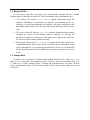
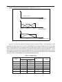
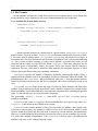
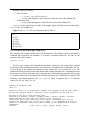
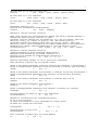
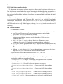
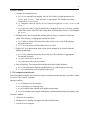
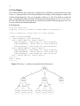
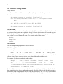
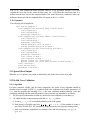
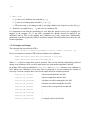
USER’S MANUAL1 for
Fuzzy Decision Trees
FID3.5
Cezary Z. Janikow
Department of Mathematics and Computer Science
University of Missouri – St. Louis
[email protected]
FID35 is one of the FID programs originally proposed in [1][2]. It is a recursive partitioning
method for pattern classification. There are three major components:
1. Domain partitioning for continuous domains. Other domains must be partitioned.
This was not a major emphasis of this work so it was added afterwards. Two
methods are available.
2. Tree build. The system uses the entropy gain measure to guide attribute selection
for building the tree, while applying approximate reasoning matching.
3. Inference. The system uses two groups of inferences: set based and exemplar
based, for assigning classifications to new events.
A number of other extensions have been implemented, such as those dealing with unknown
features, with excessive domain sizes, to force classification, k-fold cross-validation, and noise
and missing value induction.
Please report any bugs, ideas, inconsistencies, or other comments to [email protected], with
Subject=FID. If you have publications/applications related to FID, or wish to place a comment or
be placed on a mailing list, please visit the web site: http://www.cs.umsl.edu/~janikow/fid.
1
Current Version and Future Work
The next version (v4) will add option to create a multi-dimensional forest. The previous v4 has
been dumped for stability reasons.
FID3.5 changes FID3.4 by adding k-fold cross-validation, artificial noise and missing value
induction, and updating/testing the executables. See sections 2.12 and 2.13 for information on
these new features. There is also a Java GUI available, which requires the executable detailed in
this manual. The GUI has its own manual; however, we recommend reading this manual first.
2
User’s Manual
2.1 How to Obtain the Package
Currently, the package is available on-line at http://www.cs.umsl.edu/~janikow/fid. User
manuals are available at the same place.
You may also download Linux / Unix Solaris / Windows executables (command-line
versions) and selected sample data files.
1. Last modified 7/11/2015
2
2.2 Required Files
FID35 uses three input files, specified on the command-line. Example files are available.
Detailed syntax is described in section 2.4. These are attribute, data, and parameter files.
1. The attribute file (such as data.attrs) contains information about the
attributes, definitions of partitioning sets and the corresponding names, etc.
Attributes w/o predefined partitions are identified, with some restrictions on the
partitioning preprocessing. The files also contains the definition of the decision
class.
2. The event, or data file (such as data.dat) contains information about training
examples: the values of each attribute (numeric, linguistic, or missing), the
decision value (numeric or linguistic), and weight value (weight of the event). One
file may be used for training, another for testing.
3. The parameter file (such as par.template) contains default values for all of the
configurable options. These values may be overwritten by specifying their values
on the command line, or by modifying the default file. In fact, it is recommended
that the included parameter file be modified to customize the options to the user’s
needs.
2.3 Sample Data
A sample case is provided. It includes both attribute and data files, called data.attrs
and data.dat, respectively. The attributes used are X and Size. X has three nominal values: A, B,
C, while Size is a linear attribute with 0..1 domain and predefined fuzzy sets Small, Medium,
Large, as illustrated in Figure 1. The decision variable Classification is linear, with two fuzzy sets
Yes and No.
3
Figure 1: Illustration of the sample data - details in data.attrs.
Set of {A, B, C}
X, nominal type
Small
0 0.1
Medium
0.4 0.6
Yes
0.9 1
Size, linear type
No
0.5
0
Large
1
Classification, linear
The data.dat data file contains six sample events presented in Table 1: Note that three events
belong to Yes (those with values of 0 have membership 1 in Yes and membership 0 in No). The other
three events belong to the No category (but in general explicit values can be anywhere between 0
and 1 because this was a linear decision). Also note that some domain values are unknown (-1), and
those known are a mixture of values from the universe of discourse and the domain of fuzzy terms.
By inspection, except for the unknown values, the Yes events (the first three) can be described as
having A value for the attribute X (except for that unknown case).
Table 1: Sample data.
Training
event
1
2
3
4
5
6
Numerical domains
X
Size
A
-1
A
B
-1
B
0
0.4
0.8
0.5
0.5
Large
Classification
0
0
0
1
No
No
Weight
1
1
1
1
1
1
4
2.4 File Formats
In both attribute and data files, blank lines can be used to separate entries. Even though line
breaks should be used to separate records, newer implementations do not require that.
2.4.1 Attribute file format (data.attrs)
NumberOfAttributes
AttrName attrType numLingVals [lowerBd upperBd [minNumVals maxNumVals]]
LingValName [point1 point2 point3 point4]
...
...
classType NumClasses [lowerBd upperBd]
ClassName [point1 point2 point3 point4]
...
[] denotes optional elements (or required only in a given context). NumberOfAttributes is a
natural number, it must be at least 1. NumberClasses is also natural number, but it must be at least
2. All names must be without spaces. attrType and classType may take on one of two values, 0
for nominal and 1 for linear (nominal is used to denote all non-linear cases, such as partial ordering
etc., that is when no linear ordering of values can be defined; at present such values are not
clustered, and the values are used explicitly. When classType = 0 then some inferences are not
avail- able (those of interpolative nature). At present, linear type assumes that the domain is
continuous. Discrete values must be treated as either nominal (no conceptual distance) or linear
(distance between different values has a meaning) continuous.
numLingVals specifies the number of linguistic definitions following this header. Value -1
identifies that the attribute needs to be partitioned, and thus no definitions follow the header. The
definitions start with LingValName... and use normalized values in 0..1. Note that nominal attribute
cannot be partitioned at present (see the above paragraph), and such a combination results in an
error.
lowerBd and upperBd (floats) define the range of values for linear attributes and linear class
variable. If the event data are already normalized, 0 and 1 should be used as in the example below.
Explicit boundary values rather than those extracted from actual data allow extending the possible
range. For the nominal type, the values should not be present.
The relationship upperBd > lowerBd >= 0 must hold. upperBd and lowerBd are used to
normalize event data.
minNumVals and maxNumVals apply to discretization thus they are required only when numLingVals = -1, and otherwise they should not be present.
minNumVals is the minimal number of fuzzy sets to generate per attribute, and it applies only
to bottom-up discretization (no minimal is enforced in top-down discretization, which is more
selective rather than global and thus can result in some less relevant attributes not partitioned).
However, even the bottom-up discretization can return fewer fuzzy sets on an attribute (see section
2.5) under some unlikely circumstances. If no minNumVals is desired, enter 1 (an undiscretized
attribute is the same as one with one linguistic value).
5
maxNumVals is the maximal number of fuzzy sets to generate per attribute. It is enforced in both
discretizations. If max is not desired, enter some large number. Note that in the bottom-up
discretization, small max will force combining sets on attributes that end up with too many sets.
Top-down discretization works by splitting, so small max will force stopping splitting attributes
reaching that many sets.
If you want to have say five fuzzy sets per each attribute, give 5 5 for minNumVals and maxNumVals. Keep in mind, however, that min can be missed in bottom-up, and that it is not used in
top-down discretization.
point1,...,point4 can be present only for linear variables. Values must be expressed in
the normalized range 0..1.
0 <= point1 <= point2 <= point3 <= point4 <= 1
For example, the following is the contents of the sample data.attrs file, which defines the
attributes of Section 2.3.
Figure 2 The data.attrs. file (corresponds to Figure 1).
2
x03
A
B
C
Size 1 3 0 1
Small 0 0 0.1 0.6
Medium 0.1 0.4 0.6 0.9
Large 0.4 0.9 1 1
1201
Yes 0 0 0.5 1
No 0 0.5 1 1
2.4.2 Event file format (data.dat)
NumEvents numOfAttributes
Attr1Value Attr2Value ... decisionValue weightValue
...
All entries must come from the appropriate domains, as defined in the attribute file. Attribute-values are listed in the same order as the attributes are defined in that file. All attribute-values must be:
•
•
•
-1 for unknown values in either linear or nominal attributes
linear attributes only:
o [lowerBd..upperBd] for the given attribute - attribute may be prepartitioned or not
o a linguistic term from the domain of the given attribute - only if attribute
is pre- partitioned
nominal attributes only:
o values from among the listed linguistic values for the attribute
6
Decision values are required:
•
•
linear decision:
o [lowerBd..upperBd] for class, or
o a fuzzy term (linguistic value from those listed for class in the attribute file)
nominal decision:
o a term (from the linguistic values listed for class in the attribute file)
weightValueare values between 0 and 1, For example, Figure 3 lists the contents of the sample
data.dat file. All weights are 1.
Figure 3 The data.dat file (corresponds to data in Table 1).
62
A001
-1 0.4 0 1
A 0.8 0 1
B 0.5 1 1
-1 0.5 No 1
B Large No 1
2.4.3 Parameter file format (par.template)
The parameter file contains default values for all parameters. The defaults can be overwritten by
command line arguments. An alternative is to create a modified default file. An entry in the
parameter file has the format:
keyword value
The keyword is simply used to describe the parameter, and may be any string value (it should
be the name of the actual parameter but it does not have to, correspondence is positional). The keyword can begin in any column and whitespace must separate the keyword from the value. The
parameters must be specified in the order shown in the example parameter file. All parameters must
be included, even if they will not be used. Comments may be included in the parameter file by using
a # symbol to indicate the beginning of the comment (up to new line). Blank lines are ignored. The
following is the default parameter file, par.template, which is supplied with FID35. Boolean
values are 0 for “no” and 1 for “yes”.
#Format of Parameter File
#FID 3.4
#Anything after a # is considered a comment and ignored to end of line. Blank
#lines are ignored. Order is important and no parameters may be left out.
#T-norm to use for f1 when building tree
#choices are minimum, product, bounded product, drastic product, and best.
#these choices are also used for f2Build, f1Inf, and f2Inf.
#best means the t-norm resulting in the highest information gain will be
#chosen for each node that will be split. NOTE: it is suggested dprod not be
#used for inferences unless fuzzy sets overlap so that membership is always 1
#somewhere
f1Build
prod #[min | prod | bprod | dprod | best]
7
#T-norm used for f2 when building tree
f2Build
min
#[min | prod | bprod | dprod | best]
#T-norm used in f1 for inference
f1Inf
prod #[min | prod | bprod | dprod | best]
#T-norm used in f2 for inference
f2Inf
min
#[min | prod | bprod | dprod | best]
#Inference method to use
#choices are set-based and example-based
infKind
set
#[set | example]
#method to resolve internal conflicts
#The valid options for InternalConflict depend upon which inference method is
#chosen and which external conflict is used
#internal conflict methods for set based are: all (use all leaves), best(use
#majority class), cg (center of gravity), mcg (max center gravity)
#inference methods for example based are: all(use all leaves), best (use
#majority class), maxx(use example with highest membership in leaf),maxxk(use
#example with highest combined membership in leaf and decision class)
InternalConflict
best #[best | cg | mcg | all | maxx | maxxk]
#method to resolve external conflicts
#(meaning depends on which inference chosen above)
#maximum value allowed for set-based inference is 3,
#maximum value allowed for example-based inference is 2
ExternalConflict
0
#[0 | 1 | 2 | 3]
#options specifying weights to use in particular inferences
#the following 5 options are all boolean values
#used in set-based inferences involving internal best/external 0 and external 1
#used in example based inferences involving external 0/internal maxx and maxxg
usePkL
0
#[0 | 1]
#used in set-based inferences with external 0/internal cg and mcg and external 1
#used in example-based inferences with external 0/internal maxx and maxxg
usePL
0
#[0 | 1]
#used in set-based inferences with external 0/internal best and cg
useArea
0
#[0 | 1]
#used in set-based inferences with external 1
useRatio
0
#[0 | 1]
#used in example-based inferences with external 0/internal all and best
useWeight
0
#[0 | 1]
#stretch domain for delta to use in set inferences
stretchSetDelta
0
#[0 | 1]
#Degree of fuzzification fon unrecognized events
#0 is no fuzzification,
#1 means fuzzification is only performed for linear values
#2 means all values are fuzzified
fuzStopLevel
1
#fuzStartLevel to start with
fuzStartLevel
0
#[0 | 1 | 2]
#[0 | 1 | 2]
#Use IV method to reduce gain for large domains
iv
0
#[0 | 1]
8
#Information content at which expansion should be stopped
minBuildIN
0.2
#[0..1]
#Minimal event count at which expansion should be stopped
minBuildPN
1
#[>= 0]
#Minimal gain level at which attribute will not be used for expansion
minGain
0.1
#[0..1]
#Minimal event count
minInfPN
0.2
#[> 0]
#Minimal ratio of PkN/PN in a leaf to be used in inferences
#not using the majority decision in the leaf
#0 indicates all values are used, 1 indicates only those above average
minInfPkNQt
0
#[0..1]
#Minimal ratio of PkN/PN in a leaf to be used in inferences
#using the majority decision in the leaf
#0 indicates each best decision is used, 1 indicates only those best decision
#takin ALL examples in the leaf is used
minInfPKappaNQt
0
#[0..1]
#Chi-square test. Specify 0 if no test should be performed, otherwise indicate
#signifcance level of test
#Significance levels: 1=0.1, 2=0.05, 3=0.025, 4=0.01 (2 is suggested)
chi
0
#[0..4]
#Used to determine if Chi-squared test is unreliable. If PhatkNp is
#greater than or equal to Rchi, for any k,p, then it is unreliable
Rchi
4.0
#any value, but 4 is recommended
#Randomize the random seed
random
1
#[0 | 1]
#Print tree?
tree
short #[none | short | long]
#Output file for tree
#not printed if none chosen above
treeOut
tree.file
#Perform testing using events from a file?
# (0=interactive testing, otherwise specify name of file)
testIn
data.dat
#[0 | filename]
#Output file for testing. If interactive testing was chosen above, then output
#will go to stdout and this paramter will be ignored
testOut
test.file
#[filename]
#Spreadsheet filename--this option is provided in case the user wants output
#written to a file which can be used in spreadsheet software
#specify 0 if this option should not be used
spread
0
#[0 | filename]
#discretization type
discretType
0
#[0 top-down,1 bottom-up]
#parameters for bottom-up discretization
9
#clusterStop - used in bottom-up discretization to control
#level of clustering before forming fuzzy sets
clusterStop
0.2
#mergeStop - used in bottom-up discretization to control
#level of merging of fuzzy sets
mergeStop
0.05
#CF - pruning coefficient
#The higher value, the more tree is pruned
CF
0
#[0..1]
#K - coefficient used to build tree
#K coefficient decides how fuzzy terms cross each other
#K is used when fuzzy variable must be partitioned
K
0.5
#[0..1) K cannot be 1
# Stop noise and missing value inducer after being run on training data
stopAfterInducer
0
#[0 no; 1 yes]
# Simulate random noise in data
# 0: do not add noise
# 1: add noise only to training data
# 2: add noise only to testing data
# 3: add noise to both
addNoise
0
# specify whether to add noise to linear only, nominal only, or both types of
attributes
addNoiseToAttr
0
#[0 linear only; 1 nominal only; 2 both]
# specify the probability of adding noise to a given event
addNoiseProb
1.0
#[0..1]
# specify the percent noise to add
addNoiseAmount
0.1
#[0..1]
# Simulate randomly missing values in data
# 0: do not remove values
# 1: remove values only from training data
# 2: remove values only from testing data
# 3: remove values from both
missingValue
0
# specify the probability of an event value being removed
missingValueProb
0
#[0..1]
2.5 Discretizations
Two discretizations are available: local top-down, and global bottom-up. Generally, top-down
works by splitting domains, and only works with the most relevant attributes. Bottom-up works by
merging potential sets, and it works globally on all attributes.
2.5.1 Local top-down discretization
The top-down discretization performs data-driven discretization by splitting sets spanned over
linear non-prepartitioned attributes. Splitting is data driven, while constructing a decision tree.
Only splits necessary for a quality tree are performed. Thus, less relevant attributes remained nonpartitioned. maxNumVals cause a given attribute to be excluded from splitting when the number of
generated fuzzy sets reaches this value.
10
2.5.2 Global bottom-up discretization
The bottom-up discretization performs data-driven discretization by joining neighboring sets.
The initial sets are created in the first stage of clustering, in which neighboring data samples are
clustered according to some error criteria (not to exceed clusterStop). These global clusters are
then projected onto individual attributes (those linear non-prepartitioned), generating the initial
fuzzy sets.
In the second stage, sets are merged, according to some quality measure (and not to exceed
mergeStop error). Attributes with fewer sets than minNumVals are excluded from further
consideration. Attributes with more than maxNumVals, at the end, are forced into additional
merging. Note that clustering can produce fewer sets than minNumVals, in which case the attribute
will not be subjected to merge. If this happens, reducing clusterStop should reduce the level of
clustering.
2.6 How to Execute
1. Command-line invocation:
FID35 attrFile eventFile paramFile k - v a l u e [ l a b e l ] [options| -p]
a. attrFile, eventFile, and paramFile are required and must be supplied in the
given order. No specific extensions are assumed.
b. k-value is required for all executions. Set to “1” to run in normal mode
without cross validation, otherwise specify the number of folds for crossvalidation (up to 99).
c. label: if k-value > 1, specify a label to identify text file outputs in crossvalidation. (See section 2.12 for details on running with cross validation.)
d. options are optional arguments which may be supplied on the command line in any
order. The values specified in options override the values specified in the parameter
file.
e. additional -p option directs FID3.5 to run the partitioning preprocessor only. A new
output attrFile.gen is generated in the format of the attribute file.
2. options are case-sensitive. Boolean values are 0 for “no”, 1 for “yes”.
-random 0|1 : randomize the random seed
-iv 0|1 : use IV method to reduce gain for large domains. This applies to both
tree building and the top-down discretization
-fuzStopLevel 0|1|2 : degree for fuzzifying unrecognizable event--explained
in paramter file
-fuzStartLevel 0|1|2: fuzzify level to start inference procedure at
-f1build min|prod|bprod|dprod|best : T-norm used for f1 when building
tree
-f2build min|prod|bprod|dprod|best : T-norm used for f2 when building
tree
-f1inf min|prod|bprod|dprod|best : T-norm used for f1 during inference
-f2inf min|prod|bprod|dprod|best : T-norm used for f2 during inference
-infkind set|example : inference method to use (set-based or example-based)
11
-internal best|cg|mcg|all|maxx|maxxk : method used to resolve internal
conflicts
-external 0|1|2|3 : method used to resolve external conflicts
-usePkL 0|1 : use PkL weight in slected inference
-usePL 0|1: use PL weight in selected inference
-useArea 0|1 : use area as weight in selected inference
-useRatio 0|1 : use ratio of PkL and PL as weight in selected inference
-stretch 0|1 : stretch domain for delta to use in set inferences
-tree short|long|none : specifies whether to create tree and what format to
make
-treeout 0|filename : name of file to print tree to--ignored when value of
tree is none. Specify 0 for tree to be printed to stdout
-testin 0|filename : specify filename for testing events or 0 for interactive
testing
-testout filename : file to write testing results to; ignored if interactive testing
-spread 0| filename : spreadsheet file to store testing results in
-minBuildIN 0..1 : information content to stop expansion at
-minBuildPN >=0 : minimal event count to stop expansion at
-minGain 0..1 : minimal gain to stop expansion of node at
-minInfPN >0 : min total event count in a leaf to be considered in the inferences
-minInfPkNQt 0 .. 1 : minimal ratio of PkN/PN to be used in-leaf if not using the
majority decision
-minInfPKappaNQt 0 .. 1 : minimal ratio of PkN/PN to be used in-leaf if using the
majority decision only
-chi 0..4 : significance level of chi-squared test (0=no test). 1=10%, 2=5%,
3=2.5%, 4=1%
-Rchi 0..numEvents : used to determine if chi-square test is reliable. A value of
4 is recommended. The smaller it is, the more lenient the test.
-discretType 0|1 : 0 for local top-down, 1 for global bottom-up
-clusterStop 0..1 : max error for clustering in the bottom-up discretization.
Lower values would reduce the level of clustering and shift discretization toward
merging
-mergeStop 0..1 : max error allowed in merging, the after-clustering process of
the bottom-up discretization.
-CF 0..1 :coefficient used in pruning procedure. 0 means no pruning.
-K 0..1 :coefficient used when data must be partitioned. K can’t be set to 1
-pruningoff - turns off pruning
-stopAfterInducer: will stop FID after noise and/or missing values are
introduced to the training file. See section 2.13 for more detail on this function.
12
-addNoise setting attrsAffected noiseProb noiseAmount
Artificially add random noise to data. Here are the required option arguments:
setting: controls how event values are modified to simulate noisy data
1: run only on training data; 2: run only on testing data; 3 run on
both training and testing data.
attrsAffected: whether linear and/or nominal attributes are changed.
0: linear only; 1 nominal only; 2 both
noiseProb [0..1]: the probability of adding noise to each event
noiseAmount [0..1]: the percent noise to add (this is percentage of
domain size for one standard deviation)
-missingValue setting missingValueProb
Artificially remove values from event file(s). Here are the required option
arguments:
setting: controls how event values are modified
1: run only on training data; 2: run only on testing data; 3 run on
both training and testing data.
missingValueProb [0..1]: the probability of removing a particular
event value
2.7 Explanation of Inferences
In a fuzzy tree, information is much more fuzzified (distributed) over the tree than in a
traditional decision tree. Moreover, fuzzy matching causes a sample to be matched against
potentially many leaves. Inferences are designed to infer the classification from such information.
FID35 uses two different methods of inference: set-based and exemplar-based. Each has
several ways of resolving internal (in a leaf) and external (across leaves) conflicts. Generally, setbased inferences treat leaves as fuzzy sets, while those exemplar-based treat leaves as supertraining exemplars.
Some inferences are not available if the decision is nominal (those which rely on interpolation
common in fuzzy reasoning).
2.7.1 Set-based inference
This inference uses the areas and/or centroids of the fuzzy sets to compute the decision value for a
testing example. The following are descriptions of the external conflicts for set-based inference,
with the allowed internal conflicts for each listed underneath. NOTE: there is an option named
stretch which will shift the delta values so that the range is [0,1]. This is useful in cases where
the responses are mapped to a particular function and the range of the function wishes to be preserved. However, the manner in which the deltas are stretched may change the membership of the
example in the fuzzy sets.
13
External Conflicts:
1. Average over multiple leaves.
a. best: Uses centroid from majority class in leaf. Allowed weight parameters are
usePkL and useArea. This inference is appropriate for nominal decisions,
except when useArea is set.
b. cg: Computes center of gravity of leaf. Allowed weights are usePkL, useArea, and
usePL.
c. mcg: Uses max-center of gravity method by scaling the fuzzy sets of decision variables
by the PkL values in the leaf and cutting them off where they intersect. Valid weights
are usePL.
2. Multiple leaves, not averaged (the resulting delta is always a centroid of a decision
class). This inference is appropriate nominal decisions.
a. best: When selecting a decision class, only use the event count of the majority
decision in the leaf.
b. all: Use event counts of all decision classes in a leaf.
3. Single leaf - uses information from leaf in which example to be classified has the
highest membership.
a. best: Uses centroid of majority class in the leaf. This inference is appropriate
for nominal decisions.
b. cg: Uses center of gravity of leaf.
c. mcg: Uses max-center gravity method.
4. Max sum gravity. The stretch option should not be used in this inference.
a. best: uses information from the modified fuzzy set of the majority class only
b. all: uses information from all modified fuzzy sets
2.7.2 Exemplar-based inference
Selected training examples are retained/created as exemplars and the inference procedure returns
the class of the “closest” exemplar.
Internal conflicts
a. all: Exemplar over all examples.
b. best: Exemplar over majority class.
c. maxx: Exemplar from example with highest membership.
d. maxxk: Exemplar from example with highest combined membership and majority class.
External Conflicts:
1. All leaves are exemplars.
2. Multiple leaves, looking for support for individual decisions.
3. Use one leaf as exemplar.
14
2.8 Tree Display
This section illustrates the way the tree is displayed in two different versions, based on the value
of the tree input parameter. The following illustrates the display while running the sample files
with the default parameters. Tree can be printed to stdout or to a file. The format is exactly the
same, except that a file output will start with a dump of the run parameters. If f1Build or f2Build
have the value BEST, the t-norm which was selected for each node will be displayed as well. Tree
level are printed with standard indentation.
2.8.1 Short tree
Printing short tree
Stopping criteria: minIN=0.2 minBuildPN=1.0 minGain=0.0
Using IV method to reduce gain for large domains
---TREE : T-norm is Minimum
[] : IN=0.95 PN=8.00 : Yes=5.00 No=3.00
[x=A] : IN=0.50 PN=3.00 : Yes=2.67 No=0.33
[x=A][Size=Small] : IN=0.52 PN=1.73 : Yes=1.53 No=0.20
[x=A][Size=Medium] : IN=0.81 PN=1.33 : Yes=1.00 No=0.33
[x=A][Size=Large] : IN=0.65 PN=1.20 : Yes=1.00 No=0.20
[x=B] : IN=0.98 PN=4.00 : Yes=1.67 No=2.33
[x=B][Size=Small] : IN=0.99 PN=1.33 : Yes=0.73 No=0.60
[x=B][Size=Medium] : IN=0.97 PN=3.25 : Yes=1.29 No=1.96
[x=B][Size=Large] : IN=1.00 PN=2.60 : Yes=1.20 No=1.40
[x=C] : IN=0.92 PN=1.00 : Yes=0.67 No=0.33
---------TOTAL 7 leaves
---------Figure 4 The above tty display corresponds to the following tree:
Attr=x
Yes=5.00
No=3.00
A
Attr=Size
Yes=2.67
No=0.33
Small
Yes=1.53
No=0.2
Attr=Size
Yes=1.67
No=2.33
Large
Small
Medium
Yes=1.00
No=0.33
C
B
Yes=1.00
No=0.2
Yes=0.73
No=0.6
Attr=Size
Yes=0.67
No=0.33
Large
Medium
Yes=1.29
No=1.96
Yes=1.2
No=1.4
15
2.8.2 Long tree
Printing long tree
Stopping criteria: minIN=0.2 minBuildPN=1.0 minGain=0.0
Using IV method to reduce gain for large domains
---TREE : T-norm is Minimum
[] : IN=0.95 PN=8.00 : Yes=5.00 No=3.00
Wghts:
0
1
2
3
4
5
6
7
8
9
0: 1.000 1.000 1.000 1.000 1.000 1.000
[x=A] : IN=0.50 PN=3.00 : Yes=2.67 No=0.33
Wghts:
0
1
2
3
4
5
6
7
8
9
0: 1.000 0.333 1.000 0.000 0.333 0.000
[x=A][Size=Small] : IN=0.52 PN=1.73 : Yes=1.53 No=0.20
RS=0.065 rs=1.000 bestDec=0
Wghts:
0
1
2
3
4
5
6
7
0: 1.000 0.333 0.000 0.000 0.200 0.000
[x=A][Size=Medium] : IN=0.81 PN=1.33 : Yes=1.00 No=0.33
RS=0.167 rs=1.000 bestDec=0
Wghts:
0
1
2
3
4
5
6
7
0: 0.000 0.333 0.333 0.000 0.333 0.000
[x=A][Size=Large] : IN=0.65 PN=1.20 : Yes=1.00 No=0.20
RS=0.100 rs=1.000 bestDec=0
Wghts:
0
1
2
3
4
5
6
7
0: 0.000 0.000 0.800 0.000 0.200 0.000
[x=B] : IN=0.98 PN=4.00 : Yes=1.67 No=2.33
8
9
8
9
8
9
Wghts:
0
1
2
3
4
5
6
7
8
9
0: 0.000 0.333 0.000 1.000 0.333 1.000
[x=B][Size=Small] : IN=0.99 PN=1.33 : Yes=0.73 No=0.60
RS=0.429 rs=1.000 bestDec=0
Wghts:
0
1
2
3
4
5
6
7
8
9
0: 0.000 0.333 0.000 0.200 0.200 0.200
[x=B][Size=Medium] : IN=0.97 PN=3.25 : Yes=1.29 No=1.96
RS=0.645 rs=1.000 bestDec=1
Wghts:
0
1
2
3
4
5
6
7
8
9
0: 0.000 0.333 0.000 1.000 0.333 0.625
[x=B][Size=Large] : IN=1.00 PN=2.60 : Yes=1.20 No=1.40
RS=0.571 rs=1.000 bestDec=1
Wghts:
0
1
2
3
4
5
6
7
8
9
0: 0.000 0.000 0.000 0.200 0.200 1.000
[x=C] : IN=0.92 PN=1.00 : Yes=0.67 No=0.33
RS=0.250 rs=1.000 bestDec=0
Wghts:
0
1
2
3
4
5
6
7
8
9
0: 0.000 0.333 0.000 0.000 0.333 0.000
---------TOTAL 7 leaves
----------
16
2.9 Interactive Testing/Output
Output format:
exName: attrValue attrValue ... => fuzzy Term | fuzzyTerm1:value fuzzyTerm2:value ...
Example:
do you have an event to recognize? [0:no 1:yes]: 1
Give the event (2 attribute values in (-1..1) or linguistic values)
: B 0.3
x1 : B 0.300 => No:0.5873 | Yes:0.8254 No:1.0000
do you have an event to recognize? [0:no 1:yes]: 0
2.10 File Testing
FID35 accepts the same files as those for training data. However, the last two fields of each record
are optional (classification and weight). A value of -1 for the classification will cause the last two
fields to be ignored. Output can go to stdout or a file, based on the testOut input parameter. However, in both cases the format is the same. The output is made of three parts:
RunInfo
ExampleInfo
Summary
2.10.1 RunInfo
This part dumps the input parameter used for the run.
2.10.2 ExampleInfo
Example attr attr ... || Class1 Class2 ...Delta:Best Actual Class [Error]
name
val
val ... || term
term . . .
value:term val
term[*][error]
where italic denotes variable values, term refers to a fuzzy term, value refers to a number, and val
refers to either a fuzzy term or a numeric value (depending on the attribute type).
For example, for the previous data it might look as:
Example X
Size ||
Yes No
x1
0
1.00 0.10 0.050:Yes
A
||
Delta:Best
Actual
Class
1.000
No
Error
*
0.950
* Denotes examples which were classified incorrectly. Error follows if
actual decision is a numerical value.
The first field contains a generated name for the test example. The next fields preceding the divider
bars contain the values of each attribute the example. The fields following the dividers contain the
membership of the computed delta in each of the decision classes. The Delta:Best field contains
the computed delta and the decision class in which the delta has the highest membership.
17
The Actual field contains the actual decision value (if it was provided), and the Class field
contains the best class for the actual decision value. An * will follow the actual best class if it
differs from the best class for the computed delta. If the actual decision is a numerical value, the
difference between it and the computed delta will appear in the Error field.
2.10.3 Summary
The following will be displayed:
Total testing examples =
Total examples with available fuzzy classification =
total classified =
total unclassified =
percentage classified =
Total examples with available numeric classification =
total classified =
total unclassified =
percentage classified =
average quadratic error on delta =
average standard deviation on delta =
Total examples with any classification available =
total classified =
total unclassified =
percentage classified =
total correct on best =
total incorrect on best =
percent correct (vs. classified) =
percent correct (vs. those with available classification) =
total classified =
total unclassified =
percentage classified =
2.11 Spread Sheet Output
When the spread option is set, output is delimited by tabs in the form of an m by n table.
2.12 K-fold Cross Validation
2.12.1 Algorithm
For better statistical validity, and for better comparison, the results of any algorithm should be
reproduced and averaged. In FID 3.5, we added 𝑘 -fold cross validation with a single parameter k. If
𝑘 = 1, then the program runs normally. If 𝑘 > 1, the cross validation module partitions event data
accordingly and then runs the main FID module 𝑘 -times. In detail, our algorithm is as follows:
1.
The user specifies the number of folds (𝑘 ) desired for cross validation of event data (𝐸 ).
2.
𝐸
is subdivided into 𝑘 subsets/groups such that 𝐸 = {𝐺! , … , 𝐺! } where:
a. Events {𝑒! , … , 𝑒! ∈ 𝐸} are randomly added to each of the groups.
b. Each group is of roughly equal size: 𝐺! ~ 𝐺!!! for 𝑖 = 1. . 𝑘 − 1. If the number of events is
not evenly divisible by 𝑘 , the remainder is dispersed one-by-one to groups starting with 𝐺! .
c. Each event from the original data is a member of one and only one group: {𝑒 ∈ 𝐺! | 𝑒 ∉
𝐺! ∀𝑗 ≠ 𝑖}.
18
3.
For 𝑖 = 1. . 𝑘 :
a. 𝑉! is the set of validation data such that 𝑉! = 𝐺!
b. 𝑇! is the set of training data such that: 𝑇! = {𝐸 – 𝑉! }
c. FID is run using 𝑇! as training set and 𝑉! as testing/validation set. Output is saved to file (𝑂! ).
4.
Results are averaged from 𝑂! , … , 𝑂! and saved to a summary file.
It is important to note that the partitioning of event data into groups occurs before anything else
happens in the program. If 𝑘 > 1, any other command line options entered are applied to the
individual runs of FID on the training and validation sets 𝑇! and 𝑉! respectively. Additionally,
partitioned event files prepared by FID are saved into multiple files and can then be used by the user
in other algorithms.
2.12.2 Examples and Output
The command line invocation for FID is:
FID35 attrFile eventFile paramFile k-value [label] [options| -p]
Here is an example invocation of FID with and without cross-validation:
FID35 data.attrs data.dat par.template 2 fid_test
FID35 data.attrs data.dat par.template 1
When k>1, a label for output files must be provided. This is so the data files individually produced
during cross validation can be saved for inspection or use with another algorithm if desired.
By default, FID results are published to tree.file and test.file when no cross validation is
used. When cross validation is used, many files are produced so you can examine the contents of
each step. Given the example above, here are the output files that would be produced:
fid_test_k1_outTest
// the test results from the first fold
fid_test_k1_outTree
// the tree output from the first fold
fid_test_k1_training
// the data set used for training the first fold
fid_test_k1_testing
// the data set used for testing the first fold
fid_test_k2_outTest
// same as above except for the second fold
fid_test_k2_outTree
…
fid_test_k2_training
…
fid_test_k2_testing
…
fid_test_results.avg
// averaged values from all folds
19
2.13 Noise & Missing Value Induction
2.12.1 Algorithm
Noise or missing values can occur either in the training data, or in the application (testing) data.
Generally, the training data can be cleaned up and processed more extensively, but the quality of
application data is often less known. We thus added a module that can take any data and induce
these conditions in a controllable way. Again, this module can be used solely to generate such data
for any classification algorithm as the resulting data files are saved.
To add noise, the user must specify a few parameters: the noise amount, the probability for noise
to occur on any given event, and a few options for how the noise can be applied. Noise can be
added through command line options (section 2.6) or through the parameters file (section 2.4.3).
Anytime noise is added to testing data, it is actually done after the tree has been built, so only
attributes used by the tree are affected. FID can add noise to linear attributes only, nominal only,
or to both. If nominal features are included in the data, the noise probability is the independent
probability of change for each nominal feature in an attribute. If a given value is selected for
change, it will randomly switch to another possible value for that attribute. All possible values
have the same probability, with the exception of the original value which is removed from the pool
of options.
When adding noise to a linguistic value of a linear attribute, FID retrieves the centroid of that
linguistic value (as defined by the attributes file), applies the noise algorithm, and replaces the
original linguistic term with the new continuous value.
Every linear attribute has a lower and upper domain boundary denoted by 𝛼 and 𝛽 such that for a
given attribute, all its event values fall within its domain. For every value 𝑣! in any given attribute,
if 𝑣! is selected for noise based on the independent probability of noise parameter given by the
user, the new value for 𝑣! is: 𝑣! ← 𝑣! + Ν(0, 𝜎) where 𝜎 = 𝑁𝑜𝑖𝑠𝑒 ∗ (𝛽 – 𝛼). In other words, 𝑣!
will be modified by a random variable drawn from a normal distribution in which one standard
deviation is equal to the noise amount times the domain size. If the new value exceeds one of the
domain boundaries, it is truncated to the boundary itself.
FID 3.5 also has the ability to remove features (i.e. add missing values to data). The user simply
provides the probability of removing any given event value. If an event value is selected by the
algorithm to be removed, its value is changed to −1 representing missing features. Again, so
manipulated data can be generated to be used in another algorithm.
2.12.2 Order of Processing
It is important to clarify where the noise and missing value manipulations occur with reference to
discretization and cross validation.
20
If cross validation is used, the original data is separated multiple times into random training/testing
sets, and each set is used independently. For each cross validation run (if no cross validation, the
below are done just once):
1.
Noise is applied to the training data if applicable
2.
Some features are removed from the training data if applicable
3.
Any continuous attribute without a discrete domain is then discretized
4.
FID builds the tree using the training data
5.
Noise is applied to the testing data (only to attributes used by the tree) as applicable
6.
Some features are removed from the testing data (only on attributes used by the tree) as
applicable
7.
FID tests the tree using the testing data.
When using cross validation, noise, and/or missing values, FID saves all the modified files for the
user to inspect and compare to the originals as desired. In particular, for noise and missing values,
the modified event file has a “.gen” extension. It is also possible to stop processing after step 2 or 3
above. This is useful for anyone wishing to use the files in other algorithms. In this case, a user
simply selects an event file (training or testing data) and runs the files through FID for noise,
missing values, and/or discretization.
3 Some Literature
Some earlier experiments with a previous version are reported in
[1] Cezary Z. Janikow, “Fuzzy Processing in Decision Trees”, in Proceedings of the International Symposium on Artificial Intelligence, 1993, pp. 360-367.
Early description of the methodology can be found in
[2] C.Z. Janikow, “Fuzzy Decision Trees: Issues and Methods”, IEEE Transactions of Man, Systems, Cybernetics. Vol 28, Issue 1, 1998.
For more extensive literature by the author, please see http://www.cs.umsl.edu/people/janikow.
The basis for the decision tree, as well as the IV method, follows
[3] J.R. Quinlan, “Induction on Decision Trees”, Machine Learning, Vol. 1, 1986, pp. 81-106.
Processing unknown attribute values in decision tree follows the ideas outlined in
[4] J.R. Quinlan, “Unknown Attribute Values in Induction”, in Proceedings of the Sixth International Workshop on Machine Learning, 1989.
Top-down discretization is described in
[5] C.Z. Janikow and Maciej Fajfer. “Fuzzy Partitioning with FID3.2”. Proceedings of the 18th
International Conference of the North American Fuzzy Information Society, IEEE 1999, pp.
467-471.
21
Bottom-up discretization follows the ideas of J.W. Grzymala-Busse
[6] M.R. Chmielewski and J.W. Grzymala-Busse. “Global Discretization of Continuous
Attributes as Preprocessing for Machine Learning”. In T.Y. Lin and A.M. Wilderberger
(eds.), Soft Computing: Rough Sets, Fuzzy Logic, Neural networks, Uncertainty Management,
Knowledge Discovery, 1995, pp. 294-297.
extended for fuzzy sets and it is described in
[7] Maciej Faifer and C.Z. Janikow. “Bottom-up Partitioning in Fuzzy Decision Trees”. Proceedings of the 19th International Conference of the North American Fuzzy Information Society, IEEE 2000, pp. 326-330.