1
NAVAL POSTGRADUATE SCHOOL
Monterey, California
DISSERTATION
A Software Architecture for the Construction and
Management of Real-Time Virtual Worlds
by
David R. Pratt
June 1993
Dissertation Supervisor:
Dr. Michael J. Zyda
Approved for public release; distribution is unlimited.
UNCLASSIFIED
SECURITY CLASSIFICATION OF THIS PAGE
REPORT DOCUMENTATION PAGE
1b. RESTRICTIVE MARKINGS
UNCLASSIFIED
1a. REPORT SECURITY CLASSIFICATION
2a SECURITY CLASSIFICATION AUTHORITY
3. DISTRIBUTION/AVAILABILITY OF REPORT
Approved for public release;
distribution is unlimited
2b. DECLASSIFICATION/DOWNGRADING SCHEDULE
4. PERFORMING ORGANIZATION REPORT NUMBER(S)
5. MONITORING ORGANIZATION REPORT NUMBER(S)
6a. NAME OF PERFORMING ORGANIZATION
7a. NAME OF MONITORING ORGANIZATION
Computer Science Dept.
Naval Postgraduate School
6b. OFFICE SYMBOL
(if applicable)
Naval Postgraduate School
CS/Pr
6c. ADDRESS (City, State, and ZIP Code)
Monterey, CA
7b. ADDRESS (City, State, and ZIP Code)
Monterey, CA 93943-5000
93943-5000
8a. NAME OF FUNDING/SPONSORING
ORGANIZATION
8b. OFFICE SYMBOL
(if applicable)
9. PROCUREMENT INSTRUMENT IDENTIFICATION NUMBER
10. SOURCE OF FUNDING NUMBERS
PROGRAM
PROJECT
TASK
ELEMENT NO.
NO.
NO.
8c. ADDRESS (City, State, and ZIP Code)
WORK UNIT
ACCESSION NO.
11. TITLE (Include Security Classification)
A Software Architecture for the Construction and Management of Real-Time Virtual Worlds (U)
12. PERSONAL AUTHOR(S)
Pratt, David Russell
13a. TYPE OF REPORT
Doctoral Dissertation
13b. TIME COVERED
FROM 01/90
TO
14. DATE OF REPORT (Year, Month, Day)
15. PAGE COUNT
158
06/93
June 1993
16. SUPPLEMENTARY NOTATION
The views expressed in this thesis are those of the author and do not reflect the official
policy or position of the Department of Defense or the United States Government.
17.
FIELD
18. SUBJECT TERMS (Continue on reverse if necessary and identify by block number)
COSATI CODES
GROUP
SUB-GROUP
Computer Graphics, Simulator, Simulation, Networks, Virtual worlds,
Artificial Reality, Synthetic Environments, NPSNET
19. ABSTRACT (Continue on reverse if necessary and identify by block number)
As military budgets shrink, the Department of Defense (DoD) is turning to virtual worlds (VW) to solve problems
and address issues that were previously solved by prototype or field exercises. However, there is a critical void of
experience in the community on how to build VW systems. The Naval Postgraduate School’s Network Vehicle Simulator (NPSNET) was designed and built to address this need. NPSNET is a populated, networked, interactive, flexible, three dimensional (3D) virtual world system. This dissertation covers the construction and management of the
VW in NPSNET. The system, which uses both standard and non-standard network message formats, is fully networked allowing multiple users to interact simultaneously in the VW. Commercial off the shelf (COTS), Silicon
Graphics Incorporated (SGI) workstations, hardware was used exclusively in NPSNET to ensure the usefulness and
the portability of the system to many DoD commands. The core software architecture presented here is suitable for
any VW.
20. DISTRIBUTION/AVAILABILITY OF ABSTRACT
SAME AS RPT.
x UNCLASSIFIED/UNLIMITED
22a. NAME OF RESPONSIBLE INDIVIDUAL
Dr. Michael J. Zyda
DD FORM 1473, 84 MAR
21. ABSTRACT SECURITY CLASSIFICATION
UNCLASSIFIED
DTIC USERS
22b. TELEPHONE (Include Area Code)
(408) 656-2305
83 APR edition may be used until exhausted
All other editions are obsolete
i
22c. OFFICE SYMBOL
CS/Zk
SECURITY CLASSIFICATION OF THIS PAGE
UNCLASSIFIED
Approved for public release; distribution is unlimited
A Software Architecture for the Construction and
Management of Real-Time Virtual Worlds
by
David R. Pratt
B.S.E.E., Duke University, 1983
M.S. C.S., Naval Postgraduate School, 1988
Submitted in partial fulfillment of the
requirements for the degree of
DOCTOR OF PHILOSOPHY IN COMPUTER SCIENCE
from the
NAVAL POSTGRADUATE SCHOOL
June 1993
Author:
______________________________________________
David R. Pratt
Approved By:
___________________________
Man-Tak Shing
Associate Professor Of Computer Science
___________________________
Herschel H. Loomis, Jr.
Professor of Electrical and Computer
Engineering
___________________________
Yuh-jeng Lee
Assistant Professor of Computer Science
___________________________
Richard Franke
Professor of Mathematics
___________________________
Michael J. Zyda
Associate Professor Of Computer Science
Dissertation Supervisor
Approved By: ______________________________________________________
Gary J. Hughes, Acting Chairman, Department of Computer Science
Approved By:
_______________________________________________
Richard S. Elster, Dean of Instruction
ii
ABSTRACT
As military budgets shrink, the Department of Defense (DoD) is turning to virtual worlds (VW) to solve
problems and address issues that were previously solved by prototype or field exercises. However, there is a
critical void of experience in the community on how to build VW systems. The Naval Postgraduate School’s
Network Vehicle Simulator (NPSNET) was designed and built to address this need. NPSNET is a populated,
networked, interactive, flexible, three dimensional (3D) virtual world system. This dissertation covers the
construction and management of the VW in NPSNET. The system, which uses both standard and nonstandard network message formats, is fully networked allowing multiple users to interact simultaneously in
the VW. Commercial off the shelf (COTS), Silicon Graphics Incorporated (SGI) workstations, hardware was
used exclusively in NPSNET to ensure the usefulness and the portability of the system to many DoD
commands. The core software architecture presented here is suitable for any VW.
iii
ACKNOWLEDGMENTS
There are many people who deserve a tremendous amount of thanks and credit for their help along the
way. If I was to thank each and every one of them this section would be longer than the body of the dissertation. So, if I left you out please forgive me. A few people deserve a special mention. First and foremost Dr.
Mike Zyda, my committee chairman, dissertation supervisor, mentor, co-PI, confidant, and friend. If it wasn’t
for him and Dr. Robert McGhee taking a chance on me I never would have had the opportunity to come back
to the school. The members of my Doctoral Committee, Dr. Man-Tak Shing, Dr. Yuh-Jeng Lee, Dr. Hershel
Loomis, and Dr. Richard Franke for letting me do this in my own manner.
Our sponsors, Maj. Dave Neyland, Mr. George Lukes, Mr. Stanley Goodman, LtCol. Michael Proctor,
and many others who saw the value in what we were doing and allowed us to continue on with our work with
world class facilities. The PES-Team at Space Applications Corporation, Karren Darone, Bob Bolluyt,
Sophia Constantine, Chanta Quillen, and Vikki Fernandez, all have my deepest thanks for letting me sit in
their offices for three months to start writing this puppy.
All the students who submitted themselves to do a masters with me and as a result found out the late
nights computer geeks pull deserve more credit and thanks than I could ever give them. Hopefully, they
learned something along the way.
There is a group of people who have helped me and put up with me and done almost anything I asked
them to with promptness and professionalism, the Departmental Technical Staff. Walter Landaker kept the
hardware running whenever it was humanly possible. How Rosalie Johnson put up with my constant requests
for system support is beyond me. Terry Williams and Hank Hankins bought just about anything I wanted.
Last but not least, Hollis Berry. The Sergeant Major was always ready and willing to put me on a airplane
with a moment’s notice. Not only could I have not finished this without the help of these and the rest of the
wonderful people on the Technical Staff, but nobody could do any work at all.
And finally, on a personal note, two people have my everlasting thanks. Sue West who was there for
the first part whenever I needed to talk and had nothing but faith in my abilities to complete this program.
Shirley Isakari who has my love and respect for showing me there is more to life than work, even for us “Type
A” people. Even if Mike sent her.
xiv
TABLE OF CONTENTS
I. INTRODUCTION ........................................................................................................................................ 1
A. INTRODUCTION ............................................................................................................................... 1
B. DEFINITION OF VIRTUAL WORLDS ............................................................................................ 2
C. OVERVIEW OF PROBLEM .............................................................................................................. 3
D. GOALS AND MOTIVATION............................................................................................................ 3
1. Goals Of Research......................................................................................................................... 3
2. Motivation ..................................................................................................................................... 4
E. PROBLEM DOMAIN BACKGROUND ............................................................................................ 5
F. ORGANIZATION OF CHAPTERS .................................................................................................... 7
II. VIRTUAL WORLDS: MAJOR CHALLENGES AND ISSUES .............................................................. 8
A. OVERVIEW ........................................................................................................................................ 8
B. COST REDUCTION ........................................................................................................................... 8
C. WORLD CONSTRUCTION AND MAINTENANCE ....................................................................... 9
D. WORLD POPULATION..................................................................................................................... 9
E. REALISTIC ICON INTERACTION................................................................................................. 10
F. MACHINE LIMITATIONS............................................................................................................... 10
1. Processor...................................................................................................................................... 11
2. Graphics....................................................................................................................................... 11
3. Network ....................................................................................................................................... 12
G. HUMAN COMPUTER INTERACTION.......................................................................................... 13
H. CONCLUSIONS ............................................................................................................................... 14
III. OVERVIEW OF SIGNIFICANT EXISTING VIRTUAL WORLD SYSTEMS ................................... 15
A. OVERVIEW ...................................................................................................................................... 15
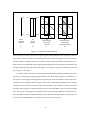
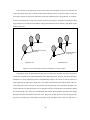
B. VIDEOPLACE................................................................................................................................... 15
C. REALITY BUILT FOR TWO........................................................................................................... 16
D. THE VIRTUAL WIND-TUNNEL.................................................................................................... 16
E. BOLIO................................................................................................................................................ 17
F. UNC WALK-THROUGH / MOLECULAR MODELING ............................................................... 17
G. SIMNET............................................................................................................................................. 19
H. SUMMARY....................................................................................................................................... 22
IV. NPSNET OVERVIEW............................................................................................................................ 23
V. VIRTUAL WORLD DATABASE CONSTRUCTION ........................................................................... 26
A. COORDINATE SYSTEMS .............................................................................................................. 27
B. WORLD SEGMENTATION............................................................................................................. 28
C. TERRAIN SKIN GENERATION ..................................................................................................... 33
D. ROAD / RIVER OVERLAY............................................................................................................. 36
E. ICON DATABASE............................................................................................................................ 40
F. ICON PLACEMENT ON THE TERRAIN ....................................................................................... 42
G. TERRAIN DATABASE MODIFICATION ..................................................................................... 45
H. TERRAIN DATABASE MAINTENANCE ..................................................................................... 48
I. SUMMARY ........................................................................................................................................ 52
VI. STRUCTURE OF THE SOFTWARE .................................................................................................... 54
A. INHERENT PARALLELISM........................................................................................................... 56
B. TASKS ............................................................................................................................................... 58
1. Start Up Process .......................................................................................................................... 58
iv
2. User Input Management .............................................................................................................. 65
3. Entity Dynamics .......................................................................................................................... 66
4. Scene Management...................................................................................................................... 67
5. Rendering .................................................................................................................................... 68
6. Network Management ................................................................................................................. 71
C. DATA FLOW AND SEQUENCING ................................................................................................ 72
1. Interproccess Data Flow .............................................................................................................. 72
2. Process Sequencing and Synchronization ................................................................................... 74
D. SUMMARY....................................................................................................................................... 76
VII. ENTITY DYNAMICS ........................................................................................................................... 79
A. ENTITY CONTROL ......................................................................................................................... 79
B. ENTITY MOTION ............................................................................................................................ 80
1. Sea Entities .................................................................................................................................. 80
2. Land Entities................................................................................................................................ 80
a. Non-Dynamics Based Entities ..............................................................................................80
b. Dynamics Based Entities ......................................................................................................83
3. Air Entities................................................................................................................................... 84
C. COLLISION DETECTION AND RESPONSE ................................................................................ 86
1. Moving / Static Collision............................................................................................................. 87
2. Moving / Moving Collision ......................................................................................................... 91
D. SUMMARY....................................................................................................................................... 95
VIII. VIRTUAL WORLD POPULATION ................................................................................................... 97
A. REACTIVE BEHAVOIR SYSTEMS ............................................................................................... 97
1. Zig-Zag Paths .............................................................................................................................. 98
2. Environment Limitation .............................................................................................................. 98
3. Edge of the World Response ....................................................................................................... 99
4. Fight or Flight............................................................................................................................ 100
B. SCRIPTING SYSTEM .................................................................................................................... 101
1. Script Content............................................................................................................................ 102
2. Script Generation....................................................................................................................... 103
3. Script Playback.......................................................................................................................... 105
C. NETWORK ENTITY ...................................................................................................................... 105
D. SUMMARY..................................................................................................................................... 106
IX. SCENE MANAGEMENT..................................................................................................................... 108
A. VIEW VOLUME MANAGEMENT ............................................................................................... 109
1. Field of View Determination..................................................................................................... 109
2. Terrain Selection ....................................................................................................................... 111
a. NPSNET..............................................................................................................................112
b. NPSStealth ..........................................................................................................................112
3. Real-Time Modification ............................................................................................................ 113
B. LEVEL OF DETAIL SELECTION................................................................................................. 115
1. Icons .......................................................................................................................................... 116
2. Terrain ....................................................................................................................................... 117
a. Multiple Resolution Terrain Selection................................................................................119
b. Placement of Icons on Multiple Resolution Terrain...........................................................120
C. SUMMARY ..................................................................................................................................... 121
X. NETWORK MANAGEMENT............................................................................................................... 123
A. NETWORK HARNESS .................................................................................................................. 123
B. PROTOCOLS .................................................................................................................................. 125
1. Network Management ............................................................................................................... 125
2. Object Maintenance................................................................................................................... 126
v
3. Entity Maintenance.................................................................................................................... 126
C. DEAD RECKONING ...................................................................................................................... 127
D. STANDARD PROTOCOL INTEGRATION ................................................................................. 129
E. EXPERIMENTAL RESULTS......................................................................................................... 132
XI. CONCLUSIONS ................................................................................................................................... 134
A. LIMITATIONS OF WORK ............................................................................................................ 134
B. VALIDATION OF WORK ............................................................................................................. 135
1. Tomorrow’s Realities Gallery, SIGGRAPH ‘91....................................................................... 135
2. Zealous Pursuit .......................................................................................................................... 136
C. CONTRIBUTIONS ......................................................................................................................... 137
D. FUTURE WORK............................................................................................................................. 138
E. FINAL COMMENT......................................................................................................................... 140
LIST OF REFERENCES............................................................................................................................ 141
INITIAL DISTRIBUTION LIST ............................................................................................................... 147
vi
LIST OF TABLES
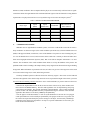
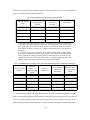
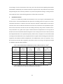
Table 1: DISTANCE TRAVELED PER FRAME ........................................................................................ 27
Table 2: POLYGONS IN SCENE VERSUS FRAME RATE ...................................................................... 30
Table 3: DISTRIBUTION OF OBJECTS IN THE FORT HUNTER-LIGGETT TERRAIN DATABASE 30
Table 4: TERRAIN DATABASE SIZE ........................................................................................................ 48
Table 5: LEVELS OF CONTROL FOR NON-DYNAMICS CONTROLLED ENTITIES ......................... 80
Table 6: ENTITY / OBJECT COLLISION RESOLUTION BY ENTITY SPEEd ...................................... 90
Table 7: SCRIPT PARAMETERS GENERATED FROM SELECTED PATH ........................................ 104
Table 8: NUMBER OF POLYGONS IN DIFFERENT TERRAIN LOD CONFIGURATIONS .............. 118
Table 9: DEAD RECKONING THRESHOLDS AND COMPUTATIONAL LOAD ............................... 127
vii
LIST OF FIGURES
Figure 1.
Figure 2.
Figure 3.
Figure 5.
Figure 4.
Figure 6.
Figure 7.
Figure 8.
Figure 9.
Figure 10.
Figure 11.
Figure 12.
Figure 13.
Figure 14.
Figure 15.
Figure 16.
Figure 17.
Figure 18.
Figure 19.
Figure 20.
Figure 21.
Figure 22.
Figure 23.
Figure 24.
Figure 25.
Figure 26.
Figure 27.
Figure 28.
Figure 29.
Figure 30.
Figure 31.
Figure 32.
Figure 33.
Figure 34.
Figure 35.
Figure 36.
Figure 37.
Figure 38.
Figure 39.
Figure 40.
Figure 41.
Figure 42.
Figure 43.
Figure 44.
Figure 45.
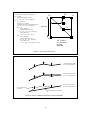
Process Interconnection........................................................................................................ 12
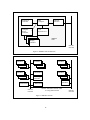
SIMNET Node Architecture................................................................................................. 20
SIMNET Network ................................................................................................................ 20
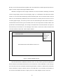
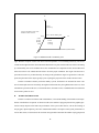
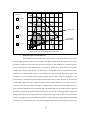
Annotated NPSNET Screen ................................................................................................. 24
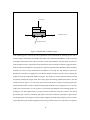
NPSNET Controls ................................................................................................................ 25
NPSNET World Coordinate System .................................................................................... 28
NPSNET Body Coordinate System...................................................................................... 29
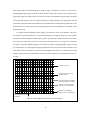
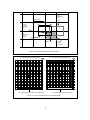
Quadtree Method of Subdivision.......................................................................................... 31
Gridded Terrain Database Subdivision ................................................................................ 32
Database Partitioning by Object Type.................................................................................. 32
Terrain Database as an Quadtree Grid.................................................................................. 33
Database Terminology.......................................................................................................... 34
Construction of Elevation Grid from Unevenly Spaced Points............................................ 35
Construction of T-Mesh Terrain........................................................................................... 36
Decomposition of a Lake into the Component Polygons..................................................... 37
Construction of a Road Polygons ......................................................................................... 38
Construction of Texture Coordinate for Road Polygons...................................................... 39
Terrain Priority Numbering.................................................................................................. 39
Dynamic Entity Definition File ............................................................................................ 40
Sample of an OFF Model File .............................................................................................. 41
Sample ANIM File ............................................................................................................... 42
Generation of Elevations ...................................................................................................... 43
Effects of Multiple Resolutions on Object Placement ......................................................... 43
Correction of Gap Created by Placing Icons on Large Slopes............................................. 44
Computation of On Ground Pitch and Roll.......................................................................... 45
Terrain Node Structure ......................................................................................................... 46
Determination of the Placement of Craters .......................................................................... 47
Relationships and Terms Used in Terrain Paging ................................................................ 49
Quadtree File Structure Used for Terrain Paging................................................................. 52
Bounding Box Used for Terrain Paging............................................................................... 53
Active Area, Before and After Terrain Paging..................................................................... 53
Conceptual Sequencing of the Processes ............................................................................. 54
First Level Parallelizaton...................................................................................................... 57
Second Level Parallelization ................................................................................................ 58
Start Up Process Functions................................................................................................... 59
Terrain Configuration File.................................................................................................... 61
Memory Mapping the Elevation File ................................................................................... 61
Allocation of Database Specific Sized Drawing Buffers ..................................................... 62
Material Cross Reference File .............................................................................................. 63
Map Centering Algorithm .................................................................................................... 64
Construction of Grey Scale Elevation Shades...................................................................... 65
System Queue Filter ............................................................................................................. 67
Display Buffer Data Structure .............................................................................................. 69
The Scene Management and Drawing Process Data Flow................................................... 69
The Four Phases of Rendering Traversals............................................................................ 70
viii
Figure 46.
Figure 47.
Figure 48.
Figure 49.
Figure 50.
Figure 51.
Figure 52.
Figure 53.
Figure 54.
Figure 55.
Figure 56.
Figure 57.
Figure 58.
Figure 59.
Figure 60.
Figure 61.
Figure 62.
Figure 63.
Figure 64.
Figure 65.
Figure 66.
Figure 67.
Figure 68.
Figure 69.
Figure 70.
Figure 71.
Figure 72.
Figure 73.
Figure 74.
Figure 75.
Figure 76.
Figure 77.
Figure 78.
Figure 79.
Figure 80.
Figure 81.
Figure 82.
Figure 83.
Figure 84.
Figure 85.
Figure 86.
Figure 87.
Figure 88.
Figure 89.
Figure 90.
Figure 91.
Figure 92.
Figure 93.
Algorithm for Rotating Billboards ....................................................................................... 71
Primary Interproccess Data Flows........................................................................................ 73
Semaphore Synchronization of Filling Buffers.................................................................... 77
Semaphore Synchronization of Drawing Buffers................................................................. 78
Sea Entity Motion / State Vector Relationship..................................................................... 81
Use of Polygon Normal to Determine Pitch and Roll .......................................................... 82
Use of Projected Point to Determine Pitch and Roll ............................................................ 82
Forces Applied to Tracked Vehicle...................................................................................... 84
Wheeled Vehicle Turning..................................................................................................... 85
Quaternion Orientation......................................................................................................... 86
Area of Concern for Collisions............................................................................................. 88
Subdivision of Area of Concern ........................................................................................... 89
Bounding Cylinder Vs. Bounding Sphere ............................................................................ 90
Fast Moving Entity Collision Volume ................................................................................. 91
First Level Distance Based Collision Check ........................................................................ 92
Collision Detection Using Bounding Spheres...................................................................... 93
Ray Casting to Determine Collision Point For Entity A ...................................................... 93
Ray Intersection Distance Collision Test ............................................................................. 94
Collision Resolution Algorithm ........................................................................................... 94
Graphical Representation of Collision Resolution Algorithm ............................................. 95
Glancing Collisions Resolution............................................................................................ 96
Graphic Representing of Zig-Zag Behavior ......................................................................... 98
Algorithmic Representation of Zig-Zag Behavior ............................................................... 99
Edge of the World Behavior............................................................................................... 100
Fight Response ................................................................................................................... 101
Typical NPSNET Script ..................................................................................................... 103
Sample Path Layout............................................................................................................ 105
Script Playback Algorithm ................................................................................................. 106
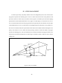
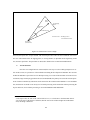
The View Frustum.............................................................................................................. 108
View Volume and Volume Passed to Renderer ................................................................. 110
Construction of View Triangle........................................................................................... 111
Grid Square Bound Box ..................................................................................................... 112
Selection of Grid Squares................................................................................................... 113
Effect of Increasing the Field of View ............................................................................... 114
Perspective Projection’s Effect on Apparent Size.............................................................. 115
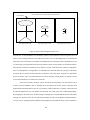
Level of Detail Ranges ....................................................................................................... 116
Effect of Differing Outlines on Model Switching.............................................................. 117
Level of Detail Blending .................................................................................................... 118
Terrain Level of Detail for the Terrain............................................................................... 119
Terrain LoD Selection Algorithm ...................................................................................... 120
Fill Polygon to Hide Edge Gap .......................................................................................... 121
Terrain Resolution Array and Elevation Determination .................................................... 122
NPSNET Network Harness ................................................................................................ 124
Sample Formats of NPSNET Messages ............................................................................. 126
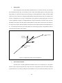
Error Based Dead Reckoning and Actual Paths ................................................................. 128
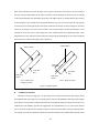
Position Error Correction Methods .................................................................................... 130
Network Harness Showing Protocol Converters................................................................ 131
Final Network Harness Structure ....................................................................................... 131
ix
I. INTRODUCTION
A.
INTRODUCTION
Much has been written of the promise of virtual worlds (VW) technology. However, very little has been
published on the implementation of such systems. And what has been published has shown a remarkable enamoration with the hardware and not with the enabling software. This dissertation deals almost exclusively
with the software aspects of a VW system developed at the Department of Computer Science, Naval Postgraduate School (NPS). We have named this system the Naval Postgraduate School’s Networked Simulator
or NPSNET for short [ZYDA91A][ZYDA92].
In NPSNET, we have identified some of the salient characteristics and challenges faced in the construction and management of VW systems. On identifying these characteristics, we were able to construct a framework which we have successfully used as a test bed for exploration of our ideas and proposed solutions. These
ideas have included, but are not limited to, network management, dynamic terrain1, vehicle dynamics, paging
terrain databases, and terrain database construction.
There is a considerable amount of publication on VWs in both the popular and academic press lately. It
has gotten difficult to open up a magazine without an article on or advertisement for a VW system. VW systems are also known as Virtual Reality (VR), Artificial Reality, Synthetic Environments, Cyberspace, or
Real-time Interactive Three Dimensional Computer Graphics [RHEI91]. Several of these terms have come to
have a negative connotation due to their over use and hype. Almost every program that uses computer graphics claims to be a VW system, usually by a marketing person trying to hype the system. With articles in the
popular press warning us of the sociological implications of VW systems and the hype from the marketing
force, VW is in real danger of becoming the Artificial Intelligence (AI) of the 90’s. Much like AI, the field is
in its infancy. The ground breaking work has been done and many people can see the potential, but major
work still has to be accomplished. One crucial component is the integration of and documentation of the com-
1. In this dissertation terrain and terrain database are meant to include all fixed entities. This
includes cultural features, such as buildings, roads, and bridges, as well as vegetation, such as trees,
crops, ground cover.
15
ponent processes of a sample implementation. That is the main thrust of this dissertation, how a virtual world
system can be constructed on a low cost commercially available graphics workstation.
B.
DEFINITION OF VIRTUAL WORLDS
Before we go much further, we need to establish a good working definition of what a VW is and what
it is not. There are a myriad of definitions depending on where you look and what the author wants to convey.
Each of the texts, [BENE92], [GELE91], [HAMI91], [HELS90], [RHEI91] and [KRUG91], has its own
slight twist on it. Even a Senate hearing, [USS91], and a business survey, [MILL92], have failed to come up
with a universally accepted definition. But there are some common elements in all of them. In the paper that
first hypothesized about VW, Ivan Sutherland calls the ultimate display one that provides us with an interactive window on the world [SUTH65]. That captures the fundamental and accepted aspects of a VW. It is a
world transposed in time or space, either real or imagined, that the user can interact with in real-time.
Humans are cultural creatures; we live and function best in a populated environment. We look around
and see things, the players2 in the world. When we interact with these players, they exhibit some degree of
autonomy, they react to the environmental stimuli. Different types of players respond in different ways to the
stimuli. Assume we are approaching an icon in the VW. If it is a wall, it will just stay there and prevent our
movement. If it is an icon representing a small furry creature, it might scurry away. The world that we live in
is not just made up of static objects, such as the wall, but also, and perhaps more importantly, of a collection
of the players we encounter, the small furry creatures. Together the wall and the creature, and all the other
objects, make up the population of the VW.
The physical properties of the real world can be rigorously applied and be the main reason for the
world’s existence, as in [LEVI92] and [BROO90]. Or reality can be fanciful and real physics has no bearing
on the design or interaction, as in [BUTT92] and many of the worlds constructed by VPL. The interaction
with the world can be accomplished on several different levels, but the key is to immerse the user in the world
so that the user is literally sucked into the experience. Some believe that in order to immerse the user in a VW
system you need to have a Helmet Mounted Display (HMD) and a DataGlove. Others, the author included,
contend that it can be done by reading a good book with some imagination. While the book may give the user
2. Throughout this dissertation, we use the term player to mean any entity capable of interaction in
the virtual world. This entity may be a real person interacting with the system locally or via a network or a computer controlled thing used to populate the world. The term user is reserved exclusively for the human player. Ideally, there should be no apparent distinction between the two, sort
of a VW Turing test.
16
a sense of presence, it fails miserably in the interaction axis. Zeltzer has developed an Autonomy-InteractionPresence cube that places VW at the (1,1,1), maximum along each of the axes [ZELT92].
In summary, a VW system can be characterized by being a bidirectional, highly interactive populated
world transposed in time or space and the physical rules that govern the real world may or may not apply.
NPSNET has not solved all the issues in developing a complete VW, but we have made significant strides in
that direction.
C.
OVERVIEW OF PROBLEM
The state of the art in VW is limited to a few simple players with simple interaction in a simplistic world.
Very often, it is a single user flying around and the only thing he can do is look at the world. The interactivity
in that type of system is only slightly higher than reading a book. The systems that do support multiple users
use expensive special purpose hardware and software. This hardware and software is unavailable to all except
a few select military projects.
The problem then becomes how can a VW be created and maintained3. The literature has a few examples of how the hardware components can be connected to build such a system, or how to use commercial
software to construct limited worlds but in both cases, the enabling software is skimmed over or hypothesized
[BENE92] [GELE91] [HAMI91] [HELS90] [RHEI91] [KRUG91]. Likewise, there is an abundance of research on how to do a small component in isolation [BADL91] [ZELT89B] [BROO88]. What is lacking is
some unifying methodology to connect all the various parts together into a single coherent virtual world, sort
of a Stephen Hawking of Virtual Worlds. That is the goal of this dissertation, to build and document a highly
interactive, extensible virtual world. In order to do this, the component research and the overview documents
have to be merged into a single working system.
D.
GOALS AND MOTIVATION
As with all research, this project has certain motivations and goals behind it. In this section we briefly
discuss some of the goals of the research and our motivation for those goals.
1.
Goals Of Research
Our goals for this research were simple:
3. As the user interacts with the VW, certain portions of the world can change. An example of this is
the addition of a crater where a missile hit. The maintenance of the VW is the management of the
modification of the VW database that occur at run-time, such as the placement of the crater.
17
Build and operate a complex and highly populated virtual world.
Construct a modular framework for interaction with the virtual world.
Provide multiple user interaction in the shared virtual world.
Use commercially available graphics workstations as the world generator.
As it turns out in many cases, goals that are simple tend to be over simplifications. The first goal
required that we have many players in the world each doing their own thing, but interacting with the other
players. It also required that there be a multitude of interaction capabilities and a complex environmental database or playing field. To a large extent, the second goal was contradictory with the rapid fulfillment of the
first. It is much harder to develop an efficient generic framework than it is to solve a particular instance. But
we knew that this system was going to be used for many different purposes, so it had to be modular and flexible. The third goal was that of providing a mechanism where more than one user could interact in a shared
data space. This required the actions of one user to be visible to the other users and have them affect the shared
world equally. The rationale for this was that humans are social creatures and we enjoy interacting with each
other, via whatever medium. The goal of using commercially available workstations required the development of quite a few of the routines that high-end flight simulation systems have embedded in hardware. Such
systems are documented only in internal, corporate proprietary reports that are not generally available. By the
same token, the embedding of the routines in hardware limits the flexibility of the systems. Such hidden and
task specific work does not contribute to the general development of accessible VWs.
2.
Motivation
The goals of this research are noble, but they are well motivated by what we perceive as funda-
mental requirements. The first and foremost motivation was to lower the cost of entry into a multi-player environment. In 1991, the price of a virtual world system was estimated at approximately $250,000 [USS91].
Other systems ranged in price upwards of $350,000 for a SIMNET network node [IDA90]. Clearly, this is
not the price that many institutions, much less private individuals could afford. By using commercially available workstations, in this case the Silicon Graphics Inc. (SGI) IRIS 4D line, the cost of hardware development
is amortized over the mass market, rather than limited to a few special projects. Also, it is in the vendor’s best
interest to continue the hardware development to ensure its competitive position in the market place. This
frees us up from the role of hardware developer and allows us to focus on the enabling software.
It has been well documented that humans are three dimensional (3D) visual creatures. Fred Brooks
and Tom Furness have proven over and over during their careers that users understand better and are able to
grasp new concepts better when they are presented in 3D [BROO88][USS91]. Combat is, by its very nature,
18
three dimensional. Both sides are constantly looking to use the terrain to their advantage and to deny any advantage to the enemy. In order to gain a better understanding of the terrain where a battle will be fought, it is
standard practice to build a small 3D sand table of the terrain to aid in the visualization. However, due to the
processing requirements, most of the Constructive Combat Models (Janus and BBS for example) are strictly
two dimensional (2D) [TITA93] [CECO90]. The lack of a 3D representation of the terrain has lead to some
obvious tactical errors when scenarios are being set up. This in turn, has lead to the discounting of some of
the simulations results. Also, certain physical impossibilities, such as the physical colocation of two entities,
are not even considered by the model. If the scenario designers had a 3D representation of the terrain available
to them during the construction of the engagement, they could place the entities in more realistic locations.
[GARV88] and [KRAU91] proved that VWs can serve as a valuable training and research and development tool. However, this is only true if the students and the developers can get access to the VW systems
in a timely and cost effective manner. This historically has not been the case. There have been only a few
expensive systems which have been available and these systems have been dedicated to particular applications. In order to increase the benefit of VWs, the systems themselves must become more pervasive. In this
era of shrinking dollar, this will only happen if the systems are inexpensive and flexible enough for the users
to procure. After all, if the training and testing equipment is not cost effective it makes no sense to do it.
Finally, we have seen a lot of good research going on without a true sense of the bigger picture.
Brooks’s view of the computer scientist as a toolsmith is a valid one [BROO88]. There is no way that something can be constructed until the tools have been built. Yet there is a time when you must shift the emphasis
from building the tools and start construction of the major system. Many of the components of VWs are already here, or being worked on. It is time now to start the construction of a meaningful VW.
E.
PROBLEM DOMAIN BACKGROUND
The focus of this dissertation has been on the iterative development of a flexible and expandable VW
test-bed. A ground combat world was chosen as a test-bed system for the following reasons:
Highly Interactive World -- both User / Computer and User / User Interaction
Populated Environment -- both Moving Vehicles and Static Objects
Demanding Graphical Requirements
Dynamic Database Requirements
Available Terrain/Object Databases
Real World Application with Large Amount of Subject Area Expertise Available Locally
Ground combat is the action of bringing two or more opposing land based armed units together for an
engagement where one side tries to destroy the other. The armed units can be as simple as a single individual
19
or as complex as a full fledged corps, in excess of 100,000 men and vehicles. Combat by its very nature is
highly interactive. Each side is constantly trying to maneuver into a position of advantage over the other while
expending a minimum amount of resources. As such, the units are forced to react to each other and to the
underlying terrain. When the engagement becomes computerized, the users are forced to interact with the
computer that acts as a mediator in the engagements. In addition to its role as mediator, the computer is also
responsible for modeling the world state and ensuring only valid actions take place. It is this interaction that
forces Zeltzer’s Interaction point value close to one.
With the exception of a few types of engagements, such as sniper fire, most of the engagements have
multiple players on each side. The number of players in the engagement demands the system to be well populated. Yet, very often the resources are not available for each player to be controlled by a human controller.
As such, autonomous players controlled by the computer must be introduced into the VW. These players
should behave in a manner consistent with their manned counterparts. One of the many interesting aspects of
ground combat is that not only do the vehicles, or dynamic players, interact with each other but with the static
entities on the database as well. The static entities include things like buildings, trees, etc. These are things
that do not move during the course of an engagement but might undergo a change of state and can influence
the outcome of an engagement. For example, a building might block the line-of-sight between two players
until it is destroyed at which time the two players can then interact. Thus, there has to be a high level of autonomy in the computer controlled players.
Over the years, the range of ground combat weapons has increased dramatically. However, the underlying terrain has not changed all that much. As a result, most of the engagements that use line-of-sight weapons are limited by the terrain to approximately 3500 meters or less [GARV88]. Even this small distance
requires that forty-nine square kilometers of data be available for immediate rendering. In order to ensure a
sense of presence, the terrain has to be of sufficient resolution to capture the critical features of the environment and yet coarse enough to be rendered in real-time. This is the classic trade-off of quality versus speed.
Not only does the database have to be of high quality, but it must be able to be modified over time. As an
engagement proceeds, the underlying terrain can, and normally does, undergo a significant modification, such
as shells landing and leaving craters or a berm being built. Users who have been in combat know how to exploit these modifications to their advantage and expect to see the terrain database be modified. If the terrain
is not rendered at a fast enough frame rate, if it is too coarse, or if does not respond to events, the user’s sense
of presence approaches zero. This requirement puts a very heavy load on the graphics system.
20
Due to the nature of NPS, we had ready access to terrain and entity databases. This allowed us to focus
on the development of the software rather than on the geometric modeling of the world. Also, since virtually
all the students at NPS are United States military officers, we had a ready pool of task area experts who could
serve as a validation reference for the models and designs we constructed. Unfortunately, ground combat is
a real world problem and promises to continue to be for many years to come. Therefore, the modeling and
representation of ground combat is a useful and practical problem. Just like University of North Carolina Chapel Hill chose three topic areas to ground their research in reality (Architecture, Molecular Modeling, and
Radiation Therapy) we have chosen ours in a field where the our resources and task experts are available
[USS91].
F.
ORGANIZATION OF CHAPTERS
The body of this dissertation is broken down into three main sections. The first of these sections is the
introduction. First, we present an introduction to the concepts, definitions, and motivation of our research,
Chapter I. The second part of the section contains a description of the challenges faced by the virtual worlds
researcher, Chapter II. The third chapter, Chapter III, of this section contains a description of a few of the
major virtual world systems.
The second section covers the NPSNET system. Chapter IV introduces and gives a brief overview of
NPSNET. Originally, NPSNET was a VW designed to simulate ground combat. As such, the terrain database,
which in this case is the world database, is extremely important to the performance of the system. The construction and organization of the world database is the first topic covered in this section, Chapter V. Once the
data formats and rationale have been presented, we then cover the organization of the software at an abstract
level, Chapter VI. From there on, the chapters focus in detail on the original software components developed
as part of this dissertation in more detail. Chapter VII covers how vehicle dynamics are implemented. This
includes weapons effects and contact detection and response. Population of the VW by computer controlled
forces is covered in Chapter VIII. The next chapter, Chapter IX, covers the issues of scene management. Included in this topic are things like level of detail, culling, and view volume determination. The final chapter
of this section, Chapter X, covers the network in detail. In this chapter, we discuss the network harness, dead
reckoning, and bandwidth limitations.
The final section is comprised of a single chapter, Chapter XI, containing the conclusions, recommendations, and the contributions of the NPSNET system. The NPSNET User’s Guide and source code is available from the author on-line.
21
II. VIRTUAL WORLDS: MAJOR CHALLENGES AND ISSUES
A.
OVERVIEW
NPSNET represents a significant research undertaking in the development of a workstation based real-
time vehicle simulation system. It encompasses several of the major areas of computer science, making contributions to each as they pertain to a real-time vehicle simulation system. In a recent industry survey, practitioners in the VW field were asked what they viewed as the major challenges of the next decade [MILL92].
The twenty-four different answers can be broken down into several major areas: Too Much Hype / Marketing,
Sociological Implications, Cost Reduction, Machine Limitations, World Complexity, and Human / Computer
Interaction. The first two items, Too Much Hype / Marketing and Sociological Implications, are best left for
the MBA’s and the sociologist and will not be discussed further here. The remaining areas are pertinent to
our work and the application of them are discussed at length in the chapters dealing with NPSNET, Chapter
IV through Chapter IX. In this chapter, we present some of the major challenges and issues that we had to
deal with during the development of NPSNET. They are presented briefly in this chapter to lay a foundation
and to provide an overview of the design decisions that went into NPSNET. These issues are not limited to
NPSNET, or even workstation based simulation systems, but rather across the entire VW development platforms.
B.
COST REDUCTION
NPSNET was developed on the Silicon Graphics Inc. IRIS 4D (SGI) family of workstations. By using
a commercially available workstation it is possible to amortize the cost of hardware development over many
users and thereby reducing the unit cost of each of the network nodes. By using a workstation as the hardware
base, we further reduce the cost of each node since the organization can use the workstation for other purposes
when it is not involved in a simulation exercise. This is something that the dedicated hardware simulators can
not do. The use of workstations does complicate the construction of the system since many of the functions
embedded in hardware in the dedicated simulators must be done in software, thereby slowing the frame rate
down. A further advantage of using the SGI workstation is that they are software binary compatible across
the entire workstation product line. This allows the user to tailor the hardware suite to his cost and perfor-
22
mance requirements. The challenge was to use a commercially available general purpose graphics workstations instead of special purpose hardware and image generator combination.
C.
WORLD CONSTRUCTION AND MAINTENANCE
The run-time world database contains two major types of data: the physical characteristics, and the geo-
metric or visual representation of the icons. Both share the common requirements of having to be flexible,
expandable, and rapidly accessed. The physical characteristics portion of the database consists of the static
and dynamic parameters of the entities and responses to stimuli. These are the parameters that are input into
the rules and functions that govern the behavior of the entities in the VW. The geometric component of the
world is comprised of the graphics primitives needed to represent the visually correct world. Very often the
two databases are combined into a single run-time database that makes up the VW. The user then relies on
the VW software to interact with the database to construct the desired VW. The architecture of the software
is discussed below.
The requirements of flexibility and expandablity go together for any computer system. Unfortunately,
they often are at cross purposes with efficiency. The classic data structures example of this is the linked list
versus the array. The linked list is extremely flexible and expandable, but requires O(n) access time. The array, on the other hand, is a fixed construct in terms of size and structure, but can be accessed in O(1) time. In
the case of NPSNET, speed was more important than flexibility at run-time. As such, we had to develop a
system that can be configured at start up but still ran efficiently.
The actual construction of the VW’s physical and geometric databases is not difficult, but is very time
consuming. The construction of the physical database is task specific and research intensive. Looking up and
inputting the tremendous number of parameters required to insure correct behavior and appearance takes
quite a while. In some cases the cost of producing the geometric database exceeds that of the hardware
[PRC92]. The physical modeling of the icons for the non-run-time geometric database is relatively straightforward and is covered in detail in [SGI92] and [SSI92]. Thus the challenge is to reuse existing databases
rather than develop new ones.
D.
WORLD POPULATION
Even with low-cost workstations, there are not enough resources for every simulated vehicle to be con-
trolled by a human. To alleviate this problem we use scripted vehicles, Semi-Automated Forces (SAF), and
Autonomous Agents (AA). Scripted vehicle motion is controlled by a prewritten sequence of actions. The
script can be recorded from a previous exercise, generated by a combat model, or hand written by the scenario
23
designer. A SAF unit has a human exercising control over a key or lead vehicle and all of the other vehicles
follow the lead. Even though they are following the lead of the key vehicle, they are making small, task level,
decisions for themselves. An AA is a fully automated unit. In this case, an AA unit would be given a high
level goal and the automated controller would in turn execute the tasks required to complete the goal. The
important difference between the two is the removal of the man in the loop. This complicates the construction
of the agents considerably. The fundamental challenge is to populate with enough entities so that the human
player can interact with them.
E.
REALISTIC ICON INTERACTION
One thing that we have noticed in the many demonstrations that we have given is that the user does not
focus on what is there, but what is missing or done incorrectly. When we first modeled power lines, we did
it as single line segment from pole to pole. Quite a few people noticed and commented on them. When the
power lines where modeled as curves, nobody seemed to notice them. The fact that we modeled the lines as
Bezier curves vice catenary curves, did not take away from the appearance of correctly modeled power lines.
The reason for this is that one of the fastest ways to destroy the illusion of presence is to present to the user
something that is incorrect or inconsistent with the user’s expectations. All physical entities behave according
to certain rules and users expect these rules to be followed. Some of these rules might be physics based, i.e.
power lines are curved, or doctrinally based, i.e. in the United States you drive on the right side of the road.
These are the rules that have to govern all players in the VW. The challenge is to make the entities mimic how
the user expects them to act within the resources available.
F.
MACHINE LIMITATIONS
Over the last several years, the cost of computer hardware has fallen while the processing power has
increased by at least an order of magnitude. For example, this year we bought a machine that has two orders
of magnitude faster graphics and at least one of processing ability for a quarter of the price of a machine we
bought five years ago. Despite this, NPSNET runs at the same frame rate as FOGM [ZYDA92][SMIT87].
There is a very simple reason for this. The capabilities of the NPSNET system are enhanced until an unacceptable frame rate is met. This is the computer graphics version of the closet metaphor, the amount of clothes
you have will expand to fill all available closet space. This is true not only of the graphics subsystem but also
of the network and processor components as well.
24
1.
Processor
The amount of computation that is involved in a networked VW exceeds what is currently avail-
able from a single Central Processing Unit (CPU). For this reason, we have explored the use of parallel processing and spread the computational load among several processors within a workstation. The use of true
distributed processing (using the CPUs on multiple machines connected over the network) was considered
and then discounted. By using the remote procedure call mechanism, we would place an even higher load on
the network which is the most limited resource we have. This would also add a level of complexity to the
system we sought to avoid.
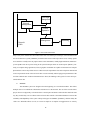
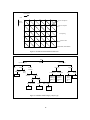
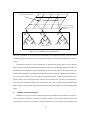
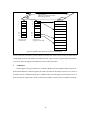
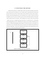
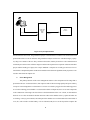
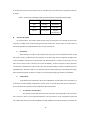
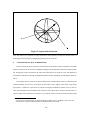
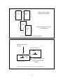
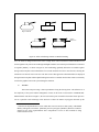
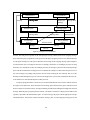
Conceptually, the management routines required by a VW can be divided up into five general processes: User Input Management, Vehicle Dynamics, View Volume Determination, Rendering, and Network
Management. Figure 1 shows the connection and relationship of each of the processes. The User input management routines monitor the state of all the input devices and provides the inputs into the VW. The vehicle
dynamics process moves the vehicle across the terrain based upon the physical model of the vehicle, underlying terrain, interaction with other entities, and user inputs. In the case of AA or SAF, this process also contains the intelligence to control the player. Scene Management is the process of placing the eyepoint in the
world, constructing the field of view (fov), determining what is in the fov or culling, and which polygons will
be passed to the renderer and in what order. Culling is normally a two step process with coarse culling done
by the culling process and fine grain, or window clipping, done by the renderer. The renderer process converts
the geometric primitives into the colored pixels on the screen. The final process is the network management
process. This process provides network services by monitoring the network, buffering any incoming messages, and putting any outgoing messages on the network. The challenge is to construct these processes in such
a way that they all fit within the available CPU resources.
2.
Graphics
Humans are fundamentally visual creatures; we receive most of our environmental stimuli via our
eyes. As such, the graphical presentation of the information is critical if we desire to achieve any sense of
presence. As a result of this, the users are given most of information and feedback by means of a graphical
representation of an out-the-window (OTW) view. This metaphor is suitable for vehicular simulation, that is
the way we view the world when we are in a vehicle. The visual realism of the scene and the frame rate are
the two most important parameters in the display, although there is some dispute which is more important
[BROO88]. Ideally, the user would be presented with a photographic quality display of the OTW scene at
25
User Input
Management
Network
Management
Vehicle
Dynamics
Network
Cable
Scene
Management
Rendering
Figure 1. Process Interconnection
thirty to sixty hertz. Studies have shown that a frame rate of six frames per second (fps) is the minimum frame
rate for an interactive system [AIRE90A]. Smooth motion starts at fifteen fps and in excess of thirty fps the
user is unable to visually notice any improvement. Some communities, notably flight simulation, demand sixty hertz update rates due to perceived lag in the system from input action to visual response [E&S91]. Currently, no computer image generators (CIGs) or graphics workstation are capable of construction of complex
photorealistic scenes at any of these rates. For this reason, the requirement exists to develop three dimensional
icons to represent the items in the real world. The icons are normally reduced polygon representations of the
real from which the user can draw informational cues. Thus, the challenge is how good of a scene can be presented and how fast.
3.
Network
The NPSNET system was designed from the beginning as a networked simulator. This allows
multiple users to be on different workstations and interact over the network. The use of the network allows
players who are not physically co-located to share a virtual space and interact with each other much the same
way they would if they were in vehicles in the real world. The network is the ideal mechanism to increase the
scaleablity and adaptability of the system. Thorpe in his paper on SIMNET, [THOR87], calls this ability the
“dial a war.” What this allows us to do, is to create as simple or as complex an engagement as we want by
26
selecting which and how many simulation systems are going to be connected to the network. In a sense, the
network is the supreme integration tool. However, it does not come free of cost. In order for multiple users to
communicate, a standard network protocol and connections must be used.
The use of a commercially available network imposes certain limitations. The foremost of these
is the limited bandwidth. This combined with the network latency are the two physical limitations imposed
by the network. Network management limitations, such as unreliable delivery, also have to be considered.
Network programming is a complex matter that is poorly understood by most and practiced by few. Yet, in
order to have a scalable and flexible system, the network must be mastered efficiently. The challenge is to
develop a simple, yet flexible and efficient, network interface and management routines.
G.
HUMAN COMPUTER INTERACTION
Since NPSNET was designed to run on a workstation rather than a vehicle mock-up, a new user inter-
face had to be designed. The information had to be presented to the user in such a way that he feels immersed
in the simulation. In a vehicle mock-up, this is a fairly easy task since the user’s physical setting correspond
to what he expects to see in the real vehicle. On a workstation, it is a considerably more difficult task. The
user’s field of view is not completely enclosed by the simulation, but rather only a small fraction of it is occupied by the display. The use of large screen televisions increases the amount of viewing area but at loss of
resolution. Furthermore, since the fov is so small, the user can easily get lost in the VW. To avoid disorientation, it is common practice to provide a two dimensional Plan View Display (PVD) showing the users location [BROO88]. While this helps the user locate himself, it further takes away from the screen space
available for OTW view. The OTW view is further restricted when the status information, speed, heading,
location, etc., are included in the display. Rather than using dedicated input devices, we chose to use a commercially available joystick, mouse, keyboard, and button and dial box as input devices. This further helped
to reduce the sense of immersion.
To see what can be done with simple interfaces like the one we are using, we went to the local video
arcade. It does not take long to notice the games that the customers are playing have three major features in
common, fast graphics display, sound and high degree of interactivity. These three features, when combined
coherently, possess that ability to completely immerse the user in the VW. The challenge then became to combine these areas on the workstation to immerse the user in the VW.
27
H.
CONCLUSIONS
As stated above, a lot of work has been done on these challenges, not just at NPS but at other places as
well. Some of these systems are presented in the next chapter. The key thing to remember is that there are
significant technological limitations to the underlying hardware. It is the design and construction of the enabling software that can compensate for these limitations. That is the primary purpose of NPSNET, to serve
as a software architectural frame work for the construction and management of real-time virtual worlds.
28
III. OVERVIEW OF SIGNIFICANT EXISTING VIRTUAL WORLD SYSTEMS
A.
OVERVIEW
While NPSNET is not the first VW system, it is one of the most ambitious and useful ever undertaken
by an academic institution. Like all research, it is built on the systems that have gone before it. In this chapter,
we review some of the more well known systems. While these systems were chosen as a representative sample of a certain types of VW applications and implementations; it is by no means an all inclusive list. Other
VW systems are referenced in the rest of this document where they are applicable.
B.
VIDEOPLACE
Krueger developed the first in the series of video based systems in 1970 when he was at the University
of Minnesota. Videoplace is unique among the systems discussed here in that it is video based [KRUG91].
The user is placed in front of a lit white Plexiglass panel, to provide a high contrast for the video cameras.
The cameras are then aimed at the user to record images. These images are then processed with custom hardware and combined with computer generated images. The resulting images are then displayed on a large projection screen. The use of video technologies allows thirty hertz input / output rates. These rates, combined
with the custom hardware, provide for an extremely interactive system. The basic premise of Videoplace is
that the human silhouette can interact with itself, other silhouettes, or computer generated entities. This paradigm allows for a wide range of possibilities. In his book, [KRUG91], Krueger discusses some of these potential applications at length. The common thread through all of them in that they are art or interpersonal
communications systems, rather than scientific or exploratory systems.
The very strength of the system is its limiting factor. Since all motion tracking and input is done via
video cameras, the system is inherently two dimensional. While it is possible to construct a three dimensional
version by using orthogonal cameras, the display is still a projected image on a screen. Likewise, since the
system uses a back lit panel, the size of the world is limited to the size of the panel. Based upon observations
of a version of Videoplace at the Tomorrow’s Realities Gallery at SIGGRAPH 1991, the users quickly tire of
the paradigm, despite the high level of interaction.
29
C.
REALITY BUILT FOR TWO
Reality Built for Two (RB2) is a combination of off-the-shelf hardware and VPL’s custom software
[BLAN90][BLAN92]. The key aspect of this system is the complete immersion of the user. This is done by
the use of VPL’s EyePhones and DataGlove. The EyePhones, VPL’s trademarked name for their helmet
mounted display (HMD), completely blocks the user’s field of view. As a result, the only visible image are
the computer generated graphics presented on the two small LCD displays. The computer graphics displayed
in the HMD is a subset of the VW that was modeled using RB2 Swivel. Once the user is satisfied with the
world created by RB2 Swivel, it is then exported to the SGI IRISes for traversal and rendering. The DataGlove, a full hand input device, is used to interact with the system. Both the DataGlove and the EyePhones
have Polhemus sensors mounted on them to sense the position and orientation of the user’s hand and head,
respectively. The input data is fed into a Macintosh II and is processed by the Body Electric Software that
computes the world dynamics and the viewpoint. The dynamics of the system can be modified by the visual
programming interface provided with Body Electric. When the dynamics of the frame have been computed,
the frame generation synchronize signal to the two SGI Irises is set and Isaac, the real-time renderer, renders
the scene for each of the eyes. Recently, the Crystal Rivers Convolvotron was added to the system to provide
3D sound cues to the user and thus increase the feeling of presence in the VW. The use of two graphics engines to drive a single HMD is not unique. Since many of the graphics engines do not handle two simultaneous visual channels very well. This fact alone has increased the cost of an HMD based system by almost a
third.
D.
THE VIRTUAL WIND-TUNNEL
The Virtual Wind-Tunnel is a system designed and built at the NASA-Ames Research Center to explore
numerically generated unsteady flow fields [LEVI92]. In this system, the flow fields around an object are
computed a priori and stored for use by the simulation system. A DataGlove is used to place the start of the
marker flows. These flows are represented as a stream of “bubbles” going across the display. The location of
each of the “bubbles” is determined by the previous location and the direction of the flow. The in-between
positions are computed by means of a second order Runga-Kutta integration to give a smooth flow across the
screen. By moving and gesturing with the DataGlove, the starting location and number of marker flows can
be modified. This allows the user to keep the number of flows to a minimum, while still being able to examine
the areas of interest. The flows are presented to the user by means of a pair of boom mounted CRTs. CRTs
can be used for this application since all the weight is supported by the boom and not the user’s head. The
30
CRTs are also brighter and have better resolution than the LCD displays. However, they are monochrome.
Through clever manipulation of the red and blue bit planes, the designers are able to generate stereoscopic
displays from a single channel display. While the boom mount does not have the same freedom of motion as
an HMD, it is adequate for the representation of the data. The key feature of this system is its ability to combine a static database, the flow field data, and the dynamic actions of the particles and present the results to
the user in an intuitive manner.
E.
BOLIO
The Bolio system is the name given to the Integrated Graphical Simulation Platform (IGSP) designed
and built by Zeltzer’s group at the MIT Media Lab [BRET87][ZELT89A][ZELT89B]. The interesting point
of this system is the use of reusable modular components that can be linked at compile time to form a tailored
system. This has allowed the system be used for such diverse research projects as insect locomotion, teleoperation of robotic arms, user interaction, and path planning [STUR89A][STUR89B].
Bolio is built around the traditional input / compute / draw loop. It is this loop that provides that flexibility in the system. The input modules can be drivers for such devices as the keyboard or a DataGlove. The
key aspect is that they all provide a standard interface. The same is true of the compute or dynamics section
of the loop. If the user wants to include complex dynamics or control routines, the rest of the code does not
have to be modified as long as the routines conform to the standard interfaces. The graphics routines are
slightly more specific due to the nature of the graphics calls and platforms. It is this flexibility and reuse of
code that has allowed one single set of software to be used for a diverse set of applications [ZELT89A]. An
excellent overview on how Bolio can be used as a harness for task level animation can be found in [BADL91].
The flexibility does not come free of cost. Bolio is capable of supporting only eight simple polyhedral
objects at five frames per second [DWOR91]. Part of this is due to the platform and part is due to the software
harness overhead required to support the generic interfaces.
F.
UNC WALK-THROUGH / MOLECULAR MODELING
The Department of Computer Science, University of North Carolina at Chapel Hill (UNC) has con-
structed many separate virtual world systems [RHEI91]. For the sake of this overview, we focus on two of
the main thrusts, architectural walk-throughs and molecular modeling.
The initial UNC work on architectural walk-throughs was driven by their desire to visualize the new
computer science building before it was built. The initial version of the work, first presented in [BROO86],
was an 8000 polygon model of the building and used a Binary Space Partitioning (BSP) tree for hidden sur-
31
face removal. The output was displayed on a wide screen projection system, standard monitor, and a stereoscopic display. The input of the building data in the system was done by a combination of Autocad and a
modification to a microchip design program. The data was then preprocessed into the working model before
it was passed to the View Instancer for viewpoint selection and rendering. The view point was selected by
means of a mouse, Polhemus, data-tablet, or joystick. The resulting system provided a frame about every
three seconds. The third version running on one of the early versions of UNC’s Pixel-Planes image generator
was able to achieve nine frames per second. To partially compensate for the frame rate, a two dimensional
floor plan was also provided to help the user navigate through the building.[BROO86]
The work on walk-throughs was extended in [AIRE90A] and [AIRE90B]. There were two fundamental
improvements on the original system: better database organization and improved lighting model. The database was reorganized into Potentially Visible Sets (PVS) rather than a pure BSP tree. This takes advantage
of the properties of buildings. Buildings are divided into a series of rooms, therefore, not all polygons in one
room are visible from all other rooms. Likewise, after the design process is complete, buildings form a relatively static database. The PVS organization allows for the rapid culling of the non-visible polygons in the
other rooms. This is similar to the work done by Funkhouser for the new computer science building at the
University of California, Berkeley [FUNK92]. The second improvement was the addition of a radiosity light
model. The use of radiosity and its use of diffuse lighting characteristics and polygon subdivision improves
the overall image quality. When the user is moving, the coarse flat shaded model is used. When the viewpoint
is stationary, the coarse polygon model is replaced by progressively more complex radiosity lit scenes.
The area of molecular modeling has been an active area of research at UNC [BROO77][BROO88][OUHY89][BROO90][SERL92]. Specifically the areas of force feedback, dynamics, and Helmet Mounted Displays (HMD) have been stressed. The work on force feedback has made extensive use of the Argonne Remote
Manipulator (ARM) device. This is a robotic remote manipulator arm commonly used for the handling of toxic and radioactive materials in an isolation booth. This proved to be particularly useful for the GROPE and
GRIP series of projects since the servo motors controlling the movement of the arm could be controlled to
provide resistance, both positive and negative, to the user. The construction of the ARM allows the chemist
to try to physically fit the molecules together and feel the forces involved. Audio cues provide an additional
channel to the user’s senses for conveying information. The use of HMDs has given the chemist the ability
to view molecules in three dimensions and study the forces and the orientations of the individual atoms. The
key contribution of this work has been that of visualization and manipulation of a physical phenomena in a
intuitive and computationally correct manner.
32
G.
SIMNET
To a large extent, DARPA’s and the US Army’s Simulation Networking (SIMNET) system can be con-
sidered the only true virtual world system in existence today [THOR87][GARV88][IDA90]. When SIMNET
was initiated in 1983, it was meant to serve as a proof of principle technology demonstration of a networked
man in the loop, real-time, immersive battle simulation [IDA90]. It has since grown to over fifteen sites capable of conducting a mechanized battalion level engagement with close air support [GARV88].
The history of SIMNET is a classic example of a DARPA high risk research project that has had a fundamental impact on how training is conducted. The idea for the use of computer graphics grew out of the use
of the video disk based gunnery trainers of the late seventies and early eighties. These trainers could train an
individual tank crew, but could not teach the interaction between the tanks. For this, a radically new approach
had to be taken. The tanks had to interact with both the targets and each other. Clearly a network connection
was required. To construct a system such as this required a quantum leap in the technology of the day
[IDA90].
DARPA assumed the project management role and the subcontractors, BBN, Deltagraphics, and Perceptionics built the dedicated and task specific hardware and software required for the simulators. DARPA
realized at the time that task specific hardware was not the best solution, but since no commercially available
systems met the specifications, it was the only way to go. The resulting hardware configuration is shown in
Figure 2, all of which is available from a single vendor, BBN.[IDA90]
As Thorpe points out in [THOR87], the key to the success of SIMNET is the network connecting the
microprocessor based simulator nodes. Figure 2 shows the architecture of the SIMNET node. Normally, multiple nodes are connected via the Ethernet network to provide force-on-force engagements, Figure 3. The use
of the network allows a certain amount of scalability and flexibility that is not normally found in the more
traditional combat models. The ability to “dial-a-war” allows the network to be used for multiple engagements at the same time and for a task organization of the equipment mix.
The use of a standardized network protocol allows the connection of dissimilar equipment to the network [POPE89]. It is these protocols that communicate the changes of each entity’s appearance, and the transient events it generates, to the rest of the simulators on the network. The majority of the network traffic is
the Appearance Protocol Data Unit (PDU). This PDU contains the information required for first order dead
reckoning1, location, orientation, and speed. As long as an entity’s speed and orientation does not change,
1. Dead Reckoning is discussed in detail in Chapter X.
33
Sound Cue
Generator
Host
Computer
Network
Interface
Computer
Image
Generator
User
Input Devices
Display
Display
Channels
Display
Channels
Channels
SIMNET
Node
Ethernet
Network
Figure 2. SIMNET Node Architecture
M-1
M-1
Simulator
M-1
M-1
M-1
M-1
Simulator
M-1
M-1
M-1
M-1
Simulator
M-1
M-1
M- 2/3
M-1
Simulator
M-1
M-1
SAF
Workstation
AH-64
M-1
Simulator
M-1
M-1
Data Logger
Recorder
Stealth
Workstation
A-10
Simulator
Logistics
Workstation
Ethernet
Network
Defense Simulation Internet (DSI)
T-1 Long Haul Network
Figure 3. SIMNET Network
34
Ethernet
Network
there is no need to send an appearance PDU across the network. This significantly reduces the network loading and allows more entities to be modeled. By their very nature, transient events, such as weapons fire, detonations, collisions, and resupply, are not predictable events. As a result, whenever this type of event occurs
a PDU is sent out.
SIMNET was and is a success because a tremendous amount of time and effort were spent on the functional requirements of mechanized combat. Even with this limited scope, SIMNET never was intended to be
the complete or perfect solution. But rather it introduced the concept of a 70% solution. If the most important
cues are provided to the user, the user’s mind is able to fill in the remaining details. By putting the user in an
enclosed environment, the tank or aircraft mock-up, and providing him with auditory and visual cues, even
cartoon like graphics, the user quickly becomes immersed in the interaction with the other players on the network. [THOR87][IDA90]
SIMNET’s success at team tactics training has been mirrored with its role as a test bed for new weapons
system development. This was demonstrated in the Line-of-Sight Forward Heavy (LOS-F-H) test conducted
in 1988. This test was designed to determine the effectiveness of a weapon that was still on the drawing board.
The weapons systems were modeled in software and connected to the network. This test proved two important
things. The first of which is that weapon’s effectiveness and tactics can be evaluated prior to it full scale construction and deployment. Once the tactics were developed, they could be practiced and further refined. This
would have normally occurred at costly, controlled, and scarce field trials. In many cases, the tactics would
have to be discarded in actual combat. The other was the use of a detailed recording capability for the after
action review. By examining the events that happened, the users were able to determine exactly what was
going on and how to counter advances by the other side and exploit their equipment. [GARV88]
The SIMNET System, or Planet SIMNET as it is sometimes called, is a true virtual world system since
it covers a large geographic area, has many players, the players interact in an intuitive manner, the users action
are reflected in the world state, and the users feel immersed in the action. In many ways, this is the holy grail
of virtual world systems. It’s weaknesses are the very things that made it a success. A task specific suite of
hardware and software are available from only one vendor. The rapid development lead to poorly documented
and ill structured code. While it has proven to have limited flexibility and scalability, it suffers from growing
pains and technological limitations of the hardware.
35
H.
SUMMARY
In this chapter, we have seen some of the major VW systems and their uses. It is from some of the ideas
gathered from the study of these systems, and other work done at NPS, that NPSNET was built. Ideally, what
we would like to have is a system with the complexity of SIMNET, the real world modeling ability of the
Virtual Wind Tunnel, the flexibility of Bolio, the sense of presence of RB2, the interaction of Videoplace,
and the durability and usefulness of UNC’s work. Our system may not yet achieved all of these goals, but, as
shown in the next chapter, it comes pretty close.
36
IV. NPSNET OVERVIEW
NPSNET was designed and built at the Department of Computer Science, Naval Postgraduate School,
as a test-bed for the exploration and experimentation of virtual worlds. As part of the design process we carefully reviewed all of our previous simulators; FOG-M, VEH, MPS I, MPS II, MPS III, and CCWF [SMIT87][OLIV88][FICT88][WINN89][CHEE90][WEEK89]. Each one of these had some interesting
components, but they also had some weaknesses. What we did in NPSNET was to extract the useful algorithms and develop new ones as needed to implement the desired features. In this section, we discuss in detail
the database formats, structure of the software, and the algorithms needed to populate the world, manage the
network, move the entities, and efficiently manage the graphics pipeline.
NPSNET started in February of 1990 as a test bed to explore a proposed terrain database format. Since
that time, over ten master’s level students have contributed to its development. What started as a simple single
vehicle with one kilometer square world, now has expanded to a fully networked system capable of supporting 500 vehicles of any of 2000 different types in a world exceeding 100 kilometers on a side. As NPSNET
has continued to grow, it has been compared favorably to the U.S. Army’ s SIMNET system. While this is
true in many respects, there are some fundamental differences. The foremost among these is the equipment
that the system was designed to run on. NPSNET can run on a single SGI Indigo Elan, while SIMNET requires a vehicle mock-up, computer image generator, host computer, and sound generator. The SIMNET system is also extremely weapon system specific. The node configured to emulate an M1 cannot be reconfigured
to become an M2. The lost of flexibility comes from the use of the mock-up and the complexity of the simulator code. The mock-up adds a sense presence and realism that NPSNET, a workstation based system, does
not match. NPSNET was designed to be as flexible and extensible as possible. To a large extent, this prevented the inclusion of some of the more specific weapons systems features. However, since the system is extensible, we have been able to add some of these features into certain versions of NPSNET.
Rather than
using an accurate vehicle mock-up, NPSNET users interact with the system by means of a Spaceball,
Keyboard, Buttons / Dials box, and/or Mouse. Having a wide variety of controls allows the user to select the
interface metaphor that is most appropriate for the task and what the user feels most comfortable with using.
37
Recently, the Ascension Bird and VPL EyePhones have been added to the available input and output devices.
Figure 4 contains a diagram showing the NPSNET controls.
NPSNET was designed to run on a single workstation. As such, the available visual display was limited
to that of a single display console. The current display, Figure 5, is a combination of the 3D out-the-window
(OTW) view, the 2D elevation shaded map, and the information panel. The size and the location of the 3D
OTW view was determined by default, that is the screen area that is covered by the scan converter we use to
record the graphics display. Across the top of the screen is the information panel. This window contains textual information such as location, speed, orientation, frame rate, and weapon status. The third window is the
optional 2D elevation shaded display. The 2D map can be hidden if the user decides that the screen space is
better utilized by the 3D OTW view. The advantage of this window is it shows the vehicle’s location in the
world with relation to all the other vehicles and the database.
Information Panel
Two
Dimensional
Elevation
Shaded
Map
Three Dimensional Out-the-Window (OTW) View
Figure 5. Annotated NPSNET Screen
Since the initial release of NPSNET in the Fall of 1991, over forty schools, government organizations,
defense contractors, and commercial firms have received at least one version of NPSNET or some of the support code. The uses for this code include: autonomous agent studies, constructive combat model visualization,
terrain visualization, weapons evaluation, and low cost stealth nodes. It is the flexibility and modularity of
the code and of the database that allows a single system to be readily adaptable for these varied uses.
38
Space Ball Buttons
S
E
L
E
C
T
U
N
T
E
T
H
E
R
M
E
N
U
Stop
Zero
View
Zero
Pitch
Zero
View Tilt
Dec.
Sense
Inc.
Sense
View
Rezero
From/To SpaceBall
Speed
Mouse
Pitch
Elevation
Direction
External View Controls
Speed
Increase
Left
Turn
Speed
Decrease
Right
Turn
+Rotation
+Radius
+Elevation
-Rotation
-Radius
-Elevation
F3: Toggle numbers/icons on the 2D Display
F11: Display Cross hairs
F12: Prevent backing up
Pressing the 1-9 keys gives you a field of view
equal to ten times the value of the pressed key.
The following apply to the Stealth Vehicle only:
F9: Stop
Pad 4:
Look Left
Pad 6:
Look Right
Pad 2:
Look Down
Pad 8:
Look Up
Pad 5:
Reset Look Angle and Speed
Pad 3:
Decrease Elevation
Pad 9:
Increase Elevation
Figure 4. NPSNET Controls
39
V. VIRTUAL WORLD DATABASE CONSTRUCTION
The NPSNET world consists of three interconnected components. The first of these is the terrain skin.
This is implemented as a polygonal covering to represent the topology of the area. Different colors and textures are used for the polygons to convey a sense of soil or ground cover type. Fixed zero height features, such
as roads, rivers, lakes, and fields, are all part of the polygon skin. Anything that is static on the database but
has an elevation, such as buildings, trees, and telephone poles, are part of the second database. These static
objects are used to increase the complexity and thus the realism of the world database. The final database is
the dynamic entity database. This database contains all of the players that move in the world. The first two
databases are discussed in this section, the dynamic entity database is covered in Chapter VII ENTITY DYNAMICS. The icon database that contains the description of the static and dynamic entities is part of the static
entity database.
The world in NPSNET is that of ground combat. As such there are certain features we can exploit.
While the world is three dimensional, all of the objects are attached to the ground. All of the action occurs on
the ground, or in relatively close proximity, and no entity goes below ground level. As such, the terrain is only
a single polygon deep. Thus, the world segmentation ends up being a 2 1/2 D problem, 3D environment projected on to a 2D plane. When we model such things as buildings, a 3D representation is used to segment the
world. Another feature we can exploit is that the players are relatively slow moving objects. Obviously, missiles and ballistic projectiles are the exception. As shown in Table 1, even ballistic weapons do not travel a
significant distance, often less than one unit of database resolution, during one frame. Since this is the case,
we can reduce the computational and graphics load by limiting the search area and grouping the objects together.
Ground combat engagements take place over a limited area. Wars might cover thousands, or even millions, of square kilometers, but battles seldom cover more than a couple of hundred square kilometers. This
allows the use of a Casini flat earth projection1 for the terrain database and the use of Universal Transverse
1. A Casini projection is an equidistant flat earth projection. It is only valid for small areas of the
earth since it discounts the curvature of the earth and the differing distance separating longitude
lines at different latitudes. In essence, one degree of longitude is held as a constant for the entire
database resulting in the flat earth model. For large differences in latitudes, the approximation error
results in extremely inaccurate placement and navigation.
40
Mercator (UTM) coordinates. The assumption that the players are concerned only with local areas is significant in that it allows the segmentation of the world into different regions. This also limits the viewing distance
requirements. The player does not have to see beyond the range of its sensor and weapon systems.2
Table 1: DISTANCE TRAVELED PER FRAME
Player Type
Speed
(KPH)
Ground
Frame Rate
Max Distance Per
Frame (Meters)
100
27.76
15
1.85
50
13.88
15
0.93
Aircraft
1400
388.89
15
25.93
Ballistic Munition
3000
833.33
15
55.56
Ship
A.
Speed
(Meters/Sec)
COORDINATE SYSTEMS
NPSNET uses two right handed coordinate systems, one for the world and the second for the icons’s3
body coordinates. As shown in Figure 6, the world coordinate system has (0,0,0) located at Mean Sea Level
(MSL) at the upper left hand, or northwest, corner of the database. The positive X axis is heading east, positive Y is the altitude above sea level, and Z increases to the south. This is contrary to almost all other simulation and Geographic Information Systems (GIS). But on the Silicon Graphics architecture it is more
efficient. The orientation of the world coordinate frame allows us to keep the database in the positive XZ
quadrant and the vehicle’s heading is the simple offset by ninety degrees from the normal zero degree heading
being north. When information is presented to the user, all values are given as if the origin was in the south
west corner with X being east, Y north, and Z being elevation.
The body coordinate system was likewise chosen for efficiency, Figure 7. The X axis is to the front and
roll causes the right side of the vehicle to dip down. The Y axis represents the height of the vehicle, yaw turns
the icon to the left. Heading, which is about the Y axis in world coordinates, is positive rotation to the icon’s
2. Much of the implementation work in this section was done with two of my thesis students, William Osborne and Randall Mackey. The ideas and algorithms were developed during many long
conversations and tutorials. They did the preliminary implementations, I have redone significant
portions of their code and algorithms after they completed their degrees. Portions of this work has
appeared in their master’s level thesis, [OSBO91] and [MACK91].
3. For the purpose of this dissertation, we will use Zyda’s definition of a 3D icon as a low polygon
count representation of a real world object [ZYDA90A]. The purpose of the icon is to give the user
the visual cues required to identify the presence and type of an object, not necessarily a faithful representation of the object’s true appearance. An object is a specific instantiation of an icon at a particular location and orientation.
41
Y
Y Axis
Positive Up
Origin at NorthWest corner of the
database at Mean Sea level.
X Axis Positive heading East
(0,0,0)
Z Axis
Positive
Heading
South
X
Terrain
Database
Coverage
(XMAXSIZE,0,ZMAXSIZE)
Z
Figure 6. NPSNET World Coordinate System
right. With the exception of some work done on aircraft dynamics, we use heading exclusively. The Z axis
extends out the right side of the vehicle. Rotation about the Z axis, pitch, results in the nose of the icon rotating
up. Unfortunately, this set of coordinate axes is also nonstandard. To compensate for this, most models from
other sources have to be rotated about X and Z to be in the proper orientation. The origin of all the icons is
positioned in such a way so that when they are sitting on the ground their origin is at ground level. This simplifies the placement of the objects greatly by not requiring the projection of the models onto the terrain.
In order to maintain constancy with most military systems, all distances are measured in meters. One
unit of UTM equals one meter. Internally, all angular measurements obey the right hand rule. However, when
information is presented to the user, or external interfaces, the intuitive and / or standard units of measurement
and reference points are used.
B.
WORLD SEGMENTATION
In order to construct an efficient VW world database, a firm understanding of the limitations and capa-
bilities of the hardware is required. As shown in Table 2, the number of polygons passed to the graphics pipeline has a major impact on the frame rate performance of the system. Other factors, such as the texturing of
the polygons, depth complexity, and vertex transformation all have an impact on the system performance as
well. In this section, we discuss how the world can be segmented to minimize the number of polygons passed
42
Y UP (YAW)
X FRONT (ROLL)
Z RIGHT (PITCH)
Figure 7. NPSNET Body Coordinate System
to the rendering process. Not only does the segmentation of the world benefit the rendering process, but as
shown in Chapter VII ENTITY DYNAMICS and Chapter IX SCENE MANAGEMENT, it helps to speed up
and simplify other aspects of the VW as well. Table 3 shows the distribution of objects based verses the size
of the grid squares used to segment the world. This data was derived from the Fort Hunter Liggett terrain database [LANG90]. This database is a representative sample of a populated 3D VW database and is commonly
used due to its lack of security classification. The database is of average size, fifty kilometers square. The
distribution of the objects is slightly skewed in that the database contains a portion of the ocean along the
southwest corner and a significant number of canopies. The canopies are used to represent a densely wooded
area, thereby reducing the polygon count. The average object count among populated grid squares, ones that
contain at least one object, is 3.9. The icons used to represent the objects average seventeen polygons each.
The last column in Table 3 assumes constant terrain polygon skin density of two polygons for every 125 meter
square area. From the tables, we can see that if we passed the entire database to the rendering pipeline, we
would get a new frame approximately every three seconds on a SGI Iris 240/VGX. To achieve our desired
goal of thirty fps, at most two 1000 meter grid squares can be used. Of these two grid squares, approximately
one full grid square will be clipped out by the window clipping. The smaller the grid squares, the less of them
will be clipped out by the window clipping and more can be put in the field of view. This allows us to optimize
43
the number of polygons passed to the graphics pipeline. A more detailed discussion of scene management can
be found in Chapter IX SCENE MANAGEMENT.
Table 2: POLYGONS IN SCENE VERSUS FRAME RATE
Polygons In The
Scene
Rendering Speeda
(Polygons per
Second)
Time To Render
One Frame
(Seconds)
Frame Rateb
1,000,000
30,000
3.3333
0.3
10,000
30,000
0.3333
3.0
1,000
30,000
0.0333
30.0
500
30,000
0.0167
60.0
100
30,000
0.0033
300.0
a. The figure of 30,000 polygons per second is considerably lower than most manufacturers claim for their image generators. Since most of the performance specifications come
from optimized tests, the claimed number can be very misleading. 30,000 is an approximate number of effective polygons per second that can be achieved in a VW application.
[ORTO91]
b. The Frame Rates can be misleading at the higher numbers. Many graphics display
devices have a minimum refresh rate, pixel fill rate, vertex transform rate, and maximum
buffer swapping rate which prevents the frame rate from going above a certain rate, typically around sixty hertz. Also, other factors such as a minimum application delay time
limit the number of frames possible in any given time span.[HUSN91]
Table 3: DISTRIBUTION OF OBJECTS IN THE FORT HUNTER-LIGGETT TERRAIN DATABASE
Grid Square Size
(Meters)
Maximum
Number of
Objects per Grid
Square
Number of
Grid Squares
Average Number
of objects per
Grid Square
Average Polygon
Count per Grid
Square
125
18
160,000
0.20
5.38
250
36
40,000
0.79
45.51
500
164
10,000
3.18
182.10
1000
329
2,500
12.71
728.90
50,000
31,779
1
31,779.00
860,243.00
To segment the world, there are three basic approaches. The first two, quadtree and gridded, are location
based. A location based subdivision has the database segmented by the location of the object in the VW. As
a result, a tree and a building could be in the same segment if they are close enough to each other. The two
methods differ in the their hierarchical structure. As shown in Figure 8, the quadtree is based on the recursive
44
spatial subdivision of the area. Each one of the quadrants is subdivided into four sub-quadrants until some
minimum resolution is reached. For a much more in-depth discussion of quadtrees and their applications, refer to [SAME90a] and [SAME90b]. The gridded subdivision, Figure 9, has a flat single level structure based
upon a single fixed resolution. The remaining database segmentation scheme is to break the VW up by object
type, Figure 10. In this scheme, all the trees of the same type are grouped together regardless of their location
in the VW. The location based subdivision methods are efficient in terms of location queries, i.e. what objects
are close to Point X and Point Y, but inefficient in the determination of type based queries, i.e. where are all
the large oak trees. The object type segmentation scheme is the reverse. Since almost all of our database queries are location based, i.e. render all objects in this grid square or what is the pitch and roll at Point X, we
chose a location based approach.
Fourth Level
(1 X1 Square)
First Level
(8 X8 Squares)
(The Entire Figure)
Third Level
(2 X 2 Squares)
Second Level
(4 X 4 Squares)
Figure 8. Quadtree Method of Subdivision
One version of NPSNET4 uses a combination of the two location database segmentation methods. As
shown in Figure 11, the resulting structure is a grid of quadtrees. Each of the quadtrees covers one square
kilometer and is rooted at the northwest corner indexed by the location in kilometers. The quadtree contains
4. During the three years of development, several different version of NPSNET were built. For the
most part we are discussing the developmental version of NPSNET, not the Demonstration or
Stealth version. When those systems are discussed, it is explicitly noted.
45
East (X axis)
(0,0)
Lower Grid Square
South
(Z axis)
Upper Grid Square
}
Post Spacing
Elevation Post
(XMAXSIZE, ZMAXSIZE)
Figure 9. Gridded Terrain Database Subdivision
Root
Dynamic Objects
Ships
Aircraft
Helicopters
Terrain
Static Objects
Ground
Vehicles
Buildings
Fixed
Wing
Vegetation
Commercial
Residential
Trees
Rocks
Building 1
Building 2
Building 3
Building 4
etc.
House 1
House 2
House 3
House 4
etc.
Tree 1
Tree 2
Tree 3
Tree 4
etc.
Rock 1
Veh 5
Wheeled
Tracked
Tanks
APCs
T72 M1 M60
M113
Veh 1
Veh 2
M2/3
BMP
Veh 3
Veh 4
Figure 10. Database Partitioning by Object Type
46
Gridded One Kilometer Posts
Four Level Quadtrees
Containing the Terrain
Polygons
Terrain Polygons
Figure 11. Terrain Database as an Quadtree Grid
four levels of resolution. The 125m is the source data and the lowest resolution. The 250m, 500m, and 1000m
resolution polygons are generated by down sampling the Digital Elevation Matrix (DEM) for the elevation
vertices.
The distance between two of the elevation posts is called the post spacing, Figure 12. The elevation
posts are the measured and correlated points of reference to the real world. The post spacing is also known as
the resolution of the database, while the correlation of the elevation posts to their real world location is the
accuracy of the database. It is possible to have a database with a one meter post spacing, and an accuracy of
four to five meters. Ideally, the accuracy and the post spacing should be as small as possible. However, as
shown in Table 2, the more polygons in the scene, the slower the frame rate. This forces a compromise between frame rate and terrain resolution. This is discussed in more detail in Chapter IX SCENE MANAGEMENT. Figure 12 also shows the overlaying of the second and third level quadtrees on the underlying gridded
terrain.
C.
TERRAIN SKIN GENERATION
NPSNET uses two types of terrain, mesh and polygonal. Depending on the source data, one or both ver-
sions of the terrain are constructed. If all that is available is a DEM, we only construct the mesh version since
no information is lost. If the source database contains vegetation, road, river, and soil type information, also
47
East (X axis)
Third Level Quadtree Polygon
(0,0)
Lower Grid Square
South
(Z axis)
Upper Grid Square
Second
Level
Quadtree
Polygon
}
Post Spacing
Elevation Post
(XMAXSIZE, ZMAXSIZE)
Figure 12. Database Terminology
known as 2D culture files, both representations are constructed. The mesh representation is created first and
then, if needed, the polygon representation is constructed over the array of elevations from the mesh.
NPSNET uses a constant grid post spacing in both the X and Z directions in terms of meters. One of the
most common sources of terrain data is the Defense Mapping Agency’s Digital Terrain Elevation Data
(DTED) [DMA86]. DTED is available in one degree by one degree cells, nominally sixty nautical miles
square. Level 1, three arc seconds data, has a nominal resolution of approximately 100 meters between posts.
Level 2, one arc second, has data approximately every thirty meters. The data is stored in terms of the spherical coordinates that have to be converted to the Cassini projection. In the Cassini projection, the constant
spacing in the spherical coordinates results in unevenly spaced elevation points. To convert the data into a
constant spaced grid, a location weighting scheme is used, Figure 13. The NPSNET grid post is the weighted
average of all the DTED grid posts within one grid size radius of the desired point. This results in the introduction of some error in the elevation of the grid posts. The error introduced is small compared to digitization
error of the source DTED data. The specification states that the DTED elevation posts will correlate to the
corresponding real world locations within thirty meters in the X, Y, and Z directions. If a constant spaced
DEM is used as input, the interpolation routines are not needed and the accuracy of the database is preserved.Mesh terrain, the simpler, faster, and less realistic of the two, uses the SGI GL t-mesh routine for rendering,
48
Grid Posts
2
Data Points
A
C
B
1
4
3
Area of Consideration
Radius of One Post Spacing
D
E
5
Elevation of Point 1 = Elev B * X/(Dist 1B/SD) + Elev C* X/(Dist 1C/SD) + Elev D* X/(Dist 1D/SD) +Elev E* X/(Dist 1E/SD)
Number of Points within the Area
Where X = One post spacing weighting factor
SD = Dist 1B + Dist 1C + Dist 1D + Dist 1E
Figure 13. Construction of Elevation Grid from Unevenly Spaced Points
Figure 14. The vertices are the grid posts. The elevations are stored at each of the grid posts, while the X and
Z coordinates are computed from the post indices and the post spacing. The advantage of this method is the
fast rendering of the terrain skin. Each grid post is passed to the rendering pipeline twice, once for each strip,
rather than six times, once for each adjacent triangle. Depending on the number of grid squares in view, this
results in a speed up of one to two frames per second on a SGI 240/VGX. The down side of this approach is
the loss of the roads and micro-terrain that can be represented in the polygonal version. Each strip is drawn
from start to finish with no breaks for the decaling of the road polygons. Since the finest resolution terrain
polygon is the upper or lower triangle, it cannot accurately represent the underlying true shape of the soil
types and vegetation.
The polygonal terrain gives a much better representation of the surface features of the terrain and allows
for the efficient placement of roads. Triangles are used as the default shape for the polygonal skin since they
are guaranteed to be planar. The polygonal representation of the terrain allows for multiple polygons within
the bounds of the upper and lower triangles. Figure 15 shows how a lake and the surrounding shoreline are
decomposed into the component polygons. After subdivision, the polygons are grouped by grid square into
upper and lower triangles. This ensures that all the coplanar polygons are together. The guarantee of planarity
allows the user of the Z-buffer decaling algorithm to decal the roads over the terrain skin [AKEL90]. The
49
End Point
for Second Row
Start Point
for Second Row
End Point
for First Row
Start Point
for First Row
Figure 14. Construction of T-Mesh Terrain
generation of the roads and the priority scheme are discussed in detail in the following section, “ROAD / RIVER OVERLAY”. In addition to the speed penalty for using polygons versus t-meshes, the other drawback is
the introduction of T vertices. These are places where three polygons abut each other. Due to numerical precision errors in the hardware, a pixel might drop out and the background color bleed though. In these cases,
this is especially noticeable when screen subdivision is used to improve the appearance of the textures. The
work around we used was to draw a big polygon under the terrain that was the same, at least very close to the,
color of the terrain. This way the bleed through was not as noticeable. However this does require the rendering
of an additional large polygon and increases the scene depth complexity.
D.
ROAD / RIVER OVERLAY
The road and river datafiles are most often provided as a network of vertices and segments. The seg-
ments then have to be expanded to the width specified by a width attribute. This process, depicted in Figure
16, can be broken down to three major steps. The segment, defined by Point 1 and Point 2 in Figure 16A., is
expanded into the polygon shown in Figure 16B. This can be done in the general case by determining the direction of the segment, then by constructing two points one half the road width plus and minus ninety degrees
from the end point. In Figure 16B, Point 1 generates Point A from one half the road width and plus ninety
degrees, Point B is offset negative ninety degrees. The same process is repeated to generate points C and D.
50
Upper Polygons
Lake Polygons
Terrain Polygons
Lower Polygons
Figure 15. Decomposition of a Lake into the Component Polygons
The resulting road polygon is defined by points A, B, D, and C. This polygon is then projected on the DEM,
Figure 16C. The next step is to decompose the road polygon into polygons that are planar with the upper and
lower triangles generated by the DEM. The resulting vertices are generated one of three ways: Original road
polygon vertex, DEM elevation post, or Intersection of the side of the DEM polygon and the side of the road
polygon. Once the vertices are generated, they are sorted in counter clockwise order. The ordering of the vertices is simplified by the fact that the intersection of two non-concave polygons is guaranteed to be non-concave. Thus, we can simply average the points to find an interior point and determine the angle to each of the
vertices from the center point. Sometimes, a single vertex is generated multiple times. The most common reason is a DEM elevation post and points generated by the side intersection process being the same point. To
remove the duplicates, all points are checked to see how close they are to the next point in the sorted list. If
two or more points are within a certain tolerance, normally 0.1 meters, they are considered as duplicates and
all but one of them are discarded. As shown in Figure 16D, it is not uncommon for a single road polygon to
generate upwards of ten polygons.
The generation of the texture coordinates is shown in Figure 17. The texture map is assumed to cover
the width of the road once. The texture pattern repeats over the length of the road polygon once every road
width. To determine the S coordinate of the texture, a line is constructed from the end segments through the
51
Pt 2
Pt C
Pt D
Pt 1
Pt A
Pt B
Initial
2D Road
Segment
2D
Road
Polygon
2D
Road Polygon
Overlaid on
3D Grid
3D
Road Polygons
Created from
3D Grid Elevations
A.
B.
C.
D.
Figure 16. Construction of a Road Polygons
point in question. This line is parallel to the original segment and perpendicular to the end segments. The distance from the intersection of the start end segment to the point in question along the new line is divided by
the road width. The resulting value is the S coordinate. A similar approach is taken to determine the T coordinate. This line is perpendicular to the original segment and parallel to the end segments. The distance from
the right hand road polygon edge, Side BD in Figure 16, to the point in question divided by the road width
gives yields the T coordinate.
As mentioned above, the roads are decaled onto the terrain using the algorithm in [AKEL90]. To do this
efficiently, we had to develop a polygon priority scheme. The scheme, shown in Figure 18, contains the relative priority of each polygon of the polygons in the grid square. The lowest number is the first one drawn,
the highest last. The polygonal skin has a priority value of one, indicating that nothing is below it. Priority
values between two and ten are decaled onto the terrain. Currently ten, the road level, is the only one used in
this range. As the polygons are read into the preprocessor to create the quadtrees, they are sorted in ascending
order. This way the rendering process can quickly check for any road segment that has to be decaled. Likewise, this guarantees that any canopies and objects will be drawn last. The object priority value, ninety-nine,
is a special flag indicating that it is an instantiation of an icon and it is drawn last.
52
(1,1)
(0,1)
(0,1)
Center line
(0,0.5)
(0,0)
(1,0.25)
T
Coordinate
Value
(1,0) (0,0)
Polygon Vertex in Question
S Coordinate Value
Figure 17. Construction of Texture Coordinate for Road Polygons
Level 99: Objects
Level 20: Canopy Sides
Level 19: Canopy Tops
Level 10: Roads
Level I: Terrain Skin
Figure 18. Terrain Priority Numbering
53
E.
ICON DATABASE
NPSNET uses three basic icon formats ANIM, NPSOFF, and DRP binary. The use of standard icon for-
mats allows the rapid addition, modification, and inclusion of icons. It also provides a buffer from icons in
different formats, thus we are able to use a wide range of other organizations’ icons by simply writing a converter into one of the supported formats. These three formats were chosen for their efficiency, availability of
icons, and the requirements of our sponsors. In addition to the icon description files, an additional ASCII file
is used to determine which models are to be loaded at run-time. Figure 19 shows a sample of one of these
files. The lines starting with an O are object header lines. For multi-component models, the F indicates the
offsets for the origin of the nested frame. For all of the multi-component models, the point of articulation is
the origin of the nested coordinate frame. The two lines which start with an M are the minimum and maximum
values for the icon’s bounding box. The line tagged by P indicates if the icon is armed and / or capable of
resupplying others. By editing this file, it is possible to change the iconic representation of any entity and update the icon database to represent new entities in the database.
O defa 0 0 1
P 0 0
M -1.000001 0.000000 -0.951057
M 0.999999 2.236068 0.951057
O
P
M
M
defd 100 100 1
0 0
-1.000001 0.000000 -0.951057
0.999999 2.236068 0.951057
O
F
F
P
M
M
m1 1 101 3
0.000000 1.510000 0.000000
1.655800 0.380000 0.000000
1 0
-4.345000 0.000000 -2.240000
5.695801 2.370000 2.240000
O
P
M
M
m1-d 101 101 1
0 0
-4.345000 -0.075004 -2.824220
5.028599 3.138165 2.363559
Model Name, Alive Index, Dead Index,
Number of Components
Capabilities Armed Resupply
Minimum Bounding Box Values
Maximum Bounding Box Values
Offset for First Coordinate Frame
Offset for Second Coordinate Frame
Figure 19. Dynamic Entity Definition File
The Naval Postgraduate School’s Object File Format (NPSOFF), is a text based object and scene description language developed at NPS to provide a common icon description format [ZYDA91B]. This is the
format for all of the dynamic icons and a considerable number of the static icons. Figure 20 contains a portion
54
of an NPSOFF icon description. NPSOFF was chosen as the primary model description language for its simplicity, modeling tools available, and the number of icons available locally, currently in excess of 200.
defmaterial cowmat6
emission 0.000000 0.000000 0.000000
ambient 0.039216 0.039216 0.039216
diffuse 0.196078 0.196078 0.196078
specular 0.000000 0.000000 0.000000
shininess 0.000000
alpha 1.000000
defend
setmaterial cowmat0
Material Definition
Setting Current Material
Polygon Definition
defpoly
0.000000 1.000000 0.000000
4
-1.000000 1.500000 0.500000
-1.000000 1.500000 -0.500000
1.000000 1.500000 -0.500000
1.000000 1.500000 0.500000
Polygon Normal
defpoly
0.000000 -1.000000 0.000000
4
-1.000000 0.500000 0.500000
-1.000000 0.500000 -0.500000
1.000000 0.500000 -0.500000
1.000000 0.500000 0.500000
Number of Vertices
Vertices
Figure 20. Sample of an OFF Model File
The ANIM format was developed at The Visual Systems Laboratory, Institute for Simulation and Training, University of Central Florida (IST/UCF), by Curtis Lisle [TEC92]. Our work in support of DARPA’s
WAR BREAKER program dictated that we use this format for the Stealth version of NPSNET. It is an ASCII
based object description format used as the output from IST/UCF’s S1000 database traversal routines. In
many respects, it is a subset of NPSOFF. It allows only flat shaded polygons in the icons. A short sample of
an ANIM icon’s polygonal description is contained in Figure 21.
Since a considerable number of icons in the world are made up of simple flat shaded polygons, we developed a striped down binary version of NPSOFF called DRP. This format differs from the two formats
above in that it is not only binary, but integral in the file is the world location of the icons. By combining the
location and description of the icons into a single file, the number and size of the files have been reduced.
Likewise, so has the flexibility of the datafiles. Since all the polygons, in this format, are simple flat shaded,
it was possible to optimize the data structure for the SGI GL’s v3f and n3f graphics calls and sort the icon’s
polygons by color.
55
Number of
Polygons in
the Model
dflt_model_1
27
255 255 255 0 4
4
-0.000003 -10.000010 16.180336
9.510556 3.090159 6.180325
-0.000006 9.999989 6.180343
-9.510570 -3.090176 16.180342
255 255 255 0 4
4
-0.000003 -10.000010 16.180336
9.510569 -3.090172 16.180338
0.000006 9.999989 6.180328
-9.510559 3.090172 6.180328
56 199 160 0 5
3
-0.000001 -0.000003 22.360680
-9.510577 -3.090176 16.180347
-0.000003 -10.000010 16.180336
200 98 170 0 5
3
-0.000002 -0.000003 22.360680
-0.000008 -10.000013 16.180340
9.510563 -3.090170 16.180328
-0.000008 -10.000013 16.180340
Model Name
RGB, Shade, and
Priority Values
Number of Vertices
Vertices
Figure 21. Sample ANIM File
F.
ICON PLACEMENT ON THE TERRAIN
Assuming the XZ location of the icon is known, the placement of an icon on the terrain is a two step
process. The first is the determination of the elevation at the desired location on the polygonal skin. The second step is the correct orientation of the model on the terrain. As shown in Figure 22, the determination of the
elevation is a straightforward process which has its root in the Gouraud shading algorithm. First, the elevations are interpolated along the two of the sides of the terrain polygon. Then a line is constructed between
these two points and passing though the point in question. The point’s elevation can then be interpolated from
this line. This process works quite well, but is computationally intensive. To reduce the number of times this
routine has to be called, the elevations of all static objects are computed once at start up time and then stored.
In some versions of NPSNET, the static object’s elevations are computed as part of the preprocessing step
and stored in the DRP format along with the object description.
When multi-resolution terrain is used, it is possible to end up with flying tanks and trees and tunnelling
aircraft, as shown in Figure 23. To avoid this, a different elevation determination routine must be called for
each of the resolutions. The grid elevations, Y0, Y1, Y2, and Y3 from Figure 22, are the corners of the
quadtree level for the selected resolution, Figure 8. This amounts to a “snap to ground” for ground entities.
This is covered in more detail in the following section, “Placement of Icons on Multiple Resolution Terrain”.
56
/*Compute the elevation by interpolation*/
if x = 0.0 then
/*Interpolate along the X axis*/
Y = Y0 + ((Y2 - Y0) * Z) / gridsize)
else
X1 = gridsize - X
percentage = X / gridsize
/*Compute the elevation along the diagonal*/
Y4 = Y0 + ((Y3 - Y0) * percentage)
if (Z < X)
/*Upper Triangle*/
/* Interpolate along X Axis*/
Y5 = Y0 + ((Y1 - Y0) * percentage)
/*Along the Z axis*/
Y = Y5 + ((Y4 - Y5) * (Z / X))
else
/*Lower Triangle*/
/* Interpolate along X Axis*/
Y5 = Y2 + (Y3 - Y2) * percentage
/*Along the Z axis*/
Y = Y5 + (((Y4 - Y5) * (gridsize - Z)) / X1)
Y5
Y0
Y1
Z
Y
X
grid size
Y4
X1
Y3
Y2
All Y values
are elevations
at point
indicated
Figure 22. Generation of Elevations
Original Elevation Profile
(Level 4 of the Quadtree)
Medium Elevation Profile
(Level 3 of the Quadtree)
Low Elevation Profile
(Level2 of the Quadtree)
Trees at the original
elevations
Terrain Polygon Cross Section
Figure 23. Effects of Multiple Resolutions on Object Placement
57
The second step in the placement of icons on the terrain is the orientation of the icon to conform to the
terrain. Most static objects do not conform to the terrain, rather they sit level. As shown in Figure 24, this can
result in the creation of a gap between the bottom of the object and the terrain’s polygonal skin. To avoid this,
we have extended the base of static icon several meters below the origin to compensate for small gaps. Most
large structures are not built on terrain that has a large pitch and the trees have relatively small trunks so this
method works well.
Gap Between Terrain
and Icon
Original Icons
Extended Portion
of the Icon
Extended Icons
Figure 24. Correction of Gap Created by Placing Icons on Large Slopes
The dynamic objects do pitch and roll as they move over the terrain. In reality, they have a suspension
system that compensates for small deformations in the underlying terrain. However, the correct dynamics
simulation of a vehicle suspension system is computationally complex. As a result, we treat the vehicle as a
single rigid body. By ignoring the suspension, it is possible to determine the pitch and roll of the vehicle by
use the three points shown in Figure 25. The point, Pf, out along the body X axis, determines the pitch of the
vehicle, while the one along the body Z axis, Ps, determines the roll. The pitch angle is determined by taking
the elevation of the icon’s origin, Po, and subtracting that from Pf. Then taking the arctangent of the height
difference divided by the distance from the Po to Pf. The process is then repeated for the roll using Ps. The
projection of Pf and Ps gives an adequate representation of the orientation of the vehicle for most cases. A
58
more detailed description of the dynamics used in the entity motion routines can be found in Chapter VII ENTITY DYNAMICS.
Pf
Ps
Pf
Roll
Pitch
Po
Po
Po
Ps
Side View
Pitch = Arctan(Pf[Y] - Po[Y])
Front View
Roll = Arctan(Ps[Y] - Po[Y])
Top View
Figure 25. Computation of On Ground Pitch and Roll
G.
TERRAIN DATABASE MODIFICATION
During the course of a battle, the terrain undergoes some changes. Trees get knocked down or blown
up, buildings collapse, berms are built and breached, and craters form where rounds impact. Combined, these
actions are what is commonly known as dynamic terrain; modification of the terrain database during the execution of the VW scenario. To allow the database to be modified, the database itself must be built in such a
manner that a large amount of preprocessing is not required. The run-time structures must be flexible enough
to allow the addition and deletion of polygons during execution, and the run-time structures must be available
to the host and the Computer Image Generators (CIGs). The majority of the separate host and CIG configurations, down load the terrain database from the host to the CIG at the beginning of a scenario. Once the files
are preprocessed and / or down-loaded, they cannot be modified. It is for this reason that many systems which
use Binary Space Partitioning (BSP) Trees and separate host / CIG cannot do dynamic terrain.
As shown in Figure 26, the basic structure of the terrain node in NPSNET has an object pointer which
points to the static icons in the database. To add an object to the grid square, all that has to be done is instantiate the object and add the record to the linked list. The next time the grid square is drawn, the updated object
59
is displayed. To remove an object from the database, the reverse is done. The instance of the object is deleted
from the linked list. Linked lists were used rather than binary trees for the storage of the objects pointers. As
shown in Table 3, there are relatively few objects in each grid square. We determined analytically that the
savings in computational cost would not be worth the added complexity of the code for managing the binary
search trees.
/*The obstacle node contains the location and the type of an obstacle*/
struct obslocstruct{
int type;
/*index into the icon type array*/
float xloc, zloc;
/*location of the object*/
float yloc[4];
/*Elevation of the object 0 high, 3 low*/
struct obslocstruct *next;
};
/*mesh data structure*/
struct meshnodetype {
int color;
/*index in the material array*/
float elev;
float normal[3];
};
/*this is the basic array for the map.
the array is mapgrid[NUMOFGRID][NUMOFGRID] */
struct mapgridstruct{
struct vehlistsctruct *vehlist;
/*list of vehicles in the grid square*/
struct obslocstruct *obstaclelist; /*list of objects in the grid square*/
float elev;
/*Grid Post Elevation*/
int reslevel;
/*Current Level of detail*/
struct meshnodetype meshdata;
/*Struct containing the mesh information*/
};
Figure 26. Terrain Node Structure
There are two basic approaches to modifying the appearance of an object; an object can be scaled, or it
can be switched out for another model. The use of scaling is particularly useful for things like craters and
berms that have one basic shape, but vary greatly in size. This allows the use of one icon that can be scaled
to achieve the desired size. When an icon is scaled, the original icon is left in place and the scale parameter
is changed for the entire icon. The default value of the three scale values, X, Y and Z, is 1.0 indicating the
object’s initial size is correct.
Model switching is used when a model undergoes a major change. An example of this is when a tree
is blown up and all that is left is the stump. This method has proven to be quite successful when combined
with the collision detection approach discussed in Chapter VII ENTITY DYNAMICS. While this method
provides for faster rendering than the scaling method, one less operation has to be performed, it does take
more memory since there are more icon descriptions are required.
60
Terrain Cross Section
Location of Original Craters
Flight of Projectile
Location of New Craters
Location at
Frame I - 1
Location at Frame T
Figure 27. Determination of the Placement of Craters
The placement of craters on the terrain is extremely important in the NPSNET VW. As shown in Figure
27, the elevation of a projectile is checked against that of the ground in every frame. In an early version of
NPSNET, slow missiles were used and the terrain was relatively flat. This is represented by the lower arrow
in the figure. Therefore, the crater was placed on the polygonal skin at the XZ location where the missile was
projected to be at the end of the current frame, Frame T in the figure. This was a crude approximation to the
location, but it was not a noticeable difference. In subsequent versions, faster missiles and hillier terrain were
used. It was now much more apparent where the missiles were impacting the terrain. The location error became quite noticeable, as shown by the upper missile path in the figure. This required that the intersection of
the flight of the projectile with polygon skin be used to give the true impact point. A binary search along the
last flight segment can approximate the location of intersection of the missile flight and the terrain quite rapidly. It was now much more apparent where the missiles were impacting on rugged terrain.
Walters developed a system where bridges, berms and craters could be created and destroyed dynamically. The icons that he used were a combination of the model switching and scaling methods. This proved to
be quite easy to implement and produced good results in NPSNET. [WALT92]
61
H.
TERRAIN DATABASE MAINTENANCE
As the VW’s terrain database becomes progressively larger and of higher resolution, the size of the da-
tabase increases dramatically. While this might seem like a obvious statement, its full impact is not felt until
large databases are used and the structure of the software has to be changed to support the large databases.
Table 4 shows the size of a selected few of the gridded databases used in the NPSStealth system as a function
of terrain database size. The polygonal databases for the same terrain and post spacing average approximately
one and a half orders of magnitude larger than the gridded databases. Clearly, the larger databases cannot fit
entirely into an average size main memory (32 - 64 Megabytes of RAM) with the icon database, program executable, and locked operating systems pages. Theoretically, the paging mechanism of virtual memory can
alleviate this by paging the portions of the database in and out of memory. There are two fundamental problems with this approach. The first is that the swap space is limited. On most of the SGI workstations in the
Graphics Laboratory, the system swap space is only fifteen megabytes of disk space. To increase the swap
space would require the reformatting and partitioning of the disk. Even increasing the swap space and real
memory, the databases will eventually exceed the capacity of the machines. The second problem, assuming
enough swap space and main memory, is the paging algorithm used. The machine does not pull a page into
memory until an attempt is made to access it, basic demand paging. The problem with this is that for time
critical systems, such as a VW, this introduces an unacceptable and unpredictable delay into the system.
Table 4: TERRAIN DATABASE SIZE
Database Name
Size
(Kilometers)
Post spacing
(Meters)
Size
(Grid posts)
Number of
Grid posts
File Size
(Kilobytes)
5
1388 X 1431
1,986,228
65,546
Fort Irwin
6X7
Fort Irwin
54 X 54
125
433 X 433
187,489
6,187
Nellis AFB
177 X 111
500
355 X 223
82,715
2,730
50 X 50
125
401 X 401
160,801
5,306
Northwest Iraq
274 X 115
125
2193 X 921
2,019,753
66,652
Northwest Iraq
274 X 115
250
1097 X 461
505,717
16,689
Northwest Iraq
274 X 115
500
549 X 231
126,819
4,185
Fort Hunter-Liggett
We took two basic approaches to addressing the database size problem, one for gridded terrain in
NPSStealth and a separate one for the polygonal terrain in NPSNET. The two methods share a common approach, that of implementing predictive paging of the terrain database. Predictive paging, also known as op-
62
timal paging, differs from demand paging on when the pages are brought into memory. As stated above,
demand paging brings the page in when it is referenced, thus creating a delay in the execution. Predictive paging brings the page into memory before it is referenced. For the terrain database, the logical page, the amount
of information brought in by the user as opposed to the physical page which is system dependent, is called a
load module. The load module is the smallest unit of the database that can independently addressed. For the
gridded terrain, it is a single post, whereas for the polygonal terrain, the load module is the quadtree rooted
at the kilometer post.
To continue with the operating systems analogy, the working set of the terrain database is the active
area, Figure 28. The bounds of the active area can be determined by sweeping the field of view one complete
horizontal revolution around the location of the eyepoint. Any grid square contained in the area covered by
the sweep is part of the active area. The size of the active area allows the user to swing his view around in
360 degrees without any database paging. To account for the predictive paging algorithm, to page in terrain
beyond the field of view, and simplify the paging algorithm, the active area was increased in size from a circle
with a radius of one view distance to a square with a side length of two times the view distance plus two load
modules. Figure 28 shows the relationship of all of the geometric components in the determination of the active area.
Field of View (fov)
1000 meter square serving
as center square
1200 by 1200 meter bounding
box containing driven vehicle
Dynamic 16 by 16 kilometer
active area in main memory
Terrain Area Extending
Eastern Limit of the Database
Terrain Area extending
to Southern Limit of the
Database
Figure 28. Relationships and Terms Used in Terrain Paging
63
To maintain the active area current, including the predictive paging portion, in NPSStealth a separate
database management process is spawned. This process is only spawned when there are sufficient CPUs
available on the workstation. On a single processor workstation, the additional overhead and delays introduced by the database management process are higher than the delays created by the system’s paging algorithm. Using shared memory, the management process creates an active area slightly larger than described
above. The additional area is added to the major direction of travel, the next area expected to be brought in.
The database management process then enters a nested loop and references all of the grid posts in the computed area. Since the SGIs use First In, First Out (FIFO) memory page management, all of the grid posts in
the active area have been recently referenced. Those not currently in memory are paged in at this time. The
grid posts that are paged in are on the forward edge of the direction of travel and outside of the field of view.
Thus, rather than having the rendering process wait on the grid posts being brought into memory, the maintenance process waits. After a traversal is completed, the process then sleeps a short period of time. By sleeping, the management process frees up the CPU for other tasks much like the standard UNIX demons. The
length of time the process is put to sleep is dependent on the velocity of the player. The slower the player
moves, the fewer grid squares it will traverse per unit time, and the longer the process can sleep.
To make this work, the management process must treat the grid posts as if they were in main memory.
As noted above, the terrain database does not all fit into main memory. To get around this limitation, the terrain datafile is defined and constructed as a memory mapped file. This is a file that is stored as a “memory
image.” The data is physically stored the same way it would be in main memory. The base of the file is given
an offset in memory and the file is then treated as if it was real memory. The operating system manages the
paging of the data from the file much the same way it manages main memory paging. In essence what was
done was to increase the swap space of the system by making the datafile a swap space. There are three disadvantages to this approach. The first is the added level of indirection in the operating system paging of the
data. This is easily overcome by the use of the predictive paging process described above. The second drawback is the added complexity in the addressing scheme. Since the pointer to the base of the file is a one dimensional array pointer, the 2D address mapping function has to be coded by the programmer. This is easily
coded into a macro that abstracts out the details and improves readability of the code. The final drawback is
when an NFS mounted file system is used. Not only is there the delay in the paging of the data, but the network delay and bandwidth limitations now become a factor. The use of memory mapped files works quite
well on the SGI, but it limits the portability of the code to other platforms.
64
The polygonal terrain has a different structure and hence a different access method. As stated above,
the polygonal terrain database is partitioned into an array of four level quadtrees. It is possible to take advantage of this structure by making each of the load modules equal to one of the quadtrees. The basic structure
of the quadtree file is shown in Figure 29. Since all of the Polygon Count and Index arrays are of the same
size, they can be read in a single read. Along with the arrays, a total polygon count is also read in. This determines the size of the read buffer and the polygon data. Since the Count and Index arrays are a constant size,
there is no need to free them to reallocate the memory. Rather, all that is required is the reassignment of pointers to the arrays. Since the polygon count varies, the memory space is freed and reallocated for each of the
polygon array reads. The determination of optimal quadtree size was driven by the graphics, network, performance, and common military usage. In our sample databases (Fort Hunter-Liggett, Fort Irwin, and The Fulda
Gap), a four level quadtree file was less than two kilobytes in size. This small size allowed the information
to be read in two Network File System (NFS) reads, the limitation on the size of Ethernet packets being the
determining factor. The next larger files, 2000 meter based nodes, were going to be over four times as large.
In terms of graphics performance, a 1000 meter polygon provides the same cover as sixty-four 125 meter
polygons. Experimentally, we determined that the use of 2000 meter polygons did not add much to the scene,
in some instances there was a noticeable and disconcerting distortion of the terrain, and the graphics performance was not increased a significant amount. The use of 1000 meter grid squares is also a function of the
common use of one kilometer grid squares in military operations. While the 500 meter based quadtree files
were smaller and each of the two reads was faster, we could add another level of resolution, and improve the
graphics performance, without impacting the network or disk loading due to the buffer and packet sizes.
To manage the reading in of the load modules, four separate processes are spawned. Each one of these
processes is responsible for the paging of the terrain in one of the cardinal directions (north, east, south, west)
and freeing the memory in the opposite direction. To determine which, if any, load module is to be paged in,
the concept of a bounding box is used, Figure 30. The vehicle is initially centered in the middle of the box.
When it gets to one of the edges of the bounding box, the next strip of load modules is read off the disk, Figure
31. The main application process monitors the location of the vehicle within the bounding box. When the vehicle goes outside the box, the main process increments the semaphore. This unblocks the reading process for
that direction and the next strip of terrain is paged in while the previous one is paged out. Since the terrain
pages are read only, they are not written back to disk. Once the paging of the strip has been completed, the
process blocks itself. Then a new bounding box is created at the next load module boundary. As shown in
Figure 30, the bounding box is larger than the size of the load modules. The overlay created by the size dif-
65
File number
4900
0000
50 by 50 array.
Only 16 by 16 elements contain
data at any given time.
0049
0
1
2
3
82
83
84
3
6
.
.
.
.
2
3
Polygon count
for each node
0
1
2
3
4949
polygon
descriptions
.
.
.
.
82
83
84
.
.
.
Index to first
polygon at each node
Figure 29. Quadtree File Structure Used for Terrain Paging
ference, in this case 100 meters, provides a buffer zone where the vehicle can move back and forth without
causing thrashing of the load modules. On a IRIS 240/VGX, a player can travel approximately 2000 kilometers per hour before the paging of the database becomes visually noticeable.
I.
SUMMARY
In this chapter we have presented the two of the three databases used in NPSNET and how they are for-
matted and maintained. Combined together, the features presented in this chapter form the core of some of
the unique aspects of NPSNET. Being able to simultaneously do terrain paging, terrain and object level of
detail, and dynamic replacement of icons at run-time put NPSNET in the forefront of simulation technology.
66
Next
Bounding
Box
1000 meters
User’s
Vehicle
Reaches
Bounding
Box
1200 meters
}
Bounding
Box
Surrounding
Driven
Vehicle
200 meters
Center
Square
Kilometer
Figure 30. Bounding Box Used for Terrain Paging
16 x 1 kilometer strip to be paged in
16 x 1 kilometer strip just paged in
16 x 1 kilometer strip just paged out
16 x 1 kilometer strip about to be paged out
Figure 31. Active Area, Before and After Terrain Paging
67
VI. STRUCTURE OF THE SOFTWARE
Almost all VW systems have a common software structure. This structure is dictated by the basic functions of a VW system. These functions are: to receive input, construct a representation of the world, and display the result to the user. The basic run-time structure of all networked VW systems is shown in Figure 1.
Obviously, the network management process is not needed if the VW is not part of a network. Not shown in
this diagram is the start up process. The Start-Up process reads in the data and constructs the world before
control is passed to the processes in Figure 1. The remaining processes are part of what is known as the input
/ compute / draw loop. A conceptual sequencing of the processes in contained in Figure 32. The Dynamics
and Scene Management processes are combined into the Compute process in the figure. The Renderer process
(software) is combined with the graphics pipeline (hardware) to form the Draw process. This chapter serves
to present an overview of the structure of the software. We also discuss the implications the parallelization of
the software. Specifically, we focus on the sequencing and interconnection of the component processes. The
processes are covered in more detail in the following chapters.
Start Up
Process
Time
Input
Process
Compute
Process
Renderer
Process
Figure 32. Conceptual Sequencing of the Processes
68
As discussed earlier in "MACHINE LIMITATIONS", there are more processing requirements in a
complex, populated VW than a single CPU can handle. To get around the current limitations of a single processor, there are two possible courses of action: Get a faster processor or use more than one processor.
While using a faster processor will speed up the execution of the system, there are a few real world considerations that have to be taken into account. The first of these is the operating system. SGI’s IRIX is a derivation of UNIX. As such, there are a considerable number of demons running as part of the operating system.
These demons run at seemingly random times for varying lengths of time. If the machine has a single processor, the demons will have to share it with the VW system. The net result of this is that the user perceives a
skipped frame or stutter. The frame rate will be fairly constant, or changing smoothly, and then all of a sudden
the display will freeze for a brief period of time while the demons run. If a real time clock1 is used, all of the
entities will jump to their correct locations during the next frame. This gives the impression of a dropped
frame.
In network VWs, a more fundamental problem exists with the use of a single processor. When Protocol
Data Units (PDUs) arrive at the node from other nodes they must be buffered. Depending on the buffer size
of the network interface card and the network loading, data is lost if it is not processed or buffered as soon as
it arrives at the node. Most UNIX network interface drivers can buffer a single message. As a result, if two
PDUs are received during a single execution loop of the system, one of the messages is lost. An interrupt handler can be constructed to buffer the incoming messages. However, this will have the same effect as the UNIX
demons on the frame rate. To process the PDUs in the application, the interrupts will have to be disabled to
prevent corruption of data, once again allowing an opportunity for a message to be lost.
The other option is to execute a portion of the code in parallel on multiple processors. On a two processor system, a single threaded2 VW system does not necessarily suffer the same delay imposed by the demons
as if it were running on a single processor system. In such a system, the demons run on the second processor.
There is the same problem with the network management. The only way to avoid the problem with losing
1. For our purposes a “real-time clock” is synonymous with a wall clock. Time is measured in a
monotonically increasing manner corresponding with real time. This is different than a CPU clock
which measures the amount of CPU time that was used by a process, or a timed frame clock where
each frame is assumed to take the same amount of time, both of which can result in the perceived
speeding up or slowing down of the controlled entity. The speed of the clock can be faster or slower
than real-time as long as it has constant intervals. The reference time for the clock can be set or
reset at the user’s discretion.
69
PDUs from the network is to have a process that listens to the network and buffers the messages for later retrieval. The PDUs can then be processed by the application in the appropriate place in the control flow.
Even as processors get faster, which they inevitably do, the computational requirements of the VW will
continue to exceed the capabilities of a single processor. As with almost all systems, there is a bottleneck in
the VW architecture. In all of the NPSNET systems, as well as many others, it is the rendering process that
is the limiting factor on the frame rate. To reduce the impact of this, a considerable amount of resources are
given to the rendering process. In addition to the graphics pipeline3, a CPU should be devoted to the rendering
process. This is what has been done in NPSNET. The impact of the parallelization on the frame rate was minimal, only one to two frames per second, but we were able include real-time contact detection, double the
number of entities to 500, and use more realistic dynamics later without impacting the frame rate on a SGI
240/VGX. When the resulting system is run in the single thread mode, not only do we lose the benefit of the
parallelization but the additional computational load costs about another frame per second. As we can see, the
isolation of the bottleneck process allows us to improve the actions of the VW without affecting the frame
rate or the realism. The rest of this chapter covers the inherent parallelism in a ground combat VW in specific,
gives an overview of what each process does, and then ties them all together by discussing the sequencing
mechanisms needed for efficient operation.
A.
INHERENT PARALLELISM
As discussed above, the network and graphics processes are obvious candidates for parallelization.
These are not the only tasks that can be performed in parallel. The motion of the individual players is also
done in parallel. On the macro level, this is done via separate nodes on the network. At the micro level, the
player action loop can be parallelized. It is at this level that we have to be concerned with coarse versus fine
2. A processing thread is an execution stream running at a given moment. A single threaded process
has one flow of control in the program and hence only one portion of the code is being executed at
any given instance. A parallel program has multiple threads and might have several different or the
same portion of the code being executed at any given moment by the different threads. Threads can
be created, or spawned, and terminated, or killed, once or multiple times during the execution of the
program. The threads can share all, some or none of the following: memory space, file descriptors,
interrupt routines, I/O devices, and processors.
3. The graphics pipeline is the integral set of hardware that is comprised of the polygon engine and
the pixel managers, or raster engine. This portion of the hardware, when in a separate box, is often
called the Computer Image Generator (CIG). Its function is to take the graphics primitives passed
by the CPU, or host, and convert them to pixels on the screen. Most modern systems have a considerable amount of parallel hardware to accomplish this, we will not discuss it further. For more
information, refer to [AKEL88], [FUCH89], [E&S92], and [E&S91].
70
grain parallelism4. All of our workstations are members of the SGI IRIS 4/D series. As such, they have MIPS
processors. These are complete microprocessors that function best in a multi-instruction, multi-data (MIMD)
configuration. Also there is a significant overhead on the creation and management of new threads with such
systems [SGI91a]. It is these hardware constraints that forced us to use the coarse grain parallelization paradigm in NPSNET. Even with these limitations, a significant amount of computation and rendering can be
done in parallel. This allows us to redraw Figure 32 as Figure 33. The vertical axis is time, blocks shown at
the same level are done in parallel. Horizontally across the picture are the tasks.
Start Up
Process
Time
Input
Process
Compute
Process
Renderer
Process
Figure 33. First Level Parallelizaton
Since the distances the players move is relatively small, Table 1, it is possible to run the ballistic computations before the player motion routines. Likewise the selection of the view volume is independent of the
movement of the ballistics, so these can be done in parallel as well. Figure 34 shows the resulting structure
of the software. It is a further refinement of Figure 33. The Compute process has been broken down into the
movement and contact detection routines which make up the Dynamics process and the Scene Management
4. There is no clear cut differentiation between coarse and fine grain parallelism. There is a grey
area that can be considered both. The definition that we use for fine grain parallelism is the parallelization of loops. This is also known as homogeneous parallel programming. Heterogenous parallel
programming, or coarse grain parallelism, is the breaking up of dissimilar blocks of code to run on
separate processors.
71
Process. Likewise, the Rendering process has been broken down into three component parts. Not shown in
the figure is the clearing and preparation required by the Rendering process each frame.
Start Up
Process
Time
Network Receive
Process
Input
Process
Move the Driven
Entity / Dynamics
Move the
Undriven Entities
Dynamics
Critical Path of the Single
Thread Architecture Without
Parallelization
Network Send
Interface
Compute Eye
Point / Scene Management
Contact
Detection
Draw the
Terrain
Draw
Undriven Entities
Draw the
Driven Entity
Figure 34. Second Level Parallelization
B.
TASKS
We have been discussing the tasks performed by each of the process blocks in the abstract sense. In this
section, we discuss them in a functional manner, what they have to do. Where significant research was done,
Dynamics, VW Population, Scene Management, and Network Management, the procedural discussion is covered in the following chapters. The other tasks, Start Up Process, User Input Management, and Rendering,
are covered in slightly more detail in this chapter only.
1.
Start Up Process
The start-up process’s main function is the configuration of the VW in preparation for the input /
compute / draw loop. The functions that have to be performed are shown in Figure 35. While all VW systems
have the same basic requirements for configuration, we cover the NPSStealth’s start up process in detail. This
is the most complex and flexible of all the systems we have built and as such requires more from the start up
process.
72
Read Flags
Configure Graphics System
Read Configuration File
Allocate Memory
Read Terrain Database
Read Icon Descriptions
Build 2D Map
Open Network Port
Figure 35. Start Up Process Functions
Part of the flexibility of the VW comes from the ability to pass command line switches to the initialization process. The switches provide a means to alter the default configuration of the system. These include things like the network interface, terrain database, icon files, and image parameters. Since the switches
set the values of the internal flags, this reading and processing of the switches is the first step in the start up
process.
The next step is the initialization of the graphics subsystem. Naturally, the detail of the initialization of the graphics subsystem is dependent on the type of equipment used. There are certain high level tasks
that are common to all the systems. These include things like the allocation of bit planes, window configuration and opening, construction of the color maps, and configuration of the interaction devices. For more specific information on the configuration of the graphics process, refer to a graphics programmer’s guide such
as [SGI91B]. The initialization of the graphics subsystem allows messages to be displayed concerning the
status of the start up process. This is a very important feature, since the set up process can take a considerable
amount of time. If users are not provided feedback on the status, they might think the system has crashed.
The Terrain Configuration File, Figure 36, contains the database dependent information. By reading this data in from a file, the system can be configured at run-time to use different databases representing
different parts of the world at varying resolutions. The file is formatted so that there is a text string identifying
73
the purpose of the variable and the variable name on the line above the data. The first parameter is the maximum viewing distance. It is used in the construction of the view triangle and is covered in detail in Chapter
IX The next four data elements specify the coverage of the database. The first two are in kilometers and are
used for human readability. The system itself uses the next two which specifies the number of grid posts in
the X and Z direction. These values are used to do boundary checking and to determine the size of the memory
mapped file. The grid size, or post spacing, is expressed in meters. The remaining file entries are all file names
of the files that contain the desired database components. The first of these is the elevation post file. This is
the only required file. Rather than being read in, the file is memory mapped to make it appear that it is an
extension of the virtual memory system. The road file contains the polygonal description of the road segments. The next entry has not been implemented yet. This is the file that will contain the micro-terrain polygons for stored terrain deformations. The keyword “NULL” indicates that there is no file associated with this
entry. The remaining two files contain the location of the objects on the terrain. The first one is a binary file
that contains the iconic description of the objects and the instances of the object in a single file. The second
file is an ASCII file of the object locations. By using two files to contain the object locations, we have
achieved a compromise between speed and flexibility. The binary file can be read in faster and is more compact, while the ASCII file is easier to add, modify, or delete instances. The purpose of having the configuration file was to store the database parameters outside of the program so that a single executable can use
multiple databases. We were able to do this without a loss of efficiently.
The next function of the Start up process is the allocation of memory for the terrain database. The
icon and entity databases are a static size and the memory space is allocated at compile time. The memory
mapping of the terrain is done using the code in Figure 37. The advantages of using a memory mapped terrain
database are discussed in the preceding section, "TERRAIN DATABASE MAINTENANCE". The drawing
buffers, discussed in more detail in Chapter IX, are allocated as a two dimensional arrays using the code in
Figure 38. It is important to note that the resulting array is not in a contiguous memory space. Due to the nature of the malloc command, the array might be spread out over the entire data space. This is especially important when doing non-two dimensional array indexing operations. The use of dynamic arrays allows the
flexibility to have different viewing distances and database sizes with very little loss of efficiently.
The reading of the road polygon file completes the polygonal skin of the terrain. As mentioned in
Chapter V, the road polygons are stored as a linked list hanging off of the appropriate elevation post. As the
polygons are read in, the memory is allocated dynamically as the lists are built. This allows the user to determine if roads are needed at run time.
74
Default view distance (VIEWDIST)
10000
Number of kilometers east-west (NUMOFKMX)
274
Number of kilometers north-south (NUMOFKMZ)
115
Number of grids east-west (NUMOFGRIDX)
549
Number of grids north-south (NUMOFGRIDZ)
231
Gridsize (GRIDSIZE)
500
Elevation Datafile (BINARYELEVFILE)
/work/data/nwiraq4/datafiles/nwiraq500.mesh
Road datafile (ROADFILE)
/work/data/nwiraq4/datafiles/nwiraq500.roads
Terrain data path (DATAPATH)
NULL
Object Data (OBJECTSPATH)
NULL
Special Object Data file (OBJECTSPATH)
/work/data/nwiraq4/datafiles/nwiraq.obj
Figure 36. Terrain Configuration File
/*Create file handle*/
dirt_fd=open(BINARYELEVFILE,O_RDONLY);
if(dirt_fd == -1){
printf(“Unable to open the terrain file %s\n”,BINARYELEVFILE);
printf(“Error # %1d “,errno);
fflush(stdout);
perror(“”); /*print out system text message*/
exit(0);
}
/*compute the file size*/
fsize = sizeof(MAPGRIDSTRUCT)*NUMOFGRIDX*NUMOFGRIDZ;
/*memory map the file, mapgrid is the pointer to the base of the file*/
mapgrid = mmap(0,fsize,PROT_WRITE,MAP_PRIVATE,dirt_fd,0);
if((int)mapgrid < 0){
/*an error occurred*/
printf(“Memory map error number %d “, errno);
fflush(stdout);
perror(“”); /*print out system text message*/
exit(0);
}
Figure 37. Memory Mapping the Elevation File
75
/*since we only care about the stuff that is offset from the minx, minz to maxx, maxz we don't have to allocate
draw buffer space for the entire grid matrix, but rather a VIEWDIST by VIEWDIST matrix. To this let's add a
little fudge factor, how about 1.5 VIEWDIST?*/
buffdim = (int) 1.5*(VIEWDIST/GRIDSIZE);
/*allocate the memory for the buffers*/
for (jx=0;jx<NUMOFBUFFERS;jx++){
/*allocate the x direction*/
if((displaybuffer[jx].terrain.drawarray =
(BUFFERELEMENT **)malloc(sizeof(BUFFERELEMENT *) * buffdim)) == NULL){
printf(“Unable to malloc displaybuffer[%1d].terrain.drawarray\n”,jx);
exit(0);
}
/*and each of the Z columns*/
for (ix = 0;ix<buffdim;ix++){
if((displaybuffer[jx].terrain.drawarray[ix] =
(BUFFERELEMENT *)malloc(sizeof(BUFFERELEMENT)*buffdim)) == NULL){
printf(“Unable to malloc displaybuffer[%1d].terrain.drawarray[%1d]\n”, jx, ix);
exit(0);
}
}
}
Figure 38. Allocation of Database Specific Sized Drawing Buffers
In the NPSNET system, the quadtree polygonal data files are used instead of the memory mapped
terrain file. In NPSNET’s Start up process, the terrain data structures described in Chapter V are allocated
and filled. The quadtree files that make up the active area are read in and the hot box is initialized with the
assumed position of the driven entity being the center of the database. At this time, the semaphores to control
the terrain paging and the paging processes are created and immediately blocked.
NPSOFF is a general purpose icon description file format developed at the NPS [ZYDA91B]. One
of the things it does especially well is the definition of lights and materials. Taking advantage of this, we
chose to use the NPSOFF file format for the storage of the lights and the materials used in the NPSStealth.
Likewise, NPSOFF was used as the primary icon format for all of the objects in all of our systems. The use
of a standard icon format is critical to the successful population of a VW. The actual construction of the icons
is tedious and time consuming, it much easier and faster to use a model that has already been developed. The
list of icons to be loaded is contained in an ASCII file the user can edit. This allows the user to select the
number and types of icons required for the particular VW he is planning on using. Once again, the use of external ASCII configuration files provides an ability to tailor the initial population of the VW to the application.
76
The material cross reference file, Figure 39, serves several different functions. The first of these
is the reduction of the size of the terrain files. The is done by storing the two thirty-two bit colors for the upper
and lower triangles in the cross reference array and only the index, an eight bit char, in the terrain file. While
this increases the cost of binding a color by one indirection, the size reduction of the data structure allows for
better cache performance. The file also contains the texture and material identifiers for the specific terrain
type. By having this in a central file, we can avoid duplication of storage and initialization. A further function
is the ability to reconfigure the appearance of the terrain. Since a cross reference acts as a central mediator of
the colors, by changing the values in the file the appearance of the terrain can be changed.
Dirt
Sandy_hardpacked_soil
agriculture_-_brown_&_green
agriculture_-_brown
agriculture_-_brown
Green_ground_cover
Residential/industrial
Impassable_water
Cement
BUG_Sandy
NPS_ID SIMNET_ID Color upper/lower Material
0 102
FF2D83BE FF5483BE
12
1 83
FF2E5D59
FF1E4F49
17
2 24
FF2E4159
FF1E3149
10
3 82
FF2E4159
FF1E3149
10
4 57
FF004300
FF005300
19
5 120
FF737373
FF8B8B8B 4
6 43
FF460000
FF910000
14
7 129
FF737373
FF8B8B8B 4
80
FF2D83BE FF5483BE
12
###
Road
Railroad
Paved_Road
Dirt_Trail
Pipeline
Airstrip
NPS_ID SIMNET_ID Color Material
0 15
FF222222
5
1 129
FF000000
1
2 27
FF1E3149
6
3 102
FF22227f
9
4 72
FF101010
1
###
Fences
Picket
Panelled
NPS_ID SIMNET_ID Color Material
0 15
FFFFFFFF
2
1 109
FF5991C5
2
Figure 39. Material Cross Reference File
The texture identifier values from the material cross reference file, Figure 39, are used as the key
for binding the textures during run-time. The texture identifiers correspond to the SIMNET polygon identifiers and are labeled SIMNET_ID in the datafile. The textures are drawn from a palette of approximately one
hundred and fifty textures that came from a multitude of sources. By assigning each texture a unique number,
we can read in only the textures required by the models or terrain. The same rationale is applied to the material
identifiers in the file.
As discussed in [AIRE90A], the availability of a 2D map is helpful for navigational tasks. We
have found that the 2D map is also useful as a mechanism for the determination of the location of the driven
77
entity in relationship to the other players. To facilitate the visualization of the other players and the terrain
features, the map has multiple scales. The five scales are full, half, quarter, eighth, and sixteenth scale. The
full scale map contains the entire database at a lower resolution, every fourth grid post is used as a mesh vertex. This is done to reduce the polygon count and the time it takes to render the map. Polygon reduction is
also applied to the half and quarter scale maps. Since the higher resolution maps do not display the entire database, some means of database windowing had to be done. To accomplish this, we implemented the algorithm in Figure 40. When a resolution is selected, the driven entity is located in the center of the map. The
east-west and north-south limits are then determined by the resolution scale and the location in the database.
The map stays fixed until the driven entity moves out of the inner box, at which time a new map is created
reflecting the new position of the driven entity. The overlay planes are used to display the location of the active players in the world. Since the map remains static and only the players icons change from frame to frame,
redrawing only the icons reduces the graphics requirements. In order to give some appreciation for the contour of the terrain, the terrain is elevation shaded using the algorithm in Figure 41. This results in the lowest
elevation being black, while the highest is white. With Fort Hunter-Liggett and Eastern Saudi Arabia - Kuwait
- Iraq (East SAKI), databases we found it particularly useful to shade the zero elevation, mean sea level, to
blue to represent the ocean.
/*Figure out what area we are going to draw*/
left = pos[X] - MAPSIZEX/scale; /* Entity position - Size of the database along the X axis / Zoom Factor*/
right = pos[X] + MAPSIZEX/scale;
bottom = pos[Z] - MAPSIZEZ/scale;
top = pos[Z] + MAPSIZEZ/scale;
if (left < 0){/* The desired map extends off to the left (West) of the database*/
right -= left; /*Shift the map to the right by the amount it goes negative*/
left = 0.0;
}
if (right > MAPSIZEX){/*Right (East) Overlap*/
left -= (right - MAPSIZEX);
right = MAPSIZEX;
}
if (bottom < 0){/*Bottom (North) Overlap*/
top -= bottom;
bottom = 0.0;
}
if (top > MAPSIZEZ){/*Top (South) Overlap*/
bottom -= (top - MAPSIZEZ);
top = MAPSIZEZ;
}
Figure 40. Map Centering Algorithm
78
/*Build the color step. This is done once at set up*/
/*If we use too many colors it doesn't look good, a COLORSTEP of 16 looks good*/
colorstep = (max_elevation - min_elevation)/COLORSTEP;/* elevation range of each color band*/
colordelta = 255/(COLORSTEP +1); /* Differences in color for each color band*/
if (GETELEV(ix,jx) == 0.0){/* treat zero Elevation as the Ocean*/
RGBcolor(0,46,113); /* a nice blue color*/
}
else{
/*interpolate the color of the elevation point*/
colorint = (int)(colordelta + colordelta*(ELEV(ix,jx) - min_elevation) /colorstep));
/*use a grey scale color ramp*/
RGBcolor(colorint,colorint,colorint);
}
Figure 41. Construction of Grey Scale Elevation Shades
The final step is the set up process in initializing the network. What is involved in the connection
and set up of the network is discussed in detail in Chapter X. The reason that the network connection is the
last step in the set up process is two-fold. The first of these is network consistency. If the system terminates
before completing initialization, but after it has connected to the network, all the other nodes on the network
will have corrupted databases reflecting the receipt of a PDU from a node that is not on the network. By connecting the last thing, all of the other functions have completed successfully. The second reason is the storage
of the PDUs. The system uses a fixed buffer size that is based upon the expected worse case frame rate and
the estimated network load. All of the PDUs from the time the network has been connected until the first
frame will have to be buffered. Since the set up process can take a considerable amount of time, this could be
a considerable number of messages. Faced with this, the buffer will have to be artificially large to support this
artificial one time peak load or discard PDUs. Rather than doing either one of these, we chose to make the
network connection the last thing done in the Start up process to minimize the time, and thus the number of
PDUs, outside of the main loop.
2.
User Input Management
The user input management process is the primary means of inputting data into the system during
execution. The data corresponds to the user’s control input of the entity. As shown in Figure 4, NPSNET has
79
a rich selection of user input devices. The input from each of these devices has to be managed in a way that
is consistent with the device. For example, the up arrow key and SpaceBall forward both result in the entity
going faster. However, the up arrow key, a “button” device, returns zero or one, and the SpaceBall, a “valuator” device, returns a range of values based upon the user’s actions. In this case, the up arrow key adds five
meters per second to the speed, while the input from the SpaceBall is scaled by the user selected sensitivity
factor and then added to the speed. This brings up an interesting point. In NPSNET, the user controls the location of the entity by controlling the acceleration. By this we mean, that the entity’s speed is assumed to be
constant without user input. When the user lets go of the SpaceBall or stops pressing the up/down arrow keys
the speed remains constant. This was done to prevent user fatigue of having to consistently hold down a key
or continually press on the SpaceBall.
There are two fundamentally different ways of getting the information from the device into the
system. The first of these is polling. Polling, the querying of the device status, is used only in the demonstration version of NPSNET to get the position and orientation of the Ascension Bird. This special case device is
the only one that is currently used that is not supported by the SGI’s built-in input queueing mechanism, the
second method of inputting the values into the system. As shown in Figure 42, when the user performs an
action, the operating system passes the action through a filter. If the action is one that the developer has specified and the focus of input is into the system, it is passed through the filter and put on the queue in the device
and value format. When the system reaches the input routines, the queue is read for all the stored input values.
This input paradigm is fundamentally identical to the structure of the network process, both use asynchronous
buffered input. The structure of the network process is discussed in detail in Chapter X.
Additional in-depth treatment of user interfaces, beyond what has been said above, is necessary to
fully appreciate this critical topic. [LAUR90] is a fine text that provides a good overview of user interfaces.
NPSNET uses the vehicle metaphor paradigm described in [WARE90] to control the entities. For more specifics on a particular paradigm or methodology, see [CHAP92], [MACK90], [ROBI92], [WENZ92], and
[SUTH65] all of which provide an interesting perspective into user interfaces for a VW.
3.
Entity Dynamics
Entity dynamics is the science of modeling the motion of vehicles in their operating environment.
In NPSNET, there are three fundamental kinds of dynamic entities: air, ground, and sea. Each of the three
types have their own dynamics routines. This is a result of the differing environments that the entities operate
in. The aircraft are not concerned, for the most part, with collisions with ground based objects, but do have
80
Application
Specific
Input
Filter
User’s Random Actions
Input
Process
Developer's Allowed
Inputs
Figure 42. System Queue Filter
three dimensional movement. The ground based player’s orientation has to conform to the terrain surface and
ground entities have to react to collisions with ground based objects such as trees. The third category of players, ships, are a mixture of the two. They conform to the surface, but they do not have to do contact detection
with the objects on the terrain. All three categories do share the requirement to respond to collisions with other
players and the fourth type of player, the weapon. NPSNET’s weapons are in reality special cases of air entities that have simplified dynamic models and extended contact detection algorithms. Entity dynamics is discussed in more detail in Chapter VII.
4.
Scene Management
The primary function of the scene management routines is the composition of the image that is
presented to the user. As discussed above, this requires a trade off between image quality and speed. The key
concept of scene management is to determine if is it faster to exclude a polygon from the rendering process
or to let the rendering process handle it. As discussed in detail in Chapter IX, there are several components
to the construction of the image. The first of these is the determination of the view volume, or what and how
much do we see. This can further be broken down into where in the database is the eye point and where are
we looking, or the eye point controls, and what part of the database is in our horizontal and vertical fields of
view (fov). The second is at what fidelity, or level of detail (LoD), do we see the objects that comprise the
81
image. Once the eye point has been positioned and the appropriate icons are selected, a data list is prepared
for rendering traversal. The construction of the rendering list can be done as part of the culling or the entire
list could be created before it is passed to the rendering process. Likewise, the rendering list can take any one
of several forms depending on the machine and system architecture. The simplest type of list for the renderer
and the most complex for the scene management process is a transformed primitive list. At the other end of
the spectrum is the rendering list which is made up of the entire database. Since fine grain, or window, clipping is done by the renderer, it is possible to dump the entire VW database into the rendering process and let
the hardware clip out what is not visible. The key purpose of the scene management routines is to find the
cross over point between the two methods. Chapter IX discusses the trade-offs involved and the methodologies needed to efficiently construct a useful rendering list.
5.
Rendering
Rendering, or drawing, involves the transformation of the graphics primitives selected by the
scene management process into pixels on the screen. Since the discussion of the data structures and rationale
for them are discussed in detail in Chapter IX, they are only touched on lightly here and presented solely in
the context of the rendering process. The rendering process is a two part operation. The second part of the
rendering process is the actual transformation of the primitive into a lit, shaded, textured, Z-buffered pixel.
This is fundamentally a hardware process and is not discussed any further in this dissertation.
The first part of the rendering process is the traversal of the rendering list to extract the graphics
primitives. The display buffer, bufftype, shown in Figure 43, is the key to the database traversal process. At
first glance, the structure seems to be extremely inefficient in terms of memory utilization. Considering the
fact that we use two display buffers, it seems even worse. However, what we did was sacrifice memory to
gain speed. By using this type of structure, we are able to reduce the amount of the database the renderer’s
traversal routines are required examine. The rationale behind having two display buffers is shown in Figure
44. Based upon our empirical studies on an SGI 120/GTX, 240/VGX, and 320/VGX, the rendering process
takes considerably more CPU time than the other processes. As such, we want to have the data available for
it ready whenever it completes rendering the current frame, while at the same time preserving the original
data so the next frame can be computed and stored in the other display list buffer. The net result of this is the
producer - consumer relationship shown in Figure 44.
The actual traversal of the display buffer is a multistep process, Figure 45. The first step is the rendering of the polygonal skin of the terrain. To do this, the “terrain.drawarray” is traversed in a nested loop in
82
/*used to build lists to pass to the display process*/
/*draw (0 to vehcount), don't draw (notshownveh - (MAXVEH -1)) */
struct drawlisttype {
VEHPOSTYPE thedrivenveh;
/*the driven entity*/
int vehcount;
/*number of entities in the view triangle*/
int notshownveh;
/*number of entities outside of the view triangle*/
int near[MAXVEH];
/* what resolution to draw it*/
DRAWVEHPOSTYPE list[MAXVEH]; /*Entity state orientation and position vector*/
int vehno[MAXVEH];
/*the entity index*/
};
/*what terrain to draw*/
struct drawdirtbuffertype {
int minx, maxx, minz, maxz;
/*the size of the bounding box for the view triangle*/
char **drawarray;
/*2D array flags used to determine resolution and LoD*/
};
char waiting;
/* the buffer structure for the producer-consumer*/
struct bufftype {
usema_t *semaphore;
/*the semaphore for this buffer*/
char fillflag, waiting;
/* True / False if the buffer is filled / or being waited on*/
struct drawdirtbuffertype terrain;
/*the array of grid squares to draw*/
struct drawlisttype models;
/* the array of entities to render */
};
Figure 43. Display Buffer Data Structure
Time
Scene Management
Process
Rendering
Process
Start of Frame
Buffer 0
Full
Buffer 1
Buffer
End of Frame
Swap
Buffer 1
Buffer 0
Buffer 0
Buffer 1
Filling the
Buffer
Draining the
Buffer
Figure 44. The Scene Management and Drawing Process Data Flow
83
the X and Z directions. If the resolution value is non zero, the resolution and the XZ coordinates are used as
an index into the quadtree data structure to render the polygons associated with that grid square. Once the
polygon list is retrieved, the polygons are then rendered. When all of the terrain skin has been rendered the
objects are then drawn. The “terrain.drawarray” is once again traversed to determine what resolutions are to
be used for each of the selected grid squares. The resolution value serves as an index into the object’s elevation array to ensure the object is planted on the ground. (See Chapter V for a more in-depth discussion of elevation determination.) For each of the selected grid squares, the objects are rendered at the selected elevation
and LoD.
Polygon
Skin
Rendering
Object
Rendering
Entity
Rendering
Missile / Explosions
Rendering
Figure 45. The Four Phases of Rendering Traversals
The third pass of the display buffer by the rendering process is done to render the entities. The
“models.list” array contains two stacks. The first stack’s base is at “models.list[1]” and it’s head is at “models.vehcount”. This stack contains the entities that are in the field of view. A for loop is used to render all of
the entities on the stack based upon the positions, orientations and types of the entity specified. The level of
detail for the particular entity is contained in “models.near” array. The second stack grows down to “models.notshownveh” from “models.list[MAXVEH -1].” The locations of the models in the second stack are used
only by the 2D map to show where the entities are currently located in conjunction with the “models.vehno”
array. “models.list[0]” is a special location containing the description of the currently driven entity.
84
The fourth pass of the database is done to render the currently active missiles and explosions. The
same techniques as the entity rendering are used to select the missiles. The difference is that a single stack of
missiles, only those in the field of view, is used. The explosion array is used to position the texture maps of
the blast in the world. Since the texture maps that simulate explosions have an alpha component, they must
be drawn last or there might be interference with the Z-buffer values. Since the explosions are rendered as a
textured polygons, the algorithm in Figure 46 is used to ensure the polygon is perpendicular to the eye point.
This same technique can be applied to trees and other symmetrical objects. By using rotating billboards for
this category of objects, we can dramatically reduce the polygon count on the database in exchange for a few
more computational cycles.
/*Compute the amount to rotate the billboard, 90 degrees from the line of sight*/
if ((explode_pos[X] - Entity_pos[X]) == 0.0) { /*When Delta X == 0, fatan2 infinity and gags*/
rotamount = 0.0; /*0 Radians*/
}
else{
/*Find the arctangent of delta Z over delta X*/
rotamount = fatan2((explode_pos[X] - Entity_pos[X]), (explode_pos[Z] - Entity_pos[Z]));
}
/*Draw the billboard*/
pushmatrix();
/*Translate to the origin of the billboard */
translate(explode_pos[X], explode_pos[Y], explode_pos[Z]);
/*Rotate so it is at 90 degrees from the line of sight */
rot(rotamount/DEGTORAD, 'Y');
/*Draw the flat Explosion*/
popmatrix();
}
Figure 46. Algorithm for Rotating Billboards
The remaining functions of the renderer are to draw the 2D map and the information panel. The
2D map uses the “models.list” and “models.vehno” arrays to specify where the entities are and what their entity number is. It also uses the elevation posts from the terrain to generate an elevation shaded display. The
values for the information panel are derived from “models.list[0]” and system parameters.
6.
Network Management
As stated above, the function of the network management routines is to control the flow of PDUs
on to and off of the network. The network management routines are actually made up of two components, the
85
send interface and receive process5, Figure 34. The send interface acts as a formatter and is called directly
from the application. Once the data is formatted, a system call is made and the data is turned over to the operating system’s network demon for actual placement on the wire. Since the application can control when it
has data to send, this is part of the application process.
The receive process is made up of two components. When a PDU is received from the network
demon, the read process reads the message into a buffer and holds it there. The application’s network read
routine then reads it from the buffer in the appropriate place in the simulation loop. At this time, the data is
formatted into the internal formats and processed by the application. This formatting and processing might
amount to nothing more than discarding the message if the application does not support the function specified
in the PDU. The implementation of the network interface and PDU formats are covered in more detail in
Chapter X.
C.
DATA FLOW AND SEQUENCING
So far this chapter has generally dealt with the functional requirements of the software components. For
the most part, these components have been dealt with in isolation. The remaining portion of this chapter covers the interconnection of the components both in terms of data, data flow, and in time sequencing.
1.
Interproccess Data Flow
As shown in the section on rendering above, the processes need to communicate with each other
to achieve their desired functions. The display buffer is one example of the data flow from one process to
another. In Figure 47, a simplified data flow diagram shows some of the data that has to be passed from process to process. Purposely not shown in Figure 47 or discussed in this section, are the global data stores, such
as the global flags and terrain database, that are available to all of the processes. The data that is generated or
transformed in one process and then passed to another is the focus of this section.
As shown in Figure 44, the rendering process receives a filled display buffer from the scene management process. As stated above, this contains the information needed to render the scene in an efficient
manner. It also contains a flag indicating that the buffer is full and that the rendering process can use the data.
5. For the purpose of the Network process, we define an interface as a piece of code that is called by
a function to convert some data. It retains the callers thread of execution and returns to the caller
upon completion. A process is spawned and maintains it own thread of execution and communicates to the caller by means of shared memory. In the final version of the network harness, the putting of messages on the network was implemented as an interface and the getting of messages was
implemented as a process.
86
Start Up
Process
Updated State Vectors
Input
Process
Network Management
Process
User Input
Updated State Vectors
Dynamics
Process
Entity
State
Information
Ready For Start of Next Frame
Eye Point
Information
Scene Management
Process
Filled Display Buffers
Render
Processing
Ready for
Next Buffer
Figure 47. Primary Interproccess Data Flows
The data flow out of the renderer is a single variable indicating that the buffer has been emptied. As discussed
in "Process Sequencing and Synchronization", this serves as an indication that the computing of the next
frame can begin.
In addition to the frame commence flag from the renderer, the input process receives data from
the user via the system’s input queue. In the case of NPSNET-1+, the Ascension Bird is also polled as an input
data flow. This data is then correlated and transformed into internal formats before it is passed on to the dynamics process.
The dynamics process combines the data from the input process, the messages that have been buffered by the network manager to form the input, and the current state of entities to develop the current state of
the world. In addition to the input flows mentioned above, the latest version of the NPSStealth has been modified to accommodate a socket based connection from a true dynamics based simulation of the Unmanned Air
Vehicle (UAV). In the NPSStealth version, the dynamics and control of the UAV are computed on a separate
computer and the results are fed to the systems’s dynamic process over the Ethernet using point to point socket communications. The output of the dynamics process is the location, orientation, and status of the driven
entity and all other players in the world. Part of the dynamics process manages the temporal events6, so the
results of these are also output. As shown in Figure 47, the data flows out of the dynamics process, going to
87
both the network management process and to the scene management process. Certain events, such as the
change in velocity of driven entity or the firing of a weapon system, that originate in the local host and need
to be communicated to others hosts, make up the data passed to the network manager. The scene management
process is sent the eye point data necessary to efficiently perform its given task.
As shown in Figure 47 and discussed above, the scene management process receives the eye point
information from the dynamics routine. It then uses this data, combined with the global flags and the player
and terrain databases, to generate the display buffers. The display buffer is then passed to the rendering process completing the actions required to render a frame.
The network process, when active, receives information from the dynamics process. It then formats the data into PDUs and manages the placement of them on the physical network. The outputs from the
dynamics process are the buffered PDUs read off of the network. This data flow is provided as an input to the
dynamics process.
In this section, we have discussed the major data flows. Some of the smaller flows, such as the
data passed between the input process and the renderer to manage the menus or between the input process and
the network management process to enable / disable the network, are important from the control and management point of view, but are outside the normal data flow.
2.
Process Sequencing and Synchronization
In the way we use them, sequencing and synchronization have a subtle but important difference.
Process sequencing is ensuring that the processes run in the correct order, for example the renderer always
runs after the scene management process. Process synchronization is making sure that the process runs at the
correct time with the correct data. An example of this is that display buffer A is rendered before display buffer
B is rendered. Single threaded processes have built in sequencing and synchronization, the thread of execution steps from one portion of the code to the next. Parallel processes have multiple threads that must be sequenced and synchronized, normally by some external means. During the initial stages of the discussion, we
assume that we do not have any machine imposed limitations. This represents the ideal case. After the presentation of the ideal case, the real world implementation of NPSNET on an SGI platform is covered.
The idealized case is presented in Figure 34. Notice how the logical process we have discussed
has been parallelized across different processors and interwoven with each other. The prime example of this,
6. A temporal event is a discrete event that happens at some particular time that affects the state of
the world. An example of this is a missile being fired. The flash of the launch is a temporal event.
The same applies to muzzle flashes, explosions, and collisions.
88
is the distribution of the dynamics process across the different processors to accommodate the driven entity
and the other players. This process is interwoven with the scene management process. As a player is moved,
a check is done to determine if it is in the view volume. If so it is added to the display buffer and rendered.
While that one player is being rendered, the next is being moved. As shown in Figure 34, the critical path
starts at the input process, goes though the dynamics process of the driven entity, then the construction of the
view volume, and ends at the renderer. The reason for this is simple. The controls have to be read to determine
how the dynamics are going to affect the driven entity. Once the location and orientation of the driven entity
are determined, the eye point can then be used to construct the view volume. The view volume in turn determines which of the other player’s icons is passed to the renderer. The renderer is itself distributed across different processes, the terrain is being rendered while the various players are also being drawn. The primary
synchronization is the determination of when a frame is complete, and when a new view volume has been
computed and which display buffer to write into. Both sequencing and synchronization are accomplished by
means of semaphores. Semaphores are also used to enforce mutual exclusion to the PDU input buffer, to make
sure we are not reading and writing at the same time.
As mentioned above, that is how an ideal system works. In our implementation of NPSNET, we
found some limitations of the hardware that we had to deal with. Foremost among these was that only one
process can write to a window at a time, the graphics pipeline is a not a shareable resource among the separate
threads. This requires the locking of the pipe from all other processes when graphics primitives are being
passed from a process to the renderer.This results in locking and unlocking the graphics pipeline to do anything that is displayed on the screen, such as pop-up menus, which are controlled by the user input process.
In addition to the time required to lock the pipe, the amount of time required to reload the graphics context is
quite high. Even with aggressive scene management, NPSNET is extremely graphics bound. A further limitation was that all of our machines have a finite number of processors, and context switching does take some
overhead. Knowing these three data points, we decided not to develop the system architecture shown in Figure 34. The resulting structure has three active processes, in addition to the terrain management process discussed in Chapter V. The main process combines the input, dynamics, scene management, and network PDU
writing processes into a single thread. The rendering thread receives the filled display buffer from the main
process and passes to the hardware graphics pipeline. The network thread buffers the incoming PDUs to be
read by the main process.
While this architecture only uses three threads, it has proven to be quite efficient. We have done
empirical studies on this architecture on a SGI 120/GTX, 240/VGX, and 320/VGX, and the rendering process
89
is the bottleneck. To ensure correct timings, the rendering process was locked to the second CPU. On the two
CPU models, the UNIX demons, network read process, and the main process all ran on the first CPU. The
four CPU model has the network on CPU four and CPU three processed the main thread. For all of these tests,
the limiting factor was the rendering process. We were able to double the number of players to 500, and implement real time collision detection without affecting the frame rate. Naturally, when more entities are within the field of view, the system slows down due to the rendering bottleneck.
The system’s main input / compute / draw loop architecture is basically a producer - consumer
configuration with a buffer size of two. The two buffers are labeled Buffer 0 and Buffer 1 in Figure 44. The
main loop fills one buffer while the renderer is drawing from the other. The synchronization points are when
each of the threads are done with their respective buffer and must mark it as available for the other process.
As shown in the code fragments in Figure 48 and Figure 49, semaphores are used to guarantee mutual exclusion to the fill and waiting flags. We chose spin wait semaphores for the buffer rather then block semaphores,
since each of the processes have their own CPUs. In such a case, one spin waiting does not affect processing
of the other process. The coding was also simpler, and we could avoid the overhead of blocking / unblocking
a process.
For both the ideal and actual architectures, the network process functions basically in the same
manner. The incoming PDUs are buffered asynchronously from the network. The last step of the input process reads the PDU queue. Semaphores are used to enforce mutual exclusion in order to prevent the corruption
of the incoming PDU queue.
D.
SUMMARY
In this chapter, we have developed and justified a basic software architecture for a real time VW. While
many of the design decisions we took were geared towards the implementation of NPSNET on an SGI workstation, the fundamental architecture can be applied to all VW systems.
90
/* This code fragment is used by the scene management process to fill the
buffer*/
/*swap the active buffer, “fbuff” stands for filling buffer*/
fbuff = (fbuff + 1) % 2;
/*semaphore block wait for the buffer to empty*/
/*get exclusive access to the fillflag and waiting variables*/
ussetlock(bufflock[fbuff]);
if(displaybuffer[fbuff].fillflag){
/*the buffer is full, so wait until it is empty*/
displaybuffer[fbuff].waiting = TRUE; /*mark it as waiting*/
/*if we don’t give up the lock, we will cause deadlock*/
usunsetlock(bufflock[fbuff]);
/*decrement the semaphore and wait*/
uspsema(displaybuffer[fbuff].semaphore);
}
else{
/*the buffer is empty, start to fill it*/
usunsetlock(bufflock[fbuff]); /*give up the lock*/
}
/*Buffer Fill routines go here*/
/*Allow the drawing of this buffer*/
/*get access to the variables*/
ussetlock(bufflock[fbuff]);
/*mark the buffer as full*/
displaybuffer[fbuff].fillflag = TRUE;
if (displaybuffer[fbuff].waiting){
/*the graphics process is waiting on this*/
displaybuffer[fbuff].waiting = FALSE;
usunsetlock(bufflock[fbuff]);
/*increase the semaphore to allow the drawing process
to unblock*/
usvsema(displaybuffer[fbuff].semaphore);
}
else{
/*nobody was waiting on it so just keep going*/
usunsetlock(bufflock[fbuff]);
}
Figure 48. Semaphore Synchronization of Filling Buffers
91
/* This code fragment is used by the render process to fill the buffer*/
/*swap the active buffer, “dbuff” stands for drawing buffer*/
dbuff = (dbuff + 1) % 2;
/*Get access to variables*/
ussetlock(bufflock[dbuff]);
if(!displaybuffer[dbuff].fillflag){
/*The desired buffer is empty*/
/*wait until that buffer is available */
displaybuffer[dbuff].waiting = TRUE;
usunsetlock(bufflock[dbuff]);
/*decrement and wait*/
uspsema(displaybuffer[dbuff].semaphore);
}
else{
/*buffer is full, draw it*/
usunsetlock(bufflock[dbuff]);
}
/*The drawing routines go here*/
/*free up the buffer and mark it as empty*/
ussetlock(bufflock[dbuff]);
displaybuffer[dbuff].fillflag = FALSE;
if(displaybuffer[dbuff].waiting){
/* the fill process is waiting for the buffer*/
displaybuffer[dbuff].waiting = FALSE;
usunsetlock(bufflock[dbuff]);
/*increment and allow the fill process to proceed*/
usvsema(displaybuffer[dbuff].semaphore);
}
else{
/*nobody is waiting*/
usunsetlock(bufflock[dbuff]);
}
Figure 49. Semaphore Synchronization of Drawing Buffers
92
VII. ENTITY DYNAMICS
Dynamics is the study of relationships between the forces on and the resulting motion of entities. There
are many different aspects in the construction of systems based on dynamics. Some systems, such as SIMNET, have extremely accurate dynamics to simulate the actions of the real world [GARV88]. Other systems,
such as most of the VPL systems, have very little real world dynamics [BLAN90]. For NPSNET, we developed and implemented a set of simple, yet realistic, dynamics models that run in real-time. The entities in
NPSNET move in a manner consistent with what the user would expect to see in the real world. Since no one
dynamics model works for all types of entities, we divided the entity types into groups based upon the environment that they operate in. Thus the sea, land, and air entities each have a different dynamics model.
In this chapter, we present a brief overview of the mechanisms used to control and maneuver the entities. This is followed by a discussion of the dynamics models used to describe the motion of the entities in
the VW. The chapter concludes with a detailed discussion of the mechanism used to detect collisions between
entities and objects.
A.
ENTITY CONTROL
In NPSNET there are two types of controlling mechanisms. They are based on the dynamics model used
to control the entity, the user controls the forces which act upon the entity. For the air entities, the user uses
the SpaceBall, a six degree of freedom joystick input device, to mimic the stick and keys to control the engine
thrust, aircraft trim, and rudder. The force values associated with the control surfaces and engine are part of
the aircraft dynamics model. For the land entities that use a dynamics model, the SpaceBall and key combinations are used to control the forces directly.
The motion of entities which do not have a specific dynamics model, ships and some land vehicles, is
determined using first order positional and zero order orientation control. Table 5 shows the different control
orders and their effects. For example, the first order control of position used in NPSNET requires the user to
provide an input to change the speed of the controlling entity. If the user does not touch any of the input devices, the entity continues at the same speed until it collides with something or it runs out of fuel. Likewise
the zero order control over orientation dictates which direction the entity is heading. For land and sea entities,
this is a two dimensional heading since the pitch and roll must conform to the polygonal skin. Since air entities
93
do not have that restriction, the pitch and yaw are controlled by the user and motion is permitted in three dimensions.
Table 5: LEVELS OF CONTROL FOR NON-DYNAMICS CONTROLLED ENTITIES
B.
Control Level
Position
Orientation
Zero
Position
Orientation
First
Speed
Turn Rate
Second
Acceleration
Angular
Acceleration
ENTITY MOTION
As discussed above, the routines which describe entity movement have been divided into three basic
categories according to the normal operating environment of the entity. In this section, we discuss some of
the salient algorithms and implementation issues involved in each one.
1.
Sea Entities
The modeling of sea entities is the simplest of the three types for two fundamental reasons. At the
time of this writing, a model based on true dynamics of sea entities has not been completed. In addition, the
ocean in NPSNET is flat, and as a result, the pitch, roll, and elevation of a sea entity are all trivially zero. The
state vector of the sea entity is made up of its speed and heading. As shown in Figure 50, these parameters
are sufficient to determine the location of the entity. The speed and heading of ships are modified directly by
SpaceBall inputs. This often results in very unrealistic ship movement, particularly in the turning of the ships.
Other students and faculty at NPS are currently involved in implementing ship dynamics for NPSNET.
2.
Land Entities
As mentioned in the introduction, the focus of NPSNET is on land combat. Thus, the majority of
work has been in the modeling of land entities. In this section we present the models used to control the behavior of both the non-dynamics based and dynamics based land entities.
a.
Non-Dynamics Based Entities
Non-dynamics based land entities share the same basic control algorithm as the sea entities
above. However, there are a few significant differences. The first of these is in the computation of pitch and
roll, which is discussed in "ICON PLACEMENT ON THE TERRAIN" and shown in Figure 25. Initially, the
94
Location
At Current Frame
A
∆Z = sin ( heading ) × ∆time
Location
At Last Frame
Heading
Vector
A
∆X = cos ( heading ) × ∆time
Figure 50. Sea Entity Motion / State Vector Relationship
normal of the polygon was used to determine the pitch and roll of the entity on the terrain. While this method
works well when the entity is completely on a single polygon, Figure 51 shows the result when the entity
crosses polygon boundaries. This instantaneous change of orientation is unrealistic and visually disconcerting. To correct this, we decided to use the projected point method1. As shown in Figure 52, the projection of
the point along the positive X axis is used determine the pitch of the entity. This is used to realistically model
the cresting of a ridge or traversing a valley. Care must be taken to position the projected point at the front of
the entity’s bounding box. If it is too far out, the entity starts to crest the ridge before it has gotten to it. Likewise, if the point is too close to the center of the entity, the nose digs into the opposite side of the valley. The
same methodology, with the point projected out to the side, is applied to determine the roll of the entity. While
this is not an accurate model of the entity’s suspension system, the visual results are quite good.
The second major difference between the sea and land entity movement routines, relates to
the size of the icons. The land entities are at least one and sometimes two orders of magnitudes smaller than
the sea entities. This allows them to be considerably more maneuverable, and thus, the direct control of the
heading is not as disconcerting as it was for sea entities.
1. A version of this method was presented in [SMIT87]. We have drastically modified the algorithm
to use it in NPSNET.
95
Polygon
Normal
Entity is completely on a single
polygon. Pitch and roll is equal to
the polygon’s normal.
Entity is cresting a ridge, but
the center is still on the upward
polygon.
The entity’s center has just crossed
the polygon boundary and the pitch
and roll changed to conform to the
downward polygon.
Entity Center Point
Figure 51. Use of Polygon Normal to Determine Pitch and Roll
Entity is completely on a
single polygon. Both the
center and projected points
are on the same polygon. The
entity’s pitch is equal to that
of the polygons.
As the entity crests the hill, the
projected point moves over to
the next polygon. The pitch is
now between the upward and
downward sloping polygons.
The center point has moved
onto the downward sloping
polygon. The pitch of the
entity and the polygon are
now the same.
Entity Center Point
Front Projected Point
Figure 52. Use of Projected Point to Determine Pitch and Roll
96
b.
Dynamics Based Entities2
The dynamics based land entities are grouped into two classes depending on their suspension
mechanism: wheeled entities and tracked entities. The two movement routines for the classes, differ in how
propulsive forces are applied, but they both share some common dynamics properties. Among these is the use
of “close enough” friction to approximate the effect of real friction [WILH88]. Correctly modeling the effects
of friction is a complex process, which is further complicated by trying to incorporate different soil types and
plane orientations and include the effects of gravity. To simplify the process, we assign each soil type a stick
angle and a resistive force. The stick angle is the angle of the polygon at which the entity starts to slide. The
resistive force is the amount of force opposing the motion of an entity and is tangent to the surface of the polygon. The resistive force is based upon the soil type and is independent of the orientation of the polygon. The
force of gravity is combined with the resistive force to produce the moving frictional force. Since gravity pulls
downward, the total frictional force is less when the entity is going down hill than when it is going up hill.
Thus, as in the real world, entities subject to a constant force decelerate going up hill, accelerate going down
hill, and maintain a constant velocity on level ground. When no force is being applied to an entity, the friction
forces causes it to slow down and eventually stop.
The first category of dynamics based land entities are the tracked entities. These are entities
such as tanks, bulldozers, self-propelled artillery, and armored personnel carriers. As shown in Figure 53, we
modeled this class of entities with two propulsive forces. Each of these forces represents one of the entity’s
tracks and is parallel to the central axis of the entity. The forces are offset from the center of mass allowing a
torque to be applied to the entity. When the two forces are equal, the torques cancel out and the entity moves
in a straight line. If the forces are unequal, the entity turns to the side of the weaker force. To rotate the entity
around its Y axis, equal and opposite forces are applied as shown in the figure. The forces model the actual
track speeds of the real vehicles.
Wheeled entities are the other major class of land entities. This class is modeled with a fixed
rear axle and a steerable front axle, Figure 54. The single propulsive force is applied along the central longitudinal axis of the entity. When the front wheels are straight, the entity moves straight ahead. However, when
the user turns the front wheels, the entity turns at angle θ per unit time, as a function of the commanded steer2. Hyun Park’s Master’s Thesis, [PARK92], contains more details of the implementation of the
wheeled and tracked dynamics model. In [WALT92], Alan Walters extends Park’s work to include
the effects of soil type and slope. As two of my students, many of the ideas were developed jointly
during our discussions. Detailed derivations of the dynamics equations can be found in their
respective theses.
97
Resulting Motion
Resulting Motion
fr
fl
fr
Applied Forces
fl
Figure 53. Forces Applied to Tracked Vehicle
ing angle α , the length parameter of the entity d, and the turning radius ρ . The turning radius can be derived
from the length of the entity and the commanded steering angle using the following equation:
ρ =
2
2
( ( 2d ) ⁄ ( tan α ) ) + d
The simplified dynamics models discussed here for land entities are realistic enough to ensure acceptable behavior and simple enough to be run in real-time.
3.
Air Entities3
The land based entity models discussed above, allow only two and a half dimensional motion be-
cause the entities are bound to the polygon skin representing the terrain and cannot roll over or pitch up. The
airborne entities, on the other hand, are free to move in all three dimensions. This presents a more complex
problem. One important issue is what happens when the entity goes though a ninety degree (vertical) pitch
maneuver. Physically, the heading instantly switches by 180 ° and the world appears to be upside down. When
this happens to a vertical gyroscope a real physical phenomenon known as gimbal lock occurs. In a simula-
3. The aircraft dynamics model was developed by one of my students, Joseph Cooke, and is presented in detail in his thesis, [COOK92]. The model is presented here for completeness since it is
an integral component of NPSNET.
98
d
α
Center of Mass
θ
d
t
q
ρ
Path
α
θ
Center of Turn
Figure 54. Wheeled Vehicle Turning
tion, a similar problem exists because the Euler angle rates are unbounded at ninety degrees. To eliminate the
problem in simulation, one solution is to never allow an air entity to go through 90 ° , but instead to make a
discontinuous maneuver to avoid this singularity (i.e. hard-coding a jump between 89.99 ° to 90.01 ° ). In addition to this problem, the computation of Euler angles is computationally expensive involving transcendental
functions. To avoid this cost a new way of determining the position of the air entity was used. Quaternions
are a means of describing an orientation in three dimensional space. The quaternion vector is a four component vector, Figure 55. The first three components of the vector are the vector representing the unit orientation
vector, v . The remaining scalar represents the rotation around the axis, Φ . The quaternion orientation model
can be computed directly from the dynamics model. However, display and network standards require the conversion of the quaternion vector into Euler angles, so the entire benefit of quaternions is not realized in the
current version of NPSNET.
A complete aerodynamics model is used to describe the motion of the aircraft through three dimensional space. The model takes into account all of the control surface deflection of a normal aircraft and
such factors as engine spool-up characteristics. Specific aircraft data, such as engine thrust, maximum control
surface deflection, weight, lift coefficients, etc., are stored in an ASCII file which is read as part of the initialization of the Start-up process. This data is then used to determine the coefficients for the dynamics equa-
99
Φ
v
Figure 55. Quaternion Orientation
tions. This allowed us to implement a single model that could realistically simulate the characteristics of a
wide range of aircraft simply by changing the parameters of an ASCII file.
C.
COLLISION DETECTION AND RESPONSE4
In the real world, all objects experience contact detection and response, and it is important to model this
behavior in the VW as well, because it is unnatural for things to be interpenetrated without incurring any damage. Seeing such events occur destroys the sense of the reality that we are trying to create. The drawback to
meeting this requirement is the large computational load involved in adequately determining the contact location.
The simplest form of contact is one object sitting on top of another object. There is contact along the
common boundary. In most cases, the response to this contact is static support of the object on top by the
object below. A collision is a special case of contact involving the instantaneous contact of two or more entities. This instantaneous action indicates that at least one of the objects has a velocity associated with it. A
simple example of the difference between the two is as follows: Contact is when one leans statically against
4. This section is based largely on William Osborne’s Master Thesis, [OSBO91]. This work was
done under my supervision and represents an implementation of my ideas.
100
a wall; collision occurs when one walks into the wall. Since the only form of contact detection in NPSNET
is the motion of entities over the polygon skin and the placement of objects on the terrain, both discussed in
the proceeding sections, "ICON PLACEMENT ON THE TERRAIN", "Land Entities", and "Sea Entities",
we do not discuss them further here. Instead, we focus on the collision detection required by moving entities.
Once a collision has been detected, the system has to enter a resolution phase. In the case of someone walking
into a wall, the cessation of forward motion and a quick glance around to make sure no one saw what just
happened are typical responses. If a faster speed was involved, there might be some form of injury as well.
This little example brings up a very interesting point. Collision response involves both physical and behavioral components. In this case, the change in motion and injury were physical responses, while the looking
around was the behavioral response. It is both these types of responses we are trying to capture in the collision
detection and response.
Since we are limiting our discussion to moving entities, we have subdivided the problem into two areas,
both of which are discussed in detail below. The first case deals with a moving entity and a static entity. The
second case involves two moving entities. This division is based upon the different requirement for detection
and response in each of the cases.
1.
Moving / Static Collision
The simpler of the two cases of collisions is the case involving moving objects and static objects.
An example of this case is a tank running into a tree. If we were to use a brute force method of checking every
object against each other, in every frame we would have to determine if the tank collided against all possible
trees. In the case of the Fort Hunter-Liggett database, this amounts to over 31,000 objects, Table 3. When we
consider that this check has to be done for each of the 500 moving entities in the world, this amounts to over
15,500,000 collision detection operations per frame, or 232,500,000 per second at 15Hz. Assuming that each
test took only ten operations (a simple two dimensional distance check takes about this many mathematical
operations) we require a 2,325,000,000 Flop machine just to do the contact detection in real-time. Clearly,
the brute force approach is not the most efficient way to do this.
Rather than using brute force, we exploit three of the key aspects of the NPSNET world: the world
is segmented into grid squares, the objects and entities are smaller than the grid squares, and entities move a
relatively small distance in each frame. The segmentation of the world is discussed at length in Chapter V.
The relatively small size of all the objects and entities means that they do not extend more than one grid square
101
along any axis. As shown in Table 1, each of the entities travel a small distance, less than one grid square per
frame.
Exploiting these three facts, we can limit the area of concern to a three by three set of grid squares,
Figure 56. The adjoining grid squares must be included to test objects that extend over the grid square boundary or when the entity crosses over the boundary. From the figure and Table 3, we can see that, on the average,
we only have to do collision detection against less than two objects for each entity per frame. When there are
a large number of objects in each grid square, the area of concern can be further reduced by divided the location of the entity in the central grid square into one of four bins. As shown in Figure 57, each of the bins needs
to checked against the three neighboring grid squares. Due to the sparseness of our sample databases, this
enhancement was not added into NPSNET. The three by three array is chosen by selecting the center grid
square as the current location of the entity.
Each Square Represents One Grid Square
Some Objects are in
Two Grid Squares
Radius of
Detection
Figure 56. Area of Concern for Collisions
The first level collision detection is based upon the entity’s height above the terrain. Since all of
the objects are attached to the polygon skin, if an entity is above the tallest object in the grid square, there is
no chance for a collision to occur. If it is below the maximum height, then the collision detection algorithm
proceeds to the next level.
102
Above &
Left
Above
Upper
Left
Quadrant
Left
Grid Square
Below &
Left
Lower
Left
Quadrant
Above &
Right
Upper
Right
Quadrant
Lower
Right
Quadrant
Below
Right
Grid Square
Below &
Right
Figure 57. Subdivision of Area of Concern
In the second level of contact detection, the two dimensional distances between all of the objects
and the entity are computed. Stored with each of the objects is a bounding cylinder, Figure 58. We chose a
cylinder rather than a sphere, since it was a closer approximation of the shape of the object. Specifically, the
trees are fifteen meters tall, but only five meters wide. The use of a bounding sphere would yield many erroneous collisions. If the two dimensional distance is less than the sum of the object’s and entity’s radii, a third
level check is done. The final check ensures that the entity above ground elevation is less than height of the
object. If the entity passes all of these test, a collision has occurred.
Once a collision has been detected, the system enters into a resolution phase. In the interest of
speed, we have chosen to use a table driven response system similar to [HAHN88]. Shown in Table 6 is a
small extract of the system collision resolution table. The basic rules are quite simple; the faster the entity is
traveling the more damage is caused, the more mass in the object, the more damage to the entity, weapons
103
Terrain Footprint of
Bounding Cylinder
Terrain Footprint of
Bounding Sphere
Figure 58. Bounding Cylinder Vs. Bounding Sphere
always cause maximum damage due to their explosive nature. This simple table driven approach produced
very good results with a minimal additional computational load.
Table 6: ENTITY / OBJECT COLLISION RESOLUTION BY ENTITY SPEEd
Tree
House
Rock
Tank
Stop/Nonea
Destroyed/Knocked Over
Destroyed/Stump
Stop/None
Destroyed/None
Destroyed/Ruins
Stop/None
Destroyed/None
Destroyed/None
Airplane
Destroyed/None
Destroyed/Knocked Over
Destroyed/Stump
Destroyed/None
Destroyed/None
Destroyed/Ruins
Stop/None
Destroyed/None
Destroyed/None
Missile
Destroyed/Destroyed
Destroyed/Destroyed
Destroyed/Destroyed
Destroyed/Destroyed
Destroyed/Destroyed
Destroyed/Destroyed
Destroyed/None
Destroyed/None
Destroyed/None
a. Each of the three lines are formatted as Entity Result / Object Result. The lines are based upon
the entities speed, with slow, medium, and fast from top to bottom.
As mentioned previously, two of the important characteristics of NPSNET are the use of slow entities and small objects relative to the grid size of the database. If either of these facts are not true, the methodology presented here does not work in its entirety. To compensate for larger objects, the size of the area
104
that has to be checked has to be expanded from three by three to five by five grid squares or larger. When the
size of the objects are small compared to the area of concern, the same types of checks can be performed.
When the speeds of the entities are significantly larger than the size of the entity, the radius check can skip
objects along the path. To compensate for this, we use a volume that is swept out by the path of the entity
from its last position to the current positions, Figure 59. This is first level collision detection test used for the
missiles in NPSNET.
Location at Frame N
A
A
B
B
A
A
Location at Frame N - 1
Swept Volume Intersects
Object B
Bounding Sphere
Misses Object B
Figure 59. Fast Moving Entity Collision Volume
2.
Moving / Moving Collision
If an entity has not collided with an object, it is then checked to see if it has hit any of the other
entities. To improve efficiency, we have divided the collision detection algorithm down into three levels.
Each of the levels is increasingly more complex and accurate. The first level is checking to see if any other
entity is within one hundred meters along the X or Z axis. As shown in Figure 60, the first rough cut serves
the same function as the grid based selection of the objects presented above. If an entity passes the first level
check, the bounding spheres and the three dimensional distance between the entities are used to determine if
contact has actually occurred, Figure 61. The bounding spheres used are not true bounding spheres, but rather
spheres in which the radius equals the maximum distance along any axis from the origin of the icon. This
105
results in a slightly smaller sphere that might exclude the corners of the object. This increases the chance that
any collision reported is actually a true collision.
Entity Not Considered Further
Entity Passes
First Level Check
100m From Entity
Location of Entity
Figure 60. First Level Distance Based Collision Check
The first two levels of the collision detection are used to determine if a collision has occurred, but
does not give any indication where the collision occurred. To identify the location of the collision, we use a
modified version of ray tracing from [GLAS89]. Normally, ray tracing is a computationally expensive process which is not run in real-time. However, we are using only a single ray and icons with a low polygon count
(normally less than 200 polygons per icon). As a result, the additional computational load is not too significant if we apply the ray tracing technique judiciously. Hence, it is the final check. A ray is cast from the origin
of one of the entities to the origin of the other, Figure 62. This ray passes through the collision point and the
polygons that have interpenetrated the other entity. From these intersections, we can determine where, in
body and world coordinates, the collision has occurred. If the summation of the distances from the origin to
the polygon intersection is less than the distance between the entities, then no collision has occurred, Figure
63.
Once the collision point has been determined, collision resolution must be performed. Presented
algorithmically in Figure 64 and graphically in Figure 65, the response is based upon the angle and speed of
106
Entity
A
Spheres Only Overlap
(Erroneous Detection)
Entity
B
Entity
A
Spheres and Entities Overlap
(Valid Detection)
Entity
B
Figure 61. Collision Detection Using Bounding Spheres
Possible Intersected
Polygon
Moving Entity B
Origin
Origin
Ray
Intersection Point
Actual Intersected
Polygon
Moving Entity A
Figure 62. Ray Casting to Determine Collision Point For Entity A
107
|Ac, Ap| + |Bp, Bc| < |Ac, Bp|
No Collision Occurred
Bc
Ap
Bp
Ac
|Ac, Ap| + |Bp, Bc| > |Ac, Bp|
Collision Occurred
Bc
Ap
Ac
Bp
Figure 63. Ray Intersection Distance Collision Test
if other entity is a dynamic entity{
Check for angle of impact;
If ( (angle >=85 && <= 95) ||
/*Right Side Impact*/
(angle >= 175 && angle <= 185) ||
/*Rear Side Impact*/
(angle <= 5) || (angle >= 355) ||
/*Front Impact*/
(angle >= 265 && angle <= 275)){
/*Left Side Impact */
if (speed of colliding vehicle > constant){
Kill both Entities;
}
}
else{/* Not going fast enough to be a catastrophic kill*/
Stop both;
}
else {/*Glancing collision*/
Bounce off each other;
Diminish speed of both;
}
}
Figure 64. Collision Resolution Algorithm
108
impact. Basically, if there is a head-on or side-impact collision at high speed, both entities are killed. At slower speeds, both entities stop. When the angle is a glancing, the entities bounce off each other with a reduced
speed and new heading, Figure 66.
If Entity A is struck and
Entity B’ s relative
heading is in any of the
non-shaded areas, it is
considered a glancing
Collision. All others are
stop/kill collisions.
Entity
A
Figure 65. Graphical Representation of Collision Resolution Algorithm
D.
SUMMARY
The single most interesting thing we found out was the introduction of true dynamics models made the
entities difficult to control. As humans, we are not trained to think in quantitative forces. Rather we judge the
amount of force to apply based upon the intermediate results. For example, we do not figure out that it takes
five newtons to move a box, we continually push harder until the box moves. It is difficult on the VW to develop the same feel for forces we have in the real world. For this reason, all of the systems have an autopilot
and all stop features so that when the user controlling the entity becomes hopelessly lost, the system can be
reset and the user can resume control from a known state.
While the collision detection we have implemented is admittedly simple, it works quite well. It
has been very interesting to watch how the tactics of the games have changed. Speeds are slower, there is no
more hiding inside buildings, and the users are avoiding the areas with a lot of trees. We attribute this to the
109
Original
Headings
New
Headings
Spring
Force
Entity
B
Entity
A
Moment of Collision
Entity
B
Entity
A
After Collision Resolution
Figure 66. Glancing Collisions Resolution
self preservation instinct. If the user is going to die trying to drive their icon in a group of trees, chances are
he will avoid them. An exception to this is when a user wants to go and “harvest” the trees by shooting them,
which seems to be one of the more popular pastimes in the NPSNET “Sierra Club Edition.” In the “Al Gore”
version the trees shoot back.
110
VIII. VIRTUAL WORLD POPULATION
As stated in the definition of VW, one of the key aspects of a VW is the population of the world. By
population we mean the number of active entities within the world. An active entity is anything in the world
that is capable of exhibiting a behavior. A human controlled player is definitely an active entity, while the
tree that gets blown up is in the grey area between being an active and a static entity. A rock that just sits there
is definitely a static entity. For our purposes, we have divided all of the active entities into four general categories based upon the control mechanism. The categories are: reactive behavoir system, scripting system, network entity and driven entity. Recently, the term “Computer Generated Forces” (CGF) has come to group all
entities that are under computer control into a single category. In NPSNET, both the reactive behavoir system
and scripting system controlled entities are part of this category. The controlling mechanisms of the first three
are the topic of this chapter. The final category, the driven entity control is discussed in Chapter VII.
A.
REACTIVE BEHAVOIR SYSTEMS
A reactive behavoir system in the context used in NPSNET is a system capable of controlling an entity
“intelligently.” It is the use of the word intelligently that can create some controversy. For our purposes we
are defining intelligence as the execution of a basic behavior when a stimulus is applied to an entity. The
true expert systems, such as the one described in [CULL92], are implemented outside of NPSNET and communicate over the network. As such, these entities are treated as network controlled entities. What NPSNET
does provide is a limited reactive behavoir system that controls the motion of what can be considered as the
“noise entities.” These are the entities that are used to populate the world when there are not enough human
or networked entities to make the scenario interesting. This section discusses the dynamic entities only; the
response of static entities to stimuli is covered in "Moving / Static Collision".
The NPSNET noise entity reactive behavoir system has four basic behaviors; zig-zag paths, environment limitation, edge of the world response, and fight or flight. The behaviors have been grouped by the stimuli that causes the behavior to be triggered. The zig-zag behavior uses an internal timer to initiate the behavior.
Environment limitation and edge of the world response are both dependent of the location of the entity in the
database as the source of stimuli. The fight or flight behavior is triggered by external stimuli. The behaviors
are covered in more detail below. The fifth behavior, collision detection, is handled as part of the dynamics
process and is covered in the preceding section on "COLLISION DETECTION AND RESPONSE".
111
1.
Zig-Zag Paths
After running many trials with human controlled entities, we noticed when they were shooting,
they would lead the entity they were shooting at. After a while, these human players got quite good at long
range gunnery. To make the scenarios more interesting, we decided that the noise entities needed to exhibit
some sort of evasive maneuvers. Using the standard military doctrine that when an entity is in combat it never
travels in a straight line for very long, we decided that a zig-zag behavior would be appropriate. The rule set
is shown graphically in Figure 67, and algorithmically in Figure 68. Basically, sometime between T and 2T,
depending on the speed of the entity and a random number, the entity makes a turn between zero and fortyfive degrees left or right. The time limitation was imposed to prevent jittering entities and a randomness factor. The random direction turns prevent the human users from lining up targets at long distances and as a
result increases the realism of the scenario.
Potential
Turn Angle
Actual Vehicle
Path
45°
45°
Potential Turn
Range
Figure 67. Graphic Representing of Zig-Zag Behavior
2.
Environment Limitation
All entities have a normal operational environment. In the case of a land entity, it is the ground.
Likewise a ship is expected to operate only on the water. This is a key behavior of the noise entities. While it
is quite humorous to see a ship go sailing over the mountains, it is not very realistic and destroys any sense
112
if(
(entity->alive) && (!entity->control) &&
/*alive and a noise entity*/
(current_time > entity->turntime) &&
/* on the path long enough*/
(entity->speed >= 1.0) &&
/*moving fast*/
( (!flags.networking) ||
/*the network is off or */
(flags.networking && flags.masterflag))){/* this is the master node*/
/* generate a turn time based upon the speed*/
ix = minimum_of(LENGTHOFTURNTIME,
(rand() % LENGTHOFTURNTIME - (int)entity->speed));
/*make sure it stays on track at least one LENGTHOFTURNTIME*/
entity->turntime = current_time + LENGTHOFTURNTIME*2 - ix;
/*make it turn*/
entity->direction += (float)((rand() % 90) -45);
/*if the network is active, send out a update message*/
if (flags.networking)
sendupdatemess(current_time,entity);
}
Figure 68. Algorithmic Representation of Zig-Zag Behavior
of realism. To avoid this problem, we instituted two simple rules, one for ships and one for ground based entities, as part of the noise entity behavior. The ship rule is simply that ships have to stay in the zero elevation
areas. When the elevation of the polygonal skin exceeds zero, the ship turns around. Since we only represent
ships at sea, this works quite well. A better approach is to check the soil type and ensure that it is of type water.
This way lakes and rivers could be navigated as well. For ground based entities the opposite holds true. They
must stay on terrain above zero elevation. These simple rules prevent us from representing tanks in Death
Valley and ships on the Great Lakes, but are adequate for the noise entities with our current terrain databases.
3.
Edge of the World Response
NPSNET was designed to run for a long time before it had to be restarted and initially we used a
small terrain patch. To allow the system to run for extended periods of time, we had to develop a behavior to
handle the situation of the entities reaching the edge of the world. The only suitable behavior was to have the
entities turn around and go back from whence they came. As shown in Figure 69, this rule is activated when
the entity has entered the buffer zone around the edge of the database. The entity then reverses direction and
heads back into the main part of database. If the entity is initialized at a slow enough speed in the buffer zone,
it will constantly reverse itself. To avoid this, all entities are checked to make sure they are not initialized in
113
the buffer zone. If they are in the buffer zone, they are moved just outside of it preserving the direction and
speed.
Frame N
Entity is
approaching
the Buffer
Zone.
Frame N+1
Entity has
entered the
Buffer Zone
and turned
around.
FrameN+2
Entity has
left the
Buffer Zone.
Buffer Zone
South Edge of the Database
Figure 69. Edge of the World Behavior
It is interesting to note some of the other ways that the edge of the world was handled in the past.
One system blew up all the entities when they reached the edge of the world. After awhile the driven entity
was the only one left alive, provided the user could steer well enough to avoid the edge. Another system put
the entities in a tight spiral. While it was cute, once again the entities tended to all end up on the edge of the
world. Another was the system that just flew off in the wild blue yonder. Both of these approaches ended up
limiting the number of noise entities that were still active after a while. Our personal favorite was one of the
first versions of NPSNET. A bug allowed us to drive off the terrain and into and over the rest of the program.
It was a wild ride until the segmentation fault.
4.
Fight or Flight
Very few real people will sit idly by and allow themselves to be shot. To mimic this, we developed
the fight or flight behavior. The first phase of the behavior is the receipt of the stimuli, in this case missiles
that comes close enough to be sensed by, but not to kill, the entity. The “sensor range” is shown in Figure 70.
A smaller box is within the near miss box, this is the kill box where the missile will kill the entity. Any missile
within the near miss box will trigger the behavior. If the missile is within the kill box, the entity is tagged as
114
dead. The dead behavior overrides all others. The response to the missile in the kill box varies according to
the type of entity being modeled. If the entity is unarmed, it turns and aligns its direction of travel with that
of the missile and heads off at maximum speed. This is the flight response. It assumes that the entity firing is
located along the reverse azimuth of the missile path and tries to get away from it as fast as it can. The opposite
end of the spectrum is the fight response used by the entities that are armed. As shown in Figure 70, the entity
turns forty-five degrees every time it senses a missile. Once it comes within a one turn of the missile’s reverse
azimuth, the noise entity fires a missile along the reverse azimuth towards the original firing entity. These
simple behaviors have made the scenarios much more interesting and challenging. The user cannot randomly
shoot at the noise entities with impunity; they shoot back.
Path of Entity
Path of Entity
Path of
Return fire
Near Miss
Box
Path of the
missile
Near Miss
Box
Path of the
missile
Case 2: Entity fires back
Case 1: Entity turns
in flight of missile
Figure 70. Fight Response
B.
SCRIPTING SYSTEM
Much like a script in a stage play, a script contains a list of instructions that the entity follows during
the simulation. One of the major uses of scripting systems, known to the SIMNET community as data loggers,
is the ability to record scenarios and play them back later. The playback ability provides an after action review
capability that can faithfully reproduce the engagement. This reproducibility is a key factor in the analysis
process. It allows for all the routes and time sequences to be held constant while varying a single parameter.
For example, the routes of a squadron of attack aircraft can be scripted to test out different anti-aircraft missile
115
engagement ranges. If the aircraft were manned, then there could be subtle differences in timing, routes, and
pilot mental state that could affect the outcome of the tests. Since the aircraft are scripted, they will fly the
same route over and over again until the testers, not the pilots, get tired. A similar scenario can be constructed
for an after action review. During an after action review the evaluators sit down with the trainees and discuss
the actions taken during the exercise. Rather than relying on the memory of the participants and evaluators,
the recorded script provides a “ground truth” of what really happened. Thus, the focus of the review can be
the “why” of the exercise instead of the “what.” A comprehensive review of scripting systems can be found
in [WEST91].
The major drawbacks of scripting systems are their major strength. They are an unchanging recording
of what has happened. As a result of this, after the introduction of a new event, the rest of the script must be
invalidated. For example, in the aircraft scenario above, the aircraft might have acted differently if the missile
was launched from 10,000 meters away versus the 3,500 meters in the script. Likewise in the after action review, if a tank had gone left then right, some of the subsequent actions might not have been the same. A pure
scripting system cannot handle this type of modification. What can be done is to have the script manage the
entity until some interaction occurs. At that time, the control of the entity is passed off to an expert system.
The expert system then controls the entity until it can rejoin the scripted actions.
The scripting of entities in NPSNET is a two phase task. The first phase is the generation of the script
by automated or manual means. Once the script has been generated, it can then be played back. Both of phases
are discussed in detail below. Prior to discussing the generation and playback of the scripts, we discuss the
content of the scripts.
1.
Script Content
The content of the script varies from system to system in terms of both format and content. None-
theless, there are certain attributes that are shared among all scripting systems. These are the preservation of
time stamps and entity state information. The time stamp is used to sequence the events in the script and to
indicate at what time the script data should be applied. The state information contains the dead reckoning parameters, component orientation, status information, and location. What constitutes the state information depends on the system. A single time stamp and state information entry are grouped into a script line. A line of
the script, much like an actor’s line in a play, is the smallest sequencing action and is treated as an atomic
unit. When a script is written or read, it is done a line at a time. This way the sequencing of the actions are
preserved.
116
The NPSNET script shown in Figure 71 is a fragment of a National Guard Exercise that was held
in 1988 in the National Training Center, Fort Irwin, CA. For NPSNET, we made the decision that the scripts
were to be human readable and as such all of the scripts are in ASCII. At first glance, the script is utterly
meaningless, even in ASCII, but the numbers are actually highly formatted. The first set of three numbers
is the time stamp for the script line. The entity identifier, entity type, and which side it belongs to comprise
the required data to select the entity and icon for this script line. The next three are the location of the entity
in database coordinates. For all non-aircraft, the Y component is 0.0 indicating that the entity follows the
ground. The next four numbers are used to determining the fire control solution. The last floating point number is the speed of the entity. The fire and alive flag complete the script line. These are true / false flags used
to determine the status of the entity and the appropriate response by the system.
00
00
00
00
00
00
00
00
00
00
00
00
00
00
00
00
00
00
11
13
13
13
13
14
15
15
15
59 2 8161.926270 0.0 8174.560547 135.989869 0.000000 0.000000 0.000000 12.496254 0 1
56 2 9659.545898 0.0 5527.709961 178.391381 156.804391 0.000000 0.000000 2.778167 0 1
107 61 8621.704102 0.0 8938.416016 170.537046 10.795384 0.000000 0.000000 0.000000 0 1
58 2 7601.989746 0.0 8732.117187 201.021437 118.372680 0.000000 0.000000 0.000000 0 1
58 2 7601.989746 0.0 8732.117187 0.000000 180.000014 0.000000 0.785398 0.000000 0 0
124 1 9361.876953 0.0 9833.312500 203.685402 0.000000 0.000000 0.000000 8.330992 0 1
59 2 8125.976562 0.0 8209.289062 135.989869 168.226653 0.000000 0.000000 0.000000 0 1
57 2 7855.773926 0.0 8645.324219 162.891606 0.000000 0.000000 0.000000 12.500731 0 0
60 2 9689.331055 0.0 5599.487305 175.381522 160.417411 0.000000 0.000000 12.507100 1 1
Format
Hours Minutes Seconds Entity_Number Entity_Type X_Position Y_Position Z_Position
Direction View_Direction Gun_Elevation Above_Ground_Level Speed Fire_Flag Alive_Flag
Figure 71. Typical NPSNET Script
2.
Script Generation
There are two fundamentally different types of script generation systems. The first is the manual
method. In this method, the script developer manually enters the data, usually as a series of way points. This
can be accomplished in several different ways. The two most common are a text entry system and pointing
device entry. In the text entry system, the developer uses a text editor to enter all of the data. Not only is this
a time consuming and error prone to type all the numbers in, but the speeds, locations and times must all be
117
computed by hand. The second, more practical, way of generating scripts by hand is to use a pointing device
to select the way points and a valuator, single degree of freedom, device to select the speed of each segment
or the time stamp at each way point. Once the path has been laid out, Figure 72, the state parameters and timings are computed by the computer, Table 7. The underlined parameters were input by the user, the others
were computed by the computer. Once the data is generated, it is stored in a file for later playback. The accuracy of the placement of the entities is limited to the resolution of the input device. This can result is unintentional co-location of multiple entities. Seeing two tanks merge into a single icon destroys all sense of
reality built by the system, not to mention collision detection processing. Despite that caveat, using the pointing device is a quick way of generating the scripts and it works relatively well for new scripts [CECI91].
Table 7: SCRIPT PARAMETERS GENERATED FROM SELECTED PATHa
Segment
Start Position
End Position
Speed
Start Time
Stop Time
A-B
0, 0
100, 20
10.0
0:00:00
0:00:10.2
B-C
100, 20
110, 30
5.0
0:00:10.2
0:00:13
C-D
110, 30
50, 35
1.9
0:00:13
0:00:45
D-E
50, 35
0, 15
5.0
0:00:45
0:0055.8
a. Underlined values are input by the user. All other values are computed.
The second method of script generation is the automated recording of the entity’s actions, known
as data logging. In this system, every time the state of the entity changes, it is recorded automatically by the
computer and stored in the script. Once again, there are two basic ways of doing this. The first is the method
used by NPSNET to generate scripts. In this system, the actions of only the driven entity are recorded. It is
possible to build a compound script by using the play and record feature which integrates the actions of the
currently driven entity with the existing script. The second, and perhaps more common, way of automatically
generating a script, is the use of a recording device that records the states of all of the entities at once. Most
often this is done by some type of network monitoring device. As packets are placed on the network, the data
logger reads, time stamps and records them. Since maintaining an accurate state of the world at run time requires the transfer of the state information across the network anytime it changes (See Chapter X for more
details about the network component), the PDU stream provides the ideal data and format for the script file.
118
Point D
Point C
Point E
Point B
Point A
Figure 72. Sample Path Layout
3.
Script Playback
Once the scripts have been generated, the next step is the playback. In this phase, the script is read
in line by line and applied to the scenario at the appropriate time. The algorithm in Figure 73 shows how this
is done in NPSNET. As each of the lines are read in, the time stamp in the script is compared to the elapsed
time in the scenario. If the scenario time is greater, then the line is applied to the appropriate entity. If the
script time is greater, the function keeps the data in a static area of memory for the next call to the script read
function. One concession we made to the interactive play of scripted entities is the script reading by dead entities. If an entity is marked as dead, the script lines for that entity are ignored. This was done after we noticed
a disconcerting amount of reincarnation going on1. Currently this is the only deviation from the preprogrammed script allowed in NPSNET.
C.
NETWORK ENTITY
A network entity is a special type of entity in that it is transparent to the host what or who is actually
controlling the entity. The only thing the host needs to know are the dead reckoning parameters to update the
1. The entities are reincarnated when their next script line is read in from the script file. The script
line was generated by one the previously mentioned methods. In the original script, the entity did
not die.
119
read_the_script_file()
{
static float next_script_time;
static entity_state script_entity;
/*the time of the next line*/
/*the entity state parameters*/
while (current_time < next_script_time){
/*if the current time is less than the next script line*/
if (script_entity.alive != FALSE){
/*Apply the script line, if the entity is alive*/
entity_array[script_entity.id] = script_entity;
}
/*read the script file*/
read (scriptfile, next_script_time, script_entity);
}
}
Figure 73. Script Playback Algorithm
entity positions between PDU updates. Dead reckoning is discussed in detail in "DEAD RECKONING".
Much like the scripted entities, the network entities receive periodic updates from some source and are dead
reckoned between the updates. Unlike the scripted entities, there is no way of knowing when the next update
is coming or where the entity will be located when the update arrives. This places even more importance on
the dead reckoning algorithm. The issue of network latency can become a problem over long haul or saturated
networks. To minimize the latency, all pending messages are applied to the entities during each frame. This
ensures that the system is operating with the most current data possible.
D.
SUMMARY
The combination of noise, scripted, networked, and user controlled entities has contributed greatly to
the success of NPSNET. When the system is brought up in the single user mode, the user always asks where
the other players are. This stems largely from human nature. We are social creatures and enjoy the interaction
with other people, or at least what we perceive as other people. By combining the computer generated forces
(CGF) and the human controlled entities in a controlled manner, it presents a challenge to the user to determine which of the entities are live and which are CGF. This increases the user’s belief that the world contains
more people in it than it actually does. As mentioned above, having a large population is a key requirement
in a VW. The requirement is further modified, in the case of NPSNET, to ensure a large realistic behaving
120
population. As we presented in this chapter, the entities that make up population can come from several different sources, as long as to the user they appear to be human controlled.
121
IX. SCENE MANAGEMENT
As discussed previously, the primary function of the scene management process is the selection of the
polygons to be passed to the rendering process. The view volume, also known as the viewing frustum, is that
part of the VW that is visible to the user from the current eyepoint. It is defined by the near and far clipping
planes and the vertical and horizontal field of views, Figure 74. In this chapter, we discuss how the view volume is constructed and used to select the polygons that are the pertinent parts of the database. Once the parts
of the database that are in view are selected, the scene management process determines if it is possible to reduce the level of detail (LoD) of the representation of the features in the database without affecting the scene
quality. The creation of a view volume and LoD processing, combine to reduce the number of polygons
passed to the rendering process. The catch with this process is that the elimination of polygons from the scene
must take less time than rendering them. If it takes longer to cull than to render, it makes no sense to do the
culling at all.
Near Clipping
Plane
Vertical
Field of View
Far Clipping
Plane
Eye Point
Horizontal
Field of View
Figure 74. The View Frustum
122
Not included in either of the following sections is the polygon reduction that is done as part of the database construction. This includes such tricks as representing a group of trees as a canopy or as a tree line and
the use of textures1. The use of canopies and tree lines are a form of permanent LoD processing. The trees are
always modeled as an aggregated unit. While this looks good at a distance, as the user approaches the feature,
it looks progressively less realistic. As a result, canopies are normally used in areas that are non-trafficable
and those of lesser interest. The use of textures, on the other hand, adds realism as an user gets closer to the
feature2. Texture mapping reduces the polygon requirements by being able to represent a complex face as a
single polygon. For example a window on a wall can be represented as two coplanar polygons or a single
polygon with the image of the wall mapped on to it. Adding a second window requires an additional polygon
or a modification to the texture. As the wall gets more complex, the number of polygons increases whereas it
can still be represented by a single polygon and a texture map. Combined, texture mapping and object aggregation can significantly reduce the number of polygons in a VW database.
A.
VIEW VOLUME MANAGEMENT
As discussed above, the view volume is the portion of the database that is visible to the user at any given
instance. This volume is a subset of what is passed to the graphics pipeline. As shown in Figure 75, the reason
for this is that some of the graphics primitives cross the view volume boundary. It is faster and easier to let
the graphics hardware clip these polygons out of the window than it is for the application software to cull
them from the draw list. As such, in this section we focus on the macro level, the selection of grid squares
that comprise the view volume, rather than the micro level, the selection of individual polygons.
1.
Field of View Determination
When a human moves around, the portion of the world that they see changes. While this may seem
like an overly simplistic statement, it is crucial in the whole concept of the view volume determination. The
view volume is a function of the human’s position, orientation of the head, atmospheric conditions, and time
of day levels. In the virtual world, the same parameters should be taken in consideration during the construction of the scene. In NPSNET we took all these factors into consideration except the light. The reason for this
1. A texture is an image that is mapped onto a polygon.
2. This holds true up to a point. Geospecific textures, satellite photographs for example, tend to
have a limited resolution. Once you get close enough to the polygon being texture mapped, the pixels of the textures become discernible. As a result, the realism is degraded. Most icon textures have
enough resolution to prevent the user from seeing the individual pixels.
123
2D Projection of the
View Volume
Volume Passed to the
Rendering Process
Figure 75. View Volume and Volume Passed to Renderer
simple; it is always 1500 in NPSNET. In this section, we describe how each of these parameters affect the
construction of the view volume.
The most important factor in the determination of the view volume is the position and orientation
of the user. As shown in Figure 76, a vector is constructed from the user’s location to the look-at point. The
length of the vector is unimportant, the direction of the vector is what matters. The look-at vector’s angle is
a function of the heading and the view angle3. This vector is then used as a center line of the view volume. In
order to ensure that all visible grid squares are passed to the graphics pipeline, the center point of the view
triangle, the projection of the view volume onto a two dimensional plane, is projected one post spacing along
the reverse look-at vector. The angle of the left hand side clipping plane is the angle of the look-at vector minus one half the field of view angle. The right hand side clipping plane adds half of field of view angle to the
look-at vector. The left hand side vertex is determined by projecting a point along the left hand clipping plane
vector for the viewing distance. The same process is repeated for the right hand side. The near clipping plane
is a fixed distance of one meter from the user’s eye point. In order to prevent the squashing or stretching of
3. The view angle is the angle the user’s “head” is turned from the heading, or direction of travel.
This allows the user to go in a straight line and still look around. This is analogous to looking out
the side window while driving a car. For example, if a car was heading 10 ° and the driver is looking out the left hand window, a view angle of 270 ° , the resulting look-at vector orientation is 280 ° .
124
Look At
Vector
Far Clipping
Plane
1/2 Field of
View
1/2 Field of View
Look At Vector = Heading Vector +
View Direction Vector
View Point
(Center Point)
Figure 76. Construction of View Triangle
the scene, the aspect ratio4 is kept constant. The current aspect ratio is three to four to match the screen window size. The location of the far clipping plane, or viewing distance, is dependent on the fog density, frame
rate, and users preference. This parameter is discussed in detail below in "Real-Time Modification".
2.
Terrain Selection
Once the view triangle has been constructed, the next step is to select which grid squares are vis-
ible. In this section, we present two of the methods used during the development of NPSNET. We used one
method in NPSNET as part of the level of detail processing. As a result of the relaxation of terrain at lower
resolutions, larger terrain polygons had to be used. In NPSStealth, the primary focus was the accurate placement of entities controlled by other nodes on the network on the common terrain database. To accommodate
this, the decision was made not to do any level of detail processing on the terrain skin. When processing the
objects and icons, level of detail processing is used in both NPSNET and NPSStealth.
4. The aspect ratio, the ratio of the vertical field of view, is a fixed ratio to the horizontal field of
view. If the ratio of the angles is different, than the ratio of the window height and width dimensions, the image is distorted.
125
a.
NPSNET
To account for the terrain level of detail processing, discussed at length in "Terrain" below,
the selection of terrain in NPSNET is done only partially before it is passed off to the next process. Shown in
Figure 77 is the bounding box that is built from the center, left, and right vertices of the view triangle. To
determine the bounds of the box, the minimum and maximum X and Z coordinates of the three vertices are
used. We then determine which quadtree node contains the minimum and maximum extents along the X and
Z axes. The bounding box information is then passed to the level of detail processing phase to determine
which terrain polygons are to be drawn.
2D Projection of the
View Volume
Grid Square Based
Bounding Box
Figure 77. Grid Square Bound Box
b.
NPSStealth
The bounding box approach described above, with one exception, is used as the first pass for
the NPSStealth system. The exception being, the bounding box minima and maxima are expressed in grid
square coordinates rather than in the root of the quadtrees. This is a function of the decision not to use level
of detail processing for the terrain skin in NPSStealth. The second pass is the connection of the three vertices.
To do this, we use the algorithm presented in Figure 78. Basically, we are interested in which grid squares the
line segment passes through, not the exact coordinates of the line segment at every point. Once the three
126
vertices have been connected, the bounding box is scanned to fill in the middle of the view triangle, Figure
78. An additional function of this scan is to expand the view triangle by one grid square in each direction.
When t-mesh rendering is used, this additional grid square pushes the start / stop of the strips out a little
further. This ensures that a slightly larger area is passed to the renderer then what the user can see. By doing
this, we can ensure that the complete view triangle is drawn.
Mark the Grid Square containing the Vertices as drawable
for {Loop through all three line segments that make up the View Triangle}
Compute Equation of the line
Xgrid = X grid coordinate of the starting point
While Xgrid <= X grid coordinate of the ending point
Xgrid = Xgrid + Grid Size
Zgrid = Xgrid * Slope + Z intercept
Mark the Grid Square containing Xgrid, Zgrid as drawable
/*To fill in the rest of the view triangle*/
for (Xgrid = Minimum Bounding Box X to Maximum Bounding Box X)
/*Find the bottom marked Grid Square*/
Zstart = Minimum Bounding Box
While (Xgrid, Zstart is unmarked and Zstart < Maximum Bounding Box Z)
Zstart = Zstart +1
/*Find the top marked Grid Square*/
Zstart = Maximum Bounding Box
While (Xgrid, Zend is unmarked and Zend > Minimum Bounding Box Z)
Zend = Zend -1
/*Fill in the boxes between
for (Zgrid = Zstart to Zend)
Mark the Grid Square containing Xgrid, Zgrid as drawable
Figure 78. Selection of Grid Squares
3.
Real-Time Modification
In NPSNET, there are two view volume parameters that can be changed during the running of a
scenario. The first of these is the field of view. The number keys control the horizontal field of view, which
can vary from ten degrees to ninety degrees. As mentioned above, the vertical field of view is a function of
the horizontal field of view, thus preserving the aspect ratio. By decreasing the field of view, the user can
emulate the use of a zoom telescope. The icons in the distance appear closer since they now occupy a larger
portion of the screen. This effect is shown in Figure 79. The user can increase the frame rate by selecting a
smaller field of view. The frame rate increases since there are fewer grid squares in the view triangle. The
increase in frame rate can be negated by increasing the view distance, the other modifiable parameter.
The change in the view distance can be controlled by the user or the system. Since the number of
grid squares, which can be translated in to the number of polygons, in the scene has a significant impact on
127
Screen Outline
Constant Object Size in World Coordinates and Screen Size
Ten Degree Field of View
Forty Degree Field of View
Ninety Degree Field of View
Figure 79. Effect of Increasing the Field of View
the frame rate, we decided that the user should have control over this parameter. This was especially obvious
when we were working with the five meter data for Fort Irwin, CA. On a SGI Indigo Elan, we could maintain
thirty frames per second with a view distance of one hundred meters. While the system responded well, it was
very hard to get a good appreciation for the terrain. When we had a viewing distance of two thousand meters,
the frame rate was down to around one or two frames per second. At this frame rate, control was impossible.
Since we could adjust the viewing distance, we could indirectly control the frame rate. This gave us the ability
to position the eye point at the desired location at interactive rates, thirty hertz, using the two dimensional
map as a reference. After we positioned ourselves, we then extend the viewing distance to generate a useful
view in three dimensions as a much slower frame rate.
There are two instances when the system controls the viewing distance. The first of these was in
an early version of NPSNET when we attempted to do fixed frame rates. In this system, if the frame took
longer than the allotted amount of time, the view distance would be reduced by a constant. If the frame took
less than the allotted time, the view distance was increased. The results of this were visually disappointing.
By changing how far out the scene was drawn, things would appear in one frame and not the next. Particularly
annoying was when the frame rate was right on the boundary and the viewing distance would alternate between two values. A damping function helped, but this approach was discarded in favor of level of detail pro-
128
cessing. The remaining instance of the system controlling the viewing distance is when fog is used. The
density of the fog is inversely proportional to the obscuration distance. As the fog thickens, we decrease the
viewing distance to reflect the new obscuration distance. Since everything beyond the obscuration distance
is rendered in the same color as the fog, there is no reason to pass it to the graphics pipeline. When the density
of fog is decreased, the viewing distance is increased accordingly.
B.
LEVEL OF DETAIL SELECTION
LoD processing relies on the feature that perspective projections causes things to appear smaller the fur-
ther away they are from the viewer, Figure 80. The basic result of this is that the finer details cannot be seen
when things are far away. Specifically, when polygons transform to less than one screen pixel, they are combined. There are several factors that determine the visibility of the icons. Such things such as atmospheric
effects, lighting, and shading all affect the LoD. The primary factor is the distance between the icon and the
user’s eye point. As such, this is the factor on which NPSNET based its LoD processing.
Constant Sized Objects in World Coordinates
Increasing Distance from View Point
Far Clipping Plane
Eye Point
Figure 80. Perspective Projection’s Effect on Apparent Size
In this section, we discuss the two types of LoD processing used in NPSNET. We have broken down
the LoD processing into two functional areas, one for icons and one for the terrain, since the effects are fundamentally different in these two cases. Each of the algorithms and effects are discussed in the following sections.
129
1.
Icons
The same basic algorithm is used for both the moving entities and the fixed objects. We have cho-
sen a simple model switch algorithm. As shown in Figure 81, the icon representation is chosen based upon
which bin the distance between the icon and the view point falls into. While this seems relatively simple, it
is somewhat of an art. Trial and error are used to determine which models and ranges are optimal. However,
there are some rules that can be applied to the selection of the parameters. Foremost of these is the preservation of the icon’s outline. As shown in Figure 82, the changing shape of the outline can be quite noticeable if
it is done too close to the user. A simple five polygon box can be used to represent a truck at a distance, while
an airplane needs to be represented by a slightly different minimum polygon representation. Color is another
important attribute that must be preserved. We modeled trees with a texture on them to represent leaves.
While this looked good close up, at a distance the texture was not visible. So we took off the texture beyond
a certain distance. However, the untextured trees were a lighter shade in the distance. As a result, it was very
obvious where the LoD boundary was. To compensate for this, we had to make the trees in the distance a
darker shade to match the color of the texture, so the removal of the texture was not noticeable.
Eye Point
Object Not Rendered
High LoD
Medium LoD
Low LoD
Large Ship
High LoD
Medium LoD
Low LoD
Far Clipping
Plane
Tank
High LoD
Medium LoD
Low LoD
Airplane
High LoD
Medium LoD
Low LoD
Building
Figure 81. Level of Detail Ranges
The switch of the models themselves presents an interesting problem. Figure 81 shows a sample
of the discrete model switching distances used in NPSNET. When the distance increases from one bin to the
130
High LoD Model
Medium LoD Icon
Low LoD Icon
Outline
Differences
High to Low Transition
High to Medium Transition
Figure 82. Effect of Differing Outlines on Model Switching
next, one model is changed in the for the next in a single frame. The two different resolution models are not
shown together at any time. Some of the high-end flight simulators use a technique to blend the two LoD models together [E&S91]. As shown in Figure 83, this methodology gradually blends the two models together
during a transition phase. This method allows for a smooth transition from one LoD to the next, allowing the
transitions to be moved closer to the user. The down side of this approach is that both models are displayed
during the transition phase and the alpha blending between the two models. Both of these features can actually
increase the graphics load on the system during the transition.
2.
Terrain5
The terrain LoD processing is based upon distance being the driving factor. The difference is in
the complexity of the system and the management of icons on the terrain. As discussed in "WORLD SEGMENTATION" and shown in Figure 8, the VW is divided up into a hierarchical structure based upon location. It is possible to take advantage of this structure to reduce the number of polygons that make up the
5. Much of the implementation work on which this section is based was done jointly with Randall
Mackey and appears in his thesis, [MACK91],and in a joint paper, [PRAT92]. His thesis contains a
detailed review of the implementation and a comprehensive review of other methods of doing
multi-resolution terrain.
131
100% High LoD
75% High LoD
50% High LoD
25% High LoD
0% High LoD
0% Low LoD
25% Low LoD
50% Low LoD
75% Low LoD
100% Low LoD
Figure 83. Level of Detail Blending
polygon skin that represents the terrain. As shown in Figure 84 and Table 8, the use of LoD processing significantly reduces the number of polygons that are passed to the graphics pipeline.The reduction of the number of polygons in the terrain does not come free. There is an additional complexity in the placement of icons
and the selection of resolution for the terrain. This section covers both these topics in detail.
Table 8: NUMBER OF POLYGONS IN DIFFERENT TERRAIN LOD CONFIGURATIONS
LoD Configuration
High Resolution
Range Bins
(meters)
Number of Polygons
0-6000
2080
High Resolution
Medium High Resolution
0-3000
3000-6000
1008
High Resolution
Medium High Resolution
Medium Low Resolution
0-2000
2000-4000
4000-6000
641
High Resolution
Medium High Resolution
Medium Low Resolution
Low Resolution
0-1500
1500-3000
3000-4500
4500-6000
435
132
Resolution
1000 m
500 m
Field of View
250 m
Resolution
Boundary
125 m
Figure 84. Terrain Level of Detail for the Terrain
a.
Multiple Resolution Terrain Selection
Since NPSNET terrain data structures are based upon a hierarchical scheme, the size of the
terrain polygons doubles at each lower level of detail. The highest resolution grid post spacing is 125 meters.
The lower resolutions are 250, 500, and 1000 meters respectively. The challenge is to rapidly select the
correct polygons from the four different levels of resolution. To do this, we use the concentric circles shown
in Figure 84. as the boundary between two different levels of resolution. The low resolution nodes, those
which are at are within the field of view, are selected and are processed using the algorithm in Figure 85 to
determine the level of resolution for the particular subnode. Since all of the nodes are axis aligned, we can
use a fast circle / rectangle intersection check to determine if the node is within, intersects, or outside of the
LoD boundary. When the node is completely outside of the resolution boundary, it is drawn at the lower
resolution. If it is entirely inside the LoD range, it is passed to the next level. When the boundary intersects a
node, the node is adjacent to a lower resolution node. This might require the use of fill polygons to hide the
differences in elevations along the resolution seams. Figure 86 shows the resulting gap and the required fill
polygon to hide the seam. The fill polygons are only required when there are two or more of the node vertices
outside of the higher resolution boundary and the lower resolution polygon is higher than the thinned high
resolution vertex. An important point is that the fill polygon should have the same polygon normal as the
133
adjacent lower resolution polygon. By doing this, the fill polygon blends and is not noticeable, even though
it is a vertical wall. If at any point a node or subnode is entirely outside of the field of view, the rest of the tree
rooted at that node is discarded. If it is partially or completely within the field of view, it is retained for future
processing.
If the 1000m node is within Low Resolution Circle and the Field of View
If 1000m node is within Medium Low Resolution Circle
For each 500m node in the current 1000m node that is in the Field of View
If the 500m node is within Medium High Resolution Circle
For each 250m node in the current 500m node that is in the Field of View
If the 250m node is within High Resolution Circle
For each 125m node in the current 250m node that is in the Field of View
Render node at 125m resolution
Else
Render node at 250m resolution
Else
Render node at 500m resolution
Else
Render node at 1000m resolution
Figure 85. Terrain LoD Selection Algorithm
b.
Placement of Icons on Multiple Resolution Terrain
As mentioned in "ICON PLACEMENT ON THE TERRAIN" and shown in Figure 23, it is
possible to have flying trees and aircraft under the terrain on multiple resolution terrain. To avoid this, we
have taken two approaches, one for objects and a second for the dynamic entities. Both share the terrain
resolution determination data structure and algorithm. Once the appropriate terrain resolution has been
selected using the algorithm discussed above, an entry is made into an array indicating the resolution level.
Each entry into this array corresponds to one of the grid squares in the view triangle. As shown in Figure 87,
the entry in the array provides the key to determining which size grid square to use to determine the elevation
of the icon. Since the database is constructed as a hierarchical quadtree, the correct X, Z of the corners of the
terrain polygon can be obtained by simply performing a modulo function on the coordinates of the icon. As
part of the reading in of the objects or the preprocessor, the four elevations that correspond to the levels of
resolution are computed and stored with the object’s location. This way, there is not the performance penalty
134
Fill Polygon
Thinned
Vertex
Thinned
Vertex
Look At Vector
Look At Vector
The Thinned Vertex is higher than
the corresponding point on the lower
LoD Polygon, no fill polygon is
needed.
The Thinned Vertex is lower than
the corresponding point on the lower
LoD Polygon, a fill polygon is
needed.
Figure 86. Fill Polygon to Hide Edge Gap
of having to compute the elevation value during the scenario. Since the locations of the entities are not known
at start-up, the elevation of the underlaying terrain must be computed at run-time. For sea and land entities,
the offset from the underlying terrain and the entity’s Y origin is set to zero. This amounts to forcing all of
the entities to follow the terrain’s polygonal skin. For air entities, the elevation parameter, or above ground
level (AGL), is used to provide an offset to the ground level computer for the current location. This ensures
that the entity remains above the ground at the correct height.
C.
SUMMARY
In this chapter, we have discussed the construction and management of the view volume and how to
select polygons to pass to the rendering process. As shown in Table 2, the fewer polygons in the scene, the
more frames we can display in a given amount of time. However, we do not want to sacrifice the scene quality. By careful application of the methods presented in this chapter, it is possible to construct a VW with both
interactive frame rates and good scene quality.
The culling and LoD algorithms we have presented here are fairly specific to the NPSNET type of environment of large gridded terrain databases. Since the traversal methods and the distribution of polygons are
characteristic of a particular type of VW database, the algorithms discussed in this chapter will not be as ef-
135
Sample Entity Location:
Resolution Entry:
Don’t draw this Grid Square
Resolution Entry:
Grid Square Size:
X,Z of Y0, Y1, Y2, and Y31:
Resolution Entry:
Grid Square Size:
X,Z of Y0, Y1, Y2, and Y3:
Resolution Entry:
Grid Square Size:
X,Z of Y0, Y1, Y2, and Y3:
Resolution Entry:
Grid Square Size:
X,Z of Y0, Y1, Y2, and Y3:
234,254
0
1
High Resolution
125m
(125,250), (125,375), (250,250), (250,375)
2
Medium High Resolution
250m (Every two posts)
(0,250), (0,500), (250,250), (500,250)
3
Medium Low Resolution
500m (Every four posts)
(0,0), (0,500), (500,0), (500,500)
4
Low Resolution
500m (Every four posts)
(0,0), (0,1000), (1000,0), (1000,1000)
1. Refer to Figure 22. for Elevation Interpolation Algorithm.
Figure 87. Terrain Resolution Array and Elevation Determination
ficient in other types of VWs. Significant work has done in culling and LoD for another major type of VW,
building interiors, at both the University of California, Berkeley and the University of North Carolina, Chapel
Hill [FUNK92] [AIRE90A].
136
X. NETWORK MANAGEMENT
SIMNET showed what can be done when a large collection of simulators are connected to a network
and are capable of interacting with one another [THOR87]. While the NPSNET system is nowhere near the
cost or complexity of the SIMNET system, many of the same lessons and concepts apply [ZYDA92]. Key
among the network issues are the concepts of database consistency and timeliness of interaction.
The development of a network process is not a complex matter. Nonetheless, it is a tedious, time consuming, and poorly documented process. The NPSNET harness process was developed to provide the user
community with a simple, clear and well documented network interface. This in turn supports rapid integration of different components into the NPSNET simulation system via the network.
A.
NETWORK HARNESS
The implementation of Ethernet on the SGI computers limits the number of processes that can commu-
nicate reliably using the same port address to a single process [SGI90A]. However, it is possible to have several different processes running concurrently on the multiple-processor computers that need to access the
network. To get over the limitation, we use a network demon process. The network demon allows up to 32
independent processes to run simultaneously.
Communication management in NPSNET is handled by this network demon. Currently, the network
demon uses the Ethernet network and TCP/IP multicast packets of our own design. In this section, we discuss
the network demon, its interface to the NPSNET system and NPSNET “player” programs. Player programs
developed by users are stand alone applications that provide specific world interaction functionality.
The high level structure of the network harness is shown in Figure 88. The harness is divided into two
main sections, the network demon and the player program interface, which communicate via shared memory.
The principal purpose of the network demon is to provide low level data and network management support
for user written NPSNET player programs. The well defined player program interface routines allow the network demon to provide the low level data and network management routines in an application independent
manner.
When the demon is invoked, it spawns a child process to listen to the network and to manage the incoming message queue. This process uses a block read of the network socket. A blocked read acts as an interrupt driven process. The receive process only consumes CPU cycles when there is data to be read from the
137
Player Program
Network Send
Interrupt
Network Read
Message Data
Request for
Message
Message Data
Shared Memory
Outgoing
Message Queue
Incoming
Message Queue
Message Data
Message Data
Network
Send Message
Process
Network
Receive Message
Process
Network Demon
Message
Message Data
Message
Local Area
Network
Figure 88. NPSNET Network Harness
network. The send process operates on the same principle of using a blocked read on the outgoing message
queue. When the player program has a message to send, the player program generates a user defined interrupt
to wake up the send process. This process then takes the message off the outgoing message queue and places
it on the network. Once a message has been sent, a read flag is checked to see if multiple processes are using
the demon as a concentrator. If there are multiple processes, the message is placed on the incoming message
queue with the read bit of the sending process set to READ. The send process then checks the queue to see if
any more messages are pending and processes them or blocks awaiting the next interrupt. The use of the
blocking read and interrupt have proven crucial to the design of the system. These mechanisms allow the network demon to run with minimal impact on other processes.
The player program interface consists of a set of routines that allow the user to interact with the network
at a high level of abstraction. These functions include setting up the shared memory space with the network
demon, creation of a network read key, message formatting, and the actual sending and reading of the network
message. When the player program joins the network, a bit mask is created for a unique process address, and
a pointer is provided to the shared address space. To send a message, the player calls the appropriate message
transmittal routine. The interface routines format the message, place it on the outgoing message queue, and
138
generate the interrupt to wake up the network demon’s send process. This method allows the player process
to continue processing independent of the network load.
The network read process works much the same way. When the player program does a network read,
the incoming message queue is scanned for unread messages. All of the messages are tagged by a bit mask
corresponding to the player process read keys. The received messages are returned to the player program in
one of two formats. The player can select message-at-a-time retrieval. In this process, a pointer to a single
message is returned in the raw format. Once all the pending messages have been read, a pointer to NULL is
returned. This method is advantageous when the player program is only concerned with a small subset of the
entities and the programmer desires to write his own message filter. The second method of retrieving messages is the block read. In this process, all the pending messages are applied to the entity database by a default
set of routines. This is the more common and efficient usage of the read routines.
B.
PROTOCOLS
One of the interesting things we have read about the Ethernet network is that it is more efficient to have
a few long messages rather than many short messages [TANE89]. This influenced the creation of the types
and formats for the messages. This, combined with the use of a dead reckoning algorithm to move the entities
between updates, lead us to the development of five simple message types. Samples of all of these messages
formats are shown in Figure 89. The messages are in ASCII format to facilitate network monitoring. While
the ASCII representation of the values consumes more network bandwidth, the ease of use and monitor ability
were more important. All the messages are prefaced by an ASCII tag to facilitate decoding.
As mentioned above, it is more efficient to have a few long messages rather than many short ones. For
this reason we combined all of the entity state parameters into a single message. This has the additional benefit of updating all of the entity parameters at the same time. This eliminates the need for special message
formats for weapons firing and ensures accurate placement and orientation of the entity. Between updates,
the entities are dead reckoned. This reduced the network traffic to less than 10% of what would be required
if the positions of the entities were sent out every frame. There is no noticeable loss of entity placement accuracy. Dead reckoning is covered in more detail in "DEAD RECKONING".
1.
Network Management
Two message types, NEWSTATMESS and DELSTATMESS, are used when a station enters or
leaves the networked environment. These are used solely as administrative messages and do not affect the
appearance of any entity. When the station designated as the master station receives the NEWSTATMESS,
139
NEWSTATMESS
~10
Tag Entity_Number
DELSTATMESS
!10
Tag Entity_Number
SWITCHMESS
@10 14
Tag Old_Entity_Number New_Entity_Number
CHANGEVEHTYPEMESS
#10 2
Tag Entity_Number New_Entity_Type
UPDATEMESS
$00 10 15 10 2 145.0 0.0 2334.0 34.0 0.0 0.0 0.0 4.8 1 1
Tag Hours Minutes Seconds Entity_Number Entity_Type X_Position Y_Position Z_Position
Direction View_Direction Gun_Elevation Above_Ground_Level Speed Fire_Flag Alive_Flag
Figure 89. Sample Formats of NPSNET Messages
it sends the current entity states of all computer controlled entities. All other stations on the network mark the
entity specified in the message as a network entity and send out an updated state vector for all entities they
control. Upon receipt of the DELSTATMESS, all stations convert the driven entity to computer controlled.
2.
Object Maintenance
One of the features of NPSNET is the capability to allow the user to change entities during the
process of the simulation. The SWITCHMESS notifies all the other nodes on the network that the user has
changed entities. This does not affect the appearance of any of the entities. Not only can the user change
which entity he is driving, but by using the CHANGEVEHTYPEMESS, the entity type can be changed. This
message allows the game master to change the types of entities during a simulation exercise
3.
Entity Maintenance
The UPDATEMESS is the largest and most common message format used in NPSNET. It ac-
counts for almost all network traffic. Before we discuss this message, the concept of the state of the entity in
NPSNET must be covered. When an entity is being moved over the terrain by first order (speed and direction)
dead reckoning, the location of the entity can be accurately predicted as long as the entity’s speed and direction vectors do not change. Thus, the dead reckoning parameters must be updated only when the speed or di-
140
rection change. The tilt, roll and location of the entity can be derived from the last updated position and the
terrain database. Additionally, the orientation of the turret, the gun elevation, entity destruction, and weapons
firing all change the state of the entity. Whenever any of these state parameters changes, a message must be
sent to update the entity’s dead reckoning parameters at all the other network nodes.
C.
DEAD RECKONING
The use of a commercially available network, Ethernet in our case, imposes certain limitations. The
foremost of these is the limited bandwidth. This requires the networking protocols to operate in a resource
constrained environment. To minimize the network load, there should be a detailed model of each entity at
each node on the network. While this minimizes the network load, it maximizes the computational requirements of each of the nodes. The other extreme is the sending of the entity state (position, orientation, and velocity) information every update. This requires a minimal amount of computation at the receiving end, but
maximizes the network load. What dead reckoning does is seek to find a point in between where the network
and computational loads are at an optimal mix [IST92]. Table 9 shows a comparison of several different dead
reckoning time based thresholds versus computational loads. To update a dead reckoning position takes three
assignments, three additions and three multiplications. The multiplications count as two operations. To update from the network takes three assignments. The number of bytes in a message is the approximate length
of a SIMNET Appearance PDU [POPE89].
Table 9: DEAD RECKONING THRESHOLDS AND COMPUTATIONAL LOADa
Number
of
Entities
D. R.
Interval
(Seconds)
Frames
Per
Second
Computational
Load
(FLOPS)
Network
Load
(Bytes / Sec)
1
0.0667
15
45
2,550
100
0.0667
15
4,500
25,500
1
1
15
171
170
100
1
15
17,100
1,700
1
5
15
178
34
100
5
15
17,800
3,400
a. The Computational and Network loading levels reflect that average load over the
dead reckoning interval. In this table, peak loads are discounted.
141
From analyzing the data in Table 9, we determined that increasing the time between network updates plays a significant part in the overall network loading. The almost two orders of magnitude in the network loading, served as proof that dead reckoning was required for a large scale exercise. By exploiting dead
reckoning, it is possible to maintain a low resolution model of every entity’s dynamics at each node and one
high resolution model at the controlling node [BLAU92]. The controlling node maintains both models and
only sends out packets when the difference in position or orientation between the two exceeds a certain
threshold, the reduces the computational load of each of the individual workstations while still maintaining
network consistency. There are two types of dead reckoning thresholds, time based and error based. In time
based dead reckoning, Table 9 is an example, a PDU is sent out at fixed intervals. In error based dead reckoning, a PDU is sent out when the difference between the controlling high fidelity model and the dead reckoned model exceeds a certain error threshold. A graphical depiction of error based dead reckoning thresholds
is shown in Figure 90.
Dead Reckoned Path
Update message
Received
Actual Entity Path
Figure 90. Error Based Dead Reckoning and Actual Paths
As mentioned above, dead reckoning uses the entity state variables to derive the current location,
X , and orientation of the entity based upon some known starting point, X' , and elapsed time since the last
update, ∆τ . The order and parameters of the dead reckoning algorithm determines what makes up the state
variable. The order of the dead reckoning algorithm is determined by the highest derivative of the positional
142
graph. Equation 10.1 through Equation 10.3 are the three different order dead reckoning algorithm for the X
component of the positions. The other components of the state vector have corresponding equations. Zero order dead reckoning is strictly position and / or orientation information, X' , Equation 10.1. First order dead
reckoning, shown in Equation 10.2, includes the positional and / or angular velocities, Ẋ , as well as the information from the zero order dead reckoning. Equation 10.3, second order dead reckoning, also contains the
positional and / or angular accelerations, Ẋ˙ . The higher order algorithm used, the more computationally complex the dead reckoning becomes and fewer messages are needed to be send out across the network to accurately predict the position and orientation of the entity. Other more esoteric dead reckoning algorithms are
contained in [IST91].
X = X'
Equation 10.1
X = X' + ∆ τẊ
Equation 10.2
1
X = X' + ∆τẊ + ∆τ2 Ẋ˙
2
Equation 10.3
When an entity exceeds the dead reckoning threshold and a message is sent out, a discrepancy exists between the entity’s computed position and the actual position as stated in the message. As shown in Figure 91, there are two basic methods of correcting the location of the entity. The first and simpler method is
the use of “snap back.” In this method, the location of the entity is corrected immediately. While this is simpler to implement, it results in the apparent jumping of the entities. Visually this can be quite disconcerting.
The second more complex method is the “smooth back” method. In this method, the future position of the
entity is computed and a smooth path is calculated to intersect the projected path. In addition to being more
complex than the “snap back,” it can result in the entity chasing its correct location. This can become a problem when the position of the entity must be computed accurately for weapon effects and formation movement.
The major advantage of the “smooth back” method is the lack of the visual disconcerting jump that result from
the “snap back” method. If the dead reckoning thresholds are set low enough, the amount of positional error
between the updated and the computed position is small. In this case, the jump of the entity is not as noticeable and the “snap back” method should be used. When a large discrepancy exists, the jump is quite noticeable. In these cases, “smooth back” is the best choice.
D.
STANDARD PROTOCOL INTEGRATION
While the NPSNET protocols were the minimal set required and quite efficient for the small scale ex-
periments run in our laboratory, they were not standard. In order to integrate the Simulation Networking
143
Computed
Path
Dead Reckoned
Future Path Intersection
Dead Reckoned
Position
Position
Message Update
Message Update
Position
Position
Position Correction
Using Snap Back
Position Correction
Using Smooth Back
Figure 91. Position Error Correction Methods
(SIMNET) and Distributed Interactive Simulation (DIS) protocols, the protocol converters, shown in Figure
92, were required to translate the PDU formats [POPE89] [IST92]. While this initial approach was easy to
implement, it was not as efficient as we had hoped. This lead to a restructuring of the network demon. At the
same time, the emphasis shifted from a multi-client capable demon to a single-client highly optimized version. To accomplish this, the network demon was completely rewritten and simplified. The resulting structure
is shown in Figure 93. Part of this optimization process was the migration of the formatter routines from a
demon function to application specific routines in the user program. Keeping with the module oriented structure of NPSNET, all of the application’s network routines were kept in a single source file with standard interfaces. The same function interfaces used in NPSNET were used in the NPSStealth with SIMNET
protocols. This allowed the rapid integration of the new network protocols and the subsequent update of the
network routines to fully integrate the system into the DARPA sponsored exercise, Zealous Pursuit.
An interesting aside is the comparison of the NPSNET and SIMNET network protocols. The SIMNET
architecture makes several assumptions and trade-offs that affect the operation of the system. The three most
significant of these are: the use of a three dimensional velocity vector, the inclusion of the pitch and roll as
part of the state vector, and the five second update. None of these are part of the NPSNET network architecture. When the pitch and roll are included in the state vector, an update message must be sent across the net-
144
Player Program
Network Send
Interrupt
Network Read
Message Data
Request for
Message
Message Data
Shared Memory
Incoming
Message Queue
Outgoing
Message Queue
Message Data
Message Data
Message Data
Network
Send Message
Process
Network
Receive Message
Process
Network Demon
Protocol Converter
Protocol Converter
Message
Message
Local Area
Network
Figure 92. Network Harness Showing Protocol Converters
Player Program
Protocol Converter
Protocol Converter
Request
for Data
Simulation
PDUs
Simulation
PDUs or NULL
Receive Message
Buffer
Network
Send
Interface
Simulation
PDUs
Association
PDUs
Network Receive Process
Local Area Network
Figure 93. Final Network Harness Structure
145
work to reflect any change in the orientation. Thus, as an entity drives across the terrain, every time it comes
to a polygon joint, a message is sent to reflect the new orientation. The use of the three dimensional velocity
vector, X, Y, and Z components, is consistent with this. Both serve to reduce to a bare minimum the computational load of the dead reckoning process. NPSNET views the cross over point between computational and
network load slightly differently. The use of a single dimensional speed vector and an align-to-ground function, which computes the pitch and roll, increases the dead reckoning computational load but decreases the
network load. This design decision represents that of trying to find the cross over point in the cost curves.
Both NPSNET and SIMNET use standard Ethernet, but the processors in the SGI are much more powerful
than the Masscomp host used in SIMNET. This allowed us to trade bandwidth for computational costs.
SIMNET requires that an appearance PDU be sent at least every five seconds. The reason for the periodic updates is two fold. The first is to ensure that all entities have the generating entity still on the network.
Since multicasting does not guarantee delivery, the periodic sending of PDUs helps to reduce the problem of
lost packets by providing a means of sending redundant packets. If an entity has not been heard from for two
and a half update intervals, twelve seconds, it is assumed that it dropped off the network. Likewise, when an
appearance PDU is received from a previously unreported entity, a new entity is created at the local host.
These two mechanisms combine to provide the same functionality as the DELSTATMESS and NEWSTATMESS, respectively. The exceptions being that in NPSNET the entities default case is computer controlled
and NPSNET uses active notification of changes to the network.
E.
EXPERIMENTAL RESULTS
From our experience, the network loading, as measured in PDUs per second, is highly dependent on the
users (both number and type), scenario, and the current actions. As such the network loading is difficult to
predict accurately.
We have done an empirical evaluation of the network demon using an Excelan EX5000 Network Analyzer and the departmental Ethernet. The source data for this test was a SIMNET Data Logger tape of an engagement at Fort Hunter-Liggett, California. In a test of the network load, we averaged approximately 100
messages a second for a period of 20 minutes coming from 270 different entities. The average packet length,
including network header, was 149 bytes. During the exercise, the average PDU rate was approximately, 100
PDUs per second with a peak of 210 PDUs in a second. The average PDU rate was slightly below the normal
rate of a PDU a second per entity due to the static nature of most of the entities in the network. The simulation
146
PDU traffic accounted for 50% of the network load, but only 1% of the network bandwidth. The maximum
one second burst was 2.3% of the bandwidth. These results are well within acceptable network load limits.
During the Zealous Pursuit VIP demonstration on 12/11/92, Loral Defense Systems - Akron took measurements from the network [NEYL93]. These measurements showed that there was an average SIMNET
PDU rate of 142 packets per second. The network encryption devices had a limitation of approximately 170
PDUs per second1, so the scenario was constructed to stay within that limit. To accommodate the encryption
limit, of the approximately one hundred entities on the network, only the three high performance aircraft simulators were manned. Approximately ten transient munition entities, such as SCUDS, bombs, and rockets,
were active during the course of the exercise. Moving computer controlled entities, or Semi-Automated Forces (SAFOR), accounted for approximately seventy of the entities. Static destructible entities accounted for
the rest.The average network traffic accounted for 340 Kbit/Sec or 3.4% of the theoretical bandwidth and
10% of the actual bandwidth. Using a real exercise as a networked load, we are able to verify the correctness
and efficiency of our network interface. Even with all this network load, NPSStealth maintained a frame rate
of 20-30Hz.
1. If the maximum PDU rate was reached, the encryption devices would slow down and buffer the
messages. If the buffer overflowed, the devices would crash.
147
XI. CONCLUSIONS
In this, the final chapter, we present some of the conclusions that we have drawn from our experience
developing NPSNET. We try to do an honest evaluation of our work, not only the good parts, but also the
problems. The chapter concludes with a brief discussion of some of the future work that we hope to undertake
in the future along with others interested in real-time distributive interactive simulation.
A.
LIMITATIONS OF WORK
It is hard to be objective when evaluating one’s own work, but no work is ever perfect. There are many
things that are not supported in NPSNET, but we must remember that NPSNET was designed to model a
ground combat world. As such, we focused on the limitations which affect that world. The main limitations
of NPSNET fall into three areas: Dynamic Terrain, Real World Dynamics, and Atmospheric Effects. Dynamic Terrain is the ability to modify the underlying polygon database. While we have implemented destructible
entities and have added above-ground deformations to the terrain, we have not implemented modifications
that require the removal of a terrain polygon and its replacement by the polygons modeling the deformations.
This is not just a limitation of NPSNET, since nearly all VW system have this limitation. There are two reasons for this. The first is the CPU and graphics processing required to remove a polygon and replace it with
many others. The second reason leads directly into the second area of limitations. The accurate modeling of
dynamics is a computationally intensive process. If we were to accurately model the effects of weapon’s impact on the terrain or use the complete mobility model, the system would not run in real-time. Furthermore,
many of the parameters needed to run the dynamics models are classified. The use of models or data with
such parameters will require the security classification of NPSNET. This would prevent the distribution of
the software and prohibit its development in the Graphics and Video Laboratory. However, some of the users
of NPSNET have modified the code to take advantage of their ability to run in a classified environment. The
final area of weakness for NPSNET is atmospheric effects. While NPSNET does model different densities
and colors of fog, time of day, clouds, smoke, and rain are not currently part of the system. This has been a
matter of priorities; up until this year we have not had any of our sponsors willing to fund research into this
area.
148
B.
VALIDATION OF WORK
Perhaps the most significant tests of NPSNET were the two major opportunities to validate our archi-
tecture and contributions in large scale VW demonstrations. Each of these presented a slightly different
chance to test and stress the system. The remainder of this section covers the two exercises and the contributions / lessons we learned from each of them.
1.
Tomorrow’s Realities Gallery, SIGGRAPH ‘91
SIGGRAPH ‘91 presented us with the first major opportunity to display NPSNET in a public set-
ting. For the show we constructed a small network of two SGI IRIS 4D/340 VGXs and one SGI IRIS 4D/35
TG. This allowed up to three human controlled entities. The remaining twenty-nine entities were computer
controlled. Since we were interested in the interactions between players, the world was limited to a two kilometer square area of Fort Hunter-Liggett, CA that we enhanced with additional buildings and trees. This small
world kept the entities in a confined area and forced them to interact with each other.
During the duration of the show, we estimate that over 4000 people used NPSNET. All novice
players were given brief instructions on how to operate the controls and basic strategy. Some tried it for a
couple of minutes and left, others got good at operating NPSNET and hung around the booth so much that
they started to give instructions to the novice players.
It was from talking to the users that we learned what other people thought about the NPSNET system. The most common complaint was the dislike of the SpaceBall. Most of the novice users had problems
decoupling the forward translation for speed and the pitch to control the elevation of the main gun. After several minutes, most had adapted to the SpaceBall and could control the entity effectively. What was amazing
to us was the level of immersion that the users felt. People would block out the rest of the world and be totally
engrossed with the actions they were experiencing in the VW. This served to reinforce our claim that if the
interactivity level is high enough, and the scene is realistic enough, the user will be completely immersed into
the experience without the need for mock-ups or specialized hardware. Thus, we were able to prove that it
was possible to build a VW system on a workstation.
While it was transparent to the users, this served as a validation of the software architecture. The
system worked without crashing during the entire show on all three platforms. The frame rates were maintained and the entities communicated their positions across the network the way we had expected. The only
problem with the system that we encountered was that occasionally packets would get lost on the network
149
and entities would not come back to life. This required that the station controlling the autonomous entities be
taken off the network, reset the entities, and then rejoin the network.
2.
Zealous Pursuit
Zealous Pursuit was the first exercise in the ARPA’s War Breaker program [NEYL93]. This pro-
gram is designed to use simulation to exercise sensor, intelligence, and command and control functions. The
framework of this program is to test and improve the Time Critical Target (TCT) hunting and killing ability
of the military. While ARPA is the lead agency in this program, all the services have supporting programs
and are players in the exercises.
It is a logistical and budgetary impossibility to co-locate all the players in one physical location.
However, all the players needed to talk to each other. To do this the Defense Simulation Network (DSI), supplemented by leased T-1 telephone lines, was used as Wide Area Network (WAN) to provide connectivity.
For Zealous Pursuit, the scenario called for the integration of twelve combat models / simulators that had never been attached to the network before. In addition to these systems, there were other nodes on the network
that had been connected to the network previously. As discussed in Chapter X, there were approximately 100
total active entities. The exercise “took place” in an area 274 x 114Km in north west Iraq.
NPSStealth, one of the many NPSNET derivatives, provided a vital capability initially as a stealth
display. A stealth display is a passive entity on the network, it can see what is going on but it does not broadcast its position and cannot be seen by other nodes on the network. This was used extensively by the participants to determine their location and orientation. Since NPSStealth can run on any SGI IRIS 4D, each of the
players were able to do the network connectivity debugging at their home locations. This saved in terms of
both travel time and contract costs. Because NPSStealth is more capable and forgiving than the BBN Stealth,
it was dubbed the “Silver” standard. Final testing was done using the BBN Stealth at IDA, the “Gold” standard. During the initial phases of the exercise, the NPSStealth was used extensively as the terrain database
viewing and validation tool. The network monitoring capabilities of NPSStealth were used to determine
when, who, how often, and what types of packets were being put out on the network. On more the one occasion, we were called upon to determine the cause of failures.
As the exercise progressed, the NPSStealth took on several new roles. The network harness was
modified to allow the system to emulate an F-151 to provide additional entities on the network. There was
also a problem with the visualization of the Unmanned Air Vehicle (UAV) simulated sensor display. Basically, there was none. We modified NPSStealth to provide a green scale Forward Looking Infrared Radar
150
(FLIR) display to replicate the actual sensor display. This was used extensively during the later parts of the
exercise as a command and control and target designation platform.
C.
CONTRIBUTIONS
The most significant contribution made to the body of computer science during the development of
NPSNET was the integration of many different fields into a single coherent system. By delving into most of
the major fields of computer science, we had to extract what was pertinent to a VW. This is distinct from a
rote application of existing concepts and algorithms, as it was much more a synthesis and fusion process. As
shown in the previous chapters, we have made a contribution to each of these fields. We have developed, implemented, and documented novel software structures, database formats, and algorithms which are required
to build and maintain a VW.
In the realm of software architectures, the contribution was the development, implementation, and documentation of a large scale multi-processor VW system.To support this, we developed a significant number
of algorithms and data structures to manage and populate the databases that make up the VW. The most significant contribution to the database structure was the development of terrain paging for both polygonal and
mesh databases.
As mentioned above, entity dynamics is still a limitation of NPSNET. Nonetheless, we have made significant contributions to the area of entity modeling. This was done by developing simple visually correct dynamics models that can run in real time from a large number of entities on a COTS workstation. To control
these entities, we developed a set of simple, yet extensible, behaviors to increase the realism of their actions.
To increase the realism of the entity’s actions even further, a real-time collision detection algorithm was developed and implemented. To allow repetitive tests, a scripting system was built into NPSNET.
As discussed in detail in Chapter X, we have designed and implemented a complete networking scheme.
This scheme proved to be able to efficiently manage distributed entities with very little data loss over long
periods of time and high entity loads. Furthermore, by also implementing standard network protocols, we
were able to bring the workstation into the distributed simulation environment.
The most far reaching result of NPSNET’s success is the impact we have made to the real-time graphics
community. We have developed and demonstrated flexible and general techniques for controlling the number
of polygons passed to the graphics pipeline and still retain good scene quality. By providing source code and
1. An amusing point is that we did not implement the F-15’s dynamics model. As a result we could
perform maneuvers that the other simulators could not do, such as stopping in midair and instantaneous turns. It was fun flying against them.
151
publishing references on the construction and management of virtual worlds, we have been able to significantly reduce the entry cost into virtual worlds for the entire graphics and simulation communities. We also
have made VW technology even more accessible by constructing NPSNET on commercially available Silicon Graphics IRIS workstations. The combination of these two major contributions has had a major impact
in the academic, industrial, and military simulation communities.
In the first chapter, we listed the goals and motivations for NPSNET. In achieving these goals, we have
done what has never been done before. We have built a complete networked VW on a COTS workstation. In
doing this, we have had to push both the limits of the hardware and the supporting software. The success of
our work is evidenced by the distribution of our software to over forty sites, portions of the results published
in numerous papers, and the role it has played in serving as the foundation for many other virtual worlds. Our
notable contributions to the field of computer science included aiding AI researchers visualize the path of
their vehicles, providing tools to understand the actions of a combat model, determining when a network node
was producing incorrect data, and, perhaps most importantly, proving that it is possible to build a system that
can encompass an entire VW on a single workstation.
D.
FUTURE WORK
NPSNET is very much a work in progress. We are constantly improving the system. In this section, we
briefly discuss some of the projects that are underway or planned. Obviously, we are working on incorporating better dynamics in the entity models. Specifically, we are investigating the use of expert systems to control the movement of entities in a more realistic manner. We have several projects currently underway to
model the behavior of nautical entities, an area that has been sorely overlooked. As the focus of NPSNET
shifts to a larger battlefield, we will have to include space based platforms. The issues of dynamic terrain and
atmospheric effects are topics of current funded research proposals. We are also in the process of rewriting a
major portion of our code in an object oriented language. While the design and implementation of NPSNET
were object based, it did not take advantage of the features of languages such as C++. As workstations become more powerful, we are constantly trying to improve our systems to take advantages of the added capabilities.
A project we have currently underway, and is rapidly expanding, is the integration of traditional constructive combat models into NPSNET. By doing this we are able to take advantage of the significant sunk
cost of the development of the models, while at the same time taking advantage of the visual capabilities of
a three dimensional virtual world. Extending this work will lead us into the modeling of urban terrain. When
152
we can efficiently model the large terrain databases, such as the ones we are currently using, with the urban
areas having the fidelity to enter a building and look around, we will have truly developed a seamless VW.
The most daunting challenge that lies before us, and the most significant topic for a follow on dissertation, is the construction of corps and theater level simulations. While individual battles might only involve a
couple hundred entities ranging over several hundred square kilometers, corps and theater exercises involve
upwards of 300,000 entities over thousands of square miles. In order to have sufficient entities in the world,
constructive combat models will have to be used to populate the world. Most often these models represent the
entities at an aggregate level; e.g. a single object in the model represents several actual entities. This requires
that the object in the model be disaggregated for a realistic representation to the human player in a virtual
world. This itself, the realistic portrayal of behavior of the entities in a manner that is consistent with the actions of the higher level model, represents a significant challenge. A further problem with the sheer number
of the entities is how the state of the world is maintained. While the tank commander might only be interested
in the entities in the local area, the corps commander tracks major units across the entire theater and the airborne command and surveillance platforms track thousands of entities over the majority of the area. Each one
of these platforms has different requirements in terms of entity updates, the amount of data required, and the
terrain database. One of the problems is the allocation of network bandwidth. From the extrapolation of the
data in Table 9, we can see that the bandwidth constraints of T-1 long haul, Ethernet and FDDI networks limit
the scalability of the current architectures2. To solve this formidable problem, aggregation and filtering
schemes will have to be developed. Even if all of the data was received at a node on the network, the host will
still have to process the data and maintain the state of the world. This computational load alone exceeds the
processing ability of most, if not all, of the current processors. To accommodate this large number of entities,
a form of parallel processing will have to be used to distribute the load across the nodes on the network. In
our work in NPSNET, we have not solved these problems. Instead, we have constructed a software architecture which can be used as a test-bed for the development of and experimentation with progressively larger
virtual worlds.
2. We are often told that technology will provide us with a solution to the network bandwidth problem, most often in the form of FDDI, ATM, and fiber optic cables. In reality, these technologies will
only help to forestall the overloading of the network. Network bandwidth, like all other finite
resources, suffers from the “closet syndrome.” Regardless of the size of closet, it will eventually fill
up. At that point you must get a bigger closet, throw some things away, or organize the things in the
closet. It is our contention that by organizing the closet, you can achieve much better utilization of
resources, regardless of size.
153
E.
FINAL COMMENT
The design and implementation of NPSNET is based on what Thorpe has called the “70% Solution”
[THOR87]. Basically, it states that if you can provide the user with 70% of what is in the real world, his brain
will fill in the rest. It is this last thirty percent that we will continue to work on. Realistically, we will never
completely replicate the real world in a VW. As such, NPSNET will never be done.
Finally, we offer an objective evaluation by Lance Kindl, the son of one of the doctoral students, on
using NPSNET. “This is better than NintendoTM!”
The End
154
LIST OF REFERENCES
[AIRE90A]
Airey, John M., Rohlf, John H. and Brooks, Frederick P. Jr. “Towards Image Realism with
Interactive Update Rates in Complex Virtual Building Environments,” Computer Graphics,
Vol. 24, No. 2, March 1990, pp. 41.
[AIRE90B]
Airey, John Milligan “Increasing Update Rates in the Building Walkthrough System with
Automatic Model-Space Subdivision and Potentially Visible Set Calculations,” UNC
Technical Report TR90-027, July 1990 (Airey’s PhD Thesis).
[AKEL88]
Akeley, Kurt, and Jermoluk, Tom, “High-Performance Polygon Rendering,” Computer
Graphics, Vol. 22, No. 4, August 1988.
[AKEL90]
Akeley, Kurt, “Hidden Charms of the Z-Buffer,” IRIS Universe, Vol 11, 1990.
[APPI92]
Appino, Perry A. et al “An Architecture for Virtual Worlds,” Presence, Vol. 1, No. 1, Winter
1992, pp. 1.
[BADL91]
Badler, Norman, Brian Barsky, and David Zeltzer, “Making Them Move: Mechanics,
Control, and Animation of Articulated Figures,” Morgan Kaufmann Publishers, Inc, Sna
Mateo, California, 1991.
[BENE92]
Benedikt, Michael “Cyberspace: First Steps,” MIT Press, Cambridge, Massachusetts, 1992.
[BLAN90]
Blanchard, Chuck, et al, “Reality Built for Two: A virtual Reality Tool,”,Computer
Graphics, Vol. 24, No.2, March 1990, pp. 35.
[BLAN92]
Blanchard, Chuck, and Lasko-Harvill, “Humans: The Big Problem in VR,”SIGGRAPH 92
Course Notes, Course 9 “Implementation of Immersive Virtual Envronments,” Chicago,
July 1992.
[BLAU92]
Blau, Brian, Hughes, Charles E., Moshell, J. Michael and Lisle, Curtis “Networked Virtual
Environments,” Computer Graphics, 1992 Symposium on Interactive 3D Graphics, March
1992, pp.157.
[BRET87]
Brett, Cliff, Pieper, Steve and Zeltzer, David “Putting It All Together: An Integrated Package
for Viewing and Editing 3D Microworlds,” Proceedings 4th Usenix computer Graphics
Workshop, Cambridge, MA, October 8-9, 1987.
[BROO77]
Brooks, Frederick P. Jr. “The Computer “Scientist” as Toolsmith - Studies in Interactive
Computer Graphics,” Information Processing 77, B. Gilchrist, ed., pp. 625-634, IFIP, NorthHolland Publishing Company (1977).
[BROO86]
Brooks, Frederick P. Jr. “Walkthrough - A Dynamic Graphics System for Simulating Virtual
Buildings,” Proceedings of the 1986 Workshop on Interactive 3D Graphics, Chapel Hill, 23 24 October 1986, pp. 9-21.
[BROO88]
Brooks, Frederick P. Jr. “Grasping Reality Through Illusion - Interactive Graphics Serving
Science,” Proceedings of CHI ‘88.
155
[BROO90]
Brooks, Frederick P. Jr., Ming Ouh-young, Batter, James J. and Kilpatrick, P. Jerome
“Project GROPE - Haptic Displays for Scientific Visualization,” Computer Graphics, Vol.
24, No. 4, August 1990, pp. 177.
[BUTT92]
Butterworth, Jeff, et. al. “3DM: A Threee Dimensional Modeler Using a Head-Mounted
Display,” Computer Graphics, 1992 Symposium on Interactive 3D Graphics, March 1992,
pp. 135.
[CECI91]
Cecil, Carl P. “NPSNET: Semi-Automated Forces Integration,” Master’s Thesis, Naval
Postgraduate School, September 1991.
[CECO90]
CECCOM (AMSEL-RD-SE-MCS), “Brigade / Battalion Battle Simulation: System
Overview,” Ft. Leavenworth, KS, September 1990.
[CHAP92]
Chapman, Dale and Ware, Colin “Mainpulating the Future: Predictor Based Feedback for
Velocity Control in Virtual Environment Navigation,” Computer Graphics, 1992
Symposium on Interactive 3D Graphics, March 1992, pp. 63.
[CHEE90]
Cheeseman, Curtis P., “Moving Platform Simulator III: An Enhanced High-Performance
Real-Time Simulator with Multiple Resolution Display and Lighting,” M.S. Thesis, Naval
Postgraduate School, Monterey, California, June 1990.
[COOK92]
Cooke, Joseph: “NPSNET: Flight Simulation Dynamic Modeling Using Quaternions,”
Master’s Thesis, Naval Postgraduate School, March 1992.
[CULL92]
Culpepper, Michael: “An Expert System for Tank Company Offensive Actions,” Master’s
Thesis, Naval Postgraduate School, March 1992.
[DMA86]
Defense Mapping Agency, “Product Specifications for Digital Terrain Elevation Data
(DTED),” Specification PS/ICD200 PS/ICF/200, April 1986.
[DWOR91]
Dworkin, Paul, “When Simulation and Reality Collide,” Master’s Thesis Proposal,
Massachusettes Institute of Technology, October 1991.
[E&S91]
Evans and Sutherland Computer Corporation, “ESIG 4000 Technical Overview,” Evans and
Sutherland Simulation Division, Salt Lake City, Utah, 1991.
[E&S92]
Evans & Sutherland Computer Corporation, “Technical Report for the Freedom Series,”
Evans & Sutherland Computer Corporation, Salt Lake City, UT, October 1992.
[FICT88]
Fichten, Mark A. and Jennings, David H., “Meaningful Real-Time Graphics Workstation
Performance Measurements,” Master’s Thesis, Naval Postgraduate School, Monterey,
California, December 1988.
[FUCH89]
Fuchs, Henry, et. al. “Pixel-Planes 5: A Heterogeneous Multiprocessor Graphics System
Using Processor-Enhanced Memories,” Computer Graphics, Vol. 23, No. 3, August 1989.
[FUNK92]
Funkhouser, Thomas A., Sequin, Carlo H and Teller, Seth “Management of Large Amounts
of Data in Interactive Building Walkthroughs,” Computer Graphics, Proceedings of the 1992
Symposium on Interactive 3D Graphics, March 1992, pp. 11.
[GARV88]
Garvey, Richard E. and Monday, Paul, “SIMNET (SIMulator NETwork),” BBN Technical
Note, Ft. Knox, KY., July 1988.
156
[GELE91]
Gelernter, David “Mirror Worlds, or the Day Software Puts the Universe in a Shoebox...
How It Will Happen and What It Will Mean,” Oxford University Press, New York, 1991.
[GLAS89]
Glassner, Andrew S., “An Introduction to Ray Tracing,” Academic Press, San Diego, CA
1989.
[HAHN88]
Hahn, James K., “Realistic Animation of Rigid Bodies,” Computer Graphics, Vol. 22, No. 4,
August 1988.
[HAMI91]
Hamit, Francis and Thomas, Wes “Virtual Reality: Adventures in Cyberspace,” 1991.
[HELS90]
Helsel, Sandra and Roth, Judith Paris “Virtual Reality: Practice, Theory and Promise,” 1990.
[HUSN91]
Husni, Philippe, “Visual Simulation White Paper,” Silicon Graphics Delveopers Forum, San
Francisco, May 1991.
[IDA90]
Institute for Defense Analysis, “SIMNET,” Draft, Arlington, VA., May 1990.
[IST91]
Institute for Simulation and Training, “Protocol Data Units for Entity Information and
EntityInteraction in a Distributed Interactive Simulation (DRAFT),” Version 1.0, IST-PD90-2,Orlando, FL, September 199
[IST92]
Institute For Simulation and Training, “Distributed Interactive Simulation: Operational
Concept,” Draft 2.1, Orlando, FL, September 1992.
[KRAU91]
Krause, Michael D., “The Battle of 73 Easting,” Center of Military History & Defense
Advanced Research Projects Agency, Washington, D.C., August 1991.
[KRUG91]
Krueger, Myron W. “Artificial Realities II,” Addison-Wesley Publishing Co., Reading,
Massachusetts, 1991.
[LANG90]
Lang, Eric and Wever, Peter, “SDIS Version 3.0 User’s Guide,” BBN Systems and
Technologies, Bellevue, Washington, August 1990.
[LAUR90]
Laurel, Brenda “The Art of Human-Computer Interface Design,” Addison-Wesley
Publishers, Reading, Massachusetts, 1990.
[LEVI92]
Levit, Creon and Bryson, Steve, “Lessons learned while implementing the virtual
windtunnel project,” SIGGRAPH 92 Course Notes, Course 9 “Implementation of Immersive
Virtual Envronments,” Chicago, July 1992.
[MACK90]
Mackinlay, Jock D., Card, Stuart K. and Robertson, George G. “Rapid Controlled Movement
Through a Virtual 3D Workspace,” Computer Graphics, Vol. 24, No. 4, August 1990, pp.
171.
[MACK91]
Mackey, Randall Lee “NPSNET: Hierarchical Data Structures for Real-Time ThreeDimensional Visual Simulation,” Master’s Thesis, Naval Postgraduate School, September
1991.
[MILL92]
Miller, Richard K., Terri C. Walker, and Marcia E. Rupnow,” Survey on Virtual Reality,”
Survey Report #201, Future Technology Surveys, Inc., Lilburn, GA, 1992.
157
[NASH92]
Nash, Dave “NPSNET: Modeling the In-Flight and Terminal Properties of Ballistic
Munitions,” Master’s Thesis, Naval Postgraduate School, Monterey, California, September
1992.
[NEYL93]
Neyland, David, Major USAF, "The Zealous Pursuit Exercise Overview and Lessons
Learned," ARPA/ASTO Technical Report, Arlington, VA, March 1993.
[OLIV88]
Oliver, Michael R. and Stahl, David J., “Interactive, Networked, Moving Platform
Simulators,” Master’s Thesis, Naval Postgraduate School, Monterey, California, December
1987.
[ORTO91]
Orton, David, “Tuning Visual Simulation Systems ‘The Image Generation’,” Presention
given at Silicon Graphics Developer’s Forum, San Francisco, May 1991.
[OSBO91]
Osborne, William Dale “NPSNET: An Accurate Low-Cost Technique for Real-Time
Display of Transient Events: Vehicle Collisions, Explosions and Terrain Modifications,”
Master’s Thesis, Naval Postgraduate School, September 1991.
[OUHY89]
Ouh-young, Ming, Beard, David V. and Brooks, Frederick P. Jr. “Force Display Performs
Better than a Visual Display in a Simple 6-D Docking Task,” Proceedings of the IEEE
robotics and Automation Conference, May 1989.
[PARK92]
Park, Hyun: “NPSNET:Real-Time 3D Ground-Based Vehicle Dynamics,” Master’s Thesis,
Naval Postgraduate School, March 1992.
[POPE89]
Pope, Arthur, “SIMNET Network Protocols,” BBN Systems and Technologies, Report No.
7102,Cambridge, MA, July 1989.
[PRAT92]
Pratt, David R. et. al., “NPSNET: A Networked Vehicle Simulation With Hierarchical Data
Structures,” Procedings of IMAGE VI Conference, Scotsdale, AZ, July 1992.
[PRC92]
Planning Research Corporation, “Standard Simulator Database Interchage Format (SIF) for
High Detail Input/Output and Distributed Processing (DRAFT),” McLean, VA, April 1992.
[RHEI91]
Rheingold, Howard “Virtual Reality,” Summit Press, 1991.
[ROBI92]
Robinett, Warren and Holloway, Richard “Implementation of Flying, Scaling and Grabbing
in Virtual Worlds,” Computer Graphics, 1992 Symposium on Interactive 3D Graphics,
March 1992, pp.189.
[SAME90a]
Samet, Hanan, “The Design and Analysis of Spatial Data Structures,” Addison-Wesley,
Reading, Massachusetts, 1990a.
[SAME90b]
Samet, Hanan, “Applications of Spatial Data Structures,” Addison-Wesley, Reading,
Massachusetts, 1990.
[SERL92]
Serles, Mark C. “Ineractive Modeling Enhanced with Constraints and Physics - With
Applications in Molecular Modeling,” Computer Graphics, Proceedings of the 1992
Symposium on Interactive 3D Graphics, March 1992, pp. 175.
[SGI90A]
Silicon Graphics, Inc. (SGI) “Network Communications Document Version 1.0,” Document
Number 007-0810-010, Mountain View, CA, 1990.
158
[SGI91B]
Silicon Graphics, Inc. (SGI) “Graphics Library Programming Guide,” Document Number
007-1210-040, Mountain View, CA, 1991.
[SGI91a]
Silcon Graphics Incorporated,”Parallel Programming of the Silcon Graphics Computer
Systems,” Document Number 007-0770-020, Mountain View, CA, November 1991.
[SGI92]
Silcon Graphics Incorporated, “Iris Performer Programing Guide,”Document Number 0071680-010, Mountain View, CA, November 1991.
[SMIT87]
Smith, Douglas B., and Dale G. Streyle, An Inexpensive Real-Time Interactive ThreeDimensional Flight Simulation System, Master’s Thesis, Naval Postgraduate School,
Monterey, California, June 1987.
[SSI92]
Software Systems Incorperated, “Multigen Modeler’s Guide,” Revison 12.0, San Jose, CA,
December 1992.
[STUR89A]
Sturman, David J., Zeltzer, David and Pieper, Steve “The Use of Constraints in the bolio
System”.Notes specifically written for the SIGGRAPH ‘89 course.
[STUR89B]
Sturman, David J., Zeltzer, David and Pieper, Steve “Hands-on Interaction with Virtual
Environments,” Proceedings of ACM SIGGRAPH Symposium on User Interface Software
and Technology, Williamsburg, Va, November 1989.
[SUTH65]
Sutherland, Ivan E., “The Ultimate Display,” Proceedings of IFIP 65, Vol 2, pp 506, 1965.
[TANE89]
Tanenbaum, Andrew S. (1989). “Computer Networks”, Second Edition, Prentice Hall,
Englewood Cliffs, NJ, 1989.
[TEC92]
U. S. Army Topographic Enginneering Center, “War Breaker Database Developement
Package,” U. S. Army Topographics Enginneering Center, Ft. Belvoir, VA, October 1992.
[THOR87]
Thorpe, Jack A., “The New Technology of Large Scale Simulator Networking: Implections
for Mastering the Art of Warfighting,” Procedings of the 9th Interservice/Imdustry Training
System Conference, Nov. - Dec 1987.
[TITA93]
Titan Tactical Applications, “User Manual Janus 3.0 Model,” Contract No. 60-90-D-0002,
Delivery Order #37, Titan Tactical Applications, Software and Simulation Support Group,
Leavenworth, KS, 1993.
[USS91]
United States Senate, Committee on Commerce, Science, and Transportation, “Hearing on
the New Development in Computer Technology: Virtual Reality,” Washington, D.C., May
1991.
[WALT92]
Walters, Alan “NPSNET: Dynamic Terrain & Cultural Features,” Master’s Thesis, Naval
Postgraduate School, Monterey, California, September 1992.
[WARE90]
Ware, Colin and Osborne, Steven “Exploration and Virtual Camera Control in Virtual Three
Dimensional Environments,” Computer Graphics, vol. 24, No. 2, March 1990, pp. 175.
[WARR92]
Warren, Pat and Walter, Jon “NPSNET: JANUS-3D - Providing a 3D Display for a
Traditional Combat Model,” joint Master’s Thesis, Naval Postgraduate School, Monterey,
California, September 1992.
159
[WEEK89]
Weeks, Gordon K., Jr. and Charles E. Phillips, Jr., “The Command and Control Workstation
of the Future: Subsurface and Periscope Views,” M.S. Thesis, Naval Postgraduate School,
Monterey, California, June 1989.
[WENZ92]
Wenzel, Elizabeth M. “Localization in Virtual Acoustic Displays,” Presence, Vol. 1, No. 1,
Winter 1992, pp. 80.
[WEST91]
West, Phillip D. “NPSNET: A High Level Transient Event Animation System,” Master’s
Thesis, Naval Postgraduate School, September 1991.
[WILH88]
Wilhelms, Jane et al., “Dynamic Animantion: interaction and control,” Visual Computer,
Springer-Verlag, 1988.
[WINN89]
Winn, Michael C. and Strong, Randolph P., “Moving Platform Simulator II: A Networked
Real-Time Simulator with Intervisibility Displays,” Master’s Thesis, Naval Postgraduate
School, Monterey, California, June 1989.
[ZELT89A]
Zeltzer, David, Pieper, Steve and Sturman, David J. “An Integrated Graphical Simulation
Platform,” Proceedings Graphics Interface ‘89, London, Ontario, June 19-23, 1989.
[ZELT89B]
Zeltzer, David “Implementing and Interacting with Real-time Microworlds,” ACM
SIGGRAPH ‘89 Course 29 Notes.
[ZELT92]
Zeltzer, David “Autonomy, Interaction, and Presence,” Presence, Vol. 1, No. 1, Winter 1992,
pp. 127.
[ZYDA88]
Zyda, Michael J., McGhee, Robert B., Ross, Ron S., Smith, Doug B. and Streyle, Dale G.,
“Flight Simulators for Under $100,000,” IEEE Computer Graphics & Applications, Vol. 8,
No. 1, January 1988.
[ZYDA90A]
Zyda, Michael J. and Pratt, David “Zydaville,” on ACM SIGGRAPH Video Review, Vol. 60,
August 1990, entitled “HDTV & The Quest for Virtual Reality”.
[ZYDA90B]
Zyda, Michael J., Fichten, Mark A., and Jennings, David H. ,”Meaningful Graphics
Workstation Performance Measurements,” Computers & Graphics, Vol. 14, No. 3, 1990,
Great Britain: Pergamon Press, pp.519-526.
[ZYDA91A]
Zyda, Michael J. and Pratt, David, “NPSNET: A 3D Visual Simulator for Virtual World
Exploration and Experimentation,” 1991 SID International Symposium Digest of Technical
Papers, May 1991, pp. 361-364.
[ZYDA91B]
Zyda, Michael, “CS4202: Computer Graphics Course Notes Book 7,” Naval Postgraduate
School, Monterey, CA, 1991.
[ZYDA92]
Zyda, Michael J., Pratt, David R., Monahan, James G. and Wilson, Kalin P. “NPSNET:
Constructing a 3D Virtual World,” Computer Graphics, 1992 Symposium on Interactive 3D
Graphics, March 1992, pp. 147.
160
INITIAL DISTRIBUTION LIST
Defense Technical Information Center
Cameron Station
Alexandria, VA 22034-6145
2
Dudley Knox Library
Code 52
Naval Postgraduate School
Monterey, CA 93943-5002
2
Director of Research Administration
Code 08
Naval Postgraduate School
Monterey, CA 93943
1
Dr. Michael J. Zyda, Code CS/ZK
Computer Science Department
Naval Postgraduate School
Monterey, CA 93943
2
Mr. David R. Pratt, Code CS/PR
Computer Science Department
Naval Postgraduate School
Monterey, CA 93943
4
Major David Neyland, USAF
ARPA/ASTO
3701 North Fairfax Ave
Arlington, VA 22203
1
LTC Michael D. Proctor
TRAC- MTRY
Naval Postgraduate School
Monterey, CA 93943
1
161