1
Basic Radar Altimetry Toolbox v3.0
User Manual
February 2011
Contents
1. Introduction........................................................................................................................................ 1
1.1. Global Overview ......................................................................................................................... 1
1.2. Toolbox Contents....................................................................................................................... 1
1.2.1. BRAT Library..................................................................................................................... 1
1.2.1.1. CODA.......................................................................................................................... 1
1.2.1.2. BRATHL...................................................................................................................... 2
1.2.2. BRAT Console Applications............................................................................................ 2
1.2.3. BRAT GUI Applications.................................................................................................... 2
1.2.3.1. BratGui ........................................................................................................................ 3
1.2.3.2. BratDisplay.................................................................................................................. 3
1.2.3.3. BratScheduler ............................................................................................................. 3
2. Data read and processed .................................................................................................................. 4
2.1. Background................................................................................................................................ 4
2.2. Level 1B/2 data products........................................................................................................... 4
2.3. Higher-level products................................................................................................................ 5
3. How to install and uninstall BRAT................................................................................................... 6
3.1. Supported Platforms.................................................................................................................. 6
3.2. The BRAT Distribution CD......................................................................................................... 6
3.3. MS Windows............................................................................................................................... 6
3.3.1. Installing the binary distribution ..................................................................................... 6
3.3.2. Installing from source ....................................................................................................... 7
3.3.3. Uninstalling........................................................................................................................ 7
3.4. Linux............................................................................................................................................ 7
3.4.1. Installing the binary distribution ..................................................................................... 7
3.4.2. Installing from source ....................................................................................................... 8
3.4.3. Uninstalling........................................................................................................................ 8
3.5. Mac OS X..................................................................................................................................... 8
3.5.1. Installing the binary distribution ..................................................................................... 8
3.5.2. Installing from source ....................................................................................................... 9
3.5.3. Uninstalling........................................................................................................................ 9
4. BRAT Graphical User Interface (GUI) ............................................................................................ 10
4.1. Overview.................................................................................................................................... 10
4.2. Starting with BRAT GUI........................................................................................................... 10
4.2.1. Create a workspace ........................................................................................................ 10
4.2.2. Create a dataset ............................................................................................................... 11
4.2.3. Create an operation ........................................................................................................ 13
4.2.3.1. Select source data ................................................................................................... 14
4.2.3.2. Define expressions ................................................................................................... 15
4.2.3.2.1. Generalities ........................................................................................................ 15
4.2.3.2.2. X, Y and Data Expressions ................................................................................ 16
4.2.3.2.3. Selection criteria expression .............................................................................. 17
4.2.3.3. Output ....................................................................................................................... 18
4.2.3.4. Export........................................................................................................................ 19
4.2.4. Create a view ................................................................................................................... 19
4.3. BRAT GUI tabs description..................................................................................................... 22
4.3.1. Workspace menu ............................................................................................................ 22
4.3.2. Datasets tab..................................................................................................................... 23
4.3.2.1. Creation of a dataset ................................................................................................. 24
4.3.2.2. Management of the data files list .............................................................................. 24
4.3.2.3. Selection of data files ................................................................................................ 24
4.3.2.4. Data file information .................................................................................................. 25
4.3.3. Operations tab................................................................................................................. 25
4.3.3.1. Manage Operations .................................................................................................. 26
4.3.3.2. Define source data ................................................................................................... 28
4.3.3.3. Define expressions ................................................................................................... 29
4.3.3.4. Expression information and parameters ................................................................... 30
4.3.3.4.1. Units .................................................................................................................. 31
4.3.3.4.2. Functions .......................................................................................................... 31
4.3.3.4.3. Formulas............................................................................................................ 35
4.3.3.4.4. Algorithms .......................................................................................................... 36
4.3.3.4.5. Data computation .............................................................................................. 38
4.3.3.4.6. Resolution and Filters ........................................................................................ 39
4.3.4. Views tab.......................................................................................................................... 41
4.3.4.1. Management of the views ......................................................................................... 42
4.3.4.2. Data to be visualised ................................................................................................. 42
4.3.4.3. General plot properties ............................................................................................. 43
4.3.4.4. Display Expression properties .................................................................................. 43
4.3.5. Logs tab........................................................................................................................... 44
5. Visualisation interface .................................................................................................................... 45
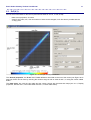
5.1. ‘Y=F(X)’...................................................................................................................................... 45
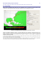
5.2. ‘Z=F(Lon, Lat)’........................................................................................................................... 48
5.2.1. Display properties ........................................................................................................... 49
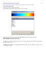
5.2.2. Color table editor............................................................................................................ 51
5.2.2.1. Two-color gradient color tables ............................................................................... 52
5.2.2.2. Multi-color gradient color tables ................................................................................ 52
5.2.3. Contour table editor........................................................................................................ 53
5.3. ‘Z=F(X,Y)’................................................................................................................................... 54
5.4. Vector Plots............................................................................................................................... 55
6. BRAT scheduler interface............................................................................................................... 56
6.1. Pending Tasks tab.................................................................................................................... 56
6.2. Processing Tasks tab ............................................................................................................... 57
6.3. Ended Tasks tab....................................................................................................................... 58
6.4. Scheduler Logs tab .................................................................................................................. 59
7. Using BRAT in ‘command lines’ mode with parameter files ....................................................... 60
7.1. Creating an output netCDF file............................................................................................... 60
7.2. Visualising an output netCDF file through BRAT................................................................. 62
7.3. Using the parameter files to process many datasets ........................................................... 63
8. BRATHL Application Programming Interfaces (APIs) ................................................................. 65
8.1. Data reading function.............................................................................................................. 65
8.2. Cycle/date conversion functions ............................................................................................ 66
8.3. Date conversion/computation functions ............................................................................... 67
8.4. Named structures..................................................................................................................... 68
Annex A. List of datasets read by BRAT.......................................................................................... 70
Annex B. Y=F(X) parameter file keys................................................................................................ 74
Annex C. Z=F(X,Y) parameter file keys............................................................................................ 76
Annex D. Display parameter file keys.............................................................................................. 79
Annex E. BRATHL-IDL API................................................................................................................. 84
Annex F. BRATHL-MATLAB API........................................................................................................ 96
Annex G. BRATHL-Fortran API....................................................................................................... 107
Annex H. BRATHL-C API.................................................................................................................. 112
Basic Radar Altimetry Toolbox User Manual
1
1. Introduction
1.1. Global Overview
The Basic Radar Altimetry Toolbox (BRAT) is a collection of tools and tutorial documents designed to facilitate the
processing of radar altimetry data. BRAT is able to handle most distributed radar altimetry data formats, providing
support for ingesting, processing, editing (to a certain extent), generating statistics, visualising and exporting the
results.
BRAT consists of several modules operating at different levels of abstraction. These modules can be Graphical
User Interface (GUI) applications, command-line tools, interfaces to existing applications (such as IDL and
MATLAB) or application program interfaces (APIs) to programming languages such as C and Fortran.
The main BRAT functions are:
Data Import and Quick Look: basic tools for extracting data from standard formats and generating quicklook images.
Data Export: output of data to the netCDF binary format, ASCII text files, or GeoTiff+GoogleEarth; raster
images (PNG, JPEG, BMP, TIFF, PNM) of visualisations can be saved.
Statistics: calculation of statistical parameters from data.
Combinations: computation of formulas involving combinations of data fields (and saving of those
formulas).
Resampling: over- and under-sampling of data; data binning.
Data Editing: data selection using simple criteria, or a combination of criteria (that can also be saved)
Exchanges: data editing and combinations can be exchanged between users
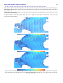
Data Visualisation: display of results, with user-defined preferences. The viewer enables the user to
display data stored in the internal format (netCDF).
APIs are available with data reading, date and cycle/pass conversion and statistical computation functions for C,
Fortran, IDL and MATLAB, allowing the integration of BRAT functionality in custom applications. For the most
common use cases (selection, combinations, visualisations, etc.), command-line tools are available that can be
configured by creating parameter files. For beginners, we recommend using the BRAT GUI application, which
enables the operator to easily specify the processing parameters required by each tool (and then invoke those
tools at the push of a button).
BRAT is provided as Open Source Software, enabling the user community to participate in further development and
quality improvement.
1.2. Toolbox Contents
BRAT consists of the following parts:
1.2.1. BRAT Library
The core part of the toolbox is the BRAT library package itself. This package provides data ingestion functionality
for each of the supported data products. The data access functionality is provided via two different layers, called
CODA and BRATHL:
1.2.1.1. CODA
The first BRAT layer (formerly known as BRATLL) is implemented using the Common Data Access framework
CODA. CODA allows direct access to product data, supporting a very wide range of products and formats. It
provides a single consistent hierarchical view on data independent of the underlying storage format.
The version of CODA that comes with BRAT supports over 200 altimetric product files. All product file data is
accessible via the CODA C library. Furthermore, the version of CODA in BRAT also comes with a set of commandline tools (codacheck, codacmp, codadump, and codafind). Typically, BRAT users will not need to deal with the
CODA library directly (although it is included if it is needed), but the CODA command-line tools can be useful for
investigating or debugging product data files directly.
Basic Radar Altimetry Toolbox User Manual
2
More information about the CODA framework and tools can be found in the CODA documentation, supplied in the
BRAT doc/coda/ directory in (HTML format). Be aware that in order for the CODA command-line tools to function
correctly in a BRAT environment, the user must manual set the CODA_DEFINITION path environment variable to
include the location of the BRAT data directory (i.e. the data/ subdirectory of the BRAT installation root directory).
This is necessary because the CODA command-line tools need to be told where to find the BRAT product format
definition files. In order to check if everything is set properly, the command:
codadd list
will yield a list of all the products CODA recognises. (For a correct BRAT configuration, this list will e.g. include
JASON and River_Lake products.)
More information about the specific altimetry product formats made accessible from BRAT through CODA can be
found in the CODA definitions documentation, supplied in the BRAT doc/codadef/ directory (HTML format), and in
Chapter 2, Data read and processed and Annex A, List of Datasets read by BRAT.
1.2.1.2. BRATHL
The second layer of BRAT provides an abstraction to the product data to make it easier for the user to get the most
important data from a product. A single function will allow the user to ingest selected altimetric product data values
(from one or more files), into an array. It is also possible (in the same function call) to request statistics on the
ingested data and to perform calculations on the data values (e.g. field1 + field2). In addition to the ingestion
function, a number of date and cycle data structures and conversion functions are also available.
The BRATHL library is implemented in C++, and built on top of the CODA framework (plus various other third-party
libraries). It is possible to develop programs that make direct use of the C++ classes that make up the BRATHL
library, but this is mainly intended for the (rare) case in which users need to develop BRATHL itself.
Instead, the simple public BRATHL functionality described earlier is accessible via C, Fortran, IDL, and MATLAB
interfaces.
More information about the various BRATHL APIs can be found in Chapter 8, BRATHL Application Programming
Interfaces (APIs).
More information about the C++ BRATHL API can be found in the BRAT reference manual, supplied in the BRAT
doc/ directory (PDF format).
1.2.2. BRAT Console Applications
Most BRAT users will not be programmers and will interact with the BRAT library via the use of one or more of the
supplied executable applications.
The toolbox contains a number of console applications that are to be run from the command-line. These
applications shield the user from the library and the programming level by providing a set of the most commonly
needed BRAT functionalities (data computations, data conversions, etc.). These functionalities are in turn userconfigurable by so-called parameter files that can easily be created, stored, and shared.
The console applications included in BRAT 2.0 are: BratCreateYFX, BratCreateZFXY, BratListFieldNames,
BratShowInternalFile, BratStats, BratExportAscii and BratExportGeoTiff.
In addition, BRAT also contains the lower-level CODA console applications mentioned in Section 1.2.1.1, as well as
the similarly low-level ncdump and ncgen utilties. These latter two are part of the netCDF library and can be used to
inspect (ncdump) or create (ncgen) data files in the netCDF format.
More information about the BRAT Console Applications can be found in Chapte r 7, Using BRAT in ‘command lines’
mode with parameter files.
1.2.3. BRAT GUI Applications
In order to provide a truly pleasant, user-friendly interface to the BRAT functionality, BRAT also contains three
applications that present a Graphical User Interface (GUI). It is expected that most BRAT users will primarily
interact with BRAT through these applications.
Basic Radar Altimetry Toolbox User Manual
3
1.2.3.1. BratGui
BratGui is the main BRAT application. It allows the user to create and manage Workspaces, Datasets, Operations
and Views at a very high level of abstraction, and with all the power and convenience of a modern-day graphical
user interface. BratGui is built on top of the BRAT Console Applications, which it invokes 'under the hood', shielding
the user from having to deal with command line options or parameter files directly.
There is a price to pay for the convenience of BratGui: not all functionality of the console applications is available
through BratGui. If the users reach the limits of what can be done with BratGui, they will have to learn to work with
the console applications after all. For a majority of important uses, however, the functionality of BratGui should be
sufficient.
More information about BratGui can be found in Cha pter 4, BRAT Graphical User Interface (GUI).
1.2.3.2. BratDisplay
BratDisplay is the BRAT visualisation component used as a component of BratGui but also available as a
standalone utility. It is partially a GUI Application because it presents a windowed environment for further
interaction with the visualisation, and partially a Console Application as it needs a parameter file as input and has to
be started from the command-line.
As with the Console Applications, many users will typically interact with BratDisplay through BratGui only, but it is a
useful tool to be aware of.
More information about BratDisplay can be found in Chapter 5, Visualisation interface.
1.2.3.3. BratScheduler
BratScheduler enables BRAT user to delay the execution of an Operation (e.g. having it running at night). It is
available through BratGUI in the Operations tab, but can also be accessed through its own icon/executable (to
check and modify a scheduled task, in particular).
More information about BratScheduler can be found in Chapte r 6, BRAT scheduler interface.
Basic Radar Altimetry Toolbox User Manual
4
2. Data read and processed
2.1. Background
The Basic Radar Altimetry Toolbox is able to read most distributed radar altimetry data, from (ERS-1 & 2 (ESA),
Topex/Poseidon (NASA/CNES), Geosat Follow-On (US Navy), Jason-1 (CNES/NASA), Envisat (ESA), Cryosat
(ESA) and Jason-2 (CNES/NASA/EUMETSAT/NOAA) missions. The different types of data readable and
processed by the Basic Radar Altimetry Toolbox are listed below (f or a description of the exact datasets with their
nomenclature, see Annex A. , List of datasets read by BRAT).
Note that data stored in arrays (e.g. waveforms) are not available individually (i.e. you can't access one value in the
array) through the Graphical User Interface, but “only” through the API (See Chapter 8, BRATHL Application
Programming Interfaces (APIs)), except for high-resolution GDR data (10, 18 and 20-Hz data ) that you can access
individually via the GUI.
NetCDF COARDS-CF compliant data can be read by BRAT. Note, however, that no warning/error message will be
issued if different data are mixed, thus leading to incoherent datasets.
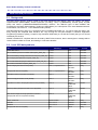
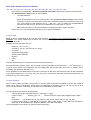
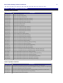
2.2. Level 1B/2 data products
Data
Satellite(s)
Data center
Format
Level 1B & level 2
Cryosat
ESA
ESA PDS
RA-2 wind/wave product for Meteo Users (RA2_WWV_2P)
Envisat
ESA
ESA PDS
RA-2 Fast Delivery Geophysical Data Record (RA2_FGD_2P) Envisat
ESA
ESA PDS
RA-2 Geophysical Data Record (RA2_GDR_2P)
Envisat
ESA
ESA PDS
RA-2 Intermediate Geophysical Data Record (RA2_IGD_2P)
Envisat
ESA
ESA PDS
RA-2 Sensor Data Record (RA2_MWS_2P)
Envisat
ESA
ESA PDS
Interim Geophysical data record (IGDR)
Jason-1, Topex/Poseidon
AVISO
PO.DAAC
binary
Geophysical data record (GDR)
Jason-1, Topex/Poseidon
AVISO
PO.DAAC
binary
Operational Sensor Data Record (OSDR)
Jason-1
AVISO
PO.DAAC
binary
Sensor Geophysical data record (SGDR)
Jason-1
AVISO
PO.DAAC
binary
Operational / Interim / Geophysical data record (O/I/GDR)
Jason-2
AVISO
EUMETSAT
NOAA
netCDF
Sensor (Interim) Geophysical data record (S(I)GDR)
Jason-2
AVISO
EUMETSAT
NOAA
netCDF
Sea Surface Height Anomaly Operational / Interim /
Geophysical data record (SSHA O/I/GDR)
Jason-2
AVISO
EUMETSAT
NOAA
netCDF
Topex waveforms
Topex/Poseidon
PO.DAAC
binary
RA OPR
ERS-1 and 2
CERSAT
ESA PDS
RA WAP
ERS-1 and 2
CERSAT
ESA PDS
Geophysical data record (GDR)
GFO
NOAA
binary
Basic Radar Altimetry Toolbox User Manual
5
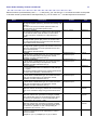
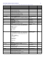
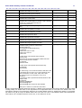
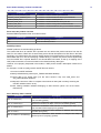
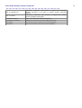
2.3. Higher-level products
Data
Satellite(s)
Data center
Format
Along-track Delayed-Time and Near Real Time Sea Level
Anomalies (DT- & NRT-SLA) (Ssalto/Duacs multimission
products)
Cryosat , Jason-1, Jason-2,
Topex/Poseidon, GFO, Envisat,
ERS-2, ERS-1
AVISO
netCDF
Along-track Delayed-Time and Near Real Time Absolute
Dynamic Topography (DT- & NRT-ADT) (Ssalto/Duacs
multimission products)
Cryosat*, Jason-1, Jason-2,
Topex/Poseidon, GFO, Envisat,
ERS-2, ERS-1
AVISO
netCDF
Gridded Delayed-Time and Near Real Time Maps of Sea
Level Anomalies (DT- & NRT-MSLA) (Ssalto/Duacs
multimission products)
merged
AVISO
netCDF
Gridded Delayed-Time and Near Real Time Maps of Sea
Level Anomalies mapping error (DT- & NRT-MSLA)
(Ssalto/Duacs multimission products)
merged
AVISO
netCDF
Gridded Delayed-Time and Near Real Time Maps of Sea
Level Anomalies geostrophic velocities (DT- & NRT-MSLA)
(Ssalto/Duacs multimission products)
merged
AVISO
netCDF
Gridded Delayed-Time and Near Real TimeMaps of Absolute
Dynamic Topography (DT- & NRT-MADT) (Ssalto/Duacs
multimission products)
merged
AVISO
netCDF
Delayed-Time and Near Real Time Absolute Dynamic
Topography geostrophic velocities (DT- & NRT-MADT)
(Ssalto/Duacs multimission products)
merged
AVISO
netCDF
Along-track Delayed-Time Sea Level Anomalies (DT-SLA)
(monomission product)
Cryosat*, Jason-1, Jason-2,
Topex/Poseidon, Envisat, ERS-2
AVISO
netCDF
Along-track Delayed-Time Corrected Sea Surface Height
( DT-CorSSH) (monomission product)
Cryosat*, Jason-1, Jason-2,
Topex/Poseidon, Envisat, ERS-2
AVISO
netCDF
Along-track Sea Surface Height Anomalies ( AT-SSHA)
Topex/Poseidon, Jason-1
PO.DAAC
binary
Along-track Gridded Sea Surface Height Anomalies (ATGSSHA)
Topex/Poseidon, Jason-1
PO.DAAC
binary
Gridded Near Real Time Maps of Significant Wave Height
(NRT-MSWH ) (mono- and multi-mission products)
Jason-1, Jason-2, Topex/Poseidon,
Envisat, GFO, merged
AVISO
netCDF
Gridded Near Real Time Maps of Wind Speed modulus (NRT- Jason-1, Jason-2, Topex/Poseidon,
MWind)
Envisat, GFO, merged
AVISO
netCDF
Heracles along-track land-ice (multimission products)*
Cryosat*, Envisat
ESA
netCDF
Heracles crossover land-ice (multimission products)
Cryosat , Envisat
ESA
netCDF
Cryosat , Envisat, merged
ESA
netCDF
Cryosat , Envisat, merged
ESA
netCDF
Gridded Heracles Leading Edge Width (LEW) land-ice
(multimission products)*
Cryosat , Envisat, merged
ESA
netCDF
River & Lake products
Envisat
ESA
binary
*
*
Gridded Heracles SHA land-ice (multimission products)
*
*
Gridded Heracles Sigma0 land-ice (multimission products)
*
*
*
*
* Forecoming dataset, or forecoming satellite for this dataset
Basic Radar Altimetry Toolbox User Manual
6
3. How to install and uninstall BRAT
3.1. Supported Platforms
BRAT binaries are available as single-file installer packages for the three major operating systems: Windows 1,
Linux2, and Mac OS X 3. These standalone installers can be downloaded from the BRAT Website
(http://earth.esa.int/BRAT/html/data/toolbox_en.html) or copied from the top-level directory of the BRAT
Distribution CD.
On not directly supported platforms and for certain purposes, BRAT will have to be compiled from source. A source
archive is therefore also available, but as compilation is a rather complex affair it is highly recommended to try one
of the binary installers first.
3.2. The BRAT Distribution CD
The BRAT Distribution CD contains:
•The binary installers for the supported platforms.
•The source archive.
•A copy of all the BRAT documentation (also already included in the binary installers).
•A large directory of sample data files (which is too large to be included in the binary installers).
3.3. MS Windows
3.3.1. Installing the binary distribution
The Windows version of BRAT is supported only for Windows XP. The binary distribution contains pre-built versions
of the full toolbox as well as all the BRAT documentation and examples. For the IDL and MATLAB interfaces, prebuilt versions are included that will work with IDL 6.3 or higher and MATLAB R15 (v7.5) or higher.
The BRAT Windows binary installer is found in the file:
brat-3.0-windows-installer.exe
In order to install BRAT, double-click on the installer file and follow the instructions.
By default, BRAT will be installed in C:/Program Files/BRAT-3.0/, or in the user's local profile directory when
installed as a user without Administrator privileges. It is also possible to specify a custom installation location during
the installation process.
After installation, the BRAT Console and GUI applications are immediately ready for use. A shortcut to the BratGui
application will have been placed on the desktop and is also accessible via the Start > Programs > Brat menu. In
order to use the Console Applications (including BratDisplay), open a command window and call the applications
directly from their installed location (C:/Program Files/ BRAT-3.0/bin/ by default, or else wherever you instructed the
installer to install BRAT).
There a number of optional software prerequisites to using BRAT after installation:
•If you plan on using the C interface, you should have a C or C++ compiler installed on your system. The C
interface has been verified to work with Microsoft Visual Studio 10.
•If you plan on using the Fortran interface, you should have a FORTRAN 77 or Fortran 90 compiler installed on
your system.
•If you plan on using the IDL interface, you need a recent version of IDL for Windows: The IDL interface has been
verified to work with IDL version 6.3 and higher.
1 Windows® is a registered trademark of Microsoft Corporation in the United States and other countries.
2 Linux® is the registered trademark of Linus Torvalds in the U.S. and other countries.
3 Mac OS X® is a registered trademark of Apple Inc. in the U.S. and other countries.
Basic Radar Altimetry Toolbox User Manual
7
•If you plan on using the MATLAB interface you need a recent version of MATLAB for Windows: The MATLAB
interface will only work with MATLAB version 7.5 (R15) and higher.
3.3.2. Installing from source
Generally, installation from source will be necessary if:
•You want to use IDL or MATLAB interfaces to BRAT for versions of these applications that are incompatible with
the pre-compiled interfaces in BRAT.
The BRAT source distribution can be found in the file:
brat-3.0-src.tar.gz
After unpacking this archive in a suitable location, instructions for configuring, compiling and installing BRAT for
Windows can be found in the top-level file INSTALL.txt
3.3.3. Uninstalling
Open the ‘Add/Remove Programs’ control panel, and select the BRAT entry. Everything created during installation
will then be removed.
Alternatively, choose the 'Uninstall BRAT' menu item from Start > Programs > BRAT (or wherever you installed
BRAT) – this will have the same result.
These uninstall methods only work for BRAT installations created through the binary installations. For BRAT
installations from source, you will need to remove the various files and directories manually.
3.4. Linux
3.4.1. Installing the binary distribution
BRAT is developed on platforms running the Debian GNU/Linux and RedHat EL 4 operating systems. Other Linux
distributions (especially ones released in the past two years or so) are quite likely to work equally well, provided the
operating system contains the following components:
•X11 Windowing System (BRAT has been tested on Xorg Xserver v1.1.1 and higher)
•GTK 2 libraries (BRAT has been tested on libgtk2 v2.8.20 or higher)
•C run-time libraries (BRAT has been tested on libc6 v2.3.6 or higher)
You will have to consult your Linux distribution's package manager to verify or update these components, but in
general it is easier to install the BRAT binary distribution and simply see if it works or not (if it does not, you can
always try to compile BRAT from source – see below for details).
The binary distribution contains pre-built versions of the full toolbox as well as all the BRAT documentation,
examples, C and Fortran interfaces. Because of inherent library versioning and path issues on the Linux platform,
no IDL or MATLAB interfaces are included in the binary installation. If desired, these can be created by compiling
from source for your specific installed version of IDL or MATLAB.
The BRAT Linux binary installer is found in the file:
brat-3.0.a-linux-installer.bin
In order to install BRAT, double-click on the installer file from a desktop manager window (or execute it from a
command-line shell) and follow the instructions. (If you downloaded the installer via a network it may have been
given the wrong file permissions and not be recognised by the system as executable. You should run the command
‘chmod +x brat-3.0-linux-installer.bin’ in order to make it executable.)
By default, BRAT will be installed in $HOME/brat-3.0/ (where $HO ME stands for the user's home directory), or
/usr/local/brat-3.0/ when installed as the root user. It is also possible to specify a custom installation location during
the installation process.
After installation, the BRAT Console and GUI applications are immediately ready for use. A shortcut to the BratGui
application will have been placed on the desktop . In order to use the Console Applications (including BratDisplay),
Basic Radar Altimetry Toolbox User Manual
8
open a command-line shell and call the applications directly from their installed loca tion ($HOME/BRAT-3.0/bin or
else wherever you instructed the installer to install BRAT).
There are a number of optional software prerequisites to using BRAT after installation:
•If you plan on using the C interface, you should have the GNU C or C++ compiler installed on your system. The C
interface has been verified to work with GNU C/C++ 4.1.1.
•If you plan on using the Fortran interface, you should have a FORTRAN 77 or Fortran 90 compiler installed on
your system. The Fortran interface has been verified to work with GNU Fortran 4.1.1.
3.4.2. Installing from source
Generally, installation from source on Linux will only be necessary if:
•You want to use the IDL or MATLAB interfaces to BRAT.
•You are on a system that is older than the one used to create the BRAT Linux binary distribution (in which case
BRAT will fail to run if installed as a binary).
The BRAT source distribution can be found in the file:
brat-3.0-src.tar.gz
After unpacking this archive in a suitable location, instructions for configuring, compiling and installing BRAT on
Linux (or other Unix-based systems) can be found in the top-level file INSTALL.
3.4.3. Uninstalling
In the installation folder (the default one or the one chosen), there is a script called uninstall-brat-3.0-linux which
can be executed to remove everything created during the installation.
There is also a shortcut, called ‘Uninstall Basic Radar Altimetry Toolbox’, which can be double-clicked from within
your desktop manager (if you use the KDE or GNOME desktop environment) to get the same result.
3.5. Mac OS X
3.5.1. Installing the binary distribution
BRAT is supported on Intel- and PowerPC-based systems running Mac OS X versions 10.4 or later.
This binary distribution contains pre-built versions of the full toolbox as well as all the BRAT documentation,
examples, C and Fortran interfaces. Because of inherent library versioning issues on the Mac OS Unix-based
platform, no IDL or MATLAB interfaces are included in the binary installation. If desired, these can be created by
compiling from source for your specific installed version of IDL or MATLAB.
The BRAT Mac OS X binary installer is found in the disk image file:
brat-3.0-macosx-ppc.dmg (for PowerPC)
or:
brat-3.0-macosx-i386.dmg (for Intel)
In order to install BRAT, double-click on the image file to mount and open it. Then copy the BratGui appplication
that is inside the disk image to your Applications folder.
After installation, the BRAT Console and GUI applications are immediately ready for use. BratGui can be started by
double-clicking the Applications/BratGui icon.
In order to use the Console Applications (including BratDisplay), drag the 'brat' folder from the image window to any
appropriate location. Then, using e.g. the Terminal application, run the applications via a console directly from
brat/bin.
There a number of optional software prerequisites to using BRAT after installation:
•If you plan on using the C interface, you should have the GNU C or C++ compiler installed on your system. The C
interface has been verified to work with GNU C/C++ 4.1.1.
Basic Radar Altimetry Toolbox User Manual
9
•If you plan on using the Fortran interface, you should have a FORTRAN 77 or Fortran 90 compiler installed on
your system. The Fortran interface has been verified to work with GNU Fortran 4.1.1.
3.5.2. Installing from source
Generally, installation from source on Mac OS X will only be necessary if:
•You want to use the IDL or MATLAB interfaces to BRAT.
The BRAT source distribution can be found in the file:
brat-3.0-src.tar.gz
After unpacking this archive in a suitable location, up-to-date instructions for configuring, compiling and installing
BRAT on Mac OS X can be found in the top-level file INSTALL.
3.5.3. Uninstalling
To uninstall BRAT, simply move the installed BratGui application and brat folder to the trash.
Basic Radar Altimetry Toolbox User Manual
10
4. BRAT Graphical User Interface (GUI)
4.1. Overview
The BRAT Graphical User Interface (GUI) is a windowed interface to the BRAT Tools. Note that not all tool
functions are accessible from the GUI (some options are only available using the command files directly).
The BRAT GUI includes:
•a “Workspace” menu
•a “Datasets” tab
•an “Operations” tab
•a “Views” tab
•a “Logs” tab
BRAT GUI basically creates parameter files (see Section 7, Using BRAT in ‘command lines’ mode with parameter
files), that are stored in an 'Operations' and a 'Views' folders, and runs several executables. It also enables to save
your preferences and work.
The next section of this manual (4.2, Starting with BRAT GUI) explains the basics of the interface. For more
detailed information about all the functionalities, see section 4.3, BRAT GUI tabs description.
4.2. Starting with BRAT GUI
Using BRAT GUI is basically a 4-step process.
You have to:
1. define a 'Workspace': preferences to be saved and retrieved for future use (see section 4.2.1, Create a
workspace)
2. define one or several 'Dataset(s)': the data you want to work on (see section 4.2.2, Create a dataset)
3. define one or several 'Operation(s)' (see section 4.2.3, Create an operation):
define 'Data Expressions': the field(s) you wish and what you what to do with them (one field with respect to
one or two others, combine them, statistics, resampling…)
(optionally) define 'Selection criteria': edit the data and/or select them with respect to your criteria
(geographical, time, thresholds,…)
Execute it to create an output file
4. define your “View(s)”: visualise the results of your operations.
Execute it to open the data visualisation tool, and produce an output image (to be saved in PNG, JPEG,
BMP, TIFF, PNM) (see section 4.2.4, Create a view)
BRAT GUI is organised in four tabs (Datasets, Operations, Views and Logs), and a 'Workspace' menu. Each tab
corresponds to a different function, and to a different step in the process, so you'll have to use all of them one after
the other.
This section gives the main information for a quick-start with BRAT GUI. For more complete information, see the
relevant sections within the 4.3, BRAT GUI tabs description.
Basic Radar Altimetry Toolbox User Manual
11
4.2.1. Create a workspace
When you open BRAT GUI, the software asks for the name and location of the ‘Workspace’ you will be working in.
A 'Workspace' is a way of saving your preferences, computations and generally the work done with BRAT GUI.
Some or all elements of a workspace can be imported into another workspace. There is no specific tab for the
Workspace, only the menu the furthest to the left.
It is highly recommended to save your workspace (ctrl+s, or ‘save’ in the workspace menu) while working. You
will be asked whether or not you wish to save the workspace when you quit BRAT GUI. Note that if you answer “no”
and have not saved anything previously, none of your work can be recalled later.
If there are already one or more valid workspace(s), BRAT GUI recalls the last used Workspace by default.
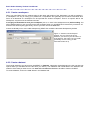
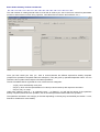
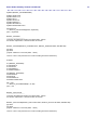
Figure 1: 'Create a new workspace'
window. You can choose to save it
wherever you want on your hard drive or
local network, and name it as you prefer
(preferably in such a way you will
remember what's in it).
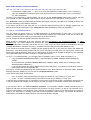
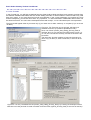
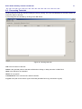
4.2.2. Create a dataset
The first tab opened if you have never used BRAT is ‘ Datasets’ (otherwise, the default tab is the the one that was
opened when you left BRAT GUI the last time you used it). This 'Datasets' tab is dedicated to the definition and
selection of the data you want to use. You must define at least one dataset to be able to further use BRAT.
To create a dataset, click on the 'new' button in the Datasets tab.
Basic Radar Altimetry Toolbox User Manual
12
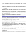
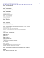
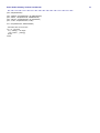
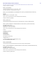
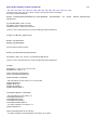
Figure 2: The Dataset tab as it appears when opening a new Workspace. The “New” button enables to create a
new dataset.
Default name for a new dataset is 'Dataset_1', with the number incrementing each time you create a dataset. You
are strongly encouraged to re-name it, so that you'll remember what's in it when using it later on. To rename it,
simply select the name, type in another one and press the Enter key.
When you have created your dataset and named it, you then have to add one or more data file(s), chosen from
your hard drive, CD/DVD driver, local network or other medium,. You can do so:
by using the 'Add Files' button. At least one file is necessary.
If you wish to add a long list of files, the ‘ Add Dir’ button allows you to choose all of the files within a folder by
simply choosing the folder in which they are stored. Be careful that some data have header files in their data folders
(you can remove them after selecting the whole folder) that won't be considered as homogeneous with the data
files by BRAT.
By dragging and dropping one or several files, or even a complete directory. Note that you have to have created
the dataset beforehand.
Only coherent datasets are possible (i.e. same format, same data product). BRAT netCDF outputs can be used,
even several of them, provided they have exactly the same variables, with the same names. The 'Check Files'
button enable to verify this homogeneity.
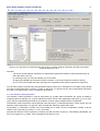
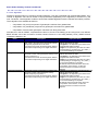
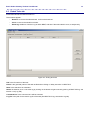
Once you have added at least one data file, if you click on one file name in the list, you can see, right, information
about the available fields within the data product, and (for netCDF files), about the file description below.
You can pre-select files relevant for your work by using the ' Define selection criteria' button and the 'Apply
selection criteria' check box (see 4.3.2.3, Selection of data files), in order not to uselessly process files out of
desired area/period/cycle or pass. This feature DOES NOT EXTRACT DATA from files, it “only” selects relevant
files.
Basic Radar Altimetry Toolbox User Manual
13
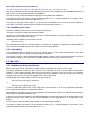
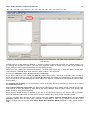
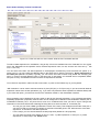
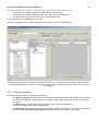
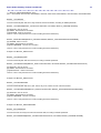
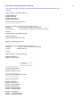
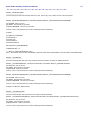
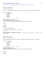
Figure 3: A dataset. On the left, the list of files; right (top) the list of available fields for the selected file format,right
(bottom), the description of the selected field as it appears in the data dictionary. Bottom left box give the file
description for netCDF data.
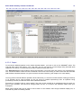
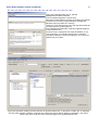
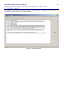
4.2.3. Create an operation
When you have defined which data you want to work on, you have to define what you want to do with them. This is
done in the ‘Operations’ tab.
If none exist, you have to create an Operation. Click on the 'new' button.
Default name for a new Operation is 'Operations_1', with the number incrementing each time you create an
operation. You are strongly encouraged to re-name it, so that you'll remember what's in it when using it later on. To
rename it, simply select the name, type in another one and press the Enter key.
Basic Radar Altimetry Toolbox User Manual
14
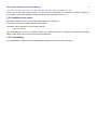
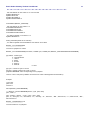
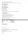
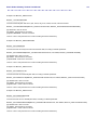
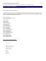
Figure 4: An empty 'Operations' tab. The 'New' button enable to create a new 'Operation'.
Otherwise, you may work with a previously saved operation. The 'Operation Name' dropdown list contains all the
already defined operations within the workspace, which can be selected, renamed, duplicated, modified... Note that
if you change the name of an operation within the ‘name’ box, it renames your operation. To copy an operation, use
the 'Duplicate' button.
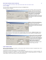
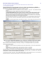
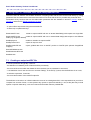
4.2.3.1. Select source data
The information about the source data are in the leftmost part of the Operations tab.
You first have to choose the dataset you want to work with from the list of existing datasets (topmost box). Then,
within this dataset, the whole list of available fields is proposed, organised as a tree. If the data are split in different
records, click on the '+' to expand the tree, '-' to flatten it.
The description of each field is given in a tooltip appearing when your mouse goes over the name of the field.
Basic Radar Altimetry Toolbox User Manual
15
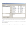
Figure 5: Choosing a dataset (here two datasets are available); below, the tree with records and data fields.
4.2.3.2. Define expressions
4.2.3.2.1.Generalities
An operation consists mainly in the definition of 'Expressions'.
An expression can be simple (one data field), or complex (with the use of arithmetic combinations, functions
applied on several fields, etc.).
In the second column box of the 'Operations' tab ('Data expression'), you can see four categories of Expressions:
- X
- Y (optional)
- Data
- Selection criteria (optional)
At least one expression as 'X', and one as 'Data' must be defined for an Operation to be valid.
These expressions can be filled by several means, the quickest being by drag & drop : drag a field from the
leftmost list and drop it in either one of those, or in the 'Expression' box (you can also use contextual menus by
right-clicking either on the data fields or on the expressions, or use the 'Insert expression' and/or 'Insert field'
button, or type in an empty expression the field names and functions you want to apply)
Note that only one expression can be defined as X, and (optionally) one as Y, whereas up to twenty can be defined
as Data.
An Expression can be:
-
only one field in a dataset (typically, for a map, longitude as X-axis, latitude as Y-axis, and e.g. significant
wave height as Data, etc.)
Basic Radar Altimetry Toolbox User Manual
16
-
a combination of fields, either +,-,* and /, or by using the available Functions (see 4.3.3.4.2, Functions ).
a pre-set combination of fields among the ones you will find in the ‘Formulas’ (see 4.3.3.4.3, Formulas),
e.g. SSH computation.
To check if your expression is well formulated, you can click on the ' Check syntax' button (note, however, that this
won't provide you with a validation of the relevance of your expression from the point of view of physics).
The 'Show Info.' button provides information about the original units (the ones defined in the data products) and
the units used during computation or selection.
If you want to go back on your work later on, of to save an expression as formula, we strongly suggest that you
take the time to fill the information in the 'Title/comment' fields (available by clicking on the button)
4.2.3.2.2.X, Y and Data Expressions
You can change the name of any X, Y or Data Expression, by double-clicking on their name, or by using the
contextual menu available by right-click. This will then be the default name on the plots, on the axis or near to the
scale if you have not given a title to your Expression (in the title/comment).
You can change the unit as it appears above the Expression box.
BRAT is able to understand all SI units and their sub-units as defined in the International System , i.e. case
sensitive (e.g. “ms” means milliseconds, whereas “Ms” would means megaseconds). There are also “count” for
data without dimension, and “dB” (see section 4.3.3.4.1, Units ).If you let “count” (which is the default) as unit, the
resulting data will be in the basic SI unit (e.g. in metres, even if the field you used was defined in mm).
If you choose a pre-saved formula, a default unit will appear as the unit. If you select one field in the dataset list
and insert it, it will automatically be filled with the correct unit (but if you finally write your own formula, beware that
the final unit might be different). If the unit you defined does not fit the unit of the data as defined, an error message
will be generated (again, this does not work for complex expressions).
On any X, Y or Data Expression, you can apply 'data computation' (see 4.3.3.4.5, Data computation ), to:
-
compute statistics at each point (same X, optionally same Y): MEAN, STDDEV (standard deviation),
COUNT.
- do some arithmetic operations between files within a dataset: adding, subtracting or multiplying: SUM,
SUBTRACTION, PRODUCT)
- it can also be used for the display (MEAN, FIRST, LAST, MIN, MAX), if you prefer to visualise, for instance,
the last value rather than the mean one.
Note that to compute the statistics for the Data Expressions as a whole (Number of valid data, Mean, Standard
deviation, Minimum, Maximum), you can use the 'Compute Statistics' button.
There are two main kinds of Operations:
- one – or several – Data expression(s) with respect to another one (X), leading to a “curve” plot
- or one – or more – Data expression(s) with respect to two others, leading to a “map” plot
In the first case, you'll fill only the “X” expression; in the second, you'll fill both X and Y expressions. Note that X and
Y can be Longitude and Latitude, but can also be any other two fields or combination of fields within the dataset.
If you fill both X and Y, you have to define a resolution. For Longitude, Latitude a default resolution (1/3 of a
degree for both axis), minimum and maximum are proposed. For other X and/or Y, a step of 1 is proposed, but no
minimum and maximum. You can define a step, minimum and maximum values, or use the minimum and maximum
value of your expression by clicking on the 'Get min/max expression values' button). The number of intervals is
automatically computed from those elements, and cannot be directly changed.
Basic Radar Altimetry Toolbox User Manual
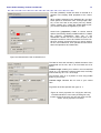
17
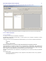
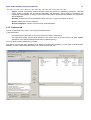
Figure 6: An 'Operations' tab window when both X and Y are filled. Note the 'Resolution and filter Information'
below the Expression box
Note that
-
you cannot choose different resolutions for different data expressions within the same operation (they all
share the same X and Y!).
by choosing a step, you may sub-sample your source data.
Changing the Min/Max can be used to extract a smaller X-Y area (as well as the selection criteria).
And, of course, the smaller the steps, the higher the computation time! (and the heavier the output file)
You can also choose to smooth and/or extrapolate the data by means of a Loess filter so as to obtain a fully colored
plot (and not individual tracks or points on a map). In that case, you will have to fill in the corresponding information
for X and Y, too (see section 4.3.3.4.6, Resolution and Filters).
4.2.3.2.3.Selection criteria expression
The Selection criteria expression is used to select data e.g. by date and/or boundaries, etc. and/or for editing it
using flag values, thresholds, etc. Logical, relational functions can be used, separated by && ('and'), || ('or') or with !
('not'). Only the data fulfilling the whole set of conditions, and not equal to default values, are selected.
The Selection criteria expression can be filled the same way than X, Y and Data expression. There can be only one
Selection criteria expression. It is optional; when it is filled the 'Selection criteria' title is bold.
All the fields, or combination of fields of the source data can be used. To use a combination of fields, it can be
clearer to use a formula (see section 4.3.3.4.3, Formulas).
Note that the selection criteria expression is working only with the basic SI units (i.e. when defining thresholds, you
have to put values in e.g. meters, even if the data source field is in mm).
Basic Radar Altimetry Toolbox User Manual
18
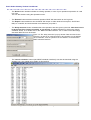
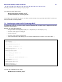
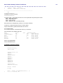
Figure 7: An example of a Selection criteria expression (Ocean data editing for Envisat GDRs.
4.2.3.3. Output
To process the defined operation on the whole selected dataset., you have to click on the ‘Execute’, button. The
Logs tab then opens (see section 4.3.5, Logs tab), and you can see the current task(s) being executed (both
operations and views), comments during execution (verbose mode) and errors.
The “Delay Execution” button enable to launch the Operation or an export (see next section) at a scheduled time.
The “Launch scheduler” button launch the scheduler, which have to be running in order to have the task executed
(NB. the Brat scheduler interface icon gives access to the same interface). (see chapter 6 for more details).
You may perform several different operations at the same time (i.e. execute one while another is being processed),
or an operation and a view (provided you are not trying to visualise expression(s) from an operation being
processed). However, this will slow down each individual execution.
Executing an operation build an output netCDF. The name of this netCDF file is predefined using the name you
gave to your operation, and cannot be changed within the GUI. It is stored in the Operation folder within your
workspace.
BRAT output netCDF files can be used as source data in a new dataset, seen though the BRAT Display tool, or
used with any other tool reading netCDF.
Basic Radar Altimetry Toolbox User Manual
19
4.2.3.4. Export
You can choose to export the output data by clicking on the ' Export' button.
Several formats are available:
-
NetCDF (the same than the automatic one, but you can choose where you want it, and how it is named)
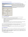
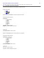
Figure 8: Export pop-up window for
netCDF export: you can choose the
name and location of the exported file.
The operation can be re-executed
before export or not (depending if
modifications were done or not)
'delay execution' enables to programme
the scheduler and have the processing
done later.
-
Ascii
Figure 9: Export pop-up window for
Ascii export. You can choose the name
and location of the exported file.
'delay execution' enables to programme
the scheduler and have the processing
done later.
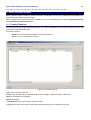
The Ascii export can also be seen (once saved) through a built-in text viewer (' Edit Ascii export' button)
-
GeoTiff (if the axis of the operation are longitude and latitude), which also provides a Google Earth KML
export format.
Figure 10: 'Export pop-up window for
GeoTiff export. You can choose the
name and location of the exported
file. You can also create a KML file to
visualise the GeoTiff in GoogleEarth.
Min, Max and color table can be
defined for the data expression.
'delay execution' enables to
programme the scheduler and have
the processing done later.
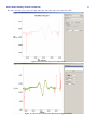
4.2.4. Create a view
When you have executed your operation, you may want to have a look at the results in a graphical way. This is
done through the ‘Views’ tab.
If none exist, you have to create a View. Click on the 'new' button.
Default name for a new View is 'Displays_1', with the number incrementing each time you create an operation. You
are strongly encouraged to re-name it, so that you'll remember what's in it when using it later on. To rename it,
simply select the name, type in another one and press the Enter key.
Basic Radar Altimetry Toolbox User Manual
20
The main interest of creating several Views is to be able to retrieve your view in the future, with all its parameters
(minimum and maximum on each axis, projection, color table with its minimum and maximum, etc.).
Figure 11: An empty 'Views' tab. The 'New' button enable to create a new 'View'.
Once you have named your view, you have to choose between the different expressions already computed
(outputs from operations computed within the workspace). They are given by operation/expression name. You can
refresh the list to update it with respect to the latest operations.
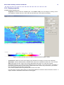
The list of available data is organised as a tree, with three main categories:
- Y=F(X), which are basically curve plots
- Z=F(X,Y), which are the representation of a value (in colors/contours) with respect to two others
- Z=F(Lon,Lat), i.e. maps
Under each category (click on '+' to expand the tree, '-' to flatten it), you will see the names of the operations
already computed, and under each operation, the list of Data expressions defined within this operation.
The operations are listed in one category or the other depending on the way they were defined (see section 4.3.4.2,
Data to be visualised for more details)
Basic Radar Altimetry Toolbox User Manual
21
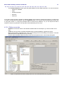
Figure 12: A 'View' tab with one view created. Note the list of available data left.
To select a data expression for visualisation, drag & drop it from the 'Available' list to the 'Selected' list. You will the
see in the 'Selected' box the operation name, the data expression name, its unit, and the unit of the axis (1 st dim
unit, 2nd dim unit).
You can select more than one data expression to be displayed. Provided they have the same axis (same X, or
same X and Y), you can overlay the different data on the same plot by using the check box ‘ Group expressions in
the same plot’ (default is checked). Typically, you can have a color and a contour map plotted one overlaying the
other, or curves of several different colors on the same plot. If unchecked, or if the data are not compatible, BRAT
will open as many visualisation windows as there are expressions selected.
To un-select an expression, either use the arrow button, or press on the 'Delete' key on your keyboard.
‘With Animation’ can be used to animate a series of plots (Z=F(X,Y) or Z=F(Lon,Lat)). If you have several identical
expression names from several operations (e.g. if you have computed the same expression at different dates) and
if you check this option, you will have access to the ‘animation toolbar’ in the visualisation interface.
Some properties can be defined for the plot, either for the all plot (general properties), or for each data expression
separately (Expression properties). Most of them can be changed or be defined in the visualisation window (see 5,
Visualisation interface) but, if only done there, have to be re-defined each time you launch a plot. Filling those
information in the Views tab has the advantage of being able to re-use them later on, for another plot.
-
-
You can give your View a 'title' (just below the ‘name’ of the view). This will appear as the title of the plot. It
can also be used as a reminder. By default, it is the title of the field given in the ‘title/comment’ of the data
expression, or the name of the data expression.
For the maps, you can choose between several projections (default is a 3D projection)
You can define a sub-set to be plotted (by X min, X max, Y (=data expression or =axis) min, Y (=data
expression or =axis) max) in the 'Zoom' boxes.
Basic Radar Altimetry Toolbox User Manual
-
22
The name of the plotted expression.
By default, this will be the title of the expression given in the ‘title/comment’ of the data expression, or the
name of the data expression (if no title was given). It will be used either as title of the color scale, or as title
of the axis.
For the Z=F(X,Y) and Z=F(Lon,Lat) cases,
-
East/North Component can be selected to display vector plots, in which one expression has to be
selected as north component and a different one for east component. Only one vector plot can be
displayed at a time. Both expressions must be of the same data type.
- A choice between ‘solid color ’ and ‘contour’ representation. It is of course highly recommended to
choose at most two different fields to be displayed on the same plot, one represented in solid colors, the
other in contours, to be able to see something on the plot.
- Minimum and maximum of the color scale
- The color scale, among a pre-defined list of color scales, or in previously made and saved color scale
(see section 6.2.1.Color table editor).
For Z=F(Lon,Lat), you have necessarily X=Longitude, Y=Latitude. However, when you use other fields as X and/or
Y, you may wish to switch them – this is the goals of the 'invert X/Y' check box
The ‘Execute’ button will launch the visualisation tool (see chapter 5 for a description of this interface). You can see
in the ‘Log’ tab the current executions (both operations and views) and the errors.
4.3. BRAT GUI tabs description
4.3.1. Workspace menu
A 'workspace' is a way of saving your preferences, computations and generally the work done with BRAT.
A workspace contains definitions of:
-
Datasets, that define the collections of files of the same kind you want to use,
-
Operations, for reading and/or processing and/or selecting data within a dataset ,
An operation produces an intermediate file (netCDF) and a parameter file. Alternatively, data can be
exported, in netCDF, Ascii or GeoTiff and KML.
-
Formulas, to enable you to use pre-defined combinations of data fields or to define them yourself and reuse them later.
-
Views, that plot results of one or more operations
A ‘view’ produces a parameter file and opens the visualisation tool
All these are stored within a folder named from the workspace, with a sub-folder for each part: Datasets, Displays,
Formulas and Operations. Displays and Operations folders include parameter files (.par), which define the Views
and Operations done, and the latter also include the netCDF intermediate files produced by the tool.
Workspace folders can be copied and exchanged. Results saved within a workspace can be accessed even if the
source data are not available (but warning messages will be emitted when opening the workspace if some source
data are not available).
Workspaces in BRAT GUI are managed by the menu the further to the left. It contains the following items:
-
'New': creates a new workspace
-
'Open': opens a previously saved workspace
-
'Save': (or ctrl+s) saves the current workspace and all its datasets, operations, formulas and views
Basic Radar Altimetry Toolbox User Manual
23
-
'Import': imports a previously saved workspace within the current one (Datasets, Operations, Formulas
and/or Views). Formulas can be imported separately, but otherwise, Views need the Operations and
Operations need Datasets, so that you can't import Views without Operations and Datasets, nor Operations
without Datasets.
-
'Rename': renames the current workspace (note that it is not a copy, but a change of name)
-
'Delete': deletes the current workspace
-
'Recent workspaces': lists the 2 most recently used workspaces
4.3.2. Datasets tab
This tab is dedicated to the choice of the source data product files.
In this tab window:
-
The selected files’ names are on the left; as well as the tools to select them.
-
The right-hand display lists all fields defined for this kind of data and, below there is a more detailed
description of the selected field (extracted from the data dictionary).
You may define as many datasets as you wish.
Note that if you want the same operation to be applied to several files separately, you will have to define several
datasets, or use the parameter files directly with a script (see section 7.3).
Figure 13: Example of dataset with netCDF data selected.
Basic Radar Altimetry Toolbox User Manual
24
4.3.2.1. Creation of a dataset
-
The ‘Dataset Name’ dropdown list contains all the defined dataset names and allows you to select and
rename a dataset. You have to give the dataset a name (with no spaces or special characters in the name).
If you change the name within the ‘name’ box, and press the Enter key it renames your dataset.
-
The
'New'
button
creates
a
new
This can also be done using the Datasets menu.
dataset,
with
a
name
like
'Datasets_2'
-
The 'Delete' button enables to delete an existing dataset , if your dataset is not used in an Operation.
This can also be done using the Datasets menu.
4.3.2.2. Management of the data files list
The 'Files in dataset' list includes all the files of the dataset. Note that only coherent datasets are possible (i.e.
same format, same data product).
-
The ‘Clear’ button will remove the whole list.
-
You can delete the selected file by using the ‘ Remove’ button, or the ‘delete’ key on your keyboard.
-
The ‘Up’ ‘Down’ and ‘Sort’ buttons are useful when the order in which files are processed is important (e.g.
subtracting one file from another).
‘Up’ moves the selected file upwards in the list,
‘Down’ moves it downwards.
‘Sort’ puts the whole list into alphabetical or numerical order. It can also be used to check for two
occurrences) of the same file, or missing files, or to remove unwanted files from a list.
4.3.2.3. Selection of data files
Data can be selected in a quite long list of altimetry data (see 2, Data read and processed). File names don't have
to be the original ones. However, files within a dataset have to be of the same data product (no mixing of e.g.
Envisat and Jason-1 GDR data).
-
The ‘Add files’ button (at the bottom of the window) enables you to select those data files you wish to work
on. Drag&drop of files within the interface has the same result.
-
If there are a lot of files, you should preferably select a whole folder by clicking on ‘ Add Dir’, or proceed in
several steps. Otherwise, some files names could be truncated, thus leading to an error. Drag&drop of a
directory within the interface has the same result.
-
the ‘Check files’ button at the bottom of the window checks for the dataset coherence.
For a more automatic selection of data files, you can use the data pre-selection function:
-
the 'Define selection criteria' button enables to pre-select only the files relevant for your work.
To use this feature, you have to define the kind of data and the selection criteria, then tick the “Apply
selection criteria” before selecting e.g. a whole folder of data. When you add the files or the whole
directory, the selection will be applied, and only the relevant files will appear within your dataset.
-
Date/Time are to be defined as YYYY-MM-DD HH:MM:SS (if no HH:MM:SS are given, default is 00:00:00).
Alternatively, Julian days since 1950 can be used Longitude / Latitude given are the North and South, West
and East limits. Latitudes South of the Equator are negatives. Longitudes can be written either as 0-360 or
-180 – 180. (thus example left is 350-0°E, 40-50°N)
-
You can check what was done using the ' Show selection report' button. This feature uses the information
given in the data 'headers' to select only the files that could include the area (or period) of interest, or the
files matching the selected cycle(s)/pass(es). Note that this implies that the possibilities of selection
depends on the satellite/data product, since the headers do not always include the same information.
Basic Radar Altimetry Toolbox User Manual
25
Figure 14: Example data selection criteria definition:
top, choose your satellite/data product (here, Jason-2)
Once this is done, you can choose below the date/time period,
Latitude/longitude, cycle number, and/or pass number.
Note that the choice in latitude in inactivated in Jason-2 GDR
case, as in most GDR cases, since those data files typically
includes data for a full half-orbit (thus all the files have the
same minimum and maximum in latitude, making such a
selection irrelevant).
4.3.2.4. Data file information
On the right of the Datasets tab, you can see information about the fields within the source data product.
The list of all the fields of the currently selected file is divided into 6 columns:
-
'Full name': the fully described name in the file structure hierarchy and related to the record.
'Record': the record containing the field. Many altimetry data products have only 'header' and 'data' records
while others have more (e.g. Envisat ones)
'Name': the short field name
'Unit': the unit of the field
'Format': the format of the field inside the file. In BRAT all fields are read as floating-point values (double).
'Dim': Dimension of the field (number of values in arrays, if the data is stored in an array)
You can sort the fields alphabetically by clicking on ‘name’, ‘record’, ‘unit’, ‘format’, or ‘dim’ (off screen), at the top of
the box, or view a field whose name begins with one or more letters by typing them (fast).
Under the list there is the 'Fields description' box with a detailed description of the currently selected field (as
extracted from the data dictionary)
Left, under the file list is a 'File description' box, that give the information about the file for netCDF products.
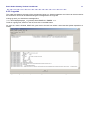
4.3.3. Operations tab
This tab is dedicated to the definition of what kind of computation(s) and/or selection(s) you want to apply on the
data.
Building an operation in fact creates a 'parameter' files (.par), which keeps all the informations and which is stored
in the Workspace Operations folder. Executing an operation use either t he BRATCreateYFX or the
BRATCreateZFXY programme on this parameter file to generate the output of the operation. The whole process
can however be done completely through the GUI.
In this Operations tab window:
-
The management of the operations is at the top.
Basic Radar Altimetry Toolbox User Manual
26
- The data source (datasets and fields available within) are on the left.
- The middle part shows the different Expressions within the current Operation
- The right-hand part shows the content of the selected Expression.
You may define as many Operations as you wish.
Note that an Operation must contains at least one X expression, and one Data expression.
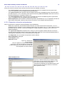
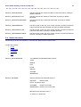
Figure 15: Operations tab, with an operation being built. Left the dataset chosen is called 'test_dataset', with
Envisat GDR data product; below the list of fields within the ra2_mds record being expanded. In the middle, only
one Expression is defined yet ('lat' as X). Right, the content of the 'lat' expression (only one field, in this case), its
unit is degrees.
4.3.3.1. Manage Operations
Several functions are meant to 'manage' the operations.
-
-
The 'Name of operations' dropdown list contains all the defined operation names and allows you to select
and rename an operation. When renaming an operation, take care that it does not copy it, but it replaces
the old one.
The 'New' button is used to create a new operation, with a name like 'Operations_2'
This can also be done using the Operations menu.
The 'Duplicate' button enables you to copy an existing operation, and modify it (e.g. change the dataset for
another one with the same kind of data at another date, change the selection criteria, etc.).
Basic Radar Altimetry Toolbox User Manual
27
-
The 'Delete' button enables to delete an existing operation, if none of your operation's expression is used
in a View.
This can also be done using the Operations menu.
-
The 'Execute' button executes the active operation. BRAT GUI then switch to the 'Logs' tab.
The 'Export' button enables to save the BRAT GUI output on either another format (Ascii, GeoTiff and
KML) or in netCDF, and under another name wherever you prefer it.
-
The 'Delay execution' button schedules the active operation at a time given by the user. Note that it won't
be processed if the 'Launch scheduler' is not running. So please remember to click on the 'launch
scheduler' button, or to double-click on the “BRAT scheduler interface” icon in order to have the task(s)
executed. BRAT GUI can be closed.
Figure 16: The “delay execution” pop-up window. Date and time for the
execution, as well as an optional name for the operation can be defined.
Once scheduled, such an operation can be viewed or removed within
BRAT scheduler interface.
-
The 'Launch scheduler' button opens BRAT scheduler interface (it can also be launched using the
desktop icon). See chapter 6 for details on this interface.
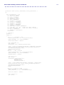
Figure 17: An example of Ascii export as seen though the built-in text viewer.
Basic Radar Altimetry Toolbox User Manual
-
28
The 'Compute Statistics' button gives the global statistics for each Data expression. You can thus retrieve:
o Number of valid data,
o
Mean,
o
Standard deviation,
o
Minimum,
o
Maximum,
If you want to apply the same operation to different datasets, and be able to compare their outputs, you will have to
re-create it as many times as needed, using the ‘ Duplicate’ button. You can also use the parameter file directly with
a script (see section 7.3, Using the parameter files to process many datasets ). Or, you can export the data in
netCDF for future use (otherwise, the output file will be replaced by the new one)
4.3.3.2. Define source data
-
'Datasets' box lists the names of the datasets available within this workspace: you have to select one of
them
'Fields' box shows the list of all fields available within the selected dataset, organised as a tree.
Right-click provides a contextual menu, with 'sort ascending' and 'sort descending' at the bottom, to sort the
data field names in alphabetical order (or reverse).
To know some information about one field, hover the mouse pointer over it, and a tooltip will appear.
Figure 18: Operations tab with a tooltip active over one of the data fields ('alt_cog_ellip').
Basic Radar Altimetry Toolbox User Manual
29
4.3.3.3. Define expressions
In the middle of the Operations tab is the tree with the expressions, including the selection applied. You have four
kinds of expressions:
- 'X': as axis (the data will be organised relative to the values within this field); only one X expression is
possible, and one is necessary.
- 'Y (optional)': to be used as second axis (e.g. X=longitude, Y=latitude); only one Y expression is possible
- 'Data': at least one Data expression is necessary, but you can add up to twenty of them.
- 'Selection criteria' (optional; the title is bold when it is filled) : it enables to select data e.g. by date and/or
boundaries, etc. and/or for editing it using flag values, thresholds, etc. Logical, relational functions can be
used, separated by && ('and'), || ('or') or with ! ('not'). All the fields, or combination of fields of the source
data can be used. To use a combination of fields, it can be clearer to use a formula. Note that the selection
criteria expression is working only with the basic SI units (i.e. when defining thresholds, you have to put
values in e.g. meters, even if the data source field is in mm).
X an Y are used as axis: BRAT will read the source data and extract, for each X (optionally Y), the corresponding
value of each Data expression fulfilling the conditions defined as 'selection criteria'.
All expressions can be filled the same ways.
The expressions can be filled by several means :
- The quickest is by drag & drop : drag a field from the leftmost list and drop it in either one of those, or in
the 'Expression' box;
- you can also use the contextual menus that appear by right-clicking either on the data fields or on the
expressions,
Figure 19: An example of menu that appears by right-click on a data field
(here, the 'lat' field'). 'Set as X', 'Set as Y' and 'Set as Data' define the
chosen field as either X, Y or Data. 'Insert into Selection criteria' insert the
field within the Selection criteria expression. 'Sort' enable to sort all the fields
in either ascending or descending (alphabetical) order.
Figure 20: Example of menu that appears by right-click on a data
expression (here called 'test'). Note that here one data field
('alt_cog_ellip') is selected (left-click); if no data field is selected,
this item is inactive.
'Insert empty expression' will add a new expression (in 'Data'), or
replace the active expression by an empty one (in X and Y).
'Insert (field) into expression' add the selected data field (if any) in
the active expression. 'Insert function' enable to use the list of
mathematical and logical functions, and 'Insert formula' insert one
of the predefined expressions saved.
'Sort' enable to sort all the expressions (if there's more than one)
by their name in either ascending or descending (alphabetical)
order.
-
or use the 'Insert field' button (which will insert the selected data field in the active expression).
or you can always use the 'Insert expression' (which will insert an empty expression, to be filled by one or
several combined fields) and type in an empty expression the field names and functions you want to apply,
using your keyboard
Basic Radar Altimetry Toolbox User Manual
30
Since you can do more than insert one field, a set of functions is available, as well as
-
-
The 'Insert Function' button opens the pop-up window with the list of available functions (see section
4.3.3.4.2, Functions ) for the complete list and specifications)
The 'Insert Formula' button opens the pop-up window with the list of available formulas. A set of those is
pre-defined (see 4.3.3.4.3, Formulas); more can be saved using 'Save as Formula' button and re-used, in
the same Workspace or imported in another one
The 'Insert Algorithm' button opens the pop-up window with the list of available algorithms (see section
4.3.3.4.4, Algorithms) for the complete list and specifications)
'Delete expression' button enables to delete an expression (the Delete key on your keyboard has also the
same effect). Remember, however, that you have to have an X and a Data expression defined.
4.3.3.4. Expression information and parameters
When an expression is selected, several parameters can be filled/used.
-
-
-
-
'Unit' of the expression: this text field is filled whenever you define a data field as expression, or use a
predefined formula. Default is 'count' (meaning, without unit). See section 4.3.3.4.1, Units below for details
about the units you can use. The unit of the Selection criteria expression is always 'count', since it is a
logical expression)
The 'Type of the expression' dropdown list is mainly of use for longitude, latitude and time as X and Y,
and help manage specific needs for those type of data. Most of the time it should be automatically filled. If
a discrepancy is detected, an error can be issued in the Logs tab.
The 'Expression' box: this where the expression itself is defined
'Data Computation' rolling list
'Check Syntax' button
'Show info' button
Figure 21: ''Show Info'
pop-up window.
Here it is applied on a Sea Surface Height
expression. You can see that the original data
product expresses all the fields in mm, whereas
the computation is done in metres
'Title/Comment' button
Figure 22: 'Title/Comment' pop-up window. Filling
those fields can be useful for later references. The
unit is the one defined for the expression.
The title will be displayed as the default name of the
field in the plots (if no title is entered, it will be the
data expression name).
Basic Radar Altimetry Toolbox User Manual
-
31
when X and Y are both filled, a 'Resolution and filter information' appears at the bottom of the window.
The 'Set Resolution / Filter' button is used to define:
o The data resolution.
When choosing both X and Y, you 'grid' the data. Thus you have to define a step in both X and Y,
as well as a minimum and maximum for both axis. Pre-defined steps are proposed, but may not fit
your need. Minimum and Maximum are 0 – 360°,-90° – 90° by default for longitude/latitude
(whatever the data source), but have to be defined for any other type of X and Y.
o
Filter: BRAT provides you with the possibility of smoothing the data, using Loess filter
See section 4.3.3.4.6, Resolution and Filters for more precise information.
4.3.3.4.1.Units
BRAT is able to understand all SI units and their sub-units, as defined in the International System , i.e. case
sensitive: “ms” means milliseconds, whereas “Ms” would means megaseconds), plus “count” for data without
dimension, and “dB”.
Typically, the units you might use are:
- metres (m, mm, cm, km,...)
- seconds (s, ms, etc., but also hours, h, days)
- m/s (km/s,...)
- degrees East (longitude)
- degrees North (latitude)
- degrees
- count
- dB
Note that all data fields are converted in SI units in the data dictionary.
Thus practical units such as “TECU” are converted (1 TECU (Total Electron Content Unit) = 1 × 10¹⁶ electrons/m²).
If you let “count” (which is the default) as unit, the resulting data will be in the basic SI unit (e.g. in metres, even if
the field(s) you used was defined in mm)
Every Operation is computed using SI units even if a sub-unit is defined for the data source and for the Expression
(e.g. metres instead of cm, mm or km). Thus you can put ‘km’ as unit even if the data source field is defined in mm
and still end up with correct values.
4.3.3.4.2.Functions
The 'Functions' button provides a simple way of including (and knowing) the available functions and constants
which can be used in expressions. The functions are organised by categories, but you can have a look at all of
them. For each function, if selected, you will see a short explanation of what it does.
You can use those functions for, among others:
- compute geostrophic velocities modulus : sqrt(sqr(U) + sqr(V))
- a test on a flag:
Surface_type == 0
will return only the ‘open ocean’ flagged Jason-1 GDR
data
- boundaries:
is_bounded(-130, alt_cog_ellip-ku_band_ocean_range ,100) (or: (alt_cog_ellipku_band_ocean_range >= -130) && (alt_cog_ellip-ku_band_ocean_range <= 100)) select only the data for
which the uncorrected altimetric distance is between -130 and +100 metres
They are available for processing or selecting a data expression.
Basic Radar Altimetry Toolbox User Manual
32
Basics functions (not listed below) are +, -, *, /, and ( and ); you can also use '^' to indicate a number to the power
of another number (or data field or data expression) e.g. '10^-6' means '10 -6'. Use the keyboard to insert them.
Name
!
!=
&&
||
<
<=
==
>
>=
~
&
|
()
Description
logical negation operator NOT
The logical negation operator (!) reverses the meaning of its
operand.
The result is true if the converted operand is false; the
result is false if the converted operand is true.
not-equal-to operator
The not-equal-to operator (!=) returns true if the operands
do not have the same value; otherwise, it returns false
A != B is true (when no default in A or B) if abs(A-B) >=
epsilon
logical AND operator
The logical AND operator (&&) returns the boolean value
true if both operands are true and returns false otherwise.
Logical AND has left associativity.
logical OR operator
The logical OR operator (||) returns the boolean value true if
either one operand is true or both operands are true and
returns false otherwise.
Logical OR has left associativity
less than
It yields values of the Boolean type. The value returned is
false (0) if the relationship in the expression is false;
otherwise, the value returned is true (1).
less than or equal to
It yields values of the Boolean type. The value returned is
false (0) if the relationship in the expression is false;
otherwise, the value returned is true (1).
equal-to operator
A == B is true (when there is no default in A or B) if abs(AB) < epsilon
The equal-to operator returns true (1) if both operands have
the same value; otherwise, it returns false (0).
greater than
It yields values of the Boolean type. The value returned is
false (0) if the relationship in the expression is false;
otherwise, the value returned is true (1).
greater than or equal to
It yields values of the Boolean type. The value returned is
false (0) if the relationship in the expression is false;
otherwise, the value returned is true (1).
bitwise not operator
Takes the value as an integer (a default value if the floating
point one is outside the integer range) and reverses each
bit.
bitwise and operator
Takes the value of each operand as an integer (a default
value if the floating point one is outside the integer range)
and does an and operation on each corresponding bit
And operation: 0011 & 0101 = 0001
bitwise or operator
Takes the value of each operand as an integer (a default
value if the floating point one is outside the integer range)
and does an or operation on each corresponding bit
Or operation: 0011 & 0101 = 0111
parenthesis operator
Isolates an expression (or a sub expression) in order to
take it as a whole.
Exemple: A * (B + C) multiplies (B + C) by A. without
Syntax
Type
! expr1
Logical
expr1 != expr2
Relational
expr1 && expr2
Logical
expr1 || expr2
Logical
arithmetic expr1 <
arithmetic expr2
Logical
arithmetic expr1 <=
arithmetic expr2
Logical
==
Relational
arithmetic expr1 >
arithmetic expr2
Relational
arithmetic expr1 >=
arithmetic expr2
Relational
~ expr1
Bitwise
operator
expr1 & expr2
Bitwise
operator
expr1 | expr2
Bitwise
operator
(expr1)
Basic Radar Altimetry Toolbox User Manual
DV
PI
PI2
PI4
abs
ceil
cos
cosd
deg2rad
deg_normalize
dv (DV)
exp
floor
frac
iif
iif3
int
is_bounded
is_bounded_strict
is_default
log
log10
max
parentheses, B would by multiplied by A and then C added
Default value
PI value
PI/2 value
PI/4 value
absolute value
Calculates the absolute value.
ceiling of a value
Calculates the ceiling of a value.
cosine (radian)
Calculates the cosine (radian) of a value.
cosine (degree)
Calculates the cosine (degree) of a value.
Translates Degree to Radian.
Normalizes longitude (degree)
Z = deg_normalize(X, Y) returns a value which makes the
following expressions true: Z = Y + n*360, X <= Z < X+360
Default value
exponential
Calculates the exponential.
floor of a value
Calculates the floor of a value
fractional parts
Calculates the fractional parts of a value.
Inline if
If the first parameter is true (not 0 and not default value),
the second parameter is returned, otherwise the third one is
returned.
Logically equivalent to:
if (param1 is true)
return param2
else
return param3
end if
Inline if with default value case
If the first parameter is true (not 0 and not default value),
the second parameter is returned. If is is 0, the third one is
returned, otherwise (it is a default value) the fourth one is
returned.
Logically equivalent to:
if (param1 is default value)
return param4
else
if (param1 is true)
return param2
else
return param3
end if
end if
integer parts
Calculates the integer parts of a value.
Checks whether a value x is included between two
values (min/max).
is_bounded(min, x, max)
Checks whether a value x is stricly included between
two values (min/max).
is_bounded_strict(min, x, max)
Checks whether a value is a default value (1: yes, 0: no)
logarithm
Calculates the logarithm of a value
base-10 logarithm
Calculates the base-10 logarithm of a value
Maximum
Calculates the larger of two values
33
DV
PI
PI2
PI4
abs(param1)
Constant
Constant
Constant
Constant
Math&Trigo
ceil(param1)
Math&Trigo
cos(param1)
Math&Trigo
cosd(param1)
Math&Trigo
deg2rad(param1)
deg_normalize(param1,
param2)
Math&Trigo
geographical
DV
exp(param1)
Constant
Math&Trigo
floor(param1)
Math&Trigo
frac(param1)
Math&Trigo
iif(param1, param2,
param3)
Logical
iif3(param1, param2,
param3, param4)
Logical
int(param1)
Math&Trigo
is_bounded(param1,par
am2,param3)
Relational
is_bounded_strict(para
m1,param2,param3)
Relational
is_default(param1)
log(param1)
Logical
Math&Trigo
log10(param1)
Math&Trigo
max(param1,param2)
Basic Radar Altimetry Toolbox User Manual
min
mod
rad2deg
round
rnd
sign
sin
sind
sqr
sqrt
tan
tand
to_date
Minimum
Calculates the smaller of two values
floating-point remainder
Calculates the floating-point remainder
Translates Radian to Degree
rounded value
Calculates the rounded value
rounded value
Calculates the rounded value of a number x with a decimal
precision of n figures after decimal point.
rnd(x,decimal precision)
Checks the sign of a value (-1: negative, 1: positive or
zero)
sine (radian)
Calculates the sine (radian) of a value.
sine (degreee)
Calculates the sine (degreee) of a value.
square
Calculates the square of a value.
square root
Calculates the square root of a value.
tangent (radian)
Calculates the tangent (radian) of a value.
tangent (degree)
Calculates the tangent (degree) of a value.
Date formats conversion
Translates a string value into a date value
Allowed formats are:
YYYY-MM-DD HH:MN:SS.MS string.
For instance:
'1995-12-05 12:02:10.1230'
'1995-12-05 12:02:10'
'1995-12-05'
34
min(param1,param2)
mod(param1,param2)
Math&Trigo
rad2deg(param1)
round(param1)
Math&Trigo
Math&Trigo
Rnd(param1,param2)
Math&Trigo
sign(param1)
Math&Trigo
sin(param1)
Math&Trigo
sind(param1)
Math&Trigo
sqr(param1)
Math&Trigo
sqrt(param1)
Math&Trigo
tan(param1)
Math&Trigo
tand(param1)
Math&Trigo
to_date(param1)
Date&Time
a Julian string: format:positive 'Days Seconds
Microseconds'
Seconds must be stricty less 86400 and Microseconds
must be stricty less than 1000000
For instance:
'2530 230 4569'
a Julian string: format:positive decimal Julian day
For instance:
'850.2536985'
For Julian string, it can contain its reference date at the end
by specifying @YYYY where YYYY is the reference year
that's must be one of 1950, 1958, 1985, 1990, 2000
The reference year YYYY stands for YYYY-01-01
00:00:00.0
If no reference date is specified the default reference date
(1950) is used.
For instance:
'2530 230 4569@2000'
'850.2536985@1990'
'850.2536985@1950' is equal to '850.2536985'
Dates prior to 1950-01-01 00:00:00.0 are invalid
NOTE: except when explicitly stated (as with iif3, is_default) every expression involving a default value (also called
missing value) is a default value. A true expression is an expression which is not 0 and not a default value. The
descriptions below are for expressions which do not contain default values (to simplify their writing). For example
the result of ‘A || B’ (A or B) is a default value if B is one even if A is true. 0 and default values are considered as
false values (! X is a default value if X is also one, so X is false and ! X too)
Basic Radar Altimetry Toolbox User Manual
35
4.3.3.4.3.Formulas
In the Formula box, you will find pre-defined formulas (Sea Surface Height and Sea Level Anomaly formulas from
the different satellites’ GDR fields, and also 'Ocean editing' formulas, to use as selection criteria to select only valid
data over ocean). If you have saved as formula an expression in the current workspace (or imported one from
another workspace), you will also find it here. Any expression, i.e. valid combination of data fields and functions can
be saved as formula. You can insert a developed formula and modify it, or use a formula as part of an expression.
The formula will appear either by its name only (if you leave the ‘as alias’ checked), or complete (if you un-check
‘as alias’).
Figure 23: The 'Formulas' pop-up window, with the list of
available formulas, top (sorted in alphabetical order).
Here, one of them (Ocean_data_editing_Envisat_GdrA) is
selected, thus you can see the unit of the formula ('count', i.e.
no unit, this is a selection formula), and the full formula in the
box below.
The check-box 'As alias' enables to insert the formula by its
name only ('as alias') or, when unchecked, to insert in its full
extent.
Figure 24: use of a pre-defined formula (Ocean_data_editing_Envisat_GdrA), by inserting its developed version
Note the use in this particular formula of another formula as alias (%{SLA_Envisat_GdrA} on the next to last line)
Basic Radar Altimetry Toolbox User Manual
36
4.3.3.4.4.Algorithms
Algorithms provide means of computing complex operations. They are pre-defined and compiled within BRAT. They
include an algorithm name and a number of input parameters (depending on the algorithm) to be filled in by the
user. The button “insert algorithm” enable to access the available algorithms with the relevant information provided.
Three algorithms are available at this time:
–
computation of U (zonal) component of geostrophic velocities from gridded data
–
computation of V (meridional) component of geostrophic velocities from gridded data
–
computation of across-track geostrophic velocities from along-track data.
Note that, as in the all of BRAT, computations are done in SI units. If the field(s) you are using have a unit defined,
BRAT will take care of the conversion. However, beware if there is no unit really defined (“count”). BRAT will then
consider the data as in S.I.
Name
Description
Input parameters
BratAlgoGeosVelAtp
Geostrophic velocity computation for along-track
data; result is the value of the geostrophic velocity
component perpendicular to the track.
Input data must contain at least longitude, latitude
and a field corresponding to an height information.
BratAlgoGeosVelGridU
Geostrophic velocity computation for gridded data;
result is the value of the geostrophic velocity zonal
(North) component, U.
Input data must contain at least longitude, latitude
and a field corresponding to an height information.
BratAlgoGeosVelGridV
Geostrophic velocity computation for gridded data;
result is the value of the geostrophic velocity
meridional (East) component, V
Input data must contain at least longitude, latitude
and a field corresponding to an height information.
Latitude: to be replaced by the name of the
latitude field within the data
Longitude: to be replaced by the name of the
longitude field within the data
Height: to be replaced by the name of a field
corresponding to an height (e.g. SLA, ADT...),
or a formula enabling to compute it.
Latitude: to be replaced by the name of the
latitude field within the data
Longitude: to be replaced by the name of the
longitude field within the data
Height: to be replaced by the name of a field
corresponding to an height (e.g. SLA, ADT...),
or a formula enabling to compute it.
5: latitude North and South below which the
computation won't be done, to take into
account the lack of Coriolis force at the
Equator.
Latitude: to be replaced by the name of the
latitude field within the data
Longitude: to be replaced by the name of the
longitude field within the data
Height: to be replaced by the name of a field
corresponding to an height (e.g. SLA, ADT...),
or a formula enabling to compute it.
5: latitude North and South below which the
computation won't be done, to take into
account the lack of Coriolis force at the
Equator
Basic Radar Altimetry Toolbox User Manual
37
Figure 25: Insert Algorithm pop-up, with the
BratAlgoGeosVelGridV selected.
A list of available algorithm is shown (top)
Description of the selected algorithm is available (just below)
as well as the necessary input parameters (middle) and
standard output unit (here m/s, bottom).
Clicking on “OK” will insert the call to the algorithm within the
current expression (it will appear as
exec('”BratAlgoGeosVelGridV”,Latitude,Longitude,Height,5)
in the expression box.
You then have to change the four input parameters (or not;
most of the time, only “Height” will have to be changed;
sometimes Latitude is “lat” and Longitude is “lon”) to fit your
dataset and your needs.
Figure 26: Operation resulting from the insertion of algorithms (here the “V” algorithm is visible; the “U” algorithm
has also been inserted). Latitude, Longitude and 5 have been left as default; Height is replaced by “grid_0001”,
which is the name of the Sea Level Anomaly height in the gridded dataset used.
Basic Radar Altimetry Toolbox User Manual
38
4.3.3.4.5.Data computation
Figure 27: Choice of the data computation
The data computation is used whenever you have several values of a field for a given (X) or (X,Y). This is typically
the case for:
- crossover points between tracks
- several files available for different dates
- sub-sample data
Possible computations are:
-
'MEAN' (default) : computes the mean for all values of the field within the dataset at each X (or (X,Y))
'COUNT': returns the number of values of the field within the dataset at each X (or (X,Y))
'FIRST': returns the first encountered value of the field within the dataset (in the order of the list of files as it
appears in the ‘dataset’ tab)
- 'LAST': returns the last encountered value of the field within the dataset (in the order of the list of files as it
appears in the ‘dataset’ tab)
- 'MAX': gives the maximum value of the field within the dataset
- 'MIN': gives the minimum value of the field within the dataset
- 'PRODUCT:' multiplies the selected field for each file within the dataset
- 'STDDEV': computes the standard deviation for all values of the field within the dataset at each X (or (X,Y))
- 'SUBTRACTION': subtracts the selected field for each file from the first of the list (file order dependent)
- 'SUM': adds the selected field for each file
Take care, however, that for along-track data, on a given ground track, longitudes or latitudes are scarcely ever
exactly the same from one cycle to the next. So if you want to (e.g.) average data over several cycles for a given
track with respect to only longitude or latitude, you will have to round the data in the X expression (see round or
rnd functions).
Basic Radar Altimetry Toolbox User Manual
39
4.3.3.4.6.Resolution and Filters
When you fill both X and Y, you 'grid' the data. You then have to define the grid parameters, i.e. minimum,
maximum and step, for the whole operation. Note that by choosing a step, you may sub-sample your source
data, and that by changing the Min/Max you can extract a smaller X-Y area.
- for longitude/latitude, Minimum and Maximum are set by default to 0 – 360°,-90° – 90° (whatever the data
source),
for any other type of X and Y, Minimum and maximum have to be defined.
The 'Get min/max expression' button is here to help you: if you don't have an idea of what the values of
your field could reasonably be, this will provide you with the absolute minimum and maximum of your
expression (note that if your dataset include a long list of files, it can take some time to be computed).
The unit in which the minimum and maximum have to be defined are those defined in the corresponding
expressions, and are recalled, top of each sub-part of the window.
- Pre-defined steps are proposed (1/3° for longitude and latitude, 1 for any other data), but may not fit your
need. The number of intervals is automatically computed from those elements, and cannot be directly
changed.
However, note that the higher the step, the smaller the resolution, and the longer the execution time for the
operation.
Figure 28: 'Set X/Y resolution' pop-up window. Left, for X,Y different from Longitude and Latitude at the opening;
right, once clicked on 'Get min/max expression' values for both X and Y. Min, Max and step can be modified.In
this example, you can e.g. put -0,4 and 0 as minimum and maximum for both axis, and 0.01 as step.
BRAT provides you with the possibility of “smoothing”, “binning”, or to extrapolate the data, using Loess filter
There are three different filters :
-
'Smooth': smoothes the values of the data where there are already data (i.e. it will not fill in gaps between
tracks)
- 'Extrapolate': fills in the gaps between values (with some overlay on continents)
- 'Loess': smoothes and fills in the gap values (with some overlay on continents)
The choice depend on the result you want. ‘Extrapolate tends’ to keep data ground tracks visible. ‘Smooth’ spreads
out the data, but tends to level the maxima and minima and to generate ‘data’ on continents from ocean-only
measurements. ‘Loess’ does both extrapolation and smoothing.
If you select one of them, you have t fill the ‘ Loess cut-off’ value for each axis (both X and Y), i.e. the number of
grid points before the Loess filter becomes equal to zero (odd number) are then to be
Basic Radar Altimetry Toolbox User Manual
40
Typical Loess filter cut-off values depend on the Step you choose and on the kind of filter you have selected in your
field (Smooth, Extrapolate or Loess). They are odd numbers (if you fill in an even number, the number used will be
your number+1).
The general rule is that the higher the cut-off value, the more spread out the data will be, since the radius of action
of the filter will be greatest.
For good results to render along-track data, values of 31 begins to gives rather correct results, even if they still
show a hint of ground tracks.
Figure 29: The same data (Envisat Significant wave height) computed with (top to bottom) ‘Smooth’, ‘Extrapolate’
and ‘Loess’ filters, and with (left) a Loess cut-off value of 9 (all with a resolution of 1/3°). With a Loess cut-off of 9,
tracks are still visible.
Basic Radar Altimetry Toolbox User Manual
41
Figure 30: Envisat Significant wave height computed with a ‘ Loess’ filter and a Loess cut-off value of 31 in
longitude and latitude.
4.3.4. Views tab
When you have executed your operation, you may want to have a look at the results in a graphical way. This is
done through the ‘Views’ tab. For Display window description, see chapter 5, Visualisation interface. The main
interest of creating several Views is to be able to retrieve your view in the future, with all its parameters (minimum
and maximum on each axis, projection, color table with its minimum and maximum, etc.).
The name is used to call the parameter file that will be executed to display the data and if need be to retrieve your
view in the future.
The tab is split in several parts:
-
The management of the views is at the top.
Data panels
General plot properties just underneath the View names
Display Expression properties bottom right, under the selected data.
4.3.4.1. Management of the views
-
The 'Name of views' dropdown list contains all the defined operation names and allows you to select and
rename an operation. When renaming a view, take care that it does not copy it, but it replaces the old one.
The 'New' button is used to create a new view, with a name like 'Displays_2'
This can also be done using the Views menu.
The 'Delete' button enables to delete an existing view
This can also be done using the Views menu.
The 'Execute' button launches the visualisation interface, with the parameters defined in the Views tab.
4.3.4.2. Data to be visualised
The data that can be visualised through BRAT GUI are data from an operation, if only a simple one. You can't
visualise directly any file without undergoing the definition of a dataset and an operation.
To include a data expression for visualisation, you have to insert it in the 'Selected data' list, either by drag & drop,
or by using the arrows button.
Basic Radar Altimetry Toolbox User Manual
-
42
'Available' data lists all the operations and expressions computed in the current workspace. They are
sorted through three main categories:
o 'Y=F(X)', which are basically curve plots
o
'Z=F(X,Y)', which are the representation of a value (in colors/contours) with respect to two others
o
'Z=F(Lon,Lat)', i.e. maps
Under each category (click on '+' to expand the tree, '-' to flatten it), you will see the names of the operations
already computed, and under each operation, the list of Data expressions defined within this operation.
The operations are listed in one category or the other depending on the way they were defined:
-
if the Y expression was not filled (only X expression defined), the operation can only be in the 'Y=F(X)'
category.
If (X,Y)=(Longitude,Latitude), the operation can only be in Z=F(Lon,Lat)
If (X,Y)(Longitude,Latitude), then the operation will be in both Y=F(X) and Z=F(X,Y), the former as an
“animation” of Z=F(X) for each Y
The one exception to this categorisation is for expressions including altimetric Waveforms, for which only with an X
expression is defined, but which can also be visualised as Z=F(X,Y). This is due to the fact that waveform data
fields are stored as arrays of values, thus the array index has been defined as a virtual supplementary field. In fact,
even if only X can be defined in this case, an operation including a waveform field can be compared to the
(X,Y)(Longitude,Latitude) case.
-
'Selected' data lists the data expression selected for visualisation. You can put there more than one data
expression, provided there are compatible, i.e.
o for Y=F(X), same X, Data expression must be of the same unit (e.g. metres, but also centimetres
and metres)
o For Z=F(X,Y), same X, same Y, any data expression
-
The 'Refresh' button refresh the list of available data
The '=>' button enables to switch a data expression from the 'available' list to the 'selected' list, as an
alternative to drag & drop
and the '<=' button enables to delete it from the selected list (the 'Delete' key can also be used)
4.3.4.3. General plot properties
You can just create a view and drag&drop whatever expression you want to visualise. More properties are,
however, available, and can be useful.
Figure 31: General properties box (for a Z=F(X,Y) data expression).
-
The 'Title' text box is meant to define the title of your plot (top of the plot for Y =F(X) and Z=F(X,Y), near the
color scale for maps)
'With animation' check-box is available for Z=F(X,Y) and Z=F(Lon,Lat).
If you have computed several identical operations (same X, same Y, same Data expression names,
Basic Radar Altimetry Toolbox User Manual
43
different operations names, however), you can select all of them and choose to animate them (see the
section about the visualisation interface 5.2, ‘Z=F(Lon, Lat)’).
-
-
The 'Projection' dropdown list is available only for Z=F(Lon,Lat). Several map projections are proposed.
Default is '3D projection', but the list also includes
o Azimuthal equidistant
o
Lambert azimuthal
o
Lambert cylindrical
o
Mercator
o
Mollweide
o
Near-Sighted Perspective
o
Orthographic
o
Plate Carree
o
Robinson
o
Stereographic
The 'Zoom' boxes can be used
o for Y=FX) to delimit either or both axis, to look only at part of the curve, or to limit the range for the
data (about the same for Z=F(X,Y))
o for maps, to zoom on a region.
4.3.4.4. Display Expression properties
The Display expression properties box active content depends on the category of data selected. It applies on one
expression and only one (click on an expression in the 'Selected' list to define properties for this expression, and
only this one)
-
Y=F(X)
Expression 'Name' text box. Default is the expression title (if any), or its name.
If from a Z=F(X,Y) operation, 'X axis' dropdown list enable you to choose between the two possible axis
(the one defined as X or the. You will then have an animations of curves at each Y
'X label' text box proposes you to enter a name for the axis ( Default is the expression title (if any), or its
name)
If from an data expression including a Waveform data field, ' X axis' dropdown list enables you to choose
between the Waveform index (which is the most relevant) and the X expression you defined as abscissa. If
you leave X as Waveform index, you will be able to see the series of waveforms for each values of the X
expression you defined in the operation (e.g. Latitude at 20Hz).
'X label' text box proposes you to enter a name for the axis ( Default is the expression title (if any), or its
name)
-
Z=F(X,Y)
Expression 'Z=F(X,Y)' text box. Default is the expression title (if any), or its name.
'Minimum', 'Maximum' and name of the 'color table'
'Solid color' or 'Contour' check-box (either one, or both can be checked)
'invert X/Y' check box, if you decide that it makes more sense to switch the axis
'East/North Component' check box if the field corresponds to a vector plot. Vector plots require one north
and one east component, and only one vector plot can be visualized at a time.
-
Z=F(Lon,Lat)
same than Z=F(X,Y), except for the 'invert X/Y' check box: for maps, this is not possible, the X and Y axis
are defined as respectively longitude and latitude, without possibility of change
Basic Radar Altimetry Toolbox User Manual
44
4.3.5. Logs tab
The ‘Logs’ tab displays the state of the programmes being run. Several operations and views can be executed at
the same time. Errors can be detected using the messages from the Logs tab.
If things go well, you should have messages like:
'===> Task 'DisplayDisplays_17' (pid 284) SUCCESSFULLY ENDED <===
To kill an ongoing task, select it in the list, and click on the ' Kill' button.
As soon as a task is finished, BRAT GUI goes back to the tab from where it was launched (either Operations or
Views)
Figure 32: Logs tab, with two operations running. The execution of a View is also registered on this tab. .
Basic Radar Altimetry Toolbox User Manual
45
5. Visualisation interface
The visualisation interface is called by executing a command file from the ‘ views’ tab of the GUI. It can also be
used with a command file.
The visualisation options are quite different for an ‘ Y=F(X)’ (curve) than for a ‘Z=F(lon,lat)’ (map); the other plots
('Z=F(X,Y)') have functionalities from both types.
5.1. ‘Y=F(X)’
Figure 33: An example Y=F(X) visualisation
In the ‘File’ menu, you can save your plot, in different image format (bmp – windows bitmap – jpeg, png, pnm or
tiff).
The ‘View’ menu enables you to display or not the right-hand panel with the properties.
Basic Radar Altimetry Toolbox User Manual
46
First tab (‘datasets’) recalls the name of the field as it
appears in the Display Field properties of the ‘Views’
tab.
When a field is selected in this ‘datasets’ tab, you have
some options to choose the color and style (full, dots,
etc.) of the line and of the points (none by default,
circles, crosses, etc.). If there are several fields to plot,
you can thus enhance the legibility of your plot.
Second tab (‘properties’) enable to choose several
options (some being already available within the ‘ views’
tab; however, modifications done only in the
visualisation window will not be saved as part of the
workspace and thus cannot be recalled for future use.
We thus strongly recommend that you choose options
as min, max of both axis, units, plot title and axis name
within the Operations and Views tabs.
Figure 34: Datasets tab of the visualisation tool
The label of each axis includes by default the name of the
plotted field and its unit, with \n for line break and \t for
space.
‘Fallback range’ enables you to select in a more restricted
range (e.g. you selected a whole ground track, but finally
wish to look only at a -10 + 10°N range.
You can also zoom in on a portion of curve using middle
button of your mouse.
‘Current range’ indicates the min max of your current
view.
To go back to the first opened view, type on ‘r’.
Figure 35: Y-axis properties of a Y=F(X) plot, with only
one field selected for view. Label (including the unit),
number of ticks in the axis, min and max of the axis are
shown. X-axis properties are similar.
Basic Radar Altimetry Toolbox User Manual
Figure 36: Zoom of the same curve than above
Figure 37: Two curves overlaid, with different point glyphs defined
47
Basic Radar Altimetry Toolbox User Manual
48
5.2. ‘Z=F(Lon, Lat)’
In the 'File' menu, you can save your plot, in different image format (bmp – windows bitmap – jpeg, png, pnm or
tiff).
The 'View' menu enables you
-
-
to display or not display the right-hand panel with the properties.
display the color bar or not
display the animation toolbar (if relevant, i.e. if you are visualising a series of fields with the same name
and chose the option ‘With animation’). Once in this toolbar, you can launch the animation of the fields,
stop it and control its speed.
to open the color table editor and the contour table editor
Figure 38: Animation toolbar (available for a series of fields with the same name, option ‘ With animation’ chosen).
The animation is available as visualisation (not to be saved). ‘ Animate’ launch the animation, Reset reset the
animation to the first frame. The number after is the number of the frame. ‘ Loop’ enables to loop the animation and
‘Speed’ to choose its speed (in frames per second).
Figure 39: An example Z=F(lon, lat) visualisation, with default projection (3D) and the ‘Ozone’ color table
Basic Radar Altimetry Toolbox User Manual
49
5.2.1. Display properties
Available display properties are:
-
'Projection': several of them are available (see 4.2.4 Create a view). You can change it on the fly, even if
you decided on another one in the ‘view’ tab of the GUI (but your choice will not be saved)
Figure 40: Same plot than above, but with a different projection (Plate Carree)
-
'Centre point': define the centre of the display (only relevant for 2D maps, not for the ‘3D’ projection)
'Data layers': lists the different fields visualised and if each one is visualised as solid color or as contours.
'Edit' open either the color table or the contour table editor (see section 5.2.2 and 5.2.3 below)
With these editors you can modify previous definitions (but, once again, your choices will not be saved). If
two fields are superimposed, you can switch contours and colors. This is why, in this case, you will have
two color tables in your plot (one for each field)
The number of labels and the range define those for the color table.
For vector plots, a vector scaling factor [0.1-20] will be enabled to increase or reduce the size of vectors. A
Glyphs checkbox substitutes vector lines for arrow glyphs.
Basic Radar Altimetry Toolbox User Manual
Figure 41: Visualisation with color and contour (for the same field)
-
'View': There are 3 tabs available:
o 'State': used to save a particular display for the duration of the session and to recall it by its
number.
'Clear': erases all the saved displays,
'Full' goes back to a full-sized view of the chosen area (if a zoom had been made)
o 'Zoom': used to visualise a specified area, defined by its minimum and maximum longitude and
latitude respectively (this does not work for the ‘3D’ projection).
o 'Z-height': only available for the 3D projection, it is used to render field values at the surface as
bumpiness (radius gives the height, factor the scale factor).
50
Basic Radar Altimetry Toolbox User Manual
51
5.2.2. Color table editor
Several color tables are available within BRAT.
You can use any one of them. You can also make your own color table.
Figure 42: The color table editor, with the list of predefined tables
In the 'File' menu of the color table editor, 'Load color table' loads a previously made color table.
'Recent color table' recall recently used ones,
and use 'Save as' to save the one you’ve just done.
The 'Edit' menu enables to change the number of color within an existing color table and the interpolation
between the different colors.
The 'Mode' menu enables to choose between predefined color tables, two-color gradient color tables or multicolor gradient color tables.
Basic Radar Altimetry Toolbox User Manual
52
5.2.2.1. Two-color gradient color tables
The two-color gradient color table editor enables to make a color table by defining its first and last colors.
Colors are defined by their Red, Green and Blue components and Alpha channel (for transparency).
Default is black (RGB=0,0,0) for both and no transparency (A=255). You can click on ‘apply’ to look at the way it
shows on your plot. When you are satisfied of your color table, you can save it and recall it in future sessions.
Figure 43: Two-color gradient color table editor
5.2.2.2. Multi-color gradient color tables
The multi-color gradient color table editor works much as the two-color one, except that you have to define not only
the first and last values, but also define intermediate one(s).
The definition of colors is the same (Red, Green, Blue + Alpha channel) and you also have a cursor beneath the
preview of the table that enables you to place your new color in the range.
To add a new color , click on ‘0’ in the 'X-values' list, then on 'Insert color'. You will then have a new value, ‘1’, that
you can change by moving the cursor. When you have placed your new value in the range, define your color .
Repeat the operation as many time as you wish to add colors. Note that you do not have to define 255 colors (if
you want a 255-color table) one by one, since the software interpolates between the values you are giving, so
choosing 5 or 7 of them is usually sufficient.
You can click on 'Apply' to look at the way it shows on your plot. When you are satisfied with your color table, you
can save it and recall it for future sessions.
Basic Radar Altimetry Toolbox User Manual
53
Figure 44: Multi-color gradient, color table editor. When first opening it (left) and after defining 5 colors over the
whole range ; equally distributed (on the right
5.2.3. Contour table editor
The contour table editor enables you to choose the range and number of contours that you wish to see on your
plot, the width and color of the lines and whether you want labels on the contours or not and if so, which style.
Note that your contour table cannot be saved and re-used for future use.
Figure 45: Contour table editor
Basic Radar Altimetry Toolbox User Manual
54
5.3. ‘Z=F(X,Y)’
Most of the functionalities for this kind of plot matches those for X=Lon, Y=Lat, except:
-
there are no projection, of course
X and Y axis name, min, max and number of ticks can be changed, much like what is possible with the
'Y=F(X)' plots.
Figure 46: An example Y=F(X) visualisation
The 'General properties', the 'X axis' and 'Y axis' definitions are similar to the one of the curves (see Figure 35 on
page 46). Zoom can be done by choosing the min/max range in both or either X and Y, or using the mouse middle
button.
The 'Data layers' box, with the color table and the contour choices are the same than maps (see 5.2.1, Display
properties, and also 5.2.2, Color table editor and 5.2.3, Contour table editor).
Basic Radar Altimetry Toolbox User Manual
55
5.4. Vector Plots
Vector plots are displayed when fields from the visualization tab are selected as East and North vector
components. Both components have to be present, otherwise an error message will be issued.
Figure 47: An example vector plot visualisation for geostrophic velocities
Vectors are naturally visualized as arrows. To avoid creating too much overhead in machines with low or no
graphic acceleration, the amount of vectors displayed varies according to the zoom level: zooming in increases the
number of elements visualized and zooming out will combine a number of vectors together, averaging their
magnitude, direction and origin.
A Vector Scale parameter can be used to increase or reduce the size of vectors, which is particularly useful if the
area of interest contains elements of small magnitude.
The range fields will display the magnitudes available in the data, starting from 0 until the maximum magnitude.
This maximum value can be edited and therefore provides an alternative way to scale the vectors.
Basic Radar Altimetry Toolbox User Manual
56
6. BRAT scheduler interface
BRAT scheduler interface enable to postpone execution of operations. It has to be programmed through BRAT GUI
(by clicking on the 'delay execution' button)
BRAT scheduler can be launched either from BRAT GUI or from the desktop icon. If it is not open and running,
no scheduled task will be processed.
6.1. Pending Tasks tab
Pending tasks tab list all the executions delayed. The name and date/time for the start is listed, as well as the
command line that will be launched.
Two buttons appear:
–
'Remove' to remove the selected task. It will not be launched.
–
'Clear' to remove the whole list of tasks.
Figure 48: Pending tasks tab
'Uid' is the ID number of the task
'Name' is the (optional) name of the task as filled when clicking on 'delay execution' in BRAT GUI
'Start' is the start time as scheduled
'Status' is pending.
'Command line' is the command as it will be executed
'Log file' is the path for the result Log file of the task (like BRAT GUI Log, see section Log tab)
Basic Radar Altimetry Toolbox User Manual
57
6.2. Processing Tasks tab
Pending tasks tab list all the executions delayed currently running. The name and date/time for the start is listed, as
well as the status of the task.
A processing task can be killed, by clicking on the 'kill' button.
Figure 49: Pending tasks tab
'Uid' is the ID number of the task
'Name' is the (optional) name of the task as filled when clicking on 'delay execution' in BRAT GUI
'Start' is the start time as scheduled
'Status' is 'in progress'.
'Command line' is the command as it will be executed
'Log file' is the path for the result Log file of the task (like BRAT GUI Log, see section Log tab)
Basic Radar Altimetry Toolbox User Manual
58
6.3. Ended Tasks tab
Ended task tab lists the tasks that had run.
Three buttons appear:
–
'Remove' to remove the selected task. It will not be launched.
–
'Clear' to remove the whole list of tasks.
–
'Show log' enables to view the Log as within BRAT, and thus if the task ended in error, to analyse why.
Figure 50: Ending tasks tab
'Uid' is the ID number of the task
'Name' is the (optional) name of the task as filled when clicking on 'delay execution' in BRAT GUI
'Start' is the start time as scheduled
'Status' is ended or error. Look at the log by clicking on the button at right to see why (this log is BRAT GUI log, see
section 4.3.5 (Log Tab)
'Command line' is the command as it will be executed
'Log file' is the path for the result Log file of the task (like BRAT GUI Log, see section Log tab)
Basic Radar Altimetry Toolbox User Manual
59
6.4. Scheduler Logs tab
The Scheduler Logs tab list the activity of the scheduler. This log is different from BRAT GUI log (to which you can
access through the Ended Task of the scheduler interface)
Figure 51: Scheduler Logs tab
Basic Radar Altimetry Toolbox User Manual
60
7. Using BRAT in ‘command lines’ mode with parameter files
The GUI is there to ease the use of BRAT. However, everything made with the GUI can be made directly by writing
parameter files and execute them and more than what can be done with the GUI is possible with parameter files.
Dictionaries of key functions that can be called within parameter files are available in annex B (Y=F(X), annex C
(Z=F(X,Y) and annex D (Display parameter file keys).
‘-h’ option offers help for launching the executable file
‘-k' offers help on parameter keys
BratCreateYFX.exe
create an output netCDF with one or several data field(s) with respect to a single field
BratCreateZFXY.exe
create an output netCDF with one or several data field(s) with respect to two different
fields (e.g. longitude, latitude)
BratDisplay.exe
enable to visualise an output netCDF
BratExportAscii.exe
export an output to Ascii
BratExportGeoTiff.exe
wrapper)
export gridded data from a netCDF product to GeoTiff (with optional GoogleEarth
BratListFieldNames.exe
BratShowInternalFile.exe
BratStats.exe
7.1. Creating an output netCDF file
A ‘Create’ parameter file typically consist of:
- the definition of a dataset (a list of files that will be processed),
- the name of the record within the dataset in which the data you are interested in are stored,
- = the definition of an X axis and of one or several ‘Field(s)’; in the Z=F(X,Y) case, also the definition of an Y-axis,
- a selection expression, if need be
- the name and location of the netCDF output file.
The definition of the axis or of a field includes the name of an existing data field, or the expression that you wish to
compute from several of them, a name (without any spaces or special characters), a unit, a title (that may include
spaces or special characters), a min and a max and information about a possible filter
Basic Radar Altimetry Toolbox User Manual
#----- GENERAL PROPERTIES ----DATA_MODE=MEAN
#----- DATASET ----RECORD=ra2_mds
FILE=File1
FILE=File2
…
#----- FIELDS ----Y=lat
Y_NAME=lat
Y_TYPE=Latitude
Y_UNIT=degrees_north
Y_TITLE=Latitude
Y_FILTER=DV
Y_MIN=DV
Y_MAX=DV
Y_INTERVALS=DV
Y_LOESS_CUTOFF=DV
X=lon
X_NAME=lon
X_TYPE=Longitude
X_UNIT=degrees_east
X_TITLE=Longitude
X_FILTER=DV
X_MIN=DV
X_MAX=DV
X_INTERVALS=DV
X_LOESS_CUTOFF=DV
FIELD=ra2_wind_sp
FIELD_NAME=my_first_field
FIELD_TYPE=Data
FIELD_UNIT=mm/s
FIELD_TITLE=Altimeter wind speed modulus
FIELD_FILTER=DV
FIELD_MIN=DV
FIELD_MAX=DV
FIELD_INTERVALS=DV
FIELD_LOESS_CUTOFF=DV
FIELD=alt_cog_ellip - ku_band_ocean_range - mod_dry_tropo_corr - inv_barom_corr (tot_geocen_ocn_tide_ht_sol1 + tidal_load_ht + long_period_ocn_tide_ht) solid_earth_tide_ht - geocen_pole_tide_ht - sea_bias_ku - ra2_ion_corr_ku mwr_wet_tropo_corr
FIELD_NAME=SSH
FIELD_TYPE=Data
FIELD_UNIT=m
FIELD_TITLE=my second field
FIELD_FILTER=DV
FIELD_MIN=DV
FIELD_MAX=DV
FIELD_INTERVALS=DV
FIELD_LOESS_CUTOFF=DV
#----- SELECT ----#----- OUTPUT ----OUTPUT=output_file.nc
61
Basic Radar Altimetry Toolbox User Manual
62
Example parameter file for creating a Z=F(X,Y) output
You create the netCDF file by typing
‘BratCreateZFXY.exe command_file.par’
(or ‘BratCreateYFX.exe command_file.par’ )
You will then have a netCDF file that you can either visualise through the tool provided within BRAT, or with some
other tool capable of reading netCDF.
7.2. Visualising an output netCDF file through BRAT
To visualise an output file, you have to write a second parameter file. This kind of file is simpler than the one
needed to create a netCDF.
Basically, the commands needed are:
-
the type of data to be displayed (Y=F(X) ==> 0 Z=F(Lat,Lon) ==> 2 Z=F(X,Y) ==> 1)
-
the name of the file(s) to be displayed
-
the title, projection
-
the name of the field(s) to be displayed
-
some information about the display (min, max, name, whether there is a contour or not, color table…)
#!/usr/bin/env BratCreateZFXY
#Type:Z=F(X,Y)
#----- DATASET ----FILE=Createenvisat_cycle.nc
#----- GENERAL PROPERTIES ----DISPLAY_TITLE=title of the plot
DISPLAY_PLOT_TYPE=1
DISPLAY_GROUPBY_FILE=Y
DISPLAY_PROJECTION=3D
#----- sigma_0_ku FIELD ----FIELD=sigma_0_ku
#----- sigma_0_ku FIELDS PROPERTIES ----DISPLAY_NAME=sigma_0_ku
FIELD_GROUP=1
DISPLAY_MINVALUE=0.00000
DISPLAY_MAXVALUE=50.000
DISPLAY_CONTOUR=N
DISPLAY_SOLID_COLOR =Y
DISPLAY_COLORTABLE=DV
Example ‘display’ parameter file
You open the visualisation tool by typing:
‘BratDisplay.exe command_file.par’
Basic Radar Altimetry Toolbox User Manual
63
7.3. Using the parameter files to process many datasets
A typical case in which using the parameter files will be much easier than using the GUI is when you want to
process the same operation on all the altimetry satellite cycles or for a long series of them. Parameter files enable
you to write a script that will process the same operation on a number of files.
You can either write the parameter file directly, or you can make the parameter file through the GUI, test it on one
cycle and then modify it (right-click) by replacing the cycle number by a character that will be replaced
consecutively by a list of cycle numbers through a script;
#!/usr/bin/env BratCreateZFXY
# SRC_DATA_DIR and CYCLE are environment variables that can be set in a shell # script
FILE=${SRC_DATA_DIR}/JA1_GDR_2PAP${CYCLE}_001.CNES
FILE=${SRC_DATA_DIR}/JA1_GDR_2PAP${CYCLE}_002.CNES
FILE=${SRC_DATA_DIR}/JA1_GDR_2PAP${CYCLE}_003.CNES
RECORD = data
VERBOSE = 2
ALIAS_NAME = SLA_JASON
ALIAS_VALUE = altitude - range_ku - model_dry_tropo_corr - inv_bar_corr - (ocean_tide_sol1 +
ocean_tide_equil + load_tide_sol1) - solid_earth_tide - pole_tide - sea_state_bias_ku iono_corr_alt_ku - rad_wet_tropo_corr - mss
X
= longitude
X_TYPE
= longitude
X_NAME
= Longitude
X_UNIT
= DV
X_TITLE
= Longitude
X_MIN
= DV
X_MAX
= DV
X_INTERVALS = 1800
Y
= latitude
Y_TYPE
= latitude
Y_NAME
= Latitude
Y_UNIT
= DV
Y_TITLE
= Latitude
Y_MIN
= DV
Y_MAX
= DV
Y_INTERVALS = 900
# SLA_JASON is an alias see ALIAS_NAME and ALIAS_VALUE above
FIELD = %{SLA_JASON}
FIELD_TYPE = data
FIELD_NAME = SLA
FIELD_UNIT = m
FIELD_TITLE = Sea Level Anomalies - Cycle ${CYCLE}
FIELD_FILTER = LOESS_EXTRAPOLATE
X_LOESS_CUTOFF
= 5
Y_LOESS_CUTOFF
= 5
SELECT = is_bounded(-1.0, %{SLA_JASON},1.0)
OUTPUT
= ${BRATHL_DATA_DIR}/JasonSLA${CYCLE}.nc
OUTPUT_TITLE = Jason - Cycle ${CYCLE}
An example parameter file for creating output netCDF for several cycles (SLA from Jason-1 GDRs)
Basic Radar Altimetry Toolbox User Manual
REM Set the cycle number
SET CYCLE=109
REM Set the data source path
SET SRC_DATA_DIR=D:\data\gdr_jason\cycle_%CYCLE%
REM Launch 'BRAT create Z=F(X,Y)' process
BratCreateZFXY C:\BRAT\MyCmdPath\BratCreateZFXYJasonSLASample.par
REM -----------------------------REM Set another cycle number
SET CYCLE=110
REM Set the data source path
SET SRC_DATA_DIR=D:\data\gdr_jason\cycle_%CYCLE%
REM Launch 'BRAT create Z=F(X,Y)' process
BratCreateZFXY C:\BRAT\MyCmdPath\BratCreateZFXYJasonSLASample.par
An example script for DOS (to be inserted in a .bat file) to launch a parameter file over several cycles
#!/bin/bash
# BratCreateZFXYJasonSLASample.sh
# Set the cycle number
export CYCLE=109
# Set the data source path
export SRC_DATA_DIR=/data/gdr_jason/cycle_%CYCLE%
# Launch 'BRAT create Z=F(X,Y)' process
BratCreateZFXY BRAT/MyCmdPath/BratCreateZFXYJasonSLASample.par
# -----------------------------# Set the cycle number
export CYCLE=110
# Set the data source path
export SRC_DATA_DIR=/data/gdr_jason/cycle_%CYCLE%
# Launch 'BRAT create Z=F(X,Y)' process
BratCreateZFXY BRAT/MyCmdPath/BratCreateZFXYJasonSLASample.par
An example Shell script for Linux for launching a parameter file over several cycles
64
Basic Radar Altimetry Toolbox User Manual
65
8. BRATHL Application Programming Interfaces (APIs)
Some functions of BRAT are not available through the GUI, but through C, Fortran, IDL and MATLAB APIs. Note
that for IDL and MATLAB under Linux and Mac OS you need to compile the API before being able to use them –
they are not included in the binary distributions of BRAT.
8.1. Data reading function
BRATHL_READDATA reads data from a set of files; each measurement for a data is a scalar value (a single
number). It also gives statistics (e.g. a mean over a geographical area)
Possible arguments of this function are:
[in] fileNames: file name string (one file) or file names array
[in] recordName: Name of the fields record (for netCDF files the recordName is 'data')
[in] selection: Expression involving data fields which has to be true to select returned data. (if the string is empty
nothing is selected (in other words all of the data is taken)
[in] dataExpressions: Expression string (one expression) or expressions array applied to data fields to build the
wanted value.
[in]
units:
Wanted
unit
for
each
expression
(string
(one
unit)
or
units
array).
(if empty string, no unit conversion is applied to the data of the corresponding expression. When a unit
conversion has to be applied, the result of the expression is considered to be the base unit (SI). For
example if the wanted unit is grammes/litre, the unit of the expression is supposed to be
kilogrammes/m3 (internally all data are converted to the basic unit of the actual fields unit which is
coherent with the above assumption).
[in/out] results: Data read. Must be an array (dim = number of dataExpressions) of values to read.
[in] ignoreOutOfRange: Skip excess data. 0=false, other = true
Must be false if ‘statistics’ is true.
[in] statistics: returns statistics on data instead of data themselves
0=false, other = true
If statistics is true, ignoreOutOfRange must be false.
The returned values (5 values) for each expression are:
- Count of valid data taken into account.
Invalid data are those which are equal to the default/missing value
- Mean of the valid data.
- Standard deviation of the valid data
- Minimum value of the valid data
- Maximum value of the valid data
[in] defaultValue: value to use for default/missing values
This is the value you want to indicate that a value is missing or invalid.
return 0 or error code.
Syntax: see annexes
for IDL
for MATLAB
for Fortran
for C
Basic Radar Altimetry Toolbox User Manual
8.2. Cycle/date conversion functions
Two functions are available to convert between cycle/pass and date.
Syntax: see annexes
for IDL
for MATLAB
for Fortran
for C
BRATHL_CYCLE2YMDHMSM Converts a cyle/pass into a date
Arguments of this function are:
[in] mission :
0 : Topex/Poseidon
1 : Jason-1
2 : ERS2
3 : Envisat
4 : ERS1-A
5 : ERS1-B
6 : GFO
[in] cycle : number of cycles
[in] pass : number of passes in the cycle
Outputs are:
[out] dateYMDHMSM : date to convert
BRATHL_YMDHMSM2CYCLE Converts a date into a cycle/pass
Arguments of this function are:
[in] mission : mission type :
0 : Topex/Poseidon
1 : Jason-1
2 : ERS2
3 : Envisat
4 : ERS1-A
5 : ERS1-B
6 : GFO
[in] dateYMDHMSM : date to convert
Outputs are:
[out] cycle : number of cycles
[out] pass : number of passes in the cycle
66
Basic Radar Altimetry Toolbox User Manual
67
8.3. Date conversion/computation functions
A set of functions is available to convert between the different kinds of date formats:
-
days-seconds-microseconds dates:
-
Julian decimal dates:
-
year, month, day, hour, minute, second, microsecond dates:
Syntax: see annexes
for IDL
for MATLAB
for Fortran
for C
BRATHL_DAYOFYEAR
Retrieves the day of year of a date
BRATHL_NOWYMDHMSM
Gets the current date/time
BRATHL_SETREFUSER1
Set user-defined reference dates
BRATHL_SETREFUSER2
Set user-defined reference dates
BRATHL_DIFFDSM
Computes the difference between two days-seconds-microseconds dates
(date1 - date2)
the result is expressed in a decimal number of seconds
BRATHL_DIFFJULIAN
Computes the difference between two decimal Julian dates (date1 - date2)
the result is expressed in a decimal number of seconds
BRATHL_DIFFYMDHMSM
Computes the difference between two year, month, day, hour, minute,
second, microsecond dates (date1 - date2)
the result is expressed in a decimal number of seconds
BRATHL_DSM2JULIAN
Converts a days-seconds-microseconds date into a decimal Julian date,
according to refDate parameter
BRATHL_DSM2SECONDS
Converts a days-seconds-microseconds date into seconds, according to
refDate parameter
BRATHL_DSM2YMDHMSM
Converts a days-seconds-microseconds date into a year, month, day,
hour, minute, second, microsecond date
BRATHL_JULIAN2DSM
Converts a decimal Julian date into a days-seconds-microseconds date,
according to refDate parameter
BRATHL_JULIAN2SECONDS
Converts a decimal Julian date into seconds, according to refDate
parameter
BRATHL_JULIAN2YMDHMSM
Converts a decimal Julian date into a year, month, day, hour, minute,
second, microsecond date
Basic Radar Altimetry Toolbox User Manual
68
BRATHL_SECONDS2DSM
Converts seconds into a days-seconds-microseconds date, according to
refDate parameter
BRATHL_SECONDS2JULIAN
Converts seconds into a decimal Julian date, according to refDate
parameter
BRATHL_SECONDS2YMDHMSM
Converts seconds into a a decimal Julian date, according to refDate
parameter
BRATHL_YMDHMSM2DSM
Converts a year, month, day, hour, minute, second, microsecond date into
a days-seconds-microseconds date, according to refDate parameter
BRATHL_YMDHMSM2JULIAN
Converts a year, month, day, hour, minute, second, microsecond date into
a decimal Julian date, according to refDate parameter
BRATHL_YMDHMSM2SECONDS
Converts a year, month, day, hour, minute, second, microsecond date into
seconds, according to refDate parameter
8.4. Named structures
Several structures are also available, to represent the different kinds of date formats
Syntax: see annexes
for IDL
for MATLAB
for Fortran
for C
BRATHL_DATEYMDHMSM
YYYY-MM-DD HH:MN:SS:MS date structure
YEAR
MONTH
DAY
HOUR
MINUTE
SECOND
MUSECOND
BRATHL_DATEDSM
day/seconds/microseconds date structure
REFDATE
reference date
DAYS numbers of days
SECONDS
numbers of seconds
MUSECONDS numbers of microseconds
REFDATE is the reference date i.e :
0: 1950-01-01 00:00:00.0
Basic Radar Altimetry Toolbox User Manual
69
1: 1958-01-01 00:00:00.0
2: 1985-01-01 00:00:00.0
3: 1990-01-01 00:00:00.0
4: 2000-01-01 00:00:00.0
5: user reference 1
6: user reference 2
values of 5 and 6 allow users to set two specific reference dates of their
choice (see BRATHL_SETREFUSER1 and BRATHL_SETREFUSER2
functions)
BRATHL_DATESECOND
decimal seconds date structure
REFDATE
reference date - see :BRATHL_DATEDSM
NBSECONDS decimal numbers of seconds (seconds.microseconds)
BRATHL_DATEJULIAN
decimal Julian date structure
REFDATE
reference date - see :BRATHL_DATEDSM
JULIAN decimal Julian day
Basic Radar Altimetry Toolbox User Manual
70
Annex A. List of datasets read by BRAT
Cryosat product overview
product type
description
SIR_LRM_1B
SIRAL L1B LRM product
SIR_SAR_1B
SIRAL L1B SAR mode product
SIR_SIN_1B
SIRAL L1B SARin mode product
SIR1LRM_0M
SIRAL MON-LRM/TRK product (Rx1 channel)
SIR2LRM_0M
SIRAL MON-LRM/TRK product (Rx2 channel)
SIR1SAR_0M
SIRAL MON-SAR product (Rx1 channel)
SIR2SAR_0M
SIRAL MON-SAR product (Rx2 channel)
SIR_SIN_0M
SIRAL MON-SARin product
SIR_SIC40M
SIRAL MON-CAL4 product
SIR1LRC11B
SIRAL CAL1-LRM product (Rx1 channel)
SIR2LRC11B
SIRAL CAL1-LRM product (Rx2 channel)
SIR1SAC11B
SIRAL CAL1-SAR product (Rx1 channel)
SIR2SAC11B
SIRAL CAL1-SAR product (Rx2 channel)
SIR_SIC11B
SIRAL CAL1-SARin product
SIR_SICC1B
SIRAL complex CAL1-SARin product
SIR1SAC21B
SIRAL CAL2-SAR product (Rx1 channel)
SIR2SAC21B
SIRAL CAL2-SAR product (Rx2 channel)
SIR1SIC21B
SIRAL CAL2-SARin product (Rx1 channel)
SIR2SIC21B
SIRAL CAL2-SARin product (Rx2 channel)
SIR_LRM_2_
SIRAL L2 product from LRM processing
SIR_FDM_2_
SIRAL L2 product from fast delivery ocean processing
SIR_SIN_2_
SIRAL L2 product from SARin processing
SIR_SID_2_
SIRAL L2 product from SARin degraded processing
SIR_SAR_2A
SIRAL L2 product from SAR step 1 processing
SIR_SAR_2B
SIRAL L2 product from SAR step 2 processing
SIR_GDR_2A
SIRAL L2 consolidated product including SAR step 1 data (SIR_SAR_2A)
SIR_GDR_2B
SIRAL L2 consolidated product including SAR step 2 data (SIR_SAR_2B)
SIR_LRMI2_
SIRAL intermediate L2 product from LRM processing
SIR_FDMI2_
SIRAL intermediate L2 product from fast delivery ocean processing
SIR_SINI2_
SIRAL intermediate L2 product from SARin processing
SIR_SIDI2_
SIRAL intermediate L2 product from SARin degraded processing
SIR_SARI2A
SIRAL intermediate L2 product from SAR step 1 processing
SIR_SARI2B
SIRAL intermediate L2 product from SAR step 2 processing
Jason-2 product overview
product type
description
JA2_OPN_2P
The Operational Geophysical Data Record (OGDR), produced on a NRT basis
JA2_OPR_2P
The reduced Operational Geophysical Data Record(SSHA-OGDR), produced on a NRT basis
JA2_IPN_2P
The Interim Geophysical Data Record (IGDR)
JA2_IPR_2P
The reduced Interim Geophysical Data Record (SSHA-IGDR), produced on a NRT basis
JA2_IPS_2P
The Sensor Interim Geophysical Data Record (SIGDR)
JA2_GPN_2P
The Geophysical Data Record (GDR)
Basic Radar Altimetry Toolbox User Manual
71
JA2_GPR_2P
The reduced Geophysical Data Record (SSHA-GDR), produced on a NRT basis
JA2_GPS_2P
The Sensor Geophysical Data Record (SGDR)
Envisat product overview
product type
description
RA2_FGD_2P
RA-2 Fast Delivery Geophysical Data Record
RA2_GDR_2P
RA-2 Geophysical Data Record
RA2_IGD_2P
RA-2 Intermediate Geophysical Data Record
RA2_MWS_2P
RA-2 Sensor Data Record
RA2_WWV_2P
RA-2 wind/wave product for Meteo Users
Jason-1 product overview
product type
description
JA1_OSD_2P
The Operational Sensor Data Record (OSDR), produced on a NRT basis
JA1_IGD_2P
The Interim Geophysical Data Record (IGDR)
JA1_GDR_2P
The Geophysical Data Record (GDR)
JA1_SDR_2P
The Sensor Geophysical Data Record (SGDR)
Topex/Poseidon product overview
Topex/Poseidon radar altimetry products
product type
description
MGDR_cycle_header_File
Merged GDR Topex/Poseidon cycle header file
MGDR_pass_file
Merged GDR Topex/Poseidon pass file
MGDR_crossover_point_file
Merged GDR Topex/Poseidon crossover point file (XNG)
SDR_pass_file
SDR Topex/Poseidon pass file
ERS-1 and 2 product overview
ERS-1 and ERS-2 radar altimetry products
product type
description
OPR_pass_file
Same as the off-line intermediate product but enhanced with all geophysical corrections
and precise orbit altitude.
URA
Radar Altimeter Fast delivery
WAP
Radar Altimeter Waveform product
GFO product overview
product type
GDR
description
The GDR is generated from GFO Sensor Data Records (SDRs), precise laser orbit
ephemerides provided by NASA Goddard Space Flight Center and Raytheon ITSS,
environmental corrections, and ancillary geophysical variables.
PODAAC product overview
Physical Oceanography Distributed Active Archive Center radar altimetry products for Jason-1 and
Topex/Poseidon
Basic Radar Altimetry Toolbox User Manual
72
product type
description
J1SSHA_CYCLE_HEADER_FILE
The PODAAC JASON-1 SSHA cycle header file
TPSSHA_CYCLE_HEADER_FILE
The PODAAC TOPEX/POSEIDON SSHA cycle header file
J1SSHA_PASS_FILE
The PODAAC JASON-1 SSHA pass file
TPSSHA_PASS_FILE
The PODAAC TOPEX/POSEIDON SSHA pass file
J1SSHA_ATG_FILE
The PODAAC JASON-1 Along Track Gridded SSHA file
TPSSHA_ATG_FILE
The PODAAC TOPEX/POSEIDON Along Track Gridded SSHA file
River and Lake product overview
ENVISAT-ERS Exploitation River and Lake Products
product type
description
RLH
River/Lake Hydrology Product
RLA
River/Lake Altimetry Product
NetCDF products
NetCDF products are self describing products.
This means that when an netCDF file is opened one can retrieve the product structure from the file
itself. For this reason, BRAT will not store fixed product format descriptions for HDF files in the Data
Dictionary (you will therefore also not find netCDF product format descriptions in this documentation).
What BRAT will do is use the underlying netCDF library to retrieve the product format dynamically
once an netCDF file is opened. Based on this format BRAT will create, on the fly, a mapping of the
HDF product structure to one that is based on the Data Dictionary data types
However, to be properly interpreted in the toolbox, a HDF product needs a description module to be
added.
For example, in order to (really) read a netCDF files we need to:
1.Access to netCDF attributes
2.Identify default/missing values (see _FillValue standard attribute)
3.Convert data to its actual value (not the value stored in file): see scale_factor and
add_offset standard attributes.
4.Interpret the structure of file to compute actual values of data (and not solely returning the
netCDF variables values 'as is').
5.Avoid making available variables belonging to data structure (which are not the data
themselves)
Aviso Altimetry data in netCDF
product type
description
NRT- or DT-MSLA (h)
Ssalto/Duacs multimission Near real-time or Delayed time Maps of sea
level anomalies (gridded)
NRT- or DT-MSLA (uv)
Ssalto/Duacs multimission Near real-time or Delayed time Geostrophic
velocities associated to the Maps of sea level anomalies (gridded)
NRT- or DT-MSLA (err)
Ssalto/Duacs multimission Near real-time or Delayed time Maps of sea
level anomalies Formal mapping error (gridded)
NRT- or DT-SLA
Ssalto/Duacs multimission Near real-time or Delayed time Sea level
anomalies (along-track)
NRT- or DT-NRT- or DT-MADT (h)
Ssalto/Duacs multimission Near real-time or Delayed time Maps of
absolute dynamic topography (gridded)
Basic Radar Altimetry Toolbox User Manual
NRT- or DT-MADT (uv)
Ssalto/Duacs multimission Near real-time or Delayed time Geostrophic
velocities associated to the Maps of absolute dynamic topography
(gridded)
NRT- or DT-ADT
Ssalto/Duacs multimission Near real-time or Delayed time Absolute
dynamic topography (along-track)
Monomission DT-SLA
Delayed time Sea level anomalies (along-track)
Monomission DT-CorSSH
Delayed time Corrected sea surface height (along-track)
NRT-MSWH
Near real-time Maps of Significant wave height (gridded)
NRT-MWind
Near real-time Maps of Wind speed modulus (gridded)
73
Basic Radar Altimetry Toolbox User Manual
74
Annex B. Y=F(X) parameter file keys
NOTE: The following table of parameter file keyword help can be always be obtained by calling: “BratCreateYFX
-k”.
FILE
Type : Str Count : [1-n]
Input file name.
RECORD
Type : Str Count : 1
Record set name to take into account for a file.
OUTPUT
Type : Str Count : 1
Name of created/modified file.
OUTPUT_TITLE
Type : Str Count : [0-1]
Title of created/modified file (string describing the
content and which should appear as a graphic title,
for example).
(Default="")
SELECT
Type : Expr Count : [0-n]
True for record values selected.
(Default=1)
FIELD
Type : Expr Count : [1-20]=X
Expression of fields of *RECORD* to take into account.
FIELD_NAME
Type : Name Count : X
Name of the *FIELD* data
FIELD_TYPE
Type : KW1
Count : X
Type of *FIELD* data.
FIELD_UNIT
Type : Unit Count : X
Unit of *FIELD* expression.
FIELD_TITLE
Type : Str Count : X
Long name describing *FIELD*. The one which should
appear in graphics on axis or legends, for example.
DATA_MODE
Type : KW2
Count : [0-1]
Keyword to indicate how data are stored/computed.
(Default=MEAN)
X
Type : Expr Count : 1
Expression of fields of *RECORD* to take into account.
X_NAME
Type : Name Count : 1
Name of the *X* data
X_TYPE
Type : KW1
Count : 1
Type of *X* data (normally X, T or longitude).
X_UNIT
Type : Unit Count : 1
Unit of *X* expression
X_TITLE
Type : Str Count : 1
Long name describing *X*. The one which should appear
in graphics on axis or legends, for example.
ALIAS_NAME
Type : Name Count : [0-n]=N
Name of an alias. An alias is a value which can be used
anywhere in another value of field by mean of
Basic Radar Altimetry Toolbox User Manual
%{NAME} construct. Names are case sensitive.
If a name reference (%{XXX}) does not correspond to
an actually defined alias, the expansion is an empty
string.
(Default=None)
ALIAS_VALUE
Type : Str Count : N
The value of the alias. ALIAS_VALUE keyword must have at
least as many occurences as the ALIAS_NAME one.
VERBOSE
Type : Int Count : [0-1]
Amount of output: 0=None...5=Debug.
(Default=0)
=====================
Description of types:
Name
String beginning with a letter and containing only letters,
digits and '_'
Int
Integer
Expr
Combination of fields of the current record.
An expression which can contain function calls like
trigonometric, conversion, test...
Str
String. Leading and trailing blanks are ignored.
Unit
Unit string conforming to Udunits package and the special
keyword 'DATE' which means that the data is a date.
KW1
Keywords: X/Y/Z/T/Latitude/Longitude/Data
KW2
Keywords: FIRST/LAST/MIN/MAX/MEAN/STDDEV/COUNT
75
Basic Radar Altimetry Toolbox User Manual
76
Annex C. Z=F(X,Y) parameter file keys
NOTE: The following table of parameter file keyword help can be always be obtained by calling: “BratCreateZFXY
-k”
FILE
Type : Str Count : [1-n]
Input file name.
OUTPUT
Type : Str Count : 1
Name of created/modified file.
OUTPUT_TITLE
Type : Str Count : [0-1]
Title of created/modified file (string describing the
content and which should appear as a graphic title,
for example).
(Default="")
SELECT
Type : Expr Count : [0-n]
True for record values selected.
(Default=1)
RECORD
Type : Str Count : 1
Record set name to take into account for a file.
DATA_MODE
Type : KW2
Count : [0-1]
Keyword to indicate how data are stored/computed.
(Default=MEAN)
POSITION_MODE
Type : KW3
Count : [0-1]
How position is computed.
(Default=NEAREST)
OUTSIDE_MODE
Type : KW4
Count : [0-1]
How data outside limits are managed.
(Default=STRICT)
X
Type : Expr Count : 1
Expression of fields of *RECORD* to take into account.
X_NAME
Type : Name Count : 1
Name of the *X* data
X_TYPE
Type : KW1
Count : 1
Type of *X* data (normally X, T or longitude).
X_UNIT
Type : Unit Count : 1
Unit of *X* expression
X_TITLE
Type : Str Count : 1
Long name describing *X*. The one which should appear
in graphics on axis or legends, for example.
X_INTERVALS
Type : Int Count : 1
Number of intervals between Min and Max for *X*.
(Default=180 for lat 360 for lon)
X_MIN
Type : Flt Count : 1
Min value for *X* expression storage.
(Default=-90 for lat, -180 for lon)
X_MAX
Type : Flt Count : 1
Max value for *X* expression storage.
(Default=90 for lat, 180 for lon)
Basic Radar Altimetry Toolbox User Manual
X_LOESS_CUTOFF
Type : Int Count : 1
Distance (in dots) where LOESS filter reaches 0 along
X axis. Must be an odd integer. If 1 or 0, Distance
computation is disabled. Needed only if at least
one filter is asked.
(Default=0)
Y
Type : Expr Count : 1
Expression of fields of *RECORD* to take into account.
Y_INTERVALS
Type : Int Count : 1
Number of intervals between Min and Max for *Y*.
(Default=180 for lat 360 for lon)
Y_NAME
Type : Name Count : 1
Name of the *Y* data.
Y_TYPE
Type : KW1
Count : 1
Type of *Y* data (normally X, T or longitude).
Y_UNIT
Type : Unit Count : 1
Unit of *Y* expression.
Y_TITLE
Type : Str Count : 1
Long name describing *Y*. The one which should appear
in graphics on axis or legends, for example.
Y_MIN
Type : Flt Count : 1
Min value for *Y* expression storage.
(Default=-90 for lat, -180 for lon)
Y_MAX
Type : Flt Count : 1
Max value for *Y* expression storage.
(Default=90 for lat, 180 for lon)
Y_LOESS_CUTOFF
Type : Int Count : 1
Distance (in dots) where LOESS filter reaches 0 along
Y axis. Must be an odd integer. If 1 or 0, Distance
computation is disabled. Needed only if at least
one filter is asked.
(Default=0)
FIELD
Type : Expr Count : [1-20]=X
Expression of fields of *RECORD* to take into account.
FIELD_NAME
Type : Name Count : X
Name of the *FIELD* data
FIELD_TYPE
Type : KW1
Count : X
Type of *FIELD* data.
FIELD_UNIT
Type : Unit Count : X
Unit of *FIELD* expression.
FIELD_TITLE
Type : Str Count : X
Long name describing *FIELD*. The one which should
appear in graphics on axis or legends, for example.
FIELD_FILTER
Type : KS1
Count : X
How to filter the data.
ALIAS_NAME
Type : Name Count : [0-n]=N
Name of an alias. An alias is a value which can be used
anywhere in another value of field by mean of
77
Basic Radar Altimetry Toolbox User Manual
ALIAS_VALUE
VERBOSE
%{NAME} construct. Names are case sensitive.
If a name reference (%{XXX}) does not correspond to
an actually defined alias, the expansion is an empty
string.
(Default=None)
Type : Str Count : N
The value of the alias. ALIAS_VALUE keyword must have at
least as many occurences as the ALIAS_NAME one.
Type : Int Count : [0-1]
Amount of output: 0=None...5=Debug.
(Default=0)
=====================
Description of types:
Name
String beginning with a letter and containing only letters,
digits and '_'
Flt
Floating point number
Int
Integer
Expr
Combination of fields of the current record.
An expression which can contain function calls like
trigonometric, conversion, test...
Str
String. Leading and trailing blanks are ignored.
Unit
Unit string conforming to Udunits package and the special
keyword 'DATE' which means that the data is a date.
KW1
Keywords: X/Y/Z/T/Latitude/Longitude/Data
KW2
Keywords: FIRST/LAST/MIN/MAX/MEAN/STDDEV/COUNT
KW3
Keywords: EXACT/NEAREST
EXACT: Measures which are exactly on boundaries
(grid lines) are keeped others are ignored
NEAREST: Get the nearest boundary.
KW4
Keywords: STRICT/RELAXED/BLACK_HOLE
STRICT: Measure outside limits are ignored
RELAXED: Measure outside limits are ignored if
they are farther than a half step from
the limit.
BLACK_HOLE: Everything outside the limit is
considered to be on the limit.
KS1
Set of keywords from: NONE, LOESS_SMOOTH, LOESS_EXTRAPOLATE,
LOESS (LOESS means LOESS_SMOOTH and LOESS_EXTRAPOLATE)
78
Basic Radar Altimetry Toolbox User Manual
79
Annex D. Display parameter file keys
NOTE: The following table of parameter file keyword help can be always be obtained by calling: “BratDisplay –k”.
FILE
Type : Str Count : [1-n]
Input file name.
FIELD
Type : Expr Count : [1-23]=X
Expression of fields of *RECORD* to take into account.
FIELD_GROUP
Type : Int Count : X
Group id from where belongs *FIELD*. generally used to
group many fields in one plot.
DISPLAY_PROPERTIES
Type : Bool Count : [0-1]
Indicates if property panel is shown.
(Default=No)
DISPLAY_TITLE
Type : Str Count : [0-1]
Title of the plot to be displayed.
(Default="")
DISPLAY_ANIMATIONBAR
Type : Bool Count : [0-1]
Keyword to indicate if property panel is shown.
(Default=No)
DISPLAY_COLORBAR Type : Bool Count : [0-1]
Keyword to indicate if color bar (legend) is shown.
(Default=Yes)
DISPLAY_CENTERLAT
Type : Flt Count : [0-1]
Latitude of the projection's center point.
(Default=0)
DISPLAY_CENTERLON
Type : Flt Count : [0-1]
Longitude of the projection's center point.
(Default=0)
DISPLAY_PROJECTION
Type : KW9
Count : [0-1]
Projection to use for mapping the world globe.
(Default=3D)
DISPLAY_COASTRESOLUTION
Type : KW6
Count : [0-1]
Resolution of the coast line drawm on the map.
Recommended value: low.
(Default=low)
DISPLAY_ZOOM_LON1
Type : Flt Count : [0-1]
Zoom area west side.
(Default=-180)
DISPLAY_ZOOM_LON2
Type : Flt Count : [0-1]
Zoom area east side.
(Default=180)
Basic Radar Altimetry Toolbox User Manual
DISPLAY_ZOOM_LAT1
Type : Flt Count : [0-1]
Zoom area south side.
(Default=-90)
DISPLAY_ZOOM_LAT2
Type : Flt Count : [0-1]
Zoom area north side.
(Default=90)
DISPLAY_GROUPBY_FILE
Type : Bool Count : [0-1]
For world plot. When several files are in input, this
parameter indicates if fields are displayed in the same
plot (group field by file) or in different plots (one plot
by file).
(Default=Yes)
DISPLAY_XMINVALUEType : Flt Count : [0-1]
Minimum X coordinate value to use in XY plot.
(Default=min of data values for X axis)
DISPLAY_XMAXVALUE
Type : Flt Count : [0-1]
Maximum X coordinate value to use in XY plot.
(Default=max of data values for X axis)
DISPLAY_YMINVALUEType : Flt Count : [0-1]
Minimum Y coordinate value to use in XY plot.
(Default=min of data values for Y axis)
DISPLAY_YMAXVALUE
Type : Flt Count : [0-1]
Maximum Y coordinate value to use in XY plot.
(Default=max of data values for Y axis)
DISPLAY_XLABEL
Type : Str Count : [0-1]
X axis label to be displayed.
(Default=field title or field name)
DISPLAY_YLABEL
Type : Str Count : [0-1]
Y axis label to be displayed.
(Default=field title or field name)
DISPLAY_XTICKS
Type : Int Count : [0-1]
Number of ticks for the X axis.
(Default=6)
DISPLAY_YTICKS
Type : Int Count : [0-1]
Number of ticks for the Y axis.
(Default=6)
DISPLAY_NAME
Type : Str Count : [0-n]=W
Field name to be displayed.
DISPLAY_OPACITY
Type : Flt Count : 0 or W
Opacity of the color value map image:
1.0 color is totally opaque
0.0 is completely transparent.
(Default=0.7)
DISPLAY_MINVALUE Type : Flt Count : 0 or W
Minimum color table value to use in plot.
(Default=min of data values)
80
Basic Radar Altimetry Toolbox User Manual
DISPLAY_MAXVALUE Type : Flt Count : 0 or W
Maximum color table value to use in plot.
(Default=max of data values)
DISPLAY_NUMCOLORLABELS
Type : Int Count : 0 or W
Number of labels shown on the plot's color bar.
(Default=2)
DISPLAY_COLORTABLE
Type : Str Count : 0 or W
Name of a predefined color table:
Aerosol
Blackbody
BlackToWhite
Cloud
Ozone
GreenToRed
Rainbow
RedToGreen
WhiteToBlack
or name of a file containing the color table definition
(absolute or relative path).
(Default=Aerosol)
DISPLAY_COLORCURVE
Type : KW5
Count : 0 or W
Set the color table on a specific curve.
(Default=Linear)
DISPLAY_CONTOUR Type : Bool Count : 0 or W
Indicates if the contour layer of the field is shown or not.
(Default=No)
DISPLAY_CONTOUR_NUMBER
Type : Int Count : 0 or W
Number of contour lines to generate
(equally spaced contour values between specified range
See DISPLAY_CONTOUR_MINVALUE and DISPLAY_CONTOUR_MAXVALUE).
(Default=5)
DISPLAY_CONTOUR_LABEL
Type : Bool Count : 0 or W
Indicate if the contour labels (value) are shown or not.
(Default=No)
DISPLAY_CONTOUR_LABEL_NUMBER
Type : Int Count : 0 or W
Number of labels on each contour.
(Default=1)
DISPLAY_CONTOUR_MINVALUE
Type : Flt Count : 0 or W
Minimum value to use to contour calculation.
Default values are the same as the color scale one.
(Default=min of data values)
DISPLAY_CONTOUR_MAXVALUE
Type : Flt Count : 0 or W
Maximum value to use to contour calculation.
Default values are the same as the color scale one.
(Default=max of data values)
DISPLAY_SOLID_COLOR
Type : Bool Count : 0 or W
81
Basic Radar Altimetry Toolbox User Manual
Indicates if color layer of the field is shown or not.
(Default=Yes)
DISPLAY_EAST_COMPONENT
Type : Bool
Count : 0 or W
Indicates if this field is the East component of a vector plot.
(Default=No)
DISPLAY_NORTH_COMPONENT
Type : Bool
Count : 0 or W
Indicates if this field is the North component of a vector plot.
(Default=No)
DISPLAY_COLOR
Type : KW7
Count : 0 or W
Color name of the XY plot field.
(Default=randow color)
DISPLAY_POINTS
Type : Bool Count : 0 or W
Indicates if points are displayed in a XY plot
(for the field).
(Default=No)
DISPLAY_LINES
Type : Bool Count : 0 or W
Indicates if line is displayed in a XY plot (for the field).
(Default=Yes)
DISPLAY_POINTSIZE Type : Flt Count : 0 or W
Size of the points (XY plot, for the field).
(Default=1.0)
DISPLAY_LINEWIDTH Type : Flt Count : 0 or W
Width of the line (XY plot, for the field).
(Default=0.8)
DISPLAY_STIPPLEPATTERN
Type : KW10 Count : 0 or W
Stipple pattern for the line (field) (XY plot).
(Default=Full)
DISPLAY_POINTGLYPH
Type : KW8
Count : 0 or W
Glyph of the points (field) (XY plot).
(Default=Circle)
DISPLAY_POINTFILLED
Type : Bool Count : 0 or W
Indicates if points are filled or not.
(Default=Yes)
ALIAS_NAME
Type : Name Count : [0-n]=N
Name of an alias. An alias is a value which can be used
anywhere in another value of field by mean of
%{NAME} construct. Names are case sensitive.
If a name reference (%{XXX}) does not correspond to
an actually defined alias, the expansion is an empty
string.
(Default=None)
ALIAS_VALUE
Type : Str Count : N
The value of the alias. ALIAS_VALUE keyword must have at
least as many occurences as the ALIAS_NAME one.
VERBOSE
Type : Int Count : [0-1]
Amount of output: 0=None...5=Debug.
(Default=0)
82
Basic Radar Altimetry Toolbox User Manual
=====================
Description of types:
Name
String beginning with a letter and containing only letters,
digits and '_'
Bool
Boolean
true if : YES/Y/TRUE/T/OUI/O/VRAI/V/1
false if : NO/N/FALSE/F/NON/N/FAUX/0
Flt
Floating point number
Int
Integer
Expr
Combination of fields of the current record.
An expression which can contain function calls like
trigonometric, conversion, test...
Str
String. Leading and trailing blanks are ignored.
KW5
Keywords: cosine, linear, sqrt (square root)
KW6
Keywords: In incresing resolution: crude, low, intermediate,
full
KW7
Keywords: AQUAMARINE, BLACK, BLUE, BLUE VIOLET, BROWN,
CADET BLUE, CORAL, CORNFLOWER BLUE, CYAN, DARK GREY,
DARK GREEN, DARK OLIVE GREEN, DARK ORCHID,
DARK SLATE BLUE, DARK SLATE GREY, DARK TURQUOISE,
DIM GREY, FIREBRICK, FOREST GREEN, GOLD, GOLDENROD,
GREY, GREEN, GREEN YELLOW, INDIAN RED, KHAKI,
LIGHT BLUE, LIGHT GREY, LIGHT STEEL BLUE, LIME GREEN,
MAGENTA, MAROON, MEDIUM AQUAMARINE, MEDIUM BLUE,
MEDIUM FOREST GREEN, MEDIUM GOLDENROD, MEDIUM ORCHID,
MEDIUM SEA GREEN, MEDIUM SLATE BLUE,
MEDIUM SPRING GREEN, MEDIUM TURQUOISE,
MEDIUM VIOLET RED, MIDNIGHT BLUE, NAVY, ORANGE,
ORANGE RED, ORCHID, PALE GREEN, PINK, PLUM, PURPLE,
RED, SALMON, SEA GREEN, SIENNA, SKY BLUE, SLATE BLUE,
SPRING GREEN, STEEL BLUE, TAN, THISTLE, TURQUOISE,
VIOLET, VIOLET RED, WHEAT, WHITE, YELLOW,
YELLOW GREEN.
KW8
Keywords: ARROW, CIRCLE, CROSS, DASH, DIAMOND, HOOKEDARROW,
SQUARE, THICKARROW, THICKCROSS, TRIANGLE
KW9
Keywords: 3D, Azimuthal Equidistant, Lambert Cylindrical,
Lambert Azimuthal, Mercator, Mollweide, Plate Caree,
Robinson
KW10
Keywords: DASHTINY, DASH, DASHDOT, DOT, FULL
83
Basic Radar Altimetry Toolbox User Manual
Annex E. BRATHL-IDL API
The BRAT-IDL API consists of a handful of IDL 'named structures' and functions.
==================
'named structures':
==================
BRATHL_DATEYMDHMSM
BRATHL_DATEDSM
BRATHL_DATESECOND
BRATHL_DATEJULIAN
BRATHL_DATEYMDHMSM named structure
-----------------------------------This structure represents a YYYY-MM-DD HH:MN:SS:MS date structure :
YEAR
MONTH
DAY
HOUR
MINUTE
SECOND
MUSECOND
Example :
MyDate={BRATHL_DATEYMDHMSM}
MyDate.YEAR=2003
MyDate.MONTH=12
MyDate.DAY=5
MyDate.HOUR=18
MyDate.MINUTE=0
MyDate.SECOND=21
MyDate.MUSECOND=1069
BRATHL_DATEDSM named structure
-----------------------------------This structure represents a day/seconds/microseconds date structure:
REFDATE
reference date
DAYS
numbers of days
SECONDS
numbers of seconds
MUSECONDS
numbers of microseconds
REFDATE is the reference date i.e :
0: 1950-01-01 00:00:00.0
1: 1958-01-01 00:00:00.0
2: 1985-01-01 00:00:00.0
3: 1990-01-01 00:00:00.0
4: 2000-01-01 00:00:00.0
5: user reference 1
6: user reference 2
values of 5 and 6 allow the user to set two specifics reference date of his choice
(see BRATHL_SETREFUSER1 and BRATHL_SETREFUSER2 functions)
84
Basic Radar Altimetry Toolbox User Manual
:
Example :
MyDate={BRATHL_DATEDSM}
MyDate.REFDATE=3
MyDate.DAYS=423
MyDate.SECONDS=5
MyDate.MUSECONDS=0
BRATHL_DATESECONDS named structure
-----------------------------------This structure represents a decimal seconds date structure:
REFDATE
reference date - see :BRATHL_DATEDSM
NBSECONDS
decimal numbers of seconds (seconds.microseconds)
:
Example :
MyDate={BRATHL_DATESECONDS}
MyDate.REFDATE=0
MyDate.NBSECONDS=56236.0253
BRATHL_DATEJULIAN named structure
-----------------------------------This structure represents a decimal julian date structure:
REFDATE
reference date - see :BRATHL_DATEDSM
JULIAN
decimal julian day
:
Example :
MyDate={BRATHL_DATESECONDS}
MyDate.REFDATE=0
MyDate.JULIAN=123.569
==================
Functions
==================
==================
Date conversion/computation functions
==================
BRATHL_DAYOFYEAR
BRATHL_DIFFDSM
BRATHL_DIFFJULIAN
BRATHL_DIFFYMDHMSM
BRATHL_DSM2JULIAN
BRATHL_DSM2SECONDS
BRATHL_DSM2YMDHMSM
BRATHL_JULIAN2DSM
BRATHL_JULIAN2SECONDS
BRATHL_JULIAN2YMDHMSM
BRATHL_SECONDS2DSM
BRATHL_SECONDS2JULIAN
85
Basic Radar Altimetry Toolbox User Manual
86
BRATHL_SECONDS2YMDHMSM
BRATHL_NOWYMDHMSM
BRATHL_YMDHMSM2DSM
BRATHL_YMDHMSM2JULIAN
BRATHL_YMDHMSM2SECONDS
BRATHL_SETREFUSER1
BRATHL_SETREFUSER2
==================
Cycle/date conversion functions
==================
BRATHL_CYCLE2YMDHMSM
BRATHL_YMDHMSM2CYCLE
==================
Data reading function
==================
BRATHL_READDATA
BRATHL_DAYOFYEAR
-----------------------------------Retrieves the day of year of a date
BRATHL_DAYOFYEAR(BRATHL_DATEYMDHMSM dateYMDHMSM, ULONG
dayOfYear)
[in] dateYMDHMSM : date
[out] dayOfYear : day of year of the date parameter
returns 0 or error code (see Date error codes in brathl general documentation)
Example :
MyDate={BRATHL_DATEYMDHMSM}
MyDate.YEAR=2003
MyDate.MONTH=12
MyDate.DAY=5
MyDate.HOUR=18
MyDate.MINUTE=0
MyDate.SECOND=21
MyDate.MUSECOND=1069
dayOfYear=0L
r = BRATHL_DAYOFYEAR(MyDate, dayOfYear)
print, r, dayOfYear
BRATHL_DIFFDSM
-----------------------------------Computes the difference between two dates (date1 - date2)
the result is expressed in a decimal number of seconds
BRATHL_DIFFDSM(BRATHL_DATEDSM date1, BRATHL_DATEDSM date2, DOUBLE diff)
[in] date1
[in] date2
[out] diff : difference in seconds (date1 - date2)
Basic Radar Altimetry Toolbox User Manual
return 0 or error code (see Date error codes in brathl general documentation)
Example:
d1={BRATHL_DATEDSM}
d1.REFDATE=3
d1.DAYS=423
d1.SECONDS=5
d1.MUSECONDS=0
d2={BRATHL_DATEDSM}
d2.REFDATE=2
d2.DAYS=36
d2.SECONDS=54
d2.MUSECONDS=2536
diff = 0.0D
r = BRATHL_DIFFYMDHMSM(d1, d2, diff)
print, r, diff
BRATHL_DIFFJULIAN
-----------------------------------Computes the difference between two dates (date1 - date2)
the result is expressed in a decimal number of seconds
BRATHL_DIFFJULIAN(BRATHL_DIFFJULIAN date1, BRATHL_DIFFJULIAN date2, DOUBLE diff)
[in] date1
[in] date2
[out] diff : difference in seconds (date1 - date2)
return 0 or error code (see Date error codes in brathl general documentation)
Example: see BRATHL_DIFFDSM
BRATHL_DIFFYMDHMSM
-----------------------------------Computes the difference between two dates (date1 - date2)
the result is expressed in a decimal number of seconds
BRATHL_DIFFYMDHMSM(BRATHL_DIFFYMDHMSM date1, BRATHL_DIFFYMDHMSM date2, DOUBLE diff)
[in] date1
[in] date2
[out] diff : difference in seconds (date1 - date2)
return 0 or error code (see Date error codes in brathl general documentation)
Example: see BRATHL_DIFFDSM
BRATHL_DSM2JULIAN
-----------------------------------Converts a days-seconds-microseconds date into a decimal julian date, according to refDate parameter
BRATHL_DSM2JULIAN(BRATHL_DATEDSM dateDSM, INT refDate, BRATHL_DATEJULIAN dateJulian);
87
Basic Radar Altimetry Toolbox User Manual
[in] dateDSM : date to convert
[in] refDate : date reference conversion
[out] dateJulian : result of the conversion
return 0 or error code (see Date error codes in brathl general documentation)
Example :
dIn={BRATHL_DATEDSM}
dIn.REFDATE=3
dIn.DAYS=423
dIn.SECONDS=5
dIn.MUSECONDS=0
dOut={BRATHL_DATEJULIAN}
refDateDestination = 0
r = BRATHL_DSM2JULIAN(dIn, refDateDestination, dOut)
print, r, dOut.REFDATE, dOut.JULIAN
BRATHL_DSM2SECONDS
-----------------------------------Converts a days-seconds-microseconds date into secnods, according to refDate parameter
BRATHL_DSM2SECONDS(BRATHL_DATEDSM dateDSM, INT refDate, BRATHL_DATESECOND dateSeconds);
[in] dateDSM : date to convert
[in] refDate : date reference conversion
[out] dateSeconds : result of the conversion
return 0 or error code (see Date error codes in brathl general documentation)
Example: see BRATHL_DSM2JULIAN
BRATHL_DSM2YMDHMSM
-----------------------------------Converts a days-seconds-microseconds date into a year, month, day, hour, minute, second, microsecond date
BRATHL_DSM2YMDHMSM(BRATHL_DATEDSM dateDSM, BRATHL_DATEYMDHMSM dateYMDHMSM);
[in] dateDSM : date to convert
[in] refDate : date reference conversion
[out] dateYMDHMSM : result of the conversion
return 0 or error code (see Date error codes in brathl general documentation)
Example:
dIn={BRATHL_DATEDSM}
dIn.REFDATE=3
dIn.DAYS=423
dIn.SECONDS=5
dIn.MUSECONDS=0
dOut={BRATHL_DATEYMDHMSM}
refDateDestination = 0
88
Basic Radar Altimetry Toolbox User Manual
89
r = BRATHL_DSM2YMDHMSM(dIn, dOut)
print, r, dOut.YEAR, dOut.JULIAN, dOut.MONTH, dOut.DAY, dOut.HOUR, dOut.MINUTE, dOut.SECOND, dOut.MUSECOND
BRATHL_JULIAN2DSM
-----------------------------------Converts a decimal julian date into a days-seconds-microseconds date, according to refDate parameter
BRATHL_JULIAN2DSM(BRATHL_DATEJULIAN dateJulian, INT refDate, BRATHL_DATEDSM dateDSM);
[in] dateJulian : date to convert
[in] refDate : date reference conversion
[out] dateDSM : result of conversion
return 0 or error code (see Date error codes in brathl general documentation)
BRATHL_DSM2YMDHMSM(BRATHL_DATEDSM dateDSM, BRATHL_DATEYMDHMSM dateYMDHMSM);
[in] dateDSM : date to convert
[in] refDate : date reference conversion
[out] dateYMDHMSM : result of the conversion
return 0 or error code (see Date error codes in brathl general documentation)
Example: see BRATHL_DSM2JULIAN
BRATHL_JULIAN2SECONDS
-----------------------------------Converts a decimal julian date into seconds, according to refDate parameter
BRATHL_JULIAN2SECONDS(BRATHL_DATEJULIAN dateJulian, INT refDate, BRATHL_DATESECOND dateSeconds)
[in] dateJulian : date to convert
[in] refDate : date reference conversion
[out] dateSeconds : result of conversion
return 0 or error code (see Date error codes in brathl general documentation)
Example: see BRATHL_DSM2JULIAN
BRATHL_JULIAN2YMDHMSM
-----------------------------------Converts a decimal julian date into a year, month, day, hour, minute, second, microsecond date
BRATHL_JULIAN2YMDHMSM(BRATHL_DATEJULIAN dateJulian, BRATHL_DATEYMDHMSM dateYMDHMSM);
[in] dateJulian : date to convert
[in] refDate : date reference conversion
[out] dateYMDHMSM : result of conversion
return 0 or error code (see Date error codes in brathl general documentation)
Example: see BRATHL_DSM2YMDHMSM
BRATHL_SECONDS2DSM
-----------------------------------Converts seconds into a days-seconds-microseconds date, according to refDate parameter
BRATHL_SECONDS2DSM(BRATHL_DATESECOND dateSeconds, INT refDate, BRATHL_DATEDSM dateDSM);
Basic Radar Altimetry Toolbox User Manual
90
[in] dateSeconds : date to convert
[in] refDate : date reference conversion
[out] dateDSM : result of the conversion
return 0 or error code (see Date error codes in brathl general documentation)
Example: see BRATHL_DSM2JULIAN
BRATHL_SECONDS2YMDHMSM
-----------------------------------Converts seconds into a a decimal julian date, according to refDate parameter
BRATHL_SECONDS2YMDHMSM(BRATHL_DATESECOND dateSeconds, INT refDate, BRATHL_DATEJULIAN dateJulian)
[in] dateSeconds : date to convert
[in] refDate : date reference conversion
[out] dateJulian : result of the conversion
return 0 or error code (see Date error codes in brathl general documentation)
Example: see BRATHL_DSM2JULIAN
BRATHL_NOWYMDHMSM
-----------------------------------Gets the current date/time,
LIBRATHL_API int32_t brathl_NowYMDHMSM(brathl_DateYMDHMSM *dateYMDHMSM);
[out] dateYMDHMSM : current date/time
BRATHL_NOWYMDHMSM(BRATHL_DATEYMDHMSM dateYMDHMSM)
Example: see BRATHL_DSM2JULIAN
dOut={BRATHL_DATEYMDHMSM}
r = BRATHL_NOWYMDHMSM(dOut)
print, r, dOut.YEAR, dOut.JULIAN, dOut.MONTH, dOut.DAY, dOut.HOUR, dOut.MINUTE, dOut.SECOND, dOut.MUSECOND
BRATHL_YMDHMSM2DSM
-----------------------------------Converts a year, month, day, hour, minute, second, microsecond date into a days-seconds-microseconds date,
according to refDate parameter
BRATHL_YMDHMSM2DSM(BRATHL_DATEYMDHMSM dateYMDHMSM, INT refDate, BRATHL_DATEDSM dateDSM)
[in] dateYMDHMSM : date to convert
[in] refDate : date reference conversion
[out] dateDSM : result of the conversion
return 0 or error code (see Date error codes in brathl general documentation)
Example: see BRATHL_DSM2JULIAN
Basic Radar Altimetry Toolbox User Manual
91
BRATHL_YMDHMSM2JULIAN
-----------------------------------Converts a year, month, day, hour, minute, second, microsecond date into a decimal julian date,
according to refDate parameter
BRATHL_YMDHMSM2JULIAN(BRATHL_DATEYMDHMSM dateYMDHMSM, INT refDate, BRATHL_DATEJULIAN dateJulian)
[in] dateYMDHMSM : date to convert
[in] refDate : date reference conversion
[out] dateJulian : result of the conversion
return 0 or error code (see Date error codes in brathl general documentation)
Example: see BRATHL_DSM2JULIAN
BRATHL_YMDHMSM2SECONDS
-----------------------------------Converts a year, month, day, hour, minute, second, microsecond date into a seconds,
according to refDate parameter
BRATHL_YMDHMSM2SECONDS(BRATHL_DATEYMDHMSM
dateSeconds)
dateYMDHMSM,
[in] dateYMDHMSM : date to convert
[in] refDate : date reference conversion
[out] dateSeconds : result of the conversion
return 0 or error code (see Date error codes in brathl general documentation)
Example: see BRATHL_DSM2JULIAN
BRATHL_SETREFUSER1
BRATHL_SETREFUSER2
-----------------------------------Set user-defined reference dates
BRATHL_SETREFUSER1(STRING dateRef)
[in] dateRef : date to set - format: YYYY-MM-DD HH:MN:SS.MS
return 0 or error code (see Date error codes in brathl general documentation)
Example:
dateRefUser1 = '2001 01 12 14:57:23:1456'
dateRefUser2 = '2005 11 14'
brathl_setrefuser1(dateRefUser1)
brathl_setrefuser2(dateRefUser2)
MyDate={BRATHL_DATEDSM}
INT
refDate,
BRATHL_DATESECOND
Basic Radar Altimetry Toolbox User Manual
92
. Set user-defined ref. date 2001 01 12 14:57:23:1456
MyDate.REFDATE=5
MyDate.DAYS=423
MyDate.SECONDS=5
MyDate.MUSECONDS=0
AnotherDate={BRATHL_DATEDSM}
. Set user-defined ref. date 2005 11 14
AnotherDate.REFDATE=6
AnotherDate.DAYS=423
AnotherDate.SECONDS=5
AnotherDate.MUSECONDS=0
; ref. date for MyDate is now 2005 11 14
MyDate.REFDATE=6
brathl_setrefuser2('2005 05 18 13:08:00')
; ref. date for MyDate and AnotherDate is now 2005 05 18 13:08:00
BRATHL_CYCLE2YMDHMSM
-----------------------------------Converts a cyle/pass into a date
BRATHL_CYCLE2YMDHMSM(INT mission, ULONG cycle, ULONG pass, BRATHL_DATEYMDHMSM dateYMDHMSM)
[in] mission : mission type :
0 : Topex/Poseidon
1 : Jason-1
2 : ERS2
3 : Envisat
4 : ERS1-A
5 : ERS1-B
6 : GFO
[in] cycle : number of cycle to convert
[in] pass : number of pass in the cycle to cinvert
[out] dateYMDHMSM : date corresponding to the cycle/pass
return 0 or error code (see Cycle/date conversion error codes in brathl general documentation)
Example:
cycle=120L
pass=153L
mission=3
dOut={BRATHL_DATEYMDHMSM}
r = BRATHL_CYCLE2YMDHMSM(mission, cycle, pass, dOut)
print, "result ", r
print, "mission ", mission , " cycle ", cycle, " pass ", pass
print, "Y", dOut.year, " M ", dOut.month, " D ", dOut.day, " H ", dOut.hour, " MN ", dOut.minute, " S ", dOut.second, " MS ",
dOut.muSecond
BRATHL_YMDHMSM2CYCLE
-----------------------------------Converts a date into a cycle/pass
Basic Radar Altimetry Toolbox User Manual
93
BRATHL_YMDHMSM2CYCLE(INT mission, BRATHL_DATEYMDHMSM dateYMDHMSM, ULONG cycle, ULONG pass)
[in] mission : mission type :
0 : Topex/Poseidon
1 : Jason-1
2 : ERS2
3 : Envisat
4 : ERS1-A
5 : ERS1-B
6 : GFO
[in] dateYMDHMSM : date to convert
[out] cycle : number of cycle
[out] pass : number of pass in the cycle
return 0 or error code (see Cycle/date conversion error codes in brathl general documentation)
Example:
cycle=0L
pass=0L
mission=1
dIn={BRATHL_DATEYMDHMSM}
dIn.YEAR=2003
dIn.MONTH=12
dIn.DAY=5
dIn.HOUR=18
dIn.MINUTE=0
dIn.SECOND=21
dIn.MUSECOND=1069
r = BRATHL_YMDHMSM2CYCLE(mission, dIn, cycle, pass)
print, "result ", r
print, "Y", dOut.year, " M ", dOut.month, " D ", dOut.day, " H ", dOut.hour, " MN ", dOut.minute, " S ", dOut.second, " MS ",
dOut.muSecond
print, "mission ", mission , " cycle ", cycle, " pass ", pass
BRATHL_READDATA
-----------------------------------Read data from a set of files
Each measure for a data is a scalar value (a single number)
[in] fileNames : file name string (one file) or file names array
[in] recordName : Name of the fields record (for netCDF files recordName is 'data')
[in] selection : Expression involving data fields which has to be true to select returned data.
(if empty string no selection is done (all data is
selected)
[in] dataExpressions : Expression string (one expression) or expressions array applied to data fields to build the wanted value.
[in] units : Wanted unit for each expression (string (one unit) or units array).
(if empty string, no unit conversion is applied to the data of the corresponding
expression. When a unit conversion has to be applied, the result
of the expression is considered to be the base unit (SI). For
example if the wanted unit is gram/l, the unit of the expression
is supposed to be kilogram/m3 (internaly all data are converted
to base unit of the actual fields unit which is coherent with
the above assumption).
[in/out] results : Data read. Must be an array (dim = number of dataExpressions) to
values to read.
[in] ignoreOutOfRange : Skip excess data.
0=false, other = true
Must be false if statistics is true.
Basic Radar Altimetry Toolbox User Manual
[in] statistics : returns statistics on data instead of data themselves
0=false, other = true
If statistics is true, ignoreOutOfRange must be false.
The returned values (5 values) for each
expression are:
- Count of valid data taken into account.
Invalid data are those which are equal to the
default/missing value
- Mean of the valid data.
- Standard deviation of the valid data
- Minimum value of the valid data
- Maximum value of the valid data
.
[in] defaultValue : value to use for default/missing values
This is the value you want to indicate that a value
is missing or invalid.
return 0 or error code.
Example:
; Set data input file
files=SINDGEN(3)
files[0]="/data/samples/JA1_GDR_2PaP124_001.CNES"
files[1]="/data/samples/JA1_GDR_2PaP124_002.CNES"
files[2]="/data/samples/JA1_GDR_2PaP124_003.CNES"
; Set record name
record="data"
; Set data selection - (set selection = "" to retrieve all data row)
selection="latitude > 20 && latitude < 30"
; Set expressions (here 2 expressions)
expr=SINDGEN(2)
; A compute expression
expr[0]="latitude + longitude"
; A single expression
expr[1]="swh_ku"
; Set units for each expression
units=SINDGEN(2)
; Convert unit to radians for expression 1 (latitude + longitude)
units[0]="radians"
; No unit conversion for expression 2 (swh_ku) - result will be in SI unit.
units[1]=""
; Create results array (dimension is number of expression)
dataResults=DINDGEN(2)
ignoreOutOfrange=0
; No statistics
statistics=0
; Default value is 0
defaultValue=0
; Call ReadData function
r = BRATHL_READDATA(files, record, selection, expr, units, dataResults, ignoreOutOfrange, statistics, defaultValue)
print, "return code ", r
94
Basic Radar Altimetry Toolbox User Manual
print, size(dataResults)
print, "NDIMS", size(dataResults, /N_DIMENSIONS)
print, "DIMS" , size(dataResults, /DIMENSIONS)
print, "NELTS", size(dataResults, /N_ELEMENTS)
print, "TYPE", size(dataResults, /TYPE)
dim = size(dataResults, /DIMENSIONS)
; Print data value on the screen
for i = 0, 1 do begin
for j = 0,dim[1] - 1 do begin
print, "Data", i ,j, data[i,j]
endfor
endfor
95
Basic Radar Altimetry Toolbox User Manual
Annex F. BRATHL-MATLAB API
The BRATHL-MATLAB API consists of just a handful of MATLAB structures and functions.
==================
structures
==================
BRATHL_DATEYMDHMSM = 0
BRATHL_DATEDSM = 1
BRATHL_DATESECOND = 2
BRATHL_DATEJULIAN = 3
To create a structure, use BRATHL_CREATESTRUCT (see description below)
BRATHL_DATEYMDHMSM structure
-----------------------------------This structure represents a YYYY-MM-DD HH:MN:SS:MS date structure :
YEAR
MONTH
DAY
HOUR
MINUTE
SECOND
MUSECOND
Example :
MyDate=BRATHL_CREATESTRUCT(0)
MyDate.YEAR=2003
MyDate.MONTH=12
MyDate.DAY=5
MyDate.HOUR=18
MyDate.MINUTE=0
MyDate.SECOND=21
MyDate.MUSECOND=1069
BRATHL_DATEDSM structure
-----------------------------------This structure represents a day/seconds/microseconds date structure:
REFDATE
reference date
DAYS
numbers of days
SECONDS
numbers of seconds
MUSECONDS
numbers of microseconds
REFDATE is the reference date i.e :
0: 1950-01-01 00:00:00.0
1: 1958-01-01 00:00:00.0
2: 1985-01-01 00:00:00.0
3: 1990-01-01 00:00:00.0
4: 2000-01-01 00:00:00.0
5: user reference 1
6: user reference 2
values of 5 and 6 allow the user to set two specifics reference date of his choice
(see BRATHL_SETREFUSER1 and BRATHL_SETREFUSER2 functions)
:
96
Basic Radar Altimetry Toolbox User Manual
Example :
MyDate=BRATHL_CREATESTRUCT(1)
MyDate.REFDATE=3
MyDate.DAYS=423
MyDate.SECONDS=5
MyDate.MUSECONDS=0
BRATHL_DATESECONDS structure
-----------------------------------This structure represents a decimal seconds date structure:
REFDATE
reference date - see :BRATHL_DATEDSM
NBSECONDS
decimal numbers of seconds (seconds.microseconds)
:
Example :
MyDate=BRATHL_CREATESTRUCT(2)
MyDate.REFDATE=0
MyDate.NBSECONDS=56236.0253
BRATHL_DATEJULIAN structure
-----------------------------------This structure represents a decimal julian date structure:
REFDATE
reference date - see :BRATHL_DATEDSM
JULIAN
decimal julian day
:
Example :
MyDate=BRATHL_CREATESTRUCT(3)
MyDate.REFDATE=0
MyDate.JULIAN=123.569
==================
Functions
==================
==================
structure creation functions
==================
BRATHL_CREATESTRUCT
==================
Date conversion/computation functions
==================
BRATHL_DAYOFYEAR
BRATHL_DIFFDSM
BRATHL_DIFFJULIAN
BRATHL_DIFFYMDHMSM
BRATHL_DSM2JULIAN
BRATHL_DSM2SECONDS
BRATHL_DSM2YMDHMSM
BRATHL_JULIAN2DSM
BRATHL_JULIAN2SECONDS
BRATHL_JULIAN2YMDHMSM
97
Basic Radar Altimetry Toolbox User Manual
BRATHL_SECONDS2DSM
BRATHL_SECONDS2JULIAN
BRATHL_SECONDS2YMDHMSM
BRATHL_NOWYMDHMSM
BRATHL_YMDHMSM2DSM
BRATHL_YMDHMSM2JULIAN
BRATHL_YMDHMSM2SECONDS
BRATHL_SETREFUSER1
BRATHL_SETREFUSER2
==================
Cycle/date conversion functions
==================
To convert cycle <-> date, these functions use an asci parameter file (ascii file) with records :
field 1 : Name of the mission
field 2 : Cycle reference
field 3 : Pass reference
field 4 : Reference date in decimal julian day
Each field has to be separated by, at least, a non-numeric character
The file can contained several records for a same mission.
Only the field with the greatest date is taken into account
You can add records.
You can add comments, commented lines start by '#' character.
If the file doesn't exist, default values are :
Name
Cycle
Jason-1
Topex/Poseidon
ERS2
ERS1-A
ERS1-B
ENVISAT
99
442
66
15
42
30
Pass
Reference date
230
230
598
1
108
579
19987.9081795
19987.9127535
18831.768334
15636.938955
16538.6732895
19986.106016
BRATHL_CYCLE2YMDHMSM
BRATHL_YMDHMSM2CYCLE
BRATHL_DAYOFYEAR
-----------------------------------Retrieves the day of year of a date
dayOfYear = BRATHL_DAYOFYEAR(BRATHL_DATEYMDHMSM dateYMDHMSM)
[in] dateYMDHMSM : date
[out] dayOfYear : day of year of the date parameter
Example :
98
Basic Radar Altimetry Toolbox User Manual
MyDate={BRATHL_DATEYMDHMSM}
MyDate.YEAR=2003
MyDate.MONTH=12
MyDate.DAY=5
MyDate.HOUR=18
MyDate.MINUTE=0
MyDate.SECOND=21
MyDate.MUSECOND=1069
dayOfYear=0L
r = BRATHL_DAYOFYEAR(MyDate, dayOfYear)
print, r, dayOfYear
BRATHL_DIFFDSM
-----------------------------------Computes the difference between two dates (date1 - date2)
the result is expressed in a decimal number of seconds
BRATHL_DIFFDSM(BRATHL_DATEDSM date1, BRATHL_DATEDSM date2, DOUBLE diff)
[in] date1
[in] date2
[out] diff : difference in seconds (date1 - date2)
return 0 or error code (see Date error codes in brathl general documentation)
Example:
d1={BRATHL_DATEDSM}
d1.REFDATE=3
d1.DAYS=423
d1.SECONDS=5
d1.MUSECONDS=0
d2={BRATHL_DATEDSM}
d2.REFDATE=2
d2.DAYS=36
d2.SECONDS=54
d2.MUSECONDS=2536
diff = 0.0D
r = BRATHL_DIFFYMDHMSM(d1, d2, diff)
print, r, diff
BRATHL_DIFFJULIAN
-----------------------------------Computes the difference between two dates (date1 - date2)
the result is expressed in a decimal number of seconds
BRATHL_DIFFJULIAN(BRATHL_DIFFJULIAN date1, BRATHL_DIFFJULIAN date2, DOUBLE diff)
[in] date1
[in] date2
[out] diff : difference in seconds (date1 - date2)
return 0 or error code (see Date error codes in brathl general documentation)
99
Basic Radar Altimetry Toolbox User Manual
Example: see BRATHL_DIFFDSM
BRATHL_DIFFYMDHMSM
-----------------------------------Computes the difference between two dates (date1 - date2)
the result is expressed in a decimal number of seconds
BRATHL_DIFFYMDHMSM(BRATHL_DIFFYMDHMSM date1, BRATHL_DIFFYMDHMSM date2, DOUBLE diff)
[in] date1
[in] date2
[out] diff : difference in seconds (date1 - date2)
return 0 or error code (see Date error codes in brathl general documentation)
Example: see BRATHL_DIFFDSM
BRATHL_DSM2JULIAN
-----------------------------------Converts a days-seconds-microseconds date into a decimal julian date, according to refDate parameter
BRATHL_DSM2JULIAN(BRATHL_DATEDSM dateDSM, INT refDate, BRATHL_DATEJULIAN dateJulian);
[in] dateDSM : date to convert
[in] refDate : date reference conversion
[out] dateJulian : result of the conversion
return 0 or error code (see Date error codes in brathl general documentation)
Example :
dIn={BRATHL_DATEDSM}
dIn.REFDATE=3
dIn.DAYS=423
dIn.SECONDS=5
dIn.MUSECONDS=0
dOut={BRATHL_DATEJULIAN}
refDateDestination = 0
r = BRATHL_DSM2JULIAN(dIn, refDateDestination, dOut)
print, r, dOut.REFDATE, dOut.JULIAN
BRATHL_DSM2SECONDS
-----------------------------------Converts a days-seconds-microseconds date into secnods, according to refDate parameter
BRATHL_DSM2SECONDS(BRATHL_DATEDSM dateDSM, INT refDate, BRATHL_DATESECOND dateSeconds);
[in] dateDSM : date to convert
[in] refDate : date reference conversion
[out] dateSeconds : result of the conversion
return 0 or error code (see Date error codes in brathl general documentation)
Example: see BRATHL_DSM2JULIAN
100
Basic Radar Altimetry Toolbox User Manual
101
BRATHL_DSM2YMDHMSM
-----------------------------------Converts a days-seconds-microseconds date into a year, month, day, hour, minute, second, microsecond date
BRATHL_DSM2YMDHMSM(BRATHL_DATEDSM dateDSM, BRATHL_DATEYMDHMSM dateYMDHMSM);
[in] dateDSM : date to convert
[in] refDate : date reference conversion
[out] dateYMDHMSM : result of the conversion
return 0 or error code (see Date error codes in brathl general documentation)
Example:
dIn={BRATHL_DATEDSM}
dIn.REFDATE=3
dIn.DAYS=423
dIn.SECONDS=5
dIn.MUSECONDS=0
dOut={BRATHL_DATEYMDHMSM}
refDateDestination = 0
r = BRATHL_DSM2YMDHMSM(dIn, dOut)
print, r, dOut.YEAR, dOut.JULIAN, dOut.MONTH, dOut.DAY, dOut.HOUR, dOut.MINUTE, dOut.SECOND, dOut.MUSECOND
BRATHL_JULIAN2DSM
-----------------------------------Converts a decimal julian date into a days-seconds-microseconds date, according to refDate parameter
BRATHL_JULIAN2DSM(BRATHL_DATEJULIAN dateJulian, INT refDate, BRATHL_DATEDSM dateDSM);
[in] dateJulian : date to convert
[in] refDate : date reference conversion
[out] dateDSM : result of conversion
return 0 or error code (see Date error codes in brathl general documentation)
BRATHL_DSM2YMDHMSM(BRATHL_DATEDSM dateDSM, BRATHL_DATEYMDHMSM dateYMDHMSM);
[in] dateDSM : date to convert
[in] refDate : date reference conversion
[out] dateYMDHMSM : result of the conversion
return 0 or error code (see Date error codes in brathl general documentation)
Example: see BRATHL_DSM2JULIAN
BRATHL_JULIAN2SECONDS
-----------------------------------Converts a decimal julian date into seconds, according to refDate parameter
BRATHL_JULIAN2SECONDS(BRATHL_DATEJULIAN dateJulian, INT refDate, BRATHL_DATESECOND dateSeconds)
[in] dateJulian : date to convert
[in] refDate : date reference conversion
[out] dateSeconds : result of conversion
return 0 or error code (see Date error codes in brathl general documentation)
Basic Radar Altimetry Toolbox User Manual
102
Example: see BRATHL_DSM2JULIAN
BRATHL_JULIAN2YMDHMSM
-----------------------------------Converts a decimal julian date into a year, month, day, hour, minute, second, microsecond date
BRATHL_JULIAN2YMDHMSM(BRATHL_DATEJULIAN dateJulian, BRATHL_DATEYMDHMSM dateYMDHMSM);
[in] dateJulian : date to convert
[in] refDate : date reference conversion
[out] dateYMDHMSM : result of conversion
return 0 or error code (see Date error codes in brathl general documentation)
Example: see BRATHL_DSM2YMDHMSM
BRATHL_SECONDS2DSM
-----------------------------------Converts seconds into a days-seconds-microseconds date, according to refDate parameter
BRATHL_SECONDS2DSM(BRATHL_DATESECOND dateSeconds, INT refDate, BRATHL_DATEDSM dateDSM);
[in] dateSeconds : date to convert
[in] refDate : date reference conversion
[out] dateDSM : result of the conversion
return 0 or error code (see Date error codes in brathl general documentation)
Example: see BRATHL_DSM2JULIAN
BRATHL_SECONDS2JULIAN
-----------------------------------Converts seconds into a decimal julian date, according to refDate parameter
BRATHL_SECONDS2JULIAN(BRATHL_DATESECOND dateSeconds, INT refDate, BRATHL_DATEJULIAN dateJulian)
[in] dateSeconds : date to convert
[in] refDate : date reference conversion
[out] dateJulian : result of the conversion
return 0 or error code (see Date error codes in brathl general documentation)
Example: see BRATHL_DSM2JULIAN
BRATHL_SECONDS2YMDHMSM
-----------------------------------Converts seconds into a a decimal julian date, according to refDate parameter
BRATHL_SECONDS2YMDHMSM(BRATHL_DATESECOND dateSeconds, INT refDate, BRATHL_DATEJULIAN dateJulian)
[in] dateSeconds : date to convert
[in] refDate : date reference conversion
[out] dateJulian : result of the conversion
return 0 or error code (see Date error codes in brathl general documentation)
Basic Radar Altimetry Toolbox User Manual
103
Example: see BRATHL_DSM2JULIAN
BRATHL_NOWYMDHMSM
-----------------------------------Gets the current date/time,
LIBRATHL_API int32_t brathl_NowYMDHMSM(brathl_DateYMDHMSM *dateYMDHMSM);
[out] dateYMDHMSM : current date/time
BRATHL_NOWYMDHMSM(BRATHL_DATEYMDHMSM dateYMDHMSM)
Example: see BRATHL_DSM2JULIAN
dOut={BRATHL_DATEYMDHMSM}
r = BRATHL_NOWYMDHMSM(dOut)
print, r, dOut.YEAR, dOut.JULIAN, dOut.MONTH, dOut.DAY, dOut.HOUR, dOut.MINUTE, dOut.SECOND, dOut.MUSECOND
BRATHL_YMDHMSM2DSM
-----------------------------------Converts a year, month, day, hour, minute, second, microsecond date into a days-seconds-microseconds date,
according to refDate parameter
BRATHL_YMDHMSM2DSM(BRATHL_DATEYMDHMSM dateYMDHMSM, INT refDate, BRATHL_DATEDSM dateDSM)
[in] dateYMDHMSM : date to convert
[in] refDate : date reference conversion
[out] dateDSM : result of the conversion
return 0 or error code (see Date error codes in brathl general documentation)
Example: see BRATHL_DSM2JULIAN
BRATHL_YMDHMSM2JULIAN
-----------------------------------Converts a year, month, day, hour, minute, second, microsecond date into a decimal julian date,
according to refDate parameter
BRATHL_YMDHMSM2JULIAN(BRATHL_DATEYMDHMSM dateYMDHMSM, INT refDate, BRATHL_DATEJULIAN dateJulian)
[in] dateYMDHMSM : date to convert
[in] refDate : date reference conversion
[out] dateJulian : result of the conversion
return 0 or error code (see Date error codes in brathl general documentation)
Example: see BRATHL_DSM2JULIAN
BRATHL_YMDHMSM2SECONDS
------------------------------------
Basic Radar Altimetry Toolbox User Manual
104
Converts a year, month, day, hour, minute, second, microsecond date into a seconds,
according to refDate parameter
BRATHL_YMDHMSM2SECONDS(BRATHL_DATEYMDHMSM
dateSeconds)
dateYMDHMSM,
[in] dateYMDHMSM : date to convert
[in] refDate : date reference conversion
[out] dateSeconds : result of the conversion
return 0 or error code (see Date error codes in brathl general documentation)
Example: see BRATHL_DSM2JULIAN
BRATHL_SETREFUSER1
BRATHL_SETREFUSER2
-----------------------------------Set user-defined reference dates
BRATHL_SETREFUSER1(STRING dateRef)
[in] dateRef : date to set - format: YYYY-MM-DD HH:MN:SS.MS
return 0 or error code (see Date error codes in brathl general documentation)
Example:
dateRefUser1 = '2001 01 12 14:57:23:1456'
dateRefUser2 = '2005 11 14'
brathl_setrefuser1(dateRefUser1)
brathl_setrefuser2(dateRefUser2)
MyDate={BRATHL_DATEDSM}
. Set user-defined ref. date 2001 01 12 14:57:23:1456
MyDate.REFDATE=5
MyDate.DAYS=423
MyDate.SECONDS=5
MyDate.MUSECONDS=0
AnotherDate={BRATHL_DATEDSM}
. Set user-defined ref. date 2005 11 14
AnotherDate.REFDATE=6
AnotherDate.DAYS=423
AnotherDate.SECONDS=5
AnotherDate.MUSECONDS=0
; ref. date for MyDate is now 2005 11 14
MyDate.REFDATE=6
brathl_setrefuser2('2005 05 18 13:08:00')
; ref. date for MyDate and AnotherDate is now 2005 05 18 13:08:00
INT
refDate,
BRATHL_DATESECOND
Basic Radar Altimetry Toolbox User Manual
105
BRATHL_CYCLE2YMDHMSM
-----------------------------------Converts a cyle/pass into a date
BRATHL_CYCLE2YMDHMSM(INT mission, ULONG cycle, ULONG pass, BRATHL_DATEYMDHMSM dateYMDHMSM)
[in] mission : mission type :
0 : Topex/Poseidon
1 : Jason-1
2 : ERS2
3 : Envisat
4 : ERS1-A
5 : ERS1-B
6 : GFO
[in] cycle : number of cycle to convert
[in] pass : number of pass in the cycle to cinvert
[out] dateYMDHMSM : date corresponding to the cycle/pass
return 0 or error code (see Cycle/date conversion error codes in brathl general documentation)
Example:
cycle=120L
pass=153L
mission=3
dOut={BRATHL_DATEYMDHMSM}
r = BRATHL_CYCLE2YMDHMSM(mission, cycle, pass, dOut)
print, "result ", r
print, "mission ", mission , " cycle ", cycle, " pass ", pass
print, "Y", dOut.year, " M ", dOut.month, " D ", dOut.day, " H ", dOut.hour, " MN ", dOut.minute, " S ", dOut.second, " MS ",
dOut.muSecond
BRATHL_YMDHMSM2CYCLE
-----------------------------------Converts a date into a cycle/pass
BRATHL_YMDHMSM2CYCLE(INT mission, BRATHL_DATEYMDHMSM dateYMDHMSM, ULONG cycle, ULONG pass)
[in] mission : mission type :
0 : Topex/Poseidon
1 : Jason-1
2 : ERS2
3 : Envisat
4 : ERS1-A
5 : ERS1-B
6 : GFO
[in] dateYMDHMSM : date to convert
[out] cycle : number of cycle
[out] pass : number of pass in the cycle
return 0 or error code (see Cycle/date conversion error codes in brathl general documentation)
Example:
cycle=0L
pass=0L
Basic Radar Altimetry Toolbox User Manual
106
mission=1
dIn={BRATHL_DATEYMDHMSM}
dIn.YEAR=2003
dIn.MONTH=12
dIn.DAY=5
dIn.HOUR=18
dIn.MINUTE=0
dIn.SECOND=21
dIn.MUSECOND=1069
r = BRATHL_YMDHMSM2CYCLE(mission, dIn, cycle, pass)
print, "result ", r
print, "Y", dOut.year, " M ", dOut.month, " D ", dOut.day, " H ", dOut.hour, " MN ", dOut.minute, " S ", dOut.second, " MS ",
dOut.muSecond
print, "mission ", mission , " cycle ", cycle, " pass ", pass
Basic Radar Altimetry Toolbox User Manual
107
Annex G. BRATHL-Fortran API
The BRATHL-C API consists of just a handful of Fortran functions.
Below is the list of Fortran APIs functions.
A description of each function is detailed in the BRATHL documentation in html or latex format (search for refmanhtml or refman-latext sub-directories in your BRATHL directories installation). Note: When installing BRAT Toolbox,
you have to selected 'Documentations' component.
==================
Date conversion/computation functions
==================
brathl_DayOfYear
brathl_DiffDSM
brathl_DiffJULIAN
brathl_DiffYMDHMSM
brathl_DSM2Julian
brathl_DSM2Seconds
brathl_DSM2YMDHMSM
brathl_JULIAN2DSM
brathl_JULIAN2Seconds
brathl_JULIAN2YMDHMSM
brathl_SECONDS2DSM
brathl_SECONDS2Julian
brathl_SECONDS2YMDHMSM
brathl_NowYMDHMSM
brathl_YMDHMSM2DSM
brathl_YMDHMSM2Julian
brathl_YMDHMSM2Seconds
Date conversion/computation example:
PROGRAM TESTDATE_F
IMPLICIT NONE
INCLUDE "brathlf.inc"
INTEGER IREFDATESRC
DOUBLE PRECISION ISECONDS
INTEGER IREFDATEDEST
INTEGER ODAYS
INTEGER OSECONDS
INTEGER OMUSECONDS
INTEGER
INTEGER
INTEGER
INTEGER
INTEGER
INTEGER
Y
M
D
H
MN
SEC
Basic Radar Altimetry Toolbox User Manual
INTEGER MS
INTEGER RESULT
CHARACTER*128 ERRSTR
CHARACTER*28 REFUSER
INTEGER TMP
C
REFUSER = '1952 02 18'
CALL BRATHLF_SETREFUSER1(REFUSER)
IREFDATESRC = REF20000101
IREFDATEDEST = REF19500101
IREFDATEDEST = REFUSER1
ISECONDS = 86460.16936D0
ODAYS = 0
OSECONDS = 0
OMUSECONDS = 0
&
RESULT = BRATHLF_SECONDS2DSM(IREFDATESRC, ISECONDS, IREFDATEDEST,
ODAYS, OSECONDS, OMUSECONDS)
IF (RESULT .NE. BRATHL_SUCCESS) THEN
CALL BRATHLF_ERRNO2STRING(RESULT, ERRSTR)
WRITE(*,*) 'ERROR: ' // ERRSTR
STOP
END IF
WRITE(*,*) ' IREFDATESRC:', IREFDATESRC,' ISECONDS:', ISECONDS,
&
' IREFDATEDEST:', IREFDATEDEST, ' ODAYS:', ODAYS, ' OSECONDS:',
&
OSECONDS, ' OMUSECONDS:', OMUSECONDS
C -----------------------------------------------------&
RESULT = BRATHLF_DSM2SECONDS(IREFDATESRC, ODAYS, OSECONDS,
OMUSECONDS, IREFDATEDEST, ISECONDS)
IF (RESULT .NE. BRATHL_SUCCESS) THEN
CALL BRATHLF_ERRNO2STRING(RESULT, ERRSTR)
WRITE(*,*) 'ERROR: ' // ERRSTR
STOP
END IF
&
&
WRITE(*,*) ' IREFDATESRC:', IREFDATESRC,' ISECONDS:', ISECONDS,
' IREFDATEDEST:', IREFDATEDEST, ' ODAYS:', ODAYS, ' OSECONDS:',
OSECONDS, ' OMUSECONDS:', OMUSECONDS
C -----------------------------------------------------RESULT = brathlf_DSM2YMDHMSM(IREFDATESRC, ODAYS, OSECONDS,
&
OMUSECONDS, Y, M, D, H, MN, SEC, MS)
IF (RESULT .NE. BRATHL_SUCCESS) THEN
CALL BRATHLF_ERRNO2STRING(RESULT, ERRSTR)
WRITE(*,*) 'ERROR: ' // ERRSTR
STOP
END IF
&
&
&
WRITE(*,*) ' IREFDATESRC:', IREFDATESRC,' Y:', Y,
' M:', M, ' D:', D, ' H:', H,' MN:', MN,' SEC:', SEC,' MS:', MS,
' ODAYS:', ODAYS, ' OSECONDS:',
OSECONDS, ' OMUSECONDS:', OMUSECONDS
C -----------------------------------------------------&
RESULT = brathlf_YMDHMSM2DSM( Y, M, D, H, MN, SEC, MS,
IREFDATEDEST, ODAYS, OSECONDS, OMUSECONDS,)
IF (RESULT .NE. BRATHL_SUCCESS) THEN
CALL BRATHLF_ERRNO2STRING(RESULT, ERRSTR)
WRITE(*,*) 'ERROR: ' // ERRSTR
STOP
END IF
&
WRITE(*,*) ' IREFDATESRC:', IREFDATESRC,' Y:', Y,
' M:', M, ' D:', D, ' H:', H,' MN:', MN,' SEC:', SEC,' MS:', MS,
108
Basic Radar Altimetry Toolbox User Manual
&
&
109
' ODAYS:', ODAYS, ' OSECONDS:',
OSECONDS, ' OMUSECONDS:', OMUSECONDS
C -----------------------------------------------------END
==================
Cycle/date conversion functions
==================
To convert cycle <-> date, these functions use an asci parameter file (ascii file) with records:
field 1 : Name of the mission
field 2 : Cycle reference
field 3 : Pass reference
field 4 : Reference date in decimal julian day
Each field has to be separated by, at least, a non-numeric character
The file can contained several records for a same mission.
Only the field with the greatest date is taken into account
You can add records.
You can add comments, commented lines start by '#' character.
If the file doesn't exist, default values are :
Name
Cycle
Jason-1
99
Topex/Poseidon
442
ERS2
66
ERS1-A
15
ERS1-B
42
ENVISAT
30
Pass
Reference date
230
19987.9081795
230
19987.9127535
598
18831.768334
1
15636.938955
108
16538.6732895
579
19986.106016
brathl_Cycle2YMDHMSM
brathl_YMDHMSM2Cycle
Cycle/date conversion example:
PROGRAM TESTCYCLE_F
IMPLICIT NONE
INCLUDE
INTEGER
INTEGER
INTEGER
"brathlf.inc"
C
P
MISSION
INTEGER
INTEGER
INTEGER
INTEGER
INTEGER
INTEGER
INTEGER
Y
M
D
H
MN
SEC
MS
INTEGER RESULT
CHARACTER*128 ERRSTR
MISSION = ENVISAT
C = 120
P = 153
&
RESULT = BRATHLF_CYCLE2YMDHMSM(MISSION, C, P,
Y, M, D, H, MN, SEC, MS)
Basic Radar Altimetry Toolbox User Manual
IF (RESULT .NE. BRATHL_SUCCESS) THEN
CALL BRATHLF_ERRNO2STRING(RESULT, ERRSTR)
WRITE(*,*) 'ERROR: ' // ERRSTR
STOP
END IF
WRITE(*,*) ' MISSION:', MISSION,' CYCLE:', C,
&
' PASS:', P,
&
' Y:', Y,
&
' M:', M, ' D:', D, ' H:', H,' MN:', MN,' SEC:', SEC,' MS:', MS
C -----------------------------------------------------&
RESULT = BRATHLF_YMDHMSM2CYCLE(MISSION,
Y, M, D, H, MN, SEC, MS, C, P)
IF (RESULT .NE. BRATHL_SUCCESS) THEN
CALL BRATHLF_ERRNO2STRING(RESULT, ERRSTR)
WRITE(*,*) 'ERROR: ' // ERRSTR
STOP
END IF
&
&
&
WRITE(*,*) ' MISSION:', MISSION,' CYCLE:', C,
' PASS:', P,
' Y:', Y,
' M:', M, ' D:', D, ' H:', H,' MN:', MN,' SEC:', SEC,' MS:', MS
END
==================
Data reading function
==================
brathl_ReadData
Example:
PROGRAM P
IMPLICIT NONE
CHARACTER*(100) NAMES(10)
CHARACTER*(10) Record
CHARACTER*(120) Selection
CHARACTER*(200) Expressions(20)
CHARACTER*(20) Units(20)
REAL*8
Result(1000,20)
LOGICAL*4
Ignore
LOGICAL*4
Statistics
REAL*8
Default
INTEGER*4
INTEGER*4
INTEGER*4
NbValues
NbResults
ReturnCode
INCLUDE "brathlf.inc"
NAMES(1)
NAMES(2)
NAMES(3)
Record
Selection
Expressions(1)
Units(1)
Expressions(2)
Units(2)
NbValues
NbResults
=
=
=
=
=
=
=
=
=
=
=
'JA1_GDR_2PaP124_001.CNES'
'JA1_GDR_2PaP124_002.CNES'
'JA1_GDR_2PaP124_003.CNES'
'data'
'latitude > 20'
'latitude + longitude'
'radians'
'swh_ku'
'm'
1000
-1
110
Basic Radar Altimetry Toolbox User Manual
Ignore
Statistics
Default
ReturnCode
$
$
$
$
$
$
$
$
$
$
$
$
= .false.
= .false.
= 1.0E100
= brathlf_ReadData(3,
NAMES,
Record,
Selection,
2,
Expressions,
Units,
Result,
NbValues,
NbResults,
Ignore,
Statistics,
Default)
print *, NbResults
print *, ReturnCode
END
111
Basic Radar Altimetry Toolbox User Manual
112
Annex H. BRATHL-C API
The BRATHL-C API consists of just a handful of C structures and functions.
Below is the list of C APIs functions.
A description of each function is detailed in the BRATHL documentation in html or latex format (search for refmanhtml or refman-latext sub-directories in your BRATHL directories installation). Note: When installing BRAT Toolbox,
you have to selected 'Documentations' component.
==================
Date conversion/computation functions
==================
brathl_DayOfYear
brathl_DiffDSM
brathl_DiffJULIAN
brathl_DiffYMDHMSM
brathl_DSM2Julian
brathl_DSM2Seconds
brathl_DSM2YMDHMSM
brathl_JULIAN2DSM
brathl_JULIAN2Seconds
brathl_JULIAN2YMDHMSM
brathl_SECONDS2DSM
brathl_SECONDS2Julian
brathl_SECONDS2YMDHMSM
brathl_NowYMDHMSM
brathl_YMDHMSM2DSM
brathl_YMDHMSM2Julian
brathl_YMDHMSM2Seconds
Date conversion/computation example :
#include <brathl.h>
#include <brathl_error.h>
void
void
void
void
PrintfDateDSM(brathl_DateDSM *d);
PrintfDateSecond(brathl_DateSecond *d);
PrintfDateJulian(brathl_DateJulian *d);
PrintfDateYMDHMSM(brathl_DateYMDHMSM *d);
int main (int argc, char *argv[])
{
double diff = 0;
brathl_DateSecond dateSeconds;
brathl_DateDSM dateDSM;
brathl_DateDSM dateDSM2;
brathl_DateJulian dateJulian;
brathl_DateJulian dateJulian2;
brathl_DateYMDHMSM dateYMDHMSM;
brathl_DateYMDHMSM dateYMDHMSM2;
brathl_refDate refDate = REF19500101;
brathl_refDate refDateDest = REF19500101;
char Buff[1024];
Basic Radar Altimetry Toolbox User Manual
memset(brathl_refDateUser1, '\0', BRATHL_REF_DATE_USER_LEN - 1);
memset(&dateSeconds, '\0', sizeof(dateSeconds));
memset(&dateDSM, '\0', sizeof(dateDSM));
memset(&dateDSM2, '\0', sizeof(dateDSM2));
memset(&dateJulian, '\0', sizeof(dateJulian));
memset(&dateJulian2, '\0', sizeof(dateJulian2));
memset(&dateYMDHMSM, '\0', sizeof(dateYMDHMSM));
memset(&dateYMDHMSM2, '\0', sizeof(dateYMDHMSM2));
puts ("saisir Référentiel Source : \n"
"1 --> 1950\n"
"2
"3
"4
"5
"x
--> 1958\n"
--> 1990\n"
--> 2000\n"
--> user 1\n"
Exit\n");
c = getchar();
getchar();
switch (c)
{
case 'X'
case 'x'
return
case '1'
case '2'
case '3'
case '4'
:
:
0;
: refDate
: refDate
: refDate
: refDate
=
=
=
=
REF19500101;
REF19580101;
REF19900101;
REF20000101;
break;
break;
break;
break;
case '5' :
refDate = REFUSER1;
puts ("saisir la date du réfétentiel au format YYYY MM DD hh:mn:s:ms ");
gets (Buff);
strncpy (brathl_refDateUser1, Buff, BRATHL_REF_DATE_USER_LEN - 1);
break;
}
default : refDate = REF19500101;
puts ("saisir Référentiel Destination : \n"
"1 --> 1950\n"
"2
"3
"4
"5
"x
--> 1958\n"
--> 1990\n"
--> 2000\n"
--> user 1\n"
Exit\n");
c = getchar();
getchar();
switch (c)
{
case 'X'
case 'x'
return
case '1'
case '2'
case '3'
case '4'
:
:
0;
: refDateDest
: refDateDest
: refDateDest
: refDateDest
=
=
=
=
REF19500101;
REF19580101;
REF19900101;
REF20000101;
break;
break;
break;
break;
case '5' :
refDateDest = REFUSER1;
puts ("saisir la date du réfétentiel au format YYYY MM DD hh:mn:s:ms ");
//fgets (brathl_refDateUser1, strlen(refDateUser), stdin);
gets (Buff);
strncpy (brathl_refDateUser1, Buff, BRATHL_REF_DATE_USER_LEN - 1);
break;
default : refDateDest = REF19500101;
113
Basic Radar Altimetry Toolbox User Manual
}
printf("ref. dest %d %s\n", refDateDest, brathl_refDateUser1 );
do
{
puts
"1
"2
"3
"4
"5
"6
"7
"8
"9
"A
"B
"C
"D
"E
"F
"N
"Q
"x
("\nConversion : \n"
- Seconds --> DSM\n"
- DSM -->Seconds\n"
- Julian --> DSM\n"
- DSM -->Julian\n"
- YMDHMSM --> DSM\n"
- DSM -->YMDHMSM\n"
- Seconds --> Julian\n"
- Julian --> Seconds\n"
- Seconds --> YMDHMSM\n"
- YMDHMSM --> Seconds\n"
- Julian --> YMDHMSM\n"
- YMDHMSM -->Julian\n"
- diff Date1 - Date2 (YMDHMSM)\n"
- diff Date1 (ref. src) - Date2 (ref. dest) (DSM)\n"
- diff Date1 (ref. src) - Date2 (ref. dest) (Julian)\n"
- Now --> YMDHMSM\n"
- YMDHMSM --> Quantieme\n"
Exit\n");
c = getchar();
getchar();
switch (c)
{
case '1' : // Seconds --> DSM
memset(&dateSeconds, '\0', sizeof(dateSeconds));
memset(&dateDSM, '\0', sizeof(dateDSM));
dateSeconds.refDate = refDate;
puts ("nbSeconds :");
gets (Buff);
sscanf(Buff, "%lf", &dateSeconds.nbSeconds);
result = brathl_Seconds2DSM(&dateSeconds, refDateDest, &dateDSM);
printf("result %d %s\n", result, brathl_Errno2String(result));
PrintfDateSecond(&dateSeconds);
PrintfDateDSM(&dateDSM);
break;
case '2' : // DSM -->Seconds
memset(&dateSeconds, '\0', sizeof(dateSeconds));
memset(&dateDSM, '\0', sizeof(dateDSM));
dateDSM.refDate = refDate;
puts ("D S M :");
gets (Buff);
sscanf(Buff, "%ld%*c%ld%*c%ld ",
&dateDSM.days,
&dateDSM.seconds,
&dateDSM.muSeconds );
result = brathl_DSM2Seconds(&dateDSM, refDateDest, &dateSeconds);
printf("result %d %s\n", result, brathl_Errno2String(result));
PrintfDateSecond(&dateSeconds);
PrintfDateDSM(&dateDSM);
break;
case '3' : // Julian --> DSM
memset(&dateDSM, '\0', sizeof(dateDSM));
memset(&dateJulian, '\0', sizeof(dateJulian));
dateJulian.refDate = refDate;
puts ("julian :");
gets (Buff);
114
Basic Radar Altimetry Toolbox User Manual
115
sscanf(Buff, "%lf", &dateJulian.julian);
result = brathl_Julian2DSM(&dateJulian, refDateDest, &dateDSM);
printf("result %d %s\n", result, brathl_Errno2String(result));
PrintfDateJulian(&dateJulian);
PrintfDateDSM(&dateDSM);
break;
case '4' : // DSM -->Julian
memset(&dateJulian, '\0', sizeof(dateJulian));
memset(&dateDSM, '\0', sizeof(dateDSM));
dateDSM.refDate = refDate;
puts ("D S M :");
gets (Buff);
sscanf(Buff, "%ld%*c%ld%*c%ld ",
&dateDSM.days,
&dateDSM.seconds,
&dateDSM.muSeconds );
result = brathl_DSM2Julian(&dateDSM, refDateDest, &dateJulian);
printf("result %d %s\n", result, brathl_Errno2String(result));
PrintfDateJulian(&dateJulian);
PrintfDateDSM(&dateDSM);
break;
case '5' : // YMDHMSM --> DSM
memset(&dateDSM, '\0', sizeof(dateDSM));
memset(&dateYMDHMSM, '\0', sizeof(dateYMDHMSM));
puts ("YYYY MM DD hh:mn:s:ms :");
gets (Buff);
sscanf(Buff, "%4d%*c%2d%*c%2d%*c"
"%2d%*c%2d%*c%2d%*c%6d",
&dateYMDHMSM.year, &dateYMDHMSM.month, &dateYMDHMSM.day,
&dateYMDHMSM.hour,
&dateYMDHMSM.minute,
&dateYMDHMSM.muSecond);
result = brathl_YMDHMSM2DSM(&dateYMDHMSM, refDateDest, &dateDSM);
printf("result %d %s\n", result, brathl_Errno2String(result));
PrintfDateYMDHMSM(&dateYMDHMSM);
PrintfDateDSM(&dateDSM);
break;
case '6' : // DSM -->YMDHMSM
memset(&dateYMDHMSM, '\0', sizeof(dateYMDHMSM));
memset(&dateDSM, '\0', sizeof(dateDSM));
puts ("D S M :");
gets (Buff);
sscanf(Buff, "%ld%*c%ld%*c%ld ",
&dateDSM.days,
&dateDSM.seconds,
&dateDSM.muSeconds );
result = brathl_DSM2YMDHMSM(&dateDSM, &dateYMDHMSM);
printf("result %d %s\n", result, brathl_Errno2String(result));
PrintfDateYMDHMSM(&dateYMDHMSM);
PrintfDateDSM(&dateDSM);
break;
case '7' : // Seconds --> Julian
memset(&dateSeconds, '\0', sizeof(dateSeconds));
memset(&dateJulian, '\0', sizeof(dateJulian));
dateSeconds.refDate = refDate;
puts ("nbSeconds :");
gets (Buff);
sscanf(Buff, "%lf", &dateSeconds.nbSeconds);
&dateYMDHMSM.second,
Basic Radar Altimetry Toolbox User Manual
116
result = brathl_Seconds2Julian(&dateSeconds, refDateDest, &dateJulian);
printf("result %d %s\n", result, brathl_Errno2String(result));
PrintfDateSecond(&dateSeconds);
PrintfDateJulian(&dateJulian);
break;
case '8' : // Julian --> Seconds
memset(&dateSeconds, '\0', sizeof(dateSeconds));
memset(&dateJulian, '\0', sizeof(dateJulian));
dateJulian.refDate = refDate;
puts ("julian :");
gets (Buff);
sscanf(Buff, "%lf", &dateJulian.julian);
result = brathl_Julian2Seconds(&dateJulian, refDateDest, &dateSeconds);
printf("result %d %s\n", result, brathl_Errno2String(result));
PrintfDateSecond(&dateSeconds);
PrintfDateJulian(&dateJulian);
break;
case '9' : // Seconds --> YMDHMSM
memset(&dateSeconds, '\0', sizeof(dateSeconds));
memset(&dateYMDHMSM, '\0', sizeof(dateYMDHMSM));
dateSeconds.refDate = refDate;
puts ("nbSeconds :");
gets (Buff);
sscanf(Buff, "%lf", &dateSeconds.nbSeconds);
result = brathl_Seconds2YMDHMSM(&dateSeconds, &dateYMDHMSM);
printf("result %d %s\n", result, brathl_Errno2String(result));
PrintfDateSecond(&dateSeconds);
PrintfDateYMDHMSM(&dateYMDHMSM);
break;
case 'A' : // YMDHMSM --> Seconds
case 'a' : // YMDHMSM --> Seconds
memset(&dateSeconds, '\0', sizeof(dateSeconds));
memset(&dateYMDHMSM, '\0', sizeof(dateYMDHMSM));
puts ("YYYY MM DD hh:mn:s:ms :");
gets (Buff);
sscanf(Buff, "%4d%*c%2d%*c%2d%*c"
"%2d%*c%2d%*c%2d%*c%6d",
&dateYMDHMSM.year, &dateYMDHMSM.month, &dateYMDHMSM.day,
&dateYMDHMSM.hour,
&dateYMDHMSM.minute,
&dateYMDHMSM.muSecond);
result = brathl_YMDHMSM2Seconds(&dateYMDHMSM, refDateDest, &dateSeconds);
printf("result %d %s\n", result, brathl_Errno2String(result));
PrintfDateSecond(&dateSeconds);
PrintfDateYMDHMSM(&dateYMDHMSM);
break;
case 'B' : // Julian --> YMDHMSM
case 'b' : // Julian --> YMDHMSM
memset(&dateYMDHMSM, '\0', sizeof(dateYMDHMSM));
memset(&dateJulian, '\0', sizeof(dateJulian));
dateJulian.refDate = refDate;
puts ("julian :");
gets (Buff);
sscanf(Buff, "%lf", &dateJulian.julian);
result = brathl_Julian2YMDHMSM(&dateJulian, &dateYMDHMSM);
printf("result %d %s\n", result, brathl_Errno2String(result));
PrintfDateJulian(&dateJulian);
PrintfDateYMDHMSM(&dateYMDHMSM);
break;
&dateYMDHMSM.second,
Basic Radar Altimetry Toolbox User Manual
case 'C' : // YMDHMSM -->
case 'c' : // YMDHMSM -->
memset(&dateJulian, '\0',
memset(&dateYMDHMSM, '\0',
117
Julian
Julian
sizeof(dateJulian));
sizeof(dateYMDHMSM));
puts ("YYYY MM DD hh:mn:s:ms :");
gets (Buff);
sscanf(Buff, "%4d%*c%2d%*c%2d%*c"
"%2d%*c%2d%*c%2d%*c%6d",
&dateYMDHMSM.year, &dateYMDHMSM.month, &dateYMDHMSM.day,
&dateYMDHMSM.hour,
&dateYMDHMSM.minute,
&dateYMDHMSM.muSecond);
&dateYMDHMSM.second,
result = brathl_YMDHMSM2Julian(&dateYMDHMSM, refDateDest, &dateJulian);
printf("result %d %s\n", result, brathl_Errno2String(result));
PrintfDateJulian(&dateJulian);
PrintfDateYMDHMSM(&dateYMDHMSM);
break;
case 'D' : // diff Date1 (ref. src) - Date2 (ref. dest) (YMDHMSM)
case 'd' : // diff Date1 (ref. src) - Date2 (ref. dest) (YMDHMSM)
memset(&dateYMDHMSM, '\0', sizeof(dateYMDHMSM));
memset(&dateYMDHMSM2, '\0', sizeof(dateYMDHMSM2));
puts ("Date 1 YYYY MM DD hh:mn:s:ms :");
gets (Buff);
sscanf(Buff, "%4d%*c%2d%*c%2d%*c"
"%2d%*c%2d%*c%2d%*c%6d",
&dateYMDHMSM.year, &dateYMDHMSM.month, &dateYMDHMSM.day,
&dateYMDHMSM.hour,
&dateYMDHMSM.minute,
&dateYMDHMSM.muSecond);
puts ("Date 2 YYYY MM DD hh:mn:s:ms :");
gets (Buff);
sscanf(Buff, "%4d%*c%2d%*c%2d%*c"
"%2d%*c%2d%*c%2d%*c%6d",
&dateYMDHMSM2.year, &dateYMDHMSM2.month, &dateYMDHMSM2.day,
&dateYMDHMSM2.hour,
&dateYMDHMSM2.minute,
&dateYMDHMSM2.muSecond);
diff = 0;
result = brathl_DiffYMDHMSM(&dateYMDHMSM, &dateYMDHMSM2, &diff);
printf("result %d %s\n", result, brathl_Errno2String(result));
PrintfDateYMDHMSM(&dateYMDHMSM);
PrintfDateYMDHMSM(&dateYMDHMSM2);
printf("\t----> Difference : %lf \n", diff);
break;
case 'E' : // diff Date1 (ref. src) - Date2 (ref. dest) (DSM)
case 'e' : // diff Date1 (ref. src) - Date2 (ref. dest) (DSM)
memset(&dateDSM, '\0', sizeof(dateDSM));
memset(&dateDSM2, '\0', sizeof(dateDSM2));
dateDSM.refDate = refDate;
dateDSM2.refDate = refDateDest;
puts (" Date 1 D S M :");
gets (Buff);
sscanf(Buff, "%ld%*c%ld%*c%ld ",
&dateDSM.days,
&dateDSM.seconds,
&dateDSM.muSeconds );
puts (" Date 2 D S M :");
gets (Buff);
sscanf(Buff, "%ld%*c%ld%*c%ld ",
&dateDSM2.days,
&dateDSM2.seconds,
&dateDSM2.muSeconds );
&dateYMDHMSM.second,
&dateYMDHMSM2.second,
Basic Radar Altimetry Toolbox User Manual
118
diff = 0;
result = brathl_DiffDSM(&dateDSM, &dateDSM2, &diff);
printf("result %d %s\n", result, brathl_Errno2String(result));
PrintfDateDSM(&dateDSM);
PrintfDateDSM(&dateDSM2);
printf("\t----> Difference : %lf \n", diff);
break;
case 'F' : // diff Date1 (ref. src) - Date2 (ref. dest) (Julian)
case 'f' : // diff Date1 (ref. src) - Date2 (ref. dest) (Julian)
memset(&dateDSM, '\0', sizeof(dateDSM));
memset(&dateDSM2, '\0', sizeof(dateDSM2));
dateJulian.refDate = refDate;
dateJulian2.refDate = refDateDest;
puts ("Date 1 julian :");
gets (Buff);
sscanf(Buff, "%lf", &dateJulian.julian);
puts ("Date 2 julian :");
gets (Buff);
sscanf(Buff, "%lf", &dateJulian2.julian);
diff = 0;
result = brathl_DiffJulian(&dateJulian, &dateJulian2, &diff);
printf("result %d %s\n", result, brathl_Errno2String(result));
PrintfDateJulian(&dateJulian);
PrintfDateJulian(&dateJulian2);
printf("\t----> Difference : %lf \n", diff);
break;
case 'N' : // Now --> YMDHMSM
case 'n' : // Now --> YMDHMSM
memset(&dateYMDHMSM, '\0', sizeof(dateYMDHMSM));
result = brathl_NowYMDHMSM(&dateYMDHMSM);
printf("result %d %s\n", result, brathl_Errno2String(result));
PrintfDateYMDHMSM(&dateYMDHMSM);
break;
case 'Q' : // YMDHMSM --> Quantième
case 'q' : // YMDHMSM --> Quantième
memset(&dateYMDHMSM, '\0', sizeof(dateYMDHMSM));
puts ("YYYY MM DD hh:mn:s:ms :");
gets (Buff);
sscanf(Buff, "%4d%*c%2d%*c%2d%*c"
"%2d%*c%2d%*c%2d%*c%6d",
&dateYMDHMSM.year, &dateYMDHMSM.month, &dateYMDHMSM.day,
&dateYMDHMSM.hour,
&dateYMDHMSM.minute,
&dateYMDHMSM.muSecond);
uint32_t quantieme;
result = brathl_Quantieme(&dateYMDHMSM, &quantieme);
printf("result %d %s\n", result, brathl_Errno2String(result));
PrintfDateYMDHMSM(&dateYMDHMSM);
printf("\t----> Quantieme : %ld \n", quantieme);
break;
default
}
: break;
if ((c != 'X') && (c != 'x'))
{
puts("Press enter key to continue");
getchar();
}
} while ((c != 'X') && (c != 'x'));
&dateYMDHMSM.second,
Basic Radar Altimetry Toolbox User Manual
119
return 0;
}
//-------------------------------------void PrintfDateDSM(brathl_DateDSM *d)
{
printf("\tbrathl_DateDSM days %ld seconds %ld museconds %ld ref. %d %s\n",
d->days, d->seconds, d->muSeconds, d->refDate, brathl_refDateUser1);
}
//-------------------------------------void PrintfDateSecond(brathl_DateSecond *d)
{
printf("\tbrathl_DateSecond nbSeconds %lf ref. %d %s\n",
d->nbSeconds, d->refDate, brathl_refDateUser1);
}
//-------------------------------------void PrintfDateJulian(brathl_DateJulian *d)
{
printf("\tbrathl_DateJulian julian %lf ref. %d %s\n",
d->julian, d->refDate, brathl_refDateUser1);
}
//-------------------------------------void PrintfDateYMDHMSM(brathl_DateYMDHMSM *d)
{
printf("\tbrathl_DateYMDHMSM year %ld month %ld day %ld hour %ld minute %ld second %ld musecond %ld
ref. %s\n",
d->year, d->month, d->day, d->hour, d->minute, d->second, d->muSecond, brathl_refDateUser1);
}
==================
Cycle/date conversion functions
==================
To convert cycle <-> date, these functions use an asci parameter file (ascii file) with records :
field 1 : Name of the mission
field 2 : Cycle reference
field 3 : Pass reference
field 4 : Reference date in decimal julian day
Each field has to be separated by, at least, a non-numeric character
The file can contained several records for a same mission.
Only the field with the greatest date is taken into account
You can add records.
You can add comments, commented lines start by '#' character.
If the file doesn't exist, default values are :
Name
Cycle Pass Reference date
Jason-1
Topex/Poseidon
ERS2
ERS1-A
ERS1-B
ENVISAT
99
442
66
15
42
30
230
230
598
1
108
579
19987.9081795
19987.9127535
18831.768334
15636.938955
16538.6732895
19986.106016
Basic Radar Altimetry Toolbox User Manual
brathl_Cycle2YMDHMSM
brathl_YMDHMSM2Cycle
Cycle/date conversion example
#include <brathl.h>
#include <brathl_error.h>
void
void
void
void
PrintfDateDSM(brathl_DateDSM *d);
PrintfDateSecond(brathl_DateSecond *d);
PrintfDateJulian(brathl_DateJulian *d);
PrintfDateYMDHMSM(brathl_DateYMDHMSM *d);
int main (int argc, char *argv[])
{
uint32_t cycle = 0;
uint32_t pass = 0;
int32_t result = BRATHL_SUCCESS;
char c;
double diff = 0;
brathl_mission mission;
brathl_DateYMDHMSM dateYMDHMSM;
char Buff[1024];
memset(&dateYMDHMSM, '\0', sizeof(dateYMDHMSM));
puts ("saisir la mission
"1 --> TOPEX\n"
"2 --> JASON1\n"
"3 --> ERS2\n"
"4 --> ENVISAT\n"
"5 --> ERS1_A\n"
"6 --> ERS1_B\n"
"7 --> GFO\n"
"x Exit\n");
: \n"
c = getchar();
getchar();
switch (c)
{
case 'X'
case 'x'
return
case '1'
case '2'
case '3'
case '4'
case '5'
case '6'
case '7'
:
:
0;
: mission
: mission
: mission
: mission
: mission
: mission
: mission
=
=
=
=
=
=
=
TOPEX; break;
JASON1; break;
ERS2; break;
ENVISAT; break;
ERS1_A; break;
ERS1_B; break;
GFO; break;
}
break;
default : mission = TOPEX;
do
{
puts
"1
"2
"x
("\nConversion Cycle <--> Date: \n"
- Cycle --> Date YMDHMSM\n"
- Date YMDHMSM -->Cycle\n"
Exit\n");
120
Basic Radar Altimetry Toolbox User Manual
121
c = getchar();
getchar();
switch (c)
{
case '1' : // Cycle --> Date YMDHMSM
memset(&dateYMDHMSM, '\0', sizeof(dateYMDHMSM));
cycle = pass = 0;
puts ("Cycle Pass:");
gets (Buff);
sscanf(Buff, "%ld%*c%ld ", &cycle, &pass);
result = brathl_Cycle2YMDHMSM(mission, cycle, pass, &dateYMDHMSM);
printf("result %d %s\n", result, brathl_Errno2String(result));
printf("\tcycle %d pass %d\n", cycle, pass);
PrintfDateYMDHMSM(&dateYMDHMSM);
break;
case '2' : // Date YMDHMSM -->Cycle
memset(&dateYMDHMSM, '\0', sizeof(dateYMDHMSM));
cycle = pass = 0;
puts ("YYYY MM DD hh:mn:s:ms :");
gets (Buff);
sscanf(Buff, "%4d%*c%2d%*c%2d%*c"
"%2d%*c%2d%*c%2d%*c%6d",
&dateYMDHMSM.year, &dateYMDHMSM.month, &dateYMDHMSM.day,
&dateYMDHMSM.hour,
&dateYMDHMSM.minute,
&dateYMDHMSM.muSecond);
result = brathl_YMDHMSM2Cycle(mission, &dateYMDHMSM,
&cycle, &pass);
printf("result %d %s\n", result, brathl_Errno2String(result));
printf("\tcycle %d pass %d\n", cycle, pass);
PrintfDateYMDHMSM(&dateYMDHMSM);
break;
default
}
: break;
if ((c != 'X') && (c != 'x'))
{
puts("Press enter key to continue");
getchar();
}
} while ((c != 'X') && (c != 'x'));
return 0;
}
//-------------------------------------void PrintfDateDSM(brathl_DateDSM *d)
{
printf("\tbrathl_DateDSM days %ld seconds %ld museconds %ld ref. %d %s\n",
d->days, d->seconds, d->muSeconds, d->refDate, brathl_refDateUser1);
}
//-------------------------------------void PrintfDateSecond(brathl_DateSecond *d)
{
printf("\tbrathl_DateSecond nbSeconds %lf ref. %d %s\n",
d->nbSeconds, d->refDate, brathl_refDateUser1);
}
//-------------------------------------void PrintfDateJulian(brathl_DateJulian *d)
{
printf("\tbrathl_DateJulian julian %lf ref. %d %s\n",
&dateYMDHMSM.second,
Basic Radar Altimetry Toolbox User Manual
122
d->julian, d->refDate, brathl_refDateUser1);
}
//-------------------------------------void PrintfDateYMDHMSM(brathl_DateYMDHMSM *d)
{
printf("\tbrathl_DateYMDHMSM year %ld month %ld day %ld hour %ld minute %ld second %ld musecond %ld
ref. %s\n",
d->year, d->month, d->day, d->hour, d->minute, d->second, d->muSecond, brathl_refDateUser1);
}
==================
Data reading function
==================
brathl_ReadData
Example:
#include
#include
#include
#include
<stdio.h>
<stdlib.h>
"brathl.h"
"brathl_error.h"
int main(int argc, char **argv)
{
char
*Names[10];
int32_t
ReturnCode;
double
*Data[2]
= {NULL,NULL};
int32_t
Sizes[2]
= {-1, -1};
char
*Expressions[2];
char
*Units[2];
int32_t
ActualSize;
Names[0]
Names[1]
Names[2]
= "JA1_GDR_2PaP124_001.CNES";
= "JA1_GDR_2PaP124_002.CNES";
= "JA1_GDR_2PaP124_003.CNES";
Expressions[0]
Units[0]
Expressions[1]
Units[1]
ReturnCode
}
=
=
=
=
"latitude + longitude";
"radians";
"swh_ku";
"m";
= brathl_ReadData(3, Names,
"data",
"latitude > 20",
2,
Expressions,
Units,
Data,
Sizes,
&ActualSize,
0,
0,
0);
printf("Return code
: %d\n", ReturnCode);
printf("Acutal number of data: %d\n", ActualSize);
return 0;