1
NCX-030021
AMSR-E Data Users Handbook
4th Edition
March 2006
Global environment change has become a worldwide concern in recent years. In order to clarify
such environmental change, in the U.S., satellites of the Earth Observing System (EOS) series have
been developed for the purpose of monitor the Earth environment using remote sensing technology
from space. "Aqua" is the second satellite of the EOS series. "Advanced Microwave Scanning
Radiometer for EOS (AMSR-E)" of JAXA is loaded onto "Aqua" as a joint mission between Japan and
the U.S.
Aqua was launched by a Delta 2 rocket in May 2002 from Vandenberg, California in the U.S, and is
in a circular orbit of altitude 705 km, inclination angle 98 degree and period 99 min.
Since one month after the Aqua launch, AMSR-E observation data has been received at the NASA
ground stations at Alaska in the U.S. and Svalbard Island in Norway, processed to de-packet data at
NASA/GSFC and transmitted to JAXA/EOC by network.
JAXA had conducted calibration and validation of these AMSR-E observation data for about one
year. As the result, the AMSR-E products are now available to distribute to public users.
After March 1, 2005, AMSR-E products processed by using algorithm version 3 are published.
The purpose of this handbook is to provide users with necessary information for proper utilization
of AMSR-E products. We hope AMSR-E products as described in this handbook contribute to studies
on global environment change monitoring, preservation and so on.
March 2006
Earth Observation Center
Japan Aerospace Exploration Agency
AMSR-E DATA USERS HANDBOOK
AMSR-E Data Users Handbook
Contents
1
INTRODUCTION..................................................................................................................... 1-1
1.1 Purpose .................................................................................................................................. 1-1
1.2 Scope...................................................................................................................................... 1-1
1.3 Mission Overview .................................................................................................................. 1-2
1.3.1 Aqua Mission.................................................................................................................. 1-2
1.3.2 AMSR-E Mission ............................................................................................................ 1-4
1.4 Responsibilities of the Related Countries .............................................................................. 1-5
1.5 Development Policy of AMSR-E Data Processing Algorithm ............................................... 1-6
2
OVERVIEW OF THE AQUA SPACECRAFT .......................................................................... 2-1
2.1 Spacecraft .............................................................................................................................. 2-1
2.2 Overview of the Onboard Instruments................................................................................... 2-2
2.2.1 Advanced Microwave Scanning Radiometer for EOS (AMSR-E) .................................. 2-2
2.2.2 Atmospheric Infrared Sounder (AIRS) ........................................................................... 2-4
2.2.3 Advanced Microwave Sounding Unit (AMSU)............................................................... 2-5
2.2.4 Clouds and Earth’s Radiant Energy System (CERES)................................................... 2-6
2.2.5 Moderate Resolution Imaging Spectroradiometer (MODIS) ......................................... 2-8
2.2.6 Humidity Sounder for Brazil (HSB) ............................................................................... 2-9
2.3 AMSR-E Detailed Explanation ............................................................................................ 2-11
2.3.1 AMSR-E Operations Principle ..................................................................................... 2-11
2.3.2 Elements and Appearance............................................................................................ 2-13
2.3.3 Explanation of the Components ................................................................................... 2-15
2.3.3.1 Antenna Part......................................................................................................... 2-15
2.3.3.2 Calibration Part ................................................................................................... 2-16
2.3.3.3 Receiver ................................................................................................................ 2-17
2.3.3.4 Antenna Drive Assembly....................................................................................... 2-18
2.3.3.5 Signal Processor................................................................................................... 2-19
2.3.3.6 Thermal Controller............................................................................................... 2-19
2.3.3.7 Power Distribution Unit ....................................................................................... 2-20
2.3.3.8 Disturbance Control Mechanism.......................................................................... 2-20
2.3.3.9 Deployment Mechanism........................................................................................ 2-21
2.3.4 Operation Mode ........................................................................................................... 2-22
2.3.4.1 Definition of Operation Mode .............................................................................. 2-22
2.3.4.2 Transition of Operation Mode .............................................................................. 2-24
2.3.5 Radiometric Characteristics ........................................................................................ 2-24
2.3.5.1 Observation Frequency and Polarization............................................................. 2-24
2.3.5.2 Main Beam Efficiency........................................................................................... 2-25
2.3.5.3 Temperature Resolution........................................................................................ 2-25
2.3.5.4 Dynamic Range..................................................................................................... 2-25
2.3.5.5 Linearity................................................................................................................ 2-26
2.3.6 Calibration ................................................................................................................... 2-26
2.3.6.1 Low Temperature Calibration .............................................................................. 2-26
2.3.6.2 High Temperature Calibration ............................................................................. 2-27
2.3.7 Geometric Characteristics ........................................................................................... 2-27
i
CONTENTS
2.3.7.1
2.3.7.2
2.3.7.3
2.3.7.4
2.3.7.5
2.3.7.6
2.3.7.7
2.3.7.8
3
Off Nadir Angle and Incidence Angle................................................................... 2-27
Scan Angle and Swath Width ................................................................................ 2-29
Rotation Speed, Scan Cycle and Sampling Interval.............................................. 2-29
Sampling Period, Integrated Time and Sampling Interval ................................... 2-30
Beam Width and Footprint ................................................................................... 2-30
Overlap and Underlap.......................................................................................... 2-31
Frequency Registration ........................................................................................ 2-32
Pointing ................................................................................................................ 2-32
OUTLINE OF THE GROUND SYSTEMS ............................................................................... 3-1
3.1 Overall System ....................................................................................................................... 3-1
3.1.1 JAXA System.................................................................................................................... 3-1
3.1.2 NASA Side Equipment ..................................................................................................... 3-2
3.2 AMSR-E Data Processing System.......................................................................................... 3-4
3.3 Earth Observation Data and Information System.................................................................. 3-5
3.4 EOSDIS.................................................................................................................................. 3-6
3.5 Outline of AMSR-E Ground System Operation...................................................................... 3-7
3.5.1 Data Acquisition............................................................................................................. 3-7
3.5.2 RBD / PDS Data Processing.......................................................................................... 3-7
3.5.3 Data Reception from NASA............................................................................................ 3-8
3.5.4 Standard Product Processing......................................................................................... 3-9
4
OUTLINE OF THE AMSR-E PRODUCTS .............................................................................. 4-1
4.1 Product Definitions................................................................................................................ 4-1
4.1.1 Product Level Definitions............................................................................................... 4-1
4.1.2 Scene Definitions............................................................................................................ 4-1
4.1.3 Standard Product Definition............................................................................................... 4-3
4.1.3.1 Level 1 Product....................................................................................................... 4-3
4.1.3.2 Higher Level Product ............................................................................................. 4-4
4.2 Level 1 Processing Algorithm................................................................................................ 4-6
4.2.1 Editing............................................................................................................................ 4-6
4.2.2 Level 1A Processing ....................................................................................................... 4-7
4.2.3 Level 1B Processing ..................................................................................................... 4-13
4.2.4 Level 1B Map Processing............................................................................................. 4-15
4.3 Higher Level Processing Algorithm..................................................................................... 4-16
4.3.1 Level 2 Processing ....................................................................................................... 4-16
4.3.1.1 Water Vapor ......................................................................................................... 4-16
4.3.1.2 Cloud Liquid Water .............................................................................................. 4-18
4.3.1.3 Precipitation ......................................................................................................... 4-20
4.3.1.4 Sea Surface Wind Speed ....................................................................................... 4-21
4.3.1.5 Sea Surface Temperature...................................................................................... 4-22
4.3.1.6 Snow Depth........................................................................................................... 4-24
4.3.1.7 Sea Ice Concentration........................................................................................... 4-26
4.3.1.8 Soil Moisture......................................................................................................... 4-27
4.3.2 Level 2 Map Processing ............................................................................................... 4-29
4.3.3 Level 3 Processing ....................................................................................................... 4-29
4.4 Product Format ................................................................................................................... 4-29
5
EOIS Data Service ................................................................................................................5-1
5.1 Outline of EOIS Services ....................................................................................................5-1
5.2 Data Distribution Method......................................................................................................5-2
ii
AMSR-E DATA USERS HANDBOOK
5.3 Product Search and Order.....................................................................................................5-3
5.3.1 Scene Order....................................................................................................................5-3
5.3.2 Data Set Order ...............................................................................................................5-5
5.3.3 Standing Order...............................................................................................................5-5
5.3.4 Support Information for Product Search and Order......................................................5-6
5.4 Product Distribution ..............................................................................................................5-8
5.4.1 Distribution Method .......................................................................................................5-8
5.4.2 Online Product Distribution...........................................................................................5-8
5.4.3 Sample Data Distribution...............................................................................................5-9
5.5 User Services from EORC ..................................................................................................5-9
6
AMSR-E Operation Status and Results .................................................................................... 6-1
6.1
6.2
6.3
6.3
Initial Check-out on Orbit...................................................................................................... 6-2
Calibration and Validation.................................................................................................... 6-3
Calibration and Validation Plan and Result ......................................................................... 6-5
Utilization of AMSR and GLI Data........................................................................................ 6-5
Appendix
Appendix-1 Acronyms and Abbreviations ................................................................................... A1-1
Appendix-2 Related Information ................................................................................................ A2-1
Appendix-3 AMSR-E Product Format ........................................................................................ A3-1
iii
CONTENTS
List of Figures
Figure 1.3-1 Appearance of Aqua on Orbit...................................................................................1-2
Figure 2.1-1
Figure 2.2-1
Figure 2.2-2
Figure 2.2-3
Figure 2.2-4
Figure 2.2-5
Figure 2.2-6
Figure 2.3-1
Figure 2.3-2
Figure 2.3-3
Figure 2.3-4
Figure 2.3-5
Figure 2.3-6
Aqua Spacecraft........................................................................................................2-1
AMSR-E Appearance ...............................................................................................2-3
AIRS Appearance.....................................................................................................2-4
AMSU Appearance ..................................................................................................2-6
CERES Appearance..................................................................................................2-7
MODIS Appearance .................................................................................................2-9
HSB Appearance ....................................................................................................2-10
Operation Principle of AMSR-E ............................................................................2-12
Appearance of AMSR-E.........................................................................................2-14
AMSR-E System Block Diagram...........................................................................2-15
AMSR-E Mode Transition .....................................................................................2-25
Position of HTS and CSM ......................................................................................2-27
AMSR-E Geometric Characteristics Model
(Off Nadir Angle & Incidence Angle) ....................................................................2-29
Figure 2.3-7 Alignment of Primary Radiometer .........................................................................2-29
Figure 2.3-8 AMSR-E Geometric Characteristics Model
(Sampling Interval, Beam width, Footprint and Overlap).......................................2-31
Figure 3.1-1 Aqua Ground Segment Overview (AMSR-E Related Parts)....................................3-3
Figure 3.2-1 AMSR-E Data Processing System ...........................................................................3-4
Figure 4.1-1
Figure 4.1-2
Figure 4.1-3
Figure 4.2-1
Figure 4.2-2
Figure 4.2-3
Figure 4.2-4
Scene Definition of Level1, 1B and 2 Product .........................................................4-1
Map Projection Method ............................................................................................4-2
Definition of Target Area of Level 3 Product for PS ...............................................4-3
Processing Flow of Data Editing ..............................................................................4-6
Concept of Data Editing (Example: Input data is RBD.) .........................................4-7
Level 1A Product Processing Flow ..........................................................................4-7
Processing Flow for Calculation of Conversion Coefficient
to Antenna Temperature...........................................................................................4-8
Figure 4.2-5 Conceptual Diagram of Radiometric Information Calculation.................................4-9
Figure 4.2-6 Processing Flow of Calculation of Longitude and Latitude ...................................4-10
Figure 4.2-7 Relationship between View Vector and the Corrected Observation Point .............4-10
Figure 4.2-7 Definition of Coordinate System............................................................................4-12
Figure 4.2-8 Level 1B Product Processing Flow ........................................................................4-13
Figure 5.1-12 Level 1B Product Processing Flow.......................................................................4-14
Figure 4.2-9 Observation Image and Product Storing Range......................................................4-15
Figure 4.2-10 Concept of Map Projection...................................................................................4-16
Figure 4.3-1 Soil Moisture – ISW Relationship..........................................................................4-28
Figure 4.3-2 GVI – ISW Relationship derived from SSM/I .......................................................4-28
Figure 5.3-1 Product Versions for Standing Order .................................................................5-6
Figure 5.3-2 Screen Image (Image Catalog) ...........................................................................5-7
Figure 5.3-3 Screen Image (Display of Scene in Map) ...........................................................5-7
Figure 6-1 Aqua/AMSR-E Information Webpage ........................................................................5-2
Figure 6.1-1 AMSR First Image (Observation date: June 2 ~ 4, 2002) .....................................5-3
Figure 6.2-1 AMSR/AMSR-E Webpage.......................................................................................5-5
iv
AMSR-E DATA USERS HANDBOOK
Figure 6.3-1 AMSR-E Data for Weather Forecasts ......................................................................5-6
Figure 6.3-2 AMSR-E Data Publication Services.......................................................................5-7
List of Tables
Table 1.3-1 Major Targets and Purpose of Aqua Observation......................................................1-3
Table 1.3-2 Observation Targets and Purposes of AMSR-E ........................................................1-4
Table 1.4-1 Roles and Responsibilities of US, Japan and Brazil ..................................................1-5
Table 2.1-1 Aqua Main Characteristics.........................................................................................2-2
Table 2.2-1 AMSR-E Main Characteristics ..................................................................................2-3
Table 2.2-2 AIRS Main Characteristics ........................................................................................2-5
Table 2.2-3 AMSU Main Characteristics......................................................................................2-6
Table 2.2-4 CERES Main Characteristics.....................................................................................2-8
Table 2.2-5 MODIS Main Characteristics ....................................................................................2-9
Table 2.2-6 HSB Main Characteristics........................................................................................2-10
Table 2.3-1 AMSR-E System Configuration ..............................................................................2-13
Table 2.3-2 Main Performance of the Antenna Part....................................................................2-16
Table 2.3-3 Main Performance of the HTS.................................................................................2-17
Table 2.3-4 Main Performance of the CSM ................................................................................2-17
Table 2.3-5 Main Performance of the Receiver ..........................................................................2-18
Table 2.3-6 Main Performance of the Antenna Drive Assembly ................................................2-19
Table 2.3-7 Main Performance of the Signal Processor..............................................................2-19
Table 2.3-8 Main Performance of the Power Distribution Unit ..................................................2-20
Table 2.3-9 Relationship between Aqua Spacecraft Status and AMSR-E Operation Mode.......2-23
Table 2.3-10 On/Off of AMSR-E Component in each Mode and Output Data ..........................2-24
Table 2.3-11 Temperature Resolution of AMSR-E ....................................................................2-26
Table 2.3-12 Beam Width and Footprint.....................................................................................2-32
Table 2.3-13 Overlap Ratio (Nominal) .......................................................................................2-32
Table 3.2-1
Table 3.3-1
Table 3.4-1
Table 3.5-1
Function of AMSR-E Processing System..................................................................3-4
Function of EOIS/DDMS ..........................................................................................3-5
The Outline of EOSDIS Components Related to AMSR-E.......................................3-6
RBD and PDS Delivered from NASA to JAXA/EOC...............................................3-7
Table 4.1-1
Table 4.1-2
Table 4.1-3
Table 4.1-4
Table 4.1-5
Table 4.1-6
Table 4.2-1
AMSR-E Product Level Definitions..........................................................................4-1
Map Projection Method .............................................................................................4-2
AMSR-E Level 1 Products ........................................................................................4-4
AMSR-E Level 2 Products ........................................................................................4-4
AMSR-E Level 2Map Products .................................................................................4-5
AMSR-E Level 3 Product..........................................................................................4-6
Definitions of Coordinate System............................................................................4-12
Table 5.1-1
Table 5.1-2
Table 5.3-1
Table 5.3-2
Table 5.3-3
User Definition ..........................................................................................................5-1
EOIS Data Services ...................................................................................................5-1
AMSR-E Products (Available to Scene Search)........................................................5-3
Source Information for Requesting Ordered Products...............................................5-4
AMSR-E Products (Available to Data Set Search)....................................................5-5
v
CONTENTS
Table 5.3-4 AMSR and GLI Image Catalog Data.........................................................................5-6
Table 5.4-1 Data Distribution Method ..........................................................................................5-8
Table 5.4-2 Sample Data Provided though the Internet ................................................................5-9
Table 6-1 Main Events after Launch of AMSR-E.........................................................................5-1
vi
AMSR-E DATA USERS HANDBOOK
1
INTRODUCTION
It is well known that the earth environment consists of the interconnection among the ocean, the
land, the atmosphere and the organism on the earth. To clarify the earth environment as a system,
continuous and global observations are essential. Therefore, many countries are proceeding the project
under international cooperation. As a part of the project, NASA developed the EOS Aqua satellite that
was put into the orbit whose Ascending Node local time is PM. Also, JAXA developed the ADEOS-II
satellite that was put into the orbit whose Descending Node local time is AM.
AMSR-E (Advanced Microwave Scanning Radiometer for EOS Aqua) was developed by JAXA
and is aboard Aqua. AMSR-E was developed based on AMSR that JAXA had developed for the
ADEOS-II satellite.
AMSR-E and AMSR are the radio sensors that precisely measure faint radio waves radiated from
the earth surface and atmosphere by themselves with multiple frequency bands. Their purpose is to
understand the global water circulation. Different from optical sensors, radio sensors can always
observe regardless of the weather condition or the daylight condition. Putting AMSR and AMSR-E
into AM and PM orbits respectively enable us to grasp the environment change within a day. AMSR
and AMSR-E are expected to greatly contribute to better understanding of the earth environment
system.
1.1 Purpose
This handbook provides the necessary information to the user to utilize AMSR-E data including
information related to standard products and also introduces reference information such as the Aqua
spacecraft, onboard instruments, and ground systems.
1.2 Scope
This document consists of 5 sections and 3 appendixes:
Section 1:
Describes purpose, scope, and overview of Aqua and AMSR-E mission.
Section 2:
Introduces the specifications of the Aqua satellite system and mission
instruments, the outline of Aqua orbit, and its operation policy. Moreover,
detail specification of AMSR-E instrument is introduced.
Section 3:
Introduces the outline of the ground systems of JAXA and NASA.
1-1
Section 1 INTRODUCTION
Section 4:
Explains the outline of AMSR-E products provided by JAXA and their data
format.
Section 5:
Presents the outline of the AMSR-E product services to be provided by
JAXA/EOIS.
Section 6:
Present the result of AMSR-E mission after launch, including initial on-orbit
checkout, calibration and validation and major observation results.
Appendix 1~3: Contain the acronym list, reference information and product format.
1.3 Mission Overview
1.3.1 Aqua Mission
Aqua is one of a series of space based platforms that are central to NASA's Earth Science Enterprise
(ESE), a long-term study of the scope, dynamics and implications of global change. The Aqua
program is composed of Aqua and other spacecraft*1 and a data distribution system (ESDIS: Earth
Science Data and Information System). The Aqua project is an international project with cooperation
of the United States, Japan and Brazil in development of the spacecraft and ground system.
Additionally, multidisciplinary teams of scientists and researchers from North and South America,
Asia, Australia and Europe put the data to work.
The focus for the Aqua Project is the multi-disciplinary study of the Earth's Interrelated Processes
(atmosphere, oceans, and land surface) and their relationship to earth system changes. Comprehensive
measurements taken by its onboard instruments allow scientists to assess long-term change, identify
its human and natural causes and advance the development of models for long-term forecasting.
Figure 1.3-1 Appearance of Aqua on Orbit
*1
: EOS series satellite includes EOS Terra (launched in December 1999) and EOS Aura (launched in July 2004)
1-2
AMSR-E DATA USERS HANDBOOK
The major targets and purposes for Aqua observation are shown in Table 1.3-1 about each field of the
atmosphere, the ocean, land area, and cryosphere.
Table 1.3-1 Major Targets and Purpose of Aqua Observation
Category
Atmosphere
Targets
Reason
Ocean
Targets
Reason
Land
Targets
Reason
Cryosphere
Targets
Reason
Observation Target and Reason
Aerosol , Temperature, Humidity, Cloud, Precipitation and Radiative energy fluxes
Atmospheric temperatures and humidities are central variables for local and global weather conditions.
Aerosols are tiny particles of water and solid matter (e.g. sea salt, volcanic ash) suspended in the
atmosphere. They influence weather patterns by absorbing or scattering solar energy and by attracting
condensation to form clouds. Clouds are the major source of fresh water for the planet. They also impact
the climate by reflecting solar energy into space (cooling) and by trapping heat emitted by the Earth
(warming).
Ocean Color, Sea Surface Temperature and Sea Surface Wind
Variations within the oceans can affect fisheries around the world, and the amount of spatial distribution of
heat and chemical exchanges between the ocean and atmosphere. Variations in sea surface temperatures in
particular can indicate changes that can impact ocean productivity and weather on a global scale.
Fire occurrence, Land cover and land use change, Surface temperature, Surface wetness, Vegetation
dynamics, Volcanic effects
Land cover type (e.g. vegetation, crops) and extent influence the climate regionally and globally. Variations
in the climate are both affected by and contributors to land use change.
Snow cover, Sea Ice
Snow cover influences the climate by reflecting light away from the Earth and by keeping heat from
escaping from the soil, allowing the formation of cold air masses and limiting frost penetration into the
ground. The amount of snow cover may indicate forthcoming flooding or drought. Sea ice affects the
climate through its ability to insulate water against heat loss and strong reflection of solar energy, reducing
the amount of solar radiation absorbed at the Earth's surface.
Aqua was launched by a Delta 2 rocket at 2:55 am on May 4, 2002 (PDT) from Vandenberg,
California in the U.S. After launch, Aqua was placed into an orbit, which covers the earth globally
every 16 days, and observes data required for an elucidation of the process which affect the earth
environment until the end of design life (6 years). The observation data is recorded to the data recorder
on the satellite, and then it is transmitted to the ground via X band approximately once an orbit and
received at EOS Polar Ground Stations (EPGSs), which are located in Alaska, US and Svalbard,
Norway. The received observation data undergoes fundamental preprocessing at NASA
GSFC(Goddard Space Flight Center) and is then distributed to the processing organization of each
sensor data including JAXA which performs data processing of AMSR-E
Moreover, Aqua mission operation planning and scheduling, tracking and control (such as
monitoring satellite health, orbit determination, attitude control and so on) are also performed at GSFC.
In addition operation commands are transmitted and HK telemetry data are received mainly at the
EPGSs, but this is also performed as a backup operation at White Sands Complex (WSC) via the
Tracking and Data Relay Satellite (TDRS).
1-3
Section 1 INTRODUCTION
1.3.2 AMSR-E Mission
The AMSR-E is a twelve channel, six frequency total power passive microwave radiometer system.
It measures brightness temperatures at 6.925, 10.65, 18.7, 23.8, 36.5, and 89.0 GHz. Vertically and
horizontally polarized measurements are taken at all channels. AMSR-E measures geophysical
parameters supporting several global change sciences and monitoring efforts. Here, various physical
parameters observed by AMSR-E, and their observation purposes are shown in Table 1.3-2.
Table 1.3-2 Observation Targets and Purposes of AMSR-E
Target
Precipitation
Sea Surface
Temperature
Water Vapor
Wind Speed
Cloud Liquid Water
Sea Ice
Snow Cover
Soil Moisture
Purpose
Precipitation has extremely important roles, through provision of water to the biosphere and as an
air conditioning agent that removes excess heat from the surface (through evaporation) and
making the Earth habitable. The AMSR-E measures rain rates over both land and ocean. Over the
ocean, the AMSR microwave frequencies can probe through smaller cloud particles to measure
the microwave emission from the larger raindrops.
Over the ocean, AMSR-E provides sea surface temperatures (SST) through cloud cover of no
precipitation, supplementing infrared-based measurements of SST that are restricted to cloud-free
areas. SST fluctuations are known to have a profound impact on weather patterns across the
globe, and the AMSR's all-weather capability could provide a significant improvement in our
ability to monitor SST's and the processes controlling them.
The total integrated water vapor of the atmosphere is measured over the ocean, which is important
for the understanding of how water is cycled through the atmosphere. Since water vapor is the
Earth's primary greenhouse gas, and it contributes the most to future projections of global
warming, it is critical to understand how it varies naturally in the Earth system.
Ocean surface roughness is also measured by AMSR-E, which is converted into a near-surface
wind speed. These winds are one important component of how much water is evaporated from the
surface of the ocean.
AMSR-E cloud water estimates over the ocean help studies of whether clouds, and their ability to
reflect sunlight, increase or decrease under various conditions. This could be an important
feedback mechanism that either enhances or mitigates global warming, depending on whether
clouds increase or decrease with warming.
Monitoring of sea ice parameters, such as ice type and extent, is necessary to understand how this
frozen blanket over the ocean acts to change climate through its ability to insulate the water
against heat loss to the frigid atmosphere above it, and through its ability to reflect sunlight that
would otherwise warm the ocean.
In much the same way as the AMSR can see large ice particles in the upper reaches of rain
systems, it also measures the scattering effects of snow cover. These measurements are
empirically related to snow cover depth and water content based upon field measurements. Like
sea ice, snow cover has a large influence on how much sunlight is reflected from the Earth. It also
acts as a blanket, keeping heat from escaping from the underlying soil, and allowing deep cold air
masses to develop during the winter. It further provides an important storage mechanism for water
during the winter months, which then affects how much surface wetness is available for
vegetation and crops in the spring.
Wet soil can be identified in the AMSR observations if not too much vegetation is present.
Surface Wetness is important for maintaining crop and vegetation health, and its monitoring on a
global basis would allow drought-prone areas to be monitored for signs of drought.
AMSR-E always operates in the normal mode after Aqua routine operation start on orbit. AMSR-E
observation data is received at EPGSs approximately once per orbit together with the other sensor data,
and the data is transmitted to Earth Observation Center (EOC) of JAXA after performing fundamental
pre-processing by GSFC. At JAXA/EOC, the AMSR-E observation data is processed to brightness
1-4
AMSR-E DATA USERS HANDBOOK
temperature (Low level processing), and then various physical parameters are calculated (Higher level
processing). And these products are delivered to users as JAXA standard products. Moreover,
AMSR-E HK telemetry data is transmitted from GSFC to JAXA/EOC via network and it is used for
monitoring of AMSR-E instrument operation status.
Additionally, the AMSR-E brightness temperature data processed at JAXA/EOC is delivered to
NASA. These AMSR-E data is processed to various physical parameters at Marshall Space Flight
Center (MSFC) of NASA and provided to users as NASA standard products.
1.4 Responsibilities of the Related Countries
As described in the section 1.3, mainly NASA promotes the Aqua project as an international project
between United States, Japan and Brazil.
Table 1.4-1 shows the roles and responsibilities of US, Japan and Brazil on the development and
operation of the Aqua satellite and instruments, and also shows the responsibilities on data acquisition,
processing.
Table 1.4-1 Roles and Responsibilities of US, Japan and Brazil
Roles
Development of Spacecraft and Instruments
Spacecraft Bus
Advanced Microwave Scanning Radiometer for EOS Aqua (AMSR-E)
Atmospheric Infrared Sounder (AIRS)
Advanced Microwave Sounding Unit (AMSU)
Humidity Sounder for Brazil (HSB)
Clouds and the Earth’s Radiant Energy System (CERES)
Moderate Resolution Imaging Spectrometer (MODIS)
Operation of Spacecraft and instruments
Launch
Satellite Operation Planning, Tracking and Controlling
Satellite and Instrument Status Monitoring
Data Acquisition and Processing
Data Acquisition
Pre-processing of All Instruments Data
AMSR-E Data Processing
Low Level
Higher Level
AIRS Data Processing
AMSU Data Processing
HSB Data Processing
CERES Data Processing
MODIS Data Processing
Responsible Country
U.S.
Japan
Brazil
O
O
O
O
O
O
O
O
O
O
O
O
O
O
O
O
O
O
O
O
O
O
O
1-5
Section 1 INTRODUCTION
1.5 Development Policy of AMSR-E Data Processing Algorithm
The AMSR-E high level product processing algorithm was contemplated and developed by the
joint science team of Japan-U.S. The algorithm development by the joint science team examines an
algorithm in both Japan and U.S. at first, and develops JAXA algorithm and NASA algorithm,
respectively. At a certain stage, comparison and examination of these algorithms are done, and, finally
they are unified as a Joint algorithm.
Before a joint algorithm is established, AMSR-E data is processed at both JAXA and NASA, based
on both JAXA and NASA algorithms. The AMSR-E products processed by JAXA algorithm is
delivered to users as “JAXA Standard Products”, and NASA’s one is delivered as “NASA Standard
Products”.
After a joint algorithm is established, all AMSR-E data is processed at only JAXA and the products
are delivered as “AMSR-E Standard Products” to not only JAXA users but also NASA users.
1-6
AMSR-E DATA USERS HANDBOOK
2
OVERVIEW OF THE AQUA SPACECRAFT
2.1 Spacecraft
The Aqua science instruments are hosted by TRW's modular, standardized spacecraft bus. It
accommodates payload refinement and or replacement without impacting the design or the
development schedule. Moreover, this bus system is scalable to meet the needs of future remote
sensing missions (including EOS Aura). The spacecraft is built of lightweight composite materials to
allow for increased payload weight and reduced launch costs. The Earth-facing side of the spacecraft
is devoted solely to the Aqua instruments, maximizing fields-of-view.
Figure 2.1-1 provides a graphical description of the Aqua satellite and Table 2.1-1 shows its main
characteristics.
AMSR-E Sensor Unit
Solar Array Paddle
S Band Zenith Antenna
-Y
+X
MODIS
AMSU-A1
AMSR-E Control Unit
AMSU-A2
AIRS
+Z
(Nadir)
HSB
CERES
S Band Nadia Antenna
X Band Antenna
Figure 2.1-1 Aqua Spacecraft
2-1
Section 2 OVERVIEW OF THE AQUA SPACECRAFT
Table 2.1-1 Aqua Main Characteristics
Item
Stowed (at Launch)
Scale
Deployed (on Orbit)
Total (at Launch)
Satellite Bus
Weight
Mission Instruments
Propellant
Electric Power End of Mission Life
Life
Design Life
Type
Altitude
Inclination
Period
Orbit
Recurrent Period
Revolutions per Recurrent Period
Orbit Interval on Equator
Local sun time at descending node
Launch Vehicle
Launch
Launch Site
Launch Date and Time
Characteristics
2.68m / 2.49m / 6.49m (X/Y/Z)
4.81m / 16.70m / 8.04m (X/Y/Z)
2,934 kg
1,750 kg
1,082 kg
102 kg
4,860 W
6 years
Sun Synchronous Sub-Recurrent
705 km
98.2˚ ±0.1˚
98.8 min.
16 days
233 rev./16 days
Approx. 140 km
PM1:30 ±15 min.
Delta II Class
Vandenberg Air Force Base
2:55 am May 4, 2002 (PDT)
2.2 Overview of the Onboard Instruments
The observatory on Aqua includes 6 science instruments, namely Advanced Microwave Scanning
Radiometer for EOS Aqua (AMSR-E), Atmospheric Infrared Sounder (AIRS), Advanced Microwave
Sounding Unit (AMSU), Humidity Sounder for Brazil (HSB), Clouds and the Earth’s Radiant Energy
System (CERES) and Moderate Resolution Imaging Spectrometer (MODIS)
2.2.1 Advanced Microwave Scanning Radiometer for EOS (AMSR-E)
(1) Mission Overview
AMSR-E is a microwave radiometer for six frequency bands from 6.9GHz to 89GHz. Each
frequency band is monitored by vertical and horizontal polarized wave. AMSR-E scans the Earth’s
surface by mechanically rotating the antenna and acquires radiance data of the Earth’s surface.
The aperture diameter of AMSR-E antenna is 1.6m, and its spatial resolution is about 5km in the
89GHz band and about 60km in the 6.9GHz band of the largest wavelength. It conically scans and
keeps an angle of incidence on the earth surface (a nominal of 55 degrees) to be constant and
minimizes the effect of sea surface wind on the sea surface temperature and accomplishes a swath
width of about 1450km. Further, AMSR-E has a function to acquire radiance temperatures of deep
space (about 2.7K) for calibrating observation data and high temperature calibration source.
2-2
AMSR-E DATA USERS HANDBOOK
Development Agency: JAXA (Japan Aerospace Exploration Agency)
Observation Target:
Water Vapor, Cloud Liquid Water, Precipitation, Sea Surface Wind,
Sea Surface Temperature, Sea Ice, Snow Cover, Soil Moisture
(2) Main Characteristics
Figure 2.2-1 provides the AMSR-E appearance, and Table 2.2-1 shows the main characteristics.
Figure 2.2-1 AMSR-E Appearance
Table 2.2-1 AMSR-E Main Characteristics
Items
Characteristics
Observation Frequency
6.925 GHz
Spatial Resolution
Band Width
Polarization
Incident Angle
Cross polarization
Swath Width
Dynamic Range
Precision
Sensitivity
Quantifying Bit Number
Data Rate
Electric Power
Weight
Antenna Unit
Size
Control Unit
50 km
350 MHz
100 MHz
0.34K
12 bit
10.65 GHz
0.7K
18.7 GHz
23.8 GHz
36.5 GHz
25 km
15 km
200 MHz
400 MHz 1000 MHz
Horizontal and Vertical
55˚
less than –20 dB
more than 1,450 km
2.7-340 K
1 K (1 ) as target
0.7K
0.6K
0.7K
10 bit
87.392 Kbps
350 ±35 W
324 ±15 kg
1.95 x 1.7 x 2.4 m
0.8 x 1.0 x 0.6 m
89.0 GHz
A
B
5 km
3000 MHz
54.5˚
1.2K
2-3
Section 2 OVERVIEW OF THE AQUA SPACECRAFT
2.2.2 Atmospheric Infrared Sounder (AIRS)
(1) Mission Overview
AIRS is designed to meet the NOAA requirement of a high-resolution infrared (IR) sounder to
fly on future operational weather satellites. AIRS, AMSU, and HSB measurements are analyzed
jointly to filter out the effects of clouds from the infrared data in order to derive clear-column air
temperature profiles and surface temperatures with high vertical resolution and accuracy.
AIRS is a high-resolution sounder which consists of the IR Spectrometer and the Visible and
Near IR sensor. The IR Spectrometer covers the spectral range between 3.74 and 15.4 µm to
measure simultaneously in 2,378 spectral channels (spectral resolution (λ/∆λ) is 1,200). The Visible
and Near IR sensor covers the spectral range between 0.4 and 1.0 µm to measure in 4 channels. The
high spectral resolution enables the separation of the contribution of unwanted spectral emissions
and, in particular, provides spectrally clean “super windows,” which are ideal for surface
observations.
Development Agency: NASA/JPL (Jet Propulsion Laboratory)
Observation Targets: Atmospheric Temperature Profiles, Humidity Profile, Total
Precipitable Water, Fractional Cloud Cover, Cloud Top Height,
Cloud Top Temperature, Skin Surface Temperature, Day/Night
Surface Temperature Difference, Outgoing Day/Night Longwave
Surface Flux, Sea Surface Temperature, Precipitation Estimate,
Tropopause and Stratopause Height, Outgoing Longwave Spectral
Radiation, Cloud Optical Thickness, Surface Spectral Emissivity,
Surface Albedo, Net Shortwave Flux
(2) Main Characteristics
Figure 2.2-2 provides the AIRS appearance, and Table 2.2-2 shows the main characteristics.
Figure 2.2-2 AIRS Appearance
2-4
AMSR-E DATA USERS HANDBOOK
Table 2.2-2 AIRS Main Characteristics
Items
IR Spectrometer
Visible and Near IR
Spatial Resolution
Accuracy
FOV / IFOV
Swath Width
Data Rate
Electric Power
Weight
Size
Observation Wave Length
Spectral Resolution
Wave length
Characteristics
3.74 - 15.4 m
1,200 λ/∆λ
0.4 - 1.0 m
Horizontal: 13.5 km (Nadir)
Vertical:
1 km
Temperature: 1 K Emissivity: 0.05
±49.5˚ (Cross track) / 1.1˚
1650 km
1.30 Mbps
256 W
156 kg
139.7 x 151.2 x 76.2 cm
2.2.3 Advanced Microwave Sounding Unit (AMSU)
(1) Mission Overview
AMSU is designed primarily to obtain profiles of stratospheric temperature and to provide a
cloud-filtering capability for tropospheric observations. AMSU observes in a 23.8 – 89 GHz
frequency range by 15 channels in which each has the beam width of 3.3˚. Channels 3 to 14 on
AMSU are situated on the low-frequency side of the oxygen resonance band (50-60 GHz) and are
used for temperature sounding. Channel 1, located on the first (weak) water vapor resonance line, is
used to obtain estimates of total column water vapor in the atmosphere. Channel 2, at 31 GHz, is
used to indicate the presence of rain. Channel 15 on AMSU-A, at 89 GHz, is used to indicate
precipitation, using the fact that at 89 GHz ice more strongly scatters radiation than it absorbs or
emits.
AMSU is divided into two modules, AMSU-A1 and AMSU-A2, channels 3-15 are assigned to
AMSU-A1, and channels 1 and 2 are assigned to AMSU-A2.
The observation data by the channels 1 and 2 of AMSU is used for calibration of the air humidity
data of AIRS.
Development Agency: NASA/GSFC (Goddard Space Flight Center)
Observation Target:
Atmospheric Temperature, Humidity, etc.
2-5
Section 2 OVERVIEW OF THE AQUA SPACECRAFT
(2) Main Characteristics
Figure 2.2-3 provides the AMSU appearance, and Table 2.2-3 shows the main characteristics.
AMSU-A1
AMSU-A2
Figure 2.2-3 AMSU Appearance
Table 2.2-3 AMSU Main Characteristics
AMSU-A1
Items
Observation Frequency
AMSU-A2
Data Rate
Size
Observation Frequency
Data Rate
Size
Spatial Resolution
FOV / IFOV
Swath Width
Electric Power
Weight
Characteristics
Channel 3 - 14
: 50 - 60 GHz
Channel 15
: 89 GHz
1.316 Kbps
65.5 x 29.9 x 59.2 cm
Channel 1
: 23.8 GHz
Channel 2
: 31 GHz
0.350 Kbps
54.6 x 64.9 x 69.7 cm
40 km (Nadir)
±49.5˚ / 3.3˚
1650 km
125 W
100 kg
2.2.4 Clouds and Earth’s Radiant Energy System (CERES)
(1) Mission Overview
CERES measures the radiative flows at the top of atmosphere (TOA). The CERES experiment
attempts to provide a better understanding of how different cloud processes, such as convective
activity and boundary-layer meteorology, affect the TOA fluxes. This understanding help determine
2-6
AMSR-E DATA USERS HANDBOOK
the radiative flux divergence, which enters directly into physically based, extended-range weather
and climate forecasting. CERES also provides information to determine the surface radiation
budget, which is important in atmospheric energetics, studies of biological productivity, and air-sea
energy transfer.
CERES instruments use a scanner very similar to ERBE (Earth Radiation Budget Experiment) of
a NOAA satellite, and its accuracy is improved by adopting bi-axial scan mode. Moreover, the same
sensors are flown on TRMM (Tropical Rainfall Measuring Mission) and Terra, which are the EOS
series satellites, and are operational at this time. However, about CERES on TRMM, a fault voltage
flow occurred after launch, and acquisition of the data is limited to intermittent operation.
The Terra and Aqua each carry two identical instruments: one operates in a cross-track scan
mode and the other in a biaxial scan mode (TRMM carries only one instrument).
Development Agency: NASA/LaRC (Langley Research Center)
Observation Target:
Radiation Flux, etc.
(2) Main Characteristics
Figure 2.2-4 provides the CERES appearance, and Table 2.2-4 shows the main characteristics.
Figure 2.2-4 CERES Appearance
2-7
Section 2 OVERVIEW OF THE AQUA SPACECRAFT
Table 2.2-4 CERES Main Characteristics
Items
Observation Wave Length
Spatial Resolution
FOV
IFOV
Data Rate
Electric Power / 1 unit
Weight / 1 unit
Size / 1unit
Characteristics
Short Wave Channel : 0.3 - 5 m
Long Wave Channel : l8 - 12 m
All Channel
: 0.3 - >100 m
20 km (Nadir)
Cross Track : ±78˚
Azimuth
: 360˚
14 mrad
9.5 Kbps
Average
: 47 W
Maximum
:104 W (in Biaxial Scan mode)
50 kg
60 x 60 x 70 cm
2.2.5 Moderate Resolution Imaging Spectroradiometer (MODIS)
(1) Mission Overview
The MODIS instrument employs a conventional imaging spectroradiometer concept, consisting
of a cross-track scan mirror and collecting optics, and a set of linear arrays with spectral interference
filters located in four focal planes. The optical arrangement provides imagery in 36 discrete bands
between 0.4 and 14.5 µm selected for diagnostic significance in Earth science. The spectral bands
have spatial resolutions of 250, 500, or 1,000 m at nadir. Signal-to-noise ratios are greater than 500
at 1-km resolution (at a solar zenith angle of 70˚), and absolute irradiance accuracies are < ±5%
from 0.4 to 3 µm (2% relative to the sun) and 1 percent or better in the thermal infrared (3.7 to 14.5
µm).
MODIS instruments provide daylight reflection and day/night emission spectral imaging of any
point on the Earth at least every 2 days, operating continuously.
Development Agency: NASA/GSFC
Observation Target:
Cloud, Radiation Flax, Aerosol, Land cover, Land use change,
Vegetation various, Surface temperature, Sea surface temperature,
Ocean Color, Snow cover, Atmospheric temperature, Humidity,
Sea Ice, etc.
(2) Main Characteristics
Figure 2.2-5 provides the MODIS appearance, and Table 2.2-5 shows the main characteristics.
2-8
AMSR-E DATA USERS HANDBOOK
Figure 2.2-5 MODIS Appearance
Table 2.2-5 MODIS Main Characteristics
Items
Observation Wave
Length
Spatial Resolution
FOV
Swath Width
Data Rate
Electric Power
Weight
Size
Characteristics
Band
Wave Length
Band
Wave Length
Band
1
13
0.662 - 0.672 m
25
0.620 - 0.670 µm
2
14
0.673 - 0.683 m
26
0.841 - 0.876 µm
3
15
0.743 - 0.753 m
27
0.459 - 0.479 µm
4
16
0.862 - 0.877 m
28
0.545 - 0.565 µm
5
17
0.890 - 0.920 m
29
1.23 - 1.25 µm
6
18
0.931 - 0.941 m
30
1.628 - 1.652 µm
7
19
0.915 - 0.965 m
31
2.105 - 2.155 µm
8
20
3.660 - 3.840 m
32
0.405 - 0.420 µm
9
21
3.929 - 3.989 m
33
0.438 - 0.448 µm
10
22
3.929 - 3.989 m
34
0.483 - 0.493 µm
11
23
4.020 - 4.080 m
35
0.526 - 0.536 µm
12
24
4.433
4.496
m
36
0.546 - 0.556 µm
Band 1, 2: 250 m Band 3 – 7: 500 m Band 8 – 36: 1000 m
±55˚
Cross Track: 2330 km Along Track: 10 km (Nadir)
Day area: 10.06 Mbps Night area: 3.2 Mbps Average: 6.2 Mbps
225 W (Max.) 162.5 W (Min.)
229 kg
1.044 x 1.184 x 1.638 m
Wave Length
4.482 - 4.549 µm
1.360 - 1.390 µm
6.535 - 6.895 µm
7.175 - 7.475 µm
8.400 - 8.700 µm
9.580 - 9.880 µm
10.780 - 11.280 µm
11.770 - 12.270 µm
13.185 - 13.485 µm
13.485 - 13.785 µm
13.785 - 14.085 µm
14.085 - 14.385 µm
2.2.6 Humidity Sounder for Brazil (HSB)
(1) Mission Overview
The HSB instrument is a passive 4-channel radiometer that receives and measures radiation from
the atmosphere in order to obtain data on humidity profiles for weather forecasting. The HSB
receiver channels are configured to operate in DSB (Double Sideband) with frequencies centered at
150 GHz (channel 17) and 183,31 GHz (channels 18, 19 and 20).
2-9
Section 2 OVERVIEW OF THE AQUA SPACECRAFT
The observation data by HSB is used for the improvement in accuracy of the air humidity and
precipitable water profile computed from AIRS observation data like AMSU.
Development Agency: INPE (Instituto Nacional de Pesquisas Espaciais)
Observation Target:
Atmospheric Humidity, etc.
(2) Main Characteristics
Figure 2.2-6 provides the HSB appearance, and Table 2.2-6 shows the main characteristics.
Figure 2.2-6 HSB Appearance
Table 2.2-6 HSB Main Characteristics
Items
Observation Frequency
Spatial Resolution
FOV / IFOV
Swath Width
Data Rate
Electric Power
Weight
Size
2-10
Characteristics
Channel 17
: 150 GHz
Channel 18 - 20
: 183.31 GHz
13.5 km (Nadir)
±49.5˚ / 1.1˚
1650 km
4.2 kbps
80 W
60 kg
52.6 x 70 x 65 cm
AMSR-E DATA USERS HANDBOOK
2.3 AMSR-E Detailed Explanation
2.3.1 AMSR-E Operations Principle
AMSR-E is the microwave radiometer of acquiring radiance data about the surface of the earth
respectively by vertical and horizontal polarized wave as antenna equivalent noise temperature of six
frequency bands from 6.9GHz to 89GHz.
An operation principle of AMSR-E in orbit is shown in the Figure 2.3-1. The AMSR-E sensor unit
is carried in the satellite flight direction tip part, and surface incidence projection of an antenna beam
serves as the conical scan which moves forward while drawing the circle of diameter about 1660 km
by flying, rotating to a Z-axis counterclockwise rotation.
The antenna beam direction has the angle of off-nadir of 47.5˚ toward the Z-axis, and it becomes
55˚ as incidence angle on the surface of the earth by the effect on a globular form of the earth.
The dependence on the incidence angle of the radiometric character of the microwave radiation
meter is strong, but by using the conical scanning form whose incidence angle on the surface is
constant, it secures a good character without depending on observation points. The influence of the sea
surface wind to an incidence angle of 55˚ is small, and it sets up as an angle that the difference in the
vertical and the horizontal polarized wave is big. As for the signal processing component, it is the
design which takes in the surface of the earth observation data beyond ±75˚ around the X axis
direction. On the other hand, about the interference of low or high temperature calibration source to a
main beam, it is the design which does not have any interference in the range of -61˚ to 58˚ for 6.9 GHz,
and ±61˚ for the other frequencies. Therefore, as the effective earth observation data, the data
acquired around the X axis direction in the scanning angle range beyond ±61˚ are decided to be
adopted, and this angle is corresponding to observation swath width of 1450 km.
In order to carry out 10km sampling interval for the satellite flight direction, in consideration of the
ground speed of Aqua which flies at the altitude of 705km, the cycle of a conical scan is made into 1.5
sec nominal so that a sensor unit may rotate one time about in 10km of earth surface distance. This
rotation speed is equivalent to 40 rpm, and secures a sample interval in the scanning direction with 10
km by setting up a sample period in the scanning direction with 2.6msec.
In addition, since the additional beam about 89 GHz sets up about 15km inter-channel offsets to the
satellite flight direction, the sampling interval of the satellite flight direction of the data for 3 scan
serves as 5km nominal. A sampling period in the scanning direction is set up with 1.3 msec, and it is
being made a sample interval in the scanning direction is 5 km nominal.
The IFOV (footprint, specified in half value) of each antenna beam is the oval form which major
2-11
Section 2 OVERVIEW OF THE AQUA SPACECRAFT
axis is the satellite flight direction, and the IFOV is about 6.5km x 4km (satellite flight direction x
scanning direction at 89GHz) in the condition of 1.6m aperture diameter of the antenna. The
observation data of the area, which length is about 10km corresponding to the integral time of 2.6
msec (with 89GHz, 1.3 msec) in the scanning direction, become the equivalent data on 1 pixel (spatial
resolution). The underlap is what has no overlap between pixels of the scan lines or the scan direction.
AMSR-E is designed for no underlap.
In order to observe six frequency bands, six primary radiometers are taken in the antenna unit in the
side-by-side. Beam center of each radiometer points to different portion of main reflector. For this
reason, the angles of the beam, which points to earth surface simultaneously from the main reflector,
differ on each frequency. Then, each frequency and the beam center of each polarization wave are
designed so that it may pass along the same scanning line, by shifting and arranging the primary
radiometer of each frequency in the satellite flight direction. It is designed the footprint of each
frequency observes the same point on the surface of the earth by changing the observation timing of
each frequency to compensate for a deviation in the scanning direction. A relative position deviation of
the footprint for every frequency is frequency registration.
Axis of Rotation
Y
X
Z
θ
θ
Scan Angle: θ (±61 deg)
Swath Width: 1440 km (Nominal)
1660 km (Nominal)
Ground Trace
Figure 2.3-1 Operation Principle of AMSR-E
2-12
AMSR-E DATA USERS HANDBOOK
2.3.2 Elements and Appearance
AMSR-E is composed by two units, which are Sensor Unit and Control Unit. The system
configuration of AMSR-E and its appearance are shown below.
(1) System Configuration
Several units and components shown in Table 2.3-1 compose AMSR-E.
Table 2.3-1 AMSR-E System Configuration
Unit
Sensor Units
(SENS UNIT)
Components
Antenna Part
Calibration Part
Receiver
Antenna Drive Assembly
(Antenna Drive Mechanism)
Signal Processor
(Sensor Unit)
Thermal Controller
(Sensor Unit)
Power Distribution Unit
(Sensor Unit)
Orbital Balancing Mechanism
/ Orbital Balancing Electronics
Structure (Sensor Unit)
Deployment Mechanism
Control Unit
(CONT UNIT)
Code
Main Function
ANT
CAL
Introduce the micro radiation wave of the earth to a receiver.
It consists of low and high temperature source for calibration
of observation data.
RX
After carrying out low noise amplification of the microwave
inputted from the antenna part, band restriction is carried out at
observation band width, and then, the data is amplified,
detected and integrated, and output to a signal processing part.
Moreover, a required temperature monitor is performed for
calibration of the observation data.
It rotates the antenna, receiver, etc. of AMSR-E at a fixed
rotation speed.
It performs A/D conversion of the observation data from a
receiving part, calibration control of a receiving part, each part
control in the sensor unit by the command received from SPC,
telemetry data acquisition of sensor unit, and output of the
telemetry data to SPC.
It performs heater control in a sensor by the command from
SPS.
It receives electric power from PDUC and distributes it to each
component in the sensor unit.
It performs weight balance adjustment of rotation part of
sensor unit on orbit.
It supports and fixes each component of sensor unit.
At the time of a launch, it stows the main reflector, and deploys
it on orbit.
It unifies each component electrically and mechanically.
Driving assembly is composed in the sensor unit, and
electronic part is composed in the control unit.
It receives observation data and telemetry data from SPS, adds
the other telemetry data such as spacecraft telemetry, edits it to
the designated format and outputs it to spacecraft. Moreover, it
receives command commands from spacecraft, controls each
component in the control unit and forwards necessary
commands to the sensor unit. Additionally, it performs rotation
and momentum control of ADA and MWA.
It performs heater control in a sensor by the command from
SPC.
It receives electric power from spacecraft and distributes it to
PDUS and each component in the control unit.
In order to compensate the momentum by antenna rotation for
scanning, it consists of a momentum wheel, which rotates to
opposite direction by the same momentum energy as antenna
rotation.
It supports and fixes each component of control unit.
It unifies each component electrically and mechanically.
ADA
(ADM)
SPS
TCS
PDUS
OBM
/OBE
STRS
DEP
Integration Parts
Antenna Drive Assembly
(Antenna Drive Electronics)
Signal Processor
(Control Unit)
ADA
(ADE)
SPC
Thermal Controller
(Control Unit)
Power Distribution Unit
(Control Unit)
Momentum Wheel Assembly
TCC
PDUC
Structure (Control Unit)
Integration Parts
STRC
-
MWA
2-13
Section 2 OVERVIEW OF THE AQUA SPACECRAFT
(2) Appearance
Figure 2.3-2 shows the appearance of AMSR-E.
Main Re
ent
sm
bration
Part
Primary
Radiometer
O
Appearance of Sensor Unit and Each Part Name
Appearance of Control Unit
Figure 2.3-2 Appearance of AMSR-E
2-14
AMSR-E DATA USERS HANDBOOK
(3) System Block Diagram
Figure 2.3-3 shows the system block diagram of AMSR-E.
Figure 2.3-3 AMSR-E System Block Diagram
2.3.3 Explanation of the Components
Composition, main function, and performance are explained about each component of AMSR-E.
However, the performance shown below is specification value and may be improved through
verification of the instrument after launch.
2.3.3.1 Antenna Part
(1) Structure
The AMSR-E antenna part consists of a main reflector and a primary radiometer. Moreover, the
primary radiometer is constituted by the horn antennas for each 6GHz, 10GHz, 18/23GHz (common
use), 36GHz and 89GHz (two units), and the separating unit for vertical and horizontal polarization
wave. Additionally, a band rejection filter and high pass filter is equipped to the separating unit of
18/23 GHz common use primary radiometer to separate each observation frequency.
2-15
Section 2 OVERVIEW OF THE AQUA SPACECRAFT
(2) Function
Main functions of the Antenna part are shown in below.
Introduce the micro radiation wave of the earth to a receiver.
It has enough beam width to guarantee necessary spatial resolution.
It has enough beam efficiency to guarantee necessary observation accuracy.
Separate vertical and horizontal polarization wave and introduce them to receiver.
(3) Performance
Main performance of the Antenna part is shown below.
Table 2.3-2 Main Performance of the Antenna Part
Item
Frequency [GHz] (Nominal)
Band Width [MHz] (Nominal)
Beam Width [deg] (Nominal)
Cross Polarization
Main Beam Efficiency
Polarization
Number of Primary Radiometer
6.925
350
2.2
10.65
100
1.5
1
1
Performance
23.8
36.5
400
1000
0.92
0.42
Less than -20 dB
More than 90%
Horizontal and Vertical
1
1
18.7
200
0.80
89.0A
3000
0.19
89.0B
3000
0.18
1
1
2.3.3.2 Calibration Part
(1) Structure
AMSR-E Calibration part consists of the CSM (Cold Sky Mirror) which acquires the brightness
temperature (about 2.7 K) of deep space and the HTS (High Temperature Source) by which
temperature control was carried out near normal temperature, in order to calibrate observation data.
(2) Function
Main functions of the Calibration part are shown in below.
HTS is the electric wave absorber which controlled temperature uniformly, emits the
microwave used as the standard of calibration, and inputs it into a primary radiometer.
CSM introduces the microwave background radiation (2.7K) from deep space to a primary
radiometer.
(3) Performance
Main performance of the Calibration part is shown below.
2-16
AMSR-E DATA USERS HANDBOOK
Table 2.3-3 Main Performance of the HTS
Item
Frequency [GHz] (Nominal)
Band Width [MHz] (Nominal)
Reflective characteristic
Temperature Control Range
Temperature measurement accuracy
Polarization
6.925
350
Performance
18.7
23.8
36.5
200
400
1000
Less than -35 dB
27 ˚C ± 10 ˚C
Within 0.3 ˚C (0.1˚C as target)
Horizontal and Vertical
10.65
100
89.0
3000
Table 2.3-4 Main Performance of the CSM
Item
Frequency [GHz] (Nominal)
Band Width [MHz] (Nominal)
Mirror Type
Beam Width (Nominal)
Polarization
6.925
350
10.65
100
Performance
18.7
23.8
36.5
200
400
1000
Offset parabola
Less than 10 deg
Horizontal and Vertical
89.0
3000
2.3.3.3 Receiver
(1) Structure
The receiver is independent to horizontal and vertical polarization wave for every frequency,
respectively.
(2) Function
Main functions of the Receiver are shown in below.
After carrying out low noise amplification of the microwave input from the antenna part,
band restriction is carried out at observation band width, and then, the data is amplified,
detected and integrated, and output to a signal processing part.
Temperature monitor is performed necessary for calibration of the observation data.
It has AGC (Auto Gain Control) function controlled by the command from the signal
processor.
It has a DC/DC converter and supplies the electric power in the voltage that is stabilized
primary power.
(3) Performance
Main performance of the Receiver is shown below.
2-17
Section 2 OVERVIEW OF THE AQUA SPACECRAFT
Table 2.3-5 Main Performance of the Receiver
Item
Frequency [GHz] (Nominal)
IF Center Frequency [GHz] (Nominal)
Band Width [MHz] (Nominal)
Noise Factor [dB]
(The value on lower line is target)
Integration Time [ms] (Nominal)
6.925
350
1.25
1.16
10.65
2.5
100
1.52
1.5
Performance
18.7
23.8
2.5
2.2
200
400
2.3
2.7
2.01
2.48
2.5
36.5
2.5
1000
4.4
4.1
89.0
4.5
3000
6.7
6.0
1.2
2.3.3.4 Antenna Drive Assembly
(1) Structure
The Antenna Drive Assembly consists of an antenna drive mechanism and antenna drive
electronics. The antenna drive mechanism mainly consists of the following parts. In addition, the
antenna drive electronics is contained in the control unit.
Motor
Bearing
Slip ring
Encoder
Commutator
(2) Function
Main functions of the Antenna Drive Assembly are shown in below.
It rotates the antenna, receiver, etc. of AMSR-E at a fixed rotation speed.
Earth surface is conically scanned by rotating the antenna part, the receiver, etc. of AMSR-E
at a fixed rotation speed.
With a fixing shaft, a rotation portion is held through bearing.
Electric power and signal are exchanged between fixed part and rotating part through the
slip ring.
The encoder monitors rotation position and speed.
(3) Performance
Main performances of the Antenna Drive Assembly are shown in below.
Table 2.3-6 Main Performance of the Antenna Drive Assembly
Item
Rotation Speed
Rotation Direction
2-18
Performance
40 rpm ± 1% RMS
Counterclockwise rotation to the Z-axis
AMSR-E DATA USERS HANDBOOK
2.3.3.5 Signal Processor
(1) Structure
The Signal Processor consists of the Signal Processor of the Sensor unit (SPS) and Signal
Processor of the Control unit (SPC). SPC contains the electronics of the Orbital Balance
Mechanism (OBM). Moreover, SPC and its interface part have a redundant system.
(2) Function
Main functions of the Signal Processor are shown below.
It carries out A/D conversion of the observation data from receiver, and edits the data into
the specified format with calibration data and telemetry data, and sends it to a satellite
system.
Gain and offset control of the Receiver is performed.
Electric discharge timing from the integration equipment of the Receiver and hold timing
control are performed.
Temperature measurement of the Sensor Unit and the Control Unit is performed.
The command from a satellite system is processed and it provides for other components of
AMSR-E. Moreover, telemetry data from other components of AMSR-E is edited, and it
sends out to a satellite system.
It has a DC/DC converter and supplies the electric power in the voltage that is stabilized
primary power.
(3) Performance
Main performance of the Signal Processor is shown below.
Table 2.3-7 Main Performance of the Signal Processor
Item
A/D Conversion Resolution
Number of Channels of Temperature Sensor
Frequency of Temperature Measurement
Performance
6.9 GHz
: 12 bits
Others
: 10 bits
SPS
: 32 channels
SPC
: 22 channels
1.5 sec. (in Normal Observation)
2.3.3.6 Thermal Controller
(1) Structure
The Thermal Controller consists of the Thermal Controller of Sensor Unit (TCS) and the
Thermal Controller of Control Unit (TCC).
2-19
Section 2 OVERVIEW OF THE AQUA SPACECRAFT
(2) Function
Main functions of the Thermal Controller are shown below.
The TCS receives a command from the SPS, and performs heater control in the sensor unit
with ON/OFF control system.
The TCC receives a command from the SPC, and performs heater control in the Control
Unit and Sensor Unit with ON/OFF control system.
2.3.3.7 Power Distribution Unit
(1) Structure
The Power Distribution Unit is consists of the Power Distribution Unit of Sensor Unit (PDUS)
and the Power Distribution Unit of Control Unit (PDUC).
(2) Function
Main functions of the Power Distribution Unit are shown in below.
The PDUS receives electric power from the PDUC, and distributes it to each component of
the Sensor Unit. Moreover, it has a capacitor bank.
The PDUC receives electric power from the Aqua spacecraft, and distributes it to the PDUS
and each component of the Control Unit. Moreover, it has a capacitor bank.
(3) Performance
Main performance of the Power Distribution Unit is shown below.
Table 2.3-8 Main Performance of the Power Distribution Unit
Item
Maximum Electric Power
Performance
Sensor Unit : more than 533 W
Control Unit : more than 900 W
2.3.3.8 Disturbance Control Mechanism
(1) Structure
The Disturbance Control Mechanism consists of the Disturbance Control Mechanism of sensor
unit and the Disturbance Control Mechanism of control unit. The Disturbance Control Mechanism
of sensor unit consists of the Orbital Balancing Mechanism (OBM) and the Orbital Balancing
2-20
AMSR-E DATA USERS HANDBOOK
Electronics (OBE), and the Disturbance Control Mechanism of control unit consists of the
Momentum Wheel Assembly (MWA) and the wheel control electronics. Moreover, the electronics
of Disturbance Control Mechanism is contained in the Signal Processor of control unit.
(2) Function
Main functions of the Disturbance Control Mechanism are shown below.
In order to compensate moment energy caused by antenna rotation for scan, it has the
Momentum Wheel Assembly (WMA), which rotates to an opposite direction with the
equivalent energy to antenna rotation.
It has the OBM for performing mass balance adjustment of a sensor unit rotation on orbit.
WMA and OBM are controlled by the command received from Aqua spacecraft.
It runs up and down of antenna rotation so that attitude of a satellite may not be affected as
much as possible.
2.3.3.9 Deployment Mechanism
(1) Structure
The Deployment Mechanism mainly consists of the following parts.
Holding Structure
Hinge
Joint
Dumper
Latch
(2) Function
Main function of the Deployment Mechanism is shown below.
It stows the main reflector of antenna at the time of launch, and deploys it on orbit.
(3) Performance
Main performance of the Deployment Mechanism is shown below.
It has sufficient torque to deploy the main reflector of antenna on orbit.
After deployment of the main reflector of antenna, it secures it for keeping necessary
alignment accuracy.
2-21
Section 2 OVERVIEW OF THE AQUA SPACECRAFT
2.3.4 Operation Mode
2.3.4.1 Definition of Operation Mode
There are six operation modes shown below for AMSR-E. The relationship between the Aqua
satellite operation status and the AMSR-E operation mode is shown in Table 2.3-9. Moreover, ON /
OFF of the component to each mode of AMSR-E, and the output data in those cases are shown in
Table 2.3-10.
(1) Normal Mode
It is the mode to acquire and edit the observation data and to output as the mission data to the
Aqua spacecraft. All components including receiver are turned on in this mode. In the observation
mode, mission data and HK telemetry data are output to the spacecraft. Moreover, this mode
includes a standby status until starting of observation after turning on a receiving part and the heater
for HTS.
(2) Sleep Mode
In this mode, the observation is stopped. ADM and MWA are rotating at normal speed. A receiver
power supply is turned off and a sleep mode heater setup for controlling each apparatus to
permissible temperature within the limits is carried out. AMSR-E moves from the normal mode to
this mode corresponding to the safe mode of the Aqua spacecraft.
(3) Survival Mode
In this mode, each equipment is kept in the temperature range that it can work. Rotation of ADM
and MWA is stopped and a survival heater setup for controlling each apparatus to permissible
temperature within the limits is carried out. And, as for this mode, only telemetry and command
processing are being carried out in the signal processor.
(4) All Off Mode
In this mode, all equipments are tuned off. AMSR-E is in this mode at the time of the launch,
antenna deployment, and sensor unit release.
2-22
AMSR-E DATA USERS HANDBOOK
(5) Run Up
The mode until it carries out the run up of the ADM and the MWA and they carry out stable
rotation from a stopping to normal speed. As acceleration preparation, a series of operation or status
are included, such as ON of the heater for ADM to acceleration operation, a heater setting change,
etc.
In order to suppress the influence on the satellite side of turbulence in permissible value, rotation
speed is increased through several steps. Moreover, rotation speed correction of MWA and balance
adjustment of the sensor unit by OBM is performed if needed. Here, normal rotation speed of ADM
and MWA is 40 rpm and 3400 rpm respectively.
(6) Run Down
It is the mode, which runs down the ADM and the MWA from normal rotation to stop. A series of
operation or states are included, such as slowdown operation and a heater setting change, etc. This
mode isn't used on orbit as nominal operation of AMSR-E.
Table 2.3-9 Relationship between Aqua Spacecraft Status and AMSR-E Operation Mode
Status of Aqua Spacecraft
Mode
Status
Launch
At the launch.
Propulsion During Orbit Maneuver.
Standby
Preparation period of Routine
operation.
Science
Routine Operation.
Safe
Anomaly verification and
measurement.
Survival
Power supply is restricted to
the minimum.
O: Available X: Not Available
AMSR-E Operation Mode
Run up Run down
Sleep
X
X
X
O
O
O
All off
O
O
Survival
X
O
Normal
X
X
O
O
X
X
O
X
O
O
O
O
O
O
O
O
X
O
O
X
O
O
X
O
O
X
Table 2.3-10 On/Off of AMSR-E Component in each Mode and Output Data
Component
Mode
Sensor Unit
Control Unit
Output
Data
OBM/OBE
SPS
TCS
ADE
MWA
SPC
TCC
RX
All off
X
X
X
X
X
X
X
X
PA, PB
Survival
X
O*1
O
O
X
X
O
O
HK
Run up
X
O*1
O
O
O
O
O
O
HK
Run down
X
O*1
O
O
O
O
O
O
HK
Sleep
X
O*1
O
O
O
O
O
O
HK
Normal
O
O*1
O
O
O
O
O
O
Mission data, HK
O: On X: Off
*1: It turns on, only when a sensor unit needs to be balance adjusted.
RX: Receiver
OBM/OBE: Orbital Balance Mechanism/Electronics
SPS: Signal Processor of Sensor Unit
TCS: Thermal Controller of Sensor Unit
ADE: Antenna Drive Electronics
MWA: Momentum Wheel Assembly
SPC: Signal Processor of Control Unit
TCC: Thermal Controller of Control Unit
PA: Passive Analog Telemetry
PB: Passive Bi-level Telemetry
2-23
Section 2 OVERVIEW OF THE AQUA SPACECRAFT
2.3.4.2 Transition of Operation Mode
AMSR-E is launched in the all off mode and then, performs temperature control of equipment in the
survival mode until starting of antenna deployment and sensor unit release. At the time of antenna
deployment and sensor unit release, operation mode is changed to the all-off mode which once turns
off all equipments, and then, deployment/release are performed by ordnances etc. The operation mode
is changed to the survival mode after antenna deployment / sensor unit release. And then the antenna
run-up operation is started at the designated timing. During the run up of antenna, balance adjustment
of the sensor unit is carried out by OBM if needed. When ADM and MWA rotation reach normal speed,
the operation mode is shifted to a sleep mode, and finally is shifted to the normal mode by performing
power supply ON of the receiver, and a heater setup. Figure 2.3.4 shows the mode transition of
AMSR-E after the antenna deployment and the sensor unit release.
In addition, although AMSR-E usually operates in the normal mode, which always observes, it can
be shifted to a sleep mode, a run down, and the survival mode if needed.
All Off
Co mmand
Co mmand
Survival
Co mmand
Run up
Run down
Balance Adjustment of
Sensor unit, if necessary
Co mmand
Sleep
Co mmand
Co mmand
Urgent Operation
Normal
Figure 2.3-4 AMSR-E Mode Transition
2.3.5 Radiometric Characteristics
2.3.5.1 Observation Frequency and Polarization
As for the observation frequency and polarized wave of AMSR-E, it is the same specifications in
2-24
AMSR-E DATA USERS HANDBOOK
comparison with ADEOS-II /AMSR except for a 50GHz band (50.3GHz and 52.8GHz) that was
removed.
2.3.5.2 Main Beam Efficiency
Main beam efficiency is prescribed in the mean inside the observation range, which is the rate of the
polarized wave toward all the receiving electric power contained in the angle range of 2.5 times of the
beam width. More than 90% is required to the main beam efficiency of each observation frequency of
AMSR-E.
2.3.5.3 Temperature Resolution
A temperature resolution of each observation frequency of AMSR-E is shown in the following.
Table 2.3-11 Temperature Resolution of AMSR-E
Frequency
6 GHz
10 GHz
18 GHz
23 GHz
36 GHz
89 GHz-A
89 GHz-B
Polarization
Horizontal
Vertical
Horizontal
Vertical
Horizontal
Vertical
Horizontal
Vertical
Horizontal
Vertical
Horizontal
Vertical
Horizontal
Vertical
Temperature Resolution
Actual
Specification
Target
Performance (rms)
0.34 K
0.30 K
0.33 K
0.34 K
0.30 K
0.30 K
0.70 K
0.60 K
0.54 K
0.70 K
0.60 K
0.47 K
0.70 K
0.60 K
0.46 K
0.70 K
0.60 K
0.48 K
0.60 K
0.55 K
0.44 K
0.60 K
0.55 K
0.45 K
0.70 K
0.65 K
0.40 K
0.70 K
0.65 K
0.45 K
1.20 K
1.10 K
0.98 K
1.20 K
1.10 K
0.78 K
1.40 K
1.10 K
0.79 K
1.20 K
1.10 K
1.12 K
2.3.5.4 Dynamic Range
The dynamic range of AMSR-E is 2.7K∼340K. Necessary dynamic range is kept by adjusting the
gain/offset of a receiver so that high temperature and a low-temperature calibration output may be
settled in a predetermined output range.
2-25
Section 2 OVERVIEW OF THE AQUA SPACECRAFT
2.3.5.5 Linearity
The linearity of AMSR-E is ±1% (rms). (Spec. value)
2.3.6 Calibration
AMSR-E acquires a low temperature and high temperature calibration data during the scanning
period for 1.5 second to calibrate the influence of a change in gain of the receiver. Figure 2.3-5 shows
the position of HTS and CSM.
Figure 2.3-5 Position of HTS and CSM
2.3.6.1 Low Temperature Calibration
Low temperature calibration is carried out by observing deep space (brightness temperature 2.7K)
using CSM. However, calibration brightness temperature shifts from 2.7K under the influence of
satellite structure, strut and so on.
For brightness temperature of the low temperature calibration source, radiation of the Earth,
radiation of the Moon, radio interferometry from GEO satellite, stray light from the Sun, the satellite
structure, and the Earth reflected in the main reflector affects as an error factor. Among these error
factors, especially, influence of the Earth and Moon radiation, radio interferometry and stray light
from the Sun is relatively large, and is corrected through level 1A processing (see the section 4.2.2).
2-26
AMSR-E DATA USERS HANDBOOK
2.3.6.2 High Temperature Calibration
High temperature calibration data is acquired by observing HTS, which is the wave absorber by
which temperature is controlled to 300K.
For brightness temperature of the high temperature calibration source, non-uniformity of the HTS
and difference of temperature measured by the Pt sensor have been detected as an error factor. These
errors are corrected through level 1A processing (see the section 4.2.2).
2.3.7 Geometric Characteristics
In order to grasp the geometric characteristic of AMSR-E, it is necessary to grasp synthetically off
nadir angle, incidence angle, scanning angle, swath width, beam width concerning IFOV, foot print
considering IFOV and integration time, pointing and so on.
2.3.7.1 Off Nadir Angle and Incidence Angle
Off nadir angle and incidence angle are the geometric parameters related to earth form and a
satellite’s altitude, and depend for the hardware design of AMSR-E on the direction of a beam to an
AMSR-E coordination system. The relations of these parameters are shown in the Figure 2.3-6.
In AMSR-E, when the satellite orbit altitude is set to 705km and an earth radius is set to 6373km,
the off nadir angle is set up so that the incidence angle may become 55˚. Consequently, the off nadir
angle is designed so that it may become 47.5˚ nominal.
As for 89GHz, 2 beams of 89GHzA and 89GHzB whose offset on each of the satellite flight
directions is 15km nominal are being used, and the surface of the earth surface distance of the
89GHzA-B is 1498km nominal by setting off nadir angle of 89GHzB at 47.0˚. In this case, the s
incidence angle of 89GHzBs is set at 54.5 degree nominal.
Additionally, six primary radiometers use the main reflector simultaneously, as shown in Figure
2.3-7. Consequently, arrangement and direction of each radiometer is offset geometrically, to realize
47.5˚ of sensor off nadir angles.
2-27
Section 2 OVERVIEW OF THE AQUA SPACECRAFT
AMSR-E
Off Nadir Angle
: θ1
Figure 2.3-6 AMSR-E Geometric Characteristics Model (Off Nadir Angle & Incidence Angle)
6 GHz-HOR
89 GHz-HORN-B
N
Y
ZF
18/23 GHz-HORN
89 GHz HORN A
XF
Figure 2.3-7 Alignment of Primary Radiometer
2-28
AMSR-E DATA USERS HANDBOOK
2.3.7.2 Scan Angle and Swath Width
The off nadir angle of AMSR-E is set as 47.5˚, and when the movable part containing the antenna
carries out counterclockwise conical scan centering around the earth center direction (the direction of
the Z-axis), the earth surface projection of the beam center on the basis of an AMSR-E fixed part
draws the circumference with a diameter of 1660km.
Furthermore, when a ±61˚ scanning angle is secured to the satellite flight direction (the direction of
the X-axis), the earth surface projection width of the scanning angle range secures the nominal swath
width of 1450km.
The precondition for securing the scanning angle in H/W design of AMSR-E is that there is no
interference into the course of the main beam from the primary radiometer to main reflector, and from
main reflector to earth surface, within the predetermined scanning angle. Moreover, it is also a
precondition that the acquisition and processing of data that include an effective scan are performed in
the signal processor.
As for interference of the main beam, it is the design that there is no interference within the range of
±61˚ for 6.9 GHz, or within the range of –61˚ ~ +58˚ for the other frequency.
Moreover, in the signal processor, since data ±75˚ or more is taken in as observation data, the
scanning angle is secured enough.
Moreover, about 6.9GHz, the interference to the view in the range of +58˚ – +61˚ does not influence
to a gain, beam efficiency, cross polarization, and the amount of generating. For this reason, as a
design, scanning angle of ±61˚ and the swath width of 1450km or more are substantially securable in
all observation frequencies.
2.3.7.3 Rotation Speed, Scan Cycle and Sampling Interval
As geometrical principle of AMSR-E, The sampling interval of the satellite flight direction
corresponds to the ground distance of the satellite flight direction which is set by the time an AMSR-E
rotation part carries out data acquisition at arbitrary rotation angles, makes one revolution after that
and acquires data again at the same rotation angle (scanning cycle). The geometric model is shown in
the Figure 2.3-8.
When the satellite altitude is set to 705 km and an earth radius is set to 6373 km, the ground speed of
Aqua is 6.76 km/sec. When an AMSR-E rotation part rotates by 40rpm nominal, it rotates one time
exactly by scanning cycle 1.5sec. In this case, the sampling interval of the satellite flight direction is
10.14km nominal.
2-29
Section 2 OVERVIEW OF THE AQUA SPACECRAFT
Satellite Movement Distance
(Procee ding Dire ction)
Figure 2.3-8 AMSR-E Geometric Characteristics Model
(Sampling Interval, Beam width, Footprint and Overlap)
2.3.7.4 Sampling Period, Integrated Time and Sampling Interval
Earth surface projection of AMSR-E beam center is drawing the circle with a diameter of 1660km.
When the rotation speed of an AMSR-E rotation part is 40rpm nominal, if a sampling cycle is set as
2.6msec, the scanning direction sampling interval is 8.87km nominal.
Since a sampling cycle is 1.3msec in the case of 89GHz, the scanning direction sampling interval is
4.44km nominal. Moreover, the integration time of frequency other than 89GHz is 2.488msec nominal,
and it is 1.1875msec nominal for 89GHz.
2.3.7.5 Beam Width and Footprint
The beam width is designed so that it may be realized as a character of the antenna part. The beam
width design value of the antenna part is shown in the Table 2.3-12.
On the other hand, the projection form on the surface of the earth and the distance of the surface of
the earth (hereinafter referred as “footprint”) of the main beam depends on satellite altitude, the off
2-30
AMSR-E DATA USERS HANDBOOK
nadir angle and beam width, and it is decided corresponding to the earth form.
As shown in Figure 2.3-8, the footprint of the satellite flight direction is geometrically determined
considering a maximum to the minimum of the beam width to the satellite flight direction as an earth
surface incidence range. The footprint corresponding to the nominal beam width of each frequency
band is also shown in Table 2.3-12 about the case where the satellite altitude was set to 705km and an
earth radius is set to 6373km.
Table 2.3-12 Beam Width and Footprint
Frequency
6.925 GHz
10.65 GHz
18.7 GHz
23.8 GHz
36.5 GHz
89 GHz A
89 GHz B
Beam Width
(Nominal)
2.2˚
1.5˚
0.8˚
0.9˚
0.4˚
0.2˚
0.2˚
Footprint
(Scanning×Proceeding)
43.2 x 75.4 km
29.4 x 51.4 km
15.7 x 27.4 km
18.1 x 31.5 km
8.2 x 14.4 km
3.7 x 6.5 km
3.5 x 5.9 km
Remarks
In case of;
Satellite Altitude: 705 km
Earth Radius: 6378 km
2.3.7.6 Overlap and Underlap
The overlap of the satellite flight direction is the ratio of the length of the portion, which the
footprint in the following scan overlaps. Conversely, the condition where overlap was lost is called
underlap.
Similarly, the overlap of the scanning direction is the ratio of the scanning direction length of the
portion that the footprint of the next integration section overlaps. Conversely, the condition where
overlap was lost is called underlap.
The overlap ratio of every observation frequency is shown in the Table 2.3-13 about both in the
flight direction/scanning direction as the nominal condition.
Table 2.3-13 Overlap Ratio (Nominal)
Frequency
6.925 GHz
10.65 GHz
18.7 GHz
23.8 GHz
36.5 GHz
89 GHz A/B
Overlap Ratio
Scanning
Flight
82.6%
86.6%
76.3%
80.3%
62.9%
63.0%
66.2%
67.8%
46.5%
29.5%
42.5%
22.6%
2-31
Section 2 OVERVIEW OF THE AQUA SPACECRAFT
2.3.7.7 Frequency Registration
About frequency registration, the following error factors are taken into consideration about each of
the satellite flight direction and the scanning direction.
< Scanning direction >
Antenna beam direction error
Observation timing gap
(Time correction gap for every frequency until it acquires the data of same point on the earth
surface.)
< satellite flight direction >
Antenna beam direction error
Effect on satellite progress
(Time gap for every frequency until it acquires the data of same point on the earth surface.)
In the above factors, the factors that may be generated in the stage of design or manufacture are the
antenna beam direction error and the observation timing gap. Moreover, the factors that may occur
after a launch are the effect on satellite progress and the antenna beam direction error caused by its
heat deformation, etc.
The influence of the satellite flight direction influences both directions of the flight direction and
the scanning direction strictly. Since the influence is maximized when AMSR-E is observing at nadir
(at the crossing time of X-Z face), the influence is evaluated under this condition. On the other hand, it
is negligible quantitatively about the scanning direction.
From the result of the design with consideration to each error factor, the beam center of each
frequency and each polarization wave passes along the same scanning line except for an 89GHz B, and
the error is less than ±0.16˚ in the satellite proceeding direction.
Moreover, the center of a sampling of the scanning direction is less than ±0.26 degrees from the
sampling start position of 89GHzA.
2.3.7.8 Pointing
The inclination gap of the antenna beam bore site of an AMSR-E sensor is based on the AMSR-E
coordination system defined as a center of ADM attachment side. Furthermore, at the position which
the antenna beam sets to the satellite advance direction (scanning angle center), error factor of the
inclination angle to the scanning direction and the advance direction is evaluated respectively. The
2-32
AMSR-E DATA USERS HANDBOOK
error factor could be divided into two elements; the change error element that depends on time and the
fixed error element that does not depend on time. Among these, since the fixed error ingredient is fixed,
it can be corrected by improving of the angle error recognition accuracy also including evaluation by
observation data. However, about a variable error, an observation data error is affected as it is.
2-33
AMSR-E DATA USERS HANDBOOK
3
OUTLINE OF THE GROUND SYSTEMS
3.1 Overall System
The main components of the ground segment of Japan and the U.S. that carry out mission operation
of Aqua and AMSR-E are listed below. An overview of the ground segment is shown in Figure 3.1-1.
3.1.1 JAXA System
(1) Earth Observation Center (EOC)
Earth Observation Center (EOC) of JAXA is the central organization for AMSR-E mission
operation. In EOC, the following systems perform AMSR-E data processing, archiving and
providing data services to users. The outline of AMSR-E Data Processing System and the Earth
Observation Data and Information System (EOIS) are described in sections 3.2 and section 3.3,
respectively.
AMSR-E data processing system
EOIS / Data Distribution and Management System (EOIS/DDMS)
- MCS
: Media Conversion Subsystem
- DSS
: Data Storage Subsystem
- SMSS : Schedule Management Subsystem
- IRS
: Information Retrieval Subsystem
- BDS
: Browse data Distribution Subsystem
- ADS
: Advertisement Subsystem
- DDS
: Data Distribution Subsystem
- ISS
: Information Service System
- CIS
: Catalogue Interoperability Subsystem
In addition to the above, the following two systems are used for AMSR-E mission
operation in JAXA/EOC.
MIFS: Mission Information File Server
Irrespective of the kind of satellite, or the contents of processing, the common information
used by two or more systems is stored, and provided to the system of EOC if needed.
Order desk
The order to process data is received off-line (Fax etc.) from general users, and is input into the
SMSS. Moreover, it becomes the contact point to provide the user with the processed data
3-1
Section 3 OUTLINE OF THE GROUND SYSTEMS
recorded on the designated media by the MCS.
(2) Earth Observation Research Center (EORC)
EORC of JAXA is the organization responsible to verify the higher level standard products (level
2 and level 3) and to develop and improve the higher level standard product processing algorithm.
Additionally, in EORC, research product and data set, other than the standard product, are processed
experimentally.
3.1.2 NASA Side Equipment
Mission operation of Aqua is carried out by NASA/EOSDIS (Earth Observation System Data and
Information System). EOSDIS components related to the AMSR-E mission operations are listed
below. In addition please see descriptions of other programs in section 3.4.
NASA EOS Polar Ground Stations (EPGS)
EOS Data and Operation System (EDOS)
- Ground Station Interface Facilities (GSIFs)
- Level Zero Processing Facility (LZPF)
- NASA Server
EOS Operation Center (EOC)
Flight Dynamics System (FDS)
Science Investigator-led Processing Systems (SIPS) for AMSR-E
Distributed Active Archive Centers (DAACs)
- National Snow and Ice Data Center (NSIDC) DAAC
- Physical Oceanography DAAC (PO.DAAC)
EOS Data Gateway
White Sands Complex (WSC)
3-2
AMSR-E DATA USERS HANDBOOK
TLM & CMD
(Backup)
TDRS
Aqua
CMD
TLM &
CMD
(Backup)
TLM
Missioin Data
WSC
EDOS
Mis sion Data (X band)
GSIF
EPGS
From EOIS
Valid Info.
EOS
Data Gateway
TLM Da ta (S band)
AMSR -E Sc ie nc e PDS, GBA D PDS
CMD
CMD
LZPF
AMSR-E
SIPS
Re al Time HK TLM D ata
Orbit Da ta
(definitive)
NASA/EOC
Node Info.
NASA
Server
FDS
To EOS D ata Gate wa y
AMSR -E L2, L3
(EOS Pr oduct)
NSIDC
DAAC
AMSR -E L1A
PO.DAAC
AMSR -E Sc ie nc e RBD
GBAD R BD
NASA/EOSDIS
Users
AMSR -E Sc ie nc e RBD
GBAD R BD
DAACs
AMSR -E L1A
Re al Time HK TLM D ata
Orbit Da ta (de finitiv e)
Node Info.
(8m m tape)
AMSR -E Sc ie nc e PDS, GBA D PDS
(Ba ckup, on dema nd)
IMFS
NASDA
JAXA
EORC
DDS
IERS Data , etc .
AMSR -E L1B (TBD )
AMSR-E Data Processing System
IST
AMSR -E L1B , L2 (TB D)
Wor k
Order
NRT Data
Users
Wor k
Re sult
P roducts
Proce ssing
Re sult
Br ows
BDS
IRS
P roducts
SMSS
Order
Va lid
Info.
Order
DSS
Inv entry
CIS
Produc ts
ISS
MCS
Produc ts
EOIS/DDMS
O rd er D esk
Produc ts
Order
JAXA/EOC
Order (only PI)
U ser
Inv entry, Brows, Pr oducts
On-line
Off-line
Figure 3.1-1 Aqua Ground Segment Overview (AMSR-E Related Parts)
3-3
Section 3 OUTLINE OF THE GROUND SYSTEMS
3.2 AMSR-E Data Processing System
AMSR-E data processing system consists of the level 1 processing system and the higher level
processing system. The level 1 processing system is exclusive use for AMSR-E data processing, but
the higher level processing system is jointly used with the higher level processing of
ADEOS-II/AMSR data. Here, conceptual Figure of AMSR-E data processing system is shown in
Figure 3.2-1. The functions of the AMSR-E data processing system are listed in Table 3.2-1.
ADEOS-II/AMSR
Level 1 Processing
System
AMSR Level 1
AMSR/AMSR-E
Higher Level
Processing System
AMSR-E Level 1
AMSR-E
Level 1 Processing
System
Figure 3.2-1 AMSR-E Data Processing System
Table 3.2-1 Function of AMSR-E Processing System
Items
Operation management
Operation Planning and
Scheduling
Data processing
I/O Management
Algorithm Management
Product Check
Product Inspection
Instrument Support Toolkit
(IST)
3-4
Function
Processing control of AMSR-E data is performed. It is
possible to be able to check the status of data processing and to
control data processing stop and re-start manually by operator.
The processing plan (work order) is generated to perform data
processing (for both planned and ordered processing).
Level 1 processing and higher level processing is carried out
(JAXA algorithm or joint algorithm is used for Higher level
processing). Moreover, browse data is created from the level 3
product.
Here, details of the AMSR-E data processing are described in
chapter 4.
Data exchange between the AMSR-E data processing system
and the other systems is controlled in accordance with the
interface protocol specified by JAXA.
Version management of various software and parameters used
in level 1 and higher level processing is performed.
Mainly during the initial checkout period after launch, detailed
quality evaluation is performed for all level 1 products.
During routine operation phase, the quality of the level 1 and
higher level product is picked up at random and inspected by
the operator. In addition, if anomalous data is found by the
random inspection, the data is inspected in detail.
Aqua definitive orbit data, orbital event information (node
information: north and south pole crossing time of satellite on
orbit), and AMSR-E real time telemetry data are acquired from
NASA/EOC via network. The IST software is created by
NASA to supply organizations of all Aqua sensor providers.
Related System
Level 1
Higher
O
O
O
O
O
O
O
O
O
O
O
O
O
O
AMSR-E DATA USERS HANDBOOK
3.3 Earth Observation Data and Information System
The Earth Observation Data and Information System (EOIS) Data Distribution and Management
System (DDMS) is a user front-end system that offers the Earth Observation Satellite Data Catalogue
Information Service as well as the related products to help you to utilize the earth observation satellite
data. This system manages the various information necessary to select the earth observation data by
using a database and distributes it online as well as provides the standard processed data through a
variety of media and formats. Table 3.3-1 shows the function of subsystems of EOIS/DDMS related to
AMSR-E mission operations.
Table 3.3-1 Function of EOIS/DDMS
System
Subsystem
Function
The MCS is the system to copy processed data from the Data Storage
Media Conversion Subsystem
Subsystem onto distribution media for users. The subsystem also has
Data
(MCS)
the format conversion function.
Generation
System
Data Storage Subsystem The Data Storage Subsystem is the system to store and manage satellite
data, including AMSR-E data, in a readable form.
(DSS)
Schedule Management
The Schedule Management Subsystem is the system to input and edit
order information, grasp production status, manage transport of
Subsystem
deliverables, and manage stock and order of distribution media.
(SMSS)
The Information Retrieval Subsystem is the system to register and
Schedule
Information Retrieval
manage information related to earth observation data, such as
Management
Subsystem
processing information, scene information, etc., and provide response
System
(IRS)
to query from other subsystems to its requestor.
User Request Management The User Request Management Subsystem is the system to receive data
orders through the EUS. The system informs its status for each order
Subsystem
based on the user request to the users by online.
(URS)
Catalogue data
The Browse Data Distribution Subsystem is the system to generate and
Browse data Distribution
manage sampling data and compression data as the image catalog data,
Distribution
Subsystem (BDS)
and to distribute the data to users by a network or media.
System
Data Distribution Subsystem The Data Distribution Subsystem is the system to exchange data by
network with JAXA/EOC external facilities, such as NASA.
(DDS)
On-Line
Information
Network Management
The Network Management Subsystem is the system to monitor
System
network load within JAXA/EOC and manage the network security, the
Subsystem
log information, and the network users.
(NMS)
ISS is the client system for receiving requests of the catalog
information, reference demand of image catalog data and order demand
Information Service System (ISS)
of earth observation data from the on-line users.
The Catalogue Interoperability Subsystem (CIS) the system that has a
function to covert the protocol for a catalogue service in order to ensure
Catalogue Interoperability Subsystem (CIS)
the interoperability with the NASA/EOSDIS inventory system (IMS
server). And it also relays messages between EUS and the EOIS server.
3-5
Section 3 OUTLINE OF THE GROUND SYSTEMS
3.4 EOSDIS
EOSDIS (EOS Data and Information System) is the ground system of the U.S./NASA, which
carries out mission operation planning, status monitoring, etc. of all the satellites and sensors of EOS
series including Aqua, and also carries out data acquisition, processing, preservation, etc. The main
facility of EOSDIS is installed in NASA/GSFC (Goddard Space Flight Center). Here, the outline of
EOSDIS components is described in Table 3.4-1, especially for parts related to AMSR-E mission
operations.
Table 3.4-1 The Outline of EOSDIS Components Related to AMSR-E
System
Function outline
EPGS is the ground station located at Alaska in the U.S., and Svalbard of Norway, and
receives observation data via X band, and telemetry data reception via S band. Moreover,
EPGS receives operation command from NASA/EOC and transmit it to the satellite via S
EPGS
band. Acquired observation data and telemetry data is once stored at GSIF, and transmitted to
LZPF via network.
GSIF is installed in EPGS of both Alaska and Svalbard, respectively. The observation data
GSIF
acquired via X band is stored during short time until the data transmission to the LZPF is
confirmed.
LZPF creates RBD and PDS of the AMSR-E observation data and orbit, and attitude data
(GBAD data) from observation data and telemetry data that is acquired by EPGS and
EDOS
transmitted via GSIF. Moreover, AMSR-E and GBAD RBD are transmitted to JAXA/EOC
LZPF
via network. Here, transmission to JAXA/EOC of RBD is carried out based on the protocol
that JAXA specifies. For this reason, the server for data transmission (NASA server) is
installed in EDOS. Moreover, PDS is transmitted to NSIDC DAAC. Furthermore, telemetry
data is processed and transmitted to NASA/EOC.
PO.DAAC receives AMSR-E level 1A data from JAXA/EOC via network, and transmits it to
PO.DAAC
AMSR-E SIPS.
NSIDC DAAC receives AMSR-E PDS and GBAD PDS from LZPF via network, and
DAAC*1
archives them. The archived PDS is provided to JAXA/EOC by using physical media (8mm
NSIDC
tape), when JAXA/EOC requires it. Furthermore, NSIDC DAAC receives the AMSR-E
DAAC
higher level product that AMSR-E SIPS creates (EOS product) via network and archive it,
and provides it to users on demand.
AMSR-E SIPS receives AMSR-E level 1A data from JAXA/EOC via PODAAC, and
AMSR-E SIPS*2
processes it to the higher level product by using NASA algorithm. The created higher level
product is transmitted to NSIDC DAAC via network for archiving.
FDS has responsibility to control Aqua orbit and performs orbit maneuver if needed.
Moreover, FDS generates definitive orbit data and orbital event information (node
FDS
information: north and south pole crossing time of satellite on orbit), and transmits it to
NASA/EOC.
NASA/EOC performs mission operations planning of Aqua satellite and sensors, and
generate command. (Basically any commands are not generated for AMSR-E mission
operation during routine operation phase, because AMSR-E always operates in normal
NASA/EOC
mode.)
Moreover, the definitive orbit data and orbital event information acquired from FDS are
transmitted to IST installed in JAXA/EOC.
EOS Data Gateway is the catalogue system of NASA and provides interoperability among
EOS Data Gateway
major catalogue systems of earth observation data of the world*3 including JAXA/EOIS.
WSC is the transmission and receiving station for the NASA's data relay satellite (TDRS),
WSC
and performs command transmission and telemetry reception as backup for Aqua mission
operations.
*1: Currently, seven DAACs are existing in the U.S.
*2: SIPS is a data processing system for which NASA provides funding, and it is directly managed by PI.
*3: The U.S., Japan, Canada, Germany, Australia, Russia, Israel.
3-6
AMSR-E DATA USERS HANDBOOK
3.5 Outline of AMSR-E Ground System Operation
3.5.1 Data Acquisition
The observation data of AMSR-E is packetized in CCSDS format together with the other sensor
data on orbit, is transmitted to the ground station via X band, and is received at the high latitude ground
station of NASA located at Alaska and Svalbard (EPGSs).
The AMSR-E observation data is transmitted to the ground stations once per each orbit. That is,
about 100 minutes observation data recorded on the onboard recorder is transmitted to the ground by
one downlink. In addition, as routine operating, an AMSR-E sensor operates only in the normal mode,
and there is no mode to obtain calibration data, so observation data is always acquired when operating.
All the data acquired at the ground stations including AMSR-E observation data is transmitted to
EDOS/LZPF through GSIF.
3.5.2 RBD / PDS Data Processing
In EDOS/LZPF, RBD (Rate Buffered Data) and PDS (Production Data Set) are created from the
acquired packet data. RBD is created for the operational purpose of the near real time data users
(weather forecasting, etc.). For this reason, RBD processing is carried out in the unit of a downlink,
without data editing (no deleting overlapped data, fill data gap, etc. and quality check). On the other
hand, for PDS data processing, overlapped data is deleted, data gap is filled, and the quality is checked.
The result of quality check is added to the PDS data as quality information.
The RBD and PDS delivered from NASA to JAXA/EOC as necessary data for AMSR-E data
processing is listed in the Table 3.5-1.
Table 3.5-1 RBD and PDS Delivered from NASA to JAXA/EOC
Item
Contents
AMSR-E Science Data AMSR-E observation data
RBD
GBAD Data
Definitive orbit data and attitude data of Aqua
AMSR-E Science Data AMSR-E observation data
PDS
GBAD Data
Definitive orbit data and attitude data of Aqua
GBAD: Ground Based Attitude Determination
3-7
Section 3 OUTLINE OF THE GROUND SYSTEMS
3.5.3 Data Reception from NASA
At JAXA/EOC, RBD and orbital event information created by NASA is received and processed to
level 1 and higher level products. In this section, the outline of data reception from NASA is described.
(1) Observation Data, Orbit Data and Attitude Data
As for AMSR-E observation data (AMSR-E Science Data), and orbit and attitude data (GBAD
Data), RBD is usually delivered to JAXA/EOC. These RBD is transmitted from LZPF through
NASA server via network, is received by using EOIS/DDS of JAXA/EOC, and is automatically
inputted into the AMSR-E Data Processing System. RBD transmission to JAXA/EOC is basically
completed within 160 minutes after the data is acquired at EPGS.
If RBD file is still not delivered within the limit time, JAXA requests re-sending of the concerned
RBD by Web interface, or requests NASA/NSIDC DAAC to send the corresponding PDS. In
accordance with the request from JAXA/EOC, PDS is shipped from NSIDC/DAAC to JAXA/EOC
by physical media (8mm tape), and is inputted into AMSR-E Data Processing System. However, at
NSIDC/DAAC, PDS delivery is available 24 – 48 hours after data receipt at EPGS.
RBD receipt or non-receipt is judged by operator of the AMSR-E Data Processing System in
accordance with monitoring of the level 1 processing plan (work order), or the orbital event
information described in the following.
(2) Orbital Event Information
The orbital event information (node information) created by NASA/FDS is transmitted from
NASA/EOC to IST of AMSR-E processing system once per day. The orbital event information
consists of the orbit number and satellite crossing time of south/north pole, as necessary information
for extracting and editing of AMSR-E data in scene unit (half orbit from pole to pole). The AMSR-E
data processing plan (work order) is created from this orbital event information.
(3) Definitive Orbit Data
In AMSR-E data processing, the predictive orbit data included in GBAD data is usually used.
However, when higher accuracy of data processing is required in the future, definitive orbit data is
3-8
AMSR-E DATA USERS HANDBOOK
needed. This definitive orbit data is created by NASA/FDS, and is transmitted from NASA/EOC to
IST of AMSR-E data processing systems by 1 time per day.
3.5.4 Standard Product Processing
In the AMSR-E data processing system, the following kinds of automatic processing (partially
operator is working) are carried out in accordance with the previously defined parameters, etc.
Standard processing
- Planned processing
- Order processing
Near real time data processing
Re-processing
Catalog processing
The outline of each processing is shown below.
(1) Standard processing
Standard processing is the routinely performed level 1 – 3 data processing by using RBD or PDS,
and divided to two kinds of processing, planned processing and order processing.
a) Planned Processing
Planned processing is to routinely produce the products, which are previously decided, in
accordance with the processing plan created from orbital event information, whether the products
are ordered or not. For planned processing, the fixed parameters previously specified are used.
The AMSR-E level 1A created in the planned processing is provided to the
NASA/PO.DAAC.
b) Order processing
Order processing is to produce the product in accordance with the work order that is prepared
based on the demand from users by EOIS/SMSS. For order processing, fixed kinds of processing
are performed in accordance with a menu (parameter) previously specified by EOIS. In addition,
two kinds of processing priority are defined, one is urgent processing and the other is normal
3-9
Section 3 OUTLINE OF THE GROUND SYSTEMS
processing, and these processing priorities are informed from EOIS/SMSS by using work order.
The urgent processing is performed prior to any other processing.
(2) Near real time data processing
Near real time data processing is to produce the product of previously defined contents
(extracting of the interest region, etc.) and to provide it to users (Near real time data users) until the
specified due time for the purpose of operational use, such as weather forecasting.
(3) Re-processing
When parameters or algorithm of processing is updated, the products (level 1 - 3) and browse that
have already been generated as standard processing are processed again by using updated
parameters or algorithm. Product reprocessing depends on which parameter or algorithm is updated.
(4) Catalogue processing
Catalogue processing is to produce browse data by sampling the Level 3 products (daily)
generated routinely as standard processing.
AMSR-E data processing described in the above is performed in accordance with the following
priority.
1: Order Processing (Priority: “Urgent”)
2: Near real time data processing
3: Standard Processing and Catalogue Processing
4: Order Processing (Priority: “Normal”)
5: Re-processing
3-10
AMSR-E DATA USERS HANDBOOK
4
OUTLINE OF THE AMSR-E PRODUCTS
4.1 Product Definitions
4.1.1 Product Level Definitions
AMSR-E product level is defined as shown in the Table 4.1-1.
Table 4.1-1 AMSR-E Product Level Definitions
Level
Level 0
Level 1A
Level 1B
Level 1B Map
Level 2
Level 2 Map
Level 3
Definition
Processing Type
Quality of AMSR-E RBD or PDS is inspected and the result is attached as a quality flag.
Radiometric and geometric correction is carried out for the level 0 data, conversion
coefficient of antenna temperature and count value of antenna temperature is calculated,
and 1 scene data is extracted.
Brightness temperature is calculated from observed count value by using conversion
coefficient included in level 1A product.
Level 1B product re-sampled on map projection.
Geophysical parameters concerning to water are calculated from level 1B product.
Level 2 product re-sampled on map projection.
Level 1B product and level 2 product is averaged daily and monthly, and spatially
re-sampled on grid, which globally covers the world.
Not Deliverable
Planned
Planned
Order
Planned
Order
Planned
4.1.2 Scene Definitions
(1) Level 1A / Level 1B / Level 2
The scene of AMSR-E level 1A, level 1B and level 2 products is defined as a half orbit from
center of scanning at southernmost point to northernmost point. These products contain 10
scan overlapping at the beginning and end of each scene, as shown in figure 4.1-1. Level 2
product covers from the scan including the northernmost point or the southernmost point in
the scanning central point to the scan just before the one including the next northernmost
point or the next southernmost point.
Time
Level 1A, 1B Product
Overlap (10 scan)
Scan data including North/South most point
Overlap (10 scan))
Level 2 Product
Figure 4.1-1 Scene Definition of Level1, 1B and 2 Product
4-1
Section 4 OUTLINE OF THE AMSR-E PRODUCTS
(2) Level 1B Map / Level 2 Map
Product size is 300 x 300 pixel, and each pixel is defined as approximately 10 km x 10 km.
That is, scene size of a map is approximately 3000 km x 3000 km.
The map projection method is selected from Equi-rectangular (EQR), Mercator (MER) or
Polar Stereographic (PS). (see table 4.1-1 and figure 4.1-2)
As the earth model, WGS 84 is adopted.
Referential latitude for scene extracting is selected from the following 3 types. Here, the
definition of referential latitude is the latitude of the point of contact at which the earth
(sphere) is projected onto the map (plane).
•
•
•
Standard Latitude
: For EQR and MER, the standard latitude is set onto the 0˚ (equator).
For PS, the standard latitude is set onto the ±90˚ (pole)
Scene Center
: Latitude of scene center by which users specify for map extracting.
Specified Latitude : Latitude specially specified by users. User can specify latitude every
5˚.
90Þ N
PS
60Þ
Table 4.1-2 Map Projection Method
Latitude
EQR
MER
Equator
0˚ - 60˚
60˚ - 90˚
Projection Method
EQR
MER
PS
O
O
x
x
x
O
60Þ
PS
90Þ S
Figure 4.1-2 Map Projection Method
(3) Level 3
Level 3 is global map product
There are 2 kinds of map projection method, one is EQR and the other is PS.
Grid interval of EQR is 0.25˚ and PS is 25 km.
The definition of the target area for PS map is shown in Figure 4.1-3 (a) – (c).
4-2
AMSR-E DATA USERS HANDBOOK
latit.
33.92 deg.
longit. 279.26 deg.
latit.
30.98 deg.
longit. 168.35 deg.
latit. : -39.23 deg.
longit. : 317.76 deg.
180deg.
210
330
150
20
20
latit. : 25 deg.
180deg.
210
30
40
300
120
60
40
240
60
270deg.
90deg.
300
90deg.
240
120
210
30
0deg.
latit.
34.35 deg.
longit. 350.03 deg.
latit.
31.37 deg.
longit. 102.34 deg.
latit. : -41.45 deg.
longit. : 225.00 deg.
150
180deg.
120
60
80
270deg.
60
150
20
60
80
80
330
latit. : 43 deg.
0deg.
40
240
latit. : -39.23 deg.
longit. : 42.24 deg.
latit. : -41.45 deg.
longit. : 135.00 deg.
(a) Brightness Temp. & Sea Ice Concentration (b) Brightness Temp. & Sea Ice Concentration
(North Hemisphere)
(South Hemisphere)
270deg.
90deg.
300
60
330
30
0deg.
latit. : 35 deg.
latit. : 43 deg.
(c) Snow Depth
(North Hemisphere)
Figure 4.1-3 Definition of Target Area of Level 3 Product for PS
4.1.3 Standard Product Definition
4.1.3.1 Level 1 Product
(1) Level 1A Product
Dummy data is filled for the missing packets in level 0 data.
Extracted to scene of half orbit from pole to pole.
Bit array of the observation data (10 or 12 bits) is converted to 16 bits.
Influence of the Earth radiation on low temperature calibration source (CSM: Cold Sky
Mirror ) for 6 GHz is corrected.
Influence of the Moon radiation on CSM is corrected.
Radio interferometry from GEO satellite at 10 GHz is corrected.
Stray light from the Sun to CSM for 6 GHz is corrected.
Temperature of high temperature calibration source (HTS: High Temperature noise Source)
is corrected.
Longitude and latitude, incidence angle, sun azimuth and sun elevation are calculated for
corresponding observation data.
Amount of the missing packets is checked and quality information is appended.
Land/Ocean flag is appended.
(2) Level 1B Product
Antenna temperature is calculated from digital count value in level 1A product.
Scanning bias is corrected for 6 GHz.
Calibration curve is applied for antenna temperature.
Antenna temperature is converted to brightness temperature
Observation data within ±61˚ of antenna angle is extracted.
4-3
Section 4 OUTLINE OF THE AMSR-E PRODUCTS
(3) Level 1B Map Product
Level 1B data projected onto map (EQR, MER or PS).
Table 4.1-3 AMSR-E Level 1 Products
Products
Data Unit
Frequency
Data Volume*1
*2
Level 1A
Scene (Half orbit)
29/day
38 MB
Level 1B
Scene (Half orbit)
29/ day *2
32 MB
Level 1B Map
Scene (EQR, MER or PS)
Order
5 MB*3
*1: Estimated data volume per data unit
*2: Revolutions per day = 14.5rev./day
*3: The data volume depends on the map projection method and standard latitude.
4.1.3.2 Higher Level Product
(1) Level 2 Product
Geophysical parameters are calculated from level 1B data.
As same as level 1B product, geometric information, quality information and ancillary
information (time tag of each scan based on TAI93, and orbit number) are appended.
Table 4.1-4 AMSR-E Level 2 Products
Product
Code
Data Unit
Frequency*1
Water Vapor
WV
Scene (Half orbit)
29/day
Cloud Liquid Water
CLW
Scene (Half orbit)
29/day
Amount of Precipitation
AP
Scene (Half orbit)
29/day
Sea Surface Wind
SSW
Scene (Half orbit)
29/day
Sea Surface Temperature
SST
Scene (Half orbit)
29/day
Snow Depth
SWE
Scene (Half orbit)
29/day
Sea Ice Concentration
IC
Scene (Half orbit)
29/day
Soil Moisture*3
SM
Scene (Half orbit)
29/day
*1: Revolutions per day = 14.5rev./day
*2: Estimated data volume per data unit
*3: Addition to standard product from processing algorithm ver. 2
Data Volume*2
2.6 MB
2.6 MB
2.6 MB
2.6 MB
2.6 MB
2.6 MB
2.6 MB
2.6 MB
(2) Level 2 Map Product
Level 2 data projected onto map (EQR, MER or PS).
Each pixel data is re-sampled to 10 km interval by using nearest neighbor method.
4-4
AMSR-E DATA USERS HANDBOOK
Table 4.1-5 AMSR-E Level 2Map Products
Product
Code
Data Unit
Frequency
Data
Volume*1
Water Vapor
WV
Scene
Order
5.5 MB
Cloud Liquid
Water
CLW
Scene
Order
5.5 MB
Amount of
Precipitation
AP
Scene
Order
5.5 MB
Sea Surface
Wind
SSW
Scene
Order
5.5 MB
Sea Surface
Temperature
SST
Scene
Order
5.5 MB
Snow Depth
SWE
Scene
Order
5.5 MB
Sea Ice
Concentration
IC
Scene
Order
5.5 MB
Soil Moisture*2
SM
Scene
Order
5.5 MB
Referential Latitude
Map
EQR
MER
PS
EQR
MER
PS
EQR
MER
PS
EQR
MER
PS
EQR
MER
PS
EQR
MER
PS
EQR
MER
PS
EQR
MER
PS
Standard
O
O
O
O
O
O
O
O
O
O
O
O
O
O
O
O
O
O
O
O
O
O
O
O
Scene
Center
O
O
O
O
O
O
O
O
O
O
O
O
O
O
O
O
Specified
O
O
O
O
O
O
O
O
O
O
O
O
O
O
O
O
O
O
O
O
O
O
O
O
*1: Estimated data volume per data unit
*2: Addition to standard product from processing algorithm ver. 2
(3) Level 3 Product
Level 1B data (Brightness Temperature) and level 2 data (Geophysical Parameters) are
averaged temporarily and spatially. 2 kinds of temporarily averaged data are produced, one
is for daily data and the other is for monthly data. The averaged data is projected onto global
map of EQR or PS.
Data unit is specified as global data for each product, however these are divided to the
ascending path data and the descending path data. Here, the ascending path data and
descending path data is defined as follows.
•
•
Ascending : Observation data from the South Pole to the North Pole.
Descending : Observation data from the North Pole to the South Pole.
4-5
Section 4 OUTLINE OF THE AMSR-E PRODUCTS
Table 4.1-6 AMSR-E Level 3 Product
Product
Code
Data Unit
Frequency
TB
Global (A/D)
1/day, month
Water Vapor
Cloud Liquid Water
Amount of
Precipitation
Sea Surface Wind
Sea Surface
Temperature
WV
CLW
Global (A/D)
Global (A/D)
1/day, month
1/day, month
AP
Global (A/D)
1/day, month
SSW
Global (A/D)
1/day, month
SST
Global (A/D)
1/day, month
Snow Depth
SWE
Global (A/D)
1/day, month
Brightness
Temperature
Map
EQR
PS (North)
PS (South)
EQR
EQR
EQR
Data Volume*1
1.98 MB*2
0.26 MB*2
0.20 MB*2
1.98 MB
1.98 MB
1.98 MB
EQR
EQR
1.98 MB
1.98 MB
EQR
PS (North)*3
PS (North)
PS (South)
EQR
1.98 MB
0.47 MB
0.26 MB
0.20 MB
1.98 MB
Sea Ice
IC
Global (A/D)
1/day, month
Concentration
*4
Soil Moisture
SM
Global (A/D)
1/day, month
A: Ascending
D: Descending
*1: Estimated data volume per data unit
*2: There are 12 channels data of brightness temperature, and the data volume of 1 file correspond to 1
channel data.
•
Horizontal polarization (6 ch.): 6.9, 10.65, 18.7, 23.8, 36.5, 89.0 GHz
•
Vertical polarization (6 ch.): 6.9, 10.65, 18.7, 23.8, 36.5, 89.0 GHz
*3: SWE projected onto PS of south hemisphere is not produced.
*4: Addition to standard product from processing algorithm ver. 2
4.2 Level 1 Processing Algorithm
4.2.1 Editing
Processing flow of AMSR-E data editing is shown in Figure 4.2-1.
Start
Input Mission Data
Interpolation of Anomalous Data
Quality Flag Set
Check, Delete and Sort of Data
Time Conversion
Marge and Extract of Data
End
Figure 4.2-1 Processing Flow of Data Editing
For AMSR-E de-packet RBD, quality check (missing data, duplicate data and so on), deleting of
unnecessary data (direct broadcast data) and sorting by packet sequence counter and time is carried
out.
Next the RBD (or PDS) is divided to processing unit, which is scene of half orbit (southernmost
4-6
AMSR-E DATA USERS HANDBOOK
point ~ northernmost point) and includes overlapping for data processing. When several files are
existing as input data for this data editing, these files are merged. Format conversion of the edited data
of scene unit is carried out and engineering data is calculated. Additionally, the parity bit and missing
data of this converted data is checked. The missing and anomalous data is interpolated, or filled by
dummy data. And, quality flags of these data are set up.
In the editing process, time system of input data (Science/GBAD) is converted from TAI time based
on 1958 to TAI time of 1993. And then, trigger time of 1 cycle corresponding to each scan is
calculated.
Here, concept of data editing is shown in Figure 4.2-2.
1 Scen e (Hal f orb it)
1 Scen e (Hal f orb it)
1 Scen e (Hal f orb it)
RB D # 1
De lete Re dun da nt D ata
(C hose h igh er qu ali ty da ta )
RB D # 2
RB D: Rate Buffered Data
Overla p
for Proce ssing
Figure 4.2-2 Concept of Data Editing (Example: Input data is RBD.)
4.2.2 Level 1A Processing
Level 1A processing is carried out to derive geometric and radiometric information from edited
AMSR-E data, as shown in Figure 4.2-3.
Start
Calculate Radiometric Inf.
Calculate Geometric Inf.
End
Figure 4.2-3 Level 1A Product Processing Flow
4-7
Section 4 OUTLINE OF THE AMSR-E PRODUCTS
(1) Calculation of the Radiometric Information
Processing flow for calculation of radiometric information is shown in Figure 4.2-4.
Start
Estimation of CSM
Temperature
Detection of the Equivalent
Gain Offset
Estimation of HTS Temperature
Average of CSM
Calibration data
Calculation of Conversion Coef.
to Antenna Temp.
Average of HST
Calibration data
End
Figure 4.2-4 Processing Flow for Calculation of Conversion
Coefficient to Antenna Temperature
a) Detection and Equation of the Equivalent Gain Offset
The range from which low and high temperature calibration data was acquired on the same
AGC (Antenna Gain Control) level (gain and offset) is specified. And then, the calibration data of
same AGC level is averaged. Data of different gain and offset is not averaged.
b) Correction of CSM and HTS Calibration Data
Observation count value of the low and high temperature calibration source (CSM and HTS) is
corrected, as shown in below.
Correction of HTS calibration data: Correction algorithm is applied.
Correction of CSM calibration data: Radiation from the Moon and the Earth, radio
interferometry from GEO satellite, and stray light from the Sun are removed.
c) Calculation of Conversion Coefficients to Antenna Temperature for all Frequencies
The coefficients of linear equation (A, B) converting observation count value (Ca) to antenna
temperature (Ta) are calculated from expected temperature of HTS (Th), average of high
4-8
AMSR-E DATA USERS HANDBOOK
temperature calibration data (Ch), expected temperature of CSM and average of low temperature
calibration data (Cc). (See Figure 4.2-5)
T a = A × Ca + B
A=
Th − Tc
Ch − C c
B=
Th − Tc
× (−C c ) + T c
Ch − Cc
Temperature.[K]
Temperature of HTS (Th)
Antenna Temperature (TA)
Slope: A
Temperature of CSM (TC)
Gain
Offset: B
Count
Low Temperature
Calibration Data (Cc)
Observation Count
Value (Cobs)
High Temperature
Calibration Data (Ch)
Figure 4.2-5 Conceptual Diagram of Radiometric Information Calculation
(2) Calculation of the Geometric Information
The following calculation is carried out in this process.
Calculate the following information.
•
Latitude and longitude of the observation point.
•
Calculate elevation angle and direction angle of the Sun, and incident angle and direction
angle of land surface.
Set Land/Ocean flag for all observation frequency
a) Latitude and Longitude of the observation point
The processing flow is shown in Figure 4.2-6, about calculation of latitude and longitude of
the observation point on the earth.
4-9
Section 4 OUTLINE OF THE AMSR-E PRODUCTS
Start
Setting of view vector
(in antenna coordinate)
by using
observation data
View vector correction
using geometric
correction function
Geometric correcting
function is derived from
error distribution of
absolute position
Conversion to
AMSR-E coordinate
Conversion to
spacecraft coordinate
Conversion to
orbit coordinate
Conversion to ECI
(Mean of 2000)
by using orbit data
Conversion to ECI
(True of Date)
Concerning precession
and nutation
Conversion to
pseud ECR
by using antenna
rotation speed
Conversion to ECR
by using measurement
of alignment of AMSR-E
and spacecraft
by using GAST calculated
from observation time
by using pole motion of
the earth rotation axis
Calculation of
longitude & latitude
by using attitude data
End
ECI: Earth-Centered Inertial Coordinate System
ECR: Earth-Centered Rotating Coordinate System
GAST: Greenwich Apparent Sidereal Time
Figure 4.2-6 Processing Flow of Calculation of Longitude and Latitude
• View vector correction
Elevation angle and direction angle of view vector is corrected in accordance with position
error in satellite progressive direction (∆ Line) and scanning direction (∆ Pixel). ∆ Pixel is
corrected by adjusting of direction angle. ∆ Line is corrected by adjusting of both elevation and
direction angle. Figure 4.2-7 shows the relationship between view vector and the corrected
observation point.
View vector
Correction of
elevation and direction angle
Corrected view vector
Observation point
Error
(in satellite progressive direction)
Satellite progressive direction
Scan
Error (in scan direction)
Corrected
observation point
Figure 4.2-7 Relationship between View Vector and the Corrected Observation Point
4-10
AMSR-E DATA USERS HANDBOOK
• Coordinate Conversion
Latitude and longitude information is the position corresponding to observation data of 89
GHz, and calculated from observation time and satellite position for each observation point
through coordination system conversion of vector. Earth model is the WGS 84 and the calculated
latitude is geodetic latitude. Geometric information for observation frequency other than 89 GHz
is not included in Level 1A product. But this information can be converted from geometric
information of 89 GHz using relative registration parameter, which is one of core metadata. On
the other hand, when geometric information of 89 GHz is substituted for the other observation
frequency, its position error on the Earth surface is expected about 5 through 10 km.
Conversion method of geometric information using the relative registration parameter is
described in the "Format Description of Level-1A Product", which is attached to this handbook as
appendix 3.
Here, the definitions of coordinate systems are shown in Table 4.2-1 and Figure 4.2-7, for
calculation of longitude and latitude of observation point.
4-11
Section 4 OUTLINE OF THE AMSR-E PRODUCTS
Table 4.2-1 Definitions of Coordinate System
Coordinate System
Symbol
Antenna Coordinate
System
R
AMSR-E Coordinate
System
A
Spacecraft Coordinate
System
S
Orbit Coordinate
System
O
ECI
(Mean of 2000)
I2000
ECI
(True of Date)
ITrue
Pseudo ECR
ECR
Origin/Axis
Origin (OR)
XR
YR
ZR
Origin (OA)
XA
YA
ZA
Origin (OS)
XS
YS
ZS
Origin (OO)
XO
YO
ZO
Origin (O I2000)
X I2000
Y I2000
Z I2000
Origin (O ITrue)
X ITrue
Y ITrue
Z ITrue
Origin (OG)
XG
YG
ZG
Origin (OG)
XG
YG
ZG
G
Definitions
Center of antenna rotation axis
Same as XA, in case of rotation angle 0˚*1
Same as YA, in case of rotation angle 0˚*1
Same as ZA
Center of rotation
Same direction as spacecraft roll axis
ZA x XA
Same direction as spacecraft yaw axis
Gravity point of spacecraft
Spacecraft roll axis
Spacecraft pitch axis
Spacecraft yaw axis
Gravity point of spacecraft
YO x ZO
Opposite direction of orbit angular momentum vector
Earth center direction
Earth center
Mean equinox direction
Z I2000 x X I2000
Vertical direction to mean equatorial plane
Earth center
True equinox direction
Z ITrue x X ITrue
Vertical direction to true equatorial plane
Earth center
Prime meridian direction
ZG x XG
True earth rotation axis
Earth center
Prime meridian direction on equatorial plane
ZG x XG
Based on the IERS Referential Point (IRP)
*1: "Rotation angle 0" is defined as the moment in which rotation start is triggered. Position error of
antenna rotation is corrected when conversion to antenna coordinate system is carried out.
ZI, ZG
ZI
True North P ole
True North P ole
XO
XS (X A)
YO
YS (Y A)
ZO
ZS(ZA)
True Equatorial P lane
True Equatorial P lane
η: Argu men t
of La tit ud e
Ω: R ig ht Asse nsion
XI
θg : Sidereal
Time
i: Incl inati on
An gl e
XI
Ascend in g
Node
YG
YI
YI
Sate lli te Orbi t
XG
(a) Relationship between Coordinate System
of AMSR-E, Spacecraft and ECI
(b) Relationship between Coordinate System
ECI and ECR
Figure 4.2-7 Definition of Coordinate System
4-12
AMSR-E DATA USERS HANDBOOK
b) Solar elevation angle and a direction angle at observing point
Solar elevation angle and the solar direction angle corresponding to the observation position of
89GHz are calculated from the latitude and longitude of the observing point, and the position
information of the Sun.
c) Land surface incidence angle and direction angle of observing view vector
Land surface incidence angle and direction angle of observation view direction vector are
calculated from the latitude and longitude of the observing point, and the position information of
the Sun.
d) Land/Ocean Flag
Land/Ocean flag information is retrieved from the existing database using latitude and
longitude information, and is set up.
4.2.3 Level 1B Processing
Input data of level 1B processing is level 1A product and the processing flow is shown in Figure
4.2-8.
Start
Calculate antenna temperature
Scan bias correction
Application of calibration curve
Calculate Brightness Temperature
Extract Observation Data
End
Figure 4.2-8 Level 1B Product Processing Flow
4-13
Section 4 OUTLINE OF THE AMSR-E PRODUCTS
(1) Calculate Antenna Temperature
Observation count value Cobs is converted to antenna temperature TA by using the antenna
conversion coefficients A and B derived from level 1A product processing.
(2) Scan Bias Correction
Scan-bias of 30 points at the first part of a scan data (total 196 points) in level 1B product are
corrected by using conversion coefficients.
(3) Application of Calibration Curve
Antenna temperature TA is converted to the corrected antenna temperature TA’ by using
calibration coefficients C1, C2, C2, C4 and C5.
′
2
3
4
TA = C1 + C 2 ⋅ TA + C 3 ⋅ TA + C 4 ⋅ TA + C 5 ⋅ TA
Corrected
Temperature [K]
Temperature of HTS (Th)
Antenna Temperature (TA)
Start
Temperature of CSM (TC)
Calculate Brightness Temperature
Extract Observation Data
Un-corrected
Temperature [K]
End
Temperature
of
CSM
Antenna
Temperature
c)
Figure 5.1-12 Level 1B (T
Product
Processing
FlowTemperature of CSM
(TC)
(TA)
(4) Calculation of Brightness Temperature
Brightness temperature (V polarization: TBvb and V polarization: TBhb) is calculated from the
antenna temperature TA of each V and H polarized wave.
4-14
AMSR-E DATA USERS HANDBOOK
TBvb = AvvTAv + AhvTAh + 2.7Aov
TBhb = Ahh TAh + AvhTAv + 2.7Aoh
(5) Extraction of Observation Data
The observation data within the range of ±61 degrees in which the data is not influenced by CSL
and HTS is extracted from the observation data acquired within the range of ±75 degrees in the level
1A product.
Satellite Flight Direction
Scanning Direction
Level 1B
Level 1A
-61[deg]
+61[deg]
+75[deg]
-75[deg]
AMSR-E
Figure 4.2-9 Observation Image and Product Storing Range
4.2.4 Level 1B Map Processing
Level 1B Map product processing is to extract level 1B product in accordance with specified center
latitude and standard latitude, and to project it onto map using the specified projection method
(Equi-Rectangular, Mercator or Polar Stereographic).
Data of the area, which is projected onto map, is extracted from a level 1B product based on
the specified center latitude.
The extracted level 1B data is divided to blocks and corresponds based on center positions
of output fixed area (3000 km x 3000 km) and the extracted level 1B.
4 corner positions of each block extracted from level 1B product are converted according to
the specified map projection method.
Position of each pixel is previously known, because output area of level 1B Map product is
fixed. And so, coefficients from coordinate system of output area to level-1B area are
calculated from the known position and mapped position of the extracted level 1B.
Level 1B data block corresponding to the pixel of output area is extracted by using the
conversion coefficients of coordinate system. And observation brightness temperature is
calculated using Nearest Neighbor technique.
When there is no level-1B data corresponding to the output area, 0 is set as brightness
temperature.
4-15
Section 4 OUTLINE OF THE AMSR-E PRODUCTS
Center for
Extracting
Extracting for
Output Area
Map Projection
Map Projected
Level 1B Product
Level 1B Product
Level 1B Map Product
(300 x 300 pixel)
Figure 4.2-10 Concept of Map Projection
4.3 Higher Level Processing Algorithm
4.3.1 Level 2 Processing
Seven kinds of the geophysical parameters are calculated from AMSR-E level 1B data. The
calculated geophysical parameters are Water Vapor, Cloud Liquid Water, Amount of Precipitation, Sea
Surface Wind, Sea Surface Temperature, Sea Ice Concentration and Snow Water Equivalent.
4.3.1.1 Water Vapor
(1) Input Data
For water vapor processing, the following information is necessary as input data.
AMSR-E Level 1 Product
•
18.7, 23.8, 36.5 GHz Brightness Temperature (V/H Polarization)
•
Longitude / Latitude
•
Incidence Angle
•
Observation Time
Land / Ocean Flag
Sea Ice Map (AMSR / AMSR-E Level 3 Product, etc.)
Sea Surface Temperature
Sea Surface Wind
Temperature at 850 hPa
(2) Algorithm Overview
a) Land and Sea ice Mask
Land and sea ice is masked by using land/ocean flag and sea ice data. Sea ice data is revised
once a day by using the latest data such as AMSR/AMSR-E sea ice level 3 products. If a FOV of
4-16
AMSR-E DATA USERS HANDBOOK
AMSR-E is judged as land or sea ice, then the flag ‘land/sea ice' is set and the retrieval is
terminated.
b) Quality Check of AMSR-E Brightness Temperature Data
If below conditions are false, then the flag bad 'TBB' is added and the retrieval is terminated.
Brightness temperatures T19V, T19H, T24V, T24H, T37V and T37H are within the range
from 90 K to 300 K,
T19V - T19H is positive,
T24V - T24H is positive,
T37V - T37H is positive, and
T24V - T19V is less than TBD K.
c) Quality Check of Ancillary Data
If sea surface wind speed (Vs) of ancillary data set is out of the range from 0 to 60 m/s, a
default value Vs = 5 m/s is set.
If sea surface temperature (SST) of ancillary data set is out of the range from 0 to 35 ˚C,
the flag 'others ' is added and the retrieval is terminated.
If temperature at 850 hPa (T85) of ancillary data set is out of the range from 200 K to 300
K, a default value T85 = SST - 10 K is set. .
d) Calculation of Index of Cloudiness & Quality Check
Sea surface emissivities at 19 GHz V/H, 24 GHz V/H, and 37 GHz V/H are calculated from
frequency, Sea Surface Temperature (SST), and incidence angle, and the derived emissivities are
corrected with SST and Sea Surface Wind Speed. And then, the index of cloudiness (CCI) is
calculated. If the CCI is less than -0.05, the flag 'bad TBB' is added and the retrieval is quit.
e) Decision of Clear, Cloudy, or Rain Category
If T19V is larger than 240 K, it is assumed to be rainy condition.
If T19V is less than 240 K and CCI is larger than 0.2, it is assumed to be cloudy condition.
If T19V is less than 240 K and CCL is less than 0.2, it is assumed to be clear condition.
f) Calculation of Vertical Mean Temperature of Atmosphere and Square of Atmospheric
Transmittance & Quality Check
For each channel, i.e. 18.7 GHz V/H, 23.8 GHz V/H, 36.5 GHz V/H, square of atmospheric
4-17
Section 4 OUTLINE OF THE AMSR-E PRODUCTS
transmittance (Tr) and vertical mean temperature of atmosphere (Ta) are calculated from
temperature at 850hPa (T85), sea surface emissivity, sea surface temperature (SST) and
brightness temperature iteratively. In the case that Ta cannot be obtained or vertical mean
temperature of atmosphere-sea surface system
is less than TBB, the flag ‘bad TBB’, is added
and the retrieval is terminated.
g) Calculations of Water Vapor Content Iindex and Cloud Liquid Water Index
Cloud liquid water index (CWI) is derived from brightness temperature V/H, atmospheric
transmittance (Tr) and vertical mean temperature of atmosphere (Ta) at 18.7 GHz and 36.5 GHz.
And then, water vapor index (PWI) is calculated from the CWI, atmospheric transmittance (Tr) at
18.7 GHz and 23.8 GHz and the coefficients obtained from the specified look up table. The
coefficients are determined so that we can get the maximum correlation between PWI and PWA
from radio sonde.
h) Conversion PWI to Water Vapor Content
PWI is converted to total water vapor content (PWA, kg/m2) using a look-up table, which is
designed as the provability of PWA with AMSR retrievals is equivalent to that of PWA with radio
sonde. If PWI is out of range of look-up table, the flag 'low accuracy' is added.
i) Heavy rain Correction to Water Vapor Content
In the case of rainy category, PWA is corrected by T19H/19V.
If T19/T19V is less than 0.884
PWA = PWA-1.51.
If T19H/T19V is more than 0.884
PWA = PWA+(T19H/T19V-0.884)/(0.960-0.884)* 16.5- 1.51.
4.3.1.2 Cloud Liquid Water
(1) Input Data
For cloud liquid water processing, the following information is necessary as input data.
4-18
AMSR-E DATA USERS HANDBOOK
AMSR-E Level 1 Product
•
6.925, 10.65, 18.7, 23.8, 36.5 GHz Brightness Temperature (V/H Polarization)
•
Longitude / Latitude
•
Incidence Angle
Land Map (1/12˚ Resolution)
(2) Algorithm Overview
a) Quality Check of AMSR-E Brightness Temperature Data
This process checks whether the Brightness Temperature input of 5 frequencies fall into the
range of possible ocean observations. Lower and upper bound for each channel and for the
difference between vertical polarization and horizontal polarization are preset. The subroutine
returns a flag of 1 if the brightness temperature values fall outside these bounds.
b) Normalization of Brightness Temperature Data
This is a utility procedure that normalizes the brightness temperature observations by
adjusting the brightness temperature to a constant incidence angle of 55˚. This routine also adds
the geophysical offsets to remove the absolute calibration error. There is one offset number for
each channel.
c) Land and Sea ice Mask
This process takes as input the latitude and the longitude of a cell and determines whether it is
close to land or coast by comparing the input with an l/12 degree resolution land bit map. The
subroutine then returns 1 to indicate land or 0 otherwise.
Moreover, total ice concentration is calculated from the latitude and the brightness
temperatures by using AMSR team ice algorithm.
An error flag is set if any check returns true and the corresponding cell is excluded from the
calculation of cloud liquid water.
d) Calculation of Cloud Liquid Water
Integrated cloud liquid water is calculated from brightness temperature of 10 channels (5
4-19
Section 4 OUTLINE OF THE AMSR-E PRODUCTS
frequencies X 2 polarization) by using a Linear Statistical Regression (LSR) algorithm. In this
processing, a combination of coefficients is utilized and these are specified in accordance with a
simulation in which brightness temperatures for a wide variety of ocean scenes (sea surface
temperature, wind speed, water vapor and cloud liquid water) are computed by the Radiative
Transfer Model (RTM). These coefficients were found such that the rms difference between
estimated value and the true value for the specified environmental scene was minimized
If the value of cloud liquid water is above 0.18 mm, it flags the observation as having rain.
4.3.1.3 Precipitation
(1) Input Data
For precipitation (rain rate) processing, the following information is necessary as input data.
AMSR Level 1 Product
•
18.7, 36.5, 89.0 GHz Brightness Temperature (V/H Polarization)
•
Longitude / Latitude
•
Incidence Angle
Sea Surface Temperature (AMSR level 3 product)
Sea Ice Concentration (AMSR level 3 product)
(2) Algorithm Overview
Combinations of both emission and scattering signatures are used in retrieval algorithm. The
algorithm retrieves rainfall over ocean and land areas except for the following surfaces: coastal (~25
km from coastal line), sea ice, snow-covered land, and desert areas. Separate algorithms are applied
for over ocean and over land regions. Generally, retrievals over ocean have better quality than those
over land. The sea ice flag is based on sea ice concentration retrievals from AMSR provided by the
EOC integrated retrieval system. Snow-covered land and desert surface detection is based on
AMSR brightness temperatures and embedded in the precipitation retrieval algorithm.
a) Precipitation Retrieval Algorithm (Ocean)
A combination of emission and scattering signature is used as the key parameter for rainfall
determination.
4-20
AMSR-E DATA USERS HANDBOOK
f = (1−
D
PCT
) + 2(1−
)
PCT0
D0
where D is the depolarization of 18.7 GHz (D = TB19V - TB19H), and D0 is D at the threshold of
rain onset; PCT is the polarization corrected brightness temperature defined PCT = 1.818TB89V 0.818TB89H, and PCT0 is PCT at the threshold of rain onset.
D0 and PCT0 are determined monthly for every 3° (latitude) x 6° (longitude) box based on 37
GHz depolarization and sea surface temperature, and are saved in a file as a look-up table. The
relationship between f and rainfall rate is determined by radiative transfer calculation result with
consideration of beam-filling effect, and can be expressed by the following equation.
R =α
f
β
where α and β are spatial scale-dependent coefficients. The dependence of α and β on spatial
scale is due to the spatial dependence of beam-filling effect.
b) Precipitation Retrieval Algorithm (Land)
The land portion of precipitation retrieval algorithm uses 18.7 and 89 GHz brightness
temperatures. It is expressed by the following equation.
R = a(DTB − DTB 0 )
where a=0.2 is a coefficient derived from radiative transfer model simulations; DTB =TB18.7 TB89. DTB0 is DTB at the threshold of rain onset that is determined monthly for every 3° (latitude)
x 6° (longitude) box and is saved in a file as a look-up table.
4.3.1.4 Sea Surface Wind Speed
(1) Input Data
For sea surface wind speed processing, the following information is necessary as input data.
AMSR-E Level 1 Product
•
10.65, 36.5 GHz Brightness Temperature (V/H Polarization)
4-21
Section 4 OUTLINE OF THE AMSR-E PRODUCTS
•
6.925 GHz Brightness Temperature (H Polarization)
(2) Algorithm Overview
Sea surface wind speed (SSW) is retrieved mainly from 36.5 GHz vertical (V) and horizontal (H)
brightness temperature of AMSR by a graphical method. The retrieval is restricted to no rain
condition since the brightness temperature of 36.5 GHz is saturated under rainy condition, SSW
obtained only from 36.5 GHz has a large anisotropic feature depending on an angle between
antenna direction and wind direction. Its anisotropic feature is corrected by using two data from
36.5 and 10.65 GHz, since 10.65 GHz data are less anisotropic. Even under rainy condition, 10.65
and 6.925 GHZ data are not saturated, so wind speed is retrieved by using those H data. Retrieval
accuracy of wind speed using 10.65 and 6.925 GHz becomes worse than using 36.5 GHz, since a
sensitivity of 10.65 and 6.925 GHz to wind speed is not so strong.
36.5 GHz data is used for the algorithm of standard products processing. 6.925 GHz and 10.65
GHz data is used for research product, which is provided from EORC.
4.3.1.5 Sea Surface Temperature
(1) Input Data
For cloud liquid water processing, the following information is necessary as input data.
AMSR-E Level 1 Product
•
6.925, 10.65 GHz Brightness Temperature (V/H Polarization)
•
23.8, 36.5 GHz Brightness Temperature (H Polarization)
•
Incidence angle
(2) Algorithm Overview
a) Incident angle correction
Corrections for the brightness temperature due to incident 'angle variation are given by the
following equations;
dA = -2.9 x (A-55.0) .......... 6(V)
dA = -2.7 x (A-55.0) .......... 10(V)
4-22
AMSR-E DATA USERS HANDBOOK
Where A is the incident angle. The horizontal polarization data are also corrected by similar
equations.
b) Atmospheric correction
A correction for atmospheric opaque is obtained from a pair of two temperatures of 23 GHz
and 37 GHz (V polarization). Because brightness temperatures of 23 V and 37 V are changed
with SST, the table is made with 5 ˚C interval of SST from 0 to 35 ˚C. It is necessary to omit data
contaminated by rain, since SST accuracy becomes worse in rain areas. Its judge is made by
counting the number of pixels within 6 GHz or 10 GHz spatial resolution. If the number of pixels
with out of range is larger than a threshold, SST is missing.
c) Surface wind correction
Brightness temperature of V polarization is constant under condition of sea surface wind speed
less than 7-8 m/s. But, the one with H polarization increases uniformly. Above 7 - 8 m/s, both
brightness temperature of V and H polarization increase with wind speed. Based on this
correlation, corrections for sea surface wind are calculated independently from two frequencies;
6 V and 6 H, and 10 V and 10 H, which are already corrected for atmospheric opaque.
d) Land contamination correction
Contamination by land emission increases drastically when the pixel approaches a shoreline,
or the pixel includes an island. Here, land contamination is removed for cases that it is less than 2
K For pixels of contamination larger than 2 K, SST is missing.
e) Sun glitter removal
Sun glitter is checked by using a relative angle between the antenna beam and sun direction,
which is given by LIB. SST is missing for pixels with the relative angle larger than 30˚.
4-23
Section 4 OUTLINE OF THE AMSR-E PRODUCTS
f) Salinity correction
Salinity effect cannot be neglected when SST is high as 30 ˚C, and an amount of correction is
an order of 0.1 or 0.3 K. Its effect is calculated in advance by using the climate salinity, and data
set of correcting salinity effect is prepared with spatial resolution of 1 degree. This data set is not
modified even after the launch.
g) Sea ice removal
Sea ice is checked by using the same table as atmospheric correction. If the value exceeds 5.5
K in the latitude larger than 65˚, the pixel is contaminated. SST is missing when the number of
pixels with sea ice contamination exceeds a specified value.
h) Conversion to SST
The relationship between 6V (or 10V) and SST is calculated by using the complex relative
dielectric constant.
i) Spatial running mean
The temperature resolution at 6 GHz is about 0.3 K for one pixel, which is corresponding to
about 0.6 ˚C of SST. It is necessary to reduce its noise. A current method is a spatial running mean
with 5 pixels by 5 pixels (50 km by 50 km area). The simulation indicates the reduced noise
becomes less than 0.1 K after applying 5 by 5 running mean.
4.3.1.6 Snow Depth
(1) Input Data
For snow water equivalence processing, the following information is necessary as input data.
AMSR Level 1 Product
•
18.7 and 89 GHz Brightness Temperature (V Polarization)
•
36.5 GHz Brightness Temperature (V/H Polarization)
•
Longitude / Latitude
•
Incidence Angle
Land/sea/ice
Topography
4-24
AMSR-E DATA USERS HANDBOOK
Snow class (Strum et al, 1995)
Snow (im)possible
(2) Algorithm Overview
a) Detection of the Snow Region
The first step is to determine the kind of surface present (flat land, water body on land, ice,
ocean, mountainous terrain, snow climatologically (im)possible, forest cover). Unless the surface
is flat land without heavy forest cover, the procedure flags the surface type and does not attempt
to compute the snow depth. For flat land without heavy forest cover, the algorithm proceeds to
the next step, which reads, in AMSR channel brightness temperatures.
Next a rough surface temperature (either snow covered or snow free) will be calculated. These
estimated temperatures would also be used to determine whether snow cover is possible for this
pixel. A threshold (275K) is used as the threshold for the present time.
When there is raining or wet snow, no accurate snow parameter estimates can be produced.
The rain and wet snow tests will then be applied.
Liquid precipitation can affect the microwave signatures over land. Thus, when it is raining,
snow parameters may not be retrieved. A multi frequency procedure to filter the rain cases is
adopted to remove the pixels affected by the rain signal.
Wet snow can confound snow depth retrievals by depressing the scattering behaviour of the
snow. Ultimately, this leads to underestimation of the pack. Unfortunately, at present there is little
that can be done to overcome this problem directly although at least the detection of wet snow is
possible by using a combination of information about the surface temperature, polarization
difference at 36.5 GHz.
b) Calculation of Snow Depth
Compared with non-snow surfaces, therefore, a snowpack has a distinctive electromagnetic
signature at frequencies above 25 GHz. When viewed using passive microwave radiometers from
above the snowpack, the scattering of upwelling radiation depresses the brightness temperature
of the snow at increasingly high frequencies. This scattering behavior of snow can be exploited to
detect the presence of snow on the ground. Having detected the snow, it is then possible to
estimate the snow depth of the pack using the degree of scattering.
4-25
Section 4 OUTLINE OF THE AMSR-E PRODUCTS
Wet soil snow depth is estimated by the following equation.
SD = 1.66 x ΔTb
Otherwise, dry soil snow depth is estimated by the following equation.
SD = a×ΔTb / (1 - ff)
The DTB term is the difference in brightness temperature between 18.7 GHz and 36.5 GHz
channels (vertical polarization). The a coefficient should, therefore, be varied both spatially and
temporally and so we have computed a set of coefficients for each month of the year. The spatial
distribution of the coefficients is achieved using the seasonal snow pack classification of Sturm et
al. (1995) which divides the northern hemisphere into 6 dominant regional snow types. ff is the
forest fraction in percent.
4.3.1.7 Sea Ice Concentration
(1) Input Data
For sea ice concentration processing, the following information is necessary as input data.
AMSR-E Level 1 Product
•
6.925, 18.7 GHz Brightness Temperature (V Polarization)
•
36.5 GHz Brightness Temperature (V/H Polarization)
•
Longitude / Latitude
•
Incidence Angle
(2) Algorithm Overview
The technique uses data from the 6 GHz and 37 GHz channels at vertical polarization to obtain an
initial estimate of sea ice concentration and ice temperature. The derived ice temperature is then
utilized to estimate the emissivities for the corresponding observations at all the other channels. Ice
concentrations are derived mainly from 37 GHz and 19 GHz channels, as in the Bootstrap technique,
but makes use of emissivities instead of brightness temperatures to minimizes errors associated with
spatial changes in sea ice temperatures.
The ice temperature is in the end normalized using the derived ice concentration value, for it to
4-26
AMSR-E DATA USERS HANDBOOK
represent temperature only of the sea ice part of the satellite observational area.
4.3.1.8 Soil Moisture
(1) Input Data
For soil moisture processing, the following information is necessary as input data.
AMSR Level 1 Product
•
6.925, 10.6, 18.7, 36.5, 89.0 GHz Brightness Temperature (V/H Polarization)
•
Longitude / Latitude
•
Incidence Angle
(2) Algorithm Oveview
In general, at a smooth interface between two semi-infinite media, the emissivity is equal to
one minus the Fresnel power reflectivity, which is calculated by using dielectric constant of the
media and incident angle. Among the water surface emissivities at AMSR observing frequencies,
6.9; l0.6, 18.7, 36.5 and 89 GHz, the emissivity is larger at the higher frequency than at the lower
one for both polarizations.
The following index, the discrepancy between the brightness temperatures at two frequencies
divided by one at lower frequency, can be used as an index for surface wetness.
ISW =
(Tbhigh − Tblow )
Tblow
ISW :Index of Surface Wetness
Tbhigh :Brightness Temperature (High Frequency)
Tblow : Brightness Temperature (Low Frequency)
The temperature dependency of ISW is negligible. Figure 4.3-1 shows the relationship
between observed surface soil moisture and are ISW calculated by the combination of the
brightness temperatures at 36.5 GHz and 6.9 GHZ obtained through the AMR experiments. This
combination shows the best performance.
4-27
Index of Soil Wetness
Section 4 OUTLINE OF THE AMSR-E PRODUCTS
90
52 0
55 0
58 0
61 0
64 0
Volumetric moisture content [%]
67 0
70 0
Figure 4.3-1 Soil Moisture – ISW Relationship
Vegetation canopy reduces the signal of land surface wetness, that is, the dependency of ISW
on surface soil moisture. Figure 4.3-2 shows the relationship between Global Vegetation Index
(GVI) and ISW using 19 GHz and 37 GHz channels of SSM/I. The maximum value of ISW
decreases as GVI increases. The liner regression equation for soil moisture estimation is shifted
with keeping its slope angle as the equation satisfies a maximum surface soil wetness and its
Index of Soil Wetness
corresponding ISW identified empirically under each vegetation condition.
Global Vegetation Index
Figure 4.3-2 GVI – ISW Relationship derived from SSM/I
4-28
AMSR-E DATA USERS HANDBOOK
4.3.2 Level 2 Map Processing
Level 2 product is projected onto the map in accordance with specified reference latitude and map
projection method (Equi-Rectangular, Mercator or Polar Stereographic), as described in the section
4.1.2. Here, level 2 map processing method is the same as level 1B Map product.
Moreover, When packet is missed caused by any reasons, the observation data corresponding to the
portion into which the missing packet is filled by dummy data. Dummy data value is always -9999.
4.3.3 Level 3 Processing
The level 1B and level 2 data of 1 day is projected to the map in accordance with the specified
projection technique (Equi-Rectangular or Polar Stereographic) as described in the section 4.2.2, and
then the arithmetic average of 1 day is computed on each grid. Moreover, level 3 data for 1 day of each
geophysical parameter is inputted for 1 month, arithmetic average of 1 month is computed on each
grid, as the same way as 1 day average calculation. These statistical values are computed for
observation data on ascending orbit and descending orbit respectively.
When packet is missed caused by any reasons, the observation data corresponding to the portion
into which the missing packet is filled by dummy data. Dummy data value is always
-9999.Additionally, when there is no data in a grid, -8888 is set to the grid as dummy data.
4.4 Product Format
As a format which stores AMSR-E level 1 - 3 products, HDF is applied by the following reasons.
Various toolkits are available
It is easy to access from a user, HDF does not depend on computer environment, for example
It is easy to adapt to system, because ECS of NASA also applies this as standard format.
The detailed format of AMSR-E level 1 ~ 3 products is specified in the documents, which are listed
in below and attached to this handbook as the appendix 3.
AMSR-E Level 1 Product Specifications (including level 1A, 1B and 1B Map)
AMSR-E Level 2 Product Specifications
AMSR-E Level 2 Map Product Specifications
AMSR-E Level 3 Product Specifications
4-29
AMSR-E DATA USERS HANDBOOK
5
EOIS Data Service
The Earth Observation Data and Information System (EOIS) provides comprehensive on-line
information services. In using the EOIS, users are able to implement searches against the earth
observation data and view the related information and its browse as well.
5.1 Outline of EOIS Services
EOIS provides data services to users categorized into Principle Investigator (PI), General
Researcher and Guest User, as shown in table 5.1-1. The outline of EOIS services are listed in the
table 5.1-1.
Table 5.1-1 User Definition
User Category
Principle Investigator
(PI)
General Researcher
Guest User
Definition
Data is offered to PI from JAXA free of charge to achieve a common research purpose in
cooperation with JAXA at the research.
General researchers need user registration. They can obtain earth observation satellite data
from EOIS free of charge via internet. (Available data is limited)
Guest users need neither a special qualification nor application to obtain data at catalogue
price.
Table 5.1-2 EOIS Data Services
Services
PI
Scene Order
Scene Search
O
Product Order
O
Sample Data Download
O
Data Set Order
Data Set Search
O
Data Set Order
O
Standing Order
Product Order
O*2
Image Catalog
Display of Image Catalog
O
Editing of Image Catalog
O
Map
Observation Area Indicate
O
Status Search
Status Search
O
Product Download
O
*1: Corresponding section in this document.
Users
General Researcher
O
O
Guest User
O
O*2
O
Reference*1
5.3.1(1)
5.3.1(2)
5.4.3
5.3.2(1)
5.3.2(2)
5.3.3(1)
O
O
O
O
5.3.4(1)
5.3.4(1)
O
O
5.3.4(2)
O
O
*2: By other services than EOIS user service
5.3.4(3)
5.4.2
Users can use EOIS data services, shown in the table 5.1-2, by accessing to “Data search & Data
Order” menu in the EOC web site (www.eoc.jaxa.jp/homepage.html).
5-1
Section 5 EOIS DATA SERVICES
The outline of EOIS services are explained in the following sections of this document. For more
detail, “EOIS User’s Manual” is available for PIs, general researchers and guest users respectively.
Users can obtain the “EOIS User’s Manual” from the web site of EOIS data services.
5.2 Data Distribution Method
There are three kinds of method for data distribution to users (scene order, data set order and
standing order).
(1) Scene Order
Each scene can be specified by satellite, sensor, observation date and location
(latitude/longitude or GRS/WRS). Users order on a scene-by-scene basis. For scheduled products,
this service is available to all users including PIs, general researchers and guest users. Moreover,
this service is available to PIs for ordered products.
(2) Dataset Order
Users can order a specified multiple-kinds or multiple-days products of a specified sensor as a
single dataset. This service is available only to PIs. Because the purpose of this data set order is to
deliver large number of the products of planned processing to users at a time, the ordered products
cannot be selected by using this method.
(3) Standing Order
Users specify conditions (i.e., sensor, processing level, products, period or latitude/longitude)
for JAXA to process data in advance. Data are stored in media and delivered to users at the
requested frequency (e.g., 16 days, one month). This service is available only to PIs. When
latitude/longitude is specified as one of the conditions, EOC will deliver data, the scene center of
which falls in the specified latitude/longitude range.
5-2
AMSR-E DATA USERS HANDBOOK
5.3 Product Search and Order
5.3.1 Scene Order
(1) Scene Search
Scene search is a function to allow users to search catalog information of the Earth observation
data that are archived in the EOC. Users can search data that meet search conditions such as
satellite, sensor, observation date and location (latitude/longitude or GRS/WRS). This service is
available to all users. For AMSR-E all scheduled products, listed in Table 5.3-1, are available for
scene search.
Table 5.3-1 AMSR-E Products (Available to Scene Search)
Level
1A、1B
2
Physical Parameters
WV, CLW, AP, SSW, SST, IC, SM*3
TB (for 12 channels)
WV, CLW, AP, SSW, SST, SM*3
Day
3
Month
IC
SWE
*1: EQR Equi-rectangular PS Polar Stereo (South hemisphere) PN
*2: A Ascending orbit data), D Descending orbit data)
*3: Addition to standard product from processing algorithm ver. 2
Map
Projection*1
EQR PS PN
O
O
O
O
O
O
O
O
Polar Stereo (North hemisphere)
Note
*2
A/D
*2
A/D
*2
A/D
*2
A/D
Search results are displayed as a list with detailed descriptions. If processed products for
ordered production are archived in the EOC, information on the processed products is displayed as
part of the detailed information on scheduled products, which is the information that was used to
generate requested products.
If a user wishes to specify the location by latitude/longitude, the user can do so by graphically
selecting the area on the map that is displayed on the monitor. Observation area (coverage), which
is included in a search result, can be graphically displayed on the map that is displayed on the
monitor.
(2) Product Order
PIs can submit a request for a scene order for any scheduled product and ordered product via
the scene search results screen (on-line). This service is available to general researchers for
5-3
Section 5 EOIS DATA SERVICES
scheduled product request.
For AMSR-E, processing information of scheduled products is displayed as a search result. All
users need to do is choose products from the search result and specify media. For ordered products,
users need to do a catalog search of scheduled products (refer to Table 5.3-2) and choose scenes
from the search result. Based on the inventory information of the selected scenes, users need to
create order information by specifying order parameters such as processing level and map
projection parameters.
Table 5.3-2 Source Information for Requesting Ordered Products
Ordered Products
Source Information for Requesting
AMSR-E Level 1B Map
L1B
Level 2 Map WV, CLW, AP, SSW, SST, IC, SWE, SM*1 L2 WV, CLW, AP, SSW, SST, IC, SWE, SM*1
*1: Addition to standard product from processing algorithm ver. 2
Guest users should request products via the data distribution agent* specified by JAXA.
*: In FY2005, the Remote Sensing Technology Center (RESTEC) is the data distribution agent.
(3) Product Version
a) Scheduled Products
Scheduled products data are processed using the current and previous versions of product
processing algorithm, and are archived in the EOC and available for users. If a user uses the
EOIS online services, the user can search data that were generated using a specified version of
processing algorithm by specifying Product Version Number for the search.
b) Ordered Products
For ordered products, only data which are processed using the current version of processing
algorithm are available for users.
5-4
AMSR-E DATA USERS HANDBOOK
5.3.2 Data Set Order
(1) Data Set Search
Data set search is a function to allow users to search data set, which includes specified multiple
kinds or multiple-days products of a specified sensor. Users can search data set by using
observation date and data set name. This service is available only to PIs. For AMSR-E data set,
listed in Table 5.3-3, are available for data set search.
Table 5.3-3 AMSR-E Products (Available to Data Set Search)
Data Set
Contents
AMSR-E
Level 1A, 1B
Level 2+3 (Day)
WV, CLW, AP, SSW, SST, SWE, IC, SM*2
Level 3 (Day, Month) TB (for 12 channels), WV, CLW, AP, SSW, SST, SWE, IC, SM*2
*1: Addition to standard product from processing algorithm ver. 2
(2) Data Set Order
PIs can submit a request for a data set via the data set search results screen (on-line).
5.3.3 Standing Order
(1) Product Order
Users are requested to complete the order form (paper sheet). If a total processing volume
requested by PIs exceeds the EOC processing capability, the PC (Project Coordinator) of
JAXA/EORC will coordinate with the registered users to maintain the proper processing load.
(2) Product Versions
For Standing Order, users can choose from options of “Current version” or “Version not
specified”. When “Current version” is chosen, data which are produced using the current version
of processing software at the time of media production, are delivered, e.g., Ver. 3 in Figure 5.3-1.
When “Version not specified” is chosen, the most recent version of data for the requested period
are delivered, e.g., if Ver. 2 and Ver.3 are archived, Ver. 3 data are delivered.
5-5
Section 5 EOIS DATA SERVICES
<<Archived Data>>
Old version
Ver.2
New version
Ver.3 (Re-processed)
(Not re-processed)
@
Update Algorithm
Ver.3
@
Record in Media
<<Products for Distribution>>
Current version requested
Ver.3
(No products) *
Ver.3
Version not specified
Ver.3
Ver.2
Ver.3
* Media production is on hold until re-processing using Ver. 3 is completed.
Figure 5.3-1 Product Versions for Standing Order
5.3.4 Support Information for Product Search and Order
EOIS provides users with support information for product search and order.
(1) Display of Image Catalog
For products shown in Table 5.3-4, image catalog can be displayed for the products which are
extracted as the result of scene search or data set search, and it helps users to confirm observation
areas and cloud coverage, among other things.
Table 5.3-4 AMSR and GLI Image Catalog Data
Level
Physical Parameters
Day
3
Day
Month
TB (6.9, 36.5, 89 GHz Vertical Polarization)
WV, CLW, AP, SSW, SST, SM*3
IC
SWE
*1: EQR Equi-rectangular PS Polar Stereo (South hemisphere) PN
*2: A Ascending orbit data), D Descending orbit data)
*3: Addition to standard product from processing algorithm ver. 2
Map
Projection*1
EQR
O
O
O
PS
O
O
-
PN
O
O
O
Note
*2
A/D
*2
A/D
*2
A/D
*2
A/D
Polar Stereo (North hemisphere)
Products with multiple band data are displayed in RGB color. A single band data can be
displayed in pseudo-color using pre-defined pallet information. Brightness and size of image
catalog can be adjusted, and scene shift line can be displayed.
5-6
AMSR-E DATA USERS HANDBOOK
AMSR-E Level3 (SST)
Figure 5.3-2 Screen Image (Image Catalog)
(2) Display of Map
For the products which are extracted as the result of scene search or data set search,
observation area can be displayed on the coverage map screen.
Figure 5.3-3 Screen Image (Display of Scene in Map)
(3) Status Search
PIs and general researchers can confirm the preparation status of the product that was ordered
via scene order or data set order. If a PI or general researcher selects “Online data download” for
ordered product, the product can be downloaded from EOIS online. (see 5.4.1 (2))
5-7
Section 5 EOIS DATA SERVICES
5.4 Product Distribution
5.4.1 Distribution Method
For scene order, CD-ROM, 8mm tape, DLT tape, DVD-R and on-line are available as media for
data distribution to PIs. Basically, a physical medium contains a single product. However, if a multifile option is specified, multiple-products can be stored on a physical medium. For general
researchers, only on-line product distribution is available. For guest users, products are delivered
from the agent specified by JAXA (As of FY2005, RESTEC) by CD-ROM.
For datasets, CD-ROM, 8mm tape, DVD-R and on-line are available as product distribution
method to PIs.
For standing order, CD-ROM, 8mm tape, DVD-R and DLT are available as product distribution
method to PIs.. Basically a physical medium contains a series of specified products. However, for
some products, a combination of different products can be recorded in one medium. EOC will
determine available combinations of products, from which users choose what meets their needs.
Data distribution methods for the scene order, data set order and standing order are summarized in
Table 5.4-1 intended for PI and general researchers.
Table 5.4-1 Data Distribution Method
Service
Scene Order
Data Set Order
Standing Order
CD-ROM
O
O
X
@: Available to PIs and general researchers
8mm
O
O
O
O: Available to PI
Media
DVD-R
O
O
O
DLT
X
X
O
Online
@
O
X
X: Not available
The format of product in distribution media is NCSA-HDF
5.4.2 Online Product Distribution
PI and general researchers can confirm whether or not the product is ready to download on the
“Order status result screen”. If “On-line” button is displayed on the record, the product can be
downloaded. Moreover, an e-mail is sent to users as notification when the product is ready to
download.
Product for download are compressed (gzip). Download file includes a shipping list (text file),
5-8
AMSR-E DATA USERS HANDBOOK
and is archived by tar.
5.4.3 Sample Data Distribution
Pre-selected products are staged on a server for a pre-defined period, allowing downloading via
the Internet. This service is available to all users including guest users.
Sample data can be downloaded by clicking “Sample data button” in the scene search result
screen. If sample data is not ready, PI can apply for acquiring sample data.
In consideration of ordinary Internet environments, the file size of products available through this
service is around 10 Mbytes (max. 50 MB). To meet this constraint, Level 3 products of AMSR-E
are available and staged in the server for about 3 months. For specific product names, refer to Table
5.4-2.
Table 5.4-2 Sample Data Provided though the Internet
Level
3
*1: EQR
*2: A
Day
Month
Map
*1
Projection
EQR PS PN
O
O
O
O
O
O
O
O
Physical Parameters
TB (for 12 channels)
WV, CLW, AP, SSW, SST, SM*3
IC
SWE
Equi-rectangular PS
Ascending orbit data), D
Polar Stereo (South hemisphere) PN
Note
*2
A/D
*2
A/D
*2
A/D
*2
A/D
Polar Stereo (North hemisphere)
Descending orbit data)
*3: Addition to standard product from processing algorithm ver. 2
Files for download are compressed with an extension “gz”.
5.5 User Services from EORC
Earth Observation Research Center (EORC) provides PIs with the services. For AMSR-E,
basically services from EORC are same as for ADEOS-II/AMSR, and the services are described in
the document “ADEOS-II Users Handbook” in detail. Users can get this document from EORC
website. The URL is as follows.
http://sharaku.eorc.jaxa.jp/ADEOS2/doc/document.html
5-9
AMSR-E DATA USERS HANDBOOK
6
AMSR-E Operation Status and Results
In this chapter, it is introduced around the information related to the AMSR-E about the results of
initial check-out on orbit, calibration and validation, observation results, etc. AMSR-E on Aqua was
launched on May 4, 2002 (PDT), and AMSR-E is operating continuously with no major trouble as of
March 2006.
Main events after launch of ADEOS-II are shown as follows:
Table 6-1
2002
Main Events after Launch of AMSR-E
Date (JST)
May 4
May 5 ~ 24
May 18
May 24 ~ 30
May 30
2003
June 2 ~ 4
June 28
July 29 ~ August 8
September 12 ~ September 20
June 18
September 19
October 29 ~ November 6
2004
March 12
November 4
2005
March 1
イベント
Launched by a Delta 2 rocket from Vandenberg, California
in the U.S
AMSR-E run-up (Increase antenna rotation to normal
operation speed (40 rpm))
AMSR-E mission data transmission is started
Content of the observational data becomes 0 intermittently.
It is confirmed that the content of the observational data is
not 0
AMSR-E first image acquisition (press release: June 12)
No data due to LLM (Light Load Mode)
AMSR-E level 1 products were released.
AMSR-E higher level products (algorithm version 1)were
released.
No Data due to Sleep mode to avoid electro-magnetic storm
caused by high solar activities.
AMSR-E higher level products (algorithm version 2)were
released.
Data Deficit of AMSR-E 89GHz receiver A.(Not available
yet)
AMSR-E level 1 product (algorithm version 2) and higher
level products (algorithm version 3) were released.
JAXA has modified the production codes of Level 2 precipitation and snow products to
accommodate the data deficit of the AMSR-E 89GHz receiver A. Each 89GHz receiver A (89A) and
receiver B (89B) brightness temperatures (Tb) was separately used in the previous codes. After the
modification, both 89A and 89B Tb in a circle with radius 12.5km are averaged and used for
retrieving geophysical parameters. Although retrievals were not performed in the previous codes
when the 89A Tb were missing, modified codes can retrieve geophysical parameters even with only
89B Tb.
6-1
Section 6
AMSR-E OPERATION STATUS and RESULTS
The latest operation status of AMSR-E sensor and ground system is announced from
“Aqua/AMSR-E Information” on EOC webpage.
Aqua/AMSR-E Informatio:
http://www.eoc.nasda.go.jp/amsr-e/index_e.html
Figure 6-1
6.1
Aqua/AMSR-E Information Webpage
Initial Check-out on Orbit
Aqua was successfully launched by a Delta II rocket at 2:54:58 (PDT) on May 4, 2002, from the
Vandenberg Launch Site in California. As scheduled, the Aqua spacecraft successfully separated
from the Delta II rocket on its first orbit at 3:54 (PDT), and AMSR-E was powered on at 4:50 (PDT)
on May 4.
AMSR antenna run-up was completed during the period from May 5 to 24. Successful completion
of these operations were confirmed by analyzing of telemetry data from satellite. After that, initial
checkout was performed on orbit during three months, to check functions of bus instruments and
mission instrument.
During initial checkout phase, AMSR acquired observation data from June 2 to 4, 2002. These
observation data were released as the first image of AMSR-E on June 12.
6-2
AMSR-E DATA USERS HANDBOOK
Images are from three-day
averaged data (June 2-4 UTC,
2002) of AMSR-E descending
paths. Brightness temperatures of
89.0-GHz (both vertical and
horizontal
polarization)
and
23.8-GHz (vertical polarization)
channels were used. Black
indicates missing data. Areas
around the north and south poles
are black since AMSR-E is not
able to acquire data in those areas.
The upper image is the global map.
Over the oceans, cold temperatures, which usually correspond to strong precipitation areas, are
highlighted by bright yellow; colors varying from aqua to dark blue correspond to increases of water
vapor and clouds. Snow coverage, dry and cold land surfaces, and sea-ice distribution in both polar
regions are also indicated by bright yellow.
Three-day average data (June 2-4
UTC,
2002)
of
sea-surface
temperature (SST) was acquired.
SST was estimated by using the
6.925-GHz vertical polarization
channel, with atmospheric and
sea-surface wind corrections by
other frequency channels. The
greatest advantage of microwave
observation is the capability to
estimate SST through clouds. In
addition, the 6.925-GHz channels
enable us to observe SST over the
global oceans including cold SST
regions, while the TRMM/TMI
10-GHz channels are only appropriate for warmer SST regions. Land areas are masked in gray, and white
indicates areas with missing data due to the presence of sea ice and strong precipitation. Many of the higher
SST values along coastlines are not real but result from microwave emission from land areas. This effect will be
improved by algorithm validation.
Figure 6.1-1
AMSR First Image (Observation date: June 2 ~ 4, 2002)
6.2 Calibration and Validation
(1) Calibration Overview
AMSR calibration is defined as the task for evaluation and adjustment of Brightness
Temperature (TB) data. Outline of AMSR data calibration after launch is described as in below.
6-3
Section 6
AMSR-E OPERATION STATUS and RESULTS
a) Brightness Temperature Calibration
TB data was evaluated, it is called as radiometric calibration that includes absolute
evaluation of TB value and relative evaluation of scan bias. Radiometric noise, physical
temperature of components of GLI sensor are monitored regularly.
b) Geometric Calibration
Evaluation includes rough beam patterns, inter-channel co-registration and absolute position
accuracy. Antenna rotation speed, attitude notation and the like was monitored regularly.
c) Data Quality Evaluation
Includes evaluations of the quality of initial data, the soundness of all engineering values and
deductive algorithms.
(2) Validation Overview
Major objectives of the AMSR validation is to define accuracy of products quantitatively, to
generate the products with required accuracy and to improve the algorithms if necessary. Outline
of AMSR data validation after launch is described as in below.
a) Evaluation of Accuracy of Physical Quantities
Accuracy of physical quantities is evaluated. Although the method differs with each quantity,
comparing the physical quantities will generally do evaluation estimated from AMSR data with
independently measured quantities (survey data, aircraft data and other similar satellite data).
b) Evaluation of Data Quality
Initial quality is evaluated, the same as for Level 1. Data insufficiencies resulting from
algorithm malfunction and the like and image quality when viewed as images is evaluated.
6-4
AMSR-E DATA USERS HANDBOOK
6.3 Calibration and Validation Plan and Result
Such as accuracy of the data included in AMSR and the GLI product obtained by calibration
and validation are open to the public on the AMSR/AMSR-E webpage and the GLI webpage as
notes to handle the product. URL of AMSR/AMSR-E and GLI are as follows.
AMSR/AMSR-E:
http://suzaku.eorc.jaxa.jp/AMSR/index_e.htm
Notes to handle product
Detailed Info. of Cal/Val
Figure 6.2-1
AMSR/AMSR-E Webpage
Details of calibration and validation of AMSR-E, such as a plan and validation data, can be
obtained from these homepages. However, access to a certain part of information is limited, and
only PIs of AMSR-E have accesses to the data.
6.3 Utilization of AMSR and GLI Data
(1) AMSR-E data for weather forecasts
The Japan Meteorological Agency (JMA) started using data from AMSR-E for its weather
forecasting operations on November 17, 2004. In recent years, the most commonly used
forecasting method is numerical weather predictions by reproducing the atmospheric movements
on a computer. The accuracy of the numerical weather prediction heavily depends on the quality
and quantity of observation data and numerical models. Data from a satellite is very important
input information for the predictions because a satellite can acquire homogenous data from the
6-5
Section 6
AMSR-E OPERATION STATUS and RESULTS
vast ocean areas which are otherwise very difficult to observe.
Since November 17, water vapor volume and precipitation strength information estimations
based on AMSR-E data have been inputted into the numerical weather predictions. With the
additional information, water vapor distribution on the ocean can be more precisely input, and that
contributes to improving the accuracy of the predictions. The following images show an example
of the improvement in forecasting accuracy at the time of localized heavy rain in Fukui Prefecture.
The above images are six- and nine-hour forecasts at 3:00 p.m. on July 18, 2004 (Japan time). A and B are
forecast results with and without AMSR-E respectively, and C shows actual precipitation. With AMSR-E,
estimated rain strength (indicated by an orange arrow) is closer to actual precipitation, thus forecast accuracy
is obviously improved. Without AMSR-E, the forecasted area of precipitation is extended to the offshore of
Yamaguchi Prefecture (indicated by an orange oblong), but the area gets smaller with AMSR-E. Analysis and
forecast results were provided by the Japan Meteorological Agency.
Figure 6.3-1
AMSR-E Data for Weather Forecasts
(2) Publication of AMSR-E Data
AMSR-E data is published through AMSR/AMSR-E webpage shown in figure 6.2-1.
AMSR-E data publication services from AMSR/AMSR-E webpage are shown in below
El Nino Watch
: Daily states of El Nino observed by AMSR-E
Kuroshio Monitor
: Daily states of Japan current observed by AMSR-E
Tropical Cyclones Database : Tropical Cyclones observed by AMSR and AMSR-E
6-6
AMSR-E DATA USERS HANDBOOK
El Nino Watch
Tropical Cyclones Database
Figure 6.3-2
Kuroshio Monitor
AMSR-E Data Publication Services
6-7
AMSR-E DATA USERS HANDBOOK
Appendix 1 ACRONYMS and ABBREVIATIONS
ADA
ADE
ADEOS-II
ADM
ADS
AIRS
AMR
AMSR
:
:
:
:
:
:
:
:
AMSR-E
:
AMSU
ANT
AP
:
:
:
BDS
:
CAL
CATS
CCI
CCSDS
:
:
:
:
CCT
CD-ROM
CEOS
:
:
:
CERES
:
CIS
:
CLW
CSM
CWI
:
:
:
DAAC
:
DAS
DAT
DEP
DDMS
:
:
:
:
DDS
DRS
DSS
:
:
:
ECS
EDOS
EOC
EOC
EOIS
:
:
:
:
:
EORC
:
A
Antenna Drive Assembly
Antenna Drive Electronics
ADvanced Earth Observing Satellite-II
Antenna Drive Mechanism
Advertisement Subsystem (JAXA)
Atmospheric Infrared Sounder
Airborne Microwave Radiometer
Advanced Microwave Scanning
Radiometer
Advanced Microwave Scanning
Radiometer for EOS
Advanced Microwave Sounding Unit
ANTenna part
Amount of Precipitation
B
Browse data Distribution Subsystem
(JAXA)
C
CALibration part
Catalogue Subsystem (JAXA)
Cloudiness Index
Consultative Committee for Space Data
Systems
Computer Compatible Tape
Compact Disk Read Only Memory
Committee on Earth Observation
Satellites
Clouds and the Earth's Radiant Energy
System
Catalogue Interoperability Subsystem
(JAXA)
Cloud Liquid Water
Cold Sky Mirror
Cloud Water Index
D
Distributed Active Archive Center
(NASA)
Data Analysis System (JAXA)
Digital Audio Tape
DEPloyment mechanism
Data Distribution and Management
System (JAXA)
Data Distribution Subsystem
Data Retrieval Subsystem (JAXA)
Data Storage System (JAXA)
E
EOSDIS Core System
EOS Data and Operation System
Earth Observation Center (JAXA)
EOS Operation Center (NASA)
Earth Observation Data and Information
System (JAXA)
Earth Observation Research Center
(JAXA)
EOS
EOSDIS
EPGS
EQR
ERBE
ESDIS
ESE
EUS
FD
FDS
FTP
GSFC
GSIF
GUI
GVI
HDF
HK
HSB
HTS
IC
INPE
IRS
ISW
JAXA
JPEG
JPL
LAN
LaRC
LSR
LZPF
MCS
MIFS
MLP
MO
MODIS
MSFC
MWA
NASA
NASDA
:
:
:
:
:
:
Earth Observing System (NASA)
EOS Data and Information System
EOS Polar Ground Station (NASA)
Equi-Rectangular Map Projection
Earth Radiation Budget Experiment
Earth Science Data and Information
System (NASA)
: Earth Science Enterprise
: EOIS User interface Software
F
: Floppy Disk
: Flight Dynamics System (NASA)
: File Transfer Protocol
G
: Goddard Space Flight Center (NASA)
: Ground Station Interface Facility (NASA)
: Graphical User Interface
: Global Vegetation Index
H
: Hierarchical Data Format
: Housekeeping
: Humidity Sounder for Brazil
: High Temperature Source
I
: Sea Ice Concentration
: Instituto Nacional de Pesquisas Espaciais
: Information Retrieval Subsystem (JAXA)
: Index of Surface Wetness
J
: Japan Aerospace Exploration Agency
: Joint Photographic Coding Experts Group
: Jet Propulsion Laboratory (California
Institute of Technology)
L
: Local Area Network
: Langley Research Center (NASA)
: Linear Statistical Regression
: Level Zero Processing Facility (NASA)
M
: Media Conversion Subsystem (JAXA)
: Mission Information File Server
(JAXA)
: Multi-layer Perception
: Magneto Optical disk
: MODerate resolution Imaging
Spectrometer
: Marshall Space Flight Center (NASA)
: Momentum Wheel Assembly
N
: National Aeronautics and Space
Administration
: National Space Development Agency of
Japan
A1-1
Appendix 1 ACRONYMS and ABBREVIATIONS
NCSA
: The National Center for Supercomputing
Applications
NOAA
: National Oceanic and Atmospheric
Administration
NRT
: Near Real Time Data (Directory)
NSIDC
: National Snow and Ice Data Center
(University of Colorado at Boulder)
O
OBE
: Orbital Balancing Electronics
OBM
: Orbital Balancing Mechanism
P
PA
: Passive Analog telemetry
PB
: Passive Bilevel telemetry
PC
: Personal Computer
PDS
: Production Data Set
PDUC
: Power Distribution Unit Control unit
PDUS
: Power Distribution Unit Sensor unit
PI
: Principal Investigator
PN
: Polar Stereo Map Projection (North)
PO.DAAC : Physical Oceanography Distributed
Active Archive Center
PS
: Polar Stereo Map Projection (South)
R
RBD
: Rate Buffered Data
RX
: Receiver
RESTEC : Remote Sensing Technology Center of
Japan
S
SDS
: Scientific Data Sets
SIPS
: Science Investigator-led Processing
System (NASA)
SMSS
: Schedule Management Subsystem
(JAXA)
SPC
: Signal processor Control unit
SPS
: Signal processor Sensor unit
STRC
: Structure (Control unit)
STRS
: Structure (Sensor unit)
SSM/I
Special Sensor Microwave/Imager
SST
: Sea Surface Temperature
SSW
: Sea Surface Winds
SWE
: Snow Water Equivalent
T
TAI
: International Atomic Time
TB
: Brightness Temperature
TBD
: To Be Determined
TCC
: Thermal Controller (Control unit)
TCS
: Thermal Controller (Sensor unit)
TDRS
: Tracking and Data Relay Satellite
TMI
: TRMM Microwave Imager
TOA
: Top of the Atmosphere
TRMM
: Tropical Rainfall Measuring Mission
U
URL
: Universal Resource Locator
URS
: User Request Management Subsystem
(JAXA)
USGS
: United States Geological Survey
W
WV
: Water Vapor
WSC
: White Sands Complex (NASA)
A1-2
WWW
: World Wide Web
AMSR-E DATA USERS HANDBOOK
Appendix 2 RELATED INFORMATION
A2.1 Reference Documents
The titles, provider, and contents of the reference documents are shown below:
(1) “EOIS User Interface Software Users Manual”
Prepared by: JAXA
Contents: Utilization manual of the EOIS User I/F Software (EUS) which is a client
software of the EOIS of JAXA.
(2) “Earth Observation Data and Information System Users Manual”
Prepared by: JAXA
Contents: Document which explains the operation method of the EOIS.
A2.2 Related Sites over Internet
URLs of the homepages related to Aqua or AMSR-E are listed below.
Japanese Sites
(1) JAXA Homepage
http://www.jaxa.jp/index_e.html
(2) JAXA/EOC Home page
http://www.eoc.jaxa.jp/homepage.html
a) EOIS
https://isswww.eoc.jaxa.jp/iss/en/index.html
(3) JAXA/EORC Homepage
http://www.eorc.jaxa.jp/eorctop.htm
a) AMSR/AMSR-E Homepage (JAXA/EORC)
http://sharaku.eorc.jaxa.jp/AMSR/index_e.htm
(4) Restec Homepage
http://www.restec.or.jp/restec_e.html
A2-1
Appendix 2 RELATED INFORMATION
Overseas Sites
(1) NASA Homepage
http://www.nasa.gov/
(2) GSFC Homepage
http://www.gsfc.nasa.gov/
a) Aqua Homepage
http://aqua.gsfc.nasa.gov/
b) EOSDIS Homepage
http://spsosun.gsfc.nasa.gov/New_EOSDIS.html
(3) AMSR-E Homepage (NASA/MSFC)
http://wwwghcc.msfc.nasa.gov/AMSR/
(4) MODIS Homepage (NASA/GSFC)
http://ltpwww.gsfc.nasa.gov/MODIS/
(5) AMSU Homepage (NOAA/NESDIS)
http://orbit-net.nesdis.noaa.gov/crad/st/amsuclimate/amsu.html
(6) AIRS Homepage (NASA/JPL)
http://www-airs.jpl.nasa.gov/
(7) HSB Homepage (INPE)
http://www.inpe.br/programas/hsb/ingl/index.html
(8) CERES Homepage (NASA/LaRC)
http://asd-www.larc.nasa.gov/ceres/ASDceres.html
(9) NCSA HDF Homepage
http://hdf.ncsa.uiuc.edu/
A2-2
AMSR-E DATA USERS HANDBOOK
A2.3 Contact Points
Data Distribution Service
(1) General Users
Application and Service Dept.
Remote Sensing Technology Center of Japan
Roppongi First Bldg.
1-9-9, Roppongi, Minato-ku,
Tokyo 106-0032, Japan
TEL: +81-3-5561-9777 FAX: +81-3-5574-8515
E-mail: [email protected] URL: http://www.restec.or.jp/restec_e.html
(2) Specific Users (PI, RA)
Order Desk
JAXA Earth Observation Research Center (EORC)
Harumi Island Triton Square Office Tower X 23F
1-8-10 Harumi, Chuo-ku,
Tokyo 104-6023 Japan
TEL: +81-3-6220-1306 FAX: +81-3-6221-0205
E-mail: [email protected] URL: http://www.eorc.jaxa.jp/eorctop.htm
Contact point related to EOIS
Order Desk
Earth Observation Division Earth Observation Department
Remote Sensing Technology Center of Japan (RESTEC)
JAXA Earth Observation Center
1401 Numanoue, Ohashi, Hatoyama-machi,
Hiki-gun, Saitama, Japan, 350-0302
TEL: 81-49-298-1307 FAX: 81-49-298-1398
E-mail: [email protected]
Contact point related to This Document
JAXA Earth Observation Center
1401 Numanoue, Ohashi, Hatoyama-machi,
Hiki-gun, Saitama, Japan, 350-0302
TEL: 81-49-298-1200 FAX: 81-49-298-1001
URL: http://www.eoc.jaxa.jp/homepage.html
A2-3
AMSR-E DATA USERS HANDBOOK
Appendix 3 AMSR-E Product Format
The following documents, which specify the detailed format of AMSR-E level 1 ~ 3 products, are
attached to this handbook.
AMSR-E Level 1 Product Specifications (including level 1A, 1B and 1B Map)
AMSR-E Level 2 Product Specifications
AMSR-E Level 2 Map Product Specifications
AMSR-E Level 3 Product Specifications
A3-1


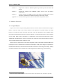
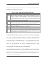
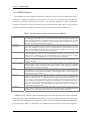
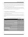

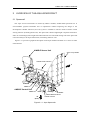
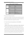
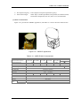
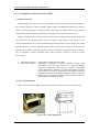
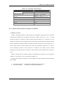
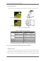
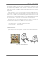
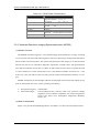
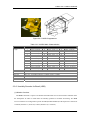
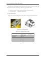
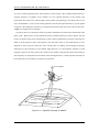
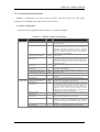
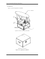
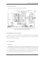
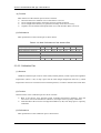
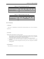
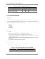
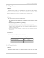
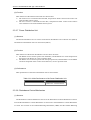
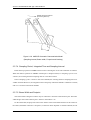


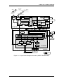
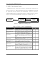
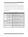
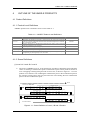
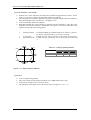
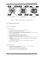
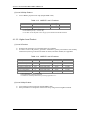
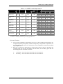
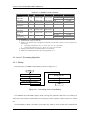
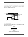
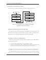
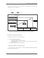
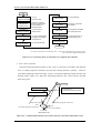

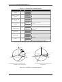
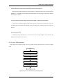
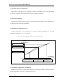
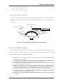
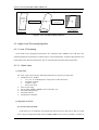


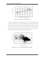


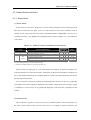
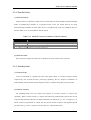
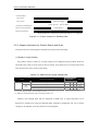

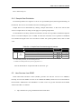

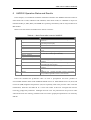

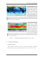

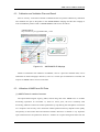
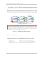
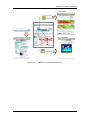

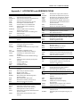


![[English] 1 MB](http://vs1.manualzilla.com/store/data/005724727_1-d0907da86b06d0402fef0dce028404c5-150x150.png)