1
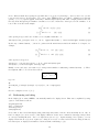
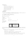
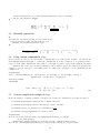
DEPARTMENT OF MATHEMATICS TECHNICAL REPORT A GRADUATE STUDENT'S GUIDE TO LATEX AND AMS-LATEX DR. RAFAL ABLAMOWICZ FEBRUARY 2003 No. 2003-1 TENNESSEE TECHNOLOGICAL UNIVERSITY Cookeville, TN 38505 A Graduate Student’s Guide to LATEX and AMS-LATEX Rafal Ablamowicz Department of Mathematics, Box 5054 Tennessee Technological University Cookeville, Tennessee 38501, U.S.A. E-mail: [email protected] May 26, 2003 Abstract In this article we will show the basic usage of LATEX in writing mathematical papers. We will concentrate on describing various parts of a standard source document of type ‘article’, from its preamble through sections with mathematical contents to references. Usage of several standard commands from LATEX, AMS-LATEX, and, amsmath, amsthm, and amssymb packages will be discussed. We will also briefly discuss the usage of ttuthesis.sty style file for composing master theses and doctoral dissertations that conform to the requirements of the TTU Graduate School.1 Keywords: Source file, composing or typesetting, displaying formulas, automatic referencing, LATEX, LATEX 2ε , AMS-LATEX, TEX. Contents 1 The structure of a LATEX document 2 2 Proclamations 2.1 Basic LATEX proclamations . . . . . . . . . . . . . . . . . . . . . . . . . . . . . . . . . . . . . . . . . . . 2.2 Proof environment . . . . . . . . . . . . . . . . . . . . . . . . . . . . . . . . . . . . . . . . . . . . . . . 4 4 5 3 Basic LATEX 3.1 Formatting first . . . . . . . . . . 3.2 Itemizing and numbering . . . . 3.3 Displaying mathematics - general 3.4 Spacing of mathematical symbols 3.5 Referencing and citing . . . . . . . . . . . . . . . . . . . . . . . . . . . . . . . . . . . . . . . . . . . . . . . . . . . . . . . . . . . . . . . . . . . . . . . . . . . . . . . . . . . . . . . . . . . . . . . . . . . . . . . . . . . . . . . . . . . . 6 . 6 . 7 . 8 . 9 . 10 4 Formatting displayed formulas 4.1 Example of array environment . . . . . . . . . . . . . . . . . . 4.2 Example of align environment . . . . . . . . . . . . . . . . . . 4.3 Example of matrices created with array . . . . . . . . . . . . . 4.4 Example of a matrix created with pmatrix . . . . . . . . . . . 4.5 Example of a table created with array . . . . . . . . . . . . . . 4.6 Example of a more complicated table with tabular . . . . . . . 4.7 Example of another usage of labeled align . . . . . . . . . . . 4.8 Example of splitting long expressions with multline and split 4.9 Example of gather and gather* . . . . . . . . . . . . . . . . . . . . . . . . . . . . . . . . . . . . . . . . . . . . . . . . . . . . . . . . . . . . . . . . . . . . . . . . . . . . . . . . . . . . . . . . . . . . . . . . . . . . . . . . . . . . . . . . . . . . . . . . . . . . . . . . . . . . . . . . . . . . . . . . . . . . . . . . . . . . . . . . . . . . . . . . . . . . . . . . . . . . . . . . . . . . . . . . . . . . . . . . . . . . . . . . . . . . . . . 1 At . . . . . . . . . . . . . . . . . . . . . . . . . . . . . . . . . . . . . . . . . . . . . . . . . . . . . . . . . . . . . . . . . . . . . . . . . . . . . . . . the time of writing of this article. Please check the current style and formatting requirements in the TTU Graduate School. 1 11 11 12 12 14 15 16 16 17 18 5 Additional examples 5.1 Braces and over braces . . . . . . . . . 5.2 Products and sums . . . . . . . . . . . 5.3 Binomial expressions . . . . . . . . . . 5.4 Using custom commands in align . . 5.5 A more complicated example of align 5.6 Commands with optional arguments . . . . . . . . . . . . . . . . . . . . . . . . . . . . . . . . . . . . . . . . . . . . . . . . . . . . . . . . . . . . . . . . . . . . . . . . . . . . . . . . . . . . . . . . . . . . . . . . . . . . . . . . . . . . . . . . . . . . . . . . . . . . . . . . . . . . . . . . . . . . . . . . . . . . . . . . . . . . . . . . . . . . . . . . . . . . . . . . . . . . . . . . . . . . . . . . . . . . . . . . . . . . . . . . . . . . . . . . . 18 18 18 19 19 19 20 6 Back matter 20 6.1 References . . . . . . . . . . . . . . . . . . . . . . . . . . . . . . . . . . . . . . . . . . . . . . . . . . . . 20 6.2 Index . . . . . . . . . . . . . . . . . . . . . . . . . . . . . . . . . . . . . . . . . . . . . . . . . . . . . . 21 7 Summary 21 A Final words 21 B The end 22 1 The structure of a LATEX document In this article by LATEX we mean LATEX 2ε which is the current version of LATEX used by PCTEX32 ver. 4 and higher installed in Bruner 305. Many of the commands and structures described in this article, like for example \documentclass{...}, do not apply to the older version of LATEX called LATEX 2.09. The main reference for this article is [5]. The source file of a LATEX document has an extension .tex and it is divided into several parts including a preamble and a body (see Figure 1). Fortunately, we can use ready-made templates from PCTEX32 software. Just go to Help → PCTEX Helper → Templates → Article and select the right article template. A better way is just to copy some existing file and modify it. For example, if one downloads all necessary files needed to compose a master thesis from [1], among the files one will find Thesis.tex source file which provides a structure (skeleton) for a thesis or a dissertation. It already contains all necessary parts of the LATEX thesis document, so it is enough to copy it and modify the contents of the remaining files.2 It will suffice to say that the preamble contains definitions and instructions that affect the entire document while the body is the document itself. When the document is complicated, like a master thesis, or to simplify its creation, it helps to create chapters, appendices, and even references as separate .tex files rather than create one big file with the entire document. This approach was taken when creating template files for the master thesis that are posted and described at [1]. Then, command include is used to include these separate files in the final document. Notice that in that case the skeleton file of a thesis, Thesis.tex has a very simple structure as shown on [1]. Once the .tex file is finished, it is then typeset (or composed) by pressing the button Typeset in PCTEX32. Notice that in the drop-down box to left of the Typeset button one must have a word LaTeX appear, and not Plain TeX or AMSTeX, or an error will result. When the document such as sample.tex is composed, at least two files are created: sample.aux and sample.log. One can ignore the sample.aux and, for the most part, also the sample.log unless errors are reported and typesetting is terminated. Usually, when error is spotted in the source file, PCTEX32 will stop scrolling down the .log file to show a line number where the error occurred, a precise place where the error occurred, and a question mark indicating a need for the user input. User can cancel typesetting altogether, or ask to open the editor in which case PCTEX32 will display the source file with the cursor positioned at the error. It is possible, of course, upon canceling the typesetting to open the .log file in the editor to read it more carefully. Usually the error can be located and fixed without having to open the .log file. If no errors are found, PXTeX32 may need to run the typesetter again and again in order to get the mapping between the labels and the actual numbers or references right. Eventually, when finished, a .dvi file is created that has the same name as the source file, hence sample.dvi in this case. Then, a DVI viewer opens to display the file. This file can then be printed or converted to a Postscript file with extensions .ps from File → Save As menu. For more information see [3]. 2 The thesis skeleton file uses in fact a ‘report’ format rather than an ‘article’ format due to its complexity. 2 \documentclass{article} %%% Here starts the preamble of the document %%% Formatting commands, if needed \setlength{\oddsidemargin}{-0.25in} \setlength{\textwidth}{7.00in} \setlength{\topmargin}{-0.25in} \setlength{\textheight}{9.0in} ... \mathsurround 1.5pt %%% Commands to load extra packages, if needed \usepackage{amsmath} \usepackage{amssymb} ... %%% Custom definitions and macros \def\beq{\begin{equation}} \def\eeq{\end{equation}} ... \newcommand{\Id}{{\bf 1}} \newcommand{\ed}{\end{document}} ... %%% New environments \newtheorem{lemma}{Lemma} ... %%% Here starts the top matter of the document body \begin{document} \title{...} \author{...} \date{...} \maketitle \tableofcontents %%% Here starts the abstract \begin{abstract} ... \end{abstract} %%% Here starts the main matter of the document body \chapter{...} \section{...} \subsection{...} \appendix{...} ... %%% Here starts the back matter of the document body \begin{thebibliography}{9} ... \end{thebibliography} \end{document} Figure 1: The structure of an ‘article’ document In this article we will concentrate primarily on specific LATEX commands and examples of their usage that are useful when writing a mathematical paper or a thesis. However, it is expected that these examples will also be useful when preparing a quiz or a test. Then, it is enough of course to have one .tex file which is nothing else but a modified article template. 3 2 Proclamations Proclamations in LATEX are theorems, propositions, lemmas, definitions, corollaries, etc., which otherwise constitute major components of any mathematical writing. They come in different styles and can be numbered in many different ways. We will discuss the basic ones that are already predefined in LATEX and a few more fancy ones that become available upon loading package amsthm. Notice that to load this package we have placed in the preamble command \usepackage{amsthm}. This way, we are loading three of the most useful packages that extend LATEX: \usepackage{amsmath} \usepackage{amssymb} \usepackage{amsthm} 2.1 Basic LATEX proclamations In order to use a proclamation, it needs to be defined first in the preamble with the command \newtheorem. For example, to define theorem, proposition, lemma, corollary, example, definition, and remark environments, we place the following commands in preamble: \newtheorem{theorem}{Theorem} \newtheorem{proposition}{Proposition} \newtheorem{lemma}{Lemma} \newtheorem{corollary}{Corollary} \newtheorem{example}{Example} \newtheorem{definition}{Definition} \newtheorem{remark}{Remark} To invoke any of these proclamations, it needs to be used as a an environment. For example, to state a theorem one begins the theorem environment with \begin{theorem} and ends the theorem with \end{theorem} as follows: \begin{theorem} In category {\bf Set}, the monomorphisms are just the injective functions (the functions $f$ such that $f(x)=f(y)$ implies $x=y.)$ \label{T:set1} \end{theorem} which gives Theorem 1. In category Set, the monomorphisms are just the injective functions (the functions f such that f(x) = f(y) implies x = y.) The first argument in \newtheorem{theorem}{Theorem} is the name for the environment that will invoke the theorem; the second argument Theorem is the name that will be printed. LATEX will automatically number the proclamation and print the text in a suitable font. Any proclamation may have an optional argument; for instance \begin{theorem}[Pierce’s Theorem] In category {\bf Set}, the monomorphisms are just the injective functions (the functions $f$ such that $f(x)=f(y)$ implies $x=y.)$ \label{T:set2} \end{theorem} which gives Theorem 2 (Pierce’s Theorem). In category Set, the monomorphisms are just the injective functions (the functions f such that f(x) = f(y) implies x = y.) Notice that since we have used labels \label{T:set1} and \label{T:set2} with a theorem counter T, we can now refer to theorems. For instance, in Theorem 2 we have shown how an optional parameter can be used. If we now insert another proclamation, its numbering will start afresh. For example, 4 \begin{definition} An arrow $f : A \rightarrow B$ is an {\bf epimorphism} if, for any pair of arrows $g : B \rightarrow C$ and $h : B \rightarrow C,$ the equality $g \circ f = h \circ f$ implies that $g=h.$ \label{D:epi} \end{definition} Definition 1. An arrow f : A → B is an epimorphism if, for any pair of arrows g : B → C and h : B → C, the equality g ◦ f = h ◦ f implies that g = h. Notice that we have introduced yet another counter D for definitions. This way, Definition 1 is our definition number 1. It is possible to number all proclamations consecutively, in which case our first definition would have number 3 since we have stated two theorems so far. It is also possible to number proclamations within a section. For more information see [5]. When the package amsthm is loaded, additional options become available. One of them is the style of a proclamation. There are three styles: (i) plain, the most emphatic, and the default, (ii) definition, less emphatic, (ii) remark, the least emphatic. The style of all proclamations is set in the preamble with the command \theoremstyle{...}. In this article we have used \theoremstyle{plain} which is also the default style used by LATEX. Another option available with amsthm is to use the ∗ -ed version of \newtheorem which defines a proclamation that is not numbered but named. For example, in the preamble we have defined two such proclamations: Main Theorem and Limit Theorem. \newtheorem*{main}{Main Theorem} \newtheorem*{limit}{Limit Theorem} For instance, we can now use the latter proclamation as follows: \begin{limit} Let $\bf D$ be a diagram in a category $\cC,$ with sets $V$ of vertices and $E$ of edges. If every $V$-indexed and every $E$-indexed family of objects in $\cC$ has a product and every pair of maps in $\cC$ has an equalizer, then $\bf D$ has a limit. \end{limit} Limit Theorem. Let D be a diagram in a category C, with sets V of vertices and E of edges. If every V -indexed and every E -indexed family of objects in C has a product and every pair of maps in C has an equalizer, then D has a limit. Although we have shown only a few examples, they apply also to all other proclamations. 2.2 Proof environment The proof environment is of course for proofs. It begins with \begin{proof} and ends with \end{proof} delimeters, and it is defined in the amsthm package. For example: \begin{proof} This is a proof that is ended by the standard q.e.d. symbol. \end{proof} produces 5 Proof. This is a proof that is ended by the standard q.e.d. symbol. When the proof ends with an equation but not the text, it is customary to omit the q.e.d. symbol . Then, we do the following: \begin{proof} This is a proof that is ended with an equation and not the standard q.e.d. symbol. $$ A=B. $$ \renewcommand{\qedsymbol}{} \end{proof} produces Proof. This is a proof that is ended with an equation and not the standard q.e.d. symbol. A = B. It is possible to substitute for the word Proof another phrase, for example “Uniqueness”, as in Uniqueness. This is the proof. where we have used an optional argument [Uniqueness] as follows \begin{proof}[Uniqueness] This is the proof. \end{proof} Finally, the optional argument may contain a reference to a theorem. Such reference is especially desirable if the proof does not immediately follow the proven theorem or proposition. For instance, above we stated Theorem 2. If we wanted to prove it now, we should say \begin{proof}[Proof of Theorem~\ref{T:set2}] State the proof. \end{proof} which will print Proof of Theorem 2. State the proof. For more information we again refer to [5]. 3 3.1 Basic LATEX Formatting first First let me say that one should not modify any formatting commands in the Thesis.tex file as these commands are specifically set to conform to the Graduate School requirements. Thus, the following remarks are only to be used when one works with other LATEX documents such as, for example, quizzes or tests. Usually, when submitting an article to a professional journal, journal editors provide their own style file. One big advantage of using LATEX is that it is very easy to change the layout of the entire article just by using a different style file. For example, the following \documentclass{...} command has been modified to accept an article style file from Elsevier Publishing \documentclass{elsart} ... while the following command accepts a style file from Kluwer Publishers: 6 \documentstyle[namedreferences]{kapproc} ... Since essentially everything else may remain the same in the document, it is no surprise why LATEX is so popular among mathematicians and scientists. In case one wants to modify the default page setup from Default Template, one should use the Page Format Template from PCTEX32. Notice the following commands at the top of this source file. We used these margin setting commands to format this article. • First we set the left margin - The default is 1 inch, so the following command sets a 0.75-inch left margin. \setlength{\oddsidemargin}{-0.25in} • Then we set the width of the text - What is left will be the right margin. In this case, right margin is 8.5in 0.75 - 7.00in = 0.75in. \setlength{\textwidth}{7.00in} • To set the top margin, since the default is 1 inch, we use the following command to set it to 0.75-inch: \setlength{\topmargin}{-0.25in} • To set the height of the text we issue the following command. What is left will be the bottom margin. In this case, bottom margin is 11.00in - 0.75in - 9.00in = 1.00in \setlength{\textheight}{9.50in} 3.2 Itemizing and numbering The above bulleted items were created using the so-called itemized environment as follows: \begin{itemize} \item This is the first item, for example, $f(x) = \sin(2x-3).$ \item While a domain for $f$ is $\[-\pi,\pi).$ \end{itemize} When typeset, this produces • This is the first item, for example, f(x) = sin(2x − 3). • While a domain for f is [−π, π). If one prefers to number listed items, one would need to use the so called enumerated environment as follows: \begin{enumerate} \item This is the first item, for example, $f(x) = \sin(2x-3).$ \item While a domain for $f$ is $\[-\pi,\pi).$ \end{enumerate} When typeset, this produces 1. This is the first item, for example, f(x) = sin(2x − 3). 2. While a domain for f is [−π, π). Here one can see the first advantage of using LATEX: its ability to automatically re-number listed items when a new item is inserted. For example, let us insert a new item in between the two items above: 7 \begin{enumerate} \item This is the first item, for example, $f(x) = \sin(2x-3).$ \item Here is a new item, say, $\cos(4x+\pi)$ function. \item While a domain for $f$ is $\[-\pi,\pi).$ \end{enumerate} After typesetting we get 1. This is the first item, for example, f(x) = sin(2x − 3). 2. Here is a new item, say, cos(4x + π) function. 3. While a domain for f is [−π, π) with a new numbering. Instead of the numbers one can use letters, but the labels are not changed then automatically. We use again the first environment. \begin{itemize} \item[(a)] This is the first item, for example, $$ f(x) = \sin(2x-3). $$ \item[(b)] While a domain for $f$ is $[-\pi,\pi).$ \item[(c)] The third item now will be displayed and numbered: \begin{equation} f(x) = \sin(2x-3). \label{eq:sine} \end{equation} \item[(b)] While a domain for $f$ is $[-\pi,\pi).$ \end{itemize} We get: (a) This is the first item, for example, f(x) = sin(2x − 3). (b) While a domain for f is [−π, π). (c) The third item now will be displayed and numbered: f(x) = sin(2x − 3). (1) We will see further that LATEX automatically renumbers equations, sections, subsections, figures, references - you name it! For example, suppose that we want to cite a reference where more information on basic LATEX commands can be found. This would be a book by Hahn listed as reference [2]. Notice that in the source file we refer to that bibliography position via its label hahn1993 using the command \cite{hahn1993} which produces [2]. This way, if we insert a new bibliography item before Hahn’s book, our reference to Hahn’s book in the text wouldn’t need to be changed since the label hahn1993 does not change. What will change is the number which could then be [2] instead. 3.3 Displaying mathematics - general If one wants to display a mathematical formula inline one may find that the text that surrounds it seems a bit too crowded. For example, suppose that ∀ > 0 ∃ δ > 0 so that |f(x) − L| < whenever |x − x0 | < δ. In order to control the amount of empty space around the inline mathematics, one inserts in the preamble, that is, in the top part of the source document between \documentclass{article} and \begin{document} the following command \mathsurround 1.5pt 8 where 1.5pt is the amount of extra space around the math. Usually 1.5pt is sufficient. However, then commas, periods, colons, semicolons, question marks, etc. need to be placed inside of the math environment or there will be a gap between the mathematical expression and the symbol. Compare, for example, f(x) = sin(x) , g(x) = cos(x) with f(x) = sin(x), g(x) = cos(x). A good rule is, however, to display long and complicated mathematical expressions rather than show them inline. Thus, it is better to state the definition of a limit as follows: Definition 2. We say that limx→x0 f(x) = L if ∀ > 0 ∃ δ > 0 so that |f(x) − L| < whenever |x − x0| < δ. Notice the spacing, automatic numbering, and font change. The above Definition 2 has been entered as \begin{definition} We say that $\lim_{x \to x_0} f(x) = L$ if $\forall \, \epsilon >0 \; \exists \, \delta >0$ so that $|f(x) - L| < \epsilon$ whenever $|x - x_0| < \delta.$ \label{def:limit} \end{definition} Notice that in display mode $$\lim_{x \to x_0} f(x) = L$$ produces the following lim f(x) = L. x→x0 instead of limx→x0 f(x) = L. Notice also that we have displayed f(x) = sin(2x−3) in item (a) above instead of making it appear inline like this f(x) = sin(2x − 3). In order to display f(x) = sin(2x − 3) we used double dollar signs in $$f(x) = \sin(2x-3)$$ as opposed to single dollar signs as in $f(x) = \sin(2x-3)$ to display it inline. 3.4 Spacing of mathematical symbols LATEX provides a large variety of mathematical symbols. For example, • Greek characters like α, β, γ, . . . , θ, ω, . . . that are entered as $\alpha,\beta,\gamma,\ldots,$. If you forget their codes, in PCTEX32 go to Help → PCTeX Helper → Math and select Lower Case Greek Letters or Upper Case Greek Letters. • Miscellaneous symbols like Re, Im, ∂, ∞, ∅, ∇, ∀, ∃, . . . . They can be found by going in PCTEX32 to Help → PCTeX Helper → Math and selecting Miscellaneous Ord Symbols. • Binary operations like ±, ×, ◦, u, t, ∨, ∧, ⊕, ⊗, . . . . You can find them by going in PCTEX32 to Help → PCTeX Helper → Math and selecting Binary Operations. • Relations like ≤, , ⊂, ⊆, ∈, ≥, ⊃, ⊇, ≡, ', ≈, ⊥, . . . . In PCTEX32 go to Help → PCTeX Helper → Math and select Relations. • Negated relations like 6<, 6⊆, 6=, 6≡, 6', 6∼ =, . . . . In PCTEX32 go to Help → PCTeX Helper → Math and select Negated Relations. • Horizontal arrows like ←, →, ⇐, ⇒, ⇔, 7→, ←-, ,→, . . . . In PCTEX32 go to Help → PCTeX Helper → Math and select Horizontal Arrows. • Vertical arrows like ↑, ↓, %, &, . . . . In PCTEX32 go to Help → PCTeX Helper → Math and select Vertical Arrows. P Q R H T S W V N L • Large operators like , , , , , , , , , , . . . . In PCTEX32 go to Help → PCTeX Helper → Math and select Large Operators. Pointing to any symbol in the above menus will reveal its LATEX code while clicking on it will insert into the source document. However, when writing mathematical formulas often one needs to control spacing between symbols. Consider theses two expressions: A = {x ∈ X | xβ ≥ (xy)g(x, y) > (x + 1)2l − α} 2l A = { x ∈ X | xβ ≥ (xy) g(x, y) > (x + 1) − α } 9 (2) (3) Notice different small extra spacings in (3) which have been created by inserting \, after \{ and before \}, and between (xy)\,g(x,y). In increasing order of space sizes, LATEX has these pre-defined commands for horizontal spacing: \,, \:, \;, \quad, \qquad. Generally, command \hspace{5ex}, that takes a length parameter like 5ex increases horizontal spacing in formulas. Sometimes one needs to insert these extra spaces for the formula to look better. Here is another such example. Z π (a) sin xdx = 2, (b)| − f(x)| (4) 0 Z π (c) sin x dx = 2, (d) |−f(x)| (5) 0 where spacing in (5) seems better. It has been accomplished with this code: \mbox{(c)} \int_{0}^{\pi} \sin x \, dx =2, \qquad \mbox{(d)} \, \left|-f(x)\right| \label{eq:eq2} By the way, command \mbox{...} is used to print text in Roman characters inside the math mode. Compare, for example, Z π (c) sin xdx = 2, and (d)| − f(x)| (6) Z0 π (c) sin x dx = 2, and (d) |−f(x)| (7) 0 where (7) has been typed as \mbox{(c)} \, \int_{0}^{\pi} \sin x \, dx =2, \quad \mbox{and} \quad \mbox{(d)} \, \left|-f(x)\right| \label{eq:eq4} Finally, one nice and easy to use feature is to box important formulas or results using command \boxed{...}. Then, the argument will be boxed. It works as follows: Z ∞ 2 e−x dx = √ π −∞ typed as $$ \boxed{\int_{-\infty}^{\infty} e^{-x^{2}} \, dx = \sqrt{\pi}} $$ For more examples we refer to [4, 5]. 3.5 Referencing and citing In the display (1) we wanted LATEX to automatically number the displayed item. That was accomplished by using equation environment as follows: \begin{equation} f(x) = \sin(2x-3). \label{eq:sine} \end{equation} Notice that we have labeled this display using \label{eq:sine} where sine is a label arbitrarily chosen. Once it has been assigned, we can now refer to this displayed function via the \ref command as (\ref{eq:sine}). Then we can say something like that: “Let’s now differentiate function (1)”. Again, inserting a new equation or a new displayed item in front of (1) won’t require us to change how we refer to it since its label has not changed! Instead, if we insert just one displayed and numbered item, its number will change to (2). 10 One more comment: In the label \label{eq:sine} we have an optional name eq for a counter that counts equations. It is convenient to have it although it is not required: \label{sine} would do too. In the code of the Definition 2 we have used \label{def:limit}. One can really label practically anything. For example, we can refer to this section as section 3.1 because a label has been inserted right after the \section{...} command as \section{Formatting first} \label{formatting} In order to refer to this section it is enough now to invoke the label via \ref{formatting} which gives number 3.1. As you may have guessed, if we insert a new section in front of this section, when we refer to this section again via \ref{formatting}, number 2 will appear instead of 1. By the way, if one mistypes a label in \cite or \ref, which is equivalent to typing label that does not exist, LATEX will return question marks in the document. For example, if instead of typing \cite{gratzer1999,gratzer2000} that yields [4, 5] one types \cite{gratzer1998,gratzer200}, upon typesetting LATEX will return [?, ?] with question marks. The same applies to \ref command: We will get “equation (??)” since we have typed by mistake (\ref{eq:myeq}) while label myeq has not been assigned as a value to the counter eq. 4 Formatting displayed formulas In this section we will show examples how to display mathematical formulas, and how to create tables, and more complicated expressions. This is not meant to be a complete review of all possible commands and packages, but only a review of the most frequently used structures that may be useful to students writing a thesis. For a complete reference, see [4] and [5]. 4.1 Example of array environment In this example we show how a bunch of lines is entered as an array where array just means the way objects are arranged or positioned in the display. For example, \begin{equation} \begin{array}{l} \e_1\e_2=\e_1\w\e_2+A_{12}+g_{12}=\e_1\w\e_2+B_{12} \\[0.5ex] (\e_1\e_2)\tilde{\phantom{x}}=-\e_1\w\e_2-A_{12}+g_{12}=-\e_1\w\e_2+B_{21} \\ \qquad =-\e_1\w\e_2+(B^\top)_{12} \end{array} \label{eq:8} \end{equation} e1e2 = e1 ∧ e2 + A12 + g12 = e1 ∧ e2 + B12 (e1e2 )˜ = −e1 ∧ e2 − A12 + g12 = −e1 ∧ e2 + B21 = −e1 ∧ e2 + (B > )12 (8) The single parameter l in \begin{array}{l} says that the single item on each line is left-justified in the space provided for it (see more below). If we wanted to center it or to right justify it, we would use c or r instead. Symbols \\ mark the end of each line (or row) but [0.5ex] in \\[0.5ex] allows for extra vertical space between the first and the second line. Since no such extra spacing was entered at the end of the second line, the third line seems to be too close to the second line. We can fix it with \begin{equation} \begin{array}{l} \e_1\e_2=\e_1\w\e_2+A_{12}+g_{12}=\e_1\w\e_2+B_{12} \\[0.5ex] (\e_1\e_2)\tilde{\phantom{x}}=-\e_1\w\e_2-A_{12}+g_{12}=-\e_1\w\e_2+B_{21} \\[0.5ex] \qquad =-\e_1\w\e_2+(B^\top)_{12} \end{array} 11 \label{eq:88} \end{equation} e1e2 = e1 ∧ e2 + A12 + g12 = e1 ∧ e2 + B12 (e1e2 )˜ = −e1 ∧ e2 − A12 + g12 = −e1 ∧ e2 + B21 = −e1 ∧ e2 + (B > )12 (9) Notice that display (9) looks better than (8). Notice also that in both displays there was one single number assigned to the entire array. 4.2 Example of align environment We can display equations (9) differently using command align which allows us to align equal signs. Note however, that this very useful command is not present in standard LATEX but is available upon loading the amsmath package with the command \usepackage{amsmath} (see the preamble). We again refer to [4] and [5] for more information. \begin{align} \e_1\e_2 &=\e_1\w\e_2+A_{12}+g_{12}=\e_1\w\e_2+B_{12} \\[0.5ex] (\e_1\e_2)\tilde{\phantom{x}} &=-\e_1\w\e_2-A_{12}+g_{12}=-\e_1\w\e_2+B_{21} \\[0.5ex] &=-\e_1\w\e_2+(B^\top)_{12} \end{align} e1e2 = e1 ∧ e2 + A12 + g12 = e1 ∧ e2 + B12 (10) (e1e2 )˜ = −e1 ∧ e2 − A12 + g12 = −e1 ∧ e2 + B21 (11) > = −e1 ∧ e2 + (B )12 (12) Notice that & has been placed in front of each = sign that needs to be lined up. Notice also that each equation has received a separate number! It may or may not be a desired feature. It may be desirable to refer to the whole display and use only one number (13) as in \begin{align}\label{eq:allthree} \e_1\e_2 &=\e_1\w\e_2+A_{12}+g_{12}=\e_1\w\e_2+B_{12} \notag \\[0.5ex] (\e_1\e_2)\tilde{\phantom{x}} &=-\e_1\w\e_2-A_{12}+g_{12}=-\e_1\w\e_2+B_{21} \\[0.5ex] &=-\e_1\w\e_2+(B^\top)_{12} \notag \end{align} e1e2 = e1 ∧ e2 + A12 + g12 = e1 ∧ e2 + B12 (e1e2 )˜ = −e1 ∧ e2 − A12 + g12 = −e1 ∧ e2 + B21 (13) > = −e1 ∧ e2 + (B )12 where we have used command \notag to indicate that we don’t want numbers displayed in lines 1 and 3. This is getting complicated! The best reference for these more advanced environments like \begin{align}...\end{align}, \begin{align*}...\end{align*}, \begin{gather}...\end{gather}, and \begin{gather*}...\end{gather*} we refer to [5]. Note however, that these very useful commands are not present in standard LATEX but become available upon loading the amsmath package with the command \usepackage{amsmath} (see the preamble). 4.3 Example of matrices created with array The following code displays a matrix with a vertical solid line: 12 \begin{equation} \left( \begin{array}{cc|c} 1 & 2 & 3 \\ 0 & 0 & 1 \\ 0 & 0 & 2 \end{array} \right) \label{eq:firstsolution} \end{equation} that gives 1 0 0 2 3 0 1 0 2 (14) 2 3 0 1 0 2 (15) You can also use square brackets as follows: \begin{equation} \left[ \begin{array}{cc|c} 1 & 2 & 3 \\ 0 & 0 & 1 \\ 0 & 0 & 2 \end{array} \right] \label{eq:secondsolution} \end{equation} that gives 1 0 0 Notice that in both cases we have used parameters {cc|c} after \begin{array} where c indicates centering. If numbers were negative, centering may not give the best looking matrix: \begin{equation} \left[ \begin{array}{cc|c} 1 & 2 & 3 \\ 9 & 0 & -1 \\ 0 & -5 & 2 \end{array} \right] \label{eq:secondsolution2} \end{equation} that gives 1 2 9 0 0 −5 So try 13 3 −1 2 (16) \begin{equation} \left[ \begin{array}{rr|r} 1 & 2 & 3 \\ 9 & 0 & -1 \\ 0 & -5 & 2 \end{array} \right] \label{eq:secondsolution3} \end{equation} that gives 1 2 3 9 0 −1 0 −5 2 (17) where matrix (17) looks better than matrix (16). By the way, there needs to be a one-to-one mapping between the displayed items and their labels, hence no two labels may be the same, of course. You may have guessed also that the vertical bar | in {rr|r} is responsible for the vertical line separating the third column form the second. We could have more vertical lines if they made sense. For example, \begin{equation} \left[ \begin{array}{r|r|r} 1 & 2 & 3 \\ 9 & 0 & -1 \\ 0 & -5 & 2 \end{array} \right] \end{equation} that gives 1 2 3 9 0 −1 0 −5 2 (18) Since no label was entered for this last display, we can’t refer to it even though it is numbered. 4.4 Example of a matrix created with pmatrix Let’s work some more with matrices. To get this matrix 0 0 0 0 q 0 0 0 0 −1 −q 0 0 0 0 1 0 0 0 0 1 B= 1 1 −1 −1 0 q 1 1 −1 0 −1 q 1 1 0 −1 −1 q 1 0 −1 − q q −1 − q 1 0 0 0 0 1 −1 − q q −1 − q 0 0 0 0 1 1 −1 − q q . 0 0 0 0 (19) we use the following code. Notice that this code is much simpler than the one required to create matrices with the array environment and that the delimeters are automatically placed around the matrix entries. 14 \begin{equation} B = \begin{pmatrix} 0 & 0 & 0 & 0 & q & -1-q & 1 & 1 0 & 0 & 0 & 0 & -1-q & q & -1-q & 1 0 & 0 & 0 & 0 & 1 & -1-q & q & -1-q 0 & 0 & 0 & 0 & 1 & 1 & -1-q & q 1 & 1 & -1 & -1 & 0 & 0 & 0 & 0 q & 1 & 1 & -1 & 0 & 0 & 0 & 0 -1 & q & 1 & 1 & 0 & 0 & 0 & 0 -1 & -1 & q & 1 & 0 & 0 & 0 & 0 \end{pmatrix}. \label{eq:ourB} \end{equation} \\ \\ \\ \\ \\ \\ \\ where we have used a \begin{pmatrix}...\end{pmatrix} environment. There some 10 different ways matrices can be entered but we won’t be discussing them here and refer the reader to [4] or [5]. 4.5 Example of a table created with array The following code produces a table: $$ \begin{array}{|r|c|} \Hline & \\[-2ex] \cl(B) & \e_2 \\ & \\[-2ex] \hline & \\[-1ex] \e_1 & \e_1\w\e_2+a \\ \e_2 & 1 \\ \e_1\w\e_2\w\e_3 &-c\e_1\w\e_2-\e_1\w\e_3+a\e_2\w\e_3 \\[1.2ex] \Hline \end{array} $$ e2 C`(B) e1 e2 e1 ∧ e2 ∧ e3 e1 ∧ e2 + a 1 −ce1 ∧ e2 − e1 ∧ e3 + ae2 ∧ e3 While we have already met the array environment above, in this table several custom-made commands (macros) have been used. These commands are defined in the preamble using \newcommand definition. Let’s review some of them here: • Command \e produces bolded letter e and is shorter to type than {\bf e}. Likewise command(s) (i) \cA, \cB, \cC,... give calligraphic A, B, C, · · · ; ~ a, ~c, · · · ; (ii) \vA, \va, \vc, ... give vectors A,~ (iii) \w is a short for \wedge, the wedge product ∧ in the Clifford algebra C`(Q); (iv) \cl produced the italicized symbol for the Clifford algebra as in C`; (v) \Hline produces a thicker horizontal line than the standard command \hline used in the middle; (vi) [-2ex] used after the end of line symbol \\ produces a negative extra vertical spacing. 15 Although not used in the above table, symbols very often used in mathematical papers are R for the real field, C for the complex field, H for the quaternionic division ring, Z for the ring of integers. These the so called “math black board letters” are part of another package amssymb which one can load in the preamble using the command \usepackage{amssymb}. Note that to get for example R one can use the long name ${\mathbb R}$ or the abbreviated macro \BR defined in the preamble (and likewise for other letters). Then, $\BR^3$ gives the real 3-dimensional Euclidean space R3 . 4.6 Example of a more complicated table with tabular The following is an example of a more complicated table that has been created using tabular environment specifically suited for creating tables. From: 8:15 8:30 9:30 9:40 10:40 To: 8:30 9:30 9:40 10:40 10:50 10:50 11:30 12:10 1:15 1:45 11:30 12:10 1:15 1:45 2:45 Room: BR119 BR119 Event: BR119 PT-S2 PT-S1 Analysis BR123 RT-S1A BR123 RT-S1B BR119 Saturday, May 25 Event: Room: Event: Room: Event: Announcements No parallel sessions Break No parallel sessions Break Geometry Structures Physics BR124 RT-S2A BR126 RT-S3A BR127 RT-S4A BR124 RT-S2B BR126 RT-S3B BR127 RT-S4B Lunch Coffee Social General meeting and closing Room: Room: Event: Applications BR112 RT-S5A BR112 RT-S5B The code for this table looks as follows: \begin{center} \begin{small} \begin{tabular}{|r|r|c c|c c|c c|c c|c c|} %12 columns \multicolumn{12}{c}{\bf{Saturday, May 25}} \\\hline From: & To: & Room: & Event: & Room: & Event: & Room: & Event: & Room: & Event: & Room: & Event:\\\hline 8:15 & 8:30 & BR119 & \multicolumn{9}{c|}{\bf{Announcements}} \\\hline 8:30 & 9:30 & BR119 & PT-S1 & \multicolumn{8}{c|}{\emph{No parallel sessions}} \\\hline 9:30 & 9:40 & \multicolumn{10}{c|}{\emph{Break}} \\\hline 9:40 & 10:40 & BR119 & PT-S2 & \multicolumn{8}{c|}{\emph{No parallel sessions}} \\\hline 10:40 & 10:50 & \multicolumn{10}{c|}{\emph{Break}} \\\hline & & \multicolumn{2}{|c|}{\emph{Analysis}} & \multicolumn{2}{|c|}{\emph{Geometry}} & \multicolumn{2}{|c|}{\emph{Structures}} & \multicolumn{2}{|c|}{\emph{Physics}} & \multicolumn{2}{|c|}{\emph{Applications}} \\\hline 10:50 & 11:30 & BR123 & RT-S1A & BR124 & RT-S2A & BR126 & RT-S3A & BR127 & RT-S4A & BR112 & RT-S5A \\\hline 11:30 & 12:10 & BR123 & RT-S1B & BR124 & RT-S2B & BR126 & RT-S3B & BR127 & RT-S4B & BR112 & RT-S5B \\\hline 12:10 & 1:15 & \multicolumn{10}{c|}{\bf{Lunch}} \\\hline 1:15 & 1:45 & \multicolumn{10}{c|}{\bf{Coffee Social}} \\\hline 1:45 & 2:45 & BR119 & \multicolumn{9}{c|}{\bf{General meeting and closing}} \\\hline \end{tabular} \end{small} \end{center} Notice that in order to reduce the size of the entire table we have temporarily used small environment that reduces the size of all fonts. That environment of course starts with \begin{small} and ends with \end{small}. 4.7 Example of another usage of labeled align In this example we use again the \begin{align}...\end{align} environment but we label each equation. 16 \begin{align} X+ X\tilde{~} & = \Id, \label{eq:X1}\\ X^2 & = X, \label{eq:X2}\\ X X\tilde{~} & = 0 \label{eq:X3}. \end{align} X + X˜ = 1, (20) 2 X = X, XX˜ = 0. 4.8 (21) (22) Example of splitting long expressions with multline and split Here we show how to split a long expression among several lines using a new environment from the amsmath package that needs to be loaded extra into LATEX. It is \begin{multline}...\end{multline}. For more information about this very useful command not present in standard LATEX we again refer to [4] and [5]. To load it, use command \usepackage{amsmath}. \begin{multline} (1+q)z^2+(-q^2 K_4+K_4+q K_2-1+K_2)z+K_4 K_2 + K_2^2\\ -K_4-K_2+q K_4-q^2 K_4^2-q K_4^2-q^2 K_2 K_4+q K_2^2 = 0, \end{multline} that gives (1 + q)z 2 + (−q2 K4 + K4 + qK2 − 1 + K2 )z + K4 K2 + K22 − K4 − K2 + qK4 − q2 K42 − qK42 − q2 K2 K4 + qK22 = 0, (23) There is also a command split that allows one to split very long formulas. One convenient feature of using split versus array or align is that it generates one number for the formula. For example, f(x) =(x1x2x3 x4x5x6 x7x8 )6n−7 + (x1 x2x3x4 x5x6x7 x8)9n+7 + (x1 x2)8n−9 + (x3x4 )4n+10 + (x1 x2 + x3x4 + x5x6 + x7x8)6n − (x1 x3) 6n−9 + (x2x4 ) 4n−10 + (x1x4 + x2x3 + x6x8 + x5x8 ) (24) 6n−12 has been typed as \begin{equation} \label{eq:longone} \begin{split} f(x)= &(x_{1}x_{2}x_{3}x_{4}x_{5}x_{6}x_{7}x_{8})^{6n-7} + (x_{1}x_{2}x_{3}x_{4}x_{5}x_{6}x_{7}x_{8})^{9n+7} \\ &+ (x_{1}x_{2})^{8n-9}+(x_{3}x_{4})^{4n+10} + (x_{1}x_{2}+ x_{3}x_{4}+x_{5}x_{6}+x_{7}x_{8})^{6n} \\ &- (x_{1}x_{3})^{6n-9}+(x_{2}x_{4})^{4n-10} +(x_{1}x_{4}+ x_{2}x_{3}+x_{6}x_{8}+x_{5}x_{8})^{6n-12} \end{split} \end{equation} Notice the difference when the same formula 24 is entered in the multline environment: f(x) = (x1x2x3 x4x5 x6x7x8 )6n−7 + (x1 x2x3x4 x5x6x7 x8)9n+7 + (x1x2 )8n−9 + (x3 x4)4n+10 + (x1x2 + x3x4 + x5x6 + x7x8 )6n − (x1 x3)6n−9 + (x2x4 )4n−10 + (x1x4 + x2 x3 + x6x8 + x5x8 )6n−12. (25) The above has been typed as 17 \begin{multline} f(x) = (x_{1}x_{2}x_{3}x_{4}x_{5}x_{6}x_{7}x_{8})^{6n-7} + (x_{1}x_{2}x_{3}x_{4}x_{5}x_{6}x_{7}x_{8})^{9n+7} \\ + (x_{1}x_{2})^{8n-9}+(x_{3}x_{4})^{4n+10}+(x_{1}x_{2} + x_{3}x_{4}+x_{5}x_{6}+x_{7}x_{8})^{6n} \\ - (x_{1}x_{3})^{6n-9}+(x_{2}x_{4})^{4n-10} + (x_{1}x_{4}+ x_{2}x_{3}+x_{6}x_{8}+x_{5}x_{8})^{6n-12} \label{eq:longone2} \end{multline} See [5] for more information. 4.9 Example of gather and gather* Command the gather* environment is a better version of the $$...$$ displaying while allowing much control over spacing while $$...$$ does not allow for any control. The gather* environment differs from gather environment in that the displayed item or items is not (are not) numbered. For example, \begin{gather*} \alphaq(b_1) = \displaystyle{\frac{(q-1)\Id}{q} + \frac{b_1}{q}}, \quad \alphaq(b_2) = \displaystyle{\frac{(q-1)\Id}{q} + \frac{b_2}{q}}, \\[0.5ex] \alphaq(b_1 b_2) = \displaystyle{\frac{(1-2q+q^2)\Id}{q^2}+\frac{(q-1)b_1}{q^2}+ \frac{(q-1)b_2}{q^2}+\frac{b_{21}}{q^2}}. \end{gather*} Notice that the horizontal spacing in the first row is controlled with command \quad while the vertical spacing is increased thanks to [0.5ex]. In this environment displayed items are centered. αq (b1 ) = αq (b1b2 ) = (q − 1)1 b1 + , q q αq (b2 ) = (1 − 2q + q2 )1 (q − 1)b1 (q − 1)b2 b21 + + + 2. q2 q2 q2 q The remaining examples come from files that came with PCTEX32. 5 5.1 Additional examples Braces and over braces $$ \{\underbrace{\overbrace{\mathstrut a,\ldots,a} ^{k\;a\mathchar‘’\rm s}, \overbrace{\mathstrut b,\ldots,b} ^{l\;b\mathchar‘’\rm s}}_{k+l\rm\;elements}\}. $$ k a’s l b’s z }| { z }| { {a, . . . , a, b, . . ., b}. | {z } k+l elements 5.2 (q − 1)1 b2 + , q q Products and sums $$ \prod_{j\ge0}\biggl(\sum_{k\ge0}a_{jk}z^k\biggr) =\sum_{n\ge0}z^n\,\Biggl(\sum_ 18 \frac{\scriptstyle k_0,k_1,\ldots\ge0}{\scriptstyle k_0+k_1+\cdots=n} a_{0k_0}a_{1k_1}\ldots\,\Biggr). $$ Y X j≥0 5.3 ajk z k k≥0 = X X zn n≥0 ! a0k0 a1k1 . . . . k0 ,k1 ,...≥0 k0 +k1 +···=n Binomial expressions $$ \frac{(n_1+n_2+\cdots+n_m)!}{n_1!\,n_2!\ldots n_m!} ={n_1+n_2\choose n_2}{n_1+n_2+n_3\choose n_3} \ldots{n_1+n_2+\cdots+n_m\choose n_m}. $$ (n1 + n2 + · · · + nm )! = n1 ! n2! . . .nm ! 5.4 n1 + n2 + n3 n1 + n2 + · · · + nm n1 + n2 ... . n2 n3 nm Using custom commands in align In the following we show we use custom-made commands that were defined in the preamble. We will use the \newcommand{\reversion}[1]{#1 \, \tilde{}} command that is, in fact, a function of one parameter that ie referred to as #1. This command puts a tilde symbol ˜ to the right of a symbol entered as the argument. The funny command is just a crude way of leaving a blank space whose width is equal to the width of its argument. For example, to enter an empty space of the width equal to the width of the equal sign = we use \phantom{=} in the formula below. \begin{align} C(13) - \reversion{R(13)} &= 2(q^2-q)\Id + (-1-q^2+2q)b_1 + (-1-q^2+2q)b_2 \notag \\ &\phantom{=} +(1-q)b_{12} + (1-q)b_{21}, \label{eq:C13R13} \end{align} C(13) − R(13)˜= 2(q2 − q)1 + (−1 − q2 + 2q)b1 + (−1 − q2 + 2q)b2 + (1 − q)b12 + (1 − q)b21, 5.5 (26) A more complicated example of align In the following more complicated example of align, we use several new commands not previously encountered: • Command \displaystyle enlarges the size of displayed fractions; • Command \hspace*{5ex} enters a horizontal space equal to 5ex units; • Command \frac{t_1 b_2}{q}} creates a small fraction t 1 b2 q ; • Commands \notag and \phantom were described earlier. \begin{align} XX_1 &= (-K_6 q+K_2 q+K_4)\Id+K_2 b_1+\displaystyle{\frac{t_1 b_2}{q}} + K_4 b_{12} \notag\\ &\phantom{=} \hspace*{5ex}+K_5 b_{21}+K_6 b_{121}, \label{eq:XX1} \\[1ex] XX_2 &= K_1 \Id+\displaystyle{\frac{t_2 b_1}{q^2 (1+q)}+\frac{t_3 b_2}{q^3 (1+q)}19 \frac{b_{12}}{q(1+q)}}\notag \\ &\phantom{=} \hspace*{5ex}+K_5 b_{21}+K_6 b_{121},\label{eq:XX2}\\[1ex] XX_3 &= K_1\Id+\displaystyle{\frac{t_4 b_1}{q (q^3+2 q^2+2 q+1)}+ \frac{t_5 b_2}{q^2 (q^3+2 q^2+2 q+1)}}\notag \\ &\phantom{=} \hspace*{5ex}-\displaystyle{\frac{(q-1) b_{12}}{q^3+2 q^2+2 q+1}} +K_5 b_{21}+K_6 b_{121}, \label{eq:XX3} \end{align} XX1 = (−K6 q + K2 q + K4 )1 + K2 b1 + t1 b2 + K4 b12 q + K5 b21 + K6 b121, (27) t2b1 t3b2 b12 + − q2 (1 + q) q3(1 + q) q(1 + q) + K5 b21 + K6 b121, (28) XX2 = K1 1 + t4b1 t5b2 + q(q3 + 2q2 + 2q + 1) q2 (q3 + 2q2 + 2q + 1) (q − 1)b12 − 3 + K5b21 + K6 b121, q + 2q2 + 2q + 1 XX3 = K1 1 + 5.6 (29) Commands with optional arguments We have already given one example of a command \newcommand{\reversion}[1]{#1 \, \tilde{}} that takes one argument or parameters. Then, it can be applied to many different entries, for example, u˜ or A˜ just by entering $\reversion{u}$ or $\reversion{A}$. Another pretty convenient trick from [5] that saves lots of typing is shown next. Placing in the preamble \newcommand{\NewSum}[1][n]{a_{1}+a_{2}+\cdots+a_{#1}} allows one to vary the final index. Then \NewSum[m]$ prints a1 + a2 + · · ·+ am while \NewSum[2k]$ prints a1 + a2 + · · · + a2k . Since the parameter [.] is optional, its default value of [n] from the definition is used when no parameter is entered. Thus, \NewSum$ prints a1 + a2 + · · · + an. As one may have guessed, the \newcommand may take more parameters up to nine, but only the first my be optional. For example, \newcommand{\TwoSum}[2][n]{#2_{1}+#2_{2}+\cdots+#2_{#1}} takes two parameters! Then $\TwoSum{a}$ prints a1 + a2 + · · · + an while $\TwoSum[m]{b}$ prints b1 + b2 + · · · + bm . 6 6.1 Back matter References Finally, we are getting to the references. In an article, as a rule, references are very simple. The simplest way to insert them is to start the environment thebibliography. For example, here is a listing of two reference items from our bibliography: \begin{thebibliography}{9} \bibitem{hahn1993} Jane Hahn (1993): ‘‘{\LaTeX} for Everyone: A Reference Guide and Tutorial for Typesetting Documents Using a Computer’’, Prentice Hall, Upper Saddle River. % \bibitem{gratzer1999} George Gr\"{a}tzer (1999): ‘‘First Steps in {\LaTeX}’’, Birkh\"{a}user, Boston. (136 pages, \$15.37, {\sc ISBN}: 0817641327.) \end{thebibliography} 20 where we have separated the bibliographical entries with a percent sign just for convenience. Notice that in style references will be numbered. Labels hahn1993 in \bibitem{hahn1993} and gratzer1999 in \bibitem{gratzer1999} follow an easy to remember convention: last name followed by the year of publication. Then, in the text one can refer (or cite) a reference using the command \cite{...}. For example, we can refer to the above two items listed in our references at the end of this article as [2] and [4]. It is also possible to refer to two or more items with one \cite{hahn1993,gratzer1999} command to get [2, 4]. One can also cite specific pages. For instance, \cite[pages~2--12]{gratzer1999} will give [4, pages 2–12]. The only rule to remember about these labels is that they cannot start with a space and cannot contain a comma or a space. Although there may be more than one thebibliography environment in article, one normally doesn’t use that feature unless one wants to list references at the end of each chapter, for example. Furthermore, then in each bibliography the entries will be numbered from 1. However, let me show here standard formatting rules of the AMS. Only the titles are emphasized, and only the volume numbers of the journals are set in boldface. \begin{thebibliography}{9} \bibitem{Hamermesh} Hamermesh, M., \emph{Group Theory and Its Application to Physical Problems}, Addison-Wesley, London, 1962. % \bibitem{ablam1998} Ablamowicz, R., \emph{Spinor representations of Clifford algebras: A symbolic approach} Computer Physics Communications, 1998, {\bf 115}, pp. 510--535. \end{thebibliography} which gives References [1] Hamermesh, M., Group Theory and Its Application to Physical Problems, Addison-Wesley, London, 1962. [2] Ablamowicz, R., Spinor representations of Clifford algebras: A symbolic approach, Computer Physics Communications, 1998, 115, pp. 510–535. Command \begin{thebibliography}{9} has an argument. In our example this argument is 9. This tells LATEX that the widest reference number it will need to generate is one character wide. Use 99 for more than 9 items but less then 100, and then use 999 for one hundred or more items. 6.2 Index It is possible in larger documents to insert index entries that will be automatically collected in an index file by LATEX. We will not go into discussing this feature as it is not normally used when writing articles or theses, although it is very desirable when typesetting books. Anyone interested is referred to [5]. 7 Summary For additional sources of information about ttuthesis.sty style file we refer to [1] and files posted there. In particular, in this article we have not addressed issues related to the insertion of graphics into a LATEX document. Reader is advised to download at least one of Thesis.dvi or Thesis.ps or Thesis.pdf for a detailed information how to embed various graphics files of types .ps, .eps, .bmp, .wmf into a LATEX document. There, one can also find how to embed into a LATEX document pieces of LATEX code or pictures exported by Maple [6]. A Final words An appendix part of the article follows the command \appendix. It has been inserted right above as 21 \appendix \section{Final words} \label{App:fw} From that point on, commands \section{...} ordinarily used to produce section titles will now produce appendix titles that are now labeled rather than numbered. For example, this first appendix is just Appendix A since we have labeled it \label{App:fw} and referred to it via \ref{App:fw}. Here, App is just a new name for the appendix counter. The next appendix entered below will be Appendix B. Finally, a small advice. In the preamble one can find a new command \newcommand{\ed}{\end{document}. It is convenient to use \ed anywhere in the body of the text to indicate a temporary end of the document. This is because typesetting will stop whenever this command is encountered. It is convenient not to typeset the whole document when one works on a small part of it say on page 4 of a 20 pages paper. Once this part is revised, one can delete that command from the text or at least remark it with a percent sign so that it will be ignored. Another convenient method of preparing long documents such as thesis or dissertation is to split the body of the document into separate .tex files that are read into the typesetter only when they are “included” with the command \include discussed in the sample master thesis Thesis.tex that can be downloaded from [1]. B The end This last appendix may contain some additional information. References [1] Rafal Ablamowicz, web page http://www.math.tntech.edu/TTUthesis/thesis.html. [2] Jane Hahn (1993): “LATEX for Everyone: A Reference Guide and Tutorial for Typesetting Documents Using a Computer”, Prentice Hall, Upper Saddle River. [3] Personal TEX, Inc.: PCTEX32 User Manual, version 4.2, 12 Madrona Street, Mill Valley, CA 94941, U.S.A. [4] George Grätzer (1999): “First Steps in LATEX”, Birkhäuser, Boston. (136 pages, $15.37, ISBN: 0817641327.) [5] George Grätzer: “Math Into LATEX: An Introduction to LATEX and AMS-LATEX”, 3rd ed. Birkhäuser, Boston. (520 pages, $34.97, ISBN: 0817641319.) [6] Maple 8 - A general purpose computer algebra system, Waterloo Maple Incorporated, Waterloo, Canada, URL: http://www.maplesoft.com 22