1
ISAT EXERCISE
Overview
This exercise was created for the Fox-Wolf Watershed Alliance - Stormwater 2003 Conference.
Funding was provided by the University of Wisconsin – Sea Grant Institute and UW – Land
Information Computer Graphics Facility. The authors are Brea Lemke and David Hart.
This exercise was designed as an introductory exercise to NOAA’s ISAT program. The
assumptions are that this exercise will be presented to land use or water resource professionals or
municipal officials that have little or no experience in stormwater modeling and its connectivity
to Geographic Information Systems (GIS).
ISAT is an extension to ESRI’s ArcView 3.3. (Note: This exercise may not work with ArcView
3.2a.) Spatial Analyst is also required as an add-on to ArcView. Internet connection is also
needed to download ISAT and the data used in this exercise.
ISAT Extension Download & Set-up
1) Download the ISAT extension from NOAA at www.csc.noaa.gov/crs/is
2) Create a folder under your c: drive and name “isat”.
Extract (unzip) the contents of the isat.zip to: c:/isat/
To extract “zipped” files, a free trail version of WinZip is available at www.winzip.com.
3) Run the setup.exe file.
See the set-up instructions that came with isat.zip for further information about system
requirements and other detailed set-up information.
Obtain Data for ISAT Analysis
1) C-CAP land cover data can be obtained from www.csc.noaa.gov/crs/lca/. For this example
download the imagery for Wisconsin.
To do this: Navigate to this web site, then under the “getting the Data” heading, click on “Online
Data Access”. Click on the non-interactive location link, located at the bottom of the page.
Click on the Great Lakes star. Under Wisconsin, click on “Download 2001 Land Cover Data”.
Coastal Change Analysis Program (C-CAP) land cover are useful for many coastal management
issues, including Wetland Monitoring, Measuring Shoreline Change, and Natural Hazards
mapping.
This land cover satellite imagery and land cover change analysis was conducted for the U.S.
Coastal Zone of the Great Lakes (including Wisconsin shorelines) using Landsat Thematic
Mapper in 1996 and Landsat Enhanced Thematic Mapper in 2001.
1
2) The satellite image (.img file extension) will be saved as a “zipped” file. Unzip this file,
allowing use of the file.
3) Open ArcView and create a new view. Choose “No” to add data to the View now.
From the “File” menu, choose “Extensions” and add the extension “IMAGINE Image Support”.
This extension allows ArcView to read Imagine (.img) files.
4) Add the theme “ccap_wis_late.img”. Be certain that in the Add Theme window the “Data
Source Types” is set at “Image Data Source”. Turn the theme “On” so that it is visible in the
map window.
5) Save the project as “isat_exercise.apr”
The ISAT extension cannot run analysis on Imagine files (.img) or Import Binary Raster (.flt)
files. Instead, these files need to be converted to a grid format for use in ISAT. NOAA has
developed an ArcView Extension, C-CAP Data Handler to complement the functionality of
ISAT and to provide an easy conversion of C-CAP data into a grid format.
6) Download the C-CAP Data Handler from www.csc.noaa.gov/crs/lca/av_ext.html
7) Unzip the file “ccapdatahandler.zip”.
8) The file “ccapdatahand.avx” is the ArcView Extension file. This file must be moved to the
folder that houses ArcView 3.x Extensions. Typically this is located at:
C:\ESRI\AV_GIS30\ARCVIEW\EXT32
9) Back in the ArcView project, “image_conversion”, add the new extension. Under the “File”
menu selected “Extensions”. From the new menu that appears place a checkmark in front of the
“C-CAP Data Handler” and select “Ok”.
10) A small CCAP notice screen will appear informing the user that “This extension was built to
work with CCAP Land Cover Data. A new menu has been added to your View GUI.” Click
“Ok”. Notice this new menu is located after the “Help” menu and is named “C-CAP Data
Handler”.
Note: Data conversion to grid format will require additional space on your hard drive. It’s
recommended that approximately 50 megabytes is available on your hard drive.
11) Now to begin the process of data conversion. Select the newly added “C-CAP Data
Handler” command to open the pull-down menu. Choose “Import Imagine File”. Select this file
as “ccap_wis_late.img” or the c-cap file that you downloaded from NOAA. Another screen will
appear asking the user to rename the file to be saved as the grid. Save the file as
“ccap_wis_grd”.
12) It will take several minutes for ArcView to process this file. The new theme,
“ccap_wis_grd” will soon appear. Notice that the C-CAP Data Handler created a land cover
legend for this data.
2
Open the Attribute Table for the “ccap_wis_grd” theme.
Notice that the image file has been converted into millions of polygon features and are classified
by fourteen land classes and a general land cover levels. These general land cover levels or
“Level 1 Classification” is a direct aggregation of the standardized C-CAP classification scheme.
Close the Attribute Table.
13) Open the Legend Editor and create a color scheme that has clear differentiation of land cover
classifications. Change the “Legend Type” to “Unique Value” and the “Values Field” to
“Level1”. Now, save this legend. Double click on the grid theme to open the “Legend Editor”.
Click on the “Save” button. In the Save Legend screen, save the legend in the same folder as the
grid theme and name this file the same. It will however have a different file extension (.avl)
denoting that it is a descriptive legend file. In this case, save as “ccap_wis_grd.avl”.
14) Remove the file “ccap_wis_late.img” from the View, by selecting “Delete Theme” from the
“Edit” command. Save the project.
Additional Functionality of C-CAP Data Handler:
•
•
•
•
•
Grid Cip and Buffer – allows for the creation of a new grid theme of a specific area of
interest.
Create Class Groups – allows for the creations of separate grid themes for a chosen
class or set of classes, and to analyze the number and size of groupings of contiguous
pixels within those classes.
Use of Change Analysis Data – allows for the distinction of what the data was
“Changed To” or “Changed From” as well as displaying the data in “Full” or “Level 1
Classifications”.
From / To Land Cover Change – ability to create a new grid theme showing specific
land cover changes within a region.
Create Change Matrix – allows for the creation of a table that quantifies the amount of
change that occurs between each of the land cover types.
(See the C-CAP Data Handler User Manual for more information.)
Create Impervious Surface Analysis Project
1) With the project “isat_exercise.apr” open, select the “Extensions” command from the “File”
menu.
2) Add by selecting the “Spatial Analyst” Extension and the “Impervious Surface Analyst Tool”
Extension. Turn off the “C-CAP Data Handler”.
3) Be certain that the C-CAP Wisconsin Land Cover Grid is in the view. This layer is the Land
Cover Grid in the ISAT analysis.
Note: If the error message, “429 can’t create activeX component” appears during the use of
ISAT, you may need to install Microsoft XML Parser. To install Microsoft XML Parser, run
msxml3.exe, which was included in the ISAT zip file that you downloaded.
3
4) Now, add the Analysis Theme for ISAT. For this example this theme is the
“24k_watershed_n.shp”. Be certain that the Data Source Type is set as “Feature Data Source”.
5) Open the Legend Editor and change the foreground of this theme to hollow (no fill) and the
outline of the polygons to a bright blue.
6) We will also add a Wisconsin county shapefile, from ESRI, with population per square mile.
Add the “wisc_cnty_esri_n” theme. Open the legend for the county shapefile; Change the
legend type to graduated color and the values field to “pop90_sqmi”.
7) Turn on this theme and notice how the counties correspond to the land cover and watershed
data. Change the coloring of the county data theme in the Legend Editor, so that there is a bright
outline color and no fill color.
8) Turn off the county theme.
At this point, features of ISAT’s Analysis Theme, the watershed data theme in this example, can
be selected using the Select Features tool. ISAT will perform an analysis on these specific
features, this limiting the processing data and requiring less data storage.
9) For this exercise, we will perform an ISAT analysis on the Great Lakes coastal areas of
Wisconsin, which are included in our land cover grid.
10) To begin using the Impervious Surface Analysis Tool (ISAT), click on the “Impervious
Surface Tools” command. In the pull-down menu, select “Change Coefficients”.
A coefficient table will appear. These are the impervious surface coefficients for the listed land
cover classifications. Notice near the top, the “Coefficient Set” is set on “CCAP_CT”. These
coefficients were derived based on impervious surface data in the state of Connecticut. For
Wisconsin impervious surface analysis, it is suggested that coefficients are derived for the
specific area of analysis.
However, for this exercise (which is meant as a simple introduction to ISAT) we will use the
default “CCAP_CT” Coefficient Set.
Select “Quit” to close the Change Coefficients screen.
More Details for “Change Coefficients” Command:
• To create a New Coefficient Set, click on “New” and provide a new name for the set.
There is an option to model the new set after an existing coefficient set.
• To change a specific coefficient, click on a particular cell, type in the new number, and
press enter. When completed with all changes, select the “Apply” button to save.
• For more information, refer to the “Tool Assumptions/Technical Info” section of the
ISAT manual.
4
11) Select the “Run Impervious Surface Analysis” from the “Impervious Surface Tools” pulldown menu. A new screen will appear, fill in the following information:
Land Cover Grid: “Ccap_wisc_late”
Land Cover Grid Units:
“Meter”
•
•
C-CAP data are in meters when downloaded off NOAA’s web site.
Land cover data in feet will yield results in acres and land cover data in meters will yield
results in hectares.
Analysis Theme:
Analysis Field:
Coefficient Set:
Which Coefficient:
“24k_watershed_n.shp”
“Sdednr_wt_”
“CCAP_CT”
“Calcuate”
This is where we will add our population density data. In the Calculation screen that appears, be
certain the “Pop. Density Theme” is “Wisc_cnty_esri_n.shp”. In the Definition Field, select
“Pop90_sqmi”. Enter the number “500” for the “High” value and “55” for the “Low” value.
Click “Ok” to close this screen.
Back in the Impervious Surface Analysis Tool window, use the “Browse” button to navigate to
the directory where you want your data saved (for example c:/isat directory). Name the “Output
Shapefile” “imperv_surface.shp”. Click in the “Theme Name” command line, the name
“imperv_surface” will appear. (If not, type this in.) Click on the “Run” button to start the
analysis.
A notice will appear, “Performing Impervious Surface Analysis. Please wait…”
The processing will take a minute or two.
If any grid cells in the selected polygon have no data or values, a warning will appear. Check
the imperv_surface.shp table to determine which polygons are affected. In making your final
interpretation, it will be important to remember these polygons.
12) When the processing has completed, the new theme “imperv_surface” will appear on the
map and in the legend. The Impervious Surface Tool has classified each watershed polygon that
overlaps with the land cover data. The watershed polygons are now classified by the potential
impact to water quality based on the estimated percentage of imperviousness within each
watershed.
The Impervious Layer is broken into classic NEMO colors:
• Green polygons depict areas that are < 10% impervious surface (water quality is
Protected),
• Yellow polygons correspond to areas that are between 10% - 25% impervious surface
(water quality is Degraded), and
• Red polygons represent areas of > 25% impervious surface (water quality is Impacted).
13) Open the attribute table for the new theme. Notice that the Impervious Surface Tool has
retained the key field from the watershed shapefile and has returned data on total acres/hectares,
5
total impervious surface acres/hectares and percentage of impervious surfaces. The polygons
that did not have data (which you would have received a previous warning for) are displayed
with an “N” in the “Complete” column of the attribute table.
14) After closing the attribute table, save the project as “isat_exercise.apr”.
Land Cover Change Scenarios
ISAT also allows for Land Cover Change Scenarios, thus predicting the effect that land cover
change will have on water quality. In this example we will create two scenarios that will
demonstrate the effects of high intensity development on surrounding watersheds.
1) First, create a new shapefile named “dvlpmt_1.shp”. Using the “Draw Rectangle” button,
draw a box around the Green Bay – Appleton corridor. Save this shapefile.
2) Create a second shapefile named “dvlpmt_2.shp”. This time, draw a rectangle around
Superior and its surroundings. Save the shapefile.
3) From the “Impervious Surface Tools” command, select “Run Impervious Surface Analysis”
from the pull-down menu.
6
4) In the ISAT screen, enter the same parameters from the first analysis. Again these are:
Land Cover Grid: “ccap_wisc_grd”
Land Cover Grid Units:
“Meter”
Analysis Theme:
“24k_watershed_n.shp”
Analysis Field:
“Sdednr_wt_”
Coefficient Set:
“CCAP_CT”
Which Coefficient: “Calcuate”
Pop. Density Theme:
“Wisc_cnty_esri_n.shp”
Definition Field:
“Pop90_sqmi”
High: “500”
Low: “55”
Save the “Output Shapefile” as “is_dev.shp” and change the “Theme Name” to “is_dev”.
In the “Land Cover Change Scenarios” half of the screen, select the “Add” button. For the first
scenario, change the land cover classes within “Dvlpmt_1.shp” theme to “High Intensity
Development”.
Press the “Add” button again to allow for a second scenario. For this scenario, change the land
cover classes within “Dvlpmt_2.shp” theme to “High Intensity Development”.
There is no addition to the number of scenarios that can be added, however keep in mind that the
more scenarios added, the longer the processing time.
Select the “Run” button to begin the process.
A notice will appear, “Performing Impervious Surface Analysis. Please wait…”
The processing will again take a minute.
5) The “is_dev” theme will appear with a new analysis depicting the potential impact to water
quality based on the estimated percentage of imperviousness within each watershed. Notice that
the watersheds around the Development 1 and Development 2 Scenarios have experienced a
change with reduced water quality. Notice, that not just the watersheds within the confines of
the Development Scenarios have been impacted.
Local hydrology would be a good addition to provide additional background information on the
impacts of potential developments or other changes in land cover.
The impacts of the two scenarios can also be seen in the attribute tables. The calculations of the
percentages of imperviousness can be compared from the original scenario to the new scenarios.
7
Other ISAT Features:
View ISAT Parameters for a Theme
This function allows the user to review the parameters that were entered in the ISAT
analysis, to create an impervious surface theme.
View ISAT Metadata for a Theme
This function allows the user to view the metadata created for an impervious surface
theme.
8