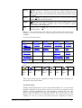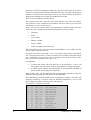
Download User Manual of version 4.1

τ
ARGUS
Version 4.1
User’s Manual
Project: Argus Open Source-project
Date: November 2014
Contributors:
Statistics Netherland, P.O. Box 24500
2490 HA The Hague, The Netherlands
email: [email protected]
Peter-Paul de Wolf (Modular), Anco Hundepool, Sarah Giessing (GHMITER,
audit), Juan-José Salazar (Optimisation methods), Jordi Castro (Network
solutions, CTA)
Contents
1 Introduction..............................................................................................................................5
1.1 Preface.........................................................................................................................................5
1.2 About the name ARGUS.............................................................................................................6
1.3 Contact........................................................................................................................................6
1.4 Open Source................................................................................................................................6
1.5 Acknowledgments ......................................................................................................................7
1.6 Latest improvements....................................................................................................................8
1.7 The structure of this manual........................................................................................................8
2 Producing Safe tables...............................................................................................................9
2.1 Introduction.................................................................................................................................9
2.2 Sensitive cells in magnitude tables..............................................................................................9
2.3 Sensitive cells in frequency count tables...................................................................................11
2.4 Table redesign...........................................................................................................................11
2.5 Secondary cell suppression........................................................................................................11
2.6 Information loss in terms of cell costs.......................................................................................12
2.7 Series of tables...........................................................................................................................12
2.8 The Hypercube/GHMITER method...........................................................................................13
2.8.1 The hypercube method....................................................................................................13
2.8.2 The ARGUS implementation of GHMITER...................................................................14
2.9 Optimisation models for secondary cell suppression.................................................................17
2.10 The Modular approach.............................................................................................................19
2.11 The modular approach for linked tables...................................................................................23
2.12 Network solution for large 2 dimensional tables with one hierarchy.......................................24
2.13 Controlled Tabular Adjustment...............................................................................................25
2.14 Controlled rounding.................................................................................................................28
2.15 Audit........................................................................................................................................30
2.16 Functional design of τ-argus ...................................................................................................33
3 A tour of τ-ARGUS................................................................................................................34
3.1 Preparation.................................................................................................................................34
3.1.1 First steps........................................................................................................................35
3.1.2 Open a microdata file......................................................................................................35
3.1.3 Specify metafile...............................................................................................................36
3.1.4 Specify tables..................................................................................................................40
3.2 The process of disclosure control..............................................................................................42
3.2.1.1 Cell information........................................................................................................43
3.2.1.2 Recode......................................................................................................................45
3.2.1.3 Secondary Suppression.............................................................................................48
3.2.1.4 Summary Window....................................................................................................50
3.3 Save the safe table.....................................................................................................................51
4 Reference Section - Description of the Menu Items..............................................................53
4.1 Menu structure..........................................................................................................................53
4.2 Viewing the table.......................................................................................................................55
4.2.1 A priori info.....................................................................................................................58
4.2.2 Global recoding...............................................................................................................59
4.2.3 Secondary suppression....................................................................................................63
4.2.3.1 Hypercube.................................................................................................................63
4.2.3.2 Modular....................................................................................................................65
4.2.3.3 Optimal.....................................................................................................................65
4.2.3.4 Network....................................................................................................................66
4.2.3.5 After the suppression................................................................................................67
4.2.4 Controlled Tabular Adjustment.......................................................................................68
4.2.5 Controlled rounding.........................................................................................................69
4.2.6 The audit procedure.........................................................................................................73
4.2.7 The Options at the Bottom of the table............................................................................75
4.3 The File menu............................................................................................................................77
4.3.1 File | Open Microdata......................................................................................................77
4.3.2 File | Open Table ............................................................................................................79
4.3.3 File | Open Table Set.......................................................................................................81
4.3.4 File | Open Batch Process................................................................................................82
4.3.5 File | Exit.........................................................................................................................82
4.4 The Specify menu......................................................................................................................82
4.4.1 Specify | Metafile [for microdata]....................................................................................82
4.4.2 Specify | Metafile [SPSS System files]............................................................................85
4.4.3 Specify | Metafile [for tabular data].................................................................................87
4.4.4 Specify | Specify Tables [for microdata].........................................................................88
4.4.5 Specify | Specify tables [for tabular data]........................................................................95
4.5 The Modify menu......................................................................................................................96
4.5.1 Modify | Select Table......................................................................................................96
4.5.2 Modify | Linked Tables...................................................................................................97
4.6 The Output menu.....................................................................................................................101
4.6.1 Output | Save Table.......................................................................................................101
4.6.2 Output | View Report.....................................................................................................103
4.6.3 Output | Generate apriori...............................................................................................105
4.6.4 Output | Write Batch File...............................................................................................107
4.7 The Help menu........................................................................................................................107
4.7.1 Help | Contents..............................................................................................................107
4.7.2 Help | News...................................................................................................................107
4.7.3 Help | Options................................................................................................................107
4.7.4 Help | About..................................................................................................................108
5 Further descriptions..............................................................................................................110
5.1 Meta data files.........................................................................................................................110
5.1.1 Meta data for fixed format micro data ..........................................................................110
5.1.2 Meta data for free format micro data ............................................................................113
5.1.3 Meta data for SPSS system files...................................................................................114
5.1.4 Meta data for tabular data files......................................................................................114
5.2 Hierarchy file...........................................................................................................................116
5.3 Codelist file.............................................................................................................................117
5.4 Global recode file....................................................................................................................117
5.5 The JJ-file format....................................................................................................................118
5.6 The apriori file.........................................................................................................................119
5.7 The Batch command file..........................................................................................................121
5.8 Log file....................................................................................................................................125
6 Index.....................................................................................................................................127
τ-ARGUS (4.0) user's manual
4
1 INTRODUCTION
1.1
Preface
This is the user's manual for τ-ARGUS version 4.1. τ-ARGUS is a software tool
designed to assist a data protector in producing safe tables. This manual describes
the first Open Source version of τ-ARGUS. After a long history of development at
Statistics Netherlands (CBS) as closed software, CBS has decided to convert
τ-ARGUS towards Open Source. This process coincides with the formal retirement
of the main developer, Anco Hundepool. With the financial support of Eurostat we
have been able to do this transformation and we hope that the future of τ-ARGUS is
secured. The main aim of this transition project was to port the current (version
3.5) of τ-ARGUS to an open environment. So this version 4.1 does not contain many
new extensions. The whole user-interface has been rewritten in JAVA, replacing the
old Visual Basic version. The aim of this transition is to be in an open environment
and also be platform independent. So also a UNIX version is possible now.
Nevertheless with respect to the previous release of τ-ARGUS we have made a few
steps forward, and τ-ARGUS now has facilities to protect tables via Controlled
Tabular Adjustment (CTA). These routines for this have been developed by Jordi
Castro of the Polytechnic University of Catalonia.
We have also added the option to use a free open solver in addition to the classical
commercial solvers like CPLEX and Xpress. However we expect that these
commercial solvers are still very much needed, when we want to protect large
serious tables.
The purpose of τ-ARGUS is to protect tables against the risk of disclosure, i.e. the
accidental or deliberate disclosure of information related to individuals from a
statistical table. This is achieved by modifying the table so that it contains less
detailed information. τ-ARGUS allows for several modifications of a table: a table
can be redesigned, meaning that rows and columns can be combined; sensitive
cells can be suppressed and additional cells to protect these can be found in some
optimum way (secondary cell suppression). Also rounding and CTA can be used to
protect sensitive tables.
The purpose of the present manual is to give a potential user enough information so
that he can understand the general principles on which τ-ARGUS is based, and also
allow him to use the package. So it contains both general background information
and detailed program information. For a more in-depth theoretical background we
refer to the handbook “Statistical Disclosure Control” by Anco Hundepool, Josep
Domingo-Ferrer, Luisa Franconi, Sarah Giessing, Eric Schulte Nordholt, Keith
Spicer and Peter-Paul de Wolf (ISBN: 978-1-119-97815-2, Wiley, 2012.
τ-ARGUS is one of a twin set of disclosure control packages. For the protection of
microdata - μ-ARGUS - has been developed, which is the twin brother of τ-ARGUS.1
Also μ-ARGUS has been ported to Open Source.
1
5
See Anco Hundepool et al., 2014, μ-ARGUS version 5.1 user’s manual, Statistics Netherlands, The Hague, The
Netherlands.
τ-ARGUS (4.1) user's manual
1.2
About the name ARGUS
Somewhat jokingly the name ARGUS can be interpreted as the acronym of ‘Anti-Reidentification General Utility System’ 2. As a matter of fact, the name ARGUS was
inspired by a myth of the ancient Greeks. In this myth Zeus has a girl friend named
Io. Hera, Zeus’ wife, did not approve of this relationship and turned Io into a cow.
She let the monster ARGUS guard Io. ARGUS seemed to be particularly well qualified
for this job, because it had a hundred eyes that could watch over Io. If it would fall
asleep only two of its eyes were closed. That would leave plenty of eyes to watch
Io. Zeus was eager to find a way to get Io back. He hired Hermes who could make
ARGUS fall asleep by the enchanting music on his flute. When Hermes played his
flute to ARGUS this indeed happened: all its eyes closed, one by one. When Hermes
had succeeded in making ARGUS fall asleep, ARGUS was decapitated. ARGUS’ eyes
were planted onto a bird’s tail - a type of bird that we now know under the name of
peacock. That explains why a peacock has these eye-shaped marks on its tail. This
also explains the picture on the cover of this manual. It is a copperplate engraving
of Gerard de Lairesse (1641-1711) depicting the process where the eyes of ARGUS
are being removed and placed on the peacock’s tail. 3
Like the mythological ARGUS, the software is supposed to guard something, in this
case data. This is where the similarity between the myth and the package is
supposed to end, as we believe that the package is a winner and not a loser as the
mythological ARGUS is.
1.3
Contact
Feedback from users will help improve future versions of τ-ARGUS and is therefore
greatly appreciated. The authors of this manual can be contacted directly for
suggestions that may lead to improved versions of τ-ARGUS in writing or otherwise;
e-mail messages can also be sent to [email protected].
1.4
Open Source
In the open source world the responsibility for the software is different. The idea
behind open source is that the software code is no longer owned by one institute
(Statistics Netherlands), but the source is available for anybody. Anybody can also
contribute to the code and make his own extensions. Nevertheless we do not want
to have many different versions of the software and many diversions.
Therefore there will always be one official version of τ-ARGUS. In order to achieve
this we need a body to make decisions about further developments and extensions
for the official τ-ARGUS. This responsibility will be in the hands of a small
committee. This committee will be a sub-group of the Eurostat technical working
group on Statistical Confidentiality. They will make decisions on whether a new
extension/correction will be allowed in the official versions of τ-ARGUS, and also
make recommendations for future extensions.
2
This interpretation is due to Peter Kooiman, former head of the methodology department at Statistics
Netherlands.
3
The original copy of this engraving is in the collection of ‘Het Leidsch Prentenkabinet’ in Leiden, The
Netherlands.
τ-ARGUS (4.1) user's manual
6
Nevertheless the above mentioned email address ([email protected]) will remain open
for questions.
1.5
Acknowledgments
τ-ARGUS was started as part of the EU 4 th framework SDC-project and became a
mature software tool as part of the CASC project that was partly sponsored by the
EU under contract number IST-2000-25069. This support is highly appreciated.
The CASC (Computational Aspects of Statistical Confidentiality) project is part of
the Fifth Framework of the European Union. The main part of τ-ARGUS has been
developed at Statistics Netherlands by Aad van de Wetering and Ramya
Ramaswamy (who wrote the kernel) and Anco Hundepool (who wrote the
interface). However this software would not have been possible without the
contributions of several others, both partners in the CASC-project and outsiders.
Recent extensions of τ-ARGUS have been made possible during the European
CENEX-SDC-project (grant agreement 25200.2005.001-2005.619), the ESSNetSDC project (grant agreement 25200.2005.003-2007.670.) and the ESSnet SDC
harmonisation (61102.2010.004-2010.579).
The Open Source transition was supported by a Eurostat grant (61102.2012.0012012.102).
The German partners Statistisches Bundesamt (Sarah Giessing and Dietz
Repsilber) have contributed the GHMITER software, which offers a solution for
secondary cell suppression based on hypercubes. Peter-Paul de Wolf has built a
search algorithm based on non-hierarchical optimal solutions. This algorithm
breaks down a large hierarchical table into small non-hierarchical subtables, which
are then individually protected. A team led by JJ Salazar of the University La
Laguna Tenerife, Spain, has developed the optimisation routines. Additionally
Jordi Castro, Universitat Politècnica de Catalunya. Barcelona, has developed a
solution based on networks. Jordi Castro also developed the CTA solution.
The controlled rounding procedure has been developed by JJ Salazar in a project
sponsored by ONS. In order to enhance the usability τ- ARGUS now also can handle
SPSS-system files. For using τ-ARGUS in combination with SAS, several reports
have been produced during the ESSnet projects. These reports and also the SAStools are available from the CASC/ESSNet website.
The audit routine was first developed by Karl Luhn of the University of Ilmenau
and further developed by Destatis.
For solving these optimisation problems, τ-ARGUS traditionally uses commercial
LP-solvers. Traditionally we use Xpress as an LP-solver. This package is kindly
made available for users of τ-ARGUS in a special agreement between the τ-ARGUSteam and FICO, the developers of Xpress. Alternatively τ-ARGUS can also use the
CPLEX-package. Users can choose either solver to link to τ-ARGUS (provided, of
course, they purchase a license for the solver chosen). However users already
having a licence for one of these packages for other applications can use their
current licence for τ-ARGUS as well.
Starting with this Open Source version also free Open Solvers can now also be
used to solve the optimisation models behind Cell Suppression, rounding and CTA.
7
τ-ARGUS (4.1) user's manual
1.6
Latest improvements
The latest extensions in version 4.1 of τ-ARGUS are :
1.7
•
New structure of the interface, making the table itself the central window.
•
Controlled Tabular Adjustment.
•
Rewritten Open Source Code in JAVA.
•
C++ dlls for data manipulation and the modular approach have been
adapted for the Open Source compilers.
•
The use of free Open Solvers complementary to the commercial solvers.
The structure of this manual
The remaining part of this manual consists of four chapters and an index.
In Chapter 2 we will give a short introduction to the theory and methodology.
However for a more fundamental description we refer to the Wiley handbook on
Statistical Disclosure Control4. This handbook is the result of the joined work of
the SDC specialist in Europe working together for a long period.
In Chapter 3 a short tour of τ-ARGUS will be given as a first impression of the
program.
Chapter 4 is the reference manual of τ-ARGUS. It will describe in detail the program.
This chapter is organized by the menu items of τ-ARGUS.
Chapter 5 gives details of files used by τ-ARGUS.
The manual is concluded with an index.
4
Anco Hundepool, Josep Domingo-Ferrer, Luisa Franconi, Sarah Giessing, Eric Schulte Nordholt,
Keith Spicer, Peter-Paul de Wolf (2012), Statistical Disclosure Control, ISBN: 978-1-119-97815-2,
Wiley.
τ-ARGUS (4.1) user's manual
8
2 PRODUCING SAFE TABLES
2.1
Introduction
The growing demands from researchers, policy makers and others for more and
more detailed statistical information lead to a conflict. Statistical offices collect
large amounts of data for statistical purposes. The respondents are only willing to
provide the statistical offices with the required information if they can be certain
that these statistical offices will treat their data with the utmost care. This implies
that respondents' confidentiality must be guaranteed. This imposes limitations on
the amount of detail in the publications. Practice and research have generated
insights into how to protect tables, but the problem is not yet definitively solved.
Before we go into more details, the basic ideas on which τ-ARGUS is based, we give
a sketch of the general ideas. At first sight one might find it difficult to understand
that information presented in tabular form presents a disclosure risk. After all, one
might say that the information is presented only in aggregate form.
Safe tables are produced from unsafe ones by applying certain SDC measures to
the tables. These SDC measures - as far as they are implemented in τ-ARGUS - are
discussed in the present section. Some key concepts such as sensitive cells,
information loss and the like are discussed as well.
2.2
Sensitive cells in magnitude tables
5
The well-known dominance rule is often used to find the sensitive cells in tables,
i.e. the cells that cannot be published as they might reveal information on
individual respondents. More particularly, this rule states that a cell of a table is
unsafe for publication if a few (n) major (largest) contributors to a cell are
responsible for a certain percentage (k) of the total of that cell. The idea behind this
rule is that in that case at least the major contributors themselves can determine
with sufficient precision the contributions of the other contributors to that cell. The
choice n=3 and k=70% is not uncommon, but τ-ARGUS will allow the users to
specify their own values of n and k.
As an alternative the prior-posterior rule has been proposed. The basic idea is that a
contributor to a cell has a better chance to estimate competitors in a cell than an
outsider, and also that these kind of intrusions can occur rather often. The precision
with which a competitor can estimate is a measure of the sensitivity of a cell. The
worst case is that the second largest contributor will be able to estimate the largest
contributor. If this precision is more than p%, the cell is considered unsafe. An
extension is that also the global knowledge about each cell is taken into account. In
that case we assume that each intruder has a basic knowledge of the value of each
contributor of q%. Note, that it is actually the ratio p/q that determines which cells
are considered safe, or unsafe. In this version of ARGUS, the q-parameter is fixed to
100. Literature refers to this rule as (minimum protection of) p %-rule. If the
5
9
See section 4.2 Disclosure risk assessment I: primary sensitive cells of the SDC-Handbook (Hundepool et
all (2012)).
τ-ARGUS (4.1) user's manual
intention is to state a prior-posterior rule with parameters p 0 and q0, where q0 < 100,
choose the parameter p of the p %-rule as p = p0/q0*100. See Loeve (2001)6
With these rules as a starting point it is easy to identify the sensitive cells, provided
that the tabulation package has the facility not only to calculate the cell totals, but
also to calculate the number of contributors and the n individual contributions of
the major contributors. Tabulation packages like ABACUS (from Statistics
Netherlands) and the package ‘SuperCross’ developed in Australia by Space-Time
Research have that capacity. In fact τ-ARGUS not only stores the sum of the n major
contributions for each cell, but the individual major contributions themselves. The
reason for this is that this is very handy in case rows and columns etc. in a table are
combined. By merging and sorting the sets of individual contributions of the cells
to be combined, one can quickly determine the major contributions of the new cell,
without going back to the original file. This implies that one can quickly apply the
dominance rule or the p%-rule to the combined cells. Combining rows and
columns (table redesign) is one of the major tools for reducing the number of
unsafe cells.
This too is the reason why τ-ARGUS can read microdata files and build the tables
itself. However due to continuous demands from users we have now also provide
the option to read ready-made tables, but with the restriction that the options for
table redesign will not be available in that case.
A problem, however, arises when also the marginals of the table are published. It is
no longer enough to just suppress the sensitive cells, as they can be easily
recalculated using the marginals. Even if it is not possible to exactly recalculate the
suppressed cell, it is possible to calculate an interval that contains the suppressed
cell. This is possible if some constraints are known to hold for the cell values in a
table. A commonly found constraint is that the cell values are all nonnegative.
If the size of such an interval is rather small, then the suppressed cell can be
estimated rather precisely. This is not acceptable either. Therefore it is necessary to
suppress additional information to achieve sufficiently large intervals.
Several solutions are available to protect the information of the sensitive cells:
•
Combining categories of the spanning variables (table redesign). Larger
cells tend to protect the information about the individual contributors
better.
•
Suppression of additional (secondary) cells to prevent the recalculation of
the sensitive (primary) cells.
The calculation of the optimal set (with respect to the loss of information) of
secondary cells is a complex OR-problem. τ-ARGUS has been built around this
solution, and takes care of the whole process. A typical τ-ARGUS session will be one
in which the users will first be presented with the table containing only the primary
unsafe cells. The user can then choose how to protect these cells. This can involve
the combining of categories, equivalent to the global recoding of μ-ARGUS. The
result will be an update of the table with fewer unsafe cells (certainly not more) if
the recoding has worked. At a certain stage the user requests the system to solve
the remaining unsafe cells by finding secondary cells to protect the primary cells.
At this stage the user can choose between several options to protect the primary
sensitive cells. Either they choose the hypercube method or the optimal solution. In
6
Loeve, Anneke, 2001, Notes on sensitivity measures and protection levels, Research paper, Statistics
Netherlands. Available at http://neon.vb.cbs.nl/casc/related/marges.pdf
τ-ARGUS (4.1) user's manual
10
this case they also has to select the solver to be used, Xpress or CPLEX. After this,
the table can be stored for further processing if necessary, and eventual publication.
2.3
Sensitive cells in frequency count tables
In the simplest way of using τ-ARGUS, sensitive cells in frequency count tables are
defined as those cells that contain a frequency that is below a certain threshold
value. This threshold value is to be provided by the data protector. This way of
identifying unsafe cells in a table is the one that is implemented in the current
version of τ-ARGUS It should be remarked, however, that this is not always an
adequate way to protect a frequency count table. 7 Yet it is applied a lot. Applying a
dominance rule or a p% rule is useless in this context. One should think about
possible disclosure risks that a frequency count table poses and possible disclosure
scenarios in order to simulate the behaviour of an intruder. Such an analysis would
probably come up with different insights than using a simple thresholding rule, e.g.
like the one sketched in the reference just mentioned. We just mention here the
risks of group-disclosure; when a (small) group of respondents have all the same
score on a certain category. This risk is often also referred to as the problem of
100%-cells. Further research on this topic is being carried out at a.o. Statistics
Netherlands.
2.4
Table redesign
If a large number of sensitive cells are present in a table, it might be an indication
that the spanning variables are too detailed. In that case one could consider
combining certain rows and columns in the table. (This might not always be
possible because of publication policy.) Otherwise the number of secondary cell
suppressions might just be too enormous. The situation is comparable to the case of
microdata containing many unsafe combinations. Rather than eliminating them
with local suppressions one can remove them by using global recodings. For
tabular data we use the phrase “table redesign” to denote an operation analogous to
global recoding in microdata sets. The idea of table redesign is to combine rows,
columns etc., by adding the cell contents of corresponding cells from the different
rows, columns etc. It is a property of the sensitivity rules that a joint cell is safer
than any of the individual cells. So as a result of this operation the number of
unsafe cells is reduced. One can try to eliminate all unsafe combinations in this
way, but that might lead to an unacceptably high information loss. Instead, one
could stop at some point, and eliminate the remaining unsafe combinations by
using other techniques such as cell suppression.
2.5
Secondary cell suppression
Once the sensitive cells in a table have been identified, possibly following table
redesign it might be a good idea to suppress these values. In case no constraints on
the possible values in the cells of a table exist this is easy: one simply removes the
cell values concerned and the problem is solved. In practice, however, this situation
hardly ever occurs. Instead one has constraints on the values in the cells due to the
7
11
See section 5.2 Disclosure risks of the SDC-Handbook (Hundepool et all (2012)).
τ-ARGUS (4.1) user's manual
presence of marginals and lower bounds for the cell values (typically 0). The
problem then is to find additional cells that should be suppressed in order to protect
the sensitive cells. The additional cells should be chosen in such a way that the
interval of possible values for each sensitive cell value is sufficiently large. What is
“sufficiently large” can be specified by the data protector in τ-ARGUS by specifying
the protection intervals.
In general the secondary cell suppression problem turns out to be a hard problem,
provided the aim is to retain as much information in the table as possible, which, of
course, is a quite natural requirement. The optimisation problems that will then
result are quite difficult to solve and require expert knowledge in the area of
combinatorial optimisation.
2.6
Information loss in terms of cell costs
8
In case of secondary cell suppression it is possible that a data protector might want
to differentiate between the candidate cells for secondary suppression. It is possible
that they would strongly prefer to preserve the content of certain cells, and are
willing to sacrifice the values of other cells instead. A mechanism that can be used
to make such a distinction between cells in a table is that of cell costs. In τ-ARGUS it
is possible to associate different costs with the cells in a table. The higher the cost
the more important the corresponding cell value is considered and the less likely it
will be suppressed. We shall interpret this by saying that the cells with the higher
associated costs have a higher information content. The aim of secondary cell
suppression can be summarised by saying that a safe table should be produced
from an unsafe one, by minimising the information loss, expressed as the sum of
the costs associated with the cells that have secondarily been suppressed.
τ-ARGUS offers several ways to compute these costs. The first option is to compute
the costs as the sum of the contributions to a cell. Alternatively another variable in
the data file can be used as the cost function. Secondly this cost can be the
frequency of the contributors to a cell, and finally each cell can have cost = 1,
minimising the number of suppressed cells.
2.7
Series of tables
In τ-ARGUS it is possible to specify a series of tables that will be protected one by
one, and independently of each other. It is more efficient to choose this option
since τ-ARGUS requires only a single run through the microdata in order to produce
the tables. But also for the user it is often more attractive to specify a series of
tables and let τ-ARGUS protect them in a single session, rather than have several
independent sessions.
8
See section 4.6 Information loss measures for tabular data of the SDC-Handbook (Hundepool et all (2012).
τ-ARGUS (4.1) user's manual
12
2.8
The Hypercube/GHMITER method
9
In order to ensure tractability also of big applications, τ-ARGUS interfaces with the
GHMITER hypercube method of R. D. Repsilber of the Landesamt für
Datenverarbeitung und Statistik in Nordrhein-Westfalen/Germany, offering a quick
heuristic solution. The method has been described in depth in Repsilber (1994),
Repsilber (1999) and Repsilber (2002), for a briefer description see Giessing and
Repsilber (2002).
2.8.1 The hypercube method
The approach builds on the fact that a suppressed cell in a simple n-dimensional
table without substructure cannot be disclosed exactly if that cell is contained in a
pattern of suppressed, nonzero cells, forming the corner points of a hypercube.
The algorithm subdivides n-dimensional tables with hierarchical structure into a set
of n-dimensional sub-tables without substructure. These sub-tables are then
protected successively in an iterative procedure that starts from the highest level.
Successively, for each primary suppression in the current sub-table, all possible
hypercubes with this cell as one of the corner points are constructed.
If protection against inferential disclosure is requested, for each hypercube, a lower
bound for the width of the suppression interval for the primary suppression that
would result from the suppression of all corner points of the particular hypercube
will be estimated. To estimate that bound, it is not necessary to implement the time
consuming solution to the corresponding Linear Programming problem. Only if it
turns out that the bound is sufficiently large, the hypercube becomes a feasible
solution.
If no protection against inferential disclosure is requested, any hypercube will be
considered feasible. This may of course lead to some cases of underprotection.
For any of the feasible hypercubes, the loss of information associated with the
suppression of its corner points is computed. The particular hypercube that leads to
minimum information loss is selected, and all its corner points are suppressed.
Note that the information loss concept of the hypercube method is slightly different
from the one of the other, linear programming based methods for secondary cell
suppression offered by τ-ARGUS it operates rather like a two-stage concept. In the
first way, the algorithm will look at the number of additional suppressions
(additional to those that are already suppressed because they a primary unsafe, or
because they were selected as secondary suppression in another subtable) that
would be caused by the selection of a particular candidate hypercube. If there is
more than one hypercube that would result in the same, smallest number of
additional secondary suppressions, at second priority the method will select the one
with the smallest sum of costs associated to the suppression of the corresponding
additional secondary suppressions. Cell costs associated to a cell are indeed a
logarithmic transformation of the cell value plus eventually a large constant, if the
cell is a marginal cell of the current sub-table.
9
13
The section on GHMiter has been contributed by Sarah Giessing, Federal Statistical Office of Germany
65180 Wiesbaden; E-mail: [email protected].
See section 4.4.3 Algorithms for secondary cell suppression of the SDC-Handbook (Hundepool et all
(2012)).
τ-ARGUS (4.1) user's manual
After all sub-tables have been protected once, the procedure is repeated in an
iterative fashion. Within this procedure, when cells belonging to more than one
sub-table are chosen as secondary suppressions in one of these sub-tables, in
further processing they will be treated like sensitive cells in the other sub-tables
they belong to. The same iterative approach is used for sets of linked tables.
It should be mentioned here that the ‘hypercube criterion’ is a sufficient but not a
necessary criterion for a ‘safe’ suppression pattern. Thus, for particular subtables
the ‘best’ suppression pattern may not be a set of hypercubes – in which case, of
course, the hypercube method will miss the best solution and lead to some
overprotection. Other simplifications of the heuristic approach that add to this
tendency for over-suppression are the following: when assessing the feasibility of a
hypercube to protect specific target suppressions against interval disclosure, the
method
•
is not able to consider protection maybe already provided by other cell
suppressions (suppressed cells that are not corner points of this hypercube)
within the same sub-table,
•
does not consider the sensitivity of multi-contributor primary suppressions
properly, that is, it does not consider the protection already provided in
advance of cell suppression through aggregation of these contributions,
•
attempts to provide the same relative ambiguity to (eventually large)
secondary suppressions that have been selected to protect cells in a linked
sub-table, as if they were single-respondent primary suppressions, while
actually it would be enough to provide the same absolute ambiguity as
required by the corresponding primary suppressions.
2.8.2 The ARGUS implementation of GHMITER
•
In the implementation offered by ARGUS, GHMITER makes sure that a single
respondent cell will never appear to be corner point of one hypercube only,
but of two hypercubes at least. Otherwise it could happen that a single
respondent, who often can be reasonably assumed to know that he is the
only respondent, could use his knowledge on the amount of his own
contribution to recalculate the value of any other suppressed corner point
of this hypercube.
•
As explained above, GHMITER uses an elaborate internal cost assignment
mechanism which is essential to achieve an optimal performance (given
the natural restrictions of the simple heuristic approach, of course). This
mechanism should not be cast out of balance. Therefore, the user’s choice
of the cell costs (c.f. 3.1.4, 4.4.4) does not have any impact, when using the
hypercube method.
•
For tables presenting magnitude data, if protection against inferential
disclosure is requested (see the upper part of the pop-up window below)
τ-ARGUS will ensure that GHMITER selects secondary suppressions that
protect the sensitive cells properly. Only cells will be considered feasible
as secondary suppressions that are large enough to give enough protection
to the target sensitive cell as explained in Giessing (2003).
τ-ARGUS (4.1) user's manual
14
15
•
The standard implementation of the hypercube is that extra protection is
given to singleton cells, i.e. cells with only one contributor. As this
contributor knows exactly the cell value he might be able to undo the
protection. But this extra protecting can be disabled.
•
In order to achieve this, τ-ARGUS computes a suitable sliding protection
ratio (for explanation see Giessing (2003), τ-ARGUS will display the value
of this ratio in the report file) to be used by GHMITER. If in the screen above
the option “Protection against inferential disclosure required” is
inactivated, GHMITER will not check whether secondary suppressions are
sufficiently large.
•
As mentioned above, GHMITER is unable to 'add' the protection given by
multiple hypercubes. In certain situations, it is not possible to provide
sufficient protection to a particular sensitive cell (or secondary
suppression) by suppression of one single hypercube. In such a case,
GHMITER is unable to confirm that this cell has been protected properly,
according to the specified sliding protection ratio. It will then reduce the
sliding protection ratio automatically, and individually, step by step for
those cells, the protection of which the program cannot confirm otherwise.
In steps 1 to 9 we divide the original ratio by k, values of k from 2 to 10,
and if this still does not help, in step 10 we divide by an extremely large
value, and finally, if even that does not solve the problem, step 11 will set
the ratio to zero). The τ-ARGUS report file will display the number of cases
where the sliding protection range was reduced by finally confirmed
sliding protection ratio.
•
Note, that that the number of cases with range reduction reported by this
statistic in the report file is very likely to exceed the actual number of cells
concerned, because cells belonging to multiple (sub-) tables are counted
multiple times. In our experience this concerns particularly the cases,
where the protection level was reduced to an‚ ‘infinitely‘ small (positive)
value (in step 10, see above). Step 10 is usually required to confirm
protection of large, high level secondary suppressions, which are likely to
appear in multiple tables, especially in processing of linked tables. By the
τ-ARGUS (4.1) user's manual
way, terms “reduction of the sliding protection ratio” and “reduction of the
protection level” are used synonymously in the report file.
•
Note that step 11 will make cells eligible for secondary suppression that
τ-ARGUS considers as ‘protected’ (so called ‘frozen’ cells, for discussion of
this option see for instance Giessing (2003).
As this is inconsistent with the current view on protected cells in τ-ARGUS this will
lead to the following error message:
The cell value and the codes of those suppressed frozen cells are then displayed by
τ-ARGUS :This information is also written in the file “frozen.txt” in the tempdirectory.
τ-ARGUS (4.1) user's manual
16
When the status of these cells is changed into ‘unprotected’ before re-running the
hypercube method, the solution will be a feasible solution for τ-ARGUS. Zero cells
are consider to be frozen as well in the hypercube. Those frozen cells can be
ignored
Negative values
The hypercube method has no problems when certain cells are negative.
References on GHMITER
Repsilber, R. D. (1994), ‘Preservation of Confidentiality in Aggregated data’, paper
presented at the Second International Seminar on Statistical Confidentiality,
Luxembourg, 1994
Repsilber, D. (1999), ‘Das Quaderverfahren’ - in Forum der Bundesstatistik, Band
31/1999: Methoden zur Sicherung der Statistischen Geheimhaltung, (in German)
Repsilber, D. (2002), ‘Sicherung persönlicher Angaben in Tabellendaten’ - in
Statistische Analysen und Studien Nordrhein-Westfalen, Landesamt für
Datenverarbeitung und Statistik NRW, Ausgabe 1/2002 (in German)
Giessing, S. and Repsilber, D. (2002), ‘Tools and Strategies to Protect Multiple Tables
with the GHQUAR Cell Suppression Engine’, in ‘Inference Control in Statistical
Databases’ Domingo-Ferrer (Editor), Springer Lecture Notes in Computer Science Vol.
2316.
Giessing, S. (2003), ‘Co-ordination of Cell Suppressions: strategies for use of
GHMITER’, Proceedings of the Joint ECE/Eurostat work session on statistical data
confidentiality (Luxembourg, 7-9 April 2003)
2.9
Optimisation models for secondary cell suppression
10
τ-ARGUS applies different approaches to find optimal and near-optimal solutions.
One of these approaches is based on a Mathematical Programming technique
which consists of solving Integer Linear Programming programs modelling the
combinatorial problems under different methodologies (Cell Suppression and
Controlled Rounding). The main characteristic of these models is that they share
the same structure, thus based only on a 0-1 variable for each cell. In the Cell
Suppression methodology, the variable is 1 if and only if the cell value must be
suppressed. In the Controlled Rounding methodology, the variable is 1 if and only
if the cell value must be rounded up. No other variables are necessary, so the
number of variables in the model is exactly the number of cells in the table to be
protected. In addition, the model also imposes the protection level requirements
(upper, lower and sliding) in the same way for the different methodologies (Cell
Suppression and Controlled Rounding). These requirements ask for a guarantee
that an attacker will not get too narrow an interval of potential values for a
sensitive cell, which he/she will compute by solving two linear programming
programs (called attacker problems). Even if a first model containing this twoattacker problem would lead to a bi-level programming model, complex to be
solved in practice, a Benders' decomposition approach allows us to convert the
attacker problems into a set of linear inequalities. This conversion provides a
10
17
The optimisation models have been built by a team of researchers headed by Juan-José Salazar-Gonzalez of
the University La Laguna, Tenerife, Spain. Other members of the team were: G. Andreatta, M. Fischetti, R.
Betancort Villalva, M.D. Montesdeoca Sanchez and M. Schoch
τ-ARGUS (4.1) user's manual
second model for each methodology that can be efficiently solved by a modern
cutting-plane approach. Since the variables are 0-1, a branching phase can be
necessary, and the whole approach is named "branch-and-cut algorithm".
Branch-and-cut algorithms are modern techniques in Operations Research that
provide excellent results when solving larger and complicated combinatorial
problems arising in many applied fields (like routing, scheduling, planning,
telecomunications, etc.). Shortly, the idea is to solve a compact 0-1 model
containing a large number of linear inequalities (as the ones above mentioned for
the Cell Suppression and for the Controlled Rounding) through an iterative
procedure that does not consider all the inequalities at the same time, but generates
the important ones when needed. This dynamic procedure of dealing with large
models allows the program to replace the resolution of a huge large model by a
short sequence of small models, which is termed a "decomposition approach". The
on-line generation of the linear inequalities (rows) was also extended in this work
to the variables (columns), thus the algorithm can also works on tables with a large
number of cells, and the overall algorithm is named "branch-and-cut-and-price" in
the Operations Research literature.
To obtain good performance, the implementation has also considered many other
ingredients, standard in branch-and-cut-and-price approaches. For example, it is
fundamentally the implementation of a pre-processing approach where redundant
equations defining the table are eliminated, where variables associated to nonrelevant cells are removed, and where dominated protection levels are detected.
The pre-processing is fundamental to make the problem as small as possible before
starting the optimization phase. Another fundamental ingredient is the heuristic
routine, which allows the algorithm to start with an upper bound of the optimal loss
of information. This heuristic routine ensures the production of a protected pattern
if the algorithm is interrupted by the user before the end. In other words, thanks to
the heuristic routine, the implemented algorithm provide a near-optimal solution if
the execution is cancelled before having a proof of optimality. During the implicit
enumeration approach (i.e., the branch-and-cut-and-price) the heuristic routine is
called several times, thus providing different protected patterns, and the best one
will be the optimal solution if its loss of information is equal to the lower bound.
This lower bound is computed by solving a relaxed model, which consists of
removing the integrability condition on the integer model. Since the relaxed model
is a linear program, a linear programming solver must be called.
We have not implemented our own linear programming solver, but used a
commercial solver which is already tested by other programmers for many years. A
robust linear programming solver is a guarantee that no numerical trouble will
appear during the computation.
That is the reason to requires either CPLEX (from ILOG) or Xpress (from FICO).
Because the model to be solved can be applied to all type of table structures (2dim, 3-dim, 4-dim, etc), including hierarchical and linked tables, we cannot use
special simplex algorithm implementations, like the min-cost flow computation
which would required to work with tables that can be modelled as a network (e.g.,
2-dimensional tables or collections of 2-dim tables linked by one link). On this
special table, ad-hoc approaches (solving network flows or short path problems)
could be implemented to avoid using general linear programming solvers.
In any case, future works will try to replace the commercial solvers by freely
available linear-programming solvers.
τ-ARGUS (4.1) user's manual
18
2.10 The Modular approach
11
The modular (HiTaS) solution is a heuristic approach to cell suppression in
hierarchical tables. Hierarchical tables are specially linked tables: at least one of
the spanning variables exhibits a hierarchical structure, i.e. contains (many) subtotals.
In Fischetti and Salazar (1998) a theoretical framework is presented that should be
able to deal with hierarchical and generally linked tables. In what follows, this will
be called the mixed integer approach. In this framework, additional constraints to a
linear programming problem are generated. The number of added constraints
however, grows rapidly when dealing with hierarchical tables, since many
dependencies exist between all possible (sub-)tables containing many (sub-)totals.
The implemented heuristic approach (HiTaS) deals with a large set of (sub)-tables
in a particular order. A non hierarchical table can be considered to be a hierarchical
table with just one level. In that case, the approach reduces to the original mixed
integer approach and hence provides the optimal solution. In case of a hierarchical
table, the approach will provide a sub-optimal solution that minimises the
information loss per sub-table, but not necessarily the global information loss of
the complete set of hierarchically linked tables.
In the following section, a short description of the approach is given. For a more
detailed description of the method, including some examples, see e.g., De Wolf
(2002).
HiTaS deals with cell suppression in hierarchical tables using a top-down
approach. The first step is to determine the primary unsafe cells in the base-table
consisting of all the cells that appear when crossing the hierarchical spanning
variables. This way all cells, whether representing a (sub-)total or not, are checked
for primary suppression. Knowing all primary unsafe cells, the secondary cell
suppressions have to be found in such a way that each (sub-)table of the base-table
is protected and that the different tables cannot be combined to undo the protection
of any of the other (sub-)tables. The basic idea behind the top-down approach is to
start with the highest levels of the variables and calculate the secondary
suppressions for the resulting table. The suppressions in the interior of the
protected table is then transported to the corresponding marginal cells of the tables
that appear when crossing lower levels of the two variables. All marginal cells,
both suppressed and not suppressed, are then ‘fixed’ in the calculation of the
secondary suppressions of that lower level table, i.e., they are not allowed to be
(secondarily) suppressed. This procedure is then repeated until the tables that are
constructed by crossing the lowest levels of the spanning variables are dealt with.
A suppression pattern at a higher level only introduces restrictions on the marginal
cells of lower level tables. Calculating secondary suppressions in the interior while
keeping the marginal cells fixed, is then independent between the tables on that
lower level, i.e., all these (sub)-tables can be dealt with independently of each
other. Moreover, added primary suppressions in the interior of a lower level table
are dealt with at that same level: secondary suppressions can only occur in the
same interior, since the marginal cells are kept fixed.
However, when several empty cells are apparent in a low level table, it might be
the case that no solution can be found if one is restricted to suppress interior cells
only. Unfortunately, backtracking is then needed.
11
19
See section 4.4.4 Secondary cell suppression in hierarchical and linked tables of the SDC-Handbook,
Hundepool et all (2012).
τ-ARGUS (4.1) user's manual
Obviously, all possible (sub)tables should be dealt with in a particular order, such
that the marginal cells of the table under consideration have been protected as the
interior of a previously considered table. To that end, certain groups of tables are
formed in a specific way (see De Wolf (2002)). All tables within such a group are
dealt separately, using the mixed integer approach.
The number of tables within a group is determined by the number of parentcategories the variables have one level up in the hierarchy. A parent-category is
defined as a category that has one or more sub-categories. Note that the total
number of (sub)-tables that have to be considered thus grows rapidly.
Singletons
Singleton cells should be treated with extra care. The single respondent in this cell
could easily undo the protection if no extra measures were taken. The most
dangerous situation is that there are only two singletons in a row, or one and one
other primary unsafe cell. These singletons could easily disclose the other cell.
We have added options for extra singleton protection in the following situations.
1.
If on a row or column of a subtable there are only two singletons and no other
primary suppressions.
2.
If there is only one singleton and one multiple primary unsafe cell.
3.
If a frequency rule is used, it could happen that two cells on a row/column are
primary unsafe, but the sum of the two cells could still be unsafe. In that case
it should be prevented that these two cells protect each other.
Cells within a table sometimes consist of exactly one contributor. Such a cell is
called a singleton. Linear sensitivity rules will usually label this cell as (primary)
unsafe. When cell suppression is used to protect a table with unsafe cells, these
singletons need to be taken care of in a special way.
Within a suppression pattern, contributors in singletons may be able to recalculate
other suppressed cells. Obviously, a contributor could always insert its own
contribution and thereby recalculate its own suppressed cell. This could in turn lead
to the possibility of recalculating other suppressed cells in the same suppression
pattern. Whenever such a recalculated cell is (primary) unsafe, this means
disclosure.
Within the current models used to determine suppression patterns, it is not possible
to take all possible situations into account when singletons are part of a suppression
pattern. However, an important group of instances of disclosure by singletons, is
when a singleton is part of a row with exactly one additional (also primary)
suppression.
4.
If on a row or column of a subtable there are only two singletons and no other
primary suppressions.
5.
If there is only one singleton and one multiple primary unsafe cell.
6.
If a frequency rule is used, it could happen that two cells on a row/column are
primary unsafe, but the sum of the two cells could still be unsafe. In that case
it should be prevented that these two cells protect each other.
Note that the last situation is not really a singleton problem, but this problem is
handeled in the same way.
To prevent this kind of disclosure, it would be sufficient to force an additional
(third) suppression in the same row. In prior versions of τ-ARGUS this was
accomplished by increasing the protection levels of one of the (primary) unsafe
cells in the row. In short, the protection level of one of the primary suppressed cells
τ-ARGUS (4.1) user's manual
20
was raised in such a way that the other primary suppression would not be able to
give sufficient protection. The largest primary unsafe cell in the row got the cell
value of the other unsafe cell in the row, plus a small value, as protection level.
Indeed, this forces a third suppression in the row.
However, since the cell value of one of the suppressed cells was involved, this
meant that the increased protection level of this cell could become quite large,
which would have an effect on the suppression pattern in one of the other
dimensions. In certain situations this led to oversuppression.
To circumvent this problem, the newly implemented approach adds a virtual cell to
the table. That virtual cell is assigned a value equal to the sum of the two primary
suppressed cells in the row, and is given the status `(primary) unsafe'. That virtual
cell then only has to be protected against exact disclosure, i.e., it suffices to impose
a small protection interval.
The table below shows an example table, displaying the singleton problem. In the
first table the values of the cells are given, with in bold, red, italic the (primary)
unsafe cells. The second table shows the names of the cells, where cij stands for the
cell with coordinates (i, j).
Total
X1
X2
X3
X4
Total
227
73
33
93
25
A
146
52
15
62
17
B
81
24
18
31
8
Total
X1
X2
X3
X4
Total
c00
c01
c02
c03
c04
A
c10
c11
c12
c13
c 14
B
c20
c21
c22
c23
c24
Example table to explain Singleton Problem.
Bold and red means (primary) unsafe.
Now assume that cell c12 = (A,X2) is a singleton and cell c14 = (A,X4) is unsafe
according to a p%-rule with p=10. Hence, cell c14 is the only other (primary) unsafe
cell in that row. To protect cell c14 against disclosure by the contributor of singleton
c12, a `virtual cell cv is defined with value 32. Moreover, that virtual cell is given a
small protection interval, (32,33) say. The relations that define the table structure,
including the virtual cell, are given below:
21
τ-ARGUS (4.1) user's manual
___________________________
c00 = c01 + c02 + c03 + c04
c10 = c11 + c12 + c13 + c04
c20 = c21 + c22 + c23 + c24
c00 = c10 + c20
c01 = c11 + c21
c02 = c12 + c22
c03 = c13 + c23
c04 = c14 + c24
cv = c12 + c14
_____________________________
Table showing the relations defining table structure of table above
Within τ-ARGUS, this procedure is implemented in both the optimal approach as
well as in the modular approach. For the modular approach, this procedure is
applied to each subtable separately, whenever a subtable is dealt with within the
modular approach.
This special attention to singletons is only given when the other suppressed cell in
the same row is a `true' primary suppression. This is natural, since it has to be done
prior to the search for secondary suppressions. In the modular approach, a
hierarchical table is divided into many, non-hierarchical, subtables. Secondary
suppressions in one table sometimes temporarily become primary suppressions in
other tables during the process. I.e., those suppression are not `true' primary
suppressions. It is therefore also natural not to construct virtual cells in case a
singleton is in the same row with exactly one other primary suppression that was
originally a secondary suppression. This is indeed the way it is implemented in the
modular approach.
In previous versions of τ-ARGUS a similar procedure was available. But then the
additional protection was achieved by increasing the protection level of the
singleton cell. This would lead however also in additional protection in other
dimensions and would create over-protection
Negative values
The implementation by Fischetti and Salazar does not allow for negative values.
However it is not uncommon, that some cells in a table have negative values.
Therefore additional measures have been taken. If in a subtable during the process
negative values are found, all cell values are increased such that the lowest value
becomes positive. Of course the margins have to be recalculated, but a safe
protection pattern will be found.
References on the modular method
Fischetti, M. and J.J. Salazar-González (1998). Models and Algorithms for Optimizing Cell
Suppression in Tabular Data with Linear Constraints. Technical Paper, University of
La Laguna, Tenerife.
P.P. de Wolf (2002). HiTaS: a heuristic approach to cell suppression in hierarchical tables.
Proceedings of the AMRADS meeting in Luxembourg (2002).
Additional reading on the optimisation models can be found at the CASC-website
(http://neon.vb.cbs.nl/casc/Related/99wol-heu-r.pdf)
τ-ARGUS (4.1) user's manual
22
2.11 The modular approach for linked tables
When tables are linked through simple linear constraints, cell suppressions must
obviously be coordinated between tables. The most typical case is when tables
share common cells (usually marginals), i.e., when they are linked through
constraints saying literally that cell X of table A is identical to cell Y of table B.
Suppose a set of N tables, {T1,…,TN}, need to be protected. These tables are
assumed to be linked. Each table has a hierarchical structure that may differ from
the hierarchical structures of the other tables. However, it is assumed that tables
using the same spanning variables have hierarchies that can be covered. Loosely
speaking this means that a single hierarchy can be constructed such that all
hierarchies of the same variable in the N tables are a sub hierarchy of the cover
hierarchy. See De Wolf and Giessing (2009) for more details. In the context of preplanned table production processes which are typically in place in statistical
agencies for the production of certain sets of pre-specified standard tabulations, it
is normally no problem to satisfy these conditions. Literally speaking, the
assumption is that tables in a set of linked tables may present the data in a
breakdown by the same spanning variable at various amounts of detail. But only
under the condition that, if in one of the tables some categories of a spanning
variable are grouped into a certain intermediate sum category, during SDC
processing this intermediate sum category is considered in any other table
presenting the data in a breakdown of the same spanning variable and at that much
detail.
The idea is then as follows. Suppose that the N tables {T1,…,TN} that need to be
protected simultaneously, contain M different spanning variables. Since the
hierarchies are supposed to be coverable, an M-dimensional table exists having all
the specified tables as subtables. The spanning variables will be numbered 1 up to
M.
Each spanning variable can have several hierarchies in the specified tables. Denote
i
i
those hierarchies for spanning variable i by H 1 ,..., H I i where Ii is the number of
different hierarchies of variable i.
Define the M-dimensional table by the table with spanning variables according to
hierarchies G1,…,GM such that, for each i = 1,..., M hierarchy Gi covers the set of
i
hierarchies { H j } with j = 1,…, Ii. This M-dimensional table will be called the
cover table. See De Wolf and Giessing (2009) for more details.
Then use the Modular approach (see section 2.10) on the cover table TC, but only
consider those subtables that are also subtables of at least one of the specified
tables T1,…,TN and disregard the other subtables.
I.e., the procedure of the Modular approach is followed, but during that process any
simple subtable that is not a subtable of any of the tables in the set { T1,…,TN} is
skipped. I.e., the order the simple subtables will be protected, is the same as in the
‘complete’ Modular approach, only some subtables will be skipped.
See De Wolf and Hundepool (2010) for a practical application of the Adjusted
Modular Approach.
23
τ-ARGUS (4.1) user's manual
References on the modular approach for linked tables
De Wolf, P.P. and S. Giessing (2009), Adjusting the τ-ARGUS modular approach to deal
with linked tables, Data & Knowledge Engineering, Volume 68, Issue 11, pp. 11601174.
De Wolf, P.P. and A. Hundepool (2010), Three ways to deal with a set of linked SBS tables
using τ-ARGUS, Privacy in Statistical Databases, J. Domingo-Ferrer and E. Magkos
(Eds.), Springer 2010, LNCS 6344 pp. 66-74.
2.12 Network solution for large 2 dimensional tables with one hierarchy
τ-ARGUS also contains a solution for the secondary cell suppression based on
network flows. This contribution is by Jordi Casto of the Universitat Politècnica de
Catalunya in Barcelona. The network flows solution for cell suppression
implements a fast heuristic for the protection of statistical data in two-dimensional
tables with one hierarchical dimension (1H2D tables). This new heuristic sensibly
combines and improves ideas of previous approaches for the secondary cell
suppression problem in two-dimensional general, see Castro(1994) and positive
tables, see Kelly(1992) and Castro(2003) tables. Details about the heuristic can be
found in Castro(1996) and Cox(1995). Unfortunately this approach is only possible
for two-dimensional tables with only one hierarchy, due to the limitations of the
network flows.
The heuristic is based on the solution of a sequence of shortest-path subproblems
that guarantee a feasible pattern of suppressions (i.e., one that satisfies the
protection levels of sensitive cells). Hopefully, this feasible pattern will be close to
the optimal one.
The current package is linked with three solvers: CPLEX7.5/8.0 see ILOG(2000)
PPRN see Castro(1996), and an efficient implementation of the bidirectional
Dijkstra’s algorithm for shortest-paths (that will be denoted as ”Dijkstra”) see
Ahuja(1993). Later releases of CPLEX will also work if the interface routines are the
same than for version 8.0. The heuristic can use any of the three solvers for the
solution of the shortest path subproblems, although Dijkstra is recommended (and
the default one) for efficiency reasons. CPLEX is needed if a lower bound of the
optimal solution want to be computed. The auditing phase can be performed with
either CPLEX or PPRN.
and Dijkstra were implemented at the Dept. of Statistics and Operations
Research of the Universitat Politècnica de Catalunya, and are included in NF CSP.
PPRN was originally developed during 1992–1995, but it had to be significantly
improved within the CASC project to work with NF CSP. Dijkstra was completely
developed in the scope of CASC. The third solver, CPLEX, is a commercial tool, and
requires purchasing a license. However, PPRN is a fairly good replacement—
although not so robust— for the network flows routines of CPLEX. Therefore, in
principle, there is no need for an external commercial solver, unless lower bounds
want to be computed.
PPRN
Even though two of the three solvers are included in the distribution of NF CSP,
this document only describes the features of the heuristic, and from the user’s point
of view. A detailed description of PPRN and Dijkstra’s solvers can be found in
Castro(1996) and Ahuja(1993), respectively.
The current implementation in τ-ARGUS however only uses the Dijkstra and the
PPRN solvers. We have restricted ourselves from commercial solvers here as the
network flows give already a very fast solution.
τ-ARGUS (4.1) user's manual
24
References on the network solution
Ahuja, R.K, Magnanti, T.L., Orlin, J.B., Network Flows, Prentice Hall (1993).
Castro, J., PPRN 1.0, User’s Guide, Technical report DR 94/06 Dept. of Statistics and Operations Research, Universitat Politècnica de Catalunya, Barcelona, Spain, 1994.
Castro, J., Network flows heuristics for complementary cell suppression: an empirical
evaluation and extensions, in LNCS 2316, Inference Control in Statistical
Databases, J. Domingo-Ferrer (Ed), (2002) 59–73.
Castro, J., Nabona, N. An implementation of linear and nonlinear multicommodity network
flows. European Journal of Operational Research 92, (1996) 37–53.
Cox, L.H., Network models for complementary cell suppression. J. Am. Stat. Assoc. 90,
(1995) 1453–1462.
ILOG CPLEX, ILOG CPLEX 7.5 Reference Manual Library, ILOG, (2000).
Kelly, J.P., Golden, B.L, Assad, A.A., Cell Suppression: disclosure protection for sensitive
tabular data, Networks 22, (1992) 28–55.
Castro, J. User’s and programmer’s manual of the network flows heuristics package for cell
suppression in 2D tables Technical Report DR 2003-07, Dept. of Statistics and
Operations Research, Universitat Politècnica de Catalunya, Barcelona, Spain,2003;
See http://neon.vb.cbs.nl/casc/deliv/41D6_NF1H2D-Tau-ARGUS.pdf
2.13 Controlled Tabular Adjustment12
The purpose of controlled tabular adjustment (also known as minimum-distance
controlled tabular adjustment or simply CTA) is to find the closest safe table to the
original one. Since CTA is a perturbative method, this goal is achieved by
publishing a table where the values of sensitive cells have been modified according
to some predefined protection levels, and the remaining non-sensitive cells are
minimally changed to guarantee the table additivity.
The example illustrates CTA on a small two-dimensional table with one sensitive
cell in boldface, with lower and upper protection levels equal to five (table (a) of
the example). Depending on the 'protection direction' of the sensitive cell, either
'lower' or 'upper', which has to be decided, the value to be published for this cell
will be respectively less or equal than the original cell value minus the lower
protection level, or greater or equal than the original cell value plus the upper
protection level. In the example, if the protection direction is 'lower', then the value
published or the sensitive cell should be less or equal than 35; the optimal adjusted
table for this case is shown in table (b) of the example. If the protection direction is
'upper', then the value must be greater or equal than 45, as shown in table (c) of the
example. In a larger and more complex table, with many sensitive cells, the
obtention of the protection directions that provide the minimal changes to nonsensitives cells is not as easy as in the example. CTA has thus to be formulated and
solved as an optimization problem, in particular as a mixed integer linear problem
(MILP).
Example of a CTA solution: The cell (M2P3) is a sensitive cell with lower and
upper protection level 5. Protected tables with 'lower protection direction' and
'upper protection direction' (i.e., value of sensitive is respectively reduced and
increased by five units)
12
25
See section 4.5.2 A post-tabular method: Controlled tabular adjustment of the Handbook
τ-ARGUS (4.1) user's manual
M1
P1
20
P2
24
P3
28
72
M2
38
38
40
116
M3
40
39
42
121
98
101
110
309
Original table (a)
P1
P2
P3
P1
P2
P3
M1
15
24
33
72
25
24
23
72
M2
43
38
35
116
33
38
45
116
M3
40
39
42
121
40
39
42
121
98
101
110
309
98
101
110
309
Adjusted table
Lower protection direction (b)
I
Adjusted table
Upper protection direction (c)
CTA was introduced in the manuscript Dandekar and Cox(2002) and,
independently and in an extended form, in Castro(2006) (in the latter it was named
minimum-distance controlled perturbation method). CTA has shown to have both a
small disclosure risk see Castro(2012) and small information loss see Castro and
González(2014).
The parameters that define any CTA instance are:
•
A general table ai, i =1,...,n, with m linear relations Aa=b.
•
Upper and lower bounds u and l for the cell values, assumed to be known
by any attacker: l ≤ a ≤u
•
Vector of nonnegative weights associated to the cell perturbations wi,
i=1,...,n.
•
Set
•
Lower and upper protection levels for each primary cell lplp and uplp
P⊆1,... , n of sensitive cells.
p∈P
CTA finds the safe table x closest to a, using some distance
τ-ARGUS (4.1) user's manual
l (w)
26
Problem (3) has |P| binary variables, 2n continuous variables and m + 4|P|
constraints. The size of (3) is much less than that of the cell suppression problem.
For instance, for a table of 8000 cells, 800 primaries, and 4000 linear relations,
CTA formulates a MILP of 800 binary variables, 16000 continuous variables and
7200 constraints (these figures would be 8000, 12,800,000 and 32,000,000 for cell
suppression).
The benefits of CTA are not limited to a smaller size of the resulting MILP
problem. CTA can be easily extended with constraints to meet some data quality
criteria see Cox et al (2005). It has also been experimentally observed that the
information loss of CTA solutions is comparable (in some instances even better) to
that of cell suppression see Castro and Giessing(2006).
References on the controlled tabular adjustment solution
L.H. Cox, J.P. Kelly and R. Patil (2005), Computational aspects of controlled tabular
adjustment: algorithm and analysis. B. Golden, S. Raghavan, E. Wassil, eds. The
Next wave in Computer, Optimization and Decision Technologies, Kluwer, Boston,
MA, 45–59.
J. Castro, Minimum-distance controlled perturbation methods for large-scale tabular data
protection, European Journal of Operational Research, 171 (2006) 39–52.
J. Castro (2012), On assessing the disclosure risk of controlled adjustment methods for
statistical tabular data, International Journal of Uncertainty, Fuzziness and
Knowledge-Based Systems, 20 921–941.
J. Castro and S. Giessing (2006), Testing variants of minimum distance controlled tabular
adjustment, in Monographs of Official Statistics. Work session on Statistical Data
Confidentiality, Eurostat-Office for Official Publications of the European
Communities, Luxembourg, 2006, 333–343. ISBN 92-79-01108-1.
J. Castro and J.A. González (2014), Assessing the information loss of controlled tabular
adjustment in two-way tables, Lecture Notes in Computer Science, 8744, 11–23.
R.A. Dandekar and L.H. Cox (2002), Synthetic tabular data: An alternative to
complementary cell suppression, manuscript, Energy Information Administration,
US Department of. Energy.
27
τ-ARGUS (4.1) user's manual
2.14 Controlled rounding
13
Controlled rounding is a rounding procedure that, differently from other rounding
methods, yields additive rounded tables. That is to say that the rounded values add
up to the rounded totals and sub-totals shown in the table. This property not only
permits the release of realistic tables but also makes it impossible to reduce the
protection by “unpicking” the original values by exploiting the differences in the
sums of the rounded values. The Controlled Rounding Procedure (CRP)
implemented in τ-ARGUS also allows the specification hierarchical tables.
Controlled rounding is a SDC method that is most effective for frequency tables. In
fact, this method gives adequate protection to small frequencies by creating
uncertainty also with respect to zero values (i.e. empty cells). The same cannot be
said for suppression in the way it is implemented now in τ-ARGUS.
Restricted and non-restricted controlled rounding
In Zero-restricted Controlled Rounding the rounded values are chosen leaving
unaltered the original values that are already multiples of the rounding base, while
rounding the others to one of the adjacent multiples of this base. The modified
values are chosen so that the sum of the absolute differences between the original
values and the rounded ones is minimized under the additivity constraint.
Therefore, some values will be rounded up or down to the most distant multiple of
the base in order to satisfy the constraints. In most cases such a solution can be
found but in some cases it cannot. The zero-restriction constraint in CRP can be
relaxed allowing the values to be rounded to a nonadjacent multiple of the base.
This relaxation is controlled by allowing a maximum number of steps. For
example, consider rounding the value 7 when the base equals 5. In zero-restricted
rounding, the solution can be either 5 or 10. If 1 step is allowed, the solution can be
0, 5, 10 or 15. In general, let z be the integer to be rounded in base b, then this
number can be written as
z=ub+r ,
where ub is the lower adjacent multiple of b (hence u is the floor value of z/b) and
r is the remainder. In the zero-restricted solution the rounded value, a, can take
values:
{
a=ub if r=0 ;
a= ub
if r≠0.
(u+1) b
{
If K steps are allowed, then a, can take values:
{
a=max {0, (u+ j )}b , j =−K ,… , K ,if r=0;
a=max {o ,(u+ j )}b , j=−K ,… ,( K +1) ,if r≠0.
Optimal, first feasible and RAPID solutions
14
For a given table there could exist more than one controlled rounded solutions; any
of these solutions is a feasible solution. The Controlled Rounding Program
13
14
See section 5.4.3 Rounding of the Handbook.
For further details see Salazar, Staggermeier and Bycroft (2005 Controlled rounding implementation, UNECE Worksession on SDC, Geneva)
τ-ARGUS (4.1) user's manual
28
embedded in τ-ARGUS determines the optimal solution by minimising the sum of
the absolute distances of the rounded values from the original ones. Denoting the
cell values, including the totals and sub-totals, with zi and the corresponding
rounded values with ai, the function that is minimised is
N
∑ ∣zi −ai∣,
i=1
where N is the number of cells in a table (including the marginal ones). The
optimisation procedure for controlled rounding is a rather complex one (NPcomplete program), so finding the optimal solution may take a long time for large
tables. In fact, the algorithm iteratively builds different rounded tables until it finds
the optimal solution. In order to limit the time required to obtain a solution, the
algorithm can be stopped when the first feasible solution is found. In many cases,
this solution is quite close to the optimal one and it can be found in significantly
less time.
The RAPID solution is produced by CRP as an approximated solution when not
even a feasible one can be found. This solution is obtained by rounding the internal
cells to the closest multiple of the base and then computing the marginal cells by
addition. This means that the computed marginal values can be many jumps away
from the original value. However, a RAPID solution is produced at each iteration
of the search for an optimal one and it will improve (in terms of the loss function)
over time. τ-ARGUS allows to stop CRP after the first RAPID is produced, but this
solution is likely to be very far away from the optimal one.
Protection provided by controlled rounding
The protection provided by controlled rounding can be assessed by considering the
uncertainty about the disclosive true values achieved releasing rounded values; that
is the existence interval that an intruder can compute for the rounded value. We
assume that also the values of the rounding base, b, and the number of steps
allowed, K, are released together with the rounded table. Furthermore, we assume
that it is known that the original values are frequencies (hence nonnegative
integers).
Zero-restricted rounding
Given a rounded value, a, an intruder can compute the following existence
intervals for the true value, z:
z∈[0, b−1] if a=0
z∈[a−b+1, a+b−1]if a≠0.
For example, if the rounding base is b=5 and the rounded value is a=0, a user can
determine that the original value is between 0 and 4. If the rounded value is not 0,
then users can determine that the true value is between plus or minus 4 units from
the published value.
K-step rounding
As mentioned before, it is assumed that the number of steps allowed is released
together with the rounded table. Let K be the number of steps allowed, then an
intruder can compute the following existence intervals for the true value z:
29
τ-ARGUS (4.1) user's manual
z∈[0, (K +1)b−1]if a<( K +1) b
z∈[ a−( K +1) b+1, a+( K +1) b−1] if a≥(K +1)b.
For example, assume that for controlled rounding with b=5 and K=1, a=15, then a
user can determine that z ∈[6, 24].
Choosing the parameters for Controlled Rounding
The parameters that can be chosen for rounding are the rounding base, b, and the
number of steps allowed. If their value is released, users (including potential
intruders) will be able to compute existence intervals for the true values according
to the formulae given above. Then, the choice of the parameters’ values depends on
the protection required for the disclosive values. Of course, the larger the existence
interval the greater the protection but also the damage caused to the data. The
choice of the rounding base, then, should be made by the data protector considering
the protection requirements and the damage caused to the data. A discussion on
how existence intervals can be related to protection requirements can be found, for
example, in Willenborg and de Waal (2001). Below we give some general
considerations on the effect of different choices of the rounding base.
Frequencies are disclosive if their values are not larger than a chosen threshold, say
f. In τ-ARGUS the minimal rounding base is b=f. When this value is chosen,
disclosive values can be rounded either to 0 or to b. Hence, an intruder would know
that all published zeros are disclosive values, while he or she could not determine if
a published value equal to b is a disclosive value or a larger, safe, one. In some
cases this protection can be considered insufficient because it is required that the
existence interval for values rounded to zero contains at least one safe value. Then
the value of b must be chosen to be greater than f or the number of steps allowed
must be greater than zero. It must be stressed, however, that the larger the base and
the greater the damage inflicted to the data (including safe values). In some cases,
data protector may be happy with a base that is less than the minimum frequency
threshold. For example, it could be decided that the width of the existence interval
must be not less than the minimum frequency. In this case, the base should be
chosen to be the minimal integer not smaller than f 2 . Using a smaller base than
the minimum safe frequency can be achieved in τ-ARGUS by lowering the threshold
before computing the table. This “trick” is allowed in rounding because the
procedure does not change if the disclosive cells are changed (unlike secondary
suppression).
2.15 Audit
When a table is protected by cell suppression, by making use of the linear relation
between published and suppressed cell values in a table (including its margins), it
is always possible for any particular suppressed cell of a table to derive upper and
lower bounds for its true value. This holds for either tables with non-negative
values, and those tables containing negative values as well, when it is assumed that
instead of zero, some other (possibly tight) lower bound for any cell is available to
data users in advance of publication. The interval given by these bounds is called
the ‘feasibility interval’. The example below illustrates the computation of the
feasibility interval in the case of a simple two-dimensional table where all cells
may only assume non-negative values:
τ-ARGUS (4.1) user's manual
30
Example
1
2
Total
1
X11
X12
7
2
X21
X22
3
3
3
3
6
9
7
16
Total
For this table the following linear relations hold:
X 11+ X 12=7 ( R1)
X 21+ X 22=3( R2)
X 11+ X 21=6(C1)
X 12 +X 22=4(C2)
with X ij ≥0 for all (i , j )
Using linear programming methodology, it is possible to derive systematically for
max
any suppressed cell in a table a upper bound ( X ) and a lower bound
min
( X 11 ) for the set of feasible values. In the example above, for cell (1,1) these
min
bounds are ( X 11 )
= 3 and
max
( X 11 ) = 6 .
A general mathematical statement for the linear programming problem to compute
upper and lower bounds for the suppressed entries of a table is given in Fischetti
and Salazar (2000)15.
Note that in the current implementation the τ-ARGUS audit routine computes upper
and lower bounds (i.e. the feasibility intervals) for the suppressed entries of a
hierarchical table considering the full set of table relations – even, if the table is a
hierarchical table. After obtaining these feasibility intervals, they are compared to
the protection intervals (c.f. subsection on protection levels in section 4.3.2.
Protection level of the SDC-Handbook, Hundepool et al(2012)) and the result of
this comparison will be reported to the user. When a table has been protected
properly, the feasibility interval of each primary sensitive cell should cover the
protection interval. These intervals will be shown by τ- ARGUS.
Auditing a hierarchical table
It should be noted that secondary cell suppression algorithms like Modular and
Hypercube relying on a backtracking procedure (c.f. the subsection on linked and
hierarchical tables in section 4.4.4. Secondary cell suppression in hierarchical and
linked tables of the SDC-Handbook, Hundepool et all(2012)) assign secondary
suppressions considering only a part of the table relations at a time, e.g. those
referring to the ‘current’ subtable. These methods are able to protect each subtable
properly in the sense that the feasibility intervals of the sensitive cells indeed cover
the protection intervals. But this holds only, if the feasibility intervals are
computed considering only the table relations of the particular subtable. But for a
hierarchical table, feasibility intervals computed on basis of the set of relations for
the full table normally tend to be closer than those computed on basis of separate
sets of relations corresponding to individual sub-tables. Hence, in a hierarchical
15
31
Fischetti, M, Salazar Gonzales, J.J. (2000), Models and Algorithms for Optimizing Cell Suppression
Problem in Tabular Data with Linear Constraints, in Journal of the American Statistical Association, Vol.
95, pp 916
τ-ARGUS (4.1) user's manual
table, it is not unlikely that the Audit routine discovers that some cells were not
protected properly.
Discovering singleton problems
Making use of the additional knowledge of a respondent, who is the single
respondent to a cell (a so called ‘singleton’), it is possible to derive intervals that
are much closer than without this knowledge. The audit routine could be used to
identify problems in this respect in the following way: in advance of running the
audit routine, set the status of a particular singleton cell from “unsafe” to “safe”.
τ-ARGUS (4.1) user's manual
32
2.16 Functional design of τ-ARGUS
33
τ-ARGUS (4.1) user's manual
3 A TOUR OF τ-ARGUS
In this chapter, we explain and display the key features of τ- ARGUS. τ-ARGUS is a
menu driven program, and here we describe a number of menu steps the user will
follow in order to prepare a table for output in a ‘safe’ form. The aim of the tour is
to guide the user through the basic features of the program without describing
every feature in detail. The only pre-requisite knowledge is basic experience of the
Windows environment. In Chapter 4 (Reference) a more systematic description of
the different parts of τ-ARGUS will be given. Chapter 3 can be read as a standalone
chapter as there is enough detail to enable the user to run the program. However,
not every option is covered and the user is pointed in the direction of the Reference
chapter in a number of instances. In addition, back references to the theory
explained in Chapter 2 are also indicated. In this tour we will use the data in the file
tau_testW.asc, which comes with the installation of τ- ARGUS.
This file will be installed in a subdirectory of the installation called DATA. In most
situations the user will not have write permission in that directory. So saving any
information must be done in a folder,where the user has write permission.
In this tour we will start with the fixed format data file tau_testW.asc, build a table
from that file and go through the process of disclosure control and finish with
saving a protected safe table.
The key windows for preparation of the data and the processes of disclosure
control (depicted graphically in the figure in section 2.16) are explored in this tour,
which are given below.
3.1
Preparation
•
First steps. Before using τ-ARGUS for the first time, some options should be
set to make τ-ARGUS better usable in your environment. E.g. you can select
the solver you want to use in secondary cell suppression. See section 3.1.1
•
Open Microdata. This involves selecting both the microdata and the
associated metadata. See section 3.1.2
•
Specify Metafile. This shows how the metafile can be entered when there in
no metafile available, or can be edited after being read in but before any
tables are being specified. This includes options such as declaring variables
to be explanatory or response, and setting up the hierarchical structure of
the data and the location of the variables in the file. See section 3.1.3
•
Specify Tables. Declare the tables for which protection is required, along
with the safety rule and minimum frequency rule on which the primary
suppressions will be based. When this has been finished the tables will be
computed or read in. See section 3.1.4
•
Process of Disclosure Control. The main window of τ-ARGUS will show the
table that we have computed or read in and when all the safety rules for
primary suppressions have been applied.
You can inspect the table; get information about the number of unsafe cells
etc. It contains options to modify the table using global recoding. There are
several options to make the table safe via secondary cell suppression and
•
τ-ARGUS (4.1) user's manual
34
rounding. Also an audit procedure is available to check quality of any
secondary suppression pattern. See section 3.2
•
Save Table. The user can save the ‘safe’ table in a number of formats as
will be seen in section 3.3.
3.1.1 First steps
Via (Help|Options) you can open the options window.
Before starting the process of protecting a table, you can customise τ- ARGUS. Some
methods for secondary suppression (the modular and the optimal), but also the
audit procedure require an external linear programming solver. For the complex
problems of τ-ARGUS we have concluded that the use of high quality commercial
solvers can be efficient. However also a free solver can be chosen as a good
alternative. Although τ-ARGUS is freeware software these solvers are commercial
packages and you have to acquire a licence for them separately. More information
can be found on the CASC-website (http://neon.vb.cbs.nl/casc/) The choice of this
solver must be made before protecting a table. The choices are either Xpress or
CPLEX or Free solver, the different LP_solver supported by τ- ARGUS. See also
section 2.9 for more details.
For CPLEX the name of the licence file must specified.
Once this window has been opened details of the solver can be entered. Also the
maximum time the solver is allowed to spend on each sub-table in Modular can be
specified. However always a feasible solution is sought.
And the name of the logbook, by default
can be chosen.
TAULOGBOOK.TXT
in the temp-directory
3.1.2 Open a microdata file
In this tour we only deal with how to open a fixed format microdata file (see
sections 3.1.2 to 3.1.4). If an already constructed table is to be used, then go to the
Reference chapter (section 4.3.2). To start disclosure control with τ-ARGUS there are
two possible options:
35
τ-ARGUS (4.1) user's manual
1. Open a microdata file from which a table can be constructed,
2. Open an already completed table,
3. Open a SPSS systemfile containing the microdata
Opening an already completed table is not part of this tour. See section 4.3.2,
neither is the SPSS-option.
Both a microdata file and the metadata file describing this microdata file are
required. The microdata file must be either a fixed format ASCII file or a free format
file with a specified separator. By clicking (File|Open Microdata) you can specify
both the name of the microdata file and the name of the file containing the
metadata.
Τ-ARGUS,
expects the microdata and metadata file to be stored in separate files. The
simplest way to use the program is to use the extension .ASC for the (fixed format)
datafile and .RDA (Record Description for Argus) for the metadata file. If the
name of the metadata file is the same as the datafile, except for the extension, and it
already exists in the same directory, τ- ARGUS will fill in the name of this metadata
file automatically in the second textbox. If no metadata file is specified, the
program has the facility to specify the metadata interactively via the menu option
(Specify|Metafile). This is also the place to make changes to the metadata file. In
subsection 3.1.3 we will give a description of the metadata file for τ- ARGUS.
3.1.3 Specify metafile
When you enter or change the metadata file interactively using τ- ARGUS the option
(Specify|Metafile) will bring you to the following screen:
τ-ARGUS (4.1) user's manual
36
The key elements of this window are the definitions for each variable. Most
variables will be defined as one of the following.
•
Explanatory Variable: a variable to be used as a categorical (spanning)
variable when defining a table.
•
Response Variable: a numerical variable to be used as a cell item in a table.
•
Weight variable: a variable containing the sampling weighting scheme.
More details on these variables along with the others options can be found in the
Reference chapter (subsection 4.4.1).
Other important features of this window are as follows.
•
Codelist: τ-ARGUS will always automatically build the codelists for the
explanatory variables from the datafile. However you can enhance the
presentation of the information if you can specify a codelist file (a list-ofcodes of the explanatory variables) as follows.
◦Automatic: The codelist is created from the categories in the variable.
◦Codelist file: The codes can be read in from an external file. Each
category can contain a label. The codelist is only used for enhancing
the presentation but always τ-ARGUS will build a codelist from the
datafile itself.
•
Missing values: this gives information on the missing values which are
attached to a codelist. Two distinct missing value indicators can be set (the
reason for this is for the purposes of indicating different reasons for
missing values: for example perhaps non-responses of different forms:
maybe one code for the response ‘don't know’, and another for ‘refusal’).
Missing values however are not required.
•
Hierarchical codes: The hierarchy can be derived from
◦the digits of the individual codes in the data file or
◦a specified file containing the hierarchical structure. See section 5.2
Examples are shown in the metafile information below.
37
τ-ARGUS (4.1) user's manual
The Metafile
The metafile describes the variables in the microdata file, both the record layout
and some additional information necessary to perform the SDC-process. Each
variable is specified on one main line, followed by one or more option lines. The
options ine always start with an option name enclosed in "<" and ">".An example
is shown here. The leading spaces shown only serve only to make the file more
readable; they have no other meaning.
Year 1 2 " x"
<RECODEABLE>
<TOTCODE> "Total"
IndustryCode 4 5 "99999"
<RECODEABLE>
<TOTCODE> "Total"
<DISTANCE> 1 3 5 7 9
<HIERARCHICAL>
<HIERLEVELS> 3 1 1
Size 9 2 "99"
<RECODEABLE>
<TOTCODE> "Alles"
Region 12 2
<RECODEABLE>
<TOTCODE> "Total"
<DISTANCE> 2 4 4 4 4
<CODELIST> "REGION.CDL"
<HIERARCHICAL>
<HIERCODELIST> "D:\TauJava3\Datata\region2.hrc"
<HIERLEADSTRING> "@"
Wgt 15 4
<WEIGHT>
<DECIMALS> 1
Var1 19 9
<NUMERIC>
Var2 28 10
<NUMERIC>
<DECIMALS> 2
Var3 38 10
<NUMERIC>
Var4 48 10
<NUMERIC>
Var5 58 10
<NUMERIC>
Var6 68 10
<NUMERIC>
Var7 78 10
<NUMERIC>
Var8 88 10
<NUMERIC>
Request 99 1
<NUMERIC>
Details of the variables
‘Year’ : For this variable begins on position 1 of each record , is 2 characters long
and missing values are represented by 99. It is also recodeable implicitly stating
that it is an explanatory or spanning variable used to create the tables.
‘IndustryCode’: For this variable begins on position 4 of each record and is 5
characters long. Missing values are represented by 99999. As well as being
τ-ARGUS (4.1) user's manual
38
recodeable this variable is hierarchical and the hierarchy structure is specified. The
first 3 characters are in the top hierarchy level, the 4 th character in the second level
and the 5th character in the lowest level.
‘Size’: For this variable begins on position 9 of each record and is 2 characters
long, and missing values are represented by 99. It is also recodeable.
‘Region’: For this variable begins on position 12 of each record and is 2 characters
long. There is no missing value. There is a codelist file region.cdl and of a
hierarchical codelist file region2.hrc. Examples of these files are shown here.
Note: the codelist file is not essential; the content is only used to enhance some
information on the screen. The hierarchical information however plays an essential
role as it describes the structure of the table and the relation between the cells.
Note: In both files the code for Total is not specified. τ- ARGUS always explicitly
assumes that there will be a total in each dimension of the table. Without totals
there are no additivity constrains and hence there is no problem of Secondary Cell
Suppression.
The file region.cdl:
1,Groningen
2,Friesland
3,Drenthe
4,Overijssel
5,Flevoland
6,Gelderland
7,Utrecht
8,Noord-Holland
9,Zuid-Holland
10,Zeeland
11,Noord-Brabant
12,Limburg
Nr,North
Os,East
Ws,West
Zd,South
The file region.hrc:
Nr
@ 1
@ 2
@ 3
Os
@ 4
@ 5
@ 6
@ 7
Ws
@ 8
@ 9
@10
Zd
@11
@12
Additional details of these coding files can be found in the sections 5.3 and 5.2.
39
τ-ARGUS (4.1) user's manual
3.1.4 Specify tables
When the metadata file is ready, the tables to be protected can be specified. This is
achieved via Specify|Tables. A window to specify the tables is presented. In the
example here we have a 2 dimensional table (2 explanatory variables; Size x
Region) and a response variable (Var2). A safety rule (p%-rule) has been defined.
The key elements of this window are as follows.
Explanatory variables
On the left is the listbox with the explanatory variables.
Click on ‘>>’ moves the selected variables to the next box in which the selected
explanatory variables can be seen. From the box on the left hand side, containing
explanatory variables, the variables that will be used in the row or the column of
the table, in a 2-way table can be selected. Up to six explanatory variables can be
selected to create a table, but higher dimensions will restrict the options to process
a table.
Cell items
The ‘cell items’ box contains the variables, which were declared as ‘response
variables’ in the metafile. By using the ‘>>’ button they can be moved to the
‘response variable’ box to be used in the defined table.
Response variable
Any variable in the cell items box can be chosen as the response variable. Also the
implicit variable <freq> for making a frequency table.
τ-ARGUS (4.1) user's manual
40
Shadow variable
The shadow variable is the variable which is used to apply the safety rule. By
default this is the response variable. More details on the Shadow variable can be
found in section 4.4.4 in the Reference chapter.
Cost variable
This variable describes the cost of each cell. These are the costs that are minimised
when the pattern of secondary suppressed cells are calculated (see section 2.6 in the
Theory chapter for the further details). By default this is the response variable but
other choices are possible. If the response or any other explicitly specified variable
is used for this purpose, the radio button 'variable' should be selected. Then, any
variable name can be transferred from the cell items to the cost variable window.
However if the name is empty by default the response variable will be chosen. It is
also possible to use the frequency of the cells as a cost-function. This will suppress
cells minimising the number of contributors to each cell. A third option is that the
number of cells to be suppressed is minimised, irrespective of the size of their
contributions (unity option – cost variable is set to 1 for each cell). However this
tends to the suppression of totals and marginals. Also a distance function is
available. More details will be given in the Reference Chapter along with an
example (section 4.4.4). Note that choice of the cost variable does not have any
impact when using the hypercube method for secondary suppression.
Weight
If the data file has a sample weight, specified in the metadata file, the table can be
computed taking this weight into account. In this case, the 'apply weights' box
should be ticked. More details will be given in the Reference Chapter along with an
example (section 4.4.4).
The safety rule
The concept of safety rules is explained in section 2.2 in the chapter on Theory. In
this window the left side of the window allows the type of rule to be selected, this
is usually either the dominance rule or p% rule, along with the necessary parameter
values. Several rules together can be set for any particular table.
Additionally, the minimum number of contributors (threshold rule) can be chosen.
In the window this is referred to as the ‘Minimum Frequency’
Now for the readability of this chapter, brief summaries are provided of the
Dominance and p% rules.
Dominance rule
This is sometimes referred to as the (n,k) rule. The rule states that if the sum of
contributions of the largest n contributors to a cell is more than k%, the cell is
considered disclosive.
This is the traditional rule; however we recommend to use the p% rule as a better
alternative. The p%-rule focusses more on the individual contributors to a cell.
p% rule
The p% rule says that if the value of a cell x1 can be estimated to an accuracy of
better than p% of the true value then it is disclosive where x1 is the largest
contributor to a cell.
This rule can be written as:
41
τ-ARGUS (4.1) user's manual
c
p
x1
∑ x i≥ 100
for the cell to be non-disclosive where c is the total number of
ii=3
contributors to the cell and the intruder is a respondent in the cell.
It is important to know that when entering this rule in τ- ARGUS the value of n refers
to the number of intruders in coalition (who wish to group together to estimate the
largest contributor). In general n = 1.
A typical example would be that the sum of all reporting units excluding the largest
two must be at least 10% of the value of the largest. Therefore, in τ- ARGUS set p=10
and n =1 as there is just one intruder in the coalition, respondent x2.
Note: we only consider the situation for the largest contributor, as this is the worst
case. If the largest is safe all contributors are safe.
The choice of safety rule is specified by the user and the chosen parameters can
then be entered. From these parameters symmetric safety ranges are computed
automatically prior to the secondary suppressions.
For the minimum frequency rule, a safety range is calculated from the user given
range. This is usually a small positive value and is required to enable secondary
suppression to be carried out.
A manual safety range is also required for cells that can be made unsafe by
intervention of the user.
Other options such as the ‘Request Rule’ or the ‘Holding Rule’ will be looked at in
more detail in the Reference chapter (section 4.4.4).
When everything has been filled in, click '˅' to transport all the specified
parameters describing the table to the ‘listwindow’ on the bottom. As many tables
as you want may be specified, only limited by the memory of the computer. If a
table is to be modified press the ‘^’ button.
Creating the Table
Pressing the ‘Compute tables’ button will invoke τ-ARGUS to actually compute the
tables requested and the process to start disclosure control may be invoked. τARGUS will come back showing the (first) table in a spreadsheet like view number
of unsafe cells per variable, per dimension, as explained in the next section 3.2.
3.2
The process of disclosure control
When the table(s) have been calculated, the main-window of τ- ARGUS will show the
(first) table.
τ-ARGUS (4.1) user's manual
42
Safe cells are shown in black, whilst cells failing the safety rule and/or minimum
frequency rule are displayed in red.
Only the top2 levels of a hierarchy are shown initially. But at the bottom of the
window there are options to open more levels. Also clicking on the '+'before a code
will open a level of the hierarchy. In the example we have opened the 3rd level of
the region variable.
The user now has to decide whether to carry out secondary suppressions
immediately or to perform some recoding first. There are other options such as
changing the status of individual cells manually, this will be discussed further in
the Reference chapter (see section 4.2).
3.2.1.1 Cell information
Cells can be selected in the table by clicking with the cursor on a specific cell. In
that case, information about the selected cell is shown on the right top part of the
window.
The status of the cell can be one of the following. Some of the terms will be
explained later in this section but others are expanded upon in the Reference
section 4.2.
43
•
Safe: Does not violate the safety rule
•
Safe (from manual): manually made safe during this session
•
Unsafe: According to the safety rule
•
Unsafe (request): Unsafe according to the Request rule.
τ-ARGUS (4.1) user's manual
•
Unsafe (frequency): Unsafe according to the minimum frequency rule.
•
Unsafe (zero cell) Unsafe because the zero-cells are considered unsafe.
•
Unsafe (from manual): Manually made unsafe during this session.
•
Protected: Cannot be selected as a candidate for secondary cell
suppression.
•
Secondary: Cell selected for secondary suppression.
•
Secondary (from manual): Unsafe due to secondary suppression after
primary suppressions carried out manually.
•
Zero: Value is zero and cannot be suppressed.
•
Empty: No records contributed to this cell and the cell cannot be
suppressed.
Change Status
The second pane (‘Change Status’) on the right will allow the user to change the
cell–status.
•
Set to Safe: A cell, which has failed the safety rules, can be declared safe
by the user.
•
Set to Unsafe: A cell, which has passed the safety rules, can be declared to
be unsafe by the user.
•
Set to Protected: A safe cell is set so that it cannot be selected for
secondary suppression.
•
Set Cost: Change the value of the Cost-value for this cell
•
Use 'a priori' information (see below).
A Priori Info
This option is an a priori option to be mainly used for microdata which allows the
user to feed τ-ARGUS a list of cells where the status of the standard rules can be
overruled i.e. the status of the cells is already specified. The associated file
specifying this information is free format. The format will be:
Code of first spanning variable, Code of second spanning variable, Status of cell
(u = unsafe, p = protected (not to be suppressed), s = safe).
Also the cost-function can be changed here for a cell. This will make the cell more
likely to become secondary cell suppression, when the value is low or less likely
when the value is high.
Nr, 4, u
Zd, 6, p
5, 5, c, 1
A full description of the aproiri file can be found in section 5.6
τ-ARGUS (4.1) user's manual
44
3.2.1.2 Recode
The recode button will bring the user to the recoding system. Recoding is a very
powerful method of protecting a table. Collapsed cells usually have more
contributors and therefore tend to be much safer.
Hierarchical Recoding
The first window shows the variables available for recoding
In this example, the ‘Region’ variable has been selected for recoding. As ‘Region’
is a hierarchical variable, the codes are shown in a hierarchical tree. The user can
either fold or unfold the branches by clicking on the ‘+’ or ‘-‘ boxes which results
in showing or omitting codes from the table, or by choosing an overall maximum
hierarchical level. (See the following windows for details). Pressing the ‘Apply’
button followed by ‘Close’ will actually apply the selected recoding and show the
resulting table. Press the undo-button – it is now possible to go back to the original
recoding scheme. Below this there are two windows, one showing the recode
window prior to applying the recoding for the hierarchical variable ‘Region’ and
the second after the folding of the tree.
The next window shows the new hierarchical codes after collapsing all second
level categories
45
τ-ARGUS (4.1) user's manual
By clicking 'Apply' and 'Close', we go back to the main window which shows the
table after recoding:
τ-ARGUS (4.1) user's manual
46
Non Hierarchical Recoding
In this example the non-hierarchical ‘Size’ variable has been selected to be
recoded. The user can either write the required recodings in the edit box or import
them from a previously written file. In the example the line 2:2-6 results that
categories 2,3,4,5,and 6 will be recoded into a new category 2. Note that τ-argus
will give a warning that some codes have not been recoded. They will remain
unchanged. The user will know whether this is harmful or not.
47
τ-ARGUS (4.1) user's manual
Once the recoding has been applied (both for hierarchical and non hierarchical
data) the table can again be displayed. If there are now no cells, which fail the
safety rules, the table can be saved as a protected table. However, if there are still a
number of unsafe cells, secondary suppression needs to be carried out. This is
necessary as the table is not yet safe. If only the cells failing the safety rules are
suppressed, other cell values could be obtained by differencing.
3.2.1.3 Secondary Suppression
The Suppress button is an important button. It will activate the modules for
computing the necessary secondary suppressions as described above. There are a
number of options here.
•
Hypercube
•
Modular
•
Network
•
Optimal
Hypercube
This is also known as the GHMITER method. The approach builds on the fact that a
suppressed cell in a simple n-dimensional table without substructure cannot be
disclosed exactly if that cell is contained in a pattern of suppressed, nonzero cells,
forming the corner points of a hypercube.
τ-ARGUS (4.1) user's manual
48
Modular
This partial method will break the hierarchical table down to several nonhierarchical tables, protect them and compose a protected table from the smaller
tables. As this method uses the optimisation routines, an LP-solver is required: this
will be either Xpress or CPLEX, or the free solver The routine used can be specified
in the Options window, this will be discussed later.
Optimal
This method protects the hierarchical table as a single table without breaking it
down into smaller tables. As this method uses the optimisation routines, an LPsolver is required: this will be either Xpress or CPLEX. The routine used can be
specified in the Options window; see section 4.7.3.
Network
This is a Network Flow approach for large unstructured 2 dimensional tables or a 2
dimensional table with one hierarchy (the first variable specified). This method is
also based on optimisation techniques, but does not require an external solver like
Xpress or CPLEX.
As alternatives for cell suppression we canalso apply rounding and Controlled
Tabular Adjustment (CTA)
Rounding
The controlled rounding procedure can be applied. The user has to specify the
rounding base. Note that this option requires the Xpress solver or the free solver.
See section 4.2.5
Controlled Tabular Adjustment (CTA)
This method will modify a table such that the unsafe cells are replaced by their
upper or lower protection level and the remaining cells are modified such that the
table is still additive. See section 4.2.4
Choose the suppression method
The radio-buttons at the right lower part of the window allow selecting the desired
suppression method. Clicking on the Suppress button will then start the process of
calculating the secondary suppressions. When this process has finished the
protected table will be displayed and also the user will be informed about the
number of cells selected for secondary suppression and the time taken to perform
the operation. The secondary suppressed cells will be shown in blue.
49
τ-ARGUS (4.1) user's manual
3.2.1.4 Summary Window
By clicking on 'Table Summary', the summary window is obtained. The summary
window gives an overview of the cells according to their status.
•
Freq: The number of cells in each category
•
# rec: The number of observations in each category
•
Sum Resp: Total cell value in each category
•
SumCost: The sum of the cost variable. Here it is equal to the response
variable.
τ-ARGUS (4.1) user's manual
50
By clicking on 'Close', we return to the table window.
The table can now be written to an output file in the required format. Any cells
which have been selected for suppression will be replaced by 'X', unless another
option is chosen.. The safe table can be saved by using 'Output|Save table' menu on
the main menu. See section 4.6.1.
3.3
Save the safe table
When the table is safe it may be written to the hard disk of the computer. The user
has six options:
1. As a CSV file. This Comma separated file can easily be read into Excel. Please
note that τ-ARGUS uses the ‘,’ as the field-separator in this CSV-file. This might
influence opening the CSV file in Excel. A solution for this is to change the
settings in the Windows control-panel or use the 'Data|Text to Columns' option
of Excel. This is a typical tabular output maintaining the appearance of the table
in τ-ARGUS.
2. A CSV-file for a pivot table. This offers the opportunity to make use of the
facilities of pivot tables in Excel. The status of each cell can be added here as an
option (Safe, Unsafe or Protected for example). The information for each cell is
displayed on a single line unlike standard csv format.
3. A text file in the format code-value, separated by commas. Here, the cell status
is again an option. Also empty cells can be suppressed from the output file if
required. The information for each cell is displayed on a single line similar to
the CSV file for a pivot table.
4. SBS format. This is a special format required for sending data to Eurostat.
5. A file in intermediate format for possible input into another program. This
contains protection levels and external bounds for each cell. This table could
even be read back into τ-ARGUS.
6. A file in the JJ-format. This format has been introduced by JJ Salazar as an
intermediate between the normal table and the structures required in the
optimisation routines.
51
τ-ARGUS (4.1) user's manual
Finally, a report will be generated to a user specified directory. This report will also
be displayed on the screen when the table has been written. It will contain details
such as table structure, safety rules (and number of cells failing), secondary
suppression method (and number of cell failing) and details of any recodes. An
example is shown in the Reference section 4.6.2. As this is an HTML-file it can be
viewed easily later or printed.
τ-ARGUS (4.1) user's manual
52
4 REFERENCE SECTION - DESCRIPTION OF THE MENU
ITEMS
Chapter 3 gave a brief introduction of the most frequently used options within
τ-ARGUS. In this section a more detailed description of the program by menu-item is
presented. In chapter 5 some general descriptions are given.
Compared with the previous versions of τ- ARGUS (before 4.0 and before the Open
Source version) the main window of τ- ARGUS looks rather different. A window with
the unsafe combinations by variable and by code was presented. This information
however was seldom used and the main focus of the users of τ- ARGUS was on the
table itself. So from version 4.0 onwards the main window of τ- ARGUS will show
the table(s) itself.
4.1
Menu structure
There are five menu headings:
File
Under File either a microdata file or tabular data file can be opened
together with the meta data file describing the data; also a set of tables for
the linked table procedure can be opened.
In addition there is the option to open a Batch process file and to Exit.
53
τ-ARGUS (4.1) user's manual
Specify
Specify allows the metadata to be entered or edited and the user can
specify the tables to be protected along with primary sensitivity rules.
When tabular data is the starting point the details about the table can be
specified
Modify
Under Modify, the table to be protected can be selected and the linked
tables procedure can be carried out.
Output
Output allows the suppressed table to be saved. In addition there is also
view report and write a batchfile. Also a tool to generate a-priory
information can be found here.
Help
Finally, there is a Help menu, with contents, news, options and about-box
of the program.
Below is a list of the menu items which are shown under each of the menu
headings. As some of the items are context specific they will not all be always
available.
Overview of the menu-items
File
Specify
Modify
Output
Help
Open
Microdata
Metafile
Select Table
Save Table
Contents
Open Table
Specify
Tables
Linked
Tables
View
Report
News
Open Table
Set
Generate
apriori
Options
Open Batch
Process
Write Batch
File
About
Exit
The most important items of the menu can also be reached via the corresponding
icons:
Open
Micro
data
Open
Table
Metadata
Specify
Tables
Select
table
Save
Table
View
Report
Help
These menu items will be explained in detail in the sections following the
description of the main window.
The Main window
Starting with the Open Source version (4.0) the main window of τ- ARGUS has been
changed completely. In the previous versions an overview was presented of the
number of unsafe combinations for each explanatory variable and each code.
However this information was hardy used and the focus of the user is on the
table(s) itself. So from now on the table itself is the central point (the main
window) of τ-ARGUS. As soon as the table has been completed, the table is
τ-ARGUS (4.1) user's manual
54
presented here and the process of disclosure control is controlled from this main
window.
4.2
Viewing the table
On the left side the table itself is shown in a spreadsheet view. Safe cells are black,
unsafe cells (those failing the primary suppression rule) are red. In this example
there are 12 unsafe cells and by viewing the table the user can now see the actual
cells that are unsafe.
Any secondary suppressed cells are shown in blue (there are none at this stage, in
this example) and empty cells have a hyphen (-). The two check-boxes on the leftbottom give some control over the layout.
•
If the 3-digit separator box at the bottom is checked, the window will show
the cell-values, using the 3 digits separator to give a more readable format.
•
The Output view shows the table, with all the suppressed cells replaced by
an ‘X’; this is how the safe table will be published, but without the colours
distinguishing between primary and secondary suppressions.
For some windows, the complete table cannot be seen on the screen. In these cases
there will be scrollbars at the bottom and the right of the table above, which can be
used to display the unseen columns.
55
τ-ARGUS (4.1) user's manual
For large tables one does not want to see the whole table on the screen, which is
virtually impossible. Therefore τ- ARGUS will show only the first two levels of the
hierarchal structures. If you want to see more you can open and close certain parts
of the table by clicking on the codes with a ‘+’ or “-“sign. This works similar to the
way you open and close certain parts in the Windows explorer. Via ‘Change View’
at the bottom of the screen you can also select the level of each hierarchy you want
to see both horizontally and vertically.
Example of a 3-dimensional table
3-dimensional tables cannot be displayed as a whole. τ- ARGUS can only show a 2dimensional layer of the table. So for higher dimensional table two variables are
selected to be show. For the other variables combo-boxes are shown. These comboboxes allow for the selection of a specific layer of the table. Just select the
corresponding code and that layer will be shown.
If you want to see another combination of two explanatory variables, go to “Select
view” at the bottom of the window. See section 4.2.7.
τ-ARGUS (4.1) user's manual
56
Additional information in the View Table window
Clicking on a cell in the main body of the table makes information about this cell
visible in the Cell Information pane.
Here, the following information can be seen:
1. the cell-value
2. the cell status
3. the value of cost variable
4. the value of the shadow variables
5. the number of contributors
6. the values of the largest contributors of the shadow variable
In addition for a primary unsafe cell also the required lower and upper protection
levels are shown. If you put your mouse over this value, also the lower and upper
protection as a distance to the cell value is shown together with the same value as a
percentage.
Information about the Holding level and the Request protection variable are also
displayed here.
The status of the cell can be:
•
Safe: Does not violate the safety rule
•
Safe (from manual): manually made safe during this session
•
Unsafe: According to the safety rule
•
Unsafe (request): Unsafe according to the Request rule.
•
Unsafe (frequency): Unsafe according to the minimum frequency rule.
•
Unsafe (from manual): manually made unsafe during this session (see
‘Change Status’ below).
•
Protected: Cannot be selected as a candidate for secondary cell suppression
(see ‘Change Status’ below).
•
Secondary: Cell selected for secondary suppression.
•
Secondary (from manual): Unsafe due to secondary suppression after
primary suppressions carried out manually (see ‘Change Status’ and
‘Secondary suppressions’ below).
•
Empty: No records contributed to this cell and the cell cannot be
suppressed.
Change Status
The second pane (‘Change Status’) on the right will allow the user to change the
cell–status.
57
•
Set to Safe: A cell, which was unsafe, e.g. due to the safety rules is made
safe by the user.
•
Set to Unsafe: A cell, which has passed the safety rules is made unsafe by
the user. Hence the manual safety margin is applied
τ-ARGUS (4.1) user's manual
•
Set to Protected: A safe cell is set so that it cannot be selected for
secondary suppression. Note: use this option with care as the result might
be that no solution can be found. Alternatively consider to set the costvariable to a very high value.
•
Set Cost: Change the cost function for a cell.
4.2.1 A priori info
This option allows you to feed τ-ARGUS a list of cells where the status of the
standard rules can be overruled. E.g. a cell must be kept confidential or not for
other reasons that just because of the sensitivity rules. By modifying the costfunction you can influence the selection of the secondaries. E.g. the cells
suppressed last year can get a preference for the suppression this year by giving
this cell a small value for the cost-function.
The option ‘Expand trivial levels’ is important. Often in a table with hierarchies,
some levels in a hierarchy break down in only one lower level. This implies that
there are different cells in a table which are implicitly the same. Changing the
status of one of them might lead to inconsistencies and serious problems. E.g. one
if the two is unsafe and the other is protected, the solution is impossible. If you
select the option ‘Expand trivial levels’, τ-ARGUS will always modify all cells that
are the same if you modify one of them.
The format of the file is free format. The separator can be chosen.
The format is:
Code of first spanning variable, Code of second spanning variable,…, Status of cell
(u = unsafe, p = protected (not to be suppressed), s = safe).
Also the cost-function can be changed here for a cell. This will make the cell more
likely to become secondary cell suppression, when the value is low, or less likely
when the value is high.
Normally the sensitivity rules will also give the required protection levels for
unsafe cells. But sometimes, e.g. in the case of ‘manual unsafe cells’ the user might
want to specify the required protection level different for a standard percentage.
After the keyword ‘pl’, the lower and upper protection levels can be given for a
specific cell. Note that the protection levels will always have to be positive, as they
are considered as distances from the cell-value.
A full description of the apriori file is given in section 5.6.
Nr,
Zd,
5,
Zd,
4,
6,
5,
5,
u
p
c, 1
pl, 100, 200
When the apriori file has been applied τ- ARGUS will show an overview of the
changes that have been made to the table.
τ-ARGUS (4.1) user's manual
58
4.2.2 Global recoding
The recode button will open the recoding options. Recoding is a very powerful
method of protecting a table. Collapsed cells tend to have more contributors and
therefore tend to be much safer.
Recoding a variable always starts with the original codes. It is not possible to refine
a recoding. If required you must start with a complete new recoding.
Recoding a non-hierarchical variable
There is a clear difference in recoding a hierarchical variable compared to a nonhierarchical variable.
In the non-hierarchical case the user can specify a global recoding manually. Either
enter the recoding described below manually or read it from a file. The default
extension for this file is .GRC. Details can also be found in section 5.4.
59
τ-ARGUS (4.1) user's manual
There are some standards about how to specify a recode scheme.
Always the new code is specified first followed by a colon (`:`). After that the set
of old codes to be collapsed into the new code is specified.
All codelists are treated as alphanumeric codes. This means that codelists are not
restricted to numerical codes only. However, this also implies that the codes '01'
and ' 1' are considered different codes and also 'aaa' and 'AAA' are different. In a
recoding scheme the user can specify individual codes separated by a comma (,) or
ranges of codes separated by a hyphen (-). The range is determined by treating the
codes as strings and using the standard string comparison. E.g. `0111`< `11` as the
`0` precedes the `1` and `ZZ’< `a` as the uppercase `Z` precedes the lowercase `a`.
Special attention should be paid when a range is given without a left or right value.
This means every code less or greater than the given code. In the first example, the
new category 1 will contain all the codes less than or equal to 49 and code 4 will
contain everything larger than or equal to 150.
Example:
for a variable with the categories 1,…,182 a possible recode is then:
1: - 49
2: 50 - 99
3: 100 – 149
4: 150 –
τ-ARGUS (4.1) user's manual
60
for a variable with the categories 01 till 10 a possible recode is:
1: 01 , 02
2: 03 , 04
3: 05 – 07
4: 08 , 09 , 10
An important point is not to forget the colon (:) if it is forgotten, the recode will not
work.
Recoding 3: 05,06,07 can be shortened to 3: 05-07.
Additionally, changing the coding for the missing values can be performed by
entering these codes in the relevant textboxes.
Also a new codelist with the labels for the new coding scheme can be specified.
This is entered by means of a codelist file. An example is shown here. (note, there
are no colons is this file)
1,Groningen
2,Friesland
3,Drenthe
4,Overijssel
5,Flevoland
6,Gelderland
7,Utrecht
8,Noord-Holland
9,Zuid-Holland
10,Zeeland
11,Noord-Brabant
12,Limburg
Nr,North
Os,East
Ws,West
Zd,South
Pressing the ‘Apply’ button will actually restructure the table. The variable
concerned will be displayed in red and additionally an x is shown in front of the
variable. If required, recoding can easily be undone by pressing 'undo recoding'.
The window will return to the originally coding structure. If there is any error in
the recoding such as certain codes not being found when pressing the ‘Apply’
button, an error message will be shown at the bottom of the screen. Alternatively, a
warning could be issued; e.g. if the user did not recode all original codes, τ- ARGUS
will inform the user. This may have been the intention of the user, therefore the
program allows it. In the above example a τ- ARGUS message informs the user that 4
codes have not been changed.
At the end of the operation τ-ARGUS will ask you whether or not a modified
recoding scheme must be saved or not.
61
τ-ARGUS (4.1) user's manual
Once the ‘Close’ button has been pressed, τ- ARGUS will present the table with the
recoding applied.
Recoding a hierarchical variable
In the hierarchical case the code scheme is typically a tree. To global recode a
hierarchical variable requires a user to manipulate a tree structure. The standard
Windows tree view is used to present a hierarchical code. Certain parts of a tree
can be folded and unfolded with the standard Windows actions (clicking on ‘+’ and
‘-‘).
The maximum level box at the top of the screen offers the opportunity to fold and
unfold the tree to a certain level.
Pressing the ‘Apply’ button will actually restructure the table. If required, a
recoding may always be undone.
τ-ARGUS (4.1) user's manual
62
4.2.3 Secondary suppression
When the table is ready, the most commonly used method to protect a table is
secondary cell suppression
With suppress the table will be protected by causing additional cells to be
suppressed. This is necessary to make a safe table.
Suppression Options
There are a number of suppression options, which can be seen on the bottom right
hand side of the window.
•
Hypercube
•
Modular
•
Optimal
•
Network
4.2.3.1 Hypercube
This is also known as the GHMITER method. The approach builds on the fact that a
suppressed cell in a simple n-dimensional table without substructure cannot be
63
τ-ARGUS (4.1) user's manual
disclosed exactly if that cell is contained in a pattern of suppressed, nonzero cells,
forming the corner points of a hypercube. Selecting the hypercube method will lead
to the following window being showed by τ-ARGUS.
will select secondary suppressions that protect the sensitive cells properly
against the risk of inferential disclosure, to some extent, if the user activates the
option “Protection against inferential disclosure required”. If the option is
inactivated, on the other hand, GHMITER will not check secondary suppressions to
be sufficiently large.
GHMITER
For more explanation, and detailed information on the hypercube see section 2.8.
The lower part of the window above enables the user to affect the setting of two
parameters, “Max sub-codelist size” and “Max sub-table size” that GHMITER uses
for memory allocation.
If the option ‘normal size’ is active, the default values mentioned below will be
used. Ticking the option ‘large size’ will lead to a setting of 250 and 25000,
respectively.
“Max sub-codelist size” must exceed the largest maximum sub-codelist size of all
explanatory variables of the table. The maximum sub-codelist size of a
(hierarchical) variable is the largest number of categories on the same
(hierarchical) level that contribute to the same category on the (hierarchical) level
just above. The default value for “Max sub codelist size” is 200.
“Max sub-table size” must exceed the number of cells in the largest subtable, e.g.
the product of the maximum sub-codelist sizes taken over all explanatory variables.
The default value is 6000.
Note that we strongly recommend designing tables so that they fit the ‘normal’
setting, e.g. better think about restructuring the table rather than using the ‘large’
option. The better approach (instead of using the ‘large’ option) would be to
introduce a (more detailed) hierarchical structure into the table, because in this way
the table will provide more information to the user.
The Cancel button will bring you back to the main window, without protecting the
table.
τ-ARGUS (4.1) user's manual
64
4.2.3.2 Modular
This partial method will break down the hierarchical table into several nonhierarchical tables, protect them and compose a protected table from the smaller
tables. As this method uses the optimisation routines, an LP-solver is required: this
can be either Xpress or CPLEX or a free solver. The routine used can be specified in
the Options box, this will be discussed later.
After starting the modular procedure a little window will be shown. This allows to
select three additional rules to be applied. At the end of section 2.10 more
information on these three rules can be found.
4.2.3.3 Optimal
This method protects the (hierarchical) table as a single table without breaking it
down into smaller tables. As this method uses the optimisation routines, an LPsolver is required: this can be either Xpress or CPLEX or a free solver. The routine
used can be specified in the Options box, this will be discussed later.
It is the responsibility of the users of τ- ARGUS to apply for a licence for one of these
commercial packages themselves. Information on obtaining one of these licences
will be found in a ‘read.me’ file supplied with the software or on the CASC
website.
The same window as in Modular is shown to select the 3 additional rules; see
above.
By choosing ‘Suppress/Optimal’ a further question is asked. The question is ‘How
much time do you allow the system to compute the optimal solution’.
When the specified time limit has been reached τ-ARGUS will ask you what to do.
This can be twofold, you allow τ-ARGUS to continue for a new amount of time, or
not. The window below allows you to specify this.
Note that τ-ARGUS will check only at a specific location in a cycle whether or not
the time has elapsed.
65
τ-ARGUS (4.1) user's manual
4.2.3.4 Network
This is a Network Flow approach for large unstructured 2 dimensional tables with
only one hierarchy (the first variable specified). The user has the option of
selecting an optimisation method ( PPRN and Dykstra). Both optimisation methods
are available free of an additional licence. By default the Dykstra solution is
advised.
τ-ARGUS (4.1) user's manual
66
As the network solution is a heuristic to find an approximation of the real optimal
solution, it cannot be expected that always an optimal solution is found.
Nevertheless it is guaranteed that at least a good feasible solution is found in a
relatively short time. The order in which the primaries are provided to the network
algorithm could influence the solution found. Therefore three options are available
to order the primaries.
4.2.3.5 After the suppression
After selecting one of the options and after clicking the Suppress button, τ- ARGUS
will run and display a protected table after informing the user of the number of
cells selected for secondary suppression and the time taken to perform the
operation.
The secondary suppressed cells will be shown in blue.
67
τ-ARGUS (4.1) user's manual
When the user is satisfied with the table it can be saved (see section 4.6.1 for the
possible formats). Via the menu Output|Save table you can specify the format and
start the process of saving a table.
4.2.4 Controlled Tabular Adjustment
A method new in version 4.0 of τ- ARGUS is a method called Controlled Tabular
Adjustment. Instead of suppressing a set of cells, a selected set of cells is modified.
The aim is to change the sensitive cells such that the cells are replaced by a value
larger that the upper protection level or smaller than the lower protection level. i.e.
far enough away from the unsafe value.. And a set of safe cells is modified such
that the resulting table is additive again. Of course we try to minimise the
information loss.
More information can be found in section 2.13.
We have implemented two variants. A standard version, suitable for general cases,
and an expert version for the specialists.
τ-ARGUS (4.1) user's manual
68
The standard version will run CTA without any further questions.
The expert version will show the following window: You can e.g. select the solver
and the type of CTA. We further refer to the detailed CTA documentation.
4.2.5 Controlled rounding
The “Round” option in the View Table window is active only if the Xpress licence
is selected in the Help|Option window, or the free solver will be used.. The reason
for this is that for Xpress, τ-ARGUS has access to the Mixed Integer Model (MIP),
thanks to the cooperation of Dash Inc. This option allows to round the selected
table with the Controlled Rounding Program (see Section 2.14 for details on this
method). The CPLEX licence used in combination with τ- ARGUS however does not
include the MIP modules.
In general, rounding is more appropriate for frequency tables than for magnitude
tables.
The next figure shows the simple frequency table obtained from the test data using
the variable Size and Region.
69
τ-ARGUS (4.1) user's manual
Rounding can be applied also to tables with no unsafe cells. The choice of the
minimum threshold and whether zeros are safe or not has an effect on the minimal
possible rounding base, as it will be explained in the Option paragraph.
When rounding has been chosen and the round-button has been pressed, the
following window will be shown. You can enter a few parameters.
τ-ARGUS (4.1) user's manual
70
Rounding Options
The controlled rounding window allows to set the following parameters:
71
•
Rounding Base
Cell values will be changed to multiples of the base. The minimum
rounding base is equal to the maximum between the minimum frequency
threshold and twice the highest Protection Level set for an unsafe cell (with
the Dominance or p-q rule). See the Section 2.2 for details on safety rules
and section 2.6 protection levels. If no rule is specified the minimum base
is 1. Rounding can be used to round a table for “cosmetic” motives.
•
Number of steps allowed
This value specifies the maximum number of steps allowed in order to find
a feasible solution when a zero-restricted one does not exist. The default
value is 0, i.e. zero-restricted. Higher values can be chosen by selecting the
value from the drop-down menu. Note that the higher the number of steps
allowed the lengthier is the search, hence the greater the risk of hitting the
time constraint. At any rate, if a zero-restricted solution exists, this is the
solution provided, whatever the number of steps allowed.
•
Max computing time
This value determines the time after which the user is prompted for a
decision about continuing or stopping the search. The default value is 20
minutes. When the maximum time is hit the user is prompted to enter a
new maximum time or to choose to terminate the search.
•
Partitions
This option enables the partitioning of the table into sub-tables
corresponding to each category of the first spanning variable. This option
is recommended for tables with more than approximately 150,000 cells.
Partitioning can only be used in this version when the first variable is nonhierarchical. The first variable should be such that the sub-tables have
τ-ARGUS (4.1) user's manual
maximum size of about 150,000 cells and also trying to keep their number
low; performance may be improved by wisely choosing the partitioning
variable. See Section (rounding theory) for further details.
•
Stopping Rule
These options allow to control the quality of the rounded solution. The user can
choose:
•
First Rapid
The solution is obtained by rounding conventionally (to the closest
multiple of the base) the internal cells and then the marginal values are
obtained by addition. This solution is likely to present several values that
have a large distance from the original values. This option should be used
with extreme care and, likely, when everything else fails;
•
First feasible
The solution provided is the first rounded one that has the specified
number of jumps, regardless of its optimality. This means that there could
exist other solutions that have a lower overall distance from the original
table. In many cases, when optimality is not crucial, this solution is quite
close to the optimal one and it can be found in a shorter time;
•
Optimal
This option provides the fully optimal controlled rounded solution.
The rounded table
The next figure shows the rounded table with the values rounded to multiples of 5.
Note that the values that were originally zero (hence empty cells denoted with a
dash) are still shown as a dash while the values that have been rounded down to
zero are shown as zeros.
τ-ARGUS (4.1) user's manual
72
4.2.6 The audit procedure
After the secondary cell suppression procedure has been carried out all cells should
have been properly protected. Cell suppression guarantees that unsafe cells cannot
be estimated to a narrower interval that the required protection interval. The
realised upper and lower bounds can be computed by solving two linear
programming problems for each unsafe cell. This can be rather an effort doing it all
manually, but the audit procedure will do this. Note that the Model solved by the
audit procedure will check only for the required protection levels, but not for the
additional singleton protection. See also section 2.15.
The Audit option will only be active after secondary cell suppression. By activating
the procedure all the linear programming problems for all unsafe (both primary and
secondary) cell will be computed. When completed a message will be showing
whether all cells were protected correctly.
73
τ-ARGUS (4.1) user's manual
If in the unfortunate case the protection was not optimal according to the audit
procedure a list of problems will be shown. Also the problematic cells will be
highlighted.
For each unsafe cell the realised lower and upper bounds will be shown. If you put
your mouse on the value also the distance to the real value and the corresponding
percentage will be shown
τ-ARGUS (4.1) user's manual
74
4.2.7 The Options at the Bottom of the table
At the bottom of this window there are a few additional options. These options will
be described here.
Select View
By clicking on Select View a dialog box below pops up. The user can specify
which variable is preferred in the row and the column. In the two-dimensional case,
the table can only be transposed. In the higher dimensional case, the remaining
variables will be in the layer. For these layer variables a combo-box will appear at
the top of the table, where the user can select a code. This will show the
corresponding slice of the table.
For a 3 dimensional table, this window is as follows:
75
τ-ARGUS (4.1) user's manual
Table summary
Pressing 'table summary' provides a table summary giving an overview of the
number of cells according to their status. The example shown here refers to the
case after secondary suppression has been performed.
The headings in the summary window are as follows:
Freq: The number of cells in each category
# rec: The number of observations in each category
Sum resp: Total cell value in each category
Sum cost: The sum of the cost variable.
Hor. Levels and Vert. levels
A large (hierarchical) table can never be shown completely on the screen. Therefor
τ-ARGUS will start by showing only the top-2 levels of the hierarchy. With these
options you can specify that more levels of the table must be shown.
Alternatively you can click on the + and – symbols of the hierarchical codes in the
table to fold and unfold parts of the table.
3 dig separator
This removes or inserts the character separating the thousands for the values in the
table.
Output View
This option allows the table to be shown as it will be output, with suppressed cells
(primary and secondary) replaced by a X.
τ-ARGUS (4.1) user's manual
76
4.3
The File menu
τ-ARGUS can read data in two ways. The first option is that τ- ARGUS will read the
data from a microdata file (fixed format, free format and a SPSS_systemfile),
which is explained in section 4.3.1. From this microdata τ-ARGUS can then build
one or more tables and during this tabulation process compute all necessary
additional information, needed to fully protect a table. This is the most flexible way
allowing using all the functionality of τ-ARGUS.
The second option is the input and treatment of a pre-tabulated data and is dealt
with in section 4.3.2. Only one of these options can be used at one time, a pretabulated table and tables computed from microdata cannot be read in τ- ARGUS
simultaneously.
A set of pre-tabulated tables can be read into τ- ARGUS and via the linked tables
procedure be protected. See section 4.3.3.
τ-ARGUS can also be used in batch, see section 4.3.4.
Finally the τ-ARGUS can be closed.
4.3.1 File | Open Microdata
The File|Open microdata menu allows the user to specify the microdata file (both
fixed and free format or a SPSS-system file) and optionally the metadata file.
In this dialog box the user can select the microdata-file or the SPSS system file and
optionally the corresponding metadata file
By default the microdata-file has extension .asc and the metafile .rda. .(Note, the
user may use any file extension, but is advised to use default names).
When the user clicks on
77
he will get the traditional open file dialog box.
τ-ARGUS (4.1) user's manual
This box enables searching for the required files. Other file-extensions can be
chosen when clicking on the files of type listbox. When the user has selected the
microdata file a suggestion for the metafile (with the same name but with the
extension .rda) is given but only when this file exists. Note, both files do not
necessarily have to have the same name.
If a user selects a data file with another extension,τ- ARGUS will remember this and
will suggest this extension in a future use of τ-ARGUS.
A full description of the metadata file can be found in section 5.1.
When the data file has been selected and optionally the meta data file, you can
proceed to the menu options Specify|Metafile to edit/modify the meta data file and
to Specify|Tables to specify the tables required. See section 4.4 and 4.4.4.
4.3.2 File | Open Table
This is the option allowing the input of tabular data into τ- ARGUS. In this case, an
already-constructed table is read in. This is reached by selecting ‘Open Table’ in
the file menu of τ-ARGUS.
τ-ARGUS (4.1) user's manual
78
The name of the file containing the table to be opened (in the format given below)
needs to be specified in the first line. Optionally the name of the file containing the
metadata is entered in the second line. Later on you will be offered the option of
adapting the metadata or even enter the metadata from scratch.
There is a great flexibility with this option.
The structure of the file is that each line/record describes one cell in free format.
The separator is to be specified in the metadata. The more detail is given for each
cell, the more τ-ARGUS can do for you.
In any case for each cell the codes of the explanatory variables and the cell value
need to be given. Optionally the following information can be specified:
•
Frequency
•
Status
•
Cost variable
•
Shadow variable
•
Top-n variables
•
Lower and upper protection levels
The more details are given for each cell to more flexibility τ- ARGUS offers in a later
stage to apply sensitivity rules etc.
If only the cell status is provided, τ- ARGUS can only use that and give each unsafe
cell a fixed protection level of some percentage to be specified. If also the largest
say 2 contributors are provided, τ- ARGUS can apply most of the sensitivity rules,
like a p% rule of a dominance rule (up to n=2).
It is important
1. To stress that all the cells of a table have to be specified as τ- ARGUS will
not compute any (sub-)totals. In most situations this is simply impossible.
2. A table has to be additive. Theoretically this is trivial, but many methods to
protect a table even require strict additivity.
After clicking ‘OK’ you can either proceed by adapting the metadata via Specify|
Metafile or by specifying the table details via Specify|Table.
This (artificially generated) datafile shows 2 explanatory variables, cell value, cell
frequency and the top 3 values in each cell. With this information τ-ARGUS is still
able to apply the primary sensitivity rules, like p% rule.
An example of a 2 dimensional table
T, T, 2940 ,48, 200,200,200
T, A, 745 ,12, 200,100,100
T, B, 810 ,12, 200,100,100
T, C, 685 ,12, 200,100,100
T, D, 700 ,12, 200,100,100
1, T, 795 ,12, 200,100,100
1, A, 350 ,3,
200,100,50
1, B, 190 ,3,
100,50,40
1, C, 150 ,3,
100,40,10
1, D, 115 ,3,
50,40,25
2, T, 670 ,12, 200,100,100
2, A, 115 ,3,
50,40,25
2, B, 340 ,3,
200,100,40
79
τ-ARGUS (4.1) user's manual
2,
2,
3,
3,
3,
3,
3,
4,
4,
4,
4,
4,
C,
D,
T,
A,
B,
C,
D,
T,
A,
B,
C,
D,
115
120
785
190
115
325
165
690
100
175
115
310
,3,
,3,
,12,
,3,
,3,
,3,
,3,
,12,
,3,
,3,
,3,
,3,
50,40,25
100,10,10
200,100,100
100,50,40
50,40,25
200,100,25
100,40,25
200,100,100
50,25,25
100,50,25
50,40,25
200,100,10
Alternatively if only the status is given to τ-ARGUS , there is no other option than to
use the status and treat all unsafe cells as ‘manually’ unsafe and apply the manual
safety margin.
T,
T,
T,
T,
T,
1,
1,
1,
1,
1,
2,
2,
2,
2,
2,
3,
3,
3,
3,
3,
4,
4,
4,
4,
4,
T, 2940 ,u
A, 745 ,s
B, 810 ,s
C, 685 ,s
D, 700 ,s
T, 795 ,s
A, 350 ,s
B, 190 ,s
C, 150 ,s
D, 115 ,s
T, 670 ,s
A, 115 ,s
B, 340 ,s
C, 115 ,u
D, 120 ,u
T, 785 ,s
A, 190 ,s
B, 115 ,s
C, 325 ,s
D, 165 ,s
T, 690 ,s
A, 100 ,s
B, 175 ,s
C, 115 ,s
D, 310 ,s
For tables of dimension 3 or higher, additional columns for the explanatory
variables need to be added as well as additional rows to allow for the increased
depth of the table.
The next step will be to optionally edit the metadata and then read the table.
τ-ARGUS (4.1) user's manual
80
4.3.3 File | Open Table Set
When the linked tables procedure will be used in combination with tabular input,
the option “Open Table Set” must be used to read a set of tables in τ-ARGUS. The
“Open Table” option as described above (4.3.2) allows for only one single
individual table.
In this option a set of tables with the corresponding metadata files (*.rda) is
specified.
When the set is complete, press the OK-button.
After pressing the OK-button, you will be guided automatically to the Specify
Tables window. This is described in section 4.4.5.
In the linked tables approach it is no longer possible to modify the metadata.
As the same rules will be applied to each individual table, you will be guided to the
Specify Tables window only once. The choices will be applied to each table.
This implies that all tables in a linked set should have the same additional
variables, as described in the previous section 4.3.2.
Please note that it is advisable to read each table in τ-ARGUS before. This to be sure
that the specification of the tables and the metadata is correct, before starting the
linked tables procedure.
4.3.4 File | Open Batch Process
This option allows the user to run the commands in batch mode from opening the
microdata and metadata, protecting the table and creating the output of the final
table(s).
If the last line of the batch-file is <GOINTERACTIVE> τ- ARGUS will first perform
all the actions as specified in the batch-file and then open the main menu and
giving the control to the user to continue the work in the interactive modus.
81
τ-ARGUS (4.1) user's manual
The lay-out of the batch-file is described in section 5.7.
Note that a log file is maintained of all actions. This is the place to look if
something might go wrong, as a batch-process typically does not report to a GUI.
By default the log file is “Logbook.txt” in the temp-directory, but in the batch-file a
different file can be chosen. Also from the command-line a log file name can be
specified. See also section 5.7.
4.3.5 File | Exit
Exits the τ-ARGUS-session.
4.4
The Specify menu
The metadata structure is different for describing microdata and tabular data.
Therefor the structure of the metadata file (RDA-file) is different and also the
window to specify and modify the metadata is different. The version presented
depends on the type of data that has been selected. We will first describe the
situation for microdata (section 4.4.1) and then for tabular data (section 4.4.3).
4.4.1 Specify | Metafile [for microdata]
Clicking on ‘Specify|Metafile’ gives the user the opportunity to either edit a
metafile already read in or to enter the metadata information directly at the
computer from scratch.
In this dialog box all attributes of the variables can be specified. This is a good
alternative to manually edit the rda-file outside τ- ARGUS. τ-ARGUS does a moderate
checking of the rda-file, but no guarantee can be given for a proper functioning of a
manually edited rda-file. The rda-file has been explained in detail in section 5.1.
Here, the editing of a rda-file within τ-ARGUS is looked at.
τ-ARGUS (4.1) user's manual
82
If under File|Open Microdata an rda-file has been specified, this dialog box shows
the contents of this file. If no .rda-file has been specified the information can be
specified in this dialog box after pushing the New button. As default "New" is
substituted as the variable name, but the user is expected to fill in a correct name.
Apart from defining a new variable, an existing one can be modified or deleted.
In the left top field the file type (fixed, free format or SPSS) can be specified.
The following attributes for each variable can be specified or edited:
•
name of the variables
•
its first position in the data file (for fixed format)
•
its field-length
•
the number of decimals (for numerical variables).
•
Furthermore, the role of variable can be specified or edited (more detail on
these can be seen in section 4.3.1):
•
explanatory variable: This can be used as a spanning variable in the row or
column of the table
•
response variable: This can be used as a cell-item
•
weight variable: This specifies the sampling-weight of the record and is
based on the sampling design used.
The following are special variable types and have not been previously described.
As they are specific to designating safety rules, more detail is given in section
4.4.4.
Holding Indicator
The Holding indicator: sometimes groups of records belong together. E.g. if a set
of records describe the contributions of one business to various cells. So it could be
better to apply the confidentiality protection at the business level in all cells of the
table, especially the marginal cells. This variable is the group identifier. τ- ARGUS
expects the records of a group to be together in the input datafile. An example is
shown in section 4.4.4.
Request Protection
The Request protection option is used if the Request Rule under ‘Specify tables’ is
to be applied. This variable indicates whether or not a record asked for protection.
This is further explained in section 4.4.4. Additionally the codes specifying
whether a respondent asked for asking protection is to be specified; two different
codes are possible, corresponding to two different sets of parameters in the
sensitivity rule. This rule is often used in Foreign Trade Statistics.
Distance function
When finding a pattern of secondary suppressions, most methods try to minimalize
some kind of cost function. Often the costs are some value linked to each cell.
Some users like to group the secondaries close to the primaries. The advantage is
that loss of information is grouped in certain parts of the table.
This can be achieved by used the distance function. The costs for each cell depend
on the number of steps the cell is apart from a primary. For each step the cost can
be specified, with a maximum of 5.
The distance function can only be applied in combination with the modular
suppression method.
83
τ-ARGUS (4.1) user's manual
Total code
Optionally a code for the total can be chosen; the default is "Total".
Additional Specifications
Other attributes, which may be edited or specified are missing value options,
(optional, not required) codelist files, (optional, not required) hierarchies.
Details on these options have been given in section 4.3.1.
In summary, for codelist the ‘automatic’ option simply generates the codes from
the data. Specifying a codelist, allows the user to supply an additional file
(usually .cdl) containing the labels attached to the codes. These labels are used to
enhance the information by τ- ARGUS on the screen. In both cases τ- ARGUS will use
the codes that it finds in the datafile.
Hierarchies can either be derived from the digits in the codes or from a file (usually
.hrc)
The RDA file
Here is an example of a rda file for microdata. This has already been shown in
section 4.3.1 and is shown here for completeness. (Note, the dots at the bottom just
means that here a shortened version of the file is presented.)
Year 1 2
<RECODEABLE>
IndustryCode 4 5 99999
<RECODEABLE>
<HIERARCHICAL>
<HIERLEVELS> 3 1 1 0 0
<DISTANCE> 1 3 5 7 9
Size 9 2 99
<RECODEABLE>
<TOTCODE> Alles
Region 12 2
<RECODEABLE>
<CODELIST> "REGION.CDL"
<HIERARCHICAL>
<HIERCODELIST> "region2.hrc"
<HIERLEADSTRING> "@"
<DISTANCE> 2 4 4 4 4
Wgt 15 4 9999
<DECIMALS> 1
<WEIGHT>
Var1 19 9 999999999
<NUMERIC>
Var2 28 10 9999999999
<NUMERIC>
<DECIMALS>
2 ………………
See also section 5.1.1 for a more detailed description
τ-ARGUS can also read free format data files. In that case there are slight differences.
You select free format in the combo box in the left upper corner. And specify the
separator used. The parameter starting position is no longer valid and will not be
visible.
τ-ARGUS (4.1) user's manual
84
4.4.2 Specify | Metafile [SPSS System files]
When τ-ARGUS works with a SPSS system file the specification of the meta data is
twofold. The data is stored in the SPSS system file and also the metadata. But the
metadata available in the SPSS system file is not enough for τ-ARGUS. E.g. no
information on hierarchies is available. So the SPSS metadata is only a starting
point. The metadata has to be extended. The procedure is that τ-ARGUS will retrieve
the SPSS meta data and then expects the user to extend the metadata, using the
familiar window; see section 4.4.1. However certain variables in the metadata
cannot be changed any more as we have to guarantee that the extended metadata is
still applicable to the SPSS system file. E.g. the length of the variables cannot be
modified nor the number of decimals nor the name.
Selecting the variables.
If no RDA file but only the SPS-system file has been specified you have to select
the variables of interest running τ- ARGUS. At the bottom of the metadata window
you will find a button “SPSS meta”. This will bring you to a window showing all
variables available. Make a selection.
If the RDA-file has been specified too this step is not needed.
Extending the metadata
Secondly the meta data has to be filled in that could not be automatically retrieved
from the system file. SPSS gives only the basic information like variable names,
field length. But northing about SDC-specific information
The working of τ-ARGUS when using a SPSS system file is very similar to the fixed
format version, However you will see that certain fields cannot be changed as they
are implied by SPSS. This is to guarantee that the τ- ARGUS metadata is still
applicable to the SPSS system file.
85
τ-ARGUS (4.1) user's manual
Often τ-ARGUS cannot decide whether a variable from SPSS is a spanning variable
or a response variable (eg AGE recoded numerically in SPSS). Also the
hierarchical information has to be added. Refer to section 4.4.1.
When the metadata is ready, you can save it in the traditional way. This RDA file
can also be used if you want to use this SPS system file again.
For the rest will behave exactly as if a fixed format microdata input file had been
used. Only if you start computing tables computing the tables τ- ARGUS will
automatically first extract the data from SPSS before computing the tables. Apart
from a small delay you will not notice this.
4.4.3 Specify | Metafile [for tabular data]
When a tabular datafile has been selected, the metadata window will have a
different form. Clicking on ‘Specify|Metafile’ gives the opportunity to either edit
the metafile already read in or to enter the metafile information directly at the
computer. In section 5.1.4 a detailed description of the metafile for tabular data can
be found
Below is displayed the ‘Specify metafile’ window for tabular input data.
Above the list of variables the separator used to separate the variables in the
datafile can be specified.
Here, the variables can be specified or edited as required.
The options are:
•
‘Explanatory’ – The spanning variables used to produce the table.
•
‘Response’– The variable used to calculate the cell total.
•
‘Shadow’– The variable is used as a shadow variable.
τ-ARGUS (4.1) user's manual
86
•
‘Cost’– The variable is used as the cost-variable.
•
‘Lower prot .Level’ – The lower protection level
•
‘Upper prot. Level’ – The upper protection level
•
‘Frequency’ – This indicates the number of observations making up the
cell total. If there is no frequency variable each cell is assumed to consist
of a single observation.
•
‘topN variable’ – This shows if this variable is defined as one of the top N
contributors to the cell. The pre-defined value for TopN is 1. The first
variable declared as ‘topN’ will contain the largest values in each cell, the
second variable so declared will contain the second largest values etc.
•
‘Status indicator’ – allows a variable in the left-hand pane to be declared as
a Status Indicator. Typically cells can be declared as Safe, Unsafe or
Protected.
The codelist and the hierarchy are the same as for microdata, so we refer to section
4.4.1.
For explanatory variables the code for the total has to be specified. We strongly
recommend strongly that the user also provides the values for the totals himself,
but if needed he can ask τ- ARGUS to compute these totals. However it should be
noted that when the option to compute the totals by τ- ARGUS is selected you will
lose vital information as the cell status. See also section 4.4.5 In any case, τ-ARGUS
needs these totals as they play an important role is the structure of a table and also
are important for the suppression models.
87
τ-ARGUS (4.1) user's manual
4.4.4 Specify | Specify Tables [for microdata]
In this dialog box the user can specify the tables which require protection. In one
run of τ-ARGUS more than one table can be specified, but the tables will be
protected separately unless they are linked (have at least one variable in common).
In that case they can be protected simultaneously if required. In section 4.5.2 the
idea of linked tables will be discussed.
Also, the user has to specify the parameters for the dominance rule or p% rule and
the minimum number of contributors in a cell, etc. At present τ- ARGUS allows up to
6-dimensional tables, but due to the capacities of the LP-solver used (either Xpress
or CPLEX depending on the user’s license or the free solver) and the complexity of
the optimisations involved, tables of this complexity can only be protected by the
hypercube method (see section 2.8 in the Theory chapter). The solutions based on
optimisation are limited to 4 dimensions.
Below is a typical window obtained when specifying tables with the p%-rule
applied.
In section 4.4 details of variable definitions in the metafile were explained. Now
consider how the variables defined in the metafile are used to create a table along
with an associated safety rule.
τ-ARGUS (4.1) user's manual
88
The explanatory (or spanning) variables
On the left is the listbox with the explanatory variables.
When the user clicks on ‘>’ or ‘<’ the selected variable is transported to the next
box. From the left box with explanatory variables the user can select the variables
that will be used as the spanning variables in the row or the column of the table.
Cell items
Here, is a list of variables that can be used as response, shadow or cost variables in
the disclosure control. By pressing the '>' or '<' they can be transferred to or from
the windows on the right.
The response variable
From the list of cell items the user can select a variable as a response variable. This
is the variable for which the table to be protected is calculated.
If <freq> is selected a frequency table will be computed. As the neither dominance
rule nor the p% rule are meaningful in this situation, the cannot be used for
frequency tables.
The shadow variable
The shadow variable is the variable that is used to apply the safety rule. By default
this is the response variable, but it is possible to select another variable. The safety
rules are built on the principle of the characteristics of the largest contributors to a
cell. If a variable other than the response variable is a better indicator this variable
can be used here; e.g. the turnover (a proxy for the size of the enterprise) can be a
suitable variable to apply the safety rule, although the table is constructed using
another (response) variable.
The cost variable
This variable describes the costs of suppressing each individual cell; these costs are
used by the internal workings of the secondary suppression routines. Note that the
choice of the cost variable does not have any effect when the hypercube method is
used for secondary cell suppression. See 2.7.1 for information about how cell costs
are determined during execution of the hypercube method. With exception of the
hypercube method, these costs are minimised when the secondary suppressed cells
are determined. By default, this is the response variable but two other choices are
possible as well as the use of a different response variable.
Use the frequency of the cells as a cost-function: this will minimise the number of
records contributing to the cells to be suppressed.
The number of cells to be suppressed is minimised, irrespective of the size of their
contributions (Unity option). However this might lead to the suppression of many
marginal.
A Box-Cox like-transformation can be applied to the individual values of the cost
variable before minimisation of the cost function. The simplified Box Cox function
used here is xλ where x is the cost variable and λ is the transformation parameter.
For example if λ = 0.5 a square root transformation is used and if λ =0 a log
transformation will be applied. Applying this to the unity-choice is rather
meaningless.
Weight
If the data file has a sample weight, specified in the metadata, the table can be
computed taking these weights into account.
89
τ-ARGUS (4.1) user's manual
If the ‘Apply Weights’ box is ticked, the weights are applied to the cell entries as
for the simple application of normal sampling weights in a survey. In addition
these weights are used in applying the safety rules. When we have a sample the
normal idea behind the sensitivity rules that the largest contributions can make a
good estimate of each other is no longer valid. The solution is that we artificially
create a complete cell by assuming that each contribution is in fact as many
contributions as its sample weight. And we apply the sensitivity rules on this cell.
An example might help here.
For example if there is a cell with two contributions:
100, weight 4
10, weight 7
The cell value = (4 x 100) + (7 x 10) = 470. Without considering the weights there
are only two contributors to the cell 100 and 10. However by taking account of the
sampling weights the cell values are approximately 100, 100, 100, 100, 10, 10, 10,
10, 10, 10 and 10. The largest two contributors are now 100 and 100. These are
regarded as the largest two values for application of the safety rules. If the weights
are not integers, a simple extension is applied.
The safety rule
The concept of safety rules is explained in section 2.2 On the left side of the
window the type of rule that can be selected along with the value of the parameters
is shown. The possible rules are:
•
Dominance Rule
•
P% Rule
•
Request Rule (this rule is described in detail later in this section)
Additionally, the minimum number of contributors may be chosen (in the
'minimum frequency' box).
Two dominance rules and two P% rules can be applied to each table. When 2 rules
are specified, for a cell to be declared non-disclosive, it must satisfy both rules.
Dominance Rule
This is sometimes referred to as the (n,k) rule where n is the number of
contributors to a cell contributing more than k% of the total value of the cell (if the
cell is to be defined as unsafe). A popular choice would be to set n equal to 3 and k
equal to 75%. An example of the window when specifying a single dominance rule
is shown at the start of this section.
P% rule
The p% rule says that if x1 can be determined to an accuracy of better than P% of
the true value then it is disclosive where x1 is the largest contributor to a cell.
The rule can be written as:
c
p
x1
∑ xi≥ 100
for the cell to be non-disclosive where c is the total number of
i=3
contributors to the cell and the intruder is a respondent in the cell.
It is important to know that when entering this rule in τ-ARGUS the value of N refers
to the number of intruders in coalition (who wish to group together to estimate the
largest contributor).
τ-ARGUS (4.1) user's manual
90
A typical example would be that the sum of all reporting units excluding the largest
two must be at least 10% of the value of the largest. Therefore, in τ-ARGUS set p=10
and n =1 as there is just one intruder in the coalition, respondent x2.
For the dominance rule and the p%-rule the safety ranges required (as a result of
applying the rule) can be derived automatically. The theory gives formulas for the
upper limit only, but for the lower limit there is a symmetric range. See e.g. Loeve
(2001). (This is referenced in Section 2.2 (Theory))
As this rule focusses better on the protection of individual contributors the τ-ARGUS
team is convinced that the p%-rule is to be preferred over the dominance rule. This
is also the advice in Europe.
Request Rule
This is a special option applicable in certain countries relating to e.g. foreign trade
statistics. Here, cells are protected only when the largest contributor represents
over (for example) 70% of the total and that contributor asked for protection.
Therefore, a variable indicating the request is required.
This option requires an additional variable in the data, with e.g. 0 representing no
request for that particular business, and 1 representing a request where the
particular cell value is > x% of the cell total. In fact there is an option for two
different thresholds. The min freq is interpreted such that if a cell has at least one
request and the cell-freq is below the freq-threshold, that cell is considered to be
unsafe as well. Even if the request is not the largest one. The idea is that in that
case a large non requesting contributor could reveal the smaller requesting
contributor.
Note that the 3 rules (dom. rule, p% rule and request rule) do not make any sense if
there are positive and negative contributions to a cell.
Minimum Frequency
If this box is checked, a rule controlling the minimum number of contributors to a
cell will be specified. If the number of contributors is less than this value, the cell
is considered unsafe.
Freq
Here, the minimum number of contributors can be stated. This is sometimes known
as the threshold rule. It is also possible to specify no safety rule apart from a
minimum frequency value.
Frequency-range
As described above, for the dominance rule and the P%-rule safety ranges can be
derived automatically. However, the theory does not provide any safety range for
the minimum frequency rule. Therefore, the user must provide a safety-range
percentage required to allow secondary suppressions to be carried out. For
example, if this value was set to equal 30%, it would mean an attacker would not
be able to calculate an interval for this cell to within 30% of the actual value when
looking at the safe output. Following this, the secondary suppressions may be
carried out.
Manual Safety Range
When a cell is set manually unsafe (an option to discussed later), τ-ARGUS cannot
calculate safety-ranges itself. Therefore, the user must supply a safety-percentage
91
τ-ARGUS (4.1) user's manual
for this option for the same reasons as in the above section, to allow secondary
suppressions to be applied.
Zero Unsafe
If all contributions to a cell are zero, the cell value will be zero too. Applying
sensitivity rules here has some problems. Is the sum of the largest 3 zeros larger
than zero? Nevertheless all contributions to this cell can be easily disclosed. If cells
with total contributions of zero are to be regarded as unsafe, this box has to be
checked. A manual safety range will also be required, not as a percentage but as a
value at the level of the cell-item.
Missing = safe
If one of the spanning variables of a cell has a code missing, this cell is often no
longer sensitive. The idea behind this is that the respondent in this cell is not
identifiable. When this option is checked, all cells for which at least one spanning
variable has a missing value is considered safe, whatever all the sensitivity rules
say. If this option is not checked the normal procedures as for all other cells are
applied.
Holding Indicator
This section on the Holding Indicator is best read after section 4.2
In some countries, confidentiality protection is applied to businesses at different
levels. For example, as in the U.K. a number of ‘reporting units’ (the lower level of
unit) within a cell might belong to an ‘enterprise group’ (higher level). The level at
which the confidentiality rule is applied clearly matters. The holding indicator
allows such groupings to be defined and used in one or more of the safety rules.
This is now illustrated with an example looking at both the p% rule and the
threshold rule at the same time.
τ-ARGUS (4.1) user's manual
92
Consider the following dataset
Cell Ref
93
Cell Ref
Cell value Enterprise
(reporting
group
unit)
800
20
599
1
800
20
344
1
800
20
244
1
800
30
355
1
800
20
644
2
800
30
433
2
τ-ARGUS (4.1) user's manual
800
30
323
3
800
30
343
3
900
20
23
4
900
20
43
5
900
20
34
5
900
20
53
5
900
30
700
6
900
30
200
6
900
30
60
7
900
30
40
8
900
30
10
9
Assume the following safety rules
•
Threshold rule: At least 3 enterprise groups (higher level units) in a cell
•
P% rule: The sum of all the reporting units (lower level units) excluding
the largest 2 must be at least 10% of the value of the largest.
There are 4 cells in the table along with the margins. The cell we are interested in
here is Cellref 900,30: 5 reporting units, 4 enterprise groups
At the reporting unit the values are 700,200,60,40,10
At the enterprise group the values are 900,60,40,10
This rule has been designed so that when the P% rule is applied to this cell:
With reporting units the cell is safe. 10+60+40 = 110. This is greater than 10% of
the largest value (70) so the cell is safe.
With enterprise groups the cell is unsafe. 40+10 = 50. This is less than 10% of the
largest value (90) so the cell is unsafe.
Apply the threshold rule to the enterprise groups (Hold. =3) and P% rule to the
reporting units.
Once again a safety range percentage is required.
The output from the application of this rule is shown below. Two cells fail the
threshold rule with the holding rule applied.
The threshold rule has been applied correctly using the holding indicator as the
correct cells are safe (that would be unsafe if the holding indicator was not being
used).
After all the options have been selected compute the table
When all the necessary information has been given, click '˅' to transport all the
specified parameters to the ‘listwindow’ on the bottom. As many tables as required
can be specified but as the size of the memory of a computer is restricted it is not
advisable to select too many tables. To modify an already made table press the ‘^’
button.
τ-ARGUS (4.1) user's manual
94
Click on ‘Compute Tables’ to compute the tables. In case of an SPSS system file
SPSS will first be called to export the necessary microdata automatically to a
scratch fixed format ASCII file in the TEMP directory.
When the table(s) has been computed, the first table will be shown.
4.4.5 Specify | Specify tables [for tabular data]
When the ‘Specify|Metafile’ option is followed the ‘Specify|Table metadata’
option is also available and the window is displayed here. This will allow the
application of safety rules such as the Dominance Rule and the P% rule. Section
4.4.4 (specifying tables from microdata) will explain these safety rules and other
options in detail.
In the safety rule frame, the type of rule can be selected along with the value of the
parameters. These are the dominance rule and P% rule. Additionally, the minimum
number of contributors can be chosen (threshold rule), via ticking and filling-in the
minimum frequency box. If both the status and some information to apply the
sensitivity rules have been supplied, both options ‘use given status’ and ‘use safety
rules’ are enabled and the user can chose which one to use.
Depending one the amount of detail in the table file some options will be disabled.
If no top1 and top2 information is provided, the p%-rule cannot be used.
There is an option to calculate the possibly missing marginals and totals. This
option should be used only as an emergency. It is always better to provide τ-ARGUS
with a full, complete table. When τ-ARGUS has to compute these marginals all
safety information will be ignored.
When all the options have been completed, pressing the ‘OK’ button will invoke
τ-ARGUS to actually compute the table requested. Now the process of disclosure
control can begin.
95
τ-ARGUS (4.1) user's manual
4.5
The Modify menu
4.5.1 Modify | Select Table
This dialog box enables the user to select the table they want to see. If the user has
specified only one table, this table will be selected automatically and this option
cannot be accessed. In the example window shown here the first table is a 2
dimensional table (Size x Region) followed by a 3 dimensional table (Size x
Region x IndustryCode). Select the table to be processed and press the OK-button.
4.5.2 Modify | Linked Tables
This option is available when the tables specified have at least one explanatory or
spanning variable in common and have the same response variable.
When the tables are built from micro data, the tables can be specified using the
screen below. See also section 4.4.4.
An example is shown.
τ-ARGUS (4.1) user's manual
96
When the tables are supplied to τ-ARGUS as tabular input see section 4.3.3 (Open
Table set). When supplying a set of ready made tables it should be clear to τ-ARGUS
which explanatory variables are in fact the same dimension. They should have the
same name, even if the level of detail is different.
The next step is to further define the tables. This is similar to the procedure in
Specify Tables (see section 4.4.5). The same choices for the parameters etc. are
applied to each table. It will be clear that all tables should have the same amount of
detail. Otherwise the choices cannot be applied to all tables. So it is not possible
that one table just has a Status indicator and another table has the top-2 allowing
for applying the p%-rule.
97
τ-ARGUS (4.1) user's manual
E.g. if a regional variable is an explanatory variable in two tables, but in one table
it is at the level of province and in the other at the level of municipality, they
should nevertheless have the same name. If not τ-ARGUS will not recognise them as
a link.
The set of linked tables can be protected using the hypercube (see section 2.8) and
the extended modular approach (see section 2.11).
When protecting a set of linked tables the restriction is that all tables are a sub-set
of a theoretical cover table. The cover table is formed by building a table spanned
by all explanatory variable from the individual tables and using the longest code
list for each dimension. The dimensions are decided by looking for different names
of explanatory variables.
As long as the cover table does not have more than 4 dimensions the linked tables
approach is possible.
In the current implementation there is one restriction. For each of the spanning
variables in the cover table the codelist and the hierarchy should be present in one
of the linked tables. For all other tables the codelists and the hierarchy should be a
subset of this cover hierarchy. And of course the set of linked tables should be
consistent. The cells that are logical the same should have exactly the same value
and status. If not the protection of the cover table will fail.
When tabular data is the starting point, it is the responsibility of the user that the
tables are consistent. This means that the cell values of corresponding cells are the
same and also the status. If not this is an inconsistent situation. The modular
approach is very strict on complete additivity, as the optimisation routines behind
modular require this. The hypercube is a bit more relaxed.
τ-ARGUS (4.1) user's manual
98
The set of linked tables can now be protected by pressing ‘Suppress via modular’
or ‘suppress via hypercube’. τ-ARGUS will then start an automatic procedure.
When the modular approach is selected, the subtables will be loaded in the cover
table. The cover table will then be protected via an extra batch-run of τ-ARGUS and
in the end the results (suppression pattern) will be transferred to the original
subtables. If this procedure might fail, information could be found in the log-file of
τ-ARGUS. See also section 5.8.
Modular will ask for the selection of the singleton rules as usual.
When making the cover table τ-ARGUS will check for consistencies. E.g cells that
are in the overlapping part of a table and who are by definition equal should have
the same value status, protection level etc. If τ-ARGUS finds some inconsistencies, it
will be reported.
In the example the value of cell “Total,Nr” (4373664.0) and “12,Total”
(1441228.0) are not correct. In two different input files the status is not equal.
99
τ-ARGUS (4.1) user's manual
When the hypercube is selected, all the input files for the hypercube will be
prepared and the linked table procedure of the hypercube will be started to protect
the set of tables. Also the hypercube does not like inconsistencies in e.g. the status.
These will be reported in the file PROTO002 in the temp-directory.
If successful the following information will be shown:
τ-ARGUS (4.1) user's manual
100
When the protection has been completed, the linked tables procedure can be closed
and the individual protected subtables can be inspected and stored as normal tables.
4.6
The Output menu
4.6.1 Output | Save Table
There are six options of saving the tables
As a CSV file. This Comma Separated file can easily be read into Excel. Please
note the Excel should interpret the comma as a separator. If your local settings are
101
τ-ARGUS (4.1) user's manual
different you could use the Excel option ‘Data|Text to Columns’, This a typical
tabular output maintaining the appearance of the table in τ-ARGUS.
CSV-file for a pivot table. This offers the opportunity to make use of the facilities
of pivot table in Excel. The status of each cell can be added here as an option (Safe,
Unsafe or Protected for example). The information for each cell is displayed on a
single line unlike standard csv format
A text file in the format code-value, this is separated by commas. Here, the cell
status is again an option. Also empty cells can be suppressed from the output file if
required. The information for each cell is displayed on a single line similar to the
CSV file for a pivot table. There are two possibilities. Either the unsafe cells are
shown as an ‘x’, as it should be in the final publication or the exact status can be
printed in the output file in addition to the cell value. Optionally empty cells can be
suppressed.
When the status is added to the output file τ-ARGUS can use 14 different statuses.
They can also be found in the report file.
Number
Status
1
Safe
2
Safe (manual)
3
Unsafe
4
Unsafe (request)
5
Unsafe (Freq)
6
Unsafe (Zero cell)
9
Unsafe (manual)
10
Protected
11
Secondary
12
Secondary (from man.)
13
Empty (non-struct.)
14
Empty
Note: 7 and 8 are no longer used. But in order to be compatible with older
versions of τ-ARGUS we did not change the numbers.
A SBS-format file. This file contains the information required by Eurostat for
different surveys like the SBS-survey. Each line describes one cell in the table.
First all the spanning variables, with the levels in the hierarchy, then the cell
value, the cell frequency, the status and the dominance percentage. If the 2
largest contributors have been computed this percentage is the sum of the
largest two, otherwise the largest one. It will be obvious that this output format
is not possible if a table has been used as input, with only the status or maybe a
cell frequency.
The cell status can be:
A
Frequency unsafe
B
Dominance unsafe with one contributor
τ-ARGUS (4.1) user's manual
102
C
Dominance unsafe with two contributors
D
Secondary unsafe
V
Safe
A file in intermediate format for possible input into another program. This
contains protection levels and external bounds for each cell. This file could
even be read back into τ-ARGUS, using the read tables option
The options are:
•
Write only the status
•
Add the results of the audit procedure (realised lower and upper
bounds)
•
Write information at the holding level, like the frequency.
•
Suppress the empty cells.
Of course certain options are only available if appropriate.
Finally, a report will be generated to a user specified directory. This report will
be shown, when the table has been written. As this is an HTML-file it can be
viewed easily later.
A file in JJ-format. This is an intermediate format used in τ-ARGUS. See
section 5.5.
Some options are applicable to several output-versions. These are grouped
together under “General Options”.
4.6.2 Output | View Report
Views the report file which has been generated with Output|Save Table. An
example of a part of the output HTML file is shown here.
As can be seen the essential information, for somebody other than the user, about
which rules have been applied to make the data safe is displayed along with details
of any recoding.
103
τ-ARGUS (4.1) user's manual
A nicer view of the report will be obtained if you open the report in a web-browser:
τ-ARGUS (4.1) user's manual
104
4.6.3 Output | Generate apriori
In many situations it is desirable to coordinate the secondary suppressions between
tables. This can be because of links between tables. Suppressions in one table
should also be suppressions on the other table.
But also when protecting monthly tables it could be a good idea to coordinate
suppressions between the different months. A secondary suppression in month 1
could be an ideal candidate for secondary suppression in month 2. This could be
achieved by changing the suppression weights for these cells.
The apriori option is the way to change the default suppression weights etc. But
this leaves the task of generating the apriori file.
Via this option the protected file as generated by τ-ARGUS can be converted into an
apriori file. The table has to be saved in the format code-value with the ‘Add
Status’-option selected.
105
τ-ARGUS (4.1) user's manual
For each status the user can select which action in the apriori file has to be created.
This can be a change of the suppression weight, give a new status, or nothing at all.
The user has to specify the protected file (written in the right format (saved as
code/value plus status) and the apriori file to be generated.
Also the correspondence between the variables must be specified. It is not always
the case that the first spanning variable is also the first spanning variable in the
apriori file. Even the number of variable can be different. If not all variables of the
safe file will be available in the newly to be protected file, only the score for the
total will be used. This is often the case if the apriori file is generated for a linked
tables problem.
The separator to be used in the apriori file must be specified as well; a comma is
the default.
Pressing the ‘Go’-button will generate the apriori file and the ‘ready’-button will
bring you back to the main menu of τ-ARGUS.
τ-ARGUS (4.1) user's manual
106
4.6.4 Output | Write Batch File
The commands used in interactive mode can be saved into a file for future use. τARGUS will write a batch file containing the commands necessary to achieve the
current situation of the τ-ARGUS run so far. For more information on the batch
facility see section 4.3.3
For example the following shows the dominance rule (n=3, k= 75) applied to the
Size by Region table with Var2 as the response variable. The threshold value = 5
with a safety range = 30%. Modular secondary suppression was applied. The last
line indicates that τ-ARGUS will not stop after these commands but become an
interactive program.
<OPENMICRODATA>
<OPENMETADATA>
<SPECIFYTABLE>
<SAFETYRULE>
<READMICRODATA>
<SUPPRESS>
<GOINTERACTIVE>
4.7
"C:\Program Files\TauARGUS\data\tau_testW.asc"
"C:\Program Files\TauARGUS\data\tau_testW.rda"
"Size""Region"|"Var2"|""|""
NK(3,75)|NK(0,0)|FREQ(5,30)|
MOD(1)
The Help menu
4.7.1 Help | Contents
This shows the contents page of the help file and from there makes the help
available. This program has context-sensitive help.
4.7.2 Help | News
Information on the latest developments is shown. Old friends can see here which
new extensions have been included in this version of τ- ARGUS and information
about bugs is shown here as well.
4.7.3 Help | Options
There are a number of options, which can be changed here. The colours indicating
the status of a cell can be altered.
In order to make a hierarchical table more readable, the different levels of the
hierarchy will be indicated with an increasing grey background. If you like
different colours, you can adapt this.
For the modular solution the maximum computing time per subtable can be
specified. This could speed up the computations, but on the other hand might give a
less optimal solution.
Also the name of the logfile (see section 5.8) can be changed here. By default it is
Logbook.txt in the temp-directory.
Finally the solver for the optimisation routines must be specified. The options are:
CPLEX or Xpress or a free solver. τ- ARGUS can work with all three solvers.
If the CPLEX optimisation routine is being used, the location of the licence file can
be specified here. For Xpress the name of the licence file is prescribed and fixed
107
τ-ARGUS (4.1) user's manual
(XPAUTH.XPR) The Xpress licence file has to be stored in the τ- ARGUS program
directory.
τ-ARGUS will store the information of all these options in the registry and will use it
in future runs. It is advisable but not necessary to open this window at the start of a
τ-ARGUS session to ensure the correct solver has been chosen.
4.7.4 Help | About
Shows the about box.
τ-ARGUS (4.1) user's manual
108
109
τ-ARGUS (4.1) user's manual
5 FURTHER DESCRIPTIONS
5.1
Meta data files
The meta data plays a vital role in τ-ARGUS. The meta data is always specified and
stored in a separate file. As τ-ARGUS can read both micro data as input as tabular
data, the meta data descriptions will be different as well. Nevertheless there are
many similarities, especially between meta data for fixed and free format micro
data.
The meta data can always be changed/adapted/entered via the menu item Specify|
Metadata, see sections 4.4.1, 4.4.2 and 4.4.3.
As no standard meta data system is available which is powerful enough to manage
the complete metadata specification necessary for Statistical Disclosure Control we
had to develop something specially for τ-ARGUS.
The metadata file (default extension .RDA) has globally the same structure for all
the different file types that can be handled by τ-ARGUS. i.e fixed format/free format
microdata, SPSS system files or tabular data.
For each variable the name is specified followed by its position in the file and
possible missing values. Following this specification additional information can be
specified. These specifications always start with a keyword enclosed by “<”and”>”
followed by the specifications.
The metadata is always stored in a plain text file without any tabs or so. If you wish
you could enter/modify the metadata file with e.g. Notepad, but not with Word. It
is then your own risk that the metadata is syntactically correct. τ-ARGUS will check
the meta data file when it is read, but to a certain limit. The best way is to modify
the metadata via the τ-ARGUS program
We will first describe in section 5.1.1the meta data file a fixed format micro data
file. In the subsequent sections the special issues for the other file formats (free
format and SPSS) will be described. In section 5.1.4 the meta data for tabular data
files will be dscribed.
5.1.1 Meta data for fixed format micro data
For fixed format for each variable the starting position and the field length have to
be specified. Also the possible missing values must be specified as well as the role
that a variable can play in the SDC-analysis, like spanning variable (also known as
explanatory variable), cell item, weight, etc. Additional extra specifications can be
entered. as well, like codelists and hierarchical structures.
The metafile describes the variables in the microdata file, both the record layout
and some additional information necessary to perform the SDC-process. Each
variable is specified on one main line followed by one or more option lines.
The first line gives the name of the variable followed by the starting position for
each record, the width of the field and optionally one or two missing value
indicators for the record. Missing values are not required in τ-ARGUS, but they can
play a role when deciding whether or not a cell is unsafe.
For fixed format microdata it is not necessary to specify all the variables in the file.
Only the variables used in τ-ARGUS have to be specified. When reading the data
τ-ARGUS (4.1) user's manual
110
τ-ARGUS will ignore the fields not described. This will improve the speed of
processing.
The following lines explain specific characteristics of the variable:
• <RECODEABLE>
This variable can be recoded and used as an explanatory variable
in a table
• <CODELIST>
This explanatory (or spanning) variable can have an associated
codelist which gives labels to the codes for this particular variable.
The name of the codelist file follows this <CODELIST>
command. The default extension is .CDL. See section 5.3
• <NUMERIC>
This numeric variable can be used as cell-item.
• <DECIMALS>
The number of decimal places specified for this variable
• <WEIGHT>
This variable contains the weighting scheme
• <HIERARCHICAL>
This variable is hierarchical. The codings are structured so that
there is a top code such as Region (N,S,E,W) and within each of
these are smaller more specific areas (and possibly sub-areas).
Tables may be viewed at different levels of hierarchy.
• <HIERLEVELS>
The hierarchy is derived from the digits of the codes itself. The
specification is followed by a list of integers denoting the width of
each level. The sum of these integers should be the width of the
total code. An example is shown beneath the rda file below.
• <HIERCODELIST>
The name of the file describing the hierarchical structure. Default
extension .HRC. See section 5.2.
• <HIERLEADSTRING>
The string/character that is used to indicate the depth of a code in
the hierarchy. See section 5.2
• <REQUEST>
This variable contains the status denoting whether or not a
respondent asked for protection
• <HOLDING>
This variable contains the indication whether a group of records
belong to the same group/holding
Here is an example of a rda file for microdata. (Note, the dots at the bottom just
means that here a shortened version of the file is presented.)
YEAR 1 2 99
<RECODEABLE>
IndustryCode 4 5 99999
<RECODEABLE>
<HIERARCHICAL>
<HIERLEVELS> 3 1 1 0 0
Size 9 2 99
<RECODEABLE>
Region 12 2 99
<RECODEABLE>
<CODELIST> Region.cdl
<HIERCODELIST> Region2.hrc
<HIERLEADSTRING> @
<HIERARCHICAL>
111
τ-ARGUS (4.1) user's manual
Wgt 14 4
<NUMERIC>
<DECIMALS> 1
<WEIGHT>
Var1 19 9 999999999
<NUMERIC>
Var2 28 10 9999999999
<NUMERIC>
<DECIMALS> 2
…………
Explanation of the details of the variables
‘Year’: For this explanatory/spanning variable each record begins on position 1, is
2 characters long and missing values are represented by 99. It is also recodeable
implicitly stating that it is an explanatory or spanning variable used to create the
tables.
‘IndustryCode’: For this variable each record begins on position 4 and is 5
characters long. Missing values are represented by 99999. As well as being
recodeable this variable is hierarchical and the hierarchy structure is specified. The
first 3 characters are in the top hierarchy level, the 4 th character in the second level
and the 5th character in the lowest level. As ‘Industry’ is a 5 digit variable there are
5 digits specified for the hierarchical structure. This is the reason for the 2 zeros at
the end.
‘Size’: For this variable each record begins on position 9 and is 2 characters long,
and missing values are represented by 99. It is also recodeable.
‘Region’: For this variable each record begins on position 12 and is 2 characters
long. Missing values are represented by 99. Region has a codelist. See section 5.3.
Region is also a hierarchical variable. As the hierarchical structure cannot be
derived from the structure of the coding scheme itself the hierarchical structure is
described in a special .HRC file. See section 5.2. The hierarchical structure is
described with an indentation structure. Therefore the indentation character
(HIERLEADSTRING) has to be specified. Here an @ was chosen.
‘Wgt’: For this variable each record begins on position 14 and is 4 characters in
length. There is 1 decimal place for these values and the variable is defined as a
weight. A missing value is not allowed here.
Two numeric variables are also shown in the above rda file. These numeric
variables (not defined as weights) are those to be used as cell items i.e. response
variables used in creating the table.
‘Var1’: This variable begins on position 19 and is 9 characters long. Missing
values are represented by 999999999 and it is numeric. However the missing
values for numerical variables will be ignored. The missing values problem should
have been solved by e.g. imputation techniques, but it is outside of the scope of
τ-ARGUS.
‘Var2’: This variable begins on position 28 and is 10 characters long. Missing
values are represented by 9999999999 and it is numeric. This variable has 2
decimal places.
The representation in an rda file for the Request rule and Holding Indicator are
shown here for completeness.
Request rule
τ-ARGUS (4.1) user's manual
112
Request 99 1
<REQUEST> "1" "2"
Here the request indicator is in column 99 and is one character long. Individuals (or
companies) wishing to make use of this rule are represented by 1 or 2, Any other
value will be interpreted as ‘no request’. Two different parameters-sets for the
request rule can be specified, the first set will be applied to the companies where
the first code has been specified, the second set to the companies with the second
code. The request rule is further explained in section 4.4.4.
This rule is used in foreign trade statistics and based on a special regulation..
Holding Indicator
entgroup 101 4
<HOLDING>
Here the variable ‘entgroup’ is in column 101 and is four characters long. This
variable is to act as the holding indicator (see section 4.3.1 for further explanation).
The records of a holding should be grouped together in the input datafile. τ-ARGUS
will not search through the whole file to try to find all records for a holding. Before
applying the sensitivity rules all records of one holding are grouped together and
treated as one contribution.
5.1.2 Meta data for free format micro data
For a free-format datafile the RDA is a little bit different. Notably the first line
specifies the separator used. This indicates to τ-ARGUS that the record description is
for a free-format file. And for each variable the starting position is no longer
specified, as this is meaningless in a free-format datafile. For the rest there are no
differences compared to the fixed format version. The example given above for a
fixed format file will now looks as:
<SEPARATOR> ","
YEAR
2 99
<RECODEABLE>
Sbi
5 99999
<RECODEABLE>
<HIERARCHICAL>
<HIERLEVELS> 3 1 1 0 0
GK
2 99
<RECODEABLE>
Regio
2 99
<RECODEABLE>
<CODELIST>
REGION.CDL
<HIERARCHICAL>
<HIERCODELIST>
region2.hrc
<HIERLEADSTRING> @
Wgt 4 9999
<NUMERIC>
<DECIMALS> 1
<WEIGHT>
Var1
9 999999999
<NUMERIC>
Var2
10 9999999999
<NUMERIC>
113
τ-ARGUS (4.1) user's manual
<DECIMALS>
2
..
..
5.1.3 Meta data for SPSS system files
When the microdata is stored in a SPSS System file τ-ARGUS can also read this
data. However some special rules have to be taken into account. It is assumed that
a valid license for SPSS is available on the computer, because τ-ARGUS will call
SPSS to read the data from the systemfile. Also part of the metadata will be
retrieved from SPSS. However not all meta data needed for τ-ARGUS is available in
SPSS, so the user has to enter the additional metadata himself. See section 4.4.2
In fact τ-ARGUS will call SPSS to export the data and will create a fixed format
scratch file in the temp-directory. After that τ-ARGUS will work similar to working
with fixed format ASCII files.
The first time you open a SPSS systemfile, no metadata file can and has to be
specified.
After opening the SPSS system file in this menu option SPSS will be called and the
meta data (Variable names, field length, missing values) available in SPSS will be
read. This is a process that takes a bit of time and should not be interrupted by
pressing any key or so. However no progress information can be showed on the
screen.
If you reopen an SPSS system file with a meta data file, τ-ARGUS will check
whether all the variables in the RDA file are really available in the system file.
The RDA file is very similar to the RDA file for a fixed format ASCII file. One
exception is that the first line will read
<SPSS>
5.1.4 Meta data for tabular data files
When a tabular datafile has been selected, the metadata file will have a different
structure. Clicking on ‘Specify|Metafile’ gives the opportunity to either edit the
metafile already read in or to enter the metafile information directly at the
computer.
As tabular input is always expected to be free format, first the separator has to be
specified.
The variables can have the following role:
• <RECODEABLE>
The spanning variables used to produce the
table. The same as for microdata input files,
like hierarchical structures and codelist
• <TOTCODE>
Code for the total of a codelist
• <NUMERIC>
Response Variable – The variable used to
calculate the cell total.
• <NUMERIC> <SHADOW>
Shadow variable – The variable is used as a
shadow variable.
τ-ARGUS (4.1) user's manual
114
• <NUMERIC> <COST>.
Cost variable – The variable is used as the
cost-variable
• <NUMERIC>
<LOWERPL>
Lower protection level – The lower protection
level
• <NUMERIC> <UPPERPL>
Upper protection level – The upper protection
level
• <FREQUENCY>.
Frequency – This indicates the number of
observations making up the cell total. If there
is no frequency variable each cell is assumed
to consist of a single observation
• <MAXSCORE>
‘topN variable’ – This shows if this variable is
defined as one of the top N contributors to the
cell. The pre-defined value for TopN is 1. The
first variable declared as ‘topN’ will contain
the largest values in each cell, the second
variable so declared will contain the second
largest values etc.
• <STATUS>
>‘Status Indicator’ – allows a variable in the
left-hand pane to be declared as a Status
Indicator. Typically cells can be declared as
Safe, Unsafe or Protected
• <SAFE>
The code used for indicating that a cell is safe
• <UNSAFE>
The code used for indicating that a cell is
unsafe
• <PROTECT>
The code used for indicating that a cell is
protected and cannot be used for secondary
suppression
For explanatory variables the code for the total has to be specified. We recommend
strongly that the user also provides the values for the totals himself, but if needed
he can ask τ-ARGUS to compute these totals. In any case, τ-ARGUS needs these totals
as they play an important role is the structure of a table and also are important for
the suppression models.
<SEPARATOR>
“,”
<SAFE> s
<UNSAFE> u
<PROTECT> p
expvar1
<RECODABLE>
<TOTCODE> T
expvar2
<RECODABLE>
<TOTCODE> T
respvar
<NUMERIC>
freq
<FREQUENCY>
115
τ-ARGUS (4.1) user's manual
top1
<MAXSCORE>
top2
<MAXSCORE>
top3
<MAXSCORE>
stat
<STATUS>
5.2
Hierarchy file
Hierarchical structures play an important role in τ-ARGUS. The hierarchical
structures can often be derived from the code itself. E.g. the NACE classification is
an example of this. In other situations the structure is not so clear. In that case the
whole structure has to be specified. A hierarchical structure is in fact a tree. And a
tree can be described easily by indentation. In τ-ARGUS a hierarchical structure can
be described in a simple text-file, using Notepad or something similar. The default
extension is .HRC.
One level deeper means a new sub-node in the tree. In the example given below
only two levels are shown, but many more levels are allowed. The indentation (an
@ in this example) character has to be specified separately in the RDA file.
Note that the total code is never specified in these .HRC files, as τ-ARGUS always
assumes that the total will be computed.
Note also that in this situation the codes 1 to 9 in a fixed format file have a leading
space. This space should be used in the HRC-file as well.
region2.hrc
Nr
@ 1
@ 2
@ 3
Os
@ 4
@ 5
@ 6
@ 7
Ws
@ 8
@ 9
@10
Zd
@11
@12
τ-ARGUS (4.1) user's manual
116
5.3
Codelist file
Codelists can be specified for explanatory variables. The codes are stored in a
separate file (default extension .CDL).
However the codes are only used to enhance certain windows during the
processing. τ-ARGUS itself will create the coding schemes for the variables used
during the processing of the datafile. So a code not specified in the .CDL-file will
not cause any problem, only the label is not available. Also codes specified but not
found in the data file will be ignored.
The structure of the file is simple. Each line contains a code and a label separated
by a “,”
region.cdl
1,Groningen
2,Friesland
3,Drenthe
4,Overijssel
5,Flevoland
6,Gelderland
7,Utrecht
8,Noord-Holland
9,Zuid-Holland
10,Zeeland
11,Noord-Brabant
12,Limburg
Nr,North
Os,East
Ws,West
Zd,South
5.4
Global recode file
Global recoding is a powerful method to reduce the number of primary unsafe
cells. It reduces the size of the table, but the advantage is also that the number of
primary unsafe cells is reduced. It is a classical balance to decide how far you
should go when applying global recodes, but often the resulting table contains
much more information, compared to a table with many, but suppressed cells.
For a hierarchical coding scheme τ-ARGUS allows recoding via collapsing the tree
structure of the hierarchy. But for non-structured codelists the global recode must
be specified manually
The structure is always: A new code is assigned to a set of old codes. So all the old
codes are collapsed into the new code. A set can be either a list of individual codes,
separated by a comma, or an interval indicated by a lower code, dash upper code. If
the upper or lower code is not specified an open interval is assumed.
Examples:
For a variable with the categories 1,…,182 a possible recode is then:
1: - 49
2: 50 - 99
3: 100 – 149
117
τ-ARGUS (4.1) user's manual
4: 150 –
This implies that every code below 49 will be recoded into the new code 1,all
codes between 50 and 99 will be the new code 2 etc.
For a variable with the categories 01 till 10 a possible recode is:
1: 01 , 02
2: 03 , 04
3: 05 – 07
4: 08 , 09 , 10
An important point is not to forget the colon (:) if it is forgotten, the recode will not
work.
Recoding 3: 05,06,07 can be shortened to 3: 05-07.
And the two different schemes can be combined as well
1: 02 - 06, 09
is a valid recode as well.
5.5
The JJ-file format
The JJ-file format has been introduced to establish a link between the (hierarchical)
tables and the structures required for the optimisation routines used in Cellsuppression etc.
Basically it is a set of table-cells and a set of relations between them. The layout is
free-format separated by one or more spaces.
The first line is a zero
The second line is the number of cells.
Then all cells are described. The entries on a line are:

A sequence number

The cell value

The value of the cost-function

The status (s = safe, m = secondary suppression, u = primary unsafe,
z = protected cell or empty)

The lower bound

The upper bound

The lower protection level

The upper protection level

The sliding protection level (never used in τ-ARGUS)
Then the number of relations
Then follow all the relations.
Each relation starts with a ‘0’followed by the number of cells in that relations and a
colon (‘:’). Then the sequence-number of the total cell (followed by a (-1) and all
the sub-cells (followed by a (1).
τ-ARGUS (4.1) user's manual
118
Example of a part of a JJ-file:
0
162
0 16847646.84 20000 s
1 4373664.00 5192 s
2 1986129.00 2358 s
3 1809246.00 2148 s
4
578289.00
686 s
5 3703896.00 4397 s
...
...
...
...
63
0 9 : 0 (-1) 18 (1) 36
0 9 : 1 (-1) 19 (1) 37
0 9 : 2 (-1) 20 (1) 38
0 9 : 3 (-1) 21 (1) 39
0 9 : 4 (-1) 22 (1) 40
...
...
...
...
5.6
0.00
0.00
0.00
0.00
0.00
0.00
25271470.26
25271470.26
25271470.26
25271470.26
25271470.26
25271470.26
(1)
(1)
(1)
(1)
(1)
(1)
(1)
(1)
(1)
(1)
54
55
56
57
58
72
73
74
75
76
(1)
(1)
(1)
(1)
(1)
0.0100
0.0100
0.0100
0.0100
0.0100
0.0100
90
91
92
93
94
(1)
(1)
(1)
(1)
(1)
0.0100
0.0100
0.0100
0.0100
0.0100
0.0100
108
109
110
111
112
(1)
(1)
(1)
(1)
(1)
0.00
0.00
0.00
0.00
0.00
0.00
126
127
128
129
130
(1)
(1)
(1)
(1)
(1)
144
145
146
147
148
(1)
(1)
(1)
(1)
(1)
The apriori file
The apriori file can be used to modify the characteristics of a cell before the
secondary cell suppression routines are called. You can modify the following
characteristics:
•
Cell status
•
Cost-function
•
Protection levels
The apriori file is a simple text-file that can be created with notepad and similar
programs. The layout of the apriori file is simple. First the codes of the spanning
variables are given, separated by a semicolon (“;”), then the code indicating the
change requested and the depending on the code some additional parameters
Code
Parameters
Description
S
-
Status becomes safe
U
-
Status become (manually) unsafe
P
-
Status becomes protected
C
New cost value
A low cost-value will make it more
likely that this cell becomes a
candidate
for
secondary
suppressions. A high value will
decrease this chance.
This can be used to coordinate
suppression
patterns
between
successive years of a certain table
119
τ-ARGUS (4.1) user's manual
PL
New protection level
If smaller or larger protection is
required, this can be indicated here
Note: changing the status of a cell is of course limited. E.g. a primary unsafe cell
cannot become protected, nor can a protected cell become unsafe.
The cost function must always be positive.
It is recommended to restrict the use of setting a cell status to protected. If you
want to prevent that a cell will become a secondary suppression, give it a high cost
value. If this cell is nevertheless suppressed, there will be a good reason for this.
Putting a cell to protected, might lead to infeasible problems with all the
consequences of that.
An example:
Nr, 4, u
Zd, 6, p
5, 5, c, 1
The apriori file allows you to feed τ-ARGUS a list of cells where the status of the
standard rules can be overruled. E.g. a cell must be kept confidential or not for
other reasons that just because of the sensitivity rules. By modifying the costfunction you can influence the selection of the secondaries. E.g. the cells
suppressed last year can get a preference for the suppression this year by giving
this cell a small value for the cost-function.
The option ‘trivial levels’ is important. Often in a table with hierarchies, some
levels in a hierarchy break down in only one lower level. This implies that there are
different cells in a table which are implicitly the same. Changing the status of one
τ-ARGUS (4.1) user's manual
120
of them might lead to inconsistencies and serious problems. E.g. one of the two is
unsafe and the other is protected, the solution is impossible. If you select the option
‘Expand for trivial levels’, τ-ARGUS will always modify all cells that are the same if
you modify one of them.
5.7
The Batch command file
τ-ARGUS has originally been designed as an interactive program. A complete menudriven design guides you through all steps of the process. However a growing need
for a batch version emerged after that. Since then τ-ARGUS has been extended with a
batch version. The batch commands are sores in a separate text-file. These
commands can be executed from the command line or via the menu (File|Open
Batch process. See section 4.3.4.
Alternatively the batch file can be used in a real batch environment as well. Just
invoke τ-ARGUS with the command
Taupath\TAUARGUS param1 param2 param3
where Taupath is the name of the directory where you installed τ-ARGUS, param1 is
the name of the file with batch commands; see below. Param2 is optional, and is
the name of the logfile. If omitted τ-ARGUS will write a logbook in the file
LOGBOOK.TXT in the temp-directory. See also section 5.8. Param3 is the parameter
specifying the temp-directory. If omitted the default temp-directory will be used.
When using τ-ARGUS interactively a batch file can be generated via the menu
Output|Write Batch file. See section 4.6.4. But we advise you to inspect the results
of this action before using this generated batch-file.
Layout of the batch-file
A file can be written in a text editor and called from this command. Lines starting
with “//” will be considered as comment and will be ignored.
The possible commands are shown here.
121
Command
Parameters
LOGBOOK
Name of the logbook file; If not specified the default
logbook file will be used.
OPENMICRODATA
Data file name with microdata
OPENTABLEDATA
File name containing tabular data
OPENMETADATA
Metadata file name
τ-ARGUS (4.1) user's manual
SPECIFYTABLE
"ExpVar1""ExpVar2""ExpVar3"|"RespVar"|
"ShadowVar"|"Costvar"|Lambda
ShadowVar, Costvar and Lambda are optional. If not
specified then ShadowVar, Costvar equal the Response
Variable. For lambda the default is 1.
If the cost variable is specified either a numerical
variable is specified or ‘-1’ is chosen for frequency or ‘2’ for unity or -3 for the distance function.
(See section 4.4.4 for the explanation for the use of
lambda)
CLEAR
Clears all and starts a new session.
SAFETYRULE
This command is used for primary suppression.
All these parameters are described in the section Specify
tables, 4.4.4
A set of safety rule specifications separated by a “|”
Each safety spec starts with "P", "NK" "ZERO",
"FREQ", "REQ","WGT","MIS" or "MAN" and between
brackets the parameters
P: (p,n) with the n optional. (default = 1). So (20,3).
A p% rule with p=20% and n=3
NK: (n,k). A n,k-dominance rule with n = the size of the
coalition and k the max. percentage.
ZERO: (ZeroSafetyRange)
FREQ:(MinFreq, FrequencySafetyRange)
REQ: (Percent1, Percent2, SafetyMargin)
All rules can appear several times,
The first two P, NK are for the individual level; the
following two for the holding level,
The first FREQ and REQ are at the individual level the
second one is for the holding.
ZERO, the zero safety range parameter, can be given
only once for each safety rule.
MIS: 0 = cells with a missing code are unsafe if the
safety-rules are violated; 1 = these cells are always safe.
(Default = 0.)
WGT: 0 no weights are used, 1 = apply weights for
computing the tables and in the safety rules Default = 0
MAN: (Manual safety margin). This margin is used e.g.
of a table with only the status is read, or if via the apriori
option a cell is set to manually unsafe. The default value
= 20.
READMICRODATA
τ-ARGUS (4.1) user's manual
Just reads the microdata file and calculates the table(s),
no parameters are required
122
READTABLE
Just reads the tabular inputfile;
If the only parameter = 1 the “compute missing totals”
procedure will be used. Default = do not compute this.
APRIORI
This reads an a-priori file
The parameters are: Filename, Table number, the
separator, IgnoreError, ExpandTrivial
IgnoreError: if 1 then lines causing an error will be
ignored.
ExpandTrivial: if 1 then a line will be applied to all
trivial levels in the hierarchy; see also section 5.6
SUPPRESS
This command applies the secondary suppression.
The possible options are:
GH: Hypercube
MOD: Modular
OPT: Optimal
NET: Network
RND: Controlled rounding
CTA: Controlled Tabular Adjustment
The parameters are a few parameters between brackets;
The first parameter is always the table number.
GH(TabNo, A priori Bounds Percentage, ModelSize,
ApplySingleton)
ModelSize 0 = normal, 1 indicates the large model.
ApplySingleton: 1 = yes,0 = no; default = yes if the
table has frequency-information, no if not.
MOD(TabNo, MaxTimePerSubtable,
SingleMultiple, MinFreq)
SingleSingle,
The last 3 parameters are the singleton options. Each
parameter can be 0 or 1. If 1 the option is activated.
OPT(TabNo, MaxComputingTime)
NET(TabNo)
RND(TabNo, RoundingBase, Steps, MaxTime,
Partitions, StopRule)
- Steps: number of steps allowed, normally 0
(default)
- MaxTime: Max computing time (10 = default)
- Partitions: 0, 1 (0 = no partitioning (default), 1 =
apply the partitioning procedure)
- StopRule: 1 = Rapid only, 2 = First feasible
solution, 3 = optimal solution (3 =default)
CTA(TabNo)
123
τ-ARGUS (4.1) user's manual
SOLVER
Indicate whether you will be using CPLEX, Xpress or a
Free solver. Only needed when the type of solver has
not yet been specified on the computer during a
previous interactive session of τ-ARGUS or if you want to
use a different solver.. The only parameter allowed is
CPLEX, XPRESS or FREE.
Note: the name of the CPLEX licence file should have
been made known already to τ-ARGUS in a previous
interactive session.
WRITETABLE
TabNo, P1, P2,Filename
P1: Output type:
1. CVS-file
2. CSV file for pivot table
3. Code, value file
4. SBS-output format
5. Intermediate file
6. JJ format file
P2: Options String. This string contains a series of 3
letter combinations, the first two are the option and the
third one can only be + or -, indicating whether or not
this option is selected or not
The options are:
AR: write the audit results in an intermediate file
AS: write additionally the status; i.e. do not replace the
cell value by an x for unsafe cells, but give the
value and a status indicator. This is a number
between 1 and 14 see section 4.6.1.
For CTA and rounding this means that the original
and the modified value are written.
FL: write variable names on the first line
HI: write holding level information in an intermediate
file
HL: write also the hierarchical levels in a SBS file
QU: embed codes in quotes
SE: Suppress empty cells
SO: write only the status in an intermediate file
TR: remove trivial levels in the output file.
Note: not all options can be used in all situations. Such
options will simply be ignored and do not cause an
error. See the Save Table option in the interactive mode
to see which options are valid in which situation or
section 4.6.1.
GOINTERACTIVE
This will start the GUI of τ-ARGUS and allows to
continue interactively.
A typical batch file would look like this: (note that everything after a // will be
treated as comment)
τ-ARGUS (4.1) user's manual
124
A batch file using micro data
//datafile
<OPENMICRODATA> "C:\Program Files\TauARGUS\data\tau_testW.asc"
//metafile
<OPENMETADATA> "C:\Program Files\TauARGUS\data\tau_testW.rda"
//Exp|resp|shadow|cost -1=unit -2=freq -3=dist
<SPECIFYTABLE>
"Size""region"|"var2"|"var3"|"var3"
<SAFETYRULE>
P(15,3)|FREQ(3,20)|ZERO(10)
<SPECIFYTABLE>
"Size""Year"|"var2"|"var3"|"var3"
<SAFETYRULE>
NK(3,70)|FREQ(3,20)|ZERO(20)
<READMICRODATA>
<SUPPRESS>
GH(1,75)
<WRITETABLE> (1,1,AS+,"D:\TauJava3\Datata\x1.csv")
<SUPPRESS>
GH(2,75)
<WRITETABLE> (2,2,QU+,"D:\TauJava3\Datata\y11.csv")
<SUPPRESS>
MOD(1)
<WRITETABLE> (1,3,AS-,"D:\TauJava3\Datata\x20.txt")
<SUPPRESS>
MOD(2)
<WRITETABLE> (2,4,SE+,"D:\TauJava3\Datata\y20.tab")
<SUPPRESS>
OPT(1,5)
<WRITETABLE> (1,1,AS+,"D:\TauJava3\Datata\x3.csv")
<GOINTERACTIVE>
A batch file using tabular data
<OPENTABLEDATA> "E:\TauArgusVB\Datata\Nace3Size.tab"
<OPENMETADATA> E:\TauArgusVB\Datata\Nace3Size.RDA"
<SPECIFYTABLE>
"IndustryCode""Size"|"Var2"|"Var2"|"Var2"
//<SAFETYRULE>
<READTABLE>
<SUPPRESS>
MOD(1)
<WRITETABLE>
(1,3,3,"E:\TauArgusVB\Datata\Nace3SizeSafe.txt")
<GOINTERACTIVE>
In the above example the <SAFETYRULE> command was disabled as in this
example it is assumed that that table already containes the status of each cell.
However if the tabular input contains more information (frequency, TopN) the
safety rule command could easily be used here as well.
If more than one table has to be processed, the <CLEAR> command could make a
new start in a session.
5.8
Log file
τ-ARGUS will write a log-file. This describes among others the commands used
during the runs of τ-ARGUS. If gives a log of the use of τ-ARGUS. Especially for the
batch process this file could give some information about the progress of the
process. Notably is some error has occurred, as a batch version cannot inform the
user interactively. Below is given a small example. Please note that new
information is always added to this file. So from time to time the user should delete
this file to clean his computer.
By default the logfile is the file TAULOGBOOK.TXT in the temp-directory. In the
options window the name of the logfile can be changed for the remainder of the
current session and future sessions.
125
τ-ARGUS (4.1) user's manual
The Temp directory is normally something like
C:\Documents and Settings\USER\Local Settings\Temp
where USER is the name of the current user. Of course in specific circumstances the
network administrator might have a chosen different location.
When running in batch-mode it is possible to change the name of the log-file with a
batch command in the batch-file or as the second parameter on the commandline.
See section 4.3.4
23-Oct-2014
23-Oct-2014
23-Oct-2014
23-Oct-2014
23-Oct-2014
23-Oct-2014
23-Oct-2014
23-Oct-2014
23-Oct-2014
23-Oct-2014
23-Oct-2014
23-Oct-2014
23-Oct-2014
23-Oct-2014
23-Oct-2014
23-Oct-2014
23-Oct-2014
23-Oct-2014
23-Oct-2014
23-Oct-2014
23-Oct-2014
16:17:27
16:17:27
16:17:27
16:17:35
16:17:35
16:17:35
16:17:35
16:17:35
16:17:35
16:17:35
16:17:35
16:17:35
16:17:35
16:17:36
16:17:36
16:17:36
16:17:36
16:17:36
16:17:36
16:17:36
16:17:37
:
:
:
:
:
:
:
:
:
:
:
:
:
:
:
:
:
:
:
:
:
23-Oct-2014 16:17:37 :
23-Oct-2014 16:17:37 :
23-Oct-2014 16:17:37 :
23-Oct-2014 16:17:37 :
23-Oct-2014 16:17:37 :
23-Oct-2014 16:17:39 :
23-Oct-2014 16:17:39 :
23-Oct-2014 16:17:39 :
23-Oct-2014 16:17:39 :
23-Oct-2014 16:17:39 :
23-Oct-2014 16:17:39 :
23-Oct-2014 16:17:39 :
23-Oct-2014 16:17:40 :
23-Oct-2014 16:17:40 :
23-Oct-2014 16:17:40 :
23-Oct-2014 16:17:40 :
23-Oct-2014 16:17:40 :
23-Oct-2014 16:17:41 :
23-Oct-2014 16:17:41 :
23-Oct-2014 16:17:41 :
23-Oct-2014 16:17:41 :
23-Oct-2014 16:17:42 :
23-Oct-2014 16:17:42 :
23-Oct-2014 16:17:42 :
Start of TauArgus run
Version 4.0.1 (beta) build 3
-------------------------Start of batch procedure; file: D:\TauJava3\Datata\manual.arb
<OPENMICRODATA> "C:\Program Files\TauARGUS\data\tau_testW.asc"
<OPENMETADATA> "C:\Program Files\TauARGUS\data\tau_testW.rda"
<SPECIFYTABLE>
"Size""region"|"var2"|"var3"|"var3"
<SAFETYRULE>
P(20,3)|FREQ(3,30)|ZERO(20)
<SPECIFYTABLE>
"Size""Year"|"var2"|"var3"|"var3"
<SAFETYRULE>
NK(3,70)|FREQ(3,30)|ZERO(20)
<READMICRODATA>
Start explore file: C:\Program Files\TauARGUS\data\tau_testW.asc
Start computing tables
Table: Size x Region | Var2 has been specified
Table: Size x Year | Var2 has been specified
Tables have been computed
Micro data file read; processing time 1 seconds
Tables from microdata have been read
<SUPPRESS>
GH(1,75)
Start of the hypercube protection for table Size x Region | Var2
End of hypercube protection. Time used 1 seconds
Number of suppressions: 10
The hypercube procedure has been applied
10 cells have been suppressed
<WRITETABLE> (1,1,AS+,"D:\TauJava3\Datata\x1.csv")
Table: Size x Region | Var2 has been written
Output file name: D:\TauJava3\Datata\x1.csv
<SUPPRESS>
GH(2,75)
Start of the hypercube protection for table Size x Year | Var2
End of hypercube protection. Time used 1 seconds
Number of suppressions: 5
The hypercube procedure has been applied
5 cells have been suppressed
<WRITETABLE> (2,2,QU+,"D:\TauJava3\Datata\y11.csv")
Table: Size x Year | Var2 has been written
Output file name: D:\TauJava3\Datata\y11.csv
<SUPPRESS>
MOD(1)
Start of the modular protection for table Size x Region | Var2
End of modular protection. Time used 0 seconds
Number of suppressions: 10
<WRITETABLE> (1,3,AS-,"D:\TauJava3\Datata\x20.txt")
Table: Size x Region | Var2 has been written
Output file name: D:\TauJava3\Datata\x20.txt
<SUPPRESS>
MOD(2)
Start of the modular protection for table Size x Year | Var2
End of modular protection. Time used 0 seconds
Number of suppressions: 5
<WRITETABLE> (2,4,SE+,"D:\TauJava3\Datata\y20.tab")
Table: Size x Year | Var2 has been written
Output file name: D:\TauJava3\Datata\y20.tab
<SUPPRESS>
OPT(1,5)
End of Optimal protection. Time used 0 seconds
Number of suppressions: 12
<WRITETABLE> (1,1,AS+,"D:\TauJava3\Datata\x3.csv")
Table: Size x Region | Var2 has been written
Output file name: D:\TauJava3\Datata\x3.csv
<GOINTERACTIVE>
τ-ARGUS (4.1) user's manual
126
6 INDEX
A
JJ-file.........................................................51, 103, 118
Apriori.......................................................58, 105, 119
M
B
Magnitude table..........................................................9
Batch.......................................................................126
meta data.................................................................110
C
missing....................37p., 61, 84, 92, 96, 110, 112, 122
Controlled Tabular Adjustment.................................68
Cplex.......................7, 11, 18, 35, 49, 65, 88, 107, 124
Modular....................................................................19
N
D
negative values....................................................17, 22
dominance rule..............9, 11, 41, 88, 91, 95, 107, 122
P
F
p % rule...............................9pp., 41, 88, 91, 94p., 122
Free solver................................................................65
R
Frequency table.........................................................11
G
Request rule.....................................42p., 84, 92, 111p.
S
global recoding.............................10p., 34, 59, 62, 117
Sensitive cell.............................................9, 11, 31, 64
H
Singleton.............................................................20, 32
Holding............................42, 57, 83, 93, 111, 113, 122
J
127
X
Xpress........................7, 11, 18, 35, 49, 65, 69, 88, 124
τ-ARGUS (4.1) user's manual