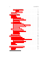
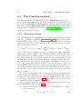
1
GIAnT The Generic InSAR Analysis Toolbox User Manual Piyush S Agram Romain Jolivet Mark Simons TIM E [email protected] Copyright: Do not make money with that. If you do, we will sentence you to write a full PhD thesis. Contents Contents 0.1 About This Document . . . . . . . 0.2 Who Will Use This Documentation 0.3 Citation . . . . . . . . . . . . . . . 0.4 Acknowledgements and Credits . . 0.5 Request for feedback . . . . . . . . 1 Introduction 1.1 Overview . . . . . . . . . 1.2 Features . . . . . . . . . 1.3 Algorithms . . . . . . . . 1.4 Programming philosophy 1.5 Future work . . . . . . . . . . . . . . . . . . . . . . . . . . . . . . . . . . . . . 2 Installation 2.1 Pre-requisites . . . . . . . . . . . . 2.1.1 Python 2.6 or higher . . . . 2.1.2 Numerical Python (NumPy) 2.1.3 Scientific Python (SciPy) . . 2.1.4 Cython . . . . . . . . . . . 2.1.5 Matplotlib . . . . . . . . . . 2.1.6 h5py . . . . . . . . . . . . . 2.1.7 pygrib . . . . . . . . . . . . 2.1.8 pywavelets . . . . . . . . . . 2.1.9 LXML . . . . . . . . . . . . 2.2 Optional . . . . . . . . . . . . . . . 2.2.1 ffmpeg or mencoder . . . . . 2 . . . . . . . . . . . . . . . . . . . . . . . . . . . . . . . . . . . . . . . . . . . . . . . . . . . . . . . . . . . . . . . . . . . . . . . . . . . . . . . . . . . . . . . . . . . . . . . . . . . . . . . . . . . . . . . . . . . . . . . . . . . . . . . . . . . . . . . . . . . . . . . . . . . . . . . . . . . . . . . . . . . . . . . . . . . . . . . . . . . . . . . . . . . . . . . . . . . . . . . . . . . . . . . . . . . . . . . . . . . . . . . . . . . . . . . . . . . . . . . . . . . . . . . . . . . . . . . . . . . . . . . . . . . . . . . . . . . . . . . . . . . . . . . . . . . 2 7 7 7 8 8 . . . . . 11 11 12 12 13 13 . . . . . . . . . . . . 15 16 16 16 17 17 18 18 18 19 19 20 20 CONTENTS 2.3 2.4 3 2.2.2 pyresample . . . . . . . . . . . 2.2.3 HDFview . . . . . . . . . . . . 2.2.4 iPython . . . . . . . . . . . . . 2.2.5 bpython . . . . . . . . . . . . . 2.2.6 pykml . . . . . . . . . . . . . . 2.2.7 ImageMagick . . . . . . . . . . 2.2.8 xmlcopyeditor . . . . . . . . . . Installation . . . . . . . . . . . . . . . 2.3.1 Building extensions . . . . . . . 2.3.2 Non-standard installations . . . Automated installation of pre-requisites 3 Using GIAnT 3.1 Python . . . . . . . . 3.2 Working with HDF5 3.3 Matplotlib . . . . . . 3.4 GIAnT conventions . . . . . . . . . . . . . . . . . . . . . . . . . . . . . . . . . 4 Preparing data for processing 4.1 Inputs . . . . . . . . . . . . . . . . 4.1.1 Using geocoded stacks 1 . . 4.2 Outputs . . . . . . . . . . . . . . . 4.3 Directory structure . . . . . . . . . 4.4 Preparing XML files . . . . . . . . 4.4.1 Writing the data.xml file . 4.4.2 Writing the sbas.xml file . 4.4.3 Writing the mints.xml file 4.4.4 Writing more XML files . . 4.5 Preparing the Interferogram Stack . 4.6 Checklist . . . . . . . . . . . . . . . . . . . . . . . . . . . . . . . . . . . . . . . . . . . . . . . . . . . . . . . . . . . . . . . . . . . . . . . . . . . . . . . . . . . . . . . . . . . . . . . . . . . . . . . . . . . . . . . . . . . . . . . . . . . . . . . . . . . . . . . . . . . . . . . . . . . . . . . . . . . . . . . . . . . . . . . . . . . . . . . . . 20 21 21 21 21 22 22 22 23 24 24 . . . . . . . . . . . . . . . . . . . . . . . . . . . . . . . . . . . . . . . . . . . . . . . . 27 29 29 30 30 . . . . . . . . . . . 31 31 33 34 34 35 36 39 41 43 43 44 . . . . . . . . 47 48 48 50 50 51 53 54 54 . . . . . . . . . . . . . . . . . . . . . . . . . . . . . . . . . . . . . . . . . . . . . . . . . . . . . . . . . . . . . . . . . . . . . . . . . . . . . . . . . . . . . . . . 5 Removing orbital ramps and stratified tropospheric facts 5.1 Inputs . . . . . . . . . . . . . . . . . . . . . . . . . . 5.2 Outputs . . . . . . . . . . . . . . . . . . . . . . . . . 5.3 Atmospheric corrections . . . . . . . . . . . . . . . . 5.3.1 Theory and methodology . . . . . . . . . . . . 5.3.2 Implementation and possible options . . . . . 5.3.3 Empirical corrections . . . . . . . . . . . . . . 5.4 Orbital errors estimation . . . . . . . . . . . . . . . . 5.4.1 Network De-Ramping . . . . . . . . . . . . . . . . . . . . . . . . . . . . . . . . . . . . . . . . . . . . . . . arti. . . . . . . . . . . . . . . . . . . . . . . . 4 CONTENTS 5.4.2 5.5 GPS De-Ramping Theory . . . . . . Implementation . Checklist . . . . . . . . . . . . . . . . . . . . . . . . . . . . . . . . . . . . . . . . . . . . . . . . . . . . . 6 Time-series: SBAS 6.1 Inputs . . . . . . . . . . . . . . . . . . . . . 6.2 Outputs . . . . . . . . . . . . . . . . . . . . 6.3 The SBAS method . . . . . . . . . . . . . . 6.3.1 Inversion Strategy . . . . . . . . . . . 6.3.2 Uncertainties estimation . . . . . . . 6.3.3 Outputs . . . . . . . . . . . . . . . . 6.3.4 Checklist . . . . . . . . . . . . . . . . 6.4 The NSBAS method . . . . . . . . . . . . . 6.4.1 Inversion strategy . . . . . . . . . . . 6.4.2 Traditional stacking 1 as special case 6.4.3 Uncertainties estimation . . . . . . . 6.4.4 Outputs . . . . . . . . . . . . . . . . 6.4.5 Checklist . . . . . . . . . . . . . . . . 6.5 The TimeFun method . . . . . . . . . . . . 6.5.1 Inversion strategy . . . . . . . . . . . 6.5.2 Uncertainties estimation . . . . . . . 6.5.3 Outputs . . . . . . . . . . . . . . . . 6.5.4 Checklist . . . . . . . . . . . . . . . . 6.6 Important Note . . . . . . . . . . . . . . . . . . . . . . . . . . . . . . . . . . . . . . . . . . . . . . . . . . . . . . . . . . . . . . 7 Time-series: MInTS 7.1 The MInTS Algorithm . . . . . . . . . . . . . . 7.2 Forward Wavelet Transform . . . . . . . . . . . 7.3 Time-series inversion of the wavelet coefficients . 7.3.1 Inversion strategy . . . . . . . . . . . . . 7.3.2 Uncertainties estimation . . . . . . . . . 7.4 Inverse Wavelet Transform . . . . . . . . . . . . 7.5 Note . . . . . . . . . . . . . . . . . . . . . . . . 7.6 Checklist . . . . . . . . . . . . . . . . . . . . . . . . . . . . . . . . . . . . . . . . . . . . . . . . . . . . . . . . . . . . . . . . . . . . . . . . . . . . . . . . . . . . . . . . . . . . . . . . . . . . . . . . . . . . . . . . . . . . . . . . . . . . . . . . . . . . . . . . . . . . . . . . . . . . . . . . . . . . . . . . . . . . . . . . . . . . . . . . . . . . . . . . . . . . . . . . . . . . . . . . . . . . . . . . . . . . 55 55 56 57 . . . . . . . . . . . . . . . . . . . 59 59 59 60 60 60 61 62 62 62 64 64 64 65 65 66 67 67 68 68 . . . . . . . . 69 69 70 71 71 73 73 74 74 8 Visualization and Geocoding 75 8.1 Interactive visualization . . . . . . . . . . . . . . . . . . . . 75 8.2 Movies . . . . . . . . . . . . . . . . . . . . . . . . . . . . . . 76 8.3 KML . . . . . . . . . . . . . . . . . . . . . . . . . . . . . . . 77 1 Velocity estimates CONTENTS 8.4 5 Geocoding . . . . . . . . . . . . . . . . . . . . . . . . . . . . 78 Appendices 78 A I/O A.1 A.2 A.3 A.4 A.5 . . . . . . . . . . . . . . . 79 79 80 80 81 81 81 81 82 82 83 83 83 83 83 83 . . . . . 85 85 85 87 87 87 Utilities Text files . . . . . . . . . . . . . . . . . . . Binary files . . . . . . . . . . . . . . . . . HDF5 Files . . . . . . . . . . . . . . . . . GMT netcdf files . . . . . . . . . . . . . . XML Files . . . . . . . . . . . . . . . . . . A.5.1 XML format . . . . . . . . . . . . . A.5.2 Creating XML file . . . . . . . . . A.5.3 Reading XML file . . . . . . . . . . A.6 DEM RSC file for non ROI PAC data . . . A.7 GPS Input Files . . . . . . . . . . . . . . . A.7.1 Option 1: Velocity type station list A.7.2 Option 2: Station-wise time series . Option a: Classic Station List . . . Option b: SOPAC station list . . . Station File example . . . . . . . . B Time-series Utilities B.1 Temporal characterization . . . . B.1.1 Dictionary of functions . . B.1.2 Putting functions together B.1.3 SBAS Formulation . . . . B.2 Network utilities . . . . . . . . . . . . . . . . . . . . . . . . . . . . . . . . . . . . . . . . . . . . . . . . . . . . . . . . . . . . . . . . . . . . . . . . . . . . . . . . . . . . . . . . . . . . . . . . . . . . . . . . . . . . . . . . . . . . . . . . . . . . . . . . . . . . . . . . . . . . . . . . . . . . . . . . . . . . . . . . . . . . . . . . . . . . . . . . . . . . . . . . . . . . . . . . . . . . . . . . . . . . . . . . . . . . . . C Image utilities 89 C.1 MInTS image routines . . . . . . . . . . . . . . . . . . . . . 89 C.2 Stack routines . . . . . . . . . . . . . . . . . . . . . . . . . . 89 D Wavelets 91 D.1 Convention . . . . . . . . . . . . . . . . . . . . . . . . . . . 91 D.2 Routines . . . . . . . . . . . . . . . . . . . . . . . . . . . . . 92 D.3 Other wavelets . . . . . . . . . . . . . . . . . . . . . . . . . 93 E Solvers 95 E.1 Least squares . . . . . . . . . . . . . . . . . . . . . . . . . . 95 E.2 Regularized L2 norm . . . . . . . . . . . . . . . . . . . . . . 95 E.3 Iteratively reweighted least squares . . . . . . . . . . . . . . 96 6 Bibliography CONTENTS 97 Preface 0.1 About This Document This document describes GIAnT. It is organized following the steps most users will follow for their interferometric SAR time series processing. We begin with a description of how to install the software, with extensive details for Linux and OS-X users. We have not tested this software on a Windows platform. We then describe, step by step, the different techniques implemented in GIAnT. 0.2 Who Will Use This Documentation This documentation is designed for both scientists who are content to use pre-packaged tools for analysing their synthetic aperture radar (SAR) interferogram stack and for experienced interferometric SAR (InSAR) timeseries algorithm developers. The latter are likely to want to study the source code, compare the performance of numerous algorithms and even incorporate additional processing approaches into GIAnT. Users who want to modify the source will need to have familiarity with scripting, software installation, and programming, but are not necessarily professional programmers. We hope that any user-improvements will be shared with the developers so that all users can benefit from them. 0.3 Citation We make this source code available at no cost in hopes that the software will enhance your research. Commercial use of any part of this software is not allowed without express permission from the authors. 7 8 CONTENTS A number of individuals have contributed significant time and effort towards the development of this software. Please recognize these individuals by citing the relevant peer-reviewed papers and making relevant acknowledgements in talks and publications. [[[Include citations when ready.]]] 0.4 Acknowledgements and Credits The authors of this software were supported by NASA solid earth and natural hazards program (NNX09AD25G), the Keck Institute for Space Studies (KISS) and the Caltech Tectonics Observatory (CTO). The Authors thank the Gordon and Betty Moore foundation for financial support of the CTO. The authors thank all those people who contributed in helping to develop this program and those who volunteered to be guinea pigs, among them B. Riel, G. Peltzer, C. Lasserre and M.-P. Doin. The data used to generate the front page graphics were provided by Marie-Pierre Doin, ISTerre, France. The data processing from the raw SAR data to the interferograms is described in Doin et al. [2011]. We produced the time series using GIAnT. The snapshots are created using the Generic Mapping Tool [Wessel and Smith, 1995]. 0.5 Request for feedback Your suggestions and corrections are essential to improve this software suite and the documentation. Please report any errors, inaccuracies or typos to the GIAnT development team at [email protected]. License THE ACCOMPANYING PROGRAMS ARE PROVIDED UNDER THE TERMS OF THIS PUBLIC LICENSE (" AGREEMENT ") . ANY USE , REPRODUCTION OR DISTRIBUTION OF THE PROGRAM CONSTITUTES RECIPIENT ’ S ACCEPTANCE OF THIS AGREEMENT . a . Generic InSAR Analysis Toolbox ( GIAnT ) - Copyright ( c ) 2012 , California Institute of Technology b . Python - based Atmospheric Phase Screen estimator ( PyAPS ) Copyright ( c ) 2012 , California Insitute of Technology c . Variable Resolution Interferogram Resampler ( VarRes ) - Copyright ( c ) 2012 , California Institute of Technology 1. Definitions " Contribution " means : a ) in the case of the initial Contributor , the initial code and documentation distributed under this Agreement , and b ) in the case of each subsequent Contributor : i ) changes to the Program , and ii ) additions to the Program ; where such changes and / or additions to the Program originate from and are distributed by that particular Contributor . A Contribution ’ originates ’ from a Contributor if it was added to the Program by such Contributor itself or anyone acting on such Contributor ’ s behalf . " Contributor " means any person or entity that distributes the Program . " Program " means the Contributions distributed in accordance with this Agreement . 9 10 CONTENTS " Recipient " means anyone who receives the Program under this Agreement , including all Contributors . 2. Grant of Rights Redistribution and use in source and binary forms , with or without modification , are permitted provided that the following conditions are met : a ) Program and derivative works may not be sold , nor may they be used in a commercial product or activity . b ) Derivative works of the Program , in both source and binary forms , must reproduce the above copyright notice , this list of conditions and the following disclaimer in the documentation and / or other materials provided with the distribution . c ) Contributors may not remove or alter any copyright notices contained within the Program . d ) Each Contributor must identify itself as the originator of its Contribution , if any , in a manner that reasonably allows subsequent Recipients to identify the originator of the Contribution . 3. Usage The Program is the work of many developers , each of whom owns the copyright to the code they wrote . There is no central copyright authority you can license the code from . The proper way to use the Program is to examine it to understand how it works , and then write your own modules . Sorry , there is no free lunch here . 4. No Warranty THIS SOFTWARE IS PROVIDED BY THE COPYRIGHT HOLDERS AND CONTRIBUTORS " AS IS " AND ANY EXPRESS OR IMPLIED WARRANTIES , INCLUDING , BUT NOT LIMITED TO , THE IMPLIED WARRANTIES OF MERCHANTABILITY AND FITNESS FOR A PARTICULAR PURPOSE ARE DISCLAIMED . Chapter 1 Introduction 1.1 Overview The Generic InSAR Analysis Toolbox (GIAnT) is a suite of commonly used time-series interferometry algorithms in a common Python framework. Improvements in synthetic aperture radar (SAR) interferometry over the past couple of decades allow accurate measurement of ground surface deformation with unprecedented spatial coverage. Various packages are available to compute one or several interferograms, e.g, ROI PAC [Rosen et al., 2004a], DORIS [Kampes et al., 2003], the new ISCE [Rosen et al., 2011], GMTSAR [Sandwell et al.] or variants, like NSBAS [Doin et al., 2011]. Observing large amplitude deformation signals, such as surface deformations due to earthquakes, is now a routine process. However, the detection of lower amplitude signals, such as interseismic accumulation, creeping faults, seasonal subsidence, etc., is more challenging. Time series analysis methods are used to enhance the signal-to-noise ratio and to study the temporal variability of surface deformation. The InSAR community uses a wide variety of methods and algorithms for interferometric time-series analysis. However, no common modular framework exists that allows researchers to quickly apply these wide range of algorithms on a single data set and compare their relative merits or limitations. Development of GIAnT is primarily motivated by: 1. The need for standardization of data formats for ease in sharing timeseries products. 2. Benchmarking of time-series InSAR algorithms. 3. Direct comparison of performance of various published algorithms. 11 12 CHAPTER 1. INTRODUCTION 4. A modular framework for efficient development of future time-series approaches. GIAnT provides utility libraries of functions that are commonly used in various time-series approaches and includes demonstration scripts of various techniques. All the functions and scripts are documented in detail, allowing users to use these directly for data analysis or as building blocks for any time-series approach they would like to implement in the same framework. 1.2 Features Some of key features of GIAnT include: 1. It is free. 2. It provides a Python-based framework. 3. Source code is distributed along with the package. 4. Use of memory mapped files facilitating analysis of large interferogram stacks. 5. A simple interface to weather model based atmospheric phase screen corrections [http://earthdef.caltech.edu Jolivet et al., 2011]. 6. Direct calls to optimized linear algebra libraries like LAPACK, BLAS etc that can be optimized for speed using packages like ATLAS/ Intel MKL. 7. A set of interactive data visualization scripts. 8. Simple parallelization using Python’s multiprocessing (shared memory) module for performance. 1.3 Algorithms The time-series analysis routines in GIAnT can be broken down into two stages - spatial analysis and temporal analysis. GIAnT users can choose to analyze their data sets in radar (range, azimuth) coordinates directly or transform their data into wavelet domain before analysis. For the temporal analysis, the users can choose to work with the traditional piece-wise linear SBAS formulation [Berardino et al., 2002] or use a parameterized functional form of their choice [Hetland et al., 2011]. GIAnT modules have 1.4. PROGRAMMING PHILOSOPHY 13 been designed in a manner that allows users to combine various types of spatial and temporal analysis algorithms as desired. The following time-series techniques have already been implemented and are provided with GIAnT for immediate use. 1. Small Baseline Subset (SBAS) [Berardino et al., 2002]. 2. N-SBAS [Lopez-Quiroz et al., 2009, Doin et al., 2011, Jolivet et al., 2012]. 3. Multiscale Insar Time-Series (MInTS) [Hetland et al., 2011]. 4. Timefn (Temporal analysis part of MInTS applied directly in data domain). 1.4 Programming philosophy GIAnT consists of two types of programs - modules and scripts. In GIAnT, modules are building blocks combined in a preferred order within a script. We use modules to implement processing steps that are common to various time-series techniques. We have consciously chosen to implement the various time-series algorithms as scripts for ease of understanding. We expect that most of the end users will not be expert programmers and the processing flow should be easy to comprehend by studying the scripts directly. Even though we want to keep an eye on the evolution of the future versions of GIAnT, these tools are OpenSource, and therefore, we accept, with great pleasure, any contributions you could make to add algorithms, improve existing routines or develop new methods. 1.5 Future work This first release of GIAnT focuses on building a framework and implementing some of the basic time-series InSAR algorithms. The package will constantly be maintained and updated. Bug reports and fixes can be reported on the website http://earthdef.caltech.edu. GIAnT in its current form does not address all aspects of time-series InSAR and the future versions are expected to address the following issues: 1. The processing chain is expected to start with wrapped data. Phase unwrapping will be included as a processing step. If starting with 14 CHAPTER 1. INTRODUCTION unwrapped data, consistency checks will be incorporated to identify unwrapping errors. 2. Algorithms for estimation of DEM Error in the wrapped domain that are already available in the public domain [e.g, Hooper et al., 2007, Ducret et al., 2011] will be incorporated into GIAnT. 3. Tidal load corrections [DiCaprio and Simons, 2008] will be included as a package similar to the atmospheric corrections. This component will be important for the analysis of coastal regions and continental scale data sets. 4. Incorporation of Persistent Scatter algorithms [e.g, Hooper et al., 2007, Shanker and Zebker, 2007, Hooper, 2008]. 5. Inclusion of more complete error covariance models and propagation of uncertainty estimates through various stage of time-series InSAR processing. 6. Optimization of various algorithms, including the option of analysis on distributed systems. Chapter 2 Installation Most of GIAnT consists of python programs that just need to be copied to a specified location. We include a simple Python setup script for components of GIAnT that are in Fortran or C. A large number of other Python modules need to be installed in order for GIAnT to work on your machine. Installing these pre-requisites are relatively easy. Generic Linux We recommend using a package manager like apt or yum to install the prerequisites before installing GIAnT. We provide command lines to install the required Python libraries on a Linux Ubuntu machine. OS-X A convenient way to install all the pre-requisites is to use the package manager MacPorts (free)1 . Installing MacPorts on OS-X machines is straightforward but requires Xcode2 (free). We provide command lines to install the required Python libraries using MacPorts. Please be sure to run these commands as root. Another package manager called Fink is available3 but the installation of all the libraries required by GIAnT has never been tested with Fink. 1 http://www.macports.org https://developer.apple.com/xcode/ 3 http://www.finkproject.org 2 15 16 2.1 CHAPTER 2. INSTALLATION Pre-requisites All the following pre-requisites may be installed from source. Although, we strongly advise the use of a package manager for beginners. 2.1.1 Python 2.6 or higher GIAnT uses Python (http://www.python.org) and you will need a minimum of Python 2.6, for various pre-requisite packages to work seamlessly. If for some reason, you choose to build Python from source, please ensure that you use the same set of compilers for building any of the other packages for Python. Also ensure that you get the development package for Python for Linux. On OS-X, all required libraries for GIAnT are available on MacPorts, for Python 2.6 or Python 2.7. The suggested commands are for Python 2.7 but can de adapted by changing “27” to “26” in the commands. Ubuntu - 12.04: >> apt-get install python2.7 python2.7-dev OS-X: >> port install python27 >> port select python python27 2.1.2 Numerical Python (NumPy) GIAnT makes extensive use of NumPy (http://numpy.scipy.org) for representing datasets as arrays and for many array manipulation routines. We also use some FFT and linear algebra routines provided with NumPy. numpy.int, numpy.float and numpy.float32 are the most common data formats used at various stages of processing arrays and data. Ubuntu - 12.04: >> apt-get install python-numpy OS-X: >> port install py27-numpy If you want to improve the performance of Numpy, we suggest using LAPACK, BLAS and ATLAS libraries. For more details on installing numpy from source using these libraries, see http://docs.scipy.org/doc/numpy/ 2.1. PRE-REQUISITES 17 user/install.html. On OS-X, a variant of Numpy that includes LAPACK, BLAS and the optimization ATLAS libraries is available on MacPorts. We suggest users to install the variant including compilation by gcc 4.5: OS-X: >> port install py27-numpy +atlas +gcc45 2.1.3 Scientific Python (SciPy) SciPy (http://scipy.org) contains many functions for linear algebra operations, FFTs and optimization. SciPy also includes support for sparse matrices and provides solvers for various types of optimization problems. Ubuntu - 12.04: >> apt-get install python-scipy OS-X: >> port install py27-scipy Vanilla distributions of SciPy obtained through utilities like yum and apt are typically not optimized. For best performance on large Linux computers, SciPy must be compiled with ATLAS / Intel MKL support. On Apple computers, the optimized SciPy distribution can be installed by typing: OS-X: >> port install py27-scipy +atlas +gcc45 2.1.4 Cython Cython (http://www.cython.org) is a language that makes writing C extensions for the Python language as easy as Python itself. Cython is ideal for wrapping external C libraries and for writing fast C modules that speeds up the execution of Python code. Ubuntu - 12.04: >> apt-get install cython (or) >> easy_install cython OS-X: 18 CHAPTER 2. INSTALLATION >> port install py27-cython (or) >> easy_install cython 2.1.5 Matplotlib Matplotlib (http://matplotlib.sourceforge.net) is a python 2D plotting library which produces publication quality figures in a variety of hardcopy formats and interactive environments across platforms. We use matplotlib for displaying output and for our interactive time-series viewers. Ubuntu - 12.04: >> apt-get install python-matplotlib OS-X: >> port install py27-matplotlib 2.1.6 h5py h5py (http://code.google.com/p/h5py) provides a NumPy interface to Hierarchial Data Format 5 (HDF5) memory mapped files. We use h5py for storage and retrieval of named variables during various stages of processing. A big advantage of h5py is it allows us to access slices of large matrices directly from a file, without having to use up memory resources needed to read the entire matrices. The latest version of MATLAB also uses the HDF5 format and it is possible to directly read in .mat files into Python using scipy.io.loadmat. Ubuntu - 12.04: >> apt-get install python-h5py OS-X: >> port install py27-h5py 2.1.7 pygrib GIAnT can directly interact with PyAPS modules to use weather model data for atmospheric phase screen corrections. pygrib (http://code.google. com/p/pygrib) provides the interface for directly reading in GRIB-format weather data files in Python. Successful installation of pygrib needs grib api, openjpeg, jasper, libpng, zlib (including all development versions) which can 2.1. PRE-REQUISITES 19 all be obtained using standard repository management tools. Pygrib also needs the basemap or pyproj module for python to be installed. Ubuntu - 12.04: >> apt-get install zlib1g zlib1g-dev >> apt-get install libpng12-0 libpng12-dev >> apt-get install libjasper1 libjasper-dev >> apt-get install libopenjpeg2 libopenjpeg-dev >> apt-get install libgrib-api-1.9.9 libgrib-api-dev libgrib-api-tools >> apt-get install python-mpltoolkits.basemap >> apt-get install pyproj >> easy_install pygrib Unfortunately, pygrib is not directly available using a package manager on all Linux machines. You will have to follow instructions on the Google code page to install pygrib after installing all the required packages. On OS-X computers, you can install pygrib using macports (all the dependencies will follow with that command): OS-X: >> port install py27-pygrib 2.1.8 pywavelets The MInTS Hetland et al. [2011] time-series approach uses wavelets for spatial analysis. We provide our own Meyer wavelet library for analysis with the original MInTS approach. However, GIAnT also allows one to use other wavelets for spatial decomposition of unwrapped interferograms using the pywt (http://github.com/nigma/pywt) package. Ubuntu - 12.04: >> apt-get install python-pywt OS-X: >> port install py27-pywavelets (or) >> easy_install pywavelets 2.1.9 LXML GIAnT uses XML files for setting up data and processing parameters. Specifically, we use the eTree module from lxml to construct input XML 20 CHAPTER 2. INSTALLATION files and the objectify module from lxml to read in XML files. LXML (http://lxml.de) should be available as a standard repository on most linux distributions. Ubuntu - 12.04: >> apt-get install python-lxml OS-X: >> port install py27-lxml 2.2 Optional We would also recommend installing the following packages before installing GIAnT. 2.2.1 ffmpeg or mencoder We will need one of the two packages to use the matplotlib.animation submodule for making movies. Ubuntu - 12.04: >> apt-get install ffmpeg mencoder OS-X: >> port install ffmpeg Mencoder is not available through MacPorts (maybe through Fink). 2.2.2 pyresample Pyresample is a Python package that allows for easy geocoding of swath data (interferograms etc). We use pyresample to generate movies in the geocoded domain. Pyresample can be downloaded from http://code. google.com/p/pyresample/. If pyproj is already installed on your machine, you can install pyresample using the command Ubuntu - 12.04 and OS-X: >> easy_install pyresample 2.2. OPTIONAL 2.2.3 21 HDFview HDFview is open source software for exploring the contents of an HDF file. The latest version can be downloaded from http://www.hdfgroup.org/ hdf-java-html/hdfview/index.html. Ubuntu - 12.04: >> apt-get install hdfview HDFview does not exist through MacPorts but can be easily installed following the instructions on the HDFview website. 2.2.4 iPython Interactive Python (iPython) [Pérez and Granger, 2007] provides a rich toolkit for Python that allows users to work with the python interpreter in an environment similar to MATLAB or IDL. Ubuntu - 12.04: >> apt-get install ipython OS-X: >> port install py27-ipython 2.2.5 bpython bpython http://bpython-interpreter.org/ is a simple interface to the python interpreter. We recommend bpython when iPython cannot be used, for example when you are on a NFS partition. Ubuntu - 12.04: >> apt-get install bpython OS-X: >> port install py27-bpython 2.2.6 pykml pykml (http://packages.python.org/pykml/) is a Python library for creating, parsing and manipulating KML files. GIAnT can output time-series products to KML files for immediate visualization in Google Earth. 22 CHAPTER 2. INSTALLATION Ubuntu - 12.04 and OS-X: >> easy_install pykml 2.2.7 ImageMagick This is typically a part of the standard Linux distributions. We use ImageMagick’s convert utility to make parts of PNG files transparent for display usign KML/KMZ files. Ubuntu - 12.04: >> apt-get install imagemagick OS-X: >> port install imagemagick 2.2.8 xmlcopyeditor xmlcopyeditor http://xml-copy-editor.sourceforge.net/ is a simple editor for XML. The XML files used in GIAnT or ISCE can be easily modified using a text editor but xmlcopyeditor makes the task a little simpler. We recommend installing the package from source. 2.3 Installation GIAnT has the following directory structure. GIAnT | |---| |---| |---| |---| |---| |---| |---- (INSTALL directory) tsinsar (Time-series library) pyaps (Atmospheric corrections) SCR (Time-series analysis scripts) geocode (Geocoding library and scripts) solvers (Solvers) setup.py (Installation script) setup.cfg (Setup configure file) 2.3. INSTALLATION 23 Identify the directory in which you want to install GIAnT and make it your current working directory. Checkout the latest version of the code as svn co http://earthdef.caltech.edu/svn/giant cd giant/GIAnT svn co http://earthdef.caltech.edu/svn/pyaps Do not move the contents of the repository directory to another location as that may affect automatic updating of the repository using svn in the future. C and Fortran modules need to be built using C and Fortran compilers (see Section 2.3.1). The final step is to include the full path of the giant/GIAnT directory to the environment variable PYTHONPATH. This will allow python to import these modules whenever they are used in any script. Using Bash: >> export GIANT=/directory/where/you/did/copy/GIAnT >> export PYTHONPATH=$GIANT:$PYTHONPATH Using Csh: >> setenv GIANT ’/directory/where/you/did/copy/GIAnT’ >> setenv PYTHONPATH $GIANT:$PYTHONPATH These commands should be included in your .bashrc or .cshrc files. 2.3.1 Building extensions The setup script builds the gsvd module which contains our interface to the generalized SVD decomposition from LAPACK, similar to SciPy’s interface to LAPACK and BLAS in this directory. The gsvd is used for L2 norm regularized inversions in GIAnT. The default settings uses the default C and fortran compilers to build extensions. The setup.cfg file can also be modified to force the machine to use a specific fortran compiler. If you have multiple Fortran and C compilers on your machine, you should specify the version compatible with your installation of python as shown below: >>CC=Compiler python setup.py build_ext --fcompiler=compiler-options On OS-X, the default compiler will be clang. This will cause some problems if you use any regularized inversions. Therefore, on OS-X, if you 24 CHAPTER 2. INSTALLATION linked Numpy and Scipy to Atlas, as mentioned previously, you want to compile gsvd using: >> CC=gcc-mp-4.5 python setup.py build_ext --fcompiler=gnu95 The compiler options can also be included in the setup.cfg file before executing setup.py . If your LAPACK/BLAS libraries were not built with gfortran, readup on the ”–fcompiler” option for numpy distutils. Alternate installation Alternately, identify the directories in which the LAPACK, BLAS and ATLAS libraries are located. Compile using f2py in the gsvd directory. >> f2py gensvd.pyf dggsvd.f -LPATH_TO_LIBS -llapacklib -lblaslib -latlaslib On Ubuntu - 12.04: >> f2py gensvd.pyf dggsvd.f -llapack -lblas -latlas Test the compiled module using the provided test.py. Ensure that you are using the f2py corresponding to the numpy version you want to use. 2.3.2 Non-standard installations If you happened to install any of the above pre-requisite libraries yourself and if they are not located in the Standard library directories for your OS, include the paths to the shared object files (libxxxxxxxxx.so) to the environment variable LD LIBRARY PATH. This set of tools has not been tested, or even installed, on Windows operated machines. 2.4 Automated installation of pre-requisites We maintain a simple puppet (http://puppetlabs.com/puppet/puppet-open-source) script for automatic installation of pre-requisite software on an Ubuntu 12.04/ 12.10 machine at http://earthdef.caltech.edu/boards/3/topics/ 74. We hope that users will contribute similar scripts for other Linux distributions and make it available to other GIAnT users. We also maintain a table of required packages for various OS and Linux distributions at http://earthdef.caltech.edu/documents/4. We again 2.4. AUTOMATED INSTALLATION OF PRE-REQUISITES 25 hope that active users will contribute to this table and add support for other Linux distributions. Chapter 3 Using GIAnT GIAnT is distributed with implementations of SBAS [Berardino et al., 2002, Doin et al., 2011] and MInTS [Hetland et al., 2011] techniques. The prepackaged implementations are meant to work with outputs from ROI PAC [Rosen et al., 2004b], ISCE [Rosen et al., 2011], DORIS [Kampes et al., 2003], GMTSAR [Sandwell et al.] or GAMMA [GAMMA Remote Sensing Research and Consulting AG, 2013]. In our description of the various processing steps, we used the term “stack” to denote a three-dimensional cube of data, the dimensions typically corresponding to range direction, azimuth direction and either number of interferograms or SAR acquisitions. Our usage of the term “stack” should not be interpreted as some form of velocity estimate. Figure 3.1 describes the work flow in the current implementation of various time-series InSAR algorithms implemented in GIAnT. However, the main strength of GIAnT lies in its modular implementation of the algorithms which allows users to implement their own version of the different time-series techniques and to extend GIAnT. As shown in Figure 3.1, there are multiple stages in the analysis: 1. Stack preparation Unwrapped interferograms are read from various locations on disk and are consolidated into a data cube. The data cube is stored along with other auxiliary information in a hierarchical data format (HDF5) file. Chapter 4 describes this step in detail. 2. Stack preprocessing Preprocessing of the stack including orbit deramping and topo-correlated atmospheric phase correction. The outputs are stored in a HDF5 file. Chapter 5 describes each of the preprocessing steps in detail. 27 28 CHAPTER 3. USING GIANT 3. Time-series estimation The time-series is estimated from the processed stack using a technique of choice. Currently, you can choose between various SBAS techniques (Chapter 6) and MInTS (chapter 7). GIAnT workflow Unwrapped IFGs Coherence Weather models Common Mask Metadata GPS data PrepIgramStack.py ProcessStack.py MInTS chain SBAS chain DatatoWavelet.py SBASInvert.py (or) NSBASInvert.py (or) TimefnInvert.py InvertWaveletCoeffs.py (or) InvertWaveletCoeffs_fol ds.py WavelettoData.py Visualization Figure 3.1: GIAnT workflow for using InSAR time-series analysis. The main strength of GIAnT is the modular implementation of these various stages. The modules can themselves be used to extend GIAnT and implement other time-series techniques. Before processing any data, we strongly advise the users to familiarize themselves with various features of GIAnT, that will help them use the 3.1. PYTHON 29 toolbox more effectively. 3.1 Python For users who are familiar with MATLAB or IDL, the transition to Python should be fairly easy. Two resources that we recommend for users who are new to Python are • The tentative Numpy turorial- http://scipy.org/Tentative_NumPy_ Tutorial • Numpy for MATLAB users http://mathesaurus.sourceforge.net/ matlab-numpy.html 3.2 Working with HDF5 The Hierarchical data format (HDF) allows us to save large amounts of data in an organized and easy to access manner. GIAnT uses HDF5 files in the same way that users use .mat files in MATLAB or .sav files in IDL. In GIAnT, all HDF5 files and the datasets they contain are stored with a “help” attribute. We recommend that the users become familiar with the h5py [Collette, 2008] module interface in Python for reading and displaying data sets using matplotlib. A good introductory tutorial can be found at http://h5py.alfven.org/docs-2.0/intro/quick.html. To determine the overview of the contents of a HDF5 file, use ####Overview description of file $ h5dump -a help Filename.h5 To determine the contents of the HDF5 and their description #####List contents $ h5ls Filename.h5 #####List contents with description $ h5ls -v Filename.h5 | grep Data To dump an array from HDF5 to a binary file, use h5dump. This command can also be used to crop the array before writing it to a file. HDFview is another tool that we strongly recommend for browsing through the contents of a HDF file. 30 CHAPTER 3. USING GIANT 3.3 Matplotlib GIAnT uses matplotlib [Hunter, 2007] for plotting. Some familiarity with matplotlib will allow users to write their own visualization codes for debugging and understanding the processing chain. Two useful tutorials can be found at • http://matplotlib.sourceforge.net/users/pyplot_tutorial.html • http://matplotlib.github.com/users/image_tutorial.html 3.4 GIAnT conventions Various processing stages in GIAnT conform to few simple rules. Units The unwrapped interferograms are converted to millimeters (mm) before any preprocessing. The atmospheric phase screen from PyAPS and GPS data are also converted to millimeters. Master-slave Typically, users prefer to use the most recent amongst the pair of SAR acquisitions as the master scene when generating interferograms. GIAnT has been designed to be flexible and automatically figures out the correct connectivity matrix even if the order of master and slave acquisitions do not adhere to a consistent convention. We would still recommend the users to the latest SAR acquisition as the master scene in every pair consistently. Ground-to-satellite The line-of-sight direction corresponds to the vector from ground position to the satellite. All the estimated time-series products are always estimated with respect to the ground, i.e, in the case of purely vertical deformation positive values represent uplift and negative values represent subsidence. Angles The incidence angle provided by the user as a file or as a constant input is always measured with respect to the ground. This information is used for projecting estimated atmospheric path delays and GPS data along the line-of-sight. Help attributes All the metadata values in input XML files must include a <help> field. All datasets in HDF5 files must be stored with a help attribute. This requirement is designed to aid users in understanding the relevance of input, output and intermediate products. Chapter 4 Preparing data for processing During this first step of the processing, all the necessary metadata and the unwrapped interferograms are sorted and organized into an HDF5 file and a few additional binary files, specially formatted for GIAnT. Inputs are data from outputs of ROI PAC, DORIS, GMTSAR, GAMMA or ISCE. As we would like to provide the most generic toolbox, we tried to implement readers for the most common datasets, but slight changes might be needed to adapt GIAnT to your case. In this section we describe how to use two scripts located in GIANT/SCR: • prepxml SBAS.py and prepxml MInTS.py create the XML files needed to specify processing options to GIAnT. • PrepIgramStack.py reads the input data and creates files for GIAnT. 4.1 Inputs To run these steps, the user needs to gather the following files: • The unwrapped interferograms in radar coordinates (range, azimuth) and in radians produced by ROI PAC, DORIS, GMTSAR, GAMMA or ISCE. If the users have geolocated unwrapped interferograms that they wish to analyze, they should take a look at Section 4.1.1 before proceeding. • The corresponding coherence files. 31 32 CHAPTER 4. PREPARING DATA FOR PROCESSING • A list of the Interferograms, with the perpendicular baseline and the sensor code name. • A Radar simulation file containing the pixels elevation, i.e, the DEM in radar coordinates. If you are using a processor other than ROI PAC, you will have to generate a ROI PAC style rsc file including the approximate latitude and longitude values for the four corners (see Appendix A). This information is needed for subsetting weather model data. • An example.rsc file(ROI PAC) (or) interferogram.out and master.res files (DORIS) (or) insarProc.xml file (ISCE) or image.PRM and unwrap.grd files (GMTSAR) (or) date.mli.par (GAMMA). • Optional: Two files containing each pixels latitude and longitude (binary files, same size as the interferograms, real single precision). These files can be GRD files in the case of GMTSAR. • Optional: A mask file (binary file, same size as the interferogram, real single precision, 0 for False, 1 for True). This file can be a GRD file in case of GMTSAR. We use the following setup for processing time-series with GIAnT. It is relatively simple to modify the stack1 preparation script to use a different setup if desired. We pass the list of interferograms as an ASCII with four columns: the two first columns are the interferograms dates of acquisition coded over 6 or 8 digits (yymmdd or yyyymmdd), the third one is the perpendicular baseline while the last one is the sensor code name. Please make sure that the perpendicular baselines specified in here are consistent within the interferometric network, otherwise, the implemented Digital Elevation Model error estimation will produce incorrect results. A little example: 030104 031011 -384.6568006539 ENV 030104 031220 -412.2747552730 ENV 030104 041204 -346.6693732534 ENV 19920917 19920604 -158.938138675459 ERS 19921126 19920604 -194.461966044758 ERS 19921126 19920917 -35.4173555703392 ERS .... You can optionally not provide the sensor name if you are using data from a single satellite. If you choose to mix data from multiple sensors, please 1 Three-dimensional dataset and not a velocity estimate 4.1. INPUTS 33 Flowchart for PrepIgramStack Unwrapped IFGs List of IFGs + Bperp Coherence Common Mask Filenames Metadata Parameters Inputs userfn.py data.xml Metadata includes DEM, Lat, Lon files in radar coordinates Mask + Crop Multilook Common reference Output: HDF5 file Output: Lat, Lon, DEM Figure 4.1: Work flow for preparing an interferogram stack. ensure that the corresponding wavelength fields are populated in the rdict dictionary in PrepIgramStack.py. If all data is from a single sensor, the wavelength is automatically read in from the example rsc file. You will also need to provide a mapping from the dates to a filename on disk as a python function (Section 4.5). We would also like to point out that most users will probably end up customizing the PrepIgramStack.py script according to their own needs. Some users may prefer to read in the filenames and the associated wavelengths directly from an ASCII file. Implementing such changes should be trivial and we leave it up to the users to implement their favorite strategy. 4.1.1 Using geocoded stacks 1 If the users have processed their interferograms individually and plan to combine them in geocoded domain, they should make the following changes to make GIAnT treat the data as if it was radar coded (range, azimuth). 1. Create latitude and longitude files of the same size as your geocoded unwrapped interferograms. 34 CHAPTER 4. PREPARING DATA FOR PROCESSING 2. Crop your DEM to the same size as your geocoded unwrapped interferograms. 3. Make sure that undefined data is set to NaN in PrepIgramStack.py where the interferograms are read into a HDF5 file. 4. You will also need to include entries for the four corners of the DEM in a ROI PAC style RSC file. See Appendix A. 4.2 Outputs A HDF5 file containing the following datasets is computed: • Jmat: Matrix linking the interferograms to the acquisition dates, made of 0, 1 and -1. • bperp: Vector of the perpendicular baseline values. • cmask: Mask map of the pixels. • dates: Dates of acquisition. • tims: Time of acquisition in the specific ordinal reference. • usat: Satellite sensor code name. • igram: 3D matrix of size n × l × w, where n is the number of interferograms, l and w are the interferograms length (number of pixels along azimuth) and width (number of pixels along range). Additionally, the binary files containing each pixels latitude, longitude and elevation are also output if the corresponding inputs are provided. Finally, PNG format previews of the interferograms are created. 4.3 Directory structure The first step is to create a working directory. The sub-directories are automatically created as needed by the different scripts. The default file and directory names can be modified by the different scripts if needed. The typical structure of the working directory is: 4.4. PREPARING XML FILES 35 |-Working directory (Xml + scripts + metadata) | |---Figs | | | |----- Igrams (Raw interferograms) | | | |----- Atmos (Atmospheric corrections) | | | |----- Ramp (Deramped) | |---Stack (All the h5 files) | |---Atmos (All the weather model data) | |---RESP (Wavelet Impulse Response, Only if you use MInTS) 4.4 Preparing XML files The inputs to the SBAS and MInTS scripts are controlled using XML files. We currently use three XML files - one for data parameters (data.xml), one for the processing parameters of SBAS style chains (sbas.xml) and one for processing parameters of MInTS (mints.xml). An example of these files can be found in the GIAnT/example directory and in the Appendices. These XML files are prepared using the prepxml SBAS.py or the prepxml MInTS.py scripts. These scripts can be modified to add additional processing parameters as desired. The parameter values in the XML files should be modified as per requirement and the processing strategy. In the following, we describe the possible options included. Currently, the scripts are designed to work with data in radar (range, azimuth) coordinates. The XML files produced by the prepxml XXXX.py scripts can also be modified in a text editor. To run these scripts, type: >> python prepxml_SBAS.py or >> python prepxml_MInTS.py Note that the structure of the XML files changes as we add more options to the processing chain and need more control parameters. The help fields 36 CHAPTER 4. PREPARING DATA FOR PROCESSING in the XML files have been added to describe each of the options for the benefit of users. 4.4.1 Writing the data.xml file Both prepxml XXXX.py scripts start by writing the XML file corresponding to your dataset (data format, additional looks, crop region etc). In the scripts, these parameters are parsed through the routine prepare_data_xml. You should modify the arguments of this routine according to your needs. For the data to be read in successfully, a meaningful reference region has to be provided. If a reference region is not provided, average bias is corrected from each interferogram. The syntax is: prepare_data_xml(self, fname, proc=’RPAC’,looks=1, cohth=0.0, mask=’’,xlim=None, ylim=None, rxlim=None, rylim=None, latfile=’’, lonfile=’’, hgtfile=’’, inc=23.0, h5dir=’Stack’, atmosdir=’Atmos’, figsdir=’Figs’, respdir=’RESP’, unwfmt=’RMG’, demfmt=’RMG’, corfmt=’RMG’, chgendian=False, endianlist=[’UNW’,’COR’,’HGT’]), masktype=’f4’) The only non-optional argument is: • fname - The name of the example rsc file from ROI PAC. This file contains parameters like the width of the image, its length, the sensors wavelength.... An example can be found in the directory GIAnT/example. . The optional arguments are: Param proc looks cohth Type STR Help Processor used for generating the interferograms. Can be RPAC, DORIS, ISCE, GAMMA or GMT. INT Number of additional looks. No looks is default. FLOAT Coherence threshold for SBAS pixel selection. This parameter allows to throw out pixel with a coherence value lower than cohth. No pixels are rejected by default. Default RPAC 1 0.0 4.4. PREPARING XML FILES mask STR file length INT width INT xmin INT xmax INT ymin INT ymax INT rxmin INT rxmax INT rymin INT rymax INT latfile STR File for common mask for pixels. This mask has to be the same size as your interferograms, and consist on a binary grid of 1 and 0 or NaN. Number of azimuth lines in the unwrapped files Number of range pixels in the unwrapped files First pixel of cropping limit in Range direction Last pixel of cropping limit in Range direction First line of cropping limit in Azimuth direction Last line of cropping limit in Azimuth direction First pixel of reference region in Range after cropping Last pixel of reference region in Range after cropping First line of referene region in Azimuth after cropping Last line of reference region in Azimuth after cropping Latitude file. The latitude file is a binary file, that has the same size as your interferograms, that specifies the latitude of each pixel. It is encoded has real, single precision. If this file is not provided, then, GIAnT uses a crude and simple linear transformation to calculate the geographic coordinates of the pixels. This is needed only by the PyAPS module. If you specify a latfile, you need to specify a lonfile. 37 None From rsc file From rsc file None None None None None None None None None 38 CHAPTER 4. PREPARING DATA FOR PROCESSING lonfile STR hgtfile STR inc h5dir FLOAT (or) STR STR atmosdir STR figsdir STR respdir STR unwfmt RMG/FLT demfmt RMG/FLT corfmt chgendian RMG/FLT BOOL endianlist List of STR Longitude file. The longitude file is a binary file, that has the same size as your interferograms, that specifies the latitude of each pixel. It is encoded has real, single precision. If this file is not provided, then, GIAnT uses a crude and simple linear transformation to calculate the geographic coordinates of the pixels. This is needed only by the PyAPS module. If you specify a lonfile, you need to specify a latfile. Altitude file. The hgt file is a RMG file (ROI PAC style) or a binary file, that has the same size as your interferograms. It specifies the altitude, in meters, of each pixels. Incidence angle. Can be a constant or a file of the same dimensions as lat/lon. Used only by PyAPS. Directory where all the HDF5 files will be stored. Directory where all the atmospheric data will be stored. Directory where all the figures will be stored. Directory where the Impulse response for wavelet transform are stored (MInTS case). Specifies the format of the interferogram files. RMG is the standerd ROI PAC output for unwrapped interferograms (real, single precision, amplitude and phase). FLT is a simple binary file (real, single precision). Specifies the format of the Digital Elevation Model file. Specifies the format of the correlation files. Swaps bytes if true for the file types specified in the endianlist Specifies the file type concerned by byte swapping if chgendian is True. None None 23.0o . ./Stack ./Atmos ./Figs ./RESP RMG RMG RMG False ’UNW’, ’COR’, ’HGT’ 4.4. PREPARING XML FILES masktype 4.4.2 STR Type of data in the provided mask file (optional) Can be any dtype used in Numpy. 39 ’f4’ Writing the sbas.xml file If you intend to use any of the three SBAS style methods provided here, you will need to create a sbas.xml file by modifying the script prepxml SBAS.py according to your needs. The informations about your processing strategy are parsed through the routine prepare_sbas_xml. The syntax is: prepare_sbas_xml(self, netramp=False, atmos=’’, demerr=False, nvalid=0, regu=False, masterdate=’’, filt=1.0, gpsramp=True, stnlist=’’, stntype=’’, gpspath=’’, gpstype=’’, gpsvert=False, gpspreproc=False, gpsmodel=False, unwcheck=False, gpspad=3, gpsmin=5, tropomin=1, tropomax=None, tropolooks=8) The optional arguments are: Param netramp Type BOOL gpsramp BOOL atmos STR demerr BOOL Help Network deramping: True/False. Interferograms are flattened by estimating and removing a best fit ramp. The best fit ramp parameters are re-estimated in a network sense. For more details, refer to section 5.4.1. GPS deramping: True/False. Interferograms are flattened using displacement informations from a GPS network. Atmospheric corrections: ECMWF/ERA/NARR/MERA/TROPO. The stratified component of the tropospheric is mapped from Global Atmospheric Models or estimated from the phase/elevation relationship (TROPO) and removed to the interferograms. For more details, refer to section 5.3. DEM Error estimation: True/False. Estimation of the Digital Elevation Model error during the Time Series analysis. Default False False None False 40 CHAPTER 4. PREPARING DATA FOR PROCESSING nvalid INT regu BOOL masterdate STR stnlist stntype gpspath gpstype STR BOOL (or) STR STR STR gpsvert gpspreproc gpsmodel gpspad BOOL BOOL BOOL INT gpsmin INT tropomin INT tropomax INT tropolooks INT Minimum number of interferograms where a pixel is coherent. The pixel will be included in the Time Series analysis only if its coherence is higher than cohth in more than valid interferograms. Regularization of time functions: True/False. Activate the automatic determination of the regularization parameter in the Time Function inversion. For more details, refer to chapter 6.5.1. Time to be used as reference (yyyymmdd). Default is the first date of the time series if not specified. Path to the GPS station list. Code name for the type of station list. Can be True/ False/ velocity. 0 Directory where GPS data are stored. Type of GPS file that can be used (sopac or velocity). Use the verticals of GPS data. Preprocess GPS time series with splines. Use the modeled GPS time series as input. Half-width of the window around a GPS station. Minimum number of GPS stations per scene to proceed to the GPS de-ramping process. The process stops if less than gpsmin stations are found for one scene. Minimum scale for empirical estimation of topography correlated atmosphere. Minimum scale for empirical estimation of topography correlated atmosphere. If not defined, determined from dimensions. Number of looks to be applied to interferogram before empirical estimation of topography correlated atmosphere. None None False None. None None False False False 3 5 1 None 8 4.4. PREPARING XML FILES 4.4.3 41 Writing the mints.xml file If you intend to use the MInTS method, you will need to create a mints.xml file by modifying the script prepxml MInTS.py according to your needs. The informations about your processing strategy are parsed through the routine prepare_mints_xml.py. The syntax is: prepare_mints_xml(self, netramp=False, atmos=’’, demerr=False, minscale=2, regu=True, masterdate=’’, minpad=0.1, shape=True, smooth=3, skip=2, wvlt=’meyer’, gpsramp=True, stnlist=’’, stntype=’’, gpspath=’’, gpstype=’’, gpsvert=False, gpspreproc=False, gpsmodel=False, uwcheck=False, kfolds=1, lamrange=[-5,5,50], tropomin=1, tropomax=None, tropolooks=8) The optional arguments are: Param netramp Type BOOL gpsramp BOOL atmos STR demerr BOOL minscale INT maxscale INT Help Network deramping: True/False. Interferograms are flattened by estimating and removing a best fit ramp. The best fit ramp parameters are re-estimated in a network sense. For more details, refer to section 5.4.1. GPS deramping: True/False. Interferograms are flattened using displacement informations from a GPS network. Atmospheric corrections: ECMWF/ERA/NARR/MERA. The stratified component of the tropospheric is mapped from Global Atmospheric Models and removed to the interferograms. For more details, refer to chapter 5.3. DEM Error estimation: True/False. Estimation of the Digital Elevation Model error during the Time Series analysis. Number of smallest scales (or) highest frequency components to be ignored during reconstruction. Number of largest scales (or) smallest frequency components to be ignored during reconstruction. Default False False None False 1 0 42 regu masterdate minpad shape smooth skip wvlt stnlist stntype gpspath gpstype gpsvert gpspreproc gpsmodel gpspad gpsmin kfolds CHAPTER 4. PREPARING DATA FOR PROCESSING BOOL Regularization of time functions: True/False. Activate the automatic determination of the regularization parameter in the Time Function inversion. For more details, refer to chapter 6.5.1. STR Time to be used as reference (yyyymmdd). Default is the first date of the time series. FLOAT Minimum amount of mirroring to be applied to images before converting to Dyadic length for wavelet transforms. Expressed as fraction of the width of the image. BOOL Shape smoothing to be applied to the regularization matrix. See Hetland et al. [2011] for details. INT Spatial smoothing of the regularization parameter in k-fold cross validation. INT Number of pixels to skip during estimation of the penalty parameters in k-fold cross validation. This reduces the execution time. STR Name of the wavelet used for MInTS. Can be meyer or any valid string from pywt. STR Path to the GPS station list. BOOL Code name for the type of station list. Can (or) be True/ False/ velocity. STR STR Directory where GPS data are stored. STR Type of GPS file that can be used (sopac or velocity). BOOL Use the verticals of GPS data. BOOL Preprocess GPS time series with splines. BOOL Use the modeled GPS time series as input. INT Half-width of the window around a GPS station. INT Minimum number of GPS stations per scene to proceed to the GPS de-ramping process. The process stops if less than gpsmin stations are found for one scene. INT Number of folds for k-fold cross validation in the MInTS inversions. False None 0.1 False 3 2 meyer None None None None False False False 3 5 8 4.5. PREPARING THE INTERFEROGRAM STACK lamrange LIST tropomin INT tropomax INT tropolooks INT 4.4.4 Range of penalty parameter values to search across in logspace. First and second elements represent the min and max values in log space and the last values represents the number of steps. Minimum scale for empirical estimation of topography correlated atmosphere. Minimum scale for empirical estimation of topography correlated atmosphere. If not defined, determined from dimensions. Number of looks to be applied to interferogram before empirical estimation of topography correlated atmosphere. 43 [-5, 50] 1 None 8 Writing more XML files Another routine called prepare_gen_xml exists and can be easily modified to produce any XML file. Any other time series analysis method, radically different from the SBAS methods or the MInTS method provided here should include its own XML files and its own XML writer. Users are strongly encouraged to implement their own techniques and the associated XML file structure. 4.5 Preparing the Interferogram Stack PrepIgramStack.py script is used to prepare the stack2 of raw interferograms. We strongly encourage the user to copy this script in the working directory and to modify it according to the demands of the dataset. This script first reads the parameters in the data.xml file and the interferogram list in the ifg.list file. Then the script uses a user-defined function to map the interferogram dates to a physical file on disk. The function must be defined in a standalone python file called userfn.py (default). The users can start with the template provided in the example directory. PrepIgram.py uses the user-defined function to read the unwrapped interferograms and the coherence files, crops them to the desired region, excludes the pixels with a coherence lower than cohth, removes the mean from the reference region and stores them in the output HDF5 file. It 2 Three dimensional data set and not velocity estimates 5, 44 CHAPTER 4. PREPARING DATA FOR PROCESSING finally formats the latitude, longitude, elevation and incidence (optional) files if provided. You can run PrepIgramStack.py as follows: >> python PrepIgramStack.py -h -i INAME -o ONAME -x DXML -f FIGS -u USERPY Like all the scripts included in GIAnT, using the -h flag as input provides a detailed description and input options for the script. The input options for PrepIgramStack.py are: • -h: Ask for help. • -i INAME: INAME Input file name containing interferograms acquisition dates, perpendicular baseline and sensor code name. Default is ifg.list. • -o ONAME: ONAME Output HDF5 file name. Default is RAW-STACK.h5. • -x DXML: DXML data.xml filename. Default is data.xml. • -f FIGS: FIGS Directory in the general figure directory where interferograms previews are stored. Default is Igrams. • -u USERPY: USERPY Python script with the user defined function makefnames. PrepIgramStack.py currently supports RMG or plain binary files which are either in short, integer, float32 or float64 format. Any other format would require some additional changes in the PrepIgramStack.py script. The input formats for the files are read in from the data.xml file. If users develop readers for data in other formats, we strongly encourage them to share these with the community. 4.6 Checklist Here is a summary of the actions and commands to prepare your dataset: 1. Create a working directory. 2. Gather the necessary files: interferograms, coherence files, radar simulation (DEM in radar coordinates) file, example.rsc/interferogram.out files, interferogram list, latitude and longitude files (optional), mask file (optional), incidence angle file (optional). 4.6. CHECKLIST 45 3. Copy to the working directory and modify the prepxml SBAS.py or prepxml MInTS.py files. 4. Run: python prepxml_SBAS.py or python prepxml_MInTS.py. 5. Copy PrepIgramStack.py to the working directory and modify it if needed. 6. Copy userfname.py to the working directory and modify it. 7. Run: python PrepIgramStack.py [Options] 8. Check that you have a new HDF5 file and have a look at the PNG previews just created. 9. If you provided lat, lon and incidence angle files as inputs make sure that equivalent binary files are created in the h5dir directory. Chapter 5 Removing orbital ramps and stratified tropospheric artifacts Once the data are has been read into a HDF5 file, the user may proceed to the stack pre-processing by applying atmospheric corrections and the estimation of residual orbit errors. These corrections are performed by the ProcessStack.py script. No major change is required in this script, unless the users wants to implement their own correction strategy. Again, we ask users to share their extensions of this script with the community. ProcessStack.py uses the parameters provided in the data.xml and sbas.xml (default) or mints.xml files. It processes the data stored into the previously created HDF5 file (default: Stack/RAW-STACK.h5) and the latitude, longitude, elevation and incidence (optional) files. To execute, type: >> python ProcessStack.py -h -i INAME -o ONAME -x DXML -p PXM The command line options are: • -h: Ask for help. • -i INAME: INAME Input HDF5 file. Default is RAW-STACK.h5. • -o ONAME: ONAME Output HDF5 file. Default is PROC-STACK.h5. • -x DXML: DXML Data XML file. Default is data.xml. • -p PXML: PXML SBAS/MInTS XML file. Default is sbas.xml. 47 48 CHAPTER 5. REMOVING ORBITAL RAMPS AND STRATIFIED TROPOSPHERIC ARTIFACTS 5.1 Inputs To run this script, the user needs to make sure the following files are available: • The output HDF5 file from the PrepIgramStack.py script. • The sbas.xml or the mints.xml files. • The latitude, longitude, elevation and incidence (optional) files produced by the PrepIgramStack.py script. • The password section of model.cfg in the pyaps directory to be filled out, if it is desired to used weather models for correcting stratified tropospheric delay. • The GPS data files, as described below. 5.2 Outputs The output is, by default, stored in the HDF5 file Stack/PROC-STACK.h5. The file name may be modified using the command line -o flag. This file contains the following datasets: • Jmat: Matrix linking the interferograms to the acquisition dates, made of 0, 1 and -1. • bperp: Vector of the perpendicular baseline values. • cmask: Mask map of the pixels. • dates: Dates of acquisition. • tims: Time of acquisition in the specific ordinal reference. • figram/igram: 3D matrix containing the corrected interferograms. Its size is n × l × w, where n is the number of interferograms, l and w are the interferograms length (number of pixels along azimuth) and width (number of pixels along range). • ramp: Array of ramp parameters. Its size is n × p where n is the number of interferograms and p the number of ramp parameters per interferogram. 5.2. OUTPUTS 49 Flowchart for ProcessStack sbas.xml (or) mints.xml HDF5 file from PrepIgramStack Atmospheric corrections Lat+Lon +DEM from PrepIgramStack Inputs DEM from PrepIgramStack data.xml Empirical multiscale approach Weather model approach Network inversion of parameters PyAPS - every SAR acquisition Automatic download of weather model IFG corrections Deramp each IFG Compare GPS to each IFG Network inversion of parameters Network or direct inversion of parameters Orbital error correction GPS data from SOPAC or file IFG corrections Output: HDF5 file Figure 5.1: Work flow for processing an interferogram stack. • igram_aps: Synthetic delay maps of each interferograms from the selected Global Atmospheric Model (Optional). • sar_aps: Synthetic delay maps of each SAR acquisitions from the selected Global Atmospheric Model (Optional). CHAPTER 5. REMOVING ORBITAL RAMPS AND STRATIFIED TROPOSPHERIC ARTIFACTS 50 5.3 Atmospheric corrections We use the PyAPS [Jolivet et al., 2011, Jolivet and Agram, 2012] module for implementing weather model based interferometric phase delay corrections. The python module is well documented, maintained and can be freely downloaded 1 . To use it in GIAnT, there is no need to download it as it is part of the package. PyAPS currently includes support for ECMWF’s ERA-Interim, NOAA’s NARR and NASA’s MERRA weather models. The outputs from our processing modules include phase screen simulations for individual SAR scenes as well as phase corrections for each interferogram. PNG previews of the atmospheric corrections are saved (by default in the directory Figs/Atmos). 5.3.1 Theory and methodology Following Doin et al. [2009] and Jolivet et al. [2011], we produce tropospheric delay maps from atmospheric data provided by Global Atmospheric Models. This method aims to correct differential atmospheric delay correlated with the topography in interferometric phase measurements. Global Atmospheric Models (hereafter GAMs), such as ERA-Interim (European Center for Medium-Range Weather Forecast), MERRA (Modern-Era Retrospective Analysis, Goddard Space Flight Center, NASA) or regional models such as NARR (North American Regional Reanalysis, National Oceanographic and Atmospheric Administration) provide estimates of the air temperature, the atmospheric pressure and the humidity as a function of elevation on a coarse resolution latitude/longitude grid. In PyAPS, we use this 3D distribution of atmospheric variables to determine the atmospheric phase delay on each pixel of each interferogram. For a given GAM dataset, we select grid points overlapping with the spatial coverage of the SAR scene. Atmospheric variables are provided at precise pressure levels. We vertically interpolate these values to a regular grid between the surface and a reference altitude, zref , above which the delay is assumed to be nearly unchanged with time (∼ 30000 m). We then compute the delay function on each of the selected grid points of the GAM as a function of height. The LOS single path delay δLsLOS (z) at an elevation 1 http://pyaps.googlecode.com 5.3. ATMOSPHERIC CORRECTIONS 51 z is given by [Doin et al., 2009, Jolivet et al., 2011]: δLsLOS (z) = 10−6 cos(θ) Z zref Rd e k1 Rd e k2 − (P (z) − P (zref )) + k1 + k3 2 dz , gm Rv T T z (5.1) where θ is the local incidence angle, Rd = 287.05 J.kg−1 .K−1 and Rv = 461.495 J.kg−1 .K−1 are respectively the dry air and water vapor specific gas constants, gm is a weighted average of the gravity acceleration between z and zref , P is the dry air partial pressure in Pa, e is the water vapor partial pressure in Pa, and T is the temperature in K. The constants are k1 = 0.776 K.Pa−1 , k2 = 0.716 K.Pa−1 and k3 = 3.75 · 103 K2 .Pa−1 . We compute the absolute atmospheric delay at each SAR acquisition date. For a pixel ai at an elevation z at acquisition date i, we select the 4 surrounding grid points, 1, 2, 3 and 4. At each of these four grid points, we compute the delays at elevation z: di1 (z), di2 (z), di3 (z) and di4 (z). The resulting delay at the pixel ai is the bilinear interpolation of di1 (z), di2 (z), di3 (z) and di4 (z). As the latitude/longitude grid of the NARR is based on a Lambert Conic sampling, we add a spatial linear resampling of the delay functions to match with a regular grid. Finally, we combine the absolute delay maps corresponding to the SAR scenes to produce the differential delay maps used to correct the interferograms. Details and validation of our approach are available in Doin et al. [2009] and Jolivet et al. [2012]. 5.3.2 Implementation and possible options The script ProcessStack.py automatically downloads the atmospheric data into the directory Atmos (by default) before estimation the corrections to be applied to the interferograms. If the data has already been downloaded, it will not download it again. Each weather model has a different file naming convention, thus allowing users to determine the applicability and the effectiveness of different weather models on their interferogram stack2 . PyAPS does not interpolate the weather model data in time and uses model information from the epoch closest to the SAR acquisition times. PyAPS can use three different GAMS (including automatic download) and the preferred model needs to be specified in the sbas/mints.xml file: 2 Three dimensional dataset and not velocity estimates CHAPTER 5. REMOVING ORBITAL RAMPS AND STRATIFIED TROPOSPHERIC ARTIFACTS 52 • ECMWF: ERA-Interim Re-Analysis products are downloaded from the ECMWF repository in Europe3 . We use the variables Temperature, Geopotential Height and Relative Humidity (default) at each Pressure Levels. If you are working on a machine with a non-US IP address, you should use this option. You need to register on the ECMWF website and provide your password in the file GIAnT/pyaps/model.cfg (a template is provided). Follow these steps to set up your access 1. Agree to terms and conditions To get your personalized access key from ECMWF, by read and agree to this license http://data-portal.ecmwf.int/data/d/ license/interim_full/. 2. Register Register at https://apps.ecmwf.int/registration/ with the same email address used to agree to the terms and conditions. 3. Login Login at https://apps.ecmwf.int/auth/login/. 4. Sign the agreement Sign the agreement at http://apps.ecmwf.int/datasets/licences/ general/. 5. Copy your key to model.cfg Obtain your API key from https: //api.ecmwf.int/v1/key/ and copy it to your model.cfg file. PyAPS only downloads the fields of interest from the ECMWF archive - Humidity and Temperature as a function of pressure level. Each file (global for single time eopch) is about 28MB in size. • ERA: ERA-Interim Re-Analysis products are available from the repository hosted by the University Corporation for Atmospheric Research (UCAR), Boulder, CO, USA4 . We use the variables Temperature, Geopotential Height and Relative Humidity (default) at each Pressure Levels. If you are located in the US, you can download the ERAInterim data faster from the UCAR archives. You need to register on the ERA Interim page at the UCAR website and provide your password in the file GIAnT/pyaps/model.cfg (a template is provided). You will need to register for access to the ERA Interim full resolution data set here http://rda.ucar.edu/datasets/ds627.0/. Once you have an active registered login, scroll down to the bottom of the same 3 4 http://data-portal.ecmwf.int/ http://rda.ucar.edu/ 5.3. ATMOSPHERIC CORRECTIONS 53 webpage and click on data access. You will need to agree to the terms and conditions before proceeding. You might have to wait for a email confirming your access to the data set. This dataset can only be accessed from within the United States. Each file is about 89MB in size. Our scripts do not attempt to subset this dataset. • NARR: NARR Re-Analysis product is downloaded from the repository hosted by the National Oceanic and Atmospheric Administration (NOAA), USA. We use the variables Temperature, Geopotential Height and Relative Humidity (default) at each Pressure Levels. NARR covers North America at a resolution of about 30 km and has a temporal resolution of 3 hours. The original data is distributed on a non-uniform grid. PyAPS computes delay functions on the original grid and reinterpolates these functions onto a regular lat-lon grid before estimating corrections. No special login is needed to access this dataset. Each file is about 56MB in size. • MERRA: MERRA Re-Analysis product is downloaded from the repository hosted by the NASA Goddard Space Flight Center, USA5 . We use the variables Temperature, Pressure level height and Relative humidity. No special login is needed to access this dataset. Users are strongly encouraged to report on the effectiveness of GAMs, send us feedback on PyAPS or implement their own modules in PyAPS to share it with the community. More details can be found in the PyAPS manual available online. In future versions of GIAnT, we plan to provide direct access to OSCAR’s atmospheric phase delay maps (Jet Propulsion Laboratory, NASA), produced by merging GAMs and MODIS (Moderate Resolution Imaging Spectroradiometer, NASA) measurements and third party GPS-based tropospheric corrections. 5.3.3 Empirical corrections If users prefer assuming a simple linear relationship with topography, the stratified atmospheric phase contributions can be estimated from the data itself. We optionally provide an implementation of a multi-scale approach Lin et al. [2010b]. The atmos parameter in the XML file needs to be set to TROPO. 5 http://goldsmr3.sci.gsfc.nasa.gov 54 CHAPTER 5. REMOVING ORBITAL RAMPS AND STRATIFIED TROPOSPHERIC ARTIFACTS 5.4 Orbital errors estimation Users are strongly encouraged to flatten the interferograms and correct for orbital errors prior to any time series analysis. We provide two methods for estimating orbital effects on interferograms, a network de-ramping and a GPS-based estimation method. If atmospheric corrections are activated, orbital errors will be estimated on corrected interferograms. 5.4.1 Network De-Ramping This option is activated by setting the netramp parameter to True in the sbas.xml or mints.xml files. The process has been described by multiple studies, including Biggs et al. [2007], Cavalié et al. [2008], Lin et al. [2010a], Jolivet et al. [2012]. First, orbital errors are estimated independently on each interferogram using a least square scheme. By default, for the interferogram composed of two SAR acquisitions with indices i and j, we minimize the l2 norm, ||dij (x, y) − Rij (x, y)||2 , where dij (x, y) is the value of the pixel at range x and azimuth y, and Rij (x, y) = eij · xy + aij · x + bij · y + cij , (5.2) where aij , bij , cij and eij are referred to as orbital parameters for the interferogram ij. The orbital term equation can be modified by changing the inputs of the estramp function in the ProcessStack.py script, so that, if poly = 1, if poly = 3, if poly = 4, Rij (x, y) = ci,j , Rij (x, y) = aij · x + bij · y + cij , (default) Rij (x, y) = eij · xy + aij · x + bij · y + cij . (5.3) (5.4) (5.5) Then, to ensure consistency in the interferometric network, we re-estimate the orbital parameters in a network sense. We estimate the orbital parameters for each SAR acquisition i, by inverting the linear systems given by, aij = ai − aj , bij = bi − bj , cij = ci − cj , dij = di − dj . (5.6) (5.7) (5.8) (5.9) Finally, we combine the re-estimated orbital parameters to produce orbital correction maps consistent with interferometric network and correct each interferogram. Other ramp functions can be easily incorporated in the GIAnT/tsinsar/stackutils.py file. 5.4. ORBITAL ERRORS ESTIMATION 5.4.2 55 GPS De-Ramping This option is activated by setting the gpsramp to True in the sbas.xml or mints.xml files. GPS velocities can be provided using a single ASCII file or in the SOPAC format. An example is available in the Appendices. Theory The GPS-based de-ramping technique starts by choosing the GPS stations overlapping with the SAR scene out of a station list provided by the user. The selected GPS stations latitude and longitude coordinates are then projected into the Radar geometry (Range, Azimuth) using the latitude and longitude files, if provided, or the SAR scene 4 corners (provided in the example.rsc/interferogram.out file). The GPS displacements are projected onto the Line-Of-Sight direction using the incidence angle and the heading and compared to the surrounding pixels (default is a 3 pixels wide window). We estimate the orbital parameters by minimizing GP S GP S (x, y) is the GPS dis(x, y)||2 , where, Dij ||dij (x, y) − Rij (x, y) − Dij placement projected into the LOS at a range x and azimuth y, dij (x, y) is the phase value averaged over a 3 pixels wide (default) window centered on x and y. Only those GPS stations with colocated coherent InSAR observations are used to estimate the ramps. The orbital function is specified by the option poly (default, poly= 3) in the function estramp_gps. Two options are available. If the netramp option is set to True in the Xml file, we estimate each SAR scene orbital parameter at once, ensuring consistency of the orbital parameters in the network sense. Orbital errors are given by, if poly=1, Rij (x, y) = ci − cj , (5.10) if poly=3, Rij (x, y) = (ai − aj ) · x + (bi − bj ) · y + ci − cj , (default) (5.11) if poly=4, Rij (x, y) = (ei − ej ) · xy + (ai − aj ) · x + (bi − bj ) · y + ci − cj , (5.12) where, ai , bi , ci and ei are referred to as the orbital parameters for the scene i. Orbital parameters are then combined to produce orbital error maps and correct each interferogram. If the netramp option is set to False, orbital errors are estimated independently on each interferogram. In such case, orbital errors are given CHAPTER 5. REMOVING ORBITAL RAMPS AND STRATIFIED TROPOSPHERIC ARTIFACTS 56 by: if poly=3, if poly=1, if poly=4, Rij (x, y) = aij · x + bij · y + cij , Rij (x, y) = cij , Rij (x, y) = eij · xy + aij · x + bij · y + cij , (5.13) (5.14) (5.15) where, aij , bij , cij and dij are referred to as the orbital parameters for the interferogram ij. We strongly advise the user to set both gpsramp and netramp options to True. GPS displacements can be computed in three different ways: • By using the actual raw GPS time series (not recommended). • Using a smoothed version using cubic splines by setting the gpspreproc option to True in the sbas.xml or mints.xml file (recommended). • By using modeled GPS time series. One can use modelled time series (SOPAC) or only a GPS velocity field. Using modelled GPS time series is very convenient because it allows to use any functional form. It is also possible to use only the GPS velocities as input to flatten the interferograms. If a crude deformation model is available, it is possible to simulate a dense network of GPS stations and flatten the interferograms. Implementation Using the actual GPS time series, smoothed or not, is the default behavior, when the gpsderamp code name is set to True in the sbas.xml or mints.xml files. The netramp option in the XML file ensures consistency of the orbital parameters in the network sense. The option gpsvert will force the software to use vertical GPS displacements. The option gpspreproc will smooth the GPS time series before using them (recommended). The user needs to specify the path to the GPS station list, using the option stnlist in the XML file, and what type of list it is, using the option stntype in the XML file. The station list type can be • False: This specifies the default station list type, based on the SOPAC format. The station list file is a 14 columns file, as the ones one can download from SOPAC6 . Only the columns 1, 5, 6 and 8 are used and are station code names in 4 digits, latitude, longitude and starting date of the time series, respectively. 6 http://garner.ucsd.edu/pub/timeseries/measures 5.5. CHECKLIST 57 • True: The station list is a 3 columns Ascii file specifying the station code name (4 digits) and its latitude and longitude coordinates. • velocity: The station list is a 6 columns Ascii file specifying the station code name (4 digits), its latitude and longitude coordinates and the North, East and Up velocities. An example can be found in Appendices. In that case, no GPS station files will be used. The GPS station files corresponding to the code names in the station file list need to be in the directory specified by the option gpspath in the XML file. In the SOPAC standard, each station file name has to be the 4 digits station code followed by CleanFlt.neu (ex: ctmsCleanFlt.neu for the station ctms). Each file is an ASCII file starting by a header, describing the modeled time series, followed by 9 columns, specifying the date (floating point), the year (integer), the day of the year, North displacement, East displacement, Up displacement, North uncertainty, East uncertainty and Up Uncertainty. An example can be found in the Appendices and in the example directory. 5.5 Checklist 1. Check the outputs from the previous step. 2. Gather GPS data in a directory and create a station list file. 3. Copy the ProcessStack.py script to your working directory. 4. Run: python ProcessStack.py [Options] 5. Weather model data will be automatically downloaded as needed. 6. Check the new HDF5 file and the newly created PNG previews. Chapter 6 Time-series: SBAS Small Baseline Subset-like Time Series analysis are among the most common strategies to describe the ground displacements from a pile of interferograms. The name Small Baseline Subset (hereafter SBAS) was primarily chosen by Berardino et al. [2002], but now represents a wide range of methods [e.g, Usai, 2003, Schmidt and Bürgmann, 2003, Cavalié et al., 2007, Lopez-Quiroz et al., 2009]. We have included three implementations of such algorithms in GIAnT - SBAS, N-SBAS and TimeFun. We also provide a way to estimate uncertainties in the estimated time-series products using a cross-validation based approach. 6.1 Inputs The input files are outputs from ProcessStack.py or PrepIgramStack.py, including: • The HDF5 file from ProcessStack.py (default is Stack/PROC-STACK.h5) or PrepIgramStack.py (default is Stack/RAW-STACK.h5). • The XML file containing the informations about the dataset (typically, data.xml). • The XML file containing the informations about the processing strategies (typically, sbas.xml). 59 60 CHAPTER 6. TIME-SERIES: SBAS 6.2 Outputs The output dataset is organized in a single HDF5 file (default is Stack/LS-PARAMS.h5 for the SBAS chain, Stack/NSBAS-PARAMS.h5 for the NSBAS chain and Stack/TIME-FUN.h5 for the time function inversion). 6.3 6.3.1 The SBAS method Inversion Strategy The SBAS method is implemented in the scripts SBASInvert.py located in the directory GIAnT/SCR. This script uses the informations enclosed in the sbas.xml and data.xml files and the datasets in the HDF5 input file from either PrepIgramStack.py or ProcessStack.py. In the traditional SBAS approach, the set of interferometric phase observations writes as a linear combination of individual SAR scene phase values for each pixel independently: d = Gm ⇐⇒ Φij = j−1 X δϕn , (6.1) n=i where Φij is the pixel phase of the interferogram combining acquisition i and j (i.e. in the data vector d) and δϕn is the pixel phase increment between acquisition time n and n + 1 (.i.e in the model vector m). Here, we select pixels where the dataset is complete (i.e. all interferograms and all acquisition dates are available). This way, we form the linear operator G once and invert it only once using a least squares scheme. To run this script, type: >> python SBASInvert.py -h -i FNAME -o ONAME -d DXML -p PXML The command line options are: • -h: Ask for help • -i FNAME: FNAME input HDF5 file. Default is PROC-STACK.h5. • -o ONAME: ONAME output HDF5 file. Default is LS-PARAMS.h5. • -d DXML: DXML data XML file. Default is data.xml. • -p PXML: PXML parameter XML file. Default is sbas.xml. 6.3. THE SBAS METHOD 6.3.2 61 Uncertainties estimation The script SBASxval.py provides an uncertainty estimate for each pixel and epoch. For each pixel, a Jacknife test is performed using subsets generated on the basis of SAR acquisitions. For all SAR acquisitions, we form and invert for the linear system dn = Gn mn corresponding to the dataset without the nth acquisition date. For a dataset with M interferograms, combining N acquisitions, we invert for N linear systems. The standard deviation of the mn vectors represents the uncertainty. Note that the master SAR acquisition is included in all the subsets and is used as the temporal reference. To run this script, type: >> python SBASxval.py -h -i FNAME -o ONAME -d DXML -p PXML The command line options are: • -h: Ask for help • -i FNAME: FNAME input HDF5 file. Default is PROC-STACK.h5. • -o ONAME: ONAME output HDF5 file. Default is LS-PARAMS.h5. • -d DXML: DXML data XML file. Default is data.xml. • -p PXML: PXML parameter XML file. Default is sbas.xml. 6.3.3 Outputs Outputs are stored in a HDF5 file. Default is Stack/LS-PARAMS.h5 for SBASInvert.py and Stack/LS-xval.py for SBASxval.py. The variables are: • cmask: Mask map of the pixels. • dates: Dates of acquisitions. • mName: Name of each model parameter function. • masterind: Index of the master acquisition date. • parms: Output parameter vectors of each pixels inversion. • rawts: Raw time-series for each pixel. • recons: Filtered Time Series for each pixel. 62 CHAPTER 6. TIME-SERIES: SBAS • regF: Regularization indicator for model parameters. • tims: Time vector in years, with respect to the master date. • error: Error estimation (only with SBASxval.py). For visualization, please refer to section 8. 6.3.4 Checklist 1. Copy the SBASInvert.py script to your working directory. 2. Run: python SBASInvert.py [Options]. 3. Wait a minute or two. 4. Copy the plotts.py script to your working directory. 5. Check the results by running: python plotts.py [Options]. See section 8. 6. If you are happy, copy the SBASxval.py script to your working directory. 7. Run: python SBASxval.py [Options] 6.4 The NSBAS method The NSBAS method is implemented in the scripts NSBASInvert.py and NSBASxval.py located in the GIAnT/SCR directory. These scripts use the parameters in sbas.xml and data.xml files and the datasets in the HDF5 input file from either PrepIgramStack.py or ProcessStack.py. Extended descriptions of the inversion can be found in Lopez-Quiroz et al. [2009], Doin et al. [2011] and Jolivet et al. [2012]. 6.4.1 Inversion strategy This script NSBASInvert.py estimates the LOS phase change of each pixel independently using a linear system built with an ensemble Γ of interferograms and a set of a priori constraints combining N acquisition dates: d = Gm ⇐⇒ Pj−1 ∀(i, j) ∈ Γ Φij = n=i δϕn ∀k ∈ [2, N ] 0 = Pk−1 k n=1 δϕn − f (∆tk ) + eBperp (6.2) 6.4. THE NSBAS METHOD 63 where, Φij is the pixel phase value for the interferogram combining acquisition i and j (.i.e in the data vector d), δϕn is the phase increment between acquisition n and n + 1, ∆tk = tk − t0 , e is a Digital Elevation Model error estimation, Bkperp is the perpendicular baseline between satellite paths at acquisition 1 and k. f is a parametric representation of the temporal form of the deformation. This function needs to be specified in the userfn.py file, using the NSBASdict function. By default, it is assumed to be of the form: f (t) = at2 + vt + c, (6.3) where a is the pixel acceleration, v is the pixel velocity and c is a constant. The resulting linear operator G can be written, 0 0 .. . .. . 0 0 , D ··· 0 0 0 .. . 1 −f (∆t1 ) −Bperp 2 −f (∆t2 ) −Bperp 3 −f (∆t3 ) −Bperp .. .. . . 1 1 1 ··· 1 0 1 1 1 1 ··· 1 N −f (∆tN ) −Bperp 1 0 1 1 1 1 1 .. . (6.4) where D is the design matrix relating acquisitions to interferograms through equation 6.2. The function f is used as a regularization function. Its contribution in the linear operator G is weighted by a parameter γ, small enough so that, if the SBAS network is complete (i.e. no link between acquisitions is missing), the bottom part of G does not influence the inversion and is a fit to the data. If the SBAS network is incomplete and disconnected subsets arise, then the functional form links these subsets. By default, we set the γ parameter to 1e-4. This value can be modified using the command line option -gamma. Practically, the NSBASInvert.py script reads the HDF5 file, creates the full linear operator G. Then, pixel by pixel, it selects the lines and columns of G corresponding to this particular pixel’s interferometric network and invert the system using this new operator. Each model parameters are stored in the output HDF5 file, together with the phase filtered and un- 64 CHAPTER 6. TIME-SERIES: SBAS filtered evolution. This script is parallelized and multiple threads can be used on a single machine. To run this script, type: >> python NSBASInvert.py -h -i FNAME -o ONAME -d DXML -p PXML -nproc NPROC -gamma GAMMA The command line options are: • -h: Ask for help. • -f FNAME: Name the of the input HDF5 file. Default is Stack/PROC-STACK.h5. • -o ONAME: Name of the output HDF5 file. Default is Stack/NSBAS-PARAMS.h5. • -d DXML: DXML is the data Xml file. Default is data.xml. • -p PXML: PXML is the parameter Xml file. Default is sbas.xml. • -nproc NPROC: Number of processes. Default is 1. • -gamma GAMMA: Weighting parameter. Default is 1e-4. 6.4.2 Traditional stacking 1 as special case The simplest method to analyze a pile of interferograms is to estimate the Line-of-Sight velocities. Even though such an analysis does not take into account temporal variations in deformation rates compared to robust timeseries methods, it is still a good way to quickly look at one’s dataset. The traditional velocity estimation by stacking is just a special case of NSBAS inverstion that uses a linear function in time to tie observations between disconnected interferogram clusters. The velocity map is stored as one of the estimated model parameters in the output HDF5 file. 6.4.3 Uncertainties estimation The script NSBASxval.py has not been written for now, but should be available soon. 1 Velocity estimates 6.4. THE NSBAS METHOD 6.4.4 65 Outputs Outputs are stored in a HDF5 file. Default is Stack/NSBAS-PARAMS.h5 for NSBASInvert.py. The variables are: • cmask: Mask map of the pixels. • dates: Dates of acquisitions. • mName: Name of each model parameter function. • gamma: Weighting parameter value. • ifgcnt: Number of interferogram used for each pixel. • masterind: Index of the master acquisition date. • parms: Output parameter vectors of each pixels inversion. • recons: Reconstructed filtered Time Series of each pixels. • rawts: Reconstructed un-filtered Time Series. • regF: Regularization indicator for model parameters. • tims: Time vector in years, with respect to the master date. For visualization, please refer to section 8 6.4.5 Checklist 1. Copy the NSBASInvert.py script to your working directory. 2. Modify the userfn.py function, if you want a constraint function different from the default one. 3. Run: python NSBASInvert.py [Options]. 4. Copy the plotts.py script to your working directory. 5. Check the results by running: python plotts.py [Options]. See section 8. 66 CHAPTER 6. TIME-SERIES: SBAS 6.5 The TimeFun method The TimeFun method is implemented in the TimefnInvert.py script, located in the GIAnT/SCR directory. These scripts use the information enclosed in the sbas.xml and data.xml files and the datasets in the Hdf5 files from either PrepIgramStack.py or ProcessStack.py. This inversion method is extensively described in Hetland et al. [2011], where it is applied in the wavelet domain. 6.5.1 Inversion strategy The TimeFun method is an implementation of the temporal inversion scheme developed originally for MInTS [Hetland et al., 2011] directly in the data domain. This method allows one to describe each pixel’s phase evolution using a dictionary of user defined functions. For each pixel (m, n), we invert the following linear system, X ij dmn = Gmmn ⇐⇒ ∀(i, j) ∈ ΓΦmn = αkmn (f k (ti ) − f k (tj )) + emn Bperp , ij (6.5) where Γ is the set of all interferograms ij combining the SAR acquisitions with indices i and j, ti and tj are the SAR acquisition times, Φmn ij is the pixel’s phase value of interferogram ij (i.e. in the dmn vector). f k are a set of user defined functions chosen in the provided library that includes seasonal oscillations, polynomial forms, spline functions, integrated spline functions, step functions etc, αkmn are the corresponding coefficients (i.e. in the vector ij mmn ). Bperp is the perpendicular baseline of the interferogram ij and emn is the Digital Elevation Model error term. You can turn on the estimation of emn using the demerr option in the XML file. We build the linear operator G once and only for pixels that have valid phase observations in all the interferograms. To set up your functional form, you need to modify the file userfn.py. Unless you already did this before, copy this file from GIAnT/SCR to your working directory and modify the function timedict using the possible keywords (see Appendices, section B.1.1). This file needs to be provided as no default behaviour is assumed by the script. Two options are possible to invert this linear system and need to be set in the sbas.xml file (see section 4.4.2): • if regu is False, then, for each pixel mn, we minimize the cost function, Fcmn given by, Fcmn = ||Gmmn − dmn ||22 . (6.6) 6.5. THE TIMEFUN METHOD 67 The resulting model is the classic non-regularized least-square solution. • if regu is True, then, for each pixel mn, we minimize the cost function, Fcmn given by, Fcmn = ||Gmmn − dmn ||22 + λ2 ||Hmmn ||22 , (6.7) where, H is the laplacian operator. In that case, the damping parameter λ is chosen using a generalized singular value decomposition approach. The regularization is only applied on interpolating functions such as the spline functions and the integrated spline functions, and not on the other functions. To run this script, type: >> python TimefnInvert.py -h -i FNAME -o ONAME -d DXML -p PXML -nproc NPROC -u USER The command line options are: • -h: Ask for help. • -i FNAME: Name of the input Hdf5 file. Default is Stack/PROC-STACK.py. • -o ONAME: Name of the output Hdf5 file. Default is Stack/TS-PARAMS.py. • -d DXML: DXML is the data Xml file. Default is data.xml. • -p PXML: PXML is the parameter Xml file. Default is sbas.xml. • -nproc NPROC: Number of processes. Default is 1. • -u USER: The python script with the user defined time dictionary function. Default: userfn.py. 6.5.2 Uncertainties estimation The script Timefnxval.py provides an estimation of the uncertainties on the model parameters, using a Jacknife approach and can be used the same way as TimefnInvert.py. 68 CHAPTER 6. TIME-SERIES: SBAS 6.5.3 Outputs The output datasets are stored in a HDF5 file (default is Stack/TS-PARAMS.h5). The datasets are: • parms: Inverted parameters. • recons: Reconstructed phase evolution. • mName: Name of the functions specified in userfn.py. • regF: Vector indicating wether a function is regularized or not. • tims: Time vector. • dates: Acquisition dates. • cmask: Mask map of the pixels. • masterind: Index of the master SAR acquisition. For visualization, please refer to section 8 6.5.4 Checklist 1. Copy the script TimefnInvert.py to your working directory. 2. Copy (if not done already) and modify the file userfn.py. 3. Run: python TimefnInvert.py [Options]. 4. Check Results using plotts.py (see section 8). 6.6 Important Note We have described three different implementations of SBAS-type algorithms in this manual. One of the key strengths of GIAnT is its modularity. It should be fairly simple for the user to incorporate any features from the MInTS processing chain into their SBAS-type processing strategy A simple example would be to explore the use of Covariance matrices and the shape smoothed regularization in Timefun similar to MInTS. Chapter 7 Time-series: MInTS Multiscale InSAR Time-Series (MInTS) [Hetland et al., 2011] was originally developed at Caltech and is different from traditional SBAS approaches in two significant ways. 1. The interferometric phase data is transformed into wavelet domain before temporal inversion. 2. A dictionary of user-defined functions is used to describe the temporal evolution of surface deformation. The original MInTS software was developed in a MATLAB framework and is available for download at https://secure.earth.lsa.umich.edu/ groups/lithosphere/wiki/eb455/MInTS.html. We have reimplemented the entire package in Python for speed and efficiency. Some of the important components of GIAnT like the Meyer wavelet library and the Tikhonov solver were written primarily for implementing the various MInTS algorithms in Python. 7.1 The MInTS Algorithm The MInTS processing chain has been extensively described in Hetland et al. [2011]. The processing steps include wavelet transform of the interferograms, parametrized inversion of the wavelet coefficients and inverse wavelet transform of the coefficients. These steps are implemented in the scripts called DatatoWavelet.py, InvertWaveletCoeffs.py and WavelettoData.py. The MInTS processing chain typically follows the atmospheric removal and the flattening of the interferograms, using ProcessStack.py. 69 70 CHAPTER 7. TIME-SERIES: MINTS 7.2 Forward Wavelet Transform The forward wavelet transform process is done using the DatatoWavelet.py script, located in the GIAnT/SCR directory. This step includes: 1. Inpainting - Small decorrelated holes in the interferograms are filled in with an inpainting algorithm. We use a Python version of the inpaint nans utility [D’Errico, 2006]. 2. Mirroring - Fast Wavelet Transform (FWT) algorithms are set up to work on matrices of dyadic lengths. We mirror our inpainted images to dyadic lengths before transforming the data. The bounds of the original data in the mirrored array are also saved for future use. The option minpad in the mints.xml file ensures a minimum fraction of the interferogram width and length will be used for mirroring (default is 0.1). 3. Forward Wavelet Transform - We apply the FWT to the mirrored data. We provide support for Meyer wavelets through our own Python library derived from the Wavelab package [Buckheit and Donoho, 1995] and for other wavelets through the pywt package [Wasilewski, 2012]. To use the Meyer wavelets, set the option wvlt to meyer in the mints.xml file. 4. Reliability Measure - We also compute the reliability measure of wavelet coefficients by convolving the absolute value of the impulse response with a binary mask representing original and interpolated data. This script has been parallelized using Python’s multiprocessing module and the results of this processing step are stored in Stack/WAVELET.h5. To run DatatoWavelet.py, type: >> python DatatoWavelet.py -h -i INAME -o ONAME -nchunk NCHUNK -nproc NPROC -d DXML -p PXML The command line options are: • -h: Ask for help. • -i INAME: input Hdf5 file. Default is defined by the parameters in the parameter Xml file (i.e. if no pre-processing is asked, default is Stack/RAW-STACK.h5, otherwise, it is Stack/PROC-STACK.h5). • -o ONAME: output Hdf5 file. Default is Stack/WAVELET.h5. 7.3. TIME-SERIES INVERSION OF THE WAVELET COEFFICIENTS 71 • -d DXML: data XML file. Default is data.xml. • -p PXML: parameter Xml file. Default is mints.xml. • -nchunk NCHUNK: Number of interferograms processed in parallel. Default is 40. • -nproc NPROC: Number of processes to operate on a chunk. Default is 1. The outputs datasets are stored in a HDF5 file (default is Stack/WAVELET.h5). The datasets are: • Jmat: Matrix linking interferograms to the acquisition dates, made of 0, 1 and -1 (also called connectivity matrix). • bperp: Vector of the perpendicular baseline values. • cmask: Mask map of the pixels. • dates: Dates of acquisition. • offset: Bounds of the mirrored array. • tims: Vector of time of acquisition with respect to the master. • wvlt: Stack of wavelets from the interferograms. • wts: Stack of the Wavelet weights. 7.3 7.3.1 Time-series inversion of the wavelet coefficients Inversion strategy The time-series inversion of the wavelet coefficients is done using the script InvertWaveletCoeffs.py or InvertWaveletCoeffs folds.py, located in the GIAnT/SCR directory. The inversion scheme is similar to the one used in the TimeFun method (Section 6.5.1). dmn = Gmmn ⇐⇒ ∀(i, j) ∈ Γ X ij Wijmn = αkmn (f k (ti ) − f k (tj )) + emn Bperp (7.1) where Wijmn refers to the particular wavelet coefficient with index mn in interferogram ij. Once again the dictionary of temporal functions is passed 72 CHAPTER 7. TIME-SERIES: MINTS to our inversion script using the userfn.py. If the user decides to use a non-parametric inversion scheme using splines or integrated splines, the solutions are regularized as described in Appendix E. InvertWaveletCoeffs folds.py represents our optimized implementation of the original MInTS, using a k -fold cross validation approach to chose the damping parameter. To run the inversion, type: >> python InvertWaveletCoeffs.py -h -i INAME -o ONAME -d DXML -p PXML -nproc NPROC The command line arguments are: • -h: Ask for help. • -i INAME: input Hdf5 file. Default is Stack/WAVELET.h5. • -o ONAME: output Hdf5 file. Default is Stack/WAVELET-INV.h5. • -d DXML: data XML file. Default is data.xml. • -p PXML: parameter Xml file. Default is mints.xml. • -nproc NPROC: Number of processes. Default is 1. The outputs datasets are stored in a Hdf5 file (default is Stack/WAVELET-INV.h5). The datasets are: • Jmat: Matrix linking interferograms to the acquisition dates, made of 0, 1 and -1 (also called connectivity matrix). • bperp: Vector of the perpendicular baseline values. • cmask: Mask map of the pixels. • dates: Dates of acquisition. • model: Description of the function used in the inversion. • offset: Bounds of the mirrored array. • tims: Vector of time of acquisition with respect to the master. • wvlt: Stack of wavelets from the interferograms. 7.4. INVERSE WAVELET TRANSFORM 7.3.2 73 Uncertainties estimation The script InvertWaveletCoeffs xval.py provides an estimation of the uncertainties on the model parameters using the generalized singular value decomposition approach and may be used the same way as InvertWaveletCoeffs.py. 7.4 Inverse Wavelet Transform The wavelet coefficients estimated in the previous step are transformed into model parameter space using the Inverse Wavelet Transform (IWT). This step is implemented in the WavelettoData.py script, located in the GIAnT/SCR directory. The image is cropped back to dimensions of the original data set and the deformation time-series is then recreated by putting together the temporal functions and the estimated model parameters. The results are stored in Stack/WS-PARAMS.h5.To run this step, type: >> python WavelettoData.py -h -i INAME -o ONAME -d DXML -p PXML -nchunk NCHUNK -nproc NPROC -u USER The command line arguments are: • -h: Ask for help. • -i INAME: input Hdf5 file. Default is Stack/WAVELET-INV.h5. • -o ONAME: output Hdf5 file. Default is Stack/WS-PARAMS.h5. • -d DXML: data XML file. Default is data.xml. • -p PXML: parameter XML file. Default is mints.xml. • -nchunk NCHUNK: Number of interferograms processed in parallel. Default is 40. • -nproc NPROC: Number of processes to operate on a chunk. Default is 1. • -u USER: Python script with the user defined python function. Default is userfn.py . The outputs datasets are stored in a HDF5 file (default is Stack/WS-PARAMS.h5). The datasets are: 74 CHAPTER 7. TIME-SERIES: MINTS • Jmat: Matrix linking interferograms to the acquisition dates, made of 0, 1 and -1 (also called connectivity matrix). • cmask: Mask map of the pixels. • dates: Dates of acquisition. • masterind: Index of the master date. • model: Model parameters maps. • modelstr: Model description. • recons: Reconstructed phase at each date of acquisition. • tims: Vector of time of acquisition with respect to the master. 7.5 Note One of the strengths of GIAnT is it’s modularity. We currently provide the original implementation of MInTS with the GIAnT. However, it should be trivial for the users to reuse modules from the SBAS-type algorithms and apply them to the wavelet coefficients directly. 7.6 Checklist 1. Convert interferograms to the wavelet domain: python DatatoWavelet.py [Options] 2. Check the Hdf5 file produced. 3. Copy (if you have not done so before) the userfn.py file in your working directory, and modify the MInTS dictionnary of functions. 4. Run python InvertWaveletCoeffs.py [Options]. 5. Check the Hdf5 file produced. 6. Run python WavelettoData.py [Options]. 7. Check the results using the script plotts.py. 8. Run python InvertWaveletCoeffs_xval.py to get the uncertainties. 9. Run python WavelettoData.py -f WAVELET-INV-xval.h5. Chapter 8 Visualization and Geocoding 8.1 Interactive visualization We provide a visualization tool, called plotts.py, located in GIAnT/SCR. This tool can be used with any time series output from GIAnT. You can run plotts.py, typing: >> python plotts.py -h -e -f FNAME -i TIND -m MULT -y YINF YSUP -ms MSIZE -mask MASKFILE MASKXML -raw -model -zf The command line options are: • -h: Ask for help • -f FNAME: FNAME input HDF5 file with time-series estimates. Default is Stack/LS-PARAMS.h5. • -i TIND: index of the slice to display. • -m MULT: multiplicative factor. Default is 0.1 (i.e. results in cm). • -y YINF YSUP: the lower and upper colorbar plot limits. Default is -25 25. • -ms MSIZE: Marker size on the phase evolution plot. Reduce if error bars are too small. Default is 5. • -mask MASKFILE MASKXML: MASKFILE is a binary file used for masking output data, if needed. MASKXML is the Xml file that contains the width and length of the binary file. Default is no mask. 75 76 CHAPTER 8. VISUALIZATION AND GEOCODING • -raw: Flag to display the filtered and un-filtered time series of a pixel (Only for NSBAS outputs). • -model: Plot the modeled phase value, along with the phase change (works only with NSBAS,TimeFun and MInTS) . • -zf : Change the reference time for plotting. • -e: Plot the errorbars if available (works with Xval scripts). 8.2 Movies We include a simple python script GIANT/SCR/make movie.py to build a quick movie of your estimated time-series in radar coordinates. This script can be used as a template in combination with the geocoding library to make movies in geocoded domain as well. You can generate movies of your time-series using >> python make_movie.py -h -i FNAME -o ONAME -nslice NSLICE -y YINF YSUP -win GWIN -model -pix I0 J0 -fps FPS -geo DXML The command line options are: • -h: Ask for help • -i FNAME: FNAME input HDF5 file with time-series estimates. Default is Stack/LS-PARAMS.h5. • -o ONAME: output movie name. Default: movie.mp4 . • -nslice NSLICE: Number of time-slices to divide your total time span into. Default: 100. • -y YINF YSUP: the lower and upper colorbar plot limits. Default is -25 25. • -win GWIN: Width of the Gaussian window in years used for interpolation. Default: 0.33. • -pix I0 J0: (Azimuth,Range) coordinates of pixel in radar coordinates, whose time-series will also be plotted. • -model: If you use a parameteric inversion, use the model to interpolate rather than the reconstructed time-series. Default: False 8.3. KML 77 • -fps: Frames per second for the movie. Default: 10. • -geo DXML: The data.xml file. If provided, the movie will be generated in geo-coded domain. 8.3 KML The estimated time-series can also be spit out as a KML file with a timeslider for immediate visualization in Google Earth. The script is similar to the one that generates movies. The code does include system calls to ImageMagick’s convert command for making parts of the image transparent and zip command to generate a KMZ file from the generated KML and PNG files. A colorbar is also automatically generated as an overlay. >> python make_kml.py -h -i FNAME -x XNAME -o ONAME -nslice NSLICE -y YINF YSUP -win GWIN -model -dir DIRI -trans The command line options are: • -h: Ask for help • -i FNAME: FNAME input HDF5 file with time-series estimates. Default is Stack/LS-PARAMS.h5. • -o ONAME: output movie name. Default: movie.mp4 . • -nslice NSLICE: Number of time-slices to divide your total time span into. Default: 100. • -y YINF YSUP: the lower and upper colorbar plot limits. Default is -25 25. • -win GWIN: Width of the Gaussian window in years used for interpolation. Default: 0.33. • -model: If you use a parameteric inversion, use the model to interpolate rather than the reconstructed time-series. Default: False • -x DXML: The data.xml file. This is needed as the file includes information about the lat/lon files. • -trans: The undefined data in the images (NaNs) are made transparent. Default: False 78 8.4 CHAPTER 8. VISUALIZATION AND GEOCODING Geocoding GIAnT includes geocoding library routines in GIAnT/geocode directory. GIAnT uses the pyresample library to transform data to and from radar domain and geocoded domain. Currently, PyAPS and our geocoding modules only support the WGS84 format. Extending support to other projections should be relatively simple using pyresample. An example script to geocode results from our output HDF5 files has been included in GIANT/SCR/rdr2geo.py. The users should copy this script and suitably modify it for their applications. Besides flat binary files, the users should also be able to output data to GMT netcdf format and OGR VRT files using the provided library. Appendix A I/O Utilities A.1 Text files We include a bunch of functions in tsio.py to read in data from ASCII files into python arrays and lists. • textread(fname,strformat) R This is very similar to textread utilities from MATLAB . [fname,index,bperp] = textread(’input.txt’,’S I K F’) S - String, I - Integer, F - Float, K - Skip The function returns a single list of values that are read in form a space/tab delimited text file. • read rsc(fname) This allows us to read in a ROI PAC style RSC file into a python dictionary. rdict = read_rsc(’example.unw’) Note that the .rsc extension in the file name is optional. Elements of the dictionary can be accessed as rdict[’WIDTH’], rdict[’FILE_LENGTH’] etc. • write rsc(rdict,fname) Writes the contents of the dictionary to file give by fname. The keys of the dictionary become the headings for the entries of the RSC file. 79 80 APPENDIX A. I/O UTILITIES A.2 Binary files We include the following functions to read in files from binary files into numpy arrays. • load mmap(fname, nxx, nyy, map, nchannels, channel, datatype, quiet, conv) This allows to memory map data in a binary file to a numpy array. This function can handle BIL, BIP and BSQ data formats. The default values are (map=’BSQ’, nchannels=1, channel=1, datatype=numpy.float32, conv=False). Mapping the file to a numpy array allows us to access the contents of the file directly like in an array. #To map a simple float file of size 100 x 100 arr = load_mmap(fname, 100, 100) #To map an RMG file of size 100 x 100 with phase in channel 2 arr = load_mmap(fname, 100, 100, map=’BIL’, nchannels=2, channel=2) • load flt(fname, nxx, nyy, datatype, scale, conv) Load a simple flat binary file into memory. Unlike the memory map, all the data is loaded into memory. • load rmg(fname, nxx, nyy, datatype, scale, conv) Load both channels of an RMG file into memory. A.3 HDF5 Files We have two simple utilities for reading and writing HDF5 files in tsio.py. These should only be used for simple debugging applications and for small datasets. HDF5 file interface through h5py is already fairly simple and we mostly make direct calls to h5py functions to deal with HDF5 files. • saveh5(fname,rdict) Save the contents of specified dictionary (rdict) to a given HDF5 file (fname). The keys of the dictionary automatically become dataset names. • loadh5(fname) Returns the contents of a HDF5 file (fname) in a dictionary. The names of the datasets becomes the keys in the dictionary. A.4. GMT NETCDF FILES A.4 81 GMT netcdf files We include simple utilities to read data directly from GMT-style netcdf (grd) files. These are used to load data from GMTSAR products. • load grd(fname, var=’z’) Load a variable (var) from a given GMT-style netcdf file (fname). • get grddims(fname, var=’z’) Get the dimensions of a variable (var) from a given GMT-style netcdf file (fname). A.5 XML Files We use XML files to set processing parameters for our scripts. We include utilities for reading and writing XML files in tsxml.py. All XML processing is done through the TSXML class defined in tsxml.py. We use the lxml.eTree package to generate XML files and lxml.objectify to read them. A.5.1 XML format All data entries in our XML files are of format. <params> <width> <value>500</value> <type>INT</type> <help>Width of interferograms.</help> </width> </params> By design, we force all XML field entries (other than branch nodes) to have a help string describing the parameter. This has been enforced to ensure that processing parameters are easily understood by users from different backgrounds. Currently, we support INT, FLOAT, BOOL and STR data types. A.5.2 Creating XML file #Creating XML with params as root node. g = TSXML(’params’) 82 APPENDIX A. I/O UTILITIES br = g.addnode(g.root,’params’) g.addsubelement(br,’width’,100,’Width of interferograms.’) g.writexml(’data.xml’) The TSXML class includes utilities to prepare data.xml, sbas.xml and mints.xml. These different XML files are used for processing and are created using the prepxml.py utility provided with the scripts. We also provide a method to create a generic XML file using keywords. A.5.3 Reading XML file #Reading an XML file. h = tsinsar.TSXML(’data.xml’,File=True) wid = h.data.master.width All the data in XML is converted into a structured object that can be directly used in your scripts. A.6 DEM RSC file for non ROI PAC data Here is an example RSC file to be included with the radar simulation or DEM in case, the data was processed using a processor other than ROI PAC. The dimensions are the most important part of this file. The latitude and longitude values are read in to determine the approximate bounds of the scene for subsetting weather model data. WIDTH 350 FILE_LENGTH 500 LAT_REF1 38.5 LON_REF1 -119.5 LAT_REF2 37.3 LON_REF2 -118.0 LAT_REF3 38.5 LON_REF3 -119.5 LAT_REF4 37.3 LON_REF4 -118.0 AZIMUTH_PIXEL_SIZE 180.000000 RANGE_PIXEL_SIZE 63.300000 A.7. GPS INPUT FILES A.7 A.7.1 83 GPS Input Files Option 1: Velocity type station list The station locations and average velocities are provided in a single file. a001 a002 a003 a004 .... A.7.2 11.80000 12.00000 12.00000 12.00000 42.80000 42.80000 43.00000 43.20000 0.00604 0.00591 0.00592 0.00592 0.01106 0.01106 0.01119 0.01131 -0.00000 -0.00000 0.00000 0.00000 Option 2: Station-wise time series The coordinates of the GPS station can be provided in two different ways: Option a: Classic Station List 7odm 34.11640714 -117.09319315 ab01 52.20950520 -174.20475602 ab02 52.97060620 -168.85467007 ab04 63.65686535 -170.56744305 ... Option b: SOPAC station list This data can be retrieved by e-mail from the SOPAC archive. 7odm -2407750.9707 -4706536.6674 3557571.4197 34.11640714 -117.09319315 762.0806 2004.4932 0.0048 0.0059 0.0046 0.0024 0.0043 0.0074 ab01 -3896562.8770 -395471.6423 5017141.8417 52.20950520 -174.20475602 25.4568 2004.4932 0.0031 0.0019 0.0037 0.0018 0.0019 0.0045 ab02 -3776808.0832 -744083.8296 5068728.1267 52.97060620 -168.85467007 192.7802 2004.4932 0.0024 0.0014 0.0029 0.0017 0.0014 0.0034 ab04 -2799600.4279 -465105.4035 5692966.4183 63.65686535 -170.56744305 136.5690 2004.4932 0.0025 0.0011 0.0044 0.0015 0.0010 0.0048 .... Station File example The time-series of individual stations must be described in the SOPAC format. \\ \\ \\ \\ 84 APPENDIX A. I/O UTILITIES ################################################################# # Refined Model Terms: # # n component # slope 1: -0.0088 +/- 0.0000 m/yr (1999.1932 - 2010.0644) # offset 1: -0.0002 +/- 0.0002 m (1999.6178) # annual: 0.0012 +/- 0.0001 m; phase: 4.10 # semi-annual: 0.0003 +/- 0.0000 m; phase: 2.84 # # e component # slope 1: -0.0153 +/- 0.0000 m/yr (1999.1932 - 2010.0644) # offset 1: 0.0013 +/- 0.0002 m (1999.6178) # annual: 0.0007 +/- 0.0001 m; phase: 4.51 # semi-annual: 0.0004 +/- 0.0001 m; phase: 1.48 # # u component # slope 1: 0.0000 +/- 0.0001 m/yr (1999.1932 - 2010.0644) # offset 1: -0.0031 +/- 0.0006 m (1999.6178) # annual: 0.0048 +/- 0.0002 m; phase: 3.98 # semi-annual: 0.0008 +/- 0.0001 m; phase: 2.53 # # ---------------------------------------------------------------# ################################################################## 1999.1932 1999 071 0.0486 0.0834 -0.0011 0.0025 0.0020 0.0026 1999.1959 1999 072 0.0488 0.0828 -0.0004 0.0024 0.0019 0.0025 1999.1986 1999 073 0.0484 0.0829 0.0000 0.0024 0.0019 0.0026 1999.2014 1999 074 0.0492 0.0820 -0.0030 0.0025 0.0020 0.0026 1999.2041 1999 075 0.0491 0.0827 -0.0006 0.0026 0.0021 0.0027 1999.2068 1999 076 0.0490 0.0821 -0.0015 0.0024 0.0019 0.0025 1999.2096 1999 077 0.0493 0.0828 0.0006 0.0024 0.0019 0.0026 1999.2123 1999 078 0.0496 0.0835 0.0008 0.0027 0.0021 0.0028 1999.2151 1999 079 0.0497 0.0827 0.0025 0.0026 0.0021 0.0028 1999.2178 1999 080 0.0489 0.0821 -0.0012 0.0025 0.0020 0.0026 ... Appendix B Time-series Utilities B.1 Temporal characterization One of the strengths of GIAnT is the freedom for representing the temporal behaviour of surface deformation as a combination of functions from a predefined dictionary, including b-splines and integrated b-splines. We provide a simple framework to call this dictionary of functions and build design matrices. The related functions are included in the file tsutils.py. The most relevant function is tsutils.Timefn(rep,t). B.1.1 Dictionary of functions We currently provide support for the following functions. It is trivial to customize and add functions to the dictionary. • Linear rate Python representation [’LINEAR’,[t1,t2,...,tN]] is equivalent to N rows of design matrix such that fk (t) = (t − tk ) (B.1) • Polynomial Python representation [’POLY’,[p1,p2,...,pN],[t1,t2,...,tN]] is equivalent to sum([p1,..,pN])+N rows of the design matrix such that fi,k (t) = (t − ti )k i ∈ [0, 1, ..., pi ] (B.2) • Power Python representation [’POW’,[p1,p2,...,pN],[t1,t2,...,tN]] is 85 86 APPENDIX B. TIME-SERIES UTILITIES equivalent to N rows of the design matrix such that fk (t) = (t − tk )pk (B.3) • Exponential decay Python representation [’EXP’,[t1,t2,...,tN],[tau1,tau2,...,tauN]] is equivalent to N rows of the design matrix such that t − tk fk (t) = 1 − exp · u (t − tk ) (B.4) τk • Logarithmic decay Python represetntation [’LOG’,[t1,t2,...,tN],[tau1,tau2,...,tauN]] is equivalent to N rows of the design matrix such that t − tk fk (t) = log 1 + · u (t − tk ) (B.5) τk • Step function Python representation [’STEP’,[t1,t2,...,tN]] is equivalent to N rows of the design matrix such that fk (t) = u (t − tk ) (B.6) • Seasonal Python representation [’SEASONAL’,[tau1,tau2,...,tauN]] is equivalent to 2N rows of the design matrix such that t f2k−1 (t) = cos 2π τk t (B.7) f2k (t) = sin 2π τk • B-Splines Python representation [’BSPLINE’,[Ord1,...,OrdN],[n1,...,nN]] is equivalent to prod([n1,...nN])*len(t) rows of the design matrix. “Ordk ” represents the order and “nk ” represents the number of equally spaced splines between minimum and maximum values of the time vector. • Integrated B-Splines Python representation [’ISPLINE’,[Ord1,...,OrdN],[n1,...,nN]] is equivalent to prod([n1,...nN])*len(t) rows of the design matrix. “Ordk ” represents the order and “nk ” represents the number of equally spaced splines between minimum and maximum values of the time vector. B.2. NETWORK UTILITIES B.1.2 87 Putting functions together rep = [ [’LINEAR’,[0.0,9.5]], [’EXP’,[4.0,8.0],[1.0,3.0]], [’BSPLINE’,[3],[16]], [’LOG’,[2.0,9.0],[1.0,3.0]], [’SEASONAL’,[0.5,1.0]], [’ISPLINE’,[3],[16]]] H,vname,rflag = tsutils.Timefn(rep,t) H represents the design matrix, vname is a list with a unique name for each parameter in our temporal model and rflag is a vector indicating if the particular parameter needs to be regularized. The rflag vector is automatically used to construct the regularization operator. If multiple families of splines are used with different scales, each family has a unique regularization flag. Thus, the regularization operator automatically takes this into account. B.1.3 SBAS Formulation We also use the same Timefn to generate the design matrix for implementing SBAS. H,vname,rflag = Timefn([’SBAS’,[masterind]]) We allow the users to choose a master scene other than first SAR acquisition for formulation their time-series inversions. The users may need to make minor adjustments to the returned matrix depending on the exact implementation of the inversion scheme. Examples of such adjustments can be found in various SBAS-style scripts distributed with GIAnT. B.2 Network utilities We also provide a set of functions to create interferogram network related matrices. 88 APPENDIX B. TIME-SERIES UTILITIES • ConnMatrix(dates,sensor) Creates the connectivity matrix [1, −1] for the interferogram network using the dates and satellite sensor as inputs. • conntoPairmat(Jmat) Returns an edge list of interferograms using the connectivity matrix as input. • conntoAdjmat(Jmat) Returns the adjacency matrix using the connectivity matrix as input. • adjmattoAdjlist(Amat) Returns the adjacency list using the adjacency matrix as input. • simpleCycle(Jmat) Returns a list of all simple cycles using the connectivity matrix as input. Appendix C Image utilities GIAnT also includes a few 2D array manipulation routines, typically used in preparing interferograms before processing. C.1 MInTS image routines These are routines used in preprocessing interferograms before wavelet transforms in MInTS. • mints.inpaint(matrixwithnans) The routine inpaints nans in the input matrix similar to the inpaint nans (http://www.mathworks.com/matlabcentral/fileexchange/ 4551-inpaintnans) package developed by John D’ Errico. We have only implemented the spring metaphor. • mints.Mirrortodyadic(matrix, frac) Mirrors the input matrix to a dyadic length such that a specfied fraction is always mirrored. This is done to reduce edge effects in the wavelet transforms. Mirroring fraction is typically 20%. C.2 Stack routines These routines are used for processing stacks in general and are included in stackutils.py . • Lookdown(matrix,looks,method,varF̄alse) Multi-looking of interferograms. Method can either be - mean or median. If desired, the variance of multi-looked chips are also returned. 89 90 APPENDIX C. IMAGE UTILITIES • estramp(phs,mask,poly) Estimates the ramp polynomial for an unwrapped interferogram using a mask. Poly can be either 1, 3 or 4. • deramp(phs,ramppoly) Deramping of interferograms using a polynomail. Poly can be of length 1 (constant), 3 (Planar) or 4 (Product of linear terms). • nanmean(x) Returns the mean of an array while taking care of NaNs. Appendix D Wavelets The original implementation of MInTS Hetland et al. [2011] used the Meyer wavelet routines in the Wavelab850 package (http://www-stat.stanford. edu/~wavelab) for all wavelet operations. We have rewritten the Meyer wavelet routines in Python and have added new ones for analyzing rectangular datasets. We have also added routines that efficiently compute the impulse response and the reliability score of wavelet coefficients over interpolated holes. All routines related to the Meyer wavelet transforms can be found in meyer.py. We have also included support for different wavelet functions using the pyWavelets package. The interface to meyer.py has been replicated for these set of wavelet basis in wvlt.py. Though, we prefer to work with Meyer wavelets in our work these other wavelets can be used in the development of future applications. In our approach, we use wavelets to reduce the effect of spatially correlated noise in the estimated time-series. We explicitly avoid interpreting the information at various spatial scales as different components of deformation/ orbits / atmosphere like Shirzaei and Walter [2011], as these may be dependent on the family of wavelets used for analysis. D.1 Convention The original version of MInTS used cells to store matries of wavelet coefficients. We have decided to retain all the wavelet coefficients in a single 2D matrix (same size as original data matrix) for faster access during timeseries inversions. This also allows us to use other features of MInTS directly for time-series analysis of InSAR data directly, instead of the wavelet coeffi91 92 APPENDIX D. WAVELETS cients if needed. Instead of the cell structure, we provide a lookup function that returns the four corners of the sub-matrix that contains the coefficients at a particular scale and quadrant. We have also reversed the labelling of scales in MInTS to directly relate the scale to the number of wavelet coefficients at any particular scale. Figure D.1 describes the convention used in MInTS to store the wavelet coefficients. [1,MM] [1,1] II NN III IV [NN,1] [NN,MM] MM Figure D.1: Wavelet transform convention of an image of size (NN × MM). We always assume that NN ≥ MM in the routines. The smallest scale for analysis is 3 (corresponding to 8 pixels along width) and the highest scale corresponds to log2 (MM)−1 (corresponding to half the width of the image). The quadrants are named according to the convention shown above. D.2 Routines The functions in our custom written Meyer wavelet library (meyer.py) are • w = meyer.fwt2 meyer(matrix,degree,minscale) 2D wavelet transform of rectangular matrix. Scale definition is with D.3. OTHER WAVELETS 93 respect to the width of the image. Dyadic lengths assumed. “degree” and “minscale” always set to 3, for all the functions. • mat = meyer.iwt2 meyer(matrix,degree,minscale) 2D inverse wavelet transform of rectangular matrix. Scale definition is with respect to the width of the image. Dyadic lengths assumed. “degree” and “minscale” always set to 3, for all the functions. • ii,jj = meyer.get corners(matrix.shape,scale,quadrant) Returns the minimum and maximum values of rows and columns of the sub-matrix corresponding to the specified scale and quadrant, from a given wavelet coefficient matrix. This mechanism is the alternative to the cell structure used in the original MInTS software. • meyer.impulse resp(matrix.shape,fname) Writes the impulse response for 2D wavelet transform for a matrix of given shape to a specified HDF5 file. This is an important change to MInTS and now allows us to apply MInTS to very large matrices with ease. The impulse response for a matrix of given size (dyadic lengths) must be computed and stored before the analysis of the wavelet coefficients. • wt = meyer.CoeffWeight(mask,responsefname) Computes the reliability of wavelet coefficients using the mask of real and interpolated data, and the HDF5 file containing the appropriate impulse response as inputs. D.3 Other wavelets The functions in our generalized wavelet library (wvlt.py) are designed to be compatible with our original Meyer wavelet library. The corresponding functions are • w = wvlt.fwt2(matrix,wvlt=’db12’) • mat = wvlt.iwt2(matrix,wvlt=’db12’) • ii,jj = wvlt.get corners(matrix.shape,scale,quadrant) • wvlt.impulse resp(matrix.shape,fname,wvlt=’db12’) • wt = wvlt.CoeffWeight(mask,responsefname,wvlt=’db12’) Appendix E Solvers Various inversion algorithms are used to various stages of processing in GIAnT. We have included a set of customized solvers in the solver directory. E.1 Least squares Numpy and Scipy have inbuilt optimized least squares solvers. We use these solvers with the default conditional parameter of rcond= 1.0e − 8 for stability. E.2 Regularized L2 norm We use Tikhonov regularization for inversions in our MInTS (Chapter 7) implementation and for TimefnInvert (Chapter 6) . Our implementation of Tikhonov regularization is included in tikh.py in the solver directory. We use the class TIKH to setup and solve our problems. We set up the regularized minimization formulation as argmin ||G · m − d||2 + λ||H · m||2 (E.1) m where G is the design matrix, m represents model parameters, H is the smoothing or damping matrix and d represents the set of observations. The regularization parameter λ can be chosen in multiple ways: 1. Generalized Cross Validation (GCV) 2. Curvature of the L-curve 95 96 APPENDIX E. SOLVERS 3. Quasi optimality condition 4. K-fold cross validation Our implementation of the first three methods is based on the regutools toolbox Hansen [2007]. We have adopted LAPACK’s dggsvd routine to compute the generalized SVD. Our generalized SVD (gsvd module) returns a factorization that is different from the one returned by cgsvd from regutools. We have suitably modified our solver functions to account for this. As suggested on the regutools webpage, we also implemented a pre-processor for the regularization operator (H) using a rank revealing QR decomposition from UTV tools Fierro et al. [1999]. All the four algorithms can be ranked according to performance as follows: Table E.1: Performance of various regularization parameter selection algorithms. Method GCV L-curve Quasi optimality K-folds E.3 Speed Fast Fast Fastest Slow Smoothness of solution Roughest Rough Smoothest Moderately smooth Iteratively reweighted least squares We also included an implementation of the IRLS solver in the script iterL1.py. We use IRLS for empirical correction of topography-correlated atmosphere [Lin et al., 2010b]. Bibliography P. Berardino, G. Fornaro, R. Lanari, and E. Sansosti. A new algorithm for surface deformation monitoring based on small baseline differential sar interferograms. IEEE TGRS, 40:2375–2383, 2002. J. Biggs, T. Wright, Z. Lu, and B. Parsons. Multi-interferogram method for measuring interseismic deformation: Denali fault, alaska. GEOPHYSICAL JOURNAL INTERNATIONAL, 170(3):1165–1179, Sep 2007. ISSN 0956-540X. Jonathan B. Buckheit and David L. Donoho. Wavelab and reproducible research, 1995. URL http://www-stat.stanford.edu/~wavelab. O. Cavalié, M. P. Doin, C. Lasserre, and P. Briole. Ground motion measurement in the Lake Mead area, Nevada, by differential synthetic aperture radar interferometry time series analysis: Probing the lithosphere rheological structure. J. Geophys. Res., 112(B3), MAR 13 2007. ISSN 0148-0227. doi: {10.1029/2006JB004344}. O. Cavalié, C. Lasserre, M. P. Doin, G. Peltzer, J. Sun, X. Xu, and Z. K. Shen. Measurement of interseismic strain across the Haiyuan fault (Gansu, China), by InSAR. Earth Planet. Sci. Lett., 275(3-4):246–257, NOV 15 2008. ISSN 0012-821X. doi: {10.1016/j.epsl.2008.07.057}. Andrew Collette. Hdf5 for python, 2008. URL http://h5py.alfven.org. John D’Errico. Inpaint nans, 2006. URL http://www.mathworks.com/ matlabcentral/fileexchange/4551. C. DiCaprio and M. Simons. Importance of ocean tidal load corrections for differential insar. Geophys. Res. Lett., 35(L22309), 2008. doi: 10.1029/ 2008GL035806. 97 98 BIBLIOGRAPHY M. P. Doin, S. Guillaso, R. Jolivet, C. Lasserre, F. Lodge, G. Ducret, and R. Gradin. Presentation of the small baseline nsbas processing chain on a case example: The etna deformation monitoring from 2003 to 2010 using envisat data. In FRINGE 2011 ESA Conference, Frascati, Italy, September 2011. ESA. M. P. Doin, C. Lasserre, G. Peltzer, O. Cavalie, and C. Doubre. Corrections of stratified tropospheric delays in SAR interferometry: Validation with global atmospheric models. J. App. Geophys., 69(1, Sp. Iss. SI):35–50, SEP 2009. ISSN 0926-9851. doi: {10.1016/j.jappgeo.2009.03.010}. G. Ducret, M.P. Doin, R. Grandin, C. Lasserre, and S. Guillaso. Dem corrections before unwrapping in a small baseline strategy for insar time series analysis. In Geoscience and Remote Sensing Symposium (IGARSS), 2011 IEEE International, pages 1353–1356. IEEE, 2011. R. D. Fierro, P. C. Hansen, and P. S. K. Hansen. Utv tools: Matlab templates for rank-revealing utv decompositions. Numerical Algorithms, 20:165–194, 1999. GAMMA Remote Sensing Research and Consulting AG. Gamma software, 2013. URL http://www.gamma-rs.ch/. P. C. Hansen. Regularization tools version 4.0 for matlab 7.3. Numerical Algorithms, 46:189–194, 2007. E. A. Hetland, P. Muse, M. Simons, Y. N. Lin, P. S. Agram, and C. J. DiCaprio. Multiscale insar time series (mints) analysis of surface deformation. J. Geophys. Res., 117(B02404), 2011. doi: 10.1029/2011JB008731. A. Hooper. A multi-temporal insar method incorporating both persistent scatterer and small baseline approaches. Geophys. Res. Lett., 35(L16302), 2008. doi: 10.1029/2008GL034654. A. Hooper, P. Segall, and H. Zebker. Persistent scatterer insar for crustal deformation analysis, with application to volcán alcedo, galápagos. Journal of Geophys. Res., 112(B07407), 2007. doi: 10.1029/2006JB004763. John D. Hunter. Matplotlib: A 2d graphics environment. Computing in Science & Engineering, 9(3):90–95, 2007. URL http://link.aip.org/ link/?CSX/9/90/1. R. Jolivet and P. S. Agram. Python-based atmospheric phase screen mitigation using atmospheric re-analysis, 2012. URL http://pyaps. googlecode.com. BIBLIOGRAPHY 99 R. Jolivet, R. Grandin, C. Lasserre, M. P. Doin, and G. Peltzer. Systematic insar tropospheric phase delay corrections from global meteorological reanalysis data. Geophys. Res. Lett., 38(L17311), 2011. doi: 10.1029/2011GL048757. R. Jolivet, C. Lasserre, M.-P. Doin, S. Guillaso, G. Peltzer, R. Dailu, and J. Sun. Shallow creep on the haiyuan fault revealed by insar. JGR, In Press, 2012. B. Kampes, R. Hanssen, and Z. Perski. Radar interferometry with public domain tools. Frascati, Italy, December 2003. ESA. Y. N. Lin, M. Simons, E. A. Hetland, P. Muse, and C. DiCaprio. A multiscale approach to estimating topographically-correlated propagation delays in radar interferogram. Geochem. Geophys. Geosys., 2010a. Y. N. Lin, M. Simons, E. A. Hetland, P. Muse, and C. DiCaprio. A multiscale approach to estimating topographically correlated propagation delays in radar interferograms. G-Cubed, 11(Q09002), 2010b. P. Lopez-Quiroz, M.-P. Doin, F. Tupin, P. Briole, and J.-M. Nicolas. Time series analysis of Mexico City subsidence constrained by radar interferometry. J. App. Geophys., 69(1, Sp. Iss. SI):1–15, SEP 2009. ISSN 0926-9851. doi: {10.1016/j.jappgeo.2009.02.006}. Fernando Pérez and Brian E. Granger. Ipython: A system for interactive scientific computing. Computing in Science & Engineering, 9(3):21–29, 2007. URL http://link.aip.org/link/?CSX/9/21/1. P. Rosen, S. Hensley, G. Peltzer, and M. Simons. Updated repeat orbit interferometry package released. Eos Trans. AGU, 85((5)):47, 2004a. P. Rosen, S. Hensley, G. Peltzer, and M. Simons. Updated repeat orbit interferometry package released. EOS Trans. AGU, 85(5):47, 2004b. doi: 10.1029/2004EO050004. P. Rosen, E. Gurrola, G. Sacco, and H. A. Zebker. Insar scientific computing environment- the home stretch. San Francisco, CA, USA, December 2011. AGU. AGU Fall Meeting. D. Sandwell, R. Mellors, X. Tong, M. Wei, and P. Wessel. Open radar interferometry software for mapping surface deformation. EOS Trans. AGU, 28(92). doi: 10.1029/2011EO280002. 100 BIBLIOGRAPHY D. A. Schmidt and R. Bürgmann. Time-dependent land uplift and subsidence in the Santa Clara valley, California, from a large interferometric synthetic aperture radar data set. J. Geophys. Res., 108:2416–+, September 2003. doi: 10.1029/2002JB002267. P. Shanker and H. Zebker. Persistent scatterer selection using maximum likelihood estimation. Geophysical Research Letters, 34(22):L22301, 2007. M. Shirzaei and T. R. Walter. Estimating the effect of satellite orbital error using wavelet-based robust regression applied to insar deformation data. IEEE TGRS, 49(11):4600 – 4605, 2011. S. Usai. A least squares database approach for SAR interferometric data. IEEE Transactions on Geoscience and Remote Sensing, 41(4):753–760, 2003. Filip Wasilewski. Pywavelets - discrete wavelet transforms in python, 2012. URL http://www.pybytes.com/pywavelets/. P. Wessel and W. Smith. New version of the generic mapping tools released. Eos Trans. AGU, 76(329), 1995.