Download Capturing and Processing Soil GHG Fluxes Using the LI

Capturing and Processing Soil
GHG Fluxes Using the LI-8100A
App. Note 138
Introduction
The LI-8100A Automated Soil CO2 Flux System is designed to measure CO2 efflux from soils using automated
chambers and a closed-transient measurement approach.
While CO2 is an important gas in many contexts, it is not
the only gas of interest for many research applications. By
exploiting some simple ‘hooks’ in the system, a third party
analyzer capable of measuring other trace gases can be
interfaced with the LI-8100A System, and LI-COR’s data
processing software (SoilFluxPro™) can be used to compute
fluxes for these additional gases. In this application note
we describe considerations for selecting an appropriate
third party analyzer to interface with the system, how to
integrate it into the system, and the procedure used to
compute fluxes of additional gases in SoilFluxPro. A case
study is also presented demonstrating methane flux
measurements using an Ultra-Portable Greenhouse Gas
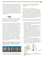
Analyzer (Ultra-Portable GGA, model 915-0011), manufactured by Los Gatos Research, a member of the ABB
group, integrated into the LI-8100A System (Figure 1).
Figure 1. A multiplexed LI-8100A System deployed with the Los
Gatos Research Ultra-Portable Greenhouse Gas Analyzer
(model 915-0011).
Flow, Volume, and Pressure
Considerations
There are three flow loops inside a multiplexed LI-8100A
System: the primary sampling loop between the multiplexer and chamber, the subsampling loop between the
LI-8100A and the multiplexer, and the pressure regulation
loop inside the multiplexer. Each of these loops operates at
a different flow rate. The nominal flow rate through the
subsampling loop is between 1.5 and 1.7 SLPM at near
atmospheric pressure.
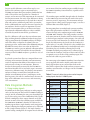
Figure 2. Plumbing schemes for connecting an additional
analyzer to the LI-8100A System. Left hand panel: series
configuration. Right hand panel: parallel configuration.
In a multiplexed configuration, the subsampling loop is
where any additional analyzer should be placed, either in
series with the air outlet from the LI-8100A or in parallel
(Figure 2). Series placement is possible when the additional analyzer does not use its own internal pump and is
capable of operating at the same flow rate and pressure as
the LI-8100A. Parallel placement is required when the
additional analyzer operates at a different pressure or flow
rate different than the LI-8100A. In either configuration it
is possible for the additional analyzer to cause a slight
over-pressure on the LI-8100A optical bench. Care should
be taken to avoid creating flow restrictions in the subsampling loop and where these cannot be avoided it may
be necessary to adjust the bias on the pressure regulation
loop. To adjust the pressure regulation loop:
Continued on next page
2
1. With all plumbing modifications and the additional
analyzer in place, note the LI-8100A optical bench
pressure when all flow pumps are off.
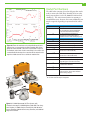
2. Open the LI-8150 multiplexer and remove the
splashguard that covers the fuses.
3. Locate the blue Pressure Adjust potentiometer (up
and to the left of the fuses, as highlighted in Figure 3).
4. Turn on all flow pumps and look at the LI-8100A
optical bench pressure. If it is different from the
pressure noted in Step 1 use a small flat head screwdriver to adjust the Pressure Adjust potentiometer to
minimize the pressure difference between when the
pumps are on or off. Note that it may not be possible to
bring the pressure differential to zero between when
the flow pumps are on and off; within ± 0.5 kPa would
be typical. If there is some offset, the calibration
procedures outlined below should be followed to
ensure that the LI-8100A performs as expected.
The quantitative impact of the added volume on dC/dt can
be evaluated by considering the equation used to calculate
flux F (mole m-2s-1). This equation is derived based on the
assumption of a single fixed volume V (m3) with homogeneous air density ρ. For simplicity, in this discussion the
effects of water corrections are neglected. This however,
does not change the conclusions. Thus,
F=
ρV dC
S dt
(1)
where F is the flux of trace gas (mole m-2s-1), where ρ is air
density (mole m-3), dC/dt is the time rate of change in mole
fraction of the gas being measured (s-1), and S (m2) is the
soil surface area over which the flux occurs. For a flux F,
the trace gas mole fraction rate of change dC/dt is proportional to the total number of molecules in the system ρV.
For a well-mixed system, when an additional volume
Vadded that contains a gas of density ρadded, is inserted into
the system, equation 1 becomes
F=
( ρ system Vsystem + ρ added Vadded ) dC
S
dt
(2)
But ρsystem = Psystem/RTsystem, where R is the universal gas
constant, and similarly for the added volume. Substituting
these expressions and factoring gives,
ρ system (Vsystem + Vadded
F=
Figure 3. Pressure Adjust potentiometer.
When operating with a single chamber and standalone
LI-8100A analyzer control unit, the third party analyzer
should be placed on the AIR OUT line from the LI-8100A
using one of the plumbing schemes described in Figure 2.
The plumbing configuration follows the same guidelines
when placing the additional analyzer in the subsampling
loop of a multiplexed system. The flow rate between an
LI-8100A and a single chamber, and the flow rate in the
subsampling loop of a multiplexed system, are both
nominally between 1.5 and 1.7 SLPM.
The volume of the additional analyzer will have at least
two kinetic effects: 1) it brings additional air to the system,
which dilutes trace gas entering the system from the soil
surface and reduces the measured trace gas mole fraction
rate of change (dC/dt); and 2) it creates a time delay in the
onset of a monotonic concentration increase or decrease.
Accurate fluxes can still be measured if the added volume
is sufficiently small.
S
Padded Tsystem
)
Psystem Tadded dC
dt
(3)
For data processing using SoilFluxPro, an effective volume
Veffective for the addition can be defined for the added
analyzer and entered into the software.
Veffective = Vadded
Padded Tsystem
Psystem Tadded
(4)
Thus, the total volume used in equation (1) becomes
simply Vsystem + Veffective and the density is ρsystem. The
system density is computed using Psystem (Pa) from the
pressure measurement in the LI-8100A optical bench, and
Tsystem (K) from the chamber air temperature. There are
inherently small variations in Veffective due to changes in
Tsystem and Psystem, but these are generally small and subsequently neglected.
In many cases, the impact of an added volume on flux
calculations will be modest as Veffective for many modern
trace gas analyzers is small. For example, in the case study
presented at the end of this application note, if the additional volume of the Ultra-Portable GGA were neglected,
the error would be less than 1.5%.
3
By trapping air making its way around the measurement
circuit, the volume of a third-party gas analyzer may also
introduce an additional time delay and have other effects
that can compromise the flux measurement. The magnitudes of these effects are related to the analyzer’s volume
Vadded (m3), its operating pressure and temperature, and the
flow rate through it. We can qualitatively assess the kinetic
consequences of adding the volume by defining a time
constant for the effective volume of the added analyzer and
comparing it empirically to tested cases. We define a time
constant τadded (s)
τ added =
ρ added Vadded
U added
(5)
where Uadded is the molar flow rate (moles s-1) delivered to
the analyzer, ρ is air density (mole m-3) in the analyzer
evaluated at the analyzer’s internal temperature and
pressure, and Vadded (m3) is its actual volume.
Time constants for different analyzers or model volumes
inserted into the LI-8100A subsampling loop are shown in
Table 1. The time constant for the gas analyzer in the
LI-8100A is 0.5 s, while that for the Ultra-Portable GGA
inserted in a parallel configuration is about 4.6 seconds;
nevertheless, as shown below, both the LI-8100A and the
integrated LI-8100A/Ultra-Portable GGA give accurate
fluxes. We have also tested the impact of adding other
volumes in series configurations, and found that accurate
fluxes were observed when a volume was added having a
time constant of about 7 seconds, but not 17 seconds
(Table 1). Based on these results, we expect that thirdparty analyzers added in series or parallel with time
constants less than 5 to 7 seconds may work well. We
recommend fluxes made with any other configuration not
shown here be validated. Validation can be straightforward if the third-party analyzer measures CO2 as well as
other gases of interest.
Table 1. Time constants for different analyzers or volumes
added to the LI-8100A subsampling loop. Temperatures
and pressures pertain to conditions inside the added
volumes or analyzers.
Analyzer or
added volume
Configuration Volume
(cm3)
LI-8100A
Series
Ultra-Portable GGA Parallel
the appropriate volumes, adjusting the dead band to
accommodate delays, and computing fluxes using
SoilFluxPro.
Calibration Considerations
The calibration procedures outlined in the LI-8100A user
manual are adequate for normal operation of the instrument where optical bench pressure is not significantly
altered from ambient. However, when plumbing additional
volumes into the system, small pressure differences can
cause offsets in the gas measurements when the standard
calibration procedure is followed. These offsets tend to be
small and may only be apparent when a CO2 measurement
is available at two different points in the system.
When operating with a third party analyzer plumbed into
the system an alternative calibration routine can be used:
1. With the system plumbed for operation with the third
party analyzer, turn on the flow pumps and note the
optical bench pressure.
2. Disconnect the hose from the air inlet (AIR IN) and
connect the calibration rig as shown in Figure 4.
3. With the flow pumps on, adjust the flow rate through
the rotometer such that bench pressure on the
LI-8100A is as close as possible to what it was in Step 1.
A slight pressure difference (±0.5 kPa) may be unavoidable and is okay. It is critical however, that flow
through the rotometer exceeds the flow through the
LI-8100A and that some small excess flow leaves the
vent tube in the calibration rig. A flow rate of 2.0 to 2.5
LPM through the rotometer may be suitable to meet
the demand of the LI-8100A pump and have a small
flow out the vent.
4. When the gas concentration reading stabilizes, set the
zero, span or span 2 using the LI-8100A interface
software as described in the LI-8100A user manual.
5. Calibrating the third party analyzer following this same
procedure may be advisable, as well. Check with its
manufacturer for calibration details.
Flow Rate τadded Flux
(s) OK?
(SLPM)
P
(kPa)
T
(°K)
14.5
98
323
1.7
0.5
Yes
325
18.75
300
0.8
4.6
Yes
Test volume 1
Series
200
98
298
1.7
7.1
Yes
Test volume 2
Series
500
98
298
1.7
17.7
No
The configurations reported in Table 1 all affect dC/dt and
introduce time delays. But for systems with appropriate
time constants, accurate fluxes can be obtained by entering
Figure 4. Calibration rig used to calibrate the LI-8100A at
operating pressure.
4
Despite careful calibration, some offsets may be seen
between CO2 and water vapor as measured by the
LI-8100A and some third party analyzer plumbed in line
with it. These offsets can appear due to a number of
reasons, and are not necessarily important in the context of
the flux measurement. For water vapor, differences during
a given flux measurement may be expected due to interactions with surfaces at different points in the system that
lead to a differential time response for water vapor for the
two analyzers. For this reason it is important to record
both the concentration of the gas of interest and water
vapor from the additional analyzer, or where available,
record the dry mole fraction for the gas of interest.
For CO2, differences will occur due to an inherent time
delay resulting from the additional analyzer being physically separated from the LI-8100A’s analyzer; the magnitude of this delay is related to the volume, flow rate,
operating pressure, and location of the additional analyzer.
But differences may also occur to due to drift of the
LI-8100A over time or pressure induced calibration offsets
as discussed previously. It should also be noted that the
accuracy of the LI-8100A’s analyzer is specified as 1.5% of
reading.
In a closed system where fluxes are computed from a rate
of change, measurement of absolute concentration may
seem less important than ability of the analyzer to accurately measure a change in concentration. However,
because the absorptance measured by the LI-8100A is a
non-linear function of CO2 (and water vapor) concentration over its calibration range, the absolute concentration
and rate of change are interrelated, and offsets in the
absolute concentration may have a small impact on the
flux. In practice, this effect is small and arises because the
slope of the calibration curve increases with increasing
CO2 concentration.
Data Integration Methods
1. Using analog signals
If available on the third party analyzer, its analog outputs
can be used to integrate data on the LI-8100A resulting in
a single .81x file containing the time series for multiple gas
species that can be processed in SoilFluxPro. If the system
includes a multiplexer these output channels can be fed
into one or more of the three auxiliary inputs available for
the 8100-104 or 8100-104C chambers. In software, the
auxiliary inputs from a single chamber can be mapped to
all ports, allowing the third party analyzer to be connected
at only a single location (Figure 5). For single chamber
systems lacking a multiplexer, the outputs must be fed into
one or more of the four auxiliary inputs available through
the 8100-663 Auxiliary Sensor Interface, regardless of the
chamber used.
The auxiliary inputs available through either the chambers
or the 8100-663 are measured in volts with 13 bit resolution over a 0 to 5V input range. The instrument software
supports linear scaling (general purpose input), as well as a
Steinhart-Hart conversion (Figure 5).
For integrating data in a multiplexed system an auxiliary
input cable (part number 392-08577) is available that
connects directly to the auxiliary inputs on the 8100-104
and 8100-104C chambers. This cable provides a weatherized connection at the chamber and bare leads to interface
to the third party analyzer’s analog outputs. One cable will
be necessary for each channel in use, and due to the cable’s
length, the analyzer must be placed near the chamber it is
connected to. A 2 m cable (392-07955) is also available that
allows the additional analyzer to be attached directly to the
LI-8150 in place of a chamber, allowing the LI-8150,
LI-8100A and third-party analyzer to be collocated up to
15 m from the chambers. Only one of the 392-07955 cables
is required to access all three of the auxiliary inputs. Pin
outs for both cables are given in Table 2.
For connecting to the 8100-663 Auxiliary Sensor Interface
a user supplied cable with a suitable connection to the
third party analyzer on one end and bare leads on the
other will be required. For details on how to connect to the
auxiliary sensor interface see Chapter 2 of the LI-8100A
user manual.
Table 2. Pin outs of cables that can be used to integrate
analog signals into the LI-8100A System.
392-08577
Wire color
Pin Description
1 Analog input (+)
Brown
2 4 mA limited, 5 VDC Pink
regulated reference
output
392-07955
Description
Wire color
Ground
White
Brown
Chamber temp.
signal (+)
Analog Ground
Green
Grey
Auxiliary input V4+
Yellow
Grey
3
100 mA limited,
5 VDC supply
Blue
4
Not used
5
50 mA limited,
unregulated output
Red
Chamber stop
signal
6
30 mA limited,
switched 5 VDC
supply
Yellow
Auxiliary input V3+
Pink
7
Analog input (-)
Green
Blue
8
Ground
White
Chamber open and
close signal
Auxiliary input V2+
9
N/A
N/A
Switched 5V supply Orange
control
10
N/A
N/A
Voltage supply to
chamber
Red
Tan
5
deviations accounted for in the curve fitting process. Over
longer time scales, the asynchronous nature of clock drift
ensures that without some intervention the offset will not
be a constant value.
There is no internal mechanism in the LI-8100A that allows
the instrument clock to be synchronized to a standard, or for
it to act as a standard for other connected devices. In its
typical application, the LI-8100A system runs independently
and relies on the user to manually set its clock through its
interface software before collecting data.
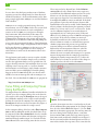
Figure 5. Analog input settings. For a linear voltage input select
General Purpose Input and use the m and b coefficients to
scale the raw voltage to meaningful engineering units:
recorded value = mVin + b. In multiplexed configuration use Fix
to port to route the analog inputs from one chamber to all the
other chambers. This will ensure that the third party analyzer’s
data is recorded in the correct location in the data file.
2. Using an external data file
For users wishing to automate clock synchronization there
is hope however. The LI-8100A configuration grammar
supports pushing a time and date stamp to the instrument
through either its serial or Ethernet interfaces. This allows
a computer or microcontroller connected to the instrument to serve as an external standard for the instrument’s
clock. In many cases the external standard can be the
third-party analyzer (more details below).
Where analog signals are not available, it is possible to
integrate a separate data file from a third party analyzer in
post processing using the import feature in SoilFluxPro.
This allows fluxes to be computed for data collected
remotely from the LI-8100A when analog outputs are not
available from the additional analyzer. It is necessary that
the data to be imported have time stamps that are reasonably synchronized with the LI-8100A; fixed offsets can be
accounted for. The import routine will select or generate a
data point from the import file for each record of the
LI-8100A file. If there is not an exact match, it will pick the
two closest values and interpolate. Thus, 1 Hz data is best,
but is not required. The import routine supports native
text file formats used by Los Gatos Research, Gasmet,
Picarro, and Aerodyne Research, and can also be configured to match a variety of others. For details on how to
import external files see the SoilFluxPro user manual.
Configuration grammar
Time keeping and clock synchronization between the
To restart the measurement, send the following:
LI-8100A and other system clocks
<SR><CMD><MEAS>START</MEAS></CMD></SR>
Importing data from a third party analyzer into the
LI-8100A’s .81x files through SoilFluxPro Software is done
by matching time stamps between the two data sets. This
requires that the two devices keep time relatively consistently between each other. In cases where an offset exists in
the timestamps, a fixed offset can be applied and accounted for in SoilFluxPro during importation. This
requires, however, that the offset be constant over the
entire data set being processed. On short time scales it may
be reasonable to assume drift is minimal and that the
offset is approximately constant, with any additional small
When a measurement is not active the following command
can be used to set the time and date:
<SR><CFG><CLOCK><TIME>{HHMMSS}</
TIME><DATE>{YYYYMMDD}</DATE></CLOCK></
CFG></SR>
In situations where automated clock synchronization
would be desirable, it is unlikely that there will be open
windows where a measurement is not active (eg continuous sampling with a multiplexed system). Thus, before
sending the command to update the clock, it will be
necessary to send the following command to end the active
measurement:
<SR><CMD><MEAS>STOP</MEAS></CMD></SR>
This will restart the measurement using the settings from
the active configuration. To avoid file naming errors that
will prevent the measurement from restarting, select
append mode when configuring and starting the initial
measurement through the interface software.
All commands sent to the LI-8100A need to be followed
with a line feed (ASCII 10) for the instrument to recognize
them. The instrument sends an acknowledgment after
receiving a valid command.
6
8100sync.exe
In cases where the third-party analyzer runs a Windows
operating system (for example many Los Gatos Research
and Picarro analyzers), clock synchronization can be done
using a simple application, 8100sync.exe, and the Windows
Task Scheduler.
8100sync.exe is a simple program that stops the active
measurement, sets the LI-8100A clock to the system clock,
and restarts the measurement. It can be configured to
connect to the LI-8100A via a serial port or through a
LAN connection. When launched the first time, the
application prompts the user to select a serial port for
communication. Entering 0 at the prompt will toggle the
application to use an Ethernet connection and prompt the
user to enter the instrument’s IP address. This information
is compressed into a simple configuration file that is stored
in the same directory as 8100sync.exe for easy access. On
subsequent runs, the application uses these settings to
work out how to connect to the instrument with no user
interaction.
The application can be made to run on a regular schedule
using Windows Task Scheduler. Simply create a task that
executes the application daily at a user specified time. We
suggest choosing some time after midnight when an active
sampling event is not expected (i.e., between chamber
measurements) or when losing a single chamber measurement is of little concern. Midnight is when file splitting
happens on the LI-8100A if daily files are chosen, and it
would be best not to interrupt this with an attempt to set
the clock. You can download the 8100sync.exe program at:
These may need to be adjusted later. Under Dilution
correct with select the channel where water vapor was
recorded from the additional analyzer and use the scalar
below it to scale the value to mol/mol. In the example,
water vapor was logged on V4 as mmol/mol, so it needs to
be multiplied by 0.001 to convert to mol/mol. If the third
party analyzer reports dry mole fraction, then no additional dilution correction is needed. Under Vext input the
effective volume calculated using the equation presented
under Flow, Volume and Pressure considerations. In this
case the additional analyzer has an actual volume of
approximately 325 cm3 and operates at 18.75 kPa and
300.12 °K. At a chamber pressure of 100 kPa and temperature of 298.5 °K the effective volume was 60.62 cm3.
It should be noted that in the example presented here
effective volume is treated as a constant. But in practice
chamber temperature and pressure are typically not
constant, leading to an effective volume that may be
different for each measurement. However, when the
effective volume is small relative to the total system
volume the error associated with treating it as a constant
may not be important; For the example presented here,
changing the chamber temperature by 25 °C affects the
total volume by less than 0.1% and for a 5 kPa change in
chamber pressure, the effect is less than 0.04%.
http://www.licor.com/8100sync.exe
Curve Fitting and Computing Fluxes
Using SoilFluxPro
To compute fluxes for additional variables included in the
.81x file access the recompute dialog; this can be done for
all records in a file using the Recompute icon at the top of
the SoilFluxPro window, or for a single record by double
clicking the record in the summary view and going to the
Recompute tab in that record’s observation view. Figure 6
shows the recompute window for a single record.
In the recompute dialog, click the + under Flux Computations to add an additional variable for which fluxes are to
be computed. Under Gas column label: select the variable.
In the example here methane mole fraction was logged as
umol/mol through auxiliary input V2. Check the box for
Curve Fit and select start and stop times for the curve fit.
™
Figure 6. The Recompute dialog.
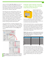
Open the observation view for a record and go to the tab
for the additional flux computation. In the example shown
here, the tab is labeled Fit#2 V2 (Figure 7). Use the Guidance tab to determine appropriate start and stop times for
the curve fitting. In the example dataset, a start time
between 40 and 100 seconds and a stop time of greater
than 220 seconds would work (shaded areas in Figure 7).
For the start time look for the initial plateau and select a
time in that window. For stop time, select a time after the
7
values level off. If the Stop Time Analysis curve does not
level off or is very noisy, it is possible that the measurement length was too short. Once appropriate start and stop
times have been determined it will be necessary to go back
and recompute the data set if these times differ from the
times used in the initial flux computation.
Note that for gas species with large fluxes and low resistance to diffusion in the soil, long measurement periods
may lead to underestimations of the final flux due to
buildup of the gas in the soil air space during the measurement. For gas species with low fluxes, such as methane,
long measurement periods may be required to get enough
data for a good curve fit. This means when measuring
methane and carbon dioxide together, it will often be
necessary to use different stop times for the two gases in
the flux computation, with the stop time for carbon
dioxide occurring much before that of methane.
Once satisfied with the curve fitting and summary values,
the Export icon at the top of the main SoilFluxPro window
can be used to export the summary values. For additional
details on computing additional fluxes and exporting data
see the SoilFluxPro manual accessed under Help in the
software.
Example measurements using the
Los Gatos Research Ultra-Portable
Greenhouse Gas Analyzer
An Ultra-Portable GGA
(model 915-0011) from Los
Gatos Research, a member of
the ABB group, was integrated
into a multiplexed LI-8100A
System (Figure 1) using a
parallel plumbing configuration as shown in Figure 2. Data
from the analyzer was brought
into the LI-8100A System using its analog outputs. Data
collection was tested using both connection schemes
described under Data Integration Methods. Wiring for the
two cable sets tested is described in Table 3.
The Ultra-Portable GGA had an actual volume of approximately 325 cm3 and operated at 18.75 kPa and 300.12 °K.
Flow rate through the Ultra-Portable GGA was 0.8 SLPM.
A chamber pressure of 100 kPa and temperature of 298.5
°K was used to compute the effective volume for the UltraPortable GGA and an effective volume of 60.62 cm3 was
used for all flux computations.
Table 3. Cable connections used to integrate data from the
Ultra-Portable GGA. A pre-assembled version of the Turck
to DB-9 cable described here is available from LI-COR
(part number 9981-188).
DB-9 connector to
Ultra-Portable GGA
CH4 signal (pin 1)
CO2 signal (pin 2)
H2O signal (pin 3)
CH4 ground (pin 6)
CO2 ground (pin 7)
H2O ground (pin 8)
Figure 7. Viewing the curve fit for additional flux computations
and using Guidance to select appropriate start and stop times.
Windows with appropriate start and stop times are shaded in
red.
392-08577 wire color
(three cables were used)
Brown (cable 1)
Brown (cable 2)
Brown (cable 3)
Green (cable 1)
Green (cable 2)
Green (cable 3)
392-07955
wire color
Red
Pink
Yellow
Green
Green
Green
Initial experiments were done in the lab to compare a
known flux to the flux as determined from each analyzer’s
time series data. Known fluxes were generated by injecting
pure CO2 at a constant rate through a mass-flow controller
into a sealed collar below an 8100-104 chamber. Data from
these experiments are presented in Table 4 and show that
for an artificial flux produced by mass-flow the LI-8100A
and Ultra-Portable GGA give the same and expected
result.
8
Table 4. Comparison of known mass-flow fluxes between
the LI-8100A and Ultra-Portable GGA. Fluxes are given as
μmol m-2 s-1 plus or minus one standard deviation.
Injection Rate Expected Flux
(SCCM)
LI-8100A
Ultra-Portable
GGA
0.1
0.2
0.4
2.40 ± 0.01
4.73 ± 0.01
9.40 ± 0.01
2.62 ± 0.13
4.68 ± 0.16
9.17 ± 0.15
2.62 ± 0.13
4.69 ± 0.16
9.18 ± 0.15
0.8
18.73 ± 0.01
18.15 ± 0.17
18.16 ± 0.17
The system was deployed on a mowed lawn and an artificial peat bog in Lincoln, NE to measure fluxes of carbon
dioxide and methane. The two analyzers were cross
calibrated prior to the laboratory experiments, but no
subsequent calibration was preformed prior to the field
deployments. Figure 8 shows a comparison of the ranges
and initial offsets in carbon dioxide concentration as
reported by the two analyzers. While they showed a rather
variable offset in concentration at the start of each measurement, the magnitude of change in concentration over
each flux measurement was very similar for both analyzers
at both sites.
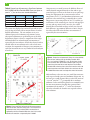
Comparisons were made between the diffusive fluxes of
carbon dioxide computed from these data and are presented in Figure 9. Fluxes at the lawn site were quite large
during the deployment due to warm weather (mean
temperature of 25.7 °C) and abundant soil moisture, and
quite low at the artificial bog, presumably due to cooler
temperatures (mean temperature of 19.4 °C) and low gas
conductance of the saturated peat. Once fit with appropriate start and stop times for the curve fits, the carbon
dioxide fluxes from both analyzers at both sites showed
little difference (approximate difference of 0.3%) despite
the offsets observed in the absolute concentrations as
reported by the two instruments.
y = 0.9972x - 0.1009
R2 = 0.9922
Figure 9. Comparison of exponential fluxes for carbon dioxide
from the lawn and bog sites for the Ultra-Portable GGA
(FCO2-UGGA) and the LI-8100A (FCO2-8100). For the lawn site the
curve fits were done for the Ultra-Portable GGA using a 40
second start time and 120 second stop time. For the UltraPortable GGA at the bog site a 30 second start time and a 120
second stop time were used. At both sites start times for the
LI-8100A were 20 seconds and stop times were 120 seconds.
Methane fluxes at the two sites were small, but consistent
with expected trends given soil conditions (Figure 10). At
the lawn site a small negative flux was observed (mean of
-3.3 × 10-4 μmol m-2 s-1), presumably due to methane
oxidation. At the artificial bog fluxes were nominally zero
for most measurements, but did show positive fluxes
(maximum of 0.18 μmol m-2 s-1) in the late afternoon
when the soil under the chamber was exposed to direct
solar radiation.
Figure 8. Range and initial offset for the flux measurements
made at the lawn and artificial bog sites. The initial offset is
computed as the initial carbon dioxide concentration as
reported by the Ultra-Portable GGA minus the initial carbon
dioxide concentration as reported by the LI-8100A.
9
Useful Part Numbers
The table below contains a list of useful parts that can be
used to connect the LGR Ultra-Portable GGA (or other
third party analyzers) to the LI-8100A/LI-8150 and soil
chamber(s). The 9981-188 and 9981-189 contain preassembled kits; note, however, that some additional parts
may be required, depending on your method of connection.
Complete Kits
9981-188
Additional Parts
Description
(1, 2)
Figure 11. LI-8100A Automated Soil Flux System, with
(clockwise from top) LI-8150 Multiplexer, 8100-104C Clear Longterm Chamber, LI-8100A Analyzer Control Unit, 8100-103 20cm
Survey Chamber, 8100-102 10cm Survey Chamber, and 8100-104
Long-term Chamber.
Bev-a-line tubing (15m roll)
300-07385
1/4” Quick-connect ‘T’ fitting
300-03367
1/4” Quick-connect ‘Y’ fitting
1/4” Quick-connect straight union
300-07124
(1, 2)
Male stainless steel quick-connect
(connects to LI-8100A AIR IN)
300-07125
(1, 2)
Female stainless steel quick-connect
(connects to LI-8100A AIR OUT)
294-03334
0-2.5 LPM flow meter (rotometer)
300-08118
1/8” NPT to 1/4” quick-connect right
angle fitting (two used with rotometer)
392-08577 (1)
Auxiliary sensor input cable for 8100-104
or 8100-104C chambers
392-07955 (1)
Turck to bare leads cable, 2m long
314-03430
2
Pre-assembled Turck to DB-9 cable
for connecting the Ultra-Portable GGA
to the LI-8150 (includes 392-07955).
Pre-assembled hose assembly for
plumbing the Ultra-Portable GGA in
parallel to the LI-8100A subsampling loop.
300-03123
1
Description
9981-189 (1, 2)
8150-250
Figure 10. Fluxes for methane and carbon dioxide at the lawn
and bog sites as measured by the Ultra-Portable GGA. Curve
fitting for carbon dioxide is the same as described in Figure 9.
For methane at the lawn site the curve fitting is the same as for
carbon dioxide. At the bog site a start time of 30 seconds and a
stop time of 300 seconds was used for the methane flux.
(1)
(1)
Male DB-9 connector with shielded
housing (used to access Ultra-Portable
GGA’s analog outputs)
For use with analog connections.
For use with external analyzer integration.
10
NOTES
11
LI-8100A System Specifications
Analyzer Control Unit
LI-8150 Multiplexer
Power Requirements: 10.5 VDC to 28 VDC; 3 A @ 12 V (36 W)
maximum during warm-up; 1 A @ 12 V (12 W) average
Operating Temperature Range: -20 °C to 45 °C
Relative Humidity Range: 0% to 95% RH, Non-Condensing
Weatherproof Rating: Tested to IEC IP55 standard
Dimensions: 29 cm L x 38.1 cm W x 16.5 cm H (11.4” x 15” x 6.5”)
Weight: 5.3 kg (11.8 lbs) without battery; 6.7 kg (14.8 lbs) with
battery
Battery Weight: 1.4 kg (3.0 lbs)
Memory: 18 MB flash memory for data collection (32 MB total)
Compact Flash Card: Type I industrial grade, 1 GB with adapter
sleeve included, will accept Type II with appropriate adapter
sleeve
Wireless PC Card: Fixed wireless networking Type II PC Card.
Cisco Systems Aironet® 350 Series 11 Mbps DSSS for Wi-Fi
(802.11b) networking
RS-232 Maximum Output Rate: 1 Hz
RS-232 Baud Rate: 57,600 bps
Hand-held Device Requirements: Apple iOS 4.0 or greater
Pressure Sensor Range: 15 kPa to 115 kPa
Pressure Sensor Accuracy: 1.5% over 0 °C to 85 °C
Maximum Gas Flow Rate: ~2.0 lpm
Dimensions: 40.6 cm L x 57.2 cm W x 21.1 cm H (16” x 22.5” x 8.3”)
Weatherproof Rating: Tested to IEC IP55 standard
Weight: 9.4 kg (20.7 lbs), 8 ports; 11.2 kg (24.8 lbs) 16 ports
Operating Temperature Range: -20 to 45 °C
Operating Humidity Range: 0 to 95% RH, non-condensing
Maximum Spread: 30.0 m (98.4 ft)
Flow Rate to Chambers: ~3.0 lpm (non-adjustable)
Flow Rate Between LI-8100A and LI-8150: ~2.0 lpm
Power Requirements: 10.5 VDC to 14.5 VDC (120 VAC and 240 VAC
with optional power supply)
Soil Temperature Thermistor (optional): ±1.0 °C from -20 to 50 °C
Long-Term Chamber - 8100-104
Volume: 4076.1 cm3
Soil Area: 317.8 cm2 (49.3 inches2)
Baseplate Dimensions: 48.3 cm L x 38.1 cm W x 33.0 cm H (19" x
15" x 13")
Weatherproof Rating: Tested to IEC IP55 standard
Air Temperature Thermistor:
Operating Range: -20 to 45 °C
Accuracy: ± 0.5 °C over 0 °C to 70 °C
Cable Length: 15 m (49.2 ft)
Weight: 5.9 kg (13 lbs)
Infrared Gas Analyzer
Measurement Principle: Non-Dispersive Infrared
Traceability: Traceable to WMO standards for CO2. NIST traceable LI-610 Portable Dew Point Generator for H2O
CO2
Measurement Range: 0 ppm to 20,000 ppm
Accuracy: 1.5% of reading
Drift at 0 ppm: <0.15 ppm/°C
Span Drift1: <0.03%/°C
Total Drift at 370 ppm: <0.4 ppm/°C
RMS Noise at 370 ppm with 1 sec signal averaging: <1 ppm
Sensitivity to water vapor: <0.1 ppm CO2/mmol/mol H2O
H2O
Measurement Range: 0-60 mmol/mol
Accuracy: 1.5% of reading
Drift at 0 mmol/mol: <0.003 mmol/mol/°C
Span Drift1: <0.03%/°C
Total Drift at 10 mmol/mol: <0.009 mmol/mol/°C
RMS Noise at 10 mmol/mol with 1 sec signal averaging: <0.01
mmol/mol
Sensitivity to CO2: <0.0001 mmol/mol H2O/ppm CO2
1Residual
error after zero correction
Clear Long-Term Chamber - 8100-104C
Volume (Serial numbers 2024 and below): 4076.1 cm3
Volume (Serial numbers 2025 and above): 3876.1 cm3
Soil Area: 317.8 cm2 (49.3 inches2)
Baseplate Dimensions: 48.3 cm L x 38.1 cm W x 33.0 cm H (19" x
15" x 13")
Weatherproof Rating: Tested to IEC IP55 standard
Air Temperature Thermistor:
Operating Range: -20 to 45 °C
Accuracy: ±0.5 °C over 0 °C to 70 °C
Cable Length: 15 m (49.2 ft)
Weight: 5.9 kg (13 lbs)
LI-COR Biosciences - Global Headquarters
4647 Superior Street
Lincoln, Nebraska 68504
Phone: +1-402-467-3576
Toll free: 800-447-3576
Fax: +1-402-467-2819
[email protected] • [email protected] • www.licor.com/env
Regional Offices
LI-COR GmbH, Germany
Serving Andorra, Albania, Cyprus, Estonia, Germany, Iceland, Latvia,
Lithuania, Liechtenstein, Malta, Moldova, Monaco, San Marino,
Ukraine, and Vatican City.
LI-COR Biosciences GmbH
Siemensstraße 25A
61352 Bad Homburg, Germany
Phone: +49 (0) 6172 17 17 771
Fax: +49 (0) 6172 17 17 799
[email protected] • [email protected]
LI-COR Ltd., United Kingdom
Serving Denmark, Finland, Ireland, Norway, Sweden, and UK.
LI-COR Biosciences UK Ltd.
St. John’s Innovation Centre
Cowley Road
Cambridge
CB4 0WS
United Kingdom
Phone: +44 (0) 1223 422102
Fax: +44 (0) 1223 422105
[email protected] • [email protected]
© 2015, LI-COR, Inc. LI-COR and SoilFluxPro are trademarks or registered trademarks of LI-COR, Inc.
All other trademarks belong to their respective owners.
979-15121
Rev. 1, 10/15