No category

Download Chapter 1 Installing GeneMarker HID

100

101

102

103

104

105

106

107

108

109

110

111

112

113

114

115

116

117

118

119

120

121

122

123

124

125

126

127

128

129

130

131

132

133

134

135

136

137

138

139

140

141

142

143

144

145

146

147

148

149

150

151

152

153

154

155

156

157

158

159

160

161

Transcript

SOFTGEN ETI
CS
®
STR HumanI
dent
i
t
ySof
t
war
e
User M anual
SO FTGEN ETI
CS®
Sof
tware PowerTool
sf
or Geneti
c Anal
ysi
s
www.
sof
tgeneti
cs.
com
Copyright, Licenses and Trademarks
©2001-2015 SoftGenetics LLC. All rights reserv ed. No part of this publication may be
reproduced, transmitted, transcribed, or translated into any language in any form by any
means without the written perm ission of SoftGenetics LLC. Th e software is copyrighted
and cannot be altered or given to a third part y without the written authorization from Soft
Genetics LLC. The s oftware may be licen sed from SoftGeneticsLLC. Mutation
Explorer, Mutation Surveyor, JelMarker,ChimerMarker, NextGENe and GeneMarker are
trademarks of SoftGenetics LLC. All other product names and/or logos are trademarks of
their respective owners.
Limited Liability of Using the Software
In no event shall SoftGenetics LLC. be liab le for direc t, indirect, incidental, special,
exemplary, or consequential dam ages (including, but not lim ited to, procurem ent of
substitute goods or services; loss of use, data, or profit s; or business interruption),
however caused and any theory of liability, wh ether in con tract, strict liability, o r tort
(including negligence or otherwise) arising in any way out of use of this software, even if
advised of the possibility of such damage.
SoftGenetics End User License Agreement
GeneMarkerHID & GeneMarker HID auto
NOTICE TO USER: PLEASE READ THIS CONTRACT CAREFULLY. BY
DOWNLOADING, INSTALLING, OR USING ALL OR ANY PORTION OF THE SOFTWARE
YOU ACCEPT ALL THE TERMS AND CONDITIONS OF THIS AGREEMENT.
CLICKING ON THE “ACCEPT,” OR “I AGREE,” BUTTON IS THE SAME AS SIGNING
THIS AGREEMENT. IF YOU ARE INSTALLING THIS SOFTWARE FOR ANOTHER
USER, YOU ACKNOWLEDGE THAT THE ULTIMATE END USER HAS READ AND
AGREED TO THE TERMS OF THIS AGREEMENT. IF YOU ARE INSTALLING THIS
SOFTWARE FOR AN ORGANIZATION, YOU ACKNOWLEDGE AND AGREE THAT YOU
ARE AUTHORIZED TO BIND THE ORGANIZATION TO THE TERMS OF THIS
AGREEMENT. IF AN ORGANIZATION USES THIS SOFTWARE, THE ORGANIZATION
AGREES TO ALL THE TERMS AND CONDITIONS OF THIS AGREEMENT.
IF YOU DO NOT AGREE TO ANY OF THE TERMS CONTAINED IN THIS AGREEMENT,
DO NOT DOWNLOAD, INSTALL, OR USE THIS SOFTWARE.
1. Definitions. "Software" means (a) all of the contents of the files (delivered electronically
or on physical media), disk(s), CD‐ROM(s) or other media with which this Agreement is
provided, including but not limited to (i) SoftGenetics’s or third party computer
information, data, or software; (ii) related explanatory written materials or files
("Documentation"); and (iii) fonts and other output mechanisms; and (b) upgrades,
modified versions, updates, additions, and future copies of the Software, if any, licensed
to you by SoftGenetics (collectively, "Updates").
2. "Use" or "Using" means to access, install, download, copy or otherwise benefit from
using the functionality of the Software.
3. "Permitted Number" means one (1) unless otherwise indicated under a valid license
(e.g. volume license) granted by SoftGenetics.
4. "Computer" means a virtual machine or a physical electronic device that accepts
information in digital or similar form and manipulates it for a specific result based on a
sequence of instructions.
5. "SoftGenetics" means SoftGenetics, LLC State College, PA 16803
6. Software License. As long as you comply with the terms of this End User License
Agreement (the "Agreement") and pay all license fees for the Software, SoftGenetics
grants to you a non‐exclusive license to Use the Software for the purposes described in
the Documentation. Some third party materials included in the Software may be subject
to other terms and conditions, which are typically found in a "Read Me" file located near
such materials.
6.1. General Use. You may install and Use a copy of the Software on your compatible
computer. You may also use the Software on a computer file server provided concurrent
use does not exceed the Permitted Number. No other network use is permitted, including
but not limited to, using the Software either directly or through commands, data or
instructions from or to a computer not part of your internal network, for internet or web
hosting services or by any user not licensed to use a copy of the Software through a valid
license from SoftGenetics.
6.2. Distribution. This license does not give you the right to distribute or sublicense the
Software to others. A separate agreement with SoftGenetics is required for any
distribution or sublicensing of the Software.
6.3. Backup Copy. You may make one backup copy of the Software, provided your backup
copy is not installed or used on any Computer other than for archival purposes. You may
not transfer the rights to a backup copy unless you transfer all rights in the Software to
subsequent authorized user.
6.4. Home Use. You, as the primary user of the computer on which the Software is
installed, may also install the Software on one of your home computers. However, the
Software may not be used on your home computer at the same time the Software is being
used on any other computer.
6.5. Research Use Only. User acknowledges and agrees that the Software is licensed by
SoftGenetics for research use only. Any violation of this restriction on use shall constitute
a breach of this Agreement. User assumes all risk for use of the Software. User further
acknowledges that User is responsible for validating the Software for use in User’s
intended applications. Due to the nature of computers, software, operating systems and
installation procedures, SoftGenetics cannot accept any liability or responsibility for
validation of the Software in any of User’s applications.
7. Intellectual Property Rights. The Software and any copies that you are authorized by
SoftGenetics to make are the intellectual property of and are owned by SoftGenetics and
its suppliers. The structure, organization and code of the Software are the valuable trade
secrets and confidential information of SoftGenetics and its suppliers. The Software is
protected by copyright, including without limitation by United States Copyright Law,
international treaty provisions and applicable laws in the country in which it is being used.
You may not copy the Software, except as set forth in this Agreement ("Software
License"). Any copies that you are permitted to make pursuant to this Agreement must
contain the same copyright and other proprietary notices that appear on or in the Software.
You also agree not to (a) modify, adapt, translate, or create derivative works based on the
Software, or (b) reverse engineer, decompile, disassemble or otherwise attempt to
discover the source code of the Software except to the extent that (i) you may be expressly
permitted to decompile under applicable law, (ii) it is essential to do so in order to achieve
operability of the Software with another software program, and (iii) you have first
requested SoftGenetics to provide the information necessary to achieve such operability
and SoftGenetics has not made such information available. SoftGenetics may impose
reasonable conditions and request a reasonable fee before providing such information.
Any information supplied by SoftGenetics or obtained by you, as permitted hereunder, may
only be used by you for the purpose described herein and may not be disclosed to any
third party or used to create any software which is substantially similar to or performs the
same function(s) as the Software. Requests for information should be directed to
SoftGenetics.
8. Trademarks shall be used in accordance with accepted trademark practice, including
identification of trademarks owners' names. Trademarks can only be used to identify
printed output produced by the Software and such use of any trademark does not give you
any rights of ownership in that trademark. SoftGenetics and other owners of any
trademarks contained in the Software reserve all rights to limit and/or condition use of any
of their trademarks.
9. Except as expressly stated above, this Agreement does not grant you any intellectual
property rights in the Software.
Indemnity. You agree to hold harmless, indemnify and defend SoftGenetics, its officers,
directors, employees, agents, and affiliates from and against any claims, demands, losses,
damages, fines and expenses (including attorney’s fees and costs) arising out of your use
of the Software, any instrument on which the Software is operating, and related
Documentation. Without limiting the foregoing, you also agree to hold harmless, indemnify
and defend SoftGenetics, its officers, directors, employees, agents, and affiliates from and
against any matters relating to any claims that you have (i) viewed, downloaded, encoded,
compressed, copied or transmitted any materials (other than materials provided by
SoftGenetics) in connection with use of the Software or any instrument on which the
Software is operating in violation of another party’s rights or in violation of any law.
Transfer. You may not rent, lease, sublicense or transfer your rights in the Software,
or authorize all or any portion of the Software to be copied onto another user’s Computer
except as may be expressly permitted herein. You may, however, transfer all your rights to
Use the Software to another person or legal entity provided that: (a) you also transfer this
Agreement, any instrument on which the Software operates, the Software and all other
software or hardware bundled or pre‐installed with the Software, including all copies,
Updates and prior versions, and all copies of font or other output software converted into
other formats, to such person or entity; (b) you retain no copies, including backups and
copies stored on a Computer; and (c) the receiving party accepts the terms and conditions
of this Agreement and any other terms and conditions upon which you legally purchased a
valid license to the Software. Notwithstanding the foregoing, you may not transfer
education, pre‐release, or not-for-resale copies of the Software.
10.
Multiple Environment Software / Multiple Language Software / Dual Media Software /
Multiple Copies/ Bundles / Updates. If the Software supports multiple platforms or
languages, if you receive the Software on multiple media, if you otherwise receive multiple
copies of the Software, or if you received the Software bundled with other software or with
an instrument, the total number of your Computers on which all versions of the Software
are installed may not exceed the Permitted Number. You may not rent, lease, sublicense,
lend or transfer any versions or copies of such Software you do not Use. If the Software is
an Update to a previous version of the Software, you must possess a valid license to such
previous version in order to Use the Update. You may continue to use the previous version
of the Software on your Computer after you receive the Update to assist you in the
transition to the Update, provided that: the Update and the previous version are installed
on the same Computer; the previous version or copies thereof are not transferred to
another party or Computer unless all copies of the Update are also transferred to such
party or Computer; and you acknowledge that any obligation SoftGenetics may have to
support the previous version of the Software may be ended upon availability of the Update.
12.
If the Software is used to connect with or download information from any other
software program, system, or database, you agree that SoftGenetics does not control the
features, operations, or information practices of any third party websites, computer
systems, or databases.
11.
13.
LIMITED WARRANTY. SoftGenetics warrants to the person or entity that purchases
a license for the Software for use pursuant to the terms of this license that the Software
will perform substantially in accordance with the Documentation for a period of ninety (90)
days following receipt of the Software when used on the recommended hardware
configuration. Any non‐substantial variation of performance from the Documentation does
not establish a warranty right. THIS LIMITED WARRANTY DOES NOT APPLY TO
UPDATES, SOFTWARE CONVERTED INTO OTHER FORMATS, PRE‐RELEASE
(BETA), TRYOUT, PRODUCT SAMPLER, OR NOT-FOR-RESALE (NFR) COPIES OF
THE SOFTWARE. To make a warranty claim, you must return the Software to the
location where you obtained it along with proof of purchase within such ninety (90) day
period. If the Software does not perform substantially in accordance with the
Documentation, the entire liability of SoftGenetics and your exclusive remedy shall be
limited to either, at SoftGenetics option: (1) the replacement of the Software, or (2) the
refund of the license fee you paid for the Software. THE LIMITED WARRANTY SET
FORTH IN THIS SECTION GIVES YOU SPECIFIC LEGAL RIGHTS. YOU MAY HAVE
ADDITIONAL RIGHTS WHICH VARY FROM JURISDICTION TO JURISDICTION.
DISCLAIMER. THE FOREGOING LIMITED WARRANTY STATES THE SOLE AND
EXCLUSIVE REMEDIES FOR SOFTGENETICS'S OR ITS SUPPLIER'S BREACH OF
WARRANTY. SOFTGENETICS AND ITS SUPPLIERS DO NOT AND CANNOT
WARRANT THE PERFORMANCE, MERCHANTABILITY OR RESULTS YOU MAY
OBTAIN BY USING THE SOFTWARE. EXCEPT FOR THE FOREGOING LIMITED
WARRANTY, YOU ACKNOWLEDGE AND AGREE THAT SOFTGENETICS HAS MADE NO
OTHER EXPRESS WARRANTIES TO YOU REGARDING THE SOFTWARE AND THAT
THE SOFTWARE IS BEING PROVIDED TO YOU “AS IS’ WITHOUT WARRANY OF ANY
OTHER KIND. SOFTGENETICS SPECIFICALLY DISCLAIMS ALL OTHER WARRANTIES
WITH REGARD TO THE SOFTWARE, EXPRESS OR IMPLIED, INCLUDING, WITHOUT
LIMITATION ANY IMPLIED WARRANTIES OF FITNESS FOR A PARTICULAR PURPOSE,
MERCHANTABILITY, MERCHANTABLE QUALITY, NONINFRINGEMENT OF THIRD
PARTY RIGHTS, INTEGRATION, OR SATISFACTORY QUALITY. SOFTGENETICS AND
ITS SUPPLIERS MAKE NO OTHER WARRANTIES, CONDITIONS,
REPRESENTATIONS OR TERMS, EXPRESS OR IMPLIED, WHETHER BY STATUTE,
COMMON LAW, CUSTOM, USAGE OR OTHERWISE AS TO ANY OTHER MATTERS.
The provisions of this disclaimer shall survive the termination of this Agreement,
howsoever caused, but this shall not imply or create any continued right to Use the
Software after termination of this Agreement.
14.
LIMITATION OF LIABILITY. IN NO EVENT WILL SOFTGENETICS OR ITS
SUPPLIERS BE LIABLE TO YOU FOR ANY LOSS OF USE, INTERRUPTION OF
BUSINESS, DAMAGES, CLAIMS OR COSTS WHATSOEVER OR ANY
CONSEQUENTIAL, INDIRECT, INCIDENTAL DAMAGES, OR ANY LOST PROFITS OR
LOST SAVINGS, EVEN IF A SOFTGENETICS REPRESENTATIVE HAS BEEN ADVISED
OF THE POSSIBILITY OF SUCH LOSS, DAMAGES, CLAIMS OR COSTS, OR FOR ANY
CLAIM BY ANY THIRD PARTY. THE FOREGOING LIMITATIONS AND EXCLUSIONS
APPLY TO THE EXTENT PERMITTED BY APPLICABLE LAW IN YOUR JURISDICTION.
SOFTGENETICS'S AGGREGATE LIABILITY AND THAT OF ITS SUPPLIERS UNDER
OR IN CONNECTION WITH THIS AGREEMENT SHALL BE LIMITED TO THE AMOUNT
PAID FOR THIS LICENSE, IF ANY. SoftGenetics is acting on behalf of its suppliers for the
purpose of disclaiming, excluding and/or limiting obligations, warranties and liability as
provided in this Agreement, but in no other respects and for no other purpose.
15.
Export Rules. You agree that the Software will not be shipped, transferred or exported
into any country or used in any manner prohibited by the United States Export
Administration Act or any other export laws, restrictions or regulations (collectively the
"Export Laws"). In addition, if the Software is identified as export controlled items under the
Export Laws, you represent and warrant that you are not a citizen, or otherwise located
within, an embargoed nation (including without limitation Iran Iraq, Syria, Sudan, Libya,
Cuba, North Korea, Serbia and Crimea) and that you are not otherwise prohibited under
the Export Laws from receiving the Software. All rights to Use the Software are granted on
condition that such rights are forfeited if you fail to comply with the terms of this Agreement.
17. Governing Law. This Agreement will be governed by and construed in accordance
with the substantive laws in force in the State of Pennsylvania, United States of
16.
America.
18. General
Provisions. This is the entire agreement between you and SoftGenetics
regarding the license of the Software, and it supersedes any prior representations,
discussions, undertakings, communications, or advertising related to the Software.
This Agreement may only be modified by a writing executed by an authorized officer
of SoftGenetics, except that Updates may be licensed to you by SoftGenetics with
additional or different terms. SoftGenetics may assign this Agreement to an affiliate
or any other third party at SoftGenetics’s sole discretion.
May2015
Table of Contents GeneMarker® HID v.2.7.6
CHAPTER 1 INSTALLING GENEMARKER HID .................................................................................................... 5
COMPUTER SYSTEM REQUIREMENTS ........................................................................................................................... 6
LOCAL-LICENSING OPTION ......................................................................................................................................... 6
Installation....................................................................................................................................................... 6
Local Registration ............................................................................................................................................ 7
Local Upgrade.................................................................................................................................................. 7
NETWORK-LICENSING OPTION .................................................................................................................................... 7
Install License Server Manager........................................................................................................................ 8
Register License Server Manager for GeneMarker HID Usage ........................................................................ 8
Install GeneMarker HID Software on the Client Computer ............................................................................. 9
Upgrade of License Server Manager ............................................................................................................. 10
Upgrade of GeneMarker HID Software on Client Computer......................................................................... 10
QUESTIONS .......................................................................................................................................................... 10
CHAPTER 2 GENERAL PROCEDURE ................................................................................................................ 11
IMPORT DATA FILES ............................................................................................................................................... 12
Procedure ...................................................................................................................................................... 12
Features......................................................................................................................................................... 12
RAW DATA ANALYSIS ............................................................................................................................................. 13
Main Toolbar Icons ........................................................................................................................................ 14
What to Expect .............................................................................................................................................. 15
PROCESS DATA ...................................................................................................................................................... 17
Run Wizard Template Selection .................................................................................................................... 17
Run Wizard Data Process .............................................................................................................................. 18
Run Wizard Additional Settings ..................................................................................................................... 20
ADJUST ANALYSIS PARAMETERS................................................................................................................................ 21
Re-analyze with Run Wizard.......................................................................................................................... 21
Re-analyze with Auto Run ............................................................................................................................. 21
Re-analyze Individual Samples ...................................................................................................................... 22
CHAPTER 3 MAIN ANALYSIS OVERVIEW ....................................................................................................... 23
MAIN ANALYSIS WINDOW....................................................................................................................................... 24
Sample File Tree ............................................................................................................................................ 24
Synthetic Gel Image and Electropherogram with Peak Table ....................................................................... 26
Report Table .................................................................................................................................................. 30
MENU OPTIONS .................................................................................................................................................... 31
File Menu....................................................................................................................................................... 31
View Menu .................................................................................................................................................... 32
Project Menu ................................................................................................................................................. 35
Applications Menu ........................................................................................................................................ 36
Tools Menu.................................................................................................................................................... 37
Help Menu ..................................................................................................................................................... 38
MAIN TOOLBAR ICONS............................................................................................................................................ 38
ADDITIONAL ANALYSIS OPTIONS ............................................................................................................................... 40
Browse By All Colors ...................................................................................................................................... 40
Profile Comparison View ............................................................................................................................... 40
CHAPTER 4 FRAGMENT SIZING STANDARDS ................................................................................................ 43
SIZE TEMPLATE EDITOR ........................................................................................................................................... 44
Procedure ...................................................................................................................................................... 46
August 2015
Table of Contents
Icons and Functions ....................................................................................................................................... 47
What to Expect .............................................................................................................................................. 48
SIZE CALIBRATION CHARTS....................................................................................................................................... 49
Procedure ...................................................................................................................................................... 52
Icons and Functions ....................................................................................................................................... 52
What to Expect .............................................................................................................................................. 53
SQ Flagging .................................................................................................................................................... 53
CHAPTER 5 PANEL EDITOR ........................................................................................................................... 55
OVERVIEW ........................................................................................................................................................... 56
Project Panel .................................................................................................................................................56
Panel Templates ............................................................................................................................................ 56
Sample List .................................................................................................................................................... 57
Overlay Trace ................................................................................................................................................ 57
Panel Table .................................................................................................................................................... 60
PROCEDURE .......................................................................................................................................................... 60
Pre-Defined Panels ........................................................................................................................................ 61
Custom Panel Creation .................................................................................................................................. 61
Adjusting Panels - Manual and Automated Panel Calibration ......................................................................62
OPTIONS, FUNCTIONS AND ICONS ............................................................................................................................. 63
Menu Options ............................................................................................................................................... 63
Toolbar Icons ................................................................................................................................................. 64
Saving a panel with signal information ......................................................................................................... 65
Project Panel ................................................................................................................................................. 66
WHAT TO EXPECT .................................................................................................................................................. 66
CHAPTER 6 REPORTS AND PRINTING ............................................................................................................ 71
REPORT TABLE ...................................................................................................................................................... 72
Allele List ....................................................................................................................................................... 72
Forensics........................................................................................................................................................ 72
Bin Table ........................................................................................................................................................ 73
Peak Table ..................................................................................................................................................... 74
Allele Count ................................................................................................................................................... 75
LIMS REPORT ....................................................................................................................................................... 76
PRINT REPORT....................................................................................................................................................... 77
Report Content Options ................................................................................................................................ 78
Include Customizable Logo in the Print Report ............................................................................................. 80
Icons and Functions ....................................................................................................................................... 81
CODIS REPORT ..................................................................................................................................................... 82
SAVE PROJECT ....................................................................................................................................................... 82
CHAPTER 7 MIXTURE ANALYSIS ................................................................................................................... 85
OVERVIEW ........................................................................................................................................................... 86
PROCEDURE .......................................................................................................................................................... 86
Identify the Presence of a Mixture ................................................................................................................ 86
Mixture Analysis ............................................................................................................................................ 88
MIXTURE ANALYSIS RESULTS.................................................................................................................................... 89
WHAT TO EXPECT MIXTURE ANALYSIS AND DATABASE SEARCH ...................................................................................... 90
With Reference File(s) ................................................................................................................................... 90
Without a Reference File ............................................................................................................................... 91
ICONS AND FUNCTIONS ........................................................................................................................................... 94
SAVE AND EXPORT RESULT TABLES ............................................................................................................................ 95
MIXTURE ANALYSIS EQUATIONS ............................................................................................................................... 95
2
August 2015
Table of Contents
CHAPTER 8 RELATIONSHIP TESTING ............................................................................................................ 99
Overview ..................................................................................................................................................... 100
Procedure .................................................................................................................................................... 103
Icons and Functions ..................................................................................................................................... 105
What to Expect ............................................................................................................................................ 106
KINSHIP ANALYSIS USING IDENTITY BY DESCENT ......................................................................................................... 108
Overview ..................................................................................................................................................... 108
Procedure .................................................................................................................................................... 109
Icons and Functions ..................................................................................................................................... 109
Multi-Pair Kinship Analysis .......................................................................................................................... 111
DATABASE SEARCH: LOCATE DUPLICATE SAMPLES AND NEAREST RELATIVES ................................................................... 112
Overview ..................................................................................................................................................... 112
Procedure .................................................................................................................................................... 112
Icons and Functions ..................................................................................................................................... 113
Importing Population Specific Allele Frequency and Mutation Rate Information ...................................... 116
Building the Database ................................................................................................................................. 116
Save and Print Report.................................................................................................................................. 117
AUTOMATED PEDIGREE TRIO DIAGRAMS AND ANALYSIS USING FAMILY GROUP TOOL ....................................................... 118
Procedure: ................................................................................................................................................... 118
Deducing Missing Parent Genotype ............................................................................................................ 119
Editing Personal Information ...................................................................................................................... 120
Save Report ................................................................................................................................................. 121
PATERNITY INDEX CALCULATIONS ............................................................................................................................ 122
Overview ..................................................................................................................................................... 122
Procedure .................................................................................................................................................... 122
Save and Print Reports ................................................................................................................................ 122
CHAPTER 9 CELL LINE AUTHENTICATION – PERCENT SAME GENOTYPE SEARCH ........................................ 123
OVERVIEW ......................................................................................................................................................... 124
BUILDING YOUR DATABASE.................................................................................................................................... 124
SEARCHING THE DATABASE .................................................................................................................................... 126
CHAPTER 10 ADDITIONAL TOOLS ............................................................................................................... 129
AUTOMATED CONTROL CONCORDANCE ................................................................................................................... 130
NEGATIVE CONTROL CONCORDANCE ....................................................................................................................... 131
CONTAMINATION CHECK ....................................................................................................................................... 131
FILENAME GROUP EDITOR ..................................................................................................................................... 136
OUTPUT TRACE DATA ........................................................................................................................................... 137
PROJECT COMPARISON ......................................................................................................................................... 137
CONVERT TXT TO BINARY ..................................................................................................................................... 138
EXPORT ELECTROPHEROGRAM................................................................................................................................ 139
REPLICATE COMPARISON TOOL............................................................................................................................... 139
CHAPTER 11 USER MANAGEMENT ............................................................................................................. 145
OVERVIEW ......................................................................................................................................................... 146
PROCEDURE ........................................................................................................................................................ 146
USER MANAGER .................................................................................................................................................. 146
HISTORY ............................................................................................................................................................ 147
SETTINGS ........................................................................................................................................................... 147
EDIT HISTORY/AUDIT TRAIL ................................................................................................................................... 148
INDEX.......................................................................................................................................................... 149
3
August 2015
Table of Contents
4
August 2015
Chapter 1 Installing GeneMarker HID
Chapter 1 Installing GeneMarker HID
Chapter 1 Installing GeneMarker HID
Computer System Requirements
Local-Licensing Option
Network-Licensing Option
Questions
5
August 2015
Chapter 1 Installing GeneMarker HID
Computer System Requirements
GeneMarker HID software has been tested and validated for various computer systems. The recommended
system requirements are:
Windows® PC
OS: Windows® Vista, Windows® 7, and Windows® 8
Processor: Pentium® III, 1 GHz CPU
RAM: 512MB
Available hard disk space: 20GB
Intel® Powered Macintosh®
Parallels® desktop for Mac (Mac OS/virtual machine dependent) or Apple™ Boot Camp or VMware® Fusion
(Mac OS/virtual machine dependent)
RAM: 2GB
Available hard disk space: 20GB
Installation of GeneMarker HID is not supported on Linux or UNIX-based operating systems.
GeneMarker HID will only recognize PC file formats. To convert Macintosh file formats to PC file formats,
please download the ABI PRISM® 3100 Genetic Analyzer Conversion Utilities to convert Mac files to PC files at:
http://www.appliedbiosystems.com/support/software/3100/conversion.cfm
Local-licensing Option
The local-licensing option is the “traditional” setup. Each license is installed on and registered to a specific PC.
Installation
1.
Insert the SoftGenetics CD into the optical or CD-ROM drive. If your
computer is not set to automatically open a CD, navigate to the optical
or CD-ROM drive on the computer and open the directory.
2. Double-click the GeneMarker HID Setup executable file (EXE)
3. The Installation Wizard will launch
4. Click the Next button in the Welcome window
5. Read the SoftGenetics End User License Agreement and click the I Agree
button and Next in the Read Me File window
6. Select “Install GeneMarker HID (Recommended)” in the Select Program
window and click Next
7. Click Next in the Destination Location window to install GeneMarker
HID in the default folder. Click the Browse button to choose a different
installation directory
NOTE: The default Destination Location for the GeneMarker HID program is
C:\ProgramFiles\SoftGenetics\GeneMarker HID\ver#
8. Click Next in the Select Program Manager Group window to accept the
default Program Manager Group
NOTE: Changing the Program Manager Group default may affect program
operability. It is recommended to accept the default.
9. Click Next in the Start Installation window to install GeneMarker HID
10. Click Finish in the Installation Complete window
11. The Installation Wizard will close
12. Eject the SoftGenetics CD
13. Launch GeneMarker HID by double-clicking the GeneMarker HID
desktop icon OR open the Start menu and navigate to SoftGenetics →
GeneMarker HID, the version that was just installed → GeneMarker HID
program
14. The Configure/Registration window will appear. Click Register Now to
register the local license
15. Click Register Local Text-based Key from the Choose Registration
Method dialog box
6
August 2015
Chapter 1 Installing GeneMarker HID
Local Registration
1.
2.
The Register Local Text-based Key window appears
If the computer GeneMarker HID is being installed on has an internet
connection, select Online Registration. If the computer does not have
an internet connection or is connected to a proxy server, select Offline
Registration.
Online Registration
A. Locate the Account and Password on the SoftGenetics CD.
B. Enter your Account, Password, and e-mail address information in the
appropriate fields
C. The Request Code information is automatically generated by
GeneMarker HID
D. Click Register
E. Your software will be registered automatically. A confirmation e-mail
will be sent to you once registration is complete.
NOTE: Some characters can commonly be misread. If you get an error
trying to register, check for number “1” and lower case letter “L” or
number “0” and upper case letter “O” confusion.
F. Launch GeneMarker HID and begin analysis
Offline Registration
A. Copy and paste the entire Request Code string and type your Account
and Password information from the SoftGenetics CD into the body of an
e-mail
B. Send the email to [email protected]
C. The Registration ID will be sent to you (via email) within one business
day
D. Copy and paste the Registration ID from the e-mail into the Registration
ID field
E. Click Register
F. Launch GeneMarker HID and begin analysis
Local Upgrade
When using the default installation settings, each version of GeneMarkerHID will be installed in its own version
specific directory. Thus installing a new version of the program will not overwrite any previous installations.
Custom panels, size standards, and other files can then be transferred from the old version to the new version if
desired.
Upgrade Procedure — Text-based
1.
2.
3.
4.
5.
6.
7.
Double-click the GeneMarker HID executable file (EXE) on the SoftGenetics Upgrade CD.
Proceed through the Installation Wizard as described in the Installation section above
Once the Installation Wizard is complete, launch GeneMarker HID by double-clicking the new GeneMarker
HID desktop icon OR open the Start menu and navigate to SoftGenetics → GeneMarker HID, the version that
was just installed → GeneMarker HID program
The Configure/Registration window appears. Click Register Now to register the local license
Click Register Local Text-based Key from the Choose Registration Method dialog box
Proceed through the Registration steps as described in the Registration section above
Launch GeneMarker HID and begin analysis
Network-licensing Option
In the network licensing option, GeneMarkerHID programs share their licensing information over a local
network. GeneMarkerHID can be installed on any number of PCs, but the maximum number of simultaneous
7
August 2015
Chapter 1 Installing GeneMarker HID
users is equal to the number of purchased network licenses. The LSM uses text-based registration—no hardware
is required. Both software components are installed from the same EXE. The computer where License Server
Manager Program is installed is considered the “Server” computer. Computers on the network other than the
Server are called “Client” computers.
Installing License Server Manager will require restarting the system to complete installation. Please save all
work and close all applications before installing LSM.
Install License Server Manager
NOTE: The LSM controls which computers are able to access GeneMarkerHID. If the computer running the LSM
is turned off, no computer will be able to access GeneMarkerHID, as the LSM will be nonfunctional. For this
reason it is recommended that the LSM be installed on a computer that is always on, or always on during
working hours.
1.
Insert the SoftGenetics CD into the optical or CD-ROM drive. If your
computer is not set to automatically open a CD, navigate to the optical
or CD-ROM drive on the computer and open the directory.
2. Double-click the GeneMarker HID Setup executable file (EXE)
3. The Installation Wizard will launch
4. Click the Next button in the Welcome window
5. Read the SoftGenetics End User License Agreement and click the I Agree
button in the Read Me File window
6. Select “Install License Server Manager” in the Select Program window
and click Next
7. Click Next in the Destination Location window, Next in the Select
Program Manager Group window, and Next in the Start Installation
window to enter the LSM installation wizard
8. Click the Next button in the Welcome window
9. Read the SoftGenetics End User License Agreement and click the I Agree
button in the Read Me File window
10. Click Next in the Destination Location window to install LSM in the
default folder. Click the Browse button to choose a different installation
directory
NOTE: The default Destination Location for the License Server Manager
program is C:\ProgramFiles\SoftGenetics\License Server
11. Click Next in the Start Installation window to install License Server Manager
12. Select the Launch License Server Manager option and click Finish
13. Click OK in the Install window to restart the system.
14. The Installation Wizard will close and the system will restart
15. Eject the SoftGenetics CD
Register License Server Manager for GeneMarker HID
Usage
1.
Open License Server from the System or Icon Tray by clicking the LSM
icon, which is a purple ‘S’.
NOTE: A red star indicates the License server is not running. The icon with
a white star indicates the License Server is running properly.
NOTE: If the purple ‘S’ icon is not present in your icon tray, you may need
to first run the LSM. To do this, open the main Start menu and navigate to:
All Programs
SoftGenetics
License Server
License Server (EXE)
8
August 2015
Chapter 1 Installing GeneMarker HID
After clicking the License Server EXE, the Purple S icon should be available in your Icon Tray.
2.
3.
4.
5.
You may receive a message that the LSM is not registered. Click OK in
the dialog box to proceed with registering License Server from the
License Server Manager console.
Click the Register button to activate the Register Product window
Select GeneMarker HID from the Register Product Name drop-down
menu.
If the computer License Server is being installed on has an internet
connection, select the Online Registration tab (default). If the
computer does not have an internet connection select the Offline
Registration tab.
Online Registration
A. Locate the Account and Password on the SoftGenetics CD
B. Enter your Account, Password, and e-mail address information in the
appropriate fields
C. The Request Code information is automatically generated by
License Server
D. Click Register
E. Your software will be registered automatically. A confirmation email will be sent to you once registration is complete.
NOTE: Some characters can commonly be misread. For this reason
copy/pasting is strongly recommended.
F. Restart License Server to apply the registration information.
Offline Registration
G. Copy and paste the entire Request Code string and type your Account
and Password information from the SoftGenetics CD into the body of an
e-mail
H. Send the email to [email protected]
I. The Register ID will be sent to you (via email) within one business day
J. Copy and paste the Registration ID from the e-mail into the Register ID
field of the Offline Registration tab
K. Click Register
This should complete the registration process.
Install GeneMarker HID Software on the Client Computer
Now that the LSM has been registered, GeneMarkerHID must be installed on client computers, and then
configured to the License Server Manager.
1.
Proceed with installing GeneMarker HID software on the client
computer as described in the “Local-licensing Option, Installation”
section above until the Configure/Registration window appears
2. Click Configure Network Client to configure the client software to
contact License Server Manager
3. Click Configure Connection to License Server Manager from the
Choose Network Configuration dialog box
4. Input Server Name or Server IP Address
5. Click Configure and GeneMarker HID software will automatically
open if connection is properly established and a license is available.
NOTE: It may not be obvious, but Configure is a button in the third
window to the right. Click this button to test the configuration of the
specified Server Name or IP Address.
9
August 2015
Chapter 1 Installing GeneMarker HID
Upgrade of License Server Manager
Activate the License Server Manager console
Repeat “Register License Server Manager for GeneMarker HID Usage” section above
Upgrade of GeneMarker HID Software on Client Computer
Install GeneMarker HID software on the client computer by following the procedure in the “Install GeneMarker
HID software on the client computer” section above.
If the network configuration has not changed the software should activate without configuring the IP address of
License Server.
Questions
If you have any questions during installation, setup, or program operation, please contact us at (814) 237-9340
OR (888) 791-1270 OR email us at [email protected]
10
August 2015
Chapter 2 General Procedure
Chapter 2 General Procedure
Chapter 2 General Procedure
Import Data Files
Raw Data Analysis
Process Data
Adjust Analysis Parameters
11
August 2015
Chapter 2 General Procedure
Import Data Files
After installing GeneMarker HID software you are ready to begin fragment analysis. First, raw data files must
be uploaded to the program. Below is the list of file types supported by GeneMarker HID. Note: many AB 3500
instruments have an option to export .hid files with normalized peak heights. For greatest accuracy of data
analysis, GeneMarker HID reads the non-normalized peak heights of files that are compatible with the software.
ABI - .fsa, ., .hid
MegaBACE - .rsd
Beckman-Coulter - .esd
Spectrumedix - .smd
Generic - .scf, .sg1
Procedure
1.
2.
3.
4.
5.
6.
7.
Launch GeneMarker HID
Click Open Data
The Open Data Files box will appear
Click Add button
The Open dialog will appear
Navigate to directory containing raw data files
Select all files by CTRL+A or use CTRL and/or SHIFT
keys to select individual samples
8. Click Open button in the Open dialog
9. The files selected will appear in the Data File List field
10. Click OK button in the Open Data Files box and the
samples will be uploaded to GeneMarker HID
Features
There are several features available in the Open Data Files box to make data upload easier.
Add…
Used to locate and select raw data files for upload. Click the arrow button next to the Add button to see the four
most recently accessed directories.
Remove
Used to remove samples from the Data File List. Highlight the sample to remove by single left-clicking it in the
Data File List then click Remove.
Remove All
Removes all sample files from the Data File List field.
Add Folder…
Click Add Folder to upload raw data files from a specific folder in the file directory tree. Click the Default
hyperlink to choose a folder to which GeneMarker HID will always open when the Add or Add Folder buttons
are clicked.
Auto Elevate
This feature uses negative Y axis values in the primer front to elevate the dye channels. It is useful in some
research applications to check this box
Channels
Reporting, especially print reports from non-color printers, may require that the dye name is included. Dye
names of Applied Biosystem, AB (ThermoFisher), Promega and Qiagen available for the imported data files.
Initial default dye names are set to AB dye names. To change the dye name setting for the data channels:
1. Select the Channels button
2. Select the tab for the number of colors (4, 5, or 6 dye chemistry)
3. Select Change Chemistry
4. Select the appropriate manufacturer
5. Click Save to set this as the default for the dye names
12
August 2015
Chapter 2 General Procedure
The dye names will be displayed in the Main analysis screen and in any print report where the dye display is
selected in the print report settings (see chapter 6 for Report and Printing). Data amplified with PowerPlex
Fusion®-6C is used in the figures below to illustrate the display and reporting that includes dye names.
Dye icon in the main tool bar displays the dye names
for each channel. Allele reports displaying the dye
name for each trace; especially beneficial for allele
reports printed in black.
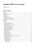
Raw Data Analysis
Once the raw data files are uploaded, the Raw Data Main Analysis window appears. Double-click the samples in
the Sample Tree to open the individual Raw Data Traces. The Synthetic Gel Image displays the unprocessed data in
a traditional gel format with larger fragments located on the right. The Electropherograms display fluorescent
signal intensities as a single line trace for each dye color. The signal intensities, recorded in Relative Fluorescent
Units (RFUs), are plotted along a frame scale in the Raw Data Analysis window with fragment mobility from right
to left. The largest size fragments are on the far right of the trace.
13
August 2015
Chapter 2 General Procedure
Raw Data Analysis Window
Sample Tree
Synthetic Gel Image
Raw Trace Data
Project
Summary
Main Toolbar Icons
Spike Removal: Removes peaks from voltage spikes caused by micro-air bubbles or debris in the laser
path. This option is selected by default in the Run Wizard.
Saturation Correction: A synthetic peak is created based on peak shape before and after saturation. The
results of these will be less accurate than that of non-saturated peaks. This option is selected by default
in the Run Wizard.
Smooth: This function smoothes the baseline by eliminating smaller noise peaks. This option is selected
by default in the Run Wizard.
Baseline Subtraction: Selecting this option will remove the baseline completely so that the Y-axis will be
raised above the noise level. This option is selected by default in the Run Wizard.
Auto Pull-up Removal: Automatically removes peaks caused by wavelength bleed-through to other
wavelengths. This option is selected by default in the Run Wizard.
Manual Pull-up Correction: This allows the user to manually adjust larger pull-up peaks in case the
Auto Pull-up Removal function has not corrected the problem. It is recommend to de-select Pull-up
Correction in the Run Wizard when using this function.
2nd Derivative Trace: This feature reduces high background noise and sharpens peaks. Baseline
fluctuation caused from dye blobs or the DNA template in PCR can also be reduced with this function.
It is recommended to de-select Spike Removal in the Run Wizard when this function has been activated.
Note: Raw data icons are applied to the raw data. These icons are recommended for research applications; user
management can exclude access rights for analysts.
14
August 2015
Chapter 2 General Procedure
What to Expect
The raw data correction icons can be selected individually in the Raw Data Analysis window. The images below
demonstrate how the data will look before (left image) and after (right image) the parameter is applied.
Range
AutoRange - Analyzes from 0 to end of trace for size call
Manual Range – user-defined range
Right-click in gel image and select Get Start Point
Smooth
Fourier frequency transformation (FFT) to determine frequency domain
Use only top 40% of lowest frequencies
Smoothing broadens peaks and therefore you can lose resolution
Enhanced Smooth - Same as Smooth but use only top 20% of lowest frequencies
Baseline Subtraction
Use 20% of lowest intensities (to the right of the beginning of the range)
Looks at trace in 500-600 frame sections
Pullup Correction
Ax=B
A being the major coefficient
Input matrix or use single dye adjustment up to 0.20 for small corrections
When Manual Pullup correction is chosen, a .txt or .mtx matrix file can be uploaded and used to deconvolute
dye colors.
15
August 2015
Chapter 2 General Procedure
NOTE: De-select automatic Pullup Correction in the Run Wizard Data Process box if a manual matrix correction
has been applied.
Saturated Peak Correction
ABI instrument saturated peaks are typically >8000 RFU
The top of a saturated peak looks split
A small pullup peak may be present under the saturated peak
GeneMarker HID takes the small pullup peak and adds it to the split in the saturated peak
Spike Removal
Caused by overheating of camera chip, voltage spike, etc
Spikes usually only 1-2 frames wide; peaks usually 5-10 frames wide
Create a first derivative trace of the raw data
Spikes are the 1st DT outliers (3-5 sigma)
16
August 2015
Chapter 2 General Procedure
Second Derivative Trace
(A1-A2)-(A2-A3) = A1+A3-2(A2)
Use when you have a fat base to your peaks (ex. Dye blob under peak, etc)
NOTE: Do not use 2nd DT with Spike Removal because real peaks look like spikes.
Process Data
After the raw data files have been uploaded to GeneMarker HID, they are ready to be processed. The processing
step includes application of a sizing standard, filtering of noisy peaks, and comparison to a known allelic Panel.
GeneMarker HID combines all these steps in one simple tool called the Run Wizard. To access the Run Wizard
simply click the Run Project icon in the main toolbar.
Run Wizard Template Selection
Procedure
1.
2.
3.
4.
Click the Run Project icon in the toolbar.
The Run Wizard Template Selection dialog box will
appear.
Select a template (a previously saved set of size standard,
standard color, and analysis type named for future use),
OR select a new combination of size standard, standard
color, and analysis type.
Click Next when finished.
Icons and Functions
Template Name
Select from existing pre-made templates or create your own by entering a Template Name and clicking the Save
button. When the settings for all sections of the template have been completed (Template Selection, Data Process
and Additional Settings) use the Back button to return to the Template selection screen and then select Save.
Note: only individuals with access rights to change analysis parameters may save Run Wizard Templates.
To create a new template, click Select an existing template or create one. A template can also be selected from the
list of available templates in the left section of the window and then saved for future use by clicking the Save
button.
If you do not want to use a template, select the appropriate size standard, standard color, and type of analysis;
Use last template will automatically be selected.
Panel
GeneMarker HID comes preloaded with many common kit Panels including Promega’s PowerPlex kits and
ABI’s Identifiler kit. Additional Panels can be imported by selecting the Open Files icon next to the Panel field. A
custom Panel can be created in the Panel Editor tool. See Chapter 5 Panel Editor.
17
August 2015
Chapter 2 General Procedure
Panel Editor: A Panel can be selected from any available from the drop-down menu or can be viewed
and selected by clicking the Panel Editor icon.
Import a Panel: If a Panel cannot be found in the Panel Editor tool, it can be imported by clicking on the
Import a Panel icon.
Size Standard
GeneMarker HID comes preloaded with many common size standards including GeneScan 500. GS600, ILS 500,
ILS600. A custom Size Standard can be created by selecting the Size Template Editor icon next to the Size Standard
field. GS500_1 is a commonly used size standard .xml file; the two smallest fragment, the 250 bp fragment and
the two largest fragments are disabled - See Chapter 4 Fragment Sizing Standards.
Size Template Editor: This allows the user to check sample files against a selected size standard,
modify and save the size standard for future use, or create a new size standard.
Standard Color
Select the dye color which contains the internal lane standard.
Analysis Type
The Analysis Type option is inactivated in GeneMarker HID.
Run Wizard Data Process
Procedure
5.
6.
The Data Process window of Run Wizard appears.
Select the appropriate analysis settings in the Data Process
window and click Next to continue.
Icons and Functions
Raw Data Analysis
Auto Range (frame)
The range in camera frames will automatically find the processable data range. If
Auto Range is not selected, manually enter the start and end frame numbers of the
data set for analysis.
NOTE: If automatic size call fails due to high saturation in the primer front, de-select
Auto Range and manually input the required data range.
Intensity Coefficients: This is a research application that should be excluded
from user access rights for all but lab manager and administrators. It allows
for manual correction of excessive bleed-through peaks; best used for
experiments with one-color analysis. Allows for manual correction of low RFU by using an number greater
than 1 to increase the RFU
Smooth
Smoothes the baseline by eliminating smaller noise peaks.
Enhanced Smooth
This feature is used only in cases where the data is extremely difficult to analyze and cannot be
corrected with the Smooth function.
Peak Saturation
The software will analyze saturated data points by creating a synthetic estimate of the peak shape
based on the curves prior to saturation. The results will be less accurate than that of nonsaturated peaks.
18
August 2015
Chapter 2 General Procedure
Baseline Subtraction
This function removes the baseline completely so that the Y-axis will be raised above the noise
level. It uses 20% of lowest intensities (to the right of the beginning of the range) and looks at the
trace in 500-600 frame sections
Enhanced Baseline Subtraction
This feature is used only in cases where the data has excessive baseline in one or more of the
dyes, or has an interfering slope from the ion front in the smaller marker ranges. The function
uses the second derivative of the absolute value for every 30 data points and looks at the trace in
300 frame sections
In situations where there is an extended ion front in the mini-STR range Enhanced Baseline Subtraction
should be used.
Pull-up Correction
This function removes peaks caused by wavelength bleed-through to other wavelengths. The function
should be disabled if a Manual Pull-up Correction was used in the Raw Data Analysis window.
Spike Removal
Removes peaks from voltage spikes caused by micro-air bubbles or debris in the laser path. Spikes are
typically less than a base-pair wide. Do not select Spike Removal when 2nd Derivative Trace has been applied.
Size Call
GeneMarker HID offers two sizing methods:
Local Southern
Used in most genotyping software applications and is recommended for most analyses. This method is
based on the idea that smaller size fragments run faster. Plot a size v. time graph and overlay a size v.
1/time graph to determine linear trace. (Southern, E.M. “Measurement of DNA Length by Gel
Electrophoresis.” 1979. Analytical Biochemistry. 100, 319-323).
Cubic Spline Method
Cubic Spline is offered as an alternative method that may be more appropriate for some data. This method
uses a cubic equation to connect known points on the size v. time graph. An example of a cubic equation:
ax3+bx2+cx+d. (The Astrophysical Journal. December 1, 1994. 436, pages 787-794.)
19
August 2015
Chapter 2 General Procedure
Local Southern Method
Cubic Spline Method
Allele Call
The Allele Call section allows the user to set allele calling range, detection thresholds and filters.
Auto Range
The software will identify peaks in the processable data range for each lane.
Manual Range
To select a specific analysis region, de-select Auto Range and input the desired base pair range. Peaks outside the
Manual Range will not be called.
Peak Detection Threshold
NOTE: The Peak Detection Threshold parameters are only applied to peaks outside of the Panel Markers. To
adjust settings for peaks within Panel Marker ranges, see Chapter 5 Panel Editor.
Min Intensity
Minimum RFU threshold of peak height used for peak detection. Peaks below this value will not be called.
Max Intensity
Maximum RFU threshold of peak height. Peaks above this value will be flagged with a yellow Allele Label,
given a Quality Rank of Check, and marked with HI Quality Reasoning.
Percentage Global Max
Relative minimum intensity of allele peaks to the 5th highest peak in the dye color used for peak detection.
Peaks below this value will not be called.
Save Icon will save any changes to the analysis template (Run Wizard Settings)
Run Wizard Additional Settings
Procedure
7.
8.
The Run Wizard Additional Settings box appears
Select an Allelic Ladder and adjust the Peak Score
parameters or check Auto Select Best ladder and Auto
Panel Adjust.
9. Click OK
10. The Data Processing box appears
11. The data is sized, peaks are filtered, and the Panel is
applied
12. Click OK when the Data Processing box is finished.
Functions
Allelic Ladder
Permits the selection of a sample containing an allelic ladder. If the user selects one ladder, the ladder will be in
bold font and is set to the top electropherogram in the Main Analysis window. All samples will be analyzed using
this selected ladder.
20
August 2015
Chapter 2 General Procedure
Allele Evaluation
Peak Score
User-definable confidence level of the allele call. Peak score is an algorithm that takes into account signalto-noise ratio and peak morphology. Rejected samples appear in red, samples that need to be checked
appear in yellow, and samples that have passed appear in green.
Auto Select Best Ladder
GeneMarker HID identifies ladder samples in the dataset as defined in the View → Preference → Forensic →
Ladder Identifier field. Ladder samples are then compared to the chosen Panel. Each ladder that is within the
range of the selected panel will pass and appears in bold font in the Sample File Tree.. Auto Select Best Ladder
will analyze each sample file with the passing ladder that best matches that sample. The print report provides
the file name of reference ladder used for each sample.
Auto Panel Adjustment
When selected, the Markers and Bins of the chosen Panel will be aligned with the peak positions of the Ladder
samples in the dataset (within a five basepair shift). Ladder samples are identified by GeneMarker HID as
defined in the View → Preference → Forensic → Ladder Identifier field. Major alleles and variant (or virtual) alleles
are specified in the Control Column in the Panel editor. See Chapter 5 Panel Editor. This information is used for
pattern recognition and automatic panel adjustment.
NOTE: Panels that do not contain variant (virtual) alleles can be manually adjusted in the Panel Editor by first clicking
the Major Adjustment of Panel icon then the Minor Adjustment of Panel icon.
NOTE: Panel must be saved with signal information
For optimum Auto panel adjustment. See Chapter 5 .
Adjust Analysis Parameters
After the clicking OK in the Run Wizard Additional Settings box, the Data Processing
box appears. The raw data is being processed and sized, then the filtering parameters
are applied, and finally a Panel is applied (if selected). Click OK in the Data
Processing box when analysis is complete.
Review the results in the Main Analysis window. See Chapter 3 Main Analysis
Overview. If you notice many false positive peak calls, you may need to adjust the
analysis parameters. There are three options for adjusting the analysis parameters as
discussed below.
NOTE: Manual edits will be lost when data is re-analyzed.
Re-analyze with Run Wizard
To re-analyze with the Run Wizard tool, simply click the Run Project icon in
the main toolbar. The Run Wizard will launch and the most recently selected
parameters will be displayed. Adjust parameters as necessary and click OK in
the Run Wizard Additional Settings box. The Use Old Calibration box will appear
with the option to Call Size Again. Only select Call Size Again if the Run
Wizard Template Selection Size Standard selection was changed or any of the Run
Wizard Data Process Raw Data Analysis parameters were changed. Click the
Apply to All button. The Data Processing box will appear again and the data
will be re-analyzed with the new parameters.
Re-analyze with Auto Run
To re-analyze with Auto Run, first select Project → Options. The Project Options Settings box will appear. This box offers
all the same parameters settings as are available in the Run Wizard. Use the tabs to view the Template Selection, Data
Process, and Additional Settings boxes. Click OK when finished. Next, select Project → Auto Run. The data will be reanalyzed with the new parameters.
NOTE: The Additional Settings Allele Evaluation Peak Score parameters can be changed in the Project Options Settings box
and will be applied to the data without having to re-analyze the data with Run Wizard or Auto Run.
21
August 2015
Chapter 2 General Procedure
Re-analyze Individual Samples
To re-analyze an individual sample, dye color, or marker, click the Call
Allele icon in the main toolbar. The arrow next to the icon opens the dropdown menu with additional options. Click an option from the drop-down
and the Recall Allele box will appear. Adjust parameters as necessary and
click OK. The new parameters will be applied.
All Samples
Applies the new parameter settings to all samples in the dataset – similar to
Run Wizard and Auto Run.
Open Samples
Applies the new parameter settings only to samples that are checked in the
Sample File Tree.
Current Sample
Applies the new parameter settings only to the sample highlighted in the Sample File Tree.
Call the Dye
Applies the new parameter settings to the dye selected in the Recall Allele → Call Allele by Dye field.
Call the Marker
Applies the new parameter settings to the marker selected in the Recall Allele → Call Allele by Marker field.
22
August 2015
Chapter 3 Main Analysis Overview
Chapter 3 Main Analysis Overview
Chapter 3 Main Analysis Overview
Main Analysis Window
Menu Options
Main Toolbar Icons
Additional Analysis Options
23
August 2015
Chapter 3 Main Analysis Overview
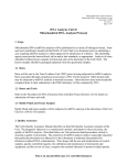
Main Analysis Window
The main window of GeneMarker HID has an easy to use layout. The sample files are displayed on the left, the
Synthetic Gel Image is displayed at the top, Electropherograms appear below the gel image, and the Report Table is
on the right side of the window.
To resize the frames in the Main Analysis window, simply place the cursor over the partitions that separate the
Synthetic Gel Image/Electropherogram/Sample File Tree/Report Table. The cursor will change to a two-headed arrow
bisected by two vertical lines. Hold down the left mouse button and drag the gray vertical line in the direction
you wish. To open and close the frames, use the Show/Hide icons in the main toolbar.
Main Analysis Window
Sample File Tree
Report Table
Synthetic Gel Image
Electropherogram
Project
Summary
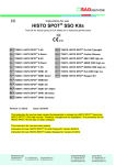
Sample File Tree
The Sample File Tree of the main analysis window contains two folders. The
first is the Raw Data folder which, when expanded, displays a list of all the
dataset samples. When a sample is double-clicked its preprocessed
electropherogram trace will appear in the Raw Data Analysis window. See
Chapter 2 General Procedure.
The second folder, Allele Call, also contains a list of all the samples, but
when the filename is double-clicked the sample’s electropherogram trace
appears in the Main Analysis window with all sizing information and allele
call filtering applied. The Allele Call folder also flags each sample with a
green sheet, yellow sheet or red strike-through indicating size calling
success. See Chapter 4 Fragment Sizing Standards. A red question mark
indicates one or more of the analysis parameters were not met for that sample (rules were fired). Detailed
flagging is found in the allele label and the peak table below the electropherogram in the quality reasons column.
24
August 2015
Chapter 3 Main Analysis Overview
Red question mark flagging is also assigned to samples with null marker(s) and samples with AMEL and Y-STR
marker conflict(s) when amplified with a multiplex that contains AMEL and Y-STRs in addition to autosomal
markers.
Right-click the sample filename in the Raw Data or Allele Call folder to see additional options.
Sorting Options
Select Page
Opens electropherogram traces for the number of samples specified in the View → Preference → Display Settings
→ Max Chart # In Page field. Hot Key = Page Up/Page Down
Select Next Group
In descending order, selects the same number of samples previously selected by Select Page, grouping options
(see Sample Grouping section below) or double-click option.
Select Max
Opens electropherogram traces for the number of samples specified in the
View → Preference → Display Settings → Max # Open Charts.
Deselect All
Unselects all selected samples in the Sample File Tree list and closes the
electropherogram traces.
Sort Samples
Opens the Sort Sample Options box. Select First, Second, and Third Order
sorting from the drop-down menu options Sample Type, File Name, Lane
Number, Well ID, and Size Score. Hot Key = F3
Search Options
Search File
Opens the File Search box. Enter any part of a filename to search for the sample in the list. Click the Search
button. Left-click and use CTRL or SHIFT key to highlight samples then click the Open Selected button. The
electropherograms of the selected samples will open in the Main Analysis window. Hot Key = CTRL+F
Sample Information
Sample Info
Opens the Sample Information box. A list of Properties appears and includes
information like; Sample Name, Well ID, Lane Number, Instrument Name,
and Chemistry. The list of Properties varies depending on the file type. Hot
Key = F2
Edit Comments
Opens the Edit Comments box. Enter information in the Comments field. The
last ten comments will be stored and can be subsequently selected for future
samples. The Sample Comments will appear on the Print Report. See Chapter
6 Reports and Printing. Hot Key = F4
Disable Samples
Disable Sample
Opens the Input Disable Reason box and marks the sample with a red strikethrough. A disabled sample cannot be selected for display in the Main
Analysis window and will not appear in the Report Table if View → Preference
→ Options → Show Disabled Samples in Report is deselected. Select a Comment
Template or enter a new comment in the Comments field and click OK to
disable the sample. Hot Key = CTRL+DEL
Add Samples
From the main toolbar, select Project → Add Samples to Project. The Open Data
Files box will appear. Click the Add button to select additional samples to
add to the project and click OK. The added samples will be sized and the
25
August 2015
Chapter 3 Main Analysis Overview
allele calls will be filtered according to the parameters set in the Run Wizard.
Sample Grouping
From the main toolbar, select Project → Apply Sample Grouping. The File Name Group Editor tool will appear (See
Chapter 8 Additional Tools). Select Group and Control identifiers and click Match. Click OK to apply the
matched groups. Group numbers will appear next to the filenames in the Sample File Tree. Use the Select Next
Group right-click menu option OR CTRL+PageUp/Down to open samples in a group. To disable the Sample
Grouping feature, go to View → Preference → Others and uncheck Enable Sample Grouping.
Synthetic Gel Image and Electropherogram with Peak Table
The Synthetic Gel Image and Electropherogram displays are associated in the Main Analysis window. Both display
the fragment information in a visual form. When GeneMarker HID is initially launched, all dye colors are
displayed in the Synthetic Gel Image and Electropherogram at once. Single left-click the Show Color icon in the
main toolbar to cycle through the dye colors or use the Show Color drop-down menu to disable individual
colors or Show/Hide All colors.
Navigation
Zoom In/Out
In the Synthetic Gel Image or the Electropherogram, hold down
the left mouse button and drag a box from upper left to
lower right around the area you would like to zoom in on.
To zoom back out, hold down the left mouse button and
drag a box in the opposite direction from lower right to
upper left. The user may also use the Zoom icons in the
main toolbar to zoom in and out. The main analysis
window also allows the user to manually set the x and y
axis with the Set Axis icon.
Horizontal Movement
The Synthetic Gel Image and the Electropherogram are
synchronized to allow the user to view both images at once.
To move the images in the horizontal direction, use the top
slider bar (below the toolbar) to scroll the image in either
direction, or hold down the right mouse button and drag
the trace right or left.
Marker/Locus Specific Viewing
To scroll through individual markers/loci, select a marker from the Marker drop-down list in the main toolbar.
To view subsequent markers, use the Up/Down Arrow keys.
Synthetic Gel Image Features
The Synthetic Gel Image displays all samples in the dataset vertically. The direction of fragment mobility is
horizontal with the small size fragments on the left and the larger fragments on the right so that the gel aligns
with the electropherogram trace display. Move the mouse pointer over the Synthetic Gel Image to reveal the
sample lane filename.
Image Utilities
Click the Image Utilities icon in the upper left corner of the Synthetic Gel Image. A fly-out menu appears
with the following options:
Copy to Clipboard
Copies the Synthetic Gel Image to the Windows clipboard for pasting into other applications such as
Microsoft PowerPoint.
Save Image
Allows the user to save the Synthetic Gel Image as a BMP image file.
26
August 2015
Chapter 3 Main Analysis Overview
Show in Window
Opens a separate window containing the Synthetic Gel Image. The separate window can be maximized for
closer gel image inspection.
Image Display
Intensity
Move the Intensity slide bar, located in the upper left corner of
the Synthetic Gel Image, up and down to adjust the intensity of the
fragments displayed.
Grey-Scale
Go to View → Preference → Display Settings → Gel Image. Select
Gray for Single Dye to change the single dye Synthetic Gel Image
to black and white when only a single dye color is selected (when
multiple dye colors are selected the fragments will appear in their
respective colors). Click the Background in White option to
reverse the black and white exposure for single dye color gel
images.
Electropherogram and Peak Table Features
The Electropherogram displays fluorescent signal intensities from capillary electrophoresis instruments as a single
line trace for each dye color. The signal intensities are recorded in Relative Fluorescent Units (RFUs) which are
plotted along the y-axis. Along the x-axis are the basepair sizes of the fragments. The frame units plotted along
the x-axis in the original Raw Data Analysis window are converted to basepair size units as defined by the Size
Standard selected and the Internal Lane Standard (ILS) of the individual samples. Fragment mobility is from
right to left with the smallest size fragments on the far left of the trace.
The Peak Table contains information about the called peaks currently displayed in the Electropherogram.
Electropherogram Trace Display
Range
The basepair size range (x-axis) is as set in the Run Wizard Data Process Allele Call options box. The RFU
range (y-axis) is variable and will re-adjust according to the maximum peak height in the trace. To
manually set x and y-axis ranges, use the Set Axis icon in the main toolbar.
Cursor Locator
The x and y-axis position of the mouse pointer in the electropherogram is displayed in the upper right
corner of the electropherogram.
Allele Call
If a Panel is applied to the data, then grey horizontal bar Markers will appear above the electropherogram
indicating locus ranges. Bin ranges appear as dye-colored brackets above and below the sample trace. Allele
Labels appear below the electropherogram and are associated with the center of each called peak which is
also marked by a light grey vertical line in the electropherogram. If a Panel is not applied, then Allele Labels
for called peaks will only indicate the basepair size of the peak.
27
August 2015
Chapter 3 Main Analysis Overview
The red horizontal line (seen here in the figure on the right) is to alert analysts to trends in the data. These
areas of the data have a more elevated baseline or noise-to-signal ratio (often associated with poorly
resolved peaks) than the nearby regions of the trace which sometimes masks very minor peaks.
Peak Table
The Peak Table can be displayed below the Electropherogram by clicking the Show Chart/Table icon in the
main toolbar. Right-click in the Peak Table and select Show Columns. The Show Columns fly-out appears
with column options.
Dye
Indicates the dye color of the peak.
Size
Indicates the basepair size of the peak (x-axis).
Height
Indicates the peak height in RFUs (y-axis).
Height Ratio
The value obtained when the peak’s height is divided by
the height of the highest peak in the dye color or Marker.
Area
Indicates the area under the curve of the peak. The area
calculation begins and ends along the x-axis as indicated
by the Start and End columns of the Peak Table
respectively.
Area Ratio
The value obtained when the peak’s area is divided by the
area of the highest peak in the dye color or Marker.
Marker (Panel Only)
Indicates which Marker (Locus) the peak is contained in.
Allele (Panel Only)
Indicates which Bin the peak is contained in.
Difference (Panel Only)
Indicates the absolute value in basepairs of how far the peak center is from the Bin center.
Quality (Panel Only)
Assigns a Pass/Check/Undetermined quality ranking for each peak with regard to the peak Score as set in the
Run Wizard Additional Settings box (See Chapter 2 General Procedure) and/or software editing of the
original raw data, such as correction of saturated peaks (SAT Repaired).
Score
The peak quality score is calculated based on signal-to-noise ratio and peak shape or morphology. Lower
scores indicate poorer quality peaks. Additionally, the Score value is a based on an exponential curve.
Start/End
Indicate the beginning and end of the Area calculation for the peak.
Allele Comments
Software and user edited comments appear in the Comments column.
Sample Comments
Added by the user with a right mouse click on the sample name in the sample list at left; select Edit
Comments to add new comment or select a comment from the list
28
August 2015
Chapter 3 Main Analysis Overview
Quality Reasons
Indicates the reason why a peak received a Quality rank of Check or Undetermined. For explanation of the
two and three letter codes see below OR click the Help icon above the Report Table.
LS = Low Score
Quality Score is based on Signal-to-Noise
Ratio and Peak Morphology and the Pass,
Check, Reject ranges are set in the Run
Wizard Additional Settings box.
OL = Off Ladder
Peak is outside of the marker range.
OB = Out of Bin
Peak is within the marker range but
outside of a bin.
BC = Bin Conflict
More than one called peak present within
a bin.
SR = Saturated (Repaired)
Intense peaks with characteristic
morphology are identified and “repaired”
for allele calling.
number of peaks expected as set in the
Panel Editor Edit Panel box.
LO = Low Intensity
Single peak called below the Minimum
Homozygote Intensity threshold because a
second peak was detected above N-x
percentage value as set in the Panel Editor
Edit Marker box
HI = High Intensity
Peak intensity approaches and/or exceeds
the maximum peak intensity filter as set in
the Run Wizard Data Process box.
IMB = Heterozygote Imbalance
Peak intensity does not exceed the
minimum percentage of the major peak
within the marker as set in the Panel Editor
Edit Marker box.
SP = Saturated (Pull- up)
Intense peaks may cause “pull-up” or
additional peaks to appear in other dye
colors.
IHE = Inconclusive Heterozygous
Peak intensity is within the heterozygous
inconclusive range set for this locus in the
Panel Editor Edit Panel box.
PL = Beyond Ploidy
When the number of peaks identified
within a marker exceeds the maximum
IHO = Inconclusive Homozygous
Peak intensity is within the homozygous
inconclusive range set for this locus in the
Panel Editor Edit Panel box.
Save Peak Table
Click the Save Peak Table icon in the main toolbar to export the Peak Table information currently being
displayed in Excel (.xls) or tab-delimited Text (.txt) format. All samples peak information for only the dye
colors selected will be exported in the table. Additionally, the user can right-click in the Peak Table and select
Copy Table (Hot Key = CTRL+C) to place the current table information onto the Windows clipboard. The
information can then be pasted into most common spreadsheet or word processing programs including
Microsoft Excel.
Editing Peaks
Double-click the vertical grey peak center bar to select a peak. Right-click anywhere in the Electropherogram
or Peak Table to see additional menu options.
Insert Allele
Right-click at the place in the electropherogram where you would like to add
an allele and select Insert Allele. The basepair size or bin name will be applied
in the Allele Label and the peak specifications will be calculated and displayed
in the Peak Table.
Delete/Undelete Allele
Right-click at the vertical grey bar indicating the center of the called peak or the
peak cell in the Peak Table and select Delete (Hot Key = DEL). To call the allele
again, right-click the peak and select Undelete (Hot Key = SHIFT+DEL).
29
August 2015
Chapter 3 Main Analysis Overview
Confirm/Unconfirm Allele
If a peak is given a low quality score, it will receive a Check (yellow) or Undetermined (red) Quality ranking.
To give the peak a Pass (green) Quality ranking, right-click the peak center bar and select Confirm (Hot Key
= CTRL+M). The peak will be marked Pass (green) and receive a “Confirmed” comment in the Peak Table.
To un-confirm the allele, select Unconfirm from the right-click menu (Hot Key = CTRL+ALT+M).
Confirm/Unconfirm All
Confirm All and Unconfirm All options perform the same actions as the Confirm/Unconfirm allele except that
the Quality ranking for all peaks in that dye color for that sample will be affected.
Edit Allele
Right-click an allele in the Electropherogram or Peak Table and select Edit Allele. The Edit Allele box appears.
Add or change the values in the Allele and/or Size field. The Allele field will be blank if no Panel has been
applied to the dataset. Check Confirm the Allele to automatically give the peak a Quality rank of Pass (green).
Allele Comments
Right-click an allele in the Electropherogram or Peak Table and select Edit
Comments. The Edit Allele Comments box appears. Select a comment from the
Comments Template list or enter a new comment in the Comments field. Click OK
and the comment will appear in the Comments column of the Peak Table. Only
one user edited comment can be added to a peak. Comments automatically
generated by the software cannot be removed. Additional user comments will
simply be added next to the software comment.
View History
Opens the Show Edit History window. Shows a record of all manual edits performed on the peak. The Show
Edit History window is only active when the Help → User Management → Settings → Record Data Edit History
option is selected. Print preview and print or save as jpeg, png or pdf for paperless record of audit trail. See
Chapter 9 User Management.
Report Table
The Main Analysis window Report Table contains additional information about sample peaks. See Chapter 6
Reports and Printing.
Navigation
The Report Table is linked to the other frames in the Main Analysis window. Double-click on the desired allele OR
use the Arrow keys to move to the cell of interest and hit Enter key OR use Alt + Arrow keys to move to
different cells and zoom in on the peak in the Electropherogram.
Select multiple cells by holding down SHIFT key OR hold left mouse
button and drag over desired cells.
The rules by which the Report Table and other frames in the Main
Analysis window are linked are controlled by options in the View →
Preferences → Others tab.
Display Settings
Click the Report Settings icon in the Report Table toolbar. The Allele
Report Settings box will appear. Select different Report Styles to see
additional options. Additionally, select View → Preferences → Others →
Show Disabled Samples in Report to include samples that are disabled in
the Sample File Tree.
Sort Options
Sort by Marker
Select Sort by Marker from the right-click menu and choose from the fly-out menu to sort Ascending or Descending.
If Ascending is chosen, then low quality peaks will be sorted to the top of the table. If Descending is chosen, then
the lower quality peaks will be placed at the bottom of the table. This option is only available with Marker Table
and Allele Count Report Styles.
30
August 2015
Chapter 3 Main Analysis Overview
Sort by Column
Select Sort by Column from the right-click menu and choose from the fly-out menu to sort Ascending or
Descending. If Ascending is chosen, then lesser values will be sorted to the top of the table and greater values to
the bottom the table and vice versa if Descending is chosen. This option is available with all Report Styles.
Editing Peaks
To edit peaks, first left single or double-click the cell in the Report Table then right-click to see menu options or
use Hot Keys.
Delete Peaks
Right-click the peak cell in the Report Table and select Delete Peaks (Hot Key = DEL). The deleted peak will be
removed from the Report Table.
Confirm Peaks
If a peak is given a low quality score, it will receive a Check (yellow) or Undetermined (red) Quality ranking. To
give the peak a Pass (green) Quality ranking, right-click the peak cell and select Confirm Peaks (Hot Key =
CTRL+M). The peak will be marked Pass (green).
Peak Information
Hold down CTRL key and click the peak cell of interest. The Allele Peak Info box will appear containing
information such as Sample, Dye, Size, Marker, Allele, Score and Comments. The information in these fields
cannot be edited. This option is only available with Allele List, Marker Table, and Peak Table Report Styles.
Save Report Table
To save all information currently displayed in the Report Table, click the Save Report icon in the Report Table
toolbar. Choose a directory, enter a filename (ProjectName_AlleleReport is the default) and save as an Excel (.xls)
or tab-delimited Text (.txt) file.
To export only selected cells in the report table, first select the cells by left-mouse drag across the cell range or
hold SHIFT key and select cells. Right-click on the highlighted cells and select Copy (Hot Key = CTRL+C). The
information is saved to the Windows clipboard and can be pasted into any common word processor or
spreadsheet program like Microsoft Excel. The row and column headers for those cells will be copied with the
highlighted cell information.
Menu Options
The following menu options can be found in the menu bar of the Main Analysis window.
File Menu
The File menu contains functions for opening and saving raw and processed data.
Open Data
Launches the Open Data Files window where the user can select raw data files for
upload into GeneMarker HID. Accepted file formats include .fsa, .ab1, .abi, .scf, .rsd,
.esd, .smd, .smr. See Chapter 2 General Procedure.
Open Project
Opens a folder search window where the user can select to open previously saved
SoftGenetics GeneMarker HID project files (.sgf, .sfp)
Re-Open Project
Saves the last four projects that were opened by GeneMarker HID and allows the user to launch any one of those
four projects directly.
Save Project
Saves a SoftGenetics GeneMarker HID project (.sgf, .sfp) to a specified directory. Raw data files and analyzed
data files with edits are saved within a project file. Pull-down peaks may result from changes in optical
alignment or polymer of the genetic analyzer. These data are now included in the traces of saved GeneMarker
HID Projects (.SGF files).
31
August 2015
Chapter 3 Main Analysis Overview
Close All
Closes a project without exiting the program.
NOTE: It is recommended to select Close All before exiting the program.
Exit
Closes the GeneMarker HID program.
View Menu
The View menu contains options for how the data is displayed in the Main
Analysis window.
Show Navigator/ Gel Image/ Report
Toggles the Sample File Tree, Synthetic Gel Image, or Report Table frames open and
closed in the Main Analysis window.
Preference…
Activates the three-tab Preferences box.
Start up Settings
The Start up Settings tab, effective only at start up, allows you to select the Run Method and General Settings.
Run Method
Classic: Appropriate for experienced users. The user will move
through the program data input, settings, and display options
without prompting, by simply following the program’s sequential
analysis flow.
Wizard: Activates the Run Wizard which will guide the user through
the program’s operation. This setting is best for the inexperienced
user.
General Settings
Show Navigator: When selected, the Sample File Tree will automatically
be displayed in the Main Analysis window after data processing.
Show Gel Image: When selected, the Synthetic Gel Image will
automatically be displayed in the Main Analysis window after data
processing. (this is turned off by default and may be displayed automatically by checking the box).
Show Report: When selected, the Report Table will automatically be displayed in the Main Analysis window
after data processing.
Import Directories: to set a default folder for import of raw data and project files. This option decreases the
amount of navigation needed when folder locations are designated for import of data and projects
Display Settings
The Display Settings tab is used to set how the data is displayed in the electropherograms.
Allele Label
Decimal Precision: Select 0 to 2 decimal places for peak size labeling.
Mark Off-Allele as ‘OL’: Select this option to label alleles that are
outside of allele ranges as ‘OL’.
Mark Off-Bin as ‘OB’: Peaks within a marker range, but outside of a bin
will be labeled ‘OB’.
Use Size String for Label: Select this option to label peaks in the
electropherograms according to size instead of the allele label. To
display a rounded size string, set the Decimal Precision to 0.
Larger Font: Doubles the font size of the allele label characters. This
increased font size will carry over to the Print Report.
Flag Variant Alleles in Ladder: Select this option to flag peaks detected
in variant allele bins of allelic ladders.
Show All Allele Labels: Will display all allele labels when all dyes are
displayed in the electropherogram (default is to display allele labels of
32
August 2015
Chapter 3 Main Analysis Overview
dye 1 only when all dyes are overlaid in the electropherogram).
Set Missed Allele as Single Line in Ladder: Allele labels for missed ladder peaks will be placed one row above
allele labels of peaks that were called.
Alternative Label [ ] for IHO/IHE peaks: A special options for peaks flagged with IHE or IHO. The allele label
will appear at the top of the peak, with the user specified flag on a yellow background.
Chart Settings
Max # of Open Charts: Select the maximum number of samples you would like to display as an
electropherogram at one time (Max = 96). Use the Sample File Tree right-click option Select Max to open the
number of samples specified.
Max Chart # in Page: Select the maximum number of sample electropherograms you would like displayed in
the Main Analysis window at one time (Max = 8). Use the Sample File Tree PageUp/Down option to select
subsequent groups of samples.
Max Allele Label Layers: Select the number of allele label layers to view at once (Max = 10). This determines
how far you must zoom in to clearly read neighboring allele labels and affects how the print report will be
displayed.
Show Loci with multiline: Select this option to display the names of all markers above the electropherogram
when two or more dyes are displayed.
Show Saturation Alert Line: Displays a red, horizontal line under the X axis in regions where saturation
and/or elevated baseline were detected in the raw data
NOT Scale Y Axis for Negative Control: Zooming in and out will not affect Y-axis scaling for samples marked
as negative controls.
Show Sample Name: Displays the sample name, as read from the data file, above the electropherogram, in
parentheses after the file name.
Peak Label
Choose up to four labels (size, height, area, score) to display as a flag next to individual peaks in the
electropherogram.
Position: Choose to place the peak label at either the top of the peak, to the right side of the peak, or in the
allele label in the Electropherogram. Display of height ratios (selected in the Forensic tab) require the display
at peak top.
Gel Image
Gray for Single Dye: When selected will display and print the gel image with a black background and white
bands. When deselected the gel image will display a black background and colored bands (depending on
dye color chosen to view).
NOTE: When all dye colors are selected, the bands in the gel image will be displayed in color regardless if
this option is selected.
Background in White: Only available when Gray for Single Dye is selected. Will invert the gel image so that the
background will be white and the band fragments will be black.
Sample Tree
Flag Low Quality ILS as ‘SQ’: Samples with low quality Size Standard peaks will be flagged with ‘SQ’. See
Chapter 4 Fragment Sizing Standards.
Consider Gender for Flag ?: Impacts multiplex chemistries that contain Y-STR marker(s). N
Forensic
The Forensic tab allows the user to determine the display of Ladders and
Controls in the Report Table and to establish file labeling conventions for
Ladders and Controls.
Show Ladder Samples in Report: When selected, the samples designated
as Ladders by the Ladder Identifier field will appear in the Report
Table.
Show Control Samples in Report: When selected, the samples
designated as Positive and Negative Controls by the Positive/Negative
Control Identifier fields will appear in the Report Table.
Mark Deleted/Edited Peaks with Symbols: when selected samples that
are deleted are marked with an χ at the top of the peak. Samples that
were edited are marked with an E at the top of the peak.
Label Peak Ratio: Select from displaying peak ratio from height or area
33
August 2015
Chapter 3 Main Analysis Overview
in peak flags when displayed at top of peaks (see Display Settings tab) on the electropherogram
Ladder Identifier: Enter common filename nomenclature for Ladder samples in the dataset (must be in all
capital letters). Upon first analysis, GeneMarker HID will automatically scan the dataset filenames for the
Ladder Identifier values and subsequently label the Ladder samples with an “LD:” and display the sample
filename in blue font in the Sample File Tree. Default is “LADDER”.
NOTE: The Ladder Identifier option affects the operation of the Auto Select Best Ladder and Automatic Panel
Adjustment features in the Run Wizard Additional Settings box. After modifying the Ladder Identifier field,
re-activate Run Wizard and proceed through Data Process. The Auto Select Best Ladder and Automatic Panel
Adjustment features may now be selected.
Positive Control Identifier: Enter common filename nomenclature for Positive Control samples in the dataset
(must be in all capital letters). Upon first analysis, GeneMarker HID will automatically scan the dataset
filenames for the Positive Control Identifier values and subsequently label the Positive Control samples with a
“PC:” and display the sample filename in green font in the Sample File Tree. Default is “-PC-“.
Negative Control: Enter common filename nomenclature for Negative Control samples in the dataset (must
be in all capital letters). Upon first analysis, GeneMarker HID will automatically scan the dataset filenames
for the Negative Control Identifier values and subsequently label the Negative Control samples with an “NC:”
and display the sample filename in red font in the Sample File Tree. Default is “-NC-”.
NOTE: To implement a change in the Identifier fields, right-click any sample in the Sample File Tree and select
Set Sample Type Auto Identify.
Report Settings
The Report Settings tab allows users to select how data is displayed in
the Report Table.
Automatically Re-Sort Report: Check this option if you would like
GeneMarker HID to automatically re-sort the report every time you
modify alleles. Un-check this feature if you want the report to
remain sorted until you choose to re-sort.
Automatically Scroll Charts to Alleles When Selected in Report: You
may choose whether to scroll to alleles in the trace when selecting
the allele in the report. Leave this feature on to have the software
automatically call up alleles in the trace when you double-click on
them in the report.
Show Disabled Samples in Report: GeneMarker HID identifies
samples that failed during electrophoresis or size calling. The
default setting excludes the disabled samples from the report. The
option may be selected to have failed or user-disabled samples to
be identified in the report.
Open Multiple Charts When Browsing Report: Double clicking an entry in the allele report table will open a
new electropherogram for each new sample selected.
Add Prefix to Saved File Name of Ladders and Controls: Automatically adds the prefix Ladders_ to the allelic
ladder file names when saving report, and Controls_ prefix to any samples designated as PC or NC (set in
the Forensic Tab of Preferences)
Show LIMS Report Settings Box: Displays the LIMS report settings box when the LIMS Report option is
selected from the report table. See Chapter 6 Reports and Printing.
Others
The Others tab has additional selections for the project.
Enable Sample Grouping: When Project → Apply Sample
Grouping is implemented, the Enable Sample Grouping option
will be automatically selected. De-select Enable Sample
Grouping to inactivate the Apply Sample Grouping option.
The Apply Sample Grouping information is saved and can be
recalled by selecting Enable Sample Grouping. See Chapter 8
Additional Tools – Filename Group Editor.
Automatically Save Run Wizard Parameters to INI file:
Automatically saves the Run Wizard parameters in an .ini
34
August 2015
Chapter 3 Main Analysis Overview
file when the project is saved. The location is the same location as the saved project and the name
of this file is the name given to the SaveProjectName_RunWizardParameters.ini.
Channels: Opens the Set Channels box and allows the user to choose from ABI, MegaBACE, and
Beckman-Coulter standard dye colors. The user can also manually enter dye color and name.
The default channel color setup is ABI. See Chapter 2 General Procedure.
Folder Settings: By default GeneMarker imports panels, size standards, and templates from specific folders
installed with the program. If the standard installation location is used, these folders can be found in
C:\Program Files (x86)\SoftGenetics\GeneMarker\V2.4.1\. When at the Run Wizard, the selection of
panels, size standards, and templates available from the dropdown menus is directly pulled from these
folders by default.
The Folder Settings tool gives the user the option to change these default locations. In other words,
GeneMarker can be made to automatically import panels, size standards, and/or templates from an
alternative location instead. This is particularly useful for users with a network setup, with files stored at a
shared location. The folder settings tool gives the user two options for changing the default folders
Each: When the “Each” radio button is selected (see figure above) the user may give new paths
individually to the Panel, Size Standard, and Template folders. To use the default location installed
with GeneMarker for a given folder, simply check the “Using Default Folder” box.
Integrated: With this option the user may give the location of a new directory, which contains a template
folder, a size standard folder, and a panel folder. The program uses name recognition to identify each
folder. The Panel folder must contain the word “panel”; the size standard folder must contain the word
“size” and the template folder must contain the word “template”. Again, simply check the “Using
Default Folder” box to use the default (unmodified) setup.
For both options, file paths must be entered exactly and should not include any spaces (unless a file name
has a space in it). Network locations should be preceded by two back slashes ( \\ ).
Project Menu
The Project menu contains options for how the data is processed and printed.
Run
Activates the Run Wizard and begins the data processing setup. This allows the
user to select or adjust program settings in a sequential manner. The same
process action can also be accomplished by clicking the Run icon in the toolbar.
Auto Run
GeneMarker HID will process data using the last set of parameters selected. If
one or more of the parameters require changing to improve analysis, select Project
→ Options, change the desired setting(s), and re-process the samples for analysis.
Add Samples to Project
The user can add samples to a project that has already been sized and analyzed. When selected, the Open Data
Files box will appear. Click Add to select individual files to the project and click OK. The raw data file will be
sized and processed with the same settings as the other files in the project and added to the bottom of the Sample
File Tree.
Print Report
Selecting Print Report launches the Print Report Settings box which allows the user to define display settings in the
Print Report. The software permits printing of the sample electropherograms. You can choose to print all
samples, selected samples, or print samples along with the allele table, if desired. See Chapter 6 Reports and
Printing.
35
August 2015
Chapter 3 Main Analysis Overview
Options
Allows you to access and change parameters in the Project Option Settings window. This three-tab window
contains settings identical to the Run Wizard. Adjust settings in the Project Options Settings box before selecting
Auto Run. See Chapter 2 General Procedure.
NOTE: Auto Run does not need to be selected after adjusting the Additional → Allele Evaluation → Peak Score
settings. The changes will automatically be applied when the Project Option Settings window is closed.
Project Comments
Allows the user to write free-form comments regarding the analysis. These comments are saved with the project
file and can be displayed in the Print Report.
Contamination Check
Select the Contamination Check to compare all samples within a project for:
1. lane – to – lane contamination
2. Contamination from profiles saved to a database (for example, the embedded contamination database
containing staff genotypes)
Please see Chapter 10, Additional Tools, for detailed instructions on using the contamination check.
Applications Menu
The Applications menu contains individual modules for specific data and
analysis types. These modules present advanced features and reporting
options necessary for the particular application.
Pedigree
Display and check genotype calls using a pedigree chart. Data must be run
with the correct size standard and Panel prior to using the Pedigree function.
See Chapter 7 Relationship Testing.
Export CODIS
Developed for forensic scientists analyzing short tandem repeat fragment data. Exports the CMF 3.2 (.xml) and
CMF 1.0 (.dat) files for upload into the FBI’s CODIS database. See Chapter 6 Reports and Printing.
Profile Comparison View
Allows the user to graphically display any combination of samples and dye colors. This feature includes a 2Dimensional and a 3-Dimensional view of the selected samples.
Relationship Testing
Contains tools for familial search, identities duplicate samples and potential near relatives from the relationship
testing database, provides likelihood ratios for each match; kinship analysis (parent/child, sibs, half-sibs,
aunt/uncle, grandparent and cousin) and automated pedigree drawing with deduced genotype of missing
parent based on child(ren) and available parent where possible.
Mixture Analysis
GeneMarker HID identifies the presence of potential mixture samples,
designates allele peaks, and calculates peak area or height ratios in the
main analysis screen. The Mixture Analysis Application is activated from
the Applications menu in the main analysis screen. Mixture analysis
identifies the mixture samples and any single source contributor samples in
a file name tree, considers all possible allele combinations, calculates the
Mixture Ratio, residual score, heterozygous imbalance for each genotype
combination, and calculates the likelihood ratio for single source samples
that are potential contributors to the mixture, searches database for single
source file or a profile deduced from the mixture sample, matches profiles
and calculates the LR.
36
August 2015
Chapter 3 Main Analysis Overview
Cell Line Authentication
This application enables users to do a percent match comparison between samples in their current project, and
sample genotypes saved in a database (i.e. cell lines), making it ideal for cell line authentication.
Tools Menu
The Tools menu contains the Panel and Size Editors in addition to other helpful modules. Chapter 4 contains
details on the Panel Editor and Chapter 5 contians details on the Size Template Editor. Please see Chapter 9 for
details of all additional tools.
Panel Editor
Provides a variety of tools to adjust, edit, and create control Panels. See Chapter 5 Panel Editor.
Size Template Editor
Allows the comparison of sample files against a selected size standard, to modify and save the size standard for
future use, or create a customized size standard. See Chapter 4 Fragment Sizing Standards.
Positive Control Template Editor
This menu enables the user to enter positive control genotypes; making them available in the third screen of the
Run Wizard for automated positive control concordance. See Chapters 2 General Procedure and 9 Additional
Tools.
File Conversion
This tool allows import of time and distance files from custom genetic analyzers for use with files formatted by
the Convert Text to Binary File tool.
Project Comparison
Allows the user to compare the same data set (two different projects) and detect differences based on a number
of parameters including peak size and height, quality score, and commented alleles. See Chapter 8 Additional
Tools.
Pedigree File Name Match
Allows the user to automatically add additional files to a previously created pedigree tree. A .smp file is
exported. See Chapter 8 Relationship Testing.
File Name Group Tool
Used specifically with the MSI and LOH applications, the Filename Group Tool allows users to define how
reference samples and tumor samples should be grouped or paired. A Text (.txt) file is exported. See Chapter 9
Additional Tools.
Convert Text to Binary Files
For customers developing their own instrumentation, the Convert Text to Binary Files option allows users to
upload four or five-color Text files (without headers) for conversion into SCF (four-color data) or SG1 (five-color
data) trace files for analysis with GeneMarker HID. See Chapter 9 Additional Tools.
Replicate Comparison
Many labs choose to run and process multiple replicates of their samples. This ensures that a genotype is still
available in cases of contamination, allele drop out, or reaction failure. Concordance between replicates can then
be used to export the consensus genotype of the sample.
Output Trace Data
Provides the option to output the raw or sized trace data as a TXT or SCF file. Select the samples to include, dye
colors, data type, and the directory to output the trace files. See Chapter 9 Additional Tools.
Export Electropherogram
Allows the user to export the trace images to a specified folder.
37
August 2015
Chapter 3 Main Analysis Overview
Magic Wizard
Contains three option boxes: Start Your Project, Run and Report.
Start Your Project
Allows the user to easily access the Open Data or Open Project
upload windows. The user can also re-open the four previously
opened projects by selecting the black arrow next to Open Project.
Run
Selecting Run launches the Run Wizard. Selecting AutoRun will
process the data automatically with the process options currently selected.
Procedure.
See Chapter 2 General
Report
Allows the user to Save Project or Print Report. Selecting Print Report will launch the Print Report Settings box.
See Chapter 6 Reports and Printing.
Show Last Event
Opens the last active Data Process action.
Help Menu
Help
Launches a searchable version of this manual.
User Management
Allows an administrator to assign access rights to different users. Also used to set up the password protection
feature. See Chapter 10 User Management.
About…
Displays information specific to the version of GeneMarker HID running on the computer. Also contains links
to email Technical Support and the SoftGenetics website.
Main Toolbar Icons
Open Data
Opens data input dialog box to begin analysis.
Run Project
Opens Run Wizard for processing the data.
Show/Hide Toggles
Displays or hides the Sample File Tree, Synthetic Gel Image, and Report Table frames,
respectively.
Print Report
Provides the user display options for the Print Report.
Show Color
Allows the user to select all colors to view, hide all colors, or choose a single dye layer. Choose a single
dye by single left mouse clicking on the icon.
Zoom In
Use the icon to zoom in on the image, or hold down the left mouse button and draw a box, from the top
left corner to bottom right corner, around the area you wish to zoom in.
Zoom Out
Use the icon to zoom out on the image, or hold down the left mouse button and draw a box, from the
bottom right corner to top left corner.
38
August 2015
Chapter 3 Main Analysis Overview
Set Axis
The default setting automatically sets the Y-axis according to the maximum peak intensity of the
samples. Two other options are available: auto fit the Y-axis using peak intensities of the alleles, or the
user can select the ranges for the X- and Y-axis.
Browse by All Colors
Displays a comparative view of sample electropherograms by dye color. Individual samples can be
selected from the drop-down menu.
Allele Call Icons
These icons are only available after the raw data has been processed and the Sample File Tree Allele Call folder is
selected.
Size Calibration
Displays calibration charts for linearity of lane analysis.
Show Chart/Table
Toggles display to show only the Peak Table, the Peak Table and Electropherogram, or just the
Electropherogram.
Save Peak Table
Exports the Peak Table as an Excel (.xls) file or tab-delimited Text (.txt) file.
Call Allele
Call alleles by sample(s), by marker, or by dyes. Permits slight modifications to the samples without
having to activate Run Wizard again. Settings to change include Peak Detection Threshold, Stutter Peak
Filter, and Peak Score Threshold.
Marker Drop-down Menu
Allows the selection of a marker to view. This is available after the samples have
been compared to a Panel.
Event Log
Displays each lane’s processing success or failure.
Magic Wizard
Activates the Start Your Project, Run and/or Report dialog boxes.
Report Table Icons
The icons are located directly above the Report Table.
Report Settings
Allows the user to customize Report Table display settings.
Save Report
Exports the Report Table as an Excel (.xls) file or tab-delimited Text (.txt) file.
Customize Bin Column
Allows the user to select which bins to include/exclude in the Report Table.
39
August 2015
Chapter 3 Main Analysis Overview
Additional Analysis Options
In addition to the Main Analysis window, there are two other
display options in which the sample data can be viewed: Browse
By All Colors and the Profile Comparison View.
Browse By All Colors
Click the Browse by All Colors icon in the Main Analysis
window toolbar.
Navigation and peak editing options in the All Color Browser is
similar to the Main Analysis window.
To scroll through samples in the All Color Browser, click the
drop-down menu in the upper right corner and select a sample
from the list. Once a sample is selected in the drop-down
menu, you can use the Up/Down Arrow keys to scroll through
samples.
Icons and Functions
Zoom In/Out
Use these icons to increase/decrease the zoom aspect of the electropherograms.
Show/Hide Mouse Cross Lines
When selected, x and y-axis grid lines will appear at the tip of the mouse cursor along with the basepair
size and RFU value of the mouse cursor position.
Show/Hide Bin Ranges
When selected, the Bin brackets at the top and bottom of the electropherogram trace will appear.
Auto Scale Markers
When selected, the RFU intensities of low peaks are adjusted to match the intensity of the highest peak
in the dye color. When low peaks are increased, the intensity magnification factor is noted in the
Marker (2X – 8X).
Print
Opens the Print Report settings box. See Chapter 6 Reports and Printing.
Profile Comparison View
Applications → Profile Comparison View
The Profile Comparison View was developed as an easy way to compare several sample traces at once.
Procedure
1.
2.
3.
4.
5.
6.
7.
Select several samples from the Sample List by placing a
check mark in the empty box to the left of the filename.
Click OK
The traces will appear in the window to the right.
Slide the 2D Offset bar to the right to de-convolute the traces.
Select the Line List tab to open the list of traces present in the
viewer. Select any trace to bold the trace line.
Select a marker from the drop-down list to view one marker
at a time.
Select Show 3D to see the traces in a three dimensional view.
40
August 2015
Chapter 3 Main Analysis Overview
Icons and Functions
Dye Color
Single click to scroll through the dye colors
Zoom In/Out
Single click to zoom in or out on the center of the Trace View window.
Tools
All viewing options are selected by default. Unselect these options to change the Trace View settings.
Save
Save the Trace View image as a Bitmap (.bmp) file.
41
August 2015
Chapter 4 Fragment Sizing Standards
42
August 2015
Chapter 4 Fragment Sizing Standards
Chapter 4 Fragment Sizing Standards
Chapter 4 Fragment Sizing Standards
Size Template Editor
Size Calibration Charts
43
August 2015
Chapter 4 Fragment Sizing Standards
Size Template Editor
The Size Template Editor is a tool in GeneMarker HID for creating and modifying Size Standards. To open the
Size Template Editor, select Tools → Size Template Editor from the menu bar OR click the Size Template Editor icon
in the Run Wizard Template Selection box.
Due to differential fragment mobility in capillary gel electrophoresis, a sizing standard must be applied. Each
sample run through a CE instrument will contain an Internal Lane Standard (ILS). The ILS contains peaks of
known size and is usually tagged with red or orange fluorescent dye. Since the ILS dye-labeled fragments
migrate through the same capillary as the other dye-labeled sample fragments, they are subject to the same
environmental conditions and can therefore be used as a guide to determine the size of the other fragments in
the sample. A Size Standard template is applied to each ILS and sizes between the known ILS peaks are
interpolated.
NOTE: GeneMarker HID is optimized to size fragments with linear mobility. Larger fragments or those run
through a high viscosity gel (i.e. agarose) do not migrate linearly and therefore cannot be analyzed with
GeneMarker HID at this time.
Size Template Editor
Size Standard List
The Size Standard List contains all pre-defined Size Standards and any custom-made Size Standards. Single-left
click a Size Standard in the list to select it. The Expected Size Standard trace and Size Table will appear on the right.
Additional Options
To see additional options for each Size Standard, right-click the Size Standard name and the right-click menu
will appear with the following options.
44
August 2015
Chapter 4 Fragment Sizing Standards
Delete Size Standard
Select Delete to delete the Size Standard from the Size Standard List and from the SoftGenetics GeneMarker
HID Size Standard directory.
NOTE: This action is irreversible.
Export Size Standard
Opens the Save As window. Choose a directory folder and click Save. The Size Standard will be copied to
the selected directory and will also remain in the Size Standard List and SoftGenetics GeneMarker HID Size
Standard directory. The Size Standard will be exported as an XML file which can be opened with Internet
Explorer, Microsoft Excel, or Notepad.
Reload Size Standard
Click Reload to undo editing changes to the Size Standard. The most recently saved Size Standard will be
restored.
NOTE: If the user selects Save Size Standard and then answers “NO” to the “Size Standard has been
changed, save changes?” the changes will remain in the Expected Size Standard and Size Table until the user
chooses Reload or GeneMarker HID program is closed.
Sample List
The Sample List contains a list of all the samples in the dataset. Double-click the filename and the sample’s ILS
trace will appear in the Sample ILS frame. Use the Up/Down Arrow keys to scroll through samples in the list.
Expected Size Standard and Size Table
The Expected Size Standard frame displays, as a trace, all the known fragment peaks that are expected to appear in
the Sample ILS. Single left-click a green triangle atop a peak to select the peak. The green triangle will turn
yellow when the peak is selected.
Additional Options
Once a peak is selected, right-click anywhere in the Expected Size Standard frame. The right-click menu will
appear with the following options.
Edit Size
The Edit Size box appears. Adjust parameters and click OK.
Size: Enter the expected basepair size of the ILS fragment.
Comments: Enter free form text regarding the Size.
Enabled: When selected, a “1” will appear in the Expected Size Table. Deselect
this option to disable the Size in the Size Standard. The size standard files
GS500_1 has disabled the 250 bp fragment as recommended by the
manufacture due to differences in migration of this fragment. Disabled sizes
will be used for pattern recognition in the sample ILS but will not be used to size fragments in the other dye
colors. Disable a Size if its position is variable from sample to sample.
NOTE: If the Enabled value is changed in the Size Table, you must click another cell in the Size Table before
saving the Size Standard or the change will not take effect.
Insert Size
Right-click at the position in the Expected Size Standard frame or in the Sample ILS where the Size should be
placed. The Edit Size box will appear. GeneMarker HID will automatically interpolate the value in the Size
field if there are two or more Sizes present in the trace. Adjust as necessary and click OK. A green triangle
will appear at the cursor position indicating where the new Size was placed.
NOTE: The height of the new Size in the Expected Size Standard trace is dependent on the height of the peak
in the corresponding Sample ILS trace.
Delete Size
Select Delete Size to remove the Size completely from the Size Standard. Alternatively, the Size can be
disabled by deselecting Enabled in the Edit Size box or by placing a “0” in the Enabled column of the Expected
Size Table.
NOTE: Sizing is often more successful when there are many Sizes in the Size Standard.
45
August 2015
Chapter 4 Fragment Sizing Standards
Set Value to Column
Makes all values in the column equal to the value in the highlighted cell. Only available in the Expected Size
Table.
Sample ILS
The Sample ILS frame displays the selected sample’s ILS trace. Click the Show Dye icon in the toolbar to cycle
through the other dye colors. Right-click at a peak without a green triangle indicator and choose Insert Size. The
Edit Size box will appear. Adjust as necessary and click OK. The green triangle will now appear atop the peak
and also in the Expected Size Standard.
Match Score
Appears in the upper right corner of the Sample ILS and corresponds to the degree of pattern match between the
sample’s ILS and the Size Standard selected. Perfect matches receive a score of 100, no correlation receives a
score of 0.
Navigation in the Sample ILS frame is similar to the navigation options in the Main Analysis window. See
Chapter 3 Main Analysis Overview.
Procedure
As mentioned previously, Size Standards are created to assign basepair size information to fragment peaks in a
sample ILS. The other dye color fragment peak positions are then interpolated based on a linear size scale from
the basepair sizes assigned to the peaks in the ILS. GeneMarker HID’s Size Template Editor tool allows users to
apply pre-defined commercial Size Standards or create new custom Size Standards based on the dataset ILSs.
Pre-defined Size Standards include:
5C120
ET400-R
ET550-R
ET900-R
GS-100-250
GS-75-300
GS200
GS350
GS400
GS500
GS500_1
HD400
ILS500
ILS600
Liz120
Rox1000
SEQ_600
Pre-Defined Size Standards
There are two ways to choose a pre-defined Size Standard for the dataset. If the Size Standard name is known,
simply single left-click the Size Standard name in the Size Standard List and click OK in Size Template Editor. The
selected Size Standard will then appear in the Size Standard field of Run Wizard Template Selection box and will be
used to size the data.
Alternatively, if the Size Standard name is not known, follow the Best Match steps below.
1.
2.
3.
4.
5.
In Size Template Editor, select BestMatch → Match All
The Data Processing box appears
GeneMarker HID cycles through all Size Standards
Click OK when Data Process is finished
The Size Standard with the best average Match Score across all samples
in the dataset will be highlighted in the Size Standard List and appear in
the Expected Size Standard frame
NOTE: BestMatch will not always choose the correct Size Standard. User
inspection is required.
6. Once the Size Standard is chosen, click OK in the Size Template Editor
7. The selected Size Standard will then appear in the Size Standard field of
Run Wizard Template Selection box and will be used to size the data.
Custom Size Standard Creation
Follow the steps below to create a new Size Standard based on the dataset currently uploaded to GeneMarker
HID.
46
August 2015
Chapter 4 Fragment Sizing Standards
1.
In Size Template Editor, select File → New Size Standard OR click the New
Size Standard icon
2. The Input Dialog box appears
3. Enter a Size Standard name and click OK
4. The Expected Size Standard frame will be blank
5. Right-click at a known peak in the Sample ILS frame
6. Select Insert Size
7. The Insert Size box appears
8. Enter the basepair size of the peak in the Size field
and click OK
9. A green triangle will appear atop the peak in the
Sample ILS and a new peak will appear in the
Expected Size Standard frame
10. Continue Insert Size operation for the rest of the
peaks in the Sample ILS
11. GeneMarker HID will interpolate Size values after
two peaks are added to the Size Standard
NOTE: It is recommended to use the interpolated Size
values when creating a Size Standard due to the
differential migration patterns of each sample.
12. When the Size Standard is complete, select File →
Save Changes OR click Save Changes icon
13. Click OK in Size Template Editor
14. Proceed with Run Wizard data analysis
Icons and Functions
The following are explanations of menu and icon options in Size Template Editor.
Menu Options
The Size Template Editor contains three menu options – File, BestMatch, and Help.
The File menu allows the user to create, save, and export Size Standards. The
BestMatch menu contains options for selecting a Size Standard. The Help menu
shows navigation hints for Size Template Editor.
File Menu
New Size Standard
Opens the Input Dialog box with a field to enter a new Size Standard name.
Follow the steps above – Custom Size Standard Creation.
Delete Current Size Standard
Deletes the Size Standard that is currently highlighted in the Size Standard
List
NOTE: This action is irreversible.
Save Changes
Saves edits and changes to the Size Standard in the SoftGenetics GeneMarker HID Size Standard directory
Save as New Size Standard
Opens the Input Dialog box with a field to enter a new Size Standard name. The Size Standard is added to
the Size Standard List and saved in the SoftGenetics GeneMarker HID Size Standard directory.
Import Size Standard
Opens a Windows Explorer window to the SoftGenetics GeneMarker HID Size Standard directory. Use the
Import Size Standard option to find previously exported Size Standard Files (.xml) on local or networked
computers.
Export Size Standard
Exports the currently selected Size Standard in the Size Standard List as an XML file to a specified directory
on a local or network computer.
Import ABI Size Standard
47
August 2015
Chapter 4 Fragment Sizing Standards
Opens a Windows Explorer window to the same folder the sample files were uploaded from.
Export ABI Size Standard
Exports the currently selected Size Standard in the Size Standard List as an XML file to a specified directory
on a local or network computer.
Export Project Size Standard
Exports the size standard used to process the current project to the desired folder or directory.
Exit
Closes the Size Standard Editor tool. Be sure to save changes to the Size Standard before exiting.
BestMatch
Match Selected
When selected, the Data Process box appears. Each sample in the dataset is compared to the currently
highlighted Size Standard in the Size Standard List. The green triangle indicators are adjusted to give the
best match possible.
Match All
When selected, the Data Process box appears. All samples in the dataset are compared to each Size Standard.
The Match Scores for each sample are averaged together. The Size Standard with the highest average Match
Score for the dataset is chosen as the Best Match.
Help
The Help menu contains a link to Hot Keys in Size Template Editor. Click Hot Keys and the Size Editor Action
Help box appears.
Toolbar Icons
Size Template Editor
Found in the Run Wizard Template Selection box or in the Tools menu.
Create New Size Standard
Opens the Input Dialog box with a field to enter a new Size Standard name. Allows for the creation of a
new Size Standard.
Save Changes
Saves modifications made to the Size Standard to the SoftGenetics GeneMarker HID Size Standard
directory.
Delete
Deletes the Size Standard that is currently highlighted in the Size Standard List.
NOTE: This action is irreversible.
Show Dye
Allows the user to select a single dye color to view in the Sample ILS frame. Cycle through the colors
by left-clicking the icon or use the drop-down menu.
Size Match
Automatically places the green size marker triangles atop the peaks of the sample trace and matches it
with the selected Size Standard.
What to Expect
Once the Size Standard is created, it can be applied to the dataset. Save the edited Size Standard in Size Template
Editor then exit Size Template Editor. If the Size Template Editor was accessed via the Run Wizard Template Selection
box icon then the selected Size Standard will appear in the Size Standard field. If the Size Template Editor was
accessed via the Tools menu then click the Run Process icon in the Main Analysis toolbar. The Run Wizard will
appear. Select the Size Standard from the Size Standard drop-down menu in the Run Wizard Template Selection
48
August 2015
Chapter 4 Fragment Sizing Standards
box. Proceed through the other Run Wizard boxes and click OK when the Data Process window is complete. The
Size Standard will be applied.
The success of size calling for each sample is indicated by the green, yellow, and red sheet next to the sample
filename in the Sample File Tree of the Main Analysis window. The lane sizing quality is determined by the Match
Score which in turn is a calculation of how closely the sample’s ILS peaks match to the selected Size Standard. If
a sample receives a low Match Score, the sample will be marked with a yellow sheet. If the size calling failed (the
sample’s ILS peaks could not be aligned with the Size Standard selected) then the sample will be marked with a
red strike-through. When low score or failed samples occur, select the Size Calibration Charts icon in the main
toolbar to correct the size calling.
Low Match Score and Failed Samples
Size Calibration Charts
The Size Calibration Charts tool is designed to aid the user in determining success or failure of size call after
GeneMarker HID’s automatic sizing is performed. Click the Size Calibration Charts icon in the main toolbar of
the Main Analysis window. As mentioned previously, once a Size Standard has been applied to the dataset, Size
Match Score indicators appear next to the filename in the Main Analysis window Sample File Tree. Samples with a
high Match Score are indicated by a green sheet; those with a low Match Score have a yellow sheet. Samples
where size calling failed receive a red strike-through. To analyze how each individual sample was matched to
the Size Standard selected, access the Size Calibration Charts. Within Size Calibration Charts, the user can modify
how each sample was sized and view the statistical information for disabled Size Standard peaks.
Sample List
The Sample List includes filename, Match Score, and disabled peak information for each sample in the dataset.
Sort the list by single left-clicking the column header. The list will re-sort in ascending or descending order
based on the values in the column selected. Single left-click a sample to view its Sample ILS and Calibration Plots
on the right OR use the Up/Down Arrow keys. Right-click the sample row and select Mark as Failed to disable
the sample; select Unmark Failed to reverse the action. Disabled samples will appear “greyed-out” in the Sample
List.
49
August 2015
Chapter 4 Fragment Sizing Standards
Score
The Score column displays the sample’s Match Score which corresponds to the degree of pattern match between
the sample’s ILS and the Size Standard selected. Perfect matches receive a score of 100; no correlation receives a
score of 0 and the sample is considered to have failed size calling.
Disabled Size Columns
The Sizes that were disabled in the Size Standard (see Size Template Editor section above) will appear as column
headers in the Sample List. If no Sizes were disabled then only the Sample Name and Score columns will appear in
the Sample List. The basepair size position of the disabled peak is reported for each sample. If the disabled peak
is at the beginning or end of the Size Standard, no basepair size position will reported.
Size Calibration Charts
Disabled Size Statistics
If Sizes were disabled in the Size Standard (see previous section – Size Template Editor), then the Disabled Size
Statistics table will appear in the bottom left corner of the Size Calibration Charts window. The average basepair
position, the standard deviation, and the difference between the maximum and minimum basepair positions
across all samples are calculated for each ILS peak matched to the disabled peak’s position. No statistics will be
calculated for disabled peaks at the beginning or end of the Size Standard.
Size Standard Trace
The Size Standard Trace displays a synthetic trace of the selected Size Standard. Enabled Sizes are red; disabled
Sizes are grey. Each peak in the Size Standard Trace represents the expected basepair size of peaks in the sample
ILS.
Sample ILS
The Sample ILS displays the currently selected sample’s ILS trace. Single left-click samples in the Sample List to
see additional samples OR use the Up/Down Arrow keys. The green triangle peak indicators appear atop peaks
that correspond to the enabled Sizes in the Size Standard Trace. The basepair size associated with the green
triangle peak indicator is located above the electropherogram. The peaks selected for size calling can be edited
in the Sample ILS frame as described below.
50
August 2015
Chapter 4 Fragment Sizing Standards
Navigation in the Sample ILS frame is similar to navigation options in the Main Analysis window. See Chapter 3
Main Analysis Overview.
Editing Size Call
Single left-click a green triangle peak indicator to select it. The triangle that is currently selected will be
yellow. To move the green triangle, hold down the CTRL key and left-click and drag it to the desired
position. Right-click the green triangle peak indicator or right-click the top of an unmarked peak to see
additional options.
Delete Peak
Removes the green triangle peak indicator from the Sample ILS and the peak will not be considered in the
Match Score calculation. The Match Score calculation is updated when Update Calibration is selected.
Add Peak
Right-click at the peak position and select Add Peak. A green
triangle peak indicator will appear at the cursor position. To move
the green triangle hold down the CTRL key and left-click and drag
it to the desired position. The newly added peak will be included
in the Match Score calculation. The Match Score calculation is
updated when Update Calibration is selected.
NOTE: Add Peak is only available when no other green triangle
peak indicator is selected.
Fix Size
When selected, the Calibration Editor box appears. Enter the correct basepair size of the peak and click OK.
NOTE: Only Sizes that occur in the selected Size Standard can be entered in the Calibration Editor Size field.
The peak will be “fixed” at the specified basepair position and all green
triangle peak indicators to the left and right of the “fixed” peak will be
adjusted to correctly align with the chosen Size Standard.
The Fix Size feature is useful when the selected Size Standard has uniformly
spaced peaks and the sample ILS has additional peaks due to pull-up or other
experimental abnormalities thereby influencing the pattern recognition
algorithm.
NOTE: Fix Size is not active for manually added peaks or peaks outside the Size Standard range.
Reset Peaks
Select Reset Peaks to eliminate manually added peaks and/or extra green triangle peak indicators after Fix
Size.
NOTE: Deleted peaks will not be recalled when Reset Peaks is selected.
Update Calibration
After editing peaks in the Sample ILS, select Update Calibration. The Match Score for the sample will be
recalculated based on the edited peak indicator positions. When Size Calibration Charts is closed, the Size
Match Score indicators next to the filenames in the Sample File Tree in the Main Analysis window will be
updated.
Copy Current Calibration Data
When selected, the frame position and basepair position of the green triangle peak indicators for the selected
sample will be copied to the Windows clipboard and can be pasted into a spreadsheet or word processing
program such as Microsoft Excel or Word.
Calibration Plots
The Calibration Plots chart the migration linearity of the ILS
fragment peaks for each sample. The charts plot the peak basepair
positions on the y-axis as a function of time (raw data frame
numbers) on the x-axis. As the linearity of the line decreases so
does the Match Score for the sample. Incorrectly identified peaks
will result in a low Match Score.
Double-click a Calibration Plot to select the sample in the Sample List
and display the sample in the Sample ILS. The currently selected
51
August 2015
Chapter 4 Fragment Sizing Standards
sample filename will appear red in the upper left corner of the Calibration Plot.
Procedure
After a Size Standard has been chosen and the data is processed by the Run Wizard, the Size Calibration Charts
can be used to correct improperly sized samples.
1. Click the Size Calibration Charts icon in the main toolbar
2. The Calibration Charts window appears
3. Select a sample to edit in the Sample List
4. The sample’s ILS appears in the Sample ILS frame
5. Right-click in the Sample ILS frame and chose Add, Delete, or Fix Size to correct size call
6. Right-click again and select Update Calibration
7. The changes will be implemented for the sample and the Match Score will be updated
8. When editing is finished, close Size Calibration Charts
9. The Size Match Score indicators in the Sample File Tree of the Main Analysis window will be updated
Icons and Functions
Toolbar Icons
Size Calibration
Found in the main toolbar of the Main Analysis window.
View Mode
Change the layout of the Calibration Plots frame. Adjust the maximum number of rows and columns
displayed. Maximum number of rows and columns is 5.
Chart Synchronize
When selected, both the Expected Size Standard and Sample ILS traces become synchronized. This
option is not selected by default.
Preprocess Raw Data
Select Preprocess Raw Data to smooth the samples’ raw data ILS.
Auto Fit Y
Provides the option to automatically fit the Sample ILS’s y-axis by the maximum peak height in the
trace OR by only the highest matched peaks.
Print
Provides Print Preview and Print of size calibration page, providing a physical record of size
calibration for the project.
Save
Allows the user to save the size calibration pages as .png images.
Manual Calibration
Provides the option of manually entering standard peak sizes if many peaks have been modified. This
window contains three columns: Standard Size (fragment sizes of standards used for size calling),
Peak Position (in frames), and Size (sizes are automatically entered, but easily edited).
52
August 2015
Chapter 4 Fragment Sizing Standards
What to Expect
It is important to verify sizing accuracy prior to analyzing a dataset. If a sample is not sized correctly, peaks may
be called Off Ladder (OL) if a panel is applied. Incorrect sizing most dramatically affects larger size fragments.
Before & After Editing Size Call
SQ Flagging
SQ (“Size Quality”) flagging is an option that may be selected in the Display Settings tab of the View >
Preferences menu. When this preference is selected, samples that have low quality size standard peaks will be
designated with a red SQ in the main analysis window. NOTE: the Allele call Auto Range must be deselected
and start and end points designated such that they will include all size fragments of the ILS. Samples that will
receive an SQ indicator include:
Samples where some of the size fragment are
not detected in the linear range for size
calibration:
53
August 2015
Chapter 5 Panel Editor
Samples in which all ILS fragments are detected for pattern recognition and are in the linear range – but one or
more of the peaks is of low quality and not called during the allele calling in the main analysis window:
SQ flagging provides additional Size Standard information to the analyst. SQ flagging may indicate that the size
standard has a linear migration but the resolution of the capillary is questionable.
54
August 2015
Chapter 5 Panel Editor
Chapter 5 Panel Editor
Chapter 5 Panel Editor
Overview
Procedure
Icons and Functions
What to Expect
55
August 2015
Chapter 5 Panel Editor
Overview
The Panel Editor can be accessed from the Tools menu in the Main Analysis window OR via the Panel Editor icon
in the Run Wizard Template Selection box. The purpose of a Panel is to outline the position of expected alleles.
Loci or Markers give a range where a group of alleles is expected to appear and Bins indicate the specific
basepair position of the expected allele. In GeneMarker HID, Markers are indicated by a horizontal gray bar
across the top of the electropherogram. Bins are indicated by the dye-colored brackets at the top and bottom of
the electropherogram.
NOTE: Only in the Panel Editor do the vertical gray bars within the electropherogram indicate the center of the
Bin. For all other views in GeneMarker HID, the vertical gray bars in the electropherogram indicate the center of
the detected peak.
Panel Editor
Project Panel
The Project Panel list includes the template panel used for the project and all allelic ladder samples that fit the
pattern recognition to the selected template panel. These ladder file names are in bold font in the main analysis
window when Select Best Ladder is used for the Run Wizard. GeneMarker HID selects the best fit ladder from
this list as the reference ladder for each sample in the project. The reference ladder for a given sample is listed on
the print report.
Panel Templates
The Panel Template List includes a list of all pre-defined and custom Panels saved
to the Panels folder in the SoftGenetics GeneMarker HID directory. Single leftclick on the panel name to display the trace. Single right-click on the Panel name
to displaythe pop-up menu of options. . Double-click the Panel name to expand
the folder and view the Markers associated with the Panel. Single left-click the
Marker name to display that Marker in the Overlay Trace frame.
Additional Options
To see additional options for each Panel, right-click the Panel name and the right-click menu will appear with
the following options.
56
August 2015
Chapter 5 Panel Editor
Edit Panel
Opens the Edit Panel box. Editing the Panel Name field will change how the Panel
is labeled in Panel Editor. Set the Ploidy from Monoploid (1) to Decaploid (10) to
Unlimited. If the number of peaks within a Marker exceeds the Ploidy setting,
the additional peaks will be labeled Off Ladder (OL) and given the
Undetermined (red) Quality rank and PL Quality Reasoning. When Unlimited is
selected the PL rule is never fired.
Delete Panel
Select Delete (Hot Key = DEL) to delete the Panel from the Panel List and from the SoftGenetics GeneMarker HID
directory.
NOTE: This action is irreversible.
Export Panel
Opens the Save As window. Choose a directory folder and click Save. The Panel will be copied to the selected
directory and will also remain in the Panel List and SoftGenetics GeneMarker HID Panel directory. The Panel
will be exported as an XML file which can be opened with Internet Explorer, Microsoft Excel, or Notepad.
Reload Panel
Click Reload to undo editing changes to the Panel. The most recently saved Panel will be restored.
NOTE: If the user makes changes to the panel and then answers “NO” to the “The Panel has been changed, save
changes to file?” the changes will remain in the Overlay View until the user chooses Reload Panel or GeneMarker
HID program is closed.
Sample List
The Sample List contains all the samples uploaded to GeneMarker HID in the current project. Samples with a
checkmark next to the filename will be displayed in the Overlay View. Double-click the sample filename OR
right-click the sample and choose Select/De-Select to enable/disable it in the Overlay View. Right-click any sample
in the list and choose Select All/De-Select All to display all or no sample traces in the Overlay View.
Sorting Options
Sample Name
Sorts the samples in alphanumeric descending order. Sample Name sorting is the default option.
Size Score
Sorts the samples by the lane size score as it appears in the Size Calibration Charts (See Chapter 4 Fragment
Sizing Standards). Samples with higher scores will appear at the top of the list.
Overlay Trace
The Overlay Trace displays all selected samples in the Sample List. The Marker bars appear above the
electropherogram and the Bins appear within the electropherogram as brackets at the top and bottom. The
center of the Bin is indicated by the vertical grey bar in the electropherogram (only in Panel Editor). The Overlay
Trace view can be changed by clicking the Trace Mode icon in the toolbar. Other options include Max & Average
and Gel Image.
Navigation in the Overlay Trace frame is similar to the navigation options in the Main Analysis window. See
Chapter 3 Main Analysis Overview.
Marker Options
Create Marker
Hold down CTRL key and left-click and drag across peaks in the Overlay View. A light-blue hashed box will
appear. Right-click in the hashed box and select Create Marker. The Create Marker box appears. Adjust
parameters and click OK.
Marker Name: Edit the Marker Name field to change how the Marker will be
labeled in the Panel.
Boundary: The basepair range of the Marker is defined by the range of the
light-blue hashed box and is therefore inactive in the Create Marker box. To
edit the Boundary, see Edit Marker below.
Nucleotide Repeat
57
August 2015
Chapter 5 Panel Editor
Auto Detect: Based on the peaks present in the Overlay View, GeneMarker HID will attempt to detect the
number of nucleotides in each repeat unit of the alleles and place Bins at the appropriate interval.
Set by Manual: Select this option if the number of nucleotides in the allele repeat unit is known and
GeneMarker HID will place Bins at the specified interval.
Auto Binning
Fixed Bin Width: Check this option to enter the number of basepairs on the right and left of the center of the
Bins. If 0.5 is selected as the Bin Width then the total Bin range will be 1.0 basepairs.
Auto Label: When deselected, the Bins are automatically labeled with the basepair size of the Bin position to
the nearest tenth of a basepair. If selected, the basepair size is rounded up to a whole number value.
Edit Marker
Double-click the Marker bar OR right-click the Marker bar and select Edit Marker. The Edit Marker box appears.
Adjust parameters and click OK.
NOTE: The Edit Marker box can also be accessed by right-clicking the Marker name in the Panel List and selecting
Edit.
Marker Parameters
Marker Name: Edit the Marker Name field to change how the Marker
will be labeled in the Panel.
Nucleotide Repeats: Use the Nucleotide Repeats drop-down menu (1-6)
or enter a value into the field to set the number of basepairs expected
between each allele in the Marker.
Boundary: To move a Marker left or right, hold down SHIFT key and
left-click and drag the Marker bar. To adjust the basepair range over
which a Marker is located, hold down SHIFT key and mouse-over
the edge of the Marker bar until a double-headed arrow appears then
left-click and drag the Marker edge to increase or decrease the range
OR right-click the Marker bar and select Edit Marker. The Edit Marker
box appears. Adjust the Boundary field values as necessary.
Additionally, if a Marker needs only slight adjustment to the right or
left, right-click the Marker bar and select Adjust Marker. The Marker
will move automatically to align with the closest peaks.
Filtering Parameters
Min Homozygote Intensity: Sets the minimum RFU value at which the
software will call a peak if it is the only peak in a marker. The
number of peaks in a marker is determined by the number of peaks
above the Min Heterozygote Intensity level.
Min Heterozygote Intensity: Sets the minimum RFU value at which the software will call peaks if there is
more than one peak in a marker. The number of peaks in a marker is determined by the number of peaks
above this minimum intensity level.
NOTE: If the minimum homozygous and minimum heterozygous vaues are different from each other, a
single peak above the(inconclusive heterozygous) Min Heterozygote Intensity but below Min Homozygote
Intensity will be called and labeled with a Check Quality and LO Quality Reason if a second peak is detected
above the N-x Stutter Filter value. The second peak will not be called however, because it is below the Min
Heterozygote Intensity threshold.
Inconclusive Range: If desired, set an inconclusive range for homozygous and heterozygous peaks. Peaks
within the inconclusive range will be flagged with a Check Quality and IHO (inconclusive homozygous) or
IHE (inconclusive heterozygous) Quality Reason . This setting is helpful for flagging peaks that are above
the minimum detection level but are not high enough to include in statistics (within the stochastic range).
Max Heterozygote Imbalance: Uses the percentage of the highest peak in a marker to define the maximum
peak threshold. For example, if the threshold is set to 60%, the height of all allele peaks must reach at least
60% of the height of the highest peak in that particular locus. If a peak does not reach that height, it is
flagged with a Check Quality and IMB Quality Reason.
Min Heterozygote Imbalance: Uses a percentage of the highest peak in a marker to define the minimum peak
threshold. If a peak does not reach the minimum imbalance threshold, the peak will not be called. This
function is the equivalent to a filter, allowing users to filter out peaks that are less than a given percent of the
highest peak within the marker.
58
August 2015
Chapter 5 Panel Editor
Stutter Filter: Forward and reverse stutter peaks commonly caused by PCR/chemical reactions can be
removed using the Stutter Filter. In forensic analysis, the stutter positions of interest are N-4, N-8, and N+4,
relative to the highest peaks in the marker (given tetra-nucleotide repeat units). The “x” refers to the
number of nucleotide repeats specified in the Marker Parameters – Nucleotide Repeats field. The settings are in
percentage of the primary peak. Peaks in the N-x, N-2x, N+x positions that are below the stutter threshold
will not be called.
NOTE: The stutter filter is meant to eliminate the extra steps of analyzing peaks caused by instrument
anomalies. Set all Stutter Filter settings to “0%” if all peaks must be called.
Apply Filter to All Markers: When selected, the values in the filtering parameters fields will be applied to all
Markers in the Panel. To optimize the stutter filter, set each marker with stutter values determined during
your lab validation procedures.
Edit Marker Bins
Right-click the Marker bar and select Update Alleles.
parameters and click OK.
The Update Marker Alleles box will appear.
Adjust
Nucleotide Repeat
Auto Detect: Based on the peaks present in the Overlay View, GeneMarker
HID will attempt to detect the number of nucleotides in each repeat unit
of the alleles and place Bins at the appropriate interval.
Set by Manual: Select this option if the number of nucleotides in the allele
repeat unit is known and GeneMarker HID will place Bins at the
specified interval.
Auto Binning
Fixed Bin Width: Check this option to enter the number of basepairs on
the right and left of the center of the Bins. If 0.5 is selected as the Bin
Width then the total Bin range will be 1.0 basepairs.
Auto Label: When deselected, the Bins will be automatically labeled with
the basepair size of the Bin position to the nearest tenth of a basepair. If
selected, the number will be rounded up to a whole number value.
To associate Bins with a different Marker, hold down CTRL key and leftclick and drag across peaks at the edge of a Marker. A light blue hashed box
will appear. Right-click in the hashed box and select Change Marker. The Edit
Group Allele box will appear. Select New Marker and a pre-defined name will
appear. Use this Marker label or create a new name and click OK. The
highlighted Bins are now incorporated into the newly created Marker.
Delete Marker
Right-click the Marker bar and select Delete Marker OR right-click the Marker name in the Panel List and select
Delete (Hot Key = DEL).
Bin Options
Create Bin
To create a Bin position, right-click in the electropherogram at the exact position to place the new Bin. Select
Insert Allele. The Allele Editor box will appear. Adjust parameters and click OK.
Allele: Enter a name for the Bin. All peaks that appear within the Bin will display this value in the Allele
Label in the Main Analysis window.
Size: Indicates the basepair position of the center of the Bin.
Boundary: Indicates the range of the Bin on either side (Left and Right)
of the Bin center.
Marker: Select which Marker to associate the Bin with. The Markers to
the right and left of the Bin position will be displayed as well as the
option to create a new Marker for the Bin. All Bins must be associated
with a Marker.
Comments: Free-form text field to associate a comment with the Bin.
Control Gene: Select Control Gene if the Bin contains a major peak in the
Ladder samples. Bins marked as Control Gene will display the Allele
59
August 2015
Chapter 5 Panel Editor
Label below the Electropherogram trace of the Ladders in the Main Analysis window. Bins marked “0” will
not display an Allele Label even if a peak is present.
Edit Bin
Right-click the vertical grey bar in the center of the Bin in the Overlay Trace. Select Edit Allele and the Allele Editor
box appears. Adjust parameters and click OK. See Create Bin section above for explanation of Allele Editor
options.
To move a bin, hold down SHIFT key and left-click and drag the vertical grey bar in the center of the Bin to the
right or left. Let go of the SHIFT key and mouse button and the Bin will remain in place. To edit the range of a
Bin in the Overlay View, click the Trace Mode icon to view the Gel Image. Hold down SHIFT and mouse over the
vertical white line of the Bin edge. When a double-headed arrow appears, hold down left-click and drag the Bin
edge to adjust the range.
Delete Bin
Right-click the vertical grey bar in the center of the Bin in the Overlay Trace. Select Delete Allele. The Bin will be
deleted from the Panel. To delete multiple Bins, hold down CTRL key and left-click and drag across peaks in the
Overlay View. A light-blue hashed box will appear. Right-click in the hashed box and select Delete Alleles. The
Bins highlighted by the hashed box will be removed from the Panel.
Panel Table
The Panel Table displays Marker and Bin information for the dye color displayed in the Overlay Trace frame. All
columns except Dye and Marker can be edited in the Panel Table. Right-click a highlighted cell and select Set
Value to Column to make all values in the column equal to the value in the highlighted cell.
Dye
Indicates the dye color of the Bin.
Marker
Indicates which Marker the Bin is contained in.
Size
Indicates the position of the Bin center in basepairs.
Left/Right Range
Indicates the range of the Bin on either side of the Bin center.
Allele Name
Peaks that appear within the Left/Right Range of the Bin will be labeled with the Allele Name.
Control
Bins marked with a “1” are considered major alleles in the Ladder
sample and will be marked with an Allele Label and a darkened
rectangle to mark the bin in the Main Analysis window. Bins marked
with a “0” are minor peaks and will not receive an Allele Label, the bin
will be marked with an clear rectangle in the Main Analysis window.
NOTE: The designation of 0 and 1 in the Control column is used to
assist with pattern recognition in the AutoPanel Adjust algorithm.
Distance/kb
Allows the user to input the distance (in kb) that each allele is from the
beginning of the sequence. For example, “38.1” means that the allele is
38.1 kb from the beginning of the sequence.
NOTE: This option is not applicable for forensic STR analysis.
Comments
Free-form text field to associate a comment with the Bin.
Procedure
60
August 2015
Chapter 5 Panel Editor
As mentioned previously, Panels are created to outline the position, in basepairs, of expected peaks. In
GeneMarker HID, the Panels associated with several commercially distributed human identiy kits are included.
Examples of some of the pre-defined Panels include Promega’s Powerplex kits and ABI’s Identifiler and Yfiler
kits. GeneMarker HID also offers the opportunity to create a new custom Panel if the pre-defined Panels do not
include a kit that the user is working with. Below is a discussion of how to use the pre-defined Panels or create a
new Panel with GeneMarker HID’s Panel Editor tool.
The Panels displayed by default include:
PowerPlex® 16
PowerPlex® S5
PowerPlex® Y
PowerPlex® Y23PowerPlex® ES
PowerPlex®ESX16 and 17
PowerPlex®EXI16 and 17
PowerPlex® 18
PowerPlex® 21
PowerPlex® Fusion 5C and 6C
DIPplex®
PowerPlex® EURO
Investigator24Plex®
GenePrint® FFFL
GenePrint® CTTv
Globalfiler ®AmpFℓSTR® COfiler®
AmpFℓSTR® Identifiler®
AmpFℓSTR® MiniFiler™
AmpFℓSTR® Profiler Plus®
AmpFℓSTR® Profiler®
AmpFℓSTR® SEfiler™
AmpFℓSTR® SGM Plus®
AmpFℓSTR® Yfiler®
Pre-Defined Panels
The pre-defined Panels appear in the Panel List. Single-click any Panel in the Panel List to select it. In addition to
the Panels displayed by default, the user has the option to import standard Panels and Bins Text files. Follow
the steps below to import Panels and Bins Text files.
Panels and Bins Files
1.
2.
3.
In Panel Editor, select File → Import ABI Panels from the menu bar.
The Import Panels from GeneMapper box appears.
Click the access button next to the Panel File field. A Windows Explorer
window will appear.
4. Navigate to the location of the Panels.txt file and click Open.
5. Next, click the access button next to the Bins Load from File field and locate
the Bins.txt file.
6. Click Open.
NOTE: Select Bins Auto Build if a Bins.txt file does not exist.
7. Click OK in the Import Panels from GeneMapper box.
8. All Panels in the Panels.txt file will be uploaded into GeneMarker HID.
9. Designate virtual bins by entering a 0 in the control column of the table below the electropherogram.
10. Select a newly uploaded Panel from the Panel List.
11. Edit the Markers and Bins so that they align with the peaks in the dataset.
12. Save the edited Panel and close Panel Editor.
13. Click the Run Project icon in the Main Analysis window.
14. Select the Panel from the Panel field in the Run Wizard Template Selection box.
15. Proceed through Run Wizard and data analysis. See Chapter 2 General Procedure and Chapter 3 Main
Analysis Overview.
Custom Panel Creation
Follow the steps below to create a new Panel based on the dataset currently uploaded to GeneMarker HID.
Automatic Panel Creation
1.
2.
3.
4.
5.
In Panel Editor, select File → Create New Panel from the menu bar or click the Create New Panel icon.
The Create New Panel box appears.
Enter a name for the Panel in the Name field. This will be the
Panel name that is displayed in the Panel List.
The Type will, by default, display the Analysis Type chosen
initially in Run Wizard Template Selection. The only option in
GeneMarker HID is HID Analysis Type.
Select Automatically Create
a. Use All Samples will create a Panel based on an
overlay of all the sample peaks in the dataset
61
August 2015
Chapter 5 Panel Editor
b.
Use Selected Samples will create a Panel based only on the samples selected in the Panel Editor Sample
List
6. Click the double-arrow button to expand the dialog box and see additional parameters
7. If required, check the Fixed Bin Width option and enter a value for the left and right Bin ranges
8. When finished, click OK
9. The new Panel will be created and added to the Panel List
NOTE: New Panels are created based on the Max & Average View Mode. More intense peaks are given higher
priority for Bin placement when peaks do not overlap perfectly.
10. Edit the Markers and Bins as described in the previous section – Panel Editor Overview.
11. Follow steps 10-14 above.
Manual Panel Creation
1.
2.
3.
4.
5.
6.
7.
In Panel Editor, select File → Create New Panel from the menu bar or click the Create New Panel icon.
Enter a Panel name in the Name field
Choose the appropriate Analysis Type from the Type drop-down menu
Select Manually Create
When finished, click OK
The Panel name will appear in the Panel List; however, no Markers or Bins will be associated with the Panel
Follow the steps in the previous section – Panel Editor Overview – to create Markers and Bins
Create a Marker in Panel Editor
Adjusting Panels - Manual and Automated Panel
Calibration
It is common for panel alignment to be shifted due to variations in
genetic analyzers or run conditions (such as temperature, injection
time). Markers or bins can be manually aligned to the allele ladder
using the shift and mouse key or the panel can be automatically
calibrated using the auto-select best ladder and auto-panel adjust in
the third screen of the run wizard (as part of the analysis parameter
62
August 2015
Chapter 5 Panel Editor
template in Chapter 3).
Align all of the bins within a marker
1. Hold down the shift key
2. At the same time place the mouse over the gray marker name bar at the top of the electropherogram
3. The marker rectangle will be outlined in red and the panel name will be in red font when the adjust
feature is active
4. Drag the marker to align the bins with the peaks of the
allelic ladder
5. Save the panel with signal information (the turquoise
save icon) to enable the major panel adjust feature to
work in future projects
Align an individual bin
1.
2.
3.
4.
5.
Select the gray vertical bar of the bin with
the mouse – the bar will turn blue
Hold down the shift key and click on the
gray, vertical bar for the bin
The vertical bar will be outlined in red and
the panel name will be in red font
Use the mouse to drag the gray vertical bar
to the center of the peak
Save the aligned panel with signal
information
Options, Functions and Icons
The following are explanations of menu and icon options in Panel Editor.
Menu Options
The Panel Editor contains three menu options – File, Tools, and Help. The File menu allows the user to create, save,
and export Panels. The Tools menu contains options for datasets with allelic ladder samples and exporting a
Panel. The Help menu contains navigation hints for Panel Editor.
File Menu
Create New Panel
Launches the Create New Panel dialog box with the options to create a new Panel Automatically or Manually
Delete Current Panel/Marker
Deletes the Panel or Marker that is currently highlighted in the Panel List
Save Changes
Saves edits and changes to the Panel in the SoftGenetics GeneMarker HID Panel directory (Hot Key = CTRL+S)
Save as New Panel
63
August 2015
Chapter 5 Panel Editor
Opens the Input Dialog box with a field to enter a new Panel name. The Panel is added to the Panel List and
saved in the SoftGenetics GeneMarker HID Panel directory.
Import Panels
Opens a Windows Explorer window to the same folder the sample files were uploaded from. Use the Import
Panels option to find previously exported Panel Files (.xml) on local or networked computers.
Import Pre-Defined Panels
Opens the SoftGenetics GeneMarker HID MLPA Panel folder. Use this option to find additional MRC Holland
MLPA Panels.
Import ABI Panels
Launches the Import Panels from GeneMapper box. Opens Panels and Bins Text files and converts them to single
Panel files in XML format for use in GeneMarker HID.
Export Panel
Exports the currently selected Panel in the Panel List as an XML file to a specified directory on a local or network
computer.
Exit
Closes the Panel Editor tool. Be sure to save changes to the Panel before exiting.
Tools Menu
Match Ladder
Opens the Select Ladder box. Choose an allelic ladder sample from the drop-down menu. Click OK and the
Panel will adjust slightly to align with the peaks in the selected ladder sample.
NOTE: Large differences between peak and Bin position cannot be resolved with the Match Ladder function.
Virtual Panel
Select a Panel from the Panel List and click Virtual Panel in the Tools menu. The Create Virtual Panel process box
will appear. Click OK and a new Panel will be added to the Panel List labeled VPanel_PanelName. This newly
created Panel is an adjusted version of the original panel selected in the Panel List. GeneMarker HID attempts to
align the original Panel to the Ladder sample peaks based on an average calculation.
NOTE: It is recommended to use Virtual Panel only when small adjustments to the Marker and Bin placement
are required. Use Major Panel Adjustment icon for larger adjustments.
Export the Project Panel
Exports the currently selected Panel in the Panel List as an XML file to a specified
directory on a local or network computer.
Help Menu
The Help menu contains a link to Hot Keys in Panel Editor. Click Hot Keys and the
Panel Editor Action Help box appears.
Toolbar Icons
Panel Editor
Found in the Run Wizard Template Selection box OR the Tools menu.
Create New Panel
Opens the Create New Panel box. Follow the steps in the Create a Custom Panel section above.
Save Changes
Permanently saves Panel edits to the currently opened Panel file which is located in the SoftGenetics
GeneMarker HID Panel directory.
Save Changes with Signal Info
Permanently saves all Panel edits, including height information which is used with the Major Panel
Adjustment feature.
64
August 2015
Chapter 5 Panel Editor
NOTE: A Panel must be correctly aligned with peaks in the dataset before selecting Save Changes with Signal
Info in order for the AutoPanel Adjust in the RunWizard and the Major Panel Adjustment features to work
correctly.
Delete Current Panel/Marker
Deletes whichever Panel or Marker is currently highlighted in the Panel List. This action is irreversible.
Show Dye
Allows the user to select a single dye color to view in the Overlay View. Cycle through the colors by
left-clicking on the icon.
Trace Mode
Single left-click to cycle through the options or use the drop-down menu.
Trace Overlay displays all traces of the selected samples in the Samples List one dye color at a time.
Single click any trace in the Trace Overlay frame and the trace will become bold and the associated
sample will be highlighted in the Sample List.
Max & Average displays two traces in the electropherogram. The darker color line corresponds to
the maximum peak height at that position and the lighter color line corresponds to the average of
all selected sample traces at that position.
Gel Image displays selected samples as a synthetic gel image. Bin ranges in the Gel Image mode
appear as white vertical lines and can be manipulated by holding down SHIFT and dragging the
white lines left or right.
Check Range in Edit When activated, the software will warn the user if they set the left or right range of an
allele to overlap with another allele. This feature will prevent the user from setting allele boundaries too
close to neighboring alleles. This option is selected by default.
Major Adjustment of Panel Uses previously defined size and height information located in the Panel file
when the panel was previously saved with signal information, to identify Marker and Bin positions. To
be used when a Panel must be adjusted by 1 - 5 basepairs in order to align with the dataset peaks. For use
only with panels that do not contain variant alleles (0 in the control column)
Minor Adjustment of Panel Aligns the center of the Bin to the center of the nearest peak (within one
basepair of the Bin). For use only with panels that do not contain variant alleles (0 in the control
column)
Saving a panel with signal information
For optimal automatic panel adjustment, a panel should be
adjusted manually the first time and then saved with signal
information from several ladder samples from the same genetic
analyzer and used for analysis of any samples from that analyzer.
To manually adjust alignment hold down the shift key and use the
mouse to shift all of the bins for a marker with the entire gray
horizontal bar containing the marker name; or to shift individual
bins hold down the shift and use the mouse to move the vertical
bar into place. This signal information is used to adjust to any
normal variation of different runs from the analyzer.
For example, if the laboratory routinely uses two 3130 genetic analyzers (3130_1 and 3130_2) there would be a
panel saved with ladder signal from each genetic analyzer.
Saving the panel with signal information from the ladders provides the program with the information needed to
automatically adjust the panel with subsequent data. A common occurrence is a difference due to run time variation,
causing a shift in the peaks of 1-5 base pairs. The major panel adjustment icon can be used to automatically align the
panel to the current ladders.
65
August 2015
Chapter 5 Panel Editor
Project Panel
Once a panel has been aligned and saved with ladder signal information
it can be set as the project panel. This panel has signal information and is
used to automatically adjust to multiple ladder files in a project. Right
click on the panel name in the list of panels and select Set As Project
Panel. The panel name will be displayed at the top of the panel list
under the heading Project Panel. Exit from the panel editor and the
project panel will be applied to the project.
What to Expect
Once a Panel has been created, aligned and saved with signal information, it can be applied to the dataset. Save
the edited Template Panel with signal information in Panel Editor then exit the Panel Editor. If the Panel Editor
was accessed via the Run Wizard Template Selection box icon, then the selected Panel will appear in the Panel
field. If the Panel Editor was accessed via the Tools menu, then click the Run Process icon in the Main Analysis
toolbar. The Run Wizard will appear. Select the Panel from the Panel drop-down menu in the Run Wizard
Template Selection box. Proceed through the other Run Wizard boxes and click OK when the Data Process
window is complete. The Panel will be applied.
The summary bar at the bottom of the main analysis screen displays information about the results. Ladder errors
may be flagged with a yellow vertical bar and green allele label to alert the analyst if a non-control, minor peak is
higher than expected (figure 1). If any peaks are not in the expected bin they are flagged with red allele labels
and red vertical bars (figure 2). The analyst can return to the panel editor to determine if there were problems
with the capillary for that particular ladder (figure 3).
Figure 1 Yellow and green flagging alerts the analyst that although the panel is aligned with
the ladder bins, some of the minor peaks in this ladder have a higher RFU than expected.
66
August 2015
Chapter 5 Panel Editor
Figure 2 One of the ladder samples in this run has peaks that are out of the bins.
These out of bin peaks are flagged with red allele label and red vertical bars
Often on full CE runs, there is slight migration variation from beginning to the end of the run. In the following
images we see several allelic ladders that migrated more quickly than the others. The auto-panel adjust and auto
select best ladder parameters provide the needed minor shift to align bins (including variant or virtual bins). A
list of all passing ladders is located in the Project Panle list under the panel Name. Select the allelic ladder from
this list to highlight it in the electropherogram and see the bin alignment.
67
August 2015
Chapter 5 Panel Editor
The first two allelic ladders show a migration shift Globalfiler_Panel_GF_ladder1 and ladder 2 (left). When
Globalfiler_Panel_H01 is selected from the list the electropherogram displays the aligned bins for this ladder file.
After the Panel is applied to the dataset, the Markers and Bins appear in the Electropherogram and Report Table. In
the Electropherogram, the Markers are horizontal grey bars, the Bins appear as dye-colored brackets above and
below the trace, and the center of the peaks are marked with a vertical grey bar. Peaks that fall outside of the
Markers are marked Off Ladder (OL). Peaks that fall within the marker but outside of a bin are marked OB.
The allele ladder that best matches a sample file is used by the Auto Select Best Ladder in the Run Wizard. The
file name of the ladder used for a sample is displayed in the allele report. See Chapter 6 Reports and Printing.
68
August 2015
Chapter 5 Panel Editor
Alternative work flow – Select the desired panel from the drop-down list in the analysis settings to use
one panel for all samples in a project. When this workflow is followed, the specified ladder electropherogram
will be fixed at the top of the page and the page down key will open the sample electropherograms; allowing
easy comparison of the allelic ladder and each sample.
69
August 2015
Chapter 6 Reports and Printing
70
August 2015
Chapter 6 Reports and Printing
Chapter 6 Reports and Printing
Chapter 6 Reports and Printing
Report Table
Print Report
CODIS Report
Save Project
71
August 2015
Chapter 6 Reports and Printing
Report Table
The general features of the Report Table were outlined in Chapter 3 Main Analysis Overview. Here we will
discuss and give examples of each Report Style available in the Report Table.
Allele List
The Allele List Report Style displays the basepair size (or Allele Label, if a Panel is applied) of the called peaks.
The sample names are listed in rows in the far left column and peaks are numbered in columns at the top of the
table.
Features
Report sample by Sample Name or File Name
Show Only Uncertain Alleles
When selected, displays only the peaks with Quality ranks of Check (yellow)
and Undetermined (red).
Show Rejected Low Score Alleles
When selected, the peaks with peak scores below the Run Wizard Additional
Settings Allele Evaluation Peak Score Reject setting will be displayed in the
table.
Hide Extra Sample Names
When data is displayed in Vertical Orientation, the sample names are
repeated for each row of data that the sample is associated with. If Hide
Extra Sample Names is selected, then the sample name will only appear
once in the first of the rows it is associated with.
Forensics
The Forensics Report Style displays the Quality rank and Allele Label of
each called peak. Samples are listed in rows in the far left column and
Panel Marker names indicate the columns at the top of the table.
Forensics is the default Report Style in GeneMarker HID.
NOTE: Forensics requires that a Panel is applied to the data. See
Chapter 5 Panel Editor.
Features
Options
Extend Diploid Homozygous: Repeats the same Allele Label in the second
allele position of the marker when only one peak is detected in the
marker. Only active when the Edit Panel Ploidy option is set to 2Diploid.
Show Allele Name/Size (0.1bp)/Height/Area: Allele Name is displayed in the
Report Table by default regardless of table Orientation. Select to display
Size, Height, and/or Area of the peak all within the same cell.
Parentheses separate the peak statistics from the Allele Name. Only
enabled when Vertical Orientation is selected.
Show File Name check box to display file name column in exported report table.
Show Sample Name check box to display sample name column in exported
report table.
Orientation
Horizontal: Sample names appear on the left in rows and Markers appear
at the top in columns.
Vertical: Sample names appear in the far left column in rows with
Markers listed in the second column. Alleles in order of base pair size
appear at the top in columns.
72
August 2015
Chapter 6 Reports and Printing
Exclude Sample Index: to exclude consecutive numbering column in exported table
Show _____ when no allele call: Allows user to specify a symbol or short word to enter in the cell of the allele report when there is
no peak (no amplicon) at that marker. If not selected these cells will be empty in the allele report.
Show Only Uncertain Alleles: When selected, displays only the peaks with Quality ranks of Check (yellow) and
Undetermined (red).
Show Rejected Low Score Alleles: When selected, the peaks with peak scores below the Run Wizard Additional
Settings Allele Evaluation Peak Score Reject setting will be displayed in the table.
Hide Extra Sample Names: When data is displayed in Vertical Orientation, the sample names are repeated for each
row of data that the sample is associated with. If Hide Extra Sample Names is selected, then the sample name will
only appear once in the first of the rows it is associated with.
Exclude Report Header: Beneficial for import into eDNA and some LIMS systems.
Bin Table
If a peak is detected in at least one sample, the Bin Table Report Style will report the presence or absence of a peak
at that position for the rest of the samples in the dataset.
Features
Options
Abide By Panel: When selected, the table will show only called
alleles within Panel Marker ranges. This option is only active when
a Panel is applied to the data.
Show Type Symbol: Enter values to indicate the presence of a peak at
the position (Positive), the absence of a peak at the position
(Negative), and a Check or Undetermined Quality rank at the
position (Suspected).
Show Intensity (Raw): Displays the peak intensity (RFU) value for all
Positive and Suspected peak positions. A “0” value is given to
Negative positions. Selecting Raw will show the peak intensity
values for all positions including Negative positions.
Show Peak Area: Displays the peak area value for all Positive and
Suspected peak positions. Dollar signs “$” separate values if more than one display option is selected.
Orientation
Horizontal: Sample names appear on the left in
rows and Markers appear at the top in columns.
Vertical: Sample names appear in the far left
column in rows. Markers and Alleles, in order of
basepair size, appear at the top in columns.
Show Only Uncertain Alleles:
When selected,
displays only the peaks with Quality ranks of
Check (yellow) and Undetermined (red).
Show Rejected Low Score Alleles: When selected, the
peaks with peak scores below the Run Wizard
Additional Settings Allele Evaluation Peak Score
Reject setting will be displayed in the table.
Hide Extra Sample Names: When data is displayed
in Vertical Orientation, the sample names are
repeated for each row of data that the sample is
associated with. If Hide Extra Sample Names is
73
August 2015
Chapter 6 Reports and Printing
selected, then the sample name will only appear once in the first of the rows it is associated with.
Additional Functions
Allele Editing Options
The Bin Table Report Style offers additional options when a cell in the table is right-clicked.
Insert a Peak at this Bin Site
To indicate the presence of a peak at a position when it has been labeled with a Negative Type Symbol, rightclick the cell and select Insert a Peak at this Bin Site. The Negative Type Symbol will change to a Positive or
Suspected Type Symbol depending on the Quality rank of the peak. (Hot Key = INS)
Delete
To indicate the absence of a peak at a position that has been labeled with a Positive or Suspect Type Symbol,
right-click the peak cell and select Delete. The Type Symbol will change to Negative. (Hot Key = DEL)
Confirm
To indicate the peak present at the position is truly a peak, right-click the peak cell and select Confirm Peaks.
Only peaks centered within a Panel Bin will change from Suspect Type Symbol to Positive Type Symbol when
confirmed. Once a peak is confirmed, it cannot be unconfirmed, only deleted. (Hot Key = CTRL+M)
Delete Bin Columns
To completely eliminate an entire column in the Report Table, left-click any cell within the column then rightclick the cell and select Delete Bin Columns. When Vertical Orientation is selected, the Report Table rows which
contain the Bin information will be deleted (not the columns which contain the sample information).
Binning Options
To adjust which Bins are displayed and to merge Bins in the Report Table,
click the Bin icon in the toolbar of the Report Table. The Report Bin
Columns box will appear.
Display Bins
By default, all Bins will be selected with a checkmark at the
beginning of the row. Individually deselect Bins for exclusion from
the Report Table by single left-clicking the checkmark box. To
deselect all, right-click any cell in the Report Bin Columns box and
select Uncheck All. To deselect only a few Bins, left-click a cell to
highlight the row then hold CTRL or SHIFT key and select
additional rows. Next, right-click and select Check or Uncheck to
include or exclude the Bins, respectively. Click OK in the Report Bin Columns box when finished and only
the Bins with checkmarks will be displayed in the Report Table.
Merge Bins
To make two or more Bins become one Bin, single left-click a row to highlight it. Next, hold down SHIFT
key to select additional rows. Right-click the highlighted rows and select Merge Bins. (Hot Key = CTRL+M)
Click OK in the Report Bin Columns box when finished, and the selected Bins will be averaged together.
Only Bins immediately adjacent to one another may be selected for merging. Only the height and area for
the first peak in the new merged Bin will be reported.
Peak Table
The Peak Table Report Style displays user-defined peak statistics. Sample
names are displayed in the far left column in rows and the Marker
names are in the column adjacent to the sample names. In columns at
the top of the table are the selected peak statistic information labels.
The column options available in the Peak Table Report Style are similar to
the options available in the Peak Table that appears below the
Electropherograms. See Chapter 3 Main Analysis Overview for column
option definitions.
74
August 2015
Chapter 6 Reports and Printing
Features
Options
Size Range (bps): When selected, allows the user to define a specific basepair range. Only the peaks within the
range will be displayed within the Report Table.
Abide By Panel: When selected, the table will show only called alleles within Panel Marker ranges. This option is
only active when a Panel is applied to the data.
Grouped by Markers: When selected, alleles within the Marker will be listed one after the other in the columns at
the top of the table. When de-selected, each allele will be represented by a row so that the Marker name may be
listed several times according to the number of alleles in the Marker. This option is only active when a Panel is
applied to the data.
Columns
Click the Columns button to open the Set Peak Table Columns box. All column options are listed in the All
Columns field on the left. The columns currently being displayed in the Report Table are listed in the Selected
Columns field on the right.
Selecting Columns
Single left-click options in the All Columns field and click the Add button to
add the column option to the Selected Columns field. Hold down CTRL or
SHIFT key to select multiple options then click Add. Click the Add All
button to move all the options in the All Columns field to the Selected
Columns field.
De-selecting Columns
Single left-click options in the Selected Columns field and click Remove to
move the column option to the All Columns field. Hold down CTRL or
SHIFT key to select multiple options then click Remove. Click the Remove
All button to move all the options in the Selected Columns field to the All
Columns field.
Click OK in the Set Peak Table Columns box and the Allele Report Settings box when finished. The options in the
Selected Column field will be displayed along the top of the table in columns.
Show Only Uncertain Alleles: When selected, displays
only the peaks with Quality ranks of Check (yellow)
and Undetermined (red).
Show Rejected Low Score Alleles: When selected, the
peaks with peak scores below the Run Wizard
Additional Settings Allele Evaluation Peak Score Reject
setting will be displayed in the table.
Hide Extra Sample Names: When data is displayed in
Vertical Orientation, the sample names are repeated for
each row of data that the sample is associated with. If
Hide Extra Sample Names is selected, then the sample
name will only appear once in the first of the rows it is
associated with.
Allele Count
The Allele Count Report Style displays the number of alleles present in
the Panel Marker. Sample names are listed in rows in the left column
and Markers are listed along the top row in columns. A Total Number
column lists the number of peaks detected in the sample.
NOTE: Allele Count requires that a Panel is applied to the data. See
Chapter 5 Panel Editor.
75
August 2015
Chapter 6 Reports and Printing
Features
Orientation
Horizontal: Sample names appear on the left in rows
and Markers appear at the top in columns.
Vertical: Markers appear on the left in rows and
sample names appear at the top in columns.
Show Rejected Low Score Alleles: When selected, the
peaks with peak scores below the Run Wizard
Additional Settings Allele Evaluation Peak Score Reject
setting will be displayed in the table.
Hide Extra Sample Names: This feature is not active for
Allele Count Report Style.
LIMS Report
The LIMS report is a specialized functioned designed for LIMS
exporting compatibility. Access the LIMS report settings by
clicking the triangle icon to the right of the save icon, and then
selecting Save LIMS Report.
If the View > Preference setting “Show LIMS Report Settings Box”
is turned off, the LIMS settings window will be hidden, allowing
the user to save the LIMS report without modifying the contents
of the report.
Dyes: Select the dye colors to be included in the report.
Sample Name or File Name: Have samples labeled by their
external file name, or their internal sample name.
Show Deleted Peaks: Include deleted peaks in the report.
Show [**] When No Allele Call: If no allele calls are present at a
specified marker for a given sample, the program will print **.
If this option is deselected, the marker will be skipped for that
sample instead. Note that you can type a symbol other than **,
for example “NA”, or “None”.
Show Only Uncertain Alleles: Only alleles with red or yellow flagging (i.e. they are in the “check” or “fail” range
for at least one parameter) will be exported in the report.
Size Range: Only include allele from the specified size range, otherwise use the default size range.
Abide by Panel: Only include peaks that are present in the project Genotyping panel.
Grouped by Marker: If Marker is selected from the Columns list (see below), markers from all samples will be
grouped together.
Columns…: Select which values to include in the report. Click on an item and then click “Add”. Items in the right
window are included in the report, items in the left window are excluded. Items will be displayed according to
the order in which they have been added.
Show Rejected Low Score Alleles: Alleles that were rejected because of low score will be included in the report.
Hide Extra Sample Names: The sample name will be displayed for each sample only once, instead of appearing on
every row.
76
August 2015
Chapter 6 Reports and Printing
Print Report
The GeneMarker HID Print Report displays Electropherogram and/or Peak Table information for all or selected
samples in a dataset. To access the Print Report, go to Project → Print Report OR click the Print Report icon in the
Main Analysis window. The Print Report options box will appear. Select desired settings and click Preview to
view the Print Report before printing or click OK to begin printing without previewing the report. The reference
ladder (best match) used for each sample and the run date and time for the sample are listed in the first line for
each given sample..
NOTE: The View → Preference → Display Settings options will affect how the Print Report is displayed.
GeneMarker HID Print Report
77
August 2015
Chapter 6 Reports and Printing
Report Content Options
The basic printing options allow the user to choose the Print Type, Samples to print, Dyes to include, and Content
options. Each electropherogram will be automatically labeled with its respective sample file name in the printed
report. The user may also save commonly used print settings as templates. Simply select the desired options,
type a Template Name, and then click the save button. Clicking a template will load that template's settings.
Standard options can be found under the Standard tab, advanced options under the Advanced tab, and page
settings may be found under the Page tab.
The Standard Tab:
Print Type
Normal: All Print Report options are available when Normal Print
Type is selected.
Chart Overlay: Prints only the Electropherogram with the report.
Samples
All Samples: Prints all the samples in the project.
Selected Samples: Prints only those sample files that have been
selected in the Main Analysis window Sample File Tree.
Contents
Electropherogram: Prints the peak trace for each dye color and sample selected.
NOTE: The zoom setting of the Electropherogram in the Main Analysis window will be represented in the Print
Report. Zoom out fully to include all peaks in the Print Report.
Peak Table
Peak Table: Prints the Peak Table for each dye color.
Follow Trace Chart: The peak table for each dye channel will directly follow that dye channel's trace.
Start after All Charts Finished: The opposite of the above option - the peak table for each sample will begin below
every trace.
Start on Separate Page: The peak table will begin after every trace, but will always start on a new page.
NOTE: If neither Electropherogram nor Peak Table were selected, the Print Report will contain a list of each dye
color selected for each sample selected and the allele count within each dye color.
Forensic Table: Prints the allele calls (genotype) table on the final report
Dyes
Dye 1-6: Click the checkbox to include the dye color in the Print Report.
Mix Dyes: Prints all selected dye colors on one electropherogram.
Hide Bins: uncheck this box to remove the bin markers from the X axis of electropherograms in the print report
Advanced Tab
Print Project Comments: Includes the Project Comments at the top of the Print Report. Select Each Page option to
display the Project Comments on each page in the report. Select
Word Wrap to engage word wrapping.
Print Report Header: Includes Institution and User ID from User
Management and Template, Panel Name, from the Analysis
Template. Select On Each Page to include the header on each page.
Label Dyes & Peak Numbers: Labels dye color with number of peaks
for each electropherogram.
Implement Y Axis Settings: Prints the report using the Y-axis settings
the user selected in the Main Analysis window Set Axis icon.
New Page for Each Sample: Prints a new page for each sample instead of continuing on the same page as the
previous sample (not available if Grouped by Dye is selected).
78
August 2015
Chapter 6 Reports and Printing
Grouped by Dye: Organizes the electropherograms in the Print Report such that samples are listed in order of dye
color selected i.e. all samples in blue first, then all samples in green, etc. (often used in combination with Print
Samples with Grouping option).
Mark Deleted/Edited Peaks: Prints an x above a deleted peak and an E above an edited peak in the
electropherogram.
Label Peak Ratio: Select this option to print the peak ratios on the electropherogram of the print report (available
when the View – Preferences – Display Settings is selected for peak top).
Print Markers: The Marker label bars appear above the electropherogram.
Print Alleles: The Allele Labels appear below the electropherogram.
Abide by Panel: Prints only alleles within a Panel. Alleles that are outside the Panel are not included in the
printed report.
Auto Scale Markers When selected, the RFU intensities of low peaks are adjusted to match the intensity of the
highest peak in the dye color. When low peaks are increased, the intensity magnification factor is noted in the
Marker (2X – 8X).
Print Edited Peak Only: Only peaks that have been edited are included in the peak table.
Print Samples with Grouping: print and/or save samples by group when the grouping tool is applied in the main
analysis window. To save a pdf file for each sample: apply sample grouping in main analysis screen, make each
sample its own ‘group’, select print samples with grouping in the print options. When saving, select Save Group
Samples as one file.
Chart Height: Use this feature to customize the size of the electropherogram in the print report.
The Page Tab
Size Type: Select the desired document format from the dropdown menu. The width(mm) and height(mm) of the
selection will be displayed below. Selecting custom will
enable the user to manually input the height and width of
the document.
Margin(mm): Input the desired margins for the document.
Distance is measured from the respective page border.
Orientation: Select either Portrait (vertical) or Landscape
(horizontal).
Creating a New Template and Editing Existing Templates
To create a new print template, simply input a name in the
"Template Name field" and then click the Save button at the
bottom-center of the Print Report window. The template saves the current settings in all three tabs - allowing the
user to make their specifications once, and then save them for future use.
To update an existing template, simply select the template, make the settings change(s), and then click the Save
icon. The template will be immediately updated.
To delete an existing template, select the template, then click the Delete button.
79
August 2015
Chapter 6 Reports and Printing
Print Preview:
Click the print preview button to see a preview of the print report prior to printing or saving it. Once in the print
preview you can easily re-open the settings window - allowing the user to experiment with different display
options and immediately see updates in the print report. The icons and functions of the print preview are
described in more detail below.
Include Customizable Logo in the Print Report
GeneMarkerHID allows the user to include a customizable logo in print reports generated from the main
analysis screen. The steps for doing this as are follows:
1.
2.
3.
Save the your lab’s logo image file using one of the following image formats: .jpg, .jpeg, .bmp, .ico, .emf,
or .wmf (Note: .png is NOT permitted).
Move the file to the following directory:
C:\program files(x86)\SoftGenetics\GeneMarkerHID\[your version number]\
Rename the file “PartnerLogo”(no space).
After completing the above steps, your logo will appear on all print reports generated from the main analysis
window. For best results, use images that arerectangular. To disable the logo, simply delete the PartnerLogo file,
or name it something other than “PartnerLogo”.
80
August 2015
Chapter 6 Reports and Printing
Icons and Functions
The following icons are available in the Print Preview window prior to
printing the Print Report.
Print
Opens the Print options box. Select a printer, the print range and
the number of copies.
Export to File
Opens the Export Report to Files box. Save each page of the Print
Report as an individual image file JPEG, PNG or PDF. Select the
directory to export the files to. When saving as a group the file name will be
the first file of the group. See View- Preferences – Report Settings if a prefix
of Ladders and Controls is desired for allelic ladder, positive and negative control files.
Named by sample name saves each PNG or JPEG under the sample name.
81
August 2015
Chapter 6 Reports and Printing
Start by Page Number combines the page number and the sample name for the
saved file name.
Save Group samples as one file names the file with the file name of the first
sample in the group.
Named by page number saves each file by the page number within the report.
Page Setup
Opens the Page Setup box. Choose the paper size, margins and orientation (Portrait or Landscape).
Content Options
Opens the Print Report options box. See the section above - Report Content Options.
Zoom to Fit
Zooms out to view the entire Print Preview page.
Zoom to Width
Zooms in to view the Print Preview page at maximum width without losing information off the screen.
Zoom Ratio
Enter percentage numbers to increase or decrease the zoom aspect of the Print Preview page.
CODIS Report
Tools → Export CODIS
The CODIS Report feature allows users to create an
exportable report file for easy input into the CODIS
database.
The CODIS Export window will appear with several
options for modifying the header and classifying the
samples. To change the classification information
for the samples simply click the cell you wish to
modify and select from the options in the dropdown menu.
Once you’ve updated the information click OK and
the option to save the CODIS file will appear. Select
a location and save as either a CMF1.0 (.dat) file,
CMF3.0 (xml) or CMF3.2 (.xml) [As per US DOJ CODIS Interface Specification (CMF 3.0) CONTRACT NO. ITOP
97-0087 Sub Task Order 26CODIS and Interface Specification (CMF 3.2) Revision 9 DOJ-FBI-2005-C-2431] file.
Click Save.
Save Project
After a dataset is analyzed and edited, the project can be saved as
a SoftGenetics GeneMarker HID Project (SGF).
Project files
contain the raw, unprocessed data files, the sample files after
processing, the process parameters, and all edits. The project file
does not contain any custom or modified Panels or Size
Standards. To export a custom Panel, see Chapter 5 Panel Editor.
82
August 2015
Chapter 6 Reports and Printing
To export a custom Size Standard, see Chapter 4 Fragment Sizing Standards.
NOTE: Previous versions of GeneMarker HID saved projects in SFP format. This format can be opened with
current GeneMarker HID versions.
To save a project, go to File → Save Project in the Main Analysis window. The Save Project box will open. Select a
directory and enter a project name. Click Save.
To re-open the project, go to File → Open Project in the Main Analysis window. The last folder accessed by
GeneMarker HID will appear. Navigate to the directory containing the SGF (or SFP) file and click Open.
Additionally, the last four projects that were opened by GeneMarker HID appear when the File → Reopen Project
fly-out menu is selected. Click a project from the fly-out menu and it will be uploaded to GeneMarker HID.
83
August 2015
Chapter 7 Mixture Analysis
84
August 2015
Chapter 7 Mixture Analysis
Chapter 7 Mixture Analysis
Chapter 7 Mixture Analysis
Overview
Procedure
Icons and Functions
What to Expect
Save and Export Results
Search Database
Mixture Analysis Equations
85
August 2015
Chapter 7 Mixture Analysis
Overview
Mixture analysis is required for many samples that are not single source, as in the case of some crime
scene and missing persons and unidentified human remains applications. The mixture analysis
application was developed using recommendations of the DNA commission of the International
Society of Forensic Genetics (Gill et al., 2006) and methods of Clayton et al., 1998 and Gill et al., 1998.
GeneMarker HID mixture analysis follows the steps involved in the interpretation of STR mixture
data (Clayton et al. 1998).
 Identify the Presence of a Mixture
 Designate Allele Peaks
 Identify the number of potential contributors
 Estimate the relative ratio of the individuals contributing to the mixture
 Consider all possible allele combinations
 Compare References Samples
GeneMarker HID identifies the presence of potential mixture samples, designates allele peaks, and
calculates peak area or height ratios in the main analysis screen. The Mixture Analysis Application is
activated from the Applications menu in the main analysis screen. Mixture analysis identifies the
mixture samples and any single source contributor samples in a file name tree, considers all possible
allele combinations, calculates the Mixture Ratio, residual score, heterozygous imbalance for each
genotype combination, and calculates the likelihood ratio for single source samples that are potential
contributors to the mixture. Often, as in the case of male/female cell separation, a single major
contributor profile of the perpetrator can be identified in the results table. This genotype can be
exported directly to the Relationship Testing database in GeneMarker to search for exact matches or
close relatives, even in cases where there is no suspect reference sample.
Procedure
Identify the Presence of a Mixture
The presence of a mixture is determined by setting the needed parameters in the third plate of the
Run Wizard. The criteria are used for identifying potential mixtures include: presence of more than
two peaks in for a marker, severe peak height imbalance between alleles of a locus (also see Panel
Editor, stutter peak filter, chapter 5), and apparent stutter product above the normally expected
range.
1.
2.
3.
4.
5.
6.
From the Main Analysis Screen select File Open data or Open project Add Okay
Launch Run Wizard from pop-up menu or from Project drop-down menu
Select Appropriate Template and Run Parameters (see chapter 3)
Select Mixture Analysis in third screen of the Run Wizard
Enter desired values for Valid Mixture Peak Percentage and Min Number of Peaks/Marker
(3 is appropriate for a mixture from two contributors)
Review allele calls and summary information
86
August 2015
Chapter 7 Mixture Analysis
Review Results
1.
2.
3.
Ladder and controls are automatically
identified based on nomenclature
specified in View Preferences
Forensic
Action summary presented at the bottom
of the screen indicates number of samples,
automated positive and negative control
concordance, ladder flagging (see chapter
5 Panel Editor), number of samples failed
and flagged (caused rule firing).
Samples that meet the mixture criteria are
identified as potential mixture - MX:
87
August 2015
Chapter 7 Mixture Analysis
Mixture Analysis
1.
2.
Select Applications Mixture Analysis
Launch Mixture Analysis Settings







Analysis Type – Peak Height or Area
Minimum HIM: heterozygous imbalance
minimum is on a sliding scale dependent on the
Range – Right click to edit Min. HIM
parameters
Maximum Residual – “…we infer that the likelihood of the peak areas given the
combination of genotypes is high if the residual is low.” (P. Gill et al. 1998) is
calculated as
using peak areas and mean Mx to compare the observed proportions to the expected
proportions.
Minimum Major Weight parameter allows selection of potential combinations based
on the Mixture Proportion (Mx)
Set minimum stutter ratio and drop-out intensity. In cases where a valid allele
combination would result with allele drop out, a Q is used to represent a possible
un-amplified allele. The value set in the parameter for allele drop out is used in the
HIM and Mx calculations. For example if the genotype of a mixture is 11, 12, 13 and
the intensities are 1000, 1000 and 200 one of the valid combinations could be 11,12
and 13,Q. In this case the Major Mx is (1000 + 1000)/(1000 + 1000 + 200 +100) and the
minor HIM is 100/200 or 0.5. But if the intensity of 13 was less than 100 the intensity
of the drop-out peak would be set at the same intensity as 13.
Contributor detection threshold allows for possible contributor when there is an
incomplete profile.
Preloaded Allele frequency values are the same as those described in Chapter 8
Relationship Testing. . The edit icon allows individuals with access right approval to
easy add or remove other population allele frequency .txt tab delimited tables (see
chapter 8 for file format template) Allele Freuqency Tables
Allele frequency tables for major US populations may be selected from the drop down menus in the Select Allele
Frequency Settings box. If results of all populations are preferred, select the Use all Populations box and the final
report will append with the results using each of the tables sequentially. The Delete button may be used by
individuals with access rights to remove any population frequency tables that are not needed by the laboratory.
Use the Open folder icon to import formatted allele frequency tables for other populations.



Skip Unmatched Markers in Cumulative LR calculation allows for LR calculation in
the cases of incomplete profiles.
Overlay – when Show Invalid Combinations is selected all possible genotype
combinations are displayed in the results table. Red font indicates that the
combination did not meet the analysis parameters. Black font indicates that the
genotype combination meets the analysis parameters. If this option is de-selected
88
August 2015
Chapter 7 Mixture Analysis

only the combinations that met the analysis parameters are displayed in the result
table.
Report – Save Parameters when Saving Report – creates an .ini file with the same
name as the report; providing verification of mixture analysis parameters used to
generate each report.
Mixture Analysis Results
Mixture Calculations Results
File Name Tree
Trace or Report Display Option
The file name tree in mixture analysis groups files by the number of contributors. When a file under ‘Two
Contributors’ is selected, any single source samples from the project that are potential contributors to the
mixture are displayed underneath the mixture sample file name. Contributor file names are automatically listed
in the dropdown menu at the bottom of the screen and peak ratio results are used to determine if the profile is a
major or minor contributor.
Mixture calculation results are displayed in the results table. All possible allele combinations are displayed,
along with the major Mx ratio, residual score, and major and minor heterozygous imbalance ratios. Please see
Mixture Analysis Equations section at the end of this chapter for mixture analysis equations. Allele combinations
that meet all of the mixture analysis parameters are in black font, other combinations are in red font.
The Report table on the right side of the mixture analysis screen lists:
1. Marker Name (AMEL and Y markers are not included in LR calculations)
2. Alleles called in the mixture
3. Probability of Inclusion (PI) and Probability of Exclusion (PE) for any selected mixture sample (two
contributors or three or more contributors)
89
August 2015
Chapter 7 Mixture Analysis
4.
5.
6.
7.
Genotypes of contributors
Likelihood ratio for selected contributors
Combined Probability of Inclusion (CPI)
Combined Probability of Exclusion (CPE)
The analysis should record the hypothesis being tested and any other notes on the analysis in the comments
section. When the result table is copy/pasted or exported as .txt files the comments are automatically saved with
the report table, providing more efficient accountability and presentation of results.
What to Expect Mixture Analysis and Database Search
With Reference File(s)
The File Name Tree indicates that two single
source files are potential contributors to the
evidence mixture. The analyst may select a
potential contributor file from the drop-down
menu at the bottom of the report. The
genotypes combinations and ratio results are
displayed in the result table. The Report table
at the right of the screen provides the LR for
each marker. The Combined LR is displayed
at the bottom of the screen. The combined LR
is the likelihood that this individual
contributed to the mixture versus a random
person from the population contributed to the
mixture. Use the Trace Data to toggle from the
LR report to the traces. Use the Show all
combinations toggle to display either all
genotypes; black font for combinations that
conform to all of the mixture analysis
parameters and red font the combinations that
do not conform with the mixture analysis
parameters OR toggle to display only the
black font.
Submit a reference profile to the Relationship Testing Database
A profile from a reference sample can be submitted
directly to the Relationship Testing Database from
this mixture analysis screen.
1. Use the Submit Genotypes to
Database icon
2. Select the appropriate file(s)
3. Submit
4. OK
90
August 2015
Chapter 7 Mixture Analysis
Search Relationship Testing Database for exact matches
1. Use the Search Database icon to search the database
for exact matches
2. Select the desired profile from the drop-down menu
3. File name(s) of matching profiles will be added to
the drop-down menu
4. LR s are displayed in the Report Table
Before search database icon the drop-down list has only the
single source reference files listed
After Selecting the profile to search the database, all files that
match are displayed in the drop-down menu
Select the file to display the LR results in the Report Table
What to Expect
Without a Reference File
In some cases only the mixture sample and the
victim reference sample are available. For
example, DNA isolation from rape cases often
has successful male/female cell separation that
provides a mixture where the perpetrator is the
major contributor and the victim is the minor
contributor. Results shown in the following figure allow the analyst to identify a single profile that
corresponds to the perpetrator in the Major Contributor column. This profile can be used to:
1. Search the database in GeneMarker for an exact match or match right from the mixture
analysis screen
2. Search for potential relative (see Chapter 8 section Data Base Search: Finding Nearest Relatives)
3. Save and export for use with external database searches.
Submit a profile from deconvolution of mixture sample to the Relationship
Testing Database
1.
2.
3.
Toggle to display only the allele combinations that conform to the
mixture analysis parameters
Review to confirm that a single profile has resulted for the major
contributor
Select Submit Major, Submit and OK
NOTE: Please back up the Database file on a regular basis.
91
August 2015
Chapter 7 Mixture Analysis
Search Relationship Testing Database for matching profiles
1.
2.
3.
4.
Use the Search Database icon to search the database for exact
matches
Select the desired profile from the drop-down menu
File name(s) of matching profiles will be added to the drop-down
menu
LR s are displayed in the Report Table
Before using the search database icon the drop-down list has only
the single source reference files listed
After selecting the profile to search the database, all files that match are
displayed in the drop-down menu. These results indicate that there is an
individual XYZ in the database that matches the major contributor in this
mixture, in addition to the de-convolution profile from the mixture
sample.
Select the file to display the LR results in the Report Table
Files can be saved in CODIS format by using the Export CODIS icon from
the Genetic Database Editor
92
August 2015
Chapter 7 Mixture Analysis
Hypothesis Testing Options
To calculate likelihood ratios from a comparison of the null hypothesis to alternate hypotheses, the analyst
should select contributor 1 and contributor 2 from the drop-down menus at the bottom of the analysis screen.
Check the appropriate box(es) under the Contested heading to contest contributor 1 or contest contributor 2 or
contest both contributors to the mixture. Screen saves of samples and examples of comments are presented
below. Please go to the Mixture Analysis – Likelihood Ratio and Hypothesis testing section for example
calculations.
Contesting contributor two as a contributor to the mixture
93
August 2015
Chapter 7 Mixture Analysis
Contesting contributor 1 as a contributor to the mixture.
Contesting both contributors to the mixture
Icons and Functions
Mixture Analysis Parameters
Launches the Mixture Analysis Settings Dialog Box
Edit Database
Navigates to the Edit Database function in Relationship Testing
Submit Genotypes to Database
Allows direct submission of reference file genotypes to the relationship testing database
Locus Name Group Editor
Allows the user to group different format names for recognition of a single marker
Toggle
Toggle between 1) all possible allele combinations (black and red font) and 2) only the allele combinations that
conform to the mixture analysis parameters (black font)
Show Color
Allows the user to select all colors to view, hide all colors, or choose a single dye layer in the trace view.
Choose a single dye by single left mouse clicking on the icon.
Marker
Select a Marker or Locus to view in the Electropherogram Charts
Submit to Relationship Testing
Submit the genotypes from
Database
deconvoluted mixture sample, Major contributor,
94
August 2015
Chapter 7 Mixture Analysis
minor contributor or unknown. The contributor label is unknown if the mixture approximately 1:1; neither file fits the
definition of major or minor contributor
Search Relationship Testing Database
Search for exact matches and the likelihood ratio results without navigating to the
Relationship Testing Application. Results are displayed in the mixture analysis screen.
Report Options
Right mouse click on the mixture analysis report table results to activate edit confirmation,
submit, copy and save options
Save and Export Result Tables
Right click on the genotype combination table or the
likelihood ratio report to copy and paste the results
into an existing document. Select Export to save tables
as a .txt tab delimited file. Comments that are typed in
by the analyst are saved with the likelihood ratio
report.
Mixture Analysis Equations
Major Mx = (A + B) / (A + B + C + D)
User selects whether to use peak height or peak area in the analysis parameters. For these examples, peak height
was selected as an analysis parameter.
Example using peak height Marker D3s1358:
Mx =(972 +932) / (972 +932 +343 +526)
= 0.69
The major contributor accounts for 69 % of the DNA in the
mixture sample.
Residual
Observed proportions are calculated from the data. Expected
proportions are calculated using the methods of Gill et al. Forensic
Sci. Intern. 91:41-53. (table at right) Average Major Mx is
determined from a series of iterations.
Example for D3s1358
Observed proportions
Expected proportions
95
August 2015
Chapter 7 Mixture Analysis
14
15
16
17
0.1237
0.1897
0.3505
0.3361
(1-Mx)/2 = 0.14
(1-Mx)/2 = 0.14
Mx/2 = 0.36
Mx/2 = 0.36
Residual = 0.0034
Heterozygous Imbalance (HIM)
Example for D3s1358
Major HIM = 932/972 = 0.96
Minor HIM = 343/526 = 0.65
Exclusion Probability for mixture profiles uses the allele frequency of a given population for each allele in a
mixture sample. GeneMarker HID calculates exclusion probabilities for two person mixtures and mixtures of
three or more contributors. When the CPE is multiplied by 100 (RMNE – Random man not excluded) it provides
information about the percent of people in the population that are excluded from being contributors of the
mixture because they have one or more alleles that are not present in the mixture.
Probability of Inclusion (PI)
PI = (p1 + p2 + …. + pi)2
Combined Probability of Inclusion (CPI)
PI1 x PI2 x …..x PIi
Probability of Exclusion (PE)
PE = 1 – (p1 + p2 +….pi)2
Combined Probability of Exclusion (CPE)
CPE = 1 – [(1-PE1) x (1 – PE2)x….x(1 – PEi)]
PI, CPI, PE, CPE examples
PI for D3s1358
= (0.1404 + 0.2463 + 0.2315 + 0.2118)2
= 0.6889 or 69% of population are included
based on this one marker
PE for D3s1358
= 1 - (0.1404 + 0.2463 + 0.2315 + 0.2118)2
= 0.3111 or 31% of the population are
exclude based on this one marker
CPI = 1.21E-09 or 0.000000121%
When multiplied, the PIs of each marker
provide the cumulative PI (multiply by 100
to have the percent of the population that
can be included as potential contributors to the mixture.
CPE or NRME = 1 – 1.21E-09 or 99.9999998% of the population can be excluded as potential contributors to this
mixture.
CPE = 1 – [(1-PE1) x (1 – PE2)x….x(1 – PEi)]
96
August 2015
Chapter 7 Mixture Analysis
Likelihood Ratios – Hypothesis testing and calculations
Likelihood Ratios are obtained by comparing the null hypothesis (which has a probability of 1) to an alternate
hypothesis. When there are two contributors to a mixture there are several alternate hypotheses that the analyst
may want to test. Several scenarios comparing Probability of the Null Hypothesis to the Probability of the
Alternate Hypothesis are listed below with sample calculations.
Scenario 1
The project contains a mixture profile and one single source profile that is a potential contributor to the mixture.
Null hypothesis = this individual is a contributor to the mixture sample
Alternate hypothesis = some other random, unrelated person from the population is the contributor
Probability of Alternate hypothesis
p2 for homozygotes
2p1p2 for heterozygotes
Examples
D3S1358
Alleles Frequency
16
0.2315
17
0.2118
LR = 1/(2 x 0.2315 x 0.2118) = 10.197
D18S51
Allele
12
Frequency
0.1276
LR = 1/(0.1276 x 0.1276) = 61.42
When two potential contributor profiles are available the following scenarios may be tested.
Scenario 2
Null Hypothesis, Mixture is from A and B
Alternate hypothesis, mixture is from person B and one unknown person unrelated to A
The project contains a mixture and two single source potential contributors. Both single source samples are
selected and person A is contested. In the column for Major contributor allele combinations, we see there is
only one viable allele combination for the major contributor (person A) – 12, 14 or (a,b)
Example for D8S1179
Alleles
Major contributor (a,b)
12, 14
Minor contributor (a,c)
10, 12
Mixture
10, 12, 14
PowerPlex 16 US Caucasian allele frequencies
10
0.1020
12
0.1454
14
0.2015
97
August 2015
Chapter 7 Mixture Analysis
1
LR = (2 x 0.1454 x 0.2015) = 17.06
Scenario 3
Null Hypothesis, Mixture is from A and B
Mixture is from A and an unknown person, unrelated to B
The project contains a mixture and two single source
potential contributors. Both single source samples are
selected and person B is contested. In the column for minor
contributor allele combinations, we see there are three viable
allele combinations for the minor contributor (person B) –
10,12; 10,14; 10,10 or (a,c; b,c; cc)
1
LR = (0.1020 x 0.1020) + (2 x 0.2015 x 0.1020) + (2 x 0.1454 x 0.1020)
=
1
0.0812
= 12.32
Scenario 4
Null Hypothesis, Mixture is from A and B
Mixture is from two unknown people unrelated to A
and B
The project contains a mixture and two single source
potential contributors. Both single source samples are
selected and both are contested. As in the above
scenarios, there is only one viable allele combination for
person A and there are three viable allele combinations
for person B.
1
Likelihood ratio = (2 x a x b) x ((c x c) + (2 x b x c) + (2 x a x c))
LR = 1/(2x 0.1454 x 0.2015) x ((0.1020 x 0.1020) + (2 x 0.2015 x 0.1020) + (2 x 0.1454 x 0.1020))
LR = 210.245
98
August 2015
Chapter 8 Relationship Testing
Chapter 8 Relationship Testing
Chapter 8 Relationship Testing
Pedigree Analysis
Kinship Analysis using Identity by Descent
Data Base Search: Finding Nearest Relatives
Automated Pedigree Diagrams
Paternity Index using
99
August 2015
Chapter 8 Relationship Testing
Pedigree Analysis
Overview
Relationship testing involves testing known genotypes in a familial relationship for simple Mendelian
Inheritance laws. Since the core loci selected for forensic genotyping demonstrate the Mendelian characteristics
of segregation and independent assortment, the Pedigree tool in GeneMarker HID is an excellent choice to
determine genetic relationships between family members.
The Pedigree module is designed to aid identification of inheritance patterns and abnormalities for medical
forensics. All individuals in the Pedigree Tree are directly linked to their corresponding Electropherograms. To
display the Electropherogram for a sample, simply double-click on the sample’s node in the Pedigree Tree and the
Electropherogram will appear in the Charts tab. The link between the Pedigree Tree and Electropherogram Charts
makes relationship analysis quick and efficient.
To activate the Pedigree function, select Applications  Pedigree from the Main Analysis window menu bar.
NOTE: The dataset must be sized and a Panel applied prior to using the Pedigree function.
Pedigree Application
Pedigree Tree
The Pedigree Tree displays, in a standard format, the relationship between different nodes or individuals in the
sample dataset. Older generations appear at the top of the Pedigree Tree, younger generations near the bottom.
Males are represented as square nodes, females as circle nodes. Horizontal lines indicate mates, vertical lines
indicate offspring.
Once a node is added to the Pedigree Tree, right-click the node to see additional options.
Select/Deselect Individual Node
To view the electropherogram for an individual, right-click their node and select Select Node OR double-click the
node and the electropherogram trace will appear in the Charts tab on the right. To hide the sample’s
electropherogram, right-click the node and select Deselect Node. When a node is selected in the Pedigree Tree, the
corresponding sample in the Sample List becomes highlighted.
100
August 2015
Chapter 8 Relationship Testing
Add/Edit/Delete Individual
If an individual is the first to be added to the Pedigree Tree, a family must be designated for the person. If the
person is already added to the Pedigree Tree, right-click and select Edit Node to change that person’s
characteristics. To delete an individual from the Pedigree Tree, right-click the node and select Delete Node.
Family Name
Enter a name for the family in the free form text box. The Family Name field will not appear after the first
individual is added to the Pedigree Tree. All subsequent individuals added will be considered members of
the family.
Person Info
Name: Free form text box to enter a name for the individual.
Display the individual’s name in the Pedigree Tree by clicking the
Show Individual ID icon in the toolbar.
Gender: Select either Male, Female, or Unknown gender for the
individual. Male nodes are squares, female nodes are circles, and
Unknown gender nodes are displayed as a circle within a square.
Father/Mother: When more than one mate is displayed for a Mother
or Father, a drop-down menu allows the user to choose which
possible parent to associate with the child.
NOTE: The Gender and Father/Mother options are not available
when adding a mate.
Affected Status
Affected Status options are available to mark individual nodes for genetic linkage calculations. Before
marking individual nodes with Affected Status, click the Pedigree Parameters icon in the toolbar and adjust
settings accordingly.
Unknown: The individual’s phenotype is unknown. The node is displayed as an empty square or circle.
Unaffected: The individual does not show signs of the expected phenotype. The node is filled in white.
Affected: The individual expresses the phenotype. The node is filled in with diagonal hashed lines.
Sample File
Select the individual’s sample file from the drop-down list. Only samples in the current dataset will be
available. If no sample file is chosen, the node will be grayed out. Additionally, drag and drop a sample
from the Sample List onto a node to associate the sample with the individual node.
Add Family Members
To add family members to the Pedigree Tree, right-click a node and select Add Mate or Add Child. The Add Mate or
Add Child box will appear. Enter the individual’s information and click OK.
Display Conflicts
Once a family is created in the Pedigree Tree, GeneMarker HID will automatically identify any Mendelian
inheritance conflicts between Parents and Children or between Siblings. Click the Show Conflict with
Parents/Siblings icon in the toolbar to alternate between the two modes. Nodes with conflicts will appear red.
Mouse over the red node and a list of Markers or loci with conflicts will appear. Single left-click the Marker
name and the family members’ electropherograms will appear in the Charts tab on the right. The conflicting
Marker will appear red.
Additionally, suspect Markers are indicated in the Pedigree Tree by a question mark symbol “?” next to the
individual’s node. Suspect Markers include those which contain additional peaks or low quality peaks. Mouse
over the node with suspect Markers and a list of Markers or loci with suspect peaks will appear. Single left-click
the Marker name and the individual’s electropherogram will appear in the Charts tab on the right. The suspect
Marker will appear red.
101
August 2015
Chapter 8 Relationship Testing
Show Inheritance Conflicts
Samples List
The Samples List displays the filename and individual ID for each sample in the current dataset. Drag and drop
samples from the Sample List to nodes in the Pedigree Tree to associate individuals with the family.
Electropherogram Charts
The electropherogram traces for the samples in the Sample List appear in the Charts tab. Double-click a node or
single-click the Marker name in the Conflict or Suspect list of the Pedigree Tree and the electropherogram trace for
the Marker will appear. If a Child node is selected, the Mother and Father traces will also appear in the Charts
tab.
Navigation and allele editing in the Electropherogram Charts is similar to navigation options in the Main Analysis
window. See Chapter 3 Main Analysis Overview.
NOTE: After alleles are edited in the Electropherogram Charts, click the Update Sample Data icon in the toolbar.
Conflict and Suspect Marker identification will be adjusted accordingly. Additionally, allele changes made in
the Pedigree tool will be applied in the Main Analysis window.
Edit Suspect Alleles
102
August 2015
Chapter 8 Relationship Testing
Procedure
Although allele calls can be edited in the Pedigree tool, it is easier to begin a relationship test analysis with good,
clean traces. In order to begin with the best sample traces, complete size calling, Panel alignment, and allele
editing in the Main Analysis window prior to launching the Pedigree tool. To launch the Pedigree tool, select
Applications → Pedigree from the menu bar of the Main Analysis window.
File types accepted or generated by GeneMarker HID Pedigree module:
Pedigree File (PRE, PED) – Contains information about the Pedigree Tree display.
Individual Sample Accordance File (SMP) – Contains Family and Individual ID information associated with
specific sample file names.
Loci Description File (DAT) – Contains gene frequency information generated in the Pedigree Parameters box.
There are two ways to begin a relationship test with the Pedigree tool: upload a previously created pedigree file,
OR create an entirely new pedigree file. The procedures are described below.
Upload Previously Created Pedigree
1. In Pedigree tool, click the Open Pedigree File icon
2. The Load Pedigree File box appears
3. Click the Open Files icon next to the Pedigree Files field
4. Use the Windows Explorer window to locate the Pedigree File (PED,
PRE)
5. Select the file and click Open
NOTE: The Pedigree File selected must be associated with the samples currently uploaded to GeneMarker HID.
If the sample filenames are not the same, the Pedigree Tree will appear grey and will not link with the Sample List
or Electropherogram Chart.
6.
7.
The directory path will appear in the Pedigree File field
The same directory path and filename will appear in the Individual Sample Accordance File field if the SMP file
is located in the same folder
8. If the SMP file is located in a different directory, click the Open Files icon next to the Individual Sample
Accordance File field, select the correct directory, and click Open
9. Click OK in the Load Pedigree File box
10. The information in the Pedigree and SMP files will recreate the Pedigree Tree and associate the nodes with
the samples in the dataset.
Create an SMP File from a PED/PRE File
If an SMP file does not exist for a Pedigree File or has been lost, a
new SMP file can be generated with the Pedigree File Name Match
tool.
1. In the Main Analysis window menu bar, select Tools →
Pedigree File Name Match
2. The SMP File box appears
3. Click the Open button
4. Select a previously created Pedigree File (PED or PRE)
5. Click the Add button
6. Select all the samples included in the Pedigree File
7. Click the Process button
8. The SMP Table box will appear with filenames aligned in family groups
9. Click the Save As button
10. Save the SMP file to the same directory that contains the Pedigree File
11. Proceed through steps 1-10 above.
103
August 2015
Chapter 8 Relationship Testing
Create New Pedigree
1. In Pedigree tool, click the New Pedigree File icon
2. The New Family (New Individual) box appears
3. Enter a Family Name, the Individual’s Name, Gender, and the
Sample File to associate with the Pedigree Tree node
4. Click OK
5. The individual’s node will appear in the Pedigree Tree and the
individual ID information will appear next to the sample name in the
Sample List.
6. Continue to add family members by right-clicking at the node and
selecting Add Mate/Child
7. Mouse over red highlighted nodes in the Pedigree Tree to view
Conflicts and Suspect Markers – see section above – Pedigree Tree
8. Edit alleles in the Electropherogram Charts as required – see section
above – Electropherogram Charts
Save Pedigree File
After the Pedigree has been created and modified, there are two options for saving the information: save the
Pedigree File and/or export the Pedigree Tree as an image.
Save Pedigree File
1.
2.
3.
4.
5.
6.
7.
In Pedigree tool, click the Save Pedigree File icon
The Save Pedigree File box appears
Click the Save icon next to the Pedigree File field
The Windows Explorer directory window appears
Enter a filename and select a directory
Click Save
The directory path and filename will appear in all three fields of the
Save Pedigree File box
8. Click OK
9. Three files will be saved to the specified directory (PRE, SMP, and
DAT).
10. To reopen the files in Pedigree tool, follow steps 1-10 of the Upload
Previously Created Pedigree section above
Save Pedigree Tree
1.
2.
3.
4.
5.
Right-click anywhere in the Pedigree Tree
Select Export Bitmap
The Save As window appears
Enter a filename, choose a directory, and click Save
The Pedigree Tree will be saved as an image file (BMP)
Extended Pedigree Files
All personal information is saved and retrieved with
the pedigree, smp and dat files, including affected
status and deceased. Extended family trees can be built
saved and added to, as additional information becomes
available.
104
August 2015
Chapter 8 Relationship Testing
Icons and Functions
New Pedigree File
Select New Pedigree File to create a new pedigree with multiple families OR select New Family to add a
family to the pedigree file. Enter the first family member’s information into the New Family (New
Individual) box and click OK to create a new Pedigree Tree.
Open Pedigree File
Launches the Load Pedigree File box.
automatically upload) and click OK.
Select a PED or PRE file to upload (the SMP file will
Save Pedigree File
Launches the Save Pedigree File box. Enter filename and change directory to save the Pedigree Files
(PRE, SMP, DAT).
Show Individual Name
When selected, the individual ID will be displayed in the nodes of the Pedigree Tree.
Update Sample Data
Select to refresh the Mendelian inheritance calculation after a node or allele is edited.
Pedigree Parameters
Launches the Loci Description box. Enter the Affection Locus Description, Gene Frequencies, Select
Markers, Number of Liability Classes, Penetrances, Recombination Values, and view the Allele Label
and Frequencies.
Show Conflict
Toggle between Show Conflict with Parents and Show Conflict with Sibling. Conflicting and suspected
Markers based on Mendelian inheritance are highlighted.
Family
Select a family from the currently uploaded pedigree file to view and edit.
Marker
Select a Marker or Locus to view in the Electropherogram Charts.
105
August 2015
Chapter 8 Relationship Testing
Show Color
Allows the user to select all colors to view, hide all colors, or choose a single dye
layer. Choose a single dye by single left mouse clicking on the icon.
Zoom In
Use the icon to zoom in on the image, or hold down the left mouse button and draw
a box, from the top left corner to bottom right corner, around the area you wish to
zoom in.
Zoom Out
Use the icon to zoom out on the image, or hold down the left mouse button and draw
a box, from the bottom right corner to top left corner.
Set Axis
The default setting automatically sets the Y-axis according to the maximum peak
intensity of the samples. Two other options are available: auto fit the Y-axis using
peak intensities of the alleles, or the user can select the ranges for the X- and Y-axis.
Browse by All Colors
Displays a comparative view of sample electropherograms by dye color. Individual
samples can be selected from the drop-down menu.
What to Expect
Mendelian inheritance is guided by Mendel’s two basic laws: Segregation and Independent
Assortment. The law of segregation describes how phenotypes are an expression of two
alleles inherited independently, one from each parent. Independent assortment is the idea
that the inheritance of one gene or allele does not affect the likelihood of inheritance of a
different gene. Today we have found that this is not true of all genes, some genes are
invariably linked and inherited together. Linked genes do not follow Mendelian inheritance
patterns.
With GeneMarker HID’s Pedigree module, Mendelian inheritance patterns can be analyzed.
That is, alleles are inherited independently, one from each parent, and alleles are not
influence by the inheritance of other alleles. Forensic STR loci were selected because they
follow the laws of Mendelian genetics.
In the example below, the child’s Marker D7S820 is highlighted red. The child’s Allele 8
matches with the mother and father; however, the child’s Allele 10 does not match with
either the father or the mother. Because Allele 10 does not match an allele from the father or
mother, it can be assumed that one of the parents is not related to the child. Because all
three individuals share Allele 8, it cannot be determined which parent is not related to the
child. Review additional loci to determine which parent is unrelated.
106
August 2015
Chapter 8 Relationship Testing
Mendelian Inheritance of Alleles
107
August 2015
Chapter 8 Relationship Testing
Kinship Analysis using Identity by Descent
Overview
STR profiles of two individuals can be compared to determine the likelihood that they have a specific
relationship versus the likelihood that they are unrelated. Kinship analysis compares STR profiles from
individuals to determine likelihood of a family relationship versus the likelihood that two individuals with these
STR profiles are unrelated. The formulas used to calculate the level of kinship depend on:
1.
Probabilities that 2, 1 or 0 alleles will be shared (IBD identity by descent) given a specific relationship
2.
The probability of a specific genotype X given genotype Y at all loci, under the conditions that X and Y
have 2, 1, or 0 alleles IBD
GeneMarker HID uses established, rigorous statistical analysis (Kinship formulas from Brenner 2004; Eisenberg
and Planz 2007) to calculate probabilities and likelihood ratios for different relationship levels including:
Parent/child, Siblings, Half-siblings, Uncle/Nephew, Cousins and Grandparents.
[P2(xy) Φ2] + [P1(xy) Φ1] + [P0(xy) Φ0]
Where:
P2(xy) = Probability of 2 alleles IBD (I) given the genotypes of sample x and sample y
P1(xy) = Probability of 1 alleles IBD (T) given the genotypes of sample x and sample y
P0(xy) = Probability of 0 alleles IBD (O) given the genotypes of sample x and sample
Identity by Descent (IBD Φ2, Φ1, Φ0 ) for
each relationship category:
Parent – Child
Siblings
Half-siblings
Cousins
Uncle/nephew
Grandparent/
Grandchild
Φ2
0
0.25
0
0
0
0
Φ1
1
0.5
0.5
o.25
0.5
0.5
Φ0
0
0.25
0.5
0.75
0.5
0.5
108
August 2015
Chapter 8 Relationship Testing
Procedure
Although allele calls can be edited in the Relationship Testing tool, it is easier to begin a relationship test analysis
with good, clean traces. In order to begin with the best sample traces, complete size calling, Panel alignment,
and allele editing in the Main Analysis (see chapter 2 General Procedure) window prior to launching the
Relationship Testing tool.
File types accepted or generated by GeneMarker HID Pedigree module:
Pre/Ped files
SGF
TXT
BMP
The Save to DataBase function allows easy updates of the relationship testing database. The default database
includes 13 CODIS markers and should be used with complete profile samples. Additional markers can be
added to the database.
To launch the Kinship Analysis function, select Applications → Relationship Testing from the menu bar of the Main
Analysis window.
1.
2.
3.
4.
5.
6.
7.
Open data file or previously saved
project
Run Wizard to call alleles
Select Relationship Testing from the
Applications drop down menu
Select Allele Frequency of the
appropriate population from the Tools
drop down menu
Select Kinship Analysis Tool – use drop
down menus to select individuals for
comparison
Select the desired relationship level and
likelihood ratio, probability or both at
the kinship analysis settings
Probabilities for the occurrence of the genotypes within the population having a specific relationship or
being unrelated for each locus and all loci combined are displayed in table form.
Likelihood ratios for each locus and combined likelihood ratio of a related (parent/child, sibling, half
sibling) are presented in table form.
Icons and Functions
Relationship Testing Main Drop-down menus
Select from File, DataBase or Tool options
Relationship Testing Tools include:
Family Group Tool – for automated pedigree trio drawing
Allele Frequency for major US populations (Budwole 2001 et al.)
Mutation Rate specified by AABB
Population Statistics for the family groups under analysis
(2pq = heterozygotes and p2 + p(1-p)θ where θ=0.01) = homozygotes
Genetic Analysis Settings – allows setting the above options at the same time
109
August 2015
Chapter 8 Relationship Testing
New Pedigree File
Select New Pedigree File to create a new pedigree with multiple families OR select New Family to add a
family to the pedigree file. Enter the first family member’s information into the New Family (New
Individual) box and click OK to create a new Pedigree Tree.
Open Pedigree File
Launches the Load Pedigree File box.
automatically upload) and click OK.
Select a PED or PRE file to upload (the SMP file will
Save Pedigree File Launches the Save Pedigree File box. Enter filename and change directory to save
the Pedigree Files (PRE, SMP, DAT).
Show Individual Name
When selected, the individual ID will be displayed in the nodes of the Pedigree Tree.
Update Sample Data
Select to refresh the Mendelian inheritance calculation after a node or allele is edited and after selection
a different family when the ’show genotype’ display is used
Relationship Testing Parameters
Launches the Relationship Testing Settings box. Options for selected samples or all samples, selecting the
appropriate allele frequency for the population, mutation rate, and prior probability, gender known
and limits based on LR or minimum number of retrieved samples.
Show Conflict
Toggle between Show Conflict with Parents and Show Conflict with Sibling. Conflicting and suspected
Markers based on Mendelian inheritance are highlighted.
Show Genotype
Toggle between Displaying and Not Displaying the Genotypes of the selected node
Family
Select a family from the currently uploaded pedigree file to view and edit.
Marker
Select a Marker or Locus to view in the Electropherogram Charts.
Show Color
Allows the user to select all colors to view, hide all colors, or choose a single dye layer. Choose a single
dye by single left mouse clicking on the icon.
Zoom In
Use the icon to zoom in on the image, or hold down the left mouse button and draw a box, from the top
left corner to bottom right corner, around the area you wish to zoom in.
Zoom Out
Use the icon to zoom out on the image, or hold down the left mouse button and draw a box, from the
bottom right corner to top left corner.
Set Axis
The default setting automatically sets the Y-axis according to the maximum peak intensity of the
samples. Two other options are available: auto fit the Y-axis using peak intensities of the alleles, or the
user can select the ranges for the X- and Y-axis.
110
August 2015
Chapter 8 Relationship Testing
Browse by All ColorsDisplays a comparative view of sample
electropherograms by dye color. Individual samples can be
selected from the drop-down menu.
Save Kinship Report as .txt file or right click to copy/paste
Multi-Pair Kinship Analysis
The kinship analysis tool also supports Multi-Pair analysis - enabling the user to make multiple comparisons
simultaneously, as opposed to selecting each pair individually. To navigate to the Multi-Pair kinship analysis
module, simply open the Kinship Analysis tool and click the Multi_Pair tab.
The Multi-Pair module offers two methods of analyzing the data, depending on whether or not the Using Specific
Sample option is selected.
Procedure When Using Specific Sample is not Selected
In this case, simply select that samples that you would like to compare, and click the refresh button. The results
will appear in the window to the right. Comparisons will be made between each sample in the selection. For
example if samples 'A', 'B' , and 'C' were selected, results will be shown for AB, AC, and BC.
Procedure When Using Specific Sample is Selected
Selecting the option Using Specific Sample will allow the user to select a sample from the dropdown menu in the
upper-left quadrant of the screen. This method differs from that described above in that the selected sample
(from the dropdown) will be compared to each selected sample in the file list. For example, if sample 'A' is
selected from the dropdown, and samples 'B', 'C', and 'D' are selected in the sample list, results will be shown for
AB, AC, and AD.
Only do analysis with clean genotype With this option selected, only samples with zero flagging will be included in
the calculations, whether or not they have been selected.
111
August 2015
Chapter 8 Relationship Testing
Database Search: Locate Duplicate Samples and Nearest Relatives
Overview
Missing person identification may be necessary in many situations: mass natural disasters (earthquakes, tsunamis), human
attacks (Sept 11 World Trade Center), war, or in the cases of thousands of missing children and adults reported every year. The
database function of GM HID is capable of closed system searches for same sample matches – in the case where a DNA
sample of the missing individual is available from personal use items. In the case where there is no personal sample available
the kinship formulas (IBD) are used to find highest likelihood ratio scores for each relationship level. The database includes all
CODIS markers and should be used with complete profile samples. The Save to DataBase function allows easy updates of the
relationship testing database. It is strongly recommended to back up the database files on a regular basis.
Procedure
1.
2.
3.
4.
5.
Open data file or previously saved project
Run Wizard to call alleles
Select Relationship Testing from the Applications drop down menu
Select Tools - Allele Frequency of the appropriate population from the Tools drop down menu
Select Tools – Genetic Analysis Settings if settings other than the defaults are desired
Individual sample
1. Tools > family group tool > OK to allow selection of each individual in the file as a separate node
2. Use the Family dropdown menu to select the individual file
3. Right click on the node and select find family from the drop-down menu
4. Left click on the Report icon in the tool bar to display the file name and any duplicates of that file found
in the data base. The samples with the highest LR for each relationship type are displayed in
descending order, in addition to the sex, number of matched alleles and matched markers
Sample in Pedigree Tree
1.
2.
3.
Import or draw Pedigree Tree See Chapter 7 Pedigree
Analysis and Automated Pedigree Tree.
Right click on the node and select find family from the
drop-down menu
Left click on the Report icon in the tool bar to display
the file name and any duplicates of that file found in
the data base. The samples with the highest LR for each
relationship type are displayed in descending order, in
addition to the sex, number of matched alleles and
matched markers
112
August 2015
Chapter 8 Relationship Testing
Search Database for .txt file genotype
Use this function if the genotype is only available from an archived file --the .fsa or .hid data file is not available.
Format the .txt tab delimited file as in the example below – the exact format is required for the program to
recognize the genotype. The file must be saved as .txt tab delimited.
1.
2.
3.
4.
5.
6.
7.
8.
Open a saved project in the main analysis
screen
Select Applications – Relationship Testing
Select Tools – Allele frequency and select
the appropriate table
Select File --- New Pedigree
Fill in the sample identifier or name and
click on Manual Input and the open folder
Icon
Use the open folder icon in the Genotype
Editor to add genotypes from a .txt file
Select the desired genotype for the search
(right click on the open area at the left to
Remove Selected Files or to Clear all file in
order to import additional genotypes).
Select Ok in both the Genotype Editor and New Individual Dialogs to display the node of the selected
individual – then right click and select find family as in the above searches to search the database
Icons and Functions
Relationship Testing Main Drop-down menus
Select from File, DataBase or Tool options
Relationship Testing Tools include:
Family Group Tool – for automated pedigree trio drawing
Allele Frequency for major US populations
Mutation Rate specified by AABB
Population Statistics for the file under analysis
Genetic Analysis Settings – allows setting the above options at the
same time, additional settings include limiting the number of files
113
August 2015
Chapter 8 Relationship Testing
retrieved in the database search by a minimum number, minimum likelihood ratio, gender known or gender not
known, and Advanced settings -- to limit the search to specified relationship levels (the default is to search and
display potential same individual, father/son, mother/daughter, sibling and half sibling).
Allele Frequency Tables
Allele frequency tables for major US populations may be selected from the drop down menus in the Select Allele
Frequency Settings box. If results of all populations are preferred, select the Use all Populations box and the final
report will append with the results using each of the tables sequentially. The Delete button may be used by
individuals with access rights to remove any population frequency tables that are not needed by the laboratory.
Use the Open folder icon to import formatted allele frequency tables for other populations.
Allele Frequency Tables and Sources:
PowerPlex 16Hill, C.R., Duewer, D.L., Kline, M.C., Coble, M.D., Butler, J.M. (2013) Forensic Sci. Int. Genet. 7: e82e83 (Supplemental Material Table 2).
CODIS 13_2001_Budowle et al.
Budowle B, Shea B, Niezgoda S, Chakraborty R.
CODIS STR loci data from 41 sample populations. J Forensic Sci 2001:46;(3):453–489.
http://projects.nfstc.org/workshops/resources/literature/CODIS%20STR%20Loci%20Data%20from%2041%20S
ample.pdf
African American, US Caucasian and Hispanic from the FBI column in Budowle 2001 were previously published
in: Budowle B, Moretti TR, Baumstark AL, Defenbaugh DA, Keys KM. Population data on the thirteen CODIS
core short tandem repeat loci in African Americans, U.S. Caucasians, Hispanics, Bahamians, Jamaicans, and
Trinidadians. J Forensic Sci 1999;44:1277–86.
ESX_ESI 2010_Hill et al.
Carolyn R. Hill, David L. Duewer, Margaret C. Kline, Cynthia J. Sprecher, Robert S. McLaren, Dawn R. Rabbach,
Benjamin E. Krenke, Martin G. Ensenberger, Patricia M. Fulmer, Douglas R. Storts, John M. Butler Concordance
and population studies along with stutter and peak height ratio analysis for the PowerPlex® ESX 17 and ESI 17
Systems
FSI:Genetics April 2010
http://www.cstl.nist.gov/strbase/NISTpop.htm
http://www.fsigenetics.com/article/S1872-4973(10)00071-2/abstract
GlobalFiler Hill, C.R., Duewer, D.L., Kline, M.C., Coble, M.D., Butler, J.M. (2013) Forensic Sci. Int. Genet. 7: e82e83 (Supplemental Material Table 2).
Fusion
Hill, C.R., Duewer, D.L., Kline, M.C., Coble, M.D., Butler, J.M. (2013) Forensic Sci. Int. Genet. 7: e82-e83
(Supplemental Material Table 2).
Identifiler_15_2003_Butler et al.
John M. Butler, Ph.D.; Richard Schoske, M.A.; Peter M. Vallone, Ph.D.; Janette W. Redman; and Margaret C.
Kline, M.S. Allele Frequencies for 15 Autosomal STR Loci on U.S. Caucasian, African American, and Hispanic
Populations J Forensic Sci, July 2003, Vol. 48, No. 4 Paper ID JFS2003045_484
http://www.cstl.nist.gov/biotech/strbase/pub_pres/Butler2003a.pdf
New Pedigree File
Select New Pedigree File to create a new pedigree with multiple families OR select New Family to add a
family to the pedigree file. Enter the first family member’s information into the New Family (New
Individual) box and click OK to create a new Pedigree Tree.
114
August 2015
Chapter 8 Relationship Testing
Open Pedigree File
Launches the Load Pedigree File box.
automatically upload) and click OK.
Select a PED or PRE file to upload (the SMP file will
Save Pedigree File
Launches the Save Pedigree File box. Enter filename and change directory to save the Pedigree Files
(PRE, SMP, DAT).
Show Individual Name
When selected, the individual ID will be displayed in the nodes of the Pedigree Tree.
Update Sample Data
Select to refresh the Mendelian inheritance calculation after a node or allele is edited and after selection
a different family when the ’show genotype’ display is used
Relationship Testing Parameters
Launches the Relationship Testing Settings box. Options for selected samples or all samples, selecting the
appropriate allele frequency for the population, mutation rate, and prior probabilitiy.
Show Conflict
Toggle between Show Conflict with Parents and Show Conflict with Sibling. Conflicting and suspected
Markers based on Mendelian inheritance are highlighted.
Show Genotype
Toggle between Displaying and Not Displaying the Genotypes of the selected node
Family
Select a family from the currently uploaded pedigree file to view and edit.
Marker
Select a Marker or Locus to view in the Electropherogram Charts.
Show Color
Allows the user to select all colors to view, hide all colors, or choose a single dye
layer. Choose a single dye by single left mouse clicking on the icon.
Zoom In
Use the icon to zoom in on the image, or hold down the left mouse button and
draw a box, from the top left corner to bottom right corner, around the area you
wish to zoom in.
Zoom Out
Use the icon to zoom out on the image, or hold down the left mouse button and
draw a box, from the bottom right corner to top left corner.
115
August 2015
Chapter 8 Relationship Testing
Set Axis
The default setting automatically sets the Y-axis according to the maximum peak
intensity of the samples. Two other options are available: auto fit the Y-axis using
peak intensities of the alleles, or the user can select the ranges for the X- and Y-axis.
Browse by All Colors
Displays a comparative view of sample electropherograms by dye color.
Individual samples can be selected from the drop-down menu.
Importing Population Specific Allele Frequency and Mutation Rate Information
The Relationship Testing application in GeneMarker HID has the allele frequencies
for major USA populations and the mutation rates specified by AABB pre-loaded.
Customization with population specific allele frequency and mutation rates is easily
accomplished using the open folder icon of the allele frequency and mutation rate
tools. Population specific allele frequency and mutation rate tables must follow the
format of preloaded files and be saved as a .txt tab delimited file.
Tools Allele Frequency

 Save
Building the Database
DataBase > Save to DataBase and select from three different routes.
1. Directly from the current project – Submit
2. From a CMF file – select Load from CMF and navigate to the saved file(s)
3. From a TXT file – select Load from TXT and navigate to the saved file(s)
116
August 2015
Chapter 8 Relationship Testing
Use the format of the spread sheet shown here for importing genotypes as .txt tab delimited
files. The AID column has the file name. Each marker heading is in duplicate and the
extended homozygous format is used for the allele calls. If there is a marker with allele drop
out or null allele double asterisk ** should be used in that cell. Please see Report Table in
Chapter 3.
Genotypes saved to the database from a .txt file must have the format at follows:
AID column = sample identification
Row 1 B – The marker names (case sensitive) repeated as below
Save and Print Report
‘Find Family’ Report – right click on the report to copy/paste directly into an existing document or
report
Or export as a .txt file
117
August 2015
Chapter 8 Relationship Testing
Automated Pedigree Trio Diagrams and Analysis using Family Group
Tool
When a naming convention is followed the Family Group Tool enables matching of files into family groups.
Procedure:
1.
2.
3.
4.
5.
6.
7.
8.
Select Applications → Relationship Testing from the
menu bar of the Main Analysis window
Match by Sections, Positions or Group Order and
then Match Whole Words  OK
The Pedigree for the families is drawn and displayed
at the left of the Sample List.
Right click on a node for edit or
analysis options.
Select Family displays all
electropherograms for the pedigree
tree at the right.
Select Node or parents, siblings
displays electropherograms
Edit Node allows editing of file or
electropherogram information – Be
sure to use the refresh key after any
changes
Add Mate or child to expand the
pedigree
Allele conflicts are listed and the node is
highlighted in red. Clicking on the marker in
the list links to the section of the
electropherogram where the conflict can be
visualized.
118
August 2015
Chapter 8 Relationship Testing
Renaming Tool:
If the file names are not adequate for use in the family group editor, the renaming tool
provides transient naming conventions and allows the user to use the automated pedigree
drawing instead of manually diagramming the pedigree.
Procedure:
1. Click on the
icon to activate the renaming tool
2. Enter values that have a family identifier
file_relationship field
3. C = Child, F=Father, M=Mother – for several children
in a family group, number them C1, C2, C3…
4. Enter Group Identification and Control Identification
values as previously described for the family
Grouping Tool
5. Click Match and then OK to draw the pedigrees
6. Right mouse click on the parent node – select Edit
Node
7. Click the ‘contested’ box to obtain the PI calculation
results using the trio or motherless case PI equations from AABB Recommendations
for Relationship Testing
Deducing Missing Parent Genotype
The partial genotype of a missing parent is deduced based on the allele calls of the available parent and the
child(ren). In the example below the father and three children genotypes were available. The Missing Mother
genotype is deduced based on the genotypes of children and father. Deduced allele calls are indicated with
underlines. Question marks indicate allele calls that cannot be made with the available data.
119
August 2015
Chapter 8 Relationship Testing
Editing Personal Information
Add/Edit/Delete Individual
If an individual is the first to be added to the Pedigree Tree, a family must be designated for the
person. If the person is already added to the Pedigree Tree, right-click and select Edit Node to change
that person’s characteristics. To delete an individual from the Pedigree Tree, right-click the node and
select Delete Node.
Family Name
Enter a name for the family in the free form text box. The Family Name field will not appear after
the first individual is added to the Pedigree Tree. All subsequent individuals added will be
considered members of the family.
Person Info
Name: Free form text box to enter a name for the individual.
Display the individual’s name in the Pedigree Tree by clicking
the Show Individual ID icon in the toolbar.
Gender: Select either Male, Female, or Unknown gender for
the individual. Male nodes are squares, female nodes are
circles, and Unknown gender nodes are displayed as a circle
within a square.
120
August 2015
Chapter 8 Relationship Testing
Father/Mother: When more than one mate is displayed for a Mother or Father, a drop-down menu
allows the user to choose which possible parent to associate with the child.
NOTE: The Gender and Father/Mother options are not available when adding a mate.
Affected Status
Affected Status options are available to mark individual nodes for genetic linkage calculations.
Before marking individual nodes with Affected Status, click the Pedigree
Parameters icon in the toolbar and adjust settings accordingly.
Unknown: The individual’s phenotype is unknown. The node is displayed as an empty square or
circle.
Unaffected: The individual does not show signs of the expected phenotype. The node is filled in
white.
Affected: The individual expresses the phenotype. The node is filled in with diagonal hashed
lines.
Contested
Select Contested to activate the ability to identify a file as an alleged father, unidentified human
remains (UHR) or a contested child
Sample File
Select the individual’s sample file from the drop-down list. Only samples in the current dataset
will be available. If no sample file is chosen, the node will be grayed out. Additionally, drag and
drop a sample from the Sample List onto a node to associate the sample with the individual node.
From Database
Select the individual’s sample file from the drop-down list. Any sample that was previously
saved to the database will be available.
Add Family Members
To add family members to the Pedigree Tree, right-click a node and select Add Mate or Add Child. The
Add Mate or Add Child box will appear. Enter the individual’s information and click OK.
Save Report
Export Bitmap to save the diagram
121
August 2015
Chapter 8 Relationship Testing
Paternity Index Calculations
Overview
Paternity index (PI) is calculated using the Recommendations of AABB Standards For Relationship Testing
Laboratories, Appendix 8). The combined PI is displayed to the right of the file of the alleged father and the
Calculation Details tab contains the results for each marker. As with the Identity by Descent calculations, the
user may opt to allow for mutation (allele conflicts) using the analysis parameters and the AABB mutation rates.
Procedure
1.
2.
3.
4.
5.
6.
7.
8.
9.
Open a saved project file or import raw data
and complete analysis as in chapter 3.
Tools – Select the desired Allele Frequncy
Table (or use all populations)
Tools – Relationship Testing – Tools – Family
Grouping Tool
Group families as in the previous section.
Right mouse click on the alleged father node
and edit node.
Select Alleged Father in the Contested
section.
The PI is displayed in the table.
Select Calculation Details for the results at
each locus
Right mouse click on the table to copy/paste
or save as .txt tab delimited file
Save and Print Reports
Activate the Save or Copy/Paste for Print reports by using a right mouse click anywhere in the results table.
Tables are saved as .txt tab delimited files or may be copy/pasted into an existing report.
122
August 2015
Chapter 9 Cell Line Authentication – Percent Same Genotype Search
Chapter 9 Cell Line Authentication – Percent Same
Genotype Search
Chapter 9 Cell Line Authentication - Percent Same Genotype Search
Building a Database
Searching the Database
Exporting Results
123
August 2015
Chapter 9 Cell Line Authentication – Percent Same Genotype Search
Cell Line Authentication
Overview
Cell line authentication is the process of using genetic markers to determine if the cells in a culture
sample are in fact the expected type. Cell line authentication has become a necessity in many fields,
thanks in part to revelations that a significant number of cell lines are either contaminated or
misidentified entirely.
Typically, a cell culture is sampled and amplified using a commercially available qfPCR kit. The
genotype obtained from this amplification is then compared to a database of known genotypes to
determine the most probable match. GeneMarkerHID's Cell Line Authentication module provides
database and searching functionality, both of which are described in
detail below.
Opening the Cell Line Authentication Application
To open the Cell Line Authentication Application simply navigate to
Applications > Cell Line Authentication. Like other GeneMarkerHID
applications, you must have a current project loaded in order to enter
this application.
Icons and Features
Save Icon: Launches the "Save As" dialog box. Search Results may be exported as either an
excel (.xls) or text (.txt) file. (Also: File > Save Report.)
Submit to Database: Opens the "Submit Genotypes" dialog, which enables the user to save
genotypes to GeneMarkerHID's Cell Line database. Genotypes can be uploaded from
samples in the current project, or from samples saved in a text file. (Also: File > Submit to Database.)
Database Editor: Launches the "Genetics Database Editor" from which the user can manage,
edit, and delete genotypes in the Cell Line Database. (Also: File > Database Editor.)
Refresh: Used to refresh search results. This is most commonly needed after changing the
percent match threshold.
Building Your Database
GeneMarkerHID provides a built in database to which the user can save Cell Line genotypes. (Note
that the Cell Line database is unique and separate from the Relationship Testing database. The user
has two methods of populating the database: importing sample genotypes from the current project,
or importing genotypes saved in a text file.
Importing Genotypes from the Current Project
1. Enter the Cell Line Authentication Application (Applications > Cell Line Authentication).
2. Navigate to the "Submit Genotypes" dialog box by either clicking the "Submit to Database"
icon, or by navigating to File > Submit to Database.
3. Sample Genotypes derived from samples in your current project will be displayed in the
Submit Genotypes window. Use the checkbox in front of each sample to choose whether or
not so submit it to the database.
4. After making your selections click Submit. You should receive a confirmation that the
genotypes were uploaded successfully. The sample genotypes are now saved in the database.
124
August 2015
Chapter 9 Cell Line Authentication – Percent Same Genotype Search
Importing Genotypes from a Text File
This option is more commonly used to transfer a large, preexisting database into GeneMarkerHID.
It's also useful for submitting genotypes from cultures for which samples are no longer available.
1.
Begin by formatting your database in Microsoft Excel or another spreadsheet program. Use
the exact formatting shown below
Specifically, the phrase "AID" should be written in the upper left-hand corner of the spreadsheet. List
each marker name twice (once for each allele). Use ** with sample and markers for which no data is
available. No cell should be left blank.
2.
3.
After formatting the table, save it as a tab-delimited text file (.txt).
Enter the Cell Line Authentication Application (Applications > Cell Line Authentication).
125
August 2015
Chapter 9 Cell Line Authentication – Percent Same Genotype Search
4.
5.
6.
Navigate to the "Submit Genotypes" dialog box by either clicking the "Submit to Database"
icon, or by navigating to File > Submit to Database.
Click Load From Text, and then navigate to your saved text file.
You should see the contents of the text file displaed in the Submit Genotypes dialog box.
7.
8.
Click Submit to save the genotypes to the database.
You should receive a confirmation that the genotypes were succesffully saved.
Searching the Database
Once you have established your database, you can use the Cell Line Authentication Application to
query your samples against the database and search for the closest matches.
1.
2.
3.
4.
5.
Load your raw data files, process them, and make any necessary edits. (See Chapter 2:
General Procedure for more information.)
Enter the Cell Line Authentication application (Applications >
Cell Line Authentication).
Use the dropdown menu (in the column labeled "Sample") to
select a sample file from your current project.
When you use the dropdown to select a sample, two things will
happen: (1) That sample's genotype, obtained from your current
project, will appear in the sample genotype table directly below
the dropdown. (2) The program will automatically search your
Cell Line database for samples that most closely match the
selected sample.
Results are displayed in right half of the Cell Line Application.
Select a result to display that sample's genotype in the Reference
column. Differences are highlighted in yellow.
126
August 2015
Chapter 9 Cell Line Authentication – Percent Same Genotype Search
Adjusting the Match Percentage
When searching the database, GeneMarkerHID uses a percent match calculation to compare
genotypes. The user may set a Percent Match Threshold, such that only the matches meeting this
threshold are displayed. Next to the words "Show Matches Greater Than" is a field in which the user
may input their desired match threshold (0 - 100%). Only matches great than or equal to this number
will be displated. Clikc the Refresh Icon (binoculars) to update the results.
Sex Marker
The marker name typed in the "Sex Marker" field is ignored during the seach, and is not used to
calculate the percent match value.
Managing Your Database
Overview
You can manage your database from the Cell Line Authentication Application by navigating to File >
Database Editor, or by clicking the Database Editor icon. Either method will open the Genetics
Database Editor tool.
Samples saved in the database are listed in the main window. Use the < > buttons to page forward
and backwards, or use the |< >| buttons to move directly to the first and last page, respectively.
Simply click on an entry to display that sample's genotype in the lower table. Double click on a cell to
edit the value. Other details relating to the selected sample, e.g. sex, ID number, and sample name,
are displayed in the lower left corner of the window.
List Conditions
The options in the "List Conditions" section allow the user to search for a specific sample, or restrict
the collection of samples that is being displayed.
127
August 2015
Chapter 9 Cell Line Authentication – Percent Same Genotype Search
Check the ID range box and input the desired range to show only samples with IDs that fall within
that range. Select a Sex to only display samples of that sex. Finally, input a sample name to display
samples that share that name. Click the refresh icon to see that changes take effect.
Other Icons and Features
Save Icon
Save any changes that have been made to a sample.
Refresh Icon
Update the display. Use the refresh icon to search for a sample using the "Sample Name" field,
or to implement any other "List Conditions".
Export Codis
Launches the CODIS Export tool, which can be used to export a genotype or genotypes in
CODIS format.
128
August 2015
Chapter 10 Additional Tools
Chapter 10 Additional Tools
Chapter 10 Additional Tools
Automated Control Concordance
Filename Group Editor
Output Trace Data
Project Comparison
Convert TXT to Binary
Export Electropherogram
129
August 2015
Chapter 10 Additional Tools
Automated Control Concordance
Positive Control Template Editor
1.
2.
3.
4.
Tools Positive Control Template Editor to
launch dialog box
Import Genotypes from samples using
dropdown menu
Select from functions to Add new positive
control samples, Edit or Delete files
Select the appropriate positive control file from the dropdown menu in the run wizard. Summary
message is located at the bottom of the main analysis window. For example, if a project has one positive
control file that is in agreement with the positive control template, the message is PC error 0/1.
Example of Positive and
Negative samples in
concordance with controls
5.
If the positive control samples are not in agreement with the template the message will be
PC error 1/1 and red lines will indicate the peaks in error.
Example of Positive sample not in
concordance with positive control
template
130
August 2015
Chapter 10 Additional Tools
Negative Control Concordance
1.
2.
3.
Use View Preferences Forensic to
select the file name recognition
GeneMarker automatically changes font
of negative control file name to red in
Filename Tree
Any negative control sample that has
peak(s) will result in a negative control
(NC error) in the Project Summary Bar
Contamination Check
This link enables analysts to automatically detect any lane-to-lane contamination within a project and compare
each sample of a project to a staff database to detect potential contamination from someone who has handled the
samples. In order to search the staff database it is necessary to first save the desired genotypes to a
contamination database. This database is separate from the relationship testing (Chapter 8) and cell line
authentication (Chapter 9 percent same genotype search).
Icons and Features
Save Icon: Launches the "Save As" dialog box. Search Results may be exported as either an excel (.xls)
or text (.txt) file.
Submit to Database: Opens the "Submit Genotypes" dialog, which enables the user to save genotypes
to GeneMarkerHID's Contamination database. Genotypes can be uploaded from samples in the current
project, or from samples saved in a text file.
Database Editor: Launches the "Contamination Database Editor" from which the user can manage, edit,
and delete genotypes in the Contamination Database.
Refresh: Used to refresh search results. This is most commonly needed after changing the Similarity
Ratio threshold.
Display Name: Choose between displaying sample names or file names (default).
Saving reference genotypes to the contamination database
1.
2.
Main tool bar – Project – Contamination Check.
Click on the Database icon at the right side of the screen The dropdown box at With Data
base is empty at this point. It will be available from the dropdown menu after files have
been added to the database.
131
August 2015
Chapter 10 Additional Tools
3.
Submit genotypes to the Contamination Check Database
a. If the samples are in the current project, submit to database by clicking the Submit button in
the lower right (Figure 2 below)
b. To submit archived genotypes from CODIS format .cmf files, click the Load from CMF – Add –
select the file(s) -- OK
c. To submit archived genotypes from .txt files, format the .txt file exactly as shown in Figure 1
below. Row 1 must have AID (accession ID number) in the first cell followed by the marker
names. Marker names are case specific and must match the marker names of the genotyping
panel. Click the Load from TXT – Add – select the file -- OK
Figure 1 Txt file format required to save genotypes to the database from a .txt file.
Figure 2 Submit Genotypes screen. When submitting profiles to the contamination database from a current
project., name, department and short comments identifiers can also be included with the profile in the
contamination database by typing them in the appropriate cell before clicking the Submit button.
To remove profiles from the contamination database
1.
2.
3.
4.
Select the Contamination Database Editor icon
Right mouse click on the profile and select Delete
Hold down the Ctl key and click with the mouse to select several sample, or the Shift key and mouse
select consective samples, right mouse click on the highlighted samples and delete all highlighted
profiles from the databse
If the databse is large, use the List Conditions and refresh icon to locate samples to delete using the ID
Range or the sample name.
132
August 2015
Chapter 10 Additional Tools
Checking project for potential contamination:
A project with data from MX2005 study (http://www.cstl.nist.gov/strbase/interlab/MIX05.htm) is used below
to demonstrate the contamination check process. The samples are a two person mixture and a single source file;
all of the allele calls of the single source file are included in the mixture. We use these to simulate lane-to-lane
contamination where one of the genotypes is contained within the other. Table 1 displays the allele call and peak
heights for the two samples. Note that all allele calls have a green flag (there are no allele calls with quality
reason flags). It is recommended to resolve any quality reason flags before entering the contamination check. The
percent similarity is calculated using only the green labeled alleles (alleles that have passed all analysis
parameters or that have been confirmed by the analyst in the main analysis window). If a sample has any quality
reason flagged peaks, the sample is used for the contamination check, however, the flagged alleles will not be
used in calculating the Similarity Ratio.
Similarity Ratio = # of reference sample alleles included in the comparison sample x 100
Total # of reference sample alleles
Contamination check parameters include: Excluding control files or files with null markers, the similarity ratio
value, option to use one sample as the comparison profile, compare all samples in project to each other and/or
compare all samples in the project to genotypes in a database. Samples with more null markers than specified in
the Exclude Sample Settings will be excluded from the contamination check (Figure 3). Check boxes for Match
Type are used to specify lane-to-lane similarity of genotypes (Within Project) and/or samples of the project
compared to genotypes within a database (With Database).
Select the preferred settings at the top of the screen. Results for sample to sample comparison are displayed
when the Within Project tab is selected (Figure 1). The results from the Contamination Database are displayed at
the With DB tab (Figure 2). Columns can be reordered by clicking on the column header.
133
August 2015
Chapter 10 Additional Tools
Figure 1: In Group 1, 100% of the Reference sample alleles are included in the comparison sample. In Group 2,
55% of the alleles in the reference sample are included in the comparison sample. The last column of each row
contains the shared genotype. The results can be saved as a .txt or .xlxs, .xls file from the disk icon.
Figure 2: The With DB tab displays the results comparing samples from the project to reference samples in the
database. The single source file from the case and several other single source files were previously saved to the
database to provide matches to the two samples of the project for this demonstration. The results indicate that
100% of the allele calls in MX05case2_victim sample are included in the comparison samples 1 and 2. Four
samples from the database (Reference Samples) have greater than 50% similarity to the Control Sample
MX05case2_evidence.fsa of the current project. Note also that reference samples retrieved from the databse are
designated with DB:filename in the Reference Sample column.
Table 1: Genotypes of the two samples used in Figures 1 and 2 as examples of positive matches for the
contamination tool.
134
August 2015
Chapter 10 Additional Tools
Figure 3 A: When the Null Marker allowance is set to 0 any sample with null markers is excluded from the
comparison. In this example Samples PAT_2_C and PAT_2_M have two null markers. They are not included in
comparison.
Figure 3B: To include samples with null markers, increase the null Markers setting to the desired amount and
click the search (binoculars) icon to refresh the table. Lines 19 and 20 show the results for these samples in the
refreshed table.
135
August 2015
Chapter 10 Additional Tools
Filename Group Editor
Project → Apply Sample Grouping OR Tools → File Name Group Tool
The Filename Group Editor can be used to group family members or other related samples in the dataset based on
their filenames for simplified analysis.
Procedure
1.
2.
3.
Select Project → Apply Sample Grouping
The File Name Group Editor window appears
Click the Load Files icon and select all files to pair if
the dataset samples do not automatically appear in the
File Name List field
4. Choose Match by Sections or Match by Fixed Position
5. Enter values for the Group Identification and Control
Identification fields
6. Enter a Control Identifier value and click Match
7. The samples from the File Name List will be paired into
groups in the Matched Groups window
8. When the samples are grouped correctly, click OK OR
click the Save Groups to File icon to save the
grouping information as a tab-delimited Text file
9. The File Name Group Editor window will close and the grouping information will appear next to the sample
filenames in the Sample File Tree in the Main Analysis window (if Project → Apply Sample Grouping was
chosen).
10. To navigate by group in the Sample File Tree, hold down the CTRL key and hit the PageUp/Down keys.
Sample groups will be opened consecutively.
Icons and Functions
Load Files
Opens a directory window where raw data files can be located and uploaded to the Filename Group
Editor
Add Files
Opens a directory window where additional raw data files can be uploaded into the Filename List field
Remove Files
Removes any files selected in the Filename List. Select multiple files to remove by holding down the
SHIFT key and selecting additional samples
Save Groups to File
Saves the filenames of the samples paired in the Matched Groups field. Samples identified as Controls
will be in the first column of the Matched Groups tab-delimited Text file.
Match by Sections
Automatically separates the sample filenames into groups based on the specified Section Separators.
Group Identification: Identifies how to match the filenames into groups based on the section entered into the
Compare by Section field. The section of the filename specified will be highlighted red in the File Name List.
Control Identification: Identifies which section of the filename contains the reference vs. sample information
based on the section number entered in the Match to Identifier by Section field. The section of the filename
specified will be highlighted green in the File Name List.
Match by Fixed Position
Allows the user to manually identify the characters of the filename
for grouping the samples. Section Separators like “_ , -“ are counted as
individual characters.
136
August 2015
Chapter 10 Additional Tools
Group Identification: Enter the number of the beginning and ending character to identify how to group the
samples. The section of the filename specified will be highlighted red in the File Name List.
Control Identification: Enter the number of the beginning and ending character to identify which part of the
filename contains the control identifier. The section of the filename specified will be highlighted green in the File
Name List.
Control Identifier
Enter the character from the Control Identification section (highlighted green) that describes the control or
reference sample. Example: N = normal or R = reference. Select Case Sensitive if the Control Identifier needs to
be identified by upper or lower case letters.
Control Match Mode
Choose either Whole Words or Include.
Whole Words should be used if the characters entered into the Control Identifier field need to match exactly.
Include should be selected if the characters in the Control Identifier field only need to be identified in the filename,
i.e. not an exact match.
Output Trace Data
Tools → Output Trace Data
The Output Trace Data tool exports raw or sized data of uploaded sample
files as Text (.txt) or SCF (.scf) files.
Procedure
1.
2.
3.
4.
5.
6.
Select whether to export the data as a Text or SCF file
Choose the directory and folder to save the exported data to in the
Output File Name field.
Select the samples to include in the output file from the Select Samples
field.
Select which dye color data to export from the Select Dyes field.
Select whether to export raw or sized data from the Data Type options.
Click Export to export the data to the specified folder.
Project Comparison
Tools → Project Comparison
The Project Comparison tool can serve three functions. First, it can be used to compare two independent analysts’
analyses. Second, it can be used as a validation tool to determine differences in allele calls based on analysis
parameters or instrument runs. Third, it can be used to compare the projects if the sample names are not
identical, as would be the case if the samples were analyzed on two different genetic analyzers.
Procedure for comparison of projects with same file names
1. After initial dataset analysis, select Tools → Project Comparison
2. The Project Comparison window appears
3. Click the Open Project to Compare icon
4. Use the file directory window to locate and select a previously saved SoftGenetics project file (.sgf, .sfp)
NOTE: Projects with similar datasets and analysis types should be chosen.
5. Click Open and the second project will be uploaded to the Project Comparison tool
6. The first project originally loaded into GeneMarker HID will be marked as the Reference (R=>) and the
second project uploaded to the Project Comparison tool is marked as the Sample (S=>)
7. Click the Project Comparison Settings icon to choose parameters to compare between the projects
8. Differences will be indicated in the report table on the right. When a difference is selected, each project’s
electropherogram and peak table will be displayed on the left.
137
August 2015
Chapter 10 Additional Tools
Procedure for comparison of projects where the same samples have different names
1.
2.
3.
4.
5.
Follow steps 1-4 above
Click Open and both projects will be listed at the right of
the screen
Click on the ‘Edit File Groups’ icon to group files of same
sample together
Click Match and Ok
Same as 6-8 above
Project Comparison Tool
Icons and Functions
Open Project to Compare
Opens a directory window for the user to identify a similar project to compare to the project already
running in GeneMarker HID. The first project in GeneMarker HID will be considered the Reference
project and the project uploaded to the Project Comparison tool will be considered the Sample project.
Project Comparison Settings
Launches the Project Comparison Settings box with several
options for running the comparison.
Peak Matched By: Allows the user to choose the principal parameters
for comparison.
Peak Compare Items: Options for which parameters should be
compared and marked as different.
Peak Comparison Threshold: Allows the user to qualify the ranges for
detecting differences in peak attributes.
Convert TXT to Binary
Tools → Convert Text to Binary Files
The Convert Text to Binary tool allows the user to upload trace data information in Text (.txt) file format for
conversion into a four-color SCF file or a five-color SG1 file. The SCF and SG1 files can then be read by
GeneMarker HID and translated into chromatograms. This tool is useful for institutions developing their own
fragment analysis instruments.
Procedure
1.
2.
3.
4.
Click the Load Text File button and select Text (.txt) files to
convert
Once files are uploaded, they will appear in the Text File field
The software will automatically calculate a Recommended
Ratio for the user to condense the number of frames in a
single trace
Enter a condense frames by XX number in the Condense
Frames field
138
August 2015
Chapter 10 Additional Tools
5.
Click Export to SG1 if exporting a five-color trace, click Export to SCF if exporting a four-color trace.
Export Electropherogram
Tools →Export Electropherogram
The Export Electropherogram tool allows the user to export the
trace images to a specified folder.
Procedure
1. Use a dropdown menu to specify the output folder.
2. Specify the prefix and suffix for the exported file name. The
full file name will be Prefix+Sample name+”_”+Dye
name+Suffix+Extension name.
3. Select samples, Dyes and Image Size
4. Use a dropdown menu to specify the export format. JPEG
and PNG are both available. PNG is recommended.
Replicate Comparison Tool
Tools → Replicate Comparison Tool
Many labs choose to run and process multiple
replicates of their samples. This ensures that a
genotype is still available in cases of contamination,
allele drop out, or reaction failure. Concordance
between replicates can then be used to deduce the
genotype of the sample.
The Replicate Comparison Tool is designed for projects in
which multiple replicates of each sample have been
uploaded. This tool compares replicates from the same
sample to each other, with the goal of determining a
“Consensus Genotype”. The results of this comparison
are displayed in the tool’s Report Table. If a
comparison resulted in a conflict (e.g. one replicate had
the genotype 11, 12 and its counterpart had 11, 13) the
marker is flagged. The user has the ability to address
these flags by entering the deduced genotype through
a dropdown menu. Replicates must be grouped prior
to utilizing the tool. This can be done in the in the tool
itself (Edit file groups icon) or via the “apply sample
groupings” option in the project menu of the main
analysis window.
Procedure
11. Import raw data files.
12. Process data using the Run Wizard
13. Use the Main Analysis Window and Report Table to review flagged size and allele calls, and to make any
necessary edits.
14. Group replicates using the File Name Group Editor (project → apply sample grouping).
15. Select Tools → Replicate Comparison Tool
16. Choose comparison settings or use defaults.
17. View results in the Report Table.
18. If desired export results.
139
August 2015
Chapter 10 Additional Tools
Icons and Functions
Replicate ComparisonSettings
Opens the replicate comparison settings window, where the user may determine which qualities of each
replicate are compared to one another.
Peak Compare Items – select which quantities to include in the comparison. Marker Name and Allele Name are
initially selected.
Peak Match By – For convenience, some peak comparison items are grouped into three categories. Select one of
the three categories to automatically select the relevant comparison parameters.
Peak Comparison Threshold – As described below, any conflicts arising from the comparison of two or more
replicates are flagged. Here, the user may restrict flagging to only cases in which the difference surpasses a preset threshold.
As an example, suppose the height of a peak was 1000 RFU, and the height of the corresponding peak in a
replicate was 1050 RFU. If the Max Height Difference was set to 10%, this conflict would not be flagged, as it is a
difference of only 5%.
NOTE: Peak comparison thresholds will be grayed-out unless the corresponding comparison item is selected in
the Peak Comparison Items section.
Edit File Groups
Opens the File Name Group Editor, allowing the user to group or re-group samples within the Replicate
Comparison Tool.
Viewing Options
Use these icons to scroll through dye colors, zoom in, zoom out, and set the
axis ranges, respectively. These icons are synonymous with their
counterparts in the Main Analysis Screen.
Browse by All Color
Opens the All Color Browser, which allows the user to see the alignment of each separate dye trace for a
given sample. Use the sample dropdown menu in the upper right corner to change samples.
Show Chart/Table
Displays a chart below each electropherogram which includes information such as peak size, heights,
and user comments. Right click on the table to modify its contents.
Save Report
Use this icon to save the Report Table as a tab-delimited text file. Click the inverted triangle to switch
between export formats. All exports contain a header with project and analysis information.
Whole Report – With this option selected, the Report Table will be exported in its entirety.
Final Report – Exports a header, the status column, and the final genotype column only.
Final Report With Only Valid Alleles – Identical to the Final Report option, with the exception that markers with
none selected as the final genotype (see below) will be excluded from the export.
Regardless of which option is selected, the user will receive a warning if they attempt to export the report table if
Discordant (D) calls are present. Use the pop up dialog box to bypass this message.
Sort Report
Use this icon to sort replicate groups in the Report Table. There are two sorting options.
140
August 2015
Chapter 10 Additional Tools
Sort by Group Sequence – With this option selected, replicate groups will be sorted according to their order in the
Main Analysis Window file tree.
Sort by Status – With this option selected, replicate pairs with Discordant calls (D) or Null calls (N) will be sorted
to the top of the table. Accordingly, Concordant (C) replicate pairs will be sorted to the bottom of the Report
Table.
Select the preferred sorting option from the dropdown, and then click the refresh icon (white paper with arrows)
to have the sorting take effect.
The Report Table
In the replicate comparison tool, synonymous replicates are compared according to the parameters set in the
Replicate Comparison Settings window. The results of this comparison are organized and displayed in the Report
Table.
The replicate Group Number is in the first column of the table, and the name of the first sample of each group is
listed in the second column of the table, under the Sample Name header. Allele calls for each replicate are
enumerated in the next columns and rows.
The Status Column – The status column is the focal point of the Report Table, as it displays the concordance of
related replicates. The status column is automatically filled with a C, for Concordant, if the replicates are
identical, or if differences are less than predetermined thresholds. If the replicates are different, or differences are
greater than predetermined thresholds, the status column is filled with a D, for Discordant. Finally, if only one
replicate produced any allele calls at a given marker, the status column is filled with an N, for Null.
Final Genotypes Column – The final genotypes column displays the consensus genotype for each marker of each
replicate group.
Concordant Case - If the status column is
filled with a C, the final genotype column is
automatically filled with the genotype of both
replicates.
Null Case - If the status column is filled with
an N, the final genotype column is
automatically filled with the genotype of the
replicate which has allele calls.
Discordant Case – If the status column is
filled with a D, the Final Genotypes column is
left blank.
In this case, it is up to the user to manually
determine the final genotype. This can be
done using a dropdown menu in the
corresponding cell of the Final Genotypes
column.
From the dropdown menu, select the
genotype for the entire locus. The dropdown
menu can be accessed from any of the final
genotype cells in the same row as the
discordant marker. After selecting a genotype,
the status will change to E, for Edit, to reflect
that the locus has been manually changed.
141
August 2015
Chapter 10 Additional Tools
The user also has the
option of selecting “none”
instead of a consensus
genotype. Markers for
which none is selected are
not exported in the “Final
Report with Valid Alleles
Only” export option.
Selecting the consensus
genotype:
The Electropherogram
An electropherogram is displayed for each sample in a replicate group. The electropherograms are positioned
directly to the left of the report table. It displays the alignment of samples within replicate groups. The
electropherogram field behaves exactly like its counterpart in the main analysis window: draw a box from leftto-right to zoom in, and draw a box from right-to-left to zoom out. However, allele calls cannot be edited while
in the Replicate Comparison Tool.
Clicking on an allele call in the report table will take you directly to the marker containing that call in the
electropherogram trace. Double-clicking on the C, D, or N in the status column will also display the
corresponding locus in the Electropherogram.
Other Features and Considerations
Disable Entire Replicates
The replicate comparison tool allows the user to remove entire replicate groups from the comparison. To do this,
simply right-click on the Sample Name column of a replicate group and select Disable. Allele and status calls of
disabled replicates will be colored dark grey. Simply right click on the Sample Name column and click Enable to
undo these effects.
142
August 2015
Chapter 10 Additional Tools
Disabled replicates are never exported, regardless of which reporting option is selected.
Disabling Allelic Ladders
Because the report table expands to include every allele call for a given
replicate group, it is recommended that Allelic ladders be disabled prior
to entering the tool. Otherwise the report table will expand to include
every ladder peak, making analysis of relevant peaks more difficult.
To disable ladder samples, in the Main Analysis Window simply right
click on a ladder sample and select Disable.
NOTE: You may be prompted to re-process your samples. If the disabled
ladder was used in your analysis procedure, select No.
File grouping must be done after allelic ladder samples have been
disabled. Otherwise, the ladders will be included in the replicate
comparison window.
143
August 2015
Chapter 11 User Management
144
August 2015
Chapter 11 User Management
Chapter 11 User Management
Chapter 11 User Management
Procedure
User Manager
History
Settings
Edit History/Audit Trail
145
August 2015
Chapter 11 User Management
Overview
User management may be implemented after installation of GeneMarker HID. The administrator activates User
Management from the Help drop-down menu. User management provides control of user access rights and
automatically generates an audit trail of all edits.
Procedure
1.
2.
3.
Select Help → User Management
The Login box appears
Click Run User Protection to activate the setup
Administrator
4. Enter Organization Name, an Administrator username
and password
5. Click OK
6. You are now logged in as the Administrator
7. Click the Add User button to add additional users
8. Click the Access Rights button to set up user type access
permissions
9. Be sure to select Run User Protection and click OK to exit
10. Login is required to open GeneMarker HID after the User
Manager is activated.
User Manager
The User Manager tab displays user information and contains options for creating and deleting users.
User Window
Displays all users by name, type and creation date
Organization
Enter your organization name
Run User Protection
When selected, users will be prompted to log on with a user
name and password. When deselected, any person can launch
GeneMarker HID without a username and password.
Add User
Launches the Add User box where a new username and
password can be input. This is also where the user type can be
chosen. A user can be deleted by right-clicking the username
and selecting Delete User.
NOTE: Only the Administrator can add and delete users.
My Password
Launches the Change Password box where the user that is logged in
can enter a new password. The new password must be entered
twice to ensure accuracy.
Access Rights
Launches the Access Rights of User Types box where the different
access rights available to each user type can be identified. Clicking
the Set Default button will return the Access Rights for the User
Type selected back to factory defaults.
NOTE: Only the Administrator can change Access Rights for a User
Type.
Change User
Prompts for a confirmation of action then launches the Login box.
146
August 2015
Chapter 11 User Management
History
The User Manager History tab monitors user activity associated
with the user manager function.
Date/Time
Records the computer’s date and time for the activity.
User
Identifies the username of the person that performed the
activity.
Events
Records the user manager activity that was performed.
Comments
Gives additional information for the event that was performed.
For example, if a user is added, then the username of the person
that was added is recorded under Comments.
Print
Use the Print button to preview the User Management History, print the history or save as a .png, pdf or .jpeg
file.
Settings
The User Manager Settings tab contains additional options for the User
Management function.
Overtime Protection
When selected, GeneMarker HID will logout the user after the
specified time entered in the Wait field. When the user is logged out,
the status of the analysis remains unchanged until the user logs back
in (with username and password).
Record Data Edit History
When selected, any changes made to the allele calls of the project will
be saved in the Edit History log. Please see Edit History section below
for more information.
147
August 2015
Chapter 11 User Management
Edit History/Audit Trail
When Record Data Edit History is selected in the User Manager Settings box (see User Management Settings
section above), any change to allele calls in the analysis will be recorded. Changes can also be recovered in the
Edit History feature.
Procedure
1.
2.
3.
Click the Show Chart/Table icon in the Main Analysis window.
The Peak Table will appear below the sample electropherogram.
Make changes to allele calls by right-clicking any cell in that
allele’s row in the Peak Table or right-click the grey vertical bar
at the center of the peak in the electropherogram.
4. Choose to Edit Allele, Edit Comments, Add/Delete Allele, and
Confirm. See Chapter 3 Main Analysis Overview.
5. Once a change has been made to the allele call, notice the pink
shading in the No. column of the Peak Table. This indicates a
change has been made to that allele.
6. Right-click any changed allele and select View History.
7. The Show Edit History window appears.
8. Select a change from the Edit History List to view changes in
the Current/Old Values table. Changes will be highlighted in
red.
9. To recover a change, right-click the row in the Edit History List and select Recover Old Value. A star will
appear in the Recover column.
10. Click OK and click Yes when the warning prompts you to confirm.
Edits History Window
Use the Print Preview button in the lower right to Print the Edit History Window or save it as a .png or .jpeg file.
The Print / Saved Edit History
Report contains the project
header with institution, User,
run date time for the project
and parameters. The table
provides a record of each edit,
time, organization, user, and
operation.
148
August 2015
Index
Index
2
2D Offset .......................................................................40
nd
2 Derivative Trace ......................................................14
A
ABI Identifiler ................................................................61
Abide by Panel ..............................................................79
Access Rights ...............................................................146
Account and Password ................................................ 7, 9
Add Child .....................................................................104
Add Family Members .......................................... 101, 121
Add Folder.....................................................................12
Add Individual ..................................................... 101, 120
Add Mate ....................................................................104
Add Samples .................................................................25
Add Samples to Project .................................................35
Add User .....................................................................146
Adjusting Panels ............................................................62
Administrator ..............................................................146
Affected Status.................................................... 101, 121
Affection Locus Description ........................................105
agarose gel ....................................................................44
allele boundaries...........................................................65
Allele Call ......................................................................20
Allele Call folder ............................................................24
Allele Comments ...........................................................30
Allele Count Report Style ..............................................75
Allele Evaluation ...........................................................21
Allele Label ............................................................ 32, 105
Allele List .......................................................................72
Allelic Ladder.................................................................20
Analysis Type ................................................................18
Apply Filter to All Markers ............................................59
Apply Sample Grouping ................................................34
Audit Trail ...................................................................148
Auto Fit Y.......................................................................52
Auto Identify .................................................................34
Auto Panel Adjustment .................................................21
Auto Pull-up Removal ...................................................14
Auto Range ............................................................. 18, 20
Auto Run .......................................................................35
Auto Scale Markers ................................................. 40, 79
Auto Select Best Ladder ................................................21
Automated Pedigree Drawings .....................................99
Automatic Panel Creation .............................................61
Automatically Re-Sort Report .......................................34
Automatically Scroll Charts to Alleles When Selected in
Report .......................................................................34
B
Baseline Subtraction ......................................... 14, 15, 19
BC = Bin Conflict ............................................................29
BestMatch .....................................................................46
BestMatch Match All.....................................................48
BestMatch Match Selected .......................................... 48
Bin Boundary ................................................................ 59
Bin Options ................................................................... 59
Bin range ...................................................................... 58
Bin Table ....................................................................... 73
Binning ................................................................... 58, 59
Bins ............................................................................... 68
Browse by All Colors ..............................39, 106, 111, 116
Browse By All Colors ..................................................... 40
C
Calibration Plots ........................................................... 51
Call Allele ...................................................................... 39
Call Allele icon .............................................................. 22
Change Password ....................................................... 146
Change User ............................................................... 146
Chart Overlay ............................................................... 78
Chart Settings ............................................................... 33
Chart Synchronize ........................................................ 52
Check Range in Edit ...................................................... 65
Child ........................................................................... 102
Classic ........................................................................... 32
Client computer.............................................................. 8
Close All ........................................................................ 32
CMF 1.0 .................................................................. 36, 82
CMF 3.0 .................................................................. 36, 82
CODIS Report .......................................................... 36, 82
Color Matrix ................................................................. 15
Combined Probability (CPI) .......................................... 96
Combined Probability of Exclusion (CPE) ..................... 96
confidence level ........................................................... 21
Confirm Peaks .............................................................. 31
Confirm/Unconfirm Allele ............................................ 30
contact us ..................................................................... 10
Contamination Check ................................................. 131
Control Concordance.......................................... 129, 130
Control Gene ................................................................ 59
Control Identification ......................................... 136, 137
Control Identifier ........................................................ 137
Control Match Mode .................................................. 137
convert Macintosh file formats ...................................... 6
Convert Text to Binary................................................ 138
Convert Text to Binary Files.......................................... 37
Create an SMP File ..................................................... 103
Create Bin ..................................................................... 59
Create Marker .............................................................. 57
Create New Panel ............................................. 61, 63, 64
Create New Pedigree.................................................. 104
Create New Size Standard ............................................ 48
Cubic Spline Method .................................................... 19
Current/Old Values..................................................... 148
Custom Panel Creation ................................................. 61
Custom Size Standard Creation .................................... 46
Customize Bin Column ................................................. 39
149
August 2015
Index
D
F
DAT format .................................................................103
Data File List ..................................................................12
Data Processing....................................................... 20, 21
Database Search ............................................. 91, 99, 112
Decimal Precision ..........................................................32
Deducing Missing Parent Genotype ............................119
Delete Bin .....................................................................60
Delete Individual ................................................. 101, 120
Delete Marker ......................................................... 59, 63
Delete Panel ............................................................ 57, 63
Delete Peaks .................................................................31
Delete Size ....................................................................45
Delete Size Standard ............................................... 45, 47
Delete/Undelete Allele .................................................29
Deselect Node .............................................................100
Difference .....................................................................28
Disable Samples ............................................................25
disabled samples ...........................................................34
Disabled Size Columns ..................................................50
Display Conflicts ..........................................................101
Display Settings .............................................................32
Distance/kb ...................................................................60
familial relationship .................................................... 100
Family ......................................................... 105, 110, 115
Family Name....................................................... 101, 120
Father ................................................................. 101, 121
file labeling conventions............................................... 33
File Name Group ........................................................ 136
File Name Group Tool................................... 37, 136, 139
file types ....................................................................... 12
Filename Group Editor ............................................... 136
Filtering Parameters ..................................................... 58
Fix Size .......................................................................... 51
Fixed Bin Width ............................................................ 59
Forensic Preferences Tab ............................................. 33
Forensics Report Style .................................................. 72
fragment mobility......................................................... 44
frame ............................................................................ 18
Frequencies ................................................................ 105
E
Edit Allele ......................................................................30
Edit Bin ..........................................................................60
Edit Bins ........................................................................59
Edit History .................................................................148
Edit History List ...........................................................148
Edit Individual ..................................................... 101, 120
Edit Marker ...................................................................58
Edit Marker Bins............................................................59
Edit Panel ......................................................................57
Edit Size .........................................................................45
Editing Peaks ........................................................... 29, 31
Editing Size Call .............................................................51
Electropherogram .........................................................26
Electropherogram Trace Display ...................................27
Enable Sample Grouping ...............................................34
Enhanced Baseline Subtraction.....................................19
Enhanced Smooth .........................................................18
Event Log ......................................................................39
Exit ................................................................................32
Export ABI Size Standard ...............................................48
Export Calibration Data .................................................51
Export CODIS ........................................................... 36, 82
Export electropherogram..............................................37
Export Electropherogram ............................................139
Export Panel ............................................................ 57, 64
Export Size Standard ............................................... 45, 47
Export the Project Panel ...............................................64
Export to SCF ...............................................................139
Export to SG1 ..............................................................139
Extend Diploid Homozygous .........................................72
Extended Pedigree Files ..............................................104
G
Gel Image ..................................................................... 65
Gel Image Display ......................................................... 27
Gel Image Display Settings ........................................... 33
Gender................................................................ 101, 120
Gene Frequencies ....................................................... 105
GeneMarker HID Local version ................................... 6, 8
GeneMarker HID Network version ................................. 8
General Settings ........................................................... 32
generation .................................................................. 100
Group Identification ........................................... 136, 137
Grouped by Dye............................................................ 79
H
Heterozygous Imbalance (HIM) .................................... 96
HI = High Intensity ........................................................ 29
Hide Extra Sample Names ............................................ 72
Hide Toggles ................................................................. 38
Horizontal Movement .................................................. 26
Horizontal Report Table ............................................... 72
I
IHE = Inconclusive Heterozygous .................................. 29
IHO=Inconclusive Homozygous .................................... 29
ILS Statistics .................................................................. 50
IMB = Heterozygote Imbalance .................................... 29
Implement Y Axis Settings ............................................ 78
Import a Panel .............................................................. 18
Import ABI Panels ................................................... 61, 64
Import ABI Size Standard .............................................. 47
Import Data Files .......................................................... 12
Import Panels ............................................................... 64
Import Panels from GeneMapper ................................ 61
Import Pre-Defined Panels ........................................... 64
Import Size Standard .................................................... 47
independent assortment ............................................ 100
Independent Assortment ........................................... 106
150
August 2015
Index
Individual ID ........................................................ 101, 120
Individual Sample Accordance File..............................103
inheritance patterns ...................................................100
Insert Allele ...................................................................29
Insert Size ......................................................................45
Installation ......................................................................6
Installation Wizard ...................................................... 6, 8
Intensity ........................................................................20
Intensity Coefficients ....................................................18
Internal Lane Standard (ILS) ..........................................44
K
Kinship Analysis..................................................... 99, 108
Kinship analysis equations ..........................................108
L
Label Dyes & Peak Numbers .........................................78
Ladder Identifier ..................................................... 21, 34
Ladder Label ..................................................................34
Lane Score .....................................................................50
Line List .........................................................................40
Linked User Manual ......................................................38
Linux ................................................................................6
LO = Low Intensity.........................................................29
Local Southern ..............................................................19
Loci Description File ....................................................103
Login ...........................................................................146
Low template flagging...................................................58
LS = Low Score ..............................................................29
M
Macintosh .......................................................................6
Magic Wizard .......................................................... 38, 39
Major Adjustment of Panel ...........................................65
Major Mx ......................................................................95
Manual Calibration .......................................................52
Manual Panel Creation .................................................62
Manual Pull-up Correction ............................................14
Manual selection of Range............................................20
Mark Off-Allele as ‘OL’ ..................................................32
Marker Boundary ..........................................................58
Marker Drop-down Menu .............................................39
Marker Options .............................................................57
Marker Parameters .......................................................58
Markers .........................................................................68
Match by Fixed Position ..............................................136
Match by Sections .......................................................136
Match Ladder ................................................................64
Match Score .................................... 46, 48, 49, 50, 51, 52
Matched Groups .........................................................136
mates ..........................................................................100
Max # of Open Charts ...................................................33
Max & Average .............................................................65
Max Allele Label Layers .................................................33
Max Chart # in Page ......................................................33
Maximum Imbalance ....................................................58
Mendelian inheritance ................................................106
Mendelian Inheritance ............................................... 100
Menu Options .............................................................. 31
Merge Bins ................................................................... 74
minimum computer requirement .................................. 6
Minimum Heterozygote Intensity ................................ 58
Minimum Homozygote Intensity .................................. 58
Minimum Imbalance .................................................... 58
Minor Adjustment of Panel .......................................... 65
Mix Dyes ....................................................................... 78
Mixture Analysis ............................................... 36, 85, 88
Mixture analysis database search ................................ 90
Mixture Analysis Equations .......................................... 95
Mixture analysis likelihood ratios ................................. 97
Mixture analysis overview ............................................ 86
Mixture analysis procedure .......................................... 86
Mixture analysis results ................................................ 89
Modify Size Standard.................................................... 46
Mother ............................................................... 101, 121
N
Navigation .................................................................... 26
Negative Control .......................................................... 34
Negative Control Concordance .................................. 131
New Family ................................................................. 104
New Individual............................................................ 104
New Page for Each Sample ........................................... 78
New Pedigree File ....................................... 105, 110, 114
New Size Standard Creation ......................................... 47
new template ............................................................... 17
Nucleotide Repeat .................................................. 57, 59
Nucleotide Repeats ...................................................... 59
Number of Liability Classes ........................................ 105
O
Off Ladder peaks .......................................................... 53
Off Ladder Peaks .......................................................... 68
Offline Registration .................................................... 7, 9
offspring ..................................................................... 100
OL = Off Ladder ............................................................ 29
one-color analysis......................................................... 18
Online Registration ..................................................... 7, 9
Open Data .............................................................. 31, 38
Open Data Files ............................................................ 12
Open Pedigree File ..............................103, 105, 110, 115
Open Project .......................................................... 31, 83
Options ......................................................................... 36
Output Trace Data ................................................ 37, 137
Overlay Trace ............................................................... 57
Overtime Protection ................................................... 147
P
Panel............................................................................. 17
Panel Creation .............................................................. 60
Panel Editor 17, 18, 20, 21, 29, 37, 55, 56, 57, 61, 62, 63,
64, 66, 72, 75, 82, 112
Panel List ...................................................................... 56
Panel Table ................................................................... 60
151
August 2015
Index
Panels and Bins Files .....................................................61
Password .....................................................................146
Paternity Index (PI) .....................................................122
Peak Compare Items ...................................................138
Peak Comparison Threshold .......................................138
Peak Detection Threshold .............................................20
Peak Information ..........................................................31
Peak Label .....................................................................33
Peak Matched By ........................................................138
Peak Saturation .............................................................18
Peak Score.....................................................................21
Peak Table ............................................................. 28, 148
Peak Table Columns ......................................................75
Peak Table Report Style ................................................74
PED format ..................................................................103
Pedigree ................................................................ 36, 100
Pedigree Analysis .......................................... 99, 100, 123
Pedigree Drawing Automation....................................118
Pedigree File ...............................................................103
Pedigree File Name Match ............................................37
Pedigree Parameters .................................. 105, 110, 115
Pedigree tool...............................................................100
Pedigree Tree ..............................................................100
Penetrances ................................................................105
Percentage ....................................................................20
PL = Beyond Ploidy ........................................................29
Positive Control .............................................................34
Positive Control Template Editor .......................... 37, 130
PRE format ..................................................................103
Pre-Defined Panels........................................................61
Pre-Defined Size Standards ...........................................46
Preferences box ............................................................32
Preprocess Raw Data ....................................................52
Print ..............................................................................81
Print Alleles ...................................................................79
Print Markers ................................................................79
Print Page Setup............................................................82
Print Project Comments ................................................78
Print Report 25, 32, 35, 36, 38, 40, 71, 77, 78, 79, 81, 82,
85
Print Report Content Options .......................................78
Probability of Exclusion (PE) .........................................96
Probability of Includsion (PI) .........................................96
Profile Comparison View......................................... 36, 40
Project Comments ........................................................36
Project Comparison .............................................. 37, 137
Project Comparison Settings .......................................137
Project Option Settings .................................................36
Project Panel .................................................................56
Promega Powerplex ......................................................61
Pullup Correction ..........................................................15
Pull-up Correction .........................................................19
Q
Quality...........................................................................28
Quality Reasons ............................................................29
question mark symbol ................................................101
R
Raw Data Analysis ........................................................ 18
Raw Data folder ............................................................ 24
Raw Data Main Analysis window.................................. 13
Raw Data Traces ........................................................... 13
Re-analyze Individual Samples ..................................... 22
Re-analyze with Auto Run ............................................ 21
Re-analyze with Run Wizard ......................................... 21
Recombination Values ................................................ 105
Record Data Edit History ............................................ 147
Recover Old Value ...................................................... 148
Refresh Pedigree ........................................ 105, 110, 115
Registration .................................................................... 7
Registration ID ............................................................ 7, 9
Relationship Testing ............................................. 36, 100
Reload Panel ................................................................. 57
Reload Size Standard .................................................... 45
Reopen Project ............................................................. 83
Re-Open Project ........................................................... 31
Replicate Comparison .................................................. 37
Replicate Comparison Tool......................................... 139
Report Settings ............................................................. 39
Report Settings icon ..................................................... 30
Report Settings Preferences Tab .................................. 34
Report Style .................................................................. 72
Report Table ........................................................... 30, 72
Report Table Layout ..................................................... 72
Report Table Orientation ............................................. 72
Residual ........................................................................ 95
RMNE ........................................................................... 96
Run ......................................................................... 35, 38
Run Method ................................................................. 32
Run Project ............................................................. 17, 38
Run User Protection ................................................... 146
Run Wizard ............................................................. 17, 32
Run Wizard Additional Settings .................................... 20
Run Wizard Data Process ............................................. 18
Run Wizard Template Selection ................................... 17
S
Sample File Tree ........................................................... 24
Sample Grouping .......................................................... 26
Sample ILS .............................................................. 46, 50
Sample Information...................................................... 25
Sample Score ................................................................ 50
Sample Search Options ................................................ 25
Sample Sorting Options ................................................ 25
Saturated Peak Correction ........................................... 16
Saturation Correction ................................................... 14
Save as New Panel ........................................................ 63
Save as New Size Standard ........................................... 47
Save Changes ................................................................ 48
Save Changes to Panel.................................................. 64
Save Changes with Signal Info ...................................... 64
Save Peak Table ...................................................... 29, 39
Save Pedigree File................................104, 105, 110, 115
Save Pedigree Tree ..................................................... 104
152
August 2015
Index
Save Project ............................................................ 31, 82
Save Report ...................................................................39
Save Report Table .........................................................31
Save Run Wizard Parameters ........................................34
SCF file ........................................................................138
Score .............................................................................28
Second Derivative Trace ...............................................17
segregation .................................................................100
Segregation .................................................................106
Select Markers ............................................................105
Select Node .................................................................100
Select/Deselect Individual Node .................................100
Server computer .............................................................8
Set Axis .................................................. 39, 106, 110, 116
Set Channels .................................................................35
Set Sample Type ............................................................34
SFP format ....................................................................83
SG1 file ........................................................................138
SGF format ....................................................................82
Show 3D ........................................................................40
Show Chart/Table .........................................................39
Show Color ...................................... 38, 94, 106, 110, 115
Show Columns ..............................................................28
Show Conflict .............................................. 105, 110, 115
Show Conflict with Parents .........................................101
Show Conflict with Siblings .........................................101
Show Control Samples in Report ..................................33
Show Disabled Samples in Report .................................34
Show Gel Image ............................................................32
Show Individual Name ................................ 105, 110, 115
Show Ladder Samples in Report ...................................33
Show Last Event ............................................................38
Show Navigator .............................................................32
Show Only Uncertain Alleles .........................................72
Show Rejected Low Score Alleles ..................................72
Show Report .................................................................32
Show Toggles ................................................................38
Show Type Symbol ........................................................73
Show/Hide icons ...........................................................24
Size Calibration ....................................................... 39, 52
Size Calibration Charts ..................................................49
Size Call .........................................................................19
Size Call Methods ..........................................................19
Size Editor Action Help ..................................................48
Size Match.....................................................................48
size standard .................................................................18
Size Standard ................................................................83
Size Standard List ..........................................................44
Size Standard Statistics .................................................50
Size Template Editor ................................... 18, 37, 44, 48
Smooth ............................................................. 14, 15, 18
SMP format ................................................................ 103
SoftGenetics website .................................................... 38
software version ........................................................... 38
SP = Saturated (Pull- up) ............................................... 29
Spike Removal .................................................. 14, 16, 19
SR = Saturated (Repaired) ............................................ 29
Standard Color.............................................................. 18
Start up Settings ........................................................... 32
Start Your Project ......................................................... 38
Start/End ...................................................................... 28
Stutter .......................................................................... 59
Stutter Filter ................................................................. 59
Synthetic Gel Image...................................................... 26
system requirements ..................................................... 6
T
Technical Support ......................................................... 38
Template Name ............................................................ 17
Trace Mode .................................................................. 65
Trace Overlay ............................................................... 65
U
UNIX ............................................................................... 6
Update Calibration ....................................................... 51
USB key....................................................................... 6, 8
USB port ................................................................. 6, 7, 9
Use last template ......................................................... 17
Use Size String for Label ............................................... 32
User ID ........................................................................ 7, 9
User Management................................................ 38, 146
User Manager History ................................................ 147
User Manager Settings ............................................... 147
V
Vertical Report Table .................................................... 72
View History ......................................................... 30, 148
View Mode ................................................................... 52
Virtual or variant alleles in panels ................................ 60
Virtual Panel ................................................................. 64
VPanel_PanelName ...................................................... 64
Z
Zoom In .................................................38, 106, 110, 115
Zoom In/Out ................................................................. 26
Zoom Out ..............................................38, 106, 110, 115
153
August 2015

Top types

Top brands

Top types

Top brands

Top types

Top brands

Top types

Top brands

Top types

Top brands

Top types

Top brands

Top types

Top brands

Top types

Top brands

Top types

Top brands

Top types

Top brands

Top types

Top brands

Top types

Top brands

Top types

Top brands

Download Chapter 1 Installing GeneMarker HID