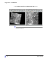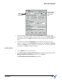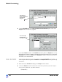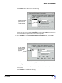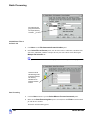
1
ERDAS IMAGINE
Tour Guides
™
®
ERDAS IMAGINE V8.5
®
ERDAS , Inc.
Atlanta, Georgia
®
Copyright 1991-2001 by ERDAS , Inc. All Rights Reserved.
Printed in the United States of America.
ERDAS Proprietary - Delivered under license agreement.
Copying and disclosure prohibited without express written permission from ERDAS, Inc.
ERDAS Worldwide Headquarters
2801 Buford Highway, NE
Atlanta, Georgia 30329-2137 USA
www.erdas.com
Toll Free: 877/GO ERDAS (463-7327)
Phone: 404/248-9000
Fax: 404/248-9400
User Support: 404/248-9777
ERDAS in Europe, Africa, Middle East, Asia/Pacific Rim
Phone: 011 44 1223 881 774
Fax: 011 44 1223 880 160
All Other Worldwide Inquiries
Phone: 404/248-9000
Fax: 404/248-9400
Acknowledgments
ERDAS would like to extend our thanks to the following data providers:
-
U.S. Geological Survey, EROS Data Center, Sioux Falls, SD
-
City of Oxford, OH - GeoOne, Inc.
-
ESA/EURIMAGE, Rome, Italy - Distributed by NRSC
Warning
All information in this document, as well as the software to which it pertains, is proprietary material of ERDAS, Inc., and is subject to an ERDAS
license and non-disclosure agreement. Neither the software nor the documentation may be reproduced in any manner without the prior written
permission of ERDAS, Inc.
Specifications are subject to change without notice.
Trademarks
Copyright © 2001 ERDAS, Inc. All rights reserved. ERDAS, ERDAS IMAGINE, IMAGINE Advantage, IMAGINE Essentials, IMAGINE
Professional and Stereo Analyst are registered trademarks of ERDAS, Inc. CellArray, IMAGINE Developers’ Toolkit, IMAGINE Expert Classifier,
IMAGINE IFSAR DEM, IMAGINE NITF, IMAGINE OrthoBASE, IMAGINE OrthoRadar, IMAGINE Radar Interpreter, IMAGINE Radar
Mapping Suite, IMAGINE StereoSAR DEM, IMAGINE Subpixel Classifier, IMAGINE Vector, and IMAGINE VirtualGIS are trademarks of
ERDAS, Inc. Other brand and product names are the properties of their respective owners. 5/01 Part No. 28.
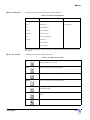
Table of Contents
Table of Contents . . . . . . . . . . . . . . . . . . . . . . . . . . . . . . . . . . . . . . . . . . . . . . . . . . . . . . . . . . . . iii
List of Tables . . . . . . . . . . . . . . . . . . . . . . . . . . . . . . . . . . . . . . . . . . . . . . . . . . . . . . . . . . . . . . xv
Preface . . . . . . . . . . . . . . . . . . . . . . . . . . . . . . . . . . . . . . . . . . . . . . . . . . . . . . . . . . . . . . . . . . xvii
About This Manual . . . . . . . . . . . . . . . . . . . . . . . . . . . . . . . . . . . . . . . . . . . . . . . . . . . . . . . . . . . . . . . . . . . . . xvii
Example Data . . . . . . . . . . . . . . . . . . . . . . . . . . . . . . . . . . . . . . . . . . . . . . . . . . . . . . . . . . . . . . . . . . . . . . . . . xvii
Time Required . . . . . . . . . . . . . . . . . . . . . . . . . . . . . . . . . . . . . . . . . . . . . . . . . . . . . . . . . . . . . . . . . . . . . . . . . xvii
Documentation . . . . . . . . . . . . . . . . . . . . . . . . . . . . . . . . . . . . . . . . . . . . . . . . . . . . . . . . . . . . . . . . . . . . . . . . xvii
Printed Documentation . . . . . . . . . . . . . . . . . . . . . . . . . . . . . . . . . . . . . . . . . . . . . . . . . . . . . . . . . . . . . . xvii
On-Line Documentation . . . . . . . . . . . . . . . . . . . . . . . . . . . . . . . . . . . . . . . . . . . . . . . . . . . . . . . . . . . . . xviii
Documentation Functions . . . . . . . . . . . . . . . . . . . . . . . . . . . . . . . . . . . . . . . . . . . . . . . . . . . . . . . . . . . . .xix
Conventions Used in This Book . . . . . . . . . . . . . . . . . . . . . . . . . . . . . . . . . . . . . . . . . . . . . . . . . . . . . . . . . . . . xx
Getting Started . . . . . . . . . . . . . . . . . . . . . . . . . . . . . . . . . . . . . . . . . . . . . . . . . . . . . . . . . . . . . . . . . . . . . . . . xxi
ERDAS IMAGINE Icon Panel . . . . . . . . . . . . . . . . . . . . . . . . . . . . . . . . . . . . . . . . . . . . . . . . . . . . . . . . . .xxi
ERDAS IMAGINE Menu Bar . . . . . . . . . . . . . . . . . . . . . . . . . . . . . . . . . . . . . . . . . . . . . . . . . . . . . . . . . . .xxi
Dialogs . . . . . . . . . . . . . . . . . . . . . . . . . . . . . . . . . . . . . . . . . . . . . . . . . . . . . . . . . . . . . . . . . . . . . . . . . . xxx
More Information/Help . . . . . . . . . . . . . . . . . . . . . . . . . . . . . . . . . . . . . . . . . . . . . . . . . . . . . . . . . . . . . . . . . . . xxx
Section I
IMAGINE Essentials™ . . . . . . . . . . . . . . . . . . . . . . . . . . . . . . . . . . . . . . . . . . . . . . . . . . . . . . . . 1
CHAPTER 1
Viewer . . . . . . . . . . . . . . . . . . . . . . . . . . . . . . . . . . . . . . . . . . . . . . . . . . . . . . . . . . . . . . . . . . . . 3
Introduction . . . . . . . . . . . . . . . . . . . . . . . . . . . . . . . . . . . . . . . . . . . . . . . . . . . . . . . . . . . . . . . . . . . . . . . . . . . . 3
Display Preferences . . . . . . . . . . . . . . . . . . . . . . . . . . . . . . . . . . . . . . . . . . . . . . . . . . . . . . . . . . . . . . . . . . . . . . 3
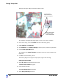
Check Band-to-Color Gun Assignments . . . . . . . . . . . . . . . . . . . . . . . . . . . . . . . . . . . . . . . . . . . . . . . . . . . 3
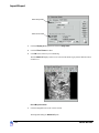
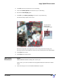
Display an Image . . . . . . . . . . . . . . . . . . . . . . . . . . . . . . . . . . . . . . . . . . . . . . . . . . . . . . . . . . . . . . . . . . . . . . . . . 6
Display Options . . . . . . . . . . . . . . . . . . . . . . . . . . . . . . . . . . . . . . . . . . . . . . . . . . . . . . . . . . . . . . . . . . . . . . 8
Utility Menu Options . . . . . . . . . . . . . . . . . . . . . . . . . . . . . . . . . . . . . . . . . . . . . . . . . . . . . . . . . . . . . . . . . . . . . 10
Use Inquiry Functions . . . . . . . . . . . . . . . . . . . . . . . . . . . . . . . . . . . . . . . . . . . . . . . . . . . . . . . . . . . . . . . . 10
Take Measurements . . . . . . . . . . . . . . . . . . . . . . . . . . . . . . . . . . . . . . . . . . . . . . . . . . . . . . . . . . . . . . . . . 12
View Menu Options . . . . . . . . . . . . . . . . . . . . . . . . . . . . . . . . . . . . . . . . . . . . . . . . . . . . . . . . . . . . . . . . . . . . . . 14
Arrange Layers . . . . . . . . . . . . . . . . . . . . . . . . . . . . . . . . . . . . . . . . . . . . . . . . . . . . . . . . . . . . . . . . . . . . . 14
Zoom . . . . . . . . . . . . . . . . . . . . . . . . . . . . . . . . . . . . . . . . . . . . . . . . . . . . . . . . . . . . . . . . . . . . . . . . . . . . . 16
Animated Zoom . . . . . . . . . . . . . . . . . . . . . . . . . . . . . . . . . . . . . . . . . . . . . . . . . . . . . . . . . . . . . . . . . . . . . 18
Box Zoom . . . . . . . . . . . . . . . . . . . . . . . . . . . . . . . . . . . . . . . . . . . . . . . . . . . . . . . . . . . . . . . . . . . . . . . . . 19
Real-time Zoom . . . . . . . . . . . . . . . . . . . . . . . . . . . . . . . . . . . . . . . . . . . . . . . . . . . . . . . . . . . . . . . . . . . . . 19
Display Two Images . . . . . . . . . . . . . . . . . . . . . . . . . . . . . . . . . . . . . . . . . . . . . . . . . . . . . . . . . . . . . . . . . 19
Link Viewers . . . . . . . . . . . . . . . . . . . . . . . . . . . . . . . . . . . . . . . . . . . . . . . . . . . . . . . . . . . . . . . . . . . . . . . 20
Compare Images . . . . . . . . . . . . . . . . . . . . . . . . . . . . . . . . . . . . . . . . . . . . . . . . . . . . . . . . . . . . . . . . . . . . 21
Unlink Viewers . . . . . . . . . . . . . . . . . . . . . . . . . . . . . . . . . . . . . . . . . . . . . . . . . . . . . . . . . . . . . . . . . . . . . . 21
Raster Menu Options . . . . . . . . . . . . . . . . . . . . . . . . . . . . . . . . . . . . . . . . . . . . . . . . . . . . . . . . . . . . . . . . . . . . . 22
iii
Table of Contents
Create an AOI Layer . . . . . . . . . . . . . . . . . . . . . . . . . . . . . . . . . . . . . . . . . . . . . . . . . . . . . . . . . . . . . . . . . 22
Adjust Image Contrast . . . . . . . . . . . . . . . . . . . . . . . . . . . . . . . . . . . . . . . . . . . . . . . . . . . . . . . . . . . . . . . 26
Use Piecewise Linear Stretches . . . . . . . . . . . . . . . . . . . . . . . . . . . . . . . . . . . . . . . . . . . . . . . . . . . . . . . . 27
Manipulate Histogram . . . . . . . . . . . . . . . . . . . . . . . . . . . . . . . . . . . . . . . . . . . . . . . . . . . . . . . . . . . . . . . . 29
Adjust Shift/Bias . . . . . . . . . . . . . . . . . . . . . . . . . . . . . . . . . . . . . . . . . . . . . . . . . . . . . . . . . . . . . . . . . . . . 31
Use Mouse Linear Mapping . . . . . . . . . . . . . . . . . . . . . . . . . . . . . . . . . . . . . . . . . . . . . . . . . . . . . . . . . . . 32
Raster Editor . . . . . . . . . . . . . . . . . . . . . . . . . . . . . . . . . . . . . . . . . . . . . . . . . . . . . . . . . . . . . . . . . . . . . . . . . . 34
Interpolate . . . . . . . . . . . . . . . . . . . . . . . . . . . . . . . . . . . . . . . . . . . . . . . . . . . . . . . . . . . . . . . . . . . . . . . . . 35
Fill with Value . . . . . . . . . . . . . . . . . . . . . . . . . . . . . . . . . . . . . . . . . . . . . . . . . . . . . . . . . . . . . . . . . . . . . . 36
Raster Attribute Editor . . . . . . . . . . . . . . . . . . . . . . . . . . . . . . . . . . . . . . . . . . . . . . . . . . . . . . . . . . . . . . . . . . . 38
Make Layers Transparent . . . . . . . . . . . . . . . . . . . . . . . . . . . . . . . . . . . . . . . . . . . . . . . . . . . . . . . . . . . . . 39
Manipulate CellArray Information . . . . . . . . . . . . . . . . . . . . . . . . . . . . . . . . . . . . . . . . . . . . . . . . . . . . . . . 41
Edit Column Properties . . . . . . . . . . . . . . . . . . . . . . . . . . . . . . . . . . . . . . . . . . . . . . . . . . . . . . . . . . . . . . . 41
Profile Tools . . . . . . . . . . . . . . . . . . . . . . . . . . . . . . . . . . . . . . . . . . . . . . . . . . . . . . . . . . . . . . . . . . . . . . . . . . . 47
Display Spectral Profile . . . . . . . . . . . . . . . . . . . . . . . . . . . . . . . . . . . . . . . . . . . . . . . . . . . . . . . . . . . . . . . 47
Display Spatial Profile . . . . . . . . . . . . . . . . . . . . . . . . . . . . . . . . . . . . . . . . . . . . . . . . . . . . . . . . . . . . . . . . 50
View Surface Profile . . . . . . . . . . . . . . . . . . . . . . . . . . . . . . . . . . . . . . . . . . . . . . . . . . . . . . . . . . . . . . . . . 52
Image Drape . . . . . . . . . . . . . . . . . . . . . . . . . . . . . . . . . . . . . . . . . . . . . . . . . . . . . . . . . . . . . . . . . . . . . . . . . . . 54
Change Options . . . . . . . . . . . . . . . . . . . . . . . . . . . . . . . . . . . . . . . . . . . . . . . . . . . . . . . . . . . . . . . . . . . . 55
Change Sun Position . . . . . . . . . . . . . . . . . . . . . . . . . . . . . . . . . . . . . . . . . . . . . . . . . . . . . . . . . . . . . . . . 56
Dump Contents to Viewer . . . . . . . . . . . . . . . . . . . . . . . . . . . . . . . . . . . . . . . . . . . . . . . . . . . . . . . . . . . . . 57
Start Eye/Target . . . . . . . . . . . . . . . . . . . . . . . . . . . . . . . . . . . . . . . . . . . . . . . . . . . . . . . . . . . . . . . . . . . . 57
Manipulate the Observer and Field of View . . . . . . . . . . . . . . . . . . . . . . . . . . . . . . . . . . . . . . . . . . . . . . . 58
CHAPTER 2
Image Catalog . . . . . . . . . . . . . . . . . . . . . . . . . . . . . . . . . . . . . . . . . . . . . . . . . . . . . . . . . . . . . . 61
Introduction . . . . . . . . . . . . . . . . . . . . . . . . . . . . . . . . . . . . . . . . . . . . . . . . . . . . . . . . . . . . . . . . . . . . . . . . . . . 61
Set Catalog Preferences . . . . . . . . . . . . . . . . . . . . . . . . . . . . . . . . . . . . . . . . . . . . . . . . . . . . . . . . . . . . . . . . . . 61
Create an Image Catalog . . . . . . . . . . . . . . . . . . . . . . . . . . . . . . . . . . . . . . . . . . . . . . . . . . . . . . . . . . . . . . . . . . 62
Add Information . . . . . . . . . . . . . . . . . . . . . . . . . . . . . . . . . . . . . . . . . . . . . . . . . . . . . . . . . . . . . . . . . . . . 63
Perform Graphical Queries . . . . . . . . . . . . . . . . . . . . . . . . . . . . . . . . . . . . . . . . . . . . . . . . . . . . . . . . . . . . . . . . 64
Select Area . . . . . . . . . . . . . . . . . . . . . . . . . . . . . . . . . . . . . . . . . . . . . . . . . . . . . . . . . . . . . . . . . . . . . . . . 64
Run Query . . . . . . . . . . . . . . . . . . . . . . . . . . . . . . . . . . . . . . . . . . . . . . . . . . . . . . . . . . . . . . . . . . . . . . . . 65
View Information . . . . . . . . . . . . . . . . . . . . . . . . . . . . . . . . . . . . . . . . . . . . . . . . . . . . . . . . . . . . . . . . . . . . 67
Modify Views . . . . . . . . . . . . . . . . . . . . . . . . . . . . . . . . . . . . . . . . . . . . . . . . . . . . . . . . . . . . . . . . . . . . . . . 67
Archive Data . . . . . . . . . . . . . . . . . . . . . . . . . . . . . . . . . . . . . . . . . . . . . . . . . . . . . . . . . . . . . . . . . . . . . . . . . . . 69
CHAPTER 3
Map Composer . . . . . . . . . . . . . . . . . . . . . . . . . . . . . . . . . . . . . . . . . . . . . . . . . . . . . . . . . . . . . 73
Introduction . . . . . . . . . . . . . . . . . . . . . . . . . . . . . . . . . . . . . . . . . . . . . . . . . . . . . . . . . . . . . . . . . . . . . . . . . . . 73
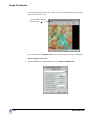
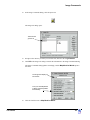
Create a Map . . . . . . . . . . . . . . . . . . . . . . . . . . . . . . . . . . . . . . . . . . . . . . . . . . . . . . . . . . . . . . . . . . . . . . . . . . . 73
Start Map Composer . . . . . . . . . . . . . . . . . . . . . . . . . . . . . . . . . . . . . . . . . . . . . . . . . . . . . . . . . . . . . . . . . . . . 74
Prepare the Data Layers . . . . . . . . . . . . . . . . . . . . . . . . . . . . . . . . . . . . . . . . . . . . . . . . . . . . . . . . . . . . . . . . . . 76
Draw the Map Frame . . . . . . . . . . . . . . . . . . . . . . . . . . . . . . . . . . . . . . . . . . . . . . . . . . . . . . . . . . . . . . . . . . . . . 76
Adjust the Size of the Map Frame . . . . . . . . . . . . . . . . . . . . . . . . . . . . . . . . . . . . . . . . . . . . . . . . . . . . . . 79
Adjust the Position of the Map Frame . . . . . . . . . . . . . . . . . . . . . . . . . . . . . . . . . . . . . . . . . . . . . . . . . . . . 80
iv
ERDAS IMAGINE
Table of Contents
Edit the Map Frame . . . . . . . . . . . . . . . . . . . . . . . . . . . . . . . . . . . . . . . . . . . . . . . . . . . . . . . . . . . . . . . . . . . . . . 81
Delete the Map Frame . . . . . . . . . . . . . . . . . . . . . . . . . . . . . . . . . . . . . . . . . . . . . . . . . . . . . . . . . . . . . . . . . . . . 82
Add a Neatline and Tick Marks . . . . . . . . . . . . . . . . . . . . . . . . . . . . . . . . . . . . . . . . . . . . . . . . . . . . . . . . . . . . . 83
Change Text/Line Styles . . . . . . . . . . . . . . . . . . . . . . . . . . . . . . . . . . . . . . . . . . . . . . . . . . . . . . . . . . . . . . 85
Make Scale Bars . . . . . . . . . . . . . . . . . . . . . . . . . . . . . . . . . . . . . . . . . . . . . . . . . . . . . . . . . . . . . . . . . . . . . . . . 87
Create a Legend . . . . . . . . . . . . . . . . . . . . . . . . . . . . . . . . . . . . . . . . . . . . . . . . . . . . . . . . . . . . . . . . . . . . . . . . 88
Add a Map Title . . . . . . . . . . . . . . . . . . . . . . . . . . . . . . . . . . . . . . . . . . . . . . . . . . . . . . . . . . . . . . . . . . . . . . . . . 90
Place a North Arrow . . . . . . . . . . . . . . . . . . . . . . . . . . . . . . . . . . . . . . . . . . . . . . . . . . . . . . . . . . . . . . . . . . . . . 92
Write Descriptive Text . . . . . . . . . . . . . . . . . . . . . . . . . . . . . . . . . . . . . . . . . . . . . . . . . . . . . . . . . . . . . . . . . . . . 94
Save the Map Composition . . . . . . . . . . . . . . . . . . . . . . . . . . . . . . . . . . . . . . . . . . . . . . . . . . . . . . . . . . . . 95
Print the Map Composition . . . . . . . . . . . . . . . . . . . . . . . . . . . . . . . . . . . . . . . . . . . . . . . . . . . . . . . . . . . . . . . . 95
Edit Composition Paths . . . . . . . . . . . . . . . . . . . . . . . . . . . . . . . . . . . . . . . . . . . . . . . . . . . . . . . . . . . . . . . . . . 97
CHAPTER 4
Classification . . . . . . . . . . . . . . . . . . . . . . . . . . . . . . . . . . . . . . . . . . . . . . . . . . . . . . . . . . . . . . 101
Introduction . . . . . . . . . . . . . . . . . . . . . . . . . . . . . . . . . . . . . . . . . . . . . . . . . . . . . . . . . . . . . . . . . . . . . . . . . . 101
Use Unsupervised Classification . . . . . . . . . . . . . . . . . . . . . . . . . . . . . . . . . . . . . . . . . . . . . . . . . . . . . . . . . . 101
Generate Thematic Raster Layer . . . . . . . . . . . . . . . . . . . . . . . . . . . . . . . . . . . . . . . . . . . . . . . . . . . . . . 102
Evaluate Classification . . . . . . . . . . . . . . . . . . . . . . . . . . . . . . . . . . . . . . . . . . . . . . . . . . . . . . . . . . . . . . . . . 104
Create Classification Overlay . . . . . . . . . . . . . . . . . . . . . . . . . . . . . . . . . . . . . . . . . . . . . . . . . . . . . . . . . 104
Analyze Individual Classes . . . . . . . . . . . . . . . . . . . . . . . . . . . . . . . . . . . . . . . . . . . . . . . . . . . . . . . . . . . 106
CHAPTER 5
Vector Querying and Editing . . . . . . . . . . . . . . . . . . . . . . . . . . . . . . . . . . . . . . . . . . . . . . . . . .109
Introduction . . . . . . . . . . . . . . . . . . . . . . . . . . . . . . . . . . . . . . . . . . . . . . . . . . . . . . . . . . . . . . . . . . . . . . . . . . 109
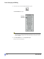
Query Vector Data . . . . . . . . . . . . . . . . . . . . . . . . . . . . . . . . . . . . . . . . . . . . . . . . . . . . . . . . . . . . . . . . . . . . . . 109
Copy Vector Data . . . . . . . . . . . . . . . . . . . . . . . . . . . . . . . . . . . . . . . . . . . . . . . . . . . . . . . . . . . . . . . . . . 109
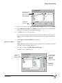
Display Vector Layers . . . . . . . . . . . . . . . . . . . . . . . . . . . . . . . . . . . . . . . . . . . . . . . . . . . . . . . . . . . . . . . 111
Change Vector Properties . . . . . . . . . . . . . . . . . . . . . . . . . . . . . . . . . . . . . . . . . . . . . . . . . . . . . . . . . . . . 112
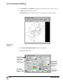
View Attributes . . . . . . . . . . . . . . . . . . . . . . . . . . . . . . . . . . . . . . . . . . . . . . . . . . . . . . . . . . . . . . . . . . . . 114
Use the Marquee Tools to Select Features . . . . . . . . . . . . . . . . . . . . . . . . . . . . . . . . . . . . . . . . . . . . . . . 116
Use the Criteria Function . . . . . . . . . . . . . . . . . . . . . . . . . . . . . . . . . . . . . . . . . . . . . . . . . . . . . . . . . . . . . 118
Edit Vector Layers . . . . . . . . . . . . . . . . . . . . . . . . . . . . . . . . . . . . . . . . . . . . . . . . . . . . . . . . . . . . . . . . . . . . . . 119
Create New Vector Layer . . . . . . . . . . . . . . . . . . . . . . . . . . . . . . . . . . . . . . . . . . . . . . . . . . . . . . . . . . . . 123
Create Attributes . . . . . . . . . . . . . . . . . . . . . . . . . . . . . . . . . . . . . . . . . . . . . . . . . . . . . . . . . . . . . . . . . . . 127
Create a Simple Shapefile Layer . . . . . . . . . . . . . . . . . . . . . . . . . . . . . . . . . . . . . . . . . . . . . . . . . . . . . . . 128
CHAPTER 6
Polynomial Rectification . . . . . . . . . . . . . . . . . . . . . . . . . . . . . . . . . . . . . . . . . . . . . . . . . . . . .135
Introduction . . . . . . . . . . . . . . . . . . . . . . . . . . . . . . . . . . . . . . . . . . . . . . . . . . . . . . . . . . . . . . . . . . . . . . . . . . 135
Rectify a Landsat Image . . . . . . . . . . . . . . . . . . . . . . . . . . . . . . . . . . . . . . . . . . . . . . . . . . . . . . . . . . . . . . . . . 135
Perform Image to Image Rectification . . . . . . . . . . . . . . . . . . . . . . . . . . . . . . . . . . . . . . . . . . . . . . . . . . . 135
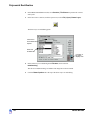
Display Files . . . . . . . . . . . . . . . . . . . . . . . . . . . . . . . . . . . . . . . . . . . . . . . . . . . . . . . . . . . . . . . . . . . . . . 135
Start GCP Tool . . . . . . . . . . . . . . . . . . . . . . . . . . . . . . . . . . . . . . . . . . . . . . . . . . . . . . . . . . . . . . . . . . . . 137
Select GCPs . . . . . . . . . . . . . . . . . . . . . . . . . . . . . . . . . . . . . . . . . . . . . . . . . . . . . . . . . . . . . . . . . . . . . . 140
Tour Guides
v
Table of Contents
Calculate Transformation Matrix from GCPs . . . . . . . . . . . . . . . . . . . . . . . . . . . . . . . . . . . . . . . . . . . . . 146
Digitize Check Points . . . . . . . . . . . . . . . . . . . . . . . . . . . . . . . . . . . . . . . . . . . . . . . . . . . . . . . . . . . . . . . 146
Resample the Image . . . . . . . . . . . . . . . . . . . . . . . . . . . . . . . . . . . . . . . . . . . . . . . . . . . . . . . . . . . . . . . . 148
Verify the Rectification Process . . . . . . . . . . . . . . . . . . . . . . . . . . . . . . . . . . . . . . . . . . . . . . . . . . . . . . . 149
Rotate/Flip/Stretch Images . . . . . . . . . . . . . . . . . . . . . . . . . . . . . . . . . . . . . . . . . . . . . . . . . . . . . . . . . . . . . . . 150
CHAPTER 7
Image Commands . . . . . . . . . . . . . . . . . . . . . . . . . . . . . . . . . . . . . . . . . . . . . . . . . . . . . . . . . . 153
Introduction . . . . . . . . . . . . . . . . . . . . . . . . . . . . . . . . . . . . . . . . . . . . . . . . . . . . . . . . . . . . . . . . . . . . . . . . . . 153
Image Commands . . . . . . . . . . . . . . . . . . . . . . . . . . . . . . . . . . . . . . . . . . . . . . . . . . . . . . . . . . . . . . . . . . . . . . 153
CHAPTER 8
Import/Export . . . . . . . . . . . . . . . . . . . . . . . . . . . . . . . . . . . . . . . . . . . . . . . . . . . . . . . . . . . . . 161
Introduction . . . . . . . . . . . . . . . . . . . . . . . . . . . . . . . . . . . . . . . . . . . . . . . . . . . . . . . . . . . . . . . . . . . . . . . . . . 161
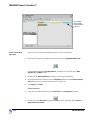
Import a SPOT Scene . . . . . . . . . . . . . . . . . . . . . . . . . . . . . . . . . . . . . . . . . . . . . . . . . . . . . . . . . . . . . . . . . . . 161
Check Preview Options . . . . . . . . . . . . . . . . . . . . . . . . . . . . . . . . . . . . . . . . . . . . . . . . . . . . . . . . . . . . . 163
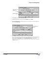
Check Import Options . . . . . . . . . . . . . . . . . . . . . . . . . . . . . . . . . . . . . . . . . . . . . . . . . . . . . . . . . . . . . . . 165
Export LAN Data . . . . . . . . . . . . . . . . . . . . . . . . . . . . . . . . . . . . . . . . . . . . . . . . . . . . . . . . . . . . . . . . . . . . . . . 167
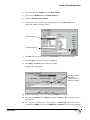
Create .tif Files . . . . . . . . . . . . . . . . . . . . . . . . . . . . . . . . . . . . . . . . . . . . . . . . . . . . . . . . . . . . . . . . . . . . . . . . 169
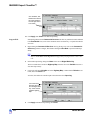
Import Generic Binary Data . . . . . . . . . . . . . . . . . . . . . . . . . . . . . . . . . . . . . . . . . . . . . . . . . . . . . . . . . . . . . . 173
Data View . . . . . . . . . . . . . . . . . . . . . . . . . . . . . . . . . . . . . . . . . . . . . . . . . . . . . . . . . . . . . . . . . . . . . . . . 174
Enter Image Dimensions . . . . . . . . . . . . . . . . . . . . . . . . . . . . . . . . . . . . . . . . . . . . . . . . . . . . . . . . . . . . 176
Save Options . . . . . . . . . . . . . . . . . . . . . . . . . . . . . . . . . . . . . . . . . . . . . . . . . . . . . . . . . . . . . . . . . . . . . 177
Preview the Image . . . . . . . . . . . . . . . . . . . . . . . . . . . . . . . . . . . . . . . . . . . . . . . . . . . . . . . . . . . . . . . . . 178
Get Image Information . . . . . . . . . . . . . . . . . . . . . . . . . . . . . . . . . . . . . . . . . . . . . . . . . . . . . . . . . . . . . . . . . . 178
Edit Image Information . . . . . . . . . . . . . . . . . . . . . . . . . . . . . . . . . . . . . . . . . . . . . . . . . . . . . . . . . . . . . . 178
View Image Information . . . . . . . . . . . . . . . . . . . . . . . . . . . . . . . . . . . . . . . . . . . . . . . . . . . . . . . . . . . . . 179
CHAPTER 9
Batch Processing . . . . . . . . . . . . . . . . . . . . . . . . . . . . . . . . . . . . . . . . . . . . . . . . . . . . . . . . . . 181
Introduction . . . . . . . . . . . . . . . . . . . . . . . . . . . . . . . . . . . . . . . . . . . . . . . . . . . . . . . . . . . . . . . . . . . . . . . . . . 181
Set up/Start the Scheduler on NT and 2000 . . . . . . . . . . . . . . . . . . . . . . . . . . . . . . . . . . . . . . . . . . . . . . . . . . 182
Use Batch with a UNIX System . . . . . . . . . . . . . . . . . . . . . . . . . . . . . . . . . . . . . . . . . . . . . . . . . . . . . . . . . . . . 183
Execute a Single File/Single Command . . . . . . . . . . . . . . . . . . . . . . . . . . . . . . . . . . . . . . . . . . . . . . . . . . . . . 183
Execute Multiple Files/Single Command—Run Now . . . . . . . . . . . . . . . . . . . . . . . . . . . . . . . . . . . . . . . . . . . . 185
Set TIFF Image File Preferences . . . . . . . . . . . . . . . . . . . . . . . . . . . . . . . . . . . . . . . . . . . . . . . . . . . . . . 185
Start the Image Command Tool . . . . . . . . . . . . . . . . . . . . . . . . . . . . . . . . . . . . . . . . . . . . . . . . . . . . . . . 186
Start the Batch Wizard . . . . . . . . . . . . . . . . . . . . . . . . . . . . . . . . . . . . . . . . . . . . . . . . . . . . . . . . . . . . . . 187
Execute Multiple Files/Single Command—Run Later . . . . . . . . . . . . . . . . . . . . . . . . . . . . . . . . . . . . . . . . . . . 190
Add Multiple Files . . . . . . . . . . . . . . . . . . . . . . . . . . . . . . . . . . . . . . . . . . . . . . . . . . . . . . . . . . . . . . . . . . 192
Execute Multiple Files/Multiple Commands . . . . . . . . . . . . . . . . . . . . . . . . . . . . . . . . . . . . . . . . . . . . . . . . . . 195
Set Up . . . . . . . . . . . . . . . . . . . . . . . . . . . . . . . . . . . . . . . . . . . . . . . . . . . . . . . . . . . . . . . . . . . . . . . . . . . 195
Run First Command . . . . . . . . . . . . . . . . . . . . . . . . . . . . . . . . . . . . . . . . . . . . . . . . . . . . . . . . . . . . . . . . 197
Run Next Command . . . . . . . . . . . . . . . . . . . . . . . . . . . . . . . . . . . . . . . . . . . . . . . . . . . . . . . . . . . . . . . . 197
Run Another Command . . . . . . . . . . . . . . . . . . . . . . . . . . . . . . . . . . . . . . . . . . . . . . . . . . . . . . . . . . . . . 198
Create Variables . . . . . . . . . . . . . . . . . . . . . . . . . . . . . . . . . . . . . . . . . . . . . . . . . . . . . . . . . . . . . . . . . . . 199
vi
ERDAS IMAGINE
Table of Contents
Modify Variables . . . . . . . . . . . . . . . . . . . . . . . . . . . . . . . . . . . . . . . . . . . . . . . . . . . . . . . . . . . . . . . . . . . 200
Select Input Files . . . . . . . . . . . . . . . . . . . . . . . . . . . . . . . . . . . . . . . . . . . . . . . . . . . . . . . . . . . . . . . . . . . 202
Set Start Time . . . . . . . . . . . . . . . . . . . . . . . . . . . . . . . . . . . . . . . . . . . . . . . . . . . . . . . . . . . . . . . . . . . . . 203
Work with Variables . . . . . . . . . . . . . . . . . . . . . . . . . . . . . . . . . . . . . . . . . . . . . . . . . . . . . . . . . . . . . . . . . . . . 204
Create a New Variable . . . . . . . . . . . . . . . . . . . . . . . . . . . . . . . . . . . . . . . . . . . . . . . . . . . . . . . . . . . . . . 204
Prepare . . . . . . . . . . . . . . . . . . . . . . . . . . . . . . . . . . . . . . . . . . . . . . . . . . . . . . . . . . . . . . . . . . . . . . . . . . 204
Start Batch Wizard . . . . . . . . . . . . . . . . . . . . . . . . . . . . . . . . . . . . . . . . . . . . . . . . . . . . . . . . . . . . . . . . . 205
Create a New Variable . . . . . . . . . . . . . . . . . . . . . . . . . . . . . . . . . . . . . . . . . . . . . . . . . . . . . . . . . . . . . . 206
Add Additional Files to the Batch Job . . . . . . . . . . . . . . . . . . . . . . . . . . . . . . . . . . . . . . . . . . . . . . . . . . . 208
Start Processing . . . . . . . . . . . . . . . . . . . . . . . . . . . . . . . . . . . . . . . . . . . . . . . . . . . . . . . . . . . . . . . . . . . 208
Check the Output Directory . . . . . . . . . . . . . . . . . . . . . . . . . . . . . . . . . . . . . . . . . . . . . . . . . . . . . . . . . . . 209
Additional Information . . . . . . . . . . . . . . . . . . . . . . . . . . . . . . . . . . . . . . . . . . . . . . . . . . . . . . . . . . . . . . . . . . 209
Save/Load Options . . . . . . . . . . . . . . . . . . . . . . . . . . . . . . . . . . . . . . . . . . . . . . . . . . . . . . . . . . . . . . . . . 209
Batch Job Files . . . . . . . . . . . . . . . . . . . . . . . . . . . . . . . . . . . . . . . . . . . . . . . . . . . . . . . . . . . . . . . . . . . . 210
Section II
IMAGINE Advantage™ . . . . . . . . . . . . . . . . . . . . . . . . . . . . . . . . . . . . . . . . . . . . . . . . . . . . . . . 213
CHAPTER 10
Fourier Transform Editor . . . . . . . . . . . . . . . . . . . . . . . . . . . . . . . . . . . . . . . . . . . . . . . . . . . . .215
Introduction . . . . . . . . . . . . . . . . . . . . . . . . . . . . . . . . . . . . . . . . . . . . . . . . . . . . . . . . . . . . . . . . . . . . . . . . . . 215
Create an .fft Layer . . . . . . . . . . . . . . . . . . . . . . . . . . . . . . . . . . . . . . . . . . . . . . . . . . . . . . . . . . . . . . . . . . . . . 215
Start the Fourier Transform Editor . . . . . . . . . . . . . . . . . . . . . . . . . . . . . . . . . . . . . . . . . . . . . . . . . . . . . . . . . 218
Edit Using Menu Options . . . . . . . . . . . . . . . . . . . . . . . . . . . . . . . . . . . . . . . . . . . . . . . . . . . . . . . . . . . . . . . . 221
Use Low-Pass Filtering . . . . . . . . . . . . . . . . . . . . . . . . . . . . . . . . . . . . . . . . . . . . . . . . . . . . . . . . . . . . . . 221
Use a Circular Mask . . . . . . . . . . . . . . . . . . . . . . . . . . . . . . . . . . . . . . . . . . . . . . . . . . . . . . . . . . . . . . . . 227
Use a Rectangular Mask . . . . . . . . . . . . . . . . . . . . . . . . . . . . . . . . . . . . . . . . . . . . . . . . . . . . . . . . . . . . . 229
Use a Wedge Mask . . . . . . . . . . . . . . . . . . . . . . . . . . . . . . . . . . . . . . . . . . . . . . . . . . . . . . . . . . . . . . . . . 230
Edit Using Mouse-Driven Tools . . . . . . . . . . . . . . . . . . . . . . . . . . . . . . . . . . . . . . . . . . . . . . . . . . . . . . . . . . . . 232
Use Low-Pass Filtering . . . . . . . . . . . . . . . . . . . . . . . . . . . . . . . . . . . . . . . . . . . . . . . . . . . . . . . . . . . . . . 233
Use High-Pass Filtering . . . . . . . . . . . . . . . . . . . . . . . . . . . . . . . . . . . . . . . . . . . . . . . . . . . . . . . . . . . . . . 233
Apply a Wedge Mask . . . . . . . . . . . . . . . . . . . . . . . . . . . . . . . . . . . . . . . . . . . . . . . . . . . . . . . . . . . . . . . 235
Combine Edits . . . . . . . . . . . . . . . . . . . . . . . . . . . . . . . . . . . . . . . . . . . . . . . . . . . . . . . . . . . . . . . . . . . . . 236
CHAPTER 11
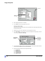
Image Interpreter . . . . . . . . . . . . . . . . . . . . . . . . . . . . . . . . . . . . . . . . . . . . . . . . . . . . . . . . . . . 239
Introduction . . . . . . . . . . . . . . . . . . . . . . . . . . . . . . . . . . . . . . . . . . . . . . . . . . . . . . . . . . . . . . . . . . . . . . . . . . 239
Subsetting an Image . . . . . . . . . . . . . . . . . . . . . . . . . . . . . . . . . . . . . . . . . . . . . . . . . . . . . . . . . . . . . . . . . . . . 239
Subsetting an Image Without Snapping . . . . . . . . . . . . . . . . . . . . . . . . . . . . . . . . . . . . . . . . . . . . . . . . . 241
Subsetting an Image With Snap to Raster . . . . . . . . . . . . . . . . . . . . . . . . . . . . . . . . . . . . . . . . . . . . . . . 245
Apply Spatial Enhancement . . . . . . . . . . . . . . . . . . . . . . . . . . . . . . . . . . . . . . . . . . . . . . . . . . . . . . . . . . . . . . 247
Apply Convolution . . . . . . . . . . . . . . . . . . . . . . . . . . . . . . . . . . . . . . . . . . . . . . . . . . . . . . . . . . . . . . . . . . 248
Check the File . . . . . . . . . . . . . . . . . . . . . . . . . . . . . . . . . . . . . . . . . . . . . . . . . . . . . . . . . . . . . . . . . . . . . 250
Apply Crisp . . . . . . . . . . . . . . . . . . . . . . . . . . . . . . . . . . . . . . . . . . . . . . . . . . . . . . . . . . . . . . . . . . . . . . . 251
View Results . . . . . . . . . . . . . . . . . . . . . . . . . . . . . . . . . . . . . . . . . . . . . . . . . . . . . . . . . . . . . . . . . . . . . . 253
Apply Radiometric Enhancement . . . . . . . . . . . . . . . . . . . . . . . . . . . . . . . . . . . . . . . . . . . . . . . . . . . . . . . . . . 254
Apply Brightness Inversion . . . . . . . . . . . . . . . . . . . . . . . . . . . . . . . . . . . . . . . . . . . . . . . . . . . . . . . . . . . 255
Tour Guides
vii
Table of Contents
Reverse . . . . . . . . . . . . . . . . . . . . . . . . . . . . . . . . . . . . . . . . . . . . . . . . . . . . . . . . . . . . . . . . . . . . . . . . . 256
Apply Spectral Enhancement . . . . . . . . . . . . . . . . . . . . . . . . . . . . . . . . . . . . . . . . . . . . . . . . . . . . . . . . . . . . . 258
Use Tasseled Cap . . . . . . . . . . . . . . . . . . . . . . . . . . . . . . . . . . . . . . . . . . . . . . . . . . . . . . . . . . . . . . . . . 258
Check Results . . . . . . . . . . . . . . . . . . . . . . . . . . . . . . . . . . . . . . . . . . . . . . . . . . . . . . . . . . . . . . . . . . . . . 260
Use the Indices Function . . . . . . . . . . . . . . . . . . . . . . . . . . . . . . . . . . . . . . . . . . . . . . . . . . . . . . . . . . . . 261
CHAPTER 12
Orthorectification . . . . . . . . . . . . . . . . . . . . . . . . . . . . . . . . . . . . . . . . . . . . . . . . . . . . . . . . . . 267
Introduction . . . . . . . . . . . . . . . . . . . . . . . . . . . . . . . . . . . . . . . . . . . . . . . . . . . . . . . . . . . . . . . . . . . . . . . . . . 267
Rectify a Camera Image . . . . . . . . . . . . . . . . . . . . . . . . . . . . . . . . . . . . . . . . . . . . . . . . . . . . . . . . . . . . . . . . . 267
Perform Image to Image Rectification . . . . . . . . . . . . . . . . . . . . . . . . . . . . . . . . . . . . . . . . . . . . . . . . . . 267
Check for Map Model . . . . . . . . . . . . . . . . . . . . . . . . . . . . . . . . . . . . . . . . . . . . . . . . . . . . . . . . . . . . . . . 269
Perform Geometric Correction . . . . . . . . . . . . . . . . . . . . . . . . . . . . . . . . . . . . . . . . . . . . . . . . . . . . . . . . 270
Resample the Image . . . . . . . . . . . . . . . . . . . . . . . . . . . . . . . . . . . . . . . . . . . . . . . . . . . . . . . . . . . . . . . . 279
Calibrate the Image . . . . . . . . . . . . . . . . . . . . . . . . . . . . . . . . . . . . . . . . . . . . . . . . . . . . . . . . . . . . . . . . 280
CHAPTER 13
Terrain Surface Interpolation . . . . . . . . . . . . . . . . . . . . . . . . . . . . . . . . . . . . . . . . . . . . . . . . . 283
Introduction . . . . . . . . . . . . . . . . . . . . . . . . . . . . . . . . . . . . . . . . . . . . . . . . . . . . . . . . . . . . . . . . . . . . . . . . . . 283
Create a Surface . . . . . . . . . . . . . . . . . . . . . . . . . . . . . . . . . . . . . . . . . . . . . . . . . . . . . . . . . . . . . . . . . . . . . . . 283
Import an ASCII File . . . . . . . . . . . . . . . . . . . . . . . . . . . . . . . . . . . . . . . . . . . . . . . . . . . . . . . . . . . . . . . . 284
Perform Surfacing . . . . . . . . . . . . . . . . . . . . . . . . . . . . . . . . . . . . . . . . . . . . . . . . . . . . . . . . . . . . . . . . . . 287
Display the Surface . . . . . . . . . . . . . . . . . . . . . . . . . . . . . . . . . . . . . . . . . . . . . . . . . . . . . . . . . . . . . . . . . 288
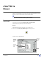
CHAPTER 14
Mosaic . . . . . . . . . . . . . . . . . . . . . . . . . . . . . . . . . . . . . . . . . . . . . . . . . . . . . . . . . . . . . . . . . . 291
Introduction . . . . . . . . . . . . . . . . . . . . . . . . . . . . . . . . . . . . . . . . . . . . . . . . . . . . . . . . . . . . . . . . . . . . . . . . . . 291
Mosaic Using Air Photo Images . . . . . . . . . . . . . . . . . . . . . . . . . . . . . . . . . . . . . . . . . . . . . . . . . . . . . . . . . . . 291
Set Input Images . . . . . . . . . . . . . . . . . . . . . . . . . . . . . . . . . . . . . . . . . . . . . . . . . . . . . . . . . . . . . . . . . . . 294
Identify Areas of Intersection . . . . . . . . . . . . . . . . . . . . . . . . . . . . . . . . . . . . . . . . . . . . . . . . . . . . . . . . . 299
Draw a Cutline . . . . . . . . . . . . . . . . . . . . . . . . . . . . . . . . . . . . . . . . . . . . . . . . . . . . . . . . . . . . . . . . . . . . 300
Define Output Images . . . . . . . . . . . . . . . . . . . . . . . . . . . . . . . . . . . . . . . . . . . . . . . . . . . . . . . . . . . . . . . 303
Run the Mosaic . . . . . . . . . . . . . . . . . . . . . . . . . . . . . . . . . . . . . . . . . . . . . . . . . . . . . . . . . . . . . . . . . . . . 304
Display the Mosaic . . . . . . . . . . . . . . . . . . . . . . . . . . . . . . . . . . . . . . . . . . . . . . . . . . . . . . . . . . . . . . . . . 305
Mosaic Using LANDSAT Images . . . . . . . . . . . . . . . . . . . . . . . . . . . . . . . . . . . . . . . . . . . . . . . . . . . . . . . . . . . 306
Display Input Images . . . . . . . . . . . . . . . . . . . . . . . . . . . . . . . . . . . . . . . . . . . . . . . . . . . . . . . . . . . . . . . 306
Add Images for Mosaic . . . . . . . . . . . . . . . . . . . . . . . . . . . . . . . . . . . . . . . . . . . . . . . . . . . . . . . . . . . . . . 308
Stack Images . . . . . . . . . . . . . . . . . . . . . . . . . . . . . . . . . . . . . . . . . . . . . . . . . . . . . . . . . . . . . . . . . . . . . 310
Match Images . . . . . . . . . . . . . . . . . . . . . . . . . . . . . . . . . . . . . . . . . . . . . . . . . . . . . . . . . . . . . . . . . . . . . 310
Run the Mosaic . . . . . . . . . . . . . . . . . . . . . . . . . . . . . . . . . . . . . . . . . . . . . . . . . . . . . . . . . . . . . . . . . . . . 311
Display Output Image . . . . . . . . . . . . . . . . . . . . . . . . . . . . . . . . . . . . . . . . . . . . . . . . . . . . . . . . . . . . . . . 312
Mosaic Color Balancing Using Color Infrared Aerial Photos . . . . . . . . . . . . . . . . . . . . . . . . . . . . . . . . . . . . . 314
Add Images for Mosaic . . . . . . . . . . . . . . . . . . . . . . . . . . . . . . . . . . . . . . . . . . . . . . . . . . . . . . . . . . . . . . 316
Set Exclude Areas . . . . . . . . . . . . . . . . . . . . . . . . . . . . . . . . . . . . . . . . . . . . . . . . . . . . . . . . . . . . . . . . . 317
Mosaic Color Balancing . . . . . . . . . . . . . . . . . . . . . . . . . . . . . . . . . . . . . . . . . . . . . . . . . . . . . . . . . . . . . 319
Match Images . . . . . . . . . . . . . . . . . . . . . . . . . . . . . . . . . . . . . . . . . . . . . . . . . . . . . . . . . . . . . . . . . . . . . 321
Run The Mosaic . . . . . . . . . . . . . . . . . . . . . . . . . . . . . . . . . . . . . . . . . . . . . . . . . . . . . . . . . . . . . . . . . . . 322
Display Output Image . . . . . . . . . . . . . . . . . . . . . . . . . . . . . . . . . . . . . . . . . . . . . . . . . . . . . . . . . . . . . . . 323
viii
ERDAS IMAGINE
Table of Contents
CHAPTER 15
Viewshed Analysis . . . . . . . . . . . . . . . . . . . . . . . . . . . . . . . . . . . . . . . . . . . . . . . . . . . . . . . . . .325
Introduction . . . . . . . . . . . . . . . . . . . . . . . . . . . . . . . . . . . . . . . . . . . . . . . . . . . . . . . . . . . . . . . . . . . . . . . . . . 325
Create a Viewshed . . . . . . . . . . . . . . . . . . . . . . . . . . . . . . . . . . . . . . . . . . . . . . . . . . . . . . . . . . . . . . . . . . . . . . 325
Start an Image Drape Viewer . . . . . . . . . . . . . . . . . . . . . . . . . . . . . . . . . . . . . . . . . . . . . . . . . . . . . . . . . 326
Start the Viewshed Analysis Tool . . . . . . . . . . . . . . . . . . . . . . . . . . . . . . . . . . . . . . . . . . . . . . . . . . . . . . 327
Add First Observer . . . . . . . . . . . . . . . . . . . . . . . . . . . . . . . . . . . . . . . . . . . . . . . . . . . . . . . . . . . . . . . . . 329
Add Another Observer . . . . . . . . . . . . . . . . . . . . . . . . . . . . . . . . . . . . . . . . . . . . . . . . . . . . . . . . . . . . . . . 330
Link the Viewers and Set Eye and Target Positions . . . . . . . . . . . . . . . . . . . . . . . . . . . . . . . . . . . . . . . . 332
Save the Viewshed . . . . . . . . . . . . . . . . . . . . . . . . . . . . . . . . . . . . . . . . . . . . . . . . . . . . . . . . . . . . . . . . . 333
Query Viewshed Data . . . . . . . . . . . . . . . . . . . . . . . . . . . . . . . . . . . . . . . . . . . . . . . . . . . . . . . . . . . . . . . 334
Add Area Column to the CellArray . . . . . . . . . . . . . . . . . . . . . . . . . . . . . . . . . . . . . . . . . . . . . . . . . . . . . 335
Query the Viewshed Layer . . . . . . . . . . . . . . . . . . . . . . . . . . . . . . . . . . . . . . . . . . . . . . . . . . . . . . . . . . . 336
Finish . . . . . . . . . . . . . . . . . . . . . . . . . . . . . . . . . . . . . . . . . . . . . . . . . . . . . . . . . . . . . . . . . . . . . . . . . . . . 337
Section III
IMAGINE Professional™ . . . . . . . . . . . . . . . . . . . . . . . . . . . . . . . . . . . . . . . . . . . . . . . . . . . . .339
CHAPTER 16
Spatial Modeler . . . . . . . . . . . . . . . . . . . . . . . . . . . . . . . . . . . . . . . . . . . . . . . . . . . . . . . . . . . .341
Introduction . . . . . . . . . . . . . . . . . . . . . . . . . . . . . . . . . . . . . . . . . . . . . . . . . . . . . . . . . . . . . . . . . . . . . . . . . . 341
Start Model Maker . . . . . . . . . . . . . . . . . . . . . . . . . . . . . . . . . . . . . . . . . . . . . . . . . . . . . . . . . . . . . . . . . . . . . . 341
Create Sensitivity Layer . . . . . . . . . . . . . . . . . . . . . . . . . . . . . . . . . . . . . . . . . . . . . . . . . . . . . . . . . . . . . . . . . 342
Define Input Slope Layer . . . . . . . . . . . . . . . . . . . . . . . . . . . . . . . . . . . . . . . . . . . . . . . . . . . . . . . . . . . . . 344
Define Input Flood Plain Layer . . . . . . . . . . . . . . . . . . . . . . . . . . . . . . . . . . . . . . . . . . . . . . . . . . . . . . . . 349
Define Input Land Cover Layer . . . . . . . . . . . . . . . . . . . . . . . . . . . . . . . . . . . . . . . . . . . . . . . . . . . . . . . . 349
Define Function . . . . . . . . . . . . . . . . . . . . . . . . . . . . . . . . . . . . . . . . . . . . . . . . . . . . . . . . . . . . . . . . . . . . 351
Define Output Raster Layer . . . . . . . . . . . . . . . . . . . . . . . . . . . . . . . . . . . . . . . . . . . . . . . . . . . . . . . . . . . 352
Save and Run the Model . . . . . . . . . . . . . . . . . . . . . . . . . . . . . . . . . . . . . . . . . . . . . . . . . . . . . . . . . . . . . 353
Enhance SPOT Data . . . . . . . . . . . . . . . . . . . . . . . . . . . . . . . . . . . . . . . . . . . . . . . . . . . . . . . . . . . . . . . . . . . . 354
Define Input SPOT Layer . . . . . . . . . . . . . . . . . . . . . . . . . . . . . . . . . . . . . . . . . . . . . . . . . . . . . . . . . . . . 356
Define Input Convolution Kernel . . . . . . . . . . . . . . . . . . . . . . . . . . . . . . . . . . . . . . . . . . . . . . . . . . . . . . . 356
Define Function . . . . . . . . . . . . . . . . . . . . . . . . . . . . . . . . . . . . . . . . . . . . . . . . . . . . . . . . . . . . . . . . . . . . 357
Define Output Raster Layer . . . . . . . . . . . . . . . . . . . . . . . . . . . . . . . . . . . . . . . . . . . . . . . . . . . . . . . . . . . 358
Save and Run the Model . . . . . . . . . . . . . . . . . . . . . . . . . . . . . . . . . . . . . . . . . . . . . . . . . . . . . . . . . . . . . 359
Combine Models . . . . . . . . . . . . . . . . . . . . . . . . . . . . . . . . . . . . . . . . . . . . . . . . . . . . . . . . . . . . . . . . . . . 359
Combine Sensitivity Layer with SPOT Data . . . . . . . . . . . . . . . . . . . . . . . . . . . . . . . . . . . . . . . . . . . . . . . . . . . 360
Define Input Scalar . . . . . . . . . . . . . . . . . . . . . . . . . . . . . . . . . . . . . . . . . . . . . . . . . . . . . . . . . . . . . . . . . 361
Define Function . . . . . . . . . . . . . . . . . . . . . . . . . . . . . . . . . . . . . . . . . . . . . . . . . . . . . . . . . . . . . . . . . . . . 361
Define Output Raster Layer . . . . . . . . . . . . . . . . . . . . . . . . . . . . . . . . . . . . . . . . . . . . . . . . . . . . . . . . . . . 363
Save and Run the Model . . . . . . . . . . . . . . . . . . . . . . . . . . . . . . . . . . . . . . . . . . . . . . . . . . . . . . . . . . . . . 364
Display New Layer . . . . . . . . . . . . . . . . . . . . . . . . . . . . . . . . . . . . . . . . . . . . . . . . . . . . . . . . . . . . . . . . . . . . . . 365
Adjust Colors . . . . . . . . . . . . . . . . . . . . . . . . . . . . . . . . . . . . . . . . . . . . . . . . . . . . . . . . . . . . . . . . . . . . . . 366
Test the Output . . . . . . . . . . . . . . . . . . . . . . . . . . . . . . . . . . . . . . . . . . . . . . . . . . . . . . . . . . . . . . . . . . . . . . . . 369
Add Annotation to a Model . . . . . . . . . . . . . . . . . . . . . . . . . . . . . . . . . . . . . . . . . . . . . . . . . . . . . . . . . . . . . . . 370
Generate a Text Script . . . . . . . . . . . . . . . . . . . . . . . . . . . . . . . . . . . . . . . . . . . . . . . . . . . . . . . . . . . . . . . . . . 373
Print the Model . . . . . . . . . . . . . . . . . . . . . . . . . . . . . . . . . . . . . . . . . . . . . . . . . . . . . . . . . . . . . . . . . . . . . . . . 376
Tour Guides
ix
Table of Contents
Apply the Criteria Function . . . . . . . . . . . . . . . . . . . . . . . . . . . . . . . . . . . . . . . . . . . . . . . . . . . . . . . . . . . . . . 378
Define Input Raster Layers . . . . . . . . . . . . . . . . . . . . . . . . . . . . . . . . . . . . . . . . . . . . . . . . . . . . . . . . . . . 380
Define Criteria . . . . . . . . . . . . . . . . . . . . . . . . . . . . . . . . . . . . . . . . . . . . . . . . . . . . . . . . . . . . . . . . . . . . . 380
Define Output Raster Layer . . . . . . . . . . . . . . . . . . . . . . . . . . . . . . . . . . . . . . . . . . . . . . . . . . . . . . . . . . 382
Minimizing Temporary Disk Usage . . . . . . . . . . . . . . . . . . . . . . . . . . . . . . . . . . . . . . . . . . . . . . . . . . . . . . . . . 384
Set Preferences . . . . . . . . . . . . . . . . . . . . . . . . . . . . . . . . . . . . . . . . . . . . . . . . . . . . . . . . . . . . . . . . . . . 385
Making Your Models Usable by Others . . . . . . . . . . . . . . . . . . . . . . . . . . . . . . . . . . . . . . . . . . . . . . . . . . . . . . 386
Prompt User . . . . . . . . . . . . . . . . . . . . . . . . . . . . . . . . . . . . . . . . . . . . . . . . . . . . . . . . . . . . . . . . . . . . . . 386
Providing a User Interface to Your Model . . . . . . . . . . . . . . . . . . . . . . . . . . . . . . . . . . . . . . . . . . . . . . . . 386
Using Vector Layers in Your Model . . . . . . . . . . . . . . . . . . . . . . . . . . . . . . . . . . . . . . . . . . . . . . . . . . . . . . . . 399
Vector Layers as a Mask . . . . . . . . . . . . . . . . . . . . . . . . . . . . . . . . . . . . . . . . . . . . . . . . . . . . . . . . . . . . 399
Add Attributes to Vector Layers . . . . . . . . . . . . . . . . . . . . . . . . . . . . . . . . . . . . . . . . . . . . . . . . . . . . . . . 411
Debug Your Model . . . . . . . . . . . . . . . . . . . . . . . . . . . . . . . . . . . . . . . . . . . . . . . . . . . . . . . . . . . . . . . . . . . . . 418
Eliminate Incomplete Definition . . . . . . . . . . . . . . . . . . . . . . . . . . . . . . . . . . . . . . . . . . . . . . . . . . . . . . . 418
Eliminate Object type Mismatch . . . . . . . . . . . . . . . . . . . . . . . . . . . . . . . . . . . . . . . . . . . . . . . . . . . . . . . 430
Eliminate Division by Zero . . . . . . . . . . . . . . . . . . . . . . . . . . . . . . . . . . . . . . . . . . . . . . . . . . . . . . . . . . . 444
Use AOIs in Processing . . . . . . . . . . . . . . . . . . . . . . . . . . . . . . . . . . . . . . . . . . . . . . . . . . . . . . . . . . . . . 449
CHAPTER 17
Advanced Classification . . . . . . . . . . . . . . . . . . . . . . . . . . . . . . . . . . . . . . . . . . . . . . . . . . . . . 455
Introduction . . . . . . . . . . . . . . . . . . . . . . . . . . . . . . . . . . . . . . . . . . . . . . . . . . . . . . . . . . . . . . . . . . . . . . . . . . 455
Supervised vs. Unsupervised Classification . . . . . . . . . . . . . . . . . . . . . . . . . . . . . . . . . . . . . . . . . . . . . . 455
Perform Supervised Classification . . . . . . . . . . . . . . . . . . . . . . . . . . . . . . . . . . . . . . . . . . . . . . . . . . . . . . . . . 455
Define Signatures using Signature Editor . . . . . . . . . . . . . . . . . . . . . . . . . . . . . . . . . . . . . . . . . . . . . . . . 456
Use Tools to Evaluate Signatures . . . . . . . . . . . . . . . . . . . . . . . . . . . . . . . . . . . . . . . . . . . . . . . . . . . . . 468
Perform Supervised Classification . . . . . . . . . . . . . . . . . . . . . . . . . . . . . . . . . . . . . . . . . . . . . . . . . . . . . 480
Perform Unsupervised Classification . . . . . . . . . . . . . . . . . . . . . . . . . . . . . . . . . . . . . . . . . . . . . . . . . . . . . . . 484
Generate Thematic Raster Layer . . . . . . . . . . . . . . . . . . . . . . . . . . . . . . . . . . . . . . . . . . . . . . . . . . . . . . 485
Evaluate Classification . . . . . . . . . . . . . . . . . . . . . . . . . . . . . . . . . . . . . . . . . . . . . . . . . . . . . . . . . . . . . . . . . . 487
Create Classification Overlay . . . . . . . . . . . . . . . . . . . . . . . . . . . . . . . . . . . . . . . . . . . . . . . . . . . . . . . . . 487
Analyze Individual Classes . . . . . . . . . . . . . . . . . . . . . . . . . . . . . . . . . . . . . . . . . . . . . . . . . . . . . . . . . . . 490
Use Thresholding . . . . . . . . . . . . . . . . . . . . . . . . . . . . . . . . . . . . . . . . . . . . . . . . . . . . . . . . . . . . . . . . . . 492
Use Accuracy Assessment . . . . . . . . . . . . . . . . . . . . . . . . . . . . . . . . . . . . . . . . . . . . . . . . . . . . . . . . . . . 497
CHAPTER 18
IMAGINE Expert Classifier™ . . . . . . . . . . . . . . . . . . . . . . . . . . . . . . . . . . . . . . . . . . . . . . . . . . 503
Introduction . . . . . . . . . . . . . . . . . . . . . . . . . . . . . . . . . . . . . . . . . . . . . . . . . . . . . . . . . . . . . . . . . . . . . . . . . . 503
Create a Knowledge Base . . . . . . . . . . . . . . . . . . . . . . . . . . . . . . . . . . . . . . . . . . . . . . . . . . . . . . . . . . . . . . . . 503
Set Up the Output Classes . . . . . . . . . . . . . . . . . . . . . . . . . . . . . . . . . . . . . . . . . . . . . . . . . . . . . . . . . . . 503
Enter Rules for the Hypothesis . . . . . . . . . . . . . . . . . . . . . . . . . . . . . . . . . . . . . . . . . . . . . . . . . . . . . . . . 506
Add an Intermediate Hypothesis . . . . . . . . . . . . . . . . . . . . . . . . . . . . . . . . . . . . . . . . . . . . . . . . . . . . . . . 510
Copy and Edit . . . . . . . . . . . . . . . . . . . . . . . . . . . . . . . . . . . . . . . . . . . . . . . . . . . . . . . . . . . . . . . . . . . . . 512
Test the Knowledge Base . . . . . . . . . . . . . . . . . . . . . . . . . . . . . . . . . . . . . . . . . . . . . . . . . . . . . . . . . . . . 514
Create a Portable Knowledge Base . . . . . . . . . . . . . . . . . . . . . . . . . . . . . . . . . . . . . . . . . . . . . . . . . . . . . . . . . 519
Data . . . . . . . . . . . . . . . . . . . . . . . . . . . . . . . . . . . . . . . . . . . . . . . . . . . . . . . . . . . . . . . . . . . . . . . . . . . . 519
Methodology . . . . . . . . . . . . . . . . . . . . . . . . . . . . . . . . . . . . . . . . . . . . . . . . . . . . . . . . . . . . . . . . . . . . . . 519
Open a Knowledge Base . . . . . . . . . . . . . . . . . . . . . . . . . . . . . . . . . . . . . . . . . . . . . . . . . . . . . . . . . . . . 520
x
ERDAS IMAGINE
Table of Contents
Examine the Knowledge Base . . . . . . . . . . . . . . . . . . . . . . . . . . . . . . . . . . . . . . . . . . . . . . . . . . . . . . . . 521
Derive Slope Values . . . . . . . . . . . . . . . . . . . . . . . . . . . . . . . . . . . . . . . . . . . . . . . . . . . . . . . . . . . . . . . . 522
Build Hypotheses . . . . . . . . . . . . . . . . . . . . . . . . . . . . . . . . . . . . . . . . . . . . . . . . . . . . . . . . . . . . . . . . . . 525
Set ANDing Criteria . . . . . . . . . . . . . . . . . . . . . . . . . . . . . . . . . . . . . . . . . . . . . . . . . . . . . . . . . . . . . . . . . 527
Check Other Hypotheses . . . . . . . . . . . . . . . . . . . . . . . . . . . . . . . . . . . . . . . . . . . . . . . . . . . . . . . . . . . . 529
Introduce Spatial Logic to the Knowledge Base . . . . . . . . . . . . . . . . . . . . . . . . . . . . . . . . . . . . . . . . . . . 529
Check Buildings Hypothesis . . . . . . . . . . . . . . . . . . . . . . . . . . . . . . . . . . . . . . . . . . . . . . . . . . . . . . . . . . 532
Identify Choke Points . . . . . . . . . . . . . . . . . . . . . . . . . . . . . . . . . . . . . . . . . . . . . . . . . . . . . . . . . . . . . . . 533
Run the Expert Classification . . . . . . . . . . . . . . . . . . . . . . . . . . . . . . . . . . . . . . . . . . . . . . . . . . . . . . . . . 536
Evaluate River Areas . . . . . . . . . . . . . . . . . . . . . . . . . . . . . . . . . . . . . . . . . . . . . . . . . . . . . . . . . . . . . . . . 538
Use Pathway Feedback . . . . . . . . . . . . . . . . . . . . . . . . . . . . . . . . . . . . . . . . . . . . . . . . . . . . . . . . . . . . . 539
Section IV
IMAGINE Radar Interpreter™ . . . . . . . . . . . . . . . . . . . . . . . . . . . . . . . . . . . . . . . . . . . . . . . . . . 543
CHAPTER 19
IMAGINE Radar Interpreter™ . . . . . . . . . . . . . . . . . . . . . . . . . . . . . . . . . . . . . . . . . . . . . . . . . . 545
Introduction . . . . . . . . . . . . . . . . . . . . . . . . . . . . . . . . . . . . . . . . . . . . . . . . . . . . . . . . . . . . . . . . . . . . . . . . . . 545
Suppress Speckle Noise . . . . . . . . . . . . . . . . . . . . . . . . . . . . . . . . . . . . . . . . . . . . . . . . . . . . . . . . . . . . . . . . . 545
Calculate Coefficient of Variation . . . . . . . . . . . . . . . . . . . . . . . . . . . . . . . . . . . . . . . . . . . . . . . . . . . . . . 549
Run Speckle Suppression Function . . . . . . . . . . . . . . . . . . . . . . . . . . . . . . . . . . . . . . . . . . . . . . . . . . . . 550
Use Histograms to Evaluate Images . . . . . . . . . . . . . . . . . . . . . . . . . . . . . . . . . . . . . . . . . . . . . . . . . . . . 552
Enhance Edges . . . . . . . . . . . . . . . . . . . . . . . . . . . . . . . . . . . . . . . . . . . . . . . . . . . . . . . . . . . . . . . . . . . . . . . . 554
Enhance Image . . . . . . . . . . . . . . . . . . . . . . . . . . . . . . . . . . . . . . . . . . . . . . . . . . . . . . . . . . . . . . . . . . . . . . . . 557
Wallis Adaptive Filter . . . . . . . . . . . . . . . . . . . . . . . . . . . . . . . . . . . . . . . . . . . . . . . . . . . . . . . . . . . . . . . . 557
Apply Sensor Merge . . . . . . . . . . . . . . . . . . . . . . . . . . . . . . . . . . . . . . . . . . . . . . . . . . . . . . . . . . . . . . . . 560
Apply Texture Analysis . . . . . . . . . . . . . . . . . . . . . . . . . . . . . . . . . . . . . . . . . . . . . . . . . . . . . . . . . . . . . . 564
Adjust Brightness . . . . . . . . . . . . . . . . . . . . . . . . . . . . . . . . . . . . . . . . . . . . . . . . . . . . . . . . . . . . . . . . . . . . . . 567
Adjust Slant Range . . . . . . . . . . . . . . . . . . . . . . . . . . . . . . . . . . . . . . . . . . . . . . . . . . . . . . . . . . . . . . . . . . . . . 568
Section V
IMAGINE Vector™ . . . . . . . . . . . . . . . . . . . . . . . . . . . . . . . . . . . . . . . . . . . . . . . . . . . . . . . . . . 571
CHAPTER 20
IMAGINE Vector™ . . . . . . . . . . . . . . . . . . . . . . . . . . . . . . . . . . . . . . . . . . . . . . . . . . . . . . . . . . . 573
Introduction . . . . . . . . . . . . . . . . . . . . . . . . . . . . . . . . . . . . . . . . . . . . . . . . . . . . . . . . . . . . . . . . . . . . . . . . . . 573
Copy Vector Data . . . . . . . . . . . . . . . . . . . . . . . . . . . . . . . . . . . . . . . . . . . . . . . . . . . . . . . . . . . . . . . . . . . . . . 574
Manipulate Info Files . . . . . . . . . . . . . . . . . . . . . . . . . . . . . . . . . . . . . . . . . . . . . . . . . . . . . . . . . . . . . . . . . . . . 576
Change Vector Symbology . . . . . . . . . . . . . . . . . . . . . . . . . . . . . . . . . . . . . . . . . . . . . . . . . . . . . . . . . . . . . . . 583
Add Pattern Polygon Fill . . . . . . . . . . . . . . . . . . . . . . . . . . . . . . . . . . . . . . . . . . . . . . . . . . . . . . . . . . . . . 586
Build Topology . . . . . . . . . . . . . . . . . . . . . . . . . . . . . . . . . . . . . . . . . . . . . . . . . . . . . . . . . . . . . . . . . . . . . . . . 589
Clean Vector Layer . . . . . . . . . . . . . . . . . . . . . . . . . . . . . . . . . . . . . . . . . . . . . . . . . . . . . . . . . . . . . . . . . . . . . 590
Section VI
Appendix . . . . . . . . . . . . . . . . . . . . . . . . . . . . . . . . . . . . . . . . . . . . . . . . . . . . . . . . . . . . . . . . . 593
APPENDIX A
Tour Guides
xi
Table of Contents
Additional Information . . . . . . . . . . . . . . . . . . . . . . . . . . . . . . . . . . . . . . . . . . . . . . . . . . . . . . 595
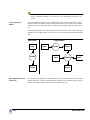
Classification . . . . . . . . . . . . . . . . . . . . . . . . . . . . . . . . . . . . . . . . . . . . . . . . . . . . . . . . . . . . . . . . . . . . . . . . . 595
Flow Chart . . . . . . . . . . . . . . . . . . . . . . . . . . . . . . . . . . . . . . . . . . . . . . . . . . . . . . . . . . . . . . . . . . . . . . . 595
Advanced Classification . . . . . . . . . . . . . . . . . . . . . . . . . . . . . . . . . . . . . . . . . . . . . . . . . . . . . . . . . . . . . 596
Signature Editor . . . . . . . . . . . . . . . . . . . . . . . . . . . . . . . . . . . . . . . . . . . . . . . . . . . . . . . . . . . . . . . . . . . 596
Fourier Transform Editor . . . . . . . . . . . . . . . . . . . . . . . . . . . . . . . . . . . . . . . . . . . . . . . . . . . . . . . . . . . . . . . . 597
Fourier Editor Menu Bar . . . . . . . . . . . . . . . . . . . . . . . . . . . . . . . . . . . . . . . . . . . . . . . . . . . . . . . . . . . . . 597
Fourier Editor Tool Bar . . . . . . . . . . . . . . . . . . . . . . . . . . . . . . . . . . . . . . . . . . . . . . . . . . . . . . . . . . . . . . 597
Image Catalog . . . . . . . . . . . . . . . . . . . . . . . . . . . . . . . . . . . . . . . . . . . . . . . . . . . . . . . . . . . . . . . . . . . . . . . . . 598
Image Catalog Menu Bar . . . . . . . . . . . . . . . . . . . . . . . . . . . . . . . . . . . . . . . . . . . . . . . . . . . . . . . . . . . . 599
Image Catalog Tool Bar . . . . . . . . . . . . . . . . . . . . . . . . . . . . . . . . . . . . . . . . . . . . . . . . . . . . . . . . . . . . . 599
Image Catalog CellArray . . . . . . . . . . . . . . . . . . . . . . . . . . . . . . . . . . . . . . . . . . . . . . . . . . . . . . . . . . . . . 600
Adding Custom Maps . . . . . . . . . . . . . . . . . . . . . . . . . . . . . . . . . . . . . . . . . . . . . . . . . . . . . . . . . . . . . . . 601
Image Interpreter . . . . . . . . . . . . . . . . . . . . . . . . . . . . . . . . . . . . . . . . . . . . . . . . . . . . . . . . . . . . . . . . . . . . . . 606
Image Interpreter Functions . . . . . . . . . . . . . . . . . . . . . . . . . . . . . . . . . . . . . . . . . . . . . . . . . . . . . . . . . . 606
Import/Export . . . . . . . . . . . . . . . . . . . . . . . . . . . . . . . . . . . . . . . . . . . . . . . . . . . . . . . . . . . . . . . . . . . . . . . . . 611
Data View Menu Bar . . . . . . . . . . . . . . . . . . . . . . . . . . . . . . . . . . . . . . . . . . . . . . . . . . . . . . . . . . . . . . . . 611
Data View Tool Bar . . . . . . . . . . . . . . . . . . . . . . . . . . . . . . . . . . . . . . . . . . . . . . . . . . . . . . . . . . . . . . . . . 611
ImageInfo Menu Bar . . . . . . . . . . . . . . . . . . . . . . . . . . . . . . . . . . . . . . . . . . . . . . . . . . . . . . . . . . . . . . . . 612
ImageInfo Tool Bar . . . . . . . . . . . . . . . . . . . . . . . . . . . . . . . . . . . . . . . . . . . . . . . . . . . . . . . . . . . . . . . . . 612
Map Composer . . . . . . . . . . . . . . . . . . . . . . . . . . . . . . . . . . . . . . . . . . . . . . . . . . . . . . . . . . . . . . . . . . . . . . . . 613
Map Composer Menu Bar . . . . . . . . . . . . . . . . . . . . . . . . . . . . . . . . . . . . . . . . . . . . . . . . . . . . . . . . . . . . 616
Map Composer Tool Bar . . . . . . . . . . . . . . . . . . . . . . . . . . . . . . . . . . . . . . . . . . . . . . . . . . . . . . . . . . . . . 617
Annotation Tool Palette . . . . . . . . . . . . . . . . . . . . . . . . . . . . . . . . . . . . . . . . . . . . . . . . . . . . . . . . . . . . . 618
Ungroup Elements in Map Composer . . . . . . . . . . . . . . . . . . . . . . . . . . . . . . . . . . . . . . . . . . . . . . . . . . . 620
Mosaic . . . . . . . . . . . . . . . . . . . . . . . . . . . . . . . . . . . . . . . . . . . . . . . . . . . . . . . . . . . . . . . . . . . . . . . . . . . . . . 620
Mosaic Tool Menu Bar . . . . . . . . . . . . . . . . . . . . . . . . . . . . . . . . . . . . . . . . . . . . . . . . . . . . . . . . . . . . . . 621
Mosaic Tool Tool Bar . . . . . . . . . . . . . . . . . . . . . . . . . . . . . . . . . . . . . . . . . . . . . . . . . . . . . . . . . . . . . . . 621
Rectification . . . . . . . . . . . . . . . . . . . . . . . . . . . . . . . . . . . . . . . . . . . . . . . . . . . . . . . . . . . . . . . . . . . . . . . . . . 623
Input and Reference Images . . . . . . . . . . . . . . . . . . . . . . . . . . . . . . . . . . . . . . . . . . . . . . . . . . . . . . . . . 624
GCP Tool Menu Bar . . . . . . . . . . . . . . . . . . . . . . . . . . . . . . . . . . . . . . . . . . . . . . . . . . . . . . . . . . . . . . . . 625
GCP Tool Bar . . . . . . . . . . . . . . . . . . . . . . . . . . . . . . . . . . . . . . . . . . . . . . . . . . . . . . . . . . . . . . . . . . . . . 625
Record Ground Control Points . . . . . . . . . . . . . . . . . . . . . . . . . . . . . . . . . . . . . . . . . . . . . . . . . . . . . . . . 626
Spatial Modeler . . . . . . . . . . . . . . . . . . . . . . . . . . . . . . . . . . . . . . . . . . . . . . . . . . . . . . . . . . . . . . . . . . . . . . . . 626
About Model Maker . . . . . . . . . . . . . . . . . . . . . . . . . . . . . . . . . . . . . . . . . . . . . . . . . . . . . . . . . . . . . . . . . 626
Creating Graphical Models . . . . . . . . . . . . . . . . . . . . . . . . . . . . . . . . . . . . . . . . . . . . . . . . . . . . . . . . . . . 628
Defining Model Files and Parameters . . . . . . . . . . . . . . . . . . . . . . . . . . . . . . . . . . . . . . . . . . . . . . . . . . . 628
Solving Problems . . . . . . . . . . . . . . . . . . . . . . . . . . . . . . . . . . . . . . . . . . . . . . . . . . . . . . . . . . . . . . . . . . 629
Determine Input Data . . . . . . . . . . . . . . . . . . . . . . . . . . . . . . . . . . . . . . . . . . . . . . . . . . . . . . . . . . . . . . . 630
Determine Functions . . . . . . . . . . . . . . . . . . . . . . . . . . . . . . . . . . . . . . . . . . . . . . . . . . . . . . . . . . . . . . . . 630
Model Maker Viewer and Tool Palette . . . . . . . . . . . . . . . . . . . . . . . . . . . . . . . . . . . . . . . . . . . . . . . . . . 631
Model Maker Viewer Tool Bar . . . . . . . . . . . . . . . . . . . . . . . . . . . . . . . . . . . . . . . . . . . . . . . . . . . . . . . . 632
Model Maker Tool Palette . . . . . . . . . . . . . . . . . . . . . . . . . . . . . . . . . . . . . . . . . . . . . . . . . . . . . . . . . . . . 633
Table Tool . . . . . . . . . . . . . . . . . . . . . . . . . . . . . . . . . . . . . . . . . . . . . . . . . . . . . . . . . . . . . . . . . . . . . . . . . . . . 635
Table Tool Menu Bar . . . . . . . . . . . . . . . . . . . . . . . . . . . . . . . . . . . . . . . . . . . . . . . . . . . . . . . . . . . . . . . 635
Table Tool Tool Bar . . . . . . . . . . . . . . . . . . . . . . . . . . . . . . . . . . . . . . . . . . . . . . . . . . . . . . . . . . . . . . . . 636
Terrain Surface Editor . . . . . . . . . . . . . . . . . . . . . . . . . . . . . . . . . . . . . . . . . . . . . . . . . . . . . . . . . . . . . . . . . . 637
3D Surfacing Dialog Menu Bar . . . . . . . . . . . . . . . . . . . . . . . . . . . . . . . . . . . . . . . . . . . . . . . . . . . . . . . 637
xii
ERDAS IMAGINE
Table of Contents
3D Surfacing Dialog Tool Bar . . . . . . . . . . . . . . . . . . . . . . . . . . . . . . . . . . . . . . . . . . . . . . . . . . . . . . . . . 637
Vector . . . . . . . . . . . . . . . . . . . . . . . . . . . . . . . . . . . . . . . . . . . . . . . . . . . . . . . . . . . . . . . . . . . . . . . . . . . . . . 638
Vector Tools . . . . . . . . . . . . . . . . . . . . . . . . . . . . . . . . . . . . . . . . . . . . . . . . . . . . . . . . . . . . . . . . . . . . . . 638
Viewer . . . . . . . . . . . . . . . . . . . . . . . . . . . . . . . . . . . . . . . . . . . . . . . . . . . . . . . . . . . . . . . . . . . . . . . . . . . . . . . 639
About the Viewer . . . . . . . . . . . . . . . . . . . . . . . . . . . . . . . . . . . . . . . . . . . . . . . . . . . . . . . . . . . . . . . . . . . 639
Viewer Menu Bar . . . . . . . . . . . . . . . . . . . . . . . . . . . . . . . . . . . . . . . . . . . . . . . . . . . . . . . . . . . . . . . . . . . 640
Viewer Tool Bar . . . . . . . . . . . . . . . . . . . . . . . . . . . . . . . . . . . . . . . . . . . . . . . . . . . . . . . . . . . . . . . . . . . . 642
Duplicated Functionality . . . . . . . . . . . . . . . . . . . . . . . . . . . . . . . . . . . . . . . . . . . . . . . . . . . . . . . . . . . . . 643
Keyboard Shortcuts . . . . . . . . . . . . . . . . . . . . . . . . . . . . . . . . . . . . . . . . . . . . . . . . . . . . . . . . . . . . . . . . . 643
Histogram Edit Tools . . . . . . . . . . . . . . . . . . . . . . . . . . . . . . . . . . . . . . . . . . . . . . . . . . . . . . . . . . . . . . . . 644
Histogram Numbers . . . . . . . . . . . . . . . . . . . . . . . . . . . . . . . . . . . . . . . . . . . . . . . . . . . . . . . . . . . . . . . . 645
Manipulating Lookup Table Breakpoints . . . . . . . . . . . . . . . . . . . . . . . . . . . . . . . . . . . . . . . . . . . . . . . . . 645
Image Drape Menu Bar . . . . . . . . . . . . . . . . . . . . . . . . . . . . . . . . . . . . . . . . . . . . . . . . . . . . . . . . . . . . . . 645
Image Drape Tool Bar . . . . . . . . . . . . . . . . . . . . . . . . . . . . . . . . . . . . . . . . . . . . . . . . . . . . . . . . . . . . . . . 646
Index . . . . . . . . . . . . . . . . . . . . . . . . . . . . . . . . . . . . . . . . . . . . . . . . . . . . . . . . . . . . . . . . . . . 647
Tour Guides
xiii
Table of Contents
xiv
ERDAS IMAGINE
List of Tables
Table
Table
Table
Table
Table
Table
Table
Table
Table
Table
Table
Table
Table
Table
Table
Table
Table
Table
Table
Table
Table
Table
Table
Table
Table
Table
Table
Table
Table
Table
Table
Table
Table
Table
Table
Table
Table
Table
Table
Table
Table
Table
Table
Table
Table
Table
Table
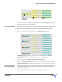
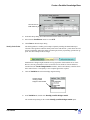
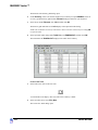
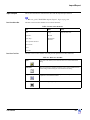
1: ERDAS IMAGINE Documentation Functions . . . . . . . . . . . . . . . . . . . . . . . . . . . . . . . . . . . xix
2: Session Menu Options . . . . . . . . . . . . . . . . . . . . . . . . . . . . . . . . . . . . . . . . . . . . . . . . . . xxii
3: Main Menu Options . . . . . . . . . . . . . . . . . . . . . . . . . . . . . . . . . . . . . . . . . . . . . . . . . . . . xxiv
4: Tools Menu Options . . . . . . . . . . . . . . . . . . . . . . . . . . . . . . . . . . . . . . . . . . . . . . . . . . . xxv
5: Utility Menu Options . . . . . . . . . . . . . . . . . . . . . . . . . . . . . . . . . . . . . . . . . . . . . . . . . . . xxvi
6: Help Menu Options . . . . . . . . . . . . . . . . . . . . . . . . . . . . . . . . . . . . . . . . . . . . . . . . . . . xxvii
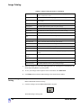
2-1: Image Catalog Preferences . . . . . . . . . . . . . . . . . . . . . . . . . . . . . . . . . . . . . . . . . . . . . 61
12-1: Film X and Film Y Coordinates . . . . . . . . . . . . . . . . . . . . . . . . . . . . . . . . . . . . . . . . . 274
16-1: Class Values for n3_landcover_RC . . . . . . . . . . . . . . . . . . . . . . . . . . . . . . . . . . . . . . 350
16-2: Conditional Statement Class Values . . . . . . . . . . . . . . . . . . . . . . . . . . . . . . . . . . . . . 352
16-3: Training Samples of Chaparral and Riparian Land Cover . . . . . . . . . . . . . . . . . . . . . . 379
16-4: Complete Criteria Table . . . . . . . . . . . . . . . . . . . . . . . . . . . . . . . . . . . . . . . . . . . . . . 382
19-1: Coefficient of Variation Values for Look-averaged Radar Scenes . . . . . . . . . . . . . . . . 549
19-2: Speckle Suppression Parameters . . . . . . . . . . . . . . . . . . . . . . . . . . . . . . . . . . . . . . . 551
19-3: Filtering Sequence . . . . . . . . . . . . . . . . . . . . . . . . . . . . . . . . . . . . . . . . . . . . . . . . . . 552
A-1 Signature Editor . . . . . . . . . . . . . . . . . . . . . . . . . . . . . . . . . . . . . . . . . . . . . . . . . . . . . 596
A-2 Fourier Editor Menu Bar . . . . . . . . . . . . . . . . . . . . . . . . . . . . . . . . . . . . . . . . . . . . . . . 597
A-3 Fourier Editor Tool Bar . . . . . . . . . . . . . . . . . . . . . . . . . . . . . . . . . . . . . . . . . . . . . . . . 597
A-4 Image Catalog Menu Bar . . . . . . . . . . . . . . . . . . . . . . . . . . . . . . . . . . . . . . . . . . . . . . . 599
A-5 Image Catalog Tool Bar . . . . . . . . . . . . . . . . . . . . . . . . . . . . . . . . . . . . . . . . . . . . . . . 599
A-6 Image Catalog Data Characteristics . . . . . . . . . . . . . . . . . . . . . . . . . . . . . . . . . . . . . . . 600
A-7 Image Interpreter Functions . . . . . . . . . . . . . . . . . . . . . . . . . . . . . . . . . . . . . . . . . . . . 606
A-8 Data View Menu Bar . . . . . . . . . . . . . . . . . . . . . . . . . . . . . . . . . . . . . . . . . . . . . . . . . . 611
A-9 Data View Tool Bar . . . . . . . . . . . . . . . . . . . . . . . . . . . . . . . . . . . . . . . . . . . . . . . . . . . 611
A-10 ImageInfo Menu Bar . . . . . . . . . . . . . . . . . . . . . . . . . . . . . . . . . . . . . . . . . . . . . . . . . 612
A-11 ImageInfo Tool Bar . . . . . . . . . . . . . . . . . . . . . . . . . . . . . . . . . . . . . . . . . . . . . . . . . . 612
A-12 Map Composer Menu Bar . . . . . . . . . . . . . . . . . . . . . . . . . . . . . . . . . . . . . . . . . . . . . 616
A-13 Map Composer Tool Bar . . . . . . . . . . . . . . . . . . . . . . . . . . . . . . . . . . . . . . . . . . . . . . 617
A-14 Annotation Tool Palette . . . . . . . . . . . . . . . . . . . . . . . . . . . . . . . . . . . . . . . . . . . . . . . 618
A-15 Mosaic Tool Menu Bar . . . . . . . . . . . . . . . . . . . . . . . . . . . . . . . . . . . . . . . . . . . . . . . . 621
A-16 Mosaic Tool Tool Bar . . . . . . . . . . . . . . . . . . . . . . . . . . . . . . . . . . . . . . . . . . . . . . . . 621
A-17 GCP Tool Menu Bar . . . . . . . . . . . . . . . . . . . . . . . . . . . . . . . . . . . . . . . . . . . . . . . . . 625
A-18 GCP Tool Bar . . . . . . . . . . . . . . . . . . . . . . . . . . . . . . . . . . . . . . . . . . . . . . . . . . . . . . 625
A-19 Model Maker Viewer Menu Bar . . . . . . . . . . . . . . . . . . . . . . . . . . . . . . . . . . . . . . . . . 632
A-20 Model Maker Viewer Tool Bar . . . . . . . . . . . . . . . . . . . . . . . . . . . . . . . . . . . . . . . . . . 632
A-21 Model Maker Tool Palette . . . . . . . . . . . . . . . . . . . . . . . . . . . . . . . . . . . . . . . . . . . . . 633
A-22 Table Tool Menu Bar . . . . . . . . . . . . . . . . . . . . . . . . . . . . . . . . . . . . . . . . . . . . . . . . . 635
A-23 Table Tool Tool Bar . . . . . . . . . . . . . . . . . . . . . . . . . . . . . . . . . . . . . . . . . . . . . . . . . . 636
A-24 3D Surfacing Dialog Menu Bar . . . . . . . . . . . . . . . . . . . . . . . . . . . . . . . . . . . . . . . . . . 637
A-25 3D Surfacing Dialog Tool Bar . . . . . . . . . . . . . . . . . . . . . . . . . . . . . . . . . . . . . . . . . . 637
A-26 Vector Tools . . . . . . . . . . . . . . . . . . . . . . . . . . . . . . . . . . . . . . . . . . . . . . . . . . . . . . . 638
A-27 Viewer Menu Bar. . . . . . . . . . . . . . . . . . . . . . . . . . . . . . . . . . . . . . . . . . . . . . . . . . . . 640
A-28 Viewer Menu Bar, Continued . . . . . . . . . . . . . . . . . . . . . . . . . . . . . . . . . . . . . . . . . . . 641
A-29 Viewer Tool Bar . . . . . . . . . . . . . . . . . . . . . . . . . . . . . . . . . . . . . . . . . . . . . . . . . . . . 642
A-30 Histogram Edit Tools . . . . . . . . . . . . . . . . . . . . . . . . . . . . . . . . . . . . . . . . . . . . . . . . . 644
A-31 Image Drape Menu Bar . . . . . . . . . . . . . . . . . . . . . . . . . . . . . . . . . . . . . . . . . . . . . . . 645
A-32 Image Drape Tool Bar . . . . . . . . . . . . . . . . . . . . . . . . . . . . . . . . . . . . . . . . . . . . . . . . 646
Tour Guides
xv
List of Tables
xvi
ERDAS IMAGINE
Preface
About This Manual
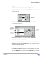
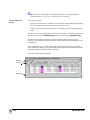
The ERDAS IMAGINE Tour Guides™ manual is a compilation of tutorials designed to help you
learn how to use ERDAS IMAGINE® software. This is a comprehensive manual, representing
ERDAS IMAGINE and its add-on modules. Each guide takes you step-by-step through an
entire process. The tour guides are not intended to tell you everything there is to know about any
one topic, but to show you how to use some of the basic tools you need to get started.
This manual serves as a handy reference that you can refer to while using ERDAS IMAGINE
for your own projects. Included is a comprehensive index, so that you can reference particular
information later.
There are several sections to this manual. These sections are based upon the way in which
ERDAS IMAGINE is packaged. The following sections are composed of the tour guides you
go through in a step by step fashion to learn detailed information about the various ERDAS
IMAGINE functions.
•
Section I—IMAGINE Essentials™
•
Section II—IMAGINE Advantage™
•
Section III—IMAGINE Professional™
•
Section IV—IMAGINE Radar Interpreter™
•
Section V—IMAGINE Vector™
Section VI, Appendices, contains further information about interface buttons and menus.
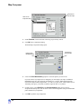
Example Data
Data sets are provided with the software so that your results match those in the tour guides. The
data used in the tour guides are in the <IMAGINE_HOME>/examples directory.
<IMAGINE_HOME> is the variable name of the directory where ERDAS IMAGINE resides.
When accessing data files, you must replace <IMAGINE_HOME> with the name of the
directory where ERDAS IMAGINE is loaded on your system.
Time Required
Each individual tour guide takes a different amount of time to complete, depending upon the
options you choose and the length of the tour guide. The approximate completion time is stated
in the introduction to each tour guide.
Documentation
The ERDAS IMAGINE Tour Guides manual is part of a whole suite of printed and on-line
documentation that you receive with ERDAS IMAGINE software.
Printed Documentation
Following is a list of printed documentation that is available with ERDAS IMAGINE software.
These may have been delivered in printed form or as digital .pdf files. The pdf files may be
found in the <IMAGINE_HOME>/help/hardcopy folder:
•
Tour Guide
ERDAS Field Guide™ (also as FieldGuide.pdf)
xvii
Preface
On-Line Documentation
xviii
•
ERDAS IMAGINE Configuration Guide (ConfigGuide.pdf)
•
ERDAS IMAGINE Tour Guides ™(TourGuide.pdf)
•
ERDAS Macro Language Reference Manual (only as EML.pdf)
•
ERDAS Spatial Modeler Language Reference Manual (only as SML.pdf)
•
ERDAS IMAGINE Read Me First document
•
ERDAS IMAGINE V8.5 Release Notes
•
FLEXlm End Users Guide (only as enduser.pdf)
•
What’s New in ERDAS IMAGINE V8.5 (only as Whats_New_in_IMAGINE_85.pdf)
Following is a list of on-line manuals that can be found in the On-Line Help in ERDAS
IMAGINE software. This list may change depending on your software package and add-on
modules you have purchased:
•
Introduction to ERDAS IMAGINE On-Line Help
•
Annotation On-Line Manual
•
AOI On-Line Manual
•
Classification On-Line Manual
•
Expert Classifier On-Line Manual
•
Stereo Analyst On-Line Manual
•
HyperSpectral On-Line Manual
•
IMAGINE Command and Function Syntax On-Line Manual
•
IMAGINE Interface On-Line Manual
•
Image Catalog On-Line Manual
•
Image Interpreter On-Line Manual
•
Import/Export On-Line Manual
•
Map Composer On-Line Manual
•
OrthoBASE On-Line Manual
•
Radar Mapping Suite On-Line Manual
•
IFSAR DEM on-Line Manual
•
StereoSAR DEM On-Line Manual
ERDAS IMAGINE
Documentation
Documentation
Functions
•
OrthoRadar On-Line Manual
•
Generic SAR Node On-Line Manual
•
Rectification On-Line Manual
•
Session On-Line Manual
•
Preferences On-Line Manual
•
Spatial Modeler On-Line Manual
•
Tools and Utilities On-Line Manual
•
Vector On-Line Manual
•
Viewer On-Line Manual
•
Viewer Raster Tools On-Line Manual
•
Virtuality On-Line Manual
•
Graphical Models Reference Guide
•
DLL Reference Guide
•
Imagizer On-Line Manual
•
Appendices
The following table depicts the different types of information you can extract from ERDAS
IMAGINE documentation.
TABLE 1: ERDAS IMAGINE Documentation Functions
Tour Guides
If you want to...
Read...
Install ERDAS IMAGINE
ERDAS IMAGINE Release Notes, then
ERDAS IMAGINE Configuration Guide
Set up hardware for use with ERDAS IMAGINE
ERDAS IMAGINE Configuration Guide
Learn about new features in the latest release
What’s New in IMAGINE 8.5 (PDF)
Learn to use ERDAS IMAGINE
ERDAS IMAGINE Tour Guides
Learn about GIS and image processing theory
ERDAS Field Guide
See what a particular dialog does
On-Line Help
Get quick information for a button or function
On-Line Help or Status Bar Help
Learn how to most effectively use the On-Line
Help system
Introduction to ERDAS IMAGINE OnLine Help
Learn more about the Image Interpreter functions
ERDAS IMAGINE Tour Guides
xix
Preface
TABLE 1: ERDAS IMAGINE Documentation Functions
Conventions Used in
This Book
If you want to...
Read...
Use the Spatial Modeler Language to write models
ERDAS Spatial Modeler Language Reference Manual
Customize the ERDAS IMAGINE graphical user
interface (GUI)
ERDAS Macro Language Reference
Manual
Write custom application programs within ERDAS
IMAGINE
ERDAS Developers’ Toolkit On-Line
Manual
In ERDAS IMAGINE, the names of menus, menu options, buttons, and other components of
the interface are shown in bold type. For example:
“In the Select Layer To Add dialog, select the Fit to Frame option.”
When asked to use the mouse, you are directed to click, Shift-click, middle-click, right-click,
hold, drag, etc.
xx
•
click—designates clicking with the left mouse button.
•
Shift-click—designates holding the Shift key down on your keyboard and simultaneously
clicking with the left mouse button.
•
middle-click—designates clicking with the middle mouse button.
•
right-click—designates clicking with the right mouse button.
•
hold—designates holding down the left (or right, as noted) mouse button.
•
drag—designates dragging the mouse while holding down the left mouse button.
ERDAS IMAGINE
Getting Started
The following paragraphs are used throughout the ERDAS IMAGINE documentation:
These paragraphs contain strong warnings or important tips.
These paragraphs direct you to the ERDAS IMAGINE software function that accomplishes the described task.
These paragraphs lead you to other areas of this book or other ERDAS® manuals for
additional information.
NOTE: Notes give additional instruction.
Shaded Boxes
Shaded boxes contain supplemental information that is not required to execute the steps of
a tour guide, but is noteworthy. Generally, this is technical information.
Getting Started
To start ERDAS IMAGINE, type the following in a UNIX command window: imagine, or
select ERDAS IMAGINE 8.5 from the Start menu.
ERDAS IMAGINE begins running; the icon panel automatically opens.
ERDAS IMAGINE Icon
Panel
The ERDAS IMAGINE icon panel contains icons and menus for accessing ERDAS IMAGINE
functions. You have the option (through the Session | Preferences menu) to display the icon
panel horizontally across the top of the screen or vertically down the left side of the screen. The
default is a horizontal display.
The icon panel that displays on your screen looks similar to the following:
The various icons that are present on your icon panel depend on the components and add-on
modules you have purchased with your system.
ERDAS IMAGINE Menu
Bar
The menus on the ERDAS IMAGINE menu bar are: Session, Main, Tools, Utilities, and
Help. These menus are described in this section.
NOTE: Any items which are unavailable in these menus are shaded and inactive.
Tour Guides
xxi
Preface
Session Menu
1.
Click on the word Session in the upper left corner of the ERDAS IMAGINE menu bar.
The Session menu opens:
These menus are
identical to the ones
on the icon panel.
Click here to end
the ERDAS IMAGINE
session
You can also place your
cursor anywhere in the
icon panel and press
Ctrl-Q to exit ERDAS
IMAGINE
The following table contains the Session menu selections and their functionalities:
TABLE 2: Session Menu Options
Selection
xxii
Functionality
Preferences
Set individual or global default options for many
ERDAS IMAGINE functions (Viewer, Map
Composer, Spatial Modeler, etc.).
Configuration
Configure peripheral devices for ERDAS IMAGINE.
Session Log
View a real-time record of ERDAS IMAGINE
messages and commands, and to issue commands.
Active Process List
View and cancel currently active processes running in ERDAS IMAGINE.
Commands
Open a command shell, in which you can enter
commands to activate or cancel processes.
Enter Log Message
Insert text into the Session Log.
Start Recording Batch Commands
Open the Batch Wizard. Collect commands as
they are generated by clicking the Batch button
that is available on many ERDAS IMAGINE
dialogs.
Open Batch Command File
Open a Batch Command File (*.bcf) you have
saved previously.
ERDAS IMAGINE
Getting Started
TABLE 2: Session Menu Options (Continued)
Selection
Functionality
View Offline Batch Queue
Open the Scheduled Batch Job list dialog, which
gives information about pending batch jobs.
Flip Icons
Specify horizontal or vertical icon panel display.
Tile Viewers
Rearrange two or more Viewers on the screen so
that they do not overlap.
Close All Viewers
Close all Viewers that are currently open.
Main
Access a menu of tools that corresponds to the
icons along the ERDAS IMAGINE icon bar.
Tools
Access a menu of tools that allow you to view
and edit various text and image files.
Utilities
Access a menu of utility items that allow you to
perform general tasks in ERDAS IMAGINE.
Help
Access the ERDAS IMAGINE On-Line Help.
Exit IMAGINE
Exit the ERDAS IMAGINE session (keyboard
shortcut: Ctrl-Q).
Main Menu
2.
Click on the word Main in the ERDAS IMAGINE menu bar. The Main menu opens
The following table contains the Main menu selections and their functionalities:
Tour Guides
xxiii
Preface
.
TABLE 3: Main Menu Options
Selection
Functionality
IMAGINE Credits
Open ERDAS IMAGINE credits.
Start IMAGINE Viewer
Start an empty Viewer.
Import/Export
Open the Import/Export dialog.
Data Preparation
Open the Data Preparation menu.
Map Composer
Open the Map Composer menu.
Image Interpreter
Open the Image Interpreter menu.
Image Catalog
Open the Image Catalog dialog.
Image Classification
Open the Classification menu.
Spatial Modeler
Open the Spatial Modeler menu.
Vector
Open the Vector Utilities menu.
Radar
Open the Radar menu.
VirtualGIS
Open the VirtualGIS menu.
OrthoBASE
Open the OrthoBASE Startup dialog.
Tools Menu
3.
xxiv
Click on the word Tools in the ERDAS IMAGINE menu bar. The Tools menu opens:
ERDAS IMAGINE
Getting Started
The following table contains the Tools menu selections and their functionalities:
TABLE 4: Tools Menu Options
Selection
Functionality
Edit Text Files
Create and edit ASCII text files.
Edit Raster Attributes
Edit raster attribute data.
View Binary Data
View the contents of binary files in a number of
different ways.
View IMAGINE HFA File Structure
View the contents of the ERDAS IMAGINE
hierarchical files.
Annotation Information
View information for annotation files, including
number of elements and projection information.
Image Information
Obtain full image information for a selected
ERDAS IMAGINE raster image.
Vector Information
Obtain full image information for a selected
ERDAS IMAGINE vector coverage.
Image Command Tool
Open the Image Command dialog.
Coordinate Calculator
Transform coordinates from one spheroid or
datum to another.
Create/Display Movie Sequences
View a series of images in rapid succession.
Create/Display Viewer Sequences
View a series of images saved from the Viewer.
Image Drape
Create a perspective view by draping imagery
over a terrain DEM.
Manage PostScript and TrueType Fonts
Add new fonts to ERDAS IMAGINE annotation
via FontTastic Font Manager.
View EML ScriptFiles
Open the EML View dialog, which enables you
to view, edit, and print ERDAS IMAGINE dialogs.
Utilities Menu
4.
Tour Guides
Click on Utilities on the ERDAS IMAGINE menu bar. The Utilities menu opens:
xxv
Preface
The following table contains the Utilities menu selections and their functionalities:
TABLE 5: Utility Menu Options
Selection
xxvi
Functionality
JPEG Compress Images
Compress raster images using the JPEG compression technique and save them in an ERDAS
IMAGINE format.
Decompress JPEG Images
Decompress images compressed using the JPEG
Compress Images utility.
Convert Pixels to ASCII
Output raster data file values to an ASCII file.
Convert ASCII to Pixels
Create an image from an ASCII file.
Convert Images to Annotation
Convert a raster image to polygons saved as
ERDAS IMAGINE annotation (.ovr).
Convert Annotation to Raster
Convert an annotation file containing vector
graphics to a raster image file.
Create/Update Image Chips
Provide a direct means of creating chips for one
or more images.
Mount/Unmount CD-ROM
Mount and unmount a CD-ROM drive.
Create Lowercase Parallel Links
Make a set of links to items on CD for systems
that convert CD paths to uppercase.
Font to Symbol
Create a symbol library to use as annotation characters from an existing font.
Create Font Tables
Create a map of characters in a particular font.
Compare Images
Open Image Compare dialog. Compare layers,
raster, map info, etc.
Reconfigure Raster Formats
Start a DLL to reconfigure raster formats.
ERDAS IMAGINE
Getting Started
TABLE 5: Utility Menu Options (Continued)
Selection
Functionality
Reconfigure Vector Formats
Start a DLL to reconfigure vector formats.
Reconfigure Resample Methods
Start a DLL to reconfigure resampling methods.
Reconfigure Geometric Models
Start a DLL to reconfigure the geometris models.
Help Menu
5.
Select Help from the ERDAS IMAGINE menu bar. The Help menu opens.
NOTE: The Help menu is also available from the Session menu.
The following table contains the Help menu selections and their functionalities:
TABLE 6: Help Menu Options
Selection
6.
Tour Guides
Functionality
Help for Icon Panel
View the On-Line Help for the ERDAS IMAGINE icon panel.
IMAGINE Online Documentation
Access the root of the On-Line Help tree.
IMAGINE Version
View which version of ERDAS IMAGINE you
are running.
IMAGINE DLL Information
Display and edit DLL class information and DLL
instance information.
From the Help menu, select Help for Icon Panel. The following Help page displays in
your default internet browser:
xxvii
Preface
Back button
Click to return
to the last topic
viewed
Show/Hide button
Displays or hides the
navigation pane
Browse buttons
Click to move to the
next or previous
topic in the browse
sequence
Slider bar
Use the slider bar
to scroll through
long help topics
Location bar
Displays the
location of the
current help
file
Hyperlinks
Click on the
blue*
underlined
words to link
to other help
topics
* blue is the default link color; your system may be different
The ERDAS IMAGINE On-Line Help (OLH) system is a collection of on-line manuals that
functions just like an internet website. The OLH system includes help for all of the dialogs in
ERDAS IMAGINE, as well as in-depth Help files that provide more details about a process.
Each manual covers a specific topic. These manuals can be printed for convenience. The
individual html files may also be bookmarked for quick reference.
7.
Click the
button at the upper right corner of the help topic. The Navigation
Pane displays in the left portion of your browser.
xxviii
ERDAS IMAGINE
Getting Started
Contents
Click on this
tab to view the
Table of
Contents
Index
Click on this tab to
look up help topics by
keyword
Search
Click on this tab to
perform a Full Text
Search for a word or
phrase
Show/Hide button
Displays or hides the
navigation pane
Use the slider
bars to scroll
through the
navigation
pane
Click the + to
open a book and
browse its topics
Click the - to
close a book and
hide its topics
Click once to select
a topic. Double-click
to open a topic. The
currently displayed
topic is highlighted
in the Table of
Contents.
8.
Click on the + beside the Viewer On-Line Manual in the Contents tab to view all of the
topics in the Viewer manual.
9.
Double-click on the Viewer topic.
10.
The first page of the Viewer Manual is displayed. Use the
and
browse
buttons to jump from topic to topic and the scroll bars to page through a topic. Click on
any hyperlinked text to jump to that topic. Click the Back button to return to the point
from which you jumped.
Tour Guides
11.
Use the Contents, Index, and Search tabs when looking for a specific title, subject, or
word or phrase.
12.
Select File | Exit from the On-Line Help file menu bar when you are finished reading
On-Line Help. The Help window is closed.
xxix
Preface
Dialogs
A dialog is a window in which you enter file names, set parameters, and execute processes. In
most dialogs, there is very little typing required—simply use the mouse to click on the options
you want to use.
Most of the dialogs used throughout the tour guides are reproduced from the software, with
arrows showing you where to click. These instructions are for reference only. Follow the
numbered steps to actually select dialog options.
For On-Line Help with a particular dialog, click the Help button in that dialog.
All of the dialogs that accompany the raster and vector editing tools, as well as the Select Layer
To Add dialog, contain a Preview window, which enables you to view the changes you make to
the Viewer image before you click Apply.
Most of the functions in ERDAS IMAGINE are accessible through dialogs similar to the one
below:
More
Information/Help
As you go through the tour guides, or as you work with ERDAS IMAGINE on your own, there
are several ways to obtain more information regarding dialogs, tools, or menus, as described
below.
On-Line Help
There are two main ways you can access On-Line Help in ERDAS IMAGINE:
•
select the Help option from a menu bar
•
click the Help button on any dialog.
Status Bar Help
The status bar at the bottom of the Viewer displays a quick explanation for buttons when the
mouse cursor is placed over the button. It is a good idea to keep an eye on this status bar, since
helpful information displays here, even for other dialogs.
xxx
ERDAS IMAGINE
More Information/Help
Bubble Help
The Preference Editor enables you to turn on Bubble Help, so that the single-line Help displays
directly below your cursor when your cursor rests on a button or frame part. This is helpful if
the status bar is obscured by other windows.
Tour Guides
xxxi
Preface
xxxii
ERDAS IMAGINE
Section I
IMAGINE Essentials™
Tour Guides
1
Section I IMAGINE Essentials™
2
ERDAS IMAGINE
CHAPTER 1
Viewer
Introduction
In this tour guide, you can learn how to:
•
set Preferences
•
display an image
•
query for pixel information
•
arrange layers
•
adjust image contrast
•
link Viewers
•
use the Area of Interest (AOI) function
•
use the Raster menu functions (Raster Attribute Editor, Measurement tools, etc.)
Approximate completion time for this tour guide is 45 minutes.
Display Preferences
Prepare
ERDAS IMAGINE should be running and a Viewer should be open.
Check Band-to-Color
Gun Assignments
ERDAS IMAGINE allows you to set up default band-to-color gun assignments for Landsat
MSS, Landsat TM, SPOT, and AVHRR data in the Preference Editor.
1.
Click on the word Session in the upper left corner of the ERDAS IMAGINE menu bar.
2.
From the Session menu, click on Preferences.
The Preference Editor opens.
Tour Guides
3
Viewer
Drag this
scroll bar
down to
see all of
the eml
preferences
Click here
to select the
preference
categories
Click here
to see on-line
help for this
dialog
Click here
to see on-line
help for this
category
3.
Drag the scroll bar on the right side of the dialog down to see all of the User Interface &
Session preferences (User Interface & Session is the default under Category).
You may change these or any other preferences at any time by selecting the preference category
(click on the list below Category) and then editing the text in the text entry fields.
4.
Under the User Interface & Session category in the Preference Editor, locate the
preferences for the AVHRR Band Defaults, MSS Band Defaults, Spot Band Defaults,
and TM Band Defaults.
The number that is entered for these defaults shows the band that is used for the Red, Green, and
Blue color guns in your display. You may change these defaults. These are the band assignments
that display in the Layers to Colors section of the Select Layer To Add dialog when it opens.
These assignments can also be changed in the Select Layer To Add dialog for specific files.
Check Viewer Preferences
1.
With the Preference Editor still open, click on the Category list and select Viewer.
The Viewer preferences display.
2.
Drag the scroll bar on the right of the dialog down to see all of the Viewer preferences.
These preferences control the way the Viewer automatically displays and responds each time it
is opened.
Check Preference Editor Help
1.
Click on Help in the lower right corner of the dialog.
The On-Line Help for the Preference Editor opens.
4
ERDAS IMAGINE
Display Preferences
2.
When you are through studying the Preference Editor help file, select File | Exit from the OnLine Help file menu bar.
The On-Line Help file closes.
View Category Help
1.
Click the Category Help button on the Preference Editor.
The On-Line Help for this category, Viewer, opens.
Tour Guides
5
Viewer
2.
When you are through studying the Viewer preferences help file, select File | Exit from the Online Help file menu bar.
3.
Click the Close button on the Preference Editor.
NOTE: If you have changed any preferences, you can save them at this time by clicking the User
Save or Global Save buttons on the Preference Editor dialog.
Display an Image
Next, you display a Landsat Thematic Mapper (TM) image of Gainesville, Georgia in a Viewer.
Prepare
Since the data files in the <IMAGINE_HOME>/examples directory are read only, you may
want to copy them to a new directory and change the file permissions. Remember,
<IMAGINE_HOME> is the variable name for the directory where ERDAS IMAGINE resides.
1.
In the Viewer menu bar, select File | Open | Raster Layer.
You can also open this dialog using either of these two methods:
— use the keyboard shortcut, Ctrl-r
6
ERDAS IMAGINE
Display an Image
— click on this icon in the Viewer tool bar.
The Select Layer To Add dialog opens.
Type the
file name
in this
text field
2.
Filename
part
Click on this
popup list to
change file types
Click here
to select file
A preview of the
image displays
here
In the Select Layer To Add dialog, click on the Recent button.
A dialog with a listing of the most recent files you have opened displays. You can individually
select these files and then click OK to display them quickly in the Select Layer To Add dialog.
3.
Click Cancel in the List of Recent Filenames dialog.
4.
In the Select Layer To Add dialog, click on the Goto button.
A dialog with a listing of the most recent directories you have opened displays. You can
individually select these directories, or enter the name of a new directory, and then click OK to
display that directory quickly in the Select Layer To Add dialog.
5.
Click Cancel in the Select a Directory dialog.
NOTE: The Recent and Goto buttons in the Select Layer To Add dialog are helpful for quickly
locating and displaying a file or directory you work with often.
Filename Part
The framepart under Filename is called a filename part. A filename part is a tool used to
select specific files for use in an ERDAS IMAGINE function. A filename part consists of:
Tour Guides
•
a text field—for entering the file name by typing it in, or clicking on, the file from the
scroll list.
•
a scrolling list—shows the name of all files with the default extension in the selected
directory. Files can be selected by clicking on the name in the list.
7
Viewer
6.
In the filename part of the Select Layer To Add dialog, click on the file lanier.img.
This is a Landsat TM image of the Gainesville, Georgia area, including Lake Lanier.
Information about this file is reported in the bottom, left corner of the Select Layer To Add
dialog. This true color image has seven bands, 512 columns, and 512 rows.
7.
Click on the Raster Options tab at the top of the Select Layer To Add dialog.
The Raster Options display.
Click this file tab
to display the
raster options
Click here to
display the
image in the
Viewer
Change the layer
to color band
assignment here
8.
Under Layers to Colors, display band 4 in the Red color gun, band 5 in the Green color
gun, and band 3 in the Blue color gun.
1.
Note the display options in the Select Layer To Add dialog.
Display Options
8
ERDAS IMAGINE
Display an Image
Display Options Defaults
The default settings of the Raster Options tab are briefly described below:
•
Orient Image to Map System—This checkbox is enabled if calibration is saved to
the image file. If there is no calibration, this option is disabled. When enabled, the image
is displayed using calibration. Otherwise, the calibration is ignored.
•
Clear Display—When this checkbox is enabled, and a new image is loaded, the image
currently displayed in the Viewer is removed. Disable this checkbox to overlay images.
•
Fit to Frame—If this checkbox is enabled, the image is magnified or reduced to fit the
Viewer window at its current size.
•
Data Scaling—The Viewer performs a two standard deviation stretch by default.
Click this checkbox to select an alternate data range to stretch.
If you want to save the contrast stretched values with the image, you can use the
Radiometric Enhance | LUT Stretch option of Image Interpreter.
•
Zoom by—If Fit to Frame is disabled, then you can enter the zoom ratio for the data
in this data field.
•
Set View Extent—Allows you to specify the upper left and lower right coordinates of
the portion of the image to display.
The coordinates in this dialog set the area of the image to display in the Viewer. This is
useful if you have an image that is larger than the Viewer window, or if you want only
a specific portion of a large image to display in the Viewer.You can also select View |
Extent from the Viewer menu bar.
•
No Stretch—Click to display data without applying the normal two standard deviation
stretch.
•
Background Transparent—Click to make the background of gray scale,
pseudocolor, and true color areas transparent—the layer underneath shows through.
Background areas are automatically transparent in thematic layers.
•
Using—Resampling is appropriate if the image is magnified (a magnification factor
greater than one). Use one of the following resampling methods: Nearest Neighbor,
Bilinear Interpolation, Cubic Convolution.
These methods of resampling are discussed in "CHAPTER 9: Rectification" of the
ERDAS Field Guide.
Tour Guides
9
Viewer
2.
Click OK in the Select Layer To Add dialog to display the file.
The file lanier.img is displayed in the Viewer. The name of the file and the layers selected are
written in the Viewer title bar.
Click here to minimize the window
The title bar shows
the Viewer number
and name of image
displayed
In the title bar,
hold and drag to
move the Viewer
Drag on any
of the corners
to resize the Viewer
Single-line help and coordinates
display in this Status Bar
Utility Menu Options
Use the scroll bars
to roam in an image
The Utility menu on the Viewer enables you to access four separate groups of functions:
•
inquiry functions
•
measurement tool
•
layer viewing
•
information
Each function group is separated by a line in the pulldown menu.
Use Inquiry Functions
You can query a displayed image for information about each pixel using the inquiry functions.
Prepare
The file lanier.img must be displayed in a Viewer.
1.
Select Utility | Inquire Cursor from the Viewer menu bar.
A white crosshair displays in the Viewer and the Inquire Cursor dialog opens.
10
ERDAS IMAGINE
Utility Menu Options
Map projection/spheroid
listed here
Drag the crosshair
over the image in the Viewer
or click here to move it
Pixel information
reported in this
CellArray
Click arrows to move
the Inquire cursor
Click the circle to move the Inquire
cursor to the center of the image
Drag the scroll bars
for more details
Drag any corner to enlarge
the CellArray for more information
You can move the Inquire Cursor in the Viewer using any of these methods:
•
drag the white crosshair over the image.
•
enter new coordinates into the CellArray™ of the Inquire Cursor dialog. The Inquire
Cursor moves when you move the mouse cursor back into the Viewer.
•
click on the black arrows at the bottom of the Inquire Cursor dialog.
As the crosshair is moved, the information in the Inquire Cursor dialog automatically updates.
2.
The CellArray in the Inquire Cursor dialog reports a variety of pixel information. Drag on the
horizontal scroll bar (or enlarge the Inquire Cursor dialog by dragging any corner) to show all
of the pixel information available in the CellArray.
Change Inquire Cursor Style
You can change the color and shape of the Inquire Cursor to make it more visible in the Viewer.
1.
To change the color of the Inquire Cursor, select Utility | Inquire Color from the Viewer menu
bar.
The Inquire Color dialog opens.
Hold on the popup
list to select a new
color
2.
Tour Guides
Select a new color for the Inquire Cursor by holding on the Inquire Color popup list and
dragging to select the desired color.
11
Viewer
3.
Click OK in the Inquire Color dialog.
The Inquire Cursor changes colors.
4.
To change the shape of the Inquire Cursor, select Utility | Inquire Shape from the Viewer
menu bar.
The Inquire Shape dialog opens
Click to select
a new shape
Click to make the
Inquire Cursor an
icon or a cursor
Click here to
apply the new shape
to the Inquire Cursor
5.
Click on circle.cursor in the scroll list that displays, then click Apply.
The Inquire Cursor becomes a circle.
6.
In the Inquire Shape dialog, click on the Use Cursor button, then Apply to return the Inquire
Cursor to the original crosshair shape.
7.
Click Close in the Inquire Shape and the Inquire Cursor dialogs.
The Inquire Cursor is cleared from the Viewer.
Take Measurements
The Measurement tool enables you to measure points, lines, polygons, rectangles and ellipses
in the displayed layer. Both distance and area are reported in the units you select.
1.
Click on the Measurement icon in the Viewer tool bar or select Utility | Measure from the
Viewer menu bar.
The Measurement Tool viewer opens.
12
ERDAS IMAGINE
Utility Menu Options
Click to print
Click to
locate point
coordinates
The Measurement Tool viewer has a menu bar and a tool bar like the Viewer.
2.
Click on the Measure Positions icon in the Measurement tool bar.
This tool gives the individual point coordinates (x, y) in the image.
The Measurement tools work similarly to the Annotation tools. For information about the
Annotation Tool Palette, see "APPENDIX A: Additional Information" on page 618.
3.
Move the cursor into the Viewer and click anywhere.
In the Measurement Tool viewer, the location of the point displays in the type of units in which
the file is saved.
4.
Next, click on the Polyline icon in the Measurement Tool viewer tool bar.
5.
Move the cursor into the Viewer and drag to measure a length between two points. You can then
click to add a vertex to the length. Middle-click (or double-click, depending on how your
Preferences are set) to end the measurement.
The length is displayed in the Measurement Tool viewer.
Tour Guides
13
Viewer
The Measurement Tool
The Measurement Tool viewer acts as a text editor. The measurements are entered as text
that can be edited, copied, or printed like any other text. You can print the measurement text
in the dialog using any one of the following methods:
6.
•
Measurement Tool viewer menu bar—select File | Print.
•
Keyboard shortcut—with the mouse cursor in the Measurement Tool viewer, press CtrlP.
•
Measurement Tool viewer tool bar—click on this icon.
Select one of the above ways to print and a Print dialog opens, which allows you to enter the
printer device name to be used.
Click here
to print
Enter printer
device name here
7.
Enter the Printer name and click OK in the Print dialog. If you do not wish to print, click
Cancel.
8.
Experiment with the other measurement tools if you like, and when you are done, select File |
Close from the Measurement Tool viewer menu bar (or press Ctrl-d with the cursor in the
Measurement dialog) to close the Measurement Tool viewer.
You are asked if you want to save the measurements. Save them if you like.
View Menu Options
Arrange Layers
Prepare
ERDAS IMAGINE should be running, and lanier.img should be displayed in a Viewer.
14
ERDAS IMAGINE
View Menu Options
1.
In the Viewer tool bar, click the Open icon to open another layer on top of lanier.img.
The Select Layer To Add dialog opens.
2.
In the Select Layer To Add dialog under Filename, click on lnsoils.img. This is a thematic
soils file of the Gainesville, Georgia area.
3.
Click on the Raster Options tab at the top of the Select Layer To Add dialog.
4.
Check to be sure that the Clear Display checkbox is disabled (not selected), so that
lanier.img is not cleared from the Viewer when lnsoils.img is displayed.
5.
Click OK in the Select Layer To Add dialog to display the file.
Now, both lanier.img and lnsoils.img are displayed in the same Viewer, with lnsoils.img
on top.
6.
To bring lanier.img to the top of the Viewer, select View | Arrange Layers from the Viewer
menu bar.
The Arrange Layers dialog opens.
Click and drag
this box to the top
to change the
order of the
displayed layers
Click here to
redisplay layers
in the new order
7.
In the Arrange Layers dialog, drag the lanier.img box above the lnsoils.img box, as
illustrated above.
When you release the mouse button, the layers are rearranged in the Arrange Layers dialog so
that the lanier.img box is first.
Tour Guides
15
Viewer
8.
Click Apply in the Arrange Layers dialog to redisplay the layers in their new order in the
Viewer.
The layers are now reversed.
9.
Zoom
Click Close in the Arrange Layers dialog.
In this section, you zoom in by a factor of 2 and create a magnifier window. Once the image is
enlarged, you can roam through it.
Prepare
lanier.img should be displayed on top of lnsoils.img in a Viewer at a magnification of 1 (this
is the case if you have been following through this tour guide from the beginning).
1.
Select View | Zoom | In by 2 from the Viewer menu bar.
The images are redisplayed at a magnification factor of 2.
The Zoom options are also available from:
— the Quick View menu (right-hold on the Viewer image) under
Zoom | Zoom In by 2
— the Viewer tool bar by clicking this icon.
2.
Move the scroll bars on the bottom and side of the Viewer window to view other parts of the
image.
To move by small increments, you can click the small triangles at either end of the scroll bars.
To move by larger increments, drag the scroll bars.
You can also enlarge the Viewer window by dragging any corner.
3.
Select View | Create Magnifier from the Viewer menu bar.
A white cursor box opens in the center of the image. This area is displayed in a small magnifier
window that opens over the top corner of the Viewer.
16
ERDAS IMAGINE
View Menu Options
Image in this new Viewer
is a magnified view of
the image area under
this cursor box
4.
With your pointer inside the white cursor box, hold and drag the box around the image.
The data in the magnifier window change as the cursor box is moved over the image. This
technique is called chip extraction, which is used in the Rectification tools to help you precisely
identify ground control points (GCPs).
Magnifying Areas
There are four ways to change the size of the area magnified:
•
With the cursor on any corner (or side) of the cursor box, drag the box until it is the
desired size.
•
Place the cursor on the lower right corner of the magnifier window and drag the
magnifier window until it is the desired size.
•
Press the space bar to enter precise positioning coordinates in the inquire box dialog.
•
Use the Quick View menu (from the right mouse button) or the View menu (from the
Viewer menu bar) to zoom in either Viewer.
As you try these methods, you notice that each change in size is reflected in the other
window. As the cursor box is adjusted, the magnification in the magnifier window is
adjusted to accommodate the new area. Likewise, as the magnifier window is adjusted, the
cursor box changes to reflect the new size and proportion.
5.
Tour Guides
In the Viewer menu bar, select File | Close Other Viewers to close the magnifier window.
17
Viewer
Other methods of zooming in and out of imagery are Animated Zoom, Box Zoom, and Realtime Zoom.
Animated Zoom
Animated Zoom enables you to zoom in and out of the Viewer’s image in a series of steps that
are similar to animation. The image is resampled after it is magnified or reduced.
Prepare
Display lanier.img in the Viewer.
1.
Select Session | Preferences.
2.
In the Preference Editor dialog, select Viewer from the Category list.
3.
Click the checkbox for Enable Animated Zoom.
4.
Click User Save then Close in dialog, and go back to the Viewer.
5.
Click the Zoom In By Two icon.
The Viewer zooms into the image in a simulated animation by a factor of 2. The Viewer center
is maintained.
6.
Click the Zoom Out By Two icon.
The Viewer zooms out of the image in a simulated animation by a factor of 2. The Viewer center
is maintained.
7.
Click either the Interactive Zoom In or the Interactive Zoom Out icon.
8.
Click on a location on the image.
The Viewer recenters the image to that location and zooms in or out in a simulated animation
by a factor of 2.
Animated zoom also works with View | Zoom | In by X and Out by X.
18
ERDAS IMAGINE
View Menu Options
Box Zoom
Box Zoom is used to select a boxed area in the image. When zooming in or out by using the
zoom recentering icons, the boxed image enlarges or reduces within the Viewer.
Prepare
Display lanier.img in the Viewer.
1.
Select Session | Preferences.
2.
In the Preference Editor dialog, select Viewer from the Category list.
3.
Click to select Enable Box Zoom.
4.
Click User Save then Close in dialog, and go back to the Viewer.
5.
Click the Interactive Zoom In icon.
6.
Click and drag a box in the image.
The selected area of the image is magnified to fit the Viewer.
7.
Select the Interactive Zoom Out icon.
8.
Click and drag a box in the image.
The area displayed in the Viewer is reduced to fit in the box. Space surrounding the reduced
image is populated with available imagery.
Real-time Zoom
When you select either of the Interactive Zoom tools, you can to zoom into and out of images
in real time by holding the middle mouse button and moving the mouse upward and downward
over the image.
NOTE: You can also hold down the Control key and press on the left mouse button to zoom in
real time.
Prepare
Display lanier.img in the Viewer. There is no need to set up a preference for this feature.
1.
Select either of the Interactive Zoom icons.
2.
Position the cursor in the Viewer, and hold the middle mouse button.
3.
Move the mouse forward to zoom in on the image.
The image magnifies at a constant rate, depending on how far forward you move the mouse.
4.
Hold the middle mouse button and move the mouse backward.
The image reduces at a constant rate, depending on how far downward on the image you move
the mouse.
Display Two Images
Tour Guides
Two or more Viewers can be geographically or spectrally linked so that when you roam in one
image, that area is simultaneously displayed in the linked Viewer(s).
19
Viewer
Types of Linking
•
Geographically linked—the same image area displays in all linked Viewers.
•
Spectrally linked—enhancements made to an image are also made in other Viewers if
that same image, or portions of it, are displayed in other Viewers.
Prepare
lanier.img should be displayed on top of lnsoils.img in a Viewer window, at a magnification
of 2.
1.
Drag on a lower corner of the Viewer so that it occupies the entire left half of the screen.
2.
In the Viewer menu bar, select View | Split | Split Horizontal.
The Viewer is divided in half, horizontally, to form two Viewers.
3.
In the tool bar of the new Viewer, click the Open icon.
The Select Layer To Add dialog opens.
4.
In the Select Layer To Add dialog under Filename, click on the file lnsoils.img.
5.
Click on the Raster Options tab at the top of the dialog.
6.
Confirm that Zoom by is set to 1.00.
7.
Click OK in the Select Layer To Add dialog.
The file lnsoils.img is displayed in the second Viewer.
Link Viewers
1.
In the first Viewer, select View | Link/Unlink Viewers | Geographical.
The Link/Unlink Instructions display.
2.
20
Move your pointer to the second Viewer.
ERDAS IMAGINE
View Menu Options
The pointer becomes a Link symbol.
3.
Move the pointer to the first Viewer.
The No Link symbol displays as the cursor in the first Viewer. Clicking in this Viewer
discontinues the link operation.
4.
To link the Viewers, click anywhere in the second Viewer.
The two Viewers are now linked. A white cursor box opens over the image in the second
Viewer, indicating the image area displayed in the first Viewer.
You can move and resize this cursor box as desired, and the image area in the first Viewer
reflects each change. This is similar to the magnification box you used earlier.
Compare Images
1.
Drag the cursor box in the second Viewer to a new location.
The image area selected in the second Viewer is displayed in the first Viewer.
2.
Drag the scroll bars in the first Viewer to roam in the image.
The white cursor box in the second Viewer moves as the image area in the first Viewer changes.
You could also use the Roam icon in the Viewer tool bar to roam over the image. Just move
the hand across the Viewer image to change the view.
Unlink Viewers
1.
In either Viewer, select View | Link/Unlink Viewers | Geographical to unlink the Viewers.
The Link/Unlink Instructions display.
2.
Tour Guides
Move the pointer to the other Viewer.
21
Viewer
The unlink cursor displays.
3.
Click anywhere inside the Viewer to unlink the Viewers.
4.
In the menu bar of the second Viewer, select File | Close.
The second Viewer closes.
5.
In the first Viewer, select File | Clear to clear the Viewer.
Raster Menu
Options
Create an AOI Layer
These options allow you to define an AOI in the image, excluding other parts of the image.
Specific processes can be applied to this AOI only, which can save considerable time and disk
space. The option to use a specified AOI for processing is available from many dialogs
throughout ERDAS IMAGINE.
This exercise tells you how to create an AOI layer that can be saved as a file and recalled for
later use.
NOTE: Each Viewer can display only one AOI layer at a time.
Prepare
Display lanier.img in a Viewer. You must have an image displayed in the Viewer to create an
AOI layer.
1.
Select File | New | AOI Layer from the Viewer menu bar.
ERDAS IMAGINE creates an AOI layer.
2.
Select View | Arrange Layers from the Viewer menu bar to verify that the AOI layer has been
created.
The Arrange Layers dialog opens, and should look similar to the following example:
22
ERDAS IMAGINE
Raster Menu Options
This signifies that an
AOI layer was created
Click here
when you have
verified the
creation of the
AOI layer
3.
After verifying the creation of the AOI layer, click Close in the Arrange Layers dialog.
Later, you are asked to name the layer and save it to a file.
Open AOI Tools
1.
Select AOI | Tools from the Viewer menu bar (or click the Tools icon on the tool bar).
The AOI tool palette displays.
Click to select
an AOI
Click to draw
a rectangular AOI
Tour Guides
Click to plant
a seed to grow a
regional AOI
2.
Click on the Rectangle icon in the AOI tool palette.
3.
Move the cursor into the Viewer window. Drag and then release to draw a rectangle over the
AOI. Include a portion of the water when designating the AOI.
23
Viewer
A rectangular AOI displays in the Viewer.
Rectangular AOI
Selecting AOIs
Following are some tips regarding the selection of the AOI:
•
You can move the AOI by dragging the AOI to a new location.
•
You can resize the AOI by dragging any of the handles at the corners and sides of the
bounding box, or by pressing the space bar to enter precise coordinates.
•
The x in the center of the bounding box marks the center coordinate of the AOI.
Select Styles
1.
Select AOI | Styles from the Viewer menu bar.
The AOI Styles dialog opens.
24
ERDAS IMAGINE
Raster Menu Options
Enter new number to
change flash interval
for chaser lights
Right-hold to
select a new color
Click to fill the AOI
polygon with a color
Click to see
On-Line Help
for this dialog
Click to apply the new
style to the AOI
This dialog enables you to change the style of the AOI display.
2.
Experiment in the AOI Styles dialog with the line widths and colors to find a style that looks
best on the displayed image.
3.
When you are finished, click Close in the AOI Styles dialog.
Set Seed Properties
1.
Next, select AOI | Seed Properties from the Viewer menu bar.
The Region Growing Properties dialog opens.
Adjust the Spectral
Euclidean Distance
here
Click to select
an AOI to constrain
the region growing
This dialog enables you to define the region that grows from the seed.
2.
In the Region Growing Properties dialog, change the Spectral Euclidean Distance to 5.00.
3.
Click Set Constraint AOI in the Region Growing Properties dialog.
The Choose AOI dialog opens.
4.
Tour Guides
In the Choose AOI dialog, select Viewer under AOI Source and then click OK.
25
Viewer
5.
Click the Region Grow AOI icon in the AOI tool palette.
Click this tool to plant seeds, or points in the Viewer, from which to grow a regional AOI. The
region grows in the Viewer as an AOI that can be selected.
6.
Move the cursor into the Viewer window and click on the water inside the rectangular AOI to
indicate where you want the region growing to take place.
A status meter displays in the status bar of the Viewer. You may click Cancel to terminate the
region grow process. The meter dismisses when the region growing process is complete. The
area you selected in the Viewer is surrounded by a second bounding box and chaser lights.
7.
Click Close in the Region Growing Properties dialog.
Save AOI
1.
Select File | Save | AOI Layer As from the Viewer menu bar.
The Save AOI As dialog opens. This dialog allows you to save the selected AOIs as a layer (.aoi
extension) that can be used again for other functions.
2.
Enter a name for the AOI layer under Save AOI as (the .aoi extension is added automatically).
Pay special attention to the directory where the file is saved, so you can find the layer later.
If you wanted to save specific AOIs only, you could turn on the Selected Only checkbox
in the Save AOI As dialog, and only selected AOIs would be saved to a file.
3.
Click OK in the Save AOI As dialog.
This layer can now be used in any dialog where a function can be applied to a specific AOI layer.
You can also edit this layer at any time, adding or deleting areas.
Arrange Layers
1.
Select View | Arrange Layers from the Viewer menu bar.
The Arrange Layers dialog opens.
2.
In the Arrange Layers dialog, right-hold over the AOI Layer and select Delete Layer from the
AOI Options menu.
3.
Click Apply and then Close in the Arrange Layers dialog.
The file lanier.img is redisplayed in the Viewer without the AOI layer.
Adjust Image Contrast
When images are displayed in ERDAS IMAGINE, a linear contrast stretch is applied to the data
file values, but you can further enhance the image using a variety of techniques.
Prepare
The file lanier.img should be displayed in a Viewer.
26
ERDAS IMAGINE
Raster Menu Options
1.
In the Viewer menu bar, select Raster | Contrast | Brightness/Contrast.
The Contrast Tool dialog opens.
Adjust
brightness
here
Click here to
reset to original
contrast
Adjust
contrast
here
Click here or here
to apply changes
2.
In the Contrast Tool dialog, change the numbers and/or use the slider bars to adjust the image
brightness and contrast.
3.
Click Apply.
The image in the Viewer is redisplayed with new brightness values.
4.
Click Reset and Apply in the Contrast Tool dialog to undo any changes made to the Viewer
image.
5.
Click Close in the Contrast Tool dialog.
1.
In the Viewer menu bar, select Raster | Contrast | Piecewise Contrast.
Use Piecewise Linear
Stretches
The Contrast Tool dialog for piecewise contrast opens.
Tour Guides
27
Viewer
Adjust contrast
and brightness
here
Specify range
of lookup table
to modify here
Set lookup
table ranges
here
Click here to reset
to the original
lookup table
Select color
gun to affect
contrast
The Contrast Tool
This tool enables you to enhance a particular portion of an image by dividing the lookup
table into three sections: low, middle, and high. You can enhance the contrast or brightness
of any section using a single color gun at a time. This technique is very useful for enhancing
image areas in shadow, or other areas of low contrast.
The brightness value for each range represents the midpoint of the total range of brightness
values occupied by that range.
The contrast value for each range represents the percent of the available output range that
particular range occupies.
As one slider bar is moved, the other is automatically adjusted, so that there is no gap in the
lookup table. This tool is set up so that there are always pixels in each data file value from 0
to 255. You can manipulate the percentage of pixels in a particular range, but you cannot
eliminate a range of data file values.
2.
With your pointer over the image in the Viewer, right-hold Quick View | Inquire Cursor.
The Inquire Cursor dialog opens and an Inquire Cursor is placed in the Viewer.
28
ERDAS IMAGINE
Raster Menu Options
3.
In the Viewer, drag the intersection of the Inquire Cursor to the lake. Move the Inquire Cursor
over the water while keeping an eye on the lookup table values in the blue color gun, as reported
in the Inquire Cursor dialog.
This gives you an idea of the range of data file values in the water. You can stretch this range
to bring out more detail in the water.
4.
In the Contrast Tool dialog, click Blue under Select Color.
5.
Under Range Specifications, set the Low range From 34 To 55 and press Return on your
keyboard.
6.
Drag the Brightness slider bar (the top slider bar) to 50.
7.
Click Apply in the Contrast Tool dialog.
The water now has more contrast and shows more detail.
If your image is at a magnification of 1, this new detail may be difficult to see. You can zoom
in to a magnification of 2 using the Quick View menu in the Viewer.
8.
In the Contrast Tool dialog, click Reset and then Apply to return the image to the original
lookup table values.
9.
Click Close in the Contrast Tool dialog.
10. Click Close in the Inquire Cursor dialog.
Manipulate Histogram
1.
In the Viewer menu bar, select Raster | Contrast | Breakpoints.
The Breakpoint Editor opens.
Tour Guides
29
Viewer
Allows you to set
histogram display
options
Indicate which
histograms
to view
Click to
apply changes
to the red
histogram only
Click to
apply changes
made to all
histograms
Enlarge the
histograms
by dragging on
any corner
2.
Click on the popup list at the top of the Breakpoint Editor and select Red.
Each of the three histogram graphics in the Breakpoint Editor can be expanded up to full size
by selecting the appropriate histogram from the popup menu at the top of the Break Point Editor.
The parts of the histogram graphic are described in the following illustration.
30
ERDAS IMAGINE
Raster Menu Options
Histogram Edit Tools
The highest
frequency
represented
The Y axis
represents both
the frequencies
of the histogram
and the range
of output values
for the lookup table
The histogram of the
input values (white)
does not change
3.
The lookup table
graph with
breakpoints
(small squares)
The histogram of
the output values
(red) changes as
you manipulate the
lookup table graph
The X axis
represents the
range of values
(for 8-bit data, the
range is 0 to 255)
Click on the popup list at the top of the Breakpoint Editor and select RGB.
All three histograms redisplay in the Breakpoint Editor.
4.
Experiment by dragging the breakpoints of the lookup table graphs in the different color guns
(Red, Green, and Blue).
5.
Click Apply All in the Breakpoint Editor to view the results of your changes in the image.
6.
To undo the edits you just made, select Raster | Undo from the Viewer menu bar.
1.
In the Breakpoint Editor, click the Shift/Bias icon on the tool bar.
Adjust Shift/Bias
The Shift/Bias Adjustment dialog opens.
Tour Guides
31
Viewer
Shift moves the
lookup table graph
left and right
(X direction)
Bias moves the
lookup table graph
up and down
(Y direction)
The lookup table graph and the output histogram are updated in the Histogram Tool dialog as
you manipulate the information in the Shift/Bias Adjustment dialog.
2.
In the Shift/Bias Adjustment dialog, drag the Shift slider bar to the right.
Notice that the value in the number field to the left increases as you move the slider bar. This is
the number of pixels that the lookup table graph is moved.
3.
In the Shift/Bias Adjustment dialog, double-click on the number in the Shift number field and
change the number field to 20. Press Enter on your keyboard.
4.
In the Breakpoint Editor, click Apply All.
The image is redisplayed using the new lookup table. It is very dark.
5.
In the Shift/Bias Adjustment dialog, return the Shift value to 0.
6.
In the Breakpoint Editor, click Apply All to return the image to its original contrast.
7.
Repeat steps (2. through step 6., using the Bias option.
8.
When you are finished, click Close in the Shift/Bias Adjustment dialog.
1.
In the Breakpoint Editor, click the Red Mouse Linear Mapping icon, which is located on the left
border of the Red histogram.
Use Mouse Linear
Mapping
The Red Mouse Linear Mapping dialog opens.
32
ERDAS IMAGINE
Raster Menu Options
Move this dot left and right
to shift the lookup table graph.
Move the dot up and down
to rotate the lookup table graph.
Click here to
disable this
option
Linear Mapping
Moving the dot in the center of the grid left and right shifts the lookup table graph in the
histogram graphic left or right. Moving the dot up and down rotates the lookup table graph,
changing the slope. Up rotates the graph counterclockwise and down rotates the graph
clockwise.
As the dot is moved, the numbers on the right side of the dialog are automatically updated.
The Rotate number reports the angle of the rotation ramp, with 180 being a straight
horizontal line and 90 being a straight vertical line. The Shift number reports the pixel value
at the center of the lookup table graph.
2.
In the Red Mouse Linear Mapping dialog, click the Rotate button to disable the rotate option.
3.
Drag the dot in the center of the grid left or right to shift the red lookup table graph.
4.
In the Breakpoint Editor, click the Run icon for the red histogram to update the image in the
Viewer.
5.
In the Red Mouse Linear Mapping dialog, click the Rotate button to turn it on and the Shift
button to turn it off.
6.
Drag the dot in the grid up or down to change the slope of the lookup table graph.
7.
Click the Run icon for the red histogram to update the Viewer image.
8.
Click Close in the Red Mouse Linear Mapping dialog.
9.
With your cursor over the red histogram graph, right-hold Graph Options | Undo All Edits.
10. Click Apply All in the Breakpoint Editor to return the Viewer image to its original contrast.
11. Click Close in the Breakpoint Editor.
12. Select File | Clear from the Viewer menu bar.
Tour Guides
33
Viewer
Raster Editor
The Raster Editor enables you to edit portions of the displayed image using various tools in the
Viewer Raster menu. When a specific raster editing tool is in use, that tool locks the Viewer,
therefore, work with one tool must be completed before opening another one.
All of the dialogs that accompany the raster editing tools contain a preview window, which
enables you to view the changes you make to the Viewer image before you click Apply.
Prepare (UNIX)
You must have a writable file displayed to use this function. Follow the steps below to create a
writable file to work with.
1.
In a command window, copy lndem.img to testdem.img by typing the following:
cp $IMAGINE_HOME/examples/lndem.img /your directory/testdem.img
Press Return on your keyboard.
2.
Change read/write permissions by typing the following in the command window:
chmod 644 testdem.img
Press Return on your keyboard and close the command window.
Prepare (PC)
1.
Open the Explorer.
2.
Copy lndem.img from the <IMAGINE_HOME>/examples directory to the directory of your
choice.
3.
Right-click and select Rename to rename the file testdem.img.
4.
Right-click on the file, and select Properties.
5.
In the Attributes section of the General tab, make sure Read-only is not checked.
6.
Click OK in the Properties dialog.
Open the Image
1.
Open testdem.img in the Viewer.
This is a DEM file of the Gainesville, Georgia area, corresponding to the lanier.img data you
have been using.
2.
If it is not already displayed, select AOI | Tools from the Viewer menu bar to open the AOI
tool palette.
The AOI tool palette displays. The AOI tools are used to define the area(s) to be edited.
3.
34
Click on the Ellipse icon in the AOI tool palette and then drag near the center of the Viewer
image to draw an elliptical AOI, measuring about 1” to 2” in diameter.
ERDAS IMAGINE
Raster Editor
When the mouse button is released, the AOI is surrounded by chaser lights and a bounding box.
Interpolate
1.
In the Viewer menu bar, select Raster | Interpolate.
The Interpolate dialog opens.
Click this icon
to digitize points
Click this icon
to lock the
designated tool
Digitize Points
Digitizing points helps you to control the overall surface generated by the raster editing
function. However, you should digitize points only when you know the general areas in the AOI
that are bad. The Interpolation function uses the data values of the digitized points and the
boundary of the AOI to generate a new surface.
Tour Guides
1.
Click on the Digitize Points icon in the Interpolate dialog, then click on the Lock icon.
2.
Click at least 12 times in the AOI in the Viewer to digitize 12 points.
35
Viewer
The point coordinates display in the CellArray in the Interpolate dialog.
3.
When you are finished digitizing points, click the Lock icon in the Interpolate dialog again to
disable it.
4.
In the Interpolate dialog under Buffer Points, enter 25 to allow up to 25 points in the
computation.
5.
In the Interpolate dialog under Polynomial Order, enter 3 to increase the polynomial order of
interpolation.
6.
Click Apply in the Interpolate dialog.
7.
An Attention box displays, asking if you want to remove the data stretch lookup table. Click
Yes.
8.
A Warning box displays, suggesting that you recalculate the statistics. Click OK.
The new surface displays inside the AOI.
9.
Observe the changes in the AOI and then select Raster | Undo from the Viewer menu bar.
The data values return to the original values. This lets you undo the edit without changing the
original data values.
NOTE: Undo works only for the last edit applied.
10. Click Close in the Interpolate dialog.
Fill with Value
Set Constant Value
If the area to be edited is a flat surface, you may use a constant value to replace the bad data
values.
1.
Select Raster | Fill from the Viewer menu bar.
The Area Fill dialog opens.
36
ERDAS IMAGINE
Raster Editor
Click here
to apply
the specified
area fill
The preview
window displays
what the AOI
fill looks like
2.
In the Area Fill dialog, click Apply to accept the Constant function and its defaults.
The AOI is replaced with a Constant value of zero—the area is black.
3.
Select Raster | Undo from the Viewer menu bar.
The image returns to the original values.
4.
In the Area Fill dialog, enter 1500 in the Fill With number field and click Apply.
Now the AOI fill area is white.
5.
Select Raster | Undo from the Viewer menu bar.
The image returns to the original values.
Set Global Value
1.
In the Area Fill dialog, click on the Function popup list and select Majority.
This option uses the majority of the pixel values in the AOI to replace all values in the AOI.
2.
Click Apply in the Area Fill dialog.
The AOI displays the newly generated surface.
3.
After observing the changes, select Raster | Undo from the Viewer menu bar.
4.
Click Close in the Area Fill dialog.
5.
Select File | Clear from the Viewer menu bar.
Save the AOI layer in the Viewer if you like.
Tour Guides
37
Viewer
Raster Attribute
Editor
You can easily change the class colors in a thematic file. Here, you change the colors in
lnsoils.img.
Prepare
Display lnsoils.img in a Viewer.
1.
In the Viewer menu bar, select Raster | Attributes.
The Raster Attribute Editor opens.
Column titles
Select class to
edit here or by
clicking in the
Viewer
Right-hold
here for a
list of colors
Expand the
CellArray by
dragging on
any corner
The CellArray in the Raster Attribute Editor is for manipulating the raster attributes and
selecting classes to edit. To change the color of a class, you can select that class in two ways:
•
with your cursor in the Viewer, click on the class you want to edit, or
•
with your cursor in the Row column of the Raster Attribute Editor CellArray, click the class
to edit.
You use both methods in the following examples.
2.
Move your cursor inside the Viewer and click on an area.
That class is highlighted in yellow in the Raster Attribute Editor CellArray, and the current color
assigned to that class is shown in the bar underneath the Color column.
3.
In the CellArray, right-hold with your cursor over the Color patch for the selected class and
select Other.
The Color Chooser dialog opens.
38
ERDAS IMAGINE
Raster Attribute Editor
Select colors
here
Click here to
make the new
color display in
the Viewer
Colorwheel
Enable
transparent
layers here
A preview of
the selected
color displays
here
A dot is present on the colorwheel itself, indicating the current color of the selected class. This
color is also shown in the preview window in the lower, right corner of the dialog.
4.
In the Color Chooser dialog, change the color of the selected class by dragging the dot on the
colorwheel to another spot on the colorwheel. Then, click the Apply button.
The selected class changes color in both the Viewer image and the Raster Attribute Editor
CellArray.
You can also change the class color using any of these methods:
1) enter RGB (red, green, blue) or IHS (intensity, hue, saturation) values in the Color
Selector number fields in the Color Chooser dialog, or
2) click the Standard tab in the Color Chooser dialog to select from a list of predefined
colors, or
3) move the slider bars in the Color Chooser dialog
5.
In the Raster Attribute Editor, select Edit | Undo Last Edit.
The change you made in step 4. is undone.
6.
Click Close in the Color Chooser dialog.
7.
Select File | Close from the Raster Attribute Editor.
Make Layers
Transparent
If you have more than one file displayed in a Viewer, you can make specific classes or entire
files transparent. In this example, you make the overlaid soils partially transparent so that the
Landsat TM information shows through.
1.
Display lanier.img over lnsoils.img in a Viewer. Be sure that the Clear Display checkbox
is disabled under Raster Options when you are in the Select Layer To Add dialog.
2.
In the Viewer menu bar, select View | Arrange Layers.
The Arrange Layers dialog opens.
Tour Guides
39
Viewer
3.
In the Arrange Layers dialog, drag the lnsoils.img box on top of the lanier.img box.
4.
Click Apply, then Close in the Arrange Layers dialog.
Edit Raster Attributes
1.
Select Raster | Attributes from the Viewer menu bar.
The Raster Attribute Editor displays.
The objective is to select a class that covers a section of lanier.img that you would like to see
through lnsoil.img. Then, you can make that class transparent.
2.
Select the class to become transparent, either by clicking in the Viewer or in the Row column
of the CellArray.
3.
In the Raster Attribute Editor CellArray, right-hold on the color button in the Color column of
the selected class and drag to select Other from the popup list that displays.
The Color Chooser dialog opens.
Click here and enter .40, or
use the slider bar at right to set
the number field to .40
Click checkbox
to use opacity
4.
In the Color Chooser dialog, click on the Use Opacity checkbox.
5.
At O (which stands for Opacity), change the number to .40 (opacity percentage of 40) using
either the number field or the slider bar.
6.
Click Apply in the Color Chooser dialog.
The selected color becomes partially transparent, allowing you to see lanier.img underneath.
40
7.
Experiment with different ways to change class color and opacity.
8.
When you are finished, click Close in the Color Chooser dialog.
ERDAS IMAGINE
Raster Attribute Editor
Manipulate CellArray
Information
1.
With your cursor in the title bar of the Raster Attribute Editor, drag it to the top of your screen.
2.
Drag one of the bottom corners of the Raster Attribute Editor down until all rows of the
CellArray are visible.
3.
Drag the corners of the Raster Attribute Editor horizontally until all columns are visible.
NOTE: The CellArray probably occupies most of your screen.
Select Rows
To select one row, simply click in the Row column of the desired row. That row is
highlighted in yellow. You can select sequential rows by middle-clicking in additional rows.
Shift-click in a selected row to deselect a row. You can also select rows using the Row
Selection menu that opens when you right-hold in the Row column.
Select Columns
To select one column, click in the title box of the desired column. That column is highlighted
in blue. You can select multiple columns by middle-clicking in the title bar of additional
columns. Shift-click in a selected column to deselect it.
Choose Column Options
Many column options are available from the Column Options menu, which opens when
you right-hold in a column title bar. You can have multiple columns and rows selected at the
same time.
You use many of these features in the following steps.
Resize Columns
You can make each column in the CellArray narrower and then reduce the width of the entire
dialog, so that it takes up less room.
Edit Column Properties
1.
Click on the Column icon in the Raster Attribute Editor.
The Column Properties dialog opens.
Tour Guides
41
Viewer
Click here to
activate this
function
Click here to
select the
Color column
2.
In the Column Properties dialog, select Color under Columns and activate the Show RGB
checkbox.
3.
Click OK in the Column Properties dialog.
4.
In the Raster Attribute Editor, place your cursor on the column separator in the header row
between the Color and Red columns.
The cursor changes from the regular arrow to a double-headed arrow. You can now change the
size of the Color column.
5.
Drag the double-headed arrow to the right to make the Color column wider.
6.
Repeat this procedure, dragging the double-headed arrow to the left, to narrow the other
columns.
Generate Statistics
1.
In the Raster Attribute Editor CellArray, select the entire Red column by clicking in the Red
title box.
The entire column is highlighted in blue.
2.
With your cursor in the Red title box, right-hold Column Options | Compute Stats.
The Statistics dialog opens.
42
ERDAS IMAGINE
Raster Attribute Editor
Column
selected
Column
statistics
The Statistics for the column selected are reported.
Column Statistics
These statistics include:
3.
•
Count—number of classes selected
•
Total—sum of column figures (in this example, total area)
•
Min—minimum value represented in the column
•
Max—maximum value represented in the column
•
Mean—average value represented (Total/Count)
•
Stddev—standard deviation
Click Close in the Statistics dialog.
Select Criteria
1.
In the Raster Attribute Editor CellArray, select the Class_Names column by shift-clicking in
the Class_Names title box.
Now the Class_Names and Red columns are both selected; both columns are highlighted in
blue.
Next, you generate a report that lists all of the classes and the area covered by each. You do not
include classes with an area of 0 (zero).
2.
With your cursor in the Row column (not the header row of the Row column), right-hold Row
Selection | Criteria.
The Selection Criteria dialog opens.
Tour Guides
43
Viewer
All columns
in the CellArray
are listed here
Click here
and it displays
here
Click here, then here, then here
to define the criteria (automatically written
to the Criteria definition box)
3.
In the Selection Criteria dialog under Columns, click Red.
$“Red” is written in the Criteria definition box at the bottom of the dialog.
4.
Under Compares, click >.
5.
In the calculator, click 0.
The Criteria should now read:
$ “Red” > 0
This criteria selects all classes in the CellArray with an area that is greater than 0.
6.
Click Select in the Selection Criteria dialog to select these rows in the CellArray.
All rows except 0, 12, and 34 are selected (i.e., highlighted in yellow). These rows are not
selected because the opacity for each of these categories is 0.
7.
Click Close in the Selection Criteria dialog.
Generate Report
1.
With your cursor in a Class_Names title box, right-hold Column Options | Report.
The Report Format Definition dialog opens.
44
ERDAS IMAGINE
Raster Attribute Editor
Enter report title
and header here
Enter text to
precede the page
number on the bottom
of the report
Specify statistics
to include here
Click here to
generate a report
2.
In the Report Format Definition dialog under Title, add for lnsoils.img to the default text
string.
3.
Under Header, add for lnsoils.img to the default text string.
4.
Under Statistics, click on each checkbox to include all available statistics in the report.
5.
Click OK in the Report Format Definition dialog to generate the report.
A Job Status dialog opens, indicating the progress of the function.
When the function is complete, the report displays in an IMAGINE Text Editor.
Tour Guides
45
Viewer
Use these menu
bar and tool bar
items to save and
edit report
6.
To save the report, in the Text Editor menu bar, select File | Save As.
The Save As dialog opens.
7.
Enter a name for the report, such as soilsreport.txt.
8.
Click OK in the Save As dialog.
The file name is written in the title bar of the Text Editor window.
9.
In the Text Editor menu bar, select File | Close.
10. Select File | Close from the Raster Attribute Editor.
Save your changes to the Raster Attribute Editor if you like.
11. In the Viewer tool bar, click the Erase icon to clear the window.
46
ERDAS IMAGINE
Profile Tools
Profile Tools
Prepare
ERDAS IMAGINE should be running and a Viewer should be open.
Display Spectral Profile
The spectral profile display is fundamental to the analysis of hyperspectral data sets. As the
number of bands increases and the band widths decrease, the remote sensor is evolving toward
the visible/infrared spectrometer. The reflectance (DN) of each band within one (spatial) pixel
can be plotted to provide a curve approximating the profile generated by a laboratory scanning
spectrometer. This allows estimates of the chemical composition of the material in the pixel. To
use this tool, follow the steps below.
1.
In the Viewer menu bar, select File | Open | Raster Layer.
The Select Layer To Add dialog opens.
2.
In the Select Layer To Add dialog, select hyperspectral.img under Filename.
3.
Click the Raster Options tab at the top of the dialog.
4.
In the Raster Options, click the Fit to Frame checkbox to activate it and then click OK.
The file hyperspectral.img is displayed in the Viewer.
5.
In the Viewer menu bar, select Raster | Profile Tools.
The Select Profile Tool dialog opens.
6.
Accept the Spectral default and click OK in the Select Profile Tool dialog.
The Spectral Profile viewer opens.
Tour Guides
47
Viewer
Click here to
create a new
profile point in
the Viewer
7.
In the Spectral Profile viewer, click on the Create icon and then select a pixel of interest by
clicking it in the Viewer image.
The data for the selected pixel are displayed in the Spectral Profile viewer.
NOTE: The pixel can be moved around the displayed image by dragging it.
Analyze Data
1.
In the Spectral Profile viewer menu bar, select Edit | Chart Options.
The Chart Options dialog opens.
48
ERDAS IMAGINE
Profile Tools
Click this tab to
view the options
for the Y axis
2.
In the Chart Options dialog, click on the Y Axis tab at the top of the dialog.
3.
Set Min to 20 and Max to 180 to control the numerical range.
4.
Click Apply and then Close in the Chart Options dialog.
The selected range is shown in detail in the Spectral Profile viewer.
5.
In the Spectral Profile viewer menu bar, select Edit | Plot Stats.
The Spectral Statistics dialog opens.
Click to
select Mean
Adjust the
window size here
6.
In the Spectral Statistics dialog, change the Window Size to 7.
7.
Select Mean and click Apply.
The mean (within the selected window) of Profile 1 is depicted on the graph.
Tour Guides
8.
Click Cancel in the Spectral Statistics dialog.
9.
Select File | Close from the Spectral Profile viewer.
49
Viewer
Wavelength Axis
Data tapes containing hyperspectral imagery commonly designate the bands as a simple
numerical sequence. When plotted using the profile tools, this yields an x-axis labeled as 1,
2, 3, 4, etc. Elsewhere on the tape or in the accompanying documentation is a file which lists
the center frequency and width of each band. This information should be linked to the image
intensity values for accurate analysis or comparison to other spectra, such as the Spectra
Libraries.
To do this, the band position information must be entered into a linkable format, which is an
.saf file. An example of this format can be seen by using a texteditor or vi command to
view one of the .saf files in <IMAGINE_HOME>/etc. Once this file is created, it can be
linked with the Spectral Profile by using the Edit | Use Sensor Attributes option.
Display Spatial Profile
The Spatial Profile display function allows the analyst to view the reflectance(s) of the pixels
along a user-defined polyline. The display can be viewed in either two-dimensional (one band)
or perspective three-dimensional (multiple bands) mode. To use this tool, follow the steps
below.
Prepare
The file hyperspectral.img should be displayed in a Viewer, with the Fit to Frame
checkbox activated.
1.
In the Viewer menu bar, select Raster | Profile Tools.
The Select Profile Tool dialog opens.
2.
Click on the Spatial button in the Select Profile Tool dialog and then click OK.
The Spatial Profile viewer opens.
50
ERDAS IMAGINE
Profile Tools
3.
Click on the Polyline icon in the Spatial Profile viewer tool bar and then draw a polyline on the
image in the Viewer. Click to set vertices and middle-click to set an endpoint.
The spatial profile is displayed in the Spatial Profile viewer.
Analyze Data
1.
Select Edit | Plot Layers from the Spatial Profile viewer menu bar.
The Band Combinations dialog opens.
Click here and
then here
to add the layer
to the plot
2.
Tour Guides
Add Layers 2 and 3 to the Layers to Plot column by individually selecting them under Layer
and clicking the Add Selected Layer button.
51
Viewer
3.
Click Apply and then Close in the Band Combinations dialog.
Layers 1, 2, and 3 are plotted in the Spatial Profile viewer.
NOTE: Moving the cursor around in the Spatial Profile viewer gives you the pixel values for the
x and y coordinates of the layers.
4.
In the Plot Layer box to the right of the tool bar in the Spatial Profile viewer, click on the up
arrow to view layers 4 and 5.
5.
Select Edit | Plot Layers from the Spatial Profile viewer to again bring up the Band
Combinations dialog.
6.
In the Band Combinations dialog, click the Add All button.
7.
Click Apply and Close.
As in the Spectral Profile viewer, you can select Edit | Chart Options to optimize the display.
8.
View Surface Profile
Select File | Close from the Spatial Profile viewer menu bar.
The Surface Profile can be used to view any layer (band) or subset in the data cube as a relief
surface. To use this tool, follow the steps below.
Prepare
The file hyperspectral.img should be displayed in a Viewer with the Fit to Frame checkbox
activated.
1.
In the Viewer menu bar, select Raster | Profile Tools.
The Select Profile Tool dialog opens.
2.
In the Select Profile Tool dialog, click the Surface button and then click OK.
The Surface Profile viewer opens.
52
ERDAS IMAGINE
Profile Tools
3.
Click on the Rectangle icon in the Surface Profile viewer and then select an AOI in the Viewer
by dragging to create a box around it.
When the mouse button is released, the surface profile for the selected area is displayed in the
Surface Profile viewer. As with all of the profile tools, selecting Edit | Chart Options allows
you to optimize the display.
Analyze Data
It may be desirable to overlay a thematic layer onto this surface. For example, a vegetation map
could be overlaid onto a DEM surface, or an iron oxide map (Landsat TM3/TM1) onto a
kaolinite peak (1.40 µm) layer. In this example, you overlay a true color image.
1.
In the Surface Profile viewer, select Edit | Overlay True Color.
The Overlay TrueColor on Surface dialog opens.
Tour Guides
53
Viewer
Click to select
the file
Change the
RGB band
combinations
here
2.
In the Overlay TrueColor on Surface dialog, select hyperspectral.img under Overlay File.
3.
Under Band Combination, enter 55 for Red, 34 for Green, and 2 for Blue.
4.
Click OK in the Overlay TrueColor on Surface dialog.
5.
When you are finished analyzing the data, select File | Close from the Spatial Profile viewer
menu bar.
For more information on Hyperspectral Image Processing or the Hyperspectral Profile
Tools, see "CHAPTER 5: Enhancement" in the ERDAS Field Guide.
Image Drape
It is possible to access the Image Drape utility either through the Tools menu in the ERDAS
IMAGINE menu bar or through the Viewer. Here, you access the Image Drape utility via the
Viewer.
Prepare
ERDAS IMAGINE should be running and a Viewer should be open.
1.
Click the Open icon in the Viewer tool bar.
The Select Layer To Add dialog opens.
2.
In the Select Layer To Add dialog under Filename, select the file eldodem.img.
3.
Click OK in the Select Layer To Add dialog.
The file eldodem.img displays in the Viewer.
54
ERDAS IMAGINE
Image Drape
4.
Click the Open icon again in the Viewer tool bar.
The Select Layer To Add dialog reopens.
5.
In the Select Layer To Add dialog under Filename, select the file eldoatm.img.
6.
Click the Raster Options tab at the top of the dialog.
7.
In the Raster Options, click the Clear Display checkbox to turn it off. This allows
eldoatm.img to display on top of eldodem.img.
8.
Click OK in the Select Layer To Add dialog.
Now, both eldodem.img and eldoatm.img are displayed in the same Viewer, with the
eldoatm.img layer on top.
9.
Select Utility | Image Drape from the Viewer menu bar.
An Image Drape viewer displays, with the overlapping images in it.
Click this icon to
open a file in the
Image Drape viewer
Click on this icon to
open the Observer
Positioning tool
Click on this icon to
open the Sun
Positioning tool
Change Options
1.
Select Utility | Options from the Image Drape viewer menu bar.
The Options dialog opens.
Tour Guides
55
Viewer
Click on this tab to edit
background options
Click to apply your
changes and close this
dialog
Click to apply no changes
and close this dialog
2.
Click on the Background tab in the Options dialog.
3.
In the Background options, hold on the popup list next to Background Color and select
Gold.
4.
Click Apply in the Options dialog.
The background of the image in the Image Drape viewer is now gold.
5.
Click Close in the Options dialog.
1.
Select View | Sun Positioning from the Image Drape viewer menu bar.
Change Sun Position
The Sun Positioning dialog opens.
Click here to apply
your changes
Drag this dot to
change the position
of the sun
2.
In the Sun Positioning dialog, drag the dot to another position on the target. The center of the
target indicates the sun position at high noon.
3.
Click Apply and then Close in the Sun Positioning dialog.
Note how the shadows across the image change to reflect the different sun position you have
selected.
56
ERDAS IMAGINE
Image Drape
Dump Contents to
Viewer
1.
Select Utility | Dump Contents to Viewer from the Image Drape viewer menu bar.
A second Viewer opens, displaying another view of the image in the Image Drape viewer.
2.
Select File | Close in the first Viewer to clear it from the screen.
3.
Select View | Link/Unlink with Viewer from the Image Drape viewer menu bar.
An instructions box opens, directing you to click in the Viewer to which you want the Image
Drape viewer to be linked.
4.
Click in the Viewer you just created.
The viewers are now linked and a Positioning tool displays in the Viewer.
The point of
observation (“target”)
Positioning tool
The observer’s pointof-view (“eye”)
NOTE: The bounding box in the Viewer image pictured above is for visual purposes only, and
does not actually appear in the Viewer window.
Start Eye/Target
1.
To make the Positioning tool easier to see in the Viewer, select Utility | Selector Properties
from the Viewer menu bar.
The Eye/Target Edit dialog opens.
Tour Guides
57
Viewer
Hold on this popup
list to change the
selector color
2.
In the Eye/Target Edit dialog, hold on the Selector Color popup list and select a color that
displays well in the Viewer image (e.g., Yellow).
3.
Click OK in the Eye/Target Edit dialog.
The dialog closes and the color of the Positioning tool is updated to the designated color.
Manipulate the Observer
and Field of View
You can manipulate the observer and the observer’s field of view in several ways. See steps (1.
through step 3. below to learn how to obtain different views using the Positioning tool and the
Position Parameters dialog.
Use the Positioning Tool
1.
Click on the Observer Positioning icon in the Image Drape viewer tool bar.
The Position Parameters dialog opens.
Control ground
level positioning
here
Control sea
level positioning
here
Manipulate the
Field of View here
2.
Drag on the Eye marker of the Positioning tool to change the observer’s point of view in the
Image Drape viewer.
The data in the Position Parameters dialog updates to reflect the changes in the observer’s
position. The view in the Image Drape viewer is also updated.
58
ERDAS IMAGINE
Image Drape
If the image in the Image Drape viewer does not completely refresh when the mouse button
is released, click the Update icon.
3.
Next, drag on the Target marker of the Positioning tool to change the point of observation in
the Image Drape viewer.
The data in the Position Parameters dialog updates to reflect the changes in the point of
observation. The view in the Image Drape viewer is also updated.
4.
Change the position of both the observer and the target at once by dragging on the line that
connects them in the Viewer.
The data in the Position Parameters dialog and the Image Drape viewer is updated.
5.
In the Image Drape viewer, click the Goto icon to return to the original position of the observer
and the target.
The image and the Positioning tool in the Viewer are updated to their original position. The
Position Parameters dialog is also updated.
Use the Position Parameters Dialog
1.
In the Position Parameters dialog, change the FOV to 90 and the Roll to 45, then click Apply.
The image in the Image Drape viewer is updated to reflect this change.
2.
In the Position Parameters dialog under Observer Position, enter 3000 in the AGL (Above
Ground Level) number field.
3.
Click Apply and then Close in the Position Parameters dialog.
For more information about the Viewer, see "APPENDIX A: Additional Information" on
page 595.
Tour Guides
59
Viewer
60
ERDAS IMAGINE
CHAPTER 2
Image Catalog
Introduction
In this tour guide, you can learn how to:
•
set catalog preferences
•
create an Image Catalog
•
add information to a catalog
•
perform queries
•
view the information in a catalog
•
modify the views/information
•
save and restore a specific area of coverage
•
archive data
•
add custom maps
Approximate completion time for this tour guide is 15 minutes.
Set Catalog
Preferences
Prepare
ERDAS IMAGINE should be running. It is not necessary to have a Viewer open.
1.
In the ERDAS IMAGINE menu bar, select Session | Preferences.
The Preference Editor opens.
2.
In the Preference Editor under the Category list, select Image Catalog.
The default preferences for the Image Catalog display.
The following table lists and describes the various catalog preferences.
Table 2-1: Image Catalog Preferences
Tour Guides
Preference
Function
Catalog Directory
The default directory that the catalog uses to save and open catalogs.
Default Catalog
The name of the catalog that is opened by default when the Image Catalog
starts.
Canvas Backdrop
The backdrop file (ArcInfo coverage) that is displayed when the Graphical
Query viewer is initially displayed. This must be one of the files named in
catalog.cov.
Archive Media
The name of the default media used by the archive function of the catalog.
61
Image Catalog
Table 2-1: Image Catalog Preferences (Continued)
Water Color
The default color used for all of the area outside of the polygons in a coverage,
which is assumed to be water.
Land Color
The default color used to fill the polygons in an area coverage.
Border Color
The default color used to draw the border around each of the polygons in an
area coverage.
Line Style
The default style used for lines in a line coverage.
Point Symbol
The default symbol used for points in a point coverage.
Symbol Color
The default color used for point symbols in a point coverage.
Symbol Size
The default size of point symbols (in points) in a point coverage.
Footprint Color
The default color used for image footprints.
Footprint Selected
Color
The default color used for selected image footprints.
Footprint Fill Style
The default style used to fill image footprints.
Show Map Grid
Used to control the display of the map grid at startup.
Grid Color
The default color used for the Lat/Lon grid.
Show Grid Labels
Used to control the display of the text grid labels.
Grid Label Color
The default color used for the map grid text labels.
Level of Detail
Maximum level of detail to use when displaying maps (e.g., local,
global).
Show Map
Outlines
Enable to display the map outlines at startup.
Map Outline Color
The default color used to display the map outlines.
Map Outline Style
The default line style used for the map outlines (e.g., solid, dashed).
Restore Directory
The default destination directory for restoring an image.
3.
Make any changes you wish to the catalog preferences by entering the new information in the
fields and pressing Return on your keyboard.
4.
To save your changes and accept them as the new defaults, click User Save.
5.
Click Close on the Preference Editor dialog to close the Preference Editor.
Create an Image
Catalog
Prepare
ERDAS IMAGINE should be running.
1.
Click the Catalog icon in the ERDAS IMAGINE icon panel.
The default Image Catalog opens.
62
ERDAS IMAGINE
Create an Image Catalog
NOTE: You can specify a default catalog via Session | Preferences in the ERDAS IMAGINE
menu. More information on how to do this is located in the “Set Catalog Preferences” section of
this tour guide.
For the following example, however, use the default catalog which is distributed with ERDAS
IMAGINE.
Add Information
1.
Select Edit | Catalog Image or click on the Add Image icon in the Image Catalog tool bar.
The Catalog Image dialog opens.
Click here to select
this file to add to the
Image Catalog
2.
Tour Guides
Click here to
add the selected
file to the Image
Catalog
In the Catalog Image dialog file list, select 30meter.img.
63
Image Catalog
3.
Click Add, and then Close in the Catalog Image dialog.
30meter.img is recorded in the Image Catalog.
NOTE: If you were to select 30meter.img and then select Add All, all files with an .img
extension would be added to the Image Catalog.
Perform Graphical
Queries
Prepare
The Image Catalog should be open and it should contain the images in the
<IMAGINE_HOME>/examples directory.
1.
Select View | Graphical Query Viewer or click the Visual Query icon in the Image Catalog
tool bar.
The Graphical Query viewer opens.
Select Area
First, select an area of the map in which you want to query the images, and then you run the
query.
1.
Click the Select Area for Zooming icon in the Graphical Query viewer tool bar.
The pointer becomes a crosshair.
2.
With the crosshair, draw a bounding box that covers the entire continental United States.
When the mouse button is released, the United States is magnified in the Graphical Query
viewer. Note that more detail is presented as the backdrop is zoomed.
64
ERDAS IMAGINE
Perform Graphical Queries
Run Query
1.
Click the Query icon in the Graphical Query viewer tool bar.
The files of images located within the designated query area (the continental US) are
highlighted in yellow in the Image Catalog. Tiny rectangles on the map in the Graphical Query
viewer mark the location of these images.
Tour Guides
65
Image Catalog
2.
Click the Zoom In icon in the Graphical Query viewer tool bar.
3.
Place the Zoom In tool over one of the black dots in the map in the Graphical Query viewer and
click until the dot is magnified to a yellow box.
4.
Click the Select icon in the Graphical Query viewer tool bar.
5.
With the Select tool, click on the yellow box you just magnified. Note that all of the other
images located in the Graphical Query viewer are characterized by red boxes.
The corresponding filename is highlighted in the Image Catalog.
6.
Click the Display Single icon in the Image Catalog tool bar.
The selected image displays in a Viewer.
7.
Repeat steps (2. through (6., selecting a red box on the map to display another image. Note that
when the box is selected, it turns yellow.
If necessary, click the Roam icon in the Graphical Query viewer tool bar, and then drag the
image in the Graphical Query viewer to manipulate the image view. (If you reset the display, be
prepared to start back at step 1. in "Select Area")
NOTE: Magnified boxes that are deselected are red in color; selected boxes are yellow.
8.
66
In the Image Catalog tool bar, click the Display Another icon to display the image you selected
in step 7. in a second Viewer.
ERDAS IMAGINE
Perform Graphical Queries
View Information
1.
To view all of the information for the image in your first Viewer in one convenient form,
highlight that file in the Image Catalog by clicking on the Record number of that file.
The file is highlighted in yellow.
2.
In the Image Catalog dialog, select View | Form View or click the Catalog Default icon.
The Form View dialog opens, listing the characteristics of the file you selected.
3.
In the bottom left corner of the Form View dialog, there are up and down arrows. Click twice
on the down arrow, noting that the information in the Form View dialog corresponds with the
highlighted file in the Image Catalog.
4.
Click Close to close the Form View dialog.
5.
Another way to view information on individual files is to use the ImageInfo dialog. Select View
| Image Info from the Image Catalog or click the Info icon.
The ImageInfo dialog opens.
6.
Select File | Close from the ImageInfo dialog.
1.
In the Graphical Query viewer, select File | Area Definition.
Modify Views
The Area Definition dialog opens.
Tour Guides
67
Image Catalog
Enter the coordinates
manually here
or
Follow these
instructions here
The Area Definition dialog lets you store the extent of particular areas of interest for quick
retrieval. For example, if your study area covers the states of North and South Dakota, you could
save a view of just that area. You can either enter the coordinates manually into the Area
Definition dialog, or you can select an area by drawing a box in the Graphical Query viewer.
The upper left and lower right coordinates are the coordinates of the area currently viewed in
the Graphical Query viewer. You can save these coordinates to a bounding box file (.bbox).
2.
Click Save in the Area Definition dialog.
The Defined Areas dialog opens.
Enter the
directory
and file
name here
3.
In the Defined Areas dialog under Filename, enter the name USA in the directory of your
choice and then click OK.
4.
Click Cancel in the Area Definition dialog to close it.
5.
In the Graphical Query viewer, click the Roam icon and then drag on the image to view a
different area.
6.
In order to recall the view you saved as USA.bbox, select File | Area Definition in the
Graphical Query viewer, and then click Open in the Area Definition dialog.
The Defined Areas dialog opens.
7.
68
In the Defined Areas dialog under Filename, click on USA.bbox.
ERDAS IMAGINE
Archive Data
8.
Click OK in the Defined Areas dialog.
The Defined Areas dialog closes and the coordinates in the Area Definition dialog change.
9.
Click Apply and then Cancel in the Area Definition dialog.
The Graphical Query viewer redisplays the view you saved as USA.bbox.
Archive Data
The following steps detail how data are archived.
You must have a non-rewinding tape device already configured in order to archive data.
1.
Select the image in the Viewer by clicking on its Record number in the Image Catalog.
The file is highlighted in yellow.
2.
In the Image Catalog, select File | Archive, or click on the Archive icon in the tool bar.
The Archive dialog opens.
Tour Guides
69
Image Catalog
Click here to
set up the tape
Click here to
select the
media type
Enter the
location of
the tape here
Follow steps (3. through (6. for initial setup only.
3.
In the Archive dialog, click Log New Tape in Database to set up the tape to be used.
4.
Click on the Media Type popup list and select either tape_8mm or tape_exabyte.
5.
Enter the Location of the tape. This is simply a note to yourself, indicating where you store the
tape or which tape you are using (e.g., top shelf or tape #16).
6.
Click Log Tape in Database to add this tape to the list of available tapes. A message displays
with the identification number that should be placed on the tape for later retrieval. The new tape
number is displayed in the scrolling list of available tapes.
7.
Click the tape from the list.
8.
Click Device to select the actual tape device to which you archive. A list of configured tape
devices displays.
9.
In the Select Configured Devices dialog, click the device to which you archive. It must be
configured as a non-rewinding device.
10. Click Select to select the device.
11. In the Archive dialog, click Archive to archive the selected image.
12. You are instructed to place the selected tape in the selected device. Click Continue when the
tape is loaded.
You are informed when the process is complete.
NOTE: For subsequent images, omit steps (3. through (6.
70
ERDAS IMAGINE
Archive Data
For more information about the Image Catalog, see "APPENDIX A: Additional
Information" on page 595.
Tour Guides
71
Image Catalog
72
ERDAS IMAGINE
CHAPTER 3
Map Composer
Introduction
The ERDAS IMAGINE Map Composer is an editor for creating cartographic-quality maps and
presentation graphics. Maps can include single or multiple continuous raster layers, thematic
(GIS) layers, vector layers, and annotation layers.
Map Composer’s extensive annotation capabilities allow you to automatically generate text,
legends, scale bars, grid lines, tick marks, borders, symbols, and more. You can select from over
16 million colors, multiple line styles, and over 60 text fonts.
Approximate completion time for this tour guide is 40 minutes.
Create a Map
In this tutorial, you create a map using the file modeler_output.img in the
<IMAGINE_HOME>/examples directory. This file contains SPOT panchromatic data overlaid
with an environmental sensitivity analysis file.
In creating this map, you use these basic steps:
•
plan the map
•
start Map Composer
•
prepare the data layers
•
draw the map frame
•
add a neatline and tick marks
•
make scale bars
•
create a legend
•
add a map title
•
place a north arrow
•
write descriptive text
•
print the map
This tour guide also contains information about editing map frames, deleting map frames, and
editing map compositions.
Tour Guides
73
Map Composer
Start Map Composer
Prepare
You must have ERDAS IMAGINE running.
1.
Start Map Composer by clicking the Composer icon on the ERDAS IMAGINE icon panel.
The Map Composer menu displays.
Click here to
create a new map
2.
In the Map Composer menu, select New Map Composition to create a new map
composition.
You can also create a new composition by selecting File | New | Composition from the
Viewer menu bar.
The New Map Composition dialog opens.
Type a name
for your map
here
Specify map
size here
in meters
or in inches
Click here
to make
a new map
74
ERDAS IMAGINE
Start Map Composer
3.
In the New Map Composition dialog under New Name, type a unique name for your map (such
as tour.map). Be sure that you have write permission in the directory where you are creating
the new map.
4.
Drag across the value in Map Width to select it.
5.
Type 7.5 and then press the Return key on your keyboard.
6.
Drag across the value in Map Height to select it.
7.
Type 10.0 and then press the Return key on your keyboard.
Most printers have a small margin on all sides of a sheet that are unprintable. Therefore, even
though you output your map to 8.5” × 11.0” paper, you must specify a smaller size here for the
actual live area of the map. This ensures that no part of the map occupies that unprintable area,
and it leaves a margin around the edge of the composition.
8.
Accept the Display Scale 1 of 1.00 and inches for the Units.
9.
Click OK in the New Map Composition dialog.
A blank Map Composer viewer displays along with the Annotation tool palette.
NOTE: The tool palette that displays on your screen may look different from the following one,
depending upon your ERDAS IMAGINE preferences.
Title bar
Menu bar
Annotation tool palette
Tool bar
Compose
map here
Status bar
10. With your cursor in the Map Composer viewer, right-hold Fit Map To Window from the
Quick View menu so that you can see the entire map composition page.
Tour Guides
75
Map Composer
Prepare the Data
Layers
You must determine what data layer(s) you are going to use in your composition and then
display the layer(s) in a Viewer window. In this exercise, you use modeler_output.img from
the <IMAGINE_HOME>/examples directory.
Prepare
ERDAS IMAGINE must be running, and you must have a Viewer and a Map Composer viewer
open.
1.
In the Viewer, click the Open icon on the tool bar or select File | Open | Raster Layer from
the menu bar.
The Select Layer To Add dialog opens.
Second, click here to
display the Raster Options
The file type
should be *.img
First, click here
to select the file
A preview of
the image
displays here
Draw the Map Frame
76
2.
In the Select Layer To Add dialog under Filename, click on modeler_output.img. Be sure
that the source directory is <IMAGINE_HOME/examples> (the default).
3.
Click on the Raster Options tab and then select the Fit to Frame option so that you can see
the entire file and can more easily select the area to include in the map.
4.
Click OK in the Select Layer To Add dialog.
You can now begin creating your map composition. The first step in creating your map is to
define the map frame.
ERDAS IMAGINE
Draw the Map Frame
What is a Map Frame?
A map frame is drawn, resized, and selected like other annotation elements, but a map frame
works like a Viewer. Map frames can contain raster, vector, and annotation layers that you
want to include in your composition.
Although map frames display the layer(s) you want to include in a map composition, the data
in a map frame are not copied, but are referenced. When you create a map frame, simply
click in the Viewer where the layers you want to use in the map are displayed.
Map Frame Dimensions
There are three ways to select the dimensions of a map frame. You use different options
depending on the image area you want in the final map composition. The dimensions of a
map frame are expressed in the following ways:
•
The map area is the area in the Viewer that is displayed in the map frame in the map
composition. It corresponds to the dimensions of the area on the ground in map units.
•
The frame area is the area used by the map frame in the map composition. It is the area
on the page occupied by a particular image. It is defined in page units.
•
The scale (like the scale used in geometric correction) is the ratio of distance in the map
frame to the distance that is represented on the ground. For example, you can define an
area showing a scale of 1:24,000.
Prepare
A Viewer must be open, with the data layer you want to use in your composition displayed in
it. You must also have an open Map Composer viewer.
1.
From the Annotation tool palette, click the Map Frame icon to draw the boundary of the map
frame.
2.
Near the top of the Map Composer viewer, Shift-drag your cursor downward at an angle to draw
the map frame. You position and size the map frame later.
NOTE: Pressing the Shift key while drawing the map frame allows you to draw a perfect square.
When the mouse is released, the Map Frame Data Source dialog opens.
Tour Guides
77
Map Composer
3.
In the Map Frame Data Source dialog, click the Viewer button to select the source image from
the Viewer.
The Create Frame Instructions dialog displays.
4.
Click anywhere in the image in the Viewer to reference the displayed image to the new map
frame.
The Map Frame dialog opens, giving you options for sizing, scaling, and positioning the map
frame.
Click here to adjust
the size of the map
frame
Click here to adjust
the position of the
map frame
Click here to enter
the scale of the data
in the map frame
Click here to enter
map frame height
and width in inches
Click here to enter
map frame X
and Y coordinates
A cursor box also displays in the Viewer. This cursor box allows you to select the area you want
to use in the map composition.
78
ERDAS IMAGINE
Draw the Map Frame
Adjust the Size of the
Map Frame
You can move the map frame in the Map Composer viewer window and the cursor box in
the Viewer by dragging and resizing them with the mouse, or you can move one or both
boxes by manipulating the information in the Map Frame dialog. You can also rotate the box
in the Viewer if you want to change the orientation.
Next, you move the map frame by setting parameters in the Map Frame dialog. Then you
can select the image area you like by using the mouse to move the cursor box in the Viewer.
The three buttons at the top of the Map Frame dialog allow you to adjust two parameters
while keeping the other frozen. Start by selecting the size of the map frame (Change Scale
and Frame Area), and then freeze that option to select the scale and position of the map
frame (Change Scale and Map Area).
Your map frame is positioned according to the following illustration:
1.0” (X)
5.5” x 5.5”
1.0”
9.0” (Y)
10”
3.5”
The origin of the Map Composer viewer is the lower left corner.
Tour Guides
1.
In the Map Frame dialog, click the Change Map and Frame Area (Maintain Scale) option
so that you can accurately size the map frame in the Map Composer viewer window.
2.
In the Map Frame dialog, double-click on the value in Frame Width to select it.
3.
Type 5.5 for the width of the map frame and then press the Return key on your keyboard.
4.
Double-click on the value in the frame Height (to the right of Frame Width) to select it.
5.
Type 5.5 for the height of the map frame and then press the Return key on your keyboard.
79
Map Composer
Adjust the Position of
the Map Frame
1.
In the Map Frame dialog, click the Change Scale and Map Area (Maintain Frame Area)
option so that you can select a map area in the Viewer without losing the dimensions of the map
frame in the Map Composer viewer.
2.
In the Map Frame dialog, under Upper Left Frame Coordinates, change the Y value to 9.0.
Press Return on your keyboard.
3.
Double-click on the value in Scale 1 to select it.
4.
Type 50000. Press Return on your keyboard.
5.
With your cursor inside the cursor box in the Viewer, drag the cursor box to the area you want
to display in the map composition.
6.
When the cursor box is positioned to your satisfaction, click OK in the Map Frame dialog to
reference that portion of the image to the map composition.
The image area that you selected in the Viewer is now displayed in the map frame in the Map
Composer viewer.
7.
80
To enlarge the image in the Map Composer viewer, drag on the corners of the Map Composer
viewer to enlarge it, and the right-hold to select Fit Map To Window from the Quick View
menu.
ERDAS IMAGINE
Edit the Map Frame
8.
You are now finished with the Viewer, so select File | Close from the Viewer menu bar to
close it.
Choose Your Path
Edit the Map Frame
•
If you are satisfied with your map frame and the image area you have selected, proceed to
Add a Neatline and Tick Marks on page 83.
•
If you want to edit your map frame or change the image area you selected, proceed to “Edit
the Map Frame”.
The Map Composer is very flexible in allowing you to place a map frame in a composition based
on scale, image area, etc. Once you have placed a map frame in a composition, you can move
it, change the size of it, and change the image area within it.
If you want to change the image you are using, you must delete the map frame and redraw
it or edit the .map file.
Choose Your Path
Tour Guides
•
To edit the map frame, proceed with this section.
•
To delete the map frame, proceed to Delete the Map Frame on page 82.
•
To edit the .map file, proceed to Edit Composition Paths on page 97.
81
Map Composer
1.
To edit a map frame, click the Select Map Frame icon in the Annotation tool palette.
2.
Click in the map frame you want to edit to select it.
3.
In the Map Composer viewer, select Annotation | Element Properties or double-click in
the map frame.
A new Viewer opens, with the image you are using displayed. A white cursor box indicates the
area currently in the map frame. The Map Frame dialog also opens, displaying the settings you
originally entered to position and size the map frame.
4.
Change the information in the Map Frame dialog and/or move the cursor box in the Viewer.
5.
Click OK in the Map Frame dialog when you are satisfied with the map frame.
6.
Select File | Close from the Viewer menu bar.
Delete the Map
Frame
If you want to delete the map frame altogether, follow the next series of steps.
Deleting a map frame cannot be undone.
Prepare
You must have your map composition open.
1.
In the Map Composer viewer menu bar, select View | Arrange Layers.
The Arrange Layers dialog opens.
Press the third mouse
button to delete
this map frame
Click here to delete
the map frame
82
ERDAS IMAGINE
Add a Neatline and Tick Marks
2.
In the Arrange Layers dialog, move your pointer to the box titled
MapFrame__modeler_output.img and right-hold to select Delete Layer from the Frame
Options popup list.
3.
In the Arrange Layers dialog, click Apply to delete the map frame.
4.
Click Close in the Arrange Layers dialog.
You are now ready to redraw the map frame. Return to Draw the Map Frame on page 76.
Add a Neatline and
Tick Marks
Now, add a neatline and labeled tick marks around the image in the map composition.
Neatlines and Tick Marks
•
A neatline is a rectangular border around a map frame.
•
Tick marks are small lines along the edge of the map frame or neatline that indicate
regular intervals of distance. Tick marks are usually labeled in meters, feet, or other
units.
The Map Composer allows you to generate a neatline and labeled tick marks at the same
time. A set of these elements for a map frame is actually a group of line and text elements
that is automatically generated to your specifications. (You can also generate grid lines in
the same step, but grid lines are not included in this map.)
Prepare
You must have a Map Composer viewer open containing a map frame referenced to a
georeferenced image in order to generate georeferenced tick marks. The Annotation tool palette
must also be open.
1.
If you have not already done so, right-hold Fit Map To Window in the Map Composer viewer
so that you can see the entire map composition page.
2.
Click the Grid/Tick icon on the Annotation tool palette.
3.
Click on the image inside the map frame on which you want to place the neatline and tick marks.
The Set Grid/Tick Info dialog opens.
Tour Guides
83
Map Composer
Specify neatline
here
Enter tick mark
information here
for the horizontal
axis
Click here to
copy horizontal
tick information to
the vertical axis
4.
Accept the default of Neat line to put a neatline around the map and leave the Margin at 0 so
that the neatline fits to the edge of the map frame.
5.
In the Horizontal Axis options, drag across the Length Outside field to select it.
6.
Type a tick length of 0.06. Press Return on your keyboard.
Tick marks extend 0.06” outside of the map frame.
7.
Drag across the Spacing field to select it.
8.
Type 5000. Press Return on your keyboard.
The Number of lines is about 4, indicating that there are 4 horizontal tick marks (depending
on the actual image area you selected).
9.
Click the Copy to Vertical option to apply these settings to the vertical axis.
The same settings are applied to the vertical axis.
10. Click the Vertical Axis tab to verify neatline and label information for the vertical axis.
11. Click Apply in the Set Grid/Tick Info dialog to place the neatline and tick marks on the map.
12. If you are satisfied with the appearance of the neatline, click Close in the Set Grid/Tick Info
dialog. Otherwise, you may make adjustments in the Set Grid/Tick Info dialog and click Redo
to apply them. Your map should look similar to the following:
84
ERDAS IMAGINE
Add a Neatline and Tick Marks
Change Text/Line Styles
The text and line styles used for neatlines, tick marks, and grid lines depend on the default
settings in the Styles dialog. You can either set the styles before adding this annotation to your
map, or you can change the styles once they are placed in the map.
Next, set the line style to 1 point for the neatline and tick marks, and the text size to 10 points
for the tick labels.
1.
Select the group of ticks, tick labels, and the neatline by clicking on any of the number labels
outside of the map frame.
A selection box displays around the entire group.
2.
From the Map Composer viewer menu bar, select Annotation | Styles.
The Styles dialog opens.
Hold on this popup
list to select Other
Tour Guides
85
Map Composer
3.
In the Styles dialog, hold on the popup list next to Line Style and select Other.
The Line Style Chooser dialog opens.
Change the
line width
here
4.
In the Line Style Chooser dialog next to Width, enter 1.00 to change the width in points.
5.
Click Apply and then Close in the Line Style Chooser dialog.
The group redraws with the new line width.
6.
In the Styles dialog, hold on the popup list next to Text Style and select Other.
The Text Style Chooser dialog opens.
Verify that the
text size is 10
points
7.
In the Text Style Chooser dialog, verify that the Size is 10.00.
8.
Click Apply and then Close in the Text Style Chooser dialog.
9.
Deselect this annotation group by clicking anywhere in the map composition window outside
of the selection box.
10. Click Close in the Styles dialog.
86
ERDAS IMAGINE
Make Scale Bars
Make Scale Bars
A scale bar indicates the scale of the image on the map. You can create one scale bar, or several,
showing the scale in different units. A scale bar is actually a group of elements that is
automatically generated to your specifications.
In this section, place two scale bars in your map composition, showing scale in kilometers and
miles. Then center them under the map frame.
You can create scale bars only for map frames containing georeferenced data.
Prepare
You must have a map composition open and it must contain georeferenced data. The Annotation
tool palette must also be open.
1.
To place scale bars, select the Scale Bar tool from the Annotation tool palette.
2.
Move the cursor into the Map Composer viewer and the cursor changes to the scale bar
positioning cursor.
3.
Drag the mouse to draw a box under the right corner of the map frame in the Map Composer
viewer, outlining the length and location of the scale bar(s).
You can change the size (length) and location later, if needed.
When you release the mouse button, the Scale Bar Instructions dialog is activated.
4.
Follow the instructions in the Scale Bar Instructions dialog by clicking in the map frame to
indicate that this is the image’s scale you are showing.
The Scale Bar Properties dialog opens.
Tour Guides
87
Map Composer
Click here
and here
to select units
Click here to
center scale bars
on each other
Select length of
scale bars here
5.
In the Scale Bar Properties dialog under Units, select Kilometers and Miles by clicking the
appropriate checkboxes.
6.
Set the Maximum Length to 2.0 inches. Press Return on your keyboard.
7.
Click Apply in the Scale Bar Properties dialog.
The scale bars display where you drew the box in the Map Composer viewer.
8.
If you are satisfied with the appearance of the scale bar, click Close in the Scale Bar Properties
dialog. Otherwise, you may make adjustments in the Scale Bar Properties dialog and click
Redo to apply them.
Reposition Scale Bars
1.
Create a Legend
If you need to move the scale bars, first select them by clicking on one of the scale bars. To
move, simply drag the selection box to the desired position. Remember to click outside the
selection box to deselect the scale bars.
A legend is a key to the colors that are used in a map. Legends created in the Map Composer
are actually groups of elements that are generated automatically to your specifications.
Next, you create a legend explaining the four colors used in the overlaid environmental
sensitivity analysis.
Prepare
You must have a map composition open that contains thematic data. The Annotation tool palette
should also be open.
1.
88
Click on the Legend icon in the Annotation tool palette.
ERDAS IMAGINE
Create a Legend
2.
Move the cursor into the Map Composer viewer and the cursor changes to the legend
positioning cursor.
3.
Click in the Map Composer viewer under the left side of the map frame to indicate the position
of the upper left corner of the legend.
4.
Click in the map frame to indicate that this is the image you want to use to create the legend.
You are reminded to do this with the following dialog:
The Legend Properties dialog opens, with the Basic properties displayed. The class names are
listed under Legend Layout.
Click here for
title properties
Middle-click here
to select multiple
rows
Click here to
change the class
name to SPOT
Panchromatic
5.
Under Legend Layout, click in the Class_Names field (entitled Class_5) of Row number
6.
6.
Type SPOT Panchromatic. Press Return on your keyboard.
7.
Under Legend Layout, move your cursor to the Row column and click on Row 2, then
middle-click on Row 6 to select the classes to display in the legend.
Rows 2 and 6, and the rows in between them are highlighted in yellow. These are the only
entries that are used in the legend.
Tour Guides
89
Map Composer
8.
In the Legend Properties dialog, click the Title tab at the top of the dialog.
Click this tab
to view title
properties
Click on this
popup list to
specify alignment
9.
Click on the Title Alignment popup menu and select Left-Justified.
10. In the Legend Properties dialog, click Apply.
The legend is drawn in the Map Composer viewer.
11. If you are not satisfied with the appearance of your legend, you may make adjustments in the
Legend Properties dialog and click Apply or Redo to apply them.
12. Click Close in the Legend Properties dialog when finished.
Reposition Legend
1.
Add a Map Title
If you wish to reposition the legend, click on any of the color patches or text strings in the legend
to select it. To move, hold and drag the selection box to the desired position. Remember to click
outside the selection box to deselect the legend.
Prepare
You must have a map composition and the Annotation tool palette open.
90
1.
Click on the Text icon in the Annotation tool palette.
2.
Move your cursor to the top of the map in the Map Composer viewer. The cursor becomes an
I-beam, indicating that you are placing text.
ERDAS IMAGINE
Add a Map Title
3.
Click where you want to place the text. The spot where you click is the bottom left corner of
your text string.
The Annotation Text dialog opens.
Type text
string here
4.
Move your pointer into the Enter Text String area in the Annotation Text dialog.
5.
Type Environmental Sensitivity Analysis in the text field.
6.
Click OK in the Annotation Text dialog to place the text in the map composition.
The text string is now displayed in the map composition.
Change Text Style
1.
Click on the text string in the Map Composer viewer to select it.
2.
From the Map Composer menu bar, select Annotation | Styles.
The Styles dialog opens.
3.
In the Styles dialog, hold on the popup list next to Text Style and select Other.
The Text Style Chooser dialog opens.
4.
In the Text Style Chooser dialog, change the text Size to 20 points.
The preview window at the bottom right corner of the Text Style Chooser dialog illustrates the
change in point size.
5.
In the Text Style Chooser dialog, click on the Custom tab.
6.
In the scrolling list of font names, scroll to the top of the list and select Antique-Olive.
The preview window at the bottom right corner of the dialog illustrates the selected font.
Tour Guides
7.
Click Apply in the Text Style Chooser dialog to change the selected text in the map
composition.
8.
Click Close in the Text Style Chooser dialog if you are satisfied with your changes.
91
Map Composer
Position Text
1.
Double-click on the text string you just edited.
The Text Properties dialog opens, which allows you to edit, position, and align the text.
Edit text
string here
Enter text
string X,Y
position here
Specify
horizontal
and vertical
alignment
here
2.
In the Text Properties dialog, under Position, drag across the X value to select it.
3.
Type 7.5/2 to calculate the center of the map. Press Return.
The value 3.75 is returned.
Place a North Arrow
92
4.
Change the Y value to 9.5 and press Return on the keyboard.
5.
Under Alignment, the Vertical default should be Bottom. Click the Center radio
button under Horizontal. This indicates that position 3.75 × 9.5 (that you just entered) is to be
the bottom center of the text string.
6.
Click Apply in the Text Properties dialog to center the text.
7.
Click Close in the Text Properties dialog.
8.
Deselect the text by clicking elsewhere in the background of the Map Composer viewer.
Map Composer contains many symbols, including north arrows. These symbols are predrawn
groups of elements that are stored in a library. Other symbols include school, church, marsh,
landmark, and many others.
ERDAS IMAGINE
Place a North Arrow
Prepare
You must have a map composition and the Annotation tool palette open.
1.
If the Styles dialog is not currently open, select Annotation | Styles from the Map Composer
menu bar.
The Styles dialog opens.
Hold on this
popup list to
select Other
2.
In the Styles dialog, hold the popup list next to Symbol Style and select Other.
The Symbol Chooser dialog opens.
Click here to
select from a
list of north
arrows
Change the
size here
Select this
north arrow
3.
In the Symbol Chooser dialog, click on the popup list and select North Arrows.
4.
Select north arrow 4 from the North Arrows list.
The preview window at the bottom right corner of the Symbol Chooser dialog displays north
arrow 4.
5.
In the Symbol Chooser dialog, change the Size to 36 points (a size of 72 points is equal to one
inch), and press Return on the keyboard.
The preview window at the bottom right corner of the Symbol Chooser dialog displays the north
arrow as it looks in the map composition.
6.
Click Apply and then Close in the Symbol Chooser dialog to make this the default symbol.
Note that the North Arrow is now the default symbol for Symbol Style in the Styles dialog.
Tour Guides
93
Map Composer
7.
Select the Symbol tool from the Annotation tool palette.
8.
In the Map Composer viewer, click under the map image, between the legend and the scale bars.
The north arrow is placed on your composition. You can reposition it by clicking on it to select
it, then dragging it to the new position.
You can also double-click on a selected symbol to bring up the Symbol Properties dialog. Here,
you can enter size and positioning measurements.
Write Descriptive
Text
You can add descriptive text to your map to provide more information. The steps below include
the instructions for adding two lines of text. However, you may add more if you like.
Prepare
You must have a map composition and the Annotation tool palette open.
1.
If the Styles dialog is not currently open, select Annotation | Styles from the Map Composer
menu bar.
The Styles dialog opens.
2.
In the Styles dialog, hold on the Text Style popup list and select Other.
The Text Style Chooser dialog opens.
3.
In the Text Style Chooser dialog, change the text Size to 10 points.
4.
Click on the Custom tab at the top of the Text Style Chooser dialog.
5.
Check to be sure that Fill Style is set to solid black.
6.
Click Apply to change the defaults.
7.
Click Close in the Text Style Chooser dialog and in the Styles dialog.
Place Text
1.
Click on the Text icon in the Annotation tool palette to use the text option to write descriptive
text.
2.
Click in the bottom right side of the map composition to indicate where you want to place the
text.
The Annotation Text dialog opens.
3.
94
Move your pointer into the Annotation Text dialog and type the following lines under Enter
Text String. At the end of the first line, press Return to left-align the text.
ERDAS IMAGINE
Print the Map Composition
San Diego, California<return>
Environmental Sensitivity Analysis
You may click the ASCII File button to import the text from an existing ASCII text file.
4.
Click OK in the Annotation Text dialog to place the text.
The Annotation Text dialog automatically closes.
Save the Map
Composition
1.
Save your map composition by clicking the Save icon in the Map Composer tool bar.
You can also save a composition by selecting File | Save | Map Composition from the
Map Composer menu bar.
Print the Map
Composition
ERDAS IMAGINE supports many output devices, including electrostatic plotters, continuous
tone color printers, and PostScript devices. The printers you can use vary depending on your
system configuration. These steps illustrate how to print to a PostScript printer.
1.
Click on the Composer icon from the ERDAS IMAGINE icon panel.
The Map Composer menu displays.
2.
Select Print Map Composition from the Map Composer menu, or select File | Print from
the Map Composer viewer menu bar.
The Compositions dialog opens.
Tour Guides
95
Map Composer
Click here to
print the map
Click on the
map name here
3.
Under Filename, click on the name of the map you previously created.
4.
Click OK in the Compositions dialog.
The Print Map Composition dialog opens.
Select printer
destination here
5.
Click here to
print the map
Click on the Print Destination popup list to select the printer you want to use.
If you do not have any output devices configured, you can output your map to an ERDAS
IMAGINE image file (.img extension), and display it in a Viewer. When displaying maps
converted to image format, assign bands 1, 2, 3 to R, G, B, respectively, in the Select Layer To
Add dialog. This gives you an idea of what the map looks like if it is printed.
96
6.
For this exercise, select EPS File in the Print Destination popup list to create an
encapsulated PostScript file. This file can be sent to a PostScript printer using the standard file
print command for your platform.
7.
Click OK to print the map composition.
ERDAS IMAGINE
Edit Composition Paths
Edit Composition
Paths
This section describes how to edit a map composition when you want to use another image in
an existing map frame, or if the original image you used has been moved to another directory.
.map File
When you create a map or a graphic using Map Composer, a file is created with the .map
extension. This file contains all of the specifications for your composition, such as size,
position of the image, name of the image, annotation, etc. When you display or print a map
composition, the software reads this .map file and recreates the map you originally
composed.
So, although you place an image in a composition, you are actually only referencing it. The
name of the image you are using is listed in the .map file. Therefore, when that image is
enhanced or changed in any way, the image in the map composition also changes because it
is the same image.
It is necessary to edit a .map file if you wish to move an image that has been used in a map
composition to a new directory.
Editing Annotation
The annotation in a map composition can be edited interactively with the Annotation tools in
the Annotation tool palette, using the same methods you used to place the annotation when
you originally created the map.
Prepare
You must have a saved map composition (.map file).
1.
Click the Composer icon on the ERDAS IMAGINE icon panel.
The Map Composer menu displays.
Click here to
edit the composition
Tour Guides
97
Map Composer
2.
In the Map Composer menu, select Edit Composition Paths.
The Map Path Editor displays.
3.
In the Map Path Editor, select File | Open or click the Open icon.
The Compositions dialog opens.
4.
In the Compositions dialog under Filename, select the map file you wish to edit (e.g.,
tour.map).
5.
Click OK in the Compositions dialog.
The information for the selected map file displays in the Map Path Editor.
6.
In the Map Path Editor under Frame, click MapFrame_modeler_output.img.
The type of Layer and Layer Information displays for the image. Note the path name for this
image (located under Layer Information in the Name section).
7.
Under Frame, click on Composition.
8.
Under Layer Information, type the new file name or directory name in the Name text entry
field.
9.
Click Apply in the Map Path Editor.
The changes you made are applied to the map composition.
After you make each individual edit to each frame or layer, you must click Apply.
98
ERDAS IMAGINE
Edit Composition Paths
10. If you do not want the changes you have just made, click the Reset button.
11. When you are satisfied with your changes, save the file by selecting File | Save from the Map
Path Editor menu bar.
For more information about cartography, see "CHAPTER 12: Cartography" of the
ERDAS Field Guide.
For more information about the Map Composer, see "APPENDIX A: Additional
Information" on page 595.
Tour Guides
99
Map Composer
100
ERDAS IMAGINE
CHAPTER 4
Classification
Introduction
Classification is the process of sorting pixels into a finite number of individual classes, or
categories of data based on their data file values. If a pixel satisfies a certain set of criteria, then
the pixel is assigned to the class that corresponds to that criteria.
In this tour guide, you perform a basic unsupervised classification of an image file (.img).
All of the data used in this tour guide are in the <IMAGINE_HOME>/examples directory.
You should copy the germtm.img file to a different directory so that you can have write
permission to this file.
Approximate completion time for this tour guide is 20 minutes.
Use Unsupervised
Classification
This section shows you how to create a thematic raster layer by letting the software identify
statistical patterns in the data without using any ground truth data.
ISODATA Classifier
ERDAS IMAGINE uses the ISODATA algorithm to perform an unsupervised classification.
The ISODATA clustering method uses the minimum spectral distance formula to form
clusters. It begins with either arbitrary cluster means or means of an existing signature set.
Each time the clustering repeats, the means of these clusters are shifted. The new cluster
means are used for the next iteration.
The ISODATA utility repeats the clustering of the image until either a maximum number of
iterations has been performed, or a maximum percentage of unchanged pixel assignments
has been reached between two iterations.
Performing an unsupervised classification is simpler than a supervised classification because
the signatures are automatically generated by the ISODATA algorithm.
In this example, you generate a thematic raster layer using the ISODATA algorithm.
Prepare
You must have ERDAS IMAGINE running.
Tour Guides
101
Classification
1.
Click on the DataPrep icon in the ERDAS IMAGINE icon panel.
The Data Preparation menu opens.
Click here to start
the Unsupervised
Classification utility
Generate Thematic
Raster Layer
1.
Select Unsupervised Classification from the Data Preparation menu to perform an
unsupervised classification using the ISODATA algorithm.
The Unsupervised Classification (Isodata) dialog opens.
Enter germtm.img
here
Enter 24 for the
maximum number
of times the process
runs
This should
be set to .950
Enter
germtm_isodata.img
here
Enter 10 here to
generate 10
classes
(i.e., signatures)
Click here to
start the process
102
2.
Click Close in the Data Preparation menu to clear it from the screen.
3.
In the Unsupervised Classification dialog under Input Raster File, enter
germtm.img. This is the image file that is classified.
ERDAS IMAGINE
Use Unsupervised Classification
4.
Under Output File, enter germtm_isodata.img in the directory of your choice.
This is the name for the output thematic raster layer.
Set Initial Cluster Options
The Clustering Options allow you to define how the initial clusters are generated.
5.
Under Clustering Options, enter 10 in the Number of Classes field.
Choose Processing Options
The Processing Options allow you to specify how the process is performed.
1.
Enter 24 in the Maximum Iterations number field under Processing Options.
This is the maximum number of times that the ISODATA utility reclusters the data. It prevents
this utility from running too long, or from potentially getting stuck in a cycle without reaching
the convergence threshold.
2.
Confirm that the Convergence Threshold number field is set to .950.
Convergence Threshold
The convergence threshold is the maximum percentage of pixels whose cluster assignments
can go unchanged between iterations. This threshold prevents the ISODATA utility from
running indefinitely.
By specifying a convergence threshold of .95, you are specifying that as soon as 95% or
more of the pixels stay in the same cluster between one iteration and the next, the utility
should stop processing. In other words, as soon as 5% or fewer of the pixels change clusters
between iterations, the utility stops processing.
3.
Click OK in the Unsupervised Classification dialog to start the classification process. The
Unsupervised Classification dialog closes automatically.
A Job Status dialog displays, indicating the progress of the function.
NOTE: This process could take up to 15 minutes, depending upon your hardware capabilities.
Tour Guides
4.
In the Job Status dialog, click OK when the process is 100% complete.
5.
Proceed to the “Use Unsupervised Classification” section to analyze the classes, so that you can
identify and assign class names and colors.
103
Classification
Evaluate
Classification
After a classification is performed, you can use a classification overlay or recode the classes to
evaluate and test the accuracy of the classification.
Create Classification
Overlay
In this example, you use the Raster Attribute Editor to compare the original image data with the
individual classes of the thematic raster layer that was created from the unsupervised
classification (germtm_isodata.img). This process helps identify the classes in the thematic
raster layer. You may also use this process to evaluate the classes of a thematic layer that was
generated from a supervised classification.
Prepare
ERDAS IMAGINE should be running and you should have a Viewer open.
Display Files
1.
Select File | Open | Raster Layer from the Viewer menu bar to display the
germtm.img continuous raster layer.
The Select Layer To Add dialog opens.
Click on this file tab
to see the raster
options
Click here to select
germtm.img
2.
In the Select Layer To Add dialog under Filename, select germtm.img.
3.
Click the Raster Options tab at the top of the Select Layer To Add dialog.
4.
Set Layers to Colors at 4, 5, and 3, respectively.
5.
Click OK in the Select Layer To Add dialog to display the image file.
6.
Select File | Open | Raster Layer from the Viewer menu bar to display the thematic raster
layer, germtm_isodata.img, over the germtm.img file.
The Select Layer To Add dialog opens.
7.
104
Under Filename, open the directory in which you previously saved germtm_isodata.img
by entering the directory path name in the text entry field and pressing the Return key on your
keyboard.
ERDAS IMAGINE
Evaluate Classification
8.
Select the file germtm_isodata.img from the list of files in the directory.
You are going to evaluate/identify the classes in this file.
9.
Click the Raster Options tab at the top of the Select Layer To Add dialog.
10. Click Clear Display to turn off this checkbox.
11. Click OK in the Select Layer To Add dialog to display the image file.
Open Raster Attribute Editor
1.
Select Raster | Attributes from the Viewer menu bar.
The Raster Attribute Editor displays.
2.
In the Raster Attribute Editor, select Edit | Column Properties to rearrange the columns in
the CellArray so that they are easier to view.
The Column Properties dialog opens.
Click here to move
this column
Click here to
move the
selected column up
Click here to
rearrange columns
3.
In the Column Properties dialog under Columns, select Opacity, then click Up to move
Opacity so that it is under Histogram.
4.
Select Class_Names, then click Up to move Class_Names so that it is under Color.
5.
Click OK in the Column Properties dialog to rearrange the columns in the Raster Attribute
Editor.
The Column Properties dialog closes.
Tour Guides
105
Classification
The data in the Raster Attribute Editor CellArray should appear similar to the following
example:
Analyze Individual
Classes
Before you can begin to analyze the classes individually, you need to set the opacity for all of
the classes to zero.
1.
In the Raster Attribute Editor, click on the word Opacity at the top of the Opacity column to
select all of the classes.
2.
In the Raster Attribute Editor, right-hold on the word Opacity at the top of the Opacity
column and select Formula from the Column Options menu.
The Formula dialog opens.
Click here to apply a 0
value to the Opacity column
3.
Click here to close
this dialog
Click here to enter a 0
in the Formula
In the Formula dialog, click 0 in the number pad.
A 0 is placed in the Formula field.
106
ERDAS IMAGINE
Evaluate Classification
4.
In the Formula dialog, click Apply to change all of the values in the Opacity column to 0, and
then click Close.
5.
In the Raster Attribute Editor, click and hold on the color patch under Color for Class 1 in the
CellArray and change the color to Yellow. This provides better visibility in the Viewer.
6.
Verify the Opacity for Class 1 in the CellArray is set to 1.
This class is shown in the Viewer.
7.
In the Viewer menu bar, select Utility | Flicker to analyze which pixels are assigned to this
class.
The Viewer Flicker dialog opens.
8.
Turn on the Auto Mode in the Viewer Flicker dialog by clicking on the checkbox.
The flashing black pixels in the germtm.img file are the pixels of this class. These areas are
water.
9.
In the Raster Attribute Editor, click inside the Class_Names column for Class 1. (You may
need to double-click in the column.) Change this name to Water and then press Return on the
keyboard.
10. In the Raster Attribute Editor, click and hold on the Color patch for Water and select Blue
from the popup list. (You may need to select the entire row for this class first.)
11. After you are finished analyzing this class, click Cancel in the Viewer Flicker dialog and set
the Opacity for Water back to 0 in the Raster Attribute Editor. Press Return on the keyboard.
12. Change the Color for Class 2 in the CellArray to Yellow for better visibility in the Viewer.
13. Change the Opacity for Class 2 to 1 and press Return on the keyboard.
This class is shown in the Viewer.
14. In the Viewer menu bar, select Utility | Flicker to analyze which pixels are assigned to this
class.
The Viewer Flicker dialog opens.
15. Turn on the Auto Mode in the Viewer Flicker dialog.
The flashing yellow pixels in the germtm.img file should be the pixels of this class. These are
forest areas.
16. In the Raster Attribute Editor, click inside the Class_Names column for Class 2. (You may
need to double-click in the column.) Change this name to Forest, then press Return on the
keyboard.
17. In the Raster Attribute Editor, click and hold on the Color patch for Forest and select Pink
from the popup list. (You may need to select the entire row for this class first.)
18. After you are finished analyzing this class, click Cancel in the Viewer Flicker dialog and set
the Opacity for Forest back to 0. Press Return on the keyboard.
Tour Guides
107
Classification
19. Repeat these steps with each class so that you can see how the pixels are assigned to each class.
You may also try selecting more than one class at a time.
20. Continue assigning names and colors for the remaining classes in the Raster Attribute Editor
CellArray.
21. In the Raster Attribute Editor, select File | Save to save the data in the CellArray.
22. Select File | Close from the Raster Attribute Editor menu bar.
23. Select File | Clear from the Viewer menu bar.
For more information about the Classification, see "APPENDIX A: Additional
Information" on page 595.
108
ERDAS IMAGINE
CHAPTER 5
Vector Querying and Editing
Introduction
The IMAGINE Vector capabilities are designed to provide you with an integrated GIS package
for raster and vector processing. The Vector tools in ERDAS IMAGINE are based on the ESRI
data models, therefore ArcInfo vector coverages, ESRI shapefiles, and ESRI SDE vectors can
be used in ERDAS IMAGINE with no conversion.
This tour guide explains how to edit vector layers
The data used in this tour guide are in the <IMAGINE_HOME>/examples directory.
Replace <IMAGINE_HOME> with the directory where ERDAS IMAGINE is installed on
your system (e.g., /usr/imagine/850).
ESRI SDE layers cannot be edited. They can only be displayed, queried, and symbolized.
A Digitizing Template is supplied in the information packet for ERDAS IMAGINE V8.5.
For more information about IMAGINE Vector, see "CHAPTER 20: IMAGINE Vector™"
on page 573.
This tour guide covers the following topics:
•
creating new vector layers
•
changing vector properties
•
creating attributes
Approximate completion time for this tour guide is 55 minutes.
Query Vector Data
NOTE: The following section covers only the native Vector functionalities in ERDAS IMAGINE.
If you have the IMAGINE Vector module, please see “Section V IMAGINE Vector™” on
page 571.
Copy Vector Data
Prepare
Move to the directory where you want to create your workspace. Start ERDAS IMAGINE from
this directory. Make sure this is a directory in which you have read/write permission.
Tour Guides
109
Vector Querying and Editing
1.
Click on the Vector icon from the ERDAS IMAGINE icon panel.
The Vector Utilities menu opens.
Click here to
copy sample
vector layer
The vector utilities in this menu should NOT be run on open vector layers. Close the layer
you are using before running the utility, and do NOT attempt to open the layer until the
process is complete.
2.
In the Vector Utilities menu, select Copy Vector Layer.
The Copy Vector Layer dialog opens.
110
ERDAS IMAGINE
Query Vector Data
Enter vector layer
to copy here
Enter new vector
layer name here
Click here to
start copy
3.
In the Copy Vector Layer dialog under Vector Layer to Copy, select the file named zone88.
4.
Under Output Vector Layer, enter zone88 in the directory of your choice. This should be
the directory from which you started ERDAS IMAGINE.
5.
Click OK in the Copy Vector Layer dialog.
A Job Status dialog displays to track the progress of the function. When the Copy ArcInfo
coverage process is complete, the files are copied and you are ready to proceed with this tour
guide.
6.
Display Vector Layers
Click Close in the Vector Utilities menu to dismiss it.
Prepare
ERDAS IMAGINE should be running and a Viewer should be open. You must have completed
the section, “Copy Vector Data” on page 109.
1.
In the Viewer menu bar select File | Open | Vector Layer.
The Select Layer To Add dialog opens.
Enter vector
layer to
display here
Confirm that the
directory listed
here is the
directory in
which you
copied zone88
Click here to
display the
vector layer
Tour Guides
111
Vector Querying and Editing
2.
Under Filename select zone88 from the directory in which you saved it in the last section.
3.
Click OK to display the layer in the Viewer.
The zone88 polygon layer is displayed in the Viewer, similar to the following example:
Change Vector
Properties
1.
Select Vector | Viewing Properties from the Viewer menu bar.
The Properties dialog opens.
Click the check
boxes to select
the features to
display. Use the
popup lists to
modify properties.
Click to apply
new styles to
the displayed
vectors
112
Right-hold this
color patch to
select another
highlight color
for selected
features
Click to use
attribute-based
symbology
ERDAS IMAGINE
Query Vector Data
This dialog allows you to determine which and how vector features (lines, points, attributes,
polygons, tics, and nodes) are displayed. You can also select the color to use for selected
features.
In this example, the lines are currently displayed in the Viewer using the default styles shown
in the Properties dialog.
2.
In the Properties dialog, click to turn off the Arcs checkbox, then click to turn on Points.
3.
Click Apply in the Properties dialog.
Now, points are displayed in the Viewer and lines are not. These are the polygon label points.
4.
In the Properties dialog, click Points, Arcs, Polygon, and then Apply, so that lines and
polygons are displayed and points are not.
5.
Left-hold (for UNIX) or left-click (for PC) on the popup list next to Arcs and select Other to
change the line style used.
The Line Style Chooser dialog opens.
Change line
width here
Change line
color here
Current line
style is
shown here
6.
In the Line Style Chooser dialog, change the Width to 2.00 points.
7.
Left-hold (UNIX) or left-click (PC) on the Outer Color popup list and select Red.
8.
Click Apply and then Close in the Line Style Chooser dialog.
The Line Style Chooser dialog closes. The new line style is reflected in the Properties dialog.
9.
Click Apply in the Properties dialog to change the displayed vectors in the Viewer.
The vectors are redrawn in the Viewer as thick, red lines.
10. In the Properties dialog, right-hold on the popup list next to Arcs and select Other again.
The Line Style Chooser dialog opens.
Tour Guides
113
Vector Querying and Editing
11. Change the Outer Color back to Black and the Width back to 0.500 points, then click
Apply.
12. Click Close in the Line Style Chooser dialog and then click Apply in the Properties dialog.
The lines are redisplayed in black.
Display Attributes in the Viewer
1.
In the Properties dialog, click the Points and Attribute checkboxes, then click on the popup
list under Attribute and select ZONING.
2.
Click Apply in the Properties dialog.
The polygon label points and zone numbers display in the Viewer.
3.
In the Properties dialog, click the Attribute checkbox to deselect it, and then click Apply.
4.
Click Close in the Properties dialog.
5.
An Attention dialog displays, asking if you want to save these styles in a symbology file. Click
No.
The Properties dialog closes.
View Attributes
1.
In the Viewer tool bar, click the Tools icon (or select Vector | Tools from the Viewer menu
bar).
The Vector tool palette displays
114
ERDAS IMAGINE
Query Vector Data
Use the Select
tool to select
features
NOTE: Depending on the package you have, your tool palette may include more icons than the
one pictured above. If you have the IMAGINE Vector module, please see “Section V IMAGINE
Vector™” on page 571 for a description of the entire Vector tool palette.
2.
With your cursor in the Viewer, click on a polygon to select it (the Select tool is enabled by
default in the Vector tool palette).
The selected polygon is highlighted in yellow.
3.
Shift-click on another polygon to add to the selection.
Now two polygons are highlighted in yellow.
4.
Click outside of the polygons (within the Viewer) to deselect everything.
5.
In the Viewer menu bar, select Vector | Attributes.
The Attributes dialog displays, as in the following example:
Tour Guides
115
Vector Querying and Editing
Use the menu
bar items to
create and
edit attributes
Attributes for
the displayed
layer are
shown here
Polygon attributes are displayed in a CellArray. Therefore, you have access to the same tools
that you use in other CellArrays.
6.
In the Viewer, click on another polygon to select it.
The polygon is highlighted in yellow in the Viewer, and the corresponding record in the
Attributes CellArray is also highlighted.
7.
Click on a record number under Record in the Attributes CellArray to select it.
That record is highlighted in the CellArray and the corresponding polygon is highlighted in the
Viewer.
8.
With your cursor in the Record column of the Attributes CellArray, right-hold Row
Selection | Select All.
All features in both the CellArray and the Viewer are selected.
9.
With your cursor in the Record column of the Attributes CellArray, right-hold Row
Selection | Select None to deselect all features.
1.
In the Viewer menu bar, select Vector | Options.
Use the Marquee Tools
to Select Features
The Options dialog opens.
116
ERDAS IMAGINE
Query Vector Data
Click here to
restrict selection
to only those
features within
the marquee
boundary
2.
In the Options dialog under Select By, click the Contained In checkbox.
3.
Click Apply in the Options dialog.
When you use the marquee tools in the Vector tool palette now, only the features completely
contained within the boundary of the marquee are selected.
4.
Click the Marquee icon in the Vector tool palette.
5.
Drag to draw a rectangle in the Viewer.
When you release the mouse button, the polygons and lines contained within the rectangle are
selected (outlined in yellow). The corresponding attributes are selected in the Attribute
CellArray.
6.
In the Viewer, click outside of the polygons to deselect all features.
7.
Click the Line Selection icon in the Vector tool palette.
8.
In the Viewer, click to start drawing a line over the vectors and either double-click or middleclick once (depending on how your Preferences are set) to terminate the line.
The features that intersect the line are selected in the Viewer and in the Attribute CellArray.
9.
In the Viewer, click outside of the polygons to deselect everything.
10. Click Close in the Options dialog.
Tour Guides
117
Vector Querying and Editing
Use the Criteria Function
1.
With your cursor in the Record column of the Attributes CellArray, right-hold Row
Selection | Criteria.
The Selection Criteria dialog opens.
Select items here
to create criteria
statement here
Next, you create a criteria statement to select only those polygons that have an area greater than
5,000,000 square feet.
2.
In the Selection Criteria dialog, click on AREA under Columns.
$”AREA” is now written in the Criteria statement box at the bottom of the Selection Criteria
dialog.
3.
Under Compares, click on >.
The greater than symbol displays in the Criteria statement.
4.
Use the numeric keypad to enter the number 5000000.
The Criteria statement now reads:
$”AREA” > 5000000
5.
Click Select to compare the attributes in the Attributes CellArray against this criteria
statement.
Only those records that meet the criteria are selected and highlighted in the Viewer and
Attributes CellArray.
Now, you further refine the criteria by limiting the selection to only those polygons that are both
greater than 5,000,000 square feet and in zone 4.
118
6.
In the Selection Criteria dialog, click the and button.
7.
Under Columns, click ZONING.
8.
Under Compares, click ==.
ERDAS IMAGINE
Edit Vector Layers
9.
In the numeric keypad, click 4.
The Criteria statement now reads:
$”AREA” > 5000000 and $”ZONING” == 4
10. Click Select in the Selection Criteria dialog.
All polygons greater the 5,000,000 square feet and in zone 4 are selected in the Viewer and in
the Attribute CellArray.
11. Click Close in the Selection Criteria dialog.
12. In the Viewer, click outside of the polygons (within the Viewer) to deselect everything.
13. Click Close in the Vector tool palette.
14. Select File | Close from the Attributes dialog.
15. Select File | Clear from the Viewer.
Edit Vector Layers
For this section, display a Landsat TM raster layer, then overlay the vector layer you have been
using.
Prepare
ERDAS IMAGINE should be running and you should have a Viewer open.
1.
Select File | Open | Raster Layer from the Viewer menu bar or click the Open icon on the
tool bar.
The Select Layer To Add dialog opens.
2.
In the Select Layer To Add dialog under Filename, select germtm.img from the file list.
3.
Click the Raster Options tab at the top of the dialog, and then click on the Fit to Frame
option so that the entire layer is visible in the Viewer.
4.
Click OK in the Select Layer To Add dialog.
The file germtm.img is displayed in the Viewer.
5.
In the Viewer menu bar, select File | Open | Vector Layer.
The Select Layer To Add dialog opens.
Tour Guides
119
Vector Querying and Editing
6.
In the Select Layer To Add dialog under Filename, select zone88.
NOTE: If zone88 does not appear in the file list, click on the popup list next to File Type and
select Arc Coverage.
7.
Click the Vector Options tab at the top of the dialog, and then confirm that the Use
Symbology checkbox is turned off. Also, make sure that the Clear Display checkbox is
turned off, so that the raster layer remains in the Viewer.
8.
Click OK in the Select Layer To Add dialog.
The vector layer is displayed over the raster layer. Since the vectors are black, they may not be
easily visible.
9.
With your cursor in the Viewer, right-hold Quick View | Zoom | Rotate and Magnify Area.
A white rotation box displays in the Viewer and a Rotate/Magnify Instructions box also
displays.
10. Drag the white rotation box so that it is positioned over the vector layer in the Viewer. Make it
just big enough to cover the vectors, then double-click within the rotation box to magnify that
area.
The Rotate/Magnify Instructions box dismisses and both the raster and vector layers are
magnified in the Viewer.
For other methods of zooming into an area of interest, see "Animated Zoom", "Box
Zoom", and "Real-time Zoom", starting on page 18.
Change Viewing Properties
1.
In the Viewer menu bar, select Vector | Viewing Properties.
The Properties dialog opens.
Click here
and then hold
here to edit the
nodes
Hold on this popup
list to select Other
Click here to display
points in the vector
layer, then hold here
to edit the point style
2.
120
In the Properties dialog, hold on the popup list next to Arcs and select Other.
ERDAS IMAGINE
Edit Vector Layers
The Line Style Chooser dialog opens.
3.
In the Line Style Chooser dialog, change the Width to 2.00 points, and hold on the Outer
Color popup list to select White.
4.
Click Apply and then Close in the Line Style Chooser dialog.
5.
Click Points in the Properties dialog to display points.
6.
Hold on the popup list next to Points and select Other to change the style of the points so that
they are more visible.
The Symbol Chooser dialog opens.
Select symbol
to use here
Select symbol
color here
A preview of
the selected
symbol
displays here
7.
In the Symbol Chooser dialog under Menu, click Black Filled Circle.
8.
Hold on the Use Color popup list and select White.
9.
Change the Size to 4.00 points.
10. Click Apply and then Close in the Symbol Chooser dialog.
The new style is reflected in the Properties dialog (although you cannot see it because it is a
white symbol against a white background).
11. In the Properties dialog, click Nodes, then hold on the popup list next to All and select Other
to change the style of nodes.
The Symbol Chooser dialog opens.
12. Change the Size of the symbol to 6.00 points.
13. Hold on the Use Color popup list and change the color of the symbol to something that is
visible over germtm.img, such as Magenta.
14. When you have selected a color, click Apply and then Close in the Symbol Chooser dialog.
15. Click Apply in the Properties dialog.
Tour Guides
121
Vector Querying and Editing
The vectors and points are drawn in white, and the nodes appear in the color you selected in step
13.
16. Click Close in the Properties dialog.
17. An Attention dialog displays, asking if you want to save your changes to a symbology file. Click
No.
Use Editing Tools and Commands
1.
In the Viewer menu bar, select Vector | Tools.
The Vector tool palette displays.
For information about the Vector tools, see “Viewer” on page 639.
2.
In the Vector tool palette, move the selector over each of the icons to view the
single-line help that describes them in the lower portion of the Viewer.
3.
In the Viewer menu bar, select Vector | Enable Editing.
4.
In the Viewer, click on a line that you want to edit.
The selected line is highlighted in yellow and it is enclosed in a rotation box. You can simply
hold and drag the entire box to move the line. You can hold and drag any of the handles on the
box to enlarge or reduce the size of the line, or you can rotate the box.
5.
In the Vector tool palette, click on the Split tool.
Your pointer is now a white crosshair when you move it back into the Viewer.
6.
122
Click somewhere on the selected line to split it into two lines.
ERDAS IMAGINE
Edit Vector Layers
A node is placed where you clicked.
7.
Click again on the line you split.
Only that part of the line is selected, since it is now two lines.
8.
Shift-click on the other part of the split line.
Now both parts of the line are selected.
9.
In the Viewer menu bar, select Vector | Join.
The node is removed, and the two lines form a single line again.
10. With the line still selected, select Vector | Reshape from the Viewer menu bar.
The vertices of the line display, similar to the following example.
Vertices
Each vertex is marked by a black dot in the example above.
11. Drag one of the vertices to a new location to reshape the line.
12. Select Vector | Undo from the Viewer menu bar to undo this edit.
The line is restored to its original shape and it is deselected.
NOTE: To delete a vertex, you can Shift-middle click. To add a vertex, middle-click.
Create New Vector Layer
1.
Click the Viewer icon in the ERDAS IMAGINE icon panel.
A new Viewer opens.
2.
In the new Viewer (Viewer #2) select File | Open | Raster Layer.
The Select Layer To Add dialog opens.
3.
Tour Guides
In the Select Layer To Add dialog, select IMAGINE Image from the File Type popup list.
123
Vector Querying and Editing
4.
Under Filename, click on the file germtm.img.
5.
Click on the Raster Options tab at the top of the dialog and confirm that the Fit to Frame
option is enabled.
6.
Click OK in the Select Layer To Add dialog.
The file germtm.img displays in the Viewer.
7.
In the Viewer #2 menu bar, select File | New | Vector Layer.
The New Vector Layer dialog opens.
8.
In the New Vector Layer dialog under Vector Layer, enter a name for the new layer, such as
zone88subset, in the directory of your choice.
Vector coverages include Arc Coverage, SDE Vector Layer, and Shapefile.
9.
Click OK in the New Vector Layer dialog.
The New Arc Coverage Layer Option dialog opens.
10. Confirm that Single Precision is selected.
11. Click OK in the New Arc Coverage Layer Option dialog.
The title bar in Viewer #2 reflects the name of the new vector layer you are creating.
12. In the menu bar of Viewer #1, select Vector | Options.
The Options dialog opens.
124
ERDAS IMAGINE
Edit Vector Layers
Click here to select
Contained In
13. In the Options dialog under Select By, click Contained In.
14. Click Apply and then Close in the Options dialog.
15. In the menu bar of Viewer #1, select Vector | Attributes.
The Attributes dialog opens.
Click here to be
sure that Point
Attributes is
selected
16. In the Attributes dialog menu bar, click on View and make sure that Point Attributes is
selected.
17. In Viewer #1, click on the Zoom Out by 2 icon.
Tour Guides
125
Vector Querying and Editing
Export Zoning Attributes
1.
Click on the Ellipse Marquee icon in the Vector tool palette.
2.
Shift-drag to draw a circle over the vector layer in Viewer #1.
The lines and points completely contained within the circle are selected in the Viewer and in the
Attributes CellArray. You are going to export the ZONING attributes for the selected rows and
import them into the new vector layer you are creating in Viewer #2.
3.
Click the ZONING column header in the Attributes CellArray to select that column (use the
bottom scroll bar to view the ZONING column).
The ZONING column is highlighted in green.
4.
With your cursor in a column header of the Attributes CellArray, right-hold Column Options
| Export.
The Export Column Data dialog opens.
Enter a name
for the ASCII
file here
Click here to
export data
to an ASCII
file
5.
In the Export Column Data dialog, enter a name for the ASCII file you are creating, such as
zoning. The .dat extension is added automatically.
6.
Click OK in the Export Column Data dialog.
7.
Select Vector | Copy from the Viewer #1 menu bar.
The selected lines and points are copied into the paste buffer.
8.
Click anywhere in Viewer #2, then select Vector | Paste from the Viewer #2 menu bar.
The selected vectors are displayed in Viewer #2.
9.
In Viewer #2, click outside of all lines and points of the vector layer to deselect everything.
10. In the Attributes dialog, select File | Close.
126
ERDAS IMAGINE
Edit Vector Layers
11. In the menu bar of Viewer #2, select File | Save | Top Layer.
12. In the menu bar of Viewer #2, select Vector | Attributes.
The Attributes dialog displays, but it is empty because this new layer has no attribute data. It
must be cleaned or built. You can also create attributes using the Edit | Create Attributes
option of the Attributes dialog. Use this method now, then run Build later.
Create Attributes
1.
In the Attributes dialog, select View | Point Attributes to select point attributes for display.
2.
In the Attributes dialog, select Edit | Create Attributes.
The Attributes CellArray fills with the basic point attributes.
Next, you create a new column in the Attributes CellArray for the ZONING attribute that you
exported from the original Attributes CellArray.
3.
In the Attributes dialog, select Edit | Column Attributes.
The Column Attributes dialog opens.
Specify column
parameters here
Click here to
create a new
column
4.
In the Column Attributes dialog, click New to add a new column to the CellArray.
The options on the right side of the dialog are now enabled, so that you can define the
parameters of the new column.
Tour Guides
5.
For the column Title, enter ZONING. Press Return on your keyboard.
6.
For Type, click on the popup list and select Integer.
7.
For Precision, click on the popup list and select Single.
8.
For Display Width, accept the default of 12.
9.
Click OK in the Column Attributes dialog to create the new column.
127
Vector Querying and Editing
The Attributes CellArray now has a new column called ZONING. This new column is placed
to the right of the last column.
10. Click in the header of this new column (ZONING) to select it.
The column is highlighted in blue.
11. With your cursor in the Record column, right-hold Row Selection | Select All.
12. With your cursor in a column header, right-hold Column Options | Import.
The Import Column Data dialog opens.
Enter ASCII
file name
here
13. In the Import Column Data dialog, enter the name of the ASCII file that you created in the
Export Column Data dialog in step 5. (i.e., zoning.dat).
14. Click OK.
The Attributes CellArray now has the same ZONING column and attributes as the original
Attributes CellArray.
15. Select File | Close from the menu bar of Viewer #2. When asked if you would like to save
changes, click Yes.
The Attributes dialog automatically closes.
Create a Simple
Shapefile Layer
1.
Click the Viewer icon in the ERDAS IMAGINE icon panel.
A new Viewer opens.
2.
128
In the new Viewer (Viewer #2) select File | Open | Raster Layer.
ERDAS IMAGINE
Edit Vector Layers
The Select Layer To Add dialog opens.
3.
In the Select Layer To Add dialog, select IMAGINE Image from the File Type popup list.
4.
Under Filename, click on the file germtm.img.
5.
Click on the Raster Options tab at the top of the dialog and confirm that the Fit to Frame
option is enabled.
6.
Click OK in the Select Layer To Add dialog.
The file germtm.img displays in the Viewer.
7.
With your cursor in the Viewer, right-hold Quick View | Zoom | Rotate and Magnify Area.
A white rotation box displays in the Viewer and a Rotate/Magnify Instructions box also
displays.
8.
Drag the white rotation box so that it is positioned over the same area that was covered by the
zone88 vector coverage. Double-click within the rotation box to magnify that area.
The Rotate/Magnify Instructions box dismisses and the raster layer is magnified in the Viewer.
For other methods of zooming into an area of interest, see "Animated Zoom", "Box
Zoom", and "Real-time Zoom", starting on page 18.
9.
In the Viewer #2 menu bar, select File | New | Vector Layer.
The New Vector Layer dialog opens.
10. Under File of Type, select Shapefile (*.shp) from the pulldown list.
11. In the New Vector Layer dialog under Vector Layer, enter a name for the new layer, such as
zone88shapefile, in the directory of your choice.
Vector coverages include Arc Coverage, SDE Vector Layer, and Shapefile.
12. Click OK in the New Vector Layer dialog.
The New Shapefile Layer Option dialog opens.
13. Select Polygon Shape from the pulldown list.
14. Click OK in the New Shapefile Layer Options dialog.
Tour Guides
129
Vector Querying and Editing
Create a Shapefile Coverage
1.
In the Viewer tool bar, click the Tools icon (or select Vector | Tools from the Viewer menu
bar).
The Vector tool palette displays
2.
In the Vector tool palette, click on the Polygon tool.
For more information on using the Shapefile editing tools, see the Vector Tools Diagram
page in the Vector On-Line Manual.
3.
Using the Inquire Cursor, find the triangular field at X: 726102.951800, Y: 497901.936911.
4.
Left-click at the north end of the field and begin digitizing a shapefile coverage of the field.
Left-click to begin
digitizing the field
The polygon tool
automatically draws
the closing line
Left-click to add
vertices to the field
Middle-click
to close the polygon
130
ERDAS IMAGINE
Edit Vector Layers
Your polygon should look something like this:
NOTE: The raster layer of these images have been washed out for the purposes of illustration.
5.
Open the Vector Attributes table by selecting Vector | Attributes from the Viewer menu bar
or by clicking on the Vector Attributes button in the Vector Tool palette.
6.
The Vector Attributes table displays:
Editing the Shapefile Layer
7.
Tour Guides
To divide this polygon into two polygons, select the Polygon Split tool from the Vector Tools
palette.
131
Vector Querying and Editing
8.
Left-click once just outside the left side of the polygon. Move your cursor across the middle and
outside of the right side of the polygon so that the split line divide the polygon into no more than
two parts. It should look similar to this:
9.
Middle-click to end the split line. The polygon has split into two polygons and should look like
this:
10. Notice that the Area and Perimeter columns were automatically updated in the Vector Attributes
table:
11. Next you will create a new polygon that shares a common border with an existing polygon. To
do this, select the Append Polygon tool from the Vector tools palette.
132
ERDAS IMAGINE
Edit Vector Layers
12. To begin digitizing the field below the original polygon, left-click Inside of the existing
polygon. Continue to left-click to add vertices until you have digitized the entire field. Your line
should end up within the same polygon in which you started and look like this:
13. Double-click to close the polygon. The new polygon should look like this:
14. Again note that the columns in the Vector Attributes Table update to show the area and
perimeter of the new polygon.
15. Next you will reshape this polygon so that it contains more of the field. To do this, you will need
to select the Replace Polygon tool from the Vector tools palette.
Tour Guides
133
Vector Querying and Editing
16. Again, start your digitizing by left-clicking inside of the polygon you want to replace. Continue
left-clicking to add vertices to the polygon. Your line should end up within the same polygon in
which you started and look similar to this:
17. Double-click inside of the starting polygon to reshape the existing polygon to include the newly
digitized area. Your new polygon should look like this:
18. The Area and Perimeter values in the Vector Attributes table reflect the dimensions of the
polygon:
19. Click File | Close from the Viewer menu bar. When asked if you would like to save your
changes, click Yes.
The Attributes dialog automatically closes.
For more information about IMAGINE Vector, see "APPENDIX A: Additional
Information" on page 595.
134
ERDAS IMAGINE
CHAPTER 6
Polynomial Rectification
Introduction
Rectification is the process of projecting the data onto a plane and making it conform to a map
projection system. Assigning map coordinates to the image data is called georeferencing. Since
all map projection systems are associated with map coordinates, rectification involves
georeferencing.
Approximate completion time for this tour guide is 1 hour.
Rectify a Landsat
Image
Perform Image to Image
Rectification
In this tour guide, you rectify a Landsat TM image of Atlanta, Georgia, using a georeferenced
SPOT panchromatic image of the same area. The SPOT image is rectified to the State Plane map
projection.
In rectifying the Landsat image, you use these basic steps:
Display Files
•
display files
•
start Geometric Correction Tool
•
record GCPs
•
compute a transformation matrix
•
resample the image
•
verify the rectification process
First, you display the image to be rectified and an image that is already georeferenced.
Prepare
ERDAS IMAGINE must be running and a Viewer open.
1.
Click the Viewer icon on the ERDAS IMAGINE icon panel to open a second Viewer.
The second Viewer displays on top of the first Viewer.
Tour Guides
135
Polynomial Rectification
2.
In the ERDAS IMAGINE menu bar, select Session | Tile Viewers to position the Viewers
side by side.
3.
In the first Viewer’s tool bar, click the Open icon (or select File | Open | Raster Layer).
The Select Layer To Add dialog opens.
Click here to
select Raster
Options
Select the
tmAtlanta file
A preview of
the image
displays here
4.
In the Select Layer To Add dialog under Filename, click on the file
tmAtlanta.img.
This file is a Landsat TM image of Atlanta. This image has not been rectified.
5.
136
Click the Raster Options tab at the top of the Select Layer To Add dialog.
ERDAS IMAGINE
Rectify a Landsat Image
The Raster Options display in the Select Layer To Add dialog.
Click this popup list
to select Gray Scale
Click OK when
finished
Display layer 2
Click on
Fit to Frame
6.
Click the Display as popup list and select Gray Scale.
7.
Under Display Layer, enter 2.
The preview
image is
displayed in
gray scale
Depending upon your application, it may be easier to select GCPs from a single band of
imagery. The image tmAtlanta.img displays in True Color by default.
8.
Click Fit to Frame, so that the entire image is visible in the Viewer.
9.
Click OK in the Select Layer To Add dialog.
The file tmAtlanta.img displays in the first Viewer.
10. In the second Viewer tool bar, click the Open icon (or select File | Open | Raster Layer).
The Select Layer To Add dialog opens.
11. In the Select Layer To Add dialog, click on the file panAtlanta.img.
This file is a SPOT panchromatic image of Atlanta. This image has been georeferenced to the
State Plane map projection.
12. Click OK in the Select Layer To Add dialog.
The file panAtlanta.img displays in the second Viewer.
Start GCP Tool
You start the Geometric Correction Tool from the first Viewer—the Viewer displaying the file
to be rectified (tmAtlanta.img).
1.
Select Raster | Geometric Correction from the first Viewer’s menu bar.
The Set Geometric Model dialog opens.
Tour Guides
137
Polynomial Rectification
Select Polynomial
2.
In the Set Geometric Model dialog, select Polynomial and then click OK.
The Geo Correction Tools open, along with the Polynomial Model Properties dialog.
Click Close
3.
Click Close in the Polynomial Model Properties dialog to close it for now. You select these
parameters later.
The GCP Tool Reference Setup dialog opens.
138
ERDAS IMAGINE
Rectify a Landsat Image
Click OK to
accept the default
4.
Accept the default of Existing Viewer in the GCP Tool Reference Setup dialog by clicking
OK.
The GCP Tool Reference Setup dialog closes and a Viewer Selection Instructions box opens,
directing you to click in a Viewer to select for reference coordinates.
5.
Click in the second Viewer, which displays panAtlanta.img.
The Reference Map Information dialog opens showing the map information for the
georeferenced image. The information in this dialog is not editable.
6.
Tour Guides
Click OK in the Reference Map Information dialog.
139
Polynomial Rectification
The Chip Extraction Viewers (Viewers #3 and #4), link boxes, and the GCP Tool open. The link
boxes and GCP Tool are automatically arranged on the screen (you can turn off this option in
the ERDAS IMAGINE Preferences). You may want to resize and move the link boxes so that
they are easier to see.
Chip Extraction
Viewer
Link box
In this tour guide, you are going to rectify tmAtlanta.img in the first Viewer to
panAtlanta.img in the second Viewer.
Select GCPs
When the GCP Tool is started, the tool is set in Automatic GCP Editing mode by default.
The following icon is active, indicating that this is the case.
140
ERDAS IMAGINE
Rectify a Landsat Image
1.
In the first Viewer, select one of the areas shown in the following picture by clicking on that
area. The circled areas are locations for GCPs. You should choose points that are easily
identifiable in both images, such as road intersections and landmarks.
The point you have selected is marked as GCP #1 in the Viewer and its X and Y inputs are listed
in the GCP Tool CellArray.
Tour Guides
2.
In order to make GCP #1 easier to see, right-hold in the Color column to the right of GCP #1
in the GCP Tool CellArray and select the color Black.
3.
In Viewer #3 (the Chip Extraction Viewer associated with the first Viewer), drag the GCP to
the exact location you would like it to be.
141
Polynomial Rectification
NOTE: (UNIX only) To view the GCP while you are dragging it, turn off the Use Fast
Selectors checkbox in the Viewer category under Session | Preferences (this change
does not take effect until the Viewer is restarted).
4.
In the GCP Tool, click on the Create GCP icon.
5.
In the second Viewer, click in the same area that is covered in the source Chip Extraction
Viewer (Viewer #3).
The point you have selected is marked as GCP #1 in the Viewer, and its X and Y coordinates
are listed in the GCP Tool CellArray.
6.
142
In order to make GCP #1 easier to see in the second Viewer, right-hold in the Color column to
the left of the X reference for GCP #1 in the GCP Tool CellArray and select the color Black.
ERDAS IMAGINE
Rectify a Landsat Image
The GCP Tool should now look similar to the one pictured below:
Select the color
for the source
GCP here
These are the X and Y file
coordinates for GCPs in the
input image (tmAtlanta.img)
These are the X and Y map
coordinates for GCPs in the
reference image (panAtlanta.img)
7.
In Viewer #4 (the Chip Extraction Viewer associated with the second Viewer), drag the GCP to
the same location you moved it to in Viewer #3.
8.
Click on the Create GCP icon in the GCP tool bar.
9.
Return to the source Viewer (the first Viewer) and click to digitize another GCP.
10. In order to make GCP #2 easier to see, right-hold in the Color column to the right of GCP #2
in the GCP Tool CellArray and select the color Magenta.
11. In Viewer #3, drag the new GCP (GCP #2) to the exact location you would like it to be.
12. Repeat steps (4. and 5. to digitize the same point in the second Viewer.
13. As in step 10., you can change the color of the GCP marker to make it easier to see.
14. Digitize at least two more GCPs in each Viewer (ontmAtlanta.img in the first Viewer and
panAtlanta.img in the second Viewer) by repeating the above steps. The GCPs you digitize
should be spread out across the image to form a large triangle (i.e., they should not form a line).
15. Choose colors that enable you to see the GCPs in the Viewers.
After you digitize the fourth GCP in the first Viewer, note that the GCP is automatically
matched in the second Viewer. This occurs with all subsequent GCPs that you digitize.
After you digitize GCPs in the Viewers, the GCP Tool CellArray should look similar to the
following example:
Tour Guides
143
Polynomial Rectification
Selecting GCPs
Selecting GCPs is useful for moving GCPs graphically or deleting them. You can select
GCPs graphically (in the Viewer) or in the GCP CellArray.
•
To select a GCP graphically in the Viewer, use the Select icon.
Select it as you would an annotation element. When a GCP is selected, you can drag it
to move it to the desired location.
You can also click on any GCP coordinate in the CellArray to enter new coordinates.
•
To select GCPs in the CellArray, click in the Point # column, or use any of the
CellArray selection options in the right mouse button menu (right-hold in the Point #
column).
Deleting a GCP
To delete a GCP, select the GCP in the CellArray in the GCP Tool and then right-hold in the
Point # column to select Delete Selection.
144
ERDAS IMAGINE
Rectify a Landsat Image
Compute Transformation Matrix
A transformation matrix is a set of numbers that can be plugged into polynomial equations.
These numbers are called the transformation coefficients. The polynomial equations are
used to transform the coordinates from one system to another.
The Transformation tab in the Polynomial Model Properties dialog shows you a scrolling
list of the transformation coefficients arranged in the transformation matrix. To access the
Polynomial Model Properties dialog and the Transformation tab, click the Display Model
Properties icon in the Geo Correction Tools.
The coefficients are placed in the transform editor in two ways:
•
the Transformation tab CellArray is automatically populated when the model is
solved in the GCP Tool
•
using the CellArray located in the GCP tool to enter them directly from the keyboard.
In this tour guide, the transformation coefficients are calculated from the GCP Tool, and are
automatically recorded in the Transformation tab.
Preparation
A minimum number of GCPs is necessary to calculate the transformation, depending on the
order of the transformation. This number of points is:
(t + 1)(t + 2)
-------------------------------2
Where t is the order of the transformation.
If the minimum number of points is not satisfied, then a message displays notifying you of
that condition, and the RMS errors and residuals are blank. At this point, you are not allowed
to resample the data.
Change Order of Transformation
To change the order of the transformation, use the Polynomial Model Properties dialog
(available from the Geo Correction Tools). Using this dialog, select the Parameters tab at
the top of the dialog. This tab allows the polynomial order to be altered.
Tour Guides
145
Polynomial Rectification
Calculate
Transformation Matrix
from GCPs
Start Automatic Transform Calculation
The Auto Calculation function is enabled by default in the GCP Tool. The Auto Calculation
function computes the transformation in real time as you edit the GCPs or change the selection
in the CellArray.
With the Automatic Transform Calculation tool activated, you can move a GCP in the Viewer
while watching the transformation coefficients and errors change at the top of the GCP Tool.
You may want to turn off the Auto Calculation function if your system or computation is taking
too long.
NOTE: Some models do not support Auto Calculation. If this is the case, the function is
disabled.
1.
If your model does not support Auto Calculation, click on the Calculate icon in the GCP Tool
tool bar.
NOTE: The transformation matrix contains the coefficients for transforming the reference
coordinate system to the input coordinate system. Therefore, the units of the residuals and RMS
errors are the units of the input coordinate system. In this tour guide, the input coordinate
system is pixels.
Digitize Check Points
Check points are useful in independently checking the accuracy of your transformation.
2.
In the GCP Tool, turn all of the GCPs to yellow by right-holding Select All in the
Point # column and then right-holding Yellow in each of the two Color columns.
3.
Right-hold Select None in the Point # column of the GCP Tool CellArray to deselect the
GCPs.
4.
In the last row of the CellArray, right-hold in each of the two Color columns and select
Magenta.
All of the check points you add in the next steps are Magenta, which distinguishes them from
the GCPs.
5.
Select the last row of the CellArray by clicking in the Point # column next to that row.
6.
Select Edit | Set Point Type | Check from the GCP Tool menu bar.
All of the points you add in the next steps are classified as check points.
7.
Select Edit | Point Matching from the GCP Tool menu bar.
The GCP Matching dialog opens.
146
ERDAS IMAGINE
Rectify a Landsat Image
Click here to activate
this checkbox
Set the Correlation
Threshold here
8.
In the GCP Matching dialog under Threshold Parameters, change the Correlation
Threshold to .8, and then press the Return key on your keyboard.
9.
Click the Discard Unmatched Point checkbox to activate it.
10. Click Close in the GCP Matching dialog.
11. In the GCP Tool, click the Create GCP icon and then the Lock icon.
12. Create 5 check points in each of the two Viewers, just as you did for the GCPs.
NOTE: If the previously input points were not accurate, then the check points you designate may
go unmatched and be automatically discarded.
13. When the 5 check points have been created, click the Lock icon in the GCP Tool to unlock the
Create GCP function.
14. Click the Compute Error icon in the GCP Tool to compute the error for the check points.
The Check Point Error displays at the top of the GCP Tool. A total error of less than 1 pixel
error would make it a reasonable resampling.
Tour Guides
147
Polynomial Rectification
15. To view the polynomial coefficients, click the Model Properties icon in the Geo Correction
Tools.
The Polynomial Model Properties dialog opens.
16. Once you have checked the tabs of the Polynomial Model Properties dialog, click Close in the
Polynomial Properties dialog.
Resample the Image
Resampling is the process of calculating the file values for the rectified image and creating the
new file. All of the raster data layers in the source file are resampled. The output image has as
many layers as the input image.
ERDAS IMAGINE provides these widely-known resampling algorithms: Nearest Neighbor,
Bilinear Interpolation, and Cubic Convolution
Prepare
Resampling requires an input file and a transformation matrix by which to create the new pixel
grid.
1.
Click on the Resample icon in the Geo Correction Tools.
The Resample dialog opens.
Enter file name
for the new
georeferenced
image file
Output map
projection should
be State Plane
Click here to select the
Bilinear Interpolation
resampling method
Click here to exclude
zero file values in statistics
for output file
148
ERDAS IMAGINE
Rectify a Landsat Image
2.
In the Resample dialog under Output File, enter the name tmAtlanta_georef.img for the
new resampled data file. This is the output file from rectifying the tmAtlanta.img file to the
coordinate system of the panAtlanta.img file.
NOTE: Be sure to enter the output file in a directory where you have write permission and at
least 25 Mb of free disk space.
3.
Under Resample Method, click the popup list and select Bilinear Interpolation.
4.
Click Ignore Zero in Stats., so that pixels with zero file values are excluded when statistics
are calculated for the output file.
5.
Click OK in the Resample dialog to start the resampling process.
A Job Status dialog opens to let you know when the processes complete.
6.
Verify the Rectification
Process
Click OK in the Job Status dialog when the job is 100% complete.
One way to verify that the input image (tmAtlanta.img) has been correctly rectified to the
reference image (panAtlanta.img) is to display the resampled image
(tmAtlanta_georef.img) and the reference image and then visually check that they conform
to each other.
1.
Display the resampled image (tmAtlanta_georef.img) in the first Viewer. Use the Clear
Display option in the Select Layer To Add dialog to remove tmAtlanta.img from the Viewer
before the resampled image is opened.
2.
When tmAtlanta.img closes in the first Viewer, you are asked if you want to save your
changes. Click No in all of the Save Changes dialogs.
The Geometric Correction Tool exits.
3.
Tour Guides
Right-hold Geo. Link/Unlink under the Quick View menu in the first Viewer.
149
Polynomial Rectification
4.
Click in the second Viewer to link the Viewers together.
5.
Right-hold Inquire Cursor under the Quick View menu in the first Viewer.
The inquire cursor (a crosshair) is placed in both Viewers. An Inquire Cursor dialog also opens.
6.
Drag the inquire cursor around to verify that it is in approximately the same place in both
Viewers. Notice that, as the inquire cursor is moved, the data in the Inquire Cursor dialog are
updated.
7.
When you are finished, click Close in the Inquire Cursor dialog.
Rotate/Flip/Stretch
Images
It is often necessary to perform a first-order rectification to a layer displayed in the Viewer. You
may need to rotate, flip, or stretch the image so that North is up.
Prepare
1.
Display the file tmAtlanta.img in a Viewer.
2.
In the Viewer, select Raster | Geometric Correction.
The Set Geometric Model dialog opens.
Choose Model Properties
3.
In the Set Geometric Model dialog, click Affine and then OK.
The Geo Correction Tools open, along with the Affine Model Properties dialog.
Enter scaling
options here
Click here
to choose
the direction
to rotate
150
Select one of
these options
to flip images
4.
Change the Rotate Angle to 25.
5.
Select the desired Reflect Option in the Affine Model Properties dialog, then click Apply and
Close.
6.
Click on the Resample icon in the Geo Correction Tools.
ERDAS IMAGINE
Rotate/Flip/Stretch Images
The Resample dialog opens.
Enter file name
for the new
georeferenced
image file
Click here to select the
Bilinear Interpolation
resampling method
Output map
projection is
Unknown
Click here to exclude
zero file values in statistics
for output file
7.
In the Resample dialog under Output File, enter the name tmAtlanta_rotate.img.
8.
Under Resample Method, click the popup list and select Bilinear Interpolation.
9.
Click Ignore Zero in Stats., so that pixels with zero file values are excluded when statistics
are calculated for the output file.
10. Click OK in the Resample dialog to start the resampling process.
A Job Status dialog opens to let you know when the processes complete.
11. Click OK in the Job Status dialog when the job is 100% complete.
Check Results
Tour Guides
1.
Open a new Viewer.
2.
Click the Open icon, then select tmAtlanta_rotate.img from the directory in which you saved
it.
3.
Click the Raster Options tab, and click the Display as dropdown list to select Gray Scale.
4.
In the Display Layer section, select Layer 2.
5.
Click OK in the Select Layer To Add dialog.
151
Polynomial Rectification
6.
Compare tmAtlanta_georef.img and tmAtlanta_rotate.img side by side.
For more information about polynomial rectification, see "APPENDIX A: Additional
Information" on page 595.
152
ERDAS IMAGINE
CHAPTER 7
Image Commands
Introduction
ERDAS IMAGINE gives you access to a tool called the Image Commands tool. With it, you
can take any file supported by ERDAS IMAGINE and perform many types of operations. One
such operation is using the Image Commands tool to create a world file. You can then use the
world file with other software packages, such as ESRI’s ArcView.
In this tour guide, you can learn how to:
•
access the Image Commands tool
•
create a world file from a .tif file
Approximate completion time for this tour guide is 15 minutes.
Image Commands
With the Image Commands tool, you can make many changes to your files.
Prepare
ERDAS IMAGINE must be running
Use Image Interpreter Utilities
1.
Click the Interpreter icon on the ERDAS IMAGINE icon panel.
The Image Interpreter menu opens.
Click the Utilities option
2.
Click Utilities in the Image Interpreter menu.
The Utilities menu opens.
Tour Guides
153
Image Commands
Select the Subset option
to create a .tif file
Use the Subset Function
1.
In the Utilities menu, select Subset.
The Subset dialog opens.
Type the input file
here, then select the
.tif file type for the
output file
154
ERDAS IMAGINE
Image Commands
2.
In the Subset dialog, click the Open icon below Input File.
3.
In the Input File dialog, navigate to the <IMAGINE_HOME>/examples directory, and select
the file germtm.img.
4.
Click OK in the Input File dialog to transfer germtm.img to the Subset dialog.
5.
Click the Open icon under Output File.
6.
In the Output File dialog, navigate to a directory where you have write permission.
7.
Click the File Type dropdown list and choose TIFF.
8.
Type the name germtm in the Filename window, then press Return on your keyboard.
The .tif extension is automatically added. By using the Subset utility in this fashion, you can
quickly create a TIFF image from an image file.
9.
Click OK in the Output File dialog.
The Subset file updates accordingly.
10. Click OK in the Subset dialog to generate germtm.tif.
A Job Status dialog opens, tracking the progress of the function.
11. When the Job is complete, click OK in the Job Status dialog.
You can set a preference in the User Interface & Session category to automatically
dismiss the Job Status dialog once a job is complete.
Check the TIFF file
Tour Guides
1.
Click the Viewer icon on the ERDAS IMAGINE icon panel.
2.
Click the Open icon, and click the Recent button in the Select Layer To Add dialog.
3.
Select the file you just created, germtm.tif.
4.
Click the Raster Options tab, and select Fit to Frame.
5.
Click OK in the Select Layer to Add dialog.
155
Image Commands
The TIFF image displays in the Viewer. Notice that it is in the State Plane projection, indicated
in the status area of the Viewer.
You can create a world file
from this .tif file
Now, you can take the file germtm.tif and create a world file using the Image Command Tool.
Start the Image Command Tool
1.
156
From the Tools menu of ERDAS IMAGINE, select Image Command Tool.
ERDAS IMAGINE
Image Commands
2.
In the Image Commands dialog, click the Open icon.
The Image File dialog opens.
Select the file
germtm.tif
3.
Navigate to the directory in which you saved the file, and select the file germtm.tif.
4.
Click OK in the Image File dialog to transfer the information to the Image Commands dialog.
The Image Commands dialog updates accordingly, and the Map Model to World option is
activated.
The Image File displays in
this window
Once you click Map Model
to World, the field updates
automatically
5.
Tour Guides
Click the checkbox next to Map Model to World.
157
Image Commands
By default, the Image Commands tool assigns the same name to the output file, but with the .tfw
extension. In this case, the file name is germtm.tfw. The world file is saved in the same
directory as the image you create it from.
6.
If you wish, click the Open icon, and navigate to a different directory in which you want to save
the world file. If not, proceed to step 9.
The File Selector dialog opens.
7.
Type the name germtm.tfw in the Filename window, then press Return on your keyboard.
8.
Click OK in the File Selector dialog.
9.
Click OK in the Image Commands dialog to start the process.
A Job Status dialog opens, which tracks the progress of the function.
10. When the job is complete, click OK in the Job Status dialog.
You can set a preference in the User Interface & Session Category of the Preference
Editor, Keep Job Status Box, which allows the Job Status box to close automatically
upon completion of a job.
Check for .tfw file
158
1.
Using a UNIX shell or the Microsoft Explorer, navigate to the directory in which you created
germtm.tif, and generated germtm.tfw.
2.
Note the presence of the file in that directory.
ERDAS IMAGINE
Image Commands
The .tfw file resides in the same
directory as the .tif file it was
generated from
Now, you can use the .tfw file to supply georeferencing information to other software packages,
such as ArcView. Georeferencing information includes coordinate information.
Tour Guides
159
Image Commands
160
ERDAS IMAGINE
CHAPTER 8
Import/Export
Introduction
The ERDAS IMAGINE Import function allows you to import a wide variety of data types for
use in ERDAS IMAGINE. The Export function lets you convert image (ERDAS IMAGINE
.img file format) files into one of several data formats.
In this tour guide, you can learn how to:
•
import SPOT data from CD
•
import ERDAS 7.x GIS and Generic Binary Data files
•
export an image file in the ERDAS 7.x LAN format
•
create a TIFF file
•
view raw data values using the Data View option
•
view image data information using the ImageInfo utility
Approximate completion time for this tour guide varies depending upon the data you are
importing or exporting.
Import a SPOT
Scene
Prepare
Before you can import data from a peripheral device, such as a tape drive or a CD-ROM drive,
you must configure the device in ERDAS IMAGINE.
Refer to the current ERDAS IMAGINE Installation Guide for configuration instructions.
This section takes you through the steps to import SPOT data. Since each individual has
different types of SPOT data, these steps are only an example.
1.
If your Session Log is not already open, select Session | Session Log from the ERDAS
IMAGINE menu bar.
The Session Log displays real-time messages about what is happening throughout the import
process. Following these messages closely helps you understand what is happening.
2.
Click on the Import icon on the ERDAS IMAGINE icon panel.
The Import/Export dialog opens:
Tour Guides
161
Import/Export
Select Import
or Export here
Default file
extension is
shown in
parentheses
Click here to
select configured
input device
Click to see
the raw data values
of the input file
Click here to
see a list of data
types
Click here
to select media
Filename part:
Enter the output
directory and file
name here
Directory bar:
Click on this
popup list to
change directories
The Import button is enabled when the dialog first opens, so that all of the prompts that display
in the dialog are for importing data. When you click on the Export button, the prompts change
to options for exporting data.
3.
Click on the Type popup list to select SPOT from the list of available importers.
4.
Confirm that the Media defaults to CD ROM.
Displayed under Input CDROM is a list of configured CD-ROM drives.
5.
Click to select the device from which you want to import data.
If it is necessary to configure a new device, see the current ERDAS IMAGINE Installation
Guide.
6.
Under Output File, enter a name for the output file in the directory of your choice. You can
click on the directory bar popup list or enter the directory name in the filename part to select a
different directory.
7.
Click OK in the Import/Export dialog.
8.
Watch the Session Log to see a report of the activities of the import process.
The Import SPOT dialog opens:
162
ERDAS IMAGINE
Import a SPOT Scene
Shows information about
the selected image
Shows map projection
information, if available
Click to go to the next
image on CD, if a
multi-image CD
Click to go to the previous
image on CD, if a
multi-image CD
Click here to define
options for the preview
image
Click here to see
a preview image before
importing the data
Check Preview Options
1.
Tour Guides
Click on Preview Options and the following dialog opens:
163
Import/Export
Preview Options Dialog
The Preview Options allow you to import a decimated (i.e., reduced) version of the image
file. You can view the image before importing to be sure that this is the image you want, or
to define a subset area of the image to import.
The Preview Options dialog is the same for all importers. For example, if you were importing
a Landsat TM scene and you wanted to preview the image, the Preview Options dialog would
be identical to the one on page 163.
In the Preview Options dialog, you can set:
•
Size of the displayed image—up to 512 × 512 or 1024 × 1024.
•
Decimation—Nearest Neighbor (provides a faster preview image, although it may
appear blocky) or Average Pixel (averages groups of pixels, which provides a smooth
image but may take longer, especially with large images).
•
Preview Bands—the bands that are assigned the red, green, and blue colors in the
previewed image (this option may not be applicable to some data).
•
Coordinate Type—the type of coordinates used to define the subset. If there is no map
information in the source image, only File coordinates are available.
•
Subset Definition—define a subset area for previewing or importing.
2.
Click OK in the Preview Options dialog.
3.
Click Preview in the Import SPOT dialog.
A Job Status dialog displays, indicating the progress of the function.
When the Job Status bar shows 100 (indicating that the job is 100% done), the dialog
automatically closes. A Viewer window similar to the following opens and displays the preview
image:
164
ERDAS IMAGINE
Import a SPOT Scene
Preview images have a .preview.img file extension. Because the preview image is
decimated, it is not suitable for image processing.
Check Import Options
1.
In the Import SPOT dialog, click on Import Options.
The Import Options dialog opens. This dialog is similar to the Preview Options dialog.
NOTE: Like the Preview Options dialog, the Import Options dialog is the same for every type
of importer.
2.
Tour Guides
Select Utility | Inquire Box from the SPOT_test.preview.img Viewer menu bar.
165
Import/Export
The Inquire Box Coordinates dialog opens and a rectangular box (the Inquire Box) is displayed
in the center of the Viewer.
Subset an Area
You can select a subset area to be imported by moving and resizing the Inquire Box in the
Viewer:
•
to resize the Inquire Box, hold and drag on the sides or corners of the box
•
to move the Inquire Box, hold and drag in the center of the box
The coordinates update in the Inquire Box dialog as you move and/or resize the Inquire Box.
3.
When you have selected the subset area to import, click on From Inquire Box in the Import
Options dialog.
The coordinates for the subset area display in the Import Options dialog.
Sometimes, when map coordinate information is not available in the source image, there
are apparent differences between the Inquire Box coordinates and those transferred to the
Import Options dialog. However, the imported image subset matches the area bounded by
the inquire box.
4.
Click OK in the Import Options dialog.
5.
Click OK in the Import SPOT dialog.
A Job Status dialog displays, indicating the progress of the import process:
Depending on your eml Preferences, when the Job Status bar shows 100 (indicating that the
job is 100% done), you must either click OK to close the dialog or the dialog closes
automatically.
6.
166
Open a Viewer window and display the output file.
ERDAS IMAGINE
Export LAN Data
See "CHAPTER 4: Raster and Vector Data Sources" of the ERDAS Field Guide for more
information on importing data.
Export LAN Data
In this section, you export one of the image example files to an ERDAS Version 7.x LAN file.
Prepare
ERDAS IMAGINE should be running and the Import/Export dialog should be open.
Choose Export Options
Tour Guides
1.
In the Import/Export dialog, click on Export.
2.
Click on the Type popup list to see a list of available exporters
3.
Click to select LAN (Erdas 7.x) from the Type popup list.
4.
Confirm that the Media lists File.
5.
Enter lanier.img under Input File.
6.
In the Import/Export dialog, ERDAS IMAGINE automatically enters lanier.lan as the output
file. You may change this name if you want.
167
Import/Export
7.
Click OK in the Import/Export dialog.
The Export ERDAS 7.5 LAN Data dialog opens:
8.
Click OK in the Export ERDAS 7.5 LAN Data dialog.
A Job Status dialog displays.
The file lanier.lan now resides in the selected directory.
168
ERDAS IMAGINE
Create .tif Files
Creating LAN Data
ERDAS IMAGINE also creates two other files when it exports the LAN data:
•
lanier.pro—contains map projection information
•
lanier.sta—contains file statistics
These file formats are used in ERDAS 7.5 software. In ERDAS IMAGINE, map projection
and file statistics are included in the image file format. You may delete the files lanier.pro
and lanier.sta if desired, since they are not used in this exercise.
Create .tif Files
In this section, run an ERDAS IMAGINE process, producing a .tif file instead of an image file.
NOTE: Since the input image is georeferenced, the output TIFF image has geotiff tags. If you
wish to produce a TIFF World file, select the Write option in the TIFF image file category of the
Preference Editor.
1.
Click on the Classifier icon from the ERDAS IMAGINE icon panel.
The Classification menu opens.
Click here to start the
Unsupervised Classification
2.
Click on Unsupervised Classification from the Classification menu.
The Unsupervised Classification (Isodata) dialog appears.
Tour Guides
169
Import/Export
Select the input file here
Name the output file here
Uncheck the Output Signature
Set Filename checkbox
Change the number of
classes to 30
3.
Click the Open icon by Input Raster File.
The Input Raster File dialog opens.
4.
In the Input Raster File dialog, click dmtm.img, then click OK.
The raster file, dmtm.img, is located in the <IMAGINE_HOME>/examples directory.
5.
Click the Open icon next to Output Cluster Layer Filename.
The Filename dialog opens.
6.
Navigate to a directory where you have write permission.
7.
Click the File Type dropdown list, and select TIFF (*.tif).
8.
Type in dmtm1.tif in the Filename field, and then click OK.
9.
Change the Number of Classes to 30. This tells the classifier how many classes to create.
10. Deselect the Output Signature Set Filename checkbox.
11. Click OK at the bottom of the Unsupervised Classification dialog.
170
ERDAS IMAGINE
Create .tif Files
The Isodata to dmtm1.tif dialog appears to perform classification of the file.
The resulting classification is created in the .tif format.
Check the Classification
1.
Click the Viewer icon to open a Viewer.
2.
From the Viewer tool bar, click the Open icon.
3.
In the Select Layer To Add dialog, click the Recent button.
4.
Select the file dmtm1.tif from the top of the list.
Select dmtm1.tif from the top
of the Recent Files list
Tour Guides
5.
Click OK in the List of Recent Files dialog.
6.
Click the Raster Options tab of the Select Layer to Add dialog.
171
Import/Export
Select Gray Scale
Select Fit to Frame
7.
Click the Display as dropdown list and select Gray Scale.
8.
Click the Fit to Frame checkbox.
9.
Click OK in the Select Layer To Add dialog.
The file dmtm1.tif displays in the Viewer. The various shades of gray denote different classes
of land cover.
Check Map Information
1.
Click the ImageInfo Icon on the Viewer tool bar.
The ImageInfo dialog for dmtm1.tif opens.
172
ERDAS IMAGINE
Import Generic Binary Data
Note map and
projection
information
Note the information in the Map Info section and that the Projection Info section shows that
the map is georeferenced to State Plane.
2.
When you are finished, click File | Close in the ImageInfo dialog.
3.
Click File | Close in the Viewer containing dmtm1.tif.
Import Generic
Binary Data
In this section, you import the lanier.lan file that you just exported. This file could be imported
using the ERDAS 7.x LAN import function. However, you are using this file to learn how the
Generic Binary Data dialog works.
This function is designed for importing data types for which there are currently no specific
ERDAS IMAGINE importers.
Tour Guides
1.
In the Import/Export dialog, click on Import.
2.
Click on the Type popup list and select Generic Binary.
3.
Select File from the Media popup list.
4.
Under Input File, select lanier.lan. Change directories if needed by clicking on the directory
bar.
173
Import/Export
ERDAS IMAGINE
automatically
enters this
output file
name with
.img extension
Click here to
select input file
Click here to see
raw data values and
header information
Directory bar:
Click this
popup list to
change directories
5.
Under Output File, ERDAS IMAGINE automatically enters lanier.img as the file name. If
you try to save the file in the <IMAGINE_HOME>/examples directory, an Attention message
warns you that lanier.img already exists.
6.
If the Attention dialog displays, click No.
This prevents the original lanier.img file from being overwritten.
7.
In the Import/Export dialog, enter lanier2.img as the Output File in the directory of your
choice.
8.
In the Import/Export dialog, click OK.
The Import Generic Binary Data dialog opens.
This dialog requires you make many inputs that define the data structure for ERDAS
IMAGINE. In some cases, you can get the information for these inputs from the header data of
the file (using the Data View option from the Import/Export dialog), but you may have to rely
on prior knowledge or assumption for the information.
You must enter the correct inputs for the data you are importing. The defaults for this
dialog are not acceptable for importing.
Data View
1.
Click on the Data View button in the Import/Export dialog.
The DataView dialog opens. The data, as initially displayed, may not appear to be very useful.
The following steps result in a display from which you can extract the information needed to
complete the generic import.
Data View is also available from the Utility menu on the ERDAS IMAGINE menu bar.
174
ERDAS IMAGINE
Import Generic Binary Data
LAN File Format
The LAN format has the following characteristics:
•
the first 128 bytes of the file are header data
•
the number of bands is stored as a 16-bit integer in bytes 9 and 10
•
the number of columns is stored as a 32-bit integer in bytes 17-20
•
the number of rows is stored as a 32-bit integer in rows 21-24
With this knowledge, you can look at the data values in these bytes to obtain the information
needed to import the file as generic binary data.
2.
In the DataView dialog, click on Data Type and select Unsigned 16 bit.
3.
In the DataView dialog, click on Byte Order and select Intel.
4.
Set the Offset to 8 and check that the Format is Decimal.
The DataView dialog is updated to look like the following:
Unsigned 16 bit data
selected because
number of bands
is two bytes
Offset equals 8 because
number of bands begins
in byte 9
Number
of bands
Data field
displays
actual data
values
Tour Guides
5.
In the DataView dialog, click on Data Type and select Unsigned 32 bit.
6.
In the DataView dialog, click on Byte Order and select Intel.
175
Import/Export
7.
Set the Offset to 16 and check that the Format is Decimal.
The DataView dialog is updated.
Unsigned 32-bit
data is selected
because the
number of
columns and
rows are
four bytes each
Offset equals 16 because
number of columns begins
in byte 17
Number
of columns
Number
of rows
Enter Image Dimensions
1.
In the Import Generic Binary Data dialog, next to File Header Bytes, enter 128.
This is the number of bytes in the header, before the actual data values begin.
2.
Under Image Dimensions, for # Rows, enter 512.
3.
Under Image Dimensions, for # Cols, enter 512.
4.
Under Image Dimensions, for # Bands, enter 7.
The Import Generic Binary Data dialog is updated.
176
ERDAS IMAGINE
Import Generic Binary Data
Enter number
of header
bytes here
Enter image
dimensions
and number
of bands here
Click here to
see a preview
of the image
Save Options
1.
Click on Save Options.
The Save Options File dialog opens.
Enter name for
the options file
Click here
to save file
This dialog allows you to save the inputs you have entered to a .gen file. It can be recalled and
loaded into the Import Generic Data dialog whenever you are importing data with this structure.
This keeps you from having to find and enter the necessary inputs again.
2.
Under File name, enter LAN and move the cursor out of the text field.
ERDAS IMAGINE automatically appends the default .gen file extension. Use a descriptive
name that helps you to recognize the type of inputs saved in the file.
3.
Tour Guides
Click OK in the Save Options File dialog.
177
Import/Export
These inputs are now saved and can be used again, when appropriate.
To load the .gen file at a later time, click on the Load Options button in the Import
Generic Binary Data dialog.
Preview the Image
1.
In the Import Generic Binary Data dialog, click on Preview.
A Job Status dialog displays. When the Job Status bar shows 100 (indicating that the job is
100% done), the dialog closes automatically.
A Viewer automatically opens and displays the file lanier2.preview.img. The .preview file
extension is added to indicate that this is a decimated preview file (not suitable for processing).
2.
Open another Viewer window and display the file lanier.img.
You see that the two files are similar in appearance. The difference in these files is that
lanier.img has map projection information and lanier2.preview.img does not. This is
because when lanier.img was exported to a .lan file, the map information was exported to
lanier.pro, which is a format used in ERDAS 7.5. The map projection data in lanier.pro was
not imported with the Generic Binary Data importer.
However, the imported image does contain statistics (similar to the statistics exported to
lanier.sta), because statistics are recalculated after a raster file is imported.
3.
Get Image
Information
In the ERDAS IMAGINE menu bar, select Session | Close All Viewers.
The ImageInfo utility is a function that gives you information about ERDAS IMAGINE image
files. With this function you can access any image file and see the:
•
date of last modification
•
number of Layers
•
layer information: Width, Height, Type, Block Width, Block Height, Data Type,
Compression, and Pyramid Layer status for each layer in the file
•
calculated statistics
•
map coordinates, when available
•
map projection information, when available
NOTE: ImageInfo can only be used for image files. Use Vector Info for vector coverages.
Edit Image Information
178
In image files that have write permission, you can edit file information or perform the following
operations using the ImageInfo dialog:
•
change layer name
•
compute statistics
•
add, change, or delete map information
ERDAS IMAGINE
Get Image Information
View Image Information
•
add, change, or delete map projection
•
delete calibration
•
access the Raster Attribute Editor to change file attributes, such as color, histogram values,
etc.
In this section, you use the ImageInfo utility to learn more about the lanier.img file.
1.
Select Tools | Image Information from the ERDAS IMAGINE menu bar.
The ImageInfo dialog opens.
This option is also accessible from Session | Tools | Image Information on the
ERDAS IMAGINE menu bar.
2.
Select File | Open from the ImageInfo menu bar, or click the Open icon on the tool bar.
The Image Files dialog opens. This dialog allows you to select a file for which information is
displayed in the ImageInfo dialog.
Select
lanier.img
3.
Under Filename, select lanier.img.
4.
Click OK in the Image Files dialog.
The information for lanier.img displays in the ImageInfo dialog.
Tour Guides
179
Import/Export
Menu bar
Tool bar
Click on this popup
list to select the
layer for which to
display info
Map and Projection
Info display only for
georeferenced data.
Using ImageInfo is a
good way to find out
if an image is
georeferenced.
Status bar displays
single-line help
5.
Look over the information listed in the dialog.
The functions in the ImageInfo menu bar are described in detail in"ImageInfo Menu Bar"
on page 612 and the functions in the tool bar are described in "ImageInfo Tool Bar" on
page 612.
Since this is a write-protected file, none of these values can be changed. If you want to practice
editing image information with this dialog, you can copy lanier.img to the directory of your
choice and change the write protections. Then open the writable file in the ImageInfo dialog and
click on Edit to use the editing functions.
6.
Select File | Close from the ImageInfo menu bar when you have read the information in the
dialog.
For more information about Import/Export, see "APPENDIX A: Additional Information"
on page 595.
180
ERDAS IMAGINE
CHAPTER 9
Batch Processing
Introduction
The ERDAS IMAGINE Batch Wizard allows you to process one or more files with one or more
commands at any time, from immediately to many years in the future.1 This is useful if you have
a process that requires a long time to run and you want to run it when your system is at minimum
utilization (e.g., during the night). It is also useful if you wish to run a repetitive task many
times, such as executing the reprojection command to reproject hundreds of images.
Some of the ERDAS IMAGINE functions that can be included in a Batch job are:
•
classification
•
rectification
•
radar processing
•
Image Interpreter
•
import/export
•
reproject
Most of the processing dialogs in ERDAS IMAGINE, such as Importers, Exporters, Image
Interpreter functions, Data Preparation functions, and others have a Batch button. This button
is used to place the command in the Batch queue instead of actually performing the operation.
Off-line processing allows unattended operation, enabling you to log off if you wish.
The Batch wizard is distributed as part of the IMAGINE Essentials module, but can be
used with functions from other modules. Consequently, some portions of this chapter may
not compute successfully unless you also have an IMAGINE Advantage license, because
functions from that module are used in the examples.
On systems where off-line processing is not available, the options for processing at a later
time are not available.
On Microsoft Windows NT, your account must have administrator privilege to schedule
jobs at a later time.
Approximate completion time for this tour guide varies, depending upon the data you
select for Batch processing.
1. Under Windows NT, a job cannot be scheduled beyond the end of the current month.
Tour Guides
181
Batch Processing
Set up/Start the
Scheduler on NT and
2000
Before you can use the Batch Wizard to schedule jobs to run at a later time on Windows NT
systems, you must set up and run the Scheduler. This requirement means that the account that
starts Scheduler must remain logged-in for the scheduled job to run.
You must log in as an administrator or as a person with administrator privileges to set up and
start the Scheduler. Once started, the Scheduler is available for use by any other person with
administrative privileges.
1.
From the Start menu, select Settings | Control Panel.
2.
On the Control Panel, select the
icon.
Select Schedule
from the Services
dialog
3.
Scroll through the Services window and select Schedule, then click the Startup button.
Select Automatic
Enter your account and
password information here
4.
182
In the Service dialog, select Automatic as the Startup Type, then click the This Account
checkbox. Enter your account name and password, confirm your password, and then click OK.
ERDAS IMAGINE
Execute a Single File/Single Command
Click Start to start
the Scheduler
5.
Click the Start button in the Services dialog.
NOTE: The ability to run Batch at a later time is built using the Windows scheduler, which is
part of the at command. Refer to the Windows help to learn more about the use of the at
command.
NOTE: (Microsoft Windows NT) If you are submitting jobs for processing later and you are
using mapped network drives, then you need to ensure that these maps are in place when the
Batch job runs. Typically, a mapped drive is only available to the current user unless the
Reconnect at Logon option was checked on the Map Network Drive dialog when the drive
was mapped.
If this option is not checked, then when the Batch process is run by the Scheduler, it is not able
to find the drive. This is one of the reasons to make sure that the Schedule service runs as your
account name. This ensures that remembered network drive maps are reestablished when the
Batch process runs.
NOTE: (Microsoft Windows 2000 and Microsoft Office 2000) If you are using Windows 2000 or
have installed Office 2000 on Windows NT, the Scheduler service is replaced by a new service
called the Microsoft Task Scheduler. In this environment, you no longer need to have
administrator privileges to submit jobs; however, you do still need to have administrator
privileges to start the Task Scheduler service.
Use Batch with a
UNIX System
Unlike the Scheduler on NT, you do not have to be an administrator or a person with
administrator privileges to set up Batch to run on a UNIX system.
On UNIX, the ability to run Batch at a later time is built using the UNIX cron system. See the
man pages for more information about cron and the at command on UNIX.
Execute a Single
File/Single
Command
This operation is very useful for performing lengthy processes on large files.
1.
Tour Guides
From the ERDAS IMAGINE icon bar, click the Interpreter icon and then select GIS
Analysis | Clump to open the Clump dialog.
183
Batch Processing
2.
In the Clump dialog, select <IMAGINE_HOME>/examples/lnsoils.img for the Input File
name and <your_workspace>/lnsoils_clump.img for the Output File name.
Where <your_workspace> is the Default Output Directory specified in the User Interface
& Session category in the Preference Editor, and <IMAGINE_HOME> is the directory where
ERDAS IMAGINE is installed.
3.
In the Clump dialog, click the Batch button. The Batch Wizard opens with the Select Type
of Command Processing panel displayed. The Use commands as they are button is
already selected.
Use commands
as they are is
already selected
for you
4.
Click the Next > button. The Select When to Process Commands panel displays. The
Start Processing Now button is already selected. If you wish to process the file immediately,
go to step 6.
The Batch job is
scheduled to begin
now
5.
184
If you wish to process the file at a later time, click the Start Processing Later At... option,
and set the time you wish it to begin processing.
ERDAS IMAGINE
Execute Multiple Files/Single Command—Run Now
6.
Click the Finish button in the Select When to Process Commands panel to begin
processing. A double Job Status dialog opens showing the progress of each individual file along
with progress of the overall job. When the job is complete, the OK button is enabled.
This meter tracks the
progress of an individual file
This meter tracks the
progress of all the files in the
Batch job
7.
Click OK to close the status meter.
The clump operation is complete. If you wish, you can open a Viewer and check the file.
Execute Multiple
Files/Single
Command—Run
Now
The ability to execute a command on multiple files is very useful. In the following example, the
Batch Wizard is used to compute statistics for several TIFF images.
NOTE: You must provide your own TIFF files for this exercise.
See "CHAPTER 7: Image Commands" on page 153 for instructions on how to use Image
Interpreter utilities to create TIFF images from image files.
It is important to note that some processes depend upon the physical extents of the
imagery, or the number of bands, or data types, or the projection parameters, etc. You
must be aware of both the requirements of the processes (commands) as well as the
differences between the file types to be processed. In many cases, the data sets provided
to multifile processing jobs must share common physical and ephemeral aspects.
Set TIFF Image File
Preferences
1.
Tour Guides
Select Session | Preferences from the ERDAS IMAGINE menu bar to open the Preference
Editor dialog, and select the TIFF Image Files category.
185
Batch Processing
Make sure that edits are allowed
2.
Ensure that the Edits Allowed option is enabled (checkbox checked). If you want this to be
the default, click User Save. Click Close.
Now you are ready to start the Image Command Tool, which provides Batch access to many of
the functions that the Image Information tool provides interactively.
Start the Image
Command Tool
1.
Select Tools | Image Command Tool from the ERDAS IMAGINE menu bar to open the
Image Commands dialog.
2.
Click the File Open icon on the Image Commands dialog. In the File Selector dialog, click the
Files of Type popup list and select TIFF. Select a TIFF file and click OK. The options on the
Image Commands dialog are now enabled.
NOTE: If you do not have a TIFF file, one is created in the exercises of "CHAPTER 7: Image
Commands" on page 153.
186
ERDAS IMAGINE
Execute Multiple Files/Single Command—Run Now
Select the Compute
Statistics option
3.
Check the Compute Statistics checkbox on the Image Commands dialog.
1.
Click the Batch button in the Image Commands dialog.
Start the Batch Wizard
The Batch Wizard starts, and the Select Type of Command Processing panel displays. If
you click the Finish button now, the job runs on the selected file. However, it is more useful to
automate the process to run on several files.
2.
Select the Modify commands manually option in the Select Type of Command
Processing panel.
3.
Click the Next > button to display the Edit Commands/Create Variables panel.
Notice that the command, visible in the window, contains the full path of the selected file. In
order for the software to be able to make file name substitutions from a list, there must be a
variable into which the substitution is made. This is done in the following step.
Tour Guides
187
Batch Processing
This is the
file name
Undo
Replace
argument icon
Insert variable icon
4.
Create and insert
variables icon
Save
Load
Click the Create and Insert Variables button to create variables.
This tool examines the command for file names and replaces them with variables. In this case,
one variable called Input is created and replaces a specific file and path.
For more information about variables, see “Work with Variables” on page 204.
The Batch commands can be saved for future use. See "Save/Load Options" on page 209.
The variable displays in
the command line as well
as the variable dropdown
list
5.
188
Click the Next > button to display the Select Files to Process panel.
ERDAS IMAGINE
Execute Multiple Files/Single Command—Run Now
Add files to the Input
list by clicking this
button
6.
Select the Add Files button. This opens the File Selector dialog. Click the File Type popup list
and select TIFF.
NOTE: If you are working on the Windows platform, files can be added to the Input list by
dragging and dropping from Explorer.
7.
Select another TIFF file, and then click the Multiple Files Selection tab.
8.
Click the Use the following Selection Pattern checkbox. The default wild card displayed
in the Selection Pattern field selects all TIFF files in the specified directory. You may modify
the wild card as needed.
Click the Use the
following Selection
Pattern checkbox
The Selection Pattern
is based on the file you
choose for input
Tour Guides
189
Batch Processing
9.
Click the OK button on in the Multiple File Selection tab. The specified TIFF files are added
to the list in the Select Files to Process panel in the Input column.
NOTE: You can repeat step 6. through step 8. to choose TIFF files from other directories.
This row is selected,
indicated by the
yellow highlight
NOTE: Entries in the list may be selected by clicking in the number column as shown above,
and then removed from the list with the Delete icon.
10. Click Finish to start computing statistics on the listed images now. A double Job Status dialog
displays showing the progress of each individual file along with progress of the total job. When
the job is complete, the OK button is enabled. Click OK to close the Job Status dialog.
Execute Multiple
Files/Single
Command—Run
Later
In the following example, you are going to perform reprojection on all of the Lake Lanier related
files in the ERDAS IMAGINE examples directory.
NOTE: For Windows NT users, you must be an administrator or a person with administrator
privileges to run a Batch process at a later time.
1.
From the ERDAS IMAGINE icon bar, click the DataPrep icon and then select Reproject
Images to open the Reproject Images dialog. Select lanier.img as the Input File and
lanier_reproj.img as the Output File. Select UTM WGS 84 South from the Categories
popup list. Select UTM Zone 25 from the Projection popup list.
NOTE: If you are creating projections of your own, do not include a slash (/ or \) in the name.
The Batch processor uses the presence of a slash in a name to decide if it is an argument to be
converted to a variable.
190
ERDAS IMAGINE
Execute Multiple Files/Single Command—Run Later
Save the Output File in
the directory of your
choice
Set the projection here
Click the Batch button
2.
Click the Batch button. The Batch Wizard starts with the Select Type of Command
Processing panel. Select the Modify commands automatically option.
3.
In the Batch Wizard, click the Next > button to open the Edit Commands/Create
Variables panel. Ensure the Commands tab is selected. Using the horizontal scroll button,
scroll about 2/3 to the left and observe that Input and Output variables have already been
created in the command line.
For more information about variables, see the “Work with Variables” section on
page 204.
4.
Click the Next > button. The Select Files to Process panel opens with the selected input
file displayed.
The popup list in the Select Files to Process panel determines which variable is populated
when the Add Files button is pressed. In this example, there is only an Input variable.
Tour Guides
191
Batch Processing
Select popup list
Add files
Delete files
By default, there is always an Input column in the list, which corresponds to the default Input
variable.
Add Multiple Files
1.
Click the Add Files button. The Select Batch Files dialog opens.
2.
Select lnaspect.img from the Select Batch Files dialog. Click the Multiple File Selection
tab and click the Use the following Selection Pattern checkbox. Edit the Selection
Pattern field to insert ln before the asterisk. It should look like this:
<IMAGINE_HOME>/examples/ln*.img
Where <IMAGINE_HOME> represents the installation directory of ERDAS IMAGINE on
your system.
192
ERDAS IMAGINE
Execute Multiple Files/Single Command—Run Later
The Selection Pattern has
been changed to include all
files that start with ln
3.
Click the OK button in the Select Batch Files dialog.
The input files are displayed under the Input column. Select and delete any duplicate or
unwanted files by clicking in the numbered column next to the file name and then clicking the
Delete Files icon. This list of input files may be saved for future use.
See “Additional Information” on page 209 for information about saving files.
These are all the
files that begin with
ln located in the
directory identified
in the Selection
Pattern window
4.
Tour Guides
Click the Next > button to open the Select When to Process Commands panel. Click the
Start Processing Later At checkbox. Use the default time of the next available minute.
193
Batch Processing
This Batch file begins
on 21 October 1999 at
3:09 p.m.
When you schedule
Batch jobs later, a
Name is assigned.
Names cannot contain
certain characters or
spaces. Batch
renames the job
accordingly.
The following characters are converted to a - (dash) when present in the Name field of
the Select When to Process Commands panel: \, /, *, ?, |, <, and >. Spaces and
tabs are converted to an _ (underscore).
5.
Click the Finish button to begin processing. The Scheduled Batch Job List dialog opens,
displaying all current Batch jobs.
Status starts as
WAITING
You can use the scroll
bar to see the complete
path of the Job File
The Scheduled Batch Job List dialog may be opened any time by selecting Session | View
Off-line Batch Queue from the ERDAS IMAGINE menu bar.
When the job begins, the Status changes from WAITING to ACTIVE. When the job has
finished, the Status changes from ACTIVE to DONE.
When the job is done, the log file can be viewed by first selecting the job in the Scheduled Batch
Job list dialog, and then clicking the Log button. This is useful for checking to see if your Batch
command ran successfully on all of the input files.
194
ERDAS IMAGINE
Execute Multiple Files/Multiple Commands
The log displays in a
text editor
Execute Multiple
Files/Multiple
Commands
This procedure is most useful for very complex operations on multiple files involving many
commands where the output from one command becomes the input to a succeeding command.
In the following example, you are going to perform three operations on each of the Lake Lanier
related files in the ERDAS IMAGINE examples directory.
It is important to note that some processes depend upon the physical extents of the
imagery, or the number of bands, or data types, etc. You must be aware of both the
requirements of the processes (commands) as well as the differences between the file types
to be processed. In many cases, the data sets provided to multifile processing jobs must
share common physical and ephemeral aspects.
Set Up
1.
Tour Guides
Select Session | Preferences from the ERDAS IMAGINE menu bar to open the Preference
Editor dialog, and select the Batch Processing category.
195
Batch Processing
Batch commands should run in record mode
2.
Ensure that the Run Batch Commands in Record Mode option is enabled (checkbox
checked).
This preference tells ERDAS IMAGINE to run the commands and record them simultaneously.
When running in Record Mode, you are typically collecting a series of commands to automate.
Since the first command typically produces input for the next command, it is desirable to have
the command run as soon as it is placed into the current list of commands.
Once the command has completed, the resulting file is available to be selected as input to the
next command. In this case, the Create and Insert Variables button can be used to identify
and replace intermediary files with temporary file variables, so that only the final output file is
left on disk, and not all of the intermediate steps.
Optionally, you can select the Run commands as they are recorded checkbox on the
Record Commands for Automation panel. This sets the preference for the current session
without changing your general preferences.
3.
In the Preference Editor, click the Image Files (General) category, then click to deselect the
Compute Pyramid Layers option. You do not want pyramid layers to be generated for the
temporary files. Rather, you can run the Image Command Tool as a Batch process to create
pyramid layers for the output files only.
4.
Click User Save in the Preference Editor, then click Close.
5.
Select Session | Start Recording Batch Commands from the ERDAS IMAGINE menu
bar to start the Batch Wizard. The Record Commands for Automation panel displays.
Note that the flashing record light, located in the lower left corner of the Batch Wizard dialog,
has been activated.
196
ERDAS IMAGINE
Execute Multiple Files/Multiple Commands
Batch commands
display in this window
This is the flashing
record unit
Run First Command
1.
From the ERDAS IMAGINE icon bar, click the Interpreter icon and then select Radiometric
Enhancement | Histogram Equalization to open the Histogram Equalization dialog.
2.
Select <IMAGINE_HOME>/examples/lanier.img for the Input File name and
<your_workspace>/image1.img for the Output File name.
Where <your_workspace> is the Default Output Directory specified in the User Interface
& Session category in the Preference Editor and <IMAGINE_HOME> is the directory where
ERDAS IMAGINE is installed.
Save the Output File
in the directory of your
choice
Click the Batch
button to add the
command to the
Batch Wizard
3.
Click the Batch button in the Histogram Equalization dialog. The command to perform
histogram equalization is added to the Record Commands for Automation panel. The
histogram equalization process starts and a Job Status dialog displays. When the process is
done, click OK.
1.
To open the Brightness Inversion dialog, select Brightness Inversion from the
Radiometric Enhance menu you opened in the first command.
Run Next Command
Tour Guides
197
Batch Processing
2.
Select <your_workspace>/image1.img for the Input File name and
<your_workspace>/image2.img for the Output File name. The Batch option is now
enabled.
This is the output
file from the first
Batch command
The output from the
first Batch command
is used to create the
output for the
second Batch
command
Click the Batch
button to add the
second Batch
command to the list
3.
Click the Batch button. The command to perform brightness inversion is added to the Record
Commands for Automation panel. The histogram brightness inversion starts and a Job
Status dialog displays. When the process is done, click OK.
These are the Batch
commands you
created. Note the
exact files involved
are specified
Run Another Command
You can also use Batch to create pyramid layers of your data. Now you instruct the Image
Command Tool to create pyramid layers for the output files only.
1.
198
From the Tools menu of the ERDAS IMAGINE menu bar, select Image Command Tool.
In the Image File window of the Image Commands dialog, select the file you generated in the
last example, image2.img.
ERDAS IMAGINE
Execute Multiple Files/Multiple Commands
Select the image
output from the last
Batch request
Select the Compute
Pyramid layers option
2.
Click the Compute Pyramid Layers checkbox, then click the Options button next to
Compute Pyramid Layers to open the Pyramid Layers Options dialog. Notice the Kernel
Size, and that the External File option is not checked. You want the output file to contain
internal pyramid layers rather than having the pyramid layers stored in an external .rrd file.
Click OK in the Pyramid Layers Options dialog.
Click OK
3.
Click the Batch button in the Image Commands dialog. The command to create pyramid layers
is added to the Record Commands for Automation panel. The pyramid layer generation
starts and a Job Status dialog displays. When the process is done, click OK.
If you examine the contents of the Record Commands for Automation panel at this time,
you notice that the commands explicitly name the input and output files. The next procedure
converts the input and output file names into variables so that these commands may be applied
to a larger set of input files.
Create Variables
Tour Guides
1.
On the Record Commands for Automation panel, click the Next > button. The Select
Type of Command Processing panel displays. Select the Modify commands
automatically option.
2.
On the Select Type of Command Processing panel, click the Next > button. The Edit
Commands/Create Variables panel displays.
199
Batch Processing
Now, the files have
been replaced by
variables: Input,
Temp1, and Output
Modify Variables
This procedure creates an intermediate file that is used to pass the output of the first process to
the input of the second. There is no need to keep this file and use disk space. Also, you might
want the output file name to be a little more meaningful than image2. The following steps tell
you how to modify variables.
1.
Click the Variables tab to gain access to the variable editing tools.
The Input variable
is defined by you
The Input variable is of type User. This means that you provide the names of the input files.
This is accomplished in subsequent steps using the Select Files to Process panel.
2.
200
Select the Temp1 variable. This represents the intermediate files that are not needed after
processing. The Delete Before Processing checkbox is automatically selected to remove
these files before processing begins. This prevents problems arising from the existence of an old
file. The Delete After Processing checkbox is also automatically selected to remove these
temporary files when processing finishes.
ERDAS IMAGINE
Execute Multiple Files/Multiple Commands
The Temp1 variable is
automatically
generated
Temp1 is deleted both
before and after
processing
3.
Select the Output variable. This represents the name of the final output file. The Delete
Before Processing checkbox is checked automatically to remove these files before
processing begins. This prevents problems arising from the existence of an old file.
The Output file is
also automatically
generated
Use the Set button to
edit the replacement
pattern, and give the
Output a different
name
Notice that the Output variable as well as the Temp1 variable described above are of the Type
Auto. This means the software is responsible for creating the file names that are substituted for
the variables at run time.
By default, the software uses the output directory that you specified in step 2. under Execute
Multiple Files/Multiple Commands on page 197. For the file name, it uses a combination of the
root name of the input file and the last specified output file (in this example, image2).
4.
Tour Guides
Click the Set button. Click in the Pattern window and edit the text string to change image2
to inverse, and then click OK.
201
Batch Processing
Change this portion of the
Pattern to the new name: inverse
NOTE: If your input files have the same root name (e.g., 03807701.nec, 03807701.nwc)
change Input.root to Input.name in the Pattern window. This includes the extension and
thus preserves the uniqueness of the file name.
Select Input Files
1.
Click the Next > button to open the Select Files to Process panel. The original input file is
listed in the Input column.
2.
Click the Add Files button. The Select Batch Files dialog opens.
3.
Select lnaspect.img from the Select Batch Files dialog. Click the Multiple File Selection
tab and click the Use the following Selection Pattern checkbox. Edit the Selection
Pattern field to insert ln before the asterisk. It should look like this:
<IMAGINE_HOME>/examples/ln*.img
Where <IMAGINE_HOME> represents the ERDAS IMAGINE installation directory.
202
ERDAS IMAGINE
Execute Multiple Files/Multiple Commands
Insert ln in the Selection
Pattern window to select
all files in the directory
starting with the letters ln
4.
Click the OK button on the Select Batch Files dialog.
The input files are displayed under the Input column. Select and delete any duplicate or
unwanted files by clicking in the numbered column next to the file name and then clicking the
Delete Files icon. This list of input files may be saved for future use.
See “Additional Information” on page 209 for details on how to save lists of input files.
Set Start Time
1.
Click the Next > button to open the Select When to Process Commands panel. Click the
Start Processing Later At checkbox. Use the default time of the next available minute.
2.
Click the Finish button to begin processing. The Scheduled Batch Job List dialog opens,
displaying all current Batch jobs.
The Status of the
Batch job is still
WAITING
When the job begins, the Status changes from WAITING to ACTIVE. When the job has
finished, the Status changes from ACTIVE to DONE.
Tour Guides
203
Batch Processing
When the job is done, the log file can be viewed by first selecting the job and then clicking the
Log button in the Scheduled Batch Job List dialog.
The Scheduled Batch Job List dialog may be opened any time by selecting Session | View
Off-line Batch Queue from the ERDAS IMAGINE menu bar.
3.
When the Batch jobs are finished, indicated by DONE in the Status column, click Close in
the Scheduled Batch Job List dialog.
If you wish, you can check the files you just generated in a Viewer.
NOTE: You may also wish to change your preferences back to the default of Compute
Pyramid Layers in the Image Files (General) category of the Preference Editor.
Work with Variables
This section deals with modification of automatically created variables for the purpose of
generalizing a command file.
Create a New Variable
A new variable is helpful in the case of an application requiring multiple inputs. The
automatically created variables always consist of a single Input, a single Output, and as many
Temp variables as necessary. If you are creating a Batch command file that can be used by
others, it is much more readable if the Temp variables are replaced by variable names that are
meaningful.
When creating variables, it is important to know the distinction between User variables and
Auto variables. The value of a User variable is derived from the Select Files to Process
panel. You must provide the appropriate value for each User variable in the CellArray.
The value of an Auto variable is generated by the software from parameters specified in the
pattern window of the Set dialog. If you recall, you worked with the dialog generated by
pressing the Set button, the Edit Replacement Pattern dialog in "Modify Variables" on page
200.
In the following example, you are going to create a variable, OutputDir, which enables another
person to enter an output directory of his or her choice for files processed by Batch. For this
exercise, you have selected a number of files that you want to reproject.
Prepare
First, you have to start the application from which you launch the Batch Wizard.
ERDAS IMAGINE must be running.
1.
Click the Interpreter icon. From the Image Interpreter menu, select Utilities. From the
Utilities menu, select Subset.
The Subset dialog opens.
204
ERDAS IMAGINE
Work with Variables
Select
lnaspect.img as
the Input File
You can use the
Subset dialog to
generate TIFF
files
2.
In the Subset dialog, click the Open icon underneath Input File. In the Input File dialog,
navigate to the <IMAGINE_HOME>/examples directory. Choose the file lnaspect.img from
the /examples directory. Click OK in the Input File dialog to transfer the file to the Subset
dialog.
3.
Click the Open icon underneath Output File. In the Output File dialog, navigate to the
directory of your choice. Click the File Type dropdown list and select TIFF. In the Filename
window, type lnaspect, then press Return on your keyboard. The .tif extension is appended
automatically. Click OK in the Output File dialog.
1.
Click the Batch button in the Subset dialog.
2.
In the Select Type of Command Processing panel of the Batch Wizard dialog, click the
Modify commands automatically checkbox. Then, click Next >.
Start Batch Wizard
The Edit Commands/Create Variables panel displays.
Tour Guides
205
Batch Processing
The Input and
Output variables are
automatically
assigned
3.
Click the Variables tab on the Edit Commands/Create Variables panel. Click on the
Output variable to observe its properties.
Click the Output
variable to observe
its properties
Notice in the Pattern window of the Variables tab that the path to the Output file is so long
that it does not completely fit within it. This directory can be replaced with a new variable called
OutputDir. You can set the Pattern of the OutputDir variable to any directory you choose.
This makes your command shorter.
Create a New Variable
Since you know that you want your new variable to be named OutputDir, and you know you
want it to replace the current path in the Pattern of the Output variable with it, you can begin
editing there.
1.
Make sure that the Variables tab displays the Output variable’s details.
2.
Click in the Pattern window and remove the entire directory structure you want to replace.
Once you have eliminated it, type in the following:
$(OutputDir)
206
ERDAS IMAGINE
Work with Variables
Your Pattern window then looks like the following:
Replace the original
path with the new
variable OutputDir
You have to create the new variable, OutputDir, so that the variable Output does not generate
errors in your Batch script, and knows where to place output files.
3.
In the Variables tab of the Edit Commands/Create Variables panel, click the New
button.
The Variables tab changes to accommodate a new variable.
The new variable
is added to the list;
now you supply
properties
4.
In the Name section of the Variables tab, type the name OutputDir.
5.
Click the Type dropdown list and choose Auto.
6.
In the Pattern window, type the path to the directory and folder that you want generated files
to be saved in.
Your Variables tab looks like the following:
Tour Guides
207
Batch Processing
All output files are
going to be stored in
the output directory
/usr/data
Add Additional Files to
the Batch Job
1.
Click Next > in the Edit Commands/Create Variables panel.
2.
In the Select Files to Process panel, click the Select Files to Add button, and add all files
with in the <IMAGINE_HOME>/examples directory that start with the letters ln using the
Multiple File Selection tab.
If you need to review how to add multiple files, see "Add Multiple Files" on page 192.
These are all the
files that begin with
ln and are located in
the directory
identified in the
Selection Pattern
window
Start Processing
1.
Click the Next > button to open the Select When to Process Commands panel.
2.
Make sure the Start Processing Now option is selected, then click Finish to start the Batch
job with the new variable.
The double Job Status dialog opens.
208
ERDAS IMAGINE
Additional Information
3.
Check the Output
Directory
When the process completes, click OK in the Job Status dialog.
Now, you can check the output directory to see the files that have been stored there. In this
example, the directory holds TIFF files you created from image files using the Subset utility of
Image Interpreter.
1.
Using a UNIX shell or Microsoft Explorer, navigate to the directory you specified as the Output
Directory.
2.
Check for the new TIFF files created from all files starting with ln in the
<IMAGINE_HOME>/examples directory.
Additional
Information
Save/Load Options
The Edit Commands / Create Variables panel and the Select Files to Process panel
provide methods for saving and loading the Batch commands and input file lists, respectively.
Save
Click the Save icon to save the commands in the Edit Commands/Create Variables panel
to a text (.bcf) file, and the input file list in the Select Files to Process panel to a text (.bls)
file for later use. The Save Batch Commands dialog opens, allowing you to enter a new file
name.
Tour Guides
209
Batch Processing
Load
Click the Load icon to load a previously saved command (.bcf) file or input file list (.bls) file.
A Load Batch Commands dialog opens, allowing you to select from a previously saved list of
files. These lists are text files that may be created outside of ERDAS IMAGINE.
Batch Job Files
Several files are created for each Batch job that runs at a later time. The default file name root
is batch_job. The file name can be seen in the Name field of the Select When to Process
Commands panel. File names for each Batch job are listed in the Scheduled Batch Job List
dialog.
PC Version
The following are PC versions of Batch job files that are located in the Batch job directory. The
default Batch job directory is $PERSONAL/batch, and you can go to Session |
Preferences | Batch Processing to change the Batch Job Directory.
210
•
batch_job.bat—This is an MS-DOS Batch file. This file sets up the environment for the
ERDAS IMAGINE applications and runs “batchprocess,” which runs the commands found
in the batch_job.bcf file.
•
batch_job.bcf—These are ERDAS IMAGINE Batch command files. These files hold the
variable definitions and issue the ERDAS IMAGINE commands to perform the step, or
steps, required to complete a job.
•
batch_job.bls—These files contain lists of input files.
•
batch_job.id—This file contains a job number assigned by the system. This file is deleted
automatically to indicate completion of the job.
•
batch_job.lck—This is an empty file that is created when the job actually starts running.
This indicates the job is ACTIVE. When the job is done, it is deleted.
•
batch_job.log—This file contains the results of the Batch job.
ERDAS IMAGINE
Additional Information
UNIX Version
These are UNIX versions of Batch job files:
Tour Guides
•
batch_job.bcf—These are ERDAS IMAGINE Batch command files. These files hold the
variable definitions and issue the ERDAS IMAGINE commands to perform the step, or
steps, required to complete a job.
•
batch_job.bls—These files contain lists of input files.
•
batch_job.id—This file contains a job number assigned by the system. This file is deleted
automatically to indicate completion of the job.
•
batch_job.job—This is a UNIX shell script. This file sets up the environment for the
ERDAS IMAGINE applications and runs “batchprocess,” which runs the commands found
in the batch_job.bcf file.
•
batch_job.lck—This is an empty file that is created when the job actually starts running.
This indicates the job is ACTIVE. When the job is done, it is deleted.
•
batch_job.log—This file contains the results of the Batch job.
211
Batch Processing
212
ERDAS IMAGINE
Section II
IMAGINE Advantage™
Tour Guides
213
Section II IMAGINE Advantage™
214
ERDAS IMAGINE
CHAPTER 10
Fourier Transform Editor
In this tour guide, you enhance and destripe a 512 × 512 subset of a Landsat Thematic Mapper
image using both interactive and automatic methods available in the ERDAS IMAGINE Fourier
Analysis tools.
Introduction
Not all of the edits in this tour guide necessarily enhance the image. Many exercises are
performed simply to show you how they affect the image. When you use these techniques on
other data sets, you may want to experiment with different methods, or combinations of
methods, to find the techniques that work best.
It is highly recommended that you read the Fourier Analysis section, beginning on
page 183 of the ERDAS Field Guide, before going through this tour guide.
If you are a new to ERDAS IMAGINE, it is recommended that you go through the tour
guide "CHAPTER 1: Viewer" before using the Fourier Transform Editor.
Approximate completion time for this tour guide is 45 minutes.
Create an .fft Layer
In order to use the Fourier Transform Editor, you must first create a Fourier Transform (.fft)
layer from the input image.
Prepare
ERDAS IMAGINE must be running and you must have a Viewer open.
Display File
1.
Select File | Open | Raster Layer from the Viewer menu bar.
The Select Layer To Add dialog opens.
Tour Guides
215
Fourier Transform Editor
Click here to
view the raster
options
Click here to
select the file
TM_1.img
Click here
to display
the file
2.
In the Select Layer To Add dialog under Filename, click on TM_1.img.
3.
Click on the Raster Options tab at the top of the dialog and then select Gray Scale from the
Display as popup list.
4.
The Display Layer section updates so that you can select which layer of the file to display.
Accept the default of Layer 1.
5.
Click OK to display the image file in the Viewer.
NOTE: You do not have to display a file before computing the .fft layer. This step is included to
show you the image before any Fourier editing is performed.
216
ERDAS IMAGINE
Create an .fft Layer
6.
Click the Image Interpreter icon on the ERDAS IMAGINE icon panel.
The Image Interpreter menu displays.
Click here to
use the Fourier
Analysis tools
7.
Select Fourier Analysis from the Image Interpreter menu.
The Fourier Analysis menu opens.
Click here to
create an FFT
layer
8.
Click here to
start the
Fourier Editor
Select Fourier Transform from the Fourier Analysis menu.
The Fourier Transform dialog opens.
Tour Guides
217
Fourier Transform Editor
Enter input
image file
name here
Enter output
.fft file name
here
Select layers
to use here
9.
In the Fourier Transform dialog under Input File, type in TM_1.img.
Layer 1 of this file is badly striped. In this example, you work with only one layer to make the
processing go faster. However, the techniques you use are applicable to multiple layers.
10. The name for the Output File, TM_1.fft, is automatically generated. Make sure it is in a
directory in which you have write permission. The default is your default data directory set by
Session | Preferences.
11. Enter 1:1 in the Select Layers field.
12. Click OK in the Fourier Transform dialog to create the new file.
A Job Status dialog displays, showing the progress of the function. When the process is 100
percent complete, click OK.
Start the Fourier
Transform Editor
With the .fft file created, you are ready to begin using the Fourier Transform Editor.
1.
In the Fourier Analysis menu, select Fourier Transform Editor.
The Fourier Editor opens.
218
ERDAS IMAGINE
Start the Fourier Transform Editor
Menu bar
Tool bar
FFT layer
displayed
here
2.
In the Fourier Editor, click the Open icon on the tool bar, or select File | Open from the menu
bar.
The Open FFT Layer dialog opens.
Enter FFT
layer to open
here
3.
In the Open FFT Layer dialog under FFT Layer, enter the path and name of the .fft layer you
created in steps (9. through (10. on page 218 (e.g., TM_1.fft).
Since this file contains only one layer, the Layer Number defaults to 1. However, if the file
contained more than one layer, you could choose the layer to edit here. Edits performed on one
layer can be applied to all layers of the .fft file using the File | Save All option on the Fourier
Editor menu bar.
Tour Guides
219
Fourier Transform Editor
4.
Click OK to display the selected file in the Fourier Editor.
A status meter opens as the layer is read. Then the layer is displayed.
You can resize the Fourier Editor window to see the entire file.
5.
Click on any point inside the Fourier Editor and the coordinates of that point are shown in the
status bar. Hold and drag to dynamically update the coordinates.
Fourier Editor Coordinates
The coordinates are referred to as (u,v) with the origin (u,v = 0,0) at the center of the image.
See the illustration below.
-u,-v
u,-v
0,0
-u,v
u,v
Since Fourier images are symmetrical, a point in one quadrant is exactly the same as the
corresponding point in the opposite quadrant. For example, point (64,170) is the same as
point (-64,-170). For this reason, all edits are automatically performed on both halves of the
image at the same time.
220
ERDAS IMAGINE
Edit Using Menu Options
Edit Using Menu
Options
As previously stated, the menu bar and mouse-driven tools offer the same techniques and kinds
of edits, only the method is different. In the menu bar options, you enter all parameters into
dialogs. In many cases you want to use the mouse to view the coordinates of the .fft layer, so
that you know what information to enter into the dialogs. In the next series of steps, you use
some of the menu bar editing options. Then, in the next section, you perform many of those
same edits using the mouse-driven tools.
Use Low-Pass Filtering
Low-pass filtering allows you to attenuate the high-frequency components of the image, but
allows the low-frequency components to pass through.
1.
Select Mask | Filters from the Fourier Editor menu bar.
The Low/High Pass Filter dialog opens.
Select filter
to use here
Select window
function here
Set window
radius here
Filter Types
When the Filter Type is set to Low Pass, its function is the same as the Low Pass Filter
icon on the tool bar.
When the Filter Type is set to High Pass, its function is the same as the High Pass Filter
icon on the tool bar.
You use these mouse-driven tools later in this tour guide.
2.
In the Low/High Pass Filter dialog, click on the Window Function popup list and select
Ideal.
An ideal window function produces a sharp transition at the edge of the filter.
Tour Guides
221
Fourier Transform Editor
3.
Change the Radius to 10.00.
4.
Leave all other parameters as is and click OK.
A low-pass filter is applied to all values outside of the radius of 10.00. Therefore, the image is
black, except for a small white circle in the center.
Removing this much of the layer removes much of the content of the image, so you may want
to undo this edit and try again.
5.
Select Edit | Undo from the Fourier Editor menu bar.
The image is restored to its original state.
Select a Different Filter
1.
Select Mask | Filters.
2.
In the Low/High Pass Filter dialog, click on the Window Function popup list and select
Ideal.
3.
Enter a Radius of 80.00.
4.
Click OK in the Low/High Pass Filter dialog.
All frequencies outside the radius of 80 are attenuated and frequencies inside the radius are
unaffected. The .fft layer looks similar to the following example:
222
ERDAS IMAGINE
Edit Using Menu Options
Save the File
1.
Select File | Save As from the Fourier Editor menu bar.
The Save Layer As dialog opens.
Enter a new
name for the
FFT layer here
2.
In the directory of your choice, enter a name for the new .fft layer, such as TM1lowpass.fft.
3.
Click OK to save the file.
Apply an Inverse Fourier Transformation
Now, perform an inverse Fourier transformation so that you can view the original image and see
what effect this edit had on it.
You must save your edits before performing an Inverse Transform Operation.
Tour Guides
223
Fourier Transform Editor
1.
In the Fourier Editor, click the Run icon on the tool bar or select File |
Inverse Transform from the menu bar.
The Inverse Fourier Transform dialog opens.
Enter a new
name for the
.img layer here
Be sure to use a
directory in which
you have write
permission
2.
In the Inverse Fourier Transform dialog under Output File, enter a name for the new output
file, such as inverse_TM1.img. This file has an .img extension by default. Be sure to use a
directory in which you have write permission.
3.
Click OK to create the new file.
A Job Status dialog displays, indicating the progress of the function.
4.
When the Job Status dialog indicates that the file is created, click OK and then display the file
in a Viewer.
Your file should look similar to the following example:
224
ERDAS IMAGINE
Edit Using Menu Options
For the other edits performed in this tour guide, you can save the .fft layer and perform an
inverse Fourier transform at any time. The steps for doing so are not repeated here. However,
the result is shown so that you can see how each edit affects the image.
Apply Other Filters
1.
In the Fourier Editor, click the Open icon on the tool bar, or select File | Open from the menu
bar.
2.
In the Open FFT Layer dialog under FFT Layer, enter the name of the first .fft layer you
displayed (e.g., TM_1.fft).
3.
Click OK to display the selected file in the Fourier Editor.
4.
When the file displays, select Mask | Filters from the Fourier Editor menu bar.
5.
In the Low/High Pass Filter dialog, click on the Window Function popup list and select
Butterworth.
This is a smoother function than the Ideal. Use a radius of 80.00, just as with the Ideal.
6.
Change the Radius to 80.00.
7.
Click OK in the Low/High Pass Filter dialog.
The .fft layer and the resulting image are shown in the following picture:
Tour Guides
225
Fourier Transform Editor
This filter eliminated much of the image content because the radius was too small.
8.
Try this same exercise using a Radius of 300.00, rather than 80.00
The resulting image looks like the following example:
The image is visibly smoothed (perhaps too much). However, the striping remains. You remove
the stripes using the wedge filter later in this tour guide. You could try using the Butterworth
filter with an even larger radius or the other windows.
The following graphics illustrate some of these other scenarios.
226
ERDAS IMAGINE
Edit Using Menu Options
9.
Use a Circular Mask
Tour Guides
Type: Low Pass
Window: Hanning
Radius: 100.00
Type: High Pass
Window: Hanning
Radius: 20.00
Type: Low Pass
Window: Bartlett
Radius: 150.00
Type: Low Pass
Window: Gaussian
Radius: 200.00
Redisplay the original .fft layer in the Fourier Editor.
There are several bright spots in the .fft layer, such as those in the upper left quadrant. These
can be eliminated using the circular mask option.
227
Fourier Transform Editor
1.
With your cursor in the Fourier Editor, click in the center of one of these bright areas. There is
one at (u,v) = (-58,-199). You use this coordinate here, but you can use another if you like.
2.
When you have selected a coordinate, select Mask | Circular Mask from the Fourier Editor
menu bar.
The Circular Mask dialog opens.
Select window
function here
Enter center
coordinate here
Enter radius here
This option is the same as if you were to click on the Circular Mask icon on the tool bar.
3.
In the Circular Mask dialog, click on the Window Function popup list and select
Butterworth.
4.
Enter -58 for the Circle Center, U and -199 for the Circle Center, V.
5.
Enter a Circle Radius of 20.
6.
Click OK in the Circular Mask dialog to edit the .fft layer.
The bright spot disappears. This edit does not affect the appearance of this particular image very
much, since it is such a small area and because the edited area is quite far from the center of the
image where most of the image content is contained. However, this technique can be used to
remove spikes caused by errant detectors and other types of periodic noise that are manifested
by concentrated areas of high or low frequency in the .fft layer.
As an experiment, you create two circles of low frequency to see how they affect the image.
7.
In the Fourier Editor, select Mask | Circular Mask.
8.
In the Circular Mask dialog, enter a Circle Center, U of 44 and a Circle Center, V of 57.
9.
Enter a Circle Radius of 20.00 and a Central Gain of 10.00.
10. Click OK in the Circular Mask dialog.
The .fft layer and resulting image look like the following example:
228
ERDAS IMAGINE
Edit Using Menu Options
The resulting image has a pronounced diagonal striping, in addition to the original striping.
NOTE: Remember to select another circle center coordinate before trying each new window.
Use a Rectangular Mask
The rectangular mask allows you to mask a rectangular area of the .fft layer. This is similar to
the circular mask in that it allows you to edit non-central regions of the Fourier image.
1.
Make sure the .fft file you created in the previous section, “Use a Circular Mask”, is displayed
in the Fourier Editor.
2.
In the Fourier Editor menu bar, select Mask | Rectangular Mask.
The Rectangular Mask dialog opens.
Select window
function here
Enter coordinates
of rectangle here
Tour Guides
3.
In the Rectangular Mask dialog, click on the Window Function popup list and select Ideal.
4.
Enter an upper left u (UL U) of 80 and an upper left v (UL V) of 80.
5.
Enter a lower right u (LR U) of 255 and a lower right v (LR V) of 255.
6.
Click OK in the Rectangular Mask dialog.
229
Fourier Transform Editor
The top left and bottom right corners of the .fft layer are black. To mask the other two corners,
you must repeat this procedure.
7.
Select Mask | Rectangular Mask.
8.
In the Rectangular Mask dialog, click on the Window Function popup list and select Ideal.
9.
Enter an upper left u (UL U) of 80 and an upper left v (UL V) of -255.
10. Enter a lower right u (LR U) of 255 and a lower right v (LR V) of -80.
11. Click OK in the Rectangular Mask dialog.
The top, right and bottom, left corners of the .fft layer are now black also, making the .fft layer
look like a cross.
The resulting image is visibly smoother than the original.
Use a Wedge Mask
The wedge mask option is often used to remove striping in imagery that appears in the .fft layer
as radial lines. Most of the striping in the Landsat image you are using is manifested in the .fft
layer as the bright, nearly vertical line that passes through the origin.
1.
If it is not already displayed, open the original .fft layer in the Fourier Editor
(i.e., TM_1.fft).
2.
With your cursor in the Fourier Editor, click in the center of one of the bright areas that make
up the line. You need to enter this information in the dialog. For this example, you use (35, 186).
3.
Select Mask | Wedge Mask.
The Wedge Mask dialog opens.
230
ERDAS IMAGINE
Edit Using Menu Options
Select window
function here
4.
In the Wedge Mask dialog for the Center Angle, enter the following expression to calculate
the center of the wedge, based on the coordinate that you selected.
-atan(-185/36)
5.
Press Return on your keyboard. The value returned is 78.99.
Wedge Mask Angles
The angles are measured as shown in the illustration below.
90°
180°
0,0
270° (-90°)
6.
45°
0°
315° (-45°)
Enter a Wedge Angle of 10.00.
This is the total angle of the wedge, in this case, 5.00 degrees on either side of the center.
7.
Click OK to edit the layer.
The resulting .fft layer looks similar to the following example:
Tour Guides
231
Fourier Transform Editor
After performing an inverse Fourier transform, the resulting image is destriped.
Edit Using MouseDriven Tools
The mouse-driven tools allow you to perform the same types of edits as in the menu options,
but they are a bit easier to use since they are more interactive than the dialogs. You can extend
a filter radius or indicate where to place a mask simply by dragging the mouse.
1.
If it is not already displayed, open the original .fft layer in the Fourier Editor (e.g., TM_1.fft).
2.
From the Fourier Editor menu bar, select Edit | Filter Options.
The Filter Options dialog opens.
Select window
function here
This is where you set the window that is used for all subsequent mouse-driven editing options.
However, you can change this window at any time. The Minimum Affected Frequency
option allows you to enter the minimum frequency value that is affected by the filter. Setting
this value to a number less than 10.00 might eliminate very low frequency data that are crucial
to the content of the image.
232
3.
In the Filter Options dialog, click on the Window Function popup list and select Ideal.
4.
Click OK.
ERDAS IMAGINE
Edit Using Mouse-Driven Tools
Use Low-Pass Filtering
The first tool you use is the Low-Pass Filter tool.
1.
Click the Low-Pass Filter icon on the Fourier Editor tool bar.
2.
With your cursor in the center of the Fourier Editor, drag toward the right until the u coordinate
in the status bar reads 80. Then release the mouse.
The image is filtered as soon as the mouse is released. This is equivalent to the second filtering
operation you performed using the menu bar tools.
You can select Edit | Undo at any time to undo an edit. Select File | Revert to undo a series
of edits. The Low-Pass Filter tool remains active until you either select another tool or click the
Select tool.
Use High-Pass Filtering
Next, you use the High-Pass Filter tool.
1.
Select Edit | Filter Options from the Fourier Editor menu bar.
2.
In the Filter Options dialog, click on the Window Function popup list and select
Hanning.
3.
Click OK in the Filter Options dialog.
4.
Click the High-Pass Filter icon on the tool bar.
5.
With your cursor in the center of the Fourier Editor, drag toward the right until the u coordinate
in the status bar reads 20. Release the mouse button.
The image is filtered as soon as the mouse is released. The combination of filters is shown in
the following example:
Tour Guides
233
Fourier Transform Editor
6.
Select File | Save As from the menu bar.
The Save Layer As dialog opens.
7.
In the Save Layer As dialog, enter a new name for the .fft layer, such as TM1highpass.fft. Be
sure to use a directory in which you have write permission.
8.
Click OK to save the layer.
9.
Click the Run icon on the tool bar or select File | Inverse Transform from the menu bar to
create an inverse Fourier layer for display.
10. In the Inverse Fourier Transform dialog, enter a name for the new .img layer in the directory of
your choice, such as TM1highpass.img.
11. Click OK.
A Job Status dialog displays, indicating the progress of the function.
12. When the Job Status dialog indicates that the new .img layer is created, click OK and then
display the layer in a Viewer.
Your new image should look similar to the following example:
234
ERDAS IMAGINE
Edit Using Mouse-Driven Tools
Apply a Wedge Mask
Tour Guides
In the next exercise, you remove the nearly vertical radial line in the image, thereby removing
the striping in the original image.
1.
Redisplay the original .fft layer in the Fourier Editor if you have not already done so.
2.
The Hanning window is still selected from the previous section, so you do not change it.
3.
Click the Wedge Mask icon on the tool bar.
4.
Using the following example as a guide, with your cursor over the center of the line, drag to the
right until the lines of the wedge are about 20 degrees apart. Release the mouse button.
235
Fourier Transform Editor
Position your cursor
in this area
The image is filtered as soon as you release the mouse, and similar to the following example. The
resulting image is also shown.
Combine Edits
You may combine as many edits as you like during an editing session. Since the Fourier
Transform and Inverse Fourier Transform are linear operations, the effect of each edit on the
resulting image is independent of the others. Here, you perform a low-pass filter over the
wedged .fft layer that you just created.
1.
236
With the .fft layer that you just created displayed in the Fourier Editor, click the Low-Pass Filter
tool.
ERDAS IMAGINE
Edit Using Mouse-Driven Tools
2.
With your cursor in the center of the Fourier Editor, drag toward the right until the u coordinate
in the status bar is about 200.
The .fft layer and resulting image look similar to the following:
For more information about the Fourier Transform Editor, see "APPENDIX A:
Additional Information" on page 595.
Tour Guides
237
Fourier Transform Editor
238
ERDAS IMAGINE
CHAPTER 11
Image Interpreter
Introduction
Image Interpreter is a group of over 50 functions that can be applied at the touch of a button to
images with parameters you input. Most of the Image Interpreter functions are algorithms
constructed as graphical models with Model Maker. These algorithms are common
enhancements and utilities that have been made easily accessible through the Image Interpreter.
NOTE: Some of these functions are found in other parts of ERDAS IMAGINE, but are also listed
in Image Interpreter for convenience.
The models used in Image Interpreter functions can be edited and adapted as needed with Model
Maker (from Spatial Modeler) or the Spatial Modeler Language.
See the Spatial Modeler section of this manual for a description of the relationship
between Spatial Modeler Language, Model Maker, and Image Interpreter. See
"CHAPTER 11: Geographic Information Systems" of the ERDAS Field Guide for more
information on modeling.
Approximate completion time for this tour guide is 50 minutes.
Subsetting an Image
Many images used in IMAGINE cover a large area, while the actual area being studied can only
cover a small portion of the image. To save on disk space and processing time, IMAGINE will
let you make new images out of a subset of the entire dataset.
In this exercise, you will use the Subset Utility to take a subset of a small urbanized Area of
Interest (AOI) from a much larger Landsat scene of San Diego.
Prepare
ERDAS IMAGINE should be running with a Viewer open.
1.
Select File | Open Raster Layer from the Viewer menu bar.
The Select Layer to add dialog opens.
Tour Guides
239
Image Interpreter
Click OK
Select
dmtm.img
2.
Select dmtm.img from the list of examples.
3.
Click on OK to have the image display in the Viewer.
Selecting an AOI to Subset
In this section, you use the Subset utility to take a small Subset from a large image without using
the Snap to Raster option.
1.
With the cursor in the Viewer, right-click to access the Quick-View menu.
2.
Select Inquire Box... from the Quick-View menu. The Inquire Box dialog displays. The title
of this dialog is Viewer #1: dmtm.img.
Uncheck the
Snap to Raster
checkbox
Enter these
coordinates
in the Inquire
Box dialog.
3.
Click on the Snap to Raster checkbox to uncheck this option. This will tell the Subset function
to use the exact coordinates you enter for the Inquire Box.
4.
Enter the following coordinates into the Inquire Box dialog:
ULX: 1698385.570
ULY: 288632.691217
LRX: 1702282.557434
LRY: 284900.708704
240
ERDAS IMAGINE
Subsetting an Image
5.
Click Apply on the Inquire Box dialog. The Inquire Box moves to the new coordinates.
6.
Use the Zoom Tool
to zoom in on the Area of Interest.
The image in your Viewer should look something like this:
Note that the corners
of the Inquire Box
are not snapped
to the pixel centers.
Subsetting an Image
Without Snapping
1.
Click on the Interpreter icon in the ERDAS IMAGINE icon panel.
The Image Interpreter menu opens. Each of the buttons in the Image Interpreter menu
displays a submenu of Image Interpreter functions
Tour Guides
241
Image Interpreter
.
Ellipses indicate
that these buttons
display another dialog
with additional
options
Click here to see
an On-Line Help
file describing this
dialog
2.
Select Utilities from the Image Interpreter menu and the Utilities menu opens
.
Click here to see
an On-Line Help
file describing this
dialog
242
ERDAS IMAGINE
Subsetting an Image
3.
Select Subset from the Utilities menu and the Subset dialog opens.
Enter input file here
Enter output
file here
Click here to import
coordinates
from the Inquire Box
in the Viewer
Click here to start
the Subsetting process
4.
Under Input File in the Subset dialog, enter dmtm.img.
This is a Landsat TM image of San Diego, California.
5.
Under Output File, enter subset_no_snap.img in a directory where you have write
permission.
6.
Click OK to begin the Subsetting process.
A Job Status bar displays, indicating the progress of the subsetting operation.
Status
updates here
7.
Title bar tells
which function
is running
Depending on your eml Preferences (under Session | Preferences | User Interface &
Session | Keep Job Status Box), when the Job Status bar shows 100, indicating that the
job is 100% done, you must either click OK to close the dialog or the dialog closes
automatically.
Displaying the Subset with the Original Data
Tour Guides
1.
The original image should still be displayed in the Viewer.
2.
Select File | Open from the menu bar on the Viewer.
243
Image Interpreter
The Select Layer to Add dialog displays.
Click here
to access the
Raster Options
tab
3.
Click the Recent button to open a list of recently accessed files.
4.
Select subset_no_snap.img from the List of Recent Files.
5.
Click OK to dismiss the List of Recent Files.
6.
Click the Raster Options tab
Click here to
open a list
of recently
accessed files
Click here
to uncheck
the Clear Display
option
244
7.
Uncheck the Clear Display option so the new subset of the original image will appear
superimposed on the original image.
8.
Click OK.
ERDAS IMAGINE
Subsetting an Image
The subset displays in the Viewer over the original image.
The darker pixels
belong to the subset
Note the original
Inquire Box
The pixels appear to “shift.”
Actually, the pixels are redrawn
to match the exact coordinates
of the Inquire Box. Note how
the corner of the Inquire box
is centered in the Subset pixel.
When a subset of an image is taken from an inquire box that is not snapped to the pixel grid of
the original image
9.
Click on the Clear Top Layer icon
to remove subset_no_snap.img from the Viewer.
The original image and the Inquire Box should still be displayed in the Viewer.
Subsetting an Image
With Snap to Raster
1.
Tour Guides
In the Inquire Box dialog, click the Snap to Raster checkbox to make sure it is active
(checked). Click Apply.
245
Image Interpreter
The Inquire Box snaps to the pixels centers and looks like this:
The Inquire Box
snaps to the center
of the included pixels.
These guides appear
to show the edges
of the included pixels.
The coordinates in the Inquire Box dialog update to reflect the new corner coordinates.
2.
In the Utilities dialog, click on the Subset button. The Subset dialog displays.
3.
Under Input File, enter dmtm.img.
4.
In the Output File, enter subset_snap.img in a directory where you have write permission.
5.
Click the From Inquire Box button.
The coordinates in the Subset Definition area update to reflect the corner coordinates of the
Inquire Box.
6.
Click OK to start the Subsetting Process.
The Subsetting Progress meter appears, displaying the progress of the subsetting.
Viewing the Snapped Subset
1.
Select File | Open from the menu bar in the Viewer.
The Select Layer to Add dialog opens.
2.
Click on the Recent button.
The List of Recent Files dialog displays.
3.
246
Select subset_snap.img from the list.
ERDAS IMAGINE
Apply Spatial Enhancement
4.
Click OK on the List of Recent Files to close the dialog.
5.
Click on the Raster Options tab in the Select Layer to Add dialog.
6.
Deselect the Clear Display option.
7.
Click OK to open subset_snap.img in the Viewer on top of dmtm.img.
The subsetted image displays in the Viewer.
The pixels line up
with the pixels
in the original image.
Because the Inquire Box was snapped to the centers of the pixels before the image was
processed, the pixels in the output file will line up exactly with the pixels in the original image.
8.
Click Close on the Viewer.
9.
Click Close on the Utilities menu.
Apply Spatial
Enhancement
Prepare
ERDAS IMAGINE should be running with a Viewer open.
In this section, you use the convolution and crisp Spatial Enhancement functions to enhance
images.
1.
Tour Guides
Click on the Interpreter icon in the ERDAS IMAGINE icon panel.
247
Image Interpreter
The Image Interpreter menu opens.
2.
Select Spatial Enhancement from the Image Interpreter menu and the Spatial
Enhancement menu opens.
Click here to see
an On-Line Help
file describing this
dialog
Apply Convolution
1.
248
Select Convolution from the Spatial Enhancement menu and the Convolution dialog
opens.
ERDAS IMAGINE
Apply Spatial Enhancement
Enter kernel to use
Select kernel
from this
scroll list
Enter output file here
Enter input file here
Edit selected
kernel or
create new one
Click here to
add this function
to a batch file
Click here to
apply this function
to an area of interest
This interactive Convolution tool lets you perform convolution filtering on images. It provides
a scrolling list of standard filters and lets you create new kernels. The new kernels can be saved
to a library and used again at a later time.
NOTE: Do not close the Image Interpreter menu, as you continue using it in the next section.
Select Input/Output Files
1.
In the Convolution dialog, under Input File, enter lanier.img.
2.
Under Output File, enter convolve.img in the directory of your choice. It is not necessary to
add the .img extension when typing the file name—ERDAS IMAGINE automatically appends
the correct extension.
NOTE: Make sure you remember in which directory the output file is saved. This is important
when you try to display the output file in a Viewer.
Select Kernel
Next, you must select the kernel to use for the convolution. A default kernel library containing
some of the most common convolution filters is supplied with ERDAS IMAGINE. This library
is opened in the Kernel Selection part of this dialog.
1.
From the scrolling list under Kernel, click on 3x3 Edge Detect.
2.
Click on the Edit button in the Kernel Selection box.
The 3 × 3 Edge Detect dialog opens.
Tour Guides
249
Image Interpreter
For this exercise, you use the Kernel Editor to simply view the kernel used for the
3 × 3 Edge Detect filter. However, if desired, you could make changes to the kernel at this time
by editing the CellArray.
3.
Select File | Close from the 3 × 3 Edge Detect dialog.
4.
Click OK in the Convolution dialog.
A Job Status dialog displays, indicating the progress of the function.
5.
When the Job Status dialog shows that the process is 100% complete, click OK.
1.
Select File | Open | Raster Layer from the Viewer menu bar.
Check the File
The Select Layer To Add dialog opens
250
2.
In the Select Layer To Add dialog under Filename, click on lanier.img.
3.
Click OK to display the file in the Viewer.
4.
Open a second Viewer window by clicking on the Viewer icon in the ERDAS IMAGINE icon
panel.
ERDAS IMAGINE
Apply Spatial Enhancement
5.
Select File | Open | Raster Layer from the menu bar of the Viewer you just opened.
The Select Layer To Add dialog opens.
6.
In the Select Layer To Add dialog under Filename, enter the name of the directory in which
you saved convolve.img, and press the Return key on your keyboard.
7.
In the list of files, click on convolve.img and then click OK.
The output file generated by the Convolve function, convolve.img, displays in the second
Viewer.
8.
In the ERDAS IMAGINE menu bar, select Session | Tile Viewers to compare the two files
side by side.
9.
When you are finished comparing the two files, select File | Clear from the menu bar of each
Viewer.
1.
Select Crisp from the Spatial Enhancement menu.
Apply Crisp
The Crisp dialog opens.
Tour Guides
251
Image Interpreter
Enter input file here
Click here to
add this function
to a batch file
Click here to
view or edit the
graphical model
for this function
Enter output
file here
Click here to
apply this function
to an area of interest
The Crisp dialog is a good example of the basic Image Interpreter dialog. Other dialogs may
have more prompts for inputs, depending on the function. Each dialog opens with default entries
that are acceptable for use. These entries can be changed, if necessary, to achieve specific
results.
2.
Under Input File in the Crisp dialog, enter panAtlanta.img.
This is a SPOT panchromatic scene of downtown Atlanta, Georgia.
3.
Under Output File, enter crisp.img in the directory of your choice as the output file.
4.
Under Output Options in the Crisp dialog, turn on the Stretch to Unsigned 8 bit checkbox
by clicking on it.
This option produces the output file in unsigned 8-bit format, which saves disk space.
Use the View Option
1.
Click on the View button at the bottom of the Crisp dialog.
The Model Maker viewer window opens and displays the graphical model used for the Crisp
function.
252
ERDAS IMAGINE
Apply Spatial Enhancement
The View button in each Image Interpreter dialog lets you view the graphical model behind
each function. If you want to change the model for a specific purpose, you can edit it through
the Model Maker and apply the edited function to the image by running the model in Model
Maker.
See "CHAPTER 16: Spatial Modeler" for information on editing and running a model in
Model Maker.
2.
Exit the Model Maker by selecting File | Close All.
3.
Click OK in the Crisp dialog to start the process.
A Job Status dialog opens, indicating the progress of the function.
4.
When the Job Status dialog shows that the process is 100% complete, click OK.
1.
Display panAtlanta.img in a Viewer.
View Results
Tour Guides
253
Image Interpreter
2.
Display crisp.img, the output file generated by the Crisp function, in the other Viewer.
3.
Note the differences between the two images; crisp.img appears to be sharper.
4.
Use the Zoom In tool in the Viewer tool bar to zoom in for a closer look at the crispening of the
image in crisp.img.
5.
When you are through, close all the Viewers at once by selecting Session | Close All
Viewers from the ERDAS IMAGINE menu bar.
6.
Click Close in the Spatial Enhancement menu.
NOTE: Do not close the Image Interpreter menu, as you continue using it in the next section.
Apply Radiometric
Enhancement
1.
In the Image Interpreter menu, select Radiometric Enhancement.
The Radiometric Enhance menu opens.
254
ERDAS IMAGINE
Apply Radiometric Enhancement
Click here to access
the Brightness Inversion
function
In this section, you use both the Inverse and Reverse options of the Image Inversion
function to enhance images. Inverse emphasizes detail in the dark portions of an image. Reverse
simply reverses the DN values.
Apply Brightness
Inversion
1.
In the Radiometric Enhance menu, select Brightness Inversion.
The Brightness Inversion dialog opens.
Enter output
file name here
Select this option
to reduce file size
Click here
to see model
in Model Maker
Tour Guides
Select option
here
2.
In the Brightness Inversion dialog under Input File, enter loplakebedsig357.img.
3.
Under Output File, enter inverse.img in the directory of your choice.
4.
Under Output Options, turn on the Stretch to Unsigned 8 bit checkbox by clicking on it.
5.
Under Output Options, click on Inverse.
255
Image Interpreter
6.
Click OK in the Brightness Inversion dialog to start the process.
A Job Status dialog displays, indicating the progress of the function.
Reverse
1.
Select Brightness Inversion from the Radiometric Enhance menu.
The Brightness Inversion dialog opens.
2.
In the Brightness Inversion dialog, enter loplakebedsig357.img as the input file.
3.
Enter reverse.img in the directory of your choice as the Output File.
4.
Turn on the Stretch to Unsigned 8 bit checkbox under Output Options.
5.
Click OK in the Brightness Inversion dialog to start the process.
A Job Status dialog displays, indicating the progress of the function.
View Changes
1.
Open a Viewer and display inverse.img.
2.
Right-hold within the Viewer and select Fit Window to Image from the Quick View menu.
The Viewer changes size to bound the image data.
3.
Select View | Split | Split Vertical from the Viewer menu bar.
A second Viewer opens.
4.
In the second Viewer, click on the Open icon (this is the same as selecting File | Open | Raster
Layer from the Viewer menu bar).
The Select Layer To Add dialog opens.
5.
From the Select Layer To Add dialog, open the file reverse.img.
6.
In the second Viewer, select View | Split | Split Vertical from the Viewer menu bar.
A third Viewer opens.
7.
With your cursor in Viewer #3, press Ctrl-r on your keyboard (this is just another way to open
a raster layer).
The Select Layer To Add dialog opens.
8.
256
From the Select Layer To Add dialog, open the file loplakebedsig357.img.
ERDAS IMAGINE
Apply Radiometric Enhancement
9.
Resize the Viewers on screen so that you can see all three Viewers. Note the differences
between inverse.img and reverse.img compared to the original file.
10. When you are through, close all three Viewers by selecting Session | Close All Viewers
from the ERDAS IMAGINE menu bar.
11. Click Close in the Radiometric Enhance menu.
NOTE: Do not close the Image Interpreter menu, as you continue using it in the next section.
Tour Guides
257
Image Interpreter
Apply Spectral
Enhancement
1.
In the Image Interpreter menu, click on Spectral Enhancement.
The Spectral Enhancement menu opens.
Click here to select
Tasseled Cap
In this section, you use the following Spectral Enhancement functions:
•
Tasseled Cap
•
RGB to IHS
•
IHS to RGB
•
Indices
Use Tasseled Cap
1.
In the Spectral Enhancement menu, select Tasseled Cap.
The Tasseled Cap dialog opens.
258
ERDAS IMAGINE
Apply Spectral Enhancement
Enter input
file here
Enter output
file here
Click to
select this
option
Click to set
coefficients
2.
Under Input File, enter lanier.img. That image is a Landsat TM image of Lake Lanier,
Georgia, which was obtained by the Landsat 5 sensor.
3.
Enter tasseled.img in the directory of your choice as the Output File name.
4.
Under Output Options, turn on the Stretch to Unsigned 8 bit checkbox by clicking on it.
5.
Click on Set Coefficients.
The Tasseled Cap Coefficients dialog opens.
Tour Guides
259
Image Interpreter
The coefficients that display are the standard default entries for Landsat 5 TM Tasseled Cap
transformation. For this exercise, you use the default entries, although you may change these
entries at any time.
6.
Click OK in the Tasseled Cap Coefficients dialog.
7.
Click OK in the Tasseled Cap dialog to start the function.
A Job Status dialog opens to report the state of the job.
8.
When the Job Status dialog indicates that the job is Done, click OK.
1.
Open a Viewer and display lanier.img.
2.
Open a second Viewer and then open the Select Layer To Add dialog by clicking on the Open
icon in the Viewer tool bar.
3.
In the Select Layer To Add dialog, enter the name of the directory in which you saved
tasseled.img, press Return on your keyboard, and then click tasseled.img in the file list to
select it.
4.
Click the Raster Options tab at the top of the Select Layer To Add dialog. Under
Layers to Colors, use layer 1 as Red, layer 2 as Green, and layer 3 as Blue.
5.
Click OK in the Select Layer To Add dialog.
Check Results
The image, tasseled.img, shows a degree of brightness, greenness, and wetness, as calculated
by the Tasseled Cap coefficients used.
•
260
Layer 1 (red) = the brightness component (indicates areas of low vegetation and high
reflectors)
ERDAS IMAGINE
Apply Spectral Enhancement
6.
Use the Indices Function
•
Layer 2 (green) = the greenness component (indicates vegetation)
•
Layer 3 (blue) = the wetness component (indicates water or moisture)
When you are through, close the Viewers by selecting Session | Close All Viewers from
the ERDAS IMAGINE menu bar.
Next, you apply a mineral ratio from the Indices function to a Landsat TM image. Such ratios
are commonly used by geologists searching for specific mineral deposits in the earth.
For more information on this transformation, see "CHAPTER 5: Enhancement" in the
ERDAS Field Guide.
1.
In the Spectral Enhancement menu, select Indices.
The Indices dialog opens.
Enter input
file here
Click to select
sensor type
Enter output
file here
Click to
select this
option
Function
scroll list
Function definition
displays here for
selected function
2.
Under Input File, enter tmAtlanta.img.
3.
Enter mineral.img in the directory of your choice as the Output File.
4.
Under Select Function, click MINERAL COMPOSITE in the scrolling list.
This index is a composite of three mineral ratios.
Tour Guides
•
Clay minerals = band 5 / band 7
•
Ferrous minerals = band 5 / band 4
261
Image Interpreter
•
Iron oxide = band 3 / band 1
NOTE: Notice how the selected function is defined beside the Function label, underneath the
Select Function scroll list.
5.
Under Output Options, turn on the Stretch to Unsigned 8 bit checkbox by clicking on it.
6.
Click OK in the Indices dialog to start the process.
A Job Status dialog displays, indicating the progress of the function.
7.
When the Job Status dialog indicates that the job is Done, click OK.
Choose RGB to IHS
Next, you use the RGB to IHS function (red, green, blue to intensity, hue, saturation) and the
reverse IHS to RGB function to enhance the image information obtained by this mineral ratio.
The purpose of this function is to produce an input file for the IHS to RGB function.
1.
Select RGB to IHS from the Spectral Enhancement menu.
The RGB to IHS dialog opens.
2.
Enter the mineral ratio output from the previous exercise (mineral.img) as the Input File.
3.
Enter RGBtoIHS.img (in the directory of your choice) as the Output File.
4.
Click OK in the RGB to IHS dialog.
A Job Status dialog displays, reporting the progress of the function.
5.
When the Job Status dialog indicates that the job is Done, click OK.
Choose IHS to RGB
Now, you convert the IHS image back into an RGB image.
262
ERDAS IMAGINE
Apply Spectral Enhancement
1.
Select IHS to RGB from the Spectral Enhancement menu.
The IHS to RGB dialog opens.
2.
In the IHS to RGB dialog, enter RGBtoIHS.img output from the previous exercise as the
Input File.
3.
Enter IHStoRGB.img as the Output File in the directory of your choice.
4.
On the IHS to RGB dialog, click Stretch I & S.
This option applies a global Min-Max contrast stretch to the Intensity and Saturation values in
the image before converting.
5.
Click OK in the IHS to RGB dialog.
A Job Status dialog displays, reporting the progress of the function.
6.
When the Job Status dialog indicates that the job is Done, click OK.
View the Results
1.
Open three Viewers and then open the following files for comparison.
•
Tour Guides
mineral.img—mineral ratio index. Proper interpretation can reveal the presence or
absence of iron, clay, or ferrous minerals.
263
Image Interpreter
264
•
RGBtoIHS.img—red, green, and blue values converted to intensity, hue, and saturation
values. This image does not appear similar to the input file. It is not meant for
interpretation; it is only meant to produce an input for the IHS to RGB function.
•
IHStoRGB.img (see special instructions below)—intensity, hue, and saturation values
converted to red, green, and blue values (appears similar to mineral.img). The intensity
and saturation (red and blue) values have been contrast-stretched for better interpretation.
ERDAS IMAGINE
Apply Spectral Enhancement
In the Open Raster Layer dialog, when displaying IHStoRGB.img, be sure to load Layer
1 as Red, Layer 2 as Green, and Layer 3 as Blue. This is because the order of the layers
was reversed in the transformation.
2.
When you are through comparing the files, close the Viewers by selecting Session | Close
All Viewers in the ERDAS IMAGINE menu bar.
3.
Click Close in the Image Interpreter menu.
The Image Interpreter and Spectral Enhancement menus close.
For more information about Image Interpreter, see "APPENDIX A: Additional
Information" on page 595.
Tour Guides
265
Image Interpreter
266
ERDAS IMAGINE
CHAPTER 12
Orthorectification
Introduction
Rectification is the process of projecting the data onto a plane and making it conform to a map
projection system. Assigning map coordinates to the image data is called georeferencing. Since
all map projection systems are associated with map coordinates, rectification involves
georeferencing.
The orthorectification process removes the geometric distortion inherent in imagery caused by
camera/sensor orientation, topographic relief displacement, and systematic errors associated
with imagery. Orthorectified images are planimetrically true images that represent ground
objects in their true “real world” X and Y positions. For these reasons, orthorectified imagery
has become accepted as the ideal reference image backdrop necessary for the creation and
maintenance of vector data contained within a GIS.
By performing space resection, the effects of camera/sensor orientation have been considered
and removed. By defining a DEM or constant elevation value (ideal for use in areas containing
minimal relief variation), the effects of topographic relief displacement can be considered and
removed.
For information on block bundle adjustment, see the IMAGINE OrthoBASE™ Tour Guide
and the IMAGINE OrthoBASE™ User’s Manual.
Approximate completion time for this tour guide is 30 minutes.
Rectify a Camera
Image
Perform Image to Image
Rectification
In this tour guide, you orthorectify a camera image of Palm Springs, California, using a NAPP
(National Aerial Photography Program) photo.
In rectifying the camera image, you use these basic steps:
Tour Guides
•
display Camera image
•
start Geometric Correction Tool
•
enter the Camera model properties
•
record GCPs
•
resample or calibrate the image
267
Orthorectification
Prepare
ERDAS IMAGINE should be running and a Viewer open. You must have write permission in
a file if you wish to calibrate it. In a command shell, copy ps_napp.img to a directory in which
you have write permission and at least 10 Mb of space. Set the permissions on ps_napp.img
to read, write, execute using the chmod 777 ps_napp.img command (on UNIX).
Next, you should verify that ps_napp.img has no map or projection information. Select
Tools | Image Information from the ERDAS IMAGINE menu bar. Open your copy of
ps_napp.img. Select Edit | Delete Map Model and click Yes in the Attention dialog that
opens. Close the ImageInfo dialog, and begin this exercise.
1.
Select File | Open | Raster Layer from the Viewer menu bar, or click the Open icon in the
Viewer tool bar.
The Select Layer To Add dialog opens.
2.
In the Select Layer To Add dialog under Filename, select ps_napp.img from the directory
into which you copied it.
3.
Click OK in the Select Layer To Add dialog to display the camera image in the Viewer.
The file ps_napp.img opens in the Viewer. The Viewer image is displayed with a view of the
top, left corner of the photo, as shown in the following picture:
268
ERDAS IMAGINE
Rectify a Camera Image
Check for Map Model
Before you continue with geometric correction, you must first make sure that the image does
not already have a map model.
1.
From the Viewer tool bar, click the ImageInfo icon.
The ImageInfo dialog opens.
The model is listed
here
2.
Look in the Geo. Model section. If the Geo. Model section says Camera, you must delete
the map model, therefore, proceed to step 3. If there is no model, proceed to "Perform Geometric
Correction" on page 270.
3.
Select Edit | Delete Map Model from the ImageInfo menu bar.
4.
Select File | Close from the ImageInfo menu bar.
Redisplay the file
1.
Tour Guides
Click the Close icon in the Viewer currently displaying ps_napp.img.
269
Orthorectification
2.
Click the Open icon, and select ps_napp.img from the directory in which you saved it.
3.
Move your cursor around the image and note the small coordinates in the status area.
The small coordinates are pixel coordinates, not map coordinates. You can now proceed with
geometric correction.
Perform Geometric
Correction
1.
Select Raster | Geometric Correction from the Viewer menu bar.
The Set Geometric Model dialog opens.
Click here to
select Camera
2.
In the Set Geometric Model dialog, click on Camera, and then click OK.
The Geo Correction Tools open.
The Camera Model Properties dialog also opens.
270
ERDAS IMAGINE
Rectify a Camera Image
Enter the X
and Y principal
point
coordinates
here
Enter the DEM
file name here
Enter the focal
length here
Click here to select
the elevation units
Select the units
for the principal
points and
focal length
here
Check to be sure
that this checkbox
is deactivated
Set Camera Model Properties
1.
In the Camera Model Properties dialog, enter the DEM file (ps_dem.img) under Elevation
File.
NOTE: Upon request, the data provider supplies the camera calibration certificate with the film
at the time of purchase. This certificate provides the information needed for steps (2. and 3.
2.
In the Camera Model Properties dialog under Principal Point, enter -0.004 for X and accept
0.000 as the default for Y. Then enter 152.804 for the Focal Length.
NOTE: From the camera calibration certificate, there may be several possible types of the
Principal Point coordinates. The Principal Point of Symmetry is preferable.
3.
In Units under Principal Point, accept the default of Millimeters.
NOTE: The X and Y Principal Point coordinates, Focal Length, and Fiducial Film
coordinates must all be entered in the same units.
4.
For this example, make sure that the Account for Earth’s curvature checkbox not selected.
You should only account for the Earth’s curvature when using small-scale images or when
it is necessary to take this factor into account. Alternately activating and deactivating this
option (and then clicking Apply) allows you to observe changes to the RMS error.
Accounting for the Earth’s curvature slows down the rectification process.
Edit Fiducials
1.
Click on the Fiducials tab at the top of the Camera Model Properties dialog.
The Fiducial options display.
Tour Guides
271
Orthorectification
Click here to view
the Fiducials options
Click here to select
this Fiducial Type
Click here to select
the Viewer in which
to locate fiducials
2.
Under Fiducial Type, click the first icon.
3.
Under Viewer Fiducial Locator, click the Toggle icon.
4.
Follow the instructions by clicking in the Viewer that contains ps_napp.img.
A link box opens in the first Viewer, and the Chip Extraction Viewer also displays
(the second Viewer).
5.
In the first Viewer, drag the link box to the point in the image you want to digitize (as illustrated
in the following example). Place the center of the link box on the dot at the center of the point
(where the crosshair intersects).
NOTE: Identifying the dot may sometimes require Breakpoint/LUT adjustments.
272
ERDAS IMAGINE
Rectify a Camera Image
Drag on this
scroll bar to
view the top
or bottom of
the image
Drag on this scroll
bar to view the
left and right sides
of the image
The second Viewer displays the point in the image that you have chosen with the link box.
6.
In the Camera Model Properties dialog, click the Place Image Fiducial icon.
Move your cursor into the Chip Extraction Viewer (the second Viewer), and click on the center
point where the crosshair intersects.
Click here to place
the image fiducial
The point coordinates display under Image X and Image Y in the Fiducials CellArray of the
Camera Model Properties dialog.
7.
Tour Guides
Create three more fiducials by repeating steps (5. and 6. for the points in the three other corners
of the image in the first Viewer. Move clockwise around the image in the Viewer, using the
Viewer scroll bars, as shown in the following diagram:
273
Orthorectification
Drag the scroll bars
to view the image in
clockwise order
(Point #2)
Begin digitizing here
(point #1)
(Point #3)
(Point #4)
It is crucial that you follow step 7. exactly to match the points with the coordinates in step
1.
Enter Film Coordinates
1.
It is necessary to enter the Film coordinates into the Camera Model Properties dialog manually.
The data provider can include this information in the camera calibration certificate.
Being sure to match the point numbers with the proper coordinates, enter the Film X and Film
Y coordinates from the following table:
Table 12-1: Film X and Film Y Coordinates
Point #
Film X
Film Y
1
-106.000
106.000
2
105.999
105.994
3
105.998
-105.999
4
-106.008
-105.999
When the last Film coordinate has been entered in the Camera Model Properties dialog, the
Status changes to Solved and the Error is calculated. This indicates that the interior
orientation parameters have been solved.
274
ERDAS IMAGINE
Rectify a Camera Image
An error of less than 1.0000 is acceptable. An error of greater than 1.0000 indicates that the
points were inaccurately measured or poorly identified.
2.
In the Camera Model Properties dialog under Viewer Fiducial Locator, click the
Toggle icon.
The Chip Extraction Viewer (the second Viewer) closes.
3.
Click on the Orientation tab in the Camera Model Properties dialog.
The Orientation options display.
Enter new
parameters
If you have known parameters for the Rotation Angle and Perspective Center Position
derived from another triangulation package, or if you have estimated values, you can enter them
in the Orientation tab. Select the appropriate settings: Unknown, Estimate, or Fixed.
If no changes are being made to the Orientation, you do not need to click Apply (therefore,
it is deactivated).
NOTE: If Account for Earth’s curvature is selected under the General tab (see step 4.),
then the Orientation options are disabled.
Change Projection
1.
Click on the Projection tab in the Camera Model Properties dialog.
The Projection options display.
2.
Tour Guides
In the Projection options, click on Add/Change Projection.
275
Orthorectification
The Projection Chooser dialog opens.
Click here to
select UTM
Click here to view
the Custom options
Click here once
the desired options
have been chosen
3.
In the Projection Chooser dialog, click on the Custom tab.
4.
Confirm that Projection Type lists UTM.
5.
Confirm that Datum Name lists NAD27.
6.
Confirm that 11 is the UTM Zone.
7.
Click OK in the Projection Chooser dialog.
The projection information you just entered displays under Current Reference Map
Projection in the Camera Model Properties dialog.
8.
In the Camera Model Properties dialog, click on the popup list next to Map Units and select
Meters (this activates the Apply button).
9.
Click Apply and then Save As in the Camera Model Properties dialog.
Name the Geometric Model
276
1.
The Geometric Model Name dialog opens.
2.
In the Geometric Model Name dialog under Filename, enter the name GeoModel in the
directory of your choice. The .gms file extension is added automatically.
3.
Click OK in the Geometric Model Name dialog.
ERDAS IMAGINE
Rectify a Camera Image
Start the GCP Tool and compute RMS Error
1.
In the Geo Correction Tools, click on the GCP Tool icon.
The GCP Tool Reference Setup dialog opens.
2.
In the GCP Tool Reference Setup dialog, select GCP File under Collect Reference Points
From, and then click OK.
The Reference GCC File dialog opens.
3.
In the Reference GCC File dialog under Filename, select ps_camera.gcc.
The reference points in this file were obtained from USGS 1:24,000 scale topographical maps
using a digitizer.
4.
Click OK in the Reference GCC File dialog.
A Chip Extraction Viewer (the second Viewer), a link box, and the GCP Tool open.
These file coordinates were
previously measured and saved
in the source file, ps_napp.img
5.
These reference coordinates
are from the ps_camera.gcc file
In the GCP Tool, click on the Calculate icon.
NOTE: The orthorectification models do not have the option of Automatic Transform
Calculation.
Tour Guides
277
Orthorectification
Clicking this icon solves the model and calculates the RMS error and residuals. The Control
Point Error for the X and Y values is displayed in the upper, right-hand corner of the GCP
Tool.
NOTE: The GCP Tool requires a minimum of three GCPs to run the model and at least six GCPs
to make the model accurate and stable.
6.
Click Save in the Camera Model Properties dialog.
Resampling vs. Calibration
Resampling
Resampling is the process of calculating the file values for the rectified image and creating
the new file. All of the raster data layers in the source file are resampled. The output image
has as many layers as the input image.
ERDAS IMAGINE provides these widely-known resampling algorithms:
•
Nearest Neighbor
•
Bilinear Interpolation
•
Cubic Convolution
Calibration
Instead of creating a new, rectified image by resampling the original image based on the
mathematical model, calibrating an image only saves the mathematical model into the
original image as a piece of auxiliary information. Calibration does not generate new images,
so when the calibrated image is used, the math model comes into play as needed.
For example, if you want to see the calibrated image in its rectified map space in a Viewer,
the image can be resampled on the fly based on the math model, by selecting the Orient
image to map system option in the Select Layer To Add dialog.
A major drawback to image calibration is that the processes involved with the calibrated
image is slowed down significantly if the math model is complicated. One minor advantage
to image calibration is that it uses less disk space and leaves the image’s spectral information
undisturbed.
It is recommended that image calibration be used only when necessary, due to the
drawbacks of the process.
Choose Your Path
278
•
If you would like to resample the camera image, proceed to "Resample the Image" on page
279.
•
If you would like to calibrate the camera image, proceed to "Calibrate the Image" on page
280.
ERDAS IMAGINE
Rectify a Camera Image
Resample the Image
Prepare
Resampling requires an input file and a transformation matrix by which to create the new pixel
grid.
1.
In the Geo Correction Tools, click on the Resample icon.
The Resample dialog opens.
Enter the output
file name here
Click on this popup
list to select
Cubic Convolution
Change the output
cell sizes here
Click to enable
this option
2.
In the Resample dialog under Output File, enter GeoModel.img in the directory of your
choice.
3.
Under Resample Method, click on the popup list and select Cubic Convolution.
4.
Under Output Cell Sizes, enter 10 for X and 10 for Y.
NOTE: The default Output Cell Sizes are based on the triangulation. The smaller the pixel
size, the larger the output file size.
5.
Click the Ignore Zero in Stats. checkbox to activate it.
6.
Click OK in the Resample dialog.
A Job Status dialog displays, indicating the progress of the function.
Tour Guides
7.
When the Job Status dialog indicates that the process is 100% complete, click OK.
8.
Display GeoModel.img in a Viewer to view the resampled orthoimage.
279
Orthorectification
Calibrate the Image
Prepare
You must have completed the steps to rectify ps_napp.img on pages 267 through 278.
1.
In the Geo Correction Tools, click on the Calibrate Image icon.
A Calibrate Image warning box displays, indicating that “performing image calibration requires
the termination of the Geo Correction Tool and reopening the image in the Viewer.”
2.
Click OK in the Calibrate Image warning box.
The Geo Correction Tool and all its associated dialogs close. The file ps_napp.img closes and
then reopens in the Viewer, with the Orient Image to Map System option turned off.
3.
To apply the calibration to the image in the Viewer, redisplay the output image with the Orient
Image to Map System option turned on.
NOTE: Once calibrated, this image cannot be reused in the orthorectification process using the
information/coordinates files provided. Calibration must be deleted (Edit | Delete Map
Model in the ImageInfo dialog) for this file to be used again for this tour guide.
4.
In the Viewer, click on the Info icon to view the calibration information.
The ImageInfo dialog opens, displaying the information for the calibrated image.
280
ERDAS IMAGINE
Rectify a Camera Image
For more information about rectification, see "APPENDIX A: Additional Information"
on page 595.
For a more in-depth discussion of the concepts behind rectification, see "CHAPTER 9:
Rectification" of the ERDAS Field Guide.
Tour Guides
281
Orthorectification
282
ERDAS IMAGINE
CHAPTER 13
Terrain Surface Interpolation
Introduction
The Surfacing Tool enables you to create a three-dimensional surface from irregularly spaced
points. Supported input data include:
•
ASCII point files
•
Arc point and line coverages
•
ERDAS IMAGINE *.ovr layers
•
existing raster images (IMG)
All input data sources must have X, Y, and Z values. Surface Interpolation calculates Z values
at spatial locations where no Z samples exist in the input data source. The output is a continuous
raster image that contains Z values calculated from the interpolation process.
The ERDAS IMAGINE Surface Tool uses a TIN interpolation method. At each point where
there is a known value, that known value remains unchanged in the output surface. Where the
value is not known, it is interpolated from the surrounding known values.
Two TIN interpolation methods are available in the Surface Tool: Linear and Nonlinear. The
Linear interpolation method, which makes use of a first-order polynomial equation, results in
the TIN triangles being defined as angular planes. The Nonlinear interpolation method, which
uses a fifth-order polynomial, results in a smooth surface. In this case, the TIN triangle areas are
not considered to be planes, but areas that have rubber sheet characteristics. The Linear
interpolation method is quicker and the results more predictable. However, the Nonlinear
interpolation method produces more continuous results from irregularly distributed data sets
where the observed phenomena has a rolling, nonangular surface characteristic.
Approximate completion time for this tour guide is 15 minutes.
Create a Surface
Prepare
ERDAS IMAGINE must be running and a Viewer open.
1.
Click on the DataPrep icon on the ERDAS IMAGINE icon panel.
The Data Preparation menu opens.
Tour Guides
283
Terrain Surface Interpolation
Click here to start
the Surface Tool
2.
In the Data Preparation menu, click Create Surface.
The 3D Surfacing dialog opens.
3.
Click Close in the Data Preparation menu to clear it from the screen.
1.
In the 3D Surfacing dialog, click the Read Points icon.
Import an ASCII File
The Read Points dialog opens.
284
ERDAS IMAGINE
Create a Surface
Click this popup
and select ASCII
File
Enter the name of
the source file here
2.
In the Read Points dialog, click on the popup next to Source File Type and select ASCII File.
3.
Under Source File Name, enter lnpts.dat.
This file is located in the <IMAGINE_HOME>/examples directory, where
<IMAGINE_HOME> is the location of ERDAS IMAGINE on your system.
4.
Click OK in the Read Points dialog.
The Read Points dialog closes, and the Import Options dialog opens.
Click on this tab
to preview the
input data
5.
Tour Guides
In the Import Options dialog, click the Input Preview tab to see how the ASCII file is imported
and mapped under the present parameter settings.
285
Terrain Surface Interpolation
From the Input Preview display, you can tell that the Separator Character is the comma
and that Field 1 should be ignored.
6.
Click the Field Definition tab.
7.
Click on the popup list next to Separator Character and select Comma.
8.
In the Column Mapping CellArray, alter the Input Field Number column values vertically
from 1, 2, 3 to 2, 3, 4 in order to ignore the ID column of the input file.
9.
Click OK in the Import Options dialog.
A Job Status dialog opens, reporting the progress of the function.
10. When the Job Status dialog shows that the process is 100% complete, click OK.
286
ERDAS IMAGINE
Create a Surface
The X, Y, and Z columns of the 3D Surfacing CellArray are now populated with 4,411 rows of
X, Y, and Z coordinates.
11. If you like, you can save these points as a Point Coverage (.arcinfo) or an Annotation
Layer (.ovr) by selecting File | Save As from the 3D Surfacing dialog menu bar.
Perform Surfacing
1.
In the 3D Surfacing dialog, click the Perform Surfacing icon.
The Surfacing dialog opens. The extent and cell size defaults are filled in automatically, based
on the source ASCII file.
Tour Guides
287
Terrain Surface Interpolation
Enter the path
and name of the
output file here
The information
in these fields is
automatically
generated
Click here to
select the
surfacing method
Click to enable
this checkbox
Click OK to run
the Surfacing
program
The two options for a surfacing method are Linear Rubber Sheeting (1st Order Polynomial
solution) and Non-linear Rubber Sheeting (5th Order Polynomial solution).
2.
Under Output File, enter the name of the output file (e.g., surface.img) in the directory of
your choice.
3.
Click on the popup list next to Surfacing Method and select Non-linear Rubber
Sheeting.
4.
Click the Ignore Zero In Output Stats checkbox to enable it.
5.
Click OK in the Surfacing dialog.
A Job Status dialog displays, stating the progress of the function.
6.
When the Job Status dialog reads that the function is 100% complete, click OK (if necessary).
1.
Click the Open icon in a Viewer.
Display the Surface
The Select Layer To Add dialog opens.
2.
288
In the Select Layer To Add dialog under Filename, enter the name of the output file you
created in step 2., beginning with the directory path in which you saved it.
ERDAS IMAGINE
Create a Surface
3.
Click OK in the Select Layer To Add dialog.
The output image is displayed in the Viewer for you to examine.
To edit portions of the resulting surface, use the raster editing techniques described in
"CHAPTER 1: Viewer", “Raster Editor” on page 34.
For more information see "Terrain Surface Editor" on page 637.
Tour Guides
289
Terrain Surface Interpolation
290
ERDAS IMAGINE
CHAPTER 14
Mosaic
Introduction
This tour guide gives you the steps for mosaicking two or more image files to produce one
image file. The mosaicking process works with rectified and/or calibrated images. Here, you are
shown how to mosaic air photo images as well as LANDSAT images.
Approximate completion time for this tour guide is 45 minutes.
Mosaic Using Air
Photo Images
In this section, you use a template to mosaic two air photo images.
The two files to be mosaicked are air-photo-1.img and air-photo-2.img.
These data files are air photo images of the Oxford, Ohio area.
Prepare
ERDAS IMAGINE should be running and a Viewer should be open.
1.
In the Viewer, select File | Open | Raster Layer or click the Open icon.
The Select Layer To Add dialog opens.
Click here
to access
the raster
options
Click here
to display
the file
Click here
to select
the file
Preview
window
Tour Guides
291
Mosaic
2.
In the Select Layer To Add dialog under Filename, select air-photo-1.img from the file list.
3.
Click the Raster Options tab at the top of the Select Layer To Add dialog.
4.
Click the Fit to Frame option to enable it.
5.
Click OK in the Select Layer To Add dialog.
The file air-photo-1.img displays in the Viewer.
292
6.
Click on the Viewer icon in the ERDAS IMAGINE icon panel to create a second Viewer.
7.
Repeat steps (1. through (5. for the second Viewer, selecting air-photo-2.img this time.
ERDAS IMAGINE
Mosaic Using Air Photo Images
8.
Position the Viewers side by side by selecting Session | Tile Viewers from the ERDAS
IMAGINE menu bar.
You can resize each Viewer so that they take up less screen space by dragging any corner of the
Viewer.
9.
In the ERDAS IMAGINE icon panel, click on the DataPrep icon.
The Data Preparation menu displays.
Click to start the
Mosaic Tool
10. In the Data Preparation menu, select Mosaic Images.
The Mosaic Tool viewer opens.
Tour Guides
293
Mosaic
Menu bar
Tool bar
Files to be
mosaicked are
displayed on the
canvas
Status bar
displays singleline help
11. Click Close in the Data Preparation menu to clear it from the screen.
Set Input Images
1.
In the first Viewer containing air-photo-1.img, select AOI | Tools.
The AOI tool palette displays.
294
ERDAS IMAGINE
Mosaic Using Air Photo Images
2.
In the AOI tool palette, click on the Polygon icon.
3.
In the first Viewer, draw a polygon around the entire image, outlining its shape, by dragging to
draw lines and clicking to draw vertices (i.e., on-screen digitize the outline of the image).
Middle-click to close the polygon.
NOTE: If you do not have a three-button mouse, you can double-click to close the polygon.
When you are finished, the AOI layer is highlighted with a dotted line and the image is
surrounded by a bounding box. The image in the first Viewer should look like the following
example:
Create a Template
1.
When you have finished drawing the polygon, select File | Save | AOI Layer As in the first
Viewer.
The Save AOI As dialog opens.
Tour Guides
295
Mosaic
Enter the directory and
file name here
Click here to save
the AOI
2.
Under Save AOI as, enter template.aoi in the directory of your choice and click OK.
3.
In the Mosaic Tool viewer, select Edit | Add Images.
The Add Images for Mosaic dialog opens.
Select this file
Click this radio button
and then click the
accompanying Set
button
4.
296
Under Image Filename, select air-photo-1.img.
ERDAS IMAGINE
Mosaic Using Air Photo Images
5.
Under Image Area Options, click the Template AOI button, and then click the
accompanying Set button.
The Choose AOI dialog opens.
Click on this radio button
Enter the appropriate
path and file name here
Click here when finished
6.
In the Choose AOI dialog under AOI Source, select File.
7.
Under AOI File, select template.aoi from the directory in which you saved it.
8.
Click OK in the Choose AOI dialog.
9.
Select Edit | Image List from the Mosaic Tool viewer.
The Mosaic Image List displays.
10. Click Add in the Add Images for Mosaic dialog.
The data for air-photo-1.img display in the Mosaic Image List CellArray and a graphic of the
image displays on the canvas of the Mosaic Tool viewer.
Tour Guides
297
Mosaic
11. In the Add Images for Mosaic dialog under Image Filename, select air-photo-2.img.
12. Under Image Area Options, click the Compute Active Area button.
13. Click Add and then Close in the Add Images for Mosaic dialog.
The data for air-photo-2.img display in the Mosaic Image List CellArray, and a graphic of the
image displays on top of the air-photo-2.img graphic in the canvas of the Mosaic Tool viewer.
Click this for input
mode
Match histograms
using this icon
298
ERDAS IMAGINE
Mosaic Using Air Photo Images
Identify Areas of
Intersection
1.
In the Mosaic Tool viewer, click on the Input icon to verify that the input mode is activated.
2.
Click on the Image Matching icon.
The Matching Options dialog opens.
Click on this radio
button
Click here to apply
the change
3.
In the Matching Options dialog under Matching Method, click the Overlap Areas button.
4.
Click OK in the Matching Options dialog.
5.
In the Mosaic Tool viewer, click on the Intersection icon to activate the intersect mode.
6.
In the canvas of the Mosaic Tool viewer, click on a line that intersects the two images.
The lines that overlap the two images are highlighted in yellow.
Tour Guides
299
Mosaic
Click this line
Draw a Cutline
The Mosaic Tool enables you to draw one cutline through all the images or a single cutline in
an individual image.
1.
In the Mosaic Tool viewer, click on the Cutline Selection icon.
Viewer #3 opens, displaying the two images as they intersect.
300
ERDAS IMAGINE
Mosaic Using Air Photo Images
Zoom in here
2.
Use the Zoom In tool in the Viewer #3 tool bar to zoom in on the spot where you draw your
cutline. (Do this by selecting the Zoom In tool and then clicking on the spot for which you want
a closer view.)
3.
Select the Line tool from the AOI tool palette.
Once in the Viewer, the cursor becomes a crosshair.
4.
In Viewer #3, draw the cutline by dragging inside the intersecting portion of the two images (the
portion marked by the AOI box) (i.e., on-screen digitize the intersecting portion). Middle-click
when finished.
NOTE: When drawing cutlines, it is best to trace linear landmarks, such as rivers or roads. This
conceals any seams in the resulting mosaic.
NOTE: If you do not have a three-button mouse, you can double-click to close the polygon.
5.
In the Mosaic Tool viewer, click on the AOI Cutline icon.
The Choose AOI dialog opens.
6.
Tour Guides
In the Choose AOI dialog under AOI Source, select the Viewer button and click OK.
301
Mosaic
7.
An Attention dialog opens, warning you that cutlines can be lost if projection is changed. Click
Yes in the dialog.
The cutline is highlighted in red in the Mosaic Tool viewer canvas.
8.
Click the Function icon in the Mosaic Tool viewer.
The Set Overlap Function dialog opens.
302
ERDAS IMAGINE
Mosaic Using Air Photo Images
Click these options
Click Apply
9.
In the Set Overlap Function dialog under Intersection Type, select Cutline Exists.
10. Under Select Function, select Cut/Feather.
11. In the Set Overlap Function dialog, click Apply and then Close.
12. NOTE: The cutline viewer will automatically zoom to whatever is in the mosaic tool. In order
to only show the overlapping area in the viewer, you need to click scale canvas to fit selected
objects.
Define Output
Images
1.
In the Mosaic Tool viewer, click on the Output icon to activate the output mode.
2.
In the Mosaic Tool viewer, click on the Output Image icon.
The Output Image Options dialog opens.
Tour Guides
303
Mosaic
Make sure Union is
selected
3.
In the Output Image Options dialog under Define Output Map Area(s), make sure that
Union of All Inputs is selected and click OK.
1.
In the Mosaic Tool viewer, select Process | Run Mosaic.
Run the Mosaic
The Run Mosaic dialog opens.
Enter the name of
the output file here
Click this check
box to activate it
304
ERDAS IMAGINE
Mosaic Using Air Photo Images
2.
In the Run Mosaic dialog under Output File Name, enter AirMosaic in the directory of your
choice, the press Return on your keyboard.
3.
Click the Stats Ignore Value checkbox to activate it.
4.
Click OK in the Run Mosaic dialog.
A Job Status dialog displays, showing the progress of the function.
5.
Click OK when the Job Status dialog reads that the function is 100% complete.
NOTE: The Job Status dialog may close automatically, depending on your settings in
Session | Preferences | User Interface & Session | Keep Job Status Box.
Display the Mosaic
1.
Click on the Viewer icon in the ERDAS IMAGINE icon panel.
A new Viewer displays.
2.
Click the Open icon in the Viewer you just created.
The Select Layer To Add dialog opens.
3.
In the Select Layer To Add dialog under Filename, select AirMosaic.img from the directory
in which you saved it, and then click OK.
AirMosaic.img is displayed in the Viewer.
4.
Tour Guides
Compare AirMosaic.img to the original images (air-photo-1.img and air-photo-2.img).
305
Mosaic
Mosaic Using
LANDSAT
Images
In this section of the tour guide, you mosaic LANDSAT images of MSS and TM scenes.
The three files to be mosaicked are: wasia1_mss.img, wasia2_mss.img, and
wasia3_tm.img.
These data files are LANDSAT images of Kazakhstan, in the former USSR.
Prepare
ERDAS IMAGINE should be running and a Viewer should be open.
Display Input
Images
1.
In the Viewer, select File | Open | Raster Layer or click the Open icon.
The Select Layer To Add dialog opens.
Click on this
file tab to
view the raster
options
Click here to
select the file
306
A preview of
the image
displays here
2.
In the Select Layer To Add dialog under Filename, click on wasia1_mss.img
3.
Click the Raster Options tab at the top of the Select Layer To Add dialog.
4.
Click the Clear Display option to disable it (this ensures that currently displayed files are not
cleared in the Viewer).
5.
Click the Background Transparent option to enable it.
6.
Check to be sure that the Fit to Frame option is enabled.
7.
Click OK in the Select Layer To Add dialog.
ERDAS IMAGINE
Mosaic Using LANDSAT Images
The file wasia1_mss.img displays in the Viewer.
8.
Repeat steps 1. through 7., opening wasia2_mss.img and wasia3_tm.img in the same
Viewer you used for wasia1_mss.img.
9.
When finished, you should be able to see all three files in the Viewer:
10. In the ERDAS IMAGINE icon panel, click on the DataPrep icon.
The Data Preparation menu displays.
Select Mosaic Images
11. In the Data Preparation menu, select Mosaic Images.
Tour Guides
307
Mosaic
The Mosaic Tool viewer opens.
Menu bar
Tool bar
Files to be
mosaicked are
displayed on this
Canvas
Status bar displays
single-line help
Refer to “Mosaic” on page 620 for a description of the Mosaic Tool menu bar and tool
bar.
12. Click Close in the Data Preparation menu to clear it from the screen.
Add Images for
Mosaic
1.
In the Mosaic Tool viewer, click on the Add Images icon.
The Add Images for Mosaic dialog opens.
308
ERDAS IMAGINE
Mosaic Using LANDSAT Images
Begin by selecting
this file and this
radio button
Select this file
second and this file
third
Click here to
add each of the
selected files
2.
In the Add Images for Mosaic dialog under Image Filename, select wasia1_mss.img.
3.
In the Add Images for Mosaic dialog, click the Compute Active Area button under Image
Area Options to enable it, and then click Add.
The file wasia1_mss.img displays as image number 1 in the canvas of the Mosaic Tool
viewer.
4.
Repeat steps (2. and 3., adding wasia2_mss.img and wasia3_tm.img to the canvas of the
Mosaic Tool viewer. (Note that in step 3. the Compute Active Area button is already
enabled.)
When you are finished adding the three images, the Mosaic Tool viewer should look like the
following:
Tour Guides
309
Mosaic
5.
Stack Images
Click Close in the Add Images for Mosaic dialog.
The images in the Mosaic Tool viewer are positioned as if they were regular photos that a person
stacked by hand. One image intersects everything below it in the stack.
1.
Experiment with the stacking order in the Mosaic Tool viewer by clicking on any or all of the
images in the canvas and then clicking on any of the icons pictured below:
2.
When you are finished experimenting with the stacking icons, click outside of the images in the
canvas of the Mosaic Tool viewer to deselect the image(s).
1.
Click the Image Matching icon in the Mosaic Tool viewer.
Match Images
The Matching Options dialog opens.
2.
310
In the Matching Options dialog under Matching Method, select Overlap Areas.
ERDAS IMAGINE
Mosaic Using LANDSAT Images
3.
Click OK in the Matching Options dialog.
4.
Click on the Intersection icon in the Mosaic Tool tool bar.
5.
In the Mosaic Tool tool bar, click the Function icon.
The Set Overlap Function dialog opens.
6.
In the Set Overlap Function dialog under Select Function, select Average and then click
Apply.
7.
Click Close in the Set Overlap Function dialog.
1.
In the Mosaic Tool viewer, select Process | Run Mosaic.
Run the Mosaic
The Run Mosaic dialog opens.
Enter the name of
the output file here
Choose the
appropriate directory
by clicking here
Click here to run
the mosaic
2.
Tour Guides
In the Run Mosaic dialog under Output File Name, enter a name for the output file in the
directory of your choice (e.g., wasia_mosaic.img).
311
Mosaic
3.
Click OK in the Run Mosaic dialog.
A Job Status dialog displays, stating the progress of the mosaic operation.
4.
Click OK in the Job Status dialog when the mosaic operation is finished.
NOTE: The mosaic operation can take up to ten minutes to run, based upon your hardware
capabilities and the size of the files.
5.
Select File | Close from the Mosaic Tool viewer to clear it from the screen.
You are asked if you want to save the changes in the Mosaic Tool viewer. Save them if you like
or click No to dismiss the dialog.
Display Output
Image
1.
Click the Viewer icon in the ERDAS IMAGINE icon panel to open a second Viewer.
2.
In the Viewer you just opened, select File | Open | Raster or click the Open icon.
The Select Layer To Add dialog opens.
3.
In the Select Layer To Add dialog under Filename, click on the file wasia_mosaic.img (or
the output mosaic image you previously created). Remember to look in the directory in which
you saved the file.
4.
Click the Raster Options tab at the top of the Select Layer To Add dialog.
5.
Check to be sure that the Fit to Frame option is enabled.
6.
Click OK in the Select Layer To Add dialog.
The output mosaic file displays in the Viewer.
312
ERDAS IMAGINE
Mosaic Using LANDSAT Images
7.
In the ERDAS IMAGINE menu bar, select Session | Tile Viewers to position the Viewers
side by side.
8.
Compare the input mosaic images in the first Viewer to the output mosaic image in the second
Viewer. You can resize the Viewers by dragging on any of their corners.
For more information about Mosaic, see "APPENDIX A: Additional Information" on
page 595.
Tour Guides
313
Mosaic
Mosaic Color
Balancing Using
Color Infrared
Aerial Photos
In this section of the tour guide, you mosaic color- infrared aerial photograph images of eastern
Illinois, USA. The color red in the photos represents vegetation with deep reds representing
healthy vegetation.
The nine files to be mosaicked are: 2-2.img, 2-3.img, 2-4.img, 3-2.img, 3-3.img, 3-4.img,
4-2.img, 4-3.img, and 4-4.img.
For UNIX only! The nine files you need to use are located on the Data and Documentation
CD-ROM that was shipped with IMAGINE 8.5. Before beginning this tour, you will need
to copy these files from the examples folder on the Data and Documentation CD-ROM to
IMAGINE_HOME/examples.
Prepare
ERDAS IMAGINE should be running and a Viewer should be open.
1.
In the Viewer, select File | Open | Raster Layer or click the Open icon.
The Select Layer To Add dialog opens.
314
2.
In the Select Layer To Add dialog under Filename, click on 2-2.img.
3.
Click the Raster Options tab at the top of the Select Layer To Add dialog.
4.
In the Layers to Colors box make sure Red is 1; Green is 2; and Blue is 3.
5.
Click the Clear Display option to disable it (this ensures that currently displayed files are not
cleared in the Viewer).
6.
Click the Fit to Frame option to enable it.
ERDAS IMAGINE
Mosaic Color Balancing Using Color Infrared Aerial Photos
7.
Click the Background Transparent option to enable it.
8.
Click OK in the Select Layer To Add dialog.
The file 2-2.img displays in the Viewer.
9.
Repeat steps 1. through 8., opening 2-3.img, 2-4.img, 3-2.img, 3-3.img, 3-4.img, 4-2.img,
4-3.img, and 4-4.img in the same Viewer you used for 2-2.img.
When finished, you should be able to see all nine files in the Viewer.
You will see patterned color differences in some of the images. Some spots in some of the
photos will appear brighter or darker than the rest of the image. In order to adjust these color
differences, you will use the Mosaic Color Balancing option in the Mosaic Tool.
10. In the ERDAS IMAGINE icon panel, click on the DataPrep icon.
The Data Preparation menu displays.
Tour Guides
315
Mosaic
The Mosaic Tool viewer opens.
12. Click Close in the Data Preparation menu to clear it from the screen.
Add Images for
Mosaic
1.
In the Mosaic Tool viewer, click on the Add Images icon.
The Add Images for Mosaic dialog opens.
2.
In the Add Images for Mosaic dialog under Image Filename, select 2-2.img.
3.
In the Add Images for Mosaic dialog, make sure the Use Entire Image button is selected, and
then click Add.
The file 2-2.img displays as image number 1 in the canvas of the Mosaic Tool viewer.
4.
Repeat steps 2. and 3., adding 2-3.img, 2-4.img, 3-2.img, 3-3.img, 3-4.img, 4-2.img, 43.img, and 4-4.img to the canvas of the Mosaic Tool viewer.
When you are finished adding the nine images, the Mosaic Tool viewer should look like the
following:
316
ERDAS IMAGINE
Mosaic Color Balancing Using Color Infrared Aerial Photos
5.
Click Close in the Add Images for Mosaic dialog.
1.
Click the Image Matching icon in the Mosaic Tool viewer.
Set Exclude Areas
The Matching Options dialog opens.
Tour Guides
317
Mosaic
2.
Select Color Balancing, and under Matching Method choose For All Images.
3.
Click on Set Exclude Areas at the top of the Matching Options dialog.
The Set Exclude Areas dialog opens.
The overview shows the full extent of the image, and the detail view allows you to zoom in on
specific areas to create AOIs to be excluded from the Color Balancing process. Use the link
cursor to isolate AOIs.
4.
318
Image 2-2.img will be the first image displayed in the viewers. Left hold your mouse and drag
the link cursor to the dark body of water in the upper left of the center of the image.
ERDAS IMAGINE
Mosaic Color Balancing Using Color Infrared Aerial Photos
In the Detail View, the area is magnified so you can create specific AOIs to exclude from the
Color Balancing process.
5.
Click Create Polygon AOI.
6.
Your cursor becomes a cross hair when inside a view. Use the Detail View to create polygons
around the dark water bodies.
7.
When you have finished, use the link cursor to identify any other areas in the image that need
to be excluded such as other dark bodies of water, isolated bright urban areas, or bright areas of
sun glint.
8.
Create a polygon around each of the areas you wish to exclude from color balancing, and click
Apply.
9.
Use the arrow keys or the drop down box to select the next image, 2-3.img
Continue identifying AOIs to exclude through all nine images. Click Apply after excluding
areas in each image. Click Close in the Set Exclude Areas dialog when finished.
Mosaic Color
Balancing
1.
Click the Set button in the Matching Options dialog.
The Set Color Balancing Method dialog opens.
Tour Guides
319
Mosaic
2.
Choose Manual Color Manipulation and click OK..
The Mosaic Color Balancing dialog opens.
320
ERDAS IMAGINE
Mosaic Color Balancing Using Color Infrared Aerial Photos
3.
The first image, 2-2.img, is displayed. If 2-2.img did not need color balancing, you could skip
it, and use the Arrow Keys or the Drop Down Menu in the top left corner to choose another
image.
4.
Choose the surface method you want to use in order to color balance the image. You may choose
from Parabolic, Conic, Linear, or Exponential.
Unless you are using Linear as your surface method, you can click on Common center for
all layers in order to use the same center point in each layer of the image.
5.
For image 2-2.img, select Conic, and enable Common center for all layers.
6.
Click Compute Setting and click on Preview. The preview viewer displays the color
balanced image.
7.
Click Accept after previewing the color balanced image to accept it for mosaicking.
The computed settings are based on the surface method chosen.The Image Profile box at the
top right of the Mosaic Color Balancing dialog depicts the chosen surface method as a red
line plotted against a profile of the pixel values shown as a green line between the center point
and end point in the image. Results are best when the red line of the surface method matches the
general trend of the green line of the image profile.
8.
Repeat steps 3. through 6. for images 2-3.img, 2-4.img, 3-2.img, 3-3.img, 3-4.img, 42.img, 4-3.img, and 4-4.img.
9.
Click Close in the Mosaic Color Balancing dialog.
1.
Click the Image Matching icon in the Mosaic Tool viewer.
Match Images
The Matching Options dialog opens.
Tour Guides
2.
In the Matching Options dialog under Matching Method, select For All Images
3.
Select Band by Band under Histogram Type.
4.
Click OK in the Matching Options dialog.
5.
Click on the Intersection icon in the Mosaic Tool tool bar.
6.
Click on the Set Default Cutlines icon.
321
Mosaic
An attention box will appear. Click yes and continue.
7.
In the Mosaic Tool tool bar, click the Function icon.
The Set Overlap Function dialog opens.
8.
In the Set Overlap Function dialog under Intersection Type, select Cutline Exists and
Cut/Feather then click Apply.
9.
Click Close in the Set Overlap Function dialog.
1.
In the Mosaic Tool viewer, select Process | Run Mosaic.
Run The Mosaic
The Run Mosaic dialog opens.
Enter the name of the
output file here
Choose the
appropriate directory
by clicking here
Click here to run the
mosaic.
322
ERDAS IMAGINE
Mosaic Color Balancing Using Color Infrared Aerial Photos
2.
In the Run Mosaic dialog under Output File Name, enter a name for the output file in the
directory of your choice (e.g., color_infrared.img).
3.
Click OK in the Run Mosaic dialog.
A Job Status dialog displays, stating the progress of the mosaic operation.
4.
Click OK in the Job Status dialog when the mosaic operation is finished.
NOTE: The mosaic operation can take up to ten minutes to run, based upon your hardware
capabilities and the size of the files.
5.
Select File | Close from the Mosaic Tool viewer to clear it from the screen.
1.
Click on the Viewer icon in the ERDAS IMAGINE icon panel.
Display Output
Image
A new Viewer displays.
2.
Click the Open icon in the Viewer you just created.
The Select Layer To Add dialog opens.
Tour Guides
3.
In the Select Layer To Add dialog under Filename, select color_infrared.img from the
directory in which you saved it, and then click OK.
4.
Click the Raster Options tab at the top of the Select Layer To Add dialog.
5.
Check to be sure the Fit to Frame option is enabled.
6.
Click OK in the Select Layer To Add dialog.
323
Mosaic
The mosaicked output image displays in the viewer.
324
ERDAS IMAGINE
CHAPTER 15
Viewshed Analysis
Introduction
One of the many tasks you can perform using IMAGINE Advantage is Viewshed Analysis. This
tour guide describes how to use this analysis tool.
Viewshed Analysis allows you to position an observer on a DEM in a Viewer and determine the
visible areas within the terrain. You can adjust the observer’s height either above ground level
or above sea level and set the visible range.
This tool is useful for planning the location and height of towers used for observation or
communications. It might also be used to determine areas that lie within poor reception of
standard broadcast towers and are thus potential cable markets.
In this tour guide, you can learn how to:
•
start an Image Drape viewer
•
start the Viewshed tool
•
work with multiple observers
•
query Viewshed data and layers
Approximate completion time for this tour guide is 15 minutes.
Create a Viewshed
In this exercise, you create a viewshed, and analyze the terrain within it.
Prepare
ERDAS IMAGINE must be running with a Viewer open.
1.
Click the Open icon in the Viewer (or select File | Open | Raster Layer).
2.
In the Select Layer To Add dialog, navigate to the <IMAGINE_HOME>/examples directory.
3.
Select the file eldodem.img, then click the Raster Options tab.
4.
In the Raster Options tab, make sure that the Fit to Frame checkbox is active.
5.
Click OK in the Select Layer To Add dialog.
Add the Raster Image
1.
Tour Guides
Click the Open icon again, and navigate to the <IMAGINE_HOME>/examples directory.
325
Viewshed Analysis
2.
Select the file eldoatm.img, then click the Raster Options tab.
3.
In the Raster Options tab, make sure that the Clear Display checkbox is not active.
4.
Click OK in the Select Layer to Add dialog.
Both files are displayed in the Viewer.
Start an Image Drape
Viewer
1.
From the menu bar of the Viewer displaying eldodem.img, select Utility | Image Drape.
The Image Drape Viewer opens displaying eldodem.img, which supplies terrain relief, and
eldoatm.img, which supplies the color. Position the Image Drape Viewer so that it does not
cover the first Viewer you opened. Now, you can set the level of detail.
Set the Level of Detail
1.
Select View | LOD Control from the Image Drape viewer menu bar.
The Level Of Detail dialog opens.
Change DEM
level of detail
in this field
Change raster
level of detail
in this field
You can also
change the
level of detail
using these
meter controls
2.
In the field next to DEM LOD (%), enter 100, and press Return on your keyboard.
3.
Click Apply to increase the level of detail in the Image Drape viewer.
4.
Click Close to dismiss the Level Of Detail dialog.
Your two Viewers now look like the following:
326
ERDAS IMAGINE
Create a Viewshed
Start the Viewshed
Analysis Tool
1.
Click the Interpreter icon on the ERDAS IMAGINE icon bar.
The Image Interpreter menu opens.
Select Topographic
Analysis
2.
From the Image Interpreter menu, select Topographic Analysis.
The Topo Analysis menu opens.
Tour Guides
327
Viewshed Analysis
Click Viewshed
3.
From the Topo Analysis menu, select Viewshed.
A Viewer Selection Instructions dialog opens.
4.
Click in the Viewer containing eldodem.img and eldoatm.img.
The Viewshed dialog opens.
5.
328
At this time, click Close on both the Image Interpreter menu and the Topo Analysis menu
to remove them from your display.
ERDAS IMAGINE
Create a Viewshed
Click the Observers tab to add an observer
Select Multiple Viewsheds
An observer marker is automatically placed in the center of the Viewer containing
eldodem.img.
6.
In the Function tab of the Viewshed dialog, click the popup list next to Output Type to select
Multiple Viewsheds.
1.
Click the Observers tab in the Viewshed dialog.
Add First Observer
The Observers tab of the CellArray displays.
Specify the observer’s position in these columns
2.
Click in the cell of the X column to enter 471950.88, then press Return on your keyboard.
3.
Click in the cell of the Y column to enter 4421011.47, then press Return on your keyboard.
4.
Click Apply in the Viewshed dialog.
The viewshed layer is generated and displays in the Viewer.
Tour Guides
329
Viewshed Analysis
The area of the
viewshed is marked
by a circle
Add Another Observer
1.
Click Create in the Viewshed dialog.
A new observer is added to the CellArray.
The second observer is added in Row 2
330
Click Create
2.
Click in the cell of the second observer’s X column to enter 472474.65, then press Return on
your keyboard.
3.
Click in the cell of the second observer’s Y column to enter 4419343.08, then press Return on
your keyboard.
4.
Click Apply in the Viewshed dialog.
ERDAS IMAGINE
Create a Viewshed
The second viewshed layer is generated and displays in the Viewer.
Portions of the two
viewsheds
intersect, evidenced
by the overlap of the
red circles
5.
Click the Function tab in Viewshed dialog to view the legend.
The Function tab opens, displaying the legend of the viewshed.
The legend displays here, in the Function tab
There are two basic kinds of output. The Viewshed outputs provide a binary analysis of
visibility within the specified range. In other words, the image is color-coded to show only
visible or hidden areas. The Height outputs provide a color-coded map of the invisible
areas indicating the amount of change in observer height required to see a given zone.
Tour Guides
331
Viewshed Analysis
Link the Viewers and Set
Eye and Target Positions
1.
Using your mouse, move the Eye of the Positioning tool on top of Observer 1.
2.
Move the Target on top of Observer 2 in the Viewer.
The Eye of the
position tool is
placed on top
of Observer 1
The Target of the
position tool is
placed on top
of Observer 2
As you move the Positioning tool, the 3D image in the Image Drape viewer is updated.
Observer 1 is now looking at the location of Observer 2. The 3D image is positioned so that
the target is centered in the Image Drape viewer.
3.
332
Switch the Eye and Target of the Positioning tool in the Viewer.
ERDAS IMAGINE
Create a Viewshed
Observer 2 is now looking at the location of Observer 1.
Again, the 3D image rotates to match the Eye and Target positions of the Viewer.
Save the Viewshed
What can we do with a saved viewshed? For example, the saved viewshed can be used to create
a map composition.
1.
In the Viewshed dialog, click Save.
The Save Viewshed Image dialog opens.
Type the name of the
viewshed image here in the
directory of your choice
2.
In a directory where you have write permission, type vs_tour.img in the Viewshed File
window.
3.
Click OK to dismiss the Save Viewshed Image dialog.
A Viewshed Analysis progress meter appears while the image is saved.
Tour Guides
333
Viewshed Analysis
4.
Query Viewshed Data
Click Close to dismiss the Viewshed dialog.
In this section, use the Raster Attribute Editor to query the viewshed layer in the Viewer.
Create Class Names for Viewshed Regions
1.
Select Raster | Attributes from the Viewer menu bar.
The Raster Attribute Editor opens.
Add a column
for class names
2.
Select Edit | Add Class Names from the Raster Attribute Editor menu bar.
A new column is added to the front of the Raster Attributes CellArray.
334
3.
In Row 1 of the Class Names column, enter Perimeter, and press Return on your keyboard.
4.
In Row 2, enter Hidden Region, and press Return on your keyboard.
5.
In Row 3, enter Visible by One Observer, and press Return on your keyboard.
6.
In Row 4, enter Visible by Two Observers, and press Return on your keyboard.
ERDAS IMAGINE
Create a Viewshed
Class Names identify
each of the areas in the
viewshed
Add Area Column to the
CellArray
1.
Now select Edit | Add Area Column from the Raster Attribute Editor menu bar.
The Add Area Column dialog opens.
Click OK to
accept hectares
2.
Select acres from the Units popup list and click OK to dismiss the Add Area Column dialog.
The Area column is added to end of the Raster Attributes CellArray.
3.
Select Edit | Column Properties from the Raster Attribute Editor menu bar.
The Column Properties dialog opens.
Tour Guides
335
Viewshed Analysis
Use the Up and
Down buttons to
rearrange columns
4.
In the Columns field, select Histogram, and click the Up button four times to move it below
the Color column.
5.
Now select Area, and click the Up button until it is between Color and Histogram.
6.
Click OK to apply these changes to the CellArray. The Column Properties dialog closes.
7.
Select File | Save in the Raster Attribute Editor to save all edits to the CellArray.
Columns are
displayed in the
new order
You can now easily view the size and location of visible and hidden areas in the viewsheds.
Query the Viewshed
Layer
336
1.
Click an area inside the Viewer. The corresponding class is highlighted in the CellArray of the
Raster Attribute Editor dialog.
2.
When you complete your query of the data, select File | Close in the Raster Attribute Editor
to dismiss the dialog.
ERDAS IMAGINE
Create a Viewshed
Finish
Tour Guides
1.
Click Close in the Viewshed dialog.
2.
Select File | Close in the Viewer.
3.
Select File | Close Image Drape in the Image Drape viewer.
337
Viewshed Analysis
338
ERDAS IMAGINE
Section III
IMAGINE Professional™
Tour Guides
339
Section III IMAGINE Professional™
340
ERDAS IMAGINE
CHAPTER 16
Spatial Modeler
Introduction
In ERDAS IMAGINE, GIS analysis functions and algorithms are accessible through three main
tools:
•
script models created with the Spatial Modeler Language (SML)
•
graphical models created with Model Maker
•
pre-packaged functions in Image Interpreter
Spatial Modeler Language
SML is the basis for all GIS functions in ERDAS IMAGINE, and it is the most powerful. It is
a modeling language that allows you to create script (text) models for a variety of applications.
Using models, you can create custom algorithms that best suit your data and objectives.
Model Maker
Model Maker is essentially the SML with a graphical interface. This enables you to create
graphical models using a palette of easy-to-use tools. Graphical models can be run, edited,
saved, or converted to script form and edited further using the SML.
This tour guide focuses on Model Maker.
Image Interpreter
The Image Interpreter houses a set of common functions that are created using either Model
Maker or the SML. They have been given a dialog interface to match the other processes in
ERDAS IMAGINE. In most cases, you can run these processes from a single dialog. However,
the actual models are also delivered with the software, so that you can edit them if you want
more customized processing.
For more information on Image Interpreter functions, see "CHAPTER 11: Image
Interpreter" on page 239.
Approximate completion time for this tour guide is 3 hours.
Start Model Maker
Prepare
ERDAS IMAGINE should be running and a Viewer should be open.
Tour Guides
341
Spatial Modeler
1.
Click the Modeler icon on the ERDAS IMAGINE icon panel.
The Spatial Modeler menu displays.
2.
Click on Model Maker in the Spatial Modeler menu to start Model Maker.
The Model Maker viewer and tool palette open.
ERDAS IMAGINE is delivered with several sample graphical models that you can use as
templates to create your own models. Open these models in Model Maker by selecting File |
Open from the Model Maker viewer menu bar or clicking the Open icon on the tool bar.
3.
Create Sensitivity
Layer
Click Close in the Spatial Modeler menu to clear it from the screen.
When three input thematic layers are combined, the resulting file has meaningful class values.
These values may also be easily color coded in the final output file so that they are visible over
the SPOT panchromatic reference data.
Therefore, you recode the data values of the input files so that the most environmentally
sensitive areas have the highest class value and the least have the lowest value. You use class
values 0-4, with 4 being the most environmentally sensitive and 0 being the least. This recode
also facilitates defining the conditional statement within the function. These recodes are done
at the same time the files are defined in the Raster dialog.
Prepare
You must have Model Maker running.
NOTE: Refer to the model pictured on page 343 when going through the following steps.
342
1.
Click on the Raster icon in the Model Maker tool palette.
2.
Click on the Lock icon.
ERDAS IMAGINE
Create Sensitivity Layer
3.
Click in the Model Maker viewer in four different places to place three input Raster graphics
and one output Raster graphic.
4.
Select the Function icon in the Model Maker tool palette.
5.
Click in the Model Maker viewer window to place a Function graphic on the page between the
three inputs and the one output Raster graphic.
6.
Select the Connect icon in the Model Maker tool palette.
7.
Connect the three input Raster graphics to the Function and the Function to the output Raster by
simply dragging from one graphic to another.
Your model should look similar to the following example:
Tour Guides
8.
In the Model Maker tool palette, click the Lock icon to disable the lock tool.
9.
Click the Select icon.
343
Spatial Modeler
10. In the Model Maker viewer menu bar, select Model | Set Window to define the working
window for the model.
The Set Window dialog opens.
Click on this popup
list to select Intersection
You want the model to work on the intersection of the input files. The default setting is the union
of these files.
11. In the Set Window dialog, click on the Set Window To popup list and select Intersection.
12. Click OK in the Set Window dialog.
Define Input Slope Layer
1.
In the Model Maker viewer, double-click the first input Raster graphic.
The graphic is highlighted and the Raster dialog opens.
344
ERDAS IMAGINE
Create Sensitivity Layer
First, click on
the Open icon
to select the
slope file
Click here to
select
processing
window
Click here, then here,
to recode class values
2.
In the Raster dialog, click on the Open icon under File Name.
The File Name dialog opens.
3.
In the File Name dialog under Filename, click on the file slope.img and then click OK.
This image has some noise around the edges that you want to eliminate, so you use a subset of
this image in the model. To take a subset, you display the file in a Viewer and select the
processing window with an inquire box.
Display Slope Layer
1.
Click the Open icon in a Viewer (or select File | Open | Raster Layer from the menu bar).
The Select Layer To Add dialog opens.
Tour Guides
345
Spatial Modeler
Click here to
select the
Raster Options
Click here to
select slope.img
A preview of
the image
displays here
2.
In the Select Layer To Add dialog under Filename, click on the file slope.img.
3.
Click on the Raster Options tab at the top of the dialog, and then select the Fit to Frame
option.
4.
Click OK in the Select Layer To Add dialog to display the file in the Viewer.
Select Area to Use
1.
346
With your cursor in the Viewer, right-hold Quick View | Inquire Box.
ERDAS IMAGINE
Create Sensitivity Layer
A white inquire box opens near the center of the image displayed in the Viewer. The Inquire
Box Coordinates dialog also opens. The title of this dialog is Viewer #1: slope.img.
2.
Hold inside the inquire box in the Viewer and drag the box to the desired image area. You use
the entire image area you select, except for the edges.
You can reduce or enlarge the inquire box by dragging on the sides or corners.
NOTE: You may wish to select nearly the entire image area with the inquire box, as this is
helpful when you compare your output image with the example output image at the end of this
exercise.
3.
In the Raster dialog, under Processing Window, click From Inquire Box.
The coordinates in the Raster dialog now match the coordinates in the Inquire Box Coordinates
dialog.
4.
Click Close in the Inquire Box Coordinates dialog.
Recode Classes
Now that the processing window is defined, you can recode the values.
1.
In the Raster dialog, click the Recode Data option.
2.
Click the Setup Recode button.
The Recode dialog opens.
You recode this file so that the classes with a slope greater than 25% have a class value of 1 and
all other classes are 0 (zero). This is easy to do using the Criteria option of the Row Selection
menu.
3.
With your cursor in the Value column of the Recode dialog, right-hold Row Selection |
Criteria.
The Selection Criteria dialog opens.
Tour Guides
347
Spatial Modeler
Click here
and it displays
here
Next, you select all classes with a slope greater than 25%. By looking at the Recode dialog, you
can see that all classes greater than Value 4 have a slope greater than 25%. You can then invert
your selection to recode all classes with values less than 25%.
4.
In the Selection Criteria dialog, under Columns, click Value.
$ “Value” is displayed in the Criteria window at the bottom of the dialog.
5.
Under Compares, click >.
6.
In the calculator, click the number 4.
The Criteria window now shows $ “Value” > 4.
7.
In the Selection Criteria dialog, click Select to select all classes meeting that criteria in the
Recode dialog.
All classes greater than 4 are highlighted in yellow in the Recode dialog.
8.
Click Close in the Selection Criteria dialog.
9.
In the Recode dialog, confirm that the New Value is set to 1.
10. In the Recode dialog, click Change Selected Rows to give the selected classes a new value
of 1.
11. With your cursor in the Value column of the Recode dialog, right-hold Row Selection |
Invert Selection to deselect all currently selected classes and select all nonselected classes.
12. Enter a New Value of 0 in the Recode dialog.
13. Click Change Selected Rows to give the selected classes a new value of 0.
14. Click OK in the Recode dialog.
The Recode dialog closes.
15. Click OK in the Raster dialog.
348
ERDAS IMAGINE
Create Sensitivity Layer
The Raster dialog closes. The Raster graphic in the Model Maker viewer now has
n1_slope_RC written under it.
Define Input Flood Plain
Layer
1.
Double-click the second Raster graphic in the Model Maker viewer.
The graphic is highlighted and the Raster dialog opens.
2.
In the Raster dialog, click on the Open icon under File Name.
The File Name dialog opens.
3.
In the File Name dialog under Filename, select the file floodplain.img and then click OK.
This file does not need to be subset or recoded.
4.
Click OK in the Raster dialog.
The Raster dialog closes and n2_floodplain is written underneath the second Raster graphic.
Define Input Land Cover
Layer
1.
Double-click the third Raster graphic in the Model Maker viewer.
The graphic is highlighted and the Raster dialog opens.
2.
In the Raster dialog, click on the Open icon under File Name.
The File Name dialog opens.
3.
In the File Name dialog under Filename, select the file landcover.img and then click OK.
You recode this file so that the most sensitive areas have the highest class value.
4.
In the Raster dialog, click the Recode Data option.
5.
Click the Setup Recode button.
The Recode dialog opens.
6.
Tour Guides
In the Value column of the Recode dialog, click on 1 to select it.
349
Spatial Modeler
7.
In the New Value box, enter a New Value of 4.
8.
Click Change Selected Rows to recode Riparian to 4.
Now both Riparian and Wetlands have a class value of 4.
9.
With your cursor in the Value column, right-hold Row Selection | Invert Selection.
Now all classes are selected except one (Riparian).
10. With your cursor in the Value column, Shift-click on 4 to deselect Wetlands.
11. With your cursor in the Value column, Shift-click on 0 to deselect the background.
Your Recode dialog looks like the following:
Rows in yellow are
recoded to a value of 1
12. Enter a New Value of 1.
13. Click Change Selected Rows.
14. Click OK to close the Recode dialog.
15. In the Raster dialog, click OK.
n3_landcover_RC is written under the third Raster graphic in the Model Maker viewer.
Now, all of the files are set up so that the most sensitive areas have the higher class values:
Table 16-1: Class Values for n3_landcover_RC
Class
350
Value
> 25 percent slope
1
flood plain
1
riparian & wetlands
4
undeveloped land
1
ERDAS IMAGINE
Create Sensitivity Layer
These values are used in the next step to create the sensitivity file.
Define Function
1.
In the Model Maker viewer, double-click the Function graphic.
The graphic is highlighted and the Function Definition dialog opens.
Select the
Conditional
Functions here
Click here
and it displays
here
Next, you use a conditional statement to create a new file that contains only the environmentally
sensitive areas.
2.
In the Function Definition dialog, click on the Functions popup list and select
Conditional.
3.
Click on CONDITIONAL in the box below Functions.
The CONDITIONAL function is placed in the function definition window at the bottom of the
dialog.
4.
Type the following statement in the definition box, replacing the previously created condition
statement:
CONDITIONAL { ($n3_landcover_RC==0)0,
($n3_landcover_RC==4)4,
($n1_slope_RC==1)3,
($n2_floodplain==1)2,
($n3_landcover_RC==1)1 }
NOTE: The file names can be added to your function definition simply by clicking in the
appropriate spot in the function definition, and then clicking on the file name in the list of
Available Inputs.
Tour Guides
351
Spatial Modeler
This creates a new output file with the class values 0-4. Each class contains the following:
Table 16-2: Conditional Statement Class Values
Class
Contents
0
developed
1
undeveloped land
2
flood plain
3
> 25 percent slope
4
riparian & wetlands
Areas with a class value of 4 are the most environmentally sensitive, and are therefore
unsuitable for development. Classes 3-1 are also environmentally sensitive, but proportionally
less so. Further analysis determines whether classes 3-1 are eligible for development.
5.
Take a moment to check over the conditional statement you just entered to be sure it is 100%
accurate. The model does not run if the information has not been entered accurately.
6.
Click OK in the Function Definition dialog.
The Function Definition dialog closes and CONDITIONAL is written under the Function
graphic.
Define Output Raster
Layer
1.
In the Model Maker viewer, double-click the output Raster graphic.
The graphic is highlighted and the Raster dialog opens.
2.
Under File Name, type the name sensitivity.img for the new output file.
NOTE: Be sure that you specify a directory in which you have write permission.
3.
Click the Delete if Exists option so that the output file is automatically overwritten when the
model is run again.
4.
Click on the File Type popup list and select Thematic.
5.
Click OK in the Raster dialog.
The Raster dialog closes and n4_sensitivity is written under the output Raster graphic in the
Model Maker viewer.
Your model should look similar to the following example:
352
ERDAS IMAGINE
Create Sensitivity Layer
Save and Run the Model
1.
In the Model Maker viewer tool bar, click the Save icon (or select File | Save As from the
Model Maker viewer menu bar) to save the model.
The Save Model dialog opens.
2.
Tour Guides
Enter a name for the model. Be sure you are saving in a directory in which you have write
permission.
353
Spatial Modeler
Enter the name of the
model here
Click OK
3.
Click OK in the Save Model dialog.
Run the Model
You can now run this portion of the model to see if it works correctly.
1.
In the Model Maker viewer tool bar, click the Run icon (or select Process | Run from the
Model Maker viewer menu bar) to run the model.
While the model runs, a Job Status dialog opens, reporting the status of the model.
2.
Enhance SPOT Data
When the model is finished, click OK in the Job Status dialog.
To enhance the detail in the SPOT data, you run a convolution kernel over it before it is
combined with the sensitivity layer. This portion of the model includes a Raster input, a Matrix
input, a Function, and a Raster output.
Follow the next series of steps to create this portion of the model in a new Model Maker viewer.
After you have verified that this portion runs correctly, you paste it into the first Model Maker
viewer.
NOTE: Refer to the model pictured on page 356 when going through the following steps.
1.
Click the new Window icon in the Model Maker viewer tool bar or select File | New to create
a new Model Maker viewer.
The new Model Maker viewer opens.
354
ERDAS IMAGINE
Enhance SPOT Data
2.
Click on the Raster icon in the Model Maker tool palette, then click the Lock icon.
3.
Click twice in the Model Maker viewer to place the input and output Raster graphics.
4.
Click on the Matrix icon in the Model Maker tool palette.
5.
Click in the Model Maker viewer to place the input Matrix graphic.
This is where you define the convolution kernel.
6.
Click on the Function icon in the Model Maker tool palette.
7.
Click on the Model Maker viewer to place a Function graphic on the page.
Place the Function graphic between the two inputs and the output Raster graphic.
Tour Guides
8.
Click on the Connect icon.
9.
Connect the input Raster graphic to the Function, the input Matrix to the Function, and the
Function to the output Raster.
355
Spatial Modeler
This part of the model looks similar to the following example:
10. In the Model Maker tool palette, click the Lock icon to disable the Lock tool.
11. Click the Select icon.
Define Input SPOT Layer
1.
Double-click the input Raster graphic in the Model Maker viewer.
The graphic is highlighted and the Raster dialog opens.
2.
In the Raster dialog, click on the Open icon under File Name.
The File Name dialog opens.
3.
In the File Name dialog under Filename, click on the file spots.img and then click OK.
4.
Click OK in the Raster dialog.
The Raster dialog closes, and n1_spots is written under the input Raster graphic.
Define Input
Convolution Kernel
In Model Maker, you have access to built-in kernels or you can create your own. In this exercise,
use the built-in 5 × 5 summary filter.
1.
Double-click the input Matrix graphic.
The Matrix Definition and Matrix dialogs open.
356
ERDAS IMAGINE
Enhance SPOT Data
Click here to
select the
kernel
Selected kernel shown here
Click here to
select the size
2.
In the Matrix Definition dialog, click on the Kernel popup list and select Summary.
3.
Click on the Size popup list and select 5x5.
The kernel displays in the Matrix dialog.
4.
Click OK in the Matrix Definition dialog.
The Matrix Definition and Matrix dialogs close, and n3_Summary is written under the Matrix
graphic in the Model Maker viewer.
Define Function
1.
Double-click the Function graphic in the Model Maker viewer.
The Function Definition dialog opens.
Tour Guides
357
Spatial Modeler
Click here
and it opens
here
Click here and inputs automatically
display in the designated prototype here
2.
Click CONVOLVE from the list below Functions.
The CONVOLVE statement displays in the function definition window.
3.
Click in the first prototype (<raster>), and then click on $n1_spots under Available Inputs
to define the raster input.
4.
Click in the second prototype (<kernel>), and then click on $n3_Summary under Available
Inputs to define the kernel.
5.
Click OK to close the Function Definition dialog.
The Function Definition dialog closes and CONVOLVE is written below the Function graphic
in the Model Maker viewer.
Define Output Raster
Layer
1.
Double-click the output Raster graphic in the Model Maker viewer.
The Raster dialog opens.
2.
In the Raster dialog under File Name, type the name spot_summary for the new output file.
The .img extension is added automatically.
Be sure that you specify a directory in which you have write permission.
358
3.
Click on the Delete if Exists option.
4.
Confirm that Continuous is selected for the File Type.
5.
Click OK in the Raster dialog.
ERDAS IMAGINE
Enhance SPOT Data
The Raster dialog closes and n2_spot_summary is written under the Raster graphic in the
Model Maker viewer.
Save and Run the Model
1.
In the Model Maker viewer tool bar, click the Save icon (or select File | Save As from the
Model Maker viewer menu bar) to save the model.
The Save Model dialog opens.
2.
Enter a name for the model, such as convolve.gmd, being sure that you specify a directory in
which you have write permission.
3.
Click OK in the Save Model dialog.
Run the Model
You can now run this portion of the model to see if it works correctly.
1.
In the Model Maker viewer tool bar, click the Run icon (or select Process | Run from the
Model Maker viewer menu bar) to run the model.
While the model runs, a Status box opens, reporting the status of the model.
2.
Combine Models
When the model is finished running, click OK in the Status box.
You now use the Copy and Paste commands to combine these two separate models into one.
Make sure that both models you created are open.
1.
In the menu bar of the second model you created, select Edit | Select All.
You can also select objects by clicking and dragging in the Model Maker viewer. All
objects contained within the selection box that you draw are selected.
2.
Tour Guides
Click the Copy icon in the tool bar of the same model (or select Edit | Copy from the menu
bar) to copy the selected objects to the paste buffer.
359
Spatial Modeler
3.
Click the Paste icon in the tool bar of the first model (or select Edit | Paste from the menu bar)
to paste the second model into the first Model Maker viewer.
The second model is pasted on top of the first model.
4.
Close the second Model Maker viewer by selecting File | Close.
NOTE: Do not select File | Close All, as this closes both of the models.
5.
Drag the pasted model to the right in the Model Maker viewer, so that it does not overlap the
first model.
You can resize the Model Maker viewer to see the entire model.
6.
Combine Sensitivity
Layer with SPOT
Data
Click outside of the selection to deselect everything.
With both the thematic sensitivity layer (sensitivity.img) and the SPOT data
(spot_summary.img) defined, you can use these two files as the input raster layers in a
function that combines the two files into one final output. A Scalar is also used in the function
to offset the data file values in the SPOT image by five, so that the sensitivity analysis does not
overwrite any SPOT data.
NOTE: Refer to the model pictured on page 364 when going through the next set of steps.
360
1.
Click on the Function icon in the Model Maker tool palette.
2.
Click in the Model Maker viewer below the output raster graphics (n4_sensitivity and
n7_spot_summary) to place a Function graphic.
3.
Click on the Scalar icon in the Model Maker tool palette.
4.
Click in the Model Maker viewer to the left of the Function graphic you just positioned to place
an input Scalar.
5.
Click on the Raster icon in the Model Maker tool palette.
6.
Click in the Model Maker viewer below the Function to place an output Raster graphic.
ERDAS IMAGINE
Combine Sensitivity Layer with SPOT Data
7.
Click on the Connect icon and then on the Lock icon.
8.
Connect the input Raster graphics (n4_sensitivity and n7_spot_summary) to the Function,
the input Scalar to the Function, and then the Function to the output Raster.
9.
Click the Lock icon to disable the lock tool.
10. Click the Select icon.
Define Input Scalar
1.
Double-click the Scalar graphic in the Model Maker viewer.
The Scalar dialog opens.
Enter value
here
2.
In the Scalar dialog, enter a Value of 5.
3.
Click on the Type popup list and select Integer.
4.
Click OK in the Scalar dialog.
Change scalar
type here
The Scalar dialog closes and n11_Integer displays under the Scalar graphic in the Model
Maker viewer.
Define Function
Next, you create a file that shows sensitivity data where they exist and allows the SPOT data to
show in all other areas. Therefore, you use the conditional statement.
1.
Double-click the untitled Function graphic in the Model Maker viewer.
The Function Definition dialog opens.
Tour Guides
361
Spatial Modeler
When you click here,
it displays here
2.
In the Function Definition dialog, click on the Functions popup list and select Conditional.
3.
In the list under Functions, click on EITHER.
The EITHER statement and prototype arguments display in the function definition window.
4.
Double-click in the first prototype <arg1>, then click $n4_sensitivity under Available
Inputs to automatically replace the prototype with an argument.
5.
Double-click in the prototype <test>, then click $n4_sensitivity.
The function definition now reads:
EITHER $n4_sensitivity IF ($n4_sensitivity) OR <arg2> OTHERWISE
6.
Click on the Functions popup list and select Analysis.
7.
Double-click the remaining prototype, <arg2>, and then scroll down the list under
Functions and click on the first STRETCH function to replace <arg2>.
The STRETCH function and its prototype arguments are inserted into the function definition.
362
ERDAS IMAGINE
Combine Sensitivity Layer with SPOT Data
8.
Click on <raster>, then click on the file name $n7_spot_summary under Available
Inputs.
9.
Click on <stdcount>, then click on the number 2 on the calculator.
10. Using this same method, replace <min> with 0 and <max> with 250.
The STRETCH function uses two standard deviations to stretch the data file values of
spot_summary.img between 0 and 250. The scalar is added to ensure that there are no data
file values between 0 and 4, since these are the values in the sensitivity file.
11. Click in front of OTHERWISE to insert the cursor in the function definition.
12. Click + on the calculator, then $n11_Integer under Available Inputs, to add the scalar to the
function.
The final function definition should look like the following:
13. Click OK in the Function Definition dialog.
The Function Definition dialog closes, and EITHER $n4_sensitivity IF is written under the
Function graphic in the Model Maker viewer.
Define Output Raster
Layer
1.
Tour Guides
Double-click the untitled output Raster graphic.
363
Spatial Modeler
The Raster dialog opens.
2.
In the Raster dialog, enter the file name sensitivity_spot for the new output file.
Be sure that you specify a directory in which you have write permission.
3.
Click on the Delete if Exists option.
4.
Click on the File Type popup list and select Thematic.
5.
Click OK in the Raster dialog.
The Raster dialog closes, and n12_sensitivity_spot is written under the Raster graphic in the
Model Maker viewer.
Your final model should look like the following example:
Save and Run the Model
1.
364
In the Model Maker viewer tool bar, click the Save icon (or select File | Save from the Model
Maker viewer menu bar) to save the model.
ERDAS IMAGINE
Display New Layer
Run the Model
You can now run the entire model.
2.
In the Model Maker viewer tool bar, click the Run icon (or select Process | Run from the
Model Maker viewer menu bar) to run the model.
While the model runs, a Job Status dialog opens, reporting the status of the model.
3.
Display New Layer
When the model is finished running, click OK in the Job Status dialog.
Once your model has run, the new output file is created. You can display this file in a Viewer
and modify the class colors and class names of the overlaid sensitivity analysis.
Prepare
You must have run the model and you must have a Viewer open.
1.
In the Viewer tool bar, click the Open icon (or select File | Open | Raster Layer from the
Viewer menu bar).
The Select Layer To Add dialog opens.
Tour Guides
2.
Under Filename, click the file sensitivity_spot.img.
3.
Click on the Raster Options tab at the top of the dialog and confirm that the Fit to Frame
option is selected, so that you can see the entire layer.
4.
Click OK to display the file.
365
Spatial Modeler
Adjust Colors
The sensitivity analysis is displayed with a gray scale color scheme.
1.
In the Viewer menu bar, select Raster | Attributes.
The Raster Attribute Editor opens. You add a Class Names column.
2.
In the Raster Attribute Editor, select Edit | Add Class Names.
A new Class_Names column is added to the CellArray.
Next, rearrange the columns so that the Color and Class Name columns come first. This
makes it easier to change the colors of the overlaid sensitivity analysis.
3.
366
In the Raster Attribute Editor, select Edit | Column Properties.
ERDAS IMAGINE
Display New Layer
The Column Properties dialog opens.
First, click on
the column
name here,
then click on
the action
here
Click here to change
the order of the columns
4.
Click on Color under Columns, then click Top to make Color the first column in the Raster
Attribute Editor.
5.
Click OK in the Column Properties dialog to change the order of the columns.
The Raster Attribute Editor now looks similar to the following example:
This is class 1, notice the
Histogram value
Next, change the colors and class names.
6.
To change the color of the class 1, with your pointer over the color patch for that class, righthold Other.
The Color Chooser dialog opens.
Tour Guides
367
Spatial Modeler
Drag this dot
to select a color
on the color
wheel
Enter RGB values
here or move the
slider bars
A preview of the
selected color
displays here
Drag this slider
bar upward to
enhance the
RGB
This dialog gives you several options for changing the class colors. You can move the black dot
on the color wheel, use the slider bars, select colors from a library (under the Standard tab),
or enter RGB values.
7.
Experiment with each of these methods to alter the class colors of classes 1 through 4. Change
class 1 to Green, class 2 to Yellow, class 3 to Tan, and class 4 to Red.
When you have selected the desired color for a class, click Apply and then Close in the Color
Selector dialog. Then redisplay the Color Chooser for the next class by moving your cursor to
that color patch and right-holding a specific color or Other.
8.
Click in the Class_Names column of class 1.
9.
Type Undeveloped Land. Press Return on your keyboard.
Your cursor is now in the class name field of class 2.
10. Type Floodplain for class 2. Press Return.
11. Type >25 Percent Slope for class 3. Press Return.
12. Type Riparian and Wetlands for class 4. Press Return.
368
ERDAS IMAGINE
Test the Output
New class
names go in this
column
Test the Output
The following steps describe how to compare your output with the one delivered with ERDAS
IMAGINE.
Prepare
You must have completed the Spatial Modeler tour guide up to this point, creating
sensitivity_spot.img in the process. The file sensitivity_spot.img should be displayed in
a Viewer.
Tour Guides
1.
Display the file <IMAGINE_HOME>/examples/modeler_output.img in a second
Viewer.
2.
Select Session | Tile Viewers from the ERDAS IMAGINE menu bar to position the two
Viewers side by side, so that you can view both images at once.
369
Spatial Modeler
3.
In Viewer #1, select View | Link/Unlink Viewers | Geographical.
A Link/Unlink Instructions dialog opens, instructing you to click in Viewer #2 to link the two
Viewers.
4.
Click in Viewer #2 to link the two Viewers and close the Link/Unlink Instructions dialog.
If sensitivity_spot.img is a subset of modeler_output.img, a white bounding box
displays in Viewer #2 (modeler_output.img), marking the area of the image that is
shown in Viewer #1 (sensitivity_spot.img).
5.
Select Utility | Inquire Cursor from either Viewer’s menu bar.
6.
Compare the two images using the Inquire Cursor.
7.
When you are finished, click Close in the Inquire Cursor dialog.
8.
Right-click in the Viewer displaying sensitivity_spot.img to access the Quick View menu.
9.
Select Geo Link/Unlink.
10. Click in the Viewer containing modeler_output.img to break the link.
Add Annotation to a
Model
You can add annotation to a model to make it more understandable to others, or to help you
remember what the model does. It is also a helpful organizational tool if you create several
models and need to keep track of them all.
Next, add a title and an explanation of each function to the model you just created.
Prepare
You must have the model open.
NOTE: Refer to the model pictured on page 373 when going through the next set of steps.
Add a Title
1.
Select the Text icon in the Model Maker tool palette.
2.
Click near the center of the top of the model page to indicate where you want to place the text.
The Text String dialog opens.
370
ERDAS IMAGINE
Add Annotation to a Model
3.
Type these words in the Text String dialog:
Sensitivity Analysis Model
4.
Press Return on your keyboard, and then click OK in the Text String dialog.
The text string you typed in step 3. displays on the page.
Format Text
1.
Click on the text string you just added to select it. The string is reversed out (white on black)
when it is selected.
2.
On the Model Maker viewer menu bar, select Text | Size | 24.
The text string is redisplayed at the new point size. If the text overwrites any of the graphics in
the model, you can simply click on it to select it and then drag it to a new location.
3.
In the Model Maker viewer menu bar, select Text | Style | Bold.
The text string is redisplayed in bold type.
NOTE: If you want to edit a line of text, simply double-click it to bring up the Text String dialog
again. Correct your entry or type a new one.
Add Text to a Function Graphic
1.
In the Model Maker tool palette, select the Text tool and then the Lock tool to add text to the
first Function graphic.
2.
Click on the center of the CONDITIONAL Function graphic, toward the top of the graphic.
The Text String dialog opens.
3.
Type the following words in the Text String dialog:
Create a sensitivity file by
4.
Press Return on your keyboard, and then click OK in the Text String dialog.
5.
Click under the first line of text to add another line.
6.
In the Text String dialog, type:
combining Slope, Floodplain, and Landcover
Tour Guides
7.
Press Return on your keyboard and then click OK in the Text String dialog.
8.
Repeat step 5. to add a third line of text:
371
Spatial Modeler
using a conditional statement.
9.
Click OK.
All three text strings display over the Function graphic, but they are very large.
Format Text
1.
In the Model Maker tool palette, click on the Lock icon to disable the lock tool and then click
on the Select icon.
2.
Click on the first line on the Function graphic to select it.
3.
Shift-click on the second and third lines to add to the selection.
4.
Using the same procedure you used to change the point size and style of the title, change these
lines to 14 points, Normal.
You may also want to adjust the positioning (simply drag on the text).
Add Text to Other Graphics
1.
Add the following lines of text to the CONVOLVE function:
Enhance the SPOT image
using a summary filter.
2.
Next, add these two lines to the final output raster (n12_sensitivity_spot):
Overlay of sensitivity analysis on
SPOT Panchromatic image.
372
ERDAS IMAGINE
Generate a Text Script
Your annotated model should look like the following example.
3.
Generate a Text
Script
Save the model by selecting File | Save from the menu bar.
The graphical models created in Model Maker can be output to a script file (text) in SML. Select
Tools | Edit Text Files from the ERDAS IMAGINE menu bar, and then edit these scripts
using the SML syntax. Re-run or save the edited scripts in the script library.
SML is designed for advanced modeling, and encompasses all of the functions available in
Model Maker, as well as:
•
conditional branching and looping
•
complex data types
•
flexibility in using raster objects
To generate a script from a graphical model, follow these steps:
Tour Guides
373
Spatial Modeler
Prepare
The graphical model must be open.
1.
In the Model Maker viewer menu bar, select Process | Generate Script.
The Generate Script dialog opens.
Enter a new
file name here
Click here to
generate the script
The Script Name defaults to the same root name as the graphical model. Scripts have the
extension .mdl.
2.
If you do not want to use the default, enter a new file name under Script Name.
3.
Click OK to generate the script.
The model is now accessible from the Model Librarian option of Spatial Modeler.
4.
From the ERDAS IMAGINE icon panel, click the Modeler icon.
The Spatial Modeler menu displays.
5.
374
Select the Model Librarian option in the Spatial Modeler menu.
ERDAS IMAGINE
Generate a Text Script
The Model Librarian dialog opens.
Click here
to select
the model
Click here
to edit
From this dialog you can edit, delete, or run script models.
6.
Under Model Library, select the name you used for your model in step 2.
7.
Click Edit in the Model Librarian dialog.
The model is displayed in the Text Editor, as in the following example:
Tour Guides
375
Spatial Modeler
Annotation in scripts is located at the top of the file, in the order in which it was entered.
If you want the annotation to be in the order of processing, annotate your graphical model
from top to bottom.
8.
Select File | Close from the Text Editor menu bar.
9.
Click Close in the Model Librarian dialog and the Spatial Modeler menu.
Print the Model
You can output graphical models as ERDAS IMAGINE annotation files (.ovr extension) and as
encapsulated PostScript files (.eps extension). You can also output directly to a PostScript
printer.
Prepare
You must have a graphical model open.
1.
In the Model Maker viewer menu bar, select File | Page Setup.
The Page Setup dialog opens.
376
ERDAS IMAGINE
Print the Model
Indicate margins
around the outside
edges of each page
here
Enter printer
paper size here
Enter magnification
or reduction to apply
before printing here
Specify portrait
or landscape
printing here
The default setting specifies a 8.5” × 11” page size. This is acceptable for most PostScript
printers.
2.
In the Page Setup dialog, adjust the size of the Page Margins to suit your preferences.
3.
Click OK.
4.
In the Model Maker viewer menu bar, select File | Show Page Breaks.
Dotted lines indicate page breaks according to the page size specified in the Page Setup dialog.
You may have to use the scroll bars on the bottom and side of the Model Maker viewer to see
these page breaks.
5.
If your model takes up more than one page, you may want to rearrange it so that it fits on a single
sheet.
6.
In the Model Maker viewer tool bar, click the Print icon (or select File | Print from the Model
Maker viewer menu bar).
The Print dialog opens.
Select to print
the entire model
Select to print
specific pages
7.
Tour Guides
In the Print dialog, select the page(s) to print in the From and To boxes, or select All to print
the entire model.
377
Spatial Modeler
8.
Apply the Criteria
Function
Click OK to print the model.
The Criteria function in Model Maker simplifies the process of creating a conditional statement.
In this example, you use data from a thematic raster layer and a continuous raster layer to create
a new output layer. The input layers include a Landsat TM file and a slope file. This model
performs similar to a parallelepiped classifier, but uses slope and image statistics in the decision
process. The output file contains four classes: chaparral in gentle slopes, chaparral in steep
slopes, riparian in gentle slopes, and riparian in steep slopes.
For information on the parallelepiped classifier, see "CHAPTER 17: Advanced
Classification" page 455.
The model you create looks like this:
Evaluate Training Samples
Before beginning, the ERDAS IMAGINE Classification tools were used to gather training
samples of chaparral and riparian land cover. This was done to determine the minimum and
maximum data file values of each class in three of the seven TM bands (4, 5, 3). These values
are listed in the following table:
378
ERDAS IMAGINE
Apply the Criteria Function
Table 16-3: Training Samples of Chaparral and Riparian Land Cover
Chaparral
Band
Riparian
Min
Max
Min
Max
4
31
67
55
92
5
30
61
57
87
3
23
37
27
40
Slopes below class value 3 are less than 8 percent, and therefore are characterized as gentle.
Slopes in class value 3 or above are greater than 8 percent, and are characterized as steep. These
values are used in the criteria function.
Prepare
You must have Model Maker running, with a new Model Maker viewer displayed.
Tour Guides
1.
Click on the Raster icon in the Model Maker tool palette, then click the Lock icon.
2.
Click three times in the Model Maker viewer to place the two input Raster graphics and the one
output Raster graphic.
3.
Click on the Criteria icon in the Model Maker tool palette.
4.
Click in the Model Maker viewer to place the criteria graphic between the input and output
Raster graphics.
5.
Click on the Connect icon.
6.
Connect the input Raster graphics to the criteria and the criteria to the output Raster graphic.
7.
Click the Lock icon to disable the lock tool.
8.
Click the Select icon.
379
Spatial Modeler
Define Input Raster
Layers
1.
Double-click the first Raster graphic in the Model Maker viewer.
The Raster dialog opens.
2.
In the Raster dialog, click on the Open icon under File Name.
The File Name dialog opens.
3.
In the File Name dialog under Filename, select the file dmtm.img and click OK.
4.
Click OK in the Raster dialog.
The Raster dialog closes and n1_dmtm is written underneath the Raster graphic.
5.
Double-click the second Raster graphic.
The Raster dialog opens.
6.
In the Raster dialog, click on the Open icon under File Name.
The File Name dialog opens.
7.
In the File Name dialog, select the file slope.img and click OK.
8.
Click OK in the Raster dialog.
The Raster dialog closes and n2_slope is written underneath the Raster graphic.
Define Criteria
1.
Double-click the Criteria graphic in the Model Maker viewer.
The Criteria dialog opens.
380
ERDAS IMAGINE
Apply the Criteria Function
Click here to
select a file,
then click here
to select a
descriptor
Change the number of rows here
2.
Click here to add a column—columns display here
In the Criteria dialog, click on $n2_slope under Available Layers.
The descriptor fields associated with that layer are now listed in the Descriptor popup list.
3.
Click on the Descriptor popup list to select the Value descriptor.
4.
Click Add Column to add that descriptor to the Criteria Table.
5.
Under Available Layers, click on $n1_dmtm(4), then click Add Column to add a column
for the minimum data file values in band 4.
6.
Click Add Column again to add a column for the maximum data file values in band 4.
7.
Repeat this procedure for $n1_dmtm(5) and $n1_dmtm(3).
There are now eight columns in the Criteria Table.
8.
Change the number of Rows to 4, because the final output file has four classes.
9.
Click in the first row of the $n2_slope column and type <3. Press Return on your keyboard.
10. Under $n2_slope, enter >=3 in row 2, <3 in row 3, and >=3 in row 4.
11. In the same manner, enter the minimum and maximum data file values for chaparral and riparian
in the Criteria Table.
Rows 1 and 2 correspond to chaparral, and rows 3 and 4 correspond to riparian (see the chart
on page 379).
The Criteria dialog should look like the one in the following diagram:
Tour Guides
381
Spatial Modeler
Use the scroll bars to view all columns
The complete Criteria Table should look similar to the following table:
Table 16-4: Complete Criteria Table
$n2_slope.
“Value”
$n1_dmtm(4)
$n1_dmtm(4)
$n1_dmtm(5)
$n1_dmtm(5)
$n1_dmtm(3)
$n1_dmtm(3)
1
<3
>31
<67
>30
<61
>23
<37
2
>=3
>31
<67
>30
<61
>23
<37
3
<3
>55
<92
>57
<87
>27
<40
4
>=3
>55
<92
>57
<87
>27
<40
Row
12. When all of the values are entered into the Criteria Table, click OK.
The Criteria dialog closes and All Criteria is written under the criteria graphic.
Define Output Raster
Layer
1.
Double-click the output Raster graphic in the Model Maker viewer.
The Raster dialog opens.
2.
In the Raster dialog under File Name, enter the name slope_ppdclass, then Return on your
keyboard.
Be sure that you specify a directory in which you have write permission.
382
3.
Click on the Delete if Exists option.
4.
Click on the Data Type popup list and select Unsigned 4-bit.
5.
Confirm that Thematic is selected in the File Type popup list.
ERDAS IMAGINE
Apply the Criteria Function
6.
Click OK in the Raster dialog.
The Raster dialog closes and n3_slope_ppdclass is written under the output Raster graphic.
7.
In the Model Maker viewer menu bar, select Model | Set Window to define the working
window for the model.
The Set Window dialog opens.
Click on this popup
list to select Intersection
You want the model to work on the intersection of the input files. The default setting is the union
of these files.
8.
In the Set Window dialog, click on the Set Window To popup list and select
Intersection.
9.
Click OK in the Set Window dialog.
Save the Model
1.
Click the Save icon or select File | Save As from the Model Maker viewer tool bar to save
your model.
The Save Model dialog opens.
2.
In the Save Model dialog, enter a name for your model.
Be sure you are saving the model in a directory in which you have write permission.
Tour Guides
3.
Click OK in the Save Model dialog.
4.
In the Model Maker viewer tool bar, click the Run icon (or select Process | Run from the
Model Maker viewer menu bar) to run the model.
383
Spatial Modeler
While the model runs, a Job Status dialog opens, reporting the status of the model.
5.
When the model is finished, click OK in the Job Status dialog.
6.
If you like, display slope_ppdclass.img in a Viewer to view the output image of your model.
The image displays in gray scale. The class values are defined in the criteria function where:
1—chaparral in gentle slopes, 2—chaparral in steep slopes, 3—riparian in gentle slopes, and
4—riparian in steep slopes.
For more information about the Spatial Modeler, see "APPENDIX A: Additional
Information" on page 595.
Minimizing
Temporary Disk
Usage
The Spatial Modeler attempts to perform operations in memory where possible, but there are
some common operations that produce temporary files. Any time a Global operation is
performed on an intermediate result, a temporary file is produced. For example, if the Global
Maximum pixel value is required for an image being calculated, nothing other than an estimate
may be produced without actually generating the image.
If an intermediate image is going to be used in two or more additional functions in a model, a
temporary file is created. Also if nonpoint functions like Spread and Clump are preformed on
intermediate results, or if their results are used in further processes, temporary files are created.
384
ERDAS IMAGINE
Minimizing Temporary Disk Usage
There are two types of temporary files created by Spatial Modeler: temporary files, which are
declared as such; and intermediate files, which get created due to the mix of operations. The
amount of space required by temporary files can be controlled to some degree by user
preferences. By default, Spatial Modeler is shipped to maintain the highest degree of precision
at the expense of disk space. The default data type for both temporary and intermediate files is
double precision floating point, which uses 8 bytes to store a pixel value. Depending on your
needs, you can cut the size of your temporary files in half.
Set Preferences
1.
Select Session | Preferences from the ERDAS IMAGINE menu bar.
2.
In the Preference Editor, select the Spatial Modeler category.
3.
Set Float Temp Type to Single Precision Float.
4.
Set Float Intermediate Type to Single Precision Float.
Spatial Modeler, by default, also does not constrain the area your model processes, so temporary
files extend to the union of all your input images. If, for example, you are doing an operation on
two input images and your results are only valid in areas where both images exist, then setting
the following preference may significantly reduce your temporary space requirements:
5.
Set Window Rule to Intersection.
Also to ensure the temporary files get created on a disk drive where space is available, check
the following preference:
6.
In the Preference Editor, select the User Interface & Session category.
7.
Set the Temporary File Directory to a local disk with sufficient free space.
In some cases, you may be able to adequately predict the output data range of a calculation. For
example, if you calculate NDVI within your model, you know that at most, it can range from 0.5 to 0.5. In this case, you could
•
store the result as floating point, taking at least 4 bytes per pixel, or
•
scale the results to 0-255 in order to store the result as unsigned 8-bit data, taking just 1 byte
per pixel. In this case since you know the range, you can re-scale the data by simply adding
0.5 then multiplying by 255, without the need for any temporary files.
For more extensive examples of how models may be written without the use of temporary
disk space use Model Maker to open: 8bit_pca.gmd and 8bit_res_merge.gmd in the
<IMAGINE_HOME>/etc/models directory, where <IMAGINE_HOME> is the location
of ERDAS IMAGINE on your system.
Tour Guides
385
Spatial Modeler
Making Your Models
Usable by Others
Prompt User
When you specify specific input rasters or vectors in your model, their complete path is stored
in the model. The same is true when you specify output files. So, to give someone else your
models, they need to redefine all the inputs and outputs.
Starting with ERDAS IMAGINE 8.3, inputs and outputs can be set to Prompt User so that no
absolute paths are contained in the model. The model, in turn, may easily be shared without the
need to redefine any inputs or outputs.
Providing a User
Interface to Your Model
Another method of producing a model that can not only be easily shared with others, but is also
very easy to run, is to write an EML front-end to your model.
Prepare
You must have ERDAS IMAGINE running.
1.
Click the Modeler icon on the ERDAS IMAGINE icon panel.
The Spatial Modeler menu opens.
Select Model Maker
2.
Click Model Maker on the Spatial Modeler menu.
A blank Spatial Modeler viewer opens along with the Model Maker tool palette.
Open an Existing Model
1.
Select File | Open or click on the Open Existing Model icon in the tool bar.
The Load Model dialog opens.
386
ERDAS IMAGINE
Making Your Models Usable by Others
Select
8bit_res_merge.gmd
from the list
2.
Select 8bit_res_merge.gmd in the Load Model dialog, and click OK.
The model opens in the Spatial Modeler viewer.
3.
Select Process | Generate Script.
The Generate Script dialog opens.
Tour Guides
387
Spatial Modeler
4.
Click the Open icon in the Generate Script dialog, and navigate to a directory where you have
write permission.
5.
Name the file 8bit_res_merge.mdl, then click OK in the dialog.
Save the .mdl file in a
location where you have
writer permission—you can
then edit the file
Remember where you saved the file. You use it again on page 393.
6.
Click OK in the Generate Script dialog.
Edit the Model
1.
In the Spatial Modeler menu, click on Model Librarian.
2.
Navigate to the directly in which you saved 8bit_res_merge.mdl, and select it.
Select the model
from your writable
directory
Click Edit to make
changes to the model
3.
388
Click on the Edit button in the Model Librarian dialog.
ERDAS IMAGINE
Making Your Models Usable by Others
The following SML script is displayed in the Editor:
# Principal Components Resolution Merge
# Input Multispectral (8-bit)
# Principal Components
# Replace PC1 with High Res Data
# Inverse PC
# Output Merged Image (8-bit)
# Input High Resolution (8-bit)
# Stretch to Approximate PC1 Data Range
#
# set cell size for the model
#
SET CELLSIZE MIN;
#
# set window for the model
#
SET WINDOW INTERSECTION;
#
# set area of interest for the model
#
SET AOI NONE;
#
# declarations
#
Float RASTER n1_dmtm FILE OLD NEAREST NEIGHBOR AOI NONE
“$IMAGINE_HOME/examples/dmtm.img”;
Integer RASTER n23_spots FILE OLD NEAREST NEIGHBOR AOI NONE
“$IMAGINE_HOME/examples/spots.img”;
Integer RASTER n29_merge_small FILE DELETE_IF_EXISTING IGNORE
0 ATHEMATIC 8 BIT UNSIGNED INTEGER
“c:/temp/merge_small.img”;
FLOAT MATRIX n3_Output;
FLOAT MATRIX n11_Output;
FLOAT MATRIX n26_Output;
FLOAT TABLE n16_Output;
{
#
# function definitions
#
#define n31_memory Float(STRETCH ($n23_spots(1) , 3 , 0 , 255 ))
n3_Output = COVARIANCE ( $n1_dmtm );
n11_Output = MATTRANS ( EIGENMATRIX ($n3_Output) );
n26_Output = MATINV ( $n11_Output ) ;
#define n7_memory Float(LINEARCOMB ( $n1_dmtm - GLOBAL MEAN (
Tour Guides
389
Spatial Modeler
$n1_dmtm ) , $n11_Output ))
n16_Output = EIGENVALUES ( $n3_Output ) ;
#define n22_memory Float(FLOAT((($n31_memory - 127.5) * 3 *
(SQRT($n16_Output[0]))) / 127.5))
#define n38_memory Float(STACKLAYERS($n22_memory ,
$n7_memory(2: NUMLAYERS ($n7_memory))))
n29_merge_small = LINEARCOMB ( $n38_memory , $n26_Output ) +
GLOBAL MEAN ( $n1_dmtm );
}
QUIT;
4.
Locate “$IMAGINE_HOME/examples/dmtm.img” (in bold above) on line 24 and change
it to arg1.
5.
Locate “$IMAGINE_HOME/examples/spots.img” (in bold above) on line 25 and change
it to arg2.
6.
Locate “c:/temp/merge_small.img” (in bold above) on line 26 and change it to arg3.
The code now has arg1, arg2, and arg3
7.
Select File | Save, or click on the Save Current Document icon in the Editor.
Edit the EML
390
1.
Select File | New, or click on the New icon in the Editor.
2.
Select File | Open, or click on the Open icon.
3.
In the Load File dialog, type *.eml for the File Name and press Return on your keyboard.
ERDAS IMAGINE
Making Your Models Usable by Others
This searches for EML scripts in the directory.
4.
Select 8bit_res_merge.eml, and click OK in the Load File directory.
The .eml file is located in <IMAGINE_HOME>/scripts, where <IMAGINE_HOME> is
the location of ERDAS IMAGINE on your system.
The following EML script displays in the Editor:
component res_merge {
frame res_merge {
title “Resolution Merge”;
geometry 140,120,250,230;
statusbar;
filename hi_res_pan;
filename outputname;
button ok;
filename multi_spec {
title above center “Multispectral File:”;
info “Select the multispectral input file.”;
shortform;
geometry 0,10,245,49;
select getpref (“eml” “default_data_path”)+”/*.img”;
Tour Guides
391
Spatial Modeler
filetypedef “raster”;
on input {
if (($multi_spec != ““) & ($hi_res_pan != ““) &
($outputname != ““)) { enable ok;
}
else
{
disable ok;
}
}
}
filename hi_res_pan {
title above center “High Resolution Pan File:”;
info “Select the high resolution pan input file.”;
shortform;
geometry 0,70,245,49;
select getpref (“eml” “default_data_path”)+”/*.img”;
filetypedef “raster”;
on input {
if (($multi_spec != ““) & ($hi_res_pan != ““) &
($outputname != ““)) { enable ok;
}
else
{
disable ok;
}
}
}
filename outputname {
title above center “Output File:”; info “Select output file.”;
shortform;
geometry 0,130,245,49;
select getpref (“eml” “default_output_path”)+”/*.img”;
filetypedef “raster” pseudotypes off creatable on;
newfile;
on input {
if (($multi_spec != ““) & ($hi_res_pan != ““) &
($outputname != ““)) { enable ok;
}
else
{
disable ok;
}
}
}
button ok {
title “OK”;
info “Accept all info and issue the job.”;
392
ERDAS IMAGINE
Making Your Models Usable by Others
geometry 35,190,82,25;
on mousedown {
disable ok;
job modeler -nq
“d:/erdas/models/8bit_res_merge.mdl”
-meter
-state
quote($multi_spec)
quote($hi_res_pan)
quote($outputname)
;
unload;
}
}
button cancel {
title “Cancel”;
info “Cancel this process, do not run the job.”;
geometry 140,190,82,25;
on mousedown {
unload ;
}
}
on framedisplay {
disable ok;
}
}
on startup {
display res_merge;
}
}
5.
Tour Guides
Locate “d:/erdas/models/8bit_res_merge.mdl” (in bold above) on line 74, and change it
to the location and name of the script you generated.
393
Spatial Modeler
Change this section of
the code to reflect the
location of the .mdl file
you edited with arg1,
arg2, and arg3
6.
Select File | Save As.
Save the .eml file with a
new name in a directory
where you have write
permission
7.
In the Save As dialog, navigate to a directory where you have write permission.
8.
Save the .eml file as 8bit_res_merge_TG.eml, then click OK in the Save As dialog.
Set Session Commands
1.
394
On the ERDAS IMAGINE menu bar select Session | Commands.
ERDAS IMAGINE
Making Your Models Usable by Others
The Session Command dialog opens.
Your most recent commands are listed here
2.
In the Command field enter the following command (replacing the directory with the one you
chose).
load “c:/temp/8bit_res_merge.eml”
Type the load command, plus the location of the .eml file here to execute the model
3.
Press Return on your keyboard.
The following dialog displays:
Tour Guides
395
Spatial Modeler
Select these files from
the /examples
directory
Save the Output File in
a directory where you
have write permission
4.
For the Multispectral File, select dmtm.img from the /examples directory.
The file dmtm.img is located in the <IMAGINE_HOME>/examples directory, where
<IMAGINE_HOME> is the location of ERDAS IMAGINE on your system.
5.
For the High Resolution Pan File, select spots.img from the examples directory.
6.
For the Output File, select a directory in which you have write permission, and enter the name
8bit_res_merge_TG.img, then press Return on your keyboard.
7.
Click OK.
A Job Status dialog opens, tracking the progress.
8.
When the job is 100% complete, click OK in the dialog.
You can set the Keep Job Status Box in the User Interface & Session category of
the Preference Editor so that the Job Status box is dismissed automatically after an
operation is performed.
396
ERDAS IMAGINE
Making Your Models Usable by Others
Check the Results
1.
In the ERDAS IMAGINE icon panel, click the Viewer icon.
2.
Click the Open icon, and navigate to the directory in which you saved the Output File you just
created, 8bit_res_merge_TG.img
3.
Click OK in the Select Layer To Add dialog to add the file.
The image displays in the Viewer.
4.
Click the Open icon, and navigate to the /examples directory.
5.
Select the file dmtm.img from the list, then click the Raster Options tab.
6.
Deselect the Clear Display option.
7.
Click OK in the Select Layer To Add dialog.
The multispectral file, dmtm.img, lends the color to the resulting file:
8bit_res_merge_TG.img.
Tour Guides
397
Spatial Modeler
Use the Swipe Utility
1.
From the Viewer menu bar, select Utility | Swipe.
2.
Move the slider bar back and forth to see how the two images compare.
3.
When you are finished, close the Swipe utility.
Check the spots.img image
The panchromatic image, spot.img, is the image that lends the detail to the image you created:
8bit_res_merge_TG.img.
1.
Click the Viewer icon on the ERDAS IMAGINE icon panel to open a new Viewer.
2.
Click the Open icon, and navigate to the /examples directory in the Select Layer To Add dialog.
3.
Select the file spots.img, then click OK in the Select Layer To Add dialog.
The file spots.img displays in the Viewer. Note the detail in the image.
398
ERDAS IMAGINE
Using Vector Layers in Your Model
4.
When you are finished evaluating the images, select Session | Close All Viewers from the
ERDAS IMAGINE menu bar.
5.
Close the editors.
6.
Save changes to your .eml file, 8bit_res_merge_TG.eml.
7.
Close the .gmd file, do not save changes.
Using Vector Layers
in Your Model
Vector layers may be used in several different ways within models. All processing is done in
raster format. However, converting the vector layers to raster is done on the fly at either a default
resolution or one specified to meet the level of detail required by the application.
Vector Layers as a Mask
One simple application of vector layers is to use polygonal boundaries to cookie-cut your
imagery. Whether the polygons represent political boundaries, ownership boundaries, zoning,
or study area boundaries, they may be used to limit your analysis to just the portions of the
imagery of interest.
In the following example you use a vector coverage to not just cookie-cut an image but to
generate an output image for visual presentation that highlights the study area. Inside the study
area, you enhance the image, while outside the study area you blur the image to further
distinguish the study area.
Tour Guides
399
Spatial Modeler
Prepare
You must have ERDAS IMAGINE running.
1.
Click the Modeler icon on the ERDAS IMAGINE icon panel.
The Spatial Modeler menu opens.
Select Model Maker
2.
Click on the Model Maker button in the Spatial Modeler menu.
A blank Model Maker viewer opens along with tools.
Set up the Model
400
1.
Click on the Raster icon in the Model Maker tool palette.
2.
Click near the top center of the Model Maker viewer.
3.
Click on the Matrix icon in the Model Maker tool palette.
4.
Click to the left of the Raster object in the Model Maker viewer.
5.
Click on the Matrix icon again in the Model Maker tool palette.
6.
Click to the right of the Raster object in the Model Maker viewer.
ERDAS IMAGINE
Using Vector Layers in Your Model
7.
Click on the Function icon in the Model Maker tool palette.
8.
Click below and to the left of the Raster object in the Model Maker viewer.
9.
Click on the Function icon again in the Model Maker tool palette.
10. Click below and to the right of the Raster object in the Model Maker viewer.
11. Click on the Raster icon in the Model Maker tool palette.
12. Click below the first Function object in the Model Maker viewer.
13. Click on the Raster icon again in the Model Maker tool palette.
14. Click below the second Function object in the Model Maker viewer.
15. Click on the Function icon in the Model Maker tool palette.
16. Click below and between the Raster objects just placed in the Model Maker viewer.
17. Click on the Vector icon in the Model Maker tool palette.
18. Click to the left of the Function object just placed in the Model Maker viewer.
19. Click on the Raster icon in the Model Maker tool palette.
20. Click to the right of the Function object just placed in the Model Maker viewer.
Tour Guides
401
Spatial Modeler
21. Using the Connection tool, and optionally the Lock tool, connect the objects in the model as
depicted in the following picture:
When you are finished, the model looks like the following:
Add Matrix Properties
1.
Make sure the Selector tool is active.
2.
Double-click the top left Matrix object in the Model Maker viewer.
The Matrix Definition and Matrix dialogs open.
402
ERDAS IMAGINE
Using Vector Layers in Your Model
Select the 5 × 5 Summary Kernel
3.
Using the Kernel popup list select Summary.
4.
Using the Size popup list select 5x5.
5.
Click the OK button in the Matrix Definition dialog.
Add Raster Properties
1.
Double-click the top Raster object in the Model Maker viewer.
Select the file
here
Tour Guides
403
Spatial Modeler
2.
Click the Open icon to open the File Name dialog.
3.
Select germtm.img from the examples directory, and click OK in the File Name dialog.
4.
Click OK in the Raster dialog to accept the file germtm.img.
Add Matrix Properties
1.
Double-click the top right Matrix object in the Model Maker viewer.
2.
Verify that Low Pass is selected in the Kernel popup list.
3.
Using the Size popup list select 7x7.
4.
Click the OK button in the Matrix Definition dialog.
Add Function Properties
1.
Double-click the left Function object.
The Function Definition dialog opens.
Define the Analysis
Function using
Inputs in this
window
404
2.
From the Analysis Functions select CONVOLVE ( <raster> , <kernel> ), this should be the
third item on the list.
3.
In the lower portion of the Function Definition dialog, click in the middle of <raster>.
4.
Under Available Inputs, click on $n1_germtm.
5.
In the lower portion of the Function Definition dialog, click in the middle of <kernel>.
6.
Under Available Inputs, click on $n2_Summary.
ERDAS IMAGINE
Using Vector Layers in Your Model
7.
Click OK in the Function Definition dialog.
Add Function Properties
1.
Double-click the right Function object.
2.
From the Analysis Functions select CONVOLVE ( <raster> , <kernel> ), this should be the
third item on the list.
3.
In the lower portion of the Function Definition dialog, click in the middle of <raster>.
4.
Under Available Inputs, click on $n1_germtm.
5.
In the lower portion of the Function Definition dialog, click in the middle of <kernel>.
6.
Under Available Inputs, click on $n3_Low_Pass.
Your function string should look like the following:
CONVOLVE ( $n1_germtm , $n3_Low_Pass )
7.
Click OK in the Function Definition dialog.
Add Raster Properties
1.
Double-click the Raster object that is output from the Function on the left.
Click this
checkbox
Tour Guides
2.
In the lower left corner of the dialog click the checkbox Temporary Raster Only.
3.
Click OK in the Raster dialog.
405
Spatial Modeler
Add Raster Properties
1.
Double-click the Raster object that is output from the Function on the right.
2.
In the lower left corner of the dialog click the checkbox Temporary Raster Only.
3.
Click OK in the Raster dialog.
Add Vector Properties
1.
Double-click the Vector object in the lower left corner of the model.
The Vector dialog opens.
Select zone88 in the
/examples directory
2.
Click the Open icon under Vector Layer Name.
3.
In the Vector Layer Name dialog, navigate to the /examples directory, and select zone88.
4.
Click OK in the Vector Layer Name dialog.
5.
Click OK in the Vector dialog to accept the Vector Layer Name.
Add Function Properties
1.
Double-click the final Function object.
The Function Definition dialog opens.
406
ERDAS IMAGINE
Using Vector Layers in Your Model
Select the
Conditional
Function
Edit the
Function here
2.
In the Functions popup list, select Conditional.
3.
In the list of Functions, select EITHER <arg1> IF ( <test> ) OR <arg2> OTHERWISE,
this should be the second item on the list.
4.
In the lower portion of the Function Definition dialog, click in the middle of <arg1>.
5.
Under Available Inputs, click on $n6_memory.
6.
In the lower portion of the Function Definition dialog, click in the middle of <test>.
7.
Under Available Inputs, click on $n9_zone88.
8.
In the lower portion of the Function Definition dialog, click in the middle of <arg2>.
9.
Under Available Inputs, click on $n7_ memory.
10. Click OK in the Function Definition dialog.
Add Raster Properties
1.
Double-click the final output Raster object.
The Raster dialog opens.
Tour Guides
407
Spatial Modeler
The output
file name is
listed here
408
2.
Click the Open icon and navigate to a directory where you have write permission.
3.
In the Filename section of the File Name dialog, type hilight_germtm.img for the output
image name, then click OK in the File Name dialog.
4.
Click on Delete If Exists checkbox.
5.
Click on the OK button in the Raster dialog.
ERDAS IMAGINE
Using Vector Layers in Your Model
Your completed model should like the following:
Execute the Model and Check Results
1.
Select Process | Run, or click on the Execute the Model icon in the tool bar.
A Job Status dialog opens tracking the progress of the function.
2.
Click OK in the Job Status dialog when it reaches 100% complete.
Next, use the Viewer to examine your output image and locate the highlighted area.
Tour Guides
3.
Click the Viewer icon in the ERDAS IMAGINE icon bar.
4.
Click the Open icon and navigate to the directory in which you saved the output file,
hilight_germtm.img, then click OK in the dialog to display the file.
409
Spatial Modeler
5.
Use the Zoom In tool to view the highlighted area.
Notice that the area you emphasized with the model is sharp, while the area surrounding it is
fuzzy.
6.
410
When you are finished viewing the image select File | Close from the Viewer menu bar.
ERDAS IMAGINE
Using Vector Layers in Your Model
Add Attributes to Vector
Layers
Another application of using vector layers in models is to calculate summary information about
your imagery for each polygon in a vector layer. This summary information can then be stored
as an additional attribute of the vector layer.
Prepare
You must have ERDAS IMAGINE running.
Copy Vector Layers
1.
Click the Vector icon on the ERDAS IMAGINE icon bar.
The Vector Utilities menu opens.
Click Copy Vector Layer
1.
Click the Copy Vector Layer button on the Vector Utilities menu.
The Copy Vector Layer dialog opens.
Tour Guides
411
Spatial Modeler
Keep the name
of the file the
same
This is a directory
in which you have
write permission
2.
In the Vector Layer to Copy section, navigate to the <IMAGINE_HOME>/examples
directory, and select zone88.
3.
In the Output Vector Layer section, navigate to a directory where you have write permission.
4.
Type the name zone88, then press Enter on your keyboard.
5.
Click OK in the Copy Vector Layer dialog.
A Job Status dialog opens tracking the progress.
6.
When the job is finished, click OK in the Job Status dialog.
7.
Click Close in the Vector Utilities menu.
Set up the Model
1.
Click the Modeler icon on the ERDAS IMAGINE icon panel.
The Spatial Modeler menu opens.
Select Model Maker
2.
Click on the Model Maker button in the Spatial Modeler menu.
A blank Model Maker viewer opens along with the tools.
3.
412
Click on the Raster icon in the Model Maker tool palette.
ERDAS IMAGINE
Using Vector Layers in Your Model
4.
Click near the upper left corner of the Model Maker viewer.
5.
Click on the Vector icon in the Model Maker tool palette.
6.
Click to the right of the Raster object in the Model Maker viewer.
7.
Click on the Function icon in the Model Maker tool palette.
8.
Click below and between the Raster and the Vector objects in the Model Maker viewer.
9.
Click on the Table icon in the Model Maker tool palette.
10. Click below the Function object in the Model Maker viewer.
11. Using the Connection tool, and optionally the Lock tool, connect the Raster object and the
Vector object to the Function object as inputs.
12. Using the Connection tool, connect the Function object to the output Table object.
When you are finished, the model looks like the following:
Tour Guides
413
Spatial Modeler
Add Raster Properties
1.
Confirm the Selector tool is active.
2.
Double-click the Raster object.
3.
In the Raster dialog, click the Open icon to open the File Name dialog.
4.
Select germtm.img from the /examples directory and click OK in the File Name dialog.
5.
Click OK in the Raster dialog to accept the file germtm.img.
Add Vector Properties
1.
Double-click the Vector object.
The Vector dialog opens.
414
ERDAS IMAGINE
Using Vector Layers in Your Model
Select the file from the
directory in which you
copied it
2.
Click the Open icon to open the Vector Layer Name dialog.
3.
Select the copy of zone88 you made earlier, and click OK in the Vector Layer Name dialog.
4.
Click OK in the Vector dialog.
Add Function Properties
1.
Double-click the Function object.
The Function Definition dialog opens.
Choose the Zonal
Function
2.
Tour Guides
In the Functions popup list, select Zonal.
415
Spatial Modeler
3.
In the list of Functions, select ZONAL MEAN ( <zone_raster> , <value_raster> ), this
should be the sixteenth item on the list.
4.
In the lower portion of the Function Definition dialog, click in the middle of <zone_raster>.
5.
Under Available Inputs, click on $n2_zone88.
6.
In the lower portion of the Function Definition dialog, click in the middle of <value_raster>.
7.
Under Available Inputs, click on $n1_germtm(4).
8.
Click on the OK button in the Function Definition dialog.
Add Table Properties
1.
Double-click the Table object.
The Table Definition dialog opens.
416
2.
Verify that Output is selected.
3.
Under the Output Options, click on the Output to Descriptor or Attribute checkbox.
4.
For the Existing Layer Type popup list, select Vector Layer.
5.
For File, select the copy of zone88 from the directory in which you saved it earlier.
6.
Since we are computing a new attribute, for Attribute, type MEAN-NIR.
7.
The Data Type popup list should now be enabled, so select Float.
ERDAS IMAGINE
Using Vector Layers in Your Model
The Table Definition dialog should look as follows:
Make sure Output
is selected
Click Output to
Descriptor or Attribute
Choose an existing
vector layer
Select zone88
Name a new Attribute
Data type is integer
8.
Click OK in the Table Definition dialog.
Your model should now look like the following:
Execute the Model and Check the Results
1.
Tour Guides
Select Process | Run, or click on the Execute the Model icon in the tool bar.
417
Spatial Modeler
2.
When the Job Status dialog is 100% complete, click OK.
3.
Click the Viewer icon in the ERDAS IMAGINE icon bar.
4.
In the Viewer, select Open | Vector Layer from the File menu.
5.
In the Select Layer To Add dialog, select the copy of zone88 you created and click OK.
6.
From the Viewer’s Vector menu select Attributes.
7.
In the Attribute CellArray, scroll to the right to see the newly created MEAN-NIR field.
The values in this column represents the mean pixel value from band 4 (near infrared) of
germtm.img for each of the polygons in zone88.
Debug Your Model
Model Maker facilitates creating a model to accomplish your task, but it may still take some
effort to get your model running successfully. Model Maker works hand in hand with Modeler.
Model Maker is used to create models graphically. To execute these models, Model Maker
creates an SML script, which it hands off to Modeler for execution. Modeler does all of the
syntax and error checking, so finding an error in your model is not a single step operation. The
following exercises demonstrate some of the common errors encountered in building new
models.
Eliminate Incomplete
Definition
In building a model, Model Maker provides prototypes for function arguments to be replaced
with actual arguments. In this exercise, you see what happens if you forget to replace a
prototype.
Prepare
You must have ERDAS IMAGINE running.
1.
Click the Modeler icon on the ERDAS IMAGINE icon panel.
The Spatial Modeler menu opens.
418
ERDAS IMAGINE
Debug Your Model
Select Model Maker
2.
Click Model Maker on the Spatial Modeler menu.
A blank Spatial Modeler viewer opens along with the Model Maker tool palette.
Create the Model
1.
Click on the Raster icon in the Model Maker tool palette.
2.
Click to place a Raster object in the upper left corner of the Model Maker viewer.
3.
Click on the Matrix icon in the Model Maker tool palette.
4.
Click to place the Matrix object to the right of the Raster object in the Model Maker viewer.
5.
Click on the Function icon in the Model Maker tool palette.
6.
Click to place the Function object below and centered between the Raster object and the Matrix
object in the Model Maker viewer.
7.
Click on the Raster icon in the Model Maker tool palette.
8.
Click to place the Raster object below the Function object in the Model Maker viewer.
9.
Click on the Connection icon in the Model Maker tool palette.
10. Click on the Lock icon in the Model Maker tool palette. It changes to reflect the locked state.
11. Connect the first Raster object and the Matrix object to the Function object as inputs.
Tour Guides
419
Spatial Modeler
12. Connect the Function object to the final Raster object as an output.
13. Click on the Selector icon in the Model Maker tool palette.
14. Click on the Lock icon in the Model Maker tool palette to turn it off.
Your model now looks like the following:
Add Raster Properties
1.
Double-click the first Raster object.
The Raster dialog opens.
420
ERDAS IMAGINE
Debug Your Model
Select the file
here
2.
Click the Open icon in the Raster dialog to open the File Name dialog.
3.
In the File Name dialog, select the file dmtm.img from the /examples directory.
The file dmtm.img is located in <IMAGINE_HOME>/examples, where
<IMAGINE_HOME> is the location of ERDAS IMAGINE on your system.
4.
Click OK in the File Name dialog.
The Raster dialog updates with the appropriate File Name.
5.
Click OK in the Raster dialog.
Add Matrix Properties
1.
In the Model Maker viewer, double-click the Matrix object.
The Matrix Definition dialog opens.
Tour Guides
421
Spatial Modeler
Choose Summary and 5 × 5
2.
From the Kernel list, select Summary.
3.
From the Size list, select 5 × 5.
4.
Click OK in the Matrix Definition dialog.
Add Function Properties
1.
Double-click the Function object.
The Function Definition dialog opens.
Selections you
make display
here
422
ERDAS IMAGINE
Debug Your Model
2.
Confirm that the Functions dropdown list shows Analysis.
3.
Under Functions, select CONVOLVE ( <raster> , <kernel> ).
4.
In the lower portion of the Function Definition dialog, click in the middle of <raster>.
5.
Under Available Inputs, click on $n1_dmtm.
At this point you would normally replace the <kernel> prototype, but you are going to
intentionally forget to do that.
6.
Click the OK button.
Add Raster Properties
1.
Double-click the output Raster object.
The Raster dialog opens.
2.
Click the Open icon, then navigate to a directory where you have write permission.
3.
In the File Name dialog, enter sharp_dmtm.img for the output image name.
4.
Click OK in the File Name dialog.
The new file, sharp_dmtm.img, is listed in the Raster dialog.
5.
Tour Guides
Click on the Delete If Exists checkbox.
423
Spatial Modeler
This option allows you to run the model many times. You may have to run the model more than
once to get it working.
6.
Click on the OK button in the Raster dialog.
At this point, your model should look similar to the following:
7.
Select Process | Run or click on the Execute the Model icon in the tool bar.
A Job Status dialog opens, which tracks the progress of the model execution.
You receive an error similar to the following:
424
ERDAS IMAGINE
Debug Your Model
Note the line
number the error
occurs on
Correct the Model
The next step is to figure out what this error means.
1.
Click OK to dismiss the Error dialog.
2.
Click OK to dismiss the Job Status dialog.
You can set the Keep Job Status Box in the User Interface & Session category of
the Preference Editor so that the Job Status box is dismissed automatically after an
operation is performed.
3.
In the Model Maker viewer, select Process/Generate Script.
The name of the model
displays here
4.
In the Generate Script dialog, click the Open icon, and navigate to a directory where you have
write permission.
5.
Enter the name sharpen.mdl, and click OK.
Start the Model Librarian
1.
Tour Guides
In the Spatial Modeler dialog, click on the Model Librarian button.
425
Spatial Modeler
Select Model Librarian
The Model Librarian dialog opens.
Select the model
sharpen.mdl from the list
426
2.
Navigate to the correct directory, then select sharpen.mdl.
3.
Click on the Edit button in the Model Librarian dialog.
ERDAS IMAGINE
Debug Your Model
Select the Current
Line Number option
from this menu
4.
In the Editor window, select View | Current Line Number.
The Current Line Number dialog opens.
Enter the Line Number
you want to view
5.
In the Current Line Number dialog, enter 36 for the Line Number (the line number referred
to in the Error dialog).
6.
Click the Go To button.
This highlights the line containing the error as depicted in the following picture:
Tour Guides
427
Spatial Modeler
The line, 36,
is highlighted
If you examine the selected line, just to the right of the equal sign is a function, which also serves
as a label to a Function object in the graphical model. Most syntax errors occur in Function
definitions. In general, you generate a script so you can relate the line number given in the error
message back to a particular Function object in the model.
Correct the Function
1.
In the Model Maker viewer, double-click the Function object, CONVOLVE.
2.
Examine the function definition to determine the error.
In this case, you determine the function definition still has an argument prototype, <kernel>,
that needs to be replaced with an actual argument.
3.
In the lower portion of the Function Definition dialog, click in the middle of <kernel>.
4.
Under Available Inputs, click on $n2_Summary.
Your Function Definition dialog now looks like the following:
428
ERDAS IMAGINE
Debug Your Model
The input
$n2_Summary
replaces
<kernel>
5.
Click OK in the Function Definition dialog.
Execute the Model
1.
Select Process | Run or click on the Execute the Model icon in the tool bar.
The model should run to completion without error this time.
2.
Click on the OK button to dismiss the Job Status dialog.
Check the Results
Tour Guides
1.
Click the Viewer icon to open a new Viewer.
2.
Click the Open icon, then navigate to the directory where you saved the file
sharp_dmtm.img.
3.
Select the file sharp_dmtm.img, then click OK in the Select Layer To Add dialog to open it
in the Viewer.
429
Spatial Modeler
4.
Eliminate Object type
Mismatch
When you are finished viewing the image, click File | Close in the Viewer to close the image.
There are five basic object types that can be either inputs to or outputs from a model. These are:
•
Raster
•
Vector (input only)
•
Matrix
•
Table
•
Scalar
Depending on the arguments, each function produces a particular object type.
For example, the GLOBAL MAX function produces a Scalar if the argument is either a Matrix
or a Table. However, it produces a Table if the argument is a Raster. In other words, for either
a Matrix or a Table, the maximum value may be represented by a single number (i.e., Scalar).
A Raster has a maximum value in each individual spectral band, so the result in this case is a
Table of maximum values: one for each band. In order to be consistent, this is still true for a
Raster with only one band. In this case a table is produced with a single entry.
In the following exercise, you build a model that rescales an image based on the maximum pixel
value that actually occurs in an image. You do this using the GLOBAL MAX function. Initially,
you incorrectly treat the output of the GLOBAL MAX function as a Scalar so you can see the
type of error generated.
Prepare
You must have ERDAS IMAGINE running.
1.
430
Click the Modeler icon on the ERDAS IMAGINE icon panel.
ERDAS IMAGINE
Debug Your Model
The Spatial Modeler menu opens.
Select Model Maker
2.
Click Model Maker on the Spatial Modeler menu.
A blank Spatial Modeler viewer opens along with the Model Maker tool palette.
Create the Model
1.
Click on the Raster icon in the Model Maker tool palette.
2.
Click to position the Raster object in the upper left corner of the Model Maker viewer.
3.
Click on the Function icon in the Model Maker tool palette.
4.
Click to position the Function object below and to the right of the Raster object in the Model
Maker viewer.
5.
Click on the Scalar icon in the Model Maker tool palette.
6.
Click to position the Scalar object below and to the right of the Function object in the Model
Maker viewer.
7.
Click on the Function icon in the Model Maker tool palette.
8.
Click to position the Function object to the left of the Scalar object in the Model Maker viewer.
9.
Click on the Raster icon in the Model Maker tool palette.
10. Click to position the Raster object below the Scalar object in the Model Maker viewer.
Tour Guides
431
Spatial Modeler
11. Click on the Connection icon in the Model Maker tool palette.
12. Click on the Lock icon in the Model Maker tool palette. It changes to the locked state.
13. Connect the first Raster to the first Function.
14. Also connect the first Raster to the second Function.
15. Connect the first Function to the Scalar.
16. Connect the Scalar to the second Function.
17. Connect the second Function to the final output Raster.
NOTE: You may want to refer to the following diagram of the model to verify your connections.
Connections may be broken or deleted by using the Connection tool in the reverse direction of
the existing connection.
18. Click on the Selector icon in the Model Maker tool palette.
19. Click on the Lock icon in the Model Maker tool palette to turn it off.
432
ERDAS IMAGINE
Debug Your Model
Your model should look like the following:
Add Raster Properties
1.
Double-click the first Raster object.
The Raster dialog opens.
Tour Guides
433
Spatial Modeler
Select the file
spots.img
2.
Click the Open icon on the Raster dialog, and navigate to the /examples directory.
3.
In the Open File dialog, select spots.img and click OK.
Add Function Properties
1.
Double-click the first Function object.
The Function Definition dialog opens.
434
ERDAS IMAGINE
Debug Your Model
Select Global
from the
Functions list
2.
In the Functions popup list, select Global.
3.
In the list of Global functions, select GLOBAL MAX ( <arg1> ).
4.
In the lower portion of the Function Definition dialog, click in the middle of <arg1>.
5.
Under Available Inputs, click on $n1_spots.
6.
Click OK in the Function Definition dialog.
Add Scalar Properties
1.
Double-click the Scalar object.
The Scalar dialog opens.
Confirm that the Type
is set to Float
2.
Verify that the Type is set to Float, and click OK.
You select Float to insure the model uses floating point arithmetic instead of integer arithmetic.
You do this because you are calculating a ratio between 255 and the GLOBAL MAX. In other
words, you want to be able to multiply the pixel values by numbers such as 1.3, 2.1, or 3.4 and
not just 1, 2, or 3.
Tour Guides
435
Spatial Modeler
Add Function Properties
1.
Double-click the second Function object.
The Function dialog opens.
The function
definition
appears here
2.
Using the calculator portion of the Function Definition dialog enter 255 / .
3.
Under Available Inputs click on $n3_Float.
4.
In the calculator portion of the Function Definition dialog click on *.
5.
Under Available Inputs click on $n1_spots.
6.
Click OK in the Function Definition dialog.
Add Raster Properties
1.
Double-click the output Raster object.
The Raster dialog opens.
436
ERDAS IMAGINE
Debug Your Model
Make sure
you click the
Delete If
Exists
checkbox
2.
Click the Open icon in the Raster dialog, then navigate to a directory where you have write
permission.
3.
Enter stretched.img for the output image name, then click OK in the File Name dialog.
Save the file in
a directory
where you
have write
permission
4.
In the Raster dialog, click the Delete If Exists checkbox.
You may have to run the model more than once to get it working.
5.
Tour Guides
Click on the OK button.
437
Spatial Modeler
At this point, your model should look similar to the following:
Execute the Model
1.
Select Process | Run or click on the Execute the Model icon in the tool bar.
A Job Status dialog opens.
438
ERDAS IMAGINE
Debug Your Model
You receive an error like the following:
The next step is to figure out what this error means.
2.
Click OK to dismiss the Error dialog.
3.
Click OK to dismiss the Job Status dialog.
Check the On-Line Help
When a model is executed, an Assignment statement is generated for each Function object in
the model. The error is telling you that one of the Function objects in the model is generating a
different object type than what you have it connected to.
You know that in one of our Function objects we using the GLOBAL MAX function, and in the
other you are just doing arithmetic. At this point, you can use the online documentation to help
out.
Tour Guides
1.
Click Help | Help for Model Maker.
2.
Click on the hyperlink to the Spatial Modeler Language Reference Manual in the third
paragraph. The on-line manual is in Adobe® portable document format (SML.pdf). It will open
in a new browser window.
3.
In the Navigation Pane, click on the + beside Section II SML Function Syntax to view all
topics included in that section.
4.
Click on the Arithmetic topic to open that page in the Acrobat viewer.
439
Spatial Modeler
Click here
to expand
Section II
Click here
to display
the Arithmetic
page
You can use
the Zoom feature
to adjust the zoom
to a comfortable reading level
Click here to link
to the Standard Rules page
5.
After reading the topic, click on the hyperlink to open the Standard Rules page. The
Standard Rules for Combining Different Types topic displays.
6.
Scroll down to the Object Types section.
While this section contains some very useful information, it gives no indication that anything is
wrong with the Function in which you are doing simple arithmetic.
7.
In the Navigation Pane, click on the + beside Global to view all the pages under this topic..
8.
Click on GLOBAL MAX (Global Maximum) to display this topic.
9.
Scroll down to the Object Types section.
Note the on-line documentation states, “If <arg1> is a RASTER, the result is a TABLE with the
same number of rows as <arg1> has layers”. In your model, you incorrectly connected the
output of GLOBAL MAX of a Raster to a Scalar instead of a Table.
10. Select File | Exit from the On-Line Help dialog.
440
ERDAS IMAGINE
Debug Your Model
Correct the Model
1.
In the Model Maker viewer, click on the Scalar object.
2.
Select Edit | Clear, or press the Delete key on your keyboard.
3.
Click on the Table icon in the Model Maker tool palette.
4.
Click to position the Table object in the location where the Scalar object was in the Model
Maker viewer.
5.
Using the Connection tool, connect the first Function to the Table, and the Table to the second
Function.
The Table replaces the
Scalar you originally
placed in the model
Add Table Properties
1.
Using the Selector tool, double-click the Table object in the Model Maker viewer.
The Table Definition dialog opens.
Tour Guides
441
Spatial Modeler
Select the Float Data
Type
2.
Click the Data Type popup list, and select Float.
3.
Click on the OK button.
Correct Function Properties
1.
Double-click the second Function object.
Notice Model Maker replaced the name of the deleted Scalar object with a <scalar> place
holder. It did this to remind you what was there before. In this case, you replace <scalar> with
a Table.
Replace the
<scalar> place
holder
2.
442
In the lower portion of the Function Definition dialog, click in the middle of <scalar>.
ERDAS IMAGINE
Debug Your Model
3.
Under Available Inputs, click on $n6_Output.
The correct input,
$n6_Output
displays in the
window
4.
Click on the OK button in Function Definition dialog.
Execute the Model
1.
Select Process | Run or click on the Execute the Model icon in the tool bar.
The model should run to completion without error this time.
2.
Click on the OK button to dismiss the Job Status dialog.
The other advantage our model has, by properly treating the output of the GLOBAL MAX
function as a Table, is that it works whether the input image has only a single band or hundreds
of bands. Remember that, with multispectral data, the Table generated by the GLOBAL MAX
function has an entry for each band representing the maximum value in each band, respectively.
When we multiply a Raster by a Table, each band in the Raster is multiplied by the
corresponding entry in the Table. This allows our model to work on all bands at once without
having to loop through each band.
View the Results
1.
Tour Guides
Click the Viewer icon to open a new Viewer.
443
Spatial Modeler
2.
Click the Open icon, then navigate to the directory where you saved the file
sharp_dmtm.img.
3.
Select the file stretched.img, then click OK in the Select Layer To Add dialog to open it in
the Viewer.
When you are finished, click File | Close in the Viewer to close the image.
Eliminate Division by
Zero
Now that you are familiar with the tools and interface of the Spatial Modeler, the following
two examples,"Eliminate Division by Zero" and "Use AOIs in Processing" do not have
detailed instructions, or as many screen captures to guide you through the process.
Calculating band ratios with multispectral imagery is a very common image processing
technique. Calculating a band ratio can be as simple as dividing one spectral band by another.
Any time division is done, care should be taken to avoid division by zero, which is undefined.
In the following model, you can see what errors division by zero can cause and how to correct
these errors.
Prepare
You must have Model Maker running.
Create the Model
1.
444
Click on the Raster icon in the Model Maker tool palette.
ERDAS IMAGINE
Debug Your Model
2.
Click near the upper left corner of the Model Maker viewer.
3.
Click on the Function icon in the Model Maker tool palette.
4.
Click below and to the right of the Raster object in the Model Maker viewer.
5.
Click on the Raster icon in the Model Maker tool palette.
6.
Click below and to the right of the Function object in the Model Maker viewer.
7.
Click on the Connection icon in the Model Maker tool palette.
8.
Click on the Lock icon in the Model Maker tool palette.
9.
Connect the first Raster object to the Function object as an input.
10. Connect the Function object to the final Raster object as an output.
11. Click on the Selector icon in the Model Maker tool palette.
12. Click on the Lock icon in the Model Maker tool palette to turn it off.
Add Raster Properties
1.
Double-click on the first Raster object.
2.
Select ortho.img from the examples directory and click OK.
Add Function Properties
1.
Double-click on the Function object.
2.
Under Available Inputs, click on $n1_ortho(1).
3.
In the Calculator portion of the Function Definition dialog, click on the / key.
4.
Under Available Inputs, click on $n1_ortho(2).
5.
Click on the OK button.
Add Raster Properties
1.
Double-click on the output Raster object.
2.
Navigate to a directory where you have write permission, and enter veg_index.img for the
output image name.
3.
Click on the Delete If Exists (you are going to run the model more than once to get it working
properly).
4.
Click on the OK button.
At this point, your model should look similar to the following:
Tour Guides
445
Spatial Modeler
Execute the Model
1.
Select Process | Run or click on the Execute the Model icon in the tool bar.
After your model appears to have run to completion you receive the following error:
Next, you attempt to avoid dividing by zero by setting the output pixel value to zero any place
there would be a division by zero.
2.
Click OK to dismiss the Error dialog.
3.
Click OK to dismiss the Modeler status dialog.
Change Function Properties
446
1.
In the Model Maker viewer, double-click on the Function object.
2.
Click on the Clear button to start our function definition from scratch.
3.
In the Functions popup list, select Conditional.
ERDAS IMAGINE
Debug Your Model
4.
In the list of functions, select EITHER <arg1> IF ( <test> ) OR <arg2> OTHERWISE, this
should be the second item on the list.
5.
In the lower portion of the Function Definition dialog, click in the middle of <arg1>.
6.
In the Calculator portion of the Function Definition dialog, click on the 0 key.
7.
In the lower portion of the Function Definition dialog, click in the middle of <test>.
8.
Under Available Inputs, click on $n1_ortho(2).
9.
In the Functions popup list select Relational.
10. In the list of functions select ==, this should be the first item on the list.
11. In the Calculator portion of the Function Definition dialog click on the 0 key.
12. In the lower portion of the Function Definition dialog, click in the middle of <arg2>.
13. Under Available Inputs, click on $n1_ortho(1).
14. In the Calculator portion of the Function Definition dialog, click on the / key.
15. Under Available Inputs, click on $n1_ortho(2).
Your Function Definition dialog should now contain the following:
16. Click on the OK button.
Execute the Model
1.
Select Process | Run, or click on the Execute the Model icon in the tool bar.
After all the careful checking for division by zero you get the same error.The reason you still
get the same error is that Modeler evaluates the entire statement at once. As it turns out, the error
is generated when you do an Integer division by zero. So in order to avoid the integer division
and the resulting error, you can use floating point arithmetic to set the output pixel value. You
can force the use of floating point arithmetic by simply declaring our input Raster to be of type
Float.
2.
Click OK to dismiss the Error dialog.
3.
Click OK to dismiss the Modeler status dialog.
Change Raster Properties
Tour Guides
1.
In the Model Maker viewer, double-click on the input Raster object.
2.
In the lower central portion of the Raster dialog, in the Declare As popup list select Float.
447
Spatial Modeler
3.
Click on the OK button.
4.
Select Process | Run or click on the Execute the Model icon in the tool bar.
The model now runs successfully to completion without any errors. However, if you view the
resulting image, veg_index.img, you notice that it is relatively dark and does not contain
much detail.
This happens because, even though you are calculating a floating-point ratio, you are still
outputting an integer result. So, all resulting output pixel values are being truncated to integers.
This includes all pixels where the pixel value in band two is larger than the pixel value in band
one—these are all set to 0 instead of retaining values such as 0.25, 0.833, or 0.498. In order to
maintain the information being calculated, all you have to do is change the type of output file
being generated.
Change Raster Properties
1.
In the Model Maker viewer, double-click on the output Raster object.
2.
In the Raster dialog in the Data Type popup list select Float Single.
3.
Click on the OK button.
4.
Select Process | Run or click on the Execute the Model icon in the tool bar.
If you view the resulting output image now, you see the full detail from the computations, which
are available for further analysis.
448
ERDAS IMAGINE
Debug Your Model
Use AOIs in Processing
Area Of Interest (AOI) processing can be used to restrict the area processed of individual images
or of the model as a whole. AOIs can be used as masks to cookie cut the desired portions of
images. When and how the mask is applied may not be of much interest in a model utilizing
point operations. However, in models doing neighborhood operations, when the AOI is applied
yields differing results.
For example, if you cookie cut the input image with an AOI before doing an edge detection
filter, the model produces artificial edges around the AOI. In this case, you want to do the edge
detection on the original input image and cookie cut the results with the AOI. Besides using
AOIs as processing masks, Vector layer inputs may also be used. In the following example, you
generate and use an AOI to smooth out the appearance of the water in Mobile Bay.
Prepare
You must have Model Maker running.
1.
Click on the Raster icon in the Model Maker tool palette.
2.
Click near the upper left corner of the Model Maker viewer.
Create AOI
Tour Guides
1.
In a Viewer, open mobbay.img from the /examples directory.
2.
In the Viewer, click on the Show Tool Palette for Top Layer icon.
3.
Select the Region Grow AOI tool from the palette.
4.
Click a dark portion of the water near the southeast corner of the image.
5.
From the AOI menu select Seed Properties.
6.
Click the Area checkbox to turn it off.
449
Spatial Modeler
7.
Enter 20.0 for the Spectral Euclidean Distance.
8.
Click on the Redo button.
Add Raster Properties
1.
Double-click on the first Raster object.
2.
Select mobbay.img from the /examples directory.
3.
Click on the Choose AOI button on the right side of the Raster dialog.
4.
Select Viewer as the AOI Source and click OK.
5.
Click OK in the Raster dialog.
Add Raster Properties
1.
Click on the Raster icon in the Model Maker tool palette.
2.
Click to the right of the existing Raster in the Model Maker viewer.
3.
Double-click this newly placed Raster object.
4.
Select mobbay.img from the /examples directory.
5.
This time do not select an AOI, but rather just click OK in the Raster dialog.
Add Matrix Properties
1.
Click on the Matrix icon in the Model Maker tool palette.
2.
Click just to the right of the two Raster objects in the Model Maker viewer.
3.
Double-click this newly placed Matrix object.
4.
In the Size popup list select 5 × 5.
5.
Click OK.
Add Function Properties
450
1.
Click on the Function icon in the Model Maker tool palette.
2.
Click below n3_Low_Pass in the Model Maker viewer.
3.
Connect n2_mobbay and n3_Low_Pass to the newly placed Function object.
4.
Double-click on the Function object.
5.
From the analysis Functions select CONVOLVE ( <raster> , <kernel> ), this should be the
third item on the list.
6.
In the lower portion of the Function Definition dialog, click in the middle of <raster>.
7.
Under Available Inputs, click on $n2_mobbay.
ERDAS IMAGINE
Debug Your Model
8.
In the lower portion of the Function Definition dialog, click in the middle of <kernel>.
9.
Under Available Inputs, click on $n3_Low_Pass.
10. Click OK.
Add Raster Properties
1.
Click on the Raster icon in the Model Maker tool palette.
2.
Click below the Function object in the Model Maker viewer.
3.
Connect the Function object to the new Raster object.
4.
Double-click the new Raster object.
5.
Click Temporary Raster Only.
6.
Click OK.
Add Function Properties
1.
Click on the Function icon in the Model Maker tool palette.
2.
Click to the left of n5_memory in the Model Maker viewer.
3.
Connect n1_mobbay, n2_mobbay, and n5_memory to the Function object.
4.
Double-click on the Function object.
5.
In the Functions popup list select Conditional.
6.
In the list of functions select EITHER <arg1> IF ( <test> ) OR <arg2> OTHERWISE, this
should be the second item on the list.
7.
In the lower portion of the Function Definition dialog, click in the middle of <arg1>.
8.
Under Available Inputs, click on $n5_memory.
9.
In the lower portion of the Function Definition dialog, click in the middle of <test>.
10. Under Available Inputs, click on $n1_mobbay.
11. In the lower portion of the Function Definition dialog, click in the middle of <arg2>.
12. Under Available Inputs, click on $n2_mobbay.
Tour Guides
451
Spatial Modeler
Your Function Definition dialog should now contain the following:
$n5_memory is the filtered image, $n1_mobbay has the AOI mask, and $n2_mobbay is
the original image.
13. Click OK.
Add Raster Properties
1.
Click on the Raster icon in the Model Maker tool palette.
2.
Click below the new Function object in the Model Maker viewer.
3.
Connect the Function object to the Raster object.
4.
Double-click on the output Raster object.
5.
Navigate to a directory where you have write permission and enter smooth_water.img for
the output image name.
6.
Click on the Delete If Exists, in case you need to run the model more than once to get it
working properly.
7.
Click on the OK button.
Your model should look like the following:
452
ERDAS IMAGINE
Debug Your Model
Execute the Model
Tour Guides
1.
Select Process | Run or click on the Execute the Model icon in the tool bar.
2.
Use the Viewer and the Swipe tool to compare the original mobbay.img and the new
smooth_water.img.
453
Spatial Modeler
Compare the image on the left, above, with the image on the right. The image on the right has
been visibly smoothed in the areas of water. You can see this more clearly if you use the Swipe
utility in the Viewer.
454
ERDAS IMAGINE
CHAPTER 17
Advanced Classification
Introduction
Classification is the process of sorting pixels into a finite number of individual classes, or
categories of data based on their data file values. If a pixel satisfies a certain set of criteria, then
the pixel is assigned to the class that corresponds to that criteria.
There are two ways to classify pixels into different categories:
Supervised vs.
Unsupervised
Classification
•
supervised
•
unsupervised
Supervised classification is more closely controlled by you than unsupervised classification. In
this process, you select pixels that represent patterns you recognize or that you can identify with
help from other sources. Knowledge of the data, the classes desired, and the algorithm to be used
is required before you begin selecting training samples.
By identifying patterns in the imagery, you can train the computer system to identify pixels with
similar characteristics. By setting priorities to these classes, you supervise the classification of
pixels as they are assigned to a class value. If the classification is accurate, then each resulting
class corresponds to a pattern that you originally identified.
Unsupervised classification is more computer-automated. It allows you to specify parameters
that the computer uses as guidelines to uncover statistical patterns in the data.
In this tour guide, you perform both a supervised and an unsupervised classification of the same
image file.
All of the data used in this tour guide are in the <IMAGINE_HOME>/examples directory.
You should copy the germtm.img file to a different directory so that you can have write
permission to this file.
Approximate completion time for this tour guide is 1 hour, 15 minutes.
Perform Supervised
Classification
This section shows how the Supervised Classification tools allow you to control the
classification process.
You perform the following operations in this section:
Tour Guides
•
define signatures
•
evaluate signatures
•
process a supervised classification
455
Advanced Classification
Prepare
ERDAS IMAGINE must be running and a Viewer must be open.
Define Signatures using
Signature Editor
The ERDAS IMAGINE Signature Editor allows you to create, manage, evaluate and edit
signatures (.sig extension). The following types of signatures can be defined:
•
parametric (statistical)
•
nonparametric (feature space)
In this section, you define the signatures using the following operations:
•
collect signatures from the image to be classified using the area of interest (AOI) tools
•
collect signatures from the Feature Space image using the AOI tools and Feature Space
tools
Display File
1.
Select File | Open | Raster Layer from the Viewer menu bar or click the Open icon on the
Viewer tool bar to display the image file to be classified.
The Select Layer To Add dialog opens.
Click here to select
the raster options
Click here to
display the image
Set values to
4, 5, 3
Click on
Fit to Frame
456
2.
In the Select Layer To Add dialog under Filename, select germtm.img. This is the image file
that is going to be classified.
3.
Click on the Raster Options tab at the top of the dialog, and then set the Layers to
Colors to 4, 5, and 3 (red, green, and blue, respectively).
4.
Click the Fit to Frame option to enable it.
ERDAS IMAGINE
Perform Supervised Classification
5.
Click OK in the Select Layer To Add dialog.
The file germtm.img displays in the Viewer.
Open Signature Editor
1.
Click on the Classifier icon on the ERDAS IMAGINE icon panel.
The Classification menu displays.
Click here to start the
Signature Editor
2.
Select Signature Editor from the Classification menu to start the Signature Editor.
The Signature Editor opens.
Tour Guides
3.
In the Classification menu, click Close to remove this menu from the screen.
4.
In the Signature Editor, select View | Columns.
457
Advanced Classification
The View Signature Columns dialog opens.
These rows
should not
be selected
5.
In the View Signature Columns dialog, select all of the rows by Shift-holding in the first row of
the first Column and dragging down.
6.
Shift-click Red, Green, and Blue in Column boxes 3, 4, and 5 to deselect these rows.
These are the CellArray columns in the Signature Editor that you remove to make it easier to
use. These columns can be returned at any time.
7.
In the View Signature Columns dialog, click Apply.
The Red, Green, and Blue columns are deleted from the Signature Editor.
8.
Click Close in the View Signature Columns dialog.
Use AOI Tools to Collect Signatures
The AOI tools allow you to select the areas in an image to be used as a signature. These
signatures are parametric because they have statistical information.
1.
Select AOI | Tools from the Viewer menu bar.
The AOI tool palette displays.
458
ERDAS IMAGINE
Perform Supervised Classification
Select tool
Polygon tool
Region growing
(seed) tool
2.
Use the Zoom In tool on the Viewer tool bar to zoom in on one of the light green areas in the
germtm.img file in the Viewer.
3.
In the AOI tool palette, click on the Polygon icon.
4.
In the Viewer, draw a polygon around the green area you just magnified. Click and drag to draw
the polygon and click to draw the vertices. Middle-click or double-click to close the polygon
(depending on what is set in Session | Preferences).
After the AOI is created, a bounding box surrounds the polygon, indicating that it is currently
selected. These areas are agricultural fields.
Tour Guides
459
Advanced Classification
5.
In the Signature Editor, click on the Create New Signature(s) from AOI icon or select Edit |
Add from the menu bar to add this AOI as a signature.
6.
In the Signature Editor, click inside the Signature Name column for the signature you just
added. Change the name to Agricultural Field_1, then press Return on the keyboard.
7.
In the Signature Editor, hold in the Color column next to Agricultural Field_1 and select
Green.
8.
Zoom in on one of the light blue/cyan areas in the germtm.img file in the Viewer.
9.
Draw a polygon as you did in steps (2. through step 4.).
These areas are also agricultural fields.
10. After the AOI is created, a bounding box surrounds the polygon, indicating that it is currently
selected. In the Signature Editor, click on the Create New Signature(s) from AOI icon or select
Edit | Add to add this AOI as a signature.
11. In the Signature Editor, click inside the Signature Name column for the signature you just
added. Change the name to Agricultural Field_2, then press Return on the keyboard.
12. In the Signature Editor, hold in the Color column next to Agricultural Field_2 and select
Cyan.
Select Neighborhood Options
This option determines which pixels are considered contiguous (i.e., similar values) to the seed
pixel or any accepted pixels.
1.
460
Select AOI | Seed Properties from the Viewer menu bar.
ERDAS IMAGINE
Perform Supervised Classification
The Region Growing Properties dialog opens.
Enter 300 here
Enter 10 here
Click here to create
an AOI at the
Inquire Cursor
2.
Click on the Neighborhood icon in the Region Growing Properties dialog.
This option specifies that four pixels are to be searched. Only those pixels above, below, to the
left, and to the right of the seed or any accepted pixels are considered contiguous.
3.
Under Geographic Constraints, the Area checkbox should be turned on to constrain the
region area in pixels. Enter 300 into the Area number field and press Return on your keyboard.
This is the maximum number of pixels that are in the AOI.
4.
Enter 10.00 in the Spectral Euclidean Distance number field.
The pixels that are accepted in the AOI are within this spectral distance from the mean of the
seed pixel.
5.
Next, click on Options in the Region Growing Properties dialog.
The Region Grow Options dialog opens.
6.
In the Region Grow Options dialog, make sure that the Include Island Polygons checkbox
is turned on in order to include polygons in the growth region.
7.
Click Close in the Region Grow Options dialog.
Create an AOI
1.
Tour Guides
In the AOI tool palette, click on the Region Grow icon.
461
Advanced Classification
2.
Click inside a bright red area in the germtm.img file in the Viewer.
This is a forest area. A polygon opens and a bounding box surrounds the polygon, indicating
that it is selected.
3.
In the Region Growing Properties dialog, enter new numbers in the Area and Spectral
Euclidean Distance number fields (e.g., 500 for Area and 15 for Spectral Euclidean
Distance) to see how this modifies the AOI polygon.
4.
In the Region Growing Properties dialog, click Redo to modify the AOI polygon with the new
parameters.
Add a Signature
462
1.
After the AOI is created, click on the Create New Signature(s) from AOI icon in the Signature
Editor to add this AOI as a signature.
2.
In the Signature Editor, click inside the Signature Name column for the signature you just
added. Change the name to Forest_1, then press Return on the keyboard.
3.
In the Signature Editor, hold in the Color column next to Forest_1 and select Yellow.
4.
In the Region Growing Properties dialog, enter 300 in the Area number field.
ERDAS IMAGINE
Perform Supervised Classification
Add Another Signature
1.
In the Viewer, select Utility | Inquire Cursor.
The Inquire Cursor dialog opens and the inquire cursor (a white crosshair) is placed in the
Viewer. The inquire cursor allows you to move to a specific pixel in the image and use it as the
seed pixel.
2.
Drag the intersection of the inquire cursor to a dark red area in the germtm.img file in the
Viewer. This is also a forest area.
3.
In the Region Growing Properties dialog, click Grow at Inquire. Wait for the polygon to open.
4.
After the AOI is created, click on the Create New Signature(s) from AOI icon in the Signature
Editor to add this AOI as a signature.
5.
In the Signature Editor, click inside the Signature Name column for the signature you just
added. Change the name to Forest_2, then press Return on the keyboard.
6.
In the Signature Editor, hold in the Color column next to Forest_2 and select Pink.
7.
Click Close in the Inquire Cursor dialog and the Region Growing Properties dialog.
Arrange Layers
1.
Now that you have the parametric signatures collected, you do not need the AOIs in the Viewer.
Select View | Arrange Layers from the Viewer menu bar.
The Arrange Layers dialog opens.
Tour Guides
463
Advanced Classification
Right-hold over this
button to delete the
AOI layer
Click here to apply
the changes you have
made to the Viewer
2.
In the Arrange Layers dialog, right-hold over the AOI Layer button and select Delete Layer
from the AOI Options menu.
3.
Click Apply in the Arrange Layers dialog to delete the AOI layer.
4.
You are asked if you want to save the changes before closing. Click No.
5.
In the Arrange Layers dialog, click Close.
Create Feature Space Image
The ERDAS IMAGINE Feature Space tools allow you to interactively define areas of interest
(polygons or rectangles) in the Feature Space image(s). A Feature Space signature
(nonparametric) is based on the AOI(s) in the Feature Space image. Use this technique to extract
a signature for water.
1.
Select Feature | Create | Feature Space Layers from the Signature Editor menu bar.
The Create Feature Space Images dialog opens.
464
ERDAS IMAGINE
Perform Supervised Classification
Enter germtm.img
Click here to
output to a Viewer
Click on
germtm_2_5.fsp.img
Click here to
create image
2.
In the Create Feature Space Images dialog under Input Raster Layer, enter
germtm.img. This is the image file from which the Feature Space image is generated.
Under Output Root Name, the default name is germtm. This is the root name for the Feature
Space image files that are generated.
Verify that the directory where the Feature Space image files are saved has write
permission.
3.
In the Create Feature Space Images dialog, click the Output to Viewer option so that the
Feature Space image is displayed in a Viewer.
4.
Under Feature Space Layers, click the number 8 in the FS Image column in the
CellArray to select the germtm_2_5.fsp.img row. (You may need to scroll down to get to FS
Image number 8.)
The output Feature Space image is based on layers two and five of the germtm.img file.
Layers two and five are selected since water is spectrally distinct in this band combination.
5.
Click OK in the Create Feature Space Images dialog to create the Feature Space image for
layers two and five of the germtm.img file.
The Create Feature Space Images dialog closes, then the Job Status dialog opens.
Click here to close
this dialog
Tour Guides
465
Advanced Classification
After the process is completed, a Viewer (Viewer #2) opens, displaying the Feature Space
image.
6.
Click OK in the Job Status dialog to close this dialog.
Link Cursors in Image/Feature Space
The Linked Cursors utility allows you to directly link a cursor in the image Viewer to the
Feature Space viewer. This shows you where pixels in the image file are located in the Feature
Space image.
1.
In the Signature Editor, select Feature | View | Linked Cursors.
The Linked Cursors dialog opens.
This is
set to 2
Click to select
the Feature Space
viewer
Click to link
the Viewers
Click to close
this dialog
466
Click to
unlink Viewers
2.
Click Select in the Linked Cursors dialog to define the Feature Space viewer that you want to
link to the Image Viewer.
3.
Click in Viewer #2 (the Viewer displaying the Feature Space image).
ERDAS IMAGINE
Perform Supervised Classification
The Viewer number field in the Linked Cursors dialog changes to 2. You could also enter a 2
in this number field without having to click the Select button.
4.
In the Linked Cursors dialog, click Link to link the Viewers, then click in the Viewer displaying
germtm.img.
The linked inquire cursors (white crosshairs) open in the Viewers.
5.
Drag the inquire cursor around in the germtm.img Viewer (Viewer #1) to see where these
pixels are located in the Feature Space image. Notice where the water areas are located in the
Feature Space image. These areas are black in the germtm.img file (Viewer #1).
Define Feature Space Signature
Any Feature Space AOI can be defined as a nonparametric signature in your classification.
1.
Use the polygon AOI tool to draw a polygon in the Feature Space image. Draw the polygon in
the area that you identified as water. You may need to zoom in on the images (i.e., zoom in on
either or both the Feature Space image or germtm.img) to draw the polygon. The Feature
Space signature is based on this polygon.
Draw a polygon
in the area identified
as water
2.
After the AOI is created, click on the Create New Signature(s) from AOI icon in the Signature
Editor to add this AOI as a signature.
3.
The signature you have just added is a nonparametric signature. Select Feature |
Statistics from the Signature Editor menu bar to generate statistics for the Feature Space AOI.
A Job Status dialog displays, stating the progress of the function.
4.
When the function is 100% complete, click OK in the Job Status dialog.
The Feature Space AOI now has parametric properties.
Tour Guides
467
Advanced Classification
5.
In the Signature Editor, click inside the Signature Name column for the signature you just
added. Change the name to Water, then press the Return key on the keyboard.
6.
In the Signature Editor, hold in the Color column next to Water and select Blue.
7.
In the Linked Cursors dialog, click Unlink to unlink the viewers.
The inquire cursors are removed from the viewers.
8.
In the Linked Cursors dialog, click Close.
9.
Now that you have the nonparametric signature collected, you do not need the AOI in the
Feature Space viewer. Select View | Arrange Layers from the Viewer #2 menu bar.
The Arrange Layers dialog opens.
10. In the Arrange Layers dialog, right-hold over the AOI Layer button and select Delete Layer
from the AOI Options popup list.
11. Click Apply in the Arrange Layers dialog to delete the AOI layer.
12. You are asked if you want to save the changes before closing. Click No.
13. In the Arrange Layers dialog, click Close.
14. Practice taking additional signatures using any of the signature-generating techniques you have
learned in the steps above. Extract at least five signatures.
15. After you have extracted all the signatures you wish, select File | Save As from the Signature
Editor menu bar.
The Save Signature File As dialog opens.
16. Use the Save Signature File As dialog to save the signature set in the Signature Editor (e.g.,
germtm_siged.sig).
17. Click OK in the Save Signature File As dialog.
Use Tools to Evaluate
Signatures
Once signatures are created, they can be evaluated, deleted, renamed, and merged with
signatures from other files. Merging signatures allows you to perform complex classifications
with signatures that are derived from more than one training method (supervised and/or
unsupervised, parametric and nonparametric).
Next, the following tools for evaluating signatures are discussed:
468
•
alarms
•
contingency matrix
•
feature space to image masking
•
signature objects
•
histograms
•
signature separability
•
statistics
ERDAS IMAGINE
Perform Supervised Classification
When you use one of these tools, you need to select the appropriate signature(s) to be used
in the evaluation. For example, you cannot use the signature separability tool with a
nonparametric (Feature Space) signature.
Tour Guides
469
Advanced Classification
Prepare
You should have at least ten signatures in the Signature Editor, similar to the following:
Set Alarms
The Signature Alarm utility highlights the pixels in the Viewer that belong to, or are estimated
to belong to a class according to the parallelepiped decision rule. An alarm can be performed
with one or more signatures. If you do not have any signatures selected, then the active
signature, which is next to the >, is used.
1.
In the Signature Editor, select Forest_1 by clicking in the > column for that signature. The
alarm is performed with this signature.
2.
In the Signature Editor menu bar, select View | Image Alarm.
The Signature Alarm dialog opens.
Click to change the
parallelepiped limits
3.
Click Edit Parallelepiped Limits in the Signature Alarm dialog to view the limits for the
parallelepiped.
The Limits dialog opens.
4.
In the Limits dialog, click Set to define the parallelepiped limits.
The Set Parallelepiped Limits dialog opens.
470
ERDAS IMAGINE
Perform Supervised Classification
The Signature Alarm utility allows you to define the parallelepiped limits by either:
5.
•
the minimum and maximum for each layer in the signature, or
•
a specified number of standard deviations from the mean of the signature.
If you wish, you can set new parallelepiped limits and click OK in the Set Parallelepiped Limits
dialog, or simply accept the default limits by clicking OK in the Set Parallelepiped Limits
dialog.
The new/default limits display in the Limits CellArray.
6.
Click Close in the Limits dialog.
7.
In the Signature Alarm dialog, click OK.
The alarmed pixels display in the Viewer in yellow. You can use the toggle function (Utility |
Flicker) in the Viewer to see how the pixels are classified by the alarm.
Be sure that there are no AOI layers open on top of the Alarm Mask Layer. You can use
View | Arrange Layers to remove any AOI layers present in the Viewer.
Tour Guides
471
Advanced Classification
8.
In the Signature Alarm dialog, click Close.
9.
In the Viewer #1 menu bar, select View | Arrange Layers.
The Arrange Layers dialog opens.
10. In the Arrange Layers dialog, right-hold over the Alarm Mask button and select Delete Layer
from the Layer Options menu.
11. Click Apply to delete the alarm layer from the Viewer.
12. You are asked if you want to save the changes before closing. Click No.
13. In the Arrange Layers dialog, click Close.
472
ERDAS IMAGINE
Perform Supervised Classification
Evaluate Contingency
Contingency Matrix
The Contingency Matrix utility allows you to evaluate signatures that have been created
from AOIs in the image. This utility classifies only the pixels in the image AOI training
sample, based on the signatures. It is usually expected that the pixels of an AOI are classified
to the class that they train. However, the pixels of the AOI training sample only weight the
statistics of the signature. They are rarely so homogenous that every pixel actually becomes
assigned to the expected class. The Contingency Matrix utility can be performed with
multiple signatures. If you do not have any signatures selected, then all of the signatures are
used.
The output of the Contingency Matrix utility is a matrix of percentages that allows you to
see how many pixels in each AOI training sample were assigned to each class. In theory,
each AOI training sample would be composed primarily of pixels that belong to its
corresponding signature class.
The AOI training samples are classified using one of the following classification algorithms:
•
parallelepiped
•
feature space
•
maximum likelihood
•
Mahalanobis distance
NOTE: The classification decision rule that is going to be used in the actual image
classification should be determined so that it can also be used in the Contingency Matrix
utility.
1.
In the Signature Editor, select all of the signatures by Shift-clicking in the first row of the Class
column and then dragging down through the other classes.
2.
In the Signature Editor menu bar, select Evaluate | Contingency.
The Contingency Matrix dialog opens.
Tour Guides
473
Advanced Classification
Click to select
Feature Space
Click to start
the process
3.
In the Contingency Matrix dialog, click on the Non-parametric Rule popup list and select
Feature Space.
See "CHAPTER 6: Classification" of the ERDAS Field Guide for more information on
decision rules.
4.
Click OK in the Contingency Matrix dialog to start the process.
A Job Status dialog displays, stating the progress of the function.
5.
When the process is 100% complete, click OK in the Job Status dialog.
The IMAGINE Text Editor opens (labelled Editor, Dir), displaying the error matrix.
6.
After viewing the reference data in the Text Editor, select File | Close from the menu bar.
7.
Deselect the signatures that were selected by right-clicking in the Class column and choosing
Select None from the Row Selection menu.
Generate a Mask from a Feature Space Signature
The Feature Space to Image Masking utility allows you to generate a mask from a Feature Space
signature (i.e., the AOI in the Feature Space image). Once the Feature Space signature is defined
as a mask, the pixels under the mask are identified in the image file and highlighted in the
Viewer. This allows you to view which pixels would be assigned to the Feature Space
signature’s class. A mask can be generated from one or more Feature Space signatures. If you
do not have any signatures selected, then the active signature, which is next to the >, is used.
The image displayed in Viewer #1 must be the image from which the Feature Space image was
created.
1.
In the Signature Editor, select Feature | Masking | Feature Space to Image.
The FS to Image Masking dialog opens.
474
ERDAS IMAGINE
Perform Supervised Classification
This checkbox should be
turned off (disabled)
Click to create
the mask
2.
In the Signature Editor, click in the Class row for Water to select that signature.
The mask is generated from this Feature Space signature.
3.
Disable the Indicate Overlap checkbox, and click Apply in the FS to Image Masking dialog to
generate the mask in Viewer #1.
A mask is placed in the Viewer.
4.
In the FS to Image Masking dialog, click Close.
5.
Deselect the Water feature.
View Signature Objects
The Signature Objects dialog allows you to view graphs of signature statistics so that you can
compare signatures. The graphs display as sets of ellipses in a Feature Space image. Each ellipse
is based on the mean and standard deviation of one signature. A graph can be generated for one
or more signatures. If you do not have any signatures selected, then the active signature, which
is next to the >, is used. This utility also allows you to show the mean for the signature for the
two bands, a parallelepiped, and a label.
1.
In the Signature Editor menu bar, select Feature | Objects.
The Signature Objects dialog opens.
Enter 2 here
Enter 4 here
Click here to start
the process
Tour Guides
475
Advanced Classification
2.
In the Signature Editor, select the signatures for Agricultural Field_1 and Forest_1 by
clicking in the Class row for Agricultural Field_1 and Shift-clicking in the Class row for
Forest_1.
3.
In the Signature Objects dialog, confirm that the Viewer number field is set for 2.
4.
Set the Std. Dev. number field to 4.
5.
Enable the Label checkbox by clicking on it.
6.
Click OK in the Signature Objects dialog.
The ellipses for the Agricultural Field_1 and Forest_1 signatures are displayed in the
Feature Space viewer.
Compare Ellipses
By comparing the ellipses for different signatures for a one band pair, you can easily see if
the signatures represent similar groups of pixels by seeing where the ellipses overlap on the
Feature Space image.
•
When ellipses do not overlap, the signatures represent a distinct set of pixels in the two
bands being plotted, which is desirable for classification. However, some overlap is
expected, because it is rare that all classes are totally distinct.
When the ellipses do overlap, then the signatures represent similar pixels, which is not
desirable for classification.
476
7.
In the Signature Objects dialog, click Close.
8.
Deselect the signatures for Agricultural Field_1 and Forest_1.
ERDAS IMAGINE
Perform Supervised Classification
Plot Histograms
The Histogram Plot Control Panel allows you to analyze the histograms for the layers to make
your own evaluations and comparisons. A histogram can be created with one or more
signatures. If you create a histogram for a single signature, then the active signature, which is
next to the >, is used. If you create a histogram for multiple signatures, then the selected
signatures are used.
1.
In the Signature Editor, move the > prompt to the signature for Agricultural Field_1 by
clicking under the > column.
2.
In the Signature Editor menu bar, select View | Histograms or click on the Histogram icon.
The Histogram Plot Control Panel and the Histogram dialogs open.
Enter 5 here
Click here to create
histogram plot
3.
In the Histogram Plot Control Panel dialog, change the Band No number field to 5 in order to
view the histogram for band 5 (i.e., layer 5).
4.
Click Plot.
The Histogram dialog changes to display the histogram for band 5. You can change the different
plot options and select different signatures to see the differences in histograms for various
signatures and bands.
5.
Tour Guides
In the Histogram Plot Control Panel dialog, click Close. The two Histogram dialogs close.
477
Advanced Classification
Compute Signature Separability
The Signature Separability utility computes the statistical distance between signatures. This
distance can be used to determine how distinct your signatures are from one another. This utility
can also be used to determine the best subset of layers to use in the classification.
The distances are based on the following formulas:
•
euclidean spectral distances between their means
•
Jeffries-Matusita distance
•
divergence
•
transformed divergence
The Signature Separability utility can be performed with multiple signatures. If you do not have
any signatures selected, then all of the parametric signatures are used.
1.
In the Signature Editor, select all of the parametric signatures.
2.
In the Signature Editor menu bar, select Evaluate | Separability.
The Signature Separability dialog opens.
Set this number
field to 3
Click here
Click here to
start process
478
3.
In the Signature Separability dialog, set the Layers Per Combination number field to 3, so
that three layers are used for each combination.
4.
Click Transformed Divergence under Distance Measure to use the divergence algorithm
for calculating the separability.
ERDAS IMAGINE
Perform Supervised Classification
5.
Confirm that the Summary Report checkbox is turned on under Report Type, in order to
output a summary of the report.
The summary lists the separability listings for only those band combinations with best average
and best minimum separability.
6.
In the Signature Separability dialog, click OK to begin the process.
When the process is complete, the IMAGINE Text Editor opens, displaying the report.
This report shows that layers (i.e., bands) 2, 4, and 5 are the best layers to use for identifying
features.
Tour Guides
7.
In the Text Editor menu bar, select File | Close to close the Editor.
8.
In the Signature Separability dialog, click Close.
479
Advanced Classification
Check Statistics
The Statistics utility allows you to analyze the statistics for the layers to make your own
evaluations and comparisons. Statistics can be generated for one signature at a time. The active
signature, which is next to the >, is used.
1.
In the Signature Editor, move the > prompt to the signature for Forest_1.
2.
In the Signature Editor menu bar, select View | Statistics or click on the Statistics icon.
The Statistics dialog opens.
3.
Perform Supervised
Classification
After viewing the information in the Statistics dialog, click Close.
The decision rules for the supervised classification process are multilevel:
•
nonparametric
•
parametric
In this example, use both nonparametric and parametric decision rules.
See "CHAPTER 6: Classification" of the ERDAS Field Guide for more information on
decision rules.
480
ERDAS IMAGINE
Perform Supervised Classification
Nonparametric
If the signature is nonparametric (i.e., Feature Space AOI), then the following decision rules
are offered:
•
feature space
•
parallelepiped
With nonparametric signatures you must also decide the overlap rule and the unclassified
rule.
NOTE: All signatures have a nonparametric definition, due to their parallelepiped
boundaries.
Parametric
For parametric signatures, the following decision rules are provided:
•
maximum likelihood
•
Mahalanobis distance
•
minimum distance
In this tour guide, use the maximum likelihood decision rule.
Output File
The Supervised Classification utility outputs a thematic raster layer (.img extension) and/or
a distance file (.img extension). The distance file can be used for post-classification
thresholding. The thematic raster layer automatically contains the following data:
•
class values
•
class names
•
color table
•
statistics
•
histogram
The image file also contains any signature attributes that were selected in the Supervised
Classification utility.
1.
In the Signature Editor, select all of the signatures so that they are all used in the classification
process (if none of the signatures are selected, then they are all used by default.)
2.
In the Signature Editor menu bar, select Classify | Supervised to perform a supervised
classification.
NOTE: You may also access the Supervised Classification utility from the Classification dialog.
The Supervised Classification dialog opens.
Tour Guides
481
Advanced Classification
Enter
germtm_superclass.img
here
Click to define attributes
for signatures
Enter
germtm_distance.img
here
Click to create
a distance file
Click to select
Feature Space
Click to select
Maximum
Likelihood
Click to start
the process
3.
In the Supervised Classification dialog, under Output File, type in
germtm_superclass.img.
This is the name for the thematic raster layer.
4.
Click the Output Distance File checkbox to activate it.
In this example, you are creating a distance file that can be used to threshold the classified image
file.
5.
Under Filename, enter germtm_distance.img in the directory of your choice.
This is the name for the distance image file.
NOTE: Make sure you remember the directory in which the output file is saved. It is important
when you are trying to display the output file in a Viewer.
Select Attribute Options
1.
In the Supervised Classification dialog, click Attribute Options.
The Attribute Options dialog opens.
482
ERDAS IMAGINE
Perform Supervised Classification
Click here
Click here to close
this dialog
The Attribute Options dialog allows you to specify the statistical information for the signatures
that you want to be in the output classified layer. The statistics are based on the data file values
for each layer for the signatures, not the entire classified image file. This information is located
in the Raster Attribute Editor.
2.
In the Attribute Options dialog, click Minimum, Maximum, Mean, and Std. Dev., so that
the signatures in the output thematic raster layer have this statistical information.
3.
Confirm that the Layer checkbox is turned on, so that the information is presented in the Raster
Attribute Editor by layer.
4.
In the Attribute Options dialog, click Close to remove this dialog.
Classify the Image
1.
In the Supervised Classification dialog, click on the Non-parametric Rule popup list to select
Feature Space.
You do not need to use the Classify Zeros option here because there are no background zero
data file values in the germtm.img file.
2.
Click OK in the Supervised Classification dialog to classify the germtm.img file using the
signatures in the Signature Editor.
A Job Status dialog displays, indicating the progress of the function.
3.
When the process is 100% complete, click OK in the Job Status dialog.
See "CHAPTER 6: Classification" of the ERDAS Field Guide for information on how the
pixels are classified.
4.
Tour Guides
Select File | Close from the Signature Editor menu bar and from the Viewer #2 menu bar.
Click Yes when asked if you would like to save the changes to the Signature Editor.
483
Advanced Classification
5.
Click Close in the Raster tool palette.
6.
Select File | Clear from the Viewer #1 menu bar.
7.
Proceed to the:
•
“Perform Unsupervised Classification” section on page 484 to classify the same image
using the ISODATA algorithm.
•
“Evaluate Classification” section on page 487 to analyze the classes and test the accuracy
of the classification, or
The super classification image is pictured on the left, and the distance image is pictured on the
right.
Perform
Unsupervised
Classification
This section shows you how to create a thematic raster layer by letting the software identify
statistical patterns in the data without using any ground truth data.
ERDAS IMAGINE uses the ISODATA algorithm to perform an unsupervised classification.
The ISODATA clustering method uses the minimum spectral distance formula to form clusters.
It begins with either arbitrary cluster means or means of an existing signature set, and each time
the clustering repeats, the means of these clusters are shifted. The new cluster means are used
for the next iteration.
The ISODATA utility repeats the clustering of the image until either a maximum number of
iterations has been performed, or a maximum percentage of unchanged pixel assignments has
been reached between two iterations.
Performing an unsupervised classification is simpler than a supervised classification, because
the signatures are automatically generated by the ISODATA algorithm.
In this example, you generate a thematic raster layer using the ISODATA algorithm.
484
ERDAS IMAGINE
Perform Unsupervised Classification
Prepare
You must have ERDAS IMAGINE running.
1.
Click on the Classifier icon in the ERDAS IMAGINE icon panel to start the Classification
utility.
The Classification menu opens.
Click here to start
the Unsupervised
Classification utility
Generate Thematic
Raster Layer
1.
Select Unsupervised Classification from the Classification menu to perform an
unsupervised classification using the ISODATA algorithm.
The Unsupervised Classification dialog opens.
Tour Guides
485
Advanced Classification
Enter germtm.img here
Click here to turn off
the Output Signature Set
filename part
Enter germtm_isodata.img
here
Enter 24 for the maximum number
of times the process can run
Enter 10 here to generate
10 classes (i.e., signatures)
This should be
set to .950
Click here to
start the process
2.
Click Close in the Classification menu to clear it from the screen.
3.
In the Unsupervised Classification dialog under Input Raster File, enter
germtm.img. This is the image file that you are going to classify.
4.
Under Output Cluster Layer, enter germtm_isodata.img in the directory of your choice.
This is the name for the output thematic raster layer.
5.
Click Output Signature Set to turn off the checkbox.
For this example, do not create a signature set. The Output Signature Set filename part is
disabled.
Set Initial Cluster Options
The Clustering Options allow you to define how the initial clusters are generated.
1.
Confirm that the Initialize from Statistics checkbox under Clustering Options is turned
on.
This generates arbitrary clusters from the file statistics for the image file.
2.
Enter a 10 in the Number of Classes number field.
Set Processing Options
The Processing Options allow you to specify how the process is performed.
1.
486
Enter 24 in the Maximum Iterations number field under Processing Options.
ERDAS IMAGINE
Evaluate Classification
This is the maximum number of times that the ISODATA utility reclusters the data. It prevents
this utility from running too long, or from potentially getting stuck in a cycle without reaching
the convergence threshold.
2.
Confirm that the Convergence Threshold number field is set to .95.
Convergence Threshold
The convergence threshold is the maximum percentage of pixels that has cluster assignments
that can go unchanged between iterations. This threshold prevents the ISODATA utility
from running indefinitely.
By specifying a convergence threshold of .95, you are specifying that as soon as 95% or
more of the pixels stay in the same cluster between one iteration and the next, the utility
should stop processing. In other words, as soon as 5% or fewer of the pixels change clusters
between iterations, the utility stops processing.
3.
Click OK in the Unsupervised Classification dialog to start the classification process. The
Unsupervised Classification dialog closes automatically.
A Job Status dialog displays, indicating the progress of the function.
Evaluate
Classification
4.
Click OK in the Job Status dialog when the process is 100% complete.
5.
Proceed to the Evaluate Classification section to analyze the classes so that you can identify and
assign class names and colors.
After a classification is performed, the following methods are available for evaluating and
testing the accuracy of the classification:
•
classification overlay
•
thresholding
•
recode classes
•
accuracy assessment
See "CHAPTER 6: Classification" of the ERDAS Field Guide for information on
thresholding and accuracy assessment.
Create Classification
Overlay
In this example, use the Raster Attribute Editor to compare the original image data with the
individual classes of the thematic raster layer that was created from the unsupervised
classification (germtm_isodata.img). This process helps identify the classes in the thematic
raster layer. You may also use this process to evaluate the classes of a thematic layer that was
generated from a supervised classification.
Prepare
ERDAS IMAGINE should be running and you should have a Viewer open.
Tour Guides
487
Advanced Classification
Display Files
1.
Select File | Open | Raster Layer from the Viewer menu bar or click the Open icon in the
tool bar to display the germtm.img continuous raster layer.
The Select Layer To Add dialog opens.
Click on this file tab
to see the raster
options
Click here to select
germtm.img
488
2.
In the Select Layer To Add dialog under Filename, select germtm.img.
3.
Click the Raster Options tab at the top of the Select Layer To Add dialog.
4.
Set Layers to Colors at 4, 5, and 3, respectively.
5.
Click OK in the Select Layer To Add dialog to display the image file.
ERDAS IMAGINE
Evaluate Classification
6.
Click the Open icon again in the Viewer tool bar to display the thematic raster layer,
germtm_isodata.img, over the germtm.img file.
The Select Layer To Add dialog reopens.
7.
Under Filename, open the directory in which you previously saved germtm_isodata.img
by entering the directory path name in the text entry field and pressing the Return key on your
keyboard.
You are going to evaluate/identify the classes in this file.
8.
Select the file germtm_isodata.img from the list of files in the directory you just opened.
9.
Click the Raster Options tab at the top of the Select Layer To Add dialog.
10. Click Clear Display to turn off this checkbox.
11. Click OK in the Select Layer To Add dialog to display the image file.
Open Raster Attribute Editor
1.
Select Raster | Attributes from the Viewer menu bar.
The Raster Attribute Editor displays.
2.
In the Raster Attribute Editor, select Edit | Column Properties to rearrange the columns in
the CellArray so that they are easier to view.
The Column Properties dialog opens.
Tour Guides
489
Advanced Classification
Click here to move
this column
Click here to
move the
selected column up
Click here to rearrange
the columns
3.
In the Column Properties dialog under Columns, select Opacity, then click Up to move
Opacity so that it is under Histogram.
4.
Select Class_Names, then click Up to move Class_Names so that it is under Color.
5.
Click OK in the Column Properties dialog to rearrange the columns in the Raster Attribute
Editor.
The Column Properties dialog closes.
The data in the Raster Attribute Editor CellArray should appear similar to the following
example:
Analyze Individual
Classes
Before you can begin to analyze the classes individually, you need to set the opacity for all of
the classes to zero.
1.
490
In the Raster Attribute Editor, click on the word Opacity at the top of the Opacity column to
select all of the classes.
ERDAS IMAGINE
Evaluate Classification
2.
In the Raster Attribute Editor, right-hold on the word Opacity at the top of the Opacity
column and select Formula from the Column Options menu.
The Formula dialog opens.
Click here to
enter a 0 in
the Formula
Click here to
apply a 0 value
to the Opacity
column
3.
Click here to
close this dialog
In the Formula dialog, click 0 in the number pad.
A 0 is placed in the Formula field.
4.
In the Formula dialog, click Apply to change all of the values in the Opacity column to 0, and
then click Close.
5.
In the Raster Attribute Editor, hold on the color patch under Color for Class 1 in the CellArray
and change the color to Yellow. This provides better visibility in the Viewer.
6.
Change the Opacity for Class 1 in the CellArray to 1 and then press Return on the keyboard.
This class is shown in the Viewer.
7.
In the Viewer menu bar, select Utility | Flicker to analyze which pixels have been assigned to
this class.
The Viewer Flicker dialog opens.
8.
Turn on the Auto Mode in the Viewer Flicker dialog.
The flashing black pixels in the germtm.img file are the pixels of this class. These areas are
water.
9.
In the Raster Attribute Editor, click inside the Class_Names column for Class 1. Change
this name to Water and then press the Return key on the keyboard.
10. In the Raster Attribute Editor, hold on the Color patch for Water. Select Blue from the popup
list.
11. After you are finished analyzing this class, click Cancel in the Viewer Flicker dialog and set
the Opacity for Water back to 0. Press the Return key on the keyboard.
12. Change the Color for Class 2 in the CellArray to Yellow for better visibility in the Viewer.
Tour Guides
491
Advanced Classification
13. Change the Opacity for Class 2 to 1 and press the Return key on the keyboard. This class is
shown in the Viewer.
Use the Flicker Utility
1.
In the Viewer menu bar, select Utility | Flicker to analyze which pixels were assigned to this
class.
The Viewer Flicker dialog opens.
2.
Turn on the Auto Mode in the Viewer Flicker dialog.
The flashing red pixels in the germtm.img file should be the pixels of this class. These are
forest areas.
3.
In the Raster Attribute Editor, click inside the Class_Names column for Class 2. (You may
need to double-click in the column.) Change this name to Forest, then press the Return key on
the keyboard.
4.
In the Raster Attribute Editor, hold on the Color patch for Forest and select Pink from the
popup list.
5.
After you are finished analyzing this class, click Cancel in the Viewer Flicker dialog and set
the Opacity for Forest back to 0. Press the Return key on the keyboard.
6.
Repeat these steps with each class so that you can see how the pixels are assigned to each class.
You may also try selecting more than one class at a time.
7.
Continue assigning names and colors for the remaining classes in the Raster Attribute Editor
CellArray.
8.
In the Raster Attribute Editor, select File | Save to save the data in the CellArray.
9.
Select File | Close from the Raster Attribute Editor menu bar.
10. Select File | Clear from the Viewer menu bar.
Use Thresholding
The Thresholding utility allows you to refine a classification that was performed using the
Supervised Classification utility. The Thresholding utility determines which pixels in the new
thematic raster layer are most likely to be incorrectly classified.
This utility allows you to set a distance threshold for each class in order to screen out the pixels
that most likely do not belong to that class. For all pixels that have distance file values greater
than a threshold you set, the class value in the thematic raster layer is set to another value.
The threshold can be set:
•
with numeric input, using chi-square statistics, confidence level, or Euclidean spectral
distance, or
•
interactively, by viewing the histogram of one class in the distance file while using the
mouse to specify the threshold on the histogram graph.
Since the chi-square table is built-in, you can enter the threshold value in the confidence level
unit and the chi-square value is automatically computed.
492
ERDAS IMAGINE
Evaluate Classification
In this example, you threshold the output thematic raster layer from the supervised classification
(germtm_superclass.img).
Prepare
ERDAS IMAGINE must be running and you must have germtm_superclass.img displayed
in a Viewer.
1.
Click on the Classifier icon in the ERDAS IMAGINE icon panel to start the Classification
utility.
The Classification menu displays.
2.
Select Threshold from the Classification menu to start the Threshold dialog.
The Threshold dialog opens.
3.
Tour Guides
Click Close in the Classification menu to clear it from the screen.
493
Advanced Classification
4.
In the Threshold dialog, select File | Open or click the Open icon to define the classified image
and distance image files.
The Open Files dialog opens.
Type in the correct
path name and
then press Return here
Click here to load files
Select Classified and Distance Images
1.
In the Open Files dialog under Classified Image, open the directory in which you previously
saved germtm_superclass.img by entering the directory path name in the text window and
pressing Return on your keyboard.
2.
Select the file germtm_superclass.img from the list of files in the directory you just opened.
This is the classified image file that is going to be thresholded.
3.
In the Open Files dialog, under Distance Image, open the directory in which you previously
saved germtm_distance.img by entering the directory path name in the text entry field and
pressing Return on your keyboard.
4.
Select the file germtm_distance.img from the list of files in the directory you just opened.
This is the distance image that was created when the germtm_superclass.img file was
created. A distance image file for the classified image is necessary for thresholding.
5.
Click OK in the Open Files dialog to load the files.
6.
In the Threshold dialog, select View | Select Viewer and then click in the Viewer that is
displaying the germtm_superclass.img file.
Compute and Evaluate Histograms
1.
In the Threshold dialog, select Histograms | Compute.
The histograms for the distance image file are computed. There is a separate histogram for each
class in the classified image file.
494
ERDAS IMAGINE
Evaluate Classification
The Job Status dialog opens as the histograms are computed. This dialog automatically closes
when the process is completed.
2.
If desired, select Histograms | Save to save this histogram file.
3.
In the CellArray of the Threshold dialog, move the > prompt to the Agricultural Field_2 class
by clicking under the > column in the cell for Class 2.
4.
Select Histograms | View.
The Distance Histogram for Agricultural Field_2 displays.
Click here to
close dialog
5.
Hold arrow under
histogram and drag
it to here
Select the arrow on the X axis of the histogram graph to move it to the position where you want
to threshold the histogram.
The Chi-Square value in the Threshold dialog is updated for the current class (Agricultural
Field_2) as you move the arrow.
6.
In the Threshold dialog CellArray, move the > prompt to the next class.
The histogram is updated for this class.
7.
Repeat the steps, thresholding the histogram for each class in the Threshold dialog CellArray.
See "CHAPTER 6: Classification"of the ERDAS Field Guide for more information on
thresholding.
8.
After you have thresholded the histogram for each class, click Close in the Distance Histogram
dialog.
Apply Colors
1.
In the Threshold dialog, select View | View Colors | Default Colors.
Use the default setting so that the thresholded pixels appear black and those pixels remaining
appear in their classified color in the thresholded image.
Tour Guides
495
Advanced Classification
2.
In the Threshold dialog, select Process | To Viewer.
The thresholded image is placed in the Viewer over the germtm_superclass.img file. Yours
likely looks different from the one pictured here.
Use the Flicker Utility
1.
In the Viewer menu bar, select Utility | Flicker to see how the classes were thresholded.
The Viewer Flicker dialog opens.
2.
When you are finished observing the thresholding, click Cancel in the Viewer Flicker dialog.
3.
In the Viewer, select View | Arrange Layers.
The Arrange Layers dialog opens.
496
4.
In the Arrange Layers dialog, right-hold over the thresholded layer (Threshold Mask) and
select Delete Layer from the Layer Options menu.
5.
Click Apply and then Close in the Arrange Layers dialog. When asked if you would like to
save your changes, click No.
6.
In the Threshold dialog, select Process | To File.
ERDAS IMAGINE
Evaluate Classification
The Threshold to File dialog opens.
Process Threshold
1.
In the Threshold to File dialog under Output Image, enter the name germtm_thresh.img
in the directory of your choice.
This is the file name for the thresholded image.
2.
Click OK to output the thresholded image to a file.
The Threshold to File dialog closes.
3.
Wait for the thresholding process to complete, and then select File | Close from the Threshold
dialog menu bar.
4.
Select File | Clear from the Viewer menu bar.
NOTE: The output file that is generated by thresholding a classified image can be further
analyzed and modified in various ERDAS IMAGINE utilities, including the Image Interpreter,
Raster Attribute Editor, and Spatial Modeler.
Recode Classes
After you analyze the pixels, you may want to recode the thematic raster layer to assign a
new class value number to any or all classes, creating a new thematic raster layer using the
new class numbers. You can also combine classes by recoding more than one class to the
same new class number. Use the Recode function under Interpreter (icon) | GIS
Analysis to recode a thematic raster layer.
See "CHAPTER 11: Geographic Information Systems" of the ERDAS Field Guide for
more information on recoding.
Use Accuracy
Assessment
The Accuracy Assessment utility allows you to compare certain pixels in your thematic raster
layer to reference pixels, for which the class is known. This is an organized way of comparing
your classification with ground truth data, previously tested maps, aerial photos, or other data.
In this example, you perform an accuracy assessment using the output thematic raster layer from
the supervised classification (germtm_superclass.img).
Prepare
ERDAS IMAGINE must be running and you must have germtm.img displayed in a Viewer.
1.
Tour Guides
Click the Classifier icon in the ERDAS IMAGINE icon panel.
497
Advanced Classification
The Classification menu displays.
Click here to start the
Accuracy Assessment
Utility.
2.
Select Accuracy Assessment from the Classification menu to start the Accuracy
Assessment utility.
The Accuracy Assessment dialog opens.
Check the Accuracy Assessment CellArray
The Accuracy Assessment CellArray contains a list of class values for the pixels in the classified
image file and the class values for the corresponding reference pixels. The class values for the
reference pixels are input by you. The CellArray data reside in the classified image file (e.g.,
germtm_superclass.img).
1.
Click Close in the Classification menu to clear it from the screen.
2.
In the Accuracy Assessment dialog, select File | Open or click the Open icon.
The Classified Image dialog opens.
498
ERDAS IMAGINE
Evaluate Classification
Enter the correct
path name here
Select germtm_superclass.img
from this list
3.
In the Classified Image dialog, under Filename, open the directory in which you previously
saved germtm_superclass.img by entering the directory path name in the text entry field
and pressing Return on your keyboard.
4.
Select the file germtm_superclass.img from the list of files in the directory you just opened.
This is the classified image file that is used in the accuracy assessment.
5.
Click OK in the Classified Image dialog to load the file.
6.
In the Accuracy Assessment dialog, select View | Select Viewer or click the Select Viewer
icon, then click in the Viewer that is displaying the germtm.img file.
7.
In the Accuracy Assessment dialog, select View | Change Colors.
The Change colors dialog opens.
This color should
be set to white
Click here
This color should
be set to yellow
In the Change colors dialog, the Points with no reference color patch should be set to
White. These are the random points that have not been assigned a reference class value.
Tour Guides
499
Advanced Classification
The Points with reference color patch should be set to Yellow. These are the random points
that have been assigned a reference class value.
8.
Click OK in the Change colors dialog to accept the default colors.
Generate Random Points
The Add Random Points utility generates random points throughout your classified image.
After the points are generated, you must enter the class values for these points, which are the
reference points. These reference values are compared to the class values of the classified
image.
1.
In the Accuracy Assessment dialog, select Edit | Create/Add Random Points.
The Add Random Points dialog opens.
Enter 10 here
The Distribution Parameters
should be Random
Click here to start
the process
2.
In the Add Random Points dialog, enter a 10 in the Number of Points number field and press
Return on your keyboard.
In this example, you generate ten random points. However, to perform a proper accuracy
assessment, you should generate 250 or more random points.
3.
Confirm that the Search Count is set to 1024.
This means that a maximum of 1024 points are analyzed to see if they meet the defined
requirements in the Add Random Points dialog. If you are generating a large number of points
and they are not collected before 1024 pixels are analyzed, then you have the option to continue
searching for more random points.
NOTE: If you are having problems generating a large number of points, you should increase the
Search Count to a larger number.
The Distribution Parameters should be set to Random.
4.
500
Click OK to generate the random points.
ERDAS IMAGINE
Evaluate Classification
The Add Random Points dialog closes and the Job Status dialog opens.
This dialog automatically closes when the process is completed. A list of the points is shown in
the Accuracy Assessment CellArray.
5.
In the Accuracy Assessment dialog, select View | Show All.
All of the random points display in the germtm.img file in the Viewer. These points are white.
6.
Analyze and evaluate the location of the reference points in the Viewer to determine their class
value. In the Accuracy Assessment CellArray Reference column, enter your best guess of a
reference relating to the perceived class value for the pixel below each reference point.
As you enter a value for a reference point, the color of the point in the Viewer changes to yellow.
If you were performing a proper accuracy assessment, you would be using ground truth
data, previously tested maps, aerial photos, or other data.
7.
In the Accuracy Assessment dialog, select Edit | Show Class Values.
The class values for the reference points appear in the Class column of the CellArray.
8.
In the Accuracy Assessment dialog, select Report | Options. The Error Matrix, Accuracy
Totals, and Kappa Statistics checkboxes should be turned on.
The accuracy assessment report includes all of this information.
See "CHAPTER 6: Classification" of the ERDAS Field Guide for information on the error
matrix, accuracy totals, and Kappa statistics.
9.
In the Accuracy Assessment dialog, select Report | Accuracy Report.
The accuracy assessment report displays in the IMAGINE Text Editor.
10. In the Accuracy Assessment dialog, select Report | Cell Report.
Tour Guides
501
Advanced Classification
The accuracy assessment report displays in a second ERDAS IMAGINE Text Editor. The report
lists the options and windows used in selecting the random points.
11. If you like, you can save the cell report and accuracy assessment reports to text files.
12. Select File | Close from the menu bars of both ERDAS IMAGINE Text Editors.
13. In the Accuracy Assessment dialog, select File | Save Table to save the data in the
CellArray.
The data are saved in the classified image file (germtm_superclass.img).
14. Select File | Close from the Accuracy Assessment dialog menu bar.
15. If you are satisfied with the accuracy of the classification, select File | Close from the Viewer
menu bar.
If you are not satisfied with the accuracy of the classification, you can further analyze the
signatures and classes using methods discussed in this tour guide. You can also use the thematic
raster layer in various ERDAS IMAGINE utilities, including the Image Interpreter, Raster
Editor, and Spatial Modeler to modify the file.
For more information about Classification, see "APPENDIX A: Additional Information"
on page 595.
502
ERDAS IMAGINE
CHAPTER 18
IMAGINE Expert Classifier™
Introduction
This chapter is designed to introduce you to the IMAGINE Expert Classifier™. The IMAGINE
Expert Classifier is composed of two modules: the Knowledge Engineer and the Knowledge
Classifier. The Knowledge Engineer provides the interface for an expert with first-hand
knowledge of the data and the application to identify the variables, rules, and output classes of
interest and create the hierarchical decision tree. The Knowledge Classifier provides an
interface for a non-expert to apply the knowledge base and create the output classification.
This set of exercises guides you through the basic process of creating a new knowledge base
from scratch. The Knowledge Engineer tools and their uses are presented.
Create a Knowledge
Base
In this tour guide you can learn how to:
•
add hypotheses
•
enter rules for hypotheses
•
edit variables for the rules
•
copy and edit existing rules
•
test a knowledge base
Approximate completion time for this tour guide is 30 minutes.
Set Up the Output
Classes
For the purpose of this exercise, suppose that you are determining Residential and Commercial
Services map classes from imagery and existing mapped data. (The example classes are a subset
of the lanier.ckb provided in the examples directory.)
This very simple two class example provides an opportunity to use and become familiar with
the tools and processes of the Knowledge Engineer. The Knowledge Engineer aids in the
process of designing a knowledge base by allowing you to set up a framework which can be
easily be edited and rearranged during the design process.
Start the Knowledge Engineer
1.
Tour Guides
Click the Classifier icon and select Knowledge Engineer from the Classification menu.
503
IMAGINE Expert Classifier™
Click here to start the
Knowledge Engineer
The Knowledge Engineer dialog starts with blank slates in the edit window, the decision tree
overview section, and the Knowledge Base component list (Hypotheses, Rules, and
Variables).
Decision tree
overview
section
Edit window
Knowledge
Base
component list
Place Hypotheses into the Edit Window
1.
Select Edit | New Hypothesis to add the first hypothesis.
The Hypo Props (Hypothesis Properties) dialog opens with untitled.ckb in the title bar, a
default hypothesis name: New Hypothesis, and the Color is set to Grayscale.
504
ERDAS IMAGINE
Create a Knowledge Base
Type the new
class name
here
Specify the
color Orange
2.
Change the default hypothesis Name to the first class name, Residential.
3.
Since you want Residential to be an output class, the Create an Output Class checkbox is
left checked.
You are going to give colors to each of the classes.
4.
Click the Specify radio button in the Color section. Then use the pulldown menu to select
Orange as the color for this class.
Selecting Colors for Output Classes
If a color is not specified for an output class, it is automatically made grayscale. As
additional grayscale output classes are added, grayscale values for each of the grayscale
classes are automatically updated and stretched evenly across the range from white to black.
This occurs even if some other classes are assigned specific colors.
5.
Now click the Apply button in the Hypo Props dialog.
A green rectangle with the hypothesis name Residential and chip color appears in the edit
window and an outline of the rectangle appears in the knowledge tree overview window. You
probably noticed that there are diagonal lines through the hypothesis rectangle in the edit
window. These lines remain until conditions have been added that can make the hypothesis true
or false.
Tour Guides
6.
Select Edit | New Hypothesis once again to set up the next class, Commercial Services.
Enter the class Name and Specify Red as the color for the class.
7.
Click Apply in the Hypo Props dialog to add the class.
8.
Click Close on the Hypo Props dialog.
505
IMAGINE Expert Classifier™
New classes display
in the edit window, in
the overview, and in
the component list
Enter Rules for the
Hypothesis
1.
Select the Create Rule Graphic Tool icon from the Knowledge Engineer dialog icon bar.
2.
Move the cursor, which changes to the shape of a rule, and click on the green hypothesis
rectangle for Residential.
A yellow rule rectangle, called New Rule, is attached to the hypothesis rectangle,
Residential, by a line that is mirrored in the knowledge tree overview.
506
ERDAS IMAGINE
Create a Knowledge Base
A new rule is
added to the
Residential
class
3.
Double-click the yellow New Rule rectangle to open the Rule Props (Rule Properties) dialog.
Enter the name for
the new rule here
Click here to create
a new variable
4.
Change the Name of the rule to Vegetated Within City and leave the Compute from
Conditions radio button selected for Rule Confidence.
Enter Variables for the Rule
1.
Click within the cell under Variable and select New Variable from the popup list.
The Variable Props dialog opens.
Tour Guides
507
IMAGINE Expert Classifier™
Type the name of the
variable here
Select Raster as the
Variable Type
Select lnput.img here
2.
Change the Variable Name to Highway Map, and change the Variable Type to Raster.
Changing the type to Raster switches the bottom part of the dialog to the Raster Variable
Options, providing a different set of choices than for the Scalar variable type.
3.
Click the Select Image File icon, then navigate to and select lnput.img from the
<IMAGINE_HOME>/examples directory.
Select lnput.img
A preview displays
508
4.
Click OK in the Select Image dialog to add the file to the Variable Props dialog.
5.
Click the Apply button in the Variable Properties dialog to add Highway Map to the rule
properties CellArray.
ERDAS IMAGINE
Create a Knowledge Base
Highway Map is the
Variable
Change the Value
6.
Click Close to dismiss the Variable Props dialog.
7.
In the Rule Props dialog, click in the cell under Value and select Other.
8.
Into the highlighted cell, type 7 and press Return on your keyboard (7 is the class number for
urban areas in lnput.img).
The Value is now
set to 7
9.
Click Apply in the Rule Props dialog to enter the changes, then Close.
The new rule with its attached variable appears in the edit window. Notice that the diagonal lines
in the hypothesis, Residential, and rule, Vegetated Within City, rectangles have
disappeared for the hypothesis and rule you have edited. This is because at least one complete
condition is now set.
Tour Guides
509
IMAGINE Expert Classifier™
The Variable
Highway Map
has been added
to the tree
Add an Intermediate
Hypothesis
In this section, you add an intermediate hypothesis as well as its conditions.
1.
Select the Create Hypothesis graphic tool and click on the rule, Vegetated Within City.
An intermediate hypothesis, New Hypothesis, is attached to the rule, linked by a New
Hypothesis == TRUE variable.
2.
Double-click the New Hypothesis rectangle to open the Hypo Props dialog.
3.
In the Hypo Props dialog, change the name to Vegetation and deselect the Create an Output
Class checkbox since you do not want this to be an output class.
4.
Click Apply, then Close.
Create a New Rule
510
1.
Using the Create Rule graphic tool, place a New Rule on the Vegetation hypothesis.
2.
Double-click on the New Rule to open the Rule Props dialog, and change the rule Name to
High IR and Low Visible.
ERDAS IMAGINE
Create a Knowledge Base
3.
Click in the cell below Variable and select New Variable.
4.
Type the name TM Band 4 in the Variable Name field.
5.
Change the Variable Type to Raster
6.
Click the Open icon to open the Select Image dialog, and select lanier.img from the
<IMAGINE_HOME>/examples directory.
Select lanier.img
A preview displays
7.
Click OK in the Select Image dialog to add lanier.img to the Variable Props dialog.
8.
Click the Layer dropdown list and select (:Layer_4).
9.
Click Apply, then Close in the Variable Props dialog.
The Rule Props dialog updates.
Now that you have
created the
Variable, change its
Relation and Value
10. In the Rule Props dialog, click in the cell below Relation and select >=.
11. Click, then select Other from the Value cell, change the Value to 21, then press Return on
your keyboard.
12. Now, using step 3. through step 11. above, add layer 2 of lanier.img as the second variable
(row 2 under the AND column), name it TM Band 2, set Relation to < and set the value to 35.
Tour Guides
511
IMAGINE Expert Classifier™
Two Variables, their
Relations and Values
have been added to
the rule High IR and
Low Visible
13. Click Apply, then Close in the Rule Props dialog.
Copy and Edit
Since the hypothesis for the Commercial Services class has very similar rules and conditions
to the Residential class, some of the conditions can be used directly, or copied and edited to
save time.
1.
Begin editing the Commercial Services class by placing a new rule on the Commercial
Services hypothesis rectangle, then double-clicking the New Rule to open the Rule Props
dialog.
Refer to "Enter Rules for the Hypothesis"on page 506 if you forget how to create a new
rule.
2.
In the Rule Props dialog, change the Name of the rule to Bright Within City.
The first variable that is needed is Highway Map, which is now in the Variable list since it
was entered previously.
3.
Click in the cell below Variable and select Highway Map, confirm that the Relation is set
to ==, and set the Value to 7.
As before, this makes the variable equal to the urban area from lnput.img.
The Commercial
Services class has
the rule Bright Within
City, which has the
Variable Highway
Map.
4.
512
Click Apply in the Rule Props dialog, then Close.
ERDAS IMAGINE
Create a Knowledge Base
5.
Now use the Create Hypothesis graphic tool to place a new hypothesis (which is an intermediate
hypothesis) on the Bright Within City rule rectangle.
See "Add an Intermediate Hypothesis"on page 510 if you forgot how to create a
hypothesis.
6.
Double-click on the New Hypothesis to open the Hypo Props dialog.
7.
In the Hypo Props dialog, name the new hypothesis Bright and deselect the Create an
Output Class checkbox.
8.
Click Apply, then Close in the Hypo Props dialog.
The Knowledge Engineer dialog updates accordingly.
The Bright
Hypothesis has
been added using
the Create
Hypothesis icon
Since the rule to be attached to the Bright hypothesis is very similar to the High IR and Low
Visible rule that is attached to the Vegetation hypothesis, you can make a copy of it to paste
and edit.
9.
Click on the High IR and Low Visible rule.
10. Right-click, and select Copy from the Options menu.
11. Click on the Bright hypothesis, then right-click and select Paste from the Options menu.
A new rule is attached to the Bright hypothesis with a default name of High IR and Low
Visible (1) (the (1) is added since it is a copy).
12. Double-click the High IR and Low Visible (1) rule to open the Rule Props dialog.
13. In Rule Props dialog for the new rule, change the Name to High IR and High Visible.
Tour Guides
513
IMAGINE Expert Classifier™
The only change that needs to be made to the variables is the Relation for TM Band 2.
14. Change the Relation for TM Band 2 to >=.
15. Click Apply, then Close in the Rule Props dialog.
The portion of
the tree visible in
the edit window
is highlighted in
the overview
window
Rule properties
have been
changed for the
High IR and High
Visible rule
At this point, two hypotheses and their conditions have been entered. Now, the two classes can
be tested to see what pixels are allocated to them.
Test the Knowledge
Base
1.
On the Knowledge Engineer dialog tool bar, select the Run Test Classification icon (or select
Evaluate | Test Knowledge Base).
The Knowledge Classification dialog opens in Test Mode at the SELECT THE CLASSES
OF INTEREST panel, along with a new Viewer where the test classification is displayed. All
active enabled classes are selected by default.
514
ERDAS IMAGINE
Create a Knowledge Base
The Selected
Classes are
Residential and
Commercial
Services
2.
Leave the two classes, Residential and Commercial Services, selected in the Selected
Classes section of the Knowledge Classification dialog.
3.
Click Next to go to the next panel of the Knowledge Classification dialog.
If the Prompt User option had been selected instead of entering file names for the
variables, an intermediate panel, SELECT THE INPUT DATA FOR CLASSIFICATION,
would appear here to allow entry of file names.
The Select Classification Output Options panel allows you to set the number of best classes
per pixel, set an output area and set an output cell size. The defaults are used here since you
only have two classes and small images that are the same size and have the same cell size.
Also note the grayed-out options for Output Classified Image, Output Confidence Image,
and Output Feedback Image. These images are made temporary files in Test Mode, but can
be selected as output files when running Knowledge Classifier in regular (non-test) mode
from the Classification menu.
Tour Guides
515
IMAGINE Expert Classifier™
Click OK to
generate the
test
classification
4.
Click OK in the Knowledge Classification dialog to start the test classification.
A status bar opens. When the classification has completed, the test classification image is
displayed in the Viewer.
5.
Click OK to dismiss the status bar when the classification is finished.
6.
In the Knowledge Engineer dialog, click on the Start Classification Pathway Feedback Mode
icon.
The Classification Path Information dialog is opened along with a cursor in the Viewer.
516
ERDAS IMAGINE
Create a Knowledge Base
Details about the class under
the cursor display here
7.
Move the cursor into the orange and red areas in the Viewer, which correspond to the orange
Residential class and the red Commercial Services class.
Note that when the cursor is placed on a pixel for one of the classes, the path for the class is
highlighted in the Knowledge Engineer dialog and in the overview window. In complex
knowledge bases, this feature is useful for telling at a glance which hypothesis was used to
classify the point of interest.
The class
currently under
the cursor is
highlighted in
the Knowledge
Engineer
dialog
8.
Click the Close button to dismiss the Classification Path Information dialog.
9.
Select the gray Disable Node icon, then click on the Commercial Services hypothesis
graphic to disable it.
The Commercial hypothesis path is grayed-out. This means the class is not considered when a
test classification is run (or, in the regular Knowledge Classifier, if the knowledge base has been
saved with the class disabled).
Tour Guides
517
IMAGINE Expert Classifier™
Commercial
Services is
disabled
10. To enable the Commercial Services class once again, click on the Commercial Services
hypothesis graphic with the yellow Enable Node icon (or right-click on the hypothesis graphic
and select Enable).
11. Save the knowledge base by selecting File | Save As.
12. Navigate to a directory in which you have write permission, and name the file
ResComm_Class.ckb.
13. Click OK in the Save Classification Knowledge Base As dialog.
14. Select File | Close from the Knowledge Engineer dialog, which is now entitled
ResComm_Class.ckb, to finish.
518
ERDAS IMAGINE
Create a Portable Knowledge Base
Create a Portable
Knowledge Base
This exercise is going to give you practice creating and using a portable knowledge base. In this
example, you use a knowledge base to determine areas most suitable for cross-country travel.
Data
Data available for the project includes the following:
•
a landcover classification (supervised.img)
•
a DEM (30meter.img)
•
a map of minor and major roads (roads.img)
•
a near-infrared degraded air photo with 30m resolution (mason_ap.img)
The file supervised.img shows a typical landcover classification derived from Landsat TM
data (a portion of the Landsat scene is provided as tm_860516.img along with the signature
file tm_860516.sig, which was used to produce a maximum likelihood classification). The
image shows the distribution of broad landcover categories such as different types of forestry,
human-made features, water and open ground. However, it does not show the land use of each
pixel, or how each pixel could be put to use.
Consider a scenario whereby someone wishes to traverse this area of ground with one or more
vehicles. They need to use the landcover information, along with other ancillary data to help
determine which areas can be traversed easily and which cannot.
Methodology
Given these data sets, we can start to envisage expert rules that are based on these data (and data
derived from them) to determine the ease of crossing a particular area.
Prepare
ERDAS IMAGINE must be running.
1.
Click the Classifier icon in the ERDAS IMAGINE icon panel.
The Classification menu opens.
Tour Guides
519
IMAGINE Expert Classifier™
Click here to start the
Knowledge Engineer
2.
Click Knowledge Engineer in the Classification menu.
An empty Knowledge Engineer dialog opens.
Open a Knowledge Base
Next, you can open the mobility_factors.ckb knowledge base to examine what expert rules
are used and how their components were created.
1.
In the Knowledge Engineer dialog, click the Open icon, or select File | Open.
The Open Classification Knowledge Base dialog opens.
2.
520
Navigate to the <IMAGINE_HOME>/examples directory, and select the file
mobility_factors.ckb.
ERDAS IMAGINE
Create a Portable Knowledge Base
<IMAGINE_HOME> is the directory where ERDAS IMAGINE resides on your system.
3.
Click OK in the Open Classification Knowledge Base dialog to load the file.
The knowledge base of mobility factors opens.
Examine the Knowledge
Base
This knowledge base was created by defining as many of the variables as would be needed as
possible. For example, roads are going to be the easiest areas to traverse, so a variable was
needed to define where roads are that can be used.
1.
In the Knowledge Engineer dialog, click on the Variables tab.
The variables for the mobility_factors.ckb knowledge base display.
Double-click the
Roads variable to see
its properties
2.
In the Variables list, double-click the Roads variable.
The Variable Props dialog opens.
Tour Guides
521
IMAGINE Expert Classifier™
The Variable
Type is Raster
Raster Variable
Options are set to
Imagery
The Leave
Undefined (Prompt
Analyst) checkbox
is enabled
In the Variable Properties dialog, you can see that the Variable Type is Raster and the
Imagery option is selected because the input is an image.
This knowledge base is transportable—you may want to pass it to a colleague in another office,
or reuse it yourself to automate a production process. So, rather than selecting a specific image
to be used, the Leave Undefined checkbox is selected and a prompt for the type of data that
you want the end user to supply is typed in the Info window (i.e., Select road coverage).
The same type of imagery variables have been defined for the landcover classification (Terrain
Categorization), Digital Elevation Model (DEM) and air photo (Aerial Photo).
Some of the imagery variables are used directly in rules (such as the Terrain Categorization
variable being used to identify open ground in the image). Others are used indirectly to calculate
variable values.
For example, open ground (e.g., grass, scrub) is also good for vehicles to cross, but not if the
ground is steeply sloping. The fact that an area is open ground can be determined from the
landcover classification (the Terrain Categorization variable), but you do not have an image
that provides slope directly. However, you do have a digital elevation model (the DEM
variable), which can be used to derive slope.
Derive Slope Values
1.
In the Variables tab, double-click the variable called Slope from model.
The Variable Props dialog updates accordingly.
522
ERDAS IMAGINE
Create a Portable Knowledge Base
These are the
properties for the
Slope from model
variable
The Slope from
model variable uses
a Graphic Model
Notice that the variable is again raster in nature, so the Variable Type is set to Raster. In this
case, however the Graphic Model option of the Raster Variable Options has been
selected. The graphic model associated with this variable is named slope.gmd.
2.
In the Variable Props dialog, click on the Edit Model button to view the graphic model.
A Spatial Modeler viewer opens, which contains the model that defines the Slope from
model variable.
Tour Guides
523
IMAGINE Expert Classifier™
This is the model that the variable Slope from model uses to calculate the slope of any
location.
To make the knowledge base transportable, you do not want to define actual image names in the
slope.gmd model. Instead, the INPUT RASTER and the OUTPUT RASTER of the model
have been set to PROMPT_USER.
In the Variable Properties dialog, the PROMPT_USER Input Node that was the output in the
model has been defined as the Output, and the following CellArray has been used to define
which variables should be used to supply which Input Node. In this instance, clicking in the
Variable Definition cell gave the list of defined variables from which DEM was selected.
524
ERDAS IMAGINE
Create a Portable Knowledge Base
Select the spatial model
node that represents the
calculated variable
(Output)
Select variables as inputs to the
spatial model in the CellArray
here
Thus, a variable has been defined that calculates values on the fly as needed from another
variable (in this case, slope is derived from a DEM).
3.
Click the Close Model icon, or select File | Close from the Spatial Modeler viewer.
The Spatial Modeler viewer closes.
4.
Build Hypotheses
Click Close in the Variable Props dialog.
Since you have looked at how the two main types of input variable can be defined, now you can
look at how each hypothesis is built in the knowledge base.
The knowledge base mobility_factors.ckb displays:
Tour Guides
525
IMAGINE Expert Classifier™
The first two hypotheses, Wide Road and Narrow Road, are fairly simple. The expert rule
in these cases is that something identified as a road is going to be easily traversable by the
vehicles, with major roads being better than minor roads.
Consequently, the Wide Road hypothesis has two rules (i.e., they each have an OR statement
so that either needs to be true for the hypothesis to be true). The first looks for major roads (DN
value 2) in the Roads variable (roads.img), and the second looks for pixels that are potentially
identified as roads by the supervised classification.
hypotheses
1.
rules
conditions
Double-click on the Highway category rule.
The Rule Props dialog opens.
526
ERDAS IMAGINE
Create a Portable Knowledge Base
Use the scroll bar
to see the
Confidence value
in the CellArray
The Rule Props dialog shows how this particular rule depends on the Terrain Categorization
(supervised.img) file.
2.
In the Rule Props dialog, click the horizontal scroll bar until you can see the Confidence value,
0.80.
3.
In the Knowledge Engineer dialog, click on the Major Road rule.
Its properties display in the Rule Props dialog.
4.
Click the horizontal scroll bar until you can see the Confidence value, 0.98.
The Confidence for
the Major Road rule
is set higher than
that for the Highway
category rule
Note that the Confidence field for the Highway category rule has been set to a much lower
value than the Confidence for the Major Road rule. This is because you are less certain of
the results from a maximum likelihood classification than you would be from a road map.
The next four hypotheses work on the same basis. The expert rule is that open ground types are
good for vehicle passage. As slopes get steeper, however, the open ground becomes less and
less manageable until it becomes impassable at very steep angles.
5.
Set ANDing Criteria
Tour Guides
Click Close in the Rule Props dialog.
These hypotheses also demonstrate the ANDing of criteria in a rule. The Flat solid open
ground (go) hypothesis has only one rule, but that rule has two conditions. Both conditions
must be true for a rule to be true.
527
IMAGINE Expert Classifier™
hypothesis
1.
rule
conditions
Double-click the Slope from model <= 4 condition.
The Rule Props dialog opens.
Value must be
less than or
equal to 4
In the List of Conditions CellArray, the slope calculated by the Slope from model variable
must be less than or equal to 4 degrees, and (i.e., AND, note the far left column of the CellArray)
the Solid open ground variable must be true before this rule can be true.
2.
Click Close in the Rule Props dialog.
The rule Flat solid open ground is defined by an intermediate hypothesis: Solid open
ground.
3.
528
In the Knowledge Engineer dialog, click the horizontal scroll bar and move it to the right until
you can see the intermediate hypothesis Solid open ground.
ERDAS IMAGINE
Create a Portable Knowledge Base
intermediate
hypothesis
rules
conditions
The intermediate hypothesis Solid open ground uses the Terrain Categorization variable
to identify various types of open ground cover.
Check Other Hypotheses
You can check the other hypotheses listed along the left side of the Knowledge Engineer dialog.
1.
Position the horizontal scroll bar to the extreme left in the Knowledge Engineer dialog.
2.
Move the vertical scroll bar down until you see the Water (no go) hypothesis.
The Water (no go) hypothesis is a simple expert rule that states that if the Terrain
Categorization variable shows that a location is water, it is impassable.
3.
Note the hypothesis below Water (no go): Soft Ground (no go).
Similarly, the Soft Ground (no go) hypothesis is a simple expert rule that states that if the
Terrain Categorization variable shows that a location is a type of wetland, it is impassable.
Introduce Spatial Logic
to the Knowledge Base
The three forest hypotheses are more complicated, and show how spatial operators can be used
within the IMAGINE Expert Classifier to create a spatially aware classifier (rather than a
traditional per-pixel classifier).
1.
Tour Guides
Use the vertical scroll bar to scroll down to the various forest hypotheses.
529
IMAGINE Expert Classifier™
The expert rule is that open forest canopies are easier to traverse than closed forest canopies
because space between trunks is not as large with a closed canopy (i.e., trees are older and have
large trunks). However, it is difficult to determine canopy closure on a per-pixel basis.
To a certain degree, canopy closure can be inferred from the type of tree cover. For instance, if
the cover is coniferous, then it is more likely that you have a close canopy and close trunks.
However, this is more difficult to state for mixed and other types of tree cover.
Consequently, this particular hypothesis also looks at panchromatic aerial photography to try
and determine crown closure. However, you cannot determine crown state on a per-pixel basis.
Instead, the Tree Density model variable (using the Aerial Photo and Terrain
Categorization variables as inputs) executes a graphical model (texture.gmd).
2.
Click the Variables tab in the Knowledge Engineer dialog.
Double-click Tree
Density model
3.
Double-click to select the Tree Density model variable.
The Variable Props dialog for the Tree Density model variable opens:
530
ERDAS IMAGINE
Create a Portable Knowledge Base
Graphic Model is selected
for the variable option
4.
Note that the Raster Variable Options for the Tree Density model variable is set to
Graphic Model.
The model that provides information for the Tree Density model variable is texture.gmd.
5.
Click the Edit Model button in the Variable Props dialog.
The Spatial Modeler viewer opens, which displays the model texture.gmd.
Tour Guides
531
IMAGINE Expert Classifier™
This model, texture.gmd, is a model that looks at every location that has been determined to
be tree cover (from the Terrain Categorization variable), and analyzes both the air photo DN
value at that location and the DN values in surrounding locations (using a 3 × 3 moving window)
to determine local texture. This spatial variable is then used in the Close Forest (no go),
Medium Density forest (slow go), and Open Forestry (go) hypotheses to determine the
relative density of the tree canopy, and thereby determine the relative ease of vehicular passage.
6.
Select File | Close from the Spatial Modeler viewer.
7.
Click Close in the Variable Props dialog displaying properties for the Tree Density model
variable.
Check Buildings
Hypothesis
The Buildings (no go) hypothesis is a simple expert rule that states that if the Terrain
Categorization shows that a location is a type of urban area, it is impassable.
Confidences are kept low on these rules so that they do not override the Wide Road and
Narrow Road hypotheses. That is, roads within urban areas are still traversable.
1.
Double-click on the Suburban rule attached to the Buildings (no go) hypothesis.
The Rule Props for the Suburban rule open.
532
ERDAS IMAGINE
Create a Portable Knowledge Base
This rule uses an
AND statement
2.
In the Rule Props dialog, move the horizontal scroll bar all the way to the right.
3.
Notice that the Confidence values are set to 0.75.
4.
Click Close in the Rule Props dialog.
Identify Choke Points
The final hypothesis is another good example of spatially enabling the IMAGINE Expert
Classifier. This hypothesis identifies choke points in the road network—points where the road
narrows considerably and traffic cannot circumnavigate, thereby representing a potential no go
point. The main example of this is bridges.
Identification of bridges might sound like an easy proposition: find roads that are on water.
However, the only information we have on location of water bodies is from the landcover
classification (the Terrain Categorization variable), which cannot identify water that flows
below other features. Consequently, a more complex approach is required.
1.
Click the Variables tab in the Knowledge Engineer dialog.
Double-click the
Identify possible
bridges model variable
2.
In the Variables tab, double-click Identify possible bridges model.
The Variable Props dialog for the variable Identify possible bridges model opens.
Tour Guides
533
IMAGINE Expert Classifier™
This variable also uses
a Graphic Model
3.
Click the Edit Model button in the Variable Props dialog.
The model used to identify potential bridges, identify_bridges.gmd, shows the expert rule.
534
ERDAS IMAGINE
Create a Portable Knowledge Base
Since you cannot immediately identify roads over water, you must instead look at roads in close
proximity to water. This could be done by buffering (performing a Search function) on the roads
and overlaying this with the location of water pixels. However, many roads simply run
alongside lakes or rivers and do not necessarily therefore constitute a choke hazard. Instead, it
is better to identify roads that occur in close proximity to at least two discrete water bodies (i.e.,
one on either side of the bridge).
Therefore, identify_bridges.gmd first identifies all water pixels from the landcover
classification. These locations are fed into two processes. The first finds all locations that are in
close proximity to water by using a 5 × 5 circular moving window). These are then overlain with
road locations (from Roads and Terrain Categorization variables) to identify roads in close
proximity to water. At the same time, the water pixels are run through a Clump process to
produce uniquely numbered, discrete water bodies. A Focal Diversity function is then used at
each location determined to be a road in close proximity to water to determine how many of
these discrete water bodies are close by. If more than two water bodies are identified, then that
road is flagged as being a potential bridge or other choke point. This information is then used in
the Bridges/landings (Choke Point) expert rule.
This provides a clear example of how the IMAGINE Expert Classifier can be used to integrate
spatially aware rules. In this case, the values of neighboring pixels are analyzed to help
determine the land use (bridge as opposed to road) of the target pixels.
4.
Click the Close Model icon, or select File | Close from the Spatial Modeler viewer.
Also note that the Bridges/landings (Choke Point) hypothesis is always going to occur at
pixel locations that have also met the requirements to be in the Wide Road or Narrow Road
classes (it is extremely difficult to create expert rules that are always mutually exclusive).
Consequently, the Confidence values on the Bridges/landings rule have been set higher
than those for the normal road rules. In this way, the Bridges/landings (Choke Point)
hypothesis always takes precedence in the classifications.
5.
In the Knowledge Engineer dialog, double-click the Bridges/landings rule.
The Rule Props dialog for Bridges/landings opens.
Tour Guides
535
IMAGINE Expert Classifier™
Check the
Confidence value
6.
Move the horizontal scroll bar to the right see the Confidence value.
7.
Note that the Confidence of the variable Identify possible bridges model is set to 0.99.
8.
Click Close in the Rule Props dialog.
9.
Click Close in the Variable Props dialog.
1.
In the Knowledge Engineer dialog, click the Run icon, or select Evaluate | Test Knowledge
Base.
Run the Expert
Classification
The Knowledge Classification (Test Mode) dialog opens on the Select the Classes of
Interest panel.
536
ERDAS IMAGINE
Create a Portable Knowledge Base
You want to see results for all of the classes; therefore, you can proceed to the next panel.
2.
Click the Next button in the Knowledge Classification (Test Mode) dialog.
The Select the Input Data for Classification panel opens.
Use the scroll
bar to see the
values
assigned to
variables
This panel enables you to identify the files to be used as variables, which were set to the Leave
Undefined (Prompt Analyst) state.
3.
Use the vertical scroll bar to see the variables and their corresponding files.
In this Knowledge Base, the Roads variable is associated with roads.img, the Terrain
Categorization variable is associated with supervised.img, the DEM variable is associated
with 30meter.img, and the Aerial Photo variable is associated with mason_ap.img.
4.
Click Next in the Knowledge Classification (Test Mode) dialog.
The Select Classification Output Options panel opens.
Change the Best
Classes Per Pixel
value to 2
Confirm that the
Cell Size is set to
Minimum
5.
Tour Guides
Change the Best Classes Per Pixel value to 2.
537
IMAGINE Expert Classifier™
6.
Confirm that the Cell Size is set to Minimum.
7.
Click OK in the Select Classification Output Options panel of the Knowledge
Classification (Test Mode) dialog.
Job Status dialogs open, tracking the progress of the expert classification.
8.
When the job is complete, click OK in the Job Status dialogs.
You can set a preference to automatically close the Job Status dialog after computation is
complete. It is located in the User Interface & Session category of the Preference
Editor.
When the process is complete, the classification displays in a Viewer.
Evaluate River Areas
Now that the classification is complete, you should zoom in and see what the IMAGINE Expert
Classifier designated as potential bridges.
1.
538
In the Viewer tool bar, click the Zoom In icon.
ERDAS IMAGINE
Create a Portable Knowledge Base
2.
Move your mouse into the Viewer, and click on an area of the river.
3.
Click as many times as necessary in order to see the detail of the area.
Two bridges are
located in this
area of the
image
4.
Zoom in further until you can see yellow pixels at bridge locations, which indicate the
Bridges/landings (Choke Point) class.
If you refer back to the Knowledge Engineer dialog, you can see that the
Bridges/landings (Choke Point) hypotheses has a yellow color square. Therefore,
pixels in that class are also yellow.
Use Pathway Feedback
You can use the pathway feedback cursor to analyze the classification in the Viewer.
1.
Tour Guides
Click the Classification Pathway Feedback Mode icon in the Knowledge Engineer dialog.
539
IMAGINE Expert Classifier™
The Classification Path Information dialog opens.
The class
beneath the
inquire cursor
is identified
here
In the Classification Path Information dialog, the second row in the CellArray specifies the
second most likely class (hypothesis) for this pixel (since you requested the 2 Best Classes
Per Pixel on page 537).
An inquire cursor is placed in the Viewer containing the classification, and the pathway it
corresponds to is highlighted in red in the Knowledge Engineer dialog.
2.
Click the Select icon from the Viewer tool bar.
3.
Using your mouse click, hold, and drag the inquire cursor to a yellow pixel in the Viewer.
The Classification Path Information dialog and the Knowledge Engineer dialog update
accordingly.
The hypothesis, rule, and condition are outlined in red
4.
Continue to move the inquire cursor around in the Viewer, and analyze the results in the
Classification Path Information dialog and the Knowledge Engineer dialog.
5.
When you are finished, click Close in the Classification Path Information dialog.
A graphical model (clean_up_mobility.gmd) is supplied for removing the salt and
pepper classification pixels from the final land-use map. This model uses a focal majority,
but avoids altering the road and water classes.
540
ERDAS IMAGINE
Create a Portable Knowledge Base
Select File | Close in the Viewer containing the classification.
Select File | Close in the Knowledge Engineer dialog.
The knowledge base mobility_factors.ckb is an example of how a knowledge base can be
built to take into account spatial rather than (or as well as) spectral per-pixel relationships to
derive land use information. It also shows how commonly repeated tasks can be automated for
repeating within an organization, or to repeat the same methodology at other organizations.
instead of running several separate spatial models and trying to integrate the results, the entire
process is captured in one knowledge base that can be easily applied to other data and other
locations, with consistent results.
Tour Guides
541
IMAGINE Expert Classifier™
542
ERDAS IMAGINE
Section IV
IMAGINE Radar Interpreter™
Tour Guides
543
Section IV IMAGINE Radar Interpreter™
544
ERDAS IMAGINE
CHAPTER 19
IMAGINE Radar Interpreter™
Introduction
Building a model, creating a map, or rectifying an image requires certain steps, regardless of the
data you are using. However, processing radar data is application-driven, so there is no preset
path to follow. Therefore, this tour guide shows you how the functions work, but you have to
experiment on your own data files for your own applications.
The default settings in the IMAGINE Radar Interpreter module dialogs provide acceptable
results. However, it is recommended that you experiment with the settings to obtain the best
results.
NOTE: The data used in this tour guide are in the <IMAGINE_HOME>/examples directory.
Replace <IMAGINE_HOME> with the name of the directory where ERDAS IMAGINE is
installed on your system.
Although you can use the IMAGINE Radar Interpreter functions in any order, it is
recommended that you follow this tour guide in the order that it is presented. It is
important to address speckle noise before any other processing.
See "CHAPTER 5: Enhancement" in the ERDAS Field Guide for more theoretical
information about using the Radar module.
The IMAGINE Radar Interpreter is part of the IMAGINE Radar Mapping Suite™, which
also includes IMAGINE OrthoRadar™, IMAGINE StereoSAR DEM™, IMAGINE IFSAR
DEM™, and the Generic SAR Node.
Approximate completion time for this tour guide is 45 minutes.
Suppress Speckle
Noise
In this section, you display two images—one that has been despeckled, and one raw radar
image. The objective is to make the two images look alike by using the Speckle Suppression
function.
With all speckle suppression filters there is a trade-off between noise reduction and loss of
resolution. Each data set and each application has a different acceptable balance between these
two factors. The IMAGINE Radar Interpreter module Speckle Suppression filters have been
designed to be versatile and gentle in reducing noise (and resolution).
In this section, you also calculate the coefficient of variation for an image. This variable is
required to fine-tune many Speckle Suppression filters.
Tour Guides
545
IMAGINE Radar Interpreter™
When processing radar imagery, it is very important to use the Speckle Suppression
functions before other image processing functions to avoid incorporating speckle into the
image.
Prepare
ERDAS IMAGINE should be running and a Viewer should be open.
1.
In the Viewer menu bar, select File | Open | Raster Layer or click the Open icon in the tool
bar.
The Select Layer To Add dialog opens.
Click here to
display the file
Click here to
select the file
Click here to
change the
directory, if
needed
A preview of
the image
displays here
2.
In the Select Layer To Add dialog under Filename, click on loplakebed.img.
3.
Click OK in the Select Layer To Add dialog.
The loplakebed.img file is displayed in the Viewer.
546
ERDAS IMAGINE
Suppress Speckle Noise
This image is a subset from imagery taken by the Shuttle Imaging Radar (SIR-A) experiment.
It is L-band with 25 m pixels. This scene is the shore of Lop Nor Lake in the Xinjiang Province,
Peoples’ Republic of China. This is an area of desiccated overflow basins surrounded by a series
of parallel, wind-scoured, sedimentary ridges. The speckle in this image is obvious.
4.
In the ERDAS IMAGINE icon panel, click on the Viewer icon to open another Viewer.
5.
From the ERDAS IMAGINE menu bar, select Session | Tile Viewers to position and size
the Viewers so that you can see the side-by-side Viewers on the screen.
This helps you to view and evaluate the resultant image after each filter pass, and then decide if
another pass is needed to obtain the desired results.
6.
Click on the Radar icon on the ERDAS IMAGINE icon panel.
The Radar menu opens.
Tour Guides
547
IMAGINE Radar Interpreter™
Click Radar Interpreter
7.
In the Radar menu, click Radar Interpreter.
The Radar Interpreter menu opens.
Select Speckle
Suppression
8.
In the Radar Interpreter menu, select Speckle Suppression.
The Radar Speckle Suppression dialog opens.
Enter the
name of the
input file here
Enter window
size here
(windows are
always square)
Click here
to calculate the
Coefficient of
Variation
9.
548
In the Radar Speckle Suppression dialog under Input File, enter the file loplakebed.img.
ERDAS IMAGINE
Suppress Speckle Noise
Calculate Coefficient of
Variation
Next, you calculate the coefficient of variation to be used in this function.
Coefficient of Variation
The coefficient of variation, as a scene-derived parameter, is a necessary input parameter for
many of the filters. (It is also useful in evaluating and modifying VIS/IR data for input to a
4-band composite image or in preparing a 3-band ratio color composite.)
Speckle in imaging radar can be mathematically modeled as multiplicative noise with a
mean of 1. The standard deviation of the noise can be mathematically defined as:
VARIANCE
MEAN
Standard Deviation of the noise => ----------------------------------- = Coefficient of Variation
It is assumed that imaging radar speckle noise follows a Rayleigh distribution. This yields a
theoretical value for standard deviation (SD) of .52 for 1-look radar data and
SD = .26 for 4-look radar data.
The following table gives theoretical coefficient of variation values for various lookaveraged radar scenes.
Table 19-1: Coefficient of Variation Values for Lookaveraged Radar Scenes
1.
Number of
Looks (scenes)
Coefficient of
Variation Value
1
.52
2
.37
3
.30
4
.26
6
.21
8
.18
In the Radar Speckle Suppression dialog, click the checkbox for Calculate Coefficient of
Variation.
All the other options in the dialog are disabled, except for the Subset Definition and Moving
Window. If desired, you could specify a subset area of the image for which to calculate the
coefficient of variation.
2.
Under Moving Windows, confirm that the Window Size is set to 3.
3.
Click OK in the Radar Speckle Suppression dialog.
The Radar Speckle Suppression dialog closes and a Job Status dialog displays, indicating the
progress of the function.
Tour Guides
549
IMAGINE Radar Interpreter™
4.
When the Job Status dialog indicates that the job is 100% complete, click OK (if the dialog does
not close automatically).
Depending on your eml Preferences (under Session | Preferences | User
Interface & Session | Keep Job Status Box), when the Job Status bar shows 100
(indicating that the job is 100% done), you must either click OK to close the dialog or the
dialog closes automatically.
5.
If it is not already displayed, open the Session Log by selecting Session | Session Log from
the ERDAS IMAGINE menu bar.
The calculated coefficient of variation is reported in the Session Log, as shown in the
following example.
Calculated
Coefficient of
Variation is
reported here
When using the filters in the Speckle Suppression function, you should calculate the coefficient
of variation for the input image and use a number close to the calculated coefficient of variation
for optimum results.
6.
Click Close in the Session Log.
1.
In the Radar Interpreter menu, select Speckle Suppression.
Run Speckle
Suppression Function
The Radar Speckle Suppression dialog opens.
2.
Under Input File, enter the file name loplakebed.img.
3.
Under Output File, enter despeckle1.img in the directory of your choice.
NOTE: Be sure to remember the directory where you have saved the output file. This is
important when you display the output file in a Viewer.
550
4.
Under Coef. of Var. Multiplier (under Output Options), click 0.5.
5.
Under Output Options, confirm Lee-Sigma is selected from the popup list next to Filter.
ERDAS IMAGINE
Suppress Speckle Noise
6.
Under Output Options, enter .275 for the Coef. of Variation (coefficient of variation), then
press Return on your keyboard.
This is the value (.275) that was reported in the Session Log when you calculated the coefficient
of variation.
7.
Click OK in the Radar Speckle Suppression dialog.
The Radar Speckle Suppression dialog closes and a Job Status dialog displays, indicating the
progress of the function.
8.
When the Job Status dialog indicates that the job is 100% complete, click OK (if the dialog does
not close automatically).
View Results
1.
In the menu bar of Viewer #2, select File | Open | Raster Layer or click the Open icon in
the tool bar.
The Select Layer To Add dialog opens.
2.
In the Select Layer To Add dialog, select despeckle1.img as the file to open and click OK.
3.
Repeat steps (1. through (7. under "Run Speckle Suppression Function" to apply the Speckle
Suppression function iteratively to the output images, using the following parameters for passes
2 and 3.
Table 19-2: Speckle Suppression Parameters
Pass
Input file
Output file
Coef. of
Var.
Coef. of
Var.
Multiplier
Window
Size
1
loplakebed.img
despeckle1.img
0.275
0.5
3×3
2
despeckle1.img
despeckle2.img
0.195
1
5×5
3
despeckle2.img
despeckle3.img
0.103
2
7×7
You MUST enter a new output file name each time you run a speckle suppression filter. In
this exercise, name each pass sequentially (e.g., despeckle1.img, despeckle2.img,
despeckle3.img, etc.).
Tour Guides
551
IMAGINE Radar Interpreter™
Speckle Suppression Filters
The Speckle Suppression filters can be used repeatedly in as many passes as needed.
Similarly, there is no reason why successive passes must be done with the same filter.
The following filtering sequence might be useful prior to a classification.
Table 19-3: Filtering Sequence
Use Histograms to
Evaluate Images
Filter
Pass
Sigma
Value
Sigma
Multiplier
Window
Lee
1
0.26
NA
3×3
Lee
2
0.22
NA
5×5
Local Region
3
NA
NA
7 × 7 or 9 × 9
Next, the ImageInfo method of histogram display is explained.
Histograms
Viewing the histograms of an image is often helpful in determining: the need for filtering,
the type of filter to use, and the results of filtering.
You can see a histogram of an image through:
1.
•
Tools | Image Information | View | Histogram from the ERDAS IMAGINE menu
bar
•
Utility | Layer Info | View | Histogram from the Viewer menu bar
Select Tools | Image Information from the ERDAS IMAGINE menu bar.
The ImageInfo dialog opens.
2.
Select File | Open from the ImageInfo menu bar to select a file. You can also click on the Open
icon in the ImageInfo tool bar to select a file.
3.
In the Image Files dialog, click on loplakebed.img to select it and then click OK.
The information for loplakebed.img displays in the ImageInfo dialog.
552
ERDAS IMAGINE
Suppress Speckle Noise
Menu bar
Tool bar
Status bar
4.
In the ImageInfo dialog, select View | Histogram, or click the Histogram icon.
The histogram for loplakebed.img displays.
The presence of spikes
indicates the need for
speckle reduction.
5.
Tour Guides
Select File | New from the ImageInfo dialog menu bar to open another ImageInfo dialog.
553
IMAGINE Radar Interpreter™
A second ImageInfo dialog opens.
6.
Click on the Open icon in the new ImageInfo dialog.
7.
In the Open File dialog, select despeckle1.img from the directory in which you saved it and
then click OK.
The information for despeckle1.img displays in the ImageInfo dialog.
8.
In the ImageInfo dialog, click the Histogram icon.
The histogram for despeckle1.img displays.
After one pass, the
spikes have been
reduced. Also note
the separation of two
distinct classes in
the data.
9.
Repeat steps (5. through (8. of "Use Histograms to Evaluate Images" to view the subsequent
passes of speckle reduction performed (despeckle2.img, despeckle3.img).
10. When finished, click Close in the Histogram viewers.
11. Select File | Close from the ImageInfo dialogs.
12. Select File | Clear in both Viewers.
Enhance Edges
In this exercise, you create two images—one that is processed from the original image with the
Edge Enhancement function, and one that is processed from the final result of the Speckle
Suppression exercise. The objective is to demonstrate the effectiveness of Speckle Suppression
prior to Edge Enhancement.
The Edge Enhancement functions in the IMAGINE Radar Interpreter module are similar to the
Convolution and Neighborhood options in Image Interpreter.
NOTE: You can use the Edge Enhancement functions on any type of image—not just radar data.
554
ERDAS IMAGINE
Enhance Edges
1.
From the Radar Interpreter menu, select Edge Enhancement.
The Edge Enhancement dialog opens.
Select input and
output files here
Select filter here
2.
In the Edge Enhancement dialog under Input File, enter loplakebed.img.
3.
Under Output File, enter edgeuf.img in the directory of your choice.
4.
Under Output Options, click on the Filter popup list and select Prewitt Gradient.
5.
Click OK in the Edge Enhancement dialog.
The Edge Enhancement dialog closes and a Job Status dialog displays, indicating the progress
of the function.
6.
Repeat steps (1. through (5., using despeckle3.img as the Input File and edgess.img as
the Output File.
View Results
1.
In Viewer #1, select File | Open | Raster Layer.
The Select Layer To Add dialog opens.
2.
In the Select Layer To Add dialog, click on the file edgeuf.img, then click OK.
This is the edge-filtered file derived from the unfiltered radar image file.
Tour Guides
555
IMAGINE Radar Interpreter™
3.
If necessary, start another Viewer. In Viewer #2, select File | Open | Raster Layer.
4.
In the Select Layer To Add dialog, click the file edgess.img, then click OK.
This is the edge filtered file derived from the speckle-suppressed file.
5.
In the ERDAS IMAGINE menu bar, select Session | Tile Viewers to position and size the
Viewers so that you can see both of them at once on the screen.
The results should clearly show a more visible lake bed in the image that was speckle filtered
(edgess.img). As an experiment, you may now want to take the unfiltered, edge-enhanced
image (edgeuf.img) and pass it through the same Speckle Suppression process done
previously. Comparing the result of this experiment with edgess.img should show whether it
is better to perform speckle suppression before or after edge enhancement.
You can experiment with other edge enhancement filters or proceed to the next section.
556
ERDAS IMAGINE
Enhance Image
6.
Enhance Image
When you are finished comparing the images, select File | Clear in Viewer #1 and Viewer #2.
The IMAGINE Radar Interpreter module provides three image enhancement categories:
•
Wallis Adaptive Filter
•
luminance modification
•
sensor merge
Wallis Adaptive Filter
The Wallis adaptive filter is designed to adjust the contrast stretch of an image using only
the values within a local region (defined by the window size), which makes it widely
applicable. Three possible implementations of this technique are provided: Bandwise, IHS,
and PC.
•
In the Bandwise operation, the adaptive filter is passed over each band sequentially.
•
In the IHS implementation, the input RGB image is transformed into IHS space. The
adaptive filter is only passed over the intensity (I) component. The image is then
transformed back into RGB.
•
In the PC implementation, the input bands are transformed into principal components.
The filter is only passed over PC-1. An inverse principal component transform is then
performed.
In this section, you apply the Wallis adaptive filter function to an image and observe the
results.
Wallis Adaptive Filter
Prepare
Make sure the IMAGINE Radar Interpreter module is running, and display the file
radar_glacier.img in a Viewer.
Tour Guides
557
IMAGINE Radar Interpreter™
1.
In the Radar Interpreter menu, select Speckle Suppression.
The Radar Speckle Suppression dialog opens.
2.
In the Radar Speckle Suppression dialog, enter radar_glacier.img as the Input File.
3.
Type in despeckle4.img (in the directory of your choice) as the Output File.
4.
Select Gamma-MAP from the Filter popup list.
5.
Click OK in the Radar Speckle Suppression dialog to filter the image.
The Radar Speckle Suppression dialog closes and a Job Status dialog displays, indicating the
progress of the function.
6.
Click OK in the Job Status dialog when the process is complete.
7.
Select Image Enhancement from the Radar Interpreter menu.
The Image Enhancement menu opens.
Click Wallis
Adaptive Filter
8.
Click on Wallis Adaptive Filter in the Image Enhancement menu.
The Wallis Adaptive Filter dialog opens.
558
ERDAS IMAGINE
Enhance Image
Enter the
name of the
input file here
Enter the
name of the
output file here
Set window
size here
Click this check
box to activate
this option
Enter contrast
multiplier here
9.
In the Wallis Adaptive Filter dialog under Input File, enter the file despeckle4.img.
10. Under Output File, enter the name enhanced.img in the directory of your choice.
11. Under Data Type, click Stretch to Unsigned 8 Bit.
12. Under Moving Window, confirm that the Window Size is set to 3.
Rough images usually require smaller window sizes (3 × 3), whereas smooth, or cleaner, images
can tolerate larger window sizes.
13. Set the Multiplier to 3.00.
14. Click OK in the Wallis Adaptive Filter dialog.
The Wallis Adaptive Filter dialog closes and a Job Status dialog displays, indicating the
progress of the function.
15. When the Job Status dialog indicates that the job is 100% complete, click OK (if the dialog does
not close automatically).
View Results
1.
In the menu bar of Viewer #2, select File | Open | Raster Layer.
The Select Layer To Add dialog opens.
2.
Tour Guides
In the Select Layer To Add dialog, select the file enhanced.img and then click OK.
559
IMAGINE Radar Interpreter™
Apply Sensor Merge
3.
Examine the differences between the two files.
4.
When you are finished comparing the images, select File | Clear in Viewer #1 and Viewer #2.
Next, you apply the Sensor Merge function to an image and observe the results.
This package of algorithms enables you to combine imagery from different sensors. Examples
of this would be radar with TM imagery or multifrequency radar with aeromagnetic data. Three
different families of techniques are available: Principal Component, IHS, and Multiplicative
(these are similar to those in the Wallis Adaptive Filter option).
560
ERDAS IMAGINE
Enhance Image
Principal Component
In using the Principal Component techniques, you have the option to modify the gray
scale image in any of the following ways.
•
Remap—rescales the gray scale image to the range of PC-1.
•
Hist. Match—matches the histogram of the gray scale image to PC-1.
•
Multiply—rescales the gray scale image into the 0-1 range and then multiplies the gray
scale by PC-1.
•
None—replaces PC-1 with the input gray scale image.
IHS
Using the IHS family, two options exist.
•
Intensity—rescales the gray scale image to the numerical range of the intensity (I) and
then substitutes it for I.
•
Saturation—rescales the gray scale image to the numerical range of saturation (S) and
then substitutes it for S.
Multiplicative
The Multiplicative technique remaps the gray scale image to a 0-1 range. Each band is then
sequentially multiplied by the remapped gray scale image.
1.
If it is not already open, open the Image Enhancement menu by selecting Image
Enhancement from the Radar Interpreter menu.
2.
In the Image Enhancement menu, select Sensor Merge.
The Sensor Merge dialog opens.
Tour Guides
561
IMAGINE Radar Interpreter™
Enter the
name of the
output file
here
Click on this
popup list to
select the
radar image
layer
Select IHS for
the method
Select Nearest
Neighbor as
the resampling
technique
Click this
checkbox
to activate
this option
Enter the
appropriate
layers to
colors here
3.
In the Sensor Merge dialog under Gray Scale Image, enter flood_tm147_radar.img.
4.
Click on the Select Layer popup list and select 4 (the radar image layer).
5.
Enter flood_tm147_radar.img under Multispectral Image.
6.
Enter merge.img as the Output File (in the directory of your choice).
7.
Under Method, click IHS.
8.
Under Resampling Techniques, click Nearest Neighbor.
9.
Make sure that Intensity is selected under IHS Substitution.
10. In the R, G, and B boxes, enter 1 for R, 2 for G, and 3 for B (the TM image layers).
11. Under Output Options, click Stretch to Unsigned 8 bit.
12. Click OK in the Sensor Merge dialog.
The Sensor Merge dialog closes and a Job Status dialog displays, indicating the progress of the
function.
13. When the Job Status dialog indicates that the job is 100% complete, click OK (if the dialog does
not close automatically).
View Results
1.
In the menu bar of Viewer #1, select File | Open | Raster Layer.
The Select Layer To Add dialog opens.
562
ERDAS IMAGINE
Enhance Image
2.
In the Select Layer To Add dialog, click on the file flood_tm147_radar.img.
3.
Click the Raster Options tab at the top of the Select Layer To Add dialog.
4.
Under Layers to Colors, select 1 for Red, 2 for Green, and 3 for Blue.
5.
Click OK in the Select Layer To Add dialog.
6.
In Viewer #2, select File | Open | Raster Layer.
The Select Layer To Add dialog opens.
7.
In the Select Layer To Add dialog, click the file merge.img.
8.
Click the Raster Options tab at the top of the Select Layer To Add dialog.
9.
Under Layers to Colors, select 1 for Red, 2 for Green, and 3 for Blue.
10. Click OK.
Tour Guides
563
IMAGINE Radar Interpreter™
11. Examine the difference between the two files.
12. When you are finished comparing the images, select File | Clear in Viewer #1 and Viewer #2.
13. Click Close in the Image Enhancement menu.
Apply Texture Analysis
Next, apply the Texture Analysis function to an image and observe the results.
The radar data’s sensitivity to texture is an advantage over other types of imagery where texture
is not a quantitative characteristic.
NOTE: Texture analysis has been shown to be useful for geologic discrimination and vegetation
classification.
1.
From the Radar Interpreter menu, select Texture Analysis.
The Texture Analysis dialog opens.
564
ERDAS IMAGINE
Enhance Image
Enter the
input file
name here
Select operator
to use by
clicking here
Enter the
output file
name here
Enter window
size here
2.
In the Texture Analysis dialog, enter flevolandradar.img as the Input File.
3.
Enter texture.img (in the directory of your choice) as the Output File.
4.
Click on the Operators popup list and select Skewness.
5.
Under Moving Window, enter a Window Size of 5.
6.
Click OK in the Texture Analysis dialog.
The Texture Analysis dialog closes and a Job Status dialog displays, indicating the progress of
the function.
7.
When the Job Status dialog indicates that the job is 100% complete, click OK (if the dialog does
not close automatically).
View Results
Tour Guides
1.
In the menu bar of Viewer #1, select File | Open | Raster Layer.
2.
In the Select Layer To Add dialog, click on the file flevolandradar.img. This is an
agricultural subscene from Flevoland, Holland. This image is from the ERS-1 satellite in Cband with 20-meter pixels.
565
IMAGINE Radar Interpreter™
566
3.
Click OK in the Select Layer To Add dialog.
4.
In Viewer #2, select File | Open | Raster Layer.
5.
In the Select Layer To Add dialog, click the file texture.img. then click OK.
6.
Examine the difference between the two files.
7.
When you are finished comparing the images, select File | Clear in Viewer #1 and Viewer #2.
ERDAS IMAGINE
Adjust Brightness
Adjust Brightness
The Brightness Adjustment function works by adjusting pixel DN values so that each line
of constant range has the same average. In this way, the image is adjusted to have an overall,
even brightness. Therefore, you must tell ERDAS IMAGINE whether the lines of constant
range are stored in rows or columns. This depends on the flight path of the sensor and the output
raster it produces.
1.
Select Adjust Brightness from the Radar Interpreter menu.
The Brightness Adjustment dialog opens.
Enter input file
name here
Enter output file
name here
Select subset
area
Click to select
output data type
Select column here
2.
In the Adjust Brightness dialog under Input File, enter the name of the input file,
flevolandradar.img.
3.
Under Output File, enter the name of the output file, bright.img, in the directory of your
choice.
4.
Under Subset Definition, select a subset of the file if you want to apply the function to a
portion of the image rather than the entire image.
5.
Select the Data Type under Output file. The default is Float Single, which is recommended
to save disk space.
6.
Under Apply to in the Output Options, select Column.
You can often tell whether the data are stored in rows or columns by looking at the image header
data or by consulting documentation supplied with the data.
Use the Data View option from the Import/Export dialog or Tools | View Binary Data
from the ERDAS IMAGINE menu bar to read the image header data.
7.
Tour Guides
Click OK in the Adjust Brightness dialog.
567
IMAGINE Radar Interpreter™
The Adjust Brightness dialog closes and a Job Status dialog displays, indicating the progress of
the function.
8.
When the Job Status dialog indicates that the job is 100% complete, click OK (if the dialog does
not close automatically).
9.
Select File | Open | Raster layer in the Viewer menu bar.
10. Navigate to the appropriate directory, then select bright.img.
11. After processing is completed, you must view and evaluate the resultant image and decide if
another pass is needed to obtain the results you want.
See "CHAPTER 5: Enhancement" in the ERDAS Field Guide for theoretical information.
Adjust Slant Range
This section does not take you through an actual demonstration of the Slant Range
Adjustment function, since the full image is required. However, when using this function, you
follow the next series of steps.
The Slant Range Adjustment function applies only to radar data.
1.
Select Adjust Slant Range from the Radar Interpreter menu.
The Slant Range Adjustment dialog opens.
568
ERDAS IMAGINE
Adjust Slant Range
Select row or
column here
Enter sensor
information here
Indicate Surface
Definition here
Click here
for a list of
spheroid types
2.
In the Slant Range Adjustment dialog under Input File, enter the name of the input file.
3.
Under Output File, enter the name of the output file in the directory of your choice.
4.
Under Data Type, select the data type for the Output File by clicking on the popup menu.
The default is Float Single, which is recommended to save disk space but still retain precision.
5.
Under Sensor Info, you must enter sensor-specific information that is obtained either from the
data header information or from the data distributor.
Use the Data View option from the Import/Export dialog or Tools | View Binary Data
from the ERDAS IMAGINE menu bar to read the image header data.
6.
Under Apply to, select Row or Column. See the previous section on “Adjust Brightness” for
information about row and column selection.
7.
Under the Surface Definition section:
8.
•
select Flat for shuttle or aircraft data, such as SIR-A or B, or AIRSAR, or
•
select Spheroid for satellite data (ERS-1, Fuyo (JERS-1), RADARSAT, etc.)
Click OK in the Slant Range Adjustment dialog.
A Job Status dialog displays, indicating the progress of the function.
9.
When the Job Status dialog indicates that the job is 100% complete, click OK (if the dialog does
not close automatically).
10. After processing is completed, you must view and evaluate the resultant image and decide if
another pass is needed to obtain the desired results.
Tour Guides
569
IMAGINE Radar Interpreter™
570
ERDAS IMAGINE
Section V
IMAGINE Vector™
Tour Guides
571
Section V IMAGINE Vector™
572
ERDAS IMAGINE
CHAPTER 20
IMAGINE Vector™
Introduction
The IMAGINE Vector capabilities are designed to provide you with an integrated GIS package
for raster and vector processing. The vector tools in ERDAS IMAGINE are based on the ESRI
vector data model, therefore ArcInfo vector coverages, ESRI shapefiles, and ESRI SDE vectors
can be used in ERDAS IMAGINE with no conversion.
By integrating raster and vector data into one system, you can compile a complete data base of
your study area. You can overlay vectors onto current and accurate raster layers to update your
vector information, including attributes. You can also use vectors to define an area of interest
for an operation, such as classification or enhancement.
The IMAGINE Vector capabilities are divided into these levels:
•
Native—vector capabilities that are native to ERDAS IMAGINE. These functions provide
vector and attribute display and query using multiple selection tools, as well as vector
creation and editing.
•
IMAGINE Vector module—an add-on module for ERDAS IMAGINE that provides you
with additional vector utility tools and importers/exporters of various vector formats. The
utility tools include coverage clean, build, transform, create-label, raster to vector and
vector to raster conversion, and a table tool for an INFO database. The importers/exporters
handle the following data formats: DFAD, DGN, DLG, DXF, ETAK, IGES, SDTS,
TIGER, and VPF.
This tour guide mainly discusses the IMAGINE Vector module. Depending on the package
you are using, you may not be able to perform all of the steps. The Native capabilities are
discussed in "CHAPTER 5: Vector Querying and Editing" on page 109.
This tour guide covers the following topics:
•
copying vector data
•
manipulating information attributes
•
displaying vector layers
•
changing vector symbology
•
building and cleaning layers
The data used in this tour guide are in the <IMAGINE_HOME>/examples directory.
Replace <IMAGINE_HOME> with the directory where ERDAS IMAGINE is installed on
your system (e.g., /usr/imagine/850).
A Digitizing Template is supplied in the information packet for ERDAS IMAGINE V8.5.
Tour Guides
573
IMAGINE Vector™
The vector data provided with ERDAS IMAGINE do not have write permission, therefore you
need to copy them to another directory so that you can edit them. However, vector layers are not
simple files. They are stored in directories called workspaces. Using the simple UNIX copy
commands does not copy all of the necessary files. You must use the Copy utility provided with
ERDAS IMAGINE.
NOTE: If you do not have the full IMAGINE Vector module, you do not need to move the data,
since you cannot edit it.
Approximate completion time for this tour guide is 55 minutes.
Copy Vector Data
Prepare
Move to the directory where you want to create your workspace. Start ERDAS IMAGINE from
this directory. Make sure this is a directory in which you have read/write permissions.
1.
Click on the Vector icon from the ERDAS IMAGINE icon panel.
The Vector Utilities menu opens.
Click here to
copy sample
vector layer
Depending on the package you have, you may not see all of these utilities.
574
ERDAS IMAGINE
Copy Vector Data
IMAGINE Vector
This menu lists most of the tools of the IMAGINE Vector module. Through simple dialogs
generated from this menu, you can:
•
Clean a vector coverage
•
Build topology
•
Copy, Rename, Delete, and Externalize vector layers (native functions)
•
Subset vector layers
•
Mosaic polygon layers
•
Transform vector coverages from digitizer units to real-world units
•
Create polygon Labels
•
Convert Raster to Vector layers and Vector to Raster layers
•
Manipulate information tables using the Table Tool
•
Generate polygon attributes from a background image (Zonal Attributes)
•
Convert an ASCII File to a Point Layer
NOTE: Creating vector layers and vector editing tools are available through the Viewer. If
you have the IMAGINE Vector module, you can also use the Import icon to access various
external vector data types, such as DFAD, DGN, DLG, DXF, SDTS, TIGER, and VPF.
The vector utilities in the Vector Utilities menu should not be run on open vector
layers. Close the layer you are using before running the utility, and do not attempt to
open the layer until the process is complete.
2.
Select Copy Vector Layer from the Vector Utilities menu.
The Copy Vector Layer dialog opens.
Enter vector layer
to copy here
or simply click here
Enter new vector
layer name here
Click here to
start copy
3.
Tour Guides
In the Copy Vector Layer dialog under Vector Layer to Copy, enter the file name zone88.
575
IMAGINE Vector™
4.
Under Output Vector Layer, enter zone88 in the directory of your choice.
5.
Click OK in the Copy Vector Layer dialog.
A Job Status dialog displays to track the progress of the function. When copying is complete,
you are ready to proceed with this tour guide.
6.
Click OK in the Job Status dialog (if it does not dismiss automatically).
The Copy Vector Layer dialog automatically closes.
7.
Manipulate Info
Files
Click Close in the Vector Utilities menu to dismiss it.
The Table Tool is a utility for managing INFO files. It allows you to view, edit, relate,
import/export, copy, rename, delete, merge, and create INFO tables.
Prepare
ERDAS IMAGINE must be running and you must have completed the previous section, “Copy
Vector Data”.
Start Table Tool
1.
Click the Vector icon in the ERDAS IMAGINE icon panel.
The Vector Utilities menu opens.
2.
576
In the Vector Utilities menu, click on Start Table Tool.
ERDAS IMAGINE
Manipulate Info Files
The Table Tool opens.
3.
Click Close in the Vector Utilities menu to clear it from the screen.
Display an INFO File
4.
In the Table Tool, click the Open icon or select File | Open from the menu bar.
The Open Info Table dialog displays.
Click here to select
the info directory
path
Click here to select
ZONE88.PAT
5.
Tour Guides
Click here to open
the selected info
table
In the Open Info Table dialog, click the Open icon to select the info directory path.
577
IMAGINE Vector™
The Enter the info directory path dialog opens.
6.
Under Directory, check to be sure that the directory to which you copied ZONE88 is listed. If
it is not, type that directory path in under Filename and press Return on your keyboard.
7.
In the file list under Filename, click info and then click OK.
The directory path and table list for info display in the Open Info Table dialog.
NOTE: You can double-click on any table name to browse the table contents before clicking OK
to open that table.
8.
In the Open Info Table dialog under Table List, click ZONE88.PAT and then click OK.
The information for ZONE88.PAT displays in the Table Tool CellArray.
Create a New Table
1.
In the Table Tool, click on the New icon.
A second Table Tool displays. The new Table Tool CellArray is blank.
2.
In the new Table Tool, select File | New.
The Create New Table dialog opens.
578
ERDAS IMAGINE
Manipulate Info Files
Current columns
are displayed
here
Enter the
directory path
name here
Enter the new
table name here
Click here to add
a new column
Click here to update
the Table Tool
3.
In the Create New Table dialog, enter the name of an Info Directory Path in which you have
write permission, or click on the Open icon to select the directory to put the new table in.
The table list for the path you selected displays in the Create New Table dialog.
4.
In the Create New Table dialog under New Table to Create, enter the name
ZONE88_NEW.PAT, and then click Add.
The New Column dialog opens.
Enter the new
column name here
Click here to add
the new column to
the column list in
the Create New
Table dialog
Click here to select
the column type
5.
In the New Column dialog next to Column Name enter ZONE88-ID.
6.
Next to Column Type click on the popup list to select Integer.
7.
Click OK in the New Column dialog.
8.
Click OK in the Create New Table dialog.
The new table is entitled ZONE88_NEW.PAT and has a column entitled ZONE88-ID.
Tour Guides
579
IMAGINE Vector™
Column associated with
new table
New table name
NOTE: If you create a new table by clicking File | New in an existing table, the existing table
is used as a template and the column definitions of the existing table are listed in the Create New
Table dialog as the default columns of the new table.
Copy From One Table to Another
1.
In the ZONE88.PAT Table Tool, click in the column title of ZONE88-ID to select that column.
The column is highlighted in blue.
2.
In the ZONE88.PAT Table Tool, right-hold in the column title ZONE88-ID to select Column
Options | Copy.
3.
In the ZONE88_NEW.PAT Table Tool, click on the column title ZONE88-ID to select it and
then right-hold Column Options | Paste.
The ID numbers for ZONE88-ID are entered into the new table, and the ZONE88-ID column
is highlighted in blue.
Add a Column to the Table
1.
In the ZONE88_NEW.PAT Table Tool, select Edit | Add A Column from the menu bar.
The Add Column dialog opens. This dialog is similar to the New Column dialog.
2.
In the Add Column dialog next to Column Name enter NEW_ZONING.
3.
Next to Column Type click on the popup list to select Integer.
4.
Click OK in the Add Column dialog.
The NEW_ZONING column is added to ZONE88_NEW.PAT.
Relate the Tables
Let’s say that you want to compare the Zoning information in ZONE88.PAT with some new
zoning information that you have just received. First, you would need to enter the new zoning
information in the NEW_ZONING column of the ZONE88_NEW.PAT Table Tool.
580
ERDAS IMAGINE
Manipulate Info Files
1.
Follow the example and enter imaginary numbers, which somewhat differ from the ZONING
numbers, into the NEW_ZONING column. (Enter the numbers by clicking in each cell, typing
the number, and pressing Return on your keyboard.)
NOTE: For this example, it would suffice to only enter numbers for rows 1 through 13. To enter
numbers, select Edit | Enable Editing.
Enter the new
Zoning info in
this column
If you had an ASCII file with the new data in it, you could use the Column Options |
Import option.
2.
In the ZONE88_NEW.PAT Table Tool, click the Save icon to save your changes.
3.
In the ZONE88_NEW.PAT Table Tool, select File | Close from the menu bar.
4.
In the ZONE88.PAT Table Tool, select Relate | Relate from the menu bar.
The Relate Manager dialog opens.
5.
In the Relate Manager dialog, click New.
The Creating New Relate dialog opens.
Tour Guides
581
IMAGINE Vector™
Enter a name for
the Relate here
Click here to select
the source column
Enter the name of the
directory path here or
click the icon to select
a path
Click here to
update the Relate
Manager dialog
Click here to select
the target table
6.
In the Creating New Relate dialog under Relate Name, enter the name Comparison.
7.
Under Source Column, click on the popup list and select ZONE88-ID.
8.
Under Target Info Directory, enter the path in which you saved the ZONE88_NEW.PAT
Table Tool (if it is not already listed).
9.
Under Target Table, click on the popup list and select ZONE88_NEW.PAT.
10. Click OK in the Creating New Relate dialog.
The Creating New Relate dialog closes and the information is displayed in the Relate Manager
dialog.
Click OK in the
Relate Manager
NOTE: At this point, you can click Save in the Relate Manager dialog to save the relates to a
table for future use.
11. Click OK in the Relate Manager dialog.
ZONE88.PAT is now related to ZONE88_NEW.PAT.
582
ERDAS IMAGINE
Change Vector Symbology
This relationship makes it possible for you to compare the different zoning information.
NOTE: Selecting Utilities | Table Merge enables you to permanently merge the two tables
together.
12. Select Relate | Drop in the related Table Tool to drop the related columns.
Change Vector
Symbology
Prepare
ERDAS IMAGINE must be running and a Viewer open.
Display a Layer
1.
In the Viewer menu bar select File | Open | Vector Layer.
The Select Layer To Add dialog opens.
Click here to
display the
vector layer
Click here to
select the file
Arc Coverage
should be the
file type
Tour Guides
583
IMAGINE Vector™
2.
In the Select Layer To Add dialog, confirm that the File Type selected is Arc Coverage.
3.
Under Filename, select zone88.
4.
Click OK in the Select Layer To Add dialog to display the layer in the Viewer.
The zone88 polygon layer is displayed in the Viewer, similar to the following example.
5.
In the Viewer menu bar, select Vector | Symbology.
The Symbology dialog opens.
Use these menu
bar options to
create, edit,
and view
symbology
Symbology is
displayed here
The Symbology dialog has a CellArray, but it does not yet contain any records.
584
ERDAS IMAGINE
Change Vector Symbology
6.
In the Symbology dialog, select Automatic | Unique Value.
The Unique Value dialog opens.
Click here to
create new
styles
Select attribute
to use for
symbology here
In this example, you want each zone to have a different symbology.
7.
In the Unique Value dialog, click on the popup list and select ZONING.
8.
Click the Generate New Styles checkbox to enable it.
9.
Click OK in the Unique Value dialog.
The Unique Value dialog closes and the CellArray of the Symbology dialog fills with the newly
generated styles.
Every Class Name has
its own unique symbol
10. Click Apply in the Symbology dialog to apply this new symbology to the displayed layer.
The vector layer is redrawn with the new symbology. As the Symbology CellArray indicates,
red areas are zone 23, green are zone 15, dark blue are zone 4, etc.
Tour Guides
585
IMAGINE Vector™
Add Pattern Polygon Fill
Now, change the style of zone 15 (green) from a plain solid to a pattern fill over a solid.
1.
In the Symbology dialog, hold in the Symbol column for Zone 15 (Row number 14) and
select Other.
The Fill Style Chooser dialog opens.
Click this tab to
select custom
style options
2.
In the Fill Style Chooser dialog, click the Custom tab at the top of the dialog.
3.
Click the Use Pattern checkbox to activate it.
4.
Hold on the Symbol popup list and select Other.
The Symbol Chooser dialog opens.
586
ERDAS IMAGINE
Change Vector Symbology
Click on this popup
list to select USGS
Use the scroll bar
to scroll down the
USGS symbol list
Change the
symbol size here
A preview of
the currently
selected symbol
displays here
5.
Click the popup list and select USGS to display the available USGS symbols.
6.
Scroll through the symbol list under USGS and click on the marsh symbol.
NOTE: This zone is not really marsh; this example is simply to show you how the pattern fill
option works.
7.
Change the symbol Size to 24.00 points.
The preview window in the Symbol Chooser dialog displays the symbol and the symbol size
you have selected.
8.
Click Apply and then Close in the Symbol Chooser dialog.
The preview window in the Fill Style Chooser dialog displays the symbol and the symbol size
you selected in the Symbol Chooser dialog.
9.
In the Fill Style Chooser dialog, change both the X Separation and Y Separation to 10.00
points.
The new style is reflected in the preview window.
This is the
new style
10. Click Apply and then Close in the Fill Style Chooser dialog.
Tour Guides
587
IMAGINE Vector™
The Fill Style Chooser dialog closes and the new style displays in the Symbology dialog.
11. Click Apply in the Symbology dialog to apply this new style to the vector layer in the Viewer.
The polygons in Zone 15 are redrawn with the pattern fill, as in the following example:
Pattern fill is
shown here
12. In the Symbology dialog, select File | Save As.
The Save Symbology As dialog opens.
Enter symbology
file name here
13. In the Save Symbology As dialog, enter a name for the symbology file, such as zone88.evs,
in the directory of your choice.
If you use the same root name as your coverage, then this is the default symbology file when
you open this vector layer later.
588
ERDAS IMAGINE
Build Topology
14. Click OK to save the file.
15. Click Close in the Symbology dialog.
16. Select File | Clear from the Viewer menu bar.
Build Topology
After you have created or edited a vector layer, you must clean or build it to create or maintain
the topology and reset the tabular information. If possible, it is always better to run Build instead
of Clean. Clean is required only if lines intersect at locations other than nodes, or if there are
dangling lines that you wish to automatically delete. This is not the case in this exercise, so you
run Build on the new vector layer you just created.
The instructions for running Clean are included at the end of this tour guide for your reference.
Do not clean or build an open vector layer and do not attempt to open a layer that is being
cleaned or built.
In order to complete this section, you must have already completed the exercises in
"CHAPTER 5: Vector Querying and Editing" on page 109. A file you created there,
zone88subset, is used in this example.
1.
Click the Vector icon in the ERDAS IMAGINE icon panel.
The Vector Utilities menu opens.
2.
Select Build Vector Layer Topology from the Vector Utilities menu.
The Build Vector Layer Topology dialog opens.
Tour Guides
589
IMAGINE Vector™
Click here to
start build
Enter vector
layer name to
build here
3.
In the Build Vector Layer Topology dialog under Input Coverage, enter zone88subset (or
the name you used for the subset in "CHAPTER 5: Vector Querying and Editing"on page 109),
making sure you are in the proper directory.
4.
The Feature should be Polygon.
5.
Click OK in the Build Vector Layer Topology dialog.
A Job Status dialog displays, indicating the progress of the function.
6.
Click OK in the Job Status dialog when the build is complete (unless your Preferences are set
to clear the Job Status dialog upon job completion).
If you get error messages when trying to display a vector layer in ERDAS IMAGINE, build
or clean the layer, then try displaying it again. Do not build or clean an open vector layer
and do not attempt to open a layer that is being cleaned or built.
7.
Display the vector layer and attribute information to verify that the build ran successfully.
1.
In the Vector Utilities menu, click Clean Vector Layer.
Clean Vector Layer
The Clean Vector Layer dialog opens.
590
ERDAS IMAGINE
Clean Vector Layer
Click to write to a
new output and then
enter the output file
name here
Enter the input
coverage name here
2.
In the Clean Vector Layer dialog under Input Coverage, enter the name of the layer to be
cleaned (e.g., zone88).
3.
Click the Write to New Output checkbox and enter a name for the new file. This file name
must not be longer than 13 characters.
NOTE: Although creating a new file is not necessary, it is recommended.
4.
The Feature should be Polygon.
5.
For this example, accept the default values for Fuzzy Tolerance and Dangle Length.
Fuzzy Tolerance and Dangle Length
In general, fuzzy tolerance can be calculated using this formula:
scale
- ) × 0.002
( -----------------------------------------------------# of inches per coverage unit
For example, an input source map at a scale of 1:600 with coverage units in feet would have
a fuzzy tolerance of .1:
600
- ) × 0.002 =
( -----12
0.1
The dangle length value is based on the length, in map units, of the longest overshoot that
exists in the coverage. The value specified removes any dangling lines that are less than, or
equal to, the value you specify. Any lines longer than the length specified remain in the
coverage. To measure the dangle length needed for your coverage, you can use the
Measurement Tool to measure lines in the coverage.
Tour Guides
591
IMAGINE Vector™
6.
Click OK in the Clean Vector Layer dialog.
A Job Status dialog displays, indicating the progress of the function.
7.
When the clean is completed, click OK in the Job Status dialog (unless your Preferences are set
to clear the Job Status dialog upon job completion).
For more information about IMAGINE Vector, see "APPENDIX A: Additional
Information" on page 595.
592
ERDAS IMAGINE
Section VI
Appendix
Tour Guides
593
Section VI Appendix
594
ERDAS IMAGINE
APPENDIX A
Additional Information
Classification
This section describes menus and tools you use with Classification.
The tour guide,"CHAPTER 4: Classification", starts on page 101.
For an explanation of supervised and unsupervised classification, see "Supervised vs.
Unsupervised Classification" on page 455.
Flow Chart
The basic steps for both supervised and unsupervised classification are similar.
Supervised
Unsupervised
Select Training Fields
Run ISODATA
Algorithm
Edit / Evaluate Signatures
Edit / Evaluate Signatures
Classify Image
Classify Image
Evaluate Classification
Identify Classes
Evaluate Classification
Tour Guides
595
Advanced Classification
This section describes the advanced classification functions.
The tour guide,"CHAPTER 17: Advanced Classification", begins on page 455. The
tour guide,"CHAPTER 18: IMAGINE Expert Classifier™", begins on page 503.
Signature Editor
The columns in the Signature Editor are discussed in the following table.
Table A-1 Signature Editor
596
Class #
Shows you the signature in the corresponding row.
> (Current
Signature)
The > symbol identifies the current signature.
Signature Name
Identifies the signature and is used as the class name in the output thematic
raster layer. The default signature name is CLASS <number> . You can
easily change the name by entering a new one in this column. The signature
names must be unique.
Color
This is the color for the signature. It is used as the color for the class in the
output thematic raster layer as well as other signature visualization
functions, such as alarms, masking, ellipses, etc. The color can be changed
from the third mouse button menu. If you select Other, the Color Chooser
utility opens. Colors may also be set by selecting Colors from the Edit
menu of the Signature Editor.
Red, Green, and
Blue
These are the R, G, and B values used to create the color for the signature
and class.
Value
This is the output classified class value for the signature. The output class
value does not necessarily need to be the class number of the signature. This
value should be a positive integer.
Order
This is the order to process the signatures for order-dependent processes,
such as signature alarms and parallelepiped classifications.
Count
The number of pixels in the sample.
Prob.
This is the probability (a priori) or weight of the signature to be used for
functions such as maximum likelihood and separability.
P - Parametric
Identifies whether or not the signature is parametric (i.e., a mean vector and
covariance matrix exist).
I - Inverse
Covariance Matrix
Identifies whether or not the covariance matrix can be inverted, which is
necessary for such functions as maximum likelihood and divergence.
H - Histogram
Identifies whether or not histograms exist for the signature.
A - Area of Interest
Identifies whether or not the signature is associated with an area of interest
in the image.
FS - Feature Space
Identifies whether or not the signature was created from a Feature Space
image and indicates the layer pair used.
ERDAS IMAGINE
Fourier Transform Editor
Fourier Transform
Editor
This section describes the menus and tools you use with the Fourier Transform Editor.
The tour guide,"CHAPTER 10: Fourier Transform Editor", begins on page 215.
Fourier Editor Menu Bar
The Fourier Editor menu bar contains the following options.
Table A-2 Fourier Editor Menu Bar
File
Edit
Mask
New
Undo
Filters...
Open...
Filter Options...
Circular Mask...
Revert
Rectangular Mask...
Save
Wedge Mask...
Save All
Save As...
Inverse Transform...
Clear
Close
Close All
Fourier Editor Tool Bar
The Fourier Editor tool bar contains the following icons.
Table A-3 Fourier Editor Tool Bar
Tour Guides
Open
Click to open an .fft layer.
Create
Click to create a new Fourier Editor.
Save
Click to save the currently displayed .fft layer.
Clear
Click to clear the Fourier Editor.
Select
Click to use the Select tool to get coordinate information from the .fft layer.
597
Table A-3 Fourier Editor Tool Bar
Low-Pass Filter
Click to perform a low-pass filtering operation. The window used is the one
selected under Edit | Filter Options...
High-Pass Filter
Click to perform a high-pass filtering operation. The window used is the one
selected under Edit | Filter Options...
Circular Mask
Click to use a circular mask. The window used is the one selected under Edit
| Filter Options...
Rectangular Mask
Click to use a rectangular mask. The window used is the one selected under
Edit | Filter Options...
Wedge Mask
Click to use a wedge mask. The window used is the one selected under Edit |
Filter Options...
Run
Click to perform the Inverse Fourier Transform of the displayed layer.
All operations performed using the tool bar icons can also be performed with the menu bar
options. The mouse-driven tools are more interactive and may be easier to use. On the other
hand, the menu options allow you to enter precise coordinates.
Image Catalog
This section describes some of the menus and tools you work with using the Image Catalog.
The tour guide,"CHAPTER 2: Image Catalog", begins on page 61.
The ERDAS IMAGINE Image Catalog is used to record information about images for easy
access and viewing.
Image Catalog functions are available via:
•
the Image Catalog menu bar across the top of the window
•
the Image Catalog tool bar below the Image Catalog menu bar
•
a Quick View menu that opens when you right-hold the mouse cursor in the number
column of the Image Catalog window
Some functionality is duplicated in these areas. For example, to open an existing catalog, you
can:
•
598
select File | Open Catalog from the Image Catalog menu bar
ERDAS IMAGINE
Image Catalog
•
Image Catalog Menu Bar
click the Open Existing Catalog icon on the viewer tool bar
The menu bar across the top of the Image Catalog window has the following options:
Table A-4 Image Catalog Menu Bar
File
Edit
View
Open Catalog...
Catalog Layout...
Graphical Query Viewer...
New Catalog...
Catalog Image...
Form View...
Archive...
Manual Entry...
View Image (same Viewer)
Restore...
Delete Image
View Image (new Viewer)
Close
Image Info...
Use Custom Layout...
Image Catalog Tool Bar
The following icons are present in the Image Catalog tool bar:
Table A-5 Image Catalog Tool Bar
Tour Guides
Open
Click to open an existing catalog.
Display Single
Click to display the selected image in a single Viewer. A new Viewer is
created the first time an image is displayed. Thereafter, any new image
displayed replaces the one in the original Viewer.
Display Another
Click to display the selected image in another Viewer. A new Viewer is
created for each image displayed.
Info
Click to invoke the ImageInfo utility for the selected image.
Add Image
Click to add one or more images to the catalog.
Visual Query
Click to display the Image Catalog Graphical Viewer.
599
Table A-5 Image Catalog Tool Bar (Continued)
Image Catalog CellArray
Catalog Default
Click to display the catalog information for the selected image in a form view.
Archive External
Click to archive the selected image to an external storage device.
Archive Retrieval
Click to retrieve the selected image from the archive.
Manual Insert
Click to manually insert a record into the current catalog.
Delete
Click to delete the selected image(s) from the catalog. The actual image file
on the disk is not deleted.
The Image Catalog keeps a record of the data in each of the image files you have added. The
default fields of data characteristics are listed in the following table:
Table A-6 Image Catalog Data Characteristics
Characteristic
600
Description
Filename
The name of the image file minus the path.
Layers
The number of layers in the file. For a thematic image, this is almost
always 1. For continuous images, this is the number of spectral bands.
Rows
The number of rows of pixels in the image.
Columns
The number of columns of pixels in the image.
Type
Data can be thematic or athematic. Thematic data is GIS-type data
where each pixel value has a categorical meaning.
Athematic data is continuous data where the pixel value is a measure.
Pixel
The type of storage used for each pixel. See the ERDAS Field Guide for
more information on pixel types.
Projection
The name of the projection that was used to georeference the image. If
this cell is blank, then the image is not georeferenced and its footprint
cannot be displayed in the Graphical Query viewer.
Ulx
The upper left map coordinate of the file. Based on the amount of
projection information available for the image, this can be presented in
latitude/longitude, map coordinates, or pixel
coordinates. If map coordinates or pixel coordinates are
displayed, then there is insufficient projection information available to
display the image footprint in the Graphical Query viewer.
Uly
The upper left Y coordinate (see Ulx).
ERDAS IMAGINE
Image Catalog
Table A-6 Image Catalog Data Characteristics (Continued)
Characteristic
Adding Custom Maps
Description
Lrx
The lower right X coordinate (see Ulx).
Lry
The lower right Y coordinate (see Ulx).
Units
The units used for the Ulx, Uly, Lrx, and Lry coordinates. If dd does not
display here, then there is insufficient information to convert the units to
lat/lon.
Cellsize
The size in the horizontal direction for each pixel in the image.
CenterX
The lat/lon X coordinate of the center of the image.
CenterY
The lat/lon Y coordinate of the center of the image.
Catuser
The user name of the person who cataloged the image.
Logdate
The date on which the image was logged into the catalog
Status
Indicates whether an image is on-line, off-line, or archived. If an image
is archived, then the Arc fields describe its archive information.
Arclabel
The label which identifies the particular archive media label.
Arcmedia
The type of media is identified, which is either tape_8mm or
tape_9_track.
Arcuser
The user name of the person who archived the data.
Arcdate
The date on which the file was archived.
Arcsize
The number of bytes that the image occupies on the archive media.
Arcpos
The position of the archived file on the media.
Arcloc
The location of the archive media.
Path
The complete path that specifies the directory in which the image is
found on-line.
The maps which are displayed in the Image Catalog are Arc/Info coverages. The coverages are
arranged in four groups:
•
global
•
regional
•
subregional
•
local
The intent of these arbitrary groupings is to group the coverages in a small scale (world) to a
large scale (local) fashion.
Tour Guides
1.
Edit $IMAGINE_HOME/etc/catalog.cov or create it and put it in a directory in
ERDAS_ETC_PATH.
2.
Refer to the following information regarding syntax.
601
ArcInfo coverages to be used for Image Catalog backdrops are specified in the file catalog.cov,
which is found in a directory in the ERDAS_ETC_PATH (the current directory,
$HOME/.imagine830, or $IMAGINE_HOME/etc). In this file, you can specify a vector
symbology (EVS) file to be used for the style of the coverages in that group. Within each group,
you can specify global, regional, subregional, and local coverages to be displayed, depending
on the level of detail appropriate for the area being viewed.
When using EVS files with Catalog backdrops:
•
Attributes-based symbology in the EVS file is not used. All features are drawn with the
default style defined in the EVS file.
•
For the fill style specified in the EVS file for polygons, only the solid color and outline is
used—the pattern fill is not used. If there is not a solid color or outline specified, the
polygons are drawn in the preference style.
•
For line styles specified in the EVS file for lines or polygon outlines, only the outer color
and line width is used. No double lines or mark/gap patterns is used. The line width should
be specified in paper units. As a rule of thumb, you can assume that 1 point = 1/72 inch is
approximately 1 screen pixel.
•
For symbol styles specified in the EVS file for points, the symbol, size, and color is used.
The symbol size should be specified in paper units.
In the syntax of the catalog.cov file that follows, the conventions used are:
•
coverpath—the name of the coverage file (including path).
•
evspath—the optional name of the vector symbology file to be used for the style of the
coverages in the group.
•
#—the beginning of an optional comment line.
•
[...]—a key word (including the square brackets).
•
|—indicates that you should use one of the key words specified.
•
...—indicates that there may be multiple coverages specified.
The file must contain at least one coverage name.
Syntax 1: A single coverage
Enter the following commands for a single coverage:
#
# The single coverage to be used as the backdrop at all times.
#
coverpath
602
ERDAS IMAGINE
Image Catalog
For example:
#
# The single coverage to be used as the backdrop at all times. It is
# rendered using the catalog default area styles specified in the catalog
# preferences.
$IMAGINE_HOME/etc/backdrops/world
Syntax 2: Detail-level coverages
Enter the following commands for detail-level coverages:
#
# The coverage to be used as the backdrop for global detail
#
coverpath
[endglobal]
#
# The coverages to be used as the backdrop for regional detail
#
coverpath
...
[endregional]
#
# The coverages to be used as the backdrop for subregional detail
#
coverpath
...
[endsubregional]
#
# The coverages to be used as the backdrop for local detail
#
coverpath
...
[endlocal]
For example:
#
# The area coverage to be used as the backdrop. Depending on the level of
# detail appropriate and the area being viewed, one coverage will be
# drawn. It is rendered using the catalog default area styles specified in
# the catalog preferences.
#
# The coverage to be used as the backdrop for global detail
#
$IMAGINE_HOME/etc/backdrops/world
[endglobal]
#
# The coverages to be used as part of the backdrop for regional detail
#
$IMAGINE_HOME/etc/backdrops/central
Tour Guides
603
$IMAGINE_HOME/etc/backdrops/usa
$IMAGINE_HOME/etc/backdrops/africa
$IMAGINE_HOME/etc/backdrops/asia
$IMAGINE_HOME/etc/backdrops/australia
$IMAGINE_HOME/etc/backdrops/europe
$IMAGINE_HOME/etc/backdrops/southamerica
[endregional]
#
# The coverages to be used as part of the backdrop for local detail
#
[endlocal]
Syntax 3: Multiple coverage types
Enter the following commands for multiple coverage types:
#
# A group of area, line, or point coverages to be used as part of the
# backdrop. Any number of these groups may be present in the file. Based
# on the appropriate level of detail and area being viewed, one coverage
# from each group will be drawn.
#
[areas | lines | points] evspath
#
# The coverage to be used as part of the backdrop for global detail
#
coverpath
[endglobal]
#
# The coverages to be used as part of the backdrop for regional detail
#
coverpath
...
[endregional]
#
# The coverages to be used as part of the backdrop for subregional detail
#
coverpath
...
[endsubregional]
#
# The coverages to be used as part of the backdrop for local detail
#
coverpath
...
[endlocal]
[endareas | endlines | endpoints]
604
ERDAS IMAGINE
Image Catalog
For example:
#
# A group of area coverages to be used as part of the backdrop. Depending
# on the level of detail appropriate and the area being viewed, one
# coverage from this group will be drawn. It will be rendered using the
# default area styles specified in the catalog preferences.
#
[areas]
#
#The coverage to be used as part of the backdrop for global detail
#
$IMAGINE_HOME/etc/backdrops/world
[endglobal]
#
# The coverages to be used as part of the backdrop for regional detail
#
$IMAGINE_HOME/etc/backdrops/central
$IMAGINE_HOME/etc/backdrops/usa
$IMAGINE_HOME/etc/backdrops/africa
$IMAGINE_HOME/etc/backdrops/asia
$IMAGINE_HOME/etc/backdrops/australia
$IMAGINE_HOME/etc/backdrops/europe
$IMAGINE_HOME/etc/backdrops/southamerica
[endregional]
#
# The coverages to be used as part of the backdrop for subregional detail
#
$IMAGINE_HOME/etc/backdrops/midwest
$IMAGINE_HOME/etc/backdrops/northcentral
$IMAGINE_HOME/etc/backdrops/northeast
$IMAGINE_HOME/etc/backdrops/northwest
$IMAGINE_HOME/etc/backdrops/south
$IMAGINE_HOME/etc/backdrops/southcentral
$IMAGINE_HOME/etc/backdrops/southwest
[endsubregional]
#
# The coverages to be used as part of the backdrop for local detail
#
[endlocal]
[endareas]
#
# A single area coverage to be used as part of the backdrop at all times. It
# will be rendered with the default area (polygon) style in
# /data/backdrops/political.evs.
#
[areas] /data/backdrops/political.evs
/data/backdrops/political
[endareas]
#
# A single area coverage to be used as part of the backdrop at all times. It
#will be rendered with the default area (polygon) style in
Tour Guides
605
# /data/backdrops/vegetation.evs.
#
[areas] /data/backdrops/vegetation.evs
/data/backdrops/vegetation
[endareas]
#
# A single area coverage to be used as part of the backdrop at all times. It
# will be rendered with the default area (polygon) style in
# /data/backdrops/drainage.evs.
#
[areas] /data/backdrops/drainage.evs
/data/backdrops/drainage
[endareas]
#
# A single line coverage to be used as part of the backdrop at all times. It
# will be rendered with the default line style in /data/backdrops/roads.evs.
#
[lines] /data/backdrops/roads.evs
/data/backdrops/roads
[endlines]
#
# A single point coverage to be used as part of the backdrop at all times. It
# will be rendered with the default point style in
# /data/backdrops/political.evs.
#
[points] /data/backdrops/political.evs
/data/backdrops/political
[endpoints]
Image Interpreter
This section describes some of the functions and tools you use with the Image Interpreter.
The tour guide,"CHAPTER 11: Image Interpreter", begins on page 239.
Image Interpreter
Functions
The functions in Image Interpreter are briefly described in the following table:
Table A-7 Image Interpreter Functions
Function
SPATIAL ENHANCEMENT
606
Description
These functions enhance the image using the
values of individual and surrounding pixels.
Convolution*
Uses a matrix to average small sets of pixels across an image.
Non-directional Edge
Averages the results from two orthogonal 1st-derivative edge
detectors.
Focal Analysis
Allows you to perform one of several analyses on class values
in an image file, using a process similar to convolution filtering.
ERDAS IMAGINE
Image Interpreter
Table A-7 Image Interpreter Functions (Continued)
Function
Texture*
Defines texture as a quantitative characteristic in an image.
Adaptive Filter*
A filter that “adapts” the contrast stretch to the region of
interest (the area within the moving window).
Statistical Filter*
Improves pixel values that fall outside the user-selected
statistical range.
Resolution Merge
Merges imagery of different spatial resolutions.
Crisp
Sharpens the overall scene luminance without distorting the
thematic content of the image.
RADIOMETRIC ENHANCEMENT
These functions enhance the image using the
values of individual pixels.
LUT (Lookup Table) Stretch
Creates an output image that contains the data values as
modified by a lookup table.
Histogram Equalization
Applies a nonlinear contrast stretch that redistributes pixel
values so that there are approximately the same number of
pixels with each value within a range.
Histogram Match
Mathematically determines a lookup table that converts the
histogram of one image to resemble the histogram of another.
Brightness Inversion
Allows both linear and nonlinear reversal of the image intensity
range.
Haze Reduction*
De-hazes Landsat 4 and 5 Thematic Mapper data and
panchromatic data.
Noise Reduction*
Removes noise using an adaptive filter.
Destripe TM Data
Removes striping from a raw TM4 or TM5 data file.
SPECTRAL ENHANCEMENT
Tour Guides
Description
These functions enhance the image by
transforming the values of each pixel on a
multiband basis.
Principal Components
A method of compressing redundant data values into fewer
bands, which are often more interpretable than the source data.
Inverse Principal
Components
Performs an inverse principal components analysis.
Decorrelation Stretch
Applies a contrast stretch to the principal components of an
image.
Tasseled Cap
Rotates the data structure axes to optimize data viewing for
vegetation studies.
RGB to IHS
Transforms red, green, blue values to intensity, hue, saturation
values.
IHS to RGB
Transforms intensity, hue, saturation values to red, green, blue
values.
Indices
Commonly used mineral and vegetation ratios and indices.
607
Table A-7 Image Interpreter Functions (Continued)
Function
Natural Color
HYPERSPECTRAL TOOLS
Simulates natural color for multispectral data.
These functions enhance the image by helping to
compensate for atmospheric contamination of the
spectra.
Automatic Relative
Reflectance
Implements the following algorithms: Normalize, IAR
Reflectance, and Rescale.
Automatic Log Residuals
Implements the following algorithms: Normalize, Log
Residuals, and Rescale.
Normalize
Shifts each (pixel) spectrum to the same overall average
brightness.
IAR Reflectance
Internal Average Relative Reflectance—Calculates a relative
reflectance by dividing each spectrum (pixel) by the scene
average spectrum.
Log Residuals
Corrects the image for atmospheric absorption, systemic
instrumental variation, and illuminance differences between
pixels.
Rescale
Maintains the 3-dimensional integrity of the data values.
Spectrum Average
Enables you to average any set of pixels you define; they do not
need to be contiguous, and there is no limit on the number of
pixels averaged.
Signal to Noise
Commonly used to evaluate the usefulness or validity of a
particular band.
Mean per Pixel
Outputs a single band, regardless of the number of input bands,
for sensor evaluation.
Spectral Profile
Enables you to view the reflectance spectrum of a designated
pixel.
Spatial Profile
Enables you to view the reflectance(s) of the pixels along a
user-defined polyline.
Surface Profile
Enables you to view any layer (band) or subset in the data cube
as a relief surface.
Spectral Library
Laboratory measured reflectance spectra of reference minerals,
often of high purity and defined particle size.
FOURIER ANALYSIS
608
Description
These functions enhance the image by applying a
Fourier Transform to the data and enable you to
edit a Fourier image.
Fourier Transform*
A highly efficient version of the Discrete Fourier Transform
(DFT).
Fourier Transform Editor*
Enables you to edit Fourier images using many interactive tools
and filters.
Inverse Fourier Transform*
Computes the inverse two-dimensional Fast Fourier Transform
of the spectrum stored.
ERDAS IMAGINE
Image Interpreter
Table A-7 Image Interpreter Functions (Continued)
Function
Fourier Magnitude*
Converts the Fourier Transform image into an image file, which
can be opened in the Viewer.
Periodic Noise Removal*
Automatically removes striping and other periodic noise from
images.
Homomorphic Filter*
Enhances imagery using an illumination/reflectance model.
TOPOGRAPHIC ANALYSIS
These functions provide tools for enhancing and
analyzing topography in images.
Slope
Allows you to calculate slope.
Aspect
Allows you to calculate aspect.
Level Slice
Divides the data values in a user-defined number of bins.
Shaded Relief*
Allows you to produce grayscale topographical relief images.
Painted Relief*
Allows you to produce colorized topographical images
Topographic Normalize
Allows you to reduce topographic effect in digital imagery by
applying transformations such as the Lambertian or NonLambertian reflectance models.
Raster Contour*
Creates contour lines from an input elevation layer.
Surface
Generates a raster surface from various data types.
Viewshed*
Allows you to display hidden or visible areas within a set range.
Anaglyph*
Generates a color anaglyph image from a raster image and a
DEM image.
DEM Height Converter*
Converts elevation data in a DEM from one set of units to
another set of units.
GIS ANALYSIS
Tour Guides
Description
These functions provide functions for simple GIS
analysis.
Neighborhood
Evaluates the region surrounding the pixel of interest.
Clump
Identifies clumps, which are contiguous groups of pixels in one
thematic class.
Sieve
Filters clumps of specific sizes.
Eliminate
Eliminates small areas or classes and fills them based on the
values of neighboring pixels.
Perimeter
Finds the perimeter of each clump. Use only on a file which is
the output of the clump analysis.
Search
Performs a proximity analysis on an input thematic layer and
creates an output thematic layer. The resulting output contains
new class values that are assigned based on proximity to userspecified input class values.
Index
Creates a composite image file by adding together the class
values of two to four “weighted” input raster files.
609
Table A-7 Image Interpreter Functions (Continued)
Function
Description
Overlay
Creates a composite output image file by combining two to four
input image files based on the minimum or maximum values of
the input files.
Matrix
Analyzes two input raster files and produces a new file. The
new file contains class values that indicate how the class values
from the original files overlap.
Recode
Assigns a new class value number to any or all classes of an
existing image file, creating an output file using the new class
numbers.
Summary*
Produces cross-tabulation statistics that compare class value
areas between two thematic files.
Zonal Attributes
Computes statistics about a raster layer for each polygon in a
polygon coverage.
UTILITIES
These functions provide basic image processing
utilities.
Change Detection
Allows you to compute and highlight the differences between
two images.
Functions
Allows you to use a specific Spatial Modeler function for
processing.
Operators
Provides six mathematical operations: addition (+), subtraction
(-), division (/), multiplication (*), square root (POWER), and
modulus (MOD).
RGB Clustering*
Applies a simple classification and data compression technique
to 24-bit data.
Adv. RGB Clustering
Performs RGB clustering on one or more input image files.
Layer Stack
Allows you to rearrange or remove layers of data in a file.
Subset*
Allows you to copy a selected portion, or subset, of an input
data file into an output data file.
Create File
Allows you to create a file of specified size, data type, etc.
Rescale
Allows ERDAS IMAGINE to utilize any data type as input and
output.
Mask
Uses a image file to select (mask) specific areas from a
corresponding raster file and use those areas to create one or
more new files. The areas to mask are selected by class value.
Degrade*
Enables you to reduce the resolution of an image.
Replace Bad Lines
Replaces bad lines with the line above, below, or an average.
Vector to Raster
Allows you to convert a vector coverage to a raster coverage.
Reproject*
Allows you to reproject or transform raster image data from one
map projection to another.
* Indicates functions that are not graphical models.
610
ERDAS IMAGINE
Import/Export
Import/Export
This section describes the menu and tools used with the Import/Export function.
The tour guide,"CHAPTER 8: Import/Export", begins on page 161
Data View Menu Bar
The Data View menu bar contains access to these functions:
Table A-8 Data View Menu Bar
File
Edit
Help
New
Copy
Help for Data View
Open File...
Rewind
Open Tape...
Define Data
Structure...
Save Tape/File Structure
Save Record
Close
Close All
Data View Tool Bar
The Data View tool bar contains icons that provide quick access to these functions:
Table A-9 Data View Tool Bar
Tour Guides
Open
Open a File. This allows you to select the file to view in the Data Viewer
dialog.
Data View
Start a new Data View window. This allows you to open an additional Data
Viewer dialog without closing the current Data Viewer dialog.
Copy
Copy selected text from data field or Tape Structure to a paste buffer. Text can
be pasted in a Text Editor document.
Rewind
Rewind to the beginning of tape.
611
ImageInfo Menu Bar
The ImageInfo menu bar contains access to these functions:
Table A-10 ImageInfo Menu Bar
File
Edit
View
Help
Open
Change Layer Name
Histogram
Help for Image Info
New
Change Layer Type
Pixels
Print Options
Delete Current Layer
Print
Compute Statistics
Close
Compute Pyramid Layers
Close All
Delete Pyramid Layers
Add/Change Map Info
Delete Map Info
Add/Change Projection
Delete Projection
Delete Calibration
Raster Attribute Editor
Keyboard shortcuts to access these menu options are indicated by underlines. For example, to
access the File menu from the keyboard, press the Meta key and f. Once the File menu is
displayed, use the arrow keys to select an option and then press the Return or Enter key.
ImageInfo Tool Bar
The ImageInfo tool bar contains icons that provide quick access to these functions:
Table A-11 ImageInfo Tool Bar
612
Open
Open a File. This allows you to select the image file containing the
information you want to display in the ImageInfo dialog.
ImageInfo
Start a new ImageInfo dialog. This allows you to open an additional
ImageInfo dialog to display information for another image file without
closing the current ImageInfo dialog.
Print
Print the image information currently displayed.
Calculate
Compute statistics for the file based on the current image information. This is
useful if you make changes in the dialog and need to recompute the statistics
based on these changes.
ERDAS IMAGINE
Map Composer
Table A-11 ImageInfo Tool Bar (Continued)
Map Composer
Histogram
Display the histogram for the current layer.
Layer by Number
Select a layer by number. Edit the displayed number or use the nudgers to
increment or decrement.
Layer by Name
Select a layer by name. Click to display a popup list of names.
This section describes some things to consider when using the Map Composer.
The tour guide,"CHAPTER 3: Map Composer", begins on page 73.
When you create a map or a presentation graphic using Map Composer, you need to have a plan
or a blueprint to follow. You must know the output size, annotation required, etc. This
information determines the steps needed to create and output your map in ERDAS IMAGINE.
For this exercise, the specifications of the map are planned for you, but in the future, you need
to do this groundwork before starting your composition. The map you create in this tutorial
resembles the following illustration:
Tour Guides
613
Title
5.5” x 5.5”
11”
Legend
N
Scale
Text
8.5”
In the drawing, it is indicated that the map should have tick marks, scale bars, a north arrow,
legend, title, and other descriptive text.
614
ERDAS IMAGINE
Map Composer
Maps are created and displayed in Map Composer viewers, appearing similar to the following
example.
Map title
Text
Tick mark
Tick mark label
Neatline
North arrow
symbol
Legend
Scale bars
Tour Guides
615
Map Composer Menu Bar
The menu bar across the top of the Map Composer viewer has the following options:
Table A-12 Map Composer Menu Bar
File
Utility
View
Annotation
New...
Inquire Cursor...
Arrange Layers ...
Tools ...
Open...
Inquire Box...
Zoom
Undo
Save
Inquire Color...
Scale
Cut
Print...
Inquire Shape...
Background Color...
Copy
Close
Inquire Home
Map Size...
Paste
Status Bar
Group
Scroll Bars
Ungroup
Menu Bar
Reshape
Tool Bar
Raise
Borders
Lower
Layout Mode
Distribute
Flip
Align Object North
Alignment...
Element Properties...
Styles...
Attributes
616
ERDAS IMAGINE
Map Composer
There is also another menu of options, called the Quick View menu, that is available when you
right-hold while your cursor is in the Map Composer viewer.
Map Composer Tool Bar
The Map Composer tool bar includes the following icons:
Table A-13 Map Composer Tool Bar
Tour Guides
Open
Click to open an existing map composition.
Save
Click to save the map composition.
Print
Click to print the map composition.
Reset Zoom
Click to reset the zoom to the default.
Inquire Cursor
Click to start or update the Inquire cursor.
Tools
Click to bring up the Annotation tool palette.
Select
Click to select and reposition objects in the map.
617
Table A-13 Map Composer Tool Bar
Annotation Tool Palette
Zoom In
Click to zoom in by two.
Zoom Out
Click to zoom out by two.
Roam
Click to roam in the map composition.
The Annotation tools are available from the Viewer menu bar or from the Map Composer menu
bar. These tools allow you to place rectangles, squares, polygons, lines, circles, scale bars,
legends, map frames, grid lines, tick marks, text, and more in an annotation layer or in a map
composition.
When you create a new map in Map Composer, the tools are automatically displayed for you.
To display the tools at other times, select Annotation | Tools from the Map Composer menu
bar or click the Tool icon in the Map Composer tool bar. Your tool palette may look different
from the one pictured on page 75, depending upon how the Tool Palette Size and the
Combine Tools and Commands preferences are set in the Viewer category.
The functions of each of the major icons in the Annotation tool palette are described in the
following table:
Table A-14 Annotation Tool Palette
618
Select
The Select tool is used to select and reposition objects in the map. Click on an
object to select it. Shift-click to add to a selection.
Marquee
Use the Marquee tool to select multiple elements. This is also a useful tool
when selecting very small elements.
Rectangle
The Rectangle tool is used to draw filled or unfilled rectangles and squares.
Press the shift key while drawing to create a perfect square.
Ellipse
Use the Ellipse tool to draw filled or unfilled ellipses and circles. Press the
shift key while drawing to create a perfect circle.
Polygon
Draw filled or unfilled polygons with as many vertices as needed.
ERDAS IMAGINE
Map Composer
Table A-14 Annotation Tool Palette (Continued)
Tour Guides
Polyline
Draw polylines with as many vertices as needed.
Arc
Draw elliptical arcs. Press the shift key while drawing to create a perfectly
circular arc.
Symbol
Use the Symbol tool to place symbols such as north arrows.
Text
Use the Annotation Text tool to indicate where to place text. Text strings are
typed in another dialog.
Region Grow
Use the Region Growing tool to select a single pixel from which a polygonal
area “grows” based on the parameters set in the Region Growing Properties
dialog.
Map Frame
The Map Frame tool is used in a map composition for the placement and
definition of images.
Select
Map Frame
Use the Select Map Frame tool in a Map Composer viewer only to select a
map frame. Use this tool when you need to edit or reposition a map frame.
Grid/Tick
Use the Grid/Tick tool in a map composition or a Viewer to add grid lines,
tick marks, and a neatline.
Scale Bar
Use the Scale Bar tool in a map composition to add a scale bar(s) to a
composition.
Legend
Use the Legend tool to add a legend to a map composition.
Help
Click to see the On-Line Help document for Annotation tools.
Lock
Use the Lock tool to lock and unlock the currently selected tool for repeated
use.
Close
Click to close the tool palette.
619
Ungroup Elements in
Map Composer
Situations may arise in which you need to edit one or more individual elements of a complex
object (like the one you have just created). Since grids and ticks are groups of elements, they
can be ungrouped and the elements edited individually or copied, cut, or pasted.
Because of the large number of elements composing such an object, engaging in this level
of editing can be a time-consuming process.
Preparation
The set of elements that you want to ungroup must be selected.
1.
In the Map Composer menu bar, select Annotation | Ungroup to ungroup the selected
elements.
Selection boxes are drawn around each component that makes up the group.
NOTE: You may need to use the Ungroup function several times consecutively in order to
achieve the desired separation.
2.
In the Map Composer viewer, click outside any of the selection boxes to deselect everything.
3.
Select any one part of the original group by clicking on it.
You can now edit, cut, paste, copy, etc.
Regrouping Elements
4.
To regroup elements, select all elements you want included in the group by clicking the first
element, then Shift-clicking the others until all the elements you want included in the group are
selected. Then select Annotation | Group from the Map Composer menu bar.
NOTE: You can also select multiple elements at once using the Marquee tool in the Annotation
tool palette.
Mosaic
This section describes some of the menus and tools you work with using the Mosaic tool.
The tour guide, "CHAPTER 14: Mosaic", starts on page 291.
620
ERDAS IMAGINE
Mosaic
Mosaic Tool Menu Bar
The Mosaic Tool menu bar contains access to these functions:
Table A-15 Mosaic Tool Menu Bar
File
Edit
Process
New...
Image List...
Run Mosaic...
Open...
Add Images...
Preview Mosaic
Save
Delete Image(s)
Save As...
Image Matching...
Annotation...
Intersection List...
Close
Set Overlap Function...
Close All
Output List...
Output Options...
Delete Outputs
Some of the functionality of these menu items is duplicated in the tool bar, as explained in the
next section.
Mosaic Tool Tool Bar
The Mosaic Tool tool bar contains these icons:
Table A-16 Mosaic Tool Tool Bar
Add Images
Tour Guides
Click to display the Add Images for Mosaic dialog, which allows you to add
images to the Mosaic Tool viewer.
Input
Allows you to set the mode for input images.
Intersection
Allows you to preview the stitched image of the files in a Viewer window.
Output
Allows you to set the mode for output images.
Reset Canvas
Allows you to change the canvas size in the Mosaic Tool viewer so that it fits
the displayed image.
Scale Canvas
Allows you to scale the canvas in the Mosaic Tool viewer to fit selected
objects.
Select
Allows you to select a single point in the displayed image for querying.
621
Table A-16 Mosaic Tool Tool Bar (Continued)
622
Query Select
Allows you to select an area of the displayed image for querying.
Zoom In
Allows you to zoom a selected portion of the image in by 2.
Zoom Out
Allows you to zoom a selected portion of the image out by 2.
Select Area for
Zoom
A tool which allows you to draw a box in the image to select an area to zoom
in on.
Roam
A tool which allows you to view different parts of the image by dragging to
manipulate the image in the canvas.
Image List
Depending upon which mode you are in, click to display the Add Images for
Mosaic dialog, the Mosaic Intersection List, or the Mosaic Output List.
Image Resample
Click to display the Image Resample Options dialog. This tool is available
when you are using the Input mode.
Image Matching
Allows you to perform contrast matching on files in the file list. Although this
step is not required, it can help to reduce the spectral differences among the
images.
Send to Top
Click to send selected image(s) to the top in the stacking order. This tool is
available when you are using the Input mode.
Send Up One
Click to send selected image(s) up one in the stacking order. This tool is
available when you are using the Input mode.
Send to Bottom
Click to send selected image(s) to the bottom in the stacking order. This tool
is available when you are using the Input mode.
Send Down One
Click to send selected image(s) down one in the stacking order. This tool is
available when you are using the Input mode.
Reverse Order
Click to reverse the order of selected image(s) in the stacking order. This tool
is available when you are using the Input mode.
ERDAS IMAGINE
Rectification
Table A-16 Mosaic Tool Tool Bar (Continued)
Next Intersection
Click to select the next intersection. This tool is available when you are using
the Intersection mode.
Previous Intersection
Click to select the previous intersection. This tool is available when you are
using the Intersection mode.
Function
Click to display the Overlap Function dialog. This tool is available when you
are using the Intersection mode.
Default Cutline
Click to set default cutlines for intersections. This tool is available when you
are using the Intersection mode.
AOI Cutline
Click to set user-defined AOI cutlines for intersections. This tool is available
when you are using the Intersection mode.
Toggle Cutline
Click to toggle the cutline application (keep other side). This tool is available
when you are using the Intersection mode.
Delete Cutline
Click to delete the cutlines for intersections. This tool is available when you
are using the Intersection mode.
Cutline Selection
viewer
Click to open the Cutline Selection viewer. This tool is available when you
are using the Intersection mode.
Auto Cutline
Click to access the Cutline Selection viewer Auto mode. This tool is available
when you are using the Intersection mode.
Output Image
Click to set the Output Image Options dialog. This tool is available when you
are using the Output mode.
Run Mosaic
Click to run the mosaicking process. This tool is available when you are using
the Output mode.
Preview Mosaic
Click to generate and view a review of the results of the mosaicking process.
The preview will open in a temporary Viewer. This tool is available when you
are using the Output mode.
The icons in the tool bar provide quick access to the most frequently used mosaic functions.
Rectification
Tour Guides
This section describes some of the menus and tools you use when you rectify imagery.
623
The tour guides,"CHAPTER 6: Polynomial Rectification" and "CHAPTER 12:
Orthorectification", start on page 135and page 267, respectively.
Input and Reference
Images
Two types of GCPs are:
•
input GCPs, which are in the coordinate system of the source image and are digitized in the
Viewer from which you started the GCP Tool (the source Viewer).
•
reference GCPs, which are the known reference coordinates of the corresponding input
GCPs.
The input Viewer always opens the data to be rectified to the reference coordinate system. In this
instance, the input image is tmAtlanta.img and the reference image is panAtlanta.img.
With the GCP Tool and its Automatic Transform Calculation mode turned on, you can
interactively edit GCPs and calculate and edit the transformation matrix until the RMS error is
acceptably low.
The residuals, RMS error, Contribution and Match fields in the GCP Tool are not editable.
These automatically update as you edit the GCPs and recalculate the transformation (when the
Automatic Transform Calculation mode is turned on).
The GCP Tool looks like the following:
Menu bar
Tool bar
Status bar
624
ERDAS IMAGINE
Rectification
GCP Tool Menu Bar
The menu bar across the top of the GCP Tool has the following options:
Table A-17 GCP Tool Menu Bar
File
View
Edit
Load Input...
View Only Selected GCPs
Set Point Type
Save Input
Show Selected GCP in Table
Reset Reference Source...
Save Input As...
Arrange Frames on Screen
Reference Map
Projection...
Load Reference...
Tools...
Save Reference
Start Chip Viewer
Point Prediction...
Point Matching...
Save Reference As...
Close
NOTE: Not all options are always available. Invalid options appear shaded.
GCP Tool Bar
Table A-18 GCP Tool Bar
Toggle
Click to toggle the fully automatic GCP editing mode.
Calculate
Click to solve the geometric model with GCPs.
Automatic
Click to set automatic transformation calculation. When this is set, the
transformation is updated automatically as points change.
Compute Error
Click to compute the error for checkpoints.
Select
Click to activate the GCP selection tool. This tool allows you to select a GCP
symbol displayed in a viewer by clicking on it.
This is the default tool.
Tour Guides
Create
Click to create a GCP in a Viewer.
Lock
Click to lock and unlock the current tool for repeated use.
625
Table A-18 GCP Tool Bar
Record Ground Control
Points
Find in Input
Click to locate the selected point in the input image. This option finds the
point selected in the GCP Tool CellArray and highlights it in the input
Viewer.
Find in Reference
Click to locate the selected point in the reference image. This option finds the
point selected in the GCP Tool CellArray and highlights it in the reference
Viewer.
Z Value
Click to automatically update Z values based on an identified elevation
source.
Automatic Z Value
Click to automatically update Z Values.
A ground control point (GCP) is a location within an image for which the map coordinates are
known. To be useful in rectification, the coordinates of a GCP must be known in the system to
which the data are being rectified. GCPs can be recorded from a Viewer, digitizing tablet, or
from an ASCII file.
Corresponding GCPs
Any ERDAS IMAGINE image can have one GCP set associated with it. The GCP set is stored
in the data file along with the raster layers. If a GCP set exists for the top raster layer that is
shown in the Viewer, then those GCPs are shown when you bring up the GCP Tool.
In the CellArray of GCP data, located in the GCP Tool, one column shows the point ID of each
GCP. The point ID is a name given to GCPs in separate files that represent the same geographic
location. Such GCPs are called corresponding GCPs.
A default ID string is provided (something like “GCP #1”), but you can enter your own unique
ID strings to set up corresponding GCPs as needed. Even though only one set of GCPs is
associated with a raster layer, one GCP layer can include GCPs for a number of rectifications
by changing the point IDs for different sets of corresponding GCPs.
GCPs in ERDAS IMAGINE Files
GCPs that are digitized in a Viewer are stored with the raster data that are listed in the Viewer.
However, GCPs can also be recorded from a digitizing tablet or straight from the keyboard. In
these cases, they are stored alone in ERDAS IMAGINE files with the extension .gcc.
Spatial Modeler
This section describes the menus and tools you use with Spatial Modeler.
The tour guide,"CHAPTER 16: Spatial Modeler", starts on page 341.
About Model Maker
626
A model is a set of instructions for performing geoprocessing operations. Models can be created
graphically with Model Maker or in text form. Modeling with Model Maker is similar to
drawing a flow chart.
ERDAS IMAGINE
Spatial Modeler
Model Maker is not only very easy to use, it is also powerful—providing access to over 200
functions and operators in 24 categories, including:
•
analysis
•
arithmetic
•
bitwise
•
boolean
•
color
•
conditional
•
data generation
•
descriptor
•
distance
•
exponential
•
focal (scan)
•
focal apply opts
•
focal use opts
•
global
•
matrix
•
other
•
relational
•
size
•
stack statistical
•
statistical
•
string
•
surface
•
trigonometric
•
zonal
You can manipulate raster layers, vector layers, matrices, tables, and scalars. In doing so, you
can create your own algorithms to best address the goals of your project and data set.
Tour Guides
627
All of the data used in this tour guide are in the <IMAGINE_HOME>/examples directory.
Replace <IMAGINE_HOME> with the directory where IMAGINE is installed on your
system.
Creating Graphical
Models
All of the graphical models you create in Model Maker have the same basic structure: input,
function, output. The number of inputs, functions, and outputs can vary, but the overall form
remains constant. All components must be connected to one another before the model can be
run.
In the following graphic, the model on the left is the most basic form. The model on the right
illustrates a more complex model, but as you can see, it retains the same input/function/output
flow.
Basic Model
Input
Function
Output
Defining Model Files and
Parameters
628
Complex Model
Input
Function
Output
Input
Function
Input
Output
Once you have placed graphics in the Model Maker viewer, you must define what each of those
graphics represents. A question mark underneath a graphic tells you that the element is not yet
defined. All elements must be defined before the model can be run.
ERDAS IMAGINE
Spatial Modeler
Double-click on a graphic (or click on it once and select Edit | Properties) to bring up a dialog
in which you enter file names, functions, or other specifications. For example, when you
double-click on the raster graphic, the Raster dialog opens.
double-click
Solving Problems
When you use Model Maker to solve real-world problems, such as site selection, land use
planning, resource management, etc., you perform these basic steps:
Define Problem
Connect Objects
Define Objects
Additional Processes
Place Object
Graphics
Define Functions
and Operators
Run Model
Tour Guides
629
The order you use may vary from the linear method outlined here, but all of these steps must be
completed to create a syntactically correct model.
The example that follows illustrates these steps in detail.
Define Problem
Before you can begin creating a model, you should have a desired goal in mind. Once you know
what your final product should be, you can work back from there to determine what inputs you
need and what functions can be applied to those inputs.
In this example, envision yourself as an environmental planner in Del Mar, California. You
want to identify the most environmentally sensitive areas in the region so that they can be
protected. To give these sensitive areas perspective, you can overlay them onto a satellite image.
Determine Input Data
Based on the goal of this project, you first need a satellite image of the area and thematic layers
that are used for determining environmental sensitivity.
What kind of satellite data should you use?
Because the satellite image is used as a reference, you use SPOT panchromatic data. The 10
meter resolution provides good spatial detail. In addition, the black-and-white image does not
detract from the colors in the overlaid sensitivity analysis.
What thematic layers are required?
Environmental sensitivity in this study is based on the following three factors:
Determine Functions
•
flood plain—low lying areas, or flood plains, are not suitable for development due to their
fragile and changeable condition. This layer was generated by identifying buffers around
first- through fourth-order streams to approximate the actual flood plain.
•
land cover—a land cover classification of the area was produced using Landsat Thematic
Mapper data. The Riparian and Wetlands classes are the most environmentally sensitive
land cover types.
•
slope—slopes greater than 25 percent should be protected because of erosion potential.
This model incorporates three phases. Each phase includes a simple model, with inputs, a
function, and an output. The output layers derived from the first two phases are the inputs in the
last phase to create the final product. These three steps are combined into one graphical model.
The three phases are:
630
•
Create sensitivity layer—the first phase of the model is to combine the three thematic layers
into one sensitivity layer.
•
Enhance SPOT data—to increase the sharpness and contrast of the SPOT layer, you run a
convolution kernel over it.
•
Combine sensitivity layer with SPOT data—create the final product by combining the
thematic sensitivity layer and the SPOT satellite data.
ERDAS IMAGINE
Spatial Modeler
Model Maker Viewer and
Tool Palette
Following is a sample Model Maker viewer and tool palette.
Menu options
Tool bar
Model
composition
page
Scroll bar
Status bar
Tour Guides
Model Maker tool palette
631
Model Maker Viewer Menu Bar
The menu bar across the top of the Model Maker viewer has the following options:
Table A-19 Model Maker Viewer Menu Bar
File
Edit
Model
Text
Process
Help
New
Cut
Set Cell Size ...
Font
Run
Help for
ModelMaker
Open ...
Copy
Set Window...
Size
Generate Script...
Close
Paste
Set Projection...
Style
Save
Clear
Area of Interest
...
Save As ...
Select All
Revert to Saved
Invert Selection
Page Setup ...
Properties ...
Show Page Breaks
Tools ...
Help For This
Model
Imagine
Version
Snap to Grid
Overview
Optimize
Print ...
Close All
Model Maker Viewer Tool
Bar
All viewers in ERDAS IMAGINE contain tool bars. These tool bars allow you to access
commonly used functions quickly. Simply click on the icon to perform that action. The Model
Maker viewer tool bar includes the following icons:
Table A-20 Model Maker Viewer Tool Bar
632
Open
Click to open an existing graphical model.
Close
Click to close the model.
New Window
Click to open a new Model Maker viewer.
Save
Click to save the model to a file.
Print
Click to print the model.
ERDAS IMAGINE
Spatial Modeler
Table A-20 Model Maker Viewer Tool Bar
Cut
Click to cut selected object(s) from the model.
Copy
Click to copy the selected object(s) to the paste buffer.
Paste
Click to paste the buffer contents into the model. The option should be used
only after using the Copy option.
Tools
Click to bring up the Model Maker tool palette.
Run
Click to run the model. This icon is not active until the model is defined
completely.
Overview
Click to fit the entire model in the current window. This is useful for
graphically arranging your model. Annotation elements are not moved with
other elements.
NOTE: Since Model Maker does not use scalable fonts, annotation is not
displayed in this format. However, the annotation is not lost; it redisplays
when the model is enlarged to full size.
Zoom In
Model Maker Tool
Palette
Click to zoom back to full resolution, and the image is centered about the
point clicked.
The Model Maker tools allow you to place input and output objects, define functions, specify
criteria, connect components, and annotate models. Click on a tool to use it.
Table A-21 Model Maker Tool Palette
Select
Tour Guides
Used to select and reposition objects in a model. Simply click on a graphic in
the Model Maker viewer to select it. Middle-click or Shift-click to add to a
selection. Double-click on an graphic in the Model Maker viewer to bring up
that tool’s definition dialog. Drag and draw a rectangle over several objects to
select them as a group.
Raster
Used to place an input or output raster object in a model, such as satellite data
or thematic layers. The raster is undefined until you double-click on the
Raster graphic in the Model Maker viewer to open the Raster dialog.
Vector
Used to place an input vector object in a model. The vector layer is undefined
until you double-click on the Vector graphic in the Model Maker viewer to
bring up the Vector dialog.
633
Table A-21 Model Maker Tool Palette (Continued)
634
Matrix
Used to place an input or output matrix object in a model, such as a
convolution kernel. The matrix is undefined until you double-click on the
Matrix graphic in the Model Maker viewer to bring up the Matrix Definition
dialog.
Table
Used to place a table object in a model, such as a color table. The table is
undefined until you double-click on the Table graphic in the Model Maker
viewer to bring up the Table dialog.
Scalar
Used to place a scalar object in a model, such as a weighting factor. The scalar
is undefined until you double-click on the Scalar graphic in the Model Maker
viewer to bring up the Scalar dialog.
Function
Used to place a function object in a model, such as arithmetic operators,
conditional statements, distance functions, and more. The function is
undefined until you double-click on the Function graphic in the Model Maker
viewer to bring up the Function Definition dialog.
Criteria
Used to simplify the process of creating a conditional function. The criteria
are undefined until you double-click on the Criteria graphic in the Model
Maker viewer to bring up the Criteria dialog.
Connect
Used to define connections between data objects and functions. Simply click
and drag from a Data Object icon to a Function icon to connect the two. All
objects and functions must be connected before the model can be run.
Text
Used to place descriptive text on the model diagram. Click on the model page
where you want the text to be, and a dialog opens where you type the text.
Help
Click to see the On-Line Help document for the Model Maker tool palette.
Lock
Use the Lock tool to lock and unlock the currently selected tool for repeated
use.
Close
Click to close the tool palette.
ERDAS IMAGINE
Table Tool
Table Tool
This section describes the menus and tools you use with the Table Tool located in the IMAGINE
Vector module. The Vector tour guide starts on page 573.
Table Tool Menu Bar
Table A-22 Table Tool Menu Bar
File
Edit
Utilities
Relate
Open...
Enable Edit
Table Copy...
Relate...
New...
Add Rows...
Table Rename...
Drop
Clear
Add A Column...
Table Delete...
Save
Delete Selected
Rows
Table Merge...
View
New Window...
Save As...
Close
Delete Selected
Columns
Close All
Undo Last Edit
Create New
Table...
Copy
Paste
Select All Columns
Deselect All
Columns
Select All Rows
Deselect All Rows
Select Rows by
Criteria...
Tour Guides
635
Table Tool Tool Bar
Table A-23 Table Tool Tool Bar
636
Open
Click to open a table to view.
Clear
Click to close the current table and clear the CellArray display.
New
Click to start another Table Tool window.
Close
Click to close this Table Tool.
Save
Click to save your edits.
Add Column
Click to add a column to the table.
Add Row
Click to add a row to the end of the table.
Delete Column
Click to delete the selected column(s) from the table.
Delete Row
Click to delete the selected row(s) from the table.
Copy
Click to copy the currently selected columns to a buffer.
Paste
Click to paste the buffer into the selected columns.
Undo
Click to undo the last edit.
ERDAS IMAGINE
Terrain Surface Editor
Terrain Surface
Editor
This section describes the menus and tools you use with the Terrain Surface Editor.
The Terrain Surface Editor tour guide,"CHAPTER 13: Terrain Surface Interpolation",
starts on page 283.
3D Surfacing Dialog
Menu Bar
Table A-24 3D Surfacing Dialog Menu Bar
File
Row
Read...
Use Only Selected Rows
Save As...
Add Selected Rows To Used
Rows
Surface
Surfacing...
Close
Append New Rows To Bottom
3D Surfacing Dialog Tool
Bar
Table A-25 3D Surfacing Dialog Tool Bar
Tour Guides
Read Points
Click to read data from a file.
Save Points
Click to save the output to a new file.
Perform Surfacing
Click to start the surfacing program.
637
Vector
This section describes the menus and tools you use in IMAGINE Vector.
The tour guides,"CHAPTER 5: Vector Querying and Editing" and "CHAPTER 20:
IMAGINE Vector™" begin on page 109 and page 573, respectively.
Vector Tools
The main Vector tools are described briefly in the following table:
Table A-26 Vector Tools
638
Select
Use the Select tool to select features. To add to a selection, Shift-click. To
deselect everything, click outside of the selection.
Point
Use the Point tool to place a point feature in a Vector layer. Editing must be
enabled.
Tic
Use the Tic tool to place a tic feature in a vector layer. Editing must be
enabled.
Line
Use the Line tool to draw new lines in a vector layer. Click to place points
along the line where it changes direction. Double-click or middle-click to
terminate the line (depending on how your Preferences are set). Editing must
be enabled.
Split
This tool enables you to split a line into two lines. Click at the point where
you want to split the line. Editing must be enabled.
Replace
The Replace tool allows you to replace a portion of a line. Editing must be
enabled.
Polygon
The Polygon tool allows you to create a simple polygon in a vector layer.
Double-click or middle-click to close the polygon (depending on how your
Preferences are set). Editing must be enabled.
Region Growing
The Region Growing tool allows you to create a closed polygon in a vector
layer being displayed on top of an image. Editing must be enabled.
Split Polygon
The Split Polygon tool allows you to split an existing polygon into two new
polygons. This tool is used when editing shapefiles.
Replace Polygon
The Replace Polygon tool allows you to add or remove a portion of a
polygon. This tool is used when editing shapefiles.
ERDAS IMAGINE
Viewer
Table A-26 Vector Tools
Viewer
Append Polygon
The Append Polygon tool allows you to create a new polygon that shares a
border with an existing polygon. This tool is used when editing shapefiles.
Marquee
The Marquee tool enables you to select multiple features by drawing a
rectangle, in which features that are either contained in or intersect the
marquee are selected.
Ellipse Marquee
The Ellipse Marquee tool enables you to select multiple features by drawing
an ellipse, in which features that are either contained in or intersect the
marquee are selected.
Polygon Marquee
The Polygon Marquee tool enables you to select multiple features by drawing
a polygon, in which features that are either contained in or intersect the
marquee are selected.
Line Selection
The Line Selection tool enables you to select features that intersect a line.
Help
Click to see the On-Line Help document for these tools.
Lock
Click the Lock tool to retain the selected tool until another tool is selected.
Click again to unlock.
Close
Click to close the Vector tools.
The following section provides information about the Viewer.
The Viewer tour guide,"CHAPTER 1: Viewer", starts on page 3.
About the Viewer
The Viewer is the main window for displaying raster, vector, annotation, and AOI (area of
interest) data. You can open as many Viewer windows as can fit on your screen and your
window manager supports.
Viewer functions are available via:
Tour Guides
•
the Viewer menu bar across the top of the window
•
the Viewer tool bar below the Viewer menu bar
•
a Quick View menu that displays when you right-hold the mouse cursor in a Viewer
window
639
Viewer Menu Bar
The menu bar across the top of the Viewer window has the following options:
Table A-27 Viewer Menu Bar
Utility
File
View
AOI
New
Inquire Cursor...
Arrange Layers...
Tools...
Open
Inquire Box...
Create Magnifier...
Undo
Save
Inquire Color...
Tile Viewers
Cut
View to .IMG File...
Inquire Shape...
Window
Information...
Delete Raster Mask
Print...
Inquire Home
Group
Split
Clear
Measure...
Ungroup
Zoom
Close
Selector Properties...
Reshape
Scale
Close Other Viewers
Blend...
Invert Polygon
Rotate...
Element Properties...
Swipe...
Rotate/Flip/Stretch...
Flicker...
Styles...
North Arrow
Enable Hyperlinks
Seed Properties...
Scale Bar
Layer Info...
Copy Selection to AOI...
Virtual Roaming
HFA Info...
Link
Link/Unlink Viewers
Image Drape...
Tablet Input
Background Color...
Virtual GIS...
Status Bar
Scroll Bars
Menu Bar
Tool Bar
Borders
640
ERDAS IMAGINE
Viewer
NOTE: The underlined letters indicate keyboard shortcuts (see page 643).
Table A-28 Viewer Menu Bar, Continued
Vector
Raster
Annotation
TerraModel
Tools...
Enable Editing
Tools...
Palette...
Undo
Tools...
Undo
Select Layer...
Copy
Undo
Cut
Paste...
Cut
Copy
Band
Combinations...
Copy
Paste
Paste
Group
Pixel
Transparency...
Delete
Ungroup
Data Scaling...
Reshape
Reshape
Contrast
Spline
Raise
Filtering
Densify
Lower
Recode...
Generalize
Distribute
Fill...
Join
Flip
Offset Values...
Group/Ungroup
Align Object North
Interpolate...
Attributes...
Alignment...
Recompute
Statistics
Viewing
Properties...
Element
Properties...
Recompute
Statistics on
Window
Symbology...
Styles...
Options...
Attributes...
Attributes...
Seed Properties...
Seed Properties...
Geometric
Correction...
Copy Selection to
Vector...
Copy Selection to
Annotation...
Set Drop Point...
Tablet Input
Tablet Input
Help
Help for Viewer
Profile Tools...
Relief Shading
Tool...
Tour Guides
641
Viewer Tool Bar
The following icons are located in the Viewer tool bar:
Table A-29 Viewer Tool Bar
642
Open
Click to open a raster file.
Close
Click to close the top layer displayed in the Viewer without closing the
Viewer.
Info
Click to display the ImageInfo or Vector Info dialogs.
Save
Click to save the top, nonAOI layer to a file.
Print
Click to print the contents of the Viewer.
Erase
Click to close all layers in a Viewer without closing the Viewer.
Reset Zoom
Click to reset the image to the original zoom.
Zoom In
Click to zoom in by two from the center of the displayed portion of the image.
Zoom Out
Click to zoom out by two from the center of the displayed portion of the
image.
Measure
Click to measure points, lines, and areas in the displayed layer. The
Measurement tool displays.
Inquire Cursor
Click to start/update the inquire cursor. The Inquire Cursor dialog displays.
Tools
Click to display the AOI, Annotation, or Vector tool palette for the top layer.
ERDAS IMAGINE
Viewer
Table A-29 Viewer Tool Bar (Continued)
Duplicated Functionality
Keyboard Shortcuts
Profile
Click to start the Profile tools.
Select Tool
Click to reset the cursor to an arrow.
Zoom In
Click to zoom in by 2. You must click in the Viewer to indicate the center of
the zoomed area.
Zoom Out
Click to zoom out by 2. You must click in the Viewer to indicate the center of
the reduced area.
Roam
Click to roam the image. Simply drag the hand over the image to pan up,
down, left, and right.
GPS Tool
(PC Only) Click to start using the GPS tool, if it is installed.
Some functionality is duplicated in these areas. For example, when starting up an Inquire
Cursor to obtain information on individual image pixels, you can:
•
click Utility | Inquire Cursor on the Viewer menu bar
•
right-hold in the Viewer window and drag to select Inquire Cursor... from the Quick
View menu
•
click the Inquire Cursor icon on the Viewer tool bar:
You can access some Viewer options using the keyboard.
NOTE: Keyboard shortcuts for use on Sun workstations use the Meta key in the place of Alt.
Tour Guides
•
Display the File menu by typing Alt-f.
•
Display the View menu by typing Alt-v.
•
Open a raster file by typing Ctrl-r.
•
Open a vector coverage by typing Ctrl-v.
•
Open an annotation file by typing Ctrl-a.
643
•
Save a layer by typing Ctrl-s.
Following is an example of the Viewer:
Viewer Menu Bar
Viewer Tool Bar
To see the Quick View
menu, right-hold the
mouse button with the
cursor in the Viewer
window
Status Bar
Histogram Edit Tools
Five icons in the Breakpoint Editor make up the Histogram Edit tools:
Table A-30 Histogram Edit Tools
644
Insert Breakpoint
Click to add a breakpoint to the active lookup table graph. Click on the graph
where you want to add the breakpoint.
Cut Breakpoint
Click to delete a breakpoint from the active lookup table graph. Click on the
breakpoint that you want to delete.
Left-Right Curve
Click to create a curve from left-to-right between two breakpoints on the
active graph. Click on the graph where you want the curve to begin. The
curve is redrawn from the new point to the left-most point in the graph. All
points in between are deleted.
Right-Left Curve
Click to create a curve from right-to-left between two breakpoints on the
active graph. Click on the graph where you want the curve to begin. The
curve is redrawn from the new point to the right-most point in the graph. All
points in between are deleted.
Reference Line
Click to draw a dashed reference line showing the position of the breakpoint
line before editing begins. Click again to turn it off and reset the reference
line.
ERDAS IMAGINE
Viewer
Histogram Numbers
Manipulating Lookup
Table Breakpoints
When the mouse cursor is in a histogram, other numbers display near the graph to show you
values that are represented by the cursor location:
•
At the bottom center, the data value represented by the cursor location is shown.
•
At center left, the frequency (number of pixels) of that data value is shown, followed by the
cursor Y position.
The lookup table (LUT) graph can be edited by moving, adding, or deleting breakpoints.
Breakpoints are the vertices of the lookup table graph. There is a breakpoint each time the slope
of the line changes. Breakpoints are represented by small boxes along the graph line. You can
manipulate breakpoints in the following ways:
•
hold on a breakpoint and drag it to a new location
•
add a breakpoint with a Shift-click in the desired location
•
remove a breakpoint with a Ctrl-click on the breakpoint that you want to delete
•
copy a lookup table from one color gun to another using the Graph Options menu (this
menu opens when you right-hold inside the X,Y axis of a histogram)
•
use the Histogram Edit tools from the tool bar
Image Drape Menu Bar
Table A-31 Image Drape Menu Bar
File
Utility
View
Position
Raster
New
Options...
Update Display
Current
Position...
Band
Combinations
Open
Dump Contents to
Viewer
LOD Control...
Reset Position
Toggle
Transparency
Save
Arrange Layers...
Layer Info...
View to .IMG
File...
Print...
Close Top Layer
Save Position
Sun Positioning...
HFA Info
Goto Last
Link/Unlink with
Viewer
Positions
Editor...
Show Coverage in
Viewer
Clear Scene
Background Color...
Close Image
Drape
Tour Guides
645
Image Drape Tool Bar
Table A-32 Image Drape Tool Bar
646
Open
Click to open a file.
Close
Click to close the top feature layer.
ImageInfo
Click to open the Image Information dialog.
Update
Click to update (refresh) the image in the Image Drape viewer.
Print
Click to print the image in the Image Drape viewer.
Clear
Click to remove all layers from Image Drape.
Save Current
Position
Click to save the current position of the Eye and Target.
Goto
Click to return to the original position of the Eye and Target.
Observer
Positioning
Click to open the Position Parameters dialog.
Dump to Viewer
Click to dump the contents of the Image Drape viewer (3-D) to a Viewer (2D).
Sun Position
Click to open the Sun Positioning dialog.
ERDAS IMAGINE
Symbols
Index
Symbols
.gen file (generic data) 177
.preview.img file (import preview) 165
.sig file (signature file) 456
Numerics
3D Surfacing dialog 284
3X3 Edge Detect 249
3X3 Edge Detect dialog 249
A
Accuracy assessment 497
Accuracy Assessment dialog 498
Add Image icon 63, 599
Add Images for Mosaic dialog 296
Add intermediate hypothesis 510
Add Random Points dialog 500
Affine Model Properties dialog 150
Air photo images 291
AIRSAR 569
Animated Zoom 18
Annotation 73
borders 73
color 73
copy 620
cut 620
deselect 86
edit 97
grid lines 73, 83
group elements 83, 620
legend 73
line style 73
lines 85
neatline 619
paste 620
scale bar 73
select 618
style 85
change 85
Tour Guides
symbol 73
text 73, 85
font 73
point size 85
tools 618, 619
ellipse 618
grid line 83, 619
legend 88, 619
map frame 77, 619
marquee 618, 620
pointer 618
polygon 618
polyline 619
rectangle 618
scale bar 87, 619
select 617
select map frame 82, 619
symbol 94, 619
tick mark 73, 83, 619
ungroup elements 620
Annotation Text dialog 91, 94
AOI 22, 456, 473
selecting signatures 458
AOI Cutline icon 301
AOI Styles dialog 24
AOI tool palette 23, 294, 301, 458
Arc icon 619
Archive dialog 69
Archive External icon 600
Archive Retrieval 600
Archive Retrieval icon 600
ArcInfo
vector coverage 109, 573
Area Definition dialog 67
Area Fill dialog 36
Arrange Layers dialog 15, 23, 39, 82, 463, 468,
472
ASCII file 626
Attention dialog 122
Attribute Options dialog 482
Attributes viewer 115, 125, 127
647
Index
B
Band Combinations dialog 51
Band-to-color gun assignment 3
Batch
add multiple files 192
create new variable 204
modify commands automatically 205
modify commands manually 187
multiple files/multiple commands 195
multiple files/single command 185,
190
process later 190
process now 185
save/load options 209
single file/single command 183
use commands as they are 184
Batch scheduler NT 182
Box Zoom 19
Breakpoint Editor 29
Breakpoints 645
Brightness 28
adjust 27
Brightness Adjustment dialog 567
Brightness Inversion dialog 255
Build 589
Build Vector Layer Topology dialog 589
C
Camera Model 267
Camera Model Properties dialog 270
Canvas 297
Catalog Default icon 600
Catalog icon 62
Catalog Image dialog 63
CellArray 38, 116, 626
add columns 127
column
adjust size 41
Column Options menu 41, 42
GCP Tool 143
report 44
Row Selection menu 41, 116, 118, 347
648
select columns 41
select rows 41
using criteria 43
selection criteria 43
statistics 42
Change Colors 499
Change Colors dialog 499
Chart Options dialog 48
Chip extraction 17
Chip Extraction Viewer 140, 272, 277
Choose AOI dialog 297, 301
Circular Mask dialog 228
Circular Mask icon 598
Class color
change 38
Class name
edit 368
Classification 101, 104, 455, 487, 573
decision rule 480
feature space 481
Mahalanobis distance 481
maximum likelihood 481
minimum distance 481
parallelepiped 481
distance file 481
output file 481
overlay 104, 487
steps 595
supervised 455
unsupervised 101, 455, 484
Classification icon 503
Classification menu 457, 485, 504
Classification tools 378
Classified Image dialog 498
Classifier icon 457, 485, 493
Clean 589
Clean Vector Layer dialog 590
Clear icon 597
Close icon 632, 642
Coefficient of variation 550, 551
calculating 549
color balancing
ERDAS IMAGINE
D
mosaic 314
Color Chooser dialog 38, 40, 367
Color printer 95
Colorwheel (see Color Selector dialog)
Column Attributes dialog 127
Column icon 41
Column Properties dialog 41, 105, 367, 489
Composer icon 74, 95, 97
Compositions dialog 95, 98
Conditions
copy 512
Connect icon 634
Constant value 36
Contingency matrix 473
Contingency Matrix dialog 473
Contrast 28
adjust 26, 47, 48, 50, 51, 52
shift/ bias 32
Contrast matching 310
Contrast stretch
linear 26
piecewise linear 27
Contrast Tool (piecewise) dialog 27
Contrast Tool dialog 27
Convolution dialog 248
Convolution kernel 354
define 356
summary 356
Coordinate
reference 624
Copy icon 359, 633
Copy rules and conditions 512
Copy Vector Layer dialog 110, 575
Create Feature Space Maps dialog 464
Create Frame Instructions dialog 78
Create GCP tool 143
Create icon 597
Create New Signature icon 460
Create New Table dialog 578
Create Rule Graphic icon 506
Create Sensitivity Layer 342
Creating New Relate dialog 581
Tour Guides
Crisp dialog 251
Criteria (see Selection Criteria dialog)
Criteria dialog 380, 634
Criteria icon 634
Cursor box 17, 78, 80
rotate 79
Cut icon 633
Cutline 300
Cutline Selection viewer icon 300
D
Dangle length 591
Data
ASCII 126
display 135
annotation 639
AOI 639
preference 3, 61
raster 639
vector 639
export (see Export)
flood plain 349, 630
georeferenced 87
import (see Import)
land cover 349, 630
Landsat MSS 3
Landsat TM 3, 6, 135, 630
raster 573
satellite 630
sensitivity 366
combine with SPOT 360, 365
slope 344, 630
SPOT 3
SPOT panchromatic 135, 342, 354, 361,
630
enhance 354–359
subset 345
thematic 73
transparent 39
vector 73, 573
build 589
clean 589
649
Index
copy 110, 126, 574, 575
create 123
edit 119
undo 123
select 115, 116
style 112
symbology 584
Data file value
frequency 645
Data Preparation menu 102, 283
Data View 174, 567, 569
icons 611
menu bar 611
tool bar 611
Data Viewer dialog 174
DataPrep icon 102, 307
Default symbol 93
Defined Areas dialog 68
Delete icon 600
DEM 34
edit 34
Dialog xxx
3D Surfacing 284
3X3 Edge Detect 249
Accuracy Assessment 498
Add Images for Mosaic 296
Add Random Points 500
Affine Model Properties 150
Annotation Text 91, 94
AOI Styles 24
Archive 69
Area Definition 67
Area Fill 36
Arrange Layers 15, 23, 39, 82, 463, 468,
472
Attention 122
Attribute Options 482
Band Combinations 51
Brightness Adjustment 567
Brightness Inversion 255
Build Vector Layer Topology 589
Camera Model Properties 270
650
Catalog Image 63
Chart Options 48
Choose AOI 297, 301
Circular Mask 228
Classified Image 498
Clean Vector Layer 590
Color Chooser 38, 40, 367
Column Attributes 127
Column Properties 41, 105, 367, 489
Compositions 95, 98
Contingency Matrix 473
Contrast Tool 27
Contrast Tool (piecewise) 27
Convolution 248
Copy Vector Layer 110, 575
Create Feature Space Maps 464
Create Frame Instructions 78
Create New Table 578
Creating New Relate 581
Crisp 251
Criteria 380, 634
Data Viewer 174
Defined Areas 68
Edge Enhancement 555
Export Column Data 126
Export ERDAS 7.5 LAN Data 168
Eye/Target Edit 57
Feature Space to Image Masking 474
Fill Style Chooser 586
Filter Options 232
Form View 67
Formula 106, 491
Fourier Transform 217
Function Definition 351, 357, 361, 634
GCP Matching 146
GCP Tool Reference Setup 277
Generate Script 374
Geo Correction Tools 138, 148, 270
Histogram 477
Histogram Plot Control 477
Hypo Props 505
IHS to RGB 263
ERDAS IMAGINE
D
Image Files 179
ImageInfo 67, 179, 280, 552
IMAGINE Radar Interpreter module
545
Import Column Data 128
Import Generic Binary Data 174
Import Options 165, 285
Import SPOT 162
Import/Export 161, 167, 567, 569
Indices 261
Inquire Box Coordinates 166, 347
Inquire Color 11
Inquire Cursor 10, 28, 150, 463, 642
Inquire Shape 12
Interpolate 35
Inverse Fourier Transform 224
Job Status 164, 250, 305, 312, 323, 465,
576
Knowledge Base Editor 504
Legend Properties 89
Limits 470
Line Style Chooser 86, 113, 121
Link/Unlink Instructions 20, 370
Linked Cursors 466
List of Recent Files 7
Low/High Pass Filter 221
Map Frame 78, 82
Map Frame Data Source 77
Matching Options 299, 310, 317, 321
Matrix 356, 634
Measurement Tool 642
Model Librarian 375
New Column 579
New Map Composition 74
New Vector Layer 124, 129
Open FFT Layer 219
Open Files 494
Open Info Table 577
Options 55, 116, 124
Output Image Options 303
Overlay True Color on Surface 53
Page Setup 376
Tour Guides
Polynomial Model Properties 138, 145,
148
Position Parameters 58
Preview Options 163, 164
Print 14, 377
Print Map Composition 96
Projection Chooser 276
Properties 112, 120
Radar Speckle Suppression 548, 550, 558
Raster 342, 344, 347, 349, 352, 356, 380,
629, 633
Read Points 284
Recode 347, 349
Rectangular Mask 229
Red Mouse Linear Mapping 32
Reference GCC File 277
Region Grow Options 461
Region Growing Properties 25, 461
Relate Manager 581
Report Format Definition 44
Resample 148, 151, 279
RGB to IHS 262
Rule Props 507
Run Mosaic 304, 311, 322
Save AOI As 26, 295
Save As 46
Save Layer As 223, 234
Save Model 353, 359, 383
Save Options File 177
Save Signature File As 468
Save Symbology As 588
Scalar 361, 634
Scale Bar Instructions 87
Scale Bar Properties 87
Select A Directory 7
Select Layer To Add 4, 7, 15, 20, 47, 76, 96,
104, 111, 119, 123, 129, 136, 215,
250, 256, 288, 345, 365, 456, 488,
546, 555, 559, 562, 583
Select Profile Tool 47
Selection Criteria 43, 118, 347
Sensor Merge 561
651
Index
Set Geometric Model 137, 150, 270
Set Grid/Tick Info 83
Set Overlap Function 302, 311, 322
Set Parallelepiped Limits 470
Set Window 344, 383
Shift/Bias Adjustment 31
Signature Alarm 470
Signature Objects 475
Signature Separability 478
Slant Range Adjustment 568
Spectral Statistics 49
Statistics 42, 480
Styles 85
Sun Positioning 56
Supervised Classification 481
Surfacing 287
Symbol Chooser 93, 121, 586
Symbol Properties 94
Symbology 584
Table 634
Tasseled Cap 258
Tasseled Cap Coefficients 259
Text Properties 92
Text String 370, 371
Text Style Chooser 86
Texture Analysis 564
Threshold 493
Threshold to File 497
Unique Value 585
Unsupervised Classification 485
Unsupervised Classification (Isodata)
102
Vector 633
View Extent 9
View Signature Columns 458
Viewer Flicker 107, 491, 496
Wallis Adaptive Filter 558
Wedge Mask 230
Digitize Points icon 35
Digitizing tablet 626
Display Another icon 599
Display options 8
652
Display Single icon 66, 599
Display thematic data 15
Divergence 478
E
Edge Enhancement dialog 555
Electrostatic plotter 95
Ellipse icon 34, 618
Ellipse measurement 12
Enhancement 573
in graphical models 354
radiometric 254
spatial 247
spectral 258
Erase icon 46, 642
ERDAS Field Guide 281, 545, 568
ERDAS IMAGINE
start 109, 574
ERDAS IMAGINE icon panel xxi, 74, 97, 102,
161, 342, 457, 485, 493
ERDAS IMAGINE Viewer 76, 78, 365, 639
ERS-1 569
Evaluate 104, 487
Export
LAN data 167
statistics 169
Export Column Data dialog 126
Export ERDAS 7.5 LAN Data dialog 168
Eye/Target Edit dialog 57
F
Feature space 456
to image masking 474
Feature Space image 464
display image 466
Feature Space to Image Masking dialog 474
Feature Space viewer 466
Field of View (FOV) 58
Fill Style Chooser dialog 586
Filter 249
Prewitt Gradient 555
Filter Options dialog 232
ERDAS IMAGINE
G
Form View dialog 67
Formula dialog 106, 491
Fourier Analysis menu 217
Fourier Editor 218
Fourier Transform
create 215
Editor 215
start 218
using tool bar icons 232
Fourier Transform dialog 217
Frame area 77
FS to Image Masking 474
Function Definition dialog 351, 357, 361,
634
Function icon 302, 634
Fuyo 569
Fuzzy tolerance 591
G
.gen file (generic data) 177
GCP 17, 626
calculating 145
corresponding 626
delete 144
input 624
number required 145
placement 143
point ID 626
reference 624
select 144
GCP Matching dialog 146
GCP Tool 277, 624
CellArray 143
edit GCPs 624
tool bar 625
GCP Tool Reference Setup dialog 277
Generate Script dialog 374
Geo Correction Tools dialog 138, 148, 270
Geologic discrimination 564
Geometric correction 137, 270
Geometric Correction Tool
starting 137
Tour Guides
Georeferencing 135, 267
Global value 37
Graph Options menu 645
Graphical model 252
adjust class colors 366
annotation
add 370
edit 371
select 372
style 371
create 628, 630
define function 351, 357, 361
define input 344, 356, 361
define output 352, 358, 363
display output 365
edit 253
generate text script from 373
print 376
run 354, 359
save 359
title 370
using scalars in 360
view 252
Graphical Query viewer 64
Graphics
presentation 73, 613
Grid/Tick icon 619
Ground control point (see GCP)
H
Help icon 619, 634
High-Pass Filter icon 233, 598
Histogram 552
Histogram dialog 477
Histogram graphic 30
Histogram icon 477
Histogram manipulation 29
Histogram Plot Control dialog 477
Hypothesis
add intermediate 510
rules for 506
Hypothesis properties dialog 505
653
Index
I
Icons
Add Image 63, 599
AOI Cutline 301
Arc 619
Archive External 600
Archive Retrieval 600
Catalog 62
Catalog Default 600
Circular Mask 598
Classification 503
Classifier 457, 485, 493
Clear 597
Close 632, 642
Column 41
Composer 74, 95, 97
Connect 634
Copy 359, 633
Create 597
Create New Signature 460
Create Rule Graphic 506
Criteria 634
Cut 633
Cutline Selection viewer 300
DataPrep 307
Delete 600
Digitize Points 35
Display Another 599
Display Single 66, 599
Ellipse 34, 618
Erase 46, 642
Function 302, 634
Grid/Tick 619
Help 619, 634
High-Pass Filter 233, 598
Histogram 477
Image Interpreter 217, 241, 247
Image Matching 299
Import 161, 575
Info 599, 642
Input 299
Inquire Cursor 617, 642
654
Intersection 299
Legend 619
Line Selection 117
Lock 35, 619, 634
Low-Pass Filter 233, 598
Manual Insert 600
Map Frame 619
Marquee 117, 618
Matrix 634
Measure 642
Measurement 12
Modeler 342, 374
Mouse Linear Mapping 32
New Window 632
Open 7, 15, 76, 119, 136, 137, 256, 305, 323,
342, 345, 552, 554, 597, 599, 617,
632, 642
Open Existing Catalog 599
Output 303
Output Image 303
Overview 633
Paste 360, 633
Polygon 618
Polyline 13, 51, 619
Print 14, 377, 617, 632
Profile 643
Query 65
Radar 547
Raster 633
Rectangle 618
Rectangular Mask 598
Region Grow 461, 619
Reset Zoom 617
Roam 21, 618, 643
Run 33, 224, 354, 359, 598, 633
Save 95, 353, 359, 597, 617, 632, 642
Scalar 634
Scale Bar 619
Select 597, 617, 618, 633, 643
Select Area for Zooming 64
Select Map Frame 619
Shift/Bias 31
ERDAS IMAGINE
I
Statistics 480
Symbol 619
Table 634
Text 90, 619, 634
Tools 23, 114, 130, 617, 633, 642
Vector 110, 574, 589, 633
Viewer 123, 128, 135, 250, 292, 305, 323,
547
Visual Query 64, 599
Wedge Mask 598
Window 354
Zoom 633
Zoom In 16, 618, 642
Zoom Out 618, 642, 643
IHS 39
IHS to RGB 262, 263
IHS to RGB dialog 263
Image
invert 255
reverse 255
Image Catalog 62
add information 63
create 61
menu bar 599
tool bar 599
Image Commands tool 153
Image Drape viewer 55
Image Enhancement menu 558
Image Files dialog 179
Image Interpreter 9, 239, 341, 497
functions 606
Convolution 554
Neighborhood 554
Image Interpreter icon 217, 241, 247
Image Interpreter menu 217, 241, 248
Image matching 310
Image Matching icon 299
Image resampling 9
Image Stacking 310
ImageInfo
icons 612
menu bar 612
Tour Guides
tool bar 612
ImageInfo dialog 67, 179, 280, 552
ImageInfo utility 178
edit 178
IMAGINE Radar Interpreter module
using the IMAGINE Radar Interpreter
module 545
IMAGINE Radar Interpreter module dialogs
545
IMAGINE Radar Interpreter module functions
Brightness Adjustment 567
Edge Enhancement 554
Luminance Modification 557
Sensor Merge 557
Slant Range Adjustment 568
Speckle Suppression 545
Wallis Adaptive Filter 557
Import
binary data 173
column data 128
decimated image 164
generic data 173
Landsat TM 164
SPOT data 161
subset 166
Import Column Data dialog 128
Import Generic Binary Data dialog 174
Import icon 161, 575
Import Options dialog 165, 285
Import SPOT dialog 162
Import/Export dialog 161, 167, 567, 569
Index 261
Indices dialog 261
Info icon 599, 642
Input icon 299
Input Slope Layer 344
Inquire Box Coordinates dialog 166, 347
Inquire Color dialog 11
Inquire Cursor 150, 643
icon 643
style 11
655
Index
Inquire Cursor dialog 10, 28, 150, 463, 642
Inquire Cursor icon 617, 642
Inquire Shape dialog 12
Interpolate dialog 35
Intersection icon 299
Inverse Fourier Transform dialog 224
ISODATA 101, 484
J
Jeffries-Matusita 478
JERS-1 569
Job Status dialog 164, 250, 305, 312, 323,
465, 576
K
Kernel 249
CellArray 250
library 249
Keyboard shortcut 6
Knowledge Base
test 514
Knowledge Base Editor dialog 504
Knowledge engineer 503
add hypothesis 504
add intermediate hypothesis 510
ANDing criteria 527
copy and edit rules/conditions 512
enter rules for hypothesis 506
enter variable for rule 507
graphic model option 523
pathway feedback 539
prompt analyst 537
set up output classes 503
test knowledge base 514
use with spatial logic 529
L
Label point 114
Land use planning 629
LANDSAT images 306
Legend 88
columns 90
656
position 89, 90
specify contents 89
Legend icon 619
Legend Properties dialog 89
Level of Detail 326
Limits dialog 470
Line
join 123
reshape 123
split 122
Line measurement 12
Line of constant range 567
Line Selection icon 117
Line Style Chooser dialog 86, 113, 121
Link box tool 140
Link symbol 21
Link/Unlink Instructions dialog 20, 370
Linked Cursors dialog 466
List of Recent Files dialog 7
Lock icon 35, 619, 634
Lookup table (LUT) graph 645
breakpoints 645
copy 645
rotate 33
shift 33
Lookup table (LUT) values
change 26
modify 29
reset 29
Low/High Pass Filter dialog 221
Low-Pass Filter icon 233, 598
M
Magnifier window 16
Magnify image (see Zoom)
Manual insert 600
Manual Insert icon 600
Map
area 77
create 74
prepare data layers 76
steps 73
ERDAS IMAGINE
M
edit 97
file (.map) 97
name 75
output size 613
outside margin 84
planning 613
print 95
to file 96
sample 615
save 95
scale 75
size 75
title 90
units 75, 77
page 77
Map Composer
components 615
icon 74, 97
menu bar 616, 618
start 74
tool bar 617
viewer 75
Map Composer menu 74, 97
Map frame 77
adjust size 79
create 76
delete 82
dimensions 77
edit 81
position 78, 80
reference to image in Viewer 80
scale 78, 80
select 82
size 78
Map Frame Data Source dialog 77
Map Frame dialog 78, 82
Map Frame icon 619
Map Path Editor 98
Map projection 10, 135, 162, 169, 267, 600,
625
State Plane 135
Marquee icon 117, 618
Tour Guides
Mask 474
Matching Options dialog 299, 310, 317, 321
Matrix dialog 356, 634
Matrix icon 634
Measure icon 642
Measurement icon 12
Measurement Tool dialog 642
Measurement Tool viewer 12
Menu
Classification 457, 485, 504
Data Preparation 102
Fourier Analysis 217
Graph Options 645
Image Enhancement 558
Image Interpreter 217, 241, 248
Map Composer 74, 97
Radar 547
Radar Interpreter 548
Radiometric Enhance 254
Session xxii
Spatial Enhancement 248
Spatial Modeler 342, 374
Spectral Enhancement 258
Tools xxiv
Utilities xxv
Vector Utilities 110, 574, 576, 589
Mineral ratio 261
Model 626
using conditional statements 351
working window 344, 383
Model Librarian dialog 375
Model Maker 239, 252, 341
functions 362
Analysis 362
Conditional 362
CONVOLVE 358
Criteria 378
EITHER 362
STRETCH 362, 363
start 342
tool palette 633
viewer
657
Index
menu bar 632
tool bar 632
Model Maker viewer 631
Modeler icon 342, 374
Modify commands automatically 205
Modify commands manually 187
Modify variables 200
Mosaic 291
color balancing 314
cutline 300
display 305
input 294
intersection 299
output 303
run 304, 311
Mosaic Image List 297
Mosaic Tool
menu bar 621
tool bar 621
viewer 293, 308
Mouse linear mapping 32
Mouse Linear Mapping icon 32
N
Neatline 83, 84
New Column dialog 579
New Map Composition dialog 74
New variable 204
New Vector Layer dialog 124, 129
New Window icon 632
No Link symbol 21
North arrow 92
O
Observer 58
On-Line Help xxvii
Opacity 40
Open Existing Catalog icon 599
Open FFT Layer dialog 219
Open Files dialog 494
Open icon 7, 15, 76, 119, 136, 137, 256, 305,
323, 342, 345, 552, 554, 597, 599, 617,
658
632, 642
Open Info Table dialog 577
Options dialog 55, 116, 124
Orthorectification 267
Output icon 303
Output Image icon 303
Output Image Options dialog 303
Overlay thematic data 53
Overlay True Color on Surface dialog 53
Overview icon 633
P
.preview.img file (import preview) 165
Page Setup dialog 376
Paste icon 360, 633
Pattern Polygon Fill 586
Point measurement 12
Polygon icon 618
Polygon measurement 12
Polyline icon 13, 51, 619
Polynomial Model Properties dialog 138,
145, 148
Position Parameters dialog 58
PostScript 377
PostScript device 95
Preference Editor 3, 243
eml 3
saving changes 6
viewer 4
Preview Options dialog 163, 164
Preview window xxx, 34, 39, 91, 93, 587
Prewitt Gradient filter 555
Print dialog 14, 377
Print icon 14, 377, 617, 632
Print Map Composition dialog 96
Profile icon 643
Projection Chooser dialog 276
Properties dialog 112, 120
Q
Query
coordinates 11
ERDAS IMAGINE
R
pixel information 10
Query icon 65
Quick View menu 16, 28, 150, 256, 598, 617,
639
R
Radar icon 547
Radar Interpreter menu 548
Radar menu 547
Radar Speckle Suppression dialog 548, 550,
558
RADARSAT 569
Radiometric Enhance menu 254
Raster Attribute Editor 34, 38, 40, 41, 104,
105, 366, 483, 487, 489, 497
Raster dialog 342, 344, 347, 349, 352, 356,
380, 629, 633
Raster icon 633
Raster options 292
Rayleigh distribution 549
Read Points dialog 284
Real Time Zoom 19
Recode 342, 347, 349, 497
using Criteria 347
Recode dialog 347, 349
Rectangle icon 618
Rectangle measurement 12
Rectangular Mask dialog 229
Rectangular Mask icon 598
Rectification 17
image to image 135, 267
steps 135, 267
verifying 149
Red Mouse Linear Mapping dialog 32
Reference GCC File dialog 277
Region Grow icon 461, 619
Region Grow Options dialog 461
Region Growing Properties dialog 25, 461
Relate Manager dialog 581
Report Format Definition dialog 44
Resample 9, 148, 278
Bilinear Interpolation 148, 278
Tour Guides
Cubic Convolution 148, 278
Nearest Neighbor 148, 278
Resample dialog 148, 151, 279
Reset Zoom icon 617
Resource management 629
RGB 39
RGB to IHS 262
RGB to IHS dialog 262
RMS error 145, 624
residuals 624
Roam 19
Roam icon 21, 618, 643
Rotate/Magnify Instructions box 120, 129
Rotation box (rot box) 120, 122, 129
Rule Properties dialog 507
Rules
copy 512
Rules for hypothesis 506
Run icon 33, 224, 354, 359, 598, 633
Run Mosaic dialog 304, 311, 322
S
.sig file (signature file) 456
Save AOI As dialog 26, 295
Save As dialog 46
Save icon 95, 353, 359, 597, 617, 632, 642
Save Layer As dialog 223, 234
Save Model dialog 353, 359, 383
Save Options File dialog 177
Save Signature File As dialog 468
Save Symbology As dialog 588
Scalar dialog 361, 634
Scalar icon 634
Scale 77
Scale bar 87
Scale Bar icon 619
Scale Bar Instructions dialog 87
Scale Bar Properties dialog 87
Script model
annotation in 376
delete 375
edit 375
659
Index
run 375
Select A Directory dialog 7
Select Area for Zooming icon 64
Select icon 597, 617, 618, 633, 643
Select Layer To Add dialog 4, 7, 15, 20, 47,
76, 96, 104, 111, 119, 123, 129, 136,
215, 250, 256, 288, 345, 365, 456, 488,
546, 555, 559, 562, 583
Select Map Frame icon 619
Select Profile Tool dialog 47
Selection Criteria dialog 43, 118, 347
Sensor Merge 560
IHS 561
Multiplicative 561
Principal Component 561
Sensor Merge dialog 561
Session Log 161, 550
Session menu xxii, 3
Set Geometric Model dialog 137, 150, 270
Set Grid/Tick Info dialog 83
Set Overlap Function dialog 302, 311, 322
Set Parallelepiped Limits dialog 470
Set up scheduler 182
Set Window dialog 344, 383
Shadow
enhance 28
Shift/Bias Adjustment dialog 31
Shift/Bias icon 31
Signature
alarm 470
contingency matrix 473
ellipse 476
evaluate 468
feature space to image masking 474
histogram 477
merge 468
non-parametric 456, 481
parametric 456, 481
separability 478
statistics 475
Signature Alarm dialog 470
Signature Editor 456, 457
660
CellArray 596
Signature Objects dialog 475
Signature Separability dialog 478
SIR-A 547, 569
SIR-B 569
Site selection 629
Slant Range Adjustment dialog 568
Space resection 267
Spatial Enhancement menu 248
Spatial Modeler 239, 497
Library 374
Spatial Modeler Language 239, 341, 373
Spatial Modeler menu 342, 374
Spatial Profile viewer 50
Speckle noise 545
Spectral Enhancement menu 258
Spectral Profile viewer 47
Spectral Statistics dialog 49
Stacking 310
Statistics dialog 42, 480
Statistics icon 480
Styles dialog 85
Subset 240
Sun Positioning dialog 56
Supervised Classification dialog 481
Surface Profile viewer 52
Surfacing dialog 287
Symbol Chooser dialog 93, 121, 586
Symbol icon 619
Symbol Properties dialog 94
Symbology dialog 584
Symbols 92
T
Tab 216, 456
Table dialog 634
Table icon 634
Table Tool 576
CellArray 578
Tasseled Cap Coefficients dialog 259
Tasseled Cap dialog 258
Tasseled Cap transformation 258
ERDAS IMAGINE
U
Test Knowledge Base 514
Text 94
align 92
default style 94
deselect 92
edit 92
fonts 91
position 92
style 91
Text Editor 45, 474, 479
ERDAS IMAGINE 375
menu bar 46
Text entry fields 98
Text icon 90, 619, 634
Text Properties dialog 92
Text String dialog 370, 371
Text Style Chooser dialog 86
Texture 564
Texture Analysis dialog 564
Threshold 482, 492
Threshold dialog 493
Threshold to File dialog 497
Tick label 85
Tick mark 73, 83
length 84
select 85
spacing 84
Tool palette
AOI 294, 301, 458
Vector 114, 122, 130
Tools icon 23, 114, 130, 617, 633, 642
Tools menu xxiv, 567, 569
Transformation
automatic calculation 146
changing the order of 145
coefficients 145
Transformation matrix
calculate and edit 624
compute 145
Transformed divergence 478
Tour Guides
U
Unique Value dialog 585
Unlink cursor 22
Unsupervised Classification (Isodata) dialog
102
Unsupervised Classification dialog 485
Utilities menu xxv
Utility menu 174
V
Variable 204
Vector dialog 633
Vector icon 110, 574, 589, 633
Vector tool palette 114, 122, 130
Vector Utilities menu 110, 574, 576, 589
Vegetation classification 564
View Extent dialog 9
View Signature Columns dialog 458
Viewer 3
Attributes 115, 125, 127
Chip Extraction 272, 277
Feature Space 466
Image Drape 55
Measurement Tool 12
Model Maker 631
Mosaic Tool 293, 308
Viewer (ERDAS IMAGINE) 76, 78, 291, 365,
639
AOI menu 22
arrange layers in 15
close 17, 22
link 19, 150
menu bar 6, 345, 618, 639, 640
number allowed 639
open new 20
Quick View menu 150
resize 16, 293
source 624
split 256
title bar 10
tool bar 114, 130, 639, 642
unlink 21
661
Index
Viewer Flicker dialog 107, 491, 496
Viewer icon 123, 128, 135, 250, 292, 305,
323, 547
Viewshed Analysis 325
Viewshed dialog 328, 330
viewshed layer 329, 331
Visual Query icon 64, 599
W
Wallis Adaptive Filter 557
Wallis Adaptive Filter dialog 558
Warning box 280
Wedge Mask dialog 230
Wedge Mask icon 598
Window icon 354
Z
Zoom 16
Zoom icon 633
Zoom In icon 16, 618, 642
Zoom Out icon 618, 642, 643
662
ERDAS IMAGINE