1
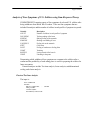
SYSTAT 11
®
Getting Started
®
WWW.SYSTAT.COM
For more information about SYSTAT® software products, please visit our WWW site
at http://www.systat.com or contact
Marketing Department
SYSTAT Software, Inc.
501,Canal Boulevard, Suite E
Pont Richmond, CA 94804-2028
Tel: (800)-797-7401
Fax: (800)-797-7406
Windows is a registered trademark of Microsoft Corporation.
General notice: Other product names mentioned herein are used for identification
purposes only and may be trademarks of their respective companies.
The SOFTWARE and documentation are provided with RESTRICTED RIGHTS. Use,
duplication, or disclosure by the Government is subject to restrictions as set forth in
subdivision (c)(1)(ii) of The Rights in Technical Data and Computer Software clause at
52.227-7013. Contractor/manufacturer is SYSTAT Software, Inc., 501,Canal
Boulevard, Suite E Point Richmond, CA 94804-2028.
SYSTAT® 11 Getting Started
Copyright © 2005 by SYSTAT Software, Inc.
501,Canal Boulevard, Suite E
Point Richmond, CA 94804-2028.
All rights reserved.
Printed in the United States of America.
No part of this publication may be reproduced, stored in a retrieval system, or
transmitted, in any form or by any means, electronic, mechanical, photocopying,
recording, or otherwise, without the prior written permission of the publisher.
1234567890
05 04 03 02 01 00
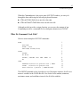
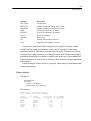
Contents
1 Introducing SYSTAT
1
User Interface . . . . . . . . . . . . . . . . . . . . . . . . . . . . . . . 1
Viewspace . . . . . . . . . . . . . . . . . . . . . . . . . . . . . . . . 2
Workspace . . . . . . . . . . . . . . . . . . . . . . . . . . . . . . . . 6
Commandspace . . . . . . . . . . . . . . . . . . . . . . . . . . . . . . 6
Reorganizing the User Interface . . . . . . . . . . . . . . . . . . . . . 7
Menus. . . . . . . . . . . . . . . . . . . . . . . . . . . . . . . . . . . 8
Dialog Boxes . . . . . . . . . . . . . . . . . . . . . . . . . . . . . . 10
Getting Help . . . . . . . . . . . . . . . . . . . . . . . . . . . . . . 13
2 SYSTAT Basics
19
Starting SYSTAT . . . . . . . . . . . . . . . . . . . . . . . . . . . . 20
Entering Data . . . . . . . . . . . . . . . . . . . . . . . . . . . . . . 21
Using Dialog Boxes . . . . . . . . . . . . . . . . . . . . . . . . 28
Commandspace . . . . . . . . . . . . . . . . . . . . . . . . . . 28
Reading an ASCII Text File . . . . . . . . . . . . . . . . . . . . . . 29
Sorting and Listing the Cases. . . . . . . . . . . . . . . . . . . . . . 34
A Quick Description . . . . . . . . . . . . . . . . . . . . . . . . . . 36
Frequency Counts and Percentages . . . . . . . . . . . . . . . . 36
Descriptive Statistics. . . . . . . . . . . . . . . . . . . . . . . . 40
Statistics By Group . . . . . . . . . . . . . . . . . . . . . . . . 42
A First Look at Relations among Variables . . . . . . . . . . . . . . 43
Subpopulations. . . . . . . . . . . . . . . . . . . . . . . . . . . 46
A Two-Sample t-Test . . . . . . . . . . . . . . . . . . . . . . . 51
A One-Way Analysis of Variance (ANOVA) . . . . . . . . . . . 54
iii
A Two-Way ANOVA with Interaction . . . . . . . . . . . . . . 60
Summary . . . . . . . . . . . . . . . . . . . . . . . . . . . . . 68
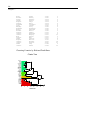
3 Data Analysis Quick Tour
69
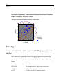
Groundwater Uranium Overview . . . . . . . . . . . . . . . . . . . 69
Potential Analyses. . . . . . . . . . . . . . . . . . . . . . . . . 70
The Groundwater Data File . . . . . . . . . . . . . . . . . . . . 71
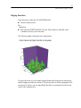
Graphics . . . . . . . . . . . . . . . . . . . . . . . . . . . . . . . . 72
Distribution Plot. . . . . . . . . . . . . . . . . .
Exploring the Groundwater Data Interactively . .
Transformed Graph . . . . . . . . . . . . . . . .
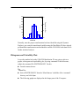
Histograms and Probability Plots . . . . . . . . .
SYSTAT Windows and Commands . . . . . . .
Transforming Data and Selecting Cases . . . . .
Dynamically Highlighted Cases . . . . . . . . .
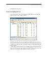
Connections between Graphs and the Data Editor
.
.
.
.
.
.
.
.
.
.
.
.
.
.
.
.
.
.
.
.
.
.
.
.
.
.
.
.
.
.
.
.
.
.
.
.
.
.
.
.
.
.
.
.
.
.
.
.
.
.
.
.
.
.
.
.
.
.
.
.
.
.
.
.
72
73
74
75
76
78
79
79
Statistics . . . . . . . . . . . . . . . . . . . . . . . . . . . . . . . . 80
Graph of Mean Uranium Levels
Output for ANOVA . . . . . . .
Outliers and Diagnostics . . . .
Shapiro-Wilk Test. . . . . . . .
Nonparametric tests . . . . . . .
.
.
.
.
.
.
.
.
.
.
.
.
.
.
.
.
.
.
.
.
.
.
.
.
.
.
.
.
.
.
.
.
.
.
.
.
.
.
.
.
.
.
.
.
.
.
.
.
.
.
.
.
.
.
.
.
.
.
.
.
.
.
.
.
.
.
.
.
.
.
.
.
.
.
.
.
.
.
.
.
.
.
.
.
.
81
82
83
83
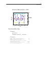
85
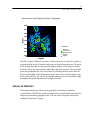
Advanced Graphics . . . . . . . . . . . . . . . . . . . . . . . . . . 86
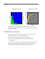
Kriging Smoother . . . . . . . . . . .
Rotation . . . . . . . . . . . . . . . .
Smoothers . . . . . . . . . . . . . . .
Page View . . . . . . . . . . . . . . .
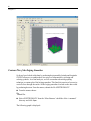
Contour Plot of the Kriging Smoother
.
.
.
.
.
.
.
.
.
.
.
.
.
.
.
.
.
.
.
.
.
.
.
.
.
.
.
.
.
.
.
.
.
.
.
.
.
.
.
.
.
.
.
.
.
.
.
.
.
.
.
.
.
.
.
.
.
.
.
.
.
.
.
.
.
.
.
.
.
.
87
88
88
89
90
Advanced Statistics . . . . . . . . . . . . . . . . . . . . . . . . . . 91
Summary . . . . . . . . . . . . . . . . . . . . . . . . . . . . . . . . 92
References for Groundwater Data . . . . . . . . . . . . . . . . . . . 93
iv
4 Command Language
95
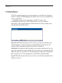
Commandspace . . . . . . . . . . . . . . . . . . . . . . . . . . . . .96
What Do Commands Look Like?.
Interactive Command Entry . . .
Command Files . . . . . . . . . .
Command Log . . . . . . . . . .
Record Script . . . . . . . . . . .
.
.
.
.
.
.
.
.
.
.
.
.
.
.
.
.
.
.
.
.
.
.
.
.
.
.
.
.
.
.
.
.
.
.
.
.
.
.
.
.
.
.
.
.
.
.
.
.
.
.
.
.
.
.
.
.
.
.
.
.
.
.
.
.
.
.
.
.
.
.
.
.
.
.
.
. .97
. .98
. 103
. 105
. 107
Working with DOS Commands . . . . . . . . . . . . . . . . . . . . 108
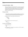
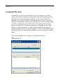
Command File Editor - FEdit . . . . . . . . . . . . . . . . . . . . . 110
To create a new command file . . . . . . . . . . . . . . . . . . 110
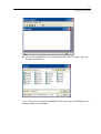
To open a command file . . . . . . . . . . . . . . . . . . . . . 112
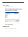
Command Templates . . . . . . . . . . . . . . . . . . . . . . . . . 118
Automatic Token Substitution . . . . . . . . . . . . . . . . . . 120
Interactive Token Substitution . . . . . . . . . . . . . . . . . . 120
Viewing Tokens . . . . . . . . . . . . . . . . . . . . . . . . . 130
Examples . . . . . . . . . . . . . . . . . . . . . . . . . . . . . . . 131
5 Working with Output
145
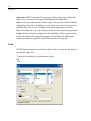
Output Pane . . . . . . . . . . . . . . . . . . . . . . . . . . . . . . 145
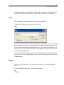
Fonts . . . . . . . . . . . . . .
Find . . . . . . . . . . . . . . .
Replace . . . . . . . . . . . . .
Headers and Footers . . . . . .
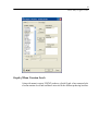
Output Pane Right-Click Menu.
.
.
.
.
.
.
.
.
.
.
.
.
.
.
.
.
.
.
.
.
.
.
.
.
.
.
.
.
.
.
.
.
.
.
.
.
.
.
.
.
.
.
.
.
.
.
.
.
.
.
.
.
.
.
.
.
.
.
.
.
.
.
.
.
.
.
.
.
.
.
.
.
.
.
.
.
.
.
.
.
. 146
. 147
. 147
. 148
. 149
Output Organizer . . . . . . . . . . . . . . . . . . . . . . . . . . . 149
To Move Output Organizer Entries. . . . . . . . . . . . . . . . 151
To Insert Tree Folder . . . . . . . . . . . . . . . . . . . . . . . 151
Configuring the Output Organizer . . . . . . . . . . . . . . . . 151
Saving Output and Graphs. . . . . . . . . . . . . . . . . . . . . . . 153
To Save Output . . . . . . . . . . . . . . . . . . . . . . . . . . 153
v
To Save Results from Statistical Analyses . . . . . . . . . . . . 156
To Save Graphs . . . . . . . . . . . . . . . . . . . . . . . . . . 156
To Export Results to Other Applications . . . . . . . . . . . . . 158
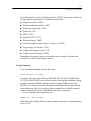
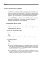
Printing. . . . . . . . . . . . . . . . . . . . . . . . . . . . . . . . . 159
Page Setup. . . . . . . . . . . . . . . . . . . . . . . . . . . . . 159
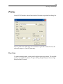
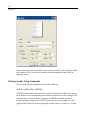
Printing Graphs Using Commands . . . . . . . . . . . . . . . . 160
6 Customization of the SYSTAT Environment
163
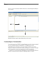
Window and Pane Size . . . . . . . . . . . . . . . . . . . . . . . . 163
Commandspace Customization . . . . . . . . . . . . . . . . . . . . 164
Hiding the Commandspace . . . . . . . . . . . . . . . . . . . . 165
Viewspace Customization . . . . . . . . . . . . . . . . . . . . . . . 165
Maximizing the Viewspace . . . . . . . . . . . . . . . . . . . . 166
Status Bar . . . . . . . . . . . . . . . . . . . . . . . . . . . . . . . 166
Menu Customization . . . . . . . . . . . . . . . . . . . . . . . . . . 167
Commands . . . . . . . . . . . .
Commands Customization . . . .
Button Customization . . . . . . .
Toolbars . . . . . . . . . . . . . .
Toolbar Customization . . . . . .
Keyboard Shortcuts . . . . . . . .
Keyboard Shortcut Customization
Menu . . . . . . . . . . . . . . .
.
.
.
.
.
.
.
.
.
.
.
.
.
.
.
.
.
.
.
.
.
.
.
.
.
.
.
.
.
.
.
.
.
.
.
.
.
.
.
.
.
.
.
.
.
.
.
.
.
.
.
.
.
.
.
.
.
.
.
.
.
.
.
.
.
.
.
.
.
.
.
.
.
.
.
.
.
.
.
.
.
.
.
.
.
.
.
.
.
.
.
.
.
.
.
.
.
.
.
.
.
.
.
.
.
.
.
.
.
.
.
.
.
.
.
.
.
.
.
.
. 167
. 168
. 171
. 172
. 173
. 175
. 177
. 178
Command File Lists . . . . . . . . . . . . . . . . . . . . . . . . . . 180
Submission From File Lists . . . . . . . . . . . . . . . . . . . . 181
Dialog Recall . . . . . . . . . . . . . . . . . . . . . . . . . . . 182
User Menus . . . . . . . . . . . . . . . . . . . . . . . . . . . . . . 183
Global Options . . . . . . . . . . . . . . . . . . . . . . . . . . . . . 185
General Options . .
Output Options . .
File Locations . . .
Using Commands .
.
.
.
.
.
.
.
.
.
.
.
.
.
.
.
.
.
.
.
.
.
.
.
.
vi
.
.
.
.
.
.
.
.
.
.
.
.
.
.
.
.
.
.
.
.
.
.
.
.
.
.
.
.
.
.
.
.
.
.
.
.
.
.
.
.
.
.
.
.
.
.
.
.
.
.
.
.
.
.
.
.
.
.
.
.
.
.
.
.
.
.
.
.
. 186
. 188
. 189
. 192
7 Applications
193
Anthropology . . . . . . . . . . . . . . . . . . . . . . . . . . . . . 194
Egyptian Skulls Data . . . . . . . . . . . . . . . . . . . . . . . 194
Astronomy . . . . . . . . . . . . . . . . . . . . . . . . . . . . . . . 196
Biology . . . . . . . . . . . . . . . . . . . . . . . . . . . . . . . . 197
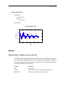
Mortality Rates of Mediterranean Fruit Flies. . . . . . . . . . . 197
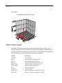
Animal Predatory Danger. . . . . . . . . . . . . . . . . . . . . 200
Chemistry . . . . . . . . . . . . . . . . . . . . . . . . . . . . . . . 202
Enzyme Reaction Velocity . . . . . . . . . . . . . . . . . . . . 202
Engineering . . . . . . . . . . . . . . . . . . . . . . . . . . . . . . 206
Robust Design - Design of Experiments . . . . . . . . . . . . . 206
Environmental Science . . . . . . . . . . . . . . . . . . . . . . . . 213
Mercury Levels in Freshwater Fish. . . . . . . . . . . . . . . . 213
Genetics . . . . . . . . . . . . . . . . . . . . . . . . . . . . . . . . 216
Bayesian Estimation of Gene Frequency . . . . . . . . . . . . . 216
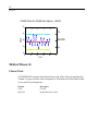
Manufacturing . . . . . . . . . . . . . . . . . . . . . . . . . . . . . 220
Quality Control . . . . . . . . . . . . . . . . . . . . . . . . . . 220
Medical Research . . . . . . . . . . . . . . . . . . . . . . . . . . . 222
Clinical Trials. . . . . . . . . . . . . . . . . . . . . . . . . . . 222
Psychology . . . . . . . . . . . . . . . . . . . . . . . . . . . . . . 235
Day Care Effects on Child Development. . . . . . . . . . . . . 235
Analysis of Fear Symptoms of U.S. Soldiers using
Item-Response Theory . . . . . . . . . . . . . . . . . . . . . . 241
Sociology . . . . . . . . . . . . . . . . . . . . . . . . . . . . . . . 244
World Population Characteristics. . . . . . . . . . . . . . . . . 244
Statistics . . . . . . . . . . . . . . . . . . . . . . . . . . . . . . . . 248
Instructional Methods. . . . . . . . . . . . . . . . . . . . . . . 248
Toxicology. . . . . . . . . . . . . . . . . . . . . . . . . . . . . . . 250
Concentration of nicotine sulfate required to
kill 50% of a group of common fruit flies . . . . . . . . . . . . 250
Data References . . . . . . . . . . . . . . . . . . . . . . . . . . . . 254
Anthropology Data Sources . . . . . . . . . . . . . . . . . . . 254
vii
Astronomy Data Source. . . . . .
Biology Data Source . . . . . . .
Biology Data Source . . . . . . .
Chemistry Data Sources. . . . . .
Engineering Reference . . . . . .
Environmental Science Sources. .
Manufacturing Data Sources . . .
Medicine Data Sources . . . . . .
Medical Research Data Reference
Psychology Data Reference . . . .
Psychology Data Reference . . . .
Sociology Data Reference . . . .
Statistics Data Sources . . . . . .
Toxicology Data Source . . . . .
Data Files
.
.
.
.
.
.
.
.
.
.
.
.
.
.
.
.
.
.
.
.
.
.
.
.
.
.
.
.
.
.
.
.
.
.
.
.
.
.
.
.
.
.
.
.
.
.
.
.
.
.
.
.
.
.
.
.
.
.
.
.
.
.
.
.
.
.
.
.
.
.
.
.
.
.
.
.
.
.
.
.
.
.
.
.
.
.
.
.
.
.
.
.
.
.
.
.
.
.
.
.
.
.
.
.
.
.
.
.
.
.
.
.
.
.
.
.
.
.
.
.
.
.
.
.
.
.
.
.
.
.
.
.
.
.
.
.
.
.
.
.
.
.
.
.
.
.
.
.
.
.
.
.
.
.
.
.
.
.
.
.
.
.
.
.
.
.
.
.
.
.
.
.
.
.
.
.
.
.
.
.
.
.
.
.
.
.
.
.
.
.
.
.
.
.
.
.
.
.
.
.
.
.
.
.
.
.
.
.
.
.
. 255
. 255
. 255
. 255
. 255
. 256
. 256
. 256
. 256
. 256
. 256
. 257
. 257
. 257
259
References . . . . . . . . . . . . . . . . . . . . . . . . . . . . . . . 284
Index
289
viii
Chapter
Introducing SYSTAT
1
Keith Kroeger
(revised by Rajashree Kamath)
SYSTAT provides a powerful statistical and graphical analysis system in a graphical
environment using descriptive menus and simple dialog boxes. Most tasks can be
accomplished simply by pointing and clicking the mouse.
This chapter provides an overview of the windows, menus, dialog boxes, and
online Help available in SYSTAT. For information on using SYSTAT's command
language, see Chapter 4.
User Interface
The user interface of SYSTAT is organized into three spaces:
Viewspace
Workspace
Commandspace
Each space in turn consists of panes with associated tabs and allows you to
accomplish specific tasks. One space and one pane within it will always be active. All
menu selections and editing apply only to this pane. To make a pane or tab active,
click it with the mouse, or select its name from the View menu. The user interface
provides menus for running statistical analyses and producing graphs. It also contains
toolbars to provide quick access to many standard statistical techniques and graphs.
1
2
Chapter 1
Viewspace
The Viewspace consists of three panes:
Output Pane
Data Editor
Graph Editor
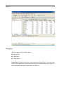
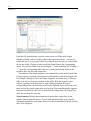
Output Pane. Graphs and statistical results appear in the Output Pane. You can perform
some of the Output Pane-related operations using the Format toolbar in this pane. For
more information about the Output Pane, see Chapter 5.
3
Introducing SYSTAT
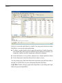
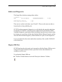
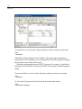
Data Editor. The Data Editor displays your data in a row-by-column format.
4
Chapter 1
Each row is a case and each column is a variable. You can type new data into an empty
Data Editor, or you can edit and transform data.
To define a variable, double-click (or right-click and choose Variable Properties)
on a variable name, which opens the Variable Properties dialog box and allows you
to name the variable, select the variable type, and specify comments.
Use the Edit menu to cut, copy, delete, and paste rows, columns, and blocks of data.
Use the Data menu to transform data and select subsets of cases.
You can perform some of the Data Editor-related operations using the Data toolbar in
this pane. See SYSTAT Data for more information about the Data Editor.
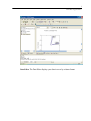
Graph Editor. Double-clicking a graph in the Output Pane or just clicking the Graph
Editor tab opens the Graph Editor.
5
Introducing SYSTAT
Use the Graph Editor toolbar and menus to edit graphs. You can:
Insert annotations and other text.
Change font, color, and line attributes.
Rescale axes.
Modify plot symbols.
Customize labels.
Edit legends.
Identify individual points in scatterplots.
Select a subset of cases using the Rectangular or Lasso tool.
You can perform many of the Graph Editor-related operations using the Graph Editing
toolbar in this pane. See SYSTAT Graphics for more information about the Graph
Editor.
6
Chapter 1
Workspace
The Workspace consists of two tabs:
Output Organizer
Dynamic Explorer
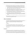
Output Organizer. Use the Output Organizer primarily to navigate through the results
of your statistical analysis. Selecting a completed procedure from the outline displays
the corresponding results in the Output Pane. You can also use the Output Organizer to
select an item, and then copy, paste, delete, or move it, allowing you to tailor SYSTAT's
output to your preferences. In addition, you can quickly move to specific portions of
output without having to use the Output Pane scrollbars.
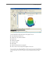
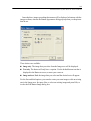
Dynamic Explorer. The Dynamic Explorer becomes active only when there is a graph
in the Graph Editor, and the Graph Editor is active. Use the Dynamic Explorer to:
Rotate and animate 3-D graphs.
Apply power transformations to values on one or more axes.
Change the confidence level for confidence intervals, ellipses, and kernels in
scatter plots.
Tune tension for smoothers.
Change the number of bars for density displays.
Zoom the graph in the direction of any of the axes.
Commandspace
The Commandspace has three tabs:
Interactive
Untitled
Log
Interactive. Selecting the Interactive tab enables you to enter commands in the
interactive mode, which issues the command after you press the Enter key. You can
save the contents of the interactive tab (excluding the > prompts) and then use the file
to submit a sequence of commands.
7
Introducing SYSTAT
Untitled. Selecting the Untitled tab enables you to work with command files in the
batch mode. You can open, edit, or submit an existing command file, whose name
replaces 'Untitled' on the tab. You could also type in an entire command file and then
save or submit it.
Log. Selecting the Log tab enables you to examine the read-only log of the commands
that you have run during your session.
Reorganizing the User Interface
The Workspace, Viewspace and Commandspace can be resized if desired. To do so:
Drag the boundaries of the panes (between Viewspace and Workspace, Workspace
and Commandspace, and Viewspace and Commandspace) in the desired direction.
You can also reposition the panes. For this:
Click the upper boundaries of the panes and drag the resulting outline to the new
position. As you drag the outline, the border thins to indicate that the item will be
docked to the main window at that location. To prevent docking, drag the item off
the main window or hold down the Ctrl key as you drag. Double-clicking the upper
boundary can undock docked items. Undocking items enlarges the remaining
panes but can result in a cluttered desktop.
The Data Editor and Graph Editor can be interchanged between the Workspace and
Viewspace by double-clicking the tab or right-clicking and selecting 'Move Tab'. The
advantage in this is that you can view any two of the tabs simultaneously.
Every toolbar except those in the tabs of the Viewspace can be repositioned by
clicking and dragging the move handle ( ). Toolbars can also be dragged and docked
to the boundary between the Viewspace and Workspace. The Output Pane, Data Editor
and Graph Editor toolbars can be toggled on and off, by right-clicking on the tabs and
selecting Show Toolbar.
You can also close spaces and toolbars. To do so:
undock them and click (
) in the upper right corner, or deselect their entry on
the View menu. Closed items can be reopened only via the View menu or by
keyboard. Keyboard short cuts are explained in Chapter 6.
8
Chapter 1
Menus
SYSTAT has a common menu bar for all the panes and tabs. There are menus for
opening, saving, and printing files, editing output, transforming data, matrix
manipulation, generating experimental designs and random samples, performing
statistical analyses, and creating graphs. At any given point of time, those menu items
that are relevant to the active pane or tab are enabled. The menu can be customized
using the Customize dialog from the View menu.
File. Use the File menu to create or open data, command and output files, save the
contents of the active pane, all panes and newly created data files, and import from
databases. The data file formats supported include SYSTAT, Excel, SPSS, SAS,
BMDP, MINITAB, S-PLUS, Statistica, Stata, JMP and ASCII files. You can submit
commands from the clipboard or from a command file. You can save output in the
SYSTAT format, or in Rich text and HTML formats. You can also preview and print
the content of the Output Pane, Data Editor, and Graph Editor. Graphs can be reviewed
using the Page Mode under the View menu. When the Graph Editor is active, you can
also export and print graphs. You can export graphs in a variety of formats including
WMF, PS, EPS, BMP, JPEG, GIF, TIFF, PNG, PCT and CGM.
Recent data, commands, and output files can be opened under the File menu.
Edit. Use the Edit menu to paste clipboard content to the active pane, change SYSTAT
options including variable display order in dialog boxes, the algorithm to be used for
random number generation, the behavior of the Enter key in the Data Editor, font
characteristics for output, data and graphs, display of statistical Quick Graphs,
inclusion of command syntax in the output, and measurement units for graphs,
reduction or enlargement of graphs, and file locations.
Output Pane. In addition to the above options, when the Output Pane is active, you
can cut, copy, and paste statistical output and other text from and into the Output
Pane, find and replace text strings, clear text and output, insert page breaks, notes
and titles into your output, and change font characteristics (including color and
size).
Data Editor. When the Data Editor is active, you can also cut, copy and paste data
from and into the Data Editor, insert cases and variables, find a specific case or
variable, and go to a desired cell in the worksheet.
Graph Editor. When the Graph Editor is active, you can also copy graphs, change
text tool font characteristics (including color and size), and change drawing
attributes.
9
Introducing SYSTAT
Output Organizer. When the Output Organizer is active, you can also cut, copy,
paste and insert tree folders, and expand and collapse trees.
View. Use the View menu to view or hide the Workspace, Viewspace, Commandspace,
toolbars and status bar, make tabs active, and launch a full screen view of the
Viewspace. This menu also allows you to create and customize toolbars, and create
shortcuts to command files. When the Output Pane is active, you can also view and edit
headers and footers, and view graphs as frames only. When the Graph Editor is active,
use the View menu to switch between the graph view and page view, and turn the
display of rulers and graph tooltips on and off.
Data. Use the Data menu to transform data values, sort cases in the data file based on
the values of one or more variables, transpose cases (rows) and variables (columns),
merge data files, select subsets of cases and specify grouping variables that split the
data file into two or more groups for analysis, and weight data for analysis based on
the value of a weight variable. When the Data Editor is active, you can also define
variable properties, and fill the worksheet to a desired number of rows.
Graph. Use the Graph menu to access the Graph Gallery and to create box plots,
histograms, scatterplots, 3-D data plots, function plots, and other graphical displays.
You can also overlap various graphs in a single frame. When the Graph Editor is active
with a graph in it, you can change the labels of scale ranges on the graph's axes, control
display of tick marks, change colors and fill patterns for the graph's elements, change
style and size of plot symbols, transpose axes, edit graph titles and legends, resize
graphs, reposition graphs on the page, and change between the available summary
chart types.
Utilities. Use the Utilities menu to retrieve data file information and current SYSTAT
settings, launch the command file editor - FEdit, record command scripts generated by
actions of the user and play them, create customized menus, access SYSTAT's BASIC
and Matrix procedures, perform calculations involving functions available in SYSTAT
(including probability calculations), power analysis, and generate a variety of
experimental designs.
Monte Carlo. Use the Monte Carlo menu to generate random samples from a variety
of univariate and multivariate distributions, generate IID Monte Carlo random samples
using rejection and adaptive rejection methods, generate Markov chain Monte Carlo
random samples using the Metropolis-Hastings algorithm and Gibbs sampling method,
and perform Monte Carlo integration.
10
Chapter 1
Analysis. Use the Analysis menu to run statistical procedures including descriptive
statistics, correlation, missing value analysis, fitting distributions, linear and robust
regression methods, hypothesis testing, analysis of variance, multivariate analysis,
quality analysis, nonparametric smoothing and testing, plotting and transforming time
series, spatial statistics, survival analysis and many others.
Help. Use the Help menu to access SYSTAT’s online Help system, update the license
for running SYSTAT beyond the specified period, check for updates to the current
version of SYSTAT, and display the copyright, version number and license information
of your copy of SYSTAT.
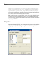
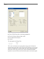
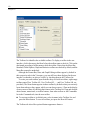
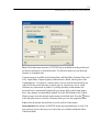
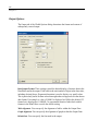
Dialog Boxes
Most menu selections in SYSTAT open dialog boxes, which you use to select variables
and options for analysis. Each dialog box may have several basic components in
separate tabs.
11
Introducing SYSTAT
Tabs. Since many SYSTAT commands provide a great deal of flexibility, not all of the
possible choices can be contained in a single dialog box. The main dialog box usually
contains the minimum information required to run a command. Additional
specifications are made in tabs. You can make a tab active by clicking it with the
mouse. Certain tabs require some input to be given in other tabs before they get
enabled. A tab may get disabled if its contents are irrelevant for the existing selections.
Command pushbuttons. Buttons that instruct SYSTAT to perform an action.
Runs the procedure for the selections you have made. This does not get
enabled in some dialog boxes unless the minimum required input is given.
Cancels the procedure. Any selections you may have made will be
discarded.
Displays help related to the dialog box. If a dialog box has more than one tab,
you will get help related to the active tab.
Resets the selections in the dialog box or active tab, to the defaults.
Resets the selections for all tabs in the dialog box.
Source variable list. A list of variables in the working data file. Only variable types
allowed by the selected command are displayed in the source list.
Target variable list(s). One or more lists, such as dependent and independent variable
lists, indicating the variables you have chosen for the analysis. If an analysis
compulsorily requires you to choose variables here, you will see '<Required>' in the
list. If a list is empty, all variables in the source list will be used for the analysis.
Special lists. Some dialog boxes display lists with multiple columns, where you can
input as many rows of input as you desire. Such lists can be customized using the four
buttons:
Insert a new row by pressing the
Delete a row by pressing the
Move a row up by pressing the
Move a row down by pressing the
icon.
icon.
icon.
icon.
Pushbuttons. Dialog boxes contain pushbuttons for performing the following tasks:
Add one or more variables to the desired target list by selecting them and then
pressing the corresponding
button.
12
Chapter 1
Remove one or more variables from a target list by selecting them and then
pressing the corresponding
button.
'Cross' a variable in the source list with one in the target list by selecting them and
then pressing the
button. You can also add crossed terms of multiple
variables directly by selecting these variables in the source list and pressing the
Cross button.
Use the
when you want to include the variables as well as all their crossed
terms. You can also use this button with multiple variables.
Use the
button to include nested terms in the target list.
Selecting variables. To add a single variable to the desired target list, you simply
highlight it on the source variable list and click the Add button. Use the Remove button
to undo your selection. You can also double-click individual variables to move them
from the source list to the target list, or vice versa. When there are more than one target
lists, this functionality will apply to one of them.
You can also select multiple variables:
To highlight multiple variables that are grouped together on the variable list, click
and drag the mouse cursor over the variables you want. Alternatively, you can click
the first one and then Shift-click the last one in the group.
To highlight multiple variables that are not grouped together on the variable list,
use the Ctrl-click method. Click the first variable, and then Ctrl-click the other
variables that you want. Avoid the name area while clicking and dragging.
You can also right-click on a variable or a highlighted set of variables and use the menu
that pops-up to add them to the desired target list, or remove them from the list.
Additional Features. Several additional features have been provided for the dialog
boxes. They are:
Keyboard shortcuts as an alternative to checkboxes and radiobuttons. Hold down
the Alt key and press the underlined letter in the caption.
The Tab key to navigate between items.
For an editbox taking numeric values, tooltips indicating the valid range, displayed
while hovering the mouse on the editbox.
Editboxes taking integer values not accepting the decimal separator as input.
Editboxes taking nonnegative values not accepting negative (-) sign as input.
13
Introducing SYSTAT
Editboxes to contain filenames of files to be opened or saved, for features that
require or support such options. Type the desired filename (with path), or press the
button and select a file.
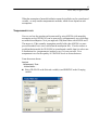
Getting Help
SYSTAT uses the standard HTML Help system to provide information you need to use
SYSTAT and to understand the results. This section contains a brief description of the
Help system and the kinds of help provided with SYSTAT.
The best way to find out more about the Help system is to use it. You can ask for
help in any of these ways:
Click the
button in a SYSTAT dialog box. This takes you directly to a topic
describing the use of the dialog box. This is the fastest way to learn how to use a
dialog box.
Right-click on any dialog box item, and select 'What's this?' to get help on that
particular item.
Hover the mouse on a menu item that would have opened a dialog box and press
F1 to get help on that particular dialog box.
Select Contents or Search from the Help menu.
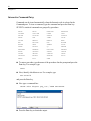
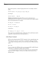
For help on commands, from the command prompt (on the Interactive tab of the
Commandspace) type:
HELP [command name]
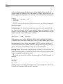
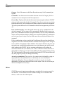
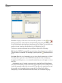
Navigating the Help System
The SYSTAT Help system has the following tabs:
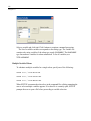
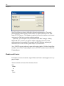
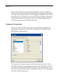
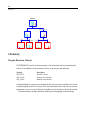
Contents. The Contents button takes you to the table of contents of the Help
system. Double-click book icons
in the Index listing to view the contents of
that section. Selecting a topic with a page icon
opens the associated Help topic.
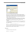
Index. Provides a searchable index of Help topics. Enter the first few letters of the
term you want to find and then double-click the topic in the list (or click and press
the Display button) to view it.
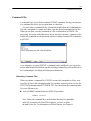
Search. Offers a full-text search of the Help system. Type the desired keyword and
press the Enter key or the List Topics button. The Help system returns all topics
14
Chapter 1
containing the specified term. Double-click the desired topic in the list (or click and
press the Display button) to view it.
The following buttons are available in the Help system:
Hide/Show. Hides or shows the Contents, Index and Search tabs.
Back. Returns to the previous Help topic.
Forward. Moves to the next Help topic, if you had pressed the Back button
previously.
Print. Prints the current topic or all sub-topics under the current heading.
Options. Enables you to stop loading a page, refresh a page, access the Windows
Internet Options settings and choose whether search keywords should be
highlighted in the listed pages or not.
Depending on the topic displayed, the following buttons may appear in the current
Help page:
How To. Provides minimum specifications for performing the analysis.
Syntax. Describes the associated SYSTAT command. SYSTAT's command
language offers some features not available in the dialog boxes.
Examples. Offers examples of analyses, including SYSTAT command input and
resulting output. Copy and paste the example input to the middle tab of the
Commandspace to submit the example as is, or modify the commands to your own
analyses before submitting them. Make sure the file paths match the file locations
you have opted for.
More. Lists analysis options and related tabs. These topics are particularly useful
for customizing your analyses.
See Also. Lists related procedures or graphs.
You can select, cut, copy, paste and print the content of any Help page.
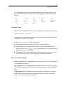
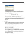
Examples
Often, the best way to learn about a procedure is through examples. The Help system
provides several examples for each statistical procedure or graph. Select the example
most relevant to your analysis or browse the examples to explore SYSTAT's
capabilities.
15
Introducing SYSTAT
The examples include all SYSTAT input. You can copy and paste the example input
(also available as files in the 'Command' folder of the SYSTAT directory) to the middle
tab of the Commandspace to submit the example as is, or you can modify the
commands to reflect your own analyses before submitting them.
The resulting output, including graphical results, follows the command input. Many
of the examples include Discussion buttons throughout the output. Pressing any of these
buttons yields a detailed explanation of the immediately preceding output. There may
also be examples that are explained in more than one step, in which case More or Next
buttons will be included in the page.
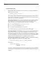
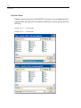
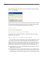
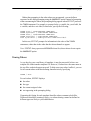
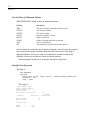
Example Command Files. The input commands for each example in the User Manual
or in the Help system are available as command files in the “Command” folder of the
SYSTAT directory. This provides an alternative way to run the examples. These files
are organized in terms of the printed manual. Each file contains commands for one
example and is named using six characters (xxyyzz.syc). The first two characters
represent the corresponding volume of the printed manual as follows:
'da' for Data (called 'Data Volume' in the Command folder)
16
Chapter 1
'gs' for Getting Started
'gr' for Graphics
's1' for Statistics I
's2' for Statistics II
's3' for Statistics III
The next two digits represent the chapter number within the volume, and the last two
digits represent the example number within the chapter. These files are organized in the
'Command' folder with eight subfolders, six of them corresponding to the six volumes
mentioned above, a 'GraphDemo' subfolder and a 'Miscellaneous' one which contains
commands of examples which are not numbered. The names of files in the
'Miscellaneous' folder are indicative of the examples they relate to. For example, to
execute the commands given in Example 1 in Chapter 2 of Statistics III, submit the
's30201.syc' file. (Depending on your file location, you may have to define paths for
files and rename them appropriately.)
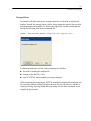
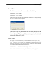
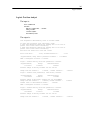
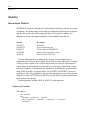
Glossary
The glossary offers an alphabetical listing of terms commonly encountered in
statistical analyses. The buttons at the top of the glossary scroll the window to the
corresponding letter. Clicking a glossary entry reveals the definition for that term. Use
the
to navigate to the top of the glossary page.
17
Introducing SYSTAT
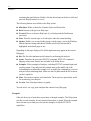
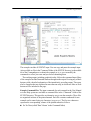
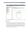
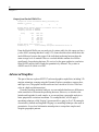
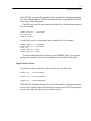
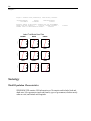
Application Gallery
In addition to examples of each procedure, SYSTAT includes examples drawn from
several fields of research. Chapter 7 provides a brief introduction to each application.
You can access the complete applications from the Contents tab of the Help system.
Double-click the Applications book icon and select Application Gallery. The available
applications are listed with icons and a brief description. Clicking on any icon will
open a page containing the detailed description, and buttons for the main Application
Gallery page, Analyses page, and Sources page.
Chapter
2
SYSTAT Basics
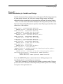
This chapter provides simple step-by-step instructions for performing basic analysis
tasks in SYSTAT, including:
Starting SYSTAT.
Entering data in the Data Editor.
Opening and saving data files.
Using menus and dialog boxes to create charts and run statistical analyses.
19
20
Chapter 2
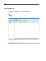
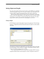
Starting SYSTAT
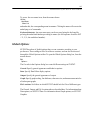
To start SYSTAT for Windows NT4, 98, 2000, ME, and XP:
Choose:
Start
Programs
Systat 11
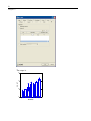
Systat 11
21
SYSTAT Basics
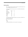
Entering Data
This section discusses how to enter data. If you prefer to start with data stored in a text
file, see “Reading an ASCII Text File” on p. 29.
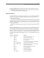
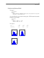
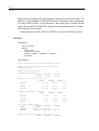
In the frozen-food section of the grocery store, we recorded this information about
seven dinners:
Brand$
Lean Cuisine
Weight Watchers
Healthy Choice
Stouffer
Gourmet
Tyson
Swanson
Calories
Fat
240
220
250
370
440
330
300
5
6
3
19
26
14
12
To enter these data into SYSTAT’s Data Editor, first save them in a SYSTAT file. To
plot them, follow these steps:
From the menus choose:
File
New
Data
This opens the Data Editor (or clears its contents if it is already open).
22
Chapter 2
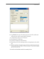
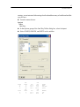
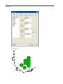
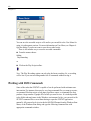
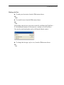
Double-click (VAR00001) to open the Variable Properties dialog box.
23
SYSTAT Basics
Type BRAND$ for the name. The dollar sign ($) at the end of the variable name
indicates that the variable contains character information.
Note: Variable names cannot exceed 12 characters.
Select String as the Variable type.
Click OK to complete the variable definition.
Repeat this process for the remaining variables, selecting Numeric as the variable
type.
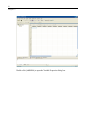
Click the top left data cell (under the name of the first variable) and enter the data.
To move across rows, press Enter or Tab after each entry. To move down columns,
press the down arrow key.
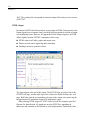
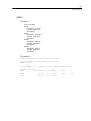
The data file in the Data Editor should look something like this:
24
Chapter 2
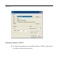
When you have finished entering the data, from the menus choose:
File
Save As...
Type SAMPLE as the name for the data file. SYSTAT adds the suffix .SYD
(SAMPLE.SYD).
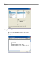
Then, from the menus choose:
Graph
Plots
Scatterplot...
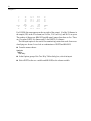
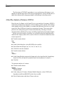
In the Scatterplot dialog box, select FAT as the X-variable and CALORIES as the
Y-variable.
25
SYSTAT Basics
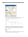
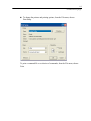
Click the Symbol and Label tab in the Scatterplot dialog box. Then, select Display
case labels in the Case Labels group, and select BRAND$ to label each plot point
with the brand of the dinner.
26
Chapter 2
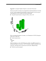
Click OK to run the command.
27
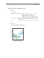
SYSTAT Basics
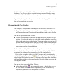
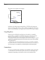
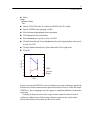
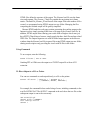
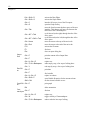
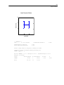
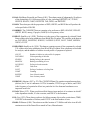
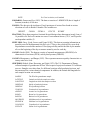
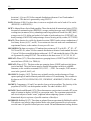
The plot is displayed in the Output Pane of the Viewspace.
500
CALORIES
Gourmet
400
Stouffer
Tyson
300
Swanson
Healthy Choi
Lean Cuisine
200
0
Weight Watch
10
20
30
FAT
Notice that the three dinners from the diet shelf fall at the lower left corner and have
fewer calories and less fat.
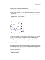
You can edit the graph after you create it.
Double-click the graph, or click on the Graph Editor tab, or double click on the tree
formed in the Output Organizer tab of the Workspace to display it in the Graph
Editor.
From the menus choose:
Graph
Options
Appearance...
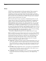
On the Fill tab, select a solid fill pattern.
On the Symbol and Label tab, change the symbol from a circle to a triangle and
increase the size of case labels to 1.5.
Click OK.
28
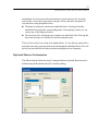
Chapter 2
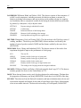
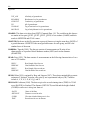
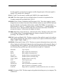
The symbols on your graph are now changed.
500
CALORIES
Gourmet
400
Stouffer
300
Tyson
Swanson
200
0
Healthy Cho
Weight
Watc
Lean
Cuisine
10
20
30
FAT
In addition to the editing options mentioned above, SYSTAT provides many more
features for editing graphs which are readily available on the right-click of the mouse
button. For more information, see Chapters 9 and 10 of the SYSTAT Graphics manual.
Using Dialog Boxes
Each time you use a dialog box to perform a step in an analysis, a command is
generated. These “commands” are SYSTAT’s instructions to perform the analysis.
Instead of using dialog boxes to generate these commands, you can use the
Commandspace and type them yourself. Whether generated by the dialog box or typed
manually, the commands from each SYSTAT session can be saved in a file, modified,
and resubmitted later.
Although many users will use dialog boxes exclusively, we introduce commands
here briefly to show how commands succinctly document the steps in your analysis. If
you do not expect to use commands, you should skip the sections showing them.
Commandspace
You can type commands in the Commandspace of the SYSTAT window at the prompt
(>) on the Interactive tab. When the Log tab is selected in the Commandspace, the
commands corresponding to your dialog box choices are also displayed in the
29
SYSTAT Basics
Commandspace. For example, the following command was generated by the
Scatterplot dialog box selections:
As you make dialog box selections, SYSTAT generates and stores the corresponding
commands. To recall previously run commands, click the Interactive tab in the
Commandspace and press F9.
Reading an ASCII Text File
This section shows you how SYSTAT reads raw (ASCII) data files created in a text
editor or word processor. SYSTAT can import ASCII files of the type .txt,.dat and .csv.
Each example shows the commands that you would see with the command prompt on;
for these examples, we need more than seven cases.
For SYSTAT to read an ASCII file, it cannot contain any unusual ASCII characters.
The file can contain no page breaks, control characters, column markers, or similar
formatting codes. SYSTAT can read alphanumeric characters, delimiters (spaces,
commas, or tabs that separate consecutive values from each other), and carriage
returns. See your word processor’s documentation to find out how to save data as an
ASCII text file.
Make sure that your text file satisfies the following criteria:
Each case begins on a new line (to read ASCII files with two or more lines of data
per case, use the BASIC procedure).
Missing data are flagged with an appropriate code.
30
Chapter 2
Imagine that someone used a text editor to enter 10 pieces of information (variables)
about 28 frozen dinners:
BRAND$
FOOD$
CALORIES
FAT
PROTEIN
VITAMINA
CALCIUM
IRON
COST
DIET$
Short names for brands
Words to identify each dinner as chicken, pasta, or beef
Calories per serving
Total fat in grams
Protein in grams
Vitamin A, percentage daily value
Calcium, percentage daily value
Iron, percentage daily value
Price per dinner in U.S. dollars
Yes, the dinner was shelved with dinners touted as “diet” or low in
calories; no, it was shelved with regular dinners
In a text editor, the data look similar to the following:
brand$ food$
lc
lc
lc
lc
lc
ww
ww
ww
hc
hc
ww
hc
ww
st
st
st
st
gor
gor
gor
chicken
chicken
chicken
pasta
pasta
chicken
pasta
pasta
chicken
chicken
chicken
pasta
chicken
beef
beef
chicken
chicken
beef
pasta
pasta
calories
fat
270
240
240
260
210
260
220
220
200
280
160
250
190
390
370
320
330
290
370
440
6
5
5
8
4
4
4
6
2
3
1
3
0
24
19
10
16
8
16
26
protein vitamina calcium
22
19
18
15
9
21
14
15
17
24
13
20
12
20
24
27
18
18
20
20
6
30
4
20
30
30
15
6
0
15
30
0
10
2
2
10
2
15
30
100
10
10
10
30
10
4
8
25
2
4
2
8
4
4
20
15
2
4
40
35
iron
cost
diet
6
10
8
8
8
15
15
15
2
15
2
8
4
15
15
8
4
10
4
10
2.99
2.99
2.99
2.15
2.15
2.79
2.79
2.79
2.00
2.00
2.49
2.00
2.49
2.99
2.99
2.69
2.99
1.75
1.99
1.75
yes
yes
yes
yes
yes
yes
yes
yes
yes
yes
yes
yes
yes
no
no
no
no
no
no
no
31
SYSTAT Basics
brand$ food$
gor
ty
ty
ty
ty
sw
sw
sw
beef
beef
chicken
chicken
chicken
chicken
beef
pasta
calories
fat
300
330
400
340
430
550
330
300
34
14
8
7
24
25
9
12
protein vitamina calcium iron
22
24
27
31
20
22
25
14
15
8
25
70
45
0
10
0
10
10
0
0
4
6
2
25
20
10
10
15
6
15
25
10
cost
diet
1.75
3.00
3.50
3.50
3.00
2.25
2.85
1.60
no
no
no
no
no
no
no
no
The first line contains names for the columns. SYSTAT will count these names (finding
10), and read 10 values for each case (dinner). We name this ASCII file FOOD.DAT.
Let us read the FOOD.DAT file and convert it to a SYSTAT file called FOOD.SYD.
From the menus choose:
File
Open
Data...
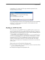
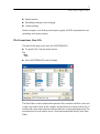
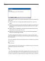
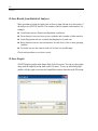
In the Open File dialog box, select All Files from the drop-down list of file types,
select FOOD.DAT from the Data directory of the SYSTAT folder, and click OK.
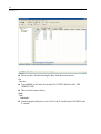
The contents of the data file are displayed in the Data Editor.
From the menus choose:
File
Save As...
Type FOOD for the filename in the Save dialog box and click OK.
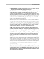
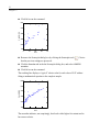
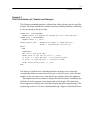
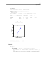
Scatterplots provide a visual impression of the relation between two quantitative
variables. Let us plot CALORIES versus FAT for this larger sample.
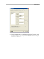
From the menus choose:
Graph
Plots
Scatterplot...
In the Scatterplot dialog box, select FAT as the X-variable and CALORIES as the
Y-variable.
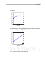
Click the Fill tab in the Scatterplot dialog box and select a solid fill for the first fill
pattern.
32
Chapter 2
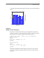
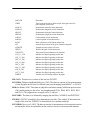
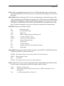
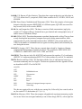
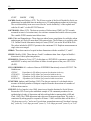
Click OK to run the command.
600
CALORIES
500
400
300
200
100
0
10
20
FAT
30
40
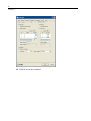
Return to the Scatterplot dialog box by clicking the Scatterplot tool (
that the previous settings are preserved.
). Notice
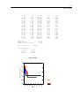
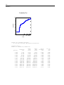
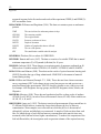
Click the Smoother tab in the the Scatterplot dialog box, and select LOWESS
smoother.
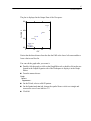
Click OK to run the command.
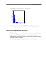
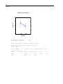
The resulting line displays a “typical” calorie value for each value of FAT without
fitting a mathematical equation to the complete sample.
600
CALORIES
500
400
300
200
100
0
10
20
FAT
30
40
The smoother indicates, not surprisingly, that foods with a higher fat content tend to
have more calories.
33
SYSTAT Basics
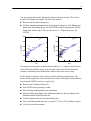
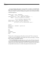
You may wonder what foods and what brands have the most calories? The fewest
calories? The highest fat content? The lowest fat content?
Return to the Scatterplot dialog box.
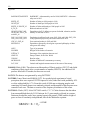
Click the Symbols and Labels tab in the Scatterplot dialog box, click Display case
labels in the Case Labels group, select BRAND$ to label each plot point with the
brand of the dinner, and set the case label size to 1.3. Repeat these steps for
FOOD$.
600
600
sw
chicken
500
ty gor
400
300
200
ty
gor st
sw
ty
st ty st
sw
ww gor
hc
lc lc
hc lc lc
hc
ww
ww
lc ww
ww
100
0
10
20
FAT
CALORIES
CALORIES
500
st
gor
30
40
400 chicken
pastabeef
chicken
beef chicken
beef
pasta
300 chicken
chicken
chicken
beef pasta
chicken
chicken
pasta
pasta
chicken
pasta
chicken
200 chicken
pasta
chicken
100
0
10
20
FAT
pasta
chicken
beef
beef
30
40
The top point in each plot is a chicken dinner made by sw—it must be fried chicken.
Notice that the beef dinner by gor at the far right (close to the 300 calorie mark)
contains considerably more fat than other dinners in the same calorie range.
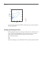
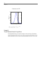
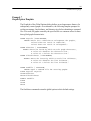
Do diet dinners really have fewer calories and less fat than regular dinners? The
dinners in the sample were selected from shelves where both regular and diet dinners
were featured (DIET$ no and yes, respectively).
Return to the Scatterplot dialog box.
Select DIET$ as the grouping variable.
Select Overlay multiple graphs into a single frame.
Deselect Display case labels in the Symbol and Label tab, and select None as the
Smoother method in the Smoother tab.
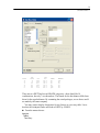
Click the Options tab in the Scatterplot dialog box.
Select Confidence kernel and enter a p value of 0.75 for a 75% confidence region.
Click OK to run the command.
34
Chapter 2
600
CALORIES
500
400
300
200
100
0
DIET
10
20
FAT
30
40
no
yes
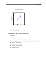
It is clear from the sample that the DIET$ yes dinners have fewer calories and less fat
than the regular dinners.
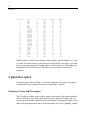
Sorting and Listing the Cases
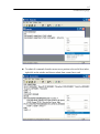
Detailed graphics and statistics may not always be what you need—sometimes you can
learn a lot simply by looking at numbers. This section shows you how to sort the
dinners by type of food (FOOD$), and within the foods, by fat content.
From the menus choose:
Data
Sort...
In the Sort dialog box, select FOOD$ and FAT as the variables, and then click OK.
35
SYSTAT Basics
From the menus choose:
Data
List Cases...
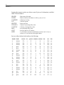
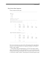
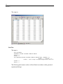
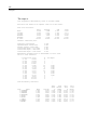
Select FOOD$, FAT, CALORIES, PROTEIN, and BRAND$ as the variables.
In the Format group, enter 7 for Column widths and 0 for Decimal places.
36
Chapter 2
Case number
1
2
3
4
5
6
7
8
9
10
11
12
13
14
15
16
17
18
19
20
21
22
23
24
25
26
27
28
FOOD$
beef
beef
beef
beef
beef
beef
chicken
chicken
chicken
chicken
chicken
chicken
chicken
chicken
chicken
chicken
chicken
chicken
chicken
chicken
pasta
pasta
pasta
pasta
pasta
pasta
pasta
pasta
FAT
8
9
14
19
24
34
0
1
2
3
4
5
5
6
7
8
10
16
24
25
3
4
4
6
8
12
16
26
CALORIE
290
330
330
370
390
300
190
160
200
280
260
240
240
270
340
400
320
330
430
550
250
210
220
220
260
300
370
440
PROTEIN
18
25
24
24
20
22
12
13
17
24
21
19
18
22
31
27
27
18
20
22
20
9
14
15
15
14
20
20
BRAND$
gor
sw
ty
st
st
gor
ww
ww
hc
hc
ww
lc
lc
lc
ty
ty
st
st
ty
sw
hc
lc
ww
ww
lc
sw
gor
gor
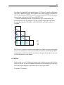
Within each type of food, the fat content varies markedly. The diet brands ww, lc, and
hc are the first entries under chicken and pasta. If the data file were larger, you would
have to scan pages and pages of listings and it would be hard to see relationships (see
the descriptors in the next section). Note that you can sort and list data in any
procedure.
A Quick Description
As an early step in data screening, it is useful to summarize the values of grouping
variables and to scan summary descriptors of quantitative variables.
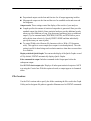
Frequency Counts and Percentages
The Crosstabs procedure on the Analysis menu features many Print options that allow
you to customize exactly what reports appear in your output. For example, the List
option reports the number of times (count) each category of a grouping variable occurs
and also the percentage each count is of the total sample size. In our “grabbing” sample
37
SYSTAT Basics
strategy, we are interested in knowing what foods and how many of each brand and diet
type we have.
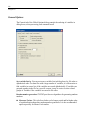
From the menus choose:
Analysis
Tables
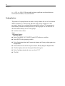
One-Way...
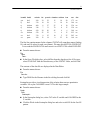
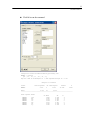
In the Options group of the One-Way Tables dialog box, select List layout.
Select FOOD$, BRAND$, and DIET$ as the variables.
Count
6
14
8
Cum
Count
6
20
28
Pct
21.4
50.0
28.6
Cum
Pct
21.4
71.4
100.0
Count
4
3
Cum
Count
4
7
Pct
14.3
10.7
Cum
Pct
14.3
25.0
FOOD$
beef
chicken
pasta
BRAND$
gor
hc
38
Chapter 2
5
4
3
4
5
Count
15
13
12
16
19
23
28
Cum
Count
15
28
17.9
14.3
10.7
14.3
17.9
42.9
57.1
67.9
82.1
100.0
lc
st
sw
ty
ww
Pct
53.6
46.4
Cum
Pct
53.6
100.0
DIET$
no
yes
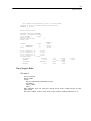
For FOOD$ (the name appears at the top right of the output), 14 of the 28 dinners in
the sample (50% in the Pct column) are chicken, 21.4% are beef, and 28.6% are pasta.
The number of dinners per BRAND$ (middle panel) ranges from three to five. There
are 15 regular (DIET$ no) dinners and 13 diet (DIET$ yes) dinners.
The List layout option is also useful for summarizing counts that result from crossclassifying two factors. Let us look at combinations of DIET$ and BRAND$.
From the menus choose:
Analsysis
Tables
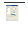
Two-Way...
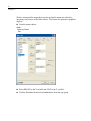
In the Options group of the Two-Way Tables dialog box, select List layout.
Select DIET$ as the row variable and BRAND$ as the column variable.
39
SYSTAT Basics
Count
4.
4.
3.
4.
3.
5.
Cum
Count
4.
8.
11.
15.
18.
23.
Pct
14.3
14.3
10.7
14.3
10.7
17.9
Cum
Pct
14.3
28.6
39.3
53.6
64.3
82.1
DIET$
no
no
no
no
yes
yes
BRAND$
gor
st
sw
ty
hc
ww
There are two DIET$ and seven BRAND$ categories—there should be 14
combinations, but only 7 are shown here. The brands for the diet dinners differ from
those for the regular dinners. By examining the actual packages, we see that st and lc
are made by the same company.
You may want to display frequencies for two factors as a two-way table. Let us
deselect the List layout feature and look at DIET$ by FOOD$.
From the menus choose:
Analysis
Tables
Two-Way...
40
Chapter 2
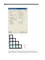
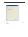
Select DIET$ as the row variable and FOOD$ as the column variable.
Deselect List layout (click the check box to deselect it if it is currently selected).
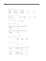
Frequencies
DIET$ (rows) by FOOD$ (columns)
beef chicken
pasta
+-------------------------+
no |
6
6
3 |
yes |
0
8
5 |
+-------------------------+
Total
6
14
8
Total
15
13
28
We failed to get any beef dinners in the DIET$ yes group.
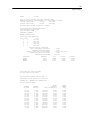
Descriptive Statistics
It is easy to request a panel of descriptive statistics. However, since we have not
examined several of these distributions graphically, we should avoid reporting means
and standard deviations (these statistics can be misleading when the shape of the
distribution is highly skewed). It is helpful to scan the sample size for each variable to
determine whether values are missing. Minimum and maximum values can help you
to set plot scales for subgroup displays.
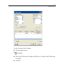
From the menus choose:
Analysis
Descriptive Statistics
Basic Statistics...
In the Column Statistics dialog box, select all of the variables in the source list
(only numeric variables are available for this command), and click OK to calculate
the default statistics.
41
SYSTAT Basics
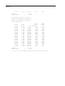
N of cases
Minimum
Maximum
Mean
Standard Dev
CALORIES
28
160.000
550.000
303.214
87.815
FAT
28
0.0
34.000
10.804
8.959
N of cases
Minimum
Maximum
Mean
Standard Dev
IRON
28
2.000
25.000
10.464
5.467
COST
28
1.600
3.500
2.544
0.548
PROTEIN
28
9.000
31.000
19.679
5.019
VITAMINA
28
0.0
100.000
18.929
22.593
CALCIUM
28
0.0
40.000
10.857
10.845
For each variable, SYSTAT gives the number of cases with nonmissing values, the
largest and smallest values, and the mean and standard deviation. CALORIES for a single
dinner range from 160 to 550 and average around 300 (303.214 to be exact). VITAMINA
ranges from 0% to 100% with a mean of 18.9%. Since the mean is not close to the middle
of the range, the distribution must be quite skewed or have a few extreme values.
42
Chapter 2
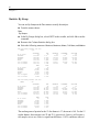
Statistics By Group
You can use By Groups on the Data menu to stratify the analysis.
From the menus choose:
Data
By Groups...
In the By Groups dialog box, select DIET$ as the variable, and click OK to run the
command.
Return to the Column Statistics dialog box.
Select the following measures: Minimum, Maximum, Mean, CI of Mean, and Median.
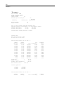
The following results are for:
DIET$
= yes
N of cases
Minimum
Maximum
Median
Mean
95% CI Upper
95% CI Lower
CALORIES
13
160.000
280.000
240.000
230.769
251.770
209.769
FAT
13
0.0
8.000
4.000
3.885
5.225
2.544
N of cases
Minimum
Maximum
Median
Mean
95% CI Upper
95% CI Lower
IRON
13
2.000
15.000
8.000
8.923
11.847
5.999
COST
13
2.000
2.990
2.490
2.509
2.754
2.265
PROTEIN
13
9.000
24.000
17.000
16.846
19.467
14.225
VITAMINA
13
0.0
30.000
15.000
15.077
22.233
7.921
CALCIUM
13
2.000
30.000
8.000
9.769
14.910
4.629
PROTEIN
15
14.000
31.000
22.000
22.133
24.519
19.748
VITAMINA
15
0.0
100.000
10.000
22.267
38.302
6.231
CALCIUM
15
0.0
40.000
6.000
11.800
18.865
4.735
The following results are for:
DIET$
= no
N of cases
Minimum
Maximum
Median
Mean
95% CI Upper
95% CI Lower
CALORIES
15
290.000
550.000
340.000
366.000
404.127
327.873
FAT
15
7.000
34.000
16.000
16.800
21.353
12.247
N of cases
Minimum
Maximum
Median
Mean
95% CI Upper
95% CI Lower
IRON
15
4.000
25.000
10.000
11.800
15.003
8.597
COST
15
1.600
3.500
2.850
2.573
2.939
2.207
The median grams of protein for the 13 diet dinners is 17; the mean is 16.8. For the 15
regular dinners, these statistics are 22 and 22.1, respectively. Later we will request a
two-sample t test to see if this is a significant difference. A 95% confidence interval
43
SYSTAT Basics
for the average cost of a diet dinner ranges from $2.27 to $2.75. The confidence
interval for the average cost of the regular dinners is larger—$2.21 to $2.94.
The By Groups variable, DIET$, remains in effect for subsequent graphical displays
and statistical analyses. To disengage it, return to the By Groups dialog box and select
Turn off.
A First Look at Relations among Variables
What are the correlations among calories, fat content, protein, and cost? We can use
correlations to quantify the linear relations among these variables.
From the menus choose:
Analysis
Correlations
Simple...
44
Chapter 2
In the Simple Correlations dialog box, select Continuous data and select Pearson
from the Continuous data drop-down list.
Select CALORIES, FAT, PROTEIN, and COST as the variables.
Click the Options tab and select Probabilities and Bonferroni. Because we study six
correlations among four variables, we use Bonferroni adjusted probabilities to
provide protection for multiple tests.
Click OK to run the command.
45
COST
PROTEIN
FAT
CALORIES
SYSTAT Basics
CALORIES
FAT
PROTEIN
COST
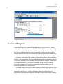
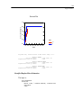
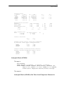
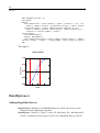
Quick Graphs. This is the Quick Graph that SYSTAT automatically generates when
you request correlations. Quick Graphs are available for most statistical procedures. If
you want to turn off a Quick Graph, use Options on the Edit menu.
The Quick Graph in this example is a scatterplot matrix (SPLOM). There is one
bivariate scatterplot corresponding to each entry in the correlation matrix that follows.
Univariate histograms for each variable are displayed along the diagonal, and 75%
normal theory confidence ellipses are displayed within each plot.
The plot of FAT and CALORIES (top left) has the narrowest ellipse, and thus, the
strongest correlation (that is, given that the configuration of the points is spread evenly,
is not nonlinear, and has no anomalies). In the correlation matrix that follows, the
correlation between FAT and CALORIES is 0.758.
Pearson correlation matrix
CALORIES
FAT
PROTEIN
COST
CALORIES
1.000
0.758
0.550
0.099
Bartlett Chi-square statistic:
FAT
1.000
0.279
-0.132
PROTEIN
1.000
0.420
COST
1.000
38.865 df=6 Prob= 0.000
Matrix of Bonferroni Probabilities
CALORIES
FAT
PROTEIN
COST
CALORIES
0.0
0.000
0.014
1.000
FAT
PROTEIN
0.0
0.903
1.000
0.0
0.156
COST
0.0
The p value (or Bonferroni adjusted probability) associated with 0.758 is printed as
0.000 (or less than 0.0005). As the scatterplot seemed to indicate, FAT and CALORIES
are correlated. PROTEIN also has a significant correlation with CALORIES
46
Chapter 2
( r = 0.55, p = 0.014 ). We are unable to detect significant correlations between
COST and CALORIES, FAT, and PROTEIN.
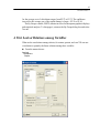
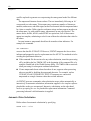
Subpopulations
The presence of subpopulations can mask or falsely enhance the size of a correlation.
With Correlations, we could specify DIET$ as a By Groups variable as we did
previously. Instead, let us examine the data graphically and use 75% nonparametric
kernel density contours to identify the diet yes and no groups. We will also look at
univariate kernel density curves for the groups.
From the menus choose:
Graph
Multivariate Displays
Scatterplot Matrix...
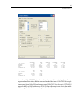
Select CALORIES, FAT, PROTEIN, and COST as the row variables.
Select DIET$ as the grouping variable.
Select Only display bottom half of matrix and diagonal and Overlay multiple graphs into
a single frame.
Select Kernel Curve from the drop-down list for Density displays in diagonal cells.
Click the Options tab in the Scatterplot Matrix dialog box.
Select Confidence kernel and enter a p value of 0.75.
Click OK.
47
SYSTAT Basics
48
PROTEIN
FAT
CALORIES
Chapter 2
COST
DIET
CALORIES
FAT
PROTEIN
COST
no
yes
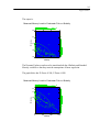
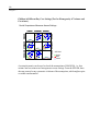
For CALORIES and FAT, look at the separation of the univariate densities on the
diagonal of the display. Notice that the price range (COST) at the bottom right for the
49
SYSTAT Basics
IRON
CALCIUM
VITAMINA
diet dinners is within that for the regular dinners. COST is the Y-variable in the bottom
row of plots. Within each group, COST appears to have little relation to CALORIES or
FAT. It is possible that COST has a positive association with PROTEIN for the regular
dinners (open circles in the COST versus PROTEIN plot).
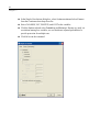
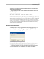
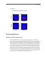
Is there a relationship between cost and nutritive value as measured by the
percentage daily value for vitamin A, calcium, and iron? Repeat the steps for the
previous plot, but select VITAMINA, CALCIUM, IRON, and COST as the row
variables.
COST
DIET
VITAMINA
CALCIUM
IRON
COST
no
yes
COST is the Y-variable for each plot on the bottom row. There is no strong relationship
between cost and nutritive value (as measured by VITAMINA, CALCIUM, and IRON),
except there is a small cluster of low-cost dinners with high-calcium content. Later, we
will find that these are pasta dinners.
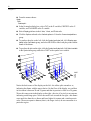
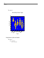
3-D Displays
In this section, we use 3-D displays for another look at calories, protein, and fat. In the
display on the left, we label each dinner with its brand code; in the display on the right,
we use the cost of the dinner to determine the size of the plot symbol.
To produce 3-D displays:
50
Chapter 2
From the menus choose:
Graph
Plots
Scatterplot...
In the Scatterplot dialog box, select FAT as the X-variable, PROTEIN as the Yvariable, and CALORIES as the Z variable.
Select Display grid lines in the X-Axis, Y-Axis, and Z-Axis tabs.
Click the Options tab and select Vertical spikes to Y from the Connectors/partitions
group.
To produce the plot on the left, click the Symbol and Label tab, click Display case
labels in the Case labels group, and select BRAND$ to label each plot point with the
brand of the dinner.
To produce the plot on the right, click the Symbol and Label tab, click Select variable
in the Symbol size group, and select COST as the symbol size variable.
s
s
t
t
h
s
s
t
l g
w
h ll l
w
h w
w
w
l
g
s
s
t
s
g
g
t
h
t
t
ss
l
w
h
h
w
w
g
g
s
s
g
ll
ww
sg
t
s
l
l
COST
4
3
2
1
Notice the back corner of the display on the left—the tallest spike extends to sw,
indicating the dinner with the most calories. On the floor of the display, we read that
its fat content is between 20 and 30 grams and that its protein is a little over 20 grams.
We see this same point in the display on the right—the size of its circle is not extreme,
indicating a mid-range price. Notice the small circle toward the far right—this dinner
costs much less than the sw dinner and has a higher fat content and a similar protein
value. The most expensive dinners (that is, the larger circles) do not concentrate in a
particular region.
51
SYSTAT Basics
A Two-Sample t-Test
One of the most common situations in statistical practice is that of comparing the
means for two groups. For example, does the average response for the treatment group
differ from that for the control group? Ideally, the subjects should be randomly
assigned to the groups.
For the food data, we are interested in possible differences in protein and calcium
between the diet and regular dinners. Thus, the dinners are not randomly assigned to
groups. In a real observational study, a researcher should carefully explore the data to
ensure that other factors are not masking or enhancing a difference in means.
In the t-test, we test the hypothesis of equality of means of diet and regular dinners.
The alternative to this hypothesis could be diet > regular, diet ‘not equal’ regular, diet
< regular. Since we have no information let us choose the second:‘not equal’:
Do diet and regular dinners differ in protein and calcium content? In this example,
we use the t-test procedure.
From the menus choose:
Analysis
Hypothesis Testing
Mean
Two Sample t-Test...
In the Two-Sample t-Test dialog box, select PROTEIN and CALCIUM as the
variables, and select DIET$ as the grouping variable.
In the Alternative type, choose ‘not equal’.
Click OK to run the command.
52
Chapter 2
40
50
40
CALCIUM
PROTEIN
30
20
10
DIET
0
16 12
8
4
Count
0
4
8 12 16
Count
no
yes
30
20
10
0
20 15 10 5
Count
DIET
0
5
10 15 20
Count
no
yes
53
SYSTAT Basics
Two-sample t test on PROTEIN grouped by DIET$ against the Alternative =’not equal’
Group
no
yes
N
15
13
Separate Variance t =
Pooled Variance t =
Mean
22.133
16.846
3.228 DF =
3.229 DF =
SD
4.307
4.337
25.4
26
Prob =
Prob =
0.003
0.003
Two-sample t test on CALCIUM grouped by DIET$against the Alternative =’not equal’
Group
no
yes
N
15
13
Separate Variance t =
Pooled Variance t =
Mean
11.800
9.769
0.501 DF =
0.487 DF =
SD
12.757
8.506
24.5
26
Prob =
Prob =
0.621
0.630
The t-test procedure produces two density plots as Quick Graphs. On the far left and
right sides of the density plot for each test variable are box plots for each category of
the grouping variable. The box plot on the left side of each graph is for the DIET$ no
group, and the box plot on the right side of each graph is for the DIET$ yes group.
The middle portion of each graph shows the actual distribution of data points, with
a normal curve for comparison.
The results in the box plots for PROTEIN are desirable. The median (horizontal line
in each box) is in the center of the box, and the lengths of the boxes are similar. Also,
the peaks of the normal curves, which represent the mean for a normal distribution, are
very close to the median values. This indicates that the distributions are symmetric and
have approximately the same spread (variance). This is not true for CALCIUM. These
distributions are right skewed and possibly should be transformed before analysis.
The mean values for PROTEIN are the same as those in the By Groups statistics—
22.133 and 16.846. The standard deviations (SD) differ little (4.307 and 4.337),
confirming what we observed in the box plots. This means that we can use the results
of the pooled-variance t test printed below the means. This test is usually the first one
you see in introductory texts and assumes that the distributions have the same shape
(that is, the variances do not differ). For PROTEIN, we conclude that the mean of 22.1
for the regular dinners does differ significantly from the mean of 16.8 for the diet
dinners (t = 3.229, p value = 0.0003).
The separate-variance t test does not require the assumption of equal variances.
Considering the distributions for CALCIUM displayed in the box plots and that the
standard deviations for the groups are 12.757 and 8.506, we use the separate-variance
t test results. We are unable to report a difference in average CALCIUM values for the
regular and diet dinners (t = 0.501, p value = 0.621).
54
Chapter 2
The discussion of SYSTAT’s procedures is very exploratory at this stage, so you
should not conclude that CALCIUM values are homogeneous. Always take the time to
think about what possible subgroups might be influencing or obscuring results.
A One-Way Analysis of Variance (ANOVA)
Does the cost of a dinner vary by brand? Let us try an analysis of variance (ANOVA)
to determine whether the average price of frozen dinners varies by brand. After looking
at the graphics earlier in this chapter, we assume that differences do exist, so we also
request the Tukey HSD test for post hoc comparison of means. This test provides
protection for testing many pairs of means simultaneously, allowing us to make
statements about which brand’s average cost differs significantly from another brand’s.
Before we run the analysis of variance, we will specify how the brands should be
ordered in the output (results will be easier to follow if we order the brands from least
to most expensive).
From the menus choose:
Data
Order...
In the Order dialog box, select BRAND$ as the variable.
Select Enter sort and type 'gor', 'hc', 'sw', 'lc', 'ww', 'st', 'ty'.
Click OK to run the command.
From the menus choose:
Edit
Options...
In the Output Results group on the Output tab, select Long from the Length dropdown list. (This will provide extended results for the analysis of variance.)
Click OK.
To request an analysis of variance:
From the menus choose:
Analysis
Analysis of Variance
Estimate Model...
In the Analysis of Variance: Estimate Model dialog box, select COST as the
dependent variable and BRAND$ as the factor variable.
Select Post hoc tests, and choose Tukey as the test.
55
SYSTAT Basics
Click OK to run the command.
Categorical values encountered during processing are:
BRAND$ (7 levels)
gor , hc , sw , lc , ww , st , ty
Dep Var: COST N: 28 Multiple R:
0.861 Squared multiple R:
0.742
Analysis of Variance
Source
Sum-of-Squares
BRAND$
6.017
DF
6
Mean-Square
1.003
F-Ratio
10.042
P
0.000
Error
2.097
21
0.100
-----------------------------------------------------------------------Least squares means.
BRAND$
BRAND$
BRAND$
BRAND$
BRAND$
BRAND$
BRAND$
=gor
=hc
=sw
=lc
=ww
=st
=ty
LS Mean
1.810
2.000
2.233
2.654
2.670
2.915
3.250
SE
0.158
0.182
0.182
0.141
0.141
0.158
0.158
N
4
3
3
5
5
4
4
56
Chapter 2
We have interrupted the output here to point out that the means are ordered by
increasing cost because of the Order feature. This feature also pertains to graphical
displays.
From the menus choose:
Graph
Summary Charts
Bar...
Select BRAND$ as the X-variable and COST as the Y-variable.
Click the Error Bars tab and select Standard error from the type group.
57
SYSTAT Basics
Click the Fill tab, select Select fill from the Fill pattern group, and select
Fill Pattern..
Click OK.
as the
58
Chapter 2
The output is:
4
COST
3
2
1
gor hc sw lc ww st
BRAND$
ty
59
SYSTAT Basics
Tukey Pairwise Mean Comparisons
We now continue with the output:
-----------------------------------------------------------------------------COL/
ROW BRAND$
1 gor
2 hc
3 sw
4 lc
5 ww
6 st
7 ty
Using least squares means.
Post Hoc test of COST
-----------------------------------------------------------------------------Using model MSE of 0.100 with 21 DF.
Matrix of pairwise mean differences:
1
2
3
4
5
6
7
1
0.0
0.190
0.423
0.844
0.860
1.105
1.440
6
7
6
0.0
0.335
2
3
4
5
0.0
0.233
0.654
0.670
0.915
1.250
0.0
0.421
0.437
0.682
1.017
0.0
0.016
0.261
0.596
0.0
0.245
0.580
7
0.0
Tukey HSD Multiple Comparisons.
Matrix of pairwise comparison probabilities:
-
1
2
3
4
5
6
7
1
1.000
0.984
0.590
0.010
0.009
0.001
0.000
2
3
4
5
1.000
0.968
0.115
0.100
0.016
0.001
1.000
0.548
0.506
0.117
0.006
1.000
1.000
0.874
0.120
1.000
0.903
0.138
6
7
6
1.000
0.742
1.000
7
------------------------------------------------------------------------------
The F ratio in the analysis-of-variance table at the beginning of the output indicates
that there are one or more differences in average price among the seven brands (F =
10.042, p value < 0.0005).
Let us read the Tukey results appearing above. SYSTAT first assigns a numeric
code to each brand and follows this with the difference in cost for each pair of means.
Differences between the gor brand and the others are reported in column 1 ($0.19 with
hc, $0.42 with sw, and $1.44 with ty). The same layout is used in the last panel to report
60
Chapter 2
the probability associated with each difference. Gor is significantly less expensive than
all brands except hc (2) and sw (3).
In column 2, notice that, on the average, the hc brand costs $0.92 less than the st
brand and $1.25 less than the ty brand. From the probability table, these differences are
significant with probabilities of 0.016 and 0.001, respectively. The only other
significant difference is the last brand in column 3—the average price for the sw brand
costs $1.02 less than the ty brand.
A Two-Way ANOVA with Interaction
Do nutrients vary by type of food? Earlier in a scatterplot matrix, we observed a small
cluster of dinners that had higher calcium values than the others. In the two-sample ttest, we were unable to detect differences in average calcium values between the diet
and regular dinners. Let us explore further by using both food type and dinner type to
define cells—that is, we request a two-way analysis of variance. Using the List feature
in Crosstabs, we found that although our sample has beef, chicken, and pasta dinners,
there were no beef dinners in the DIET$ yes group. (SYSTAT can analyze ANOVA
designs with missing cells. See SYSTAT Statistics II Chapter 3 for more information.)
Let us use Select Cases on the Data menu to omit the beef dinners, and then request
an analysis of variance for a two-by-two design (DIET$ yes and no by chicken and
pasta).
From the menus choose:
Data
Select Cases...
In the Select dialog box, select FOOD$ as Expression1.
Select <> (not equal) from the drop-down list of operators.
For Expression2, type 'beef' (include the quotation marks while working with
commands, the dialog box takes care of this.).
Click OK to run the command.
61
SYSTAT Basics
To get a bar chart of the cell means:
From the menus choose:
Graph
Summary Charts
Bar...
Select CALCIUM as the Z-variable, DIET$ as the Y-variable, and FOOD$ as the
X-variable.
Click OK.
62
Chapter 2
The output is:
63
SYSTAT Basics
Suggestion. Try using the Dynamic Explorer to rotate this 3-D bar chart.
The box plot in the two-sample t-test example shows that the distributions of calcium
for the yes and no groups are skewed and have unequal spreads. Let us use a power
transformation of CALCIUM and look at the bar chart again.
Using the Dynamic Explorer, change the ZPower value to 0.5.
Before requesting the analysis of variance, we will transform CALCIUM, taking the
square root of each value.
From the menus choose:
Data
Transform
Let...
In the Let dialog box, select CALCIUM as the variable, select SQR from the list of
mathematical functions, and select CALCIUM from the variable list and add it to the
expression. The Expression box should now look like this: SQR(CALCIUM).
Click OK to run the command.
64
Chapter 2
Now request the analysis of variance, repeating the steps in the last example, except
that here we use both DIET$ and FOOD$ as the factor variables.
Categorical values encountered during processing are:
DIET$ (2 levels)
no , yes
FOOD$ (2 levels)
chicken , pasta
Dep Var: CALCIUM N: 22 Multiple R:
Source
0.804 Squared multiple R:
Analysis of Variance
Sum-of-Squares
DF Mean-Square
DIET$
FOOD$
DIET$*FOOD$
1.807
39.298
7.908
1
1
1
1.807
39.298
7.908
Error
22.719
18
1.262
F-Ratio
1.432
31.136
6.266
0.647
P
0.247
0.000
0.022
The significant DIET$ by FOOD$ interaction suggests exercising caution when
interpreting main effects. The main effect for DIET$ does not appear to be significant
(p = 0.247)—but let us look at a scatterplot and see if that tells us anything more.
From the menus choose:
Graph
Plots
Scatterplot...
Select CALCIUM as the Y-variable and DIET$ as the grouping variable. (SYSTAT
will automatically use the case number as the X-variable.)
65
SYSTAT Basics
Select Overlay multiple graphs into a single frame.
Click the Symbol and Label tab, click Select symbol, select a circle for the first
symbol and a triangle for the second.
Check Display case labels in the Case labels group and select FOOD$ as the case
label variable.
Click the Fill tab, click Select fill in the Fill pattern group, and select a solid fill for
both the first and second fill patterns.
Click OK.
7
pasta
pasta
6
pasta
CALCIUM
5
pasta
pasta
4
chicken
chicken pasta
3chicken
chicken
pasta
2
1
0
0
pasta
chicken chicken
chicken
chicken
chicken
chicken
chicken
chicken
no
yes
chicken
chicken
5
10
15
20
Index of Case
DIET
25
The scatterplot shows that all of the dinners with a square root value for CALCIUM
over 4 are pasta dinners (which is consistent with the significant main effect for
FOOD$)—but it also shows that the highest values are also regular (DIET$ = no)
dinners. This suggests that further investigation might be warranted.
A Post Hoc Test in GLM
Since we have a significant DIET$ by FOOD$ interaction, we should be cautious about
interpreting main effects. Let us use SYSTAT’s advanced hypothesis testing capability
to request Bonferroni adjusted probabilities for tests of pairwise mean differences.
From the menus choose:
Analysis
General Linear Model (GLM)
Pairwise Comparisons...
66
Chapter 2
Specify DIET$ ∗ FOOD$ under Groups and select Bonferroni under Test.
Click OK.
COL/
ROW DIET$
FOOD$
1 no
chicken
2 no
pasta
3 yes
chicken
4 yes
pasta
Using least squares means.
Post Hoc test of CALCIUM
TEST
-------------------------------------------------------------------Using model MSE of 1.262 with 18 DF.
Matrix of pairwise mean differences:
1
2
3
4
1
0.0
4.124
0.667
2.236
2
3
4
0.0
1.570
0.0
2
3
4
1.000
0.002
0.201
1.000
0.148
1.000
0.0
-3.457
-1.888
Bonferroni Adjustment.
Matrix of pairwise comparison probabilities:
1
2
3
4
1
1.000
0.000
1.000
0.025
--------------------------------------------------------------------
We are interested in four of the six differences (and probabilities) in these panels. First
we look within diets and then within food types. For the:
regular meals (DIET$ no), the difference in average calcium content between
chicken and pasta meals is highly significant (the difference in square root units is
4.124, p < 0.0005).
diet meals (DIET$ yes), the difference in average calcium content between chicken
and pasta is not significant (1.570, p = 0.148).
pasta meals, the difference in average calcium content between the DIET$ yes and
no groups is not significant (–1.888, p = 0.201).
chicken meals, the difference in average calcium content between DIET$ yes and
no groups is not significant (0.667, p = 1.000).
It will be more clear if you see a dot display of these means.
67
SYSTAT Basics
Select
Graph
Summary Charts
Dot...
Choose CALCIUM as the Y-variable and DIET$ as the X-variable.
Specify FOOD$ as the grouping variable.
Select Overlay multiple graphs into a single frame.
Click Options and select Error Bars.
Select Standard error, specify a value of 0.9545.
Click the Error Bars tab, choose Standard error from the Type groupbox, and specify
a value of 0.9545.
Click the Options tab and select Line connected in left-to-right order.
Click OK.
7
6
CALCIUM
5
4
3
FOOD
2
chicken
pasta
1
0
no
yes
DIET
For the regular meals (DIET$ no), the error bars do not overlap, indicating a significant
difference in calcium content between pasta and chicken. However, for the diet meals
(DIET$ yes), the overlapping error bars suggest no significant difference between the
meal types.
Focusing on the pasta meals, the average calcium content for the diet meals is
within two standard errors of the average calcium content for the regular meals.
Similar observations can be made for the chicken meals.
68
Chapter 2
Summary
The first step in any data analysis is to look at your data. SYSTAT provides a wide
variety of graphs that can help you identify possible relationships between variables,
spot outliers that may unduly affect results, and reveal patterns that may suggest data
transformations for more meaningful analysis.
SYSTAT also provides a wide variety of statistical procedures for analyzing your
data. We have covered some of the most common and basic statistical techniques in
this chapter, and we have still barely scratched the surface.
Chapter
Data Analysis Quick Tour
3
This chapter provides a quick tour of SYSTAT’s capabilities, using data from a survey
of uranium found in groundwater.
Groundwater Uranium Overview
The U.S. Department of Energy collected samples of groundwater in west Texas as
part of a project to estimate the uranium reserves in the United States. Samples were
taken from five different locations, called producing horizons, and then measured for
various chemical components. In addition, the latitude and longitude for each sample
location were recorded. Several questions are of interest:
Does the uranium concentration vary by producing horizon?
Is the presence of uranium correlated to the presence of other elements?
What is the overall geographic distribution of uranium in the area?
69
70
Chapter 3
The data for the groundwater uranium study are in the file GDWTRDM.SYD.
Measurements were recorded for the following variables:
Variable
Description
SAMPLE
LATITUDE
LONGTUDE
HORIZON$
HORIZON
URANIUM
ARSENIC
BORON
BARIUM
MOLYBDEN
SELENIUM
VANADIUM
SULFATE
TOT_ALK
BICARBON
CONDUCT
PH
URANLOG
MOLYLOG
The ID of the groundwater sample
Latitude at which the sample was taken
Longitude at which the sample was taken
Initials of producing horizon
ID of producing horizon
Uranium level in groundwater
Arsenic level in groundwater
Boron level in groundwater
Barium level in groundwater
Molybdenum level in groundwater
Selenium level in groundwater
Vanadium level in groundwater
Sulfate level in groundwater
Alkalinity of groundwater
Bicarbonate level in groundwater
Conductivity of groundwater
pH of groundwater
Log of uranium level in groundwater
Log of molybdenum level in groundwater
Potential Analyses
The following kinds of analyses may be useful in analyzing the groundwater data:
Descriptives
Transformations
ANOVA
Nonparametric tests
Regression
Correlation
Cluster analysis
Discriminant analysis
71
Data Analysis Quick Tour
Spatial statistics
Smoothing techniques such as kriging
Contour plotting
In these examples, we will show you descriptive graphs, ANOVA, nonparametric tests,
smoothing, and contour plotting.
The Groundwater Data File
The data for this analysis are in the file GDWTRDM.SYD.
To open the file, from the menus choose:
File
Open
Data
Select GDWTRDM.SYD, and click Open.
The Data Editor is used to import and export data files, transform variables, select and
weight cases, and so forth. In this example, measurements were taken of the levels of
uranium and various other elements in the groundwater at each producing horizon. The
measurements for each variable can be viewed and manipulated directly in the Data
Editor.
72
Chapter 3
Graphics
Distribution Plot
Since we will be looking extensively at uranium levels, it is a good idea to take a look
at the distribution of this variable and make sure it meets assumptions for future
analyses.
To plot a histogram of URANIUM:
Click the Histogram icon in the Graph Toolbars.
Choose URANIUM and add it to the X-variable(s) list.
Click OK.
73
Data Analysis Quick Tour
SYSTAT displays the following plot in the Output Pane:
80
0.6
70
0.5
Count
50
0.4
40
0.3
30
0.2
20
0.1
10
0
0
Proportion per Bar
60
50
100
URANIUM
0.0
150
We can see that the distribution of URANIUM is skewed. To properly apply most
statistical analyses, the histogram should show a bell-shaped, normal distribution.
Exploring the Groundwater Data Interactively
The Dynamic Explorer is a tool that allows you to explore data interactively, increasing
the efficiency of your analysis. It can be used to rotate 3-D graphs, to animate 3-D
graphs, zoom the whole graph or individual axis, perform power and log
transformations, change confidence intervals, adjust tension in smoothers, and change
the number of bars on a histogram.
Double-click the graph or click the Graph Editor tab in the Viewspace.
74
Chapter 3
Click the down arrow of X-Power in the Dynamic Explorer until the graph
becomes a bell-shaped curve.
As you do this, SYSTAT is automatically calculating power data transformations of the
form URANIUM (power). A power of 0.500 is a square root transformation. A power
of 0.333 is a cube root transformation.
Transformed Graph
At a power of 0, SYSTAT automatically performs a logarithmic transformation—
for example, log(URANIUM). The log transformation appears to produce a very
good bell-shaped curve. But this judgment is subjective and it is possible to use
more formal and objective methods to examine the normality of the transformed
data. One such method is the Shapiro-Wilk test, which we discuss later.
75
Data Analysis Quick Tour
40
0.3
35
0.2
Count
25
20
15
0.1
10
Proportion per Bar
30
5
0
60 120
0.0
URANIUM
Normally, once the proper transformation has been identified using the Dynamic
Explorer, you create the transformed variable using the Data Editor. We have already
performed the transformation and included the variable URANLOG in the data file for
further statistical analysis.
Histograms and Probability Plots
Let us take another look at the URANIUM distribution. We are going to plot two
graphs, a histogram and a probability plot, by using commands. From the menus,
submit the command file GDWTR1DM.SYC. For this:
From the menus choose:
File
Submit File...
Select GDWTR1DM.SYC from the ‘Miscellaneous’ subfolder of the ‘command’
directory and click Open.
The following graphs are displayed in the Output pane of the Viewspace:
76
Chapter 3
80
Probability Plot for Uranium
0.6
70
0.5
Count
50
0.4
40
0.3
30
0.2
20
0.1
10
0
0
50
100
URANIUM
0.0
150
Proportion per Bar
60
Expected Value for Normal Distribution
Histogram for Uranium
3
2
1
0
-1
-2
-3
0
50
100
URANIUM
150
In this plot, we begin to glimpse SYSTAT’s color and overlay capabilities. This
command file created a side-by-side overlay of a histogram and a probability plot of
the URANIUM variable.
SYSTAT Windows and Commands
SYSTAT gives you the flexibility to perform your analysis the way you want:
Windows interface: icons, menus, and dialog boxes.
Typed commands: typing commands at the Commandspace.
Batch (Untitled) command files: submitting files directly or from the
Commandspace.
Additionally, all menu actions can be optionally echoed to the output pane, allowing
you to perform initial analyses using the menus, and then to cut and paste the
commands into the middle tab of the Commandspace for repeated use.
77
Data Analysis Quick Tour
Plotting Several Graphs Using Commands
The commands in the file GDWTR1DM.SYC are:
THICK=2
USE GDWTRDM
BEGIN
DENS URANIUM / HIST, FCOLOR = BLUE,
COLOR = GREEN, FILL,
TITLE='Histogram for Uranium'
PPLOT URANIUM / LOC = 6in,0in, FCOLOR = gray,
FILL, COLOR = YELLOW,
TITLE = 'Probability Plot for Uranium'
END
THICK=1
The DENS and PPLOT commands create the histogram and the probability plot,
respectively. Between the BEGIN and END statements, we can change the data file in
use and plot an unlimited number of graphs. Each graph can have its own attributes,
such as location and color.
Plotting Several Graphs Using Menus
Plotting more than one graph can be accomplished directly from SYSTAT’s menu.
From the menus choose:
Graph
Begin Single Page Mode
Choose graphs and options from menus and dialog boxes. You can choose
locations for the graphs in the Layout tab, unless you want them overlaid on top of one
another.
78
Chapter 3
Then, from the menus choose:
Graph
End Single Page Mode
Transforming Data and Selecting Cases
In the Commandspace, select and submit the line beginning with PPLOT. Using the
Dynamic Explorer in the Workspace, transform the URANIUM variable by clicking the
down arrow of X-Power until 0 is reached, yielding a log transformation.
Expected Value for Normal Distribution
Probability Plot for Uranium
3
2
1
0
-1
-2
-3
60 120
URANIUM
Notice that the probability plot is much more linear.
Using SYSTAT’s lassoing capability, you can isolate outliers.
Click the Lasso icon
and lasso the two outliers on the lower left of the graph by holding down the left mouse
button and circling them.
Click the Highlight icon
79
Data Analysis Quick Tour
to highlight the selected cases.
Dynamically Highlighted Cases
Cases selected by the Lasso tool are highlighted in the Data Editor. Open the Data
Editor to see these cases, 30 and 31, directly.
SYSTAT dynamically links data across graphs and the Data Editor. These cases are
now selected. If you were to run a statistical analysis or plot another graph at this point,
it would use only these two cases. As pointed out earlier, SYSTAT manages data and
graphics globally.
Make sure you deselect the data before continuing. Otherwise the remainder of the
analyses will be done only on the selected observations. To deselect the cases, use the
Lasso tool to select an area of the graph that contains no data points.
80
Chapter 3
Connections between Graphs and the Data Editor
For those of you with a technical inclination, here is the explanation of the connection
between the graphs and the Data Editor:
Graphs have their own data, allowing the real-time transformations of the Dynamic
Explorer and the ability to save and reload them without the original data file.
When a graph is plotted, the data in the graph are linked to the Data Editor,
allowing lassoing.
The Data Editor and the program kernel share the same data set, so all data are
“live,” and what you see is what you get. For example, if you select data in the
Graph Editor and then run a regression, the regression applies only to the selected
data.
Statistics
This part of the tour introduces SYSTAT’s statistics capability. Here, we explore the
question of whether the five producing horizons have varying levels of uranium by
performing an ANOVA of URANLOG (the log of URANIUM) versus HORIZON. This
analysis is being done based on the visual judgment that the normal distribution for
log(URANIUM) is a valid model.
In the SYSTAT window, click the ANOVA icon on the Analysis toolbar.
Select URANLOG as the dependent variable and HORIZON as the factor.
81
Data Analysis Quick Tour
Graph of Mean Uranium Levels
Along with numeric output, SYSTAT produces a Quick Graph: a line-connected plot
of mean uranium levels and confidence intervals for the different producing horizons.
82
Chapter 3
Least Squares Means
4
URANLOG
3
2
1
0
1
2
3
4
HORIZON
5
Most of SYSTAT’s statistical procedures have associated Quick Graphs. Quick
Graphs speed up analysis by providing immediate visual feedback on results. In this
Quick Graph, it is easily seen that the third group, Quartermaster, has a much higher
level of uranium.
Output for ANOVA
The numeric output of the ANOVA appears in the Output Pane.
Analysis of Variance
Source
Sum-of-Squares
HORIZON
Error
df
Mean-Square
F-ratio
14.978
4
3.744
3.252
140.484
122
1.152
P
0.014
In the analysis-of-variance table, the F test has a p value of 0.014, meaning that there
is only a 1.4% chance that these data would be measured if the individual producing
horizons have the same average level of uranium—that is, the uranium level differs
significantly by producing horizon. We saw this immediately in the Quick Graph. In
fact, in the Quick Graph we also saw that producing horizon 3, the Quartermaster
horizon, differs the most.
83
Data Analysis Quick Tour
Outliers and Diagnostics
The Output Pane also has warnings about outliers.
*** WARNING ***
Case
30 is an outlier
Case
31 is an outlier
Durbin-Watson D Statistic
First Order Autocorrelation
(Studentized Residual =
(Studentized Residual =
-4.732)
-4.732)
1.305
0.345
There are two outliers in the data: cases 30 and 31. These are the same two that we
lassoed earlier in the probability plot.
SYSTAT performs automatic diagnostics to verify that the data meet the underlying
assumptions for ANOVA, Linear Regression, and General Linear Models (GLM).
Automatic diagnostics speed up the analysis and help to produce more accurate results
by alerting you to problems with the data. Both the Durbin-Watson D statistic and the
first-order autocorrelation appear by default and these are parts of such diagnostics.
Let us crosscheck the observation made about normality of the variable URANLOG
with a formal test.
Shapiro-Wilk Test
SYSTAT performs the often-used test for normality called the Shapiro-Wilk test in its
Analysis: Descriptive Statistics feature, apart from various data summaries for
variables as well as rows.
To perform the Shapiro-Wilk test:
Click the Column Statistics icon in the Descriptive Statistics Toolbars.
84
Chapter 3
Choose URANLOG and add it to the Selected variable(s) list.
Deselect N, Minimum, Maximum, Mean, and SD.
Select Shapiro-Wilk normality test.
Click OK.
The output appears in the Output Pane:
SW Statistic
SW P-Value
URANLOG
0.926
0.000
The P-value is an indication (as in any hypothesis testing results) of whether the
hypothesis being tested (in this case the normality of the distribution) is to be accepted
or rejected. The smaller the P-value the stronger is the evidence against the hypothesis.
Since in this case the value is near 0 (0 up to 3 places of decimal) the normality
hypothesis is rejected, a different conclusion from the subjective one based on a graph.
85
Data Analysis Quick Tour
When the assumption of normal distribution cannot be justified even for a transformed
variable, we may consider nonparametric methods, which do not depend on such
assumptions.
Nonparametric tests
Now we see how the question earlier answered by using ANOVA (with normality
assumption on log(URANLOG)) can be answered by a nonparametric test, which does
not make this assumption. Now you might ask: Why then bother with ANOVA at all?
The answer is: If the normality assumption actually holds, then ANOVA is a more
powerful method, but it is not valid when the assumption fails. If we do not have a
good distribution model for URANLOG or a transformed variable, then it is safer to use
a distribution-free (nonparametric) method, even if it is not powerful. For a
nonparametric test for the equality of URANLOG levels at various horizons:
From the menus choose:
Analysis
Nonparametric Tests
Kruskal-Wallis…
Select URANLOG as the Selected variable(s) and HORIZON as the Grouping
variable.
86
Chapter 3
Output from Kruskal-Wallis Test
Categorical values encountered during processing are:
HORIZON (5 levels)
1,
2,
3,
4,
5
Kruskal-Wallis One-Way Analysis of Variance for 127 cases
Dependent variable is URANLOG
Grouping variable is HORIZON
Group
1
2
3
4
5
Count
43
18
21
29
16
Rank Sum
2851.500
986.000
1880.500
1455.000
955.000
Kruskal-Wallis Test Statistic =
15.731
Probability is
0.003 assuming Chi-square distribution with 4 df
From the Kruskal-Wallis one-way analysis-of-variance table, the chi-square test has a
p value 0.003, meaning that there is only 0.3% chance that these data would show this
much difference between the groups if the individual producing horizons have the
same average level of uranium. Thus we conclude that the uranium level differs
significantly for producing horizons. We arrived at the same qualitative conclusion
from ANOVA and its Quick Graph, but quantitatively different. The p-value in
ANOVA was 0.014; here it is 0.003.
Advanced Graphics
This part of the tour explores SYSTAT’s advanced graphics capabilities, including 3-D
rotation, animation, zooming using the Dynamic Explorer, smoothers, contour plots,
and Page view. (The graphics in this section are best viewed in 16-bit or 32-bit true
color on a high-resolution monitor.)
From the preceding statistical analysis, we can conclude that there are differences
in the uranium level between the producing horizons. However, we also have the
latitude and longitude for each sample, so we can perform a geographic analysis to
better pinpoint the variations in uranium. To accomplish this, we will apply a
smoothing technique called “kriging” (pronounced kree-ging) to fit a 3-D scatterplot
of uranium by latitude and longitude. Kriging is a smoothing technique often used in
geostatistics. It uses local information around points to extrapolate complex and
irregular geographic patterns.
87
Data Analysis Quick Tour
Kriging Smoother
From the menus, submit the file GDWTR2DM.SYC.
From the menus choose:
File
Submit File...
Select the file GDWTR2DM.SYC from the ‘Miscellaneous’ subfolder of the
‘command’ directory and click Open.
The following graph is displayed in the Output pane:
This plot shows the level of uranium against latitude and longitude (the data points)
and the kriging smoother (the surface). The plot provides us with a topography of the
uranium level, and we can see immediately that there is a pronounced peak near the
center of the sampling area.
88
Chapter 3
Rotation
If you look at the Dynamic Explorer, you will see that in addition to the X-Power,
Y-Power, and Z-Power features used in previous analyses, both the rotation arrows
and the tension features have been activated. The rotation arrows can be used
interactively to rotate the plot in three dimensions, allowing you to examine your
data from all angles. Try pressing each of the four rotation keys to examine how the
plot changes.
Notable features include:
True graphical rotation with automatic recalculation of the graph upon each
rotation. (SYSTAT does not just rotate a picture or bitmap, it physically transforms
the graph data and replots the graph and all of its elements in real time with each
rotation.)
Realistic 3-D lighting to increase the volume effect.
Notable 3-D fonts on each axis that rotate along with the graph.
The ability to view from all angles, including above and below.
Closer data points look larger and more distant points look smaller.
Smoothers
SYSTAT offers 126 nonparametric smoothers for exploratory analysis. In addition,
nineteen smoothers can be directly added to graphical output. The smoothing options
available for scatterplots are:
None
Linear
Quadratic
Log
Power
LOWESS
DWLS
Spline
Step
NEXPO
Inverse
Mean
Median
Mode
Midrange
Andrews
Bisquare
Huber
Trimmed
Kriging
Smoothers help you view your data in unique and informative ways. In this case, we
are using kriging because it is especially designed for examining spatial distributions
such as mineral deposits.
89
Data Analysis Quick Tour
Tension of Smoothers
Each smoother has a tension associated with it. If you consider the smoother to be a
string or membrane loosely attached to each data point, then the higher the tension on
the ends of the string, the less influence any individual point has and the smoother
averages across them all. The lower the tension on the ends of the string, the greater
the influence of the individual data points, and the smoother approaches a path that
passes through each point.
In addition to rotation, with the Dynamic Explorer you can alter the tension of the
kriging smoother. Increase the tension from 0.35 to 0.90. Notice how the surface
becomes flatter and lower—recall from the histogram that most samples have a low
value for the uranium level. Decrease the tension from 0.90 to 0.10. Notice how the
surface reaches out to each individual point.
Page View
If at this point you switch to Page view by clicking the toolbar’s Page view icon
you can see that you have the capabilities from the Dynamic Explorer (power, rotation,
tension, and so on) available in Page as in Graph View. In addition, you can position
the chart by dragging it around on the page.
90
Chapter 3
Contour Plot of the Kriging Smoother
So far we have looked at this data by producing horizon and by latitude and longitude.
SYSTAT allows us to combine these two pieces of information by tailoring and
coloring symbols. As a final analysis, we will use another advanced graphing
technique: a contour plot of the kriging smoother. This final plot consists of successive
vertical slices through the surface of the kriging smoother overlaid on the data coded
by producing horizon. From the menus, submit the file GDWTR3DM.SYC.
From the menus choose:
File
Submit File...
Select GDWTR3DM.SYC from the ‘Miscellaneous’ subfolder of the ‘command’
directory and click Open.
The following graph is displayed:
91
Data Analysis Quick Tour
Actual Uranium and Kriging Smoother by Geography
33.8
40
33.7
20
40
33.6
60
33.2
60
HORIZON
20
40
33.1
33.0
100.0
40
40
20
33.3
40
20
20
33.4
60
100
80
20
Latitude
33.5
100.5
101.0
101.5
Longitude
102.0
102.5
El Reno
Whitehorse
Quartermaster
Dockum
Ogalla
The plot is simply a different view of the 3-D plot, but now we can use the contours to
pinpoint the high levels of uranium with respect to the producing horizons. The peaks
of the kriging smoother are represented by tighter, brighter yellow and red contours,
while the valleys are represented by dashed blue and green contours. The actual data
points are distinguished in color and symbol by producing horizon. Notice how the
peak is in the middle of the Quartermaster group; this is why it had the highest value
in the earlier ANOVA. We can also see that the uranium level is not uniformly higher
throughout this producing horizon but is highly localized.
Advanced Statistics
The kriging smoother provided a quick geographic visualization of uranium
concentrations. SYSTAT also provides a comprehensive spatial statistics procedure for
analyzing and modeling geographic data. You can create variograms and perform
stochastic simulation or kriging.
92
Chapter 3
Summary
At this point, we have made some significant discoveries about the groundwater data:
we know exactly where the uranium is geographically concentrated both in terms of
producing horizon and latitude and longitude. We also have some very high-quality
graphics to communicate our findings in print or in a presentation. SYSTAT has taken
us from data to discovery.
By the way, this groundwater application has many other areas to explore other than
the few that we have examined in this tour. For example, we have not even looked at
the relationships between uranium and the other elements in the data set. You are
encouraged to explore the power of SYSTAT further through this application,
beginning with any of the other potential analyses mentioned earlier.
Alternatively, examine any of the other 16 applications provided with SYSTAT.
You can access them through the Application Gallery in the Help system Table of
Contents.
93
Data Analysis Quick Tour
References for Groundwater Data
The groundwater data used in these examples were obtained from the following
sources:
Original Source. Nichols, C. E., Kane, V. E., Browning, M. T., and Cagle, G. W. (1976).
Northwest Texas Pilot Geochemical Survey, Union Carbide, Nuclear Division
Technical Report (K/UR-1).
Data Reference. Andrews, D. F. and Herzberg, A. M. (1985). Data, pp. 123–126. SpringerVerlag.
Chapter
Command Language
4
Most SYSTAT commands are accessible from the menus and dialog boxes. When you
make selections, SYSTAT generates the corresponding commands. Some users,
however, may prefer to bypass the menus and type the commands directly at the
command prompt. This is particularly useful because some options are available only
by using commands, not by selecting from menus or dialog boxes. Whenever you run
an analysis--whether you use the menus or type the commands--SYSTAT stores the
processed commands in the command log.
A command file is simply a text file that contains SYSTAT commands. Saving
your analysis in a command file allows you to repeat it at a later date. Many
government agencies, for example, require that command files be submitted with
reports that contain computer-generated results. SYSTAT provides you with a
command file editor called FEdit. FEdit was originally introduced in 1988 in
SYSTAT version 4 as a 'captive' text editor for SYSTAT .
You can also create command templates. A template allows customized, repeatable
analyses by allowing the user to specify characteristics of the analysis as SYSTAT
processes the commands. For example, you can select the data file and variables to
use on each submission of the template. This flexibility makes templates particularly
useful for analyses you perform often on different data files, or for combining
analytical procedures and graphs.
95
96
Chapter 4
Commandspace
SYSTAT's command language provides functionality not available in the dialog box
interface. Using the command language also enables you to save sets of commands you
use on a routine basis.
Commands are run in the Commandspace of SYSTAT window. The
Commandspace has three tabs, each of which allows you to access different
functionality of the command language. Define the font for a tab by clicking it and
selecting Font from the Edit menu.
Interactive tab. When the Interactive tab is selected, you can type commands at the
command prompt (>) and issue them by pressing the Enter key. You can save the
contents of the Commandspace and then use the file as a batch file.
Untitled tab. Selecting the middle tab enables you to operate in batch mode. You can
open, edit, or submit an existing command file. You can also type a command file and
submit the entire file or portions of it. The tab displays the name of the command file
that is currently active. If no command file is open, this tab is labeled Untitled.
Log tab. When the Log tab is selected, you can view a record of the commands issued
during your session.
97
Command Language
When the Commandspace is the active pane of SYSTAT window, you can cycle
through the three tabs using the following keyboard shortcuts:
CTRL+ALT+TAB. Shifts focus one tab to the right.
CTRL+ALT+SHIFT+TAB. Shifts focus one tab to the left.
Although each tab provides a unique function, you can save the contents of any
Commandspace tab to a command file for subsequent submission to SYSTAT.
What Do Commands Look Like?
Here are some examples of SYSTAT commands:
XTAB
USE food
PRINT / LIST
TAB food$ brand$ diet$
STATS
CBSTAT
BY diet$
CBSTAT / MEDIAN
BY
MIN
MAX
MEAN
CI
CORR
PEARSON calories fat protein cost / BONF
SPLOM
calories fat protein cost
PLOT calories * protein / LABEL=brand$
1
2
3
4
5
6
7
8
9
10
11
12
13
The CBSTAT command on line 6 produces a set of descriptive statistics for all seven
numeric variables in the FOOD data file. Line 8 asks for the median, minimum,
maximum, means, and confidence intervals for all of the variables.
98
Chapter 4
Interactive Command Entry
Commands can be issued automatically when the Interactive tab is selected in the
Commandspace. To issue a command, type the command and press the Enter key.
SYSTAT’s statistical commands are grouped by procedure:
ANOVA
BASIC
BAYESIAN
BETACORR
CLUSTER
CONJOINT
CORAN
CORR
DESIGN
DISCRIM
FACTOR
FITDIST
GAUGE
GLM
IIDMC
LOGIT
LOGLIN
MANOVA
MATRIX
MCMC
MDS
MISSING
MIX
MSIGMA
NONLIN
NPAR
PERMAP
POSAC
POWER
PROBIT
QC
RAMONA
RANDSAMP
RANKREG
RDISCRIM
REGRESS
RIDGE
SAVINGS
SERIES
SETCOR
SIGNAL
SMOOTH
SPATIAL
STATS
SURVIVAL
TESTAT
TESTING
TLOSS
TREES
TSLS
XTAB
To enter a procedure, type the name of the procedure after the prompt and press the
Enter key. For example, type:
STATS
Next, identify which data to use. For example, type
USE ourworld
and press the Enter key.
Now type a command line:
CBSTAT urban babymort pop_1990 / MEAN SEM MEDIAN
Press the Enter key to obtain the output.
99
Command Language
To create graphs, type the desired graph command followed by the variables to use.
Specify optional settings to customize the resulting display. Valid graph commands
include:
BAR
DENSITY
DOT
DRAW
FPLOT
ICON
LINE
MAP
FOURIER
PARALLEL
PIE
PLOT
PPLOT
PROFILE
PYRAMID
QPLOT
SPLOM
WRITE
Command Syntax
Most SYSTAT commands have three parts: a command, an argument(s), and options.
command argument / options
Each procedure or command must start on a new line and options are separated from
commands by a slash (/). For example:
CBSTAT urban babymort / MEAN SEM MEDIAN
The command specifies the task--in this case, to display statistics.
The arguments are the names of the variables, URBAN and BABYMORT, the
arguments can be row(1), row(2)… only when basic statistics or stem-and-leaf plot
is requested for rows with RBSTAT.
The options (following the slash) specify which statistics you want to see. If you
do not specify any options, SYSTAT displays a default set of statistics.
Hot versus Cold Commands
Some commands execute a task immediately, while others do not. We call these hot and
cold commands, respectively.
Hot commands. These commands initiate immediate action. For example, if you type
LIST and press the Enter key, SYSTAT lists cases for all variables in the current data
file.
Cold commands. These commands set formats or specify conditions. For example,
PAGE WIDE specifies the format for subsequent output, but output is not actually
produced until you issue further commands.
100
Chapter 4
Command Syntax Rules
Upper or lower case. Commands are not case sensitive. You can type commands in
upper or lower case or both:
CBSTAT or cbstat or CbStat
The only time SYSTAT distinguishes between upper and lower case is in the values of
string variables. In other words, for a variable named SEX$, SYSTAT considers the text
values “male” and “MALE” to be different.
Abbreviating commands. You can shorten subcommands inside a module to the first
three letters (in some cases, the first two) as long as the resulting abbreviation is
unique. The same is true for grpahs and global commands. For example:
CBSTAT can be shortened as CBSTA or CBST or CBS or CB
DENSITY var can be shortened as DEN var
HELP procedure can be shortened as HE procedure
Note: Variable names must be typed in full; they cannot be abbreviated.
Retrieving commands. SYSTAT holds the most recently processed command lines in
memory. From the Interactive tab of the Commandspace, use the F9 key to scroll
through the commands. Press F9 once to recall the previous command, press it again
to see the command before that, and so on. Use the General tab of the Global Options
dialog to define the number and source of commands to retain in memory.
Continuing long commands onto a second line. To continue a command onto another
line, type a comma at the end of the line. For example, typing
CBSTAT urban babymort pop_1990 / MEAN SEM MEDIAN
is the same as:
CBSTAT urban babymort,
pop_1990 / MEAN SEM,
MEDIAN
Do not use a comma at the end of the last line of a command; this will cause SYSTAT
to wait for the rest of the command. Also one word cannot be typed into two lines for
example:
101
Command Language
USE our,
world
or
US,
E ourworld
are invalid shortcuts. In the above case the following is a valid one:
USE,
ourworld
Commas and spaces. Except when used to continue a command from one line to the
next, commas and spaces are interchangeable as delimiters. For example, the following
are equivalent:
CBSTAT urban babymort pop_1990
CBSTAT urban, babymort, pop_1990
CBSTAT urban,babymort, pop_1990
Quotation marks. You must put quotation marks around any character (string) data.
For example, type:
FIND country$ = 'Peru'
You can use either double (" ") or single (' ') quotes. If you are using dialogs to generate
commands involving string variables, you need not specify quotation marks.
Furthermore, for any command involving filenames (such as USE and SAVE), long
filenames (more than eight characters) or names using spaces require quotation marks
around the name.
Shortcuts for Transformation Statements
There are several shortcuts you can use when typing transformation statements.
Listing consecutive variables. When you want to specify more than two variables that
are consecutive in the data file, you can type the first and last variable and separate
102
Chapter 4
them with two periods (..) instead of typing the entire list. For example, instead of
typing
CBSTAT babymort life_exp gnp_82 gnp_86 gdp_cap
you can type:
CBSTAT babymort .. gdp_cap
Multiple transformations: the @ sign. When you want to perform the same
transformation on several variables, you can use the @ sign instead of typing a separate
line for each transformation. For example,
LET gdp_cap = L10(gdp_cap)
LET mil = L10(mil)
LET gnp_86 = L10(gnp_86)
is the same as:
LET (gdp_cap, mil, gnp_86) = L10(@)
The @ sign acts as a placeholder for the variable names. The variable names must be
separated by commas and enclosed within parentheses ( ).
Online Help for Commands
HELP provides information about SYSTAT commands. At the command prompt, type
HELP followed by the name of a procedure or command for which you want help.
For example, from any procedure, you can access help on the CORR procedure by
typing:
HELP CORR
If you are already in the CORR procedure, you can type just HELP or HELP followed
by the name of a command (for example, HELP CLUSTER).
You can also start help by choosing from the Help menu or by clicking the Help
button in a SYSTAT dialog box. Once you are in Help, use the buttons to locate
additional topics.
103
Command Language
Command Files
A command file is a text file that contains SYSTAT commands. Saving your analyses
in a command file allows you to repeat them at a later date.
You can create a command file by selecting the middle tab in the Commandspace.
This tab corresponds to a simple text editor; type the desired commands line by line.
When you are done, save the commands to a file or submit them to SYSTAT for
processing. In contrast to the Interactive tab, no interactive prompt (>) appears on the
middle tab; commands are not processed until the resulting command file is submitted
to SYSTAT.
As an alternative to typing SYSTAT’s commands on the middle tab, you can use the
menus and dialog boxes and then copy the resulting command log to the middle tab of
the Commandspace for editing and subsequent submission.
Submitting Command Files
When you submit a command file, SYSTAT executes the commands as if they were
typed line by line at the command prompt. For example, suppose you have a text file
of SYSTAT commands named TUTORIAL.SYC. You can execute the commands in the
file in six different ways:
Issue a SUBMIT command from any SYSTAT procedure:
SUBMIT tutorial
Note: Unless the command file is in the default directory for commands
in the File Locations tab of the Global Options, you have to define
the path for the file. For information on Global Options, see Chapter 6.
104
Chapter 4
In the SYSTAT window, from the File menu choose Submit File.
Select the middle tab in the Commandspace and open the file. From the File menu,
you can then submit the entire file (Submit Window) or from the currently selected
line (the cursor’s location) to the end or submit the line (the cursor’s location).
From the menus choose:
Utilities
User Menu
Menu List...
and click on the item from the list. For information on creating and using the User
Menu see the section on Record Script.
Double-click the file after navigating to its location in the hard disk through
Windows Explorer. The file opens in a new instance of the SYSTAT application.
Right-click in the middle tab of the Commandspace and submit the file.
Use the DOS command syntax to (open or) submit the file. The details of this
method are explained later in this chapter.
To submit a range of commands, select the commands and choose Submit Selection
from the right-click menu. If you choose either Submit Window or Submit from current
line to end, SYSTAT prompts you to specify whether to submit the range or not.
Comments in Command Files
The REM command can be used for inserting comments in command files and for
making a command inactive during the current run. All text following REM on the
same line is ignored.
REM Now we merge files side-by-side
REM MERGE file1 file2
MERGE file1 file3
The text following the first REM command remains in the command file. The MERGE
statement in the second line is not invoked.
Tip: To add comments that appear in your output, use the NOTE command.
105
Command Language
Commands to Control Output
SYSTAT provides a number of commands to save and print output, as well as to control
its appearance. These commands may be particularly useful when creating command
files.
OUTPUT command. Enables you to route subsequent plain text output to a file or a
printer.
PAGE command. Enables you to specify a narrow (80 columns, the default) or wide
format (132 columns) for output. You can also specify a title that appears at the top of
each printed output page.
FORMAT command. Enables you to specify the number of character spaces per field
displayed in data listings and matrix layouts, and the number of digits printed to the
right of the decimal point. You can also display very small numbers in exponential
notation (instead of being rounded to 0).
NOTE command. Enables you to add comments to your output. For example:
NOTE "THIS IS A COMMENT.",
"This is the second line of comments."
"It's the 'third' line here!"
Each character string enclosed in either single or double quotation marks is printed on
a separate line. A note can span any number of lines, but a single string cannot exceed
132 characters.
Command Log
SYSTAT records the commands you specify during your current session in a temporary
file called the command log. Select the Log tab in the Commandspace to view the
command log. You can view, copy, submit, and save all of the commands stored in the
command log at any time during a session. However, because the log serves as a
command recorder, you cannot edit commands using the Log tab.
106
Chapter 4
After selecting the Log tab, you can submit commands directly from the command log
in four ways:
Submit the entire log by choosing Submit Window from the File or right-click
menus.
Submit the most recently processed commands by moving the cursor to the desired
starting point and choosing Submit from current line to end from the File or rightclick menus.
Submit a subset of commands by selecting the desired commands and choosing
Submit Selection from the right-click menu.
Submit the desired line by moving the cursor to the line and choosing Submit
Current Line from the right-click menu.
To modify commands before submission, copy the log contents, paste the copied
portion to the middle tab (or the Interactive tab), edit the pasted commands, and submit
the resulting syntax.
To save the command to a file click on the tab (Interactive or Untitled or Log) and from
the menu choose:
File
Save or Save as...
To print commands click on the tab (Interactive or Untitled or Log) you want to print
commands from and choose from the menus:
File
Print…
Note: The command log records only the commands from your current session. You
cannot use the command log to recover commands from a previous session unless you
saved those commands in a command file before exiting SYSTAT. However, SYSTAT
107
Command Language
saves the log file of the session in case a fatal error occurs. You can specify the path
where you want to save the file. To specify the path:
From the menus choose:
Edit
Options...
Select File Locations tab.Click the (
desired directory.
) button from the Work data and select the
Close the session to activate the specified path.
SYSTAT chooses a default name for the file Autosave0.syc. If a command file with
the name is already there, it chooses Autosave1.syc as the name for the command file
and so on. SYSTAT deletes the file in case the user quits the session, and file remains
there only when a fatal error occurs.
Record Script
SYSTAT provides you an option to reuse a part or whole of the log file of the current
session. To start/stop recording the scripts:
From the menus choose:
Utilities
Start/Stop Recording
or
Click on the Record Script toolbar:
The Record Script dialog pops up when you stop the recording.
108
Chapter 4
You can save the recorded script to a file and/or you can add it to the User Menu for
using it in subsequent sessions. For more information on User Menu, see Chapter 6.
Quit the dialog if you do not want to save the recorded script.
There is also another way to reuse the recorded commands:
From the menus choose:
Utilities
Play Recording
or
Click on the Play Script toolbar:
Note: The Play Recording option can only play the latest recording. So, a recording
will be lost if you start recording another set of commands without saving it.
Working with DOS Commands
Some of the tasks that SYSTAT is capable of can be performed with minimum user
intervention. For instance, there may be very large command files you want to execute,
or command files that require a long time to produce output, or command files that
produce a large number of graphs all of which you want to save. It is indeed possible
to do all this and much more in the Windows environment. In fact, you can work with
SYSTAT command files even without having to open the SYSTAT application
manually. All you need to do is to invoke the MS-DOS Prompt from the Windows Start
Menu, or the Windows Run dialog and type the following command line with
appropriate command switches:
109
Command Language
"filepath1\App\systat.exe" /switch(es) "filepath2\filename.xxx"
where filepath1 is the SYSTAT installation folder path, filepath2 is the location of the
file on which SYSTAT will operate. (The quotes are required only if there are gaps in
the file path or filename.) Depending on the switch(es) and .xxx you give, the tasks
described below can be automated:
Switch .xxx
Description
Example command
/x
opens SYSTAT and submits filename.syc
opens SYSTAT and loads filename.xxx
onto the middle tab of the Commandspace
opens SYSTAT, submits filename.xxx,
and exits the application if file-not-found
errors are encountered.
opens SYSTAT, executes any commands
the user may give, and on exit, automatically saves (in CGM format) all graphs in
the Output Pane.
opens SYSTAT, and stores all error messages encountered during command execution, into filename.xxx.
opens SYSTAT, submits filename.xxx,
and exits the application if no graph is
generated on running it.
opens SYSTAT with its window minimized; you can include other keys with
this.
opens SYSTAT, executes any commands
the user may give, and on exit, saves all
the text output generated during the session into filename.xxx.
Systat /x c:\data\name1.syc
Systat /c "c:\my
data\name2.cmd"
/c
/e /x
.syc or .cmd
.syc or .cmd
.syc or .cmd
/gscgm .cgm
/elog
.dat
/gexit
/x
.syc
/m
.xxx
/out
.dat
Systat /e /x
c:\data\name3.syc
Systat /gscgm
"c:\graphs\my graph.cgm"
systat /elog
c:\data\prompt\ErrorLog.dat
Systat /gexit /x
c:\data\prompt\name4.syc
Systat /m /x
c:\data\name5.syc
systat /out
c:\data\prompt\testN.dat
Note: 1. In the command file you submit, any GSAVE, OSAVE, and EXPORT
commands, will save the graph, output and data respectively, into a filename of your
choice, which can be later used for further processing by SYSTAT or other programs,
after this session of SYSTAT has quit.
2. You can get SYSTAT to close automatically after executing a command file, by
adding a QUIT command at the end of the file.
110
Chapter 4
Command File Editor - FEdit
FEdit is a text editor that comes bundled with SYSTAT so as to help you create and edit
command files. FEdit can run as a separate program - you can edit your command files
separately while still working on another command file in SYSTAT. FEdit can also be
launched as a child program from SYSTAT. You can use it to open any number of
command files, and submit commands directly to SYSTAT without switching
windows or resorting to copy/paste.
Working with FEdit
FEdit is a full screen text editor for command files. Using FEdit, you can create new
command files, open/edit existing command files and save them for later use. You
can also print command files and submit commands from FEdit to SYSTAT.
To launch FEdit as a separate program, from the menus choose
Start
Programs
Systat 11
FEdit
To launch FEdit from Systat, from the menus choose
Utilities
Launch Fedit
To create a new command file
From the menus, choose
File
New
Start typing SYSTAT commands.For more information on SYSTAT commands.
see SYSTAT Language reference.
111
Command Language
To save the command file, select Save As from the FEdit File menu. Type in a
filename and click save.
Note: You can save an existing command file with a new name by clicking Save As
and then typing a new filename.
112
Chapter 4
To open a command file
From the FEdit menus, choose
File
Open
In Look In, click the drive that contains the command file you want to open.
Double-click the folder that contains the command file you want to open.
Click the command file name, and then click Open.
Note: If you do not see the command file you are looking for, you can choose a
different file type in Files of type.You can also open a command file you used recently
by clicking its name in the File menu.
Setting up the FEdit window
To show or hide the toolbar (statusbar), choose
View
Toolbar (Statusbar)
A checkmark appears when the toolbar (statusbar) is visible.
Note: You can drag the toolbar to any location in the window.
113
Command Language
Working with Text
To undo your last action, from the FEdit menus choose
Edit
Undo
To search for text, from the FEdit menus choose
Edit
Find...
In Find what, enter the text you want to search for, and then click Find Next.....
To find additional instances of the same text, continue to click Find Next....
You can also search and replace text by clicking the Replace option.
To change the font type, style or size, from the FEdit menus choose
Edit
Font
114
Chapter 4
Printing Command Files
To view your command file before you print it, select
File
Print Preview
115
Command Language
To change the printers and printing options, from the File menu, choose
Print Setup.
To print a command file or a selection of commands, from the File menu, choose
Print.
116
Chapter 4
Submitting commands to SYSTAT
To submit all commands in the current FEdit window to SYSTAT, right-click on
the window and choose Submit window.
117
Command Language
To submit all commands from the current cursor position to the end of the window,
right-click on the window and choose submit from current line to end.
118
Chapter 4
To submit a selection of commands, select the commands, right-click on the
window and choose submit selection.
To submit the line of current cursor position, right-click on the window and choose
Submit Current Line.
119
Command Language
Command Templates
Command files provide a method for repeating analyses across SYSTAT sessions.
Output produced by a particular command file will be identical to output produced by
any subsequent runs of the same command file (assuming the data do not change). If,
however, we change the data file in use or replace the variables used for a graph or
statistical analysis, the results will vary from the original output but still retain the same
structure. Command templates provide a method for achieving this customizability.
A command template provides a skeletal framework for graph creation, statistical
analysis, or file management. The template has the appearance of a standard command
file, but uses tokens in place of filenames, variables, numbers, or strings. Tokens serve
as substitution markers; a value must be substituted for the token for command
processing to continue. Every time you submit the command template, you can
substitute a different value for each token.
For example, suppose we were to create a template for simple linear regression. This
model requires a response variable and a predictor variable. We define the model with
placeholders for these two variables. Substituting empirical variables for these
placeholders yields regression output for that model. Either or both of these variables
120
Chapter 4
could be replaced to generate new output using the same general model for different
data.
The ampersand character denotes tokens. The text immediately following an ‘&’
corresponds to a token name. Token names may contain any number of characters,
numbers, underscores, and dollar signs, but the first character after the ampersand must
be a letter or number. Dollar signs do not denote strings and may appear anywhere in
the token name. As with variable names, token names are not case sensitive. The
names &tokn, &tOKn, &ToKn, and &TOKN are equivalent; if all of these names
appear in a template, substituting a value for one of them also substitutes that value for
the others.
In some instances, ampersands should not be treated as token indicators. For
example, the command
USE JUNE&JULY
accesses the data file JUNE&JULY. However, SYSTAT interprets the & as a token
indicator and prompts the user for replacement text for &JULY. Two methods exist for
avoiding this problematic behavior:
If the command file does not involve any token substitution, turn token processing
off by including the line TOKEN / OFF at the beginning of the command file or by
using the General tab of the Global Options dialog. Use TOKEN / ON to reactivate
token processing for subsequent command submissions.
If some ampersands denote tokens but others do not, suppress token processing
wherever needed by doubling the ampersand character. For example, replace
JUNE&JULY with JUNE&&JULY. SYSTAT interprets two consecutive
ampersands as a single character rather than a token indicator.
As SYSTAT processes commands, token substitution occurs either automatically or
interactively. In automatic substitution, information supplied in the template replaces
placeholders as they are encountered. Interactive substitution, on the other hand,
involves prompting the user for placeholder replacement information. Command
processing halts until valid information is supplied.
Automatic Token Substitution
Define tokens for automatic substitution by specifying:
TOKEN &tok = value
121
Command Language
When SYSTAT encounters &tok during command submission, the defined value
replaces the token automatically.
Quotes around token values are NOT included in the replacement value of the
token. For example:
TOKEN &str1="Depression"
BAR dscore / XLAB=&str1 TITLE='Bar graph of &str1'
defines the token &str1 to have a value of Depression. In the bar graph, Depression
appears entirely in capital letters for the x-axis label but not for the title. Because the
token value does not include the quotes, the value can be incorporated into other
strings, as in this graph title. Without quotes, labels appear in upper case, as in this xaxis label. If quotes around the token are desired in the command file, explicitly
include them in the command lines.
Interactive Token Substitution
To prompt the user for a token substitution value, precede the token text with an
ampersand in the command file. During processing, when SYSTAT initially
encounters the token, a dialog prompts for a replacement value.
Entering a value and pressing the Continue button allows processing to continue.
Pressing the Cancel button halts further submission of the command file.
If subsequent commands use a token which has already been assigned a value,
SYSTAT substitutes that value automatically. For example, the command
PLOT &y*&x
122
Chapter 4
results in dialog prompting for the tokens &y and &x. Suppose the current file has
variables named AGE and DEPRESS. If we assign DEPRESS to &y and AGE to &x, the
resulting graph plots depression score versus age. If the command file continues with:
REGRESS
MODEL &Y = CONSTANT + &X
ESTIMATE
SYSTAT computes the regression of depression score on age without prompting for
substitution values.
Validating Input. The Token Substitution dialog accepts any value supplied by the
user. However, commands typically require numbers, strings, or filenames to execute
correctly. To impose restrictions on token replacement values, define tokens using the
TOKEN command with the TYPE option, as follows:
TOKEN &tok1 / TYPE = tokentype
Valid tokentype values include: MESSAGE, OPEN, SAVE, VARIABLE, NVARIABLE,
CVARIABLE, MULTIVAR, NMULTIVAR, CMULTIVAR, STRING, NUMBER, and INTEGER.
During processing, when a token is encountered, SYSTAT scans for a definition. If
SYSTAT finds an associated TOKEN definition, a dialog consistent with the token type
appears. Otherwise, a default dialog prompts the user for information.
Resetting Tokens. Tokens can be reset individually or globally. To clear all tokens, use
TOKEN without arguments or options. Any tokens used in subsequent command lines
result in prompting for replacement values.
To reset an individual token, redefine the token using a new TOKEN command. For
example,
BAR &y*&x
TOKEN &x
DOT &y*&x
initially prompts for two token values. DOT, however, only prompts for a value for &x,
the token reset between the BAR and DOT commands.
123
Command Language
Message Tokens
In contrast to all other token types, message tokens do not function as substitution
markers. Instead, the message token yields a dialog designed to provide the user with
information about the template. To define a message token, include a command line
having the following form in your command file:
TOKEN / TYPE=MESSAGE PROMPT="Prompting text appears here."
Common information to include in the prompting text includes:
the result of running the template file.
changes to the data file, if any.
state of SYSTAT when template processing completes.
When command processing begins, SYSTAT immediately displays the prompting text
for a message token in a dialog. Based on this text, the user can elect to continue or
cancel processing. Pressing Cancel halts processing with no other commands in the
template being executed.
124
Chapter 4
Filename Tokens
Filename tokens represent any file that SYSTAT can open or save, including data files,
command files, and output files. To substitute a filename for a token, specify one of the
following:
TOKEN &file / TYPE=OPEN
TOKEN &file / TYPE=SAVE
125
Command Language
When SYSTAT encounters the token &file in the command file, a dialog prompting the
user for a filename appears. SYSTAT substitutes the name of and path to the selected
file for the corresponding token.
The OPEN type should be used when opening data files or for submitting command
files. For example:
TOKEN &datafile / TYPE=OPEN
TOKEN &cmdfile / TYPE=OPEN
USE &datafile
SUBMIT &cmdfile
Use the SAVE type for saving output, data, or graphs to files. For example:
TOKEN &gphfile
TOKEN &outfile
PLOT Y*X
GSAVE &gphfile
OSAVE &outfile
/ TYPE=SAVE
/ TYPE=SAVE
/ BMP
/ HTML
To add an instructional title to the dialog, use the PROMPT option. The specified
prompt text is limited to one line of text and appears in the titlebar of the dialog.
Single Variable Tokens
To substitute a single variable for a token, specify one of the following:
TOKEN &var / TYPE=VARIABLE
TOKEN &var / TYPE=CVARIABLE
TOKEN &var / TYPE=NVARIABLE
When SYSTAT encounters the token &var in the command file, a dialog prompting the
user to select a variable appears. If no data file is currently open, SYSTAT prompts the
user to open a file before proceeding to variable selection.
126
Chapter 4
Select a variable and click Add. Click Continue to continue command processing.
The list of available variables corresponds to the dialog type. The variable list
contains only string variables if the token type equals CVARIABLE. The NVARIABLE
type lists numeric variables for token substitution. To list all variables, use
TYPE=VARIABLE.
Multiple Variable Tokens
To substitute multiple variables for a single token, specify one of the following:
TOKEN &var / TYPE=MULTIVAR
TOKEN &var / TYPE=CMULTIVAR
TOKEN &var / TYPE=NMULTIVAR
When SYSTAT encounters the token &var in the command file, a dialog prompting the
user to select multiple variables appears. If no data file is currently open, SYSTAT
prompts the user to open a file before proceeding to variable selection.
127
Command Language
Select one or more variables and click Add to include the variable(s) in the token
replacement set. To select multiple, consecutive variables, hold down the Shift key and
click the first and last variables in the desired set. To select multiple, nonconsecutive
variables, hold down the Ctrl key and click each variable before clicking Add. Click
Continue to continue command processing.
The list of available variables corresponds to the dialog type. To list all variables,
use TYPE=MULTIVAR. The variable list contains only string variables if the token type
equals CMULTIVAR. The NMULTIVAR type lists numeric variables for token
substitution.
By default, during multiple variable substitution, SYSTAT inserts a space between
the selected variables. To specify an alternative character, use the SEPARATOR option
of the TOKEN command.
TOKEN &var / TYPE=NMULTIVAR SEPARATOR='char'
Replace char with the desired single character separator. SYSTAT truncates separators
longer than one character to the first character. The designated character does not
appear before the first variable or after the last variable.
String Tokens
To substitute a text string for a token, specify:
TOKEN &text / TYPE=STRING
128
Chapter 4
When SYSTAT encounters the token &text in the command file, a dialog prompting
the user for a string appears.
Type the desired text string. The entered string cannot exceed 256 characters in length.
The entire string, including any quotes entered as part of the string, replaces the token.
For instance, if a plot command contains a string token as an option:
PLOT Y*X / &text
you can enter a list of options such as
XLAB='X Variable' YLAB='Y Variable' SYMBOL=2
as replacement text for the token. Alternatively, to prompt for each option setting,
assign each to a separate token:
PLOT Y*X / XLAB='&text1' YLAB=&text2 SYMBOL=&symnum
Notice the tokens for the axis label strings in the preceding command line. For the
x-axis, quotes enclose the token. In this arrangement, the token replacement value
should not include quotes, but should only contain the text used to label the axis. In
contrast, for the y-axis, the token is not enclosed in quotes. The appearance of this axis
label depends on whether the quotes are included in the token replacement value:
Typing Response results in a label of RESPONSE. Without using quotes, SYSTAT
displays labels in capital letters.
Typing 'Response' results in a label of Response. Because the command line does
not include quotes around the token for the y-axis label, quotes must be included
in the replacement value for the label to match the case of the supplied text string.
129
Command Language
Numeric Tokens
To substitute a numeric value for a token, specify one of the following:
TOKEN &num / TYPE=NUMBER
TOKEN &num / TYPE=INTEGER
When SYSTAT encounters the token &num in the command file, a dialog prompting
the user for a number or integer appears.
After entering a value, press Continue. If the value is not numeric, an error occurs and
the user is prompted again. Likewise, attempts to input a decimal value for an integer
result in re-prompting. The prompting dialog continues to appear until a valid value is
entered or the Cancel button is pressed.
Custom Prompts
By default, the instruction appearing in substitution dialogs states “Replace &tok
with:”. To assist the user in entering valid information for a token, replace the default
instruction with a custom prompt using the PROMPT option of the TOKEN command.
For example, to prompt the user for a graph title, use
TOKEN &title1 / PROMPT='Enter the graph title:'
When SYSTAT encounters &title1, the following dialog appears:
130
Chapter 4
Custom prompts can include carriage returns in the prompting text, allowing you to
define the text appearing on each line of a multi-line prompt. For example:
TOKEN &var1/ TYPE=VARIABLE,
PROMPT='This is the first line,
this is the second, and,
this is the third'
results in a three-line prompt. In the absence of carriage returns, SYSTAT
automatically wraps prompting text to fit the dialog. Although the dialogs for string,
number, and integer replacement have no practical limit on the number of lines that can
be used as a prompt, the dialogs for variable selection limit custom prompts to three
lines of text.
Dialog Sequences
Processing of command files begins at the first line of the file and continues to the last
line. SYSTAT does not prompt for token replacement values until the token being
defined is encountered in a command line. This can result in undesirable sequences of
prompting dialogs. Consider the following set of commands:
TOKEN &xvar / TYPE=VARIABLE
TOKEN &xvarlabel / TYPE=STRING
TOKEN &yvar / TYPE=VARIABLE
TOKEN &yvarlabel / TYPE=STRING
PLOT &yvar*&xvar / YLAB=&yvarlabel XLAB=&xvarlabel
First, SYSTAT prompts for &yvar, the y-variable in the scatterplot. Next, a prompt for
the x-variable appears. Prompting continues by asking for a label for the y-axis and
finally for a label for the x-axis. Notice that the dialog sequence does not correspond
to the order of the TOKEN statements, but instead corresponds to the ordering of the
actual tokens in the PLOT command.
131
Command Language
Rather than prompting in the order tokens are encountered, you can define a
sequence for the dialog prompting using the IMMEDIATE option. Instead of prompting
when encountering the token, the prompting dialog appears when SYSTAT processes
the TOKEN statement. For example, to prompt for the y-variable, the y-axis label, the
x-variable, and the x-axis label, in that order, specify the following:
TOKEN &yvar / TYPE=VARIABLE IMMEDIATE
TOKEN &yvarlabel / TYPE=STRING IMMEDIATE
TOKEN &xvar / TYPE=VARIABLE IMMEDIATE
TOKEN &xvarlabel / TYPE=STRING IMMEDIATE
PLOT &yvar*&xvar / YLAB=&yvarlabel XLAB=&xvarlabel
In this case, SYSTAT prompts for information in the order of the TOKEN
statements, rather than in the order that the tokens themselves appear.
Note: SYSTAT always processes MESSAGE tokens first; these tokens do not require
the IMMEDIATE option.
Viewing Tokens
As you develop your own library of templates, it may become useful to have one
template file submit another template file. However, if tokens have the same name in
the two files, undesired output can result. To help correct any token 'conflicts', you can
list all current tokens with their defining characteristics by specifying
TOKEN / LIST
For each token, SYSTAT displays:
the token
the type
the current assigned value
text appearing in the prompting dialog
Generating this listing for each template identifies tokens common to both files.
Differences should be examined closely; two tokens sharing a name but defined as
different types are likely to yield odd behavior.
132
Chapter 4
Examples
The examples presented here illustrate some practical implementations of token
substitution. For more examples, examine the command files used in the Graph
Gallery.
Example 1
Automatic Substitution in Exploratory Analysis
In this example, automatic token substitution defines the input file to use. SYSTAT
then prompts for a variable and creates a bar graph.
TOKEN &infile = survey2
TOKEN &catvar / TYPE=VARIABLE,
PROMPT='Select the variable appearing in the bar
graph.'
USE '&infile' / NONAMES
NOTE 'File in use = &infile'
CATEGORY &catvar
BAR &CATVAR
The path to the file contains spaces and must therefore be enclosed in quotes when
defining the token. However, the quotes appearing in the token definition are not
included in the token value. To direct SYSTAT to the correct path, we use quotes
around the token in the USE command. Without those quotes, the program would look
for a file named program and would return an error.
Repeated submissions of this template allow rapid creation of exploratory bar charts
to study the distributions of variables in the SURVEY2 file. Due to the automatic
substitution, we are not prompted for a data file on each submission. To change data
files, replace the path and the file in the first TOKEN command in the template. The
note appearing in the output automatically updates to reflect the new file.
133
Command Language
Example 2
Token Substitution for Variables and Strings
Variable substitution allows templates to be used for any data file. Resulting output has
the same general structure, but varies in its content. String, number, and integer
substitution allows customization, giving output from different files unique features.
Here, we create a three-dimensional scatterplot. The string tokens provide custom
labels and a title to help differentiate the plot from other 3D plots generated from other
submissions of this template.
TOKEN &xvar / TYPE=NVARIABLE IMMEDIATE,
PROMPT='Select a variable for the x-axis.'
TOKEN &xvarlab / TYPE=STRING IMMEDIATE,
PROMPT='Enter a label for the x-axis:'
TOKEN &yvar / TYPE=NVARIABLE IMMEDIATE,
PROMPT='Select a variable for the y-axis.'
TOKEN &yvarlab / TYPE=STRING IMMEDIATE,
PROMPT='Enter a label for the y-axis:'
TOKEN &zvar / TYPE=NVARIABLE IMMEDIATE,
PROMPT='Select a variable for the z-axis.'
TOKEN &zvarlab / TYPE=STRING IMMEDIATE,
PROMPT='Enter a label for the z-axis:'
TOKEN &pltitle / TYPE=STRING,
PROMPT='Enter a title for the plot:'
TOKEN &symlabel / TYPE=CVARIABLE,
PROMPT='Select a variable to use for labeling the plot points.'
TOKEN &symsize / TYPE=NVARIABLE,
PROMPT='Select a variable to use for sizing the plot points.'
PLOT &zvar*&yvar*&xvar / SIZE=&symsize LABEL=&symlabel,
TITLE='&pltitle',
XLAB='&xvarlab' YLAB='&yvarlab' ZLAB='&zvarlab'
We use the IMMEDIATE option to ensure that the axis labeling prompts occur
immediately after the corresponding axis assignment.
In the PLOT command, we enclose the string tokens in quotation marks. Doing so
preserves the case of the entered value and prevents potential syntax errors resulting
from spaces in the replacement text.
134
Chapter 4
Variable Creation
The VARIABLE, NVARIABLE, CVARIABLE, MULTIVAR, NMULTIVAR, and CMULTIVAR
types of the TOKEN command allows the user to select a variable or variables from
those found in the current data file. These types cannot be used to create new variables.
Instead, use the STRING type for variable creation.
In this example, we create ten new variables. Each variable contains 100 cases
drawn randomly from a standard normal distribution.
TOKEN &v / TYPE=STRING,
PROMPT='Enter a name for the new variables.,
Names should be 12 characters long or less.'
BASIC
NEW
DIM &v(10)
REPEAT 100
FOR i=1 TO 10
LET &v(i)=ZRN
NEXT
RUN
The DIM statement reserves memory for ten subscripted variables, assigning a root
name supplied by the user. REPEAT generates 100 cases. The FOR..NEXT loop assigns
standard normal deviates to each of the ten variables.
Notice that although we are dealing with variables, the VARIABLE type refers to
existing variables and thus cannot be used for our purposes, namely to create new
variables.
135
Command Language
Example 3
Token Substitution for Numbers and Integers
The following commands generate a t-distribution with a reference line at a specified
location. The output includes the cumulative area up to and the probability of obtaining
a value as extreme as the given value.
TOKEN &df / TYPE=INTEGER,
PROMPT='Enter the degrees of freedom for the t-distribution.'
TOKEN &tval / TYPE=NUMBER,
PROMPT='Enter a t value.'
FPLOT y=TDF(t,&df) ; XLIMIT=&tval XLAB='t' YLAB=”Density”,
TITLE='t Distribution with &df DF'
BASIC
NEW
COMPATIBLE
LET tarea = TCF(&tval,&df)
PRINT "Area to the left of &tval =", tarea
If &tval >= 0 then LET pval = 2*(1-TCF(&tval,&df))
If &tval < 0 then LET pval = 2*(TCF(&tval,&df))
PRINT "Two-tailed p-value =", pval
RUN
The degrees of freedom for a t-distribution must be an integer so we restrict the
corresponding token to accept values of this type. t-values, however, can be decimal
numbers so we only restrict our t-value token to be a number instead of a character.
The template uses the two tokens to compute the desired statistics. In addition, the
&df token is used to generate a function plot and to title the plot. The other token,
&tval, appears as a reference line in the function plot and in the output messages. The
output using a value of 1.88 for a t-distribution having 3 degrees of freedom follows:
136
Chapter 4
t Distribution with 3 DF
0.4
”DENSITY”
0.3
0.2
0.1
0.0
-5 -4 -3 -2 -1 0
t
1
2
3
4
5
Area to the left of 1.88 = 0.922
Two-tailed p-value = 0.157
Example 4
Normal Random Deviates Using Tokens
No other distribution has received more attention or been used more often than the
normal. In keeping with this trend, we use tokens to generate random deviates from a
normal distribution with a user-specified mean and standard deviation. The user also
137
Command Language
indicates the number of deviates to create. The final command plots the normal
distribution.
TOKEN &num / TYPE=INTEGER,
PROMPT='How many standard normal random observations
should be generated?'
TOKEN &mean / TYPE=NUMBER,
PROMPT='What is the mean for the normal distribution?'
TOKEN &stdev / TYPE=NUMBER,
PROMPT='What is the standard deviation for the normal
distribution?'
BASIC
NEW
REPEAT &num
LET nrd=ZRN(&mean,&stdev)
RUN
DENSITY nrd / NORMAL
This template saves the generated deviates to a new variable named NRD.
Alternatively, you could use another token to prompt the user to specify a name for the
new variable.
Example 5
Random Number Generation Using Tokens
In this example, we combine interactive and automatic token substitution to generate
random deviates from one of four distributions: Uniform, Normal, Exponential, or
Logistic.
TOKEN &rndnum='rndnum'
TOKEN &RN='RN'
TOKEN &dist / TYPE=STRING IMMEDIATE,
PROMPT='Select a distribution by entering a letter.,
(U=Uniform; Z=Normal; E=Exponential; L=Logistic),
138
Chapter 4
Default parameter values = (0,1)'
TOKEN &num / TYPE=INTEGER,
PROMPT='How many random observations should be generated?'
BASIC
NEW
REPEAT &num
LET &dist&rndnum=&dist&RN
RUN
DENSITY &dist&rndnum / FILL=.5
The &dist token yields a dialog prompting for a single letter. We use the IMMEDIATE
option to prevent the prompt for the number of observations from appearing first.
The LET statement combines three tokens to yield one transformation statement. A
closer examination of this statement reveals some of the subtleties of token processing:
First, we need a replacement value for &dist. Due to the IMMEDIATE option, this
token already has a replacement value (U, Z, E, or L) so processing continues.
Suppose the entered value equals U.
Next we encounter the &rndnum token. The first TOKEN statement assigns this
token a value of rndnum. As a result, the left side of the LET statement becomes
LET Urndnum
After the equals sign, we again find the &dist token, which has a value of U.
The final token on this line, &RN, has an assigned value of 'RN', resulting in the
following valid transformation statement (after token substitution):
LET Urndnum = URN
The template creates a new variable with a seven-character name. The first character
of the name denotes the distribution used to generate the values, and the final six
indicate that the entries correspond to random numbers.
139
Command Language
The output after randomly generating 100 observations from a uniform distribution
follows:
16
0.16
0.14
0.12
Count
0.10
8
0.08
0.06
4
0.04
Proportion per Bar
12
0.02
0
0.00
0.0 0.1 0.2 0.3 0.4 0.5 0.6 0.7 0.8 0.9 1.0
URNDNUM
Example 6
Multiple Variable Substitution
The number of variables analyzed often varies across applications of a particular
technique. For instance, one regression model may include two variables, but another
may include four. We can create a template for each model as follows:
TOKEN/TYPE= open PROMPT = "Choose a file to run Regression"
REM Two predictors
REGRESS
MODEL &resp = CONSTANT + &v1 + &v2
ESTIMATE
REM Four predictors
REGRESS
MODEL &resp = CONSTANT + &v1 + &v2 +,
&v3 + &v4
ESTIMATE
Unfortunately, although these templates apply linear regression to user-specified
variables, these templates only apply to models involving two and four predictors,
respectively.
140
Chapter 4
To create templates allowing for a varying number of variables, use the MULTIVAR,
NMULTIVAR, and CMULTIVAR token types. Here, we create a linear regression template
allowing any number of predictors and generate hypothesis tests to determine whether
coefficients equal zero.
TOKEN &resp / TYPE = NVARIABLE,
PROMPT = 'Select the response variable.'
TOKEN &predictors / TYPE = NMULTIVAR SEPARATOR = '+',
PROMPT = 'Select the predictor variables,
for the multiple regression model.'
TOKEN &hypeff / TYPE = NMULTIVAR SEPARATOR = '&',
PROMPT='Select predictors whose coefficients,
you wish to test for differences from 0.'
REGRESS
MODEL &resp = CONSTANT + &predictors
ESTIMATE
HYPOTHESIS
ALL
TEST
HYPOTHESIS
EFFECT = &hypeff
TEST
The &predictors token represents all predictors in the model. The user selects the
variables to include and SYSTAT generates the token value by inserting a '+' between
them, yielding a valid MODEL statement.
The first HYPOTHESIS command generates a test for each coefficient in the model.
The second HYPOTHESIS omits the selected variables from the regression model and
compares the result with the original model. The EFFECT statement for this test requires
an ampersand between terms, so we define the separator for this token to be '&'.
141
Command Language
Example 7
Graph Option Template
The Graph tab of the Global Options dialog defines several appearance features for
subsequently created graphs. As an alternative, the following template prompts for
scaling percentages, line thickness, and character size before submitting a command
file. As a result, all graphs created by the specified file use common values for these
three global graph characteristics.
TOKEN &xyscale /TYPE=INTEGER,
PROMPT='Enter the % reduction or enlargement for graphs.,
Values below 100 result in reduction.,
Values above 100 result in enlargement.'
TOKEN &charsize / TYPE=NUMBER,
PROMPT='Enter the factor by which to scale graph characters.,
A value of 2 doubles the character size.,
A value of .5 halves the character size.'
TOKEN &linethickness / TYPE=NUMBER,
PROMPT='Enter the factor by which to scale line thickness.,
A value of 2 doubles the line thickness.,
A value of .5 halves the line thickness.'
TOKEN &cmdfile / TYPE=OPEN,
PROMPT='Open a command file for creating graphs'
SCALE &xyscale &xyscale
CSIZE=&charsize
THICK=&linethickness
SUBMIT &cmdfile
SCALE
CSIZE
THICK
The final three commands return the global options to their default settings.
142
Chapter 4
Example 8
Combining Analyses -- Two-Way ANOVA
Menus and dialogs offer a prescribed set of options resulting in a variety of statistics
and graphs. When performing a series of analyses or including graphs with statistical
output, using token substitution simplifies the process considerably. For example,
multidimensional scaling requires matrix input. You could generate this matrix from a
rectangular file using the CORR procedure before running MDS. You could then save
the final configuration for custom plotting. Instead of running each procedure
separately, however, we can automate the entire process using a template. You can
apply the template to any data to generate output customized to your needs.
In this example, we focus on two-way ANOVA. Using four tokens, we generate:
box plots displaying the distribution of the dependent variable for every level of
each factor.
analysis of variance results.
post-hoc tests for main and interaction effects.
an interaction plot displaying the dependent variable mean in each crossclassification of the two factors.
a residual plot.
a stem-and-leaf-plot of the resisuals.
143
Command Language
TOKEN &outfile / TYPE=SAVE PROMPT='Save ANOVA Statistics'
TOKEN &factor1 / TYPE=variable,
PROMPT='What is the first factor?'
TOKEN &factor2 / TYPE=variable,
PROMPT='What is the second factor?'
TOKEN &dep / TYPE=variable,
PROMPT='What is the dependent variable?'
NOTE 'Two-way Analysis of Variance of'
NOTE '&dep using &factor1 and &factor2 as factors'
DENSITY &dep * &factor1 &factor2 / BOX
ANOVA
CATEGORY &factor1 &factor2
DEPEND &dep
SAVE &outfile / RESID DATA
ESTIMATE
HYPOTHESIS
POST &factor1/ SCHEFFE
TEST
HYPOTHESIS
POST &factor2/ SCHEFFE
TEST
HYPOTHESIS
POST &factor1*&factor2/ SCHEFFE
TEST
USE &outfile
CATEGORY &factor1 &factor2
LINE ESTIMATE*&factor1 / OVERLAY GROUP=&factor2,
TITLE='Least Squares Means',
YLAB=&dep
PLOT student*estimate / SYM=1 FILL=1
STATISTICS
STEM student
To create the same output without a template requires the following dialogs:
Box Plot
ANOVA:Estimate Model
144
Chapter 4
three uses of GLM:Pairwise Comparisons
Line
Scatterplot
Stem
For every dialog, variable selection must occur. Creating a command file does
automate these analyses, but command files do not generalize across data files.
By using this template, we replace the eight dialogs (and the necessary
specifications for those dialogs) with four simple prompts. In addition, the resulting
template can generate results for any specified data file.
Chapter
Working with Output
5
Lou Ross
(revised by Poornima Holla)
All of SYSTAT’s output appears in the Output Pane, with corresponding entries
appearing in the Output Organizer. You can save and print your results using the File
menu. Using these options, you can:
Reorganize and reformat output.
Save data and output in text files.
Save charts in a number of graphics formats.
Print data, output, and charts.
Save output from statistical and graphical procedures in SYSTAT output files,
Rich Text Format (RTF) files, or HyperText Markup Language (HTML) files.
You can open SYSTAT output in word processing and other applications by saving
them in a format that the other software recognizes. SYSTAT offers a number of
output and graph formats that are compatible with most Windows applications.
Often, the easiest way to transfer results to other applications is by copying and
pasting using the Windows clipboard. This works well for charts, tables, and text,
although the results vary depending on the type of data and the target application.
Output Pane
The Output Pane displays statistical output and graphics. You can reorganize output
and insert formatted text to achieve any desired appearance. In addition, paragraphs
or table cells can be left-, center-, or right-aligned.
145
146
Chapter 5
Page breaks. SYSTAT automatically inserts page breaks in the output, indicated by
dashed lines. You can also insert page breaks manually from Edit menu.
Tables. Several procedures produce tabular output. You can adjust column widths by
dragging the table borders. In addition, you can format text in selected cells to have a
particular font, color, or style. To further customize the appearance of the table
(borders, shading, and so on), copy and paste the table into a word processing program.
Graphs. Double-clicking on a graph opens the Graph Editor. When a graph is being
edited, the original in the Output Pane cannot be deleted. When the Output Pane
contains more than one graph, the Graph Editor contains the last graph.
Fonts
SYSTAT displays output in an Arial font by default. You can change the appearance of
any selected output text.
To open the Font dialog box, from the menus choose:
Edit
Font...
147
Working with Output
Common formatting tools also appear on the toolbar in Customize... in the View menu,
and in the toolbar in the Output Pane. These include Bold, Italic, and Underline.
Find
You can search for specific numbers or text in the Output Pane.
To open the Find dialog box, from the menus choose:
Edit
Find…
Search strings contain either complete or partial text. SYSTAT searches the specified
direction (up or down) from the current location. A string search may consist of only
letters or letters with numbers and punctuation. For any search involving letters, you
can impose a case restriction. For example, selecting Match case prevents a search for
median from finding Median.
Note: SYSTAT operates in the active pane of the main window. Click the Output Pane
to make it active. If the Commandspace is active, SYSTAT searches in active tab of the
Commandspace.
Replace
Any text in the Output Pane can be replaced by alternative text using the Replace
feature.
To open the Replace dialog box, from the menus choose:
Edit
Replace...
148
Chapter 5
Specify both the text string to find and the desired replacement text. The search
proceeds down from the current cursor location. At each occurrence of the “find”
string, SYSTAT pauses. Click Replace to replace the found text (and move to the next
occurrence) or Find Next to continue without replacing.
Optionally, you can replace every occurrence of the “find” string by clicking
Replace All, but be careful--you cannot confirm each change and some of the
replacements may be unwanted. For example, in ANOVA output, replacing all
occurrences of var with variable yields analysis of variableiance.
Note: SYSTAT operates in the active pane of the main window. Click the Output Pane
to make it active. If the Commandspace is active, SYSTAT searches in active tab of the
Commandspace.
Headers and Footers
Use headers or footers to annotate output. Header and footer content appears on every
page of output.
To insert a header or footer, from the menus choose:
View
Header
or
View
Footer
149
Working with Output
Type the desired content in the Output Pane in the area designated by the dashed line.
Using the toolbar, you can insert page numbers, total pages, dates, times, and
filenames. Filenames include the full path to the file.
The header contains the filename and its full path, center-aligned by default. The
footer contains Page x of y (where x is the current page and y is the total number of
pages) right-justified.
Output Pane Right-Click Menu
Right-clicking in the Output Pane provides standard editing features. You can:
Cut or copy selected output.
Paste previously cut or copied output.
Delete the output.
Select all output.
Change fonts.
Cut, Copy, and Delete are available only when a selection has been made.
Output Organizer
The Output Organizer serves primarily as a table of contents for the Output Pane. Use
it to jump to any location in the Output Pane without having to scroll through long
statistical or graphical results.
150
Chapter 5
Each data file opened during a session, creates a new tree folder in the Output
Organizer. Within each tree folder, each procedure generates entries -- one for text
results and one for every graph. If there is no data file open, the entry is created under
the last tree folder. Clicking an entry scrolls the Output Pane to the corresponding
output. You can close folder icons by clicking the “-” to the immediate left. Clicking a
“+” opens the corresponding folder. However, opening and closing folders in the
Organizer does not affect the Output Pane.
A second use of the Output Organizer is to reorganize the results in the Output Pane.
Cutting, copying, or pasting in the Organizer yields parallel results in the Output Pane.
For example, clicking an icon in the Output Organizer selects that entry. Clicking a
folder icon selects all entries contained in that folder. With the Organizer entry
selected, copying (via the Edit menu or right-clicking) results in the output
corresponding to the selection being copied to the clipboard. Select a new entry and
paste to insert the copied output at the new location. Note that although the organizer
represents an outline of what will be copied from the Output Pane, the Output Pane
itself does not show the selection.
Transformations. Because transformations do not produce output, they do not
generate Output Organizer entries. To note when transformations occur, echo the
commands or add notes to the output. However, echoed commands still do not yield an
entry in the Organizer.
151
Working with Output
To Move Output Organizer Entries
You can reorganize SYSTAT’s output simply by selecting and dragging Organizer
entries to new locations. Use the Shift key to select a range of entries or the Ctrl key to
select multiple but nonconsecutive entries. Selecting a folder entry causes all items
within the folder to be selected. The Organizer places selected items immediately after
and at the same level as the location to which you drag them.
If you select items at differing levels and drag them to a new location, SYSTAT
places the entries at the level of the target location.
To Insert Tree Folder
SYSTAT generates Output Organizer entries for all statistical and graphical
procedures. You can also create customized tree folders. Use customized trees to place
output from several procedures in one location.
When you choose Insert Tree Folder from the Edit menu, SYSTAT creates a folder
name ‘New Tree Folder’. To rename it, right click on the folder and select Rename.
Headings appear just below and at the same level as the selected Organizer entry.
Configuring the Output Organizer
Output Organizer headings are often truncated at the right edge of the pane. To view
the entire heading, move the mouse over the heading.
Alternatively, you can resize the Workspace by dragging the boundary between the
Viewspace and Workspace to new locations. Position the pointer of your mouse over
the boundary until a double-headed arrow appears. Click your left mouse button and
hold it down while you drag the pane edge to the desired location.
152
Chapter 5
You can hide (or view) the entire Output Organizer without resizing it by selecting
View
Workspace
Although the Output Organizer may be hidden, subsequent output still generates
entries in the tree. Consequently, you can jump quickly to specific output by reopening
the Workspace and clicking on the entries.
Workspace settings persist across SYSTAT sessions. For example, if you hide the
Workspace and close SYSTAT, the next SYSTAT session begins with the Workspace
hidden.
You can also hide (or view) the entire Viewspace without resizing it by selecting
View
Viewspace
To view entire Viewspace in full screen mode, from the menus choose:
View
Full Screen Viewspace
153
Working with Output
Saving Output and Graphs
You can save the contents of the active tab or pane in a file. SYSTAT saves combined
statistical and graphical output in four file types. In addition, individual graphs can be
saved in number of graphic formats and statistical results can be saved as text.
When you choose Save from the File menu, what is saved depends on which pane
is active. If either the Output Organizer or the Output Pane is active, the entire contents
of both panes are saved. When you choose Save All from the File menu, the current
output, data file, and the current tab of the commandspace are all saved.
To Save Output
SYSTAT displays statistical and graphical output in the output pane. Click the Output
Organizer or Output Pane and choose Save As from the File menu to save the contents
of the pane.
Select a directory and specify a name and file type for the output. Output can be saved
as SYSTAT Output (*.SYO), SYSTAT 10.2 Output (*.SYO), Rich Text Format (*.RTF),
or HyperText Markup Language format (*.HTM).
To save output as plain ASCII text, use the OUTPUT command. SYSTAT removes
all graphs and table borders from the output file, which is assigned an extension of
154
Chapter 5
.DAT. The resulting file corresponds to statistical output files from previous versions
of SYSTAT.
HTML Output
In contrast to ASCII and rich text output, saving output in HTML format preserves the
Output Organizer as a separate frame, providing quick navigation to sections of output
in a neighboring frame. However, the appearance of the Output Organizer in HTML
differs slightly from the SYSTAT counterpart in three ways:
HTML removes all folder, graph, and output icons.
Dashes precede entries appearing under a heading.
Headings cannot be opened or closed.
Two logos appear at the end of the output. The SYSTAT logo provides a link to the
SYSTAT web page, and the other logo offers a link to the Systat Software Inc. web
page. Both links open the corresponding web page in the output area, preserving the
navigation pane for immediate return to the appropriate output.
When creating HTML output, SYSTAT creates several files using the specified
filename for identification. All graphs are saved as JPEG files, appending an
underscore and a number to the filename to yield unique names. Furthermore, three
155
Working with Output
HTML files define the structure of the output. The filename.html file sets the frame
sizes and contents. The filename_T.html file contains the navigation (tree) frame
entries. The final file, filename_O.html lists all of the output. Due to the number of files
created, we recommend saving HTML output to a new folder. Managing the files
comprising the finished output will be greatly simplified.
Because HTML underlies web page creation, presenting the resulting output on the
Internet involves simply creating a link from a web page to the filename.html file. In
addition, HTML output allows sharing your results with colleagues who do not (yet)
have SYSTAT but do have a browser; simply supply the three .html files and any related
JPEG files. The Output Organizer tree with all related output appears in the browser
window when the filename.html file is opened. By saving HTML output to a new folder,
sharing results requires only providing the viewer with all files in this folder.
Using Commands
To save output, enter the following:
OSAVE filename / RTF or HTML
Omitting RTF or HTML saves the output as a SYSTAT output file with an .SYO
extension.
To Direct Output to a File or Printer
You can use commands to send output directly to a file or the printer:
OUTPUT <filename> | VIDEO or * | PRINTER or @ |
[ /COMMANDS, ERRORS, WARNINGS ]
For example, the commands below send a listing of cases, including commands, to the
text file MYFILE.DAT. The OUTPUT * command at the end closes the text file so that
subsequent output is sent to the screen only.
USE ourworld.syd
OUTPUT myfile /COMMANDS
LIST country$ health
OUTPUT *
156
Chapter 5
To Save Results from Statistical Analyses
Many procedures include an option such as Save or Save File that saves the results of
the analysis in a SYSTAT data file. The contents of the file depend on the analysis. For
example:
Correlations can save Pearson and Spearman correlations.
Factor Analysis can save factor scores, residuals, and a number of other statistics.
Linear Regression can save residuals and diagnostics for each case.
Basic Statistics can save selected statistics for each level of one or more grouping
variables.
Crosstabs can save the count in each cell for later use as table input.
Check each procedure to see what is saved.
To Save Graphs
SYSTAT displays graphs in the Output Pane of the Viewspace. You can save the graphs
along with the output by using Save on the File menu. To save an individual graph,
double-click the graph to activate the Graph Editor and use Save As on the File menu.
157
Working with Output
By default, the file is saved as a Windows metafile (*.WMF). You can select a different
file type from the drop-down list. Available formats include:
Windows metafile (*.WMF)
Windows enhanced metafile (*.EMF)
Encapsulated postscript (*.EPS)
PostScript (*.PS)
JPEG (*.JPG)
Macintosh PICT (*.PCT)
Windows bitmap (*.BMP)
Computer graphics metafile: binary or clear text (*.CGM)
Tagged Image File Format (*.TIFF)
Graphics Interchange Format (*.GIF)
Portable Network Graphics (*.PNG)
Depending on the graphic format, you can select from a number of options when
saving the file. See the online help for details.
Using Commands
To save an individual graph, enter the following:
GSAVE filename / filetype
For filetype, enter one of the following: WMF, EMF, EPS, PS, JPG, PCT, BMP, CGM,
TIFF, GIF, or PNG. SYSTAT saves the most recently created graph as filename. Issuing
multiple, consecutive GSAVE commands results in multiple graphs being saved.
SYSTAT saves the most recent first, the graph created before the most recent graph
second, and so on. However, issuing any other command after a GSAVE command
resets the internal index for the next GSAVE to the most recent graph.
To save all graphs in the Output Pane, use:
GSAVE root / ALL filetype
When naming the resulting files, the software appends consecutive integers beginning
with 1 to root.
158
Chapter 5
To Export Results to Other Applications
You can open your saved output and charts in word processing and other applications.
In SYSTAT, save the file in a format that the other application can handle; then open
or import the file in that application. Virtually any application can handle text output,
and SYSTAT offers a number of graph formats that are compatible with most Windows
applications. Rich Text Format (RTF) is best for retaining formatting information
while keeping the graphics and statistical output together in one file. For example, you
can save a SYSTAT graph as a Windows metafile (*.WMF) and then insert or import
the metafile into most Windows word processing applications. See the target
application’s documentation for specific information.
To Export Results Using the Clipboard
Often, the easiest way to transfer results to other applications is to copy and paste using
the Windows clipboard. This works for charts as well as text, although results vary
depending on the target application.
In SYSTAT, select the output or chart.
From the menus choose:
Edit
Copy
In the other application, position the cursor where you want the output to appear.
From the menus choose:
Edit
Paste
Tips:
If you have problems with Paste, try using Paste Special on the Edit menu in the
target application. With Paste Special, you can specify whether you want to paste
the clipboard contents as text or a Windows metafile (graphic). (Note that Paste
Special is not available in all applications.)
For columns to line up properly, you must highlight text output after you paste it
and apply a fixed-pitch font (for example, Courier or Courier New). Or, use Paste
Special on the Edit menu to paste the text as a metafile graphic.
159
Working with Output
Printing
In any SYSTAT window, choose Print from the File menu to open the Print dialog box.
Select a printer and a print range. You can choose to print the current selection, the
entire print range, or a specific page range.
Page Setup
To optimize printed output, you may need to adjust various page settings. The available
options vary for different printers. To open the Page Setup dialog box, choose Page
Setup from the File menu.
160
Chapter 5
If more than one printer is installed on your system or network, you can choose which
one to print to. You can also specify paper size and orientation--portrait (tall) or
landscape (wide).
Printing Graphs Using Commands
You can print individual graphs by entering the following:
GPRINT / LANDSCAPE or PORTRAIT
SYSTAT automatically sends the most recently created graph to the default printer.
In the absence of an orientation specification, the software uses the setting for the
current printer. Issuing multiple, consecutive GPRINT commands results in
multiple graphs being printed: SYSTAT prints the most recent graph first, the
graph created before the most recent graph second, and so on. However, issuing
161
Working with Output
any other command after a GPRINT command resets the internal index for the next
GPRINT to the most recent graph.
Chapter
Customization of the SYSTAT
Environment
6
By default, the user interface contains, from top to bottom:
Toolbars
Workspace and Viewspace
Commandspace
Status Bar
However, as you work with SYSTAT, you may discover that an alternative window
organization would better match the way you work.
The interface for SYSTAT can be completely restructured to create a comfortable,
analytical environment in which you can be maximally productive. You can:
resize, hide, and reorganize windows and panes
create, reposition, and modify toolbars
assign sets of command files to a toolbar button, allowing quick submission of
commonly used commands
add a menu for frequently used commands and programs
define settings for output, data, and graph appearance
specify file locations for navigational ease
Window and Pane Size
To resize windows and panes, position the mouse pointer over the corresponding
boundary to move. When the pointer changes from the selection icon (usually an
163
164
Chapter 6
arrow) to a resize icon (usually a double-sided arrow), click and drag the boundary to
a new location.
Maximized windows must be reduced before they can be resized.
Commandspace Customization
Users who frequently use SYSTAT's command language may prefer a larger command
area for viewing and editing of command files. To change the size of the
Commandspace, hover the mouse on its upper boundary until the mouse cursor
changes to a double line, hold down the mouse and drag to a new location. The output
area is automatically resized to accommodate the resized Commandspace.
Alternatively, you can undock the Commandspace from the bottom edge of the user
interface to increase the space available for displaying output. To do this:
165
Customization of the SYSTAT Environment
Click the upper boundary of the Commandspace ensuring that the mouse pointer
does not change appearance and drag the outline to a new location without
releasing the mouse button. Hold down the Ctrl key as you drag, to prevent docking
with the user interface. Release the mouse button when the outline indicates the
desired position.
Double-click the upper boundary of a docked Commandspace to detach it into its
last undocked position.
Similarly, you can dock the Commandspace to its original position:
Click the title bar of the undocked Commandspace and drag the outline to a new
location in the user interface without releasing the mouse button. Release the
mouse button (do not press the Ctrl key while you do this) when the outline is at
the desired position and touches the lower edge of the user interface.
Double-click the title bar of an undocked Commandspace to reattach it at its last
docked position.
Hiding the Commandspace
An undocked Commandspace always appears in front of the rest of the user interface
and may obscure output. In such a situation, it can be hidden until needed. Selecting
Commandspace from the View menu, or typing Ctrl + W toggles the visibility of the
Commandspace.
Alternatively, you can hide the Commandspace and use a text editor for command
entry. See "Alternative Command Editors" in the Command Language chapter for
details.
Tip: Users who favor dialog use over typing commands should hide the
Commandspace to maximize the area available for output.
Viewspace Customization
By default, the Data Editor and the Graph Editor are in the Viewspace. However, users
may want to view the Data Editor and the Graph Editor simultaneously. To do this,
move either of these tabs to the Workspace by double-clicking the tab or right-clicking
the tab and selecting 'Move Tab'. The same facility is available to bring them back into
the Viewspace.
166
Chapter 6
It is possible to undock and dock the Viewspace and Workspace from their default
positions (the right and left edges of the user interface respectively), just like you
would for the Commandspace. For the tabs in the Viewspace, you can hide or show
their toolbars, by right-clicking the tab and clicking 'Show Toolbar'.
Maximizing the Viewspace
Almost every command and dialog box creates output, all of which appears in the
Output Pane of the Viewspace. Occasionally, statistical output or graphs may be too
large to be viewed in the Output Pane. Even data files will typically contain more
number of rows than visible in one view. Although scrollbars allow control over the
contents of the viewable area, displaying graphs or results in their entirety in a single
pane simplifies interpretation.
The most obvious method for increasing the size of the Output Pane involves
maximizing the user interface to fit the size of your monitor. You can close toolbars
that you do not use frequently. You can also resize the Commandspace or Workspace
to increase the viewable output region. The technique is analogous to that explained
for the Commandspace, the boundary in this case being the right hand side one. An
alternative way is to undock the Viewspace and then resize it by dragging out any of
its boundaries. The View menu also has a 'Full Screen Viewspace' option that will
enable you to work with the Viewspace in full screen mode. However, some output
may still require scrolling. When resizing alone cannot create an area large enough to
view your output, consider hiding elements of the user interface, such as the
Workspace or the Commandspace.
Status Bar
The status bar appears at the bottom of the user interface.
When the mouse pauses on a toolbar button or menu entry (including right-click
menus), the status bar displays a brief description of that item. These descriptions help
guide you to the most appropriate procedure for a desired task. When the Graph Editor
is active with a graph in it, the status bar displays the name of the graph element on
which the mouse pointer is currently positioned.
167
Customization of the SYSTAT Environment
The right end of the status bar shows the current condition of four keyboard states:
OVR. Displayed when overstrike mode is active. In this state, typed text replaces
the text at the current location. Disabling overstriking allows insertion of new
typed text at the current cursor location, shifting any existing text to the right (insert
mode). Toggle overstrike mode on and off using the Insert key.
CAP. Displayed when Caps Lock is active. In this state, every typed letter appears
in upper case. Use the Caps Lock key to toggle this state on and off.
NUM. Displayed when Num Lock is active. With Num Lock on, the keyboard
keypad enters numbers. With Num Lock off, the keypad moves the cursor in the
current window. The Num Lock key toggles this state on and off.
SCRL. Displayed when Scroll Lock is active. With Scroll Lock on, scrolling in the
Data Editor will only be permitted as long as the cell in which the cursor is, remains
in view.
Hiding the status bar increases the area available for a window. Uncheck the Status Bar
item on the View menu to hide the status bar.
Menu Customization
SYSTAT has a default organization for the menus and toolbars, based on similarity of
features. However, users can customize these according to their needs and
preferences. To open the Customize dialog box, from the menus choose:
View
Customize…
The four tabs in the Customize dialog box, can be used to customize menus
(including right-click or context menus), toolbars, and keyboard shortcuts. A context
menu is also available to customize menu items and toolbar buttons, as long as this
dialog is open.
Commands
Any menu, menu item within it, or toolbar button can be moved from its default
position to any other position either in the menu bar, any menu or in any toolbar. Hold
down the Alt key or keep the Customize dialog open, and drag and drop the item (there
will be a border around the item while it is being dragged) to the desired position. To
168
Chapter 6
copy an item instead of moving it, hold down the Ctrl key as well. To completely
remove an item, just drag it out of the menu and toolbar area. Dragging an item slightly
to the right creates a separator before it, while dragging it slightly to the left removes
the separator if any. All changes can be reset using the Reset and Reset All buttons in
Toolbar and Menu tabs of the Customize dialog, or the Default Settings link in the
SYSTAT Program group of the Windows Start Menu.
Commands Customization
You can also create new menus, menu items or toolbar buttons by dragging and
dropping items from the list of items in the Commands tab of Customize, into the
desired menu or toolbar position.
The Categories list contains the names of all the menus and menu items. Clicking
any of these, displays the corresponding menu items, in the Commands list. Now, all
you need to do is to drag and drop items from this list to the desired position. If you
are not sure what a particular item here corresponds to, select it to view a description
of the item, in the Description area.
169
Customization of the SYSTAT Environment
Items that have images preceding their names will be displayed as buttons with the
images on them, whereas the Button Appearance dialog pops up when you drop items
that do not.
Three choices are available:
Image only. The image that you select from the Image area will be displayed.
Text only. The button will only have a caption. Use the default button text that is
displayed in the Button text area, or enter your own text.
Image and text. Both the image that you select and the desired text will appear.
For the first and third options, you can also create your own image or edit an existing
one in the Image area. Just press New or select an existing image and press Edit, to
invoke the Edit Button Image dialog box.
170
Chapter 6
Use any of the colors shown in the palette, and any of the tools in the Tools area, to
create an image in the Picture area. The Picture area is split into pixels arranged in 16
rows by 15 columns. Clicking in the Picture area using any of the tools, colors the
pixels in various ways:
Pencil. Fills any pixel that you click on, with the color selected in the Colors area.
Fill. Fills the enclosed area (with an unbroken boundary made of a non-default
color) in which you click, with the selected color.
Color selection. Reads the color of the pixel that you click on, and automatically
selects that color in the Color area.
Line. Draws a line of the selected color along the pixels over which you press and
drag the pointer.
Rectangle. Draws a rectangle of the selected color, the line over which you press
and drag the pointer being the diagonal.
Ellipse. Draws an ellipse of the selected color, the line over which you press and
drag the pointer being the diagonal.
Copy. Copies the image in the Picture area to the clipboard.
171
Customization of the SYSTAT Environment
Paste. Pastes the image in the clipboard to the Picture area.
Delete. Clears the image in the Picture area.
When you press OK, the image will be displayed in the User-defined image area. Press
OK to use it, or press Edit to edit it further.
Button Customization
The option to edit button appearance is also available for items in the Commands list
that have default images. In fact, you can edit the button appearance and also do a lot
more for any menu, menu item or toolbar button (Even a menu item can be interpreted
as a button with text.) Simply right-click on the desired button when the Customize
dialog is open. The following context menu pops up:
Using this menu, you can:
Reset to Default. Resets the button appearance to its default state. The default state
for menu items without default images is the text displayed in the Commands list.
Copy Button Image. Copies the button image to the clipboard. You can then paste
this in the Picture area while creating new images.
Delete. Deletes the button. Alternatively, you can simply drag a button out of the
toolbar area to delete it. Note that, if you delete default buttons, you can only
retrieve them by pressing the Reset or Reset All buttons in the Toolbar and Menu
tabs of the Customize dialog.
Button Appearance. Pops up the Button Appearance dialog. Use it as explained
above to customize the selected button.
172
Chapter 6
Image, Text or Image and Text. Sets the button appearance to show the specified
image alone, text alone or both image and text.
Start Group. Inserts a separator before the selected button. This is equivalent to
dragging the button slightly to the right.
Toolbars
SYSTAT offers over 150 buttons categorized into 32 default toolbars, to provide
immediate access to most tasks. Since showing all of these buttons or toolbars would
greatly diminish the area available for output and commands, only nine default
toolbars with functionality designed to appeal to most users are set up to show in the
user interface during the installation of SYSTAT. The default buttons on each of the
nine default toolbars are:
Menu Bar. File, Edit, View, Data, Graph, Utilities, Monte Carlo, Analysis, and
Help.
Standard. New, Open, Save, Save All, Cut, Copy, Paste, Print, Print Preview,
View/Hide Workspace, View/Hide Viewspace, View/Hide Commandspace,
Recent Dialogs, Submit from File List, Start/Stop Recording, Play Recording, and
Help.
Global Options. Short Output, Medium Output, Long Output, Display Quick
Graphs, Echo Commands, Tabular Output and 3-D Graph Fonts.
Graph. Bar Chart, Line Chart, Pie Chart, Histogram, Box Plot, Scatterplot,
SPLOM, Function Plot, and Map.
Statistics. Column Statistics, Two-Way Tables, Two Sample t-Test, ANOVA:
Estimate Model, Design of Experiments Wizard, Correlations, Least Squares
Regression, Classical Discriminant Analysis, and Nonlinear: Estimate Model.
Format Bar. Font, Font Size, Bold, Italic, Underline, Font Color, Align Left, Align
Center, Align Right, and Page Break.
Header & Footer. Font, Align Left, Align Center, Align Right, Date, Time, Page
Number, Total Pages, and File Name.
Data. Variable Properties, Let, If Then Let, Standardize, Rank, Sort, Transpose,
Reshape, Select Cases, ID Variable, Weight, Frequency, Sort, Append, Merge,
Insert Variable(s), Delete Variable(s), Insert Case(s), Delete Case(s), Find
Variable, and Go To.
173
Customization of the SYSTAT Environment
Graph Editing. Copy Graph, Graph View, Page View, Text Tool Font, Drawing
Attributes, Pointer Tool, Draw Line, Draw Polyline, Draw Arrow, Draw
Rectangle, Draw Circle, Draw Ellipse, Text Tool, Pan, Zoom In, Zoom Out, Zoom
Selection, Reset Graph, Graph Tooltips, Highlight Point, Region Selection, Lasso
Selection, and Show Selection.
You can delete any of these buttons and add new buttons, but the toolbars themselves
cannot be deleted. If you modify these toolbars, but wish to revert back to their default
settings, use the Reset or Reset All button in the Toolbars tab of Customize dialog.
Of the nine default toolbars in the user interface, the first five are always visible,
whereas Format Bar, Data and Graph Editing, appear only in the Output Pane, Data
Editor and Graph Editor respectively. Also, the Header & Footer toolbar only appears
when you select Header or Footer from the View menu.
You can close the Viewspace toolbars by right-clicking on the respective tabs and
unchecking 'Show Toolbar' (and open them when required by checking 'Show
Toolbar'). Other toolbars can be closed by undocking them, and pressing ( ).
Positioning Toolbars. Toolbars can be docked to pane borders or left “floating” in front
of the user interface. To move a toolbar, click the handlebar ( )at the left or top and
drag the toolbar to the new location.
Dragging a toolbar to the left or right side of a pane attaches or docks the toolbar
vertically to that side.
Dragging a toolbar to the top or bottom of a pane attaches or docks the toolbar
horizontally.
Dragging a toolbar anywhere other than window borders creates a detached,
floating toolbar. In addition, you can hold down the Ctrl key while dragging to
prevent toolbar docking. Clicking the
in the upper right corner closes floating
toolbars.
Toolbar Customization
The Toolbars tab of the Customize dialog enables you to display or hide SYSTAT
toolbars, and create new toolbars.
174
Chapter 6
The Toolbars list identifies the available toolbars. To display a toolbar in the user
interface, click in the empty checkbox before the toolbar name to check it. Click on the
checkmark preceding a toolbar name to hide the toolbar. Notice that the Menu Bar,
Standard, Global Options, Graph and Statistics toolbars are checked by default, and the
Menu Bar cannot be unchecked.
Although the Format Bar, Data, and Graph Editing toolbars appear by default in
their respective tabs in the Viewspace, you can still have them displayed in the user
interface (so that they are always visible), by checking them in the Toolbars list.
To create your own toolbars, apart from the thirty two built-in toolbars, eight empty
toolbars named User Toolbar #01, User Toolbar #02, …, and User Toolbar #08, are
provided. (The About button appears in these toolbars by default so that you can easily
locate them wherever they appear, which you can always remove.) Turn on the display
of one or more of these by checking their names in the Toolbars list. Drag and drop the
desired menu, menu items, or toolbar buttons, from other toolbars or the Commands
list in the Commands tab, into the new toolbar.
To reset any toolbar to its default state, select its name in the Toolbars list, and
press the Reset button. To reset all toolbars, just press the Reset All button.
The Toolbars tab also offers optional button appearance features:
175
Customization of the SYSTAT Environment
Show Tooltips. Displays the button name when the mouse pauses on a button.
With Shortcut Keys. Displays the shortcut key sequence to be pressed to invoke
the same feature, along with the button tooltip.
Keyboard Shortcuts
Although SYSTAT runs in a Windows environment, many users find manipulating the
mouse to be an annoyance. Fortunately for these users, every menu item can be
accessed using the keyboard.
The F10 key activates the File menu. Once activated, use the arrow keys to navigate
through the menu system. The up and down arrows scan vertically through the active
menu. The left and right arrows open submenus or move between menus. Use Enter to
execute a selected item.
SYSTAT also offers shortcut and access keys for keyboard control of the SYSTAT
interface.
Shortcut (Accelerator) Keys. In general, shortcut keys involve holding down the Ctrl
key with a single letter to perform a specific task. Most shortcut key combinations
appear on the menus after the equivalent entry. Shortcut key behavior may depend on
the active window. For example, Ctrl + P prints the content of the Output Pane if it is
active, but prints a graph if the Graph Editor is active. The following shortcut keys are
available:
Pane/Tab Shortcut Key
Function
(Any)
create a new file in the active tab
open a file in the active tab
save the content of the active tab
save current data
cut selection, placing contents on the clipboard
copy selection to the clipboard
paste clipboard contents at the current location
delete the current selection
select entire contents of the active tab
activate the Workspace
activate the Viewspace
activate the Commandspace
activate the Output Pane
Ctrl + N
Ctrl + O
Ctrl + S
Ctrl + D
Ctrl + X
Ctrl + C, Ctrl + Insert
Ctrl + V, Shift + Insert
Del
Ctrl + A
Ctrl + 1
Ctrl + 2
Ctrl + 3
Ctrl + Shift + O
176
Chapter 6
Ctrl + Home
Ctrl + End
F10
F3
Esc
activate the Data Editor
activate the Graph Editor
launch a full screen view of the Viewspace
open the Graph Gallery
move the focus between the three spaces of the user
interface. This shortcut will not cycle between the
three tabs of the Commandspace.
cycle forward (to the right) through the tabs of the
active space.
cycle backward (to the left) through the tabs of the
active space.
move the cursor to the top of the active tab.
move the cursor to the end of the active tab.
activate the file menu
find next
closes an open dialog box
Ctrl + P
print the content of the Output Pane.
Ctrl + F
Ctrl + H, Ctrl + R
Ctrl + Z, Alt + Backspace
Ctrl + Y
find text
replace text
undo step by step, a few steps of editing done
redo step-by-step, a few steps of editing done
Ctrl + Shift + D
Ctrl + Shift + G
Ctrl + 0
Ctrl + G
Ctrl + Tab
Ctrl + ALT + Tab
Ctrl + ALT + Shift + Tab
Output
Pane
Data Edi- Ctrl + P
tor
Ctrl + F
Ctrl + H, Ctrl + R
Ctrl + Shift + P
Shift + Del
Graph Edi- Ctrl + P
tor
Del
ComCtrl + F
mandspace
Ctrl + H, Ctrl + R
Ctrl + W
Ctrl + Z, Alt + Backspace
print data
find variable
replace in column
open Variable Properties for the current column
cut the selected variable or case
print graph
delete annotation
find text
replace text
toggle visibility of Commandspace
undo or redo the last step of editing
177
Customization of the SYSTAT Environment
Access Keys. Access keys provide an alternative to accelerator keys for accessing
menu entries. Access keys open menus using the Alt key and allow navigation to
selected entries using designated letters.
The name of each menu contains one underlined letter. Pressing Alt and the
underlined letter opens the corresponding menu. After opening a menu, you can
execute any of the displayed entries.
Like the menu titles, each menu entry contains one underlined letter. Pressing this
letter runs the entry as if it had been selected using the mouse.
The list of access keys is too long to be displayed here. To view the key required for a
particular menu entry, open the menu and scan through the underlined letters. You will
quickly become familiar with the procedures and graphs you use frequently.
Keyboard Shortcut Customization
The default keyboard shortcuts may be changed and new keyboard shortcuts can be
defined using the Keyboard tab of the Customize dialog.
178
Chapter 6
Category. Lists all the menus in the Menu Bar, and one entry for all commands put
together.
Commands. Lists all the menu items under the menu selected in Category. Select a
command to see its description in the Description area.
Current Keys. Displays the keyboard shortcut(s) already assigned (either by SYSTAT
or by you) to the command selected in Commands. If you do not want to use an existing
keyboard shortcut key, select it and press the Remove button to remove the assignment.
To reset keyboard shortcuts for all commands to their default assignments, press Reset
All.
Press New Shortcut Key. Press the desired shortcut key or key combination for the
selected command. The key name will be automatically displayed in this area as you
press it. Key combinations will have to begin with Shift, Ctrl, Alt, or any combination
of these, and end with one other key. When you are satisfied with the key combination
you have typed, press Assign. You can define more than one keyboard shortcut for a
command.
If a key combination you have typed in the New Shortcut Key area has already been
assigned to some other command, then that command will be displayed in the Assigned
to area, and the Assign button will be disabled. Also, the New Shortcut Key area will
not register any external keyboard shortcuts, since such shortcuts may also be useful
while working with SYSTAT. (In fact, pressing such shortcuts will perform the
associated external task.) For instance, Alt + Tab is a Windows shortcut that lists all
open windows, allowing you to select one by holding Alt down and repeatedly pressing
Tab. This functionality offers quick navigation between the SYSTAT user interface and
any other program you may be running concurrently.
Access key customization. The access key for a menu item is indicated by typing an
ampersand before the underlined letter, in the Button text area of the Button
Appearance dialog box. You can change the access key to use, by moving the
ampersand to be just before the desired letter in the caption. Take care to see that you
do not create duplicate access keys.
Menu
SYSTAT has several context menus that pop up on right-click in various parts of its
user interface. Use the Menu tab of the Customize dialog box to customize these
menus, as well as set a few other options.
179
Customization of the SYSTAT Environment
Reset. The default menu structure of SYSTAT may be modified according to the user's
preferences and needs, as described earlier. Use the Reset button to reset the menu
structure to its default state.
Context menus are available for the Output Pane, and Data Editor Columns, Rows and
Cells, Graph Editor, Output Organizer, and Interactive, Batch, and Log tabs of the
Commandspace. To customize a context menu, select it from the drop-down list (or
right-click in the associated pane) so that it pops up. Customize it as you would
customize any other menu or toolbar. If you drag and drop toolbar buttons, the
associated text is automatically displayed (you cannot display only button images
here). Any changes are immediately applied. Press the Reset button in the Context
Menus group to reset the selected context menu to its default state. Press the button
at the top right corner or close the Customize dialog to close the popped up menu.
Font. Select the desired font and font size to be used for all the menus.
Menu animation. By default, all SYSTAT menus pop up immediately on click. You
may choose to leave it that way or use one of the two available animation effects
Unfold and Slide.
180
Chapter 6
Command File Lists
Command files can be saved in any folder. If you elect to organize your files by
projects, each folder will most likely contain data, output, and command files. This
approach groups related command files together, but may result in similar files
appearing in several project folders. On the other hand, you can store files by type,
resulting in a single folder containing only command files. In either situation, finding
a particular command file can be a difficult task. The Command File List dialog
provides a command file classification scheme that is independent of your folder
structure. Using this dialog box, you create lists of command files having some
element in common, such as "Charts with Error Bars". A list can be associated with the
Submit From File List toolbar button for immediate processing of any file contained
therein.
To open the Command File List dialog box, from the menus choose:
View
Command File List…
181
Customization of the SYSTAT Environment
Lists. Displays all defined command file lists, each of which contains a set of command
files. Select a list to view the names of all command files assigned to the list. Any file
in the selected list can be submitted using the Submit From File List toolbar button;
SYSTAT automatically links the selected list to this button.
List Contents. Displays the names of the command files assigned to the selected list.
All files in command file lists should be text-based. For example, suppose you have a
file in C:\Folder1 that produces a plot of residuals against predicted values and another
file in D:\Folder2 that produces a probability plot of residuals. You can assign both
files to a list called "Regression Diagnostics" and access each by clicking a single
toolbar button.
Modify the index of command file lists or the contents of any list using the four
customization tools. For the index of command file lists, these buttons have the
following functions:
New. Creates a new command file list. After clicking this button, type a name for
the new list and press the Enter key.
Delete. Deletes the selected list.
Up and Down Arrows. Moves the selected list up or down one entry in the index
of command file lists.
For the set of command files in a list, the four buttons have the following functions:
New. Adds a file to the selected list. When adding a file to a list, press the ellipsis
button at the right of the new entry to browse for a particular file. Alternatively,
type the path and filename into the list of command files. SYSTAT automatically
appends the currently defined path for command files to any typed filenames
without a path.
Delete. Deletes the selected command file from the list. The command file is
deleted from the list only; the file is not deleted from the user's system.
Up and Down Arrows. Moves the selected command file up or down one entry in
the current command file list. The order of the command files in the list determines
the order of the files displayed when using the Submit From File List tool.
Submission From File Lists
In addition to offering a mechanism for organizing files, command file lists also allow
submission of the files contained in the lists. As a result, you can create templates for
182
Chapter 6
custom graphs, assign them to a file list, and apply them to the current data via a mouse
click.
Use the Submit From File List button on the Standard toolbar to submit files from
previously defined command file lists.
Clicking this button presents the names of all files in a command file list. The display
contains only the filename, not the path. As a result, some lists may contain multiple
entries with the same name, but which invoke different command files. Using unique
names for command files avoids this potentially confusing situation.
Selecting a file from the displayed list submits the corresponding file for processing.
The commands contained in the file do not appear on the middle tab of the
Commandspace; file submission does not affect this tab. As a result, you can have a
command file open and submit a second file.
Although you can create several command file lists, only one can be assigned to the
Submit From File List button. Specify this list using the Command File List dialog
under the View menu. Selecting a list from the index of command file lists determines
the files available when pressing the toolbar button. You can change the list assigned
to the button by selecting a different list at any time.
Command file lists and the list of recent command files appearing on the File menu
offer similar functionality, but differ in several notable ways. First, command file lists
allow you to group your files into categories, whereas file lists based on recency of use
do not. Second, you can create multiple command file lists, each having an unlimited
number of entries. The recent command list allows only nine entries. Third, the
structure of command file lists persists across sessions, but lists of recent files change
each time you open a file. Finally, command file lists submit the selected file for
processing. The recent file list merely opens the file on the middle tab of the
Commandspace.
Dialog Recall
Dialog Recall on a toolbar provides quick, easy access to frequently used dialog boxes.
This list of dialog boxes persists across SYSTAT sessions, so if you consistently use
the same set of dialog boxes, they're always just a click away.
183
Customization of the SYSTAT Environment
Clicking the Dialog Recall button on the Standard toolbar reveals a list of the most
recently used dialog boxes from the Data, Graph, and Analysis menus. Selecting an
item from the list presents the corresponding dialog box. All options and variable lists
in the recalled dialog box reflect your specifications from the last use of that dialog.
However, opening a different data file changes the variables available for an analysis
and consequently resets all dialog boxes to their default settings.
SYSTAT automatically updates the list of dialog boxes during your sessions. The
list contains up to fifteen dialog boxes, ordered according to recency of use. Each use
of a dialog box results in a corresponding entry at the top of the Dialog Recall list. Any
other instance of that dialog in the list is removed. As a result, no dialog box appears
in the list more than once. If your list contains fifteen entries and you use a dialog box
not appearing in the list, SYSTAT adds the new dialog to the top of the list and
removes the oldest entry.
Some main dialog boxes require preliminary results before they can be used. For
instance, the Hypothesis Test dialog can only be used after estimating a model. These
contingent dialogs do appear in the Dialog Recall list, but are removed each time a data
file is opened.
Although the goal of Dialog Recall is to present the most recently used dialogs,
some main dialogs do not appear in the list. The Variable Properties and Fill Worksheet
dialog boxes, for example, do not receive list entries. Furthermore, wizards that result
in a sequence of dialogs only receive an entry for the first dialog of the sequence.
NOTE: Because most dialog boxes require variable specifications, Dialog Recall is
disabled if there is no open data file.
User Menus
SYSTAT's menus offer a dialog interface to most of the underlying command
language. You can also create an additional menu with entries designed to process sets
of commands that you frequently run. To add a user menu, from the menus choose:
Utilities
User Menu
Add/Delete/Modify…
184
Chapter 6
Menu item. Displays all the menu item names that you define. Use the
and
buttons to insert new items and delete unwanted items respectively. The names in this
list will be displayed under the Menu List sub-menu of User Menu. You can define any
number of menu items here, but the Menu List will display the first 30.
You have to associate each menu item you define to either of the following:
File. Runs the SYSTAT command file you select here, when the menu item is clicked.
Type the name of a command file including its path or press the
for it.
button and browse
User input. Runs the set of commands you type here, when the menu item is clicked.
You may want to type one or more DIALOG commands here that would pop up
frequently used dialog boxes, or a command template that you could apply on various
data files.
An alternative way of creating a user menu is by using the Record Script feature.
This feature automatically creates a menu entry if you request it to do so, and associates
it with the command scripts it has just recorded. You can see the menu item list, and
the recorded set of commands when you open the User Menu Profile dialog
subsequently. For more information about this feature, see Command Language.
185
Customization of the SYSTAT Environment
To access the new menu item, from the menus choose:
Utilities
User Menu
Menu List
and under this, the corresponding menu item name. Clicking the name will execute the
underlying set of commands.
Keyboard shortcuts. Any user menu entry can be accessed using the keyboard by
pressing the underlined number preceding its name (the full sequence would be ALT
+ U, U, L, the underlined number).
Global Options
SYSTAT has a host of global settings that you can customize according to your
preferences. These settings will be saved across sessions, and can also be accessed
through the Global Options toolbar. To open the Global Options dialog box, from the
menus choose:
Edit
Options…
The five tabs in the Options dialog box control different settings in SYSTAT.
General. Specify general appearance and behavior options.
Data. Specify Data Editor display options.
Output. Specify the general appearance of output.
Graph. Specify graph scaling, line thickness, character size, and measurement units for
all subsequent graphs.
File Locations. Set folders in which SYSTAT should look for files of different types.
The General, Output, and File Locations tabs are described here. For information about
Data options, see SYSTAT Data. For information about Graph options, see SYSTAT
Graphics.
186
Chapter 6
General Options
The General tab of the Global Options dialog controls the ordering of variables in
dialog boxes, token processing, and command recall.
Sort variable lists by. You can sort source variable lists in dialog boxes by file order or
alphabetical order. For data files with a large number of variables, it is often easier to
find variables in source lists if the variables are sorted alphabetically. If variables are
grouped together in the file for a specific reason, it may be easier to select related
groups of variables if the variables are sorted in file order.
Random number generation. SYSTAT provides two algorithms for generating random
numbers:
Mersenne-Twister. This is believed to have a far longer period and far higher order
of equidistribution than other random number generators. It is the recommended
option especially for Monte Carlo studies.
187
Customization of the SYSTAT Environment
Wichmann-Hill. This generates random numbers by a triple modulo method.
Mersenne-Twister (MT) is the default option. We recommend the MT option,
especially if the number of uniform random numbers to be generated for your Monte
Carlo exercise is large, say more than 10,000.
If you would like to reproduce results involving random number generation from
earlier SYSTAT versions, with old command files or otherwise, make sure that your
random number generation option (under Edit=> Options=> General => Random
Number Generation=>) is Wichmann-Hill (and, of course, that your seed is the same
as before).
For more details, see Chapter 4 (Data Transformations) of the `Data' volume and
Chapter 9 (Monte Carlo) of the 'Statistics II' volume.
Validate file format. When this is checked, SYSTAT will not export data files to other
supported formats unless you specify the file extension while issuing the EXPORT
command.
Perform substitutions specified by TOKEN commands. With this option selected,
SYSTAT treats the ampersand (&) character as a token indicator. During processing,
predefined or user-specified values replace every '&' and the text immediately
following them. Deselect this option to prevent these substitutions.
Command buffer. The command buffer contains the most recently processed
commands. Use this buffer for quick recall, modification, and resubmission of
commands using the F9 key. Number of commands to keep defines the size of the
buffer; use the up and down arrows to adjust the number of retrievable command lines.
The software uses the buffer to store commands generated from any of the following
sources:
From the command prompt. Commands submitted using the Interactive tab of the
Commandspace.
Submitted from files, the Commandspace, or clipboard. Commands submitted
from the middle and Log tabs of the Commandspace. This option also includes
commands submitted directly from the Windows Clipboard and command files
submitted via the SUBMIT command.
Submitted by dialogs. Commands generated after clicking the OK button in any
dialog. Select this option to use the dialog interface to generate a command line that
you expect to refine iteratively.
188
Chapter 6
Output Options
The Output tab of the Global Options dialog determines the format and content of
subsequently created output.
Data/Output Format. These settings control the default display of numeric data in the
Data Editor and in the output. Field width is the total number of digits in the data value,
including decimal places. Exponential notation is used to display very small values.
This is particularly useful for data values that might otherwise appear as 0 in the chosen
data format. For example, a value of 0.00001 is displayed as 0.000 in the default 12.3
format but is displayed as 1.00000E-5 in exponential notation. Individual variable
formats in the Data Editor override the default setting.
Table alignment. You can specify the alignment of tables within the Output Pane.
Graph alignment. You can specify the alignment of graphs within the Output Pane.
Default font. You can specify the font used in the output.
189
Customization of the SYSTAT Environment
Proportional output sets the font and font size for all output appearing in tables.
Monospaced output sets the font and font size for untabled results and stem-and
leaf diagrams.
Output results. These settings control the display of the results of your analyses.
Length specifies the amount of statistical output that is generated. Short provides
standard output (the default). Some statistical analyses provide additional results
when you select Medium or Long. Note that some procedures have no additional
output. (Tip: In command mode, DISCRIM, LOGLIN, and XTAB allow you to
add or delete items selectively. Specify PRINT=NONE and then individually
specify the items you want to print.)
To control Width, select Narrow (80 characters wide) or Wide (132 characters
wide). This applies to screen output (how output is saved and printed). The wide
setting is useful for data listings and correlation matrices when there are more than
five variables.
Display statistical Quick Graphs. You can turn the display of the Quick Graphs on and
off. By default, SYSTAT automatically displays Quick Graphs.
Echo commands in output. Includes commands in the Output pane before the
subsequent output.
Use SYSTAT classic output style. Displays all subsequent statistical output as ASCII
text using the Courier font. With this option selected, no output appears in formatted
tables.
File Locations
Use the File Locations tab to specify the folder containing the files used in the Graph
Gallery and to designate file paths to append to filenames used in SYSTAT commands.
190
Chapter 6
Graph Gallery. Specify the folder containing the command files and graphics used to
generate the Graph Gallery.
Set project directory. Resets file paths for all file types to the designated folder. All
subsequent file opening and saving occurs within this folder.
Set custom directories. As an alternative to specifying a project directory, you can
specify individual folders based on file type or file operation.
Open data. Sets the folder used for opening all SYSTAT data files (.SYD and
.SYS). When opening data files using the menus, the Open dialog initially defaults
to this folder. This is set to the SYSTAT Data folder at the time of installation.
Save data. Defines the folder used for saving all SYSTAT data files (.SYD). When
saving data files using the menus, the Save As dialog initially defaults to this
folder. If a USE command is issued without a path, SYSTAT also looks for the file
in this folder. This is set to the SYSTAT Data folder at the time of installation.
191
Customization of the SYSTAT Environment
Work data. Sets the folder used for saving all temporary data files (.SYD). If a USE
command is issued without a path, SYSTAT also looks for the file in this folder.
This is set to the Windows temporary folder at the time of installation.
Import data. Identifies the folder used for all data file importing.
Export data. Identifies the folder used for all data file exporting.
SYSTAT command files. Sets the folder used for opening and saving of SYSTAT
command files. When opening or saving command files using the menus, the
dialogs initially default to this folder. This is set to the SYSTAT Command folder
at the time of installation.
Output. Associates the designated folder with all SYSTAT output files (.SYO).
When opening or saving output files using the menus, the dialogs initially default
to this folder.
Export HTML. Defines the folder used for saving HTML output files (.HTM).
Export RTF. Defines the folder used for saving rich-text format output files
(.RTF).
ASCII output. Sets the folder used for saving ASCII output files (.DAT) created
using the OUTPUT command.
Export graphs. Identifies the folder used for saving all graphic formats.
Basic GET. Defines the folder used for reading ASCII files (.DAT) using the GET
command.
Basic PUT. Defines the folder used for writing ASCII files (.DAT) using the PUT
command.
192
Chapter 6
Using Commands
The following commands specify global output display options:
FORMAT m,n / UNDERFLOW
OUTPUT / GRAPH = LEFT
CENTER
RIGHT,
TABLE = LEFT
CENTER
RIGHT
PRINT SHORT
MEDIUM
LONG
PAGE NARROW
WIDE
GRAPH
Indicates the format for numeric output.
CLASSIC ON
OFF
FPATH path / filetype
Controls the appearance of statistical results.
Defines the alignment of tables and graphs.
Defines the length of statistical output.
Indicates the width of the output.
Includes Quick Graphs generated by statistical procedures
in the output. Use GRAPH NONE to suppress Quick
Graphs.
Specifies a path prefix to append to filenames.
For the filetype in the FPATH statement, specify one of the following: GET, PUT,
OUTPUT, SUBMIT, SAVE, WORK, USE, IMPORT, EXPORT, OSAVE, HTML, RTF, and
GSAVE.
Chapter
7
Applications
SYSTAT offers applications in the following fields:
Anthropology
Astronomy
Biology
Chemistry
Engineering
Environmental Sciences
Genetics
Manufacturing
Medical Research
Psychology
Sociology
Statistics
Toxicology
You can find these applications in the online Help. Use the Contents tab of the Help
system to access the Application Gallery. In the gallery, you will find sample analyses
with their associated commands and menu selections. All relevant data and command
files are included.
193
194
Chapter 7
Anthropology
Egyptian Skulls Data
EGYPTDM.SYD consists of four measurements of male Egyptian skulls from five
different time periods ranging from 4000 B.C. to 150 A.D.
Variable
Description
MB, BH, BL, NH
YEAR
Skull measurements
Year of measurement
The data can be analyzed to determine if there are any changes in the skull sizes
between the time periods. The researchers theorize that a change in skull size over time
is evidence of the interbreeding of the Egyptians with immigrant populations over the
years. Because there are four different measurements that characterize skull size,
multivariate techniques that allow multiple dependent variables can be used.
Dependent variables are the measurements MB, BH, BL, and NH. The predictor
variable is YEAR. Assuming that YEAR is a discrete predictor variable, then data can
be analyzed using MANOVA. Assuming that there is a linear trend to the change in
skull size, then YEAR can be treated as a continuous predictor variable.
Potential analyses include MANOVA, regression, and principal components.
Box Plot and Regression
The input is:
USE EGYPTDM
THICK=2.5
BEGIN
DENSITY MB BL*YEAR/BOX, FCOLOR=1, FILL=1, XMAX=1000,
XMIN=-5000, COLOR=3, 11, HEIGHT=5.5, WIDTH=4,
XTIC=4,
TITLE='Variation of Skull Measurements by Period'
PLOT MB BL * YEAR / SMOOTH=LINEAR, SIZE=0, XMAX=1000,
XMIN=-5000, XTIC=4, COLOR=4, HEIGHT=5.5,
WIDTH=4
END
195
Applications
The output is:
150
120
140
110
BL
MB
Variation of Skull Measurements by Period
130
120
110
-5000 -3500 -2000
YEAR
100
90
-500
80
-5000 -3500 -2000
YEAR
1000
-500
1000
MANOVA
The input is:
USE EGYPTDM
MANOVA
MODEL MB BH BL NH = CONSTANT + YEAR
ESTIMATE
The output is:
Number of cases processed: 150
Dependent variable means
MB
133.973
Regression coefficients
B = (X'X)
MB
CONSTANT
YEAR
Multiple correlations
BH
132.547
MB
0.371
-1
X'Y
BL
96.460
BH
NH
50.933
BL
NH
136.004
131.545
93.901
51.542
0.001
-0.001
-0.001
0.000
BH
0.181
BL
0.425
2
2
Adjusted R = 1-(1-R )*(N-1)/df, where N = 150, and df = 148
MB
BH
BL
0.132
0.026
0.175
NH
0.170
NH
0.022
196
Chapter 7
Plot of residuals against predicted values
ESTIMATE(1) ESTIMATE(2) ESTIMATE(3) ESTIMATE(4)
RESIDUAL(4) RESIDUAL(3) RESIDUAL(2) RESIDUAL(1)
RESIDUAL(1) RESIDUAL(2) RESIDUAL(3) RESIDUAL(4)
ESTIMATE(1) ESTIMATE(2) ESTIMATE(3) ESTIMATE(4)
Astronomy
Sunspot Cycles
SUNSPTDM.SYD consists of a calculated relative measure of the daily number of
sunspots compiled from the observations of a number of different observatories.
Variables
Description
YEAR
JAN-DEC
ANNUAL
The year the observations were made
The relative measure of sunspots for the indicated month
The mean relative measure of sunspots for the entire year
Sunspots exhibit cyclical behavior on a 10- to 11-year cycle. These cycles have
potentially important effects on the earth’s ecosystem, including weather and the
growth and development of living organisms. Understanding the natural causes and
effects of sunspot behavior are all important areas of scientific exploration.
Potential analyses include Time Series (smoothing, autocorrelation, Fourier
analysis, ARIMA, etc.) and Descriptive Statistics (variance and distribution).
197
Applications
Autocorrelation Plot
The input is:
USE SUNSPTDM
SERIES
ACF ANNUAL
The output is:
Autocorrelation Plot
Correlation
1.0
0.5
0.0
-0.5
-1.0
0
10
20
30
Lag
40
50
60
Biology
Mortality Rates of Mediterranean Fruit Flies
FRTFLYDM.SYD contains information on mortality rates for Mediterranean fruit flies
over 172 days, after which all flies were dead. Experimenters recorded the number of
flies dying each day and divided this by the number alive at the beginning of the day
to measure mortality rate for each day.
Variable
Description
DAY
LIVING
MORTRATE
Day number
Number of fruit flies alive at the beginning of the day
Mortality rate of the fruit flies for each day
198
Chapter 7
The Mediterranean fruit fly data can be used to determine the functional form of
mortality rate as a function of time. A scatterplot of these two variables suggests that
mortality rate might be a cubic function of time. Since the number of fruit flies alive
is directly determined by these two variables, the mortality rate function can be
substituted into an equation for the number of fruit flies living as a function of time
(which appears to be exponentially decreasing) to estimate parameters for the
nonlinear model.
Potential analyses include nonlinear modeling, linear regression, and
transformations.
Nonlinear Modeling Showing an Exponential Decline in Fruit Flies Over Time
The input is:
USE FRTFLYDM
NONLIN
MODEL LIVING = 1203646*exp (-(A+B*DAY+C*DAY^2)*DAY)
ESTIMATE / ITER=50
The output is:
Iteration
No.
Loss
0 0.154111D+14
1 0.150812D+14
2 0.146810D+14
3 0.141560D+14
4 0.141084D+14
5 0.141072D+14
6 0.141060D+14
7 0.141047D+14
8 0.141046D+14
9 0.141044D+14
10 0.141042D+14
11 0.141041D+14
12 0.141039D+14
13 0.141019D+14
14 0.112729D+14
15 0.711693D+13
16 0.421303D+13
17 0.511123D+12
18 0.162057D+12
19 0.256195D+11
20 0.228247D+11
21 0.222772D+11
22 0.216430D+11
23 0.138413D+11
24 0.130922D+11
25 0.130478D+11
26 0.130456D+11
27 0.130455D+11
28 0.130455D+11
29 0.130455D+11
30 0.130455D+11
31 0.130455D+11
A
0.101000D-01
-.163387D-01
-.411170D-01
-.643850D-01
-.662885D-01
-.663361D-01
-.663846D-01
-.664342D-01
-.664405D-01
-.664468D-01
-.664532D-01
-.664595D-01
-.664658D-01
-.663942D-01
0.649185D-02
0.490898D-01
0.527068D-01
0.146355D-01
-.401148D-02
-.214581D-01
-.211107D-01
-.210093D-01
-.207355D-01
-.146297D-01
-.130741D-01
-.127081D-01
-.126263D-01
-.126086D-01
-.126048D-01
-.126040D-01
-.126038D-01
-.126038D-01
B
-.102000D-01
0.106817D-01
0.293425D-01
0.458143D-01
0.470443D-01
0.470748D-01
0.471058D-01
0.471376D-01
0.471416D-01
0.471456D-01
0.471497D-01
0.471538D-01
0.471578D-01
0.471326D-01
0.192891D-01
0.542370D-02
0.211177D-02
0.160838D-02
0.246993D-02
0.328443D-02
0.326959D-02
0.325738D-02
0.322304D-02
0.245649D-02
0.223516D-02
0.218143D-02
0.216939D-02
0.216678D-02
0.216622D-02
0.216610D-02
0.216608D-02
0.216607D-02
C
0.103000D-01
0.629985D-02
0.285449D-02
-.486126D-04
-.251165D-03
-.256148D-03
-.261231D-03
-.266414D-03
-.267074D-03
-.267737D-03
-.268401D-03
-.269067D-03
-.269734D-03
-.270429D-03
-.111128D-03
-.320744D-04
-.129567D-04
-.844638D-05
-.137429D-04
-.177075D-04
-.174278D-04
-.171148D-04
-.162049D-04
0.415133D-05
0.108616D-04
0.125334D-04
0.129085D-04
0.129898D-04
0.130073D-04
0.130110D-04
0.130118D-04
0.130120D-04
199
Applications
Dependent variable is LIVING
Source
Regression
Residual
Sum-of-Squares
2.36310E+13
1.30455E+10
Total
Mean corrected
2.36441E+13
1.98290E+13
df Mean-Square
3 .87701E+12
170 .67383E+07
173
172
Raw R-square (1-Residual/Total)
=
Mean corrected R-square (1-Residual/Corrected) =
R(observed vs predicted) square
=
Parameter
A
B
C
Estimate
-0.013
0.002
0.000
A.S.E.
0.001
0.000
0.000
Param/ASE
-14.165
21.259
4.773
0.999
0.999
0.999
Wald Confidence Interval
Lower < 95%> Upper
-0.014
-0.011
0.002
0.002
0.000
0.000
1500000
LIVING
1000000
500000
0
0
50
100
DAY
150
200
Scatterplot
The input is:
USE FRTFLYDM
PLOT LIVING*DAY*MORTRATE/AX=CORNER, FILL, FCOLOR=GRAY,
COLOR=RED, XLAB='Number of Flies Living',
YLAB='Days Passed', ZLAB='Mortality Rate',
XGRID, YGRID, ZGRID,
TITLE='Fruit Fly Mortality Rates Over Time'
200
Chapter 7
The output is:
Fruit Fly Mortality Rates Over Time
Animal Predatory Danger
SLEEPDM.SYD contains information from a study on the effects of physical and
biological characteristics and sleep patterns influencing the danger of a mammal being
eaten by predators. The study includes data on the hours of dreaming and nondreaming
sleep, gestation age, and body and brain weight for 62 mammals.
Variable
Description
SPECIES$
BODY
BRAIN
SLO_SLP
DREAM_SLP
TOTAL_SLEEP
LIFE
GESTATE
PREDATION
EXPOSURE
Type of species
Body weight of the mammal in kg
Brain weight of the mammal in g
Number of hours of non-dreaming sleep
Number of hours of dreaming sleep
Number of hours of total sleep
The life span in years
The gestation age
Index of predation as a quantitative variable
Index of exposure as a quantitative variable
201
Applications
The danger faced by mammals may be due to the environment they are in or their
biological and physical characteristics. These studies are used to assess whether
physical and biological attributes in mammals play a significant role in determining the
predatory danger faced by mammals.
Potential analyses include regression trees, multiple regression, and discriminant
analysis.
Regression Tree with DIT Plots
The input is:
USE SLEEPDM
TREES
MODEL DANGER=BODY, BRAIN, SLO_SLP, DREAM_SLP, GESTATE
ESTIMATE / DENSITY=DIT
The output is:
18 cases deleted due to missing data.
Split
Variable
PRE Improvement
1
DREAM_SLP
0.404
0.404
2
BODY
0.479
0.074
3
SLO_SLP
0.547
0.068
Fitting Method: Least Squares
Predicted variable: DANGER
Minimum split index value:
0.050
Minimum improvement in PRE:
0.050
Maximum number of nodes allowed:
22
Minimum count allowed in each node:
5
The final tree contains 4 terminal nodes
Proportional reduction in error:
0.547
Node from Count
Mean
SD
Split Var
1
0
44
2.659
1.380
DREAM_SLP
2
1
14
3.929
1.072
BODY
3
1
30
2.067
1.081
SLO_SLP
4
2
6
3.167
1.169
5
2
8
4.500
0.535
6
3
23
2.304
1.105
7
3
7
1.286
0.488
Cut Value
1.200
4.190
12.800
Fit
0.404
0.408
0.164
202
Chapter 7
DANGER
DREAM_SLP<1.200
SLO_SLP<12.800
BODY<4.190
Chemistry
Enzyme Reaction Velocity
ENZYMDM.SYD consists of measurements of an enzymatic reaction measuring the
effects of an inhibitor on the reaction velocity of an enzyme and substrate.
Variable
Description
VELOCITY
SUB_CONC
INH_CONC
Reaction velocity
Substrate concentration
Inhibitor concentration
Understanding how reaction rates depend on the various reaction conditions is critical
to optimizing the yield of a reaction. Also, the functional form of the rate on reaction
parameters serves as a test of theoretical models used to interpret a chemical reaction.
Potential analyses include nonlinear modeling, bootstrapping, and smoothing.
203
Applications
Estimation using Bootstrap Method
The input is:
USE ENZYMDM
NONLIN
MODEL VELOCITY =VMAX*SUB_CONC/(KM*(1+INH_CONC/KIS)+SUB_CONC)
ESTIMATE / SAMPLE=BOOT(100)
Next, the ESTIM file is used to draw the density plots. ESTIM contains the estimated
parameters for each sample.
USE ESTIM
STATS
CBSTAT / MEAN, SD, SEM
DENSITY VMAX, KM, KIS
The output is:
VMAX
1.260
0.001
0.012
0.2
10
0.1
Count
20
0
0.0
1.23 1.24 1.25 1.26 1.27 1.28 1.29
VMAX
20
0.2
10
0.1
Count
0.3
0
0.0
24 .025 .026 .027 .028 .029 .030 .031
0.0
0
0
0
0
0
0
0
KIS
30
0.3
20
0.2
10
0.1
0
0.7
0.8
0.9
KM
Proportion per Bar
30
KIS
0.027
0.000
0.001
0.0
1.0
Proportion per Bar
0.3
Proportion per Bar
30
KM
0.846
0.003
0.033
Count
Mean
Std. Error
Standard Dev
204
Chapter 7
Nonlinear Analysis
The input is:
USE ENZYMDM
NONLIN
MODEL VELOCITY=VMAX*SUB_CONC/(KM*(1+INH_CONC/KIS)+SUB_CONC)
ESTIMATE
The output is:
Iteration
No.
Loss
0 0.356767D+01
1 0.319188D+01
2 0.289739D+01
3 0.772277D+00
4 0.154136D+00
5 0.137851D-01
6 0.136979D-01
7 0.136979D-01
8 0.136979D-01
VMAX
0.101000D+01
0.100939D+01
0.101059D+01
0.102060D+01
0.113446D+01
0.125970D+01
0.125949D+01
0.125952D+01
0.125952D+01
KM
0.102000D+01
0.987851D+00
0.961299D+00
0.872640D+00
0.845326D+00
0.847325D+00
0.846813D+00
0.846856D+00
0.846857D+00
KIS
0.103000D+01
0.650966D+00
0.480659D+00
0.753551D-01
0.292057D-01
0.268684D-01
0.271786D-01
0.271759D-01
0.271760D-01
Dependent variable is VELOCITY
Source
Regression
Residual
Sum-of-Squares
15.404
0.014
Total
Mean corrected
15.418
5.763
df
3
43
Mean-Square
5.135
0.000
46
45
Raw R-square (1-Residual/Total)
=
Mean corrected R-square (1-Residual/Corrected) =
R(observed vs predicted) square
=
Parameter
VMAX
KM
KIS
Estimate
1.260
0.847
0.027
A.S.E.
0.012
0.027
0.001
Param/ASE
104.191
31.876
31.033
0.999
0.998
0.998
Wald Confidence Interval
Lower < 95%> Upper
1.235
1.284
0.793
0.900
0.025
0.029
205
Applications
DWLS Smoother
The input is:
USE ENZYMDM
csize=1.3
THICK=1.7
BEGIN
PLOT VELOCITY*INH_CONC*SUB_CONC /SIZE=0, SMOOTH=DWLS,
TENSION =0.500,TITLE='', XLABEL='', YLABEL='',
ZLABEL='', AXES=CORNER, ACOLOR=BLACK, YGRID,
ZGRID,FCOLOR =gray, ZMAX = 1.1,HEIGHT=3.75,WIDTH=3.75,
ALTITUDE = 3.75
FACET = XY
PLOT VELOCITY*INH_CONC*SUB_CONC /SIZE=0, SMOOTH=DWLS,
TENSION =0.500,TITLE='', XLABEL='', YLABEL='',
ZLABEL='', AXES=no,sc=n0,legend=no, FCOLOR= white,
ZMAX = 1.1,tile,HEIGHT=3.75,WIDTH=3.75,ALTITUDE = 3.75
FACET
PLOT VELOCITY*INH_CONC*SUB_CONC / SIZE=0,SMOOTH=DWLS,TENSION =0.500,
TITLE='', XLABEL='', YLABEL='', ZLABEL='',
ZMAX = 1.1,HEIGHT=3.75,WIDTH=3.75,ALTITUDE = 3.75
PLOT VELOCITY*INH_CONC*SUB_CONC / SIZE=0,SMOOTH=DWLS,SURF=XYCUT,
TENSION =0.500, TITLE='', XLABEL='', YLABEL='',
ZLABEL='',ZMAX = 1.1,HEIGHT=3.75,WIDTH=3.75,
ALTITUDE = 3.75
PLOT VELOCITY*INH_CONC*SUB_CONC/ COLOR=11,FILL=1,SIZE=1.3,
TITLE= 'Enzyme Reaction Velocity by Concentration',
XLABEL= 'Substrate Concentration',
YLABEL= 'Inhibitor Concentration',
ZLABEL= 'Reaction Velocity',
ZMAX = 1.1,HEIGHT=3.75,WIDTH=3.75,ALTITUDE = 3.75
PLOT VELOCITY*INH_CONC*SUB_CONC / COLOR=2,FILL=0,SIZE=1.3,
TITLE= 'Enzyme Reaction Velocity by Concentration',
XLABEL= 'Substrate Concentration',
YLABEL= 'Inhibitor Concentration',
ZLABEL= 'Reaction Velocity',
ZMAX = 1.1,HEIGHT=3.75,WIDTH=3.75,ALTITUDE = 3.75
END
THICK=1
csize =1
206
Chapter 7
The output is:
Enzyme Reaction Velocity by Concentration
Engineering
Robust Design - Design of Experiments
DESIGNDM.SYD consists of the results of a designed experiment to improve the
performance of a fuel gauge.
Variable
Description
RUN
SPRING
POINTER
VENDOR
ANGLE
READING
The case ID
Dummy variable for the type of spring used
Dummy variable for the type of pointer used
Dummy variable for the vendor used
Dummy variable for the type of angle bracket used
The reading of the fuel gauge under the designed conditions
This example is a demonstration of the use of Design of Experiments (DOE) in the
product development process. A four-factor, two-level fractional design is used to
minimize the data collection needed to analyze the factors affecting the performance
of a fuel gauge: SPRING, POINTER, VENDOR, and ANGLE.
207
Applications
ANOVA
The input is:
USE DESIGNDM
ANOVA
CATEGORY SPRING
DEPEND READING
ESTIMATE
ANOVA
CATEGORY POINTER
DEPEND READING
ESTIMATE
ANOVA
CATEGORY VENDOR
DEPEND READING
ESTIMATE
ANOVA
CATEGORY ANGLE
DEPEND READING
ESTIMATE
The output is:
Effects coding used for categorical variables in model.
Categorical values encountered during processing are:
SPRING (2 levels)
-1,
1
Dep Var: READING
N: 16
Multiple R: 0.386
Analysis of Variance
Source
Sum-of-Squares
SPRING
Error
df
Squared multiple R: 0.149
Mean-Square
F-ratio
2.448
25.000
1
25.000
143.000
14
10.214
P
0.140
208
Chapter 7
Least Squares Means
14
READING
12
10
8
6
-1
1
SPRING
Durbin-Watson D Statistic
First Order Autocorrelation
1.103
0.404
Effects coding used for categorical variables in model.
Categorical values encountered during processing are:
POINTER (2 levels)
-1,
1
Dep Var: READING
N: 16
Multiple R: 0.000
Analysis of Variance
Source
Sum-of-Squares
POINTER
Error
Squared multiple R: 0.000
df
Mean-Square
F-ratio
0.000
1
0.000
0.000
168.000
14
12.000
P
1.000
209
Applications
Least Squares Means
READING
13
11
9
7
-1
1
POINTER
*** WARNING ***
Case
11 is an outlier
Durbin-Watson D Statistic
First Order Autocorrelation
(Studentized Residual =
2.839)
1.512
0.201
Effects coding used for categorical variables in model.
Categorical values encountered during processing are:
VENDOR (2 levels)
-1,
1
Dep Var: READING
N: 16
Multiple R: 0.270
Analysis of Variance
Source
Sum-of-Squares
VENDOR
Error
Squared multiple R: 0.073
df
Mean-Square
F-ratio
12.250
1
12.250
1.101
155.750
14
11.125
P
0.312
210
Chapter 7
Least Squares Means
14
READING
12
10
8
6
-1
1
VENDOR
Durbin-Watson D Statistic
First Order Autocorrelation
1.645
0.137
Effects coding used for categorical variables in model.
Categorical values encountered during processing are:
ANGLE (2 levels)
-1,
1
Dep Var: READING
N: 16
Multiple R: 0.463
Analysis of Variance
Source
Sum-of-Squares
Squared multiple R: 0.214
df
Mean-Square
F-ratio
3.818
ANGLE
36.000
1
36.000
Error
132.000
14
9.429
P
0.071
211
Applications
Least Squares Means
15
READING
13
11
9
7
5
-1
1
ANGLE
Durbin-Watson D Statistic
First Order Autocorrelation
1.765
0.023
Creating the Four Factor, Two Level Design Matrix
The input is:
DESIGN
SAVE XDESIGN
FACTORIAL / LEVELS=2 FACTORS=4 REPS=1
Once the design matrix is created, the following steps complete the DOE process:
Assigning variable names.
Assigning factor level labels.
Collecting and entering data.
Performing analyses.
212
Chapter 7
The output is:
Dot Plots
The input is:
USE DESIGNDM
CATEGORY SPRING POINTER VENDOR ANGLE
THICK = 6
CSIZE = 2
DOT READING*SPRING POINTER VENDOR ANGLE/LINE, SERROR=.95,
COLOR = 1, FCOLOR = 2,
TITLE = 'Fuel Gauge Designed Experiment Results'
CSIZE = 1
THICK = 1
The following plots assume we have collected data in accordance with a generated
experimental design.
213
Applications
The output is:
Fuel Gauge Designed Experiment Results
20
READING
READING
20
15
10
5
-1
1
POINTER
20
READING
READING
10
5
-1
1
SPRING
20
15
10
5
15
-1
1
VENDOR
15
10
5
-1
1
ANGLE
Environmental Science
Mercury Levels in Freshwater Fish
MRCURYDM.SYD consists of measurements of largemouth bass in 53 different
Florida lakes to examine the factors that influence the level of mercury contamination.
The pH level, amount of chlorophyll, calcium, and alkalinity were measured from
water samples that were collected. The age of each fish and the mercury concentration
in the muscle tissue were measured (older fish tend to have higher concentrations)
from a sample of fish taken from each lake. To make a fair comparison of the fish in
different lakes, the investigators used a regression estimate of the expected mercury
concentration in a three-year-old fish as the standardized value for each lake. Finally,
in 10 of the 53 lakes, the age of the individual fish could not be determined and the
average mercury concentration of the sampled fish was used.
214
Chapter 7
Variable
Description
ID
LAKE$
ALKLNTY
PH
CALCIUM
CHLORO
AVGMERC
Lake ID
Lake name
Measured alkalinity of the lake (mg/L as Calcium Carbonate)
Measured PH of the lake
Measured Calcium of the lake (mg/l)
Measured Chlorophyll of the lake (mg/l)
Average mercury concentration (parts per million) in the tissue
of the fish sampled from the lake
Number of fish sampled in the lake
Minimum mercury concentration in sampled fish from lake
Maximum mercury concentration in sampled fish from lake
Regression estimate of the mercury concentration in a 3-yearold fish from the lake
Indicator of the availability of age data on fish sampled
Log of CHLORO
SAMPLES
MIN
MAX
STDMERC
AGEDATA
LNCHLORO
Mercury is a toxic element. Its presence in the environment arises from pollution, and
it subsequently becomes part of the food chain, creating potentially harmful effects for
both animals and humans. Understanding the level and causes of contamination of the
environment by such pollutants is an important problem in environmental science.
Potential analyses include descriptive statistics (variance and distribution),
transformations, correlation and regression.
Regression of Standard Mercury Level on Lake Alkalinity
The input is:
USE MRCURYDM
PLOT STDMERC*ALKLNTY/ELL, SMOO=LINEAR, BORDER=DOX,
FILL=1,XLAB='Alkalinity', YLAB='Mercury',
TITLE='Measured Mercury Levels in Freshwater Fish vs Alkalinity',
COLOR=3, FCOLOR=2
215
Applications
The output is:
Measured Mercury Levels in Freshwater Fish vs. Alkalinity
2.0
Mercury
1.5
1.0
0.5
0.0
0
50
100
Alkalinity
150
The Dynamic Explorer can be used to transform both the Alkalinity and Standard
Mercury variables so that they meet the assumptions of linear regression.
The graph below has X-Power=0.300; Y-Power=0.200
Measured Mercury Levels in Freshwater Fish vs. Alkalinity
1.5
Mercury
1.0
0.5
0
50
100
Alkalinity
150
216
Chapter 7
Genetics
Bayesian Estimation of Gene Frequency
Rao (1973) illustrated maximum likelihood estimation of gene frequencies of O, A and
B blood groups through the method of scoring. McLachlan and Krishnan (1997) used
the EM algorithm for the same problem. This application illustrates Bayesian
estimation of these gene frequencies by the Gibbs Sampling method.
Consider the following multinomial model with four cell frequencies and their
probabilities with parameters p, q, and r with p + q + r = 1.
Let n = no + nA + nB + nAB.
Data
Model
no
nA
nB
nAB
176
182
60
17
Let us consider a hypothetical augmented data for this problem to be nO, nAA, nAO, nBB,
nBO, nAB with a multinomial model {n; (1-p-q)2, p2, 2p(1-p-q), q2, 2q(1-p-q), 2pq}.
With respect to the latter full model, nAA, nBB could be considered as missing data.
MODEL:
X ~ Multinomial6 (435; (1-p-q)2, p2, 2p(1-p-q), q2, 2q(1-p-q), 2pq)
Prior information:
(p, q, r) ~ Dirichlet (α, β, γ)
217
Applications
The full conditional densities take the form:
⎛
⎞
p2
⎟
n AA ~ Binomial ⎜⎜ n A , 2
p + 2 p(1 − p − q) ⎟⎠
⎝
⎛
⎞
q2
⎟
nBB ~ Binomial ⎜⎜ nB , 2
q + 2q(1 − p − q) ⎟⎠
⎝
p ~ (1 − q) Beta (2n AA + n AO + n AB + α , 2nOO + n AO + nBO + γ )
q ~ (1 − p ) Beta (2nBB + nBO + n AB + β , 2nOO + n AO + nBO + γ )
For generating random samples from p and q, the generated value from the beta
distribution is to be multiplied with (1-q) and (1-p) respectively. Since it is not possible
in our system to implement this, let us consider:
p ~ Beta (2n AA + n AO + n AB + α , 2nOO + n AO + nBO + γ )
q ~ Beta (2nBB + nBO + n AB + β , 2nOO + n AO + nBO + γ )
and whenever p and q appear in other full conditionals p is replaced by (1-q)p and q is
replaced by (1-p)q. By taking α=2, β=2 and γ=2.
Gene Frequency Estimation using Gibbs Sampling
The input is:
FORMAT 10 5
MCMC
GIBBS / SIZE=10000 NSAMP=1 BURNIN=1000 GAP=1 RSEED=1783
FULLCOND / VAR='NAA' DIST=N PAR1='182',
PAR2='(((1-Q)*P)^2)/((((1-Q)*P)^2)+(2*((1-Q)*P)*(1-((1-Q)*P)-((1-P)*Q))))',
INIT=40
FULLCOND / VAR='NBB' DIST=N PAR1='60',
PAR2='(((1-P)*Q)^2)/((((1-P)*Q)^2)+(2*((1-P)*Q)*(1-((1-P)*Q)-((1-Q)*P))))',
INIT=5
FULLCOND / VAR='P' DIST=B PAR1='NAA+182+17+1',
PAR2='(2*176)+182+60-NAA-NBB+1' INIT=0.1
FULLCOND / VAR='Q' DIST=B PAR1='NBB+60+17+1',
PAR2='(2*176)+182+60-NAA-NBB+1' INIT=0.5
SAVE GIBBSGENETIC.SYD
GENERATE
USE GIBBSGENETIC.SYD
LET P=(1-Q1)*P1
LET Q=(1-P1)*Q1
LET R=1-P-Q
218
Chapter 7
LET RBEP=(1-Q)*((NAA1+182+17+2)/((NAA1+182+17+2)+((2*176)+,
182+60-NAA1-NBB1+2)))
LET RBEQ=(1-P)*((NBB1+60+17+2)/((NBB1+60+17+2)+((2*176)+,
182+60-NAA1-NBB1+2)))
LET RBER=1-RBEP-RBEQ
STATS
CBSTAT P Q R RBEP RBEQ RBER/ MAXIMUM MEAN,MEDIAN MINIMUM SD,
VARIANCE N PTILE=2.5 50 97.5
BEGIN
DENSITY P RBEP/HIST XMIN=0.20 XMAX=0.35 LOC=0,0
DENSITY Q RBEQ/HIST XMIN=0.05 XMAX=0.13 LOC=0,-3
DENSITY R RBER/HIST XMIN=0.60 XMAX=0.75 LOC=0,-6
END
The output is:
SYSTAT Rectangular file created contains variables:
NAA1
NBB1
P1
Q1
3 PERCENTILES requested:
1 2.500000
2 50.000000
3 97.500000
N of cases
Minimum
Maximum
Median
Mean
Standard Dev
Variance
Method = CLEVELAND
2.5 %
50 %
97.5 %
N of cases
Minimum
Maximum
Median
Mean
Standard Dev
Variance
Method = CLEVELAND
2.5 %
50 %
97.5 %
10000
0.19547
0.30854
0.25269
0.25294
0.01558
0.00024
P
0.22310
0.25269
0.28402
RBER
10000
0.61193
0.66475
0.64007
0.63994
0.00706
0.00005
0.62581
0.64007
0.65349
10000
0.05824
0.13576
0.09009
0.09041
0.00968
0.00009
0.07214
0.09009
0.11026
Q
10000
0.60640
0.71819
0.65666
0.65665
0.01433
0.00021
0.62842
0.65666
0.68482
R
RBEP
10000
0.24054
0.29300
0.26399
0.26416
0.00676
0.00005
RBEQ
10000
0.08659
0.10903
0.09579
0.09590
0.00294
0.00001
0.25113
0.26399
0.27775
0.09045
0.09579
0.10205
219
0.08
700
0.07
600
0.06
500
0.05
400
0.04
300
0.03
200
0.02
100
0.01
0
0.20
0.25
0.30
2500
2000
Count
0.09
800
0.2
1500
1000
0.1
500
0.00
0.35
0
0.20
0.25
0.0
0.35
0.07
600
0.06
500
0.05
400
0.04
300
0.03
200
0.02
100
0.01
800
0.08
700
0.07
600
0.06
500
0.05
400
0.04
300
0.03
200
0.02
100
0.2
1000
0.1
2500
2000
Count
0.09
2000
0.2
1500
1000
0.1
Proportion per Bar
0.10
900
0.3
0
0.0
0.050 0.066 0.082 0.098 0.114 0.130
RBEQ
Proportion per Bar
1000
3000
Count
0.08
700
Proportion per Bar
800
0
0.00
0.050 0.066 0.082 0.098 0.114 0.130
Q
Count
0.30
RBEP
Proportion per Bar
Count
P
0
0.60
Proportion per Bar
900
Proportion per Bar
Count
Applications
500
0.01
0.65
0.70
R
0.00
0.75
0
0.60
0.65
0.70
0.0
0.75
RBER
Maximum likelihood estimates of p, q and r evaluated by the scoring method or the
EM algorithm are 0.26444, 0.09317 and 0.64239. With the available prior information,
the estimates of p, q and r are approximated by the Gibbs Sampling method. The
empirical estimates of p, q and r are 0.25294, 0.09041 and 0.65665 respectively. RaoBlackwellized estimates are 0.26416, 0.09590 and 0.63994 respectively.
220
Chapter 7
Manufacturing
Quality Control
BOXESDM.SYD consists of daily measurements of five randomly selected computer
components.
Variable
Description
DAY
SAMPLE
OHMS
The day the sample was taken
The sample number for the day (1-5)
The resistance of the component in ohms
Quality control charts are used regularly in manufacturing environments to keep track
of manufacturing processes, diagnose problems, and improve operations.
Potential analyses include descriptive statistics, quality control Charts, ANOVA,
and time series.
R Chart of Ohms vs Days
The input is:
USE BOXESDM
QC
SHEWHART OHMS*DAY / TYPE=R PLIMITS = .025,.975
The output is:
Number of Lines of Input Data Read
=
Number with Missing Data or Zero Weight =
Number of Samples to be Plotted
=
(Only Subgroups Containing Data are Plotted).
Estimated Population Mean
=
Estimated Population Standard Deviation =
Total N (Excluding Missing Data)
=
100
0
20
19.931
0.907
100.000
221
Applications
R Chart for OHMS with Alpha = .05000
4
UCL
RANGE
3
CENTER
2
1
0
0
LCL
5
10
15
20
25
DAY
X-bar Chart of Ohms vs Days
The input is:
USE BOXESDM
QC
SHEWHART OHMS*DAY / TYPE=XBAR
The output is:
Number of Lines of Input Data Read
=
Number with Missing Data or Zero Weight =
Number of Samples to be Plotted
=
(Only Subgroups Containing Data are Plotted).
Estimated Population Mean
=
Estimated Population Standard Deviation =
Total N (Excluding Missing Data)
=
100
0
20
19.931
0.907
100.000
222
Chapter 7
X-BAR Chart for OHMS with Alpha = .00269
22
UCL
MEAN
21
20
CENTER
19
LCL
18
0
5
10
15
20
25
DAY
Medical Research
Clinical Trials
CANCERDM.SYD contains information from a study of the effects of supplemental
Vitamin C as part of routine cancer treatment for 100 patients and 1000 controls (that
is, 10 controls for each patient).
Variable
Description
CASE
ORGAN$
Case ID
Organ affected by cancer
223
Applications
Variable
Description
SEX$
AGE
SURVATD
CNTLATD
SURVUNTR
CNTLUNTR
LOGSURVA
LOGCNTLA
LOGSURVU
LOGCNTLU
Sex of patient
Age of the patient
Survival of patient measured from first hospital attendance
Survival of control group from first hospital attendance
Survival of patient from time cancer deemed untreatable
Survival of control from time cancer deemed untreatable
Logarithm of SURVATD
Logarithm of CNTLAD
Logarithm of SURVUNTR
Logarithm of CNTLUNTR
Clinical trials of this sort are the basis for evaluating the effectiveness of any new drug
or medical treatment. They are a critical part of the FDA approval process in the U.S.
and similar evaluations in virtually all developed countries.
Potential analyses include descriptive statistics, transformations, ANOVA and
survival analysis.
Box Plot of Selected Cancer Types
The input is:
USE CANCERDM
SELECT (ORGAN$= 'Breast') OR (ORGAN$= 'Bronchus') OR,
(ORGAN$= 'Colon') OR (ORGAN$= 'Ovary') OR,
(ORGAN$= 'Stomach')
THICK = 3
CATEGORY ORGAN$
BEGIN
DEN LOGSURVA*ORGAN$ / DOX,SIZE=1.2,FILL=1, FCOLOR=BLUE,
COLOR=YELLOW,YLAB='Log Survival',
XLAB='Organ',HEI=5IN,WID=5IN,
TITLE='Survival by Cancer Type'
PLOT LOGSURVA*ORGAN$ / SMOOTH=LOWESS,TENSION=0,SIZE=0,
COLOR=1,YLAB='',XLAB='',HEI=5IN,
WID=5IN,TITLE=''
END
THICK = 1
224
Chapter 7
The output is:
Survival by Cancer Type
9
8
Log Survival
7
6
5
4
3
2
ea
Br
st
c
on
Br
s
hu
lo
Co
n
y
h
ar
ac
Ov
om
t
S
Organ
Transformation of Survival Variable
The input is:
USE CANCERDM
PPLOT SURVATD
225
Applications
Expected Value for Normal Distribution
The output is:
3
2
1
0
-1
-2
-3
0
1000
2000 3000
SURVATD
4000
5000
Expected Value for Normal Distribution
To perform an ANOVA, the variable used must produce a straight line in a probability
plot. Clearly the distribution of SURVATD is skewed and must be transformed.
3
2
1
0
-1
-2
-3
12
00
00 00 00
24 36 48
SURVATD
Using the Dynamic Explorer reduce the X-axis power from 1 through successive
exponential power transformation .9 to .1 and finally to 0, i.e. a log transformation.
The second plot should appear. Since the probability plot is much closer to a straight
line we see that a log transformation is appropriate.
226
Chapter 7
Survival Rates of Melanoma Patients
MELANMDM.SYD contains reports on melanoma patients.
Variable
Description
TIME
CENSOR
WEIGHT
ULCER
DEPTH
NODES
SEX$
SEX
The survival time for melanoma patients in days
The censoring variable
The weight variable
Presence or absence of ulcers
Depth of ulceration
Number of lymph nodes that are affected
The sex of the patient
The stratification variable coded for the analysis
Survival studies are used in the area of drug development. Survival rates of the patients
on an experimental drug are studied to determine the effectiveness of the drug in
treating melanoma. Sex may be used as a stratification variable to examine the
difference in the survival patterns of male and female patients.
Potential analyses include survival analysis and logistic regression.
Stratified Cox Regression
The input is:
USE MELNMADM
SURVIVAL
MODEL TIME =ULCER, DEPTH, NODES / CENSOR=CENSOR STRATA=SEX
ESTIMATE / COX
LTAB / CHAZ
The output is:
Time variable:
Censor variable:
Weight variable:
Input records:
Records kept for
Censoring
TIME
CENSOR
1.0
69
analysis:
Observations
Exact Failures
Right Censored
36
33
Covariate means
ULCER
DEPTH
69
=
=
1.507
2.562
Weighted
Observations
227
Applications
NODES
=
3.246
Type 1, exact failures and right censoring only.
Analyses/estimates: Kaplan-Meier, Cox and parametric models
Overall time range: [
72.000 ,
7307.000]
Failure time range: [
72.000 ,
1606.000]
Stratification on SEX specified, 2 levels
Cox Proportional Hazards Estimation
with stratification on SEX
Time variable: TIME
Censoring: CENSOR
Weight variable: 1.0
Lower time: Not specified
Iter
0
1
2
3
4
Step
0
0
0
0
0
L-L
-112.564
-108.343
-103.570
-103.533
-103.533
Results after 4 iterations
Final convergence criterion:
Maximum gradient element:
Initial score test of regression:
Significance level (p value):
Final log-likelihood:
Parameter
ULCER
DEPTH
NODES
Estimate
-0.817
0.083
0.131
0.000
0.000
32.533 with 3 df
0.000
-103.533
S.E.
0.385
0.053
0.057
t-ratio
-2.123
1.587
2.289
Life table for last Cox model
All the data will be used
The following results are for SEX = 0.
Evaluated at mean values of covariates:
ULCER=1.507, DEPTH=2.562, NODES=3.246
No tied failure times
Number
At Risk
Number
Failing
Time
Model
Survival
Probability
Model
Hazard
Rate
31.000
30.000
29.000
28.000
27.000
26.000
25.000
23.000
22.000
20.000
19.000
15.000
13.000
5.000
1.000
1.000
1.000
1.000
1.000
1.000
1.000
1.000
1.000
1.000
1.000
1.000
1.000
1.000
133.000
184.000
251.000
320.000
391.000
414.000
434.000
471.000
544.000
788.000
812.000
1151.000
1239.000
1579.000
0.967
0.934
0.900
0.865
0.829
0.793
0.758
0.721
0.682
0.638
0.596
0.547
0.491
0.361
0.032
0.034
0.036
0.038
0.041
0.042
0.043
0.048
0.053
0.062
0.065
0.079
0.098
0.236
p-value
0.034
0.112
0.022
228
Chapter 7
4.000
1.000
Group size
Number failing
1606.000
=
=
0.230
0.308
31.000
15.000
The following results are for SEX = 1.
Evaluated at mean values of covariates:
ULCER=1.507, DEPTH=2.562, NODES=3.246
No tied failure times
Number
At Risk
Number
Failing
Time
Model
Survival
Probability
Model
Hazard
Rate
38.000
37.000
36.000
35.000
34.000
33.000
32.000
31.000
30.000
29.000
28.000
27.000
26.000
25.000
23.000
22.000
21.000
20.000
18.000
16.000
15.000
1.000
1.000
1.000
1.000
1.000
1.000
1.000
1.000
1.000
1.000
1.000
1.000
1.000
1.000
1.000
1.000
1.000
1.000
1.000
1.000
1.000
72.000
125.000
127.000
142.000
151.000
154.000
176.000
229.000
256.000
362.000
422.000
441.000
465.000
495.000
584.000
645.000
659.000
749.000
803.000
1020.000
1042.000
0.998
0.973
0.949
0.923
0.898
0.873
0.848
0.823
0.798
0.772
0.747
0.720
0.692
0.663
0.634
0.603
0.569
0.536
0.501
0.464
0.427
0.002
0.024
0.025
0.026
0.027
0.028
0.028
0.029
0.030
0.031
0.033
0.035
0.038
0.041
0.043
0.048
0.055
0.058
0.063
0.071
0.077
Group size
Number failing
=
=
38.000
21.000
Of 71 cases, 5 were excluded by making graph range less than data range
229
Applications
Survival Plot
1.0
Cumulative Hazard
0.8
0.6
0.4
0.2
0.0
SEX
0
10
00
20
00
30
00
40
00
50
00
60
00
70
00
80
00
0
1
Time
Log-rank test, stratification on SEX strata range 1 to 2
Method: MANTEL
Chi-Sq statistic:
0.568 with 1 df
Significance level (p value):
0.451
Method: BRESLOW-GEHAN
Chi-Sq statistic:
1.589 with 1 df
Significance level (p value):
0.207
Method: TARONE-WARE
Chi-Sq statistic:
1.167 with 1 df
Significance level (p value):
0.280
Stratified Kaplan-Meier Estimation
The input is:
USE MELNMADM
SURVIVAL
MODEL TIME / CENSOR=CENSOR, STRATA=SEX
ESTIMATE
LTAB
230
Chapter 7
The output is:
Time variable: TIME
Censor variable: CENSOR
Weight variable: 1.0
Input records:
69
Records kept for analysis:
Censoring
69
Weighted
Observations
Observations
Exact Failures
Right Censored
36
33
Type 1, exact failures and right censoring only.
Analyses/estimates: Kaplan-Meier, Cox and parametric models
Overall time range: [
72.000 ,
7307.000]
Failure time range: [
72.000 ,
1606.000]
Stratification on SEX specified, 2 levels
Survival Plot
With stratification on SEX
All the data will be used
The following results are for SEX = 0.
Number
At Risk
Number
Failing
Time
K-M
Probability
Standard
Error
31.000
30.000
29.000
28.000
27.000
26.000
25.000
23.000
22.000
20.000
19.000
15.000
13.000
5.000
4.000
1.000
1.000
1.000
1.000
1.000
1.000
1.000
1.000
1.000
1.000
1.000
1.000
1.000
1.000
1.000
133.000
184.000
251.000
320.000
391.000
414.000
434.000
471.000
544.000
788.000
812.000
1151.000
1239.000
1579.000
1606.000
0.968
0.935
0.903
0.871
0.839
0.806
0.774
0.741
0.707
0.672
0.636
0.594
0.548
0.438
0.329
0.032
0.044
0.053
0.060
0.066
0.071
0.075
0.079
0.082
0.085
0.088
0.092
0.095
0.124
0.133
K-M
Probability
Standard
Error
Group size
=
Number failing
=
Product limit likelihood =
Mean survival time =
31.000
15.000
-58.200
2395.302
Survival Quantiles
74.000%
55.000%
33.000%
471.000
1239.000
1606.000
The following results are for SEX = 1.
Number
At Risk
Number
Failing
Time
231
Applications
38.000
37.000
36.000
35.000
34.000
33.000
32.000
31.000
30.000
29.000
28.000
27.000
26.000
25.000
23.000
22.000
21.000
20.000
18.000
16.000
15.000
1.000
1.000
1.000
1.000
1.000
1.000
1.000
1.000
1.000
1.000
1.000
1.000
1.000
1.000
1.000
1.000
1.000
1.000
1.000
1.000
1.000
72.000
125.000
127.000
142.000
151.000
154.000
176.000
229.000
256.000
362.000
422.000
441.000
465.000
495.000
584.000
645.000
659.000
749.000
803.000
1020.000
1042.000
Group size
=
Number failing
=
Product limit likelihood =
Mean survival time =
0.974
0.947
0.921
0.895
0.868
0.842
0.816
0.789
0.763
0.737
0.711
0.684
0.658
0.632
0.604
0.577
0.549
0.522
0.493
0.462
0.431
0.026
0.036
0.044
0.050
0.055
0.059
0.063
0.066
0.069
0.071
0.074
0.075
0.077
0.078
0.080
0.081
0.081
0.082
0.082
0.083
0.083
38.000
21.000
-89.404
3404.857
Survival Quantiles
74.000%
49.000%
43.000%
362.000
803.000
1042.000
Survival Plot
1.0
Survivor Function
0.8
0.6
0.4
0.2
0.0
SEX
0
10
00
20
00
30
00
40
00
50
Time
00
60
00
70
00
80
00
0
1
232
Chapter 7
Log-rank test, stratification on SEX strata range 1 to 2
Method: MANTEL
Chi-Sq statistic:
0.568 with 1 df
Significance level (p value):
0.451
Method: BRESLOW-GEHAN
Chi-Sq statistic:
1.589 with 1 df
Significance level (p value):
0.207
Method: TARONE-WARE
Chi-Sq statistic:
1.167 with 1 df
Significance level (p value):
0.280
Weibull Estimation
The input is:
USE MELNMADM
SURVIVAL
MODEL TIME = ULCER, DEPTH, NODES / CENSOR=CENSOR
ESTIMATE / EWB
QNTL
The output is:
Time variable: TIME
Censor variable: CENSOR
Weight variable: 1.0
Input records:
69
Records kept for analysis:
Censoring
69
Observations
Exact Failures
Right Censored
Weighted
Observations
36
33
Covariate means
ULCER
DEPTH
NODES
=
=
=
1.507
2.562
3.246
Type 1, exact failures and right censoring only.
Analyses/estimates: Kaplan-Meier, Cox and parametric models
Overall time range: [
72.000 ,
7307.000]
Failure time range: [
72.000 ,
1606.000]
Weibull distribution B(1)--shape, B(2)--scale
Extreme value parameterization
Time variable: TIME
Censoring: CENSOR
Weight variable: 1.0
Lower time: Not specified
Iter
0
1
Step
0
0
L-L
-346.029
-333.961
Method
BHHH
BHHH
233
Applications
2
3
4
5
6
7
8
9
10
11
0
0
0
0
0
0
1
0
0
0
-325.721
-318.696
-316.158
-312.058
-307.552
-306.814
-306.615
-306.510
-306.508
-306.508
BHHH
BHHH
BHHH
N-R
BHHH
BHHH
N-R
N-R
N-R
N-R
Results after 11 iterations
Final convergence criterion:
Maximum gradient element:
Initial score test of regression:
Significance level (p value):
Final log-likelihood:
Parameter
_B(1)_ (SCALE)
_B(2)_ (LOCATION)
ULCER
DEPTH
NODES
1.0/_B(1)_ =
Vector
Estimate
1.202
7.277
0.776
-0.154
-0.063
0.832, EXP(_B(2)_) =
Mean
Failure Time
Variance
1595.592
900.377
3716876.337
1183539.495
ZERO
MEAN
Coefficient of variation:
Group size
Number failing
1.208
=
=
69.000
36.000
0.000
0.000
14.738 with 5 df
0.012
-306.508
S.E.
0.161
0.728
0.431
0.057
0.020
t-ratio
7.470
9.990
1.800
-2.675
-3.162
1446.887
p-value
0.000
0.000
0.072
0.007
0.002
234
Chapter 7
Probability Plot
0
Quantile
-1
-2
-3
-4
-5
40
0
80
0
00 00
12 16
Time
Quantile 95.0 confidence intervals
for last model estimated: EWB (Weibull distribution)
Covariate vector:
ULCER=1.507, DEPTH=2.562, NODES=3.246
Quantile
Estimated
Time
Lower
Time
Bound
Upper
Time
Bound
Log Of
Estimated
Time
S.E. Of
Log
Time
0.999
0.995
0.990
0.975
0.950
0.900
0.750
0.667
0.500
0.333
0.250
0.100
0.050
0.025
0.010
0.005
0.001
0.637
4.418
10.193
30.935
72.263
171.618
573.787
866.645
1650.688
2870.859
3796.547
6985.190
9583.149
12306.215
16065.792
19013.916
26151.527
0.079
0.895
2.549
10.186
29.169
84.262
353.087
560.840
1101.241
1861.913
2386.677
3989.200
5152.747
6287.225
7752.889
8840.918
11313.122
5.166
21.825
40.769
93.952
179.023
349.534
932.437
1339.193
2474.271
4426.540
6039.263
12231.245
17822.869
24087.403
33292.060
40892.701
60452.137
-0.451
1.486
2.322
3.432
4.280
5.145
6.352
6.765
7.409
7.962
8.242
8.852
9.168
9.418
9.684
9.853
10.172
1.068
0.815
0.707
0.567
0.463
0.363
0.248
0.222
0.207
0.221
0.237
0.286
0.317
0.343
0.372
0.391
0.428
235
Applications
Quantile Plot
1.0
Probability
0.8
0.6
0.4
0.2
0.0
0
10000
20000
30000
Time
Psychology
Day Care Effects on Child Development
DAYCREDM.SYD consists of three measures of a child’s social competence: a measure
for behavior at dinner, a measure for behavior in dealing with strangers, and a measure
involving social problem solving in a cognitive test. In addition, there is a categorical
variable for the setting in which a child was raised, either by parents, by a babysitter,
or in a daycare center.
Variable
Description
SETTING$
SETTING
DINNER
STRANGER
PROBLEM
Daycare setting in which child is raised
Coded setting
Behavioral measure of skill during dinner
Measure of skill in dealing with a stranger
Social problem solving skill in a cognitive test
An important issue in child development is whether the daycare setting in which a child
is raised has a differential effect on social behavior. This data set offers three measures
of social competence for children in three different daycare settings--some cared for
236
Chapter 7
during the day by parents, others by a babysitter, and the rest in a daycare center. The
data set is a good candidate for MANOVA because it offers three ways of measuring
for a single latent variable—social competence. One critical issue is whether the data
satisfy the assumptions of MANOVA, especially regarding homogeneity of variance
and covariance across settings.
Potential analyses include ANOVA, MANOVA, regression, and factor analysis.
MANOVA
The input is:
USE DAYCREDM
MANOVA
PRINT LONG
CATEGORY SETTING
DEPEND DINNER, STRANGER, PROBLEM
ESTIMATE
The output is:
Effects coding used for categorical variables in model.
Categorical values encountered during processing are:
SETTING (3 levels)
1,
2,
3
Number of cases processed: 48
Dependent variable means
DINNER
1288.188
Estimates of effects
STRANGER
714.250
B = (X'X)-1 X'Y
DINNER
CONSTANT
PROBLEM
54.083
STRANGER
1308.795
PROBLEM
690.589
51.733
SETTING
1
-166.479
-62.116
-2.207
SETTING
2
109.905
-126.189
-12.533
Standardized estimates of effects
DINNER
CONSTANT
STRANGER
0.000
PROBLEM
0.000
0.000
SETTING
1
-0.278
-0.176
-0.069
SETTING
2
0.156
-0.304
-0.331
Total sum of product matrix
DINNER
STRANGER
DINNER
1.36244E+07
STRANGER
2382747.750 4713117.000
PROBLEM
241634.250 218044.000
Residual sum of product matrix
DINNER
PROBLEM
39267.667
E'E = Y'Y-Y'XB
STRANGER
PROBLEM
237
Applications
DINNER
STRANGER
PROBLEM
1.29366E+07
2099145.095 3833722.926
230259.126 149554.411
S
Y.X
DINNER
STRANGER
287479.525
46647.669
85193.843
5116.869
3323.431
33741.074
Residual covariance matrix
DINNER
STRANGER
PROBLEM
Residual correlation matrix
R
DINNER
1.000
0.298
0.349
DINNER
STRANGER
PROBLEM
Y.X
PROBLEM
749.802
STRANGER
PROBLEM
1.000
0.416
1.000
Least squares means
SETTING
=1
N of Cases =
19.000
DINNER
STRANGER
PROBLEM
LS Mean
1142.316
628.474
49.526
SE
123.006
66.962
6.282
SETTING
=2
LS Mean
SE
SETTING
=3
LS Mean
SE
N of Cases =
10.000
DINNER
STRANGER
PROBLEM
1418.700
564.400
39.200
169.552
92.301
8.659
N of Cases =
19.000
DINNER
STRANGER
PROBLEM
1365.368
878.895
66.474
123.006
66.962
6.282
Test for effect called:
CONSTANT
Null hypothesis contrast AB
DINNER
1308.795
Inverse contrast A(X'X)
-1
STRANGER
690.589
PROBLEM
51.733
A'
0.023
-1
-1
Hypothesis sum of product matrix H = B'A'(A(X'X) A') AB
DINNER
STRANGER
PROBLEM
DINNER
7.51060E+07
STRANGER
3.96299E+07 2.09108E+07
PROBLEM
2968749.169 1566469.415 117347.118
Error sum of product matrix G = E'E
DINNER
STRANGER
DINNER
1.29366E+07
STRANGER
2099145.095 3833722.926
PROBLEM
230259.126 149554.411
PROBLEM
33741.074
238
Chapter 7
Univariate F Tests
Source
SS
DINNER
7.51060E+07
Error
1.29366E+07
STRANGER
2.09108E+07
Error
3833722.926
PROBLEM
117347.118
Error
33741.074
df
MS
1 7.51060E+07
45
287479.525
1 2.09108E+07
45
85193.843
1
117347.118
45
749.802
Multivariate Test Statistics
Statistic
Wilks' Lambda
Pillai Trace
Hotelling-Lawley Trace
Test of Residual Roots
Roots
1 through
Value
0.100
0.900
8.964
245.450
0.000
0.000
3,
3,
3,
df
3
0.948
Dependent variable canonical coefficients standardized
by conditional (within groups) standard deviations
DINNER
0.578
STRANGER
0.523
PROBLEM
0.204
Canonical loadings (correlations between conditional
dependent variables and dependent canonical factors)
DINNER
0.805
STRANGER
0.780
PROBLEM
0.623
Test for effect called:
SETTING
Null hypothesis contrast AB
DINNER
1
-166.479
2
109.905
Inverse contrast A(X'X)
1
2
STRANGER
-62.116
-126.189
PROBLEM
-2.207
-12.533
-1
A'
1
0.040
-0.028
2
0.056
-1
-1
Hypothesis sum of product matrix H = B'A'(A(X'X) A') AB
DINNER
STRANGER
PROBLEM
DINNER
687808.686
STRANGER
283602.655 879394.074
PROBLEM
11375.124
68489.589
5526.593
Error sum of product matrix G = E'E
DINNER
STRANGER
DINNER
1.29366E+07
STRANGER
2099145.095 3833722.926
PROBLEM
230259.126 149554.411
P
0.000
156.504
F-Statistic
128.489
128.489
128.489
Chi-Square Statistic
1 102.306
Canonical correlations
F
261.257
PROBLEM
33741.074
df
43
43
43
Prob
0.000
0.000
0.000
239
Applications
Univariate F Tests
Source
SS
DINNER
687808.686
Error
1.29366E+07
STRANGER
879394.074
Error
3833722.926
PROBLEM
5526.593
Error
33741.074
df
2
45
2
45
2
45
Multivariate Test Statistics
Statistic
Wilks' Lambda
Pillai Trace
Hotelling-Lawley Trace
THETA
0.232
Test of Residual Roots
Roots
1 through
2 through
Canonical correlations
S
2
MS
343904.343
287479.525
439697.037
85193.843
2763.296
749.802
Value
0.723
0.290
0.364
Chi-Square Statistic
2 14.250
2
2.624
P
0.312
5.161
0.010
3.685
0.033
F-Statistic
2.519
2.488
2.547
M
0.0
1
0.482
F
1.196
6,
6,
6,
N
20.5
df
df
86
88
84
Prob
0.027
0.029
0.026
Prob
0.035
6
2
2
0.241
Dependent variable canonical coefficients standardized
by conditional (within groups) standard deviations
1
2
DINNER
-0.341
0.980
STRANGER
0.723
0.288
PROBLEM
0.554
-0.424
Canonical loadings (correlations between conditional
dependent variables and dependent canonical factors)
1
2
DINNER
0.068
0.918
STRANGER
0.852
0.404
PROBLEM
0.736
0.037
Scatterplot Matrix (SPLOM)
The input is:
USE DAYCREDM
LABEL SETTING / 1='Parent', 2 ='Sitter', 3='Center'
SPLOM DINNER STRANGER PROBLEM /GROUP=SETTING, DEN=NORM, ELL,
DASH=1,7,10, COLOR=3,1,2, FILL, SYMBOL=1,4,8, OVERLAY,
TITLE='Social Competence Measures Across Settings'
The output is:
Scatterplot Matrix (SPLOM) of the Three Social Competence Measures for
240
Chapter 7
Children in Different Day Care Settings (Test for Homogeneity of Variance and
Covariance).
Social Competence Measures Across Settings
DINNER
PROBLEM
DINNER
STRANGER
STRANGER
STRANGER
PROBLEM
DINNER
PROBLEM
DINNER
STRANGER
PROBLEM
SETTING
Parent
Sitter
Center
A scatterplot matrix can be used to check the assumptions of MANOVA, i.e., that
variance and covariances are homogeneous across settings. From the SPLOM, there
does not seem to be any systematic violations of the assumptions, which might require
a variable transformation.
241
Applications
Analysis of Fear Symptoms of U.S. Soldiers using Item-Response Theory
COMBATDM.SYD contains reports of fear symptoms by selected U.S. soldiers after
being withdrawn from World War II combat. There are nine symptoms that are
included for analysis and the number of soldiers in each profile of symptom is reported.
Variable
Description
COUNT
POUNDING
SINKING
SHAKING
NAUSEOUS
STIFF
FAINT
VOMIT
BOWELS
URINE
Number of soldiers in each profile of symptom
Violent ponding of the heart
Sinking feeling of the stomach
Shaking or trembling all over
Feeling sick at the stomach
Cold sweat
Feeling of weakness or feeling faint
Vomiting
Losing control of the bowels
Urinating in the pants
Determining which withdrawal fear symptoms are common to the soldiers after a
combat and the probability of each taking place is useful in preparing the soldiers for
future encounters.
Potential analyses include Test item analysis, factor analysis, multidimensional
scaling, and cluster analysis.
Classical Test Item Analysis
The input is:
USE COMBATDM
TESTAT
MODEL POUNDING. .
FREQ=COUNT
IDVAR=COUNT
ESTIMATE/CLASSICAL
URINE
242
Chapter 7
The output is:
Case frequencies determined by value of variable COUNT.
Data below are based on 93 complete cases for 9 data items.
Test score statistics
Mean
Std Dev
Std Err
Maximum
Minimum
N cases
Total
4.538
2.399
0.250
9.000
1.000
93.000
Average
0.504
0.267
0.028
1.000
0.111
93.000
Odd
2.473
1.333
0.139
5.000
0.000
93.000
Even
2.065
1.277
0.133
4.000
0.000
93.000
Internal consistency data
Split-half correlation
Spearman-Brown Coefficient
Guttman (Rulon) Coefficient
Coefficient Alpha - all items
Coefficient Alpha - odd items
Coefficient Alpha - even items
0.690
0.816
0.816
0.787
0.613
0.661
Approximate standard error of measurement of total score
for 15 z score intervals
z score Total score
-3.750
-4.458
-3.250
-3.258
-2.750
-2.059
-2.250
-0.860
-1.750
0.340
-1.250
1.539
-0.750
2.739
-0.250
3.938
0.250
5.137
0.750
6.337
1.250
7.536
1.750
8.735
2.250
9.935
2.750
11.134
3.250
12.334
N
0
0
0
0
10
16
6
29
10
8
8
6
0
0
0
Std Error
.
.
.
.
1.000
1.000
1.000
1.390
1.095
1.000
0.000
1.000
.
.
.
Item reliability statistics
Item
1
2
3
4
5
6
7
8
9
Label
POUNDING
SINKING
SHAKING
NAUSEOUS
STIFF
FAINT
VOMIT
BOWELS
URINE
Mean
0.903
0.785
0.559
0.613
0.538
0.452
0.376
0.215
0.097
Std Dev
0.296
0.411
0.496
0.487
0.499
0.498
0.484
0.411
0.296
ItemTotal
R
0.331
0.499
0.678
0.721
0.693
0.715
0.622
0.625
0.503
Item
Reliab
Index
0.098
0.205
0.336
0.351
0.346
0.356
0.301
0.257
0.149
Excl
Item
R
0.215
0.354
0.539
0.599
0.559
0.588
0.472
0.502
0.402
Excl
Item
Alpha
0.794
0.782
0.757
0.747
0.754
0.749
0.767
0.763
0.777
243
Applications
Logistic Test Item Analysis
The input is:
USE COMBATDM
TESTAT
MODEL POUNDING.. URINE
FREQ=COUNT
IDVAR=COUNT
ESTIMATE/LOG1
The output is:
Case frequencies determined by value of variable COUNT.
93 cases were processed, each containing 9 items
6 cases were deleted by editing for missing data or for zero or
perfect total scores after item editing.
0 items were deleted by editing for missing data or for zero or
perfect total scores after item editing.
Data below are based on 87 cases and 9 items
Total score mean =
4.230, standard deviation =
-Log(Likelihood) using initial parameter estimates =
2.164
270.981602
STEP 1 convergence criterion = 0.050000
Stage 1: estimate ability with item parameter(s) constant.
-Log(Likelihood)
270.070977
Change
-0.910626
Likelihood Ratio
2.485877
Greatest change in ability estimate was for case 80
Change from old estimate =
0.134095 , current estimate =
2.005331
Stage 2: estimate item parameter(s) with ability constant.
-Log(Likelihood)
269.662220
Change
-0.408757
Likelihood Ratio
1.504946
Greatest change in difficulty estimate was for item BOWELS
Change from old estimate =
0.084109, current estimate =
Current value of discrimination index =
1.205582
1.301014
STEP 2 convergence criterion = 0.050000
Stage 1: estimate ability with item parameter(s) constant.
-Log(Likelihood)
269.590283
Change
-0.071937
Likelihood Ratio
1.074588
Greatest change in ability estimate was for case 87
Change from old estimate =
0.006024 , current estimate =
2.011354
244
Chapter 7
Stage 2: estimate item parameter(s) with ability constant.
-Log(Likelihood)
269.548875
Change
-0.041408
Likelihood Ratio
1.042277
Greatest change in difficulty estimate was for item BOWELS
Change from old estimate =
0.031751, current estimate =
Current value of discrimination index =
1.225624
1.315291
Latent Trait Model Item Plots
SINKING
100
80
80
80
60
40
0
-4
PERCENT
100
20
60
40
20
-2
0
ABILITY
2
0
-4
4
40
0
ABILITY
2
0
-4
4
100
80
80
40
20
PERCENT
100
80
60
60
40
20
-2
0
ABILITY
2
0
-4
4
VOMIT
0
ABILITY
2
0
-4
4
PERCENT
80
PERCENT
100
80
60
40
20
-2
0
ABILITY
-2
2
4
0
-4
2
4
0
ABILITY
2
4
URINE
100
0
-4
0
ABILITY
20
-2
80
20
4
40
100
40
2
60
BOWELS
60
0
ABILITY
FAINT
100
0
-4
-2
STIFF
PERCENT
PERCENT
60
20
-2
NAUSEOUS
PERCENT
SHAKING
100
PERCENT
PERCENT
POUNDING
60
40
20
-2
0
ABILITY
2
4
0
-4
-2
Sociology
World Population Characteristics
WORLDDM.SYD contains 1990 information on 30 countries and includes birth and
death rates, life expectancies (male and female), types of government, whether mostly
urban or rural, and latitude and longitude.
245
Applications
Variable
Description
COUNTRY$
BIRTH_RT
DEATH_RT
MALE
FEMALE
GOV$
URBAN$
LAT
LON
Country name
Number of births per 1000 people in 1990
Number of deaths per 1000 people in 1990
Years of life expectancy for males
Years of life expectancy for females
Type of government
Rural or city
Latitude of the country's centroid
Longitude of the country's centroid
Countries are often classified into categories (for example, developed or third
world) based on certain socioeconomic criteria (one key group of criteria being
population statistics). This data set contains such criteria for 30 countries of various
regions and per capita income levels, allowing countries to be clustered according to
population characteristics. In addition, variables such as the type of government and
whether the country is mostly rural or urban may have an impact on these population
characteristics.
Potential analyses include ANOVA, regression, cluster analysis, multidimensional
scaling, and mapping.
Cluster Analysis
The input is:
USE WORLDDM
CLUSTER
IDVAR = COUNTRY$
JOIN BIRTH_RT DEATH_RT
The output is:
Distance metric is Euclidean distance
Single linkage method (nearest neighbor)
Cluster
and
containing
-----------Sweden
UK
Haiti
Jamaica
France
Italy
Cluster
containing
-----------Finland
Sweden
Ethiopia
Chile
UK
Spain
Were joined
at distance
-----------0.707
0.707
0.707
0.707
1.000
1.000
No. of members
in new cluster
-------------2
3
2
2
4
2
246
Chapter 7
Haiti
Ecuador
France
Canada
Algeria
Somalia
Trinidad
Italy
Hungary
Barbados
Brazil
Ecuador
Somalia
Jamaica
Jamaica
Mali
Somalia
Yemen
Algeria
Jamaica
Jamaica
Yemen
Jamaica
Sudan
Turkey
Germany
France
Libya
Haiti
CostaRica
Canada
Italy
Argentina
Trinidad
Brazil
Gambia
Barbados
Hungary
Guinea
Mali
Somalia
Bolivia
Ecuador
Algeria
Iraq
Yemen
1.000
1.000
1.414
1.414
1.414
1.414
1.414
1.581
1.581
1.581
1.581
1.581
2.236
2.236
2.915
2.915
2.915
2.915
3.162
3.606
4.950
5.148
6.083
Clustering Countries by Birth and Death Rates.
Cluster Tree
Hungary
Spain
Italy
Germany
UK
Sweden
Finland
France
Canada
Barbados
Argentina
Chile
Jamaica
CostaRica
Trinidad
Brazil
Turkey
Ecuador
Libya
Algeria
Bolivia
Iraq
Sudan
Ethiopia
Haiti
Somalia
Gambia
Guinea
Mali
Yemen
0
1
2
3
4
Distances
5
6
7
3
2
5
6
2
4
2
8
9
2
3
5
5
4
13
2
7
8
3
18
21
9
30
247
Applications
Kernel Densities Ellipses and Modal Smoothers
The input is:
USE WORLDDM
BEGIN
PLOT DEATH_RT*BIRTH_RT / XMIN=0, XMAX=60, YMIN=0, YMAX=30,
XTICK=6, SYMBOL=1, SIZE=.5,
LABEL=COUNTRY$, SMOO=MODE,
XLAB="Births per 1000 People (1990)",
YLAB="Deaths per 1000 People (1990)"
DEN .*DEATH_RT*BIRTH_RT / XMIN=0, XMAX=60, YMIN=0, YMAX=30,
XTICK=6, KERNEL, CONTOUR, ZTICK=10, ZPIP=0,
AX=0, SC=0,
TITLE="Birth and Death Rates for 30 Countries"
END
The output is:
Birth and Death Rates for 30 Countries
Deaths per 1000 People (1990)
30
Guinea
Mali
20
Ethiopia
Hungary
10
Bolivia
Gambia
Yemen
Haiti
Somalia
Sudan
Germany
Sweden
Argentina
Finland
UK
Italy
Algeria
Spain France
Turkey
Ecuador
Canada Barbados
Brazil
Libya
Iraq
Chile
Jamaica
Trinidad
CostaRica
0
0
10
20
30
40
50
Births per 1000 People (1990)
60
248
Chapter 7
Statistics
Instructional Methods
INSTRDM.SYD consists of measures of achievement on a biology exam for two groups
of students—one group simply told to study everything from a biology text in general
and the other given terms and concepts that they were expected to master. An
additional covariate, the student’s aptitude, is also included in the data set.
Variable
Description
STUDENT
INSTRUCT$
INSTRUCT
APTITUDE
ACHEIVE
Student ID
Type of instruction given
Coded variable for INSTRUCT$
Student’s undelying ability to learn
Student's score on the exam
From an education-theory standpoint, this data set is interesting because it
demonstrates the effect on “achievement” due to different study instructions. A student
is likely to show a higher level of achievement when given specific instructions on
what to know for an exam than a student who gets only general instructions. From a
statistical standpoint, it demonstrates the importance of considering covariates when
using ANOVA models. A straight ANOVA of ACHIEVE on INSTRUCT shows no
significance at the 95% confidence level, but when separating out some of the variance
using the covariate APTITUDE in an ANCOVA model, there is a significant difference
between instruction groups.
Potential analyses include ANOVA, ANCOVA, and regression.
Analysis of Covariance
The input is:
USE INSTRDM
GLM
CATEGORY INSTRUCT$ / EFFECT
MODEL ACHIEVE = CONSTANT + INSTRUCT$ + APTITUDE
ESTIMATE
249
Applications
The output is:
Effects coding used for categorical variables in model.
Categorical values encountered during processing are:
INSTRUCT$ (2 levels)
GENERAL, SPECIFIC
Dep Var: ACHIEVE
N: 20
Multiple R: 0.760
Analysis of Variance
Source
Sum-of-Squares
Squared multiple R: 0.578
df
Mean-Square
F-ratio
10.915
16.354
INSTRUCT$
APTITUDE
641.424
961.017
1
1
641.424
961.017
Error
998.983
17
58.764
P
0.004
0.001
Least Squares Means
47.0
ACHIEVE
40.5
34.0
27.5
21.0
GENERAL SPECIFIC
INSTRUCT
Durbin-Watson D Statistic
First Order Autocorrelation
2.197
-0.171
Scatterplot
The input is:
USE INSTRDM
PLOT ACHIEVE * APTITUDE / GROUP=INSTRUCT$, OVERLAY,
BORDER=NORMAL, ELL, SMOOTH=LINEAR, FCOLOR=GRAY, SYMBOL=1, 8,
FILL,
TITLE="Effect of Instructional Methods on Exam Achievement"
250
Chapter 7
The output is:
Scatterplot of Aptitude vs. Achievement with Border Densities and Confidence
Ellipses, Grouped by Instruction Method.
Effect of Instructional Methods on Exam Achievement
60
ACHIEVE
50
40
30
20
10
20
INSTRUCT
30
40
50
60
APTITUDE
70
80
GENERAL
SPECIFIC
Toxicology
Concentration of nicotine sulfate required to kill 50% of a group of common
fruit flies
WILLMSDM.SYD contains the results of a bioassay conducted to determine the
concentration of nicotine sulfate required to kill 50% of a group of common fruit flies.
The experimenters recorded the number of fruit flies that are killed at different dosage
levels.
Variable
Description
RESPONSE
The dependent variable, which is the response of the
fruit fly to the dose of nicotine sulfate (stimulus).
The logarithm of the dose.
The number of fruit flies with that response.
LDOSE
COUNT
251
Applications
In bioassay, it is common to estimate the dose required to kill 50% of a target
population. For example, a toxicity experiment may be conducted to establish the
concentration of nicotine sulfate required to kill 50% of a group of common fruit flies.
The goal is to identify the level of stimulus required to induce a 50% response rate,
where response may be any binary outcome variable and the stimulus is a continuous
variate. In bioassay, stimuli include drugs, toxins, hormones, and insecticides;
responses include death, weight gain, bacterial growth, and color change.
Potential analyses include logistic regression and survival analysis.
Logistic regression
The input is:
USE WILLMSDM
FREQ=COUNT
LOGIT
MODEL RESPONSE=CONSTANT+LDOSE
ESTIMATE
QNTL
LET LDOSEB=LDOSE-.4895
MODEL RESPONSE=LDOSEB
ESTIMATE
LET LDOSEB=LDOSE+2.634
MODEL RESPONSE=LDOSEB
ESTIMATE
The output is:
Case frequencies determined by value of variable COUNT.
Categorical values encountered during processing are:
RESPONSE (2 levels)
0,
1
Binary LOGIT Analysis.
Dependent variable: RESPONSE
Analysis is weighted by COUNT
Sum of weights =
25.000
Input records:
9
Records for analysis:
Sample split
Category
0
(REFERENCE)
1
(RESPONSE)
Total
:
L-L
L-L
L-L
L-L
L-L
Log
at iteration
at iteration
at iteration
at iteration
at iteration
Likelihood:
1
2
3
4
5
9
Count
4
5
9
is
is
is
is
is
-17.329
-13.277
-13.114
-13.112
-13.112
-13.112
Weighted
Count
15.000
10.000
25.000
252
Chapter 7
Parameter
1 CONSTANT
2 LDOSE
Estimate
0.564
0.919
t-ratio
1.138
2.334
95.0 % bounds
Parameter
Odds Ratio
Upper
Lower
2 LDOSE
2.507
5.425
1.159
Log Likelihood of constants only model = LL(0) =
-16.825
2*[LL(N)-LL(0)] =
7.427 with 1 df Chi-sq p-value = 0.006
McFadden's Rho-Squared =
0.221
Evaluation Vector
1 CONSTANT
2 LDOSE
S.E.
0.496
0.394
p-value
0.255
0.020
1.000
VALUE
Quantile Table
Probability
LOGIT
LDOSE
Upper
Lower
0.999
0.995
0.990
0.975
0.950
0.900
0.750
0.667
0.500
0.333
0.250
0.100
0.050
0.025
0.010
0.005
0.001
6.907
5.293
4.595
3.664
2.944
2.197
1.099
0.695
0.000
-0.695
-1.099
-2.197
-2.944
-3.664
-4.595
-5.293
-6.907
6.900
5.145
4.385
3.372
2.590
1.777
0.582
0.142
-0.613
-1.369
-1.809
-3.004
-3.817
-4.599
-5.612
-6.372
-8.127
44.788
33.873
29.157
22.875
18.042
13.053
5.928
3.551
0.746
-0.347
-0.731
-1.552
-2.046
-2.503
-3.081
-3.508
-4.486
3.518
2.536
2.105
1.519
1.050
0.530
-0.445
-1.047
-3.364
-7.392
-9.987
-17.266
-22.281
-27.126
-33.416
-38.136
-49.055
Case frequencies determined by value of variable COUNT.
Categorical values encountered during processing are:
RESPONSE (2 levels)
0,
1
Binary LOGIT Analysis.
Dependent variable: RESPONSE
Analysis is weighted by COUNT
Sum of weights =
25.000
Input records:
9
Records for analysis:
Sample split
Category
0
(REFERENCE)
1
(RESPONSE)
Total
:
L-L
L-L
L-L
L-L
L-L
Log
at iteration
at iteration
at iteration
at iteration
at iteration
Likelihood:
Parameter
1 LDOSEB
Parameter
1 LDOSEB
1
2
3
4
5
Count
4
5
9
is
is
is
is
is
9
Weighted
Count
15.000
10.000
25.000
-17.329
-15.060
-15.032
-15.032
-15.032
-15.032
Estimate
0.631
Odds Ratio
1.879
S.E.
0.323
t-ratio
1.950
95.0 % bounds
Upper
Lower
3.542
0.997
p-value
0.051
253
Applications
Case frequencies determined by value of variable COUNT.
Categorical values encountered during processing are:
RESPONSE (2 levels)
0,
1
Binary LOGIT Analysis.
Dependent variable: RESPONSE
Analysis is weighted by COUNT
Sum of weights =
25.000
Input records:
9
Records for analysis:
Sample split
Category
0
(REFERENCE)
1
(RESPONSE)
Total
:
L-L
L-L
L-L
L-L
L-L
Log
at iteration
at iteration
at iteration
at iteration
at iteration
Likelihood:
Parameter
1 LDOSEB
1
2
3
4
5
Parameter
1 LDOSEB
Count
4
5
9
is
is
is
is
is
9
Weighted
Count
15.000
10.000
25.000
-17.329
-15.055
-15.032
-15.032
-15.032
-15.032
Estimate
0.312
Odds Ratio
1.367
S.E.
0.159
t-ratio
1.968
95.0 % bounds
Upper
Lower
1.866
1.001
p-value
0.049
Plot of Logistic Model
The input is:
USE WILLMSDM
FREQ=COUNT
LOGIT
MODEL RESPONSE=CONSTANT+LDOSE
ESTIMATE
SAVE QUANT
QNTL
REM CREATES PLOT OF LOGISTIC MODEL WITH LIMIT LINES ADDED AT THE
REM UPPER
REM AND LOWER LIMITS FOR THE LDOSE VALUE CORRESPONDING TO A
254
Chapter 7
REM PROBABILITY HAS .50
USE QUANT
BEGIN
PLOT PROB*LDOSE / SIZE=0 XLAB=" " YLAB=" " XLIMIT=-3.364, 746,
XMIN=-5 XMAX=5 XTICK=4, ACOLOR=RED YTICK=4, YMAX=1 YMIN=0
PLOT PROB*LDOSE / SIZE=0 SMOOTH=SPLINE TENSION =0.500,
XMIN=-5 XMAX=5 XTICK=4 XLAB="LDOSE", YLAB="Probability",
YLIMIT=0.5 YTICK=4 YMAX=1, YMIN=0
USE WILLMSDM
LET PDEAD=COUNT/5
SELECT (RESPONSE=1)
PLOT PDEAD*LDOSE/SYM=2 YTICK=4 YMAX=1 YMIN=0 XMIN=-5, XMAX=5,
XTICK=4, XLAB=" " YLAB=" " SCALES=NONE, TITLE="Logistic Model"
END
The output is:
Logistic Model
1.00
Probability
0.75
0.50
0.25
0.00
-5.0
-2.5
0.0
LDOSE
2.5
5.0
Data References
Anthropology Data Sources
Original Source. Thomson, A. and Randall-McIver, R. (1905). Ancient races of the
Thebaid. Oxford: Oxford University Press.
Data Reference. Hand, D. J., Daly, F., Lunn, A.D., McConway, K.J., and Ostrowski, E.
(1994). A handbook of small data sets. New York: Chapman & Hall. pp. 299-301.
255
Applications
Manly, B.F.J. (1986). Multivariate statistical methods. New York: Chapman & Hall.
STATLIB. http://lib.stat.cmu.edu/DASL/Datafiles/EgyptianSkulls.html
Astronomy Data Source
Original Source. Waldmeir, M. (1961). The sunspot activity in the years 1610-1960.
Zurich: Schulthess and International Astronomical Union Quarterly Bulletin on Solar
Activity. Tokyo.
Data Reference. Andrews, D.F. and Herzberg, A.M. (1985). Data, pp. 67-76. SpringerVerlag.
Biology Data Source
Data Source. Carey, J.R., Liedo, P., Orozco, D., and Vaupel, J.W. (1992). Slowing of
mortality rates at older ages in large med fly cohorts. Science, pp. 258, 457-461.
Data Reference. STATLIB http://lib.Stat.cmu.edu/DASL/Datafiles/Medflies.html
Biology Data Source
Data Source. Allison and Cicchetti, (1976). Sleep in mammals: Ecological and
constitutional correlates. Science, pp. 194, 732-734.
Chemistry Data Sources
Original Source. Adapted from a conference session on statistical computing (Greco et al.,
1982).
Data Reference. Wilkinson L. and Engelman, L. (1996). SYSTAT 6.0 for Windows:
Statistics, pp. 487-488, SPSS Inc.
Engineering Reference
Devor, R.E., Chang, T. and Sutherland, J.W. (1992). Statistical quality design and control,
pp. 756-761. New York: MacMillan.
256
Chapter 7
Environmental Science Sources
Original Source. Lange, Royals, and Connor. (1993). Transactions of the American
fisheries society.
Data Reference. STATLIB http://lib.Stat.cmu.edu/DASL/Datafiles/MercuryinBass.html
Genetics Data Sources
Data Source. Linear statistical inference and its applications, 2nd ed Newyork: John Wiley
Sons.
Mclachlan, G.J. and Krishnan. T. (1997). The EM algorithm and extensions. New York:
John Wiley & Sons.
Manufacturing Data Sources
Original Source. Messina, W.S. (1987). Statistical quality control for manufacturing
managers. New York: Wiley.
Data Reference. Stenson, H. and Wilkinson, L. (1996). SYSTAT 6.0 for Windows:
Graphics, SPSS, pp.291-369.
Medicine Data Sources
Original Source. Cameron, E. and Pauling, L. (1978). Supplemental ascorbate in the
supportive treatment of cancer: Reevaluation of prolongation of survival times in
terminal human cancer. Proc. Natl. Acad. Sci. U.S.A, 75, 4538-4542.
Data Reference. Andrews, D.F. and Herzberg, A.M. (1985). Data, pp. 203-207. SpringerVerlag.
Medical Research Data Reference
Wilkinson L. and Engelman, L. (1996), SYSTAT 7.0: New Statistics, pp.235, SPSS Inc.
Psychology Data Reference
257
Applications
Wilkinson, L., Blank, G. and Gruber, C. (1996). Desktop data analysis with SYSTAT.
Upper Saddle River, NJ: Prentice Hall, p.454.
Psychology Data Reference
Stroufer, S.A., Guttmann, L., Suchman, E.A., Lazarsfeld, P.F., Staf, S.A., and Clausen, J.
A. (1950). Measurement and prediction. Princeton, N. J.: Princeton University Press.
Sociology Data Reference
Wilkinson, L., Blank, G. and Gruber, C. (1996). Desktop data analysis with SYSTAT.
Upper Saddle River, NJ: Prentice Hall, p.738.
Statistics Data Sources
Original Source. Huitema, B.E. (1980). The Analysis of covariance and alternatives. New
York: John Wiley & Sons.
Data Reference. Wilkinson, L., Blank, G., and Gruber, C. (1996). Desktop data analysis
with SYSTAT. Upper Saddle River, NJ: Prentice Hall, p. 442.
Toxicology Data Source
Hubert J. J. (1984). Bioassay. 2nd ed. Dubuque, Iowa: Kendall Hunt.
Appendix
Data Files
The following data files are ‘Read only’:
ACCIDENT• Jobson (1991). The data set relates to automobile accidents in Alberta, Canada. The
variables are –
SEATBELT$
IMPACT$
INJURY$
DRIVER$
FREQ
ADAPTOR• The `adaptor body’ is one of the components of a machine. Its outer diameter is
denoted by DIA. The data set contains the DIA of 16 adaptor bodies produced over a period
of 16 hours one in each hour. The total time period is divided into two periods of eight hours
each and the variable `EIGHT’ takes value 1 or 2 depending upon the period of its production.
Similarly variables `FOUR’ and `TWO’ are constructed. Thus the `design’ is a nested one
with `four’ nested inside `EIGHT’ and `TWO’ nested inside ‘FOUR’. The variables are-DIA
EIGHT
FOUR
TWO
ADJADAPTOR• The data set consists of the outer diameter of a component named adaptor body,
before and after correction. The two variables are
BEFORE
AFTER
ADMIT• Graduate Record Examination Verbal and Quantitative scores with a a binary indicator
of whether or not a student was awarded a Ph.D. in a graduate psychology department.
AFIFI• Afifi and Azen (1974). The dependent variable, SYSINCR, is the increase in systolic
blood pressure after administering one of four different drugs (DRUG) to patients with one
of three different diseases (DISEASE). Patients were assigned randomly to one of the four
possible drugs.
AGE1• The data set consists of two variables AGE$ and SEX$.
AGESEX• 1980 U.S. Census. These data show the distribution of (MALES) and (FEMALES)
within age groups. The variable AGE labels each age group by the upper age limit of its
members.
259
260
Appendix
AIAG• Breyfogle (2003). This data set originated from Automotive Industry Action Group
(AIAG, 1995b).The data set deals with measures of a critical quality characteristic
(MEASURE)of 80 samples.5 samples collected in each of 16 subgroups (SUBGROUP).
AIRCRAFT• Bennett and Desmarais (1975). These data show amplitude of vibration (FLUTTER)
versus time (TIME) in an aircraft wing component.
AIRLINE• Box et al. (1994). The variable PASS contains monthly totals of international airline
passengers for 12 years beginning in January, 1949.
AKIMA• Akima (1978), SAS (1986). These data are topological measurements of a three-
dimensional surface using the variables X, Y, and Z.
AM• Borg and Lingoes (1987), adapted from Green and Carmone (1970). This unfolding data set
contains similarities only between the points delineating “A” and “M,” and these similarities
are treated only as rank orders. Variables include A1 through A16.
ANSFIELD• Ansfield et al. (1977). This study examines the effects (RESPONSE$) of treatments
(TREAT$) on two patient groups (CANCER$): those with cancer of the colon or rectum and
those with breast cancer. NUMBER gives the number of patients in each
cancer/treatment/response group.
ANXIETY• . National Longitudinal Survey of Young Men (1979). The data set has been extracted
from data set NLS that already exists in SYSTAT.
BARLEY• Fisher (1935). The data are the yields of 10 varieties of barley in two years (1931 and
1932) at 6 sites in the Midwestern US.
BIRTHS• Walser (1969). The data set consists of information on the FREQUENCY of births in
each MONTH (labeled as 1,2,…,12) of a year in the University Hospital of Basel, Switzerland.
BIT5• The file contains five-item binary profiles fitting a two-dimensional structure perfectly.
Variables in the SYSTAT data file are: X(1)……X(5).
BLOCK• Neter et al. (1996). These data comprise a randomized block design. Five blocks of
judges (BLOCK) analyzed three treatments (TREAT). Subjects (judges) are stratified within
blocks, so the interaction of blocks and treatments cannot be analyzed, and the outcome of the
analysis is JUDGMENT.
BOARDS• Montgomery (2001). It is an aggregated data set on the number of nonconformities
found in 26 successive samples of 100 circuit boards. For convenience, the sample unit (or
inspection unit) is defined as 100 boards. That is, although each sample contains 100 boards,
each sample is considered a sample of size 1 from a Poisson distribution.
SAMPLE
DEFECTS
Identifier
A total count of the number of defects in each group of 100 Boards
261
Data Files
BOD• Bates and Watts (1988). Marske created these data from stream samples in 1967. Each
sample bottle is inoculated with a mixed culture of microorganisms, sealed, incubated, and
opened periodically for analysis of dissolved oxygen concentration. The variables are DAYS
nd BOD.
BOOKPREF• Conover (1999). The data set consists of the number of books sold in a week in 12
bookstores of four booksellers .The variables are
BOOK1
BOOK2 BOOK3 BOOK4
BOXES• Messina (1987, p. 126). The ohms of electrical resistance in computer boxes are
measured for five randomly selected boxes from each of 20 days of production. Thus, each
SAMPLE contains five observations of resistance in OHMS for each of 20 days (DAY).
BP• Hand et al. (1996).The data set gives the supine systolic and diastolic blood pressures (mm
Hg) for 15 patients with moderate essential hypertension, immediately before and two hours
after administering the drug, captopril.
BRODLIE• Brodlie (1980). These data are X and Y coordinates taken from a figure in Brodlie’s
discussion of cubic spline interpolation.
BULB• Mendenhall et al. (2002). A manufacturer of industrial light bulbs tries to control the
variability in length of life of the light bulbs so that standard deviation is less than 150 hours.
The data on lifetimes of the light bulbs is recorded in BULB. The data consists of LIFETIME
of 20 bulbs.
BUSES• Davis (1952). These data count the number of buses failing (COUNT) after driving 1 of
10 distances (DISTANCE).
CANCER• Morrison (1990); Bishop et al. (1975). These studies examined breast cancer patients
in three diagnostic centers (CENTER$), three age groups (AGE), whether they survived after
three years post-diagnosis (SURVIVE$), and the inflammation type (minimum/maximum) and
appearance of the tumor (TUMOR$) (malignant/benign). The variable NUMBER contains the
number of women in each cell.
CANCERDM• Cameron and Pauling (1978). The data set contains information from a study of
the effects of supplemental vitamin C as part of routine cancer treatment for 100 patients and
1000 controls (10 controls for each patient).
CASE
ORGAN$
SEX$
AGE
SURVATD
CNTLATD
Case ID
Organ affected by cancer
Sex of patient
Age of patient
Survival of patient measured from first hospital attendance
Survival of control group from first hospital attendance
262
Appendix
SURVUNTR
CNTLUNTR
LOGSURVA
LOGCNTLA
LOGSURVU
LOGCNTLU
Survival of patient from time cancer deemed untreatable
Survival of control from time cancer deemed untreatable
Logarithm of SURVATD
Logarithm of CNTLATD
Logarithm of SURVUNTR
Logarithm of CNTLUNTR
CARDOG• Wilkinson (1975). This data set contains the INDSCAL configurations of the scalings
of cars and dogs. The variables in the data set are CAR$, DOG$, C1 ,C2, D1 ,D2.
CEMENT• Birkes and Dodge (1993). The data set consists of four kinds of ingredients
INGREDIENT1, INGREDIENT2, INGREDIENT3, INGREDIENT4 corresponding to the
temperature (HEAT).
CHOICE• McFadden (1979). The data set consists of hypothetical data .The CHOICE variable
represents the three transportation alternatives (AUTO, POOL, TRAIN) each subject prefers.
The first subscripted variable in each CHOICE category represents TIME and the second,
COST. Finally, SEX$ represents the gender of the chooser.
CHOLESTEROL• The data set records the age and blood cholesterol levels for two groups of
women. Women in the first group use contraceptive pills; women in the second group do not.
A PILL value of 1 indicates that the woman takes the pill; a value of 2 indicates that she does
not. Each case has the cholesterol value CHOL for a pill user and for her age-matched control
AGE.
CITIES• Airline distances in hundreds of miles between the following global cities: BERLIN,
BOMBAY, CAPETOWN, CHICAGO, LONDON, MONTREAL, NEW YORK, PARIS,
SANFRAN, and SEATTLE.
CITYTEMP• These data consist of low and high July temperatures for eight U.S. cities in 1992.
CLOTH• Montgomery (2001). Here, the occurrences of nonconformities (DEFECTS) in each of
10 rolls of dyed cloth were counted (ROLL). The rolls were not all the same size in square
meters. Thus, the sample unit was defined as 50 square meters of cloth, and roll sizes were
expressed in these units (UNITS).
COBDOUG• Judge et al. (1988). The data set is related to the Cobb-Douglas production function
in Econometrics. The Cobb-Douglas Production function considers the effect of Labor (L) and
Capital invested (K) over the output (Q). The data set consists of 20 observations containing
the variables Y, X1 and X2, where we have Y=lnQ and X1=lnL and X2=lnK.
CODDER• These data contain the percentage of reader attention (PERCENT) in a certain
geographical area (LOCUS$) for the local newspaper.
263
Data Files
COLAS• Schiffman, Reynolds, and Young (1981). These data consist of judgments by 10 subjects
of the dissimilarity (0–100) between pairs of colas, including DIETPEPS, RC, YUKON,
PEPPER, SHASTA, COKE, DIETPEPR, TAB, PEPSI, and DIETRITE.
COLOR• These data provide the proportions of RED, GREEN, and BLUE that will produce the
color specified in COLOR$.
COLRPREF• The COLRPREF data set contains color preferences (RED, ORANGE, YELLOW,
GREEN, BLUE) among 15 people (NAME$) for five primary colors.
COMBAT• Stouffer et al. (1950). This data set is the report of fear symptoms by selected United
States soldiers after being withdrawn from World War II combat. The variables in the data set
are POUNDING, SHANKING, SINKING, NAUSEOUS, STIFF, FAINT, VOMIT, BOWELS,
URINE, COUNT.
COMBATDM• Stouffer et al. (1950). This data set contains reports of fear symptoms by selected
U.S. soldiers after being withdrawn from World War II combat. Nine symptoms are included
for analysis, and the number of soldiers in each profile of symptom is reported.
COUNT
POUNDING
SINKING
SHAKING
NAUSEOUS
STIFF
FAINT
VOMIT
BOWELS
URINE
Number of soldiers in each profile of symptom
Violent pounding of the heart
Sinking feeling in the stomach
Shaking or trembling all over
Feeling sick to the stomach
Cold sweat
Feeling of weakness or feeling faint
Vomiting
Loss of bowel control
Loss of urinary control
CONDENSE• Messina (1987, p. 22). The CONDENSE data file contains nonconformance data
(defects) for 15 lots of condensers. LOT$ is lot number, TYPE$ is type of defect, and TALLY
is the frequency of a particular defect in a particular lot. One thousand condensers were
inspected in each lot.
COVAR• Winer (1971). Winer uses this artificial data set in an analysis of covariance in which Y
is the dependent variable, X is the covariate, and TREAT is the treatment.
COX• Cox (1970). These data record tests for failures among objects after certain times (TIME).
FAILURE is the number of failures, and COUNT is the total number of tests.
CRABS• Wilkinson (1998). These data record the location of 23 fiddler-crab holes in an 80 x 80
centimeter area of the Pamet River marsh in Truro, Massachusetts.
264
Appendix
DAYCREDM• Wilkinson, Blank, and Gruber (1996). This data set consists of three measures of
a child’s social competence, including a measure for behavior at dinner, a measure for
behavior in dealing with strangers, and one involving social problem solving in a cognitive
test. In addition, there is a categorical variable for the setting in which a child was raised, either
by parents, by a babysitter, or by a daycare center.
SETTING$
SETTING
DINNER
STRANGER
PROBLEM
Daycare setting in which child is raised
Coded setting
Behavioral measure of skill during dinner
Measure of skill in dealing with a stranger
Social problem-solving skills in a cognitive test
DELTIME• Montgomery, Peck, and Vining ( 2001). The data set deals with 25 delivery times of
vending machines . The delivery time (DELTIME) of these machines is affected by the
number of cases of product stocked (CASES) and the distance walked by the route driver
(DISTANCE).
DESIGNDM• Devor, Chang, and Sutherland (1992). The data set consists of the results of an
experiment designed to improve the performance of a fuel gauge.
RUN
SPRING
POINTER
VENDOR
ANGLE
READING
The case ID
Dummy variable for the type of spring used
Dummy variable for the type of pointer used
Dummy variable for the vendor used
Dummy variable for the type of angle bracket used
The reading of the fuel gauge under the designed conditions
DIVORCE• Wilkinson, Blank, and Gruber (1996) and originally from Long (1971). This data set
includes grounds for divorce in the United States in 1971.
DOSE• These data are from a toxicity study for a drug designed to combat tumors. The data show
the proportion of laboratory rats dying (RESPONSE) at each dose level (DOSE) of the drug.
ECLIPSE• These data are from the National Aeronautics and Space Administration web site and
represent the longitude and latitude for the paths of eight future solar eclipses. Measurements
occur at two minute intervals. The data are used courtesy of Fred Espenak, NASA/GSFC.
265
Data Files
MAPNUM
TIME$
MAXLAT
MAXLON
MINLAT
MINLON
LABLAT
LABLON
RATIO
ALT
AZIMUTH
WIDTH
TOTALITY$
AUG_11_1999
JUN_21_2001
DEC_14_2001
JUN_10_2002
DEC_4_2002
MAY_31_2003
APR_8_2005
OCT_3_2005
LABEL$
ID number
Time in universal time at which eclipse will begin at the Latitude/Longitude for that case
Northernmost latitude of total obstruction
Northernmost longitude of total obstruction
Southernmost latitude of total obstruction
Southernmost longitude of total obstruction
Center latitude of total obstruction
Center longitude of total obstruction
Ratio of diameters of the Moon and the Sun
Altitude above horizon at the given Latitude/Longitude
Azimuth at which eclipse will occur
Width of the path of total obstruction
Time period of total obstruction at centerline
Indicator for ellipse beginning on this date.
Indicator for ellipse beginning on this date.
Indicator for ellipse beginning on this date.
Indicator for ellipse beginning on this date.
Indicator for ellipse beginning on this date.
Indicator for ellipse beginning on this date.
Indicator for ellipse beginning on this date.
Indicator for ellipse beginning on this date.
Variable used for labeling eclipses on graphs
EDUCATN• This data set is a subset of the data set SURVEY2.
EGYPTDM• Thomson and Randall-Maciver (1905). This data set consists of four measurements
of male Egyptian skulls from five different time periods ranging from 4000 B.C. to 150 A.D.
EKMAN• Ekman (1954). These data are judged for similarities among 14 different spectral colors.
(The variable names are the colors’ wavelengths named W584, W600, W610, W628, W651,
and W674.) The judgments are averaged across 31 subjects.
ELECSORT• This data set is obtained by merging the data files CANDIDAT and ELECTION.
ENERGY• SYSTAT created this file to demonstrate error bars. The variable SE determines the
length of the error bar. ENERGY$ is determined as low, medium, and high.
ENZYMDM• Greco, et al. (1982). The data set consists of measurements of an enzymatic reaction
measuring the effects on an inhibitor on the reaction velocity of an enzyme and substrate.
266
Appendix
ENZYME• Greco, et al. (1982). These data measure competitive inhibition for an enzyme
inhibitor. V is the initial enzyme velocity, S is the concentration of the substrate, and I is the
concentration of the inhibitor.
ESTIM• The data set consists of the estimated parameters for each sample of the data set
ENZYMDM.
EURONEW• A subset of the WORLD data. These data include 27 European countries. The
variable LABLAT is the latitude measurement of the capital, and LABLON is the longitude.
EX1• Wheaton, Muthén, Alwin, and Summers (1977). These data are attitude scales administered
to 932 individuals in 1967. The attitude scales measure anomia (ANOMIA), powerlessness
(POWRLS), and alienation (ALNTN). They also include a variable for socioeconomic index
(SEI), socioeconomic status (SES), and years of schooling completed (EDUCTN).
EX2• Duncan, Haller, and Portes (1971). These data measure peer influences on ambition. These
data include the respondent’s parental aspiration (RPARASP), socioeconomic status
(RESOCIEC), intelligence (REINTGCE), occupational aspiration (REOCCASP), and
educational aspiration (REEDASP). These data also include the respondent’s best friend’s
intelligence (BFINTGCE), socioeconomic status (BFSOCIEC), parental aspiration
(BFPARASP), occupational aspiration (BFOCCASP), and ambition (BFAMBITN).
EX3• Mels and Koorts (1989). These data are taken from a job satisfaction survey of 213 nurses.
These data include variables for job security (JOBSEC), attitude toward training (TRAING),
opportunities for promotion (PROMOT), and relations with superiors (RELSUP).
EX4A and EX4B• Lawley and Maxwell (1971). These data comprise a correlation matrix of nine
ability tests administered to 72 children.
FLEA• Lubischew (1962). The data set consists of measurements on the following four variables
on two species of flea beetles:
X1
X2
X3
X4
distance of the transverse groove to the posterior border of the paradox (in microns)
length of the elytra (in mm)
length of the second antennal point (in microns)
length of the third antennal joint. (in microns)
FOOD• These data were gathered from food labels at a grocery store.
BRAND$
FOOD$
CALORIES
FAT
PROTEIN
VITAMINA, CALCIUM, IRON
COST
Shortened name for brand
Type of dinner: chicken, pasta, or beef
Calories per serving
Grams of fat
Grams of protein
Percentage of daily value of vitamin A, calcium, and iron
Price per dinner
267
Data Files
DIET$
Yes if low in calories; no if standard
FOREARM1• Pearson and Lee (1903). The data set consists of ARMLENGH, that is length of
forearm (in inches) of 140 men.
FOSSILS• The data give the incidence of fossil specimens of various flora found at various
elevations of a site in British Columbia. The variables are:
HEIGHT
CHARA
NITALLA
JUNCUS
RUMEX
FRACTION• These data comprise a fractional factorial design where data appear in only 8 out of
16 possible cells. Each cell contains two cases. Four treatment factors (A, B, C, and D) predict
one dependent variable (Y).
FRTFLYDM• Carey, Liedo, Orozco, and Vaupel (1992). This data set contains information on
mortality rates for Mediterranean fruit flies over 172 days, after which all flies were dead.
Experimenters recorded the number of flies dying each day and divided this by the number
alive at the beginning of the day to measure mortality rate for each day.
GAUGE1• Smith (2001). The data set consists of repeated measurements (READING) of a
characteristic of ten items (ITEM), each by three persons (PERSON).
GAUGE2• Montgomery, and Runger (1993). Three operators measure a quality characteristic on
twenty units twice each.
GDWTRDM• Nichols, Kane, Browning, and Cagle (1976). The U.S. Department of Energy
collected samples of groundwater in West Texas as part of a project to estimate U.S. uranium
reserves. Samples were taken from five different locations called producing horizons, and
then measured for various chemical components. In addition, the latitude and longitude for
each sample location was recorded.
SAMPLE
LATITUDE
LONGTUDE
HORIZON$
HORIZON
URANIUM
ARSENIC
BORON
BARIUM
MOLYBDEN
SELENIUM
VANADIUM
SULFATE
The ID of the groundwater sample
Latitude at which the sample was taken
Longitude at which the sample was taken
Initials of producing horizon
ID of producing horizon
Uranium level in groundwater
Arsenic level in groundwater
Boron level in groundwater
Barium level in groundwater
Molybdenum level in groundwater
Selenium level in groundwater
Vanadium level in groundwater
Sulfate level in groundwater
268
Appendix
TOT_ALK
BICARBON
CONDUCT
PH
URANLOG
MOLYLOG
Alkalinity of groundwater
Bicarbonate level in groundwater
Conductivity of groundwater
pH of groundwater
Log of uranium level in groundwater
Log of molybdenum level in groundwater
GRADES• This data set is taken from SYSTAT manual Data, 191. The variables in this data set
are marks in four quiz (QUIZ1, QUIZ2, QUIZ3, QUIZ4) of six students (NAME$) and their
marks in MIDTERM and FINAL exams.
GROWTH• Each case in this file represents a group of plants receiving the same dose (DOSE) of
a growth hormone. GROWTH is the mean growth measure for each group, and SE is the
standard error of the mean.
HARDDIA• Taguchi (1989). The data set consists of measurements on 20 units of two
characteristics of a product: Brinell hardness number (BHN) and circular diameter
(DIAMETER).
HEAD• Frets (1921). The data consists of measurements on the following characteristics of two
sons of 25 families.
HLEN1
HBREAD1
HLEN2
HBREAD2
Head length of the first son
Head breadth of the first son
Head length of the second son
Head breadth of the second son
HELM• Helm (1959), reprinted by Borg and Lingoes (1987). These data contain highly accurate
estimates of “distance” between color pairs by one experimental subject (CB). Variables
include A, C, E, G, I, K, M, O, Q, and S.
HILLRACE• Atkinson (1986). The data set gives the record-winning times (TIME) for 35 hill
races (RACES$) in Scotland. The distance (DISTANCE) travelled and the height climbed
(CLIMB) in each race is also given. data set
RACE$
DISTANCE
CLIMB
TIME
Name of the Race
Distance covered in miles
Elevation climbed during race in feet
Record time for race in minutes
269
Data Files
HILO• These are hypothetical price data for a stock. HIGH is the highest price for that month
(MONTH and MONTH$), LOW is the low price, and CLOSE is the closing price at the end of
the month.
HISTAMINE• Morris and Zeppa (1963). It consists of data having a multivariate layout. In this
study, mongrel dogs were divided into four groups of four. The groups received different drug
treatments. The dependent variable, blood histamine in mg/mL, was measured at four times
HISTAMINE1, HISTAMINE2, HISTAMINE3 and HISTAMINE4 after administration of the
drug. The data are incomplete, since one of the dogs is missing in the last measurement.
HOSLEM• Hosmer and Lemeshow (2000).
ID
LOW
AGE
LWT
RACE
SMOKE
PTL
HT
UI
FTV
BWT
Identification Code
Low infant birth weight
Mother’s age
Mother’s weight during last menstrual period
1= white, 2= black, 3= other
Smoking status during pregnancy
History of premature labor
Hypertension
Uterine irritability
Number of physician visits during first trimester
Birth weight
HOSLEMM• Hosmer and Lemeshow (2000). It already exists in SYSTAT as HOSLEM. Four new
variables are added to it, which are fictitious:
SETSIZE
GROUP
REC
DEPVAR
The number of subjects in each strata (which is AGE for this analysis)
Identity number of strata.
Case number.
The relative position of the case in a given matched set.
ILEA• Goldstein (1987). It is a subset of data from the Inner London Education Authority (ILEA).
The data consists of information about 2069 students within 96 schools.
ACH
PFSM
VRA
Measures of achievement.
The percent of students within each school who are eligible to participate in a free
meal program.
A verbal reasoning ability level from 1 to 3.
270
Appendix
INCOME• The data here were collected from a class of students. There are two variables.
SCORES1 represents the percent score of students in a statistics test and INCOME the monthly
family income in thousand dollars.
INSTRDM• Huitema, B. E. (1980). This data set consists of measures of achievement on a biology
exam for two groups of students. One group was simply told to study everything from a
biology text in general, and the other was given terms and concepts that they were expected
to master. An additional covariate, the student’s aptitude, is also included in the data set.
STUDENT
INSTRUCT$
INSTRUCT
APTITUDE
ACHIEVE
Student ID
Type of instruction given
Coded variable for INSTRUCT$
Student’s underlying ability to learn
Student’s score on the exam
IRIS• Anderson (1939). These data measure sepal length (SEPALLEN), sepal width (SEPALWID),
petal length (PETALLEN), and petal width (PETALWID) in centimeters for three species
(SPECIES) of irises (1=Setosa, 2=Versicolor, and 3=Virginica).
JOHN• John (1971). These data comprise an incomplete block design with three treatment factors
(A, B, and C), a blocking variable with eight levels (BLOCK), and the dependent variable (Y).
JUICE• Montgomery (2001). The number of defective orange juice cans (DEFECTS) found in
each of 24 samples (SAMPLE) of 50 juice cans. Data are collected on each of three shifts
(TIME$) with eight samples taken for each shift (SHIFT$). SIZE is also a variable.
JUICE1• Montgomery (2001). It already exists in SYSTAT as JUICE. One new variable is added
to it, which is fictitious.
DEFECTS1
The number of defective orange juice cans found in each of 24 samples
(SAMPLE) of 50 juice cans.
KENTON• Neter, Kutner, Nachtsheim, and Wasserman (1996). These data comprise unit sales of
a product (SALES) under different types of package designs (PACKAGE). Each case
represents a different store.
KOOIJMAN• Kooijman (1979), reprinted in Upton and Fingleton (1990). The data consist of the
locations of beadlet anemones (Actinia equina) on the surface of a boulder at Quiberon Island,
off the Brittany coast, in May 1976.
LAB•Jackson (1991). The data set consists of four bivariate vector observations per
laboratories.Samples were tested in three different laboratories (LAB) using two different
methods (METHOD1 , METHOD2) and each LAB received four samples.The 24 observations
were recorded.
271
Data Files
LABOR• U.S. Bureau of Labor Statistics. These data show output productivity per labor hour in
1977 U.S. dollars for a 25-year period (YEAR). Other variables are US, CANADA, JAPAN, and
EUROPE.
LATIN• Neter, Kutner, Nachtsheim and Wasserman (1996). These data comprise a Latin square
design in which the response (RESPONSE) of a different square (SQUARE) was tested five
days a week (DAY) for five weeks (WEEK).
LEAD• Ott. and Longnecker (2001). The data set consists of lead concentrations (mg/kg dry
weight) of 37 stations in Kenya, obtained from a geo-chemical and oceanographic survey of
inshore waters of Mombasa, Kenya.
LEARN• Gilfoil (1982). These data demonstrate a quadratic function with a ceiling. They are from
a study showing that inexperienced computer users prefer dialog menu interfaces while
experienced users prefer command-based interfaces. SESSION is the session number, and
TASKS is the number of command-based (as opposed to dialog-based) tasks initiated by the
user during that session.
LONGLEY• Longley (1967). These data are economic data selected by Longley to illustrate
computational shortcomings of statistical software. The variables are DEFLATOR, GNP,
UNEMPLOY, ARMFORCE, POPULATN, TIME, and TOTAL.
MACHINE• These data are in the file MACHINE and represent the numbers (N) of conforming
(RESULT is 1) and nonconforming (RESULT is 0) units produced by each of five machines.
MACK• Breslow and Day (1980). The data deals with the cases of eudiometrical cancer in a
retirement community near Los Angeles. The data are reproduced in their Appendix III and
are identified in SYSTAT as MACK.SYD.
CANCER
AGE
GALL
HYP
OBESE
EST
DOS
DUR
NON
Gallbladder disease
Hypertension
Obesity
Estrogen
Dose
Duration of conjugated estrogen exposure
Other drugs
The data are organized by sets, with the case coming first, followed by four controls, and so
on, for a total of 315 observations (63 * (4 + 1)).
MANOVA• Morrison (1990). These data comprise a hypothetical experiment measuring weight
loss in rats. Each rat was assigned randomly to one of three drugs (DRUG), with weight loss
272
Appendix
measured in grams for the first and second weeks of the experiment (WEEK(1) and WEEK(2)).
SEX was another factor.
MELANMDM• Wilkinson and Engelman (1996). This data set contains reports on melanoma
patients.
TIME
CENSOR
WEIGHT
ULCER
DEPTH
NODES
SEX$
SEX
The survival time for melanoma patients in days
The censoring variable
The weight variable
Presence or absence of ulcers
Depth of ulceration
Number of lymph nodes that are affected
The sex of the patient
The stratification variable coded for analysis
MINIWRLD• This data file is a subset of OURWORLD.
MINTEMP• Barnett and Lewis (1967). The data set consists of a variable TEMP that is annual
minimum temperature (F) of Plymouth (in Britain) for 49 years.
MISSILES• Jackson (1991). These data are a covariance matrix of measures performed on 40
Nike rockets. Variables include INTEGRA1, PLANMTR1, INTEGRA2, and PLANMTR2.
MJ20• Milliken and Johnson (1984). These data are the results of a paired-associate learning task.
GROUP describes the type of drug administered. LEARNING is the amount of material
learned during testing.
MJ202• Milliken and Johnson (Example 17.1, 1984). These data are from a home economics
survey experiment. DIFF is the change in test scores between pre-test and post-test on a
nutritional knowledge questionnaire. GROUP classifies whether or not a subject received
food stamps. AGE designates four age groups, and RACE$ designates whites, blacks, and
Hispanics.
MOTHERS• Morrison (1990). These data are hypothetical profiles on three scales of mothers
(SCALE(1) to SCALE(3)) in each of four socioeconomic classes (CLASS). Other variables are
A$, B$, C$, A, B, and C.
MRCURYDM• Lange et al. (1993). The data set consists of measurements of large-mouth bass in
53 different Florida lakes to examine the factors that influence the level of mercury
contamination. Water samples were collected from which the pH level, the amount of
chlorophyll, calcium, and alkalinity were measured. A sample of fish was taken from each
lake, for which the age of each fish and mercury concentration in the muscle tissue was
measured (older fish tend to have higher concentrations). To make a fair comparison of the
fish in different lakes, the investigators used a regression estimate of the expected mercury
273
Data Files
concentration in a three-year-old fish as the standardized value for each lake. Finally, in 10 of
the 53 lakes, the age of the individual fish could not be determined and the average mercury
concentration of the sampled fish was used.
NAFTA• Two months before the North Atlantic Federal Trade Agreement approval and before the
televised debate between Vice President Al Gore and businessman Ross Perot, political
pollsters queried a sample of 350 people, asking “Are you For, Unsure, or Against NAFTA?”
After the debate, the pollsters contacted the same people and asked the question a second time.
Variables include BEFORE$, AFTER$, and COUNT.
NEWARK• Collected by the U.S. Government and cited in Chambers, et al. (1983). These data
are 64 average monthly temperatures (TEMP) in Newark, New Jersey, beginning with
January, 1964.
NLS•The data used here have been extracted from the National Longitudinal Survey of Young
Men (1979), containing information on 200 individuals on school enrollment.
NOTENR
BLACK
SOUTH
EDUC
AGE
FED
MED
CULTURE
NSIBS
LW
IQ
FOMY
School Enrollment Status (1 if not enrolled, 0 otherwise)
A race dummy (0 for white)
A region dummy (0 for non-South)
Highest completed grade
Age
Father’s education
Mother’s education
An index of reading material available in the home (1 for least, 3 for most)
Number of siblings
Log10 of wage
An IQ measure
Mean income of persons in father’s occupation in 1960
OPERA• The following data are from an editorial in The New York Times (December 3, 1987).
They represent the duration (HOURS) of various plays, films, and operas (TITLE$).
OURWORLD• Variables recorded for each case (country) include:
COUNTRY$
URBAN
LIFEEXPF, LIFEEXPM
GDP$
GDP_CAP
Names of the 95 countries used in this data file
Percentage of population living in urban areas
Years of life expectancy for females and males
Group variable with codes “Developed” and “Emerging”
Gross domestic product per capita in U.S. dollars
274
Appendix
BABYMORT, BABYMT82
BIRTH_RT
DEATH_RT
BIRTH_82, DEATH_82
B_TO_D
HEALTH, EDUC, MIL,
HEALTH84, EDUC_84
and MIL_84
POP_1983, POP_1986,
POP_1990, POP_2020
GNP_82, GNP_86
RELIGION$
GOV$
LEADER$
LITERACY
GROUP$
URBAN$
MCDONALD
LAT, LON
BABYMORT = infant mortality rate for 1990; BABYMT82 = infant mortality rate in 1982
Number of births per 1000 people in 1990
Number of deaths per 1000 people in 1990
Number of births and deaths per 1000 people in 1982
Birth to death ratio in 1990
Expenditures (in U.S. dollars) per person for health, education, and the
military in 1990 and in 1984
Populations in millions for the years 1983, 1986, and 1990; POP_2020
is the population projected by the United Nations for 2020
Gross national product in 1982 and 1986
Expenditures grouped by the religion or personal philosophy of those
who govern the country
Type of government
Religion of the leaders of countries
Percentage of the population that can read
Europe, Islamic, or the New World
Rural or urban
Number of McDonald’s restaurants per country
Latitude and longitude measurements of the center of the country
PAROLE• Maltz (1984). These data record the number of Illinois parolees (COUNT) who failed
conditions of their parole after a certain number of months (MONTH). An additional 149
parolees failed after 22 months, but these are not used.
PATTCI• The data set was generated by using PATTISON.
PATTERN• Laner, Morris and Oldfield (1957). In a psychological experiment of visual
perception, there were required 1555520 squares to color (either black with probability 0.29
or white with probability 0.71). From this a total of 1000 non-overlapping samples each
containing 16 of small squares were randomly selected, and the number of black squares were
counted in each case. The data set consists of the frequency distribution of this count.
PATTISON• Clarke (1987). In his 1987 JASA article, C. P. Y. Clarke discusses the data taken
from an unpublished thesis by N. B. Pattinson for 13 grass samples collected in a pasture.
Pattinson recorded the weeks since grazing began in the pasture (TIME) and the weight of
grass cut from 10 randomly sited quadrants, then fit the Mitcherlitz equation:
– θ 3 TIME
GRASS = θ 1 + θ2e
275
Data Files
PHYSICAL• Crowder and Hand (1990). The data set shows three groups of diabetic patients and
one control group (GROUP). The response variable is observed at 12 time points and the
corresponding variables are X1, X2 & Y1 through Y10, respectively.
PISTON•Taguchi (1989). This data set consists of diameter differences (DIA) between the
cylinder and the piston of a six-cylinder engine. The sample was selected from a month’s
(MONTHS) production of an automobile manufacture unit.
PLANTS• SYSTAT created this file to demonstrate regression with ecological or grouped data.
The variables are CO2, SPECIES, and COUNT.
PLOTS• The split plot design is closely related to the nested design. In the split plot, however,
plots are often considered a random factor. Thus, different error terms are constructed to test
different effects. Here is an example involving two treatments: A (between plots) and B
(within plots). The numbers in the cells are YIELD of the crop within plots.These data also use
PLOT, PLOT(1), and PLOT(2) as variables.
POLAR• These data show the highest frequency (FREQ) (in 1000’s of cycles per second)
perceived by a subject listening to a constant amplitude sine wave generator oriented at
various angles relative to the subject (ANGLE).
POWER• Ott and Longnecker (2001).The data set consists of deviations from target power
(POWER ) using monomers from three different suppliers (SUPPLIER) with a total number
of 27 cases.
PROCESS• Breyfogle (2003). The data set consists of the number of units checked and the
number of defects found in 10 operations step in a production process.
PUMPFAILURES• Gaver and O’Muircheartaigh (1987). It consists of the number of failures (F)
and times of observation (T) for 10 pump systems at a nuclear power plant.
PUNCH• Cornell (1985). These data measure the effects of various mixtures of watermelon
(WATERMELN), pineapple (PINEAPPL), and orange juice (ORANGE) on test ratings by
judges (TASTE) of a fruit punch.
QUAD• Cook and Weisberg (1990). This function reaches its maximum at –b/2c; however, for the
data given by Cook and Weisberg, this maximum is close to the smallest X. In other words,
little of the response curve is found to the left of the maximum.
QUAKES•The Open University (1981). The data set consists of TIME in days between successive
serious earthquakes worldwide.
RAINFALL• Lee (1989). This is a data set of December rainfall (Y) on November rainfall (X) from
1971 to 1980.
RANSAMPLE• The data set consists of 100 random observations on (X, Y, Z) where X follows
standard normal distribution, Y given X follows normal distribution with mean X and standard
276
Appendix
deviation 1, Z given (X,Y) follows normal distribution with mean X and Y and standard
deviation 1. The data set is generated by using SYSTAT.
RATS• Morrison (1990). For these data, six rats were weighed at the end of each of five weeks
(WEIGHT(1) to WEIGHT(5)).
RCITY• Adapted from a Swiss Bank pamphlet. These data include 46 international cities (CITY$),
the name of continental region (REGION$), average working hours per week (WORKWEEK),
working time (in minutes) to buy a hamburger and a large portion of french fries (BIG_MAC),
average cost (in U.S. dollars per basket) of a basket of goods and services (LIVECOST), net
hourly earnings (EARNINGS), and percentage of taxes security paid by worker (PCTTAXES).
REACT• These data involve yields of a chemical reaction (YIELD) under various combinations of
four binary factors (A, B, C, and D). Two reactions are observed under each combination of
experimental factors, so the number of cases per cell is two.
REGORTHO•The data set consists of 25 random observations on (X,Y) with X2 = X2 , X3 = X3,
X4=X4 and X5=X5 ,where X follows normal distribution with mean 5 and standard deviation
1,Y given X follows normal distribution with mean 1-X+X2 and standard deviation 1.The data
set is generated by using SYSTAT. The variables in this data set are X, Y, X2, X3, X4, X5.
REPEAT1• Winer (1971). These data contain two grouping factors (ANXIETY and TENSION) and
one trials factor (TRIAL(1) to TRIAL(4)).
REPEAT2• Winer (1971). This data set has one grouping factor (NOISE) and two trials factors
(period and dial). The trials factors must be entered as dependent variables in a MODEL
statement, so the variables are named P1D1, P1D2, ..., P3D3. For example, P1D2 means a
score in the {period1, dial2} cell.
RLONGLEY• Longley (1967). The data were originally used to test the robustness of least-
squares packages to multicollinearity and other sources of ill conditioning. The variables in
his data set are TOTAL, DEFLATOR, GNP, UNEMPLOY, ARMFORCE, POPULATN, and
TIME.
ROCKET• Components A, B, and C are mixed to form a rocket propellant. The elasticity of the
propellant (ELASTIC) was the dependent variable. The other variable is RUN.
ROTATE• Metzler and Shepard (1974). These data measure reaction time in seconds (RT) versus
angle of rotation in degrees (ANGLE) in a perception study. The experiment measured the
time it took subjects to make “same” judgments when comparing a picture of a threedimensional object to a picture of possible rotations of the object.
ROTHKOPF• Rothkopf (1957). These data are adapted from an experiment by Rothkopf in which
598 subjects were asked to judge whether Morse code signals presented two in succession
were the same. All possible ordered pairs were tested. For multidimensional scaling, the data
277
Data Files
for letter signals is averaged across sequence and the diagonal (pairs of the same signal) is
omitted. The variables are A through Z.
RYAN• Y1 and Y2 are the control variables and SAMPLE is the sample identifier.
SALARY• These data compare the low and high salaries of executives in a particular firm.
Variables include SEX and EARNINGS COUNT.
SCHOOLS• Neter, Kutner, Nachtsheim and Wasserman (1996). These data comprise a nested
design where two teachers from each of three different schools are rated. SCHOOL indicates
the school that the case describes. Each teacher variable (TEACHER(1–3)) represents a
different school; a value of “1” indicates teacher 1 for that school, “2” indicates teacher 2 for
that school, and “0” indicates that the teacher does not teach at that school. LEARNING
measures the teacher’s effectiveness (the higher, the better).
SCORES• Hand, Daly, Lunn, McConway, and Ostrowski (1993). The data set shows the results
of 10 students sitting 14 examination papers for a degree in Statistics. Each result is a
percentage. The variables are TEST1….TEST8.
SERUM• Crowder and Hand (1990). The data set consists of the antibiotic serum levels with two
types of drugs applied to the same group of volunteers in two phases at different time points (
TIME1, TIME2 ,TIME3, TIME6 ).
SLEEPDM• Allison and Cicchetti (1976). This data set contains information from a study on the
effects of physical and biological characteristics and sleep patterns influencing the danger of
a mammal being eaten by predators. The study includes data on the hours of dreaming and
non-dreaming sleep, gestation age, and body and brain weight for 62 mammals.
SPECIES$
BODY
BRAIN
SLO_SLP
DREAM_SLP
TOTAL_SLEEP
LIFE
GESTATE
PREDATION
EXPOSURE
DANGER
Type of species
Body weight of the mammal in kg
Brain weight of the mammal in g
Number of hours of nondreaming sleep
Number of hours of dreaming sleep
Number of hours of total sleep
The life span in years
The gestation age
Index of predation as a quantitative variable
Index of exposure as a quantitative variable
Danger index as a quantitative variable (based on the above two indices)
SMOKE• Greenacre (1984). The data comprise a hypothetical smoking survey in a company. The
variables are:
278
Appendix
STAFF
SMOKE
FREQ
SOCDES• Strahan and Gerbasi (1972). The 20-item version of the Social Desirability Scale was
administered as embedded items in another test to 359 undergraduate students in psychology.
The social desirability items were scored for the "social desirability" of the response and
coded as 0’s and 1’s in this SYSTAT data set.
SOFTWARE1• Musa (1979). The data set consists of failure times (TIME) (in CPU seconds,
measured in terms of execution time) of a real-time command and control software system.
The variable INTER contains inter-failure times.
SOIL• Zinke and Stangenberger. These data were taken from a compilation of worldwide carbon
and nitrogen soil levels for more than 3500 scattered sites. The full data set is available at the
U.S. Carbon Dioxide Information Analysis Center (CDIAC) site on the World Wide Web.
The subset included in SYSTAT pertains to the continental U.S. Duplicate measurements at
single sites are averaged.
SPIRAL• These data consist of a spiral in three dimensions with the variables X, Y, and Z.
SPLINE• Brodlie (1980). These data are X and Y coordinates taken from a figure in Brodlie’s
discussion of cubic spline interpolation.
SPNDMONY• Chatterjee, Price (1977). In this data set, SPENDING is consumer expenditures,
and MONEY is money stock in billions of dollars in each quarter of the years 1952–1956
(DATE).
SUB_OURWORLD• It’s a subset of data set OURWORLD that already exists in SYSTAT. The
variables are:
CTEDUC
CTHEALTH
RUEDUC
RUHEALTH
Expenditure (in US dollars) per person for education in the city
Expenditure (in US dollars) per person for health in the city
Expenditure (in US dollars) per person for education in rural area
Expenditure (in US dollars) per person for health in rural area
SUNSPTDM• Andrews and Herzberg (1985). The data set consists of a calculated relative
measure of the daily number of sunspots compiled from the observations of a number of
different observatories.
SURVEY2• In Los Angeles (circa 1980), interviewers from the Institute for Social Science
Research at UCLA surveyed a multiethnic sample of 256 community members for an
epidemiological study of depression and help-seeking behavior among adults (Afifi and
Clark, 1984). The CESD depression index was used to measure depression. The index is
constructed by asking people to respond to 20 items: “I felt I could not shake off the blues...,”
“My sleep was restless,” and so on. For each item, respondents answered “less than 1 time per
day” (score 0); “1 to 2 days per week” (score 1); “3 to 4 days per week” (score 2), or “5 to 7
279
Data Files
days” (score 3). Responses to the 20 items were summed to form a TOTAL score. Persons with
a CESD TOTAL greater than or equal to 16 are classified as depressed. Variables include:
ID
SEX
AGE
MARITAL
EDUCATN
EMPLOY
INCOME
SQRT_INC
RELIGION
BLUE to DISLIKE
TOTAL
CASECONT
DRINK
HEALTHY
CHRONIC
Subject identification number
1 = male; 2 = female
Age in years at last birthday
1 = never married; 2 = married; 3 = divorced; 4 = separated; 5 = widowed
1 = less than high school; 2 = some high school; 3 = finished high school;
4 = some college; 5 = finished bachelor’s degree; 6 = finished master’s degree;
7 = finished doctorate
1 = full time; 2 = part time; 3 = unemployed; 4 = retired; 5 = houseperson;
6 = in school; 7 = other
Thousands of dollars per year
Square root of income
1 = Protestant; 2 = Catholic; 3 = Jewish; 4 = none; 6 = other
Depression items
Total CESD score
0 = normal; 1 = depressed ( CESD ≥ 16 )
1 = yes, regularly; 2 = no
General health? 1 = excellent; 2 = good; 3 = fair; 4 = poor
Any chronic illnesses in last year? 0 = no; 1 = yes
SURVEY3• Marascuilo and Levin (1983) and Cohen (1988). This is a fictitious data set consisting
of responses of 500 men (COUNT) to the question "Does a woman have the right to decide
whether an unwanted birth can be terminated during the first three months of pregnancy?” The
response alternatives were cross-tabulated with religion. RELIGION$ and RESPONSE$ are
represented by ordinal numbers in the data.
TEACHER• Timm (2002). The data set was obtained at the University of Pittsburgh by J.
Raffaele to analyze the reading comprehension and reading rate of students . The teachers
were nested within classes. The classes were noncontract and contract classes. The variables
include:
CLASSES$
TEACHERS$
READRATE
READCOMPRE
Types of classes
Teachers
Reading rate
Reading comprehension
TETRA• These data comprise a bivariate normal distribution. Variables include X, Y and COUNT.
280
Appendix
THREAD• Taguchi et al. (1989). The data set consists of the tensile strength (STRENGTH), in
kilograms per millimeter squared, of thread samples, collected every day for two months
(MONTH) of production.
TRIAL• These data contain two variables, MALE and FEMALE.
TYPING• These data show the average speeds for the typists in three groups, using typing speed
(SPEED) and a character or numeric code for the machine used (EQUIPMNT$).
US• State and Metropolitan Area Data Book (1986), Bureau of the Census; The World Almanac
(1971).
POPDEN
PERSON
PROPERTY
INCOME
SUMMER
WINTER
LABLAT
LABLON
RAIN
People per square mile
FBI-reported incidences, per 100,000 people, of personal crimes (murder, rape,
robbery, assault)
Incidences, per 100,000 people, of property crimes (burglary, larceny, auto theft)
Per capita income
Average summer temperature
Average winter temperature
Latitude in degrees at the center of each state
Longitude at the center of each state
Average inches of rainfall per year
USCORR• The data set is a correlation matrix among 16 variables from the USSTATES data file.
Following are the variable names
ACCIDENT
DIABETES
TEACHERS
DOCTOR
CARDIO CANCER
PULMONAR
LIVER
VIOLRATE PROPRATE
TCHRSAL MARRIAGE
DIVORCE
PNEU_FLU
AVGPAY
HOSPITAL
USCOUNT• Taken from the US data. These data are the means of PERSON (personal crimes) and
PROPERTY (property crimes) within REGION$. The COUNT variable shows the number of
states over which the means were computed.
USSTATES• State and Metropolitan Area Data Book (1986). Variables include:
REGION and REGION$
DIVISION and DIVISION$
LANDAREA
POP85
ACCIDENT
Divide the country into four regions
Divide the country into nine regions
Land area in square miles, 1980
1985 population in thousands
Number of deaths by accident per 100,000 people
281
Data Files
CARDIO
Number of deaths from major cardiovascular disease per 100,000
people
CANCER
Number of deaths from cancer per 100,000 people
PULMONAR
Number of deaths from chronic obstructive pulmonary disease
per 100,000 people
PNEU_FLU
Number of deaths from pneumonia and influenza per 100,000
people
DIABETES
Number of deaths from diabetes mellitus per 100,000 people
LIVER
Number of deaths from chronic liver disease and cirrhosis per
100,000 people
DOCTORS
Number of active, nonfederal physicians per 100,000
HOSPITAL
Number of hospitals per 100,000 in 1988
MARRIAGE
Number of marriages in thousands in 1989
DIVORCE
Number of divorces and annulments in thousands in 1989
TEACHERS
Number of teachers in thousands
Average salary for teachers for the 1990 year
TCHRSAL
HSGRAD
Number of public high school graduates in the 1982–83 school
year
AVGPAY
Average annual pay for a worker in 1989
TOTALSLE
Total sale
Violent crime rate per 100,000 people in 1989
VIOLRATE
Rate of property crimes per 100,000 people in 1989
PROPRATE
PERSON
Number of persons who commit crimes
Population in thousands in 1990 as cited in the New York Times
POP90
ID$
Name of each state in the United States
COUNT
Number associated with the state
MSTROKE and FSTROKE
Risk of stroke per 100,000 males and females (adjusted to weight
each state’s various age groups equally)
INCOME89
Median household income in 1989
INCOME
Income in 1991
BUSH, PEROT, and CLINTON Vote count in 1000 for each candidate in the 1992 presidential
election
ELECVOTE
Number of electoral votes each state received in the 1992 presidential election
PRES_88$
Number of electoral votes each state received in the 1988 presidential election
GOV_93$
Newly elected governor’s political party in each state after winning the 1993 gubernatorial races
GOV_92$
Winning political parties in the 1992 gubernatorial races
282
Appendix
POVRTY91
POVRTY90
TORNADOS
HIGHTEMP
LOWTEMP
RAIN
SUMMER
WINTER
POPDEN
LABLON, LABLOT
GOVSLRY
Census Bureau’s estimate of the percentage of Americans living
below the poverty level in 1991
Poverty estimates for 1990
Number of tornados per thousand square miles from 1953 to
1991
Average high temperature
Average low temperature
Average annual rainfall
Average summer temperature
Average winter temperature
Population density
Longitude and latitude at the center of the state according to the
World Almanac and Book of Facts (1992), Pharo Books,
New York
Salaries for U.S. governors
USINCOME• These data use the average income (INCOME) compared to its region (REGION).
USVOTES• This data file breaks down the votes for CLINTON, BUSH, and PEROT by
DIVISION$.
WESTWOOD• Neter, Kutner, Nachtsheim and Wasserman (1985). A spare part is manufactured
by the Westwood Company once a month. The lot sizes manufactured vary from month to
month because of differences in demand. These data show the number of man-hours of labor
for each of 10 lot sizes manufactured. The variables are PROD_RUN, LOT_SIZE, and
MAN_HRS.
WILLIAMS• Cochran and Cox (1957). These data consist of a crossover design for an experiment
studying the effect of three different feed schedules (FEED) on milk production by cows
(MILK). The design of the study has the form of two 3 x 3 Latin squares. PERIOD represents
the period. RESIDUAL indicates the treatment of the preceding period. Other variables
include number assigned to the cow (COW) and the Latin square number (SQUARE).
WILLMSDM• Hubert (1984). This data set contains the results of a bioassay conducted to
determine the concentration of nicotine sulfate required to kill 50% of a group of common
fruit flies. The experimenters recorded the number of fruit flies that are killed at different
dosage levels.
RESPONSE
LDOSE
COUNT
The dependent variable, which is the response of the fruit fly to the dose
of nicotine sulfate (stimulus)
The logarithm of the dose
The number of fruit flies with that response
283
Data Files
WINER• Winer (1971). This design has two trials (DAY(1–2)), one covariate (AGE), and one
grouping factor (SEX).
WORDS• Caroll, Davies, and Richmond (1971). The data set WORDS contains the most
frequently used words in American English. Three measures have been added to the data. The
first is the (most likely) part of speech (PART$). The second is the number of letters
(LETTERS) in the word. The third is a measure of the meaning (MEANING$). This admittedly
informal measure represents the amount of harm done to comprehension (1 = a little, 4 = a lot)
by omitting the word from a sentence.
WORLD• Global mapping. The variables include MAPNUM, MAXLAT, MINLAT, MINLON,
MAXLON, LAT, LON, and COLOR$.
WORLD95M• For each of 109 countries, 22 variables were culled from several 1995 almanacs—
including life expectancy, birth rate, the ratio of birth rate to death rate, infant mortality, gross
domestic product per capita, female and male literacy rates, average calories consumed per
day, and the percentage of the population living in cities.
WORLDDM• Wilkinson, Blank, and Gruber (1996). This data set contains 1990 information on
30 countries including birth and death rates, life expectancies (male and female), types of
government, whether mostly urban or rural, and latitude and longitude.
COUNTRY$
BIRTH_RT
DEATH_RT
MALE
FEMALE
GOV$
URBAN$
LAT
LON
Country name
Number of births per 1000 people in 1990
Number of deaths per 1000 people in 1990
Years of life expectancy for males
Years of life expectancy for females
Type of government
Rural or urban
Latitude of the country’s centroid
Longitude of the country’s centroid
YOUTH• Harman (1976). These data contain measurements recorded for 305 females aged seven
to seventeen: height, arm span, length of forearm, length of lower leg, weight, bitrochanteric
diameter (the upper thigh), torso girth, and torso width.
284
Appendix
References
Afifi,A.A. and Azen,S.P.(1974).Statistical analysis:A computer oriented approach.New
York: Academic Press.
Allison and Cicchetti (1976). Sleep in mammals: Ecological and constitutional correlates.
Science, 194, 732—734.
Anderson, E. (1939). The irises of Gaspe peninsula. Bulletin of the American Iris Society.
59, 2—5.
Andrews, D.F. and Herzberg, A.M. (1985). Data: A collection of problems from many
fields for the student and research worker. New York: Springer-Verlag.
Ansfield, F.,et al.(1977).A phase III study comparing the clinical utility of four regiments
of 5-fluorouracil. Cancer, 39, 34—40.
Atkinson, A. C. (1986). Aspects of diagnostic regression analysis, Statistical Science, 1,
397—402.
Automotive Industry Action Group (1995b). Statistical process control(SPC) reference
manual. Chrysler Corporation, Ford Motor Company, General Motors Corporation.
Barnett, V. D. and Lewis, T. (1967) A study of low-temperature probabilities in the context
of an industrial problem. Journal of the Royal Statistical Society, Series A, 130, 177—
206.
Bates, D.M. and Watts, D.G. (1988). Nonlinear regression analysis and its applications.
New York: John Wiley & Sons.
Bennett, R.M. and Desmarais, R.N. (1975). Curve fitting of aeroelastic transient response
data with exponential functions. In Flutter Testing Techniques. Report of a conference
held at Dayton Flight Research Center, Edwards, CA, October 9—10,
1975.Washington, DC: NASA. Pp. 43—58.
Birkes, D. and Dodge, Y. (1993). Alternative methods of regression. New York: John
Wiley & Sons, pp. 177—183.
Bishop, Y.V.V., Fienberg, S.E., and Holland, F.W. (1975). Discrete multivariate analysis.
Cambridge, MA: MIT Press.
Borg,I.and Lingoes,J.(1981).Multidimensional data representations;When and why?
Ann Arbor, Mich.: Mathesis Press.
Box, G.E.P., Jenkins, G.M, and Reinsel, G. (1994). Time series anaysis: Forecasting &
control. 3rd ed. Upper Saddle River, NJ: Prentice-Hall.
Breslow, N.and Day, N.E. (1980). Statistical methods in cancer research, Vol II: The
design and analysis of cohort studies. Lyon:IARC.
Breyfogle, F.W. III (2003). Implementing six sigma: Smarter solution through statistical
methods. 2nd ed. New York: John Wiley & Sons.
Cameron, E. and Pauling, L. (1978). Supplemental ascorbate in the supportive treatment of
cancer: Reevaluation of prolongation of survival times in terminal human cancer.
285
Data Files
Proceedings of the National Academy of Sciences, USA, 75, 4538—4542.
Carey, J.R., Liedo, P. Orozco, D., and Vaupel, J.W. (1992), "Slowing of Mortality Rates at
Older Ages in Large Medfly Cohorts," Science, 258, 457—461.
Caroll, J.B., Davies, P., and Richmond.B. (1971). The word frequency book. Boston,
Mass.: Houghton-Mifflin.
Chatterjee, S. and Price, B. (1977). Regression analysis by example. 2nd ed., New York:
John Wiley & Sons.
Clarke, C.P.Y.(1987). Approximate confidence limits for a parameter function in nonlinear
regression.Journal of the American Statistical Association, 85, 544—551.
Cochran, W.G. and Cox, G. (1957). Experimental designs. New York: John Wiley & Sons.
Cohen, J. (1988). Set correlation and contingency tables. Applied Psychological
Measurement, 12, 425—434.
Conover, W.J. (1999). Practical nonparametric statistics. 3rd ed. New York: John Wiley
& Sons, pp. 371—373.
Cook, R.D. and Weisberg, S. (1990). Confidence curves in nonlinear regression.
Journal of The American Statistical Association,85 , 544—551.
Cornell, J.A. (1985). Mixture Experiments. In Koltz,S. and Johnson,N.L. (Eds.).
Encyclopedia of Statistical Sciences, Vol.5, 569—579. New York: John Wiley & Sons.
Cox,D.R. (1970). The analysis of binary data. New York:Halsted Press.
Crowder, M. J. and Hand, D.J. (1990). Analysis of repeated measures. London: Chapman
& Hall.
Devor, R. E., Chang, T., Sutherland, J. W. (1992). Statistical Quality Design and Control
New York: MacMillan.
Duncan,O.D.,Haller,A.O.,and Portes,A.(1971).Peer influence on aspirations,a
reinterpretation.Casual Models in Social Sciences,H.M.Blalock,ed.219—244.
Aldine-Atherstone.
Ekman,G. (1954). Dimensions of color visiom.Journal of Psychalogy, 38, 467—474.
Fisher, R.A. (1935). The design of experiments. 7th ed. New York: Hafner.
Frets, G.P. (1921). Heredity of head form in man. Genetica, 3,193—384.
Gaver, D.P. and O’Muircheartaigh, I.G. (1987). Robust empirical bayes analysis of event
rates, Technometrics, 29, 1—15.
Gilfoil, D.M. (1982). Warming up to computers: A study of cognitive and affective
interaction overtime.In Proceeedings: Human factors in computer systems.
Washington,D.C.: Association for Computing Machinery.
Goldstein, H.(1987). Multilevel models in educational and social research. London:
Griffin.
Greco,W.R., et. al. (1982).ROSFIT:An enzyme kinetics nonlinear regression curve fitting
package for a microcomputer. Computers and Biomedical Research, 15, 39—45.
Greenacre, M.J. (1984). Theory and applications of correspondence analysis .New York:
286
Appendix
Academic Press.
Hand, D. J., Daly, F., Lunn A. D., McConway, K. J. and Ostrowski, E. (Editors) (1993). A
handbook of data sets. London: Chapman & Hall, 363.
Harman, H.H. (1976). Modern factor analysis. 3rd ed., Chicago: University of Chicago
Press.
Helm,C.E. (1959). A multidimensional ratio scaling analysis of color relations.Technical
Report,Princeton University and Educational Testing Service,June 1959.
Hosmer, D. W. and Lemeshow, S. (2000). Applied logistic regression 2nd ed. New York:
John Wiley & Sons.
Hubert J. J. (1984). Bioassay. Second Edition. Dubuque, Iowa: Kendall Hunt.
Huitema, B. E. (1980). The analysis of covariance and alternatives. New York: John Wiley
& Sons.
Jackson, J.E. (1991). A user’s guide to principal components, John Wiley & Sons, p. 301.
Jobson, J.D. (1991). Applied multivariate data analysis, Vol II: Categorical and
multivariate methods. New York: Springer-Verlag.
John, P.W.M. (1971). Statistical design and analysis of experiments. New
York:MacMillan.
Judge, G.G., Griffiths, W.E., Lutkepohl, H., Hill, R.C. and Lee, T.C. (1988). Introduction
to the theory and practice of econometrics, 2nd ed., New York: John Wiley & Sons, pp.
275—318.
Kooijman, S.A.L.M. (1979). The description of point patterns. In R.M.Cormack and
J.K.Ord (eds.),.Spatial and Temporal Analysis in Ecology. Fairland,Md.:International
Co-operative Publishing House,pp.305—332.
Laner, S., Morris, P. and Oldfild, R.C. (1957) A random pattern screen. Quarterly Journal
of Experimental Psychology, 9, 105—108.
Lange, T. R., Royals, H. E., and Connor, L.L. (1993). Transactions of the American
Fisheries Society .
Lawley, D.N. and Maxwell, A.E. (1971). Factor analysis as a statistical method. 2nd ed.
New York: American Elsevier Publishing Company.
Lee, P.M. (1989). Bayesian statistics: An introduction, London: Edward Arnold. p.179.
Long, L.H. (ed.) (1971). The world almanac. New York: Doubleday.
Lubischew, A.A. (1962). On the use of discriminant functions in taxonomy. Biometrics, 18,
455—477.
Maltz, M.D. (1984). Recidivism .New York: Academic Press.
Marascuilo, L.A., and Levin, J.R. (1983). Multivariate statistics in the social sciences.
Monterey, Calif.: Brooks/Cole.
McFadden, D. (1979). Quantitative methods for analyzing travel behavior of individuals:
Some recent developments. In D.A. Hensher and P.R.Stopher (eds.): Behavioral Travel
Modelling. London: Croom Helm.
287
Data Files
Mels,G. and Koorts,A.S. (1989). Casual Models for various job spects.SAIPA,
24,144—156.
Mendenhall, W., Beaver, R.J., and Beaver, B.M.(2002). A brief introduction to probability
and statistics. Pacific Grove, CA: Duxbury. p. 424.
Messin, W.S. (1987).Statistical quality control for manufacturing managers. New
York:John Wiley & Sons.
Milliken,G.A. and Johnson,D.E. (1984). Analysis of messy data, Vol.1: Designed
Experiments .New York: Van Nostrand Reinhold.
Montgomery, D. C., Peck, E. A. and Vining G.G. ( 2001). Introduction to linear regression
analysis, 3rd edition. New York: John Wiley & Sons.
Montgomery, D.C. and Runger, G.C. (1993). Gauge capability and designed experiments.
Part1: Experimental design models and variance component estimation, Quality
Engineering, 6(1), 115.
Montgomery, D.C. (2001). Introduction to statistical quality control. 4th ed. New York:
John Wiley & Sons.
Morrison, D.F. (1990). Multivariate statistical methods. 3rd ed. New York: McGraw-Hill.
Musa, J. D. (1979) Software reliability data. Data and Analysis Centre for Software, Rome
Air Development Center, Rome, NY.
Neter, J., Kutner, M.H., Nachtsheim, C.J., and Wasserman, W. (1996). Applied linear
regression models. Homewood, IL: Irwin.
Nichols, C.E., Kane, V.E., Browning, M.T., and Cagle, G.W. (1976). Northwest Texas pilot
geochemical survey, Union Carbide, Nuclear Division Technical Report (K/UR-1)
Ott, R.L. and Longnecker, M. (2001). Statistical methods and data analysis, 5th edition.
Pacific Grove, CA: Duxbury. p. 223.
Pearson, K. and Lee, A. (1903). On the laws of inheritance in man. I. Inheritance of
physical characters. Biometrika, 2, 357—462.
Rothkopf, E.Z. (1957). A measure of stimulus similarity and errors in some paired associate
learning tasks. Journal of Experimental Psychology, 53, 94—101.
Ryan, T.P.(2000). Statistical methods for quality improvement. New York: John Wiley &
Sons.
Schiffman,S.S., Reynolds,M.L., and Young,F.W.(1981). Introduction to multidimensional
scaling:Theory,methods and applications. New York:Academic Press.
Smith, G.M. (2001). Statistical process control and quality improvement. Upper Saddle
River, NJ: Prentice--Hall. p. 474.
Stouffer, S.A., Guttmann, L., Suchman, E.A., Lazarsfeld, P.F.,Staf, S.A., and Clausen, J.A.
(1950). Measurement and prediction. Princeton,N.J.:Princeton University Press.
Strahan, R. and Gerbasi, K.C.(1972). Short, homogeneous versions of the CrowneMarlowe social desirability scale. Journal of Clinical Psychology,28,191-193.
Taguchi, G., El Sayed, E. A., and Hslang, T.(1989). Quality engineering in production
288
Appendix
systems. New York: McGraw-Hill. pp. 32—41.
The Open University (1981) S237: The Earth: Structure, composition and evolution.
Thomson, A. and Randall-Maciver, R. (1905) Ancient Races of the Thebaid. Oxford:
Oxford University Press.
Timm, N.H. (2002). Applied multivariate analysis. New York: Springer- Verlag.
Waldmeir, M. (1961). The Sunspot Activity in the Years 1610-1960. Zurich:
Schulthess and International Astronomical Union Quarterly Bulletin on Solar Activity,
Tokyo.
Walser, P. (1969). Untersuchung über die Verteilung der Gerburtstermine bei
dermehrgebärenden Frau, Helvetica Paediatrica Acta, Suppl. XX ad vol. 42, fasc. 3,1—
30.
Wheaton,B.,Muthen,B.,Alwin,D.F.,and Summers,G.F.(1977).Assessing reliability and
stability in panel models.Sociological methodology D.R.Heise (Ed.), 84—136.San
Francisco:Jossey-Bass.
Wilkinson, L. (1975). The effect of involvement on similarity and preference structures.
Unpublished dissertation, Yale University.
Wilkinson,L. (1998). The grammer of graphics. New York: Springer-Verlag..
Wilkinson, L., Blank, G.,and Gruber, C. (1996). Desktop data analysis with SYSTAT.
Upper Saddle River, N.J.: Prentice-Hall.
Wilkinson, L. and Engelman, L. (1996). SYSTAT 6.0 for Windows: Statistics,
pp. 487—488, SPSS Inc.
Wilkinson L. and Engelman, L. (1996), SYSTAT 7.0: New Statistics, pp. 235,
SPSS Inc.
Winer, B.J. (1971). Statistical principles in experimental design. 2nd ed., New York: McGraw Hill.
Index
&, 120
@, 102
clipboard
command submission from, 109
cut selection, 175
export results, 158
submitting commands, 187
cold commands, 99
Command buffer, 187
command files
creating, 103, 109
editing, 103, 109
lists, 180
submitting, 76, 103, 109
using FEdit, 110
Command folder, 15, 191
Command pushbuttons, 11
command templates
see templates
commands, 28, 97
abbreviating, 100
case sensitivity, 100
Clipboard submission, 109
cold, 99
Commandspace, 96
comments, 104
consecutive variables, 101
controlling output, 105
creating command files, 103
delimiters, 100
DOS, 108
editing, 103
entering, 98
files, 96, 103
help, 102
hot, 99
interactive, 96, 98
log, 96, 105
long filenames, 100
multiline commands, 100
accelerator keys, 175
access keys, 175, 177, 178
Alt key, 12, 167, 177
analysis of variance
one-way, 54
post hoc tests, 142
two-way ANOVA, 60, 142
application gallery, 17, 193
ASCII files, 8, 29, 153
bar charts, 56, 61
bitmaps, 8, 157
BMDP files, 8
BMP, 157
Bonferroni adjusted probabilities, 44, 65
boxplots, 53
buttons
appearance, 174
customization, 171
Discussion, 15
in Help system, 14
Reset, 174
shortcut keys, 175
toolbar, 182
toolbars, 172, 174
tooltips, 175
CAP, 167
CGM, 8, 157
289
290
Index
multiple transformations, 101
quotation marks, 100
recalling, 100
running, 95
shortcuts, 101
spaces in filenames, 100
submitting, 103, 105, 109
syntax, 99, 100
tokens, 119
Commandspace, 6, 28, 96
batch, 7, 76, 96
customization, 164, 165
docking, 164
fonts, 96
hiding, 165
Interactive, 6
Interactive tab, 96, 98
keyboard controls, 96, 175
Log Tab, 7, 96, 105
moving, 164
shortcut keys, 96, 175
showing, 165
undocking, 164
untitled tab, 7, 96, 103
commnad files
printing, 114
computer graphics metafiles, 157
context menu, 167, 171, 178
correlation, 43
crosstabulation, 36, 38
CTRL key, 175
customize dialog, 8
command tab, 171
keyboard tab, 177
Menu tab, 167, 178
Toolbars tab, 173
data, 190
entering, 21
Data Editor, 3, 8
Data folder, 190
Data toolbar, 172
descriptive statistics, 40
dialog boxes, 10, 28
additional features, 12
command pushbuttons, 11
command templates, 121
pushbuttons, 11
selecting variables, 12
source variable list, 11
special lists, 11
tabs, 11
target variable list(s), 11
directories
file locations, 190
DOS commands, 104, 108
drag and drop, 167, 168, 174
dynamic explorer, 6, 63
echo commands, 172, 189
Edit menu
Data Editor, 8
Graph Editor, 8
Output Organizer, 9
Output pane, 8
EMF, 157
encapsulated postscript files, 156
entering data, 21
EPS, 156, 157
Excel files, 8
exponential distribution, 137
exporting
graphics, 158
F10 key, 175
F9 key, 100
FEdit, 95, 110
file paths, 189
filenames
long names, 100
spaces in, 100
substituting for tokens, 124, 132
fonts
291
Index
Commandspace, 96
footers, 148
Formatting toolbar, 172
frequency tables, 36
GIF, 8, 157
global options, 185
Global Options toolbar, 172
Glossary, 16
GPRINT, 160
graph editing
Graph Editing toolbar, 172
Graph Editor, 4, 5, 8
Graph toolbar, 172
graphs
exporting, 158
printing, 160
saving, 153, 154, 156, 157
templates for graph options, 141
grouping variables
in scatterplots, 33
GSAVE, 157
Header and Footer toolbar, 172
headers, 148
help, 13
examples, 14
navigating, 13
online glossary, 16
Help menu, 10
contents, 13
Search, 13
hot commands, 99
HTML format, 153, 154
IMMEDIATE, 130
INS, 166
integers
substituting for tokens, 129, 135, 136, 137
Interactive tab
recalling commands, 100
JMP files, 8
JPEG files, 155, 156, 157
JPG, 157
keyboard shortcuts, 175, 177, 178, 185
landscape orientation, 160
license, 10
linear regression
examples, 139
listing data, 34
Log tab, 7
logistic distribution, 137
Macintosh PICT files, 156
Menu animation, 179
menus
analysis, 10
data, 9
edit, 8
file, 8
graph, 9
help, 10
Monte Carlo, 9
utilities, 9
view, 9
metafiles, 156
MINITAB files, 8
monospaced output, 189
normal distribution, 133, 136, 137
NUM, 166
292
Index
numbers
substituting for tokens, 129, 135, 136
one-way analysis of variance, 54
orientation, 159
output
commands, 155
directing to a file, 155
directing to a printer, 155
HTML format, 153, 154
printing graphs, 160
rich text format, 153
saving, 153, 154
saving graphs, 156
sharing results, 155
Output Format, 188
output options, 188
Output Organizer, 6
closing folders, 149
configuring, 151
dragging entries, 151
hiding, 152, 166
navigating output, 149
opening folders, 149
reorganizing output, 149, 151
resizing, 151
transformations, 150
tree folder, 151
viewing, 151, 166
Output pane, 2, 145
alignment, 145
customization, 166
find text, 147
fonts, 146
footers, 148
graphs, 145, 146
headers, 148
maximizing, 166
page breaks, 145, 146
page numbers, 148
replace text, 147
right-click editing, 149
tables, 145
page breaks, 146
page setup, 159
pairwise comparisons, 65
PCT, 157
Pearson correlations, 44
pixels, 170
PNG, 8, 157
Portable Network Graphics, 157
portrait orientation, 159, 160
PostScript files, 157
printing, 159
graphs, 160
PROMPT, 129
Proportional output, 189
PS, 8, 157
pushbuttons
commands, 11
dialog boxes, 11
Quick Graphs, 8, 45, 172, 189
QUIT, 109
random deviates, 133, 136, 137
Record Script, 107, 184
regression
linear, 139
reorganizing
user interface, 7
Reset All buttons, 168
Reset button, 174
Rich Text Format, 153
RTF, 153
SAS files, 8
saving
filename substitution, 124
graphs, 153, 156, 157
output, 153, 154
293
Index
results from statistical analyses, 156
scatterplot matrices, 45
scatterplots, 24, 31
3-D, 49
grouping variables, 33
sharing results, 155
shortcut keys, 175, 178
smoothers, 32
sorting cases, 34
SPLOMs, 45
S-PLUS files, 8
SPSS files, 8
Standard toolbar, 172
starting SYSTAT, 20
STATA files, 8
Statistica files, 8
Statistics toolbar, 172
status bar
hiding, 166
viewing, 166
stratification, 42
strings
substituting for tokens, 127, 133
Submit Window, 104
from Log tab, 106
SYC, 109
syntax
see commands
SYO, 153
SYSTAT data files, 190
integer substitution, 129, 135, 136, 137
interactive substitution, 121
messages, 123
multiple instances of a token, 121
number substitution, 129, 135, 136
opening files, 124
ordering tokens, 130
PROMPT option, 129
prompting for input, 121
resetting tokens, 121
saving files, 124
string substitution, 127, 133, 137
variable substitution, 125, 126, 133, 139
viewing tokens, 131
3-D scatterplots, 49
TIFF, 157
tokens
see templates
toolbars, 173
closing, 173
creating, 173
default buttons, 172
deleting, 173
docking, 173
dragging, 173
floating, 173
hiding, 173
positioning, 173
supplied with SYSTAT, 172
tree folder, 151
Tukey pairwise mean comparisons, 59
two-sample t test, 51
two-way analysis of variance, 60, 142
t test
two-sample, 51
Tab key, 12
templates, 124
automatic token substitution, 120, 137
custom prompts, 129
dialog sequences, 130
examples, 132, 133, 135, 136, 137, 139, 141, 142
filename substitution, 124, 132
IMMEDIATE option, 130
uniform distribution, 137
Untitled tab, 96
User Interface
Analysis, 10
Commandspace, 1
Data Editor, 3
Data menu, 9
dynamic explorer, 6
Edit menu, 8
294
Index
File menu, 8
Graph Editor, 4
Graph menu, 9
help, 13
Help menu, 10
Output Organizer, 6
Utilities menu, 9
View menu, 9
Viewspace, 1
Workspace, 1
Utilities menu
BASIC, 9
DOE, 9
FEdit, 9
Matrix, 9
power analysis, 9
Probability Calculator, 9
recording and playing scripts, 9
variables
adding, 133, 137
substituting for tokens, 125, 126, 133, 139
Wiew menu
Commandspace, 9
Workspace, 9
Viewspace
Data Editor, 2
Graph editor, 4
Output pane, 2
windows
resize, 163
shortcut keys, 175
WMF, 157
workspace
dynamic explorer, 6
output organizer, 6
296
Index