Download Building an Autonomous Audio Field Recorder

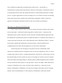
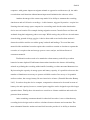
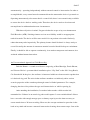
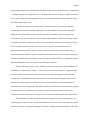
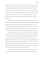
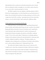
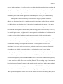
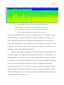
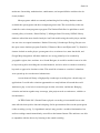
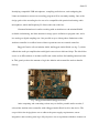
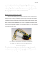
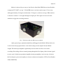
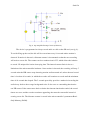
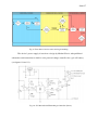
UNIVERSITY OF CALIFORNIA,
IRVINE
Building an Autonomous Audio Field Recorder
THESIS
submitted in partial satisfaction of the requirements
for the degree of
MASTER OF FINE ARTS
In Drama
by
Stephen Burnham Swift
Thesis Committee:
Associate Professor Vincent Olivieri, Chair
Professor Michael Hooker
Professor Anthony Kubiak
2013
Swift 2
Introduction
One of the first definitions of the term soundscape comes from composer and
environmentalist R. Murray Schafer. In his 1977 book, The Tuning of the World, he described
soundscapes as “auditory properties of an environment,” and further segmented soundscapes
into three main categories: keynotes (background ambiences), soundmarks (location specific
sounds), and sound signals (sounds that are out of place or raise alarm) (Schafer 9).
While the definition of soundscape has evolved, Schafer’s terminology continues to
influence modern usage. As a theatrical sound designer, I consider sound to be fundamental in
establishing a sense of place. I found Schafer’s categorizations could easily be mapped to
techniques in my toolkit: establishing background ambiences, finding iconic sounds to guide
and support the play’s context, and using contrasting sounds to grab attention.
As a musician, Schafer focuses on the relationship between soundscapes and the
human listener. This is evident in his classification system, which divides sounds by how they
are interpreted by humans. Another way to classify sounds is by their originating source:
anthropogenic (from humans and human activities), biological (other animal sound), or
geophysical (landscape elements such as wind, water, thunder, etc.) (Dumyahn and Pijanoski
1329). This analytical approach attempts to reduce human biases and has been adopted by
scientists in the fields of ecology and biology.
By dissecting soundscapes into their base components, scientists are able to quantify
an environment by its composition of sounds. For example, soundscapes can indicate the
ecological health of an area and document noise pollution from human activities. Just as
photos of a glacier taken in different years can convey the effects of climate change, two
audio recordings from one location can convey the changes in soundscape.
The procedure to capture and process pertinent data can be time intensive given the
time required to record, analyze, and edit audio—all of which occurs in the real-time domain.
Swift 3
I have identified an approach to streamline part of this process—specifically, by
autonomously recording audio when motion is detected. In this paper, I examine the value of
an autonomous field recorder and consider how the tool’s functionality shapes the recording
process. I explore applications of such a recording device in scientific research, and I identify
shared goals between the scientific and sound design communities. Finally, I detail one
approach to building an autonomous field recorder and evaluate its performance.
The Value of an Autonomous Field Recorder
I first became interested in the concept of a motion activated recordings after reading
about camera traps—automated cameras triggered by motion sensors—setup across the
Adirondack region in New York State. In 2011, the New York State Museum partnered with
the Smithsonian to publish these photos on Smithsonian Wild, a searchable online database of
camera traps from around the world (“State Museum Camera Trap Photos Online”). Curious
about what it sounded like during these animal encounters, I began to think about a
complimentary device that could be deployed to record acoustic information.
Camera traps have the advantage of being able to observe animals that would
otherwise avoid human presence using their sense of smell and sight (Kays). This is a classic
example of the observer effect, a common phenomenon where the act of observation can alter
the situation being observed. In this case, the act of residing in a location to observe animals
deters the animals from approaching. A summary paper by Kathi Borgmann for the Audubon
Society documented bird responses to foreign smells, sounds, and sights: “Birds that flush in
response to disturbance may or may not return to the original site, or may take several
minutes” (Borgmann 4). Disturbance can also lead to change in direction in travel, foraging
patterns, and nest abandonment (7). The frequency of disturbances affects the animals
Swift 4
responses, with greater impact on migrant animals as opposed to resident ones (4). An audio
recorder that could function without human input would minimize the observer effect.
Another advantage of the camera trap model is its ability to automate the recording
function on and off. Selective recordings—in this instance, triggered by motion—require less
listening time and storage space compared to a recording made for the entire duration the
device was on location. For example: during migration season, Canada Geese use lakes and
wetlands along their migratory path as rest stops. While resting, they will leave for and return
from feeding grounds in large gaggles. A device that could record audio when motion is
detected would be useful to record the group’s takeoff and landings. To record the same
material with a traditional recorder requires the recordist to remain on location to operate the
recorder, or it requires time and storage space to store, analyze, and discard hours of
extraneous material.
Traditional recorders need to be attended to when memory cards fill up or when
batteries become depleted. Each human intervention introduces the chance of disturbing
animals or polluting the recording with footfalls, breathing, or other unwanted human noises.
By increasing the capacity of storage space and battery capacity, it is possible to decrease the
number of disturbances necessary to operate said field recorder. In a survey of 16 portable
audio recorders, the average battery life was found to be 6 hours (“Portable Recorder Battery
Life”). In order to keep the device compact, compromises often need to be made in terms of
battery size and capacity; however, external power supplies can be designed to provide longer
operation times. Finally, these electronics are sensitive to climate conditions and need to be
protected from moisture.
After examining common tradeoffs in other field recorders, it was evident that any
recording device design needs to achieve a balance between features and constraints. The
most substantial benefit a motion activated field recorder provides is its ability to function
Swift 5
autonomously—operating independently without external control or intervention. In order to
accomplish this, every control must be automated from the moment the device is powered on.
Operating autonomously also means that if a control fails, there is no external entity available
to restore the device back to working order. Therefore, the device needs to be robust and
uncomplicated to withstand unforeseen circumstances.
With these objectives in mind, I began to define the scope of my own Autonomous
Field Recorder (AFR). Limiting features to focus on reliability would be an appropriate
tradeoff to make. The device will be more useful if it can perform a few tasks flawlessly
rather than many tasks imperfectly. The primary feature should be that it is always ready to
record. Secondly, the amount of extraneous material recorded should be kept to a minimum.
Finally, it should be able to operate continuously, in an outdoor temperate environment, for a
weekend without human interaction.
An Unconventional Approach to Field Recording
Push the Button—a sound art collective composing of Brad Berridge, Davin Huston,
and Vincent Olivieri—presented their installation piece “City Park” at the 2011 Long Beach,
CA Soundwalk. In the piece, the audience is immersed within an electroacoustic reproduction
of a fictional city park. The twist is that audience members can indirectly affect various
acoustic properties of the soundscape through control of linked parameters. For example,
changing the time of day affects the type and characteristics of vehicles passing by.
After attending the installation, I wondered what sounds a field recorder left
unattended for 24 hours in an actual city park would capture. I soon concluded that I did not
have a recorder with enough storage space or battery capacity, nor the time necessary to
curate sounds from a 24 hour recording. However, the concept continued to percolate in the
back of my mind and became a renewed interest after learning about camera traps. One of the
Swift 6
design requirements of my Autonomous Field Recorder was that it should have—at minimum
—enough capacity to be applicable for a “24 Hours in Location X” project, which I envision
to be a time compressed phonographic art piece assembled from recordings captured using
the AFR’s motion detection.
My interest in these location projects is related to my desire to design authentic
soundscapes for theater. Imitating authenticity can often require a tremendous amount of
highly specific information across a broad spectrum of conditions. One recording in an
environment may be accurate but not necessarily representative—the blood curdling scream
of a rabbit pierced by a predator’s talons is an extraordinary incident. A recording of a light
breeze or other common sounds may come across as generic or one dimensional. A
quintessential portrayal of a region, such as a lone loon call across a lake, has the risk of
being stereotypical. While a myriad of different individual sounds can be found in any given
location, a soundscape is not simply a sum of all these sounds; rather it is a particular subset
filtered through the context of a given environmental condition.
Factors like time of day, season, weather, activeness, perspective, and inhabitants all
contribute to a soundscape’s unique—if not always consciously distinctive—signature. The
more recordings available from any given locale increase the potential to understand the
complexities, commonalities, and abnormalities of an environment through sound. I often
find these location-specific recordings to be more powerful than a crafted assemblage of
individual raw sonic components. The field recording’s authenticity is derived from a genuine
but ephemeral set of circumstances existing in a precise moment of time, whereas the
contrived scenario is fabricated, developed, and controlled in the vacuum of an audio editor.
The uniqueness of these location specific recordings can also be advantageous. If a
sound designer wanted to use a sound effect that had never been used before, her only option
would be to create an original recording. Eric Norris, a Supervising Sound Editor in the film
Swift 7
industry, described commercially available sound libraries as a double edged sword. Some of
his favorite sounds come from these libraries because they contain well crafted high caliber
sounds. He is constantly turning to these favorites because he knows they will deliver the
needed energy, but they also can get overused for that same reason. For example, he recently
decided to stop using the Sound Ideas “Jacobs Ladder Arching” sound because he has gotten
tired of hearing it in both his own and others’ work. Instead, he is planning on recording
power lines and transformers in his neighborhood during the next California energy Flex
Alert (Norris).
The advantages of capturing original recorded material is certainly not unique to the
AFR; moreover, the AFR would be the wrong tool to choose for Norris’ electricity recordings
(as there would be no motion to detect). Even if it were the appropriate tool, there is no
guarantee that the AFR would record useful or interesting events; however, its set-and-forget
operational model requires little effort from the recordist. A more passive field recording
method may yield more opportunities to record and promote recording more frequently.
Field recording is typically not an undertaking one can do concurrently with another
activity. It is easy to pollute a recording with unwanted noises. Humans have the ability to
selectively separate, filter, and ignore simultaneous sound sources (Moulton). Microphones
do not, and their sensitivity to wind, background ambiences, and other noises can be
surprising to non-recordists. In order to achieve a high quality recording, the recordist is often
required to isolate herself and work patiently—conscientious of any sound, no matter how
minor, that might also be captured. The AFR removes the requirement that the recordist must
be present in order to start and stop recording. Instead of needing to sit quietly for extended
periods of time, the recordist is at liberty to leave the recording site.
Many unattended AFR devices could be deployed at the same time to increase the
coverage area. For instance, an array of devices could be spaced along a path in order to
Swift 8
gather information about a recorded event’s directionality. Alternatively, devices could be
placed in contrasting sites within a surrounding area (e.g. lake shore, meadow, forest floor,
etc.) as a way to achieve a broader representation of a vicinity.
The AFR is essentially a tool to take snapshots of soundscapes when the recordist is
absent. One of its primary purposes is to record sounds that occur away from the presence of
humans, such as wild animal activity. Instead of recording continuously, it selectively records
excerpts from a location. These recordings—representing actual events from a specific time
and place—can convey both a moment’s explicit actuality and serendipitous fragility.
Scientific Applications of the Autonomous Field Recorder
Soundscape Ecology is an interdisciplinary field of study sharing similar research
interests with other fields including: Spatial Ecology, the study of ecological events explained
through spatial patterns; Bioacoustics, the study of non-human acoustic communication;
Acoustic Ecology, the study of human interactions to sounds in an environment; and
Psychoacoustics, the study of perceptions and reactions to sound (“What is soundscape
ecology?” 1215). In a 2011 article by Bryan C. Pijanowski et al. formalizing Soundscape
Ecology as a field of study, the inclusion of the aforementioned fields is clearly shown in the
ecologists’ comprehensive definition of soundscape: “All biophony, geophony, and
anthrophony sounds, emanating from a given landscape to create unique acoustical patterns
across a variety of spatial and temporal scales” (“Soundscape Ecology” 204).
The seminal article identified a number of topics in need of research. One need
recognized was for “sensors that can automate the recording of sounds, that are inexpensive,
and that can be placed in large networks in hostile environments” (“Soundscape Ecology”
209). The subject of automation was address in an article by Fristrup and Mennitt using a
software based approach. The authors found:
Swift 9
Many projects have encountered significant bottlenecks in this phase. There are
many potential software tools to automate processing, but the difficulty seems to
lie in selecting the appropriate tool, and gaining sufficient experience with its
use to maximize its performance (Fristrup and Mennitt 20).
One advantage the Autonomous Field Recorder has over a software automation approach is
that the AFR applies automation during the capture process, thus pre-filtering the amount of
data necessary to analyze in software. Nevertheless, in order to facilitate an efficient study,
the authors suggest separating the acoustic monitoring process into three components:
“Detecting and delimiting events of interest, characterizing the structure of the event, and
classifying the event to a species or other class of signals” (Ibid.). The AFR’s function can be
understood through this framework: the event of interest will be detected using a motion
sensor triggered by the recording subject’s approach; the structure of the event will last until a
post-delay has timed out after motion ceases to be detected; the recorded material can be
classified through aural identification or by visually comparing spectral patterns to sample
data.
Another research goal addressed by Pijanowski et al. is that scientists need a better
way to understand how biological, anthropogenic, and geophysical sounds “differ in their
composition” (“Soundscape Ecology” 209). One way to study this topic would be to compare
data captured with an AFR to background ambient sample data from the same environment
(perhaps collected by a traditional recorder). The hypothesis is that the AFR will be primarily
triggered by biological or anthropogenic subjects and will contain contrasting spectral
patterns compared to the sample data. Aural identification can be used to confirm the content
of these recordings.
Consider again the example of migratory Canada Geese. Sample background ambient
data could be collected at the rest stop when the geese are away feeding. The AFR will collect
Swift 10
data when triggered by the geese coming or going (or any other movement). When viewed in
a spectrogram, the background ambient noise should be present in both recordings, but the
AFR will also contain spectral patterns corresponding to the geese movement. A comparison
of the spectral characteristics between the geophysical and biological sounds could then be
made.
Soundscape Ecology is an emerging field of study. Scientists have identified the value
of studying the landscapes and environments by examining their composition of sounds. In
doing so, they seek to explain the impacts of soundscapes on ecosystems and vice versa. One
of the main challenges continues to be implementing rigorous measurement and analysis of
sonic data. By equipping electrical sensors with audio recorders, more efficient sampling can
occur as long as the sensors can measure the events of interest.
Applying Audio Engineering Concepts to Soundscape Ecology
Pijanowski et al. described the parallels Soundscape Ecology shares with Spatial
Ecology, Psychacoustics, Bioacoustics, and Acoustic Ecology. Another equally important
field to soundscape ecology is Audio Engineering. Audio engineers are experts in recording,
enhancing sounds, and reproducing sounds.
Bernie Krause is one such musician and audio engineer who became interested in
recording sounds of nature. He is currently one of the prominent leaders in the field of
Soundscape Ecology with over 40 years of experience recording soundscapes. His work
bridges the scientific and artistic communities being published both in academic journals and
on commercial record labels.
An audio engineer is an excellent person for an ecologist to consult with. He or she
has the experience and skills to help the ecologist establish a recording methodology. Since
sound recordings constitute the primary data in soundscape ecology research, this is a crucial
Swift 11
process in the experiment. An audio engineer can help make informed decisions regarding the
appropriate recording tools and techniques that will be best suited for a particular study. For
example, there are advantages and disadvantages to every microphone design, and
determining what trade-offs are appropriate to make depends on the goal of the recording.
Microphones can be classified by their transducer design (dynamic, condenser,
ribbon) and directional sensitivity (omnidirectional, bi-directional, cardioid, hyper-cardioid,
etc). Microphone specifications also include noise floor and sensitivity ratings. A low noise
floor results in less self-noise bleed from the electronics in the recording. Sensitivity indicates
how efficient a microphone is at converting acoustic energy into electrical voltage (Lewis 1).
For detailed quiet sounds, a high sensitivity microphone is useful, whereas a loud thunderclap
or nearby strident birdcall might overload a microphone with a high sensitivity rating.
A microphone’s directionality has one of the more noticeable effects on a recording.
Omnidirectional microphones are equally sensitive in all directions, which typically yields a
more natural sounding recording to the human ear. As a microphone becomes more
directional, it becomes easier to focus it on a particular sound source; however, directional
microphones also exhibit a proximity effect—a coloration due to an increase in lowfrequency response affecting sound sources recorded close to the microphone (Josephson).
Krause’s typical setup combines a Sennheiser MKH 40 (a directional cardioid
condenser microphone) with a Sennheiser MKH 30 (a bi-directional condenser microphone)
in order to achieve a Mid-Side stereo recording (Robair). This recording setup is important to
his artistic process. One of his tenets is that sounds should experienced in the context of their
environment rather than attempting to isolate the sound. The Mid-Side recording format
allows him to control the blend between the recording subject and background ambience.
These specific microphone models were selected for their low noise floor rating (Ibid.). Noise
Swift 12
can be introduced by any device in the signal chain, so it is equally important that the preamplifier and digital recording device match or exceed the microphone’s noise floor rating.
There are two other important specifications to pay attention to when selecting a
digital recording device: sampling rate and bit depth. The Nyquist–Shannon sampling
theorem defines the highest frequency that can be reconstructed as one half the value of the
sampling rate frequency (Lavry 1). Bit depth is the number of binary digits each sample
contains. As bit-depth increases, the potential dynamic range—the difference between the
quietest and loudest sounds—also increases. CD quality audio (44.1 kHz sampling rate, 16bit resolution) is considered a minimum baseline for professional audio recordings. Given a
sampling rate of 44.1 kHz, the highest frequency that could be reconstructed is 22 kHz. This
bandwidth is sufficient to reproduce all the frequencies audible in the range of human
hearing, which is typically considered to be between 20 Hz and 20 kHz. A 16-bit resolution
allows for a dynamic range of 96 dB (16 bits * 6 dB/bit). The Sennheiser MHK 40 has a
dynamic range of 113 dB (Sennheiser). The 16-bit resolution is not able to represent the full
dynamic range of the microphone, which is why a 24-bit or 32-bit capable digital recorder
would a better match.
After selecting the appropriate equipment, consideration should be given to
deployment and placement of the recording equipment. For example, a dynamic
omnidirectional microphone may be suited for a general forest ambient recording, whereas a
detailed recording of ants on a log might be better served with a cardioid condenser placed a
few centimeters away from the source. Placement alone can be a major determining factor in
what material is recorded. Two recordings made with the same equipment, in the same
environment, but with different placements can yield different results (see fig. 1).
Swift 13
Fig. 1. Spectrograms of two audio recordings of Ruby Beach, Olympic
National Park by Vincent Olivieri. Left: “Standing on rocks 100 yards
from woods.” Right: “On top of 50 ft. rock, water 500 ft. in front, woods
are 500 ft. behind, [microphone] resting on rock.” (Olivieri)
The first recording captured the sound of waves crashing against the shore—highly variable
material with dynamic amplitude changes in all frequencies. The second recording shows a
drastic attenuation of frequencies above 5 kHz, with an amplitude increase in frequencies
below 1 kHz. The differences can be attributed to two factors: high frequency dissipation due
to the 50 ft. vertical increase in distance from source, and low frequency coupling due to the
microphone’s direct contact with the ground (Ibid.).
While an audio engineer can optimize microphone placement using information about
recording mechanics, an ecologist needs to consider animal habitats, movement patterns, and
migratory trends when selecting recording positions. In preparation for a field recording, the
audio engineer and ecologist should identify key factors of the project together: the biophonic
sources of interest, the biomes these sources are present in, geographic locations these
sources have been observed at, size of desired coverage area, behavior patterns of recording
subjects, minimum and maximum sound levels expected, structure and variability of sound
signals, audio frequency range of sound signals, security and stability of recording setup, and
disturbance impact of recording setup.
Swift 14
The audio engineer and ecologist should also discuss intended uses for the recordings,
and how to make recordings that serve these required purposes. In a typical scientific
analysis, the recording is translated into raster graphic data for manipulation irrespective of
sonic fidelity; whereas traditional audio editing prioritizes how the audio signals are
perceived when converted back into acoustic energy. For example, scientists will
occasionally work with sampling rates lower than 44.1 kHz since the majority of animal call
patterns produce fundamentals below 12 kHz. The sonic quality of the recording is of lesser
importance, since the relevant raster data is still present. However, if the digital recording
were to be transmitted acoustically again, humans would be able to detect the absence of the
higher frequencies. These frequencies contain harmonic information and transients which
provide noticeable tonal identifications. This information could be useful if aural
identification is required.
Aural identification uses zoologists with regional expertise to name the species in the
recording by their soundcalls (“Soundscape Ecology” 208). This species identification
method can be more feasible than an algorithmic process which requires an established
database of recordings to perform pattern matches against (“What is soundscape ecology?”
1226). Acoustic analysis also exceeds visual analysis when disparate sonic sources overlap in
the time/frequency domain and cannot be easily separated algorithmically. This might occur
when a waterfall or motor masks chorusing frogs, or when different species of insects are
creating sounds in the same frequency band. In all of these cases, setting a high sample rate
and bit depth is important to retain enough detail for aural identification.
Audio editing tools are sometimes employed to enhance the signal or decrease
background noise in order to improve the conditions for aural identification. Digital signal
processing is applied to filter the audio signals in various ways. In 2012, a study on animal
Swift 15
diversity published in the journal Ecological Indicators documented the data processing
methods used to isolate animals from the background environment:
A band-pass filter between 1 kHz and 13 kHz was applied with Goldwave©.
Due to the permanent background noise caused by wind, vegetation rustle
and/or rain (geophony sensu Qi et al., 2008 and Pijanowski et al., 2011), it
was necessary to apply a second filter. The amplitude median of the quietest
signal including noise was assessed at a level of 90 points, with a maximum
value of 215. This energy level was used as a reference to apply an amplitude
filter to all files. The filter removed all signal sections that were below a
threshold of 90 points. (Depraetere 48).
Later on, Depraetere et al. describe the difficulties evaluating animal density based on
frequency content analysis:
Background noise due to plane, car, farm machinery or train can severely impair
the measure by generating a fairly flat spectrum and hence false Hf high values
(52).
These sources generate wide-band frequency content and can mask animal sounds. Band pass
filtering can only do so much to reduce wide-band noises. When noise masks the subject,
both sounds are occupying the same frequency bands. Sophisticated noise reduction tools can
profile the audio signals in order to remove the noise while preserving the desired source
signals. Removing hiss or other unwanted acoustic artifacts is a common audio editing task,
and audio engineers specialize in removing noise efficiently and judicially.
An audio engineer can be an essential resource on the research team. He or she can
help define the technical recording standards the experiment requires, select the appropriate
equipment, review the recording setup and methodology, and assist with the post-processing
required to clean up the audio files. Soundscape ecologists examine the environment through
sound and rely on audio files as documentation. It is important that these sound recordings
Swift 16
contain accurate and significant data to study. Audio engineering best practices can be
employed to optimize the recording process in order to meet this goal.
Benefits of Collaboration Between Ecologists and Sound Designers
Sound design, a related field to audio engineering, focuses on the construction and
manipulation of sound. Common mediums include film, television, theater, video games, and
installations. Sound designers receive similar training to audio engineers, and share
similarities with audio engineering sub-disciplines such as recording engineering and audio
production. Sound designers use their knowledge of recording and audio processing to create
sounds that support a narrative and evoke an emotional response.
Field recording is an important process for sound designers. Original recordings serve
as the base material for designed sounds. Ambiences and soundbeds are used in film,
television, and theater to provide context about a scene's location. A script may require the
sound of a specific animal. Access to undisturbed habitats can be a challenge due
proliferation of human mechanical noise. An ecologist is an excellent resource to turn to for
advice regarding unique habitats, representative soundscapes, favorable research sites, or
protected lands.
Government agencies such as the National Park Service and the European
Environment Agency have established policies to designate soundscape conservation areas
(Dumyahn and Pijanoski 1329). Sometimes this involves temporarily restricting access to
habitats if, for example, the area is currently a breeding ground for a particular species.
Working with these agencies, ecologists use acoustical monitoring to ensure the policy goals
are being met. In a situation like a breeding ground, two main indicators of habitat wellbeing
are species communication regularity and a low threshold of background masking sounds
(1336). University ecology programs have also established private research sites to facilitate
Swift 17
long term acoustical monitoring studies. By partnering with soundscape ecologists, a sound
designer could assist in the monitoring studies, in exchange for access to the recorded
material. Ecologists gain a recording expert on the research team, and the sound designer
gains access to uncommon recording engagements.
One of the challenges in soundscape ecology is the lack of historical data to analyze
(Pijanowski and Krause). For example, scientists can demonstrate a correlation between
temperature and the timing of organism chorusing, but have not made a direct link to global
warming because they lack baseline material required for such a proposition (Ibid.).
University programs are attempting to remediate this by establishing databases of continuous
data—recordings collected from the same location at regular time intervals.
Another way to increase the available data to study would be through crowdsourcing.
This could expand the data set to areas not surveyed by government or university research
studies. Sound designers, recording engineers, and musicians are already producing
numerous field recordings for commercial and public use. If the soundscape ecology
community were to publish standards for soundscape ecology recordings, it would be
possible to contribute qualifying recordings for scientific study.
In an interview with Electronic Musician, Krause discussed the importance of high
quality thoroughly documented recordings:
Often there's no information on the CD about what creatures you're listening
to. We need to know about a place beyond the fact that it's an ‘alpine wood.’
In Yellowstone National Park alone, there are hundreds of different habitats.
This is really important information that people need to pay attention to.
(Robair)
The National Park Service provides some guidelines to create better documentation for field
recordings. It suggests logging latitude, longitude, elevation, date, time, temperature, wind
Swift 18
speed, site description, biome, ground porosity, vegetation cover, canopy cover, recording
equipment, and recording settings (“Acoustical Training Manual” 22-26).
One such crowdsourced project, The World Ambience SFX Library, has attempted to
establish field recording guidelines regarding audio quality, file naming, and meta-data. The
project’s goal is to collect and distribute ambiences from all over the world; within 60 days, it
attracted over 300 participants (Niederquell). The project was created by professionals in the
film industry, and its standards are heavily influenced by the priorities of film Supervising
Sound Editors. For example, submissions should be stereo 96kHz 24bit PCM files, with the
following naming scheme:
- Category: We will be using the prefix "AMB" for "ambience".
- Location Type: Please only use "Rural" or "Urban".
- Time Of Day: Please only use "Night" or "Day".
- Location: Where the recording was captured. Please use the city name or
closest thing to it. (Ibid.)
The World Ambience SFX Library requires a far lesser level of specificity than the National
Park Service guidelines, but it would be certainly possible to log the superset of data, and
submit recordings with the requested subset of information.
Perhaps only a minority of field recordists will want to participate in these
crowdsourced projects. This is perfectly acceptable, as there are many different motives for
creating field recordings. Currently, there is no official avenue to make field recordings
available for research. Recordings could be uploaded and tagged to a site such as
SoundCloud or a database such as Michigan State University’s Remote Environment
Assessment Laboratory (REAL) Library could be opened up for public submission. It would
be necessary to peer-review submissions, either through group consensus or by appointing a
Swift 19
moderator. Ownership, authorizations, entitlements, and responsibilities would need to be
clearly defined.
Most programs which are currently maintaining field recording databases make
available the spectrograms and the accompanying meta-data. The accessibility of the raw
sound files varies from program to program. The National Park Service publishes a small
curated gallery of sounds (“Sound Gallery”). Michigan State University’s REAL Library
database offered the most detailed analysis, but I had trouble using the audio player, and the
site was slow to respond sometimes. Purdue University’s Soundscape Ecology Project uses
the open source database program, Pumilio (Villanueva-Rivera and Pijanowski 71). Pumilio’s
features include an audio player, spectrogram view, waveform view, meta data fields, and
Google Maps integration. All three databases are set up primarily to be searched by
geographic region, date, and time. As a Sound Designer, it would be useful for me to be able
to keyword tag files describing the recorded material, and to be able to search for sounds by
keyword as opposed to location or time. This would be a feature to consider if a database
were opened up for crowdsourced submissions.
A crowdsourced library of high quality soundscape recordings has a broad range of
applications. It could offer scientists opportunities to study habitats all around the world.
Ambiences play a vital role in sound designs for film, television, and theater. Bringing
scientists and artists together may encourage joint projects such as conferences, exhibits, or
documentaries.
At TED Global 2013, Bernie Krause played a recording of a mournful beaver after
state officials destroyed its dam and offspring. On his presentation slide was the spectrogram
of the recording (see fig. 2). Algorithmic analysis may provide a wealth of information, but
audio recordings remain immediately accessible to the human listener. The audience was able
to empathize with the beaver by listening to the sound recording.
Swift 20
Fig. 2. “Beaver Call” recording by Bernie Krause (“Voice of the Natural World”).
Maybe this pursuit of quantitative and qualitative information about soundscapes is where the
collaboration between ecologists and sound designers can truly flourish. One of my goals as a
sound designer is to evoke an emotional reaction. If sound designers can encourage people to
become passionate about the soundscape environments, and ecologists can present research
about how these environments are evolving, some substantial advocacy could develop as an
outcome—be it a reduction of human noise pollution, improving our understanding on how
soundscapes affect the wellbeing of humans and other animals, or promoting and protecting
unique soundscapes from all across the world.
Outfitting a Field Recorder for Bioacoustic Research
A device intended for long duration autonomous recording should have three basic
features: it should be possible to operate continuously for days at a time, support control from
an external data source, and be weatherproof to withstand unknown or unexpected
Swift 21
conditions. There are a few commercial products that provide solutions for some of these
requirements.
The Song Meter SM2+ from Wildlife Acoustics (see fig. 3) is powered from four D-
size Alkaline or NiMH batteries and is rated for 280 hours of recording time. It can host up to
four 128 GB sized SDXC cards for a total of 512 GB storage space. The recorder can either
be triggered at specific times: by an absolute threshold dB SPL level, or a relative increase in
dB compared against the rolling average (configurable between +1 and +88 dB). The device
is enclosed in a weatherproof case; all connectors make a weatherproof seal when mated or
can be capped when not in use.
Fig. 3. Wildlife Acoustics Song Meter SM2+ (“Song Meter User Manual”).
The Froglogger VI-LS7 from Bedford Technical (see fig. 4) combines an off-the-shelf
portable audio recorder with a power supply, weatherproof microphone, and scheduler to
create recordings—of a user defined length—at specific times or periodically.
Swift 22
Fig. 4. Froglogger VI-LS7 (Bedford Technical).
One drawback common to these available solutions was the lack of a pre-record
buffer. A pre-record buffer is a continuous temporary recording. When the record function of
the device is engaged, material in the buffer is also stored, essentially allowing the device to
capture audio content in the immediate past. This could be useful for capturing the
environment’s context leading up to the significant event, or to ensure the start of the event
was fully recorded.
Dashcams—audio/video recorders made to mount on a car dashboard—are common
in Russia where evidence of fault is often required for insurance claims. Many models exist
that can continually record a cycle buffer of material when motion is detected.
Dashcamtalk.com has reviews and comparisons of models, but a common complaint
regarding sound quality came up again and again in the reviews. This is understandable, as
the primary purpose of these devices is surveillance, not professional location sound
recording. However, these products did outline the structure needed for a digital automatic
recording device using higher quality audio components.
Tutorials for creating audio recordings with a single-board microcontroller, such as
the Raspberry Pi and Arduino, are easily accessible on the internet. The Raspberry Pi is a
Linux based computer. Some common complications using it for audio recording are:
Swift 23
identifying compatible USB microphones, compiling audio drivers, and configuring the
Linux environment to ensure our recording program will be constantly running. One of the
design goals of the recording device was to be compatible with professional analog audio
microphones, which the Raspberry Pi did not offer out of the box.
Common limitations for audio recording with an Arduino are: the minimal RAM
available for buffering, the little amount of storage space available for program code, and a
low analog-to-digital sampling rate. One possible way to sidestep these limitations of the
Arduino controller is to offload some of these operations onto an external controller.
Rugged Circuits sells an Arduino shield, the Rugged Audio Shield (see fig. 5), which
offloads the audio pre-amplification and digital conversion to dedicated chips. The shield also
serves as an SD card host; it includes an SD card socket and has file handling functions builtin. This greatly reduces the amount of logic the Arduino microcontroller needs to handle
directly.
Fig. 5. Rugged Audio Shield (Rugged Circuits).
After comparing and contrasting various ways to build a portable audio recorder, I
selected the Arduino microcontroller with a Rugged Audio Shield to drive the device. The
scope of this first design phase was to address the power supply requirements, sensor
integration, and recording state logic. My objective was to experiment with these features on
Swift 24
top of an already functional audio recorder. Integrating analog-to-digital converters,
implementing a file system, and compiling audio drivers would overly complicate this phase
of the design. The Arduino and Audio Shield combination was very appealing, as it handled
the analog-to-digital conversion and file system functions natively.
How the Autonomous Field Recorder was Built
The device’s functionality can be divided into four main sections: motion detection,
audio processing, recording logic handling, and power supply. The Rugged Audio Shield is
compatible with microcontrollers based on the Arduino Uno/Duemilanoe schematic. Simon
Penny, Professor in Art and Mechatronics at UC Irvine, recommended a Duemilanoe based
board from Seeed Studio: the Seeeduino V3.0 with Atmega 328P (see fig. 6). This unit would
serve as the brain of the system.
Fig. 6. The device’s main components. From Bottom to Top: Seeeduino
V3.0, Rugged Audio Shield, and a custom shield with connections to
infra-red sensors (not shown).
The Seeduino offers some improvements on the Duemilanove design such as manually
selectable power source, manually selectable voltage supply, smaller USB connector, side
mounted reset switch, and the ability to enable or disable the auto-reset function.
Swift 25
Motion is detected by an array of four Passive Infra-Red (PIR) Sensors from Parallax,
component 555-28027 (see fig. 7). Each PIR sensor can detect motion up to 15 feet away
with approximately 110 degrees (horizontal) x 70 degrees (vertical) coverage. When motion
is detected, it sends a 5 volt signal through its output pin. This signal can be read on the
Arduino to trigger the recording function.
Fig. 7. Enclosure with four PIR sensors mounted.
Audio processing is primarily handled by the Rugged Audio Shield. When the device
is first booted, the program defines a few initial settings such as Input Gain and Buffer
Length. The built-in preamplifier significantly increased the noise floor level in the
recordings. Recording with an external preamp through the Line Input yielded a better signalto-noise ratio. I added an operational amplifier based preamplifier circuit (see fig. 8) before
the Line Input to power and amplify an electret condenser microphone (CUI Inc Part Number
CMA-4544PF-W).
Swift 26
Fig. 8. Op-Amp Mic Preamp Circuit (Collinson).
The device is programmed to always record audio to a file on the SD card (see fig. 9).
To avoid filling up the card, the file will be overwritten every 10 seconds unless motion is
detected. If motion is detected, a filename counter is incremented so that the next recording
will write to a new file. The counter can be a number from 0-255, which allows the Arduino
to record 256 unique files before destroying data. The internal counter limit is due to a
limitation of the microcontroller hardware. Once motion is detected, the recording will stop 5
seconds after the PIR sensor stops detecting motion and has turned off, unless the total record
time is less than 10 seconds, in which the recorder will continue to record until the minimum
time of 10 seconds has elapsed. The 5 seconds post-delay provides a method of recording the
audio decay back to the average background noise. It also acts as a smoothing function for
our PIR sensor. If the sensor turns back on before the timeout function has ended, the record
timers are reset, and the recorder continues appending data onto the current file instead of
creating a new file. The filename counter is stored in the microcontroller’s permanent ReadOnly Memory (ROM).
Swift 27
Fig. 9. Flow chart of device states and logic handling.
The device’s power supply is based on a design by Michael Davis, who published
schematics and instructions to build a solar powered charge controller for a gel cell battery
(see figures 10 and 11).
Fig. 10. 555 Based Solar/Wind Charge Controller (Davis).
Swift 28
Fig. 11. Completed Solar Charge Controller Circuit Based on Michael Davis’ Design.
The device is powered by a 12V 5 amp hour (Ah) gel cell battery (see fig. 12). The device’s
average power draw is 150 milliamps, thus the battery is capable of powering the device for
over 30 hours. The power supply also includes a solar panel that can power the device and
trickle charge the battery. The solar panel’s max power current output is rated at 0.278 amps.
Fig. 12. From Left to Right: Field Recorder, Solar Panel,
Charge Controller, Gel Cell Battery.
Swift 29
A typical self-discharge rate of a gel cell battery can be as high as 30% a month. For a 5Ah
battery, this equates to losing 0.05 Ah a day. There is a way to calculate the minimum amount
of energy required to recoup this power drain:
Amp Hours Lost per day / Solar Panel Current Output =
kiloWatts hours per meter squared per day
0.05 Ah / 0.278 A = 0.18 kWh/m2/day
The National Renewable Energy Laboratory (NREL) publishes solar radiation levels
in the United States in kiloWatt hours generated per meter squared per day (see fig. 13). The
continental United States receives the least amount of solar radiation during the month of
December. Most areas (with the possible exception to some parts of the Northeast and
Northwest) provide at least 2 kWh/m2/day, which exceeds our requirements tenfold.
Fig. 13. US Solar Radiation Map for the month of December (NREL).
After all the components had been assembled, the last consideration was protecting
the equipment from outdoor environment conditions. Other commercial and hobbyist projects
use a variety of solutions from tupperware to modified Pelican cases. The main concern was
Swift 30
protecting exposed electrical connections. All solutions kept the battery and charge controller
inside a box. Covered cutouts or insulated pass-throughs were provided for the microphone
and solar panel connections. I sourced a waterproof project box from MCM Electronics to
house the battery and controller and provide covered pass-throughs for cables (see fig. 14).
Fig. 14. Dri-box 285 Outdoor Waterproof/Weatherproof Box (MCM Electronics).
Performance of the Autonomous Field Recorder
The first tests of the device used an iPod connected to the audio shield’s line input
connection. This provided a constant audio feed; it also eliminated the microphone and
preamplifier variables. The first complication I encountered was that the expected recording
files could not be found on the SD card. Using the Arduino debugging console, I determined
that the recording start/stop loop had performed correctly, but the file did not exist. I inferred
that there was a problem with the SD card library: either mounting the card, opening the card
for write, or closing the write session. In my experimentation with the audio shield, I noticed
that it did not handle mode switching gracefully. Whenever switching between the record,
playback, and audio-stream modes, it was necessary to hard reset the device each time. It is
possible that either the Rugged Audio Shield main controller or Serial Peripheral Interface
Bus (which processes the SD card functions) had not initialized completely by the time the
Swift 31
field recorder program was asking for access to the SD card. By experimenting with the order
libraries loaded and adding in delay times to the startup sequence, the device could
successfully and consistently boot and write to the SD card.
Another file handling bug occurred if the device’s power was interrupted while a file
was open for write. This scenario occurs when the recordist disassembles the device at the
end of a recording session. I was frequently finding my last recorded file corrupted. The
solution was to add a button to allow the user to properly close the current file and end the
recording session. I added an indicator LED to provide feedback to user about the device’s
record state. When the LED is on, the device is in a record ready or a recording state. When
the LED is off, it is okay for the user to unplug the device or remove the SD card.
Once writing files worked, I next noticed that the recorded audio files contained
audible dropouts during playback. While the Rugged Circuits website advertised a sampling
rate of at least 44.1 kHz, the documentation provided this caveat:
Sampling rate is limited by the speed of the SD card (specifically, how efficient it is
internally, not necessarily how fast its SPI bus is), how fragmented the FAT
filesystem is on the card, and whether or not a file has been presized for writing. You
may want to begin with Fs=16000 and increase only if sound quality is not good
enough. If you hear clicks and dropouts on the recorded file, the sampling rate is
likely too high. (“Rugged Audio Shield Library”)
I attempted to contact Rugged Circuits for an SD card recommendation but received no reply.
Without a solid definition of performance standards to use, I selected the fastest option I
could find on the market: SanDisk Ultra 32 GB MicroSDHC. This model has a Class 10
rating, is UHS-1 enabled, and advertised transfer speeds up to 30 megabytes per second. The
SD Association defines Class 10 as being capable of transferring a minimum of 10
MegaBytes per second. Class 10 cards are recommended for full HD recording, and UHS-1
Swift 32
cards are recommended for real-time broadcasts (“SD Speed Class”). The transfer speed of 10
MB/s should be substantially more than necessary to support CD quality audio recording. A
stereo 44.1 kHz 16 bit audio file has a bit rate of 1411 Kilobits per second (approximately
177 kiloBytes per second), which is smaller than the card’s minimum speed rating by a factor
of 50.
The second factor that limits sample rate is disk fragmentation. Tests were performed
on a freshly reformatted disk to remove this variable. The third factor is if the file has been
presized for writing. This process creates the file structure beforehand, making it faster to
write to the file. Presizing was not a viable option for this use case. It requires the user to
define a file size limit (and thus time limit) before recording, which is an unknown for our
recordings. Regardless, tests were performed with the presize option enabled; however, the
sample rate could not be increased above 22 kHz without introducing audio dropouts.
As mentioned in a prior section, the audio shield’s preamplifier introduced too much
noise for professional quality recordings. During the first attempt to use an external electret
condenser microphone and preamplifier circuit, the recordings contained an overpowering
buzz. Michael Hooker, a Sound Design professor at UC Irvine, suggested this was most
likely “dirty power” from the microcontroller shield. He advised testing with an external
power source, such as a 9 volt battery, and adding smoothing capacitors into the preamplifier
circuit. When the preamplifier was powered from the 9V battery, instead of the
microcontroller power rails, the signal was clean. Based on this evidence, Hooker’s advice
was to bypass the microcontroller and power the preamplifier directly from the gel cell
battery. This worked and was the solution used.
Another limitation was that the microcontroller is limited to 32 Kilobytes of RAM;
therefore, the record buffer could not be stored in RAM. A typical cycle buffer is designed
with a fixed length, and deletes data on a First-In, First-Out basis. For example, a 10 second
Swift 33
cycle buffer would always store the last 10 seconds of data. This data is typically held in
RAM until needed in a more permanent fashion, in which it is then written to disk. 32
Kilobytes is not enough space to store even a second of a 22 kHz 16 bit mono audio file. A
cycle buffer could not be created on the SD card as the file write operations did not allow for
trimming data from the top of files. The workaround mentioned previously was to record in
10 second loops unless motion was detected. In this scenario, the length of the pre-recorded
material is determined by what point in the loop motion is detected. If a new file is opened
and motion is detected 2 seconds later, the pre-recorded length is only 2 seconds. However, if
motion is detected 8 seconds after a new file is opened, the pre-recorded length is 8 seconds.
In a cycle buffer implementation, the pre-recorded length would always be 10 seconds. One
could forgo the concept of a buffer altogether and simply record continuously to one large
file. This would reduce the duration the recorder can operate as it uses disk space more
rapidly; it also increases the amount of time needed to review the recording. A custom built
recorder would not be necessary; however, the solar charger would be useful if the recorder’s
internal batteries did not provide a long enough charge.
I conducted a controlled recording experiment to test the integration between the
sensors and recording state logic. The device was positioned on a kitchen counter facing a
pop-up toaster. Bread was inserted into the toaster, and the toaster was activated. Adjacent to
the toaster, an egg was frying on the stovetop. After setting up the experiment, no humans or
other animals were in the room to cause a false trigger. When the toast was ejected from the
toaster, the device’s sensors were engaged, triggering the device to change from its Buffer
State to its Record State (see fig. 15).
Swift 34
Fig. 15. Waveform and spectrogram of recording from experiment.
Significant event (toast ejection) highlighted in red around 5 seconds. Fainter
vertical lines on spectrogram is the sound of the egg frying.
The pre-record buffer had built up about a 5 second recording before the significant event.
After the significant event, the device was in a Record State for 10 seconds, the minimum
recording duration.
Conclusion
This study set out to rethink the traditional field recorder design in order to facilitate
multi-day unattended recording sessions. Three primary concepts of interest were identified
to be: motion based recording triggers, pre and post recording buffers, and interfacing with a
solar power source. Applications for such a device in the artistic, commercial, hobbyist, and
scientific sectors were examined.
Controlling recording states with motion based sensors was demonstrated to function
as designed. Ease of use and reliability were two big priorities of this design. Customizing the
device to automatically power on into a record ready state was a major contributing factor in
Swift 35
achieving this goal. The simplicity of the device—it either is recording or ready to record—
gives the user the needed confidence to leave the device unattended.
Power requirements can be abstracted into two variables: capacity and power draw.
There are two ways to increase the device’s operating duration: increase the power supply
capacity, or decrease the device’s power draw. The device’s power requirements were
minimal; therefore, it was easy to design a portable solar power source. While the device
could be powered directly from the solar panel, a gel cell battery provided a backup reservoir
of energy to draw from during non-daylight hours. Finally, the power supply controller
successfully regulated the battery charging and dumping cycles in order to keep the battery at
healthy charge levels.
Of the three major goals, the buffer implementation was the most challenging. In
order to implement a cycle buffer, the digital audio data needs to be written directly into
RAM. The amount of memory available directly relates to buffer length—in this case, less
than one second. I was not able to program a cycle buffer; instead, the device simulates a
buffer by constantly starting temporary recording sessions in anticipation of a triggered
recording event.
In this design, the audio signal chain was given a lower priority than the control and
power systems. It was more important to have a simple audio feature set than a custom but
untried one. As such, the audio quality of the device suffered. The Arduino microcontroller is
a great device for converting analog sensor information into digital control signals, but is not
a powerful enough machine to process digital audio.
The next step up in processing power from the Arduino would be an embedded Linux
device like the Raspberry Pi. The power supply design and recording state logic can be
directly applied to an embedded Linux system based design; however, the new system
introduces a new set of questions to be addressed:
Swift 36
What soundcards are compatible with the Raspberry Pi?
What are some of the current limitations in the Linux audio stack?
Which audio drivers are most stable?
How should the Linux system environment be configured?
What audio programming concepts are required to record audio?
How are files read and written?
How are analog sensor signals inputed and processed?
Creating a audio recorder in a computer environment will require a great deal of
programming, which understandably is not for everyone. My recommendation to someone
without a background in Computer Science or programming would be to build a controller
that interfaces with a commercially available portable audio recorder. Both the National Park
Service and the Frog Logger designs are built around commercially available audio recorders.
Products like the Zoom H4N have remote accessories that could be reverse engineered; a
custom controller could be built to mimic the remote control commands. This solution takes
advantages of the specialties of each component. The Arduino microcontroller is best suited
for sending and receiving control messages, and the Zoom H4N is a well made professional
grade audio recorder.
A field recorder is not a simple tool to design. A good recorder must have a quality
microphone capsule, preamplifier, and analog-to-digital converter. It should be easy to use,
have decent battery life, and be portable yet rugged. To design one requires knowledge of
digital audio, electronics, and embedded operating systems. The design of the tool also has a
direct impact on how it is used. Many commercial portable audio recorders sacrifice battery
capacity for a smaller device footprint. Bioacoustics monitoring systems require a rugged
enclosure. These devices also include additional remote monitoring features such as
embedded web servers, GPS antennas, and recording timers. The Autonomous Field
Swift 37
Recorder’s approach was an experimentation with a different feature: using analog sensor
input to control the audio recording function. By stripping away all traditional manual
controls, the AFR forces the user to examine how she might approach an unattended
recording session.
Swift 38
Works Cited
Borgmann, Kathi L. "A Review of Human Disturbance Impacts on Waterbirds." Audubon
California (2010), 1-23. Web. <http://www.yourwetlands.org/pdf/A%20Review%20of
%20Human%20Disturbance%20Impacts%20on%20Waterbirds.pdf>
Collinson, Andy. “Op-Amp Mic Preamp.” Circuit Exchange International, n.d. Web. 10 Nov.
2013. <http://www.zen22142.zen.co.uk/Circuits/Audio/lf071_mic.htm>
Davis, Michael. “A New & Improved Charge Controller Based on the 555 Chip.” N.p., n.d.
Web. 10 Nov. 2013. <http://mdpub.com/555Controller/index.html>
Depraetere, Marion, et al. “Monitoring animal diversity using acoustic indices:
Implementation in a temperate woodland.” Ecological Indicators. 13 (2012), 46–54.
Print.
“Dri-box 285 Outdoor Waterproof/Weatherproof Box.” MCM Electronics. N.p., n.d. 10 Nov.
2013. <http://www.mcmelectronics.com/product/21-11155>
Dumyahn, Sarah L., and Bryan C. Pijanowski. “Soundscape conservation.” Landscape
Ecology 26.9 (2011), 1327-1344. Print.
Fristrup, Kurt M., and Dan Mennitt. "Bioacoustical monitoring in terrestrial environments."
Acoustics Today 8.3 (2012), 16-24. Print.
“Froglogger VI - LS7 Information.” Bedford Technical. N.p., 26 April 2011. Web. 10 Nov.
2013. <http://www.frogloggers.com/FL-VI-LS7-Information.html>
Josephson, David. "A brief tutorial on proximity effect." Audio Engineering Society
Convention 107. Audio Engineering Society, 1999. Print.
Kays, Roland. “Museum Moment - Scientist share their camera trap treasures.” Online video
clip. YouTube. YouTube, 11 Feb. 2011. Web. 10 Nov. 2013. <http://youtu.be/
5zQDKDqAW80>
Swift 39
Krause, Bernie. “The Voice of the Natural World.” TED Global 2013. Edinburgh
International Conference Center. Edinburgh, Scotland. June 2013. Conference
Presentation. Web. 10 Nov. 2013. <http://www.ted.com/talks/
bernie_krause_the_voice_of_the_natural_world.html>
Lavry, Dan. “Sampling Theory For Digital Audio.” Lavry Engineering. N.p., 2004. Web. 10
Nov. 2013. <http://web.archive.org/web/20060614125302/http://
www.lavryengineering.com/documents/Sampling_Theory.pdf>
Lewis, Jerad. “Understanding Microphone Sensitivity.” Analog Dialogue. 46.2 (2012), 14-16.
Print.
Moulton, Dave. “The Microphone vs. the Ear.” Moulton Laboratories. N.p., 1993. Web. 10
Nov. 2013. <http://www.moultonlabs.com/more/microphone_vs_the_ear/P1/>
Michigan State University. “Remote Environmental Assessment Laboratory.” N.p.,N.d. Web.
10 Nov. 2013. <http://lib.real.msu.edu/>
National Park Service. “Acoustical Monitoring Training Manual.” U.S. Department of
Interior, National Park Service. 20 May 2013. Web. 10 Nov. 2013. <http://
www.nature.nps.gov/sound/assets/docs/NSNSDTrainingManual.pdf>
National Park Service. “Sound Gallery.” U.S. Department of Interior, National Park Service.
N.d. Web. 10 Nov. 2013. <http://www.nature.nps.gov/sound/gallery.cfm>
National Renewal Energy Laboratory. “US Solar Radiation Maps” U.S. Department of
Energy, May 2004. Web. 10 Nov. 2013. <http://www.nrel.gov/gis/solar.html>
Niederquell, Mike. “The World Ambience SFX Library" Audible Worlds. 24 July 2013. Web.
10 Nov. 2013. < http://www.audibleworlds.com/viewtopic.php?f=30&t=33>
Norris, Eric. “The Sound of Man of Steel.” L.A. Sound Group. 3rdstreetADR, Santa Monica,
CA. 15 Aug. 2013. Guest Presentation.
Swift 40
Olivieri, Vincent. “Shore 03.” Freesound, 8 July 2007. Web. 10 Nov. 2013. <http://
freesound.org/people/volivieri/sounds/37148/>
Olivieri, Vincent. “Shore 04.” Freesound, 8 July 2007. Web. 10 Nov. 2013. <http://
freesound.org/people/volivieri/sounds/37149/>
Pijanowski, Bryan C., et al. “Soundscape Ecology: The Science of Sound in the Landscape.”
BioScience. 61.3 (2011), 203-216. Print.
Pijanowski, Bryan C., et al. “What is soundscape ecology? An introduction and overview of
an emerging new science.” Landscape Ecology. 26.9 (2011), 1213-1232. Print.
Pijanowski, Bryan and Krause, Bernie. “Listening To Wild Soundscapes.” Science Friday. By
Ira Flato. NPR, 22 Apr. 2011. Web. 10 Nov. 2013. <http://www.npr.org/
2011/04/22/135634388/listening-to-wild-soundscapes>
“Portable Recorder Battery Life Test Results.” Wingfield Audio. N.p., 9 November 2009. Web.
10 Nov. 2013. <http://www.wingfieldaudio.com/portable-recorder-battery-life.html>
“Push the Button.” SoundWalk. FLOOD, Aug. 2011. Web. 10 Nov. 2013. <http://
soundwalk.org/artists/push-the-button/>
Robair, Gino. “Going Wild.” Electronic Musician, NewBay Media. 1 Apr. 2003. Web. 10
Nov. 2013. <http://www.emusician.com/news/0766/going-wild/140468>
“Rugged Audio Shield.” Rugged Circuits. N.p., n.d. 10 Nov. 2013. <http://
ruggedcircuits.com/html/rugged_audio_shield.html>
“Rugged Audio Shield Library.” Rugged Circuits. N.p., n.d. 10 Nov. 2013. <http://
ruggedcircuits.com/html/ras_library.html>
Schafer, R. Murray. The Tuning of the world. New York: Knopf, 1977. Print.
“SD Speed Class.” SD Association. N.p., n.d. Web. 10 Nov. 2013. <https://www.sdcard.org/
consumers/speed/>
Swift 41
“State Museum Camera Trap Photos Online.” The Adirondack Almanack. N.p., 10 March
2011. Web. 10 Nov. 2013. <http://www.adirondackalmanack.com/2011/03/statemuseum-camera-trap-photos-online.html>
“Sennheiser MKH 40 P 48.” Sennheiser Technical Documents. Sennheiser, n.d. Web. 10 Nov.
2013. <http://en-us.sennheiser.com/cardioid-condenser-microphone-mkh-40-p48>
Villanueva-Rivera, Luis J., and Bryan C. Pijanowski. "Pumilio: A Web-Based Management
System for Ecological Recordings." Bulletin of the Ecological Society of America 93.1
(2012): 71-81. Print.
“Song Meter User Manual.” Wildlife Acoustics; N.p., 15 Dec. 2011. Web. 10 Nov. 2013.
<http://www.wildlifeacoustics.com/images/documentation/SM2plus1.pdf>