Download Agilent VnmrJ 4.2 Familiarization Guide

Agilent
VnmrJ 4.2
Familiarization Guide
Agilent Technologies
Notices
© Agilent Technologies, Inc. 2014
Warranty
No part of this manual may be reproduced in
any form or by any means (including electronic storage and retrieval or translation
into a foreign language) without prior agreement and written consent from Agilent
Technologies, Inc. as governed by United
States and international copyright laws.
The material contained in this document is provided “as is,” and is subject to being changed, without notice,
in future editions. Further, to the maximum extent permitted by applicable
law, Agilent disclaims all warranties,
either express or implied, with regard
to this manual and any information
contained herein, including but not
limited to the implied warranties of
merchantability and fitness for a particular purpose. Agilent shall not be
liable for errors or for incidental or
consequential damages in connection with the furnishing, use, or performance of this document or of any
information contained herein. Should
Agilent and the user have a separate
written agreement with warranty
terms covering the material in this
document that conflict with these
terms, the warranty terms in the separate agreement shall control.
Manual Part Number
G7446-90569
Edition
Revision A, May 2014
This guide is valid for 4.2 and later revisions
of the Agilent VnmrJ software, until superseded.
Agilent Technologies, Inc.
5301 Stevens Creek Blvd.
Santa Clara, CA 95051
Technology Licenses
The hardware and/or software described in
this document are furnished under a license
and may be used or copied only in accordance with the terms of such license.
Restricted Rights Legend
U.S. Government Restricted Rights. Software and technical data rights granted to
the federal government include only those
rights customarily provided to end user customers. Agilent provides this customary
commercial license in Software and technical data pursuant to FAR 12.211 (Technical
Data) and 12.212 (Computer Software) and,
for the Department of Defense, DFARS
252.227-7015 (Technical Data - Commercial
Items) and DFARS 227.7202-3 (Rights in
Commercial Computer Software or Computer Software Documentation).
Safety Notices
CAUTION
A CAUTION notice denotes a hazard. It calls attention to an operating procedure, practice, or the like
that, if not correctly performed or
adhered to, could result in damage
to the product or loss of important
data. Do not proceed beyond a
CAUTION notice until the indicated
conditions are fully understood and
met.
WA R N I N G
A WARNING notice denotes a
hazard. It calls attention to an
operating procedure, practice, or
the like that, if not correctly performed or adhered to, could result
in personal injury or death. Do not
proceed beyond a WARNING
notice until the indicated conditions are fully understood and
met.
VnmrJ 4.2 Familiarization Guide
Contents
Contents
1
Introduction
9
Introduction to VnmrJ Workflow
Commonly Used VnmrJ Terms
10
11
Where to Find Help 13
Contact information 14
2
VnmrJ Interface
15
VnmrJ User Interface
16
Toolbars 17
System toolbar 17
Hardware toolbar 18
Graphics toolbar 19
Common graphics display toolbar controls
1D display spectrum toolbar controls 20
nD display toolbar controls 21
Display FID toolbar controls 23
Annotation toolbar controls 24
Command Line
19
26
Graphics Canvas 27
Tray display 28
Vertical Panels
30
Protocols Vertical Panel 31
Experiment Selector 32
Experiment Selector Tree 33
Study Queue 34
QuickSubmit vertical panel 39
Frame vertical panel 41
Viewport vertical panel 45
VnmrJ 4.2 Familiarization Guide
3
Contents
ProcessPlot vertical panel 49
ArrayedSpectra vertical panel 52
Parameter Panel
57
VnmrJ Menus 58
Acquisition Menu 58
Automation Menu 59
Edit Menu 63
Experiments Menu 66
File Menu 69
Help Menu 71
Process Menu 71
Tools Menu 74
Probe Protection 83
View Menu 85
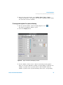
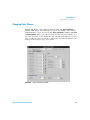
Changing Display Colors 86
To change the look and feel of the VnmrJ user interface
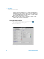
To change color options for spectral drawing 87
To change color options for plotting 88
Experiment Selector Editor
File Browser
90
93
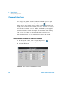
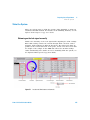
Status Charts 95
Features of the status chart window
Using the status chart 97
3
VnmrJ Preferences
Templates Tab
Queue Tab
4
96
103
104
Automation Tab 112
Automation Schedule
SQview Tab
86
114
119
120
VnmrJ 4.2 Familiarization Guide
Contents
eOptions Tab
123
Data Mirror Tab
126
SampleTags Tab
128
UserPrefs Tab
4
130
Preparing for an Experiment
Starting VnmrJ
134
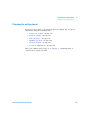
Preparing for an Experiment
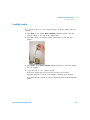
Prepare the sample
Load the sample
133
135
136
137
Tune the Probe 139
Tuning probes on systems with ProTune
Manual tuning using mtune 141
Optimize the Lock
142
Shim the System 143
Shimming on the lock signal manually
Proshim 144
Use a Proshim method in automation
Set up the Experiment
5
Acquiring Data
139
143
146
147
149
Acquire a Spectrum Manually
150
Using a Study Queue to Acquire Data 151
Build a Study Queue 151
Run a Study Queue 153
Using Express Submit with a sample changer
Stopping an Experiment
VnmrJ 4.2 Familiarization Guide
154
155
5
Contents
6
Processing Data
157
Loading Data from the Study Queue
158
Retrieving a Data Set 159
Use the file browser to open a data set 159
Use the VJ Locator to search the database 160
Fourier Transform the Data Set 162
Fourier transform of one-dimensional data
Fourier transform of two-dimensional data
162
162
Alter Processing Parameters 163
Zero-filling 163
Weighting and apodization 163
Linear prediction 163
Referencing 164
Integration 164
Phasing 164
Interacting with the Spectrum Using the Graphical Toolbar
Integration and graphics controls 165
Aligning and Stacking Spectra
Displaying and Plotting Integrals
Baseline Correction
166
167
168
Working with Viewports
169
Using Viewports Controls 170
Show and hide viewports 170
Make a viewport active 170
Add a label to the viewport 171
Set viewport layout 171
Synchronize cursors and axes 171
Set crosshair, fields, and axis display options
Assign colors to spectra by viewport 172
6
165
172
VnmrJ 4.2 Familiarization Guide
Contents
Using viewports as a spectral interpretation tool 173
Overlaying homonuclear data sets 173
Cross referencing heteronuclear data sets 175
Save Current Process or Display Parameters
7
Plotting Data
177
179
Plotting Data Saved as a Study
180
Saving and Printing a Graphics File
Plotting the Data
182
183
Changing Color Themes
187
Pasting Text into a Text Editor or Other Application
8
Customizing VnmrJ Actions
Clone a New Study
189
190
Clone Current Study
192
Clone Current Experiment
Clone Location Queue
193
194
Command and Protocol Buttons
Edit Parlib
9
195
198
Customer Training
Training
199
200
Previous Experience with Agilent NMR Software
Documentation
201
202
Sample Requirements
203
Introduction to VnmrJ 4 Operation
204
Overview of the VnmrJ 4 Interface
205
VnmrJ 4.2 Familiarization Guide
188
7
Contents
Basic (Automated) VnmrJ 4 Operation
Detailed (Manual) VnmrJ 4 Operation
Linux Training
207
211
VnmrJ 4 Administration
213
VnmrJ 4 Administration - Quick Start
Hardware Overview
Lock Frequency (lockfreq)
Administrative Chores
214
216
Customer Support Information
10
206
218
219
220
Automated Data Collection and Spectra Interpretation
221
Automated Data Acquisition 222
Sample for Automated Data Acquisition 222
Login to VnmrJ 223
Setting up the study and lock solvent 223
Building a Study 224
Customizing the parameters and starting data acquisition
Starting data acquisition using a study 226
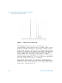
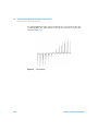
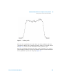
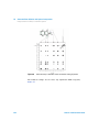
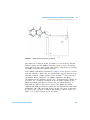
Interpreting the Indanone Spectra 227
Calibration – When is it Necessary 227
Interpretation of the Calibration Data 227
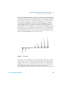
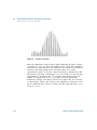
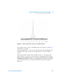
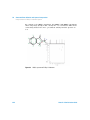
Interpretation of 2-Ethyl-1-Indanone Spectra
8
225
235
VnmrJ 4.2 Familiarization Guide
1
Introduction
Introduction to VnmrJ Workflow 10
Commonly Used VnmrJ Terms 11
Where to Find Help 13
This guide provides an overview of the Agilent VnmrJ software and how
you use it to acquire and process NMR spectra using Agilent NMR
Spectrometers. Descriptions of the VnmrJ program user interface, toolbars,
and menu items are included, along with general overview and description
of the VnmrJ workflow. For more detailed information on the various
workflow steps, see the Agilent VnmrJ Spectroscopy User Guide provided
with your system.
Agilent Technologies
1
Introduction
Introduction to VnmrJ Workflow
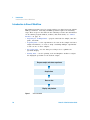
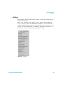
Introduction to VnmrJ Workflow
The VnmrJ program is used to acquire and process data from your Agilent
NMR spectrometer. Collecting an NMR spectrum requires the following
steps. These steps are described in the following sections. For information
on the VnmrJ program window, toolbars, and menu items, see “VnmrJ
Interface” on page 15.
• Preparing for an Experiment — prepare and load the sample, tune the
probe, and shim.
• Acquiring Data — select experiment to be run on the sample and enter
sample information, or create a study containing multiple experiments
to run on one or more samples.
• Processing Data — use the data processing tools to optimize the
spectrum display.
• Plotting Data — use the plotting tools and Graphics Toolbar to adjust
the displayed spectrum for the desired output.
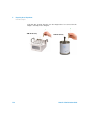
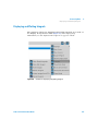
Prepare sample and select experiment
Acquire data
Process data
Display and plot data
Figure 1
10
VnmrJ workflow
VnmrJ 4.2 Familiarization Guide
Introduction
Commonly Used VnmrJ Terms
1
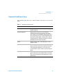
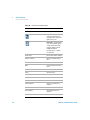
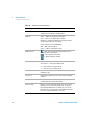
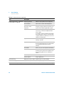
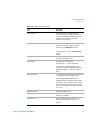
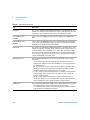
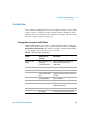
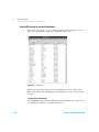
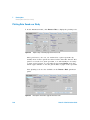
Commonly Used VnmrJ Terms
The following table lists some common VnmrJ terms that are used in this
guide.
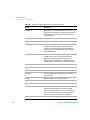
Table 1
Commonly used VnmrJ terms
Item
Description
Experiment
Combination of a pulse sequence, a parameter set, and
possibly a data set.
Experiment Protocol
Software device that creates an experiment by
executing a macro to set up parameters for a given
pulse sequence. In Review Mode, a protocol operates in
the current workspace and is typically followed by data
acquisition. In Submit Mode, a protocol adds a node to
the Study Queue for subsequent execution at run-time,
followed by the start of data acquisition.
Sample
A physical object, either a tube with liquid or a solid
sample in a rotor.
Study
Collection of one or more nodes in the Study Queue. In
general, each node represents an experiment. A study is
a list of operations to perform; it is not necessarily
associated with a specific sample or any other physical
object.
Study Queue
Interface feature that is used to display all the various
types of queues that are available in VnmrJ. The Study
Queue can be configured to show information in several
different ways.
VnmrJ 4.2 Familiarization Guide
11
1
Introduction
Commonly Used VnmrJ Terms
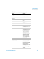
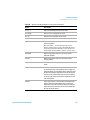
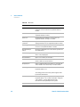
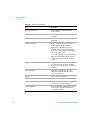
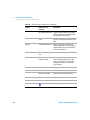
Table 1
12
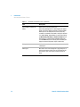
Commonly used VnmrJ terms (continued)
Item
Description
Submit Mode and Review
Mode
When you are interacting with data,
processing/plotting data, or collecting data in manual
mode, you interact with the software in Review Mode.
When you use the Study Queue to load, build, edit,
customize, or otherwise work with a study, the software
is in Submit Mode. Submit Mode is entered by clicking
the New Study, Edit Study, or Continue Study buttons.
The interface is moved into Review Mode when you
click the Done button in the Study Queue window (or it
happens automatically upon sample submission).
Viewport
Interface feature that is used to display the contents of
a workspace.
Workspace
Directories that can be thought of as digital objects to
hold an experiment and/or data set. Equivalent to the
idea of exp1, exp2, exp3, exp(n) in older versions of
Vnmr.
VnmrJ 4.2 Familiarization Guide
Introduction
Where to Find Help
1
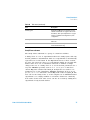
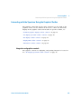
Where to Find Help
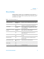
Agilent provides a complete set of documentation to get you started
generating quality data as quickly as possible. The following table contains
a summary of the manuals and user guides provided, and what kind of
information they contain.
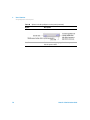
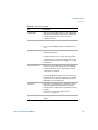
Table 2
VnmrJ manuals and their uses
Manual title
Provided as
Information in this manual
VnmrJ Installation Guide
Printed, PDF, and in
online help
Instructions on how to install Linux and the VnmrJ software
VnmrJ Administration Guide
PDF, and in online
help
How to administer the VnmrJ system, including adding and
changing users, and setting permissions and preferences
VnmrJ QuickStart
Printed, PDF, and in
online help
Step-by-step overview of how to use Agilent VnmrJ software
to collect an NMR spectrum on NMR systems with or without
a Robot Sample Changer
VnmrJ Familiarization Guide (this
document)
Printed, PDF, and in
online help
Overview of the VnmrJ software, including description of the
interface, menus, and commonly used tasks
VnmrJ Spectroscopy User Guide
PDF, and in online
help
A more in-depth description of using the VnmrJ software to
set up studies, perform shimming, and acquire, process,
display, and output data
NMR System Calibrations Guide
PDF, and in online
help
Use of VeriPulse, Autotest, and system calibrations are
described
Basic NMR Experiments
Familiarization Guide
PDF, and in online
help
Provides a more detailed discussion about some of the most
commonly used pulse sequences available in the VnmrJ
Experiment Selector
Experiment Reference Guide
PDF, and in online
help
Complete descriptions of VnmrJ experiments
Command and Parameter
Reference Guide
PDF, and in online
help
Comprehensive listing of VnmrJ commands and parameters
User Programming Guide
PDF, and in online
help
Comprehensive pulse sequence programming and
customization reference
VnmrJ 4.2 Familiarization Guide
13
1
Introduction
Contact information
Table 2
VnmrJ manuals and their uses (continued)
Manual title
Provided as
Information in this manual
CRAFT User Guide
PDF, and in online
help
Overview and step-by-step instructions for using the CRAFT
(Complete Reduction to Amplitude Frequency Table)
application within VnmrJ
BioPack Quick Start Guide
Printed, PDF, and in
online help
Step-by-step overview of using the BioPack option
BioPack User Guide
PDF, and in online
help
Complete information on how to use the BioPack option
BioPack Experiment Guides
PDF, and in online
help
Descriptions of BioPack experiments
SolidsPack User Guide
PDF, and in online
help
Describes the use of SolidsPack, used to run a solids
experiment and control solids console accessories such as
shims, variable temperature, and magic- angle spinning
3D Gradient Shimming User
Guide
PDF, and in online
help
Description of how to use the Agilent 3D Gradient shimming
software, used to map and optimize room- temperature, shim
systems without additional hardware
Contact information
USA
Address:
Agilent Technologies, Inc.
5301 Stevens Creek Blvd.
Santa Clara, CA 95051
Telephone Number:
Toll Free: +1 (800) 227 9770
Agilent website (all countries)
To find contact information for your location, click the following link,
select your country, and then click Go.
http://www.chem.agilent.com/en- us/ContactUS/Pages/ContactUs.aspx
14
VnmrJ 4.2 Familiarization Guide
2
VnmrJ Interface
VnmrJ User Interface 16
Toolbars 17
Command Line 26
Graphics Canvas 27
Vertical Panels 30
Protocols Vertical Panel 31
Parameter Panel 57
VnmrJ Menus 58
Changing Display Colors 86
Experiment Selector Editor 90
File Browser 93
Status Charts 95
This section contains descriptions of the main features of the VnmrJ
program interface.
Agilent Technologies
2
VnmrJ Interface
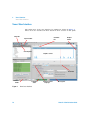
VnmrJ User Interface
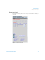
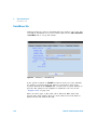
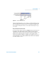
VnmrJ User Interface
The main areas of the user interface for VnmrJ are shown in Figure 2.
These areas are described in more detail in other sections of this guide.
Menu bar
Command
line
System toolbar
Graphics
toolbar
Vertical panels
Graphics canvas
Action bar
Hardware
toolbar
Figure 2
16
Acquisition
status
Parameter panels
and pages
Message box
VnmrJ user interface
VnmrJ 4.2 Familiarization Guide
VnmrJ Interface 2
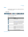
Toolbars
Toolbars
The VnmrJ toolbars provide quick access to commonly used functions. To
view a description of a toolbar icon, move the mouse cursor over the icon
until the description appears.
System toolbar
The system toolbar provides access to common system functions. It also
lets you show or hide graphics toolbars.
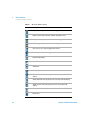
Table 3
Icon
System toolbar controls
Description
Create a new workspace.
Opens the File Browser to search for and open a file.
Opens the File Browser to find a location and save data.
Opens the Styles and Themes pop-up, where you can
select or customize colors or color themes for the
VnmrJ user interface.
Cancel a command.
Save current screen layout: graphics, parameter panel,
locator sizes.
Save current screen layout: graphics, parameter panel,
locator sizes.
Draw spectral data using a light background. This does
not change the User Interface theme.
VnmrJ 4.2 Familiarization Guide
17
2
VnmrJ Interface
Hardware toolbar
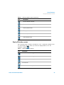
Table 3
System toolbar controls (continued)
Icon
Description
Draw spectral data using a dark background. This does
not change the User Interface theme.
Opens the Display FID toolbar controls.
Opens the 1D display spectrum toolbar controls.
Opens the nD display toolbar controls.
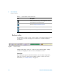
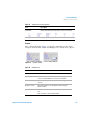
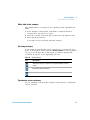
Hardware toolbar
The Hardware toolbar, located at the bottom of the VnmrJ window, shows
a trash can icon and a display area dedicated to real- time hardware
information.
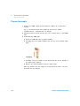
Figure 3
Hardware toolbar
Sample temperature, spin rate, lock level, and current sample changer
location are displayed to the left of the Hardware toolbar.
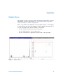
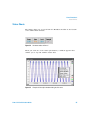
Status plots
The status plots provide useful information about sample temperature,
spin rate, lock level, and current sample changer location. For more
information, see “Status Charts” on page 95.
18
VnmrJ 4.2 Familiarization Guide
VnmrJ Interface 2
Graphics toolbar
Acquisition status
Real time events such as system being idle, locking, shimming, or
acquiring data are displayed in the field located to the right of the probe
file. If the system is active, each event’s remaining time is displayed.
Message box
To the right of the Hardware toolbar is a system message box. Error
messages and other important system information are displayed in this
area.
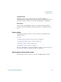
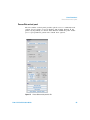
Graphics toolbar
The Graphics toolbar is used to control the interactive display in the
graphics canvas.
See also
“Common graphics display toolbar controls” on page 19
“1D display spectrum toolbar controls” on page 20
“nD display toolbar controls” on page 21
“Display FID toolbar controls” on page 23
For more information on using the graphics toolbar, see “Interacting with
the Spectrum Using the Graphical Toolbar” on page 165.
Common graphics display toolbar controls
The following tools are common to 1D, nD, and FID display toolbars.
VnmrJ 4.2 Familiarization Guide
19
2
VnmrJ Interface
1D display spectrum toolbar controls
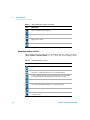
Table 4
Icon
Graphic display toolbar controls
Description
Reset to full display.
Zooms in to a region in graphics canvas defined by cursor placement.
(Click mouse once to define first cursor and then again to define second
cursor.)
To zoom further, click to define cursor positions, and then click the zoom
icon again.
Zooms out.
Pan, or “rubber band” zoom. Click once to define first cursor, then click
again and drag.
Redraw display.
Return to previous tool menu.
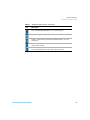
1D display spectrum toolbar controls
The following table shows the icons that appear when you click the 1D
Display icon on the graphics toolbar.
Table 5
Icon
1D display Spectrum toolbar
Description
One cursor in use, click to toggle to two cursors.
Two cursors in use, click to toggle to one cursor.
Click to expand region.
Click to expand to full spectral display.
20
VnmrJ 4.2 Familiarization Guide
VnmrJ Interface 2
nD display toolbar controls
Table 5
Icon
1D display Spectrum toolbar (continued)
Description
Display integrals menu.
Display partial integrals.
Display full integral.
Hide integrals.
Define integrals.
Adjust integral level/tilt.
Delete integrals.
Display or hide scale.
Pan or move spectral region.
Toggle threshold on or off.
Phase spectrum.
nD display toolbar controls
The following table describes the icons displayed when you click the 2D or
3d Display icon on the Graphics toolbar.
VnmrJ 4.2 Familiarization Guide
21
2
VnmrJ Interface
nD display toolbar controls
Table 6
Icon
nD display toolbar controls
Description
Display color map and show common nD graphics tool.
Display contour map and show common nD graphics tool.
Display stacked spectra and show common nD graphics tool.
Display image map and show common nD graphics tool.
One cursor in use, click to toggle to two cursors.
Two cursors in use, click to toggle to one cursor.
Expand to full display.
Pan and stretch.
Show trace.
Show projections.
Shows horizontal maximum projection across the top of the 2D
display.
Shows horizontal sum projection across the top of the 2D display.
Shows vertical maximum projection across the top of the 2D
display.
Shows vertical sum projection down the left side of the 2D display.
Rotate axes.
22
VnmrJ 4.2 Familiarization Guide
VnmrJ Interface 2
Display FID toolbar controls
Table 6
Icon
nD display toolbar controls (continued)
Description
Increase vertical scale 20%.
Decrease vertical scale 20%.
Phase spectrum menu.
First spectrum selection.
Second spectrum selection.
Enter peak pick menu.
Display FID toolbar controls
The following table contains descriptions of the commands available from
the menu that appears when you click the Display FID icon in the
Graphics toolbar.
Table 7
Display FID toolbar controls
Icon
Description
One cursor in use, click to toggle to two cursor
Two cursors in use, click to toggle to one cursor
Click to expand to full FID display
Pan and stretch.
Click to show real and imaginary
VnmrJ 4.2 Familiarization Guide
23
2
VnmrJ Interface
Annotation toolbar controls
Table 7
Display FID toolbar controls (continued)
Icon
Description
Click to show real and zero imaginary
Click to show real only
Toggle scale on and off
Phase FID
Annotation toolbar controls
The following table describes the icons displayed in the graphics toolbar
(View > Toolbars > Graphics Toolbar) in "ds", "dss", and "dconi" display modes.
Table 8
Annotation toolbar controls
Icon
Description
Toggle to show or hide annotations in graphics canvas and hard copy plot
Select annotation for editing. Use this mode to move or delete an
annotation, or change properties such as color and line thickness.
Position – displays the value of the position where it is located, in Hz, PPM,
etc. The value is updated automatically as the annotation is moved.
Text – Text with adjustable font, size, style, color, and transparency.
Line – Line with a adjustable thickness, color, and transparency.
Arrow – Arrow with adjustable thickness, color, and transparency.
Box – Box with adjustable thickness, color, and transparency, with rounded
or square corners.
24
VnmrJ 4.2 Familiarization Guide
VnmrJ Interface 2
Annotation toolbar controls
Table 8
Annotation toolbar controls (continued)
Icon
Description
Oval – Oval with adjustable thickness, color, and transparency.
Polygon – Polygon with adjustable thickness, color, and transparency.
Polyline – Connected lie segments with adjustable thickness, color, and
transparency.
X-Bar – displays its width in Hz, PPM. The value is updated automatically as
the annotation is resized.
Y-Bar – displays its height in intensity units, or for 2D data, in Hz, PPM, etc.
The value is updated automatically as the annotation is resized.
VnmrJ 4.2 Familiarization Guide
25
2
VnmrJ Interface
Command Line
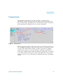
Command Line
One of the most powerful aspects of the VnmrJ software is the ability it
provides to users to execute commands and macros directly using the
Command Line. For more information on VnmrJ commands and macros,
see the Agilent VnmrJ Command and Parameter Reference Guide and
the Agilent VnmrJ User Programming Guide.
26
VnmrJ 4.2 Familiarization Guide
VnmrJ Interface 2
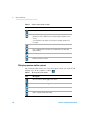
Graphics Canvas
Graphics Canvas
The Graphics Canvas is used to display and interact with graphic and text
information. For more information, see “Interacting with the Spectrum
Using the Graphical Toolbar” on page 165.
When a spectrum is first displayed on the Graphics Canvas, or the display
is refreshed, the bar above the Graphics Canvas displays the functions of
the left and right mouse buttons and the scroll wheel:
• Use the left mouse button to set the left cursor,
• Use the right button to set the right cursor
• Use the scroll wheel to adjust the vertical scale of the spectrum
Figure 4
Graphics Canvas
VnmrJ 4.2 Familiarization Guide
27
2
VnmrJ Interface
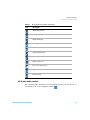
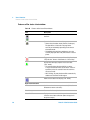
Tray display
Tray display
If you have a robot sample changer, a graphical display of the changer
gives you access to a menu of commands when you right- click the mouse
button over the tray display.
Figure 5
Table 9
28
Tray display menu
Tray display menu options
Item
Description
Show Study
Displays the queue for the selected
location in the Study Queue.
Edit Study
Loads a study into the Study Queue from
the tray display in preparation for
modification of that study.
Delete Study
Deletes the selected location queue.
Copy Study
Copy Study to clipboard.
VnmrJ 4.2 Familiarization Guide
VnmrJ Interface 2
Tray display
Table 9
Tray display menu options (continued)
Item
Description
Paste Study
Paste Study from clipboard.
Resubmit Study
Resubmits the selected location to
acquisition.
Clone Study
Clones the selected location queue.
Sample in Magnet
Displays the Sample in Magnet popup,
preloaded with that location for a sample
change operation.
Express Submit
Utility to submit a sample to a specific
location using automation, see Using
Express Submit with a sample changer.
Study Information
Displays information about Study.
Swap Queue
Swaps experiments queued in the day to
night and vice versa. Only displayed if there
is an active Study in the selected location.
VnmrJ 4.2 Familiarization Guide
29
2
VnmrJ Interface
Vertical Panels
Vertical Panels
The vertical panels area of the VnmrJ user interface provides quick access
to related functions. Each vertical panel contains one or more functional
areas where you perform tasks such as selecting experiments and setting
up data display.
Figure 6
Vertical panel tabs in VnmrJ
For more information, see “Protocols Vertical Panel” on page 31,
“QuickSubmit vertical panel” on page 39, “Frame vertical panel” on
page 41, “Viewport vertical panel” on page 45, and “ProcessPlot vertical
panel” on page 49.
30
VnmrJ 4.2 Familiarization Guide
VnmrJ Interface 2
Protocols Vertical Panel
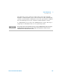
Protocols Vertical Panel
The Protocols vertical panel contains the Experiment Selector, the
Experiment Selector Tree, and the Study Queue. To show or hide one or
more of these panels, click View and then select the item you want to
show or hide. See also Experiment Selector, Experiment Selector Tree, and
Study Queue.
VnmrJ 4.2 Familiarization Guide
31
2
VnmrJ Interface
Experiment Selector
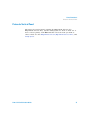
Experiment Selector
The Experiment Selector can be used to load studies into the Study Queue
or the current workspace. When an experiment is selected in Experiment
Selector, all submissions to automation can be selected by double- clicking
and experiment or dragging and dropping it to the Study Queue. You can
configure families of experiments and content by using the Experiment
Selector. Simple or complex experiments, based on an account or an
operator within an account, are accessible as needed.
Use the Experiment Selector Editor to change the order and display of
experiments/protocols within the Experiment Selector. For more
information, see “Experiment Selector Editor” on page 90.
Figure 7
32
Experiment Selector
VnmrJ 4.2 Familiarization Guide
VnmrJ Interface 2
Experiment Selector Tree
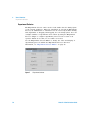
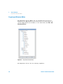
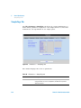
Experiment Selector Tree
The Experiment Selector Tree is a convenient way to view the available
experiments. Instead of displaying the experiments in tabs (as in the
Experiment Selector) experiments are grouped under their respective
experiment types. Use the buttons at the bottom of the panel to expand or
contract the tree and to search through the tree for an experiment using
part or all of the name.
Figure 8
VnmrJ 4.2 Familiarization Guide
Experiment Selector Tree
33
2
VnmrJ Interface
Study Queue
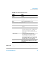
Table 10
Button
Experiment Selector buttons
Action
Type text in this field, and click the search button. The
tree view is expanded and selects the first
experiment/protocol with a name that contains the
text. Click the search button additional times to
continue the search further down the tree until the
bottom of the tree is reached, at which point the search
resumes at the top. Searching for a “Find” text that is
not matched anywhere keeps the existing tree view, but
does not match a selection.
Collapses an expanded tree
Expands the tree view
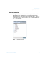
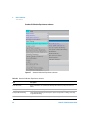
Study Queue
VnmrJ allows the ability to construct a linked list of experiments as a
Study Queue that can be performed on any given sample. The appearance
of the Study Queue changes depending on if you have a sample changer
installed, or when in Submit mode or Review mode. For more information,
see “Build a Study Queue” on page 151.
A Study Queue is used for both data acquisition and processing. Its many
functions are described in more detail in the Agilent VnmrJ Spectroscopy
User Guide.
34
VnmrJ 4.2 Familiarization Guide
VnmrJ Interface 2
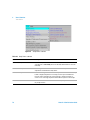
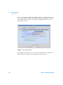
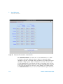
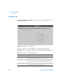
Study Queue
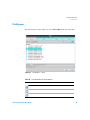
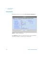
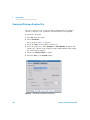
Figure 9
Table 11
Study Queue—Review mode with no sample changer
General Study Queue features
Item
Description
View
Selections that determine what is displayed in the Study Queue:
Sample — displays the study linked to the data in the current
workspace
Spectrometer — displays all studies in the current automation run
Active Sample—displays the currently acquiring study
Study Cluster—displays study cluster, if one is defined
New Study
Initializes a new study and moves the software to Submit mode
Continue Study
Used to modify the current study displayed in the Study Queue
Show Study from Location
(robot changer only)
Loads a study from the tray display
VnmrJ 4.2 Familiarization Guide
35
2
VnmrJ Interface
Study Queue
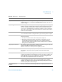
Table 12
Study Queue features — Submit Mode
Item
Description
Cancel
Abandons any changes made to the current study and returns the
software to Review mode.
DayQ (robot changer only)
Runs study according to schedule set in DayQ. The schedule is set
by the account administrator using the Automation tab of the Edit
> Preferences window.
NightQ (robot changer only)
Runs study according to schedule set in NightQ. The schedule is
set by the account administrator using the Automation tab of the
Edit > Preferences window.
Priority sample (robot
changer only)
Allows a sample to be submitted ahead of all other samples in the
current automation run. This feature is controlled by the system
administrator on an operator-by-operator basis.
Submit
Submits the current study to acquisition, using one of the following
choices:
Automation–submits the study to the Spectrometer Queue.
Foreground exp–submits the study to acquisition in the current
workspace.
Background–submits the study to a background copy of VnmrJ.
36
Foreground (shown when not
using robot sample changer)
Submits the study to acquisition in the current workspace.
Background (shown when
not using robot sample
changer)
Submits the study to a background copy of VnmrJ.
Clear Pending Exp from
Queue
Deletes all pending experiments from the current Study Queue.
VnmrJ 4.2 Familiarization Guide
VnmrJ Interface 2
Study Queue
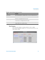
Table 13
Study Queue features — Review Mode
Item
Description
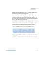
Options
Available when in Spectrometer view. Configure and update display
settings on the Spectrometer View Preference window.
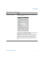
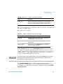
Right click over a node to access options, shown below.
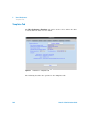
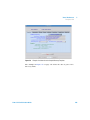
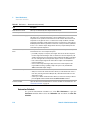
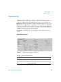
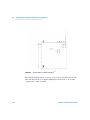
Figure 10
VnmrJ 4.2 Familiarization Guide
Study Queue node options
37
2
VnmrJ Interface
Study Queue
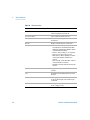
Table 14
38
Node options
Item
Description
Open Experiment
Opens selected experiment and displays parameters in the Parameter
Panel.
Delete Experiment
Removes experiment from the Study Queue.
Collapse Node
Collapses selected node so that only experiment name is displayed.
Expand Node
Expands node so that all information is displayed.
VnmrJ 4.2 Familiarization Guide
VnmrJ Interface 2
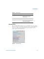
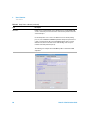
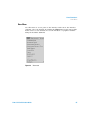
QuickSubmit vertical panel
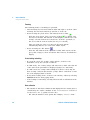
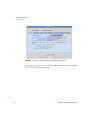
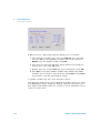
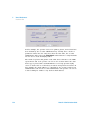
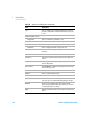
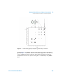
QuickSubmit vertical panel
The QuickSubmit panel provides an easy way to quickly submit samples
for acquisition.
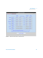
Figure 11
VnmrJ 4.2 Familiarization Guide
QuickSubmit vertical panel
39
2
VnmrJ Interface
QuickSubmit vertical panel
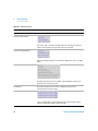
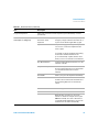
Table 15
QuickSubmit Options
Item
Description
New study
Click to begin a new study.
Continue study
Click to continue the study currently in the Study Queue.
Parameters
Enter descriptive sample parameters and comments.
Experiment queue
From the Select Experiment drop-down list, select an
experiment, then click Add to DayQ or Add to NightQ to place
the experiment in the Study Queue. Continue to add
experiments as desired.
Customize
40
Clear queue
Clears the experiments from the queue.
Submit
Submits the current QuickSubmit queue for acquisition.
Logout
Click to log out of the VnmrJ system.
Edit exp list
Edit the existing experiment list.
Message history
Click to see a log of previous messages.
VnmrJ 4.2 Familiarization Guide
VnmrJ Interface 2
Frame vertical panel
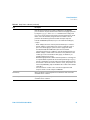
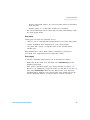
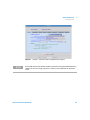
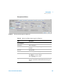
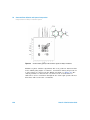
Frame vertical panel
Use the Frame vertical panel to create an inset frame. An inset frame
initially shares the same workspace and data as the viewport. However,
you can change or remove it. For details on creating and working with
insets, see the Agilent VnmrJ Spectroscopy User Guide.
Figure 12
VnmrJ 4.2 Familiarization Guide
Frame vertical panel
41
2
VnmrJ Interface
Frame vertical panel
Table 16
Frame vertical panel options
Item
Function
Inset
Default mode — left mouse
click moves the left cursor
and right mouse click moves
right mouse cursor.
Inset mode — left mouse drag
a box over a spectrum region
creates an inset frame of the
region. A viewport can have
multiple inset frames.
Exit inset mode — release
mouse button.
42
Reset frame
Resets inset frame to default
Remove selection
Removes selected frame or
item
Remove all
Removes all inset frames
Text
Lets you add text to an inset
frame.
New/Edit
Create or change a text inset
Show
Show text inset
Hide
Hide text inset
Remove selection
Remove selected text
Remove all
Removes all text
Select template
Select a saved text inset
template
Name
Give a name to the text inset
Save template
Save the text inset as a
template
Delete template
Delete the selected template
VnmrJ 4.2 Familiarization Guide
VnmrJ Interface 2
Frame vertical panel
Table 16
Frame vertical panel options (continued)
Item
Function
Graphics
Get Logo
Lets you select a logo to
show in the frame
Set Logo
Show All
Shows all graphics in the
frame
Remove All
Removes all graphics from
the frame
Misc
Show Fields
Display cr, delta, vp
etc... fields at the bottom of
the viewport.
Show Crosshair
Display cross hair and
chemical shifts of the cursor
position when the mouse is
moved over the spectrum.
This is a useful function
when the fields are not
shown, not in cursor mode
(default mode), or when
chemical shift of a peak
without moving the left
cursor is required while in
the cursor mode.
Show Axis
Show scale of the axis.
Show frame border
Check the box to display a
box around the frame.
Clear the box to display the
four corners of the selected
frame as hot spots for
resizing. No border or corner
will be displayed if a frame is
not selected. An empty
frame is not visible until it is
selected.
VnmrJ 4.2 Familiarization Guide
43
2
VnmrJ Interface
Frame vertical panel
Inset frame buttons
The buttons delete one or all inset frames and restore the default frame to
full size.
Button
Function
Delete Inset
Delete the selected inset.
Delete all
Delete all inset frames.
Full size
Restore the default frame to its full size.
Display check boxes
The check boxes control optional display features.
Check box
Function
Cross hair
Display cross hair and chemical shifts of the cursor position
when the mouse is moved over the spectrum. A useful function
when the fields are not shown, not in cursor mode (default
mode), or when chemical shift of a peak without moving the
left cursor is required while in the cursor mode.
Fields
Display cr, delta, vp etc... fields at the bottom of the
viewport.
Axis
Show scale of the axis.
Show frame border
Check the box to display a box around the frame.
Un-check the box to display the four corners of the selected
frame as hot spots for resizing. No border or corner will be
displayed if a frame is not selected. An empty frame is not
visible until it is selected.
44
VnmrJ 4.2 Familiarization Guide
VnmrJ Interface 2
Viewport vertical panel
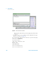
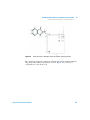
Viewport vertical panel
The Viewport vertical panel is used to set up and customize the display of
viewports.
Figure 13
VnmrJ 4.2 Familiarization Guide
Viewport vertical panel
45
2
VnmrJ Interface
Viewport vertical panel
Table 17
Viewport vertical panel options
Item
Description
Number of viewports
Used to select the number of viewports to display. Available
viewports is set in Viewports settings window.
Viewports
Select — When selected, displays that viewport
Color — Select color to display data in viewport
Workspace — Workspace number (also experiment number
shown on upper left corner of viewport)
Label — File name or user-defined label
Hide — Hide selected viewport
Active — Select to make viewport active
Viewport layout
— Auto mode, let VnmrJ arrange the viewports in an
optimized row-by-column matrix
— Stack viewports horizontally
— Arrange viewports vertically
Overlay Viewports
Overlays viewports
Stack spectra — show spectra with an offset
X — offset in X axis for stacked spectra
Y — offset in Y axis for stacked spectra
46
Color by viewport
Turns on the color option so you can select to display viewports
in different colors.
Sync Cursor
Links and synchronizes the cursors and crosshairs in multiple
viewports.
Sync Axis
Links and synchronizes axes in multiple viewports. Axis is
synchronized to the current active viewport.
Show crosshair
Displays cross hair and chemical shifts of the cursor position
when mouse is moved over the spectrum. This is a useful
function when the fields are not shown, not in cursor mode
(default mode), or chemical shift of a peak without moving the
left cursor is required while in the cursor mode.
VnmrJ 4.2 Familiarization Guide
VnmrJ Interface 2
Viewport vertical panel
Table 17
Viewport vertical panel options
Item
Description
Show fields
Shows information fields at the bottom of the active viewport:
Show axis
Displays axes in the viewports
Contour
The contour sub- panel, Figure 14, appears exclusively for the active
viewport with 2D data loaded and displayed in contour mode (dpcon).
Figure 14
Table 18
Contour controls
Contour panel
Control
Description
Contour levels
Enter a number of contours between 4 and 32 in the text field.
Spacing factor
Enter a number in the text field to specify the spacing between
contours. A number between 1.1 and 2 is recommended.
Positive contour
Select this check box to show positive contours using the default
color red.
Negative contour
Select this check box to show negative contours using the
default color blue.
Color dropdown
Select a color from the menu to use a color other then the default
color.
Each contour has a color dropdown menu.
VnmrJ 4.2 Familiarization Guide
47
2
VnmrJ Interface
Viewport vertical panel
Table 18
Contour panel (continued)
Control
Description
Multi color contours
Select this option to use the colors defined in Display Option.
If you select the Color by Viewport box, options are not displayed,
AutoScale
48
Automatically scale the spectrum by clicking.
VnmrJ 4.2 Familiarization Guide
VnmrJ Interface 2
ProcessPlot vertical panel
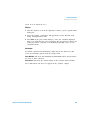
ProcessPlot vertical panel
The ProcessPlot vertical panel provides quick access to commonly- used
options for processing, on- screen display, and plotting. Options in the
panel vary depending on current data. Buttons within the panel enable
you to open parameter panels that contain more options.
Figure 15
VnmrJ 4.2 Familiarization Guide
ProcessPlot vertical panel for 1D
49
2
VnmrJ Interface
ProcessPlot vertical panel
Table 19
Options in the ProcessPlot vertical panel
Option
Description
Process
Transform all
Performs a Fourier transform for all the displayed data.
Phase zero order
Performs a zero order phase correction.
Transform FID #
Select FID # to transform.
Weighting
Select the weighting to be applied to the transform.
Interactive
Select to enter interactive weighting mode.
Transform size
Opens a menu where you can select the number of points to be
Fourier transformed (fn).
More processing - parameter
pages
Opens the Default page in the Process parameter panel tab for
more processing options
Display
Autoscale
Automatically scales the display vertically.
+/-
Click + or - to increase or decrease the vertical scale.
Arrayed spectra panel
Opens the ArrayedSpectra panel where you can set up display of
spectra and FID arrays. See “ArrayedSpectra vertical panel” on
page 52.
Reference
By solvent - Reference the spectrum for selected solvent.
By TMS - Reference the spectrum to a TMS line.
Cancel - Clears the reference line by removing any spectral
referencing present, and turns off referencing.
Axis
Select the desired y-axis units: Hertz, ppm, kHz
Display mode
Select the desired display mode: phased, absolute value, or
power
More display - parameter pages
Opens the Display page in the Process parameter panel tab for
more display options
Plot
Auto plot page
50
Executes the plot macro; then the resetplotter macro.
VnmrJ 4.2 Familiarization Guide
VnmrJ Interface 2
ProcessPlot vertical panel
Table 19
Options in the ProcessPlot vertical panel
Option
Description
Auto plot preview
Opens the Plot View popup and displays the plot in Adobe
Reader. Use the Plot View popup to save the plot to a file, send
to a plotter, or send to an e-mail address.
Print screen
Opens the Print Screen dialog box, where you can set up and
print the VnmrJ window or viewport. See “Saving and Printing a
Graphics File” on page 182.
More plotting - parameter
pages
Opens the Plot page in the Process parameter panel tab for more
display options.
VnmrJ 4.2 Familiarization Guide
51
2
VnmrJ Interface
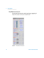
ArrayedSpectra vertical panel
ArrayedSpectra vertical panel
The ArrayedSpectra vertical tab contains parameters for displaying and
plotting spectra and FID arrays. This procedure applies equally to the
display and plotting of both spectra and FID arrays.
Figure 16
52
ArrayedSpectra vertical panel
VnmrJ 4.2 Familiarization Guide
VnmrJ Interface 2
ArrayedSpectra vertical panel
Table 20
Options in the ArrayedSpectra vertical panel
Option
Description
Show
Spectra or FIDs
Selects to show either spectra or FIDs
Horizontally
Shows the spectra side-by-side
Vertically
Aligns the spectra one above another
Auto
Depends on the previously chosen display mode:
• If the previous mode showed the spectra full screen
(vertical mode or showing only a single 1D) spectra
are aligned vertically, and the vertical offset is chosen
such that all spectra together cover the entire vertical
space.
• If the previous mode was horizontal, a vertical offset
is added to show the spectra along a diagonal.
Custom
Takes over the display properties of either horizontal,
vertical, or auto modes but allows the choice of
horizontal and vertical offsets.
Display 1D
Click the icon to show a single spectrum/FID and use
the toolbox to manipulate and zoom.
Numbers
When selected, turns on numbering of the array
elements displayed.
Values
When selected, turns on display of values for the array
elements displayed.
Misc
Transform
Fourier transform the current FID data
Drift correct
Apply drift correction (corresponds to "dc" command)
to all subspectra of the array.
Show scale
Switch on or off a scale below the first spectrum or FID
of the array.
VnmrJ 4.2 Familiarization Guide
53
2
VnmrJ Interface
ArrayedSpectra vertical panel
Table 20
Options in the ArrayedSpectra vertical panel (continued)
Option
Description
Whitewash
Aligns the spectra one above another as in the vertical
mode, but this mode shows spectra behind each other,
avoiding overprinting. Horizontal and vertical offsets
can be adjusted.
Color traces
Redisplay
Refresh the screen.
Plot Page
Send the current array display to the current plotter.
Settings on the Plot parameter panel for parameter
printing are used. Plotting from the ArrayedSpectra
vertical panel does not plot integrals, integral values,
and peak frequencies.
Plot Preview
Plot the array to a PDF file and open Acrobat reader with
the PDF of the current array. Settings on the Plot
parameter panel for parameter printing are used.
Plotting from the ArrayedSpectra vertical panel does
not plot integrals, integral values, and peak frequencies.
Choice of values
54
Start at #
The first element of the array to display
Stop at #
The last element of the array to display
Step every
The element between the beginning and end of the
array to display.
Max #
Maximum number of elements to display.
Reset values
Resets just the values to default.
Reset all
Resets all to defaults.
Chart dimensions
Enter the desired values, then adjust the positions as
needed using the buttons next to each field. Right
mouse click on the button to increase the value or left
mouse click on the button to decrease the value the
increment shown on the left side of the button.
Horiz. width
Enter the horizontal width for the chart.
VnmrJ 4.2 Familiarization Guide
VnmrJ Interface 2
ArrayedSpectra vertical panel
Table 20
Options in the ArrayedSpectra vertical panel (continued)
Option
Description
Horiz. pos.
Enter the horizontal position for the chart.
Vert. height
Enter the vertical height for the chart.
Vert. pos.
Enter the vertical position for the chart.
Numbers
Style
Flip — when selected, rotates the numbers 90 degrees
counter-clockwise
Drop-down menu — Used to select the position of the
numbers. Select Custom to specify a horizontal and vertical
positioning of the number with respect to the spectrum. Use
the horizontal and vertical fields to type the custom positions.
Horizontal
When using Custom style, lets you enter custom
horizontal position.
Vertical
When using Custom style, lets you enter custom
vertical position.
Offsets
Enabled only for vertical, whitewash, or custom array
mode.
Horizontal
Enter horizontal offset. (Note: the horizontal width must
be smaller than the screen width in order to apply any
horizontal offset.) Use the button to the right of the field
to adjust the position. Right mouse click on the button
to increase the value or left mouse click on the button
to decrease the value the increment shown on the left
side of the button.
Vertical
Enter vertical offset. Use the button to the right of the
field to adjust the position.Right mouse click on the
button to increase the value or left mouse click on the
button to decrease the value the increment shown on
the left side of the button.
VnmrJ 4.2 Familiarization Guide
55
2
VnmrJ Interface
ArrayedSpectra vertical panel
Table 20
Options in the ArrayedSpectra vertical panel (continued)
Option
Description
Current value
Middle mouse button click to set the increment to
1, 10 or 100
Cutoff
56
Increment applied to the
current setting value.
Left click to increase or
right click to decrease.
Used to avoid overlapping large lines that may reach
into the spectra above.
VnmrJ 4.2 Familiarization Guide
VnmrJ Interface 2
Parameter Panel
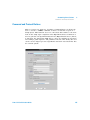
Parameter Panel
The Parameter Panel shows the pulse sequence, context- specific
information, menus, and text entry. The panels under the Acquire and
Process tabs change depending on the current pulse- sequence. Parameter
Panel information is displayed for the current experiment.
Figure 17
Parameter Panel
Each pane can be resized, reduced to a tab, or closed. Setup, acquire, or
process NMR data using the point and click feature of the interface. There
are three tabs labeled Start, Acquire, and Process below the graphics
window. The top page on each tab displays commonly used functions.
Lower pages display detailed functions. Buttons (Action Bar) to the right
of the tabs represent tab- specific actions and differ with each tab. The
interface can also be accessed using the command line above the Graphics
Canvas.
VnmrJ 4.2 Familiarization Guide
57
2
VnmrJ Interface
VnmrJ Menus
VnmrJ Menus
VnmrJ has an integrated set of tools designed to acquire a series of one
and two- dimensional data sets from a library of pulse sequences for any
given sample. Access the sophisticated experiments for routine use in a
fully automated environment.
Standard menu items are displayed at the top of the VnmrJ window. This
section lists menus in alphabetical order rather than in the order they
appear in the menu.
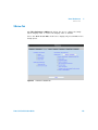
Acquisition Menu
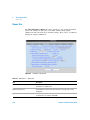
The Acquisition menu provides a convenient non- command line access to
a number of core VnmrJ commands such as go, ga, or au. The menu
option, Parameter Arrays, facilitates the creation of parameter arrays.
Figure 18
58
Acquisition menu
VnmrJ 4.2 Familiarization Guide
VnmrJ Interface 2
Automation Menu
Table 21
Acquisition menu
Item
Description
Parameter Arrays...
Opens the Array Parameter window, in
which you can create and edit
parameter arrays.
findZ0
Find Z0 for locking.
Do Gradient Shimming
Opens the gradient shimming menu
where you select the gradient map and
execute gradient shimming.
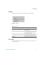
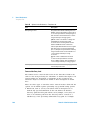
Automation Menu
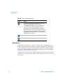
The Automation Menu provides access to automation start, stop, restart
and reset controls not generally used during ordinary sample submission
and not accessible from the Study Queue. It also provides access to
archive queues and automation logs.
Figure 19
VnmrJ 4.2 Familiarization Guide
Automation menu
59
2
VnmrJ Interface
Automation Menu
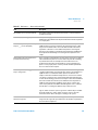
Table 22
Automation menu
Item
Description
Automation Queue
Select to display Automation Queue.
Automation Run (autodir)
Start a new study or continue an existing study from an existing automation run.
Initiate a new automation run (often done at the start of the day).
Automation File (globalenter)
Edit, create, display and submit to acquisition the "globalenter" version of a Study
Queue.
Tray Actions…
Provides functionality that is also available on the Study Queue controls or the
right-click menu on the tray locations.
Tray Archives…
Tray archives allows the user to browse completed automation runs or
automation files from previous dates.
Submit Current Parameters…
Use to manually build any desired experiment in the current workspace and to
submit to an automation queue, both day and night.
60
VnmrJ 4.2 Familiarization Guide
VnmrJ Interface 2
Automation Menu
Table 22
Automation menu (continued)
Item
Description
Foreground Acquisition...
Allows user to pause after current acquisition, pause immediately, or resume
paused study.
Automation Controls (visible when
autosampler is configured)
Pause after current Study
Pause after current
Acquisition
To pause the automation run, manually run an
emergency sample, resume the automation run, or
to pause a run to fill the magnet with cryogens.
Stop-Save-Resume
Stops the running experiment, process or plot, or
save to move on to the next experiment in the
chain or queue.
For example, if a 4 hour experiment were running
in automation and after 30 minutes it was
processed and nearly complete, then this action
allows you to choose a rational action at that time.
Stop-Discard-Resume
Stops the running experiment and move on to the
next item on the list.
Stop-Save and Stop-Discard
Functions exactly as the submenus described
above except that the queue is not resumed until
you select Resume Automation from this
submenu.
Pause NOW
Allows you to pause the experiment immediately.
Pause at scheduled time
Allows the administrator of the account to define
in advance an exact time for the automation run to
be paused along with a time for automation to
resume.
Resume Automation
Resumes any paused automation run.
Abort Automation
Stops automation run.
During the time of pausing you can use the
interface to submit more samples and to acquire
NMR data manually. You can also allow time for
cryogen fills and the magnet time to recover. The
automation run can resume automatically.
VnmrJ 4.2 Familiarization Guide
61
2
VnmrJ Interface
Automation Menu
Table 22
Automation menu (continued)
Item
Description
Background Acquisition... (visible when
no autosampler is configured)
New background run
Submits a new acquisition run to background.
Show all studies
Shows status of studies in the Study Queue.
Pause after current Study
Pause after current
Acquisition
To pause the automation run, manually run an
emergency sample, resume the automation run, or
to pause a run to fill the magnet with cryogens.
Stop-Save-Resume
Stops the running experiment, process or plot, or
save to move on to the next experiment in the
chain or queue.
For example, if a 4 hour experiment were running
and after 30 minutes it was processed and nearly
complete, then this action allows you to choose a
rational action at that time.
Stop-Discard-Resume
Stops the running experiment and move on to the
next item on the list.
Stop-Save and Stop-Discard
Functions exactly as the submenus described
above except that the queue is not resumed until
you select Resume Automation from this
submenu.
Pause NOW
Allows you to pause the experiment immediately.
Pause at scheduled time
Allows the administrator of the account to define
in advance an exact time for the acquisition run to
be paused along with a time for acquisition to
resume.
Resume Acquisition
Resumes any paused acquisition run.
Abort Acquisition
Stops acquisition run.
Show Current Log
Displays the current compact acquisition log in a text editor window.
Show Realtime Log
Displays a compact realtime acquisition log in a popup window.
ExpressSubmit for sample-in-magnet
Submits default experiment (defined in preferences) to the sample in the magnet.
62
VnmrJ 4.2 Familiarization Guide
VnmrJ Interface 2
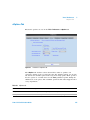
Edit Menu
Edit Menu
The available commands and options depend on the rights assigned by the
VnmrJ Administrator.
Each of the following menu options opens a dialogue that prompts the
user to enter the source and destination workspaces of the items. The
command and parameter reference refers to these tools as mp, mf, mt, md,
and mz. For more information on commands, parameters, and macros, see
the VmnrJ Command and Parameter Reference Guide.
Figure 20
VnmrJ 4.2 Familiarization Guide
Edit menu
63
2
VnmrJ Interface
Edit Menu
Table 23
Edit menu
Item
Description
Move Parameters…
Opens the Move Parameters window that allows
parameters to be moved from one experiment number to
another.
Move FID…
Opens the Move FID window to move an FID from one
experiment number to another.
Move Text…
Opens the Move Text window to move text from one
experiment number / workspace to another.
Move Display
parameters…
Opens the Move Display Parameters window to move
display parameters from one experiment number to another.
Move Integral Resets…
Opens the Move Integral Resets window to move integral
resets from one experiment number to another.
New Pulse Shapes
(Pbox)…
Opens the powerful Pbox tool for the creation of pulses and
decoupling shapes.
View Pulse Shapes…
Opens the Pulse tool, a Bloch simulator for viewing the
effects of any shaped pulse.
New/Edit Macro…
Opens a macro directly in a text editor.
Toolbar…
Enables the addition of a button to the top bar of the user
interface with a user-specific function.
Display Options
Opens a graphical interface from which you can modify and
save/recall the colors used in every tool used in VnmrJ.
Edit Config Profile…
Allows modification of what experiments are shown in the
Experiment Selector tool.
The starting point is based on the profile assigned to them
by the VnmrJ administrator
64
Edit Experiment Selector
Enables you to change the way a protocol is displayed in the
Experiment Selector. You can add or edit folders, change the
order of display, or change displayed names This
information is saved separately for each operator.
Parameter Pages
Enables you to build/modify Parameter pages.
VnmrJ 4.2 Familiarization Guide
VnmrJ Interface 2
Edit Menu
Table 23
Edit menu (continued)
Item
Description
ToolPanel Tabs
Opens the Tool Panel Editor, where you can configure what
vertical panels are available to view, and move their position
in the vertical panel pane. You can also save the
configuration in a file.
Viewports…
Enables you to toggle viewports.
It is a tool to view multiple workspaces simultaneously, on
or off.
Applications…
Enables you to define an account with collections of
Applications Directories.
An Applications Directory is a specific directory path that
could contain macros, parameter, templates, and so on. For
example, the AutoTest facility can be toggled on or off with
this menu item.
Operator Preferences…
Enables the account administrator to allow the individual
operators to manage their own preferences for the interface
to automatically preset items as email address, preferred
solvent, plotter, or notebook.
In this example Operator Preferences is not active because
in the Preferences menu, User Remembrance is not enabled.
The list of choices for this list is completely general and is
defined by the account administrator.
Preferences…
Enables the account administrator to define items such as
data saving template and default behaviors for plotting,
automatic creation of pdf plot files, and a number of operator
privileges.
This menu item is discussed in detail in “VnmrJ
Preferences” on page 103.
System Settings...
VnmrJ 4.2 Familiarization Guide
Opens a graphics tool with which system options are
defined.
65
2
VnmrJ Interface
Experiments Menu
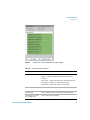
Experiments Menu
Unlike the Experiments Selector which can be configured by both the
administrators and individual operators in terms of content, the
Experiments menu shows the full selection of experiments accessible for
the account. Use the Experiment Selector tool to perform automation
submissions.
66
VnmrJ 4.2 Familiarization Guide
VnmrJ Interface 2
Experiments Menu
Figure 21
VnmrJ 4.2 Familiarization Guide
Experiments menu
67
2
VnmrJ Interface
Experiments Menu
Table 24
Experiments menu
Item
Description
Setup BioPack Experiment
(Only available when BioPack option is
enabled.) For information on using
BioPack, see the Agilent VnmrJ 4 BioPack
Users Guide.
Activate BioPack
(Only available when BioPack option is
enabled.) For information on using
BioPack, see the Agilent VnmrJ 4 BioPack
Users Guide.
Setup New Parameters for…
Executes a simple retrieval of standard
parameters for the selected experiment
and also completely clears all sample tags
(parameters used to define a sample's
identity).This is a clean slate.
Convert Current Parameters To Do…
Sets up the selected requested
experiments but retains all sample tags.
If you choose to use the Experiment
selector without first requesting New
Study by the Study Queue controls the
result is the same as this conversion.
The conversion of parameters with
retention of sample identification
parameters is the modality of "more on this
sample." The acquired data is auto saved
and added to the pre-existing data acquired
the current study
68
Setup New Parameters To Do...
Allows a simple retrieval of default
parameters for all 2D and a few 1D
experiments, according to your need.
Hadamard Experiments
Provides access to all of the Hadamard
Fast methods 2D experiments.
Solid-State Experiments
Allows access to all routine Solids NMR
experiments
VnmrJ 4.2 Familiarization Guide
VnmrJ Interface 2
File Menu
File Menu
Figure 22
Table 25
File menu
File menu
Item
Description
New Workspace
Creates a new workspace for use. Workspaces are called
exp1, exp2, and so on, up to exp9999. A workspace is a
directory where data is acquired or processed.
Join a NEW Workspace
Creates a new workspace and then actively joins the
workspace in the interface.
Following is an example of the command line equivalent:
cexp(7) jexp7
will create a new workspace and join exp7.
Open...
Accesses the Open window (also called the Experiment
Selector Editor) where you can browse for and open files.
Save As…
Opens the File Browser window where you can specify the
location and name for saving the data in the current
workspace.
VnmrJ 4.2 Familiarization Guide
69
2
VnmrJ Interface
File Menu
Table 25
File menu (continued)
Item
Description
Auto Save
Saves the data that has been acquired in an experiment
workspace using the template set up in User Preferences.
See Templates Tab.
The location and file name are automatically set based
upon the values defined in the Preferences Templates tool.
Printers…
Allows you to select a valid printer and/or plotter for
output.
Print Screen…
Allows you to print the current screen.
Auto Plot
Calls the appropriate automatic plotting routine for any
type of data in the current workspace.
Create a Plot Design…
Opens Plot Designer to create plot designs or output.
Review PDF Plots…
Allows you to review the PDF plot in Adobe Acrobat.
You can set the user preference to create a pdf plot
automatically for data that has been acquired of a given
sample.
70
Switch Operators…
Allows the current operator of the system to logout during
automation thereby freeing the system for use by another
operator.
Exit VnmrJ
Executes an exit of the VnmrJ program. It is equivalent to
typing exit in the command line.
VnmrJ 4.2 Familiarization Guide
VnmrJ Interface 2
Help Menu
Help Menu
The Help menu provides links to help and reference information.
Figure 23
Table 26
Help menu
Help menu
Item
Description
Manuals...
Opens online help where you can view manuals
in html or PDF format.
Spinsights Community Help Site...
Opens the Agilent Spinsights home page, where
you can find resources such as community
forums, downloads, and news.
Help Overlay...
Opens the Help Overlay, which gives you a
visual overview of the VnmrJ user interface.
About VnmrJ …
Opens information about the VnmrJ 4 software.
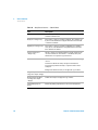
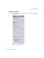
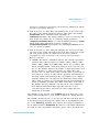
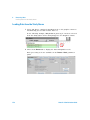
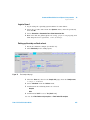
Process Menu
The Process menu provides tools for common tasks as an alternative to
the command line
VnmrJ 4.2 Familiarization Guide
71
2
VnmrJ Interface
Process Menu
Figure 24
Table 27
72
Process menu
Process menu
Item
Description
Process and Display 1D
Process and display 1D data.
Full Process
Process and display 1D data using the processing associated
with the protocol.
Drift Correct Spectrum
Apply drift correction along both axes of a 2D data set.
Automatically Set Integrals
Automatically find and set integral regions.
Baseline Correct
Apply baseline correction.
Set Spectral Width between
Cursors
Mark new spectral width on the graphics screen using the left
and right cursors and set the new spectral width.
Set Transmitter at Cursor
Mark new transmitter location on the graphics screen and set the
transmitter.
Add and Subtract 1D Data
Results are shown displayed in current when second spectrum is
selected.
Full Process 2D
Process and display 2D data using the processing and display
parameters associated with the protocol.
VnmrJ 4.2 Familiarization Guide
VnmrJ Interface 2
Process Menu
Table 27
Process menu (continued)
Item
Description
Process 2D (Individual Steps)
Step by step processing of 2D data.
Analyze
Use to analyze COSY correlations, spin simulation,
deconvolution, and regression.
CRAFT NMR
Opens the CRAFT application, (Complete Reduction to Amplitude
Frequency Table). CRAFT lets you convert an FID or a collection of
FIDs into the component NMR signals in the form of a
chemicalshift (frequency) / amplitude / linewidth table. For more
information, see the VnmrJ CRAFT User Guide.
VnmrJ 4.2 Familiarization Guide
73
2
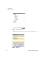
VnmrJ Interface
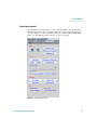
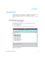
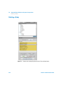
Tools Menu
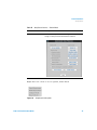
Tools Menu
Figure 25
Table 28
74
Tools menu
Tools menu
Item
Description
VeriPulse...
If VeriPulse is enabled, opens the VeriPulse
window that enables you to perform automated
testing and calibration. See the Agilent NMR
System Calibrations User Guide for information.
Study Clones…
See “Study Clones submenu” on page 77
VnmrJ 4.2 Familiarization Guide
VnmrJ Interface 2
Tools Menu
Table 28
Tools menu (continued)
Item
Description
Study Clusters...
Opens menus with commands that let you
create study clusters. A study cluster lets you
treat a set of FIDs (from different studies) as a
single group. For details, see the VnmrJ
Spectroscopy User Guide.
Study Queue Actions…
Displays two menu options:
Refresh Study Queue—Updates the study
information in the Study Queue window.
Clear Study Queue—Clears the Study Queue
window.
Workspace Information…
Opens a window that displays the status of all
workspace ongoing processes.
Probe Tuning
May display two menu options:
Auto Tune Probe…—Opens the ProTune
auto-tuning dialog window. Appears only if
ProTune accessory is installed and configured.
Manually Tune Probe…—Opens the “mtune”
panel.
Enforce ProbeID
For installed probes with ProbeID, once ProbeID
is configured in System Configuration, this
selection enables the ProbeID function.
ProbeID prepopulates calibration target values
appropriate for the current probe and ensures
that the probe file selected in the Probe popup
matches the probe that is currently attached to
the system.
Disable ProbeID
Disables ProbeID functions.
Standard Calibration Experiments
See “Standard Calibration Experiments
submenu” on page 82.
Update Locator
Opens a submenu that provides choices for
updating the different parts of the Locator
database.
VnmrJ 4.2 Familiarization Guide
75
2
VnmrJ Interface
Tools Menu
Table 28
Tools menu (continued)
Item
Description
Import Files to Locator…
Opens a window for importing files to the
Locator database.
Save Custom Locator Statement…
Opens a window to save custom Locator
statements.
Delete Custom Locator Statement…
Opens a window for deleting custom Locator
statements.
Molecular Structures
Display all—Display all molecular structures.
Plot all—Plot all molecular structures.
JChempaint…—Opens the open source
application JChempaint (molecular drawing
program) in a separate window. Select the Help
menu for an online manual.
Jmol—Opens the open source application Jmol
(3D molecular viewing program) in a separate
window. Select the Help menu for an online
manual.
76
Change Operator Password…
Opens a window for changing operator
passwords. If the operator has an operating
system login account, the password will also be
changed.
Persona Manager...
Opens the Persona Manager, where the
administrator adds and configures system
operators and personas.
Browser…
Opens a file browser window.
Locator…
Opens a Locator window.
Optional Files to Save With FID
Choose additional files that can be
automatically saved in the .fid directory.
Sample in Magnet…
Tool to command the sample changer to change
samples and to assign the sample position
currently in the magnet.
VnmrJ 4.2 Familiarization Guide
VnmrJ Interface 2
Tools Menu
Table 28
Tools menu (continued)
Item
Description
View Cryogens
Opens the CryoMonitor pop-up where you can
read the current levels of cryogens and see the
level history. This option requires that a cryogen
monitor is installed and configured in system
configuration.
Convert pre-VnmrJ 3.0 data…
Tool to convert pre-VnmrJ 3 data for use in
VnmrJ 3.x.
Select Reference Standard…
Choose the reference compounds used for
chemical shift referencing.
Study Clones submenu
The Study Clones submenu is a group of convenience utilities.
A Study Clone is a set of experiments built in the Study Queue with any
desired parameter customizations. This set of experiments is automatically
represented as a new button in the Experiment Selector. After creation,
the user can repeat the exact set of experiments simply by selecting that
button either in or out of automation and with or without a sample
changer. One use of a Study Clone is to set the desired parameters for a
very fast PROTON spectrum, such as nt=1 ss=0 gain=4 and Clone
current Exp with a button label Fast_H. It might also be useful to set
parameters for a slow quantitative PROTON experiment such as d1=60
pw(90) ss=2 nt=8 and Clone current Exp with a label as Quant_H. The
user can use the Study clones to recall complex sets of multidimensional
experiments or to simply establish a convenience button for commonly
done tasks. Clones from other clones can also be created by adding more
experiments in any desired fashion.
VnmrJ 4.2 Familiarization Guide
77
2
VnmrJ Interface
Tools Menu
Figure 26
Table 29
Study Clones submenu
Study Clones submenu
Item
Description
Clone New Study
Enters the Study Queue mode to create a new Study that shall be saved as a new
clone. Presents a “Save Study” button on the Study Queue window to save the
new Study.
Clone Current Study
Use to assign a name for the button associated with a study of a list of
experiments assembled in the Study Queue.
Clone Current Experiment
Allows user to assign a name for the button option associated with the currently
loaded or displayed experiment. For example, use this option if an FID from a
previous study is retrieved in the current workspace, and the user wants to
create a clone of the single experiment that had been acquired on that sample.
Clone Location Queue
Allows creation of a button associated with the study completed for the selected
tray sample location.
78
VnmrJ 4.2 Familiarization Guide
VnmrJ Interface 2
Tools Menu
Table 29
Study Clones submenu (continued)
Item
Description
Command and Protocol Buttons
Use the Protocols menu option to devise a method to create a button to run a
macro to setup an experiment.
In the Type field, select either Experiment or Command.
If Command is selected, a button option is created to call a macro that, for
example, analyzes the lineshape. Based on the result, the user can decide to call
a group of non-spin shim routines. A Study Clone could then be composed of a
PROTON experiment customized appropriately for running 1H lineshape,
followed by the command protocol to analyze lineshape in the Study Clone. This
Study clone can be submitted at any time and automates the task of refining
shims.
VnmrJ 4.2 Familiarization Guide
79
2
VnmrJ Interface
Tools Menu
Table 29
Study Clones submenu (continued)
Item
Description
Edit Parlib…
Enables users to view the details of any valid VnmrJ protocol. Edit/Make parlib
can also create new protocols based on the contents of the parameter set in the
current workspace.
Use the Study Clones tool to create a modified version of an already existing
protocol, such as PROTON or CARBON experiments with specific parameters for
a quick or long experiment. Do not use Edit/Make Parlib. In order to properly
utilize the tool, the user must have a basic understanding of the concept of
modules and locked parameters (Plock).
The following is an example view of Edit/Make parlib for a band-selected 2D
experiment.
80
VnmrJ 4.2 Familiarization Guide
VnmrJ Interface 2
Tools Menu
Table 29
Study Clones submenu (continued)
Item
Description
Both the apptype and the list of modules are different from the PROTON
protocol. The user can query the values and modules for the apptype parameter
by using the apptype? and modules? commands before creating a new
protocol from a pulse sequence and parameter set that originated from outside
VnmrJ, such as the user library. Assign the value for modules to the Lock
parameters list and add any parameter needed to be kept at setup time.
In the above PROTON experiment, basic protocols include the following key
concepts:
• Name—Displays the name of the set parameter and the protocol’s button.
• apptype—Displays a generic helper macro name for setting up a group of
protocols. In VnmrJ apptype is optional. Common apptypes are std1D,
homo2D, hetero2D, and lstd1Dmodules. (The names for the little
min-parameter sets that are combined to create the existing parameter set.)
• Module—Displays a module and all of the values for the parameters in that
module, type on the command line module (‘popup’,’modulename’), for
example module (‘popup’,’presat’).
• Default Starting Experiment—Define a default experiment as a starting point
to morph the default experiment into the desired experiment. Type REQexp?
from the command line to query the value for the default starting experiment.
• Customization—Shows the contents of the macro name_setup or in the case
of this example PROTON_setup. Not editable in this tool but it can be edited in
a text editor.
• User Customization—Creates a macro from the text typed in this field.
userprotocolname or for this example userPROTON.
Show Library
Opens a graphical tool to backup then remove old buttons and to review the
executable actions of buttons.
Show Library
Opens a graphical tool to backup then remove old buttons and to review the
executable actions of buttons.
VnmrJ 4.2 Familiarization Guide
81
2
VnmrJ Interface
Tools Menu
Standard Calibration Experiments submenu
Figure 27
Table 30
Standard Calibration Experiments submenu
Standard Calibration Experiments submenu
Item
Description
Probe Protection…
Opens a window to set up maximum allowed power values for probe protection. See
below.
Setup qNMR Calibrations…
Setup qNMR Calibrations-Opens a window to calibrate and set up quantitation tools.
Setup Gradient Shimming
Setup Gradient Shimming-Loads the pulse sequence and panels for making a shim map
for gradient shimming.
Shim Editor
Opens the Shim Menu Editor, where you set up or change shim menus.
82
VnmrJ 4.2 Familiarization Guide
VnmrJ Interface 2
Probe Protection
Table 30
Standard Calibration Experiments submenu
Item
Description
Shim Scheduler
Opens the Shim Maintenance Scheduler, where you set up and schedule shim service.
Run Shim Procedure
Executes the shim procedure.
Start Autotest
Opens the Auto Test window, where you can configure and run an autotest. For more
information, see the Agilent AutoTest User Guide.
Autotest Settings
Opens the Autotest settings window, where you select the parameters for AutoTest. For
more information, see the Agilent AutoTest User Guide.
Setup 3D Gradient Shimming
Selection appears only if this option is installed. Loads the pulse sequence and panels for
making a 3D shim map for gradient shimming.
Probe Protection
Probe Protection settings are global parameters used for sample
protection. Recommended settings are to leave power protection on and
using default settings.
VnmrJ 4.2 Familiarization Guide
83
2
VnmrJ Interface
Probe Protection
Table 31
84
Probe Protection
Item
Description
Use probe file
Updates pcal, alarm level, and time constant
values using values from the probe.
Use custom values
Use for advanced sample protection.
Save custom values
Saves advanced sample protection values from
the interface.
Nucleus
Displays channels with associated nuclei.
Probe protection is:
• On—Default state terminates experiments that
are predicted to exceed the alarm level. When
this happens, PSG prints the relevant rf channel
on line 3 and the error window.
• Verbose—Same settings as "on" and prints
diagnostic messages in process>text.
• Warn verbose—Alerts when 90% of alarm is
reached and terminates when alarm is
reached.
• Warn only (off)—Alerts when 90% of alarm is
reached and will not terminate.
• Off-Will not terminate when the alarm level is
reached.
Max. attenuator limit
Displays associated maxattench value for each
channel.
pcal
Tpwr level associated with 2 watts of power at
the probe.
Alarm level
An energy (power * time) value at which the
probe may be damaged or the sample may be
overheated.
Time constant
The length of time, typically 5 seconds, for the
probe cooling processes.
VnmrJ 4.2 Familiarization Guide
VnmrJ Interface 2
View Menu
View Menu
Use this menu to access parts of the interface and restore the interface
elements. Close the window by clicking the Close button in the upper right
hand corner of each window. Access the hardware or graphics toolbars
using the Toolbars submenu.
Figure 28
VnmrJ 4.2 Familiarization Guide
View menu
85
2
VnmrJ Interface
Changing Display Colors
Changing Display Colors
Using the Styles and Themes window, you can change the colors used for
the display and printing of various items in VnmrJ. To open the Styles
and Themes window, click the Display Options icon.
There are four user interface styles available (Default, Classic, Dark and
Light), and several look and feel (LAF) choices to customize the interface.
You can also set default colors for drawing 1D and 2D spectral graphics
and labels (Display). 1D and 2D spectral drawing have adjustable line
thickness for better visibility and report generation. And, when zooming
1D and 2D data, VnmrJ can automatically switch to thicker lines.
The Plot functions let you set up defaults for printing and plotting.
To change the look and feel of the VnmrJ user interface
1 On the System Toolbar, click the Display Options icon.
The Styles and Themes window opens.
2 Select the UI button.
Figure 29
86
Styles and Themes window with UI selected
VnmrJ 4.2 Familiarization Guide
VnmrJ Interface 2
To change color options for spectral drawing
3 From the drop- down menu, select Default, Classic, Light or Dark to
change the interface color theme. You can also customize further using
the tabs and selections available.
To change color options for spectral drawing
1 On the System Toolbar, click the Display Options icon.
The Styles and Themes window opens.
2 Select the Display button.
Figure 30
Styles and Themes with Display selected
3 Set the widths of lines used to draw 1D and 2D spectral graphics.
There are two Line Thickness settings, used depending on whether the
number of points in the spectral region is much smaller than the
number of pixels in the spectral drawing canvas. The corresponding
VnmrJ 4.2 Familiarization Guide
87
2
VnmrJ Interface
To change color options for plotting
Factor parameter controls when the thicker lines will be used. For
example, if the Factor parameter is set to 0.2, the thicker lines will be
used whenever the ratio of points to pixels is 0.2 or less. If desired, you
can set both Thickness values to the same number, so that line drawing
will not change when spectra are zoomed.
4 Use the other tabs and selections to customize the display of pulse
sequence (DPS), Contours, and Annotations.
To change color options for plotting
1 On the System Toolbar, click the Display Options icon.
The Styles and Themes window opens.
2 Select the Plot button.
Figure 31
88
Styles and Themes with Plot selected
VnmrJ 4.2 Familiarization Guide
VnmrJ Interface 2
To change color options for plotting
3 Set the widths of lines and colors to be used to plot 1D and 2D
spectral graphics.
The Line thickness sets the same line thickness to all lines associated
with the spectral drawing.
4 Use the other tabs and selections to customize the plotting of pulse
sequence (DPS), Contours, and Annotation.
VnmrJ 4.2 Familiarization Guide
89
2
VnmrJ Interface
Experiment Selector Editor
Experiment Selector Editor
The Experiment Selector Editor lets you customize how protocols are
displayed in the Experiment Selector in the Protocols vertical panel. To
open the Experiment Selector Editor, on the main menu click Edit > Edit
Experiment Selector.
Figure 32
Experiment Selector Editor
The Experiment Selector has the following capabilities.
90
VnmrJ 4.2 Familiarization Guide
VnmrJ Interface 2
Experiment Selector Editor
Table 32
Features of the Experiment Selector Editor
Feature
Action
Drag a protocol or folder to a new
location.
Changes the order in which folders and protocols are
displayed
OK
Closes the panel and updates the Experiment Selector
Cancel
Discards any changes and keeps the Experiment Selector
unchanged
Default
Reverts to the Agilent default order and names
Click 3rd mouse button on an item Opens a menu
Copy
Copies selected item to clipboard
Paste
Pastes the “copied” item to the position above the location
selected
Delete Entry
Deletes selected entry
New Folder
Creates a new Folder (or Node) in the tree. Type in the
desired name and then hit the “Enter” key. Failing to hit the
enter key causes the folder name to revert to “New
Folder”. In that case, click on the name and edit the name,
then press Enter.
Add to Favorites
Copies the selected item to the Favorites node.
Note: The menu item will show the name of the first
Folder/Node displayed in the Experiment Selector.
Normally, the first Node is called “Favorites”, however, this
is not required. If the first Node is called “Common”, then
the menu will display “Add To Common” and the selected
item will be copied to the “Common” Folder/Node.
Change the name for an item
NOTE
Click on the name and type a new name, then press Enter.
Failing to press the Enter key will cause the name to revert to
its original name.
Duplicate names are not allowed in the same folder/node. If you try to paste or rename an
item in a folder/node where an identical name exists, an error appears and the action is
aborted.
VnmrJ 4.2 Familiarization Guide
91
2
VnmrJ Interface
Experiment Selector Editor
NOTE
92
Experiment Selector information contained in a protocol .xml file is always active and
cannot be overridden by this Editor. Therefore, if (for example) a user has a protocol in his
vnmrsys directory area which puts that protocol into a tab named ABC, that tab (or first
level in the tree) cannot be permanently renamed, moved, or deleted. Nor can the protocol
entry be permanently deleted or removed from its defined location. A warning will appear if
one of these actions is attempted for information defined in the protocol.xml file.
VnmrJ 4.2 Familiarization Guide
VnmrJ Interface 2
File Browser
File Browser
The file browser opens when you select File > Open from the menu bar.
Figure 33
Table 33
Button
File browser — Open
Icons and buttons in the file browser
Description
Go up one level in the directory tree.
Go to user’s home directory.
Make a new folder in the current directory.
VnmrJ 4.2 Familiarization Guide
93
2
VnmrJ Interface
File Browser
Table 33
Button
Icons and buttons in the file browser
Description
Show a list of files and directories at the current
directory level.
Show the details of files and directories at the
current directory level.
Open selected file. Load into current experiment if
it is a VnmrJ 3 data file, sequence, or parameter
set.
Save file with the name shown in the File Name:
field using the extension shown in the Files of
Type: field.
Cancel selection and close the file browser.
Click and hold to assign current directory to this
button.
94
VnmrJ 4.2 Familiarization Guide
VnmrJ Interface 2
Status Charts
Status Charts
The Status charts are accessed from the Hardware Toolbar at the bottom
of the VnmrJ main window.
Figure 34
Hardware toolbar in VnmrJ
When you click one of the status plot buttons, a window appears that
enables you to log and examine status data.
Figure 35
VnmrJ 4.2 Familiarization Guide
Example of Chart-Spin window with right-click menu
95
2
VnmrJ Interface
Features of the status chart window
Features of the status chart window
Table 34
Features of the Status Plot windows
Item
Description
Select color to show/hide the associated element in
the chart.
Opens the Plot Format window. Here, you can
• Choose the orientation mode ( Portrait, Landscape)
The plot will be scaled to fit a full page either
vertically or horizontally depending on the chosen
orientation mode.
• Click print in the plot format window to cause the
currently displayed data to be printed at the selected
printer.
Toggles the x-axis units between “time-of-day” and
“elapsed-time” formats. Initial format is “time-of-day”.
Click to zoom to display only the most recent data
(“Tail” mode).
• The amount of data displayed will be set to the
x-range selected from most recent mouse “zoom-in”
operation (or last 10 seconds if zoom-in action has
not yet occurred).
• After clicking, any new plot data will be automatically
added to the end of the visible region.
Zoom out to fit data in the display (“Fill” mode).
Right-click menu items
96
Lock scale
Lock the scale to the current y axis scale. (Click tail or
fill button to remove scale lock.)
Clear history
Removes all collected plot data.
Show Min/Max
Displays the maximum and minimum values observed
since the start of data collection. (Does not appear in
the printer output.)
VnmrJ 4.2 Familiarization Guide
VnmrJ Interface 2
Using the status chart
Table 34
Features of the Status Plot windows
Item
Description
Show Status
Shows the current status of the relevant status variable.
(Does not appear in the printer output.)
Start Data Log
Opens a Save dialog box where you can specify a file
into which the plot data will be saved.
Using the status chart
This section describes the components of the status chart window, and
what you can do with them.
Data Area
Data area where data traces and the grid are drawn.
Toolbar
A set of buttons in a right- side vertical panel (for descriptions, see
Table 34.)
Popup menu
Used to select various options (right- click in data area to open the menu)
Axis Area
Values and tick marks shown to the left and below the data area, along
with an x- y grid. The Horizontal axis units are displayed in either
“Time- of- day” or “Elapsed- time” format. Initial format is “Time- of- day”.
• Elapsed time units are Hours:minutes:seconds measured from the
time that VnmrJ is started or from when “Clear Data” is selected
from the pull- down menu.
• Time of Day units are “month/day hours:minutes:seconds” in local
time.
Status line
Shows variable type and value (drawn below x- axis area).
VnmrJ 4.2 Familiarization Guide
97
2
VnmrJ Interface
Using the status chart
Zooming
The following modes of zooming are provided:
• Click and drag the left mouse button down and right to zoom in. Click
and drag the left mouse button up and left to zoom out.
• Zoom in using the green arrow “tail” button in the toolbar.
• Click the green arrow “tail” icon in the toolbar
to display only
the most recent data. The amount of data displayed will be set to the
x- range selected from most recent mouse “zoom- in” operation (or
last 10 seconds if zoom- in action has not yet occurred).
• After you click the “tail” icon, any new plot data will be
automatically added to the end of the visible region.
• Zoom out using the “fill” button
• Click the “fill” button in the right- side toolbar. This action sets the
plot y and x range to show all current data scaled to fit within the
display.
Scale locking/unlocking
• In “zoom- in” mode, the x and y ranges will be “locked” to the
boundaries set by the selected “zoom- box”.
• In “Fill” mode, the x and y ranges will autoscale to make sure that all
of the data in the plot buffer is displayed (ranges are “unlocked”).
• In “Tail” mode the x range will normally be locked to show only the
most recently collected data and the y range will be “unlocked” so that
all of the displayed data is shown.
• In any mode scaling can be “locked” to the current y values by selecting
Lock scale from the chart popup menu.
• Scale- locking is removed by selecting either the fill or tail button in the
interface
Data collection
• The amount of data that is buffered and displayed in the status plots is
controlled by the “values” attribute in the “statusbutton” sections of
HardwareBar.xml (a system resource file).
• The Current default is 1000 points. For example, values="1000".
98
VnmrJ 4.2 Familiarization Guide
VnmrJ Interface 2
Using the status chart
• If more points than “values” are collected earlier points are discarded
from the plots.
• Setting “values” to - 1 will cause all data to be retained.
• All collected Plot data can be removed by selecting “Clear History” from
the chart popup menu.
Data display
Status plots can show the following “traces”
• “Lines” a set of connecting lines drawn between successive data points
• “Points” individual “dots” displayed for each collected point
• “Set Value” The “target” or setpoint value for the relevant status
variable type
Each display trace can be made visible or hidden by selection the
associated color toggle button in the right- side toolbar.
Data Logging
A text file containing status history can be generated as follows:
• Right- click in the chart area, and then select Start Data Log from the
display popup menu.
This opens a standard system “save” dialog window (see Figure 36).
Browse to an existing file or type the name of a new file to save the log
data. Click Save File Path. When the file dialog closes, new data will
automatically be written to the specified file. Any old data in the file
will be discarded (That is, a new file will be created each time).
VnmrJ 4.2 Familiarization Guide
99
2
VnmrJ Interface
Using the status chart
Figure 36
Status chart with save window
• Only new data acquired in the plot after logging starts will be added
to the file.
• If logging is active a red “recording dot” will be displayed in the upper
right area of the plot (see Figure 36).
To stop data logging, right- click in the data area to open the chart popup
menu and select Stop Data Log.
Log file data format is:
“Time- of- day” “elapsed- time” “value”
Example output
DATE TIME VALUE
10/01 11:33:14 000:00:45 - 17.3
10/01 11:33:15 000:00:45 - 16.4
100
VnmrJ 4.2 Familiarization Guide
VnmrJ Interface 2
Using the status chart
10/01 11:33:15 000:00:46 - 15.3
Plotting
1 Click the “printer” icon in the right- side toolbar to open a system Print
dialog box.
2 Select the printer, orientation, and appearance in the General, Page
Setup, and Appearance tabs.
3 Click Print in the plot format dialog to cause the currently displayed
data to be printed at the selected printer. The plot will be scaled to fit
a full page either vertically or horizontally depending on the chosen
orientation mode.
Annotation
To include optional text information, right- click in the data area, and
select the following options from the popup menu:
Show Min Max will show the maximum and minimum values observed since
the start of data collection.
Show Status will show the current status of the relevant status variable.
Note: Annotation text does not appear in the “printer” output.
VnmrJ 4.2 Familiarization Guide
101
2
102
VnmrJ Interface
Using the status chart
VnmrJ 4.2 Familiarization Guide
VnmrJ 4.2
Familiarization Guide
3
VnmrJ Preferences
Templates Tab 104
Automation Tab 112
SQview Tab 119
Queue Tab 120
eOptions Tab 123
Data Mirror Tab 126
SampleTags Tab 128
UserPrefs Tab 130
The default behavior of VnmrJ at the user account level has several
customizable options. These options are different from those that can be
accessed by the administrator of VnmrJ. The optimal operation of these
customization options requires a properly set up probe file for the probe
in use.
Select Preferences from the Edit menu on the main VnmrJ window to access
the VnmrJ preferences setup window. Note that some of the options
appear only if the Enable Email Options check box has been selected. Ensure
that an email server has been properly configured on the host computer.
Agilent Technologies
3
VnmrJ Preferences
Templates Tab
Templates Tab
The Edit > Preferences > Templates tab can be used to select where the data
is saved and how data is to be named.
Figure 37
Preferences—Templates tab
The following describes the options for the Templates tab:
104
VnmrJ 4.2 Familiarization Guide
VnmrJ Preferences
Templates Tab
Table 35
3
Options in the Preferences—Templates tab
Item
Description
Study Directory Template
Defines where the data for all the samples is
stored. It defines the parameter svfdir. Refer
to Format of the Entry Level for the exact format
of this entry.
Sample Directory Template
Defines the directory inside the study directory
where all the data for any sample are stored. It
defines the parameter sampdirtmplt. This is
always a subdirectory for the study directory,
svfdir. Refer to Format of the Entry Level for
the exact format of this entry.
Data Template
Defines the actual name that is given to the
individual fid files. It defines the parameter
svfname. This file is saved inside
sampdirtmplt. Refer to Format of the Entry
Level for the exact format of this entry.
Automation Directory Template
Defines location of the automation directory,
where the system stores all the information to
do the automation run. It defines the parameter
autodir. Refer to Format of the Entry Level for
the exact format of this entry.
VnmrJ 4.2 Familiarization Guide
105
3
VnmrJ Preferences
Templates Tab
Table 35
Options in the Preferences—Templates tab
Item
Description
Bitmap Image Format
Drop-down menu with the following selections:
tif–This creates a TIFF format document, typical
for accurate representation of bitmap images. A
TIFF document can be read with most common
image and word processing programs.
pdf–This creates a document according to the
Adobe PDF™ document format. A PDF
document can be read using Adobe Acrobat
Reader. The PDF documents created from
VnmrJ require Adobe Reader version 5 or higher.
pcx–This creates a document using the PCX
protocol, adequate for representations of bitmap
images. PCX documents can be read with most
common image and word-processing
documents.
jpg–This creates a JPEG format document
accurate for the representation of real-life
photos. JPEG documents can be read with most
common image and word processing programs.
Time display format
Select the desired format for displaying time
from the drop-down menu.
Format of the Entry Level
The format used to enter the directories in the first three fields is the
same as was used previously for "autoname". A detailed description of it
appears under the description of "autoname" in the Command and
Parameter Reference Manual for VnmrJ. A brief description is shown
here.
There are three types of text that can be entered in these fields. All the
options can be mixed together generating very powerful saving options.
1 Fixed text, such as "/home/vnmr1/data." This is interpreted as is
without any special translations. If the text defines an absolute
directory path then this path will be used (example /vnmr/data). If
there is no absolute path then the directory will be created as a
subdirectory of the previously defined directory path. So if sample
106
VnmrJ 4.2 Familiarization Guide
VnmrJ Preferences
Templates Tab
3
directory is defined as "mysamples/today" then the subdirectory will be
created for the study directory.
2 Text enclosed in "$" signs. This will substitute the enclosed text with
the value of the VnmrJ parameter with the same name. For example
$samplename$ will be substituted with "mysample" if
samplename='mysample'. Any VnmrJ parameter can be used for this. The
most useful ones will be the ones defining sample parameters
(studyowner, samplename, solvent, etc.) and experiment parameters (pslabel
which shows what experiment is run for example). So
"$samplename$/$pslabel$" will translate into "mysample/PROTON" in the
case of a proton spectrum.
3 Text enclosed in "%" signs. This will substitute the enclosed text with
the entry on the actual enterQ file being used. This can be very cryptic
but some useful options are outlined here. For more detailed
description the user is referred to the Command and Parameter
Reference Manual.
a %DATE%: This will be substituted with the date that the spectrum is
acquired. Other allowed entries are %DAY%, %MO%, %MOC%, %YR%,
%YR2%, %HR%, %MIN% and %SEC%.%RX% where X is a number: This
will be substituted with a numerical extension in the form "00", "01",
"02" etc. The number X defines the number of digits that will be used
for the extension, so %R2% will generate "01" while %R3% will
generate "001" etc. This ensures that a unique name is generated for
every directory created. A %R2% will be appended automatically to
the study, sample and automation directory templates if no "%RX%" is
explicitly defined. One can suppress the numbering entirely using
%R0%". This is, however, not recommended for the Data Template as
it may accidentally overwrite data. When using %R0% at the end of
the "Sample Directory Template", all data on the same sample but
from different Automation Runs (typically from two or more
consecutive days) will be saved into the same sample directory,
which may be desirable.
The examples at the bottom of the Templates tab show what each of the
strings entered translates to. Some useful examples are displayed below.
The example shown in Figure 38 on page 108 will direct all study data to
home/chemp/vnmrsys/data/<operator name>. This is accomplished by the
use of the $operator_$ argument. Note that the more proper parameter to
use in VnmrJ would be $studyowner$. The data for each sample will further
be saved in a directory named <notebook>_<page>, where notebook and
VnmrJ 4.2 Familiarization Guide
107
3
VnmrJ Preferences
Templates Tab
page are the notebook and page numbers that were entered in the Start
tab of the parameter panel. The revision number is suppressed here. The
actual FIDs will be saved as <experiment>_<samplename> with a three
digit revision after it.
Figure 38
Data saving templates
The example shown in Figure 39 on page 109 illustrates the inclusion of a
fixed text in the sample directory name (Book_<notebook>).
108
VnmrJ 4.2 Familiarization Guide
VnmrJ Preferences
Templates Tab
Figure 39
3
Example–Inclusion of text in Sample Directory Template
The example in Figure 40 on page 110 shows the date is part of the
directory name.
VnmrJ 4.2 Familiarization Guide
109
3
VnmrJ Preferences
Templates Tab
Figure 40
Example—Inclusion of date in Sample Directory Template
Data from one operator can be sorted to different subdirectories according
to the date the data was recorded.
110
VnmrJ 4.2 Familiarization Guide
VnmrJ Preferences
Templates Tab
Figure 41
NOTE
3
Example—Inclusion of date in Study Directory Template
Any changes done on this window should be saved before exiting the window. Otherwise,
changes are lost. The changes require the creation of a new automation run to become
active.
VnmrJ 4.2 Familiarization Guide
111
3
VnmrJ Preferences
Automation Tab
Automation Tab
Automation preferences are set in the Edit > Preferences > Automation tab.
Figure 42
Preferences–Automation tab
The Automation tab defines the defaults that will be used for automation
experiments. Defaults are described in the following table.
112
VnmrJ 4.2 Familiarization Guide
VnmrJ Preferences
Automation Tab
Table 36
3
Preferences — Automation tab
Item
Description
Traymax
This parameter indicates what type of autosampler is actually used. If this is not set up
properly then it needs to be changed in the System Preferences window. Only vnmr1 can
make this change.
Sample Change Time
This is the approximate time required for the sample change using the autosampler, the
finding of the z0 value for the automatic locking, the automatic tuning (ProTune) and the
automatic shimming. The default value is 120 seconds which should be sufficient for
most cases. It is generally advised to round the time rounded up, so if the system needs
100 seconds to enter instead 120. This ensures that the time calculations will not fall off
because of too short estimates.
Process/Plot Time
This is the time required to process, plot and save the spectrum. The default value of 10
seconds should be sufficient. Use a longer value only if you are using a slower computer.
Shim Each Sample From
This defines the shims started by the system when the shim tries to shim a new sample.
There are two options:
1 Last shims: Last shims use the shims from the previous sample run
2 Default shims: Default shims load the shim file that is in the probe file. In actual
operation with properly prepared samples the outcome should be equivalent. If
however that range of samples and tubes used varies widely then the use of Default
shims give more consistent results.
Skip Sample if Protune Fails
This check-box appears only if ProTune is installed. If checked then the system skips the
sample in the unlikely event that the automatic tuning fails.
When the check box is not selected, the data acquisition proceeds.
Maximum Priority Samples
This defines the maximum priority samples an operator can submit in each automation
run. The right to have priority samples is granted from the VnmrJ administrative
interface.
When DayQ Exceeds Time Limit
By default, with "redirect Exp to NightQ" unselected experiments that are attempted to
be added to the DayQ but exceed the DayQ limit result in an error and are not added to the
StudyQ. With this option selected, such Experiments are added to the NightQ instead,
Select redirect Exp to NightQ if the DayQ has exceeded it's time.
Locations Selection
This drop-down menu defines whether users will be allowed to choose the sample
location manually (Let User Select option) or not (Next Available option). The Next
Available option will ignore the user input and submit the experiment queue for the next
available sample position in the autosampler.
Auto-Resubmit Errored
Locations
Select yes to automatically resubmit samples back into the queue that have errorred.
VnmrJ 4.2 Familiarization Guide
113
3
VnmrJ Preferences
Automation Schedule
Table 36
Preferences — Automation tab (continued)
Item
Description
Reuse Errored Locations
Select yes to automatically reuse samples that have errored.
Reuse Completed Locations
Select yes to automatically reuse samples that have completed.
Default Automation Temp. (C)
Defines the temperature default for all samples run in automation. If at the time New
Automation run is started, the temperature control is enabled in the account, a new
temperature can be specified at customization time. The software checks if the chosen
temperature is safe given the choice of solvent for that sample. In addition, if variable
temperature is allowed in sample changer automation, it is important to set the value for
the tin (temperature interlock) parameter contained in ~/vnmrsys/modules/cpQdefaults
be set to "w" so that the sample changer will not insert any sample until the probe has
reached the requested temperature.
When Automation Queue is
Done
This dropdown menu defines what should happen when the last sample of a StudyQ is
done and there are no more sample in the queue:
• put standby sample (loc=>traymax>) into magnet. This removes the last sample run
from the magnet thus allowing its owner to retrieve it from the autosampler tray. The
standby sample needs to be placed in the position indicated in the field, position 96 in
the case of the figure above. That particular sample location is not available for use.
• leave current sample in magnet. This leaves the last sample of the StudyQ in the
magnet for further use.
• remove current sample from magnet. Only removes the current sample from the
magnet without inserting a (standby) sample. This option is only available with
7600AS and 7510AS sample changers.
Automation Directory
Determines when a new automation directory shall be created:
• Always use current. The current automation directory is used until the user creates a
new one by selecting "Automation Run (autodir) -> New Automation Run" from the
"Automation" menu.
• Create as per schedule. A new automation directory is created on each day on which a
previous NightQ ended as defined with the "Set Time Schedule" window.
Set Time Schedule
Opens the Automation Schedule window to set time schedules for automation runs. See
“Automation Schedule” on page 114.
Automation Schedule
To open the Automation Schedule tool, click Edit > Preferences to open the
Preferences window. Then select the Automation tab and then click Set Tine
Schedule.
114
VnmrJ 4.2 Familiarization Guide
VnmrJ Preferences
Automation Schedule
Figure 43
3
Automation Schedule window—Automation Run tab
VnmrJ 4.2 Familiarization Guide
115
3
VnmrJ Preferences
Automation Schedule
Figure 44
Automation Time Scheduler—Automation File
The Automation Schedule tool allows the account administrator to define
how time is allocated during the day or night for Automation Runs
(AutoRuns, typically on demand sample automation) and Automation Files
(AutoFiles, sample queues built for submission at a time chosen by the
account administrator). Selecting the All Day check simply turns off time
management and is a better choice for a research environment as opposed
to an open system being accessed by a large number of chemists. Using
the Automation Schedule tool, the user can define different queue times for
116
VnmrJ 4.2 Familiarization Guide
VnmrJ Preferences
Automation Schedule
3
different times of the day as well as after hours' queues. At sample
submission time with the NightQ enabled, a chemist can submit certain
experiments to the day and others to the night.
There are definitions for each day of the week. The first two columns
define when the day and night starts. They are only active if the "All day"
option is not selected. The third column, Max Time per Sample, defines
how much experiment time will be allocated per sample during the day.
The column with the same name further to the right defines the maximum
time per sample during day and night runs.
The definitions for the AutoFiles are similar, with the fields defining how
long the total time for short and long queues should be and how long the
maximum time per sample allowed for short and long queues should be.
The maximum time per DayQ sample can also be made variable, for
example, to allow users longer runs during lunchtime. To do this:
1 Select the variable check box. A new button set/view appears.
2 Select a longer MaxTime per Sample to accomodate the longer allowed
"lunch queue".
3 Click it to see and/or edit the detailed DayQ time limits for that day.
VnmrJ 4.2 Familiarization Guide
117
3
VnmrJ Preferences
Automation Schedule
4 Enter the new, "split" DayQ limits by adding pieces of schedule:
a Start with first schedule part: Select the DayQ start (here 8:00 AM),
select the End (to the beginning of "lunch", here noon) and select
Maxtime (here the default 30 min). Click Add.
b Now enter the start and end times during which longer DayQs are
allowed (here 2 h). Click Add again.
c Finally, enter the second normal time period (afternoon). Click Add.
d Click Save to keep this variable schedule. The variable time limits
schedule can be erased to start afresh by clicking Clear. Click Cancel
if you want to exit this panel without saving.
A variable schedule may have more than three entries.
Note that any changes done on the automation schedule need to be saved
(red Save button) before exiting the window, otherwise they will be lost.
The changes will usually require the creation of a new automation run in
order to become active.
118
VnmrJ 4.2 Familiarization Guide
VnmrJ Preferences
SQview Tab
3
SQview Tab
The Edit > Preferences > SQview tab allows the user to change the Study
Queue display order or restore the display order to default.
Select the Show Scout Fids check box to display all prescan FIDs in the
Study Queue.
Figure 45
VnmrJ 4.2 Familiarization Guide
Preferences-SQview tab
119
3
VnmrJ Preferences
Queue Tab
Queue Tab
The Edit > Preferences > Queue tab offers options for the actual automation
queue. All settings at this page are default settings. Each sample
submission will start with these default settings. They can be overwritten
during the sample submission.
Figure 46
Table 37
Preferences–Queue tab
Preferences — Queue tab
Item
Description
Before First (Day and Night) Experiment
Defines whether the system will automatically lock and shim before the first
experiment of a sample queue.
By default run queue in
Select whether to run the queue automatically, in the foreground, or in the
background.
By default, add…
This option allows for an experiment to be automatically added by default to
each new queue. For example, "PROTON".
120
VnmrJ 4.2 Familiarization Guide
VnmrJ Preferences
Queue Tab
Table 37
3
Preferences — Queue tab (continued)
Item
Description
Allow Submission to Automation Queue
This setting activates the automation queue. If this is not desired then this
should be unchecked.
Before First (Day and Night) Experiment
If the system is equipped with a ProTune module, this selection defines
whether the system will automatically run ProTune before the first experiment
of a sample queue.
Before first acquisition equilibrate sample
Temp for ___seconds (TempPad)
This sets the amount of time that the system will wait for the temperature to
equilibrate after it inserts the sample into the magnet but before recording
any spectra. The default value is 2 seconds which should be sufficient for
experiments conducted at or near ambient temperatures. Increasing this
value has got the advantage of having the temperature better equilibrated in
the sample but the disadvantage of increasing the time required for each
sample.
After findz0 routine read lockphase from
probe file (automation only)
This is a setting for optimizing the lock system before spectra are recorded. If
selected then the lock phase is set to the value in the probe file overwriting
any value that has been set manually. The normal value for this box is
unchecked. It should only be checked if there is a suspicion that the lock
phase is not set properly. In this case the probe file should be updated with
the correct value for the lock phase.
Before sample insert, allow ___seconds for
Temp to change; Else...
This value selects the amount of time the system waits after retrieving a
completed sample but before inserting the next sample for the temperature to
equilibrate. This is a useful feature when operators are allowed to run
samples in automation at different temperatures. It can be used to avoid the
case where a sample was run at a temperature higher than the boiling point
or lower than the freezing point of the next sample's solvent. The time defined
here is the maximum time that the system will wait for the temperature to
equilibrate. If the temperature equilibrates faster, the run continues. The
actions in the pull-down menu define what will happen if such a condition is
met and there is no waiting time defined. The possible actions are:
"Ignore", which causes the system to ignore the condition and proceed with
the sample submission, "Abort", which causes the system to abort the
automation run and "Alert" which gives a warning to the operator.
Allow submission to Non-automation
Queue in Foreground
VnmrJ 4.2 Familiarization Guide
Select to allow users to run manual Study queues on one sample in the
foreground. The foreground option will run all of the StudyQ's experiments in
the current VnmrJ experiment.
121
3
VnmrJ Preferences
Queue Tab
Table 37
Preferences — Queue tab (continued)
Item
Description
Allow submission to Non-automation
Queue in Background
Select to allow users to run manual Study queues on one sample in the
background. The background option runs the single Study queue in the same
way as a standard automation run; by holding all the information in the
autodir directory.
Before First Experiment
If the system is equipped with a ProTune module, the option for automatic
tuning before the first experiment appears here If automatic tuning before the
first experiment is not desired then this box should be unchecked.
NOTE
122
Any changes done on this window need to be saved (red button Save) before exiting the
window, otherwise they will be lost. The changes will require the creation of a new
automation run in order to become active.
VnmrJ 4.2 Familiarization Guide
VnmrJ Preferences
eOptions Tab
3
eOptions Tab
Electronic options are set in the Edit > Preferences > eOptions tab.
Figure 47
Preferences-eOptions tab
The eOptions tab defines actions that will be taken to produce an
electronic output of the recorded spectra. The default options set on this
tab will be the default option with every new study queue. Each operator
has the option to override these in the Start parameter panel during the
submission of the queue. The available options define what happens after
every experiment.
Table 38
eOptions tab
Item
Description
Plot2plotter
Select to produce a hardcopy output to a defined plotter.
Save a plot
Select to save the plot in the format defined in the Bitmap Image Format field.
VnmrJ 4.2 Familiarization Guide
123
3
VnmrJ Preferences
eOptions Tab
Table 38
eOptions tab (continued)
Item
Description
Email a plot
This option is enabled only if the "Enable Email Options" is checked at the top of the
window. If it is, then the system will send a plot of the recorded spectrum as an e-mail
attachment to the e-mail address of the operator who submitted the sample.
Save JCAMP spectrum
Select to save a 1D JCAMP Spectrum in the format defined in the JCAMP Format
field.
(1D ONLY)
Email JCAMP spectrum
(1D ONLY)
Select to email a 1D JCAMP Spectrum as an e-mail attachment to the e-mail address
of the operator who submitted the sample. This option is enabled only if the "Enable
Email Options" is checked at the top of the window.
Email the fid
This option is also enabled if the "Enable Email Options" is checked at the top of the
window. If it is then the system will send the entire fid of the recorded spectrum as an
e-mail attachment to the e-mail address of the operator who submitted the sample.
This option should be used with care as NMR spectra, especially multidimensional
ones, can grow to very large sizes which may not be accommodated by the available
capacity and bandwidth of the e-mail servers.
Bitmap image format
This pull-down menu defines the format of the plot that will be saved or e-mailed.
Options are:
• tif. This creates a TIFF format document, typical for accurate representation of
bitmap images. A TIFF document can be read with most common image and word
processing programs.
• pdf. This creates a document according to the Adobe PDF™ document format. A
PDF document can be read using Adobe Acrobat Reader. The PDF documents
created from VnmrJ require Adobe Reader version 5 or higher.
• pcx. This creates a document using the PCX protocol, adequate for representations
of bitmap images. PCX documents can be read with most common image and
word-processing documents.
• jpg. This creates a JPEG format document accurate for the representation of
real-life photos but are less recommended for line-art pictures. JPEG documents
can be read with most common image and word processing programs.
JCAMP Format
This pull-down menu defines the JCAMP format for 1D that will be saved or e-mailed:
• std. Contains the processed spectrum in binary encoded text format.
• xy. X-Y ASCII text table of the processed spectrum that can be read by spreadsheet
programs like Excel or mathematical software.
124
VnmrJ 4.2 Familiarization Guide
VnmrJ Preferences
eOptions Tab
NOTE
3
Any changes done on this window need to be saved (red button Save) before exiting the
window, otherwise they will be lost. The changes will require the creation of a new
automation run in order to become active.
VnmrJ 4.2 Familiarization Guide
125
3
VnmrJ Preferences
Data Mirror Tab
Data Mirror Tab
VnmrJ provides the option to automatically store another copy of the data
recorded in automation on a local or remote disk. Use the Edit > Preferences
> Data Mirror tab to set up this feature.
Figure 48
Preferences — DataMirror tab
If the option is turned on (ON/OFF check box at the top of the window)
the feature is activated and each dataset is saved twice: first at the
locations defined in the Templates tab, second at the locations defined on
this tab. The syntax for the templates is identical to the ones in the
“Templates Tab” on page 104.
There are three types of files that can be mirrored: FIDs, Plots and
Spectra. The entire sample directory can be mirrored as well which is
defined in the last field on this tab.
126
VnmrJ 4.2 Familiarization Guide
VnmrJ Preferences
Data Mirror Tab
3
Data mirroring can be useful for backup. When used with externally
mounted or network drives, users can access data at other systems. This
can have several benefits, reducing the load on the spectrometer computer
host and reducing the need for extensive network transfers of data.
A complementary tool to this is the UNIX function of rsync. The way to
setup rsync is described in the User Programming Guide.
NOTE
Any changes done on this window need to be saved (red Save button) before exiting the
window, otherwise they will be lost. The changes will require the creation of a new
automation run in order to become active.
VnmrJ 4.2 Familiarization Guide
127
3
VnmrJ Preferences
SampleTags Tab
SampleTags Tab
The Edit > Preferences > SampleTags tab allows the system administrator to
define which parameters required for each sample will be recorded and
transferred to all experiments in one sample queue.
Figure 49
Preferences — SampleTags tab
The window displays three lists of parameters.
Table 39
128
Preferences — Sample Tags tab
Item
Description
Basic
These are parameters are the standard set captured by default with
every parameter set, such as samplename, the data directory where
data are saved, etc.
VnmrJ 4.2 Familiarization Guide
VnmrJ Preferences
SampleTags Tab
Table 39
NOTE
3
Preferences — Sample Tags tab (continued)
UserSamp Tags
Any parameters that the account owner has created and wants to have
available for all spectra. For example, a string variable named
charge_code could be created and then added to this list. That
variable would then be captured with every spectrum and would be
available for use in the data save templates.
reqparvals
This column contains the parameters that will be absolutely required to
be entered, otherwise the automation run will not be able to proceed.
Note that any parameter appearing as data saving parameter in the
Templates tab will automatically be required and does not need to be
entered again here.
Any changes done on this window need to be saved (red Save Sample Tags button) before
exiting the window, otherwise they will be lost. The changes will require the creation of a
new automation run in order to become active.
VnmrJ 4.2 Familiarization Guide
129
3
VnmrJ Preferences
UserPrefs Tab
UserPrefs Tab
The Edit > Preferences > UserPrefs tab allows the account administrator to set
up operator options.
Figure 50
Preferences — UserPrefs tab
The first task the account administrator should perform using the
UserPrefs tab is to decide the action to be taken after sample submission.
Table 40
130
Preferences — UserPrefs tab options
Item
Description
Do nothing
Enables the user to leave the list of experiments in the StudyQueue in
place for submission in full or in part to another location.
Clear Queue
Clears the experiment list while leaving the interface in submission
mode for easy creation of a new queue for other sample locations.
Quit Submit mode
Automatically "clicks" the Done button, exits the sample submission
mode and leaves the operator in Data Review mode.
VnmrJ 4.2 Familiarization Guide
VnmrJ Preferences
UserPrefs Tab
Table 40
3
Preferences — UserPrefs tab options (continued)
Item
Description
Operator logout
Quits the submit mode and logs that operator out automatically.
This may be useful for a high-volume NMR service lab with lots of
operators who tend to generally submit one sample at a time.
The account administrator should next define the interface personality at
the time of operator login.
The choices are as follows:
Table 41
Options for defining user interface at login
Choice
Description
Do nothing
Displays the manual/sample review mode - the user must
click New Study to begin an Automation.
Show Tray
Displays the manual/sample review mode showing the
automation tray
Ready for submit
Automatically "clicks" "New Study" button to enable the
submission mode of the interface
In the UserPrefs tab, the option UserPrefsRemembrance enables the user to
set values for any desired parameters that can be pre- set upon entry of
sample submission mode. The parameters can be unique for each operator,
allowing users to easily manage pre- filling of items such as preferred
solvent, notebook, email address, and so on.
NOTE
Any changes done on this window need to be saved (red button Save) before exiting the
window, otherwise they will be lost. The changes will require the creation of a new
automation run in order to become active.
Once UserPrefsRemembrance is enabled and the parameter list for
remembrance is defined by the account administrator, individual operators
can manage their own preferences for those parameters via the menu Edit>
Operator Preferences:
VnmrJ 4.2 Familiarization Guide
131
3
VnmrJ Preferences
UserPrefs Tab
In this example, the operator choices for printer, plotter, and solvent have
been defined by the account administrator by entering those checks or
parameter names into the entry box. After the first time, the account
administrator must select the Setup Default values button to assign defaults
for the user to start modifying values.
The menu for plotter and printer read valid devices known to the NMR
spectrometer and each operator can choose the location where the data
hard copy is plotted. The userRemembrance tools help prevent keying
errors of items such as a laboratory notebook and preferred solvents. In
this example the email address is controlled by the operator and not an
administrative task for the account administrator. An operator can choose
to direct PDF plot emails to any desired email address.
132
VnmrJ 4.2 Familiarization Guide
4
Preparing for an Experiment
Starting VnmrJ 134
Preparing for an Experiment 135
Prepare the sample 136
Load the sample 137
Tune the Probe 139
Optimize the Lock 142
Shim the System 143
Set up the Experiment 147
Agilent Technologies
4
Preparing for an Experiment
Starting VnmrJ
Starting VnmrJ
1 Log in to the workstation.
2 Double- click the VnmrJ icon.
The VnmrJ program window opens. See Figure 2 on page 16.
134
VnmrJ 4.2 Familiarization Guide
Preparing for an Experiment
Preparing for an Experiment
4
Preparing for an Experiment
Before you can acquire a spectrum, prepare the sample and set up the
experiment using the following steps.
• “Prepare the sample” on page 136
• “Load the sample” on page 137
• “Tune the Probe” on page 139
• “Optimize the Lock” on page 142
• “Shim the System” on page 143
• “Set up the Experiment” on page 147
After you complete these steps, go to Chapter 5, “Acquiring Data” to
review how to acquire the data.
VnmrJ 4.2 Familiarization Guide
135
4
Preparing for an Experiment
Prepare the sample
Prepare the sample
1 Prepare the NMR sample by dissolving the analyte in a deuterated
solvent.
Use a concentration that will completely dissolve the sample,
usually between ~1 mg/mL and ~50 mg/mL.
2 Transfer between 600 µL and 750 µL of the solution into a 5- mm NMR
tube.
3 Positioning the NMR tube:
a Insert the NMR tube into a spinner turbine.
b Carefully place the spinner turbine into the top of the sample depth
gauge.
Depth gauge
c Carefully center the sample on the thick black line in the middle of
the depth gauge window
d Remove the spinner- turbine from the depth gauge.
This step insures that the sample is positioned in the probe coil after
insertion into the magnet.
136
VnmrJ 4.2 Familiarization Guide
Preparing for an Experiment
Load the sample
4
Load the sample
For systems without a robot sample changer: Load the sample into the
system.
1 Click Eject on the VnmrJ Start > Standard parameter panel to lift the
current sample to the top of the magnet bore.
2 Carefully remove the current sample and replace it with the new
sample.
3 Click Insert on the Start > Standard parameter panel to lower the sample
into the magnet.
For systems with a robot sample changer:
• Load your sample into the robot tray and note the location.
Avoid blocking the location of the sample currently in the magnet.
7600/7620- AS: The current location is displayed on the LCD information
panel.
VnmrJ 4.2 Familiarization Guide
137
4
Preparing for an Experiment
Load the sample
7510- AS: The location directly over the magnet bore is reserved for the
sample currently in the magnet.
7600-AS robot tray
138
7510-AS robot tray
VnmrJ 4.2 Familiarization Guide
Preparing for an Experiment
Tune the Probe
4
Tune the Probe
Probe tuning is required when there is a significant change in the polarity
of the solvent. Changing from a non- polar organic solvent to a more polar
organic solvent or aqueous solvent generally requires retuning the probe.
Changes in the ionic strength of the solution (for example, low salt to high
salt) also require retuning of the probe.
Tuning probes on systems with ProTune
Agilent NMR Systems spectrometers equipped with ProTune provide the
features described in Table 42. To open the ProTune window, click Tools >
Probe Tuning > Auto Tune Probe. For details on tuning a system using ProTune,
see the Agilent VnmrJ Spectroscopy User Guide.
Table 42
ProTune features and functions
Feature
Button, label, or
message
Description
Diagnostic and
tuning
Motor Communication
OK, Sweep
Communication OK
Status of Ethernet communications
between the module and the
workstation
Abort Command
Stops current command
Drop-down list
Probe name and channel number
Corrected Data/Raw
Data
Toggles window to display corrected or
raw data
Tune Probe (MHz)
Tunes frequency
Threshold (dB)
Criteria for successful tuning
Refresh (times)
The number of times the plot should
update with new data
Center (MHz)
Sets center value of the sweep range
Span (MHz)
Sets span value of the sweep range
VnmrJ 4.2 Familiarization Guide
139
4
Preparing for an Experiment
Tuning probes on systems with ProTune
Table 42
ProTune features and functions (continued)
Feature
Settings
Controls and output
Button, label, or
message
Description
Absval Plot/Polar Plot
Toggles between polar plot (imaginary
and real reflection) and absolute value
plot (reflection v. frequency).
Cmd
Executes the ProTune command in the
field.
Tune/Match Backlash
Difference between the number of
steps traveled from the tune frequency
and the number of steps traveled back
to the tune frequency.
Tune/Match KHz/Step
Size
Number of KHz the dip moves in 1 step
Tune/Match
Reflection/Step
Minimum dip movement in one step
with no regard to frequency. Positive
values are inside the circle of origin,
and negative values are outside the
circle of origin.
Dip Frequency
Frequency the dip occurs
Dip Reflection
Reflection value at the dip
Match at Freq MHz
Reflection at the desired frequency
Tune
Tune motor control
Match
Match motor control
Displays the graph in full scale view.
140
VnmrJ 4.2 Familiarization Guide
Preparing for an Experiment
Manual tuning using mtune
4
Manual tuning using mtune
If your system does not include ProTune, you can manually tune the
system using Tools > Manual Tune Probe. The mtune routine runs in the
graphics canvas and uses VnmrJ panels. You can also run manual tuning
from the command line. For details on manually tuning the system, see
the Agilent VnmrJ Spectroscopy User Guide.
VnmrJ 4.2 Familiarization Guide
141
4
Preparing for an Experiment
Optimize the Lock
Optimize the Lock
Under computer control, the lock system maintains a constant field at the
sample as the static field generated by the superconducting magnet drifts
slowly with time or changes due to external interference. Locking makes
the resonance field of the deuterium in the deuterated solvent coincide
with the lock frequency.
The lock level can be viewed by clicking on the Lock button on the
hardware bar.
For information on how to perform lock optimization, see the Agilent
VnmrJ Spectroscopy User Guide.
142
VnmrJ 4.2 Familiarization Guide
Preparing for an Experiment
Shim the System
4
Shim the System
There are various ways to shim the system, either manually or using an
automated Proshim method. For details on all shimming methods, see the
Agilent VnmrJ Spectroscopy User Guide.
Shimming on the lock signal manually
Monitor the intensity of the lock signal while adjusting the shim settings.
Each shim setting controls the current through shim coils that control
magnetic field gradients in different directions. The Z direction must be
parallel to the vertical direction of the probe, and it is for this reason that
the height of the sample in the NMR tube affects the Z shim settings
rather dramatically. For details on how to manually shim the system, see
the Agilent VnmrJ Spectroscopy User Guide.
Figure 51
VnmrJ 4.2 Familiarization Guide
Location of shim buttons and controls
143
4
Preparing for an Experiment
Proshim
Proshim
With VnmrJ, you can create shim methods that can be saved and used
again. The Proshim editor is used to create or modify shim methods.
To open the Proshim window to build or edit Proshim methods, click
Tools > Standard Calibration Experiments > Shim Editor. For details on using
Proshim, see the VnmrJ Spectroscopy Users Guide.
Use the Proshim editor (Figure 52) to:
• Display the method selected in the Current Method group
• Edit the method selected in the Current Method group
• Build a new method
• Save changes to a shim method
144
VnmrJ 4.2 Familiarization Guide
Preparing for an Experiment
Proshim
Figure 52
4
Proshim window
Manage shim method files
After making edits to the shim method and Start shim is run, you can
save the edited Shim.
Use Manage shim method files to
• Save the edited shim method as a local or system shim method
• Display a shim method
• Edit a shim method
VnmrJ 4.2 Familiarization Guide
145
4
Preparing for an Experiment
Use a Proshim method in automation
• Delete a shim method
Use a Proshim method in automation
Once a Proshim method is created, it can be used to shim a sample as
part of an automated study.
1 Create a New Study and add the desired experiments to the Study
Queue.
2 On the Sample Info page, use the Select shim map pull- down to choose
a Proshim method.
3 The specified Proshim method will now be used when the study is
submitted to acquisition.
146
VnmrJ 4.2 Familiarization Guide
Preparing for an Experiment
Set up the Experiment
4
Set up the Experiment
Set up the experiment using the pages in the Start tab in the Parameter
Panel.
Figure 53
Sample Info tab of the Parameter Panel
1 Under the Start tab, select the Sample Info page.
a Fill in the information for the sample, select a Solvent, and enter the
comments.
b Enter a name in the Sample Name field to name the sample.
c Define the sample, if desired, by filling in the optional Email,
Concentration, Notebook, Page, and Comment fields.
2 Insert the sample (if not already loaded).
3 Regulate spinning and temperature on the Spin/Temp page.
4 Find Z0 and adjust the lock using the Shim and Lock pages.
5 Shim the system to adjust the field homogeneity using the controls
provided on the Shim page.
VnmrJ 4.2 Familiarization Guide
147
4
148
Preparing for an Experiment
Set up the Experiment
VnmrJ 4.2 Familiarization Guide
5
Acquiring Data
Acquire a Spectrum Manually 150
Build a Study Queue 151
Run a Study Queue 153
Using VnmrJ, spectra are typically acquired using a Study (with or
without a robot sample changer). A Study is a collection of one or more
experiments that you want to perform on one or more samples. However,
you can also acquire a single spectrum manually. This section contains
information on how to acquire spectra using VnmrJ.
Agilent Technologies
5
Acquiring Data
Acquire a Spectrum Manually
Acquire a Spectrum Manually
For manual acquisition,
1 Use the Experiment Selector or the Experiment Selector Tree in the
Protocols vertical panel to select an experiment.
2 Use the pages in the Start and Acquire tabs of the Parameter Panel to
view and change parameters. See the Agilent VnmrJ Spectroscopy User
Guide for details on acquisition settings and pages.
3 When ready, click the green Acquire button at the top of the Parameter
Panel to start acquisition.
150
VnmrJ 4.2 Familiarization Guide
Acquiring Data
Using a Study Queue to Acquire Data
5
Using a Study Queue to Acquire Data
A study is a ordered list of experiments that can be performed on any
given sample. When data is collected using the Study Queue, information
regarding that sample, including raw data, processed data, and plots, are
linked together and automatically collected into a Sample Directory. These
links allow customized information from one experiment (for example,
calibrated pulse widths, optimized sweep widths, and solvent suppression
conditions) to be automatically incorporated into subsequent acquisitions,
and the automatic addition of high- resolution reference spectra to 2D
plots.
Build a Study Queue
The Study Queue contains an ordered list of experiments you want to
perform on one or more samples (with or without a robot sample
changer). To create a study and add experiments to the Study Queue, use
the following steps.
1 Protocols vertical panel, under Study Queue, click New Study. This puts the
Study Queue in Submit mode, where you can build a study and submit
it to acquisition.
2 Double- click to select experiments from the Experiment Selector or the
Experiment Selector Tree to add to the Study Queue.
VnmrJ 4.2 Familiarization Guide
151
5
Acquiring Data
Build a Study Queue
Figure 54
Experiment Selector Tree
Each experiment is added to the Study Queue and displayed as a node.
Figure 55
152
Study Queue
VnmrJ 4.2 Familiarization Guide
Acquiring Data
Run a Study Queue
5
Run a Study Queue
1 Click Submit to run the Study Queue.
The Acquisition Status display on the hardware toolbar shows:
• the task being performed
• time left for the task to run
• Idle when waiting for a process to complete, or Inactive when no
process is being run.
The Study Queue experiment nodes appear green if completed, blue if
active, and yellow if queued.
NOTE
For systems with a robot sample changer:
The same Study Queue can be submitted to multiple samples by:
changing the sample information, selecting a sample-tray location, and clicking Submit.
VnmrJ 4.2 Familiarization Guide
153
5
Acquiring Data
Using Express Submit with a sample changer
Using Express Submit with a sample changer
The Express Submit utility uses automation to quickly submit a sample to
a specific tray location. To use Express Submit: a sample changer must be
present and selected in Edit > System Settings > System config and a default
experiment which will be added to each new study must be defined in:
Edit > Preferences > Queue tab.
1 Right- click on the location in the Tray Display that holds the sample
and select Express Submit.
Figure 56
Express submit - populate parameter values
2 In the Express Submit popup, choose the solvent, fill in the required
fields (red labels), and fill in any of the optional fields as desired.
3 Click OK to submit the default experiment to that location and close
the pop- up window.
154
VnmrJ 4.2 Familiarization Guide
Acquiring Data
Stopping an Experiment
5
Stopping an Experiment
There are four ways to stop an experiment:
• Click the Stop button.
• Click Acquisition in the VnmrJ menu bar, and then select Abort Acquisition.
• Click the Stop button in the bar at the top of the Parameter Panel
(when either the Start or the Acquire panel is selected).
• Enter aa on the command line.
VnmrJ 4.2 Familiarization Guide
155
5
156
Acquiring Data
Stopping an Experiment
VnmrJ 4.2 Familiarization Guide
6
Processing Data
Loading Data from the Study Queue 158
Retrieving a Data Set 159
Fourier Transform the Data Set 162
Alter Processing Parameters 163
Interacting with the Spectrum Using the Graphical Toolbar 165
Aligning and Stacking Spectra 166
Aligning and Stacking Spectra 166
Displaying and Plotting Integrals 167
Baseline Correction 168
Working with Viewports 169
Save Current Process or Display Parameters 177
Once a spectrum is acquired, there are a wide variety of ways you can
view and process the data. This section describes some of the most
commonly used processing tasks. See the Agilent VnmrJ Spectroscopy
User Guide for more detailed information.
Agilent Technologies
6
Processing Data
Loading Data from the Study Queue
Loading Data from the Study Queue
1 Select and drag a completed experiment node to the graphics canvas to
automatically process and load the data set.
In the following example, “Ethylindanone_Proton_01” has been selected
from the Study Queue and is being dragged to the Graphics Canvas.
2 Click on the Process tab to display the data manipulation tools.
Basic processing tools are available on the Process > Basic parameter
panel.
158
VnmrJ 4.2 Familiarization Guide
Processing Data
Retrieving a Data Set
6
Retrieving a Data Set
Before you can reprocess a data set, the desired data set must be in the
current workspace. For information on changing to a different
workspace/experiment/viewport, see the Agilent VnmrJ Spectroscopy User
Guide.
Use the file browser to open a data set
To retrieve the data: File> Open.
The resulting pop- up lets you access the desired data directory.
1 Select the desired file.
2 Click the Open button.
The selected data set is loaded into the current workspace.
Figure 57
VnmrJ 4.2 Familiarization Guide
Open dialog box
159
6
Processing Data
Use the VJ Locator to search the database
Use the VJ Locator to search the database
The VJ Locator, Figure 58, is a database browser that provides access to
data sets, experiments, shim sets, commands, and so on.
Figure 58
VJ Locator
The Locator provides quick access to information on all or part of the
disk environment. The administrator determines the scope of the Locator
actions.
Locator menu and controls
The magnifying glass and the current Locator statement are at the top of
the VJ Locator window, as shown in Figure 59.
160
VnmrJ 4.2 Familiarization Guide
Processing Data
Use the VJ Locator to search the database
Figure 59
6
Locator menus and controls
Click the magnifying glass to open a menu of currently available Locator
statements. This menu includes both statements provided by Agilent and
those customized and saved by the user for searching the database. For
more details on using the Locator, see the Agilent VnmrJ Spectroscopy
User Guide.
Drag and drop items from the locator
To select an item, click the item in the Locator list. The selected item can
be dragged to the graphics canvas or the Parameter Panel area for an
appropriate action. For example, dragging a data set to the graphics
canvas retrieves that data set into the current experiment workspace and
displays the spectrum. Dragging a workspace to the graphics canvas
selects that experiment workspace. Dragging and dropping an item has an
action appropriate to the context. Often the same effect can be obtained
by double- clicking an object.
VnmrJ 4.2 Familiarization Guide
161
6
Processing Data
Fourier Transform the Data Set
Fourier Transform the Data Set
Fourier transform of 1D and 2D data can be performed in a variety of
ways. For more information, see Fourier transform of one- dimensional
data and Fourier transform of two- dimensional data. For more
information on Fourier transform, see the Agilent VnmrJ Spectroscopy
User Guide.
Fourier transform of one-dimensional data
The data is typically Fourier transformed into a spectrum before analysis.
The data is stored as time- domain data. The FT converts it to
frequency- domain data. FT can be done using any of the following
buttons/ menu:
• The blue- green Transform button in the Action Bar
• The Transform All button on the upper left of the Process / Default page
(it is also on the Process/Weighting page)
• The Process button in the middle bottom of the Process / Basic page
• The Process menu, which has options for either Process or Display 1D and
Full Process
Fourier transform of two-dimensional data
The FT of a 2D dataset can also be done in several equivalent ways:
• The blue- green Transform button in the Action Bar
• The Full 2D Transform button on the upper left of the Process / Default
page (it is also on the Process/Weighting page and the Process/More 2D
page)
• The Process button in the middle bottom of the Process / Basic page
• The Process menu, which has options for Full Process 2D
• The full processing of a 2D spectrum requires a Fourier Transform
along two perpendicular directions, called t1 and t2. These two
processing steps can be done one at a time if desired. This allows you
to customize the processing parameters in each direction (if desired).
For more details, see the corresponding Spectroscopy Guide.
162
VnmrJ 4.2 Familiarization Guide
Processing Data
Alter Processing Parameters
6
Alter Processing Parameters
More information can be extracted from an NMR spectrum if the
processing parameters are optimized specifically for that spectrum
(optimized in ways which help answer the questions being asked).
Examples include changing the parameters that control processes like
zero- filling, weighting functions (and apodizations), linear prediction,
referencing, or integral reset points. These parameters are typically
controlled using the Process tab.
Zero-filling
Zero- filling is controlled by the Transform Size controls, which are located
on multiple pages, such as Basic, Default, Weighting, and More 1D pages.
If the number of points used is larger than the number of points acquired,
zero filling is being performed. This helps to better define shapes of the
peaks. It is common and advantageous to transform twice as many points
as were acquired. The user can transform fewer acquired data points,
which allow the FT calculation to be faster, but at the expense of a less
well- defined lineshape.
Weighting and apodization
The detailed parameters controlling the weighting functions and functions
that are applicable to the FID before the FT, are defined in the Weighting
page in the Process tab. There is also a simplified set of controls on the
Default page. Typically, weighting functions are used to increase
signal- to- noise, at the expense of broader lines. These functions are used
to remove truncation wiggles from the spectrum as needed. The
"apodization" process is when the weighting functions are used to remove
truncation wiggles
Linear prediction
All of the detailed parameters that control linear prediction are located in
the More 1D page. There is a simplified set of controls on the Default page.
The Auto buttons set up a default set of conditions for either forward or
backward linear prediction. Many of the protocols in the Experiment
VnmrJ 4.2 Familiarization Guide
163
6
Processing Data
Referencing
Selector set up appropriate parameters for using linear prediction
automatically. For more detailed information about controlling linear
prediction, see the Agilent VnmrJ Spectroscopy User Guide.
Referencing
Automatic processing uses a routine to provide default referencing for the
spectrum. To alter the referencing, use the controls located in either the
Default or the Display pages. Referencing By Solvent or By TMS
automatically analyzes the spectrum. Referencing the spectrum to a
certain cursor position requires the user to place the cursor at the desired
location in the spectrum and type in the desired numerical value for that
position in the Reference cursor to entry box.
Integration
Integral regions are automatically set up for Proton spectra during
automated processing. Further manipulations of the integral can be made
by using the controls in the Integration page on the Process tab, or in the
graphical toolbar, see Interact with the spectrum using the graphical
toolbar.
Phasing
Proper spectral phasing is automatically set up for all spectra during
automated processing. Further manipulations of the phasing can be made
using the graphical toolbar.
164
VnmrJ 4.2 Familiarization Guide
Processing Data
Interacting with the Spectrum Using the Graphical Toolbar
6
Interacting with the Spectrum Using the Graphical Toolbar
The graphics control bar for the active viewport is to the right of the
graphics canvas. Use the buttons in the bar to control the interactive
display in the graphics canvas. For details on specific toolbars, see
“Common graphics display toolbar controls” on page 19
“1D display spectrum toolbar controls” on page 20
“nD display toolbar controls” on page 21
“Display FID toolbar controls” on page 23
“Annotation toolbar controls” on page 24
Integration and graphics controls
The graphics controls for displaying, and plotting integrals is located on
the “1D display spectrum toolbar controls” on page 20.
VnmrJ 4.2 Familiarization Guide
165
6
Processing Data
Aligning and Stacking Spectra
Aligning and Stacking Spectra
Spectra can be a mixture of 1D and 2D data sets, all 2D data sets, or all
1D data sets, provided the following requirements are met:
• All selected viewports need to use a common scale.
• Data in the viewports may have different nuclei, different spectral
widths, or different spectral regions. The common scale is determined
based on data in all selected viewports and determines whether
alignment or stacking is possible. Overlaid and stacked spectra are
drawn based on the common scales.
• Alignment is enabled if more than one axis in more than one viewport
has the same axis (H1, C13 etc).
• Stacking is enabled when data in all viewports have the same axis/axes.
For details on aligning and stacking spectra, see the Agilent VnmrJ
Spectroscopy Users Guide.
166
VnmrJ 4.2 Familiarization Guide
Processing Data
Displaying and Plotting Integrals
6
Displaying and Plotting Integrals
The graphical controls for displaying and plotting integrals are located on
the Display 1D Spectrum toolbar (Figure 60). For step- by- step
instructions, see the Agilent VnmrJ Spectroscopy User Guide.
Figure 60
VnmrJ 4.2 Familiarization Guide
Controls for displaying and plotting integrals
167
6
Processing Data
Baseline Correction
Baseline Correction
Most operations performed on spectra assume a "good" baseline. Line lists,
integrations, resolution measurements, 2D volume integrations, and so on
measure intensities from "zero" and do not perform any baseline
adjustments. Perform a baseline correction operation before performing
further data reduction if the baseline in your spectrum is not "good." Two
types of baseline corrections are provided, linear and non- linear, and are
available using the buttons on the Display page of the Process tab.
168
VnmrJ 4.2 Familiarization Guide
Processing Data
Working with Viewports
6
Working with Viewports
All VnmrJ graphics are displayed in frames. The viewport has a default
frame that occupies the entire viewport graphics area. An inset frame
initially shares the same workspace and data as the original frame and is
configured in the same way as the default frame. Insets are configured
and modified using the Frame vertical panel. (See “Frame vertical panel”
on page 41.) For more information on creating and changing inset frames,
see the Agilent VnmrJ Spectroscopy User Guide.
VnmrJ 4.2 Familiarization Guide
169
6
Processing Data
Using Viewports Controls
Using Viewports Controls
Use the Viewport vertical panel to control the appearance of data in the
viewports. See “Viewport vertical panel” on page 45. The viewport controls
are present if there are two or more viewports.
Show and hide viewports
The selected viewports are arranged on the graphics canvas based on the
layout selection. See “Set viewport layout” on page 171.
1 In the Viewport vertical panel, select the check box next to each
viewport to show on the graphics canvas.
2 Clear the check box next to a view port to hide the viewport.
3 Point the cursor to the box next to the viewport label and hold down
the left mouse button to temporarily hide a viewport.
4 Release the mouse button to show the viewport.
The viewports do not change their layout on the graphics screen. This tool
is used when overlay viewports is selected.
Make a viewport active
1 In the Viewport vertical panel, click the radio button associated with a
viewport to make the viewport active.
The title bar of the active viewport is colored. The inactive viewports
have gray title bars.
2 Use the horizontal and vertical panel tools to work on the data in
active viewport or begin data acquisition using the active panel.
Experiments started from the current active panel are run in the order of
submission. Systems running an automated sample changer use only
experiment 1 (which is in viewport 1) to submit samples to the
automation queue. All other viewports are used for data processing and
analysis.
170
VnmrJ 4.2 Familiarization Guide
Processing Data
Add a label to the viewport
6
Add a label to the viewport
The default label for a viewport is the currently loaded experiment file
name.
1 In the Viewport vertical panel, click inside a viewport label box
(viewport does not have to be active).
2 Select the contents of the box and overwrite the text with new text.
3 Click outside the text box.
A new label is now associated with this viewport.
Set viewport layout
In the Viewport vertical panel, select a layout icon to arrange the view
ports on the graphics canvas. Click the Overlay Viewports to stack viewports
on top of one another. The overlay layout is useful for placing high
resolution 1D spectra on the appropriate 2D axes.
Table 43
Icon
Viewport layout
Description
Auto layout arranges viewports in an optimized row by column
matrix
Horizontal layout of viewports
Vertical layout of viewports
Synchronize cursors and axes
Use the following controls in the Viewport vertical panel to synchronize
cursors and axes.
VnmrJ 4.2 Familiarization Guide
171
6
Processing Data
Set crosshair, fields, and axis display options
Table 44
Cursors and axis
Check box
Description
Sync cursor
Select this check box to link and synchronize the
cursors and crosshairs in multiple viewports.
Sync Axis
Select this check box to link and synchronize axes in
multiple viewports. Axis is synchronized to the
current active viewport.
Set crosshair, fields, and axis display options
Use the following controls in the Viewport vertical panel to turn on or off
crosshair, fields, and axes.
Table 45
Crosshair, fields, axis display
Check Box
Description
Show crosshair
Displays cross hair and chemical shift(s) of the cursor position when mouse is moved
over the spectrum. This is a useful function when the fields are not shown, not in
cursor mode (default mode), or chemical shift of a peak without moving the left cursor
is required while in the cursor mode.
Show fields
Select this check box to show information fields at the bottom of the active viewport
canvas:
Show axis
Select this check box to show the axis or remove the check to hide the axis.
Assign colors to spectra by viewport
Use the Viewport vertical panel to assign colors to spectra displayed in
viewports.
172
VnmrJ 4.2 Familiarization Guide
Processing Data
Using viewports as a spectral interpretation tool
Table 46
6
Assigning Colors to Spectra
Check box
Description
Color by viewport
Select this check box to display the spectral
data using colors assigned by the viewport, see
Figure 13.
Default color assignment:
• Spectra are displayed using a different color
for each viewport if the box is checked.
• The spectra are displayed using the defaults
assigned in the Display options window if
this box is not checked.
Change a color assignment:
• Click on the dropdown color menu for a
viewport and select a color for the spectral
display in the viewport.
Figure 61
Setting Spectra Colors by
Viewport
Using viewports as a spectral interpretation tool
The Viewports tool displays and presents data and provides a powerful
interface to interpret spectral data. A collection of NMR data sets acquired
on a given sample are typically more informative when considered
together and simultaneously. Information presented in a 1D data set is
often complimentary to that provided by a homonuclear or heteronuclear
2D data set. Many 2D data sets are closely linked from an interpretational
point of view. Viewports provide powerful options for interrogating
spectral data.
Overlaying homonuclear data sets
When interpreting homonuclear data, concurrently consider COSY or
scalar coupling interactions (that is, through- bond) with NOESY or dipolar
coupling interactions (that is, through- space).
VnmrJ 4.2 Familiarization Guide
173
6
Processing Data
Overlaying homonuclear data sets
For example, Figure 62 shows the graphics window with COSY and NOESY
data sets in Viewports 1 and 2, respectively, collected on the
ethylindanone standard sample. The Overlay and Align Spectra buttons have
been used to provide a composite display. By selecting the Show Crosshair
check box, a yellow cursor line, or crosshair, is displayed simultaneously
in each window. The crosshairs are linked, allowing responses from one
data set to be immediately interpreted with respect to the other. This
display clearly differentiates those responses observed in the NOESY
spectrum that are derived from long- range relaxation from the vicinal and
geminal responses.
Figure 62
Overlaid COSY and NOESY spectra of ethylindanone
COSY responses are shown in green, while the phase- sensitive NOESY
data are displayed in blue and yellow.
174
VnmrJ 4.2 Familiarization Guide
Processing Data
Cross referencing heteronuclear data sets
6
Cross referencing heteronuclear data sets
Many heteronuclear data sets provide complimentary insights into
molecular structure. As shown in Figure 63 on page 175, a Viewports
overlay of HSQC and HMBC data allows visualization of both 1- bond and
long- range coupling in a single, easy- to- interpret arrangement. This type
of display is very valuable when spectra become congested, and allows
unambiguous assignment of long- range responses to 1- bond JCH spin
pairs.
Figure 63
Overlaid HSQC and HMBC spectra of ethylindanone
VnmrJ 4.2 Familiarization Guide
175
6
Processing Data
Cross referencing heteronuclear data sets
HMBC responses are shown in green, while the phase- sensitive
multiplicity- edited HSQC data are displayed in blue (odd number of
protons) and red (even number of protons).
176
VnmrJ 4.2 Familiarization Guide
Processing Data
Save Current Process or Display Parameters
6
Save Current Process or Display Parameters
In the Default page of the Process tab, there is a button labeled Save Current
Process/Display Parameters. Click this button to save a parameter set in the
dataset with all the current processing and display information, in a
manner that is suitable for GLP requirements. This action stores
parameters such as phasing, integral regions (resets points and isadj), and
the display information that would be stored by the s1 and r1 commands
(described above). (It does not store information about referencing,
symmetrization, baseline correction, or drift correction.) The next time any
Process button is clicked, the last- stored set of display parameters will be
used to display the resulting spectrum.
VnmrJ 4.2 Familiarization Guide
177
6
178
Processing Data
Save Current Process or Display Parameters
VnmrJ 4.2 Familiarization Guide
7
Plotting Data
Plotting Data Saved as a Study 180
Saving and Printing a Graphics File 182
Plotting the Data 183
Changing Color Themes 187
Pasting Text into a Text Editor or Other Application 188
Agilent Technologies
7
Plotting Data
Plotting Data Saved as a Study
Plotting Data Saved as a Study
1 In the Parameter Panel, click Process > Plot to display the plotting tools.
Figure 64
1D plot setup in the Plot page of the Process tab
These preferences, once set, are retained for a given spectrum. By
default, most of these options are turned off the first time that the Plot
panel is accessed for a given spectrum, so it will usually be necessary
to turn several options on, especially the Spectrum Current check box,
which toggles whether or not the plot includes a graph of the spectrum.
Auto plotting tools are also available on the Process > Basic parameter
panel.
Figure 65
180
Plot options in the Basic page of the Process tab
VnmrJ 4.2 Familiarization Guide
Plotting Data
Plotting Data Saved as a Study
7
2 Use the Graphics Toolbar to adjust the displayed spectrum.
Hovering the mouse over the icons displays tool tips.
3 Click Auto Preview to render a duplicate of the displayed spectrum in
Adobe Reader.
The Plot View dialog box appears.
a
Review the formatted plot and readjust as needed.
4 Select one or more check boxes on the Plot View dialog box to print,
save as a PDF file, or email the plot.
5 Click OK.
VnmrJ 4.2 Familiarization Guide
181
7
Plotting Data
Saving and Printing a Graphics File
Saving and Printing a Graphics File
After processing, the 1D or 2D spectrum is displayed in the graphics
canvas so that the scale, expansion, and threshold can be adjusted.
To print the spectrum:
1 Click File from the menu.
2 Select Print Screen.
The pop- up in Figure 66 appears.
3 Select the name of the printer to print to it.
4 Select the print area, either Viewports or VnmrJ Window. Viewport will
capture the contents of the Viewport, while VnmrJ Window will capture
the entire VnmrJ window.
5 Choose the number of copies to print.
6 Click the Print or the Preview button.
Figure 66
182
General tab of the Print Screen pop-up
VnmrJ 4.2 Familiarization Guide
Plotting Data
Plotting the Data
7
Plotting the Data
Plotting is based around the concept of a plot file. Setting up and
submitting a plot can be done from the vertical and horizontal panels and
from the command line. The Plot parameter page is accessed from the
Process tab after the spectrum or FID is displayed. Items selected on the
Plot parameter page (Figure 67 and Figure 68) are added to a temporary
plot file. The Preview button opens the plot in Adobe Reader where you
can preview it, then save or send it to a printer or email. The Print button
submits the plot file to the selected printer.
For details on plotting data, see the Agilent VnmrJ Spectroscopy User
Guide.
Plot options for 1D data
Figure 67
Table 47
The Plot parameter page for a 1D data set
Options in the 1D Plot panel
Item
Description
Spectral graphics
Spectrum
VnmrJ 4.2 Familiarization Guide
Select how to display the spectrum on the plot: Current,
Region, Full array, FID
183
7
Plotting Data
Plotting the Data
Table 47
Options in the 1D Plot panel (continued)
Item
Description
Logo
Select to include a logo on the plot: Agilent, None, or Custom
(If Custom, click Browse and then find and select the logo file
to use.)
Additional graphics options
Integral lines
Select to include full or partial lines on plot
Integral values
Select to include scaled or normalized integral values on plot
Axis
Select to display axis on plot in ppm or Hz
Peak labels
Select to display peak labels on plot in ppm or Hz
Molecule
Select if molecule is displayed on graphics canvas to include it
in the plot
Lists
184
Parameters
Select level of detail to include for parameters list: Basic, All,
or None
Integral values
Select Integral list to display integral values, then select
Scaled or Normalized
Peak positions
Select Peak list to include list of peak frequencies in lists, then
select units of ppm or Hz
Comments
Select to include comments in lists
Miniplots
Select to include miniplots in lists
Send to
In the drop-down menu, select the printer to use.
Print double-sided
If the selected printer has the ability to print double-sided,
select this option to enable double-sided printing for the plot.
Preview
Opens the plot in Adobe Reader with currently selected
options, along with the Plot View pop-up where you can select
to save the file, print it, or email it.
Print
Sends the plot with currently selected options to the selected
printer.
VnmrJ 4.2 Familiarization Guide
Plotting Data
Plotting the Data
7
Plot options for 2D data
Figure 68
The Plot parameter page for a 2D data set
Table 48
Options in the Plot parameter page for a 2D data set
Item
Description
Spectral graphics
Invert phase
Click to invert phase
Molecule
Select if molecule is displayed on graphics canvas to include it
in the plot
Trace axis
Select F1 or F2
2D plot size
Select As displayed or Fit to page
2D contours
Select to include Positive, Negative, or Both
Enter Number of contours to display
Enter the Spacing for the contours
Logo
VnmrJ 4.2 Familiarization Guide
Select to include a logo on the plot: Agilent, None, or Custom
(If Custom, click Browse and then find and select the logo file
to use.)
185
7
Plotting Data
Plotting the Data
Table 48
Options in the Plot parameter page for a 2D data set (continued)
Item
Description
Overlaid 1D spectrum
Select to include 1D spectrum at the top and side of the 2D
plot.
HiRes top spectrum (F2)
HiRes side spectrum (F1)
For each, select Saved 1D fid, Projection, or Other workspace.
Lists
186
Parameters
Select level of detail to include for parameters list: Basic, All,
or None
Comments
Select to include comments in lists
Miniplots
Select to include miniplots in lists
Send to
In the drop-down menu, select the printer to use.
Print double-sided
If the selected printer has the ability to print double-sided,
select this option to enable double-sided printing for the plot.
Preview
Opens the plot in Adobe Reader with currently selected
options, along with the Plot View pop-up where you can select
to save the file, print it, or email it.
Print
Sends the plot with currently selected options to the selected
printer.
VnmrJ 4.2 Familiarization Guide
Plotting Data
Changing Color Themes
7
Changing Color Themes
Printer and Plotter color output is defined using the Styles and Themes
window, Plot option. which provides access to the display colors and the
VnmrJ interface colors. You access the Styles and Themes window using Edit
> Display Options. There, you can set colors and save the color “theme” to a
file. Once you save a color theme file, you can import and use it at a later
time. Setting the styles and themes options are described in detail in the
Agilent VnmrJ Spectroscopy User Guide.
Figure 69
VnmrJ 4.2 Familiarization Guide
Styles and Themes window
187
7
Plotting Data
Pasting Text into a Text Editor or Other Application
Pasting Text into a Text Editor or Other Application
Text output that appears in the Integration, Cursors/Line Lists/Text Output
parameter pages can be pasted into a text editor to be saved or used
elsewhere.
1 Highlight the text to be pasted by clicking the left mouse button and
dragging the mouse to the end of the desired text.
2 Release the mouse button at the end of the desired text. The selected
text is highlighted indicating what has been selected.
3 Start the text editor or application and place the mouse cursor on the
active document.
4 Click the middle mouse button to paste the highlighted text into the
text editor.
Figure 70
188
Contents of the Display Line List text box copied into the Linux gedit text
editor.
VnmrJ 4.2 Familiarization Guide
VnmrJ 4.2
Familiarization Guide
8
Customizing VnmrJ Actions
Clone a New Study 190
Clone Current Study 192
Clone Current Experiment 193
Clone Location Queue 194
Command and Protocol Buttons 195
Edit Parlib 198
VnmrJ has incorporated tools that allow each user account to be
customized to suit the individual user tastes. There are 6 tools that can be
used to create new buttons in the Experiment Selector, each generating a
distinct button. These tools are located in the Tools > Study Clones menu.
This section describes how to use these tools to customize the Experiment
Selector.
Agilent Technologies
8
Customizing VnmrJ Actions
Clone a New Study
Clone a New Study
This tool allows the user to create a new study based on those protocols
already present in the Experiment Selector. Studies created using this tool
will inherit any subsequent changes made to those protocols. For instance,
if a Study Clone is made that includes the CARBON protocol, any
subsequent changes made to the behavior of the CARBON protocol will be
reflected in the Study Clone, also.
This tool is commonly used to create a composite study of multiple
experiments. It is also very useful when a user wants to create a
customized copy of an existing protocol without changing the original
protocol (that is, a new "Q_PROTON" button with a very long relaxation
delay, or an "overnight_CARBON" button that is parameterized to run all
night).
Selecting this tool places the software into Submit Mode and opens an
empty study in the Study Queue. The user can then populate this study
with any experiment(s) from the Experiment Selector and customize each
node in the queue as desired (double click on the node to open it in the
current workspace, make any changes, and click the green Save button on
the parameter panel toolbar). Once the study is configured as desired,
click the yellow Save Study button on the bottom of the Study Queue window.
This will open the Save Study Queue popup.
In the Save Study Queue popup window:
1 Select the Allow Customization check box if you wish to allow users to
customize the nodes in this study on a per- sample basis. Deselecting
the check box will lock the study so that users can make no changes.
2 Select the Include Sample Tags check box to write the current sampletags
into the new study clone.
3 Choose where the new study will be saved from the Applications Directory
drop- down menu.
4 Choose the tab in the Experiment Selector where the new button will
appear by selecting an existing tab from the drop- down menu, or select
New Tabname from the list and fill in the tabname field to create a new
tab.
5 Fill in the Study Name field with the name of the study. This is the
name that will appear on the new button. This name can not be the
name of a macro currently in the search tree.
190
VnmrJ 4.2 Familiarization Guide
Customizing VnmrJ Actions
Clone a New Study
8
6 Click Save/Update to create the new button.
The Experiment Selector will now be updated to reflect the addition of
the new study. Clicking this button will build the saved study in the study
queue or in the current experiment, as appropriate.
VnmrJ 4.2 Familiarization Guide
191
8
Customizing VnmrJ Actions
Clone Current Study
Clone Current Study
This tool is identical to Clone New Study (“Clone a New Study” on
page 190), except that it acts on the study currently present in the Study
Queue. This allows the user to clone a completed study or to create a
study clone while entering a study to be run on a sample.
192
VnmrJ 4.2 Familiarization Guide
Customizing VnmrJ Actions
Clone Current Experiment
8
Clone Current Experiment
This tool is typically used when the user wishes to clone the experiment
in the current workspace. In contrast to Study Clones (“Clone a New
Study” on page 190 and “Clone Current Study” on page 192), the Clone
Experiment tool creates a new parameter file that is read in directly when
the new button is selected. This truly yields an exact duplicate of the
parameter set in curpar that can be used in a study queue. This tool is
commonly used when it is desired to collect exactly the same data set on
a large number of samples.
Before selecting this tool, configure the experiment in the current
workspace as desired. Then select Tools> Study Clones> Clone Current
Experiment. The Clone Experiment popup is opened.
1 Select the Allow Customization check box if you wish to allow users to
customize the parameters in this experiment on a per- sample basis.
Deselecting the check box will lock the experiment so that the users
can make no changes.
2 Select the Include Sample Tags check box write the current sampletags
into the new experiment clone.
3 Choose where the new experiment will be saved from the Applications
Directory drop- down menu.
4 Choose the tab in the Experiment Selector where the new button will
appear by selecting an existing tab from the drop- down menu, or select
New Tabname from the list and fill in the tabname field to create a new
tab.
5 Fill in the Study Name field with the name of the study. This is the
name that will appear on the new button. This name can not be the
name of a macro currently in the search tree.
6 Click Save/Update to create the new button.
VnmrJ 4.2 Familiarization Guide
193
8
Customizing VnmrJ Actions
Clone Location Queue
Clone Location Queue
This tool allows the user to create a study clone from a location queue in
the sample tray display.
First, select a location in the sample tray (that already has a study queue
assigned to it) by clicking on that location. Then select Tools > Study Clones
> Clone Location Queue. This will open the Save Study Queue popup.
In the Save Study Queue popup window:
1 Select the Allow Customization check box if you wish to allow users to
customize the nodes in this study on a per- sample basis. Deselecting
the check box will lock the study so that the users can make no
changes.
2 Select the Include Sample Tags check box write the current sampletags
into the new study clone.
3 Choose where the new Study will be saved from the Applications Directory
drop- down menu.
4 Choose the tab in the Experiment Selector where the new button will
appear by selecting an existing tab from the drop- down menu, or select
New Tabname from the list and fill in the tabname field to create a new
tab.
5 Fill in the Study Name field with the name of the study. This is the
name that will appear on the new button. This name can not be the
name of a macro currently in the search tree.
6 Click Save/Update to create the new button.
194
VnmrJ 4.2 Familiarization Guide
Customizing VnmrJ Actions
Command and Protocol Buttons
8
Command and Protocol Buttons
This tool serves two purposes. Creating a Command Protocol allows the
user to execute a VNMRJ command or macro at run time as part of a
Study Queue. This function does not collect data but returns to the next
item in the study upon completion. The Experiment Protocol function is
used to generate an experiment button in the Experiment Selector (that is,
it generates the appropriate XML file) to call a pre- existing set- up macro
for loading a pulse sequence and parameter file. In other words, this tool
can be used to import pre- VJ3 experiments and their associated files into
the current system.
VnmrJ 4.2 Familiarization Guide
195
8
Customizing VnmrJ Actions
Command and Protocol Buttons
To create a Command Protocol:
1 Select Tools > Study Clones > Command and Protocol Buttons to open the
Protocol popup.
2 Confirm that the Command check box is selected.
3 Fill in the name to be used for the protocol.
4 Choose the tab in the Experiment Selector where the new protocol will
appear by selecting an existing tab from the drop- down menu, or select
New Tabname from the list and fill in the tabname field to create a new
tab.
5 Confirm that the Execute check box is selected
6 Fill in the field with the name of the macro to be run in the protocol.
7 Choose where the new protocol will be saved from the App Dir
drop- down menu.
8 Click Make Protocol.
9 The new Command Protocol will now appear in the Experiment
Selector.
To create an Experiment Protocol:
1 First, execute the set- up macro for the desired experiment in the
current workspace and parameterize the experiment as desired.
2 Select Tools > Study Clones > Command and Protocol Buttons to open the
Protocol popup.
3 Confirm that the Experiment check box is selected.
4 Fill in the name to be used for the protocol.
5 Choose the tab in the Experiment Selector where the new protocol will
appear by selecting an existing tab from the drop- down menu, or select
New Tabname from the list and fill in the tabname field to create a new
tab.
6 Choose the Recall current parameters check box to use the parameters
in curpar as the basis for loading the new experiment, or choose the
Execute check box and fill in the name of a set- up macro to
parameterize the new experiment.
196
VnmrJ 4.2 Familiarization Guide
Customizing VnmrJ Actions
Command and Protocol Buttons
8
7 Fill in the Req Exp field with a rational starting experiment(s) as
desired.
a Leaving this field blank will cause the new protocol to load from the
default set- up macro (based on the value of tn) when used in the
Study Queue, or it will load on top of the parameters in the current
workspace when used in Review mode.
b By filling in this field, the new protocol will check for the presence
of the specified experiments and operate on the last such parameter
set that exists in the sample queue, or it will add the required
experiment to the queue if one doesn't already exist. This is the
default behavior for the protocols supplied with the system and is
the recommended action.
8 Choose where the new protocol will be saved from the App Dir
drop- down menu.
9 Click Make Protocol.
The new protocol will now appear in the Experiment Selector. Assuming
that the Required Experiments field was populated appropriately, the protocol
will behave as do all the standard system protocols. Adding the new
protocol to a Study Queue will preserve the sample tags and locked
parameters (that is, sw, pw, solvent suppression parameters, etc.) from the
last valid starting data set in that queue, and the node can be customized
as desired.
VnmrJ 4.2 Familiarization Guide
197
8
Customizing VnmrJ Actions
Edit Parlib
Edit Parlib
This tool is used to create a complete protocol, including a set- up macro,
parlib entry, XML file, etc., for inclusion in the Experiment Selector. This
tool is intended to be used only when the starting point is a VJ3 system
protocol.
The Edit Parlib tool is commonly used to add a new protocol for acquisition
of data on a nucleus different than those supplied in the standard
Experiment Selector interface (i.e., 29Si, 17O, 23Na, etc.).
After configuring the parameters in the current workspace appropriately:
1 Select Tools > Study Clones > Edit Parlib to open the Edit Parlib popup.
2 Fill in the name to be used for the protocol.
3 Choose the tab in the Experiment Selector where the new protocol will
appear by selecting an existing tab from the drop- down menu, or select
New Tabname from the list and fill in the tabname field to create a new
tab.
4 Populate the Lock Parameters field with those parameters whose values
should be retained by subsequent experiments.
5 Fill in the By default, start with field with any protocol that must be
executed before the new one being created.
6 Fill in the User Customization field with any customization that should be
performed at set- up time.
7 Click Save/Update.
8 The new protocol will appear in the Experiment Selector.
198
VnmrJ 4.2 Familiarization Guide
VnmrJ 4.2
Familiarization Guide
9
Customer Training
Training 200
Previous Experience with Agilent NMR Software 201
Documentation 202
Sample Requirements 203
Introduction to VnmrJ 4 Operation 204
Overview of the VnmrJ 4 Interface 205
Basic (Automated) VnmrJ 4 Operation 206
Detailed (Manual) VnmrJ 4 Operation 207
Linux Training 211
VnmrJ 4 Administration 213
VnmrJ 4 Administration - Quick Start 214
Hardware Overview 216
Customer Support Information 218
Lock Frequency (lockfreq) 219
Administrative Chores 220
This chapter describes the familiarization training provided by the Agilent
installation engineer at time of installation. This training is intended to be
a general overview of the instrument, basic maintenance requirements,
software features, data acquisition and storage, file maintenance, and
other routine tasks. Comprehensive training classes are offered at various
Agilent Applications Laboratories around the world. Call your sales
representative or contact the Agilent Technologies NMR systems office
nearest you for class offerings, schedules and cost.
Agilent Technologies
9
Customer Training
Training
Training
The installation engineer is providing this training as a service to the
customer to use the spectrometer. The engineer may not be able to answer
detailed questions beyond the scope of this training. There is no
expectation that the installer can provide all of the training needs for the
customer. Training is most effective if the end user performs all the tasks.
This training covers only basic operation of a solution- state NMR
spectrometer – it does not cover the operation of spectrometers doing
bio- NMR (samples in H2O), solids, or imaging applications. This training is
for a maximum duration of one day, and for a maximum attendance of
one customer for each training session. To obtain more complete training,
or to train a larger group of people at your customer’s facility, please
suggest that the customers attend one of Agilent’s applications lab training
classes, arrange an on- site training visit, call the Agilent Technical
Assistance Center (TAC) or your local salesperson, or refer to the
appropriate manual.
200
VnmrJ 4.2 Familiarization Guide
Customer Training
Previous Experience with Agilent NMR Software
9
Previous Experience with Agilent NMR Software
If customers are already familiar with certain topics, they may choose to
skip the topics. Customers may have no knowledge of how this version of
software has changed since their last experience with a previous version
of VnmrJ software.
VnmrJ 4.2 Familiarization Guide
201
9
Customer Training
Documentation
Documentation
Give an overview of the documentation. Explain where to start looking for
information and where to get help.
• QuickStart Guide – start all new users here.
• VnmrJ 4 Administration Guide – start all new system administrators
here. This provides quick start information and detailed explanations.
• VnmrJ 4 Familiarization Guide - gives an overview of the VnmrJ 4
software and how to use it to acquire data. Also provides descriptions
of the User Interface.
• Spectroscopy User Guide – a more advanced manual for experienced
users, or for those performing more advanced experiments.
• Command and Parameter Reference Manual (CPR) – a favorite
reference manual, which contains details on every command, macro,
and parameter.
• User Programming Manual – (Optional, advanced) the primary manual
for details about writing new pulse sequences, creating shapes, or
modifying parameter characteristics. Any activity that might be called
“programming” is documented here.
• Additional manuals (Probe manuals, accessories) – these are general
reference material.
Show the customer how to get the documentation.
• Various hard- copy manuals are shipped with the spectrometer.
• Purchase hard copies.
• Visit the Agilent Spinsights site, http://www.spinsights.net. A password
is required.
• Access the online documentation using VnmrJ 4 Help, using Help >
Manuals.
• The installation DVD downloads documentation located on the VnmrJ 4
interface.
202
VnmrJ 4.2 Familiarization Guide
Customer Training
Sample Requirements
9
Sample Requirements
1 Review with the end user the contents of the Quick Start Guide,
including sections on how to prepare and load a sample.
2 Point out the depth gauge, show how to use it, and how to document
the number to which it is currently set. (The customer should document
this number in a logbook.)
VnmrJ 4.2 Familiarization Guide
203
9
Customer Training
Introduction to VnmrJ 4 Operation
Introduction to VnmrJ 4 Operation
Instruct the customer to follow all the steps in the Quick Start Guide to
acquire a spectrum. This allows customers to acquire the first spectrum
(acquire, process, plot, and save – all automatically).
Do this by preferably using the sealed “2- Ethyl Indanone” sample
(provided with the system; part number 0190185503).
204
VnmrJ 4.2 Familiarization Guide
Customer Training
Overview of the VnmrJ 4 Interface
9
Overview of the VnmrJ 4 Interface
Give an overview of the layout of the VnmrJ 4 display, using the following
list. Point out the location and simple use of:
• The Main Menu (for example, shows the location of File > Open, Edit >
System Settings, and Tools > Probe Tuning)
• The Vertical Panels (show the Protocols, Frame, and Viewport tabs)
• The Graphics Window (this is where the spectral data always appears)
• The Graphics Toolbar (shows that it can be moved and docked elsewhere)
• The Parameter panels (shows how to navigate between the Start, Acquire,
and Process tabs, and their various panels)
• The Action Toolbar (shows how to use the Show Time button on the
Acquire tab, and the Transform button on the Process tab)
• The Hardware Toolbar (point out the following: Trash Can, Real- Time
Monitors, Probe Selection, Acquisition Status, and Error- Message
Display. (Optional) up- arrow acqstatus display)
• The Command Line (optional, show how to type pwd to print the working
directory, or ls to list files)
VnmrJ 4.2 Familiarization Guide
205
9
Customer Training
Basic (Automated) VnmrJ 4 Operation
Basic (Automated) VnmrJ 4 Operation
Give the customer more insight into the operation of VnmrJ 4 by doing
the following:
1 Acquire data “In the Study Queue” – by using the Submit button and the
StudyQ.
a Acquire a queue composed of a 1H 1D (PROTON), a 13C 1D
(CARBON), APT, gCOSY, and gHSQCAD (typically on 2- ethylindanone
in CDCl3).
b Fill out the Start > Sample Info page (specifically Sample Name, Solvent,
Comment, tune, autolock, autoshim).
c Show the customer how to customize parameters for a node (within
the StudyQ, prior to acquisition). Use the Acquire > Acquisition page to
customize various parameters (that is, nt, d1, gain).
NOTE
The data is saved automatically when using the StudyQ, using the filename
templates within Edit / Preferences / Templates.
d Acquire enough data to be sure to use the New Study, Submit, and
Continue Study buttons.
2 Acquire data “Without the Study Queue” (in “manual mode”) – by using
the Acquire button.
a Show the customer how to save data in this mode by using File >
AutoSave.
3 Show the customer how to bring old data back into the StudyQ (File >
Open).
4 Show the customer how to reprocess data in the StudyQ (for example,
use the Transform button in the action bar of the Process tab)
5 Show the customer how to replot data in the StudyQ (use the Process >
Plot page, File > Print Screen, or optionally the command line)
6 Customize the protocols by adding a new button:
a Clone a study (using Tools > Study Clones > Clone Current Study)
Review where the documentation for these tasks is located within the
manuals.
206
VnmrJ 4.2 Familiarization Guide
Customer Training
Detailed (Manual) VnmrJ 4 Operation
9
Detailed (Manual) VnmrJ 4 Operation
Teach the end user detailed software operation by doing each of the
following:
1 Demonstrate the use of the features in the Main Menu (such as, File >
Open, Acquisition > Abort Acquisition, Tools > Probe tuning, and so forth).
2 Demonstrate the use of the icons in the System Toolbar (such as, Cancel
Command, Stop Acquisition). Point out the “Floating Tool Tips” that tell
you what the icon will do, even without pushing it, and the use of
context- sensitive help.
3 Demonstrate use of File > Open and File > Save As pop- up windows to
open and save data, respectively.
These windows can each be in different locations within the directory
structure.
These windows only show the files determined by “Files of Type”. They
may not show all the files in each directory unless configured to do so
with the “Files of Type” menu.
4 Demonstrate the Action bar buttons (that is, Acquire, Show Time, and
Autoprocess).
5 Demonstrate use of the command line, and adjusting the size of the
error window.
a Type pwd and ls, then show how the text output goes to the Process
> Text window.
b Adjust the size of the error window – and then hide the command
line completely – by dragging the window size.
6 (Optional) Teach the use of multiple experiments (cexp (3), jexp3, mf
(2,3), and so forth).
7 (Optional) Teach the end user closing and pinning windows, and how to
use the View menu to open closed windows. Demonstrate pinning and
closing on the graphical tool bar, the parameter panels page, the
hardware toolbar on the bottom, and a vertical panel. Show how to
redisplay closed windows by using the View menu.
8 Show how to use the depth gauge (and the knurled locking knob).
VnmrJ 4.2 Familiarization Guide
207
9
Customer Training
Detailed (Manual) VnmrJ 4 Operation
9 Insert and Eject
a from the buttons on the panels.
b from the switch on the upper barrel.
c from the command line (by typing eject and insert, or e and i.
This is optional.
NOTE
You cannot eject with one method and then insert using another method.
This may confuse the hardware.
10 Teach the end user “semi- manual” locking (push the Find z0 button).
Teach the end user manual locking (adjust Z0, lock power, and lock
gain).
An ideal target lock level is 80%, so the lock gain should be adjusted to
achieve this. Point out that users should generally note at which value
they set the lock level (to ensure that it is normal for a given lock
power, lock gain, and solvent, and to verify after time that the lock level
did not decay too much during long- term acquisitions).
11 Teach the end user “semi- manual” shimming (by using the Gradient
Shimming button on the Start > Lock page).
12 Teach the end user manual shimming (show use of the Start > Shim
page).
13 Adjust lock phase (on the Start > Lock and Start > Shim pages) while
monitoring the lock level.
(Explain that this should be done only when the system is well
shimmed, and ideally on a standard sample that has a sharp lock - like the lineshape sample. The lock phase should be documented in the
system logbook. The optimal lock phase value can change by 90 degree
steps whenever the console is power cycled.)
14 Save shims:
a To the local user account (the default, saves the shims in
~/vnmrsys/shims).
b (Optional) To the system account (/vnmr/shims).
208
VnmrJ 4.2 Familiarization Guide
Customer Training
Detailed (Manual) VnmrJ 4 Operation
9
15 Load shims:
a From the combination of the probe file and the preferences option.
b From the Shim page (Note that this may require the use of a
terminal window or the Locator to find the exact filename.)
c By dragging and dropping from the Tools > Browser window.
d (Optional) By dragging and dropping from the Tools > Locator window.
e By using the Open button in the File > Open window (you need to
select “shim” via the display menu to see the files).
16 Select a probe file, and learn how to determine if a given probe file is
either a “System” or a “User” probe file. Learn how to determine if a
given probe file is a “Probe ID” file or not. Show how ProbeID is turned
on- and- off by using the configuration page and the check boxes in the
probe pop- up window.
17 Show the customer how to review the contents of a probe file (that is,
check the Edit box, review the tabs for different nuclei).
18 Show the customer how to set the Temperature (use the Spin > Temp
page).
19 Show the customer how to set the spin rate (use the Spin > Temp page).
We suggest you also select (mark) the check box for “Control spinner
from this panel only”.
20 Tuning:
a If ProTune is installed, show how to manually use ProTune (by using
Tools > Probe Tuning > Auto Tune Probe). Tune a nucleus.
b Show the customer how to use mtune to view (monitor) the quality
of tuning (by using Tools > Probe Tuning > Manually Tune Probe).
c Using mtune, demonstrate tuning by using the knobs on the bottom
of the probe if they are accessible (no ProTune), or by using the
knobs on the ProTune box.
d (Optional) Show the customer how to tune using the Tune box on the
tether.
[To do so, set the rf on channel 1 to H1 and channel 2 to C13, then
adjust the controls on the tether box (channels = 1 or 2, gain = 8)
and tune to the resulting display].
VnmrJ 4.2 Familiarization Guide
209
9
Customer Training
Detailed (Manual) VnmrJ 4 Operation
21 Show the customer how to use the graphical toolbar:
a On a 1D spectrum, demonstrate expanding, contracting, integral
on/off, threshold, and phasing.
Ensure that every end user spends time learning how to phase
manually. This is a difficult concept to master if you have never used
it before, and it is impossible to teach over the phone, so we need at
least one user at each site to have mastered how to phase manually.
The next most confusing (but not difficult) task is integration. See
the optional topic below.
b On a 2D spectrum, demonstrate expanding, vertical- scale adjustment,
panning, trace, and rotate.
22 (Optional) Teach setting up the integral.
For beginning users, this is easier to teach by using the Process >
Integration page.
This task can also be done using the graphical toolbar.
23 Show the customer how to plot “manually” (when not using the StudyQ
for automation):
a By using the buttons on the parameter panels.
b (Optional) By entering pl pscale page on the command line
24 (Optional) Show the customer how to setup gradient shimming and
make a new map (that is, explain how to use Tools > Standard Calibration
Experiments > Set up Gradient shimming). Detailed directions on how to do
this are in the Gradient Shimming chapter of the Spectroscopy Guide.
Contrast this with gradient shimming via the Lock > Gradient Shim button,
which requires no user interaction.
25 (Optional) Show the customer how to setup arrays and then clear them
(demonstrate a pw array).
26 (Optional) Show the customer how to use the Arrayed Spectra vertical
panel to process and display arrayed data.
27 (Optional) Show the customer how to set up Quantification.
210
VnmrJ 4.2 Familiarization Guide
Customer Training
Linux Training
9
Linux Training
1 Provide the end user with written copies of the usernames and
passwords for root, vnmr1, and any other user accounts, as were set up
by the installer.
2 Show the customer how to login a user account.
3 Show the customer how to logout of a user account.
Let the users login to each account so they know each password works.
4 Show the customer how to start VnmrJ 4 (click on the icon on the
desktop, or enter vnmrj in a terminal window)
5 Show how to exit VnmrJ 4 (File > Exit VnmrJ 4).
Explain that this should be done before a user logs out of the user
account (if possible). Do this by using File > Exit in the Main menu, or
entering “exit”.
6 Show the customer how to start VnmrJ 4 Adm (which requires vnmr1
permission) (click on the icon on the desktop, or enter vnmrj adm in a
terminal window)
7 Show the customer how to reboot the host computer:
a From the Linux menu
b (Optional) From a terminal window, enter su, enter the root
password, enter reboot
8 Show the customer how to reboot the communication with the console:
su acqproc, reset the master, su acqproc, load shims.
(Discuss that “resetting the master” is optional here.)
(Run /vnmr/bin/makesuacqproc if needed.)
9 (Optional) Show the customer how to set up a printer in Linux.
10 (Optional) Show the customer how to read the manual pages in a
terminal window (that is >man ls), or call up the Help documentation
in Linux.
11 (Optional) Show the customer how to use >ps –ef, then >kill (>kill - 3
pid). (This requires root permission.)
12 (Optional) Show the customer how to tar up (data) directories into a
single tar file:
tar cvf filename.tar filename – this copies filename into
filename.tar.
VnmrJ 4.2 Familiarization Guide
211
9
Customer Training
Linux Training
tar xvf filename.tar – this extracts the contents of filename.tar.
13 (Optional) Discuss how to obtain and load patches to VnmrJ 4.
212
VnmrJ 4.2 Familiarization Guide
Customer Training
VnmrJ 4 Administration
9
VnmrJ 4 Administration
Provide training in VnmrJ 4 Administration:
1 Make a new user. (New User, [enter User Login and Interface Type], Save)
a Explain that there are three interface types: Spectroscopy, Imaging,
LC- NMR/MS. Use Spectroscopy for liquids and solids NMR.
b Explain how making a new user may not allow that user to access
existing local files in another user account [probe file, gshimlib,
shapelib, and so forth].
2 (Optional) Make a new Operator in a User Account.
3 (Optional) Show the customer how to “Switch Operators” in VnmrJ 4.
4 (Optional) Show the customer how to set the default operator password.
5 Delete a user account by highlighting the username, right- click, delete.
6 Update a user account (Configure > Users > Update users).
7 Show the customer how to set up a Printer in VnmrJ 4.
8 (Optional) Show the customer how to use VnmrJ 4 Accounting.
9 (Optional, if installed) Show the customer how to turn Probe ID
on- and- off, and use the probe popup in both modes.
VnmrJ 4.2 Familiarization Guide
213
9
Customer Training
VnmrJ 4 Administration - Quick Start
VnmrJ 4 Administration - Quick Start
Review all the topics in the Admin Quick Start chapter of the VnmrJ 4
Administration Guide.
1 Show the customer how to use Edit > Preferences (User Preferences).
2 Review the contents of every tab.
a Templates tab: Show the customer how to modify the automation
directory and file- saving parameters.
b Queue tab: Show the customer how to modify the defaults for
autolocking, autoshimming, and protune.
3 Show the customer how to use Edit > System Settings
a Show the customer how to turn on/off “automatic processing upon
drag- and- drop”.
b Show the customer how to turn on/off WYSIWYG.
Explain what this does, and that it may influence how much of the
graphics screen is used to display data.
c Show the customer how to turn on the PFG usage for each new user
(which is the same as pfgon='nny').
4 Show the customer how to select a printer and plotter for each new
VnmrJ 4 user (File > Printers).
5 Show the customer how to use Edit > System Settings > System Config
pop- up window. (Explain that this is only accessible to the vnmr1 user.)
6 (Optional) Show the customer how to use “appdirs” (Edit > Applications;
this is needed for Biopack, and so forth).
7 Show the customer how to change a password:
a In VnmrJ 4 (Tools > Change Password)
b (Optional) In VnmrJ_Adm
c (Optional) In Linux (>passwd username)
8 Explain how the Experiment Protocol buttons read the calibrations
stored in the Probe File. (When you push the Proton button, you read in
a proton parameter set, and update it to account for the values stored
in the probe file. So if the probe file is not set properly, the calibrations
– and hence the data – will not be proper). The probe file is now
required for proper operation on VnmrJ 4
214
VnmrJ 4.2 Familiarization Guide
Customer Training
VnmrJ 4 Administration - Quick Start
9
9 Show the customer how to do a probe- file calibration.
a Demonstrate it on an existing probe file (that is, using the Doped
D2O sample). Also rerun the methyl iodide calibration if time allows.
b Explain that the “target values” in some of the calibrations come
from the probe specification sheets (which may not be readily
available to the end user when they want them).
c (Optional) Add and then remove a nucleus from the probe file by
using the button on the probe popup.
10 (Optional) Show the customer how to change the probe file’s default
shimmap (Probelkmap in the probe file). Explain that this exact file is
what is used during automated acquisition (even if another map is set
in the gradient shimming parameter panels [gmapsys]).
11 (Optional) Show the customer how to start and stop the cold probe (if
appropriate) using the Cryo vertical panel
12 Document the following into a logbook:
a The console serial number (Show the customer where it is)
b Write down lockfreq (in the System Configuration panel, see the
section below)
c The air- flow and air- pressure values on both the pneumatics box and
on “the wall” (at the regulator at the source of the gas to the room)
d The current value of the lock phase
e The value that the depth gauge screw is set to
13 Save a copy of shims into /vnmr/shims
a By using the command line (svs('/vnmr/shims/shimname'))
b By using the VnmrJ 4 GUI on the Start > Lock page (type in the
whole path name: /vnmr/shims/shimname)
c By using the terminal window
14 Show the customer how to calibrate Protune.
VnmrJ 4.2 Familiarization Guide
215
9
Customer Training
Hardware Overview
Hardware Overview
1 Point out the console, the RF front end, the Pneumatics box, the probe
(Optional: ProTune, the robotics, cold- probe units, pfg cable (which
moves top- to- bottom sometimes), FTS, Remote Status Unit, Tune Box
(on the tether, and so forth).
a Show the customer where the console serial number is located
(inside the front door).
2 Review Edit > System Settings (as vnmr1) as needed to explain hardware
options.
a Write down lockfreq.
b Take a screenshot of the config pop- up window and save it in
vnmr1’s home directory as a backup. (use the Linux menu
Applications > Accessories > Take Screenshot).
3 Show the customer the customer where the extra probes (in their
boxes) are located (if appropriate).
4 Show the customer how to place a red plastic cap on the probe when it
is not in use, especially when it is in the probe case. Explain that this
is important to keep debris out of the probe, especially static- prone
particles of probe- case foam.
5 Show the customer how to power cycle the console after a power
interruption.
a Point out and explain the use of the blue- green button on VNMRS.
b There are also power switches on the RF Front End unit, the Protune
unit, the PFG amp, the console’s power supplies, and so forth.
6 Show the customer where the “master reset button” is located in the
console (again).
7 (Optional) Demonstrate probe installation and operation:
a Show the customer how to install the probe.
b Show the customer how to reposition the probe (that is, push the
probe up, push the upper barrel down, tighten the clamp).
c Show the customer how the manually tune the probe, if automated
probe tuning is not present.
8 The arrows on the directional couplers point away from the probe and
towards the filters and console.
216
VnmrJ 4.2 Familiarization Guide
Customer Training
Hardware Overview
9
9 (Optional) Explain the meanings of the console lights and the lights on
the pneumatic box.
10 (Optional) Explain how to use the FTS unit.
11 Train the customer on magnet safety and cryogen fill techniques:
• Warning signs posted
• Cryogenics handling and safety
• Magnet filling
• Flow meters and Cryogen meters
• Homogeneity disturbances
VnmrJ 4.2 Familiarization Guide
217
9
Customer Training
Customer Support Information
Customer Support Information
1 Provide the contact details to be used when help is needed.
Contact Center: 1- 800- 227- 9770, option 3, option 7.
a Show the customer where to find the console serial number (which
will be needed when you call TAC).
b Show the customer how to use Help > About VnmrJ to find the
software version and patch level.
2 Show the customer the Agilent Web site
(http://www.chem.agilent.com/en- us/ContactUS/Pages/ContactUs.aspx),
especially the “User Pages”.
a The user needs to register to use the “User Pages” (to get the
username and password).
b (Optional) Register the user right now.
3 Show the customer how to get to the Agilent Web site for NMR help.
a Through a regular Web browser (www.chem.agilent.com > Instruments
& Systems > Nuclear Magnetic Resonance).
b Through the online help within the VnmrJ 4 user interface, by
selecting Help > Spinsights Community Help Site.
218
VnmrJ 4.2 Familiarization Guide
Customer Training
Lock Frequency (lockfreq)
9
Lock Frequency (lockfreq)
Magnets lose a small amount of their current over time. The magnet “drift”
means that the frequency needed to lock the deuterium signals will
decrease slowly with time. This means that the Z0 value for any given
solvent will slowly decrease with time. Eventually the system “lockfreq”
will need to be reset to compensate. This needs to be done when the Z0
value runs out of range, making it impossible to establish lock. This will
typically be observed first on CDCl3 and C6D6. When the drift happens,
which may take six months to two years, contact Agilent service for
detailed instructions on how you can “reset your lockfreq due to magnet
drift”.
VnmrJ 4.2 Familiarization Guide
219
9
Customer Training
Administrative Chores
Administrative Chores
1 Show the customer where the NMR data from installation is stored (for
example, S/N, lineshape, and so forth).
2 Obtain sign- off on the installation.
220
VnmrJ 4.2 Familiarization Guide
VnmrJ 4.2
Familiarization Guide
10
Automated Data Collection and Spectra
Interpretation
Automated Data Acquisition 222
Building a Study 224
Interpreting the Indanone Spectra 227
This chapter contains a basic walkthrough of collecting and analyzing NMR
data using the automated tools in VnmrJ.
Agilent Technologies
10
Automated Data Collection and Spectra Interpretation
Automated Data Acquisition
Automated Data Acquisition
The automated data acquisition procedures outline several 1D and 2D
experiments using the ethylindanone sample.
These experiments demonstrate the capabilities of the spectrometer, the
correct calibration of the instrument, and validate the correct functioning
of the instrument. If a sample changer is present, submit acquisitions to
background.
The following is part of the training session. How to:
• Set up and use the VnmrJ interface
• Use the Experiment Panel to select the application type, Std1D, Hetero
2D, and Homo 2D experiments
• Set up 1D, 2D, gradient (if appropriate hardware is installed) and non
gradient protocols. Click the experimental protocols for proton and
carbon 1D, homonuclear 2D, and heteronuclear 2D experiments from
the list of protocols.
• Create, run, save data, and plot the results obtained from the composite
protocol
These experiments can be run using either the Account Owner or
Operator interface.
Refer to the Agilent VnmrJ Administration Guide for instructions on
setting the user interface (both the administrator and operator) and for
working with the VnmrJ interface.
Sample for Automated Data Acquisition
Sample
Sample size
2% 2-ethyl-1-indanone in chloroform-d 5 mm
222
Part number
01-901855-03
VnmrJ 4.2 Familiarization Guide
Automated Data Collection and Spectra Interpretation
Login to VnmrJ
10
Login to VnmrJ
1 Log in using the operating system VnmrJ Account Owner.
2 Select the account owner from the Operator menu, enter the password,
and click OK.
3 Select Automation > Automation Run > New Automation Run.
4 Make sure that the printer/plotter is set up, pfgon is set properly, and
shim map has been copied into /vnmr/shimmaps.
Setting up the study and lock solvent
1 Insert the indanone sample (01- 901855- 03).
2 Click New Study in the Study Queue.
Figure 71
The Sample info page
3 Click the Start tab, then in the Sample info page enter the Sample name:
2-ethyl-1-indanone
4 Select chloroform from the Solvent menu.
5 Confirm that the following items are selected:
• Autoplot
• Shim
6 Confirm that Lock? is set to Yes (alock <>n).
Do not click Email when study complete or Email when fid complete.
VnmrJ 4.2 Familiarization Guide
223
10
Automated Data Collection and Spectra Interpretation
Building a Study
Building a Study
Figure 72
224
Protocols tab showing Experiment Selector Tree and Study Queue
VnmrJ 4.2 Familiarization Guide
Automated Data Collection and Spectra Interpretation
Customizing the parameters and starting data acquisition
10
Common tab
In the Experiment Selector tree, select Common, Figure 72, and
double- click the following experimental protocols in the following order:
1 PROTON
2 CARBON
3 (HH)gCOSY
4 (HC)HSQCAD
5 (HC)gHMBCAD
Under Liquids, click (HH)Homo2D and select
6 TOCSY
then click Std1D, and select:
7 DEPT
8 APT
Customizing the parameters and starting data acquisition
Figure 73
Customized carbon
VnmrJ 4.2 Familiarization Guide
225
10
Automated Data Collection and Spectra Interpretation
Starting data acquisition using a study
The Study Queue contains the protocols in the order each one was selected
and should look similar to the study queue shown in Figure 73.
1 Double- click on the CARBON protocol time to retrieve the parameters.
2 Click the Acquire tab.
3 Select the Defaults C13 page (if more than one page is available).
4 Select 1000 from the Number of Scans menu.
Starting data acquisition using a study
1 Select Background from the Study Queue-Submit to pulldown menu.
2 Click Submit.
• All the protocols are locked automatically.
• Acquisition starts.
226
VnmrJ 4.2 Familiarization Guide
Automated Data Collection and Spectra Interpretation
Interpreting the Indanone Spectra
10
Interpreting the Indanone Spectra
In this section, the data obtained from the automated probe calibration
and 2% 2- ethyl- 1- indanone sample are interpreted.
• “Calibration – When is it Necessary” on page 227
• “Interpretation of the Calibration Data” on page 227
• “Interpretation of 2- Ethyl- 1- Indanone Spectra” on page 235
Calibration – When is it Necessary
The spectrometer must first be calibrated before acquiring spectra of a
sample if:
• A new probe is installed.
• The original calibration used a sample in an organic solvent and the
new sample has changed from an organic solvent to an aqueous
solvent or aqueous solvent with a high salt concentration.
• The current probe calibrations have not been verified recently.
Interpretation of the Calibration Data
The first of the spectra, shown in Figure 74, is a 1H observe with CDCl3
as the lock solvent. This data is saved as H1ref. This spectrum contains
three 13CH3I resonances centered at about 2.2 ppm. The center resonance
is from the protons attached to carbon- 12 and the two outer resonances
are from the protons attached to 13C. The other resonances in the sample
are from trimethylphosphite that has reacted with the methyl iodide.
VnmrJ 4.2 Familiarization Guide
227
10
Automated Data Collection and Spectra Interpretation
Interpretation of the Calibration Data
Figure 74
1H Sprectrum of 13C-Methyl Iodide
All trimethylphosphite has reacted to form a phosponate ester
(CH3)P(=O)(OCH3)2. This phosponate ester has a doublet at about 1.5 ppm,
methyl group attached directly to 31P and a triplet of doublets centered
around 4 ppm that arise from 13C (outer pair of doublets) and 12C inner
doublet of the methyl ester. The analysis of this sample is fully discussed
in an article by Paul Keifer in Magnetic Moments (Keifer, P.A., Magnetic
Moments, 1996, 8 (#2), 18–20). The reaction results in a sample is
partially enriched to give approximately 60% abundance of 13C in methyl
iodide. The natural abundance of 13C is 1.1% so this level of enrichment is
more then adequate for the purposes of calibration.
The spectrum, shown in Figure 75, is an array of increasing 1H pulse
widths based on the 1H pulse you specified in the Acquire window. If you
did not enter a value for the pulse width it is set to the default targets
pw90 is set to 15 ìs and tpwr of 51.
228
VnmrJ 4.2 Familiarization Guide
Automated Data Collection and Spectra Interpretation
Interpretation of the Calibration Data
10
The observe transmitter power is set to the value you specified and reduce
by 3 for the first test. If the resulting pw90 is shorter then the value you
specified (or the default, if you did not specify a pw90 target) the next
test is started. If the pw90 is longer then the target, the observe power is
increased. Two attempts are made. If the calibration fails to achieve a
pw90 that is less than the specified pw90 the AutoCalibration exits. If
either attempt yields a pw90 that is less then the specified value the
AutoCalibration routine adjusts the observe power the remaining tests are
aborted. If the pw90 is less then the specified value, the AutoCalibration
then adjusts the power until the measured pw90 is no greater then the
specified value but not more then 0.5 µs less than this value.The spectra
from a successful calibration are saved as H1pw90.
Figure 75
1
H pw Array
The carbon pwx90 calibration is the next experiment. The pulse sequence
changes from s2pul to PWXCAL. The specification for the carbon pw90
and tpwr are used as the target values. If no values were specified, the
default values of 15 µs at power, in this case pwxlvl, of 51 are used as
the target values. Just as with the proton pw90 calibration, the
AutoCalibration makes two attempts to achieve the specification and exits
VnmrJ 4.2 Familiarization Guide
229
10
Automated Data Collection and Spectra Interpretation
Interpretation of the Calibration Data
the AutoCalibration if the target specification is not reached after the
second attempt. The data from the PWXCAL are saved as C13pwx and
shown in Figure 76.
Figure 76
230
13C pwx Array
VnmrJ 4.2 Familiarization Guide
Automated Data Collection and Spectra Interpretation
Interpretation of the Calibration Data
Figure 77
10
Gradient profile
The next two experiments are run only if you have gradients. The first
experiment calibrates the Z- gradient strength, produces the profile shown
in Figure 77, and stores this information in the parameter gcal.
The next experiment calculates the ratios of the gradients to be used in
various 1H{13C} indirect detection experiments and stores this information
in the parameter Cgrad (for only 13C), Figure 78.
VnmrJ 4.2 Familiarization Guide
231
10
Automated Data Collection and Spectra Interpretation
Interpretation of the Calibration Data
Figure 78
Gradient calibrations
The next calibration is carbon observe pulse width and the pulse sequence
is changed to s2pul for direct observation of the carbon. The calibration
will follow the same pattern as the calibration of the proton pw90 and the
carbon pwx90 using default values for target values if no target
specification is given. A reference carbon spectrum is obtained first. The
full reference spectrum contains three sets of resonances, at the far right
(approximately –22 ppm) is the 13C resonance from methyl iodide, the
doublet at 10 ppm is from the 13C resonance from the phosponate
methylester, and the 1:1:1 triplet (far left) at 78 ppm is the 13C resonance
of chloroform- d, 2HCCl3. The carbon pw90 calibration is analogous to the
proton calibration. The reference carbon spectrum, shown in Figure 79, is
saved as C13ref.
232
VnmrJ 4.2 Familiarization Guide
Automated Data Collection and Spectra Interpretation
Interpretation of the Calibration Data
Figure 79
10
Proton coupled 13C spectrum of 13C-Methyl Iodide
The carbon observe pw90 is determined using a pw array, see Figure 80,
and saved as C13pw90.
The final calibration is of the proton decoupler. The first calibration step
determines the value of γ H2 at a decoupler power of 40 (the default
value).
This measurement is made using continuous wave, cw, decoupling. The
pulse sequence is the same as in the previous experiment, carbon observe
with proton decoupling, except pw is now set to a fixed value, decoupler
modulation mode; dmm is set to 'c', decoupler mode dm; is set to 'yyy', and
the decoupler offset; dof is arrayed to produce the spectra shown in
Figure 16.
VnmrJ 4.2 Familiarization Guide
233
10
Automated Data Collection and Spectra Interpretation
Interpretation of the Calibration Data
Figure 80
13C Observe pw array of proton coupled spectra3
Figure 81
Proton decoupler dof array
The first estimate of the proton decouple pw90 is made from these
spectra. Using the relationship between the pulse width and the decoupler
field strength, γ H2, shown in the equation below, the decoupler pw90 is
determined.
234
VnmrJ 4.2 Familiarization Guide
Automated Data Collection and Spectra Interpretation
Interpretation of 2-Ethyl-1-Indanone Spectra
10
The sequence is now set to ppcal and the proton decoupler 90° pulse,
pp, is determined. These spectra, shown in Figure 82 are saved as
Hdec_dept.
Figure 82
Calibration of the decoupler 90° pulse width
These parameters and calibrations are used to setup WALTZ decoupling.
This completes the calibrations. During the calibration procedure, spectra
and the array values are plotted to provide a permanent record of the
calibrations.
Interpretation of 2-Ethyl-1-Indanone Spectra
The proton NMR shows several distinct features. First, there are some
impurities in the sample. These impurities, shown in Figure 83, are at the
2% level and some crosspeaks will show up in the 2D. The very large
triplet for the methyl group has 13C satellites at J=125 Hz. The singlet at
7.24 ppm is the residual CHCl3 in the CDCl3 solvent.
VnmrJ 4.2 Familiarization Guide
235
10
Automated Data Collection and Spectra Interpretation
Interpretation of 2-Ethyl-1-Indanone Spectra
Figure 83
Proton spectrum of 2-Ethyl-1-Indanone
The protons are assigned in the two expansions. The assignments are
based upon the 2D data for the compound. The protons of the two CH2
groups in the molecule, shown in Figure 84, are magnetically
nonequivalent and show up as individual multiplets. The signals at 1.9
ppm and 1.55 ppm belong to protons on carbon 10. The two double
doublets at 2.8 ppm and 3.26 ppm belong to protons on carbon 3. A
complex multiplet at 2.6 ppm is the single proton on carbon 2.
The protons of the aromatic ring, shown in Figure 85, are assigned based
on the gHMBC and gCOSY data. Some minor impurities can be seen as
well as the residual CHCl3 signal.
If the sample is shimmed very well there may be some truncation artifact
on the CHCl3 signal.
The gradient COSY shows cross peaks describing the coupling pathways.
Some smaller cross peaks are also present in the spectrum which actually
arise from the impurities shown in Figure 86. An example of this is the
cross peak at 3.5 ppm.
236
VnmrJ 4.2 Familiarization Guide
Automated Data Collection and Spectra Interpretation
Interpretation of 2-Ethyl-1-Indanone Spectra
Figure 84
Aliphatic region of the 2-Ethyl-1-Indanone spectrum
Figure 85
Aromatic region of the 2-Ethyl-1-Indanone spectrum
VnmrJ 4.2 Familiarization Guide
10
237
10
Automated Data Collection and Spectra Interpretation
Interpretation of 2-Ethyl-1-Indanone Spectra
Figure 86
Gradient COSY of 2-Ethyl-1-Indanone
The methyl triplet in Figure 87 shows cross peaks to the H10 protons. The
H10 and H2 protons cross peaks multiplicity shows them to be weakly
coupled (the J value is small).
238
VnmrJ 4.2 Familiarization Guide
Automated Data Collection and Spectra Interpretation
Interpretation of 2-Ethyl-1-Indanone Spectra
Figure 87
10
Gradient COSY (gCOSY) of aliphatic region of 2-Ethyl-1-Indanone
Assignment of the aliphatic region, begins with H7, the most deshielded
proton, Figure 88. From H7 direct connectivity is apparent to H6. The rest
of the assignment is H6 to H5 (the other triplet) and then to H4. The
assignment of H7 to the signal at 7.72 ppm is confirmed by the gHMBC
data.
VnmrJ 4.2 Familiarization Guide
239
10
Automated Data Collection and Spectra Interpretation
Interpretation of 2-Ethyl-1-Indanone Spectra
Figure 88
Gradient COSY (gCOSY) of the aromatic region of 2-Ethyl-1-Indanone
TOCSY is a phase sensitive experiment. The cross peaks are narrower than
in the COSY giving higher “resolution”. Correlations among all protons in
a spin system are observed in the TOCSY spectrum, see Figure 89. The
critical parameter is mix. In this case mix is 0.08 seconds which is
sufficient to show correlations throughout the entire spin system. Shorter
mix times will reveal fewer correlations.
240
VnmrJ 4.2 Familiarization Guide
Automated Data Collection and Spectra Interpretation
Interpretation of 2-Ethyl-1-Indanone Spectra
Figure 89
10
TOCSY of 2-Ethyl-1-Indanone shows correlations among all protons
The expansion shows the completely defined spin system starting with the
CH3 group and ending with protons on C10, Figure 90. A total of 5
crosspeaks are seen in the row.
VnmrJ 4.2 Familiarization Guide
241
10
Automated Data Collection and Spectra Interpretation
Interpretation of 2-Ethyl-1-Indanone Spectra
Figure 90
TOCSY of 2-Ethyl-1-Indanone shows correlations among all protons
The indanone sample does not have any significant NOE crosspeaks,
Figure 91
242
VnmrJ 4.2 Familiarization Guide
Automated Data Collection and Spectra Interpretation
Interpretation of 2-Ethyl-1-Indanone Spectra
Figure 91
10
NOESY spectrum of 2-Ethyl-1-Indanone
The main area of interest in this spectrum is to note that the diagonal
will be negative and the NOESY crosspeaks will be positive. Crosspeaks
which appear to have both positive and negative components are actually
not NOE correlations but coupling artifacts.
In the gHSQC (and HSQC) experiment, see Figure 92 the protons correlate
with the carbons to which they are attached. The detected nucleus is 1H
and this results in a higher signal- to- noise then the 13C detected hetcor
experiment. When compared to the HMQC experiment, the HSQC
experiment has the advantage that the 1H – 1H homonuclear coupling do
not evolve. As a result the resolution in the 2D plane is higher in the
HSQC experiment. The higher resolution has the added advantage of
improving the signal- to- noise. The version of the HSQC experiment
supplied with NMR spectrometer systems has the added benefit that it will
distinguish –CH, –CH2, and –CH3 groups. In this case phase is indicated
by whether the crosspeak is filled in with multiple contours (above the
plane) or is a single contour (below the plane).
VnmrJ 4.2 Familiarization Guide
243
10
Automated Data Collection and Spectra Interpretation
Interpretation of 2-Ethyl-1-Indanone Spectra
By contrast to the gHSQC experiment, the gHMBC (and HMBC) experiment
shows long range (mostly 2 and 3 bond) 1H – 13C correlations. This shows
connectivity between the non - protonated carbonyl and the protons on
C- 2.
Figure 92
244
HSQC spectrum of 2-Ethyl-1-Indanone
VnmrJ 4.2 Familiarization Guide
Automated Data Collection and Spectra Interpretation
Interpretation of 2-Ethyl-1-Indanone Spectra
VnmrJ 4.2 Familiarization Guide
10
245
http://spinsights.chem.agilent.com
©
Agilent Technologies, Inc. 2014
Revision A, May 2014
*G7446-90569*
G7446-90569
Agilent Technologies