Download EMF – 18G Electric Field Probe USER MANUAL

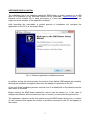
EMF – 18G
Electric Field Probe
USER MANUAL
CONTENTS
SAFETY INFORMATION
1 INTRODUCTION
2 EMF-18G SENSOR STRUCTURE AND ORIENTATION
2 CONTROL PANEL
3 FIBER OPTICAL CABLE
3 OPTICAL-USB ADAPTER
3 BATTERY RECHARGE
4 MINIMUN SYSTEM REQUIREMENTS
4 CONNECTION BETWEEN THE PC AND THE SENSORS
4 SOFTWARE INSTALLATION
5 SOFTWARE USER INTERFACE
6 SENSOR SETTINGS
7 GRAPHICAL VISUALIZATION OF THE DATA
8 DATA AND IMAGE EXPORTATION
12 COMMUNICATION PROTOCOL
13 FIRMWARE UPDATE
14 PART LIST
14 TECHNICAL SPECIFICATIONS
15 SAFETY INFORMATION
Please read carefully the contents of this manual before using the product. In particular
follow the safety recommendations, the instructions about operating procedures and
handling of the product.
Do not install or substitute parts or perform unauthorized modifications to the instrument.
Do not try to open or disassemble. Return the instrument to Microrad for maintenance and
repair services.
This product is equipped whit a lithium ion rechargeable battery. Do not open or
disassemble it, or use it in a humid or corrosive environment. Do not put, store or leave
your product near sources of heat, in direct strong sunlight, in a high temperature place or
in pressurized container. Use exclusively the provided battery charger.
1
INTRODUCTION
EMF-18G is an electric field isotropic sensor based on a new generation of diode dipoles.
Bandwidth, sensitivity and sampling speed specifications make this sensor unique in its
kind.
EMF-18G has been designed keeping in mind the measure of the electric field inside TEM
cells, GTEM cells, anechoic chambers; nevertheless it is very suitable for monitoring
applications where electric field levels are critical or to preserve the human safety.
The sensor is self-powered by a professional lithium ion battery, that allows an autonomy
up to 45 hours (depending on sampling speed setting). A complete battery charge takes
about 2 hours and only 15 minutes of recharge are needed to make the sensor up to 3
hours operative. Furthermore this kind of battery does not suffer of memory effect and
shows an excellent discharge curve.
The software application EMCViewer had been developed in order to interact with the
EMF-18G sensor and to represent measured data coming from it. The communication link
is based on a fiber optic cable and an Optical-USB adapter to avoid interference issues.
The number of EMF-18G sensors that can be simultaneously connected to the PC where
the software application EMCViewer is running is virtually unlimited (at the moment it is
possible to connect up to 8 sensors).
EMF-18G sensor offers flexibility of use, size, cost and safety features much better than
laser powered systems.
EMF-18G SENSOR STRUCTURE AND ORIENTATION
The wrapping of the EMF-18G sensor is made of thermoplastic resin characterized by low
dielectric constant and low dissipation factor.
The dipoles are built using a thick film with distributed electric constants; they are mutually
oriented at 54.7° in the space; on this way, the spatial distribution forms an equilateral
triangle, with resistive paths from the dipoles to the amplifier input of the same size and
orientation.
These specifications are the main elements underlying the extraordinary bandwidth of the
EMF-18G sensor.
2
CONTROL PANEL
The control panel is located at the bottom of the cylindrical stem of the sensor and it hosts
the optical connector (FIBER), the battery recharging connector and charge in progress
led (CHARG), the battery low led indicator (B.LOW) and the power switch (PW) that
features an integrated blue led.
Fig. 1: Bottom view: EMF-18G control panel
FIBER OPTICAL CABLE
A fiber optic link ensures noise and interference immunity during the measure operations.
The supplied fiber optic cable has a length of 10 meters and is equipped on both side with
identical male connectors; one side shall be inserted into the EMF-18G fiber connector,
the other side into the Optical-USB adapter.
Optionally longer cables are available, in order to make connection links up to 40 meters.
Do not exceed a 10 cm bend radius when handling the fiber optic cable. Tight corners may
affect the integrity of the cable and the resulting damage could be even irreversible.
Take particular care when handling the fiber optic cable and absolutely avoid to disconnect
the plug by pulling directly the fiber cable: the disconnection must be performed only by
warily pulling on the knurled part of the connector, using the fingers.
OPTICAL-USB ADAPTER
The Optical-USB adapter is the interface between the fiber optic cable and a standard USB cable that finally
connects to the PC/Tablet. The adapter is USB powered.
It is recommended to always apply the provided silicone plugs to the fiber optic connectors
of the EMF-18G sensor and of the Optical-USB adapter after use.
This ensures an effective protection from dust and other elements that may reduce or
impair the efficiency of the optical link.
3
BATTERY RECHARGE
The EMF-18G sensor alerts the user about a battery low condition: when the charge level
drops below 5%, the red led B.LOW starts flashing. In this condition, it is preferable to stop
the measure as soon as possible to avoid the sudden disruption of communication.
To resume the charge, it is sufficient to plug the provided battery charger to the CHARG.
connector. The green led starts flashing until the charge reaches the 100%, then it goes
off.
The total charging time, starting from a 10% residue, is about 2 hours; however it is
possible to achieve a 10% level of charge increment in less than 20 minutes.
When fully charged, the battery autonomy is about 45 hours, considering the EMF-18G
sensor set to operate at 1 Hz sample rate.
Note: during the recharge time the EMF-18G sensor get a not operative state.
MINIMUN SYSTEM REQUIREMENTS
The following minimum specifications are required for the PC/Tablet in order to proper
work with the EMF 6E sensor and the EMCViewer software:
•
•
•
•
Processor: 1GHz dual core 32 or 64 bit architecture.
RAM: 2 GB.
USB: availability of one free port for each sensor to interface.
OS: Microsoft Windows XP, Vista, 7, 8; 32 or 64 bit.
CONNECTION BETWEEN THE PC AND THE SENSORS
The sensor is connected to the PC through an interconnection kit that consists of:
•
•
•
Fiber optic cable.
Optic-USB adapter.
USB cable.
When working with multiple EMF-18G sensors (up to 8 sensors) each one shall be
connected to a different USB port of the PC, through its own cable kit.
Moreover each sensor shall be then turned on (PW button) so that it can be properly
detected by the software application EMCViewer.
Note: the power-on status of the sensor is indicated by the blinking blue led inside the
power button.
4
SOFTWARE INSTALLATION
The installation file of the software application EMCViewer is usually supplied on a USB
drive or is available on the Microrad internet site for download ( www.microrad.it ); the
filename of the installer file is setup_emcviewer_X_Y.exe (where X and Y identify the
major and minor number of the application release).
After launching the executable, a guided process of installation will configure the
application on the PC in a few simple steps.
Fig. 2: Software application installation process
In addition, during the setup process, the drivers of the Optical-USB adapter are installed,
allowing the automatic recognition whenever the adapter is connected to the PC.
At the end of the installation process a launch icon is created both on the desktop and the
start menu of Windows.
Before starting the EMCViewer application ensure that the sensor (or, in the case of
multiple connections, all the sensors you want to monitor) is connected and powered on.
The application software can be then started using the EMCViewer launch icon; a number
of user interfaces that equals the number of sensors connected to the PC will appear on
the screen.
5
SOFTWARE USER INTERFACE
After the launch of the EMCViewer application, each user interface that is shown on the
screen is associated with an EMF 6E sensor that is connected to the PC and powered on.
On the top bar of each user interface window is visible the name and version of the
software application, followed by the Serial Number of the sensor associated with the
interface.
Fig. 3: User interface start-up phase
Furthermore during the start-up phase of each user interface, for few seconds, the
following information about the connected sensor are shown:
•
•
•
•
Serial Number (S/N).
Date of production (Prd).
Date of calibration (Cal).
Firmware version (FW).
After that the interface enters the operating mode and the data presented on the screen
are finally related to the measured value acquired by the sensor.
Fig. 4: Data display in operative mode
6
The available data are:
•
•
•
•
•
•
Unit of measure of the electric field (V/m, A/m, W/m2 or mW/cm2, selectable in
sequence by a left click of the mouse over the unit of measure text).
Battery level indicator, both graphical and as percentage value.
Isometric value of measured field (the biggest font on the screen).
Maximum value of the measured field (it is possible to clear this value by a left click
of the mouse over it).
Temperature (°C).
Measured field components on the single axes X, Y, Z.
SENSOR SETTINGS
On the right side of the user interface there are 3 controls allowing to set the parameters
that affect the acquisition behaviours of the EMF -18G sensor:
•
The Sampling Speed control sets the sampling rate of the acquisition; it is possible
to select one of the following values, reported in the same order of the combo box:
1 Hz, 2 Hz, 4 Hz, 8 Hz, 25 Hz, 50 Hz, 1/2 Hz, 1/4 Hz, 1/10 Hz, 1/20 Hz, 1/30 Hz
Increasing the sampling speed improves the time resolution, but raises the noise
level affecting the measure. Running at 25 or 50 Hz, the noise level is greater, and
in some conditions, dealing with low field levels (<5 V/m), the measure could be
inaccurate; however such situation is highlighted by the EMCViewer user interface
by changing the background from blue to red.
•
The Smoothing Filter control allows to manage the behaviour of the smoothing
filter; the purpose of this digital filter is the "flattening" of the fluctuations of the
measured signal; it is possible to select the bandwidth of the filter among predefined
values; the smaller the selected bandwidth, the greater the effect of the "softening".
Depending on the selected sampling speed, the number of possible choices of the
bandwidth is variable, with a maximum of four selectable bandwidths when 50 or 25
Hz sampling speed is selected. In case of sampling speed equal to or less than 1
Hz, the filter is forced into the OFF mode.
•
The Frequency Adj control enables the correction of the measured values. As a
matter of fact each EMF-18G sensor stores inside its non volatile memory a look up
table needed for the correction of the measured value when the frequency of the
signal under observation is known. The correction frequency range starts from a
minimum of 0.01 MHz (10 KHz) up to 18,000 MHz (18 GHz), with steps of 0.001
MHz (1 KHz). If the check box is enabled, the fix for the selected frequency is
applied, and the selected frequency value becomes red indicating that it is no more
editable.
7
GRAPHICAL VISUALIZATION OF THE DATA
The Show/Hide Graph button located at the bottom of the user interface opens/closes the
window that shows the real-time plot of data coming from the sensor.
More specifically it is possible to view the time evolution of the isotropic values of
measured field, its X, Y, Z components, and the temperature.
Electric field data are displayed according to the field unit (V/m, A/m, W/m2, mW/cm2) that
was selected in the user interface, while temperature unit is °C.
The Play / Stop button performs the graphical data capture start and stop, manually; a
blue vertical line inside the plot delimitates the various sessions of acquisition.
Altogether it is possible to keep in memory and to display up to 180,000 samples; for
example it is possible to get 1 hour of data plot running at 50Hz sampling speed, 2 hours
at 25 Hz, 50 hours at 1 Hz and so on.
After that, the older samples are discarded to host the newer ones according to a FIFO
logic (First In First Out).
Fig. 5: Data graphical visualization
In addition the acquisition can be also controlled by a trigger logic; by activating the Trg
checkbox, a dedicated panel asks to insert two thresholds: the first threshold is used to
8
automatically start the acquisition whenever the measured isotropic field exceeded it; the
second one vice versa stops the acquisition each time the measured isotropic field falls
below it. The unit of the thresholds are the same ones selected by the user interface for
the electric field.
Fig. 6: Acquisition trigger settings
Finally, the Clear button deletes all data present in memory and clean up the plot.
By enabling the appropriate check-box in the Tracks control, it is possible to activate or
deactivate the visualization of each individual track (ISO, X, Y, Z, T).
Fig. 7: ISO, X, Y, Z, and temperature plot
Under the horizontal axis, the time is reported using the hours:minutes:seconds format.
9
The date is shown in the upper right corner of the grid using the day/month/year format.
The + and - zoom buttons within the control Tools allow to expand or reduce the
horizontal dimension of time displayed on the graph.
The Y Scale control toggles between linear and logarithmic scale for field values (while
temperature is always displayed in linear scale); selecting the logarithmic scale, the 0 dB is
dynamically assigned to the maximum isometric value Eisomax (V/m) present in the plot;
after that each point of value E (V/m) gets a corresponding value in decibels E (dB)
according to the relation:
E (dB) = 20 Log10
E (V/m)_ _
Eisomax (V/m)
Thus all values shown, expressed in decibels units, are negative (<0dB); the lower values
are clamped to -100 dB.
Note that in general, moving the mouse pointer over the chart, a tooltip appears showing
the detailed field (or temperature) values relative to the point selected by the mouse
pointer.
Fig. 8: ISO plot using the logarithmic scale
10
Fig. 9: Tooltip data on the mouse pointer
The Marker check boxes perform the highlight on the graph of the maximum and the
minimum values for each enabled track.
Fig. 10: Maximum marker for the isometric field
11
DATA AND IMAGE EXPORTATION
The Exp button in the Tools control allows to export an image of the currently displayed
plot, or to export row data.
Fig. 11: Exportation menu
Considering the image exportation, a dialog box lets to choose the format of the exported
image, Bitmap (BMP) or JPEG (JPG); furthermore it is possible to select whether to export
the plot using original colours (black background) or inverted colours (white background).
Fig. 12: Image export settings
Row data are exported using an Excel compatible format (.xls file).
Both for image or data exportation, the application asks the selection of the folder and the
file name where exported data will be saved.
12
COMMUNICATION PROTOCOL
Users can access EMF-18 data by means of custom software.
First is required to install on the PC the Virtual COM Port (VCP) driver from FTDIChip; this
driver allows to access the USB port as a standard serial UART port.
Port settings must be: 8 bit data, no parity, 1 stop bit (8n1); speed 921600 bps.
Data are continuously sent from the EMF-18G according to the sampling settings (for
instance if the sensor is set to work at 50Hz, EMF-18G sends 50 packets per second).
Each data packet is composed of 22 bytes and is organized according to the following
format:
Byte
Valore
0
55h
1
99h
2
Ex 0
3
Ex 1
4
Ex 2
5
Ex 3
6
Ey 0
7
Ey 1
8
Ey 2
9
Ey 3
10
Ez 0
11
Ez 1
12
Ez 2
13
Ez 3
14
Temperature 0
15
Temperature 1
16
Temperature 2
17
Temperature 3
18
Battery Level
19
Reserved
20
CheckSum Low
21 CheckSum High
Tab. 1: Data packet format
Field and temperature data values are 32 bits (4 bytes indexed 0,1,2,3) single precision
IEEE754 (IEC 60559). Byte with index 0 is the less significative.
The battery level is only one byte representing the charge percentage (0 to 100%).
The 16 bits checksum is the sum of all preceding packet bytes. (from byte 0 to 19).
13
Note that communication is mono-directional, from the EMF-18G sensor to the PC; for this
reason the acquisition settings are only modifiable using the EMCViewer software.
EMF-18G stores the settings on a non volatile memory and then keeps them also after
power off.
FIRMWARE UPDATE
The following procedure details how to make a firmware update of the sensor:
•
Connect the target sensor to the PC, without turning it on; note that for firmware
update purposes, a multiple sensors connection is forbidden.
•
Start the application EMCViewer FwUpdate from the Windows Start menu.
•
Select and open the file containing the new firmware (.rom extension).
•
A dialog box showing the text "Press OK to update" appears on the screen; do not
press Ok for now.
•
Turn on the sensor through the PW button and press the OK button within 4
seconds.
If the whole process was successful, the firmware of the sensor is updated in a few
seconds and a message notifies about the end of the update and the reboot of the sensor;
otherwise repeat from the first step.
PART LIST
The sensor is supplied with the following parts:
•
•
•
•
•
•
User manual in electronic format.
Calibration certificate ISO 9001: 2008 IEEE std. 1309: 2005.
10 m fiber optic cable.
USB-Optical adapter.
USB cable.
IP65 plastic case.
14
TECHNICAL SPECIFICATIONS
Sensor Type
Measured Data
Sensor Bandwidth
Amplitude Response
Dynamic range
Linearity @ 100 MHz
Isotropy @ 1,8 GHz
Temperature Stability
Maximum sampling rate
Operating Temperature
Operating Humidity
Weight
Size
Isotropic Triaxial
X,Y,Z and ISO
10 KHz ÷ 18 GHz
100 KHz ÷ 1 GHz: +/- 1 dB
1÷ 18 GHz: +/- 3 dB
0,5 ÷ 500 V/m (60 dB)
2 ÷ 300 V/m 0,5 dB
0,4 dB
0,5 dB
50 Hz (Tsample= 20 ms)
+10 ÷ +40 °C
5% ÷ 90% not condensated
< 100g
Length: 135 mm,
Diameter: Max 60 mm Min 30 mm
Tab. 2: Technical Specifications
15