Download The Oscilloscope: Operation and Applications

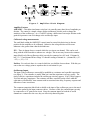
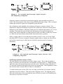
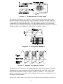
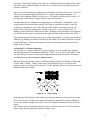
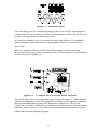
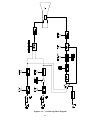
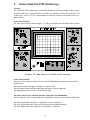
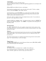
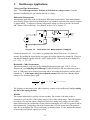
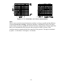
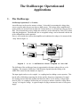
The Oscilloscope: Operation and
Applications
1.
The Oscilloscope
Oscilloscope Operation (X vs Y mode)
An oscilloscope can be used to measure voltage. It does this by measuring the voltage drop
across a resistor and in the process draws a small current. The voltage drop is amplified and
used to deflect an electron beam in either the X (horizontal) or Y (vertical) axis using an electric
field. The electron beam creates a bright dot on the face of the Cathode Ray Tube (CRT) where
it hits the phosphorous. The deflection, due to an applied voltage, can be measured with the aid
of the calibrated lines on the graticule.
First we will consider the circuitry that amplifies and conditions the voltage to be measured (the
“Amp” block in figure 1).
Figure 1. X vs. Y Deflection Block Diagram of the CRT
The deflection of the oscilloscope beam is proportional to the input voltage (after ac or dc
coupling). The amount of deflection (Volts/Division) depends upon the setting of the
AMPL/DIV control for that channel (see figure 2).
The input signal can be ac or dc coupled. Ac coupling involves adding a series capacitor. This
has the effect of blocking (removing) the dc bias and low frequency components of a signal.
Dc coupling does not have this problem and therefore allows you to measure voltages right
down to 0 Hz. Ac coupling is useful when you are trying to measure a small ac voltage that is
“on-top” of a large dc voltage. A typical example is trying to measure the noise of a dc power
supply.
-1-
Figure 2. Amplifier Block Diagram
Amplifier Features
AMPL/DIV - This abbreviated name varies but it is generally some short form of amplitude per
division. The control is a simple voltage divider (attenuator) which is used to change the
sensitivity of the oscilloscope. At a 1 volt/DIV setting, a deflection of one major division on the
graticule represents a one volt change at the oscilloscope input.
Calibrated voltage measurements
The small knob within the AMPL/DIV control must be rotated clockwise into its detente
position for the amplifiers to be calibrated. Otherwise the voltage/division will be some
unknown value greater than what the dial indicates.
INV - There is almost always a control which lets you invert one channel. This can be used
along with the ADD function to subtract two voltages. This is necessary because the common
input (black lead of the oscilloscope cable) can only be connected to a 0V node. If channel A
has V1 + V2 and channel B has voltage V1 then the reading of channel A + (-channel B) = (V1
+ V2) + (-V1) = V2
Position - For each axis there is a control which lets you shift the electron beam. With this you
can set the zero voltage point to anywhere that is convenient for you.
Oscilloscope Inputs
The input of the oscilloscope can usually be modelled as a resistance and a parallel capacitance
(see figure 3). The resistance is usually 1M6 but it and the capacitance can vary greatly. The
total or effective capacitance includes the oscilloscope circuitry (approx. 30 pF), cables (approx.
30 pF/m) and stray capacitance. The resistance will draw current from the circuit while the
capacitance will add an RC time constant with its associated time delay, frequency response and
distortion of some waveforms.
The common connection (black lead or shield) at the input of the oscilloscope goes to the metal
case as the symbol by the input connector shows. Because of this, the common input can only
be connected to a 0V point in the circuit. Since the common inputs for both the A and B
channels are connected to the case, they are effectively shorted together.
-2-
Figure 3. DC-coupled Oscilloscope Input Circuit
and Frequency Response
Frequency response is calculated or measured by applying a pure sinusoidal waveform to a
circuit. The circuit response is the output voltage divided by the input voltage. This is a complex
number that can also be expressed as a magnitude (gain) and phase.
Due to limitations in the amplifiers, the oscilloscope's frequency response is limited. The
manufacturer simply lists the half-power point for the oscilloscope without any external effects.
Half power is also called the -3dB point. At this point, the voltage has decreased to 70.7% of its
maximum. This means that only one-half of the maximum power would be dissipated in a
resistive load. Keep in mind that an oscilloscope that is rated at 20 MHz is usually only accurate
to 4 MHz for non-sinusoidal waveforms before distortion becomes a problem.
With ac coupling (figure 4), an oscilloscope has another series RC circuit. It acts like a high
pass filter (HPF). If you are viewing low frequency signals when ac coupled, not only will you
not be able to measure any dc offset, but you will also be removing some low frequency
information.
Figure 4. AC-coupled Oscilloscope Input Circuit and
Frequency Response
Oscilloscope Operation (Voltage vs Time)
The main function of an oscilloscope is to show voltage vs time. This is done by applying a
ramp (or sawtooth) waveform into the X-axis amplifier as shown in figure 5. During the rising
edge of the ramp, the electron beam scans across the screen. When the voltage drops back to
0V, the beam is turned off and quickly goes back to its starting point. This is signified by a thick
line when the beam is on and a thin one when it is off (blanked).
To obtain a stable picture on the CRT screen, the ramp waveform has to be in phase with the
signal that you want to observe. This is done with a triggering circuit. The triggering circuit
allows the oscilloscope to draw repeatedly the same waveform over and over by identifying the
same point on a repetitive waveform.
-3-
Figure 5. A Ramp-driven X-axis input
The triggering circuit allows you to select a voltage (an analog value) and an edge or slope
(positive or negative) for the triggering circuit to compare to the input waveform. When the
two are equal, the circuit puts out a pulse. This pulse triggers the ramp waveform generator to
do one cycle of its rising and falling edges. Once the ramp has started a cycle of increasing
voltage, it can not be retriggered until it has completed the full ramp and returned to 0V. This is
illustrated in figure 6 for a single cycle and in figure 7 for multiple cycles.
Figure 6. A Triggering Example
Figure 7. Several Triggering Cycles
Not only do you have control over the starting point of the ramp, but the amount of time that
the ramp takes to reach its maximum voltage (the right hand side of the CRT screen) can be
adjusted with the timebase control. In essence, you have a “window”. You can move the
window to any point on a waveform with the triggering circuit and you can change the size of
the window with the timebase.
The time-base control allows you to set the time / division that the beams takes to scan across
-4-
the screen. Just like the voltage selector, there is a calibration knob in the middle of the control.
Unless the vernier (calibration knob) is 'clicked' in to its most clockwise position, the time per
division is unknown.
When set to AUTO (automatic) triggering, the oscilloscope will always show a trace. However,
when you use a manual triggering mode (DC, AC), many strange things can happen. For
example, if the triggering voltage or level is set to +10V and the waveform never exceeds +5V,
the triggering circuit will never trigger and the screen will stay blank.
You may think that in a condition of no triggering, you would still have a bright dot on the
screen because the electron beam would go to its 'home' or undeflected position. Since the
oscilloscope is designed to work with a moving electron beam, a stationary beam can very
quickly 'burn' a hole in the phosphorous coating of the screen. To prevent this, there is a '
blanking' circuit which turns off the electron beam. Blanking occurs when there is no triggering
or when the electron beam is sweeping from the right edge back to the left side of the screen.
Time measurements are done the same way as voltage measurements. As long as the timebase is
calibrated you multiply the number of divisions by the number of seconds per division to get the
total time difference. Phase measurements are done by comparing the measured time to the
period of the waveform.
Oscilloscope Two Channel Operation
You can view two voltage waveforms at once by using two Y-axis (vertical) input channels.
The individual channels are sometimes labelled as '1' and '2' or as 'A' and 'B'. Since there is only
one electron beam, you have to share its drawing time between both waveforms. This may be
accomplished using either the chop or alternate modes.
When in the chop mode (figure 8), the oscilloscope displays a little bit of channel A, then a little
bit of B, then A, then B ....during a single sweep of the electron beam. If you increase the
timebase to about 1µs/division, you can start to see the individual pieces as it chops between one
channel and the other channel.
Figure 8. Chop Mode
In the alternate mode (figure 9), the oscilloscope will sweep the electron beam twice across the
screen. The first time it will draw the signal from channel A and the next time from channel B.
At very low timebase settings, you can see it draw one channel and then the other in successive
passes.
Note: When you use the alternate function, the two waveforms that you see are from different
points in time and the triggering circuit has to trigger twice.
-5-
Figure 9. Alternate Mode
The reason that you can see a non-flickering image on the screen is because the phosphorous
coating on the CRT has persistence. In essence, the phosphorous acts like a low pass filter and
averages several images that are drawn on the screen.
By viewing two signals at a time, you can measure relative time differences. By combining a
voltage and phase measurement (relative to the appropriate reference), you can measure a
phasor value.
With a two channel oscilloscope, you have the ability to trigger on each waveform and
electronically switch (chop or alt) between them as well. A block diagram of a oscilloscope has
now become as shown in figure 10.
Figure 10. A Simple Oscilloscope Block Diagram
Some oscilloscopes offer a way to alternately trigger as depicted in figure 11. When combined
with alternate displaying, you can stably display two waveforms of any frequency by alternately
showing each channel and triggering on the channel that is being drawn. This way, the
oscilloscope is acting like a two beam scope with both waveforms triggering at the same voltage
and slope. However, there is no way to know what the relationship is between one waveform
and the other when using alternate triggering.
-6-
Figure 11. Stable Triggering of Two Different Frequencies
If you have two waveforms that do not have the same frequency, it is still possible to show them
as two stable waveforms on a normal oscilloscope. In figure 11, you will notice that if the
triggering occurs at the 'X', both waveforms are in phase (ie. at the same phase each time the
timebase triggers). The condition for a stable display is not that two waveforms have to be of
exactly the same frequency, but that when they are triggered, they have to be in phase.
Or n·f1 = m·f2 where n, m are integers. That is not necessary, but it is sufficient. There are
many other ways to achieve a stable trace when you consider that the trigger circuit will wait for
the next triggering point. There is also a control on some oscilloscopes, called 'hold off', which
allows you to add a delay between the end of the trace being drawn and the time when the
triggering circuit starts to look for the next triggering point. That can be used to stabilize the
display under some circumstances.
Remember that all of this applies only for repetitive waveforms that are properly triggered. If
the triggering is not stable, or the waveform is not repetitive, you will see a constantly moving
image or several images offset and superimposed.
A slightly more complicated block diagram of an oscilloscope, with the typical functions found
in the laboratory, is illustrated in figure 12.
Accuracy
There are many factors affecting the accuracy of oscilloscope measurements.
There are errors due to the input channel voltage divider, timebase control, the use of
magnifiers, the accuracy to which the CRT deflection can be read, beam thickness, temperature
etc. The voltage divider error will be the same for all readings that are done on the same
timebase and voltage range, but may be different each time the range is changed. Measurements
over only two divisions can incur two to three times the error of those made over the centre
eight divisions.
If the phase angle is used in a trigonometric function, this error can be multiplied by the slope of
the function. Consider that the tangent of a 1% phase error entered at 85 degrees is much worse
(20%) than the same 1% error on a sine function (0.2%) at the same angle. To get a feel for this
look at the Taylor expansion of the trigonometric functions.
It is wise to consult the user manual for a particular instrument’s accuracy specifications.
-7-
Figure 12. Oscilloscope Block Diagram
-8-
2.
Iwatsu Model SS-5702 Oscilloscope
Accuracy
The Iwatsu SS-5702 oscilloscope is used in this laboratory. All measurements on the graticule
should be made over as many divisions as possible. For simplicity, assume the Iwatsu SS-5702
oscilloscope’s error is ±5% for a measurement on either the vertical or horizontal scales over
eight divisions.
Front Panel Controls
The front panel controls, shown in figure 13, will be described in the remainder of this section.
Figure 13. The Iwastu SS-5702 Oscilloscope
Front Panel Controls
The power, trace rotation, intensity, focus, and scale illumination controls are located at the
bottom centre.
The vertical controls and input selection are on the left side.
The horizontal controls and horizontal input selection are on the right side.
The triggering selection section is at the bottom right.
The power on/off, trace rotation, intensity, focus and scale illumination
Trace rotation has to be checked with just a straight line across the screen of the oscilloscope.
The intensity should be adjusted to a mid point (or more clockwise).
The focus of the beam can be done while observing the straight line display.
The scale illumination can be adjusted to the operator’s preference.
-9-
Vertical Inputs
Vertical channels are used for measuring voltage.
The beam is deflected vertically as a result of the signal being applied to the vertical input of the
channel (CH).
CH-1 and CH-2 are the labels for the two vertical inputs.
Each channel has a position control, a range selection switch, a pull “x5” knob, a coupling
selector switch (AC/GND/DC), and an input connector.
Each channel Range switch (VOLTS/DIV) has a smaller knob in the middle of the Range
Selector Switch. And there is an arrow showing that the Range Selector Switch is in the
“CAL” position when rotated fully clockwise.
In the centre of the two channel sections is the channel selection switch. You can choose to
have CH-1, CH-2, both (DUAL), or ADD.
In addition, CH-2 has a “Polarity” switch. You push the polarity switch in to “INVERT” the
polarity of the signal being displayed. The “NORM” or out position is the normal position of
the polarity switch.
Horizontal Inputs
The “EXT” (HORIZONTAL IN) can be supplied a voltage directly via the connector at the
bottom right of the panel, or the Horizontal can be driven by an internal timebase circuit which
generates the voltage.
Timebase
In the timebase mode, the horizontal signal is from an internal source which changes linearly
with respect to time. Hence, the beam is deflected to give us a calibration of time for the
horizontal scale.
The position control, the pull “x5” magnifier switch, the time range selection switch, and the
range “CAL” knob all affect the X-axis of the display.
Trigger Sources
The TRIGGER SOURCE may be selected from one of three sources, CH-1, CH-2, or EXT.
Look at the bottom right of the control panel.
Calibration Source
The Calibration Source is an internal source, available on the oscilloscope.
Look at the bottom right side of the front panel. The output is labelled 0.3 V.
This is a 1000 Hz, square-wave ( the 50 % duty cycle is not accurate ).
-10-
3.
Oscilloscope Applications
Voltage and Time Measurements
Note: The oscilloscope measures divisions of deflection not voltage or time. From the
divisions of deflection you can calculate the time or voltage.
Differential Measurements
An important application of the oscilloscope is differential measurements. Such measurements
are necessary because both vertical channels have one terminal connected to the chassis common
(ie single ended). To measure a floating (off ground) voltage you have to use the “invert and
add” feature of the oscilloscope. For example, in figure 14, to measure V1:
Figure 14. Differential Measurement Example
Channel A measures (V1 + V2) relative to ground while channel B measures V2 relative to
ground. By pushing the invert button you negate the voltage displayed on channel B. Then you
can add the channels together with the “ADD” display mode. The waveform now displayed is
(V1 + V2) + (- V2) = V1.
Bandwidth (-3 dB) Measurement
This measurement is easily done by first finding the maximum gain (max. VOUT / VIN at
frequency 7o) and adjusting the oscilloscope so that the sinewave fills seven divisions peak to
peak. A -3dB point can be found by increasing and/or decreasing the frequency until the gain is
reduced to 2 . If the input voltage has remained constant this will occur when the output
voltage is five divisions peak to peak.
Vout
Voutmax
1 0.707 5 divisions
2
7
The frequency is then simply read with a frequency counter or the oscilloscope. Not by reading
the dial of the signal generator.
Risetime
The risetime indicates how quickly a circuit responds. The risetime is the time it takes a
waveform to go from 10% of the voltage range to 90% of the voltage range. This is in response
to a square wave and the output voltage must settle to a steady-state voltage (0% and 100%).
Most oscilloscopes have dotted lines on the graticule marking the 10% and 90% points to aid in
this measurement. Usually these dotted lines assume that 0% is the lowest line of the graticule
and 100% is the highest line. The measurement, as shown in figure 15, also includes the risetime
of the oscilloscope and the squarewave source.
-11-
Figure.15 A Risetime and Phase Measurement
Phase
Phase is most accurately measured when the waveform is as large as possible and the difference
is measured at the zero crossings. Typically the timebase is uncalibrated so that a 180 degree
section of the waveform is expanded to the full 10 divisions of the graticule. Then the sign of the
phase can be determined by observing more than one period of both waveforms. Both
waveforms must be symmetrical about the centre line of the graticule. The angle is determined
by: phase = # of divisions * 180 degrees / 10 divisions.
-12-