1
ORTEC
®
Alpha Particle Spectrum Acquisition and Analysis
forMicrosoft® Windows® 2000, XP® Professional,
Vista® Ultimate, and Windows 7
A36-B32
Software Version 5.6
Installation, User Interface, and Reference Guide
Printed in U.S.A.
ORTEC® Part No. 795960
Manual Revision G
0211
Advanced Measurement Technology, Inc.
a/k/a/ ORTEC®, a subsidiary of AMETEK®, Inc.
WARRANTY
ORTEC* DISCLAIMS ALL WARRANTIES OF ANY KIND, EITHER EXPRESSED OR
IMPLIED, INCLUDING, BUT NOT LIMITED TO, THE IMPLIED WARRANTIES OF
MERCHANTABILITY AND FITNESS FOR A PARTICULAR PURPOSE, NOT
EXPRESSLY SET FORTH HEREIN. IN NO EVENT WILL ORTEC BE LIABLE FOR
INDIRECT, INCIDENTAL, SPECIAL, OR CONSEQUENTIAL DAMAGES,
INCLUDING LOST PROFITS OR LOST SAVINGS, EVEN IF ORTEC HAS BEEN
ADVISED OF THE POSSIBILITY OF SUCH DAMAGES RESULTING FROM THE
USE OF THESE DATA.
Copyright © 2011, Advanced Measurement Technology, Inc. All rights reserved.
*ORTEC® is a registered trademark of Advanced Measurement Technology, Inc. All other trademarks used herein are the
property of their respective owners.
TABLE OF CONTENTS
1. INTRODUCTION . . . . . . . . . . . . . . . . . . . . . . . . . . . . . . . . . . . . . . . . . . . . . . . . . . . . . . . . . . 1
1.1. About this Manual . . . . . . . . . . . . . . . . . . . . . . . . . . . . . . . . . . . . . . . . . . . . . . . . . . . . . . 1
1.2. AlphaVision 5.x Features . . . . . . . . . . . . . . . . . . . . . . . . . . . . . . . . . . . . . . . . . . . . . . . . 2
1.2.1. Comparison to AlphaVision 4 . . . . . . . . . . . . . . . . . . . . . . . . . . . . . . . . . . . . . . . 3
1.3. What’s New in AlphaVision v5.6 . . . . . . . . . . . . . . . . . . . . . . . . . . . . . . . . . . . . . . . . . . 4
1.4. Features Introduced in v5.5 . . . . . . . . . . . . . . . . . . . . . . . . . . . . . . . . . . . . . . . . . . . . . . . 4
1.4.1. New Analytical Methods and Tools . . . . . . . . . . . . . . . . . . . . . . . . . . . . . . . . . . . 5
1.4.1.1. New Peak Search for Low-Count, Asymmetric Peaks . . . . . . . . . . . . . 5
1.4.1.2. Manual Chemical Recovery . . . . . . . . . . . . . . . . . . . . . . . . . . . . . . . . . 5
1.4.2. Improved Organization of Background and QA Pulser Batches . . . . . . . . . . . . . 5
1.4.2.1. View Batch Explorer Entries in Ascending or Descending Order . . . . 6
1.4.3. Quick Search for a Specific Batch or Sample . . . . . . . . . . . . . . . . . . . . . . . . . . . 6
1.4.4. Easier Batch Setup . . . . . . . . . . . . . . . . . . . . . . . . . . . . . . . . . . . . . . . . . . . . . . . . 7
1.4.4.1. Auto-Define Samples in the Analysis Wizards . . . . . . . . . . . . . . . . . . . 7
1.4.4.2. Create Sample-Less Batch Templates . . . . . . . . . . . . . . . . . . . . . . . . . . 8
1.4.4.3. Differentiate Blanks by QA Type . . . . . . . . . . . . . . . . . . . . . . . . . . . . . 9
1.4.5. New Activity Units and Volume Units . . . . . . . . . . . . . . . . . . . . . . . . . . . . . . . . 9
1.4.6. Changes to Reporting . . . . . . . . . . . . . . . . . . . . . . . . . . . . . . . . . . . . . . . . . . . . . 10
1.4.6.1. Report Reanalysis Results with Your Custom Report Templates . . . 10
1.4.6.2. Peak FWHM Added to the Calibration Reports . . . . . . . . . . . . . . . . . 11
1.4.7. Export Spectra from the Batch Explorer to ORTEC .SPC Spectrum Files . . . . 11
1.4.8. Easier QA Limits Setup . . . . . . . . . . . . . . . . . . . . . . . . . . . . . . . . . . . . . . . . . . . 11
1.4.9. Enhanced Security . . . . . . . . . . . . . . . . . . . . . . . . . . . . . . . . . . . . . . . . . . . . . . . 12
1.4.10. New Database Management Tool for QA Results . . . . . . . . . . . . . . . . . . . . . . 13
1.4.11. MAESTRO®-32 No Longer a Required Component . . . . . . . . . . . . . . . . . . . . 13
1.5. Features Introduced in AlphaVision v5.3 . . . . . . . . . . . . . . . . . . . . . . . . . . . . . . . . . . . 14
1.5.1. ROIs Expressed in Channels or Energy . . . . . . . . . . . . . . . . . . . . . . . . . . . . . . . 14
1.5.2. Select Database and Database Management . . . . . . . . . . . . . . . . . . . . . . . . . . . 15
1.5.3. Sample Dilution Setup in the Batch Wizard . . . . . . . . . . . . . . . . . . . . . . . . . . . 15
1.5.4. New Scaling and Cursor Movement Features . . . . . . . . . . . . . . . . . . . . . . . . . . 16
1.5.5. Interactive ROI Analysis in Batch, Background, and Calibration Modes . . . . 17
1.5.5.1. Batch Mode . . . . . . . . . . . . . . . . . . . . . . . . . . . . . . . . . . . . . . . . . . . . . 17
1.5.5.2. Calibration Mode . . . . . . . . . . . . . . . . . . . . . . . . . . . . . . . . . . . . . . . . . 21
1.5.6. The Report: What You See Is What You Get . . . . . . . . . . . . . . . . . . . . . . . . . . 21
1.5.7. Changes to the Detector Assignment Worksheet . . . . . . . . . . . . . . . . . . . . . . . . 22
1.5.8. Subtracting Net Blank Activity . . . . . . . . . . . . . . . . . . . . . . . . . . . . . . . . . . . . . 23
1.5.9. QA Control Charts: Adjustable Y-Axis Scaling . . . . . . . . . . . . . . . . . . . . . . . . 24
2. INSTALLATION AND CONFIGURATION . . . . . . . . . . . . . . . . . . . . . . . . . . . . . . . . . . . . 25
2.1. Installation Notes . . . . . . . . . . . . . . . . . . . . . . . . . . . . . . . . . . . . . . . . . . . . . . . . . . . . . . 25
iii
AlphaVision®-32 v5.6 (A36-B32)
2.2. Step 1: Installing AlphaVision v5.6 . . . . . . . . . . . . . . . . . . . . . . . . . . . . . . . . . . . . . . .
2.2.1. Configuring and Customizing the Master MCB List . . . . . . . . . . . . . . . . . . . . .
2.3. Step 2: Configuring OCTÊTEs and 920s with SET920 . . . . . . . . . . . . . . . . . . . . . . . .
2.4. Step 3: Setting Peak Positions . . . . . . . . . . . . . . . . . . . . . . . . . . . . . . . . . . . . . . . . . . . .
2.5. Step 4: Reserving a “Clean Copy” of the Database . . . . . . . . . . . . . . . . . . . . . . . . . . .
2.6. Additional System Configuration Operations . . . . . . . . . . . . . . . . . . . . . . . . . . . . . . . .
2.6.1. Enabling Additional ORTEC Device Drivers and Adding New MCBs . . . . . .
2.6.2. If You Wish to Share Your Local ORTEC MCBs Across a Network . . . . . . .
2.6.3. Setting Up the IPX/SPX Network Protocol (2000 and XP Users Only) . . . . . .
2.6.3.1. Windows 2000 Setup . . . . . . . . . . . . . . . . . . . . . . . . . . . . . . . . . . . . . .
2.6.3.2. Windows XP Setup . . . . . . . . . . . . . . . . . . . . . . . . . . . . . . . . . . . . . . .
25
28
30
32
32
32
32
33
34
35
37
3. USING THE ALPHAVISION 5.x USER INTERFACE . . . . . . . . . . . . . . . . . . . . . . . . . . . .
3.1. Startup and Login . . . . . . . . . . . . . . . . . . . . . . . . . . . . . . . . . . . . . . . . . . . . . . . . . . . . . .
3.2. The User Interface . . . . . . . . . . . . . . . . . . . . . . . . . . . . . . . . . . . . . . . . . . . . . . . . . . . . .
3.2.1. The Calibration Explorer Panel . . . . . . . . . . . . . . . . . . . . . . . . . . . . . . . . . . . . .
3.2.2. Accessing Batch, Background, and QA Data in the Batch Explorer Panel . . .
3.2.2.1. Hiding or Displaying Branches in the Batch Tree . . . . . . . . . . . . . . .
3.2.3. The QA/QC Panel . . . . . . . . . . . . . . . . . . . . . . . . . . . . . . . . . . . . . . . . . . . . . . . .
3.2.4. The Library, Tracer, ROI, and QA Type Editors . . . . . . . . . . . . . . . . . . . . . . . .
3.2.4.1. The Library Editor . . . . . . . . . . . . . . . . . . . . . . . . . . . . . . . . . . . . . . . .
Building Libraries . . . . . . . . . . . . . . . . . . . . . . . . . . . . . . . . . . . .
3.2.4.2. The ROI Editor . . . . . . . . . . . . . . . . . . . . . . . . . . . . . . . . . . . . . . . . . .
3.2.4.3. The QA Type Editor . . . . . . . . . . . . . . . . . . . . . . . . . . . . . . . . . . . . . .
Creating QA Types . . . . . . . . . . . . . . . . . . . . . . . . . . . . . . . . . . .
3.2.5. The Analysis Setup Wizards . . . . . . . . . . . . . . . . . . . . . . . . . . . . . . . . . . . . . . .
3.2.6. Data Acquisition Controls . . . . . . . . . . . . . . . . . . . . . . . . . . . . . . . . . . . . . . . . .
3.2.7. The Spectrum Window . . . . . . . . . . . . . . . . . . . . . . . . . . . . . . . . . . . . . . . . . . . .
3.2.7.1. Right-Mouse-Button-Menu . . . . . . . . . . . . . . . . . . . . . . . . . . . . . . . . .
3.2.7.2. Zoom Commands on the Right-Mouse-Button Menu . . . . . . . . . . . . .
3.2.7.3. Scaling and Cursor Movement Features . . . . . . . . . . . . . . . . . . . . . .
Next Channel . . . . . . . . . . . . . . . . . . . . . . . . . . . . . . . . . . . . . . . .
Zoom In/Zoom Out . . . . . . . . . . . . . . . . . . . . . . . . . . . . . . . . . . .
Taller/Shorter . . . . . . . . . . . . . . . . . . . . . . . . . . . . . . . . . . . . . . .
Narrower/Wider . . . . . . . . . . . . . . . . . . . . . . . . . . . . . . . . . . . . .
3.2.8. The Report Window . . . . . . . . . . . . . . . . . . . . . . . . . . . . . . . . . . . . . . . . . . . . . .
3.2.8.1. Report Export Formats . . . . . . . . . . . . . . . . . . . . . . . . . . . . . . . . . . . .
3.2.9. The Event Window . . . . . . . . . . . . . . . . . . . . . . . . . . . . . . . . . . . . . . . . . . . . . . .
3.2.10. MCA View — Open MAESTRO From Within AlphaVision . . . . . . . . . . . . .
43
43
43
49
50
50
51
52
52
53
54
54
55
55
56
57
57
58
58
58
59
59
59
59
61
61
62
iv
TABLE OF CONTENTS
4. DATA MANAGEMENT OVERVIEW . . . . . . . . . . . . . . . . . . . . . . . . . . . . . . . . . . . . . . . . .
4.1. The LIMS-to-AlphaVision-Database Interface . . . . . . . . . . . . . . . . . . . . . . . . . . . . . . .
4.1.1. How the Process Works . . . . . . . . . . . . . . . . . . . . . . . . . . . . . . . . . . . . . . . . . . .
4.1.2. LIMS/AlphaVision Interface Tables . . . . . . . . . . . . . . . . . . . . . . . . . . . . . . . . .
4.1.2.1. LIMS-Batches . . . . . . . . . . . . . . . . . . . . . . . . . . . . . . . . . . . . . . . . . . .
4.1.2.2. LIMS-Samples . . . . . . . . . . . . . . . . . . . . . . . . . . . . . . . . . . . . . . . . . . .
4.2. Select Database . . . . . . . . . . . . . . . . . . . . . . . . . . . . . . . . . . . . . . . . . . . . . . . . . . . . . . .
4.3. Database Management . . . . . . . . . . . . . . . . . . . . . . . . . . . . . . . . . . . . . . . . . . . . . . . . . .
4.3.1. Deleting Records . . . . . . . . . . . . . . . . . . . . . . . . . . . . . . . . . . . . . . . . . . . . . . . .
4.3.2. Archiving a Database . . . . . . . . . . . . . . . . . . . . . . . . . . . . . . . . . . . . . . . . . . . . .
4.3.3. Creating a “Clean” AlphaVision Database . . . . . . . . . . . . . . . . . . . . . . . . . . . .
4.4. Exporting Analysis Results from the Report Display Window . . . . . . . . . . . . . . . . . .
4.5. Importing Older AlphaVision .SPC Files . . . . . . . . . . . . . . . . . . . . . . . . . . . . . . . . . . .
63
63
64
65
65
66
67
68
69
70
70
70
71
5. ALPHAVISION v5.6 TUTORIAL . . . . . . . . . . . . . . . . . . . . . . . . . . . . . . . . . . . . . . . . . . . . 73
5.1. Project — Plutonium in Soil for ABC, Inc. . . . . . . . . . . . . . . . . . . . . . . . . . . . . . . . . . . 73
5.1.1. Materials . . . . . . . . . . . . . . . . . . . . . . . . . . . . . . . . . . . . . . . . . . . . . . . . . . . . . . . 74
5.1.1.1. Samples . . . . . . . . . . . . . . . . . . . . . . . . . . . . . . . . . . . . . . . . . . . . . . . . 74
5.1.1.2. Calibration Standards . . . . . . . . . . . . . . . . . . . . . . . . . . . . . . . . . . . . . 74
5.1.1.3. Tracers and Control Solutions . . . . . . . . . . . . . . . . . . . . . . . . . . . . . . . 74
5.1.2. Step 1 — Adding Detectors to AlphaVision v5.6 . . . . . . . . . . . . . . . . . . . . . . . 74
5.1.3. Step 2 — Calibration . . . . . . . . . . . . . . . . . . . . . . . . . . . . . . . . . . . . . . . . . . . . . 76
5.1.3.1. Creating a Calibration Source Record . . . . . . . . . . . . . . . . . . . . . . . . . 77
5.1.3.2. Calibrating the Detectors . . . . . . . . . . . . . . . . . . . . . . . . . . . . . . . . . . . 80
5.1.4. Step 3 — Before Batching: Creating Libraries, QA Types, and Tracer Sets . . 95
5.1.4.1. Creating a QA Control Solution . . . . . . . . . . . . . . . . . . . . . . . . . . . . . 96
5.1.4.2. Creating a Nuclide Library . . . . . . . . . . . . . . . . . . . . . . . . . . . . . . . . 100
5.1.4.3. Creating a Tracer Record . . . . . . . . . . . . . . . . . . . . . . . . . . . . . . . . . . 104
5.1.4.4. Creating Control Sample, Reagent Blank, and Chemical Recovery QA
Types . . . . . . . . . . . . . . . . . . . . . . . . . . . . . . . . . . . . . . . . . . . . . 106
5.1.4.5. Creating an ROI Set that Includes 239Pu and 242Pu Peaks . . . . . . . . . 110
5.1.5. Step 4 — Creating and Running Batches . . . . . . . . . . . . . . . . . . . . . . . . . . . . 111
5.1.5.1. Setting Up the Batch Explorer Tree Before a New Project . . . . . . . 111
5.1.5.2. Batching Samples with the Batch Wizard . . . . . . . . . . . . . . . . . . . . . 113
5.1.6. Step 5 — Measuring Isotope-Specific Detector Background . . . . . . . . . . . . . 128
5.1.7. Step 6 — Viewing and Reporting the Chemical Recovery QA/QC . . . . . . . . 134
6. BEFORE BATCHING IN ALPHAVISION v5.6 . . . . . . . . . . . . . . . . . . . . . . . . . . . . . . . . 139
7. ANALYSIS METHODS . . . . . . . . . . . . . . . . . . . . . . . . . . . . . . . . . . . . . . . . . . . . . . . . . . . 141
7.1. Peak Search . . . . . . . . . . . . . . . . . . . . . . . . . . . . . . . . . . . . . . . . . . . . . . . . . . . . . . . . . 141
v
AlphaVision®-32 v5.6 (A36-B32)
7.2.
7.3.
7.4.
7.5.
7.6.
7.7.
vi
7.1.1. Search Engine . . . . . . . . . . . . . . . . . . . . . . . . . . . . . . . . . . . . . . . . . . . . . . . . . .
7.1.1.1. Mariscotti Method . . . . . . . . . . . . . . . . . . . . . . . . . . . . . . . . . . . . . . .
7.1.1.2. Top-Hat Correlation . . . . . . . . . . . . . . . . . . . . . . . . . . . . . . . . . . . . . .
7.1.2. Spectrum Processing . . . . . . . . . . . . . . . . . . . . . . . . . . . . . . . . . . . . . . . . . . . .
7.1.2.1. Spectrum Smoothing . . . . . . . . . . . . . . . . . . . . . . . . . . . . . . . . . . . . .
7.1.2.2. Cubic Spline Data Interpolation . . . . . . . . . . . . . . . . . . . . . . . . . . . .
Peak Fit . . . . . . . . . . . . . . . . . . . . . . . . . . . . . . . . . . . . . . . . . . . . . . . . . . . . . . . . . . . . .
7.2.1. ORTEC Algorithm . . . . . . . . . . . . . . . . . . . . . . . . . . . . . . . . . . . . . . . . . . . . . .
7.2.2. Minimization Method . . . . . . . . . . . . . . . . . . . . . . . . . . . . . . . . . . . . . . . . . . . .
7.2.2.1. Chi-Square . . . . . . . . . . . . . . . . . . . . . . . . . . . . . . . . . . . . . . . . . . . . .
7.2.2.2. Relative Deviation . . . . . . . . . . . . . . . . . . . . . . . . . . . . . . . . . . . . . . .
7.2.2.3. Residuals . . . . . . . . . . . . . . . . . . . . . . . . . . . . . . . . . . . . . . . . . . . . . .
7.2.3. Advanced Fit Control Parameters . . . . . . . . . . . . . . . . . . . . . . . . . . . . . . . . . .
7.2.4. Fit Acceptance Limits . . . . . . . . . . . . . . . . . . . . . . . . . . . . . . . . . . . . . . . . . . . .
Analyze Stripped Spectrum (Residuals) . . . . . . . . . . . . . . . . . . . . . . . . . . . . . . . . . . .
Adjust ROI Width . . . . . . . . . . . . . . . . . . . . . . . . . . . . . . . . . . . . . . . . . . . . . . . . . . . .
Partial Channel Correction . . . . . . . . . . . . . . . . . . . . . . . . . . . . . . . . . . . . . . . . . . . . . .
Region-of-Interest Analysis . . . . . . . . . . . . . . . . . . . . . . . . . . . . . . . . . . . . . . . . . . . . .
7.6.1. Adjusted Channels . . . . . . . . . . . . . . . . . . . . . . . . . . . . . . . . . . . . . . . . . . . . . .
7.6.2. Absolute Channels . . . . . . . . . . . . . . . . . . . . . . . . . . . . . . . . . . . . . . . . . . . . . .
Calculations for Absolute and Relative Analysis . . . . . . . . . . . . . . . . . . . . . . . . . . . .
7.7.1. Dilution Scaling Factor . . . . . . . . . . . . . . . . . . . . . . . . . . . . . . . . . . . . . . . . . .
7.7.2. Dilution Calculation in Batch Wizard . . . . . . . . . . . . . . . . . . . . . . . . . . . . . . .
7.7.3. Gross Counts . . . . . . . . . . . . . . . . . . . . . . . . . . . . . . . . . . . . . . . . . . . . . . . . . .
7.7.4. Background . . . . . . . . . . . . . . . . . . . . . . . . . . . . . . . . . . . . . . . . . . . . . . . . . . . .
7.7.5. Net Counts . . . . . . . . . . . . . . . . . . . . . . . . . . . . . . . . . . . . . . . . . . . . . . . . . . . .
7.7.5.1. Absolute . . . . . . . . . . . . . . . . . . . . . . . . . . . . . . . . . . . . . . . . . . . . . . .
7.7.5.2. Relative to Tracer . . . . . . . . . . . . . . . . . . . . . . . . . . . . . . . . . . . . . . . .
7.7.6. Decay-Corrected Net Counts . . . . . . . . . . . . . . . . . . . . . . . . . . . . . . . . . . . . . .
7.7.7. Counting Uncertainty . . . . . . . . . . . . . . . . . . . . . . . . . . . . . . . . . . . . . . . . . . . .
7.7.8. Total Efficiency in Absolute Analysis . . . . . . . . . . . . . . . . . . . . . . . . . . . . . . .
7.7.9. Total Efficiency in Analysis Relative to Tracer . . . . . . . . . . . . . . . . . . . . . . . .
7.7.9.1. Chemical Recovery . . . . . . . . . . . . . . . . . . . . . . . . . . . . . . . . . . . . . .
7.7.9.2. Total Efficiency Calculation . . . . . . . . . . . . . . . . . . . . . . . . . . . . . . .
7.7.10. Nuclide Activity . . . . . . . . . . . . . . . . . . . . . . . . . . . . . . . . . . . . . . . . . . . . . . .
7.7.11. Minimum Detectable Activity (MDA) . . . . . . . . . . . . . . . . . . . . . . . . . . . . . .
7.7.11.1. ANSI Standard . . . . . . . . . . . . . . . . . . . . . . . . . . . . . . . . . . . . . . . . .
7.7.11.2. General (Currie’s Equation) . . . . . . . . . . . . . . . . . . . . . . . . . . . . . .
7.7.11.3. Total MDA . . . . . . . . . . . . . . . . . . . . . . . . . . . . . . . . . . . . . . . . . . . .
7.7.12. Error Propagation . . . . . . . . . . . . . . . . . . . . . . . . . . . . . . . . . . . . . . . . . . . . . .
7.7.12.1. Total Propagated Uncertainty (TPU) Calculation . . . . . . . . . . . . . .
141
141
142
143
143
143
143
143
144
144
144
145
145
146
147
147
148
148
148
149
149
149
150
150
151
151
151
152
152
153
153
153
153
154
154
155
155
156
156
157
157
TABLE OF CONTENTS
7.7.12.2. Subtract Net Blank Activity . . . . . . . . . . . . . . . . . . . . . . . . . . . . . . 158
7.8. QA Limits Calculation . . . . . . . . . . . . . . . . . . . . . . . . . . . . . . . . . . . . . . . . . . . . . . . . . 158
APPENDIX A. DATA EXPORT EXAMPLE IN VISUAL BASIC . . . . . . . . . . . . . . . . . . . .
A.1. Introduction . . . . . . . . . . . . . . . . . . . . . . . . . . . . . . . . . . . . . . . . . . . . . . . . . . . . . . . . .
A.2. System/Software Requirements . . . . . . . . . . . . . . . . . . . . . . . . . . . . . . . . . . . . . . . . .
A.2.1. Development Environment, Components and References . . . . . . . . . . . . . . .
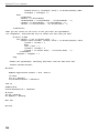
A.3. Program and Documentation . . . . . . . . . . . . . . . . . . . . . . . . . . . . . . . . . . . . . . . . . . .
A.3.1. Form Load Event . . . . . . . . . . . . . . . . . . . . . . . . . . . . . . . . . . . . . . . . . . . . . . .
A.3.2. Export Event . . . . . . . . . . . . . . . . . . . . . . . . . . . . . . . . . . . . . . . . . . . . . . . . . .
A.3.3. Batch Search Tool . . . . . . . . . . . . . . . . . . . . . . . . . . . . . . . . . . . . . . . . . . . . . .
A.4. Notes . . . . . . . . . . . . . . . . . . . . . . . . . . . . . . . . . . . . . . . . . . . . . . . . . . . . . . . . . . . . . .
161
161
161
161
162
162
164
167
167
vii
NOTE!
We assume that you are familiar with 32-bit Microsoft® Windows®
usage and terminology. If you are not fully acquainted with the
Windows environment, read the Microsoft documentation supplied
with your Windows software and familiarize yourself with a few
simple applications before proceeding.
The convention used in this manual to represent actual keys
pressed is to enclose the key label within angle brackets; for
example, <F1>. For key combinations, the key labels are joined
by a + within the angle brackets; for example, <Alt + 2>.
viii
1. INTRODUCTION
Welcome to ORTEC’s AlphaVision v5.6, the 21st-century approach to PC-based alpha
spectroscopy. We have designed AlphaVision to enhance and simplify your alpha-spectrometry
projects in almost every way. AlphaVision v5.6 includes features for managing virtually all
alpha-spectrometry projects, covering each of the necessary steps and providing features that
will enhance your results. The AlphaVision v5.6 software is divided into four major modules
that follow the alpha-spectrometry process:
!
!
!
!
Calibration
Batching, counting samples, and reporting
Hardware
Quality Assurance/Quality Control
These activities are quite distinct from one another so each has its own user interface. Therefore,
each has an icon on the Outlook Bar on the left side of the screen so you can switch easily from
one interface to another. In this manual, we refer to these separate interfaces as modes or
modules (e.g., the Calibration mode or Calibration module). Data management is of course the
heart of AlphaVision so its functions are tightly interwoven with all 4 modules (hence, there is
no separate “Data Management” module).
1.1. About this Manual
This manual is designed to help you begin using AlphaVision v5.6 today. It is an adjunct to the
HTML Help Manual, a comprehensive, on-screen manual integrated into AlphaVision v5.6. To
access the complete help manual, start AlphaVision and click on Help/Contents. The HTML
Help Manual navigates like a website, and also includes the traditional help Contents, Index, and
word Search tabs.
The core of this manual is a comprehensive, 6-step tutorial that takes you through all of AlphaVision v5.6's major features including the library, tracer, QA Type, and ROI editors; calibration,
batch, and background analysis wizard setup. Read through it and explore the software, or
actually perform the example calibration, detector background measurement, batch analysis, and
associated quality control/assurance operations. For detailed information on most topics, you
will be directed to the HTML Help Manual.
This guide is organized as follows:
Chapter 1
Introduction to AlphaVision v5.6 and the HTML and paper user manuals;
comparison between AlphaVision 5.x and 4.x; new features in
AlphaVision v5.6; and the features in the preceding AlphaVision v5
releases.
1
AlphaVision®-32 v5.6 (A36-B32)
Chapter 2
Software installation, building the master list of detectors, and network
configuration.
Chapter 3
Overview of the new AlphaVision v5.6 user interface, including the library
and calibration source editors, acquisition-setup wizards, spectrum and
analysis display, QA tools, and reporting options.
Chapter 4
Overview of AlphaVision’s data management tools, including the table
structures for building a LIMS-to-AlphaVision interface.
Chapter 5
Tutorial; a solid, step-by-step introduction to using AlphaVision v5.6's
major capabilities.
Chapter 6
A checklist of required startup tasks before you begin analyzing samples
with AlphaVision v5.6.
Chapter 7
Analysis methods.
Appendix A
Data export example in Microsoft Visual Basic.
1.2. AlphaVision 5.x Features
AlphaVision Version 5 is a major step forward in power and flexibility, and encompasses almost
every aspect of alpha spectrometry:
1.
Control and monitor up to 256 detectors on the AlphaVision “Detector Grid” display.
2.
All features are intuitive “point and click,” and use familiar Windows menu and command
operations.
3.
Simple wizard-based calibration, sample, and background analysis setup.
4.
Analysis-setup templates let you “set and forget” for reliable, consistent analyses. When
you no longer need a template, you can delete it.
5.
Dynamic detector, chamber, calibration, and process QC monitoring.
6.
On-screen, comprehensive, fully illustrated HTML User Manual navigates like a website
and has contents, index, and advanced word search.
2
1. INTRODUCTION
7.
LIMS in-and-out data handling capability – you can enter sample information or build an
interface between your LIMS and AlphaVision that will take care of it.
8.
Integrated control of Oxford® OASIS alpha spectrometers.
9.
An optional setup feature allows you to specify chamber pressure, bias, and leakage current
thresholds above which AlphaVision 5 automatically suspends data acquisition. When these
parameters fall below the threshold, counting automatically resumes.
10. Count to live-time, real-time, and MDA presets. AlphaVision 5 gives you count-to-MDA
with real-time assessment of the MDA based on the actual recovery, not on an estimate! A
great tool for the spectroscopist who wants to maximize detector capacity.
11. “Modify Acquisition Presets” feature allows you to add more counting time to a sample the
analysis is complete, so you don’t have to start over.
12. Spectral data are saved automatically by AlphaVision 5 so already-collected data survive a
power failure, system crash, or other major interruption. In fact, if only the PC shuts down,
data collection continues. Once you reboot the computer and restart AlphaVision, it
interrogates the hardware, updates accordingly, and continues.
13. Enhanced ability to create QC Control Charts. You can rapidly create a Control Chart for a
specific client, period of time, or isotope; and for controls, blanks, backgrounds.
14. The Batch Wizard allows you to add reagent blanks and control samples to batches.
1.2.1. Comparison to AlphaVision 4
Like AlphaVision 4, AlphaVision 5.x uses an Access database for data archive. It remains
compatible with SAP® BusinessObjects Crystal Reports™, comes complete with standard reports
for Analysis, Calibration, Background, Pulser Tests, and QA/QC. These features are designed to
dramatically enhance your existing data handling processes. Most of the operation features of
AlphaVision 5.x are completely new, plus all spectra, analysis, and QA data are now stored in a
database rather than in individual .SPC files. This results in improved data manageability,
efficiency, and flexibility.
In place of sample types, AlphaVision 5.x uses easy-to-set-up templates that contain your
predefined acquisition, analysis, and reporting preferences. The new Batch Wizard contains
user-defined fields for batches, individual samples, and client/contact management; allows you
to include controls and blanks within batches, as well as set up serial dilutions; and can accept
batch information from your Laboratory Information Management System (LIMS).
3
AlphaVision®-32 v5.6 (A36-B32)
1.3. What’s New in AlphaVision v5.6
The information here and in the remaining sections of this chapter serve two purposes: for
existing AlphaVision 5.x users updating to v5.6, Section 1.3 highlights new features and
functionality. For users new to AlphaVision 5.x, all these sections serve as supplements to the
software’s integrated HTML Help Manual (which is accessed within AlphaVision via the
Help/Contents command). AlphaVision v5.6 now supports the “short date format” selected as
your Windows regional setting. This date format is now applied to the following items:
!
!
!
!
!
!
!
!
!
!
!
!
!
Decay, sample collection and lab preparation date and time
Spectrum acquisition date time
QA results date and time
Detector calibration/analysis date and time
Tracer certificate creation date and time
Analysis library creation date and time
Calibration library creation date and time
Control solution creation date and time
Date and time in the QA chart
All the date and time strings on the Crystal Reports (5 types of reports)
All the date and time strings in the event window
All the date and strings in the sample search dialog
All the date and strings in the QA custom display dialog
NOTE
The default Batch Calibration and Batch Sample names are still fixed in the original
YYYY.MM.DD nnn format (e.g., 2011.01.01 005, indicating the fifth batch created on
January 1, 2011).
1.4. Features Introduced in v5.5
Overview of v5.5 features:
!
!
!
!
!
!
!
!
!
4
New analytical methods and tools
Improved organization of background and QA pulser batches
Quick search for a specific batch or sample
Easier batch setup
New activity units and volume units
Changes to reporting
Export spectra from the Batch Explorer to ORTEC .SPC spectrum files
Easier QA limits setup
Enhanced security
1. INTRODUCTION
! A new database management tool for QA results
! MAESTRO®-32 is no longer a required component for AlphaVision v5.x operation
1.4.1. New Analytical Methods and Tools
1.4.1.1. New Peak Search for Low-Count, Asymmetric Peaks
AlphaVision v5.5 introduces a new peak search/fit methodology for use when you must fit a
peak, even when count statistics, poor shape, or overlap could make it a poor candidate for the
standard AlphaVision peak search/fit algorithm. It uses an ROI Set to direct the analysis to
certain regions of the spectrum, as well as an iterative peak stripping technique. To use this
method:
Create an ROI Set that defines each region in which a peak of interest will be located.
In the Batch Wizard, select Peak Search/Fit as the analysis method on the Analysis Setup page
of the Batch Wizard, then specify the appropriate ROI Set. (If no ROI Set is specified,
AlphaVision v5.6 uses the default peak search/fit algorithm.)
The new routine starts with the highest-energy ROI in the set, and calculates a peak fit based on
the contents of the ROI. The counts in the fitted peak are stripped from the spectrum. The
routine then moves to the next-highest-energy ROI in the set and repeats the peak fitting and
stripping. When all ROIs in the set have been analyzed in this way, the remainder of the
spectrum is analyzed according to the standard peak search/fit criteria.
1.4.1.2. Manual Chemical Recovery
AlphaVision v5.5 provides an additional method for determining chemical recovery. The
Analysis Setup page of the Batch Wizard includes a Manual CR (%) feature. It allows you to
enter a percent chemical recovery, determined by an alternative method (e.g., a gamma counting
technique), and apply it to all samples in the batch. See Fig. 139 and the discussion on page 118.
1.4.2. Improved Organization of Background and QA Pulser Batches
The v5.5 Sample Explorer now introduced the same organizing tools for Background and QA
Pulser samples as for sample batches. Simply right-click and select Insert Branch to build
background and QA pulser hierarchies (Fig. 1). Accordingly, the Background Wizard, and QA
Pulser Wizard include a Batch Properties screen that lets you specify the “location” of the batch
in the database. See also Section 5.1.5.1, which describes the process for Batches.
5
AlphaVision®-32 v5.6 (A36-B32)
Fig. 1. Build Sample Hierarchies for
Background and QA Samples.
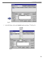
1.4.2.1. View Batch Explorer Entries in Ascending or Descending Order
The Sort Descending command has been added to the View menu. Selecting it re-sorts the
Batch Explorer Tree, reversing the order of the sample categories (e.g., Imported, Background,
QA, Batches), and sorting the entries in each category newest-entry-first. Unmarking Sort
Descending returns the sample categories to their original order, and sorts the entries oldestentry-first. Figure 2 compares the original ascending and new descending sorts.
Fig. 2. Batch Explorer Tree Sorted in Ascending and Descending Order.
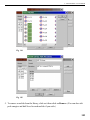
1.4.3. Quick Search for a Specific Batch or Sample
The Edit menu in Batch Mode has a new Search command that helps quickly locate a specific
unhidden batch or sample in the current database. All data categories in the Batch Explorer
panel are searched, including imported records.
6
1. INTRODUCTION
Before selecting Edit/Search, decide whether to (1) search all entries in the Batch Explorer
panel by turning View/Hide Branch off; or (2) use the Hide Branch and View/Hide Branch
commands to mask certain parts of the database from this search tool.
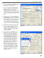
Select Edit/Search. Choose either Batch or Sample, then narrow the search by entering all or
part of the record Name and/or a range of dates. If your database is large, you may also wish to
specify the Maximum number of records to be retrieved. Click on Search to generate the list of
records matching your criteria. The Found field shows the number of hits.
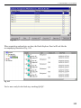
Locate the desired Batch Name or Sample Name in the results list, then double-click on it or
highlight it and click on View. See Fig. 3. When you select a batch for viewing, its component
samples are displayed in the Sample Explorer panel. When you view a sample, it is highlighted
in the Sample Explorer, and its spectrum is displayed.
Fig. 3. Quickly Locate and Display a Specific Batch or Sample Record.
1.4.4. Easier Batch Setup
1.4.4.1. Auto-Define Samples in the Analysis Wizards
The Batch, Background, and QA Pulser wizards now includes an “auto-sample” feature
that reduces your batch setup time. To use this new feature, go to the wizard’s Sample page
7
AlphaVision®-32 v5.6 (A36-B32)
and click on the auto-sample button ( ... ) below the Sample Names panel (refer to Fig. 5).
AlphaVision v5.6 will poll the system, return the list of currently available detectors (i.e, those
calibrated and available for counting), let you select the detectors to be used, then automatically
populate the sample list, one per detector. The samples names are based on the detector names.
You can then modify, add, or delete samples as needed. Figure 5 shows the automatically
populated samples based on the detectors listed in Fig. 4.
Fig. 4. List of Available Detectors For Automatic Sample
Naming.
Fig. 5. Sample Names
Assigned Based on List
of Available Detectors.
1.4.4.2. Create Sample-Less Batch Templates
Earlier releases of AlphaVision 5.x required you to assign at least one sample when defining a
new template. The Batch, Background, and QA Pulser wizards now allow you to create new
templates without assigning any samples. This makes it easy to set up one or more templates at
the outset of a project, before you are ready to begin batching. The General page now includes a
Create Template without Samples checkbox. Mark the Save As Template box, then mark this
new box, assign a template name, and begin stepping through the wizard. The wizard’s Batch
page does not require you to choose a location for the batch, and the Sample page does not
require you to define samples. All other setup steps are the same.
8
1. INTRODUCTION
1.4.4.3. Differentiate Blanks by QA Type
The MDA/Blank page of the Batch and Background wizards (see Section 1.5.8) has a new
listbox that makes it easier to locate the blank spectrum needed for your analysis. Choose the
desired Reagent Blank QA type from the Sort Blanks list (Fig. 6), then select the Blank
Spectrum to be used (Fig. 7).
Fig. 6. Select a Reagent Blank QA Type.
Fig. 7. Choose the Blank Spectrum.
1.4.5. New Activity Units and Volume Units
This release of AlphaVision gives you more choices for activity units of measure in the Tracer
Editor, Calibration Source, and Control Solution editor dialogs (Fig. 8). Choose from disintegrations per minute (DPM), curies (Ci), millicuries (mCi), microcuries (μCi), nanocuries (nCi),
picocuries (pCi), fempto-curies (fCi), millibecquerels (mBq), becquerels (Bq), and kilobecquerels (kBq). The default is DPM.
In addition, the Analysis Setup page of the Batch Wizard now lets you enter the tracer amount in
grams (g) or milliliters (mL). See Fig. 139 on page 117.
9
AlphaVision®-32 v5.6 (A36-B32)
Finally, you can now define volume on the Control Solution
editor (Section 5.1.4.1) n grams (g) or milliliters (mL).
Fig. 8. Expanded List of
Activity Units.
1.4.6. Changes to Reporting
1.4.6.1. Report Reanalysis Results with Your Custom Report Templates
The Re-Analysis Setup dialog (for
analyzing batches and reanalyzing
individual samples) now has a new
Report tab (Fig. 9) with a User
Defined Template section that
lets you generate reports from your
custom Crystal Report templates.1
Mark the checkbox, then browse
to locate the desired template. (To
produce reanalysis reports with
the default AlphaVision template,
use the Report Window.)
Fig. 9. Use Custom Templates in Reanalysis Reports.
1
This requires Crystal Reports v11, not supplied with AlphaVision v5.6. We can assist in developing custom
templates; contact your ORTEC representative or Customer Support for more information on this service.
10
1. INTRODUCTION
1.4.6.2. Peak FWHM Added to the Calibration Reports
The Nuclide Activity Summary section of the Calibration report now includes the FWHM for
each identified peak (Fig. 10). If you have an earlier version of AlphaVision 5.x, you can
generate a report showing this new parameter by updating the analysis or calibration.
Fig. 10. New Peak FWHM Column.
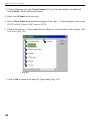
1.4.7. Export Spectra from the Batch Explorer to ORTEC .SPC Spectrum Files
AlphaVision v5.5 lets you export spectra as .SPC-format spectrum files, which can then be
viewed and manipulated in our CONNECTIONS-32 applications, such as MAESTRO-32
or GammaVision-32. To do this, right-click in the Batch Explorer Panel on the desired spectrum
( ) (Fig. 11) then choose Export from the right-mouse-button menu. A message box will
display the name of the new spectrum file. All .SPC files are exported to the C:\User
Programs\AlphaVision folder. Filenames are based on the batch name, sample name, and
comment string.
Fig. 11. Export Spectra as .SPC Files.
1.4.8. Easier QA Limits Setup
The v5.5 All Detectors checkbox on the QA Limits panel lets you click once to assign all
detectors in your system the same QA limits for a particular parameter (such as total
11
AlphaVision®-32 v5.6 (A36-B32)
background). Choose a detector, set the warning and alarm limits for the desired parameter,
mark the corresponding checkbox, then click the Apply Changes button (Fig. 12). Note also
that Total Background is now expressed on this panel in counts per day (c/d).
1.4.9. Enhanced Security
As of v5.5, only users at the Administrator security level can access the database management
tools, including the ability to select a different working database. For all other users, the
database commands are disabled.
In addition, two new access permissions have been added to the Security Levels dialog:
! Save Batch Template — Users without this permission cannot create templates in Batch
Mode.
! Move Detectors — Users without this permission cannot move detectors on the Detector
Grid.
See also Section 3.1 and the HTML Help Manual.
Fig. 12. One Click Sets A QA Limit for All Detectors.
12
1. INTRODUCTION
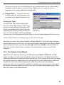
1.4.10. New Database Management Tool for QA Results
In earlier versions of AlphaVision v5.x, the Database Management dialog only allowed you to
manage the data listed in the Batch Explorer tree. However, the database also holds QA pulser
and QA background data. As of v5.5, you can view and/or delete those data by clicking on the
QA Results Edit button to open the QA Results Management dialog shown in Fig. 13. Use the
listbox at the top of the dialog to view either pulser records or background records.
Fig. 13. Manage QA Pulser and QA Background Records.
1.4.11. MAESTRO®-32 No Longer a Required Component
As of v5.5, AlphaVision no longer requires installation of the accompanying ORTEC
MAESTRO®-32 MCA Emulation software.2 Note, however, that MAESTRO is necessary to set
up and monitor alpha chambers other than ORTEC Alpha-series (Aria®, Duo™, Ensemble™) or
OCTÊTE-series instruments, and the Oxford OASIS.
You may also find MAESTRO useful for performing quick counts for methods development
work, test sources, and source activity checks outside of the AlphaVision program. Data
2
Exception: If you purchased a new ORTEC alpha spectroscopy MCB, in addition to AlphaVision v5.6, be sure to
install MAESTRO-32 and other accompanying software according to the instructions in the hardware manual.
13
AlphaVision®-32 v5.6 (A36-B32)
collected in MAESTRO are not stored in the AlphaVision database; however, they can be saved
within MAESTRO, as discussed in its Software User Manual. See also Section 3.2.10 of this
manual.
1.5. Features Introduced in AlphaVision v5.3
1.5.1. ROIs Expressed in Channels or Energy
In Batch and Background modes, AlphaVision v5.6 now lets you define ROI Sets either in
channels or energy (keV) by marking the Define ROIs in Energy (keV) checkbox in the upper
right corner of the dialog, as illustrated in Fig. 14. In Calibration mode, ROI Sets can only be
defined in channels. You must choose the unit of measure before clicking on the Update button.
For instructions on building ROI Sets, see “Creating an ROI Set for This Calibration Record,”
on page 85.
Fig. 14. ROI Sets Expressed in Channels or Energy (keV).
14
1. INTRODUCTION
1.5.2. Select Database and Database Management
AlphaVision v5.6 allows you to choose the target database for all of your project measurements
with the File/Select Database... command discussed in Section 4.2. In addition, AlphaVision
now contains a suite of database management tools that give you comprehensive control over the
contents of your AlphaVision databases. See Section 4.3 for complete information.
1.5.3. Sample Dilution Setup in the Batch Wizard
The Sample setup page of the Batch Wizard now includes a dilution feature that helps you set up
and track a 1- or 2-stage dilution. All you do is fill in the aliquot and sample volumes (and any
associated uncertainty), then click on the Calc. Dilution button at the bottom of the calculator.
To measure all of the sample, click on the Total
radio button, then enter the Sample Amount (as
volume or weight, set with the Sample Units
radio buttons in the upper right corner of the dialog)
and uncertainty. This is illustrated in Fig. 15. Note
that the Calc. Dilution button is inactive.
To use an aliquot of the sample, click on the Aliquot
radio button, then enter the amount and uncertainty
of the total Sample and of the Aliquot (Fig. 16). The
Calc. Dilution button is also inactive in this mode.
If you will be diluting your sample,
select the Dilution radio button to activate all of the fields and enable the Calc.
Dilution button (Fig. 17). This section of
the screen supports two dilutions. Enter
the appropriate amount and uncertainty
for your total sample, the volume into
which you have diluted it, and the aliquot
to be measured, then click on Calc.
Dilution to perform the arithmetic. You
can click on the calculation button as
often as you wish while setting up the
dilution(s), but be sure to click it one
final time when all of the dilution and
aliquot information has been entered.
Fig. 15. Using All of the Sample. (The
Calc. Dilution button is inactive in this
mode.)
Fig. 16. Using an Aliquot of the Total Sample. (The
Calc. Dilution button is also inactive in this mode.)
15
AlphaVision®-32 v5.6 (A36-B32)
Figure 17 shows a Sample volume of 1.0 mL being diluted into 10 mLs (a dilution of 1:10,
denoted in the Dilution calculation field as 1.000e+001). A 0.1-mL Aliquot is subsequently
diluted into 100 mL, then a 0.1-mL aliquot — a final dilution of 1:100000 — is taken for the
sample measurement.
The Tracer feature works as it did in earlier releases of AlphaVision 5. If you are adding
different amounts of tracer to each sample in the batch (rather than a uniform amount in all
samples), mark the Tracer box here and enter the amount and uncertainty on a sample-bysample basis. If you are adding a uniform amount to all samples in the batch, use the Relative
Analysis feature (see Fig. 144, page 121).
Fig. 17. Calculating the Dilution as Dilution and Aliquot Information are
Entered.
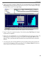
1.5.4. New Scaling and Cursor Movement Features
AlphaVision v5.6 spectrum windows now use many of the horizontal and vertical scaling and
cursor movement keys employed in our other spectroscopy products (e.g., MAESTRO-32),
including:
!
!
!
!
16
Move marker one channel left/right, <7>/<6>
Taller/shorter, <8>/<9> and <F5>/<F6>
Narrower/wider <F7>/<F8>.
Zoom in/out Keypad<+>/Keypad<!>.
1. INTRODUCTION
NOTE These keys only function when the Thumbnail window is closed.
See Section 3.2.7 for more detailed descriptions of these commands.
1.5.5. Interactive ROI Analysis in Batch, Background, and Calibration Modes
In previous versions of AlphaVision 5, if you were using multiple detectors, depending on the
gain and shift settings for each device, you might have had to create multiple ROI Sets to
accommodate detector-to-detector differences, or else repeatedly edit a single ROI Set.
AlphaVision v5.6 now offers an interactive ROI analysis that allows you to create just one ROI
Set for your multiple detectors; quickly adjust its ROIs, “on the fly,” for a particular detector;
then replace that detector’s original analysis with an ROI analysis using the customized ROI Set
(this capability cannot be used for the initial spectrum analysis, only for reanalysis). The original
ROI Set is not changed. Regardless of the original analysis method, this function performs an
ROI Based analysis with the Recalibration and Adjust ROI features turned off. The ROI
information for each customized ROI Set is saved in the database and printed in the Nuclide
Summary (ROI) section of the report.
The details of the process are different for Batch/Background analyses and for Calibrations: In
batches and backgrounds, adjusting an ROI’s boundaries and centroid simply repositions the
ROI. However, in Calibration mode, adjusting an ROI recalculates the detector calibration; this
is discussed in more detail in Section 1.5.5.2.
NOTE If you adjust 1 or more ROIs, but then do not execute the Interactive ROI Analysis
command, the old ROI limits will be restored. However, once the Interactive ROI
Analysis command has been issued, there is no undo.
1.5.5.1. Batch Mode
The following example illustrates how to perform an interactive ROI analysis in Batch mode; the
procedure is the same for both Batch and Background data sets.
1. Use the Batch Explorer to locate the proper batch, then locate the spectrum to be reanalyzed.
Click on its Analysis entry to display the current spectrum and analysis.
2. In the spectrum window, zoom in as necessary to accurately change ROI boundaries and
centroids. Click in the first ROI to be adjusted to activate it. (The active ROI has a dashed
border; inactive ROIs have solid borders.) Roll the mouse over the low-channel and highchannel ROI boundaries until the pointer changes to a two-sided arrow, then click and drag
the boundaries to reposition them, if necessary (Fig. 18).
17
AlphaVision®-32 v5.6 (A36-B32)
3. Next, reposition the centroid, if necessary. To do this, roll the mouse pointer over the small
centroid marker until the pointer changes to a four-sided arrow (Fig. 19), then click and drag
to the new centroid position. The centroid marker will now indicate the new position ( ).
Fig. 18. Click and Drag the Two-Sided Arrow to Adjust the Low- and High-Channel
ROI Boundaries. Status line will update to new ROI boundaries.
Fig. 19. Click And Drag the Four-Sided Arrow to Reposition the Centroid, If
Necessary. Status line will update to show new centroid.
18
1. INTRODUCTION
4. You are now ready to reanalyze. Right-click in the spectrum window and select Interactive
ROI Analysis from the right-mouse-button menu (see Fig. 20). After reanalysis, the energy
or channel labels on the X-axis might change.
Fig. 20. Right-Click and Select Interactive ROI Analysis to Start the Reanalysis.
5. Figure 21 shows the completed reanalysis. Note that the analysis Date/Time in the Sample
Explorer has been updated.
6. Right-click on the Analysis #1 entry and select Properties from the right-mouse-button. The
Batch Properties dialog will show a grayed checkmark in the Interactive ROI checkbox
(Fig. 22). This is your indication that this analysis has been performed with a customized
ROI Set.
7. To see the peaks in the customized ROI Set, click on the Report tab for this spectrum and
look in the Nuclide Summary (ROI) section (Fig. 23). The Analysis Method field indicates
that an interactive ROI analysis has been performed.
19
AlphaVision®-32 v5.6 (A36-B32)
Fig. 21. Reanalysis is Complete and the Analysis Date/Time Has Updated.
Fig. 22. Analysis Properties for this Sample. Note that the Interactive ROI checkbox is marked,
indicating a customized ROI Set. In addition, the Recalibrate and Adjust ROI Width features
are turned off. The customized ROIs are listed in the report.
20
1. INTRODUCTION
Fig. 23. Report Indicates an Interactive ROI Analysis and Lists the ROIs Used.
1.5.5.2. Calibration Mode
In Calibration mode, adjusting ROIs and issuing the Interactive ROI Analysis command
triggers a recalibration.
! If you change only the centroid and not the ROI start and end channels, AlphaVision
recalculates only the energy, not the efficiency.
! If you change only the ROI start and end channels and not the centroid, AlphaVision will
recalculate the efficiency, not the energy.
! Changing both the boundaries and centroid recalculates both calibrations.
1.5.6. The Report: What You See Is What You Get
In preceding AlphaVision 5 releases, the report included the sample spectrum histogram in
addition to the standard analytical information. AlphaVision v5.6 allows you to select how much
of the spectrum will be displayed on the report: Simply Zoom In on the desired spectral features
(use the right-mouse-button menu command, not the Thumbnail), then click on the Report tab.
This is illustrated in Fig. 24.
21
AlphaVision®-32 v5.6 (A36-B32)
NOTE The Nuclide Summary section of the report always contains the information for all
ROIs, not just the ROIs currently displayed in the Spectrum Window.
Fig. 24. Zoom In on the Spectrum Window to Determine the Spectrum Display in the Report.
1.5.7. Changes to the Detector Assignment Worksheet
Two new buttons, Uncheck All and Check All, have been added to the Detector Assignment
Worksheet to speed your selection of the samples you wish to count once detectors have been
assigned. Uncheck All removes all checkmarks from the Count column. Check All marks all
samples for counting.
22
1. INTRODUCTION
Fig. 25. The Detector Assignment Worksheet.
1.5.8. Subtracting Net Blank Activity
This new feature, located on
the MDA/Blank page of the
Batch and Background wizards,
subtracts the activity (not the
counts) for a selected blank
from the activity of all samples
in the batch. If this batch of
samples contains a blank, use
the Default entry in the Blank
Spectrum droplist. Otherwise,
use the Blank Spectrum droplist
to select any suitable blank from
the current database. If no blank
is available, the analysis will fail,
in which case you can right-click
on the analysis entry , choose
Update Analysis, and select an
appropriate blank (Fig. 26). The
calculation is discussed in
Section 7.7.12.2.
Fig. 26. If Current Batch Does Not Have a Blank, Select One
from the Database.
Note the addition of the Sort Blanks listbox in AlphaVision v5.6; see Section 1.4.4.3.
23
AlphaVision®-32 v5.6 (A36-B32)
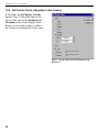
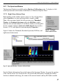
1.5.9. QA Control Charts: Adjustable Y-Axis Scaling
In QA mode, the QA/Display/Custom...
function (Fig. 27) has been improved to
let you either specify the Minimum and
Maximum values of the Y-axis (which
allows you to exclude outliers) or allow
the software to automatically set the scale.
Fig. 27. Set the Control Chart Parameters for
Both Axes.
24
2. INSTALLATION AND CONFIGURATION
This chapter discusses software and hardware installation and configuration, including how to
assign the number of inputs and memory size for OCTÊTE- and 920-series multichannel buffers
(MCBs), set peak positions, configure the list of MCBs available to AlphaVision v5.6, and
select the correct network protocol. See also the accompanying Installation and Release Notes
(Part No. 784550).
2.1. Installation Notes
NOTE FOR VISTA AND WINDOWS 7 USERS
Vista and Windows 7 do not support the IPX/SPX protocol. If you have ORTEC MCBs that
use an Ethernet connection — e.g., OCTÊTE-E or 920E — you must connect these units to a
Vista/7 PC via another interface (e.g., USB, Dual-Port Memory Interface, printer port). For
assistance, contact your ORTEC representative or our Global Service Center.
! ORTEC CONNECTIONS-32 software products are designed to operate correctly for users with
full Administrator privileges. Limiting user privileges could cause unexpected results.
! If you are upgrading from AlphaVision Version v4.x, the installation of AlphaVision v5.6
will have no effect on existing AlphaVision v4.x files, spectra, or data. You will retain the
capability to analyze .SPC files with AlphaVision v4.x.
! If you have an older version of MAESTRO-32 on your PC, the installation wizard might
prompt you to uninstall that older version.
! If you install AlphaVision v5.6 in other than the default location, c:\Program Files\
ORTEC\AlphaVision 5, you must use Crystal Reports v11 to edit the paths in the report
templates, AnalysisRpt.rpt, BackgroundRpt.rpt, CalibrationRpt.rpt, PulserRpt.rpt, and
QARpt.rpt, or else AlphaVision will not be able to find and use the templates.
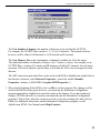
2.2. Step 1: Installing AlphaVision v5.6
1.
Insert the AlphaVision CD-ROM, select My Computer, locate the CD drive, then open
Setup.exe. In Windows 2000 and XP, this will start the AlphaVision installation wizard. In
Vista and 7, a message will indicate that Windows cannot verify the publisher of this
software. Select the “install anyway” option to start the installation wizard.
25
AlphaVision®-32 v5.6 (A36-B32)
2.
If your PC does not have Adobe Acrobat® Reader installed, the wizard will offer you an
installation option. After installing/not installing Acrobat Reader, click Next and answer the
wizard prompts.
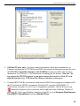
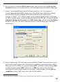
3.
On the Instrument Setup page, mark the checkbox(es) that corresponds to the instrument(s)
installed on your PC, as shown in Fig. 28. If this is an AlphaVision upgrade and not a firsttime installation, you probably already have ORTEC CONNECTIONS-32 instruments attached
to your PC. If so, they will be included on the Local Instrument List at the bottom of the
dialog, along with any new instruments. Existing instruments (i.e., those configured before
this upgrade) do not have to be powered on during this part of the installation procedure.
NOTE
You can enable other device drivers later, as described in Section 2.6.1.
To see more information on each instrument family, click on the family name and read the
corresponding Item Description on the right side of the dialog.
The OASIS Instrument driver is installed by default. You may leave this checkbox marked
even if not using an OASIS.
The Ethernet devices are automatically enabled, so there is no checkbox for them. If you
choose the add-in driver option, an additional wizard screen will open asking which add-ins
should be installed.
4.
If you want other computers in a network to be able to use your MCBs, leave the Allow
other computers to use this computer’s instruments marked so the MCB Server program
will be installed. Most users will leave this box marked for maximum flexibility.
NOTE
If your PC uses Windows XP and you wish to use or share ORTEC MCBs across a
network, be sure to read Section 2.6.2.
5.
Click on Done. The installation wizard will resume copying files.
6.
At the end of the wizard, restart the PC. Upon restart, remove the AlphaVision CD from the
drive.
7.
After all processing for new alpha hardware has finished, you will be ready to configure the
MCBs in your system. Connect and power on all local and network ORTEC instruments
that you wish to use, as well as their associated PCs. Otherwise, the software will not detect
them during installation. Any instruments not detected can be configured at a later time.
26
2. INSTALLATION AND CONFIGURATION
Fig. 28. Choose the Interface for Your Instruments.
8.
2000 and XP users only: For direct-connect instruments (those that communicate via
Ethernet) including the OCTÊTE Plus and 920E, the network default protocol must be set to
the IPX/SPX Compatible Transport with NetBIOS selection on all PCs that use these
instruments. See Section 2.6.3 for instructions on making this the default. Vista and 7 do
not support the IPX/SPX protocol so you must connect these units to a Vista PC via a
different interface (e.g., USB, Dual-Port Memory Interface, printer port).
9.
If using ORTEC MCBs on a network, make sure the MCB Server program is running on all
the PCs hosting the ORTEC instruments. (Each host PC must have MAESTRO-32,
AlphaVision, or another CONNECTIONS-32 application installed.) The MCB Server icon
( ) should be displayed in the system tray on the right side of the Windows Taskbar of
each host PC. If not, open Windows Explorer on that PC, go to c:\Program Files\Common
Files\ORTEC Shared\Umcbi, and start McbSer32.Exe.
27
AlphaVision®-32 v5.6 (A36-B32)
10. To start the MCB Configuration program on your PC, go to the Windows Start menu and
select AlphaVision 5.6, and MCB Configuration. The MCB Configuration program will
locate all of the (powered-on) ORTEC MCBs attached to the local PC and to (powered-on)
network PCs, display the list of instruments found, allow you to enter customized
instrument numbers and descriptions, and optionally write this configuration to those other
network PCs; see Section 2.2.1.
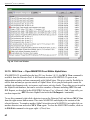
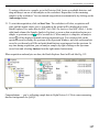
2.2.1. Configuring and Customizing the Master MCB List
The initial master list of MCBs available to the ORTEC programs on your PC is determined by
the MCB Configuration program, which you run as part of software installation or update, or
after installing a new MCB.
When MCB Configuration runs, it searches the PC and the network (if any) for MCBs, then
displays a master list of the instruments found (Fig. 29).
Fig. 29. MCB Numbering and Descriptions.
Some instruments have multiple inputs, so they appear on the master list as more than one
instrument. For example, the OCTÊTE Plus and Model 920E have 16 inputs, so can function as
16 instruments, and can appear as 16 instruments on the master list. For the remainder of this
manual, when we refer to an instrument or alpha chamber we are referring to one of the inputs
in a multiple-input unit.
28
2. INSTALLATION AND CONFIGURATION
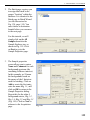
Note that you can change the instrument numbers and descriptions on this dialog by doubleclicking on an instrument entry in the Configure Instruments dialog. This will open the Change
Description or ID dialog (Fig. 30). It shows the physical detector location (read-only) and allows
you to change the ID and Description. Make the desired changes and click on Close.
Fig. 30. Change MCB Number or Description.
If you or another user have already assigned a description to a particular instrument, you can
restore the default description by deleting the entry in the Description field and re-running MCB
Configuration. After MCB Configuration runs, the default description will be displayed.
When MCB Configuration runs, the resulting MCB configuration list is normally broadcast to
all PCs on the network. If you do not want to broadcast the results, unmark the Update detector
list on all systems checkbox under the instrument list (see Fig. 29) so the configuration will
be saved only to the local PC.
The first time the system is configured, Fig. 31 will be displayed to remind you that all new
instruments must be assigned a unique, non-zero ID number.
Fig. 31. MCB Numbering First Time.
You can change all the instrument numbers by clicking on Renumber All to assign new
numbers in sequence; or click on Renumber New to renumber just the new instruments.
Figure 32 will be displayed if the list is a mixture of old and new numbers.
29
AlphaVision®-32 v5.6 (A36-B32)
Fig. 32. Renumbering Warning.
NOTE Remember that some applications use the instrument number to refer to a specific MCB
or device (e.g., the .JOB file command SET_DETECTOR 5). Therefore, you might
want to subsequently avoid changing its number so all defined processes will still
operate.
When you have completed all changes to the instrument list, click on Close to close the
Configure Instruments dialog. At this point, GammaVision and other CONNECTIONS applications
can be run on any PC, and the MCB pick list for each program on each PC can be tailored to a
specific list of instruments.
2.3. Step 2: Configuring OCTÊTEs and 920s with SET920
If you are not setting up OCTÊTE- or 920-series MCBs for the first time, skip to Section 2.4.
The number of inputs (1–16) and memory size (number of channels) for each detector input in
OCTÊTE- and 920-series MCBs is computer controlled by the SET920 program, supplied on
diskette with your hardware. Normally you will only run it when you add a new MCB to the
system, and will not use it again except to change the number of inputs or the total memory size.
If you have already set up the number of inputs and memory size for each detector in your
OCTÊTE- and/or 920-series MCBs, skip to Section 2.4.
1. To run SET920, go to the Windows Start menu and select AlphaVision 5.6 and SET920.
Figure 33 shows the opening SET920 dialog. Click on the MCB droplist and select the input
to be changed (SET920 displays only the instrument types listed above). The second field
shows the current memory size and number of inputs.
30
2. INSTALLATION AND CONFIGURATION
Fig. 33. The SET920 Configuration Dialog.
The New Number of Inputs is the number of detectors to be used by this OCTÊTE.
For example, the OCTÊTE Plus can have 1, 2, 4, 8 or 16 detectors. The normal selection,
however, will be either 8 (all internal) or 16 (8 internal and 8 external).
The New Memory Size is the total number of channels available for all of the inputs.
The individual number of channels is Memory Size / Number of Inputs. For example, in an
OCTÊTE Plus, a setting of 16 inputs and 8K memory will allot 512 channels for each input
spectrum. This can be equal to, greater than, or less than the ADC conversion gain for each
detector.
The ADC conversion gain and offset can be set for each MCB in AlphaVision (right-click on
the detector of interest, select Detector Properties..., then click on the Chamber
Properties... button), or MAESTRO (Acquire/MCB Properties...).
3. When finished editing all the MCBs, click on OK to exit the program. The changes will be
stored in the MCBs at this point, however, you must run the Instrument Configuration
program again before AlphaVision can detect and use the changes. If you have made any
changes, SET920 will ask if you want to automatically run the Instrument Configuration
program. Click on Yes, allow the search to proceed, review the resulting list, then click on
Close. For additional instructions on the Instrument Configuration program, see the
AlphaVision HTML User Manual under Help/Contents.
31
AlphaVision®-32 v5.6 (A36-B32)
2.4. Step 3: Setting Peak Positions
1. Start MAESTRO.
2. Determine the correct gain for the energy range and MCB channels selected. For example,
using 3–8 MeV and 512 channels, the energy gain is 9.765 keV/channel (5000 keV/512
channels) and the offset is 3000 keV. Using 2–10 MeV and 1024 channels, the energy gain is
7.8125 keV/channel and the offset is 2000 keV.
3. Determine the target locations for the primary alpha emission energies of the calibration
standard as [Target Channel = (Primary Emission Energy Offset)/Gain]. For example, using
a mixed Pu/U calibration standard, with a 238Pu primary energy of 5499 keV and a 238U
primary energy of 4196 keV, 3000 keV offset, and 9.765 keV/channel gain, the target
channel for 238Pu is [(5499 - 3000)/9.765] or channel 256. Similarly, the target channel for
238
U would be [(4196 - 3000)/9.765] or channel 122.
4. Clear the detector (Acquire/Clear), enable the bias voltage (Acquire/MCB Properties...,
High Voltage tab; or manually), and start data acquisition (Acquire/Start). Using the
observed peak position and the target channels determined above, adjust the energy gain (E
CAL) for the detector to locate the peaks in the proper channels. This is an iterative process
for each detector.
5. Once the gain is set, stop acquisition (Acquire/Stop), clear the detector (Acquire/Clear).
6. Repeat this process for each detector. Exit MAESTRO.
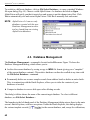
2.5. Step 4: Reserving a “Clean Copy” of the Database
We recommend that, before using AlphaVision v5.6 for the first time, you make an archive copy
of the empty AlphaVision.mdb database file. You can then use it, in conjunction with the
Database Management utilities (Section 4.3), to create new AlphaVision databases.
2.6. Additional System Configuration Operations
2.6.1. Enabling Additional ORTEC Device Drivers and Adding New MCBs
You can enable other device drivers later with the Windows Add/Remove Programs utility on
the Control Panel. Select Connections 32 from the program list, choose Add/Remove, then
elect to Modify the software setup. This will reopen the Instrument Setup dialog so you can
mark or unmark the driver checkboxes as needed and close the dialog.
32
2. INSTALLATION AND CONFIGURATION
When an MCB is added to the system, or if you change total memory size and number of
segments for a multi-input MCB such as the Model 920 or OCTÊTE-series instruments, you
cannot communicate with the new input(s) until you add it to the Master Instrument List by rerunning the MCB Configuration program, as described in Step 9 on page 28.
2.6.2. If You Wish to Share Your Local ORTEC MCBs Across a Network
NOTE If you do not have instruments connected directly to your PC or do not wish to share
your instruments, this section does not apply to you.
If your PC is running under Windows XP Service Pack 2 or higher, Vista Ultimate, or
Windows 7, the default firewall settings will prevent other computers from accessing the CONNECTIONS-32 MCBs connected directly to your PC. To share your locally connected ORTEC
instruments across a network, you must enable File and Printer Sharing on the Windows
Firewall Exceptions list. To do this:
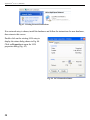
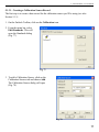
1. From the Windows Control Panel, go to the Security feature for your operating system and
access the Windows Firewall entry. Figure 34 illustrates how to access the Change
Windows Firewall Settings task from the Network Connections control panel option. This
will open the Windows Firewall dialog.
Fig. 34. Change the Firewall Settings.
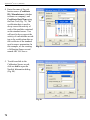
2. Go to the Exceptions tab, then click to mark the File and Printer Sharing checkbox
(Fig. 35).
NOTE This affects only the ability of other users on your network to access your MCBs.
You are not required to turn on File and Printer Sharing in order to access
networked MCBs (as long as those PCs are configured to grant remote access).
3. To learn more about exceptions to the Windows Firewall, click on the What are the risks of
allowing exceptions link at the bottom of the dialog.
33
AlphaVision®-32 v5.6 (A36-B32)
4. Click on OK to close the dialog. No restart is required.
Fig. 35. Turn on File and Printer Sharing.
2.6.3. Setting Up the IPX/SPX Network Protocol (2000 and XP Users Only)
ORTEC CONNECTIONS-32 uses all of the network “languages” — called protocols — supported
by Windows 2000 Professional and XP Professional SP2, but Vista and 7 do not support
IPX/SPX. This section describes how to select the right Windows protocols for CONNECTIONS-32 operation. If multiple protocols are installed on the various PCs in the network, only
those PCs with compatible protocols will be able to communicate with one another. No special
settings are required in that case.
CONNECTIONS-32 products with built-in Ethernet adapters, such as the OCTÊTE Plus and 920E,
communicate directly with the PCs on the network. The PCs and these units must “speak the
same language” (i.e., use the same protocol) in order to understand each other.
34
2. INSTALLATION AND CONFIGURATION
2.6.3.1. Windows 2000 Setup
There is only one setting needed on Windows
2000. To access this setup, select Settings/
Network and Dial-up Connection as shown
in Fig. 36. This will display the existing connections as shown in Fig. 37. If no network
hard-ware is shown, install the hardware and
follow the instructions for new hardware.
Fig. 36. Start Network and Dial-up Connection..
Fig. 37. Network and Dial-up Connections.
35
AlphaVision®-32 v5.6 (A36-B32)
Select the LAN connection and double click
on it to display the status dialog as shown in
Fig.38. Select Properties to display Fig. 39.
Fig. 38. LAN Connection.
Select the NWLINK IPX... as shown and
then Properties to display Fig. 40.
Fig. 39. LAN Properties.
36
2. INSTALLATION AND CONFIGURATION
Now select the Frame type to 802.3 as
shown.
Click on OK and return to the Desktop.
Fig. 40. NWLINK IPX... Protocols.
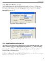
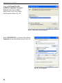
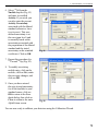
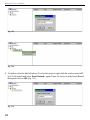
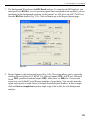
2.6.3.2. Windows XP Setup
To determine whether the NWLink IPX/SPX/NetBIOS Compatible Transport Protocol is
installed, to add it, or to select it as the default, go to the Taskbar and click on Start, then
Control Panel. In the Control Panel under “Pick a Category,” choose Network and Internet
Connections (Fig. 41).
Fig. 41. Opening the Control Panel, then Network and Internet Connections.
Under “Pick a Control Panel Icon,” click on Network Connections
(Fig. 42). This will display the LAN or High-Speed Internet
connections, as shown in Fig. 43.
Fig. 42. Network
Connections.
37
AlphaVision®-32 v5.6 (A36-B32)
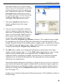
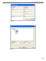
Fig. 43. Existing Network Connections.
If no network entry is shown, install the hardware and follow the instructions for new hardware,
then return to this screen.
Double-click on the existing LAN entry to
display the status dialog shown in Fig. 44.
Click on Properties to open the LAN
properties dialog (Fig. 45).
Fig. 44. LAN Connection Status.
38
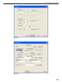
2. INSTALLATION AND CONFIGURATION
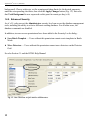
To add the NWLink IPX/SPX/NetBIOS
Compatible Transport Protocol, click on
the Install... button. This will open the
Select Network Component Type dialog
(Fig. 46).
Fig. 45. LAN Properties.
Click on Protocol to display the Select Network
Protocol dialog shown in Fig. 47.
Fig. 46. Add a New Protocol.
39
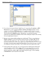
AlphaVision®-32 v5.6 (A36-B32)
Click on NWLink IPX/SPX/
NetBIOS Compatible Transport
Protocol, then click on OK to
return to the Local Area Connection Properties dialog (Fig. 48).
Fig. 47. Choose the Correct Protocol.
Select NWLINK IPX... as shown, then click on
Properties to open the dialog shown in Fig. 49.
Fig. 48. LAN Properties.
40
2. INSTALLATION AND CONFIGURATION
Set the Frame type to 802.3 as shown, then
click on OK, Close, and Close to return to
the Windows desktop.
Fig. 49. Choose the Correct Frame Type.
41
AlphaVision®-32 v5.6 (A36-B32)
42
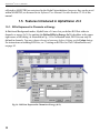
3. USING THE ALPHAVISION 5.x USER
INTERFACE
This chapter presents an overview of the new AlphaVision v5.6 user interface. For more indepth discussion of the screen features, refer to the HTML Help Manual.
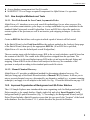
3.1. Startup and Login
To start AlphaVision, go to the Windows
Taskbar and click on Start, Programs,
AlphaVision 5.6, AlphaVision 5.6. The
login dialog will open (Fig. 50). The default
User Name from the factory is ORTEC (all
Fig. 50. Log In.
uppercase; note that AlphaVision usernames
and passwords are case sensitive). The default
password associated with ORTEC for login is o (lowercase letter o, not zero).
The default username and password are assigned to the Administrator security level, giving you
access to all AlphaVision v5.6 commands and operations. After initial login you can choose to
define additional security levels (Edit/Security Levels...) and set up new usernames and
passwords (Edit/Users...), or simply continue using the default login.
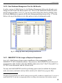
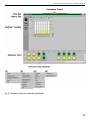
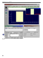
3.2. The User Interface
The AlphaVision v5.6 user interface is designed so all sample, reporting, hardware, and QA
management is accessible from the main AlphaVision screen with a few mouse clicks. The
screen is divided into 3 main functional areas:
1. Outlook Toolbar — The Outlook Toolbar contains icons for each of the 4 modules
(Calibration, Batch, Hardware, and QA/QC).
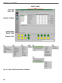
2. Detector Grid — At the bottom of the screen, the Detector Grid displays the detectors that
are currently configured for your system. The rows and columns have spreadsheet-style
headers to help you quickly locate a particular instrument. From the grid you can add,
remove, and organize MCBs and detectors; pause or stop data acquisition; clear detector
memory; adjust grid and system properties; and start MAESTRO-32 (if you choose to install
it). See the tutorial in Chapter 5 for instructions on adding detectors to the Detector Grid.
Pausing the mouse over a detector icon in the grid opens a hover box that shows the alpha
chamber and detector names, real and live times, and, when the detector is counting, the
batch and sample names.
43
AlphaVision®-32 v5.6 (A36-B32)
3. Explorer Panel — The remainder of the screen is the Explorer Panel. This is the gateway to
all of the data analyses in your AlphaVision v5.6 database.
! In Calibration and Batch modes, this panel is divided into 2 parts: The lower section,
the Spectrum/Report Window, enables you to view either the spectrum or report for a
given analysis. The upper section is, respectively, the Calibration Explorer Panel or
Batch Explorer Panel.
— The Calibration Explorer allows you to display the calibration history for each
detector in the system, and the Calibration Reports associated with each calibration
spectrum and analysis. To see this calibration history, click on one of the detectors in
the Detector Grid. The most recent calibration (i.e., the calibration now being used by
this detector) will be displayed in the Spectrum Window. Note that if you have not yet
calibrated the detector, no data will displayed for it.
— The Batch Explorer allows you to locate and view the records and reports for your
Batch, Background, and Pulser Test batches, samples, spectra, and analyses.
! In QA/QC mode, the Limits tab allows you to set up and monitor the QA control limits
and Control Charts. The Charts and Report tabs at the bottom of the panel let you
generate, view, and print the Control Charts and QA Reports.
! The Hardware Panel allows you to set up and monitor only the alpha chambers of
ORTEC Aria, Duo, Ensemble, and OCTÊTE-series instruments; and the Oxford OASIS.
To set up and monitor other instruments, you must use MAESTRO.
The commands on the File, Edit, View, and Help menus remain the same in all modules. In
addition, each module except Hardware has its own menu(s) containing unique commands. The
Outlook Bar and Detector Grid remain the same from module to module.
Figures 51 through 54 show annotated illustrations of the Calibration, Batch, Hardware, and
QA/QC interfaces and menus, respectively.
44
3. USING THE ALPHAVISION 5.x USER INTERFACE
Fig. 51. Calibration Mode Screen Features and Menus.
45
AlphaVision®-32 v5.6 (A36-B32)
Fig. 52. Batch Mode Screen Features and Menus.
46
3. USING THE ALPHAVISION 5.x USER INTERFACE
Fig. 53. Hardware Mode User Interface and Menus.
47
AlphaVision®-32 v5.6 (A36-B32)
Fig. 54. QA/QC Mode Screen Features and Menus.
48
3. USING THE ALPHAVISION 5.x USER INTERFACE
3.2.1. The Calibration Explorer Panel
The Calibration Explorer Panel (Fig. 55) is your tool for viewing and evaluating the results of
detector calibrations in the AlphaVision database. This panel lists the calibration history for the
selected detector (click on its Detector Grid icon). Note that if the detector is not yet calibrated,
no records for it will be displayed in the Calibration Explorer. Calibration records include data
such as the record Name, acquisition Date, Calibration ID, Gain, Offset, and Efficiency.
Fig. 55. The Calibration Explorer Panel.
The Calibration Explorer also allows you to Update a calibration, that is, to reanalyze the
calibration spectrum. You can also permanently remove the results from the calibration history.
These features enable you to correct errors such as entering an incorrect calibration source for
the calibration. The Update command allows you to change the calibration parameters and
create an updated calibration from the resulting analysis. Note that updating a calibration adds a
data point to the corresponding QC Chart to ensure that QC data integrity is preserved.
The Calibration Explorer tells at a glance which calibrations match the selected detector’s
current geometry/alpha-chamber shelf position; which calibrations have been analyzed and
completed vs. those still being acquired and analyzed; and which is the detector’s current
active/working calibration. In addition, you can start acquisition for a calibration that has been
set up but not yet counted, remove calibrations that are no longer needed, and update a
calibration setup to correct data entry errors.
49
AlphaVision®-32 v5.6 (A36-B32)
3.2.2. Accessing Batch, Background, and QA Data in the Batch Explorer Panel
The Batch Explorer Panel (Fig. 56) is your primary organizational tool for and portal to the
sample information in your AlphaVision database. It is also your point of access to data
imported from earlier versions of AlphaVision, instrument background records, and QA pulser
test spectra.
Fig. 56. The Batch Explorer Panel’s Components, the Batch Explorer Tree and Sample
Analysis Explorer.
The Batch Explorer Panel is an intuitive, visual representation of all your batch, background,
and QA data, organized hierarchically in levels and sublevels that you define. (Calibration data
are displayed separately in the Calibration Explorer Panel.) Your ability to modify the database
from this panel is limited; for instance, you can’t click, drag, copy, cut, paste, rename, or delete
records from it. For these kinds of operations, see the suite of database management tools
(Section 3.2.2). However, the Batch Explorer Panel provides tools for revising sample
information created in the Batch Wizard, counting batches or samples that have not been
counted yet, recounting batches or samples, analyzing existing spectra, and updating (i.e.,
overwriting) existing analyses.
The tutorial and the HTML Help Manual give detailed instructions on adding new organizational “branches” to the Batch Explorer Tree; locating analysis records; changing acquisition
presets; modifying sample properties; and counting, analyzing, and reanalyzing from the Batch
Explorer.
3.2.2.1. Hiding or Displaying Branches in the Batch Tree
It doesn’t take long to fill the Batch Tree with the entries for completed projects. To keep your
Batch Tree uncluttered and easy to read, AlphaVision v5.6 lets you hide or display one or more
of the branches in the tree. This is a 2-step process in which you flag all of the branches you
wish to hide, then hide them all with a single command.
50
3. USING THE ALPHAVISION 5.x USER INTERFACE
To flag a branch for hiding, right-click on it and select Hide Branch. To then hide the flagged
branches, go to the View menu and click on Hide Branch. All flagged branches will be
removed from view, and a checkmark will be displayed beside the command on the View menu.
To redisplay the flagged branches, just issue the View/Hide Branch command again (this will
also remove the checkmark from beside the command on the menu). To unflag a branch so that it
is no longer affected by the hide command, right-click on it and select Un-Hide Branch. You
can flag/unflag and hide/display as many branches as you wish, and at any time.
The next three figures illustrate this process. Figure 57 shows the January branch being flagged
for hiding. In Fig. 58, the View/Hide Branch command is issued, and Fig. 59 displays the result
— the January branch is no longer visible in the Batch Tree, although its entry is still fully
retained in the database and accessible by unhiding it.
Fig. 57.
Fig. 58.
Fig. 59.
Another way to simplify your Batch Tree is to create a new database for each project with the
File/Database Management... tools (see Section 3.2.2).
3.2.3. The QA/QC Panel
The QA/QC Panel (Fig. 60) is your access to the QA control limits, Control Charts, and QA
Reports. Background and Pulser QA spectra, analyses, and analysis reports are available through
the Batch Explorer Panel.
The QA window has 3 views governed by the tabs at the bottom of the panel (click on the
appropriate tab):
! Limits — This view (shown in Fig. 60) contains 5 tabs for establishing the Low and High
Warning limits and the Minimum and Maximum Error limits for all detectors, tracers, and
QA Types. The tab you select here governs which Control Chart and QA Report will be
respectively generated in the Chart and Report views.
51
AlphaVision®-32 v5.6 (A36-B32)
Fig. 60. The QA Panel, Detectors Tab.
! Chart — QA data are displayed on charts that can be produced for weekly, monthly,
quarterly, yearly, project lifetime, or customized intervals. These charts display both the data
and the set limits for each QA parameter, and update in real time as new information is added
to the AlphaVision database. The appearance of the Control Charts is tied directly to the set
points entered on the Limits tab. Error limits are drawn in red long dashes and Warning
limits in blue short dashes.
! Report — This opens the standard Report Window. QA Reports include a picture of the
associated Control Chart, the QA limits, and the mean and standard deviation of the data
displayed.
3.2.4. The Library, Tracer, ROI, and QA Type Editors
These are covered in detail in the HTML Help Manual, and their use is detailed in the Chapter 5
tutorial.
3.2.4.1. The Library Editor
There are three major types of AlphaVision libraries, accessible from the Edit menu:
! The Master Nuclide Library of alpha-particle-emitting nuclides, supplied with
AlphaVision v5.6 (Edit/Master Nuclide List...).
! The Analysis libraries including AlphaMaster (Edit/Nuclide Libraries...).
! Libraries for calibration sources and libraries for stock control solutions (Edit/Standards...).
52
3. USING THE ALPHAVISION 5.x USER INTERFACE
AlphaVision libraries contain the nuclide name, half-life, alpha-particle peak energies, and
branching ratios for each constituent. The Master Nuclide Library is a compilation of nuclear
data from PCNuDat (National Nuclear Data Center, Brookhaven National Laboratory).
There is no limit to the number of peak energies per nuclide (unlike earlier versions of
AlphaVision, which were limited to four peaks per nuclide). The nuclide peak with the highest
branching ratio is used for the peak search.
Building Libraries
The AlphaVision v5.6 nuclide library
interface is intuitive and takes just
seconds to use. From inside the
calibration and analysis library editors,
simply open the master list, click on
the nuclides you want (Fig. 61), then
click on OK — the hardest part may
be choosing the new library’s name.
For peak-search-and-fit analyses,
we recommend that you create libraries
that match as closely as possible the
expected nuclides in the samples. This
is because the AlphaVision peak-search
algorithm looks through the analysis
Fig. 61. Select Library Nuclides With a Few Mouse Clicks.
library for the peak closest in energy to
the identified peak in the spectrum. Too
many nuclides with close or overlapping alpha-emission energies may lead to misidentification
of a peak. In addition, while you will not require a large number of libraries for routine work, we
suggest that you create different libraries for each analyte type (e.g., Am, Pu, U, Th).
If you know that each alpha peak in your sample is well separated from the others, you may not
have to create specialized analysis libraries. In this case, because AlphaVision v5.6 can sum the
branching ratios included within a region of interest (ROI), all you might need is the Master
Library. Just select it within the sample processing wizards and let AlphaVision do the rest.
Once you have created a library in AlphaVision, you can quickly customize it by adding or
removing peak energies and changing energy values. When the library is no longer needed, you
can delete it.
53
AlphaVision®-32 v5.6 (A36-B32)
3.2.4.2. The ROI Editor
To open the ROI Editor, click on
Edit/ROI... or click on ROI Setup
on the Analysis Setup page in the
Batch or Background Wizard.
You can also open the ROI Editor
during manual calibration. This
dialog enables you to:
! Create a new ROI Set manually
by entering the ROI start and
end channels from the keyboard
or interactively in conjunction
with the mouse and a displayed
spectrum.
Fig. 62. Select Library Nuclides With a Few Mouse Clicks.
! Edit an ROI Set manually or
interactively, as described in Chapter 5.
! Define the peaks in the ROI Set in terms of channels or energy.
! Delete an ROI Set.
! Designate specific ROI Sets as ROI templates or non-templates, and use these designations
to filter the ROI Set droplist for the two categories of ROI records.
Instructions for creating and editing ROI Sets begin on page 85.
3.2.4.3. The QA Type Editor
AlphaVision uses QA Types (Edit/QA Types...; Fig. 63) as tools for tracking the recovery
history of tracers and control samples, and the count rate of reagent blanks for specific projects.
There are three QA Types:
! Chemical Recovery — Tracks the chemical recovery (or yield) of a tracer, and is selected at
the Batch Properties level. It allows you to quickly discriminate between different sample
types within a project, and between similar (but perhaps not quite identical) sample types for
different projects.
! Control Sample — Tracks the recovery of control standards for specific projects, and is
selected at the Sample Properties level. In conjunction with Control Solution records, it
54
3. USING THE ALPHAVISION 5.x USER INTERFACE
allows you to create one Control Solution for a given element and vary the volume added
from batch to batch within 1 or more projects. AlphaVision v5.6 tracks the recovery
regardless of the volume added from batch to batch.
! Reagent Blank — Tracks the count rate
of batch blanks for specific projects, and
is selected at the Sample Properties level.
Creating QA Types
To create a QA Type, assign a name to the
new type, select which category of QA Type
you are creating, and enter a descriptive title
Fig. 63. Create QA Types to Track Recoveries and
for the corresponding QA Control Chart that
Count Rates.
will display the recovery history for this new
type. For Control Samples and Reagent Blanks,
you must also select an appropriate nuclide library to be used in determining nuclide recoveries.
Create as many instances of each QA Type as you wish, at any time.
Each time you create a new Control Sample or Reagent Blank QA Type, and before analyzing
samples that use the new QA Type, go to the corresponding Control Sample and Reagent Blank
tabs on the QA/QC Panel, select the new QA Type, choose the Nuclides, and enter limits for
them. This activates AlphaVision’s automatic QA records update for these two QA Type
categories.
3.2.5. The Analysis Setup Wizards
AlphaVision v5.6 has four wizards (see the Process menu in Batch, Calibration, and QA
modes) to guide you, step by step, through the setup of all parameters for Batch, Background,
Calibration, and Pulser Test data acquisition and analysis. These wizards allow you to streamline
the repetitive aspects of sample analysis by creating special records called templates that hold
customized sets of data acquisition parameters, analysis specifications, and reporting
preferences. Once you’ve created the templates you need for your various projects, start one of
the wizards, choose the template you wish to use, enter the batch- and/or sample-specific data,
and you’re ready to start data collection.
55
AlphaVision®-32 v5.6 (A36-B32)
3.2.6. Data Acquisition Controls
AlphaVision v5.6 gives you 7 tools for controlling data acquisition:
1. The Calibration acquisition is performed on the detector currently selected (outlined in blue)
on the Detector Grid. It starts automatically when you click on Finish in the Calibration
Wizard, unless you specify otherwise on the first page of the Calibration Wizard.
2. If you choose to delay the count, you can count later in the Calibration Explorer Panel.
Right-click on a calibration record that shows a New status and select Start from the
right-mouse-button menu.
3. Batch, Background, and Pulser QA Test acquisitions use one or more detectors at a time.
They are normally started from the Detector Assignment Worksheet, which enables you to
assign detectors to samples either manually or automatically and then start acquisition.
4. Alternatively, you can choose to delay the count, then count later in the Batch Explorer
Panel. In the Batch Explorer Tree (the left side of the Batch Explorer), right-click on the
batch of interest, and select Count from the right-mouse-button menu. This will count or
recount the entire set of samples. You can also select a batch, go to the Sample Analysis
Explorer (the right side of the Batch Explorer) and choose 1 or more samples (not spectra or
analyses) for a recount, then right-click and select Count from the right-mouse-button
menu.
5. AlphaVision v5.6 allows you to perform “on-the-fly,” interim analyses during data
acquisition. In the Batch Explorer, right-click on the batch of interest to display its samples.
Right-click on a sample and select Interim Analysis.... AlphaVision performs an analysis
and records a “snapshot” of the spectrum at this point in the count. The interim analysis is
displayed in the Sample Explorer Panel along with the regular analysis results, and becomes
a permanent part of the data record for the batch. You can perform a new interim analysis
approximately every 5 minutes.
6. Modify Acquisition Presets allows you to increase or decrease Live Time and/or Real Time
presets for an entire set of Batch samples, Background measurements, or Pulser QA Tests.
On the Batch Explorer Panel, locate and right-click on the batch record you want, then
right-click and select Modify Acquisition Presets from the right-mouse-button-menu.
7. The Detector Menu (right-click on a detector icon) provides the final set of acquisition
controls: Pause, Continue, Abort, Stop, and Clear detector memory. These operate only on
the currently selected detector.
56
3. USING THE ALPHAVISION 5.x USER INTERFACE
3.2.7. The Spectrum Window
The Spectrum Window is available only in Batch and Calibration modes. To display it, click
on the Spectrum tab at the bottom of the Batch or Calibration Explorer Panel.
3.2.7.1. Right-Mouse-Button-Menu
Right-clicking in this window opens a menu (see Fig. 64) that allows
you to Zoom In to see more spectrum details; return to a Full
View of the spectrum; display the full-spectrum-view Thumbnail
Window, the Residuals Spectrum, and/or the ROI Bars (which
mark the start and end channels of each ROI); modify an existing ROI
Set for a sample reanalysis (Interactive ROI Analysis, discussed in
Section 1.5.5.2); and adjust the spectrum display Properties....
Figure 65 shows the Thumbnail, Residuals Spectrum, ROI Bars, and
right-mouse-button menu.
Fig. 64. The RightMouse-Button Menu.
Fig. 65. Spectrum Window Features in Batch Mode.
Note the Marker Information Line at the bottom of the Spectrum Window. It reports the position
of the vertical marker line (located in the 242Pu peak in this illustration), including the marker
location in channels and energy, the counts in the current channel, and any ROI and/or nuclide
57
AlphaVision®-32 v5.6 (A36-B32)
identification information. Sections 3.2.7.3 and 3.2.7.3 describe the accelerator keys that move
the marker and adjust the spectrum’s horizontal and vertical scaling.
Figure 66 shows the dialog for the Properties command. It allows
you to change Spectrum Window colors.
If the detector for the current spectrum was calibrated when the
spectrum was acquired, the spectrum will be displayed in energy
units (keV or MeV). If the detector was uncalibrated, the spectrum
will be displayed in channels. If you are viewing a spectrum
analysis, clicking on the Report tab at the bottom of the Spectrum
Window opens the Report Window and generates the associated
report. (Both the Calibration and Analysis Reports include a picture
of the analysis spectrum.)
3.2.7.2. Zoom Commands on the Right-Mouse-Button Menu
Fig. 66. Change Spectrum
The Zoom In command gives you a second way — in addition
Colors.
to the Thumbnail view — to take a closer look at your spectra. In
the Spectrum Window (not the Thumbnail), click and drag the
mouse pointer over a portion of the spectrum to surround it with a rubber rectangle, then release
the mouse button. The Spectrum Window will automatically adjust the horizontal and vertical
scaling to display the area enclosed in the rubber rectangle.
To zoom out to a view of the entire spectrum, simply right-click in the Spectrum Window and
select Full View. The window scaling will adjust to display the entire horizontal and vertical
extent of the spectrum.
3.2.7.3. Scaling and Cursor Movement Features
For your convenience, the AlphaVision v5.6 spectrum window now use many of the horizontal
and vertical scaling and cursor movement keys employed in MAESTRO.
NOTE These accelerators function only when the Thumbnail window is closed.
Next Channel
<6>/<7>
The right and left arrow keys move the marker by one displayed pixel in the corresponding
direction. If you have zoomed in, expanding the horizontal scale, when the marker reaches the
edge of the spectrum window, the next key press past the edge shifts the window to the next
block of channels in that direction such that the marker is now in the center of the display.
58
3. USING THE ALPHAVISION 5.x USER INTERFACE
Zoom In/Zoom Out
Keypad<+>/<->
Keypad<+> decreases the horizontal scale in the Expanded Spectrum View so the peaks appear
larger, and Keypad<-> increases the horizontal scale, making the peaks look smaller.
Taller/Shorter
<8>/<9> and <F5>/<F6>
The <8> and <9> keys decrease or increase the vertical full scale of the displayed spectrum so
the peaks appear taller or shorter, respectively.
Narrower/Wider
<F7>/<F8>
These keys increase or decrease the horizontal scale of the data display so the peaks appear
narrower or wider, respectively.
Use the Full View command to restore the spectrum to its default scaling.
3.2.8. The Report Window
All AlphaVision v5.6 reports share the same type of Report Window (Fig. 67), which allows you
to view, print, or export the report data to a variety of formats (see the HTML Help Manual for
more information on export formats). AlphaVision’s reports are completely dynamic. That is,
previously generated reports are not stored; they generate directly from the pertinent analysis
record(s) each time you click on the Report tab.
To view reports:
! Zoom in on the desired spectral feature(s) that you wish to display on page 1 of the report.
Otherwise, to display the entire spectrum, right-click in the Spectrum Window and choose
Full View. Note that the Nuclide Summary section of the report will always contain the
information for all ROIs in the spectrum, not just the ROIs currently displayed in the
Spectrum Window.
! Go to the bottom of the center panel in Calibration, Batch, or QA/QC mode and click on
the Report tab (alternatively, you can click on Report after you have selected the analysis
you wish to view).
! In Calibration mode, click on a detector, then go to the Calibration Explorer and select the
calibration you wish to view. This will generate the report.
59
AlphaVision®-32 v5.6 (A36-B32)
Fig. 67. The Report Window.
! In Batch mode, go to the Batch Explorer Panel and locate the analysis you wish to view (not
the spectrum ). Click on the analysis entry to generate its report.
! In QA/QC mode, run the QA test (if necessary) then click on the tab for the test you wish to
view.
! For the hardware tests (calibration, pulser, background, bias, chamber pressure), go to the
Detectors tab and select a particular detector, then click on the radio button for the test
parameter you want. The report will generate.
! For Control Sample, Reagent Blank, and Chemical Recovery tests, click on the tab you want,
then select a particular QA Type from the list. The report will generate.
60
3. USING THE ALPHAVISION 5.x USER INTERFACE
3.2.8.1. Report Export Formats
AlphaVision v5.6 reports can be exported in the following formats:
!
!
!
!
!
!
!
!
!
Adobe Acrobat (.PDF)
Crystal Reports (.RPT)
HTML 3.2
HTML 4.0
Microsoft Excel 97/2000 (.XLS)
Excel 97/2000, data only (.XLS)
Microsoft Word (.RTF)
Microsoft Word, rich text (.RTF)
ODBC
!
!
!
!
!
!
!
!
Record style, columns with spaces (.REC)
Record style, columns without spaces (.REC)
Report definition (.TXT)
Rich text format (.RTF)
Separated values (.CSV)
Tab-separated text (.TTX)
Text (.TXT)
.XML
3.2.9. The Event Window
The Event Window (View/Event Window), shown in Fig. 68, is AlphaVision’s error and system
tracking tool. AlphaVision uses this method instead of standard popup messages to streamline
your interactions with the software when running numerous samples simultaneously. The Event
Window records software events, their severity (Information, Warnings, and Errors), the
software module in which the events occurred, and the date and time for occurrences including:
!
!
!
!
!
!
!
!
Calibration failures
Analysis failures
QA warning or error limits exceeded
Start and end of data collection
Counting interrupted when a detector chamber exceeds pressure or leakage current limits
Counting resumes when detector chamber returns within pressure and leakage current limits
Detector is taken out of or returned to service
Instrument Configuration program used to update the Master Detector List
We strongly recommend that you routinely check the Event Window during and after data
acquisition, analysis, and QA/QC. If you wish, you can leave this window open, resize it, and
move it to an unused part of the screen (click and drag on the title bar).
61
AlphaVision®-32 v5.6 (A36-B32)
Fig. 68. The Event Window.
3.2.10. MCA View — Open MAESTRO From Within AlphaVision
If MAESTRO-32 is installed on the host PC (see Section 1.4.11), the MCA View command is
available from the Detector Grid. A full-featured session of MAESTRO-32 opens in an
independent window and runs concurrently with AlphaVision. This gives you the flexibility to
collect data and analyze spectra outside of AlphaVision. It lets you perform quick counts for
methods development work, test sources, and source activity checks. These data are not stored in
the AlphaVision database, but can be saved in a number of formats including .SPC files and
ROI Reports, as described in the MAESTRO Software User’s Manual. (And, if you wish, you
can then import the .SPC files into AlphaVision with the File/Import... command.)
To use this command, right-click a detector icon on the Detector Grid, and choose MCA View
from the right-mouse-button menu. This starts MAESTRO and displays the contents of the
selected detector. To monitor another AlphaVision detector in MAESTRO, just right-click on
another detector icon and select MCA View again. To close the MAESTRO window, click on
its File/Exit command or its upper-right × (Close) box.
62
4. DATA MANAGEMENT OVERVIEW
Data management is key to (1) maintaining a comprehensive chain of custody over your clients’
samples and (2) keeping control of hundreds of data records. AlphaVision v5.6's data
management tools include:
! The interface between your LIMS and the AlphaVision v5.6 database (Section 4.1).
! The Select Database command on the File menu (Section 69), which allows you to easily
switch between target databases for your batch and background results, libraries, templates,
calibrations, QA results, and all other entries.
! The database management and archival tools discussed in Section 4.3.
! The Batch Explorer Panel — gateway to all of the sample, background, and QA information
in the AlphaVision v5.6 database (Section 3.2.2).
! The Calibration Explorer Panel — access to all calibration information in the database
(Section 3.2.1).
! The QA/QC Panel — your access to the QA control limits, Control Charts, and QA Reports
(Section 3.2.3).
! Exporting analysis results (Section 4.4).
! Importing data from previous versions of AlphaVision (Section 4.5).
NOTE DO NOT attempt to modify the AlphaVision database! Use only the LIMS interface
tables discussed in Section 4.1. We encourage you to query the database, and it’s easy
to set up your own tailored Crystal Report formats. However, if you must “explore” the
database, make a copy of AlphaVision.mdb and explore that copy! We of course also
recommend that you frequently make a backup copy of your database.
4.1. The LIMS-to-AlphaVision-Database Interface
AlphaVision v5.6 gives you the unique ability to interface alpha-spectrometry software with
your Laboratory Information Management System (LIMS). The AlphaVision database includes
LIMS-interface tables that are linked with the Batch Wizard. You can upload the data in these
tables from your LIMS, reducing the number of transcription errors as well as the time needed
for batch setup within the Batch Wizard. The batch analysis results in the AlphaVision database
are linked referentially to the input parameters. After sample counting and analysis, these data
can be easily extracted and transferred to your LIMS. Some knowledge of databases, Microsoft
Access, and database programming are required. Your LIMS administrator will have to create
63
AlphaVision®-32 v5.6 (A36-B32)
the link between your LIMS and the AlphaVision v5.6 database. You are allowed to modify only
two AlphaVision tables, LIMS-Batches and LIMS-Samples, as described in Section 4.1.1.
There’s a one-to-many relation between the LIMS-Batches to LIMS-Samples records, so the
idea is that, through your LIMS, you will first input a new Batch record, fill it in with the desired
batch- and sample-level information, then add all of its component samples to the
LIMS-Samples table, setting the BatchID field to the new batch record’s ID.
4.1.1. How the Process Works
As a batch of samples arrives at your laboratory, enter the batch and sample information into
your LIMS. These data will be transferred to the AlphaVision v5.6 database through a process
created by your LIMS administrator.
1. Start the Batch Wizard and on Screen 1, General, open the Load from LIMS droplist, pick
one of the Batch IDs that were entered in your LIMS, then click on Next.
2. On the Batch Properties screen, you must choose the location in the Batch Explorer Tree
where this batch will be displayed. (The LIMS/AlphaVision interface cannot perform this
task for you.)
3. If the Client information and User-defined keys were entered in the LIMS, this information
will already be present at the bottom of the Batch Properties screen. If it is not present, you
can enter it at this time. Click on Next.
4. On the Sample Properties screen, the sample information will already be displayed (if it was
entered in the LIMS). Any information that was not entered into the LIMS can be entered at
this time.
5. You may wish to click on each of the samples in the batch and confirm their individual
sample properties. Modify as necessary, then click on Next.
6. If you are using a template that includes all of the acquisition, analysis, and reporting options
you want, you can now click on Finish. If you are not using a template or if you need to
make changes to the current template’s settings, continue through the remainder of the
wizard.
7. When you click on Finish, if the AutoDelete flag in the LIMS-Batches table is Yes(True),
the batch and all its samples will automatically be cleared from the interface tables so they’re
ready for the next data transfer (this step affects only the data-transfer tables and does not
affect the other information in your LIMS or AlphaVision database).
64
4. DATA MANAGEMENT OVERVIEW
8. The Detector Assignment Worksheet will open so you can assign detectors.
9. Click on the Start Now button.
4.1.2. LIMS/AlphaVision Interface Tables
4.1.2.1. LIMS-Batches
This information loads into the Batch Properties screen.
Field Name
Data Type
Description
ID
AutoNumber
Used for record sequencing only.
Name
Text (50 chars)
Name of this batch of samples.
QAType
Text (50 chars)
Name of Chemical Recovery Type for this batch (must be
exactly the same as the QA Type name created in
AlphaVision). Leave blank for no Chemical Recovery
Type.
Template
Text (50 chars)
Name of Template to use for this batch (must be exactly the
same as the batch Template name created in AlphaVision).
Leave blank for no Template.
Description
Memo
Description of this batch.
ClientInfo
Text (50 chars)
Name of Client info for this batch (must be exactly the
same as the Client Name created in AlphaVision). Leave
blank for no Client Information.
User1Key
Text (50 chars)
User-defined Key.
User1Value
Text (50 chars)
User-defined Value associated with the Key.
CreationDate
Date/Time
Date/Time when this batch was created
AutoDelete
Yes/No
The default for this value is TRUE. When TRUE, the batch
and its samples will be deleted from this table when their
data have been transferred and are no longer needed.
EditTracerInSamplePage
Yes/No
65
AlphaVision®-32 v5.6 (A36-B32)
4.1.2.2. LIMS-Samples
This information loads into the Sample Properties screen.
Field Name
Data Type
Description
ID
AutoNumber
Used for record sequencing only.
BatchID
Number (Long)
Numerical ID for this batch of samples.
Name
Text (50 chars)
Sample name
Type
Number (Long)
One of the following values: 0 = Sample, 1 = Blank,
2 = Control, 3 = Background, 4 = Pulser
CollectionDate
Date/Time
UseCollectionDate
Yes/No
DecayCorrDate
Date/Time
UseDecayCorrDate
Yes/No
LabPrepDate
Date/Time
UseLabPrepDate
Yes/No
Volume
Number (Single)
VolumeUnits
Number (Long)
One of the following values: 0 = L, 1 = mL, 2 = µL,
3 = m3, 4 = cm3, 5 = ft3, 6 = in3
VolumeUnc
Number (Single)
Uncertainty in percent
Weight
Number (Single)
WeightUnc
Number (Single)
WeightUnits
Number (Long)
One of the following values: 0 = g, 1 = kg, 2 = mg, 3 = µg
Aliquot
Number (Single)
Aliquot volume
AliquotUnc
Number (Single)
Uncertainty in percent
Comments
Text (255 chars)
Per-sample comments
QATypeID
Number (Long)
Name of QA Type for this sample (must be exactly the
same as the QA Type name created in AlphaVision).
BulkVolume
Number (Double)
BulkSourceID
Number (Long)
User1Key
Text (50 chars)
User- defined key 1
User1Value
Text (50 chars)
User- defined value associated with key 1
66
4. DATA MANAGEMENT OVERVIEW
Field Name
Data Type
Description
User2Key
Text (50 chars)
User- defined key 2 (does not appear on default report)
User2Value
Text (50 chars)
User- defined value associated with key 2 (does not
appear on default report)
IsVolume
Yes/No
If using volume select TRUE; if weight select FALSE
UseAliquot
Yes/No
TRUE if using an aliquot
TracerAmountDefined
Yes/No
If TRUE, tracer amount is defined for this sample in this
table. Set to TRUE only if tracer amount for each sample
is different.
TracerAmount
Number (Single)
Tracer amount in mL for this sample
TracerAmountUncPct
Number (Single)
Tracer amount uncertainty for this sample
UseDilution
Yes/No
If TRUE, this sample has been diluted
Dilution1
Number (Single)
The first dilution factor (D1)
Dilution1UncPct
Number (Single)
The first dilution factor (D1) uncertainty
Dilution2
Number (Single)
The second dilution factor (D2)
Dilution2UncPct
Number (Single)
The second dilution factor (D2) uncertainty
Aliquot2
Number (Single)
The second aliquot amount
Aliquot2UncPct
Number (Single)
The second aliquot amount uncertainty
NOTES
1. If tracer has been defined for a sample in batch, it must be defined for all other smaples of
the same batch
2. There is an example program on the CD called MiniLIMS with source code in Visual C++
which can help users to populate this table.
3. The first aliquot amount is in the field Aliquot (instead of Aliquot1).
4.2. Select Database
The new Select Database... command on the File menu allows you to select the target
AlphaVision v5.x database for your project measurements. Now it’s fast and easy to store all of
the batch and background results, libraries, templates, calibrations, and QA results for a specific
project in its own database, simplifying Batch Tree construction and project records archival.
When an AlphaVision data acquisition or analysis is in progress, this command is disabled.
67
AlphaVision®-32 v5.6 (A36-B32)
To switch to a different database, click on File/Select Database... to open a standard Windows
file-open dialog (Fig. 69). Choose a valid AlphaVision v5.x database and click on Open.
AlphaVision will notify you that it must close and reopen to put the change into effect. Click
Yes to automatically exit and restart AlphaVision. Click No to manually exit and restart.
NOTE AlphaVision v5.6 can use only
databases created with the new
Database Management archive
tool or cloned from an existing
AlphaVision database.
Fig. 69. Selecting a New Target AlphaVision Database.
4.3. Database Management
The Database Management... command is located on the File menu. Figure 70 shows the
Database Management dialog, which allows you to:
! Archive the current database by saving a copy in .MDB file format (giving you a “snapshot”
of the current database contents). This archive database can then be recalled at any time with
the File/Select Database... command.
! Permanently delete one or more sample records from within a batch or delete an entire batch.
This, in conjunction with the Batch Explorer, allows you to tailor the contents of your
databases as needed.
! Compact a database to recover disk space after deleting records.
The dialog’s titlebar shows the name of the current target database. To select a different
database, use File/Select Database....
The branches in the left-hand panel of the Database Management dialog mirror those in the main
screen’s Batch Explorer, with two exceptions: Unlike the Batch Explorer, this dialog displays
the various template records (
) in the current database, and, except for calibrations,
68
4. DATA MANAGEMENT OVERVIEW
you can remove them as needed. However, imported records (
because, once imported, they cannot be deleted.
) are not shown here
Fig. 70. Database Management Dialog, Showing Current Target Database.
The Status indicator in the lower right corner will indicate whether a deletion, archival, or
compaction is in progress.
Click on Done to return to AlphaVision.
4.3.1. Deleting Records
Note that calibrations cannot be deleted, however, you can delete calibration templates using this
dialog. In addition, you cannot remove a background that is in use by an analysis (you will
receive an “Unable to delete some or all of the selected records. Background spectrum is used by
other samples” message). You must first delete all the samples using that background.
To remove one or more sample measurements
from the database, use the left-hand explorer
panel to locate the batch, then click on the batch
to display its component samples in the righthand panel. Click on the sample to highlight it,
then click on Delete. A message box will ask you
Fig. 71. Deleting One or More Sample
Records.
69
AlphaVision®-32 v5.6 (A36-B32)
to confirm the deletion (Fig. 71). To remove more than one sample at a time, use <Shift +
Left-click> to highlight a contiguous block of measurements or <Ctrl + Left-click> to highlight
discontinuous measurements, then click on Delete.
To remove an entire batch,
click to highlight it but do
not highlight any of the
samples within the batch,
then click on Delete. A
message box will ask you to
Fig. 72. Deleting an Entire Batch.
confirm the deletion (Fig. 72).
While you can remove multiple samples from a batch at one time, you can only delete one batch
at a time.
IMPORTANT There is no undo for a deletion. We strongly recommend that you archive
your database before deleting any records!
Once you have removed all of the batches in a branch, you can use the Batch Explorer to remove
the branch; see Section 3.2.2.
4.3.2. Archiving a Database
To create a backup of the current database, click on Archive... to open a standard Windows filesave dialog (Fig. ?). Enter the path and filename you wish to use and click on Save.
4.3.3. Creating a “Clean” AlphaVision Database
If, after installation, you did not create a copy of the default, empty AlphaVision database for
future use, you can use the Archive and Delete features together with the Batch Explorer to
create a new, “clean” database for your next project. The AlphaVisionDemo.mdb file is a
convenient starting database. Create a backup copy of it with the Archive feature, choose it as
your target database with File/Select Database..., restart AlphaVision, use the database
management tools to remove all records from it, then the Batch Explorer to remove all unwanted
branches. You now have a blank AlphaVision database, ready to use.
4.4. Exporting Analysis Results from the
Report Display Window
AlphaVision v5.6 allows you to export analysis results to a variety of destinations in the
following formats:
70
4. DATA MANAGEMENT OVERVIEW
!
!
!
!
!
!
!
!
!
Adobe Acrobat (.PDF)
Crystal Reports (.RPT)
HTML 3.2
HTML 4.0
Microsoft Excel 97/2000 (.XLS)
Excel 97/2000, data only (.XLS)
Microsoft Word (.RTF)
Microsoft Word, rich text (.RTF)
ODBC
!
!
!
!
!
!
!
!
Record style, columns with spaces (.REC)
Record style, columns without spaces (.REC)
Report definition (.TXT)
Rich text format (.RTF)
Separated values (.CSV)
Tab-separated text (.TTX)
Text (.TXT)
.XML
These formats are available through the Report Display Window by clicking on the Export
Reports icon on the top left of the Report Window. In addition, you can set up the Report
Properties page of the four wizards to export reports to Excel 8.0, HTML 4, rich text format,
text, Microsoft Word, .PDF, tabbed text, and .XML.
For an animated example of how to export your results, see Exporting Analysis Results in the
HTML Help Manual.
4.5. Importing Older AlphaVision .SPC Files
Use the File/Import... command to import your older AlphaVision .SPC files into the new
AlphaVision v5.6 database, one or more files at a time. Once you’ve imported older data, it’s
quick and simple to analyze them within AlphaVision v5.6, adding their results to the database.
This import operation leaves your original data files completely intact. .CHN files can be
converted to the .SPC format with the CONVERT program, which is included with
MAESTRO-32.
Note the following about imported files:
! Imported files are displayed in the Batch Explorer Panel under Imported/SPC Files, in
the order in which they are imported, and are labeled according to their original filename,
without the .SPC extension (see the illustration below, which shows how the Batch
Window looks after importing .SPC files). Before importing, you may want to ensure
that your .SPC files have uniquely identifiable names.
! The timestamp for each record is displayed in the Batch Window’s sample column under
the Acquired Date/Time header. However, you may find it easiest to locate an imported
record if its filename (at the time of import) provides information about acquisition date
or project.
! Duplicate record names are allowed.
71
AlphaVision®-32 v5.6 (A36-B32)
! Once imported into the AlphaVision v5.6 database, records cannot be deleted.
! Previous versions of AlphaVision had a separate QA database. The contents of those QA
databases cannot be imported directly into the AlphaVision v5.6 database.
For instructions on importing files, see the HTML Help Manual (Help/Contents).
72
5. ALPHAVISION v5.6 TUTORIAL
This tutorial illustrates the functions and features of the calibration, batching, background, and
QA/QC processes in AlphaVision v5.6. The examples highlight typical tasks you will encounter
in alpha spectrometry — including defining, storing and retrieving project analyses and data;
and creating, storing and retrieving quality assurance records associated with a given project —
and how these tasks are simplified using AlphaVision v5.6. This page takes you through a series
of operations that present all of the steps necessary to calibrate your detectors, including creating
Calibration Source and Tracer records; building and using nuclide libraries for calibration,
analysis, and QA; creating QA Types and QC Charts for tracking the recoveries for each of your
projects; and analyzing sample batches.
The tutorial covers the following topics:
Step 1: Adding detectors to your AlphaVision system
Step 2: Calibrating your detectors
! Creating calibration source records
! Setting up the Calibration Wizard, acquiring data, and creating an ROI record for
the calibration
Step 3: Creating the control solution, nuclide library, tracer, and QA Type records necessary
for sample analysis
! Control solution records
! Nuclide libraries
! Tracer records
! QA Types and QC Charts for tracking control sample and blank activities and
chemical recoveries
Step 4: Analyzing sample batches
! Setting up the Batch Explorer Tree for a new project
! Setting up the Batch Wizard and acquiring data
Step 5: Measuring isotope-specific background
Step 6: Setting up and generating your Control Charts and reports
5.1. Project — Plutonium in Soil for ABC, Inc.
Our example is a project for ABC, Inc., that is expected to continue for five months. The first
shipment consists of 3 soil samples to be measured for 239Pu. ABC requires a blank and a control
for every batch of samples. It further requires that a control chart of the control spike recoveries
73
AlphaVision®-32 v5.6 (A36-B32)
(239Pu) be submitted once per month for this project. In addition, the contract specifies that the
background count rate in the 239Pu region of interest be monitored and reported once per month
for the detectors used to count samples and blanks. Uncertainties are to be reported at a 95%
confidence interval (using 1.96 as the sigma multiplier). The MDA calculation is to use the
batch blank and the ANSI equation (where kα = kβ = 1.645).
5.1.1. Materials
5.1.1.1. Samples
The examples below use 239Pu as analyte and control, and 242Pu as a tracer. To most effectively
use this tutorial, we recommend that you create 3 “samples” of 239Pu (containing 242Pu as a
tracer), one reagent blank, and one 239Pu control.
5.1.1.2. Calibration Standards
To create a calibration source for AlphaVision v5.6, you’ll first need to prepare a source in your
wet-chemistry laboratory (or purchase it from a source manufacturer). Good references for the
preparation and documentation of Standard Calibration Sources are ASTM C1128, 1989,
Preparation of Working Reference Materials for Alpha-Spectroscopy and ASTM C1163, 1993,
Preparation of Neodymium Fluoride Microprecipitated Sources for Alpha-Spectroscopy. We
recommend that the nuclide energies for calibration encompass the entire region of interest for
analytes of interest. For this tutorial, we use calibration sources containing 148Gd (Eα = 3.18
MeV), 237Np (Eα = 4.782 MeV), and 244Cm (Eα = 5.805 MeV) — the peak energies shown here
are the largest abundance peak energies for these nuclides.
5.1.1.3. Tracers and Control Solutions
Before you create tracer and control solution records in AlphaVision v5.6, you’ll need to prepare
these solutions in your wet-chemistry laboratory. A tracer is a solution standard that is used to
calculate the chemical recovery for your samples. A control solution is a solution standard
consisting of the analyte-nuclide of interest. In general, these standard solutions are prepared by
diluting standard reference materials obtained from NIST or another reference laboratory or
source manufacturer, or are purchased in diluted form directly from the source manufacturer.
5.1.2. Step 1 — Adding Detectors to AlphaVision v5.6
The first step is to add detectors to our Detector Grid so that we can access them in
AlphaVision v5.6. For this tutorial, we are going to use five detectors.
1. Right-click on an empty cell on the Detector Grid and select Show Master List... from the
right-mouse-button menu (Fig. 73).
74
5. ALPHAVISION v5.6 TUTORIAL
Fig. 73.
2. Figure 74 shows the Master Detector List. To add a detector to the grid, go to the Master
Detector List, left-click and hold on the detector you want, drag it from the list to the grid
(note the drag-and-drop icon in the illustration), and release the mouse button.
Fig. 74.
3. The detector’s Properties dialog will open (Fig. 75). You must enter a Detector Name. The
remaining fields are not mandatory, however, they provide useful hardware documentation,
and the information is saved in the AlphaVision database. Complete the remainder of the
dialog and click on OK. The detector icon will change from the “Please Wait” hourglass to a
“clock-face” icon.
75
AlphaVision®-32 v5.6 (A36-B32)
Fig. 75.
4. Figure 76 shows the Detector Grid after the fifth detector has been added. Continue adding
detector icons as needed. Note that you can position the detector icons anywhere on the grid
(except detectors that are acquiring) by just clicking and dragging them — for example, if
you have three OCTÊTEs you may wish to cluster the icons for each instrument in different
sectors of the grid. To simplify sample loading, we suggest that you arrange the icons to
reflect the relative positions of the hardware in your counting lab.
Fig. 76.
That’s all it takes to prepare your detector system for calibration!
5.1.3. Step 2 — Calibration
The next task is to calibrate your detectors. AlphaVision v5.6 uses a friendly setup wizard to
speed the process of calibrating detectors; storing calibration data; and viewing the results
onscreen, in Calibration Reports, and in QC Charts. Note that you must have at least two energy
peaks for calibrations.
76
5. ALPHAVISION v5.6 TUTORIAL
5.1.3.1. Creating a Calibration Source Record
The first step is to create a data record for the calibration source you’ll be using (see also
Section 5.1.1).
1. On the Outlook Toolbar, click on the Calibration icon.
2. From the menu bar, select
Edit/Standards. This will
open the Standards dialog
(Fig. 77).
Fig. 77.
3. To add a Calibration Source, click on the
Calibration Sources tab and choose Add.
The Calibration Source dialog will open
(Fig. 78).
Fig. 78.
77
AlphaVision®-32 v5.6 (A36-B32)
4. Enter the name of the calibration source (Certificate
ID), Manufacturer (whether
in-house or company), and
Certificate Date/Time using
the Date Tool (Fig. 79). The
certification date is used to
decay correct the activity of
each of the nuclides contained
on the standard source. You
will need to decay correct the
activity of each nuclide according to the certification date on
the certificate of the standard
used in source preparation. In
this example, we are creating
a Calibration Source record
named ABC Cal Source.
Fig. 79.
5. To add a nuclide to the
Calibration Source record,
click on Add to open the
Nuclide Information dialog
(Fig. 80).
Fig. 80.
78
5. ALPHAVISION v5.6 TUTORIAL
6. Select 148Gd from the
Nuclide droplist (Fig. 81)
and enter its certified
Activity. If you wish, you
can also enter the percent
Activity Uncertainty
associated with the diluted
standard (otherwise, leave
it set to zero). This userdefined uncertainty is at
the one-sigma level (and
is normally based on the
uncertainty associated with
the preparation of the diluted
standard and the stated
uncertainty on the standard
certificate). Click on OK.
Fig. 81.
7. Repeat this procedure for
244
Cm and 237Np (Fig. 82).
8. To modify an existing
nuclide entry, click on the
nuclide, click on Edit, make
the necessary changes, and
click on OK.
9. Once you have entered
the activity and uncertainty
for all the nuclides in your
standard source, click on
OK to return to the Standards dialog, then click on
Close to return to the main
AlphaVision screen.
Fig. 82.
You are now ready to calibrate your detectors using the Calibration Wizard.
79
AlphaVision®-32 v5.6 (A36-B32)
5.1.3.2. Calibrating the Detectors
Place your calibration source in the detector in the same geometry as your samples will be
counted. Evacuate the chamber to the appro-priate pressure and you’re ready to start your
calibration count. In this example, you’ll learn how to calibrate a single detector using the
Calibration Wizard.
1. To begin your count, select Process/ Calibration from the menu bar. This will open the first
screen of the AlphaVision v5.6 Calibration Wizard, General (Fig. 83). This screen allows
you to name the calibration and, if you wish, create a template to use for future calibrations.
Type a descriptive Name for the calibration and for a Template. You may choose also to
type a Description. This description is stored in the database for use in reports and assists
other users in understanding the intended use of this template. Click on Next to advance to
the Acquisition wizard page.
Fig. 83.
80
5. ALPHAVISION v5.6 TUTORIAL
2. On the Acquisition page (Fig. 84), the Live Time checkbox should already be marked and
active (if it isn’t marked, click on it). Enter the Live Time for your calibration. You may
also elect to use the pressure and leakage current Thresholds. If you mark the Thresholds
checkbox and enter maximum vacuum (Max Vacuum), minimum bias (Min Bias), and
maximum leakage current (Max Leakage I) values, AlphaVision will suspend counting if
one or both of the thresholds are exceeded. When these parameters fall below the threshold,
counting will automatically resume. In this exercise we are using a Max Vacuum of 30
Torr, a Min Bias of 45 V, and a Max Leakage I of 1000 nA.
Fig. 84.
NOTE
The upper limit of the chamber-pressure sensor is 30 Torr in OCTETE-series
instruments and 65 Torr in the OASIS. Use 30 Torr so the count will pause if a
chamber is not being pumped. A Max Bias setting of 45 V ensures that a detector
bias of 50 V is maintained (note, however, that there is some variability in detector
bias). Use 1000 nA as the maximum leakage current that signifies detector
“failure.” Alternatively, you might want to test the leakage current for your
detectors, take the average, then use twice that value as the Max Leakage I
threshold.
Click on Next to advance to the Energy/Efficiency Calibration Setup page.
81
AlphaVision®-32 v5.6 (A36-B32)
3. On the Energy/Efficiency
Calibration Setup page
(Fig. 85), you will set up the
analysis method for your
calibration. First, you must
select a Standard Source to
use for calibration. Click on
Select to open the Standard
Calibration Source dialog.
Click on the ABC Cal Source
that you created above (Fig. 86).
4. AlphaVision v5.6 allows you
to calibrate using the Auto or
Manual method. The Auto
method uses the Peak Search
and Fit parameters to integrate
the peaks from the calibration
source. The Manual method
requires you to hand-select
Fig. 85.
ROIs for efficiency calibration
and peak energies for energy
calibration. We’ll use the Manual method for this exercise, so click on the Manual radio
button. (Note that this disables the Peak Search and Fit section of the screen.)
5. Click the Initial Calibration radio button to inform AlphaVision that this is the calibration
against which future calibrations for this detector will be compared — until another Initial
Calibration is performed.
(Note that when you select Initial Calibration, the calibration Auto-Verification tool is
disabled. Auto-Verification allows you to automatically compare subsequent calibrations to
the most recent Initial Calibration for the currently selected detector.
6. Enable the Active and Decay Correction features by clicking in the checkboxes provided
(these should be set by default). The Active feature allows you to decide whether to use a
particular calibration for QA purposes.
82
5. ALPHAVISION v5.6 TUTORIAL
This feature enables you to run test calibrations of new sources (geometries or activities)
without affecting your QA data, and saving
these calibrations for future use. The Decay
Correction feature simply decay corrects
the Calibra-tion Source activity based on the
Certificate Date/Time you entered when
creating the Calibration Source record.
7. Click on the Quadratic radio button to
include a quadratic term in the energy
calibration.
8. Your next step in setting up the calibration
(and in creating this calibration template for
future reuse) is deciding how the average efficiency is to be calculated. AlphaVision v5.6
Fig. 86.
allows you to choose between a weighted
average and a simple arithmetical average
(mark or unmark the Weighted Avg. Efficiency checkbox). The weighted average weights
the contribution to the average of each peak by the number of counts in the peak. In this
example, the peak activities of the nuclides used are roughly equal so the difference between
the weighted average and simple average will be small. Therefore, we will use the simple
average by unmarking the Weighted Avg. Efficiency box.
9. The Shelf feature enables you to distinguish calibrations by shelf position in the alpha
chamber. For this example, enter a “1” in the Shelf field to indicate that the source is being
counted with the planchet holder in the uppermost shelf. The Shelf column in the
Calibration Explorer will display the number you enter here so you can easily tell which
calibration to use for different shelf positions. This means that you can have multiple
calibrations for a single detector.
Note that the default calibration for an analysis is always the most recent active calibration
performed for the detector the sample is counted with. If you decide to count a sample in a
different shelf position, the Batch Wizard allows you to choose another calibration prior to
analysis by selecting from the Calibration Set droplist on the Analysis Setup screen (see
Fig. 144 on page 121).
You have now completed setting up the calibration parameters. Click on Next to continue to
the Report page.
83
AlphaVision®-32 v5.6 (A36-B32)
10. Use the features on the Report
page (Fig. 87) if you wish to
automatically print the analysis
results and/or export them to
other file formats or custom
report templates. (You can also
do this from the Report Window.)
In this case, click on Print on
Completion.
11. Click Finish to begin counting your calibration source. The
live spectrum will be displayed
in the Spectrum Window during
acquisition. You can also observe
the count in progress using the
MCA View command, which
opens MAESTRO in an independent window. To use this
feature, go to the Detector Grid,
Fig. 87.
right-click on the icon for the
detector counting your source, and
choose MCA View from the right-mouse-button menu. MCA View allows you to view the
detector hardware directly, set ROIs, view the acquisition presets, print ROI reports, etc.,
without changing data in the AlphaVision database or interrupting the count in progress.
However, MCA View does not allow you to stop or clear a count that was started from
within Alpha-Vision v5.6 — this
protects you from accidentally
clearing the detector memory and
losing spectrum data.
12. When the count is complete, the
Manual Energy and Efficiency dialog
will open (Fig. 88). In this window,
you will use the calibration source
data to calibrate your detector, however, you will be able to change these
data to match your spectrum more
precisely if you wish. You may find
it useful to move the dialog away from
the Spectrum Window (click and drag
84
Fig. 88.
5. ALPHAVISION v5.6 TUTORIAL
by the dialog’s title bar). The accompanying illustration shows the AlphaVision screen and the
Manual Energy and Efficiency dialog arranged as you might see them during a typical
calibration (Fig. 89).
Fig. 89.
13. Creating an ROI Set for This Calibration Record
The next step is to set the ROIs for the analysis by creating a type of database record called
an ROI Set. The ROI Editor gives you two ways to enter the ROI Low (start) and High
85
AlphaVision®-32 v5.6 (A36-B32)
(end) channels interactively in conjunction with the mouse and Spectrum Window, and
manually from the keyboard. We will use the interactive method.
a. To create an ROI Set, go to the calibration dialog and click on Create New Set. This
will open the ROI Editor (Fig. 90). Note the Define ROIs in Energy (keV) checkbox in
the upper right corner of the dialog. Except in Calibration mode, AlphaVision v5.6 now
allows you to define ROI Sets either in channels or energy (keV) by marking this box. In
Calibration mode, ROI Sets are always expressed in channels.
Fig. 90.
86
5. ALPHAVISION v5.6 TUTORIAL
b. Next you’ll need to set the limits for each of the 3 ROIs by designating a Low channel,
High channel, and Centroid for each peak. To determine the precise channels, you’ll
need to zoom in on the 3 peaks. In this example, we will zoom in using the Thumbnail
window, however, you can also click and drag a rubber rectangle around the area of
interest, then right-click, and select Zoom In from the right-mouse-button menu.
To open the Thumbnail window, right-click in the
Spectrum Window and choose Show Thumbnail from
the right-mouse-button menu (Fig. 91). Figure 92 shows
the AlphaVision screen, calibration dialog, ROI Editor,
and Thumbnail arranged as you might see them during a
typical calibration.
To zoom in, go to the Thumbnail window and click and
Fig. 91.
drag the mouse diagonally across the 3 peaks; this will draw
a rubber rectangle around the area you wish to see in more
detail. Release the left mouse button. The main Spectrum Window will adjust the scale to
show the peaks you enclosed in the rubber rectangle, and the Thumbnail will highlight
the zoomed section of spectrum, as shown in Fig. 93. You are now ready to define the
ROIs.
c. In the ROI Editor, go to the ROI list and click on the -Update- entry. This prepares
AlphaVision to read the ROI start and end channels from the position of the mouse in the
Spectrum Window, as explained in the next step.
d. In the Spectrum Window, locate the lowest-energy peak that you will be using in this set.
In our example that will be 148Gd. Hold down the <Ctrl> key, left-click on the
low-channel end of the ROI, drag the mouse to the high-channel end, then release the
mouse button and the <Ctrl> key. The Low and High channels (in this example, 179 and
210, respectively) will be automatically entered in the ROI Editor (Fig. 94).
e. Next, use the mouse to manually mark the peak Centroid. In the Spectrum Window,
locate the peak centroid and click once on it. The channel you click will automatically be
entered in the Centroid field (Fig. 95); in this example, the centroid is at channel 203. (If
you miss the channel you intended, click again as often as you wish until you are
satisfied with the position you have selected, or you can enter it from the keyboard.)
87
AlphaVision®-32 v5.6 (A36-B32)
Fig. 92.
88
5. ALPHAVISION v5.6 TUTORIAL
Fig. 93.
89
AlphaVision®-32 v5.6 (A36-B32)
Fig. 94.
90
5. ALPHAVISION v5.6 TUTORIAL
Fig. 95.
f. In the ROI Editor, click on the Nuclide droplist and choose 148Gd (Fig. 96).
Fig. 96.
91
AlphaVision®-32 v5.6 (A36-B32)
g. Finally, click on Update (Fig. 97). The values you just selected will now be displayed in
the main section of the ROI Editor (Fig. 98). You have successfully created the ROI for
148
Gd.
Fig. 97.
Fig. 98.
92
5. ALPHAVISION v5.6 TUTORIAL
h. Repeat this procedure for 244Cm and 237Np (Fig. 99).
Fig. 99.
i. Your new ROI Set is now ready to use. Click on Save, assign it a New Name, and click
on OK to return to the Manual Energy and Efficiency Calibration dialog (Fig. 100).
AlphaVision will automatically load the contents of the new ROI Set into the calibration
dialog.
Fig. 100.
93
AlphaVision®-32 v5.6 (A36-B32)
14. In the calibration dialog, click on Calibrate (Fig. 101). AlphaVision will calculate and
display the efficiency and energy calibration factors, including a Status note at the bottom
of the calibration dialog (which, in Fig. 102, reads Calibration completed). Always check
this status line when you click on Calibrate. In addition, monitor the AlphaVision Event
Window for error messages pertaining to this calibration.
Fig. 101.
Fig. 102.
94
5. ALPHAVISION v5.6 TUTORIAL
Note that in Manual calibrations, AlphaVision v5.6 allows you to inspect and modify the
calibration data before committing them to the database. This enables you to adjust the
ROIs if you made an error in selecting peak channels or ROI limits.
15. Click on Save to save the calibration to the database. Click on Close to return to the main
AlphaVision screen.
16. The parameters for this Completed calibration are displayed in the upper Calibration
Explorer Panel above the Spectrum/Report Window (Fig. 103).
Fig. 103.
And that’s it! You are now ready to begin creating the next set of records you’ll need for
processing sample batches.
5.1.4. Step 3 — Before Batching: Creating Libraries, QA Types, and Tracer Sets
The next step in using AlphaVision v5.6 is to prepare the Tracer Set and Control Solution data
records the software needs in order to track the quality of sample preparation and hardware
conditions.
Before you create these data records, you’ll need to prepare the corresponding solutions in your
wet-chemistry laboratory. A tracer is a solution standard used to calculate the chemical recovery
95
AlphaVision®-32 v5.6 (A36-B32)
for your samples (242Pu is used in our example). A control solution is a standard solution
consisting of the analyte/nuclide of interest (239Pu is used in our example). In general, these
standard solutions are prepared by diluting standard reference materials obtained from NIST (or
some other reference laboratory or source manufacturer) or purchased in diluted form directly
from the source manufacturer. In either case, you’ll need to input some information about these
standards into AlphaVision before counting samples. AlphaVision makes this simple and
straightforward to do.
5.1.4.1. Creating a QA Control Solution
AlphaVision v5.6 allows you to create a control solution for a particular element and vary the
volume added from batch to batch — the software tracks the recovery regardless of the volume
added.
1. Go to the menu bar and click on Edit/Standards. This will open the Standards dialog.
2. To create a control solution record, click on the Control Solutions tab and choose Add
(Fig. 104). The Control Solution dialog will open (Fig. 105).
Fig. 104.
96
5. ALPHAVISION v5.6 TUTORIAL
Fig. 105.
3. Enter the name of the control solution (Certificate ID), Manufacturer (whether in-house or
vendor), a note about the Solution Composition; and a Certification date/time using the
Date Tool (Fig. 106).
The Certificate date is used to decay correct the activity of each of the nuclides contained in
the Control solution. Typically, control solutions contain only one nuclide, however, but you
may wish to include more; e.g., 241Am and 244Cm can be included for Am/Cm analyses. If you
use more than one nuclide, you will need to decay correct the activity of each nuclide to a
common date and time, which you should then use as the Certificate date/time for this
record. This will give AlphaVision v5.6 a single date on which to base its decay corrections.
In this example, we use one nuclide, 239Pu, for our control solution, which we have named
ABC Pu-239 Control (Fig. 107).
Finally, select from the Solution Activity Units droplist, and choose mL or g for the
Quantity Units. The resulting activity-per-volume units will be displayed beside the
Activity field on the Nuclide Information dialog (Fig. 108).
97
AlphaVision®-32 v5.6 (A36-B32)
Fig. 106.
Fig. 107.
98
5. ALPHAVISION v5.6 TUTORIAL
4. To add a nuclide to the
Control Solution record,
click on Add to open the
Nuclide Information dialog
(Fig. 108). Select 239Pu
from the Nuclide droplist,
and enter its certified
Activity in the selected
activity-per-volume units.
Fig. 108.
If you wish, you can also
enter the percent Activity
Uncertainty associated
with the diluted standard
(Fig. 109). This userdefined uncertainty is at
the one-sigma level (and
is normally based on the
uncertainty associated
with the preparation of the
diluted standard and the
stated uncertainty on the
standard certificate). Click
on OK.
Fig. 109.
5. To modify your entry, click on the nuclide, click on Edit, make the necessary changes, and
click on OK.
99
AlphaVision®-32 v5.6 (A36-B32)
6. Once you have entered the activity and uncertainty for all the nuclides in your standard
source, click on OK to return to the Standards dialog (Fig. 110), then click on Close to return
to the main AlphaVision screen.
Fig. 110.
5.1.4.2. Creating a Nuclide Library
A nuclide library is simply a list of nuclides used for an analysis. AlphaVision v5.6 analysis
libraries are created in the Nuclide Library Editor (Edit/Nuclide Libraries...). These libraries
are drawn from AlphaVision’s Master Nuclide List of alpha-emitting nuclides. All library entries
include the nuclide name, half-life, alpha-particle peak energies, and branching ratios. In an
analysis, AlphaVision sums the branching ratios of the peaks that are contained within the
energy limits of the peak region — whether (1) a user-defined ROI from an ROI Set or (2) a
software- derived region from a Peak Search and Fit analysis. For routine analyses, we
recommend that you create a nuclide library for each element of interest. Since the
AlphaVision v5.6 peak search algorithm finds the energy in the library that is closest to an
identified peak, the more nuclide-specific your libraries are, the less chance there is of
incorrectly identifying a peak.
AlphaVision 4 users note: AlphaVision v5.6 sums branching ratios automatically. For
calculating activities, there is no need to edit the branching ratios contained in the master library.
In this example, we’ll create a library for Pu analyses named ABC Pu Library.
100
5. ALPHAVISION v5.6 TUTORIAL
1. Go to the menu bar and click on Edit/Nuclide Libraries.... This will open the Nuclide
Libraries dialog (Fig. 111).
Fig. 111.
2. Click on Add... to open the Nuclide Library dialog (Fig. 112).
Fig. 112.
101
AlphaVision®-32 v5.6 (A36-B32)
3. Enter a Name — ABC Pu Library — and Description for the new library. (The read-only
Created field shows the library’s creation date/time, which is assigned by AlphaVision when
you complete the library.) You may wish to enter a Description that further describes the use
of the library (Fig. 113).
Fig. 113.
4. To add one or more nuclides to the library, click on Add.... This will open the Select Nuclide
dialog. To add a single nuclide, click on the desired one then click on OK. To add more than
one nuclide at the same time, hold down the <Ctrl> key and click on each of the desired
nuclides, then click on OK. All highlighted nuclides will be copied into the Nuclides list on
the Nuclide Library dialog. To add a contiguous block of nuclides, click on the first nuclide
in the block, hold down the <Shift> key, click on the final nuclide in the block, then click on
OK. Figure 114 shows the block selection of all 5 Pu isotopes at once. Click on OK to return
to the Nuclide Library dialog (Fig. 115).
102
5. ALPHAVISION v5.6 TUTORIAL
Fig. 114.
Fig. 115.
5. To remove a nuclide from the library, click on it then click on Remove. (You can also edit
peak energies and half-lives for each nuclide if you wish.)
103
AlphaVision®-32 v5.6 (A36-B32)
6. To complete library setup, click on OK to return to the Nuclide Libraries dialog (Fig. 116),
then click on Close to return to the main AlphaVision screen.
Fig. 116.
5.1.4.3. Creating a Tracer Record
The tracer nuclide is typically an
isotope of one of the analytes, and
emits an alpha that is energetically
distinct from the analytes (for example,
if a client is look-ing for 239Pu/240Pu,
238
Pu, and 236Pu, a typical tracer would
be 242Pu). The tracer is added to all
samples in a batch, including the blank
and the control. In this example, our
Tracer Set will be called ABC Pu242.
1. On the menu bar, click on
Edit/Tracers.... The Tracer Editor
(Fig. 117) will open.
Fig. 117.
104
5. ALPHAVISION v5.6 TUTORIAL
2. Click on the Tracer Nuclide droplist
and select 242Pu (Fig. 118).
3. Enter the Tracer Certificate Date/
Time in dd/mm/yyyy hh:mm:ss
format using the date tool (Fig. 119).
This date/time is used to decay-correct
the tracer to the data acquisition start
time.
4. Enter the tracer’s certified Activity
Concentration, and select the desired
activity units/mL. If you wish, you can
also associate a percent uncertainty
(+/!); entered at a one-sigma level)
with the activity of the tracer solution.
5. For laboratories that frequently add
tracer to sample aliquots, you can
choose between adding the tracer to
Aliquot or Total. For this example,
we’ll use Total.
Fig. 118.
6. Expected Tracer FWHM is used
for peak-search-and-fit and ROI
analyses. It works in conjunction
with Adjust ROIs in the Batch
Wizard, and allows the software to
adjust the width of analyte ROIs
based on the width of the tracer
peak. This reduces the number of
adjustments you have to make to
ROIs during the analysis process.
The value entered here is used by
the analysis algorithm as a starting
point for this adjustment. For this
example, we will use the default
setting of 70 keV.
Fig. 119.
105
AlphaVision®-32 v5.6 (A36-B32)
7. AlphaVision v5.6 enables you to
correct for the presence of up to 3
alpha-emitting contaminants in the
tracer solution. Our 242Pu tracer is
free of contaminants so we will leave
this feature disabled for the tutorial;
see Tracer Editor in the HTML Help
Manual for a complete discussion.
8. The new Tracer Set is complete
except for a name. Click on Save As
and assign a unique New Name —
ABC Pu242 in this example — to the
new record (Fig. 120).
9. To exit the dialog and return to the
main AlphaVision screen, click on
Close.
Fig. 120.
This Tracer Set record is now available
for sample analysis.
5.1.4.4. Creating Control Sample, Reagent Blank, and Chemical Recovery QA Types
There are three QA Types in AlphaVision v5.6:
! The Control Sample QA Type is used to track the recovery of control standards for a
specific project.
! The Reagent Blank QA Type is used to track the count rate of batch blanks for a specific
project.
! The Chemical Recovery QA Type tracks the chemical recovery (or yield) of a tracer. It
allows you to quickly discriminate between different sample types within a project, and
between similar (but perhaps not quite identical) sample types for different projects.
All three QA Types are set up similarly. In the next part of this tutorial we’ll cover the creation
of the Control Sample QA Type in detail, then quickly describe setup for the Reagent Blank and
Chemical Recovery types.
Before you can create a Control Sample QA Type, you must have previously set up the nuclide
library that will be used for the analysis of this type of control sample — for this tutorial, use
106
5. ALPHAVISION v5.6 TUTORIAL
ABC Pu Library. In addition, you must already have created the Control Solution record
corresponding to this QA Type, in this case, ABC Pu-239 Control.
1. On the menu bar, click on Edit/QA Types.... The main QA Types dialog will open
(Fig. 121).
Fig. 121.
2. Click on Add... to open the QA Type dialog (Fig. 122).
Fig. 122.
107
AlphaVision®-32 v5.6 (A36-B32)
3. Click on Type and select the Control Sample QA Type from the droplist. An additional
field, Library, will be added to the dialog.
4. Enter a useful Name for the new type.
5. Enter a Chart Name that describes the purpose of the chart — for this example, we are using
Pu-239 in Soils, Control, ABC contract #1234.
6. Click on the browse (...) button and select the library we created earlier for this analysis, ABC
Pu Library (Fig. 123).
Fig. 123.
7. Click on OK to return to the main QA Types dialog (Fig. 124).
108
5. ALPHAVISION v5.6 TUTORIAL
Fig. 124.
8. At this point you could click on Close and return to the main AlphaVision screen, but we
still need to set up a Reagent Blank and a Chemical Recovery QA Type. Click on Add and
select the Reagent Blank QA Type from the droplist. Next, enter ABC Pu Blank as the
Name; and Pu-239 in Soils, Blank, ABC contract #1234 as the Chart Name . Click on the
browse (...) button and select the library we created earlier for this analysis, ABC Pu Library,
then click on OK (Fig. 125).
Fig. 125.
9. Click again on Add and select Chemical Recovery QA Type from the droplist. Assign ABC
Pu242 CR as the Name; and Pu-242 CR, ABC contract #1234 as the Chart Name; then click
on OK (Fig. 126).
109
AlphaVision®-32 v5.6 (A36-B32)
Fig. 126.
10.
Click on Close to return to the main AlphaVision screen.
5.1.4.5. Creating an ROI Set that Includes 239Pu and 242Pu Peaks
The last step before creating batches is to create an ROI Set that contains a peak for 239Pu and
242
Pu. This ROI Set will then be used during the batching tutorial to identify the peak positions
for these isotopes. In this example, we are using an ROI Set, ABC Pu ROI, that contains 238Pu,
239
Pu, and 242Pu, and repeating the procedure we used on page 85 to create our calibration ROI
Set (Fig. 127).
Fig. 127.
You are now ready to create batches, start counting samples, and track QA parameters.
110
5. ALPHAVISION v5.6 TUTORIAL
5.1.5. Step 4 — Creating and Running Batches
5.1.5.1. Setting Up the Batch Explorer Tree Before a New Project
The Batch Explorer Panel is an intuitive, visual representation of your batch and sample data and
its “location” in the AlphaVision v5.6 database. Batches are organized hierarchically in levels
and sublevels that you define. Therefore, before we start batching we need to set up the Batch
Explorer Tree (the left-hand column of the Batch Explorer Panel) to reflect the nature of the
project.
1. On the Outlook Toolbar, click on the Batch icon.
2. In the left-hand column of the Batch Explorer Panel, locate the part of the default tree labeled
Batches. Right-click on this branch and choose Insert Branch... from the right-mouse-button
menu (Fig. 128). Headings with plus (+) boxes beside them contain subordinate entries. As
you click on a plus box, its subordinate “branches” expand one level and the plus sign
changes to a minus sign (!). Click on the minus box to collapse the branch.
Fig. 128.
3. Enter ABC Soils 2001 in the Insert Branch dialog (Fig. 129) and click on OK to return to the
main screen (Fig. 130). A branch can be removed (right-click and select Remove Branch...)
until you have assigned a batch to it.
111
AlphaVision®-32 v5.6 (A36-B32)
Fig. 129.
Fig. 130.
4. To further refine the Batch Explorer Tree for this project, right-click the newly created ABC
Soils 2001 branch and select Insert Branch... again. Enter Pu Analyses in the Insert Branch
dialog and click on OK (Fig. 131).
Fig. 131.
112
5. ALPHAVISION v5.6 TUTORIAL
5. Since the example project is expected to last for 5 months, we’ll insert five sub-branches —
June, July, August, September, and October — under the Pu Analyses sub-branch. To do
this, right-click on Pu Analyses and select Insert Branch.... Enter June in the Insert Branch
dialog and click on OK. Repeat for the remaining months (Fig. 132).
Fig. 132.
5.1.5.2. Batching Samples with the Batch Wizard
1. On the menu bar, click on
Process/Batch.... This will
open the first Batch Wizard
page, General (Fig. 133).
This page enables you to
Name the batch; decide
whether to base it on an
existing Template of
acquisition, analysis, and
reporting parameters; and
decide whether to save this
setup as a new template.
Notice the default naming
scheme in the format
yyyy.mm.dd 001 (002, 003,
etc.). You can either use this
default name or enter any
combination of alphanumeric
Fig. 133.
characters. In this example
we’ll name our group of 5
samples ABC Batch 1, and
will not be using or creating a template. You may also want to enter a Description of the
batch. This will be stored in the database for use in the Analysis Report. Click on Next to go
to the Batch Properties page.
113
AlphaVision®-32 v5.6 (A36-B32)
2. The Batch Properties page allows you to assign this batch to the proper “location” within the
AlphaVision v5.6 database so you can easily find the results in the future. You must choose
a destination branch before you can move to the next page of the wizard. The Batch
Properties screen displays the Batch Explorer Tree, including the ABC Soils 2001 project,
and its sub-level Pu Analyses with 5 subordinate levels, June through October. Click on the
plus (+) boxes to expand the tree to display all levels for ABC Soils 2001 and Pu Analyses,
then click on June. The spectra, analyses, and reports for this batch will now be viewable
from this location in the Batch Explorer (Fig. 134).
Fig. 134.
3. Next we’ll input Client information. This is your “onboard” client information directory.
The contents are stored in the database, and Company Name and Contact Name are
printed on the Analysis Reports. Click on the browse (...) button to open the Client
Information dialog (Fig. 135). For the purposes of this tutorial, we will only enter the
Company Name and Contact Name. Click on OK to return to Batch Properties (Fig. 136),
then click on Next to go to the Sample Properties page.
114
5. ALPHAVISION v5.6 TUTORIAL
Fig. 135.
Fig. 136.
115
AlphaVision®-32 v5.6 (A36-B32)
4. The Sample Properties screen allows you to document each sample in the batch in detail and
specify its treatment, including sample name, QA Type, volume and other physical
characteristics, a descriptive comment, and the date to which the sample should be decay
corrected. Note that AlphaVision v5.6 also has an auto-sample-creation feature
(Section 1.4.4.1), however, we will not use it in this tutorial.
The contract requirements for the ABC Project call for a blank and a control for each batch.
Click on Add to create the first entry, which will be the control. Enter the name ABC Pu
Control in the Sample dialog (Fig. 137) and click on OK to return to the Sample Properties
dialog. Next, click on the sample Type droplist and select Control (Fig. 138). For a control
sample, AlphaVision will add fields for QA Type, control solution record (Cntrl Sol), and
the Volume of control solution used. Choose our already defined ABC Pu Control QA
Type; use ABC Pu-239 Control as the Cntrl Sol; and enter a Volume of 0.5 mL. Next,
select Volume as the Sample Units and use the default unit, mL. The lower right section of
the dialog allows you to set up 1 or 2 dilutions. In this case, we will be using the entire
sample volume of 1.0 mL, so keep the default Total selection and volume entry, with no
uncertainty, as shown in Fig. 139. (The dilution feature is discussed in Section 1.5.3.)
Fig. 137.
116
5. ALPHAVISION v5.6 TUTORIAL
Fig. 138.
Fig. 139.
117
AlphaVision®-32 v5.6 (A36-B32)
AlphaVision v5.6 gives you three ways to determine chemical recovery:
! By adding individually tailored quantities of tracer to one or more samples. To tailor the
tracer quantities, mark the Tracer checkbox at the bottom right of the screen; then enter
the tracer volume and, optionally, a percent uncertainty. (The tracer volume units are set
on the template’s Analysis Setup page.)
! By entering a percent chemical recovery, determined by an alternative method (e.g., a
gamma counting technique). This value is applied to all samples in the batch. No tracer
set is required. To use this method, mark the Manual CR (%) checkbox and enter the
percent recovery and percent uncertainty.
! By adding a fixed quantity of a predefined tracer solution to each sample in the batch. To
do this, use the Tracer Amt field on the Analysis Setup screen of the wizard. In this
tutorial, we will use this method, as discussed on page 122.
NOTE
For a detailed discussion on using the Define Tracer Amount feature for
individual samples, see the AlphaVision HTML Help Manual; on the Index tab,
enter Tracer.
You can also specify the Decay Correction, sample Collection, and Lab Preparation
dates by marking the associated checkboxes and setting the date/time. To decay correct to
other than the batch acquisition date/time, select another Decay Correction date with the
date/time tool (presumably you will be setting all samples in the batch to a common decay
correction date). In this exercise, we will not use these features.
5. Next, create the reagent blank record. Click on Add, enter ABC Pu Blank in the Sample
dialog, and click on OK (Fig. 140). Select Blank from the Type list. In response,
AlphaVision will add a QA Type field to the screen. Select our example ABC Pu Blank QA
Type, then enter the sample Weight or Volume, uncertainty, and Aliquot size as needed
(again, we are using the default values; see Fig. 141).
6. Finally, add Sample 01, Sample 02, and Sample 03 to the list. Select Sample from the Type
list and use the default weight/volume values (Fig. 142). Click on Next to advance to the
Acquisition page.
118
5. ALPHAVISION v5.6 TUTORIAL
Fig. 140.
Fig. 141.
119
AlphaVision®-32 v5.6 (A36-B32)
Fig. 142.
7. Figure 143 shows the Acquisition page. For the tutorial we will use the default Live Time
preset, so leave the box checkmarked and enter a count time; our example is 5 hours. We
will not be using an MDA preset so leave the MDA checkbox unmarked.
8. Note the Thresholds fields in the middle of the screen. These fields allow you to specify
chamber pressure (Max Vacuum), bias (Min Bias), and detector leakage current (Max
Leakage I) limits that control data acquisition. If one of these parameters exceeds the
threshold you have specified, data acquisition is automatically suspended until the problem
is corrected. As soon as the pressure or leakage current drop below the limits, acquisition
restarts automatically. In this exercise we are using a Max Vacuum of 30 Torr, a Min Bias
of 45 V, and a Max Leakage I of 1000 nA. Click on Next to go to the Analysis Setup page.
9. On the Analysis Setup page (Fig. 144) you’ll set up the analysis method for your batch.
First, you must select a Nuclide Library. Click on Select... to open the Nuclide Library
dialog, and choose our library, ABC Pu Library, from the list of Available Libraries
(Fig. 145). Enter the maximum allowable peak shift (Max. Peak Mismatch) and click on
OK. This value is a threshold that tells AlphaVision the maximum allowable difference
between the expected tracer peak energy and the observed peak energy for a given count.
Define this value according to your operating procedures. For this example, we will use the
default value of 100 keV. Click on OK to return to the Analysis Setup page.
120
5. ALPHAVISION v5.6 TUTORIAL
Fig. 143.
Fig. 144.
121
AlphaVision®-32 v5.6 (A36-B32)
Fig. 145.
10. Next, choose the Analysis Method. AlphaVision v5.6 can perform No Analysis, an ROI
Based analysis, or more sophisticated Peak or Library Search/Fit techniques. In this
example, we will choose ROI Based analysis. To complete an ROI analysis, you must
specify a set of spectrum regions in the form of an ROI Set. In this tutorial, we will select
ABC Pu ROI from the ROI Set droplist. (Alternatively, you can do this after data
acquisition by completing the remainder of the wizard, counting the samples, then returning
later and completing the analysis.)
11. Because we are using an alpha-emitting tracer in this batch (242Pu), we are performing a
Relative Analysis, so leave this checkbox marked and enter the Tracer Amt. that was
added to all of the samples (Fig. 146). You may also wish to enter the uncertainty (+/-)
associated with the tracer amount. Next, choose our example Tracer Set, ABC Pu242, from
the droplist. Instead of using a predefined Tracer Set, you can create a new one (or modify
an existing one) with the Tracer Editor. Click on Next to go to the Analysis Misc. page.
12. On the Analysis Misc. page (Fig. 147) you will specify how AlphaVision calculates and
reports the analysis results. In this example, ABC, Inc., has required that we report the
results in DPM/mL. To do so, choose DPM from the Activity Units droplist (we have
already specified the volume as mL on the Sample Properties page). Click on Activity
Concentration to report in specific activity units.
122
5. ALPHAVISION v5.6 TUTORIAL
Fig. 146.
Fig. 147.
123
AlphaVision®-32 v5.6 (A36-B32)
13. ABC further requires that we report uncertainities at the 95% confidence level using a sigma
multiplier of 1.96. AlphaVision defaults to a Predefined TPU Sigma of 1 (you can also
choose 2 or 3 from this droplist). To enter a non-integer value, click on the Enter TPU
Sigma checkbox, then enter the corresponding value. We will use a sigma multiplier of
1.96, as shown in Fig. 148. You can also add Systematic and Random uncertainties that are
not included in mass and volumetric uncertainties input when creating tracers, entering
sample properties, etc. These uncertainties can be input as Unc. in Percentile or Unc. in
Activity Units; activity units are restricted to the units chosen for reports. If you choose
Unc. in Activity Units, percent uncertainties are converted to the appropriate units for
reports.
Fig. 148.
14. The Manual Chemical Recovery option is disabled in this example because we opted to
perform a Relative Analysis on the Analysis Setup page. Manual Chemical Recovery
refers to methods, other than using an alpha-emitting nuclide, of estimating the chemical
recovery of analytes. Examples of this approach are the use of 234Th (a beta emitter) for
chemical recovery determination of thorium analyses and 239Np (also a beta emitter) for
chemical recovery for neptunium analyses. In these cases, the user typically opts for a No
Analysis, then returns later and analyzes each sample — using the laboratory-determined
chemical recovery — at the completion of alpha counting.
15. Leave the Decay Correction checkbox marked (the default setting). This is the “master
control switch” for decay correction. Here is how it works: By default, AlphaVision decaycorrects to the data acquisition date/time. However, you can instead specify a different
decay-correction date/time, for each sample in a batch, on the Sample Properties page. If
you then change your mind about using the alternative decay-correction date, you can turn it
off (i.e., return to using the default decay-correction time) by unmarking the Decay
Correction box here on the Analysis Misc. page. This saves the time involved in returning
to the Sample Properties page and turning off the correction for each sample.
124
5. ALPHAVISION v5.6 TUTORIAL
16. Because we have selected an ROI Analysis on the Analysis Setup page, the Set Up Peak
Search/Fit section of the screen is inactive. Click on Next to move to the MDA Setup page.
17. Screen 7 of the Batch Wizard is the MDA/Blank setup (Fig. 149). The elements of
configuring an appropriate MDA calculation are beyond the scope of this tutorial and are
discussed in the Analysis Methods. Subtracting net blank activity is discussed in
Sections 1.5.8 and 7.7.12.2. In this example, we are using the default settings to determine
the MDA for each sample: a paired-background solution (the ANSI N13.30 equation [ANSI
Standard]), Background Spectrum as the MDA Source Type, and the default Confidence
Levels of 1.645 (95%, one-sided confidence interval). Click on Next to go to the Report
Options page.
Fig. 149.
18. Report Options (Fig. 150) is the final screen in the Batch Wizard. This screen allows you to
print out the analysis report to the default printer. In addition, you can export the results to
Microsoft Excel 8.0, HTML 4.0, rich text format (.RTF), ASCII text, Microsoft Word .DOC,
portable document format (.PDF), tabbed text, or .XML file. You can also export to a
user-defined Crystal Reports template of your choice.3 In this example, click on Print on
completion to print a single copy of the results for each analysis.
3
Note that the Report Window also allows you to print the report and export to a wider choice of formats.
125
AlphaVision®-32 v5.6 (A36-B32)
Fig. 150.
19. You have now completed the Batch Wizard setup. The next step is to click on Finish, after
which you will assign the detectors that will acquire the data for this batch.
20. When the wizard closes, the Detector Assignment Worksheet will open (Fig. 151). This is
your tool for assigning a detector to each sample in the batch and starting data acquisition.
Fig. 151.
126
5. ALPHAVISION v5.6 TUTORIAL
To assign a detector to a sample, go to the Detector Grid, locate an available detector, and
drag and drop it on one of the samples on the worksheet. Repeat this for the remaining
samples on the worksheet. You can instead assign detectors automatically by clicking on the
Auto-assign button.
21. To start data acquisition, click on Start Now. The worksheet will close, acquisition will
start, and the sample entries you’ve just made in the wizard will be displayed up in the
Batch Explorer Tree under Batches/ABC Soils 2001/Pu Analyses/June/ABC Batch 1. In the
right-hand column (the Sample Analysis Explorer) as soon as data acquisition begins on a
sample, a spectrum record will be created for it. When analysis is complete, an analysis
record will be displayed beneath each spectrum analyzed. You can then click on the
spectrum record to display the spectrum in the Spectrum Window, and click on the analysis
record to see the analysis ROIs and peak identifications superimposed on the spectrum. At
any time during acquisition, you can analyze samples by right-clicking on the spectrum
record icon and selecting Analyze from the right-mouse-button menu.
When acquisition and analysis are done, the Batch Explorer Panel will look like Fig. 152.
Fig. 152.
Congratulations — you’re collecting sample data in AlphaVision v5.6! Next comes measuring
detector backgrounds for QA/QC.
127
AlphaVision®-32 v5.6 (A36-B32)
5.1.6. Step 5 — Measuring Isotope-Specific Detector Background
The fifth step in satisfying your contractual agreement with ABC, Inc., is to measure the 239Pu background for each of the detectors you used to collect
batch data above. The Batch Explorer Tree already
has a predefined Backgrounds section (Fig. 153) so
you’re ready to use the Background Wizard, which is
an abbreviated version of the Batch Wizard. You can
now add levels and sublevels to the Backgrounds
section, but in this tutorial we will not do so.
Fig. 153.
1. On the menu bar, click on
Process/Background....
This will open the first
Background Wizard page,
General. It is essentially
identical to General page
of the Batch Wizard (see
the discussion for Fig. 133,
page 113).
In this example we’ll name
our group of background
measurements ABC Bkg 1,
and will not be using or
creating a template. You
might also want to enter a
Description of the background batch. This will be
Fig. 154.
stored in the data-base
for use in the Background
Analysis Report (Fig. 154, 155). Click on Next to go to the Batch page.
128
5. ALPHAVISION v5.6 TUTORIAL
2. The Batch page requires you
to assign this batch to the
proper “location” within the
database. It is identical to the
Batch page in Batch Wizard
(see the discussion for
Fig. 134, page 114). You
must choose a destination
branch before you can move
to the next page.
For this tutorial, we will
simply click on the All
Samples branch in the
Sample Explorer tree, as
shown in Fig. 155. Click
on Next to go to the
Sample Properties page.
3. The Sample properties
screen allows you to enter a
Name and Comment for each
background spectrum (the
remaining fields are inactive).
In this example, we’ll name
the backgrounds based on
the names of the 5 detectors
used for batching. Click on
Add to create the first entry,
enter the name Bkg 1-1, and
click on OK to return to the
Sample Properties dialog.
Repeat this for the other 4
background entries, Bkg 1-2,
Bkg 1-4, Bkg 3-2, and Bkg 3-3
(Fig. 156). Click on Next to
advance to the Acquisition
page.
Fig. 155.
Fig. 156.
129
AlphaVision®-32 v5.6 (A36-B32)
4. On the Acquisition Properties
page, we will use the default
Live Time preset, so leave the
box checkmarked and enter a
count time; our example is
5 hours (Fig. 157).
5. The Thresholds fields in
the middle of the screen are
identical to those for the Batch
Wizard. See the discussion of
these fields on page 120.
In this exercise we are using
a Max Vacuum of 30 Torr,
a Min Bias of 45 V, and a
Max Leakage I of 1000 nA.
Click on Next to go to the
Analysis Setup page.
6. On the Analysis Setup page
you’ll set up the analysis
method for your batch. First,
you must select a Nuclide
Library. Click on Select...
to open the Nuclide Library
dialog, and choose our library,
ABC Pu Library, from the
list of Available Libraries
(Fig. 158). Enter the maximum allowable peak shift
(Max. Peak Mismatch).
Define this value according
to your operating procedures.
For this example, we will use
the default value of 100 keV.
Click on OK to return to the
Analysis Setup page.
130
Fig. 157.
Fig. 158.
5. ALPHAVISION v5.6 TUTORIAL
7. The Background Wizard uses the ROI Based analysis. To complete the ROI analysis, you
must specify an ROI Set, a set of spectrum regions that correspond to the nuclide(s) you are
monitoring in the background spectrum. In this tutorial, we will select our ABC Pu ROI set
from the ROI Set droplist (Fig. 159). Click on Next to go to the Report Options page.
Fig. 159.
8. Report Options is the final wizard screen (Fig. 160). This screen allows you to export the
results to Microsoft Excel 8.0, HTML 4.0, rich text format (.RTF), ASCII text, Microsoft
Word .DOC, portable document format (.PDF), tabbed text, or .XML file. You can also
export to a user-defined Crystal Reports template of your choice. You can also print the
report and export to a wider choice of formats from the Report Window. In this example,
click on Print on completion to print a single copy of the results for each background
analysis.
131
AlphaVision®-32 v5.6 (A36-B32)
Fig. 160.
9. You have now completed the Background Wizard setup. The next step is to click on Finish,
after which you will assign the detectors that will acquire the data for this set of
backgrounds.
10. When the wizard closes, the Detector Assignment Worksheet will open (Fig. 161). This is
your tool for assigning a detector to each background and starting data acquisition. To
assign a detector to a sample, go to the Detector Grid, locate an available detector, and drag
and drop it on one of the samples on the worksheet. Repeat this for the remaining samples
on the worksheet. You can also assign detectors automatically by clicking on the
Auto-assign button. To start data acquisition, click on Start Now. The worksheet will
close, acquisition will start, and the sample entries you’ve just made in the wizard will be
displayed up in the Batch Explorer Tree under Background/All Samples/ABC Bkg 1. In the
right-hand column (the Sample Analysis Explorer) as soon as data acquisition begins on a
sample, a spectrum record will be created for it. When analysis is complete, an analysis
record will be displayed beneath each spectrum analyzed. Click on the spectrum record to
display the spectrum in the Spectrum Window, and click on the analysis record to see the
analysis ROIs and peak identifications superimposed on the spectrum.
132
5. ALPHAVISION v5.6 TUTORIAL
Fig. 161.
When acquisition and analysis are done, the Batch Explorer Panel will look like the
accompanying illustration (Fig. 162).
Fig. 162.
You’re now ready for the final step: tracking QA/QC.
133
AlphaVision®-32 v5.6 (A36-B32)
5.1.7. Step 6 — Viewing and Reporting the Chemical Recovery QA/QC
QA tests are extremely fast and easy to run in AlphaVision v5.6. Control sample and reagent
blank QA are performed automatically as each batch is analyzed. The remaining QA tests
(except Pulser, which requires a brief data acquisition) are performed in QA mode from the
QA/Tests submenu. Just click on the QA test name to evaluate all samples that have not yet
been tested for that aspect of QA. AlphaVision then flags these records so they are not tested
again.
Viewing the QA Control Charts is just as easy. Simply set up the control limits, then click on the
Charts tab at the bottom of the QA/QC Panel and AlphaVision will generate your charts. Change
the control limits, click back on the Charts view and AlphaVision will regenerate your charts to
reflect the new limits.
Now that we have created a Tracer Set for our 242Pu tracer, set up a Chemical Recovery QA Type
to track the 242Pu, and used both in counting our example batch of 5 samples, it’s time to prepare
QC charts to view the chemical recovery of our tracer solution.
1. On the Outlook Toolbar, select the QA icon. At the bottom of the QA Panel, make sure
you’re on the Limits view. Next, go to the top of the QA Panel and click on the Chemical
Recovery tab.
2. In the list of Chemical Recovery types, select ABC Pu242 CR. Click on the Chemical
Recovery checkbox so ABC Pu242 CR will be evaluated during the Chemical Recovery QA
test that follows. Now enter the Min, Low, High, and Max control limits. When you are
finished updating the limits, click on Apply Changes (Fig. 163).
3. Next, perform the QA test for Chemical Recovery. This will scan the AlphaVision database
for all data records in which the ABC Pu242 CR QA Type has been used, locate those
records that have not yet been QA tested (1 so far), and test them. From the menu bar, select
the QA/Tests/Chemical Recovery (Fig. 164).
4. It is now time to view the Control Chart. Make sure ABC Pu242 CR is highlighted on the
Limits view, then, at the bottom of the panel, click on the Chart view.
134
5. ALPHAVISION v5.6 TUTORIAL
Fig. 163.
Fig. 164.
135
AlphaVision®-32 v5.6 (A36-B32)
5. Next, choose the reporting interval for
the QC Chart. From the menu bar, click
on QA/Display/Custom..., and select
a suitable time interval (e.g., Weekly,
Monthly, etc.) from the submenu. We
will use the last entry on the submenu,
Custom.... It allows you to use the date
tool to tailor the start and end dates for
a Control Chart. In this example, we
have chosen to display the Chemical
Recoveries for ABC Soil Pu Analyses
from July 16, 2003 to January 26, 2004
(Fig. 165).
You can also either specify the
Minimum and Maximum values
of the Y-axis (which allows you to
exclude outlying points) or allow
the software to automatically set the
scale.
Fig. 165.
When you set up the start and end dates and click on OK, the Control Chart will redisplay
with your new reporting interval (Fig. 166).
5. To view the QA Report for this analysis, click on the Report view at the bottom of the
QA/QC Panel. Use the scroll bar at the right of the Report Window to view the entire report.
Click on the print button to print a copy of the Report (which shows the name of the QA
parameter being reported, and includes the corresponding QC Chart and control limits).
136
5. ALPHAVISION v5.6 TUTORIAL
Fig. 166.
6. The steps for creating and viewing the other QC Charts and Reports are very similar to the
ones covered here for Chemical Recovery.
*** This concludes the tutorial. Enjoy using AlphaVision v5.6! ***
137
AlphaVision®-32 v5.6 (A36-B32)
138
6. BEFORE BATCHING IN ALPHAVISION v5.6
AlphaVision v5.6 gives you unprecedented
flexibility and control over all aspects of alpha
spectrometry. To exercise this power, you will
need to set up some of the software features
before you begin using AlphaVision for sample
analysis. We assume here that, at minimum, you
have installed and configured your hardware and
software according to the Installation Guide
and/or Chapter 2 of this manual; read Chapter 3
or Using the User Interface in the HTML Help
Manual; and explored the features and menu
commands in Calibration, Batch, Hardware,
and QA/QC modes.
Security
! Create user access levels, if needed; and assign usernames and passwords.
Detectors
! Build a master list of available alpha chambers if this step was interrupted during software
installation.
! Populate the Detector Grid with detectors from the Master List, assign each one a unique
name (for QA tracking), and enter its properties from its accompanying data sheet.
! Assign QA limits for each detector.
Libraries and Other User-Defined Analysis Tools
! Create project- or nuclide-specific analysis libraries (this can also be done “as you go,”
during wizard setup).
! Create a calibration source library for each calibration standard.
! Create the records for control solutions.
! Set up Tracer Sets as needed (this can also be done during wizard setup).
! Set up calibration, analysis, background, and QA templates for your most common types of
data acquisitions and geometries (this can also be done during wizard setup).
QA Setup
! Set up QA Types to define and create the names of the QC Charts you will need.
! Define control and specification limits for QA reports and charts (this can also be done later).
! Perform initial energy and efficiency calibrations on the detectors just assigned to the
Detector Grid. This will mark the first appearance in the QA records of these detectors.
139
AlphaVision®-32 v5.6 (A36-B32)
Establish Detector Backgrounds
! Detector backgrounds.
! Isotope-specific backgrounds.
Batch Explorer Panel
! In the Batch, Backgrounds, and QA sections of the Batch Explorer Tree, create a sample
organization hierarchy that logically represents your projects and their tasks.
Interface Between Your LIMS and the AlphaVision v5.6 Database.
! Set up an interface between your LIMS and the AlphaVision v5.6 database if you wish. You
may also wish to set up peak-search-and-fit records (although you can do this “as you go” in
the Batch and Calibration Wizards). ROI records can be set up during calibration.
140
7. ANALYSIS METHODS
This chapter explains the AlphaVision v5.6 analysis calculations and how data the inputs are
used.
AlphaVision v5.6 provides two main categories of spectral analysis tools:
! Peak and library-based search and fit
! Region-of-interest (ROI) analysis
Peak and library search-and-fit methods use mathematical algorithms to find peaks in the
spectrum and “fit” the spectral data. In ROI analysis, you set specific channels to define the
starting and ending points of regions of interest.
AlphaVision analyzes spectra and produces peak lists containing the backgrounds, activities,
peak shape parameters, and ROIs for peaks found in the spectrum. Nuclides specified in the
sample type but not found by the analysis program are also included in the resulting peak list. If
a nuclide is identified by the analysis algorithm, the nuclide name, activity, critical level (Lc),
and minimum detectable activity (MDA) are also included in the peak list.
In addition to the peak list, each analysis also generates a single record containing data common
to the analysis as a whole. Items such as the energy calibration constants, sample volumes,
hardware descriptions, and efficiencies are stored with the analysis data. The combination of a
single analysis record and its associated peak list provides a complete history of the analysis.
The results of the analysis are stored in the AlphaVision database and can be exported in custom
report formats; and saved in Microsoft Excel 8.0 .XLS format, as well as HTML 4.0, .RTF, .TXT,
and Microsoft Word .DOC formats.
7.1. Peak Search
There are two peak-search algorithms to chose from: Mariscotti 2nd Derivative and Top-Hat
Correlation.
7.1.1. Search Engine
7.1.1.1. Mariscotti Method
In the Mariscotti method,4 the second derivatives of the spectrum are calculated according to
Eq. (8) in the Mariscotti paper. The standard deviation of the second derivatives is calculated
4
M.A. Mariscotti. "A Method for Automatic Identification of Peaks in the Presence of Background and its
Application to Spectrum Analysis," Nuclear Instruments and Methods 50, 309–320 (1967).
141
AlphaVision®-32 v5.6 (A36-B32)
according to Mariscotti Eq. (10) and multiplied by a weighting factor, the Minimum Peak
Sensitivity, to yield the weighted error of the channel counts. The software finds a peak if the
absolute value of the second derivative is greater than the weighted error for more than 3
consecutive data points.
The Minimum Peak Sensitivity factor can be set from 1.0 to 10 in increments of 0.5. Low
values will find small peaks but may also cause the program to accept some false peaks. High
values will locate large peaks but will miss some small peaks. For a Mariscotti search, a
sensitivity setting of 4 or higher will find well-defined peaks. A setting of 6 is a good starting
point for the Top-Hat Correlation. A rule of thumb is to collect at least 100 counts to obtain a
“well-defined” peak. However, with some experience, you can quantify and fit much smaller
peaks.
To further refine the peak fitting parameters you can also enter an Expected “Gaussian” Width
in channels for the peak (denoted here as Wg), and its Expected Gaussian Uncertainty in
channels (denoted as ΔWg). If the peak width found is Wf, the peak is validated if:
(1)
7.1.1.2. Top-Hat Correlation
For the Top-Hat Correlation, AlphaVision uses a zero-area top-hat filter.5 You must enter an
Expected “Gaussian” Width for the peak (which, for best results, should be within 10-30% of
the actual FWHM). This peak width value is used to calculate a correlation factor, Fcorr, and the
background. If the standard deviation of the background is STDbkg and the Minimum Peak
Sensitivity is SENS, the software finds a peak if:
(2)
Since the peak width is known a priori, there is no need to use Eq. (1) to check the width.
For both methods, Wg is the estimated Gaussian width of the peak. Because alpha peaks have
long tails on the low-energy side, Wg is best estimated from the high-energy side of the peaks
since the high-energy side of the peak can be fitted rather well with a Gaussian function.
5
K. Debertin and R.G. Helmer. Gamma- and X-Ray Spectrometry with Semiconductor Detectors, Elsevier
Science, 1988.
142
7. ANALYSIS METHODS
7.1.2. Spectrum Processing
7.1.2.1. Spectrum Smoothing
The Savitzky-Golay algorithm6 is used to smooth the spectrum before the peak search.
7.1.2.2. Cubic Spline Data Interpolation
The main characteristic of the cubic spline method7 is that it ensures the continuity of the first
and second derivatives of the extrapolated curves. By default, if the original spectrum contains
1024 channels or less, the spectrum will be extrapolated to 2048 data points. This helps to better
define the peak shape and thus improve the success of peak search and fit.
7.2. Peak Fit
7.2.1. ORTEC Algorithm
The ORTEC Algorithm fit function is given by:
(3)
where p1 through p4 are fit parameters, Ei is the energy at channel i, and erfc is the
complimentary error function.8 This function is derived by convoluting an exponential tail
function with a Gaussian function. The task of all minimization methods is to find the best
possible set of parameters p1 to p4 such that the function Yf can best represent the measured
counts throughout the spectrum.
6
Bromba, M.U.A. and Horst Ziegler. "Application Hints for Savitzky-Golay Digital Smoothing Filters," Anal.
Chem. 53, 1583-1586 (1981).
7
Press, W.H. et al. Numerical Recipes in C — The Art of Scientific Computing, 2nd Ed., Cambridge University
Press, Cambridge, 113-117 (1992).
8
ibid., 220.
143
AlphaVision®-32 v5.6 (A36-B32)
7.2.2. Minimization Method
7.2.2.1. Chi-Square
In this method, the peak fit routine tries to minimize the following quantity F:
(4)
where:
= the counts at channel i
Yi
Yf(Ei) = the counts of the calculated value at energy Ei
Si
= the standard deviation of Yi, which is
N
= the total number of channels
F is the chi-square of the fit.
7.2.2.2. Relative Deviation
In the relative deviation method, F is defined as:
where:
= the actual counts at channel i
Yi
Yf(Ei) = the value calculated by the fit function at energy Ei
Si
= the standard deviation of Yi, which is
N
= the total number of channels
Upon a successful fit, the F value defined in Eq.(3) is minimized.
144
7. ANALYSIS METHODS
7.2.2.3. Residuals
In this method, F is defined as:
(8)
where:
Yi
Yf(Ei)
Si
N
=
=
=
=
the actual counts at channel i
the value calculated by the fit function at energy Ei
the standard deviation of Yi
the total number of channels
In this minimization method, the routine tries to minimize the difference at each data point
between the fitted value and the measured counts. That is, the sum of absolute residuals are
minimized.
The Chi-Square method is the widely accepted method. You may wish to use the Relative
Deviation or Residuals methods if the spectrum contains badly overlapping peaks.
7.2.3. Advanced Fit Control Parameters
In the Marquardt nonlinear fitting method (adapted according to Press et al.9), the fitting is done
in an iterative process. The user-entered maximum number of iterations (Max Iterations on the
Peak Fit dialog) controls the maximum number of loops to iterate (to find the minimum value of
F in Eq. [4], [5], and [6]).
AlphaVision uses results obtained from the peak search to calculate initial values of p1 through
p4 and, hence, an initial F value. Then, based on the minimization method selected, the
Lavenberg-Marquardt method is used to change fit parameters p1 through p4 and calculate
another F value. In each iterative calculation, the F value of the current run is compared with the
previous one. The fitting is done (or converges) if this difference is less than a user-defined
value, ε, as follows:
(9)
9
Press, W.H. et al. Numerical Recipes in C — The Art of Scientific Computing, 2nd Ed., Cambridge University
Press, Cambridge, 633-683 (1992).
145
AlphaVision®-32 v5.6 (A36-B32)
where:
F(j) = the F value calculated after the jth iteration
F(j-1) = the F value of the previous iteration
ε
= the precision desired
For the Chi-Square minimization method (Eq. [4]), ε is user-defined in the Fit Precision field
on the Peak Fit dialog (in this case, the fit precision is the chi-square precision). Since the
chi-square value should be approximately 1.0, a value of 0.01 or 0.001 should be adequate.
If the Relative Deviation method (Eq. [5]) is used, the value in the Fit Precision field is the
precision of the total relative deviation desired, and roughly the same values can be used here as
for Chi-Square minimization.
However, for the Residuals method (Eq. [6]), the value in the Fit Precision field is the
precision of absolute residuals desired. In this case, the precision desired should depend on the
total counts of the peaks. A value between 1% to 0.1% of the total counts in each peak is
adequate.
The dimensionless Initial Lamda and Lamda Multiplier values control how “quickly” the
Marquardt routine adjusts its fitting parameters (which are the parameters in the fit function, Eq.
[3]) from one iteration to the next. The default values are suitable for most applications. If peak
fit fails, we suggest that you adjust the peak search parameters or the Max Iterations and Fit
Precision before trying to adjust Initial Lamda and Lamda Multiplier.
7.2.4. Fit Acceptance Limits
The program verifies the validity of the peak fit according to the criteria you have entered. If you
are using the Relative Deviation method, a maximum chi-square value (Maximumc2 of Fit) is
used. If the chi-square value for the fit exceeds that value, the fit to that peak (or peaks) is not
valid and no fitted values are calculated for that peak. After fitting, the fit routine not only finds
the values for p1 through p4, but also calculates the uncertainties of p1 through p4, denoted as Δp1
through Δp4. If the percentage uncertainty (Δp1/p1 * 100 and so forth) exceeds the user-entered
Maximum Uncertainty, the fit is invalid.
You can also enter the Expected (Fitted) Peak FWHM value, denoted here as FWHMexp, and
the Expected Peak FWHM Uncertainty, denoted as ΔFWHM. For each fitted peak, if the
calculated peak FWHM is FWHMi, then a valid peak must meet the following criterion:
(10)
146
7. ANALYSIS METHODS
Finally, the fit routine calculates the peak start channel, ch1, and end channel, ch2, and then
integrates the gross counts between ch1 and ch2 to obtain the sum of the measured counts from
ch1 to ch2. ch1 is calculated as 5 × FWHM on the low-energy side of the centroid. ch2 is
calculated as 3 × FWHM on the high-energy side of the centroid.
If the calculated peak area is A (see “ORTEC Algorithm,” Section 7.2.1), then the percent
difference between A and the gross counts should be less than the user-defined percent area
difference for valid peaks (the Maximum Area Difference). This is a very coarse check since
there is no algorithm that can unequivocally determine a peak’s start and end channels.
Therefore, the Expected Peak FWHM Uncertainty should not be set too small.
7.3. Analyze Stripped Spectrum (Residuals)
This option is meaningful only for ROI analyses. For the residual spectrum, the residual counts
in channel i are calculated as:
(11)
where the fit function Yf(Ei) is described in Eq. (3).
In ROI analysis, if analyze residuals is desired, the program will do a peak search and fit, and
calculate the residual spectrum from Eq. (9). This residual spectrum will then be used instead of
the original spectrum to calculate activities in the ROIs.
7.4. Adjust ROI Width
If you choose to automatically adjust the width of ROIs according to the calculated tracer peak
FWHM (by marking the Width checkbox in the Adjust ROIs section on the Batch Wizard’s
Analysis Setup page), the change in FWHM of the tracer peak is calculated as:
(12)
where:
FWHMmeas = the actual FWHM of the tracer peak
FWHMexp = the expected FWHM value of the tracer peak as entered in the Expected
Tracer FWHM field on the Tracer Editor dialog
147
AlphaVision®-32 v5.6 (A36-B32)
If an ROI is defined with a start channel ch1 and an end channel ch2, the new adjusted values are:
(13)
To adjust the ROI width, the analysis engine first performs a peak search and fit to find the
tracer peak. Once the tracer peak has been identified and fitted, its FWHM can be calculated
(FWHMexp in Eq. [12]).
7.5. Partial Channel Correction
If the count value at channel ch1 is c1 and the count value at channel ch2 is c2, a “partial” channel
with a non-integer channel number of x where ch1 < x < ch2, has interpolated counts according to
the following calculation:
(14)
If an ROI contains partial channels but you have not chosen to Correct Partial Channels, the
counts at channel x are calculated as follows:
(15)
7.6. Region-of-Interest Analysis
A region-of-interest analysis integrates the net counts over a specified region in the spectrum
and works best with well-separated peaks. The net counts are determined using Eq. (17) for an
absolute analysis or Eqs. (19) or (20) for an analysis relative to a tracer. These regions are
specified in the ROI Records. You can specify the regions in one of two ways:
7.6.1. Adjusted Channels
In a relative analysis, the ROI channels can be adjusted in 2 ways. If you mark the Recalibrate
checkbox, AlphaVision performs a peak search and fit to find the tracer peak first. The ROI
centroid energies are then shifted by the same amount that the calibrated tracer peak energy has
shifted. These ROI widths, however, are adjusted only if you mark the Width box in the Adjust
ROIs section of the Analysis Setup page within the Batch Wizard. When you mark Width, the
148
7. ANALYSIS METHODS
ROIs are adjusted according to the ratio between the actual tracer peak and the Expected Tracer
FWHM entered for the Tracer Set you are using.
To perform an “adjusted channels” ROI analysis, mark the Width and Recalibrate checkboxes
on the Analysis Setup page of the Batch Wizard, and under Recalibrate, choose Adjust Gain or
Adjust Offset. Adjust Gain and Adjust Offset allow you to correct for peak shifts in alpha
spectra. The software uses the peak position of the tracer (and the library energy for the tracer
peak) to determine if a shift in the energy of the peak has occurred. If you have selected, Adjust
Offset, AlphaVision adjusts the offset term in the calibration equation to reflect the shift in the
tracer peak; this adjusts all other peaks in the spectrum as well. If you have selected Adjust
Gain, the software adjusts the gain term in the calibration equation to reflect the shift in the
tracer peak position.
7.6.2. Absolute Channels
The ROI is entered as absolute channel numbers and are not adjusted if a recalibration is
performed. To perform an “absolute channels” ROI analysis, leave the Width and Recalibrate
checkboxes unmarked.
7.7. Calculations for Absolute and Relative Analysis
7.7.1. Dilution Scaling Factor
The dilution scaling factor is used in determining nuclide activity, chemical recovery, and MDA.
The algorithm for calculating this factor differs according to whether you use the Total sample,
an Aliquot of the sample, or an aliquot taken after one or two Dilutions of the sample. These
choices are made on the Sample Properties page of the Batch Wizard (see Section 1.5.3).
! When using the Total sample, the dilution scaling factor is 1 (one).
! For an Aliquot of the total sample, the dilution scaling factor is [Total sample size / Aliquot
size].
! The following equation is used for Dilutions.
(16)
where
D1 = Volume of dilution 1
A1 = Volume of aliquot 1
149
AlphaVision®-32 v5.6 (A36-B32)
Nuclide activity, chemical recovery, and MDA are then expressed on the report as activity per
sample or activity concentration (normalized per unit of measure), according to the choice on the
Analysis Setup page of the Batch Wizard.
7.7.2. Dilution Calculation in Batch Wizard
The Dilution feature on the Sample Properties page of the Batch Wizard (see Section 1.5.3)
supports two stages of dilutions and aliquots, uses the following algorithm.
(17)
where
= Volume of dilution 1
D1
= Volume of aliquot 1
A1
Sample size = Sample volume or weight
7.7.3. Gross Counts
The gross counts for a specific nuclide using an ROI analysis are calculated as follows:
(18)
where:
Cntg
Cnti
e
s
=
=
=
=
gross count for nuclide
count in channel i
end channel for ROI in the spectrum
start channel for ROI in the spectrum
The gross counts for a specific nuclide using a peak fit analysis are calculated as follows:
(19)
where:
Yf (E)
150
=
calculated count in energy E from Eq. (3).
7. ANALYSIS METHODS
7.7.4. Background
The background counts for a specific nuclide using an ROI analysis or peak-fit analysis are
calculated as follows:
(20)
where:
Cntb = background count for nuclide
Cnti = count in background channel i
= end channel for ROI in the background or calculated end channel from peak search
eb
and fit
= start channel for ROI in the background or calculated start channel from peak
sb
search and fit
In a peak search and fit, the start channel, sb, and end channel, eb, are calculated as:
where:
WL = peak width of the low-energy side
WH = peak width of the high-energy side
The reported background counts are scaled by Ts/Tb, where Ts is the sample count time and Tb is
the background count time.
7.7.5. Net Counts
7.7.5.1. Absolute
The net counts for a specific nuclide are calculated as:
(21)
151
AlphaVision®-32 v5.6 (A36-B32)
where:
Cntn = net counts for nuclide
= live time of sample in minutes
Ts
= live time of background in minutes
Tb
The net counts per minute are calculated as:
(22)
where:
CPMn = net counts per minute for a nuclide
7.7.5.2. Relative to Tracer
In a relative analysis, the net counts for a specific nuclide are calculated as in Eq. (21). If the
tracer has a contaminant specified, the net counts for a specific nuclide (affected by the
contaminant) are calculated as follows:
(23)
where:
PcN =
Cnttr =
percent contamination for nuclide N
net counts in tracer peak (from Eq. [20])
Once the net count has been determined, the net counts per minute can be calculated according
to Eq. (18). The contaminant counts are also decay corrected.
7.7.6. Decay-Corrected Net Counts
If the acquisition and reference times are different, the decay-corrected net counts per minute are
calculated as follows:
(24)
152
7. ANALYSIS METHODS
where:
Te = elapsed time (acquired minus reference) in minutes
Th = nuclide half-life, in minutes
7.7.7. Counting Uncertainty
Counting uncertainty, σ, is expressed as:
(25)
where C is the number of counts.
7.7.8. Total Efficiency in Absolute Analysis
When an absolute analysis is used, no chemical recovery (Cr) is computed. The total efficiency
is equal to the efficiency of the detector times the Manual Chemical Recovery, Mcr.
(26)
where:
Eft
Efd
Mcr
= total efficiency
= detector efficiency
= Manual Chemical Recovery
7.7.9. Total Efficiency in Analysis Relative to Tracer
7.7.9.1. Chemical Recovery
For a relative analysis, the Chemical Recovery (Cr) is computed next. The total efficiency of the
system is equal to the efficiency of the Detector multiplied by the Chemical Recovery and
Manual Chemical Recovery. The following equation is used to calculate the Chemical Recovery
for a relative analysis with tracer added to aliquot:
(27)
153
AlphaVision®-32 v5.6 (A36-B32)
where:
Cr
CPMtr
DPMe
BrE
=
=
=
=
chemical recovery
net counts per minute for the tracer
disintegrations per minute expected for the tracer
branching ratio for the tracer nuclide
The following equation is used to compute the Chemical Recovery for a relative analysis with
tracer added to total:
(28)
where DILUTION FACTOR is defined according to Section 7.7.1.
7.7.9.2. Total Efficiency Calculation
After the Chemical Recovery is determined in a relative analysis, the total efficiency of the
system is computed using the following equation:
(29)
where:
Eft = total efficiency
Efd = detector efficiency
Cr = manual chemical recovery
7.7.10. Nuclide Activity
The activity for a specific nuclide is calculated as follows:
(30)
where:
DPMn = disintegrations per minute computed for the nuclide
= branching ratio for alpha energy E
BrE
154
7. ANALYSIS METHODS
7.7.11. Minimum Detectable Activity (MDA)
7.7.11.1. ANSI Standard
In the ANSI Standard method10, the MDA is calculated as:
(31)
where:
Eft =
Ts =
Tb =
Br =
μ =
kα =
total detector efficiency
sample live time
blank count time or background count time (live time)
branching ratio, taken from the nuclide library
variance
confidence level (K_Alpha on the MDA Setup screen in the Batch Wizard) for Type I
error
kβ = confidence level (K_Beta on the MDA Setup screen in the Batch Wizard) for Type II
error
V = sample volume or mass
Cr = chemical recovery
For a one-sided confidence level at 95%, k = 1.645. This is the default value, however, you can
enter a different value. If a value of k = 1.645 is used, Eq. (27) is the calculation defined by
ANSI. The variance, μ, differs depending on the MDA Source Type you have selected. The
calculation for μ is:
(32)
where:
Gb = blank sample counts or background counts in the region
The blank counts or the background counts should not be scaled by the count time of the sample.
10
ANSI N13.30, Performance Criteria for Radiobioassay, American National Standards Institute, 1996.
155
AlphaVision®-32 v5.6 (A36-B32)
7.7.11.2. General (Currie’s Equation)
If you choose General (Currie’s Equation), the MDA is calculated as:
(33)
where Ld is the detection limit, in counts, defined as:
(34)
kα and kβ are confidence level factors for Type I and Type II error, respectively.11 In this case,
you can enter both kα and kβ independently as confidence level parameters on the MDA Setup
screen in the Batch Wizard (K_Alpha and K_Beta, respectively). If kα = kβ, Currie’s equation
reduces to the ANSI standard equation for paired observations (i.e., when the live time for the
background spectrum is the same as that for the analysis spectrum).
Lc is the critical level, in counts, which establishes a statistical lower limit above which one may
conclude that a signal has been detected. It is calculated as follows:
where μ = the background or blank variance in the ROI as defined in Eqn. (32).
7.7.11.3. Total MDA
(35)
where DILUTION SCALING FACTOR is defined according to Section 7.7.1.
11
L. A. Currie. "Limits for Qualitative Detection and Quantitative Determination — Application to Radiochemistry," Analytical Chemistry 40(3), 586-593, March 1968.
156
7. ANALYSIS METHODS
7.7.12. Error Propagation
AlphaVision 5 enables you to include an uncertainty term for all measured values. These
uncertainty terms are used to calculate uncertainties as follows for any calculated quantity of x.
Suppose we want to determine a quantity x that is a function of parameters u, v, ... :
x = f (u,v,...)
If the uncertainties of those parameters are σu, σv, ..., then the propagated uncertainty of the
calculated value x is given as follows:12,13
(36)
In the above equation the parameters u, v, ..., are assumed to be independent of each other. If x is
a linear function of u, v, ..., (i.e., uses only addition, subtraction, multiplication, and division
operators), the equation reduces to the familiar form, the addition of quadratures of individual
uncertainties,14 which is used by AlphaVision v5.6 (and was also used in AlphaVision v. 4).
7.7.12.1. Total Propagated Uncertainty (TPU) Calculation
The report provides the total propagated uncertainty (TPU) based on the uncertainty terms for all
measured values in an analysis. These values plus additional Random Uncertainty and
additional Systematic Uncertainty (on the Analysis Misc. screen of the Batch Wizard), are all
included in the total propagated uncertainties calculation (TPU Calculation; see also
footnote 14):
(37)
12
Bevington, Philip R. and D. K. Robinson. Data reduction and error analysis for the physical sciences, 2nd ed.,
McGraw-Hill, 1992.
13
Knoll, Glenn. Radiation Detection and Measurement, 2nd ed., Wiley & Sons, Inc., 1989.
14
NIST Technical Note 1297, Guidelines for Evaluating and Expressing the Uncertainty of NIST Measurement
Results, National Institute of Standards and Technology, 1994.
157
AlphaVision®-32 v5.6 (A36-B32)
where:
σa = activity uncertainty
σr = | random uncertainty | in activity units
σs = | systematic uncertainty | in activity units
7.7.12.2. Subtract Net Blank Activity
(38)
Results are converted to the requested units as appropriate.
For each nuclide, the absolute random and absolute total uncertainties are given by the following
equation.
(39)
The MDA for each nuclide is based on the corresponding detection limit for the blank and yields
for both blank and sample.
(40)
where Cr = chemical recovery.
7.8. QA Limits Calculation
For a set of N QA values, the averaged value is calculated from:
(41)
The standard deviation is calculated from:
(42)
158
7. ANALYSIS METHODS
The QA limits are :
Minimum =
Low
=
High
=
Maximum =
159
AlphaVision®-32 v5.6 (A36-B32)
160
APPENDIX A. DATA EXPORT EXAMPLE IN
VISUAL BASIC
A.1. Introduction
Although the AlphaVision v5.x report templates are powerful tools for reporting on individual
samples, as part of streamlining high-production operations, you might need to export complete
sets of data and information to your LIMS or create electronic deliverables. This appendix tells
you how to create a customized table of results for electronic summary of analysis results. You
can customize report formats and manipulate data that you send to your LIMS. The following
example program creates a Microsoft Excel® spreadsheet containing typical data that would be
important for an export function in your lab. The important variables, assumptions, and
requirements are documented. An electronic version is found in the \Example Code folder on
the installation CD.
This appendix gives you an example program in Microsoft Visual Basic 6 SP5 that can be used
to automate the creation of summary report tables of analysis results for batches of samples
analyzed using AlphaVision v5.6. The program exports a batch of samples, with reporting
criteria set to report in activity per unit volume and express uncertainty in percent.
A.2. System/Software Requirements
This example assumes that you have some knowledge of Visual Basic, and is not intended as a
Visual Basic tutorial. However, if your goal is to learn Visual Basic to work with the
AlphaVision database, this tutorial can be used as a learning tool to help you create your first
electronic summary report.
The program requires that you have the AlphaVisionDemo.mdb database installed with the
AlphaVision v5.6 software in c:\Program Files\Ortec\AlphaVision 5\AlphaVisionDemo.mdb
(or the location you selected within the install wizard).
A.2.1. Development Environment, Components and References
The program was developed using:
! Microsoft Windows XP Professional
! Microsoft Office 2002
! Visual Basic 6 SP5
161
AlphaVision®-32 v5.6 (A36-B32)
Components:
! None
References:
!
!
!
!
!
Microsoft Visual Basic for Applications
Microsoft Visual Basic Runtime Objects and Procedures
OLE Automation
Microsoft DAO 3.6 Object Library
Microsoft Excel 10.0 Object Library
A.3. Program and Documentation
The program is cut and pasted from the single form application. It is designed to allow you to
export the demonstration batch Pu_Demo_Batch to a Microsoft Excel spreadsheet. The program
can be easily adapted to create a text file (or other) output. Number formats, fonts, and other
flourishes can also be added. In this documentation, the program contains text comments that
provide insights on important variables, data types, and fields in the AlphaVision database. A
streamlined version, vbExportCode.doc, is located in the \Example Code folder on the
installation CD.
A.3.1. Form Load Event
The form load event loads a list box with all of the batches in the database where the following
conditions are met:
AnalysisResults.Archive = 0
AlphaVision archives previous analysis when you Update an analysis, i.e., it preserves the
record in the database and creates a new updated analysis. The AnalysisResults.Archive field
flag is set to True (!1) for archived analyses. To get the most recent updated analysis, set your
criteria to 0 (zero) for this field.
Sample.Type < 3
There are five “types” in the Sample table:
0 = Sample
1 = Blank
2 = Control
3 = Background
4 = Pulser
162
APPENDIX A. DATA EXPORT EXAMPLE IN VISUAL BASIC
By setting criteria “<3” in the Form_Load event query, you are filtering out Backgrounds and
Pulsers.
'Form Load Event
Private Sub Form_Load()
'change the mouse pointer to an hourglass while
'the batches are loading
Screen.MousePointer = vbHourglass
'this code creates a list of Batches in the lstBatchName list
Dim db As Database
Dim rs As Recordset
Dim sql As String
sql = "SELECT DISTINCT JobSpec.JobSpecName, AnalysisResults.Archive " & _
"FROM Tracer INNER JOIN ((((Sample INNER JOIN Spectra " & _
"ON Sample.SampleID = Spectra.SampleID) " & _
"INNER JOIN (AnalysisSpec INNER JOIN JobSpec " & _
"ON AnalysisSpec.AnalysisSpecID = JobSpec.AnalysisSpecID) " & _
"ON Sample.BatchID = JobSpec.BatchID) " & _
"INNER JOIN HWParameters ON Spectra.HWParametersID = " & _
"HWParameters.HWParametersID) INNER JOIN (AnalysisResults " & _
"INNER JOIN AnalysisDetails ON AnalysisResults.AnalysisResultsID = " & _
"AnalysisDetails.AnalysisResultsID) " & _
"ON (Spectra.SpectrumID = AnalysisResults.SpectrumID) " & _
"AND (AnalysisSpec.AnalysisSpecID = AnalysisResults.AnalysisSpecID)) " & _
"ON Tracer.TracerRecordID = AnalysisSpec.TracerRecordID " & _
" "WHERE (((AnalysisResults.Archive)=0)) AND Sample.Type < 3"
Set db = OpenDatabase("c:\Program Files\Ortec\AlphaVision 5\AlphaVisionDemo.mdb")
Set rs = db.OpenRecordset(sql, dbOpenDynaset, dbReadOnly)
Dim cnt As Integer
cnt = 0
Dim strPre As String
Dim strCur As String
lstBatchName.Clear
While Not rs.EOF
strCur = rs(0)
If strPre <> strCur Then
lstBatchName.AddItem strCur
strPre = strCur
End If
rs.MoveNext
cnt = cnt + 1
Wend
Screen.MousePointer = vbNormal
End Sub
163
AlphaVision®-32 v5.6 (A36-B32)
A.3.2. Export Event
The Export Event sends your data to an Excel spreadsheet. There are many ways to do this. A
faster one can most certainly be created. In this example the data set that is exported is small. For
larger data sets, you should consider a faster method for implementation. The record set is
exported with the following conditional criteria:
JobSpecName = strBatchName
The JobSpec.JobSpecName field is the Batch Name from the General Properties Page of the
Batch Wizard. This is the name that you give a batch of samples when you start the Batch
Wizard.
Sample.IsVolume = True
The Sample.IsVolume flag tells you if the user selected a volume on the Sample Properties
page of the Batch Wizard. If this value is False, then the user selected a mass. If you have not
modified the analyses of the Demo Batch, the samples are in volume units and the Volume input
in the Volume input box will be stored in Sample.Volume. If Sample.IsVolume = False, mass
was selected and the correct field to export is Sample.Weight.
AnalysisResults.Archive = 0
This is one of the most important fields to understand and we reiterate that when sample
analyses are updated, AlphaVision creates a new record for the analysis and archives the
previous. Setting this criteria to 0 (zero) ensures that the records that you see are the most
recently updated.
AnalysisSpec.ReportActivityPerSampleIndex = 1
This flag sets an index that is tied directly to the choice of activity reporting on the Analysis
Misc. page of the Batch Wizard or Update Analysis/Analysis Misc. and Properties pages. If the
choice of reporting Activity Per Sample is selected on this page during analysis, this flag is set
to 0, and the activity results are found in AnalysisDetails.Activity. If the selection is Report
Specific Activity, then this flag is set to 1, and the correct results are found in
AnalysisDetails.SpecificActivity. The uncertainties follow the same convention. Your Crystal
Report template provided with the software is designed to deal with these differences and
handles the changes in activity reporting selection.
'Export Event
Option Explicit
Private Sub cmdExport_Click()
'declare variables to give to the query
Dim strBatchName As String
164
APPENDIX A. DATA EXPORT EXAMPLE IN VISUAL BASIC
Dim
Dim
Dim
Dim
Dim
Dim
Dim
Dim
db As Database
rs As Recordset
numrecords As Long
numcols As Integer
numrows As Integer
iCnt As Integer
iLoopCnt As Integer
sql As String
strBatchName = lstBatchName.List(lstBatchName.ListIndex)
sql = "SELECT DISTINCT Sample.Name, AnalysisDetails.RegionName, " & _
"AnalysisDetails.SpecificActivity,
AnalysisDetails.SpecificTotalPropagatedUncPercent, " & _
"AnalysisDetails.BranchingRatio, AnalysisResults.DetectorEfficiency, " & _
"HWParameters.LiveTime, AnalysisResults.ChemicalRecovery, Sample.Volume, " & _
"JobSpec.JobSpecName, Sample.IsVolume, AnalysisResults.Archive, " & _
"AnalysisSpec.ReportActivityPerSampleIndex " & _
"FROM Tracer INNER JOIN ((((Sample INNER JOIN Spectra ON Sample.SampleID = " & _
"Spectra.SampleID) INNER JOIN (AnalysisSpec INNER JOIN JobSpec " & _
"ON AnalysisSpec.AnalysisSpecID = JobSpec.AnalysisSpecID) " & _
"ON Sample.BatchID = JobSpec.BatchID) INNER JOIN HWParameters " & _
"ON Spectra.HWParametersID = HWParameters.HWParametersID) " & _
"INNER JOIN (AnalysisResults INNER JOIN AnalysisDetails " & _
"ON AnalysisResults.AnalysisResultsID = AnalysisDetails.AnalysisResultsID) " & _
"ON (Spectra.SpectrumID = AnalysisResults.SpectrumID) " & _
"AND (AnalysisSpec.AnalysisSpecID = AnalysisResults.AnalysisSpecID)) " & _
"ON Tracer.TracerRecordID = AnalysisSpec.TracerRecordID " & _
"WHERE JobSpec.JobSpecName = '" & strBatchName & "'" & _
"AND Sample.IsVolume = True " & _
"AND AnalysisResults.Archive = 0 " & _
"AND AnalysisSpec.ReportActivityPerSampleIndex = 1 "
Set db = OpenDatabase("c:\Program Files\Ortec\AlphaVision 5\AlphaVisionDemo.mdb")
Set rs = db.OpenRecordset(sql, dbOpenDynaset, dbReadOnly)
'create the spreadsheet
Dim MyExcel As Excel.Application
Dim xlBook As Excel.Workbook
Dim xlSheet As Excel.Worksheet
Dim cellHeaderRow As Integer
Set MyExcel = New Excel.Application
Set xlBook = MyExcel.Workbooks.Add
Set xlSheet = xlBook.Worksheets(3)
MyExcel.Application.Visible = False
Dim cellRow As Integer
Dim cellCol As Integer
Dim intLooper As Integer
intLooper = 1
numrecords = rs.RecordCount
'Populate the Excel Spreadsheet with the contents of the Flexgrid
'first, count up the number of columns and put headings on the spreadsheet
With rs
xlSheet.Activate
.MoveFirst
For numcols = 0 To rs.Fields.Count - 1
165
AlphaVision®-32 v5.6 (A36-B32)
xlSheet.Cells(1, intLooper).Value = rs.Fields(numcols).Name
intLooper = intLooper + 1
Next
rs.MoveLast
numrows = rs.RecordCount
cellHeaderRow = rs.RecordCount - (rs.RecordCount - 1)
cellRow = rs.RecordCount - (rs.RecordCount - 2)
cellCol = rs.Fields.Count - (rs.Fields.Count - 1)
rs.MoveFirst
'Next put the values in the cells in the grid into the spreadsheet
'use iLoopCount, iStartIdx and iCnt to choose the ones that you want
Do Until rs.EOF
For numcols = 0 To rs.Fields.Count - 1
xlSheet.Cells(cellRow, cellCol).Value = rs.Fields(numcols).Value
cellCol = cellCol + 1
Next
iCnt = iCnt + 1
cellRow = cellRow + 1
cellCol = rs.Fields.Count - (rs.Fields.Count - 1)
rs.MoveNext
iLoopCnt = iLoopCnt + 1
Loop
'format the spreadsheet, obviously much more could be done with this
xlSheet.Columns.AutoFit
End With
MyExcel.Application.Visible = True 'show it
rs.Close
Set rs = Nothing
Screen.MousePointer = vbDefault
'End If
frmMain.Hide
Screen.MousePointer = vbDefault
db.Close
Set db = Nothing
Set MyExcel = Nothing
Exit Sub
End Sub
166
APPENDIX A. DATA EXPORT EXAMPLE IN VISUAL BASIC
A.3.3. Batch Search Tool
Searching for batches can be a laborious task for your uploading/exporting personnel. The input
box search tool is presented here as an example of ways to simplify and streamline this activity.
The tool allows the you to type a few characters and find quickly the batch that you are looking
for.
Private Sub txtBatchSearch_Change()
'this is a search engine that looks at the characters that the
'user is typing
'here it is used for the txtBatchSearch.Text search engine
Dim Search As String
Dim Length As Integer
Dim Count As Integer
Search = UCase(txtBatchSearch.Text)
Length = Len(Search)
If Length <> 0 Then
For Count = 0 To lstBatchName.ListCount - 1
If UCase(Left(lstBatchName.List(Count), _
Length)) = Search Then
lstBatchName.ListIndex = Count
Exit For
End If
Next Count
End If
End Sub
A.4. Notes
The uncertainty can also be reported in activity units by selecting
AnalysisDetails.SpecificActitivityUnc in the SQL. If the SQL has been modified to report
activity per sample units, the correct activity-unit field is AnalysisDetails.ActivityUnc.
The program can be modified to include all activity reporting possibilities, and the Visual Basic
code modified to export results based on the flags Sample.IsVolume,
AnalsysisResults.Archive, and AnalysisSpec.ReportActivityPerSampleIndex. These three
important flags allow you to create a very flexible application for exporting results according to
your needs.
167
AlphaVision®-32 v5.6 (A36-B32)
168