Download CCM II Notes - UCD Centre of Adhesion and Adhesives

School of Mechanical & Materials Engineering
College of Engineering & Architecture
University College Dublin
Lecture notes for the course
Computational Continuum Mechanics II
(CCM II)
Prepared by
Philip Cardiff
Declan Carolan
Alojz Ivanković
September 2014
Contents
1 Introduction
1.1 Course Outline . . . . . . . . . . . . . . . . . . . . . . . . . . . . . . . . .
1.2 Learning Outcomes . . . . . . . . . . . . . . . . . . . . . . . . . . . . . . .
2 Abaqus
2.1 Introduction . . . . . . . . . . . . . .
2.2 Problem Definition: Hole-in-a-Plate
2.3 Launching Abaqus/CAE . . . . . . .
2.4 Setting Up the Problem . . . . . . .
2.4.1 Create Model . . . . . . . . .
2.4.2 Create Geometry . . . . . . .
2.4.3 Create Materials . . . . . . .
2.4.4 Create and Assign Sections .
2.4.5 Mesh Geometry . . . . . . . .
2.4.6 Create Assembly . . . . . . .
2.4.7 Define Analysis Steps . . . .
2.4.8 Apply Boundary Conditions .
2.5 Running the Analysis . . . . . . . .
2.5.1 Create Job . . . . . . . . . .
2.5.2 Check Job . . . . . . . . . . .
2.5.3 Submit Job . . . . . . . . . .
2.6 Post-processing and verification . . .
2.6.1 Visualise Field Data . . . . .
2.6.2 Generating Graphs . . . . . .
2.6.3 Exporting Data . . . . . . . .
2.6.4 Analytical Verification . . . .
1
1
2
.
.
.
.
.
.
.
.
.
.
.
.
.
.
.
.
.
.
.
.
.
.
.
.
.
.
.
.
.
.
.
.
.
.
.
.
.
.
.
.
.
.
.
.
.
.
.
.
.
.
.
.
.
.
.
.
.
.
.
.
.
.
.
.
.
.
.
.
.
.
.
.
.
.
.
.
.
.
.
.
.
.
.
.
.
.
.
.
.
.
.
.
.
.
.
.
.
.
.
.
.
.
.
.
.
.
.
.
.
.
.
.
.
.
.
.
.
.
.
.
.
.
.
.
.
.
.
.
.
.
.
.
.
.
.
.
.
.
.
.
.
.
.
.
.
.
.
.
.
.
.
.
.
.
.
.
.
.
.
.
.
.
.
.
.
.
.
.
.
.
.
.
.
.
.
.
.
.
.
.
.
.
.
.
.
.
.
.
.
.
.
.
.
.
.
.
.
.
.
.
.
.
.
.
.
.
.
.
.
.
.
.
.
.
.
.
.
.
.
.
.
.
.
.
.
.
.
.
.
.
.
.
.
.
.
.
.
.
.
.
.
.
.
.
.
.
.
.
.
.
.
.
.
.
.
.
.
.
.
.
.
.
.
.
.
.
.
.
.
.
.
.
.
.
.
.
.
.
.
.
.
.
.
.
.
.
.
.
.
.
.
.
.
.
.
.
.
.
.
.
.
.
.
.
.
.
.
.
.
.
.
.
.
.
.
.
.
.
.
.
.
.
.
.
.
.
.
.
.
.
.
.
.
.
.
.
.
.
.
.
.
.
.
.
.
.
.
.
.
.
.
.
.
.
.
.
.
.
.
.
.
.
.
.
.
.
.
.
.
.
.
.
.
.
.
.
.
.
.
.
.
.
.
.
.
.
.
.
.
.
.
.
.
.
.
.
.
.
.
3
3
3
4
5
5
5
6
7
8
10
11
11
13
13
13
14
14
15
15
17
18
3 Ansys CFX
3.1 Introduction . . . . . . . . . . . . . . . . .
3.2 Problem Definition: Internal-Pipe-Flow .
3.3 Launching Ansys Workbench . . . . . . .
3.4 Setting up the Problem . . . . . . . . . .
3.4.1 Geometry Generation . . . . . . .
3.4.2 Mesh Generation . . . . . . . . . .
3.4.2.1 Adding Named Selections
3.4.2.2 Adjusting Inflation . . . .
.
.
.
.
.
.
.
.
.
.
.
.
.
.
.
.
.
.
.
.
.
.
.
.
.
.
.
.
.
.
.
.
.
.
.
.
.
.
.
.
.
.
.
.
.
.
.
.
.
.
.
.
.
.
.
.
.
.
.
.
.
.
.
.
.
.
.
.
.
.
.
.
.
.
.
.
.
.
.
.
.
.
.
.
.
.
.
.
.
.
.
.
.
.
.
.
.
.
.
.
.
.
.
.
.
.
.
.
.
.
.
.
.
.
.
.
.
.
.
.
.
.
.
.
.
.
.
.
.
.
.
.
.
.
.
.
.
.
.
.
.
.
.
.
19
19
20
20
20
20
21
21
22
i
.
.
.
.
.
.
.
.
.
.
.
.
.
.
.
.
.
.
.
.
.
.
.
.
.
.
.
.
.
.
.
.
.
.
.
.
.
.
.
.
.
.
Contents
3.5
3.6
3.4.3 Material Properties . . .
3.4.4 Boundary Conditions .
3.4.5 Solution Control . . . .
Running the Analysis . . . . .
Post-processing and verification
3.6.1 Visualize Field Data . .
3.6.2 Generating Graphs . . .
3.6.3 Analytical Verification .
.
.
.
.
.
.
.
.
.
.
.
.
.
.
.
.
.
.
.
.
.
.
.
.
.
.
.
.
.
.
.
.
.
.
.
.
.
.
.
.
.
.
.
.
.
.
.
.
.
.
.
.
.
.
.
.
.
.
.
.
.
.
.
.
.
.
.
.
.
.
.
.
.
.
.
.
.
.
.
.
.
.
.
.
.
.
.
.
.
.
.
.
.
.
.
.
.
.
.
.
.
.
.
.
.
.
.
.
.
.
.
.
.
.
.
.
.
.
.
.
.
.
.
.
.
.
.
.
.
.
.
.
.
.
.
.
4 OpenFOAM
4.1 Introduction . . . . . . . . . . . . . . . . . . . . . . . . . . . .
4.2 Solid Mechanics Problem Definition: Hole-in-a-Plate . . . . .
4.3 Setting Up the Problem: Hole-in-a-Plate . . . . . . . . . . . .
4.3.1 Mesh Generation . . . . . . . . . . . . . . . . . . . . .
4.3.2 Boundary and Initial Conditions . . . . . . . . . . . .
4.3.3 Material Properties . . . . . . . . . . . . . . . . . . . .
4.3.4 Solution Control . . . . . . . . . . . . . . . . . . . . .
4.4 Running the Analysis: Hole-in-a-Plate . . . . . . . . . . . . .
4.5 Post-Processing and Verification: Hole-in-a-Plate . . . . . . .
4.6 Fluid Mechanics Problem Definition: Flow-Around-a-Cylinder
4.7 Problem Specification . . . . . . . . . . . . . . . . . . . . . .
4.8 Setting Up the Problem . . . . . . . . . . . . . . . . . . . . .
4.8.1 Mesh Generation . . . . . . . . . . . . . . . . . . . . .
4.8.2 Boundary Conditions and Initial Fields . . . . . . . .
4.8.3 Material Properties . . . . . . . . . . . . . . . . . . . .
4.8.4 Solution Control . . . . . . . . . . . . . . . . . . . . .
4.9 Running the Analysis . . . . . . . . . . . . . . . . . . . . . .
4.10 Post-Processing and Verification . . . . . . . . . . . . . . . .
ii
.
.
.
.
.
.
.
.
.
.
.
.
.
.
.
.
.
.
.
.
.
.
.
.
.
.
.
.
.
.
.
.
.
.
.
.
.
.
.
.
.
.
.
.
.
.
.
.
.
.
.
.
.
.
.
.
.
.
.
.
.
.
.
.
.
.
.
.
.
.
.
.
.
.
.
.
.
.
.
.
.
.
.
.
.
.
.
.
.
.
.
.
.
.
.
.
.
.
.
.
.
.
.
.
.
.
.
.
.
.
.
.
.
.
.
.
.
.
.
.
.
.
.
.
.
.
.
.
.
.
.
.
.
.
.
.
.
.
.
.
.
.
.
.
.
.
.
.
.
.
.
.
.
.
.
.
.
.
.
.
.
.
.
.
22
23
24
24
25
25
27
28
.
.
.
.
.
.
.
.
.
.
.
.
.
.
.
.
.
.
29
29
29
31
31
34
35
36
40
40
43
43
43
43
46
47
47
48
48
Chapter 1
Introduction
1.1
Course Outline
The Computational Continuum Mechanics I (CCM I) module introduced the basics of
Continuum Mechanics, and fundamentals of the the Finite Volume (FV) method and the
Finite Element (FE) method. The CCM II module provides hands-on experience with
practical applications of the FV and FE methods by using the commercial FV package
Ansys, and the open source FV package OpenFOAM, and the commercial FE package
Abaqus. This is a practical, computer-lab based module.
The module consists of the following three computer practicals:
• Solution of a given Solid Mechanics (SM) problem (including momentum and energy) using the FE method in the Abaqus environment.
• Solution of a given Fluid Mechanics (FM) problem using the FV method in the
Ansys environment.
• Solution of a given Fluid-Structure-Interaction (FSI) problem using the FV method
in the OpenFOAM environment.
Each practical involves the following steps:
Setting up the problem - Choosing the solution domain, material models, initial and
boundary conditions, run parameters (such as tolerances, time-step size, time discretisation scheme, coupling scheme and coupling parameters, print options, etc.).
Running - Compiling and executing the code until convergence (i.e. until mesh independent results are obtained), understanding and overcoming any run-time errors.
1
Introduction
1.2. Learning Outcomes
Post-processing and verification - Displaying the required results (recognising the
most important outcomes) and verifying the accuracy of the solution against either representative analytical solutions or experimental results available in the literature.
Reporting - A short individual report is to be submitted within three weeks of practical start. The report should contain a brief summary of the steps given above with
appropriate discussion and conclusion sections.
1.2
Learning Outcomes
At the completion of the module, the students should be able to:
• Demonstrate knowledge and understanding of basic concepts of Continuum Mechanics, the FV method and the FE method through practical application.
• Identify the main steps and justify the choice of parameters required for numerical
solution of a Continuum Mechanics problem i.e. choice of solution domain, initial
and boundary conditions, material parameters, solution parameters, etc..
• Formulate, setup, solve and analyse SM, FM and FSI problems within the Ansys,
OpenFOAM and Abaqus environments.
• Explain and verify the numerical results.
• Demonstrate working experience using Ansys, OpenFOAM and Abaqus packages.
• Present and justify the main steps and findings in formulating and solving a CCM
problem.
2
Chapter 2
Abaqus
2.1
Introduction
Abaqus is a suite of FE modules. The heart of Abaqus are the analysis modules,
Abaqus/Standard and Abaqus/Explicit. Abaqus/Standard is an implicit general-purpose
FE module, while Abaqus/Explicit is an explicit dynamics FE module. The stability,
accuracy and boundedness of implicit time schemes and explicit time schemes are comprehensively described and illustrated in the CCM I module.
Abaqus/CAE incorporates the Standard and Explicit analysis modules into a Complete
Abaqus Environment (CAE) for setting up the problem, running and monitoring jobs,
and visualising results.
This chapter demonstrates Abaqus/CAE describing the steps required to solve the classical Hole-in-a-Plate problem.
2.2
Problem Definition: Hole-in-a-Plate
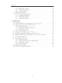
In this example, the response of a square plate (2 x 2 m) containing a circular hole
(radius = 0.5 m) subjected to a uniaxial traction is assessed, Figure 2.1. Due to the
symmetry of the problem, only the upper right corner is modelled. The purpose of this
example is to examine the state of stress in the close proximity of the hole. Additionally
the yield load of the structure is examined. The predictions are compared with the
available analytical solution.
3
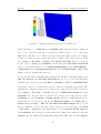
This tutorial describes how to pre-process, run and post-process a case involving linearelastic, steady-state stress analysis on a square plate with a circular hole at its centre.
The plate dimensions are: side length 4 m and radius R = 0.5 m. It is loaded with a
uniform traction of σ = 10 kPa over its left and right faces as shown in Figure 2.20. Two
the solution domain
Abaqus symmetry planes can be identified for this geometry and therefore
2.3. Launching
Abaqus/CAE
need only cover a quarter of the geometry, shown by the shaded area in Figure 2.20.
y
σ = 10 kPa
x
R = 0.5 m
σ = 10 kPa
symmetry plane
symmetry plane
4.0 m
Figure 2.20: Geometry of the plate with a hole.
Figure 2.1: Hole-in-a-Plate Geometry
The problem can be approximated as 2-dimensional since the load is applied in the
2.3
plane of the plate. Abaqus/CAE
In a Cartesian coordinate system there are two possible assumptions
Launching
to take in regard to the behaviour of the structure in the third dimension: (1) the plane
stress condition, in which the stress components acting out of the 2D plane are assumed
to be negligible; (2) the plane strain condition, in which the strain components out of
Click Start
→ plane
All Programs
→ Abaqus
6.9-1stress
→ Abaqus
CAE
to open
the 2D
are assumed negligible.
The plane
condition is
appropriate
for Abaqus/solids
thin as in
this
case;and
the plane
straintocondition
applicable
for the
CAE. A whose
black third
DOSdimension
console is
window
will
open
attempt
secure ais license
from
solids where the third dimension is thick.
university license
server.
If a exists
license
is successfully
obtained
Abaqus/CAE
will open,
An analytical
solution
for loading
of an infinitely
large, thin
plate with a circular
hole.
The
solution
for
the
stress
normal
to
the
vertical
plane
of
symmetry
is
Figure 2.2.
(σxx )x=0
%
 $
2
4
σ 1 + R + 3R
for |y| ≥ R
2y 2
2y 4
=

0
for |y| < R
(2.14)
Results from the simulation will be compared with this solution. At the end of the
tutorial, the user can: investigate the sensitivity of the solution to mesh resolution and
mesh grading; and, increase the size of the plate in comparison to the hole to try to
estimate the error in comparing the analytical solution for an infinite plate to the solution
of this problem of a finite plate.
Open∇FOAM-1.4.1
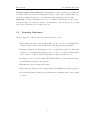
Figure 2.2: Abaqus/CAE Graphic User Interface
4
Abaqus
2.4. Setting Up the Problem
After entering the main interface of Abaqus/CAE, you are presented with several options
to start a job:
• Create Model Database allows you to begin a new analysis;
• Open Database allows you to open a previously saved model or output database
file;
• Run Script allows you to run a file containing ABAQUS/CAE commands;
• Start Tutorial allows you to begin an introductory tutorial from the online documentation.
2.4
2.4.1
Setting Up the Problem
Create Model
Select Create Model Database from the Start Session dialog box that appears. The
model will be named Model-1 by default, to rename the model right-click on Model-1 in
the model tree on the far left and select rename and change the name to holeInPlate.
Save the model database by File → Save As and save it as holeInPlate. This will
create a model database file (holeInPlate.cae) that stores all the information about
your model, except simulation result files. It is important to regularly save the model,
File → Save, in case of a crash.
To set the current working directory, on the main menu, select File → Set Work
Directory, and select a directory of choice. The working directory is where Abaqus
stores results files and temporary files. By default the working directory is set to C:\Temp
on Windows systems.
2.4.2
Create Geometry
From the main menu bar, select Part → Create to create a new part. The Create Part
dialog box appears, and is used to name the part; to choose its modelling space, type,
and base feature; and to set the approximate size. You can edit and rename a part after
you create it, but you cannot change its modelling space, type, or base feature.
Name the part Plate. Choose a three-dimensional deformable body and a solid base
feature. Select Extrusion as the base feature type. In the Approximate size text
5
Abaqus
2.4. Setting Up the Problem
field, type 20. The Approximate size sets the size and resolution of the background
drawing grid to aid in the creation of the part; it does not have any affect on the part
itself. Click Continue to exit the Create Part dialog box and enter the sketching mode.
Use the Create Lines: Connected tool located in the upper left corner of the Sketcher
toolbox to begin sketching the geometry of the plate. Create a line with the following
coordinates: (0.5, 0.0) and (2.0, 0.0), then again use the create line connected tool
to draw a line from (2.0, 0.0) to (2.0, 2.0), again from point (2.0, 2.0) to (0.0,
2.0), then from (0.0, 2.0) to (0.0,0.5). Finally, use the Create Arc: Center
and Two Endpoints tool to create an arc with a centre (0.0, 0.0) and one point at
(0.5, 0.0) and the other at (0.0, 0.5).
Figure 2.3: Drawing the Geometry Using the Sketcher Toolbox
From the prompt area (near the bottom of the main window), click Done to exit the
Sketcher. Note: if the Done button is not visible in the prompt area, continue to click
mouses right button in the viewport until it appears. The Edit Base Extrusion dialog
box will appear after Done is clicked, enter 0.1 as the part depth and click OK to finish
geometry creation.
2.4.3
Create Materials
In the Module drop down menu at the top left of the viewport, change to the Property
module. The Property module is used to create a material and to define its properties.
From the main menu bar, select Material → Create to create a new material. The
Create Material dialog box appears. It is assumed in this case that the plate is made
of mild steel with a Young’s modulus of 210 GPa. In the Create Material dialog box,
6
Abaqus
2.4. Setting Up the Problem
enter the name of the material as mildSteel. In the Create Material dialog box,
select Mechanical → Elasticity → Elastic to define the elastic material properties.
Enter 210e9 Pa as the value for Youngs modulus and 0.3 as the value for Poissons
ratio.
For many applications it is valid to assume a component to be purely linear-elastic, but
in this case the steel is assumed to be elastic-plastic. Select Mechanical → Plasticity
→ Plastic to define the plastic material properties. Enter the yield stress and plastic
strain tabulated data as shown in table 2.1.
Yield Stress (in Pa)
400e6
430e6
440e6
445e6
Plastic Strain
0.00
0.03
0.05
0.08
Table 2.1: Plastic Stress–Strain Properties
Click OK in the Create Material dialog box to complete the material definition.
Note: if linear-elastic is a valid assumption for the given model or if plasticity is not of
interest, then the plastic properties need not be defined.
Note on System Units
Abaqus has no in-built system of units, therefore all unit data must be specified in
consistent units. Some common systems of consistent units:
• SI: m, N , kg, s, P a, J, kg · m−3
• SI (mm): mm, N , tonne (1000 kg), s, M P a, mJ, tonne · mm−3
• US Unit (ft): f t, lbf , slug, s, lbf · f t−2 , f t · lbf , slug · f t−3
2.4.4
Create and Assign Sections
The material properties have been defined, and now they must be assigned to the geometry. While remaining in the Property module, on the main menu bar, select Section
→ Create to create a new section. In the Create Section dialog box, enter the name
of the section as mildSteelSection. To create a homogenous solid section with the
previously defined mildSteel properties, select Solid in the Category list and select
7
Abaqus
2.4. Setting Up the Problem
Homogenous in the Type list, then press Continue. Subsequently select mildSteel
as the material properties, then press OK.
To assign the mildSteelSection definition to the Plate part, on the main menu bar,
select Assign → Section. Select the whole Plate part in the viewport, and press
Done. Then select Ok in the Edit Section Assignment dialog box to complete the
assignment.
2.4.5
Mesh Geometry
Enter the Mesh module. The type of element should be carefully considered before
meshing a model. Different element types may make a significant difference to the accuracy of the obtained predictions. Check more details in the relevant Abaqus manuals.
As meshing is such as important issue, two separate meshing strategies are considered:
structured hexahedral elements and unstructured tetrahedral elements.
Structured Hexahedral Mesh The element shape and type must be set for the
mesh. The finite element type dictates how the underlying FE equations are formed
and can significantly affect results if the incorrect element type is chosen. To set the
element shape for a Structured Hexahedral Mesh, from the main menu bar, select Mesh
→ Controls. In the Mesh Controls dialog box, select Hex as the Element Shape,
set the Technique to Strucutred. Press OK to assign the mesh controls.
To set the element type for a Structured Hexahedral Mesh, from the main menu bar,
select Mesh → Element Type. In the Element Type dialog box, set the Element
Type to Standard; Standard means that the underlying Abaqus/Standard solver is
used that solves the FE equations using an implicit time scheme. Set the Geometric
Order to Linear; quadratic elements may be chosen to provide more accuracy, however,
more computer resources are required and quadratic elements may lead to instabilities
in certain situations. Under the Family subsection, 3D Stress should be chosen; this
means that the analysis examines the displacements/stress in the domain. If heat transfer is of interest then the Family is set to Heat Transfer, or Coupled-Temperature
Displacement if both temperature and stresses are desired. The element settings in
the bottom subsection can be left at their default values; this subsection allows elementspecific options to be specified such as hourglass control. Note: the Abaqus FE code
denoting the type of element selected can be found at the bottom of the Element Type
dialog box. In this case, the element code is C3D8R - signifying a Continuum 3D element
8
Abaqus
2.4. Setting Up the Problem
with 8 nodes, reduced integration and hourglass control. Press OK in the Element
Type dialog box to confirm the element type.
Figure 2.4: Structured Hexahedral Mesh
Next the mesh density/mesh element size must be set. To do this, seeds are specified
on the part essentially specifying the element sizes. From the main menu bar, select
Seed → Part. Set the Approximate global size to 0.1 and press OK. The element
spacing seeds are now visible on the part in the viewport. In this case a global seeding
is applied, however, local mesh refinement is possible through the use of graded edge
seeding.
To create the mesh, on the main menu bar, select Mesh → Part, and press OK. This
relatively coarse mesh provides moderate accuracy while keeping the solution time to
minimum, Figure 2.4. A finer mesh will give a more accurate solution at the expense
of more computer resources. Note: in order to create a structured hexahedral mesh
on more complex geometry, it is often necessary to partition the geometry into smaller
less complex shapes. The partition tools are found on the main menu bar at Tools →
Partition.
Unstructured Tetrahedral Mesh
This section can be skipped unless re-meshing
the model with tetrahedral elements is desired. To set the element shape for an
Unstructured Tetrahedral Mesh, from the main menu bar, select Mesh → Controls. In
the Mesh Controls dialog box, select Tet as the Element Shape, set the Technique
to Free and leave the algorithm settings unchanged. Press OK to assign the mesh
controls.
To set the element type for an Unstructured Tetrahedral Mesh, from the main menu bar,
select Mesh → Element Type. In the Element Type dialog box, set the Element
9
Abaqus
2.4. Setting Up the Problem
Type to Standard. Set the Geometric Order to Linear. Set the Family to 3D
Stress. The element settings in the bottom subsection can be left at their default values.
Note: the Abaqus FE code denoting the type of element selected can be found at the
bottom of the Element Type dialog box. In this case, the element can be seen to be
C3D4 - meaning a Continuum 3D element with 4 nodes. Press OK in the Element
Type dialog box to confirm the element type.
Figure 2.5: Unstructured Tetrahedral Mesh
2.4.6
Create Assembly
Change to the Assembly module. Add an instance of a part to the assembly by selecting
Instance → Create from the main menu bar. Select the plate part and press OK to
create an instance of the part in the assembly.
It is straight-forward to create an assembly for an integrated structure consisting on
one part such as this example. However, some models may be composed of several
parts which may have different material properties. Each part may have to be rotated
and/or translated after being instanced into the assembly. It is possible to manoeuvre
the instances using the many provided tools, such as Instance → Translate, Instance
→ Rotate, Constraint → Parallel Edge and Constraint → Coincident Point.
10
Abaqus
2.4.7
2.4. Setting Up the Problem
Define Analysis Steps
Enter the Step module. Select Step → Create, and create a new step named rampedTractionStep after the initial one. As for the Procedure type, select General →
Static, General; static means that this analysis step will be steady-state i.e. there
are no inertial effects, as explained in CCM I. In the Edit Step dialog box, specify
the following step description: the traction on the right face will be linearly
ramped up. Enter 10 as the time period; this is the time over which the analysis is run.
Non-linear Geometry effects (Nlgeom) should be set to off; Nlgeom off means small
strain theory is assumed, while Nlgeom on means finite/large strain theory is assumed.
Setting Nlgeom to on will give more accurate results in cases of large deformation but
at the expense of longer run times.
To set the actual solution time-steps during this rampedTractionStep analysis step,
change to the Incrementation tab in the Edit Step dialog box. The Type is set to
Automatic; meaning that Abaqus will automatically change the time-step during the
analysis in order to keep the run time low while maintaining stability. Setting the Type
to Fixed would result in a fixed time-step during the analysis step. For the Increment
size, set the Initial to 1 and set the Maximum to 1. Since the time period has been
defined as 10 and the maximum time-step (time increment) is 1, this means there will
be at least 10 time-steps during the simulation. Press OK to create the analysis step.
2.4.8
Apply Boundary Conditions
Change to the Load module. Even though both Dirichlet and Neumann conditions are
both boundary conditions, Abaqus refers to Neumann conditions as Loads and Dirichlet
and Symmetry conditions as Boundary Conditions. CCM I describes Dirichlet and
Neumann boundary conditions in detail. In this case a symmetry plane condition will be
applied to the left, bottom and back of the plate, while a traction acting in the positive
x direction is applied to the right face of the plate. The top and front of the plate are
traction-free.
Before applying the boundary conditions, a set will be created for each face of the
geometry to which a boundary condition will be applied. Select Tool → Set → Create,
name the set as left with the Type as Geometry, press Continue. Now select the
left face of the plate from the viewport and press Done. Similarly create the sets bottom
and back by selecting the appropriate geometry faces.
11
Abaqus
2.4. Setting Up the Problem
In addition, a surface is defined for any loads that will be applied. From the main menu
bar, select Tool → Surface → Create, name the set as rightSurf with the Type as
Geometry, press Continue. Now select the right face of the plate from the viewport
and press Done.
To create the symmetry plane boundary conditions, select BC → Create from the
main menu bar, and create a boundary condition called symmLeft in the Initial step.
Select Mechanical → Symmetry/Antisymmetry/Encastre to be the type of step,
and press Continue. In the bottom right below the viewport, click on Sets and select
left from the list, press Continue. Select XSYMM, this will produce a symmetry
plane in the x-axis direction, then press OK to apply the boundary conditions. Repeat
this process to create y-symmetry plane called symmBottom on the bottom set, and a
z-symmetry called symmBack on the back set.
Figure 2.6: Boundary Conditions
To create the traction boundary condition on the right set, select Load → Create
from the main menu bar, and create a boundary condition called tractionRight in the
rampedTractionStep step. Select Mechanical → Surface traction to be the type of
step, and press Continue. Select Surfaces in the bottom right below the viewport, and
choose right from the surfaces list, press Continue. The surface traction may now be
defined in the Edit Load dialog box. Set the Distribution to Uniform; this means
that the traction is uniform across the loaded surface. Set the Traction to General.
To set the direction of the traction vector, click on the edit in the Direction subsection
and enter (0.0, 0.0, 0.0) as the first point of the direction vector and (1.0, 0.0,
0.0) as the second point of the direction vector. This defines the traction direction to
be in the positive x direction. Set the traction Magnitude to 2e8 Pa. By default Abaqus
linearly ramps up the applied traction over the whole time period of the analysis reaching
12
Abaqus
2.5. Running the Analysis
the maximum value at the end time. Therefore in this case, as the time period is 10 s,
the traction will be 2e7 Pa at 1 s, 4e7 Pa at 2 s, 6e7 Pa at 3 s, etc. reaching 2e8 Pa at
10 s. Click OK to apply the surface traction.
Note: Abaqus assumes a traction/force free boundary condition on any faces to which
no load/displacement is applied. In this case, the front and top faces are tractionfree. For thermal analyses, Abaqus assumes an insulated (i.e. no heat flux) boundary
condition on faces to which no thermal condition is applied.
2.5
Running the Analysis
2.5.1
Create Job
In the Module list located under the toolbar, change to the Job module. From the main
menu bar, select Job → Manager. Enter the name of the job as holeInPlateJob1 and
press Continue. The Edit Job dialog box appears. In the Description field, type 3D
analysis of a hole in a plate. Click OK to accept all default job settings in the
job editor and to close the dialog box. Note: if your computer has multiple processing
cores, the Parallelisation tab allows the number of processors to be set enabling the job
to run in parallel, however, multiple run licenses are required.
2.5.2
Check Job
Having generated the job for this simulation, you are ready to run the analysis. Unfortunately, it is possible to have errors in the model because of incorrect or missing
data. A data check analysis should be performed before running the simulation. To
run a data check analysis, from the main menu bar, select Job → Data Check →
holeInPlateJob1. To check the output of the Data Check, select Job → Monitor
→ holeInPlateJob1, and the Job Monitor will appear. The top half of the dialog
box displays the information available in the status (*.sta) file that Abaqus creates for
the analysis. This file contains a brief summary of the progress of an analysis and is
described in the Abaqus Analysis User’s Manual. The bottom half of the dialog box
displays the following information:
• Log tab to display the start and end times for the analysis that appear in the log
(*.log) file.
13
Abaqus
2.6. Post-processing and verification
• Errors and Warnings tabs to display the first ten errors or the first ten warnings
that appear in the data (*.dat) and message (*.msg) files. If a particular region
of the model is causing the error or warning, a node or element set will be created
automatically that contains that region. The name of the node or element set
appears with the error or warning message, and you can view the set using display
groups in the Visualization module. It will not be possible to perform the analysis
until the causes of any error messages are corrected. In addition, you should always
investigate the reason for any warning messages to determine whether corrective
action is needed or whether such messages can be ignored safely. If more than ten
errors or warnings are encountered, information regarding the additional errors
and warnings can be obtained from the printed output files themselves.
• Output tab to display a record of each output data entry as it is written to the
output database.
2.5.3
Submit Job
When the data check analysis completes with no error messages, the analysis itself can
be run. To do this, select Job → Submit → holeInPlateJob1 to submit your job for
analysis. You should always perform a data check analysis before running a simulation
to ensure that the model has been defined correctly and to check that there is enough
disk space and memory available to complete the analysis. However, if the data check
has not been performed then Abaqus will automatically data check the model when the
job is submitted. To monitor the job as it runs, open up the job monitor, select Job →
Monitor → holeInPlateJob1. The log will display when the analysis has completed.
2.6
Post-processing and verification
When the job completes successfully, the results of the analysis are ready to be viewed
with the Visualization module. From the main menu bar, select Job → Results →
holeInPlateJob1. The Visualization module will now automatically be loaded and the
output database (results file) for the job will be opened. Alternatively, you can click
Visualization in the Module list located under the toolbar, select File → Open, select
holeInPlateJob1.odb from the list of available output database files, and click OK
to open the output database file.
14
Abaqus
2.6.1
2.6. Post-processing and verification
Visualise Field Data
To generate a contour of the stress S11, in the main menu bar, select Result → Field
output. In the Primary Variable tab of the Field Output dialog box, choose the variable
name as S, which corresponds to stress components at integration points. Choose
S11 as the Component, corresponding to the σxx component. Note: that stresses and
strains are computed most accurately at the integration points and the displacements
are computed at the nodal points. Click Apply. To plot the contours on the deformed
geometry, from the main menu bar, select Plot → Contours → On Deformed Shape.
It is possible to change the deformation scale factor for visualisation of the deformation,
from the main menu bar, select Options → Common. The Deformation Scale
Factor can be changed to 100 which should allow straightforward visualisation of the
deformation, Figure 2.7.
Note: It is possible to customise the display of the title block, state block, legend,
background colour and view orientation triad by selecting Viewport → Viewport
Annotation Options from the main menu bar.
Figure 2.7: S11 (σxx ) Stress Field at Time 1 s
Using the time controls above the top right corner of the viewport, it is possible to move
through the time-steps from time 1 s to 10 s. If the field output is changed to show
plastic equivalent strain, PEEQ, it can be seen that the top of hole experiences plastic
deformation between 6 and 7 s.
2.6.2
Generating Graphs
To plot the stress along the line from the top of the hole to the top face of the plate, a
path along this line must be defined. Select Tools → Path → Create from the main
menu bar. The Create Path dialog box appears, enter pathHoleToTop as the name,
15
Abaqus
2.6. Post-processing and verification
Figure 2.8: Equivalent Plastic Strain (P
xx ) Field at Time 10 s
and set the Type to be Point list, press Continue. Enter the first Point Coordinate as
(0.0, 0.5, 0.05) and enter the second Point Coordinate as (0.0, 2.0, 0.05), press
OK. Next a XY-Plot of σxx will be generated along this path for time 1 s. Change
to time 1 s using the time controls above the top right corner of the viewport. Then
select Tools → XY Data → Create. The Create XY Data dialog box appears,
set the source to Path, press Continue. In the subsequent XY Data from Path
dialog box, the path should be set to pathFromHoleToTop, set the Model Shape to
Undeformed, turn on Include intersections. Set the Field Output to S11. Click
Plot to view the graph in the viewport.
To save the XY Data, click Save As, and name the XY Data as holeToTopS11, press
OK. Click Cancel on the XY Data from Path dialog box to close it. Previously saved
XY Data can be plotted by selecting Tools → XY Data → Plot → nameOfXyData.
Next a plot of the force on the left set in the x direction versus time is generated. The
principle is to sum the reaction forces of the nodes on the left set in the x direction.
Select Tools → XY Data → Create, and choose OBD Field Output and press
Continue. To collect the data of reaction forces of the nodes on the left set, on the
Variables tab, select Position as Unique Nodal. Then select RF1 (Reaction force
in the direction of x-direction). On the tab Elements/Nodes, select Node sets →
Fixed. Then press Save → OK. The XY Data from ODB Output dialog box can
then be dismissed. To plot the sum of these reaction forces versus time, select Tool
→ XY Data → Create from the main menu bar, select Operate on XY data and
press Continue. Row down the operation functions column on the right side, and click
sum((A, A,...)). Multi-select (using shift-click) all the RF1 data and click Add to
16
Abaqus
2.6. Post-processing and verification
Expression. Click Plot Expression to plot the total reaction force in the x direction
on the left set versus time. Save the data for later click Save As as leftRF1.
All the RF 1 XY Data for each node on left can be removed (not the leftRF1 XY data).
Select Tool → XY Data → Manager from the main menu bar, then multi-select all
the RF 3 data - every XY Data except leftRF1 and holeToTopS11 - then click Delete.
The only two XY Data that should be left are leftRF3 and holeToTopS11.
2.6.3
Exporting Data
Abaqus/CAE allows you to write XY/Field/History data to a text file (*.rpt) in a
tabular format. Output generated this way has many uses; for instance, it can be used
to allow well-formed graphs to be generated in Excel/Matlab for written reports.
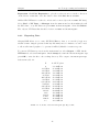
To generate XY Data reports, from the main menu bar, select Report → XY. On the
XY Data tab, select holeToTopS11. On the Setup tab, name the file holeToTops11.rpt,
press OK to write the file to the working directory. The output of holeToTops11.rpt
is shown in table 2.2.
X
holeToTopS11
0.
93.75E-03
187.5E-03
281.25E-03
375.E-03
468.75E-03
562.5E-03
656.25E-03
750.E-03
843.75E-03
937.5E-03
1.03125
1.125
1.21875
1.3125
1.40625
1.5
59.5178E+06
51.7097E+06
39.9391E+06
33.6341E+06
29.8137E+06
27.3379E+06
25.5927E+06
24.2533E+06
23.1529E+06
22.1875E+06
21.2932E+06
20.4203E+06
19.5288E+06
18.5779E+06
17.5229E+06
16.3088E+06
15.6547E+06
Table 2.2: Contents of the holeToTops11.rpt Report File
17
Abaqus
2.6.4
2.6. Post-processing and verification
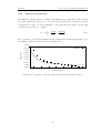
Analytical Verification
An analytical solution exists for loading of an infinitely large, thin plate with a circular
hole. The analytical solution for σxx along the left vertical plane of symmetry is given
by Equation 2.1, where P is the magnitude of the uniform stress applied on the right
boundary, and y is the y coordinate.
σxx
0.125 0.09375
=P 1+
+
y2
y4
(2.1)
The comparison of the Abaqus numerical S11 results in the holeToTops11.rpt report
file with the analytical solution is shown in Figure 2.9.
6e+07
Abaqus
Analytical
5.5e+07
Stress (in Pa)
5e+07
4.5e+07
4e+07
3.5e+07
3e+07
2.5e+07
2e+07
1.5e+07
0.6
0.8
1
1.2
1.4
1.6
1.8
x coordinate (in m)
Figure 2.9: Comparison of Abaqus Numerical S11 with the Analytical Solution
18
2
Chapter 3
Ansys CFX
3.1
Introduction
Ansys CFX software is a fluid dynamics program that has been applied to solve a wide
range of fluid flow problems. Ansys CFX is a general purpose Computational Fluid
Dynamics (CFD) software suite that combines an advanced solver with powerful preand post-processing capabilities. It includes the following features:
• An advanced coupled solver that is both reliable and robust.
• Full integration of problem definition, analysis, and results presentation.
• An intuitive and interactive setup process, using menus and advanced graphics.
Ansys CFX is capable of modeling:
• Steady-state and transient flows
• Laminar and turbulent flows
• Subsonic, transonic and supersonic flows
• Heat transfer and thermal radiation Buoyancy
• Non-Newtonian flows
• Transport of non-reacting scalar components
• Multiphase flows
• Combustion
19
Ansys CFX
3.2. Problem Definition: Internal-Pipe-Flow
• Flows in multiple frames of reference
• Particle tracking.
3.2
Problem Definition: Internal-Pipe-Flow
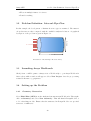
In this example the development of laminar flow in a pipe is examined. The numerical predictions are then compared with the available analytical solution. A graphical
description of the problem is given in Figure 3.1.
!"#"$"%%"
)"#"(*('"%+,"
&"#"'(("%%"
Figure 3.1: Internal Pipe Flow Geometry
3.3
Launching Ansys Workbench
Click ( Start → All Programs → Ansys 13.0 → Workbench) to open Ansys Workbench.
After a short while a window will appear. Select New Project. Save the project using
a suitable filename e.g. pipeFlow.
3.4
3.4.1
Setting up the Problem
Geometry Generation
Select Fluid Flow (CFX) from the Analysis Systems menu in Workbench. Then rightclick on Geometry and select New Geometry. This will launch DesignModeler, a
tool for sketching models. Ensure that the units used in Design Modeler are specified
as metres or millmetres.
20
Ansys CFX
3.4. Setting up the Problem
Create a new sketch based on the XYPlane. Use Circle from the Draw Toolbox of the
Sketching tab to draw a circle in the new sketch, centred on the origin and with radius
0.002 m. To change the radius, you must select Dimension from the Tree View and
then Radius and enter the radius on the left of the screen.
Select Extrude from the 3D Features toolbar. Set Base Object to be the new sketch
(Sketch 1), and set Operation to Add Material. Set Direction to Normal and Type
to Fixed. Set Depth to 0.1 m. Save the project using File→Save, and close Design
Modeler
Note: there is also an option to Import External Geometry which allows the use to
import complex geometries from other cad packages. This is useful for more complicated
geometries.
3.4.2
Mesh Generation
On the Project Schematic, right-click the Mesh cell in the Mesh system and select Edit...
to launch the Meshing Application.
3.4.2.1
Adding Named Selections
The user needs to specify the names of each boundary. The boundaries in this tutorial
will be called pipeInlet, pipeOutlet and pipeWall. To create a Named Selection
for the pipe inlet, select the small inlet face while holding down the CTRL key. Once
selected release the CTRL key. Right click in the main window and select Create Named
Selection from the menu. IN the Selection Name dialogue box, type pipeInlet.
Repeat this process for the pipeOutlet and pipeWall selections.
In the Tree View, click the Mesh object. In the Details View, ensure that the Physics
Preference and Solver Preference are set to CFD and CFX respectively. In the
details view, click to expand the Sizing group of controls and notice the default sizing
settings. You can change these if you wish to refine or coarsen the mesh. Set the Max
Face Size and Max Size to 0.1 mm.
Now, we examine the surface mesh to see the effect of the chosen length scale.To do this,
right click on Mesh in the Tree View and select Preview→SurfaceMesh. Right click
over Default Preview Group and select Generate This Surface Mesh.
21
Ansys CFX
3.4.2.2
3.4. Setting up the Problem
Adjusting Inflation
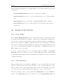
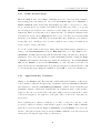
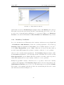
The velocity gradients near the pipe wall surfaces can vary quite significantly, therefore
it is desirable to have a higher mesh density in those regions. Ansys CFX achieves
this via the Inflation tool. Click on Inflation in the Details View. Select All Faces
in Chosen Named Selection as the option for Use Automatic inflation. Enter the
Maximum Layers as 5. You can preview the effect as before, right click on Mesh in
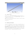
the Tree View and select Preview→Inflation as shown in Figure 3.2.
Figure 3.2: Inflation of cells (3 layers) close to the walled boundaries using Ansys
CFX.
The volume mesh can now be generated. Right click on Mesh in the Tree View and select
Generate Mesh. Save the mesh file as pipeFlow.gtm. Select File→Save Project to
save the project.
3.4.3
Material Properties
From the Workbench project page click on Solution. This will open up CFX-Pre, which
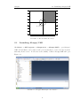
allows the user to specify the simulation physics. The window should appear as in Figure
3.3. Once open, immediately save the simulation.
To perform a quick setup, click Tools→Quick Setup Mode This will take the through
selection of the most salient options in order to run the simulation. Further refinement
of the physics is available in the Tree View of CFX-Pre.
22
Ansys CFX
3.4. Setting up the Problem
Figure 3.3: Ansys CFX-Pre Window.
On the first screen select Problem Type as Single Phase. The Fluid should be Water.
The mesh created in the previous step should be automatically selected. Proceed to the
second screen. A Steady State analysis is to be performed. Enter 0 for Reference
Pressure. Select None and Laminar for Heat Transfer and Turbulence respectively.
3.4.4
Boundary Conditions
Proceed to the third screen. This is where the boundary conditions are set up. Right click
on Boundaries→Add Boundary. Name the boundary pipeInlet. Select Inlet as
Boundary Type and pipeInlet as Location. Select a Normal Speed of 0.01 ms−1
for the Flow Specification options. Note: When the velocity at an inlet/outlet is
specified, Ansys CFX assumes the pressure boundary condition to be zero gradient.
Add a second boundary named pipeOutlet. The Boundary Type is Outlet, while
the Location is pipeOutlet. Select Average Static Pressure and 0 as the relevant
Flow Specification options. Note: When the pressure at an inlet/outlet is specified,
Ansys CFX assumes the velocity boundary condition to be zero gradient.
Finally the pipeWall boundary conditions need to be specified. Add a new boundary
condition called pipeWall. The Boundary Type is Wall. Select No Slip Wall for the
Wall Influence On Flow option. Proceed to the final setup screen, and select Finish.
The graphic of the simulation should now have arrows indicating the direction of inlet
and outlet flows as shown in Figure 3.4.
23
Ansys CFX
3.5. Running the Analysis
Figure 3.4: CFX-Pre Inlet and Outlet specified.
3.4.5
Solution Control
In the Tree View open Solver→Solver Control; this details the specification of solution schemes and time-step control. Set the Advection Scheme to Upwind. Leave
everything else as the default options.
Note: The options specified in Quick Setup Mode could also be specified by selecting
the appropriate tab in Tree View.
Save the Project.
3.5
Running the Analysis
Once all the correct physics have been specified return to the Ansys Workbench project
screen. Select Solution. This will open up a small window which will detail runtime information such as convergence and any run-time errors and warnings. Click
File→Define Run. The window shown in Figure 3.5 will appear. Begin to solve the
simulation by clicking Start Run. During run-time, the convergence details of each of
the solved variables are indicated on screen as shown in Figure 3.6. Once the simulation
has terminated, a message box will appear indicating details of the run.
24
Ansys CFX
3.6. Post-processing and verification
Figure 3.5: Ansys CFX Define Run Information Window
Figure 3.6: Convergence of solved variables in Ansys CFX.
3.6
Post-processing and verification
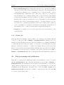
When the job is complete the results of the analysis are ready to be viewed. This is done
by clicking on Results on the Ansys Workbench screen. This will launch CFX-Post.
Upon launching, a wireframe of your model will appear as shown in Figure 3.7.
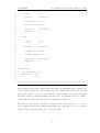
3.6.1
Visualize Field Data
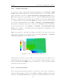
To generate a contour of the velocity along the pipe, the user must first specify a plane
on which to display the results. To do this, select Insert→Location→Plane. enter
25
Ansys CFX
3.6. Post-processing and verification
Figure 3.7: Wireframe representation of model in CFX-Post.
the name of the plane as alongPipe. Select the plane as either the XZ Plane or the
YZ Plane. Since the flow is axisymmetric the choice of Plane does not matter. In
the Tree View right click on the newly created plane and select Insert→Contour.
Name the contour velocityFringePlot. Select the Location in the Details View as
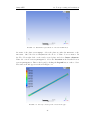
velocityFringePlot. Turn on the legend by clicking the Legend button on the toolbar.
The window should appear as shown in Figure 3.8.
Figure 3.8: Velocity contour profile of flow in the pipe.
26
Ansys CFX
3.6.2
3.6. Post-processing and verification
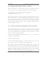
Generating Graphs
To generate a line plot of a particular variable using Ansys CFX-Post the user must first
specify a location on the geometry. To plot fluid velocity along a line for example, select
Insert→Location→Line. Enter the name of the line as axialLine. Enter the start
and end points of the line. To plot along the centreline of the pipe geometry enter (0.0
0.0 0.0) and (0.1 0.0 0.0). Select Sample and set the number of samples to 100 in
the Line Type selector. This will ensure that 100 data points of the chosen variabale
are sampled along the line.
On the Toolbar click Insert→Chart. Name the chart axialPressure. In the Details
View select the Data Series tab. Select the location of the chart as axialLine. This
will plot the data along the previously created line. Select the X-Axis tab. Change the
Data Selection Variable to Z. Select the Y-Axis tab. Change the Data Selection
Variable to Pressure. Click Apply. A chart of pressure along the centre-line of the
pipe will now appear in the main window. An example for a very coarse mesh is given
in Figure 3.9
Figure 3.9: Plot of pressure versus position along the axis of the pipe.
It is relatively easy to export the chart data for manipulation or presentation by thirdparty software. Click Export at the bottom of the Details View to export a comma
separated value file of the sampled data.
27
Ansys CFX
3.6.3
3.6. Post-processing and verification
Analytical Verification
The exact solution for the velocity profile of fully developed flow within a pipe subject
to the boundary conditions is:
R2
u(r) =
4µ
∂p
−
∂x
r 2 1−
R
(3.1)
where R is the radius of the pipe and ∂p/∂z is the pressure gradient.
The user should compare the velocity profile at the outlet to the analytical solution to
verify if the flow has fully developed over the length of pipe simulated.
Note: To model fully developed flow over the entire length of the pipe the user should
change the inlet boundary condition to be a pressure boundary condition. The specified
pressure gradient along the pipe will then be constant.
28
Chapter 4
OpenFOAM
4.1
Introduction
OpenFOAM (Open Field Operation and Manipulation) is a C++ toolbox for the development of customised numerical solvers for the solution of continuum mechanics problems. The main code branch is produced by the UK company OpenCFD Ltd. and it is
released as free and open source software under the GNU General Public License. The
Extend-Project code branch maintained by the Extend-Project Team aims to include
community contributions and so encompasses many abilities not included by the main
branch albeit possibly with more bugs.
OpenFOAM has an extensive range of features to solve anything from complex fluid
flows involving chemical reactions and turbulence, to heat transfer and electromagnetics. Primarily OpenFOAM is used to solve problems involving Computational Fluid
Dynamics, however, it is also possible to solve a variety of complex solid mechanics
problems with OpenFOAM using the Finite Volume method.
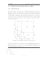
4.2
Solid Mechanics Problem Definition: Hole-in-a-Plate
The following tutorial is adapted from the OpenFOAM-1.6-ext User Guide.
This tutorial describes how to pre-process, run and post-process a case involving linearelastic, steady-state stress analysis on a square plate with a circular hole at its centre.
The plate dimensions are: side length 4 m, and radius R = 0.5 m. It is loaded with a
uniform traction of σ = 10 kPa, over its left and right faces as shown in Figure 4.1. Two
symmetry planes can be identified for this geometry and therefore the solution domain
need only cover a quarter of the geometry.
29
OpenFOAM
4.2. Solid Mechanics Problem Definition: Hole-in-a-Plate
Figure 4.1: Geometry of the plate with a hole
In this case, the problem can be approximated as 2-dimensional since the load is applied
in the plane of the plate. In a Cartesian coordinate system there are two possible
assumptions to take in regard to the behaviour of the structure in the third dimension:
(1) the plane stress condition, in which the stress components acting out of the 2D
plane are assumed to be negligible; (2) the plane strain condition, in which the strain
components out of the 2D plane are assumed negligible. The plane stress condition is
appropriate for solids whose third dimension is thin as in this case; the plane strain
condition is applicable for solids where the third dimension is thick. An analytical
solution exists for loading of an infinitely large, thin plate with a circular hole. The
solution for the stress normal to the vertical plane of symmetry is:
 σ 1 + R22 +
2y
(σxx )x=0 ) =

0
3R4
2y 4
for|y| ≥ R
for|y| < R
(4.1)
Results from the simulation will be compared with this solution. At the end of the
tutorial, the user can: investigate the sensitivity of the solution to mesh resolution
and mesh grading; and, increase the size of the plate in comparison to the hole to try
to estimate the error in comparing the analytical solution for an infinite plate to the
solution of this problem of a finite plate.
30
OpenFOAM
4.3
4.3. Setting Up the Problem: Hole-in-a-Plate
Setting Up the Problem: Hole-in-a-Plate
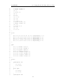
4.3.1
Mesh Generation
The domain consists of four blocks, some of which have arc-shaped edges. The block
structure for the part of the mesh in the x – y plane is shown in Figure 4.2. In OpenFOAM, all geometries are generated in 3 dimensions even if the case is a 2 dimensional
problem. Therefore a dimension of the block in the z direction has to be chosen; here,
0.5 m is selected. It does not affect the solution since the traction boundary condition
is specified as a stress rather than a force, thereby making the solution independent of
the cross-sectional area.
Figure 4.2: Block structure of the mesh for the plate with a hole
The user should change into the plateHole case in the $FOAM RUN/tutorials/solidDisplacementFoam directory and open the constant/polyMesh/blockMeshDict file in
an editor (such as Emacs), as listed below:
17
c on ve rt T oM et er s 1;
18
19
vertices
20
(
21
(0.5 0 0)
22
(1 0 0)
23
(2 0 0)
24
(2 0.707107 0)
31
OpenFOAM
(0.707107 0.707107 0)
25
26
(0.353553 0.353553 0)
27
(2 2 0)
28
(0.707107 2 0)
29
(0 2 0)
30
(0 1 0)
31
(0 0.5 0)
32
(0.5 0 0.5)
33
(1 0 0.5)
34
(2 0 0.5)
35
(2 0.707107 0.5)
36
(0.707107 0.707107 0.5)
37
(0.353553 0.353553 0.5)
38
(2 2 0.5)
39
(0.707107 2 0.5)
40
(0 2 0.5)
41
(0 1 0.5)
(0 0.5 0.5)
42
43
4.3. Setting Up the Problem: Hole-in-a-Plate
);
44
45
blocks
46
(
47
hex (5 4 9 10 16 15 20 21) (10 10 1) simpleGrading (1 1 1)
48
hex (0 1 4 5 11 12 15 16) (10 10 1) simpleGrading (1 1 1)
49
hex (1 2 3 4 12 13 14 15) (20 10 1) simpleGrading (1 1 1)
50
hex (4 3 6 7 15 14 17 18) (20 20 1) simpleGrading (1 1 1)
hex (9 4 7 8 20 15 18 19) (10 20 1) simpleGrading (1 1 1)
51
52
);
53
54
edges
55
(
56
arc 0 5 (0.469846 0.17101 0)
57
arc 5 10 (0.17101 0.469846 0)
58
arc 1 4 (0.939693 0.34202 0)
59
arc 4 9 (0.34202 0.939693 0)
60
arc 11 16 (0.469846 0.17101 0.5)
61
arc 16 21 (0.17101 0.469846 0.5)
62
arc 12 15 (0.939693 0.34202 0.5)
arc 15 20 (0.34202 0.939693 0.5)
63
64
);
65
66
patches
67
(
68
symmetryPlane left
69
(
(8 9 20 19)
70
(9 10 21 20)
71
72
)
73
patch right
74
(
(2 3 14 13)
75
(3 6 17 14)
76
77
)
78
symmetryPlane down
32
OpenFOAM
(
79
(0 1 12 11)
80
(1 2 13 12)
81
)
82
83
patch up
84
(
(7 8 19 18)
85
(6 7 18 17)
86
)
87
88
patch hole
89
(
90
(10 5 16 21)
91
(5 0 11 16)
)
92
93
empty frontAndBack
94
(
95
(10 9 4 5)
96
(5 4 1 0)
97
(1 4 3 2)
98
(4 7 6 3)
99
(4 9 8 7)
100
(21 16 15 20)
101
(16 11 12 15)
102
(12 13 14 15)
103
(15 14 17 18)
(15 18 19 20)
104
)
105
106
4.3. Setting Up the Problem: Hole-in-a-Plate
);
107
108
m er ge Pa t ch Pa ir s
109
(
110
);
111
// * * * * * * * * * * * * * * * * * * * * * * * * * * * * * * * * * * * * * * * * * * * * * * * * * * * * * * * * * * * * * * * * * * * * * * * * * //
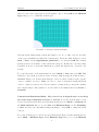
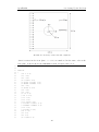
The contents of the blockMeshDict is described in the OpenFOAM User Guide.
The blocks in this blockMeshDict do not all have the same orientation. As can be seen
in Figure 4.2 the x2 direction of block 0 is equivalent to the −x1 direction for block 4.
This means care must be taken when defining the number and distribution of cells in
each block so that the cells match up at the block faces.
6 patches are defined: one for each side of the plate, one for the hole and one for the
front and back planes. The left and down patches are both a symmetry plane. Since
this is a geometric constraint, it is included in the definition of the mesh, rather than
being purely a specification on the boundary condition of the fields. Therefore they are
defined as such using a special symmetryPlane type as shown in the blockMeshDict.
The frontAndBack patch represents the plane which is ignored in a 2D case. Again this
is a geometric constraint so is defined within the mesh, using the empty type as shown
33
OpenFOAM
4.3. Setting Up the Problem: Hole-in-a-Plate
in the blockMeshDict. For further details of boundary types and geometric constraints,
the user should refer to the OpenFOAM User Guide section 5.2.1.
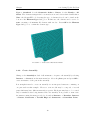
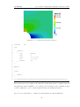
The remaining patches are of the regular patch type. The mesh should be generated
using blockMesh and can be viewed in ParaView. It should appear as in Figure 4.3.
Figure 4.3: Mesh of the hole in a plate problem
4.3.2
Boundary and Initial Conditions
Once the mesh generation is complete, the initial field with boundary conditions must
be set. For a stress analysis case without thermal stresses, only displacement D needs
to be set. The 0/D is as follows:
17
dimensions
[0 1 0 0 0 0 0];
internalField
uniform (0 0 0);
18
19
20
21
boundaryField
22
{
23
left
24
{
type
25
26
symmetryPlane ;
}
27
right
28
{
29
type
tractionDisplacement ;
30
traction
uniform ( 10000 0 0 );
31
pressure
uniform 0;
32
value
uniform (0 0 0);
33
}
34
down
35
{
34
OpenFOAM
type
36
4.3. Setting Up the Problem: Hole-in-a-Plate
symmetryPlane ;
}
37
38
up
39
{
40
type
tractionDisplacement ;
41
traction
uniform ( 0 0 0 );
42
pressure
uniform 0;
value
uniform (0 0 0);
43
}
44
45
hole
46
{
47
type
tractionDisplacement ;
48
traction
uniform ( 0 0 0 );
49
pressure
uniform 0;
value
uniform (0 0 0);
50
}
51
52
frontAndBack
53
{
type
54
56
empty ;
}
55
}
57
58
// * * * * * * * * * * * * * * * * * * * * * * * * * * * * * * * * * * * * * * * * * * * * * * * * * * * * * * * * * * * * * * * * * * * * * * * * * //
Firstly, it can be seen that the displacement initial conditions are set to (0, 0, 0) m.
The left and down patches must be both of symmetryPlane type since they are specified
as such in the mesh description in the constant/polyMesh/boundary file. Similarly the
frontAndBack patch is declared empty.
The other patches are traction boundary conditions, set by a specialist traction boundary
type. The traction boundary conditions are specified by a linear combination of: (1)
a boundary traction vector under keyword traction; (2) a pressure that produces a
traction normal to the boundary surface that is defined as negative when pointing out
of the surface, under keyword pressure. The up and hole patches are zero traction so the
boundary traction and pressure are set to zero. For the right patch the traction should
be (1e4, 0, 0) Pa, and the pressure should be 0 Pa.
4.3.3
Material Properties
Mechanical Properties
The physical properties for the case are set in the mechanicalProperties dictionary in
the constant directory. For this problem, we need to specify the mechanical properties
of steel given in Table 4.1. In the mechanical properties dictionary, the user must also
set planeStress to yes.
35
OpenFOAM
4.3. Setting Up the Problem: Hole-in-a-Plate
Property
Density
Youngs modulus
Poissons ratio
Units
kgm−3
Pa
—
Keyword
rho
E
nu
Value
7854
2 x 1011
0.3
Table 4.1: Mechanical properties for steel
Thermal properties
The temperature field variable T is present in the solidDisplacementFoam solver since
the user may opt to solve a thermal equation that is coupled with the momentum
equation through the thermal stresses that are generated. The user specifies at run time
whether OpenFOAM should solve the thermal equation by the thermalStress switch
in the thermalProperties dictionary. This dictionary also sets the thermal properties
for the case, e.g. for steel as listed in Table 4.2.
Property
Specific heat capacity
Thermal conductivity
Thermal expansion coeff.
Units
Jkg−1 K−1
Wm−1 K−1
K−1
Keyword
C
k
alpha
Value
434
60.5
1.1 x 10−5
Table 4.2: Thermal properties for steel
In this case we do not want to solve for the thermal equation. Therefore we must set
the thermalStress keyword entry to no in the thermalProperties dictionary.
4.3.4
Solution Control
As before, the information relating to the control of the solution procedure are read in
from the controlDict dictionary. For this case, the startTime is 0 s. The time step is not
important since this is a steady state case; in this situation set the time step deltaT to
1 and set the endTime to 1. The writeInterval can be set to 1. The controlDict entries
are as follows:
17
application
solidDisplacementFoam ;
startFrom
startTime ;
startTime
0;
stopAt
endTime ;
endTime
1;
deltaT
1;
18
19
20
21
22
23
24
25
26
27
28
36
OpenFOAM
29
4.3. Setting Up the Problem: Hole-in-a-Plate
writeControl
timeStep ;
writeInterval
1;
purgeWrite
0;
writeFormat
ascii ;
writ ePrecisi on
6;
30
31
32
33
34
35
36
37
38
39
w r i t e C o m p r e s s i on uncompressed ;
40
41
timeFormat
general ;
timePrecision
6;
graphFormat
raw ;
42
43
44
45
46
47
r u n T i m e M o d i f i a b l e yes ;
48
49
// * * * * * * * * * * * * * * * * * * * * * * * * * * * * * * * * * * * * * * * * * * * * * * * * * * * * * * * * * * * * * * * * * * * * * * * * * //
Discretisation Schemes and Linear-Solver Control
Let us turn our attention to the fvSchemes dictionary. Firstly, the problem we are
analysing is steady-state so the user should select SteadyState for the time derivatives
in timeScheme. This essentially switches off the time derivative terms. Not all solvers,
especially in fluid dynamics, work for both steady-state and transient problems but
solidDisplacementFoam does work, since the base algorithm is the same for both types
of simulation. The momentum equation in linear-elastic stress analysis includes several
explicit terms containing the gradient of displacement. The calculations benefit from
accurate and smooth evaluation of the gradient. Normally, in the finite volume method
the discretisation is based on Gausss theorem. The Gauss method is sufficiently accurate
for most purposes but, in this case, the least squares method will be used. The user
should therefore open the fvSchemes dictionary in the system directory and ensure the
leastSquares method is selected for the grad(D) gradient discretisation scheme in the
gradSchemes sub-dictionary:
17
d2dt2Schemes
18
{
default
19
20
steadyState ;
}
21
22
gradSchemes
23
{
24
default
leastSquares ;
25
grad ( D )
leastSquares ;
37
OpenFOAM
grad ( T )
26
27
4.3. Setting Up the Problem: Hole-in-a-Plate
leastSquares ;
}
28
29
divSchemes
30
{
31
default
none ;
32
div ( sigmaD )
Gauss linear ;
33
}
34
35
l a p l a c i a n S c h e m es
36
{
37
default
38
laplacian ( DD , D ) Gauss linear corrected ;
39
laplacian ( DT , T ) Gauss linear corrected ;
40
none ;
}
41
42
interpolationSchemes
43
{
default
44
45
linear ;
}
46
47
snGradSchemes
48
{
default
49
50
none ;
}
51
52
fluxRequired
53
{
54
default
55
D
yes ;
56
T
no ;
57
no ;
}
58
59
// * * * * * * * * * * * * * * * * * * * * * * * * * * * * * * * * * * * * * * * * * * * * * * * * * * * * * * * * * * * * * * * * * * * * * * * * * //
The fvSolution dictionary in the system directory controls the linear equation solvers
and algorithms used in the solution. The user should first look at the solvers subdictionary and notice that the GAMG solver is included with entries listed below. The
solver tolerance should be set to 10−6 for this problem. The solver relative tolerance,
denoted by relTol, sets the required reduction in the residuals within each iteration.
It is uneconomical to set a tight (low) relative tolerance within each iteration since a
lot of terms are explicit and are updated as part of the segregated iterative procedure.
Therefore a reasonable value for the relative tolerance is 0.01, or possibly even higher,
say 0.1, or in some case even 0.9.
17
solvers
18
{
19
D GAMG
20
{
21
tolerance
1e -06;
38
OpenFOAM
22
4.3. Setting Up the Problem: Hole-in-a-Plate
relTol
0.9;
smoother
GaussSeidel ;
23
24
25
c a c h e A g g l o m e r a t i o n true ;
26
27
n C e l l s I n C o a r s e s t L e v e l 20;
28
29
30
agglomerator
faceAreaPair ;
31
mergeLevels
1;
};
32
33
34
T GAMG
35
{
36
tolerance
1e -06;
37
relTol
0.9;
smoother
GaussSeidel ;
38
39
40
c a c h e A g g l o m e r a t i o n true ;
41
42
n C e l l s I n C o a r s e s t L e v e l 20;
43
44
45
agglomerator
faceAreaPair ;
46
mergeLevels
1;
};
47
48
}
49
50
stres sAnalys is
51
{
52
c o m p a c t N o r m a l S t r e s s yes ;
53
nCorrectors
1000;
54
D
1e -06;
55
}
56
57
// * * * * * * * * * * * * * * * * * * * * * * * * * * * * * * * * * * * * * * * * * * * * * * * * * * * * * * * * * * * * * * * * * * * * * * * * * //
The fvSolution dictionary contains a sub-dictionary, stressAnalysis that contains some
control parameters specific to the application solver. Firstly there is nCorrectors which
specifies the number of outer loops around the complete system of equations, including
traction boundary conditions within each time step. Set the nCorrectors to 1000 to
ensure that the solution is converged for each and every time-step.
The D keyword specifies a convergence tolerance for the outer iteration loop, i.e. sets a
level of initial residual below which solving will cease. It should be set to the desired
solver tolerance specified earlier, 10−6 for this problem.
39
OpenFOAM
4.4
4.4. Running the Analysis: Hole-in-a-Plate
Running the Analysis: Hole-in-a-Plate
The user should run the code here in the background from the command line as specified
below, so he/she can look at convergence information in the log file afterwards.
cd $FOAM RUN/tutorials/solidDisplacementFoam/plateHole
solidDisplacementFoam > log &
The user should check the convergence information by viewing the generated log file
which shows the number of iterations and the initial and final residuals of the displacement in each direction being solved. The final residual should always be less than 0.9
times the initial residual as this iteration tolerance set. Once both initial residuals have
dropped below the convergence tolerance of 10−6 the run has converged and can be
stopped by killing the batch job.
4.5
Post-Processing and Verification: Hole-in-a-Plate
The solidDisplacementFoam solver outputs the stress field σ as a symmetric tensor field
sigma. This is consistent with the way variables are usually represented in OpenFOAM
solvers by the mathematical symbol by which they are represented; in the case of Greek
symbols, the variable is named phonetically.
For post-processing individual scalar field components, σxx , σxy etc., can be generated
by running the foamCalc utility.
foamCalc components sigma
Components named sigmaxx, sigmaxy etc. are written to time directories of the case.
The σxx stresses can be viewed in ParaView as shown in Figure 4.4.
We would like to compare the analytical solution of Equation 4.1 to our solution. We
therefore must output a set of data of σxx along the left edge symmetry plane of our
domain. The user may generate the required graph data using the sample utility. The
utility uses a sampleDict dictionary located in the system directory, whose entries are
summarised below. The sample line specified in sets is set between (0.0, 0.5, 0.25)
and (0.0, 2.0, 0.25), and the fields are specified in the fields list:
17
i n t e r p o l a t i o n S c h e m e cellPoint ;
18
40
OpenFOAM
4.5. Post-Processing and Verification: Hole-in-a-Plate
Figure 4.4: σxx stress field in the plate with hole
19
setFormat
raw ;
20
21
sets
22
(
23
leftPatch
24
{
25
type
uniform ;
26
axis
y;
27
start
(0 0.5 0.25);
28
end
(0 2 0.25);
29
nPoints
100;
}
30
31
);
32
33
surfaces
34
();
35
36
fields
37
(
sigmaxx
38
39
);
40
41
// * * * * * * * * * * * * * * * * * * * * * * * * * * * * * * * * * * * * * * * * * * * * * * * * * * * * * * * * * * * * * * * * * * * * * * * * * //
The user should execute sample as normal. The writeFormat is raw 2 column format. In
an application such as GnuPlot, one could type the following at the command prompt
would be sufficient to plot both the numerical data and analytical solution:
plot [0.5:2] <datafile>, 1e4*(1+(0.125/(x**2))+(0.09375/(x**4)))
41
OpenFOAM
4.5. Post-Processing and Verification: Hole-in-a-Plate
An example plot is shown in Figure 4.5.
Figure 4.5: Normal stress along the vertical symmetry (σxx )x=0
Changing the plate size
The analytical solution is for an infinitely large plate with a finite sized hole in it.
Therefore this solution is not completely accurate for a finite sized plate. As an exercise
to estimate the error, increase the plate size while maintaining the hole size at the same
value.
Increasing Mesh Resolution and Introduce Mesh Grading
As an exercise, increase the mesh resolution in each of the x and y directions.
Additionally, grade the mesh so that the cells near the hole are finer than those away
from the hole. Design the mesh so that the ratio of sizes between adjacent cells is no
more than 1.1 and so that the ratio of cell sizes between blocks is similar to the ratios
within blocks.
Use mapFields to map the final coarse mesh results to the initial conditions for the fine
mesh, discussed in the OpenFOAM User Guide section 2.2.3. Mesh grading is described
in the OpenFOAM User Guide section 2.1.6.
42
OpenFOAM
4.6
4.6. Fluid Mechanics Problem Definition: Flow-Around-a-Cylinder
Fluid Mechanics Problem Definition: Flow-Around-aCylinder
In this example we shall investigate potential flow around a cylinder using potentialFoam.
potentialFoam: a potential flow code, i.e. assumes the flow is incompressible, steady,
irrotational, inviscid and it ignores gravity. Case name cylinder located in the $FOAM
TUTORIALS/potentialFoam directory.
potentialFoam is a useful solver to validate OpenFOAM since the assumptions of potential flow are such that an analytical solution exists for cases whose geometries are
relatively simple. In this example of flow around a cylinder an analytical solution exists
with which we can compare our numerical solution. potentialFoam can also be run
more like a utility to provide a (reasonably) conservative initial U field for a problem.
When running certain cases, this can useful for avoiding instabilities due to the initial field being unstable. In short, potentialFoam creates a conservative field from a
non-conservative initial field supplied by the user.
4.7
Problem Specification
The problem is defined as follows: the domain is 2 dimensional and consists of a square
domain with a cylinder collocated with the centre of the square as shown in Figure 4.6.
Inlet (left) with fixed velocity U = (1, 0, 0) ms−1 . Outlet (right) with a fixed pressure
p = 0 Pa. No-slip wall (bottom). Symmetry plane (top). The initial flow field is: U =
(0, 0, 0) ms−1 , p = 0 Pa– required in OpenFOAM input files but not necessary for
the solution since the problem is steady-state.
4.8
4.8.1
Setting Up the Problem
Mesh Generation
Mesh generation using blockMesh is described in tutorials in the OpenFOAM User
Guide. In this case, the mesh consists of 10 blocks as shown in Figure 4.7. Remember
that all meshes are treated as 3 dimensional in OpenFOAM. If we wish to solve a 2
dimensional problem, we must describe a 3 dimensional mesh that is only one cell thick
in the third direction that is not solved. In Figure 4.7 we show only the back plane of
the geometry, along z = −0.5, in which the vertex numbers are numbered 0–18. The
43
OpenFOAM
4.8. Setting Up the Problem
Figure 4.6: Geometry of Flow Around a Cylinder
other 19 vertices in the front plane, z = +0.5, are numbered in the same order as the
back plane, as shown in the blockMeshDict mesh description file below:
17
c on ve rt T oM et er s 1;
18
19
vertices
20
(
21
(0.5 0 -0.5)
22
(1 0 -0.5)
23
(2 0 -0.5)
24
(2 0.707107 -0.5)
25
(0.707107 0.707107 -0.5)
26
(0.353553 0.353553 -0.5)
27
(2 2 -0.5)
28
(0.707107 2 -0.5)
29
(0 2 -0.5)
30
(0 1 -0.5)
31
(0 0.5 -0.5)
32
( -0.5 0 -0.5)
33
( -1 0 -0.5)
34
( -2 0 -0.5)
35
( -2 0.707107 -0.5)
36
( -0.707107 0.707107 -0.5)
37
( -0.353553 0.353553 -0.5)
38
( -2 2 -0.5)
39
( -0.707107 2 -0.5)
40
(0.5 0 0.5)
41
(1 0 0.5)
42
(2 0 0.5)
43
(2 0.707107 0.5)
44
OpenFOAM
(0.707107 0.707107 0.5)
44
45
(0.353553 0.353553 0.5)
46
(2 2 0.5)
47
(0.707107 2 0.5)
48
(0 2 0.5)
49
(0 1 0.5)
50
(0 0.5 0.5)
51
( -0.5 0 0.5)
52
( -1 0 0.5)
53
( -2 0 0.5)
54
( -2 0.707107 0.5)
55
( -0.707107 0.707107 0.5)
56
( -0.353553 0.353553 0.5)
57
( -2 2 0.5)
( -0.707107 2 0.5)
58
59
4.8. Setting Up the Problem
);
60
61
blocks
62
(
63
hex (5 4 9 10 24 23 28 29) (10 10 1) simpleGrading (1 1 1)
64
hex (0 1 4 5 19 20 23 24) (10 10 1) simpleGrading (1 1 1)
65
hex (1 2 3 4 20 21 22 23) (20 10 1) simpleGrading (1 1 1)
66
hex (4 3 6 7 23 22 25 26) (20 20 1) simpleGrading (1 1 1)
67
hex (9 4 7 8 28 23 26 27) (10 20 1) simpleGrading (1 1 1)
68
hex (15 16 10 9 34 35 29 28) (10 10 1) simpleGrading (1 1 1)
69
hex (12 11 16 15 31 30 35 34) (10 10 1) simpleGrading (1 1 1)
70
hex (13 12 15 14 32 31 34 33) (20 10 1) simpleGrading (1 1 1)
71
hex (14 15 18 17 33 34 37 36) (20 20 1) simpleGrading (1 1 1)
hex (15 9 8 18 34 28 27 37) (10 20 1) simpleGrading (1 1 1)
72
73
);
74
75
edges
76
(
77
arc 0 5 (0.469846 0.17101 -0.5)
78
arc 5 10 (0.17101 0.469846 -0.5)
79
arc 1 4 (0.939693 0.34202 -0.5)
80
arc 4 9 (0.34202 0.939693 -0.5)
81
arc 19 24 (0.469846 0.17101 0.5)
82
arc 24 29 (0.17101 0.469846 0.5)
83
arc 20 23 (0.939693 0.34202 0.5)
84
arc 23 28 (0.34202 0.939693 0.5)
85
arc 11 16 ( -0.469846 0.17101 -0.5)
86
arc 16 10 ( -0.17101 0.469846 -0.5)
87
arc 12 15 ( -0.939693 0.34202 -0.5)
88
arc 15 9 ( -0.34202 0.939693 -0.5)
89
arc 30 35 ( -0.469846 0.17101 0.5)
90
arc 35 29 ( -0.17101 0.469846 0.5)
91
arc 31 34 ( -0.939693 0.34202 0.5)
arc 34 28 ( -0.34202 0.939693 0.5)
92
93
);
94
95
patches
96
(
97
symmetryPlane down
45
OpenFOAM
(
98
99
(0 1 20 19)
100
(1 2 21 20)
101
(12 11 30 31)
(13 12 31 32)
102
103
)
104
patch right
105
(
(2 3 22 21)
106
(3 6 25 22)
107
)
108
109
symmetryPlane up
110
(
111
(7 8 27 26)
112
(6 7 26 25)
113
(8 18 37 27)
(18 17 36 37)
114
)
115
116
patch left
117
(
(14 13 32 33)
118
(17 14 33 36)
119
)
120
121
symmetryPlane cylinder
122
(
123
(10 5 24 29)
124
(5 0 19 24)
125
(16 10 29 35)
(11 16 35 30)
126
)
127
128
4.8. Setting Up the Problem
);
129
130
m er ge Pa t ch Pa ir s
131
(
132
);
133
134
// * * * * * * * * * * * * * * * * * * * * * * * * * * * * * * * * * * * * * * * * * * * * * * * * * * * * * * * * * * * * * * * * * * * * * * * * * //
4.8.2
Boundary Conditions and Initial Fields
Editing case files by hand, set the boundary conditions in accordance with the problem
description in Figure 4.6, i.e. the left boundary should be an Inlet, the right boundary
should be an Outlet and the down and cylinder boundaries should be symmetryPlane.
The top boundary conditions is chosen so that we can make the most genuine comparison with our analytical solution which uses the assumption that the domain is infinite
in the y direction. The result is that the normal gradient of U is small along a plane
46
OpenFOAM
4.8. Setting Up the Problem
Figure 4.7: Blocks in the Cylinder Geometry
coinciding with our boundary. We therefore impose the condition that the normal component is zero, i.e. specify the boundary as a symmetryPlane, thereby ensuring that the
comparison with the analytical is reasonable.
4.8.3
Material Properties
No fluid properties need be specified in this problem since the flow is assumed to be
incompressible and inviscid.
4.8.4
Solution Control
In the system subdirectory, the controlDict specifies the control parameters for the run.
Note that since we assume steady flow, we only run for 1 time step:
17
application
potentialFoam ;
startFrom
startTime ;
startTime
0;
stopAt
endTime ;
endTime
1;
deltaT
1;
writeControl
timeStep ;
writeInterval
1;
18
19
20
21
22
23
24
25
26
27
28
29
30
31
32
47
OpenFOAM
33
4.9. Running the Analysis
purgeWrite
0;
writeFormat
ascii ;
writ ePrecisi on
6;
34
35
36
37
38
39
w r i t e C o m p r e s s i on uncompressed ;
40
41
timeFormat
general ;
timePrecision
6;
42
43
44
45
r u n T i m e M o d i f i a b l e yes ;
46
47
// * * * * * * * * * * * * * * * * * * * * * * * * * * * * * * * * * * * * * * * * * * * * * * * * * * * * * * * * * * * * * * * * * * * * * * * * * //
4.9
Running the Analysis
To execute the solver, type:
potentialFoam
4.10
Post-Processing and Verification
potentialFoam executes an iterative loop around the pressure equation which it solves
in order that explicit terms relating to non-orthogonal correction in the Laplacian term
may be updated in successive iterations. The number of iterations around the pressure
equation is controlled by the nNonOrthogonalCorrectors keyword in controlDict. In
the first instance we can set nNonOrthogonalCorrectors to 0 so that no loops are
performed, i.e. the pressure equation is solved once, and there is no non-orthogonal
correction. The solution is shown in Figure 4.8(a) (at t = 1, when the steady-state
simulation is complete). We expect the solution to show smooth streamlines passing
across the domain as in the analytical solution in Figure 4.8(b), yet there is clearly some
error in the regions where there is high non-orthogonality in the mesh, e.g. at the join
of blocks 0, 1 and 3. The case can be run a second time with some non-orthogonal
correction by setting nNonOrthogonalCorrectors to 3. The solution shows smooth
streamlines with no significant error due to non-orthogonality as shown in Figure 4.8(c).
48
OpenFOAM
4.10. Post-Processing and Verification
(a) With no non-orthogonal correction
(b) With non-orthogonal correction
(c) Analytical Solution
Figure 4.8: Streamlines of Potential Flow
Generating the Analytical Solution
Source code is included in the $FOAM TUTORIALS/potentialFoam/analyticalCylinder
directory to generate the analytical solution for the potential flow case. The velocity at
any point at a distance d and angle θ from the cylinder centre is described analytically
49
OpenFOAM
4.10. Post-Processing and Verification
as
r2
Ux = U∞ 1 − cos2θ
d
r2
Uy = U∞ 1 − sin2θ
d
(4.2)
(4.3)
where r is the cylinder radius and U∞ is the inlet flow velocity. Here, θ describes the
angle subtended from the x-axis.
It can then be run by typing:
analyticalCylinder
in the cylinder case.
The analytical solution is plotted as streamlines as shown in Figure 4.8(b). Note that
differences in the analytical and numerical solutions at the top plane are due to the fact
that the analytical solution assumes an infinite boundary and the numerical solution
specifies a zeroGradient boundary condition at that boundary.
50