Download MCNPX User`s Manual

CCC-715
MCNPX 2.4.0
OAK RIDGE NATIONAL LABORATORY
managed by
UT-BATTELLE, LLC
for the
U.S. DEPARTMENT OF ENERGY
RSICC COMPUTER CODE COLLECTION
MCNPX™ 2.4.0
Monte Carlo N-Particle Transport Code System for Multiparticle
and High Energy Applications
Contributed by:
Los Alamos National Laboratory
Los Alamos, New Mexico
RADIATION SAFETY INFORMATION COMPUTATIONAL CENTER
Legal Notice: This material was prepared as an account of Government sponsored work and describes a code
system or data library which is one of a series collected by the Radiation Safety Information Computational
Center (RSICC). These codes/data were developed by various Government and private organizations who
contributed them to RSICC for distribution; they did not normally originate at RSICC. RSICC is informed that
each code system has been tested by the contributor, and, if practical, sample problems have been run by
RSICC. Neither the United States Government, nor the Department of Energy, nor UT-BATTELLE, LLC,
nor any person acting on behalf of the Department of Energy or UT-BATTELLE, LLC, makes any warranty,
expressed or implied, or assumes any legal liability or responsibility for the accuracy, completeness, usefulness
or functioning of any information code/data and related material, or represents that its use would not infringe
privately owned rights. Reference herein to any specific commercial product, process, or service by trade name,
trademark, manufacturer, or otherwise, does not necessarily constitute or imply its endorsement,
recommendation, or favoring by the United States Government, the Department of Energy, UT-BATTELLE,
LLC, nor any person acting on behalf of the Department of Energy or UT-BATTELLE, LLC.
Distribution Notice: This code/data package is a part of the collections of the Radiation Safety Information
Computational Center (RSICC) developed by various government and private organizations and contributed
to RSICC for distribution. Any further distribution by any holder, unless otherwise specifically provided for
is prohibited by the U.S. Department of Energy without the approval of RSICC, P.O. Box 2008, Oak Ridge,
TN 37831-6362.
Documentation for CCC-715/MCNPX 2.4.0 Code Package
PAGE
RSICC Computer Code Abstract . . . . . . . . . . . . . . . . . . . . . . . . . . . . . . . . . . . . . . . . . . . . . . . . . . . . . . iii
“MCNPX User's Manual, Version 2.4.0,” LA-CP-02-408 (September 2002) . . . . . . . . . . . . . . . . . Section 1
L. S. Waters, ed., “MCNPX User's Manual, Version 2.3.0,” LA-UR-02-2607 (April 2002) . . . . . . . . Section 2
(September 2002)
i
RSICC CODE PACKAGE CCC-715
1. NAME AND TITLE
MCNPX™ Version 2.4.0:
Monte Carlo N-Particle Transport Code System for
Multiparticle and High Energy Applications.
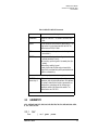
AUXILIARY PROGRAMS
GRIDCONV:
Converts output of mesh and radiography tallies to input for external graphics
programs.
HTAPE3X:
Postprocessor for MCNPX HISTP output.
MAKXSF:
Prepares MCNPX Cross-Section Libraries.
HCNV and TRX:
Convert LAHET ASCII data to binary.
XSEX3:
Analyzes a HISTP history file and generates double-differential particle
production cross sections for primary beam interactions
RELATED DATA LIBRARIES
Libraries specific to the LAHET Bertini model are included in a file called BERTIN. Gamma
production cross sections from spallation products are included in a file called PHTLIB. A new
version of PHTLIB is available for MCNPX 2.4.0, including improved data and also metastable state
information. High-energy total, reaction and elastic cross sections are contained in a file called
BARPOL.DAT.
MCNPX includes a test library of cross sections for running the sample problems, but the test
library is not suitable for real problems. Running the code requires continuous energy cross section
data included in the D00205ALLCP03 MCNPXDATA package or equivalent data. To receive the
data from RSICC, users must include MCNPXDATA on their request, license and Export
Control form.
The D00205ALLCP03 MCNPXDATA package is comprised of DLC-200/MCNPDATA,
which was released for use with MCNP4C; plus the LA150N library of 42 high energy neutron data
tables, LA150U photonuclear data for 12 isotopes, and LA150H proton data tables for 41 isotopes. In
LA150N, the neutron energy is extended to 150 MeV except for Be-9, which only goes to 100 MeV.
This library typically extends ENDF/B-VI data from 20 MeV to 150 MeV; therefore, charged particle
and recoil nuclei data will sometimes not be available below 20 MeV. Exceptions are noted in the
MCNPX User's Manual. All standard neutron libraries used with MCNP4B (originally distributed in
DLC-189 and now included in DLC-205) can be used with MCNPX; however, they will not contain
emission data for charged particles or recoil nuclei; therefore, these products will not be produced and
tracked. All neutron, photon and electron libraries developed for use with MCNP4C will work with
MCNPX2.4.0.
2. CONTRIBUTOR
Advanced Accelerator Applications, Los Alamos National Laboratory, Los Alamos, New
Mexico.
3. CODING LANGUAGE AND COMPUTER
Fortran 90 and C. IBM RS/6000, DEC Alpha, SGI, HP HP-UX, Sun, Intel Linux, Windows
PC (C00715MNYCP00).
4. NATURE OF PROBLEM SOLVED
The official release date of MCNPX 2.4.0 is August 1, 2002. MCNPX extends the
MCNP4C3 code to higher energies and more particle types. Photonuclear capability in the tabular
range is included in this release. Neutron tabular data are used as in MCNP4C3; above the table
energy limits, physics modules are used. Current physics modules include the Bertini and ISABEL
models taken from the LAHET Code System (LCS) and CEM. An old version of FLUKA is available
for calculations above the range of INC physics applicability. MCNPX eliminates the need now present
in LCS to transfer large files between separate codes. MCNPX is released with libraries for neutrons,
iii
photons, electrons, protons and photonuclear interactions. In addition, variance reduction schemes
(such as secondary particle biasing), and new tallies have been created specific to the intermediate and
high energy physics ranges. The ‘mesh’ and ‘radiography’ tallies were included for 2 and
3-dimensional imaging purposes. Energy deposition received a substantial reworking based on the
demands of charged-particle high-energy physics. An auxiliary program, GRIDCONV, converts the
mesh and radiography tally as well as standard mctal-file results for viewing by independent graphics
packages. The code may be run in parallel at all energies via PVM.
Information about MCNPX development can be found on the web site http://mcnpx.lanl.gov.
Information about the MCNPX beta test program may be obtained from Laurie Waters at LANL. A
listserver is available for beta test participants.
5. METHOD OF SOLUTION
All capabilities of MCNP4C3 have been retained. Consult the MCNPX User’s Manual for
applicability to high energy applications. MCNPX 2.4.0 has been rewritten in Fortran’90.
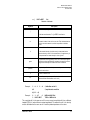
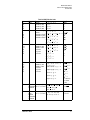
6. RESTRICTIONS OR LIMITATIONS
All standard MCNP neutron libraries over their stated ranges.
Neutrons in the LA150 library from 0.0 - 150.0 MeV in tabular range for 42 isotopes (except for 9Be
to 100 MeV).
Neutrons from 1.0 MeV in physics model regime.
Protons from 1.0 to 150.0 MeV in tabular range for 41 isotopes.
Protons from 1.0 MeV in physics model regime.
Pions, muons, and kaons are treated only by physics models.
Photons from 1 keV - 100 GeV.
Electrons from 1 keV - 1 GeV.
Neutrons do not create delayed photons.
Photonuclear interactions from 1.0 to 150.0 MeV in tabular range for 12 isotopes. No physics models
outside the tabular range are available in MCNPX 2.4.0.
For any incident particle where libraries exist (neutrons, protons, and photonuclear), MCNPX
2.4.0 users should not specify isotopes with different transition energies between tabular data and
physics models. The transition energies should be the same for each incident particle and should not
exceed the maximum energy of the selected data library.
7. TYPICAL RUNNING TIME
Runtime for the test cases was 17 minutes for the test cases on a Dell PowerEdge6400
running Linux, 37 minutes on an IBM RS/6000 Model 270, and 43 minutes on a HP B1000 (PA
8500).
8. COMPUTER HARDWARE REQUIREMENTS
MCNPX runs under Unix, Linux, and Windows operating systems and has been implemented
on IBM RS/6000 AIX, DEC Alpha Digital Unix, SGI IRIX 32 and 64-bit, HP HP-UX version 10, Sun
Solaris, Intel Linux, and Windows-based PC’s. The compiled version of the code tends to run ~8
Mbytes. Dynamic allocation makes memory demands variable on all platforms.
9. COMPUTER SOFTWARE REQUIREMENTS
C and Fortran 90 compilers are required to compile. The GNU make utility is required to
build the system on Unix and Linux platforms. The GNU make.exe utility is included for Windows
users. The only graphics support for this release is X11 http://www.x.org/Downloads_terms.htm. This
is a Fortran 90 version of MCNPX which uses standard F90 allocation schemes for dynamic variables
on all platforms. RSICC tested this release on the following systems:
1.
AIX 4.3.3 (IBM 43P-260) with XL C/C++ 4.4; XL Fortran 6.1.
2.
Dell PowerEdge6400 running RedHat Linux 7.0 with PGF90 4.0-2 and gcc.
iv
3.
4.
Intel Pentium running RedHat Linux 6.1 with PGF90 3.3-2 and pgcc.
Sun UltraSparc 60 under SunOS5.6 with F90 2.0 and C++ 5.0.
The LANL developers ran MCNPX 2.4.0 on the following systems. Their executables are
included in the distribution. Installation may fail with different compilers.
Sun-Solaris/WorkShop Fortran Compilers 6, update 2 (Fortran 95 6.2)
SGI-IRIX/MIPSpro Compilers: Version 7.30 under 64 bit IRIX and 32 bit IRIX
HP-HPUX/HP F90 v2.4.10
IBM-AIX/xlf90 Version 7 Release 1
DEC Alpha-Tru64 running OSF1 V5.0 with Compaq Fortran V5.3-915
Intel-Linux 7 with The Portland Group Fortran Group, Inc. f90 3.2-3
Windows2000 on Pentium IV - Compaq Visual Studio 6.6 and Microsoft C++ 6.0
(Note that Compaq Visual Studio 6.5 fails to compile the code, but 6.1 works.)
10. REFERENCES
a)
included in documentation
“MCNPX User's Manual, Version 2.4.0,” LA-CP-02-408 (September 2002).
L. S. Waters, ed., “MCNPX User’s Manual, Version 2.3.0,” LA-UR-02-2607 (April 2002).
b)
background references:
J. F. Briesmeister, Ed., “MCNP - A General Monte Carlo N-Particle Transport Code, Version
4C,’ LA-13709-M (April 2000).
M. B. Chadwick, P. G. Young, S. Chiba, S. C. Frankle, G. M. Hale, H. G. Hughes, A. J.
Koning, R. C. Little, R. E. MacFarlane, R. E. Prael, and L. S. Waters, “Cross Section Evaluations to
150 MeV for Accelerator-Driven Systems and Implementation in MCNPX,” Nuclear Science and
Engineering 131, Number 3 (March 1999) 293.
M. B. Chadwick, P. G. Young, R. E. MacFarlane, P. Moller, G. M. Hale, R. C. Little, A. J.
Koning and S. Chiba, “LA150 Documentation of Cross Sections, Heating, and Damage: Part A
(Incident Neutrons) and Part B (Incident Protons),” LA-UR-99-1222 (1999).
H. G. Hughes, et. al., “MCNPX™ for Neutron-Proton Transport,” International Conference
on Mathematics & Computation, Reactor Physics & Environmental. Analysis in Nuclear Applications,
American Nuclear Society, Madrid, Spain (September 27-30, 1999).
S. G. Mashnik, A. J. Sierk, O. Bersillon, and T. A. Gabriel, “Cascade-Exciton Model Detailed
Analysis of Proton Spallation at Energies from 10 MeV to 5 GeV,” Nucl. Instr. Meth. A414 (1998) 68.
(Los Alamos National Laboratory Report LA-UR-97-2905).
R. E. Prael and H.Lichtenstein, “User Guide to LCS: The LAHET Code System,”
LA-UR-89-3014, Revised (September 15, 1989).
11. CONTENTS OF CODE PACKAGE
Included are the referenced documents in (10.a) and one distribution CD which contains a
GNU compressed Unix tar file with the full source code for the MCNPX system, executable files,
installation scripts and test sets for each of the supported architectures. WinZIP 8.0 is required to
expand this file under Windows.
12. DATE OF ABSTRACT
September 2002.
KEYWORDS: CHARGED PARTICLES; COMPLEX GEOMETRY; ELECTRON;
GAMMA-RAY; HIGH ENERGY; KAON; MONTE CARLO; NEUTRON; PION;
PROTON; RADIOGRAPHY; SPALLATION; WORKSTATION
v
S
E
C
T
I
O
N
1
MCNPX User’s Manual
Version 2.4.0, September 2002
LA-CP-02-408
MCNPX™ USER’S MANUAL
Version 2.4.0
September, 2002
MCNPX User’s Manual
i
MCNPX User’s Manual
Version 2.4.0, September 2002
LA-CP-02-408
Disclaimer
This report was prepared as an account of work sponsored by an agency of the United States
Government. Neither the United States Government nor any agency thereof, nor any of their
employees, makes any warranty, express or implied, or assumes any legal liability or responsibility
for the accuracy, completeness, or usefulness of any information, apparatus, product, or process
disclosed, or represents that its use would not infringe privately owned rights. Reference herein to
any specific commercial product, process, or service by trade name, trademark, manufacturer, or
otherwise, does not necessarily constitute or imply its endorsement, recommendation, or favoring
by the United States Government or any agency thereof. The views and opinions of authors
expressed herein do not necessarily state or reflect those of the United States government or any
agency thereof.
ii
MCNPX User’s Manual
MCNPX User’s Manual
Version 2.4.0, September 2002
LA-CP-02-408
Acknowledgments
The MCNPX code and data effort represents the efforts of many people, much of whose
work is represented in this manual. The primary team members are listed below.
Code Development Team
H. Grady Hughes (team leader), Harry W. Egdorf, Franz C. Gallmeier, John S. Hendricks,
Robert C. Little, Gregg W. McKinney, Richard E. Prael, Teresa L. Roberts, Edward Snow,
Laurie S. Waters, Morgan C. White
Library Development Team
Mark B. Chadwick, Stephanie C. Frankle, Gerald M. Hale, Robert C. Little, Robert
MacFarlane, Morgan C. White, Phillip G. Young
Physics Development Team
David G. Madland, Stepan G. Mashnik, Richard E. Prael, Arnold J. Sierk
APT/AAA Target/Blanket Design and ED&D Team, LANSCE Team
Michael W. Cappiello, Rhonda K. Corzine, Phillip D. Ferguson, Michael M. Fikani, Frank D.
Gac, Michael R. James, Russell Kidman, Stuart A. Maloy, Michael A. Paciotti, Eric J.
Pitcher, Lawrence G. Quintana, Gary J. Russell
Beta Test Team
~900 users from ~200 institutions worldwide
MCNPX was originally conceived as an upgrade to the existing Los Alamos LAHET Code
System (LCS), and our deepest thanks is extended to Dr. Richard E. Prael for his support
and guidance. Without his longtime vision of providing the highest quality simulation tools
to the accelerator community, the MCNPX project could not have happened.
MCNPX 2.3.0 is based on MCNP4B, and we gratefully acknowledge the importance of that
seminal code in our work. The MCNP code series represents many thousand personyears of effort over the past 30 years, and we hope our efforts will add new vistas to this
core capability. Our special thanks goes to Dr. John Hendricks and Dr. Gregg McKinney,
as well as the numerous contributors who over the years have made MCNP a world class
code.
We also wish to express our appreciation to Dr. Alfredo Ferrari (currently with CERN) for
allowing the use of an early version of the FLUKA code in MCNPX, permitting a significant
expansion of our upper energy limits. We will endeavor in future versions of the code to
MCNPX User’s Manual
iii
MCNPX User’s Manual
Version 2.4.0, September 2002
LA-CP-02-408
upgrade this capability. In addition, we wish to express our fond appreciation for the efforts
of Dr. Stepan Mashnik, who has improved the CEM code for inclusion in MCNPX.
Dr. Nikolai Mokhov of Fermi National Laboratory has provided improved high-energy
photonuclear physics routines that will be implemented in future versions of the code. We
also wish to thank him for his part in the formal reviews of our work.
Several visitors have provided invaluable help to the nuclear data team with evaluations,
notably Dr. Satoshi Chiba (JAERI) and Dr. Arjan Koning (ECN-Petten).
Of special note is the valuable help given us by those sponsoring MCNPX classes, including William Hamilton of HQC Professional Services, Inc., Enrico Sartori of NEA, Tadakazu
Suzuki of JAERI, and Pedro Vaz of ITN, Portugal. The MCNPX classes are a vital part of
our code quality assurance program and we very much appreciate their help and support.
We would also like to thank members of the Los Alamos Export Controls Office, particularly Sarah-Jane W. Maynard, Crystal Johnson and Steve H. Remde, for their outstanding
help in dealing with the export issues for our foreign beta test team members.
Publishing Team
Finally, we wish to thank Berylene Rogers for copyediting and preparing the final document, and Patty Montoya, Barbara Olguin, Arlene Lopez, and Jean Harlow for their help in
reproducing and assembling the manual.
iv
MCNPX User’s Manual
MCNPX User’s Manual
Version 2.4.0, September 2002
LA-CP-02-408
Dedication
We dedicate this code to the memory of our respected colleague, Dr. Russell B. Kidman.
Russ was an invaluable member of the APT Target/Blanket design team and a computer
simulations expert for many projects at Los Alamos. His tragic and premature death has
left us all with a deep sense of loss.
MCNPX User’s Manual
v
MCNPX User’s Manual
Version 2.4.0, September 2002
LA-CP-02-408
TABLE OF CONTENTS
Acknowledgments . . . . . . . . . . . . . . . . . . . . . . . . . . . . . . . . . . . . . . . . . . . . iii
Dedication . . . . . . . . . . . . . . . . . . . . . . . . . . . . . . . . . . . . . . . . . . . . . . . . . . . .v
Preface . . . . . . . . . . . . . . . . . . . . . . . . . . . . . . . . . . . . . . . . . . . . . . . . . . . . xiii
1 Introduction . . . . . . . . . . . . . . . . . . . . . . . . . . . . . . . . . . . . . . . . . . . . . . . . .1
2 Warnings and Limitations. . . . . . . . . . . . . . . . . . . . . . . . . . . . . . . . . . . . . .5
3 Installation . . . . . . . . . . . . . . . . . . . . . . . . . . . . . . . . . . . . . . . . . . . . . . . . . .9
3.1 UNIX Build System . . . . . . . . . . . . . . . . . . . . . . . . . . . . . . . . . . . . . . . . . . . . . . . . 9
3.1.1 In the Beginning . . . . . . . . . . . . . . . . . . . . . . . . . . . . . . . . . . . . . . . . . . . . 9
3.1.2 Automated Building . . . . . . . . . . . . . . . . . . . . . . . . . . . . . . . . . . . . . . . . 10
3.1.3 Build Examples . . . . . . . . . . . . . . . . . . . . . . . . . . . . . . . . . . . . . . . . . . . . 12
3.1.3.1 System-Wide Installation . . . . . . . . . . . . . . . . . . . . . . . . . . . . . . . . . 12
3.1.3.2 System-Wide Installation With Existing Directories . . . . . . . . . . . . . 13
3.1.3.3 Individual Private Installation . . . . . . . . . . . . . . . . . . . . . . . . . . . . . . 14
3.1.3.4 Individual Private Installation Done Better . . . . . . . . . . . . . . . . . . . . 15
3.1.3.5 Individual Private Installation - special compilers and debugging . . 16
3.1.4 Directory Reorganization . . . . . . . . . . . . . . . . . . . . . . . . . . . . . . . . . . . . 18
3.1.5 User’s Notes . . . . . . . . . . . . . . . . . . . . . . . . . . . . . . . . . . . . . . . . . . . . . . 19
3.1.6 Multiprocessing. . . . . . . . . . . . . . . . . . . . . . . . . . . . . . . . . . . . . . . . . . . . 25
3.1.7 Programmer’s Notes . . . . . . . . . . . . . . . . . . . . . . . . . . . . . . . . . . . . . . . . 25
3.2 Windows Build System. . . . . . . . . . . . . . . . . . . . . . . . . . . . . . . . . . . . . . . . . . . . 26
3.3 Libraries and Where to Find Them . . . . . . . . . . . . . . . . . . . . . . . . . . . . . . . . . . 27
4 Input Files. . . . . . . . . . . . . . . . . . . . . . . . . . . . . . . . . . . . . . . . . . . . . . . . . .31
4.1 INP FILE . . . . . . . . . . . . . . . . . . . . . . . . . . . . . . . . . . . . . . . . . . . . . . . . . . . . . . . . 31
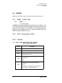
4.1.1 Initiate-Run. . . . . . . . . . . . . . . . . . . . . . . . . . . . . . . . . . . . . . . . . . . . . . . . 31
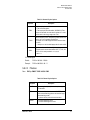
4.1.2 Continue-Run. . . . . . . . . . . . . . . . . . . . . . . . . . . . . . . . . . . . . . . . . . . . . . 32
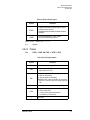
4.1.3 Message Block . . . . . . . . . . . . . . . . . . . . . . . . . . . . . . . . . . . . . . . . . . . . 34
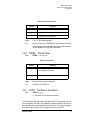
4.1.4 Problem Title Card . . . . . . . . . . . . . . . . . . . . . . . . . . . . . . . . . . . . . . . . . 34
4.1.5 Card Format . . . . . . . . . . . . . . . . . . . . . . . . . . . . . . . . . . . . . . . . . . . . . . . 34
4.1.6 Comment Cards. . . . . . . . . . . . . . . . . . . . . . . . . . . . . . . . . . . . . . . . . . . . 34
4.1.7 Horizontal Input Format . . . . . . . . . . . . . . . . . . . . . . . . . . . . . . . . . . . . . 34
4.1.8 Repeat, Interpolate, Multiply, and Jump & Log Shortcuts . . . . . . . . . 35
4.1.9 Vertical Input Format . . . . . . . . . . . . . . . . . . . . . . . . . . . . . . . . . . . . . . . 36
4.1.10 Particle Designators . . . . . . . . . . . . . . . . . . . . . . . . . . . . . . . . . . . . . . . 38
vi
MCNPX User’s Manual
MCNPX User’s Manual
Version 2.4.0, September 2002
LA-CP-02-408
4.1.11 Default Values. . . . . . . . . . . . . . . . . . . . . . . . . . . . . . . . . . . . . . . . . . . .
4.2 Input Error Messages. . . . . . . . . . . . . . . . . . . . . . . . . . . . . . . . . . . . . . . . . . . . .
4.3 Geometry Errors . . . . . . . . . . . . . . . . . . . . . . . . . . . . . . . . . . . . . . . . . . . . . . . . .
4.4 Storage Limitations . . . . . . . . . . . . . . . . . . . . . . . . . . . . . . . . . . . . . . . . . . . . . .
41
41
41
43
5 Plotting . . . . . . . . . . . . . . . . . . . . . . . . . . . . . . . . . . . . . . . . . . . . . . . . . . . 45
5.1 The Interactive Geometry Plotter . . . . . . . . . . . . . . . . . . . . . . . . . . . . . . . . . . .
5.2 Tallies & Cross-sections . . . . . . . . . . . . . . . . . . . . . . . . . . . . . . . . . . . . . . . . . .
5.2.1 Input for MCPLOT and Execution Line Options . . . . . . . . . . . . . . . . .
5.2.2 Plot Conventions and Command Syntax . . . . . . . . . . . . . . . . . . . . . . .
5.2.2.1 2D plot. . . . . . . . . . . . . . . . . . . . . . . . . . . . . . . . . . . . . . . . . . . . . . .
45
47
47
49
49
5.2.2.2 Contour plot . . . . . . . . . . . . . . . . . . . . . . . . . . . . . . . . . . . . . . . . . .
5.2.2.3 Command syntax . . . . . . . . . . . . . . . . . . . . . . . . . . . . . . . . . . . . . .
Plot Commands Grouped by Function . . . . . . . . . . . . . . . . . . . . . . . . . . . . .
5.3 Geometry. . . . . . . . . . . . . . . . . . . . . . . . . . . . . . . . . . . . . . . . . . . . . . . . . . . . . . .
5.3.1 Cell. . . . . . . . . . . . . . . . . . . . . . . . . . . . . . . . . . . . . . . . . . . . . . . . . . . . . .
5.3.2 Surface . . . . . . . . . . . . . . . . . . . . . . . . . . . . . . . . . . . . . . . . . . . . . . . . . .
5.3.2.1 Surfaces Defined by Equations. . . . . . . . . . . . . . . . . . . . . . . . . . . .
5.3.2.2 Axisymmetric Surfaces Defined by Points . . . . . . . . . . . . . . . . . . .
5.3.2.3 General Plane Defined by Three Points . . . . . . . . . . . . . . . . . . . . .
5.3.2.4 Surfaces Defined by Macrobodies . . . . . . . . . . . . . . . . . . . . . . . . .
5.3.2.4.1 BOX- Arbitrarily oriented orthogonal box . . . . . . . . . . . . . .
5.3.2.4.2 RPP - Rectangular Parallelepiped . . . . . . . . . . . . . . . . . . .
5.3.2.4.3 SPH - Sphere . . . . . . . . . . . . . . . . . . . . . . . . . . . . . . . . . . .
5.3.2.4.4 RCC - Right Circular Cylinder, Can . . . . . . . . . . . . . . . . . .
5.3.2.4.5 RHP or HEX - Right Hexagonal Prism.. . . . . . . . . . . . . . . .
5.3.2.4.6 REC - Right Elliptical Cylinder . . . . . . . . . . . . . . . . . . . . . .
5.3.2.4.7 TRC - Truncated Right Angle Cone . . . . . . . . . . . . . . . . . .
5.3.2.4.8 ELL - Ellipsoid . . . . . . . . . . . . . . . . . . . . . . . . . . . . . . . . . . .
5.3.2.4.9 WED - Wedge . . . . . . . . . . . . . . . . . . . . . . . . . . . . . . . . . . .
5.3.2.4.10 ARB - Arbitrary Polyhedron . . . . . . . . . . . . . . . . . . . . . . .
5.3.3 Geometry Data . . . . . . . . . . . . . . . . . . . . . . . . . . . . . . . . . . . . . . . . . . . .
5.3.3.1 VOL
Cell Volume . . . . . . . . . . . . . . . . . . . . . . . . . . . . . . . . . . . .
5.3.3.2 AREA Surface Area . . . . . . . . . . . . . . . . . . . . . . . . . . . . . . . . . . .
5.3.3.3 U
Universe . . . . . . . . . . . . . . . . . . . . . . . . . . . . . . . . . . . . . . . . .
49
49
50
58
58
60
60
62
62
63
63
63
64
64
65
65
66
66
67
67
68
68
69
69
5.3.3.4 FILL Fill . . . . . . . . . . . . . . . . . . . . . . . . . . . . . . . . . . . . . . . . . . . .
5.3.3.5 TRCL Cell Transformation . . . . . . . . . . . . . . . . . . . . . . . . . . . . .
5.3.3.6 LAT Lattice . . . . . . . . . . . . . . . . . . . . . . . . . . . . . . . . . . . . . . . . .
5.3.3.7 TRn Coordinate Transformation . . . . . . . . . . . . . . . . . . . . . . . . .
5.4 Materials . . . . . . . . . . . . . . . . . . . . . . . . . . . . . . . . . . . . . . . . . . . . . . . . . . . . . . .
70
71
72
73
74
MCNPX User’s Manual
vii
MCNPX User’s Manual
Version 2.4.0, September 2002
LA-CP-02-408
5.4.1 Mm Material. . . . . . . . . . . . . . . . . . . . . . . . . . . . . . . . . . . . . . . . . . . . . . 74
5.4.2 MTm S(α,β) Material . . . . . . . . . . . . . . . . . . . . . . . . . . . . . . . . . . . . . . . 76
5.4.3 MPNm Photonuclear Material . . . . . . . . . . . . . . . . . . . . . . . . . . . . . . . 77
5.4.4 TOTNU Total Fission . . . . . . . . . . . . . . . . . . . . . . . . . . . . . . . . . . . . . . 77
5.4.5 NONU Fission Turnoff. . . . . . . . . . . . . . . . . . . . . . . . . . . . . . . . . . . . . 77
5.4.6 AWTAB Atomic Weight. . . . . . . . . . . . . . . . . . . . . . . . . . . . . . . . . . . . 78
5.4.7 XSn Cross-Section File. . . . . . . . . . . . . . . . . . . . . . . . . . . . . . . . . . . . 78
5.4.8 VOID Material Void . . . . . . . . . . . . . . . . . . . . . . . . . . . . . . . . . . . . . . . 78
5.4.9 PIKMT Photon–Production Bias . . . . . . . . . . . . . . . . . . . . . . . . . . . . 79
5.4.10 MGOPT Multigroup Adjoint Transport Option . . . . . . . . . . . . . . . . 80
5.4.11 DRXS Discrete Reaction Cross-Section . . . . . . . . . . . . . . . . . . . . . 81
5.5 Physics. . . . . . . . . . . . . . . . . . . . . . . . . . . . . . . . . . . . . . . . . . . . . . . . . . . . . . . . . 82
5.5.1 MODE Problem Type . . . . . . . . . . . . . . . . . . . . . . . . . . . . . . . . . . . . . . 82
5.5.2 PHYS Energy Physics Cutoff. . . . . . . . . . . . . . . . . . . . . . . . . . . . . . . . 82
5.5.2.1 Neutrons . . . . . . . . . . . . . . . . . . . . . . . . . . . . . . . . . . . . . . . . . . . . . 82
5.5.2.2 Photons:. . . . . . . . . . . . . . . . . . . . . . . . . . . . . . . . . . . . . . . . . . . . . . 83
5.5.2.3 Electrons . . . . . . . . . . . . . . . . . . . . . . . . . . . . . . . . . . . . . . . . . . . . . 84
5.5.2.4 Protons . . . . . . . . . . . . . . . . . . . . . . . . . . . . . . . . . . . . . . . . . . . . . . 85
5.5.2.5 Other Particles . . . . . . . . . . . . . . . . . . . . . . . . . . . . . . . . . . . . . . . . . 85
5.5.3 TMP Free-Gas Thermal Temperature . . . . . . . . . . . . . . . . . . . . . . . . 86
5.5.4 THTME Thermal Times . . . . . . . . . . . . . . . . . . . . . . . . . . . . . . . . . . . . 86
5.5.5 COINC 3He Detector Coincidence . . . . . . . . . . . . . . . . . . . . . . . . . . . 87
5.5.6 Problem Cutoff Cards . . . . . . . . . . . . . . . . . . . . . . . . . . . . . . . . . . . . . . . 87
5.5.6.1 CUT Cutoffs . . . . . . . . . . . . . . . . . . . . . . . . . . . . . . . . . . . . . . . . . 87
5.5.6.2 ELPT Cell–by–cell Energy Cutoff . . . . . . . . . . . . . . . . . . . . . . . . 88
5.5.6.3 NPS History Cutoff. . . . . . . . . . . . . . . . . . . . . . . . . . . . . . . . . . . . 89
5.5.6.3 CTME Computer Time Cutoff . . . . . . . . . . . . . . . . . . . . . . . . . . . 89
5.5.7 Physics Models . . . . . . . . . . . . . . . . . . . . . . . . . . . . . . . . . . . . . . . . . . . . 89
5.5.7.1 LCA . . . . . . . . . . . . . . . . . . . . . . . . . . . . . . . . . . . . . . . . . . . . . . . . . 90
5.5.7.2 LCB . . . . . . . . . . . . . . . . . . . . . . . . . . . . . . . . . . . . . . . . . . . . . . . . . 92
5.5.7.3 LEA . . . . . . . . . . . . . . . . . . . . . . . . . . . . . . . . . . . . . . . . . . . . . . . . . 94
5.5.7.4 LEB . . . . . . . . . . . . . . . . . . . . . . . . . . . . . . . . . . . . . . . . . . . . . . . . . 95
5.6 Source Specification. . . . . . . . . . . . . . . . . . . . . . . . . . . . . . . . . . . . . . . . . . . . . . 97
5.6.1 SDEF General Source Definition . . . . . . . . . . . . . . . . . . . . . . . . . . . . 97
5.6.1.1 SIn Source Information . . . . . . . . . . . . . . . . . . . . . . . . . . . . . . . . 99
5.6.1.2 SPn Source Probability . . . . . . . . . . . . . . . . . . . . . . . . . . . . . . . . 99
5.6.1.3 SBn Source Bias . . . . . . . . . . . . . . . . . . . . . . . . . . . . . . . . . . . . 100
5.6.1.4 DSn Dependent Source Distribution . . . . . . . . . . . . . . . . . . . . . 101
5.6.1.5 SCn Source Comment . . . . . . . . . . . . . . . . . . . . . . . . . . . . . . . . 102
viii
MCNPX User’s Manual
MCNPX User’s Manual
Version 2.4.0, September 2002
LA-CP-02-408
5.6.2 KCODE Criticality Source . . . . . . . . . . . . . . . . . . . . . . . . . . . . . . . .
5.6.3 KSRC Source Points for KCODE Calculation . . . . . . . . . . . . . . . .
5.6.4 SSW Surface Source Write . . . . . . . . . . . . . . . . . . . . . . . . . . . . . . . .
5.6.5 SSR Surface Source Read. . . . . . . . . . . . . . . . . . . . . . . . . . . . . . . .
5.6.6 Subroutines SOURCE and SRCDX . . . . . . . . . . . . . . . . . . . . . . . . . . .
5.6.7 Extended Source Options . . . . . . . . . . . . . . . . . . . . . . . . . . . . . . . . . .
5.7 Tally Specification . . . . . . . . . . . . . . . . . . . . . . . . . . . . . . . . . . . . . . . . . . . . . .
5.7.1 Fna Tally . . . . . . . . . . . . . . . . . . . . . . . . . . . . . . . . . . . . . . . . . . . . . .
5.7.1.1 Surface and Cell Tallies (tally types 1, 2, 4, 6, and 7). . . . . . . . . .
5.7.1.2 Repeated Structures Tallies . . . . . . . . . . . . . . . . . . . . . . . . . . . . .
5.7.1.2.1 Multiple bin format: . . . . . . . . . . . . . . . . . . . . . . . . . . . . . .
5.7.1.2.2 Brackets: . . . . . . . . . . . . . . . . . . . . . . . . . . . . . . . . . . . . . .
5.7.1.2.3 Universe format: . . . . . . . . . . . . . . . . . . . . . . . . . . . . . . . .
5.7.1.2.4 Use of SDn card for repeated structures tallies: . . . . . . . .
5.7.1.3 Detector Tallies (tally type 5) . . . . . . . . . . . . . . . . . . . . . . . . . . . .
5.7.1.4 Pulse height Tallies (tally type 8) . . . . . . . . . . . . . . . . . . . . . . . . .
5.7.2 FCn Tally Comment. . . . . . . . . . . . . . . . . . . . . . . . . . . . . . . . . . . . . .
5.7.3 En Tally Energy . . . . . . . . . . . . . . . . . . . . . . . . . . . . . . . . . . . . . . . . .
5.7.4 Tn Tally Time . . . . . . . . . . . . . . . . . . . . . . . . . . . . . . . . . . . . . . . . . .
5.7.5 Cn Cosine Card (tally type 1 and 2) . . . . . . . . . . . . . . . . . . . . . . . .
5.7.6 FQn Print Hierarchy . . . . . . . . . . . . . . . . . . . . . . . . . . . . . . . . . . . . .
5.7.7 FMn Tally Multiplier . . . . . . . . . . . . . . . . . . . . . . . . . . . . . . . . . . . . . .
5.7.8 DEn and DFn Dose Energy and Dose Function . . . . . . . . . . . . . .
5.7.9 EMn Energy Multiplier. . . . . . . . . . . . . . . . . . . . . . . . . . . . . . . . . . . .
5.7.10 TMn Time Multiplier. . . . . . . . . . . . . . . . . . . . . . . . . . . . . . . . . . . . .
5.7.11 CMn Cosine Multiplier (tally type 1 only) . . . . . . . . . . . . . . . . . . .
5.7.12 CFn Cell-Flagging (tally types 1, 2, 4, 6, 7). . . . . . . . . . . . . . . . . .
5.7.13 SFn Surface-Flagging (tally types 1, 2, 4, 6, 7) . . . . . . . . . . . . . .
5.7.14 FSn Tally Segment (tally types 1, 2, 4, 6, 7) . . . . . . . . . . . . . . . . .
5.7.15 SDn Segment Divisor (tally types 1, 2, 4, 6, 7). . . . . . . . . . . . . . .
5.7.16 FUn Special Tally or TALLYX Input . . . . . . . . . . . . . . . . . . . . . . . .
5.7.17 FTn Special Treatments for Tallies. . . . . . . . . . . . . . . . . . . . . . . .
5.7.18 Subroutine TALLYX
User-supplied Subroutine . . . . . . . . . . . . .
5.7.19 TFn Tally Fluctuation . . . . . . . . . . . . . . . . . . . . . . . . . . . . . . . . . . .
5.7.20 TIRn The Radiography Tally . . . . . . . . . . . . . . . . . . . . . . . . . . . . . .
102
102
103
104
107
107
111
112
114
116
117
118
118
119
120
121
121
122
122
122
123
124
126
128
128
128
129
129
130
131
131
131
135
135
136
5.7.20.1 Pinhole Image Projection . . . . . . . . . . . . . . . . . . . . . . . . . . . . . .
5.7.20.2 Transmitted Image Projection . . . . . . . . . . . . . . . . . . . . . . . . . . .
5.7.20.3 Additional Radiography Input Cards . . . . . . . . . . . . . . . . . . . . . .
5.7.20.4 Reading the Radiography Tally Output. . . . . . . . . . . . . . . . . . . .
5.7.21 PERTn Perturbation . . . . . . . . . . . . . . . . . . . . . . . . . . . . . . . . . . . .
136
138
139
140
140
MCNPX User’s Manual
ix
MCNPX User’s Manual
Version 2.4.0, September 2002
LA-CP-02-408
5.7.22 TMESH The Mesh Tally . . . . . . . . . . . . . . . . . . . . . . . . . . . . . . . . . . 143
5.7.22.1 Setting up the Mesh in the INP File . . . . . . . . . . . . . . . . . . . . . . . 144
5.7.22.2 Track Averaged Mesh Tally (Type 1). . . . . . . . . . . . . . . . . . . . . . 145
5.7.22.3 Source Mesh Tally (Type 2). . . . . . . . . . . . . . . . . . . . . . . . . . . . . 147
5.7.22.4 Energy Deposition Mesh Tally (Type 3). . . . . . . . . . . . . . . . . . . . 148
5.7.22.5 DXTRAN Mesh Tally (Type 4) . . . . . . . . . . . . . . . . . . . . . . . . . . . 149
5.7.22.6 Dose Conversion Coefficients . . . . . . . . . . . . . . . . . . . . . . . . . . . 150
5.7.22.7 Processing the Mesh Tally Results . . . . . . . . . . . . . . . . . . . . . . . 152
5.8 Variance Reduction. . . . . . . . . . . . . . . . . . . . . . . . . . . . . . . . . . . . . . . . . . . . . . 153
5.8.1 IMP Cell Importance . . . . . . . . . . . . . . . . . . . . . . . . . . . . . . . . . . . . . 153
5.8.2 WWG Weight Window Generator. . . . . . . . . . . . . . . . . . . . . . . . . . . 154
5.8.3 WWGE Weight Window Generation Energies or Times . . . . . . . . 155
5.8.4 WWP Weight Window Parameter. . . . . . . . . . . . . . . . . . . . . . . . . . . 155
5.8.5 WWN Cell–Based Weight Window Bounds . . . . . . . . . . . . . . . . . . 156
5.8.6 WWE Weight Window Energies or Times . . . . . . . . . . . . . . . . . . . . 157
5.8.7 MESH Mesh-Based Weight Window Generator . . . . . . . . . . . . . . . . 158
5.8.8 EXT Exponential Transform . . . . . . . . . . . . . . . . . . . . . . . . . . . . . . . 159
5.8.9 VECT Vector Input. . . . . . . . . . . . . . . . . . . . . . . . . . . . . . . . . . . . . . . 160
5.8.10 FCL Forced Collision . . . . . . . . . . . . . . . . . . . . . . . . . . . . . . . . . . . 160
5.8.11 DDn Detector Diagnostics . . . . . . . . . . . . . . . . . . . . . . . . . . . . . . . . 161
5.8.12 PDn Detector Contribution . . . . . . . . . . . . . . . . . . . . . . . . . . . . . . . 162
5.8.13 DXT DXTRAN . . . . . . . . . . . . . . . . . . . . . . . . . . . . . . . . . . . . . . . . . . 163
5.8.14 DXC DXTRAN Contribution . . . . . . . . . . . . . . . . . . . . . . . . . . . . . . 163
5.8.15 BBREM Bremsstrahlung Biasing. . . . . . . . . . . . . . . . . . . . . . . . . . 164
5.8.16 SPABI Secondary Particle Biasing . . . . . . . . . . . . . . . . . . . . . . . . 164
5.8.17 ESPLT Energy Splitting and Roulette . . . . . . . . . . . . . . . . . . . . . . 165
5.8.18 PWT Photon Weight . . . . . . . . . . . . . . . . . . . . . . . . . . . . . . . . . . . . 166
5.9 Output Control . . . . . . . . . . . . . . . . . . . . . . . . . . . . . . . . . . . . . . . . . . . . . . . . . . 166
5.9.1 PRDMP Print and Dump Cycle . . . . . . . . . . . . . . . . . . . . . . . . . . . . . 166
5.9.2 PRINT Output Print Tables . . . . . . . . . . . . . . . . . . . . . . . . . . . . . . . . 167
5.9.3 MPLOT Plot tally while problem is running . . . . . . . . . . . . . . . . . . 169
5.9.4 PTRAC Particle Track Output. . . . . . . . . . . . . . . . . . . . . . . . . . . . . . 169
5.9.5 HISTP and HTAPE3X. . . . . . . . . . . . . . . . . . . . . . . . . . . . . . . . . . . . . . . 171
5.9.6 DBCN Debug Information . . . . . . . . . . . . . . . . . . . . . . . . . . . . . . . . . 171
5.9.7 LOST
Lost Particle . . . . . . . . . . . . . . . . . . . . . . . . . . . . . . . . . . . . . . 173
5.9.8 IDUM Integer Array . . . . . . . . . . . . . . . . . . . . . . . . . . . . . . . . . . . . . . 173
5.9.9 RDUM Floating Point Array . . . . . . . . . . . . . . . . . . . . . . . . . . . . . . . 173
5.9.10 FILES File Creation . . . . . . . . . . . . . . . . . . . . . . . . . . . . . . . . . . . . . 173
5.10 SUMMARY OF MCNPX INPUT CARDS . . . . . . . . . . . . . . . . . . . . . . . . . . . . . 174
x
MCNPX User’s Manual
MCNPX User’s Manual
Version 2.4.0, September 2002
LA-CP-02-408
6 References . . . . . . . . . . . . . . . . . . . . . . . . . . . . . . . . . . . . . . . . . . . . . . . 181
Appendix A – Examples . . . . . . . . . . . . . . . . . . . . . . . . . . . . . . . . . . . . . . 191
Appendix B – HTAPE3X for use with MCNPX . . . . . . . . . . . . . . . . . . . . . 205
Appendix C - Using XSEX3 with MCNPX. . . . . . . . . . . . . . . . . . . . . . . . . 225
MCNPX User’s Manual
xi
MCNPX User’s Manual
Version 2.4.0, September 2002
LA-CP-02-408
xii
MCNPX User’s Manual
MCNPX User’s Manual
Version 2.4.0, September 2002
LA-CP-02-408
Preface
Work on the MCNPX™1 code has been primarily sponsored by both the Accelerator Production of Tritium (APT) and Advanced Accelerator Applications (AAA) projects in
response to requests from the facility designers. Originally, MCNPX was one part of the
APT effort to provide a validated set of computer simulation tools to use in design of the
APT spallation target, surrounding lead blanket, and associated shielding. Other elements
of this program included the production of new nuclear data evaluations from 20 to 150
MeV for neutrons, and from 1 to 150 MeV for proton and photonuclear interactions. Additional work was undertaken to provide improved total, reaction, and elastic cross section
tables above 150 MeV and to improve the physics involved with the intermediate- and highenergy physics models through the CEM program. Currently the requirements of the
Accelerator Transmutation of Waste program, which is part of AAA, are directed toward
improvements in fission physics and actinide data.
Responsibility for the development of MCNPX was given to the APT Target/Blanket and
Materials Engineering Development and Demonstration (ED&D) project. A code development team under the leadership of Dr. H. Grady Hughes was formed. Because the Los
Alamos accelerator community has long supported the work of Dr. Richard Prael in the
development of the LAHETTM Code System, it was decided to build on this base by combining the capabilities of LAHET and MCNPTM into one code. This was accomplished by
extending the capabilities of MCNP4BTM to all particles and all energies, and including the
use of physics models in the code to compute interaction probabilities where table-based
data are not available. In the present version, MCNPX 2.4.0, the code has also incorporated all features of MCNP4C3.
Additional development has been provided by the theoretical efforts of the T-16 group at
Los Alamos, particularly in the areas of nuclear data evaluation and expansion of physicsbased models. A program of experimental activities was also undertaken, including measurement of various cross sections and development of more complex benchmarks
specific to the APT and AAA projects.
Our commitment to modern software management and quality assurance methods in the
development of MCNPX is very strong. The code is used for the design of high-intensity
accelerator category 2 nuclear facilities, and has already been used to design a major category 3 activity at the LANSCE high-power beamstop. MCNPX development is guided by
a set of requirements, design, and functional specification documents. Code testing is performed on a large scale by a volunteer beta test team. Code configuration management is
involves the CVS system, and methods of assessing code development progress are
being implemented. One of these involves nightly regression testing on a computer farm
of over 20 hardware/software platforms. Training courses are held regularly.
1. MCNPX, MCNP, MCNP4B, LAHET, and LAHET Code System (LCS) are trademarks of the Regents of the
University of California, Los Alamos National Laboratory.
MCNPX User’s Manual
xiii
MCNPX User’s Manual
Version 2.4.0, September 2002
LA-CP-02-408
We have also developed a unique autoconfiguration build system which allows a variety of
compilation options to be easily executed on a large number of platforms. MCNPX 2.4.0
extends the previous set of supported platforms to Windows PC. This version of the code
has also been rewritten in Fortran 90, and many of the code elements recast as modules.
Work on our ‘component architecture’ approach is also proceeding. This software engineering project fully recognizes that some elements of MCNPX are older, well tested
programs developed outside of the core MCNPX team, and may even be written in different
languages. We also see a very strong future in building the capability to interface effectively
with these, and even other types of codes, such as geometry builders, transmutation and
thermal-hydraulics packages. The MCNPX build system is the first step in this process,
and work on a formal software definition interface language is underway.
Geometry, basic tally and graphical capabilities of MCNPX do not fundamentally differ from
the standard MCNP4C code as released in 2000. Input cards have rarely been modified,
however a number of new cards have been added to control the physics model options,
set parameters for new particles, and control new tally and variance reduction features.
The present MCNPX 2.4.0 manual differs fundamentally from those released for code versions in the past (2.1.5, 2.3.0). We are now starting to build a more comprehensive
description of the code, which eventually will be issued in three parts. Vol I will cover physics and appropriate Monte Carlo methodology. Vol II will be the practical user guide for the
code. Vol III will cover items of interest to code developers. The present work is equivalent
to Volume II, and also integrates much more fundamental material than present in the previous manuals. We are also seriously rethinking information presentation, and will soon
issue a revision which incorporates a dictionary-type lookup system for card definitions.
Until the complete set of manuals is issued, we recommend using this document in tandem
with the MCNP4C manual, and the previously issued MCNPX 2.3.0 User’s Manual.
It is hoped that MCNPX will be of use to the Monte Carlo radiation transport community in
general, and we are already seeing major applications in medical and space science fields,
also in areas where tracking of low energy charged particles is important. The development of the modular approach in future versions of the code will facilitate the addition of
new capabilities to the base code and make this tool a flexible, reliable aid in the exploration of both traditional and new mixed-energy, multiparticle applications.
Laurie Waters
Deputy Group Leader
D-10, Nuclear Systems Design
Los Alamos National Laboratory
September 2002
xiv
MCNPX User’s Manual
MCNPX User’s Manual
Version 2.4.0, September, 2002
LA-CP-02-408
1
Introduction
MCNPX is a general purpose Monte Carlo radiation transport code that tracks all particles
at all energies. It is the next generation in the series of Monte Carlo transport codes that
began at Los Alamos fifty years ago. MCNPX 2.4.0 is a superset of MCNP4C3 and
MCNPX 2.3.0, LAHET 2.8 and CEM.
The MCNPX program began in 1994 as an extension of MCNP and LAHET in support of
the Accelerator Production of Tritium Project (APT). The work involved a formal extension
of MCNP to all particles and all energies, improvement of physics simulation models,
extension of neutron, proton and photonuclear libraries to 150 MeV, and the formulation of
new variance reduction and data analysis techniques. The program also included cross
section measurements, benchmark experiments, deterministic code development, and
improvements in transmutation code and library tools through the CINDER ’90 project.
Since the closure of the APT project, work on the code has continued under the
sponsorship of the Advanced Accelerator Applications (AAA) and other programs.
Since the initial release of MCNPX version 2.1 on October 23, 1997, an extensive betatest team has been formed to test the code versions prior to official release. Approximately
900 users in approximately 200 institutions worldwide have had an opportunity to try the
improvements in this version, and to provide feedback to the developers. This process is
invaluable, and we express our deepest appreciation to the participants in the beta test
program.
Applications for the code among the beta-test team are quite broad and constantly
developing. Examples include:
•
Design of accelerator spallation targets, particularly for neutron scattering facilities.
•
Investigations for accelerator isotope production and destruction programs, including
the transmutation of nuclear waste.
•
Research into accelerator-driven energy sources.
•
Medical physics, especially proton and neutron therapy.
•
Investigations of cosmic-ray radiation backgrounds and shielding for high altitude aircraft and spacecraft.
•
Accelerator-based imaging technology such as neutron and proton radiography.
•
Design of shielding in accelerator facilities.
•
Activation of accelerator components and surrounding groundwater and air.
MCNPX User’s Manual
1
MCNPX User’s Manual
Version 2.4.0, September, 2002
LA-CP-02-408
•
Investigation of fully coupled neutron-charged particle transport for lower-energy
applications.
•
High-energy dosimetry and neutron detection.
•
Design of neutrino experiments.
•
Comparison of physics-based and table-based data.
•
Charged-particle tracking in plasmas.
•
Charged-particle propulsion concepts for spaceflight.
•
Single-event upset in semiconductors, from cosmic rays in spacecraft or from the
neutron component on the earth’s surface.
•
Detection technology using charged particles (i.e., abandoned landmines).
•
Nuclear Safeguards
•
Nuclear criticality safety
•
Radiation protection and shielding
•
Oil well logging
In addition to the activities of the beta-test team, the development of MCNPX is governed
by several documents, including:
•
MCNPX Software Management Plan
•
MCNPX Requirements
•
MCNPX Design
•
MCNPX Functional Specifications
Configuration management of the code is done through CVS, which allows us to
conveniently track issues and changes. A computer test farm of 20 different software/
hardware configurations is maintained to ensure that code development does not
adversely affect any previously tested system. We are also constantly moving toward a
modular system whereby the user may easily implement alternative physics packages
(EGD01). Some restructuring of the code has already been done toward that goal,
including the development of an autconfiguration system.
In addition to describing the new interaction physics, this manual contains a summary of
information from recent MCNPX release notes, memos, publications and presentations. It
represents the work of the code development team, the nuclear data team, the physics
development team, and several outside collaborators. The manual is updated and
extended with each new code release.
2
MCNPX User’s Manual
MCNPX User’s Manual
Version 2.4.0, September, 2002
LA-CP-02-408
The reader must be aware of certain limitations in code usage. These items are listed in
Chapter 2. Chapter 3 covers code installation, and general notes on software
management.
Chapter 4 covers MCNPX Input cards. Information supplemental to the text is included in
the Appendices.
This manual is not intended to replace the existing user guides to MCNP4C (BRI00), the
LAHET Code System (PRA89), nor any other manual covering incorporated physics
modules. The user should become familiar with these works, which are extensively
referenced.
Workshops in MCNPX are also held on a regular basis (http://mcnpxworkshops.com).
MCNPX User’s Manual
3
MCNPX User’s Manual
Version 2.4.0, September, 2002
LA-CP-02-408
MCNPX User’s Manual
4
MCNPX User’s Manual
Version 2.4.0, September, 2002
LA-CP-02-408
2
Warnings and Limitations
All computer simulation codes must be validated for specific uses, and the needs of one
project may not overlap completely with the needs of other projects. It is the responsibility
of the user to ensure that his or her needs are adequately identified, and that
benchmarking activities are performed to ascertain how accurately the code will perform.
The benchmarking process for the Accelerator Production of Tritium project is extensive,
yet does not cover the entire range of possible output of MCNPX. The results of these
activities will be published separately, and the code development team will strive to make
available results from other projects. We also solicit your input for potential code features.
MCNPX is a superset of MCNP4C3 and can generally be expected to track MCNP4C3.
MCNPX is guaranteed to do everything MCNP4C3 does as well or better. The following
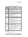
warnings and known bugs apply to the energies and particles beyond MCNP.
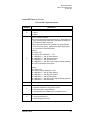
1. Pertubation methods used in MCNP have not yet been extended to the non-tabular
models present in MCNPX. MCNPX crashes if run for problems that invoke the pertubation capabilities above the MCNP energy range or beyond the MCNP particle set.
2. KCODE criticality calculations have not been extended to include 20-150 MeV neutrons. Accelerator transmutation applications should keep criticality limitations in mind
when using this feature to include high-energy neutrons in the physics-based energy
region. Below 20 MeV, MCNPX criticality calculations match MCNP.
3. Certain weight window optimizations have not been fully implemented for high energy
particles.
4. The “Mix and Match” feature has yet to be implemented. This version of MCNPX will
not switch between table based and physics based data where a number of tables
with differing upper energies are present. The switch between physics models and
tabular data is made at one energy for all materials in the problem. This energy is set
on the PHYS card by the user (see section 5.5.2). Therefore, it is desirable that one
use a set of libraries all with the same upper energy limits. Correctly implementing
this feature involves a major rewrite of data structures in MCNPX, and will be released
in a future version.
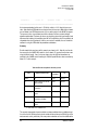
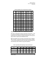
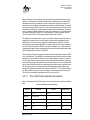
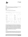
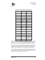
5. Charged-particle reaction products are not included for some neutron reactions below
20 MeV in the LA150N library. In calculating total particle production cross sections,
the library processing routines include only those reactions where complete angular
and energy information is given for secondary products. The new 150 MeV evaluations are built ‘on top’ of existing ENDF and JENDL evaluations which typically go to
20 MeV. Although the 150 MeV evaluations do include the detailed secondary information in the 20-150 MeV range, the < 20 MeV data typically do not. Therefore secondary production is ignored in processing that energy range. Table 4-4 lists the
actual secondary particle production thresholds in LA150N.
MCNPX User’s Manual
5
MCNPX User’s Manual
Version 2.4.0, September, 2002
LA-CP-02-408
Fixing this situation is non-trivial, and involves a re-evaluation of the low energy data.
Improved libraries will be issued, but on an isotope-by-isotope basis.
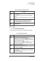
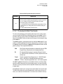
6. No explicit generation of “delta ray” knockon electrons as trackable particles is done
for heavy charged particles. Delta rays will be produced for electrons.
7. Positrons may not be used as source particles. Correcting this involves a change in
the way the particle identification numbering system is handled for electrons and
positrons. Historically this has not been treated in the same way as the method used
for neutrons in MCNP, which forms the basis for the multiparticle extension of
MCNPX.
8. Beware of the results of an F6:p tally in small cells when running a photon or photon/
electron problem. Photon heating numbers include the energy deposited by electrons
generated during photon collisions, but assume that the electron energy is deposited
locally. In a cell where the majority of the electrons lose all of their energy before exiting that cell, this is a good approximation. However, if the cell is thin and/or a large
number of electrons are created near the cell boundary, these electrons can carry significant energy into the neighboring cell, which can result in the F6:p tally for this cell
being too large. This is a known problem in MCNP, where the user is cautioned that
“all energy transferred to electrons is assumed to be deposited locally”. In MCNPX
the problem can be magnified because of the high energy nature of many applications, and also because the F6 formalism is used in the type 3 Mesh Tally. The user is
also encouraged to carefully investigate the *F8 tally, which attempts to score energy
deposition by following individual particles.
9. Continue-runs that include mesh tallies must use the last available complete restart
dump. The output file for mesh tallies is not integrated into the restart dump file
RUNTPE. However, they are written at each dump cycle. Since the mesh tally file is
overwritten at each dump, care must be taken to ensure that the files used to continue
a run were generated at the same dump cycle and that the last complete dump on the
RUNTPE file is used.
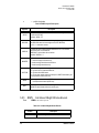
10. An old version of FLUKA is implemented in this version of MCNPX. The version of
FLUKA now in MCNPX is taken directly from the LAHET version 2.8 code, and is
known as FLUKA87. Only the high-energy portion of FLUKA is present, to handle
interactions above the INC region. This is not the latest version of FLUKA, and does
not contain any of the FLUKA code improvements added since that time. See Section
5.5.7 for further information. The FLUKA code module will be upgraded in a future
version of MCNPX.
11. The contents of the HISTP file arising from interactions processed by the CEM module do not distinguish among evaporation particles emitted before or after fission. All
are labeled as “pre-fission.” Therefore the HTAPE edits that depend on this distinction
will not produce the intended output:
•pre-fission evaporation particle production spectrum
•post-fission evaporation particle production spectrum
•fission precursor mass edit
6
MCNPX User’s Manual
MCNPX User’s Manual
Version 2.4.0, September, 2002
LA-CP-02-408
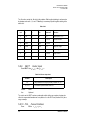
12. The CEM reaction model is of limited use when light reaction targets interact with high
energy incident particles. The Fermi-Breakup model, which usually handles the reaction dynamics of light nuclei, is not implemented into CEM in this version of MCNPX.
This means that at sufficiently high energies CEM can boil off all neutrons from a
nucleus and hands over an unphysical highly excited nucleus to the gamma deexitation module PHT. For Sodium such events have been identified already at 500 MeV
incident energy. For heavier nuclei this limit is shifted to higher energies. This will be
corrected in a future version.
13. Specifying different densities for the same material produces a warning. For charged
particles, there is a density correction in energy deposition which is not a strict linear
function. In MCNPX, the procedure is to search through all cells and find the first one
with the material in question, and use that density for the correction factor for all cells
using that material. The effect is small, so this is an adequate procedure, however
MCNPX does give a warning message when you encounter such situations. In
MCNPX, with more charged particles and greatly expanded energy range, this formerly 'small' correction now becomes increasingly important, and the usual way of
handling it is not sufficient.
MCNPX User’s Manual
7
MCNPX User’s Manual
Version 2.4.0, September, 2002
LA-CP-02-408
MCNPX User’s Manual
8
MCNPX User’s Manual
Version 2.4.0, September, 2002
LA-CP-02-408
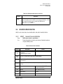
3
Installation
This chapter describes how to build MCNPX on a system. The system will need a
FORTRAN-90 compiler, a C compiler, and GNU Make 3.76 or higher.
MCNPX installs and runs on Windows & Linux PC’s, and a variety of common Unix
workstations. Some of our supported systems include:
•
IBM RS-6000 AIX
•
DEC Alpha Digital Unix
•
SGI IRIX 32 and 64-bit
•
HP HP-UX version 10
•
Sun Solaris
•
Intel I386 Linux
•
Microsoft Windows PC
The code distribution contains full source code for the MCNPX 2.4.0 system and test sets
for each of the supported architectures. The CDROM also contains a recent source
distribution of the GNU make utility needed to properly build the system.
3.1
3.1.1
UNIX BUILD SYSTEM
In the Beginning
Remember that your PATH environment variable governs the search order for finding
utilities. You should be aware of the value of your PATH environment variable by issuing the
following command:
echo $PATH
You may find it useful to set your PATH environment variable to a strategic search order so
that the utilities that are found first are the ones you intend to use. Setting of environment
variables is done differently depending upon what shell you use. Please consult the
appropriate manuals for your shell. Most systems have more than one shell. Any system
can have more than one version of any utility. You must know your utilities.
If you work on a UNIX or Linux operating system you can use the following inquiry
commands to learn if you have more than one make utility:
which make
MCNPX User’s Manual
9
MCNPX User’s Manual
Version 2.4.0, September, 2002
LA-CP-02-408
which gmake
Many systems come with a make utility that is provided by the vendor. On UNIX and Linux,
you must use the GNU make utility and it must be version 3.76 or later. Sometimes the
GNU make utility is installed in an executable file called "gmake". Sometimes system
administrators make symbolic links called "make" that when resolved, invoke the "gmake"
utility. You can make your own symbolic links in directories that you own and control so that
when you execute the "make" command you will be executing the "make" you intend to
use. You can also establish an alias in the shell runtime control file whereby any "make"
command you issue actually executes "gmake." You can also substitute the "gmake"
command everywhere you see the "make" command in the examples that follow.
The important point of this discussion is to know your "make" and use the right one,
otherwise, this automated build system can fail.
If no "make" or "gmake" is found, you either have a PATH value problem, or you need some
help from your system administrator to install GNU make.
If both "make" and "gmake" exist, query each of them to see what version you have.
make -v
gmake -v
Some vendor supplied "make" utilities do not understand the "-v" option that requests that
the version number be printed. If you see an error or usage message, then your "make" is
one of the vendor-supplied variety. Make sure you have GNU make version 3.76 or later
installed and that it is found in your search path first. If you work on a Windows platform,
this distribution is not the correct one for your needs. Please request a separate Windows
distribution. Until an automated build system for Windows is created, binary images will be
distributed.
3.1.2
Automated Building
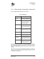
The process used when building mcnpx varies greatly depending upon the following:
•
•
•
•
hardware platform e.g. SPARC, ALPHA, I386
operating system e.g. Solaris, Linux, HP-UX
available compilers e.g f90/cc g90/gcc pgf90/gcc
mcnpx program options e.g. the default path of cross sections and other data files.
A special autoconf-generated configure script distributed with MCNPX will examine your
computing environment, adjust the necessary parameters, then generate all Makefiles in
your chosen build directory so that they all match your particular computing environment.
10
MCNPX User’s Manual
MCNPX User’s Manual
Version 2.4.0, September, 2002
LA-CP-02-408
The full structure is now in place to allow a graceful migration to individual feature tests
during the autoconfiguration process in the future.
The autoconf generated configure script will search for GNU compilers first before
attempting to locate any other compiler present on your computing environment. Please
be aware of exactly how many Fortran and C compilers exist in your computing
environment. It may be necessary to specify which Fortran and C compiler should be used.
You have that power via options given to the configure script. See the --with-FC and --withCC options later in this document.
Rather than having the one Build directory of past distributions, one is now free to create
as many build directories as desired, anywhere one wants, named anything one wants.
Through the use of options supplied to the configure script, one can vary the resulting
generated Makefiles to match a desired configuration.
Most software packages that use autoconf have a basic build procedure that looks like:
gzip -dc PACKAGE.tar.gz | tar xf cd PACKAGE
./configure
make install
This method of installation works with MCNPX. However, the development team
recommends a slightly different method so as not to clutter the original source tree with all
the products of compiling and building.
More complex packages (The GNU C compiler suite, gcc comes to mind) warn that the
simple build procedure given above is a dangerous practice, as it clutters the original
source tree with generated Makefiles and compiled objects, and makes it difficult to
support multiple builds with different options. They suggest using a different, initially empty
directory to be the target of the configure process.
gzip -dc PACKAGE.tar.gz | tar xf mkdir Build
cd Build
PATH_OF_PACKAGE-SOURCE/configure
make install
MCNPX User’s Manual
11
MCNPX User’s Manual
Version 2.4.0, September, 2002
LA-CP-02-408
The MCNPX team also makes this suggestion. Please use an empty directory somewhere
other than the source distribution's location as the target of the build. It keeps the source
tree clean and allows multiple builds with different options. Even if you think that you will
never need additional builds, it costs nothing to have the flexibility in the future.
3.1.3
Build Examples
We will illustrate the new configure and make procedure with two primary examples; A
system manager installing the MCNPX release for a system with several users, and an
individual user installing the MCNPX release for their own use. A few variations on these
themes are given.
3.1.3.1 System-Wide Installation
For purposes of the first illustration, we will assume that the MCNPX distribution has been
unloaded from CDROM or fetched from the net and is in the file /usr/local/src/
mcnpx_2.4.0.tar.gz. The system manager, logged is as root, will unload the distribution
into /usr/local/src/mcnpx_2.4.0, will build the system in /tmp/mcnpx, will install the mcnpx
executable in /usr/local/bin, and will install the libraries (end eventually the mcnp cross
sections) into /usr/local/lib. Naturally, the specific name of the mcnpx distribution archive
will vary depending on the version you have acquired.
The following example uses ell shell commands to accomplish this task. If you are more
familiar with csh, you will need to adjust things appropriately. NOTE: Comments about the
shell commands start with the '#' character. Also, don't be alarmed by the generous
amount of output from the configure and make scripts. They work hard so you don't have
to.
# go to the installation directory
cd /usr/local/src
# Unpack the distribution. This creates the directory mcnpx_2.4.0
gzip -dc mcnpx_2.4.0.tar.gz | tar xf # go to /tmp and make the build directory
cd /tmp
mkdir mcnpx
# go into that working space
cd mcnpx
12
MCNPX User’s Manual
MCNPX User’s Manual
Version 2.4.0, September, 2002
LA-CP-02-408
# execute the configure script - no special option requests for the Makefiles
# the default directory prefix is /usr/local
/usr/local/src/mcnpx_2.4.0/configure
# now make the executable mcnpx program and supporting LCS libraries
make all
# run the regression tests for your architecture
make tests
# install the executables and libraries in /usr/local
make install
# clean up. The build products are no longer needed.
cd /tmp
rm -rf mcnpx
3.1.3.2 System-Wide Installation With Existing Directories
The previous example might typically be used when a new installation of MCNPX is
performed on a system that has no pre-existing mcnpx with which to be compatible. If a
user already has mcnpx, then it may be desired to use the existing locations for the data
files and cross sections. Two options to the configure process can be used to customize
the locations where mcnpx and its data will be installed, and the default locations where
MCNPX will find those files.
When the user wants to use the normal mcnpx directory layout of:
.../bin for executables
and
.../lib for data files
MCNPX User’s Manual
13
MCNPX User’s Manual
Version 2.4.0, September, 2002
LA-CP-02-408
but does not wish to use the default directory /usr/local, then the previous example can be
adjusted with additional options. In the previous example, the configure script could be
given the option
/usr/local/src/mcnpx_2.4.0/configure --prefix=/usr/mcnpx
and the make install process would install the mcnpx binary in /usr/mcnpx/bin and the data
files in /usr/mcnpx/lib. The code will use /usr/mcnpx/lib as its default location for finding the
data files.
When the user has an existing directory layout that does not follow the mcnpx default, then
the data path itself can be customized like this:
/usr/local/src/mcnpx_2.4.0/configure --libdir=/usr/mcnpx
which will leave the default executable location as /usr/local/bin and set the location for the
data files to /usr/mcnpx.
Finally, both the --prefix and the --libdir options can be used together with the --libdir
options taking precedence over the library directory implied by the --prefix.
These options should remove the need to edit paths in the source code. In fact, with
support for these options, there are no longer any paths in the code to edit.
3.1.3.3 Individual Private Installation
For the purpose of the second illustration, we will look at a single non-privileged user
("Me") on a computer loading and building a private copy of the code. The local user
building the private copy is username me whose home directory is the directory /home/me.
The user has fetched the distribution from CDROM or from the net and has it in the file /
home/me/mcnpx_2.4.0.tar.gz. The user will unload the distribution package into /home/
me/mcnpx_2.4.0. The user will build the system in the same directory as the source, install
the binary executable in /home/me/bin, and install the binary data files (and eventually the
mcnp cross sections) in /home/me/lib. This method makes it hard to make multiple
versions with different options. A better example will follow this one.
The following example uses bourne shell commands to accomplish this task. If you are
more familiar with csh, you will need to adjust things appropriately. NOTE: Comments
about the shell commands start with the '#' character. Also, don't be alarmed by the
generous amount of output from the configure and make scripts. They work hard so you
don't have to.
# go to your user home directory
cd /home/me/
14
MCNPX User’s Manual
MCNPX User’s Manual
Version 2.4.0, September, 2002
LA-CP-02-408
# unpack the distribution that was copied from the net or a CDROM.
# This creates /home/me/mcnpx_2.4.0
gzip -dc mcnpx_2.4.0.tar.gz | tar xf # go into the unpacked distribution.
cd mcnpx_2.4.0
# execute the configure script
# the --prefix tells where to put the executables and libraries.
./configure --prefix=/home/me
# Make the executable mcnpx program, the bertin and pht libraries,
# and run the regression tests
make all; make tests
# now install the executable mcnpx program and the bertin
# and pht libraries in /home/me/bin and /home/me/lib/mcnpx
make install
3.1.3.4 Individual Private Installation Done Better
For a more flexible version of our second example, we will look at the same single nonprivileged user ("Me") on a computer loading and building a private copy of the code. This
time however, the user will use a second directory away from the mcnpx source code in
which to do the build. This can be done several times in different build directories with
different options such as debugging/non-debugging versions or different compiler types.
The local user building the private copy is again username me whose home directory is
the directory /home/me. The user has fetched the distribution from CDROM or from the net
and has it in the file /home/me/mcnpx_2.4.0.tar.gz. The user will unload the distribution
package into /home/me/mcnpx_2.4.0. (With this method, the source can be anywhere as
long as the user has the pathname to it.) The user will build the system in the local directory
/home/me/mcnpx, install the binary executable in /home/me/bin, and install the binary data
files (and eventually the mcnp cross sections) in /home/me/lib.
MCNPX User’s Manual
15
MCNPX User’s Manual
Version 2.4.0, September, 2002
LA-CP-02-408
The following example uses bourne shell commands to accomplish this task. If you are
more familiar with csh, you will need to adjust things appropriately. NOTE: Comments
about the shell commands start with the '#' character. Also, don't be alarmed by the
generous amount of output from the configure and make scripts. They work hard so you
don't have to.
# go to your user home directory
cd /home/me/
# unpack the distribution that was copied from the net or a CDROM.
# This creates /home/me/mcnpx_2.4.0
gzip -dc mcnpx_2.4.0.tar.gz | tar xf # make a local directory for a build directory. Call it "mcnpx".
mkdir mcnpx
# go into that new empty working space
cd mcnpx
# execute the configure script
# the --prefix tells where to put the executables and libraries.
../mcnpx_2.4.0/configure --prefix=/home/me
# now make the executable mcnpx program and the bertin and pht libraries,
# run the tests,
# and install in /home/me/bin and /home/me/lib
make all tests install
3.1.3.5 Individual Private Installation - special compilers and
debugging
As a final example, suppose you want basically the same thing as the previous example,
but you would like to have the debug option turned on during compilation. The compiled
16
MCNPX User’s Manual
MCNPX User’s Manual
Version 2.4.0, September, 2002
LA-CP-02-408
code will go into a private local library, /home/me/bin but you wish to use the cross section
files and LCS data files already on your system. We will assume that these data files
already exist in the directory /usr/mcnpx/data. We will assume that the source distribution
has already been unpacked by a system administrator into /usr/local/src/mcnpx_2.4.0.
If your system has only f90, it will be found and used. We decide to specify the Sun f90 and
cc compilers for this build.
# go to your user home directory
cd
# set an environment variable that identifies where the distribution lives.
# This isn't really necessary, but cuts down on typing later.
MCNPX_DIST=/usr/local/src/mcnpx_2.4.0
export MCNPX_DIST
# make a working space that reminds you it's a debug version
mkdir mcnpx-debug
cd mcnpx-debug
# execute the configure script - request debug for the Makefiles,
# also specify where to put the installed code and which compilers to use.
$MCNPX_DIST/configure --with-FC=f90 --with-CC=cc --with-LD=/usr/ccs/bin/ld --withDEBUG --prefix=/home/me --libdir=/usr/mcnpx/data
# now make the executable mcnpx program.
# We will omit the regression tests this time, although it would be a good
# idea to run them again if different compiler optimization values are used.
make install
That's all there is to it! There are many other options available with this new version of
mcnpx. Please read the User's Notes or the Programmer's Notes for more details.
MCNPX User’s Manual
17
MCNPX User’s Manual
Version 2.4.0, September, 2002
LA-CP-02-408
3.1.4
Directory Reorganization
In order to accommodate the use of the autoconf utility to generate the Makefiles, it
became necessary to arrange the source code and regression test directories a bit. We
also added a config directory to hold autoconf related code. The new directory structure is
depicted in Figure 3.1.
Each of the levels contains a collection of autoconf files and links. Removal of any of these
files will break the automated configure and make capabilities.
First Level: Data - contains data used with the bertin, phtlib, makexs targets Docs contains files describing this mcnpx distribution Test - contains the regression test files for
the various known platforms in use src - contains the source code files for mcnpx and
several related utilities miscellany - contains things that don't fit into any other category, of
interest to developers config - contains autoconf-related macros, scripts, initialization files
Second Level: bertin - builds and executes a program (hcnv) to translate LAHET text input
to binary input phtlib - builds and executes a program (trx) to translate LAHET text input to
binary input gridconv - converts output files generated by mesh tally and mctal files into a
variety of different graphics formats htape3x - reads the history tapes (optionally generated
by mcnpx) and performs post-processing on them makexs - a cross-section library
management tool that converts type 1 cross-sections to type 2 cross-sections and vice
versa, xsex3 - a utility associated with the new cross-section generation mode for mcnpx
which allows tabulation of cross-section sets based on physics models include - contains
include files shared across directories and include files localized in subdirectories mcnpx
- the organizing root directory for the mcnpx program
Third Level: cem, dedx, etc. - directories that organize the Fortran90 and C source code
files that are related to different aspects of the MCNPX program
Fourth Level: individual Fortran90 and C source code files for a particular aspect of
MCNPX.
18
MCNPX User’s Manual
MCNPX User’s Manual
Version 2.4.0, September, 2002
LA-CP-02-408
Figure 3.1 Directory Organization Structure
3.1.5
User’s Notes
Do not edit the Makefiles generated by the configure script. In order to change the contents
of the generated Makefiles, you must alter the contents of several input files that the
configure script uses. Please read the Programmer's Notes in the next subsection for
instructions.
Table 3.1 contains options which are available for use as parameters to the configure script
for mcnpx 2.4.0
MCNPX User’s Manual
19
MCNPX User’s Manual
Version 2.4.0, September, 2002
LA-CP-02-408
Table 3-1. Configure Script Parameters
Effect on the generated
Makefile if requested
Effect on the generated
makefile if NOT requested
--with-STATIC
linking of the compiled files
results in a static archive
(mcnpx.a).
STATIC is the default - cannot
be used at the same time as
SHARED.
--with-SHARED
linking of the compiled files
results in a dynamically
linked executable
(mcnpx.so).
STATIC is used - this option is
exploratory for future
releases of MCNPX.
--with-DEBUG
a debug switch appears in the
compile step for the generated Makefiles.
no debug switch appears in
the compile step for the
generated Makefiles - this
option can be used in combination with other options
such as --with-FC and -with-CC.
--with-FC=value
(substitute the desired
Fortran90 compiler
name for the value
placeholder, e.g., -with-FC=fort to use
the fort compiler)
value will be used to compile
Fortran source code - location of binary directory containing value must be in
your $PATH environment
variable.
configure will search for a
Fortran90 compiler and use
the first one it finds - this
option can be used in combination with other options
such as --with-DEBUG and
--with-CC.
--with-CC=value (substitute the desired C
compiler name for the
value placeholder,
e.g., --with-CC=gcc
to use the gcc compiler)
value will be used to compile
C source code - location of
binary directory containing
value must be in your
$PATH environment variable.
configure will search for a C
compiler and use the first
one it finds - this option can
be used in combination with
other options such as --withDEBUG and --with-FC.
Option Syntax
20
MCNPX User’s Manual
MCNPX User’s Manual
Version 2.4.0, September, 2002
LA-CP-02-408
Table 3-1. Configure Script Parameters
Effect on the generated
Makefile if requested
Effect on the generated
makefile if NOT requested
--with-LD=value (substitute the desired
link editor for the
value placeholder,
e.g., --with-LD=/usr/
ccs/bin/ld to use the
Standard Sun linker)
value will be used to link
object code - Unlike the -with-FC and --with-CC
options, whose names are
used for more than just finding the executable, The
value can be a full path to
the location of the desired ld
program as well as being a
single name like "ld".
configure will search for a
linker and use the first one it
finds. This is typically
needed on systems with
both a vendor-supplied
compiler set and the GNU
tool set. In such cases there
may be two versions of "ld"
that must be differentiated. this option can be used in
combination with other
options such as --withDEBUG and --with-FC.
--prefix=value
(substitute a full path
name for the value
placeholder, e.g., /
home/team/mcnpx)
(the path given
should be different
from the working
directory where the
build is taking place)
value will be used in the
install step to create bin and
lib data directories for
mcnpx's use.
a default value of /usr/local is
used as the full path name
for the install step. Executables then go to /usr/local/bin
and data files go to /usr/
local/lib. (permissions of the
destination may prohibit
success of installation).
--libdir=value
(substitute a full path
name for the value
placeholder, e.g., /
home/team/mcnpx)
(the path given
should be different
from the working
directory where the
build is taking place)
value will be used in the
install step to create a
library data directory for
mcnpx's use.
a default value of /usr/local/lib
is used as the full path
name for the install step
(permissions of the destination may prohibit success of
installation). This value
overrides the library portion
of the --prefix if both are
given.
--with-no_paw or
--with-no_paw=yes
this means that the symbol
NO_PAW will be defined for
compilation and actions are
taken in the source to omit
PAW capabilities when compiling.
if omitted, the default behavior is system dependent - if
the detected hardware/software platform can handle
PAW it is included .
Option Syntax
MCNPX User’s Manual
21
MCNPX User’s Manual
Version 2.4.0, September, 2002
LA-CP-02-408
Table 3-1. Configure Script Parameters
Option Syntax
--with-FFLAGS=value
There is a separate
variable that is used
for optimization
switches. See --withFOPT in this table. If
in doubt, run the configure script and
examine the system
default or system
computed values that
appear in the generated Makefile.h. You
may want to include
the defaults in the
string you specify for
FFLAGS with this
mechanism when
configure is run
again.
22
Effect on the generated
Makefile if requested
Effect on the generated
makefile if NOT requested
substitute a quoted or double
quoted string for value that
represents allowable compiler switch settings - these
settings will override the
system default or system
computed values.
if omitted, the default behavior is system dependent the detected hardware/software platform and compilers
determine what the default
FFLAGS should be.
MCNPX User’s Manual
MCNPX User’s Manual
Version 2.4.0, September, 2002
LA-CP-02-408
Table 3-1. Configure Script Parameters
Option Syntax
--with-CFLAGS=value
There is a separate
variable that is used
for optimization
switches. See --withCOPT in this table. If
in doubt, run the configure script and
examine the system
default or system
computed values that
appear in the generated Makefile.h. You
may want to include
the defaults in the
string you specify for
CFLAGS with this
mechanism when
configure is run
again.
MCNPX User’s Manual
Effect on the generated
Makefile if requested
Effect on the generated
makefile if NOT requested
substitute a quoted or double
quoted string for value that
represents allowable compiler switch settings - these
settings will override the
system default or system
computed values.
if omitted, the default behavior is system dependent the detected hardware/software platform and compilers
determine what the default
CFLAGS should be.
23
MCNPX User’s Manual
Version 2.4.0, September, 2002
LA-CP-02-408
Table 3-1. Configure Script Parameters
Option Syntax
--with-FOPT=value
There is a separate
variable that is used
for non-optimization
switches. See --withFFLAGS in this table.
If in doubt, run the
configure script and
examine the system
default or system
computed values that
appear in the generated Makefile.h. You
may want to include
the defaults in the
string you specify for
FOPT with this mechanism. FOPT settings
are always appended
to FFLAGS settings
when configure is run
again.
24
Effect on the generated
Makefile if requested
Effect on the generated
makefile if NOT requested
substitute a quoted or double
quoted string for value that
represents allowable compiler optimization switch settings - these settings will
override the system default
or system computed values.
if omitted, the default behavior is system dependent the detected hardware/software platform and compilers
determine what the default
FOPT should be.
MCNPX User’s Manual
MCNPX User’s Manual
Version 2.4.0, September, 2002
LA-CP-02-408
Table 3-1. Configure Script Parameters
Option Syntax
--with-COPT=value
There is a separate
variable that is used
for non-optimization
switches. See --withCFLAGS in this table.
If in doubt, run the
configure script and
examine the system
default or system
computed values that
appear in the generated Makefile.h. You
may want to include
the defaults in the
string you specify for
COPT with this
mechanism. COPT
settings are always
appended to
CFLAGS settings
when configure is run
again.
3.1.6
Effect on the generated
Makefile if requested
Effect on the generated
makefile if NOT requested
substitute a quoted or double
quoted string for value that
represents allowable compiler optimization switch settings - these settings will
override the system default
or system computed values.
if omitted, the default behavior is system dependent the detected hardware/software platform and compilers
determine what the default
COPT should be.
Multiprocessing
If you want to create the parallel PVM version of MCNPX, use the following configure
option:
--with -PVMLIB[= -L/path/to/pvm/libraries -lfpvm3 -lpvm3]
It is recommended that you first install PVM, as the configure scripts use various PVM
environment variables to locate the PVM libraries. One can alternatively give the path and
library names following the PVMLIB = option.
3.1.7
Programmer’s Notes
Autoconf is not new; it has been available as a configuration management tool for several
years. We have just recently adopted its use to simplify the build process for the MCNPX
end user community, to allow the flexibility to build and keep multiple versions of MCNPX,
and to improve our software development process.
MCNPX User’s Manual
25
MCNPX User’s Manual
Version 2.4.0, September, 2002
LA-CP-02-408
3.2
WINDOWS BUILD SYSTEM
If you wish to modify the source or recreate the executables, you will need the Compaq
Visual Fortran (CVF) compiler, version 6.1 or later, and the MSVC compiler, version 5.0 or
later. Once CVF and MSVC are installed, simply open a "Command Prompt" window, enter
the MCNPX\BLD directory, and execute GNU Make:
C:>Make
Be sure to execute the SETUPX.BAT file as explained above so GNU Make can be found
(it is provided as an executable in MCNPX\BIN). Also be sure that your PATH environment
variable is less than 255 characters, as this version of GNU Make has a problem if this is
exceeded. A MAKEPATH.BAT file is provided in MCNPX\BIN as an example of how to
reduce your PATH variable to a minimum set of directories (note this assumes CVF and
MSVC are installed on the C drive). The X11 library and include files are provided in
MCNPX\LIB and should not be moved from here. As on a Unix platform, you can build any
subcomponent of MCNPX by entering that directory and executing Make. All the source
files are in the MCNPX/SRC directory and one should take care in modifying any of these
files. Patches to MCNPX can be developed, as done for MCNP; however one should
contact us for the needed script file and instructions to apply such a patch. If a "stack
overflow" error is generated, this is NOT an MCNPX bug. A stack limit must be specified
upon linking. The included executable has a stack limit of 32 MBytes. This can be
increased by editing the Makfile.h file in the MCNPX\BLD\SRC\MCNPX directory (line 66)
and rebuilding MCNPX.
3.3
LIBRARIES AND WHERE TO FIND THEM
Several types of data libraries are used by MCNPX, including the XSDIR pointer file to
nuclear data tables for neutron, proton and photonuclear reactions, cross sections for the
Bertini model (BERTIN), gamma emission data for decaying nuclei (PHTLIB), photon and
electron interaction libraries, and others. Numerous questions in the beta test phase of
MCNPX have arisen concerning where these libraries should be kept, and this section of
the manual has been added for clarification.
The following set of nuclear data libraries may be used with MCNPX 2.4.0:
1. All standard neutron libraries used with MCNP4B (DLC189) can be used with
MCNPX, however they will not contain emission data for charged particles or recoil
nuclei (these were processed only in the LA150N library). Therefore charged secondaries and recoil nuclei will not be produced or tracked in MCNPX within the tabular
energy ranges.
2. MCNP4C (DLC200) libraries are the same as the MCNP4B DLC189 set, with certain
new features. These include unresolved resonances, delayed neutrons, new electron
26
MCNPX User’s Manual
MCNPX User’s Manual
Version 2.4.0, September, 2002
LA-CP-02-408
libraries (ZAIDs end in .03e), ENDL92 data, and multi-temperature U/Np tables.
DLC200 tables may be used with MCNPX, with the following cautions:
- None of the DLC200 tables have charged particle or recoil data, therefore
these will not be produced or tracked in MCNPX.
- Only the DLC200 electron tables with ZAID numbers ending in .03e will work
properly in MCNPX.
3. Special 150 MeV libraries have been produced for use with MCNPX. The neutron
library is called LA150n. The proton and photonuclear libraries are called la150h and
la150u, respectively. The LA150N library is the same as DLC200, with the addition of
150 MeV evaluations above the DLC200 energy limits. Once the proton and photonuclear components are added, the entire library will be reissued under the name
DLC200X.
4. A number of users are requesting secondary particle and recoil nuclei information for
the lower energy portions of the libraries (typically below 20 MeV). Note that some
information is available in the lower energy tables, per table 4-4 in this manual, but it is
far from complete. A proper fix to the problem will involve full re-evaluations of the
lower energy libraries, which is a time consuming and often difficult task. Nonetheless, progress is being made, and the user should look for improved library releases
in the future.
The LANL group that formats libraries for MCNP/MCNPX is currently providing 64-bit “type
2” binary files, and MCNPX 2.4.0 will only accept these. Therefore, the user will find that
older versions of 32-bit binary libraries won’t work with the 2.4.0. The program MAKXS is
provided with the MCNPX distribution to do the reformatting, and details can be found in
Appendix C of the MCNP manual. An alternative is to use “type 1” formatted, sequential
access libraries.
The XSDIR file tells the code all the information it needs to known on where to find
individual data tables. MCNPX uses the same procedure as MCNP to find the nuclear data
libraries, as described in Appendix F of the MCNP manual. If XSDIR is not in your current
directory, MCNPX will search the following places for both the libraries and XSDIR file, in
order starting from #1. We repeat that portion of the MCNP manual here, with annotations:
1. xsdir = “datapath” on the MCNPX execution line
note, “datapath’ is truncated to 8 characters, which means that it is really the
name of a file, not a path. It is easiest to assign a name via a symbolic link,
e.g.:
ln -s /home/me/lib/data/xsdir xsdir1
Then you can say: mcnpx xsdir=xsdir1
MCNPX User’s Manual
27
MCNPX User’s Manual
Version 2.4.0, September, 2002
LA-CP-02-408
2. DATAPATH = datapath in the INP file message block
this version of datapath can be a full description
3.
4.
5.
6.
7.
the current directory
the DATAPATH entry on the first line of the XSDIR file
the UNIX environmental variable: setenv DATAPATH datapath
the individual data table line in the XSDIR file
the directory specified at MCNPX compile time in the blkdat.f BLOCK DATA subroutine. This can be edited to change the directory, but the code must be recompiled.
MCNPX has come up with the following slightly modified set of directions:
In the following cases, if the desired file is found, exit the list with the success.
1. Look in the current working directory for the file.
2. Look at the DATAPATH= input directive or the DATAPATH environment variable.
2a. If there is a DATAPATH= directive in the input file, look there for the file.
2b. If there was no DATAPATH= directive then examine the DATAPATH
environment variable for a value.
2b-1. If there is an environment value, use that value as a directory to
search for the file.
2b-2. If there is no value (environment variable not set) then look for the file
again in the current working directory.
3. Look in a default place.
3a. If there was a DATAPATH= directive, then the default place is either the
value
of the DATAPATH environment variable, if there was one, or value of the preprocessor symbol LIBPREFIX from the autoconfiguration process
(typically /usr/local/lib/mcnpx).
28
MCNPX User’s Manual
MCNPX User’s Manual
Version 2.4.0, September, 2002
LA-CP-02-408
3b. If there was not a DATAPATH= directive in the input file, then the default
is just
the LIBPREFIX pre-processor symbol.
4. If the file is not found by now, then it is a fatal error.
It is required that MCNPX be run with 64 bit libraries. Earlier versions of the code could
use 32 bit libraries, however studies of long problems have shown that erroneous answer
can result with the lesser accuracy data. Conversion of Type 1 libraries to 64 bit binaries
can be done with the MAKXSF routine described in Appendix C of the MCNP manual.
The LAHET physics modules in MCNPX require three special libraries:
BERTIN (containing the elemental cross section data needed by the Bertini model),
PHTLIB (containing nuclear structure data needed to generate de-excitation photons)
BARPOL.DAT (containing new high energy total, reaction and elastic cross sections).
They are unpacked with the rest of the code, and if ‘make install’ is executed, placed in the
/lib directory. There are basically 2 ways that the code tries to find these files:
1. MCNPX tries to open the files named “bertin” and “phtlib” in the current directory. If
the user wants to keep these file in another directory, a symbolic link should be made
from whatever directory you are in when running the code. The following unix command can be used to do this:
ln -s .../home/me/lib bertin
2. A default pathname is coded in the fortran data statements in the file “.../src/lcs/
inbd.F”. This can be changed by the user, but you must remember to recompile the
code. Look for the variable currently holding the string “/usr/local/xcodes3/lcsdir/bertin” and the similar variable referencing a location for “phtlib”. Change them to reflect
the appropriate location of the two data files on your system and re-make the code. A
typical location for these two files might be “/usr/local/lib/mcnpx”. This would be the
preferable method when a community of users is accessing one copy of the code on a
single system.
As suggested above, we recommend making a symlink to the bertin and phtlib files in your
working directory. If you have more than just one person running the code from a server,
then it is probably worthwhile to edit .../src/lcs/inbd.F to point to a specific location on your
system where everyone can get the files, as in method 2 above. In the future we will build
in the ability to look for all libraries using the same method now used for the nuclear data
table libraries.
MCNPX User’s Manual
29
MCNPX User’s Manual
Version 2.4.0, September, 2002
LA-CP-02-408
30
MCNPX User’s Manual
MCNPX User’s Manual
Version 2.4.0, September, 2002
LA-CP-02-408
4
Input Files
Input to MCNPX consists of a number of files, They can be part of the code package,
generated by problem runs, or user-supplied. This section focuses on the user-supplied
INP (the default name) file which describes the problem to be run. Input cards are
summarized by card type in Section 5.10. The user will provide only a small subset of all
available input cards in a given problem. The word “card” describes a single line of input
up to 80 characters.
MCNPX input item limitations are summarized in Section 4.4. Modification of these values
is accomplished by altering the source code and recompiling.
All features of MCNPX should be used with caution and knowledge. This is especially true
of detectors and variance reduction schemes. Read and understand the relevant sections
of the manual before using them.
MCNPX accepts all standard MCNP input cards with additional card options that take
advantage of the multiparticle capabilities of MCNPX. Modifications to standard MCNP
inputs are described in Section 5.4 and following. Section 5.5.7 describes new cards
added to control the model physics options MCNPX uses when table-based data are not
available. Use of high-energy, proton, and photonuclear data library capabilities has
already been described.
Accelerator simulation applications have a need for specialized source input to describe
an incident particle beam. Usually this takes the form of a directed beam of particles,
monoenergetic, with a transverse gaussian profile. To facilitate this, a new source option
has been added to MCNPX and is described in Section 5.6.7
4.1
INP FILE
The INP file can have two forms, initiate-run and continue-run.
4.1.1
Initiate-Run
This form is used to set up a Monte Carlo problem (describe geometry, materials, tallies,
etc.) and run if message block is present. The initiate-run file has the following form:
MCNPX User’s Manual
31
MCNPX User’s Manual
Version 2.4.0, September, 2002
LA-CP-02-408
Message Block
Blank Line Delimiter
Title Card
Cell Cards
⋅
⋅
Blank Line Delimiter
Surface Cards
⋅
⋅
Blank Line Delimiter
Data Cards
⋅
⋅
Blank Line Terminator
Anything Else
} Optional
Optional but recommended
Optional
MCNPX interprets blank lines as the end of preceding information type. MCNPX will stop
reading the input file after the blank line terminator. The space following the blank line
terminator is a good place for problem documentation at the user’s discretion.
4.1.2
Continue-Run
Continue-run allows the user to pick up a previously-terminated job where it left off. For
example, a job run for 2 hours may be continued run an additional amount of time. The
user can also reconstruct the output of a previous run. A continue-run must contain C or
CN in the MCNPX execution line or message block to indicate a continue-run. It will start
with the last dump or with the mth dump with the Cm option.
In addition to the C or CN option on the MCNPX execution line, two files can be important
for this procedure: (1) the binary restart file (default name RUNTPE), and (2) an optional
continue-run input file (default name INP).
The restart file, generated by MCNPX in the initiate-run sequence, contains the geometry,
cross sections, problem parameters, tallies, and all other information necessary to restart
the job. In addition the problem results at various stages of the run are recorded in a series
of dumps. See the PRDMP card (Section 5.9.1) for a discussion of the selection of dump
times. As discussed below, the run may be restarted from any of these dumps.
The CN execution message option differs from the C option only in that the dumps
produced during the continue-run are written immediately after the fixed data portion of the
RUNTPE file rather than after the dump from which the continue-run started. The new
dumps overwrite the old dumps, providing a way for the user to prevent unmanageable
32
MCNPX User’s Manual
MCNPX User’s Manual
Version 2.4.0, September, 2002
LA-CP-02-408
growth of RUNTPE files. RUNTPE growth also can be controlled by the NDMP entry on
the PRDMP card.
The optional continue-run input file must have the word CONTINUE as the first entry on
the first line (title card), or after the optional Message Block and its blank line delimiter.
Alphabetic characters can be upper, lower, or mixed case. This file has the following form:
Message Block
Blank Line Delimiter
CONTINUE
Data Cards
⋅
⋅
Blank Line Terminator
Anything else
}Optional
Recommended
Optional
The data cards allowed in the continue-run input file are a subset of the data cards
available for an initiate-run file. The allowed continue-run data cards are FQ, DD, NPS,
CTME, IDUM, RDUM, PRDMP, LOST, DBCN, PRINT, KCODE, MPLOT, ZA, ZB, and ZC.
If none of the above items is to be changed (and if the computing environment allows
execution line messages), the continue-run input file is not required; only the run file
RUNTPE and the C option on the MCNPX execution line are necessary. For example, the
command line sequence MCNPX C or MCNPX CN will pick up the job where it stopped
and continue until another time limit or particle cutoff is reached or until you stop it
manually. This example assumes that a default restart filename from the initial run is in
your current directory.
The complete continue-run execution line option is C m or CN m, where m specifies which
dump from the restart file to pick up with. If m is not specified, the last dump is taken by
default. If the initial run producing the restart file was stopped because of particle cutoff
(NPS card, Section 5.5.6.3), NPS must be increased for a continue-run via a continue run
file. CTME in a continue-run is the number of minutes more to run, not cumulative total
time. To run more KCODE cycles, only the fourth entry KCT may be changed. Like NPS,
KCT refers to total cycles to be run, including previous ones.
In a continue-run, a negative number entered on the NPS card produces a print output file
at the time of the requested dump. No more histories will be run. This can be useful when
the printed output has been lost or you want to alter the content of the output with the
PRINT or FQ cards.
Be cautious if you use a FILES card in the initial run. See Section 5.9.10.
MCNPX User’s Manual
33
MCNPX User’s Manual
Version 2.4.0, September, 2002
LA-CP-02-408
4.1.3
Message Block
In computer environments where there are no execution line messages, the message
block is the only means for giving MCNPX an execution message. Optionally, is a
convenient way to avoid retyping an often-repeated message. The message block starts
with the string MESSAGE:. The message block ends with a blank line delimiter before the
title card. All cards before the blank line delimiter are continuation cards. The syntax and
components of the message are the same as for the regular execution line message. Any
filename substitution, program module execution option or keyword entry on the execution
line takes precedence over conflicting information in the message block. INP = filename is
not a legitimate entry in the message block. The name INP can be changed on the
execution line only.
4.1.4
Problem Title Card
The first card in the file after the optional message block is the required problem title card.
It is limited to one 80-column line and is used as a title in various places in the MCNPX
output. It can contain any information the user desires (or can even be blank) and often
contains information describing the particular problem. Note that a blank card elsewhere
is used as a delimiter or as a terminator.
4.1.5
Card Format
All input lines are limited to 80 columns. Alphabetic characters can be upper, lower, or
mixed case. Most input is entered in horizontal form; however, a vertical input format is
allowed for data cards. A comment can be added to any input card. A $ (dollar sign)
terminates data entry and anything that follows the $ is interpreted as a comment. Blank
lines are used as delimiters and terminators. Data entries are separated by one or more
blanks.
4.1.6
Comment Cards
Comment cards can be used anywhere in the INP file after the problem title card and
before the last blank terminator card. These cards must have a C anywhere in columns 15 followed by at least one blank. Comment cards are printed only with the input file listing
and not anywhere else in the MCNPX output file. The FCn input card is available for user
comments and is printed as a heading for tally n (as a tally title, for example). The SCn card
is available for user comments and is printed as a heading for source probability
distribution n.
4.1.7
Horizontal Input Format
Cell, surface, and data cards all must begin within the first five columns. The card name or
number and particle designator is followed by data entries separated by one or more
blanks. Blanks in the first five columns indicate a continuation of the data from the last
named card. An & preceded by at least one blank ending a line indicates data will continue
on the following card. Data on the continuation card can be in columns 1-80. Completely
34
MCNPX User’s Manual
MCNPX User’s Manual
Version 2.4.0, September, 2002
LA-CP-02-408
blank cards are reserved as delimiters between major sections of the input file. An
individual entry cannot be split between two cards. There can be only one card of any given
type for a given particle designation (see section 4.1.10 on page 38). Integers must be
entered where integer input is required. Other numerical data can be entered in any form
acceptable to a FORTRAN E-edit descriptor.
4.1.8
Repeat, Interpolate, Multiply, and Jump & Log Shortcuts
MCNPX allows five shortcuts to facilitate data input in some instances.
1.
nR means repeat the immediately preceding entry on the card n times. For
example, 2 4R is the same as 2 2 2 2 2.
2.
nI means insert n linear interpolates between the entries immediately preceding
and following this feature. For example, 1.5 2i 3.0 on a card is the same as 1.5
2.0 2.5 3. In the construct X ni Y, if X and Y are integers, and if Y − X is an exact
multiple of n+1, correct integer interpolates will be created. Otherwise only real
interpolates will be created, but Y will be stored directly in all cases. In the above
example, the 2.0 may not be exact, but in the example 1 4i 6 (= 1 2 3 4 5 6), all
interpolates are exact.
3.
xM means multiply the previous entry on the card M by the value x. For example,
1 1 2M 2M 2M 2M 4M 2M 2M is equivalent to 1 1 2 4 8 16 64 128 256.
4.
nJ means jump over the entry where used and take the default value. As an
example, the following two cards are identical in their effect:
DD
.1
1000
DD
J
1000
J J J is also equivalent to 3J. You can jump to a particular entry on a card without
having to explicitly specify prior items on the card. This feature is convenient if
you know you want to use a default value but can’t remember it. DBCN 7J 5082
is another example.
5.
nLOG means insert n logarithmic interpolates between the entries immediately
preceding and following this feature. For example, .001 4Log 100 is equivalent
to .001 .01 .1 1 10 100.
MCNPX User’s Manual
35
MCNPX User’s Manual
Version 2.4.0, September, 2002
LA-CP-02-408
These features apply to both integer and floating point quantities. If n (an integer) is
omitted in the constructs nR, nI, nLog and nJ, then n is assumed to be 1. If x (integer or
floating point) is omitted in xM, it is a fatal error. The rules for dealing with adjacent special
input items are as follows:
1.
nR must be preceded by a number or by an item created by R or M.
2.
nI and nLOG must be preceded by a number or by an item created by R or M,
and must be followed by a number.
3.
xM must be preceded by a number or by an item created by R or M.
4.
nJ may be preceded by anything except I and may begin the card input list.
Examples:
1 3M 2R=1 3 3 3
1 3M I 4=1 3 3.5 4
1 3M 3M=1 3 9
1 2R 2I 2.5=1 1 1 1.5 2.0 2.5
1 R 2M=1 1 2
1 R R =1 1 1
1 2I 4 3M=1 2 3 4 12
1 2I 4 2I 10=1 2 3 4 6 8 10
3J 4R is illegal.
1 4I 3M is illegal.
1 4I Jis illegal.
4.1.9
Vertical Input Format
Column input is particularly useful for cell parameters and source distributions. Cell
importances or volumes strung out on horizontal input lines are not very readable and
often cause errors when users add or delete cells. In vertical format, all the cell parameters
for one cell can be on a single line, labeled with the name of the cell. If a cell is deleted,
the user deletes just one line of cell parameters instead of hunting for the data item that
belongs to the cell in each of several multiline cell parameter cards. For source
distributions, corresponding SI, SP, and SB values are side by side. Source options, other
than defaults, are on the next line and must all be entered explicitly. The & continuation
symbol is not needed, and if present, is ignored.
In column format, card names are put side by side on one input line and the data values
are listed in columns under the card names. A # is put somewhere in columns 1-5 on the
line with the card names. The card names must be all cell parameters, all surface
parameters, or all something else. If a card name appears on a # card, there must not be
a regular horizontal card by that name in the same input file. If there are more entries on
data value lines than card names on the # line, the first data entry is a cell or surface
36
MCNPX User’s Manual
MCNPX User’s Manual
Version 2.4.0, September, 2002
LA-CP-02-408
number. If any cell names are entered, all must be entered. If cell names are entered, the
cells don’t have to be in the same order as they are in the cell cards block. If cell names
are omitted, the default order is the order of the cells in the cell card block. The same rules
apply to surface parameters, but because we presently have only one surface parameter
(AREA), column input of surface parameters is less useful.
There can be more than one block of column data in an input file. Typically, there would be
one block for cell parameters and one for each source distribution. If a lot of cell parameter
options are being used, additional blocks of column data would be needed.
We strongly suggest keeping columns reasonably neat for user readability. The column
format is intended for input data that naturally fit into columns of equal length, but less tidy
data are not prohibited. If a longer column is to the right of a shorter column, the shorter
column must be filled with enough J entries to eliminate any ambiguity about which
columns the data items are in.
Special syntax items (R, M, I, Log, and J) are not as appropriate in column format as they
are on horizontal lines, but they are not prohibited. They are, of course, interpreted
vertically instead of horizontally. Multiple special syntax items, such as 9R, are not allowed
if cell or surface names are present.
The form of a column input block is
#
S1
K1
D11 D12 ...
D1m
K2
D21 D22 ...
D2m
Kn
Dn1 Dn2 ...
Dnm
S2
...
Sm
1.
The # is somewhere in columns 1−5.
2.
Each line can be only 80 columns wide.
3.
Each column, Si through Dli, where l may be less than n, represents a regular
input card.
4.
The Si must be valid MCNPX card names. They must be all cell parameters, all
surface parameters, or all something else.
5.
D1i through Dni must be valid entries for an Si card, except that Dl+1,i through Dni
may be some J’s possibly followed by some blanks.
6.
If Dji is non-blank, Dj,i-1 must also be nonblank. A J may be used if necessary to
make Dj,i-1 non-blank.
7.
The Si must not appear anywhere else in the input file.
MCNPX User’s Manual
37
MCNPX User’s Manual
Version 2.4.0, September, 2002
LA-CP-02-408
8.
The Kj are optional integers. If any are non-blank, all must be non-blank.
9.
If the Si are cell parameter card names, the Kj, if present, must be valid cell
names. The same is true with surface parameters.
10. If the Kj are present, the Dji must not be multiple special syntax items, such as
9R.
4.1.10 Particle Designators
Several of the input cards require a particle designator to distinguish between input data
for tracked particles. Refer to the pertinent card information for instructions. The particle
designator consists of a colon followed by the particle symbol or IPT number (s)
immediately after the name of the card. At least one blank must follow the particle
designator. For example, imp:n signifies neutron importances follow; enter photon
importances on an IMP:P card. To specify the same value for more than one kind of
particle, a single card can be used instead of several. Example: IMP:E,P,N 1 1 0. With a
tally card, the particle designator follows the card name including tally number. For
example, ∗F5:N indicates a neutron point detector energy tally. In the heating tally case,
both particle designators may appear. The syntax F6:N,P indicates the combined heating
tally for both neutrons and photons
Table 4-1. MCNPX Particles
IPT
Name of Particle
Symbol
Mass (MeV)
Low Kinetic
Energy Cutoff
(MeV)
Mean Lifetime
(seconds)
(* - decayed on
production)
Original MCNP Particles
1
neutron (n)
n
939.56563
0.0
887.0
1
anti-neutron (n)
n
939.56563
0.0
887.0
2
photon (γ)
p
0.0
0.001
huge
3
electron (e-)
e
0.511008
0.001
huge
3
positron (e+)
e
0.511008
0.001
huge
Leptons
4
muon- (µ-)
|
(‘pipe’ symbol)
105.658389
0.11261
2.19703 x 10-6
4
anti-muon- (µ+)
|
105.658389
0.11261
2.19703 x 10-6
5
tau- (τ-)
*
1777.1
1.894
2.92 x 10-5 *
38
MCNPX User’s Manual
MCNPX User’s Manual
Version 2.4.0, September, 2002
LA-CP-02-408
Table 4-1. MCNPX Particles
IPT
Name of Particle
Symbol
Mass (MeV)
Low Kinetic
Energy Cutoff
(MeV)
Mean Lifetime
(seconds)
(* - decayed on
production)
6
electron neutrino
(νe)
u
0.0
0.0
huge
6
anti-electron neutrino
u
0.0
0.0
huge
7
muon neutrino (νm)
v
0.0
0.0
huge *
8
tau neutrino (νt)
w
0.0
0.0
huge *
Baryons
9
proton (p)
h
938.27231
1.0
huge
9
anti-proton (p)
h
938.27231
1.0
huge
10
lambda0 (Λ0)
l
(lower case
L)
1115.684
1.0
2.632 x 10-2 *
11
sigma+ (Σ+)
+
1189.37
1.2676
7.99 x 10-3 *
12
sigma- (Σ-)
-
1197.436
1.2676
1.479 x 10-2 *
13
cascade0 (Ξ0)
x
1314.9
1.0
2.9 x 10-2 *
14
cascade- (Ξ-)
y
1321.32
1.4082
1.639 x 10-2 *
15
omega- (Ω-)
o
1672.45
1.7825
8.22 x 10-3 *
16
lambdac+ (Λc+)
c
2285.0
2.4353
2.06 x 10-5 *
17
cascadec+ (Ξc+)
!
2465.1
2.6273
3.5 x 10-5 *
18
cascadec0 (Ξc0)
?
2470.3
1.0
9.8 x 10-6 *
19
lambdab0 (Λb0)
r
5641
1.0
1.07 x 10-4 *
Mesons
MCNPX User’s Manual
39
MCNPX User’s Manual
Version 2.4.0, September, 2002
LA-CP-02-408
Table 4-1. MCNPX Particles
IPT
Name of Particle
Symbol
Mass (MeV)
Low Kinetic
Energy Cutoff
(MeV)
Mean Lifetime
(seconds)
(* - decayed on
production)
20
pion+ (π+)
/
139.56995
0.14875
2.6033 x 10-8
20
pion- (π-)
/
139.56995
0.14875
2.6033 x 10-8
21
neutral pion (π0)
z
134.9764
0.0
8.4 x 10-17
22
kaon+ (K+)
k
493.677
0.52614
1.2386 x 10-8
22
kaon- (K-)
k
493.677
0.52614
1.2386 x 10-8
23
K0 short
%
497.672
0.000001
0.8927 x 10-10
24
K0 long
^
497.672
0.000001
5.17 x 10-8
25
D+
g
1869.3
1.9923
1.05 x 10-4 *
26
D0
@
1864.5
1.0
4.15 x 10-5 *
27
Ds+
f
1968.5
2.098
4.67 x 10-5 *
28
B+
j
5278.7
5.626
1.54 x 10-4 *
29
B0
b
5279.0
1.0
1.5 x 10-4 *
30
Bs0
q
5375.
1.0
1.34 x 10-4 *
Light Ions
31
deuteron
d
1875.627
2.0
huge
32
triton
t
2808.951
3.0
12.3 years
33
Helium-3
s
2808.421
3.0
huge
34
Helium-4 (α)
a
3727.418
4.0
huge
Particle tracking between interactions involves several physics considerations which are
described below. Atomic electron interactions will cause a charged particle to lose energy
along its track length (ionization). Certain modifications to this energy loss are determined
by “energy straggling” theory. Multiple scattering of charged particles is also implemented.
There is currently no “delta ray" production of knock-on electrons for charged heavy
particles in MCNPX, although it is present for electrons.
40
MCNPX User’s Manual
MCNPX User’s Manual
Version 2.4.0, September, 2002
LA-CP-02-408
No option for electromagnetic field tracking is currently implemented in MCNPX.
4.1.11 Default Values
Many MCNPX input parameters have default values that are summarized in Section 5.10.
Therefore you do not always have to specify explicitly every input parameter every time if
the defaults match your needs. If an input card is left out, the default values for all
parameters on the card are used. However, if you want to change a particular default
parameter on a card where that parameter is preceded by others, you have to specify the
others or use the nJ jump feature to jump over the parameters for which you still want the
defaults. CUT:P 3J −.10 is a convenient way to use the defaults for the first three
parameters on the photon cutoff card but change the fourth.
4.2
INPUT ERROR MESSAGES
MCNPX makes over 400 checks of the input file for user errors. A fatal error message is
printed, both at the terminal and in the OUTP file, if the user violates a basic constraint of
the input specification, and MCNPX will terminate before running any particles. The first
fatal error is real; subsequent error messages may or may not be real because of the
nature of the first fatal message. The FATAL option on the MCNPX execution line instructs
MCNPX to ignore fatal errors and run particles, but the user should be extremely cautious
about doing this.
Most MCNPX error messages are warnings and are not fatal. The user should not ignore
these messages but should understand their significance before making important
calculations.
In addition to FATAL and WARNING messages, MCNPX issues BAD TROUBLE messages
immediately before any impending catastrophe, such as a divide by zero, which would
otherwise cause the program to “crash.” MCNPX terminates as soon as the BAD
TROUBLE message is issued. User input errors in the INP file are the most common
reason for issuing a BAD TROUBLE message. These error messages indicate what
corrective action is required.
4.3
GEOMETRY ERRORS
There is one important kind of input error that MCNPX will not detect while processing data
from the INP file. MCNPX cannot detect overlapping cells or gaps between cells until a
particle track actually gets lost. Even then the precise nature of the error may remain
unclear. However, there is much that you can and should do to check your geometry before
starting a long computer run.
MCNPX User’s Manual
41
MCNPX User’s Manual
Version 2.4.0, September, 2002
LA-CP-02-408
Use the geometry-plotting feature of MCNPX to look at the system from several directions
and at various scales. Be sure that what you see is what you intend. Any gaps or overlaps
in the geometry will probably show up as dashed lines. The intersection of a surface with
the plot plane is drawn as a dashed line if there is not exactly one cell on each side of the
surface at each point. Dashed lines can also appear if the plot plane happens to coincide
with a plane of the problem, if there are any cookie-cutter cells in the source, or if there are
DXTRAN spheres in the problem.
Set up and run a short problem in which your system is flooded with particle tracks from
an external source. The necessary changes in the INP file are as follows:
1.
Add a VOID card to override some of the other specifications in the problem and
make all the cells voids, turn heating tallies into flux tallies, and turn off any FM
cards.
2.
Add another cell and a large spherical surface to the problem such that the
surface surrounds the system and the old outside world cell is split by the new
surface into two cells: the space between the system and the new surface,
which is the new cell, and the space outside the new surface, which is now the
outside world cell. Be sure that the new cell has nonzero importance. Actually,
it is best to make all nonzero importances equal. If the system is infinite in one
or two dimensions, use one or more planes instead of a sphere.
3.
Replace the source specifications by an inward directed surface source to flood
the geometry with particles:
SDEFSUR=mNRM = −1
where m is the number of the new spherical surface added in Step 2. If the new
surface is a plane, you must specify the portion to be used by means of POS
and RAD or possibly X, Y, and Z source distributions.
Because there are no collisions, a short run will generate a great many tracks through your
system. If there are any geometry errors, they should cause some of the particles to get
lost.
When a particle first gets lost, whether in a special run with the VOID card or in a regular
production run, the history is rerun to produce some special output on the OUTP file.
Event-log printing is turned on during the rerun. The event log will show all surface
crossings and will tell you the path the particle took to the bad spot in the geometry. When
the particle again gets lost, a description of the situation at that point is printed. You can
usually deduce the cause of the lost particle from this output. It is not possible to rerun lost
particles in a multitasking run.
MCNPX User’s Manual
42
MCNPX User’s Manual
Version 2.4.0, September, 2002
LA-CP-02-408
If the cause of the lost particle is still obscure, try plotting the geometry with the origin of
the plot at the point where the particle got lost and with the horizontal axis of the plot plane
along the direction the particle was moving. The cause of the trouble is likely to appear as
a dashed line somewhere in the plot or as some discrepancy between the plot and your
idea of what it should look like.
4.4
STORAGE LIMITATIONS
Table 4.4 summarizes some of the more important limitations that have to be considered
when setting up a problem. It may be necessary to modify MCNPX to change one or more
of these restrictions for a particular problem.
Table 4-2. Storage Limitations
Entries in the description of a cell
*1000 after processing
Total number of tallies
NTALMX = 100
Detectors
MXDT = 20
Neutron DXTRAN spheres
MXDX = 5
Photon DXTRAN spheres
MXDX = 5
NSPLT or PSPLT card entries
*10
Entries on IDUM card
*50
Entries on RDUM card
*50
*Set as a dimension in an array
MCNPX User’s Manual
43
MCNPX User’s Manual
Version 2.4.0, September, 2002
LA-CP-02-408
44
MCNPX User’s Manual
MCNPX User’s Manual
Version 2.4.0, September, 2002
LA-CP-02-408
5
5.1
Plotting
THE INTERACTIVE GEOMETRY PLOTTER
Table 5-1. Interactive Geometry Plotter Commands
Command
Result
TOP MARGIN COMMANDS
UP, RT, DN, LF
When clicked, moves the plot frame up, right, down, left
respectively
Origin
When clicked, followed by click on some point in the plot,
moves the origin to that point.
.1 .2 . 5 Zoom 1 2 5
= When double-clicked at any point on the continuum,
results in a zoom of the corresponding fraction/multiple.
= When clicked, followed by clicking on a point in the picture, will zoom to that point.
LEFT MARGIN COMMANDS
Edit
provides information for the plot cell number and coordinates at the most recent cursor click point.
CURSOR
forms a cursor to zoom into a part of the picture
SCALES
adds scales showing the dimensions of the plot
ROTATE
rotates the picture 90o
PostScript
creates a PostScript publication-quality picture in the file
plotm.ps
COLOR var
toggles colors on and off (producing a line-only drawing)
var will ether register off with COLOR toggle, or cel
(default), or can be changed using any parameters in the
right margin control string as appropriate to problem.
XY YZ ZX
alter plot perspective to corresponding planar combinations
LABEL
controls surface and cell labels
LEVEL
Toggles through universe levels in repeated structures
geometry
Cell line
MCNPX User’s Manual
Toggles through no lines, cell lines, ww mesh lines, ww cell
45
MCNPX User’s Manual
Version 2.4.0, September, 2002
LA-CP-02-408
Table 5-1. Interactive Geometry Plotter Commands
Command
Result
RIGHT MARGIN COMMANDS
(Used in Edit, COLOR, and LABEL
cel
cell labels/colors will be cell numbers
imp
cell labels/colors will be importances
rho
cell labels/colors will be atom densities
den
cell labels/colors will be mass densities
vol
cell labels/colors will be volumes (calculated or user supplied)
fcl
cell labels/colors will be forced collisions by particle type
mas
cell labels/colors will be masses
pwt
cell labels/colors will be photon production weights
mat
cell labels/colors will be material numbers (default)
tmp
cell labels/colors will be temperature 1
wwn
cell labels/colors will be weight windows 1 by particle type
ext
cell labels/colors will be exponential transform by particle
type
pd
cell labels/colors will be
dxc
cell labels/colors will be dxtran contributions
u
cell labels/colors will be universe numbers
lat
cell labels/colors will be latices
fill
cell labels/colors will be filling universes
nonu
cell labels/colors will be fission turnoffs
pac
cell labels/colors will be particle activity, column
PAR
controls particle type displayed
N
controls number on the cell quantity
Example: wwn3:p would provide photon weight windows in
the 3rd energy group and be clicked using wwn, P, & N.
BOTTOM MARGIN COMMANDS
46
MCNPX User’s Manual
MCNPX User’s Manual
Version 2.4.0, September, 2002
LA-CP-02-408
Table 5-1. Interactive Geometry Plotter Commands
Command
Result
Enter Data
Toggled on by “Click here...” click
Allows entry of parameters per prior plotting methods (e.g.
Origin 0. 0. 0. will locate plot origin at x,y,z = 0 0 0)
Redraw
redraws the picture when it needs refreshing
Plot>
returns control to the command window enabling traditional
plot commands to be entered.
End
terminates the plot session
Plotting Superimposed Weight Window Mesh
MESH off
wwn..par..N
N
WWMESH
5.2
5.2.1
can be toggled to MESH on position by clicking when a
mesh has been generated by WWINP card entry.
yields weight window particle type and number
= -1 > no lines
= 0 > MESH off
= 1 > WW MESH
appears only if WWINP file is read in.
TALLIES & CROSS-SECTIONS
Input for MCPLOT and Execution Line Options
To run only MCPLOT and plot tallies after termination of MCNPX, enter the following
command: mcnp z options, where ‘z’ invokes MCPLOT. “Options” is explained in the next
paragraph. Cross-section data cannot be plotted by this method.
The execute line command mcnpx inp = filename ixrz options causes MCNPX to run
the problem specified in filename and then the prompt mcplot > appears for MCPLOT
commands. Both cross-section data and tallies can be plotted. Cross-section data cannot
be plotted after a TTY interrupt or by use of the MPLOT card.
The execute line command mcnpx inp = filename ixz options is the most common way
to plot cross-section data. The problem cross sections are read in but no transport occurs.
The following commands cannot be used: 3D, BAR, CONTOUR, DUMP, FREQ, HIST,
PLOT, RETURN, RMCTAL, RUNTPE, SPLINE, VIEW, and WMCTAL.
MCNPX User’s Manual
47
MCNPX User’s Manual
Version 2.4.0, September, 2002
LA-CP-02-408
The following options can be entered on the execution line:
Table 5-2. MPLOT Execution Line Options
Keyword
Description
NOTEK
Suppress plotting at the terminal and send all plots to the
graphics metafile, PLOTM. NOTEK is for production and
batch situations and for when the user’s terminal has no
graphics capability.
COM=aaaa
Use file aaaa as the source of plot requests. When an EOF
is read, control is transferred to the terminal. In a production or batch situation, end the file with an END command
to prevent transfer of control. Never end the COM file with
a blank line. If COM is absent, the terminal is used as the
source of plot requests.
RUNTPE=aaaa
Read file aaaa as the source of MCNP tally data. The
default is RUNTPE, if it exists. If the default RUNTPE file
does not exist, the user will be prompted for an RMCTAL
or RUNTPE command.
PLOTM=aaaa
Name the graphics metafile aaaa. The default name is
PLOTM. For some systems this metafile is a standard postscript file and is named PLOTM.PS. When
CGS is being used, there can be no more than six
characters in aaaa.
COMOUT=aaaa
Write all plot requests to file aaaa. The default name
is COMOUT. MCPLOT writes the COMOUT file in
order to give the user the opportunity to do the same
plotting at some later time, using all or part of the old
COMOUT file as the COM file in the second run.
Unique names for the output files, PLOTM and
COMOUT, will be chosen by MCNPX to avoid overwriting existing files.
Plot requests are normally entered from the keyboard of a terminal but alternatively can
be entered from a file. A plot is requested by entering a sequence of plot commands
following a prompt character. The request is terminated by a carriage return not
immediately preceded by an & or by a COPLOT command. Commands consist of
keywords, usually followed by some parameters, entered space or comma delimited.
MCNPX User’s Manual
48
MCNPX User’s Manual
Version 2.4.0, September, 2002
LA-CP-02-408
Defaults are available for nearly everything. If MCNP is run with Z as the execute line
message, and if file RUNTPE is present with more than one energy bin in the first tally, and
if a carriage return is entered in response to the MCPLOT prompt, a lin-log histogram plot
of tally/MeV vs. energy, with error bars and suitable labels, will appear on the screen.
5.2.2
Plot Conventions and Command Syntax
5.2.2.1 2D plot
The origin of coordinates is at the lower left corner of the picture. The horizontal axis is
called the x axis. It is the axis of the independent variable such as user bin or cell number
or energy. The vertical axis is called the y axis. It is the axis of the dependent variable such
as flux or current or dose. Each axis can be either linear or logarithmic.
5.2.2.2 Contour plot
The origin of coordinates is at the lower left corner of the picture. The horizontal axis is
called the x axis. It is the axis of the first of the two independent variables. The vertical axis
is called the y axis. It is the axis of the second independent variable. The contours
represent the values of the dependent variable. Only linear axes are available.
5.2.2.3 Command syntax
Each command consists of a command keyword, in most cases followed by some
parameters. Keywords and parameters are entered blank delimited, no more than 80
characters per line. Commas and equal signs are interpreted as blanks. A plot request can
be continued onto another line by typing an & before the carriage return, but each
command (the keyword and its parameters) must be complete on one line. Command
keywords, but not parameters, can be abbreviated to any degree not resulting in ambiguity
but must be correctly spelled. The term “current plot” means the plot that is being defined
by the commands currently being typed in, which might not be the plot that is showing on
the screen. Only those commands marked with an * in the list in section C can be used
after the first COPLOT command in a plot request because the others all affect the
framework of the plot or are for contour or 3D plots only.
MCNPX User’s Manual
49
MCNPX User’s Manual
Version 2.4.0, September, 2002
LA-CP-02-408
5.2.3
Plot Commands Grouped by Function
Table 5-3. MPLOT & MCPLOT Commands
Command
Description
Device–control Commands (default is user’s terminal)
TERM n m
n specifies device type
= 0 for a terminal with no graphics capability. No plots will
be drawn on the terminal, and all plots will be sent to the
graphics metafile. TERM 0 is equivalent to putting NOTEK
on MCNP’s execute line.
= 1 Tektronix 4010 using CGS.
= 2 Tektronix 4014 using CGS.
= 3 Tektronix 4014E using CGS. This is the default.
= 4115 Tektronix using GKS and UNICOS. This is the
default.
1 Tektronix using the AIX PHIGS GKS library. This is the
default. Check with your vendor for the proper terminal
type if you are using a GKS library.
m specifies the baud rate of the terminal. The default value
is 9600
Send or don’t send plots to the graphics metafile
PLOTM.PS according to the value of the parameter aa.
FILE aa
The graphics metafile is not created until the first FILE
command is entered. FILE has no effect in the NOTEK or
TERM 0 cases.
The allowed values of aa are:
blank = only the current plot is sent to the graphics metafile.
ALL = the current plot and all subsequent plots are sent to
the metafile until another FILE command is entered.
NONE = the current plot is not sent to the metafile nor are
any subsequent plots until another FILE command is
entered.
General Commands
50
&
Continue reading commands for the current plot from the
next input line. The & must be the last thing on the line. *
COPLOT
Plot a curve according to the commands entered so
far and keep the plot open for co-plotting one or more
additional curves. COPLOT is effective for 2D plots
only. If COPLOT is the last command on a line, it
functions as if it were followed by an &.
MCNPX User’s Manual
MCNPX User’s Manual
Version 2.4.0, September, 2002
LA-CP-02-408
Table 5-3. MPLOT & MCPLOT Commands
Command
Description
FREQ n
Specifies the interval between calls to MCPLOT to be every
n histories. In KCODE calculation, interval is every n
cycles. If n is negative, the interval is in CPU minutes. If
n=0, MCPLOT is not called while MCNP is running histories. The default is n=0.
RETURN
If MCPLOT was called by MCNPX while running histories
or by PLOT while doing geometry plotting, control returns
to the calling subroutine. Otherwise RETURN has no
effect.
PLOT
PAUSE n
END
Call or return to the PLOT geometry plotter.
Use with COM = aaaa option. Hold each picture for n seconds. If no n value is provided, each picture remains until
the return key is pressed.
Terminate execution of MCPLOT.*
Inquiry Commands: When one of these commands is encountered, the
requested display is made and then MCPLOT waits for the user to enter
another line, which can be just a carriage return, before resuming. The
same thing will happen if MCPLOT sends any kind of warning or comment to the user as it prepares the data for a plot.
OPTIONS or ? or
Display a list of the MCPLOT command keywords.*
HELP
STATUS
Display the current values of the plotting parameters.*
PRINTAL
Display the numbers of the tallies in the current RUNTPE or
MCTAL file.*
IPTAL
Display the IPTAL array for the current tally. This array tells
how many elements are in each dimension of the current
8–dimensional tally.*
PRINTPTS
Display the x–y coordinates of the points in the current plot.
PRINTPTS is not available for co-plots or contour or 3D
plots.
File Manipulation Commands
RUNTPE aa n
DUMP n
MCNPX User’s Manual
Read dump n from RUNTPE file aa. If the parameter n
is omitted, the last dump in the file is read.*
Read dump n of the current RUNTPE file.*
51
MCNPX User’s Manual
Version 2.4.0, September, 2002
LA-CP-02-408
Table 5-3. MPLOT & MCPLOT Commands
Command
Description
WMCTAL aa
Write the tally data in the current RUNTPE dump to MCTAL
file aa.*
Read MCTAL file aa.*
Parameter–setting Commands:
Parameters entered for one curve or plot remain in effect for subsequent curves
and plots until they are either reset to their default values with the RESET command or are overridden, either by the same command with new values, by a conflicting command, or by the FREE command that resets many parameters. There
are two exceptions: FACTOR and LABEL are effective for the current curve only.
An example of a conflicting command is BAR, which turns off HIST, PLINEAR,
and SPLINE.
52
TALLY n
Define tally n as the current tally. *
n is the n on the Fn card in the INP file of the problem represented by the current RUNTPE or MCTAL file.
The default is the first tally in the problem, which is the lowest numbered neutron tally or, if none, then the lowest
numbered photon tally or, if none, then the lowest numbered electron tally.
PERT n
Plot a perturbation associated with a tally, where n is a
number on a PERTn card.*
PERT 0 will reset PERT n.
NONORM
Suppress bin normalization. The default in a 2D plot is to
divide the tallies by the bin widths if the independent variable is cosine, energy, or time. However, also see the
description of the MCTAL file. Bin normalization is not
done in 3D or contour plots.
FACTOR a f s
Multiply the data for axis a by the factor f and then add the
term s.*
a is x, y, or z.
s is optional. If s is omitted, it is set to zero. For the initial
curve of a 2D plot, reset the axis limits (XLIMS or YLIMS)
to the default values. FACTOR affects only the current
curve or plot.
MCNPX User’s Manual
MCNPX User’s Manual
Version 2.4.0, September, 2002
LA-CP-02-408
Table 5-3. MPLOT & MCPLOT Commands
Command
Description
Reset the parameters of command aa to their default
values.∗
RESET aa
aa can be a parameter–setting command, COPLOT, or
ALL. If aa is ALL, the parameters of all
parameter–setting commands are reset to their default
values. After a COPLOT command, only COPLOT,
ALL, or any of the parameter-setting commands that
are marked with an ∗ in this list may be reset. Resetting
COPLOT or ALL while COPLOT is in effect causes the
next plot to be an initial plot.
Titling commands. (The double quotes are required.)
TITLE n “aa”
Use aa as line n of the main title at the top of the plot.
The allowed values of n are 1 and 2. The maximum
length of aa is 40 characters. The default is the
comment on the FC card for the current tally, if any.
Otherwise it is the name of the current RUNTPE or
MCTAL file plus the name of the tally. KCODE plots
have their own special default title.
BELOW
Put the title below the plot instead of above it. BELOW
has no effect on 3D plots.
SUBTITLE x y “aa”
Write subtitle aa at location x,y, which can be
anywhere on the plot including in the margins between
the axes and the limits of the screen.
XTITLE “aa”
Use aa as the title for the x axis. The default is the
name of the variable represented by the x axis.
YTITLE “aa”
Use aa as the title for the y axis. The default is the
name of the variable represented by the y axis.
ZTITLE “aa”
Use aa as the title for the z axis in 3D plots. The default
is the name of the variable represented by the z axis.
MCNPX User’s Manual
53
MCNPX User’s Manual
Version 2.4.0, September, 2002
LA-CP-02-408
Table 5-3. MPLOT & MCPLOT Commands
Command
Description
LABEL “aa”
Use aa as the label for the current curve.∗ It is printed
in the legend beside a short piece of the kind of line
used to plot the curve. The value of LABEL reverts to
its default value, blank, after the current curve is
plotted. If LABEL is blank, the name of the RUNTPE or
MCTAL file being plotted is printed as the label for the
curve.
Commands that specify what is to be plotted.
54
FREE xy
Use variable x (y blank) or variables x and y as the independent variable or variables in the plot.* If only x is specified, 2D plots are made. If both x and y are specified,
either contour or 3D plots are made, depending on
whether 3D is in effect. See keyword FIXED for the list of
the symbols that can be used for x and y. The default
value of xy is E, and gives a 2D plot in which the independent variable is energy.
The FREE command resets XTITLE, YTITLE, ZTITLE,
XLIMS, YLIMS, HIST, BAR, PLINEAR, and SPLINE to
their defaults
∗ FIXED q n
Set n as the bin number for fixed variable q. ∗ The symbols
that can be used for q, and the kinds of bins they represent are:
F cell, surface, or detector
D total vs. direct or flagged vs. unflagged
U user–defined
S segment
M multiplier
C cosine
E energy
T time
MCNPX User’s Manual
MCNPX User’s Manual
Version 2.4.0, September, 2002
LA-CP-02-408
Table 5-3. MPLOT & MCPLOT Commands
Command
Description
Define which variables are free and define the bin
numbers of the fixed variables.
SET f d u s m c e t
TFC x
SET does the job of the FREE and several FIXED
commands in one compact command. The value of
each parameter can be a bin number (the
corresponding variable is then a fixed variable) or an ∗
(the corresponding variable is then a free variable). If
there is only one *,2D plots are made. If there are two,
contour or 3D plots are made. SET does the same
resetting of parameters that FREE does.
Plot the tally fluctuation chart of the current tally. The independent variable is NPS.
Allowed values of x are:
= M mean
= E relative error
= F figure of merit
= L 201 largest tallies vs. x (NONORM for frequency vs x)
= N cumulative number fraction of f(x) vs x
= P probability f(x) vs x (NONORM for number frequency vs
x)
= S SLOPE of the high tallies as a function of NPS
= T cumulative tally fraction of f(x) vs x
= V VOV as a function of NPS
= 1–8 1 to 8 moments of f(x)*x 1to8 vs x (NONORM for
f(x)∗∆ x ∗ x 1to8 vs x)
= 1c–8c 1 to 8 cumulative moments of f(x)*x 1to8
vs x
MCNPX User’s Manual
55
MCNPX User’s Manual
Version 2.4.0, September, 2002
LA-CP-02-408
Table 5-3. MPLOT & MCPLOT Commands
Command
KCODE i
Description
The independent variable is the KCODE cycle. The individual estimator plots start with cycle one. The average col/
abs/trk-len plots start with the fourth active cycle.
Plot k eff or removal lifetime according to the value of i:*
1 k (collision)
2 k (absorption)
3 k (track)
4 prompt removal lifetime (collision)
5 prompt removal lifetime (absorption)
11–15 the quantity corresponding to i-10, averaged over
the cycles
so far in the problem.
16 average col/abs/trk-len k eff and one estimated standard
deviation
17 average col/abs/trk-len k eff and one estimated standard
deviation by cycle skipped. Can not plot fewer than 10
active cycles.
18 average col/abs/trk-len k eff figure of merit
19 average col/abs/trk-len k eff relative error
Commands for cross section plotting
* XS m
?
MT n
MCNPX User’s Manual
Plot a cross section according to the value of m:*
= Mn a material card in the INP file. Example: XS M15. The
available materials will be listed if a material is requested
that does not exist in the INP file.
= z a nuclide ZAID. Example: XS 92235.50C. The full ZAID
must be provided. The available nuclides will be listed if a
nuclide is requested that does not exist in the INP file.
Print out a cross section plotting primer.
Plot reaction n of material XS m.* The default is the total
cross section. The available reaction numbers can be
caused to list by entering a reaction number that doesn’t
exist (e.g. 999)
56
MCNPX User’s Manual
Version 2.4.0, September, 2002
LA-CP-02-408
Table 5-3. MPLOT & MCPLOT Commands
Command
Description
PAR p
Plot the data for particle type p, where p can be n, p, e or h
of material Mn.* The default is the source particle type for
XS=Mn. For XS=z, the particle type is determined from
the data library type. For example, 92000.01g defines
PAR=p.
Must be first entry on line.
Commands that specify the form of 2D plots.
LINLIN
Use linear x axis and linear y axis.
LINLOG
Use linear x axis and logarithmic y axis. This is the
default.
LOGLIN
Use logarithmic x axis and linear y axis.
LOGLOG
Use logarithmic x axis and logarithmic y axis.
XLIMS min max
nsteps
YLIMS min max
nsteps
SCALES n
Define the lower limit, upper limit, and number of
subdivisions on the x or y axis.
nsteps is optional for a linear axis and is ineffective for
a logarithmic axis. In the absence of any specification
by the user, the values of min, max, and nsteps are
defined by an algorithm in MCNPX.
Put scales on the plots according to the value of n:
= 0 no scales on the edges and no grid.
= 1 scales on the edges (the default).
= 2 scales on the edges and a grid on the plot.
HIST
Make histogram plots.∗This is the default if the
independent variable is cosine, energy, or time.
PLINEAR
Make piece wise–linear plots.∗ This is the default if the
independent variable is not cosine, energy, or time.
SPLINE x
Use spline curves in the plots.∗ If the parameter x is
included, rational splines of tension x are plotted.
Otherwise Stinem and cubic splines are plotted.
Rational splines are available only with the DISSPLA
graphics system.
BAR
Make bar plots.∗
MCNPX User’s Manual
57
MCNPX User’s Manual
Version 2.4.0, September, 2002
LA-CP-02-408
Table 5-3. MPLOT & MCPLOT Commands
Command
Description
NOERRBAR
Suppress error bars.∗ The default is to include error
bars.
THICK x
Set the thickness of the plot curves to the value x.∗ The
legal values lie in the range from 0.01 to 0.10. The
default value of THICK is 0.02.
THIN
Set the thickness of the plot curves to the legal minimum of 0.01.∗
LEGEND x y
Include or omit the legend according to the values of
optional parameters x and y.
no x and no y: put the legend in its normal place. (the
default).
x=0 and no y: omit the legend.
x and y defined: for 2D plots only, put most of the
legend in its usual place but put the part that labels the
plot lines at location x,y.
Commands that specify the form of contour plots
CONTOUR cmin
cmax cstep %
Define cmin, cmax, and cstep as the minimum,
maximum, and step values for contours. If the optional
% symbol is included, the first three parameters are
interpreted as percentages of the minimum and
maximum values of the dependent variable. The
default values are 5 95 10 %
* available with COPLOT
5.3
GEOMETRY
CELL, SURFACE, BOX, RPP, SPH, RCC, RHP, HEX, REC, TRC, ELL, WED, ARB, VOL, AREA,
U , FILL, TRCL, LAT, TRn
5.3.1
Cell
Form:
MCNPX User’s Manual
j
m d
geom
params
58
MCNPX User’s Manual
Version 2.4.0, September, 2002
LA-CP-02-408
or j
LIKE n BUT
list.
Table 5-4. Cell Cards
Keyword
Description
= cell number; 1 ≤
j ≤ 99999
j
If cell has transformation, 1
≤ j ≤ 999 . See Section .
= 0 if the cell is a void
= material number if the cell is not a void. This indicates that the
cell is tocontain material m, which is specified on the Mm
card.
m
= absent if the cell is a void.
= cell material density. A positive entry is interpreted as the
atomic density in units of 1024 atoms/cm3. A negative entry is
interpreted as the mass density in units of g/cm3
d
= specification of the geometry of the cell. It consists of signed
geom
surface numbers and Boolean operators that specify how the
regions bounded by the surfaces are to be combined.
params
= optional specification of cell parameters by entries in the keyword = value form.
= name of another cell
n
= set of keyword = value specifications that define the
list
Example:
attributes that differ between cell n and j
3
0
-1
2
-4
#3
$ definition of cell 3
$ equivalent to next line
#(-1 2 -4)
Example:
-3.7
2
3
3
LIKE 2 BUT
-1
IMP:N=2 IMP:P=4
TRCL=1 IMP:N=10
This says that cell 3 is the same as cell 2 in every respect except that cell 3 has a different
location (TRCL=1) and a different neutron importance. The material in cell 3, the density
and the definition are the same as cell 2 and the photon importance is the same.
MCNPX User’s Manual
59
MCNPX User’s Manual
Version 2.4.0, September, 2002
LA-CP-02-408
5.3.2
Surface
5.3.2.1 Surfaces Defined by Equations
Form:
j
n
a list
Table 5-5. Surfaces Defined by Equations
Keyword
j
Description
= surface number: 1 ≤ j ≤ 99999
If surface defines a cell that is transformed with
TRCL,1
*j
= reflecting surface #
+j
= white boundary surface #
n
=absent or 0 for no coordinate transformation.
= > 0, specifies number of a TRn card.
=< 0, specifies surface j is periodic with surface n.
a
= equation mnemonic from Table Table 5-6.
list
60
≤ j ≤ 999 . See Section
= one to ten entries, as required
MCNPX User’s Manual
MCNPX User’s Manual
Version 2.4.0, September, 2002
LA-CP-02-408
Mnemonic Type
P
Plane
PX
PY
PZ
SO
Sphere
S
SX
SY
SZ
Table 5-6. MCNPX Surface Cards
Description
Equation
General
Ax + By + Cz – D = 0
Normal to X–axis
x–D=0
Normal to Y–axis
y–D=0
Normal to Z–axis
z–D=0
Centered at Origin x 2 + y 2 + z 2 – R 2 = 0
General
2
2
2
2
Centered on X–axis ( x – x ) + ( y – y ) + ( z – z ) – R = 0
Centered on Y–axis
2
2
2
2
(x – x) + y + z – R = 0
Centered on Z–axis
2
2
2
2
2
2
x + (y – y) + z – R = 0
2
2
Card Entries
ABCD
D
D
D
R
x y z R
x R
y R
z R
y + y + (z – z) – R = 0
C/X
C/Y
C/Z
CX
CY
CZ
Cylinder
Parallel to X–axis
Parallel to Y–axis
Parallel to Z–axis
On X–axis
On Y–axis
On Z–axis
2
2
2
y z R
x z R
(y – y) + (z – z) – R = 0
2
2
2
2
2
2
(x – x) + (z – z) – R = 0
(x – x) + (y – y) – R = 0
x y R
R
2
2
2
R
2
2
2
R
2
2
2
y +z –R = 0
x +z –R = 0
x +y –R = 0
K/X
K/Y
K/Z
KX
KY
KZ
Cone
Parallel to X–axis
Parallel to Y–axis
Parallel to Z–axis
On X–axis
On Y–axis
On Z–axis
2
x y z t ±1
2
2
x y z t ±1
2
2
x y z t ±1
(x – x) + (z – z) – t(y – y) = 0
(x – x) + (y – y) – t(z – z) = 0
2
2
2
2
y + z – t(x – x) = 0
x + z – t(y – y) = 0
2
2
2
(y – y) + (z – z) – t(x – x) = 0
2
x + y – t(z – z) = 0
SQ
Ellipsoid
Axis not parallel
2
2
2
A(x – x) + B(y – y) + C(z – z)
Hyperboloid to X–, Y–, or Z–axis
+ 2D ( x – x ) + 2E ( y – y )
Paraboloid
GQ
2
2
2
Cylinder
Axes not parallel
Ax + By + Cz + Dxy + Eyz
Cone
to X–, Y–, or Z–axis
+Fzx + Gz + Hy + Jz + K = 0
Ellipsoid
Hyperboloid
Paraboloid
2
2
2
x t ±1
2
y t ±1
2
z t ±1
± 1 used only
for 1 sheet
cone
ABCDE
FG x y z
+ 2F ( z – z ) + G = 0
MCNPX User’s Manual
ABCDE
FGHJK
61
MCNPX User’s Manual
Version 2.4.0, September, 2002
LA-CP-02-408
TX
TY
TZ
XYZP
2
Elliptical or
x y z ABC
2
2
2
2
2
(x – x) ⁄ B + ( (y – y) + (z – z) – A) ⁄ C – 1 = 0
circular
2
torus.
2
2
2
2
2
x y z ABC
(y – y) ⁄ B + ( (x – x) + (z – z) – A) ⁄ C – 1 = 0
Axis is
Parallel to ( z – z ) 2 ⁄ B 2 + ( ( x – x ) 2 + ( y – y ) 2 – A ) 2 ⁄ ( C 2 – 1 ) = 0
x y z ABC
X–,Y–, or Z–
axis
Surfaces defined by points
See sections 5.3.2.2
Example 1: j
PY 3
This describes a plane normal to the y–axis at y = 3 with positive sense for all points with
y > 3.
Example 2: j
K/Y 0
0
2
.25 1
This specifies a cone whose vertex is at (x,y,z) = (0,0,2) and whose axis is parallel to the
y–axis. The tangent t of the opening angle of the cone is 0.5 (note that t2 is entered) and
only the positive (right hand) sheet of the cone is used. Points outside the cone have a
positive sense.
5.3.2.2 Axisymmetric Surfaces Defined by Points
Form:
j
n
a
list
Table 5-7.
argument
meaning
j
= surface number: 1 ≤ j ≤ 99999. If surface defines a cell
that is transformed with TRCL, 1 ≤ j ≤ 999 . See Section
n
= absent for no coordinate transformation, or number
a
= the letter X, Y, or Z
of TRn card.
= one to three coordinate pairs.
list
5.3.2.3 General Plane Defined by Three Points
Form:
MCNPX User’s Manual
j
n
P
X 1 Y 1 Z 1 X 2 Y 2 Z 2X 3 Y 3 Z 3
62
MCNPX User’s Manual
Version 2.4.0, September, 2002
LA-CP-02-408
Table 5-8. General Plane Defined by Three Points
argument
meaning
j
= surface number: 1 ≤ j ≤ 99999 or ≤ 999 if repeated
structure.
n
= absent or 0 for no coordinate transformation.
= > 0, specifies number of a TRn card.
= < 0, specifies surface j is periodic with surface n.
P
= indicates this is a plane
= coordinates of points to define the plane.
(X,Y,Z)
5.3.2.4 Surfaces Defined by Macrobodies
5.3.2.4.1
BOX- Arbitrarily oriented orthogonal box
Note: all corners are 90˚
Form: BOX Vx Vy Vz
A1x A1y A1z
A2x A2y A2z
A3x A3y A3z
Table 5-9. Macrobody BOX
Argument
Description
= x,y,z coordinates of corner
Vx Vy Vz
A1x A1y A1z
= vector of 1st side
A2x A2y A2z
= vector of 2nd side
A2x A3y A3z
= vector of 3rd side
Example: BOX –1 –1 –1
2 0 0
0 2 0
0 0 2
a cube centered at the origin, 2 cm on a side, sides parallel to the major
axes.
5.3.2.4.2
RPP - Rectangular Parallelepiped
NOTE: RPP surfaces will only be normal to X Y Z axes
Form: RPP Xmin Xmax Ymin Ymax
MCNPX User’s Manual
Zmin Zmax
63
MCNPX User’s Manual
Version 2.4.0, September, 2002
LA-CP-02-408
Table 5-10. Macrobody Rectangular Parallelepiped
Argument
Description
Xmin, Xmax
= termini of box sides normal to X
Ymin, Ymax
= termini of box sides normal to Y
Zmin, Zmax
= termini of box sides normal to Z
Example: RPP
–1 1
–1 1
–1 1
equivalent to BOX above.
5.3.2.4.3
Form:
SPH - Sphere
SPH
Vx Vy Vz R
Table 5-11. Macrobody Sphere
Argument
Description
= x,y,z coordinates of center
Vx Vy Vz
= Radius in cm
R
5.3.2.4.4
RCC - Right Circular Cylinder, Can
Form:
Vx Vy Vz
RCC
Hx Hy Hz
R
Table 5-12. Macrobody Right Circular Cylinder
Argument
Description
Vx Vy Vz
= x,y,z coordinates of center of base
Hx Hy Hz
= cylinder axis vector
R
= Radius in cm
Example: RCC 0 –5 0
0 10 0
4
a 10-cm high can about the y-axis, base plane at y=–5 with radius of 4
cm.
64
MCNPX User’s Manual
MCNPX User’s Manual
Version 2.4.0, September, 2002
LA-CP-02-408
5.3.2.4.5
RHP or HEX - Right Hexagonal Prism.
NOTE: Differs from ITS (ACCEPT) format.
Form: RHP v1 v2 v3
h2 h2 h3
r1 r2 r3
s1 s2 s3
t1 t2 t3
Table 5-13. Macrobody Right Hexagonal Prism (HEX)
Descriptor
Description
v1 v2 v3
x,y,z coordinates of the bottom of the hex
h1 h2 h3
= vector from the bottom to the top
for a z-hex with height h, h1,h2,h3 = 0 0 h
r1 r2 r3
vector from the axis to the middle of the first facet
for a pitch 2p facet normal to y-axis, r1,r2,r3 = 0 p 0
s1 s2 s3
vector to center of the 2nd facet
t1 t2 t3
vector to center of the 3rd facet
Example: RHP
0 0 –4
0 0 8
0 2 0
a hexagonal prism about the z-axis whose base plane is at z=–4 with a height
of 8-cm and whose first facet is normal to the y-axis at y=2.
5.3.2.4.6
Form:
REC - Right Elliptical Cylinder
REC Vx Vy Vz
Hx Hy Hz
V1x V1y V1z
V2x V2y V2z
Table 5-14. Macrobody Right Elliptical Cylinder
Argument
Description
Vx Vy Vz
= x,y,z coordinates of cylinder bottom
Hx Hy Hz
= cylinder axis height vector
V1x V1y V1z
= ellipse major axis vector (normal to Hx Hy Hz)
V2x V2y V2z
= ellipse minor axis vector (orthogonal to Hx Hy Hz)
NOTE: If there are 10 entries instead of 12, the 10th entry is the minor axis radius, where
the direction is determined from the cross product of H and v1.
MCNPX User’s Manual
65
MCNPX User’s Manual
Version 2.4.0, September, 2002
LA-CP-02-408
Example:
REC 0 -5 0
0 10 0
400
2
a 10-cm high elliptical cylinder about the y-axis with the center of the
base at x,y,z = 0,-5,0 and with major radius 4 in the x-direction and
minor radius 2 in the z-direction
5.3.2.4.7
Form:
TRC - Truncated Right Angle Cone
TRC Vx Vy Vz
Hx Hy Hz
R1
R2
Table 5-15. Macrobody Truncated Right Angle Cone
Argument
Description
Vx Vy Vz
= x,y,z coordinates of cone bottom
Hx Hy Hz
= cone axis height vector
R1
= radius of lower cone base
R2
= radius of upper cone base
Example:
TRC -5 0 0
10 0 0
4
2
a 10-cm high truncated cone abut the x-axis with the center of the 4 cm
radius base at x,y,z = -5,0,0 and with the 2-cm radius top at x,y,z = 5,0,0
5.3.2.4.8
ELL - Ellipsoid
Form: ELL V1x V1y V1z
V2x V2y V2z
Rm
Table 5-16. Macrobody Ellipsoid
Argument
V1x V1y V1z
(if Rm > 0) = 1st foci coordinate
(if Rm < 0) = center of ellipsoid
V2x V2y V2z
(if Rm > 0 )= 2nd foci coordinate
(if Rm < 0) = major axis vector (length = major radius)
(if Rm > 0) = length of major axis (If Rm > 0)
(if Rm < 0)= minor radius length
Rm
Example:
66
Description
ELL
0 0 -2
002
6
MCNPX User’s Manual
MCNPX User’s Manual
Version 2.4.0, September, 2002
LA-CP-02-408
ELL
000
003
-2
an ellipsoid at the origin with major axis of length 6 in the z-direction and
minor axis radius of length 4 normal to the z-axis
5.3.2.4.9
WED - Wedge
NOTE: A right-angel wedge has a right triangle for a base defined by V1 and V2 and a
height V3. The vectors V1, V2, and V3 are orthogonal to each other.
Form:
WED Vx Vy Vz
V1x V1y V1z
V2x V2y V2z
V3x V3y V3z
Table 5-17. Macrobody Wedge
Argument
Description
= x,y,z coordinates of wedge vertex
VxVyVz
V1x V1y V1z
= vector of 1st side of triangular base
V2x V2y V2z
= vector of 2nd side of triangular base
V3x V3y V3z
= height vector
Example:
WED 0 0 -6
400
030
0 0 12
a 12-cm high wedge with vertex at x,y,z = 0,0,-6. The triangular base
and top are a right triangle with sides of length 4 in the x-direction and
3 in the y-direction and hypotenuse of length 5.
5.3.2.4.10
ARB - Arbitrary Polyhedron
Form: ARB ax a az
bx by bz ... hx hy hz
N1 N2 N3 N4 N5 N6
Table 5-18. Macrobody Arbitrary Polyhedron
Argument
Description
ax ay az
= x,y,z coordinates of 1st corner of polyhedron. There must
be eight x,y,z triplets to describe the eight corners of the
polyhedron.
MCNPX User’s Manual
67
MCNPX User’s Manual
Version 2.4.0, September, 2002
LA-CP-02-408
Table 5-18. Macrobody Arbitrary Polyhedron
Argument
Description
N1...N6
= four-digit number describing a side of the polyhedron in
terms of it’s corresponding two corners. (e.g. N1=1278 is
a plane / side bounded by corners 1, 2, 7 & 8 (a,b,g,h)).
NOTE: Thirty entries are required to complete the argument of the card. For polyhedrons
of fewer than six sides, zero entries must be supplied.
Example:
ARB -5 -10 -5
000
-5 -1 5
000
5 -10 -5
1234
1250
5 -10 5
1350
0 12 0
2450
000
3450
0
a 5-sided polyhedron with corners at x,y,z = (-5,10,-5) (-5,-10,5) (5,10,-5) (5,-10,5) (0,12,0), and planar facets constructed from corners
1234, etc. (note the zero entry for the 6th facet.
5.3.3
Geometry Data
5.3.3.1 VOL
Form:
VOL
Cell Volume
x1 x2 … xi
or: VOLNO
x1 x2 … xi
Table 5-19. Cell Volume Card
Argument
xi
NO
Description
= volume of cell i where i=1, 2, ... number of cells in
the problem.
= no volumes or areas are calculated.
Default:
MCNPX attempts to calculate the volume of all cells unless “NO”
appears on the VOL card. If no value is entered for a cell on the VOL
card, the calculated volume is used.
Use:
Use only if required cell volumes are not properly calculated..
NOTE: If the number of entries does not equal the number of cells in the problem, it is a
fatal error. Use the jump (nJ) feature to skip over cells for which you do not want to enter
values.
68
MCNPX User’s Manual
MCNPX User’s Manual
Version 2.4.0, September, 2002
LA-CP-02-408
5.3.3.2 AREA
Surface Area
AREA x 1 … x i … x n
Form:
Table 5-20. Surface Area Card
Argument
Description
= area of surface i where i=1, 2, ... number of surfaces in
xi
the problem.
Default:
MCNP attempts to calculate the area of all surfaces. If no value is
entered for a surface on the AREA card, the calculated area, if any, is
used.
Use:
Use only if required surface areas for F2 tallies are not properly
calculated.
Repeated Structures Cards
5.3.3.3 U
Universe
Form:
U = n (cell card entry)
or
U
n1 n2 n3. . .nj (data card)
Table 5-21. Universe Card
Argument
n
Description
= arbitrary universe number (Integer) to which cell is
assigned (0 ≤ n ≤ 10 )
= universe numbers corresponding to cells in order of cells
in the cell card section.
n1...nj
NOTE: There must be a universe number for each cell in
the problem. The jump feature can be used for cells not
assigned a universe number.
Use: Required for repeated structures.
Examples:
MCNPX User’s Manual
69
MCNPX User’s Manual
Version 2.4.0, September, 2002
LA-CP-02-408
1
0
1 −2 –3 4 –5 6 fill=1
2
0
–7 1 –3 8 u=1 fill=2 lat=1
3
0
–11
4
0
11
5
0
1
px 0
2
px 50
3
py 10
4
py –10
5
pz 5
6
pz –5
7
px 10
8
py 0
10
py 10
11
s
u=−2
u=2
–1:2:3:–4:5:–6
5 5 0 4
Cell 1 is filled with cell 2 which is designated universe 1. Cell 2 is filled with cells 3 and 4
(universe 2). It is also a square lattice cell (to be discussed later). Cell 3 is designated
universe -2 indicating it is not truncated by the sides of the cell it fills. This negative notation
of untruncated cells can save computational time.
The above example can be described with macrobodies as follows:
1
0
–20
fill=1
2
0
–30
u=1 fill=2 lat=1
3
0
–11
u=–2
4
0
11
u=2
5
0
20
20
rpp
0 50
–10 10
30
rpp
0 10
0 10
11
s
5
5
5.3.3.4 FILL
70
0
–5 5
4
Fill
Form:
fill= n (cell card entry)
or
fill=i:i j:j k:k n1 n2 n3... (fully specified fill cell card entry)
MCNPX User’s Manual
MCNPX User’s Manual
Version 2.4.0, September, 2002
LA-CP-02-408
or
fill n1 n2 n3. . .nj (data card)
Table 5-22. Fill Card
Argument
Description
= arbitrary universe number (Integer) to which cell is
assigned 0 ≤ n ≤ 10 (default = 0 = “real world universe”)
n
= lattice element parameters for the upper and lower
bounds in the i, j, k directions (fully specified fill)
i:i j:j k:k
= universe numbers corresponding to cells in order of cells
in the cell card section.
NOTE: There must be a universe number for each cell in
the problem. The jump feature can be used for cells not
assigned a universe number.
n1...nj
= universe numbers corresponding to each existing lattice
element (for fully specified fill).
Use: Required for repeated structures.
Example:
FILL=0:2 1:2 0:1
442
$ i=0,1,2 for j=1 & k=0
040
$ i=0,1.2 for j=2 & k=0
033
$ i=0,1,2 for j=1 & k=1
440
$ i=0,1.2 for j=2 & k=1
Only eight elements of this lattice exist. Elements (0,1,0), (1,1,0), (1,2,0), (0,2,1) and
(1,2,1) are filled with universe 4. Element (2,1,0) is filled with universe 2. Elements (1,1,1)
and (2,1,1) are filled with universe 3.
5.3.3.5 TRCL
Cell Transformation
Form:
TRCL (n)
or
TRCL (O1O2 O3 XX’YX’ZX’ XY’YY’ZY’ XZ’YZ’ZZ’
MCNPX User’s Manual
M)
71
MCNPX User’s Manual
Version 2.4.0, September, 2002
LA-CP-02-408
Table 5-23. Cell Transformation Card
Statement
Description
= number of the transformation: 1 < n < 999.
n
∗TRn means that the Xi,Yi,Zi are angles in degrees
rather than being the cosines of the angles.
O1 O2 O3
= displacement vector of the transformation
XX’YX’ZX’ XY’YY’ZY’ XZ’YZ’ZZ’
= rotation matrix of the transformation
= 1 (the default) means that the displacement vector
is the location of the origin of the auxiliary coordinate system, defined in the main system.
= -1 means that the displacement vector is the location of the origin of the main coordinate system,
defined in the auxiliary system
M
Use: Convenient for many geometries.
Example:
10
-1 fill=1
2 2 -7.8
-2 u=1
3 0
2 u=1
$ rcc can
21 like 1 but *trcl=(20 0 0 45 -45 90 135 45 90 90 90 0) fill=2
Cell 21 is like cell 1 but is translated to x,y,z = 20,0,0 and rotated 45 o counter-clockwise
with respect to x and y. If if the rotational matrix is left incomplete, MCNPX will calculate
what it should be, but completeness is the only way to be sure you get what you want and
get error messages if you are wrong.
5.3.3.6 LAT
Form:
Lattice
LAT=n (on cell card)
LAT
n1 n2 n3 ... nx (data card)
Table 5-24. Lattice Card
Argument
n
72
Description
= 1 = cell describes a rectangular (square) lattice
= 2 = cell describes a hexagonal (triangular) lattice
MCNPX User’s Manual
MCNPX User’s Manual
Version 2.4.0, September, 2002
LA-CP-02-408
Table 5-24. Lattice Card
Argument
Description
n1 ... nx
= lattice type for corresponding cell (1 - x) (use jump feature
to pass over cells which are not lattice cells.
Use: Required for lattices.
Example:
1
0
–20
fill=1
2
0
–30
u=1 fill=2 lat=1
3
0
–11
u=–2
4
0
11
u=2
5
0
20
20
rpp
0 50
–10 10
30
rpp
0 10
0 10
11
s
5
5
0
–5 5
4
Cell 2 is the base (0,0,0) element of a square lattice described by surface 30, a right
parallelepiped with Xmin = 0, Xmax=10, Ymin=0, Ymax=0, and infinite in the Z-direction. It
is filled with Universe 2 (cells 3 & 4) and it is assigned to universe 1, which fills and is
bounded by cell 1 (an RPP with Xmin = 0, Xmax = 50, Ymin = -10, Ymax = 10, Zmin = -5
and Zmax = 5. In this case the lattice elements (i,j,k) would be 0:4, -1:0, and 0:0.
5.3.3.7 TRn
Form: TRn
Coordinate Transformation
O1O2O3 XX’YX’ZX’ XY’YY’ZY’ XZ’YZ’ZZ’
M
Table 5-25. Coordinate Transformation Card
Statement
Description
= number of the transformation: 1 < n < 999.
n
∗TRn means that the Bi are angles in degrees rather
than being the cosines of the angles.
O1 O2 O3
= displacement vector of the transformation
B1 to B9
= rotation matrix of the transformation
MCNPX User’s Manual
73
MCNPX User’s Manual
Version 2.4.0, September, 2002
LA-CP-02-408
Table 5-25. Coordinate Transformation Card
Statement
Description
M
= 1 (the default) means that the displacement vector
is the location of the origin of the auxiliary coordinate system, defined in the main system.
= -1 means that the displacement vector is the location of the origin of the main coordinate system,
defined in the auxiliary system
Use: Convenient for many geometries.
Default:
TRn
000
100
010
001
Example:
17 4
RCC
000
*TR4
20 0 0
45 -45 90 135 45 90 90 90 0
0 12 0
1
5
Surface 17 is transformed via transformation 4 resulting in it’s being displaced to x,y,z =
20,0,0 and rotated as in the example on the TRCL card above.
Other Data Cards
All MCNPX input cards other than those for cells and surfaces are entered after the blank
card delimiter following the surface card block. The mnemonic must begin within the first
five columns.
No data card can be used more than once with the same number or particle type
designations. For example, M1 and M2 are acceptable, as are CUT:N and CUT:P, but two
M1 cards or two CUT:N cards are disallowed.
5.4
MATERIALS
Mm DRXS TOTNU NONU AWTAB XSn VOID PIKMT MGOPT
5.4.1
Form:
74
Mm
Material
Mm
ZAID1 fraction1
ZAID2 fraction2 ... keyword=value ...
MCNPX User’s Manual
MCNPX User’s Manual
Version 2.4.0, September, 2002
LA-CP-02-408
Table 5-26. Material Card
Argument
Description
m
= arbitrary material number; match with material number on
cell cards
ZAIDi
= either a full ZZZAAA.nnX or partial ZZZAAA element or
nuclide identifier for constituent i
ZZZ
= atomic number
AAA
> 0 = atomic mass
0 = naturally occurring element
nn
= the library identifier
X
= the class of data
fractioni
= + fractioni > atomic fraction
= - fractioni > weight fraction of constituent i in the material.
Keyword
Value
GAS=m
flag for density–effect correction to electron stopping
power.
m = 0 (default) calculation appropriate for material in the
condensed
(solid or liquid) state used.
m = 1 calculation appropriate for material in the gaseous
state used.
ESTEP=n
causes the number of electron substeps per energy step to
be increased to n for the material. If n is smaller than the
built–in default found for this material, the entry is ignored.
Both the default value and the ESTEP value actually used
are printed in Table 85. (default = internally set)
NLIB=id
changes the default neutron table identifier to the string id.
The neutron default is a blank string, which selects the
first matching entry in XSDIR
PLIB=id
changes the default photon table identifier to id.
(default = first match in XSDIR)
PNLIB=id
MCNPX User’s Manual
changes the default photonuclear table identifier to id
(default = first match in XSDIR)
75
MCNPX User’s Manual
Version 2.4.0, September, 2002
LA-CP-02-408
Table 5-26. Material Card
Argument
Description
ELIB=id
changes the default electron table identifier to id
(default = first match in XSDIR)
HLIB=id
changes the default proton table identifier to id
(default = first match in XSDIR)
COND
sets conduction state of a material only for el03 evaluation.
< 0 nonconductor
= 0 (default) nonconductor if at least one nonconducting
component; otherwise a conductor
> 0 conductor if at least one conducting component.
Use:
Required if you want materials in cells.
Example:
M1
NLIB=50D 1001 2
8016.50C 1
6012 1
This material consists of three isotopes. Hydrogen (1001) and carbon (6012) are not fully
specified and will use the default neutron table that has been defined by the NLIB entry to
be 50D, the discrete reaction library. Oxygen (8016.50C) is fully specified and will use the
continuous energy library. The same default override hierarchy applies to photon and
electron specifications.
5.4.2
MTm
Form:
S(α,β) Material
MTm X1 X2 ...
S(α,β) identifier corresponding to a particular component on the
Xi =
Mm card.
Default:
None.
Use:
Essential for problems with thermal neutron scatter.
Examples:
M1
1001 2 8016 1 $ light water
MT1 LWTR.07
M14
1001 26012 1$ polyethylene
MT14 POLY.03
M8
6012 1$ graphite
MT8 GRPH.01
76
MCNPX User’s Manual
MCNPX User’s Manual
Version 2.4.0, September, 2002
LA-CP-02-408
5.4.3
MPNm
Form:
Photonuclear Material
MPNm ZAPN1 ZAPN2 ...
The MPNm card allows different photonuclear ZAIDs than specified on the Mn card.
Use: Generally needed for photonuclear problems. See Phys:P card on page 83.
Example: M23 1001.60c 2 8016.60c .9 8017.60c .1
MPN23 0 8016 8016
0 means produce no photonuclear particles from hydrogen, use 8016 for 8016, and use
8016 for 8017.
5.4.4
TOTNU
Form:
Total Fission
TOTNUNO
or blank
Default:
If the TOTNU card is absent, prompt υ is used for non-KCODE
calculations and total υ is used for KCODE calculations.
Use:
All steady-state neutron problems with fission should use this card.
5.4.5
NONU
Fission Turnoff
NONUa1 a2 ... ai ... amxa
Form:
or
blank
Table 5-27. Fission Turnoff
Argument
Description
ai
= 0 fission in cell i treated as capture; gammas produced
= 1 fission in cell i treated as real; gammas produced
= 2 fission in cell i treated as capture; gammas not produced
mxa
MCNPX User’s Manual
= number of cells in the problem
77
MCNPX User’s Manual
Version 2.4.0, September, 2002
LA-CP-02-408
Default:
If the NONU card is absent, fission is treated as real fission.
Use:
Needed with SSR with fissioning neutron problems only.
Example NONU
When fission is already modeled in the source, such as SSR, it should not be duplicated
in transport and should be turned off with NONU.
5.4.6
AWTAB
Form:
Atomic Weight
AWTAB
ZAID1 AW1
ZAID2 AW2 ...
Table 5-28. Atomic Weight
Argument
Description
= ZAID used on the Mm material card excluding the X for
class of data specification
ZAIDi
=atomic weight ratios.
AWi
Default:
If the AWTAB card is absent, the atomic weight ratios from the
cross–section directory file XSDIR and cross–section tables are used.
Use:
Discouraged. Occasionally useful when XS card introduces rare
isotopes.
5.4.7
XSn
Cross-Section File
n
Form:
=
XSn
1 to 999
ZAID.nnx AW...
Use: XSDIR file entry for nuclide(s) not in XSDIR file.
5.4.8
VOID
Form:
Material Void
VOID no entries
or: VOID
Ci =
78
C1 C2 ... Ci
cell number
Default:
Use problem materials.
Use:
Debugging geometry and calculating volumes.
MCNPX User’s Manual
MCNPX User’s Manual
Version 2.4.0, September, 2002
LA-CP-02-408
5.4.9
PIKMT
Form: PIKMT
Photon–Production Bias
Z1 IPIK1
MT1,1
PMT1,1 ... MT 1, IPIK
Zn IPIKn
MTn,1
PMTn,1 ... MT n, IPIK
n
1
PMT 1, IPIK1
PMT n, IPIKn
Table 5-29. Photon Production Bias
Argument
Description
= the ZAID of the ith entry. Full or partial ZAIDs can be
specified; that is, 29000 is equivalent to 29000.50.
Zi
0 = no biasing for ZAIDi; photons from ZAIDi are produced
with the normal sampling technique.
−1 = no photons are produced from ZAIDi.
IPIKi
> 0 = there is biasing for ZAIDi. The value of IPIKi is the
number of partial photon–production reactions to be sampled.
MTi,j
PMTi,j
Default:
= identifiers for the partial photon–production reactions to be sampled (only used if IPIKi>0)
= control, to a certain extent, the frequency with which
the specified MTs are sampled. (only used if IPIKi>0)
If the PIKMT card is absent, there is no biasing of neutron–induced
photons.
If PIKMT is present, any ZAID not listed has a default value of IPIK = −1.
Use:
Only useful for biasing photon production
Example:
PIKMT26000.55 1 102001 1
29000
2
3001 2
7014 0
3002 1
8016 −1
This example results in normal sampling of all photon–production reactions for 14N. All
photons from neutron collisions with Fe are from the reaction with MT identifier 102001.
Two photon–production reactions with Cu are allowed. Because of the PMT parameters
the reaction with MT identifier 3001 is sampled twice as frequently relative to the reaction
with MT identifier 3002 than otherwise would be the case. No photons are produced from
16O or from any other isotopes in the problem that are not listed on the PIKMT card.
MCNPX User’s Manual
79
MCNPX User’s Manual
Version 2.4.0, September, 2002
LA-CP-02-408
5.4.10 MGOPT
Form:
MGOPT
Multigroup Adjoint Transport Option
MCAL IGM IPLT ISB ICW FNW RIM
Table 5-30. Multigroup Adjoint Transport Option
Keyword
MCAL
Description
= F for forward problem
= A for adjoint problem
IGM
= the total number of energy groups for all kinds of particles
in the problem. A negative total indicates a special electron–photon problem.
IPLT
= indicator of how weight windows are to be used.
= 0 means that IMP values set cell importances. Weight
windows, if any, are ignored for cell importance splitting
and Russian roulette (default).
= 1 means that weight windows must be provided and are
transformed into energy–dependent cell importances. A
zero weight–window lower bound produces an importance equal to the lowest nonzero importance for that
energy group.
= 2 means that weight–windows do what they normally do.
ISB
= Controls adjoint biasing for adjoint problems only
(MCAL=A).
= 0 means collisions are biased by infinite–medium fluxes.
(default).
= 1 means collisions are biased by functions derived from
weight–windows, which must be supplied.
= 2 means collisions are not biased.
ICW
= name of the reference cell for generated weight windows.
= 0 means weight windows are not generated (default).
≠ 0 requires volumes be supplied or calculated for all cells
of nonzero importance.
FNW
80
=normalization value for generated weight windows. The
value of the weight–window lower bound in the most
important energy group in cell ICW is set to FNW (default
= 1).
MCNPX User’s Manual
MCNPX User’s Manual
Version 2.4.0, September, 2002
LA-CP-02-408
Table 5-30. Multigroup Adjoint Transport Option
Keyword
Description
RIM
= compression limit for generated weight windows. Before
generated weight windows are printed out, the weight
windows in each group separately are checked to see
that the ratio of the highest to the lowest is less than RIM.
If not, they are compressed (default = 1000).
NOTE:
MCAL and IGM must be specified.“J” is not an acceptable value for any
of the parameters.
Use:
Required for multigroup calculation.
Presently, the standard MCNPX multigroup neutron cross sections are given in 30 groups
and photons are given in 12 groups. Thus, an existing continuous–energy input file can be
converted to a multigroup input file simply by adding one of the following cards:
MGOPT F 30
$MODE N
MGOPT F 42
$MODE N P
MGOPT F 12
$MODE P
5.4.11 DRXS
Form:
Discrete Reaction Cross-Section
DRXS ZAID1
ZAID2 ... ZAIDi ...
or blank
ZAIDi =Identifying number of the form ZZAAA.nn, where ZZ is the
atomic number, AAA the mass number, and nn the neutron
library identifier.
Use:
Discouraged.
Default:
Continuous-energy cross-section treatment if DRXS is absent.
Example:
DRXS
A blank DRXS card will use discrete reaction neutron data wherever possible.
MCNPX User’s Manual
81
MCNPX User’s Manual
Version 2.4.0, September, 2002
LA-CP-02-408
5.5
PHYSICS
MODE, PHYS, TMP, THTME, COINC, CUT, ELPT, NPS, CTME, LCA, LCB, LEA, LEB
5.5.1
MODE
Problem Type
MODE x 1 … x i
xi = particle designator
Form:
The MODE card can take any argument listed in the “Symbol” column of Table 4-1, in any
order. It must list all particles that will be transported. If a particle is designated, the antiparticle will also be transported. For example, MODE n h | e will transport neutrons and
anti-neutrons, protons and anti-protons, µ+ and µ-, electrons and positrons.Default: If the
MODE card is omitted, MODE N is assumed.
5.5.2
PHYS
Energy Physics Cutoff
5.5.2.1 Neutrons
Form: PHYS:n
EMAX EAN IUNR DNB TABL FISM RECL
Table 5-31. Neutron Physics Options
Keyword
n
EMAX
82
Description
particle designator
Upper limit for neutron or proton energy (MeV)
EAN
Analog energy limit (MeV). Implicit capture for E > Ean,
implicit capture for E < Ean.
IUNR
Unresolved resonance range probability table treatment when
data tables exist:
0 = on;
1 = off
DNB
Delayed neutron production when data tables exist.
-1 = analog;
0 = off;
> 0 = produce up to n delayed neutrons per fission n>0.
Note, in KCODE n<= 0 (biasing disallowed.)
MCNPX User’s Manual
MCNPX User’s Manual
Version 2.4.0, September, 2002
LA-CP-02-408
Table 5-31. Neutron Physics Options
Keyword
Description
TABL
Table-based physics cutoff. For:
E > Tabl use model physics;
E < Tabl use physics from data tables. WARNING! If Tabl >
emax of a data table, the cross section values at E = emax
will be used in the energy range emax - Tabl.
FISM
Fission multiplicity control. Sample the number of fission neutrons, <nu>, from a gaussian of width Fism.
= 0: sample <nu> as the integer value either above or below
<nubar>.
= -1: sample <nu> with the width appropriate for each nuclide.
Light ion recoil control. Number of light ions (h,d,t,s,a) to be
created at each neutron elastic scatter off H, D, T, 3He, 4He.
CUT:n 2J 0 is usually needed for n = h,d,t,s,a.
RECL
0 ≤ RECL ≤ 1
Use: Encouraged!
Default:
PHYS:n 100 0 0 -1 20 0 0
Example:
PHYS:n 800 10 0 3 20 -1 1
5.5.2.2 Photons:
Form:
PHYS:p EMCPF IDES NOCOH PNB
Table 5-32. Photon Physics Options
Keyword
Description
EMCPF
Upper energy limit (in MeV) for detailed photon physics treatment
IDES
0 = photons will produce electrons in MODE E problems or bremsstrahlung photons with the thick target
bremsstrahlung model
1 = photons will not produce electrons as above
NOCOH
0 = coherent scattering occurs
1 = coherent scattering will not occur
MCNPX User’s Manual
83
MCNPX User’s Manual
Version 2.4.0, September, 2002
LA-CP-02-408
Table 5-32. Photon Physics Options
Keyword
Description
PNB
-1 = Analog photonuclear particle production
0 = No photonuclear particle production
1 = Biased phtonuclear particle production
Default:
PHYS:p 100 0 0 0
Use:
Optional.
5.5.2.3 Electrons
Form:
PHYS:E EMAX IDES IPHOT IBAD ISTRG
Table 5-33. Electron Physics Options
Keyword
Description
EMAX
= upper limit for electron energy in MeV.
IDES
= 0/1 = photons will/will not produce electrons.
IPHOT
= 0/1 = electrons will/will not produce photons
IBAD
ISTRG
= 0 full bremsstrahlung tabular angular distribution.
= 1 simple bremsstrahlung angular distribution approximation.
= 0 sampled straggling for electron energy loss.
= 1 expected-value straggling for electron energy loss.
< 0 only applicable for el03 evaluation. See below for
BNUM
details.
= 0bremsstrahlung photons will not be produced
> 0 produce BNUM times the analog number of
bremsstrahlung photons. Radiative energy loss uses the
bremsstrahlung energy of the first sampled photon.
> 0 produce XNUM times the analog number of electronXNUM
induced x–rays.
= 0 x-ray photons will not be produced by electrons.
> 0 produce RNOK times the analog number of knock-on
RNOK
84
electrons.
= 0 knock-on electrons will not be produced.
MCNPX User’s Manual
MCNPX User’s Manual
Version 2.4.0, September, 2002
LA-CP-02-408
Table 5-33. Electron Physics Options
Keyword
Description
> 0 produce ENUM times the analog number of photoninduced secondary electrons.
ENUM
= 0 photon-induced secondary electrons will not be
produced.
> 0 produce bremsstrahlung on each substep
= 0 nominal bremsstrahlung production
NUMB
Default: PHYS:E 100 0 0 0 0 1 1 1 1 0
Use:
Optional.
5.5.2.4 Protons
Form:
PHYS:h
EMAX EAN TABL J ISTRG J RECL
Table 5-34. Proton Physics Options
Keyword
EMAX
Description
Upper limit for proton energy (MeV)
EAN
Analog energy limit (MeV). Implicit capture for E > Ean,
implicit capture for E < Ean.
TABL
Table-based physics cutoff. For:
E > Tabl use model physics;
E < Tabl use physics from data tables.
WARNING! If Tabl > emax of a data table, the cross section
values at E = emax will be used in the energy range emax
- Tabl.
J
ISTRG
J
MCNPX User’s Manual
Unused (be sure to put the J’s in the keyword string)
Charged particle straggling control.
0 = Vavilov model (best);
1 = continuous slowing down approximation;
-1 = old (MCNPX_2.2.4 and earlier).
(see above)
85
MCNPX User’s Manual
Version 2.4.0, September, 2002
LA-CP-02-408
Table 5-34. Proton Physics Options
Keyword
Description
Light ion recoil control. Number of light ions (h,d,t,s,a) to
be created at each proton elastic scatter off H, D, T, 3^He,
4^He. CUT:n 2J 0 is usually needed for n = h,d,t,s,a.
Note that protons having elastic scatter with hydrogen produce more protons which may produce an overwhelming
number of protons.
RECL
0 ≤ RECL ≤ 1
Default: PHYS:h 100 0 0 J 0 J 0
Use: Optional
Example: PHYS:h 800 10 150 J 0 j .2
5.5.2.5 Other Particles
Form:
PHYS:<pl>
EMAX J J J ISTRG
Table 5-35. Other Charged Particle Physics Options
Keyword
Description
EMAX
Upper limit for particle energy (MeV)
J J J
Unused (be sure to put the J’s in the keyword string)
ISTRG
Charged particle straggling control.
0 = Vavilov model (best);
1 = continuous slowing down approximation;
-1 = old (MCNPX_2.2.4 and earlier).
Use: Optional
Default: PHYS:n 100 3J 0
Example: PHYS:d 800 3J 1
5.5.3
Form:
86
TMP
Free-Gas Thermal Temperature
TMPn T1n T2n ... Tin ... TIn
MCNPX User’s Manual
MCNPX User’s Manual
Version 2.4.0, September, 2002
LA-CP-02-408
Table 5-36. Free Gas Thermal Temp.
Keyword
Description
n
= index of time on the THTME card
= temperature of ith cell at time n, in MeV.
Tin
I
= number of cells in the problem.
Default:
2.53 x 10-8 MeV, room temperature.
Use:
Optional. Required when THTME card is used. Needed for low-energy
neutron transport at other than room temperature. A fatal error occurs
if a zero temperature is specified for a non-void cell.
5.5.4
THTME
Form:
Thermal Times
THTME
t1 t2 ... tn ... tN
Table 5-37. Thermal Times
Keyword
Description
tn
= time in shakes (10-8 sec) at which thermal temperatures
are specified on the TMP card.
=total number of thermal times specified.
N
Default:
Zero; temperature is not time dependent.
Use:
Optional. Use with TMP card.
5.5.5
COINC
Form:
3He
Detector Coincidence
COINC:n I1 I2 I3 ...
In = Cell number for 3He coincidence detectors
Cells listed on the COINC card (neutrons only) must contain 3He and the problem must be
run in analog mode. Print Table 118 will tabulate the weight and number of 3He captures
per history along with the factorial moments for each listed cell. This feature is proprietary
to the sponsor and is available only in executable code versions until 4/1/03.
MCNPX User’s Manual
87
MCNPX User’s Manual
Version 2.4.0, September, 2002
LA-CP-02-408
Default:
3He
Use:
Use whenever modeling 3He coincidence
5.5.6
detector coincidence, moments, not tabulated.
Problem Cutoff Cards
5.5.6.1 CUT
Form:
Cutoffs
CUT:n T
E
WC1
WC2
SWTM
Table 5-38. CUT Card
Keyword
Description
n
= particle type/designator
T
= time cutoff in shakes, 1 shake=10-8 sec.
E
= lower energy cutoff in MeV.
WC1
= weight cutoff survival weight
WC2
= weight cutoff. If weight goes below WC1 roulette is
played to restore weight to WC2. Negative values make
WC1 and WC2 relative to importances.
Setting WC1 = WC2 = 0 invokes analog capture.
SWTM
Use:
= minimum source weight
Optional, as needed.
Neutron default:T=very large, E=0.0 MeV, WC1 = −0.50, WC2 = −0.25,
SWTM
=
minimum source weight if the general source is used.
5.5.6.2 ELPT
Form:
88
Cell–by–cell Energy Cutoff
ELPT:n
x1 x2 ... xi ... xI
MCNPX User’s Manual
MCNPX User’s Manual
Version 2.4.0, September, 2002
LA-CP-02-408
Table 5-39. Cell-by-cell Energy Cutoff
Keyword
Description
n
= particle type
xi
= lower energy cutoff of cell i
I
= number of cells in the problem.
Default:
Cutoff from Cut:n
Use:
Optional
A separate lower energy cutoff can be specified for each cell in the problem. The higher of
either the value on the ELPT:n card or the global value E on the CUT:n card applies.
5.5.6.3 NPS
History Cutoff
Form:
NPS
Default:
Infinite.
Use:
As needed to terminate the calculation. In a criticality calculation, the
NPS card has no meaning and a warning error message is issued if it
is used.
NPS
N NPP NPSMG
NPP NPSMG
Table 5-40. NPS Keyword Descriptions
Keyword
N
NPP
NPSMG
Description
=number of particle histories
Total number of histories to be run in the problem.
Number of histories for which source contributions are to be made to the detector grid. (See Section 5.7.20.2)
When the number of source histories exceeds NPSMG, the time consuming process of
determining the attenuation of the direct contribution is avoided by adding the average of
the previous direct contributions into each of the appropriate tally bins. Depending on the
time required for a particular problem, this can save from a few seconds to upward of ten
MCNPX User’s Manual
89
MCNPX User’s Manual
Version 2.4.0, September, 2002
LA-CP-02-408
minutes per history in some cases. As described above, for a monoenergetic isotropic
point source, or a monoenergetic monodirectional surface source, NPSMG=1 is adequate.
5.5.6.4 CTME
Form:
Computer Time Cutoff
CTME x
x = maximum amount of computer time (in minutes) to be spent in
the Monte Carlo calculation.
Default:
infinite.
Use:
As needed.
For a continue-run job the time on the CTME card is the time relative to the start of the
continue-run; it is not cumulative.
5.5.7
Physics Models
LCA LCB LEA LEB
These cards control physics parameters for the BERTINI, ISABEL, CEM and FLUKA
options.
These MCNPX input cards have been defined to allow the user control of physics options.
A summary of the cards follows. The options controlling the Bertini and ISABEL physics
modules are taken from the User Guide to LCS (PRA89). The user is referred to that
document for further information.
CEM allows neutrons and protons up to 5 GeV and pions up to 2.5 Gev to initiate nuclear
reactions. Valid targets are nuclei with a charge number greater than 5, and a mass
number greater than 11. The light nuclei are passed to the Bertini/ISABEL models that use
the Fermi-Breakup model in this regime. CEM consists of an intranuclear cascade model,
followed by a pre-equilibrium model and an evaporation model. Possible fission events are
initiated in the equilibrium stage for compound nuclei with a charge number greater than
70. The fragmentation of the fission event is handled by modules from the RAL fission
model. Fission fragments undergo an evaporation stage that depends on their excitation
energy. After evaporation a de-excitation of the residual nuclei follows, generating gammas
using the PHT data.
Future developments of MCNPX will allow greater freedom in the selection of physics
options (INC, pre-equilibrium, evaporation, fission, etc.) so the user may compare the
effect of varying one parameter at a time. Presently, CEM is still relatively self-contained.
All of the input values on the four cards have defaults, which will be taken in the absence
of the cards, or with the use of the MCNP-style J input option.
90
MCNPX User’s Manual
MCNPX User’s Manual
Version 2.4.0, September, 2002
LA-CP-02-408
5.5.7.1 LCA
Form:
LCA
IELAS IPREQ IEXISA ICHOIC JCOUL NEXITE NPIDK NOACT ICEM
LCA is used to select the Bertini, ISABEL or CEM models, as well as set certain
parameters used in Bertini and ISABEL. CEM is a self-contained package with no internal
options presently defined.
Table 5-41. LCA Keyword Descriptions
Keyword
Description
IELAS
0 = No nucleon elastic scattering
1 = elastic scattering for neutrons only
2 = elastic scattering for neutrons and protons (default)
IPREQ
0 = No pre-equilibrium model will be used
1 = Use pre-equilibrium model after intranuclear cascade (default)
2 = Use IPREQ=1 and IPREQ=3 randomly, with an energy-dependent probability that goes to IPREQ=3 at low energies and to IPREQ=1 at high incident
energies
3 = Use pre-equilibrium model instead of the intranuclear cascade.
Note: options IPREQ=2 and IPREQ=3 apply only when using the Bertini
intranuclear cascade model (IEXISA=0); when using the ISABEL model,
these options default to IPREQ=1
IEXISA
0 = Do not use ISABEL intranuclear cascade model for any particle
1 = Use Bertini model for nucleons and pions, with ISABEL model for other
particle types (default)
2 = Use ISABEL model for all incident particle types.
Note: The ISABEL INC model requires a much greater execution time. In addition, incident particle energies should be less than 1 GeV, or 1 GeV per
nucleon for composite particles (although it may execute at higher energies)
MCNPX User’s Manual
91
MCNPX User’s Manual
Version 2.4.0, September, 2002
LA-CP-02-408
Table 5-41. LCA Keyword Descriptions (Continued)
Keyword
ICHOIC
Description
4 integers (ijkl) which control ISABEL INC Model (default = 0023)
i = 0 Use partial Pauli blocking
i = 1 Use total Pauli blocking
i = -2 No Pauli blocking (not recommended)
j = 0 No interaction between particles already excited above the Fermi Sea
j > 0 Number of time steps to elapse between such “CAS-CAS” interactions
k = 0 Meyer’s density prescription with 8 steps
k = 1 Original (isobar) density prescription with 8 steps
k = 2 Krappe’s folded-Yukawa prescription for radial density in 16 steps, with a
local density approximation to the Thomas-Fermi distribution for the (sharp
cutoff) momentum distribution
k = 3 The same as k=0 but using the larger nuclear radius of the Bertini model
k = 4 The same as k=1 but using the larger nuclear radius of the Bertini model
k = 5 The same as k=2 but using the larger nuclear radius of the Bertini model
l = 1 Reflection and refraction at the nuclear surface, but no escape cutoff for
isobars
l = 2 Reflection and refraction at the nuclear surface, with escape cutoff for isobars
l = 3 No reflection or refraction, with escape cutoff for isobars
l = 4 The same as l=1 but using a 25 MeV potential well for pions
l = 5 The same as l=2 but using a 25 MeV potential well for pions
l = 6 The same as l=2 but using a 25 MeV potential well for pions
Note: Not all the options for the ISABEL INC model have been thoroughly
debugged.
JCOUL
1 = Use Coulomb barrier on incident charged-particle interactions (default)
0 = No Coulomb barrier for incident charged particles
NEXITE
1 = Subtract nuclear recoil energy to obtain nuclear excitation energy (default)
2 = Do not subtract nuclear recoil energy
NPIDK
1 = Force π- to terminate by decay at the pion cutoff energy
0 = Force π- to interact by nuclear capture (INC) when cutoff is reached
(default)
Note: The capture probability for any isotope in a material is proportional to
the product of the number fraction and the charge of the isotope. However,
capture on 1H leads to decay rather than interaction.
92
MCNPX User’s Manual
MCNPX User’s Manual
Version 2.4.0, September, 2002
LA-CP-02-408
Table 5-41. LCA Keyword Descriptions (Continued)
Keyword
NOACT
Description
Note: The use of the NOACT option other than the default is intended as a
diagnostic tool, allowing other processes to be more easily observed.
[PRA99]
2 = Attenuation mode (transport primary source particles without nonelastic
reactions).
1 = Do not turn off nonelastic reactions (default)
0 = Turn off all nonelastic reactions.
-1 = Compute nuclear interactions of source particles only - transport and
slowing-down are turned off. This option is for use in computing double-differential particle production cross sections with the XSEX code (See Appendix
C).
0 = Use the Bertini or ISABEL model (determined by the IEXISA parameter)
(default)
1 = Use the CEM model
ICEM
5.5.7.2 LCB
Form:
LCB FLENB1 FLENB2 FLENB3 FLENB4 FLENB5 FLENB6 CTOFE FLIM0
LCB controls which physics module is used for particle interactions depending on the
kinetic energy of the particle.
Table 5-42. LCB Keyword Descriptions
Keyword
Description
FLENB1
Kinetic Energy (Default = 3500 MeV)
For nucleons the Bertini INC model will be used below this value
FLENB2
Kinetic Energy (Default = 3500 MeV)
For nucleons the FLUKA high-energy generator will be used above this value.
Note: The probability for selecting the interaction model is interpolated linearly
between FLENB1 and FLBEN2.
Note: The version of FLUKA used in MCNPX should not be used below 500
MeV/;c (momentum).
Note: For nucleons, the Bertini model switches to a scaling procedure above
3.495 GeV, wherein results are scaled from an interaction at 3.495 GeV.
Although both models will execute to arbitrarily high energies, a plausible
upper limit for the Bertini scaling law is 10 GeV.
MCNPX User’s Manual
93
MCNPX User’s Manual
Version 2.4.0, September, 2002
LA-CP-02-408
Table 5-42. LCB Keyword Descriptions (Continued)
Keyword
Description
FLENB3
Kinetic Energy (Default = 2500 MeV)
For pions the Bertini INC model will be used below this value.
FLENB4
Kinetic Energy (Default = 2500 MeV)
For pions the FLUKA high-energy generator will be used above this value.
See Notes under FLENB2.
FLENB5
Kinetic Energy (Default = 800 MeV)
For nucleons the ISABEL INC model will be used below this value.
FLENB6
Kinetic Energy (Default = 800 MeV)
For nucleons an appropriate model will be used above this value.
for IEXISA = 2 it applies to all particle types.
for IEXISA = 1 it applies to all particles except nucleons and pions.
for IEXISA = 0 it is immaterial
See the example following this table for further explanation.
CTOFE
The cutoff kinetic energy (MeV) for particle escape during the INC when using
the Bertini model. The cutoff energy prevents low energy nucleons from
escaping the nucleus during the INC; for protons, the actual cutoff is the maximum of CTOFE and a Coulomb barrier.
CTOFE >= 0 CTOFE will be used as the cutoff energy.
CTOFE < 0 a random cutoff energy, uniformly distributed from zero to twice the
mean binding energy of a nucleon will be sampled for each projectile-target
interaction and separately for neutrons and protons. In this case the Coulomb
barrier for protons is also randomized.
The randomized cutoff energy is the default (CTOFE = -1.0).
For the ISABEL INC, the randomized cutoff energy is always used.
FLIM0
The maximum correction allowed for mass-energy balancing in the cascade
stage, used with NOBAL=1 and NOBAL=3.
FLIM0 > 0 Kinetic energies of secondary particles will be reduced by no more
than a fraction of FLIM0 in attempting to obtain a non-negative excitation of
the residual nucleus and a consistent mass-energy balance. A cascade will
be re sampled if the correction exceeds FLIM0.
FLIM0 = 0 No correction will be attempted and a cascade will be re-sampled if
a negative excitation is produced.
FLIM0 < 0 (default = -1.0) The maximum correction is 0.02 for incident energy
above 250 MeV, 0.05 for incident energy below 100 MeV, and is set equal to 5/
(incident energy) between those limits.
As an example consider:
LCB
94
3000 3000 2000 2000 1000 1000
MCNPX User’s Manual
MCNPX User’s Manual
Version 2.4.0, September, 2002
LA-CP-02-408
For IEXISAQ = 1, the default, nucleons will switch to the BERTINI model from the FLUKA
model below 3 GeV, and Pions would switch below 2 GeV. Kaons and anti-nucleons would
switch to the ISABEL model from the FLUKA model below 1 GeV. (Ions use only the
ISABEL model, and muons have no nuclear interactions. )
For IEXISA=2, nucleons and pions would also switch to the ISABEL model below 1 GeV.
Note that the nominal upper energy limit for the ISABEL model is about 1 GeV/nucleon; it
may actually execute at higher energies without crashing, but with diminished validity.
5.5.7.3 LEA
Form:
LEA
IPHT ICC NOBALC NOBALE IFBRK ILVDEN IEVAP NOFIS
LEA controls evaporation, fermi-breakup, level density parameters and fission models. All
of these are external to the particular intranuclear cascade/pre-equilibrium model chosen
(Bertini, ISABEL, or CEM), and may be used with any of these choices.
Table 5-43. LEA Keyword Descriptions
Keyword
Description
IPHT
0 = Do not generate photons in the evaporation stage.
1 = Generate de-excitation photons (default).
ICC
Defines the level of physics to be applied for the PHT physics.
0= The continuum model
1= Troubetzkoy (E1) model
2 = Intermediate model (hybrid between 1 and 2)
3 = The spin-dependent model
4 = The full model with experimental branching ratios (default)
NOBALC
0 = Use mass-energy balancing in the cascade phase.
1 = Turn off mass-energy balancing in the cascade phase (default).
Note: A forced energy balance may distort the intent of any intranuclear cascade model. Energy balancing for the INC is controlled by the input parameter FLIM0.
NOBALE
0 = Use mass-energy balancing in the evaporation stage (default).
1 = Turn off mass-energy balancing in the evaporation stage.
IFBRK
1 = Fermi breakup model for A ≤ 13 and for 14 ≤ A ≤ 20 with excitation below
44 MeV (default).
0 = Use Fermi breakup model only for A ≤ 5.
MCNPX User’s Manual
95
MCNPX User’s Manual
Version 2.4.0, September, 2002
LA-CP-02-408
Table 5-43. LEA Keyword Descriptions (Continued)
Keyword
Description
ILVDEN
-1 = Use original HETC level density formulation. See the LEB card for details
on parameter inputs.
0 = Use Gilbert-Cameron-Cook-Ignatyuk level density model (PRA88)
(default).
1 = Use the Julich level density parameterization as a function of mass number
(CLO83).
IEVAP
0 = The RAL evaporation-fission model (ATC80) will be used (default).
1 = The ORNL evaporation-fission model (BAR81) will be used.
Note: The ORNL model allows fission only for isotopes with Z≥91.
NOFIS
1 = Allow fission (default)
0 = Suppress fission
5.5.7.4 LEB
Form: LEB
YZERE BZERE YZERO BZERO
This card controls level density input options for the original HETC implementation.
Table 5-44. LEB Keyword Descriptions
Keyword
Description
YZERE
The Y0 parameter in the level density formula for Z ≤ 70
The default is 1.5; zero or negative is an error condition.
For target nuclei with Z ≤ 70, the parameters BZERE and YZERE are used to
compute level densities; the default values are those used in LAHET before
installation of the ORNL fission model.
For target nuclei with Z ≥ 71, the BZERO and YZERO parameters are used
to compute level densities for the target nucleus and fission fragments.
Note: Applies only for ILVDEN = -1.
BZERE
The B0 parameter level density formula for Z ≤ 70.
The default is 8.0; zero or negative is an error condition (see YZERE above).
Note: Applies only for ILVDEN = -1.
YZERO
The Y0 parameter in the level density formula for Z ≥ 71 and all fission fragments. The default is 1.5. Zero and negative values are an error condition
(see YZERE above).
Note: Applies only for ILVDEN = -1.
96
MCNPX User’s Manual
MCNPX User’s Manual
Version 2.4.0, September, 2002
LA-CP-02-408
Table 5-44. LEB Keyword Descriptions (Continued)
Keyword
Description
BZERO
5.6
The B0 parameter in the level density formula for Z ≥ 71 and all fission fragments. The default is 10.0 for IEVAP = 0 and is also 10.0 for IEVAP = 1. Zero
and negative values are an error condition (see YZERE above).
Note: Applies only for ILVDEN = -1.
SOURCE SPECIFICATION
SDEF, SIn, SPn, SBn, DSn, SCn, KCODE, KSRC, SSW, SSR, SOURCE, SRCDX
5.6.1
SDEF
General Source Definition
Form:
SDEFsource variable = specification ...
Use:
Required for problems using the general source. Optional for problems
using the criticality source.
Table 5-45. General Source Variables
Variable
specification
explicit
value
Description
= explicit value
= distribution
= function of another variable
Default
none
e.g. cel=1; an explicit value is given for the variable specified
distribution
e.g. cel = d1; a specification for a number of cells will be on the information card (SI), in
this case SI1.
function of..
e.g. cel=fpos=d1; cell specification will depend on position specified in appropriate SI
cards.
Cell
Determined from XXX,YYY,ZZZ and possibly UUU,VVV,WWW
SUR
Surface
Zero (means cell source)
ERG
Energy (MeV)
14 MeV
TME
Time (shakes)
0
CEL
MCNPX User’s Manual
97
MCNPX User’s Manual
Version 2.4.0, September, 2002
LA-CP-02-408
Table 5-45. General Source Variables
Variable
DIR
Description
Default
µ, the cosine of the angle between VEC
Volume case: µ is sampled uniformly in −1
to 1 (isotropic) Surface case: p(µ) = 2µ
in 0 to 1 (cosine distribution)
and UUU,VVV,WWW (Azimuthal angle
is always sampled uniformly in 0o to
360o)
Reference vector for DIR (vector notation)
Volume case: required unless isotropic
Surface case: vector normal to the surface
with sign determined by NRM
NRM
Sign of the surface normal
+1
POS
Reference point for position sampling
(vector notation)
0,0,0
RAD
Radial distance of the position from POS
or AXS
0
EXT
Cell case: distance from POS along AXS
Surface case: Cosine of angle from AXS
0
AXS
Reference vector for EXT and RAD (vector notation)
No direction
X
x-coordinate of position
0
Y
y-coordinate of position
0
Z
z-coordinate of position
0
Area of surface (required only for direct
contributions to point detectors from
plane surface source.)
None
ARA
WGT
Particle weight (explicit value only)
1
EFF
Rejection efficiency criterion for position
sampling (explicit value only)
.01
= Source particle type (i.e., h or 9)
= SF invokes spontaneous fission
= neutron if no MODE card
= lowest IPT number or symbol represented on MODE card
VEC
PAR
Example 1: SDEF(no entries)
This card specifies a 14-MeV isotropic point source at position 0,0,0 at time 0 with weight
1 (all defaults).
Example 2: SDEF par=SF Cel=d1 Pos=d2 Rad=Fpos=d3
98
MCNPX User’s Manual
MCNPX User’s Manual
Version 2.4.0, September, 2002
LA-CP-02-408
Spontaneous fission source. Source points will be selected in spheres (Pos, Rad) and
limited to fission cells by Cel. Each sampled source point will be a spontaneous fission
site (par=SF) producing the appropriate number of spontaneous fission neutrons per
fission at the appropriate energy with isotropic direction.
5.6.1.1 SIn
Source Information
SIn option I1 ... Ik
Form:
Table 5-46. Source Information Card
Variable
Description
n
= distribution number (n = 1 - 999) from corresponding distribution number on SDEF card
option
Sets how the I’s are interpreted. Allowed values are:
= [blank] or H histogram bin upper boundaries (scalar only)
= L discrete source variable values
= A points where a probability density distribution is
defined
= S distribution numbers
I1 ... Ik
= source variables or distribution numbers
SIn H Ii ... Ik
Default:
5.6.1.2 SPn
Form:
SPn
Source Probability
option
or: SPn
P1 ... Pk
-f a b
Table 5-47. Source Probability Card
Variable
Description
n
= distribution number (1-999) from corresponding distribution number on SDEF and SI cards
MCNPX User’s Manual
99
MCNPX User’s Manual
Version 2.4.0, September, 2002
LA-CP-02-408
Table 5-47. Source Probability Card
Variable
Description
option
Sets how the P’s are interpreted. Allowed values are:
= [blank] = same as D for an H or L on the SI card, probability density for an A distribution on the SI card.
= D bin probabilities for an H or L distribution
= C cumulative bin probabilities for an H or L distribution
= V for cell distributions, probability is proportional to cell
volume (x Pi if Pi’s are present)
Pi ... Pk
= source variable probabilities (must be zero for 1st histogram bin)
-f
= designator (negative number) for a built-in function
a,b
Default:
= parameters for the built-in function (Table 5-48)
SPn
5.6.1.3 SBn
Form:
D
P1 ...Pk
Source Bias
SBn option B1 ... Bk
or: SBn -f a b
n, option, f, a, and b are the same as for the SPn card, except that the
only values allowed for f are −21 and −31
Bi ... Bk = source variable biased probabilities
Default:
SBn D B1 ... Bk
Table 5-48. Special Source Probability Functions
Function No. and Input
Parameters
Description
ERG
−2 a
Maxwell fission spectrum
ERG
−3 a b
Watt fission spectrum
ERG
−4 a b
Gaussian fusion spectrum
ERG
−5 a
Evaporation spectrum
Source Variable
100
MCNPX User’s Manual
MCNPX User’s Manual
Version 2.4.0, September, 2002
LA-CP-02-408
Table 5-48. Special Source Probability Functions
ERG
−6 a b
Muir velocity Gaussian fusion spectrum
ERG
−7 a b
Spare
DIR, RAD, or EXT
−21 a
Power law p(x) = c|x|a
DIR or EXT
−31 a
Exponential: p(µ) = ceam
−41 a b
Gaussian distribution of time
TME
5.6.1.4 DSn
Dependent Source Distribution
DSn optionJ1 ... Jk
Form:
or: DSn T I1 J1 ... Ik Jk
or: DSn Q V1 S1 ... Vk Sk
Table 5-49. Dependent Source Distribution Card
Variable
Description
= distribution (1-999)
n
option
Determines how J’s are interpreted. Allowed values are:
= blank or H source variable values in continuous distribution, for scalar variables only
= L discrete source variable values follow
= S distribution numbers follow
= T values of the dependent variable follow values of the
independent variable, which must be a discrete scalar
variable
Ii
= values of the dependent variable
Q
= distribution numbers follow values of the independent
variable, which must be a scalar variable
Vi
= monotonically increasing set of values of the independent variable
Si
= distribution numbers for the dependent variable
Default:
MCNPX User’s Manual
DSn H J1 ... Jk
101
MCNPX User’s Manual
Version 2.4.0, September, 2002
LA-CP-02-408
5.6.1.5 SCn
Form:
Source Comment
SCn comment
n
=
distribution number (n=1,999)
The comment is printed as part of the header of distribution n in the source distribution
table and in the source distribution frequency table. The & continuation symbol is
considered as part of the comment, not as a continuation command.
Default:
5.6.2
No comment.
KCODE
Form:
Criticality Source
KCODENSRCK RKK IKZ KCT MSRK KNRM MRKP KC8 ALPHA
Table 5-50. KCODE Card
Variable
NSRCK
= number of source histories per cycle
RKK
= initial guess for keff
IKZ
= number of cycles to be skipped before beginning
tally accumulation
KCT
= number of cycles to be done
MSRK
KNR
MRKP
KC8
Defaults:
Description
= number of source points to allocate storage for
= normalize tallies by 0=weight / 1=histories
= maximum number of cycle values on MCTAL or
RUNTPE
= summary and tally information averaged over:
0 = all cycles
1 = active cycles only.
NSRCK=1000; RKK=1.0; IKZ=30; KCT=IKZ+100; MSRK=4500 or 2*
NSRCK; KNRM=0; MRKP=6500;KC8=1;
Use:
5.6.3
Form:
102
Required for criticality calculations.
KSRC
Source Points for KCODE Calculation
KSRCx1 y1 z1 x2 y2 z2 ...
MCNPX User’s Manual
MCNPX User’s Manual
Version 2.4.0, September, 2002
LA-CP-02-408
Table 5-51. KSRC Card
Variable
x i, y i , z i
Description
= location of initial source points
Default:
None. If this card is absent, an SRCTP source file or SDEF card must
be supplied to provide initial source points for a criticality calculation.
Use:
Optional card for use with criticality calculations.
5.6.4
SSW
Form:
Surface Source Write
SSW S1S2 (C1 ... Ck)S3 Sn keyword=values
The = signs are optional.
Table 5-52. Surface Source Write Card
Variable
Description
Si
= problem surface number, with the appropriate sense of
inward or outward particle direction, for which particle–crossing information is to be written to the surface
source file WSSA. Macrobody facets are allowed.
Ci
= problem cell number.
keyword
SYM
Values
= m symmetry option flag
m = 0, no symmetry assumed.
m = 1, spherical symmetry assumed. The list of problem
surface numbers must contain only one surface and it
must be a sphere.
m = 2, write particles to a surface bidirectionally. Otherwise,
only particles going out of a positive surface and into a
negative surface are recorded.
PTY
n1 n2 ... tracks to record
absent = record all tracks. This is the default.
ni = N, record neutron tracks
ni = P, record photon tracks
ni = E, record electron tracks
MCNPX User’s Manual
103
MCNPX User’s Manual
Version 2.4.0, September, 2002
LA-CP-02-408
Table 5-52. Surface Source Write Card
Variable
Description
C1C2 ⋅ ⋅ ⋅ Cn = list of names of all the cells from which
KCODE fission source neutrons are to be written, active
cycles only.
CEL
Default:
SYM=0
Use:
Optional, as needed.
5.6.5
Form:
SSR
PTY absent = record all particle types
Surface Source Read
SSR keyword=value keyword=value
The = signs are optional.
Table 5-53. Surface Source Read Card
Keyword
Description
OLD
S1 S2 ... Sn = list of problem surface numbers, a subset of
the surfaces on the SSW card that created the file WSSA,
now called RSSA. Macrobody surfaces are not allowed.
Default: All surfaces in original run.
CEL
C1 C2 ... Cn = like OLD but for cells in which KCODE fission
neutrons or photons were written
Default: All cells in original run.
NEW
104
Sa1 Sa2 ... San Sb1 Sb2 ... Sbn = problem surface numbers
upon which the surface source is to start particles in this
run. The n entries may be repeated to start the surface
source in a,b,... transformed locations. Default: surfaces
in the OLD list
MCNPX User’s Manual
MCNPX User’s Manual
Version 2.4.0, September, 2002
LA-CP-02-408
Table 5-53. Surface Source Read Card
Keyword
Description
m
collision option flag
= −1 start from the surface source file only those partiCOL
cles that came directly from the source without a collision
= 1 start from the surface source file only those particles
that had collisions before crossing the recording surface
= 0 start particles without regard to collisions (default)
WGT
TR
= x Each particle weight is multiplied by the constant x as
it is accepted for transport. Default: WGT = 1
= n = transformation number. Track positions and velocities
are transformed from the auxiliary coordinate system (the
coordinate system of the problem that wrote the surface
source file) into the coordinate system of the current problem, using the transformation on the TRn card, which
must be present in the INP file of the current problem
= Dn = Distribution number for a set of SIn, SPn, and SBn
cards. If the surface source is transformed into several
locations, the SIn card lists the transformation numbers
and the SPn and SBn cards give the probabilities and
bias of each transformation. Default: no transforma-
tion.
PSC
= c = a nonnegative constant that is used in an approximation to the PSC evaluation for the probability of the surface source emitting a particle into a specified angle
relative to the surface normal.
The following four keywords are used only with spherically symmetric surface sources, that is, sources generated with SYM=1 on the SSW card.
AXS
u v w = Direction cosines that define an axis through the
center of the surface sphere in the auxiliary (original)
coordinate system. This is the reference vector for EXT.
Default: No axis.
EXT
Dn n is the number of a distribution (SIn, SPn, and SBn
cards) that will bias the sampling of the cosine of the
angle between the direction AXS and the vector from the
center of the sphere to the starting point on the sphere
surface. Default: No position bias
POA
= c = Particles with a polar angle cosine relative to the
source surface normal that falls between 1 and c will be
accepted for transport. All others are disregarded and no
weight adjustment is made. Default: c=0
MCNPX User’s Manual
105
MCNPX User’s Manual
Version 2.4.0, September, 2002
LA-CP-02-408
Table 5-53. Surface Source Read Card
Use:
Keyword
Description
BCW
r zb ze 0 < zb < ze All particles with acceptable polar
angles relative to the surface normal are started so that
they will pass through a cylindrical window of radius r,
starting at zb from the center of the source sphere, and
ending at ze from the center. The axis of the cylinder is
parallel to the z-axis of the auxiliary (original) coordinate
system and contains the center of the source sphere. The
weight of each source particle is adjusted to compensate
for this biasing of position and direction.
Default: no cylindrical window
Required for surface source problems.
Example 1: Original run:SSW 1 2 3
Current run:SSR OLD 3 2 NEW 6 7
12 13 TR D5 COL 1
SI5 L 4 5
SP5 .4 .6
SB5 .3 .7
Particles starting on surface 1 in the original run will not be started in the current run
because 1 is absent from the list of OLD surface numbers. Particles recorded on surface
2 in the original run will be started on surfaces 7 and 13 and particles recorded on surface
3 in the original run will be started on surfaces 6 and 12, as prescribed by the mapping
from the OLD to the NEW surface numbers. The COL keyword causes only particles that
crossed surfaces 2 and 3 in the original problem after having undergone collisions to be
started in the current problem. The TR entry indicates that distribution function 5 describes
the required surface transformations. According to the SI5 card, surfaces 6 and 7 are
related to surfaces 3 and 2, respectively, by transformation TR4; surfaces 12 and 13 are
related to 3 and 2 by TR5. The physical probability of starting on surfaces 6 and 7 is 40%
according to the SP5 card, and the physical probability of starting on surfaces 12 and 13
is 60%. The SB5 card causes the particles from surfaces 3 and 2 to be started on surfaces
6 and 7 30% of the time with weight multiplier 4/3 and to be started on surfaces 12 and 13
70% of the time with weight multiplier 6/7.
Example 2: Original run:SSW3 SYM 1
Current run:SSRAXS 0 0 1
EXT D99
−1 .5 1
SP99 C .75 1
SI99
106
MCNPX User’s Manual
MCNPX User’s Manual
Version 2.4.0, September, 2002
LA-CP-02-408
SB99
.5.5
All particles written to surface 3 in the original problem will be started on surface 3 in the
new problem, which must be exactly the same because no OLD, NEW, COL, or TR
keywords are present. Because this is a spherically symmetric problem, indicated by the
SYM 1 flag in the original run, the position on the sphere can be biased. It is biased in the
z-direction with a cone bias described by distribution 99.
5.6.6
Subroutines SOURCE and SRCDX
Users may write their own source subroutine, source, to bypass the standard source capabilities. If there is no SDEF,
SSR, or KCODE card, then MCNPX will look for a subroutine SOURCE, and if there are
detectors or DXTRAN, MCNPX will also require a SRCDX routine.See Appendix
5.6.7
Extended Source Options
MCNPX extends the MCNP standard source (SDEF) in several ways which are now
summarized.
1. Spontaneous fission: PAR=SF
2. Character particle types: PAR=h is equivalent to PAR=9
3. The gaussian distribution (source function 41) may be used for more than time: SPn 41 a b
See the example below for specifying an accelerator beam source.
4. Surface transformations and distributions of surface transformations are allowed: SDEF
TR=n --- or: SDEF TR=Dn The transformation is applied to the particle after its
coordinates and direction cosines have been determined. See the example below for
specifying a accelerator beam source.
An additional feature has been added through the specification of a general transformation
on the SDEF card in one of two forms; TR = n or TR = Dn. In either case a general
transformation is applied to a source particle after its coordinates and direction cosines
have been determined using the other parameters on the SDEF card. Particle coordinates
are modified by both rotation and translation; direction cosines are modified by rotation
only. This allows the user to rotate the direction of the beam or move the entire beam of
particles in space. The TR=Dn card is particularly powerful, since it allows the specification
of more than one beam at a time.
An example of specifying a Gaussian beam
MCNPX User’s Manual
107
MCNPX User’s Manual
Version 2.4.0, September, 2002
LA-CP-02-408
Title
c Cell cards
...
ccc
0-nnn! cookie cutter cell
c Surface Cards
...
nnn
SQa-1b-20 0 0 0 -c2 0 0 0! cookie cutter surface
c Control Cards
SDEF
DIR=1VEC=0 0 1X=D1Y=D2Z=0CCC=cccTR=n
SP1
-41 fx0
SP2
-41fy0
TRn
φ -sinφ
φ 0sinφ
φ cosφ
φ0001
x0 y0 z0 cosφ
The SDEF card sets up an initial beam of particles travelling along the Z axis (DIR=1,
VEC=0 0 1). Information on the x and y coordinates of particle position is detailed in the
two SP cards (X=D1, Y=D2, indicating that the code must look for distributions 1 and 2,
here given by source probability distributions SP1 and SP2). The z coordinate is left
unchanged (Z=0).
There is no PAR option in this example, therefore the particle generated by this source will
be the one with the lowest IPT number in Table 4-1 (neutron).
The SP cards have three entries. The first entry is -41, which indicates sampling from a
built-in gaussian distribution (note, the function -41 is a gaussian in time in MCNP. It has
been modified for the purpose of MCNPX). It has the following density function:
2
( – c ) 


y' 2
1 x' 2
p ( x', y' ) =  exp – ---   ---- +  ----   ⁄  2πab  1 – exp ------------2 
 b   

2   a


The parameters a and b are the standard deviations of the Gaussian in x and y.
The second entry (fx or fy) on the SP cards is the full width half maximum (FWHM) of the
Gaussian in either the x or y direction, and must be computed from a and b by the user as
follows:
108
MCNPX User’s Manual
MCNPX User’s Manual
Version 2.4.0, September, 2002
LA-CP-02-408
1
--2
f x = ( 8 ln 2 ) a = 2.35482a
1
--2
f y = ( 8 ln 2 ) b = 2.35482b
The third entry represents the centroid of the Gaussian in either the x or y direction. We
recommend that the user input 0 here, and handle any transformations of the source with
a TR card as described below. Using a non-zero value will interfere with the rejection
function as specified by the “cookie cutter” option.
Note, that in Print Table 10 in the MCNPX output file, the definitions of a, b, and c are
different from those discussed above, however fwhm will be the same as the 3rd entry on
the SP cards. The parameter ‘a’ in Table 10 differs from the parameter ‘a’ above by a factor
of the square root of 2. This is a legacy item from the conversion of the -41 function from
time to space, and will be corrected in a future version.
The user generally does not want the beam Gaussian to extend infinitely in x and y,
therefore a cookie cutter option has been included to keep the distribution to a reasonable
size. CCC=ccc tells MCNPX to look at the card labeled ccc (ccc is a user-specified cell
number) to define the cutoff volume. The first entry on the ccc card is 0, which indicates a
void cell. The second number, -nnn (nnn again is a user specified number), indicates a
surface card within which to accept particles. In the example, this is a SQ surface, a 2sheet hyperboloid is defined as follows:
2
y' 2
2
 x'
---- +  ---- ≤ c
 a
 b
Any particle generated within this cell is accepted; any outside of the cell is rejected. Any
well-defined surface may be selected, and it is common to use a simple cylinder to
represent the extent of a beampipe.
In this example, a source is generated in an (x’, y’) coordinate system with the distribution
centered at the origin and the particles travelling in the z’ direction. The particle
coordinates can be modified to an (x,y) coordinate system by translation and rotation
according to the following equations, where 0 ≤ φ L ≤ π :
x = x' sin φ L – y' cos φ L + x 0
MCNPX User’s Manual
109
MCNPX User’s Manual
Version 2.4.0, September, 2002
LA-CP-02-408
y = x' cos φ L + y' sin φ L + y 0
Thus the angle φ L is the angle of rotation of the major axis of the source distribution from
the positive y-direction in the laboratory coordinate system. If cos φ L = 0.0 the angle is
90o and the major axis lies along the x-axis. The TRn card in the above example
implements this rotation matrix, however the user is warned that φ in the TRn card is equal
π.
to φ – -L
2
Defining Multiple Beams
The opportunity to specify a probability distribution of transformations on the SDEF card
is a new feature that goes beyond enabling the representation of LAHET beam sources. It
allows the formation of multiple beams which differ only in orientation and intensity; a
feature that may have applications in radiography, or in the distribution of point sources of
arbitrary intensity.
The use of a distribution of transformations is invoked by specifying TR=Dn on the SDEF
card. The cards SI, SP and optionally SB are used as specified for the SSR card on page
3-57 of the MCNP User’s Guide.
SInL I1...Ik
SPn optionP1...Pk
SBn optionB1...Ik
The L option on the SI card is required; new input checking has been implemented to
ensure this usage for both the SDEF and SSR applications. The “option” on the SP and
SB cards may be blank, D or C. The values I1...Ik identify k transformations which must be
supplied. The content of the SP and SB cards then follows the general MCNP rules.
The following example shows a case of three intersection Gaussian parallel beams, each
defined with the parameters a=0.2cm, b=0.1cm and c=2 in the notation previously
discussed. For each, the beam is normal to the plane of definition.
•
Beam 1 is centered at (0,0,-2) with the major axis of the beam distribution along the
x-axis, emitted in the +z direction, with relative intensity 1.
•
Beam 2 is centered at (-2,0,0) with the major axis of the beam distribution along the
y-axis, emitted in the +x direction, with relative intensity 2.
•
Beam 3 is centered at (0,-2,0) with the major axis of the beam distribution along the
line x=z, emitted in the +y direction, with relative intensity 3.
110
MCNPX User’s Manual
MCNPX User’s Manual
Version 2.4.0, September, 2002
LA-CP-02-408
The card SBn is used to provide equal sampling from the three beams which is
independent of the relative intensities. This example demonstrates most of the new
features. The input cards are as follows:
Title
c Cell cards
...
999
0-999 ! cookie cutter cell
c Surface Cards
...
999
SQ251000 0 0 0 -40 0 0! cookie cutter surface
c Control Cards
SDEF
DIR=1VEC=0 0 1X=D1Y=D2Z=0CCC=999TR=D3
SP1
-41 .4709640
SP2
-41.23584820
SI3
L123
SP3
123
SB3
111
TR1
0 0 -2 1 0 0 0 1 0 0 0 1
TR2
-2 0 0 0 1 0 0 0 1 1 0 0
TR3
0 -2 0 .707 0.707 .707 0 -.707 0 1 0
5.7
TALLY SPECIFICATION
Fna, FCn, En, Tn, Cn, FQn, FMn, DEn, DFn, EMn, TMn, CMn, CFn, SFn, FSn, SDn, FUn, FTn,
TALLYX, TFn, TIRn, PERTn, TMESH
MCNPX User’s Manual
111
MCNPX User’s Manual
Version 2.4.0, September, 2002
LA-CP-02-408
The tally cards are used to specify what type of information the user wants to gain from the
Monte Carlo calculation; that is, current across a surface, flux at a point, heating in a
region, etc. This information is requested by the user by using a combination of the
following cards. To obtain tally results, only the Fn card is required; the other tally cards
provide various optional features.
The n is a user-chosen tally number < 999; choices of n are given in the following section.
When a choice of n is made for a particular tally type, any other input card used with that
tally (such as En for energy bins) is given the same value of n by the user.
Much of the information on these cards is used to describe tally “bins,” subdivisions of the
tally space into discrete and contiguous increments such as cosine, energy, or time.
Usually when the user subdivides a tally into bins, MCNP can also provide the total tally
summed over appropriate bins (such as over energy bins). Absence of any bin
specification card results in one unbounded bin rather than one bin with a default bound.
No information is printed about the limits on the unbounded bin.
If there are reflecting surfaces or periodic boundaries in the problem, the user may have
to normalize the tallies in some special way (this can be done by setting the weight of the
source particles or by using the FMn card).
Printed with each tally bin is the relative error of the tally corresponding to one standard
deviation. These errors cannot be believed reliable (hence neither can the tally itself)
unless the error is fairly low. Results with errors greater than 50% are useless, results
between 20% and 50% can be believed to within a factor of a few, results between 10%
and 20% are questionable, results less than 10% are generally (but not always) reliable
except for detectors, and detector results are generally reliable below 5%. One bin of every
tally is designated for the tally fluctuation charts at the end of the output file. This bin is also
used for the weight window generator. It also is subject to ten statistical checks for tally
convergence, including calculation of the variance of the variance (VOV). The VOV can be
printed for all bins in a tally by using the DBCN card.
5.7.1
Fna
Tally
Seven basic neutron tally types, six basic photon tally types, and four basic electron tally
types are available in MCNP as standard tallies. All are normalized to be per source
particle unless changed by the user with a TALLYX subroutine or normed by weight in a
criticality (KCODE) calculation.
Mnemonic
Tally Description
F1:N or F1:P or F1:E
Current integrated over a surface particles
F2:N or F2:P or F2:E
Flux averaged over a surface
112
∗Fn units
Fn units
MeV
particles/cm2
MeV/cm2
MCNPX User’s Manual
MCNPX User’s Manual
Version 2.4.0, September, 2002
LA-CP-02-408
F4:N or F4:P or F4:E
Flux averaged over a cell
particles/cm2
MeV/cm2
F5a:N or F5a:P
Flux at a point or ring detector
particles/cm2
MeV/cm2
F6:N or F6:N,P or F6:P
Energy deposition averaged over MeV/g
a cell
jerks/g
F7:N
Fission energy deposition
averaged over a cell
MeV/g
jerks/g
F8:P or F8:E or F8:P,E
Energy distribution of pulses
created in a detector
Charge deposition
pulses
MeV
charge
N/A
+F8:E
The tallies are identified by tally type and particle type as follows. Tallies are given the
numbers 1, 2, 4, 5, 6, 7, 8, or increments of 10 thereof, and are given the particle
designator :N, :P, or :E (or :N,P only in the case of tally type 6 or :P,E only in the case of
tally type 8). Thus you may have as many of any basic tally as you need, each with different
energy bins or flagging or anything else. F4:N, F14:N, F104:N, and F234:N are all
legitimate neutron cell flux tallies; they could all be for the same cell(s) but with different
energy or multiplier bins, for example. Similarly F5:P, F15:P, and *F305:P are all photon
point detector tallies. Having both an F1:N card and an F1:P card in the same INP file is
not allowed. The tally number may not exceed three digits.
Tally types 1, 2, 4, and 5 are normally weight tallies (particles in the above table); however,
if the Fn card is flagged with an asterisk (for example, ∗F1:N), energy times weight will be
tallied. The asterisk flagging can also be used on tally types 6 and 7 to change the units
from MeV/g to jerks/g (1 jerk = 1 GJ = 109 J). The asterisk on a tally type 8 converts from
a pulse height tally to an energy deposition tally. All of the units are shown in the above
table.
Tally type 8 can also be flagged with a plus (+) to convert it from an energy deposition tally
(flagged with an asterisk) to a charge deposition tally. The tally is the negative particle
weight for electrons and the positive weight for positrons. The +F8 tally can be checked
against an F1:E type surface tally.
Only the F2 surface flux tally requires the surface area. The area calculated is the total
area of the surface that may bound several cells, not a portion of the surface that bounds
only a particular cell. If you need only the segment of a surface, you might segment the full
surface with the FSn card (see Section 5.7.14) and use the SDn card (see Section 5.7.15)
to enter the appropriate values. You can also redefine the geometry as another solution to
the problem. The detector total is restricted to 20. The tally total is limited to 100. Note that
a single type 5 tally may create more than one detector.
MCNPX User’s Manual
113
MCNPX User’s Manual
Version 2.4.0, September, 2002
LA-CP-02-408
5.7.1.1 Surface and Cell Tallies (tally types 1, 2, 4, 6, and 7)
Simple Form:Fn:pl S1 ... Sk
General Form:Fn:pl
S1 (S2 ... S3) (S4 ... S5) S6 S7 ... Τ
Table 5-54. Surface and Cell Tallies
Variable
Description
n
= tally number
pl
= particle designator
Si
= problem number of surface or cell for tallying.
T
= total over specified surfaces or cells
Only surfaces bounding cells and listed in the cell card description can be used on F1 and
F2 tallies. Tally 6 does not allow E. Tally 7 allows N only.
In the simple form above, MCNP creates k surface or cell bins for the requested tally, listing
the results separately for each surface or cell. In the more general form, a bin is created
for each surface or cell listed separately and for each collection of surfaces or cells
enclosed within a set of parentheses. Entries within parentheses also can appear
separately or in other combinations. Parentheses indicate that the tally is for the union of
the items within the parentheses. For unnormalized tallies (tally type 1), the union of tallies
is a sum, but for normalized tallies (types 2, 4, 6, and 7), the union results in an average.
See Section 5.7.1.2 for an explanation of the repeated structure and lattice tally format.
The symbol T entered on surface or cell Fn cards is shorthand for a region that is the union
of all of the other entries on the card. A tally is made for the individual entries on the Fn
card plus the union of all the entries.
If a tally label of the surfaces or cells in the output requires more than eleven characters,
including spaces, MCNP defines an alphabetical or numerical designator for printing
purposes. The designator [for example, G is (1 2 3 4 5 6)] is printed with the tally output.
This labeling scheme is usually required for tallies over the union of a long list of surfaces
or cells.
Energy Deposition Tally (F6) Note:
In the energy range where tables are available, the neutron and proton energy deposition
is determined using the neutron heating numbers in the same manner as F6 tallies are
114
MCNPX User’s Manual
MCNPX User’s Manual
Version 2.4.0, September, 2002
LA-CP-02-408
done in MCNP. These heating numbers are estimates of the energy deposited per unit
track length. In addition, the de/dx ionization contribution for the proton is added in, similar
to the electron treatment.
Above that tabular energy limit, or when no tabular data is available, energy deposition is
determined by summing several factors. For charged particles, ionization (de/dx) energy
is deposited uniformly along the track length (which is important to keep in mind when
doing a mesh tally). All other energy deposition is calculated at the time of a nuclear
interaction. The energies of secondary particles, if they are not to be tracked (i.e., not
included on the MODE card) will be deposited at the point of the interaction. Nuclear recoil
energy will always be deposited at the point of interaction. 1
In order to obtain the most accurate energy deposition tallies possible, the user must
include all potential secondary particles on the MODE card. (Electrons can be omitted,
provided the user fully understands how energy deposition for photons is done.) The
handling of energy deposition for non-tracked secondary particles differs for the energies
where libraries and physics models are used. This procedure is under review and will likely
be changed in future versions of the code.
Energies of all secondary particles except photons are added into the heating/KERMA
factors for the neutron and proton libraries. This photon treatment was implemented in the
MCNP libraries well before the development of the MCNPX code. However, since MCNP
does not track charged particles, standard practice was to include the energies of all other
particles in the heating numbers for the evaluated libraries. We are increasingly finding that
local deposition of secondary particle energies causes difficulties, particularly when the
energies of the secondaries are high, or when the user is simulating thin volumes. When
secondary particles are indicated on the MODE card, MCNPX will subtract their energies
from the heating values, and energy deposition will be handled in the regular process of
tracking those particles2.
Where there are no libraries available, de/dx, nuclear recoil, and the energies of some nontracked secondary particles are added to the F6 collision estimator. A secondary particle
can be produced either by collision or by particle decay3. In MCNPX , the energies of
neutral particles will never be added to the collision estimator (this includes neutrons,
photons, neutrinos, pi0 and neutral Kaons). This is not consistent with the library heating
factor treatment, and will be reconsidered in future versions of the code. Therefore, it is
1. In MCNPX , residual nuclei cannot be tracked. This is usually not a problem for heavy residuals, however
for light residuals, (such as a scattered hydrogen nucleus), errors in energy deposition in small volumes
can occur. This has caused some users problems when tracking in small volumes where it is unlikely that
the recoil hydrogen nucleus will not stop. We will modify this practice in an upcoming release.
2. Energies of particles which fall below minimum energy cutoffs will also be deposited locally. The user must
be certain that the value of these cutoff energies will not cause the results of the F6 tally to be in error.
3. Note that the Pi0, if included on the MODE card, will be transported before it decays, even though its lifetime is 8.4 x 10-17 seconds. This allows the user to use MCNPX tallies for that particle.
MCNPX User’s Manual
115
MCNPX User’s Manual
Version 2.4.0, September, 2002
LA-CP-02-408
especially important for the user to include all possible secondary particles on the MODE
card (especially photons and neutrinos), in order to get the most accurate energy
deposition tally.
MCNPX has the track length heating (F6n:pl) tally, where pl can now be any particle. In
addition, MCNPX also has a collision heating (+F6n) tally, which contains energy
deposition from all particles in the problem. It is not currently possible to have an F6 tally
which will do energy deposition for more than one, but less than all particles. We will
consider adding this capability in the future. Note that the pedep keyword in a Type 1 Mesh
Tally is analogous to the F6n:pl tally, and the Type 3 Mesh Tally is analogous to the +F6n
tally, although the normalizations will be different. Since the mesh tallies score energy
deposition within a mesh cell, which may contain more than one material, normalization is
per unit volume. The units of this tally are MeV/source-particle. In the F6 and +F6 tallies,
material density is available for the chosen cells, and normalization is MeV/gm/sourceparticle.
Example 1: F2:N 1 3 6 T
This card specifies four neutron flux tallies, one across each of the surfaces 1, 3, and 6
and one which is the average of the flux across all three of the surfaces.
Example 2: F1:P (1 2) (3 4 5) 6
This card provides three photon current tallies, one for the sum over surfaces 1 and 2; one
for the sum over surfaces 3, 4, and 5; and one for surface 6 alone.
Example 3: F371:N (1 2 3) (1 4) T
This card provides three neutron current tallies, one for the sum over surfaces 1, 2, and 3;
one for the sum over surfaces 1 and 4; and one for the sum over surfaces 1, 2, 3, and 4.
The point of this example is that the T bin is not confused by the repetition of surface 1.
5.7.1.2 Repeated Structures Tallies
Simple Form:Fn:pl S1 ... Sk
General Form:Fn:plS1 (S2 ... S3) ((S4 S5) < (C1 C2[I1 ... I2])<U=# < (C3 C4 C5)) ... Τ
Table 5-55. Repeated Structure Tallies
Variable
116
Description
n
= tally number.
pl
= particle designator.
Si
= problem number of a surface or cell for tallying.
MCNPX User’s Manual
MCNPX User’s Manual
Version 2.4.0, September, 2002
LA-CP-02-408
Table 5-55. Repeated Structure Tallies
Variable
Description
Ci
= problem number of a cell filled with a universe.
T
= Total over specified surfaces or cells
U=#
= problem number of a universe used on a fill card.
=
Ii
index data for a lattice cell element, with three possible
formats (always in brackets):
I1 Indicating the I1th lattice element of cell C2, as defined
by the FILL array.
I1 : I2 I3 : I4 I5 : I6 Range of one or more lattice elements. Use the same format as on the FILL card.
I1 I2 I3, I4 I5 I6 Indicating lattice element (I1, I2, I3),
(I4, I5, I6), etc.
See LAT and FILL cards for indices explanation.
Example: F4:N (5 < 4 < 2 [1 0 0])
This example could specify an F4 tally in cell 5 when it is in cell 4, when cell 4 is in cell 2,
which is a lattice, and only in lattice element [1,0,0]. While any cell (lattice, filled, or simple)
can be entered as a tally cell (e.g., S1 through S5), only cells filled with a universe can be
used in higher levels (e.g., C1 through C5.).
Important: the arrows separate different universe levels. Cell 5 in U=2 is inside cell 4 in
U=1. For C1<C2, C1 must NOT be in the same universe as C2.
5.7.1.2.1
Multiple bin format:
In addition to multiple levels, multiple entries can be used in each level of the tally chain
resulting in multiple output bins. Within the parentheses required around the tally bin chain,
other sets of parentheses can be used to indicate the union of cells as in a simple tally
description, resulting in fewer output tally bins.
((S4 S5) < (C1 C2 [I1 ... I2]) < (C3 C4 C5))
This example results in one output tally bin and will be the union of the tally in S4 plus S5
that fill C1 or C2 [elements I1 ... I2] and when C1 or C2 fills cells C3, C4, or C5. Removing the
first and third inner parentheses:
(S4 S5 < (C1 C 2 [I1 ... I2]) < C3 C4 C5)
results in the creation of 2*1*3=6 bins as follows:
MCNPX User’s Manual
117
MCNPX User’s Manual
Version 2.4.0, September, 2002
LA-CP-02-408
(S4 < (C1 C2 [I1 ... I2]) < C3),
(S5 < (C1 C2 [I1 ... I2]) < C3),
(S4 < (C1 C2 [I1 ... I2]) < C4),
(S5 < (C1 C2 [I1 ... I2]) < C4),
(S4 < (C1 C2 [I1 ... I2]) < C5),
(S5 < (C1 C2 [I1 ... I2]) < C5),
The repeated structure/lattice input tally bin format with levels that have multiple entries
automatically creates multiple output tally bins. The total number of bins generated is the
product of the number of entries at each level. If parentheses enclose all entries at a level,
the number of entries at that level is one and results in the union of all those entries. For
unnormalized tallies (type 1, 8), the union is a sum. For normalized tallies (type 2, 4, 6, 7),
the union is an average. A symbol T on the tally line creates an additional tally bin that is
the union or total of all the other tally bins.
5.7.1.2.2
Brackets:
Brackets [ ] enclose index data for lattice cell elements. Brackets make it possible to tally
on a cell or surface only when it is within the specified lattice elements. The brackets must
immediately follow a filled lattice cell. Listing a lattice cell without brackets will produce a
tally when the tally cell or surface is in any element of the lattice, provided the tally cell or
surface fills an entry at all other levels in the chain. The use of brackets is limited to levels
after the first < in the tally specification.
To tally within lattice elements of a real world (level zero) lattice cell, use the special syntax
that follows. Cell 3 contains material 1 and is bounded by four surfaces. The F4 card
specifies a tally only in lattice element (0,0,0). This syntax is required because brackets
can only follow a <.
−1.0−1
2 3 4 lat=1
3
1
F4:N
(3 < 3 [0 0 0])
5.7.1.2.3
Universe format:
The universe format, U=#, is a shorthand method of including all cells and lattice elements
filled by universe #. This format can be used in any level of the tally chain. The following
example illustrates valid shorthand U=# descriptions in the left column. The right column
shows the tally after the shorthand has been expanded. Cells 4 and 5 are filled with
universe 1.
F4:N
118
shorthand
u=1
(u=1)
(u=1 < 2 < 3)
expanded
45
(4 5)
(4 5 < 2 < 3)
MCNPX User’s Manual
MCNPX User’s Manual
Version 2.4.0, September, 2002
LA-CP-02-408
((u = 1) < 2 < 3)
(1 < u = 1 < 2 < 3)
(1 < (u = 1) < 2 < 3)
((4 5) < 2 < 3)
(1 < 4 5 < 2 < 3)
(1 < (4 5) < 2 < 3)
In complex geometries, the U=# format should be used sparingly, especially with the
multiple bin format. If 100 cells are filled by universe 1 and 10 cells are filled by universe
2, then the tally
F4:N
(u = 1 < u = 2)
F4:N
((u = 1) < (u = 2))
5.7.1.2.4
will create 1000 output tally bins. However,
will create only one output tally bin.
Use of SDn card for repeated structures tallies:
When making tallies in repeated structure and lattice geometries, often a volume or area
is required and MCNP will be unable to calculate it. Possibly the geometry causes the
calculation to fail. A universe can be repeated a different number of times in different cells
and the code has no way to determine this. There are two distinct options for entries on
the SDn card relating to repeated structures and they cannot be mixed within a single tally.
The first option is to enter a value for each first level entry on the related F card. If the entry
on the F card is the union of cells, the SD card value will be the volume of the union of the
cells. The following examples illustrate Fn card tally descriptions in the left column. The
right column shows the SDn card entries.
F4:N
(1 < 4 5 6 < 7 8)
SD4
(1 2 3 < 4 5 6 < 7 8)
(1 2 3 < (4 5 6) < (7 8))
((1 2 3) < 4 5 6 < 7 8)
V1
V1 V2 V3
V1 V2 V3
V123L
Vi = volume of cell i and V123 = volume of the union of cells 1, 2, and 3. Even though the
first line creates six tally bins, only one SD value is entered. This divisor is applied to all
bins generated by the input tally bin. You do not need to know the number of bins generated
by each input tally bin in order to use the SD card. The last line is the union of cells 1, 2,
and 3 and only one divisor is entered on the SD card.
The second option is to enter a value for each bin generated by the Fn card.
F4:N
1
2
3
4
5
6
(1 < 4 5 6 < 7 8)SD4 V 1 V 1 V 1 V 1 V 1 V 1
1
2
3
4
5
6
7
16
17
18
(1 2 3 < 4 5 6 < 7 8) V 1 V 2 V 3 V 1 V 2 V 3 V 1 ... V 1 V 2 V 3
(1 2 3 < (4 5 6) < (7 8)) V 1 V 2 V 3
1
2
3
4
5
6
((1 2 3) < 4 5 6 < 7 8) V 123 V 123 V 123 V 123 V 123 V 123
MCNPX User’s Manual
119
MCNPX User’s Manual
Version 2.4.0, September, 2002
LA-CP-02-408
j
j
V 1 = volume of cell i for bin j and V 123 = volume of the union of cells 1, 2, and 3 for bin j.
If cell i is repeated the same number of times in all six bins generated by the first line
1
2
3
above, then all six SD values for this input bin will be the same ( V 1 = V 1 = V 1 … ).
However, if cell 1 is repeated a different number of times in each bin, then different SD
values should be entered. The volume is multiplied by the number of times it is repeated.
In these cases, the total cell 1 volume for each generated bin will not be calculated. The
bin generation order is explained previously in the Fn card section. For the first line above,
the bin order is (1<4<7), (1<5<7), (1<6<7), (1<4<8), (1<5<8), and (1<6<8). The second
line above generated 18 tally bins, and 18 SD values are required in the proper sequence.
This option requires the knowledge of both the number and sequence of bins generated
by each input tally bin.
5.7.1.3 Detector Tallies (tally type 5)
Form for point detectors: Fn:pl X Y Z
±Ro
Table 5-56. Point Detector
Variable
Description
n
= tally number.
pl
= N for neutrons or P for photons,
XY Z
= location of the detector point.
±Ro
= radius of the sphere of exclusion: in centimeters, if Ro is
entered as positive, in mean free paths, if entered as negative. (Negative entry illegal in a void.)
Form for ring detectors: Fna:pl ao r
±Ro
Table 5-57. Ring Detector
Variable
120
Description
n
= tally number.
a
= the letter X, Y, or Z.
pl
= N for neutrons or P for photons,
ao
= distance along axis “a” where the ring plane intersects
the axis.
r
= radius of the ring in centimeters.
MCNPX User’s Manual
MCNPX User’s Manual
Version 2.4.0, September, 2002
LA-CP-02-408
Table 5-57. Ring Detector
Variable
Description
= same meaning as for point detectors, but describes a
sphere about the point selected on the ring.
±Ro
Default:
None.
5.7.1.4 Pulse Height Tally (tally type 8)
Simple Form:Fn:plS1 ... Sk
General Form:Fn:plS1 (S2 ... S3) (S4 ... S5) S6 S7 ...
Table 5-58. Pulse Height Tally
Variable
Description
n
= tally number.
pl
= particle designator
Si
= problem number of cell for tallying, or T.
Note: Variance reduction is not allowed for problems with regular pulse height tallies. It is
allowed for energy pulse height tallies (*F8) if there are no energy bins.
The energy bins in the pulse height tally are different than for all other tallies. Rather than
tally the particle energy at the time of scoring, the numbers of pulses depositing energy
within the bins are tallied.
5.7.2
FCn
Form:
Tally Comment
FCn
info
Table 5-59. Tally Comment Card
Variable
n
info
Default:
MCNPX User’s Manual
Description
Tally number & type
= provides title for tally in output and MCTAL file
No comment.
121
MCNPX User’s Manual
Version 2.4.0, September, 2002
LA-CP-02-408
Use:
5.7.3
Encouraged.
En
Tally Energy
En E1 ... Ek
Form:
Table 5-60. Tally Energy Card
Variable
Description
n
= tally number.
Ei
= upper bound (in MeV) of the ith energy bin for tally n.
Default:
If the En card is absent, there will be one bin over all energies unless
this default has been changed by an E0 card.
Use:
Required if EMn card is used.
5.7.4
Tn
Tally Time
Tn T1 ... Tk
Form:
Table 5-61. Tally Time Card
Variable
Description
= tally number
n
= upper bound (in shakes) of the ith time bin for tally n.
T1 ... Tk
Default:
If the Tn card is absent, there will be one bin over all times unless this
default has been changed by a T0 card.
Use:
Required if TMn card is used. Consider FQn card.
Example:
T2 −1
1
1.0+37
NT
This will separate an F2 flux surface tally into three time bins: (1) from – ∞ to −1.0 shake,
(2) from −1.0 shake to 1.0 shake, and (3) from 1.0 shake to 1.0e37 shakes, effectively
infinity. No total bin will be printed in this example.
5.7.5
Form:
122
Cn
Cosine Card (tally type 1 and 2)
Cn C1 ... Ck
MCNPX User’s Manual
MCNPX User’s Manual
Version 2.4.0, September, 2002
LA-CP-02-408
or *Cn φ1 ... φk
Table 5-62. Cosine Card
Variable
Description
= tally number.
n
= upper cosine limit of the ith angular bin for surface current
Ci
tally n.
C1 > −1.
Ck = 1.
= upper angular limit expressed in degrees
φk
φ1 < 180 φk=0
Default:
If the Cn card is absent, there will be one bin over all angles unless this
default has been changed by a C0 card.
Use:
Tally type 1 and 2. Required if CMn card is used. Consider FQn card.
C1−.866
Example:
−.5 0
.5
.866
1
or *C1 150 120 90 60 30 0
This will tally currents within the angular limits (1) 180o to 150o, (2) 150o to 120o, (3) 120o
to 90o, (4) 90o to 60o, (5) 60o to 30o, and (6) 30o to 0o with respect to the positive normal.
No total will be provided.
5.7.6
FQn
Form:
Print Hierarchy
FQn a1
a2 ... a8
Table 5-63.
Variable
Description
n
= tally number
ai
F—cell, surface, or detector
D—direct or flagged
U—user
S—segment
M—multiplier
C—cosine
E—energy
T—time
Default:
MCNPX User’s Manual
Order as given above, right to left.
123
MCNPX User’s Manual
Version 2.4.0, September, 2002
LA-CP-02-408
Use:
Highly recommended. Prints tallies in more easily readable blocks in
the output file without affecting answers.
Example:
FQ4 E S M
The output file printout will be tables with multiplier bins across the top, segments listed
vertically, and these segment-multiplier blocks printed for each energy
5.7.7
FMn
Tally Multiplier
FMn (bin set 1)(bin set 2)...T
Form:
Table 5-64. Tally Multiplier Card
Variable
Description
= tally number
n
(bin set i)
= ((multiplier set 1) (multiplier set 2) ... (attenuator set))
attenuator set=C −1 m1
px1
m2 px2 ...
multiplier set i=C m (reaction list 1) (reaction list 2) ...
special multiplier set i=C −k
C
= multiplicative constant
−1
= flag indicating attenuator rather than multiplier set
m
= material number identified on an Mm card
px
= density times thickness of attenuating material; atom density if
positive, mass density if negative
k
= special multiplier option;
(reaction list i)
= sums and products of ENDF or special reaction numbers,
described in Appendix
Example 1: FMn Cm R1 R2 : R1 R3
Example 2: FMn Cm R1 (R2 : R3)
These two examples reiterate that parentheses cannot be used for algebraic hierarchy
within a reaction list. The first example produces a single bin with the product of reaction
R1 with the sum of reactions R2 and R3. The second case creates two bins, the first of which
is reaction R1 alone; the second is the sum of R2 and R3, without reference to R1.
Example 3: F2:N1 2
124
3
4
MCNPX User’s Manual
MCNPX User’s Manual
Version 2.4.0, September, 2002
LA-CP-02-408
FM2 (C1)
Example 4: F12:N12
(C2)
3
(C3)
(C4)
T
4
FM12 C1
Example 5: F22:N
(1 2 3)4T
FM22(C1) (C2) (C3) (C4)
These three examples illustrate the syntax when only the constant-multiplier feature is
used. All parentheses are required in these examples. Tally 2 creates 20 bins: the flux
across each of surfaces 1, 2, 3, and 4 with each multiplied by each constant C1, C2, C3, C4,
and the sum of the four constants. Tally 12 creates 4 bins: the flux across each of surfaces
1, 2, 3, and 4 with each multiplied by the constant C1. Tally 22 creates 12 bins: the flux
across surface 1 plus surface 2 plus surface 3, the flux across surface 4, and the flux
across all four surfaces with each multiplied by each constant C1, C2, C3, and C4. An FQn
card with an entry of F M or M F would print these bins of the tallies in an easy-to-read
table rather than strung out vertically down the output page.
Example 6: F4:p 1
FM4 -1 2 -5 -6
SD4 1
F6:p 1
SD6
Multiplying the photon flux by volume (SD4 1) times the atom density (-1) for material 2
times the photon total cross section (-5) times the photon heating number (-6) is the same
as the F6:p photon heating tally multiplied by mass (SD6 1), namely the total energy
deposition.
Note that the positive reaction numbers are photonuclear reactions.
Example 7: F4:n 1
FM4 -1 3 -6 -7
SD4 1
Multiplying the neutron flux by volume (SD4 1) times the atom density (-1) for material 3
times the fission multiplicity, <nu> (-7), times the fission cross section (-6) gives the tracklength estimate of criticality for cell 1.
The FM card basically multiplies by any tallied quantity (flux, current) by any cross section
to give nearly all reaction rates plus heating, criticality, etc. Some common reaction
numbers are:
MCNPX User’s Manual
125
MCNPX User’s Manual
Version 2.4.0, September, 2002
LA-CP-02-408
Neutrons Photons
Protons
Photonuclear
-1
-5
1
1
Total cross section
-4
-6
4
4
Heating number
-6
Fission
A more comprehensive list is in Appendix G of the MCNP4C manual.
Several more examples of the FMn card are in Chapter 4. The DEMO example in Chapter
5 also illustrates the general form of the card.
5.7.8
DEn and DFn
Form:
Dose Energy and Dose Function
DEn
A
E1 ... Ek
DFn
B
F1 ... Fk
DFn iu=j fac=F int ic=i
Table 5-65. User Specified Dose Energy & Dose Function Cards
Variable
n
= tally number.
Ei
= an energy (in MeV).
Fi
= the corresponding value of the dose function.
A
= LOG or LIN interpolation method for energy table.
B
= LOG or LIN interpolation method for dose function
table.
Keyword
126
Description
Value
iu
1 = US units (rem/hr)
2 = international units (sieverts/hr) (default)
fac
= normalization factor for dose (default = 1.0)
= -1 ICRP60 (1990) normalization
= -2 LANSCE albatross response function
int
= energy interpolation (dose interpolation always linear)
= log loglin interpolation (default)
= lin linlin interpolation
ic
= i = standard dose function.
MCNPX User’s Manual
MCNPX User’s Manual
Version 2.4.0, September, 2002
LA-CP-02-408
Defaults:
If A or B is missing, LOG is chosen for that table.
Example:
DE5
DF5
E1 E2 E3 E4 ... Ek
LIN
F1 F2 F3 F4 ... Fk
This example will cause a point detector tally to be modified according to the dose function
F(E) using logarithmic interpolation on the energy table and linear interpolation on the
dose function table.
Table 5-66. Standard Dose Functions
value of ic
Meaning
Neutron Dose Function
10
ICRP-21 1971
20
NCRP-38 1971, ANSI/ANS-6.1.1-1977
31
ANSI/ANS-6.1.1-1991 (AP anterior-posterior)
32
ANSI/ANS-6.1.1-1991 (PA posterior-anterior)
33
ANSI/ANS-6.1.1-1991 (LAT side exposure)
34
ANSI/ANS-6.1.1-1991(ROT normal to length & rotationally
symmetric)
40
ICRP-74 1996 ambient dose equivalent
Photon Dose Function
10
ICRP-21 1971
20
Claiborne & Trubey, ANSI/ANS 6.1.1-1977
31
ANSI/ANS-6.1.1-1991 (AP anterior-posterior)
32
ANSI/ANS-6.1.1-1991 (PA posterior-anterior)
33
ANSI/ANS-6.1.1-1991 (LAT side exposure)
34
ANSI/ANS-6.1.1-1991(ROT normal to length & rotationally
symmetric)
35
(ISO isotropic)
Default:
ic = 10
Example:
DF4
DF0 ic 40 iu 1 lin fac 123.4
DF1 iu=2 fac=-2 log ic=34
Use: optional
MCNPX User’s Manual
127
MCNPX User’s Manual
Version 2.4.0, September, 2002
LA-CP-02-408
5.7.9
EMn
Form:
Energy Multiplier
EMn
M1 ... Mk
Table 5-67. Energy Multiplier Card
Variable
Description
n
= tally number.
Mi
= multiplier to be applied to the ith energy bin.
Default:
None.
Use:
Requires En card. Tally comment recommended.
5.7.10 TMn
Form:
Time Multiplier
TMn
M1 ... Mk
Table 5-68. Time Multiplier Card
Variable
Description
n
= tally number.
Mi
= multiplier to be applied to the ith time bin.
Default:
None.
Use:
Requires Tn card. Tally comment recommended.
5.7.11 CMn
Form:
Cosine Multiplier (tally type 1 only)
CMn
M1 ... Mk
Table 5-69. Cosine Multiplier Card
Variable
128
Description
n
= tally number.
Mi
= multiplier to be applied to the ith cosine bin.
MCNPX User’s Manual
MCNPX User’s Manual
Version 2.4.0, September, 2002
LA-CP-02-408
Default:
None.
Use:
Tally type 1. Requires Cn card. Tally comment recommended.
5.7.12 CFn
Form:
Cell-Flagging (tally types 1, 2, 4, 6, 7)
CFn
C1 ... Ck
Table 5-70. Cell Flagging Card
Variable
Description
n
= tally number
Ci
= problem cell numbers whose tally contributions are
to be flagged.
Default:
None.
Use:
Not with detectors or pulse height tallies. Consider FQn card.
Example:
F4:N
6
CF4
3
10 13
4
In this example the flag is turned on when a neutron leaves cell 3 or 4. The print of Tally 4
is doubled. The first print is the total track length tally in cells 6, 10, and 13. The second
print is the tally in these cells for only those neutrons that have left cell 3 or 4 at some time
before making their contribution to the cell 6, 10, or 13 tally.
5.7.13 SFn
Form:
Surface-Flagging (tally types 1, 2, 4, 6, 7)
SFn
S1 ... Sk
Table 5-71. Surface Flagging Card
Variable
Description
n
= tally number
Si
= problem surface numbers whose tally contributions
are to be flagged.
Default:
None.
Use:
Not with detectors. Consider FQn card.
MCNPX User’s Manual
129
MCNPX User’s Manual
Version 2.4.0, September, 2002
LA-CP-02-408
5.7.14 FSn
Form:
Tally Segment (tally types 1, 2, 4, 6, 7)
FSn
S1 ... Sk
Table 5-72. Tally Segment Card
Variable
Description
n
= tally number
Si
= signed problem number of a segmenting surface.
Default:
No segmenting.
Use:
Not with detectors. May require SDn card. Consider FQn card.
Example 1:
F2:N
1
FS2
−3 −4
This example subdivides surface 1 into three sections and calculates the neutron flux
across each of them. There are three prints for the F2 tally: (1) the flux across that part of
surface 1 that has negative sense with respect to surface 3, (2) the flux across that part of
surface 1 that has negative sense with respect to surface 4 but that has not already been
scored (and so must have positive sense with respect to surface 3), (3) everything else
(that is, the flux across surface 1 with positive sense with respect to both surfaces 3 and 4).
It is possible to get a zero score in some tally segments if the segmenting surfaces and
their senses are not properly specified. In Example 1 above, if all tallies that are positive
with respect to surface 3 are also all positive with respect to surface 4, the third segment
bin will have no scores.
Example 2:
F2:N
1
FS2
−3 4
The order and sense of the surfaces on the FS2 card are important. This example
produces the same numbers as does Example 1 but changes the order of the printed flux.
Bins two and three are interchanged.
Example 3:
F1:N
1 2 T
FS1
−3
T
This example produces three current tallies: (1) across surface 1, (2) across surface 2, and
(3) the sum across surfaces 1 and 2. Each tally will be subdivided into three parts: (1) that
with a negative sense with respect to surface 3, (2) that with a positive sense with respect
to surface 3, and (3) a total independent of surface 3.
130
MCNPX User’s Manual
MCNPX User’s Manual
Version 2.4.0, September, 2002
LA-CP-02-408
5.7.15 SDn
Form:
Segment Divisor (tally types 1, 2, 4, 6, 7)
SDn
(D11 82 ... D1m) (D21 D22 ... D2m)... (Dk1 Dk2 ... Dkm)
Table 5-73. Segment Divisor Card
Variable
Description
n
= tally number. n cannot be zero.
k
= number of cells or surfaces on Fn card, including T if
present.
m
= number of segmenting bins on the FSn card, including
the remainder segment, and the total segment if FSn has
a T.
Dij
= area, volume, or mass of jth segment of the ith surface or
cell bin for tally n. The parentheses are optional.
Use:
Not with detectors. May be required with FSn card. Can be used without
FSn card.
Example:
F4:N
123T
SD4
1111
Note that the SDn card can be used to define tally divisors even if the tally is not
segmented. In this example the tally calculates the flux in the three cells plus the union of
the three cells. The VOL card can be used to set the volume divisor of the three cells (to
unity, for example), but it cannot do anything about the divisor for the union. Its divisor is
the sum of the volumes (whether MCNP-calculated or user-entered) of the three cells. But
the divisors for all four of the cell bins can be set to unity by means of the SDn card. These
entries override entries on the VOL and AREA cards. See Section 5.7.1.2.4 for use with
repeated structure tallies.
5.7.16 FUn
Form:
Special Tally or TALLYX Input
FUn
X1 X2 ... Xk
or: FUn
blank
Table 5-74. TALLYX Input Card
Variable
n
MCNPX User’s Manual
Description
= tally number
131
MCNPX User’s Manual
Version 2.4.0, September, 2002
LA-CP-02-408
Table 5-74. TALLYX Input Card
Variable
Description
= input parameter establishing user bin i.
Xi
Default:
If the FU card is absent, subroutine TALLYX is not called.
Use:
Used with a user-supplied TALLYX subroutine or FTn card.
5.7.17 FTn
Form:
Special Treatments for Tallies
FTn
ID1 P1,1 P1,2 P1,3 ... ID2 P2,1 P2,2 P2,3 ...
Table 5-75. FTn Card - Special Treatment for Tallies
Variable
n
132
Description
= tally number
IDi
= the alphabetic keyword identifier for a special treatment.
keyword
Description
FRV
fixed arbitrary reference direction for tally 1 cosine
binning
TMC
time convolution.
INC
identify the number of collisions*
ICD
identify the cell from which each detector score is
made*
GEB
Gaussian energy broadening.
SCX
identify the sampled index of a specified source distribution.
SCD
identify which of the specified source distributions
was used.*
PTT
put different multigroup particle types in different user
bins*
ELC
electron current tally.
MCNPX User’s Manual
MCNPX User’s Manual
Version 2.4.0, September, 2002
LA-CP-02-408
Table 5-75. FTn Card - Special Treatment for Tallies
Variable
Description
Pi,j
= parameters for that special treatment, either a number, a parenthesis or a colon
* require FUn card.
Default:
If the FT card is absent, there is no special treatment for tally n.
Use:
Optional; as needed.
A description of the special treatments available follows with an explanation of the allowed
parameters for each.
FRV
V 1 V2 V3
The Vi are the xyz components of vector V, not necessarily normalized. If the FRV special
treatment is in effect for a type 1 tally, the direction V is used in place of the vector normal
to the surface as the reference direction for getting the cosine for binning.
GEB
a b c
The parameters specify the full width at half maximum of the observed energy broadening
in a physical radiation detector: fwhm = a + b E + cE 2 , where E is the energy of the particle.
The units of a, b, and c are MeV, MeV1/2, and none, respectively. The energy actually
scored is sampled from the Gaussian with that fwhm. See Chapter 2.
TMC
a b
All particles should be started at time zero. The tally scores are made as if the source was
actually a square pulse starting at time a and ending at time b.
INC
No parameters follow the keyword but an FUn card is required. Its bin boundaries are the
number of collisions that have occurred in the track since the creation of the current type
of particle, whether at the source or at a collision where some other type of particle created
it. If the INC special treatment is in effect, the call to TALLYX that the presence of the FUn
card would normally trigger does not occur. Instead IBU is set by calling JBIN with the
number of collisions as the argument.
ICD
MCNPX User’s Manual
133
MCNPX User’s Manual
Version 2.4.0, September, 2002
LA-CP-02-408
No parameters follow the keyword but an FUn card is required. Its bins are the names of
some or all of the cells in the problem. If the cell from which a detector score is about to
be made is not in the list on the FUn card, the score is not made. TALLYX is not called. The
selection of the user bin is done in TALLYD.
SCX
k
The parameter k is the name of one of the source distributions and is the k that appears
on the SIk card. One user bin is created for each bin of source distribution k plus a total
bin. The scores for tally n are then binned according to which bin of source distribution k
the source particle came from. The score of the total bin is the score you would see for tally
n without the special treatment, if source distribution k is not a dependent distribution.
CAUTION: For a dependent distribution, the score in the total bin is the subtotal portion of
the score from dependent distribution k.
SCD
No parameters follow the keyword but an FUn card is required. Its bins are a list of source
distribution numbers from SIk cards. The scores for tally n are then binned according to
which distribution listed on the FUn card was sampled. This feature might be used to
identify which of several source nuclides emitted the source particle. In this case, the
source distributions listed on the FUn card would presumably be energy distributions.
Each energy distribution is the correct energy distribution for some nuclide known to the
user and the probability of that distribution being sampled from is proportional to the
activity of that nuclide in the source. The user might want to include an FCn card that tells
to what nuclide each energy distribution number corresponds.
CAUTION: If more than one of the source distributions listed on the FU card is used for a
given history, only the first one used will score.
PTT
No parameters follow the keyword but an FUn card is required. Its bins are a list of atomic
weights in units of MeV of particles masquerading as neutrons in a multigroup data library.
The scores for tally n are then binned according to the particle type as differentiated from
the masses in the multigroup data library. For example, .511 0 would be for electrons
and photons masquerading as neutrons.
ELC c
The single parameter c of ELC specifies how the charge on an electron is to affect the
scoring of an F1 tally. Normally, an electron F1 tally gives particle current without regard
for the charges of the particles. There are 3 possible values for c:
c=1 to cause negative electrons to make negative scores
c=2 to put positrons and negative electrons into separate user bins
c=3 for the effect of both c=1 and c=2
134
MCNPX User’s Manual
MCNPX User’s Manual
Version 2.4.0, September, 2002
LA-CP-02-408
If c=2 or 3, three user bins, positrons, electrons and total are created.
5.7.18 Subroutine TALLYX
User-supplied Subroutine
Use: Called for tally n only if an FUn card is in the INP file.
See discussion in Appendix.
5.7.19 TFn
Form:
Tally Fluctuation
TFn
IF ID IU IS IM IC IE IT
This card specifies the bin of the tally fluctuation chart statistical information, and weight
window generator
Table 5-76. Tally Fluctuation Card
Variable
Description
n
= non-zero tally number
IF
= # of first cell, surface, or detector on Fn card
ID
= total rather than flagged or uncollided flux
IU
= # of last user bin
IS
= # of last segment bin
IM
= # of first multiplier bin on FMn card
IC
=# of last cosine bin
IE
= # of last energy bin
IT
= # of last time bin
4.
Use:
Whenever one or more tally bins are more important than the default
bin. Particularly useful in conjunction with the weight window generator.
Example: Suppose an F2 tally has four surface entries, is segmented into two segments
(the segment plus everything else) by one segmenting surface, and has eight energy bins.
By default one chart will be produced for the first surface listed, for the part outside the
segment, and totaled over energy. If we wish a chart for the fifth energy bin of the third
surface in the first segment, we would use TF2 3 2J 1 2J 5.
MCNPX User’s Manual
135
MCNPX User’s Manual
Version 2.4.0, September, 2002
LA-CP-02-408
5.7.20 TIRn
The Radiography Tally
MCNPX can generate simulated radiography images as one would expect to see from an
X-ray or pinhole projection of an object containing the particle source.This allows the
recording of both the direct (source) image as well as that due to background (scatter).
This tool is an invaluable aid to the problem of image enhancement, or extracting the
source image from a background of clutter. MCNPX includes two types of image capability;
the pinhole image projection and the transmitted image projection.
The radiography capability is based on point detector techniques, and is extensively
described in SNO96 and SNO98. In essence, the radiography focal plane grid is an array
of point detectors.
5.7.20.1 Pinhole Image Projection
In the pinhole image projection case, a point is defined in space that acts much like the
hole in a pinhole camera and is used to focus an image onto a grid which acts much like
the photographic film. The pinhole is actually a point detector and is used to define the
direction cosines of the contribution that is to be made to the grid. The pinhole position
relative to the grid is also used to define the element of the grid into which this contribution
is scored. Once the direction is established, a ray-trace contribution is made to the grid bin
with attenuation being determined for the material regions along that path. The source
need not be within the object being imaged, nor does it need to produce the same type of
particles that the detector grid has been programmed to score. The grid and pinhole will
image either source or scattered events produced within the object (see NOTRN card in
Section 5.7.20.3) for either photons or neutrons. These event type contributions can be
binned within the grid tallies by binning as source only, total, or by using special binning
relative to the number of collisions contributing cells, etc.
The pinhole image projection is set up as follows:
PIn:P
X1 Y1 Z1 R0 X2 Y2 Z2 F1 F2 F3
n is the tally number and must be a multiple of 5 since this is a detector-type tally.
P is the particle type for the tally. Only neutrons or photons are allowed. In MCNPX 2.x,
this card was called FIn:P (old input files are backward compatible).
136
MCNPX User’s Manual
MCNPX User’s Manual
Version 2.4.0, September, 2002
LA-CP-02-408
Table 5-77. Pinhole Radiography Argument Descriptions
Argument
X1, Y1, Z1
Description
The coordinates of the pinhole.
R0
Always 0 (zero) for this application.
Note, neither the pinhole nor the grid should be located within a highly scattering media.
X2, Y2, Z2
The reference coordinates that establish the reference direction cosines for the
normal to the detector grid. This direction is defined as being from X2, Y2, Z2
to the pinhole at X1, Y1, Z1.
F1
If F1>0, the radius of a cylindrical collimator, centered on and parallel to the
reference direction, which establishes a radial field of view through the object.
The radius of the pinhole perpendicular to the reference direction.
F2
F3
•
F2=0 represents a perfect pinhole
•
F2>0 the point through which the particle contribution will pass is
picked randomly. This simulates a less-than-perfect pinhole.
The distance from the pinhole at X1, Y1, Z1 to the detector grid along the
direction established from X2, Y2, Z2 to X1, Y1, Z1, and perpendicular to
this reference vector.
The grid dimensions are established from entries on FS and C cards.In this use, the first
entry sets the lower limit of the first bin, and the other entries set the upper limit of each of
the bins. These limits are set relative to the intersection of the reference direction.
An example is discussed below:
FSn
-20. 99i 20.
Cn
-20. 99i 20.
These two cards set up a 100 x 100 grid that extends from -20 cm to 20 cm in both
directions, and has 10,000 equal size bins. These bins need not be equal in size nor do
they need to be symmetric about the reference direction.
The directions of the t-axis and s-axis of the grid are set up such that if the reference
direction (the outward normal to the grid plane), is not parallel to the z-axis of the geometry,
the t-axis of the grid is defined by the intersection of the grid plane and plane formed by
the z-axis and the point where the reference direction would intersect the grid plane. If the
reference direction is parallel to the z-axis of the geometry, then the t-axis of the grid is
defined to be parallel to the y-axis of the geometry. The x-axis of the grid is defined as the
cross product of a unit vector in the “t" direction and a unit vector in the reference direction.
MCNPX User’s Manual
137
MCNPX User’s Manual
Version 2.4.0, September, 2002
LA-CP-02-408
5.7.20.2 Transmitted Image Projection
In the transmitted image projection case, the grid acts like a film pack in an X-ray type
image, or transmitted image projection. There is a cylindrical grid for generating an image.
In both cases, for every source or scatter event a ray-trace contribution is made to every
bin in the detector grid. This eliminates statistical fluctuations across the grid that would
occur if the grid location of the contribution from each event were to be picked randomly,
as would be the case if one used a DXTRAN sphere and a segmented surface tally. For
each event, source or scatter, the direction to each of the grid points is determined, and
an attenuated ray-trace contribution is made. As in pinhole image projection, there are no
restrictions as to location or type of source used. These tallies automatically bin in a
source-only and a total contribution, but could be further binned as described for the
pinhole tally.
The transmitted image projection is set up as follows:
TI(R/C)n:P
X1 Y1 Z1 R0 X2 Y2 Z2 F1 F2 F3
TIR is used to establish a grid on a plane surface
TIC is used to establish a grid on a cylindrical surface.
n is the tally number and must be a multiple of 5 since this is a detector-type tally.
P is the particle type for the tally. Only neutrons or photons are allowed. In MCNPX 2.x,
this card was called FIn:P (old input files are backward compatible).
Table 5-78. Transmitted Image Projection Argument Description
Argument
Description
X1, Y1, Z1
The coordinates used with the entries on the FSn and Cn cards to define the
detector grid. In the plane grid case, this defines the center of the grid. In the
cylindrical grid case, this defines the center of the cylinder on which the grid is
established.
R0
X2, Y2, Z2
138
Always 0 (zero) in this application, as in the pinhole case.
The reference coordinates that establish the reference direction cosines for the
outward normal to the detector grid plane, as from X2, Y2, Z2 to X1, Y1, Z1.
This is used as the outward normal to the detector grid plane for the TIR
case, and as the centerline of the cylinder for the TIC case.
MCNPX User’s Manual
MCNPX User’s Manual
Version 2.4.0, September, 2002
LA-CP-02-408
Table 5-78. Transmitted Image Projection Argument Description (Continued)
Argument
Description
•
F1
F2
F1=0 Both the source and scattered contributions will be scored at the
grid.
•
•
F1<0 Only the scatter contributions will be scored.
F1>0 is not allowed in this application.
plane grid case: Radial restriction relative to the center of the grid for contributions to be made. It defines a radial field of view on the grid.
cylindrical case: Radius of the cylinder on which the grid is to be established.
F3 = 0 All contributions are directed to the center of each grid bin.
F3
F3 < 0 Contributions are made with a random offset from the center of
the grid bin. This offset remains fixed and is used as the offset for
contributions to all of the grid bins for this event.
The grid itself is established with the use of FSn and Cn cards in the same manner as
described for the pinhole case in Section 5.7.20.1. However, X1, Y1, Z1 are now the
coordinates of the intersection of the reference direction and the grid plane. In the
cylindrical grid case, the entries on the FSn card are the distances along the symmetry
axis of the cylinder and the entries on the Cn card are the angles in degrees as measured
counterclockwise from the positive t-axis.
When this type of detector is being used in a problem, if a contribution is required from a
source or scatter event, an attenuated contribution is made to each and every detector grid
bin. Since for some types of source distributions, very few histories are required to image
the direct or source contributions, an additional entry has been added to the NPS card to
eliminate unwanted duplication of information from the source (See Section 5.5.6.3).
5.7.20.3 Additional Radiography Input Cards
A NOTRN card is added as an additional possible input. When this card appears in the INP
file, no transport of the source particles takes place, and only the direct or source
contributions are made to the detector grid. This is especially useful for checking the
problem setup or doing a fast calculation to generate the direct source image. This option
works with either the pinhole or transmitted image options.
The option is also available to turn off the printing of all of the values in each of the grid
bins in the OUTP file. The card TALNP with no arguments turns off the bin print for all
tallies in the problem. If there are entries, it turns off the bin print for the tally numbers that
are listed. If, after the run is completed, one would like to see these numbers, the printing
MCNPX User’s Manual
139
MCNPX User’s Manual
Version 2.4.0, September, 2002
LA-CP-02-408
of the bin values can be restored with the TALNP card in an INP file used in a continue
run. The tally numbers are entered on the TALNP card as negative numbers.
5.7.20.4 Reading the Radiography Tally Output
The output of the two radiography tally options is contained in the mctal file. It can be
formatted for use with external graphics programs with the gridconv routine. The user is
referred to Section 5.7.22.7 for information on how to use gridconv.
5.7.21 PERTn
Form:
Perturbation
PERTn:pl keyword=parameter(s) keyword=parameter(s)
Implement the 2nd order differential operator perturbation method.
Table 5-79.
Variable
Description
n
= unique, arbitrary perturbation number.
pl
= N, P, or N,P. Not available for other particles.
keyword
= See Table
Default:
Some keywords are required. See Table
Use:
Optional.
Table 5-80. PERT Keywords, Parameter Values, and Defaults
Keyword
Parameter Values
Default
Entries
BASIC KEYWORDS
CELL
Integer >
0
Required
Unlimited
MAT
Integer >
0
∗
1
RHO
Real, integer
∗
1
1
1
All Energies
2
1
Unlimited
ADVANCED KEYWORDS
140
METHOD
± 1, 2 , 3
ERG
Real, Integer >
RXN
Reaction number
0
MCNPX User’s Manual
MCNPX User’s Manual
Version 2.4.0, September, 2002
LA-CP-02-408
Notes: Use MAT only if the perturbation changes the material from one cell material to
another. Use with caution especially if more than one nuclide in the material is changed.
New nuclide can not be added in the new material card. RHO > 0 = perturbed atom
density; < 0 = perturbed gram density. METHOD > 0 = print change in tally; < 0 print
perturbed tally; 1/2/3 = 1st & 2nd order / 1st order / 2nd order perturbation calculation.
Limitations:
1. Large (>30%) perturbations may be wrong if the 2nd order Taylor Series expansion is
insufficient. (Try looking at 1st and 2nd order terms separately for large perturbations.) (SILENT = no warning/error message)
2. Nuclide fraction changes (MAT option) are assumed independent. Differential cross
terms are ignored. (SILENT)
3. FM tallies in perturbed cells can be wrong. Surface tallies and tallies in perturbed
cells are safe. (WARNING)
4. Detectors and pulse height tallies fail (zero perturbation)
5. DXTRAN fails (fatal error)
6. Cannot unvoid a region (fatal error).
7. Cannot introduce a new nuclide into the perturbation (fatal error)
8. Perturbations increase running time 10% - 20% each
9. Some perturbations converge slowly (small + and - ones)
10. Limited to n,p problems.
Examples of the PERT Card
Example 1:
PERT1:n,p
CELL=1
RHO=0.03
This perturbation specifies a density change to 0.03 atoms/cm 3 in cell 1. This change is
applied to both neutron and photon interactions.
Example 2:
3
1
12 1
−1
−1
−1 2 −3 4 −5 6
$ mat 1 at 1 g/cm3
−7 8 −9 10 −11 12 $ mat 1 at 1 g/cm3
…
C M1 material is semiheavy water
M1 1001 .334 1002 .333 8016 .333
C M8 material is heavy water
M8
PERT2:n
1002 .667 8016 .333
CELL=3,12 MAT=8 RHO=−1.2
This perturbation changes the material composition of cells 3 and 12 from material 1 to
material 8. The MAT keyword on the PERT card specifies the perturbation material. The
MCNPX User’s Manual
141
MCNPX User’s Manual
Version 2.4.0, September, 2002
LA-CP-02-408
material density was also changed from 1.0 to 1.2 g/cm3 to change from water to heavy
water.
Example 3: PERT3:n,p
CELL=1 10i 12
RHO=0
METHOD=−1
This perturbation makes cells 1 through 12 void for both neutrons and photons. The
estimated changes will be added to the unperturbed tallies.
Example 4: 60
13
-2.34
105 -106 -74 73 $ mat 13 at 2.34 g/cm3
…
M13
1001 −.2 8016 −.2 13027 −.2 26000
M15
1001 −.2 8016 −.2 13027 −.2 26000
PERT1:p CELL=60 MAT=15 RHO=−2.808
−.2 29000
−.2 29000
−.2
−.4
RXN=51 9i 61,91
ERG=1,20
PERT2:p CELL=60 RHO=−4.68
RXN=2
This example illustrates sensitivity analysis. The first PERT card generates estimated
changes in tallies caused by a 100% increase in the Cu (n,n’) cross section (ENDF/B
reaction types 51–61 and 91) above 1 MeV. To effect a 100% increase, double the
composition fraction (−.2 to −.4) and multiply the ratio of this increase by the original cell
density (RHO=[1.2/1.0] ∗ −2.34 = −2.808 g/cm3, where the composition fraction for
material 13 is 1.0 and that for material 15 is 1.2.) A change must be made to RHO to
maintain the other nuclides in their original amounts. Otherwise, after MCNP normalizes
the M15 card, it would be as follows, which is different from the composition of the original
material M13:
M15
1001
.333
-.167
8016
-.167
13027
-.167
26000
-.167
29000
−
The second PERT card (PERT2:p) gives the estimated tally change for a 100% increase
in the elastic (RXN=2) cross section of material 13. RHO= −2.34 ∗ 2 = −4.68 g/cm3
Example 5:
M4
6000.60C .5
M6
6000.60C 1
M8
6000.50C .5
6000.50C 1
PERT1:n
CELL=3
MAT=6
METHOD=−1
PERT2:n
CELL=3
MAT=8
METHOD=−1
The perturbation capability can be used to determine the difference between one
cross–section evaluation and another. The difference between these perturbation tallies
will give an estimate of the effect of using different cross section evaluations.
Example 6:
1
1 0.05 −1 2 −3 $ mat 1 at 0.05 x 1024 atoms/cm3
…
142
MCNPX User’s Manual
MCNPX User’s Manual
Version 2.4.0, September, 2002
LA-CP-02-408
M1
1001 .1 8016 .2
M9
1001 .1 8016 .22 92235 .7
F14:n
92235 .7
1
(−1 1 −6 −7 $ keff estimator for cell 1
PERT1:n CELL=1 MAT=9 RHO=0.051 METHOD= 1
FM14
PERT2:n
CELL=1
MAT=9
RHO=0.051
METHOD= −1
These perturbations involve a 10% increase in the oxygen atom fraction of material 1
(RHO=0.05 x [1.02/1.0] = 0.051). The effect of this perturbation on tally 14, which is a track
length estimate of keff, will be provided as a differential change (PERT1) as well as with this
change added to the unperturbed estimate of keff (PERT2). Note: if the RHO keyword is
omitted from the PERT cards, the 235U composition will be perturbed, which can produce
invalid results (see Caution #4.)
Example 7:
1
1
−1.5 −1
2 −3 4 −5 6 $ mat 1 at 1.5 g/cm3
…
M1
1001 −.4333 6000 −.2000 8016 −.3667 $ half water
$ half
plastic
M2
1001 −.6666
8016 −.3334 $ water
M3
1001 −.2000 6000 −.4000 8016 −.4000 $ plastic
PERT1:n
CELL=1
MAT=2
RHO=−1.0
METHOD=−1
PERT2:n
CELL=1
MAT=3
RHO=−2.0
METHOD=−1
This example demonstrates how to make significant composition changes (e.g., changing
a region from water to plastic.) The unperturbed material is made from a combination of
the two desired materials, typically half of each. PERT1 gives the predicted tally as if cell
1 were filled with water and PERT2 gives the predicted tally as if cell 1 were filled with
plastic. The difference between these perturbation tallies is an estimate of the effect of
changing cell 1 from water to plastic.
5.7.22 TMESH
The Mesh Tally
The Mesh Tally is a method of graphically displaying particle flux, dose, or other quantities
on a rectangular, cylindrical, or spherical grid overlaid on top of the standard problem
geometry. Particles are tracked through the independent mesh as part of the regular
transport problem, and the contents of each mesh cell written to a file at the end of the
problem. This file can be converted into a number of standard formats suitable for reading
by various graphical analysis packages. The conversion program, gridconv, is supplied as
part of the overall MCNPX package (section 5.7.22.7). Analysis of this data is limited only
by the capabilities of the graphical program being used.
MCNPX User’s Manual
143
MCNPX User’s Manual
Version 2.4.0, September, 2002
LA-CP-02-408
5.7.22.1 Setting up the Mesh in the INP File
A mesh tally is defined by several cards which are described below. All of the control cards
for mesh tallies must be in a block preceded by a card containing the word tmesh in the
first five columns, and terminated by a card containing the word endmd in the first five columns. For each mesh tally card, the following set of cards must be present which give
details on the mesh characteristics:
CORAn
CORBn
CORCn
corra(n,1), corra(n,2), ... corra(n,N)
corrb(n,1), corrb(n,2), ... corrb(n,N)
corrc(n,1), corrc(n,2), ... corrc(n,N)
where the CORAn, CORBn, and CORCn, cards are used to describe the three coordinates as defined by the mesh type (rectangular, cylindrical or spherical), prior to any trans
transformation.
In the case of rectangular meshes, CORAn represent planes perpendicular to the x-axis,
CORBn are planes perpendicular to the y-axis, and CORCn are planes perpendicular to
the z-axis. Bins do not have to be equally spaced.
In the case of the cylindrical mesh, the middle coordinate, CORBn, is the untransformed
z-axis, which is the symmetry axis of the cylinder, with radial meshes defined in the
CORAn input line. The first smallest radius may be equal to zero. The values following
CORBn define planes perpendicular to the untransformed z-axis. The values following
CORCn are positive angles relative to a counter-clockwise rotation about the untransformed z-axis. These angles, in degrees, are measured from the positive x-axis and must
have at least one entry of 360, which is also required to be the last entry. The lower limit
of zero degrees is implicit and never appears on the CORCn card.
In the case of spherical meshes, scoring will happen within a spherical volume, and can
also be further defined to fall within a conical section defined by a polar angle (relative to
the +z axis) and azimuthal angle. CORAn is the radius of the sphere, CORBn is the polar
angle and CORCn is the same as in the cylindrical case. It is helpful in setting up spherical
problems to think of the longitude-latitude coordinates on a globe.
The original capability of MCNP involving the “i” option is retained, allowing a large number
of regularly spaced mesh points to be defined with a minimum of entries on the coordinate
lines. All of the coordinate entries must be monotonically increasing for the tally mesh features to work properly, but do not need to be equally spaced. It should be noted that the
size of these meshes scales with the product of the number of entries for the three coordinates. Machine memory could become a problem for very large meshes with fine
spacing.
Additional cards which can be used with Mesh Tallies are:
ERGSHn
144
E1 E2
MCNPX User’s Manual
MCNPX User’s Manual
Version 2.4.0, September, 2002
LA-CP-02-408
MSHMFn
FMn
E1 F1 E2 F2 ...
...
Where E1 is the lower energy limit for information to be stored to the mesh n and E2 is the
upper energy limit as they appear on the ERGSH card. The default is to consider all
energies.
The entries on the MSHMF card are pairs of energies and the corresponding response
functions; as many pairs can be designated as needed.
The FM card is the same as described in the MCNP users manual. Since it must be read
and stored by the MCNP subroutines, it must not appear within the mesh data block
between the tmesh and endmd cards.
The structure of the mesh as well as what quantities that are to be written to it are defined
on two control cards in the MCNPX INP file. The general forms of the two mesh cards are:
RMESHn:P
CMESHn:P
SMESHn:P
keyword(i), i=1,10
keyword(i), i=1,10
keyword(i), i=1,10
RMESH is a rectangular mesh, CMESH is a cylindrical mesh, and SMESH is a spherical
mesh. The n is a user-defined mesh number. The last digit of n defines the type of information to be stored in the mesh1. P is the particle type being tallied, which may be absent
depending on the type of mesh tally. Up to 10 keywords are permitted, depending on mesh
type. In MCNPX , there are four general types of mesh tally cards, each with a different set
of keywords.
5.7.22.2 Track Averaged Mesh Tally (Type 1)
The first mesh type scores track averaged data; flux, fluence or current. The values can be
weighted by an MSHMF card, through the DFACT dose conversion coefficient function, or
for energy deposition.
Form: (R/C/S)MESHn:Ptraks flux dose popul pedep mfact trans
n = 1, 11, 21, 31,... (note, number must not duplicate one used for an ‘F1’ tally)
P is a particle type. There is no default. (see Table 4-1).
1. The user should be warned that the mesh tally number must be different from any other tally in the problem. For example, an f1:n tally will conflict with a RMESH1:n tally.
MCNPX User’s Manual
145
MCNPX User’s Manual
Version 2.4.0, September, 2002
LA-CP-02-408
Table 5-81. Track-Averaged Mesh Tally (type 1) Keyword Descriptions
Keyword
traks
146
Description
The number of tracks through each mesh volume
flux
The average fluence is particle weight times track length divided by volume in
units of number/cm2. If the source is considered to be steady state in particles
per second, then the value becomes flux in number/cm2/second. (default)
dose
Causes the average flux to be modified by an energy dependent dose function.
The “dose" keyword may be followed by up to four entries, where:
• If the first entry is 1 to 9, an energy dependent dose function must be supplied by the user on a MSHMF card.
• If the first entry is 10, 20, 31-35 or 40, the dose function comes from the
function “dfact” (See section 5.7.22.6 for details). The next three entries
define the input needed by that function (the four needed entries correspond to DFACT arguments ic, it, iu and acr). Also see section 5.7.8 DFn Card.
• If no entries follow the dose keyword, the default entries are 10, 1, 1, and
1.0, which form inputs into the “dfact” function. Results are in rem/hour.
popul
Causes the population to be scored in each volume, which is equivalent to the
weight times the track length.
pedep
Scores the average energy deposition per unit volume (MeV/cm3/source-particle) for the particle type P. In contrast to the 3rd type of Mesh Tally, energy
deposition can be obtained in this option for any particular particle.
This option allows one to score the equivalent of an F6:P (see Section 5.7.1)
heating tally for the particle type P. Note, the mesh is independent of problem
geometry, and a mesh cell may cover regions of several different masses.
Therefore the normalization of the pedep option is per mesh cell volume, not
per unit mass.
MCNPX User’s Manual
MCNPX User’s Manual
Version 2.4.0, September, 2002
LA-CP-02-408
Table 5-81. Track-Averaged Mesh Tally (type 1) Keyword Descriptions (Continued)
Keyword
mfact
Description
Can have from one to four numerical entries following it.
• The value of the first entry is in reference to an energy dependent response
function given on a MSHMFn card (no default).
• The second entry is 1 (default =1) for linear interpolation, and 2 for logarithmic interpolation.
• If the third entry is zero (default=0), the response is a function of energy
deposited, otherwise the response is a function of the current particle
energy.
• The fourth entry is a constant multiplier and is the only floating point entry
allowed (default=1.0).
If any of the last three entries are used, the entries preceding it must be
present so that the order of the entries is preserved. Only one mfact
keyword may be used per tally.
trans
Must be followed by a single reference to a TR card that can be used to translate and/or rotate the entire mesh. Only one TR card is permitted with a mesh
card.
5.7.22.3 Source Mesh Tally (Type 2)
The second type of Mesh Tally scores source point data, in which the weight of the source
particles P(1), P(2), P(3), ... are scored in mesh arrays 1, 2, 3, ..., therefore a separate
mesh tally grid will be produced for each particle chosen. Currently it is not possible to
choose more than one particle type in a type 2 Mesh Tally 1. However some graphics
programs will enable the user to add separate histograms together offline.
The usefulness of this method involves locating the source of particles entering a certain
volume, or crossing a certain surface. The user asks the question, “If particles of a certain
type are present, where did they originally come from?” In shielding problems, the user can
then try to shield the particles at their source. Refinements in this tally will be forthcoming
in further versions of MCNPX as user feedback is received.
This mesh tally is normalized as number per SDEF source particle.
(R/C/S)MESHn P(1) P(2) P(3) P(4) ... trans
n = 2, 12, 22, 32, ...(note, number must not duplicate one used for an ‘F2’ tally)
1. In MCNPX version 2.1.5, there was no option to chose individual particles. The type 2 Mesh Tally produced
source points for all particles in the problem in one plot.
MCNPX User’s Manual
147
MCNPX User’s Manual
Version 2.4.0, September, 2002
LA-CP-02-408
Table 5-82. Source Mesh Tally (type 2) Keyword Descriptions
Keyword
Description
P(i)
Particle type, i.e., n, p, e, etc., up to 10 particle types (see Table 4-1).
Source particles are considered to be those that come directly from the
source defined by the user, and those new particles created during nuclear
interactions. One should be aware that storage requirements can get very
large, very fast depending on the dimensions of the mesh, since a separate
histogram is created for each particle chosen. If there are no entries on this
card, the information for neutrons is scored by default.
trans
Must be followed by a single reference to a TR card that can be used to translate and/or rotate the entire mesh. Only one TR card is permitted with a
mesh card.
5.7.22.4 Energy Deposition Mesh Tally (Type 3)
The third type of Mesh Tally scores energy deposition data in which the energy deposited
per unit volume from all particles is included. This can be due to the slowing of a charged
particle, the recoil of a nuclei, energy deposited locally for particles born but not tracked,
etc. The results are similar to the scoring of an +F6:np tally as described in Section 8.3.
Note that in MCNPX the option to track energy deposition from one type of particle alone
in a problem is included in the first Mesh Tally type (see Table 5-81., keyword pedep). The
Energy Deposition Mesh Tally described here will give results for all particles tracked in the
problem, and has no option to specify a particular particle.
Note, since the mesh is independent of problem geometry, a mesh cell may cover regions
of several different masses. Therefore the normalization of the output is per mesh cell
volume (MeV/cm3/source-particle), not per unit mass.
(R/C/S)MESHn total de/dx recol tlest delct mfact nterg trans
n = 3, 13, 23, 33, ...
148
MCNPX User’s Manual
MCNPX User’s Manual
Version 2.4.0, September, 2002
LA-CP-02-408
Table 5-83. Energy Deposition Mesh Tally (type 3) Keyword Descriptions
Keyword
Description
Type of energy deposition scored:
total,
de/dx, recol,
tlest, delct
mfact
•
total = energy deposited from any source (default)
•
de/dx = ionization from charged particles
•
recol = energy transferred to recoil nuclei above tabular limits
•
tlest = track length folded with tabular heating numbers
•
delct = non-tracked particles assumed to deposit energy locally
Can have from one to four numerical entries following it.
• The value of the first entry is in reference to an energy dependent
response function given on a MSHMFn card (no default).
• The second entry is 1 (default =1) for linear interpolation, and 2 for logarithmic interpolation.
• If the third entry is zero (default=0), the response is a function of energy
deposited, otherwise the response is a function of the current particle
energy.
• The fourth entry is a constant multiplier and is the only floating point entry
allowed (default=1.0).
If any of the last three entries are used, the entries preceding it must be
present so that the order of the entries is preserved. Only one mfact
keyword may be used per tally.
nterg
Allows one to record, in a separate mesh array, the local energy deposition
only, due to particles otherwise not considered or tracked in this problem.
This allows the user to ascertain the potential error in the problem caused by
allowing energy from non-tracked particles to be deposited locally. This can
be a serious problem in neglecting the tracking of high-energy photons or
electrons.
trans
Must be followed by a single reference to a TR card that can be used to translate and/or rotate the entire mesh. Only one TR card is permitted with a
mesh card.
5.7.22.5 DXTRAN Mesh Tally (Type 4)
The fourth type of mesh tally scores the tracks contributing to all detectors defined in the
input file for the P particle type. If this mesh card is preceded by an asterisk, tracks
contributing to DXTRAN spheres are recorded. Obviously, a point detector or DXTRAN
sphere must already be defined in the problem, and the tally will record tracks
corresponding to all such defined items in the problem. The user should limit the
MCNPX User’s Manual
149
MCNPX User’s Manual
Version 2.4.0, September, 2002
LA-CP-02-408
geometrical boundaries of the grid to focus on a specific detector or DXTRAN sphere in
order to prevent confusion with multiple detectors (although the convergence of the
particle tracks should help in the interpretation).
This tally is an analytical tool useful in determining the behavior of detectors and how they
may be effectively placed in the problem.
(R/C/S)MESHn:P trans
n = 4,14, 24, 34, ... (note, number must not duplicate one used for an ‘F4’ tally)
P is a particle type (neutron or photon). There is no default. (see Table 4-1)
Table 5-84. DXTRAN Mesh Tally (type 4) Keyword Descriptions
Keyword
trans
Description
Must be followed by a single reference to a TR card that can be used to translate and/or rotate the entire mesh. Only one TR card is permitted with a mesh
card.
5.7.22.6 Dose Conversion Coefficients
MCNPX contains a number of standard dose conversion coefficients. This feature is
accessed through the dose keyword of the Type 1 Mesh Tally (See section 5.7.22.2).
150
MCNPX User’s Manual
MCNPX User’s Manual
Version 2.4.0, September, 2002
LA-CP-02-408
function DFACT(id, ic, en, it, iu, acr)
Table 5-85. DFACT Argument Descriptions
ARGUMENT
id
ic
DESCRIPTION
Particle identification number:
1 = neutron
2 = photon
Choice of conversion coefficient.
Note: The 10 and 20 options are Dose Equivalent (H), i.e., absorbed dose at a
point in tissue weighted by a distribution of quality factors (Q) related to the
LET distribution of radiation at that point.
The 30’s options are Equivalent Dose (Ht) based on an average absorbed
dose in the tissue or organ (Dt), weighted by the radiation weighting factor
(wr), summed over all component radiations.
neutrons:
10 = ICRP-21 1971
20 = NCRP-38 1971, ANSI/ANS 6.1.1 - 1977
31 = ANSI/ANS 6.1.1 - 1991 (AP anterior-posterior)
32 = ANSI/ANS 6.1.1 - 1991 (PA posterior-anterior)
33 = ANSI/ANS 6.1.1 - 1991 (LAT side exposure)
34 = ANSI/ANS 6.1.1 - 1991 (ROT normal to length & rotationally symmetric)
40 = ICRP-74 1996 ambient dose equivalent
photons
10 = ICRP-21 1971
20 = Claiborne & Trubey, ANSI/ANS 6.1.1-1997
31 = ANSI/ANS 6.1.1 - 1991 (AP anterior-posterior)
32 = ANSI/ANS 6.1.1 - 1991 (PA posterior-anterior)
33 = ANSI/ANS 6.1.1 - 1991 (LAT side exposure)
34 = ANSI/ANS 6.1.1 - 1991 (ROT normal to length & rotationally symmetric)
35 = ANSI/ANS 6.1.1 - 1991 (ISO isotropic)
en
Particle energy
it
Interpolation method
1 = logarithmic interpolation in energy, linear in function
2 = linear interpolation in energy and function
3 = recommended analytic parameterization (not available for ic=10)
iu
units of the result
1 = (rem/hr)/(particles/cm2-sec)
2 = (sieverts/hr)/(particles/cm2-sec)
MCNPX User’s Manual
151
MCNPX User’s Manual
Version 2.4.0, September, 2002
LA-CP-02-408
Table 5-85. DFACT Argument Descriptions (Continued)
ARGUMENT
DESCRIPTION
acr
Normalization factor for dose.
DFACT result will be multiplied by any factor greater or equal to 0.0 (for example, acr=1.0 means no change). The value must be a real number.
Certain special options are also available.
-1.0 = normalize DFACT results to Q=20 by dividing out the parametric form of
Q, which equals 5.0+17.0*exp(-(ln(2E))/*2/6) from ICRP60 (1990), paragraph A12.
-2.0 = Apply LANSCE albatross response function.
5.7.22.7 Processing the Mesh Tally Results
The values of the coordinates, the tally quantity within each mesh bin, and the relative
errors are all written by MCNPX to an unformatted binary file named mdata. This file is
overwritten each time a dump is written to the runtpe file. Because of this overwrite, in
doing a restart of MCNPX with a mesh tally, one must always use the last complete dump
on the runtpe file.
The gridconv program is a post-processing code used with the mdata output file. It can
also be used with the mctal output file from the radiography tally as described in Section
8.2. Gridconv converts the data arrays in mdata to forms compatible with various external
graphics packages. Those supported in MCNPX are:
PAW
PAW (Physics Analysis Workstation) is distributed through the CERN
Program Library. (http://wwwinfo.cern.ch/asd/paw/index.html)
IDL
IDL (Interactive Data Language) is a product of Research Systems,
Inc., 4990 Pearl East Circle, Boulder, Co 80301 (http://www.rsinc.com/
idl/index.cfm)
Tecplot
Tecplot is a product of Amtec Engineering, Inc., 13920 SE Eastgate
Way, Ste. 220, Bellevue, Wa 98005 (http://www.amtec.com/)
GNUPLOT
Freeware - (http://www.gnuplot.info/). Only 1- and 2-d plots supported.
Like MCNPX, gridconv will compile on several platforms. However, currently the PAW
part of the code will not compile on the Linux operating system, since some of the PAW
subroutines needed by the code are not Linux compatible. Gridconv may be compiled with
a ‘nopaw’ option.
Once gridconv is compiled, one need type only the word "gridconv" to execute the code.
The code will then prompt the user for information that is required such as file type, file
names, etc. In most cases the default value is used and a return is all that is necessary.
152
MCNPX User’s Manual
MCNPX User’s Manual
Version 2.4.0, September, 2002
LA-CP-02-408
Once the header information from mdata has been read from the file, gridconv can either
produce an ASCII file from a binary or generate the required graphics input files as
requested by the user. (Note that the ASCII file contains raw data not normalized to the
number of source particles.) The reason for the option to write an ASCII file is that
sometimes, users will want to look at the numbers in the mdata file before doing any
plotting, or check the numerical results for a test case. The ASCII option is also very useful
for porting the mdata file to another computer platform, and for reading the data into
graphics packages not currently supported by gridconv.
Gridconv is currently set up to generate one-, two-, or three-dimensional graphics input
files with any combination of binning choices. Once the input file has been generated,
gridconv gives the user the options of producing another file from the currently selected
mesh tally, selecting a different mesh tally available on this mdata file or reading
information from a different file. Of course there is always the option to exit the program.
The capabilities of gridconv have recently been expanded so that any and all tallies
written to mctal can be processed. The code is still interactive, but now shows all tallies in
the problem, from which any may be selected. The user has the option of generating oneor two-dimensional output. The user is then told about the bin structure so the one or two
free variables may be selected. The energy is the default independent variable in the onedimensional case. There is no default for the two-dimensional case. The order in which the
two-dimensional bin variables are selected does not make any difference to the output, in
that the order of the processing will be as it appears on the mctal file. Gridconv will work
with mctal files produced both by MCNPX and MCNP.
5.8
VARIANCE REDUCTION
IMP WWG WWGE WWP WWN WWE MESH EXT VECT FCL DDn PDn DXT DXC
BBREM SPABI ESPLT PWT
5.8.1
IMP
Cell Importance
Form: IMP:n x1 x2 ... xi ... xI
Table 5-86. Cell Importance Card
Descriptor
MCNPX User’s Manual
Description
n
= any particle symbol or IPT number from Table
xi
= importance for cell i
I
= number of cells in the problem
153
MCNPX User’s Manual
Version 2.4.0, September, 2002
LA-CP-02-408
Default: The default importance for all particles listed on the MODE card is
unity. If a cell importance is set to zero for any particle, all importances for that
cell will be set to zero unless specified otherwise.
Use: An IMP:n card is required with an entry for every cell unless a WWN
weight window bound card is used.
Example:
IMP:N1 2
2M 0
120R
The neutron importance of cell 1 is 1, cell 2 is 2, cell 3 is 4, cell 4 is 0, and cells 5 through
25 is 1. A track will be split 2 for 1 going from cell 2 into cell 3, each new track having half
the weight of the original track before splitting. A track moving in the opposite direction will
be terminated in about half (that is, probability=0.5) the cases but followed in the remaining
cases with twice the weight.
Weight Window Cards
See discussion in appendix.
5.8.2
WWG
Weight Window Generator
Form: WWG It Ic Wg J J J J IE
Table 5-87. Weight Window Generator
Variable
It
= problem tally number (n of the Fn card). The particular
tally bin for which the weight window generator is optimized is defined by the TFn card.
Ic
= invokes cell- or mesh-based weight window generator .
= > 0 = cell-based weight window generator with Ic as the
reference cell (typically a source cell).
= 0 = mesh-based weight window generator. (MESH card
required.)
Wg
J
154
Description
= value of the generated lower weight window bound for
cell Ic or for the reference mesh (see MESH card).
= 0 means lower bound will be half the average source
weight.
= unused
MCNPX User’s Manual
MCNPX User’s Manual
Version 2.4.0, September, 2002
LA-CP-02-408
Table 5-87. Weight Window Generator
Variable
Description
toggles energy- or time-dependent weight windows.
= 0 means interpret WWGE card as energy bins.
= 1 means interpret WWGE card as time bins.
IE
Default:
No weight window values are generated.
Use:
Optional.
5.8.3
WWGE
Times
Weight Window Generation Energies or
WWGE:nE1 E2 ... Ei ... Ej; j ≤ 15
Form:
Table 5-88. Weight Window Generation Energies or Times
Variable
Description
= particle designator
n
=upper energy or time bound for weight window group to be
Ei
generated, Ei+1 > Ei.
Default:
If this card is omitted and the weight window is used, a single energy or
time interval will be established corresponding to the energy/time limits
of the problem being run. If the card is present but has no entries, ten
energy/time bins will be generated with energies/times of Ei = 10i-8 MeV/
shake and j = 10. Both the single time/energy and the energy/
time–dependent windows are generated.
Use:
Optional.
5.8.4
Form:
WWP
WWP:n
MCNPX User’s Manual
Weight Window Parameter
WUPN WSURVN MXSPLN MWHERE SWITCHN MTIME MULT
155
MCNPX User’s Manual
Version 2.4.0, September, 2002
LA-CP-02-408
n
=
particle designator
Table 5-89. WWP Keyword Descriptions
Keyword
Description
If the particle weight goes above WUPN times the lower weight bound,
the particle will be split.
WUPN
Required: WUPN
≥ 2.
WSURVN
If the particle survives the Russian roulette game, its weight becomes
MIN (WSURVN times the lower weight bound, WGT∗MXSPLN).
Required: 1 < WSURVN < WUPN.
MXSPLN
No particle will ever be split more than MXSPLN-for-one or be rouletted
more harshly than one-in-MXSPLN.
MXSPLN=2 in zero window cells or meshes.
Required: MXSPLN > 1.
MWHERE
decides where to check a particle’s weight.
−1 = check the weight at collisions only
0 = check the weight at surfaces and collisions
1 = check the weight at surfaces only
SWITCHN
decides where to get the lower weight window bounds.
< 0 = get them from an external WWINP file.
= 0 = get them from WWNi cards.
> 0 = set the lower weight window bounds equal to SWITCHN divided by the
cell importances from the IMP card.
MTIME
MULT
5.8.5
0
1
= energy dependent windows (WWE card)
= time dependent windows (WWE card)
>1 = multiplicative constant for all lower weight bounds on WWNI:n cards or
WWNP file mesh-based windows of particle type n.
WWN
Cell–Based Weight Window Bounds
WWNi:n wi1 wi2 ... wij ... wiJ
Form:
Table 5-90. Cell-based Weight Window Bounds
Variable
n
156
Description
= particle designator
MCNPX User’s Manual
MCNPX User’s Manual
Version 2.4.0, September, 2002
LA-CP-02-408
Table 5-90. Cell-based Weight Window Bounds
Variable
Description
wij
= lower weight bound in cell j and energy or time interval Ei1 < E < Ei, E0 = 0, as defined on the WWE card. If no
WWE card, i = 1.
= 0 = no weight window game
= -1 = zero importance cell
= number of cells in the problem
J
Default:
None.
Use:
Weight windows (WWN and WWP cards) are required unless
importances (IMP card) or mesh–based windows are used.
Example 1: WWE:N E1E2 E3
WWN1:N w11w12w13w14
WWN2:N w21w22w23w24
WWN3:N w31w32w33 w34
These cards define three energy or time intervals and the weight window bounds for a fourcell neutron problem.
Example 2: WWN1:Pw11 w12w13
This card, without an accompanying WWE card, defines an energy or time independent
photon weight window for a three-cell problem.
5.8.6
WWE
Weight Window Energies or Times
WWE:n E1 E2 ... Ei ... Ej; j ≤ 99
Form:
Table 5-91.
Variable
Description
n
= particle designator
Ei
= upper energy or time bound of ith window
Ei-1
= lower energy or time bound of ith window
E0
= 0, by definition
Default:
MCNPX User’s Manual
One weight window energy.
157
MCNPX User’s Manual
Version 2.4.0, September, 2002
LA-CP-02-408
Use:
5.8.7
Form:
Optional.
MESH
Mesh-Based Weight Window Generator
MESH mesh variable=specification
Table 5-92. Superimposed Mesh Variables
Variable
Meaning
Default
GEOM
Mesh geometry; either Cartesian (“xyz” or “rec”) or cylindrical (“rzt” or
“cyl”).
xyz
x, y, and z coordinates of the reference point
None (variable
must be
present)
x, y, and z coordinates in MCNP cell geometry of the origin (bottom
center for cylindrical or bottom, left, rear for rectangular) of the superimposed mesh
0., 0., 0.
AXS
vector giving the direction of the axis of the cylindrical mesh
0., 0., 1.
VEC
vector defining, along with AXS, the plane for θ= 0
1., 0., 0.
IMESH
locations of the coarse meshes in the x direction for rectangular geometry or in the r direction for cylindrical geometry
1 course mesh
per direction
IINTS
number of fine meshes within corresponding coarse meshes in the x
direction for rectangular geometry or in the r direction for cylindrical
geometry
1 in each coarse
mesh
JMESH
locations of the coarse meshes in the y direction for rectangular geometry or in the z direction for cylindrical geometry
1 course mesh
per direction
JINTS
number of fine meshes within corresponding coarse meshes in the y
direction for rectangular geometry or in the z direction for cylindrical
geometry
1 in each coarse
mesh
KMESH
locations of the coarse meshes in the z direction for rectangular geometry or in the θ direction for cylindrical geometry
1 course mesh
per direction
KINTS
number of fine meshes within corresponding coarse meshes in the z
direction for rectangular geometry or in the θ direction for cylindrical
geometry
1 in each coarse
mesh
REF
ORIGIN
Note:
158
in th xyz (rec) mesh, the IMESH, JMESH, and KMESH are the actual
x,y,z coordinates. In the RZT (CYL) mesh, IMESH (radius) and JMESH
(height) are relative to ORIGIN and KMESH (theta) is relative to VEC.
MCNPX User’s Manual
MCNPX User’s Manual
Version 2.4.0, September, 2002
LA-CP-02-408
Use:
Required if mesh-based weight windows are used or generated.
Example:
GEOM=cyl REF=1e–6 1e–7 0 ORIGIN=1 2 3
IMESH 2.55 66.34
IINTS
66.34
2
15
$ 2 fine bins from 0 to 2.55, 15 from 2.55 to
JMESH 33.1 42.1 53.4 139.7
JINTS
Example:
6
3
KMESH .5
1
KINTS
5
5
4
13
GEOM=rec REF=1e–6 1e–7 0 ORIGIN=–66.34 –38.11 –60
IMESH –16.5 3.8 53.66
IINTS
5.8.8
EXT
10
3
8 $ 10 fine bins from –66.34 to –16.5, etc.
Exponential Transform
A1 A2... Ai ...AI
Form: EXT:n
Table 5-93. Exponential Transform Card
Descriptor
Description
= any particle designator or IPT number in Table 4-1
n
= entry for cell i
Ai
Each entry Ai is of the form A = QVm, where Q
describes the amount of stretching and Vm defines
the stretching direction.
= number of cells in the problem
I
Default:
No transform, Ai = 0.
Use:
Optional. Use cautiously. Weight windows strongly recommended.
Example:
EXT:N00
.7V2 S −SV2 −.6V9 0.5V9 SZ −.4X
VECT V9 0 0 0 V2 1 1 1
MCNPX User’s Manual
159
MCNPX User’s Manual
Version 2.4.0, September, 2002
LA-CP-02-408
The 10 entries are for the 10 cells in this problem. Path length stretching is not turned on
for photons or for cells 1, 2, and 7. Following is a summary of path length stretching in the
other cells.
Table 5-94.
Ai
Q
Vm
stretching
parameter
direction
3
.7V2
.7
V2
p = .7
toward point (1,1,1)
4
S
S
5
−SV2
S
−V2
p = Σa/Σt
away from point (1,1,1)
6
−.6V9
.6
−V9
p = .6
away from origin
8
.5V9
.5
V9
p = .5
toward origin
9
SZ
S
Z
p = Σa/Σt
along +Z-axis
10
−.4X
.4
−X
p = .4
along −X-axis
cell
5.8.9
VECT
p
= Σa/Σt
particle direction
Vector Input
Form: VECT Vm xm ym zm ... Vn xn yn zn ...
.
Table 5-95. Vector Input Card
Variable
Description
= any numbers to uniquely identify vectors Vm, Vn ...
m,n
= coordinate triplets to define vector Vm
xm y m z m
Default:
None.
Use:
Optional.
The entries on the VECT card are quadruplets which define any number of vectors for
either the exponential transform or user patches. See the EXT card (Section 5.8.8) for a
usage example.
5.8.10 FCL
Form:
160
Forced Collision
FCL:n
x1 x2 ... xi ... xI
MCNPX User’s Manual
MCNPX User’s Manual
Version 2.4.0, September, 2002
LA-CP-02-408
Table 5-96. Forced Collision CArd
Variable
Description
= particle designator
n
= forced collision control for cell i. – 1 ≤ x i ≤ 1
> 0 = applies to particles surviving weight cutoff/weight window games in the cell
< 0 = applies only to particles entering the cell
= 0 = no forced collision in cell i.
xi
= number of cells in the problem
I
Default:
xi = 0, no forced collisions.
Use:
Optional. Exercise caution.
5.8.11 DDn
Form:
Detector Diagnostics
DDn
k1 m1 k2 m2 ...
Table 5-97. Detector Diagnostics Card
Variable
Description
n
= tally number for specific detector tally
= 1 for neutron DXTRAN spheres
= 2 for photon DXTRAN spheres
ki
Let A be the average score to a DXTRAN sphere or a
detector n, Then, if
ki < 0 DXTRAN or detector scores <A=-ki are rouletted
ki > 0 DXTRAN/detector scores < ki A are rouletted
ki = 0 no Russian roulette is played on small DXTRAN/
detector scores.
mi
= criterion for printing large contributions
A diagnostic print is made at the first 600 source or collision points where a DXTRAN/
detector score is greater than miT where T = -ki or T= kiA
Defaults:
MCNPX User’s Manual
If ki is not specified on a DDn card, ki on the DD card is used. If that is
not
161
MCNPX User’s Manual
Version 2.4.0, September, 2002
LA-CP-02-408
specified, k1 on the DD card is used. If that is not specified, ki = 0.1 is
used.
A similar sequence of defaults defines mi, with a final default of mi =
1000.
Use:
Optional. Remember that Russian roulette will be played for detectors
and DXTRAN unless specifically turned off by use of the DD card.
Consider also using the PDn or DXC cards.
Example:
DXT:N
x1
y1
z1
RI1
RO1
x2
y2
z2
RI2
RO2
x3
y3
z3
RI3 RO3
DXT:P
x4
y4
z4
RI4
RO4
F15X:P
a1
r1
R1
a2
r2
R2
.15
2000
DD
.2
100
−1.1E25
DD1
DD15
.4
Detector/sphere
3000
J J
3000
10
k
m
sphere 1 −1.1E25
3000
sphere 2
.15
2000
sphere 3
.2
3000
sphere 4
.2
100
detector 1
.4
10
detector 2
.15
2000
5.8.12 PDn
J
Detector Contribution
PDn P1 P2 ... Pi ... PI
Form:
Table 5-98. Detector Contribution Card
Variable
162
Description
n
= tally number
Pi
= probability of contribution to detector n from cell i
(Default: Pi = 1)
MCNPX User’s Manual
MCNPX User’s Manual
Version 2.4.0, September, 2002
LA-CP-02-408
Table 5-98. Detector Contribution Card
Variable
I
Use:
Description
= number of cells in the problem.
Optional. Consider also using the DD card, Section 5.8.11.
5.8.13 DXT
DXTRAN
DXT:n x1 y1 z1 RI1 RO1 x2 y2 z2 RI2 RO2 ... DWC1 DWC2 DPWT
Form:
Use DXTRAN deterministic transport method. At each source or collision point a particle
is put on the outermost DXTRAN sphere, ROi, by the next event estimator. The particles
are then transported inside the DXTRAN sphere.
Table 5-99. DXTRAN Card
Variable
Description
= particle type
n
xi yi zi
= coordinates of the point at the center of the ith pair
of spheres
= radius of the ith inner sphere in cm.
RIi
NOTE: The inner sphere is only used to aim 80% of the
DXTRN particles. All particles start on the outer sphere.
ROi
= radius of the ith outer sphere in cm
DWC1
= upper weight cutoff in the spheres
DWC2
= lower weight cutoff in the spheres
DPWT
= minimum photon weight. Entered on DXT:N card
only.
Defaults:
Zero for DWC1, DWC2, and DPWT.
Use:
Optional. Consider using the DXC:N, DXC:P, or DD cards when using
DXTRAN.
5.8.14 DXC
Form:
MCNPX User’s Manual
DXTRAN Contribution
DXCm:nP1P2... Pi
...PI
163
MCNPX User’s Manual
Version 2.4.0, September, 2002
LA-CP-02-408
Table 5-100. DXTRAN Contribution Card
Variable
Description
m
= which DXTRAN sphere the DXC card applies to. If 0 or
absent, the DXC card applies to all the DXTRAN spheres
in the problem. (Default: m = 0)
n
= particle designator
Pi
= probability of contribution to DXTRAN spheres from
cell i (Default:Pi = 1)
I
= number of cells in the problem
Use:
Optional. Consider also using the DD card, Section 5.8.11.
5.8.15 BBREM
Form:
Bremsstrahlung Biasing
BBREMb1b2 b3 ...
b49m1 m2...mn
Table 5-101. Bremsstrahlung Biasing Card
Variable
Description
b1
= any positive value (currently unused).
b2 ... b49
= bias factors for the bremsstrahlung energy spectrum.
m1 ... mn
= list of materials for which the biasing is invoked.
Default:
None.
Use:
Optional.
5.8.16 SPABI
Secondary Particle Biasing
FORM: SPABI:p xxx... E1 S1 E2 S2 ...
164
MCNPX User’s Manual
MCNPX User’s Manual
Version 2.4.0, September, 2002
LA-CP-02-408
Table 5-102. Secondary Particle-Biasing Argument Descriptions
Argument
Description
p
Secondary Particle Type (see Table 4-1)
xxx...
List of primary particles to be considered.
•
For example, nphe represents reactions of neutrons, photons, protons, and electrons. No spaces are allowed.
•
If all particles are to be considered, the entry should be all.
En
Upper energy bin limit. The lower bin limit is considered to be zero.
Sn
Use Splitting if Sn > 1 Splitting
Use Roulette if 0<= Sn<=1
5.8.17 ESPLT
Energy Splitting and Roulette
N1 E1...N5 E5
Form: ESPLT:n
Table 5-103. ESPLT Card
Descriptor
Description
n
=any particle symbol or IPT number from Table 4-1
Ni
=number of tracks into which a particle will be split
Ei
=energy (MeV) at which particles are to undergo splitting
Default: Omission of this card means that energy splitting will not take place
for those particles for which the card is omitted.
Use:
Optional; use energy-dependent weight windows instead.
Example:
ESPLT:N2 .1
2 .01
.25 .001
This example specifies a 2 for 1 split when the neutron energy falls below 0.1 MeV, another
2 for 1 split when the energy falls below 0.01 MeV, and Russian roulette when the energy
falls below 0.001 MeV with a 25% chance of surviving.
MCNPX User’s Manual
165
MCNPX User’s Manual
Version 2.4.0, September, 2002
LA-CP-02-408
5.8.18 PWT
Photon Weight
Form: PWT W1 W2... Wi... WI.
Table 5-104. PWT Card
Variable
Description
= relative threshold weight of photons produced at
Wi
neutron collisions in cell i
= number of cells in the problem
I
Use: Recommended for MODE N P and MODE N P E problems without weight
windows.
NOTE: The PWT card is ignored if a WWP:P (photon weight window) exists.
5.9
OUTPUT CONTROL
PRDMP LOST DBCN FILES PRINT MPLOT PTRAC PERT
5.9.1
PRDMP
Form:
Print and Dump Cycle
PRDMP NDP
NDM
MCT
NDMP
DMMP
Table 5-105. Print & Dump Cycle Card
Variable
Description
NDP
= increment* for printing tallies
NDM
= increment* for dumping to RUNTPE file
MCT
> 0 write MCTAL file, but delete all timing information from
MCTAL and OUTP
NDMP
= maximum number of dumps on RUNTPE file
DMMP
TFC entries and rendezvous every
< 0 = 1000 particles
= 0 = 1000 particles or, if multiprocessing, 10 total during
the run
> 0 = DMMP particles
*Increment > 0: histories or KCODE cycles; < 0: running time in minutes
166
MCNPX User’s Manual
MCNPX User’s Manual
Version 2.4.0, September, 2002
LA-CP-02-408
Default:
Print only after the calculation has successfully ended. Dump every
15 minutes and at the end of the problem. Do not write a MCTAL file.
Write all dumps to the RUNTPE file. DMMP=0 (see table above).
Use:
5.9.2
Recommended, especially for complex problems.
PRINT
Form:
Output Print Tables
PRINT
x
Table 5-106. Output Print Tables
Variable
Description
= table numbers to be included in the output file
= [blank] gives the basic output print
= x1 x2 ... prints basic output plus the tables specified by
the table numbers x1, x2,
x
= −x1
...
−x2 ... prints full output except the tables specified by
x1, x2, ...
Default:
No PRINT card in the INP file or no PRINT option on the execution line
will result in a reduced output print.
Use:
Optional.
Table 5-107. MCNPX Output Tables
Table Number
Type
Table Description
10
Source coefficients and distribution
20
Weight window information
30
Tally description
35
Coincident detectors
40
Material composition
50
Cell volumes and masses, surface areas
60
basic
Cell importances
62
basic
Forced collision and exponential transform
MCNPX User’s Manual
167
MCNPX User’s Manual
Version 2.4.0, September, 2002
LA-CP-02-408
Table 5-107. MCNPX Output Tables
Surface coefficients
70
72
basic
Cell temperatures
Electron range and straggling tables
85
multigroup: flux values for biasing adjoint calcs
86
Electron bremsstrahlung and secondary production
90
KCODE source data
98
Physical constants and compile options
100
basic
102
Assignment of S(α,β) data to nuclides
110
First 50 starting histories
120
Analysis of the quality of your importance function
126
basic
Particle activity in each cell
128
Universe map
130
Neutron/photon/electron weight balance
140
Neutron/photon nuclide activity
150
DXTRAN diagnostics
160
default
TFC bin tally analysis
161
default
f(x) tally density plot
162
default
Cumulative f(x) and tally density plot
Source distribution frequency tables, surface source
170
175
shorten
Estimated keff results by cycle
178
Estimated keff results by batch size
180
Weight window generator bookkeeping summary
controlled by WWG(7), not print card
190
basic
200
Weight window generator summary
Weight windows from multigroup fluxes
198
168
Cross section tables
basic
Weight window generated windows
MCNPX User’s Manual
MCNPX User’s Manual
Version 2.4.0, September, 2002
LA-CP-02-408
Example:
PRINT
110
40
150
The output file will contain the “basic” tables plus tables 40, 110, and 150, not 160, 161,
162 (the “default” tables), and the shortened version of 175.
Example:
PRINT
170
−70 −110
The output file will contain all the “basic” tables, all the “default” tables, the long version of
table 175, and all the optional tables except tables 70, 110, and 170 applicable to your
problem.
5.9.3
MPLOT
Form:
MPLOT
Default:
None.
Use:
Optional.
Plot tally while problem is running
MCPLOT keyword=parameter
This card specifies an intermediate tally results plot of that is to be produced periodically
during the run. The entries are MCPLOT commands for one picture. The = sign is optional.
During the run, as determined by the FREQ n entry, MCRUN will call MCPLOT to display
the current status of one or more of the tallies in the problem. If a FREQ n command is
not included on the MPLOT card, n will be set to 5000. The following commands can not
appear on the MPLOT card: RMCTAL, RUNTPE, DUMP, and END. All of the commands
on the MPLOT card are executed for each displayed picture, so coplots of more than one
bin or tally are possible. No output is sent to COMOUT. MCPLOT will not take plot requests
from the terminal and returns to MCRUN after each plot is displayed. See Appendix B for
a complete list of MCPLOT commands available.
Another way to plot intermediate tally results is to use the TTY interrupt <ctrl–c>IMCPLOT
or <ctrl–c>IM that allows interactive plotting during the run. At the end of the history that
is running when the interrupt occurs, MCRUN will call MCPLOT, which will take plot
requests from the terminal. No output is sent to the COMOUT file. The following
commands can not be used: RMCTAL, RUNTPE, DUMP and END.
5.9.4
PTRAC
Particle Track Output
Form:
PTRAC
keyword=parameter(s)
Default:
See Table 5-108.
Use:
Optional.
keyword=parameter(s)
Table 5-108. PTRAC Keywords, Parameter Values, and Defaults
Keyword
MCNPX User’s Manual
Parameter Values
Default
Entries
169
MCNPX User’s Manual
Version 2.4.0, September, 2002
LA-CP-02-408
OUTPUT CONTROL KEYWORDS
BUFFER
Integer > 0
100
1
FILE
asc, bin
bin
1
MAX
Integer
10000
1
MEPH
Integer > 0
∗
1
WRITE
pos, all
pos
1
≠0
EVENT FILTER KEYWORDS
EVENT
src, bnk, sur, col, ter
∗
1–5
FILTER
Real, Integer, Mnemonic
∗
2–72
TYPE
n, p, e
∗
1–3
HISTORY FILTER KEYWORDS
NPS
Integer >
0
∗
1–2
CELL
Integer >
0
∗
Unlimited
SURFACE
Integer >
0
*
Unlimited
TALLY
Integer
≠0
∗
Unlimited
VALUE
Real, Integer
∗
Unlimited
Table 5-109. Mnemonic Values for the FILTER Keyword
170
Mnemonic
MCNP Variable
Description
X
XXX
X–coordinate of particle position (cm)
Y
YYY
Y–coordinate of particle position (cm)
Z
ZZZ
Z–coordinate of particle position (cm)
U
UUU
Particle X–axis direction cosine
V
VVV
Particle Y–axis direction cosine
W
WWW
Particle Z–axis direction cosine
ERG
ERG
Particle energy (MeV)
MCNPX User’s Manual
MCNPX User’s Manual
Version 2.4.0, September, 2002
LA-CP-02-408
Table 5-109. Mnemonic Values for the FILTER Keyword
WGT
WGT
Particle weight
TME
TME
Time at the particle position (shakes)
VEL
VEL
Speed of the particle (cm/shake)
IMP1
FIML(1)
Neutron cell importance
IMP2
FIML(2)
Photon cell importance
IMP3
FIML(3)
Electron cell importance
SPARE1
SPARE(1)
Spare banked variable
SPARE2
SPARE(2)
Spare banked variable
SPARE3
SPARE(3)
Spare banked variable
ICL
ICL
Problem number of current cell
JSU
JSU
Problem number of current surface
IDX
IDX
Number of current DXTRAN sphere
NCP
NCP
Count of collisions for current branch
LEV
LEV
Geometry level of particle location
III
III
1st lattice index of particle location
JJJ
JJJ
2nd lattice index of particle location
KKK
KKK
3rd lattice index of particle location
5.9.5
HISTP and HTAPE3X
In order to produce the LAHET - compatible HISTP files, the following card must be added
to the inp deck:
HISTP (no arguments)
5.9.6
DBCN
Form:
MCNPX User’s Manual
DBCN
Debug Information
X1
X2
X 3 ... X20
171
MCNPX User’s Manual
Version 2.4.0, September, 2002
LA-CP-02-408
Table 5-110. Debug Information Card
Variable
X1
= the starting pseudorandom number.
Default = (519)152917; (use X8 instead
X2
= debug print interval;
X3 and X4
172
Description
= history number limits for event log printing;
X5
=maximum number of events in the event log to print per
history. Default = 600;
X6
= unused.
X7
=1 produces a detailed print from the volume and surface
area calculations;
X8
= number of the history whose starting pseudorandom number is to be used to start the first history of
this problem;
X9
= closeness of coincident repeated structures surfaces.
Default = 1.E-4;
X10
= seconds between time interrupts. Default = 100 seconds;
X11
= 1 causes collision lines to print in lost particle event
log
X12
= expected number of random numbers
X13
=random number stride. Default = 152917
X14
= random number multiplier. Default = 519
X15
=1 prints the shifted confidence interval and the variance of
the variance for all tally bins
X16
= scale the score grid for the accumulation of the empirical
f(x) in print tables 161 and 162
X17
= 0 default angular treatment for partial substeps to generation sites of secondary particles;
> 0 alternate angular treatment for secondary generation;
< 0 MCNP4A treatment of electron angles at secondary
generation sites
MCNPX User’s Manual
MCNPX User’s Manual
Version 2.4.0, September, 2002
LA-CP-02-408
Table 5-110. Debug Information Card
Variable
X18
=0 default “MCNP–style” energy indexing algorithm;
1 “ITS–style” energy indexing algorithm
X20
= track previous version
Use:
5.9.7
Description
Optional.
LOST
Form:
Lost Particle
LOST LOST(1)
LOST(2)
Table 5-111. Lost Particle Card
Variable
Description
LOST(1)
= number of particles which can be lost before the job
terminates with BAD TROUBLE
LOST(2)
= maximum number of debug prints that will be made for
lost particles
Defaults:
10 lost particles and 10 debug prints.
Use:
Discouraged. Losing more than 10 particles is rarely justifiable.
5.9.8
IDUM
Integer Array
1 ≤ n ≤ 50
Form:
IDUM I1 ... In,
Default:
All array values zero.
Use:
Useful only in user-modified versions of MCNP.
5.9.9
RDUM
Floating Point Array
1 ≤ n ≤ 50
Form:
RDUM R1 ... Rn,
Default:
All array values zero.
Use:
Useful only in user-modified versions of MCNP.
Entries (up to 50) fill the RDUM array with floating point numbers.
5.9.10 FILES
Form:
MCNPX User’s Manual
File Creation
FILES unit no.
filename
access
form record length
173
MCNPX User’s Manual
Version 2.4.0, September, 2002
LA-CP-02-408
Table 5-112. File Creation Card
Variable
Description
unit no.
= 1-99
filename
= name of the file
access
= sequential or direct
= formatted or unformatted
form
record length
= record length in direct access file
Default:
None; none; sequential; formatted if sequential, unformatted if direct;
not required if sequential, no default if direct.
Use:
When a user-modified version of MCNP needs files whose
characteristics may vary from run to run. Not legal in a continue-run.
Example:
FILES 21
ANDY S F 0 22
MIKE D U 512
If the filename is DUMN1 or DUMN2, the user can optionally use the execution line
message to designate a file whose name might be different from run to run, for instance in
a continue-run.
Example:
FILES 17 DUMN1
MCNPX INP=TEST3
DUMN1=POST3
5.10 SUMMARY OF MCNPX INPUT CARDS
The following table lists the various input cards and when they are required. Two kinds of
defaults are involved in the following table: (1) if a particular entry on a given card has a
default value, that value is listed in the appropriate location on the card, and (2) the
omission of a card from the input file sometimes has a default meaning, and if so, the
default description is preceded by an asterisk.
Table 5-113. Summary of MCNPX Input Cards
Use
Card and Defaults
Page
General Categories
174
optional
Message block plus blank terminator
34
required
Problem title card
34
MCNPX User’s Manual
MCNPX User’s Manual
Version 2.4.0, September, 2002
LA-CP-02-408
Table 5-113. Summary of MCNPX Input Cards
required
Data cards plus blank terminator
optional
C Comment card
31
34
Problem type card
Geometry cards
section 5.3
on page 58
required
Cell cards plus blank terminator
34, 58
required
Surface cards plus blank terminator
31, 60
optional
VOL
0
68
optional
AREA
0
69
optional
U
optional
TRCL
0
71
optional
LAT
0
72
optional
FILL
0
70
optional
TRn
0
69
none
73
Material specification cards
optional
(e)
section 5.4
on page 74
Mm no ZAID default; 0; set internally; first match
in XSDIR; .01p; .01e
74
MTm
76
none
MPNm
77
(d)
DRXS
(d)
TOTNU
*prompt
KCODE
(d)
NONU
*fission treated as real fission
77
optional
AWTAB
*atomic weights from cross-section tables
78
optional
XSn
optional
VOID
none
78
optional
PIKMT
*no photon–production biasing
79
MCNPX User’s Manual
*fully
continuous
ν for non-KCODE; total ν for
none
81
77
78
175
MCNPX User’s Manual
Version 2.4.0, September, 2002
LA-CP-02-408
Table 5-113. Summary of MCNPX Input Cards
optional
MGOPT
optional
DRXS
*fully continuous
80
81
(d) neutron problems only
Physics Cards
(a)
MODE
section 5.5
on page 82
<pl>1...
82
(a) Required for all but MODE N
optional
PHYS:N
*huge 0 0
20
0
0
optional
PHYS:P
*100 0 0
optional
PHYS:E
*100 0 0 0 0 1 1 1 1
84
optional
PHYS:H
100 0 0 J 0 J 0
85
optional
PHYS:<pl> 100 3J 0
0
82
83
other particles
86
(e)
TMP
(e)
THTME
0
87
COINC
none
87
optional
2.53 x 10-8
86
(e) neutron problems only
optional
CUT:<pl>
optional
ELPT
cut card energy cutoff
88
optional
NPS
none
89
optional
CTME
optional
LCA
2 1 1 0023 1 1 0 1 0
91
optional
LCB
2500 2500 800 800 -1.0 -1.0
93
optional
LEA
1 4 1 0 1 0 0 1
95
optional
LEB
1.5 8.0 1.5 10.0
96
huge 0.0
−0.5 −0.25 min src. wt
none
Source specification cards
176
88
90
section 5.6
on page 97
MCNPX User’s Manual
MCNPX User’s Manual
Version 2.4.0, September, 2002
LA-CP-02-408
Table 5-113. Summary of MCNPX Input Cards
optional
SDEF
ERG=14 TME=0 POS=0,0,0 WGT=1, PAR=N
optional
SIn
H Ii
optional
SPn
D Pi ... Pk
99
optional
SBn
D Bi ... Bk
100
optional
DSn
H Ji ... Jk
101
optional
SCn
none
102
(b)
KCODE
1000 1 30 130 MAX(4500,2∗NSRCK) 0
6500 1 none
102
(c)
KSRC
none
102
optional
SSW
SYM 0
103
optional
SSR
OLD NEW COL m=0
104
optional
SOURCE & SRCDX
... Ik
97
99
107
(b) neutron criticality problems only
(c) KCODE only
Tally specification cards
section 5.7
on page 111
optional
Fna
Ro = 0 for n = 5
112
optional
FCn
none
121
optional
En
very large
122
optional
Tn
very large
122
optional
Cn
1
122
optional
FQn
FDUSMCET
123
optional
FMn
1
124
optional
DEn/DFn none
126
optional
EMn
1
128
optional
TMn
1
128
optional
CMn
1
128
MCNPX User’s Manual
177
MCNPX User’s Manual
Version 2.4.0, September, 2002
LA-CP-02-408
Table 5-113. Summary of MCNPX Input Cards
optional
CFn
none
129
optional
SFn
none
129
optional
FSn
none
130
optional
SDn
0
131
optional
FUn
(Requires SUBROUTINE TALLYX)
131
optional
TFn
1 1 last last 1 last last last
135
optional
TIRn
optional
PERT
optional
TMESH
optional
FTn
136
none
143
none
Variance reduction cards
178
140
required unless weight windows used
132
section 5.8
on page 153
required
IMP
optional
WWG
none
154
optional
WWGE
single energy or time interval
155
optional
WWP
5 3 5 0 0 0
155
required
WWN
required unless importances used
156
optional
WWE
none
157
optional
MESH
optional
EXT
0
159
optional
VECT
none
160
optional
FCL
0
160
optional
DDn
0.1 1000
161
optional
PDn
1
162
optional
DXT
–––––000
163
optional
DXC
1
163
optional
BBREM
none electron photon transport only
none
153
158
164
MCNPX User’s Manual
MCNPX User’s Manual
Version 2.4.0, September, 2002
LA-CP-02-408
Table 5-113. Summary of MCNPX Input Cards
optional
SPABI
optional
ESPLT
*no energy splitting or roulette
165
optional
PWT
−1 MODE N P or N P E only
166
164
Output Control Cards
section 5.9
on page 166
optional
PRDMP
end
optional
PRINT
*short output
167
optional
MPLOT
none
169
optional
PTRAC
none
169
optional
HISTP & HTAPE3X
171
optional
DBCN
none
171
optional
LOST
10 10
173
optional
IDUM
0
173
optional
RDUM
0
173
optional
FILES
none none sequential formatted –
173
−15 0 all 10 rendezvous points
166
*This describes the effect of not using this particular card.
MCNPX User’s Manual
179
MCNPX User’s Manual
Version 2.4.0, September, 2002
LA-CP-02-408
180
MCNPX User’s Manual
MCNPX User’s Manual
Version 2.4.0, September, 2002
LA-CP-02-408
6
References
ARM73
T. W. Armstrong and K. C. Chandler, SPAR, A FORTRAN Program for
Computing Stopping Powers and Ranges for Muons, Charged Pions, and Heavy Ions,
ORNL-4869, Oak Ridge National Laboratory, May 1973.
AAR86
P. A. Aarnio, A. Fasso, H.-J. Moehring, J. Ranft and G. R. Stevenson, CERN
TIS-RP/186 (1986), FLUKA-86 users guide.
AAR87
P. A. Aarnio, J. Lindgren, A. Fasso, J. Ranft and G. R. Stevenson, CERN-TISRP/190 (1987), FLUKA-87.
AAR90
P. A. Aarnio e. al., “FLUKA89,” Consiel Europeene Organisation pour La
Recherche Nucleaire informal report (January 2, 1990).
ART88
E. D. Arthur, The GNASH Preequilibrium-Statistical Model Code, LA-UR-88382, Los Alamos National Laboratory (February 1988).
ATC80
F. Atchison, “Spallation and Fission in Heavy Metal Nuclei under Medium
Energy Proton Bombardment,” in Targets for Neutron Beam Spallation Sources, Jul-Conf34, Kernforschungsanlage Julich GmbH (January 1980).
BAR73
V. S. Barashenkov, A. S. Iljinov, N. M. Sobolevskii, and V. D. Toneev,
“Interaction of Particles and Nuclei of High and Ultrahighy Energy with Nuclei,” Usp. Fiz.
Nauk 109 (1973) 91 (Sov. Phys. Usp. 16 (1973) 31).
BAR81
J. Barish, T. A. Gabriel, F. S. Alsmiller and R. G. Alsmiller, Jr., HETFIS HighEnergy Nucleon-Meson Transport Code with Fission, Oak Ridge National Laboratory
Report ORNL-TM-7882 (July 1981).
BAR94
V. S. Barashenkov, A. Polanski, “Electronic Guide for Nuclear Cross
Sections”, Comm. JINR E2-94-417, Dubna (1994)
BER63
M. J. Berger, “Monte Carlo Calculation of Penetration and Diffusion of Fast
Charged Particles,” in Methods in Computational Physics, Vol 1, edited by B. Alder, S.
Fernbach, and M. Rotenberg (Academic Press, New York, 1963), p. 135.
BER70
M. J. Berger and S. M. Seltzer, “Bremsstrahlung and Photoneutrons from
Thick Target and Tantalum Targets,” Phys. Rev. C2 (1970) 621.
BER63a
H. W. Bertini, Phys. Rev 131, (1963) 1801.
BER69
H. W. Bertini, Phys. Rev. 188 (1969) 1711.
MCNPX User’s Manual
181
MCNPX User’s Manual
Version 2.4.0, September, 2002
LA-CP-02-408
BET34
H. A. Bethe and W. Heitler, “On Stopping of Fast Particles and on the Creation
of Positive Electrons,” Proc. Roy. Soc. (London) A146 (1934) p 83.
BEV69
Phillip R. Bevington, “Data Reduction and Error Analysis for the Physical
Sciences, McGraw-Hill Book Company, 1221 Avenue of the Americas, New York, NY
10020, 1969
BLU50
O. Blunck and S. Leisegang, “Zum Energieverlust schneller Elektronen in
dunnen Schichten,” Z. Physik 128 (1950) 500.
BLU51
O. Blunck and R. Westphal, “Zum Energieverlust energiereicher Elektronen
in dunnen Schichten,” Z. Physik 130 (1951) 641.
BRE81
D. J. Brenner, R. E. Prael, J. F. Dicello, and M. Zaider, “Improved Calculations
of Energy Deposition from Fast Neutrons”, in Proceedings, Fourth Symposium on Neutron
Dosimetry, EUR-7448, Munich-Neuherberg (1981).
BRE89
D. J. Brenner and R. E. Prael, “Calculated Differential Secondary-particle
Production Cross Sections after Nonelastic Neutron Interactions with Carbon and Oxygen
between 10 and 60 MeV,” Atomic and Nuclear Data Tables 41, 71-130 (1989).
π
BRI00π
J. F. Briesmeister, ed., MCNPTM-A General Monte Carlo N-Particle Transport
Code, Los Alamos National Laboratory Report LA-13709-M, Version 4C (March 2000).
CHA98
M. B. Chadwick et. al., “Reference Input Parameter Library: handbook for
Calculations of Nuclear reaction Data”, IAEA-TECDOC-Draft, IAEA, Vienna (March 1998).
CAR98
L. L. Carter, R. C. Little, J. S. Hendricks, ``New Probability Table Treatment in
MCNP for Unresolved Resonances,'' 1998 Radiation Protection and Shielding Division
Topical Conference on Technologies for the New Century, Sheraton Music City, Nashville,
TN, vol. II, p. 341 (April 19-23, 1998)
CHA99a
M. B. Chadwick, P. G. Young, S. Chiba, S. C. Frankle, Hale, H. G. Hughes, A.
J. Koning, R. C. Little, R. E. MacFarlane, R. E. Prael, and L. S. Waters, “Cross Section
Evaluations to 150 MeV for Accelerator-Driven Systems and Implementation in MCNPX”,
Nuclear Science and Engineering 131, Number 3 (March 1999) 293.
CHA99b
M. B. Chadwick, P. G. Young, R. E. MacFarlane, P. Moller, G. M. Hale, R. C.
Little, A. J. Koning and S. Chiba, “LA150 Documentation of Cross Sections, Heating, and
Damage: Part A (Incident Neutrons) and Part Incident Protons)”, Los Alamos National
Laboratory Report LA-UR-99-1222 (1999). (http://t2.lanl.gov/data/he.html)
CHA81
182
A. Chatterjee, K. H. N. Murphy and S. K. Gupta, Pramana 16 (1981), p. 391.
MCNPX User’s Manual
MCNPX User’s Manual
Version 2.4.0, September, 2002
LA-CP-02-408
CHE76
V. A. Chechin and V. C. Ermilova, “The Ionization-Loss Distribution at Very
Small Absorber Thickness,” Nucl Instr. Meth. 136 (1976) 551.
CHE68
K. Chen, et. al., Phys. Rev., 166 (1968), p. 949.
CLO83
P. Cloth, et. al., “The KFA-Version of the High-Energy Transport Code HETC
and the Generalized Evaluation Code SIMPEL,” Jul-Spez-196, Kernforschungsanlage
Julich GmbH (MARCH 1983).
CLO88
P. Cloth et. al., HERMES-A Monte Carlo Program System for Beam-Materials
Interaction Studies, Kernforschungsanlage Julich GmbH, Jul-2203, May 1988.
COL00
G. Collazuol, A. Ferrari, A. Guglielmi and P. R. Sala, “Hadronic Models and
Experimental Data for the Neutrino Beam Production”, Nuclear Instruments & Methods
A449, 609-623 (2000).
COU97
J. D. Court, Combining the Results of Multiple LCS Runs, memo LANSCE12-97-43, Los Alamos National Laboratory, May 8, 1997.
COU97a
J. D. Court, More Derivations: Combining Multiple Bins in a MCNP or LAHET
Tally, memo LANSCE-12-97-66, Los Alamos National Laboratory, July 16, 1997.
CMU94
Carnegie Mellon University Software Engineering Institute, “The Capability
Maturity Model,” Guidelines for Improving the Software Process, Addison Wesley (1994).
DRE81
L. Dresner, EVAP-A Fortran Program for Calculating the Evaporation of
Various Particles from Excited Compound Nuclei, Oak Ridge National Laboratory Report
ORNL-TM-7882 (July 1981).
EVA55
R. D. Evans, The Atomic Nucleus, Robert E. Krieger Publishing Co., 1955.
EVA98
T. M. Evans, J. S. Hendricks, ``An Enhanced Geometry-Independent Mesh
Weight Window Generator for MCNP,'' 1998 Radiation Protection and Shielding Division
Topical Conference on Technologies for the New Century, Sheraton Music City, Nashville,
TN, vol. I, p. 165 (April 19-23, 1998)
FAS94a
A. Fasso, A. Ferrari, J. Ranft, P. R. Sala, G. R. Stevenson and J. M. Zazula,
“FLUKA92”, Proceedings of the Workshop on “Simulating Accelerator Radiation
Environments”, SARE1, Santa Fe, New Mexico, January 11-15, 1993. A. Palounek, ed.,
Los Alamos LA-12835-C, p. 134-144 (1994)
FAS94b
A. Fasso, A. Ferrari, J. Ranft and P. R. Sala, “FLUKA: Present Status and
Future Developments”, Proceedings of the IV International Conference on Calorimetry in
High Energy Physics, La Biodola (Elba), September 19-25, 1993, A. Menzione and A.
Scribano, eds., World Scientific, P. 394-502 (1994).
MCNPX User’s Manual
183
MCNPX User’s Manual
Version 2.4.0, September, 2002
LA-CP-02-408
FAS97
A. Fasso, A. Ferrari, J. Ranft and P. R. Sala, “An Update about FLUKA”,
Proceedings of the 2nd Workshop on “Simulating Accelerator Radiation Environments”,
SARE2, CERN-Geneva, October 9-11, 1995, CERN Divisional Report CERN/TIS-RP/9705, p. 158-170 (1997).
FAV99
J. A. Favorite and K. Adams, Tracking Charged Particles Through a Magnetic
Field Using MCNPX (U), X Division Research Note, XCI-RN(U)99-002, February 5, 1999.
FER98
A. Ferrari and P. R. Sala, “The Physics of High-Energy Reactions,” Lecture
given at the Workshop on Nuclear Reaction Data and Nuclear Reactors: Physics, Design
and Safety, International Centre for Theoretical Physics, Miramare-Trieste, Italy,
15 April–17 May 1996, proceedings published by World Scientific, A. Gandini, G. Reffo
eds., Vol 2, p. 424-532 (1998).
FIR96
R. B. Firestone and V. S. Shirley, “Table of Isotopes: 8th Edition”, John Wiley,
New York (1996)
GOU40
S. Goudsmit and J. L. Saunderson, “Multiple Scattering of Electrons,” Phys.
Rev. 57 (1940) 24.
GUD75
K. K. Gudima, G. A. Osokov, and V. D. Toneev, “Model for Pre-Equilibrium
Decay of Excited Nuclei”, Yad. Fiz 21 (1975) 260. (Sov. J. Nucl. Phys. 21 (1975) 138).
GUD83
K. K. Gudima, S. G. Mashnik and V. D. Toneev, “Cascade-Exciton Model of
Nuclear Reactions,” Nucl. Phys. A 401 (1983) 329.
HAL88
J. Halbleib, “Structure and Operation of the ITS Code System,” in Monte Carlo
Transport of Electrons and Photons, edited by Theodore M. Jenkins, Walter R. Nelson, and
Alessandro Rindi (Plenum Press, New York, 1988) 153.
HEN00a
J. S. Hendricks, ``Advances in MCNP4C,'' Radiation Protection for Our
National Priorities Spokane, Washington, September 17 - 21, 2000 (LA-UR-00-2643)
HEN00b
J. S. Hendricks, ``Point-and-Click Plotting with MCNP,'' Radiation Protection
for Our National Priorities Spokane, Washington, September 17 - 21, 2000 (LA-UR-002642)
HEN01
J. S. Hendricks, ``Superimposed Mesh Plotting in MCNP,'' International
Meeting on Mathematical Methods for Nuclear Applications, M\&C 2001, American
Nuclear Society, Salt Lake City, Utah (September 9-13, 2001)
HEN02a
J. S. Hendricks, G. W. McKinney, L. S. Waters, H. G. Hughes, E. C. Snow,
“New MCNPX Developments,” LA-UR-02-2181, 12th Biennial Radiation Protection and
Shielding Division Topical Meeting, Santa Fe, NM, American Nuclear Society, ISBN:889448-667-5, ANS Order No. 700293 (April 14-18, 2002)
184
MCNPX User’s Manual
MCNPX User’s Manual
Version 2.4.0, September, 2002
LA-CP-02-408
HOW81
R. J. Howerton, “ENSL and CDRL: Evaluated nuclear Structure Libraries”,
UCRL-50400, Vol 23, Lawrence Livermore National Laboratory (February 1981).
HUG95
H. G. Hughes and L. S. Waters, “Energy Straggling Module Prototype,” Los
Alamos National Laboratory Memorandum XTM:95-305 (U), November 29, 1995.
HUG97
H. G. Hughes, R. E. Prael, R. C. Little, MCNPX - The LAHET/MCNP Code
Merger, XTM-RN (U) 97-012, April 22, 1997.
HUG98a
H. G. Hughes, K. J. Adams, M. B. Chadwick, J. C. Comly, L. J. Cox, H. W.
Egdorf, S. C. Frankle, F. X. Gallmeier, J. S. Hendricks, R. C. Little, R. E. MacFarlane, R. E.
Prael, E. C. Snow, L. S. Waters, P. G. Young, Jr.,, “Status of the MCNP TM/LCSTM Merger
Project,” American Nuclear Society Radiation Protection and Shielding Topical
Conference, April 19–23, 1998, Nashville, TN.
HUG98b
H. G. Hughes, et. al., “Recent Developments in MCNPX,” American Nuclear
Society, Topical Meeting on Nuclear Applications of Accelerator Technology, Gatlinburg,
TN, Sept. 20–23, 1998.
HUG98c
H. G. Hughes, et. al., “MCNPX Code Development,” 4th Workshop on
Simulating Accelerator Radiation Environments, Knoxville, TN, September 14, 1998
HUG99
H. G. Hughes, et. al., “MCNPXTM for Neutron-Proton Transport,” International
Conference on Mathematics & Computation, Reactor Physics & Environmental. Analysis
in Nuclear Applications, American Nuclear Society, Madrid, Spain, September 27–30,
1999.
ICR84
International Commission on Radiation Units and Measurements (ICRU)
Report 37, Stopping Powers for Electrons and Positrons, October 1984.
IGN75
A. V. Ignatyuk, G. N. Smirenkin, and A. S. Tishin, Sov. J. Nucl. Phys. 21
(1975), p. 256.
JAN82
J. F. Janni, “Proton Range-Energy Tables, 1keV-10GeV,” Atomic Data and
Nuclear Data Tables 27, 2/3 (1982).
KAL85
PRECO-D2: Program for Calculating Preequilibrium and Direct Reaction
Double Differential Cross Sections, LA-10248-MS, Los Alamos National Laboratory
(1985).
KOC59
H. W. Koch and J. W. Motz, “Bremsstrahlung Cross-Section Formulas and
Related Data”, Rev. Mod. Phys. 31 (1959) 920.
LAN44
L. Landau, “On the Energy Loss of Fast Particles by Ionization”, J. Phys.
USSR 8 (1944) 201.
MCNPX User’s Manual
185
MCNPX User’s Manual
Version 2.4.0, September, 2002
LA-CP-02-408
LIT00
R. C. Little, J. M. Campbell, M. B. Chadwick, S. C. Frankle, J. S. Hendricks,
H. G. Hughes, R. E. MacFarlane, C. J. Werner, M. C. White, P. G. Young, ``Modern Nuclear
Data for Monte Carlo Codes,'' LA-UR-00-4979, MC2000: International Conference on
Advanced Monte Carlo for Radiation Physics, Particle Transport Simulation and
applications, Lisbon, Portugal (October 23-26, 2000)
MAC94
R. E. MacFarlane and D. W. Muir, The NJOY Nuclear Data Processing
System version 91, Los Alamos National Laboratory Report LA-12740-M (October 1994).
MAD88
D. G. Madland, “Recent Results in the Development of a Global MediumEnergy Nucleon-Nucleus Optical-Model Potential”, in: Proceedings of a Specialist’s
Meeting on Preequilibrium Reactions, Semmering Austria, February 10–12, 1988. Edited
by B. Strohmaier (OECD< Paris, 1988), p 103–116.
MAS74
S.G. Mashnik and V.D. Toneev, "MODEX - the Program for Calculation of the
Energy Spectra of Particles Emitted in the Reactions of Pre-Equilibrium and Equilibrium
Statistical Decays" [in Russian], Communication JINR P4-8417, Dubna, 1974. 25 pp.
MAS98
S. G. Mashnik, A. J. Sierk, O. Bersillon, and T. A. Gabriel, “Cascade-Exciton
Model Detailed Analysis of Proton Spallation at Energies from 10 MeV to 5 GeV”, Nucl.
Instr. Meth. A414 (1998) 68. (Los Alamos National Laboratory Report LA-UR-97-2905).
(http://t2.lanl.gov/publications/publications.html).
MCK00
G. W. McKinney, T. E. Booth, J. F. Briesmeister, L. J. Cox, R. A. Forster, J. S.
Hendricks, R. D. Mosteller, R. E. Prael, A. Sood, ``MCNP Applications for the 21st
Century,'' Proceedings of the 4th International Conference on Supercomputing in Nuclear
Applications, September 4-7, Tokyo, Japan (2000).
MCK02
G. W. McKinney, J. S. Hendricks, L. S. Waters, T. H. Prettyman, ``Using
MCNPX for Space Applications,'' LA-UR-02-2179, 12th Biennial Radiation Protection and
Shielding Division Topical Meeting, Santa Fe, NM, American Nuclear Society, ISBN:889448-667-5, ANS Order No. 700293 (April 14-18, 2002)
MOH83
H. J. Moehring, “Hadron-nucleus Inelastic Cross-sections for Use in Hadroncascade Calculations at high Energies”, CERN report TIS-RP/116 (October 1983)
MOL48
G. Moliere, “Theorie der Streuung schneller geladener Teilchen II:
Mehrfachund Vielfachstreuung,” Z. Naturforsch. 3a (1948) 78.
MOT29
N. F. Mott, “The Scattering of Fast Electrons by Atomic Nuclei,” Proc. Roy.
Soc. (London) A125 (1929) 425.
PRA88
R. E. Prael and M. Bozoian, Adaptation of the Multistage Pre-equilibrium
Model for the Monte Carlo Method (I), Los Alamos National Laboratory Report LA-UR-883238 (September 1998).
186
MCNPX User’s Manual
MCNPX User’s Manual
Version 2.4.0, September, 2002
LA-CP-02-408
PRA89
R. E. Prael and H.Lichtenstein, User Guide to LCS: The LAHET Code
System, Los Alamos National Laboratory Report LA-UR-89-3014, Revised (September
15, 1989). (http://www-xdiv.lanl.gov/XCI/PROJECTS/LCS/lahet-doc.html).
PRA94
R. E. Prael, A Review of Physics Models in the LAHETTM Code, LA-UR-941817, Los Alamos National Laboratory.
PRA95
R. E. Prael and D. G. Madland, LAHET Code System Modifications for
LAHET 2.8, Los Alamos National Laboratory Report LA-UR-95-3605 (September 1995).
PRA96
R. E. Prael, D. G. Madland, “A Nucleon-Nucleus Elastic Scattering Model for
LAHET”, in: Proceedings of the 1996 Topical Meeting on Radiation Protection and
Shielding, April 21-25, 1996, No. Falmouth, Mass., (American Nuclear Society, 1996) pp
251-257.
PRA98a
R. E. Prael, A. Ferrari, R. K. Tripathi, A. Polanski, “comparison of Nucleon
Cross Section Parameterization Methods for Medium and High Energies”, in: Proceedings
of the Fourth Workshop on Simulating Accelerator Radiation Environments (SARE4),
September 14-16, 1998, Knoxville, Tn, ed. by Tony A. Gabriel, ORNL, pp 171-181.
PRA98b
R. E. Prael, “Upgrading Physics Packages for LAHET/MCNPX”, Proceedings
of the American Nuclear Society Topical Meeting on Nuclear Applications of Accelerator
Technology, Gatlinburg, TN, Sept. 20–23, 1998.
PRA98c
R. E. Prael and W. B. Wilson, “Nuclear Structure Libraries for LAHET and
MCNPX”, Proceedings of the Fourth workshop on simulating Accelerator Radiation
Environments (SARE4), September 14-16, 1998, Knoxville, Tn, ed. by tony A.
Gabriel, ORNL, pp 183.
PRA99
R. E. Prael, “Primary Beam Transport methods in LAHET”, Transactions of
the June ANS Meeting, Boston, June 6-10, 1999.
PRA00a
R. E. Prael, “Proposed Modification to the Charged Hadron Tracking
Algorithm in MCNPX”, Los Alamos Research Note X-5-RN (U), August 23, 2000 (LA-UR00-4027)
PRA00b
R. E. Prael, "A New Nuclear Structure Library for MCNPX and LAHET3",
Proceedings of the Fourth International topical Meeting on Nuclear Applications of
Accelerator Technology, Nov 12-15, 2000, Washington DC, pp 350-352
RAD77
Radiation Shielding Information Center, HETC Monte Carlo High-Energy
Nucleon-Meson Transport Code, Report CCC-178, Oak Ridge National Laboratory
(August 1977).
RAN85
J. Ranft and S. Ritter, Z. Phys. C27 (1985) 412, 569.
MCNPX User’s Manual
187
MCNPX User’s Manual
Version 2.4.0, September, 2002
LA-CP-02-408
RIL75
M. E. Riley, C. J. MacCallum, and F. Biggs, “Theoretical Electron-Atom Elastic
Scattering Cross Sections, Selected Elements, 1 keV to 256 KeV,” Atom. Data and Nucl.
Data Tables 15 (1975) 443.
RUT11
E. Rutherford, “The Scattering of a and b Particles by Matter and the
Structure of the Atom,” Philos. Mag 21 (1911) 669.
SCH82
P. Schwandt et. al., Phys. Rev. C 26, 55 (1982).
SEL88
S. M. Seltzer, “An Overview of ETRAN Monte Carlo Methods” in Monte Carlo
Transport of Electrons and Photons, edited by T. M. Jenkins, W. R. Nelson, and A. Rindi
(Plenum Press, New York, 1988), p. 153.
SEL91
S. M. Seltzer, “Electron-Photon Monte Carlo Calculations: The ETRAN
Code,” Appl. Radiat. Isot. Vol 42, No. 10 (1991) pp 917–941.
SNO96
E. C. Snow, “Radiography Image Detector Patch for MCNP,” private
communication.
SNO98
E. C. Snow, “Mesh Tallies and Radiography Images for MCNPX,”
Proceedings of the Fourth Workshop on Simulating Accelerator Radiation Environments
(SARE4), Tony A. Gabriel, ed., (1998) 113.
STE71
3681.
R. M. Sternheimer and R. F. Peierls, Phys. Rev. B 3, no. 11 (June 1, 1971)
TRI97a
R. K. Tripathi, F. A. Cucinotta, J. W. Wilson, “Universal Parameterization of
Absorption Cross Sections”, NASA Technical Paper 3621 (January 1997)
TRI97b
R. K. Tripathi, J. W. Wilson, and f. A. Cucinotta, “New Parameterization of
neutron Absorption Cross Sections”, NASA Technical Paper 3656 (June 1997)
VAV57
P. V. Vavilov, “Ionization Losses of High-Energy Heavy Particles”, Soviet
Physics JETP 5, No. 5 (1957) 749.
WAT02
L. S. Waters, J. S. Hendricks, H. G. Hughes, G. W. McKinney, E. C. Snow,
``Medical Applications of the MCNPX Code,'' 12th Biennial Radiation Protection and
Shielding Division Topical Meeting, Santa Fe, NM, American Nuclear Society, ISBN:889448-667-5, ANS Order No. 700293 (April 14-18, 2002)
WHI99
M. C. White, R. C. Little, and M. B. Chadwick, “Photonuclear Physics in
MCNPX(X),” Proceedings of the ANS meeting on Nuclear Applications of Accelerator
Technology, Long Beach, California, November 14–18, 1999.
188
MCNPX User’s Manual
MCNPX User’s Manual
Version 2.4.0, September, 2002
LA-CP-02-408
WHI00
M. C. White, “User Interface for Photonuclear Physics in MCNP(X)”, X5MCW-00-88(U), Los Alamos National Laboratory, July 26, 2000, and March 21, 2001
(revised).
WIL97
W. B. wilson, et. al., “CINDER’90 code for Transmutation Calculations”,
Proceedings of the International Conference on Nuclear Data for Science and Technology,
Trieste, 19-24 May 1997, Italian Physical Society, Bologna, p. 1454 (1997)
YAR79
Y. Yariv and Z. Fraenkel, Phys Rev C 20 (1979) 2227.
YAR81
Y. Yariv and Z. Fraenkel, Phys Rev C 24 (1981) 488.
YOU98
G. Young, E. D. Arthur, and M. B. Chadwick, “Comprehensive Nuclear Model
Calculations: Theory and Use of the GNASH Code,” Proceedings of the IAEA Workshop
on Nuclear Reaction Data and Nuclear Reactors - Physics Design, and Safety (Trieste,
Italy, April 15–May 17, 1996
MCNPX User’s Manual
189
MCNPX User’s Manual
Version 2.4.0, September, 2002
LA-CP-02-408
190
MCNPX User’s Manual
MCNPX User’s Manual
Version 2.4.0, September, 2002
LA-CP-02-408
7
Appendix A – Examples
Example 1: Neutron production from a spallation target
One of the fundamental quantities of interest in most spallation target applications is the
number of neutrons produced per beam particle incident on target. For targets fed by
proton accelerators, this quantity is typically denoted as "n/p”. Here, we demonstrate how
one goes about calculating this quantity for a simple target geometry using MCNPX.
The geometry consists of a simple right-circular cylinder of lead, 10 cm in diameter by
30 cm long. A beam of 1-GeV protons is launched onto the target. The beam has a spot
size of 7-cm diameter, with a parabolic spatial profile (see Fig. A-1).
Figure A-1. Neutron production from a spallation target.
(
s
u
i
d
a
r
4
3
2
1
m0
a -1
e
b -2
-3
-4
0 00 0 01 0 02 0 03 0 04 0 05
In MCNPX, net neutron production is tallied implicitly and is provided by default in the
problem summary for neutrons. The problem summary shows net neutron production
resulting from nuclear interactions (this is the component that accounts for neutron
production by all particles transported using INC/Preequilibrium/Evaporation physics), and
net production by (n,xn) reactions (these are neutrons created in inelastic nuclear
interactions by neutrons below the transition energy, using evaluated nuclear data). Net
production from nuclear interactions is given by the difference of the neutron weights in the
"neutron creation" and "neutron loss" columns. A similar approach is taken to calculate
net (n,xn) production. Net neutron production may also be calculated by realizing that the
only loss mechanisms for neutrons are escape and capture. The sum of the weights in the
"neutron loss" column under "escape" and "capture" is thus equal to the net neutron
production. The values listed in the problem summary are "collision estimators," meaning
they are tallied when a collision occurs during transport. Uncertainties are not calculated
by MNCPX for these collision-estimated quantities. A reasonable upper limit on the
relative uncertainty would be given by the inverse square root of the number of source
particles launched.
We provide here five different variations for the calculation of net neutron production for
this simple target geometry. In the "base case," we transport protons, neutrons, and
MCNPX User’s Manual
191
MCNPX User’s Manual
Version 2.4.0, September, 2002
LA-CP-02-408
charged pions. The transition energy between LAHET physics and neutron transport
using tabular nuclear data is set at 150 MeV, and the LA150 library is used. All protons
are transported using LAHET physics. Nucleon and pion interactions simulated by LAHET
physics use the Bertini intranuclear cascade model. Variations from this base case are
outlined in A-1 below. For each case, 20,000 source protons were transported.
Table A-1. Neutron Problem Summaries
Case
INC Model
Particles
transported
Neutron
transition
energy
(MeV)
Proton
transition
energy
(MeV)
base
Bertini
nh/
150
0
1
Bertini
nh/
20
0
2
Bertini
nh/dtsa
150
0
3
ISABEL
nh/
150
0
4
Bertini
nh/
150
150
5
CEM
nh/
150
0
For the sake of brevity, we reproduce here just the neutron problem summaries from the
MCNPX output decks.
Base Case
sample problem: spallation target
c
neutron production with 20-MeV neutron transition energy
c
EJ Pitcher, 1 Nov 99
c
c
--- cell cards ---
c
c
Pb target
1 1 -11.4 1 -2 -3
192
MCNPX User’s Manual
MCNPX User’s Manual
Version 2.4.0, September, 2002
LA-CP-02-408
c
bounding sphere
20
c
outside universe
30
c
(-1:2:3) -4
4
--- surface cards ---
c
1 pz 0.0
2 pz 30.0
3 cz 5.0
4 so 90.0
c
--- material cards ---
c
c
Material #1: Pb without Pb-204
m1
82206.24c 0.255 82207.24c 0.221 82208.24c 0.524
c
c
--- data cards ---
mode n h /
imp:n,h,/ 1 1r 0
phys:n 1000. j 150.
phys:h 1000. j 0.
lca j j j
MCNPX User’s Manual
193
MCNPX User’s Manual
Version 2.4.0, September, 2002
LA-CP-02-408
nps
20000
prdmp j -30 j 1
c
c
--- source definition ---
c
1-GeV proton beam, 7-cm-diam, parabolic spatial profile
sdef sur 1 erg 1000. dir 1 vec 0. 0. 1. rad d1 pos 0. 0. 0. par 9
si1 a
0.0 0.1 0.2 0.3 0.4 0.5 0.6 0.7 0.8 0.9 1.0 1.1 1.2 1.3
1.4 1.5 1.6 1.7 1.8 1.9 2.0 2.1 2.2 2.3 2.4 2.5 2.6 2.7
2.8 2.9 3.0 3.1 3.2 3.3 3.4 3.5
sp1
0.00000 0.09992 0.19935 0.29780 0.39478 0.48980 0.58237
0.67200 0.75820 0.84049 0.91837 0.99135 1.05894 1.12065
1.17600 1.22449 1.26563 1.29894 1.32392 1.34008 1.34694
1.34400 1.33078 1.30678 1.27151 1.22449 1.16522 1.09322
1.00800 0.90906 0.79592 0.66808 0.52506 0.36637 0.19151
0.00000
For the base case, the neutron problem summary follows:
______________________________________________________________________
sample problem: spallation target base case
neutron creation
tracks
weight
energy
neutron loss
tracks
weight
(per source particle)
source
nucl. interaction
0
0.
0.
escape
365317
1.8249E+01
2.1995E+02
1.5801E+01
3.2136E+02
energy cutoff
0
0.
0.
particle decay
0
0.
0.
time cutoff
0
0.
0.
weight window
0
0.
0.
weight window
0
0.
0.
cell importance
0
0.
0.
cell importance
0
0.
0.
weight cutoff
0
0.
0.
weight cutoff
0
0.
0.
194
316017
energy
(per source particle)
MCNPX User’s Manual
MCNPX User’s Manual
Version 2.4.0, September, 2002
LA-CP-02-408
energy importance
0
0.
0.
energy importance
0
0.
0.
dxtran
0
0.
0.
dxtran
0
0.
0.
forced collisions
0
0.
0.
forced collisions
0
0.
0.
exp. transform
0
0.
0.
exp. transform
0
0.
0.
upscattering
0
0.
0.
downscattering
0
0.
9.8498E+00
tabular sampling
0
0.
0.
capture
0
1.4266E-02
7.6455E-02
25352
1.2660E+00
4.8878E+01
0.
0.
(n,xn)
3.9123E+00
1.8804E+01
loss to (n,xn)
fission
78320
0
0.
0.
loss to fission
photonuclear
0
0.
0.
nucl. interaction
1.8340E-01
6.1409E+01
tabular boundary
0
0.
0.
tabular boundary
0
0.
0.
(gamma,xn)
0
0.
0.
particle decay
0
0.
0.
adjoint splitting
0
0.
0.
1.9713E+01
3.4016E+02
1.9713E+01
3.4016E+02
total
394337
number of neutrons banked
368985
0
total
3668
394337
average time of (shakes)
cutoffs
neutron tracks per source particle
1.9717E+01
escape
5.7458E+00
tco
neutron collisions per source particle
2.7874E+01
capture
total neutron collisions
net multiplication
557485
0.0000E+00
.0000
1.0000E+34
4.6648E-01
eco
0.0000E+00
capture or escape 5.7417E+00
wc1
-5.0000E-01
any termination
wc2
-2.5000E-01
5.3201E+00
-The two methods for calculating total neutron production give the following results:
net nuclear interactions + net (n,xn):(15.801 - 0.1834) + (3.9123 - 1.2660)= 18.263 n/p
escapes + captures:18.249 + 0.014226= 18.263 n/p
Both methods give the same answer. Since "escapes + captures" is easier to calculate,
this is the method typically used. A reasonable upper limit on the relative uncertainty of n/
p is (20,000) ~ 0.7%.
Case 1
The first variation considered is the impact of the extension of the evaluated neutron cross
sections to 150 MeV on total neutron production. To evaluate this impact, we set the
transition energy between LAHET physics and neutron transport using evaluated nuclear
data (given by the third value on the phys:n card) to 20 MeV:
Base Case: phys:n
Case 1:
1000. j 150.
phys:n1000. j 20.
In this case, neutron transport is done in the same manner as was done traditionally with
LAHET and HMCNP. The neutron problem summary for this case is shown below.
MCNPX User’s Manual
195
MCNPX User’s Manual
Version 2.4.0, September, 2002
LA-CP-02-408
______________________________________________________________________
sample problem: spallation target: Case 1
neutron creation
tracks
weight
energy
neutron loss
tracks
weight
(per source particle)
source
nucl. interaction
0
376685
energy
(per source particle)
0.
0.
escape
367324
1.8351E+01
2.1946E+02
1.8834E+01
3.3940E+02
energy cutoff
0
0.
0.
particle decay
0
0.
0.
time cutoff
0
0.
0.
weight window
0
0.
0.
weight window
0
0.
0.
cell importance
0
0.
0.
cell importance
0
0.
0.
weight cutoff
0
0.
0.
weight cutoff
0
0.
0.
energy importance
0
0.
0.
energy importance
0
0.
0.
dxtran
0
0.
0.
dxtran
0
0.
0.
forced collisions
0
0.
0.
forced collisions
0
0.
0.
exp. transform
0
0.
0.
exp. transform
0
0.
0.
upscattering
0
0.
0.
downscattering
0
0.
9.8003E+00
0
0.
0.
capture
0
1.3626E-02
5.7541E-02
1.0137E+00
1.5895E+00
loss to (n,xn)
9964
4.9705E-01
6.8449E+00
tabular sampling
(n,xn)
20323
fission
0
0.
0.
loss to fission
photonuclear
0
0.
0.
nucl. interaction
tabular boundary
11
5.5000E-04
1.0972E-02
tabular boundary
0.
0.
particle decay
0
0.
0.
1.9848E+01
3.4100E+02
adjoint splitting
total
0
0
(gamma,xn)
397019
number of neutrons banked
387055
0.
0.
19720
9.8600E-01
1.0482E+02
11
5.5000E-04
1.0972E-02
0.
0.
1.9848E+01
3.4100E+02
0
total
397019
average time of (shakes)
cutoffs
neutron tracks per source particle
1.9851E+01
escape
5.8655E+00
tco
1.0000E+34
neutron collisions per source particle
2.8027E+01
capture
4.8948E-01
eco
0.0000E+00
capture or escape 5.8615E+00
wc1
-5.0000E-01
any termination
wc2
-2.5000E-01
total neutron collisions
net multiplication
560536
0.0000E+00
.0000
5.4273E+00
______________________________________________________________________
Net neutron production in this case is 18.364 n/p, or 0.5% above the base case value. The
difference is primarily due to the neutron multiplicity between 20 and 150 MeV in the new
150-MeV evaluations as compared to the multiplicity given by the LAHET physics models
196
MCNPX User’s Manual
MCNPX User’s Manual
Version 2.4.0, September, 2002
LA-CP-02-408
in this energy range. Since the data evaluations are considered more accurate than the
LAHET physics models, the base case value of 18.263 should be considered the better
estimate.
Note the difference in net production by nuclear interactions (15.617 n/p for the base case
versus 17.897 n/p for case 1) and by (n,xn) reactions (3.785 n/p for the base case versus
0.516 n/p for case 1) for the two cases. The difference of 2.280 n/p between the two cases
for net production by nuclear interactions is the value calculated by the LAHET modules
within mcnpx for net neutron production by neutrons in the energy range 20 to 150 MeV.
Similarly, the difference of 3.269 n/p in the values for net (n,xn) production is the value
predicted by the new 150-MeV Pb data libraries for net neutron production by neutrons
with energies between 20 and 150 MeV.
Case 2
In the second variation, we transport not only nucleons (denoted by the symbols n and h
on the mode card) and charged pions (/), but also light ions (deuterons, tritons, 3He, and
alphas, denoted by d, t, s, and a, respectively). The only differences between the two input
decks are the two cards:
Base Case: mode n h /
imp:n,h,/ 1 1r 0
Case 2:
mode n h / d t s a
imp:n,h,/,d,t,s,a 1 1r 0
Note that nuclear interactions by light ions are simulated using the ISABEL INC model.
The problem summary for this case is shown below:
______________________________________________________________________
sample problem: spallation target: Case 2
neutron creation
tracks
weight
energy
neutron loss
tracks
weight
(per source particle)
source
nucl. interaction
0
316952
energy
(per source particle)
0.
0.
escape
1.8321E+01
2.1938E+02
1.5848E+01
3.2187E+02
energy cutoff
366756
0
0.
0.
particle decay
0
0.
0.
time cutoff
0
0.
0.
weight window
0
0.
0.
weight window
0
0.
0.
cell importance
0
0.
0.
cell importance
0
0.
0.
weight cutoff
0
0.
0.
weight cutoff
0
0.
0.
energy importance
0
0.
0.
energy importance
0
0.
0.
dxtran
0
0.
0.
dxtran
0
0.
0.
MCNPX User’s Manual
197
MCNPX User’s Manual
Version 2.4.0, September, 2002
LA-CP-02-408
forced collisions
0
0.
0.
forced collisions
0
0.
0.
exp. transform
0
0.
0.
exp. transform
0
0.
0.
upscattering
0
0.
0.
downscattering
0
0.
9.8368E+00
tabular sampling
0
0.
0.
capture
0
1.4534E-02
7.7278E-02
25539
1.2753E+00
4.9548E+01
0.
0.
(n,xn)
3.9467E+00
1.9031E+01
loss to (n,xn)
fission
79010
0
0.
0.
loss to fission
photonuclear
0
0.
0.
nucl. interaction
1.8335E-01
6.2061E+01
tabular boundary
0
0.
0.
tabular boundary
0
0.
0.
(gamma,xn)
0
0.
0.
particle decay
0
0.
0.
adjoint splitting
0
0.
0.
1.9794E+01
3.4090E+02
1.9794E+01
3.4090E+02
total
395962
number of neutrons banked
370423
0
total
3667
395962
average time of (shakes)
cutoffs
neutron tracks per source particle
1.9798E+01
escape
5.7616E+00
tco
neutron collisions per source particle
2.7981E+01
capture
total neutron collisions
559626
net multiplication
0.0000E+00
.0000
1.0000E+34
4.8708E-01
eco
0.0000E+00
capture or escape 5.7574E+00
wc1
-5.0000E-01
any termination
wc2
-2.5000E-01
5.3337E+00
______________________________________________________________________
Calculated net neutron production for this case is 18.335, and examination of the net
nuclear interactions and net (n,xn) figures show very similar results to the base case. The
implication of this result is that we need not concern ourselves with light ion transport if the
quantity with which we concerned is related solely to neutrons, as neutron production by
light ions is small when we start with a proton beam.
Case 3
In this variation, we replace the Bertini INC model used in the base case for the simulation
of nucleon and pion interactions with nuclei by the ISABEL INC model (in this example,
both INC models utilize the same GCCI level density model). We invoke the ISABEL INC
model by including in the input deck the following card:
Base Case: lcaj j j
Case 3:
lca
j j 2
This changes the value of the variable IEXISA (third value on the lca card) from its default
value of 1 to 2. The neutron problem summary for this case follows:
______________________________________________________________________
sample problem: spallation target: Case 3
neutron creation
tracks
weight
energy
(per source particle)
198
neutron loss
tracks
weight
energy
(per source particle)
MCNPX User’s Manual
MCNPX User’s Manual
Version 2.4.0, September, 2002
LA-CP-02-408
source
nucl. interaction
0
302047
0.
0.
escape
1.7552E+01
2.2257E+02
1.5102E+01
3.2679E+02
energy cutoff
351353
0
0.
0.
particle decay
0
0.
0.
time cutoff
0
0.
0.
weight window
0
0.
0.
weight window
0
0.
0.
cell importance
0
0.
0.
cell importance
0
0.
0.
weight cutoff
0
0.
0.
weight cutoff
0
0.
0.
energy importance
0
0.
0.
energy importance
0
0.
0.
dxtran
0
0.
0.
dxtran
0
0.
0.
forced collisions
0
0.
0.
forced collisions
0
0.
0.
exp. transform
0
0.
0.
exp. transform
0
0.
0.
upscattering
0
0.
0.
downscattering
0
0.
9.3603E+00
0
0.
0.
capture
0
1.3946E-02
7.4771E-02
3.9089E+00
1.8916E+01
loss to (n,xn)
25121
1.2545E+00
4.9306E+01
tabular sampling
(n,xn)
78250
fission
0
0.
0.
loss to fission
photonuclear
0
0.
0.
nucl. interaction
tabular boundary
1
5.0000E-05
7.4505E-03
(gamma,xn)
0
0.
0.
0
0.
0.
1.9011E+01
3.4571E+02
adjoint splitting
total
380298
number of neutrons banked
355177
0.
0.
3823
0
1.9115E-01
6.4394E+01
tabular boundary
1
5.0000E-05
7.4505E-03
particle decay
0
0.
0.
1.9011E+01
3.4571E+02
total
380298
average time of (shakes)
cutoffs
neutron tracks per source particle
1.9015E+01
escape
5.7572E+00
tco
1.0000E+34
neutron collisions per source particle
2.6865E+01
capture
4.9166E-01
eco
0.0000E+00
capture or escape 5.7530E+00
wc1
-5.0000E-01
any termination
wc2
-2.5000E-01
total neutron collisions
net multiplication
537297
0.0000E+00
.0000
5.3162E+00
______________________________________________________________________
Note the net neutron production calculated with the ISABEL INC model is 17.569, which
is 3.8% below the value predicted by the Bertini INC model. This is consistent with other
studies that reveal slightly lower neutron production resulting from ISABEL as compared
to Bertini.
Case 4
In the next variation from the base case we use the new evaluated proton libraries for
transporting protons below 150 MeV, replacing the Bertini model used at all proton
energies in the base case. We invoke transport of protons with energies less than 150
MeV by including a phys:h card to specify the transition energy between LAHET physics
and data evaluations for proton transport:
Base Case: phys:h 1000. j 0.
MCNPX User’s Manual
199
MCNPX User’s Manual
Version 2.4.0, September, 2002
LA-CP-02-408
Case 4:
phys:h 1000. j 150.
The neutron summary table for this case is shown below.
______________________________________________________________________
sample
problem: spallation target: Case 4
neutron creation
tracks
weight
energy
neutron loss
tracks
weight
(per source particle)
source
nucl. interaction
0
308299
energy
(per source particle)
0.
0.
escape
365199
1.8244E+01
2.1884E+02
1.5415E+01
3.2024E+02
energy cutoff
0
0.
0.
particle decay
0
0.
0.
time cutoff
0
0.
0.
weight window
0
0.
0.
weight window
0
0.
0.
cell importance
0
0.
0.
cell importance
0
0.
0.
weight cutoff
0
0.
0.
weight cutoff
0
0.
0.
energy importance
0
0.
0.
energy importance
0
0.
0.
dxtran
0
0.
0.
dxtran
0
0.
0.
forced collisions
0
0.
0.
forced collisions
0
0.
0.
exp. transform
0
0.
0.
exp. transform
0
0.
0.
0
upscattering
tabular sampling
(n,xn)
0.
0.
downscattering
0
0.
9.8423E+00
7166
3.5830E-01
1.8289E+00
capture
0
1.4179E-02
7.6277E-02
78791
25324
1.2646E+00
4.9542E+01
0.
0.
3.9358E+00
1.9090E+01
loss to (n,xn)
fission
0
0.
0.
loss to fission
photonuclear
0
0.
0.
nucl. interaction
1.8665E-01
6.2865E+01
tabular boundary
0
0.
0.
tabular boundary
0
0.
0.
(gamma,xn)
0
0.
0.
particle decay
0
0.
0.
adjoint splitting
0
0.
0.
1.9709E+01
3.4116E+02
1.9709E+01
3.4116E+02
total
394256
number of neutrons banked
368932
0
total
3733
394256
average time of (shakes)
cutoffs
neutron tracks per source particle
1.9713E+01
escape
5.7563E+00
tco
neutron collisions per source particle
2.7817E+01
capture
total neutron collisions
net multiplication
556332
0.0000E+00
.0000
1.0000E+34
4.6071E-01
eco
0.0000E+00
capture or escape 5.7522E+00
wc1
-5.0000E-01
any termination
wc2
-2.5000E-01
5.3292E+00
______________________________________________________________________
Net neutron production for this case is 18.285 n/p, which is 0.1% greater than the base
case value. Thus, as for neutrons, the new 150-MeV proton evaluations for lead predict
higher neutron production by protons in the energy range 20 to 150 MeV than does the
Bertini INC model. Since the proton evaluations are considered to be more accurate than
200
MCNPX User’s Manual
MCNPX User’s Manual
Version 2.4.0, September, 2002
LA-CP-02-408
the Bertini model, the n/p value for this case should be considered more accurate than the
value calculated in the base case.
Case 5
In the final variation from the base case we use the CEM model for neutron, protons and
pions. CEM is turned on by setting the 9th entry of the LCA card to 1:
Base Case: LCA j j j
Case 4:
LCA j j j j j j j j 1
The neutron summary table for this case is shown below.
______________________________________________________________________
sample problem: spallation target: Case 5
n creation
tracks
weight
energy
neutron loss
tracks
weight
(per source particle)
energy
source
nucl. interaction
0
254437
(per source particle)
0.
0.
escape
1.5635E+01
2.1374E+02
1.2722E+01
3.1302E+02
energy cutoff
313015
0
0.
0.
particle decay
0
0.
0.
time cutoff
0
0.
0.
weight window
0
0.
0.
weight window
0
0.
0.
cell importance
0
0.
0.
cell importance
0
0.
0.
weight cutoff
0
0.
0.
weight cutoff
0
0.
0.
energy importance
0
0.
0.
energy importance
0
0.
0.
dxtran
0
0.
0.
dxtran
0
0.
0.
forced collisions
0
0.
0.
forced collisions
0
0.
0.
exp. transform
0
0.
0.
exp. transform
0
0.
0.
upscattering
0
0.
0.
downscattering
0
0.
7.3438E+00
tabular sampling
0
0.
0.
capture
0
1.3051E-02
8.5469E-02
29374
1.4667E+00
5.7124E+01
0.
0.
(n,xn)
4.5738E+00
2.1850E+01
loss to (n,xn)
fission
0
0.
0.
loss to fission
photonuclear
0
0.
0.
nucl. interaction
3619
1.8095E-01
5.6576E+01
tabular boundary
1
5.0000E-05
7.4680E-03
tabular boundary
1
5.0000E-05
7.4680E-03
(gamma,xn)
0
0.
0.
particle decay
0
0.
0.
adjoint splitting
0
0.
0.
1.7296E+01
3.3488E+02
1.7296E+01
3.3488E+02
total
91571
346009
number of neutrons banked
316635
0
total
346009
average time of (shakes)
cutoffs
neutron tracks per source particle
1.7300E+01
escape
5.7337E+00
tco
neutron collisions per source particle
2.3611E+01
capture
4.7022E-01
eco
0.0000E+00
capture or escape 5.7293E+00
wc1
-5.0000E-01
total neutron collisions
MCNPX User’s Manual
472212
1.0000E+34
201
MCNPX User’s Manual
Version 2.4.0, September, 2002
LA-CP-02-408
net multiplication
0.0000E+00
.0000
any termination
5.1842E+00
wc2
-2.5000E-01
______________________________________________________________________
Net neutron production for this case is 15.648 n/p, which is 14.3% than the base case
value. Note also that CEM took twice as long to run as the base case. Both of these factors
are well known, and CEM improvements is a very active project in the MCNPX program.
The increase in time is understood, and will be corrected in future versions through
algorithm optimization. The lower n/p values are also being extensively benchmarked, and
improvements involving the transitions from INC to Preequilibrium, and Preequilibrium to
evaporation have been developed. Until the new version is available, the user should be
cautious in using the CEM model for production calculations.
Summary
Results compiled for each case of this example are shown in A-2. Note the run time for
the case where the ISABEL INC model is used is about 15% greater than the base case
using the Bertini model. Case 2 also runs slower since the light ion interactions are
provided by the ISABEL model. Invoking the 150-MeV proton libraries slows execution by
about 11% in this example.
Table A-2. Results Compiled for Summary Cases
Case
Variation from base case
Runtime
(minutes)a
n/p
base
n/a
27.66
18.263
1
LAHET transport for 20-150
MeV neutrons
28.44
18.364
2
light ion transport & nuclear
interaction
33.55
18.335
3
ISABEL INC for nucleons and
pions
31.91
17.569
4
evaluated data used for protons below 150 MeV
30.66
18.285
5
CEM INC for nucleons and
pions
60.14
15.638
a. Cases were run on an IBM AIX box.
This example demonstrates how to calculate neutron production from a spallation target.
Use of the new LA150 library that extends evaluated nuclear data up to 150 MeV gives the
most accurate results, particularly if the new proton evaluations are used in addition to the
202
MCNPX User’s Manual
MCNPX User’s Manual
Version 2.4.0, September, 2002
LA-CP-02-408
neutron evaluations. When the quantity of interest depends only on neutrons and one
starts with a proton beam, there is no need to transport any particles other than protons,
neutrons, and charged pions, as neutron production by other particles is negligible
compared to production by these three particle types1. Use of the various LAHET physics
model options, such as the ISABEL and CEM INC modules, within MCNPX is
encouraged—this provides the user with the ability to test the sensitivity of the quantity of
interest to the different physics models. If significant differences are observed, the user
should evaluate which physics model is most appropriate for his or her particular
application. For example, total neutron production from actinide targets is known to be
more accurate if the multi-step preequilibrium model (MPM) is turned off, which is not its
default setting.
1. All particles should be included for energy deposition calculations, as discussed in Section 8.3.
MCNPX User’s Manual
203
MCNPX User’s Manual
Version 2.4.0, September, 2002
LA-CP-02-408
204
MCNPX User’s Manual
MCNPX User’s Manual
Version 2.4.0, September, 2002
LA-CP-02-408
8
Appendix B – HTAPE3X for use with MCNPX
This appendix is reprinted from “HTAPE3X for Use with MCNPX,” Richard E. Prael, Los
Alamos Report LA-UR-99-1992, April 16, 1999.
Abstract
HTAPE3X is a code for processing medium- and high-energy collision data written to a
history file by MCNPX. In addition, it provides surface flux and current edits which
supplement the standard MCNP tallies.
1. The HTAPE3X Code
HTAPE3X is a modification of the HTAPE code from the LAHET Code System [1] designed
to provide analysis of the history file HISTP optionally written by MCNPX [2]. It is primarily
intended to provide an analysis of the outcome of collisions in the medium- and highenergy range where the interaction physics is obtained from LAHET.
However, all appropriate features have been retained, even when they duplicate existing
MCNP flux and current tallies [3]. The latter features relate to editing a "surface source
write (SSW)" file (default name WSSA). For experienced LAHET users, they do provide
some options not available with standard MCNP F1 and F2 tallies.
Note that the information written to HISTP comes only from interactions processed by the
medium- and high-energy modules in MCNPX; low-energy neutron and proton (and any
photon/electron) collisions which utilize MCNP library data do not contribute to the collision
information on the history file and will not contribute to edits by HTAPE3X of collision data.
Surface crossing edits from data on the file WSSA will apply to all particle types and all
energies.
2. Input for HTAPE3X
The input structure is largely unchanged from the description in reference [1]. In general,
energy units are MeV, time units are nanoseconds, and length units are centimeters. Note
the difference in the time scale from MCNP practice.
The input file (default name INT) for HTAPE3X has the following structure:
1. Two records of title information, 80 columns each.
2. An option control record.
MCNPX User’s Manual
205
MCNPX User’s Manual
Version 2.4.0, September, 2002
LA-CP-02-408
3. Additional input as required by the chosen option.
Items 2 and 3 above are written as "list-directed input" [1]. Repeat counts are allowed,
including repeat counts for commas to take default values (i.e., "4*," expands to ",,,,").
Multiple cases may be processed; for each case the above structure applies. Slashes "/"
are allowed only in the first pair of title cards unless each title card containing one or more
slashes has an "S" in column 1.
The option control record defines the options to be used and the additional input
information that must be specified for the problem. The structure of this record is
IOPT,NERG,NTIM,NTYPE,KOPT,NPARM,NFPRM,FNORM,KPLOT,
IXOUT,IRS,IMERGE,ITCONV,IRSP,ITMULT/
Some of the parameters in this record may optionally be preceded by a minus sign whose
meaning is defined below. Thus if NTIM is specified by inserting "-3" in the option control
record, it is interpreted as NTIM = 3 with a minus-sign flag attached. In the discussion
which follows, input control parameters are treated as positive or zero quantities, even
though the flag may be present.
Table B-1. Applicability of Input Control Parameters
206
IOPT
NER
G
1
O
101
NTI
M
NTY
PE
NPA
RM
NFP
RM
KPL
OT
O
R
R
O
N
O
O
R
R
O
2,
102
O
O
R
R
3
O
O
N
103
O
O
5
N
105
IXO
UT
IMER
GE
ITCO
NV
IRSP
ITM
ULT
N
O
O
O
O
N
N
O
O
O
O
N
N
N
O
O
O
O
0
N
0
N
N
0
N
N
N
R
N
0
N
N
0
N
N
N
N
0
N
0
N
N
N
N
N
N
N
N
R
N
0
N
N
N
N
N
8
N
N
N
0
N
0
0
N
N
N
N
108
N
N
N
R
N
0
0
N
N
N
N
9,
109
O
O
R
R
O
N
N
O
O
O
O
MCNPX User’s Manual
MCNPX User’s Manual
Version 2.4.0, September, 2002
LA-CP-02-408
Table B-1. Applicability of Input Control Parameters (Continued)
IOPT
NER
G
10,
110
O
11,
111
NTI
M
NTY
PE
NPA
RM
NFP
RM
KPL
OT
O
R
R
N
N
O
N
R
R
O
12,
112
O
N
R
R
13
O
O
R
14
N
N
114
N
15
IXO
UT
IMER
GE
ITCO
NV
IRSP
ITM
ULT
N
O
O
O
O
N
N
O
N
N
N
O
N
N
O
N
N
N
O
O
N
N
O
O
O
O
N
O
N
N
N
N
N
N
O
N
N
R
N
N
N
N
N
N
O
N
N
N
O
N
O
O
N
N
N
N
115
N
N
N
R
N
O
O
N
N
N
N
16
O
N
N
0
N
O
N
N
N
N
N
116
O
N
N
R
N
O
N
N
N
N
N
R ≡ required, O ≡ optional, N ≡ not used. IRS is optional with any value of IOPT.
IOPT defines the editing option to be applied as defined below. For all but IOPT = 13, 100
may added to the basic option type to indicate that the tally over a list of cell, surface, or
material numbers will be combined in a single tally. Prefixing IOPT by a minus sign, when
allowed, indicates an option-dependent modification to the tally.
NERG , when applicable, defines the number of energy bins for the tally; the maximum is
2000. The default is 0, implying that only a total over energy will be produced. If NERG is
> I and is preceded by a minus sign, the tally in each energy bin will be divided by the bin
width to normalize per MeV. The total over energy will be unnormalized.
Table B-2. Applicability of Minus-Sign Flags on Input Control Parameters
IOPT
-IOPT
-NERG
-NTIM
-NTYPE
-NPARM
-NFPRM
1, 101
O
O
O
N
O
O
2, 102
O
O
O
N
O
N
3, 103
O
O
O
N
O
N
MCNPX User’s Manual
207
MCNPX User’s Manual
Version 2.4.0, September, 2002
LA-CP-02-408
Table B-2. Applicability of Minus-Sign Flags on Input Control Parameters (Continued)
IOPT
-IOPT
-NERG
-NTIM
-NTYPE
-NPARM
-NFPRM
5, 105
O
N
N
N
O
N
8, 108
O
N
N
N
O
N
9, 109
O
O
O
N
O
O
10, 110
O
O
O
N
O
N
11, 111
N
O
N
N
O
O
12, 112
N
O
N
N
O
O
13
O
O
O
N
N
N
14, 114
N
N
N
N
O
N
15, 115
O
N
N
N
O
N
116
O
O
N
N
O
N
O ≡ optional; N ≡ not used.
NTIM defines the number of time bins for the tally when applicable; the maximum is 100.
The default is 0, implying that only a total over time will be produced. If NTIM is > 1 and is
preceded by a minus sign, the tally in each time bin will be divided by the bin width to
normalize per nanosecond; the total over time will be unnormalized.
NTYPE defines the number of particle types for which the edit is to be performed for those
options where it is applicable; the particle type is that of the particle causing the event,
which is recorded on the history tape. The default is 0; however, some options require that
a value be supplied.
KOPT defines a sub-option for tally option IOPT. The default is 0.
NPARM usually defines the number of cells, materials, or surfaces over which the tally is
to be performed when applicable; the maximum is 400. If NPARM is preceded by a minus
sign, NPARM+ I normalization divisors will be read in as described below. The default is 0;
however, some options require that a value be supplied.
NFPRM, at present, is used only to define the number of cosine bin boundaries to read in
for particle current tallies; the maximum is 400. If NFPRM is preceded by a minus sign,
cosine bin tallies will be normalized per steradian: the total over cosine bins will remain
unnormalized (i.e., angle integrated). The default is 0.
208
MCNPX User’s Manual
MCNPX User’s Manual
Version 2.4.0, September, 2002
LA-CP-02-408
Table B-3. Particle Type Identification in HTAPE3X
Type
LAHET Usage
MCNPX Usage
0
proton
proton, p
1
neutron
neutron, n
2
π+
π+, π–
3
π0
π0
4
π–
5
µ+
6
µ–
µ –, µ +
7
deuteron
deuteron
8
triton
triton
9
3He
3He
10
alpha
alpha
11
photon
photon
12
K+
K+, K–
13
K0long
K0long
14
K0short
K0short
15
K–
16
p
17
n
18
electron
19
positron
20
neutrino
21
antineutrino
MCNPX User’s Manual
electron, positron
neutrino,
antineutrino
209
MCNPX User’s Manual
Version 2.4.0, September, 2002
LA-CP-02-408
FNORM may be used to apply an overall multiplicative normalization to all bins, except for
IOPT = 11, 111, 12, or 112. For these cases, FNORM multiplies the time variable (e.g., use
FNORM = 0.001 to convert from nanoseconds to microseconds). The default is 1.0.
KPLOT is a plot control flag; plotting is available for some options (provided it has been
installed with the code using the LANL CGS and CGSHIGH Common Graphics System
libraries). Using a 0 indicates that no PLOT file will be produced and is the default.
IXOUT is a flag to indicate that the tally will be written to a formatted auxiliary output file
for post-processing. The details (and the file name) are option-dependent; however, a 0
indicates that no such file will be written, and is the default.
IRS is the RESOURCE option flag. A non-zero value. indicates that the option will be
turned on; 0 is the default (see Section 19 below).
IMERGE is not used in HTAPE3X; see Section 20 below.
ITCONV is the TIME CONVOLUTION option flag. A non-zero value indicates that the
option will be turned on; 0 is the default (see Section 21 below).
IRSP is the RESPONSE FUNCTION option flag. IRSP > 0 indicates that the tally will be
multiplied by a user-supplied response function; IRSP < 0 indicates that the tally will be
divided by a user-supplied response function. The default is 0. For a discussion, see
Section 22 below.
ITMULT is the TIME MULTIPLIER flag. ITMULT > 0 indicates that the weights tallied will
be multiplied by the event time. This option applies only when the basic option type is 1, 2,
4, 9, 10, or 13.
The standard definitions for these input variables may not apply for some options. The
applicability of the option control parameters is summarized in Table D1.
According to the parameters specified on the option record, the following records are
required in the order specified:
•
210
For NERG > 0, a record defining NERG upper energy bin boundaries, from low to
high, defined as the array ERGB(I),I=1,NERG. The first lower bin boundary is implicitly always 0.0. The definition may be done in four different ways. First, the energy
boundary array may be fully entered as ERGB(I), I=1,NERG. Second, if two or more,
but less than NERG, elements are given (with the record terminated by a slash), the
array is completed using the spacing between energy boundaries obtained from the
last two entries. Third, if only one entry is given, it is used as the first upper energy
boundary and as a constant spacing between all the boundaries. Fourth, if only two
entries are given with the first negative and the second positive, the second entry is
used as the uppermost energy boundary, ERGB(NERG), and the first entry is inter-
MCNPX User’s Manual
MCNPX User’s Manual
Version 2.4.0, September, 2002
LA-CP-02-408
preted as the lethargy spacing between bin boundaries. Thus the record "-0.1,800./"
will specify ten equal-lethargy bins per decade from 800 MeV down.
•
For NTIM > 0, a record specifying NTIM upper time bin boundaries, from low to high,
defined as the array TIMB(I),I=1,NTIM. The first lower time boundary is always 0.0.
The same four methods that are allowed for defining the energy boundaries may also
be used to define the time bin boundaries.
Table B-4. Order of HTAPE3X Input Records
(-)IOPT,...
option control record (always required)
ERGB(I),I=1,NERG
upper energy bin limits
TIMB(I),I=1,NTIM
upper time bin limits
ITIP(I),I=1,NTYPE
particle type identifiers
LPARM(I),I=1,NPARM
surface, cell, or material identifiers
FPARM(I),I=1,NFPRM
upper cosine bin boundaries
DNPARM(I),I=1,NPARM+1
normalization divisors
original source definition record for RESOURCE option
new source definition record for RESOURCE option
ITOPT,TWIT,TPEAK,TWIT
parameters for TIME CONVOLUTION
ERESP(I),I=1,NRESP
energy grid for RESPONSE FUNCTION
FRESP(I),I=1,NRESP-1
function values for RESPONSE FUNCTION
IRESP(I),I=1,NRESP-1
interpolation scheme for- RESPONSE FUNCTION
segment definition record
or
window definition record
CN(I),I=1,3
arbitrary direction vector for defining cosine binning
•
For NTYPE > 0, a record containing NTYPE particle types in any order, defined as the
array ITIP(I),I=I,NTYPE. In the present MCNPX , the contents of a surface source file
WSSA are insufficient to distinguish between a particle and its antiparticle; it is to be
expected that this condition will be remedied in future releases of MCNPX.
•
For NPARM > 0, a record containing NPARM user-defined cell, material, or surface
numbers (integers), in any order, for which one wishes a tally to be made; these are
defined as the array LPARM(I),I=1,NPARM. If a null record ("/") is supplied with
NPARM > 0, it is treated as "1,2,3,...NPARM/". (Note: a different meaning for NPARM
is used for IOPT = 13.)
MCNPX User’s Manual
211
MCNPX User’s Manual
Version 2.4.0, September, 2002
LA-CP-02-408
•
For NFPRM > 0, a record containing NFPRM upper cosine bin boundaries, defined as
the array FPARM(I),I=1,NFPRM. The first lower cosine boundary is always -1.0. If a
null record is supplied, equal cosine bin boundaries from -1.0 to 1.0 will be defined by
default.
•
If NPARM is preceded by a minus sign, a record containing NPARM or NPARM+1 normalization divisors; these are defined in HTAPE3X as the DNPARM array. The
NPARM values are in a one-to-one correspondence with the LPARM array. The last
(NPARM+1) entry applies to a total over the NPARM entities where applicable; if omitted, it defaults to 1.0. Through this feature it is possible to input a list of volumes,
areas, or masses, as appropriate, obtained from a MCNP calculation. When IOPT >
100, the NPARM cell, surface, or material identifiers are treated as a single entity in
constructing a tally edit. In this case, the NPARM normalization divisors are summed
to a single divisor. Consequently, one may supply the full list of divisors, if appropriate,
or just supply one value for the common tally.
•
For IRS > 0, the original source definition record (in LAHET format as described in
Section 2.4 of reference [1]) followed by the new source definition record (also in
LAHET format).
•
For ITCONV ≠ 0, a LAHET source time distribution record as described in Section 2.4
of reference [1].
• For IRSP ≠ 0, three records defining the user-supplied response function:
ERESP(I),I=1,...,NRESP a monotonically increasing energy grid on which the value of
the response function is tabulated;
FRESP(I),I=1,...,NRESP the values of the response function at the above energies,
IRESP(I),I=1,...,NRESP-1 interpolation scheme indicators, where IRESP(I) indicates the
interpolation scheme to be used for the response function in the I-th energy interval.
The length NRESP < 200 is obtained from the array ERESP input (terminated by a "/”).
The user must maintain the proper correspondence among the arrays (see Section 22
below).
•
Any additional input required for the particular option. For basic option types 1, 2, or
11, this may be the specification of surface segmenting. For basic option types 9, 10,
or 12, it is the collimating window definition. Also, for basic option types 1, 9, 11, or 12,
an arbitrary vector for angular binning may be input.
3. Edit Option IOPT = 1 or 101 : Surface Current
Option 1 tallies the particle current across the NPARM-designated surfaces; it is
analogous to the MCNP F1 tally. If IOPT is preceded by a minus sign, the weight binned
212
MCNPX User’s Manual
MCNPX User’s Manual
Version 2.4.0, September, 2002
LA-CP-02-408
is multiplied by the particle energy. The number of energy bins is given by NERG The
number of particle types for which surface crossing data is to be tallied is given by NTYPE
and must be > 0. Current will be tallied on NPARM surfaces; a total over surfaces is not
performed. Any of the above particle types may be specified. Binning into NFPRM cosine
bins is defined by the value of KOPT. For KOPT = 0 or 5, the cosine is taken with respect
to the normal to the surface at the crossing point. For KOPT = 1 or 6, the cosine is taken
with respect to the x-axis. For KOPT = 2 or 7, the cosine is taken with respect to the y-axis.
For KOPT = 3 or 8, the cosine is taken with respect to the z-axis. For KOPT = 4 or 9, the
cosine is taken with respect to an arbitrary vector to be read in.
If KOPT = 5, 6, 7, 8, or 9, the current tallies are binned according to a slicing of each
surface into NSEG+1 segments by NSEG planes. In this case, all additional record of the
following form is required: "IFSEG,NSEG,FSEG(1), … FSEG(NSEG)/". For IFSEG = 1 the
segmenting planes are perpendicular to the x-axis, for IFSEG = 2 the y-axis, and for IFSEG
= 3 the z-axis. The FSEG(I) are the coordinates of the NSEG planes in increasing order.
Segmenting may also be accomplished by using segmenting cylinders. The input has the
same format as segmenting by planes; however, IFSEG negative designates cylindrical
segmenting. IFSEG = -1 indicates that the segmenting cylinders are concentric with the xaxis; IFSEG = -2 indicates that the segmenting cylinders are concentric with the y-axis;
IFSEG = -3 indicates that the segmenting cylinders are concentric with the z-axis. The
values of the FSEG array are the radii of nested concentric cylinders and must be in
increasing order. Segmenting cylinders are concentric with an axis, not just parallel.
For KOPT = 4 or 9, an additional record must be supplied with the direction cosines of the
arbitrary vector with which cosine binning is to be made. The form of this record is
"CN(1),CN(2),CN(3)/", where the parameters input are the direction cosines of the
arbitrary vector with respect to the x-, y-, and z-axes. The vector need not be normalized.
The surface current tally represents the time-integrated current integrated over a surface
area and an element of solid angle. Unless otherwise normalized, it is the weight of
particles crossing a surface within a given bin per source particle. As such, it is a
dimensionless quantity.
4. Edit Option IOPT = 2 or 102 : Surface Flux
The surface flux tally is analogous to an MCNP F2 tally. All particle types listed above may
be specified. The number of energy bins is given by NERG. The number of particle types
for which surface flux data is to be tallied is given by NTYPE and must be > 0. NFPRM is
unused. If KOPT = 1, surface segmenting is performed as in option I above; the same input
record to designate the segmenting planes or cylinders must be included as in option 1. If
IOPT is preceded by a minus sign, the particle weight is multiplied by its energy before
tallying.
MCNPX User’s Manual
213
MCNPX User’s Manual
Version 2.4.0, September, 2002
LA-CP-02-408
The surface flux tally represents the time-integrated flux integrated over surface areas.
Unless otherwise modified, it is a dimensionless quantity.
5. Edit Option IOPT = 3 or 103 : Particle Production Spectra
Option 3 may be used to tally the spectra of particles produced in nuclear interactions. It
accesses all collision records on HISTP for all particles causing collisions. If IOPT is
preceded by a minus sign, the edit is performed only for events initiated by the primary
(source) particles. For KOPT = 0 or 1, separate edits are performed for cascade and
evaporation phase production. In addition, total nucleon production from either phase is
edited. For KOPT = 2 or 3, only the cascade production is edited. For KOPT = 4 or 5, only
the evaporation phase production is edited. For KOPT = 6 or 7, only the total particle
production is edited. For KOPT = 8 or 9, only the pre-fission evaporation production is
edited. For KOPT = 10 or 11, only the post-fission evaporation production is edited. If
KOPT is even, the edit is over cell numbers; if KOPT is odd, the edit is over material
numbers. If NPARM is zero, the edit is over the entire system. The parameters NTYPE and
NFPRM are not used. If KPLOT = 1, a plot is made of each edit table. With KOPT = 0 or
1, the cascade production for neutrons and protons is simultaneously plotted (as a dotted
line) with the total production.
Unless otherwise modified, tally option 3 (or 103) represents the weight of particles
emitted in a given bin per source particle. As such, it is a dimensionless quantity.
6. Edit Option IOPT = 4 or 104 : Track Length Estimate for Neutron
Flux
Option 4 is not available in this version; use a standard F4 flux tally.
7. Edit Option IOPT = 5 or 105 : Residual Masses and Average
Excitation
Option 5 provides an edit by mass number A of the calculated residual masses and the
average excitation energy for each mass. Only nonelastic interactions are included. The
option accesses the records on HISTP for all interacting particle types. The edit is
performed for both the final residual masses and the residuals after the cascade phase. If
IOPT is preceded by a minus sign, the edit is performed for events initiated by primary
(source) particles only. For KOPT = 0, the edit is by cell numbers; if KOPT = 1, the edit is
by material numbers. If NPARM = 0, the edit is over the entire system. The parameters
NTIM, NTYPE, and NFPRM are immaterial. KPLOT = 1 will produce plots of each edit
table.
214
MCNPX User’s Manual
MCNPX User’s Manual
Version 2.4.0, September, 2002
LA-CP-02-408
Tally option 5 (or 105) represents the particle weight producing a given nuclide per source
particle; as such, it is a dimensionless quantity. The mean excitation is in units of MeV.
8. Edit Option IOPT = 6 or 106 Energy Deposition
Option 6 is not available in this version.
9. Edit Option IOPT = 7 : Mass and Energy Balance
Option 7 is not available in this version.
10. Edit Option IOPT = 8 or 108 : Detailed Residual Mass Edit
Option 8 provides a detailed edit of residual masses by Z and N, by Z only, by N only, and
by mass number A. The option accesses the records on HISTP for all interacting particle
types. If IOPT is preceded by a minus sign, the edit is performed only for events initiated
by primary (source) particles. If KOPT = 0 or 1, the edit is of the final residual masses,
including elastic collisions. If KOPT = 2 or 3, the edit is of the residuals after the cascade
phase and before evaporation. If KOPT = 4 or 5, the edit is of masses immediately
preceding fission. If KOPT is even, the edit is by cell number; if KOPT is odd, the edit is by
material number. If KPLOT = 1, plots will be produced for each edit table. Parameters
NERG, NTYPE, and NFPRM are unused. If IXOUT = 1, an auxiliary output file appropriate
for input to the CINDER program will be written; the default file name is OPT8A. Unless
otherwise modified, tally units are dimensionless (weight of a residual nuclide per source
particle).
An additional tabulation is produced which shows the estimated metastable state
production as a fraction of the total isotopic production. As illustrated in the example here,
a state is identified by its excitation energy and half-life; the estimated fraction of total
isotope production associated with the particular metastable state is shown with the
estimated relative standard deviation.
Table 8-1.
z
a
elev
t-half
fraction
2.17730D+07
4.00000D-01 0.3465
*
*
47
110
MCNPX User’s Manual
0.11770
215
MCNPX User’s Manual
Version 2.4.0, September, 2002
LA-CP-02-408
Table 8-1.
z
a
elev
t-half
fraction
47
111
0.05990
6.50000D+01
8.00000D-01 0.2001
47
116
0.08100
1.05000D+01
S.00000D-01 0.5001
48
113
0.26370
4.41500D+08
2.85714D-01 0.3195
48
115
0.17340
3.87070D+06
5.00000D-01 0.3536
48
117
0.13000
1.22400D+04
2.50000D-01 0.4331
48
119
0.14640
1.62000D+02
6.00000D-01 0.2329
11. Edit Option IOPT = 9 or 109 : Surface Current with Collimating
Window
Option 9 is identical to option 1 except that a rectangular or circular "window" is imposed
on each surface and the tally made within and without the window. The window is defined
by the intersection of a rectangular or circular tube parallel to the x-, y-, or z-axis with the
tally surface. A window definition record appears in place of the segmenting record of
option 1. For KOPT = 0, 1, 2, 3, or 4, the window is formed by the rectangular tube; the
window record has the following allowed forms:
parallel to x-axis: 1,y(min),y(max),z(min),z(max)/
parallel to y-axis: 2,z(min),z(max),x(min),x(max)/
parallel to z-axis: 3,x(min),x(max),y (min),y (max)/
For KOPT = 5, 6, 7, 8, or 9, the window is formed by a circular tube (cylinder); the window
record has the following allowed forms:
parallel to x-axis: 1,y(center),z(center),radius/
parallel to y-axis: 2,z(center),x(center),radius/
parallel to z-axis: 3,x(center),y(center),radius/
216
MCNPX User’s Manual
MCNPX User’s Manual
Version 2.4.0, September, 2002
LA-CP-02-408
12. Edit Option IOPT = 10 or 110: Surface Flux with Collimating
Window
Option 10 is identical to option 2 except that the edit is performed inside and outside a
"window" defined as in option 9. Instead of the segmenting record of option 1, a window
definition record appears, whose form is described in option 9. For KOPT = 0, the
rectangular form is used, and for KOPT = 1, the circular form is used. Parameter NFPRM
is unused.
13. Edit Option IOPT = 11 or 111 : Pulse Shape of Surface Current
For each defined bin, option 11 provides an edit of the current crossing a surface in an
energy and angle bin, the mean time t of crossing in the bin, the standard deviation σ of t
2
2
given by ( t – t ) 1⁄2, the figure of merit FOM1 given by (current)/σ2 and the figure of merit
FOM2 given by (current)/σ3.
Unless otherwise modified, the current tally is dimensionless. The units of t and σ are
nanoseconds, while FOM1 is in ns–2 and FOM2 is in ns–3. The parameter FNORM is used
to adjust the units of the time variable, which are nanoseconds in LAHET3, and does not
modify the surface current edit. Thus, to convert from nanoseconds to microseconds, use
FNORM = 0.001. The bin definition is identical to option 1, including surface segmenting,
except that NTIM is unused.
14. Edit Option IOPT = 12 or 112: Pulse Shape of Surface Current
with Window
Option 12 provides the same edits as option 11 with the same bin definition as option 9
using a collimating "window." The input is identical to option 9, with the exception that NTIM
is unused.
15. Edit Option IOPT = 13 : Global Emission Spectrum
The original definition [l] of option 13 was given by
Option 13 tallies the number of particles per unit solid angle entering the external void
region with direction cosine falling within a segment of solid angle; as such, it represents
the angular distribution of the emitted particles at a very large distance from the interaction
region. The option uses any NCOL = 4 leakage records on HISTP and all records on
HISTX indiscriminately.
MCNPX User’s Manual
217
MCNPX User’s Manual
Version 2.4.0, September, 2002
LA-CP-02-408
Surface crossing records appearing on a SSW-written file are not distinguished as to
whether they correspond to an internal surface crossing or to escape into the external void.
Therefore, for use with MCNPX, the original intent of this option may most easily be
achieved by defining the external importance 0 (leakage) region as the exterior of a sphere
containing the complete geometry; then only specifying the defining spherical surface on
the SSW card that controls the contents of the surface crossing file.
Energy binning is specified by the usual methods. The number of energy bins is given by
NERG. The number of particle types for which surface crossing data are to be tallied is
given by NTYPE and must be > 0. The polar angle bins (representing lines of latitude) are
defined by entering the NFPRM cosine values in the FPARM array. Binning in the
azimuthal angle ø corresponding to lines of longitude, is determined by the value of
NPARM, which defines NPARM equal azimuthal angle bins from a lower bound of 0° on
the first bin to an upper bound of 360° on the last bin. The value of KOPT determines the
orientation used to define the angles as shown in Figure D-1. The allowed options are as
follows:
KOPT = 1: the +z-axis defines the polar angle and ø is measured counter-clockwise from
the +x-direction;
KOPT = 2: the +z-axis defines the polar angle and ø is measured counter-clockwise from
the +y-direction;
KOPT = 3: the +x-axis defines the polar angle and ø is measured counter-clockwise from
the +y-direction;
KOPT = 4: the +x-axis defines the polar angle and ø is measured count er- clockwise from
the +z-direction;
KOPT = 5: the +y-axis defines the polar angle and ø is measured counter-clockwise from
the +z-direction;
KOPT = 6: the +y-axis defines the polar angle and ø is measured counter- clockwise from
the +x-direction.
A value of KOPT = 0 defaults to KOPT = 1. For NPARM ≥1, a null record "/" must be
supplied in place of the LPARM array; NPARM = 0 defaults to NPARM = 1, but the null
record need not be supplied. If a null record is supplied for the FPARM array, NFPRM equal
cosine bins from -1.0 to 1.0 are supplied.
The following is an example of the input for using option 13:
Title 1: Option 13 Example
Title 2: 100 Equal Solid Angle Bins
218
MCNPX User’s Manual
MCNPX User’s Manual
Version 2.4.0, September, 2002
LA-CP-02-408
13,-10,,1,1,10,10/ ,
-0.5,800./
1/
/
/
In this case, the energy is binned in 10 equal lethargy intervals of half-decade width below
800 MeV and normalized per MeV. No time binning is done. Only neutrons are edited. The
z-axis determines the polar angle, and the azimuthal angle is measured from the x-axis.
Ten azimuthal angle bins are used, and 10 equal polar angle cosine bins are defined by
taking the default. Note that the last four records could be written on one line as "-0.5,800./
1///".
Tally option 13 may be considered as the time-integrated particle current integrated over
a sphere in a void at a very large distance for the interaction region. Since it is normalized
per unit solid angle, the units are dimensionless, being sr–1 per source particle.
16. Edit Option IOPT = 14 or 114 : Gas Production
Option 14 provides an edit of hydrogen and helium gas production, by isotope, by element,
and total. Unless modified by FNORM, the units of gas production are atoms per source
particle. If KOPT = 0, the edit is by cell number; if KOPT = 1, the edit is by material. NERG,
NTIM, and NTYPE are unused. The estimate is made by tallying all H and He ions stopped
in a cell or material, including source particles.
17. Edit Option IOPT = 15 or 115 : Isotopic Collision Rate
Option 15 has been added to provide a collision rate edit by target isotope. The input has
the same meaning as for IOPT = 8, with the following exceptions: KOPT = 0 or 1 tabulates
all collisions; KOPT = 2 or 3 tabulates elastic scattering only; KOPT = 4 or 5 tabulates
nonelastic events only. If KOPT is even, the edit is by cell number; if KOPT is odd, the edit
is by material number. A CINDER removal rate input file will produced for IXOUT > 0. The
default CINDER file name is OPT15A.
MCNPX User’s Manual
219
MCNPX User’s Manual
Version 2.4.0, September, 2002
LA-CP-02-408
18. Edit Option IOPT = 16 or 116 : Recoil Energy and Damage
Energy Spectra
Option 16 provides an edit of the spectra of total recoil energy, elastic recoil energy, total
damage energy, and elastic damage energy. Also estimated are the mean weight of
recoiling fragments per history, mean weight of recoil (or damage) energy per history, and
the mean energy per fragment (the ratio of the previous two estimates). NERG specifies
the number of energy bins for the spectra; a minus sign on NERG will have the tabulation
normed per MeV (recommended to produce a true spectrum). Input variables NTIM,
NTYP, NFPRM, IXOUT, IRS, IMERGE, ITCONV, and IRSP are unused. KOPT = 0
indicates tally by cell; KOPT = 1 indicates tally by material. NPARM is the number of cells
(or materials) to be read in for the tally. If a minus sign flag is used with IOPT (IOPT = -16),
the weights tallied for the spectra will be multiplied by corresponding recoil (or damage)
energy.
At any collision, the damage energy Ed is obtained from the recoil energy Er of nucleus Ar,
Zr by the relation of Linhard [4]
Ed = Er L (Er)
using the formulation of Robinson [5]:
Table 8-2.
where the summation is over the components of the material with atom fractions fi.
220
MCNPX User’s Manual
MCNPX User’s Manual
Version 2.4.0, September, 2002
LA-CP-02-408
19. The Resource Option
The RESOURCE option allows the user to edit the data available on a history file while
altering the assumed spatial distribution of the source from that used in the original
calculation. For its application, see reference [1].
20. The Merge Option
Not used in HTAPE3X. For any tally either the HISTP file or the HISTX file is edited, but
not both.
21. The Time Convolution Option
Assume that an initial calculation has been made with the default source time distribution
(i.e., all histories start at t=O). A time-dependent tally for any of the allowed LAHET source
time distributions may then be made with HTAPE3X without rerunning the transport
calculation. For details, see reference [1].
22. The Response Function Option
Any non-zero value of the IRSP parameter allows the user to apply an energy-dependent
response function F(E), where E is the particle energy, to the current and flux tallies given
by edit option types 1, 2, 4, 9, 10, and 13. The user supplies a tabulation of the function
F(E) by the pairs of values FRESP(I), ERESP(I) which are input as the arrays
ERESP(I),I=1,...,NRESP and FRESP(I),I=1,...,NRESP described in Section 2 above. The
element IRESP(I) of the third input array then specifies an interpolation scheme for
computing the response function value within the interval ERESP(I) < E ≤ ERESP(I+1). For
IRSP > 0, the interpolated response function value multiplies the tally increment; for IRSP
< 07 it divides the tally increment.
There are five interpolation schemes that may be specified individually for each energy
interval in the response function tabulation, using the following values for IRESP(I).
1.
interval.
Constant: the response function value is the value at the lower energy of the
2.
Linear-linear: the response function is interpolated linearly in energy.
3.
Linear-log: the response function is interpolated linearly in the logarithm of
the energy.
MCNPX User’s Manual
221
MCNPX User’s Manual
Version 2.4.0, September, 2002
LA-CP-02-408
4.
energy.
Log-linear: the logarithm of the response function is interpolated linearly in
5.
Log-log: the logarithm of the response function is interpolated linearly in the
logarithm of the energy.
Any value of IRESP(I) outside the range [1,5] is treated as 1 (i.e., constant over the
interval).
The energy range for the specified response function need not span all possible particle
energies in the problem. If a particle energy falls below ERESP(1), then FRESP(1) is
used as the value of the response function. Similarly, if a particle energy exceeds
ERESP(NRESP), then FRESP(NRESP) is used as the value of the response function.
23. Executing HTAPE3X
The default file name for the input is INT; the default file name for the output is OUTT; the
default file name for the history file is HISTP; and the default file name for the surface
crossing file is HISTX for input into HTAPE3X. (The latter is written by MCNPX with the
default file name WSSA.) If option 8 is requested, the data file PHTLIB must be in the
user's file space; if option 16 is requested, the data file BERTIN must be in the user's file
space. All these file names may be defined by file replacement on the execute line:
HTAPE3X INT=my_input OUTT=my_output HISTP=file1 HISTX=file2
References
[1]
R. E. Prael and H. Lichtenstein, User Guide to LCS: The LAHET Code
System, LA-UR-89-3014, Los Alamos National Laboratory (September 1989).
http://www-xdiv.lanl.gov/XCI/PROJECTS/LCS/lahet-doc.html
[2]
H. G. Hughes, R. E. Prael, and R. C. Little, MCNPX - The LAHET/MCNP
Code Merger, X-Division Research Note XTM-RN(U)97-012, LA-UR-97-4891, Los
Alamos National Laboratory (April 1997).
http://www-xdiv.lanl.gov/XTM/hughes/LA-UR-97-4891/cover.html
[3]
J. F. Briesmeister, editor, MCNP™—A General Monte Carlo N-Particle
Transport Code, Los Alamos National Laboratory report LA-12625-M (March 1997).
http://www-xdiv.lanl.gov/XCI/PROJECTS/MCNP/manual.html
[4]
J. Linhard, V. Nielsen, and M. Scharff, Kgl. Dan. Vidensk. Selsk., Mat.-Fys.
Medd. 36, No. 10 (1968).
222
MCNPX User’s Manual
MCNPX User’s Manual
Version 2.4.0, September, 2002
LA-CP-02-408
[5]
M. Robinson, "The Dependence of Radiation Effects on Primary Recoil
Energy," Radiation Induced Voids in Metals, AEC Symp. Ser. 26, p. 397, US Atomic Energy
Commission (1971).
MCNPX User’s Manual
223
MCNPX User’s Manual
Version 2.4.0, September, 2002
LA-CP-02-408
224
MCNPX User’s Manual
MCNPX User’s Manual
Version 2.4.0, September, 2002
LA-CP-02-408
9
Appendix C– Using XSEX3 with MCNPX
1. Introduction
XSEX3 is the code which analyzes a history file produced by LAHET3 or MCNPX and
generates double-differential particle production cross sections for primary beam
interactions. Cross section plots may also be generated by creating a file to be plotted by
MCNP. It is necessary to execute either code in a specific mode, described below, to
achieve the desired cross section calculation.
The execution of XSEX3 assumes that the LAHET run was made using the option N1COL
= -1. Under this option, the incident particle interacts directly in the specified material in
which the source is located without any transport; the only possible outcomes are a
nuclear interaction or no interaction. The procedure may be used to calculate doubledifferential particle production cross sections from any of the interaction models in the
code (Bertini, ISABEL, CEM, etc.); the procedure has no meaning if such a model is not
allowed for the specified particle type at the specified energy.
2. Input for MCNPX
Since there is no way to avoid the MCNPX geometry input, the user should define a region
containing the material for which the cross sections are desired and locate the source in
that region. To avoid possible error, only one material should be defined. Note: with N1COL
= -1, MCNPX will override the source specification and construct the source as a ``pencilbeam'' in the +z-direction as required by XSEX3. Other MCNPX options may be used to
suppress either nuclear elastic or nonelastic reactions.
1. To create a HISTP file to be edited by XSEX3, include a HISTP card in the INP file.
2. Define a volume parallel beam source in the +z-direction (vec = 0 0 1) which is completely contained inside a cell with the material for which the cross sections are to be
calculated.
3. Specify the incident particle type and kinetic energy on the SDEF card.
4. Use NOACT=1 (the 8th parameter) on the LCA card.
The user may wish to suppress nuclear elastic scattering in the calculation by using
IELAS=0 on the LCA card. An AWTAB card may need to be supplied if the target isotope
has no mass in XSDIR; the value supplied is not used and is arbitrary.
As an example, the following is a sample MCNPX input for a cross section calculation:
MCNPX User’s Manual
225
MCNPX User’s Manual
Version 2.4.0, September, 2002
LA-CP-02-408
MCNPX standard cross section generation format for XSEX3 use.
c --------------------------------------------------------------c 1000 MeV protons on Sn121, an isotope not in MCNPX library,
c and for which no atomic weight is specified in XSDIR.
c Minimal geometric specification for this purpose.
c --------------------------------------------------------------c Cell - only one, spherical, radius arbitrary
c --------------------------------------------------------------1 1 -1.0 -1
2 0
1
c --------------------------------------------------------------c Surface - one sphere, radius arbitrary
c --------------------------------------------------------------1 so 50.0
c --------------------------------------------------------------c Materials
c --------------------------------------------------------------m1
50121 1
$ not in MCNPX libraries
awtab 50121 119.864 $ need value, but arbitrary
c ---------------------------------------------------------------
226
MCNPX User’s Manual
MCNPX User’s Manual
Version 2.4.0, September, 2002
LA-CP-02-408
c Source - 0 radius beam, +z-direction, 1 GeV proton
c --------------------------------------------------------------sdef erg = 1000 par = 9 dir = 1 pos = 0 0 0 rad = 0.0 vec = 0 0 1
c --------------------------------------------------------------c Options - no elastic, Bertini, energy balancing
c --------------------------------------------------------------lca 0 6j -1
lea 2j 0
c --------------------------------------------------------------c History file - "histp" required
c --------------------------------------------------------------histp
c --------------------------------------------------------------c Tallies - none
c --------------------------------------------------------------imp:h 1 0
phys:h 1000
mode h
print
nps 1000
prdmp 2j -1
MCNPX User’s Manual
227
MCNPX User’s Manual
Version 2.4.0, September, 2002
LA-CP-02-408
3. Input for XSEX3
The input file for XSEX (default name INXS) has the following structure:
1. Two records of title information, 80 columns each
2. An option control record (list-directed format)
3. Additional records as required by the chosen options (list-directed format).
Multiple cases may be processed; for each case the above input structure applies. When
multiple cases are processed, input quantities default to the preceding case. If the title
records of the second and subsequent cases contain ``/'', the record must begin with a
``\$''.
The option control record has the structure:
NERG,NANG,FNORM,KPLOT,IMOM,IYIELD,LTEST
Table 9-1.
Parameter
228
Meaning
NERG
Defines the number of energy or momentum bins for which
cross sections will be calculated. For NERG \GT 0, an energy
(momentum) boundary record is required. For NERG = 0, only
energy-integrated cross sections will be generated. The
default is 0.
NANG
Defines the number of cosine bins for which cross sections
will be calculated. For NANG not equal to 0, a angular boundary record is required. For NANG = 0, only angle-integrated
cross sections will be generated. Positive values of NANG
indicate cosine bin boundaries will be defined; negative values indicate angle bin boundaries (in degrees!) will be specified. The default is 0.
FNORM
An overall multiplicative normalization factor to be applied
to all cross sections. The default is 1.0. To convert to millibarns,
use FNORM = 1000; o obtain macroscopic cross sections, use
an atom density.
KPLOT
A plot control flag; the default is 0. Any nonzero value will
cause the output to be written to a file XSTAL in the format of
an MCNP MCTAL file for subsequent plotting (see below.)
MCNPX User’s Manual
MCNPX User’s Manual
Version 2.4.0, September, 2002
LA-CP-02-408
Table 9-1.
Parameter
Meaning
IMOM
Chooses energy or momentum to be used in cross section definition.
IMOM = 0, cross sections are tabulated by energy (MeV) and
differential cross sections are calculated per unit energy (per
MeV).
IMOM not equal 0, cross sections are tabulated by momentum
(MeV/c) and differential cross sections are estimated per unit
momentum (per MeV/c).
IYIELD
not equal to 0 estimates differential yields (or multiplicities) for
nonelastic and elastic reactions rather than cross sections.
The integral over energy and angle for each particle type will
be the multiplicity per nonelastic reaction (or unity for the
elastic scattering of the incident particle if it is included in the
calculation).
LTEST
not equal to 0 suppresses date and timing on the conventional
output file (OUTXS).
the default is 0. LTEST is used to produce output for comparison during MCNPX installation and should not be used generally.
At most two additional records may be required, depending on the values specified for
NERG and NANG.
For NERG > 0, a record defining NERG upper energy bin boundaries, from low to high,
defined as the array ERGB(I),I=1,NERG. The first lower bin boundary is implicitly always
0.0. The definition may be done in four different ways:
1. The energy boundary array may be fully entered as ERGB(I), I=1,NERG, in increasing order.
2. If two or more, but less than NERG, elements are given (with the record terminated by
a slash), the array is completed using the spacing between energy boundaries
obtained from the last two entries.
3. If only one entry is given, it is used as the first upper energy boundary and also as a
constant spacing between all the boundaries.
4. If only two entries are given with the first negative and the second positive, the second
entry is used as the uppermost energy boundary, ERGB(NERG), and the first entry is
interpreted as the lethargy spacing between bin boundaries.Thus the record ``{\bf 0.1,800./}'' will specify ten equal-lethargy bins per decade from 800 MeV down.
For NANG > 0, a record is required to define the NANG upper cosine bin boundaries. They
should be entered from low to high, with the last upper boundary equal to 1.0; the lower
MCNPX User’s Manual
229
MCNPX User’s Manual
Version 2.4.0, September, 2002
LA-CP-02-408
limit of the first bin is always -1.0. If a null record is present (only a ``/''), then the range (1,+1) is divided into NANG equal intervals.
For NANG < 0, a record is required to define the \BAR NANG \BAR lower degree bin
boundaries. They should be entered from low to high, with the last lower boundary equal
to 0.0; the upper limit of the first bin is always 180 degrees. If a null record is present (only
a ``/''),then the range (180,0) is divided into \BAR NANG \BAR equal intervals.
4. Executing XSEX3
An input file and a history file are the only required input files. The default file name for the
input is INXS, the default file name for the output is OUTXS, and the default file name for
the history file is HISTP. A value of KPLOT \NE 0 will result in the creation of a MCTALformat plot file, with default name XSTAL. These file names may be changed by file
replacement. The most general execute line has the format:
XSEX3 INXS=... OUTXS=... HISTP=... XSTAL=...
5. Plotting Output from XSEX3
The source code for XSEX3 contains a plotting package using the LANL Common
Graphics System; the latter is not generally available outside of Los Alamos National
Laboratory. A new feature has been added for this release whereby a nonzero value for
the input quantity KPLOT will cause the writing of a file XSTAL in the format of an MCNPX
MCTAL file. Plotting of XSTAL is performed by MCNPX, using the execution option
mcnpx z
followed by the required instructions
rmctal xstal
nonorm
The latter is essential since the data are normalized in XSEX3.
Each “case” in XSEX3 is expanded in the XSTAL file for each particle type produced. The
tallies are identified by the numbering scheme
100(case number) + (particle type),
230
MCNPX User’s Manual
MCNPX User’s Manual
Version 2.4.0, September, 2002
LA-CP-02-408
the latter defined in the table below. The last in the sequence corresponds to the elastic
scattering distribution of the incident particle.
When plotting XSEX3 output, the appropriate y-axis labels are ``barns/MeV/steradian'',
``barns/MeV'' or ``barns/steradian''. If the ``yield'' (multiplicity) option was used in XSEX3,
the appropriate y-axis labels are ``particles/MeV/steradian'', etc. The energy axis may be
either ``energy (MeV)'' or ``momentum (MeV/c)'' according to the XSEX3 option employed.
Table 9-2.
Type
Particle
1
proton
2
neutron
3
pi+
4
pi0
5
pi-
6
deuteron
7
triton
8
He-3
9
alpha
10
photon (prompt gamma from residual)
11
K+
12
K (all neutrals)
13
K-
14
antiproton
15
antineutron
16
elastic scattered projectile
An example of a COMOUT file produced when plotting XSTAL is shown on the next page.
rmctal xstala
MCNPX User’s Manual
231
MCNPX User’s Manual
Version 2.4.0, September, 2002
LA-CP-02-408
nonorm
tally 101 free e loglog xlims 0.1 1000. ytitle "protons/MeV" file
free c linlog xlims -1.0 +1.0 ytitle "protons/steradian" file
tally 102 free e loglog xlims 0.1 1000. ytitle "neutrons/MeV" file
free c linlog xlims -1.0 +1.0 ytitle "neutrons/steradian" file
tally 103 free e loglog xlims 0.1 1000. ytitle "pi+/MeV" file
free c linlog xlims -1.0 +1.0 ytitle "pi+/steradian" file
tally 104 free e loglog xlims 0.1 1000. ytitle "pi0/MeV" file
free c linlog xlims -1.0 +1.0 ytitle "pi0/steradian" file
tally 105 free e loglog xlims 0.1 1000. ytitle "pi-/MeV" file
free c linlog xlims -1.0 +1.0 ytitle "pi-/steradian" file
tally 106 free e loglog xlims 0.1 1000. ytitle "deuterons/MeV" file
free c linlog xlims -1.0 +1.0 ytitle "deuterons/steradian" file
tally 107 free e loglog xlims 0.1 1000. ytitle "tritons/MeV" file
free c linlog xlims -1.0 +1.0 ytitle "tritons/steradian" file
tally 108 free e loglog xlims 0.1 1000. ytitle "He-3/MeV" file
free c linlog xlims -1.0 +1.0 ytitle "He-3/steradian" file
tally 109 free e loglog xlims 0.1 1000. ytitle "alphas/MeV" file
free c linlog xlims -1.0 +1.0 ytitle "alphas/steradian" file
tally 110 free e loglog xlims 0.1 100. ytitle "photons/MeV" file
free c linlog xlims -1.0 +1.0 ytitle "photons/steradian" file
end
232
MCNPX User’s Manual
S
E
C
T
I
O
N
2
Accelerator
Production
of Tritium
MCNPX User’s Manual
Version 2.3.0, April 2002
LA-UR-02-2607
MCNPX™ USER’S MANUAL
Version 2.3.0
Laurie S. Waters, Editor
MCNPX User’s Manual
i
MCNPX User’s Manual
Version 2.3.0, April 2002
LA-UR-02-2607
Accelerator
Production
of Tritium
ii
MCNPX User’s Manual
Accelerator
Production
of Tritium
MCNPX User’s Manual
Version 2.3.0, April 2002
LA-UR-02-2607
Acknowledgments
The MCNPX code and data effort represents the efforts of many people, much of whose
work is represented in this manual. The primary team members are listed below.
Code Development Team
H. Grady Hughes (team leader), Harry W. Egdorf, Franz C. Gallmeier, John S. Hendricks,
Robert C. Little, Gregg W. McKinney, Richard E. Prael, Teresa L. Roberts, Edward Snow,
Laurie S. Waters, Morgan C. White
Library Development Team
Mark B. Chadwick, Stephanie C. Frankle, Gerald M. Hale, Robert C. Little, Robert
MacFarlane, Morgan C. White, Phillip G. Young
Physics Development Team
David G. Madland, Stepan G. Mashnik, Richard E. Prael, Arnold J. Sierk
APT/AAA Target/Blanket Design and ED&D Team, LANSCE Team
Michael W. Cappiello, Rhonda K. Corzine, Phillip D. Ferguson, Michael M. Fikani, Frank D.
Gac, Michael R. James, Russell Kidman, Stuart A. Maloy, Michael A. Paciotti, Eric J.
Pitcher, Lawrence G. Quintana, Gary J. Russell
Beta Test Team
~800 users from 175 institutions worldwide
MCNPX was originally conceived as an upgrade to the existing Los Alamos LAHET Code
System (LCS), and our deepest thanks is extended to Dr. Richard E. Prael for his support
and guidance. Without his longtime vision of providing the highest quality simulation tools
to the accelerator community, the MCNPX project could not have happened.
MCNPX 2.3.0 is based on MCNP4B, and we gratefully acknowledge the importance of that
seminal code in our work. The MCNP code series represents many thousand personyears of effort over the past 30 years, and we hope our efforts will add new vistas to this
core capability. Our special thanks goes to Dr. John Hendricks and Dr. Gregg McKinney,
MCNPX User’s Manual
iii
MCNPX User’s Manual
Version 2.3.0, April 2002
LA-UR-02-2607
Accelerator
Production
of Tritium
as well as the numerous contributors who over the years have made MCNP a world class
code.
We also wish to express our appreciation to Dr. Alfredo Ferrari (currently with CERN) for
allowing the use of an early version of the FLUKA code in MCNPX, permitting a significant
expansion of our upper energy limits. We will endeavor in future versions of the code to
upgrade this capability. In addition, we wish to express our fond appreciation for the efforts
of Dr. Stepan Mashnik, who has improved the CEM code for inclusion in MCNPX.
Dr. Nikolai Mokhov of Fermi National Laboratory has provided improved high-energy
photonuclear physics routines that will be implemented in future versions of the code. We
also wish to thank him for his part in the formal reviews of our work.
Several visitors have provided invaluable help to the nuclear data team with evaluations,
notably Dr. Satoshi Chiba (JAERI) and Dr. Arjan Koning (ECN-Petten).
We would also like to thank members of the Los Alamos Export Controls Office, particularly Sarah-Jane W. Maynard, Crystal Johnson and Steve H. Remde, for their outstanding
help in dealing with the export issues for our foreign beta test team members.
Publishing Team
Finally, we wish to thank Berylene Rogers for copyediting and preparing the final document, and Patty Montoya, Barbara Olguin, Arlene Lopez, and Jean Harlow for their help in
reproducing and assembling the manual.
iv
MCNPX User’s Manual
Accelerator
Production
of Tritium
MCNPX User’s Manual
Version 2.3.0, April 2002
LA-UR-02-2607
Dedication
We dedicate this code to the memory of our respected colleague, Dr. Russell B. Kidman.
Russ was an invaluable member of the APT Target/Blanket design team and a computer
simulations expert for many projects at Los Alamos. His tragic and premature death has
left us all with a deep sense of loss.
MCNPX User’s Manual
v
MCNPX User’s Manual
Version 2.3.0, April 2002
LA-UR-02-2607
Accelerator
Production
of Tritium
vi
MCNPX User’s Manual
MCNPX User’s Manual
Version 2.3.0, April 2002
LA-UR-02-2607
Accelerator
Production
of Tritium
Contents
Acknowledgments . . . . . . . . . . . . . . . . . . . . . . . . . . . . . . . . . . . . . . . . . . . . . . iii
Dedication . . . . . . . . . . . . . . . . . . . . . . . . . . . . . . . . . . . . . . . . . . . . . . . . . . . . . . v
Figures . . . . . . . . . . . . . . . . . . . . . . . . . . . . . . . . . . . . . . . . . . . . . . . . . . . . . . . . . x
Tables. . . . . . . . . . . . . . . . . . . . . . . . . . . . . . . . . . . . . . . . . . . . . . . . . . . . . . . . . xi
Preface . . . . . . . . . . . . . . . . . . . . . . . . . . . . . . . . . . . . . . . . . . . . . . . . . . . . . . . xiii
1
Introduction . . . . . . . . . . . . . . . . . . . . . . . . . . . . . . . . . . . . . . . . . . . . . . . 1
2
Warnings, Known bugs, and Revision Notes . . . . . . . . . . . . . . . . . . . . 5
2.1
2.2
3
MCNPX Installation . . . . . . . . . . . . . . . . . . . . . . . . . . . . . . . . . . . . . . . . 13
3.1
3.2
4
Warnings and Known Bugs . . . . . . . . . . . . . . . . . . . . . . . . . . . . . . . . . . . . . . . . . 5
Release notes. . . . . . . . . . . . . . . . . . . . . . . . . . . . . . . . . . . . . . . . . . . . . . . . . . . . 8
MCNPX Build System. . . . . . . . . . . . . . . . . . . . . . . . . . . . . . . . . . . . . . . . . . . . .
3.1.1 In the Beginning. . . . . . . . . . . . . . . . . . . . . . . . . . . . . . . . . . . . . . . . . . .
3.1.2 Automated Building . . . . . . . . . . . . . . . . . . . . . . . . . . . . . . . . . . . . . . . .
3.1.3 MCNPX Build Examples . . . . . . . . . . . . . . . . . . . . . . . . . . . . . . . . . . . .
3.1.4 Directory Reorganization . . . . . . . . . . . . . . . . . . . . . . . . . . . . . . . . . . . .
3.1.5 User’s Notes . . . . . . . . . . . . . . . . . . . . . . . . . . . . . . . . . . . . . . . . . . . . .
3.1.6 Multiprocessing . . . . . . . . . . . . . . . . . . . . . . . . . . . . . . . . . . . . . . . . . . .
3.1.7 Programmer’s notes . . . . . . . . . . . . . . . . . . . . . . . . . . . . . . . . . . . . . . .
3.1.8 Additional Software Requirements . . . . . . . . . . . . . . . . . . . . . . . . . . . .
3.1.9 Fortran-90 Compilers. . . . . . . . . . . . . . . . . . . . . . . . . . . . . . . . . . . . . . .
3.1.10 In the End... . . . . . . . . . . . . . . . . . . . . . . . . . . . . . . . . . . . . . . . . . . . . . .
Libraries and Where to Find Them . . . . . . . . . . . . . . . . . . . . . . . . . . . . . . . . . . .
13
13
14
16
21
22
26
26
32
32
33
33
Physics and Data . . . . . . . . . . . . . . . . . . . . . . . . . . . . . . . . . . . . . . . . . . 37
4.1
Intermediate Interaction Physics. . . . . . . . . . . . . . . . . . . . . . . . . . . . . . . . . . . . .
4.1.1 Intranuclear Cascade Models . . . . . . . . . . . . . . . . . . . . . . . . . . . . . . . .
4.1.2 Multistage Pre-equilibrium Models (MPM). . . . . . . . . . . . . . . . . . . . . . .
4.1.3 Fermi-Breakup Model . . . . . . . . . . . . . . . . . . . . . . . . . . . . . . . . . . . . . .
4.1.4 Evaporation Model. . . . . . . . . . . . . . . . . . . . . . . . . . . . . . . . . . . . . . . . .
MCNPX User’s Manual
37
41
42
43
43
vii
MCNPX User’s Manual
Version 2.3.0, April 2002
LA-UR-02-2607
Accelerator
Production
of Tritium
4.2
4.3
5
6
Multiparticle Extensions and General Tracking . . . . . . . . . . . . . . . . . .65
5.1
5.2
5.3
Reaction Probability Calculation . . . . . . . . . . . . . . . . . . . . . . . . . . . . . . . . . . . . . 68
Collisional Stopping Power for Heavy Charged Particles . . . . . . . . . . . . . . . . . . 68
Energy Straggling for Heavy Charged Particles . . . . . . . . . . . . . . . . . . . . . . . . . 69
5.4
Multiple Scattering for Heavy Charged Particles . . . . . . . . . . . . . . . . . . . . . . . . . 69
MCNPX Input Files . . . . . . . . . . . . . . . . . . . . . . . . . . . . . . . . . . . . . . . . .71
6.1
6.2
6.3
7
Secondary Particle biasing . . . . . . . . . . . . . . . . . . . . . . . . . . . . . . . . . . . . . . . . . 89
New and Improved Tallies and Data Analysis . . . . . . . . . . . . . . . . . . .91
8.1
viii
MCNP Card Modifications and Additions . . . . . . . . . . . . . . . . . . . . . . . . . . . . . . 71
6.1.1 Problem Type Card. . . . . . . . . . . . . . . . . . . . . . . . . . . . . . . . . . . . . . . . . 71
6.1.2 Geometry Cards . . . . . . . . . . . . . . . . . . . . . . . . . . . . . . . . . . . . . . . . . . . 71
6.1.3 Variance Reduction Cards . . . . . . . . . . . . . . . . . . . . . . . . . . . . . . . . . . . 71
6.1.4 Source Specification Cards . . . . . . . . . . . . . . . . . . . . . . . . . . . . . . . . . . 72
6.1.5 Tally Specification Cards . . . . . . . . . . . . . . . . . . . . . . . . . . . . . . . . . . . . 72
6.1.6 Material Specification Cards . . . . . . . . . . . . . . . . . . . . . . . . . . . . . . . . . . 72
6.1.7 Energy and Thermal Treatment Cards . . . . . . . . . . . . . . . . . . . . . . . . . . 73
6.1.8 Problem Cutoffs Cards . . . . . . . . . . . . . . . . . . . . . . . . . . . . . . . . . . . . . . 75
6.1.9 Peripheral Cards. . . . . . . . . . . . . . . . . . . . . . . . . . . . . . . . . . . . . . . . . . . 76
6.1.10 New Cards Specific to MCNPX . . . . . . . . . . . . . . . . . . . . . . . . . . . . . . . 76
Physics Module Options . . . . . . . . . . . . . . . . . . . . . . . . . . . . . . . . . . . . . . . . . . . 76
Extended Source Options.. . . . . . . . . . . . . . . . . . . . . . . . . . . . . . . . . . . . . . . . . . 84
New Variance Reduction Techniques . . . . . . . . . . . . . . . . . . . . . . . . . .89
7.1
8
4.1.5 Level Densities . . . . . . . . . . . . . . . . . . . . . . . . . . . . . . . . . . . . . . . . . . . . 44
4.1.6 High-Energy Fission . . . . . . . . . . . . . . . . . . . . . . . . . . . . . . . . . . . . . . . . 45
High-Energy Interactions . . . . . . . . . . . . . . . . . . . . . . . . . . . . . . . . . . . . . . . . . . . 46
Nuclear Data Tables . . . . . . . . . . . . . . . . . . . . . . . . . . . . . . . . . . . . . . . . . . . . . . 46
4.3.1 Nuclear Data Libraries . . . . . . . . . . . . . . . . . . . . . . . . . . . . . . . . . . . . . . 46
4.3.2 Photoelectric Interactions . . . . . . . . . . . . . . . . . . . . . . . . . . . . . . . . . . . . 54
8.2
The Mesh Tally . . . . . . . . . . . . . . . . . . . . . . . . . . . . . . . . . . . . . . . . . . . . . . . . . . 91
8.1.1 Setting up the Mesh in the INP File . . . . . . . . . . . . . . . . . . . . . . . . . . . . 92
8.1.2 Processing the Mesh Tally Results. . . . . . . . . . . . . . . . . . . . . . . . . . . . 100
The Radiography Tally . . . . . . . . . . . . . . . . . . . . . . . . . . . . . . . . . . . . . . . . . . . 102
8.3
8.2.1 Pinhole Image Projection . . . . . . . . . . . . . . . . . . . . . . . . . . . . . . . . . . . 102
8.2.2 Transmitted Image Projection. . . . . . . . . . . . . . . . . . . . . . . . . . . . . . . . 104
8.2.3 Additional Radiography Input Cards . . . . . . . . . . . . . . . . . . . . . . . . . . . 107
8.2.4 Reading the Radiography Tally Output. . . . . . . . . . . . . . . . . . . . . . . . . 107
Energy Deposition . . . . . . . . . . . . . . . . . . . . . . . . . . . . . . . . . . . . . . . . . . . . . . . 108
MCNPX User’s Manual
MCNPX User’s Manual
Accelerator
Production
of Tritium
8.4
8.5
9
Dose Conversion Coefficients . . . . . . . . . . . . . . . . . . . . . . . . . . . . . . . . . . . . . 113
HISTP and HTAPE3X. . . . . . . . . . . . . . . . . . . . . . . . . . . . . . . . . . . . . . . . . . . . 116
References . . . . . . . . . . . . . . . . . . . . . . . . . . . . . . . . . . . . . . . . . . . . . . 117
Appendix A – Examples . . . . . . . . . . . . . . . . . . . . . . . . . . . . . . . . . . . . . . . . . 125
Appendix B – HTAPE3X for Use with MCNPX . . . . . . . . . . . . . . . . . . . . . . . 135
Abstract . . . . . . . . . . . . . . . . . . . . . . . . . . . . . . . . . . . . . . . . . . . . . . . . . . . . . . . . . . . . .
1. The HTAPE3X Code . . . . . . . . . . . . . . . . . . . . . . . . . . . . . . . . . . . . . . . . . . . . . . . . .
2. Input for HTAPE3X . . . . . . . . . . . . . . . . . . . . . . . . . . . . . . . . . . . . . . . . . . . . . . . . . .
3. Edit Option IOPT = 1 or 101 : Surface Current . . . . . . . . . . . . . . . . . . . . . . . . . . . . .
4. Edit Option IOPT = 2 or 102 : Surface Flux . . . . . . . . . . . . . . . . . . . . . . . . . . . . . . . .
5. Edit Option IOPT = 3 or 103 : Particle Production Spectra . . . . . . . . . . . . . . . . . . . .
6. Edit Option IOPT = 4 or 104 : Track Length Estimate for Neutron Flux . . . . . . . . . .
7. Edit Option IOPT = 5 or 105 : Residual Masses and Average Excitation . . . . . . . . .
8. Edit Option IOPT = 6 or 106 Energy Deposition . . . . . . . . . . . . . . . . . . . . . . . . . . . .
9. Edit Option IOPT = 7 : Mass and Energy Balance . . . . . . . . . . . . . . . . . . . . . . . . . .
10. Edit Option IOPT = 8 or 108 : Detailed Residual Mass Edit . . . . . . . . . . . . . . . . . .
11. Edit Option IOPT = 9 or 109 : Surface Current with Collimating Window . . . . . . . .
12. Edit Option IOPT = 10 or 110: Surface Flux with Collimating Window . . . . . . . . . .
13. Edit Option IOPT = 11 or 111 : Pulse Shape of Surface Current . . . . . . . . . . . . . .
14. Edit Option IOPT = 12 or 112: Pulse Shape of Surface Current with Window . . . .
15. Edit Option IOPT = 13 : Global Emission Spectrum . . . . . . . . . . . . . . . . . . . . . . . .
16. Edit Option IOPT = 14 or 114 : Gas Production . . . . . . . . . . . . . . . . . . . . . . . . . . .
17. Edit Option IOPT = 15 or 115 : Isotopic Collision Rate . . . . . . . . . . . . . . . . . . . . . .
18. Edit Option IOPT = 16 or 116 : Recoil Energy and Damage Energy Spectra . . . . .
19. The Resource Option . . . . . . . . . . . . . . . . . . . . . . . . . . . . . . . . . . . . . . . . . . . . . . .
20. The Merge Option . . . . . . . . . . . . . . . . . . . . . . . . . . . . . . . . . . . . . . . . . . . . . . . . . .
21. The Time Convolution Option . . . . . . . . . . . . . . . . . . . . . . . . . . . . . . . . . . . . . . . . .
22. The Response Function Option . . . . . . . . . . . . . . . . . . . . . . . . . . . . . . . . . . . . . . . .
23. Executing HTAPE3X . . . . . . . . . . . . . . . . . . . . . . . . . . . . . . . . . . . . . . . . . . . . . . . .
References . . . . . . . . . . . . . . . . . . . . . . . . . . . . . . . . . . . . . . . . . . . . . . . . . . . . . . . . . .
135
135
135
142
143
144
144
144
145
145
145
146
146
146
147
147
148
148
149
150
150
150
151
151
152
Appendix C – Using XSEX3 with MCNPX . . . . . . . . . . . . . . . . . . . . . . . . . . . 153
MCNPX User’s Manual
ix
MCNPX User’s Manual
Version 2.3.0, April 2002
LA-UR-02-2607
Accelerator
Production
of Tritium
Figures
Figure 3-1.
Directory Organization Structure. ....................................................................... 22
Figure 4-1.
Interaction processes. ........................................................................................ 39
Figure 8-1.
Mesh Tally depiction of a sample spallation target neutron fluence. .................. 93
Figure 8-2.
Pinhole image projection. ................................................................................. 104
Figure 8-3.
Transmitted image projection. .......................................................................... 108
Figure 8-4.
Effect of too fine binning on energy spectra ..................................................... 108
Figure 8-5.
Energy spectra for neutrons produced from a proton beam on tungsten .......... 111
Figure A-1.
Neutron production from a spallation target. .................................................... 125
Figure B-1.
Use of the KOPT Parameter for HTAPE3X Option 13. .................................... 149
x
MCNPX User’s Manual
MCNPX User’s Manual
Accelerator
Production
of Tritium
Tables
Table 3-1.
Configure Script Parameters ............................................................................... 23
Table 3-2.
Config Directory ................................................................................................... 27
Table 3-3.
Fortran 90 Compilers ........................................................................................... 33
Table 4-1.
Summary of Physics in Intermediate Energy Models ......................................... 40
Table 4-2.
Intermediate Energy Model Recommended Ranges .......................................... 41
Table 4-3.
Summary of LA150 Libraries .............................................................................. 47
Table 4-4.
Charged Particle Production Thresholds for Low Energy Neutron Libraries ....... 49
Table 4-5.
Summary of Photon Physics Options ................................................................. 55
Table 5-1.
Particles in MCNPX ............................................................................................ 65
Table 6-1.
Setting Upper Limits for Neutron & Proton Tabular Data..................................... 74
Table 6-1.
Turning on Photonuclear Interactions.................................................................. 75
Table 6-3.
LCA Keyword Descriptions ................................................................................. 77
Table 6-4.
LCB Keyword Descriptions ................................................................................. 80
Table 6-5.
LEA Keyword Descriptions ................................................................................. 82
Table 6-6.
LEB Keyword Descriptions ................................................................................. 83
Table 7-1.
Secondary Particle-Biasing Argument Descriptions ........................................... 90
Table 8-1.
Track-Averaged Mesh Tally (type 1) Keyword Descriptions ............................... 95
Table 8-2.
Source Mesh Tally (type 2) Keyword Descriptions ............................................. 97
Table 8-3.
Energy Deposition Mesh Tally (type 3) Keyword Descriptions ........................... 98
Table 8-4.
DXTRAN Mesh Tally (type 4) Keyword Descriptions ........................................100
Table 8-5.
Pinhole Radiography Argument Descriptions ...................................................103
Table 8-6.
Transmitted Image Projection Argument Description .......................................105
Table 8-7.
NPS Keyword Descriptions ...............................................................................106
Table 8-8.
Energy Deposition Card Argument Descriptions ..............................................112
Table 8-9.
DFACT Argument Descriptions ........................................................................114
Table A-1
Neutron Problem Summaries ............................................................................126
Table A-2
Results Compiled for Summary Cases..............................................................133
Table B-1.
Applicability of Input Control Parameters ..........................................................136
Table B-2.
Applicability of Minus-Sign Flags on Input Control Parameters ........................137
Table B-3.
Particle Type Identification in HTAPE3X ..........................................................138
Table B-4.
Order of HTAPE3X Input Records ....................................................................141
MCNPX User’s Manual
xi
MCNPX User’s Manual
Version 2.3.0, April 2002
LA-UR-02-2607
Accelerator
Production
of Tritium
xii
MCNPX User’s Manual
Accelerator
Production
of Tritium
MCNPX User’s Manual
Version 2.3.0, April 2002
LA-UR-02-2607
Preface
Work on the MCNPX™1 code has been sponsored by both the Accelerator Production of
Tritium (APT) and Advanced Accelerator Applications (AAA) projects in response to
requests from the facility designers. Originally, MCNPX was one part of the APT effort to
provide a validated set of computer simulation tools to use in design of the APT spallation
target, surrounding lead blanket, and associated shielding. Other elements of this program
included the production of new nuclear data evaluations from 20 to 150 MeV for neutrons,
and from 1 to 150 MeV for proton and photonuclear interactions. Additional work was
undertaken to provide improved total, reaction, and elastic cross section tables above 150
MeV and to improve the physics involved with the intermediate- and high-energy physics
models through the CEM program. Currently the requirements of the Accelerator Transmutation of Waste program, which is part of AAA, are directed toward improvements in fission
physics and actinide data.
Responsibility for the development of MCNPX was given to the APT Target/Blanket and
Materials Engineering Development and Demonstration (ED&D) project. A code development team under the leadership of Dr. H. Grady Hughes was formed. Because the Los
Alamos accelerator community has long supported the work of Dr. Richard Prael in the
development of the LAHETTM Code System, it was decided to build on this base by combining the capabilities of LAHET and MCNPTM into one code. This involved extending the
capabilities of MCNP4BTM to all particles and all energies, and including the use of physics
models in the code to compute interaction probabilities where table-based data are not
available.
Additional development has been provided by the theoretical efforts of the T-16 group at
Los Alamos, particularly in the areas of nuclear data evaluation and expansion of physicsbased models. A program of experimental activities was also undertaken, including measurement of various cross sections and development of more complex benchmarks
specific to the APT and AAA projects.
Our commitment to modern software management and quality assurance methods in the
development of MCNPX is very strong. The code is used for the design of high-intensity
accelerator category 2 nuclear facilities, and has already been used to design a major category 3 activity at the LANSCE high-power beamstop. MCNPX development is guided by
a set of requirements, design, and functional specification documents. Code testing is performed on a large scale by a volunteer beta test team. Code configuration management is
1. MCNPX, MCNP, MCNP4B, LAHET, and LAHET Code System (LCS) are trademarks of the Regents of the
University of California, Los Alamos National Laboratory.
MCNPX User’s Manual
xiii
MCNPX User’s Manual
Version 2.3.0, April 2002
LA-UR-02-2607
Accelerator
Production
of Tritium
involves the CVS system, and methods of assessing code development progress are
being implemented. Training courses are held regularly. This manual has been developed
to support the latest MCNPX version 2.3.0 RSICC release as an updated of the previously
released document for version 2.1.5.
Geometry, basic tally and graphical capabilities of MCNPX do not fundamentally differ from
the standard MCNP4B code as released to RSICC in March 1997. The MCNPX manual
should be used as a supplement to the MCNP4B manual, although some additional
remarks are made on basic concepts where they might need clarification for the highenergy community. The primary purpose of the MCNPX manual is to describe the extensions and additional features incorporated that directly address the high-energy,
multiparticle environment envisioned in these applications. Except where noted in Chapter
2, all of the original capabilities of MCNP are intact, and MCNPX is intended to be backward-compatible with standard MCNP input files.
MCNPX code development team is now testing a version of the code fully updated to the
capabilities of MCNP4C. We are also assessing the implications of Fortran-90 conversion
on all parts of the code. We anticipate release of that code version later in 2002.
The MCNPX team is actively exploring code modularity in a component-architecture format, which will enable the simple addition of new routines into the code, and also allow the
code to communicate with related software applications. It will also give original authors
full control of their contributions. We anticipate that this advanced version of MCNPX will
be available in 2003.
It is hoped that MCNPX will be of use to the Monte Carlo radiation transport community in
general. The development of the modular approach in future versions of the code will facilitate the addition of new capabilities to the base code and make this tool a flexible, reliable
aid in the exploration of both traditional and new mixed-energy, multiparticle applications.
Laurie Waters
Deputy Group Leader
D-10, Nuclear Systems Design
Los Alamos National Laboratory
April, 2002
xiv
MCNPX User’s Manual
MCNPX User’s Manual
Version 2.3.0, April 2002
LA-UR-02-2607
Accelerator
Production
of Tritium
1
Introduction
The MCNPX program represents a major extension of the MCNP code, putting in place
the ability to track all particles at all energies. MCNPX version 2.3.0 is built on MCNP4B
as released to RSICC in 1997, LAHET version 2.8, plus extensions developed in LAHET
version 3.0. Additional development of the CEM code was also funded through this program, and preliminary capabilities were first included in MCNPX version 2.1.5.
The MCNPX program began in 1994, when several groups in the Los Alamos X, T and
LANSCE divisions proposed a program of simulation and data tool development in support
of the Accelerator Production of Tritium Project. The work involved a formal extension of
MCNP to all particles and all energies, improvement of physics simulation models, extension of neutron, proton and photonuclear libraries to 150 MeV, and the formulation of new
variance reduction and data analysis techniques. The proposal also included a program of
cross section measurements, benchmark experiments, deterministic code development,
and improvements in transmutation code and library tools through the CINDER’90 project.
Since the closure of the APT project, work on the code has continued under the sponsorship of the AAA and other programs.
Since the initial release of MCNPX version 2.1 on October 23, 1997, an extensive betatest team has been formed to test the code versions prior to official release. The initial
release of MCNPX version 2.1.5 to the beta-test team occurred on May 21, 1999. Final
corrections and supplements to the code were released to RSICC in November, 1999,
along with the current revision 1 of the User’s Manual. Approximately 800 users in ~175
institutions worldwide have had an opportunity to test the improvements in the code leading to version 2.3.0, and to provide feedback to the developers. This process is invaluable,
and we express our deepest appreciation to the participants in the beta test program.
Applications for the code among the beta-test team are quite broad and constantly developing. Examples include:
•
Design of accelerator spallation targets, particularly for neutron scattering facilities.
•
Investigations for accelerator isotope production and destruction programs, including
the transmutation of nuclear waste.
•
Research into accelerator-driven energy sources.
•
Medical physics, especially proton and neutron therapy.
•
Investigations of cosmic-ray radiation backgrounds and shielding for high altitude aircraft and spacecraft.
MCNPX User’s Manual
1
MCNPX User’s Manual
Version 2.3.0, April 2002
LA-UR-02-2607
Accelerator
Production
of Tritium
•
Accelerator-based imaging technology such as neutron and proton radiography.
•
Design of shielding in accelerator facilities.
•
Activation of accelerator components and surrounding groundwater and air.
•
Investigation of fully coupled neutron-charged particle transport for lower-energy
applications.
•
High-energy dosimetry and neutron detection.
•
Design of neutrino experiments.
•
Comparison of physics-based and table-based data.
•
Charged-particle tracking in plasmas.
•
Charged-particle propulsion concepts for spaceflight.
•
Single-event upset in semiconductors, from cosmic rays in spacecraft or from the neutron component on the earth’s surface.
•
Detection technology using charged particles (i.e., abandoned landmines).
In addition to the activities of the beta-test team, the development of MCNPX is governed
by several documents, including:
•
MCNPX Software Management Plan
•
MCNPX Requirements
•
MCNPX Design
•
MCNPX Functional Specifications
Configuration management of the code is done through CVS , which allows us to conveniently track issues and changes. A computer test farm of 20 different software/hardware
configurations is maintained to ensure that code development does not adversely any previously tested system. We are also constantly moving toward a modular system whereby
the user may easily implement alternative physics packages (EGD01). Some restructuring
of the code has already been done toward that goal, including the development of an
autconfiguration system.
In addition to describing the new interaction physics, this manual contains a summary of
information from recent MCNPX release notes, memos, publications and presentations. It
represents the work of the code development team, the nuclear data team, the physics
development team, and several outside collaborators. The manual is updated and
extended with each new code release.
Not all of the capabilities of MCNP4B are fully present in MCNPX version 2.3.0, and in
addition the reader must be aware of certain limitations in code usage. These items are
listed in Chapter 2. Chapter 3 covers code installation, and general notes on software
management.
2
MCNPX User’s Manual
MCNPX User’s Manual
Version 2.3.0, April 2002
LA-UR-02-2607
Accelerator
Production
of Tritium
Chapter 4 gives an overview of the new high-energy physics options in addition to discussing the extended 150 MeV nuclear data libraries and other tabular data available for
MCNPX. Chapter 5 describes the extended particle set, with specific notes on particle
tracking, multiple scattering and energy straggling routines.
Chapter 6 contains information on modifications and enhancements to existing MCNP4B
INP input cards, while Chapter 7 covers new variance reduction techniques. Chapter 8
describes new tallying capabilities. Information supplemental to the text is included in the
Appendices.
This manual is not intended to replace the existing user guides to MCNP4B (BRI97), the
LAHET Code System (PRA89), nor any other manual covering incorporated physics modules. The user should become familiar with these works, which are extensively referenced.
Work is now underway to fully upgrade MCNPX to MCNP4C, and to explore the possibilities inherent in conversion to Fortran-90. Classes in MCNPX are also held on a regular
basis (http://mcnpxworkshops.com).
MCNPX User’s Manual
3
MCNPX User’s Manual
Version 2.3.0, April 2002
LA-UR-02-2607
Accelerator
Production
of Tritium
4
MCNPX User’s Manual
MCNPX User’s Manual
Version 2.3.0, April 2002
LA-UR-02-2607
Accelerator
Production
of Tritium
2
Warnings, Known Bugs, and Revision Notes
Although considerable effort has gone into making MCNPX compatible with MCNP, a
number of features have not yet been included in MCNPX version 2.3.0, or have not yet
been adequately checked out. Many of these are works in progress, to be released in
future versions. Currently inoperable features are listed as warnings below.
In addition, the user must be aware of various limitations in certain code features, in order
to properly use these tools. Some of these involve long-outstanding problems yet to be
resolved in the simulation community, particularly involving the extension of variance
reduction techniques to charged particles. Others involve known features in MCNP which
have now become more important in the high energy, charged particle environment.
These are listed as caveats below. All of the items listed here form a basis for future work
on MCNPX.
All computer simulation codes must be validated for specific uses, and the needs of one
project may not overlap completely with the needs of other projects. It is the responsibility
of the user to ensure that his or her needs are adequately identified, and that benchmarking activities are performed to ascertain how accurately the code will perform. The
benchmarking process for the Accelerator Production of Tritium project is extensive, yet
does not cover the entire range of possible output of MCNPX. The results of these activities will be published separately, and the code development team will strive to make
available results from other projects. We also solicit your input for potential code
2.1
Warnings and Known Bugs
1. Parallel processing in MCNPX version 2.3.0 has yet to be extended to all high
energy code additions. See Section 3.1.6 for further discussion.
2. Pertubation methods used in MCNP have not yet been extended to the non-tabular models present in MCNPX. In MCNPX version 2.3.0 there is a bug that can
cause the code to crash if run for problems that invoke the pertubation capabilities of
MCNPX4B. This will be fixed in a future version.
3. Not all plotting features have been verified for all possible outputs. Since no
changes have been made in geometry features, the geometry plotting code works
well. However we have not yet been able to check out all the many features of mcplot.
The user should do reasonableness checks when using this feature. For example,
cross section plotting for tables other than neutrons, photons and electrons is not yet
implemented.
MCNPX User’s Manual
5
MCNPX User’s Manual
Version 2.3.0, April 2002
LA-UR-02-2607
Accelerator
Production
of Tritium
4. KCODE criticality calculations have not been extended to include high-energy
neutrons. Accelerator Transmutation applications should keep criticality limitations in
mind when using this feature to include high-energy neutrons in the physics-based
energy region. We do not anticipate problems, since criticality issues are concerned
with very low energy neutron transport, however the user should carefully check the
answers for reasonableness when using this feature.
5. ‘Next Event Estimators’, i.e., point and ring detectors, DXTRAN and radiography
tally options sometimes underpredict the true answer in MCNPX. These tallies
rely on the angular distribution data for particles produced in an interaction to predict
the ‘next event’. Information on these distributions is available in tabular form in the
libraries. This information is not easily available in the required form from physics
models used to produce secondary particles above the tabular region, therefore no
next-event contributions are made. If the user is certain that all particles in the problem will be produced from collisions within the tabular energy limits, next event estimators will work well. However, next-event estimates even at energies within the
tabular region are not accounted for properly if the source or collision particle is above
the tabular region. Thus the answer will be underestimated. Correcting this problem is
a major area of investigation for the MCNPX code developers.
6. ‘Next Event Estimators’, i.e., point and ring detectors, DXTRAN, and radiography tally options, will not work for charged particles in any energy region. This
is due to lack of proper algorithms which can treat the effects of charged-particle scattering in these semi-deterministic methods. We have begun research to solve this
long-standing problem and will implement solutions in upcoming versions of the code.
7. Certain Weight Window optimizations have not been fully implemented for high
energy particles.
8. The “Mix and Match” feature has yet to be implemented. MCNPX version 2.3.0
will not switch between table based and physics based data where a number of tables
with differing upper energies are present. The switch between physics models and
tabular data is made at one energy for all materials in the problem. This energy is set
on the PHYS card by the user (see section 6.1.7). Therefore, it is desirable that one
use a set of libraries all with the same upper energy limits. Correctly implementing this
feature involves a major rewrite of data structures in MCNPX, and will be released in a
future version.
9. Charged-particle reaction products are not included for some neutron reactions below 20 MeV in the LA150N library. In calculating total particle production
cross sections, the library processing routines include only those reactions where
complete angular and energy information is given for secondary products. The new
150 MeV evaluations are built ‘on top’ of existing ENDF and JENDL evaluations which
typically go to 20 MeV. Although the 150 MeV evaluations do include the detailed secondary information in the 20-150 MeV range, the < 20 MeV data typically do not.
Therefore secondary production is ignored in processing that energy range. Table 4-4
lists the actual secondary particle production thresholds in LA150N.
Fixing this situation is non-trivial, and involves a re-evaluation of the low energy data.
Improved libraries will be issued, but on an isotope-by-isotope basis.
6
MCNPX User’s Manual
MCNPX User’s Manual
Version 2.3.0, April 2002
LA-UR-02-2607
Accelerator
Production
of Tritium
10. Light particle residual nuclei are not transported. When a light charged particle is
the residual nucleus in a nuclear reaction in the tabular range, those charged particles
are not produced, banked, and transported in MCNPX 2.3.0. Instead, their energy is
assumed to be deposited locally. For example, the residual proton from neutron elastic scattering on H-1 is not produced or transported. This will be resolved in a subsequent version of MCNPX.
11. No explicit generation of “delta ray” knockon electrons as trackable particles is
done for heavy charged particles in 2.3.0. Delta rays will be produced for electrons.
12. The upper energy limit for photon transport is 100 GeV, and for electron transport is 1 GeV. This is a standard feature of MCNP4B, and has been inherited by
MCNPX 2.3.0. Although adequate for most uses of MCNP4B, higher energy problems
often need increased upper energy ranges, particularly at electron accelerators.
Future versions of MCNPX will remove these limitations.
13. Positrons may not be used as source particles in 2.3.0. Correcting this involves a
change in the way the particle identification numbering system is handled for electrons and positrons. Historically this has not been treated in the same way as the
method used for neutrons in MCNP4B, which forms the basis for the multiparticle
extension of MCNPX. This will be corrected in a future MCNPX version.
14. Beware of the results of an F6:p tally in small cells when running a photon or
photon/electron problem. Photon heating numbers include the energy deposited by
electrons generated during photon collisions, but assume that the electron energy is
deposited locally. In a cell where the majority of the electrons lose all of their energy
before exiting that cell, this is a good approximation. However, if the cell is thin and/or
a large number of electrons are created near the cell boundary, these electrons can
carry significant energy into the neighboring cell, which can result in the F6:p tally for
this cell being too large. This is a known problem in MCNP4B, where the user is cautioned that “all energy transferred to electrons is assumed to be deposited locally”.
(MCNP4b manual page 2-73). In MCNPX the problem can be magnified because of
the high energy nature of many applications, and also because the F6 formalism is
used in the type 3 Mesh Tally. We are investigating this issue. The user is also encouraged to carefully investigate the *F8 tally, which attempts to score energy deposition
by following individual particles.
15. Continue Runs that include Mesh Tallies must use the last available complete
restart dump. The output file for mesh tallies is not integrated into the restart dump
file Runtpe. However, they are written at each dump cycle. Since the mesh tally file is
overwritten at each dump, care must be taken to ensure that the files used to continue
a run were generated at the same dump cycle and that the last complete dump on the
Runtpe file is used.
16. An old version of FLUKA is implemented in MCNPX version 2.3.0. The version of
FLUKA now in MCNPX is taken directly from the LAHET version 2.8 code, and is
known as FLUKA87. Only the high-energy portion of FLUKA is present, to handle
interactions above the INC region. This is not the latest version of FLUKA, and does
not contain any of the FLUKA code improvements added since that time. See Section
MCNPX User’s Manual
7
MCNPX User’s Manual
Version 2.3.0, April 2002
LA-UR-02-2607
Accelerator
Production
of Tritium
4.2 for further information. The FLUKA code module will be upgraded in a future version of MCNPX.
17. The contents of the HISTP file arising from interactions processed by the CEM
module do not distinguish among evaporation particles emitted before or after
fission. All are labeled as “pre-fission.” Therefore the HTAPE edits that depend on
this distinction will not produce the intended output:
• pre-fission evaporation particle production spectrum
• post-fission evaporation particle production spectrum
• fission precursor mass edit
18. The CEM reaction model is of limited use when light reaction targets interact
with high energy incident particles. The Fermi-Breakup model, which usually handles the reaction dynamics of light nuclei, is not implemented into CEM in MCNPX
version 2.3.0. This means that at sufficiently high energies CEM can boil off all neutrons from a nucleus and hands over an unphysical highly excited nucleus to the
gamma deexitation module PHT. For Sodium such events have been identified
already at 500 MeV incident energy. For heavier nuclei this limit is shifted to higher
energies. This will be corrected in a future version.
19. Specifying different densities for the same material is a fatal error. In running a
neutron only problem, one can specify cells with the same material but different densities. The scaling for such situations is always linear and adjustments are straightforward. No so for charged particles, there is a density correction in energy deposition
which is not a strict linear function. In MCNP4B (which is the basis for the currently
released MCNPX 2.3.0), the procedure is to search through all cells and find the first
one with the material in question, and use that density for the correction factor for all
cells using that material. The effect is small, so this is an adequate procedure, however MCNP does give a warning message when you encounter such situations. In
MCNPX, with more charged particles and greatly expanded energy range, this formerly 'small' correction now becomes increasingly important, and the usual way of
handling it is not sufficient. We have therefore decided to make using the same material with more than one density a fatal error. If you want to run the problem anyway
overriding the termination, the usual MCNP4B process will be followed, but we advise
against it. Instead, we recommend that different materials be defined for areas of different densities.
2.2
Release Notes
Several corrections and improvements have been made to MCNPX version 2.3.0, new
features have been added to the User’s Manual. These are summarized below
Chapter 2 - Warnings, Caveats and Revision Notes
•
8
Caveat regarding overprediction of heating values with th 150 MeV neutron libraries
has been removed.
MCNPX User’s Manual
MCNPX User’s Manual
Version 2.3.0, April 2002
LA-UR-02-2607
Accelerator
Production
of Tritium
•
Caveats regarding KCODE, and energy straggling interpolations have been removed
•
Several known bugs and warnings have been added.
Chapter 3 - MCNPX Installation
•
MCNPX installation discussion has been revised to incorporate automated build system (Section 3.1)
•
The Cray computer platform is no longer supported. Contact the code developers if
you need to use a Cray.
•
Notes on multiprocessing have been added (Section 3.1.6)
Chapter 4- Physics and Data
•
Proton and photonuclear capability is added in the tabular region. (Photonuclear
capability in the physics region will be included in an upcoming version). See sections
4.3.1.1 and 4.3.1.2.
•
150 MeV Neutron data libraries have been updated to include Mercury and Bismuth.
A 100 MeV library on 9Be has also been added.
•
Charged Particle Production Threshold table added (Table 4-4)
•
**Nontracking change** Higher Energy Table discussion has been updated to include
barpol.dat and OLDXS information (Section 4.3.1.3) Use of the new cross sections is
now the default. . This will result in a higher neutron production rate on some targets.
•
Section 4.3.1.4 on Atomics Mass Tables added.
•
Section 4.3.1.5 on Nuclear Structure Data Library - PHTLIB added, including discussion of alternative SPEC1 file.
•
Section 4.3.2.2 revised to correct mistypes.
Chapter 5 - Multiparticle Extensions and General Tracking
•
Non-tracked particles information has been included in Table 5-1, and Appendix B has
been deleted.
•
Mass of the neutron corrected in Table 5-1.
•
Corrected the symbol for charged pions in Table 5-1 from “/” to “\”
•
Section 5.3 on Energy Straggling for Heavy Charged Particles has been revised to
include discussion of Vavilov tracking improvements.
Chapter 6
MCNPX User’s Manual
9
MCNPX User’s Manual
Version 2.3.0, April 2002
LA-UR-02-2607
Accelerator
Production
of Tritium
•
Additional cards needed for photonuclear interactions are described in Section 6.1
•
Discussion of PHYS, CUT_N and CUT_H, and EMAX revised in Section 6.1.7.
•
A list of new, MCNPX specific cards was added to section 6.1.10
•
Default parameter settings for LCA, LCB, LEA and LEB were corrected.
•
** Nontracking Change ** The default setting for IPREQ on the LCA card has been
changed to 1 (Use pre-equilibrium model after intranuclear cascade). In 2.1.5, the
default had been 0 (No pre-equilibrium model will be used). This change was made at
the overwhelming request of the users.
•
Additional NOACT options added to table 6-3, for attenuation and cross section mode.
•
Examples in Section 6.3 were reformatted for greater clarity. A note regarding the difference between the ‘a’ value defined in the manual, and that shown in Table 10 of the
MCNPX output file was included.
Chapter 7
•
Mistype in SPABI corrected.
Chapter 8
•
In version 2.1.5, cylindrical mesh tally grids must have an inner radius starting at a
value greater than 0.0. This restriction has been removed in version 2.3.0.
•
Spherical Mesh Tally option is added.
•
Clarification on normalization of Mesh Tallies is added.
•
GNUPLOT has been added to the supported gridconv graphics options. Appendix C,
which reproduces part of gridconv has been removed.
•
** Nontracking Change ** The form of the two radiography cards has been changed.
Input decks are backward compatible if the name of the card only is changed.
•
A cylindrical mesh has been added for the transmitted image option.
•
Section 8.3 on Energy Deposition has been extensively rewritten to clarify normalization, and to discuss handling of local energy deposition
•
** Nontracking Change ** +F6 no longer needs the :n,p designator.
•
Option ic=40 (ICRP-74 1996 ambient dose equivalent) has been added for neutrons in table
8-9 (DFACT)
•
Section 8.5 adds comments on the use of the histp card.
Appendices
•
Added the base case input deck to Appendix A
•
The table in Appendix B was incorporated into table 5-1. Appendix B is now the
HTAPE3X discussion
10
MCNPX User’s Manual
MCNPX User’s Manual
Version 2.3.0, April 2002
LA-UR-02-2607
Accelerator
Production
of Tritium
•
Appendix C was changed to discuss the use of the XSEX3
MCNPX User’s Manual
11
MCNPX User’s Manual
Version 2.3.0, April 2002
LA-UR-02-2607
Accelerator
Production
of Tritium
12
MCNPX User’s Manual
MCNPX User’s Manual
Version 2.3.0, April 2002
LA-UR-02-2607
Accelerator
Production
of Tritium
3
MCNPX Installation
This chapter describes how to build MCNPX on a system. The system will need a C and
FORTRAN-77 compiler.
MCNPX installs and runs on a variety of common Unix workstations. The Cray system is
no longer supported as of version 2.3.0. Some of our supported systems include:
•
IBM RS-6000 AIX
•
DEC Alpha Digital Unix
•
SGI IRIX 32 and 64-bit
•
HP HP-UX version 10
•
Sun Solaris
•
Intel I386 Linux
New hardware/operating systems are being added - check with the MCNPX team to get
the latest status.
The code distribution contains full source code for the MCNPX 2.3.0 system and test sets
for each of the supported architectures. The CDROM also contains a recent source distribution of the GNU make utility needed to properly build the system.
3.1
3.1.1
MCNPX Build System
In the Beginning
Remember that your PATH environment variable governs the search order for finding utilities. You should be aware of the value of your PATH environment variable by issuing the
following command:
echo $PATH
You may find it useful to set your PATH environment variable to a strategic search order
so that the utilities that are found first are the ones you intend to use. Setting of environment variables is done differently depending upon what shell you use. Please consult the
appropriate manuals for your shell. Most systems have more than one shell. Any system
can have more than one version of any utility. You must know your utilities.
If you work on a UNIX or Linux operating system you can use the following inquiry commands to learn if you have more than one make utility:
MCNPX User’s Manual
13
MCNPX User’s Manual
Version 2.3.0, April 2002
LA-UR-02-2607
Accelerator
Production
of Tritium
which make
which gmake
Many systems come with a make utility that is provided by the vendor. On UNIX and Linux,
you must use the GNU make utility and it must be version 3.76 or later. Sometimes the
GNU make utility is installed in an executable file called "gmake". Sometimes system
administrators make symbolic links called "make" that when resolved, invoke the "gmake"
utility. You can make your own symbolic links in directories that you own and control so
that when you execute the "make" command you will be executing the "make" you intend
to use. You can also establish an alias in the shell runtime control file whereby any "make"
command you issue actually executes "gmake." You can also substitute the "gmake" command everywhere you see the "make" command in the examples that follow.
The important point of this discussion is to know your "make" and use the right one, otherwise, this automated build system can fail.
If no "make" or "gmake" is found, you either have a PATH value problem, or you need
some help from your system administrator to install GNU make.
If both "make" and "gmake" exist, query each of them to see what version you have.
make -v
gmake -v
Some vendor supplied "make" utilities do not understand the "-v" option that requests that
the version number be printed. If you see an error or usage message, then your "make" is
one of the vendor-supplied variety. Make sure you have GNU make version 3.76 or later
installed and that it is found in your search path first. If you work on a Windows platform,
this distribution is not the correct one for your needs. Please request a separate Windows
distribution. Until an automated build system for Windows is created, binary images will be
distributed.
3.1.2
Automated Building
The process used when building mcnpx varies greatly depending upon the following:
•
•
•
•
hardware platform e.g. SPARC, ALPHA, I386
operating system e.g. Solaris, Linux, HP-UX
available compilers e.g f77/cc g77/gcc pgf77/gcc
mcnpx program options e.g. the default path of cross sections and other data files.
In past versions of MCNPX, coping with this complex set of build options required a toplevel Makefile that determined the architecture and propagated these decisions to lowerlevel Makefiles. It was not possible to go to some lower-level makefile (Build/lcs, Build/
mcnpf, ...) and do a make. It was also difficult to cope with different user-level options such
as the desire to include mesh tallies or to exclude mesh tallies, or to compile with or without
debugging.
14
MCNPX User’s Manual
MCNPX User’s Manual
Version 2.3.0, April 2002
LA-UR-02-2607
Accelerator
Production
of Tritium
A problem in the MCNPX-2.1 series with the various locations of X libraries on different
systems added to the desire for a more complete and dynamic build system. As more platforms, operating systems, options, and compilers were added, the complexity
skyrocketed.
Users of MCNPX have had to install the code and the assorted data libraries that support
it manually. In particular, the methods that the code used for locating cross section files
and the binary data files used by the LCS portions of the code were different from each
other and poorly documented. Users had to resort to manually editing the Fortran source
to customize default directories and to making symbolic links from place to place to support
finding all the different sorts of data files.
Also, in past MCNPX releases, there was only one Build directory that was hard-wired into
the distribution's make procedure. This build directory held all of the compilation and linking results. This inflexibility made it difficult to build different versions of the code in one
place with variations of options (debugging vs. non-debugging) or comparing different
compilers (Sun f77 vs. GNU g77 on Solaris, or g77 vs. the Portland Group pgf77 on Linux).
It was determined that it would be a great advantage to users if the configuration and building process of the software could better determine the hardware platform, operating
system, needed libraries, and compilers that were present and perform a more complete
customization.
A utility is available, the GNU Autoconf utility, that makes this possible.
A special autoconf-generated configure script distributed with MCNPX version 2.3 will
examine your computing environment, adjust the necessary parameters, then generate all
Makefiles in your chosen build directory so that they all match your particular computing
environment. The full structure is now in place to allow a graceful migration to individual
feature tests during the autoconfiguration process in the future.
The autoconf generated configure script will search for GNU compilers first before
attempting to locate any other compiler present on your computing environment.
Please be aware of exactly how many Fortran and C compilers exist in your computing environment. It may be necessary to specify which Fortran and C compiler
should be used. You have that power via options given to the configure script. See
the --with-FC and --with-CC options later in this document.
Rather than having the one Build directory of past distributions, one is now free to create
as many build directories as desired, anywhere one wants, named anything one wants.
Through the use of options supplied to the configure script, one can vary the resulting generated Makefiles to match a desired configuration.
MCNPX User’s Manual
15
MCNPX User’s Manual
Version 2.3.0, April 2002
LA-UR-02-2607
Accelerator
Production
of Tritium
Most software packages that use autoconf have a basic build procedure that looks like:
gzip -dc PACKAGE.tar.gz | tar xf cd PACKAGE
./configure
make install
This method of installation works with MCNPX. However, the development team recommends a slightly different method so as not to clutter the original source tree with all the
products of compiling and building.
More complex packages (The GNU C compiler suite, gcc comes to mind) warn that the
simple build procedure given above is a dangerous practice, as it clutters the original
source tree with generated Makefiles and compiled objects, and makes it difficult to support multiple builds with different options. They suggest using a different, initially empty
directory to be the target of the configure process.
gzip -dc PACKAGE.tar.gz | tar xf mkdir Build
cd Build
PATH_OF_PACKAGE-SOURCE/configure
make install
The MCNPX team also makes this suggestion. Please use an empty directory somewhere
other than the source distribution's location as the target of the build. It keeps the source
tree clean and allows multiple builds with different options. Even if you think that you will
never need additional builds, it costs nothing to have the flexibility in the future.
3.1.3
MCNPX Build Examples
We will illustrate the new configure and make procedure with two primary examples; A system manager installing the MCNPX release for a system with several users, and an
individual user installing the MCNPX release for their own use. A few variations on these
themes are given.
3.1.3.1 System-Wide Installation
For purposes of the first illustration, we will assume that the MCNPX 2.3 distribution has
been unloaded from cdrom or fetched from the net and is in the file /usr/local/src/
mcnpx_2.3.0.tar.gz. The system manager, logged is as root, will unload the distribution
into /usr/local/src/mcnpx_2.3.0, will build the system in /tmp/mcnpx, will install the
mcnpx executable in /usr/local/bin, and will install the libraries (end eventually the mcnp
16
MCNPX User’s Manual
MCNPX User’s Manual
Version 2.3.0, April 2002
LA-UR-02-2607
Accelerator
Production
of Tritium
cross sections) into /usr/local/lib. Naturally, the specific name of the mcnpx distribution
archive will vary depending on the version you have acquired.
The following example uses bourne shell commands that follow accomplish this task. If
you are more familiar with csh, you will need to adjust things appropriately. NOTE: Comments about the shell commands start with the '#' character. Also, don't be alarmed by the
generous amount of output from the configure and make scripts. They work hard so you
don't have to.
# go to the installation directory
cd /usr/local/src
# Unpack the distribution. This creates the directory mcnpx_2.3.0
gzip -dc mcnpx_2.3.0.tar.gz | tar xf # go to /tmp and make the build directory
cd /tmp
mkdir mcnpx
# go into that working space
cd mcnpx
# execute the configure script - no special option requests for the Makefiles
# the default directory prefix is /usr/local
/usr/local/src/mcnpx_2.3.0/configure
# now make the executable mcnpx program and supporting LCS libraries
make all
# run the regression tests for your architecture
make tests
# install the executables and libraries in /usr/local
make install
# clean up. The build products are no longer needed.
cd /tmp
rm -rf mcnpx
3.1.3.2 System-Wide Installation With Existing Directories
The previous example might typically be used when a new installation of MCNPX is performed on a system that has no pre-existing mcnpx with which to be compatible. If a user
already has mcnpx, then it may be desired to use the existing locations for the data files
and cross sections. Two options to the configure process can be used to customize the
locations where mcnpx and its data will be installed, and the default locations where
MCNPX will find those files.
When the user wants to use the normal mcnpx directory layout of:
MCNPX User’s Manual
17
MCNPX User’s Manual
Version 2.3.0, April 2002
LA-UR-02-2607
Accelerator
Production
of Tritium
.../bin for executables
and
.../lib for data files
but does not wish to use the default directory /usr/local, then the previous example can
be adjusted with additional options. In the previous example, the configure script could be
given the option
/usr/local/src/mcnpx_2.3.0/configure --prefix=/usr/mcnpx
and the make install process would install the mcnpx binary in /usr/mcnpx/bin and the
data files in /usr/mcnpx/lib. The code will use /usr/mcnpx/lib as its default location for finding the data files.
When the user has an existing directory layout that does not follow the mcnpx default, then
the data path itself can be customized like this:
/usr/local/src/mcnpx_2.3.0/configure --libdir=/usr/mcnpx
which will leave the default executable location as /usr/local/bin and set the location for
the data files to /usr/mcnpx.
Finally, both the --prefix and the --libdir options can be used together with the --libdir
options taking precedence over the library directory implied by the --prefix.
These options should remove the need to edit paths in the source code. In fact, with support for these options, there are no longer any paths in the code to edit.
3.1.3.3 Individual Private Installation
For the purpose of the second illustration, we will look at a single non-privileged user
("Me") on a computer loading and building a private copy of the code. The local user building the private copy is username me whose home directory is the directory /home/me. The
user has fetched the distribution from CDROM or from the net and has it in the file /home/
me/mcnpx_2.3.0.tar.gz. The user will unload the distribution package into /home/me/
mcnpx_2.3.0. The user will build the system in the same directory as the source, install
the binary executable in /home/me/bin, and install the binary data files (and eventually the
mcnp cross sections) in /home/me/lib. This method makes it hard to make multiple versions with different options. A better example will follow this one.
The following example uses bourne shell commands that follow accomplish this task. If
you are more familiar with csh, you will need to adjust things appropriately. NOTE: Comments about the shell commands start with the '#' character. Also, don't be alarmed by the
generous amount of output from the configure and make scripts. They work hard so you
don't have to.
18
MCNPX User’s Manual
MCNPX User’s Manual
Version 2.3.0, April 2002
LA-UR-02-2607
Accelerator
Production
of Tritium
# go to your user home directory
cd /home/me/
# unpack the distribution that was copied from the net or a CDROM.
# This creates /home/me/mcnpx_2.3.0
gzip -dc mcnpx_2.3.0.tar.gz | tar xf # go into the unpacked distribution.
cd mcnpx_2.3.0
# execute the configure script
# the --prefix tells where to put the executables and libraries.
./configure --prefix=/home/me
# Make the executable mcnpx program, the bertin and pht libraries,
# and run the regression tests
make all; make tests
# now install the executable mcnpx program and the bertin
# and pht libraries in /home/me/bin and /home/me/lib/mcnpx
make install
3.1.3.4 Individual Private Installation Done Better
For a more flexible version of our second example, we will look at the same single nonprivileged user ("Me") on a computer loading and building a private copy of the code. This
time however, the user will use a second directory away from the mcnpx source code in
which to do the build. This can be done several times in different build directories with different options such as debugging/non-debugging versions or different compiler types.
The local user building the private copy is again username me whose home directory is
the directory /home/me. The user has fetched the distribution from CDROM or from the
net and has it in the file /home/me/mcnpx_2.3.0.tar.gz. The user will unload the distribution package into /home/me/mcnpx_2.3.0. (With this method, the source can be
anywhere as long as the user has the pathname to it.) The user will build the system in the
local directory /home/me/mcnpx, install the binary executable in /home/me/bin, and
install the binary data files (and eventually the mcnp cross sections) in /home/me/lib.
The following example uses bourne shell commands that follow accomplish this task. If
you are more familiar with csh, you will need to adjust things appropriately. NOTE: Comments about the shell commands start with the '#' character. Also, don't be alarmed by the
generous amount of output from the configure and make scripts. They work hard so you
don't have to.
# go to your user home directory
cd /home/me/
# unpack the distribution that was copied from the net or a CDROM.
# This creates /home/me/mcnpx_2.3.0
gzip -dc mcnpx_2.3.0.tar.gz | tar xf # make a local directory for a build directory. Call it "mcnpx".
MCNPX User’s Manual
19
MCNPX User’s Manual
Version 2.3.0, April 2002
LA-UR-02-2607
Accelerator
Production
of Tritium
mkdir mcnpx
# go into that new empty working space
cd mcnpx
# execute the configure script
# the --prefix tells where to put the executables and libraries.
../mcnpx_2.3.0/configure --prefix=/home/me
# now make the executable mcnpx program and the bertin and pht libraries,
# run the tests,
# and install in /home/me/bin and /home/me/lib
make all tests install
3.1.3.5 Individual Private Installation - special compilers and
debugging
As a final example, suppose you want basically the same thing as the previous example,
but you would like to have the debug option turned on during compilation. The compiled
code will go into a private local library, /home/me/bin but you wish to use the cross section
files and LCS data files already on your system. We will assume that these data files
already exist in the directory /usr/mcnpx/data. We will assume that the source distribution
has already been unpacked by a system administrator into /usr/local/src/mcnpx_2.3.0.
To add a bit more complexity, assume for this example that we are building and running
on a Sun Solaris system that has both the GNU g77 Fortran compiler and the vendor's
commercial Fortran and C compilers installed. Systems such as Sun's Solaris and HP's
HP-UX normally do not include development compilers. These compilers are usually purchased as additional items. Versions of the GNU compilers are available on the net for
such systems. Thus, such systems may have the GNU compilers, the Vendor's commercial compilers, or both installed. In the previous example, the GNU g77 compiler would
have been used because if it exists, g77 will be found first when searching for Fortran compilers on your system. If your system has only f77, it will be found and used. We decide to
specify the Sun f77 and cc compilers over the GNU g77 and gcc compilers for this build.
The --with-LD flag may be needed in such a case because a full installation of the GNU
compiler tools can also include a GNU version of the "ld" link editor. Unfortunately, the different "ld" commands take command-line arguments whose syntax differs between the
two systems. As far as is known, this ONLY affects certain experimental uses of MCNPX
and should not be needed by normal users. It is shown in this example as a sample of how
it is used in the few cases where it is needed.
# go to your user home directory
cd
# set an environment variable that identifies where the distribution lives.
# This isn't really necessary, but cuts down on typing later.
MCNPX_DIST=/usr/local/src/mcnpx_2.3.0
20
MCNPX User’s Manual
MCNPX User’s Manual
Version 2.3.0, April 2002
LA-UR-02-2607
Accelerator
Production
of Tritium
export MCNPX_DIST
# make a working space that reminds you it's a debug version
mkdir mcnpx-debug
cd mcnpx-debug
# execute the configure script - request debug for the Makefiles,
# also specify where to put the installed code and which compilers to use.
$MCNPX_DIST/configure --with-FC=f77 --with-CC=cc --with-LD=/usr/ccs/bin/ld -with-DEBUG --prefix=/home/me --libdir=/usr/mcnpx/data
# now make the executable mcnpx program.
# We will omit the regression tests this time, although it would be a good
# idea to run them again if different compiler optimization values are used.
make install
That's all there is to it! There are many other options available with this new version of
mcnpx. Please read the User's Notes or the Programmer's Notes for more details.
3.1.4
Directory Reorganization
In order to accommodate the use of the autoconf utility to generate the Makefiles, it
became necessary to arrange the source code and regression test directories a bit. We
also added a config directory to hold autoconf related code. The new directory structure is
depicted in Figure 3.1.
Each of the levels contains a collection of autoconf files and links. Removal of any of these
files will break the automated configure and make capabilities.
First Level: Data - contains data used with the bertin, phtlib, makexs targets Docs - contains files describing this mcnpx distribution Test - contains the regression test files for the
various known platforms in use src - contains the source code files for mcnpx and several
related utilities miscellany - contains things that don't fit into any other category, of interest
to developers config - contains autoconf-related macros, scripts, initialization files
Second Level: bertin - builds and executes a program (hcnv) to translate LAHET text input
to binary input phtlib - builds and executes a program (trx) to translate LAHET text input to
binary input gridconv - converts output files generated by mesh tally and mctal files into a
variety of different graphics formats htape3x - reads the history tapes (optionally generated
by mcnpx) and performs post-processing on them makexs - a cross-section library management tool that converts type 1 cross-sections to type 2 cross-sections and vice versa,
xsex3 - a utility associated with the new cross-section generation mode for mcnpx which
allows tabulation of cross-section sets based on physics models include - contains include
files shared across directories and include files localized in subdirectories mcnpx - the
organizing root directory for the mcnpx program
Third Level: cem, dedx, etc. - directories that organize the Fortran77 and C source code
files that are related to different aspects of the MCNPX program
MCNPX User’s Manual
21
MCNPX User’s Manual
Version 2.3.0, April 2002
LA-UR-02-2607
Accelerator
Production
of Tritium
Fourth Level: individual Fortran77 and C source code files for a particular aspect of
MCNPX.
Figure 3.1 Directory Organization Structure
3.1.5
User’s Notes
Do not edit the Makefiles generated by the configure script. In order to change the contents
of the generated Makefiles, you must alter the contents of several input files that the configure script uses. Please read the Programmer's Notes in the next subsection for
instructions.
Table 3.1 contains options which are available for use as parameters to the configure
script for mcnpx 2.3.0
22
MCNPX User’s Manual
MCNPX User’s Manual
Version 2.3.0, April 2002
LA-UR-02-2607
Accelerator
Production
of Tritium
Table 3-1. Configure Script Parameters
Effect on the generated
Makefile if requested
Effect on the generated
makefile if NOT requested
--with-STATIC
linking of the compiled files
results in a static archive
(mcnpx.a).
STATIC is the default - cannot
be used at the same time as
SHARED.
--with-SHARED
linking of the compiled files
results in a dynamically linked
executable (mcnpx.so).
STATIC is used - this option is
exploratory for future releases
of MCNPX.
--with-DEBUG
a debug switch appears in the
compile step for the generated Makefiles.
no debug switch appears in
the compile step for the generated Makefiles - this option
can be used in combination
with other options such as -with-FC and --with-CC.
--with-FC=value
(substitute the desired
Fortran77 compiler
name for the value
placeholder, e.g., -with-FC=fort to use the
fort compiler)
value will be used to compile
Fortran source code - location
of binary directory containing
value must be in your $PATH
environment variable.
configure will search for a
Fortran77 compiler and use
the first one it finds - this
option can be used in combination with other options such
as --with-DEBUG and --withCC.
--with-CC=value (substitute the desired C
compiler name for the
value placeholder, e.g.,
--with-CC=gcc to use
the gcc compiler)
value will be used to compile
C source code - location of
binary directory containing
value must be in your $PATH
environment variable.
configure will search for a C
compiler and use the first one
it finds - this option can be
used in combination with
other options such as --withDEBUG and --with-FC.
--with-LD=value (substitute the desired link
editor for the value
placeholder, e.g., -with-LD=/usr/ccs/bin/ld
to use the Standard
Sun linker)
value will be used to link
object code - Unlike the -with-FC and --with-CC
options, whose names are
used for more than just finding the executable, The value
can be a full path to the location of the desired ld program
as well as being a single
name like "ld".
configure will search for a
linker and use the first one it
finds. This is typically needed
on systems with both a vendor-supplied compiler set and
the GNU tool set. In such
cases there may be two versions of "ld" that must be differentiated. - this option can
be used in combination with
other options such as --withDEBUG and --with-FC.
Option Syntax
MCNPX User’s Manual
23
MCNPX User’s Manual
Version 2.3.0, April 2002
LA-UR-02-2607
Accelerator
Production
of Tritium
Table 3-1. Configure Script Parameters
Effect on the generated
Makefile if requested
Effect on the generated
makefile if NOT requested
--prefix=value
(substitute a full path
name for the value
placeholder, e.g., /
home/team/mcnpx)
(the path given should
be different from the
working directory
where the build is taking place)
value will be used in the
install step to create bin and
lib data directories for
mcnpx's use.
a default value of /usr/local is
used as the full path name for
the install step. Executables
then go to /usr/local/bin and
data files go to /usr/local/lib.
(permissions of the destination may prohibit success of
installation).
--libdir=value
(substitute a full path
name for the value
placeholder, e.g., /
home/team/mcnpx)
(the path given should
be different from the
working directory
where the build is taking place)
value will be used in the
install step to create a library
data directory for mcnpx's
use.
a default value of /usr/local/lib
is used as the full path name
for the install step (permissions of the destination may
prohibit success of installation). This value overrides the
library portion of the --prefix if
both are given.
--with-OLDXS
the symbol OLDM is defined
that is passed as -DOLDM to
the compile step of mcnpx in
order to activate the old
cross-section capabilities.
nothing is done, new crosssection capabilities are used.
--with-no_paw or
--with-no_paw=yes
this means that the symbol
NO_PAW will be defined for
compilation and actions are
taken in the source to omit
PAW capabilities when compiling.
if omitted, the default behavior is system dependent - if
the detected hardware/software platform can handle
PAW it is included .
Option Syntax
24
MCNPX User’s Manual
MCNPX User’s Manual
Version 2.3.0, April 2002
LA-UR-02-2607
Accelerator
Production
of Tritium
Table 3-1. Configure Script Parameters
Option Syntax
--with-FFLAGS=value
There is a separate variable that
is used for optimization switches.
See --with-FOPT in this table. If
in doubt, run the configure script
and examine the system default
or system computed values that
appear in the generated Makefile.h. You may want to include
the defaults in the string you
specify for FFLAGS with this
mechanism when configure is
run again.
--with-CFLAGS=value
There is a separate variable that
is used for optimization switches.
See --with-COPT in this table. If
in doubt, run the configure script
and examine the system default
or system computed values that
appear in the generated Makefile.h. You may want to include
the defaults in the string you
specify for CFLAGS with this
mechanism when configure is
run again.
--with-FOPT=value
There is a separate variable that
is used for non-optimization
switches. See --with-FFLAGS in
this table. If in doubt, run the configure script and examine the
system default or system computed values that appear in the
generated Makefile.h. You may
want to include the defaults in the
string you specify for FOPT with
this mechanism. FOPT settings
are always appended to FFLAGS
settings when configure is run
again.
MCNPX User’s Manual
Effect on the generated
Makefile if requested
Effect on the generated
makefile if NOT requested
substitute a quoted or double
quoted string for value that
represents allowable compiler
switch settings - these settings will override the system
default or system computed
values.
if omitted, the default behavior is system dependent - the
detected hardware/software
platform and compilers determine what the default
FFLAGS should be.
substitute a quoted or double
quoted string for value that
represents allowable compiler
switch settings - these settings will override the system
default or system computed
values.
if omitted, the default behavior is system dependent - the
detected hardware/software
platform and compilers determine what the default
CFLAGS should be.
substitute a quoted or double
quoted string for value that
represents allowable compiler
optimization switch settings these settings will override
the system default or system
computed values.
if omitted, the default behavior is system dependent - the
detected hardware/software
platform and compilers determine what the default FOPT
should be.
25
MCNPX User’s Manual
Version 2.3.0, April 2002
LA-UR-02-2607
Accelerator
Production
of Tritium
Table 3-1. Configure Script Parameters
Option Syntax
--with-COPT=value
There is a separate variable that
is used for non-optimization
switches. See --with-CFLAGS in
this table. If in doubt, run the configure script and examine the
system default or system computed values that appear in the
generated Makefile.h. You may
want to include the defaults in the
string you specify for COPT with
this mechanism. COPT settings
are always appended to CFLAGS
settings when configure is run
again.
3.1.6
Effect on the generated
Makefile if requested
Effect on the generated
makefile if NOT requested
substitute a quoted or double
quoted string for value that
represents allowable compiler
optimization switch settings these settings will override
the system default or system
computed values.
if omitted, the default behavior is system dependent - the
detected hardware/software
platform and compilers determine what the default COPT
should be.
Multiprocessing
Many users have requested full multiprocessing, including the basic MCNP4B capability,
as well as extensions to the higher energy modules unique to MCNPX. A full PVM version
based on MCNPX 2.1.5 has already been prepared at Oak Ridge National Laboratory, and
that version is forming the basis for formal implementation into later versions of the code.
For those wishing to run with PVM, we recommend the following:
compile with option --with-FFLAGS=”-DMULTP =DPVM”
Unfortunately there is no --with-FLIB option for the configure script, therefore a small
amount of editing must be done in Makefile.h. FLIB should be defined as:
-L/path -lfpvm -lpvm
The user is warned that multiprocessing in 2.3.0 has not yet been extended to the higher
energy physics region. This is an area of active progress in code development.
3.1.7
Programmer’s Notes
Autoconf is not new; it has been available as a configuration management tool for several
years. We have just recently adopted its use to simplify the build process for the mcnpx
end user community, to allow the flexibility to build and keep multiple versions of mcnpx,
and to improve our software development process.
26
MCNPX User’s Manual
MCNPX User’s Manual
Version 2.3.0, April 2002
LA-UR-02-2607
Accelerator
Production
of Tritium
3.1.7.1 Where it all starts - the relevant files - what's in them
Refer to the diagram and related description given in the figure 3.1
Table 3-2. Config Directory
File Name
Purpose
local.m4
a file containing all of the macro definitions found in the configure.in files
flags.m4ac
a file that is included in aclocal.m4, it
localizes the setting of flags for different combinations of architecture,
operating system, compilers
checks.m4
a file that is included in aclocal.m4, it
checks for the required version of gnu
make and exits with instructions if not
found
configure.generic.in
a shared file used to generate configure scripts for the last level of the file
tree
install-sh
a shared header file template for the
Makefile that all of the levels will use
Makefile.h.in
a shared header file template for the
Makefile that all of the levels will use
config.guess
a script that aids recognition of computing environments when configure
is run
config.sub
a script that aids validation and
canonicalization of a computing environments when configure is run
First, Second, and Third Level directories all contain special configure.in files that propagate the automated configuration down to the next levels. The Fourth Level directories
each share the configure.generic.in file in the config directory because there is no further
propagation.
Each of the levels (1-4) also contain a special Makefile.in and Makefile.h.in files. When the
configure script runs, Makefile.h is generated, then the Makefile is generated. The first line
of each Makefile includes Makefile.h.
MCNPX User’s Manual
27
MCNPX User’s Manual
Version 2.3.0, April 2002
LA-UR-02-2607
Accelerator
Production
of Tritium
If you make changes to any of the input files or macros, it will be necessary to regenerate
the configure script so it can pick up all of the changes you have made to the component
files. To regenerate the configure scripts, use the following command from the Top Level
directory:
autoreconf --localdir=./config -f
This forces regeneration of the configure scripts that live at each directory level of the
distribution.
The --localdir=./config parameter lets autoconf know where to find the macros that are
called in the various configure.in files it encounters.
3.1.7.2 How to add a new hardware/OS/compiler
Example 1: Add the Portland Group compiler to the Linux OS on all Intel platforms (yes,
it's already there, but we will step through it).
For hardware and operating system, study the case statements in the mcnpx_2.3.0/config/config.guess and mcnpx_2.3.0/config/config.sub files. You may need to insert a
new case to handle your variation of hardware and operating system versions. Luckily,
most of the current platforms are already specified, therefore it is unlikely that you would
have to edit either of these files.
For the most recent version of autoconf, check with the <http://www.gnu.org/software/software.html#HowToGetSoftware> GNU autoconf distributions. There may be a more recent
version of autoconf's config.guess/config.sub scripts that cover your configuration if it is
not present in the MCNPX distribution.
Check the config.guess file to see if all Intel hardware platforms running Linux are specified. Several 'uname' commands at the beginning of the script set up four recognition
factors that are concatenated with ':' between them (much like the setting of the PATH
environment variable in some shell scripts). This concatenation of the machine, release,
system, and version variables is then used in a long case statement when detecting computing platforms.
Around line 336 (in the copy current as this is being written) the *:Linux:*:*) case recognizes any hardware platform (not already recognized by previous cases) that run the Linux
OS. Thus, no modifications are needed to config.guess.
Check the config.sub file to see if all Intel hardware platforms running Linux are handled
in the various case statement that handle the pieces of interest. This script tries to construct and return a string that is the concatenation of cpu type, manufacturer, and
operating system with the '-' character between them. Again, it is unlikely that you would
have to modify this file, as most current combinations are handled. Check each of the case
28
MCNPX User’s Manual
MCNPX User’s Manual
Version 2.3.0, April 2002
LA-UR-02-2607
Accelerator
Production
of Tritium
statements that use i[3,4,5,6] and *linux* to see if you have something different than what
is specified.
For specifying a compiler in use, the mcnpx_2.3.0/config/aclocal.m4 and the
mcnpx_2.3.0/config/flags.m4 macro definition files and the various configure.in files will
be needed.
The configure.in files determine the order in which the macros in the aclocal.m4 file are
activated. The order of the macro calls is very important, as some macros assume that
prior work has been done. There are configure.in files in the following directories :
•
configure.in in the mcnpx_2.3.0 directory
•
configure.in in the mcnpx_2.3.0/src directory
•
configure.in in the mcnpx_2.3.0/src/mcnpx directory
•
configure.generic.in in the mcnpx_2.3.0/config directory
All of the configure.in files contain the same order of macro invocation. The arch and
system variables are set by a call to AC_SET_ARCH from configure.in.
The macro definition of AC_SET_ARCH in aclocal.m4 uses AC_CANONICAL_SYSTEM
(which in turn uses config.guess and/or config.sub to do its work) to set our ARCH and
SYSTEM variables. These variables are then used in combination with the FCOMP variable that specifies which Fortran compiler to use.
WARNING: Assumptions are made that an expected compatible C compiler to match the
Fortran compiler has been used. You will receive warnings if the Fortran - C combination
is questionable.
Find the AC_FLAGS_BY_ARCH_SYS_COMP macro call in the aclocal.m4 file. The corresponding definition for the AC_FLAGS_BY_ARCH_SYS_COMP macro is contained in
its own file called flags.m4. The flags.m4 file is included into the aclocal.m4 file via the
m4 include macro. Because autoconf covers (redefines) the m4 include behavior, the m4
built-in macro is used to call the m4 version of include.
Within flags.m4 the ARCH, SYSTEM, FCOMP, CCOMP variables are used in various
case statements to define needed symbols. Check to see if your arch, system, fcomp, and
ccomp combination appear in this large case statement. You may need to add your
combination.
For our example we are looking for usages of intel, linux, pgf77, and gcc.
Around line 21, there is a case statement that depends on the value of the ${SYSTEM}
variable. We must have case label for the linux operating system. If linux did not occur, we
would add it as a case and define the needed symbols that our scripts will use later when
generating the various Makefile files.
MCNPX User’s Manual
29
MCNPX User’s Manual
Version 2.3.0, April 2002
LA-UR-02-2607
Accelerator
Production
of Tritium
Around line 70, we see a case statement that depends on the value of the ${ARCH} variable. We must have a case label for the intel hardware architecture. There is an i*86 label.
The * is a wildcard character and will match a variety of intel machines (i286, i386, i486,
... ). If i*86 did not appear, we would add it as a case and define the needed symbols that
our scripts will use later when generating the various Makefile files.
Throughout the rest of the flags.m4 file we find a variety of case statements that depend
on the value of the ${TFC} and ${TCC} variables in combination with ${ARCH} and ${SYSTEM}. Some of these case statements are for compiler flag settings, some of these case
statements are for linking the output of the compiler into executables (static and dynamic
linking). These flag and option setting vary by compiler vendor and hardware platform. We
must check each case statement to see if we need to add flags or options to the compile
or link steps. Make sure the pgf77 (or pg*) and gcc compilers appear as case labels in
these case statements and are set to your desired values.
If you add a new case label, new statements to an existing case label, or change the value
of any setting, you must regenerate the configure scripts at all the different levels of the file
tree hierarchy by executing the following command from within the mcnpx_2.3.0 directory:
# force regeneration of configure scripts at all levels
autoreconf --localdir=./config -f
Once the configure scripts at the various levels have been generated, you can execute
configure with the desired options that were added. For our example, we would execute
the following to get our new pgf77 compiler when we make mcnpx:
# from the top level of your build directory
# configure and request that pgf77 be used to compile Fortran
/usr/local/src/mcnpx_2.3.0/configure --with-FC=pgf77
The configure will recursively descend the necessary tree hierarchy and generate Makefiles at all levels. After successful configuration you can now make mcnpx using your new
compiler with the following command:
# from the top level of your build directory
make mcnpx
3.1.7.3 How to add a new feature via --with
Example 2: Add a new option to the configure script that will activate the use of the old
cross-section capability during the compilation of mcnpx by defining the symbol OLDM for
the compiler to recognize (yes, it's already there, but we will step through it).
This one is requires the use of mcnpx_2.3.0/config/aclocal.m4 and all of the configure.in
files at the various levels :
30
MCNPX User’s Manual
MCNPX User’s Manual
Version 2.3.0, April 2002
LA-UR-02-2607
Accelerator
Production
of Tritium
configure.in in the mcnpx_2.3.0 directory
configure.in in the mcnpx_2.3.0/src directory
configure.in in the mcnpx_2.3.0/src/mcnpx directory
configure.generic.in in the mcnpx_2.3.0/config directory
Examine one of the configure.in files. There are several examples of checking for
options, such as compiler, link method, and debug via the AC_ARG_WITH macro.
Decide where the new call to --with-OLDXS should be placed. Since it is only going to
define one extra symbol for the compile step, it could probably be placed anywhere after
the initial/default environment settings have been done (AC_CLL_DEFAULTS) and before
the environment variable adjustments will be made (AC_ENV_FLAGS_VARS) for the
detected and requested configuration. We placed it after the call that checks for the --withDEBUG option.
The first parameter to AC_ARG_WITH is the feature you are looking for, in this case,
OLDXS. Next, a descriptive string can be placed inside the quote symbols [ ]. The third
parameter is the name of the macro to be executed if --with-OLDXS is given when the configure script is called. There could be fourth parameter (as in the check for the Fortran and
C compilers) which is the name of the macro to be executed if the option is not given. We
don't want to do anything if the --with-OLDXS option is not specified, so we don't need to
supply the fourth parameter.
Go to each of the remaining configure.in files and place the AC_ARG_WITH call for handling --with-OLDXS in the same place as you did in the first configure.in file.
Now we need to define the macro that gets executed when the check for --with-OLDXS is
made. We called our macro AC_SET_OLDXS. It is important to know that where we check
for the presence of the parameter, and where we eventually act on the notice of its presence could be anywhere in the macros found throughout the aclocal.m4 file. In this case,
we would like to have a local variable set indicating that the option is present, then later,
act on that knowledge.
In aclocal.m4 our macro definition of AC_SET_OLDXS uses the special variable ${withval} that was set by the AC_ARG_WITH check for the presence of the option. If the option
is present ( = yes ), then we set a local script variable, ac_oldxs, to yes. For completeness,
we define that local variable with a default value of 'no' in the AC_CLL_DEFAULTS macro.
This gives the variable a value even if the option was not used. Later, in a more strategic
place in the code, we will test $ac_oldxs and do something appropriate.
In our case we put the code that acts to define the symbol into the AC_EXTRA_DEFINES
macro, which is called last during execution of the AC_ENV_FLAGS_VARS macro. The
code associated with our $ac_oldxs defines an extra symbol (OLDM) that will appear on
the compile line as -DOLDM.
MCNPX User’s Manual
31
MCNPX User’s Manual
Version 2.3.0, April 2002
LA-UR-02-2607
Accelerator
Production
of Tritium
After saving all of the changed files, you must regenerate the configure scripts by executing the following command from within the mcnpx_2.3.0 directory:
# force regeneration of configure scripts at all levels
autoreconf --localdir=./config -f
Once the configure scripts at the various levels have been generated, you can execute
configure with the desired feature that were added. For our example, we would execute
the following to use our new --with-OLDXS option in order to get old cross-sections activated when the Fortran code is compiled.
# from the top level of your working directory
# configure and request that the new option be used
configure --with-OLDXS
The configure will recursively descend the necessary tree hierarchy and generate Makefiles at all levels. After successful configuration you can now make mcnpx using your new
compiler with the following command:
# from the top level of your working directory
make mcnpx
3.1.8
Additional Software Requirements
If you are a casual user and do not perform any software development for MCNPX capabilities, you must have the GNU make utility, version 3.76 or greater. See your system
administrator if GNU make does not exist on your computing platform.
If you are a software developer for MCNPX capabilities or you wish to alter the way the
autoconf generation of the configure script works, you will need the following software:
GNU make, version 3.76 or higher
GNU m4, preferably version 1.4
GNU autoconf, preferably version 2.13
GNU find, preferably version 4.1
makedepend - an X Windows routine, preferably X Version 11 Release 6
3.1.9
Fortran-90 Compilers
We have tried several Fortran 90 compilers with the default (static) construction method
on several systems. The following table shows what works and what doesn't. This will
change frequently, so it is best to contact the code developers for the latest results.
32
MCNPX User’s Manual
MCNPX User’s Manual
Version 2.3.0, April 2002
LA-UR-02-2607
Accelerator
Production
of Tritium
Table 3-3. Fortran 90 Compilers
Platform/Compiler
Result
Sun-Solaris/WorkShop Compilers
5.0 FORT90 RAN 90 2.0
core dumps
SGI-IRIX/MIPSpro Compilers: Version 7.30
terminates with errors in random
places in the code
HP-HPUX/HP F90 v2.4.10
terminates with errors in random
places in the code
IBM-AIX/??? (the one that came
with AIX 3.4)
lots of syntax errors
Alpha-Tru64(OSF1 V5.0)/Compaq
Fortran V5.3-915
works
Alpha-Linux/Compaq Fortran
V1.1.0-1534 Compaq Fortran Compiler V1.1.0-1534-46B31
works, BUT behavior depends on the
file suffix:
.F =>FORTRAN 77 and .F90=> Fortran 90
Intel-Linux/pgf90 3.2-3
works
3.1.10 In the End...
Each subdirectory of the MCNPX distribution contains a different utility with its own install
target. The top level directory also has an install target that moves into the src subdirectory
and executes the install target, which covers all of the subdirectory install targets. The ultimate destination for the binary executables and associated library files depends upon
what parameters were given when running the configure script. If --prefix=VALUE was
given to the configure script, then the path represented by VALUE is the directory where
two subdirectories shown in the table below will be created and populated. If no prefix
parameter was specified for the configure, then a default directory of /usr/local is used. In
both cases the bin and lib subdirectories are created and populated.
3.2
Libraries and Where to Find Them
Several types of data libraries are used by MCNPX, including the XSDIR pointer file to
nuclear data tables for neutron, proton and photonuclear reactions, cross sections for the
Bertini model (BERTIN), gamma emission data for decaying nuclei (PHTLIB), photon and
electron interaction libraries, and others. Numerous questions in the beta test phase of
MCNPX User’s Manual
33
MCNPX User’s Manual
Version 2.3.0, April 2002
LA-UR-02-2607
Accelerator
Production
of Tritium
MCNPX have arisen concerning where these libraries should be kept, and this section of
the manual has been added for clarification.
The following set of nuclear data libraries may be used with MCNPX 2.3.0:
1. All standard neutron libraries used with MCNP4B (DLC189) can be used with
MCNPX, however they will not contain emission data for charged particles or recoil
nuclei (these were processed only in the LA150N library). Therefore charged secondaries and recoil nuclei will not be produced or tracked in MCNPX within the tabular
energy ranges.
2. MCNP4C (DLC200) libraries are the same as the MCNP4B DLC189 set, with certain
new features. These include unresolved resonances, delayed neutrons, new electron
libraries (ZAIDs end in .03e), ENDL92 data, and multi-temperature U/Np tables.
DLC200 tables may be used with MCNPX, with the following cautions:
- None of the DLC200 tables have charged particle or recoil data, therefore these will
not be produced or tracked in MCNPX.
- Only the DLC200 electron tables with ZAID numbers ending in .01e will work properly in MCNPX. .03e tables will not work. The .01e tables are included in DLC200.
- Features related to probability tables in delayed neutrons will be ignored in MCNPX.
3. Special 150 MeV libraries (described in Section 4.3 of this manual) have been produced for use with MCNPX. The neutron library is called LA150n. The proton and
photonuclear libraries are called la150h and la150u, respectively. The LA150N library
is the same as DLC200, with the addition of 150 MeV evaluations above the DLC200
energy limits, and eliminating the .03e electron tables so that .01e ZAIDs are the
default. Once the proton and photonuclear components are added, the entire library
will be reissued under the name DLC200X.
4. A number of users are requesting secondary particle and recoil nuclei information for
the lower energy portions of the libraries (typically below 20 MeV). Note that some
information is available in the lower energy tables, per table 4-4 in this manual, but it is
far from complete. A proper fix to the problem will involve full re-evaluations of the
lower energy libraries, which is a time consuming and often difficult task. Nonetheless, progress is being made, and the user should look for improved library releases
in the future.
The LANL group that formats libraries for MCNP/MCNPX is currently providing 64-bit “type
2” binary files, and MCNPX 2.3.0 will only accept these. Therefore, the user will find that
older versions of 32-bit binary libraries won’t work with the 2.3.0. The program MAKXS is
provided with the MCNPX distribution to do the reformatting, and details can be found in
Appendix C of the MCNP4B manual. An alternative is to use “type 1” formatted, sequential
access libraries.
The XSDIR file tells the code all the information it needs to known on where to find individual data tables. MCNPX uses the same procedure as MCNP4B to find the nuclear data
libraries, as described in Appendix F of the MCNP4B manual. If XSDIR is not in your current directory, MCNPX will search the following places for both the libraries and XSDIR file,
34
MCNPX User’s Manual
MCNPX User’s Manual
Version 2.3.0, April 2002
LA-UR-02-2607
Accelerator
Production
of Tritium
in order starting from #1. We repeat that portion of the MCNP4B manual here, with
annotations:
1. xsdir = “datapath” on the MCNPX execution line
note, “datapath’ is truncated to 8 characters, which means that it is really the
name of a file, not a path. It is easiest to assign a name via a symbolic link, e.g.:
ln -s /home/me/lib/data/xsdir xsdir1
Then you can say: mcnpx xsdir=xsdir1
2. DATAPATH = datapath in the INP file message block
this version of datapath can be a full description
3. the current directory
4. the DATAPATH entry on the first line of the XSDIR file
5. the UNIX environmental variable: setenv DATAPATH datapath
6. the individual data table line in the XSDIR file
7. the directory specified at MCNPX compile time in the blkdat.f BLOCK DATA subroutine. This can be edited to change the directory, but the code must be recompiled.
The actual coding in MCNP4B for this is a bit complex. Upon detailed examination, the
MCNPX team has come up with the following slightly modified set of directions:
In the following cases, if the desired file is found, exit the list with the success.
1. Look in the current working directory for the file.
2. Look at the DATAPATH= input directive or the DATAPATH environment variable.
2a. If there is a DATAPATH= directive in the input file, look there for the file.
2b. If there was no DATAPATH= directive then examine the DATAPATH
environment variable for a value.
2b-1. If there is an environment value, use that value as a directory to
search for the file.
2b-2. If there is no value (environment variable not set) then look for the file
again in the current working directory.
3. Look in a default place.
3a. If there was a DATAPATH= directive, then the default place is either the value
of the DATAPATH environment variable, if there was one, or value of the preprocessor symbol LIBPREFIX from the autoconfiguration process
(typically /usr/local/lib/mcnpx).
3b. If there was not a DATAPATH= directive in the input file, then the default is just
the LIBPREFIX pre-processor symbol.
4. If the file is not found by now, then it is a fatal error.
The MCNPX teams plans to try and clarify this in the code for a future version.
It is recommended that MCNPX be run with 64 bit libraries. Earlier versions of the code
could use 32 bit libraries, however studies of long problems have shown that erroneous
answer can result with the lesser accuracy data. Conversion of Type 1 libraries to 64 bit
MCNPX User’s Manual
35
MCNPX User’s Manual
Version 2.3.0, April 2002
LA-UR-02-2607
Accelerator
Production
of Tritium
binaries can be done with the MAKXSF routine described in Appendix C of the MCNP4B
manual.
The LAHET physics modules in MCNPX require three special libraries:
BERTIN (containing the elemental cross section data needed by the Bertini model),
PHTLIB (containing nuclear structure data needed to generate de-excitation photons)
BARPOL.DAT (containing new high energy total, reaction and elastic cross sections).
They are unpacked with the rest of the code, and if ‘make install’ is executed, placed in the
/lib directory. There are basically 2 ways that the code tries to find these files:
1. MCNPX tries to open the files named “bertin” and “phtlib” in the current directory. If
the user wants to keep these file in another directory, a symbolic link should be made
from whatever directory you are in when running the code. The following unix command can be used to do this:
ln -s .../home/me/lib bertin
2. A default pathname is coded in the fortran data statements in the file “.../src/lcs/
inbd.F”. This can be changed by the user, but you must remember to recompile the
code. Look for the variable currently holding the string “/usr/local/xcodes3/lcsdir/bertin” and the similar variable referencing a location for “phtlib”. Change them to reflect
the appropriate location of the two data files on your system and re-make the code. A
typical location for these two files might be “/usr/local/lib/mcnpx”. This would be the
preferable method when a community of users is accessing one copy of the code on a
single system.
As suggested above, we recommend making a symlink to the bertin and phtlib files in your
working directory. If you have more than just one person running the code from a server,
then it is probably worthwhile to edit .../src/lcs/inbd.F to point to a specific location on your
system where everyone can get the files, as in method 2 above. In the future we will build
in the ability to look for all libraries using the same method now used for the nuclear data
table libraries.
36
MCNPX User’s Manual
MCNPX User’s Manual
Version 2.3.0, April 2002
LA-UR-02-2607
Accelerator
Production
of Tritium
4
Physics and Data
The definitions of low-, intermediate-, and high-energy physics are greatly influenced by
the background of the user of a simulation code. In reactor physics, a 14-MeV neutron is
considered high energy, but to a particle physicist, such an energy is extremely low. There
is, however, a basis for division for these categories that can be made in the context of
Monte Carlo Simulation methods. Tabular data, whose evaluation contains a careful consideration of nuclear structure effects, forms a convenient area of “low” energy
phenomena. In the intermediate range, above the nuclear structure region (~150 MeV in
MCNPX) to a few GeV, the most common modeling methods include intranuclear/preequilibrium/evaporation models. Above the natural limitations of INC physics, other methods involving quantum effects are used, and MCNPX version 2.3.0 contains an early
version of the FLUKA code to handle high-energy interactions.
Although our knowledge of particle physics increases constantly in sophistication, it is
notable that a number of long-used techniques are still employed in the intermediate and
high-energy regions. Their speed of execution is the primary factor for retention of these
models. There is, however, a small but growing trend to use the more complex models to
extend tabular data to high-energy regimes. In addition to improvements in computational
time, an additional benefit of extended tabular data is to facilitate the use of certain variance reduction techniques at all energies. However, much research still needs to be done
to validate high-energy data to the accuracy that low energy regimes can now achieve.
MCNPX will be able to handle appropriately processed tabular data as it increases in
upper energy limit, however we will also retain the option to use intermediate and highenergy physics modules.
The fundamentals of intermediate and high-energy physics are likely unfamiliar to most
traditional users of MCNP. This chapter gives a brief explanation of the physics options
offered by MCNPX in these energy regions, and also describes improvements in nuclear
data libraries at lower energies. An excellent discussion of these concepts is given in
FER98.
4.1
Intermediate Interaction Physics
This section gives a brief overview of the basic elements common to most intermediate
energy Monte Carlo physics packages. MCNPX offers options based on three physics
packages; the Bertini and ISABEL models taken from the LAHET Code System, and the
CEM package, which has been specially adapted by the author for the MCNPX work.
Below we describe the standard components of a physics-based package in the energy
MCNPX User’s Manual
37
MCNPX User’s Manual
Version 2.3.0, April 2002
LA-UR-02-2607
Accelerator
Production
of Tritium
regime of ~150 MeV to a few GeV. In future versions of MCNPX it will be possible to run
the code with any combination of these options, however in version 2.3.0, the components
belonging to the three packages should be kept intact.
Figure 4-1 illustrates the major elements in pictorial form. In the first stage, a particle incident on a nucleus interacts with individual nucleons via particle-particle cross sections in
a potential which describes the density of the nucleus as a function of radius. Intranuclear
Cascade (INC) and pre-equilibrium models are used to describe this phase, in which highenergy particles and light ions are emitted, able to interact with other nuclei.
In Sections 4.1.1 through 4.1.6 we give more detail on the various physics models used to
simulate these processes. Table 4-1 compares the three MCNPX options in terms of the
differences in these components. Table 4-2 gives the working range of validity for each.
38
MCNPX User’s Manual
MCNPX User’s Manual
Version 2.3.0, April 2002
LA-UR-02-2607
Accelerator
Production
of Tritium
Figure 4-1. Interaction processes.
MCNPX User’s Manual
39
MCNPX User’s Manual
Version 2.3.0, April 2002
LA-UR-02-2607
Accelerator
Production
of Tritium
Table 4-1. Summary of Physics in Intermediate Energy Models
Physics Process
Bertini
ISABEL
CEM
Method
INC + EQ or
INC + PE + EQ
INC + EQ or
INC + PE + EQ
INC + PE + EQ
Intranuclear Cascade Model
Bertini INC
ISABEL INC
improved Dubna INC
Monte Carlo Technique
“spacelike”
“timelike”
“spacelike”
Nuclear Density Distribution
ρ(r)=ρ0{exp[(r-c)/a]+1}
ρ(r)=ρ0{exp[(r-c)/a]+1}
ρ(r)=ρ0{exp[(r-c)/a]+1}
c=1.07A1/3
fm
a=0.545 fm
ρ(r) = αiρ(0); i - 1,...,3
α1=0.9, α2=0.2 α3=0.01
c=1.07A1/3
fm
a=0.545 fm
ρ(r) = αiρ(0); i - 1,...,16
c=1.07A1/3 fm
a=0.545 fm
ρn(r)/ρp(r) = N/Z
ρ(r)=αiρ(0); i=1,...,7
α1=0.95, α2=0.8 α3=0.5
α4=0.2 α5=0.1 α6=0.05
α7=0.01
Nucleon Potential
VN = TF + BN
Nucleon kinetic energy
(TN) dependent potential
VN=Vi(1-Tn/Tmax)
VN = TF + BN
Pion Potential
Vπ = VN
Vπ = 0
Vπ = 25 MeV
Mean Nucleon Binding
Energy
BN ~ 7 MeV
initial BN from mass table;
the same value is used
throughout the calculation
BN ~ 7 MeV
Elementary Cross Sections
standard BERTINI INC
(old)
standard ISABEL (old)
new CEM97, last update
March 1999
A + A interactions
not considered
allowed
not considered
γA interactions
not considered
not considered
may be considered
Condition for passing from
the INC stage
cutoff energy ~ 7 MeV
different cutoff energies
for p and n, as in VEGAS
code
P=| (Wmod-Wexp)/Wexp |
P = 0.3
Nuclear density depletion
not considered
considered
not considered
Pre-equilibrium stage
MPM (LAHET) model
MPM (LAHET) model
Improved MEM (CEM97)
Equilibrium stage
Dresner model for n, p, d,
Dresner model for n, p, d,
CEM97 model for n, p, d,
t, 3He, 4He emission
(+ fission) (+ γ)
t, 3He, 4He emission
(+ fission) (+ γ)
t, 3He 4He emission
(+ fission) (+γ)
Level density
3 LAHET models for
a = a(Z, N, E*)
3 LAHET models for
a = a(Z, N, E*)
CEM97 models for
a = a(Z, N, E*)
Multifragmentation of light
nuclei
Fermi breakup as in
LAHET
Fermi breakup as in
LAHET
Fermi breakup as in
LAHET
Fission models
ORNL or RAL models
ORNL or RAL models
CEM model for σf,
RAL fission fragmentation
40
MCNPX User’s Manual
MCNPX User’s Manual
Version 2.3.0, April 2002
LA-UR-02-2607
Accelerator
Production
of Tritium
Table 4-2. Intermediate Energy Model Recommended Ranges
Variable
Bertini
Isabel
CEM
Lower energya
20 - 150 MeV
20-150 MeV
~100 MeV
Upper Energy
3.5 GeV (nucleonnucleon
2.5 GeV (pion-nucleon)
1 GeV
5GeV
Nuclei
all
all
carbon and heavier
Incident particles
p, n, pions
A<=4 and antiprotons
p, n, pions
a. All models will run outside their recommended energy limits; however, no detailed nuclear structure is contained at lower energies. At higher energies, the Bertini and CEM models will start to
underpredict certain quantities, although 10 GeV is a reasonable upper limit.
4.1.1
Intranuclear Cascade Models
The concept of an Intranuclear Cascade (INC) model is quite old and intuitively simple.A
particle incident on a nucleus will interact with individual nucleons, with final states defined
by a set of fundamental particle-particle cross sections. The nucleons are considered to
be a cold, free gas confined within a potential that describes the nuclear density as a function of radius, and Fermi motion of the nucleons is taken into account in modeling the
interactions. In some models, the quantum effects of Pauli blocking are taken into account,
however using this feature usually adds considerably to the computational time.
MCNPX offers three choices of INC models, the Bertini [BER63a, BER69], ISABEL and
CEM [MAS74] packages. The Bertini model is incorporated into MCNPX through the
LAHET implementation of the HETC Monte Carlo code developed at Oak Ridge National
Laboratory [RAD77].
An alternative INC model was also adapted for the LAHET code from the ISABEL code
[YAR78, YAR81], which allows hydrogen, helium and antiprotons as projectiles. ISABEL
is derived from the VEGAS INC code [CHE68]. It has the capability of treating nucleusnucleus interactions as well as particle-nucleus interactions (although this capability has
not been yet fully tested in LAHET or MCNP). It allows for interactions between particles
both of which are excited above the Fermi sea. The nuclear density is represented by up
to 16 density steps, rather than the three of the Bertini INC. It also allows antiproton annihilation, with emission of kaons and pions. As presently implemented, only projectiles with
A <= 4 are allowed, and antiproton annihilation is not functional. The upper incident energy
MCNPX User’s Manual
41
MCNPX User’s Manual
Version 2.3.0, April 2002
LA-UR-02-2607
Accelerator
Production
of Tritium
limit is 1 GeV per nucleon. Running time is generally 5-10 times greater per collision than
with the Bertini model.
A new third model is now offered in MCNPX version 2.3.0, the CEM code. We do note that
running times for this code are long, however a new version will be issued in a future version which substantially speeds up the code.
4.1.2
Multistage Pre-equilibrium Models (MPM)
Subsequent de-excitation of the residual nucleus after the INC phase may optionally
employ a multistage, multistep preequilibrium exciton model, or MPM [PRA88]. The MPM
is invoked at the completion of the INC, with an initial particle-hole configuration and excitation energy determined by the outcome of the cascade. At each stage in the MPM, the
excited nucleus may emit a neutron, proton, deuteron, triton, 3He or alpha; alternatively,
the nuclear configuration may evolve toward an equilibrium exciton number by increasing
the exciton number by one particle-hole pair. The MPM terminates upon reaching the equilibrium exciton number, at which point an evaporation or Fermi-Breakup model is then
applied to the residual nucleus with the remaining excitation energy.
In the LAHET/Bertini model, the inverse reaction cross sections are represented by the
parameterization of Chatterjee. The potentials from which the inverse reaction cross sections are obtained are those selected by Kalbach [KAL85] for the PRECO-D2 code.
When the ISABEL intranuclear cascade model is invoked, it is possible to determine
explicitly the particle-hole state of the residual nucleus since a count of the valid excitations
from the Fermi sea (and the filling of existing holes) is provided. To define the initial conditions for the MPM, the number of particle-hole pairs is reduced by one for each
intranuclear collision for which both exiting nucleons are below the top of the nuclear
potential well. This method is the only option implemented in MCNX to link the MPM with
the ISABEL INC.
In adapting the MPM to the Bertini INC, it has not been possible yet to extract the same
detailed information from the intranuclear cascade history. Consequently, the algorithm
which defines the interface between the Bertini INC and the MPM is a rather crude approximation, intended to permit initial evaluation of the MPM but open to further improvement.
In this case, the initial condition for the MPM is one particle-hole pair beyond the minimum
particle-hole configuration allowed by the outcome of the INC. The adaptive algorithm
used with ISABEL is quite effective. However, given the initial condition algorithm used
with the Bertini INC, the user has a choice of invoking the MPM in one of three optional
modes, (or not at all):
3. The MPM continues from the final state of the INC with the initial condition defined as
above (“normal MPM”).
42
MCNPX User’s Manual
MCNPX User’s Manual
Version 2.3.0, April 2002
LA-UR-02-2607
Accelerator
Production
of Tritium
4. The INC is used only to determine that an interaction has occurred and the MPM proceeds from the compound nucleus formed by the absorption of the incident particle
(“pure MPM”).
5. A random selection is made of one of the above modes at each collision with a probability P = min[E1/Ec, 1.0] of choosing the “pure MPM” mode where Ec is the incident
energy and E1=25 MeV (“hybrid MPM”).
An examination of the effect of these various options can be found in PRA94.
4.1.3
Fermi-Breakup Model
The Fermi-Breakup model [BRE81] replaces the evaporation model for the disintegration
of light nuclei. It treats the deexcitation process as a sequence of simultaneous breakups
of the excited nucleus into two or more products, each of which may be a stable or unstable nucleus or nucleon. Any unstable product nucleus is subject to subsequent breakup.
The probability for a given breakup channel is primarily determined from the available
phase space, with probabilities for two-body channels modified by Coulomb barrier, angular momentum, and isospin factors. The model is applied only for residual nuclei with
A<=17, replacing the evaporation model for these nuclei. In the LAHET/MCNPX implementation, only two- and three-body breakup channels are considered; it is an abbreviated
form of a more extensive implementation of the Fermi-Breakup model, with up to 7-body
simultaneous breakup, used previously for cross section calculations on light nuclei
[BRE89].
4.1.4
Evaporation Model
MCNPX, when used with the Bertini or ISABEL options, employs the Dresner evaporation
model, based on work originally due to Weisskopf . After the INC/MPM stage, residual
nuclei are in highly excited states, and energy is dissipated by evaporation of n, p, d, t, 3He
and a particles. The probability p(e) that an excited nucleus will emit a particle x with kinetic
energy e is proportional to :
Where Sx and mx are the spin and mass of particle x, scx is the cross section for formation
of the compound nucleus in the inverse reaction (bombarding the residual nucleus with
particles of energy e), E is the excitation of the residual nucleus, and w(E) is the density of
levels of the residual nucleus at excitation E. A discussion of level density options is given
in section 4.1.5 below.
Although the Dresner model can emit 19 different particles from a nucleus, only those with
Z up to 2 are implemented in MCNPX. The probability of emission of a particle is given by
MCNPX User’s Manual
43
MCNPX User’s Manual
Version 2.3.0, April 2002
LA-UR-02-2607
Accelerator
Production
of Tritium
U − Qx − δ
Rx = (2 S + 1)mx
∫ εσ
cx
(ε )ω (U − Qx − δ − ε )dε
k x Vx
Qx is the binding energy of the particle in the nucleus, and kx are taken from inverse cross
section parameterizations for each particle. Vx is the Coulomb barrier, and U is the initial
excitation energy. These integrals have been solved analytically for different particles.
4.1.5
Level Densities
As the excitation energy of a nucleus increases, excited level states get closer together in
energy1. Methods of statistical mechanics and thermodynamics have long been used to
describe the structure of a highly excited nucleus. At large excitation energy E, the density
of excited levels 1/D, where D is the average distance between levels, is of the form:
5
1
2 ( aE )
---- = Ce
D
˙
where C and a are parameters which are functions of the mass number and must be
empirically adjusted. Generally C is evaluated from the observed level density at low excitation (E~1 MeV), and a is adjusted to represent the spacing of levels found from the
resonance capture of slow neutrons (E~6 to 8 MeV). Users of intermediate energy simulations codes have long known that results are highly sensitive to how the ‘a’ parameter is
set. Three options for level density parameters are offered by the Bertini and ISABEL
codes.
Ignatyuk model: The default evaluation of the level density parameter a uses the energy
dependent formulation of Ignatyuk as implemented in GNASH [ART88], with the provision
that:
lim a ( E ) = a 0
E →0
Where E is the excitation energy and a0 is the Gilbert-Cameron-Cook level density
parameter.
1. Excellent discussions of level density physics can be found in many standard nuclear physics textbooks,
such as Chapter 11 of EVA55.
44
MCNPX User’s Manual
MCNPX User’s Manual
Version 2.3.0, April 2002
LA-UR-02-2607
Accelerator
Production
of Tritium
Julich model: A second model is the mass dependent model developed for the Julich version of HETC [DRE81]. In MCNPX it is applied as originally formulated, independent of
energy, but could be used as the low-excitation limit in the Ignatyuk model.
HETC model: The third option is the mass and isospin dependent model originally used
in the evaporation model of HETC [DRE81]:
2
( 1 + y 0 ( A – 2Z ) )
a = A ----------------------------------------------b0
where the default values b0 = 8.0 and y0 = 1.5 may be changed by the user.
4.1.6
High-Energy Fission
Two models for fission induced by high-energy interactions are included in MCNPX:
•
The ORNL Model [BAR81]
•
The Rutherford Appleton Laboratory (RAL) model [ATC80]
The RAL model allows fission for Z ≥ 71 and is the default in MCNPX. It is actually two
models, one for actinide and one for subactinide fission.The ORNL model covers fission
only for actinides.
The subactinide fission routines of the RAL model produce cross sections which tend to
be low compared to the most recent data, and use of pre-equilibrium models further reduce
these values. This is strong indication that improvements in subactnide fission models are
warranted.
MCNPX User’s Manual
45
MCNPX User’s Manual
Version 2.3.0, April 2002
LA-UR-02-2607
Accelerator
Production
of Tritium
4.2
High-Energy Interactions
MCNPX version 2.3.0 contains an early version of the FLUKA high-energy code.
Formally, this consists of the Dual Parton Model event generators HADEVT and NUCEVT
[RAN85] for hadron-hadron and hadron-nucleus collisions as implemented in the form of
EVENTQ in the FLUKA-87 hadron cascade code [AAR86, AAR87]. Some improvements,
mainly bug corrections, were made by Ferrari and Sala in the 1989-1990 period.
Since 1987 three more FLUKA event generators have been released:
a) Release contained in GEANT versions 3.16 to 3.21, and which was contained in the official FLUKA code until Spring 1993 [FAS94a, FAS94b]
b) Release contained in the official FLUKA code until Spring 1997 [FAS97, FER98]
c) The release contained in the present version of FLUKA at this time [COL00]
4.3
Nuclear Data Tables
Tabular data is needed by MCNPX in two ways. For low energy neutrons, the usual capability of MCNP4B to use tabular data has been retained. In MCNPX this capability has
been expanded to also use proton libraries, and a program is now in place to develop photonuclear capability. The collection of enhanced libraries is described in Section 4.3.1.
For interactions above library cutoff energies, additional tabular data are needed. Total,
reaction and elastic cross section data are included in MCNPX in tabular format, and supplement the high-energy physics capabilities. This work is described in Section 4.3.2.
4.3.1
Nuclear Data Libraries
It has long been known that the intranuclear cascade physics includes no nuclear structure
effects. Standard nuclear data libraries used with MCNP4B model such effects in detail,
therefore we usually see a discontinuity in predictions in going from library upper limits to
INC physics. At energies around the pion threshold1 the simpler INC physics can adequately model reaction probabilities.
Starting in 1996, the APT project undertook the extension of standard nuclear data evaluations to 150 MeV for a number of elements of interest to the plant design. At the same
time proton evaluations were also developed, and a program of photonuclear library devel1. The pion production threshold is ~290 MeV for nucleons interacting with nucleons at rest. For a nucleon
interacting with nucleons in a nucleus, additional Fermi energy in the nucleus lowers the threshold to ~200
MeV.
46
MCNPX User’s Manual
MCNPX User’s Manual
Version 2.3.0, April 2002
LA-UR-02-2607
Accelerator
Production
of Tritium
opment is underway. Since that time other programs have contributed funding for other
elements. For example, the Spallation Neutron Source (SNS) program has funded the
development of mercury evaluations in order to design their liquid mercury target. Programs involved in accelerator transmutation are working on actinide libraries. In contrast
to previous versions, MCNPX version 2.3.0 can take full advantage of all features of the
extended neutron libraries, and has added proton and photonuclear libraries. In addition,
work is underway to produce libraries of certain light ion reactions. The 150 MeV libraries
are released with MCNPX version 2.3.0 under the name LA150N, the proton libraries
under the name LA150H, and the photonuclear libraries under LA150U.
The method for evaluating neutron-, proton-, and photon-induced cross sections uses a
combination of measured cross section data and nuclear model calculations with the
GNASH code. The work has been described in detail elsewhere [CHA99]. The NJOY
nuclear data processing system [MAC94] is used to convert the nuclear data evaluations
into a form that can be used by MCNPX. New NJOY capabilities (e.g., neutron-induced
charged-particle data, incident charged-particle libraries and photonuclear libraries) have
been developed within the context of NJOY99.
The full coupling of high-energy physics modules and low energy tabular data in MCNPX
is still in development. The capability to use libraries which may each have different upper
energy limits in one problem is referred to as the “Mix-and-Match” question. In versions
2.3.0, the switch between neutron physics models and neutron tabular data is made at one
(user-specified) energy for all materials in the problem. Therefore, it is recommended that
one use a set of libraries which all have upper energy limits above the user-specified value.
The full coupling, which can handle the trade-off between libraries with different highenergy limits and physics modules will be released in MCNPX 3.0. The formal solution of
the “Mix-and-Match” problem involves reworking of various data structures in the code.
This will not be completely implemented until the end of year 2002.
4.3.1.1 The LA150 Proton and Neutron Libraries
Table 4-3 summarizes the 150 MeV neutron, proton and photonuclear libraries availble to
date.
Table 4-3. Summary of LA150 Libraries
Element
Neutrons
Protons
Hydrogen
1H, 2H
Beryllium
9Be
Carbon
natC
12C
Nitrogen
14N
14N
Oxygen
16O
16O
MCNPX User’s Manual
Photonucleara
1H, 2H
(100 MeV)
12C
16O
47
MCNPX User’s Manual
Version 2.3.0, April 2002
LA-UR-02-2607
Accelerator
Production
of Tritium
Table 4-3. Summary of LA150 Libraries (Continued)
Element
Neutrons
Protons
Photonucleara
Aluminum
27Al
27Al
27Al
Silicon
28Si, 29Si, 30Si
28Si, 29Si, 30Si
28Si
Phosphorous
31P
31P
Calcium
natCa
40Ca
Chromium
50Cr, 52Cr, 53Cr, 54Cr
50Cr, 52Cr, 53Cr, 54Cr
Iron
54Fe, 56Fe, 57Fe
54Fe, 56Fe, 57Fe
Nickel
58Ni,60Ni,61Ni,62Ni,64Ni
58Ni,60Ni,61Ni,62Ni,64Ni
Copper
63Cu, 65Cu
63Cu, 65Cu
Niobium
93Nb
93Nb
Tantalum
56Fe
63Cu
181Ta
Tungsten
182W,183W,184W,186W
182W,183W,184W,186W
Mercury
196Hg, 198Hg, 199Hg, 200Hg,
196Hg, 198Hg, 199Hg, 200Hg,
201Hg, 202Hg, 204Hg
201Hg, 202Hg, 204Hg
206Pb, 207Pb, 208Pb
206Pb, 207Pb, 208Pb
Lead
40Ca
184W
206Pb, 207
Pb,
208Pb
Bismuth
209Bi
209Bi
a. A much larger set of photonuclear data is available at http://t2.lanl.gov/data/photonuclear.html
These tables are based on IAEA Photonuclear Data Library (http://iaeand.iaea.or.at/photonuclear), and as of this writing, are available for MCNPX use on a test basis only.
Forty-two neutron evaluations have been completed for the LA150N library.The neutron
evaluations are a combination of existing ENDF/B-VI Release 5 neutron evaluations up to
20 MeV, and new evaluated data from 20-150 MeV. For the mercury isotopes, the data
below 20 MeV are from recent JENDL evaluations. Note, the Beryllium-9 neutron library is
based on work completed 10 years ago, and only goes to 100 MeV.
Proton evaluations to 150 MeV have been completed for the same materials, except that
12C and 40Ca are available rather than elemental C and Ca. In contrast to the neutron evaluations, the proton work is entirely new, as no previous ENDF/B-VI “low-energy”
evaluations existed upon which to build. The minimum energy of the LA150 proton evaluations ranges from 1 keV to 3 MeV. 150 MeV proton data libraries will be first distributed
concurrent with the release of MCNPX version 2.3.0.
48
MCNPX User’s Manual
MCNPX User’s Manual
Version 2.3.0, April 2002
LA-UR-02-2607
Accelerator
Production
of Tritium
The >20 MeV neutron and all proton evaluations include:
•
production cross sections for light particles
•
production cross sections for gammas
•
production cross sections for heavy recoil particles
•
energy-angle correlated spectra for secondary light particles
•
energy spectra for gammas and heavy recoil nuclei
The lower energy neutron libraries do not always contain complete secondary chargedparticle emission data since they are based on earlier evaluations. In these cases, the
library processing routines ignores the incomplete information. Therefore the secondary
charged particles be produced and tracked below 20 MeV only for certain isotopes.
Thresholds for particle emission are given in Table 4-4.
Table 4-4. Charged Particle Production Thresholds for Low Energy Neutron Libraries (MeV)
Isotope
ZAID
H-1
1001.24c
H-2
1002.24c
3.339
Be-9
4009.24c
14.266
16.301
C
6000.24c
20.0
20.0
20.0
N-14
7014.24c
20.0
20.0
20.0
O-16
8016.24c
20.0
20.0
20.0
Al-27
13027.24c
1.897
6.274
11.29
3.25
Si-28
14028.24c
4.0
20.0
20.0
2.746
Si-29
14029.24c
3.0
20.0
20.0
1.3
Si-30
14030.24c
8.012
20.0
20.0
4.345
P-31
15031.24c
20.0
20.0
Ca
20000.24c
20.0
20.0
20.0
20.0
Cr-50
24050.24c
1.0
20.0
20.0
2.25
Cr-52
24052.24c
3.256
20.0
20.0
1.233
Cr-53
24053.24c
2.69
20.0
20.0
1.0
Cr-54
24054.24c
6.33
20.0
20.0
1.581
Fe-54
26054.24c
0.7
20.0
20.0
3.0
Fe-56
26056.24c
2.966
20.0
20.0
0.862
MCNPX User’s Manual
Proton
Deuteron
Triton
Alpha
1.0E-11
1.0E-11
11.709
0.667
20.0
49
MCNPX User’s Manual
Version 2.3.0, April 2002
LA-UR-02-2607
Accelerator
Production
of Tritium
Table 4-4. Charged Particle Production Thresholds for Low Energy Neutron Libraries (MeV)
Fe-57
26057.24c
1.943
20.0
20.0
0.8
Ni-58
28058.24c
0.5
20.0
20.0
0.5
Ni-60
28060.24c
2.076
20.0
20.0
2.021E-8
Ni-61
28061.24c
0.549
20.0
20.0
0.07
Ni-62
28062.24c
4.532
20.0
20.0
0.445
Ni-64
28064.24c
6.627
20.0
20.0
2.481
Cu-63
29063.24c
0.9
20.0
20.0
1.742
Cu-65
29065.24c
1.375
20.0
20.0
0.112
Ni-93
41093.24c
20.0
20.0
20.0
20.0
W-182
74182.24c
20.0
20.0
20.0
20.0
W-183
74183.24c
20.0
20.0
20.0
20.0
W-184
74184.24c
20.0
20.0
20.0
20.0
W-186
74186.24c
20.0
20.0
20.0
20.0
Hg-196
80196.24c
20.0
20.0
20.0
20.0
Hg-198
80198.24c
20.0
20.0
20.0
20.0
Hg-199
80199.24c
20.0
20.0
20.0
20.0
Hg-200
80200.24c
20.0
20.0
20.0
20.0
Hg-201
80201.24c
20.0
20.0
20.0
20.0
Hg-202
80202.24c
20.0
20.0
20.0
20.0
Hg-204
80204.24c
20.0
20.0
20.0
20.0
Pb-206
82206.24c
20.0
20.0
20.0
20.0
Pb-207
82207.24c
20.0
20.0
20.0
20.0
Pb-208
82208.25c
4.236
5.816
6.403
1.0e-11
Bi-209
83209.24c
20.0
20.0
20.0
20.0
Note, no Helium-3 information or light ion production with Z>2 is currently available in the
LA150N neutron libraries below 20 MeV.
Both the LA150 neutron and proton evaluations have also been accepted for incorporation
into ENDF/B-VI as part of Release 6. A compendium [CHA99b] of neutron and proton data
50
MCNPX User’s Manual
MCNPX User’s Manual
Version 2.3.0, April 2002
LA-UR-02-2607
Accelerator
Production
of Tritium
for most LA150 materials contains an extensive set of global, tabular and graphical representations of the new data tables.
4.3.1.2 Photonuclear Production Data
Recently work has begun on a program to evaluate photonuclear cross sections to 150
MeV for a range of materials important in accelerator components, bremsstrahlung and
spallation targets, and shielding applications. Considerable interest has also been shown
by researchers involved in lower energy applications, particularly the medical industry.
Until now, such data have not been available in the ENDF/B-VI data library, nor have radiation transport codes such as MCNPX been able to use photonuclear data in a fullycoupled manner.
The GNASH code has been extended to include photonuclear processes, using a giant
dipole resonance mechanism below 20-30 MeV, and a quasideuteron mechanism at
higher energies [YOU98].Table 4-3 summarizes the currently available evaluations, which
are released with MCNPX version 2.3.0. Data for all secondary particle channels are
included, but particular emphasis has been placed on high-accuracy neutron production
cross sections. We also note that data on photonculear interactions above 150 MeV will
eventually be included in the CEM physics modules.
Work is now complete on the implementation of the new photonuclear data and physics
into MCNPX version 2.3.0 [WHI99]. If photonuclear physics is enabled in a simulation (see
section 6.1.7), the photon interaction cross section will be the sum of the photoatomic and
the photonuclear cross sections. Full compatibility with existing MCNPX features, such as
tallies, will be ensured. New summary table data are provided with relevant information
about photonuclear absorption and secondary particle production.
Because photonuclear interactions are rare events, some form of biasing is useful to
enable photonuclear simulations to run in a reasonable time. The concept currently implemented is similar in nature to the forced collision biassing. In forced collisions, a particle
traversing a cell is split in tow; one particle is forced to undergo a collision in the material
and the other is transported to the cell boundary. Both have their weights updated according to the probability that the photon would have undergone a collision before reaching the
boundary. Biased photonuclear collisions borrow from this model and split the colliding
photon in two, one particle undergoing a photoatomic collision, the other particle undergoing a photonuclear collisions, and both having their weights updated appropriately.
The initial challenge in making LA150 photonuclear data available for MCNPX lay in providing an interface between the data and the code. Photoatomic data tables already exist
for MCNPX; one option was to append the photonuclear data to the photoatomic tables.
However, photoatomic data are determined by interactions with atomic electrons, they are
therefore elemental in nature. Additionally, the evaluators who work on photonuclear data
are generally separate from those who work on photoatomic data. For these and other reasons it was decided to store photonuclear data for MCNPX on tables separate and distinct
MCNPX User’s Manual
51
MCNPX User’s Manual
Version 2.3.0, April 2002
LA-UR-02-2607
Accelerator
Production
of Tritium
from the tables providing photoatomic data. A new ‘u’ type table has been constructed for
MCNPX to hold the photnuclear data. This table follows the logic that was established for
handling multiple particle emission in neutron and proton data and codifies it in a manner
consistent for any incoming particle with multiple ejectiles. It uses established standard
conventions for laying out the data blocks such that existing sampling algorithms can be
applied.
If photonuclear physics has been enabled, in either biased or analog modes, the user must
supply material descriptions that include phtonuclear tables. The standard materials (M)
card has been extended to allow specification of photonuclear library IDs in the expected
manner (see section 6.1.6).
Photonuclear transport using physics modules above the tabular range is available and is
being tested for a near-term MCNPX release.
4.3.1.3 Higher Energy Tables
MCNPX Version 2.1.5
MCNPX includes an elastic scattering model for neutrons above 15 MeV and protons
above 50 MeV, separate from the lower-energy evaluated library cross sections. The
Monte Carlo methodology was adapted from the HERMES code [CLO88], with a rewritten
sampling algorithm for the center-of-mass scattering angle. Elastic cross section data
below 400 MeV uses a global medium-energy nucleon-nucleus phenomenological opticalmodel potential. This is an intermediate step in the effort to provide a library of both elastic
and non-elastic cross sections from a global optical-model potential for MCNPX usage, up
to ~2 GeV incident energy.
The tabulated elastic scattering cross sections were generated with an interim global
medium-energy nucleon-nucleus phenomenological optical-model potential [MAD88]. The
potential is based upon a relativistic Schrodinger representation and is applicable to neutron and proton incident energies in the range 50-500 MeV and a target mass of 20-220.
The starting point for this work was the proton optical potential of Schwandt et. al. [SCH82],
for the range 80-180 MeV.
The potential was modified to optimally reproduce experimental proton total reaction cross
sections as a function of energy, while allowing only minimal deterioration in the fits to
other elastic proton scattering observables. Further modifications in the absorptive potential were found necessary to extrapolate the modified potential to higher energies. At this
point explicit isospin was introduced and the potential was converted to a neutron-nucleus
potential by use of standard Lane model assumption and by accounting approximately for
the Coulomb correction. Final comparisons of predicted and measured elastic scattering
observables for both protons and neutrons were made for 27Al, 56Fe, and 208Pb. The
results were generally good.
52
MCNPX User’s Manual
MCNPX User’s Manual
Version 2.3.0, April 2002
LA-UR-02-2607
Accelerator
Production
of Tritium
The neutron and proton elastic cross sections so generated are tabulated for 9 mass values and 20 energies between 50 and 400 MeV. Above 400 MeV, the tabulations from
HERMES are used, and the HERMES neutron elastic cross section tabulation below 50
MeV has been extended to lower and higher masses to minimize mass extrapolation error.
Proton elastic scattering vanishes below 50 MeV in this implementation. Examples of the
use of the elastic scattering data can be found in [PRA95].
MCNPX 2.3.0
MCNPX 2.3.0 users will notice a new file called BARPOL.dat. This contains improved
data on reaction and elastic cross sections which is used in the ‘physics’, as opposed to
the ‘library’ regions of the code. The old method described above has been retained,
although the new one is the default in compiling the code. To access the old method, compile the code with the --with-OLDXS option from table 3-1.
Previously the concept of a reaction cross section for use with the intranuclear cascade
model has been implicit in the model and not explicitly defined for use in the transport process. A new cross-section treatment [PRA98a] provides a defined (explicit) reaction cross
section as well as a defined nuclear elastic cross section (previously utilized) in the
absence of data libraries; these defined cross sections determine the transport process
and constrain the corresponding reaction rates.
The new cross-section treatment has been implemented including an interpolation table
for neutron elastic and reaction cross sections derived from the new 150-MeV MCNPX
neutron libraries [CHA99a] (and some older 100-MeV libraries). Elastic scattering for protons is as implemented in LAHET2.8 [PRA96]. Proton reaction cross sections are
obtained by the methods of Barashenkov and Polanski [BAR94], with Madland's optical
model calculations [MAD88] used where available, augmented by the coding of Tripathi
[TRI97a, TRI97b] below 1 GeV and by the methods from FLUKA89 (Moehring formulation
[MOH83]) above 1 GeV. Beyond the range of the new tabular data, neutron reaction cross
sections are similarly obtained. Elastic and reaction cross sections for pions are derived
from the methods of Barashenkov and Polanski and of FLUKA89. For antinucleons and
kaons, there are no elastic cross sections available, and the reaction cross sections are
obtained only from the FLUKA89 methods.
4.3.1.4 Atomic Mass Tables
MCNPX 2.3.0 includes a new atomic mass data base [PRA98a] and the code to access it.
this is used by all the physics packages shared by LAHET and MCNPX.
MCNPX User’s Manual
53
MCNPX User’s Manual
Version 2.3.0, April 2002
LA-UR-02-2607
Accelerator
Production
of Tritium
4.3.1.5 Nuclear Structure Data Library - PHTLIB
The PHTLIB file contains nuclear structure data used in the gamma emission process following the termination of nucleon and ion emission in residual nuclei. Two versions of
PHTLIB are now available for use with MCNPX.
In the original PHTLIB released with MCNPX 2.1.5, all gamma-emitting states are allowed
to decay to ground. Data was generated from CRDL structure data [HOW81]. This is a
valid procedure for calculations where a source terminates and enough time has passed
so that no metastable states remain. However, with new applications for transmutation of
wastes, it is essential that metastable state information for residual nuclei be calculated in
MCNPX for subsequent input into codes such as CINDER’90 [WIL97].
A new version of PHTLIB is now available, which not only updates the gamma emission
data, and also terminates the emission process for nuclear levels with t1/2 >= 1 nsec. The
budapest_levels.dat file, compiled by G. Molnar, et. al, was obtained from the RIPL project
library [CHA98] to provide the basis for the new library. Data were compared with levels in
the CINDER’90 libraries, and most discrepancies resolved by reference to Firestone and
Shirley [FIR96]. Improved information about low-lying levels was also added.
We have not changed the name of the new PHTLIB library, but we do recommend that you
call it PHTLIB_SPEC1, and make a symbolic link in your current directory such as:
ln -s /home/user/data/PHTLIB_SPEC1 PHTLIB
Further information on the contents of the new library can be found in [PRA98c, PRA00b].
Although the new libraries do contain updated nuclear structure data, termination at 1
msec metastable states may cause confusion in interpretation of results. Careful thought
should go into the decision to switch to the new library. In the future we hope to produce
a method whereby the user can designate the termination time in the code.
4.3.2
Photoelectric Interactions
No change in the standard MCNP4B capability to track photoatomic interactions and electron transport has been made in MCNPX. Below we summarize part of the discussion
presented in the MCNP4B manual, with comments of interest to those using these capabilities for high-energy applications. In particular, the user should be aware that the upper
limit for interactions by photons is 100 GeV, and for electrons, 1 GeV. Cross sections for
all photon and electron interactions are taken from the ENDF library. Part of the future work
for MCNPX will be to investigate the use of the LLNL Evaluated Photon and Electron libraries, which will also raise these energy limitations.
54
MCNPX User’s Manual
MCNPX User’s Manual
Version 2.3.0, April 2002
LA-UR-02-2607
Accelerator
Production
of Tritium
4.3.2.1 Photon Interactions
Two physics treatments are offered, the “simple” and “detailed,” as described in Part D of
Chapter 2 of the MCNP4B manual. Table 4-5 summarizes the physics offered by these two
options.The ‘simple’ physics treatment is intended for high-energy photons where little
coherent scattering occurs. It is inadequate for high Z nuclides or deep penetration problems, which the user should keep in mind when performing high-energy accelerator
applications.
Table 4-5. Summary of Photon Physics Options
Process
Simple
used above energy EMCPF
on the PHYS:P card
(default=100 MeV)
Detailed
used below energy EMCPF
on the PHYS:P card
(default=100 MeV)
Capture method
analog capturea used if
WC1=0 on CUT:P card, otherwise implicitb capture used.
analog
Fluorescence
Not included
accounted for after photoelectric absorption
Photoelectric Effect
regarded as pure absorption
by implicit capture. Non-captured weight undergoes either
pair production or compton
scattering. Capture weight is
either deposited locally or
becomes a photoelectron for
transport.
Incident photon is absorbed,
and 0 to 2 fluorescent photons emitted. An orbital electron is ejected or excited.
Pair Production
Considered only in the field of a
nucleus; threshold = 1.022 MeV
Same as detailed treatment.
Mode P E: e+ and e- are created, photon terminates.
Mode P with TTB: e+ and ecreated but not transported.
Both can make TTB approximation photons.
Mode P, no TTB: energy of
e+/e- pair deposited locally. e+
annihilated, replaced by two
photons.
Incoherent (Compton) Scattering
Klein-Nishina formula
Regarded to be on free electrons
Uses form factors to account
for electron binding effects.
MCNPX User’s Manual
55
MCNPX User’s Manual
Version 2.3.0, April 2002
LA-UR-02-2607
Accelerator
Production
of Tritium
Table 4-5. Summary of Photon Physics Options (Continued)
Process
Coherent (Thompson) Scattering
Involves no energy loss, therefore no
electrons are produced for further
transport
Simple
used above energy EMCPF
on the PHYS:P card
(default=100 MeV)
Not included
Detailed
used below energy EMCPF
on the PHYS:P card
(default=100 MeV)
Scattering angle of photon is
computed, and transport continues.
a. In analog capture, a particle is killed with probability equal to the ratio of the absorption (σa) to the
total cross section (σT). Killed particles deposit their entire energy and weight in the collision cell.
b. In implicit capture, the particle weight Wn is reduced to W’n as follows:
W' n = ( 1 – σ a ⁄ σ T ) × W n . If the new weight W’n is below the problem weight cutoff as specified on
the CUT card, the particle is rouletted, resulting in fewer particles with larger weights. A fraction σa/
σT will be deposited in the collision cell corresponding to that portion of the captured particle.
4.3.2.2 Electron Interactions
Electron transport is described in detail in Part E of Chapter 2 of the MCNP4B manual.
Most users familiar with Monte Carlo techniques know that the very large number of interactions in electron transport greatly slows computational time. Therefore much work has
been done to develop techniques which take advantage of the statistical nature of electron
transport, assuming that the energy loss with each individual interaction is small compared
to the particle’s kinetic energy.In particular, energy loss and angular deflection of electrons
over short steps can be sampled from probability distributions. This “condensed history”
method of transport was first developed by Berger in 1963 [BER63]. Based on those techniques, Berger and Seltzer developed the ETRAN series of electron/photon transport
codes [SEL88]. John Halbleib and collaborators at Sandia National Laboratory used
ETRAN as the basis of the Integrated TIGER series of electron/photon transport codes
[HAL88]. The electron physics in MCNP4B and MCNPX is essentially that of the Integrated
TIGER series.
A brief discussion of the major physics models used in electron transport is given below.
We present this detail since these or modifications of these methods are also used in
heavier charged-particle transport as described in Chapter 5. This discussion is adapted
from that given in Chapter 2 of the MCNP4B manual [BRI97].
Electron Collisional Stopping Power:
Berger [BER63] gives the restricted electron collisional stopping power, i.e., the energy
loss per unit path length to collisions resulting in fractional energy transfers ε less than an
arbitrary maximum value εm, in the form:
56
MCNPX User’s Manual
MCNPX User’s Manual
Version 2.3.0, April 2002
LA-UR-02-2607
Accelerator
Production
of Tritium


dE
2(τ + 2)
–
–   = NZC  ln 〈 E ---------------〉
+
f
(
τ
,
ε
)
–
δ

m
2
 d s  εm
2I


where:
2
f
–
1
τ 2  ε m ( 2τ + 1 )
( τ, ε m ) = – 1 – β +  ------------  ------ + -------------------- ln ( 1 – ε m ) + ln [ 4ε m ( 1 – ε m ) ] +  -----------------
 τ + 1
1 – ε m

2
2
  (τ + 1)
2
Here ε and εm represent energy transfers as fractions of the electron kinetic energy E; I is
the mean ionization potential in the same units as E; β is v/c, τ is the electron kinetic
energy in units of the electron rest mass; δ is the density effect correction (related to the
polarization of the medium); Z is the average atomic number of the medium; N is the atom
density of the medium in cm-3; and the coefficient C is given by:
4
( 2πe )
C = ---------------2
mv
where m, e, and v are the rest mass, charge and speed of the electron, respectively.
The ETRAN codes and MCNP/MCNPX do not make use of restricted stopping powers, but
rather treat all collisional events in an uncorrelated, probabilistic way. Thus, only the total
energy loss to collisions is needed, and the above equations can be evaluated for the special value of εm=1/2. The reason for the 1/2 is the indistinguishability of the two outgoing
electrons. The electron with the larger energy is, by definition, the primary. Therefore, only
the range ε<1/2 is of interest. With εm=1/2, the equation for f- becomes:
f
MCNPX User’s Manual
–
2
( τ, ε m ) = – β + ( 1 –
τ 2
1
ln 2 ) +  --- + ln 2  ------------
8
  τ + 1
57
MCNPX User’s Manual
Version 2.3.0, April 2002
LA-UR-02-2607
Accelerator
Production
of Tritium
On the right side, we can express both E and I in units of the electron rest mass. Then E
can be replaced by τ on the right side of the equation. We also introduce supplementary
constants:
2
C2 = ln ( 2I )
C3 = 1 – ln 2
1
C4 = --- + ln 2
8
so the stopping power becomes:
4

dE
τ 2
( 2πe ) 
2
2
 ----------
- – δ
–
= NZ ---------------ln
[
τ
(
τ
+
2
)
]
–
C2
+
C3
–
β
+
C4

2
 τ + 1
ds
mv 

This is the collisional energy loss rate in MeV/cm in a particular medium. In MCNP/
MCNPX, we are actually interested in the energy loss rate in units of MeV-barns (so that
different cells containing the same material need not have the same density). Therefore,
we divide this equation by N and multiply by the conversion factor, 1024 barns/cm2. We
also use the definition of the fine structure constant
2
2πe
α = -----------hc
where h is Planck’s constant, to eliminate the electronic charge e from the equation. The
result is as follows:
24 2 2 2
1
dE
τ 2
( 10 α h c ) 
2
2
 ----------- – δ ----2–   = --------------------------------Z
ln
[
τ
(
τ
+
2
)
]
–
C2
+
C3
–
β
+
C4

2
 τ + 1
ds
2πmc

β
This is the form actually used in MCNP/MCNPX to present collisional stopping powers at
the energy boundaries of the major energy steps. A discussion of how collisional stopping
power is implemented for heavy charged particles is found in Section 5.2.
Electron Energy Straggling:
Because an energy step represents the cumulative effect of many individual random collisions, fluctuations in the energy loss rate will occur. Thus the energy loss will not be a
simple average, rather there will be a probability distribution f(s,∆)d∆ from which the
energy loss ∆ for the step of length s can be sampled. Landau [LAN44] studied this situation under the simplifying assumptions:
•
58
The mean energy loss for a step is small compared with the electron’s energy.
MCNPX User’s Manual
MCNPX User’s Manual
Version 2.3.0, April 2002
LA-UR-02-2607
Accelerator
Production
of Tritium
•
The energy parameter ξ defined below is large compared with the mean excitation
energy of the medium.
•
The energy loss can be adequately computed from the Rutherford cross section
(RUT11).
•
The formal upper limit of energy loss can be extended to infinity.
With these simplifications, Landau found that the energy loss distribution can be
expressed as:
f ( s, ∆ ) d∆ = φ ( λ ) dλ
in terms of φ(λ), a universal function of a single scaled variable:
2
2
2ξmυ
∆
λ = --- – ln ------------------------- + δ + β – 1 + γ
2 2
ξ
( 1 – β )I
Here, m and v are the mass and speed of the electron, δ is the density effect correction,
β=v/c, I is the mean excitation energy of the medium, and γ is Euler’s constant
(g=0.5772157...). The parameter ξ is defined by
4
2πe NZ
ξ = ---------------------s
2
mυ
where e is the charge of the electron and NZ is the number density of atomic electrons,
and the universal function is:
1 ( x + i∞ ) µ ln µ + λµ
e
φ ( λ ) = -------- ∫
dµ
2πi ( x – i∞ )
where x is a positive real number specifying the line of integration.
Blunck and Leisegang (BLU50) have extended Landau’s result to include the second
moment of the expansion of the cross section. Their result can be expressed as a convolution of Landau’s distribution with a Gaussian distribution:
 ( ∆ – ∆' ) 2
1 ∞
- d∆'
f' ( s, ∆ ) = -------------- ∫ f ( s, ∆' ) exp  -------------------2πσ –∞
 2σ 2 
Blunck and Westphal (BLU51) provided a simple form for the variance of the Gaussian:
2
4
--3
σ BW = 10eVZ ∆
MCNPX User’s Manual
59
MCNPX User’s Manual
Version 2.3.0, April 2002
LA-UR-02-2607
Accelerator
Production
of Tritium
Subsequently, Chechin and Ermilova (CHE76) investigated the Landau/Blunck-Leisegang
theory, and derived an estimate for the relative error:
ξ
ξ 3
ε CE ≅ 10 --  1 + --------
I
10I
1
– --2
caused by the neglect of higher-order moments. Based on this work, Seltzer (SEL91)
describes and recommends a correction to the Blunck-Westphal variance:
σ BW
σ = ---------------------1 + 3ε CE
This is the value for the variance of the Gaussian which is used in MCNP/MCNPX.
Electron Multiple Scattering:
ETRAN and MCNP/MCNPX rely on the Goudsmit-Saunderson theory (GOU40) for the
probability distribution of angular deflections.The angular deflection of the electron is sampled once per subset according to the distribution:
∞
F ( s, µ ) =
1
∑  l + --2- exp ( –sGl )Pl ( µ )
l=0
where s is the length of the substep, µ=cosφ is the angular deflection from the direction at
the beginning of the substep, Pl(µ) is the lth Legendre polynomial, and Gl is:
G l = 2πN ∫
1
dσ
( 1 – P l ( µ ) ) dµ
–1 d Ω
in terms of the microscopic cross section dσ/dΩ, and the atom density N of the medium.
For electrons with energies below 0.256 MeV, the microscopic cross section is taken from
numerical tabulations developed from the work of Riley (RIL75).For higher-energy electrons, the microscopic cross section is approximated as a combination of the Mott
(MOT29) and Rutherford cross sections (RUT11), with a screening correction. Seltzer presents this “factored cross section” in the form:
60
MCNPX User’s Manual
MCNPX User’s Manual
Version 2.3.0, April 2002
LA-UR-02-2607
Accelerator
Production
of Tritium
dσ
d Ω Mott
e
dσ
2
= Z --------------------------------------------- -------------------------------2 2
2
dΩ
p v ( 1 – µ + 2η ) dσ
d Ω Rutherford
2
where e, p and v are the charge, momentum and speed of the electron, respectively. The
screening correction η was originally given by Moliere (MOL48) as:
2
1 αmc 2 --3Z 2
η = ---  ----------------- Z  1.13 + 3.76  α ---- 
 β 

4  0.885p
where α is the fine structure constant, m is the rest mass of the electron, and β=v/c.
MCNP/MCNPX now follows the recommendation of Seltzer (SEL88), and the implementation in the Integrated TIGER Series, by using the slightly modified form:
2
2
--3
2
1
---
2
τ
1 ( αmc )
Z
η = ---  ----------------- Z 1.13 + 3.76  α ----  ----------------- 
 β   ( τ + 1 ) 

4  0.885p


where τ is the electron energy in units of electron rest mass. The multiplicative factor in
the final term is an empirical correction which improves the agreement at low energies
between the factored cross section and the more accurate partial-wave cross sections of
Riley.
A discussion of the extension of this theory to heavy charged particles is found in
Section 5.4.
Electron Bremsstrahlung:
MCNP and MCNP4B use the Bethe-Heitler (BET34) Born-approximation to sample
bremsstrahlung photons. Formulas and approximations relevant to the present level of
theory in MCNP4B and MCNPX can be found in the paper of Koch and Motz (KOC59).
Particular prescriptions appropriate to Monte Carlo calculations have been developed by
Berger and Seltzer (BER70). These data have been converted to tables including
bremsstrahlung production probabilities, photon energy distributions and photon angular
distributions, and are used directly in MCNP4B/MCNPX.
An alternative to the use of tabular data is a simple, material-independent probability
distribution:
2
(1 – β )
p ( µ ) dµ = --------------------------2 dµ
2 ( 1 – βµ )
MCNPX User’s Manual
61
MCNPX User’s Manual
Version 2.3.0, April 2002
LA-UR-02-2607
Accelerator
Production
of Tritium
where µ=cosφ and β=v/c is used to sample for the angle of the photon relative to the direction of the electron according to the formula:
( 2ε – 1 – β )
µ = -------------------------------( 2εβ – 1 – β )
where ε is a random number. This method is used for detectors and DXTRAN spheres
where a set of source contributions p(µ) consistent with the tabular data is not available.
On should note that although bremsstrahlung for heavy charge particles is a valid physical
phenomena, it is not currently implemented in MCNPX version 2.3.0. In intermediate
energy physics applications this source is small, however the user should be warned that
at very high energies it could become a non-negligible component.
Knock-on Electrons:
The Moller cross section for scattering of an electron by an electron is:
2 ( 2τ + 1 )
τ
dσ
C 1
1
1
= ----  ----2- + ------------------2 +  ----------------- – -------------------2- -------------------
 ( τ + 1 )
dε
E ε
ε
(
1
– ε )
(τ + 1)
(1 – ε)
where ε is the energy transfer as a fraction of electron kinetic energy E, and t is the electron
kinetic energy in units of the electron rest mass. When sampling for transportable secondary particles one wants the probability of energy transfers greater than some cutoff energy
εc below which particles will not be followed. This probability can be written:
σ ( εc ) =
1
--2
dσ
∫ε d ε dε
c
The reason for the upper limit of 1/2 is the same as that given for collisional stopping
power. Explicit integration of this equation gives
1
τ 2 1
C 1
( 2τ + 1 ) ( 1 – ε c )
σ ( ε c ) = ----  ---- –  ------------- +  ------------  --- – ε c – -------------------2- ln ------------------

E  ε c  1 – ε c  τ + 1  2
εc 
(τ + 1)
Then the normalized probability distribution for the generation of secondary electrons with
ε>εc is given by:
1 dσ
g ( ε, ε c ) dε = ------------- dε
σ ( εc ) d ε
At each electron substep, MCNP/MCNPX uses σ(εc) to determine randomly whether
knock-on electrons will be generated. If so, the distribution of σ(εc) will be used to sample
the energy of each secondary electron. Once an energy has been sampled, the angle
between the primary direction and the direction of the newly generated secondary particle
62
MCNPX User’s Manual
MCNPX User’s Manual
Version 2.3.0, April 2002
LA-UR-02-2607
Accelerator
Production
of Tritium
is determined by momentum conservation. This angular deflection is used for the subsequent transport of the secondary electron. However, neither the energy nor the direction
of the primary electron is altered by the sampling of the secondary particle. On the average, both the energy loss and the angular deflection of the primary electron have been
taken into account by the multiple scattering theories.
Note, the concept of knock-on electrons from heavy charged particles is valid, however is
not implemented in MCNPX version 2.3.0.
MCNPX User’s Manual
63
MCNPX User’s Manual
Version 2.3.0, April 2002
LA-UR-02-2607
Accelerator
Production
of Tritium
64
MCNPX User’s Manual
MCNPX User’s Manual
Version 2.3.0, April 2002
LA-UR-02-2607
Accelerator
Production
of Tritium
5
Multiparticle Extensions and General Tracking
MCNPX has expanded the capability of MCNP4B to track 34 particles, although in version
2.3.0, not all are fully transported. Those which are not transported typically have very
short halflives, and are decayed immediately upon production (these are marked by a * in
the mean lifetime column of Table 5-1). Decay of secondary particles continues until a set
of transportable particles is obtained. Table 5-1 lists all particles currently defined in
MCNPX version 2.3.0. Particles will be transferred to the “transportable” category in future
versions as appropriate models of interaction physics are obtained.
Obviously, MCNPX has only one character to designate particle symbols, therefore we
had to resort to symbols after the regular alphabet ran out. Output tables in the MCNPX
OUTP file have been extended to support the additional tracked particles in a straightforward manner.
The list of particle properties, as well as decay branching ratios for non-tracked particles
is derived from the 1998 Review of Particle Physics (PDG98). The publication of the
Review of Particle Physics is supported by the US Department of Energy, the US National
Science Foundation, the European Laboratory for Particle Physics (CERN), by implementing arrangement between the government of Japan and the United States on cooperative
research and development; and by the Italian National Institute of Nuclear Physics (INFN).
It represents the current standard of international agreement on particle physics
properties.
Table 5-1. Particles in MCNPX
IPT
Name of Particle
Symbol
Mass (MeV)
Low Kinetic
Energy Cutoff
(MeV)
Mean Lifetime
(seconds)
(* - decayed on
production)
Original MCNP Particles
1
neutron (n)
n
939.56563
0.0
887.0
1
anti-neutron (n)
n
939.56563
0.0
887.0
2
photon (γ)
p
0.0
0.001
huge
3
electron (e-)
e
0.511008
0.001
huge
3
positron (e+)
e
0.511008
0.001
huge
|
(‘pipe’ symbol)
105.658389
0.11261
2.19703 x 10-6
Leptons
4
muon- (µ-)
MCNPX User’s Manual
65
MCNPX User’s Manual
Version 2.3.0, April 2002
LA-UR-02-2607
Accelerator
Production
of Tritium
Table 5-1. Particles in MCNPX
IPT
Name of Particle
Symbol
Mass (MeV)
Low Kinetic
Energy Cutoff
(MeV)
Mean Lifetime
(seconds)
(* - decayed on
production)
4
anti-muon- (µ+)
|
105.658389
0.11261
2.19703 x 10-6
5
tau- (τ-)
*
1777.1
1.894
2.92 x 10-5 *
6
electron neutrino (νe)
u
0.0
0.0
huge
6
anti-electron neutrino
u
0.0
0.0
huge
7
muon neutrino (νm)
v
0.0
0.0
huge *
8
tau neutrino (νt)
w
0.0
0.0
huge *
Baryons
9
proton (p)
h
938.27231
1.0
huge
9
anti-proton (p)
h
938.27231
1.0
huge
10
lambda0 (Λ0)
l
(lower case L)
1115.684
1.0
2.632 x 10-2 *
11
sigma+ (Σ+)
+
1189.37
1.2676
7.99 x 10-3 *
12
sigma- (Σ-)
-
1197.436
1.2676
1.479 x 10-2 *
13
cascade0 (Ξ0)
x
1314.9
1.0
2.9 x 10-2 *
14
cascade- (Ξ-)
y
1321.32
1.4082
1.639 x 10-2 *
15
omega- (Ω-)
o
1672.45
1.7825
8.22 x 10-3 *
16
lambdac+ (Λc+)
c
2285.0
2.4353
2.06 x 10-5 *
17
cascadec+ (Ξc+)
!
2465.1
2.6273
3.5 x 10-5 *
18
cascadec0 (Ξc0)
?
2470.3
1.0
9.8 x 10-6 *
19
lambdab0 (Λb0)
r
5641
1.0
1.07 x 10-4 *
Mesons
66
20
pion+ (π+)
\
139.56995
0.14875
2.6033 x 10-8
20
pion- (π-)
\
139.56995
0.14875
2.6033 x 10-8
MCNPX User’s Manual
MCNPX User’s Manual
Version 2.3.0, April 2002
LA-UR-02-2607
Accelerator
Production
of Tritium
Table 5-1. Particles in MCNPX
IPT
Name of Particle
Symbol
Mass (MeV)
Low Kinetic
Energy Cutoff
(MeV)
Mean Lifetime
(seconds)
(* - decayed on
production)
21
neutral pion (π0)
z
134.9764
0.0
8.4 x 10-17
22
kaon+ (K+)
k
493.677
0.52614
1.2386 x 10-8
22
kaon- (K-)
k
493.677
0.52614
1.2386 x 10-8
23
K0 short
%
497.672
0.000001
0.8927 x 10-10
24
K0 long
^
497.672
0.000001
5.17 x 10-8
25
D+
g
1869.3
1.9923
1.05 x 10-4 *
26
D0
d
1864.5
1.0
4.15 x 10-5 *
27
Ds+
f
1968.5
2.098
4.67 x 10-5 *
28
B+
j
5278.7
5.626
1.54 x 10-4 *
29
B0
b
5279.0
1.0
1.5 x 10-4 *
30
Bs0
q
5375.
1.0
1.34 x 10-4 *
Light Ions
31
deuteron
d
1875.627
2.0
huge
32
triton
t
2808.951
3.0
12.3 years
33
Helium-3
s
2808.421
3.0
huge
34
Helium-4 (α)
a
3727.418
4.0
huge
Particle tracking between interactions involves several physics considerations which are
described below. Atomic electron interactions will cause a charged particle to lose energy
along its track length (ionization). Certain modifications to this energy loss are determined
by “energy straggling” theory. Multiple scattering of charged particles is also implemented.
Note that there is currently no “delta ray" production of knock-on electrons for charged
heavy particles now in MCNPX version 2.3.0, although it is present for electrons.
No option for electromagnetic field tracking is currently implemented in MCNPX. Attempts
are currently underway to develop this capability, which will be fully implemented in a
future version of the code (FAV99).
MCNPX User’s Manual
67
MCNPX User’s Manual
Version 2.3.0, April 2002
LA-UR-02-2607
Accelerator
Production
of Tritium
5.1
Reaction Probability Calculation
Interaction physics in MCNPX is determined in two ways; through table-based data, and
through on-line calculation with physics models. The physics models are used wherever
the lower-energy tabular data are missing.
MCNPX version 2.3.0 can be used with any of the existing libraries now available for use
with the MCNP4B code. These can be obtained through the RSICC facility at Oak Ridge
National Laboratory, or through the NEA outside the United States. One set of libraries,
however, is distributed directly with MCNPX; the new LA150 compendium (see Section
4.3.1).
In the physics module energy regime, the time tracking is governed by several cutoffs. The
actual interaction chosen is the minimum in time of the following:
•
Particle decay time (see Table 5-1, last column)
•
Time to the next interaction as determined by the computed cross section
•
Low energy cutoff (see Table 5-1, fifth column) Note that minimum energy cutoffs may
be set by the user to .001 MeV for most particles. Neutrons, neutral pions and neutrinos are an exception, where a 0.0 cutoff can be set. However, unless there is tabular
data or a specially implemented low energy physics model, no interactions of these
particles will occur between below the minimum recommended in Table 5-1.
•
User-specified time cutoff
5.2
Collisional Stopping Power for Heavy Charged
Particles
An improved collisional energy-loss model has been added to MCNPX, by modifying the
stopping-power module of LCS in several ways. The ionization potentials have been
enhanced to the values and interpolation procedures recommended in ICRU Report 37
(ICR84), bringing the model into closer ICRU compliance. The density effect correction
now uses the parameterization of Sternheimer and Peierls (STE71). Additional improvements to the density effect calculation recommended in ICRU Report 37 will be
incorporated in a future release.
For high-energy protons and other light charged projectiles, the approximate SPAR model
(ARM73) has been replaced with a full implementation of the maximum kinetic energy
transfer. For intermediate energies, the shell corrections to the stopping power have been
adapted from Janni (JAN82). Finally, a continuous transition in the stopping power
between the ranges 1.31 MeV/AMU (Atomic Mass Unit) for the high-energy model, and
5.24 MeV/AMU (the low energy SPAR model) is achieved with a linear interpolation
between the two models.
68
MCNPX User’s Manual
MCNPX User’s Manual
Version 2.3.0, April 2002
LA-UR-02-2607
Accelerator
Production
of Tritium
These new procedures provide a small but significant improvement over LAHET practice
above 1 MeV/AMU, while offering a smoother transition to the low energy model. A more
detailed discussion can be found in PRA98b.
Due to nonlinearities in the ionization implementation for heavy charged particles, we do
not recommend that the MCNPX user define more than one density for the same material.
Different Mn cards should be included for different densities (see Section 6.1.6).
5.3
Energy Straggling for Heavy Charged Particles
MCNPX, like MCNP4B, uses a sophisticated implementation of the Landau theory for
electrons (see Section 4.3.3.2). For heavy charged particles, the assumptions of the Landau theory break down, and the more complex Vavilov theory (VAV57) must be used. At
low energies and large step sizes, the Vavilov distribution approaches a Gaussian. At very
high energies, or small step sizes (and for electrons in almost all circumstances), the
Vavilov distribution approaches a Landau distribution. The module implemented in
MCNPX to represent the Vavilov model does attempt to account for the Gaussian and Landau limits, when step sizes and energies are appropriate for heavy charged particles. This
will be incorporated in future versions of the code.
An improved detailed logic for the use of the Vavilov straggling model for heavy charged
particles is available (and is now the default) in Version 2.3.0. Previously, the Vavilov
model was used to establish a straggled energy-loss rate closely tied to the step-lengths
of the major energy steps of the transport. The smaller angular substeps and partial substeps to boundaries or to potential interactions relied on a simple interpolation for an
estimate of energy loss. In addition, departure from the initial energy group during the substep was ignored. The new logic applies the Vavilov algorithm to each substep and to
each partial substep, and makes a better estimate of the continuous-slowing-down energy
loss (mean energy loss) across energy-group boundaries. The new treatment leads to
considerably improved results in a variety of physically interesting calculations, such as
the range of heavy charged particles. A full description of the algorithm and some examples of the results can be found in a recent Los Alamos Research Note [PRA00a].
5.4
Multiple Scattering for Heavy Charged Particles
The full Goudsmit-Saunderson model of multiple scattering for electrons as implemented
in MCNP4B/MCNPX was described in Section 4.3.3.2.
In MCNPX version 2.3.0, a small-angle Coulomb scattering treatment has been implemented for heavy charged particles. We use a Gaussian model based on a theory
presented by Rossi. In the original theory, both angular deflections and small spatial displacements were accounted for. Since the complex geometric system of MCNPX does not
yet accommodate transverse displacements in charged-particle substeps, we use only the
MCNPX User’s Manual
69
MCNPX User’s Manual
Version 2.3.0, April 2002
LA-UR-02-2607
Accelerator
Production
of Tritium
part of the theory that addresses the angular deflection. In several test cases, this slight
approximation has been found to have negligible effect on the results.
70
MCNPX User’s Manual
MCNPX User’s Manual
Version 2.3.0, April 2002
LA-UR-02-2607
Accelerator
Production
of Tritium
6
MCNPX Input Files
Standard MCNP input cards are all accepted in MCNPX, however additional card options
are now available to take advantage of the multiparticle capabilities. Modifications to standard MCNP inputs are described in Section 6.1. Section 6.2 describes new cards added
to control the Bertini, ISABEL and CEM physics options, which are used when table-based
data are not available. Use of new high-energy, proton, and photonuclear data library
capabilities has already been described in Section 4.3.
Accelerator simulation applications have a need for specialized source input to describe
an incident particle beam. Usually this takes the form of a directed beam of particles,
monoenergetic, with a transverse gaussian profile. To facilitate this, a new source option
has been added to MCNPX and is described in Section 6.3.
6.1
6.1.1
MCNP Card Modifications and Additions
Problem Type Card
MODE
The MODE card can now take any argument listed in the “Symbol" column of Table 5-1,
in any order. It must list all particles that will be transported. If a particle is designated, the
anti-particle will also be transported. For example, MODE n h | e will transport neutrons
and anti-neutrons, protons and anti-protons, µ+ and µ-, electrons and positrons.
6.1.2
Geometry Cards
VOL AREA U TRCL LAT FILL TR
No modifications have been made to any cell or surface card.
6.1.3
Variance Reduction Cards
IMP ESPLT PWT EXT VECT FCL WWE WWN WWP WWG WWGE PDn DXC BBREM
Any card with a particle designator can accept any particle symbol from Table 5-1. A new
type of biasing (secondary particle biasing) has been added and is described in Section
7.1.
Note: Detector variance reduction techniques will not work outside library energy limits.
Detector variance reduction techniques will also not work for charged particles.
MCNPX User’s Manual
71
MCNPX User’s Manual
Version 2.3.0, April 2002
LA-UR-02-2607
Accelerator
Production
of Tritium
6.1.4
Source Specification Cards
SDEF SIn SPn SBn DSn SCn SSW SSR KCODE KSRC
All source capabilities of MCNP are intact, and additional features have been added to
describe typical accelerator beams (see Section 6.3).
The argument PAR can be set to any IPT value in Table 5-1. Since particles and antiparticles have the same IPT values, an antiparticle source is designated with a minus sign.
For example, PAR=-9 will generate antiprotons in an SDEF card.
Note: In MCNPX version 2.3.0, one cannot use positrons as a source (PAR=-3). This will
be implemented in a near-term future version. As in MCNP, only one source particle can
be designated at any one time.
When PAR is absent, the source particle generated depends on the arguments of the
MODE card. The general rule in MCNP is that the particle with the lowest IPT value (see
Table 5-1) specified on the MODE card will be the source particle. Thus MODE n h / would
result in a neutron source.
A modification has been made to the built-in function for source probability, F=-41. The
gaussian distribution in time has been converted to a gaussian distribution in space in
order to model accelerator particle beams. This modification is discussed in Section 6.3.
6.1.5
Tally Specification Cards
F1:p F2:p F4:p F5a:p F6:p F7:n F8:p
Any card with a particle designator can accept all new particle types. The F6 energy deposition options have been changed to accommodate the larger particle list. A new +F6 tally
has been added to tally energy deposition from individual particle types (see Section 8.3).
New Mesh Tally and Radiography tally capabilities have been added (See Sections 8.1
and 8.2)
6.1.6
Material Specification Cards
Mm DRXS TOTNU NONU AWTAB XSn VOID PIKMT MGOPT
No changes have been made to any material specification cards for neutron problems.
We have made the designation of materials with more than one density a fatal error, due
to non-linear density scaling effects for charged particle transport. We recommend defining materials with more than one density should this case be encountered. The fatal error
can be overridden by setting the 19th entry of the DBCN card to a non-zero value. This will
disable all fatal errors, so the user should use extreme caution when doing this.
72
MCNPX User’s Manual
MCNPX User’s Manual
Version 2.3.0, April 2002
LA-UR-02-2607
Accelerator
Production
of Tritium
Additional cards are needed when specifying photonuclear libraries. Since there are a limited set of libraries available, there may not be a photonuclear table corresponding to the
neutron, proton, electron or photon ZAID’s on the Mm card. A new card has been developed to instruct the code what to do in such cases. [WHI00].
MPNn
PNZA1
PNZA2
...
PNZA#Mn Pairs
For material n, one can enter the isotope description from which to get photonuclear data
for all elements listed on the Mn card. A Zero entry for PNZA will turn off photonuclear
interactions for that particular element.
6.1.7
Energy and Thermal Treatment Cards
PHYS TMP THTME MTm
A PHYS card may be specified for any particle type, and we recommend that they be
included for all particles on the MODE card.
Charged and Neutral Particles except Photons:
The first entry on the PHYS card, is the maximum energy for the specified particle. Note
that the default EMAX can be quite low, and failing to reset this for high energy problems
will result in code termination because particle energies exceed EMAX. The code will note
the largest EMAX from all the specified PHYS cards in the problem. If a tracked particle
does not have a PHYS card, its EMAX will be set to this largest value. If no PHYS cards
are included in the problem, EMAX is set to 100 MeV for all particles.
A third argument has been added to the PHYS:n and PHYS: h cards to accommodate the
extended 150 MeV neutron and proton libraries. Set the CUT_N or CUT_H value to the
maximum energy to which table-based data will be used for neutrons (MCNPX version
2.1.5 and later) and for protons (MCNPX version 2.3.0).
The CUT parameter must be used with caution. MCNPX 2.3.0 cannot yet combine libraries
with different upper energy limits, however it is not a fatal error to call for a combination of
such libraries. Several examples can illustrate the potential problem (20 and 150 MeV
libraries are our most commonly available tables, however the user should be aware that
other upper limits might be present).
•
if CUT is set to 20.0, and all libraries have upper energies of 20.0, then libraries will be
used to 20 MeV, and physics models above that energy.
•
if CUT is set to 20.0, and all libraries have upper energies of 150.0, then libraries will
be used to 20 MeV, and physics models above that energy.
•
if CUT is set to 150.0 and any library has an upper energy of 20.0, then the code will
use the cross section values found at 20 MeV in that library from 20 to 150 MeV. No
MCNPX User’s Manual
73
MCNPX User’s Manual
Version 2.3.0, April 2002
LA-UR-02-2607
Accelerator
Production
of Tritium
attempt at extrapolation of the 20 MeV value to a value at 150 MeV will be made,
since there is currently no means determine the 150 MeV cross section value.
Note that one can specific different values for CUT_N and CUT_H. For example, specifying CUT_H = 0 will tell the code not to use any proton libraries, only physics models.
PHYS:n
PHYS:h
PHYS:e
EMAX EMCNF CUT_N
EMAX EMCNF CUT_H
j
ISTRAG
EMAX IDES IPHOT IBAD ISTRG BNUM XNUM RNOK ENUM
(see MCNP4B manual for electron definitions)
PHYS:(all other charged particles)
EMAX j
j
j
ISTRAG
Table 6-1. Setting upper limits for neutron & proton tabular data
Keyword
Description
EMAX
Upper limit for neutron or proton energy (MeV)
EMCNF
Energy boundary (MeV) above which neutrons are treated with
implicit capture and below which they are treated with analog
capture.
This variable is not read in for protons.
CUT_N
CUT_H
Energy (MeV) below which table based data are used, and
above which physics modules are used. Neutron default is
20.0 MeV, proton default is 0.0 MeV.
unused
ISTRG
0 = improved approach to Vavilov straggling (default)
1 = continuous slowing down approximation
-1 = old Vavilov treatment from 2.1.5
ISTRG was placed in the 5th position of the PHYS card for
heavy charged particles in order to be consistent with the corresponding entry on a PHYS:e card.
ISTRG is not used for neutrons
Photons:
After the maximum energies for all other particles have been set, photons are considered.
If photons are being transported, a photon maximum energy is set as the lowest of the set
of maximum energies found among photon tables in the problem. If electrons are being
transported, or only photons but with consideration of secondary electron (thick-target
bremsstrahlung) then the photon maximum energy is adjusted to be no higher than the
electron maximum energy.
74
MCNPX User’s Manual
MCNPX User’s Manual
Version 2.3.0, April 2002
LA-UR-02-2607
Accelerator
Production
of Tritium
In order to turn on photonuclear interactions, a fourth entry (PNINT) has been added to the
PHYS card when used with the ‘p’ designator [WHI00]:
PHYS:p
EMCPF
IDES NOCOH
PNINT
Table 6-2. Turning on Photonuclear Interactions
Keyword
Description
EMCPF
Upper energy limit (in MeV) for detailed photon physics treatment
IDES
0 = photons will produce electrons in MODE E problems or bremsstrahlung photons with the thick target bremsstrahlung model
1 = photons will not produce electrons as above
NOCOH
0 = coherent scattering occurs
1 = coherent scattering will not occur
PNINT
1 = Analog photonuclear interactions turned on
0 = Photonuclear interactions turned off (default)
-1 = Biased phtonuclear interactions turned on
No changes have been made to the TMP, THTME or MTm cards.
6.1.8
Problem Cutoffs Cards
CUT ELPT NPS CTME
The CUT and ELPT cards can now designate any particle symbol.
NPS can now have two arguments related to the radiography tally capability. These are
discussed in Section 8.2.2.
Note: A default set of low energy cutoffs is in place (see Table 5-1). Energies for particles
other than neutrons, neutrinos and photons can be set to a minimum of 1 keV (the exceptions can be set to 0.0 MeV). However, no interaction physics is present between 1 keV
and the default minimum.
Note: Care must be taken for non-standard code terminations when using the HTAPE3X
program. Normalization may not be what NPS indicates. See Section 8.5 for details.
MCNPX User’s Manual
75
MCNPX User’s Manual
Version 2.3.0, April 2002
LA-UR-02-2607
Accelerator
Production
of Tritium
6.1.9
Peripheral Cards
PRDMP LOST DBCN FILES PRINT MPLOT PTRAC PERT
No changes have been made in peripheral cards.
6.1.10 New Cards Specific to MCNPX
The following cards are new to MCNPX. Detailed explanations can be found in the association manual sections.
LCA LCB LEA LEB
These cards control physics parameters for the BERTINI, ISABEL, CEM and FLUKA
options. See Section 6.2
HISTP
This card will turn on the production of the LAHET-compatible HISTP file. See Section 8.5
SPABI
Secondary particle biasing variance reduction. See Section 7.1.
TMESH (R/C/S)MESHn CORAn CORBn CORCn ENDMD ERGSH MSHMF
Mesh Tally Cards. See section 8.1.
FIn PIn FSn Cn TI(R/C)n TIR TIC NOTRN TALNP
Radiography tally cards. See section 8.2.
6.2
Physics Module Options
Four new MCNPX input cards have been defined to allow the user control of physics
options. A summary of the cards follows. The options controlling the Bertini and ISABEL
physics modules are taken from the User Guide to LCS (PRA89). The user is referred to
that document for further information.
CEM allows neutrons and protons up to 5 GeV and pions up to 2.5 Gev to initiate nuclear
reactions. Valid targets are nuclei with a charge number greater than 5, and a mass number greater than 11. The light nuclei are passed to the Bertini/ISABEL models that use the
Fermi-Breakup model in this regime. CEM consists of an intranuclear cascade model, followed by a pre-equilibrium model and an evaporation model. Possible fission events are
initiated in the equilibrium stage for compound nuclei with a charge number greater than
70. The fragmentation of the fission event is handled by modules from the RAL fission
model. Fission fragments undergo an evaporation stage that depends on their excitation
energy. After evaporation a de-excitation of the residual nuclei follows, generating gammas using the PHT data.
76
MCNPX User’s Manual
MCNPX User’s Manual
Version 2.3.0, April 2002
LA-UR-02-2607
Accelerator
Production
of Tritium
Future developments of MCNPX will allow greater freedom in the selection of physics
options (INC, pre-equilibrium, evaporation, fission, etc.) so the user may compare the
effect of varying one parameter at a time. In version 2.3.0, CEM is still relatively selfcontained.
All of the input values on the four cards have defaults, which will be taken in the absence
of the cards, or with the use of the MCNP-style J input option.
LCA
IELAS IPREQ IEXISA ICHOIC JCOUL NEXITE NPIDK NOACT ICEM
LCA is used to select the Bertini, ISABEL or CEM models, as well as set certain parameters used in Bertini and ISABEL. CEM is a self-contained package with no internal options
presently defined.
Table 6-3. LCA Keyword Descriptions
Keyword
Description
IELAS
0 = No nucleon elastic scattering
1 = elastic scattering for neutrons only
2 = elastic scattering for neutrons and protons (default)
IPREQ
0 = No pre-equilibrium model will be used
1 = Use pre-equilibrium model after intranuclear cascade (default)
2 = Use IPREQ=1 and IPREQ=3 randomly, with an energy-dependent probability that goes to IPREQ=3 at low energies and to IPREQ=1 at high incident
energies
3 = Use pre-equilibrium model instead of the intranuclear cascade.
Note: options IPREQ=2 and IPREQ=3 apply only when using the Bertini
intranuclear cascade model (IEXISA=0); when using the ISABEL model,
these options default to IPREQ=1
IEXISA
0 = Do not use ISABEL intranuclear cascade model for any particle
1 = Use Bertini model for nucleons and pions, with ISABEL model for other
particle types (default)
2 = Use ISABEL model for all incident particle types.
Note: The ISABEL INC model requires a much greater execution time. In addition, incident particle energies should be less than 1 GeV, or 1 GeV per
nucleon for composite particles (although it may execute at higher energies)
MCNPX User’s Manual
77
MCNPX User’s Manual
Version 2.3.0, April 2002
LA-UR-02-2607
Accelerator
Production
of Tritium
Table 6-3. LCA Keyword Descriptions (Continued)
Keyword
ICHOIC
Description
4 integers (ijkl) which control ISABEL INC Model (default = 0023)
i = 0 Use partial Pauli blocking
i = 1 Use total Pauli blocking
i = -2 No Pauli blocking (not recommended)
j = 0 No interaction between particles already excited above the Fermi Sea
j > 0 Number of time steps to elapse between such “CAS-CAS” interactions
k = 0 Meyer’s density prescription with 8 steps
k = 1 Original (isobar) density prescription with 8 steps
k = 2 Krappe’s folded-Yukawa prescription for radial density in 16 steps, with a local
density approximation to the Thomas-Fermi distribution for the (sharp cutoff) momentum distribution
k = 3 The same as k=0 but using the larger nuclear radius of the Bertini model
k = 4 The same as k=1 but using the larger nuclear radius of the Bertini model
k = 5 The same as k=2 but using the larger nuclear radius of the Bertini model
l = 1 Reflection and refraction at the nuclear surface, but no escape cutoff for isobars
l = 2 Reflection and refraction at the nuclear surface, with escape cutoff for isobars
l = 3 No reflection or refraction, with escape cutoff for isobars
l = 4 The same as l=1 but using a 25 MeV potential well for pions
l = 5 The same as l=2 but using a 25 MeV potential well for pions
l = 6 The same as l=2 but using a 25 MeV potential well for pions
Note: Not all the options for the ISABEL INC model have been thoroughly debugged.
JCOUL
1 = Use Coulomb barrier on incident charged-particle interactions (default)
0 = No Coulomb barrier for incident charged particles
NEXITE
1 = Subtract nuclear recoil energy to obtain nuclear excitation energy (default)
2 = Do not subtract nuclear recoil energy
NPIDK
1 = Force π- to terminate by decay at the pion cutoff energy
0 = Force π- to interact by nuclear capture (INC) when cutoff is reached
(default)
Note: The capture probability for any isotope in a material is proportional to
the product of the number fraction and the charge of the isotope. However,
capture on 1H leads to decay rather than interaction.
78
MCNPX User’s Manual
MCNPX User’s Manual
Version 2.3.0, April 2002
LA-UR-02-2607
Accelerator
Production
of Tritium
Table 6-3. LCA Keyword Descriptions (Continued)
Keyword
NOACT
Description
Note: The use of the NOACT option other than the default is intended as a
diagnostic tool, allowing other processes to be more easily observed. [PRA99]
2 = Attenuation mode (transport primary source particles without nonelastic
reactions).
1 = Do not turn off nonelastic reactions (default)
0 = Turn off all nonelastic reactions.
-1 = Compute nuclear interactions of source particles only - transport and
slowing-down are turned off. This option is for use in computing double-differential particle production cross sections with the XSEX code (See Appendix
C).
ICEM
0 = Use the Bertini or ISABEL model (determined by the IEXISA parameter)
(default)
1 = Use the CEM model
MCNPX User’s Manual
79
MCNPX User’s Manual
Version 2.3.0, April 2002
LA-UR-02-2607
Accelerator
Production
of Tritium
LCB
FLENB1 BLENB2 FLENB3 FLENB4 FLENB5 FLENB6 CTOFE FLIM0
LCB controls which physics module is used for particle interactions depending on the
kinetic energy of the particle.
Table 6-4. LCB Keyword Descriptions
Keyword
Description
FLENB1
Kinetic Energy (Default = 3500 MeV)
For nucleons the Bertini INC model will be used below this value
FLENB2
Kinetic Energy (Default = 3500 MeV)
For nucleons the FLUKA high-energy generator will be used above this value.
Note: The probability for selecting the interaction model is interpolated linearly
between FLENB1 and FLBEN2.
Note: The version of FLUKA used in MCNPX version 2.3.0 should not be used
below 500 MeV/;c (momentum).
Note: For nucleons, the Bertini model switches to a scaling procedure above
3.495 GeV, wherein results are scaled from an interaction at 3.495 GeV.
Although both models will execute to arbitrarily high energies, a plausible upper
limit for the Bertini scaling law is 10 GeV.
FLENB3
Kinetic Energy (Default = 2500 MeV)
For pions the Bertini INC model will be used below this value.
FLENB4
Kinetic Energy (Default = 2500 MeV)
For pions the FLUKA high-energy generator will be used above this value.
See Notes under FLENB2.
FLENB5
Kinetic Energy (Default = 800 MeV)
For nucleons the ISABEL INC model will be used below this value.
FLENB6
Kinetic Energy (Default = 800 MeV)
For nucleons an appropriate model will be used above this value.
for IEXISA = 2 it applies to all particle types.
for IEXISA = 1 it applies to all particles except nucleons and pions.
for IEXISA = 0 it is immaterial
See the example following this table for further explanation.
80
MCNPX User’s Manual
MCNPX User’s Manual
Version 2.3.0, April 2002
LA-UR-02-2607
Accelerator
Production
of Tritium
Table 6-4. LCB Keyword Descriptions (Continued)
Keyword
Description
CTOFE
The cutoff kinetic energy (MeV) for particle escape during the INC when using
the Bertini model. The cutoff energy prevents low energy nucleons from escaping the nucleus during the INC; for protons, the actual cutoff is the maximum of
CTOFE and a Coulomb barrier.
CTOFE >= 0 CTOFE will be used as the cutoff energy.
CTOFE < 0 a random cutoff energy, uniformly distributed from zero to twice the
mean binding energy of a nucleon will be sampled for each projectile-target
interaction and separately for neutrons and protons. In this case the Coulomb
barrier for protons is also randomized.
The randomized cutoff energy is the default (CTOFE = -1.0).
For the ISABEL INC, the randomized cutoff energy is always used.
FLIM0
The maximum correction allowed for mass-energy balancing in the cascade
stage, used with NOBAL=1 and NOBAL=3.
FLIM0 > 0 Kinetic energies of secondary particles will be reduced by no more
than a fraction of FLIM0 in attempting to obtain a non-negative excitation of the
residual nucleus and a consistent mass-energy balance. A cascade will be re
sampled if the correction exceeds FLIM0.
FLIM0 = 0 No correction will be attempted and a cascade will be re-sampled if
a negative excitation is produced.
FLIM0 < 0 (default = -1.0) The maximum correction is 0.02 for incident energy
above 250 MeV, 0.05 for incident energy below 100 MeV, and is set equal to 5/
(incident energy) between those limits.
As an example consider:
LCB
3000 3000 2000 2000 1000 1000
For IEXISAQ = 1, the default, nucleons will switch to the BERTINI model from the FLUKA
model below 3 GeV, and Pions would switch below 2 GeV. Kaons and anti-nucleons would
switch to the ISABEL model from the FLUKA model below 1 GeV. (Ions use only the ISABEL model, and muons have no nuclear interactions.
For IEXISA=2, nucleons and pions would also switch to the ISABEL model below 1 GeV.
Note that the nominal upper energy limit for the ISABEL model is about 1 GeV/nucleon; it
may actually execute at higher energies without crashing, but with diminished validity.
MCNPX User’s Manual
81
MCNPX User’s Manual
Version 2.3.0, April 2002
LA-UR-02-2607
Accelerator
Production
of Tritium
LEA
IPHT ICC NOBALC NOBALE IFBRK ILVDEN IEVAP NOFIS
LEA controls evaporation, fermi-breakup, level density parameters and fission models. All
of these are external to the particular intranuclear cascade/pre-equilibrium model chosen
(Bertini, ISABEL, or CEM), and may be used with any of these choices.
Table 6-5. LEA Keyword Descriptions
Keyword
Description
IPHT
0 = Do not generate photons in the evaporation stage.
1 = Generate de-excitation photons (default).
ICC
Defines the level of physics to be applied for the PHT physics.
0= The continuum model
1= Troubetzkoy (E1) model
2 = Intermediate model (hybrid between 1 and 2)
3 = The spin-dependent model
4 = The full model with experimental branching ratios (default)
NOBALC
0 = Use mass-energy balancing in the cascade phase.
1 = Turn off mass-energy balancing in the cascade phase (default).
Note: A forced energy balance may distort the intent of any intranuclear cascade model. Energy balancing for the INC is controlled by the input parameter
FLIM0.
NOBALE
0 = Use mass-energy balancing in the evaporation stage (default).
1 = Turn off mass-energy balancing in the evaporation stage.
IFBRK
1 = Fermi breakup model for A ≤ 13 and for 14 ≤ A ≤ 20 with excitation below
44 MeV (default).
0 = Use Fermi breakup model only for A ≤ 5.
ILVDEN
-1 = Use original HETC level density formulation. See the LEB card for details
on parameter inputs.
0 = Use Gilbert-Cameron-Cook-Ignatyuk level density model (PRA88)
(default).
1 = Use the Julich level density parameterization as a function of mass number
(CLO83).
IEVAP
0 = The RAL evaporation-fission model (ATC80) will be used (default).
1 = The ORNL evaporation-fission model (BAR81) will be used.
Note: The ORNL model allows fission only for isotopes with Z≥91.
NOFIS
1 = Allow fission (default)
0 = Suppress fission
82
MCNPX User’s Manual
MCNPX User’s Manual
Version 2.3.0, April 2002
LA-UR-02-2607
Accelerator
Production
of Tritium
LEB
YZERE BZERE YZERO BZERO
This card controls level density input options for the original HETC implementation.
Table 6-6. LEB Keyword Descriptions
Keyword
Description
YZERE
The Y0 parameter in the level density formula for Z ≤ 70
The default is 1.5; zero or negative is an error condition.
For target nuclei with Z ≤ 70, the parameters BZERE and YZERE are used to
compute level densities; the default values are those used in LAHET before
installation of the ORNL fission model.
For target nuclei with Z ≥ 71, the BZERO and YZERO parameters are used
to compute level densities for the target nucleus and fission fragments.
Note: Applies only for ILVDEN = -1.
BZERE
The B0 parameter level density formula for Z ≤ 70.
The default is 8.0; zero or negative is an error condition (see YZERE above).
Note: Applies only for ILVDEN = -1.
YZERO
The Y0 parameter in the level density formula for Z ≥ 71 and all fission fragments. The default is 1.5. Zero and negative values are an error condition (see
YZERE above).
Note: Applies only for ILVDEN = -1.
BZERO
The B0 parameter in the level density formula for Z ≥ 71 and all fission fragments. The default is 10.0 for IEVAP = 0 and is also 10.0 for IEVAP = 1. Zero
and negative values are an error condition (see YZERE above).
Note: Applies only for ILVDEN = -1.
MCNPX User’s Manual
83
MCNPX User’s Manual
Version 2.3.0, April 2002
LA-UR-02-2607
Accelerator
Production
of Tritium
6.3
Extended Source Options
The extended source option has been adapted from similar capabilities in the LAHET
Code System as described in PRA99.
Two features have been added in MCNPX to the MCNP general source routines. The first
is a simple modification that permits the use of an f=-41 Gaussian probability distribution
for the X, Y or Z positional parameters on the SDEF card. In MCNP, the -41 option has
been used for a time gaussian distribution; in MCNPX the fatal error for specifying the spatial option has been removed. This allows creation of a Gaussian beam profile, however
the user should keep in mind that many realistic accelerator beams are only approximately
Gaussian, and normally have enhanced tails due to particle interactions in the upstream
accelerator. If needed, such fine detail must be specified with standard MCNP source
specification methodology.
An additional feature has been added through the specification of a general transformation
on the SDEF card in one of two forms; TR = n or TR = Dn. In either case a general transformation is applied to a source particle after its coordinates and direction cosines have
been determined using the other parameters on the SDEF card. Particle coordinates are
modified by both rotation and translation; direction cosines are modified by rotation only.
This allows the user to rotate the direction of the beam or move the entire beam of particles
in space. The TR=Dn card is particularly powerful, since it allows the specification of more
than one beam at a time.
An example of specifying a Gaussian beam is given below and may be modified at the
user’s need:
Title
c Cell cards
...
ccc
0
-nnn
c Surface Cards
...
nnn
SQ
a-1
! cookie cutter cell
b-2
0 0 0 0 -c2 0 0 0
c Control Cards
SDEF
DIR=1 VEC=0 0 1
X=D1
SP1
-41
fx
0
SP2
-41
fy
0
TRn
x0 y0 z0 cosφ -sinφ
0
Y=D2
sinφ
! cookie cutter surface
Z=0
cosφ
CCC=ccc
0
TR=n
001
The SDEF card sets up an initial beam of particles travelling along the Z axis (DIR=1,
VEC=0 0 1). Information on the x and y coordinates of particle position is detailed in the
two SP cards (X=D1, Y=D2, indicating that the code must look for distributions 1 and 2,
84
MCNPX User’s Manual
MCNPX User’s Manual
Version 2.3.0, April 2002
LA-UR-02-2607
Accelerator
Production
of Tritium
here given by source probability distributions SP1 and SP2). The z coordinate is left
unchanged (Z=0).
There is no PAR option in this example, therefore the particle generated by this source will
be the one with the lowest IPT number in Table 5-1 (neutron).
The SP cards have three entries. The first entry is -41, which indicates sampling from a
built-in gaussian distribution (note, the function -41 is a gaussian in time in MCNP. It has
been modified for the purpose of MCNPX). It has the following density function:
2
( – c ) 


1 x' 2
y' 2
p ( x', y' ) =  exp – ---   ---- +  ----   ⁄  2πab  1 – exp ------------2 
 b   

2   a


The parameters a and b are the standard deviations of the Gaussian in x and y.
The second entry (fx or fy) on the SP cards is the full width half maximum (FWHM) of the
Gaussian in either the x or y direction, and must be computed from a and b by the user as
follows:
1
--2
f x = ( 8 ln 2 ) a = 2.35482a
1
--2
f y = ( 8 ln 2 ) b = 2.35482b
The third entry represents the centroid of the Gaussian in either the x or y direction. We
recommend that the user input 0 here, and handle any transformations of the source with
a TR card as described below. Using a non-zero value will interfere with the rejection function as specified by the “cookie cutter” option.
Note, that in Table 10 in the MCNPX output file, the definitions of a, b, and c are different
from those discussed above, however fwhm will be the same as the 3rd entry on the SP
cards. The parameter ‘a’ in Table 10 differs from the parameter ‘a’ above by a factor of the
square root of 2. This is a legacy item from the conversion of the -41 function from time to
space, and will be corrected in a future version.
The user generally does not want the beam Gaussian to extend infinitely in x and y, therefore a cookie cutter option has been included to keep the distribution to a reasonable size.
CCC=ccc tells MCNPX to look at the card labeled ccc (ccc is a user-specified cell number) to define the cutoff volume. The first entry on the ccc card is 0, which indicates a void
cell. The second number, -nnn (nnn again is a user specified number), indicates a surface
card within which to accept particles. In the example, this is a SQ surface, a 2-sheet hyperboloid is defined as follows:
MCNPX User’s Manual
85
MCNPX User’s Manual
Version 2.3.0, April 2002
LA-UR-02-2607
Accelerator
Production
of Tritium
2
2
y'
2
 x'
---- +  ---- ≤ c
 a
 b
Any particle generated within this cell is accepted; any outside of the cell is rejected. Any
well-defined surface may be selected, and it is common to use a simple cylinder to represent the extent of a beampipe.
In this example, a source is generated in an (x’, y’) coordinate system with the distribution
centered at the origin and the particles travelling in the z’ direction. The particle coordinates can be modified to an (x,y) coordinate system by translation and rotation according
to the following equations, where 0 ≤ φ L ≤ π :
x = x' sin φ L – y' cos φ L + x 0
y = x' cos φ L + y' sin φ L + y 0
Thus the angle φ L is the angle of rotation of the major axis of the source distribution from
the positive y-direction in the laboratory coordinate system. If cos φ L = 0.0 the angle is
90o and the major axis lies along the x-axis. The TRn card in the above example implements this rotation matrix, however the user is warned that φ in the TRn card is equal to
π
φ – --- .
L
2
Defining Multiple Beams
The opportunity to specify a probability distribution of transformations on the SDEF card is
a new feature that goes beyond enabling the representation of LAHET beam sources. It
allows the formation of multiple beams which differ only in orientation and intensity; a feature that may have applications in radiography, or in the distribution of point sources of
arbitrary intensity.
The use of a distribution of transformations is invoked by specifying TR=Dn on the SDEF
card. The cards SI, SP and optionally SB are used as specified for the SSR card on page
3-57 of the MCNP4B User’s Guide.
SIn
SPn
SBn
L
I1...Ik
option P1...Pk
option B1...Ik
The L option on the SI card is required; new input checking has been implemented to
ensure this usage for both the SDEF and SSR applications. The “option” on the SP and
SB cards may be blank, D or C. The values I1...Ik identify k transformations which must be
supplied. The content of the SP and SB cards then follows the general MCNP rules.
86
MCNPX User’s Manual
MCNPX User’s Manual
Version 2.3.0, April 2002
LA-UR-02-2607
Accelerator
Production
of Tritium
The following example shows a case of three intersection Gaussian parallel beams, each
defined with the parameters a=0.2cm, b=0.1cm and c=2 in the notation previously discussed. For each, the beam is normal to the plane of definition.
•
Beam 1 is centered at (0,0,-2) with the major axis of the beam distribution along the
x-axis, emitted in the +z direction, with relative intensity 1.
•
Beam 2 is centered at (-2,0,0) with the major axis of the beam distribution along the
y-axis, emitted in the +x direction, with relative intensity 2.
•
Beam 3 is centered at (0,-2,0) with the major axis of the beam distribution along the
line x=z, emitted in the +y direction, with relative intensity 3.
The card SBn is used to provide equal sampling from the three beams which is independent of the relative intensities. This example demonstrates most of the new features. The
input cards are as follows:
Title
c Cell cards
...
999
0
-999
! cookie cutter cell
c Surface Cards
...
999
SQ
25
100
0 0 0 0 -4 0 0 0
c Control Cards
SDEF
DIR=1 VEC=0 0 1
X=D1
Y=D2
SP1
-41
.470964
0
SP2
-41
.2358482
0
SI3
L123
SP3
123
SB3
111
TR1
0 0 -2
100
010
001
TR2
-2 0 0
010
001
100
TR3
0 -2 0
.707 0.707
.707 0 -.707
MCNPX User’s Manual
! cookie cutter surface
Z=0
CCC=999
TR=D3
010
87
MCNPX User’s Manual
Version 2.3.0, April 2002
LA-UR-02-2607
Accelerator
Production
of Tritium
88
MCNPX User’s Manual
MCNPX User’s Manual
Version 2.3.0, April 2002
LA-UR-02-2607
Accelerator
Production
of Tritium
7
New Variance Reduction Techniques
The high-energy cascade process generates numerous particles over a very broad range
of energies (at Super Collider energies, 20 TeV + 20 TeV proton collisions, the average
number of particles generated for a central collision is ~19,000!). This is a far different situation from what the typical low energy MCNP user is accustomed, and standard methods
such as fixed cell importance biasing applied equally to all particles is not always the best
solution. At a minimum, one should consider biasing in both spatial cells and energy
groups, and the complexity of the problem leads one to consider semi-automatic schemes
such as the weight window generator, DSA, etc. Special variance reduction techniques
have also been developed in the industry to enhance the production of particles of interest.
One example is Leading Particle biasing, where production of only the highest energy,
most promptly produced particles is enhanced.
In addition, one cannot assume isotropy of particle emission at high energies, and the
actual emission pattern varies over a wide range. This anisotropy causes problems in
using detector techniques for neutral particles above library energies. Closely related to
this is the fact that no adequate algorithm yet exists for charged-particle detectors.
MCNPX has an active program of improvement in high-energy and charged-particle variance reduction techniques, and features will be added in future versions as they are
developed. MCNPX version 2.3.0 has currently implemented one special technique, Secondary Particle biasing, described in Section 7.1.
7.1
Secondary Particle Biasing
Secondary particle biasing has been introduced into the MCNPX code for two main
reasons.
•
It allows splitting of secondary particles from high-energy cascades in the energy
range of interest.
•
It allows the user to roulette the large number of particles in energy ranges that are of
no interest to the problem.
This technique is especially useful in deep penetration problems starting with very highenergy particles where the very large number of low-energy secondary particles have little
or no chance of contributing to the answer. On the other hand, one needs all of the highenergy particles that one can get.
MCNPX version 2.3.0 has been upgraded to allow the user to control the numbers of secondary particles as a function of energy and primary particle interaction. To this end, a new
card has been added to the INP file as shown below:
MCNPX User’s Manual
89
MCNPX User’s Manual
Version 2.3.0, April 2002
LA-UR-02-2607
Accelerator
Production
of Tritium
SPABI:p xxx... E1 S1 E2 S2 ...
Table 7-1. Secondary Particle-Biasing Argument Descriptions
Argument
Description
p
Secondary Particle Type (see Table 5-1)
xxx...
List of primary particles to be considered.
•
For example, nphe represents reactions of neutrons, photons, protons, and electrons. No spaces are allowed.
•
If all particles are to be considered, the entry should be all.
En
Upper energy bin limit. The lower bin limit is considered to be zero.
Sn
Use Splitting if Sn > 1 Splitting
Use Roulette if 0<= Sn<=1
As many SPABI cards as needed can be used to cover any number of secondary particle
types and there is no limit on the number of En Sn pairs.
Every time an interaction takes place in MCNPX which results in secondary particles generation, the code checks to see if secondary particle biasing is turned on. If so, the particle
causing the interaction is compared with the list of primary particles on the SPABI card to
see if these secondary particles are to be considered or not. If the primary particle is in the
list, the secondary particle energy is used to determine the energy bin and subsequent
splitting or roulette to be played before the particles are banked. An adjustment is then
made to the number of particles resulting from this type interaction scored in the summary
tables.
It should be noted that all of the split particles coming out of the bank are identical. Therefore, if there is little or no scattering media between the banked particles and the tallies,
this type of splitting could be a total waste of time. Roulette, on the other hand, eliminates
the need to transport and tally a large number of insignificant particle tallies. As with any
splitting or roulette game, the weights of the banked particles have to be adjusted to make
the tallies correct. In order to insure that the weight cutoff game does not have an adverse
effect on the particles because of this type of weight reduction, a splitting/roulette factor is
generated and banked with the particle. When the weight cutoff game is played, this factor
is used to adjust the weight much in the same way as the adjustment made for cell splitting
and roulette. This factor could probably be used to correct a weight cutoff problem encountered with the energy splitting option currently in the code.
90
MCNPX User’s Manual
MCNPX User’s Manual
Version 2.3.0, April 2002
LA-UR-02-2607
Accelerator
Production
of Tritium
8
New and Improved Tallies and Data Analysis
No fundamental changes have been made to the format of any output table as currently
found in MCNP4b, however additional lines have been added for information on the new
particles. These should be obvious, and will not be described in detail.
MCNPX includes several new tally capabilities (section 8.1, 8.2 and 8.3), as well as modifications to the Energy Deposition scoring capabilities (section 8.4). In addition, the
MCNPX distribution includes the HTAPE3X code for backward compatibility with the
LAHET Code System (section 8.5).
The new ‘visual’ tallies (Mesh and Radiography tallies) are provided with an interpretation
program, gridconv (sections 8.1.2 and 8.2.4). This stand-alone program converts the output of the tallies into a format consistent with several currently available graphics
packages. In MCNPX 2.3.0, gridconv will also convert the results of any tally contained in
a MCTAL file. This capability is described in the general gridconv discussion of section
8.1.2.
Parallel processing is not yet implemented in MCNPX; this is a major development which
will be integrated into new data structures to be added in MCNPX version 3.0. We fully
realize that applications in high energy regimes are computationally intensive, and it has
been long established practice to run Monte Carlo codes on many machines, adding the
final results together. Notes for the user on this practice are given in section 8.6
8.1
The Mesh Tally
The technique which has become known as the “Mesh Tally” has become very widely used
in many applications. The development of this method grew out of research with codes
such as LCS, GEANT, FLUKA, CALOR, and MARS at the Superconducting Super Collider
in 1993. Some form of this method is currently in standard use in most high-energy Monte
Carlo codes.
The Mesh Tally is a method of graphically displaying particle flux, dose, or other quantities
on a rectangular, cylindrical, or spherical grid overlaid on top of the standard problem
geometry. Particles are tracked through the independent mesh as part of the regular transport problem, and the contents of each mesh cell written to a file at the end of the problem.
This file can be converted into a number of standard formats suitable for reading by various
graphical analysis packages. The conversion program, gridconv, is supplied as part of the
overall MCNPX package (section 8.1.2). An example of a mesh tally plot is shown in Fig.
MCNPX User’s Manual
91
MCNPX User’s Manual
Version 2.3.0, April 2002
LA-UR-02-2607
Accelerator
Production
of Tritium
8-1. This represents a plan view of neutron fluence in a spallation target system. Analysis
of this data is limited only by the capabilities of the graphical program being used.
8.1.1
Setting up the Mesh in the INP File
A mesh tally is defined by several cards which are described below. All of the control cards
for mesh tallies must be in a block preceded by a card containing the word tmesh in the
first five columns, and terminated by a card containing the word endmd in the first five columns. For each mesh tally card, the following set of cards must be present which give
details on the mesh characteristics:
CORAn
CORBn
CORCn
corra(n,1), corra(n,2), ... corra(n,N)
corrb(n,1), corrb(n,2), ... corrb(n,N)
corrc(n,1), corrc(n,2), ... corrc(n,N)
where the CORAn, CORBn, and CORCn, cards are used to describe the three coordinates as defined by the mesh type (rectangular, cylindrical or spherical), prior to any trans
transformation.
In the case of rectangular meshes, CORAn represent planes perpendicular to the x-axis,
CORBn are planes perpendicular to the y-axis, and CORCn are planes perpendicular to
the z-axis. Bins do not have to be equally spaced.
In the case of the cylindrical mesh, the middle coordinate, CORBn, is the untransformed
z-axis, which is the symmetry axis of the cylinder, with radial meshes defined in the
CORAn input line. The first smallest radius may be equal to zero. The values following
CORBn define planes perpendicular to the untransformed z-axis. The values following
CORCn are positive angles relative to a counter-clockwise rotation about the untransformed z-axis. These angles, in degrees, are measured from the positive x-axis and must
have at least one entry of 360, which is also required to be the last entry. The lower limit
of zero degrees is implicit and never appears on the CORCn card.
In the case of spherical meshes, scoring will happen within a spherical volume, and can
also be further defined to fall within a conical section defined by a polar angle (relative to
the +z axis) and azimuthal angle. CORAn is the radius of the sphere, CORBn is the polar
angle and CORCn is the same as in the cylindrical case. It is helpful in setting up spherical
problems to think of the longitude-latitude coordinates on a globe.
The original capability of MCNP involving the “i” option is retained, allowing a large number
of regularly spaced mesh points to be defined with a minimum of entries on the coordinate
lines. All of the coordinate entries must be monotonically increasing for the tally mesh features to work properly, but do not need to be equally spaced. It should be noted that the
size of these meshes scales with the product of the number of entries for the three coordinates. Machine memory could become a problem for very large meshes with fine
spacing.
92
MCNPX User’s Manual
MCNPX User’s Manual
Version 2.3.0, April 2002
LA-UR-02-2607
Accelerator
Production
of Tritium
Figure 8-1. Mesh Tally depiction of a sample spallation target neutron fluence.
Additional cards which can be used with Mesh Tallies are:
ERGSHn
MCNPX User’s Manual
E1 E2
93
MCNPX User’s Manual
Version 2.3.0, April 2002
LA-UR-02-2607
Accelerator
Production
of Tritium
MSHMFn
FMn
E1 F1 E2 F2 ...
...
Where E1 is the lower energy limit for information to be stored to the mesh n and E2 is the
upper energy limit as they appear on the ERGSH card. The default is to consider all
energies.
The entries on the MSHMF card are pairs of energies and the corresponding response
functions; as many pairs can be designated as needed.
The FM card is the same as described in the MCNP4B users manual. Since it must be read
and stored by the MCNP subroutines, it must not appear within the mesh data block
between the tmesh and endmd cards.
The structure of the mesh as well as what quantities that are to be written to it are defined
on two control cards in the MCNPX INP file. The general forms of the two mesh cards are:
RMESHn:P
CMESHn:P
SMESHn:P
keyword(i), i=1,10
keyword(i), i=1,10
keyword(i), i=1,10
RMESH is a rectangular mesh, CMESH is a cylindrical mesh, and SMESH is a spherical
mesh. The n is a user-defined mesh number. The last digit of n defines the type of information to be stored in the mesh1. P is the particle type being tallied, which be absent
depending on the type of mesh tally. Up to 10 keywords are permitted, depending on mesh
type. In MCNPX version 2.3.0, there are four general types of mesh tally cards, each with
a different set of keywords.
1. The user should be warned that the mesh tally number must be different from any other tally in the problem. For example, an f1:n tally will conflict with a RMESH1:n tally.
94
MCNPX User’s Manual
MCNPX User’s Manual
Version 2.3.0, April 2002
LA-UR-02-2607
Accelerator
Production
of Tritium
Track Averaged Mesh Tally (type 1)
The first mesh type scores track averaged data; flux, fluence or current. The values can
be weighted by an MSHMF card, through the DFACT dose conversion coefficient function,
or for energy deposition.
(R/C/S)MESHn:P
traks flux dose popul pedep mfact trans
n = 1, 11, 21, 31,...
(note, number must not duplicate one used for an ‘F1’ tally)
P is a particle type. There is no default. (see Table 5-1).
Table 8-1. Track-Averaged Mesh Tally (type 1) Keyword Descriptions
Keyword
Description
traks
The number of tracks through each mesh volume
flux
The average fluence is particle weight times track length divided by volume in
units of number/cm2. If the source is considered to be steady state in particles
per second, then the value becomes flux in number/cm2/second. (default)
dose
Causes the average flux to be modified by an energy dependent dose function.
The “dose" keyword may be followed by up to four entries, where:
• If the first entry is 1 to 9, an energy dependent dose function must be supplied by the user on a MSHMF card.
• If the first entry is 10, 20, 31-35 or 40, the dose function comes from the
function “dfact” (see Section 8.4 for details). The next three entries define
the input needed by that function (the four needed entries correspond to
DFACT arguments ic, it, iu and acr).
• If no entries follow the dose keyword, the default entries are 10, 1, 1, and
1.0, which form inputs into the “dfact” function. Results are in rem/hour.
popul
Causes the population to be scored in each volume, which is equivalent to the
weight times the track length.
pedep
Scores the average energy deposition per unit volume (MeV/cm3/source-particle) for the particle type P. In contrast to the 3rd type of Mesh Tally, energy deposition can be obtained in this option for any particular particle.
This option allows one to score the equivalent of an F6:P (see Section 8.3)
heating tally for the particle type P. Note, the mesh is independent of problem
geometry, and a mesh cell may cover regions of several different masses.
Therefore the normalization of the pedep option is per mesh cell volume, not
per unit mass.
MCNPX User’s Manual
95
MCNPX User’s Manual
Version 2.3.0, April 2002
LA-UR-02-2607
Accelerator
Production
of Tritium
Table 8-1. Track-Averaged Mesh Tally (type 1) Keyword Descriptions (Continued)
Keyword
mfact
Description
Can have from one to four numerical entries following it.
• The value of the first entry is in reference to an energy dependent response
function given on a MSHMFn card (no default).
• The second entry is 1 (default =1) for linear interpolation, and 2 for logarithmic interpolation.
• If the third entry is zero (default=0), the response is a function of energy
deposited, otherwise the response is a function of the current particle
energy.
• The fourth entry is a constant multiplier and is the only floating point entry
allowed (default=1.0).
If any of the last three entries are used, the entries preceding it must be present
so that the order of the entries is preserved. Only one mfact keyword may be
used per tally.
trans
96
Must be followed by a single reference to a TR card that can be used to translate and/or rotate the entire mesh. Only one TR card is permitted with a mesh
card.
MCNPX User’s Manual
MCNPX User’s Manual
Version 2.3.0, April 2002
LA-UR-02-2607
Accelerator
Production
of Tritium
Source Mesh Tally (type 2)
The second type of Mesh Tally scores source point data, in which the weight of the source
particles P(1), P(2), P(3), ... are scored in mesh arrays 1, 2, 3, ..., therefore a separate
mesh tally grid will be produced for each particle chosen. Currently it is not possible to
chose more than one particle type in a type 2 Mesh Tally1. However some graphics programs will enable the user to add separate histograms together offline.
The usefulness of this method involves locating the source of particles entering a certain
volume, or crossing a certain surface. The user asks the question, “If particles of a certain
type are present, where did they originally come from?” In shielding problems, the user can
then try to shield the particles at their source. Refinements in this tally will be forthcoming
in further versions of MCNPX as user feedback is received.
This mesh tally is normalized as number per SDEF source particle.
(R/C/S)MESHn
P(1) P(2) P(3) P(4) ... trans
n = 2, 12, 22, 32, ...
(note, number must not duplicate one used for an ‘F2’ tally)
Table 8-2. Source Mesh Tally (type 2) Keyword Descriptions
Keyword
Description
P(i)
Particle type, i.e., n, p, e, etc., up to 10 particle types (see Table 5-1).
Source particles are considered to be those that come directly from the
source defined by the user, and those new particles created during nuclear
interactions. One should be aware that storage requirements can get very
large, very fast depending on the dimensions of the mesh, since a separate
histogram is created for each particle chosen. If there are no entries on this
card, the information for neutrons is scored by default.
trans
Must be followed by a single reference to a TR card that can be used to translate and/or rotate the entire mesh. Only one TR card is permitted with a mesh
card.
1. In MCNPX version 2.1.5, there was no option to chose individual particles. The type 2 Mesh Tally produced
source points for all particles in the problem in one plot.
MCNPX User’s Manual
97
MCNPX User’s Manual
Version 2.3.0, April 2002
LA-UR-02-2607
Accelerator
Production
of Tritium
Energy Deposition Mesh Tally (type 3)
The third type of Mesh Tally scores energy deposition data in which the energy deposited
per unit volume from all particles is included. This can be due to the slowing of a charged
particle, the recoil of a nuclei, energy deposited locally for particles born but not tracked,
etc. The results are similar to the scoring of an +F6:np tally as described in Section 8.3.
Note that in MCNPX version 2.3.0 the option to track energy deposition from one type of
particle alone in a problem is included in the first Mesh Tally type (see Table 8-1, keyword
pedep). The Energy Deposition Mesh Tally described here will give results for all particles
tracked in the problem, and has no option to specify a particular particle. The request to
track energy deposition by specific particle was received after this tally was developed,
and therefore was included in the more convenient Mesh Tally type 1 pedep keyword.
Note, since the mesh is independent of problem geometry, a mesh cell may cover regions
of several different masses. Therefore the normalization of the output is per mesh cell volume (MeV/cm3/source-particle), not per unit mass.
(R/C/S)MESHn
total de/dx recol tlest delct mfact nterg trans
n = 3, 13, 23, 33, ...
Table 8-3. Energy Deposition Mesh Tally (type 3) Keyword Descriptions
Keyword
total,
de/dx,
recol, tlest,
delct
98
Description
Type of energy deposition scored:
•
total = energy deposited from any source (default)
•
de/dx = ionization from charged particles
•
recol = energy transferred to recoil nuclei above tabular limits
•
tlest = track length folded with tabular heating numbers
•
delct = non-tracked particles assumed to deposit energy locally
MCNPX User’s Manual
MCNPX User’s Manual
Version 2.3.0, April 2002
LA-UR-02-2607
Accelerator
Production
of Tritium
Table 8-3. Energy Deposition Mesh Tally (type 3) Keyword Descriptions (Continued)
Keyword
mfact
Description
Can have from one to four numerical entries following it.
• The value of the first entry is in reference to an energy dependent
response function given on a MSHMFn card (no default).
• The second entry is 1 (default =1) for linear interpolation, and 2 for logarithmic interpolation.
• If the third entry is zero (default=0), the response is a function of energy
deposited, otherwise the response is a function of the current particle
energy.
• The fourth entry is a constant multiplier and is the only floating point entry
allowed (default=1.0).
If any of the last three entries are used, the entries preceding it must be present
so that the order of the entries is preserved. Only one mfact keyword may be
used per tally.
nterg
Allows one to record, in a separate mesh array, the local energy deposition
only, due to particles otherwise not considered or tracked in this problem. This
allows the user to ascertain the potential error in the problem caused by allowing energy from non-tracked particles to be deposited locally. This can be a
serious problem in neglecting the tracking of high-energy photons or electrons.
trans
Must be followed by a single reference to a TR card that can be used to translate and/or rotate the entire mesh. Only one TR card is permitted with a mesh
card.
MCNPX User’s Manual
99
MCNPX User’s Manual
Version 2.3.0, April 2002
LA-UR-02-2607
Accelerator
Production
of Tritium
DXTRAN Mesh Tally (type 4)
The fourth type of mesh tally scores the tracks contributing to all detectors defined in the
input file for the P particle type. If this mesh card is preceded by an asterisk, tracks contributing to DXTRAN spheres are recorded. Obviously, a point detector or DXTRAN
sphere must already be defined in the problem, and the tally will record tracks corresponding to all such defined items in the problem. The user should limit the geometrical
boundaries of the grid to focus on a specific detector or DXTRAN sphere in order to prevent confusion with multiple detectors (although the convergence of the particle tracks
should help in the interpretation).
This tally is an analytical tool useful in determining the behavior of detectors and how they
may be effectively placed in the problem.
(R/C/S)MESHn:P
trans
n = 4,14, 24, 34, ...
(note, number must not duplicate one used for an ‘F4’ tally)
P is a particle type (neutron or photon). There is no default. (see table 5-1)
Table 8-4. DXTRAN Mesh Tally (type 4) Keyword Descriptions
Keyword
trans
8.1.2
Description
Must be followed by a single reference to a TR card that can be used to translate and/or rotate the entire mesh. Only one TR card is permitted with a mesh
card.
Processing the Mesh Tally Results
The values of the coordinates, the tally quantity within each mesh bin, and the relative
errors are all written by MCNPX to an unformatted binary file named mdata. This file is
overwritten each time a dump is written to the runtpe file. Because of this overwrite, in
doing a restart of MCNPX with a mesh tally, one must always use the last complete dump
on the runtpe file.
The gridconv program is a post-processing code used with the mdata output file. It can
also be used with the mctal output file from the radiography tally as described in Section
8.2. Gridconv converts the data arrays in mdata to forms compatible with various external
graphics packages. Those supported in MCNPX version 2.3.0 are:
•
100
PAW
PAW (Physics Analysis Workstation) is distributed through the CERN
Program Library. (http://wwwinfo.cern.ch/asd/paw/index.html)
MCNPX User’s Manual
MCNPX User’s Manual
Version 2.3.0, April 2002
LA-UR-02-2607
Accelerator
Production
of Tritium
•
IDL
IDL (Interactive Data Language) is a product of Research Systems, Inc.,
4990 Pearl East Circle, Boulder, Co 80301 (http://www.rsinc.com/idl/index.cfm)
•
Tecplot Tecplot is a product of Amtec Engineering, Inc., 13920 SE Eastgate Way,
Ste. 220, Bellevue, Wa 98005 (http://www.amtec.com/)
•
GNUPLOT Freeware - (http://www.gnuplot.info/). Only 1- and 2-d plots supported.
Like MCNPX, gridconv will compile on several platforms. However, currently the PAW
part of the code will not compile on the Linux operating system, since some of the PAW
subroutines needed by the code are not Linux compatible. Gridconv may be compiled
with a ‘nopaw’ option (see table 3.1)
Once gridconv is compiled, one need type only the word "gridconv" to execute the code.
The code will then prompt the user for information that is required such as file type, file
names, etc. In most cases the default value is used and a return is all that is necessary.
Once the header information from mdata has been read from the file, gridconv can either
produce an ASCII file from a binary or generate the required graphics input files as
requested by the user. (Note that the ASCII file contains raw data not normalized to the
number of source particles.) The reason for the option to write an ASCII file is that sometimes, users will want to look at the numbers in the mdata file before doing any plotting, or
check the numerical results for a test case. The ASCII option is also very useful for porting
the mdata file to another computer platform, and for reading the data into graphics packages not currently supported by gridconv.
Gridconv is currently set up to generate one-, two-, or three-dimensional graphics input
files with any combination of binning choices. Once the input file has been generated,
gridconv gives the user the options of producing another file from the currently selected
mesh tally, selecting a different mesh tally available on this mdata file or reading information from a different file. Of course there is always the option to exit the program.
The capabilities of gridconv have recently been expanded so that any and all tallies written to mctal can be processed. The code is still interactive, but now shows all tallies in the
problem, from which any may be selected. The user has the option of generating one- or
two-dimensional output. The user is then told about the bin structure so the one or two free
variables may be selected. The energy is the default independent variable in the onedimensional case. There is no default for the two-dimensional case. The order in which the
two-dimensional bin variables are selected does not make any difference to the output, in
that the order of the processing will be as it appears on the mctal file. Gridconv will work
with mctal files produced both by MCNPX and MCNP.
MCNPX User’s Manual
101
MCNPX User’s Manual
Version 2.3.0, April 2002
LA-UR-02-2607
Accelerator
Production
of Tritium
8.2
The Radiography Tally
A capability has been added to MCNPX to allow the code to generate simulated radiography images as one would expect to see from an X-ray or pinhole projection of an object
containing the particle source.This allows the recording of both the direct (source) image
as well as that due to background (scatter). This tool is an invaluable aid to the problem of
image enhancement, or extracting the source image from a background of clutter. MCNPX
includes two types of image capability; the pinhole image projection and the transmitted
image projection.
The radiography capability is based on point detector techniques, and is extensively
described in SNO96 and SNO98. In essence, the radiography focal plane grid is an array
of point detectors.
8.2.1
Pinhole Image Projection
In the pinhole image projection case, a point is defined in space that acts much like the
hole in a pinhole camera and is used to focus an image onto a grid which acts much like
the photographic film. The pinhole is actually a point detector and is used to define the
direction cosines of the contribution that is to be made to the grid. The pinhole position relative to the grid is also used to define the element of the grid into which this contribution is
scored. Once the direction is established, a ray-trace contribution is made to the grid bin
with attenuation being determined for the material regions along that path. The source
need not be within the object being imaged, nor does it need to produce the same type of
particles that the detector grid has been programmed to score. The grid and pinhole will
image either source or scattered events produced within the object (see NOTRN card in
Section 8.2.3) for either photons or neutrons. These event type contributions can be
binned within the grid tallies by binning as source only, total, or by using special binning
relative to the number of collisions contributing cells, etc.
The pinhole image projection is set up as follows in version 2.1.5:
FIn:P
X1 Y1 Z1 R0 X2 Y2 Z2 F1 F2 F3
In MCNPX version 2.3.0, the form of the card has been changed (old input files are backward compatible if one replaces the control card symbol):
PIn:P
X1 Y1 Z1 R0 X2 Y2 Z2 F1 F2 F3
n is the tally number and must be a multiple of 5 since this is a detector-type tally.
P is the particle type for the tally. Only neutrons or photons are allowed, since detector
techniques do not currently work for charged particles.
102
MCNPX User’s Manual
MCNPX User’s Manual
Version 2.3.0, April 2002
LA-UR-02-2607
Accelerator
Production
of Tritium
Table 8-5. Pinhole Radiography Argument Descriptions
Argument
Description
X1, Y1, Z1
The coordinates of the pinhole.
R0
Always 0 (zero) for this application.
Note, neither the pinhole nor the grid should be located within a highly scattering media.
X2, Y2, Z2
The reference coordinates that establish the reference direction cosines for the
normal to the detector grid. This direction is defined as being from X2, Y2, Z2
to the pinhole at X1, Y1, Z1.
F1
If F1>0, the radius of a cylindrical collimator, centered on and parallel to the
reference direction, which establishes a radial field of view through the object.
F2
The radius of the pinhole perpendicular to the reference direction.
F3
•
F2=0 represents a perfect pinhole
•
F2>0 the point through which the particle contribution will pass is
picked randomly. This simulates a less-than-perfect pinhole.
The distance from the pinhole at X1, Y1, Z1 to the detector grid along the
direction established from X2, Y2, Z2 to X1, Y1, Z1, and perpendicular to this
reference vector.
The grid dimensions are established from entries on FS and C cards.In this use, the first
entry sets the lower limit of the first bin, and the other entries set the upper limit of each of
the bins. These limits are set relative to the intersection of the reference direction and the
grid plane as shown in Figure 8-2.
An example is discussed below:
FSn
-20. 99i 20.
Cn
-20. 99i 20.
These two cards set up a 100 x 100 grid that extends from -20 cm to 20 cm in both directions, and has 10,000 equal size bins. These bins need not be equal in size nor do they
need to be symmetric about the reference direction.
The directions of the t-axis and s-axis of the grid are set up such that if the reference direction (the outward normal to the grid plane), is not parallel to the z-axis of the geometry, the
t-axis of the grid is defined by the intersection of the grid plane and plane formed by the
z-axis and the point where the reference direction would intersect the grid plane. If the reference direction is parallel to the z-axis of the geometry, then the t-axis of the grid is
MCNPX User’s Manual
103
MCNPX User’s Manual
Version 2.3.0, April 2002
LA-UR-02-2607
Accelerator
Production
of Tritium
defined to be parallel to the y-axis of the geometry. The x-axis of the grid is defined as the
cross product of a unit vector in the “t" direction and a unit vector in the reference direction.
Figure 8-2. Pinhole image projection.
8.2.2
Transmitted Image Projection
In the transmitted image projection case, the grid acts like a film pack in an X-ray type
image, or transmitted image projection. The diagram in figure 8.3 shows how the planar
grid type of image capability is set up. In MCNPX 2.3.0 additional capability has been
added to allow the user to set up a cylindrical grid for generating an image. In both cases,
for every source or scatter event a ray-trace contribution is made to every bin in the detector grid. This eliminates statistical fluctuations across the grid that would occur if the grid
location of the contribution from each event were to be picked randomly, as would be the
case if one used a DXTRAN sphere and a segmented surface tally. For each event, source
or scatter, the direction to each of the grid points is determined, and an attenuated raytrace contribution is made. As in pinhole image projection, there are no restrictions as to
location or type of source used. These tallies automatically bin in a source-only and a total
contribution, but could be further binned as described for the pinhole tally.
The transmitted image projection is set up as follows in version 2.1.5:
FIn:P
X1 Y1 Z1 R0 X2 Y2 Z2 F1 F2 F3
Note that this form is the same as the pinhole image. The transmitted image capability is
turned on by setting F2 less than zero, as described below.
Version 2.3.0 changes the form of the card (old input files are backward compatible if one
replaces the control card symbol):
104
MCNPX User’s Manual
MCNPX User’s Manual
Version 2.3.0, April 2002
LA-UR-02-2607
Accelerator
Production
of Tritium
TI(R/C)n:P
X1 Y1 Z1 R0 X2 Y2 Z2 F1 F2 F3
TIR is used to establish a grid on a plane surface
TIC is used to establish a grid on a cylindrical surface.
n is the tally number and must be a multiple of 5 since this is a detector-type tally.
P is the particle type for the tally. Only neutrons or photons are allowed, since detector
techniques do not currently work for charged particles.
Table 8-6. Transmitted Image Projection Argument Description
Argument
Description
X1, Y1, Z1
The coordinates used with the entries on the FSn and Cn cards to define the
detector grid. In the plane grid case, this defines the center of the grid. In the
cylindrical grid case, this defines the center of the cylinder on which the grid is
established.
R0
Always 0 (zero) in this application, as in the pinhole case.
X2, Y2, Z2
The reference coordinates that establish the reference direction cosines for the
outward normal to the detector grid plane, as from X2, Y2, Z2 to X1, Y1, Z1.
This is used as the outward normal to the detector grid plane for the TIR case,
and as the centerline of the cylinder for the TIC case.
F1
•
F1=0 Both the source and scattered contributions will be scored at the
grid.
•
•
F2
F1<0 Only the scatter contributions will be scored.
F1>0 is not allowed in this application.
F2 must be less than 0 to turn on this type of image application in 2.1.5.
This restriction has been removed in 2.3.0. Do not make F2=0 as this
will result in a fatal error.
plane grid case: Radial restriction relative to the center of the grid for
contributions to be made. It defines a radial field of view on the grid.
cylindrical case: Radius of the cylinder on which the grid is to be established.
F3
F3 = 0 All contributions are directed to the center of each grid bin.
F3 < 0 Contributions are made with a random offset from the center of
the grid bin. This offset remains fixed and is used as the offset for contributions toll of the grid bins for this event.
The grid itself is established with the use of FSn and Cn cards in the same manner as
described for the pinhole case in Section 8.2.1. However, X1, Y1, Z1 are now the coordinates of the intersection of the reference direction and the grid plane as shown in Fig. 83. In the cylindrical grid case, the entries on the FSn card are the distances along the sym-
MCNPX User’s Manual
105
MCNPX User’s Manual
Version 2.3.0, April 2002
LA-UR-02-2607
Accelerator
Production
of Tritium
metry axis of the cylinder and the entries on the Cn card are the angles in degrees as
measured counterclockwise from the positive t-axis.
Figure 8-3. Transmitted image projection.
When this type of detector is being used in a problem, if a contribution is required from a
source or scatter event, an attenuated contribution is made to each and every detector grid
bin. Since for some types of source distributions, very few histories are required to image
the direct or source contributions, an additional entry has been added to the NPS card to
eliminate unwanted duplication of information from the source. The new NPS card now
becomes:
NPS
NPP NPSMG
Table 8-7. NPS Keyword Descriptions
Keyword
Description
NPP
Total number of histories to be run in the problem.
NPSMG
Number of histories for which source contributions are to be made to the detector grid.
When the number of source histories exceeds NPSMG, the time consuming process of
determining the attenuation of the direct contribution is avoided by adding the average of
the previous direct contributions into each of the appropriate tally bins. Depending on the
time required for a particular problem, this can save from a few seconds to upward of ten
minutes per history in some cases. As described above, for a monoenergetic isotropic
point source, or a monoenergetic monodirectional surface source, NPSMG=1 is adequate.
106
MCNPX User’s Manual
MCNPX User’s Manual
Version 2.3.0, April 2002
LA-UR-02-2607
Accelerator
Production
of Tritium
8.2.3
Additional Radiography Input Cards
A NOTRN card is added as an additional possible input. When this card appears in the INP
file, no transport of the source particles takes place, and only the direct or source contributions are made to the detector grid. This is especially useful for checking the problem
setup or doing a fast calculation to generate the direct source image. This option works
with either the pinhole or transmitted image options.
The option is also available to turn off the printing of all of the values in each of the grid
bins in the OUTP file. The card TALNP with no arguments turns off the bin print for all tallies in the problem. If there are entries, it turns off the bin print for the tally numbers that
are listed. If, after the run is completed, one would like to see these numbers, the printing
of the bin values can be restored with the TALNP card in an INP file used in a continue
run. The tally numbers are entered on the TALNP card as negative numbers.
8.2.4
Reading the Radiography Tally Output
The output of the two radiography tally options is contained in the mctal file. It can be formatted for use with external graphics programs with the gridconv routine. The user is
referred to Section 8.1.2 for information on how to use gridconv.
MCNPX User’s Manual
107
MCNPX User’s Manual
Version 2.3.0, April 2002
LA-UR-02-2607
Accelerator
Production
of Tritium
8.3
Energy Deposition
With the high energy extensions in MCNPX, considerable thought has gone into the
design and adoption of energy deposition tallies. In particular, we must address such
issues as:
•
Local energy deposition of non-tracked particles is not valid as particle energy
increases.
•
Heating numbers and Kerma factors do not exist in the physics modules. Energy deposition processes must be modeled online as interactions occur, and the individual
contributions summed. This process is termed ‘collision based’ estimate.
•
Track ionization for charged particles is not linearly distributed over a step, but can
increase or decrease as the particle slows down, depending on initial energy. MCNPX
2.3.0 always scores the energy of a particle at the beginning of a step. In most cases,
step sizes for charged particles are small, therefore little error is introduced in this process.
•
However, occasionally particles may lose so much energy in one transport step that
they will skip over some energy bins set up in a tally, causing a ‘picket fence’ structure
in energy spectra. Figure 8.4 illustrates this effect, which will show up in any spectra
plotted as a function of energy for an 800 MeV proton beam hitting a tungsten target.
Figure 8.4 Effect of too fine binning on energy spectra
a) Proton Energy deposition spectra with 100 bins. Note the ‘picket fence’ effect at high energies.
108
MCNPX User’s Manual
MCNPX User’s Manual
Version 2.3.0, April 2002
LA-UR-02-2607
Accelerator
Production
of Tritium
b) Proton energy deposition spectra with 50 bins. ‘Picket Fence’ effect has disappeared.
The exact treatment of energy deposition depends on particle type.
Photons:
In a photon-only problem, the photon heating numbers are used to estimate the energy
deposition as a function of track length in the cell. In cells where the electrons that would
be produced cannot travel very far, this is a reasonably good approximation, since the use
of heating numbers assumes that the energy from these “would-be” secondary particles is
deposited locally. However, if the cells are “thin” to electron transport, this becomes a poor
approximation, and one should use a coupled photon/electron mode to get better results.
In fact, in working with these type of coupled problems, it was found that the most consistent results, as compared to a F8:p,e tally, could be achieved if the energy deposited by
the electrons only was scored. This seems to work very well since in photon energy deposition, most if not all of the energy lost by the photon goes into creating secondary
electrons that then account for the energy deposited in the cell.
Electrons:
The electron energy deposition is evaluated as the de/dx ionization, uniformly distributed
along track length dx. Then several adjustments are made, the first of which is for x-ray
production if photons are to be produced (by including a p on the mode card). The de/dx
term is decreased by the amount of energy that goes into the secondary x-rays produced
if they are being transported, otherwise this adjustment is not made. An adjustment is
MCNPX User’s Manual
109
MCNPX User’s Manual
Version 2.3.0, April 2002
LA-UR-02-2607
Accelerator
Production
of Tritium
always made for the knock-on electrons or delta rays produced, since these will be banked
and subsequently transported and their energy deposited during that transport process.
There are also adjustments made for any auger electrons produced. In addition, if the
bremsstrahlung photons are not to be transported, the electron energy that would be lost
in their production is also distributed uniformly along the electron particle track. Of course,
if these photons are to be transported, no corrections to the electron energy deposition is
made.
Heavy Neutral and Charged Particles:
In the energy range where tables are available, the neutron and proton energy deposition
is determined using the neutron heating numbers in the same manner as F6 tallies are
done in MCNP4B. These heating numbers are estimates of the energy deposited per unit
track length. In addition, the de/dx ionization contribution for the proton is added in, similar
to the electron treatment.
Above that tabular energy limit, or when no tabular data is available, energy deposition is
determined by summing several factors. For charged particles, ionization (de/dx) energy
is deposited uniformly along the track length (which is important to keep in mind when
doing a mesh tally). All other energy deposition is calculated at the time of a nuclear interaction. The energies of secondary particles, if they are not to be tracked (i.e., not included
on the MODE card) will be deposited at the point of the interaction. Nuclear recoil energy
will always be deposited at the point of interaction.1
In order to obtain the most accurate energy deposition tallies possible, the user must
include all potential secondary particles on the MODE card. (Electrons can be omitted,
provided the user fully understands how energy deposition for photons is done.) The handling of energy deposition for non-tracked secondary particles differs for the energies
where libraries and physics models are used. This procedure is under review and will likely
be changed in future versions of the code.
Energies of all secondary particles except photons are added into the heating/KERMA factors for the neutron and proton libraries. This photon treatment was implemented in the
MCNP libraries well before the development of the MCNPX code. However, since
MCNP4B does not track charged particles, standard practice was to include the energies
of all other particles in the heating numbers for the evaluated libraries. We are increasingly
finding that local deposition of secondary particle energies causes difficulties, particularly
when the energies of the secondaries are high, or when the user is simulating thin volumes. When secondary particles are indicated on the MODE card, MCNPX will subtract
1. In MCNPX version 2.3.0, residual nuclei cannot be tracked. This is usually not a problem for heavy residuals, however for light residuals, (such as a scattered hydrogen nucleus), errors in energy deposition in
small volumes can occur. This has caused some users problems when tracking in small volumes where it
is unlikely that the recoil hydrogen nucleus will not stop. We will modify this practice in an upcoming
release.
110
MCNPX User’s Manual
MCNPX User’s Manual
Version 2.3.0, April 2002
LA-UR-02-2607
Accelerator
Production
of Tritium
their energies from the heating values, and energy deposition will be handled in the regular
process of tracking those particles1.
Where there are no libraries available, de/dx, nuclear recoil, and the energies of some nontracked secondary particles are added to the F6 collision estimator. A secondary particle
can be produced either by collision or by particle decay2. In MCNPX version 2.3.0, the
energies of neutral particles will never be added to the collision estimator (this includes
neutrons, photons, neutrinos, pi0 and neutral Kaons). This is not consistent with the library
heating factor treatment, and will be reconsidered in future versions of the code. Therefore, it is especially important for the user to include all possible secondary particles on the
MODE card (especially photons and neutrinos), in order to get the most accurate energy
deposition tally. Figure 8.5 illustrates the difference in an energy spectra for neutrons on a
tungsten target when photons are not (8.5a), or are (8.5b) included in the MODE card. The
difference made by tracking the photons is substantial.
Figure 8.4 Energy Deposition Spectra for Neutrons produced by an 800 MeV proton
beam on Tungsten
a) MODE h n / | d t s a u
1. Energies of particles which fall below minimum energy cutoffs will also be deposited locally. The user must
be certain that the value of these cutoff energies will not cause the results of the F6 tally to be in error.
2. Note that the Pi0, if included on the MODE card, will be transported before it decays, even though its lifetime is 8.4 x 10-17 seconds. This allows the user to use MCNPX tallies for that particle.
MCNPX User’s Manual
111
MCNPX User’s Manual
Version 2.3.0, April 2002
LA-UR-02-2607
Accelerator
Production
of Tritium
b) mode h n p / | d t s a u
In MCNPX version 2.3.0, the two forms of the F6 tally are:
F6:P
+F6
C1 C2 ... Cm
C1 C2 ... Cm
Table 8-8. Energy Deposition Card Argument Descriptions
Argument
C1, C2, ...
Description
Cell numbers in which to score energy deposition.
MCNPX has the standard F6n:P tally, where P can now be any particle. In addition,
MCNPX has a new +F6n tally, which contains energy deposition from all particles in the
problem. It is not currently possible to have an F6 tally which will do energy deposition for
more than one, but less than all particles. We will consider adding this capability in the
future. Note that the pedep keyword in a Type 1 Mesh Tally is analogous to the F6n:P tally,
and the Type 3 Mesh Tally is analogous to the +F6n tally, although the normalizations will
be different. Since the mesh tallies score energy deposition within a mesh cell, which may
contain more than one material, normalization is The units of this tally are MeV/source-particle. In the F6 and +F6 tallies, material density is available for the chosen cells, and
normalization is MeV/gm/source-particle.
112
MCNPX User’s Manual
MCNPX User’s Manual
Version 2.3.0, April 2002
LA-UR-02-2607
Accelerator
Production
of Tritium
8.4
Dose Conversion Coefficients
The health physics industry and regulatory authorities have published a variety of fluenceto-dose conversion coefficients, and it can be difficult for the unexperienced user to keep
track of the latest versions. In addition, much new work is in progress for providing coefficients for particles other neutrons and photons, as well as extending the limits of their
upper ranges to the high energies needed in many accelerator applications.
A new function has been added to MCNPX, which contains a number of standard dose
conversion coefficients, and efforts are being made to include the option to call this function in various tallies. In MCNPX version 2.3.0, this function is directly used through the
dose keyword of the Type 1 Mesh Tally (section 8.1.1).
If access to the MCNPX source code is available, the user can add additional factors,
although this can also be done by individually inputting values into the de/dfcards. Function DFACT is an effort to hardwire in standard values, since user input can be notoriously
subject to error. The MCNPX code developers will add more options as they become available. The acr option can also be modified to add user-defined response functions for
dosimetry monitoring devices.
function DFACT(id, ic, en, it, iu, acr)
MCNPX User’s Manual
113
MCNPX User’s Manual
Version 2.3.0, April 2002
LA-UR-02-2607
Accelerator
Production
of Tritium
Table 8-9. DFACT Argument Descriptions
ARGUMENT
DESCRIPTION
id
Particle identification number:
1 = neutron
2 = photon
ic
Choice of conversion coefficient.
Note: The 10 and 20 options are Dose Equivalent (H), i.e., absorbed dose at a
point in tissue weighted by a distribution of quality factors (Q) related to the
LET distribution of radiation at that point.
The 30’s options are Equivalent Dose (Ht) based on an average absorbed
dose in the tissue or organ (Dt), weighted by the radiation weighting factor
(wr), summed over all component radiations.
neutrons:
10 = ICRP-21 1971
20 = NCRP-38 1971, ANSI/ANS 6.1.1 - 1977
31 = ANSI/ANS 6.1.1 - 1991 (AP anterior-posterior)
32 = ANSI/ANS 6.1.1 - 1991 (PA posterior-anterior)
33 = ANSI/ANS 6.1.1 - 1991 (LAT side exposure)
34 = ANSI/ANS 6.1.1 - 1991 (ROT normal to length & rotationally symmetric)
40 = ICRP-74 1996 ambient dose equivalent
photons
10 = ICRP-21 1971
20 = Claiborne & Trubey, ANSI/ANS 6.1.1-1997
31 = ANSI/ANS 6.1.1 - 1991 (AP anterior-posterior)
32 = ANSI/ANS 6.1.1 - 1991 (PA posterior-anterior)
33 = ANSI/ANS 6.1.1 - 1991 (LAT side exposure)
34 = ANSI/ANS 6.1.1 - 1991 (ROT normal to length & rotationally symmetric)
35 = ANSI/ANS 6.1.1 - 1991 (ISO isotropic)
en
Particle energy
it
Interpolation method
1 = logarithmic interpolation in energy, linear in function
2 = linear interpolation in energy and function
3 = recommended analytic parameterization (not available for ic=10)
iu
units of the result
1 = (rem/hr)/(particles/cm2-sec)
2 = (sieverts/hr)/(particles/cm2-sec)
114
MCNPX User’s Manual
MCNPX User’s Manual
Version 2.3.0, April 2002
LA-UR-02-2607
Accelerator
Production
of Tritium
Table 8-9. DFACT Argument Descriptions (Continued)
ARGUMENT
acr
DESCRIPTION
Normalization factor for dose.
DFACT result will be multiplied by any factor greater or equal to 0.0 (for example, acr=1.0 means no change). The value must be a real number.
Certain special options are also available.
-1.0 = normalize DFACT results to Q=20 by dividing out the parametric form of
Q, which equals 5.0+17.0*exp(-(ln(2E))/*2/6) from ICRP60 (1990), paragraph
A12.
-2.0 = Apply LANSCE albatross response function.
MCNPX User’s Manual
115
MCNPX User’s Manual
Version 2.3.0, April 2002
LA-UR-02-2607
Accelerator
Production
of Tritium
8.5
HISTP and HTAPE3X
In order to produce the LAHET - compatible HISTP files, the following card must be added
to the inp deck:
HISTP (no arguments)
HTAPE3X is a code for processing medium-and high-energy collision data written to the
HISTP history file by MCNPX. In addition it provides surface flux and current edits which
supplement the standard MCNP tallies. HTAPE3X is an adaptation of the LAHET Code
System HTAPE code. Details may be found in User Guide to LCS (PRA89), and the manual as written for use in MCNPX is reproduced in Appendix B of this document.
The user should note the following comments, since HTAPE3X does not contain any provision for many of the termination options allowed by MCNPX which affect the content of
the HISTP file. The user must be aware of the possible implications on normalization of
outputs. HTAPE3X will correctly process HISTP for the following cases:
1. Normal completion after NPS histories. N=NPS is used for the degrees of freedom in
the statistical analysis to compute means and variances.
2. Termination is by (^c)k or “system crash;” HISTP lacks a final record. N is taken to be
the highest observed history number; this is a good approximation if N is large and
most histories contribute to the HISTP file.
However, other modes of termination of the MCNPX produce the following results:
3. Termination by (^c)q with NPS input record present: The correct N is unknown to
HTAPE3X and NPS is used. The user may normalize the HTAPE3X output by the ratio
NPS/N, but the calculated variances will not reflect this correction.
4. Termination on time using CTME, when NPS input record is present. See comment
#3 above.
5. If an NPS record is absent, HTAPE3X will crash in the termination stage; HISTP may
be edited as noted in comment #3 above.
116
MCNPX User’s Manual
MCNPX User’s Manual
Version 2.3.0, April 2002
LA-UR-02-2607
Accelerator
Production
of Tritium
9
References
ARM73
T. W. Armstrong and K. C. Chandler, SPAR, A FORTRAN Program for Computing Stopping Powers and Ranges for Muons, Charged Pions, and Heavy Ions, ORNL4869, Oak Ridge National Laboratory, May 1973.
AAR86
P. A. Aarnio, A. Fasso, H.-J. Moehring, J. Ranft and G. R. Stevenson, CERN
TIS-RP/186 (1986), FLUKA-86 users guide.
AAR87
P. A. Aarnio, J. Lindgren, A. Fasso, J. Ranft and G. R. Stevenson, CERN-TISRP/190 (1987), FLUKA-87.
AAR90
P. A. Aarnio e. al., “FLUKA89,” Consiel Europeene Organisation pour La
Recherche Nucleaire informal report (January 2, 1990).
ART88
E. D. Arthur, The GNASH Preequilibrium-Statistical Model Code, LA-UR-88382, Los Alamos National Laboratory (February 1988).
ATC80
F. Atchison, “Spallation and Fission in Heavy Metal Nuclei under Medium
Energy Proton Bombardment,” in Targets for Neutron Beam Spallation Sources, Jul-Conf34, Kernforschungsanlage Julich GmbH (January 1980).
BAR73
V. S. Barashenkov, A. S. Iljinov, N. M. Sobolevskii, and V. D. Toneev, “Interaction of Particles and Nuclei of High and Ultrahighy Energy with Nuclei,” Usp. Fiz. Nauk 109
(1973) 91 (Sov. Phys. Usp. 16 (1973) 31).
BAR81
J. Barish, T. A. Gabriel, F. S. Alsmiller and R. G. Alsmiller, Jr., HETFIS HighEnergy Nucleon-Meson Transport Code with Fission, Oak Ridge National Laboratory
Report ORNL-TM-7882 (July 1981).
BAR94
V. S. Barashenkov, A. Polanski, “Electronic Guide for Nuclear Cross Sections”,
Comm. JINR E2-94-417, Dubna (1994)
BER63
M. J. Berger, “Monte Carlo Calculation of Penetration and Diffusion of Fast
Charged Particles,” in Methods in Computational Physics, Vol 1, edited by B. Alder, S.
Fernbach, and M. Rotenberg (Academic Press, New York, 1963), p. 135.
BER70
M. J. Berger and S. M. Seltzer, “Bremsstrahlung and Photoneutrons from Thick
Target and Tantalum Targets,” Phys. Rev. C2 (1970) 621.
BER63a
H. W. Bertini, Phys. Rev 131, (1963) 1801.
BER69
H. W. Bertini, Phys. Rev. 188 (1969) 1711.
MCNPX User’s Manual
117
MCNPX User’s Manual
Version 2.3.0, April 2002
LA-UR-02-2607
Accelerator
Production
of Tritium
BET34
H. A. Bethe and W. Heitler, “On Stopping of Fast Particles and on the Creation
of Positive Electrons,” Proc. Roy. Soc. (London) A146 (1934) p 83.
BEV69
Phillip R. Bevington, “Data Reduction and Error Analysis for the Physical Sciences, McGraw-Hill Book Company, 1221 Avenue of the Americas, New York, NY 10020,
1969
BLU50
O. Blunck and S. Leisegang, “Zum Energieverlust schneller Elektronen in dunnen Schichten,” Z. Physik 128 (1950) 500.
BLU51
O. Blunck and R. Westphal, “Zum Energieverlust energiereicher Elektronen in
dunnen Schichten,” Z. Physik 130 (1951) 641.
BRE81
D. J. Brenner, R. E. Prael, J. F. Dicello, and M. Zaider, “Improved Calculations
of Energy Deposition from Fast Neutrons”, in Proceedings, Fourth Symposium on Neutron
Dosimetry, EUR-7448, Munich-Neuherberg (1981).
BRE89
D. J. Brenner and R. E. Prael, “Calculated Differential Secondary-particle Production Cross Sections after Nonelastic Neutron Interactions with Carbon and Oxygen
between 10 and 60 MeV,” Atomic and Nuclear Data Tables 41, 71-130 (1989).
BRI97
J. F. Briesmeister, ed., MCNPTM-A General Monte Carlo N-Particle Transport
Code, Los Alamos National Laboratory Report LA-12625-M, Version 4B (March 1997).
(http://www-xdiv.lanl.gov/XCI/PROJECTS/MCNP/manual.html).
CHA98
M. B. Chadwick et. al., “Reference Input Parameter Library: handbook for Calculations of Nuclear reaction Data”, IAEA-TECDOC-Draft, IAEA, Vienna (March 1998).
CHA99a M. B. Chadwick, P. G. Young, S. Chiba, S. C. Frankle, Hale, H. G. Hughes, A.
J. Koning, R. C. Little, R. E. MacFarlane, R. E. Prael, and L. S. Waters, “Cross Section
Evaluations to 150 MeV for Accelerator-Driven Systems and Implementation in MCNPX”,
Nuclear Science and Engineering 131, Number 3 (March 1999) 293.
CHA99b M. B. Chadwick, P. G. Young, R. E. MacFarlane, P. Moller, G. M. Hale, R. C.
Little, A. J. Koning and S. Chiba, “LA150 Documentation of Cross Sections, Heating, and
Damage: Part A (Incident Neutrons) and Part Incident Protons)”, Los Alamos National
Laboratory Report LA-UR-99-1222 (1999). (http://t2.lanl.gov/data/he.html)
CHA81
A. Chatterjee, K. H. N. Murphy and S. K. Gupta, Pramana 16 (1981), p. 391.
CHE76
V. A. Chechin and V. C. Ermilova, “The Ionization-Loss Distribution at Very
Small Absorber Thickness,” Nucl Instr. Meth. 136 (1976) 551.
CHE68
118
K. Chen, et. al., Phys. Rev., 166 (1968), p. 949.
MCNPX User’s Manual
MCNPX User’s Manual
Version 2.3.0, April 2002
LA-UR-02-2607
Accelerator
Production
of Tritium
CLO83
P. Cloth, et. al., “The KFA-Version of the High-Energy Transport Code HETC
and the Generalized Evaluation Code SIMPEL,” Jul-Spez-196, Kernforschungsanlage
Julich GmbH (MARCH 1983).
CLO88
P. Cloth et. al., HERMES-A Monte Carlo Program System for Beam-Materials
Interaction Studies, Kernforschungsanlage Julich GmbH, Jul-2203, May 1988.
COL00
G. Collazuol, A. Ferrari, A. Guglielmi and P. R. Sala, “Hadronic Models and
Experimental Data for the Neutrino Beam Production”, Nuclear Instruments & Methods
A449, 609-623 (2000).
COU97
J. D. Court, Combining the Results of Multiple LCS Runs, memo LANSCE-1297-43, Los Alamos National Laboratory, May 8, 1997.
COU97a J. D. Court, More Derivations: Combining Multiple Bins in a MCNP or LAHET
Tally, memo LANSCE-12-97-66, Los Alamos National Laboratory, July 16, 1997.
CMU94
Carnegie Mellon University Software Engineering Institute, “The Capability
Maturity Model,” Guidelines for Improving the Software Process, Addison Wesley (1994).
DRE81
L. Dresner, EVAP-A Fortran Program for Calculating the Evaporation of Various Particles from Excited Compound Nuclei, Oak Ridge National Laboratory Report
ORNL-TM-7882 (July 1981).
EVA55
R. D. Evans, The Atomic Nucleus, Robert E. Krieger Publishing Co., 1955.
FAS94a A. Fasso, A. Ferrari, J. Ranft, P. R. Sala, G. R. Stevenson and J. M. Zazula,
“FLUKA92”, Proceedings of the Workshop on “Simulating Accelerator Radiation Environments”, SARE1, Santa Fe, New Mexico, January 11-15, 1993. A. Palounek, ed., Los
Alamos LA-12835-C, p. 134-144 (1994)
FAS94b A. Fasso, A. Ferrari, J. Ranft and P. R. Sala, “FLUKA: Present Status and
Future Developments”, Proceedings of the IV International Conference on Calorimetry in
High Energy Physics, La Biodola (Elba), September 19-25, 1993, A. Menzione and A.
Scribano, eds., World Scientific, P. 394-502 (1994).
FAS97
A. Fasso, A. Ferrari, J. Ranft and P. R. Sala, “An Update about FLUKA”, Proceedings of the 2nd Workshop on “Simulating Accelerator Radiation Environments”,
SARE2, CERN-Geneva, October 9-11, 1995, CERN Divisional Report CERN/TIS-RP/9705, p. 158-170 (1997).
FAV99
J. A. Favorite and K. Adams, Tracking Charged Particles Through a Magnetic
Field Using MCNPX (U), X Division Research Note, XCI-RN(U)99-002, February 5, 1999.
FER98
A. Ferrari and P. R. Sala, “The Physics of High-Energy Reactions,” Lecture
given at the Workshop on Nuclear Reaction Data and Nuclear Reactors: Physics, Design
MCNPX User’s Manual
119
MCNPX User’s Manual
Version 2.3.0, April 2002
LA-UR-02-2607
Accelerator
Production
of Tritium
and Safety, International Centre for Theoretical Physics, Miramare-Trieste, Italy,
15 April–17 May 1996, proceedings published by World Scientific, A. Gandini, G. Reffo
eds., Vol 2, p. 424-532 (1998).
FIR96
R. B. Firestone and V. S. Shirley, “Table of Isotopes: 8th Edition”, John Wiley,
New York (1996)
GOU40
S. Goudsmit and J. L. Saunderson, “Multiple Scattering of Electrons,” Phys.
Rev. 57 (1940) 24.
GUD75
K. K. Gudima, G. A. Osokov, and V. D. Toneev, “Model for Pre-Equilibrium
Decay of Excited Nuclei”, Yad. Fiz 21 (1975) 260. (Sov. J. Nucl. Phys. 21 (1975) 138).
GUD83
K. K. Gudima, S. G. Mashnik and V. D. Toneev, “Cascade-Exciton Model of
Nuclear Reactions,” Nucl. Phys. A 401 (1983) 329.
HAL88
J. Halbleib, “Structure and Operation of the ITS Code System,” in Monte Carlo
Transport of Electrons and Photons, edited by Theodore M. Jenkins, Walter R. Nelson,
and Alessandro Rindi (Plenum Press, New York, 1988) 153.
HOW81 R. J. Howerton, “ENSL and CDRL: Evaluated nuclear Structure Libraries”,
UCRL-50400, Vol 23, Lawrence Livermore National Laboratory (February 1981).
HUG95
H. G. Hughes and L. S. Waters, “Energy Straggling Module Prototype,” Los
Alamos National Laboratory Memorandum XTM:95-305 (U), November 29, 1995.
HUG97
H. G. Hughes, R. E. Prael, R. C. Little, MCNPX - The LAHET/MCNP Code
Merger, XTM-RN (U) 97-012, April 22, 1997.
HUG98a H. G. Hughes, et. al., “Status of the MCNPTM/LCSTM Merger Project,” American
Nuclear Society Radiation Protection and Shielding Topical Conference, April 19–23,
1998, Nashville, TN.
HUG98b H. G. Hughes, et. al., “Recent Developments in MCNPX,” American Nuclear
Society, Topical Meeting on Nuclear Applications of Accelerator Technology, Gatlinburg,
TN, Sept. 20–23, 1998.
HUG98c H. G. Hughes, et. al., “MCNPX Code Development,” 4th Workshop on Simulating Accelerator Radiation Environments, Knoxville, TN, September 14, 1998
HUG99
H. G. Hughes, et. al., “MCNPXTM for Neutron-Proton Transport,” International
Conference on Mathematics & Computation, Reactor Physics & Environmental. Analysis
in Nuclear Applications, American Nuclear Society, Madrid, Spain, September 27–30,
1999.
120
MCNPX User’s Manual
MCNPX User’s Manual
Version 2.3.0, April 2002
LA-UR-02-2607
Accelerator
Production
of Tritium
ICR84
International Commission on Radiation Units and Measurements (ICRU)
Report 37, Stopping Powers for Electrons and Positrons, October 1984.
IGN75
p. 256.
A. V. Ignatyuk, G. N. Smirenkin, and A. S. Tishin, Sov. J. Nucl. Phys. 21 (1975),
JAN82
J. F. Janni, “Proton Range-Energy Tables, 1keV-10GeV,” Atomic Data and
Nuclear Data Tables 27, 2/3 (1982).
KAL85
PRECO-D2: Program for Calculating Preequilibrium and Direct Reaction Double Differential Cross Sections, LA-10248-MS, Los Alamos National Laboratory (1985).
KOC59
H. W. Koch and J. W. Motz, “Bremsstrahlung Cross-Section Formulas and
Related Data”, Rev. Mod. Phys. 31 (1959) 920.
LAN44
L. Landau, “On the Energy Loss of Fast Particles by Ionization”, J. Phys. USSR
8 (1944) 201.
MAC94
R. E. MacFarlane and D. W. Muir, The NJOY Nuclear Data Processing System
version 91, Los Alamos National Laboratory Report LA-12740-M (October 1994).
MAD88
D. G. Madland, “Recent Results in the Development of a Global MediumEnergy Nucleon-Nucleus Optical-Model Potential”, in: Proceedings of a Specialist’s Meeting on Preequilibrium Reactions, Semmering Austria, February 10–12, 1988. Edited by B.
Strohmaier (OECD< Paris, 1988), p 103–116.
MAS74
S.G. Mashnik and V.D. Toneev, "MODEX - the Program for Calculation of the
Energy Spectra of Particles Emitted in the Reactions of Pre-Equilibrium and Equilibrium
Statistical Decays" [in Russian], Communication JINR P4-8417, Dubna, 1974. 25 pp.
MAS98
S. G. Mashnik, A. J. Sierk, O. Bersillon, and T. A. Gabriel, “Cascade-Exciton
Model Detailed Analysis of Proton Spallation at Energies from 10 MeV to 5 GeV”, Nucl.
Instr. Meth. A414 (1998) 68. (Los Alamos National Laboratory Report LA-UR-97-2905).
(http://t2.lanl.gov/publications/publications.html).
MOH83 H. J. Moehring, “Hadron-nucleus Inelastic Cross-sections for Use in Hadroncascade Calculations at high Energies”, CERN report TIS-RP/116 (October 1983)
MOL48
G. Moliere, “Theorie der Streuung schneller geladener Teilchen II: Mehrfachund Vielfachstreuung,” Z. Naturforsch. 3a (1948) 78.
MOT29
N. F. Mott, “The Scattering of Fast Electrons by Atomic Nuclei,” Proc. Roy. Soc.
(London) A125 (1929) 425.
MCNPX User’s Manual
121
MCNPX User’s Manual
Version 2.3.0, April 2002
LA-UR-02-2607
Accelerator
Production
of Tritium
PRA88
R. E. Prael and M. Bozoian, Adaptation of the Multistage Pre-equilibrium Model
for the Monte Carlo Method (I), Los Alamos National Laboratory Report LA-UR-88-3238
(September 1998).
PRA89
R. E. Prael and H.Lichtenstein, User Guide to LCS: The LAHET Code System,
Los Alamos National Laboratory Report LA-UR-89-3014, Revised (September 15, 1989).
(http://www-xdiv.lanl.gov/XCI/PROJECTS/LCS/lahet-doc.html).
PRA94
R. E. Prael, A Review of Physics Models in the LAHETTM Code, LA-UR-941817, Los Alamos National Laboratory.
PRA95
R. E. Prael and D. G. Madland, LAHET Code System Modifications for LAHET
2.8, Los Alamos National Laboratory Report LA-UR-95-3605 (September 1995).
PRA96
R. E. Prael, D. G. Madland, “A Nucleon-Nucleus Elastic Scattering Model for
LAHET”, in: Proceedings of the 1996 Topical Meeting on Radiation Protection and Shielding, April 21-25, 1996, No. Falmouth, Mass., (American Nuclear Society, 1996) pp 251257.
PRA98a R. E. Prael, A. Ferrari, R. K. Tripathi, A. Polanski, “comparison of Nucleon
Cross Section Parameterization Methods for Medium and High Energies”, in: Proceedings
of the Fourth Workshop on Simulating Accelerator Radiation Environments (SARE4), September 14-16, 1998, Knoxville, Tn, ed. by Tony A. Gabriel, ORNL, pp 171-181.
PRA98b R. E. Prael, “Upgrading Physics Packages for LAHET/MCNPX”, Proceedings
of the American Nuclear Society Topical Meeting on Nuclear Applications of Accelerator
Technology, Gatlinburg, TN, Sept. 20–23, 1998.
PRA98c R. E. Prael and W. B. Wilson, “Nuclear Structure Libraries for LAHET and
MCNPX”, Proceedings of the Fourth workshop on simulating Accelerator Radiation Environments (SARE4), September 14-16, 1998, Knoxville, Tn, ed. by tony A. Gabriel, ORNL,
pp 183.
PRA99
R. E. Prael, “Primary Beam Transport methods in LAHET”, Transactions of the
June ANS Meeting, Boston, June 6-10, 1999.
PRA00a R. E. Prael, “Proposed Modification to the Charged Hadron Tracking Algorithm
in MCNPX”, Los Alamos Research Note X-5-RN (U), August 23, 2000 (LA-UR-00-4027)
PRA00b R. E. Prael, "A New Nuclear Structure Library for MCNPX and LAHET3", Proceedings of the Fourth International topical Meeting on Nuclear Applications of Accelerator
Technology, Nov 12-15, 2000, Washington DC, pp 350-352
RAD77
Radiation Shielding Information Center, HETC Monte Carlo High-Energy
Nucleon-Meson Transport Code, Report CCC-178, Oak Ridge National Laboratory
(August 1977).
122
MCNPX User’s Manual
MCNPX User’s Manual
Version 2.3.0, April 2002
LA-UR-02-2607
Accelerator
Production
of Tritium
RAN85
J. Ranft and S. Ritter, Z. Phys. C27 (1985) 412, 569.
RIL75
M. E. Riley, C. J. MacCallum, and F. Biggs, “Theoretical Electron-Atom Elastic
Scattering Cross Sections, Selected Elements, 1 keV to 256 KeV,” Atom. Data and Nucl.
Data Tables 15 (1975) 443.
RUT11
E. Rutherford, “The Scattering of a and b Particles by Matter and the Structure
of the Atom,” Philos. Mag 21 (1911) 669.
SCH82
P. Schwandt et. al., Phys. Rev. C 26, 55 (1982).
SEL88
S. M. Seltzer, “An Overview of ETRAN Monte Carlo Methods” in Monte Carlo
Transport of Electrons and Photons, edited by T. M. Jenkins, W. R. Nelson, and A. Rindi
(Plenum Press, New York, 1988), p. 153.
SEL91
S. M. Seltzer, “Electron-Photon Monte Carlo Calculations: The ETRAN Code,”
Appl. Radiat. Isot. Vol 42, No. 10 (1991) pp 917–941.
SNO96
E. C. Snow, “Radiography Image Detector Patch for MCNP,” private
communication.
SNO98
E. C. Snow, “Mesh Tallies and Radiography Images for MCNPX,” Proceedings
of the Fourth Workshop on Simulating Accelerator Radiation Environments (SARE4),
Tony A. Gabriel, ed., (1998) 113.
STE71
3681.
R. M. Sternheimer and R. F. Peierls, Phys. Rev. B 3, no. 11 (June 1, 1971)
TRI97a
R. K. Tripathi, F. A. Cucinotta, J. W. Wilson, “Universal Parameterization of
Absorption Cross Sections”, NASA Technical Paper 3621 (January 1997)
TRI97b
R. K. Tripathi, J. W. Wilson, and f. A. Cucinotta, “New Parameterization of neutron Absorption Cross Sections”, NASA Technical Paper 3656 (June 1997)
VAV57
P. V. Vavilov, “Ionization Losses of High-Energy Heavy Particles”, Soviet Physics JETP 5, No. 5 (1957) 749.
WHI99
M. C. White, R. C. Little, and M. B. Chadwick, “Photonuclear Physics in
MCNPX(X),” Proceedings of the ANS meeting on Nuclear Applications of Accelerator
Technology, Long Beach, California, November 14–18, 1999.
WHI00
M. C. White, “User Interface for Photonuclear Physics in MCNP(X)”, X5-MCW00-88(U), Los Alamos National Laboratory, July 26, 2000, and March 21, 2001 (revised).
MCNPX User’s Manual
123
MCNPX User’s Manual
Version 2.3.0, April 2002
LA-UR-02-2607
Accelerator
Production
of Tritium
WIL97
W. B. wilson, et. al., “CINDER’90 code for Transmutation Calculations”, Proceedings of the International Conference on Nuclear Data for Science and Technology,
Trieste, 19-24 May 1997, Italian Physical Society, Bologna, p. 1454 (1997)
YAR79
Y. Yariv and Z. Fraenkel, Phys Rev C 20 (1979) 2227.
YAR81
Y. Yariv and Z. Fraenkel, Phys Rev C 24 (1981) 488.
YOU98
G. Young, E. D. Arthur, and M. B. Chadwick, “Comprehensive Nuclear Model
Calculations: Theory and Use of the GNASH Code,” Proceedings of the IAEA Workshop
on Nuclear Reaction Data and Nuclear Reactors - Physics Design, and Safety (Trieste,
Italy, April 15–May 17, 1996
124
MCNPX User’s Manual
MCNPX User’s Manual
Version 2.3.0, April 2002
LA-UR-02-2607
Accelerator
Production
of Tritium
Appendix A – Examples
Example 1: Neutron production from a spallation target
One of the fundamental quantities of interest in most spallation target applications is the
number of neutrons produced per beam particle incident on target. For targets fed by proton accelerators, this quantity is typically denoted as "n/p”. Here, we demonstrate how one
goes about calculating this quantity for a simple target geometry using MCNPX.
The geometry consists of a simple right-circular cylinder of lead, 10 cm in diameter by
30 cm long. A beam of 1-GeV protons is launched onto the target. The beam has a spot
size of 7-cm diameter, with a parabolic spatial profile (see Fig. A-1).
(
s
u
i
d
a
r
4
3
2
1
m0
a -1
e
b -2
-3
-4
0 00 0 01 0 02 0 03 0 04 0 05
Figure A-1. Neutron production from a spallation target.
In MCNPX, net neutron production is tallied implicitly and is provided by default in the problem summary for neutrons. The problem summary shows net neutron production resulting
from nuclear interactions (this is the component that accounts for neutron production by all
particles transported using INC/Preequilibrium/Evaporation physics), and net production
by (n,xn) reactions (these are neutrons created in inelastic nuclear interactions by neutrons below the transition energy, using evaluated nuclear data). Net production from
nuclear interactions is given by the difference of the neutron weights in the "neutron creation" and "neutron loss" columns. A similar approach is taken to calculate net (n,xn)
production. Net neutron production may also be calculated by realizing that the only loss
mechanisms for neutrons are escape and capture. The sum of the weights in the "neutron
loss" column under "escape" and "capture" is thus equal to the net neutron production.
The values listed in the problem summary are "collision estimators," meaning they are tallied when a collision occurs during transport. Uncertainties are not calculated by MNCPX
for these collision-estimated quantities. A reasonable upper limit on the relative uncertainty would be given by the inverse square root of the number of source particles
launched.
We provide here five different variations for the calculation of net neutron production for
this simple target geometry. In the "base case," we transport protons, neutrons, and
charged pions. The transition energy between LAHET physics and neutron transport
MCNPX User’s Manual
125
MCNPX User’s Manual
Version 2.3.0, April 2002
LA-UR-02-2607
Accelerator
Production
of Tritium
using tabular nuclear data is set at 150 MeV, and the LA150 library is used. All protons
are transported using LAHET physics. Nucleon and pion interactions simulated by LAHET
physics use the Bertini intranuclear cascade model. Variations from this base case are
outlined in Table A-1 below. For each case, 20,000 source protons were transported.
Table A-1. Neutron Problem Summaries
Neutron
transition
energy
(MeV)
Proton
transition
energy
(MeV)
Case
INC Model
Particles
transported
base
Bertini
nh/
150
0
1
Bertini
nh/
20
0
2
Bertini
nh/dtsa
150
0
3
ISABEL
nh/
150
0
4
Bertini
nh/
150
150
5
CEM
nh/
150
0
For the sake of brevity, we reproduce here just the neutron problem summaries from the
MCNPX output decks.
Base Case
sample problem: spallation target
c neutron production with 20-MeV neutron transition energy
c EJ Pitcher, 1 Nov 99
c
c --- cell cards --c
c Pb target
1 1 -11.4 1 -2 -3
c bounding sphere
20
(-1:2:3) -4
c outside universe
30
4
c
c
--- surface cards --1 pz 0.0
2 pz 30.0
3 cz 5.0
126
MCNPX User’s Manual
MCNPX User’s Manual
Version 2.3.0, April 2002
LA-UR-02-2607
Accelerator
Production
of Tritium
4 so 90.0
c
--- material cards --c
c
Material #1: Pb without Pb-204
m1 82206.24c 0.255 82207.24c 0.221 82208.24c 0.524
c
c
--- data cards --mode n h /
imp:n,h,/ 1 1r 0
phys:n 1000. j 150.
phys:h 1000. j 0.
lca j j j
nps 20000
prdmp j -30 j 1
c
c --- source definition --c 1-GeV proton beam, 7-cm-diam, parabolic spatial profile
sdef sur 1 erg 1000. dir 1 vec 0. 0. 1. rad d1 pos 0. 0. 0. par 9
si1 a 0.0 0.1 0.2 0.3 0.4 0.5 0.6 0.7 0.8 0.9 1.0 1.1 1.2 1.3
1.4 1.5 1.6 1.7 1.8 1.9 2.0 2.1 2.2 2.3 2.4 2.5 2.6 2.7
2.8 2.9 3.0 3.1 3.2 3.3 3.4 3.5
sp1
0.00000 0.09992 0.19935 0.29780 0.39478 0.48980 0.58237
0.67200 0.75820 0.84049 0.91837 0.99135 1.05894 1.12065
1.17600 1.22449 1.26563 1.29894 1.32392 1.34008 1.34694
1.34400 1.33078 1.30678 1.27151 1.22449 1.16522 1.09322
1.00800 0.90906 0.79592 0.66808 0.52506 0.36637 0.19151
0.00000
For the base case, the neutron problem summary follows:
______________________________________________________________________
sample problem: spallation target base case
neutron creation
tracks
weight
energy
(per source particle)
source
nucl. interaction
particle decay
weight window
cell importance
weight cutoff
energy importance
dxtran
forced collisions
exp. transform
upscattering
tabular sampling
(n,xn)
fission
photonuclear
tabular boundary
(gamma,xn)
adjoint splitting
total
0
316017
0
0
0
0
0
0
0
0
0
0
78320
0
0
0
0
0
394337
number of neutrons banked
MCNPX User’s Manual
0.
1.5801E+01
0.
0.
0.
0.
0.
0.
0.
0.
0.
0.
3.9123E+00
0.
0.
0.
0.
0.
1.9713E+01
0.
3.2136E+02
0.
0.
0.
0.
0.
0.
0.
0.
0.
0.
1.8804E+01
0.
0.
0.
0.
0.
3.4016E+02
368985
neutron loss
escape
energy cutoff
time cutoff
weight window
cell importance
weight cutoff
energy importance
dxtran
forced collisions
exp. transform
downscattering
capture
loss to (n,xn)
loss to fission
nucl. interaction
tabular boundary
particle decay
total
average time of (shakes)
tracks
weight
energy
(per source particle)
365317
0
0
0
0
0
0
0
0
0
0
0
25352
0
3668
0
0
1.8249E+01
0.
0.
0.
0.
0.
0.
0.
0.
0.
0.
1.4266E-02
1.2660E+00
0.
1.8340E-01
0.
0.
2.1995E+02
0.
0.
0.
0.
0.
0.
0.
0.
0.
9.8498E+00
7.6455E-02
4.8878E+01
0.
6.1409E+01
0.
0.
394337
1.9713E+01
3.4016E+02
cutoffs
127
MCNPX User’s Manual
Version 2.3.0, April 2002
LA-UR-02-2607
Accelerator
Production
of Tritium
neutron tracks per source particle
1.9717E+01
neutron collisions per source particle 2.7874E+01
total neutron collisions
557485
net multiplication
0.0000E+00 .0000
escape
capture
capture or escape
any termination
5.7458E+00
4.6648E-01
5.7417E+00
5.3201E+00
tco
eco
wc1
wc2
1.0000E+34
0.0000E+00
-5.0000E-01
-2.5000E-01
-The two methods for calculating total neutron production give the following results:
net nuclear interactions + net (n,xn):
(15.801 - 0.1834) + (3.9123 - 1.2660)
= 18.263 n/p
escapes + captures:
18.249 + 0.014226
= 18.263 n/p
Both methods give the same answer. Since "escapes + captures" is easier to calculate,
this is the method typically used. A reasonable upper limit on the relative uncertainty of n/
p is (20,000) ~ 0.7%.
Case 1
The first variation considered is the impact of the extension of the evaluated neutron cross
sections to 150 MeV on total neutron production. To evaluate this impact, we set the transition energy between LAHET physics and neutron transport using evaluated nuclear data
(given by the third value on the phys:n card) to 20 MeV:
Base Case:
Case 1:
phys:n
phys:n
1000. j 150.
1000. j 20.
In this case, neutron transport is done in the same manner as was done traditionally with
LAHET and HMCNP. The neutron problem summary for this case is shown below.
______________________________________________________________________
sample problem: spallation target: Case 1
neutron creation
source
nucl. interaction
particle decay
weight window
cell importance
weight cutoff
energy importance
dxtran
forced collisions
exp. transform
upscattering
tabular sampling
(n,xn)
fission
photonuclear
tabular boundary
(gamma,xn)
adjoint splitting
total
tracks
0
376685
0
0
0
0
0
0
0
0
0
0
20323
0
0
11
0
0
397019
weight
energy
(per source particle)
0.
1.8834E+01
0.
0.
0.
0.
0.
0.
0.
0.
0.
0.
1.0137E+00
0.
0.
5.5000E-04
0.
0.
1.9848E+01
0.
3.3940E+02
0.
0.
0.
0.
0.
0.
0.
0.
0.
0.
1.5895E+00
0.
0.
1.0972E-02
0.
0.
3.4100E+02
number of neutrons banked
387055
neutron tracks per source particle
1.9851E+01
neutron collisions per source particle 2.8027E+01
total neutron collisions
560536
net multiplication
0.0000E+00 .0000
neutron loss
escape
energy cutoff
time cutoff
weight window
cell importance
weight cutoff
energy importance
dxtran
forced collisions
exp. transform
downscattering
capture
loss to (n,xn)
loss to fission
nucl. interaction
tabular boundary
particle decay
total
tracks
weight
energy
(per source particle)
367324
0
0
0
0
0
0
0
0
0
0
0
9964
0
19720
11
0
1.8351E+01
0.
0.
0.
0.
0.
0.
0.
0.
0.
0.
1.3626E-02
4.9705E-01
0.
9.8600E-01
5.5000E-04
0.
2.1946E+02
0.
0.
0.
0.
0.
0.
0.
0.
0.
9.8003E+00
5.7541E-02
6.8449E+00
0.
1.0482E+02
1.0972E-02
0.
397019
1.9848E+01
3.4100E+02
average time of (shakes)
escape
5.8655E+00
capture
4.8948E-01
capture or escape 5.8615E+00
any termination
5.4273E+00
cutoffs
tco
1.0000E+34
eco
0.0000E+00
wc1 -5.0000E-01
wc2 -2.5000E-01
______________________________________________________________________
128
MCNPX User’s Manual
MCNPX User’s Manual
Version 2.3.0, April 2002
LA-UR-02-2607
Accelerator
Production
of Tritium
Net neutron production in this case is 18.364 n/p, or 0.5% above the base case value. The
difference is primarily due to the neutron multiplicity between 20 and 150 MeV in the new
150-MeV evaluations as compared to the multiplicity given by the LAHET physics models
in this energy range. Since the data evaluations are considered more accurate than the
LAHET physics models, the base case value of 18.263 should be considered the better
estimate.
Note the difference in net production by nuclear interactions (15.617 n/p for the base case
versus 17.897 n/p for case 1) and by (n,xn) reactions (3.785 n/p for the base case versus
0.516 n/p for case 1) for the two cases. The difference of 2.280 n/p between the two cases
for net production by nuclear interactions is the value calculated by the LAHET modules
within mcnpx for net neutron production by neutrons in the energy range 20 to 150 MeV.
Similarly, the difference of 3.269 n/p in the values for net (n,xn) production is the value predicted by the new 150-MeV Pb data libraries for net neutron production by neutrons with
energies between 20 and 150 MeV.
Case 2
In the second variation, we transport not only nucleons (denoted by the symbols n and h
on the mode card) and charged pions (/), but also light ions (deuterons, tritons, 3He, and
alphas, denoted by d, t, s, and a, respectively). The only differences between the two input
decks are the two cards:
Base Case:
Case 2:
mode n h /
imp:n,h,/ 1 1r 0
mode n h / d t s a
imp:n,h,/,d,t,s,a 1 1r 0
Note that nuclear interactions by light ions are simulated using the ISABEL INC model.
The problem summary for this case is shown below:
______________________________________________________________________
sample problem: spallation target: Case 2
neutron creation
source
nucl. interaction
particle decay
weight window
cell importance
weight cutoff
energy importance
dxtran
forced collisions
exp. transform
upscattering
tabular sampling
(n,xn)
fission
photonuclear
tracks
0
316952
0
0
0
0
0
0
0
0
0
0
79010
0
0
MCNPX User’s Manual
weight
energy
(per source particle)
0.
1.5848E+01
0.
0.
0.
0.
0.
0.
0.
0.
0.
0.
3.9467E+00
0.
0.
0.
3.2187E+02
0.
0.
0.
0.
0.
0.
0.
0.
0.
0.
1.9031E+01
0.
0.
neutron loss
escape
energy cutoff
time cutoff
weight window
cell importance
weight cutoff
energy importance
dxtran
forced collisions
exp. transform
downscattering
capture
loss to (n,xn)
loss to fission
nucl. interaction
tracks
366756
0
0
0
0
0
0
0
0
0
0
0
25539
0
3667
weight
energy
(per source particle)
1.8321E+01
0.
0.
0.
0.
0.
0.
0.
0.
0.
0.
1.4534E-02
1.2753E+00
0.
1.8335E-01
2.1938E+02
0.
0.
0.
0.
0.
0.
0.
0.
0.
9.8368E+00
7.7278E-02
4.9548E+01
0.
6.2061E+01
129
MCNPX User’s Manual
Version 2.3.0, April 2002
LA-UR-02-2607
Accelerator
Production
of Tritium
tabular boundary
(gamma,xn)
adjoint splitting
total
0
0
0
395962
0.
0.
0.
1.9794E+01
0.
0.
0.
3.4090E+02
number of neutrons banked
370423
neutron tracks per source particle
1.9798E+01
neutron collisions per source particle 2.7981E+01
total neutron collisions
559626
net multiplication
0.0000E+00 .0000
tabular boundary
particle decay
total
0
0
395962
average time of (shakes)
escape
5.7616E+00
capture
4.8708E-01
capture or escape 5.7574E+00
any termination
5.3337E+00
0.
0.
0.
0.
1.9794E+01
3.4090E+02
cutoffs
tco
1.0000E+34
eco
0.0000E+00
wc1 -5.0000E-01
wc2 -2.5000E-01
______________________________________________________________________
Calculated net neutron production for this case is 18.335, and examination of the net
nuclear interactions and net (n,xn) figures show very similar results to the base case. The
implication of this result is that we need not concern ourselves with light ion transport if the
quantity with which we concerned is related solely to neutrons, as neutron production by
light ions is small when we start with a proton beam.
Case 3
In this variation, we replace the Bertini INC model used in the base case for the simulation
of nucleon and pion interactions with nuclei by the ISABEL INC model (in this example,
both INC models utilize the same GCCI level density model). We invoke the ISABEL INC
model by including in the input deck the following card:
Base Case:
lca
j j j
Case 3:
lca
j j 2
This changes the value of the variable IEXISA (third value on the lca card) from its default
value of 1 to 2. The neutron problem summary for this case follows:
______________________________________________________________________
sample problem: spallation target: Case 3
neutron creation
source
nucl. interaction
particle decay
weight window
cell importance
weight cutoff
energy importance
dxtran
forced collisions
exp. transform
upscattering
tabular sampling
(n,xn)
fission
photonuclear
tabular boundary
(gamma,xn)
adjoint splitting
total
tracks
0
302047
0
0
0
0
0
0
0
0
0
0
78250
0
0
1
0
0
380298
weight
energy
(per source particle)
0.
1.5102E+01
0.
0.
0.
0.
0.
0.
0.
0.
0.
0.
3.9089E+00
0.
0.
5.0000E-05
0.
0.
1.9011E+01
0.
3.2679E+02
0.
0.
0.
0.
0.
0.
0.
0.
0.
0.
1.8916E+01
0.
0.
7.4505E-03
0.
0.
3.4571E+02
number of neutrons banked
355177
neutron tracks per source particle
1.9015E+01
neutron collisions per source particle 2.6865E+01
total neutron collisions
537297
net multiplication
0.0000E+00 .0000
neutron loss
escape
energy cutoff
time cutoff
weight window
cell importance
weight cutoff
energy importance
dxtran
forced collisions
exp. transform
downscattering
capture
loss to (n,xn)
loss to fission
nucl. interaction
tabular boundary
particle decay
total
tracks
weight
energy
(per source particle)
351353
0
0
0
0
0
0
0
0
0
0
0
25121
0
3823
1
0
1.7552E+01
0.
0.
0.
0.
0.
0.
0.
0.
0.
0.
1.3946E-02
1.2545E+00
0.
1.9115E-01
5.0000E-05
0.
2.2257E+02
0.
0.
0.
0.
0.
0.
0.
0.
0.
9.3603E+00
7.4771E-02
4.9306E+01
0.
6.4394E+01
7.4505E-03
0.
380298
1.9011E+01
3.4571E+02
average time of (shakes)
escape
5.7572E+00
capture
4.9166E-01
capture or escape 5.7530E+00
any termination
5.3162E+00
cutoffs
tco
1.0000E+34
eco
0.0000E+00
wc1 -5.0000E-01
wc2 -2.5000E-01
______________________________________________________________________
130
MCNPX User’s Manual
MCNPX User’s Manual
Version 2.3.0, April 2002
LA-UR-02-2607
Accelerator
Production
of Tritium
Note the net neutron production calculated with the ISABEL INC model is 17.569, which
is 3.8% below the value predicted by the Bertini INC model. This is consistent with other
studies that reveal slightly lower neutron production resulting from ISABEL as compared
to Bertini.
Case 4
In the next variation from the base case we use the new evaluated proton libraries for
transporting protons below 150 MeV, replacing the Bertini model used at all proton energies in the base case. We invoke transport of protons with energies less than 150 MeV by
including a phys:h card to specify the transition energy between LAHET physics and data
evaluations for proton transport:
Base Case:
Case 4:
phys:h 1000. j 0.
phys:h 1000. j 150.
The neutron summary table for this case is shown below.
______________________________________________________________________
sample problem: spallation target: Case 4
neutron creation
source
nucl. interaction
particle decay
weight window
cell importance
weight cutoff
energy importance
dxtran
forced collisions
exp. transform
upscattering
tabular sampling
(n,xn)
fission
photonuclear
tabular boundary
(gamma,xn)
adjoint splitting
total
tracks
0
308299
0
0
0
0
0
0
0
0
0
7166
78791
0
0
0
0
0
394256
weight
energy
(per source particle)
0.
1.5415E+01
0.
0.
0.
0.
0.
0.
0.
0.
0.
3.5830E-01
3.9358E+00
0.
0.
0.
0.
0.
1.9709E+01
0.
3.2024E+02
0.
0.
0.
0.
0.
0.
0.
0.
0.
1.8289E+00
1.9090E+01
0.
0.
0.
0.
0.
3.4116E+02
number of neutrons banked
368932
neutron tracks per source particle
1.9713E+01
neutron collisions per source particle 2.7817E+01
total neutron collisions
556332
net multiplication
0.0000E+00 .0000
neutron loss
escape
energy cutoff
time cutoff
weight window
cell importance
weight cutoff
energy importance
dxtran
forced collisions
exp. transform
downscattering
capture
loss to (n,xn)
loss to fission
nucl. interaction
tabular boundary
particle decay
total
tracks
weight
energy
(per source particle)
365199
0
0
0
0
0
0
0
0
0
0
0
25324
0
3733
0
0
1.8244E+01
0.
0.
0.
0.
0.
0.
0.
0.
0.
0.
1.4179E-02
1.2646E+00
0.
1.8665E-01
0.
0.
2.1884E+02
0.
0.
0.
0.
0.
0.
0.
0.
0.
9.8423E+00
7.6277E-02
4.9542E+01
0.
6.2865E+01
0.
0.
394256
1.9709E+01
3.4116E+02
average time of (shakes)
escape
5.7563E+00
capture
4.6071E-01
capture or escape 5.7522E+00
any termination
5.3292E+00
cutoffs
tco
1.0000E+34
eco
0.0000E+00
wc1 -5.0000E-01
wc2 -2.5000E-01
______________________________________________________________________
Net neutron production for this case is 18.285 n/p, which is 0.1% greater than the base
case value. Thus, as for neutrons, the new 150-MeV proton evaluations for lead predict
higher neutron production by protons in the energy range 20 to 150 MeV than does the
Bertini INC model. Since the proton evaluations are considered to be more accurate than
the Bertini model, the n/p value for this case should be considered more accurate than the
value calculated in the base case.
MCNPX User’s Manual
131
MCNPX User’s Manual
Version 2.3.0, April 2002
LA-UR-02-2607
Accelerator
Production
of Tritium
Case 5
In the final variation from the base case we use the CEM model for neutron, protons and
pions. CEM is turned on by setting the 9th entry of the LCA card to 1:
Base Case:
Case 4:
LCA j j j
LCA j j j j j j j j 1
The neutron summary table for this case is shown below.
______________________________________________________________________
sample problem: spallation target: Case 5
n creation
tracks
weight
energy
neutron loss
tracks
weight
(per source particle)
source
nucl. interaction
particle decay
weight window
cell importance
weight cutoff
energy importance
dxtran
forced collisions
exp. transform
upscattering
tabular sampling
(n,xn)
fission
photonuclear
tabular boundary
(gamma,xn)
adjoint splitting
total
0
254437
0
0
0
0
0
0
0
0
0
0
91571
0
0
1
0
0
346009
0.
1.2722E+01
0.
0.
0.
0.
0.
0.
0.
0.
0.
0.
4.5738E+00
0.
0.
5.0000E-05
0.
0.
1.7296E+01
0.
3.1302E+02
0.
0.
0.
0.
0.
0.
0.
0.
0.
0.
2.1850E+01
0.
0.
7.4680E-03
0.
0.
3.3488E+02
number of neutrons banked
316635
neutron tracks per source particle
1.7300E+01
neutron collisions per source particle 2.3611E+01
total neutron collisions
472212
net multiplication
0.0000E+00 .0000
energy
(per source particle)
escape
energy cutoff
time cutoff
weight window
cell importance
weight cutoff
energy importance
dxtran
forced collisions
exp. transform
downscattering
capture
loss to (n,xn)
loss to fission
nucl. interaction
tabular boundary
particle decay
total
313015
0
0
0
0
0
0
0
0
0
0
0
29374
0
3619
1
0
1.5635E+01
0.
0.
0.
0.
0.
0.
0.
0.
0.
0.
1.3051E-02
1.4667E+00
0.
1.8095E-01
5.0000E-05
0.
2.1374E+02
0.
0.
0.
0.
0.
0.
0.
0.
0.
7.3438E+00
8.5469E-02
5.7124E+01
0.
5.6576E+01
7.4680E-03
0.
346009
1.7296E+01
3.3488E+02
average time of (shakes)
escape
5.7337E+00
capture
4.7022E-01
capture or escape 5.7293E+00
any termination
5.1842E+00
cutoffs
tco
1.0000E+34
eco
0.0000E+00
wc1 -5.0000E-01
wc2 -2.5000E-01
______________________________________________________________________
Net neutron production for this case is 15.648 n/p, which is 14.3% than the base case
value. Note also that CEM took twice as long to run as the base case. Both of these factors
are well known, and CEM improvements is a very active project in the MCNPX program.
The increase in time is understood, and will be corrected in future versions through algorithm optimization. The lower n/p values are also being extensively benchmarked, and
improvements involving the transitions from INC to Preequilibrium, and Preequilibrium to
evaporation have been developed. Until the new version is available, the user should be
cautious in using the CEM model for production calculations.
Summary
Results compiled for each case of this example are shown in Table A-2. Note the run time
for the case where the ISABEL INC model is used is about 15% greater than the base case
using the Bertini model. Case 2 also runs slower since the light ion interactions are pro-
132
MCNPX User’s Manual
MCNPX User’s Manual
Version 2.3.0, April 2002
LA-UR-02-2607
Accelerator
Production
of Tritium
vided by the ISABEL model. Invoking the 150-MeV proton libraries slows execution by
about 11% in this example.
Table A-2. Results Compiled for Summary Cases
Case
Variation from base case
Runtime
(minutes)a
n/p
base
n/a
27.66
18.263
1
LAHET transport for 20-150 MeV
neutrons
28.44
18.364
2
light ion transport & nuclear interaction
33.55
18.335
3
ISABEL INC for nucleons and
pions
31.91
17.569
4
evaluated data used for protons
below 150 MeV
30.66
18.285
5
CEM INC for nucleons and pions
60.14
15.638
a. Cases were run on an IBM AIX box.
This example demonstrates how to calculate neutron production from a spallation target.
Use of the new LA150 library that extends evaluated nuclear data up to 150 MeV gives the
most accurate results, particularly if the new proton evaluations are used in addition to the
neutron evaluations. When the quantity of interest depends only on neutrons and one
starts with a proton beam, there is no need to transport any particles other than protons,
neutrons, and charged pions, as neutron production by other particles is negligible compared to production by these three particle types1. Use of the various LAHET physics
model options, such as the ISABEL and CEM INC modules, within MCNPX is encouraged—this provides the user with the ability to test the sensitivity of the quantity of interest
to the different physics models. If significant differences are observed, the user should
evaluate which physics model is most appropriate for his or her particular application. For
example, total neutron production from actinide targets is known to be more accurate if the
multi-step preequilibrium model (MPM) is turned off, which is not its default setting.
1. All particles should be included for energy deposition calculations, as discussed in Section 8.3.
MCNPX User’s Manual
133
MCNPX User’s Manual
Version 2.3.0, April 2002
LA-UR-02-2607
Accelerator
Production
of Tritium
134
MCNPX User’s Manual
MCNPX User’s Manual
Version 2.3.0, April 2002
LA-UR-02-2607
Accelerator
Production
of Tritium
Appendix B – HTAPE3X for use with MCNPX
This appendix is reprinted from “HTAPE3X for Use with MCNPX,” Richard E. Prael, Los
Alamos Report LA-UR-99-1992, April 16, 1999.
Abstract
HTAPE3X is a code for processing medium- and high-energy collision data written to a history file by MCNPX. In addition, it provides surface flux and current edits which supplement
the standard MCNP tallies.
1. The HTAPE3X Code
HTAPE3X is a modification of the HTAPE code from the LAHET Code System [1]
designed to provide analysis of the history file HISTP optionally written by MCNPX [2]. It
is primarily intended to provide an analysis of the outcome of collisions in the medium- and
high-energy range where the interaction physics is obtained from LAHET.
However, all appropriate features have been retained, even when they duplicate existing
MCNP flux and current tallies [3]. The latter features relate to editing a "surface source
write (SSW)" file (default name WSSA). For experienced LAHET users, they do provide
some options not available with standard MCNP F1 and F2 tallies.
Note that the information written to HISTP comes only from interactions processed by the
medium- and high-energy modules in MCNPX; low-energy neutron and proton (and any
photon/electron) collisions which utilize MCNP library data do not contribute to the collision
information on the history file and will not contribute to edits by HTAPE3X of collision data.
Surface crossing edits from data on the file WSSA will apply to all particle types and all
energies.
2. Input for HTAPE3X
The input structure is largely unchanged from the description in reference [1]. In general,
energy units are MeV, time units are nanoseconds, and length units are centimeters. Note
the difference in the time scale from MCNP practice.
The input file (default name INT) for HTAPE3X has the following structure:
1. Two records of title information, 80 columns each.
2. An option control record.
3. Additional input as required by the chosen option.
MCNPX User’s Manual
135
MCNPX User’s Manual
Version 2.3.0, April 2002
LA-UR-02-2607
Accelerator
Production
of Tritium
Items 2 and 3 above are written as "list-directed input" [1]. Repeat counts are allowed,
including repeat counts for commas to take default values (i.e., "4*," expands to ",,,,"). Multiple cases may be processed; for each case the above structure applies. Slashes "/" are
allowed only in the first pair of title cards unless each title card containing one or more
slashes has an "S" in column 1.
The option control record defines the options to be used and the additional input information that must be specified for the problem. The structure of this record is
IOPT,NERG,NTIM,NTYPE,KOPT,NPARM,NFPRM,FNORM,KPLOT,
IXOUT,IRS,IMERGE,ITCONV,IRSP,ITMULT/
Some of the parameters in this record may optionally be preceded by a minus sign whose
meaning is defined below (see Table D2 for applicability). Thus if NTIM is specified by
inserting "-3" in the option control record, it is interpreted as NTIM = 3 with a minus-sign
flag attached. In the discussion which follows, input control parameters are treated as positive or zero quantities, even though the flag may be present.
Table B-1. Applicability of Input Control Parameters
IOPT
136
NERG
NTIM
NTYPE NPARM NFPRM KPLOT IXOUT IMERGE ITCONV
IRSP
ITMULT
1
O
O
R
R
O
N
N
O
O
O
O
101
O
O
R
R
O
N
N
O
O
O
O
2, 102
O
O
R
R
N
N
N
O
O
O
O
3
O
O
N
0
N
0
N
N
0
N
N
103
O
O
N
R
N
0
N
N
0
N
N
5
N
N
N
0
N
0
N
N
N
N
N
105
N
N
N
R
N
0
N
N
N
N
N
8
N
N
N
0
N
0
0
N
N
N
N
108
N
N
N
R
N
0
0
N
N
N
N
9, 109
O
O
R
R
O
N
N
O
O
O
O
10, 110
O
O
R
R
N
N
N
O
O
O
O
11, 111
O
N
R
R
O
N
N
O
N
N
N
12, 112
O
N
R
R
O
N
N
O
N
N
N
13
O
O
R
O
O
N
N
O
O
O
O
14
N
N
N
O
N
N
N
N
N
N
O
MCNPX User’s Manual
MCNPX User’s Manual
Version 2.3.0, April 2002
LA-UR-02-2607
Accelerator
Production
of Tritium
Table B-1. Applicability of Input Control Parameters (Continued)
IOPT
NERG
NTIM
NTYPE NPARM NFPRM KPLOT IXOUT IMERGE ITCONV
IRSP
ITMULT
114
N
N
N
R
N
N
N
N
N
N
O
15
N
N
N
O
N
O
O
N
N
N
N
115
N
N
N
R
N
O
O
N
N
N
N
16
O
N
N
0
N
O
N
N
N
N
N
116
O
N
N
R
N
O
N
N
N
N
N
R ≡ required, O ≡ optional, N ≡ not used. IRS is optional with any value of IOPT.
IOPT defines the editing option to be applied as defined below. For all but IOPT = 13, 100
may added to the basic option type to indicate that the tally over a list of cell, surface, or
material numbers will be combined in a single tally. Prefixing IOPT by a minus sign, when
allowed, indicates an option-dependent modification to the tally.
NERG , when applicable, defines the number of energy bins for the tally; the maximum is
2000. The default is 0, implying that only a total over energy will be produced. If NERG is
> I and is preceded by a minus sign, the tally in each energy bin will be divided by the bin
width to normalize per MeV. The total over energy will be unnormalized.
Table B-2. Applicability of Minus-Sign Flags on Input Control Parameters
IOPT
-IOPT
-NERG
-NTIM
-NTYPE
-NPARM
-NFPRM
1, 101
O
O
O
N
O
O
2, 102
O
O
O
N
O
N
3, 103
O
O
O
N
O
N
5, 105
O
N
N
N
O
N
8, 108
O
N
N
N
O
N
9, 109
O
O
O
N
O
O
10, 110
O
O
O
N
O
N
11, 111
N
O
N
N
O
O
12, 112
N
O
N
N
O
O
13
O
O
O
N
N
N
14, 114
N
N
N
N
O
N
MCNPX User’s Manual
137
MCNPX User’s Manual
Version 2.3.0, April 2002
LA-UR-02-2607
Accelerator
Production
of Tritium
Table B-2. Applicability of Minus-Sign Flags on Input Control Parameters (Continued)
IOPT
-IOPT
-NERG
-NTIM
-NTYPE
-NPARM
-NFPRM
15, 115
O
N
N
N
O
N
116
O
O
N
N
O
N
O ≡ optional; N ≡ not used.
NTIM defines the number of time bins for the tally when applicable; the maximum is 100.
The default is 0, implying that only a total over time will be produced. If NTIM is > 1 and is
preceded by a minus sign, the tally in each time bin will be divided by the bin width to normalize per nanosecond; the total over time will be unnormalized.
NTYPE defines the number of particle types for which the edit is to be performed for those
options where it is applicable; the particle type is that of the particle causing the event,
which is recorded on the history tape. The default is 0; however, some options require that
a value be supplied.
KOPT defines a sub-option for tally option IOPT. The default is 0.
NPARM usually defines the number of cells, materials, or surfaces over which the tally is
to be performed when applicable; the maximum is 400. If NPARM is preceded by a minus
sign, NPARM+ I normalization divisors will be read in as described below. The default is 0;
however, some options require that a value be supplied.
NFPRM, at present, is used only to define the number of cosine bin boundaries to read in
for particle current tallies; the maximum is 400. If NFPRM is preceded by a minus sign,
cosine bin tallies will be normalized per steradian: the total over cosine bins will remain
unnormalized (i.e., angle integrated). The default is 0.
Table B-3. Particle Type Identification in HTAPE3X
Type
138
LAHET Usage
MCNPX Usage
0
proton
proton, p
1
neutron
neutron, n
2
π+
π+, π–
3
π0
π0
4
π–
5
µ+
MCNPX User’s Manual
MCNPX User’s Manual
Version 2.3.0, April 2002
LA-UR-02-2607
Accelerator
Production
of Tritium
Table B-3. Particle Type Identification in HTAPE3X (Continued)
Type
LAHET Usage
MCNPX Usage
6
µ–
µ –, µ +
7
deuteron
deuteron
8
triton
triton
9
3He
3He
10
alpha
alpha
11
photon
photon
12
K+
K+, K–
13
K0long
K0long
14
K0short
K0short
15
K–
16
p
17
n
18
electron
19
positron
20
neutrino
21
antineutrino
electron, positron
neutrino,
antineutrino
FNORM may be used to apply an overall multiplicative normalization to all bins, except for
IOPT = 11, 111, 12, or 112. For these cases, FNORM multiplies the time variable (e.g.,
use FNORM = 0.001 to convert from nanoseconds to microseconds). The default is 1.0.
KPLOT is a plot control flag; plotting is available for some options (provided it has been
installed with the code using the LANL CGS and CGSHIGH Common Graphics System
libraries). Using a 0 indicates that no PLOT file will be produced and is the default.
IXOUT is a flag to indicate that the tally will be written to a formatted auxiliary output file
for post-processing. The details (and the file name) are option-dependent; however, a 0
indicates that no such file will be written, and is the default.
MCNPX User’s Manual
139
MCNPX User’s Manual
Version 2.3.0, April 2002
LA-UR-02-2607
Accelerator
Production
of Tritium
IRS is the RESOURCE option flag. A non-zero value. indicates that the option will be
turned on; 0 is the default (see Section 19 below).
IMERGE is not used in HTAPE3X; see Section 20 below.
ITCONV is the TIME CONVOLUTION option flag. A non-zero value indicates that the
option will be turned on; 0 is the default (see Section 21 below).
IRSP is the RESPONSE FUNCTION option flag. IRSP > 0 indicates that the tally will be
multiplied by a user-supplied response function; IRSP < 0 indicates that the tally will be
divided by a user-supplied response function. The default is 0. For a discussion, see Section 22 below.
ITMULT is the TIME MULTIPLIER flag. ITMULT > 0 indicates that the weights tallied will
be multiplied by the event time. This option applies only when the basic option type is 1,
2, 4, 9, 10, or 13.
The standard definitions for these input variables may not apply for some options. The
applicability of the option control parameters is summarized in Table D1.
According to the parameters specified on the option record, the following records are
required in the order specified:
•
For NERG > 0, a record defining NERG upper energy bin boundaries, from low to
high, defined as the array ERGB(I),I=1,NERG. The first lower bin boundary is implicitly always 0.0. The definition may be done in four different ways. First, the energy
boundary array may be fully entered as ERGB(I), I=1,NERG. Second, if two or more,
but less than NERG, elements are given (with the record terminated by a slash), the
array is completed using the spacing between energy boundaries obtained from the
last two entries. Third, if only one entry is given, it is used as the first upper energy
boundary and as a constant spacing between all the boundaries. Fourth, if only two
entries are given with the first negative and the second positive, the second entry is
used as the uppermost energy boundary, ERGB(NERG), and the first entry is interpreted as the lethargy spacing between bin boundaries. Thus the record "-0.1,800./"
will specify ten equal-lethargy bins per decade from 800 MeV down.
•
For NTIM > 0, a record specifying NTIM upper time bin boundaries, from low to high,
defined as the array TIMB(I),I=1,NTIM. The first lower time boundary is always 0.0.
The same four methods that are allowed for defining the energy boundaries may also
be used to define the time bin boundaries.
140
MCNPX User’s Manual
MCNPX User’s Manual
Version 2.3.0, April 2002
LA-UR-02-2607
Accelerator
Production
of Tritium
Table B-4. Order of HTAPE3X Input Records
(-)IOPT,...
option control record (always required)
ERGB(I),I=1,NERG
upper energy bin limits
TIMB(I),I=1,NTIM
upper time bin limits
ITIP(I),I=1,NTYPE
particle type identifiers
LPARM(I),I=1,NPARM
surface, cell, or material identifiers
FPARM(I),I=1,NFPRM
upper cosine bin boundaries
DNPARM(I),I=1,NPARM+1
normalization divisors
original source definition record for RESOURCE option
new source definition record for RESOURCE option
ITOPT,TWIT,TPEAK,TWIT
parameters for TIME CONVOLUTION
ERESP(I),I=1,NRESP
energy grid for RESPONSE FUNCTION
FRESP(I),I=1,NRESP-1
function values for RESPONSE FUNCTION
IRESP(I),I=1,NRESP-1
interpolation scheme for- RESPONSE FUNCTION
segment definition record
or
window definition record
CN(I),I=1,3
arbitrary direction vector for defining cosine binning
•
For NTYPE > 0, a record containing NTYPE particle types in any order, defined as the
array ITIP(I),I=I,NTYPE. In the present MCNPX version 2.3.0, the contents of a surface source file WSSA are insufficient to distinguish between a particle and its antiparticle; it is to be expected that this condition will be remedied in future releases of
MCNPX. The allowed particle types are listed in Table D3, which also indicates the
overlapping particle/antiparticle tally definition which follows the column "MCNPX
Usage."
•
For NPARM > 0, a record containing NPARM user-defined cell, material, or surface
numbers (integers), in any order, for which one wishes a tally to be made; these are
defined as the array LPARM(I),I=1,NPARM. If a null record ("/") is supplied with
NPARM > 0, it is treated as "1,2,3,...NPARM/". (Note: a different meaning for NPARM
is used for IOPT = 13.)
•
For NFPRM > 0, a record containing NFPRM upper cosine bin boundaries, defined as
the array FPARM(I),I=1,NFPRM. The first lower cosine boundary is always -1.0. If a
null record is supplied, equal cosine bin boundaries from -1.0 to 1.0 will be defined by
default.
MCNPX User’s Manual
141
MCNPX User’s Manual
Version 2.3.0, April 2002
LA-UR-02-2607
Accelerator
Production
of Tritium
•
If NPARM is preceded by a minus sign, a record containing NPARM or NPARM+1 normalization divisors; these are defined in HTAPE3X as the DNPARM array. The
NPARM values are in a one-to-one correspondence with the LPARM array. The last
(NPARM+1) entry applies to a total over the NPARM entities where applicable; if omitted, it defaults to 1.0. Through this feature it is possible to input a list of volumes,
areas, or masses, as appropriate, obtained from a MCNP calculation. When IOPT >
100, the NPARM cell, surface, or material identifiers are treated as a single entity in
constructing a tally edit. In this case, the NPARM normalization divisors are summed
to a single divisor. Consequently, one may supply the full list of divisors, if appropriate,
or just supply one value for the common tally.
•
For IRS > 0, the original source definition record (in LAHET format as described in
Section 2.4 of reference [1]) followed by the new source definition record (also in
LAHET format).
•
For ITCONV ≠ 0, a LAHET source time distribution record as described in Section 2.4
of reference [1].
•
For IRSP ≠ 0, three records defining the user-supplied response function:
ERESP(I),I=1,...,NRESP a monotonically increasing energy grid on which the
value of the response function is tabulated;
FRESP(I),I=1,...,NRESP the values of the response function at the above
energies,
IRESP(I),I=1,...,NRESP-1 interpolation scheme indicators, where IRESP(I) indicates the interpolation scheme to be used for the response function in the I-th
energy interval.
The length NRESP < 200 is obtained from the array ERESP input (terminated by
a "/”). The user must maintain the proper correspondence among the arrays (see
Section 22 below).
•
Any additional input required for the particular option. For basic option types 1, 2, or
11, this may be the specification of surface segmenting. For basic option types 9, 10,
or 12, it is the collimating window definition. Also, for basic option types 1, 9, 11, or 12,
an arbitrary vector for angular binning may be input.
The order of the input records as they appear in the INT file is illustrated in Table D4.
3. Edit Option IOPT = 1 or 101 : Surface Current
Option 1 tallies the particle current across the NPARM-designated surfaces; it is analogous to the MCNP F1 tally. If IOPT is preceded by a minus sign, the weight binned is
multiplied by the particle energy. The number of energy bins is given by NERG The number of particle types for which surface crossing data is to be tallied is given by NTYPE and
142
MCNPX User’s Manual
MCNPX User’s Manual
Version 2.3.0, April 2002
LA-UR-02-2607
Accelerator
Production
of Tritium
must be > 0. Current will be tallied on NPARM surfaces; a total over surfaces is not performed. Any of the above particle types may be specified. Binning into NFPRM cosine bins
is defined by the value of KOPT. For KOPT = 0 or 5, the cosine is taken with respect to the
normal to the surface at the crossing point. For KOPT = 1 or 6, the cosine is taken with
respect to the x-axis. For KOPT = 2 or 7, the cosine is taken with respect to the y-axis. For
KOPT = 3 or 8, the cosine is taken with respect to the z-axis. For KOPT = 4 or 9, the cosine
is taken with respect to an arbitrary vector to be read in.
If KOPT = 5, 6, 7, 8, or 9, the current tallies are binned according to a slicing of each surface into NSEG+1 segments by NSEG planes. In this case, all additional record of the
following form is required: "IFSEG,NSEG,FSEG(1), … FSEG(NSEG)/". For IFSEG = 1 the
segmenting planes are perpendicular to the x-axis, for IFSEG = 2 the y-axis, and for
IFSEG = 3 the z-axis. The FSEG(I) are the coordinates of the NSEG planes in increasing
order.
Segmenting may also be accomplished by using segmenting cylinders. The input has the
same format as segmenting by planes; however, IFSEG negative designates cylindrical
segmenting. IFSEG = -1 indicates that the segmenting cylinders are concentric with the xaxis; IFSEG = -2 indicates that the segmenting cylinders are concentric with the y-axis;
IFSEG = -3 indicates that the segmenting cylinders are concentric with the z-axis. The values of the FSEG array are the radii of nested concentric cylinders and must be in
increasing order. Segmenting cylinders are concentric with an axis, not just parallel.
For KOPT = 4 or 9, an additional record must be supplied with the direction cosines of the
arbitrary vector with which cosine binning is to be made. The form of this record is
"CN(1),CN(2),CN(3)/", where the parameters input are the direction cosines of the arbitrary vector with respect to the x-, y-, and z-axes. The vector need not be normalized.
The surface current tally represents the time-integrated current integrated over a surface
area and an element of solid angle. Unless otherwise normalized, it is the weight of particles crossing a surface within a given bin per source particle. As such, it is a dimensionless
quantity.
4. Edit Option IOPT = 2 or 102 : Surface Flux
The surface flux tally is analogous to an MCNP F2 tally. All particle types listed above may
be specified. The number of energy bins is given by NERG. The number of particle types
for which surface flux data is to be tallied is given by NTYPE and must be > 0. NFPRM is
unused. If KOPT = 1, surface segmenting is performed as in option I above; the same input
record to designate the segmenting planes or cylinders must be included as in option 1. If
IOPT is preceded by a minus sign, the particle weight is multiplied by its energy before
tallying.
The surface flux tally represents the time-integrated flux integrated over surface areas.
Unless otherwise modified, it is a dimensionless quantity.
MCNPX User’s Manual
143
MCNPX User’s Manual
Version 2.3.0, April 2002
LA-UR-02-2607
Accelerator
Production
of Tritium
5. Edit Option IOPT = 3 or 103 : Particle Production Spectra
Option 3 may be used to tally the spectra of particles produced in nuclear interactions. It
accesses all collision records on HISTP for all particles causing collisions. If IOPT is preceded by a minus sign, the edit is performed only for events initiated by the primary
(source) particles. For KOPT = 0 or 1, separate edits are performed for cascade and evaporation phase production. In addition, total nucleon production from either phase is edited.
For KOPT = 2 or 3, only the cascade production is edited. For KOPT = 4 or 5, only the
evaporation phase production is edited. For KOPT = 6 or 7, only the total particle production is edited. For KOPT = 8 or 9, only the pre-fission evaporation production is edited. For
KOPT = 10 or 11, only the post-fission evaporation production is edited. If KOPT is even,
the edit is over cell numbers; if KOPT is odd, the edit is over material numbers. If NPARM
is zero, the edit is over the entire system. The parameters NTYPE and NFPRM are not
used. If KPLOT = 1, a plot is made of each edit table. With KOPT = 0 or 1, the cascade
production for neutrons and protons is simultaneously plotted (as a dotted line) with the
total production.
Unless otherwise modified, tally option 3 (or 103) represents the weight of particles emitted
in a given bin per source particle. As such, it is a dimensionless quantity.
6. Edit Option IOPT = 4 or 104 : Track Length Estimate for Neutron
Flux
Option 4 is not available in this version; use a standard F4 flux tally.
7. Edit Option IOPT = 5 or 105 : Residual Masses and Average
Excitation
Option 5 provides an edit by mass number A of the calculated residual masses and the
average excitation energy for each mass. Only nonelastic interactions are included. The
option accesses the records on HISTP for all interacting particle types. The edit is performed for both the final residual masses and the residuals after the cascade phase. If
IOPT is preceded by a minus sign, the edit is performed for events initiated by primary
(source) particles only. For KOPT = 0, the edit is by cell numbers; if KOPT = 1, the edit is
by material numbers. If NPARM = 0, the edit is over the entire system. The parameters
NTIM, NTYPE, and NFPRM are immaterial. KPLOT = 1 will produce plots of each edit
table.
Tally option 5 (or 105) represents the particle weight producing a given nuclide per source
particle; as such, it is a dimensionless quantity. The mean excitation is in units of MeV.
144
MCNPX User’s Manual
MCNPX User’s Manual
Version 2.3.0, April 2002
LA-UR-02-2607
Accelerator
Production
of Tritium
8. Edit Option IOPT = 6 or 106 Energy Deposition
Option 6 is not available in this version.
9. Edit Option IOPT = 7 : Mass and Energy Balance
Option 7 is not available in this version.
10. Edit Option IOPT = 8 or 108 : Detailed Residual Mass Edit
Option 8 provides a detailed edit of residual masses by Z and N, by Z only, by N only, and
by mass number A. The option accesses the records on HISTP for all interacting particle
types. If IOPT is preceded by a minus sign, the edit is performed only for events initiated
by primary (source) particles. If KOPT = 0 or 1, the edit is of the final residual masses,
including elastic collisions. If KOPT = 2 or 3, the edit is of the residuals after the cascade
phase and before evaporation. If KOPT = 4 or 5, the edit is of masses immediately preceding fission. If KOPT is even, the edit is by cell number; if KOPT is odd, the edit is by material
number. If KPLOT = 1, plots will be produced for each edit table. Parameters NERG,
NTYPE, and NFPRM are unused. If IXOUT = 1, an auxiliary output file appropriate for input
to the CINDER program will be written; the default file name is OPT8A. Unless otherwise
modified, tally units are dimensionless (weight of a residual nuclide per source particle).
An additional tabulation is produced which shows the estimated metastable state production as a fraction of the total isotopic production. As illustrated in the example here, a state
is identified by its excitation energy and half-life; the estimated fraction of total isotope production associated with the particular metastable state is shown with the estimated relative
standard deviation.
z
a
elev
t-half
fraction
*
47
47
47
48
48
48
48
110
111
116
113
115
117
119
MCNPX User’s Manual
0.11770
0.05990
0.08100
0.26370
0.17340
0.13000
0.14640
*
2.17730D+07
6.50000D+01
1.05000D+01
4.41500D+08
3.87070D+06
1.22400D+04
1.62000D+02
4.00000D-01 0.3465
8.00000D-01 0.2001
S.00000D-01 0.5001
2.85714D-01 0.3195
5.00000D-01 0.3536
2.50000D-01 0.4331
6.00000D-01 0.2329
145
MCNPX User’s Manual
Version 2.3.0, April 2002
LA-UR-02-2607
Accelerator
Production
of Tritium
11. Edit Option IOPT = 9 or 109 : Surface Current with Collimating
Window
Option 9 is identical to option 1 except that a rectangular or circular "window" is imposed
on each surface and the tally made within and without the window. The window is defined
by the intersection of a rectangular or circular tube parallel to the x-, y-, or z-axis with the
tally surface. A window definition record appears in place of the segmenting record of
option 1. For KOPT = 0, 1, 2, 3, or 4, the window is formed by the rectangular tube; the
window record has the following allowed forms:
parallel to x-axis: 1,y(min),y(max),z(min),z(max)/
parallel to y-axis: 2,z(min),z(max),x(min),x(max)/
parallel to z-axis: 3,x(min),x(max),y (min),y (max)/
For KOPT = 5, 6, 7, 8, or 9, the window is formed by a circular tube (cylinder); the window
record has the following allowed forms:
parallel to x-axis: 1,y(center),z(center),radius/
parallel to y-axis: 2,z(center),x(center),radius/
parallel to z-axis: 3,x(center),y(center),radius/
12. Edit Option IOPT = 10 or 110: Surface Flux with Collimating
Window
Option 10 is identical to option 2 except that the edit is performed inside and outside a "window" defined as in option 9. Instead of the segmenting record of option 1, a window
definition record appears, whose form is described in option 9. For KOPT = 0, the rectangular form is used, and for KOPT = 1, the circular form is used. Parameter NFPRM is
unused.
13. Edit Option IOPT = 11 or 111 : Pulse Shape of Surface Current
For each defined bin, option 11 provides an edit of the current crossing a surface in an
energy and angle bin, the mean time t of crossing in the bin, the standard deviation σ of t
2
2
given by ( t – t ) 1⁄2, the figure of merit FOM1 given by (current)/σ2 and the figure of merit
FOM2 given by (current)/σ3.
Unless otherwise modified, the current tally is dimensionless. The units of t and σ are
nanoseconds, while FOM1 is in ns–2 and FOM2 is in ns–3. The parameter FNORM is used
to adjust the units of the time variable, which are nanoseconds in LAHET3, and does not
modify the surface current edit. Thus, to convert from nanoseconds to microseconds, use
FNORM = 0.001. The bin definition is identical to option 1, including surface segmenting,
except that NTIM is unused.
146
MCNPX User’s Manual
MCNPX User’s Manual
Version 2.3.0, April 2002
LA-UR-02-2607
Accelerator
Production
of Tritium
14. Edit Option IOPT = 12 or 112: Pulse Shape of Surface Current
with Window
Option 12 provides the same edits as option 11 with the same bin definition as option 9
using a collimating "window." The input is identical to option 9, with the exception that
NTIM is unused.
15. Edit Option IOPT = 13 : Global Emission Spectrum
The original definition [l] of option 13 was given by
Option 13 tallies the number of particles per unit solid angle entering the external
void region with direction cosine falling within a segment of solid angle; as such, it
represents the angular distribution of the emitted particles at a very large distance
from the interaction region. The option uses any NCOL = 4 leakage records on
HISTP and all records on HISTX indiscriminately.
Surface crossing records appearing on a SSW-written file are not distinguished as to
whether they correspond to an internal surface crossing or to escape into the external void.
Therefore, for use with MCNPX, the original intent of this option may most easily be
achieved by defining the external importance 0 (leakage) region as the exterior of a sphere
containing the complete geometry; then only specifying the defining spherical surface on
the SSW card that controls the contents of the surface crossing file.
Energy binning is specified by the usual methods. The number of energy bins is given by
NERG. The number of particle types for which surface crossing data are to be tallied is
given by NTYPE and must be > 0. The polar angle bins (representing lines of latitude) are
defined by entering the NFPRM cosine values in the FPARM array. Binning in the azimuthal angle ø corresponding to lines of longitude, is determined by the value of NPARM,
which defines NPARM equal azimuthal angle bins from a lower bound of 0° on the first bin
to an upper bound of 360° on the last bin. The value of KOPT determines the orientation
used to define the angles as shown in Figure D-1. The allowed options are as follows:
KOPT = 1: the +z-axis defines the polar angle and ø is measured counter-clockwise from the +x-direction;
KOPT = 2: the +z-axis defines the polar angle and ø is measured counter-clockwise from the +y-direction;
KOPT = 3: the +x-axis defines the polar angle and ø is measured counter-clockwise from the +y-direction;
KOPT = 4: the +x-axis defines the polar angle and ø is measured count er- clockwise from the +z-direction;
MCNPX User’s Manual
147
MCNPX User’s Manual
Version 2.3.0, April 2002
LA-UR-02-2607
Accelerator
Production
of Tritium
KOPT = 5: the +y-axis defines the polar angle and ø is measured counter-clockwise from the +z-direction;
KOPT = 6: the +y-axis defines the polar angle and ø is measured counter- clockwise from the +x-direction.
A value of KOPT = 0 defaults to KOPT = 1. For NPARM ≥1, a null record "/" must be supplied in place of the LPARM array; NPARM = 0 defaults to NPARM = 1, but the null record
need not be supplied. If a null record is supplied for the FPARM array, NFPRM equal
cosine bins from -1.0 to 1.0 are supplied.
The following is an example of the input for using option 13:
Title 1: Option 13 Example
Title 2: 100 Equal Solid Angle Bins
13,-10,,1,1,10,10/ ,
-0.5,800./
1/
/
/
In this case, the energy is binned in 10 equal lethargy intervals of half-decade width below
800 MeV and normalized per MeV. No time binning is done. Only neutrons are edited. The
z-axis determines the polar angle, and the azimuthal angle is measured from the x-axis.
Ten azimuthal angle bins are used, and 10 equal polar angle cosine bins are defined by
taking the default. Note that the last four records could be written on one line as "-0.5,800./
1///".
Tally option 13 may be considered as the time-integrated particle current integrated over
a sphere in a void at a very large distance for the interaction region. Since it is normalized
per unit solid angle, the units are dimensionless, being sr–1 per source particle.
16. Edit Option IOPT = 14 or 114 : Gas Production
Option 14 provides an edit of hydrogen and helium gas production, by isotope, by element,
and total. Unless modified by FNORM, the units of gas production are atoms per source
particle. If KOPT = 0, the edit is by cell number; if KOPT = 1, the edit is by material. NERG,
NTIM, and NTYPE are unused. The estimate is made by tallying all H and He ions stopped
in a cell or material, including source particles.
17. Edit Option IOPT = 15 or 115 : Isotopic Collision Rate
Option 15 has been added to provide a collision rate edit by target isotope. The input has
the same meaning as for IOPT = 8, with the following exceptions: KOPT = 0 or 1 tabulates
148
MCNPX User’s Manual
MCNPX User’s Manual
Version 2.3.0, April 2002
LA-UR-02-2607
Accelerator
Production
of Tritium
all collisions; KOPT = 2 or 3 tabulates elastic scattering only; KOPT = 4 or 5 tabulates nonelastic events only. If KOPT is even, the edit is by cell number; if KOPT is odd, the edit is
by material number. A CINDER removal rate input file will produced for IXOUT > 0. The
default CINDER file name is OPT15A.
Figure B-1. Use of the KOPT Parameter for HTAPE3X Option 13.
18. Edit Option IOPT = 16 or 116 : Recoil Energy and Damage
Energy Spectra
Option 16 provides an edit of the spectra of total recoil energy, elastic recoil energy, total
damage energy, and elastic damage energy. Also estimated are the mean weight of recoiling fragments per history, mean weight of recoil (or damage) energy per history, and the
mean energy per fragment (the ratio of the previous two estimates). NERG specifies the
number of energy bins for the spectra; a minus sign on NERG will have the tabulation
normed per MeV (recommended to produce a true spectrum). Input variables NTIM,
NTYP, NFPRM, IXOUT, IRS, IMERGE, ITCONV, and IRSP are unused. KOPT = 0 indicates tally by cell; KOPT = 1 indicates tally by material. NPARM is the number of cells (or
materials) to be read in for the tally. If a minus sign flag is used with IOPT (IOPT = -16),
the weights tallied for the spectra will be multiplied by corresponding recoil (or damage)
energy.
MCNPX User’s Manual
149
MCNPX User’s Manual
Version 2.3.0, April 2002
LA-UR-02-2607
Accelerator
Production
of Tritium
At any collision, the damage energy Ed is obtained from the recoil energy Er of nucleus Ar,
Zr by the relation of Linhard [4]
Ed = Er L (Er)
using the formulation of Robinson [5]:
where the summation is over the components of the material with atom fractions fi.
19. The Resource Option
The RESOURCE option allows the user to edit the data available on a history file while
altering the assumed spatial distribution of the source from that used in the original calculation. For its application, see reference [1].
20. The Merge Option
Not used in HTAPE3X. For any tally either the HISTP file or the HISTX file is edited, but
not both.
21. The Time Convolution Option
Assume that an initial calculation has been made with the default source time distribution
(i.e., all histories start at t=O). A time-dependent tally for any of the allowed LAHET source
time distributions may then be made with HTAPE3X without rerunning the transport calculation. For details, see reference [1].
150
MCNPX User’s Manual
MCNPX User’s Manual
Version 2.3.0, April 2002
LA-UR-02-2607
Accelerator
Production
of Tritium
22. The Response Function Option
Any non-zero value of the IRSP parameter allows the user to apply an energy-dependent
response function F(E), where E is the particle energy, to the current and flux tallies given
by edit option types 1, 2, 4, 9, 10, and 13. The user supplies a tabulation of the function
F(E) by the pairs of values FRESP(I), ERESP(I) which are input as the arrays
ERESP(I),I=1,...,NRESP and FRESP(I),I=1,...,NRESP described in Section 2 above. The
element IRESP(I) of the third input array then specifies an interpolation scheme for computing the response function value within the interval ERESP(I) < E ≤ ERESP(I+1). For
IRSP > 0, the interpolated response function value multiplies the tally increment; for IRSP
< 07 it divides the tally increment.
There are five interpolation schemes that may be specified individually for each energy
interval in the response function tabulation, using the following values for IRESP(I).
1. Constant: the response function value is the value at the lower energy of the
interval.
2. Linear-linear: the response function is interpolated linearly in energy.
3. Linear-log: the response function is interpolated linearly in the logarithm of the
energy.
4. Log-linear: the logarithm of the response function is interpolated linearly in
energy.
5. Log-log: the logarithm of the response function is interpolated linearly in the logarithm of the energy.
Any value of IRESP(I) outside the range [1,5] is treated as 1 (i.e., constant over the
interval).
The energy range for the specified response function need not span all possible particle
energies in the problem. If a particle energy falls below ERESP(1), then FRESP(1) is
used as the value of the response function. Similarly, if a particle energy exceeds
ERESP(NRESP), then FRESP(NRESP) is used as the value of the response function.
23. Executing HTAPE3X
The default file name for the input is INT; the default file name for the output is OUTT; the
default file name for the history file is HISTP; and the default file name for the surface
crossing file is HISTX for input into HTAPE3X. (The latter is written by MCNPX with the
default file name WSSA.) If option 8 is requested, the data file PHTLIB must be in the
user's file space; if option 16 is requested, the data file BERTIN must be in the user's file
space. All these file names may be defined by file replacement on the execute line:
HTAPE3X INT=my_input OUTT=my_output HISTP=file1 HISTX=file2
MCNPX User’s Manual
151
MCNPX User’s Manual
Version 2.3.0, April 2002
LA-UR-02-2607
Accelerator
Production
of Tritium
References
[1] R. E. Prael and H. Lichtenstein, User Guide to LCS: The LAHET Code System, LAUR-89-3014, Los Alamos National Laboratory (September 1989).
http://www-xdiv.lanl.gov/XCI/PROJECTS/LCS/lahet-doc.html
[2] H. G. Hughes, R. E. Prael, and R. C. Little, MCNPX - The LAHET/MCNP Code
Merger, X-Division Research Note XTM-RN(U)97-012, LA-UR-97-4891, Los Alamos
National Laboratory (April 1997).
http://www-xdiv.lanl.gov/XTM/hughes/LA-UR-97-4891/cover.html
[3] J. F. Briesmeister, editor, MCNP™—A General Monte Carlo N-Particle Transport
Code, Los Alamos National Laboratory report LA-12625-M (March 1997).
http://www-xdiv.lanl.gov/XCI/PROJECTS/MCNP/manual.html
[4] J. Linhard, V. Nielsen, and M. Scharff, Kgl. Dan. Vidensk. Selsk., Mat.-Fys. Medd. 36,
No. 10 (1968).
[5] M. Robinson, "The Dependence of Radiation Effects on Primary Recoil Energy," Radiation Induced Voids in Metals, AEC Symp. Ser. 26, p. 397, US Atomic Energy
Commission (1971).
152
MCNPX User’s Manual
MCNPX User’s Manual
Version 2.3.0, April 2002
LA-UR-02-2607
Accelerator
Production
of Tritium
Appendix C – Using XSEX3 with MCNP
1. Introduction
XSEX3 is the code which analyzes a history file produced by LAHET3 or MCNPX and generates double-differential particle production cross sections for primary beam interactions.
Cross section plots may also be generated by creating a file to be plotted by MCNP. It is
necessary to execute either code in a specific mode, described below, to achieve the
desired cross section calculation.
The execution of XSEX3 assumes that the LAHET run was made using the option N1COL
= -1. Under this option, the incident particle interacts directly in the specified material in
which the source is located without any transport; the only possible outcomes are a
nuclear interaction or no interaction. The procedure may be used to calculate double-differential particle production cross sections from any of the interaction models in the code
(Bertini, ISABEL, CEM, etc.); the procedure has no meaning if such a model is not allowed
for the specified particle type at the specified energy.
2. Input for MCNPX
Since there is no way to avoid the MCNPX geometry input, the user should define a region
containing the material for which the cross sections are desired and locate the source in
that region. To avoid possible error, only one material should be defined. Note: with
N1COL = -1, MCNPX will override the source specification and construct the source as a
``pencil-beam'' in the +z-direction as required by XSEX3. Other MCNPX options may be
used to suppress either nuclear elastic or nonelastic reactions.
1. To create a HISTP file to be edited by XSEX3, include a HISTP card in the INP file.
2. Define a volume parallel beam source in the +z-direction (vec = 0 0 1) which is completely contained inside a cell with the material for which the cross sections are to be
calculated.
3. Specify the incident particle type and kinetic energy on the SDEF card.
4. Use NOACT=1 (the 8th parameter) on the LCA card.
The user may wish to suppress nuclear elastic scattering in the calculation by using
IELAS=0 on the LCA card. An AWTAB card may need to be supplied if the target isotope
has no mass in XSDIR; the value supplied is not used and is arbitrary.
As an example, the following is a sample MCNPX input for a cross section calculation:
MCNPX User’s Manual
153
MCNPX User’s Manual
Version 2.3.0, April 2002
LA-UR-02-2607
Accelerator
Production
of Tritium
MCNPX standard cross section generation format for XSEX3 use.
c --------------------------------------------------------------c 1000 MeV protons on Sn121, an isotope not in MCNP library,
c and for which no atomic weight is specified in XSDIR.
c Minimal geometric specification for this purpose.
c --------------------------------------------------------------c Cell - only one, spherical, radius arbitrary
c --------------------------------------------------------------1 1 -1.0 -1
2 0
1
c --------------------------------------------------------------c Surface - one sphere, radius arbitrary
c --------------------------------------------------------------1 so 50.0
c --------------------------------------------------------------c Materials
c --------------------------------------------------------------m1 50121 1
$ not in MCNP libraries
awtab 50121 119.864 $ need value, but arbitrary
c --------------------------------------------------------------c Source - 0 radius beam, +z-direction, 1 GeV proton
c --------------------------------------------------------------sdef erg = 1000 par = 9 dir = 1 pos = 0 0 0 rad = 0.0 vec = 0 0 1
c --------------------------------------------------------------c Options - no elastic, Bertini, energy balancing
c --------------------------------------------------------------lca 0 6j -1
lea 2j 0
c --------------------------------------------------------------c History file - "histp" required
c --------------------------------------------------------------histp
c --------------------------------------------------------------c Tallies - none
c --------------------------------------------------------------imp:h 1 0
phys:h 1000
mode h
print
nps 1000
prdmp 2j -1
154
MCNPX User’s Manual
MCNPX User’s Manual
Version 2.3.0, April 2002
LA-UR-02-2607
Accelerator
Production
of Tritium
3. Input for XSEX3
The input file for XSEX (default name INXS) has the following structure:
1. Two records of title information, 80 columns each
2. An option control record (list-directed format)
3. Additional records as required by the chosen options (list-directed format).
Multiple cases may be processed; for each case the above input structure applies. When
multiple cases are processed, input quantities default to the preceding case. If the title
records of the second and subsequent cases contain ``/'', the record must begin with a
``\$''.
The option control record has the structure:
NERG,NANG,FNORM,KPLOT,IMOM,IYIELD,LTEST
Parameter
Meaning
NERG
Defines the number of energy or momentum bins for which
cross sections will be calculated. For NERG \GT 0, an energy
(momentum) boundary record is required. For NERG = 0, only
energy-integrated cross sections will be generated. The
default is 0.
NANG
Defines the number of cosine bins for which cross sections
will be calculated. For NANG not equal to 0, a angular boundary record is required. For NANG = 0, only angle-integrated
cross sections will be generated. Positive values of NANG indicate cosine bin boundaries will be defined; negative values
indicate angle bin boundaries (in degrees!) will be specified.
The default is 0.
FNORM
An overall multiplicative normalization factor to be applied
to all cross sections. The default is 1.0. To convert to millibarns,
use FNORM = 1000; o obtain macroscopic cross sections, use
an atom density.
KPLOT
A plot control flag; the default is 0. Any nonzero value will
cause the output to be written to a file XSTAL in the format of
an MCNP MCTAL file for subsequent plotting (see below.)
MCNPX User’s Manual
155
MCNPX User’s Manual
Version 2.3.0, April 2002
LA-UR-02-2607
Accelerator
Production
of Tritium
Parameter
Meaning
IMOM
Chooses energy or momentum to be used in cross section definition.
IMOM = 0, cross sections are tabulated by energy (MeV) and
differential cross sections are calculated per unit energy (per
MeV).
IMOM not equal 0, cross sections are tabulated by momentum
(MeV/c) and differential cross sections are estimated per unit
momentum (per MeV/c).
IYIELD
not equal to 0 estimates differential yields (or multiplicities) for
nonelastic and elastic reactions rather than cross sections. The
integral over energy and angle for each particle type will be the
multiplicity per nonelastic reaction (or unity for the elastic scattering of the incident particle if it is included in the calculation).
LTEST
not equal to 0 suppresses date and timing on the conventional
output file (OUTXS).
the default is 0. LTEST is used to produce output for comparison during MCNPX installation and should not be used generally.
At most two additional records may be required, depending on the values specified for
NERG and NANG.
For NERG > 0, a record defining NERG upper energy bin boundaries, from low to high,
defined as the array ERGB(I),I=1,NERG. The first lower bin boundary is implicitly always
0.0. The definition may be done in four different ways:
1. The energy boundary array may be fully entered as ERGB(I), I=1,NERG, in increasing order.
2. If two or more, but less than NERG, elements are given (with the record terminated by
a slash), the array is completed using the spacing between energy boundaries
obtained from the last two entries.
3. If only one entry is given, it is used as the first upper energy boundary and also as a
constant spacing between all the boundaries.
4. If only two entries are given with the first negative and the second positive, the second
entry is used as the uppermost energy boundary, ERGB(NERG), and the first entry is
interpreted as the lethargy spacing between bin boundaries.Thus the record ``{\bf 0.1,800./}'' will specify ten equal-lethargy bins per decade from 800 MeV down.
For NANG > 0, a record is required to define the NANG upper cosine bin boundaries. They
should be entered from low to high, with the last upper boundary equal to 1.0; the lower
limit of the first bin is always -1.0. If a null record is present (only a ``/''), then the range (1,+1) is divided into NANG equal intervals.
156
MCNPX User’s Manual
MCNPX User’s Manual
Version 2.3.0, April 2002
LA-UR-02-2607
Accelerator
Production
of Tritium
For NANG < 0, a record is required to define the \BAR NANG \BAR lower degree bin
boundaries. They should be entered from low to high, with the last lower boundary equal
to 0.0; the upper limit of the first bin is always 180 degrees. If a null record is present (only
a ``/''),then the range (180,0) is divided into \BAR NANG \BAR equal intervals.
4. Executing XSEX3
An input file and a history file are the only required input files. The default file name for the
input is INXS, the default file name for the output is OUTXS, and the default file name for
the history file is HISTP. A value of KPLOT \NE 0 will result in the creation of a MCTALformat plot file, with default name XSTAL. These file names may be changed by file
replacement. The most general execute line has the format:
XSEX3 INXS=... OUTXS=... HISTP=... XSTAL=...
4. Plotting Output from XSEX3
The source code for XSEX3 contains a plotting package using the LANL Common Graphics System; the latter is not generally available outside of Los Alamos National Laboratory.
A new feature has been added for this release whereby a nonzero value for the input quantity KPLOT will cause the writing of a file XSTAL in the format of an MCNPX MCTAL file.
Plotting of XSTAL is performed by MCNPX, using the execution option
mcnpx z
followed by the required instructions
rmctal xstal
nonorm
The latter is essential since the data are normalized in XSEX3.
Each “case” in XSEX3 is expanded in the XSTAL file for each particle type produced. The
tallies are identified by the numbering scheme
100(case number) + (particle type),
the latter defined in the table below. The last in the sequence corresponds to the elastic
scattering distribution of the incident particle.
When plotting XSEX3 output, the appropriate y-axis labels are ``barns/MeV/steradian'',
``barns/MeV'' or ``barns/steradian''. If the ``yield'' (multiplicity) option was used in XSEX3,
the appropriate y-axis labels are ``particles/MeV/steradian'', etc. The energy axis may be
either ``energy (MeV)'' or ``momentum (MeV/c)'' according to the XSEX3 option employed.
MCNPX User’s Manual
157
MCNPX User’s Manual
Version 2.3.0, April 2002
LA-UR-02-2607
Accelerator
Production
of Tritium
Type
Particle
1
proton
2
neutron
3
pi+
4
pi0
5
pi-
6
deuteron
7
triton
8
He-3
9
alpha
10
photon (prompt gamma from residual)
11
K+
12
K (all neutrals)
13
K-
14
antiproton
15
antineutron
16
elastic scattered projectile
An example of a COMOUT file produced when plotting XSTAL is shown on the next page.
158
MCNPX User’s Manual
MCNPX User’s Manual
Version 2.3.0, April 2002
LA-UR-02-2607
Accelerator
Production
of Tritium
rmctal xstala
nonorm
tally 101 free e loglog xlims 0.1 1000. ytitle "protons/MeV" file
free c linlog xlims -1.0 +1.0 ytitle "protons/steradian" file
tally 102 free e loglog xlims 0.1 1000. ytitle "neutrons/MeV" file
free c linlog xlims -1.0 +1.0 ytitle "neutrons/steradian" file
tally 103 free e loglog xlims 0.1 1000. ytitle "pi+/MeV" file
free c linlog xlims -1.0 +1.0 ytitle "pi+/steradian" file
tally 104 free e loglog xlims 0.1 1000. ytitle "pi0/MeV" file
free c linlog xlims -1.0 +1.0 ytitle "pi0/steradian" file
tally 105 free e loglog xlims 0.1 1000. ytitle "pi-/MeV" file
free c linlog xlims -1.0 +1.0 ytitle "pi-/steradian" file
tally 106 free e loglog xlims 0.1 1000. ytitle "deuterons/MeV" file
free c linlog xlims -1.0 +1.0 ytitle "deuterons/steradian" file
tally 107 free e loglog xlims 0.1 1000. ytitle "tritons/MeV" file
free c linlog xlims -1.0 +1.0 ytitle "tritons/steradian" file
tally 108 free e loglog xlims 0.1 1000. ytitle "He-3/MeV" file
free c linlog xlims -1.0 +1.0 ytitle "He-3/steradian" file
tally 109 free e loglog xlims 0.1 1000. ytitle "alphas/MeV" file
free c linlog xlims -1.0 +1.0 ytitle "alphas/steradian" file
tally 110 free e loglog xlims 0.1 100. ytitle "photons/MeV" file
free c linlog xlims -1.0 +1.0 ytitle "photons/steradian" file
end
MCNPX User’s Manual
159