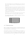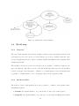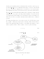
1
GPS Space Segment Monitoring Ignacio Ginés Fernández Dissertação para a Obtenção do Grau de Mestre em Engenharia Electrotécnica e de Computadores Júri Presidente: Professor José Manuel Bioucas Dias Orientador: Professor José Eduardo Charters Ribeiro da Cunha Sanguino Co-orientador: Professor António José Castelo Branco Rodrigues Vogal: Professor Francisco António Bucho Cercas December 2010 ii Acknowledgements I would like to thank Professor José Sanguino for giving me the opportunity to do this project and guide me in its realization, also for helping me with its knowledge and dedication. Thanks to the Instituto de Telecomunicações for allowing me to develop the project in the Satellites Laboratory and provide the necessary material. Last but not least, thanks to my family, friends and especially to my Portuguese friends which help me on my stage in Lisboa. Wholeheartedly thank you very much. iii iv Abstract The GPS system is the most extended satellite-based navigation system nowadays, it is increasingly being used for a wide range of applications and by a huge number of users worldwide. The aim of this project is develop a set of graphical user interfaces to track the GPS satellite constellation, also called GPS Space Segment. The information of the GPS satellites is acquired, processed and stored at the IT Monitoring Station, which becomes the starting point of this project. First of all, to a better comprehension of the work realized, it is described the essentials concepts of the GPS system. Also a study of the the characteristics of the IT Monitoring Station and its functionalities has been done. To complete this theoretical approach, a look to the state of the art of the navigation systems is done. Four applications have been developed in the context of this project, an application consists on both, a server and client side. In each application it is monitored a different concept related with the GPS satellites: elevation and azimuth, ephemeris data and the satellites position into 2D and 3D views. In this report it is described in detail the monitored data, the applications functionalities and its internal structure. The servers have been written in C and are running, as independent processes, in the IT Monitoring Station computer. The clients have been developed with Matlab, an environment that fulfills all the GUIs needs. They are standalone applications that can run in Windows OS. Furthermore, some tests have been done to check that the performance of the applications was correct. Also this report includes some applications manuals that explain everything that an user should know in order to run and use the applications. The result of this project is four tracking applications of the GPS Space Segment. Keywords: GPS, GUI, Monitoring Station, Tracking system, Matlab, Google Earth, KML v vi Contents Abstract v List of Figures ix List of Tables xi List of Abbreviations xii 1 Introduction 1 2 Technologies 3 2.1 2.2 2.3 2.4 GPS . . . . . . . . . . . . . . . . . . . . . . . . . . . . . . . . . . . . . . . . . . 3 2.1.1 Overview . . . . . . . . . . . . . . . . . . . . . . . . . . . . . . . . . . . 3 2.1.2 Principles . . . . . . . . . . . . . . . . . . . . . . . . . . . . . . . . . . . 4 2.1.3 Details . . . . . . . . . . . . . . . . . . . . . . . . . . . . . . . . . . . . . 6 IT Monitoring Station . . . . . . . . . . . . . . . . . . . . . . . . . . . . . . . . 13 2.2.1 Elements . . . . . . . . . . . . . . . . . . . . . . . . . . . . . . . . . . . 14 2.2.2 Monitoring Station architecture . . . . . . . . . . . . . . . . . . . . . . . 15 Software used . . . . . . . . . . . . . . . . . . . . . . . . . . . . . . . . . . . . . 16 2.3.1 Matlab . . . . . . . . . . . . . . . . . . . . . . . . . . . . . . . . . . . . 16 2.3.2 C programming language . . . . . . . . . . . . . . . . . . . . . . . . . . 17 2.3.3 Google Earth . . . . . . . . . . . . . . . . . . . . . . . . . . . . . . . . . 17 State of the art . . . . . . . . . . . . . . . . . . . . . . . . . . . . . . . . . . . . 18 3 Developed work 19 3.1 System architecture . . . . . . . . . . . . . . . . . . . . . . . . . . . . . . . . . 19 3.2 Elevation and azimuth . . . . . . . . . . . . . . . . . . . . . . . . . . . . . . . . 21 3.2.1 Objective . . . . . . . . . . . . . . . . . . . . . . . . . . . . . . . . . . . 21 vii 3.3 3.4 3.5 3.2.2 Monitored data . . . . . . . . . . . . . . . . . . . . . . . . . . . . . . . . 22 3.2.3 Software developed . . . . . . . . . . . . . . . . . . . . . . . . . . . . . . 22 Ephemerides . . . . . . . . . . . . . . . . . . . . . . . . . . . . . . . . . . . . . 24 3.3.1 Objective and monitored data . . . . . . . . . . . . . . . . . . . . . . . . 24 3.3.2 Software developed . . . . . . . . . . . . . . . . . . . . . . . . . . . . . . 26 World map . . . . . . . . . . . . . . . . . . . . . . . . . . . . . . . . . . . . . . 28 3.4.1 Objective . . . . . . . . . . . . . . . . . . . . . . . . . . . . . . . . . . . 28 3.4.2 Monitored Data 3.4.3 Software developed . . . . . . . . . . . . . . . . . . . . . . . . . . . . . . 30 . . . . . . . . . . . . . . . . . . . . . . . . . . . . . . . 28 3D view with Google Earth . . . . . . . . . . . . . . . . . . . . . . . . . . . . . 33 3.5.1 Objective . . . . . . . . . . . . . . . . . . . . . . . . . . . . . . . . . . . 33 3.5.2 Keyhole Markup Language (KML) . . . . . . . . . . . . . . . . . . . . . 33 3.5.3 Software developed . . . . . . . . . . . . . . . . . . . . . . . . . . . . . . 34 4 Achieved results and manuals 4.1 4.2 37 System evaluation . . . . . . . . . . . . . . . . . . . . . . . . . . . . . . . . . . 37 4.1.1 Elevation and azimuth . . . . . . . . . . . . . . . . . . . . . . . . . . . . 38 4.1.2 Ephemeris . . . . . . . . . . . . . . . . . . . . . . . . . . . . . . . . . . . 39 4.1.3 World map . . . . . . . . . . . . . . . . . . . . . . . . . . . . . . . . . . 40 4.1.4 3D view with Google Earth . . . . . . . . . . . . . . . . . . . . . . . . . 40 User manual . . . . . . . . . . . . . . . . . . . . . . . . . . . . . . . . . . . . . . 43 4.2.1 Requirements . . . . . . . . . . . . . . . . . . . . . . . . . . . . . . . . . 43 4.2.2 Elevation and azimuth . . . . . . . . . . . . . . . . . . . . . . . . . . . . 44 4.2.3 Ephemerides . . . . . . . . . . . . . . . . . . . . . . . . . . . . . . . . . 46 4.2.4 World map . . . . . . . . . . . . . . . . . . . . . . . . . . . . . . . . . . 47 4.2.5 3D view with Google Earth . . . . . . . . . . . . . . . . . . . . . . . . . 48 5 Conclusions 51 Bibliography 53 A Table - Ephemeris content 55 viii List of Figures 2.1 GPS orbits . . . . . . . . . . . . . . . . . . . . . . . . . . . . . . . . . . . . . . 5 2.2 GPS positioning . . . . . . . . . . . . . . . . . . . . . . . . . . . . . . . . . . . 6 2.3 GPS message . . . . . . . . . . . . . . . . . . . . . . . . . . . . . . . . . . . . . 7 2.4 GPS errors . . . . . . . . . . . . . . . . . . . . . . . . . . . . . . . . . . . . . . 9 2.5 Relation between the physical surface of the Earth and the ellipsoid. . . . . . . 11 2.6 Map projection concept . . . . . . . . . . . . . . . . . . . . . . . . . . . . . . . 12 3.1 System architecture . . . . . . . . . . . . . . . . . . . . . . . . . . . . . . . . . 20 3.2 Elevation and azimuth GUI . . . . . . . . . . . . . . . . . . . . . . . . . . . . . 22 3.3 Elevation and azimuth struct . . . . . . . . . . . . . . . . . . . . . . . . . . . . 23 3.4 Elevation and azimuth server flowchart . . . . . . . . . . . . . . . . . . . . . . . 23 3.5 Elevation and azimuth client diagram . . . . . . . . . . . . . . . . . . . . . . . 25 3.6 Ephemerides struct . . . . . . . . . . . . . . . . . . . . . . . . . . . . . . . . . . 26 3.7 Ephemerides server flowchart . . . . . . . . . . . . . . . . . . . . . . . . . . . . 27 3.8 Ephemerides client diagram . . . . . . . . . . . . . . . . . . . . . . . . . . . . . 28 3.9 World Map GUI . . . . . . . . . . . . . . . . . . . . . . . . . . . . . . . . . . . 29 3.10 Geographical coordinates: Latitude and longitude . . . . . . . . . . . . . . . . . 29 3.11 Cartesian coordinates: X, Y, Z . . . . . . . . . . . . . . . . . . . . . . . . . . . 30 3.12 World map server flowchart . . . . . . . . . . . . . . . . . . . . . . . . . . . . . 31 3.13 Satellite position struct . . . . . . . . . . . . . . . . . . . . . . . . . . . . . . . 31 3.14 World map client diagram . . . . . . . . . . . . . . . . . . . . . . . . . . . . . . 32 3.15 Example KML file . . . . . . . . . . . . . . . . . . . . . . . . . . . . . . . . . . 34 3.16 3D view with Google Earth. Application architecture . . . . . . . . . . . . . . . 35 4.1 Elevation and azimuth: plot evolution . . . . . . . . . . . . . . . . . . . . . . . 38 4.2 Simulated skyplot by www.alamo.edu . . . . . . . . . . . . . . . . . . . . . . . . 39 4.3 Ephemeris: current data . . . . . . . . . . . . . . . . . . . . . . . . . . . . . . . 39 ix 4.4 Ephemeris: expired data . . . . . . . . . . . . . . . . . . . . . . . . . . . . . . . 40 4.5 World map: satellite displacement . . . . . . . . . . . . . . . . . . . . . . . . . 41 4.6 World map: satellite displacement after 5 hours . . . . . . . . . . . . . . . . . . 41 4.7 3D view: satellite displacement . . . . . . . . . . . . . . . . . . . . . . . . . . . 42 4.8 3D view: satellite displacement after 3 hours . . . . . . . . . . . . . . . . . . . 42 4.9 Elevation and azimuth: starting the server . . . . . . . . . . . . . . . . . . . . . 44 4.10 Elevation and azimuth: connecting to the server . . . . . . . . . . . . . . . . . 45 4.11 Elevation and azimuth: set options and plotting . . . . . . . . . . . . . . . . . . 46 4.12 Ephemeris: starting the server . . . . . . . . . . . . . . . . . . . . . . . . . . . 46 4.13 Ephemeris GUI . . . . . . . . . . . . . . . . . . . . . . . . . . . . . . . . . . . . 47 4.14 World map: starting the server . . . . . . . . . . . . . . . . . . . . . . . . . . . 47 4.15 World map: starting the AC12 service . . . . . . . . . . . . . . . . . . . . . . . 48 4.16 World map GUI . . . . . . . . . . . . . . . . . . . . . . . . . . . . . . . . . . . 49 4.17 3D view with Google Earth: starting the server . . . . . . . . . . . . . . . . . . 50 4.18 3D view with Google Earth . . . . . . . . . . . . . . . . . . . . . . . . . . . . . 50 x List of Tables 2.1 GPS satellites generations . . . . . . . . . . . . . . . . . . . . . . . . . . . . . . 5 2.2 GPS codes characteristics . . . . . . . . . . . . . . . . . . . . . . . . . . . . . . 7 2.3 RINEX file name . . . . . . . . . . . . . . . . . . . . . . . . . . . . . . . . . . . 13 2.4 Magellan Navigation AC12 characteristics . . . . . . . . . . . . . . . . . . . . . 14 3.1 Cartesian to geographic transformation 4.1 Clients requirements . . . . . . . . . . . . . . . . . . . . . . . . . . . . . . . . . 43 4.2 Server characteristics . . . . . . . . . . . . . . . . . . . . . . . . . . . . . . . . . 43 4.3 Elevation and azimuth: displacement storage time . . . . . . . . . . . . . . . . 45 4.4 World map: displacement storage time . . . . . . . . . . . . . . . . . . . . . . . 48 4.5 3D view with Google Earth: displacement storage time . . . . . . . . . . . . . . 49 . . . . . . . . . . . . . . . . . . . . . . 30 A.1 Ephemeris data content . . . . . . . . . . . . . . . . . . . . . . . . . . . . . . . 56 xi xii List of Abbreviations ASCII American Standard Code for Information Exchange C/A code Coarse Acquisition Code CTRS Conventional Terrestrial Reference System DGPS Differential GPS DoD U.S. Department of Defense ESA European Space Agency EU European Union GIS Geographical Information System GLONASS Global Navigation Satellite System GPS Global Positioning System GRS 80 Geodetic Reference System of 1980 GUI Graphical User Interface HTTP Hypertext Transfer Protocol IOC Initial Operational Capability IODC Issue of Data Clock IODE Issue of Data Ephemeris IP Internet Protocol IST Instituto Superior Tecnico IT Instituto de Telecomunicações KML Keyhole Markup Language MCR Matlab Compiler Runtime MCS Master control station MEO Medium Earth Orbit NGS-SP3 National Geodetic Survey - Standard Product 3 P code Precision Code xiii PRN Pseudorandom Noise RF Radio Frequency RINEX Receiver Independent Exchange Format RS-232 Recommended Standard 232 SA Selective Availability SVN Space Vehicle Number TAI International Atomic Time TCP Transmission Control Protocol TOC Time of Clock TGD Timing Group Delay UDP User Datagram Protocol URA User Range Accuracy URL Uniform Resource Locator US United States UTC Coordinated Universal Time WGS 84 World Geodetic System of 1984 XML Extensible Markup Language xiv Chapter 1 Introduction The main objective of this project is develop a set of graphical applications, or GUI (Graphical User Interfaces), to monitor the position and state of the GPS (Global Positioning System) satellites. The applications must show clearly the position, orbit, state and other relevant data of the GPS satellites in real time, and also allow to save and load this stored data. This set of applications are part of the GPS Monitoring Station developed in the Satellites Laboratory of the IT (Instituto de Telecomunicações), placed on the 12th floor of the Torre Norte of the IST (Instituto Superior Técnico) Alameda campus. This project is the result of the acquired knowledge in my six months Erasmus Programme. The GPS system allows anybody, anytime and everywhere to know its position in a global coordinates system. In addition to the geographical information other information is obtained by means of a GPS receiver. The Monitoring Station developed in the Satellites Laboratory is a system that makes this data accessible to other interfaces or programs. The system acquires, process and stores the data obtained by its GPS receivers, but once the data is stored it would be appropriate to represent it graphically. In this context it seems useful to develop some applications that process this obtained data to show it graphically. Furthermore the Satellites Laboratory is equipped with 6 computers and panoramic LCD screens where the applications could run 24 hours a day. Once the problem is known and the premises are defined, the objectives of the project can be listed: 1. Understand how GPS works and its main involved components. So a basic theoretical 1 approach is needed as first step. 2. Develop the servers that will interact with the acquired data from the Monitoring Station, of course to do this is necessary to understand how the Monitoring Station works, how it gets the information from the GPS satellites and how this information is stored. Also it will be necessary to develop the clients which will represent that information, this includes learning the technologies that will be used. 3. Test the applications in long running periods. The applications should be capable of be running 24 hours a day. This report is divided in five chapters. The first one is the introduction that explains the motivation for doing the project, the problems that have to be solved and the initial objectives. The second chapter is focused on the technological part of the project: an overview of the GPS system; a general view of the structure of the IT Monitoring Station and the Satellites Laboratory; the software used on the project, Matlab, C programming language, Google Earth. . . and finally the state of the art of the GPS technology. In the third chapter there is explained the main part of the project, the developed work. The chapter is structured by applications, one section per application, and in each section it is explained its functionalities, the client and server characteristics and other significant information. In the fourth chapter there are the results of the 24 hours running period test. At the end of this fourth chapter there is a manual of the applications that explains how to use them. The last chapter are the conclusions and future work. 2 Chapter 2 Technologies The main objective of this chapter is explain the technologies and software used in the realization of the project. It begins with the principal technology which this project is based on, the GPS navigation system. For a better understanding of the work developed it seems necessary to describe some general and technical concepts of GPS. Furthermore there is a brief explanation of the software and programs used and its use is justified. Finally, at the end of the chapter, there is an overview of the state of the art of navigation systems. 2.1 GPS In this section there is an overview of what is GPS and the most important concepts used in the project, such as GPS segments, GPS standard formats for data storage, map projections. . . as well as other information not directly used in the project but with high significance to understand GPS operatively. 2.1.1 Overview GPS is a satellite-based radio navigation system that provides reliable positioning, navigation and timing. It was developed by the US (United States) DoD (Department of Defense) in the 70s. Initially it was developed as a military system to fulfill military needs and later 3 it was made available to civilians, being nowadays both accessible. The GPS system was totally operational in 1995, and it is guaranteed that at least there is a constellation of 24 operational satellites into orbit. This constellation is known as the IOC (Initial Operational Capability)[1]. GPS provides continuous positioning and timing information anywhere in the world, under any weather conditions. Because it serves an unlimited number of users, as well as being used for security reasons, GPS is a one way ranging system that can be stopped at any moment. GPS and the recent progress in space technologies has prompted a revolution in the navigation methods and also in navigation applications. Manufacturers have been able to come up with very user-friendly systems that have brought GPS applications to another dimension of use, being nowadays a very extended technology. 2.1.2 Principles • GPS segments The GPS system is divided in three segments: space segment, control segment and user segment. - Space segment. This segment consists of the GPS satellites constellation which are orbiting around the Earth. Each GPS satellite transmits a signal with several components: two sine waves (or carrier frequencies) modulated by two digital codes and a navigation message. The carriers and the codes are used mainly to determine the distance from the user’s receiver to the GPS satellites. The navigation message contains information about the satellites coordinates and other information such as the satellite status, time clock corrections, signal characteristics, etc. - Control segment. It consists of a worldwide network of tracking stations. Its primary task is track the GPS satellites in order to determine and predict the satellite location, system integrity, behavior of the satellite atomic clocks, atmospheric data and other considerations. There is one Master Control Station (MCS) located in the US at Colorado and other five monitor stations located around the equator. These monitor stations collect all the information from the satellites and transmit it to the MCS for processing. 4 - User segment. It includes all military and civilian users, GPS is available to all users worldwide. • Satellites and constellation Since the first satellites launched in the 70s, different generations of satellites have been created. They can be divided in four different types or generations. Next table 2.1 shows these generations and their main characteristics. Generation Year Characteristics 1st. Block I 1978 Built for experimental purpose with a expected lifetime of 4,5 years. Last one was taken out of service in 1995 2nd. Block II/IIA 1989 Higher navigation message data storage. Higher function periods without ground support 3rd. Block IIR 1997 Higher accuracy and autonomy. Can operate without ground corrections 180 days 4th. Block IIF 2010 First one was launched on May 2010 Table 2.1: GPS satellites generations Nowadays the number of satellites that form the constellation is 31, but 30 actually working[2]. The GPS satellites are placed in six orbital planes, as figure 2.1 illustrates, so an orbital plane can contain four or five satellites. The satellites orbit the earth with a circulation time of 11 hours 58 minutes, and with a height of the orbit about 20200 km. Orbits in this height are referred to as MEO (Medium Earth Orbit). Figure 2.1: GPS orbits 5 The satellites can be identified in two ways. The SVN (Space Vehicle Number) and the PRN (Pseudorandom Noise). The identification system used in this project is the PRN. • GPS basic idea The GPS idea is rather simple: if the distances from a point on the Earth to three GPS satellites are known, the location of the point can be determined by applying the trilateration method[3]. Each GPS satellite continuously transmits a microwave radio signal with all the information mentioned before, see 2.1.2. The GPS receiver process the acquired signal to locate its position. The receiver would be located at the intersection of three spheres, each as a radius of one receiver-satellite distance and is centered on the particular satellite, as illustrates figure 2.2. However from the practical point of view a fourth satellite is needed to account for the receiver clock offset. Figure 2.2: GPS positioning 2.1.3 Details • Signal structure Each GPS satellite transmits a microwave radio signal composed of two carrier frequencies modulated by two digital codes and a navigation message. The two carrier frequencies are generated at 1,575GHz (L1 carrier) and 1,227HHz (L2 carrier). The availability of two carrier frequencies allows to correct major GPS errors. Each GPS satellite uses a different code modulation in order to minimize the signal interference, their names are Coarse Acquisition code (C/A code) and Precision code (P code). They are commonly know as PRN because they look like random signals. The following table 2.2 shows codes characteristics. 6 Code Carrier freq, Long Tx rate Other C/A L1 1.023 bits 1.023 Mbits/s Available to all users P L1 and L2 6.1871 102 bits 10.23 Mbits/s Available to all users since 1994 Table 2.2: GPS codes characteristics The GPS navigation message, shown in figure 2.3, is a data stream added to both L1 and L2 carriers at a 50kbps rate. It contains, along with other information, satellite clock correction; the ephemeris with the coordinates of the GPS satellites as a function of time, the satellite health status, week number, etc; the almanac and atmospheric data. Figure 2.3: GPS message Some the information transmitted in the navigations message is represented in the applications developed in this project. It is useful for tracking the space segment status with high precision. • Time systems Time plays a very important role in positioning with GPS. The measure of the distance from the receiver to the satellites is based on both, the receiver and the satellite clocks. Different time systems are used worldwide for various purposes, for GPS the most important are: - Coordinated Universal Time (UTC). It is an atomic time scale based on the International Atomic Time (TAI), which is a uniform time scale computed on independent time scales generated by different atomic clocks. Occasionally the UTC is adjusted by introducing a leap second to make it similar to the time system with relation to the rotation of the 7 Earth. In 1/01/1999 TAI was 32 seconds ahead of UTC[4]. - GPS Time. Is a time scale used for referencing GPS signals. It is computed based on the time scales generated by atomic clocks at the monitor stations and onboard the GPS satellites. There are no leap seconds introduced into the GPS time, which means that is a continuous time scale. The difference between GPS and UTC time scales is given inside the GPS navigation message. • Measurements - Pseudorange measurement. Is the measure of the distance between the GPS receiver and the GPS satellite, it is used to make the computation of the position. Assuming that the receiver and satellite clocks are perfectly synchronized, the procedure of the GPS range determinations is the next: when the PRN code is transmitted from the satellite, the receiver generates an exact replica of that code. After the signal travel time in space the code will be picked up by the receiver. By comparing the transmitted code and its replica, the receiver can compute the signal travel time. Multiplying the travel time by the speed of light gives the range between the satellite and the receiver. This measure is not exactly, it is contaminated due to the fact that the receiver and satellite clocks are not synchronized, along with other errors and biases. - Carrier-phase measurement. It consists on the sum of the total number of full carrier cycles plus fractional cycles at the receiver and the satellite, multiplied by the carrier wavelength. The ranges determined with the carriers are far more accurate than those obtained with the codes. The main problem of this kind of measurements is that a receiver has no means to differentiate one cycle from another, carriers are just pure sinusoidal waves, this is commonly known as the initial cycle ambiguity. • Errors GPS pseudorange and carrier-phase measurements are both affected by several types of errors. Some of them are punctual and other systematic. They can be classified as those originated at the satellites, at the receiver and those that are due to signal propagation, as figure 2.4 illustrates. Next there are explained the most important. 8 Figure 2.4: GPS errors - GPS ephemeris errors. The satellite position as a function of time is predicted in the ground control stations. Modelling the forces acting on the GPS satellites is not perfect, which causes some errors in the estimated satellites positions, this is known as the ephemerides error and it is in the order of 2m to 5m. - Selective availability (SA). GPS was originally designed to be less precise for civilian C/A code than for military P code receivers. Surprisingly, the obtained accuracy was almost the same from both receivers. For security reasons the U.S. DoD introduced two types of errors that made the nominal horizontal and vertical errors can be up to 100m and 156m respectively. This error could be reduced by using the Differential GPS (DGPS) 1 . Finally in May 2000 the SA was turned off. - Satellite and receiver clock errors. The GPS satellite clocks, although highly accurate, are not perfect. They have an error about 8,64ns and 17,28ns per day, that corresponds a range error of 2,59m to 5,18m [5]. The performance of the satellite clock is monitored by the ground control system, the amount of drift is calculated and transmitted as a part of the navigation message [6]. Applying that correction the satellite clock error can be corrected. Also there is an error on the receivers clocks that depend on the quality of the receiver. The GPS receivers use inexpensive crystal clocks, which are much less accurate than the satellite clocks. That makes the receiver clock error much larger than the satellite clock error. 1 DGPS is technique to improve the precision of GPS, is based on the idea of having a well known position to compare with and estimate the error of the measure. 9 - Multipath error. It is a major error source for range measurement. It occurs when the GPS signal arrives at the receiver antenna through different paths. These paths can be the direct line of sight signal and reflected signals. - Receiver measurement noise. It results from the limitations of the receiver’s electronics. Of course, a good GPS system should have a minimum noise level. Some internal tests of the systems can predict some of the receiver errors such as interchannel biases and cycle lips. - Ionospheric delay. It occurs on the uppermost part of the Earth atmosphere. Summarizing, the ionosphere is a dispersive medium, it causes a delay on the transmitted signal that is frequency dependent, so the L2 delay is greater than L1 delay. Generally ionospheric delay is of the order of 5m to 15m, but can reach over 150m under extreme solar activities, at midday and near the horizon. There are some solutions to reduce this error: by combining the P code pseudorange measurements on both L1 and L2, this solution is only available for authorized users only. There are some empirical ionospheric models that can be used to correct up to 60% of the delay. - Tropospheric delay. The troposphere is a nondispersive medium for radio frequencies below 15GHz. As a result, it delays the GPS carriers and codes identically. This error cannot be removed by combining the L1 and the L2. The tropospheric delay depends on the temperature, pressure and humidity. There are also some models that can be used to reduce this error. • Datum, Coordinate systems and Map projections - Datum. To determine an user’s location with the GPS it is needed a reference surface of the Earth that approximates the irregular shape of the Earth to a smooth mathematical surface. It is used a biaxial reference ellipsoid with a well defined center and orientation. This reference ellipsoid is known as the geodetic datum and is shown in figure 2.5. - Coordinate systems. It is defined as a set of rules for specifying the locations of points. This usually involves specifying an origin of the coordinates as well as a set of reference lines with known orientation. There are several coordinates systems, they can be 10 Figure 2.5: Relation between the physical surface of the Earth and the ellipsoid. classified according to the dimensions, to the reference surface, the orientation of the axes and the origin. In GPS system the official reference system is the World Geodetic System of 1984 (WGS 84). The WGS 84 uses the Conventional Terrestrial Reference System (CTRS)2 combined with the ellipsoid of the Geodetic Reference System of 1980 (GRS 80). The broadcast ephemeris transmit by the GPS satellites will refer to the WGS 84 system, in general. Although some agencies provide the ephemerides in various formats. - Map projections. A map projection is defined as the transformation of the physical features on the curved Earth’s surface onto a flat surface called a map, as figure 2.6 illustrates. From the mathematical point of view, it is defined as the transformation of geodetic coordinates (longitude, latitude and altitude) into rectangular grid coordinates. Because of the difference between the ellipsoidal shape of the Earth and the flat projection surface, the projected features suffer from distortion. There are different kinds of projections, like the Mercator projection or Lambert conical projection, on both the areas and the scales are distorted in different degree. The Mercator projection is the standard projection for nautical purposes because of its ability to represent lines of constant course. The Mercator projection distorts the size and shape of objects as the scales increases from the Equator to the poles, where it becomes infinite. 2 CTRS is a 3D geocentric coordinated system. It is rigidly tied to the Earth and its rotation. 11 Figure 2.6: Map projection concept • Standard formats. RINEX Why it was necessary to create a GPS standard format? GPS manufacturers have their own proprietary format for storing GPS measurements, it makes difficult to combine data from receivers of different manufacturers. And also a similar problem happens when interfacing various devices. For this reasons several standard formats where developed, like the Receiver Independent Exchange Format (RINEX)[7] or the Standard Product #3 of the National Geodetic Survey (NGS-SP3) The first proposal for RINEX was developed by the Astronomical Institute of the University of Berne for the easy exchange of the GPS data to be collected during the first large European GPS campaign of data collection in 1989, which involved more than 60 GPS receivers of 4 different manufacturers. To easy exchange the collected data between the systems it was defined a standard format. Property formats developed for data storage are mostly binary, this creates a problem when combining data from different GPS receivers. The RINEX format is in the standard ASCII (American Standard Code for Information Exchange) format that provides more distribution flexibility. Since 1989 different versions of RINEX have been developed, the most recent is the 3.0, that has been used in this project. In this version there are three types of files: observation files, navigation files and meteorological files. The observation file is divided in two parts. First one is a header that contains the name of the GPS station, the coordinates of the station, information about the antenna, the type of observations realized, the observation interval in seconds and other information. 12 The second part is divided in epochs, each contains the time tag of the observation, the number and list of satellites, the various types of measurements like the pseudo-range, SNR and others. The navigation file is divide also in two parts, a header and a data section. The header is smaller compared with the observation file header, it contains the date of file creation, the agency name and other relevant information. The first record in the data section contains the satellite PRN, the time tag and the satellite clock parameters. The subsequent records contain information used to calculate the satellite position and other relevant information about the status, etc. These files have a very specific format. All the information in the header and in the data section must be in the correct position, in determinate columns of the file. The recommended naming convention for RINEX files is s̈sssdddff.yyt.̈ Next table 2.3 shows the meaning of each character. ssss station name ddd day of the year of first record ff file sequence number within the day yy last two digits of the current year t file type Table 2.3: RINEX file name 2.2 IT Monitoring Station This section explains the elements and the architecture of the IT Monitoring Station. Also there is a brief explanation of how applications developed in this project interact with the obtained data, that it is stored on the shared memory. As told in chapter 1, the station is located in the Satellites Laboratory on the 12th floor of the North Tower. The stations has been developed by Pedro Gona̧lves, a IST student. The objective of the station is to acquire the data transmitted by the GPS satellites, by means of the antennas and the GPS receivers; process it, with the developed software; and make it 13 continuously accessible to other applications. 2.2.1 Elements The Monitoring Station consists of the next elements. - GPS receiver. The station is equipped with two GPS receiver, the AC12 model from Magellan Navigation manufacturer[8]. Next table 2.4 shows its specifications. The receiver has two different operating modalities, the first one is a 3D modality in which latitude, longitude, altitude and time are calculated once the receiver gets four signals from four different GPS satellites. The other operating modality is called 2D and only needs three different GPS signals to obtain the latitude, longitude and time; being the altitude a constant variable. The time need to calculate a position vary from 10 seconds to 2 minutes. The bidirectional communication between the receivers and the computer is make with the RS-232 (Recommended Standard 232) protocol and the message format is NMEA3 (National Marine Electronics Association) or a proprietary format from Magellan manufacturer. Carrier frequency L1 (1,575GHz) Channels 12 channels Ports 2 serial ports and 1 RTCM port Precision Without corrections: 5m (horizontal) and 7,5m (vertical) Table 2.4: Magellan Navigation AC12 characteristics - Antenna. The function of the antenna is transform the electromagnetic signal into a radio frequency (RF) signal which contains the amplitude and the phase of the GPS signal. In the Monitoring Station two antennas are used to receive the GPS signals, they are placed in the roof of the North Tower and each one is connected to a GPS receiver. The model of the antenna is Novatel 351 [9] and is able to receive frequencies 3 NMEA is a standard protocol used by GPS receivers to transmit data. It is also used by other type of electronic elements like sonars, anometers,, etc. Most GPS manufacturers include special messages in addition to the standard. 14 from the L1 carrier frequency. - The computer (the core). The main functions of the computer are: do the bidirectional communication with the GPS receivers, host the web page of the IT Monitor Station4 , and finally, make accessible the obtained data from the GPS receivers to other applications, like the set of applications developed in this project. The software developed in that project is done in C programming language over Linux. This software can be divided in three parts or modules. The first module involves the communication with the GPS receiver by means of the serial interface. The software developed is able to receive and process the information obtained from the receiver, and also can send some configuration messages to receiver in order to control its behavior: initialize or restart the receiver, select the coordinates system or the navigation mode, etc. The second module developed is the web page hosted in the computer. It makes possible, to an authorized user, to access the obtained data from any part at any time. Also permits, to an administrator, to modify some parameters of the GPS receiver behavior. The third module, the most important for this project, is the interface and functions developed that allow to other applications to access the obtained data from the receivers. The applications developed in this project, specifically the servers running on the core computer, can access to real time data and send it to the graphical applications, or clients. More specific and technical details of the interfaces and functions are explained in chapter 3 together with the developed applications in this project. 2.2.2 Monitoring Station architecture The way that the elements explained in 2.2.1 are interconnected is quite simple. The two antennas are connected to the two GPS receivers. These are connected with the computer, the core or central part of the architecture, the communication between them is made by means of the RS-232 protocol. This communications is bidirectional: from the receivers to the computer by means of the messages mentioned in 2.2.1, and from the computer to the receivers with configurations commands. 4 The web page is accessible on http://www.satlab.it.pt 15 2.3 Software used In this section there is an explanation of the software used to develop the set of applications. It includes a brief summary of the software, what elements of the software have been used and, finally, the criteria of choice. More specifics details of each software are explained in chapter 3 together with the explanation of each application. 2.3.1 Matlab Matlab is a numerical computing environment that allows matrix manipulation, plotting of functions and data, creation of GUI and interface with programs written in C, among other characteristics. In this project Matlab has been used in the development of all the applications except one5 . This environment fulfill all the applications needs, of course other programming environments could be used as Java or C++, but Matlab offers an easy way to make calculations, work with numerical data and create GUIs. In the Matlab environment programs can be writen inside files, that allows an user not to use only the command line. These files are known as M-file and should be named with the .m extension. These files can contain functions, its name must be the same as the M-file. For example, if the function is application plot the M-file sould be named application plot.m. Matlab has a lot of libraries, also known as Toolboxes, that extend its capabilities for special purposes. These are the Toolboxes used in this project. - Instrument Control Toolbox. The Toolbox features used in the applications are: a framework for communicating with instruments that support the TCP (Transmission Control Protocol) and UDP (User Datagram Protocol) protocols. Functions for transferring data between the Matlab workspace and another element, this data can be binary or text. Event-based communications. Functions for recording data and event information into a text file. - Image Processing Toolbox. The Image Processing Toolbox supports a wide range of image processing operations, like spatial image transformations, analysis, filtering, etc. 5 The set of possibilities that gives Google Earth made unnecessary the use of Matlab to develop an appli- cation to monitor GPS satellites in a 3D perspective. 16 - Matlab Compiler. It allows to compile a M-file application into a standalone application. This enables the application to be run outside the Matlab environment as an executable file, for example as an .exe file for Windows OS. 2.3.2 C programming language The C programming language was created in 1972, being nowadays one of the most popular programming languages[10]. It has been used in this project in the development of the server side of the applications. As is explained in detail chapter 3, the applications follow the server/client structure. Since previous work done (see section 2.2), which this project interacts and is based on, has been developed in this language there was no necessity of choosing another language for the development of the servers. C language fulfills all the requirements of the servers that have been developed: can interact with the data obtained from the GPS receivers, it has the capacity of manage TCP or UDP sockets for data transmission. Also, it is widely used, well documented, and is platform independent, so could be used in another machine without so much effort because almost all the architectures have a C compiler. 2.3.3 Google Earth To represent GPS satellites on a 3D Earth model it has been used Google Earth [11]. This program allows to display own data, in this case GPS satellites position and their displacement, over the Earth’s surface. Google Earth shows the Earth as it looks an elevated platform such an orbiting satellite, permitting to explore the Earth’s surface from different points of view including a bird eye’s view. It maps the Earth by the superimposition of images obtained from satellite imagery, aerial photography and GIS (Geographical Information System) 3D globe. Another important factor is that it uses the WGS 84 datum ellipsoid the same that GPS system. The representation of the GPS satellites and their displacement is made by means of Keyhole Markup Language (KML) files. It is an Extensible Markup Language-based (XML) language schema for expressing geographic annotation and visualization, more specific details of KML are explained in chapter 3. Finally, Google Earth is available for several different operating 17 systems like Windows, LINUX, Mac OS, etc. 2.4 State of the art GPS is not the unique global navigation system, other countries or regions have developed or are currently developing their own navigation system. Other systems, like GALILEO, will be a real option in a few years and will provide users another option not to depend on an unique property system like the US GPS. However GPS is nowadays the most extended and used system. • GALILEO The European Union (EU) and the European Space Agency (ESA) have been developing since 2002 their own satellite navigation system, the system should be working in 2014 [12]. The first experimental satellite was launched in 2005 and it is expected to have 30 satellites in orbit. GALILEO is expected to be totally compatible with GPS. Receivers will be able to combine both signals to increase accuracy, and like GPS it will be free open to everyone, however the high-accuracy capabilities will be restricted to military and paying users. • GLONASS (Global Navigation Satellite System) Development of GLONASS began in 1976 in the formerly Soviet Union being in 1995 totally operative, following a rapid disrepair with collapse of the Russian economy. Nowadays the system has been restored, there are 24 operational satellites. GLONASS is less precise than GPS, in order of 4,46-8,38 m for latitude and longitude [13]. There are some commercial receivers that are able to combine both signals, GPS and GLONASS. This receivers have a high number of channels that allow them to be connected simultaneously to both kind of satellites. • COMPASS Is a chinese global navigation system in development, is based on its regional navigation system called Big Dipper and it is expected to be operative in 2020 [14]. 18 Chapter 3 Developed work In this chapter it is explained the set of applications developed in this project. At the beginning there is a general overview of the system, the definition of the objectives to achieve and the architecture of the applications and how they are interconnected. Next there is a particular explanation of each application that includes its main objective, the application model definition and a concise description of the software developed. If necessary some technical explanations are included for a better comprehension. 3.1 System architecture The purpose of this project is develop a set of applications to monitor the GPS Space Segment: GPS satellites position, displacement, elevation, azimuth, health status and other related information. Other aims are to show the information as clear and simple as possible, not to saturate an user with a lot of data1 , develop standalone applications that should be able to work continuously for long periods of time, without errors. To fulfill this objectives four independent applications have been developed, each one monitors a different concept of the GPS Space Segment: elevation and azimuth, ephemerides data, 2D world map and 3D view with Google Earth. Of course, instead of four independent applications they could be a big one application, but the fact of developing them as independent 1 If an user needs more detailed data it is accessible on a database where all the collected data is stored. This database has been developed in another project 19 applications gives more flexibility of use. As the IT Satellites Laboratory is equipped with 6 computer and LCD screens, each application could be running in a different screen. This way an user could have all the information as if he would be in a monitor station. Next figure 3.1 illustrates the system architecture. This architecture can be divided in three parts: Figure 3.1: System architecture • Server side. The main function of the servers is access to the receivers acquired data of the shared memory and send it, on demand, to the clients by means of TCP sockets. This data is put in the shared memory by some running programs of the Monitoring Station that are continuously processing the receivers acquired data. This shared memory can be accessible by other programs by means of some functions defined in .h files. In these files, there are defined the prototypes and the interfaces codes of the functions which are used to access the stored data. The servers developed in this project should include these .h files in order to get this data and send it. Four servers have been developed, one per application, that run as independent processes. The fact of developing an independent server for each application is conditioned by the structure of the previous work, in which this project is based on, this means that 20 if a program needs to include a particular .h file from the previous work in its code, that program must be placed in the same directory of the .h file to be included. Anyway, there is no big difference between developing a big one server or four small servers. The servers can be started all together, by means of a script, or separately. Once the server is running, it enters on a listening mode in which waits for client requests on his TCP port. When a request arrives, the server gets the updated data from the shared memory and sends it to the client. As an exception of this performance, the server that generates the KML file for the 3D view with Google Earth application does not work on demand, it is continuously updating the KML file placed in the Apache Web Server. • Communications. The transmission of data between the servers and clients is done by means of TCP sockets. The TCP protocol offers reliable and ordered data transmission in a stream of bytes opposite to UDP, which is better for high speed data streams. The Apache Web Server uses the HTTP (Hypertext Transfer Protocol) protocol over TCP/IP. • Client side. Three of the clients are standalone applications developed in Matlab. Their task is start the communications with the servers, obtain and represent continuously the received data. In next section there is a more detailed explanation of each GUI. The fourth application client is the Google Earth program which only needs a .kml file containing the server information. 3.2 3.2.1 Elevation and azimuth Objective The main objective of this application is monitor the values of elevation and azimuth of the GPS satellites that are in the coverage area of the antenna. The elevation and azimuth are calculated in real time according to both satellite and antenna position [15]. These values are represented in the GUI by means of a polar chart, where the elevation corresponds to the radius of the chart and the azimuth to the degrees relative to the y-axis. It is represented the present values and its variation in time. 21 Next figure 3.2 illustrates and example of the GUI with several satellites monitored. As can be seen in the figure, the maximum elevation corresponds to 90 ◦ , the center of the circumference, and the minimum to 0 ◦ , in the border. Figure 3.2: Elevation and azimuth GUI 3.2.2 Monitored data Know the elevation and azimuth of a GPS satellite allows an user to intuitively place it in the sky. The azimuth can be defined as the angular distance between two points in a spherical coordinate system. In this particular case, one point is the projected position of a GPS satellite onto the horizon and the other one is the reference point, the north. In the same context the elevation can be defined as the angular distance, in the vertical plane, between two horizontal points. These values are calculated every 30 seconds by the running software in the Monitoring Station, to do these calculations it is necessary to know the Cartesian coordinates of the satellites and the position of the receiver. 3.2.3 Software developed • Server side The server is written in C language. It is an independent program/process that is responsible of acquire the current values of elevation and azimuth, it is called app eph azim 22 and is placed in the /home/it/Desktop/it/GPGSV download directory. It includes the GPGSV read.h file which provides the struct, prototipes and functions required to manage the GPS receivers stored data. Specifically it uses the function GPGSV read() which needs to be called with a struct as a passed parameter. This function reads the shared memory and initializes the struct with the current values. The objects in the struct are shown in next figure 3.3. Figure 3.3: Elevation and azimuth struct To start the program it is necessary to pass the listening port number as a parameter in the terminal. Next figure 3.4 shows the flowchart of the app eph azim server. First of all there is the initialization of the server, where the socket is created with the specific configuration. Next the program waits for client petitions, when a petition arrives the struct is initialized with the correct values and is transmitted over the socket. As can be seen in the figure, once started, the server is continuously waiting for petitions. Figure 3.4: Elevation and azimuth server flowchart • Client side The GUI plays the client role in the system, where the satellites elevation and azimuth are displayed. Next figure 3.5 shows the program diagram which includes its main files and functions. 23 The M-file app elev azim.m is the main element of the program, in this file it is loaded the app elev azim.fig that contains the GUI graphical objects and characteristics. Also in the main M-file there are defined the callbacks of the GUI objects (menu bar, push buttons, plot, etc.). In the app elev conn.m are defined the functions used to connect to the server, acquire, process and store the received data. Finally if an error happens there is implemented a function that is responsible of retrying the petition and manage that error. In the app elev azim plot.m file are defined the functions related with the plot: draw the received data in the polar plot, create its legend, add and control the object callbacks associated to the plot. The plot is drawn by means of the existent Matlab function polar.m which allows to represent polar coordinates in a Cartesian plane. It has been necessary to change some parameters of the default polar function in order to represent the information properly. Some of these changes are: set the limits of the circle radius between 0 ◦ and 90 ◦ , set the maximum elevation (90 ◦ ) in the center of the circle, define 2 radial circles in the 60 ◦ and 30 ◦ position, etc. The new polar function is saved in the app elev azim dibuixa.m file. The file app elev azim save data.m is responsible of convert the graphical plot, with all the satellites info, into a .txt file. With the app elev azim load data.m this .txt can be converted into a graphical plot again. Some other functions are implemented, such as save the polar chart into an image file or change some properties about the refreshing period and memory time. In chapter 4 there is an specific explanation of the GUI and all the functionalities that it includes. 3.3 3.3.1 Ephemerides Objective and monitored data This application shows the current and expired values of the GPS ephemeris data. As mentioned before, in section 2.1.3, GPS satellites transmit in their navigation message information that contain their orbital parameters, time corrections, information health status, amongst 24 Figure 3.5: Elevation and azimuth client diagram other. This data allows to compute the satellite position for a given time instant within an interval. The variables contained in the ephemerides data are shown in the appendix A. Some of them are: - Week number : number of weeks, in the GPS time, since 05/01/1980. Used as a reference time for the ephemeris. - Satellite Health: the health of the navigation data. Used to detect if the data received is correct or there is any failure. - IODC: indictes the issue number if the data set and thereby provides the user with a convenient means of detecting any change in the correction parameters. The ephemeris data is usable for a limited period of time which is known as expiration time, usually a period of less than six hours. To find out if the ephemeris data is valid it is used the Issue of Data Ephemeris (IODE) variable. This variable provides the user a convenient mean for detecting any change in the ephemeris, if the transmitted IODE does not match with the previous one new data must be collected to update the values. 25 3.3.2 Software developed • Server side The program responsible to acquire the current values of the ephemeris data is placed in the /home/it/Desktop/it/Eph download directory. As explained in 3.2, it is necessary to use some external files where are defined the functions required to acquire this data, in this case the Eph read.h. The function used to read the data is called Eph read(). It fills the struct passed as a parameter with the current values of the shared memory. The objects that compose the struct are shown in figure 3.6. Figure 3.6: Ephemerides struct The flowchart of the app eph server is illustrated in next figure 3.7. First of all there is the initialization of the server components, once initialized the server waits for client requests. When a request is received, the current data of the ephemeris is acquired from the shared memory by means of the Eph read() function. Once the struct is initialized it is transmitted to the client via the TCP socket, but before transmitting it is necessary to convert the expiration date of the ephemerides, given in the format “Week number 2 + TOE3 ”, to a hh:ss dd/mm/yyyy format. This conversion is necessary to compute the ephemeris expiration date. 2 3 Number of weeks since 1/5/1980 Number of seconds in the current GPS week 26 Figure 3.7: Ephemerides server flowchart • Client side The GUI functionalities are quite simple. Its aim is to show the current values of the satellites ephemerides and also their expired ones. Next figure 3.8 shows the diagram of the program, which includes its main files and functions. In the app eph.m file is all the code related with the GUI and the callbacks of the graphical objects. Like in the previous application, there is a file/function which controls the connection process, the data processing and store, and the possible errors. Other functions implemented are update the GUI with the current values of the ephemeris, save those values into a file or modify the properties of the communication between client and server. The values of the ephemerides variables are usually in the correct format and units, but in some cases the content of the variable is an index which has to be translated to a usable value. The function in charge to convert the index to an appropriate value is called app eph translator.m, an example of its use could be the URA variable. The value transmitted in the navigation message is an index (an integer between 1 and 15) meanwhile the URA refers to a distance interval. The app eph translator.m file converts this index to a distance interval. For example, an index of 1 corresponds to an interval between [0 - 2,4] meters. 27 Figure 3.8: Ephemerides client diagram 3.4 3.4.1 World map Objective The idea of this application is draw the satellites current position and displacement in a 2D world map projection, the chosen one is the Mercator projection. Combined with the other developed applications an user could access all the available information related with the GPS satellites in real-time. The satellite position are referenced by means of the geographic coordinates: longitude, latitude and altitude. The GPS receivers of the IT Monitoring Station provide the satellites position by means of the Cartesian coordinates, so a transformation between Cartesian and geographic coordinates must be done. Next figure shows 3.9 the application GUI. 3.4.2 Monitored Data The monitored data of this application are the geographic coordinates of the satellite, figure 3.10 illustrates them. • Latitude: the angular distance of a point north or south of the earth’s equator. • Longitude: the angular distance of a point east or west of the meridiant at Greenwich. 28 Figure 3.9: World Map GUI • Altitude: the GPS altitude measures the users distance from the center of the satellite orbit. Figure 3.10: Geographical coordinates: Latitude and longitude The figure 3.11 shows the Cartesian coordinates X, Y, Z which are the ones obtained with the GPS receivers. A conversion between the Cartesian coordinates to the geographical coordinates must be done. This conversion is done with the Bowring procedure [16]. Next are the three equations used in this procedure, where λ is the longitude, φ the latitude and h the altitude. 29 Figure 3.11: Cartesian coordinates: X, Y, Z Y ) , arctan( X Y λ= 180o + arctan( X ) , −180o + arctan( Y ), X φ = arctan( √ X≥0 X < 0&Y > 0 (3.1) X < 0&Y < 0 z+e02 b sin3 u ), x2 +y 2 −e2 a cos3 u (3.2) √ 2 2 x +y − N , φ 6= ±90o cos φ (3.3) h= z − N + e2 N , φ = ±90o sin φ Table 3.1 show the constant values used. Constant Value First Eccentricity of Earth ellipsoid squared e2 0,00669437999014 Second Eccentricity squared e02 0,00673949674228 Semimajor axis of ellipsoid WGS-84 a 6378,137 (Km) Semiminor axis of ellipsoid WGS-84 b 6356,752142 (Km) Table 3.1: Cartesian to geographic transformation 3.4.3 Software developed • Server side The server path is /home/it/Desktop/it/SatPos download/app map. Its working principle is very similar to the previous servers. It includes a file which contains some functions 30 required to acquire the data of the shared memory, in this case the SatPos read.h file. Next figure 3.12 shows the flowchart of the server. Figure 3.12: World map server flowchart The function SatPos read() is used to read the data from the shared memory and initilize the values from the struct. The struct content is shown in figure 3.13. Once the struct is initialized with the current values of the Cartesian coordinates of the satellites, it is done the conversion to geographic coordinates. To do the mathematical operations of the Bowring procedure it is included the math.h file. Finally the information is transmitted on request to the client. Figure 3.13: Satellite position struct • Client side The GUI is also developed with Matlab, its main functionalities are similar to previous GUIs. It offers to an user the possibility of tracking the satellite positions, load and save this information into a text file or in a image file. Also offers the possibility of configure some options, like the refresh period of the information and the visibility of the satellites displacements. Next figure 3.14 shows the main elements of the GUI structure and its functionalities. 31 As in the previous applications there is a file/function that controls the connection process, it is called app map connection.m. This functions is in charge of create the connections with the server, control that the communications is correct and in case of error retry the request. Also in this function the data received from the server is processed and stored in the memory. The app map plot.m file has all the functionalities related to the image processing: draw the satellites in the correct position on the image with its identifiable colour, and control the object listeners placed in the satellite icons. Some listeners are added to the satellite icons, when a there is a click on one satellite a information windows with its exact coordinates is poped-up. For drawing the satellites in the correct position it is used a Look Up Table that converts the geographic coordinates into the pixel position on the image. This conversion is made by means of next equations[17]. First is necessary to convert latitude, and longitude to x and y values see equations 3.4 and 3.5. Then x, y must be converted to pixels on the image. x = λ − λ0 y = ln(tan( π φ + )) 4 2 Figure 3.14: World map client diagram 32 (3.4) (3.5) 3.5 3D view with Google Earth 3.5.1 Objective The purpose of this applications is developed a real time GPS constellation tracking system. For this it has been used the Google Earth program, that allows an user to represent its own data, in this case the GPS satellites, in a 3D Earth model. All the satellites from the GPS constellation and their coordinates are represented, they are grouped into two categories: those that are in the receivers coverage area and those that do not. The benefits of using Google Earth are related with its own features. It allows to explore the Earth and the sky from different views, distances and perspectives. This way the user can have a general idea of the GPS constellation, the orbits and the coverage areas. Also, it provides a high level of customization of the shown data. 3.5.2 Keyhole Markup Language (KML) To add own data to Google Earth it is used the KML files, as told in 2.3.3. The KML file specifies a set of features (place marks, images, 3D models, textual descriptions, etc.) for display own information in Google Earth. For its reference system, KML uses 3D geographic coordinates: longitude, latitude and altitude, in that order. The longitude, latitude components are as defined by the World Geodetic System of 1984 (WGS84). So the cartesian coordinates (X, Y, Z) acquired from the Monitoring Station should be converted to geographic coordiantes (longitue, latitude and altitude) before use them, as in 3.4.2. Next figure 3.15 shows an example of a KML file. First of all there is the header that defines the XML version and file encoding. Next starts the document, where the data is defined, in this case the satellite icon and its position. As can be seen the KML language is easy to use. Google Earth provides a KML reference[18] with information of all the elements defined. Elements as color styles, points, links, regions, etc. These are the most important elements used in this project. • <Placemark>: It is used to mark a point in the 3D viewer and put it in the lateral panel. Characteristics of this point should be defined inside this markup. 33 Figure 3.15: Example KML file • <IconStyle>: Specifies how icons for Placemark points are drawn. Includes some specific elements that allow to define the scale, the color, the picture, etc. • <LookAt>: Defines a virtual camera that is associated with an element, in this case the coordinates of Lisboa. When the users double-clicks the element, the camera focus it. • <Folder>: It is used to arrange other elements, in this case placemarks, hierarchically. • <NetworkLink>: This elements is used to make references to a KML file or a KMZ archive on a local or remote network. Within that element, there is the definition of the refresh options for updating the file. 3.5.3 Software developed Unlike the other developed applications in this one it has been only necessary to develop the server side. Next figure 3.16 shows all the elements of the application: the sever which is in charge of acquiring the data from the shared memory; the generated GPS satellites.kml with all the information about the satellites positions; and finally the GPS link.kml which has all the information needed to connect Google Earth with the server. As in the other servers, some external files have been used to acquire the data from the 34 Figure 3.16: 3D view with Google Earth. Application architecture shared memory. In this case the file included in the code is the SatPos read.h, which has been explained in 3.4. The server path is /home/it/Desktop/it/SatPos download and its server performance is quite easy: once initiated it acquires de current data of the satellites, converts the Cartesian coordinates to geographic coordinates and it is ready to generate the GPS satellites.kml file. This file, which includes all the information to represent the GPS constellation in Google Earth, is placed in the Apache Web Server directory4 to be accessible from external machines. It has been used the Apache Web Server directory because it provides a URL (Uniform Resource Locator) for the generated KML file5 that can be linked with Google Earth. All this process is repeated every 60 seconds by the server, this is due to the fact that the refresh period of the satellites positions information by the Monitoring Station is about 30 seconds. To start tracking the GPS satellites an user only needs to load the connection information stored in the GPS link.kml file, which includes the URL of the server, to be able to connect to it and show the satellites positions in the 3D Earth. The data displayed in Google Earth is also updated every 60 seconds. 4 5 /usr/local/apache2/htdocs http://193.136.223.249/GoogleEarth/gps/GPS satellites.kml 35 36 Chapter 4 Achieved results and manuals The purpose of the applications developed in this project is to show all the information related with the GPS satellites that are in orbit around the Earth. They are independent applications that complement each other and from the user point of view, they must be intuitive interfaces that represent the information clearly and in a user friendly way. This fourth chapter includes the results of the system evaluation realized. After developing the applications and test them, it was necessary to check that no errors occur during long running periods. Finally at the end of the chapter there are the system requirements of the applications and their manuals, that explain how to run the programs, both server and client side. 4.1 System evaluation The applications should be capable of run during long periods of time. To check that no errors occur they have been tested for periods of more than 24 hours. This section shows the results of the evaluation realized. The evaluation has been done with a MacBook Pro with internet connection that ran the applications. To be able to connect the notebook with the server it was necessary that the server had a public IP, and the listen port could be accessible from outside the IST network. Next are shown the results of that evaluation. 37 4.1.1 Elevation and azimuth Monitor the elevation and azimuth of the GPS satellites is quite similar to have a person outdoors watching the sky and taking notes of the satellites he can see 1 . If the satellite position is near the center of the plot, it means that the elevation is near 90 ◦ , the supposed user could see the satellite above him. In the same way, if the satellite would have an elevation of 10 ◦ the supossed user could see the satellite on the horizon. The figure 4.1 shows the plot after 5 hours of operation. It can be seen that some satellites that at the start were in the coverage area, after 5 hours are no longer. Others, as PRN 17 or PRN 20, continue on the coverage area an their displacement can be clearly seen. Finally tell that the application has been working for day periods without problems. Figure 4.1: Elevation and azimuth: plot evolution The figure 4.2 illustrates the simulated evolution of the elevation and azimuth. This simulation is from a external application, but it is useful to check if this project application works properly. As can be seen in both figures the displacement of the satellites is quite similar, it must be remembered that the application of this project only show the displacement of the satellites on the coverage area of the receivers whereas the simulated displacement includes all the satellites. 1 When it is said a person it means the receiver and see means the coverage area of the receiver 38 Also it can bee seen, in both figures, that in the north direction there is no satellites displacement, this is due to the fact that the orbits of the satellites does not go through the north and south poles. Figure 4.2: Simulated skyplot by www.alamo.edu 4.1.2 Ephemeris The results of the 24 hours running period were correct, no errors appear on the application or in the communication with the server. It can be seen in next figures 4.3 and 4.4, that the satellite identified with the PRN 4 transmitted an ephemeris which its expiration time was at 11:00 hours, when a new ephemeris with a different IODC and IODE was received, this new one was automatically set as the current and the expired one was set as the last. Figure 4.3: Ephemeris: current data 39 Figure 4.4: Ephemeris: expired data 4.1.3 World map As in previous applications the performance was correct, without any kind of errors during its 24 hour running period. Next figure 4.5 shows the application when it was started. It can be seen all the satellites, represented by points, over the world projection. Lets focus on the satellite identified with the PRN 2. In figure 4.6 it is possible to see the displacement of that satellite after 5 hours. Also it is possible to observe that the orbits between some satellites are quite similar, this is due to the fact that there are only five or six different orbits and the satellites share the same orbits but with a deviation, as told in 2.1.2. 4.1.4 3D view with Google Earth These are the results of the working period for the 3D view server. The server has been running for periods of days without any kind of problem. The screen-shots correspond to a 3 hour period which was the displacement memory of the application. This displacement memory is a parameter that must be configured when the server is started. Next figure 4.7 show the satellite, identified with the PRN 16, and figure 4.8 shows the same satellite after 3hours. It can be seen the satellites orbit clearly. Also it has been checked with external applications2 that the results were correct. 2 The web page http://www.n2yo.com provides a real time satellite tracking system. 40 Figure 4.5: World map: satellite displacement Figure 4.6: World map: satellite displacement after 5 hours 41 Figure 4.7: 3D view: satellite displacement Figure 4.8: 3D view: satellite displacement after 3 hours 42 4.2 User manual This section explains, step by step, how to start the applications both server and client side, tehir requirements and all the characteristics of the GUI from the user point of view. 4.2.1 Requirements The applications developed are .exe standalone programs that can run in Windows OS, it is necessary to have installed the MCR (Matlab Compiler Runtime) which allows to run applications outside the Matlab environment. Also they can run in other OS, such as Linux or Mac, under the Matlab environment. Next table 4.1 summarizes their requirements. Software Standalone Win OS (with MRC installed) Matlab environment MAC Os, Linux, Win OS Hardware Disk space 4MB per application RAM Minimum of 512MB Table 4.1: Clients requirements The servers, as told in 3.1, are continuously running on the core computer of the Monitoring Station. They can be started/stopped individually, as is explained below, or together with a script that is placed in /home/it/gui app start. Next table 4.2 details the characteristics of the core computer. CPU IntelPentium IV at 3,20GHz RAM DDR SDRAM 1x512MB Graphic card Tungsten Graphics Mesa DRI R200 Storage capacity 160GB OS OpenSUSE 11,1 Table 4.2: Server characteristics 43 4.2.2 Elevation and azimuth • Server The steps to start the server are shown in the figure 4.9. First of all is necessary to access the program directory, its path is /home/it/Desktop/it/GPGSV download. In the directory run the ./app elev azim 5001 command, where the first parameter is the name of the program and the second one is the listen port of the server. Once the server is started it remains in listening mode, waiting for requests. When a request arrives the transmitted information is printed on the terminal. This info correspond to the total number of satellites in the receiver coverage are, and the elevation and azimuth of each one. Figure 4.9: Elevation and azimuth: starting the server • Client The client is a .exe standalone applications for Windows OS. Once executed it appears the main window of the program as can be seen in figure 4.10. Clicking on the Connection menu launches a pop-up with the information of the server: IP address and listening port. Once accepted, the plot is updated with the current information of the satellites. The points represent the present elevation and azimuth of each satellite and the lines their displacement across the time. The menu item File allows an user to save the plot as an image file, or save only the information into a text file that could be loaded later. The menu Properties displays all the configurable options of the applications. It is possible to set the refresh time of the data, by default 1 minute, or change the amount of 44 Figure 4.10: Elevation and azimuth: connecting to the server stored displacement, by default is drawn the last 16 minutes of the satellites displacement. The memory capacity depends on the refresh time, table 4.3 shows the different configurable values. With a refresh time of 2 minutes is displayed a history displacement of 320 minutes, which is enough to see the displacement of the satellites while they are inside the coverage area of the receiver. Ref. time (min.) Min (min.) Max (min.) 1 16 160 2 32 320 5 80 800 Table 4.3: Elevation and azimuth: displacement storage time 45 Figure 4.11: Elevation and azimuth: set options and plotting 4.2.3 Ephemerides • Server Figure 4.12 shows the process to start the server. It is located in the /home/it/Desktop/it/Eph download directory, and is necessary to run the ./app eph 5002 command, where the second parameter is the listen port of the server. When a request arrives the transmitted data is printed in the terminal as in 4.2.2. Figure 4.12: Ephemeris: starting the server • Client The program is also a standalone application, figure 4.13 shows the application GUI. In the left area of the GUI there is the selected satellite information. There is a pop-up menu that allows to select from all the satellites ephemeris, and also between the current ephemeris or 46 the last expired ones. In the central area there is the selected ephemeris values. At the top of the application there is the menu bar: the Connection menu which is used to set the information of the server, the Properties menu that allows to change the refresh period, and finally the Save menu that allows to save the ephemeris of the selected satellite into a file. Finally in the bottom of the GUI there is the status bar where is told when was updated the information. Figure 4.13: Ephemeris GUI 4.2.4 World map • Server Figure 4.14 shows the steps to start the server. Its path is /home/it/Desktop/it/SatPos download, and is necessary to run the ./app map 5003 command, where the second parameter is the listen port of the server. Figure 4.14: World map: starting the server As well it is necessary to run the AC12 service to acquire the satellites position. It is done as figure shows 4.15 47 Figure 4.15: World map: starting the AC12 service • Client Once connected to the server it appears the main window of the program as shown in figure 4.16. The most important element of this interface is the world map projection where the satellites are drawn according to its current position. In the right side of the image there is the legend with the PRN of each satellite. If a click is made on the icon that represents the satellite a pop-up appears with more specific information of the satellite. In the bottom of the interface there is the information about the connection status and the date of the data represented. As in the previous applications, in the menu bar some properties can be set and some data can be saved or loaded. Also this application offers the possibility of drawing, or not, the displacement of the satellites. The displacement storage time is a configurable parameter. As an example, some of the possible values are shown in table 4.4. As can be seen, depending on the refresh time selected the minimum and maximum stored displacement change. Ref. time (min.) Min (min.) Max (min.) 1 14 140 2 28 280 5 70 700 Table 4.4: World map: displacement storage time 4.2.5 3D view with Google Earth • Server Starting the server of the 3D view is similar to previous. Figure 4.17 explains the process. The first two parameters are two booleans to define if is visible or not the displacement and the extrusion of the satellites, the third one sets the memory index. The index and the corresponding displacement storage time is shown in table 4.5. 48 Figure 4.16: World map GUI Also, as in 4.2.4, it is necessary to check that the AC12 service to acquire satellites position is running. Memo index Displacement (min.) 10 120 20 240 50 600 Table 4.5: 3D view with Google Earth: displacement storage time • Client The client of this application is the Google Earth program. To connect to the server is necessary to open the gps ist link.kml file with the Google Earth. Once opened, the connection to the server is realized as figure 4.18 illustrates. In the left side of the program appears all the information of the elements displayed. The satellites are grouped by two categories, if they are in the coverage are of the receivers, called visible or they do not, called not visible. Each satellite has three elements: the icon, its projection on the Earth and its displacement. As can be seen in the figure all the elements can be not displayed only unchecking its box. 49 Figure 4.17: 3D view with Google Earth: starting the server Figure 4.18: 3D view with Google Earth 50 Chapter 5 Conclusions To complete this report it is necessary to appraise if the initial objectives have been achieved, what are the key topics learned and with the obtained results what future work could be done. The initial objective of this project was to develop a set of applications to display, in real time, the status of the GPS Space Segment with the information given by the GPS receivers of the IT Monitoring Station. This objective has been achieved with the four applications developed. They are standalone applications that can display in real time the information obtained by the IT Monitoring Stations. Furthermore, each one is focused in a particular concept, allowing to display that information more clearly and preventing to represent lot of data that could stun an user. Another objective achieved is to developed applications capable of running 24 hours a day. To check this, the applications have been tested on real working conditions, getting satisfactory results. Moreover they can be used as standalone applications that can work outside the IT network, via Internet. The project realization has been divided in several well-defined stages: the theoretical approach, the applications development and their testing. My initial knowledge of the technologies involved (GPS, Matlab and KML language) was basic, therefore it was necessary a theoretical approach to these technologies as first target. With the theoretical base it was possible to developed some basic applications which became useful to learn how the IT Monitoring Station works, that was the second stage. 51 A third stage was to add some functionalities to these basic applications, once my knowledge and practice on the technologies, specifically in Matlab, allowed it. The last stage was verify that the developed applications work correctly. With the work executed and with the operative IT Monitoring Staton some future work could be done, for example: - Add new functionalities to the current applications. One possibility could be interconnect them to share information to complement each other. - Export the applications to the IT Monitoring Station web. The Matlab environment offers different possibilities to realize it: with the Matlab Builder NE for .NET and the Matlab BUilder JA for Java. - Export the applications to mobile platforms such as Android or MeeGo OS. Matlab GUIs are based on Java, it is possible without much effort to export these applications to mobile platforms. Lastly it must be told that achieve these objectives has become an interesting and satisfactory process, by the learned contents and also from the personal point of view due to the fact of developing the project in an other country, culture and learning system which has offered me a great knowledge and experience. 52 Bibliography [1] Ahmed El-Rabbany, Introduction to GPS: The Global Positioning System. Artech House, 2002. [2] U. S. Naval Observatory, Current Gps Constellation. URL: www.usno.navy.mil/USNO/time/gps/current-gps-constellation Retrieved: 28th of November 2010. [3] Langley, R. B., The Mathematics of GPS. GPS World (University of New Brunswick), 1991. [4] U. S. Naval Observatory, General Information about Earth Orientation. URL: maia.usno.navy.mil, Retrieved: 28th of November 2010. [5] Langley, R. B., Times, Clocks and GPS. GPS World (University of New Brunswick), 1991. [6] Kaplan, E., Understanding GPS Principles and Applications. Artech House Telecommunications Library, 2006. [7] Gurtner, W., The Receiver Independent Exchange Format, version 3.00. Astronomical Institute University of Bern, 2007 [8] Magellan Manufacturer, Reference Manual. A12, B12, AC12. [9] Waldemar, K., NovAtel Inc. Effect of Antenna Performance on the GPS sinal Accuracy. URL: www.novatel.com/Documents/Papers/effectofantenna.pdf. [10] Programming Language Popularity 2010. URL: www.langpop.com, Retrieved: 30th of October 2010. 53 [11] Google Earth, Program documentation. URL: www.earth.google.com, Retrieved: 30th of October 2010. [12] European Space Agency, Galileo Navigation System. URL: www.esa.int/esaNA/galileo.html, Retrieved: 30th of October. [13] Glonass, Russian system of differentional correction and monitoring. URL: www.sdcm.ru/index eng.html, Retrieved: 30th of October. [14] China Military Online, Beidou satellite navigation system to cover whole world in 2020. URL: www.eng.chinamil.com.cn/news-channels/china-military-news/2010- 05/20/content 4222569.htm Retrieved: 30th of October 2010. [15] Hofmann-Wellenhof, B.; Lichtenegger, H.; Collins J., GPS Theory and Practice. Springer-Verlag Wien, 1994. [16] Bowring, B. R., Transformation from Spatial to Geophysical Coordinates, 1976. [17] Sanguino, J., Lecture Notes on Navigation Systems [18] KML Reference, from Google Earth. URL: code.google.com/intl/en/apis/kml/documentation/kmlreference.html Retrieved: 30th of October 2010. 54 Appendix A Table - Ephemeris content Variable Description Units Week number Number of weeks, in the GPS time, since 05/01/1980 weeks URA Statistical indicator of the ranging accuracies obtain- meters (User Range Accuracy) able with a specific satellite Satellite Health The health of the navigation data. - 0 = OK and 1 = some NAV data are bad IODC Indicates the issue number of the data set and thereby (Issue of Data, Clock) provides the user with a convenient means of detecting - any change in the correction parameters TGD The bias difference between each GPS satellites P- s (Timing Group Delay) code transmissions at the L1 and L2 frequencies TOC (Time of Clock) Values for the satellite apparent clock correction af0, af1, af2 TOC (s), af0 (s), af1 (s/s), af2(s/s2 ) IODE (Issue of Data, Detect any change in ephemeris in compare to IODC - Number of seconds in the GPS week s Index that indicates the value used by the control seg- hours Eph.) TOE (Reference Time Eph.) Curve fit interval ment in determining the ephemeris parameters 55 M0 Represents the hypothetical curve arc covered by the Mean Anomaly at refer. satellite, between perigee and the reference time of the time of the Eph. ephemeris e √ Orbit eccentricity - Square root of the semi-major axis √ ( meters) Correction term of the mean angular velocity of the semi- satellite movement in the orbital plane circles/s Ω0 Right ascension of ascending node at reference time semi-circles i0 Orbit inclination with respect to the equator at refer- semi-circles A ∆n radians ence time ω Argument of perigee semi-circles Ω̇ Rate of right ascension semicircles/s IDOT Rate of inclination angle of the orbital plane semicircles/s Crs , Crc Constant sinus/cosine amplitude for orbital radius m correction Cus , Cuc Constant sinus/cosine amplitude for orbital angular rad position correction Cis , Cic Constant sinus/cosine amplitude for orbital plane inclination correction Table A.1: Ephemeris data content 56 rad