Download final bachelor thesis - Academica-e

FINAL BACHELOR THESIS
developed in the context of Erasmus Exchange Program in
fulfilment of the bachelor Technical Telecommunication
Engineering, Sound and Image of Universidad Pública de Navarra
AN EDUCATIONAL ENVIRONMENT FOR BASIC
UNDERSTANDING OF SENSOR NETWORKS
Student: Virginia Alguacil Gil
Project Managers: Jacques Tiberghien
Kris Steenhaut
Marie-Paule Uwase
ABSTRACT
The project emerges for the need to provide the students an educational environment to
understand how the wireless sensor networks works. For that, it has been created a web page
containing information about The Internet of Things (IoT), which is the title of the web, and the
Wireless Sensor Networks (WSN). By reading and seeing the contents of this website, the students
will be able to acquire a basic understanding of these issues that will serve them to understanding
the operation of WSN.
But only with the reading and viewing pictures is difficult to understand correctly how WSN works. So
that was created a simulator for WSN to be used by the students of 3rd year of engineering. To
facilitate the work of them and the teachers has been created a user’s manual that explains in detail
all the parts of the simulator and the operation of this. Thus, students will develop a more effective
learning.
1
TABLE OF CONTENTS
ABSTRACT …………………………………………………………………………………………………………………………………….. 1
TABLE OF CONTENTS ……………………….…………………………………………………………………………………………….2
LIST OF ACRONYMS ……………………….……………………………………………………………………………………………… 4
CHAPTER 1: GENERAL INTRODUCTION ……………………….………………………………………………………………….5
1.1.
1.2.
1.3.
1.4.
1.5.
1.6.
1.7.
1.8.
1.9.
BACKGROUND …………………………………………………………………………………………………………………….. 5
AIM …………………………………………………………………………………………………………………………………….. 5
DESCRIPTION ………………………………………………………………………………………………………………………. 6
TASK DECOMPOSITION AND TIME ESTIMATES …………………………………………………………………….. 6
1.4.1.PROJECT MANAGEMENT ………………………………………………………………………………………….. 6
1.4.2.ANALYSIS …………………………………………………………………………………………………………………. 7
1.4.3.DESIGN ……………………………………………………………………………………………………………………..7
1.4.4.IMPLEMENTATION …………………………………………………………………………………………………… 7
GLOBAL ESTIMATES …………………..……………………………………………………………………………………….. 8
RISKS ………………………………………………………………………………………………………………………………….. 9
IDENTIFICATION OF REQUIREMENTS ……………………….………………………………………………………… 10
IDENTIFICATION OF PARTS ………………………………………………………………………………………………… 11
IDENTIFICATION OF FUNCTIONS ………………………………………………………………………………………… 12
CHAPTER 2: DESIGN AND IMPLEMENTATION ……………………….………………………………………………………13
2.1. WEB DESIGN ……………………………………………………………………………………………………………………… 13
2.1.1.DEFINE STRUCTURE ………………………………………………………………………………………………… 13
2.1.2.LOGO WEB DESIGN ………………………………………………………………………………………………….14
2.1.3.HOME DESIGN ……………………………………………………………………………………………………….. 15
2.1.4.COLOURS WEB SELECTION ……………………………………………………………………………………… 16
2.1.5.CONTENT ……………………………………………………………………………………………………………….. 17
2.2. MANUAL DESIGN……………………………………………………………………………………………………………….. 19
2.3. WEB IMPLEMENTATION ……………………………………………………………………………………………………. 20
2.3.1.NOTEPAD ++…………………………………………………………………………………………………………….20
2.3.2.EASYPPHP ……………………………………………………………………………………………………………….22
2.3.3.PHOTOSHOP CS5 ……………………………………………………………………………………………………. 22
2.4. MANUAL IMPLEMENTATION …………………………………………………………………………………………….. 23
2.4.1.MS WORD 2010 ………………………………………………………………………………….………………….. 23
2.4.2.PHOTOSHOP CS5…………………………………………………………………………………………………….. 23
2.5. TESTING ……………………………………………………………………………………………………………………………..23
2
CHAPTER 3: PROJECT EVALUATION ……………………….……………………………………………………………………. 24
3.1. TIMELINE OF WORKLOAD……………………………………………………………………………………………………… 24
3.2. ESTIMATE AND REAL COST……………………………………………………………………………………………………..24
CHAPTER 4: CONCLUSIONS AND RECOMMENDATIONS ……………………….……………………………………… 27
REFERENCES ……………………….………………………………………………………………………………………………………. 28
ANNEX A: MEETING REPORTS ……………………….……………………………………………………………………………. 29
ANNEX B: LINK TO THE WEB AND ATTACHED CD ……………………….…………………………………………………35
3
LIST OF ACRONYMS
WSN: Wireless Sensor Networks
IoT: Internet of Things
VUB: Vrije Universiteit Brussel
EHB: Erasmus Hogeschool Brussel
ULB: Université Libre de Bruxelles
HTML: HyperText Markup Language
CSS: Cascading Style Sheets
4
CHAPTER 1: GENERAL INTRODUCTION
1.1. BACKGROUND
We are standing on the brink of a new computing and communication era. The growth of the
Internet is an on-going process: only twenty-five years ago it was connecting about a thousand hosts
and has grown ever since to link billions people through computers and mobile devices. One major
next step in this development is to progressively evolve from a network of interconnected computers
to a network of interconnected objects, from books to cars, from electrical appliances to food, and
thus create an ‘Internet of things’ (IoT).
The Internet of Things is a technological revolution that represents the future of computing and
communications, and its development depends on dynamic technical innovation in a number of
important fields, from wireless sensors to nanotechnology. It allows people and things to be
connected Anytime, Anyplace, with Anything and Anyone, ideally using Any path/network and Any
service.
To help students to know something about this it has seen fit to create an environment in which
students can acquire this knowledge and also introduce them some concepts about WSN.
Currently there is a simulator for Wireless Sensor Networks (WSN) for student of Vrije Universiteit
Brussel (VUB) with which students can acquire basic knowledge about WSN and create and simulate
these networks. But without a tool that explain students how to use the simulator may be that
students fails to understand the operation of it and WSN. So that, a user’s manual for the simulator
has been created.
1.2. AIM
The objective of this project is the development of two tools that allow students of 3rd year
of Engineering of EHB, ULB and VUB to understand how wireless sensor networks works and what
the world of Internet of Things is.
These tools should facilitate the understanding of what are and how work the sensor networks. In
addition, these will facilitate the work of teachers and save them work because of students can by
themselves achieve this knowledge.
The use of these tools can be extended to other universities and students of other studies with
similar characteristics.
5
1.3. DESCRIPTION
The first part of the project is an educational environment for basic understanding of sensor
networks created in collaboration with EHB, ULB, VUB and Fonds Prince Philippe. This web
environment has been created for students of these universities to acquire basic knowledge
about the IoT and WSN using text, images and videos. Students will also have the ability to
download documents and visit other sites to supplement the information given on the web. In the
section Design and Implementation the structure and content of the website will be explained.
The second part of the project is a user's manual for a simulator for wireless sensor networks. This
manual explains, in detail, how to use this simulator by brief explanations and images, to facilitate
students the use of the simulator. The structure of the manual will be explained in the section Design
and Implementation.
1.4. TASK DECOMPOSITION AND TIME ESTIMATES
1.4.1. PROJECT MANAGEMENT
It corresponds to the set of tasks to the project planning and project monitoring, plus all those
resulting from meetings, as well as the realization of Memory and Defense.
Task
Developing the structure
of task decomposition
Temporary planning
Project Objectives
Document
Meetings
Memory
Project Monitoring
Defense
PROJECT MANAGEMENT
Description
Schematic description of the tasks that will
make up the project development.
Estimated time required for the
development and completion of each task.
Tasks of contextualization of the project,
which will describe, plan and estimate the
background and objectives of the project.
Preparation and development of the meetings
with the Project Manager
Project Report realization.
Management of the project duration and
gaps control that may occur in the development
of each of the tasks of the project.
Preparation and organization of all the
elements necessary for a proper defense of
the Thesis to the tribunal.
TOTAL
6
Time estimate
2h
2h
10 h
6h
30 h
6h
8h
64 h
1.4.2. ANALYSIS
Correspond to the requirements analysis and identification of the functionality that will have the
tools.
Task
Identification of
requirements
Identification of
parts
Identification of
functions
ANALYSIS
Description
Enumeration and explanation of the needs required by
users in order to establish later the characteristics and
needs of the tools to be developed.
In this phase must be analysed the possible parts that
make up the manual.
This phase must be analysed the functions of each
of the parts of the simulator to make the manual.
TOTAL
Time estimate
4h
10 h
10 h
24 h
1.4.3. DESIGN
Correspond to the tasks for the design of the distribution of the different parts that make up the
tools, and detailed description of the performance of these.
Task
Interface design
DESIGN
Description
Design of the different parts that will have the web,
with which users will interact, and design of the
different sections that the user's manual of the
simulator will be divided.
TOTAL
Time estimate
14 h
14 h
1.4.4. IMPLEMENTATION
It includes the construction and testing phase.
Task
Construction
Testing
IMPLEMENTATION
Description
Implementation of the tools that make up
the project, including the writing of the
manual and the creation of the web.
Time estimate
User’s
manual
60 h
Web
80 h
Creation and execution of different tests to verify proper
operation of the tools.
TOTAL
7
140 h
2h
142 h
1.5. GLOBAL ESTIMATES
Global estimates for the tasks of the structure of task decomposition are:
- Project Management: 64 hours
- Analysis: 24 hours
- Design: 14 hours
- Construction: 142 hours
TOTAL: 244 hours
Project Management
26%
Analysis
58%
Design
10%
Construction
6%
8
1.6. RISKS
During the development of the project may occur mishaps or unexpected situations that affect
the planning of it.
Changes in the requirements: Extension of the requirements by the tutor, directly affecting project
development and completion of it.
Probability: High
Expected time: Throughout the project development
Contingency Plan: Evaluate whether the new requirements are really necessary and if
so, document the new requirements, review the design and implement the new requirements
and if it's necessary to delay the delivery of the project.
Estimates performed badly: Divergence in the estimation of expected times for each task and
therefore the date of completion of project development.
Probability: Sure
Expected time: Throughout the project development
Contingency Plan: In case the time spent is higher, if it's possible, more time will be spent
developing the tasks and if it isn't possible, the delivery of the project will be delayed.
Lack of experience of the project author: Lack of necessary knowledge to cope with some aspects of
the stages of project development and with the unexpected and unplanned situations.
Probability: Sure
Expected time: Throughout the project development
Contingency Plan: Greater dedication in hours or acquisition of the necessary training to
overcome the difficulties of the problems encountered.
Absence of the project author: Absence of the project author because of illness
or excessive work in the workplace.
Probability: Medium - High
Expected time: Throughout the project development
Contingency Plan: Delay the delivery date.
Absence of the project manager: Delays in the evaluation of documents delivered, postponement of
meetings or approval of the defense.
Probability: Low
Expected time: Throughout the project development
Contingency Plan: Delay the delivery date.
Loss of information or files: Data corruption and/or loss or files.
Probability: Low
Expected time: Throughout the project development
Contingency Plan: Perform daily backups into several storage units.
9
1.7. IDENTIFICATION OF REQUIREMENTS
As it's explained before, the project consists of two tools so there will be analysed separately from
now.
In the case of the web the requirements are:
- The title of the web should be Internet of Things.
- The web should have a main page where the title will appear and also the logos of the
collaborating institutions in the Project.
- It should be possible to select the desired language. The possible languages will be English,
French and Dutch.
- The content will be about the world of Internet of Things and Wireless Sensor Networks
(WSN) and their routing protocols.
- This content will be distributed in sections to achieve a progressive learning, starting
with simple concepts to reach the most complicated.
- It will provide a section with information about the simulator, discussed in previous sections, in
order to make the students know the existence of it and introduce students to
the user's manual that is also part of this project.
- The content should be presented in a way that attracts users by using images, videos... If there
is only text, it can be boring for them and can lose interest in the content and,
therefore, learning will be worse.
- The content should be appropriate to the users’ level (in this case 3rd year university
students of engineering). It must be clear and use appropriate vocabulary for a good
understanding by the students.
- The main page, the horizontal menu and one section, that will be used to explain the objective
of the project, will be available in the 3 languages that can be selected, as it is said in the third
point of the requirements of the web.
In the case of the manual, the main objective is to explain the most detailed and accurate possible
the menus and buttons that make up the simulator and the operation of them. For that, the
requirements are:
- It should content brief explanations with pictures of all the parts of the simulator.
- The explanations should be clear and accurate.
- The vocabulary used should be clear and appropriate to the users’ level.
10
1.8. IDENTIFICATION OF PARTS
For the structuring of the manual is necessary identify the parts that make up the simulator.
Having identified the different parts, it will be easier to define the different sections of the user's
manual of this simulator.
Analysing the simulator interface it can be distinguished the following parts:
 File Menu
 Routing Menu
 Tracking Menu (this section can't be explained in detail because is still being improved)
 Button Add a Node
 Button Add a Link
 Button Add text
 Button Delete Node or Link
 Buttons Suspend/Resume
11
1.9. IDENTIFICATION OF FUNCTIONS
Analyzing the functions of the different parts of the simulator, that have been identified in the
previous section, the structuring of the manual will be easier and also the explanation of each part,
because we have already defined each part and their respective function, so only be necessary to
develop these explanations.
According to the available menus in the simulator with their respective options, the following
functions are defined:

Create New/Open/Save/Close/Export JPEG a graph.

Simulate the operation of the DV routing protocol.

Simulate the operation of the AODV routing protocol.

Simulate the operation of the RPL routing protocol and build the DODAG.

Add or Delete a node/link/text.

Stop and Resume the simulation.
12
CHAPTER 2: DESIGN AND IMPLEMENTATION
2.1. WEB DESIGN
2.1.1. DEFINE STRUCTURE
The web design has been done in accordance with the requirements explained in other
section.
First, it has been defined the structure of the web that is divided into 3 parts:
 HEAD: here is the logo that has been designed for the web and the main menu. Also
it's located here the option to change the language by using small flags for the
available languages.
 BODY: this part contains the main content of each section of the main menu.
Furthermore, in cases that there is a submenu, it is located here on the left side.
 FOOTER: here it has been decided to put two additional sections apart of the content.
One is for the contact, in where is the information of the contact persons and it's also
possible to send a message with a question or a suggestion. The other section contains
information related to the web content that may be helpful to supplement the
information given. In this section, it's also located the name of the author of the web.
13
In addition to the page explained in the preceding paragraphs, the web includes a home page
that will serve as an introductory page. It shows the logo of the web and the options to select
the language. The index also includes the logos of the collaborators in the realization of the web.
2.1.2. LOGO WEB DESIGN
To design the logo of the web it has tried to make a logo representative of what is on the
web. To do this, it has been used wave receivers using the letters I. Thus, it has managed to
create an attractive logo while simple.
For the choice of the colours, it has been taken into account the representative colours of the 3
universities that collaborate in the project. These colours are green (VUB), blue (ULB) and red
(EHB). I has been decided to use red and blue because they combined better and also
correspond to the colours of the 3 flags to select the language that are located in the head next
to the logo.
Finally, fulfilling the requirement that the title of the web must be Internet of Things, the logo
created is:
14
2.1.3. HOME DESIGN
The home page, as discussed above, will be used as introductory page to the web. It
shows the logo of the web as main element, the options to select the language and a descriptive
phrase of the web with the logos of the collaborating institutions that are EHB, ULB, VUB and
Fonds Prince Philippe (that is the support of the web project).
To enter to the website it's necessary to select the desired language by clicking on one of the
three languages that are below the logo. It has been decided to put the choice of languages
because the web it is intended to the 3 universities named in the previous paragraph and each
one use one of these languages. For the identification of each language with the university, each
of them has a square with the colour of the university. Thus, it frees the student to choose the
language that he prefers. Note that due to the limited time and quantify of information given on
the web, only the home page, the horizontal menu and one section of the web (AIM) are in the
three languages.
Under the flags, as it has been mentioned, there is a descriptive phrase of the website with the
logos of the collaborator. Clicking on each of these logos it's possible to visit the website of them
in another window.
Finally, the resulting page is the following:
15
2.1.4. COLOURS WEB SELECTION
Having defined the structure of the web and the index page it's time to start with its
appearance.
First, it is necessary to define the colours to use. As it's already said for the logo, it has seen fit to
use the colours representatives of the 3 universities: green (VUB), blue (ULB) and red (EHB). As
the red and blue has been used for the logo, it has been decided to use green for the sides of
the web that are not part of the content.
The background in where is the content has been left white for readability and visibility of
content. Also it has been used two grey tones for the main menu and the footer. These colours
have been chosen to give a more serious aspect to the content and to read it more clearly.
The submenu, that is located in the left part of the body, has a green background to highlight it
to the rest of the content. When you move your mouse over any of the submenu options, they
change colour to stand out from the other options.
Finally, to place the user in the section in which is located the main option and the submenu
option are highlighted in grey.
16
2.1.5. CONTENT
The next step is to introduce the content: menu options, footer, texts, images…
Once that the menu options are decided, they are introduce on the web. The main menu
is on the header behind the title and the submenu is on the body, in the vertical menu. Also
there are two menu options in the footer. The following image shows the result:
The main menu decided is:
- Home
- AIM
- What is Internet of Things?
- Wireless Sensor Networks (WSN)
- Routing protocols for WSN
- Didactic Simulator
- Downloads
In the footer there are other two additional options. These are:
- Contact
- Information
17
Finally, the text and images of each section is introduced. Here is an example of one section:
At the bottom of the page, after the text of the body, it is written the reference websites or
documents where the information has been taken. To distinguish this information it is written
with cursive letter.
As it is said in the requirements of the web, the main menu (horizontal menu) and the AIM are
available in the three languages named before. To change the language only it is necessary to
click on the flag desired the desired language.
18
2.2. MANUAL DESIGN
For the design of the manual, it will be taken into account the requirements, parts and
functions defined before.
The manual is structured according to the parts that have the simulator, which are the different
menus and buttons.
First, it has been done an introduction to make known the students the need of this manual.
Then, it has been explaining one by one the menus and buttons present in the simulator. These have
been explained progressively, starting from the basics to the more complicated menus.
The first menu that has been explained is the File Menu, with which the user can create a new graph,
open an existing one, save the one created, export it to a JPEG image or close the interface. This is
the first menu explained because is the most simple and it’s also known for all because is a menu
present in all commonly used programs and also it’s necessary to know before start to create a
graph.
The next step has been to explain the buttons located at the top centre of the interface, needed to
create the graph. This buttons are Add a node, Add a link, Add text, Delete a node or link. Once the 4
buttons are explained, the user is able to create a graph which will be used for the simulation of the
routing protocols that are in the next menu.
For the explanation of the Routing menu it has been divided into 4 parts, grouping options for the
same routing protocols. First, there is a section to explain the first 2 options of randomness, and then
another 3 sections to explain each of the 3 routing protocols with their respective options. These
protocols are DV, AODV and RPL.
Finally, the last thing to explain is the Tracking menu. This menu is still being improved because it
doesn’t work correctly therefore it hasn’t been possible to give a detailed explanation. Only has been
given a brief explanation of what this menu will do.
To understand the use of the simulator will be quite helpful to have read first the content of the web.
In the following figure can be seen a page of the manual:
19
2.3. WEB IMPLEMENTATION
For the construction of the web has been used several software, each one for a different task,
to obtain the final website. This software is described below:
2.3.1. NOTEPAD ++
Notepad ++ is a text editor and source code editor for Windows with support for
multiple programming language.
This text editor has been used to write all the code to develop the web. This is the HTML, CSS
and PHP code used to create the web.
HTML (Hypertext Mark-up Language) is the main mark-up language for web pages. HTML
elements form the building blocks of all websites. It allows images and objects to be embedded
and can be used to create interactive forms. It provides a means to create structured documents
by denoting structural semantics for text such as headings, paragraphs, lists, links, quotes and
other items.
It has been used to insert all the text, images, links, etc., in all the pages that form the web.
Here some examples of this code:
<h3 class="centrado" >AN EDUCATIONAL ENVIRONMENT FOR BASIC UNDERSTANDING OF SENSOR
NETWORKS</h3>
<a href="http://www.erasmushogeschool.be/" target="_blank"> <img src="img/erasmus_logo.png"
width="130px" height="75px" alt="Logo EHB"> </a>
<div id="menu">
<ul>
…
<li> <a href="../../en/aim/aim.php">AIM</a> </li>
<li> <a href="../../en/iot/whatis.php">What is Internet of Things ?</a> </li>
…
</ul>
</div>
20
CSS (Cascading Style Sheets) is a style sheet language used to describe the presentation
semantics (the look and formatting) of a document written, in this case, in HTML. It has been
used to define the style of all the pages. It includes all font colour and styles, background styles,
element alignments, borders and sizes and many other typographic characteristics.
CSS files are inserted into HTML documents using the following syntax:
<link rel="stylesheet" href="css/landing.css" type="text/css" media="all">
For the implementation of the web it has been created two css documents, one for the home page
(landing.css) and other for the rest of the pages (main.css).
Some examples of the css code are:
body {
width: 960px;
height:100%;
margin: auto;
font-family: 'Lucida Sans Unicode', 'Lucida Grande', sans-serif;
}
.centrado {
text-align:center;
}
#main #content p {
font-size: 13px;
margin: 8px 0px;
}
21
PHP is a general-purpose server-side scripting language originally designed for Web
development to produce dynamic web pages. It is among one of the first developed server-side
scripting languages to be embedded into an HTML source document, rather than calling an
external file to process data. Ultimately, the code is interpreted by a Web server with a PHP
processor module which generates the resulting web page.
It has been used in the implementation of the web to separate the content of the header and
the footer. That is, it has been used to avoid duplication of the header and the footer in all the
pages of the web. These two parts are fixed in all pages and the only thing that changes is the
body with the content. An example is:
<?php require_once '../common/header.php' ?>
The same with the header and the footer has been done with the submenu of each section. It
has been created a single submenu for each section and it has been inserted in each page with
PHP as follows:
<?php require_once 'submenu.php' ?>
Also it has been used in the contact section of the web to send an email and to highlight the
options of the menu that are being visited.
2.3.2. EasyPPHP
EasyPHP is a complete package allowing using all the power and the flexibility that offers
the dynamic language PHP.
It has been used because it includes all the tools necessary to use PHP in windows without
having to install each of the individual components.
2.3.3. PHOTOSHOP CS5
Adobe Photoshop is a software for editing and retouched of images.
In the implementation of the web, it has been used for the design and creation of the logo and
also for the creation and optimization of other images present throughout the content of the
web.
22
2.4. MANUAL IMPLEMENTATION
For the creation of the manual only has been used two simple tools. These are:
2.4.1. MS WORD 2010
Microsoft Word is a word processing program that allows users to create professional
documents such as resumes, letters, fax cover sheets, reports, legal documents, brochures,
manuals and more.
In this project, this tool has been used for the drafting of the manual in which texts have been
introduced for explain each section of the simulator. Images have also been introduced after
having been edited with the tool described below.
2.4.2. PHOTOSHOP CS5
This tool, that is explained in the web implementation, has been used in the case of the
manual to cut the images taken from the interface of the simulator to achieve an optimization of
these and as a consequence an optimization of the size (in bytes) of the document.
2.5. TESTING
Once the project is finished, it is necessary testing the tools to verify proper operation. In the
case of this project, it will be only necessary to test the web. The tests that have been done are:
- Check that all menus work correctly, that each menu option leads to the correct part of the
web.
- Check that the links to other sites work correctly, that the web page that opens is the web
page that indicates the link.
- Check that the download links work correctly, that the downloaded document is the
document that indicates the download link.
- Check that the flags to change the language work correctly, that clicking on each of the flags,
the page that appears is in the language of that flag.
- Check that the form on the contact section works correctly, that the message written is
received for the recipients correctly.
- Check that the video present in one of the sections of the web is visualized correctly.
It has also been tested that the web is displayed properly in three different web browsers: Internet
Explorer, Google Chrome and Mozilla Firefox.
23
CHAPTER 3: PROJECT EVALUATION
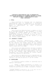
3.1. TIMELINE OF WORKLOAD
The following diagram shows how it has been distributed the workload during the development of
this project.
60
40
20
0
oct/11
3.2.
nov/11
dec/11
jan/12
feb/12
ESTIMATE AND REAL COST
The real total cost of the development of each phase has been as follows:
- Project Management: 79 hours
- Analysis: 24 hours
- Design: 20 hours
- Construction: 182 hours
TOTAL: 305 hours
Project Management
26%
Analysis
60%
Design
8%
Construction
6%
24
At this point couldn be said that the initial estimate cost was far from the actual cost of the duration
of the project. Below, there a 4 tables to compare the estimate time and the real time of each task.
Task
PROJECT MANAGEMENT
Time estimate
Real time
Developing the structure of task decomposition
2h
2h
Temporary planning
2h
2h
Project Objectives Document
10 h
15 h
Meetings
6h
6h
Memory
30 h
40 h
Project Monitoring
6h
6h
Defense
8h
8h
TOTAL
64 h
79 h
Task
Time estimate
Real time
Identification of requirements
4h
4h
Identification of parts
10 h
10 h
Identification of functions
10 h
10 h
TOTAL
24 h
24 h
Task
Time estimate
Real time
Interface design
14 h
20 h
TOTAL
14 h
20 h
Time estimate
Real time
ANALYSIS
DESIGN
IMPLEMENTATION
Task
Construction
User’s Manual
60 h
Web
80 h
140 h
80 h
180 h
100 h
Testing
2h
2h
TOTAL
142 h
182 h
TOTAL
244 h
305 h
25
The following diagram shows the difference between the initial estimate cost and the real cost.
182
200
142
160
120
80
64
79
24
40
24
14
20
0
Project
Management
Analysis
Design
Estimation
Construction
Real
The reasons of this gap are:
- Lack of knowledge in wireless sensor networks, so it has been necessary to take some weeks
to read documentation on this topic.
- Delay in the delivery of the simulator so delay to begin to draft the manual.
- Lack of knowledge and experience in making web pages, so it has been necessary to take
several days to search information to know how to create the web.
- Changes in the web design.
- Changes in the web content.
26
CHAPTER 4: CONCLUSIONS AND
RECOMMENDATIONS
In this project, it has been successfully implemented a user’s manual for a simulator of WSN
that will be useful to help beginners to understand basics about routing algorithms used in WSN and
how to use this simulator correctly.
Also it has been created a complete website to explain some concepts necessaries to understand
how the simulator works. This website provides useful information and documents to achieve a basic
understanding of WSN and IoT.
The better way to understand correctly how routing algorithms work is combining these two tools.
Once the web content has been read will be easier to understand the operation of the simulator with
the help of the user’s manual.
But these tools can be improved in future works.
In the case of the manual, it can be improved adding the explanation of the last menu of the
simulator which, as is mentioned in other part of the report, is being improved to work better. So, is
not explained in the current user’s manual.
In the case of the web site, it can be improved in some aspects. The first thing to improve is complete
the translation of the French and Dutch version of the web since, as it is said in other part of the
report, only the home page, the main menu and the AIM section are available in the 3 languages.
Also, it can be completed with more information about the same or other topics and updated if
something changes.
27
REFERENCES
[1.1] Marie-Paule Uwase
Didactic tools for learning wireless sensor networks
Master Thesis VUB September 2010
[1.2] Artemis Paradisi
A pedagogical platform for studying routing algorithms for Wireless Sensor Networks
Master Thesis VUB September 2011
[1.3] http://w3schools.com/
Accessed on November and December 2011
[1.4] http://www.php.net/
Accessed on November and December 2011
[1.5] http://www.webestilo.com/html/recortes/rec04.phtml
Accessed on December 2011
[1.6] http://elescaparatederosa.blogspot.com/2007/10/tu-e-mail-en-imagen-evitando-spam.html
Accessed on December 2011
[1.7] http://www.comocreartuweb.com/
Accessed on November 2011
[1.8] http://en.wikipedia.org/wiki/Wireless_sensor_network
Accessed on November 2011
[1.9] http://www.itu.int/osg/spu/publications/internetofthings/InternetofThings_summary.pdf
International Telecommunication Union
ITU Internet Reports 2005
Accessed on November 2011
[1.10]
http://www.iot.sztaki.hu/index.php?option=com_content&view=article&id=60&Itemid=72&lang=en
MTA SZTAKI
Computer and Automation Research Institute Hungarian Academy of Sciences
Accessed on November 2011
28
ANNEX A
MEETING REPORTS
AN EDUCATIONAL ENVIROMENT FOR BASIC UNDERSTANDING OF SENSOR NETWORKS
MEETING REPORT
Date
10/10/2011
Place
Office's Jacques Tiberghien VUB
Assistants
Jacques Tiberghien and Virginia Alguacil
Agenda
Subject of the project
Issues discussed:
- Subject of the project: the project manager has presented me the idea of the project and what
I have to do. He has given me some documents for read and learn about the subject of the
project.
Issues to do:
- Reading Artemis Paradisi Thesis.
- Ask Jacques all the doubts after the reading.
AN EDUCATIONAL ENVIROMENT FOR BASIC UNDERSTANDING OF SENSOR NETWORKS
MEETING REPORT
Date
24-28/10/2011
Place
Office's Jacques Tiberghien VUB
Assistants
Jacques Tiberghien and Virginia Alguacil
Agenda
Evolution of the reading and future work
Issues discussed:
- Evolution of the reading: I’ve asked some questions about the reading to the project manager.
- Future work: we have talked about what I have to do now.
Issues to do:
- Reading Marie-Paule Uwase Thesis.
29
AN EDUCATIONAL ENVIROMENT FOR BASIC UNDERSTANDING OF SENSOR NETWORKS
MEETING REPORT
Date
9/11/2011
Place
Office's Kris Steenhaut VUB
Assistants
Kris Steenhaut, Jacques Tiberghien and Virginia Alguacil
Agenda
How to make the web
Issues discussed:
- Web: Kris has explained me the need of the web and the content that it should have. We have
discussed about the design of the web.
Issues to do:
- Start with the design the web.
- To find information for the web content.
AN EDUCATIONAL ENVIROMENT FOR BASIC UNDERSTANDING OF SENSOR NETWORKS
MEETING REPORT
Date
14/11/2011
Place
Office's Kris Steenhaut EHB
Assistants
Kris Steenhaut and Virginia Alguacil
Agenda
Evolution of the web
Issues discussed:
- Web: We have discussed about the initial design of the web that I’ve done.
Issues to do:
- Change the colour of the logo.
- Change the colour of the background.
- Continue with the creation of the web.
30
AN EDUCATIONAL ENVIROMENT FOR BASIC UNDERSTANDING OF SENSOR NETWORKS
MEETING REPORT
Date
21-25/11/2011
Place
Office's Jacques Tiberghien VUB
Assistants
Jacques Tiberghien, Marie-Paule Uwase and Virginia Alguacil
Agenda
How to do the manual and installation of the simulator
Issues discussed:
- Manual: We have discussed about what I have to explain in the manual and how to explain it.
- Simulator: Marie-Paule has installed the simulator on my computer and has explained me how
to use it for explain this in the manual.
Issues to do:
- Start with the manual explaining the menu file and buttons to create the graph.
- Send to Marie-Paule and Jacques this part of the manual to review it.
AN EDUCATIONAL ENVIROMENT FOR BASIC UNDERSTANDING OF SENSOR NETWORKS
MEETING REPORT
Date
30/11/2011
Place
Office's Kris Steenhaut VUB
Assistants
Kris Steenhaut and Virginia Alguacil
Agenda
Review of the web
Issues discussed:
- Web: We have reviewed the web to find things to improve and errors.
Issues to do:
- Add a menu option to talk about routing protocols for Wireless Sensor Networks.
- Add reference pages after web content.
- Add a menu option to explain the aim of the web.
31
AN EDUCATIONAL ENVIROMENT FOR BASIC UNDERSTANDING OF SENSOR NETWORKS
MEETING REPORT
Date
5/12/2011
Place
Office's Marie-Paule Uwase VUB
Assistants
Marie-Paule Uwase and Virginia Alguacil
Agenda
Installation of the new version of the simulator
Issues discussed:
- New version of the simulator: Marie-Paule has installed on my computer the new version of
the simulator and has explained me how works the routing menu that in the old version didn’t
work.
- Review of the manual: we have talked about the things that I have to correct in the manual
and about some doubts that I have about the simulator.
Issues to do:
- Correct the things that we have talked that are wrong or I didn’t understand.
- Continue with the drafting of the manual.
AN EDUCATIONAL ENVIROMENT FOR BASIC UNDERSTANDING OF SENSOR NETWORKS
MEETING REPORT
Date
13/12/2011
Place
Office's Kris Steenhaut VUB
Assistants
Kris Steenhaut and Virginia Alguacil
Agenda
Review of the manual and of the web
Issues discussed:
- Manual: we have discussed about how improve the manual. Kris has suggested me to create a
table of contents.
- Web: we have taken a look to the entire web and Kris has asked me to add the contact
information about some professors. Also she has suggested me to improve the section of the
aim with some picture or graphic.
Issues to do:
- Add the table of contents in the manual.
- Add the contact information of the professors in the section of contact of the web.
- Add a graphic on the aim section of the web.
32
AN EDUCATIONAL ENVIROMENT FOR BASIC UNDERSTANDING OF SENSOR NETWORKS
MEETING REPORT
Date
14/12/2011
Place
Office's Marie-Paule Uwase VUB
Assistants
Marie-Paule and Virginia Alguacil
Agenda
Routing menu of the simulator
Issues discussed:
- Simulator: I have asked Marie-Paule some doubts about the routing menu of the simulator to
know how to explain it.
Issues to do:
- Finish the explanation of the routing menu of the simulator.
AN EDUCATIONAL ENVIROMENT FOR BASIC UNDERSTANDING OF SENSOR NETWORKS
MEETING REPORT
Date
11/01/2012
Place
Office's Marie-Paule Uwase VUB
Assistants
Marie-Paule Uwase and Virginia Alguacil
Agenda
Review of the manual
Issues discussed:
- Manual: I have explained to Marie-Paule what I have explained about the simulator. Also, I’ve
asked Marie-Paule that explains me the last part of the simulator.
Issues to do:
- Finish the manual and send it to Marie-Paule to review it.
33
AN EDUCATIONAL ENVIROMENT FOR BASIC UNDERSTANDING OF SENSOR NETWORKS
MEETING REPORT
Date
18/01/2012
Place
Office's Marie-Paule Uwase VUB
Assistants
Marie-Paule and Virginia Alguacil
Agenda
Manual delivery and review of the web
Issues discussed:
- Manual: I’ve delivered the manual to Marie-Paule to review it.
- Web: We have reviewed the web to find things to improve or errors.
Issues to do:
- Correct small details of the web to improve it.
- Start with the project report.
AN EDUCATIONAL ENVIROMENT FOR BASIC UNDERSTANDING OF SENSOR NETWORKS
MEETING REPORT
Date
31/01/2012
Place
Office's Marie-Paule Uwase VUB
Assistants
Marie-Paule and Virginia Alguacil
Agenda
Final web review and project presentation
Issues discussed:
- Web: we have taken a final look to the web to find the last things to improve.
- Presentation of the project: I’ve asked Marie-Paule some aspects about the presentation of
the project and the delivery of this.
Issues to do:
- Correct some aspect of the web and add the French translation of the web.
- Finish the project report.
34
ANNEX B
LINK TO THE WEB AND ATTACHED CD
The temporary link to access the web is the following:
http://virgi.marcosag.com/
In the attached CD are the manual and the code of the simulator for wireless sensor networks.
35
USER’S MANUAL FOR A
SIMULATOR OF WIRELESS
SENSOR NETWORKS
CREATED BY VIRGINIA ALGUACIL GIL
AS FINAL BACHELOR PROJECT
TABLE OF CONTENTS
1. INTRODUCTION ............................................................................................................6
1.1. WHY A NEW SIMUALTOR? .....................................................................................................6
1.2. WHY A USER’S MANUAL? .......................................................................................................6
2. STARTING SIMULATOR..................................................................................................7
3. FILE MENU ...................................................................................................................8
3.1. NEW........................................................................................................................................8
3.2. OPEN ....................................................................................................................................10
3.3. SAVE .....................................................................................................................................12
3.4. CLOSE ...................................................................................................................................13
3.5. EXPORT JPEG ........................................................................................................................14
4. STARTING TO CREATE OR MODIFYING A GRAPH .......................................................... 15
4.1. ADD A NODE .........................................................................................................................15
4.2. ADD A LINK ...........................................................................................................................19
4.3. ADD TEXT..............................................................................................................................24
4.4. DELETE A NODE/LINK ...........................................................................................................25
5. ROUTING MENU ......................................................................................................... 27
5.1. RANDOM AND SEQUENTIAL ................................................................................................28
5.2. DISTANCE VECTOR (DV) ROUTING PROTOCOL ....................................................................28
5.2.1. STEP DV....................................................................................................................29
5.2.2. RUN DV ....................................................................................................................31
5.3. STEP AODV ...........................................................................................................................32
5.4. RPL ROUTING PROTOCOL .....................................................................................................33
5.4.1. RPL BUILD DODAG ...................................................................................................34
5.4.2. RUN RPL ...................................................................................................................35
6. TRACKING MENU ........................................................................................................ 38
1
2
LIST OF FIGURES
Figure 1: Graphe Maker User Interface
Figure 2: Menu File
Figure 3: Create a new graph
Figure 4: Window with a message when you click on File  New
Figure 5: Window clicking on No
Figure 6: Window clicking on Yes
Figure 7: Open an existing graph
Figure 8: Window with a message when you click on File  Open
Figure 9: Window clicking on No
Figure 10: Window clicking on Yes to Open a saved graph
Figure 11: Graph selected to open
Figure 12: Save the current graph
Figure 13: Window to save the graph
Figure 14: Close the simulator
Figure 15: Window with a message when you click on File  Close
Figure 16: Window clicking on No when close the simulator
Figure 17: Export the graph in JPEG
Figure 18: Window to save the graph in JPEG
Figure 19: Buttons to create a graph
Figure 20: Add a node
Figure 21: Name of the node
Figure 22: First node added
Figure 23: Add more nodes
Figure 24: Finish to add nodes
Figure 25: Move a node
Figure 26: Information about a node
Figure 27: Node attributes
Figure 28: Select sink node
Figure 29: Sink Node
Figure 30: Add a link
Figure 31: Create a link clicking on the nodes
Figure 32: Link between node A and B
Figure 33: All links created
Figure 34: Finish to add links
Figure 35: Add costs to links
Figure 36: Change the cost of the link
3
Figure 37: Cost added to the link
Figure 38: Select one way link
Figure 39: One way link between A and C
Figure 40: All costs added to links
Figure 41: Add text
Figure 42: Write a text
Figure 43: Delete a node or link
Figure 44: Link between node B and node C deleted
Figure 45: Finish to delete nodes or links
Figure 46: Routing menu
Figure 47: Routing menu options
Figure 48: Random and Sequential options
Figure 49: Figure 49: Step DV
Figure 50: First step DV
Figure 51: Step DV intermediate
Figure 52: Attributes of the node
Figure 53: Level battery decreases
Figure 54: Battery node K has exhausted
Figure 55: Run DV
Figure 56: DV routing process
Figure 57: Node attributes of a node in the DV routing process
Figure 58: Step AODV
Figure 59: The AODV optimal route from node G to sink, with no previous routes available (image
left) and an additional optimal route from node L to sink (image right).
Figure 60: New route for node 9 after the death of node 2
Figure 61: Rpl build DODAG
Figure 62: Suspend and Resume buttons
Figure 63: Routing tables and colored links while sending messages
Figure 64: The Graph when the DODAG building process is finished.
Figure 65: Run RPL
Figure 66: RPL process
Figure 67: Some links added
Figure 68: Link costs added
Figure 69: DODAG
Figure 70: RPL
Figure 71: Path followed by message 1694 from 74 via b7 to the sink
Figure 72: Transmission paths shown by the tracking option of Graphe
4
5
1. INTRODUCTION
1.1. WHY A NEW SIMULATOR?
An open source package called “Graphe Maker” written in the Java programming language,
was chosen in a previous master thesis as the Graphical User Interface (GUI) for
implementing a simulator for three routing protocols in Wireless Sensor Networks (WSN):
Distance Vector (DV), Adhoc On Demand Distance Vector (AODV) and RPL. In the future, this
tool could be extended to include more routing protocols.
This package provides “clean” data structures for representing graphs and assigning
attributes to the nodes and the links, as well as interactive graphic methods to build the
graph and setting the values of the attributes. In addition it provides methods to save graphs
on file, to restore these graphs and even to create JPEG pictures of the graph.
This simulator was implemented to help university student understand the basics of this
protocols
for WSN. The aim was to create a didactic and interactive tool that can help motivated
students to
explore the behavior of routing protocols in specific circumstances.
1.2. WHY A USER’S MANUAL?
As it is explained in the previous paragraph, this manual was created for univerity students.
Then, to enable these students to use this simulator we have create a user's manual
explaining in detail the different parts of this interface and how tu use it. It's also explained
how to interpret the results shown on the screen when the different routing protocols are
simulated.
6
2. STARTING SIMULATOR
When you start the simulator you will see in the screen the Figure 1.
Figure 1: Graphe Maker User Interface
Now, you can do several things: create a new file, open an existing file, modify this WSN deleting
nodes or links, adding a node, adding a link or adding text…
These options are explained in the following sections.
7
3. FILE MENU
The menu File is located at the top left part of the simulator. It has 5 options as you can see in the
Figure 3: New, Open, Save, Close, Export JPEG. You can see it in the Figure 2.
Figure 2: Menu File
3.1. NEW
In the first option, New, you can create a new empty graph (Figure 3).
Figure 3: Create a new graph
If you click on New, a new window with a message will appear. You can see the window in
the Figure 4. As you can read on the message, if you continue all non saved work will be lost.
Figure 4: Window with a message when you click on File  New
8
So, If you have some work non saved and you want to save it you have to click on No.
Clicking on No you return to the previous screen (Figure 5).
Figure 5: Window clicking on No
If you haven’t got non saved work or you don’t want to save the work non saved you have to
click in Yes. Clicking on Yes you will see the following screen (Figure 6).
Figure 6: Window clicking on Yes
You have now an empty screen. Now, you can start adding nodes. This will be explained in
another section.
9
3.2. OPEN
In the second option of the menu File, Open, you can open a previously created graph that is
saved on your computer (Figure 7).
Figure 7: Open an existing graph
If you click on Open, a new window with a message will appear. You can see the window in
the Figure 8. As you can read on the message, if you continue all non saved work will be lost.
Figure 8: Window with a message when you click on File  Open
So, If you have some work non saved and you want to save it you have to click on No.
Clicking on No you return to the previous screen (Figure 9).
Figure 9: Window clicking on No
10
If you haven’t got non saved work or you don’t want to save the work non saved you have to
click on Yes. Clicking on Yes you will see the following screen (Figure 10). Here, you can
select the file that you want to open.
Figure 10: Window clicking on Yes to Open a saved graph
11
When you select the file you want to open, you will see the graph in the screen as in Figure
11.
Figure 11: Graph selected to open
3.3. SAVE
In the third option of the menu File, Save, you can save the current version of the graph
(Figure 12).
Figure 12: Save the current graph
If you click on Save, a new window will appear. You can see the window in the Figure 13. You
have to select where you can save the graph and write the file name and then click on Save.
Figure 13: Window to save the graph
12
3.4. CLOSE
In the fourth option of the menu File, Close, you can close the interface of the simulator
(Figure 14).
Figure 14: Close the simulator
If you click on Close, a new window with a message will appear. You can see the window in
the Figure 15. As you can read on the message, if you continue all non saved work will be
lost.
Figure 15: Window with a message when you click on File  Close
So, If you have some work non saved and you want to save it you have to click on No. Clicking
on No you return to the previous screen (Figure 16).
Figure 16: Window clicking on No when close the simulator
If you haven’t got non saved work or you don’t want to save the work non saved you have to
click on Yes. Clicking on Yes you exit the simulator.
13
3.5. EXPORT JPEG
In the last option of the menu File, Export JPEG, you can save the graph as a picture in a JPEG
format (Figure 17).
Figure 17: Export the graph in JPEG
If you click on Export JPEG, a new window will appear. You can see the window in the Figure
18. You have to select where you can save the graph and write the name you to the file.
Then, in the bottom of the window, in Files of Type, you have to select the Option JPEG file
and click on Save. Thus, you have the graph as a JPEG format image.
Figure 18: Window to save the graph in JPEG
14
4.
STARTING TO CREATE OR MODIFYING A GRAPH
For create or modifying a graph already created you have to use the buttons at the top of the
window as you can see in Figure 19.
Figure 19: Buttons to create a graph
For the explanation of these buttons I will do it by creating a graph from 0. So, before start adding
nodes you have to create a new file as it is explained before. You have to go to File menu and
select New.
4.1. ADD A NODE
First of all, you have to add nodes. For add a node you have to select the button “Add a
node” by clicking on it. It is important that the button is activated (in color blue) while you
are adding nodes because if not you can’t create the node (Figure 20).
Figure 20: Add a node
Then, you have to click anywhere on the screen to create the node at that point. When you
click, a window appears as shown in Figure 21.
Figure 21: Name of the node
15
You have to put a name for the node and click OK. It can be a letter, a number or a
combination of both. For the explanation I will use capital letters as you can see in the Figure
22. Once you do it and click OK, the new node appears on the window.
Figure 22: First node added
Similarly, you can add more nodes. You must repeat the previous steps for every new node
that you want to create. For add the next node it is important that you don’t deselect the
button “Add a node”. You only have to click on another part of the window and write the
name of the node. In Figure 23 you can see an example with five nodes.
Figure 23: Add more nodes
16
Once you have finished adding nodes you have to deselect the button “Add a node” clicking
on it. (Figure 24).
Figure 24: Finish to add nodes
When none of the buttons (“Add a node”, “Add a link”, “Add text”, “Delete node or link”) is
active, if you want, you can move the location of the nodes. To do this, you have to click on
the node and, without removing your finger from the mouse, move it dragging the mouse.
When you put the mouse on one node it turns blue as you can see in Figure 25.
Figure 25: Move a node
17
Also, you can click on a node and see some information about it. You have to double click on
a node and a small window with node attributes appears, as you can see in Figure 26.
Figure 26: Information about a node
The information that is given is the Mote identifier, Mote battery, Rank and Distance to sink.
You can see this information in Figure 27.
-
Mote identifier: name given to the node
-
Mote battery: number that indicates the level of the battery. 1000 indicates full battery
and 0 empty battery.
Rank: number that indicates in the RPL simulation the distance to sink expressed in
hops.
Distance to sink: number that indicates in all routing simulations the best known
distance to the sink, taking into account the “length” or “cost” function associated with
each link.
-
Figure 27: Node attributes
Figure 28: Select sink node
18
As you can see in this window there is also a check box to select the sink node. You have to
select it if you want that node is the sink node (Figure 28). For select the sink node you have
to open the Node attributes by double clicking on the node and tick the checkbox “Sink
Node” and click OK. You can distinguished the sin node by its double circle shape as shown in
Figure 29 on node A.
Figure 29: Sink Node
4.2. ADD A LINK
The next step is add links between the nodes. For add a link you have to select the button
“Add a link” by clicking on it. It is important that the button is activated (in color blue) while
you are adding links because if not you can’t create the link (Figure 30).
Figure 30: Add a link
19
Then, you have to click in one of the nodes you want to link. When you click on it, it returns
red as you can see on Figure 31. Then, you click on the other node and the link is created as
you can see in Figure 32.
Figure 31: Create a link clicking on the nodes
Figure 32: Link between node A and B
For create the rest of the links you have to repeat the procedure explained before. You have
to repeat this action as many times as the links that you wish to create. Finally, you will
obtain a graph similar to that shown in Figure 33.
20
Figure 33: All links created
When you finish to add links, you must click again on the button “Add a link” to desactivate it
(Figure 34).
Figure 34: Finish to add links
Once you have finished to add all the links, the next step before you complete your network
topology creation is to add “costs” in each link. To do this, you must double click on a certain
link, like in the nodes, and a small window with link properties appears, as you can see in
Figure 35. As you can see in this figure, the link of which the properties are shown is in color
blue.
21
Figure 35: Add costs to links
To add the “cost” you have to change the number of the parameter “Distance” (Figure 36). It
is a measure of the “cost” of using the link. It can represent a physical distance, or an average
number of retransmissions needed to transmit a message over that link. In this simulator, we
define the cost as the number of attempts needed to send successfully a message over a link.
You can change this value (Figure 36) and click OK. Then, the cost is added in the middle of
the link line as you can see in Figure 37.
Figure 36: Change the cost of the link
Figure 37: Cost added to the link
22
There are also two check boxes:
-
One way: indicates the direction of the link. If you want a bidirectional link (which is
currently the case in our simulator), you leave check box blank. If you want a
unidirectional link, you have to tick the check box (Figure 38) and then you will see the
link on the graph with an arrow like in Figure 39.
-
Active link: Boolean variable used to show if a link is active or not; it is ticked by default.
A link stops being active when one of the nodes at its extremity has an exhausted
battery.
Figure 38: Select one way link
Figure 39: One way link between A and C
After adding all the links costs (Figure 40), your network topology is ready to run any of the
supported by the simulator routing protocols.
Figure 40: All costs added to links
23
4.3. ADD TEXT
The next button is “Add Text”. You can use it if you want add some text description to the
node or at any other place on the screen.
If you select this button (Figure 41) and click anywhere on the workspace, a small window
appears as you can see on Figure 42 in where you can write the text you want.
Figure 41: Add text
Figure 42: Write a text
24
4.4. DELETE A NODE/LINK
Finally, in case that you change your mind and you want to delete a node or a link, you can
do it by selecting the button “Delete Node or Link” that is the last button on the right (Figure
43).
Figure 43: Delete a node or link
With the button selected, you have to click on the node or link that you want to delete and it
disappears as you can see in Figure 44 where link between node B and C has disappeared.
Figure 44: Link between node B and node C deleted
25
Once you have finished to delete nodes and links you must to desactivate the button “Delete
Node or Link” (Figure 45). Otherwise, it will delete any node or link that you click on the
screen.
Figure 45: Finish to delete nodes or links
Now, you have your graph finished. But if you want to add more nodes or links or change the
“cost” of the link or something on the graph, you just have to do what is explained in the
previous sections.
26
5.
ROUTING MENU
The Routing menu is located at the top left part of the simulator, next to the File menu. You can
see it in the Figure 46.
Figure 46: Routing menu
The Routing menu contains options specific to the routing protocol the user wants to run (Figure
47).
The options Random, Sequential, step DV, run DV and step AODV are used for running the
DV and AODV routing protocols. Rpl build DODAG is used to construct the DODAG for RPL routing
and run Rpl to start running the routing protocol.
Figure 47: Routing menu options
27
5.1. RANDOM AND SEQUENTIAL
The two first options, Random and Sequential, allow you to select the randomization of the
processing of the nodes (Figure 48). You have to select between this two options before run
the Distance Vector (DV) routing algorithm step by step.
With the option Random selected, the nodes are explored in random order. And with the
option Sequential selected, the nodes are explored in a sequential order.
Figure 48: Random and Sequential options
5.2. DISTANCE VECTOR (DV) ROUTING PROTOCOL
The next two options of the routing menu allow the user to simulate the DV routing protocol.
This two options are step DV and run DV.
Before explaining the menu options, it is convenient to give a simple explanation about what
this protocol is.
Andrew S. TANENBAUM, describes a DV routing algorithm as follows: “Distance Vector
routing algorithms operate by having each router maintain a table giving the best known
distance to each destination and which line to use to get there. These tables are updated by
exchanging information with the neighbors.”
We will summarize this explanation, adapted to a WSN, as follows: periodically each node
asks all its neighbors what the best distance to the sink it knows of is. Each node replies with
the distance it has stored in its routing table (initially, this distance is infinite). The inquiring
node adds to the received distances the length of the links to the answering nodes and
retains only the shortest sum. This distance and the identity of the corresponding node are
stored in the routing table.
For simulation purposes, the user is given the choice between stepping manually (step DV) or
at a predetermined pace through the successive routing cycles (run DV).
28
5.2.1. STEP DV
To run the Distance Vector (DV) routing algorithm step by step (one routing cycle at a
time) you must first determine the order of processing the nodes and links, if it will be in
a random or in a sequential order. From the Menu you must choose Random or
Sequential (Figure 48).
Then you must choose step DV to run the first routing cycle (Figure 49). The results are
shown by coloring the selected links in red as you can see on Figure 50. The scanning
cycle can be repeated step by step every time you click on step DV (Figure 51).
Figure 49: Step DV
Figure 50: First step DV
Figure 51: Step DV intermediate
29
Between cycles, the user can consult (and eventually modify) the attributes of the
different nodes and links by double clicking on them (Figure 52).
Figure 52: Attributes of the node
Each time that the step DV is executed the nodes’s battery level decreases as you can
see in Figure 53. There comes a time when the level of a node becomes 0 and it
disappears by coloring in grey (and also the links around the node), as shown in Figure
54 in node K. This happens because of initially most routes and most of the collect traffic
went through node K, but this caused its battery to get exhausted.
Figure 53: Level battery decreases
Figure 54: Battery node K has exhausted
The distance vector routing will stop when all nodes have found a stable and optimal
routing Scheme.
30
5.2.2. RUN DV
To run the Distance Vector (DV) routing algorithm continuously through all the
successive routing cycles, you must choose run DV (Figure 55).
Figure 55: Run DV
When you click on run DV the process begins. In the screen you can observe that the
selected links are colored in red, that the battery level of each node is decreasing and
that when a node dies the dead nodes and links are colored in gray and they disappear.
In Figure 56 you can see some steps of the routing protocol DV.
Figure 56: DV routing process
31
As in the previous section, step DV, you can double click on each node to view the
attributes of the node. In the Figure 57 you can see the information of node F in three
steps of the process, in where you can observe how the level of the battery decreases.
Also you can double click on each node to see the Link properties.
Figure 57: Node attributes of a node in the DV routing process
5.3. STEP AODV
Before explain how to run the AODV routing protocol a brief description of this algorithm is
given.
The Ad-hoc On-Demand Distance Vector (AODV) routing algorithm it’s an on demand routing
algorithm, meaning that it builds routes between nodes only as desired by source nodes.
Instead of updating continuously routing tables in all nodes, this algorithm waits until a
message needs to be transmitted to search for a suitable route to the destination of the
message. It tries to find a good route for send the message to the sink, possibly reusing part
of a route discovered previously by another node. The AODV maintains these routes as long
as they are needed by the sources. This “just in time” approach potentially can minimize the
traffic needed for routing, and, therefore, is attractive for wireless sensor networks.
To run the AODV routing protocol, the user is allowed to manually select the node that
initiates a routing request by just double clicking it while the AODV routing process is active.
To activate the AODV routing process you must choose step AODV (Figure 58) and then
double click the node that will initiate the routing request. Once a route is available for a
specific node, double clicking that node causes the simulated transmission of a message to
the sink.
Every time you double click on a node the optimal route is immediately selected and the
selected links are colored in red (Figure 59).
Figure 58: Step AODV
32
Figure 59: The AODV optimal route from node G to sink, with no previous routes available
(image left) and an additional optimal route from node L to sink (image right).
In these figures, you can also see how the node’s battery decreases. There comes a time
when the battery runs out and that node becomes inactive (due to battery exhaustion).
When this occurs, the affected routes are erased in the simulation and the user can request a
new search by selecting an affected node.
Figure 60 shows an example of this. In the image on right you can see the route found for
node 9 after the previous route was erased as a consequence of the death of node 2.
Figure 60: New route for node 9 after the death of node 2
5.4. RPL ROUTING PROTOCOL
The last two options of the Routing menu are Rpl build DODAG (Figure 61) and run RPL
(Figure 65). These two option are used to simulate the RPL routing protocol so, before
explain them, a brief explanation about this protocol is given.
RPL is a distance-vector routing protocol entirely defined for IPv6-based WSNs. RPL is a
proactive routing protocol, constructing its routes in periodic intervals. In one network it is
possible to run several RPL Instances. Nodes in the network are allowed to be part of more
than one Instance. Starting from one or more sink nodes, each Instance builds up a tree-like
routing structure in the network, resulting in a Destination-Oriented Directed Acyclic Graph
(DODAG).
For each RPL Instance, multiple DODAGs may exist. However, a node must not join more than
one DODAG within one Instance. A Directed Acyclic Graph (DAG) has the property that all
edges are oriented in such a way that no cycles exist. A Destination Oriented DAG (DODAG) is
a DAG where all edges are contained in paths oriented toward one or more sink nodes.
33
5.4.1. RPL BUILD DODAG
To run the RPL routing protocol you must first choose Rpl build DODAG to start the
building of the DODAG (Figure 61) in the Routing menu.
Figure 61: Rpl build DODAG
At the right side of the screen appears a panel which displays the most important node’s
attributes like its name, rank, distance to sink and parent list (Figure 63). This panel is
updated whenever occurs a change during the routing process. This helps the user to
have a detailed overview of the different stages that take place until a node gets its final
position in the network.
The color of the links changes when a node sends a message (Figure 63). The building of
DODAG is finished when all nodes have found their optimal route to sink and this is
visualized by changing the thickness of the selected links (Figure 64).
During the building the DODAG process you can use the Suspend and Resume buttons
situated at the bottom of the screen by double clicking on them (Figure 62). With the
Suspend button you can pause the simulation process and with the Resume button you
can resume the execution of the simulation.
Figure 62: Suspend and Resume buttons
Figure 63: Routing tables and colored links while sending messages
34
Figure 64: The Graph when the DODAG building process is finished.
5.4.2. RUN RPL
To simulate the continuous sending of messages from the nodes of the network towards
the sink node, you must choose run Rpl (Figure 65).
Figure 65: Run RPL
Every time a message is transmitted the selected links are blinking and the nodes
battery level is decreasing. In Figure 66 you can see some moments of the transmission
of the messages in where you can see how the level of the battery is decreasing.
When a node has no more battery energy it is removed from the screen as well as its
links to all other nodes (Figure 66 third image). The remaining nodes will select
alternative parents, if they exist, to send their messages to sink. You can always visualize
the changes in the right panel of the screen.
In the case that a node is running out of parents, it is colored red and the program stops
as it is shown in Figure 66 (third image) on node L.
Figure 66: RPL process
35
To continue the simulation, you must create new link(s) between the red coloured
node(s) and the other nodes of the network. To accomplish this you must:
1.
Click on the “Add a link” button and follow the instructions in section 5.2. You can
see the links added on Figure 67.
Figure 67: Some links added
2. Create link costs as described in section 5.2. Figure 68 shows the costs added to
links.
Figure 68: Link costs added
36
3. Choose Rpl build DODAG in the Routing menu to start a new DODAG iteration.
During this phase you can use again the Suspend/Resume button. The result is shown
on Figure 69.
Figure 69: DODAG
4. Choose run Rpl in the Routing menu to start again the continuous sending of
messages between nodes.
Figure 70: RPL
This process must be repeated every time a node is running out of parents and there is
a node in the network that has a link to the sink node.
In the opposite case, the program stops and a warning window open to inform you
that there are no more routes to the sink.
37
5.
TRACKING MENU
The last menu of the simulator is the Tracking Menu. This menu doesn't work yet correctly but
it's now being improved to can be used in a period of time.
The Tracking Menu has the functionality of displaying the itinerary of the messages coming from
the lawn mower. It shows in orange on the graph the itinerary each message followed to reach
the sink. It also displays the message number, because not all messages reach the sink and some
reach it in several copies.
Figure 71 shows a message traveling from mote 74 to the sink via mote b7. The identity of the
message (1694) can be seen at the bottom right of the screen. The graphical tracking of one of the
messages received 5 times is shown in Figure 72.
Figure 71: Path followed by message 1694 from 74 via b7 to the sink
Figure 72: Transmission paths shown by the tracking option of Graphe
38