Download SpinCore RadioProcessor LabVIEW NMR Interface

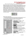
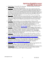
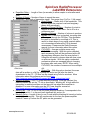
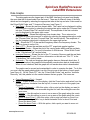
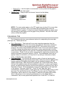
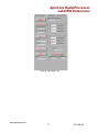
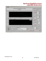
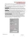
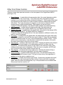
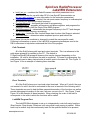
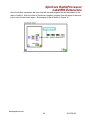
SpinCore RadioProcessor
LabVIEW Extensions
NMR Interface
User's Manual
SpinCore Technologies, Inc.
http://www.spincore.com
SpinCore RadioProcessor
LabVIEW Extensions
Congratulations and thank you for choosing a design from
SpinCore Technologies, Inc.
We appreciate your business!
At SpinCore we try to fully support the needs of our customers. If you
are in need of assistance, please contact us and we will strive to provide
the necessary support.
© 2008-2014 SpinCore Technologies, Inc. All rights reserved.
SpinCore Technologies, Inc. reserves the right to make changes to the product(s) or information herein without notice.
RadioProcessor™, PulseBlaster™, SpinCore, and the SpinCore Technologies, Inc. logos are trademarks of SpinCore Technologies, Inc.
All other trademarks are the property of their respective owners.
SpinCore Technologies, Inc. makes every effort to verify the correct operation of the equipment. This equipment version is not intended
for use in a system in which the failure of a SpinCore device will threaten the safety of equipment or person(s).
www.spincore.com
2
2014-08-28
SpinCore RadioProcessor
LabVIEW Extensions
Table of Contents
I. Overview....................................................................................................... 4
II. Installation................................................................................................... 6
Method 1: Stand-Alone Executables............................................................................ 6
Method 2: Customizable VIs..........................................................................................6
III. General Information................................................................................... 7
Running the Single Pulse NMR Interface.....................................................................7
Performing a scan.......................................................................................................... 7
Single Pulse Parameters................................................................................................8
T1 Parameters...............................................................................................................10
CPMG Parameters........................................................................................................ 11
Data Graphs.................................................................................................................. 13
Calculations Tab...........................................................................................................14
Process Data Tab..........................................................................................................19
Other Front Panel Controls......................................................................................... 21
Error messages.............................................................................................................22
Advanced VI Customization........................................................................................ 22
Path Terminals.........................................................................................................23
Error Terminals........................................................................................................ 23
LabVIEW Program Flow.......................................................................................... 23
IV. Contact Information................................................................................. 25
www.spincore.com
3
2014-08-28
SpinCore RadioProcessor
LabVIEW Extensions
I. Overview
The SpinCore RadioProcessor LabVIEW Extensions (PBLV-RP) provide the functionality
of programming and controlling RF generation and acquisition capabilities of the
RadioProcessor boards as well as viewing and processing the data using the simple NI
LabVIEW graphical programming interface.
The PBLV-RP NMR Interface is an intuitive graphical equivalent of the SpinAPI C
functions. It combines the Single Pulse, the T1 Inversion Recovery, and the CPMG
programs into one easy to use interface. The GUI (known as the front panel) has all the
scan parameters needed to control the RadioProcessor functions as well as scan status
feedback and data graphs (time and frequency domain). The scan parameters are then
used in the back-end code (known as the block diagram) to access the C functions that
control and program the RadioProcessor. The LabVIEW block diagram is a one-to-one
equivalent of the corresponding C code, without having to write code. The front panel is
shown in Figure 1.
Note: For information on using the the Digital Pulse Generation functionality of the board
in LabVIEW, please see the PulseBlaster LabVIEW Extensions documentation.
(http://www.spincore.com/support/PBLV/PBLV_Manual.pdf). For information on using the
DDS only functionality of the board please see the PulseBlaster-DDS LabVIEW Extensions
documentation (http://www.spincore.com/support/PBLV/PBLV_DDS_Manual.pdf)
www.spincore.com
4
2014-08-28
SpinCore RadioProcessor
LabVIEW Extensions
Figure 1: Example of RadioProcessor LabVIEW Extensions User Interface
www.spincore.com
5
2014-08-28
SpinCore RadioProcessor
LabVIEW Extensions
II. Installation
There are two methods of using the RadioProcessor LabVIEW Extensions. The first
method is a set of stand-alone executables which will control the RadioProcessor boards
with a simple, intuitive interface with no other necessary knowledge of LabVIEW
programming. The second method is a set of LabVIEW VIs which can be used with the
LabVIEW Development platform to create custom programs using the PBLV-RP interface.
Method 1: Stand-Alone Executables
In order for PBLV stand-alone executables to work, the following must be installed:
●
●
●
SpinCore Driver Suite - Please see the SpinCore Driver Suite Installation Guide
(http://www.spincore.com/support/spinapi/instructions/) for more information.
National Instruments LabVIEW Run-Time Engine 2010
(http://www.spincore.com/support/PBLV/LVRTE2010std.exe) - Note if you have
LabVIEW 2010 or later installed, this is not needed.
LabVIEW PulseBlaster Extensions Stand-Alone executables located here.
Method 2: Customizable VIs
In order for PBLV-DDS customizable VIs to work, the following must be installed:
● SpinCore Driver Suite - Please see the SpinCore Driver Suite Installation Guide
(http://www.spincore.com/support/spinapi/instructions/) for more information.
● National Instruments LabVIEW 8.6 or later - If you do not have LabVIEW 8.6 or later
installed, you may download a 30-day evaluation
(https://lumen.ni.com/nicif/us/lveval/content.xhtml) of the latest LabVIEW
development software.
(NOTE: Customizable VIs are availabe for versions of LabVIEW as old as LabVIEW
8.0. For customizable VIs older than LabVIEW 8.6, please contact SpinCore
Technologies via the web forum.)
● LabVIEW PulseBlaster Extensions located here.
(NOTE: Customizable VIs use the C-calling convention. For customizable VIs that
use the WINAPI calling convention please contact SpinCore Technologies via the
web forum.)
www.spincore.com
6
2014-08-28
SpinCore RadioProcessor
LabVIEW Extensions
III. General Information
Running the Single Pulse NMR Interface
The RadioProcessor NMR Inverface VI is an all-in-on RF Generation and Acquisition
environment for use with the SpinCore RadioProcessor boards. There are two methods of
running the NMR Interface program. If you choose to use an all-in-one stand-alone
application, you should use method 1. See section II above for instructions on installation.
To run the program, simply run the executable file on your computer.
If you choose to use the customizable vi package, you should use method 2 as
described in section II. When you download the PBLV-RP package, unzip the contents
into a directory on your computer. To open the NMR Interface project, run the file
“PBLV_RP_NMR_Interface.lvproj”. To open the NMR Interface program, you can navigate
to MyComputer>Examples>PBLV_RP_NMR_Interface.vi in the project and open the file, or
you can run the file “PBLV_RP_NMR_Interface.vi”. When the VI opens, click on the run
button at the top of the window to start the NMR Interface.
NOTE: The NMR Interface program may not fit on your screen. In order to view the
whole program it is suggested that you change your system display to a higher
resolution. Alternately, the program can be resized by dragging the corner of the
window, but doing so may cause undesirable warping of the front panel objects.
Performing a scan
To perform a scan using the NMR Inteface VI, you must first set up the scan
parameters by adjusting the controls in one of the parameters tabs on the right of the front
panel. Whichever tab is selected determines which type of scan is performed (Single
Pulse, T1 Inversion Recovery, or CPMG). Each of these tabs are discussed in detail below.
You must also ensure that the SpinAPI DLL Path control at the bottom correctly points to
spinapi.dll as installed on your system. Also if you want to save the data to disk, make
sure that the File Name control is correctly set, and the “Output File” check box is checked.
NOTE: On your initial scan, you must make sure that the spectrometer frequency is
set to match your magnet and system setup. Initially the spectrometer frequency is
set to the magnet in the SpinCore Technologies Lab and will probably not match
your system setup. If you are working with the customizable VIs, you can change
the default value of the spectrometer frequency control so that each time you start
your program you will not have to change this value. To do so, right click on the
“Spectrometer Frequency (MHz)” numeric control, select Data Operations>Make
Current Value Default, and save your VI.
www.spincore.com
7
2014-08-28
SpinCore RadioProcessor
LabVIEW Extensions
When you are ready to perform a scan, click on the “Start Acquire” Button at the
bottom of the front panel. The VI will then correctly configure and program the
RadioProcessor board and then start the acquisition. Whichever parameters tab is selected
will determine which type of scan to run. For example, if the “Single Pulse Parameters” tab
is selected, a Single Pulse scan will be run using the single pulse parameters. The current
progress of the scan is shown at the bottom left (See Figure 2). When the scan is
complete, the “Start Acquire” button will raise. You can also stop the scan at any time by
clicking “Stop Acquire.” When you want to view the data that was acquired during the
scan, clicking the “Download Data” button will download the time domain data from the
RadioProcessor. At this time, the graph scales will also be adjusted, the FFT of the data
will be processed, and the file will be written (if “Output File” is selected). NOTE: Data can
be downloaded at any time, even if all scans have not completed. After the data download
is complete, you may view the real, imaginary, or FFT data by selecting the appropriate tab
at the top of the graphs.
Figure 2: Status Indicators
Single Pulse Parameters
The “Single Pulse Parameters” tab, shown in Figure 3, includes all of the
parameters required to generate and acquire data for Single Pulse NMR on the
RadioProcessor boards. Following is a description of each parameter.
●
●
●
●
●
●
●
●
Figure 3: Scan Parameters for a
Single Pulse Scan
www.spincore.com
Number of Points – The number of complex
points to capture and download.
Spectrometer Frequency – Spectrometer
Frequency (in MHz). This is the frequency of the
transmitter.
Spectral Width – Spectral Width of the baseband
data in kHz.
Pulse Time – Length of pulse in microseconds.
Transient Time – Length of time to wait after
pulse before receiver is activated in
microseconds.
Repetition Delay – Length of time to wait after
each scan before continuing to the next scan in
seconds. Smaller units can be achieved by using
SI notation (e.g. 1m = 1 millisecond, 1u = 1
microsecond, 1n = 1 nanosecond).
Number of Scans – Number of scans to perform
and save to memory
Amplitude – Amplitude of transmitter signal. Can
range from 0 (off) to 1 (full power). This
parameter is non-linear.
8
2014-08-28
SpinCore RadioProcessor
LabVIEW Extensions
●
●
●
●
●
●
●
●
●
Output Phase – Phase shift of the transmitter. This will also affect the receiver's
real and imaginary phase shift accordingly.
Find Phase – This function will perform one or two scans using the single pulse
parameters and then use the FFT to determine the approximate peak output phase.
In order to get the best results, the spectrometer frequency should be exactly on
resonance. You can use the “Set Resonance” button in the “Calculations” tab to find
the resonance frequency (details for this button are in the “Calculations Tab” section
below). The process can be stopped at any time by pressing the “Stop Acquire”
button in the lower right corner.
Bypass FIR – If this box is checked, incoming data will not pass through the FIR
filter. This eliminates the need to decimate by a multiple of 8. This is useful to obtain
large or very small spectral widths, or in circumstances where the FIR is deemed
unnecessary. Please see the RadioProcessor manual for more information about
this option.
Use Shape - Select whether or not to use shaped pulses. If the box is NOT
checked, a regular non-shaped pulse (hard pulse) is output. If the box is checked,
the sinc shaped pulse is used. If you are using the customizable VIs, you can
change the shape of the pulse by modifying the shape data inside of
configureBoard.vi. More information on setting the pulse shape waveform can be
found in the SpinAPI reference (pb_dds_load() function).
CYCLOPS – Average multiple scans using CYCLOPS averaging. With this option
checked, each successive scan will be performed with a 90 degree phase difference
from the scan before it. Using this will result in cleaner data with less noise or
spurious signals. With this option unchecked, successive scans are averaged
without changing the phase after each scan. NOTE: When using CYCLOPS, the
number of scans must be a multiple of 4.
Output File – With this option checked, the scan data will be written to a fid file, a
jcamp file, and a text file after the data is downloaded to the PC. FID files can be
viewed using Felix for windows. More information about this software can be found
here (http://spincore.com/CD/RadioProcessor/felix/Felix_Instructions.html).
Blanking Enabled – Use TTL power amplifier blanking. With this checked, the
RadioProcessor will set the TTL bit as specified in “blanking bit” to high while the
transmitter is enabled and then set the same bit low when the transmitter is
disabled. For more information see the RF Power Amplfier manual at:
http://www.spincore.com/CD/RFPA/RFPA_Manual.pdf.
Blanking Bit – The TTL bit to use for power amplifier blanking. 0 corresponds to the
least significant bit, 1 to the next least significant bit, and so on. For
RadioProcessorUSB boards, this parameter should be set to 2.
Blanking Delay – Length of time (in ms) to wait with the blanking bit turned on before
enabling the transmitter. This will compensate for the time the power amplifier
needs to "warm up" before the RF pulse can be generated.
www.spincore.com
9
2014-08-28
SpinCore RadioProcessor
LabVIEW Extensions
T1 Parameters
The “T1 Parameters tab”, shown if Figure 4, includes all of the parameters required
to generate and acquire data for T1 Inversion Recovery NMR on the RadioProcessor
boards. Following is a description of each parameter. More information on T1 Inversion
Recovery and the T1 Inversion Recovery parameters can be found here
(http://www.spincore.com/T1IR/).
Number of Points – The number of complex points
to capture and download.
● Spectrometer Frequency – Spectrometer
Frequency (in MHz). This is the frequency of the
transmitter (should be set exactly on resonance).
● Spectral Width – Spectral Width of the baseband
data in kHz.
● 90º Pulse Time – Pulse length of the 90 degree
pulse in microseconds (must be greater than or
equal to 0.065 us).
● 180º Pulse Time – Pulse length of the initial 180
degree pulse in microseconds (must be greater
than or equal to 0.065 us).
● Show 180º Pulse – Used to determine if 180
degree pulse time is accurate. When pressed, this
button will perform a Single Pulse NMR scan using
the Single Pulse parameters, but with the pulse
time equal to the 90 degree pulse time from the T1
parameters. It will then scale the real data so that
the amplitude of the first point is the maximum
value and the negative of that is the minimum
value. Finally, it will run another Single Pulse NMR
scan using the Single Pulse parameters, but with
Figure 4: Scan Parameters for a T1
the pulse time equal to the 180 degree pulse time
Inversion Recovery Scan
from the T1 parameters. If this produces a
relatively flat line at 0, then it is a good value for the 180 degree pulse time.
● Transient Time – Length of time (in microseconds) to wait after the 90 degree pulse
before receiver is activated (must be greater than or equal to 0.065 us).
● Tau – Length of time (in milliseconds) between the 180 degree pulse and the 90
degree pulse.
● Repetition Delay – Length of time (in seconds) to allow sample to relax after each
scan.
● Number of Scans – Number of times to repeat the scan.
● Amplitude – Amplitude of transmitter signal. Can range from 0 (off) to 1 (full power).
● Output Phase – Phase shift of the transmitter. This will also affect the receiver's
real and imaginary phase shift accordingly.
● Bypass FIR – If this box is checked, incoming data will not pass through the FIR
filter. This eliminates the need to decimate by a multiple of 8. This is useful to obtain
large or very small spectral widths, or in circumstances where the FIR is deemed
●
www.spincore.com
10
2014-08-28
SpinCore RadioProcessor
LabVIEW Extensions
●
●
●
●
●
●
unnecessary. Please see the RadioProcessor manual for more information about
this option.
Use Shape - Select whether or not to use shaped pulses. If the box is not checked,
a regular non-shaped pulse (hard pulse) is output. If the box is checked, the sinc
shaped pulse is used. If you are using the customizable VIs, you can change the
shape of the pulse by modifying the shape data inside of configureBoard.vi. More
information on setting the pulse shape waveform can be found in the SpinAPI
reference (pb_dds_load() function).
CYCLOPS – Average multiple scans using CYCLOPS averaging. With this option
checked, each successive scan will be performed with a 90 degree phase difference
from the scan before it. Using this will result in cleaner data with less noise or
spurious signals. With this option unchecked, successive scans are averaged
without changing the phase after each scan. NOTE: When using CYCLOPS, the
number of scans must be a multiple of 4.
Output File – With this option selected, the scan data will be written to a fid file, a
jcamp file, and a text file after the data is downloaded to the PC. FID files can be
viewed using Felix for windows. More information about this software can be found
here (http://spincore.com/CD/RadioProcessor/felix/Felix_Instructions.html).
Blanking Enabled – Use TTL power amplifier blanking. With this checked, the
RadioProcessor will set the TTL bit as specified in “blanking bit” to high while the
transmitter is enabled and then set the same bit low when the transmitter is
disabled. For more information see the RF Power Amplfier manual at:
http://www.spincore.com/CD/RFPA/RFPA_Manual.pdf.
Blanking Bit – The TTL bit to use for power amplifier blanking. 0 corresponds to the
least significant bit, 1 to the next least significant bit, and so on.
Blanking Delay – Length of time (in ms) to wait with the blanking bit turned on before
enabling the transmitter. This will compensate for the time the power amplifier
needs to "warm up" before the RF pulse can be generated.
CPMG Parameters
The “CPMG Parameters” tab, shown if Figure 5, includes all of the parameters
required to generate and acquire data for CPMG NMR on the RadioProcessor boards.
Following is a description of each parameter. More information on CPMG and the CPMG
parameters can be found here (http://www.spincore.com/CPMG/).
●
●
●
●
●
●
Spectrometer Frequency – Spectrometer Frequency (in MHz). This is the frequency
of the transmitter (should be set exactly on resonance).
Spectral Width – Spectral Width of the baseband data in kHz.
90º Pulse Time – Pulse length (in microseconds) of the initial 90 degree pulse (must
be greater than or equal to 0.065 us).
180º Pulse Time – Pulse length (in microseconds) of the 180 degree pulses (must
be greater than or equal to 0.065 us).
Transient Time – Length of time (in microseconds) to wait after the 90 degree pulse
before receiver is activated (must be greater than or equal to 0.065 us).
Tau – 2*tau (in microseconds) is the time between 180 degree pulses
www.spincore.com
11
2014-08-28
SpinCore RadioProcessor
LabVIEW Extensions
Repetition Delay – Length of time (in seconds) to allow sample to relax after each
scan.
● Number of Scans – Number of times to repeat the scan.
● Amplitude – Amplitude of transmitter signal. Can range from 0 (off) to 1 (full power).
● Output Phase – Phase shift of the transmitter. This
will also affect the receiver's real and imaginary
phase shift accordingly.
● Number of Points Per Echo – Number of points to
capture at the top of each echo. Set to 0 to do a
continuous scan.
● Number of Echoes – Number of echoes to produce.
● Bypass FIR – If this box is checked, incoming data
will not pass through the FIR filter. This eliminates
the need to decimate by a multiple of 8. This is
useful to obtain large or very small spectral widths,
or in circumstances where the FIR is deemed
unnecessary. Please see the RadioProcessor
manual for more information about this option.
● CYCLOPS – Average multiple scans using
CYCLOPS averaging. With this option checked,
each successive scan will be performed with a 90
degree phase difference from the scan before it.
Using this will result in cleaner data with less noise
or spurious signals. With this option unchecked,
successive scans are averaged without changing
the phase after each scan. NOTE: When using
CYCLOPS, the number of scans must be a multiple
Figure 5: Scan Parameters for a
of 4.
CPMG Scan
● Output File – With this option checked, the scan
data will be written to a fid file, a jcamp file, and a text file after the data is
downloaded to the PC. FID files can be viewed using Felix for windows. More
information about this software can be found here
(http://spincore.com/CD/RadioProcessor/felix/Felix_Instructions.html).
● Blanking Enabled – Use TTL power amplifier blanking. With this checked, the
RadioProcessor will set the TTL bit as specified in “blanking bit” to high while the
transmitter is enabled and then set the same bit low when the transmitter is
disabled. For more information see the RF Power Amplfier manual at:
http://www.spincore.com/CD/RFPA/RFPA_Manual.pdf.
● Blanking Bit – The TTL bit to use for power amplifier blanking. 0 corresponds to the
least significant bit, 1 to the next least significant bit, and so on.
● Blanking Delay – Length of time (in ms) to wait with the blanking bit turned on before
enabling the transmitter. This will compensate for the time the power amplifier
needs to "warm up" before the RF pulse can be generated.
●
www.spincore.com
12
2014-08-28
SpinCore RadioProcessor
LabVIEW Extensions
Data Graphs
The data graphs are the largest part of the NMR Interface front panel and display
the scan data that is downloaded from the board. There are 4 different views of the data
which can be changed by selecting the appropriate tabs at the top and also 2 tabs used for
the Pulse Width Finder and T1 Inversion Recovery (see Figure 1).
● Real Data – Shows the real time domain data. The x-axis can be displayed in either
microseconds or points by selecting the appropriate option under the “Process Data”
tab (see “Process Data Tab” section below). The amplitude of the first real data
point is displayed in the upper right corner.
● Imaginary Data – Shows the imaginary time domain data. The x-axis can be
displayed in either microseconds or points by selecting the appropriate option under
the “Process Data” tab (see “Process Data Tab” section below). The amplitude of
the first imaginary data point is displayed in the upper right corner.
● FFT – Shows the FFT of the real and imaginary data in the frequency domain. The
x-axis is shown in units of Hz.
● Real + FFT – Shows the real data and the FFT magnitude graphs together.
● Pulse Width Finder – Shows the plot of the varying pulse widths and the real data
from the previous scan. For more information on this tab see “Pulse Width Finder”
in the “Calculations Tab” section below.
● Inversion Recover – Shows the plot of the T1 Inversion Recovery and the real data
from the previous T1 scan. For more information on this tab see “Plot T1” in the
“Calculations Tab” section below.
● Autoscale – The real and imaginary data graphs have an Autoscale check box. If
the box is checked, the graph will automatically rescale when data is downloaded.
When it is not checked, then the graph will not rescale when data is downloaded.
The graphs can be moved and manipulated in order to examine the data. To do this
you must use the graph palette which is a set of three icons at the bottom of each graph
(see Figure 6). On the “Real+FFT” tab, the “Pulse Width Finder” tab, and the “Inversion
Recovery” tab, this palette is in the center between the two graphs. The icons are:
●
●
Cursor Movement Tool – Unused.
Zoom — Zooms in and out of the display. click the Zoom button and select from the
following options, clockwise from the top left, to zoom in and out of the graph (see
Figure 7):
○ Zoom to Rectangle — With this option, click a point on the display you want to
be the corner of the zoom area and drag the tool until the rectangle covers the
zoom area.
○ X-zoom — Use this option to zoom in on an area of the graph along the x-axis.
○ Y-zoom — Use this option to zoom in on an area of the graph along the y-axis.
○ Zoom In about Point — With this option, click a point you want to zoom in on.
Press and hold the <Shift> key to switch between Zoom In about Point and
Zoom Out about Point.
○ Zoom Out about Point — With this option, click a point you want to zoom out
from.
www.spincore.com
13
2014-08-28
SpinCore RadioProcessor
LabVIEW Extensions
Zoom to Fit — Use this option to autoscale all x- and y-scales on the graph or
chart to view the entire graph.
Panning Tool — Drags the plot and moves it around on the display.
○
●
Figure 6:
Graph Palette
Figure 7: Zoom
Palette
NOTE: The x-axis scale marker on the FFT graph may not show 0 Hz or any other
helpful frequency divisions. This is a problem with manipulating the scales on
LabVIEW charts or graphs. To show more helpful frequency divisions, simply select
the panning tool and slightly move the graph in any direction. This will fix the scale
until you close the program.
Calculations Tab
The Calculations tab has some advanced options for manipulating the scan data
(see Figure 8). These options are:
●
●
Set to Resonance – This button will run a scan using the parameters from the
“Single Pulse Parameters” tab, then analyze the data from that scan to determine
the location (in MHz) of the strongest signal (NOTE: This function will not work
properly if the noise is high because the function looks for the most intensive peak).
It will then change the spectrometer frequency on every parameter tab to closely
match this strongest signal for the next scan. Subsequent scans will then be exactly
on resonance. Finally, it will run another scan using the single pulse parameters tab
with the calculated resonance frequency. NOTE: If the subsequent scans do not
appear exactly on resonance, you may need to try setting to resonance multiple
times, or adjusting the output phase.
Find Pulse Width – This function will perform a series of scans at varying pulse
widths to determine the approximate pulse width in which the receiver signal has the
largest amplitude (90 degree pulse length) and the amplitude closest to 0 (180
degree pulse length). When this button is pressed, the “Pulse Width Finder” tab at
the top of the graphs window will automatically be selected. In order to get the best
results, the spectrometer frequency should be set exactly on resonance (see “Set to
Resonance” above). Set the parameters for the pulse width finder on the right side
of the window. These are “Initial PW”, “Final PW” and “Step Size” (all in
microseconds, using SI notation). Finally press the “Find Pulse Width” button to start
the scans. The test will first run the “Find Phase” function (see the “Single Pulse
Parameters” section above for more details) to determine the peak output phase.
Then it will perform a scan (using the parameters set on the “Single Pulse
Parameters” tab) for every pulse width specified from “Initial PW” to “Final PW”
www.spincore.com
14
2014-08-28
SpinCore RadioProcessor
LabVIEW Extensions
incrementing at a step size of “Step Size”. After each individual scan, the magnitude
of the scan will be added to the “Stem Plot (PWF)” chart on the top of the “Pulse
Width Finder” tab and the scan will be displayed on the bottom graph. After the full
set of scans is completed, the program will determine which pulse width resulted in
the largest amplitude and will display it in the “90° pulse time (us)” box. This value
will automatically be set as the “Pulse Time (s)” control on the “Single Pulse
Parameters” tab, and as the “90° Pulse Time (s)” control in the “T1 Parameters” tab
and the “CPMG Parameters” tab. The Pulse Width Finder will also determine which
pulse width resulted in an amplitude closest to 0 and display it in the “180° pulse
time (us)” box. This value will automatically be set as the “180° Pulse Time (s)”
control in the “T1 Parameters” tab and the “CPMG Parameters” tab. The Pulse
Width Finder can be stopped at any time by pressing the “Stop Acquire” button in
the lower right corner and the largest amplitude found thus far will be selected as the
90 degree pulse width and the amplitude closest to 0 thus far will be selected as the
180 degree pulse width. See Figure 9 for an example of the Pulse Width Finder.
NOTE: Due to environmental irregularities, the RadioProcessor may perform
an occasional scan that does not fit the trend of the stem plot. In the case
that this irregularity has a magnitude larger than any of the other scans, the
PWF function will conclude that this pulse width is the 90 degree pulse width,
which is not necessarily the case. In this situation it is recommended to
manually inspect the graph and set the “Pulse Time (s)” control accordingly.
NOTE: Do not switch to different tabs or edit boxes while the Find Pulse
Width function is running. Doing so may corrupt the Find Pulse Width data
and/or damage the iSpin-NMR system. This function can be stopped at any
time using the “Stop Acquire” button in the lower right corner.
NOTE: To get an accurate result from the Pulse Width Finder, the Signal-ToNoise ratio should be at least 10.
●
Plot T1 – This function will perform a series of scans at varying values of tau to
determine the approximate value of T1. When this button is pressed, the “Inversion
Recovery” tab at the top of the graph windows will automatically be selected. Set the
parameters for the T1 Inversion Recovery finder on the right side of the window.
These are "Initial Tau”, “Final Tau” and “Step Size” (all in seconds, using SI
notation). Finally press the “Plot T1” button to start the scans. The test will perform a
series of scans for every tau specified from “Initial Tau” to “Final Tau” incrementing
at a step size of “Step Size”. For each value of tau the “Set to Resonance” function
will run first, using the parameters in the “Single Pulse Parameters” tab. Then an
Inversion Recovery scan will be run using the parameters in the “T1 Parameters” tab
(more information on T1 Inversion Recovery and the T1 Inversion Recovery
parameters can be found at http://www.spincore.com/T1IR/). After the inversion
recovery scan, the magnitude of the scan will be added to the “Stem Plot (T1)” chart
on the top of the “Inversion Recovery” tab and the scan will be displayed on the
bottom graph. After the full set of scans is completed for each value of tau, the
program will determine the value of T1 and will display it in the “T1 (s)” box. The
www.spincore.com
15
2014-08-28
SpinCore RadioProcessor
LabVIEW Extensions
function can be stopped at anytime by pressing the “Stop Acquire” button in the
lower right corner. See Figure 10 for an example of the T1 Inversion Recovery
finder.
NOTE: Due to environmental irregularities, the RadioProcessor may perform
an occasional scan that does not fit the trend of the stem plot. If the
irregularity is large, the value of T1 may be off significantly. Therefore, the
experiment may want to be repeated to ensure a more accurate value of T1.
●
●
Claculate T2 – This button will run a scan using the parameters from the “CPMG
Parameters” tab, then determine the approximate value of T2. In order to get the
best results, the scan should be ran exactly on resonance at the peak output phase.
Also, the scan should be run with one point per echo, so the function will change the
value of the “Number of Points Per Echo” parameter to 1 before it performs the
scan.
Calculate SNR – calculates the signal to noise ratio of the frequency domain data.
To use this function, select the “FFT” tab and zoom in on the range of data you want
to be your noise. Then press the “Set as Noise Range” button. The minimum
frequency should be displayed in the “Start Noise (Hz)” box and the maximum
frequency should be displayed in the “End Noise (Hz)” box. The noise range should
not include peaks in the data and should not be as wide as the spectral width. Once
you have your desired noise range selected, press the “Calculate SNR” button. The
function calculates the maximum value of the FFT data and the RMS value of the
specified noise range to determine the SNR.
www.spincore.com
16
2014-08-28
SpinCore RadioProcessor
LabVIEW Extensions
Figure 8: Calculations Tab
www.spincore.com
17
2014-08-28
SpinCore RadioProcessor
LabVIEW Extensions
Figure 9: Pulse Width Finder
www.spincore.com
18
2014-08-28
SpinCore RadioProcessor
LabVIEW Extensions
Figure 10: T1 Inversion Recovery
Process Data Tab
The Process Data Tab (see Figure 11) has some options for viewing the graphs
● Time Domain Data Units – Changes the x-axis units of all time domain graphs to
either microseconds or points.
● Expected Spurious peak – Some versions of the SpinCore RadioProcessor board
have an expected spurious peak due to crosstalk of the transmitter and receiver.
This peak will show up at a known frequency based on the set spectrometer
frequency and spectral width. The approximate frequency is calculated and
displayed in this indicator for the user's reference. NOTE: If the “Number of Scans”
parameter is used to run multiple scans, this peak may be reduced slightly or
completely depending on the number of scans and whether or not CYCLOPS is
used.
● Shift Time Data – This function allows the user to shift the time-domain (real and
imaginary) data to the left or right by a specified number of points. Select “Left” or
“Right” to specify which direction to shift the data. Use the “Points to Shift” box to
specify how many points to shift and the “Value to Shift” box to specify the value of
the shifted points. When the “Shift Time Data” button is pressed, the time-domain
www.spincore.com
19
2014-08-28
SpinCore RadioProcessor
LabVIEW Extensions
●
●
●
graphs are updated to display the new data and the FFT is taken on the new data
set. Use this option to remove any bad data from the beginning or end of your scan
data.
NOTE: If you want the data to be shifted, you must do it first. Once you have shifted
the data you can then perform the “Process Phasing” and “Line Broadening”
functions detailed below.
Process Phasing – This function allows the user to adjust the zero-order phase
correction of the frequency domain signal. When you click on the “Process Phasing”
button a phase (degrees) slider will appear. Adjust this slider to change the phasing
of the signal.
Line Broadening – This function performs exponential multiplication line broadening
on the FFT of the signal. The parameter “Line Broadening Constant” is the
exponential constant used when performing the exponential multiplication. Simply
enter in the constant you desire and push the “Line Broadening” button and the line
broadening function will be performed on the FFT of the signal.
Import Data From ASCII File – This function will import the data from a previously
saved scan into the LabVIEW NMR Interface. The file to import is specified by the
“Input File Name” parameter and must be a text file that is generated by the
“pb_write_ascii_verbose” SpinAPI function. Text files that are outputted by this
interface use this function and therefore can be read back into the program. Once
imported into the interface, all the data manipulation functions, such as “Process
Phasing” and “Line Broadening”, can be performed on the data.
Figure 11: Process Data Tab
www.spincore.com
20
2014-08-28
SpinCore RadioProcessor
LabVIEW Extensions
Other Front Panel Controls
There are some other important controls on the front panel of the SinglePulse NMR VI
(see Figure 12):
●
●
●
●
●
●
●
●
Board Number – Located below the parameters tabs, this control determines which
board number to use for the scan. If you have more than one SpinCore board
installed in your system they will be numbered starting at 0. PCI boards will be listed
first starting from the closest slot to the processor and then USB boards are listed
after these. The “read_firmware.exe” program can be used to determine which
number refers to which physical board. This program can be found here,
C:\SpinCore\SpinAPI\general, if the SpinAPI was installed in the default directory.
ADC Frequency – Located below the parameters tabs, this determines the
frequency (in MHz) of the crystal oscillator on your RadioProcessor board.
SpinAPI DLL Path – Located below the graphs tabs, this points to the spinapi.dll file
that is installed on the PC. By Default this file is installed to
C:\SpinCore\SpinAPI\dll\spinapi.dll but if this was installed in a different location, the
path to it must be changed.
File Name – Located below the graphs tabs, this determines the location and name
of the fid file, jcamp file, and text file to be saved to disk (if “Output File” is selected).
If the file or directory does not exist, it will automatically be created. NOTE: If a file
with the same name exists, a new file will be created with the number of files with
the same name added to the end of the file name.
Start Acquire – Located in the bottom right corner. Pressing this button will configure
and program the board based on the parameters specified, and then start the
acquisition. The status will be shown on the LEDs on the lower left corner of the
screen and the scan count is displayed. When the scan is complete, all LEDs will
turn off and the Start Acquire button will pop back up.
Stop Acquire – Located in the bottom right corner. Pressing this button during a
scan will stop the acquisition regardless if all scans have completed.
Download Data – Located in the bottom right corner. This will download all scan
data from the RadioProcessor board. This can be done at any time regardless of
whether or not the scan is complete or not.
Continuous – Located in the bottom right corner. Continuously programs the board,
acquires a scan, and downloads the data until the Continuous button is pressed
again. While the scans are taking place, any of the parameters can be altered and
the process functions can be run.
Figure 12: Other Front Panel Controls
www.spincore.com
21
2014-08-28
SpinCore RadioProcessor
LabVIEW Extensions
Error messages
Errors may result from two sources, either SpinAPI or LabVIEW. Errors resulting from
SpinAPI have an error code 0 and the error message is of the form “Error 0 occurred at
<some SpinAPI error message>.” If the error message is unclear, you may check the
SpinAPI documentation for more information, or contact SpinCore Technologies for
assistance. Following are some common error messages that can be seen:
●
●
●
●
●
●
No Board Present – there are no RadioProcessor boards installed in your system. If
using USB RadioProcessor, ensure that the board has power and the USB cable is
connected to your system.
Board number out of range – The board number is greater than the number of
boards detected in your system. The maximum board number is the number of
boards in the system minus one (Board numbering starts at 0).
dec_amount out of range – one of your scan parameters is inappropriate for the
board you are using (most likely the spectral width). Try changing the scan
parameters or unselecting “Bypass FIR” to clear this error.
Instruction delay is too small to work with your board – one of your time controls are
too short for the board. Try increasing the time to a value large enough for your
board. See the manual for your specific board for more information.
Your version of the RadioProcessor does not support data acquisition. - Data
acquisition has been disabled on your version of RadioProcessor. Contact
SpinCore Technologies for assistance in upgrading your board.
Board does not support DDS shape capabilities – Shaped pulses have been
disabled on your version of RadioProcessor. Contact SpinCore Technologies for
assistance in upgrading your board.
Errors with any other Error Code than 0 are LabVIEW related errors. Error 7 usually
occurs when the path to spinapi.dll is incorrect and should reflect the location of this file.
For other errors please view LabVIEW's documentation or contact SpinCore Technologies
for more help.
Advanced VI Customization
For users with LabVIEW 8.5 or later installed, you can use the VIs included in the
project to write your own RadioProcessor programs. Almost all of the SpinAPI functions
are included in the package and can be used just as in C and are named accordingly (e.g.
the C function pb_init() is represented with the VI pb_ini.vi). See the SpinAPI
documentation for more information on each of these functions. There are also some
other VIs used in the NMR Interface VI that are not SpinAPI functions. Some of these are
detailed below:
●
adjustPhasing.vi – adjusts the phase correction given Real and Imaginary FFT data
and phase to adjust to. Outputs adjusted Real and Imaginary FFT data.
www.spincore.com
22
2014-08-28
SpinCore RadioProcessor
LabVIEW Extensions
●
●
●
●
●
●
●
build_inst_rp – combines the RadioProcessor instruction parameters into a
Instruction cluster for use with other RP VIs (see SpinAPI documentation on
pb_inst_radio_shape() for more information on the instruction parameters).
CheckUndersampling.vi – checks if the set spectrometer frequency is undersampled
and returns an appropriate output frequency.
ConfigureBoard.vi – configures the board for programming.
ProgramBoard.vi – programs all frequency and phase registers, and programs the
instruction memory with the Single Pulse NMR program.
SetToResonance.vi – determines the strongest frequency in the FFT and changes
the spectrometer frequency accordingly.
shape_sinc – builds the Sinc function shape data for when Use Shape is selected.
SpuriousPeak.vi – determines where expected spurious peak should be.
Any of these VIs can be combined or changed to match the users specific needs.
Following is information on some of the LabVIEW programming techniques used in the
PBLV extensions to help better understand the flow of the program.
Path Terminals
All of the SubVIs have path input and output terminals. This is a reference to the
path where spinapi.dll is installed on the PC. The default is
C:\SpinCore\SpinAPI\dll\spinapi.dll however this may be changed depending on the
installation. All subVIs should have the path in connected. For ease of programming, the
path terminals can be daisy chained since all subVIs point to the same dll. See Figure 13
and Figure 14 for an example of chaining these terminals.
Figure 13: Path and error terminals
Figure 14: Example of chaining path and error
terminals
Error Terminals
All of the SubVIs have error input and output terminals. When a VI is built, the error
out terminal of a subVI should be connected to the error in terminal of the following subVI.
These terminals are used to help facilitate sequential execution of the functions, as well as
provide debugging information to the user if an error occurs in the VI. See Figure 13 and
Figure 14 for an example of these terminals. When chaining, the order of the subVIs
corresponds to the order in which the functions will be called.
LabVIEW Program Flow
The LabVIEW Block diagram is set up to independently control all major functions
(Start Acquire, Stop Acquire, Download, etc) using while loops running in parallel. Within
each loop is another loop that continuously waits for the specified button to be pressed.
www.spincore.com
23
2014-08-28
SpinCore RadioProcessor
LabVIEW Extensions
Once the button is pressed, the inner loop will exit and program flow will be passed to the
chain of subVIs. After the chain of functions complete, program flow will return to the inner
loop to wait for the button again. An example of this is shown in Figure 15.
Figure 15: LabVIEW Program Flow Example
www.spincore.com
24
2014-08-28
SpinCore RadioProcessor
LabVIEW Extensions
IV. Contact Information
SpinCore Technologies, Inc.
4631 NW 53rd Avenue, SUITE 103
Gainesville, FL 32653
USA
Telephone (USA):
Fax (USA):
Website:
Web Form:
www.spincore.com
352-271-7383
352-371-8679
http://www.spincore.com
http://www.spincore.com/contact.shtml
25
2014-08-28