1
SHRP 2 Renewal Project R06G
Tunnel Nondestructive Testing
Equipment User’s Manual
SHRP 2 Renewal Project R06G
Tunnel Nondestructive Testing Equipment
User’s Manual
Joshua White
Texas A&M Transportation Institute
Stefan Hurlebaus
Texas A&M University
Soheil Nazarian
The University of Texas at El Paso
and
Parisa Shokouhi
The German Federal Institute for Materials Research and Testing
TRANSPORTATION RESEARCH BOARD
Washington, D.C.
2014
www.TRB.org
© 2014 National Academy of Sciences. All rights reserved.
ACKNOWLEDGMENT
This work was sponsored by the Federal Highway Administration in cooperation with the
American Association of State Highway and Transportation Officials. It was conducted in the
second Strategic Highway Research Program, which is administered by the Transportation
Research Board of the National Academies.
COPYRIGHT INFORMATION
Authors herein are responsible for the authenticity of their materials and for obtaining written
permissions from publishers or persons who own the copyright to any previously published or
copyrighted material used herein.
The second Strategic Highway Research Program grants permission to reproduce material in this
publication for classroom and not-for-profit purposes. Permission is given with the
understanding that none of the material will be used to imply TRB, AASHTO, or FHWA
endorsement of a particular product, method, or practice. It is expected that those reproducing
material in this document for educational and not-for-profit purposes will give appropriate
acknowledgment of the source of any reprinted or reproduced material. For other uses of the
material, request permission from SHRP 2.
NOTICE
The project that is the subject of this document was a part of the second Strategic Highway
Research Program, conducted by the Transportation Research Board with the approval of the
Governing Board of the National Research Council.
The Transportation Research Board of the National Academies, the National Research Council,
and the sponsors of the second Strategic Highway Research Program do not endorse products or
manufacturers. Trade or manufacturers’ names appear herein solely because they are considered
essential to the object of the report.
DISCLAIMER
The opinions and conclusions expressed or implied in this document are those of the researchers
who performed the research. They are not necessarily those of the second Strategic Highway
Research Program, the Transportation Research Board, the National Research Council, or the
program sponsors. The information contained in this document was taken directly from the
submission of the authors. This material has not been edited by the Transportation Research
Board.
SPECIAL NOTE: This document IS NOT an official publication of the second Strategic
Highway Research Program, the Transportation Research Board, the National Research Council,
or the National Academies.
The National Academy of Sciences is a private, nonprofit, self-perpetuating society of distinguished
scholars engaged in scientific and engineering research, dedicated to the furtherance of science and
technology and to their use for the general welfare. On the authority of the charter granted to it by
Congress in 1863, the Academy has a mandate that requires it to advise the federal government on
scientific and technical matters. Dr. Ralph J. Cicerone is president of the National Academy of Sciences.
The National Academy of Engineering was established in 1964, under the charter of the National
Academy of Sciences, as a parallel organization of outstanding engineers. It is autonomous in its
administration and in the selection of its members, sharing with the National Academy of Sciences the
responsibility for advising the federal government. The National Academy of Engineering also sponsors
engineering programs aimed at meeting national needs, encourages education and research, and
recognizes the superior achievements of engineers. Dr. C. D. (Dan) Mote, Jr., is president of the National
Academy of Engineering.
The Institute of Medicine was established in 1970 by the National Academy of Sciences to secure the
services of eminent members of appropriate professions in the examination of policy matters pertaining to
the health of the public. The Institute acts under the responsibility given to the National Academy of
Sciences by its congressional charter to be an adviser to the federal government and, upon its own
initiative, to identify issues of medical care, research, and education. Dr. Harvey V. Fineberg is president
of the Institute of Medicine.
The National Research Council was organized by the National Academy of Sciences in 1916 to
associate the broad community of science and technology with the Academy’s purposes of furthering
knowledge and advising the federal government. Functioning in accordance with general policies
determined by the Academy, the Council has become the principal operating agency of both the National
Academy of Sciences and the National Academy of Engineering in providing services to the government,
the public, and the scientific and engineering communities. The Council is administered jointly by both
Academies and the Institute of Medicine. Dr. Ralph J. Cicerone and Dr. C.D. (Dan) Mote, Jr., are chair
and vice chair, respectively, of the National Research Council.
The Transportation Research Board is one of six major divisions of the National Research Council.
The mission of the Transportation Research Board is to provide leadership in transportation innovation
and progress through research and information exchange, conducted within a setting that is objective,
interdisciplinary, and multimodal. The Board’s varied activities annually engage about 7,000 engineers,
scientists, and other transportation researchers and practitioners from the public and private sectors and
academia, all of whom contribute their expertise in the public interest. The program is supported by state
transportation departments, federal agencies including the component administrations of the U.S.
Department of Transportation, and other organizations and individuals interested in the development of
transportation. www.TRB.org
www.national-academies.org
TUNNEL NONDESTRUCTIVE TESTING EQUIPMENT
USER’S MANUAL
by
Joshua White
Texas A&M Transportation Institute
Stefan Hurlebaus
Texas A&M University
Soheil Nazarian
The University of Texas at El Paso
and
Parisa Shokouhi
The German Federal Institute for Materials Research and Testing
SHRP 2 R06G
Project Title: Mapping Voids, Debonding, Delaminations, Moisture, and Other Defects Behind
or Within Tunnel Linings
November 2012
TEXAS A&M TRANSPORTATION INSTITUTE
College Station, Texas 77843-3135
Contents
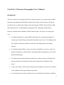
Introduction
CHAPTER 1 Ultrasonic Tomography User’s Manual
Introduction
Equipment and System Integration Requirements
Test Procedures
Inspector’s Training Requirements
Data Management Procedures
Data Analysis Procedures
Interpretation Guidelines
Limitations
Additional Information
CHAPTER 2 Portable Seismic Property Analyzer User’s Manual
Introduction
Equipment and System Integration Requirements
Test Procedures
Inspector Training Requirements
Data Management Procedures
Data Analysis Procedures
Interpretation Guidelines
Limitations (such as Technical, Operational, Environmental)
1
Other Information
CHAPTER 3 Ultrasonic Echo User’s Manual
Introduction
Equipment and System Integration Requirements
Testing Procedures
Inspector Training Requirements
Data Management Procedures
Data Analysis and Interpretation
Limitations
Other Information
References
2
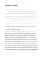
Introduction
This user’s manual includes information for three in-depth nondestructive testing devices: the
ultrasonic tomography device, the Portable Seismic Property Analyzer, and the ultrasonic echo
device. This manual can also be used as a guide for developing training courses relating to the
use of these devices in tunnels. These devices may be useful for investigating small areas where
there is reason to suspect further inspection is warranted. The manual contains additional
information about these devices that many not be available in their respective operating manuals
or their manufacturers’ websites; i.e., this manual should be considered a supplement to the
manufacturers’ information. However, links to websites and other information available through
the Internet are provided in this manual. Users of these devices should review the manufacturers’
equipment manuals and instructions before reading this manual.
The contents of the manual are mainly based on the experience of the research team
members when they used these devices for SHRP 2 R06(G). All three devices were used in
actual tunnels during the course of this SHRP 2 study.
3
CHAPTER 1: Ultrasonic Tomography User’s Manual
Introduction
This user’s manual was compiled based on the working experience of a commercially available
ultrasonic tomograph (the A1040 MIRA, produced by Acoustic Control Systems [ACS]) and
provided for the second Strategic Highway Research Program (SHRP 2) Project R06(G), HighSpeed Nondestructive Testing Methods for Mapping Voids, Debonding, Delaminations,
Moisture, and Other Defects Behind or Within Tunnel Linings. The objectives of this project
were:
•
To identify nondestructive testing (NDT) technologies for evaluating the condition of
various types of tunnel linings and tunnel-lining finishes such as tile. The techniques had
to be capable of analyzing conditions within the tunnel lining and the surrounding
substrate.
•
To evaluate the applicability, accuracy, precision, repeatability, ease of use, capacity to
minimize disruption to vehicular traffic, and implementation and production costs of the
identified technologies.
•
To conduct the required development in hardware or software for those techniques that
showed potential for technological improvement within the time limitations of the
project.
•
To prove the validity of the selected technologies and techniques to detect flaws within or
verify conditions of the targeted tunnel components.
•
To recommend test procedures and protocols to successfully implement these techniques.
4
Manufacturer’s User Manual
This field manual is not intended to replace the manufacturer’s user manual but rather to
accompany it by providing guidance for practical field use.
Two manufacturer user manuals exist: an early version produced by ACS in 2010, and a
later version produced by Germann Instruments in 2012. The 2010 version is available for
download (http://downloads.acsys.ru/eng/Documents/) or can be requested from ACS. The 2012
version is available when purchasing the system from Germann Instruments. This field manual
references the user manual produced by ACS, hereinafter referred to as the user manual.
The following information was compiled from testing both laboratory specimens with
simulated defects as well as over 170 field testing sites, including tunnel linings, continuously
reinforced concrete pavements, bonded concrete overlay airport runways, and bridge decks.
Ultrasonic Tomography Description
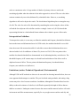
The ultrasonic tomography (UST) system used in SHRP 2 Project R06(G) is a device that
utilizes an array of ultrasonic transducers to transmit and receive acoustic stress waves for the
inspection of concrete structures. The system used, the A1040 MIRA, is produced by ACS
(http://acsys.ru/eng/production). The tomograph, shown in Figure 1.1 (left), uses a 4 by 12 grid
of mechanically isolated and dampened transducers that can fit the profile of a rough concrete
testing surface with a variance of approximately 10 mm (0.4 inch). Each row of four transducers
transmits stress waves sequentially while the remaining rows act as receivers. In this manner,
there is a wide coverage of shear wave pulses that reflect at internal interfaces where the material
impedance changes. With the help of a digitally focused algorithm (an alteration of the synthetic
aperture focusing technique [SAFT]), a three-dimensional volume is presented with each point of
5
possible reflection in half-space represented by a color scheme, scaled according to reflecting
power. This three-dimensional image can also be dissected into each of the three planes
representing its volume: the B-scan, C-scan, and D-scan (Figure 1.1, right). The B-scan is an
image slice showing the depth of the specimen on the vertical (z) axis versus the width of the
scan on the horizontal (x) axis. This slice is a plane perpendicular to the scanning surface and
parallel to the length of the device. The C-scan is an image slice showing the plan view of the
tested area, with the vertical (y) axis of the scan depicting the width parallel to the scanning
direction and the horizontal (x) axis of the scan representing the length perpendicular to the
scanning direction. Note that the scanning direction is always defined as the y-axis, as seen in
Figure 1.1, right. The D-scan is like the B-scan in that it images a plane perpendicular to the
testing surface, but it is oriented parallel to the scanning direction. On each of the scans, the
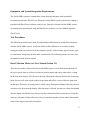
various intensities reported by the returned waves are color coded from light blue to deep red,
representing low reflectivity (typically sound concrete) and high reflectivity (any type of
impedance), respectively (Figure 1.2). With this intensity scaling, it is easy to see any
discontinuities with distinctly different wave speeds, such as voids, delaminations, cracks, and
other abnormalities.
6
y
D-scan
x
B-scan
z
C-scan
Figure 1.1. The A1040 MIRA system (left) and B-scan, C-scan, and D-scan relative to
the tomograph.
Figure 1.2. Scale of reflectivity (or acoustic impedance).
7
Equipment and System Integration Requirements
The A1040 MIRA system is a stand-alone system that only integrates with specialized
reconstruction software, IDealViewer. When the A1040 MIRA system is purchased, a laptop is
provided with IDealViewer software ready for use. Data sets collected with the MIRA system
are transferred to and analyzed using the IDealViewer software (see User Manual Appendix
IDealViewer).
Test Procedures
The following procedures have been developed and modified based on actual field evaluations
with the A1040 MIRA system. As all case studies will be different, it is necessary to adapt
testing procedures to fit the needs of the evaluation specific to the location, type of surface, type
of construction, and primary defects under consideration. The following remarks are to be used
in conjunction with the user manual.
Data Collection Modes (see User Manual Section 1.4)
There are two modes of data collection for the MIRA system: review mode and map mode. In
the review mode, data are collected as discrete point locations and can be analyzed by viewing
the B-scan on the display. This B-scan is the only information collected in this mode. In the map
mode, the user will create a grid on the test specimen and collect a series of discrete point tests
on that grid. This series of testing points is called a map. During the building of the map, the user
can observe the B-scan on the display. After the map is collected, the data set is then downloaded
onto the laptop with IDealViewer software for three-dimensional data reconstruction. Using this
software, each point of data collection is fused, or stitched, together to form a three-dimensional
image of the mapped specimen for analysis.
8
Review Mode Testing Procedures (See User Manual Section 1.4.2)
Step 1: Determine Wave Speed
In review mode, there are two options for wave speed determination. The first option is to use
the automatic wave speed generated per scan without inputting a constant wave speed. The
benefit of this approach is that the user can see the variation of wave speed over the object of
inspection. A change in wave speed signifies a change in modulus, density, and/or Poisson’s
ratio within the first few inches of the surface. In areas of deterioration or significant defects, the
automatic wave speed decreases due to path lengthening of the acoustic pulse. The second option
is to take a sample of wave speeds and use the average as a manual input. This approach allows
discontinuity details to be measured accurately (provided the modulus, density, and Poisson’s
ratio are constant), since the wave speed is fixed for the concrete medium. An average is taken
by first setting the wave speed control to automatically generate per individual scan (see user
manual Section 1.4.1). It is then necessary to collect eight to 10 randomly oriented scans in areas
free of surface deterioration or severe unevenness and attempt to collect the wave speed in
locations where potential shallow reinforcement and other shallow discontinuities will not affect
the measurements. This can be done by viewing the B-scans and attempting to measure in
between shallow reinforcement layouts if any are present. After collecting the scans, the next
step is to use the numeric average of the wave speeds and manually set the wave speed control to
this velocity.
Step 2: Set -Scanning Depth
Z-scanning depths in the review mode can be changed according to the user manual Section
1.4.2. Choosing an appropriate scanning depth (z-scanning direction) is an important decision
when using review mode. If the chosen depth is too shallow, it might be that critical information
9
regarding the depth of details is omitted. If the z-scanning depth is set too deep, the resolution of
shallow details is diminished. An appropriate z-scanning depth should be chosen after multiple
inspections via the review mode. When the operator has obtained a feel for structural
characteristics that should be included in the map, a depth should be chosen that slightly exceeds
the lowest element that needs to be captured. An example would be an analysis on concrete
pavements, where the operator is building a map for analyzing possible delamination at any
depth within the concrete section. In this case, it would be recommended that the depth be set to
only capture the depth of the overlay. This minimizes unnecessary data and improves resolution
for delamination detection. On the other hand, if the operator is to generate a map for an analysis
of bonding assessment between a top layer and a sublayer, it would be advisable to choose a
minimum z-scanning depth that at a minimum exceeds twice the depth of the top layer. This is
due to the fact that bonds that have fully separated will produce backwall multiples, or echoes,
which are repeated backwall reflections at multiples of the initial layer depth. This feature is
caused by the nearly elastic reflection of the acoustic waves as they encounter the concrete-air
original interface. The presence and intensity of such backwall echoes can depict the severity of
debonding. If few or no echoes are present, but instead a weak signal at the top layer or sublayer
interface is present, then this feature may indicate a partially bonded interface. If no interface is
detected at all, then a fully bonded pavement at that location can be expected.
Step 3: Begin Scanning
To collect the data, fully press the system to the surface very firmly, and then press the collect
trigger. Wait until the red status bar has gone to green before moving the device to another
location. It is suggested to use welder’s soapstone when scanning to mark on the concrete surface
when an interesting feature is observed. Note that the variety of parameters included in the main
10
control can be altered (see user manual Section 1.4.1), including color and analog gain, number
of periods, pause between emission pulses, operating frequency, wave speed (velocity), and time
delay. It is suggested to keep these values at their default settings unless there is a way to
calibrate the device for the object of inspection. If a known discontinuity is available for
calibration, the appropriate settings can be altered to fine-tune the measurements. Note that shear
wave frequency can be varied from 25–85 kHz so that smaller and shallower defects can be seen
at the expense of greater wave attenuation.
Map Mode Testing Procedures (See User Manual Section 1.4.3)
Step 1: Determine Grid Increments
When using map mode to construct an array of data, it is necessary to determine an appropriate
grid increment. An appropriate choice will consider the object of inspection’s lateral size and
depth. If measurements are not overlapped, the constructed images will be spotted or will be
without full coverage. If a continuous image is desired for comprehensive defect dimensioning,
scanning overlap is necessary. The transducer array has a limited aperture, due to the
combination of Snell’s Law of refraction and superposition of acoustic waves. Snell’s Law states
that the angle of incidence is equal to the angle of reflection for a given wave. By this law, an
undisturbed ultrasonic pulse will always reflect from discontinuities located half the distance
from a transducer pair. However, the modified synthetic focusing technique used in the software
image reconstruction utilizes repeated signals to develop the colored output. This means that the
signal strength (as observed by the color output of the MIRA scans) representing a given
discontinuity’s width (in the x-scanning direction) will vary in signal strength depending on how
close it is to the center of the focused aperture. The goal in continuous mapping then becomes to
11
overlap in such a manner that critical planes of inspection are fully covered by a large number of
transducer beams. Therefore, closely spaced scanning increments will better suit defects such as
small voids, clay lumps, and early propagation of small cracks, whereas general slab thickness
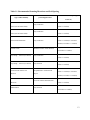
can be estimated from very widely spaced scanning increments. Table 1.1 suggests scanning
increments for generating a three-dimensional map for defect analysis. These suggestions are
experimentally determined, based on defects within 305 mm (12 inches) of the surface.
12
Table 1.1. Recommended Scanning Directions and Grid Spacing
Recommended Grid Spacing (Y
Type of Discontinuity
y-Scanning Direction
Versus X)
Voids with diameter < 50 mm (2.0
Maximum of 50 mm x 150 mm (2.0
Any orientation
inches) (air and water filled)
inches x 5.9 inches)
Voids with diameter > 50 mm (2.0
Minimum of 50 mm x 150 mm (2.0
Any orientation
inches) (air and water filled)
inches x 5.9 inches)
Optimal: 50 mm x 150 mm (2.0
Horizontal delaminations
Any orientation
inches x 5.9 inches) to 100 mm x
200 mm (3.9 inches x 7.9 inches)
No greater than 50 mm x 100 mm
Vertical cracks
Parallel to surface crack direction
(2.0 inches x 3.9 inches)
Maximum of 50 mm x 150 mm (2.0
Clay lumps < 150 mm (5.9 inches)
Any orientation
inches x 5.9 inches)
Minimum of 50 mm x 150 mm (2.0
Clay lumps > 150 mm (5.9 inches)
Any direction
inches x 5.9 inches)
Optimal: 50 mm x 150 mm (2.0
Reinforcement detail in one
Perpendicular to reinforcement
direction
layout
inches x 5.9 inches) to 100 mm x
250 mm (3.9 inches x 9.8 inches)
Reinforcement detail in two
Optimal: 50 mm x 150 mm (2.0
45° from reinforcement direction
directions
inches x 5.9 inches)
Maximum of 100 mm x 200 mm
Slab thickness
Any direction
(2.0 inches x 5.9 inches)
13
Step 2: Determine Scanning Direction (y-Scanning Direction)
The y-scanning direction is defined to be the direction perpendicular to the B-scan. When
building a map, it is necessary to choose a y-scanning direction. Since the shear wave transducers
send and receive pulses in the x-direction, the tomograph has greater resolution for objects that
pass through the x-axis, or parallel to the y-scanning direction. Therefore, the operator will have
to decide which direction is more desirable to have the greatest resolution of detail, and the yscanning direction is perpendicular to that direction. For objects under inspection that have no
defined direction (thickness calculation, delamination, some voids and lumps), the y-scanning
direction is largely irrelevant.
For example, consider that the operator desires to check longitudinal reinforcement
spacing on a concrete slab with both longitudinal and transverse reinforcement (in this scenario,
consider that the longitudinal reinforcement lies along a v-axis and the transverse reinforcement
lies along a u-axis). The desired direction for greatest resolution would be the direction
perpendicular to the longitudinal reinforcement, as it would provide the greatest detail for centerto-center measurements. Therefore, the user should choose a y-scanning direction along the vaxis.
Operators are encouraged to scan, if time permits, two orthogonal directions so that
details in both directions are collected at optimal resolution.
Step 3: Establish a Grid
For the UST system to operate in map mode, it is necessary to construct an accurate grid or
marking system to fully characterize the specimen under evaluation. The creation of a grid can
be one of the most critical jobs when building a map with the tomograph. Every grid must be
square and accurate in order to utilize the map for noting precise areas of interest.
14
There are two methods of grid construction that are recommended here. The first method
is constructing chalk lines that outline the area to be tested, including the interior grid spacing. It
is recommended to use white or blue chalk lines when it is desirable to have a water-removable
grid, while permanent grids can be established using red or black chalk. (Note: red and black
chalk contains dyes that cannot be completely removed from concrete.) The creation of the grid
starts with generating a right angle that extends a minimum of half the length of the tomograph
past the outer boundary of the desired testing surface in the x-scanning direction and half the
width of the tomograph past the outer boundary of the desired testing surface in the y-scanning
direction. The first side of this right angle can be made by popping a chalk line that is visually
approximated to be in line with the desired x- or y-scanning direction. The second side of the
right angle can be projected by using a standard framing square or by using a measuring tape to
establish a point corresponding to a 3-4-5 triangle. Once the second side of the right angle is
popped, it is necessary to mark the x- and y-scanning increments (from Step 1) on the appropriate
sides of both right angle projections. Welder’s soapstone is an excellent marking tool, as it is
highly durable on concrete surfaces, yet removal is possible with water. Once the length and
width of the grid have been marked off, it is necessary to use a measuring tape to finish marking
the perimeter of the inspection area by projecting the ends of the right angle’s sides by the
appropriate distance to establish the corner opposite the origin. Increments can then be marked
along these sides, and the interior x- and y-scanning direction gridlines can be popped via chalk
lines. When the scanning begins, it will only be necessary to place the light-emitting diode
(LED) beam from the upper left corner of the device (when viewing the control panel) on the
crosshairs of the incremented grid, using the remaining LEDs to visually square the device with
the map.
15
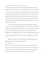
The second, albeit more permanent, method for grid placement involves constructing a
grid template from a thin sheet of plywood or particle board and using landscaping paint to spray
grid increments on the test specimen. The preferred material used in the SHRP 2 research was
3.2 mm (0.125 inch) medium-density fiberboard (MDF). A section of sheet can be as long and
wide as is appropriate for the size of the area under investigation. After cutting the sheet (which
is typically purchased in 1.2- x 2.4-m [4- x 8-ft] stock) down to the desired size, incremental rips
should be made using a table saw. The slots cut by the table saw should begin within 100 mm (4
inches) of the sheet’s edge and proceed to 100 mm from the sheet’s opposite edge. It is
recommended that the slots be made at a 50 mm increment in order for the user to apply the
landscaping paint on whichever increment is chosen. The grid established by this method is
shown in Figure 1.3.
To use this sheet as a template for the grid spacing, place it on the testing surface in the
direction of the desired x- or y-scanning direction. Use landscaping paint to mark the slotted
areas. This process can be repeated for the remaining x- or y-scanning direction by rotating the
grid template until it is square with the previously marked grid.
16
Figure 1.3. Gridlines using grid template.
Step 4: Determine Wave Speed
In map mode, it is recommended to take an average of the calculated wave speeds over the
testing area to be used as a fixed input. This approach allows discontinuity details to be measured
accurately (provided the modulus, density, and Poisson’s ratio are constant) since the wave speed
is fixed for the concrete medium. An average is taken by first setting the wave speed control to
automatically generate per individual scan (see user manual Section 1.4.1). It is then necessary to
collect eight to10 randomly oriented scans in areas free of surface deterioration or severe
unevenness and attempt to collect the wave speed in locations where potential shallow
reinforcement and other shallow discontinuities will not affect the measurements. This can be
done by viewing the B-scans and attempting to measure in between shallow reinforcement
layouts if any are present. After collecting the scans, the next step is to use the numeric average
of the wave speeds and manually set the wave speed control to this velocity.
17
Step 5: Program , , -Scanning Lengths, Wave Speed, and Other Parameters
Refer to the user manual Section 1.4.1.5 to input the selected x-, y-, and z-scanning lengths (these
are referred to in the user manual as the horizontal, vertical, and depth lengths, respectively),
wave speed, and other parameters.
Step 6: Begin Scanning
To scan with the system, place the LED light in the upper left corner (as viewed when facing the
display screen) on the crosshairs of the grid’s origin, using the light beams from the remaining
LEDs to visually square the device relative to the grid. Begin collecting data in either the x- or yscanning direction according to user manual Section 1.4.3. Either direction can be used for data
collection. To collect the data, fully press the system to the surface very firmly, and then press
the trigger on either handle. Wait until the red status bar has gone to green before moving the
device to the next location.
Step 7: Transfer Data Set and Process
Using the appropriate cables, transfer the data set from the system to the computer with the
proprietary software according to user manual Appendix IDealViewer. Analysis can take place
immediately after the dataset has been downloaded, often allowing an analysis to be started in
the field.
Inspector’s Training Requirements
Field operation training for the specific ultrasonic tomograph discussed in this manual typically
requires no more than 2 days of hands-on training. This should include a hands-on overview of
the operation of the device, an information session on the science behind shear wave ultrasonic
imaging, and hands-on training on practice specimens. General and specific certification
requirements may be required according to the agency performing testing. For example,
18
certification requirements, required by paragraphs 8.3 and 8.4, respectively, of the Recommended
Practice No. SNT-TC-1A, are provided by the American Society for Nondestructive Testing
(ASNT) nondestructive testing (NDT) Level I, Level I Limited, Level II, and Level III
certification programs for NDT employers.
•
ASNT Level I Limited technicians are only qualified to perform a specific procedure for
a specific inspection on a certain component with direct supervision and guidance of
higher-level technicians.
•
ASNT Level I technicians are only qualified to perform specific calibrations and tests
under the guidance of a higher-level technician.
•
ASNT Level II technicians are qualified to set up and calibrate systems; inspect
according to procedures; and evaluate and report the testing results for the specific
certificate issued.
•
ASNT Level III technicians are qualified to establish testing procedures and techniques
by interpreting governing codes, standards, and specifications, and they can train lowerlevel technicians.
Data Management Procedures
Data files for typical grid spacing (50–200 mm by 50–200 mm) for comprehensive maps range
from 12 kb/ft2 to 35 kb/ft2.
Data Analysis Procedures
Data reconstruction and imaging is performed automatically by the system for the twodimensional review mode, and data reconstruction and imaging is performed automatically by
19
the accompanied IDealViewer software for the three-dimensional map mode. Raw data files are
generated as .lbv, .bin, .bmp, and .cfg files.
Interpretation Guidelines
Data interpretation should be performed by an experienced operator who is familiar with
ultrasonic testing and has the appropriate NDT certifications. General interpretation guidelines
involve identifying and recording all typical features of interest, including backwall reflection,
depth to center of reinforcement, width of apparent discontinuities, etc. This can be done in
either mode, but a thorough analysis requires building a map in the map mode.
Interpretation guidelines are given below for typical features under inspection:
•
Backwall (element thickness). The backwall, or element thickness, can only be
successfully identified if there is a mismatch in impedance between the concrete and the
material beneath it. Unless the concrete is fully bonded to a material with similar
impedance, the backwall is usually readily identified by a constant high-amplitude (red)
region on the B-scan. If the backwall thickness is relatively constant, then this region
should remain unchanged when scanned at any location. A typical B-scan viewed from
the display showing the backwall location is given in Figure 1.4 (left).
20
Reinforcement
Backwall
Delamination
Multiple of delamination
Figure 1.4. B-scans showing reinforcement, backwall, delamination, and multiples.
•
Reinforcement, conduit, tendons, etc. Reinforcement, conduit, tendons, and other cablelike objects are identified by scanning perpendicular to the direction of their layout. The
operator should search for circular high-amplitude (red) regions. These are distinguished
from other possible anomalies by taking numerous scans along the direction of their
layout. The system is not capable of identifying the material of a particular anomaly, so
the operator must use good judgment to identify the anomaly. Both B-scans in Figure 1.4
show typical cross-sections of reinforcement. It is easily identified as reinforcement
because the spacing is typical for longitudinal reinforcement and is consistent along this
direction.
•
Delamination. Delamination can only be identified after the operator has established a
benchmark for the expected backwall location. Delamination is seen as a high-amplitude
region (much like the backwall), but it should not be expected to maintain a constant
depth. Delamination often occurs close to cracking (prior to spalling) and can be seen in
the B-scan to curve toward surface cracks. Figure 1.4 (right) shows a typical
delamination. Note the typical backwall depth (Figure 1.4, left) is not seen under the area
21
of delamination, but rather an echo of the delamination is seen. This is because shear
waves cannot be supported in air and do not penetrate the material beyond an air gap. The
shear waves are instead traveling back and forth between the test surface and the initial
air gap (the delamination), thus causing these multiples to occur.
•
Cracks. Cracks are the most difficult feature to ascertain due to their multiple orientations
and the pitch-catch mode of operation for the tomograph. To identify cracks as highamplitude (red) regions, the cracks must begin to form non-perpendicular to the testing
surface in order for the tomograph’s pitch-catch mode of operation to work. If they
remain perpendicular to the testing surface, they can only be distinguished by their
shadow, or complete lack of reflectivity. This is seen in the B-scans as a light blue region
with no reflections.
•
Air- and water-filled voids. Voids cannot always be discerned from delaminations until
they take an irregular shape, but they will appear as a high-amplitude region similar to
other types of air interfaces. The tomograph cannot determine the difference between airand water-filled voids.
•
Tile debonding. For tiled linings, tile debonding is usually observed by tapping the tiles
and listening for the hollow drum sound, which signifies a debonded tile. Since tile
thicknesses are usually very thin, the debonded area is seen on the tomograph but
typically appears as a high-amplitude (red) region deeper than the actual location of
debonding.
For analysis in the map mode, it is recommended to start with a volume-scan in order to
get a glimpse of the entire element under inspection and then comb through each B-, C-, and Dscan for any irregularities as outlined above. The color gain dial allows the relative intensities to
22
be decreased in order to visualize slighter changes in impedance. Note that depths to
discontinuities are usually taken as the distance to the center of the reflectivity region.
To relocate areas of interest from the map in IDealViewer to the physical grid, the
operator can use the review mode to scan until directly on top of the area of interest or can
reference the section “Origin/Boundary Establishment; Relation to Computer Model” in
Section 9 of the user manual to mark the areas accurately on the physical specimen.
Limitations
The technical, operational, and environmental limitations of the system are described below.
Technical and Operational
•
Low speed of data acquisition. If the system is used for detailed mapping in the map
mode, the user should expect the scanning process to take between 9 to 25 min/m2 (0.8–
2.3 min/ft2). The review mode can be used for single-point evaluations at much faster
rates of inspection (3–5 s per scan), but only limited-width B-scans are available for
evaluation in this mode.
•
No indication of phase change. The color palette response represents quantity of
reflectivity regions and is a measurement relative to the medium (in which there should
ideally exist zero reflectivity, the blue spectrum). As such, the type of defect is largely
guesswork on the part of the user and requires greater skill and knowledge of ultrasonics
to interpret these signals.
•
Detection of layered defects. If defects are stacked, particularly in such a manner that air
gaps are located above other types of defects, then the device can rarely determine
anything below the initial air-filled gaps. This is due to ultrasonic pulse attenuation at air
boundaries. If pulses are capable of being transmitted past air interfaces, then the
23
received signal is extremely weak and should be examined to be certain it is not a
multiple or echo of the initial flaw.
•
No reliable reinforcement detail beyond two layers of reinforcement. At the nominal
operation frequency of 50 kHz, the system has difficulty reliably detecting reinforcement
below two layers of existing reinforcement mesh.
•
Shallow defects. Due to the low frequency, spacing of the transducer array, and beam
spread of the individual transducers, defects that exist approximately 25 mm (1 inch)
from the surface cannot be expected to be received by other transducers and carry any
accurate information regarding the depth and lateral dimensions of the shallow defects.
However, near-surface anomalies with an air interface can leave a shadow on the data
collected below the near-surface defects, indicating the anomaly’s presence. This is due
to the air gaps inhibiting ultrasonic pulses to be transmitted (or received) beyond the
anomaly.
•
Small diameter objects. Small diameter objects (approximately less than 13 mm
[0.5 inches]) are not reliably detected at the nominal operational frequency of 50 kHz due
to the limitation in wavelength at wave speeds in concrete. This can be partially mitigated
by increasing the frequency to the maximum allowed central frequency of 85 kHz, but
the energy loss with higher frequencies still makes it difficult to discern smaller diameter
bars.
Environmental
The system should not be used in wet environments (no standing water on testing
surface). Additionally, the operating temperature of the system is from -10°C to 50°C.
24
Additional Information
Origin/Boundary Establishment—Relation to Computer Model
Due to the aperture of the transducer array, actual discontinuities discovered by the threedimensional analysis cannot be referenced from the established origin. The width of the
ultrasonic tomograms are dependent on the size of the grid spacing and -scanning depth and
must be superimposed on the physical grid to determine with certainty the location of a particular
defect. The process for establishing the relationship between the computer model’s origin and the
grid’s origin is described here.
After the data from each successive increment have been gathered and downloaded to the
remote computer, the three-dimensional model analysis program will allow measurements to be
made relative to the device’s aperture. Unfortunately, this aperture can be less than or greater
than the created grid, depending on the scanning depth. To be able to relate the origin of the
physical specimen (denoted as {0, 0}0) to the origin on the analysis software (denoted as {0,
0}1), the relationship between origins must be developed. To establish this relationship, several
terms must be defined as follows:
•
X0, the total x-offset between {0,0}0 and {0,0}1, taken as positive in the x-scanning
direction.
•
Y0, the total y-offset between {0,0}0 and {0,0}1, taken as positive in the y-scanning
direction.
•
X1, the chosen x-scanning increment.
•
Y1, the chosen y-scanning increment.
•
W0, the width of the tomograph array in the x-scanning direction, measured from outside
transducer to outside transducer (330 mm [13 inches] for the A1040 MIRA).
25
•
L0, the length of the tomograph array in the y-scanning direction, measured from outside
transducer to outside transducer (90 mm [3.5 inches] for the A1040 MIRA).
•
W1, the distance in the x-scanning direction from the lead LED guide to the nearest
transducer (10 mm [0.4 inch] for the A1040 MIRA).
•
L1, the distance in the y-scanning direction from the lead LED guide to the nearest
transducer (10 mm [0.4 inch] for the A1040 MIRA).
•
W3, the total width of a single B-scan as can be seen from the review or map modes.
Using the definitions defined above, the physical location of the three-dimensional
image’s origin ({0, 0}1) relative to the origin of the grid on the specimen ({0, 0}0) is defined by:
X0 = (W1 + W0/2) – W3/2
and
Y0 = L1 + L0/2
Or for the MIRA system (in mm):
X0–MIRA = (175) – W3/2
and
Y0–MIRA = 55
Again, positive values are taken to be in the x- and y-scanning directions. After
establishing this origin ({0, 0}1) on the specimen, all x- and y-dimensions taken directly from the
three-dimensional software can be measured from this point of reference.
In typical field applications, the offset varies from 100 mm (2 inches) inside the specimen
grid to 406 mm (16 inches) outside the specimen grid. If this scale of accuracy is not required for
the particular type of evaluation (say, the inspector is only interested in a nominal layer depth),
the defect location can be estimated using the direct measurements from the analysis software
26
and then pinpointed by using the device in review mode. Whether or not great accuracy is
necessary, using the review mode to fine-tune the final location can help to confidently establish
the defect location.
27
CHAPTER 2: Portable Seismic Property Analyzer User’s Manual
Introduction
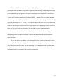
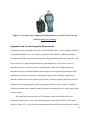
The Portable Seismic Property Analyzer (PSPA; Figure 2.1) was developed by Geomedia
Research and Development (GRD). The PSPA is an instrument designed to determine the
variation in modulus with the depth of exposed layer being concrete or asphalt. The operating
principle of the PSPA is based on generating and detecting stress waves in a medium. The PSPA
consists of two transducers and a source packaged into a handheld portable system that can
perform the ultrasonic surface wave (USW) and impact echo (IE) tests simultaneously. This
combination enhances the reliability of these methods in determining material properties and
thickness, as well as detecting defects within the members with minimal additional field-testing
time. The USW method can be used to determine the modulus of the material and relate it to
material degradation and presence of internal defects. The IE method can be used as a tool to
determine the thickness or the defects within concrete slabs or tunnel lining.
28
Electronics Box
Sensor 2
Sensor 1
Source
Figure 2.1. Portable Seismic Property Analyzer.
Equipment and System Integration Requirements
The PSPA (Figure 2.1) is an integrated data collection and reduction unit. This device consists of
four main elements. The core of the system is a solenoid-type high-frequency impact hammer
and two high frequency accelerometers, which are deployed in the sensor unit. The receivers are
connected to a data acquisition system in the electronics box. The system is operable from a
laptop computer. This computer is tethered to the hand-carried transducer unit through the cable
that carries power to the transducers and hammers and returns the measured signals to the data
acquisition board in the computer. The data collection at one point takes about 15 seconds.
As mentioned earlier, two testing methods are used in the operation of the PSPA. The
time records from the two receivers are used in the USW method to determine the properties of
the top layer with Spa Manager Software in the computer. The modulus of each point can be
obtained as soon as the data collection is completed. The PSPA also performs the IE method by
measuring the frequency content of the first sensor’s time record and estimating the layer
thickness or depth of defect.
29
Test Procedures
At each site, the first step consisted of selecting a test section and marking the test points. The
density of data collection depends on the smallest defect of interest to the agency (Azari et al.,
2012). To obtain better quality time records, there should be a good contact between the sensors
and the top surface; therefore, the surface of the test object should be smooth and clean of debris.
Then, each point is tested with the PSPA. Test procedures are documented at
http://www.geomedia.us/.
To collect data with the PSPA, the user initiates the testing sequence through the
computer. The thickness (or the required penetration depth) and test material are input by the
user as nominal values. By collecting data, the high-frequency source is activated four to six
times. The outputs of the two transducers from the last three impacts are saved and averaged
(stacked). The other (prerecording) impacts are used to adjust the gains of the preamplifiers. The
gains are set in a manner that optimizes the dynamic range.
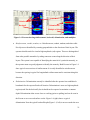
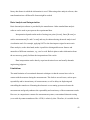
After data collection at one point, the acquired time records can be observed with the
PSPA software. In case of weak contact between the sensors and the material surface, either the
time records will be erratic or no signal will appear. In this case, the test is rejected and a new
test is performed. When the sensors achieve intimate contact with the surface, the acquired time
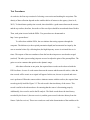
records typically look like Figure 2.2. The red record is the time history of the source. This
record is useful to the advanced user for ensuring that the source is functioning properly.
Additionally, the record is used in the IE analysis. The black record shows the time history
recorded by the Sensor 1 (the near receiver), and the green record is the time history from the
Sensor 2 (the far receiver). These two records are used in the determination of the modulus with
30
the USW method. Both records indicate the typical arrival of the surface wave followed by
reflection from the bottom of the testing object or the bottom of the internal defect.
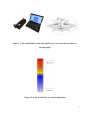
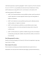
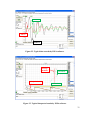
After accepting the collected waveforms, the operator can view the analyzed data, as
shown in Figure 2.3. The graph at the bottom is the phase spectrum, which is determined by
conducting a spectral analysis on the time records from the two receivers. The phase spectrum
indicates the variation in phase delay between two receivers with frequency. The green curve is
the measured phase spectrum from the time records, and the red one is the best fit to the measure
spectrum when the effect of the body waves is removed. The fitted spectrum is then used to
compute the dispersion curve (Desai and Nazarian, 1993). In the upper graph, the green dots
show the variation in modulus with thickness, which is called a dispersion curve. The dispersion
curve is directly calculated from the phase spectrum. The red solid line in this graph corresponds
to the average modulus, which is obtained by averaging the dispersion curve down to
approximately the nominal thickness of the layer. The average modulus is also shown in the
results section on the left side of the figure (i.e., 3830 ksi). Therefore, the operator can get a
qualitative feel for the variation in modulus with depth and also average modulus.
31
Sensor 2
Source
Sensor 1
Figure 2.2. Typical time records by PSPA software.
Average
modulus
Measured
Interpretation
Measured
Figure 2.3. Typical interpreted results by PSPA software.
32
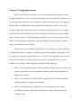
Inspector Training Requirements
Data collection and documentation are carried out through the Spa Manager Software
provided with the device. Two days of on-site training are typically required for inspectors who
are collecting data and about a week of training is required for the data analyst. The training of
the data collector and data analyst should provide the fundamentals of elastic waves, sonicseismic testing methods, and common defects in different testing media in order to set up test
parameters and interpret acquired data correctly. During data collection, the inspector should
make sure that the source is functioning properly and the receivers are in full contact with the
surface. The data interpreter should have a basic knowledge of signal processing to analyze
surface waves and body waves reliably.
General and specific certification requirements may be required, according to the agency
performing the testing. For example, certification requirements required by paragraphs 8.3 and
8.4, respectively, of the Recommended Practice No. SNT-TC-1A are provided by the American
Society for Nondestructive Testing (ASNT) nondestructive testing (NDT) Level I, Level I
Limited, Level II, and Level III certification programs for NDT employers.
•
ASNT Level I Limited technicians are only qualified to perform a specific procedure for
a specific inspection on a certain component with direct supervision and guidance of
higher-level technicians.
•
ASNT Level I technicians are only qualified to perform specific calibrations and tests
under the guidance of a higher-level technician.
•
ASNT Level II technicians are qualified to set up and calibrate systems; inspect
according to procedures; and evaluate and report the testing results for the specific
certificate issued.
33
•
ASNT Level III technicians are qualified to establish testing procedures and techniques
by interpreting governing codes, standards, and specifications, and they can train lowerlevel technicians.
Data Management Procedures
The PSPA saves the raw data in binary format from each test point with appropriate metadata
indicating the time and information about the test parameters. Upon initiation of a project, the
user will identify the location where the data have to be stored. The analysis software (Spa
Manager Software) is able to read the binary data format and also to transform the data into
American Standard Code for Information Interchange (ASCII) format. The ASCII format data
can be reanalyzed readily with new algorithms if necessary.
Data Analysis Procedures
The data analysis is defined as the processing of the raw data collected by the PSPA and includes
preprocessing, data analysis, and presentation of data. In the preprocessing phase of the IE
method, utilizing a time window to remove the surface wave energy from the time records
provides a more robust and accurate thickness measurement compared to when the entire
waveform is utilized. On the other hand, in the USW method, the surface wave energy should be
reinforced by implementing proper filters to minimize the reflection and body wave energy. The
data analysis includes fast Fourier transform of time records to frequency domain, which can be
used to determine amplitude spectrum and phase spectrum of the acquired time records.
The data presentation of the USW and IE results in the form of color contour maps,
namely “traditional with unlimited color index,” “traditional with two color index” and
“checkerboard” (Azari et al. 2012). The traditional contouring utilizes a smoothing algorithm to
ensure that the displayed contour lines change gradually and incrementally from a minimum
34
value to a maximum value. A large number of shades of primary colors are used in the
smoothing algorithm when the unlimited color index approach is selected. The two-color index
contours contain only two colors delineated by a threshold value. However, a smoothing
algorithm is still used to depict the results. The checkerboard algorithm plots a rectangular array
of cells. The value for each cell is determined by smoothing the results using the values of that
cell and the four adjacent cells to define a surface rectangle. Azari et al. (2012) showed that
representing the data in a checkerboard format enhances the evaluative power of the results.
Interpretation Guidelines
To interpret the results, it is necessary to define the modulus and frequency threshold to delineate
between the intact and delaminated areas. In USW results, the modulus threshold is set at 0.86
times the mean of the measured moduli of each slab to ensure that the delaminated areas are
detected with a level of confidence of about 95% (Azari et al. 2012). The test points with a
modulus less than the threshold are demonstrated in red, indicating that they are defective. The
threshold frequency in IE contour maps is selected based on thickness of the slab as well as
depth and extent of defect. The test points with dominant frequency less than thickness
frequency are marked as red (defective).
Limitations (such as Technical, Operational, Environmental)
Although USW and IE methods are shown to be successful in detecting internal defects, there are
some apparent disadvantages to consider. They are localized testing methods, and testing a long
section may take a lot of resources and time. In addition, although the IE method does have the
ability to show the existence of a defect, it is difficult to quantify the depth of defects that are
shallow or extensive. Inadequate contact between the sensors and the material surface will result
in inaccurate and false measurements, especially for very rough concrete surfaces and oily and
35
curved surfaces, such as tunnel linings, that cause occasional slips of devices during testing. On
the other hand, the USW method does not differentiate between an intact slab and a slab with
deep defect, and, therefore, this method is not very effective in detecting deep defects.
Other Information
More information can be found at http://www.geomedia.us/; in the SHRP 2 R06(A) final report
(to be published shortly); and in Azari et al. (2012), Boone et al. (2009), Delatte et al. (2003),
Fisk et al. (1994), Gucunski et al. (2006), Hisatake et al. (1994), Nazarian and Baker (1997), and
Nazarian et al. (2006).
36
CHAPTER 3: Ultrasonic Echo User’s Manual
Introduction
The information contained in Chapter 1, Ultrasonic Tomography User’s Manual, relating to test
procedures and data interpretation, can also apply to this device. Therefore, please review the
pertinent information in Chapter 1 as well.
An ultrasonic transducer is used to generate and/or receive ultrasonic waves in/from a test
medium. The ultrasonic echo technique involves sending and receiving ultrasonic pulses from
the same side of the test object by the same or two separate transducers. The ultrasonic pulse
velocity (UPV) is correlated to material strength or quality. The measurement of propagation
time is used to localize cracks, voids, and delaminations and/or to estimate the thickness of a
structure. Large enough defects (with respect to the ultrasonic wavelength), as well as structural
boundaries, induce a high contrast in acoustic impedance and result in the reflection of ultrasonic
waves. The reflected waves are detected in ultrasonic scans, and the two-way travel time is used
to estimate the reflector location (assuming or knowing the ultrasonic wave velocity in the test
medium).
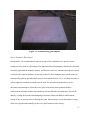
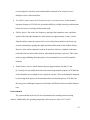
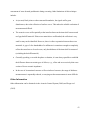
The hand-held ultrasonic transducer used for field testing and the corresponding data
acquisition/analyzer unit are shown in Figure 3.1. In tunnel testing applications, the ultrasonic
echo technique can be used to estimate the thickness of the tunnel lining as well as to detect
delaminations and voids within the lining.
37
Figure 3.1. Ultrasonic echo equipment A1220 Monolith, by Acoustic Control Systems
(ACSYS) (http://acsys.ru/eng/).
Equipment and System Integration Requirements
The ultrasonic echo equipment used is the A1220 Monolith (Figure 3.1) developed by ACSYS in
cooperation with BAM. It is a low-frequency ultrasonic flaw detector, suitable for thickness
measurement and flaw detection in heterogeneous large-grained materials such as concrete. The
array consists of 24 spring-mounted ultrasonic point transducers, out of which 12 serve as
transmitters and 12 as receivers. Because of the structure of the array, a higher amount of
ultrasonic energy is transmitted and the reflected signals are averaged, thereby minimizing the
scattering noise. However, the array is still small enough to allow testing on rough surfaces.
Since the transducers are of dry-contact type, the array is directly pressed against the test object,
and therefore no coupling agent or special preparation of the test object’s surface is required.
Testing can be done either manually (point-by-point) or automatically (over a grid) using robatic
scanner systems.
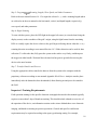
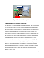
For testing larger test areas, the A1220 transducer can be mounted directly on an
automated scanning device. One such scanning system developed by BAM, the ZfP-Scanner
(shown in Figure 3.2), can be used for measurements on horizontal surfaces and vertical surfaces
38
as well as for overhead testing. Its adjustable size allows scanning in narrow areas. The scanner
is fixed to the surface using vacuum feet or plates. The speed of the ultrasonic scanning on a 1by 1-inch (2.5- x 2.5 cm) grid is about 11 ft2/h (1 m²/h). The ZfP-Scanner is not commercially
available.
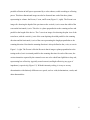
Figure 3.2. ZfP-Scanner on a test site in Chesapeake Bay Bridge Tunnel with the ultrasonic
echo equipment mounted on it.
Testing Procedures
When using dry-point contact probes, no coupling liquids need to be applied on the surface.
However, it is necessary to clean the surface from dust and sand and remove all the materials
from the surface that could prevent the penetration of low-frequency ultrasonic energy in the
material.
The location (with respect to a permanent reference) and size of the test site should be
carefully noted. In case of the scanner testing, the location of the scanner feet and the dimension
of the scanner aperture need to be carefully recorded. It is equally important to record the
orientation of the probe (i.e., its polarization) with respect to the test area or scanner opening.
39
The parameters to be set before starting with the measurements are the center frequency,
the delay time, and the voltage level. The choice of parameters depends on the particular
application, i.e., test material and required penetration depth. For testing of concrete tunnel
linings up to 3 ft (1 m) thick, a center frequency of 55 KHz could be used.
The number of test points and grid spacing depends highly on the required resolution
(i.e., the minimum size of sought defects) and the allocated time for field investigations. In the
SHRP 2 R06(G) project, a spacing of 1 inch (2.5 cm) in each direction was chosen, allowing the
scanning operation at about 11 ft2/h (or 1 m2/h), for acoustic testing requires contact.
Investigations revealed that doubling the grid spacing to 2 inches (about 5 cm) would not
compromise the accuracy of the test results. Reconstruction algorithms used for post-processing
the data (e.g., synthetic aperture technique) are most effective for grid spacing of 2 inches (about
5 cm) or less. To achieve the maximum accuracy, it might be necessary to do the measurements
with two polarizations.
Inspector Training Requirements
A 1-day training is necessary before setting out for manual testing. The training should provide
the fundamentals of ultrasonic echo testing as well as operational principles of the specific
transducer (e.g., A1220) including a hands-on training module. One or several mock-ups of
typical tunnel lining sections with sought-after features and defects may be developed for
training purposes. Handling and programming the scanning system requires 2 to 3 days of
additional training.
Some general information about the tunnel lining structure and the types of defects
sought is required for setting the test parameters. Data interpretation can be done by trained users
only and usually demands engineering judgment.
40
General and specific certification requirements may be required, according to the agency
performing testing. For example, certification requirements required by paragraphs 8.3 and 8.4,
respectively, of the Recommended Practice No. SNT-TC-1A are provided by the American
Society for Nondestructive Testing (ASNT) nondestructive testing (NDT) Level I, Level I
Limited, Level II, and Level III certification programs for NDT employers.
•
ASNT Level I Limited technicians are only qualified to perform a specific procedure for
a specific inspection on a certain component with direct supervision and guidance of
higher-level technicians.
•
ASNT Level I technicians are only qualified to perform specific calibrations and tests
under the guidance of a higher-level technician.
•
ASNT Level II technicians are qualified to set up and calibrate systems; inspect
according to procedures; and evaluate and report the testing results for the specific
certificate issued.
•
ASNT Level III technicians are qualified to establish testing procedures and techniques
by interpreting governing codes, standards, and specifications, and they can train lowerlevel technicians.
Data Management Procedures
The collected data are downloaded from the ultrasonic hardware and saved on an external hard
disk for safekeeping. Depending on the amount of data acquired, downloading might be
necessary in between a measurement cycle, or an external hard disk can be hooked up to the
instrument. Using the A1220 device on a 1- by 1-inch (2.5- by 2.5-cm) grid of size 48 by 24
inches (1225 data points, 1024 samples per signal, sampling frequency of 1 MHz) produces a 16bit binary file of 2.39 MB. The analysis software delivered with the hardware is able to read the
41
binary data format in which the information is saved. When using other analysis software, data
transformation into a different file format might be needed.
Data Analysis and Interpretation
Basic data analysis software is provided by the manufacturer. Other standard data analysis
software can be used to post-process the experimental data.
Interpretation depends on the mode of testing (one point [A-scan], linear [B-scan], or
surface measurements [D- and C-scans]) and may be enhanced using advanced analysis and
visualization tools. For example, applying SAFT to the data improves signal-to-noise ratio.
Phase analysis, on the other hand, makes it possible to distinguish between features and
anomalies of different constitutes, e.g., steel or void. Built-in plans or other information about
the test area may greatly facilitate the interpretation of the results.
Data interpretation can be done by experienced trained users and usually demands
engineering judgment.
Limitations
The main limitation of conventional ultrasonic techniques is that the sensors have to be in
contact with the structure during the measurements. This leads to several issues, such as poor
repeatability and/or inconsistency of measurements, as well as delays in displacing and
reinstalling the transducers. Mounting the ultrasonic on a scanning system accelerates the
measurements and greatly enhances the repeatability and consistency of the measurement results.
However, in comparison to contact-free measurement systems, conventional ultrasonic testing
(even with dry-contact transducers like A1220) is relatively slow. Therefore, it is suitable for the
42
assessment of areas deemed problematic during screening. Other limitations of this technique
include:
•
At (or near) block joints or other structural boundaries, the signals suffer great
disturbances, due to the reflection of surface waves. This makes the reliable evaluation of
measurements difficult.
•
The acoustic waves reflect partially at the interface between the inner shell concrete and
roof gap backfill material. If these two materials are well bonded, the reflection is very
small or may not be identified. However, there is often a separation between these two
materials. A gap of a few hundredths of a millimeter is sometimes enough to completely
reflect the sound waves. In such cases, only the thickness of the inner shell is measured
(excluding the backfill material).
•
Generally speaking, even with the phase evaluation, it is not always possible to establish
the difference between certain types of defects, e.g., a flaw and an excessively thin crosssection of lower acoustic impedance.
•
In the case of air-entrained concrete or fiber reinforced concrete, the range of thickness
measurements is reportedly reduced, or carrying out the measurements is more difficult.
Other Information
Other information can be obtained via the Acoustic Control System (2004) and Zoega et al.
(2012).
43
References
Acoustic Control System Ltd. Low-Frequency Ultrasonic Flaw Detector. Technical Passport
Operation Manual. Moscow: s.n., 2004.
Azari, H., Yuan, D., Nazarian, S., and Gucunski N. (2012). Impact of Testing Configuration and
Data Analysis Approach on Detection of Delamination in Concrete Bridge Deck with
Sonic Methods, to appear in Transportation Research Record.
Boone, S.D., Barr, P.J., and Bay, J.A. (2009). Nondestructive Analysis of a Concrete Tunnel
Model Using a Newly Proposed Combined Stress Wave Propagation Method, Journal of
Performance for Constructed Facilities, ASCE (Accepted For Publication).
Delatte, N., Chen, S., Maini, N., Parker, N., Agrawal, A., Mylonakis, G., Subramaniam, K.,
Kawaguchi, A., Bosela, P., McNeil, S., and Miller, R. (2003). Application of
Nondestructive Evaluation to Subway Tunnel System, Journal of the Transportation
Research Board 1845, pp. 127–135.
Fisk, P., Holt, R., Russell, H., and Bohlke, B. (1994). Automated, Rapid, Comprehensive NonDestructive Tunnel Testing, Proceedings of the Symposium on the Application of
Geophysics to Engineering and Environmental Problems, Boston, Mass.
Gucunski, N., Consolazio, G.R., and Maher, A. (2006). Concrete Bridge Deck Delamination
Detection by Integrated Ultrasonic Methods, International Journal Material and Product
Technology, Special Issue on Non-Destructive Testing and Failure Preventive
Technology, Vol. 26, No. 12, pp. 19–34.
Hisatake, M., Murakami, J., and Told, T. (1994). A Non-Destructive Assessment of Tunnel
Lining Stability, Proceedings of Congress on Tunneling and Ground Conditions, Cairo,
pp. 493–500.
44
Liu, W. and Scullion, T. User’s Manual for MODULUS 6.0 for Windows. Report 0-1869-2.
Texas Transportation Institute, 2001.
Liu, W., and Scullion, T. MRADAR Collecting GPR and Video Data. Technical Memorandum to
TxDOT, 2007.
Nazarian, S. and Baker, M.R. (1997). Comprehensive Inspection of Bridge Decks with
Ultrasonic Methods, in Infrastructure Condition Assessment: Art, Science, and Practice,
ASCE, pp. 405–414.
Nazarian, S., Yuan, D., Smith, K., Ansari, F., and Gonzalez, C. (2006). Acceptance Criteria of
Airfield Concrete Pavement Using Seismic and Maturity Concepts. Innovative Pavement
Research Foundation, Airport Concrete Pavement Technology Program. Report IPRF-01G-002-02-2, May 2006.
Scullion, T., Chen, Y., and Lau, C. L. COLORMAP—User’s Manual with Case Studies. Report
1341-1. Texas Transportation Institute, 1995.
Zoega, Andreas, Feldmann, Rüdiger, and Stoppel, Markus. Praktische Anwendungen
Zerstörungsfreier Prüfungen und Zukunftsaufgaben 23-24. February 2012. Fachtagung
Bauwerksdiagnose. Berlin: BAM Berlin, 2012.
45
46