Download FRAPAnalyser USER MANUAL

FRAPAnalyser
USER MANUAL
University of Luxembourg, 2009.
2
Installation
The latest version of FRAPAnalyser program can be downloaded from the internet site
http://actinsim.uni.lu/. Program does not require any specific installation. Unpack the archive on your PC
and run the file FRAPAnalyser.exe.
System Requirements
Software is developed for the Windows operating system (Windows NT or further versions).
Program was tested successfully on PC with the following parameters: processor Intel Pentium (CPU
1400 MHz), RAM 512 MB. Executable file requires just 2 MB of the hard drive space. User also needs
some free space on hard drive for storing experimental data (input files) and the results of the analysis
(output files).
Description
FRAPAnalyser is independent software package for modelling and fitting FRAP experiments.
FRAPAnalyser provides:
•
Data import/export;
•
Graphical support;
•
Normalization;
•
Modelling and data fitting by: one- and two-binding state, diffusion for circular and
rectangular bleached spots, reaction-diffusion, and the polymerization models;
•
Error analysis.
Main window
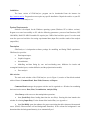
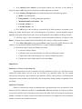
The main work window of the FRAPAnalyser (see in Figure 1) consists of four blocks marked
with red frames: Command Panel, Data Table, Datasets, and Report.
Command Panel manages the program activities and is organized as a Windows bar combining
the items into the menus: Data, Plots, Normalization, Analysis, Help.
Menu Data provides access to data manipulation operations:
•
Item [Load files] allows loading data from the text file(s). Pressing this item launches the
window for selecting Input file(s). For the format of the loaded file(s) see Appendix A.
•
Item [Set ROIs] opens the submenu for proper associating the table columns with measured
curves (FRAP, reference/whole cell and background intensities). If the column for background is not
determined then the background intensity is set automatically to 0.
3
Command panel
Datasets
Data table
Report
Figure 1. Main window of the FRAPAnalyser.
•
Item [Set bleach channel] opens the submenu to input the row index of the first time point
after the bleach.
•
Item [Delete Data] erases the workspace including the data table and the results of the
analysis.
•
Pressing the item [Save data] stores current dataset to a text (*.txt) file. Standard Windows
output dialog Save current dataset helps to specify name and location of the output file.
Item [Show Plots] of the menu Plots loads the subwindow depicting the FRAP data.
Menu Normalization runs the normalization procedures according different algorithms [1]:
•
[Double normalization] – the procedure accounts for the background fluorescence and
acquisition photobleaching.
•
[Single normalization] – the procedure accounts only for the background fluorescence.
•
[Double normalization + Full Scale] – the double normalization procedure with scaling the
FRAP data between 0 to 1.
•
[Single normalization + Full Scale] – the single normalization procedure with scaling the
FRAP data between 0 to 1.
•
[Data are already normalized] – is used in case the loaded data are already normalized.
See Appendix C for technical description the normalization procedures.
4
Menu Analysis activates the submenus of data modeling, fitting and error analysis.
•
Item [New Analysis] opens an accessory window for creating of the new analysis dataset.
See Appendix B to find out the structure of a dataset for the current version of the program.
•
Pressing the item [Delete Analysis] deletes the current analysis dataset.
•
Item Models launches a submenu for modeling the FRAP data by:
o [One binding state] the one-binding state model [2];
o [Two binding states] the two-binding state model [2];
o [Diffusion circular spot] – the diffusion model for a circular bleached spot [3];
o [Diffusion rectangular spot] the diffusion model for a rectangular bleached spot [4];
o [Binding + diffusion] – the full reaction-diffusion model [2].
o [Polymerization] – the model of actin filaments turnover {the paper is submitted}.
After a corresponding subitem is chosen the subwindow Model parameters is loaded to input
parameters of the selected model. For mathematical description of the FRAP models see Appendix D.
•
Item Analysis launches a multi-step dialog for data fitting. Analysis Step1: input (1) the
fitting model [from the abovementioned list of the FRAP models], (2) the optimization algorithm (the
Levenberg-Marquardt method or the Nealder and Mead method), (3) number of iterations for a fitting
method, (4) the first time channel and (5) the last time channel. Analysis Step2: input the initial values
for fitting model parameter. Check-out the fitting parameter(s) if it is fixed.
Item [About] of the menu Help displays information about current program version and contact
details of the developers. This information could be used for any citing the software and for
announcement for the updates.
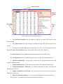
Data table visualizes the current dataset in the tabular form. Upper row contains the column
names. The first column counts the indexes of time channels. The second column represents the scanned
time moments. Other columns are defined for intensity arrays.
Datasets let make a quick overview of the loaded or processed datasets via the Data table.
Report times the performed operations as “successful” or “failed”, the attained value of the
correspondence criterion χ 2 , and the estimated parameters.
5
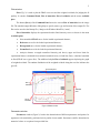
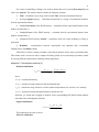
Plots window
Plots (Fig. 2) is used to plot the FRAP recoveries and the weighted residuals (for judging the fit
quality). It contains Command Panel, Plot of intensities, Plot of residuals and the menu Available
plots.
The button [Save] of the Command Panel stores the current Plot of intensities into the image
file. The standard output Windows dialog helps to specify name, type and location of the output file. The
Plot can be stored as the bitmap file (*.bmp) or the Windows MetaFile (*.wmf).
Plot of intensities displays the experimental and/or fitted intensity curves as chosen in the menu
Available plots:
•
Non-normalized FRAP curves for the loaded experimental datasets;
•
Reference curves for the loaded experimental datasets;
•
Background curves for the loaded experimental datasets;
•
Normalized curves for the loaded experimental datasets;
•
Analysis datasets: averaged normalized intensity (red boxes), upper and lower limits for
experimental data as calculated from estimated standard errors (red and blue lines), calculated (modeled
or fitted) FRAP curve (green line). The additional subplot Plot of residuals appears depicting the graph
of weighted residuals. The random distribution of the weighted residuals along the zero line indicates the
good fit.
Command panel
Plot of
intensities
Available
plots
Plot of
residuals
Figure 2. Plots window.
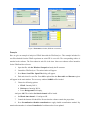
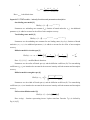
Parameters window
Parameters window (Figure 3) leads to the determination of different parameters and options. Its
appearance is determined by performed activity and/or chosen model. Parameters could be determined as
numerical values or as options from provided lists.
6
Figure 3. Parameters window (different occurrences).
Example
Here we give an example of analysis of FRAP data with the FRAPAnalyser. This example includes five
text files obtained from the FRAP experiment on actin-GFP in vero cells. The corresponding achieve is
attached to the software. The first column in each file is the time. Other two columns collect intensities
for the FRAP and the reference.
1.
Open the files with the Windows Notepad and study the file structure.
2.
Launch the FRAPAnalyser. The main window will appear.
3.
Press Data->Load Files. Input Files dialog will appear.
4.
Find and select five test files. Press OK to upload the data. Data table and Datasets regions
will appear in the main window. The accessory window SetROIs will be loaded.
5.
Choose the following options:
a. FRAP =Intensity ROI 1;
b. Reference = Intensity ROI 4;
c. Leave Background field empty;
And press OK. The window Set bleach channel will be loaded.
6.
Set Bleach time channel =11 and press OK.
7.
Control the datasets of loaded files. Be sure that the columns contain the proper data.
8.
Press Normalization->Double normalization to apply double normalization method. Pay
attention that numbers in column Normalized of each dataset have been updated.
7
9.
Press Analysis->New Analysis. In the opened window leave the name of new dataset as
proposed and press OK. Notify that new dataset was added and study its contents.
10. Press Analysis->Fitting Panel to start the data fitting. Select the following options:
a. Model = One binding state
b. Fitting method = Levenberg-Marquardt (gradient);
c. Maximum number of iterations = 200;
d. First time channel = 1;
e. Last time channel = 90;
11. Press OK and go to the second step. Control the list of fitted parameters corresponds to one
binding state model. Put the mouse arrow in the editing zone of a parameter – then the parameter range is
highlighted. Keep the default initial values for the model parameters. Press OK to run fitting procedure.
12. The final values of the correspondence criterion and model parameters will appear in the
Report. Contents of two columns Model and Residuals in the Analysis 1 dataset will be updated.
13. Press Plots->Show plots. In the appeared Plots window check all available options one after
another to see experimental and best fitted FRAP curves. Analyze the Plot of residuals.
14. Perform the analysis using two binding state model.
a. Create new Analysis dataset;
b. Perform the same steps data fitting however with two binding states model;
c. Compare the results of data fittings by one- and two-binding state model.
d. Visualize the results of data analysis by the menu Plots.
Appendixes
Appendix A. Formats of input data files
Experimental data are stored in format of the tab- delimited text files (*.txt). The first line may
contain the column names, the rest of the file are filled in by numerical values. The first column
represents the time points, other columns are the intensities (FRAP, reference/whole cell, background).
Organization of the columns in the loaded files must be absolutely similar. Number of uploaded files is
not limited.
Appendix B. Datasets
Dataset is a structure for storage of simulated and/or experimental time series for intensities. Each
dataset is stored as a table and visualized via the Data table. When the input files are loaded, new dataset
is created for each file. Name of the dataset is the same as the name of the file from that it was generated.
Number of columns in a dataset is equal to the number of columns in the original file with one additional
column reserved for the normalized intensity.
8
For reasons of modelling or fitting a new analysis dataset has to be created ([New analysis] item
of the enu Analysis). The analysis dataset contains the following columns:
•
Time – calculated as an average of the column Time from the experimental datasets.
•
Averaged Signal intensity – calculated automatically as average of normalized intensities
from all experimental datasets.
•
Standard Deviations of the FRAP intensity – estimated from the experimental datasets when
number of loaded files >1.
•
Standard Errors of the FRAP intensity – estimated from the experimental datasets when
number of loaded files >1.
•
Simulated FRAP intensity (Model) - recalculated each time when modelling or fitting is
performed.
•
Residuals – inconsistencies between experimental and simulated data, recalculated
simultaneously with Model column.
FRAPAnalyser allows creating a number of the analysis datasets for the same experimental data.
This feature can be used to test and to compare the fitting quality by several analysis procedures (made
by varying different normalization, modelling, fitting algorithms).
Appendix C. Normalization methods [1]
Double normalization
I norm (t ) =
I ref _ pre
I ref (t ) − I back (t )
⋅
I frap (t ) − I back (t )
I frap _ pre
where
I norm (t ) - normalized intensity;
I frap (t ) - measured average intensity inside the bleached spot;
I ref (t ) - measured average reference or whole studied compartment (cell , nucleus, etc.) intensity;
I back (t ) - measured average background intensity outside the cell;
Subscript _pre means the averaging of intensity in the corresponding ROI before bleach moment
after subtraction of background intensity;
Single normalization
I norm (t ) =
The notations are the same as above.
Full scale calibration
I frap (t ) − I back (t )
I frap _ pre
9
I norm1 (t ) =
I norm (t ) − I norm (t bleach )
I norm _ pre − I norm (t bleach )
Here tbleach is the bleach time.
Appendix D. FRAP models – intensity functions and parameters description
One binding state model [2]
(
FRAP(t ) = (1 − r ) 1 − ceq e
− k off (t −t bleach )
)
Parameters are: unbinding rate constant (koff), fraction of bound molecules (ceq). An additional
parameter (r) is added to account for the effect of non-complete recovery.
Two binding states model [2]
(
FRAP(t ) = (1 − r ) 1 − ceq1e
− k off 1 (t − tbleach )
− ceq 2 e
− k off 2 (t − tbleach )
)
Parameters are: the unbinding rate constants for two binding states (koff1,koff2), fractions of bound
molecules (ceq1, ceq2). An additional parameter (r) is added to account for the effect of non-complete
recovery.
Diffusion model for circular spot [3]
FRAP (t ) = a 0 + a1 ⋅ e
−
τ
2 ( t −tbleach )
⎛ ⎛
⎞
⎛
⎞⎞
τ
τ
⎟⎟ + I 1 ⎜⎜
⎟⎟ ⎟
⋅ ⎜⎜ I 0 ⎜⎜
⎟
−
−
2
(
t
t
)
2
(
t
t
)
bleach
bleach
⎠
⎝
⎠⎠
⎝ ⎝
τ=
w2
D
Here I 0 ( x ) , I 1 ( x ) – modified Bessel functions.
Parameters are: the radius of bleach spot (w) and the diffusion coefficient (D). Two normalizing
coefficients (a0, a1) are introduced to account for the non-zero intensity at bleach moment and incomplete
recovery.
Diffusion model rectangular spot [4]
⎛
⎞
w2
⎟
FRAP(t ) = a 0 + a1 ⎜1 −
2
⎜
⎟
+
4
(
−
)
w
π
D
t
t
bleach ⎠
⎝
Parameters are: the width of bleach spot (w) and the diffusion coefficient (D). Two normalizing
coefficients (a0, a1) are introduced to account for the non-zero intensity at bleach moment and incomplete
recovery.
Full reaction-diffusion model [2]
(
)
FRAP(t ) = (1 − r )invlap FRAP( p )
~
Here invlap() – function representing inverse Laplace transform. Function I ( p ) is defined by
Eq. (6) in [2].
10
Parameters are: the pseudo binding rate constant (kons), the unbinding rate constant (koff), the
diffusion coefficient (D), the radius of a bleached spot (w). An additional parameter (r) is added to
account for the effect of non-complete recovery.
Polymerization model
Equations are introduced in: Halavatyi et.al. “A Mathematical Model of Actin Filament Turnover
for Fitting FRAP Data” [submitted to the Biophysical Chemistry].
Parameters are: the association and dissociation rate constants for barbed and pointed ends (k(+)b,
k(+)p, k(-)b, k(-)p), the average length of filaments in actin subunits (L), F-actin concentration (cf).
References
[1] K. Miura, Analysis of FRAP Curves, http://www.embl.org/cmci/downloads/FRAPmanual.htm
(2007).
[2] B.L. Sprague, R.L. Pego, D.A. Stavreva, J.G. McNally, Analysis of binding reactions by fluorescence
recovery after photobleaching, Biophys J 86 (2004) 3473-3495.
[3] D.M. Soumpasis, Theoretical analysis of fluorescence photobleaching recovery experiments, Biophys
J 41 (1983) 95-97.
[4] J. Ellenberg, E.D. Siggia, J.E. Moreira, C.L. Smith, J.F. Presley, H.J. Worman, J. LippincottSchwartz, Nuclear membrane dynamics and reassembly in living cells: targeting of an inner nuclear
membrane protein in interphase and mitosis, J Cell Biol 138 (1997) 1193-1206.