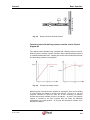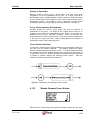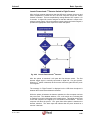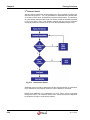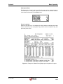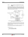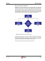
1
Volume 2 Basic Operation BASIC OPERATION Contents of Volume 2 Figures of Volume 2 ......................................................................................................... vi About Our Company ........................................................................................................ix Contacting Our Corporate Headquarters .......................................................................ix Getting User Support ................................................................................................................ ix About the Flow Computer Applications ..........................................................................x About the User Manual .....................................................................................................x Target Audience......................................................................................................................... x Manual Structure....................................................................................................................... xi Conventions Used in this Manual .............................................................................................xii Trademark References ............................................................................................................ xiii Copyright Information and Modifications Policy .......................................................................xiv Warranty, Licenses and Product Registration ............................................................. xiv All 74 06/07 ® i OMNI 6000 / OMNI 3000 User Manual Contents of Volume 2 1. Basic Operating Features ....................................................................................... 1-1 1.1. Overview of the Keypad Functions ..................................................................... 1-1 1.2. Operating Modes .................................................................................................. 1-2 1.2.1. 1.2.2. 1.2.3. 1.2.4. Display Mode ............................................................................................................. 1-2 Keypad Program Mode .............................................................................................. 1-2 Diagnostic and Calibration Mode ............................................................................... 1-2 Field Entry Mode ........................................................................................................ 1-2 1.3. Special Keys ......................................................................................................... 1-4 1.3.1. 1.3.2. 1.3.3. 1.3.4. 1.3.5. 1.3.6. Display/Enter (Help) Key ............................................................................................ 1-4 Up/Down Arrow Keys []/[]..................................................................................... 1-4 Left/Right Arrow Keys []/[] ................................................................................... 1-4 Alpha Shift Key and LED............................................................................................ 1-4 Program/Diagnostic Key [Prog/Diag] ......................................................................... 1-5 Space/Clear (Cancel/Ack) Key .................................................................................. 1-5 1.4. Adjusting the Display ........................................................................................... 1-5 1.5. Clearing and Viewing Alarms .............................................................................. 1-6 1.5.1. 1.5.2. 1.5.3. Acknowledging (Clearing) Alarms .............................................................................. 1-6 Viewing Active and Historical Alarms ......................................................................... 1-6 Alarm Conditions Caused by Static Discharges ........................................................ 1-6 1.6. Computer Totalizing............................................................................................. 1-6 2. PID Control Functions ............................................................................................ 2-1 2.1. Overview of PID Control Functions .................................................................... 2-1 2.2. PID Control Displays ............................................................................................ 2-2 2.3. Changing the PID Control Operating Mode ........................................................ 2-3 2.3.1. 2.3.2. 2.3.3. 2.3.4. 2.3.5. Manual Valve Control ................................................................................................. 2-3 Automatic Valve Control ............................................................................................ 2-3 Local Setpoint Select ................................................................................................. 2-4 Remote Setpoint Select ............................................................................................. 2-4 Changing the Secondary Variable Setpoint ............................................................... 2-4 2.4. PID Control Remote Setpoint .............................................................................. 2-4 2.5. Using the PID Startup and Shutdown Ramping Functions ............................... 2-5 2.6. Startup Ramp/Shutdown Ramp/Minimum Output Percent ............................... 2-5 2.7. PID Control Tuning............................................................................................... 2-6 2.7.1. 2.7.2. ii Estimating the Required Controller Gain For Each Process Loop ............................. 2-6 Estimating the Repeats / Minutes and Fine Tuning the Gain .................................... 2-7 ® All 74 06/07 Volume 2 Basic Operation 2.8. PID Control ........................................................................................................... 2-7 2.8.1. 2.8.2. 2.8.3. 2.8.4. 2.8.5. 2.8.6. 2.8.7. 2.8.8. 2.8.9. 2.8.10. 2.8.11. The two most common control applications are ........................................................ 2-8 Primary Variable Configuration Entries .................................................................... 2-10 Secondary Variable Configuration Entries ............................................................... 2-11 Control Output Tag .................................................................................................. 2-12 Primary Gain ............................................................................................................ 2-13 Secondary Gain (use percentages in graphic)......................................................... 2-13 Repeats per Minute.................................................................................................. 2-13 Startup and Shutdown Ramping .............................................................................. 2-15 Minimum Ramp to % ............................................................................................... 2-15 Primary Remote Setpoint Limits .............................................................................. 2-16 Closing Notes:.......................................................................................................... 2-19 3. Computer Batching Operations ............................................................................ 3-1 3.1. Introduction.......................................................................................................... 3-1 3.2. Batch Status......................................................................................................... 3-1 3.3. Common Batch Stack Selected „N‟ ..................................................................... 3-1 3.4. Common Batch Stack Selected „Y‟ ..................................................................... 3-2 3.5. Batch Schedule Stack ......................................................................................... 3-2 3.5.1. 3.5.2. Editing the Batch Stack „Manually‟ ............................................................................. 3-2 Editing the Batch Stack via „Omnicom‟ ...................................................................... 3-3 3.6. Ending a Batch .................................................................................................... 3-4 3.6.1. 3.6.2. Ending a Batch with Windows Omnicom ................................................................... 3-5 Using the Product Change Strobes to End a Batch ................................................... 3-6 3.7. Recalculate and Reprint a Previous Batch Ticket ............................................. 3-7 3.8. Batch Preset Counters ........................................................................................ 3-8 3.8.1. 3.8.2. Batch Preset Flags..................................................................................................... 3-8 Batch Warning Flags ................................................................................................. 3-8 3.9. Adjusting the Size of a Batch.............................................................................. 3-8 3.10. Automatic Batch Changes Based on Product Interface Detection .................. 3-9 4. Specific Gravity/Density Rate of Change ............................................................. 4-1 4.1. Specific Gravity/Density Rate of Change Alarm Flag ........................................ 4-1 4.2. Delayed Specific Gravity/Density Rate of Change Alarm Flag ......................... 4-1 4.3. Determining the Gravity Rate of Change Limits ................................................ 4-2 All 74 06/07 ® iii OMNI 6000 / OMNI 3000 User Manual Contents of Volume 2 5. Meter Factors ........................................................................................................... 5-1 5.1. Changing Meter Factors ...................................................................................... 5-1 5.2. Changing Meter Factors for the Running Product............................................. 5-2 5.3. Previous Meter Factor Saved data ...................................................................... 5-2 5.4. Meter Factor entries on Revision 22/26 .............................................................. 5-2 6. Proving Functions ................................................................................................... 6-1 6.1. Prover Menu Setup: ............................................................................................. 6-1 6.1.1. 6.1.2. 6.1.3. 6.1.4. 6.1.5. 6.1.6. 6.1.7. 6.1.8. 6.1.9. 6.1.10. 6.1.11. 6.1.12. 6.1.13. 6.1.14. 6.1.15. 6.1.16. 6.1.17. 6.1.18. 6.1.19. 6.1.20. 6.1.21. 6.1.22. 6.1.23. 6.1.24. iv Prover Menu Entries: ................................................................................................. 6-2 Master Meter Proving:................................................................................................ 6-3 OverTravel (Barrels/m3) ............................................................................................ 6-4 Prover Diameter ......................................................................................................... 6-4 Prover Wall Thickness ............................................................................................... 6-4 Modulus of Elasticity Thermal Expansion .................................................................. 6-4 Thermal Expansion Coefficient .................................................................................. 6-5 Base Pressure ........................................................................................................... 6-5 Base Temperature ..................................................................................................... 6-5 Run Repeatability based on Meter Factor or Counts ................................................. 6-6 Run Repeatability Maximum Deviation ...................................................................... 6-7 Inactivity Timer ........................................................................................................... 6-8 Stability Check entries ............................................................................................. 6-10 Stability Sample Time (Secs) ................................................................................... 6-11 Sample Delta Temperature ...................................................................................... 6-11 Sample Delta Flowrate............................................................................................. 6-11 Meter-Prover Temp Deviation .................................................................................. 6-11 Density Stability Time (Seconds) ............................................................................. 6-12 Meter Factor Implementation Entries: ...................................................................... 6-12 Compact Prover Entries ........................................................................................... 6-14 Brooks Compact Prover Entries .............................................................................. 6-15 Setup Entries, Auto Proving ..................................................................................... 6-17 Unidirectional Prove Operation ................................................................................ 6-20 Types of Provers using Double Chronometry Proving ............................................. 6-26 ® All 74 06/07 Volume 2 Basic Operation 7. Pulse Fidelity Checking ......................................................................................... 7-1 7.1. Overview .............................................................................................................. 7-1 7.2. Installation Practices ........................................................................................... 7-1 7.3. How the Flow Computer performs Fidelity Checking ....................................... 7-1 7.4. Correcting Errors ................................................................................................. 7-2 7.5. Common Mode Electrical Noise and Transients ............................................... 7-2 7.6. Noise Pulse Coincident with an Actual Flow Pulse .......................................... 7-2 7.7. Total Failure of a Pulse Channel......................................................................... 7-2 7.8. Alarms and Displays............................................................................................ 7-3 7.9. Max Good Pulses ................................................................................................. 7-3 7.10. Delay Cycle........................................................................................................... 7-3 8. Printed Reports ....................................................................................................... 8-1 8.1. Fixed Format Reports ............................................................................................ 8-1 8.2. Default Report Templates and Custom Reports ................................................ 8-2 8.3. Printing Reports .................................................................................................. 8-2 8.4. Audit Trail ............................................................................................................. 8-3 8.4.1. Audit Trail Report ....................................................................................................... 8-3 8.4.2. Modbus Port Passwords and the Audit Trail Report ............................................... 8-3 9. Index of Display Variables ..................................................................................... 9-1 All 74 06/07 ® v OMNI 6000 / OMNI 3000 User Manual Contents of Volume 2 Figures of Volume 2 Fig. 1-1. Flow Computer Front Panel Keypad.......................................................................................... 1-1 Fig. 1-2. Block Diagram Showing the Keypad and Display Modes .......................................................... 1-3 Fig. 2-1. Typical PID Control Application - Single Loop ........................................................................... 2-1 Fig. 2-2. Backpressure Control ................................................................................................................ 2-7 Fig. 2-3. Backpressure Control ................................................................................................................ 2-8 Fig. 2-4. Primary/Secondary Control........................................................................................................ 2-8 Fig. 2-5. Delivery Pressure Override Control ........................................................................................... 2-9 Fig. 2-6. Primary / Secondary Control...................................................................................................... 2-9 Fig. 2-7. PID Configuration Entries ........................................................................................................ 2-10 Fig. 2-8 PID Tuning Adjust Entries ....................................................................................................... 2-12 Fig. 2-9 PID ramping Functions ............................................................................................................ 2-14 Fig. 2-10 PID Tuning Adjust Entries ........................................................................................................ 2-15 Fig. 2-11 Primary Remote Setpoint Limits .............................................................................................. 2-16 Fig. 2-12 PID Tuning Adjust Entries ........................................................................................................ 2-16 Fig. 2-13 Primary Variable PID Setup Entries ......................................................................................... 2-17 Fig. 2-14 Fullscale Entries ....................................................................................................................... 2-18 Fig. 2-15 Primary and Secondary Variable Scaling ................................................................................. 2-18 Fig. 6-1 Prover Setup Entries ................................................................................................................. 6-2 Fig. 6-2 Master Meter Proving ................................................................................................................ 6-3 Fig. 6-3 Example 1 of Run Repeatability ................................................................................................ 6-7 Fig. 6-4 Example 2 of Run Repeatability ................................................................................................ 6-8 Fig. 6-5 Example 2 of Run Repeatability ................................................................................................ 6-9 Fig. 6-6 Flow rate & temperature are stable. Prove sequence may begin.............................................. 6-9 Fig. 6-7 Stability Check Entries. ............................................................................................................ 6-10 Fig. 6-8 Stability Sample Time .............................................................................................................. 6-11 Fig. 6-9 Two batches with the prove done between the batches. One retroactively uses the new meter factor while the other uses the old. ......................................................... 6-13 Fig. 6-10 Two batches with the prove occurring between the batches using a new meter factors. ....... 6-14 Fig. 6-11 Two batches with the prove occurring between the batches using a new meter factors. ....... 6-14 Fig. 6-12 Downstream and Upstream Volume setups. ........................................................................... 6-15 Fig. 6-13 Plenum Pressure Constants .................................................................................................... 6-16 Fig. 6-14 Diagram shows venting and charging the plenum pressure ................................................... 6-17 Fig. 6-15 Varaibles required to initiate an Auto Prove ............................................................................ 6-18 Fig. 6-16 The Omni calculating meter factor and verifying prover status ............................................... 6-19 Fig. 6-18 Prove Request Sequence ........................................................................................................ 6-21 vi ® All 74 06/07 Volume 2 Basic Operation Fig. 6-19 Check Stability ......................................................................................................................... 6-22 st Fig. 6-20 Launch Forward and 1 Detector ............................................................................................ 6-23 Fig. 6-21 2nd Detector Switch ................................................................................................................ 6-24 Fig. 6-22 Example of a Meter Proving Report upon completion of a prove. ........................................... 6-25 Fig. 6-23 Double Chronometry Timing Diagram (Note: The interpolated number of pulses N1 is equal to NM (Tdvol/Tdfmp) ................................................................................. 6-26 Fig. 6-24 After Run Prove Permissive Diagram ...................................................................................... 6-27 Fig. 6-25 Set the overtravel entry to zero to minimize the prove sequence time .................................... 6-28 All 74 06/07 ® vii Volume 2 Basic Operation About Our Company Measure the Difference! OMNI flow computers Our products are currently being used world-wide at: Offshore oil and gas production facilities Crude oil, refined products, LPG, NGL and gas transmission lines Storage, truck and marine loading/offloading terminals Refineries; petrochemical and cogeneration plants. OMNI Flow Computers, Inc. is the world‟s leading manufacturer and supplier of panel-mount custody transfer flow computers and controllers. Our mission is to continue to achieve higher levels of customer and user satisfaction by applying the basic company values: our people, our products and productivity. Our products have become the international flow computing standard. OMNI Flow Computers pursues a policy of product development and continuous improvement. As a result, our flow computers are considered the “brain” and “cash register” of liquid and gas flow metering systems. Our staff is knowledgeable and professional. They represent the energy, intelligence and strength of our company, adding value to our products and services. With the customer and user in mind, we are committed to quality in everything we do, devoting our efforts to deliver workmanship of high caliber. Teamwork with uncompromising integrity is our lifestyle. Contacting Our Corporate Headquarters OMNI Flow Computers, Inc. 12620 West Airport Ste #100 Sugar Land Texas 77478 Phone: 281-240-6161 Fax: 281-240-6162 World-wide Web Site: http://www.omniflow.com E-mail Addresses: [email protected] Getting User Support Technical and sales support is available world-wide through our corporate or authorized representative offices. If you require user support, please contact the location nearest you (see insert) or our corporate offices. Our staff and representatives will enthusiastically work with you to ensure the sound operation of your flow computer. All 74 06/07 ® ix OMNI 6000 / OMNI 3000 User Manual For Your Information About the Flow Computer Applications OMNI 6000 and OMNI 3000 Flow Computers are integrable into the majority of liquid and gas flow measurement and control systems. The current firmware revisions of OMNI 6000/OMNI 3000 Flow Computers are: 20.74/24.74: Turbine/Positive Displacement/Coriolis Liquid Flow Metering Systems with K Factor Linearization (US/metric units) 21.74/25.74: Orifice/Differential Pressure Liquid Flow Metering Systems (US/metric units) 22.74/26.74: Turbine/Positive Displacement Liquid Flow Metering Systems with Meter Factor Linearization (US/metric units) 23.74/27.74: Orifice/Turbine Gas Flow Metering Systems (US/metric units) About the User Manual This manual applies to .74+ firmware revisions of OMNI 6000 and OMNI 3000 Flow Computers. It is structured into 4 volumes and is the principal part of your flow computer documentation. Target Audience As a user‟s reference guide, this manual is intended for a sophisticated audience with knowledge of liquid and gas flow measurement technology. Different user levels of technical know-how are considered in this manual. You need not be an expert to operate the flow computer or use certain portions of this manual. However, some flow computer features require a certain degree of expertise and/or advanced knowledge of liquid and gas flow instrumentation and electronic measurement. In general, each volume is directed towards the following users: Volume 1. System Architecture and Installation Installers System/Project Managers Engineers/Programmers Advanced Operators Operators Volume 2. Basic Operation All Users Volume 3. Configuration and Advanced Operation Engineers/Programmers Advanced Operators Volume 4. Modbus Database Addresses and Index Numbers Engineers/Programmers Advanced Operators x ® All 74 06/07 Volume 2 Basic Operation Manual Structure The User Manual comprises 5 volumes; each contained in separate binding for easy manipulation. You will find a detailed table of contents at the beginning of each volume. Volume 1. System Architecture and Installation Volume 1 is generic to all applications and considers both US and metric units. This volume describes: Basic hardware/software features Installation practices Calibration procedures Flow computer specifications Volume 2. Basic Operation User Reference Documentation - The User Manual is structured into five volumes. Volumes 1 and 5 are generic to all flow computer application revisions. Volumes 2, 3 and 4 are application specific. These have four versions each, published in separate documents; i.e., one per application revision per volume. The volumes respective to each application revision are: Revision 20/2474: Volume #s 3a, 4a Revision 21/25.74: Volume #s 3b, 4b Revision 22/26.74: Volume #s 3c, 4c Revision 23/27.74: Volume #s 3d, 4d For example, if your flow computer application revision is 20/2474, you will be supplied with Volumes 2a, 3a & 4a, along with Volumes 1, 2, & 5. This volume is generic to all applications and considers both US and metric units. It covers the essential and routine tasks and procedures that may be performed by the flow computer operator. General computer-related features are described, such as: The application-related topics may include: Batching operations Proving functions PID control functions Audit trail Other application specific functions Depending on your application, some of these topics may not be included in your specific documentation. An index of display variables and corresponding key press sequences that are specific to your application are listed at the end of each version of this volume. Volume 3. Configuration and Advanced Operation Volume 3 is intended for the advanced user. It refers to application specific topics and is available in four separate versions (one for each application revision). This volume covers: All 74 06/07 Overview of keypad functions Adjusting the display Clearing and viewing alarms Computer totalizing Printing and customizing reports Application overview Flow computer configuration data entry User-programmable functions Modbus Protocol implementation Flow equations and algorithms ® xi OMNI 6000 / OMNI 3000 User Manual Volume 4. Modbus For Your Information Database Addresses and Index Numbers Volume 4 is intended for the system programmer (advanced user). It comprises a descriptive list of database point assignments in numerical order, within our firmware. This volume is application specific, for which there is one version per application revision. Technical Bulletins Manual Updates and Technical Bulletins – They contain updates to the user manual. You can view and print updates from our website: http://www.omniflow.com Technical bulletins that contain important complementary information about your flow computer hardware and software. Each bulletin covers a topic that may be generic to all applications or specific to a particular revision. They include product updates, theoretical descriptions, technical specifications, procedures, and other information of interest. This is the most dynamic and current volume. Technical bulletins may be added to this volume after its publication. You can view and print these bulletins from our website. Conventions Used in this Manual Typographical Conventions - These are standard graphical/text elements used to denote types of information. For your convenience, a few conventions were established in the manual‟s layout design. These highlight important information of interest to the reader and are easily caught by the eye. Several typographical conventions have been established as standard reference to highlight information that may be important to the reader. These will allow you to quickly identify distinct types of information. CONVENTION USED Sidebar Notes / InfoTips Example: INFO - Sidebar notes are used to highlight important information in a concise manner. Keys / Key Press Sequences Example: [Prog] [Batch] [Meter] [n] Screen Displays Example: xii DESCRIPTION Sidebar notes or “InfoTips” consist of concise information of interest which is enclosed in a grayshaded box placed on the left margin of a page. These refer to topics that are either next to them, or on the same or facing page. It is highly recommended that you read them. Keys on the flow computer keypad are denoted with brackets and bold face characters (e.g.: the „up arrow‟ key is denoted as []). The actual function of the key as it is labeled on the keypad is what appears between brackets. Key press sequences that are executed from the flow computer keypad are expressed in a series of keys separated by a space (as shown in the example). Sample screens that correspond to the flow computer display appear surrounded by a dark gray border with the text in bold face characters and mono-spaced font. The flow computer display is actually 4 lines by 20 characters. Screens that are more than 4 lines must be scrolled to reveal the text shown in the manual. ® All 74 06/07 Volume 2 Basic Operation CONVENTION USED Headings Example: 2. Chapter Heading 2.3. Section Heading 2.3.1. Subsection Heading Figure Captions Example: Fig. 2-3. Figure No. 3 of Chapter 2 Page Numbers Example: 2-8 Application Revision and Effective Publication Date Examples: All.74 07/06 20/24.74 07/06 21/25.74 07/06 22/26.74 07/06 23/27.74 07/06 DESCRIPTION Sequential heading numbering is used to categorize topics within each volume of the User Manual. The highest heading level is a chapter, which is divided into sections, which are likewise subdivided into subsections. Among other benefits, this facilitates information organization and cross-referencing. Figure captions are numbered in sequence as they appear in each chapter. The first number identifies the chapter, followed by the sequence number and title of the illustration. Page numbering restarts at the beginning of every chapter and technical bulletin. Page numbers are preceded by the chapter number followed by a hyphen. Technical bulletins only indicate the page number of that bulletin. Page numbers are located on the outside margin in the footer of each page. The contents of Volume 1 and Volume 5 are common to all application revisions and are denoted as All.74. Content of Volumes 2, 3 and 4 are application specific and are identified with the application number. These identifiers are included on every page in the inside margin of the footer, opposite the page number. The publication/effective date of the manual follows the application identification. The date is expressed as month/year (e.g.: July 2006 is 07/06). Trademark References The following are trademarks of OMNI Flow Computers, Inc.: OMNI 3000 OMNI 6000 OmniCom Other brand, product and company names that appear in this manual are trademarks of their respective owners. All 74 06/07 ® xiii OMNI 6000 / OMNI 3000 User Manual For Your Information Copyright Information and Modifications Policy This manual is copyright protected. All rights reserved. No part of this manual may be used or reproduced in any form, or stored in any database or retrieval system, without prior written consent of OMNI Flow Computers, Inc., Stafford, Texas, USA. Making copies of any part of this manual for any purpose other than your own personal use is a violation of United States copyright laws and international treaty provisions. OMNI Flow Computers, Inc., in conformance with its policy of product development and improvement, may make any necessary changes to this document without notice. Warranty, Licenses and Product Registration Product warranty and licenses for use of OMNI flow computer firmware and of OmniCom Configuration PC Software are included in the first pages of each Volume of this manual. We require that you read this information before using your OMNI flow computer and the supplied software and documentation. Important! If you have not done so already, please complete and return to us the product registration form included with your flow computer. We need this information for warranty purposes, to render you technical support and serve you in future upgrades. Registered users will also receive important updates and information about their flow computer and metering system. Copyright 1991-2007 by OMNI Flow Computers, Inc. All Rights Reserved. xiv ® All 74 06/07 Volume 2 Basic Operation 1. Basic Operating Features 1.1. Overview of the Keypad Functions INFO - Within the document the following convention is used to describe various key press sequences: Individual keys are shown in bold enclosed in brackets and separated by a space. Although not always indicated, it is assumed for the rest of this document that the [Display/Enter] key is used at the end of every key press sequence to enter a command. Thirty-four keys are available. Eight special function keys and twenty-six dedicated to the alphanumeric characters A through Z, 0 through 9 and various punctuation and math symbols. The [Display/Enter] key, located at the bottom right, deserves special mention. This key is always used to execute a sequence of key presses. It is not unlike that the „Enter‟ key of a personal computer. Except when entering numbers in a field, the maximum number of keys that can be used in a key press sequence is four (not counting the [Display/Enter] key). Fig. 1-1. All 74 06/07 Flow Computer Front Panel Keypad ® 1-1 Chapter 1 Basic Operating Features Key words such as „Density‟, „Mass‟ and „Temp‟ appear over each of the alphanumeric keys. These key words indicate what data will be accessed when included in a key press sequence. Pressing [Net] [Meter] [1] for instance will display net flow rates and total accumulations for Meter Run #1. Pressing the [Net] key causes net flow rates and total accumulations for all active meter runs to be displayed. In many instances, the computer attempts to recognize similar key press sequences as meaning the same thing; i.e., [Net] [1], [Meter] [1] [Net] and [Net] [Meter] [1] all cause the net volume data for Meter Run #1 to be displayed. In most cases, more data is available on a subject then can be displayed on four lines. The []/[] (up/down) arrow keys allow you to scroll through multiple screens. 1.2. Operating Modes Keyboard operation and data displayed in the LCD display depends on which of the 3 major display and entry modes are selected. 1.2.1. Display Mode This is the normal mode of operation. Live meter run data is displayed and updated every 200 msec. Data cannot be changed while in this mode. 1.2.2. Keypad Program Mode Configuration data needed by the flow computer can be viewed and changed via the keypad while in this mode. When the Program Mode is entered by pressing the [Prog] key, the Program LED glows green. This changes to red when a valid password is requested and entered. 1.2.3. Diagnostic and Calibration Mode The diagnostic and calibration features of the computer are accessed by pressing the [Diag] key ([Alpha Shift] then [Prog]. This mode allows you to check and adjust the calibration of each input and output point. The Diagnostic LED glows green until a valid password is requested and entered. 1.2.4. Field Entry Mode You are in this mode whenever the data entry cursor is visible, which is anytime the user is entering a number or password while in the Program Mode or Diagnostic Mode. 1-2 ® All 74 06/07 Volume 2 Basic Operation Fig. 1-2. All 74 06/07 Block Diagram Showing the Keypad and Display Modes ® 1-3 Chapter 1 Basic Operating Features 1.3. Special Keys 1.3.1. Display/Enter (Help) Key This key is located bottom-right on the keypad. Pressing once while in the Field Entry Mode will store the data entered in the field to memory. Pressing twice within one second will cause the contextsensitive Help to be displayed. The Help displays contain useful information regarding available variable assignments and selections. When in other modes, use it at the end of a key press sequence to enter the command. 1.3.2. Up/Down Arrow Keys []/[] These keys are located top-center on the keypad. When in the Display Mode, the []/[] keys are used to scroll through data relevant to a particular selection. When in the Program Mode, they are used to scroll through data and position the cursor on data to be viewed or changed. In the Diagnostic Mode, The up/down arrow keys are initially used to position the cursor within the field of data being changed. Once you select an input or output to calibrate or adjust, the up/down arrow keys are used as a software „zero‟ potentiometer. 1.3.3. Left/Right Arrow Keys []/[] These keys are located top-center on the keypad; to the left and right respectively of the Up/Down Arrow Keys. The []/[] keys have no effect while in the Display Mode. When in Program Mode, they are used to position the cursor within a data field. In the Diagnostic Mode, they are initially used to position the cursor within the field of data to be changed. Once you select an input or output to calibrate or adjust, the left/right arrow keys are used as software „span‟ potentiometer. 1.3.4. Alpha Shift Key and LED This key is located top-right on the keypad. Pressing the [Alpha Shift] key while in the Field Entry Mode causes the Alpha Shift LED above the key to glow green, indicating that the next valid key press will be interpreted as its shifted value. The Alpha Shift LED is then turned off automatically when the next valid key is pressed. Pressing the [Alpha Shift] key twice causes the Alpha Shift LED to glow red and the shift lock to be active. All valid keys are interpreted as their shifted value until the [Alpha Shift] key is pressed or the [Display/Enter] key is pressed. When in the Calibrate Mode, zero and span adjustments made via the arrow keys are approximately ten times more sensitive when the Alpha Shift LED is on. 1-4 ® All 74 06/07 Volume 2 Basic Operation 1.3.5. Program/Diagnostic Key [Prog/Diag] This key is located top-left on the keypad. While in the Display Mode, pressing this key changes the operating mode to either the Program or Diagnostic Mode, depending on whether the Alpha Shift LED is on. When in other modes, it cancels the current entry and goes back one menu level, eventually returning to the Display Mode. 1.3.6. Space/Clear (Cancel/Ack) Key This key is located bottom-left on the keypad. Static Discharges - It has been found that applications of electrostatic discharges may cause the Active Alarm LED to glow red. Pressing the [Space/Clear] key will acknowledge the alarm and turn off the red alarm light. Pressing this key while in the Display Mode acknowledges any new alarms that occur. The Active Alarm LED will also change from red to green indicating an alarm condition exists but has been acknowledged. When in the Field Entry Mode, unshifted, it causes the current variable field being changed to be cleared, leaving the cursor at the beginning of the field awaiting new data to be entered. With the Alpha Shift LED illuminated, it causes the key to be interpreted as a space or blank. When in all other modes, it cancels the current key press sequence by flushing the key input buffer. 1.4. Adjusting the Display Once the computer is mounted in its panel you may need to adjust the viewing angle and backlight intensity of the LCD display for optimum performance. You may need to re-adjust the brightness setting of the display should the computer be subjected to transient electrical interference. While in the Display Mode (Program LED and Diagnostic LED off), press [Setup] [Display] and follow the displayed instructions: All 74 06/07 ® 1-5 Chapter 1 Basic Operating Features 1.5. Clearing and Viewing Alarms TIP - Alarm flags are latched while the red LED is on. To avoid missing intermittent alarms, always press [Alarms] [Display] to view alarms before pressing [Cancel/Ack]. 1.5.1. Acknowledging (Clearing) Alarms New alarms cause the Active Alarm LED to glow red. Pressing the [Cancel/Ack] key (bottom left), or setting Boolean Point 1712 via a digital I/O point or via a Modbus command, will acknowledge the alarm and cause the Active Alarm LED to change to green. The LED will go off when the alarm condition clears. 1.5.2. Viewing Active and Historical Alarms To view all active alarms, press [Alarms] [Display] and use the []/[] arrow keys to scroll through all active alarms. The last 500 time-tagged alarms that have occurred are always available for printing (see Historical Alarm Snapshot Report in this chapter). 1.5.3. Alarm Conditions Caused by Static Discharges It has been found that applications of electrostatic discharges may cause the Active Alarm LED to glow red. Pressing the [Space/Clear] key will acknowledge the alarm and turn off the red alarm light. 1.6. Computer Totalizing Two types of totalizers are provided: 1) Three front panel electromechanical and non-resetable; and 2) Software totalizers maintained in computer memory. The electromechanical totalizers can be programmed to count in any units via the Miscellaneous Setup Menu (Volume 3). The software totalizers provide batch and daily based totals, and are automatically printed, saved and reset at the end of each batch or the beginning of each contract day. Daily flow or time weighted averages are also printed, saved and reset at the end of each day. Batch flow weighted averages are also available in liquid application flow computers. Software cumulative totalizers are also provided and can only be reset via the Password Maintenance Menu (Volume 3). View the software totalizers by pressing [Gross], [Net] or [Mass]. Pressing [Meter] [n] [Gross], [Net] or [Mass] will display the software for Meter Run „n‟. 1-6 ® All 74 06/07 Volume 2 Basic Operation 2. PID Control Functions 2.1. Overview of PID Control Functions Four independent control loops are available. Each loop is capable of controlling a primary variable (usually flow rate) with a secondary override variable (usually meter back pressure or delivery pressure). The primary and secondary set points can be adjusted locally via the keypad and remotely via a communication link. In addition, the primary set point can be adjusted via an analog input to the computer. Contact closures can be used to initiate the startup and shutdown ramp function which limits the control output slew rate during startup and shutdown conditions. A high or low 'error select' function causes automatic override control by the secondary variable in cases where it is necessary either to maintain a minimum secondary process value or limit the secondary process maximum value. Local manual control of the control output and bumpless transfer between automatic and manual control is incorporated. Fig. 2-1. All 74 06/07 Typical PID Control Application - Single Loop ® 2-1 Chapter 2 PID Control Functions 2.2. PID Control Displays INFO - Select PID Loop 1 through 4 by entering „n‟ as 1, 2, 3 or 4. While in the Display Mode press [Control] [n] [Display]. Press the Up/Down arrow keys to display the following screens: Screen #1 Indicates which parameter is being controlled; primary or secondary Screen #2 Shows actual primary set point being used in engineering units Screen #3 Shows actual secondary set point being used in engineering units Screen #4 INFO - Data such as set points or operating mode cannot be changed while in the Display Mode. 2-2 ® All 74 06/07 Volume 2 Basic Operation 2.3. Changing the PID Control Operating Mode INFO - Select PID Loop 1 through 4 by entering „n‟ as 1, 2, 3 or 4. To access the next two screens you must enter the [Y] to select Manual Valve or Local Setpoint even if a „Y‟ is already displayed. To cancel the Manual Mode or Local Setpoint Mode, enter [N]. Press [Prog] [Control] [n] to display the following screen: 2.3.1. Manual Valve Control To change to manual valve control enter [Y] at the 'Manual Valve (Y/N)' prompt and the following screen is displayed: Primary Variable (Measurement in engineering units) The switch from Auto to Manual is bumpless. Use the Up/Down arrow keys to open or close the valve. Press [Prog] once to return to the previous screen. Notice you are now in Manual Valve Control 2.3.2. Automatic Valve Control To change from manual to automatic valve control, enter [N] at the 'Manual Valve (Y/N)' prompt. The switch to automatic is bumpless, if a local setpoint is selected. All 74 06/07 ® 2-3 Chapter 2 PID Control Functions 2.3.3. Local Setpoint Select Enter [Y] at the 'Local Set. Pt. (Y/N)' prompt and the following screen is displayed: Primary Variable (Measurement in engineering units) The switch from Remote to Local is bumpless. Use the Up/Down arrow keys to increase or decrease the setpoint. Press [Prog] once to return to the previous screen. Notice you are now in Automatic with Local Valve Control Change the setpoint of the secondary variable here 2.3.4. Remote Setpoint Select To change from a local setpoint to a remote setpoint, enter [N] at the „Local Set. Pt.(Y/N)‟ prompt. The switch to remote setpoint may not be bumpless, depending upon the remote set point source. 2.3.5. Changing the Secondary Variable Setpoint Move the cursor to the bottom line of the above display, press [Clear] and then enter the new setpoint. 2.4. PID Control Remote Setpoint IMPORTANT! You must assign a remote setpoint input even if one will not be used. The 420mA scaling of this input determines the scaling of the primary controlled variable. 2-4 As described above, the PID control loop can be configured to accept either a local setpoint or a remote setpoint value for the primary variable. The remote setpoint is derived from an analog input (usually 4-20 mA). This input is scaled in engineering units and would usually come from another device such as an RTU. High/Low limits are applied to the remote setpoint signal to eliminate possible problems of over or under speeding a turbine meter (see Volume 1, Chapter 8 for more details). ® All 74 06/07 Volume 2 Basic Operation 2.5. Using the PID Startup and Shutdown Ramping Functions These functions are enabled when a startup and/or shutdown ramp rate between 0 and 99 percent is entered (see section „PID Setup‟ in Volume 3). Commands are provided to „Start‟ the valve ramping open, „Shutdown‟ to the minimum percent open valve or „Stop‟ the flow by closing the valve immediately once it has been ramped to the minimum percent open. These commands are accessed using the keypad by pressing [Prog] [Batch] [Meter] [n], which will display the following: 2.6. Startup Ramp/Shutdown Ramp/Minimum Output Percent Inputs are provided for startup/shutdown ramp rates and minimum output % settings. When these startup/shutdown ramp rates are applied the control output, movements will be limited to the stated % movement per ½ second (see Volume 3). On receipt of a shutdown signal, the output will ramp to the minimum output % for topoff purposes. All 74 06/07 ® 2-5 Chapter 2 PID Control Functions 2.7. PID Control Tuning IMPORTANT! PID Control Tuning - The primary variable must be tuned first. When tuning the primary variable loop, you must set the secondary setpoint high or low enough to the point where it will not take control. Otherwise, the PID loop will become very unstable and virtually impossible to tune. Adjust the primary gain and integral repeats per minute until you achieve stable control. Likewise, when tuning the secondary setpoint, the primary must be set so it cannot interfere. Once you have achieved stable control of both loops, you can then enter the setpoints established for each loop at normal operating conditions. Individual control of gain and integral action are provided for both the primary and secondary control loops. Tune the primary variable loop first by setting the secondary setpoint high or low enough to stop the secondary control loop from taking control. Adjust the primary gain and integral repeats per minutes for stable control. Reset the primary and secondary set points to allow control on the secondary variable without interference from the primary variable. Adjust the secondary gain and integral repeats per minute for stable control of the secondary variable. 2.7.1. Estimating the Required Controller Gain For Each Process Loop Each process loop will exhibit a gain function. A change in control valve output will produce a corresponding change in each of the process variables. The ratio of these changes represents the gain of the loop (For example: If a 10 % change in control output causes a 10% change in the process variable, the loop gain is 1.0. If a 10 % change in control output causes a 20 % change in process variable, the loop gain is 2.0). To provide stable control the gain of each loop with the controller included must be less than 1.0. In practice the controller gain is usually adjusted so that the total loop gain is between 0.6 and 0.9. Unfortunately the gain of each loop can vary with operating conditions. For example: A butterfly control valve may have a higher gain when almost closed to when it is almost fully open. This means that in many cases the controller gain must be set low so that stable control is achieved over the required range of control. To estimate the gain of each loop, proceed as follows for the required range of operating conditions: (1) In manual, adjust the control output for required flowing conditions and note process variable values. (2) Make a known percentage step change of output (i.e., from 20% to 22% equals a 10% change). 3 (3) Note the percentage change of each process variable (i.e., 100 m /hr to 3 110 m /hr equals a 10% change). INFO - The primary gain interacts with the secondary gain. The actual secondary gain factor is the product of the primary gain and secondary gain factors. 2-6 (1) Primary Gain Estimate = 0.75 / (Primary Loop Gain). (2) Secondary Gain = 0.75 / (Secondary Loop Gain x Primary Gain Estimate). ® All 74 06/07 Volume 2 Basic Operation 2.7.2. Estimating the Repeats / Minutes and Fine Tuning the Gain (1) Set the 'repeats / minute' to 40 for both primary and secondary loops. (2) Adjust set points so that only the primary (sec) loop is trying to control. (3) While controlling the primary (sec) variable, increase the primary (sec) gain until some controlled oscillation is observed. (4) Set the primary (sec) 'repeats/minute' to equal 0.75 / (Period of the oscillation in minutes). (5) Set the primary (sec) gain to 75% of the value needed to make the loop oscillate. (6) Repeat (2) through (5) for the secondary variable loop. 2.8. PID Control PID control may be used to position valves and adjust pump motor speeds. Information provided in previous modules, discussed how to adjust the PID output and setpoints. Before output and setpoint adjustments can be made to the PID loops, the configuration and setup entries must be programmed into the flow computer. PID control loops attempt to control a primary process variable, such as flow, by outputting an analog signal to control equipment such as a valve or variable speed pump. The flow computer is also capable of controlling a secondary variable, such as pressure under certain circumstances. The setpoint for the primary variable may either be adjusted locally using the keypad up and down arrow keys or remotely via a live analog input from another device. The primary variable controller incorporates bumpless transfer when switching between manual and automatic. Bumpless transfer is normally needed when controlling flowrate. Bumpless transfer is not provided for the secondary variable controller Fig. 2-2. All 74 06/07 Backpressure Control ® 2-7 Chapter 2 PID Control Functions 2.8.1. The two most common control applications are Fig. 2-3. Backpressure Control Flowrate control while maintaining a minimum backpressure Control Diagram #1 Accurate liquid measurement requires that the fluid being measured remains in the liquid state. To ensure this, backpressure on the meter must be maintained above the liquid‟s equilibrium vapor pressure. In this diagram, opening the control valve will increase the flowrate through the flow meter and decrease the backpressure on the flow meter. Adjusting the control valve simultaneously impacts both flow and pressure. The flow computer always attempts to control the variable, flow or pressure that is closest to its setpoint. Fig. 2-4. Primary/Secondary Control Between points A and B the flow computer is opening the valve and controlling on flow because the flowrate is closer to its setpoint. From B to C, the flow computer continues to open the valve but is now controlling on pressure because the pressure variable is closer to its setpoint. At point C, the pressure setpoint is reached so the flow computer does not make any additional adjustments to the valve position. As a result, the flowrate will continue to be less than its setpoint. 2-8 ® All 74 06/07 Volume 2 Basic Operation Fig. 2-5. Delivery Pressure Override Control Flowrate control with delivery pressure override control. Control Diagram #2 This diagram shows flowrate being controlled with a delivery pressure override. Delivery pressure override control is needed to ensure that the pipeline pressure is maintained within safe limits. Opening the control valve increases the flowrate and the delivery pressure on the pipeline. Fig. 2-6. Primary / Secondary Control Between points A and B the flow computer is opening the valve and controlling on flow because the flowrate is closer to its setpoint. From B to C, the flow computer continues to open the valve but is now controlling on pressure because the pressure variable is closer to its setpoint. At point C, the pressure setpoint is reached so the flow computer does not make any additional adjustments to the valve position. As a result, the flowrate will continue to be less than its setpoint. All 74 06/07 ® 2-9 Chapter 2 PID Control Functions Fig. 2-7. PID Configuration Entries The PID configuration entries are used by the flow computer to determine the database address of the primary and secondary variable, Remote Setpoint I/O point, Error Select, Startup Mode, and Control Output Tag. Primary Variable Configuration Entries Remote Setpoint I/O Point Secondary Variable Configuration Entries Error Select Startup Mode Control Output Tag 2.8.2. Primary Variable Configuration Entries There are three configuration entries that must be specified for the Primary control variable. The first, “Primary Assignment”, is used to specify the database address of the primary variable. In applications requiring flow and pressure control, this entry should be a flowrate variable. For example, if you want the primary control variable to be meter run 1 flowrate, the entry is 7101. Set this entry to zero if you do not require flowrate control. 2-10 ® All 74 06/07 Volume 2 Basic Operation The “remark” entry is used to enter a description of the variable, such as METER FLOWRATE. The entry may be up to 16 characters long. The last entry that must be specified for the primary control variable is, Control Action. There are two possible entries, Forward or reverse. Forward action indicates that an increase in control output increases the value of the controlled variable. Reverse acting indicates that a increase in control output decreases the value of the controlled variable. It is recommended that the action entry is always set to “forward”. If necessary, reverse the action when configuring the analog output. Remote Set Pt I/O Diagram showing local adjustment with up down arrow keys 7601 and remote showing analog input through 7603 and 7602. The setpoint for the primary variable can be adjusted locally by using the front panel keypad, or remotely via Modbus writes. The setpoint can also be provided from a remote source by providing an analog signal input to the flow computer. Enter the I/O point assignment for the analog input to be used or enter zero or 99 if a setpoint via an analog input is not required. The limits and scale for this input will be specified later when entering the PID setup entries. 2.8.3. Secondary Variable Configuration Entries There are three configuration entries that must be specified for the Secondary control variable. The first, Secondary Assignment, is used to specify the database address of the Secondary variable. In applications requiring flow and pressure control, this entry should be a pressure variable. For example, if you want the Secondary variable to be meter run 1 pressure, the entry is 7106. Set this entry to zero if you do not need pressure control. The “remark” entry is used to enter a description of the variable, such as METER PRESSURE. The entry may be up to 16 characters long. The last entry that must be specified for the secondary variable is, Control Action. There are two possible entries, Forward or reverse. Forward action indicates that an increase in control output increases the value of the controlled variable. Reverse acting indicates that a increase in control output decreases the value of the controlled variable. Error Select (Low/High) This entry is used to determine if the secondary variable should be prevented from falling below or rising above its setpoint. The control action selected for the primary and secondary variables also affects the setting for this entry. The graphic shows how to choose the correct entry. (use diagram out of Omnicom help) This entry must be set to High Error Select in applications using only one control variable. This is needed because the unconfigured control variable always has a zero error. The allowable entries are “L” for low error select and “H” for high error select. All 74 06/07 ® 2-11 Chapter 2 PID Control Functions Startup Mode (Last/Manual) The startup mode entry determines how the PID control will resume after a system reset or power up. Entering an “L” for last, specifies that the PID control should return to the operating mode that was active before the system reset. This could be either automatic or manual. Entering an “M” for manual indicates that the PID control mode will resume control in the manual mode with the output set at the last used value. 2.8.4. Control Output Tag This entry is used to identify the control loop output. Up to eight characters can be entered. For example, if this PID loop is used to adjust control valve number 100, an appropriate entry could be CV-100. Fig. 2-8 PID Tuning Adjust Entries In addition to the PID configuration entries, you must also specify the PID setup entries for each control loop. The setup entries define how the flow computer will implement PID control. To access the PID setup entries, press “program”, “control”, the number of the PID loop, 1 through 4, and the “enter” key. The first three entries, Manual Valve, Local Setpoint, and Secondary Setpoint were previously discussed in module two. For each PID loop, you must specify the: Primary Gain Secondary Gain Repeats/minute The Deadband These entries must be carefully set in order to prevent the creation of oscillations 2-12 ® All 74 06/07 Volume 2 Basic Operation and unstable control. Click on each of the items for more information. 2.8.5. Primary Gain This setting determines how responsive the control will be to changes or upsets to the primary variable. The higher the entry, the more responsive the control, but a value that is too high will cause instability and oscillations to occur. If the setting is too low, the system will be slow to respond and unable to adapt to changing conditions. The allowable entries for the primary gain entry are 0.01 through 99.99. For flow control, an initial value of 0.75 is reasonable. 2.8.6. Secondary Gain (use percentages in graphic) The secondary gain is used to trim out response variances between the primary and secondary variables. For example, movements in the control valve may produce a larger response in pressure than in Flowrate. In this case, the secondary gain is adjusted to a value that is less than one, ensuring a consistent system gain when control is automatically switching between primary and secondary variables. An initial value of 1.0 assumes that the primary and secondary variable have the same response to control valve movement. 2.8.7. Repeats per Minute This entry determines the integral action of the controller. Integral action gradually integrates the error between the measurement and the setpoint, adjusting the error to zero. The larger that this entry is, the faster the output will respond. If this entry is set too high, the system will be too responsive and the controller will overshoot the setpoint, causing instability and oscillations. An initial value of 5 is a reasonable starting point for both primary and secondary entries. Deadband PID deadband is used to minimize wear and tear on the control valve actuator in cases where the controlled variable is continuously changing. The control output of the flow computer will not change as long as the calculated PID error percentage is less than or equal to the entered deadband percentage. All 74 06/07 ® 2-13 Chapter 2 PID Control Functions Fig. 2-9 PID ramping Functions To minimize the possibility of equipment damage or spills resulting from rapid startups or shutdowns, some applications require that the flow be slowly ramped up to and ramped down from the setpoint. Digital command points in the flow computer‟s database which control the startup and shutdown for PID loop #1 are shown in the diagram. Two PID permissive flags 1722 and 1752 control the startup and shutdown ramp functions. These PID permissives may be manipulated using Boolean statements or remotely via Modbus writes. PID Start, Shutdown and Stop command points have been added to eliminate the need to manipulate the PID permissives directly. Using these command points greatly simplifies operation of the PID ramping functions. By activating the PID start command 1727, the PID permissive 1722 and 1752 is set to on. This starts ramping the flowrate towards the setpoint. When the delivery is almost complete, activating PID shutdown command 1788 resets PID permissive 1722 causing the flowrate to ramp down to the minimum valve open percentage. The delivery is terminated by activating PID stop command 1792 which resets 1752 causing the valve to close completely. 2-14 ® All 74 06/07 Volume 2 Basic Operation The additional entries required to setup the ramping functions are: Startup and Shutdown Ramping, Fig. 2-10 PID Tuning Adjust Entries 2.8.8. Startup and Shutdown Ramping These two entries are used to specify the maximum speed that the valve can open or close during startup or shutdown conditions. This is entered as a percentage of allowed movement per half second. For example, an entry of one percent per half second would require 50 seconds to move the valve from the fully closed to the fully open position. Note that the ramping control has no effect during normal operations. 2.8.9. Minimum Ramp to % This entry is used to specify the minimum percentage that the control output will be ramped down to when the shutdown command is received. When the stop command is received the control output will be immediately set to zero. All 74 06/07 ® 2-15 Chapter 2 PID Control Functions Fig. 2-11 2.8.10. Primary Remote Setpoint Limits Primary Remote Setpoint Limits Setpoint that are received by the flow computer are checked against acceptable limits to ensure safe operation and prevent damage to equipment. The flow computer limits the setpoint to a value within the low and high setpoint limits. Enter the limits in engineering units. Fig. 2-12 2-16 PID Tuning Adjust Entries ® All 74 06/07 Volume 2 Basic Operation Primary and Secondary Variable Scaling (Use a graphic that shows two scales one for flow and one for pressure using the data given below) All error comparisons between the measurements and the setpoints are performed on a percentage basis. Scaling factors are required to convert measurements and setpoints using engineering units into the percentage values needed to perform the PID error comparisons. Fig. 2-13 Primary Variable PID Setup Entries The flow computer is always going to control the PID variable, primary or secondary, that is closest to its setpoint. It is important to scale the primary and secondary variables correctly to ensure equal gain sensitivity between the primary and secondary measurements. All 74 06/07 ® 2-17 Chapter 2 PID Control Functions Fig. 2-14 Fullscale Entries It is recommended that the full scale entry is set to twice the normal setpoint value. For example if the normal flowrate is 1000 barrels per hour and the pressure setpoint is 20 psig, the full scale entries should be 2000 barrels per hour for the primary full scale entry and 40 psig for the secondary full scale entry. Fig. 2-15 Primary and Secondary Variable Scaling For the secondary variable, pressure, this entry should not be confused with the 2-18 ® All 74 06/07 Volume 2 Basic Operation span of the pressure transducer which was entered when configuring the transducer. 2.8.11. Closing Notes: The flow computer has PID control loops to control a primary process variable, such as flow, by outputting an analog signal to control equipment such as a valve or variable speed pump. The flow computer is also capable of controlling a secondary variable, such as pressure, providing override control. The flow computer attempts to control the PID variable, primary or secondary, that is closest to its setpoint. The setpoint for the primary variable can be adjusted locally by using the front panel keypad, or remotely via Modbus writes. The setpoint can also be provided from a remote source by connecting an analog signal to the flow computer. The primary variable controller incorporates bumpless transfer when switching between manual and automatic modes. Ramping functions and command points are provided to minimize the possibility of equipment damage or spills resulting from rapid startups or shutdowns. Gain and repeats per minute entries define how responsive the PID control will be. The secondary gain is used to trim out response variances between the primary and secondary variables. These entries must be carefully set in order to prevent the creation of oscillations and unstable control. It is important to scale the primary and secondary variables correctly to ensure equal gain sensitivity between the primary and secondary measurements. As a result, it is recommended that the full scale entries for the primary and secondary variables are set to twice the normal setpoint values. All 74 06/07 ® 2-19 Volume 2 3. Basic Operation Computer Batching Operations 3.1. Introduction A complete set of software batch totalizers and flow weighted averages are also provided in addition to the daily and cumulative totalizers. These totalizers and averages can be printed, saved and reset automatically, based on the number of barrels or cubic meters delivered, change of product or on demand. The OMNI flow computer can keep track of 4 independent meter runs running any combination of 16 different products. Flowmeter runs can be combined and treated as a station. The batch totalizers and batch flow weighted averages are printed, saved and reset at the end of each batch. The next batch starts automatically when the pulses from the flowmeter exceed the meter active threshold frequency. Pulses received up to that point which do not exceed the threshold frequency are still included in the new batch, but the batch start time and date are not captured until the threshold is exceeded. 3.2. Batch Status The batch status appears on the Status Report and is defined as either: In Progress ------- Batch is in progress with the meter active. Suspended ------- Batch is in progress with the meter not active. Batch Ended ----- Batch End has been received, meter not active. 3.3. Common Batch Stack Selected „N‟ Pressing [Prog] [Meter] [Enter] and using the [] key,scroll down to the following displayed entries and Select N for Common Batch and Press Enter. Password may be required. Batch Preset Units entry, allows the user to select 0=Net, 1= Gross and 2=Mass as the required Batch measurement units. All 74 06/07 ® 3-1 Chapter 3 Computer Batching Operations 3.4. Common Batch Stack Selected „Y‟ Pressing [Prog] [Meter] [Enter] and using the [] key,scroll down to the following displayed entries and Select Y for Common Batch and Press Enter. Password may be required. Batch Warning entry flag will be set when the batch preset is equal or less than the enter number here. Batch Preset Units entry, allows the user to select 0=Net, 1= Gross and 2=Mass as the required Batch measurement units 3.5. Batch Schedule Stack TIP - When ending a batch with flow occurring, remember that the next batch will start immediately after you end the current one. You should check that the batch schedule contains the correct setup information for that batch. The flow computer can be programmed with batch setup information. The batch information is stored in the batch stack. The batch stack may be configured as a common batch stack. This provides up to 24 individual batches that may be programmed into the OMNI flow computer. The batch stack may also be split into 4 independent batch stacks in the OMNI flow computer, each stack representing a meter run. This configuration allows six batches to be programmed into the flow computer for each meter run. Independent batch stacks are useful when running different products on each meter run. The flow computer will use the batch setup data for the batch last completed if the meters batch schedule stack is empty at the beginning of a new next batch. 3.5.1. Editing the Batch Stack „Manually‟ Pressing [Prog] [Batch] [Setup] or [Prog] [Meter] [n] [Batch] [Setup] displays the screen similar to that shown below. The screen shows information regarding the current running batch. The 16 character batch ID number appears on all reports and can be edited at any time during a batch. The starting size of the batch in net barrels is used to determine the value of the batch preset counter. It can be changed at any time during a batch and the batch preset counter will be adjusted accordingly. 3-2 ® All 74 06/07 Volume 2 Basic Operation By using the []/[] keys you can scroll through and modify any one of the 6 batch setups (in Independent Batch Stack) and 24 (in Common Batch Stack) in the Batch Schedule Stack. The number on the left on Line 1 is the flowmeter run number and stack position; i.e., M2:1 will be the next batch setup run for Meter #2, M2:2 the next and so on. Batch setups can be inserted before the displayed position or the displayed setup and can be deleted by entering „I‟ or „D” on Line 1. Press [Prog] twice to return to the Display Mode. 3.5.2. Editing the Batch Stack via „Omnicom‟ The user can Edit a Batch Stack by using Windows Omnicom. In Omnicom go to Operate screen and select Control, The menu will show the following list: Batch – Stack Shift. Meter Run #1 Meter Run #3 Meter Run #4 Station Batch – No Stack Shift Meter Run #1 Meter Run #2 Meter Run #3 Meter Run #4 Station Batch – Stack Shift. Using this option instructs the OMNI to end the batch on the current running product, shift the batch stack upwards, and begin a new batch on the first product in the batch stack. If a new product number was not entered into the batch stack prior to ending the batch, the OMNI will not shift the batch stack and will begin a new batch measuring the same product as the batch that just ended. Batch – No Stack Shift. Using this option instructs the OMNI to end the batch on the current running product and to begin a new batch measuring the same product as the batch that just ended. The OMNI will not shift the batch stack even if there were products entered into the batch stack prior to ending the batch. All 74 06/07 ® 3-3 Chapter 3 Computer Batching Operations Note: When utilizing the front panel of the OMNI to end a batch by pressing PROG BATCH METER 'n' ENTER or PROG BATCH ENTER, the OMNI will look at the "Disable Batch Stack Operation" setting in the Batch Scheduling configuration to determine whether it should shift the batch stack or not. If it is not checked, it will shift the batch. Select the correct batch end sequence required and a new screen will display on the Omnicom which will have an End Batch Tab. Press this tab using your mouse and the OMNI will end the batch and print out a report. Another Tab “Batch Stack”, on this screen will show the user the Batch stack if used on this meter and will allow a user to enter or delete selected batches in this stack. 3.6. Ending a Batch A batch in progress is ended by setting the appropriate “End Batch Flag‟ in the computer‟s database. This can be done manually or via Omnicom, on a timed basis, through a digital I/O point or via a Modbus command. Pressing [Prog] [Batch] [Meter] [n] keys the following screen will display: The user can Scroll down to Print & Reset and Enter Y to end a batch. This will end the batch for this meter and print a batch end report. For additional information on the next two entries see section 3.6 “Recalculate and Reprint Previous Batch” To End a Station Batch press [Prog] [Batch] and [Enter] (i.e., not specifying a meter run) will display the following: Enter [Y] to the ‟Print & Reset ?‟ question and enter your password when requested. The batch will be ended immediately and a Batch Report printed out. The above displays will vary if the PID ramping functions are enabled (see the following section). 3-4 ® All 74 06/07 Volume 2 Basic Operation 3.6.1. Ending a Batch with Windows Omnicom The user can End a Batch on a Meter or Station by using Windows Omnicom. In Omnicom go to Operate screen and select Control, The menu will show the following list: Batch – Stack Shift. Note: If using Modbus command points to end the batch instead of using the front panel, OMNI provides separate command registers to shift or not to shift the stack. Batch End - Stack Shift. 1702 = End Station Batch 1703 = End Meter 1 Batch 1704 = End Meter 2 Batch 1705 = End Meter 3 Batch 1706 = End Meter 4 Batch Batch End – No Stack Shift 2751 = End Station Batch 2752 = End Meter 1 Batch 2753 = End Meter 2 Batch 2754 = End Meter 3 Batch 2755 = End Meter 4 Batch Meter Run #1 Meter Run #2 Meter Run #3 Meter Run #4 Station Batch – No Stack Shift Meter Run #1 Meter Run #2 Meter Run #3 Meter Run #4 Station Select the meter or station to end batch and from the screen displayed in Omnicom Press the End Batch Tab. Note: If you do not wish the OMNI to end the batches on “all the meter runs configured” in the flow computer but to end the batches only on the meter runs defined as part of the Station, do not use the Batch Scheduling feature. Instead, write custom Boolean Statements to automatically end the batches for only the meter runs defined as part of the Station. Example Boolean statements to execute Hourly, Weekly, and Monthly Station Batch ends with stack shift for the meter runs defined as part of the station: Hourly: 1831)1702=1831 Weekly: 1832)1702=1832 Monthly: 1833)1702=1833 If you instead wish to execute batch ends only on an individual meter run, such as Meter 1, which may or may not be defined as part of the Station Flows and Totals, substitute 1703 (1704, 1705, or 1706 for Meter 2, 3, and 4 respectively) for 1702 in the above statements. All 74 06/07 ® 3-5 Chapter 3 Computer Batching Operations 3.6.2. Using the Product Change Strobes to End a Batch Batches can be ended and products changed by using the „Product Change Strobes‟ (Boolean 1707 and 1747 through 1750). Setting any of these Boolean commands, either through a digital input or writing it through a Modbus port, will cause the flow computer to: (1) End the batch in progress and print a batch report. (2) Determine what the next product to run will be by decoding the binary coded ‟Product Select Input‟ flags (Booleans 1743 through 1746). (3) Write the number of the selected product into the next batch stack position. (4) Pop the batch setup off the stack and start a new batch. 3-6 ® All 74 06/07 Volume 2 Basic Operation 3.7. Recalculate and Reprint a Previous Batch Ticket Recalculating a Previous Batch - For more information on this topic, see Technical Bulletin TB980202 “Recalculating a Previous Batch within the Flow Computer” included in Volume 5. To recalculate and reprint a previous batch, you must do the following: (1) Press [Prog] [Batch] [Meter] [n] [Enter] (n = meter run number). The OMNI LCD screen will display: (2) Select which previous batch you wish to recalculate. The OMNI stores the last 4 completed batches numbered as: 1 = last batch completed to 4 = oldest batch completed. (3) Press [ ] to scroll down to “Select Prev # Batch” and enter a number between 1 and 4, depending upon which batch is to be recalculated. The flow computer moves the selected previous batch data to the „previous batch‟ data points within the database (see explanation in Technical Bulletin TB-980202) (4) Enter Password when requested. Scroll to either “Enter API60” or “Enter SG60”.or %S&W. Type in a valid value and press [Enter]. (5) Scroll to “Recalculate & Print?”. Press [Y] and then [Enter]. At this time the flow computer will recalculate the batch data and send the report to the printer and the „Historical Batch Report Buffer‟ in RAM memory. The default batch report shows the batch number as XXXXXX-XX where the number ahead of the „-„ is the batch number and the number after the „-„ is the number of times that the batch has been recalculated. All 74 06/07 ® 3-7 Chapter 3 Computer Batching Operations 3.8. Batch Preset Counters INFO - In order to activate the batch preset counter you must have entered a batch size other than zero before the batch started (i.e., starting with a batch size of zero disables the preset counter feature). Batch presets can be selected for gross, net or mass units (see Volume 3; 2.7. Configuring the Meter Station). Independent batch preset counters are provided for each meter run when in the Independent Batch Stack Mode. Each batch preset counter is pre-loaded with the batch size taken from the appropriate batch schedule stack. The counter is automatically reduced by the meter runs net flow. Press [Batch] [Preset] [Meter] [n] or [Meter] [n] [Batch] [Preset] to see the current value of the counter for a particular meter run: 3.8.1. Batch Preset Flags The batch preset flags are Boolean variables within the database which are automatically set whenever the appropriate batch preset counter reaches zero. They are available for use in programmable Boolean equations and digital I/O functions. 3.8.2. Batch Warning Flags The batch warning flags are Boolean variables within the database which is automatically set whenever the appropriate batch preset counter is equal or less than the programmed batch warning value. It is available for use in programmable Boolean equations and digital I/O functions. 3.9. Adjusting the Size of a Batch INFO - The batch preset counter can be selected for gross, net or mass units (see Volume 3; 2.7. Configuring the Meter Station). The size of a running batch may change several times during the progress of the batch. This is usually due to product take-off or injection upstream of the metering station. While in the Display Mode, press [Prog] and then [Batch] [Preset] [Meter] [n] or [Meter] [n] [Batch] [Preset]. This will show the following screen. Press [Clear] and enter the number of barrels/cubic meters (lbs or kgs) that you wish to add to the size of the batch. Enter a minus number to reduce the size of the batch. 3-8 ® All 74 06/07 Volume 2 Basic Operation 3.10. Automatic Batch Changes Based on Product Interface Detection Automatic batch changes can be made by the computer by monitoring the rate of change of the product‟s specific gravity/density during the final moments of a batch. For example, a Boolean point can be programmed to be active whenever the specific gravity rate of change flag is set and the batch warning flag is set. A digital output can then be assigned to this „interface detected‟ Boolean flag and can be used to cause a „batch end‟ command. Specific gravity disturbances which may occur during the batch will be alarmed but will not be used to end a batch unless the batch warning flag has been reached. All 74 06/07 ® 3-9 Volume 2 4. Basic Operation Specific Gravity/Density Rate of Change 4.1. Specific Gravity/Density Rate of Change Alarm Flag SG & Dens - Delta Specific Gravity ( SG) refers to U.S. customary units and is measured per barrel. Delta Density ( Dens) refers to metric units and is measured in kilograms per cubic meter. The SG (or Dens) function is the smallest difference in specific gravity (or density) between two products that will form the product interface. The specific gravity/density rate of change alarm flag is a flag within the database which is set whenever the rate of change of the station gravity/density with respect to flow ( SG or Dens see sidebar) exceeds the preset limit. It is used to detect a change in flowing product and is available for use in programmable Boolean equations and digital I/O functions. 4.2. Delayed Specific Gravity/Density Rate of Change Alarm Flag In many cases the densitometer or gravitometer used to detect the product 3 3 interface is mounted many Bbls (m or liter ) ahead of the valve manifold used to cut the product and end the batch. A second gravity/density rate of change flag 3 which is delayed by the amount of line pack Bbls or m provides an accurate indication of when the interface reaches the actual valve manifold. 3 The 'Next Interface Due' counter shows the number of Bbls or m of line pack remaining before the leading edge of the product interface reaches the valve manifold. A minus number indicates that the leading edge has passed. Up to three interfaces can be tracked between the interface detector and the valve manifold. All 74 06/07 ® 4-1 Chapter 4 Specific Gravity Rate of Change 4.3. Determining the Gravity Rate of Change Limits SG & Dens - Delta Specific Gravity ( SG) refers to U.S. customary units and is measured per barrel. Delta Density ( Dens) refers to metric units and is measured per cubic meter. The SG (or Dens) function is the smallest difference in specific gravity (or density) between two products that will form the product interface. To accurately detect the product interface it is important to set the „gravity‟ rate of change limits correctly. This limit is expressed as change in Specific Gravity per 3 3 Net Bbl or m ( SG/Bbl or Dens/m see sidebar) and as such is flow rate independent. Too small a limit will cause minor disturbances to be detected and too large will cause the interface to be missed. For example: A pipeline runs ISO-Butane (0.565), N-Butane (0.585) and Propane (0.507). The smallest SG in this case is 0.585 minus 0.565, which equals 0.020 SG units. It was observed that once an interface was detected, 33 Bbls passed before the specific gravity stabilized at the new gravity. The actual gravity rate of change limit for this example is calculated as: 0.20 / 33 = 0.0006 ( SG/Bbl) To ensure that we reliably detect the gravity rate of change, we set the rate of change limits to one third of the actual expected rate of change (i.e., 0.0006/2) which is 0.0002. To enter this value, press [Prog] [Meter] [Enter]. Scroll down to 'Grav Change' and enter 0.0006. 4-2 ® All 74 06/07 Volume 2 Basic Operation 5. Meter Factors 5.1. Changing Meter Factors To do this you must edit the product file information by pressing [Prog]. Then press [Product] [Enter] to scroll through all 16 sets of product data. Pressing [Product] [n] [Enter], where „n‟ is 1-16, will allow you to go directly to data for a specific product number. A display similar to the following can be scrolled through: Move the cursor to the appropriate meter factor, press [Clear] and re-enter the required meter factor. Note that only numbers greater than 0.8000 and less than 1.2001 are allowed. The „Retroactive Barrels‟ question will not be prompted unless the meter factor you want to modify is being used at the time. All 74 06/07 ® 5-1 Chapter 5 Meter Factors 5.2. Changing Meter Factors for the Running Product Enter the Program Mode by pressing [Prog]. Then press [Factor] [Enter]; this will allow you to scroll through all meter factors; or press [Meter] [n] [Factor] [Enter] to go directly to the meter factor for Flowmeter ’n‟ (n = 1, 2, 3 or 4). Press [Clear] and then enter the required meter factor. You will be prompted to enter the number of retroactive gross barrels (or cubic meters) that the new meter factor will be applied to. Note that only numbers greater than 0.8000 and less then 1.2001 are allowed as meter factors. The meter factor will automatically replace the previous meter factor in the appropriate product information file. 5.3. Previous Meter Factor Saved data Whenever a flowmeter is proved, the new meter factor is compared against the current meter factor. Additional data such as the flow rate and a time tag is needed in order for this data to be meaningful. This „Previous Meter Factor‟ data is saved with the meter factor automatically whenever a meter factor is implemented after a prove or entered manually while it is being used. 5.4. Meter Factor entries on Revision 22/26 Meter factor entries for the above revisions are entered in the Product area and each meter will have 12 points that the user can enter. Technical Bulletin TB970803 Meter Factor Linearization explains the operation of these meter factors when proving the meter. 5-2 ® All 74 06/07 Volume 2 Basic Operation 6. Proving Functions 6.1. Prover Menu Setup: In volume 3, information is presented on the keypress sequences required to start and abort prove operations and the entries required to configure the analog I/Os such as temperature, pressure, and density. The additional entries needed to set up the prover are accessed by pressing the “program” “prove”, “setup”, and “enter” keys. There are many entries required to set up the prover. Some of the entries apply to all types of provers while others only apply to specific types such as compact or bi-directional pipe provers. For the purpose of this document entries have been divided into the following categories: ALL PROVERS ALL PROVERS EXCEPT MASTER METER COMPACT PROVERS BROOKS COMPACT PROVERS Other entries are also provided to implement automatic proving. All 74 06/07 ® 6-1 Chapter 6 Proving Functions Fig. 6-1 Prover Setup Entries 6.1.1. Prover Menu Entries: The “prover type” entry specifies the type of prover connected to the flow computer. Many of the entries required to set up a prover are unique to the prover type. The flow computer only displays entries that pertain to the prover type selected. Shown in the chart are the valid prover types. Entry 6-2 Prover Type 0- Unidirectional 1- Bi-directional 2- Unidirectional Compact 3- Bi-directional Compact 4- Master Meter ® All 74 06/07 Volume 2 Basic Operation Select 0 or 1 if more than 10,000 pulses are accumulated between detectors and connect the detector switch signals to digital input 1. If less than 10,000 pulses are accumulated between detectors, you must use double-chronometry proving for improved pulse resolution. Double-chronometry proving is enabled by selecting 2 or 3 from the prover type options and connecting the detector switch signals to terminal 7 of an E type combo module. If more than one E type combo module is installed, all E type combo module pin 7‟s must be connected together. Select the 'Master Meter' method to compare meter 1, 2 or 3 against the master meter, which is always, meter number 4. The Prover Volume entry is used to specify the water draw volume of the prover at base temperature and pressure. This is the 'round trip' volume for bidirectional provers. When using the 'Master Meter' method, enter the minimum volume that must flow through the master meter, meter number 4, for each prove run. Specifies the type of prover connected to the flow computer. Entries are unique to the prover type. Certain compact provers have an upstream and a downstream water draw Volume.The Prover Volume entry will appear as two separate entries, Prover Volume Upstream and Prover Volume Downstream. 6.1.2. Master Meter Proving: Master meter proving does not involve using a prover. Master Meter proving compares the flow through the master meter against the flow through the other meter runs. As a result, Master meter proving does not require many of the entries that must be specified for prove sequences using a prover. Fig. 6-2 All 74 06/07 Master Meter Proving ® 6-3 Chapter 6 Proving Functions The entries that must be specified for all types of provers except master meter proving are: Fig. 6-3 Required prover setup entries except for the Master Meter 6.1.3. OverTravel (Barrels/m3) The flow computer uses this entry to ensure that the sphere is ready to be launched after each prove run. To obtain this entry, estimate the volume that the sphere displaces between the second detector switch and when it arrives in the ready to launch position. Take this estimate, multiply it by 1.25, and enter it into the “overtravel” entry 6.1.4. Prover Diameter Even though the prover volume was entered in a previous entry, you must still enter some of the physical dimensions and properties of the prover. The prover diameter entry specifies the diameter of the prover tube. 6.1.5. Prover Wall Thickness This entry is used to specify the wall thickness of the prover. 6.1.6. Modulus of Elasticity Thermal Expansion This entry is used to calculate the Correction factor for pressure on steel, CPSP. The flow computer uses this entry to calculate a corrected prover volume. Shown in the chart are estimates for different types of steel. US Units Mild steel = 3.0E7, Stainless = 2.8E7 to 2.9E7 Metric Mild steel =2.07E8, Stainless = 1.93E8 to 2.0E8 6-4 ® All 74 06/07 Volume 2 Basic Operation 6.1.7. Thermal Expansion Coefficient This entry only applies to full size provers with the detectors mounted on the prover flow tube. It is the cubical coefficient of thermal expansion used to calculate the CTSP factor. The flow computer uses this entry to calculate a corrected prover volume. On compact provers, the detector switches are not mounted on the flow tube. This field is used to enter the squared coefficient of thermal expansion. Shown in the chart are estimates for different types of steel. For full sized provers this is the cubical coefficient. US Units Mild steel = .0000186, Stainless steel = .0000265 Metric Units Mild steel = .0000335, Stainless steel = .00000477 For Brooks compact provers it is the squared coefficient. US Units Carbon steel = .0000124, Stainless steel = .0000177 Metric Units Carbon steel = .0000223, Stainless steel = .0000319 6.1.8. Base Pressure This entry is used to specify the atmospheric pressure at the time that the prover was water drawn. The pressure entered here should be the gauge pressure. Normally this entry is set to zero. 6.1.9. Base Temperature This entry is used to specify the temperature at the time that the prover was water drawn. This entry is used to calculate the correction factor for temperature on steel. Because of the similarities between all prover operations, there are many entries that apply to all types of provers. Some of the entries are used to specify how the prover operation will be performed such as “number of prover runs” and inactivity timers. Other entries are used to determine if the prove is a valid prove such as repeatability and temperature deviations. The prover sequence requires that multiple prove runs occur so that sufficient data is accumulated to ensure that the resultant meter factor accurately represents the flow meter‟s true performance. Two entries are used to specify the number of consecutive acceptable runs needed to calculate a meter factor and the maximum number of runs that will be attempted. All 74 06/07 ® 6-5 Chapter 6 Proving Functions The “number of runs to average” entry specifies the number of consecutive acceptable runs needed for the prove operation to be successful. You may enter a number from 2 through 10. The “maximum number of runs” entry is used to specify the maximum number of runs that the flow computer will attempt in order to achieve a successful prove sequence. Allowable entries are from 2 through 99. This entry must be larger than the “number of runs to average”. A successful prove sequence consists of a number of consecutive runs whose results repeat within a specified tolerance. The tolerance is based on either counts accumulated between detectors or meter factor calculated at the end of each prove run. The two entries are: Run Repeatability based on Meter Factor or Counts and Run Repeatability Maximum Deviation 6.1.10. Run Repeatability based on Meter Factor or Counts Enter a zero for run repeatability based on counts or a one for repeatability based on meter factor. Repeatability based on run counts is a more stringent test but may be difficult to achieve due to changing temperature and pressures during the prove sequence. Calculating repeatability based upon the calculated meter factor takes into account variations in temperature and pressure and may be easier to achieve. 6-6 ® All 74 06/07 Volume 2 Basic Operation 6.1.11. Run Repeatability Maximum Deviation This entry is used to specify the maximum deviation that may occur between individual prove runs. This entry is a percentage of either the “prove counts” or the “calculated meter factors”. Fig. 6-3 Example 1 of Run Repeatability In this example, run repeatability is calculated based on accumulated counts between the detectors and the maximum deviation specified is .05%. The number of runs to average entry is 5. When there is just one prove run, the high and the low are the same and the deviation is zero. After the second prove run, the new high and low is determined and the deviation is .01%. After the third prove run the deviation is .05%. These calculations continue until the fifth run. Now the deviation is .07%, which is outside the specified tolerance of .05%. As a result, the first and second run results are rejected and the new low is 10004. All 74 06/07 ® 6-7 Chapter 6 Proving Functions Fig. 6-4 Example 2 of Run Repeatability Now the current deviation is .03% which is within the .05% limit. At this point, three consecutive runs have been accumulated. Two more prove runs are required. The results of the next two proves are within the tolerance. The total number of runs was 7. The number of consecutive proves accepted is 5. If more runs had been rejected, more runs could have been attempted up to the maximum number of runs entry. 6.1.12. Inactivity Timer Inactivity Timer Entry The prove sequence consists of a series of commands and resulting events. The “inactivity timer” entry is used to specify the maximum period of time, in seconds, allowed to elapse between the prove events. If this period is exceeded, the flow computer aborts the prove operation, sets a “prove failed” flag, and prints a prove abort report. 6-8 ® All 74 06/07 Volume 2 Basic Operation Make sure that you allow enough time for the sphere to travel between the detector switches at the lowest flowrate expected. When using the 'Master Meter' prove method allow enough time for the amount of flow to pass through the master meter at the lowest expected flowrate. Fig. 6-5 Example 2 of Run Repeatability Fig. 6-6 Flow rate & temperature are stable. Prove sequence may begin. Variations in temperature and flowrate during a prove sequence make it unlikely that repeatable results will be obtained. Before starting a prove sequence, the flow computer checks the temperature and flowrate for stability. All 74 06/07 ® 6-9 Chapter 6 Proving Functions 6.1.13. Fig. 6-7 Stability Check entries Stability Check Entries. Three entries are used to specify the maximum rate of change for the temperature and flowrate. Once stable conditions are obtained, the flow computer compares the meter run temperature to prover temperature. An additional entry, Density Stability Time, is required when mass proving is configured and a densitometer is installed on the prover. Stability Sample Time Sample Delta Temperature Sample Delta Flowrate Meter-Prover Temp Deviation Density Stability Time 6-10 ® All 74 06/07 Volume 2 Basic Operation 6.1.14. Stability Sample Time (Secs) This is the time interval that the flow computer uses when sampling the temperature and flowrate for stability at the beginning of a prove sequence. The rate of change for the temperature and flowrate are determined by comparing the values captured at the beginning and end of each interval. The flow computer will continue sampling until the rate of change for both the temperature and flowrate is acceptable. Fig. 6-8 Stability Sample Time The inactivity timer is running while the flow computer is checking for temperature and flowrate stability. For this reason, ensure that the value entered for the inactivity timer is sufficient to allow for stable conditions to be reached. 6.1.15. Sample Delta Temperature This entry is used in combination with the “Stability Sample Time” entry to determine if the prover temperature is stable. This entry is the maximum temperature change that can occur during the “Stability Sample Time” interval. The prove will not begin unless this condition is satisfied. 6.1.16. Sample Delta Flowrate This entry is used in combination with the “Stability Sample Time” entry to determine if the prover flowrate is stable. This entry is the maximum flowrate change that can occur during the “Stability Sample Time” interval. The prove will not begin unless this condition is satisfied. Flowrate changes that occur while a prove sequence is in progress also cause poor run repeatability. For this reason, the flow computer continues to monitor flowrate stability during each prove run. The maximum amount of change in flowrate between prove runs must not exceed this entry. All 74 06/07 ® 6-11 Chapter 6 Proving Functions 6.1.17. Meter-Prover Temp Deviation This entry is used to specify the maximum temperature difference that may exist between the prover temperature and the meter temperature for the prove sequence to continue after temperature stability has been established. The prove sequence will be aborted and a prove abort report will be printed. 6.1.18. Density Stability Time (Seconds) This entry only applies when mass proving is required and a prove densitometer is configured. Certain types of compact provers cause a momentary pressure pulse each time the prover piston is launched. This can momentarily cause inaccurate densitometer readings. The flow computer rejects these inaccurate measurements by holding the density value sampled just prior to the launch until the stability time expires. After that, normal sampling continues. Enter the delay, in seconds, required to allow the prover density signal to stabilize after launching the prover ball or piston. 6.1.19. Meter Factor Implementation Entries: A meter factor is calculated at the completion of a prove sequence. Three entries are used to determine if, and how the new meter factor will be implemented. The entries are: Auto Implement Meter Factor Apply Meter Factor Retroactively Acceptable Meter Factor Deviation The newly calculated prove meter factor is compared against the meter factor in use. The two meter factors must compare within this percentage limit. If outside of this limit, the prove report will indicate a successful prove but show that the new meter factor was not implemented. 6-12 ® All 74 06/07 Volume 2 Basic Operation Auto Implement Meter Factor Meter factors that have passed the acceptable meter factor deviation test can be automatically implemented by specifying Yes for this entry. Fig. 6-9 Two batches with the prove done between the batches. One retroactively uses the new meter factor while the other uses the old. Apply Meter Factor Retroactively If auto-implementing the meter factor, enter [Yes] to retroactively apply the Meter Factor from the beginning of the batch. Fig. 6-9 Two batches with the prove occurring between the batches using a new meter factors. The old meter factor will be back calculated out of the current batch and daily totals. The batch and daily totals will be recalculated using the new meter factor. All 74 06/07 ® 6-13 Chapter 6 Proving Functions Fig. 6-10 Two batches with the prove occurring between the batches using a new meter factors. To apply the meter factor only to the remaining portion of the batch and not recalculate the entire batch, enter NO. In this case, the meter factor reported for the batch will be the weighted average of the previous and new meter factors. 6.1.20. Compact Prover Entries Compact provers, because of their unique design, require additional setup entries in the flow computer. The entries displayed when a compact prover is selected are: Number of Passes/Run Prover Volume Upstream Prover Volume Downstream Linear Thermal Coefficient Fig. 6-11 6-14 Two batches with the prove occurring between the batches using a new meter factors. ® All 74 06/07 Volume 2 Basic Operation Number of Passes/Run Because compact provers have a small volume and flow meter pulse irregularities, run to run repeatability may be poor. As a result, a number of prove passes may be averaged together to create a single run. Enter the number of prove passes that will be averaged to make each run when using the pulse interpolation method. The number to enter is dependent on many criteria including the type of flow meter being proved. Valid entries are 1 through 25. Prover Volume Upstream & Downstream Compact provers are used to prove meters that may be upstream or downstream of the prover. The design of the compact prover results in an upstream prover volume and a downstream prover volume. These values are obtained from the prover calibration certificate. Enter the upstream and downstream prover volume in these entries. Each meter run has a related entry in the meter run setup menu that is used to select whether the upstream or downstream volume is used during the prove. Linear Thermal Coefficient In most cases, compact prover detector switches are not positioned in the prover flow tube, but are mounted externally. The distance between the optical detector switches determines the prover volume. The optical detector switches are separated by a precise distance determined by a spacing rod also known as a switch bar or Invar rod. Ambient temperature variations cause the switch bar to expand or contract, changing the measured prover volume. Enter the coefficient of thermal expansion of the switch bar. Fig. 6-12 Downstream and Upstream Volume setups. 6.1.21. Brooks Compact Prover Entries Because of the unique design that is specific to Brooks Compact Provers, some All 74 06/07 ® 6-15 Chapter 6 Proving Functions additional entries have been provided. Two entries are used and only appear when a plenum pressure I/O point is configured. Fig. 6-13 Plenum Pressure Constants Plenum Pressure Constant Compact provers use a nitrogen pressured plenum to close the displacer poppet valve when the launch command is given. Insufficient or excessive plenum pressure can cause inaccurate prove measurements and therefore must be regulated The plenum pressure needed for correct operation of the prover is a function of the prover line pressure and plenum constant. The plenum constant depends on the size of the Compact prover. Valid values for the plenum constant are shown in the chart. Plenum Pressure = (Line Pressure/Plenum Constant) + 60 Psig. Valid values are: 8 Inch = 3.5 12 Inch Mini = 3.2 12 Inch Std. = 3.2 6-16 18 Inch = 5.0 24 Inch = 5.88 Larger = Check with Manufacturer. ® All 74 06/07 Volume 2 Basic Operation Plenum Deadband % The Compact prover requires that the plenum chamber pressure be maintained within certain limits. Fig. 6-14 Diagram shows venting and charging the plenum pressure The flow computer calculates the correct plenum pressure at the beginning of each prove sequence and will charge or vent nitrogen until the measured plenum pressure is within the specified deadband percent entry. Until this is correct, the prove sequence will not continue. Ensure that you allow sufficient time in the inactivity timer entry to accommodate the time required to stabilize the plenum pressure. 6.1.22. Setup Entries, Auto Proving Automatic proving entries are used by the flow computer to decide when a meter prove is automatically initiated. Proves can be automatically initiated when there are meter run flowrate changes. The three entries needed to accomplish this are: All 74 06/07 ® 6-17 Chapter 6 Proving Functions Fig. 6-15 Varaibles required to initiate an Auto Prove Flow Rate % Change Threshold The flow computer can be set up to automatically prove a flow meter as a result of changing flowrate. A 'flowrate percent change' flag will be set if the current flowrate differs from the last meter proving flowrate by more than this percent. Minimum Flow Rate Change The 'minimum flow change' flag will be set if the current flowrate differs from the last meter proving flowrate by more than this amount. This entry eliminates unnecessary proves that would occur at low flowrates where the percentage change threshold would be a very small flowrate change. A request for an automatic prove sequence will made if the 'flowrate percent change' flag AND the 'minimum flowrate change' flag are set and remain set for the time period specified in the “Flow Stable Period” entry. Flow Stable Period The flow stable period entry, in minutes, is used with the Flow Rate % Change Threshold and Minimum Flow Rate Change entries. A change in flowrate must be sustained for at least this period of time before an auto prove sequence will be attempted. 6-18 ® All 74 06/07 Volume 2 Basic Operation Meter Down Period Automatic proving can be initiated after flow is restored through a meter run that has been shut in for a period of time. The two entries needed to configure this are: Meter Down Period and Startup Flow The “Maximum Flow Between Proves” entry is used to automatically prove a meter after a specified amount has flowed since the last prove. If a meter is shut in for more than this period of time, the meter will be flagged to be automatically proved after flow resumes. The auto prove is triggered after the volume specified in the “startup flow” entry has flowed through the meter. The period is entered in hours. Startup Flow This is the amount of flow which must occur before an auto prove is attempted after a meter has been shut in for more than the period specified in the 'meter down period' entry. This entry allows the flow to stabilize before initiating the automatic prove. Maximum Flow Between Proves The flow computer may be set up to implement an auto prove based on the quantity that has flowed through the meter since the last prove. This entry is used to specify the maximum volume that will occur between proves. Fig. 6-16 The Omni calculating meter factor and verifying prover status The flow computer processes a prove request by first verifying the status of the prover, and then performing the prove operation. The prove operation consist of setting and resetting status flags as the prove operation proceeds. At the completion of the prove sequence, the flow computer calculates the meter factor. All 74 06/07 ® 6-19 Chapter 6 Proving Functions Fig. 6-17 The Omni calculating meter factor and verifying prover status. While the flow computer can be configured to control the entire prove sequence including opening and closing valves, the examples above assumes another control system such as a PLC will actually operate the prover while providing outputs to and receiving inputs from the flow computer. 6.1.23. 6-20 Unidirectional Prove Operation ® All 74 06/07 Volume 2 Basic Operation The prover sequence that occurs is determined by the “prove setup “entries in the flow computer. This includes inactivity time, temperature and flow stability, and how the meter factor is implemented. The inactivity timer is reset after the successful completion of each prove sequence event. In addition to the temperature, pressure, and flow transducers, certain inputs and outputs must be connected to the flow computer digital I/Os. These digital I/Os are used to trigger prove events and track the status of the prove sequence. Prove Request A prove request can be made from the front panel keypad or by writing directly to address 1708. Within 500ms, the flow computer acknowledges the request by setting 1106, “prove in progress”. The status of 1106 is output to a PLC system that is responsible for lining up valves. Fig. 6-18 Prove Request Sequence The prove inactivity timer is reset and the flow computer waits for the prove permissive, 1726, to go true. The flow computer will display “No Prove Permissive” until the prove permissive signal is received. If no permissive signal is provided from an external source, the prove sequence will proceed anyway because the default value for this point is set true each time the flow computer is powered up. All 74 06/07 ® 6-21 Chapter 6 Proving Functions While waiting for the prove permissive, the inactivity timer is running. If the time expires, a “Prove Abort” report is printed. The report will indicate “Prover Inactivity”. Check Stability After the prove permissive is true, the temperature and flow rate must be stable for the prove sequence to continue. The flow computer ensures that the temperature and flowrate variation does not exceed the temperature and flow stability limits for the amount of time specified in the “Stability Time” entry. If the temperature or flowrate is not stable, the flow computer will continually try to obtain a stable measurement until the inactivity timer runs out. Either “Temperature Unstable” or “Flowrate Unstable” will be printed on the “prove abort” report. Fig. 6-19 Check Stability After the flow computer determines that the temperature and flowrate are stable, it checks to ensure that the difference between the meter temperature and prove temperature does not exceed the “Meter Prover Temperature Deviation” limit. If this limit is exceeded, the flow computer aborts the prove and prints “Prover and Meter Temperature Out of Limit” on the “prove abort” report. 6-22 ® All 74 06/07 Volume 2 Basic Operation Launch Forward and 1st Detector Switch In Flight Forward After the flow computer determines that the difference between the prover and meter temperature is within the limit, the flow computer issues the “launch forward” command. This is accomplished by setting address 1917 equal to 1 for 2 seconds. A digital I/O must be assigned so that this address is output to the external control system. When the external control system receives this signal, it operates the appropriate valves required to launch the sphere. st Fig. 6-20 Launch Forward and 1 Detector After the sphere is launched, it will pass the first detector switch. The first detector switch signal is normally connected to digital I/O 1 for pipe provers. st When the 1 switch is detected, the flow meter counts are gated into the “prove count register”. The message “In Flight Forward” is displayed on the LCD when the sphere is between the first and second detector switches. While the sphere is between the detector switches, the flow computer monitors the prover seal. The database address, 1701, must remain true, indicating that no leakage is occurring during the prove measurement. This signal can be input to the flow computer via a digital I/O or via Modbus communication. The flow computer will abort the prove if 1701 goes false while sphere is between the detector switches. The abort report will indicate that the prove aborted as a result of a bad seal. All 74 06/07 ® 6-23 Chapter 6 Proving Functions 2nd Detector Switch After the sphere passes the second detector, the flow computer processes the data from the prove run. The run repeatability is calculated and is based either on counts or meter factor, as specified in the prove setup entries. The deviation, as a percentage, between each meter run cannot exceed the deviation specified in the “prove setup” entry. If the deviation exceeds the limit, the flow computer rejects the results from earlier prove runs until the repeatability criteria is met. Fig. 6-21 2nd Detector Switch Additional prove runs will be attempted until the required number of consecutive run is achieved or the maximum number of runs to attempt is exceeded. Before each additional run is attempted, the „Over Travel‟ volume must pass through the meter. The overtravel volume is the volume that must be displaced by the sphere to return it to the launch position. 6-24 ® All 74 06/07 Volume 2 Basic Operation Subsequent Runs The flowrate is checked at the end of each prove run or round trip for bidirectional provers. The prove sequence will be aborted if the flowrate between runs varies more than the „Flow Stability Limit‟. Prove Completed When the last prove run is completed, the flow computer calculates the meter factor, resets the “prove in progress” flag, sets the “prove completed” flag, and prints the prove report. Fig. 6-22 Example of a Meter Proving Report upon completion of a prove. All 74 06/07 ® 6-25 Chapter 6 Proving Functions 6.1.24. Types of Provers using Double Chronometry Proving Unidirectional, Bi-Directional compact, and Ballistic provers (Brooks compact prover) use double chronometry proving. This also covers „Reduced Volume Pipe Provers‟ where the 10,000 count cannot be obtained between detectors and „Ballistic Provers‟ such as the Brooks Compact Prover. The double chronometry method may also be used on full sized pipe provers when Helical Turbines producing very low pulse output per unit volume. Fig. 6-23 Double Chronometry Timing Diagram (Note: The interpolated number of pulses N1 is equal to NM (Tdvol/Tdfmp) The prove sequence for unidirectional or bi-directional provers using the „double chronometry‟ method is similar to that explained previously except that additional st high-speed timers, TDVOL and TDFMP, are gated on and off when the 1 and nd 2 detectors are sensed. Several additional events, checks, and commands are required when proving with a compact unidirectional prover such as Brooks Compact Prover. These differences occur: After run permissive is satisfied. After second Detector is sensed. 6-26 ® All 74 06/07 Volume 2 Basic Operation After run permissive is satisfied Normally the flow computer issues the launch command after the prove permissive is satisfied. However, the flow computer may be configured to control the plenum pressure on a Brooks compact prover by assigning a plenum pressure I/O point. After the prove permissive has been set to true, the flow computer checks the plenum pressure. The plenum pressure must be within the limit as specified in the prove setup entries. If the plenum pressure is too high, the flow computer reduces the pressure by venting the plenum pressure. Fig. 6-24 After Run Prove Permissive Diagram If the plenum pressure is to low, the flow computer increases the pressure by activating the charge plenum command. Once the plenum pressure is adjusted, the flow computer ensures that the piston is ready to launch in the upstream position by ensuring that the “Piston Downstream” flag is false. The flow computer then issues the piston launch command. All 74 06/07 ® 6-27 Chapter 6 Proving Functions After second Detector is sensed After the second detector is sensed, the counts are gated off and the prove run command goes high. This causes the prover to return the piston to the upstream position and the piston downstream flag goes low. For the Brooks compact prover, set the overtravel entry to zero to minimize the prove sequence time. Fig. 6-25 Set the overtravel entry to zero to minimize the prove sequence time This section described how the flow computer processes a prove request. For each prove run, there are many events that must occur as a result of commands issued by the flow computer. The prove is aborted if the prove inactivity timer expires during any phase of the prove sequence. After the prove sequence is completed, the flow computer calculates the meter factor. The prove sequence for double chronometry proving is similar to a pipe prove sequence except that additional high speed timers are started and stopped as the sphere or piston passes the first and second detectors. The flow computer is also capable of controlling the plenum pressure and piston movement for Brooks compact provers. When the required number of consecutive runs within the run deviation limits are accumulated. The run data are averaged and the prove calculations are performed. The resultant meter factor is compared against the current meter factor and if it is within acceptable limits can be automatically stored in the appropriate product file and implemented retroactively for the current batch. 6-28 ® All 74 06/07 Volume 2 Basic Operation 7. 7 Pulse Fidelity Checking 7.1. Overview The object of dual pulse fidelity checking is to reduce flowmeter measurement uncertainty caused by added or missing pulses due to electrical transients or equipment failures. Correct totalizing of flow must be maintained whenever possible. This is achieved by correct installation practices, and by using turbine or positive displacement flow meters which provide two pulse train outputs. These pulse trains are called the „A‟ pulse and the „B‟ pulse. In normal operation both signals are equal in frequency and count but are always separated in phase or time. The API Manual of Petroleum Measurement Standards (Chapter 5 – Section %) describes several levels of pulse fidelity checking ranging from Level E to Level A, with Level A being the most stringent method requiring automatic totalizer corrections whenever the pulse trains are different for any reason. For all practical purposes Level A as described in the API document is probably unachievable. The OMNI Flow computer implements a significantly enhanced Level B pulse security method by not only „continuous monitoring and alarming of error conditions‟ but also correcting for obvious error situations, such as a total failure of a pulse train or by rejecting simultaneous transient pulses. No attempt is made to correct for ambiguous errors such as missing or added pulses. These errors are detected, alarmed and quantified only. 7.2. Installation Practices When using pulse fidelity checking it is assumed that the user begins with and maintains a perfect noise free installation. The user must ensure that each pulse train input to the flow computer is a clean low impedance signal which will not subject to extraneous noise or electromagnetic transients. Any regular occurrence of these types of events must cause the equipment to facilitate continued operation with a poor wiring installation which is prone to noise or transient pickup. 7.3. How the Flow Computer performs Fidelity Checking Hardware on the combo input module of the OMNI flow computer continuously monitors the phase and sequence of the two pulse trains. The flow computer also monitors the frequency of the pulse trains. The flow computer determines the correct sequence of flowmeter pulses based on the time interval between pulses rather than the absolute phase difference. It does this by comparing the leading edges of both pulse trains at a set clock interval of 16 micro seconds. Maintaining a minimum phase shift between the pulse trains as indicated below ensures that related pulse edges of each channel are (worst case) at least 5 All 74 06/07 ® 7-1 Chapter 7 Pulse Fidelity Checking clock samples apart. Maximum Pulse Minimum Phase Input Frequency Shift Required 1.5 kHz 12 to 180 degrees 3.0 kHz 22 to 180 degrees 6.0 kHz 45 to 180 degrees 12 kHz 90 to 180 degrees 16 kHz 120 to 180 degrees 7.4. Correcting Errors Missing or added pulses to either pulse train are considered ambiguous errors and cannot be corrected for. They are however detected with a 100 percent certainty and will be counted, eventually causing an alarm. Totalizing will continue using the „A‟ pulse train. 7.5. Common Mode Electrical Noise and Transients Common mode electrical noise and transients occur at the same instant in time (during the same clock period) on each pulse channel. They are detected with a certainty of 85%*. This can never be 100% because of the slight differences in time (~2 micro seconds) that it takes each pulse to travel through its associated input circuitry. These simultaneous pulses are not used to totalize but are counted and will cause and alarm. 7.6. Noise Pulse Coincident with an Actual Flow Pulse It is possible that a common mode noise pulse could occur during the same sample period as an actual flow pulse. In this case the pulse would be detected, alarmed and rejected for totalizing causing a missing flow pulse. Statistically though, worst case at 3kHz. Pulse input frequency, the odds are approximately 20:1 that the pulse should be rejected. To not reject the pulse would mean accepting 20 times as many extra pulses. The 20:1 ratio is based on the ratio of the periodic time of the flow pulse divided by the periodic time of the sample period (ie: 333.3 uS / 16uS approximately equals 21). 7.7. Total Failure of a Pulse Channel A total failure of either pulse train will be detected with 100 % certainty. The flow computer will alarm this condition and continue totalizing with the remaining pulse train as recommended in API MPMS Chapter 5 Section 5. 7-2 ® All 74 06/07 Volume 2 Basic Operation 7.8. Alarms and Displays To avoid spurious nuisance alarms such as can occur when flow begins, pulse fidelity checking is disabled until the incoming frequency exceeds a user preset frequency. Any differences in the two pulse trains will then be accumulated and used to trigger and alarm when a user preset value is exceeded. Error accumulations can be displayed or printed at any time. They are reset once per hour or by manual request. Alarms are time tagged and recorded in the historical alarm log. Note: This is a conservative performance specification. Tests on production units show that a 95% detection is a more typical number. This is due to the time skew between pulse channels being closer to 1 than 2 seconds. Modbus Database Meter Alarm Points: 1n48 Turbine Meter Comparitor Alarm Only sets when Dual Pulse Fidelity check is enabled. Alarms when maximum Error Counts/Batch setting in the Meter Run Setup has been exceeded. Will not reset until a batch has ended and a new batch has started. Alarm, “M1 Comparitor Error” will display on the LCD Alarm log and on the Historical Alarm report. 1n49 Channel A Failed Total absence of pulse on Channel A. Alarm, “M1 Channel A Fail” will display alarm on the LCD and Historical Alarm report. 1n50 Channel B Failed Total absence of pulses on Channel B. Alarm “M1 Channel B Fail” will display alarm on the LCD and historical alarm report. 1n51 Difference between Channel A and B Missing or added pulses. Alarm, “M1 Error Channel A&B” will display on the LCD and historical alarm report Trapil French Version Only If M1 Error Channel A&B alarms and the difference between Channel A and B =1 Then alarm comparator and B fail. Totalize on A and Counts B error. Don‟t Fail to B unless three consective zeros show 0 on A Channel. 7.9. Max Good Pulses Dual Error Alarm will be reset following the receipt of this number of good pulses. The normal upper limit for this field is 999,999 but it has been expanded to 999,999,999 in firmware versions (Only Revision 27.74.21+ ) 7.10. Delay Cycle Dual Pulse comparator alarm will be activated when the assumulated error counts exceeds this entered number. For the Delay Cycle enter 0-20 as the num,ber of 500ms cycle delays, differentiate between simultaneous noise with A=0 and an A Failure. This entry is found once the user enters the Password Maintenance and scrolls down in this menu. All 74 06/07 ® 7-3 Chapter 7 7-4 Pulse Fidelity Checking ® All 74 06/07 Volume 2 Basic Operation 8. Printed Reports 8.1. Fixed Format Reports Several reports use a „fixed format‟ (i.e., cannot be changed by the user). These are described below: All 74 06/07 Status Report Shows general information on current active flowmeters, batch status (In progress / Suspended / Ended), current running products, batch ID string, current alarms and future batch information. Historical Alarm Report Date and time tags of the last 500 alarms, when they occurred and are cleared. Meter run specific alarms also snapshot the gross volume and mass totalizers. Meter factor changes are also recorded here. Audit Trail Report Date and time tags of up to the last 150 changes to the flow computer database made via the local keypad. Changes made via either Modbus port will also be recorded if the password feature is being used on that port. Product File Report Shows information related to the product setup of the flow computer. For turbine/PD liquid flow computers, this data includes product name, meter factors, override gravities/densities and the equation or standard to be used for each product. Gas flow computers print product name, fluid type, calculations standard, component analysis, viscosity and isentropic overrides, SG and heating value overrides for each product. Config Data Report Lists most configuration settings currently in the flow computer. ® 8-1 Chapter 8 Printed Reports 8.2. Default Report Templates and Custom Reports The following reports are user-configurable via the OmniCom configuration program. Snapshot Report Batch Report Daily Report Prove Report 8.3. Printing Reports INFO - Entering a number between 1 and 500 at the „Hist Alarm ?‟ line will cause many previous alarms to be printed. When requesting reports, such as previous daily, batch or prover reports, you must enter a number between 1 and 8; 1 refers to the last report generated and 8 refers to the oldest report. Up to 150 previous data entry changes can be printed when the „Audit Trail‟ is requested. A Snapshot Report can be printed by pressing [Print] [Enter] and can also be printed automatically on timed intervals Other printed reports are accessed from the Program Mode. Press [Prog] [Print] [Enter] and the following selection menu will be displayed: Move the cursor to the report required and enter [Y] or the number of the historical report you wish to print ([1] refers to the latest, [2] refers to the next to latest etc). Press [Prog] twice to return to the Display Mode. 8-2 ® All 74 06/07 Volume 2 Basic Operation 8.4. Audit Trail 8.4.1. Audit Trail Report A fixed format report provides an audit trail of changes made to the flow computer database. The number of changes that can be reported depends on the type of changes made. The last 150 items are recorded. Each record consists of a unique event number, time & date tag, database index number for the variable changed and the new and old value of the variable, The starting index number and the number of points changed is recorded when changes are made remotely via a Modbus port, using OmniCom for instance. Note1: Password entries are recorded in this field. A three-digit code signifies the password source and level of the password entered. These codes are as follows: PIPELINE COMPANY NAME Date: xx/xx/xx Event No. xxx Audit Trail Report Time: xx:xx:xx Time Date xx:xx:xx xx/xx/xx 8.4.2. Modbus Report Index Number1 xxxxx Page: 1 Computer ID: REV2271 Old Value/ # of Points x.xxxxxxxxxxx New Value/ Serial Port x.xxxxxxxxxxx Port Passwords and the Audit Trail The Audit Trail Report is stored within the flow computer and is used to document and time and date stamp changes made to the flow computer database, either via the local keypad or via password protected serial port access. The report is formatted in columns as shown above: PASSWORD CODES All 74 06/07 100 Privileged Level Password entered at the keypad 300 Level A Password entered via Serial Port #3 101 Level 1 Password entered at local keypad 301 Level B Password entered via Serial Port #3 102 Level 2 Password entered at local keypad 302 Level C Password entered via Serial Port #3 103 Serial Port #2 Level A Password entered at local keypad 400 Level A Password entered via Serial Port #4 104 Serial Port #3 Level A Password entered at local keypad 401 Level B Password entered via Serial Port #4 105 Serial Port #4 Level A Password entered at local keypad 402 Level C Password entered via Serial Port #4 108 Level 1A Password entered at local keypad 500 Level A Password entered via Serial Port #1 200 Level A Password entered via Serial Port #2 501 Level B Password entered via Serial Port #1 201 Level B Password entered via Serial Port #2 502 Level C Password entered via Serial Port #1 202 Level C Password entered via Serial Port #2 503 Serial Port #1 Level A Password entered at local keypad ® 8-3 Chapter 8 8-4 Printed Reports ® All 74 06/07 Volume 2 Basic Operation 9. Index of Display Variables Index of Display Variables -These lists contain variable groups and corresponding key press sequences needed to display them. In most cases, the sequence can be reversed (i.e.: [Temp] [Meter] [n] is the same as [Meter] [n] [Temp]). In all cases, the [Display/Enter] key (keypad bottom right) must be pressed to enter the command. Some variables may not be displayed based on the application or the physical I/O assignments. DISPLAY VARIABLES VALID KEY PRESSES Flow Rates and Totalizers Batch Totalizers are displayed by including the [Batch] key before the key presses shown below: Daily & Cumulative Uncorrected Gross (IV) [Gross] or [Gross] [Meter] [n] Batch Uncorrected Gross (IV) [Batch] [Gross] or [Batch] [Gross] [Meter] [n] Daily & Cumulative Corrected Net (GSV) [Net] or [Net] [Meter] [n] Daily & Cumul. S&W Corrected Net (NSV) Batch Corrected Net [Batch] [Net] or [Batch] [Net] [Meter] [n] Batch S&W Corrected Net (NSV) Daily & Cumulative Mass [Mass] or [Mass] [Meter] [n] Batch Mass [Batch] [Mass] or [Batch] [Mass] [Meter] [n] Daily & Cumulative Energy [Energy] or [Energy] [Meter] [n] Total @ Second Reference Temperature Current Instantaneous Values Batch Totalizers are displayed by including the [Batch] key before the key presses shown below: All 74 06/07 Meter Temperatures [Temp] or [Temp] [Meter] [n] Meter Pressures [Press] or [Press] [Meter] [n] Density [Density] or [Density] [Meter] [n] Unfactored Density [Density] [Meter] [n] API Gravity & API @ Reference [SG/API] or [SG/API] [Meter] [n] Specific Gravity & SG @ Reference [SG/API] or [SG/API] [Meter] [n] Densitometer Temperatures [Density] [Temp] or [Density] [Temp] [Meter] [n] Densitometer Pressures [Density] [Press] or [Density] [Press] [Meter] [n] Prover Temperatures [Prove] [Temp] Prove Pressures & Plenum Pressure [Prove] [Press] Prover Density [Prove] [Density] Prover Density Temperature [Prove] [Density] [Temp] Prover Density Pressure [Prove] [Density] [Press] Auxiliary Inputs 1-4 [Analysis] [Input] ® 9-1 Chapter 9 Index of Display Variables DISPLAY VARIABLES VALID KEY PRESSES Calculation Factors Batch Totalizers are displayed by including the [Batch] key before the key presses shown below. Volume Correction Factors (VCF) [Temp] [Factor] or [Temp] [Factor] [Meter] [n] Pressure Correction Factors (Cpl) [Press] [Factor] or [Press] [Factor] [Meter] [n] Batch FWA Meter Factors [Batch] [Meter] [n] [Factor] Other Factors and Intermediate Calculation factors Meter Factors & K Factors [Factor] or [Meter] [n] [Factor] Pycnometer Factors [Density] [Factor] or [Density][Factor] [Meter] [n] Solartron / Sarasota / UGC Factors [Density] [Factor] or [Density][Factor] [Meter] [n] Equilibrium Pressure / A, B & F Factors [Press] [Factor] [Meter] [n] Linearizing Factor / Daily FWA LCF [Factor] Alarm Information Active Alarms [Alarms] Transducer High/Low Alarm Limits [Meter] or [Meter] [n] Product Information Product Number and Name Override API & SG Gravity Meter Factors Calculation Mode [Product] or [Product] [n] Note: n = 1-16 Prover Sequence Information Prove Counts & Run Number Meter Selected to Prove Current Prover Status Tdvol & Tdfmp Timers [Counts] or [Prove] [Counts] Batch Schedule Stack & Presets Batch ID Character String Running Product Number [Batch] [Setup] or [Meter] [n] [Batch] [Setup] Batch Preset Counters & Interface Due Line Pack Counter [Batch] [Preset] or [Meter] [n] [Batch] [Preset] Miscellaneous Displays 9-2 Current Time & Date Power Last Applied Time & Date Power Last Lost Time & Date Task Timing Display [Time] Display of Raw Input Signals [Input] Display of Raw Output Signals [Output] [Status] Hardware Inventory / Software Version [Status] Honeywell Module Status [Input] [Status] ® All 74 06/07 Volume 2 Basic Operation DISPLAY VARIABLES VALID KEY PRESSES PID Control Displays Primary Setpoint Source Local/Remote Remote Setpoint Value Primary Measurement & Setpoint Secondary Measurement & Setpoint Valve Open % & Auto/Manual Status [Control] [n] User Displays Up to eight additional displays can be programmed by the user (See Volume 3 for more details). All 74 06/07 ® 9-3