1
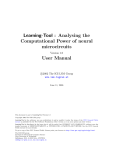
Circuit-Tool : A Tool for generating
N eural M icroC ircuits
Version 1.0
User Manual
c
2002
The IGI LSM Group
http://www.lsm.tugraz.at
June 11, 2006
This document is part of Circuit-Tool Release 1.0
Copyright 2002 The IGI LSM group
Circuit-Tool is free software; you can redistribute it and/or modify it under the terms of the GNU General Public License
as published by the Free Software Foundation; either version 2, or (at your option) any later version.
Circuit-Tool is distributed in the hope that it will be useful, but WITHOUT ANY WARRANTY; without even the
implied warranty of MERCHANTABILITY or FITNESS FOR A PARTICULAR PURPOSE. See the GNU General
Public License for more details.
To get a copy of the GNU General Public License point your browser to http://www.gnu.org/copyleft/gpl.html.
The IGI LSM group
Institute for Theoretical Computer Science
Graz University of Technology
Inffeldgasse 16/b, A-8010 Graz, AUSTRIA
mailto:[email protected], http://www.lsm.tugraz.at
Contents
1 Preliminaries
2
1.1
What is Circuit-Tool ? . . . . . . . . . . . . . . . . . . . . . . . . . . . . . . .
2
1.2
About this Manual . . . . . . . . . . . . . . . . . . . . . . . . . . . . . . . . .
2
1.3
Features of the current version . . . . . . . . . . . . . . . . . . . . . . . . . .
3
1.4
Getting and Installing Circuit-Tool . . . . . . . . . . . . . . . . . . . . . . . .
3
2 A short Tutorial
3
2.1
Initializing the model . . . . . . . . . . . . . . . . . . . . . . . . . . . . . . . .
4
2.2
Creating the Pools . . . . . . . . . . . . . . . . . . . . . . . . . . . . . . . . .
4
2.3
Making synaptic connections . . . . . . . . . . . . . . . . . . . . . . . . . . .
5
2.4
Simulating the model . . . . . . . . . . . . . . . . . . . . . . . . . . . . . . . .
8
3 Stimulus and Response
10
3.1
The Stimuls or Input Signals . . . . . . . . . . . . . . . . . . . . . . . . . . .
10
3.2
The response or the network output . . . . . . . . . . . . . . . . . . . . . . .
10
4 Input Distributions
11
5 Distributed simulations
11
6 neural microcircuit class reference
11
7 delay lines class reference
11
8 small circuits class reference
11
1
1.1
Preliminaries
What is Circuit-Tool ?
Circuit-Tool is a set of Matlab objects and scripts that allow the construction of multi“column” neural microcircuits with a distribution of parameters that match those reported in
the literature. This neural microcircuit models can then be simulated efficiently using CSIM .
1.2
About this Manual
This manual is intended to describe how to use Circuit-Tool from the (Matlab) users point
of view. It does not try to explain (or give an introduction to) the type of models which
can be constructed an simulated with Circuit-Tool . Regarding neural modeling we refer the
2
reader to [Dayan and Abbott, 2001] and [Gerstner and Kistler, 2002]. Furthermore Matlab
programming knowledge is assumed.
1.3
Features of the current version
Customizeable intra and inter “column” connectivity
Runs under Unix (Linux) and Windows
Object oriented design
Parallel simulation for large set of stimuli
1.4
Getting and Installing Circuit-Tool
Circuit-Tool is distributed under the GNU General Public License and can be downloaded
from http://www.igi.tugraz.at/circuits.
To install Circuit-Tool perform the following steps:
1. Donwload Circuit-Tool from www.igi.tugraz.at/circuits
2. Unzip the file circuits-VER.zip where VER stands for the version you have downloaded.
This will create a subdirectory lsm and lsm/circuits
3. Start Matlab and change into the directory lsm
4. Run the Matlab script install.m.
5. Add the path lsm to the Matlab search path; e. g.
• addpath(’/home/jack/lsm’)} or
• addpath(’C:\Work\Neuroscience\lsm’).
6. Change into the directory lsm/circuits/demos and play around with them.
7. Have fun using Circuit-Tool !
2
A short Tutorial
In this section we will introduce Circuit-Tool by means of an example. We will use CircuitTool to construct a model which consists of three “columns” or pools how they are called in
Circuit-Tool . The first pool consists of leaky integrate an fire neurons, the second is made
up of sigmoidal neurons and the third uses more detailed conductance based model neurons.
The pools will be connected internally and to each other (for details see below). The circuit
will be driven by two input spike trains and an analog input current. The input projects in
some kind of topographic map into the circuit.
3
Figure 1: A 3 × 3 × 10 pool of LifNeurons with origin (2,1,1)
2.1
Initializing the model
The Circuit-Tool -implementation of this model employs the Matlab class
neural microcircuit (Sec. 6). To start our construction of the model we will instantiate
an “empty” microcircuit:
>> nmc = neural microcircuit;
2.2
Creating the Pools
As the next step we will create the individual pools. First we will create a pool of integrateand-fire neurons:
>>[nmc,p lif]=add(nmc,’pool’,’type’,’LifNeuron’,’size’,[3 3 6],’origin’,[2 1 1]);
The above command creates 54 neurons of the class LifNeuron (which is a neuron type
available in CSIM ) and adds them to nmc. Note that due to the object oriented paradigm
used in Matlab the nmc object must appear also on the left hand side of the command. The
variable p lif is a handle/index to refer to that particular pool later in the programm.
The neurons are located on a three dimensional 3 × 3 × 6 integer grid with origin (2,1,1). You
can visualize this by issuing the command
>> plot(nmc);
The plot command should produce a figure which looks very much like Figure ??. As you
can see in Figure ?? some neurons are marked by magenta balls. These are inhibitory neurons
while the other are excitatory neurons. By default a neuron is choosen to be a excitatory
with a probability of 80% (this can be controlled with the frac EXC parameter).
Now we add the other two pools of neurons where we set some off-default parameters:
>> [nmc,p_sig]=add(nmc,’pool’,’type’,’SigmoidalNeuron’,...
4
Figure 2: Three pools of model neurons consisting of neurons of the classes LifNeuron, SigmoidalNeuron, and HHNeuron (from left to right) and two input pools.
’size’,[3 3 6],’origin’,[6 1 1],...
’Neuron.thresh’,1,’Neuron.beta’,2,’Neuron.tau_m’,3,...
’Neuron.A_max’,4,’Neuron.I_inject’,1,’Neuron.Vm_init’,0);
>> [nmc,p_hh ]=add(nmc,’pool’,’type’,’HHNeuron’,...
’size’,[3 3 6],’origin’,[10 1 1],...
’Neuron.Inoise’,???,’Neuron.Iinject’,[??? ???]);
The code fragment above shows how to set off-default values for some parameters of the
Neurons generated. One has to add a pair of ’Neuron.<field>’,<value> arguments to the
function call. Which fields are valid is determined by the class of the neuron (see the CSIM
Class Reference for details).
As the next step we create the input neurons. A pool of 2 excitatory spiking input neurons
>> [nmc,p_sin] = add(nmc,’pool’,’type’,’SpikingInputNeuron’,...
’size’,[1 1 2],’origin’,[0 1 5],’frac_EXC’,1.0);
and a pool of a single excitatory analog input neuron:
>> [nmc,p_ain] = add(nmc,’pool’,’type’,’AnalogInputNeuron’,...
’size’,[1 1 1],’origin’,[0 1 2],’frac_EXC’,1.0);
A visualization of the current model is shown in Figure ?? which was produce by the command
plot(nmc);.
2.3
Making synaptic connections
Now we want to set up synaptic connections between the neurons in the individual pools.
This is done by commands of the form
>> [nmc,c_idx] = add(nmc,’conn’,’dest’,<destination>,’src’,<source>,...);
5
Figure 3: Synaptic connections of the spiking input neurons to the LifNeuron pool.
where <destination> and <source> specify a set of neurons either by the handle/index of a
pool or by specifying a volume.
2.3.1
Connecting the input
To see how it works lets start by connecting the spiking inputs to the pool of LifNeurons:
>> [nmc,c(1)]=add(nmc,’conn’,’dest’,p_lif,’src’,p_sin,...
’Cscale’,1,’Wscale’,5);
Here we used the pool handles/indices as source and destination specification. The additional
parameters given specify how to scale the overall connection probability (Cscale) and the
synaptic strength (Wscale). To see the actual connectivity pattern generated you can again
use the command plot(nmc); and interaktively explore the network structure. By clicking
on a neuron you can look at presynaptic as well as postsynaptic connections. Figure ?? shows
how the input neurons are connected at the moment.
As the next step we connect the
spiking input via static synapses (Sec. ??) (default are dynamic synapses (Sec. ??) to some
subset of the pool of sigmoidal neurons by specifying a certain volume
>> [nmc,c(2)]=add(nmc,’conn’,’dest’,[6 1 1; 6 3 6],’src’,p_sin,...
’type’,’StaticSpikingSynapse’,’Cscale’,Inf);
The synaptic connection created by this command are shown in Figure ??. Note that the
setting ’Cscale’,Inf ensures that there will be a synaptic connection between each pair of
neurons in the source region and the destination region. And finaly we connect the analog
input to the pool of HHNeurons by means of a StaticAnalogSynapse. This is necessary since
StaticSpikingSynapses can not transmit analog signals.
>> [nmc,c(3)]=add(nmc,’conn’,’dest’,p_hh,’src’,p_ain,...
’type’,’StaticAnalogSynapse’,’Wscale’,0.2);
6
Figure 4: Synaptic connections of the spiking input neurons to the SigmoidalNeuron pool.
2.3.2
Making recurrent connections
Now we want to create recurrent connections with the pools themselves. The only differene
to the previous section is that now the source and destination is the same pool:
>> [nmc,c(4)]=add(nmc,’conn’,’dest’,p_lif,’src’,p_lif,...
’SH_W’,0.5,’lambda’,2.5,’Wscale’,2);
>> [nmc,c(5)]=add(nmc,’conn’,’dest’,p_sig,’src’,p_sig,...
’SH_W’,0.5,’lambda’,2,’type’,’StaticAnalogSynapse’);
>> [nmc,c(7)]=add(nmc,’conn’,’dest’,p_hh,’src’,p_hh,...
’SH_W’,0.5,’lambda’,1);
Again one can specify in addition to the destination and the source other parameters which
determine how individual synaptic connections are created. For example the parameter
lambda determines the “average distance” of synaptic connections and SH W determines the
standard deviation SD of the Gamma distribution used to generate the synaptic weights:
SD = SH W · mean. Figure ?? shows a typical postsynaptic connectivity pattern for one
neuron generated by the code above.
2.3.3
Connecting pools
In this example we connect the pool of HHneurons to the LifNeuron pool by static synapses.
>> [nmc,c(6)]=add(nmc,’conn’,’dest’,p_hh,’src’,p_lif,...
’SH_W’,0.5,’lambda’,Inf,’type’,’StaticSpikingSynapse’);
Note that using lambda=Inf has the effect that the distance between the neurons dose not
matter in determining wheter a synaptic connection will by generated or not.
7
Figure 5: Postsynaptic connections of a typical excitatory LifNeuron.
2.4
Simulating the model
Now that the model is set up we turn to the issue how to define the input and simulate the
network with these inputs.
2.4.1
Setting up the input
As we have three input neurons (2 spiking one analog) we have to define a stimulus which
consists of three channels (2 spiking one analog). The stimulus can be defined as follows:
% create empty structure
S = empty_stimulus(’nChannels’,3,’Tstim’,1);
% fill channel 1 with some spikes
S.channel(1).data
= 1*rand(1,10);
S.channel(1).spiking = 1;
% fill channel 2 with some spikes
S.channel(2).data
= 1*rand(1,20);
S.channel(2).spiking = 1;
% channel 3 is a sine wave
S.channel(3).dt
= 0.005;
S.channel(3).data
= 1+sin(2*pi*10*[0:S.channel(3).dt:1]);
S.channel(3).spiking = 0;
Note that each signal/channel can be either spiking (S.channel(i).spiking=1) or analog
(S.channel(i).spiking=0). In the later case one has to specify the temporal resolution
(S.channel(i).dt) of the signal.
8
stimulus
3.5
channel#
3
2.5
2
1.5
1
0
0.1
0.2
0.3
0.4
0.5
time [sec]
0.6
0.7
0.8
0.9
1
Figure 6: A stimulus with 2 spiking and one ananlog channel.
We adopt the convention that the first channel of the stimulus is assigned to the first input
neuron created by means of [nmc,p]=add(nmc,’pool’,... statements. Keep this convention
in mind when setting up the stimulus otherwise you may be surprised by error messages or
strange results (if the input neurons have different connections to the rest of the network).
You can use the command
>> plot_stimulus(S);
to plot the stimulus defined above. This results in the plot shown in Figure ??.
2.4.2
Defining the respones
Obviously we want to see how the network responses to the given stimulus. Therefor we must
specify what we want to record during the stimulation. The following code fragment shows
how to record the spikes of the pool of LifNeurons and the membrane voltage of a certain
subset (defined by specifiyng the appropriate volume) of the SigmoidalNeuron and HHNeuron
pool.
>> nmc = record(nmc,’Pool’,p_lif,’Field’,’spikes’);
>> nmc = record(nmc,’Volume’,[6 1 1; 8 3 1],’Field’,’Vm’);
>> nmc = record(nmc,’Volume’,[10 1 1; 12 3 1],’Field’,’Vm’);
2.4.3
Running the simulation
Now we are ready to run the simulation; lets say for 1 sec.
>> R=simulate(nmc,1,S);
This returns the cell array R which contains the response of the network. See the section
about input and output (Sec. 3) for more details about the structure of R.
9
circuit response
50
40
30
20
10
0.1
0.2
0.3
0.4
0.5
0.6
0.7
0.8
0.9
8
6
4
2
0
0.1
0.2
0.3
0.4
0.5
0.6
0.7
0.8
0.9
1
0
0.1
0.2
0.3
0.4
0.5
time [sec]
0.6
0.7
0.8
0.9
1
8
6
4
2
Figure 7: Response.
However, one can use the command
>> plot_response(R);
to plot the response R. This results in the plot shown in Figure ??.
3
Stimulus and Response
3.1
The Stimuls or Input Signals
When runing a network simulation via simulate(nmc,Tstim,S); one can specify the stimulus
S.
S has to be a struct array with the following fields:
• S.channel(i).spiking : binary flag (0/1) which determines if S.channel(i).data
should be interpreted as spike times or as an analog signal
• S.channel(i).dt : time discretization; for analog signals (S.channel(i).spiking=0)
only
• S.channel(i).data :
signal date:
vektor of the analog
(S.channel(i).spiking=0) or spike times (S.channel(i).spiking=1)
• S.info(i).Tstim : the length of the stimulus (usally used in plotting routines.
3.2
The response or the network output
After a network simulation via a command like
>> R=simulate(nmc,Tstim,S);
10
values
the response is stored in the cell array R. R{i} contains the traces specified by the i-th nmc =
record(nmc,...) statement during the setup of the simulation.
R{i} by itself is a struct array with the only field channel which is in turn a struct array
with a similar structure as an input signal (Sec. 3.1). That is
• R{i}.channel(j).data : signal data : vektor of the analog values or spike times. Note
that the data always starts at time t = 0.
• R{i}.channel(j).spiking : binary flag (0/1) which determines if data should be
interpreted as spike times or as an analog signal
• R{i}.channel(j).dt : time discretization; for analog signals only
• R{i}.channel(j).fieldName : name of the recorded field
• R{i}.channel(j).idx : handle of the object from which field the data was recorded
4
Input Distributions
5
Distributed simulations
6
neural microcircuit class reference
7
delay lines class reference
8
small circuits class reference
References
[Dayan and Abbott, 2001] Dayan, P. and Abbott, L. (2001). Theoretical Neuroscience:
Computational and Mathematical Modeling of Neural Systems. MIT Press. See also
http://people.brandeis.edu/~abbott/book/.
[Gerstner and Kistler, 2002] Gerstner, W. and Kistler, W. (2002). Spiking Neuron Models.
Cambridge University Press. See also http://diwww.epfl.ch/~gerstner/BUCH.html.
11