1
Advanced CAE Applications for Professionals
Software that works — for you.SM
ASTROS
User’s Reference Manual
for Version 20
UNIVERSAL ANALYTICS, INC.
© 1997 UNIVERSAL ANALYTICS, INC.
Torrance, California USA
All Rights Reserved
First Edition, March 1997
Second Edition, November 1997
Restricted Rights Legend:
The use, duplication, or disclosure of the information contained in this document is subject to the
restrictions set forth in your Software License Agreement with Universal Analytics, Inc. Use, duplication, or disclosure by the Government of the United States is subject to the restrictions set forth in
Subdivision (b)(3)(ii) of the Rights in Technical Data and Computer Software clause, 48 CFR
252.227-7013.
The concepts and examples contained herein is for educational purposes only and are not intended to
be exhaustive or to apply to any particular engineering problem or design. All information is subject
to change without notice. Universal Analytics Inc. does not warrant that this document is free of
errors or defects and assumes no liability or responsibility to any person or company for direct or
indirect damages resulting from the use of any information contained herein.
UNIVERSAL ANALYTICS, INC.
3625 Del Amo Blvd., Suite 370
Torrance, CA 90503
Tel: (310) 214-2922
FAX: (310) 214-3420
USER’S MANUAL
TABLE OF CONTENTS
1. INTRODUCTION . . . . . . . . . . . . . . . . . . . . . . . . . . . . 1-1
2. RUNNING ASTROS
. . . . . . . . . . . . . . . . . . . . . . . . . . 2-1
2.1.OVERVIEW . . . . . . . . . . . . . . . . . . . . . . . . . . . . . . . . . . . . 2-2
2.1.1.Executing ASTROS . . . . . . . . . . . . . . . . . . . .
2.1.2.The ASTROS Configuration and Preference Files . . . .
2.1.2.1.The Format of Preference Files . . . . . . . . . . .
2.1.3.Configuration Parameters . . . . . . . . . . . . . . . . .
2.1.4.The Configuration Sections . . . . . . . . . . . . . . . .
2.1.4.1.The Host Configuration Section . . . . . . . . . . .
2.1.4.2.The eBASE Kernel Configuration Section . . . . .
2.1.4.3.The ASTROS Configuration Section . . . . . . . .
2.1.4.4.The eBASE:APPLIB and eBASE:MATLIB Sections
2.1.4.5.The eSHELL Configuration Section . . . . . . . . .
2.1.5.Dynamic Memory . . . . . . . . . . . . . . . . . . . . .
2.1.6.The eBASE Database . . . . . . . . . . . . . . . . . . .
2.1.6.1.The Two Types of Databases . . . . . . . . . . . .
2.1.6.2.The Logical and Physical Views of the Database . .
2.1.6.3.The Physical Model . . . . . . . . . . . . . . . . .
2.1.6.4.ASSIGNing Databases . . . . . . . . . . . . . . .
2.1.6.5.Database File Names . . . . . . . . . . . . . . . .
2.1.6.6.Very Large Databases . . . . . . . . . . . . . . .
2.1.7.Host Computer Dependencies . . . . . . . . . . . . . .
.
.
.
.
.
.
.
.
.
.
.
.
.
.
.
.
.
.
.
.
.
.
.
.
.
.
.
.
.
.
.
.
.
.
.
.
.
.
.
.
.
.
.
.
.
.
.
.
.
.
.
.
.
.
.
.
.
.
.
.
.
.
.
.
.
.
.
.
.
.
.
.
.
.
.
.
.
.
.
.
.
.
.
.
.
.
.
.
.
.
.
.
.
.
.
.
.
.
.
.
.
.
.
.
.
.
.
.
.
.
.
.
.
.
.
.
.
.
.
.
.
.
.
.
.
.
.
.
.
.
.
.
.
.
.
.
.
.
.
.
.
.
.
.
.
.
.
.
.
.
.
.
.
.
.
.
.
.
.
.
.
.
.
.
.
.
.
.
.
.
.
.
.
.
.
.
.
.
.
.
.
.
.
.
.
.
.
.
.
.
.
.
.
.
.
.
.
.
.
.
.
.
.
.
.
.
.
.
.
.
.
.
.
.
.
.
.
.
.
.
.
.
.
.
.
.
.
.
.
.
.
.
.
.
.
.
.
.
.
.
.
.
.
.
.
.
.
.
.
.
.
.
.
.
.
.
.
.
.
.
.
.
.
.
.
.
.
.
.
.
.
.
.
.
.
.
.
.
.
.
.
.
.
.
.
.
.
.
.
.
.
.
.
.
.
.
.
.
.
.
.
.
.
.
.
.
.
.
.
.
.
.
.
.
.
.
.
.
.
.
.
.
.
.
.
.
.
.
.
.
.
.
.
.
.
.
.
.
.
.
.
.
2-2
2-2
2-3
2-3
2-3
2-3
2-5
2-5
2-5
2-5
2-5
2-6
2-6
2-6
2-6
2-6
2-6
2-7
2-7
2.2.UNIX-BASED COMPUTERS . . . . . . . . . . . . . . . . . . . . . . . . . . . 2-7
2.2.1.Executing ASTROS . . . . . . . . . . . . . . . . . . . . . . . . . . . . . . . . . . . . . . 2-7
2.2.2.ASTROS File Names . . . . . . . . . . . . . . . . . . . . . . . . . . . . . . . . . . . . . 2-9
ASTROS
i
USER’S MANUAL
2.2.2.1.Unique ASTROS files
2.2.2.2.Databases . . . . . .
2.2.3.The eSHELL Program . . .
2.2.4.Automatic Preference Files
2.2.5.Online Manuals . . . . . .
.
.
.
.
.
.
.
.
.
.
.
.
.
.
.
.
.
.
.
.
.
.
.
.
.
.
.
.
.
.
.
.
.
.
.
.
.
.
.
.
.
.
.
.
.
.
.
.
.
.
.
.
.
.
.
.
.
.
.
.
.
.
.
.
.
.
.
.
.
.
.
.
.
.
.
.
.
.
.
.
.
.
.
.
.
.
.
.
.
.
.
.
.
.
.
.
.
.
.
.
.
.
.
.
.
.
.
.
.
.
.
.
.
.
.
.
.
.
.
.
.
.
.
.
.
.
.
.
.
.
.
.
.
.
.
.
.
.
.
.
.
.
.
.
.
.
.
.
.
.
.
.
.
.
.
.
.
.
.
.
.
.
.
.
.
. 2-9
. 2-9
2-10
2-10
2-10
3. THE INPUT DATA STREAM . . . . . . . . . . . . . . . . . . . . . . . 3-1
3.1.INTRODUCTION . . . . . . . . . . . . . . . . . . . . . . . . . . . . . . . . . 3-1
3.2.THE RESOURCE COMMANDS . . . . . . . . . . . . . . . . . . . . . . . . . 3-5
3.2.1.THE ASSIGN COMMAND . . . . . . . . . . . . . . . . . . . . . .
3.2.2. ASSIGN COMMAND DESCRIPTIONS FOR HOST COMPUTERS
3.2.2.1. UNIX SYSTEM IMPLEMENTATION . . . . . . . . . . . . .
3.2.3.THE MEMORY COMMAND . . . . . . . . . . . . . . . . . . . . .
.
.
.
.
.
.
.
.
.
.
.
.
.
.
.
.
.
.
.
.
.
.
.
.
.
.
.
.
.
.
.
.
.
.
.
.
.
.
.
.
.
.
.
.
.
.
.
.
.
.
.
.
3-5
3-6
3-6
3-9
3.3. THE INCLUDE DIRECTIVE . . . . . . . . . . . . . . . . . . . . . . . . . . . 3-10
3.4. THE DEBUG PACKET . . . . . . . . . . . . . . . . . . . . . . . . . . . . . . 3-12
3.4.1. EXECUTIVE SYSTEM DEBUG COMMANDS . . . . . . . . .
3.4.2. DATABASE AND MEMORY MANAGER DEBUG COMMANDS
3.4.3. INTERMEDIATE RESULTS PRINTING COMMANDS . . . . .
3.4.4. MISCELLANEOUS DEBUG COMMANDS . . . . . . . . . . .
3.4.5. SEQUENCER INTERMEDIATE PRINT COMMANDS . . . . .
4. THE EXECUTIVE SYSTEM AND MAPOL
.
.
.
.
.
.
.
.
.
.
.
.
.
.
.
.
.
.
.
.
.
.
.
.
.
.
.
.
.
.
.
.
.
.
.
.
.
.
.
.
.
.
.
.
.
.
.
.
.
.
.
.
.
.
.
.
.
.
.
.
.
.
.
.
.
.
.
.
.
.
3-13
3-14
3-15
3-17
3-18
. . . . . . . . . . . . . . . 4-1
4.1. THE MAPOL PROGRAM . . . . . . . . . . . . . . . . . . . . . . . . . . . . 4-2
4.2. MAPOL EDIT COMMANDS . . . . . . . . . . . . . . . . . . . . . . . . . . . 4-3
4.3. THE STANDARD EXECUTIVE SEQUENCE . . . . . . . . . . . . . . . . . . 4-3
4.4. STANDARD EXECUTIVE SEQUENCE STRUCTURE . . . . . . . . . . . . . 4-4
4.4.1. MAPOL Declarations . . . . . . . . . . . . . . . . . . .
4.4.2. The Solution Algorithm . . . . . . . . . . . . . . . . . .
4.4.2.1. MAPOL Engineering and Utility Modules . . . . . .
4.4.2.2. The Preface Segment . . . . . . . . . . . . . . .
4.4.2.3. The Analysis/Optimization Segments . . . . . . .
4.4.3. Modifying the Standard MAPOL Sequence . . . . . . . .
4.4.4. Restart Capability . . . . . . . . . . . . . . . . . . . . .
4.4.4.1. Ensuring proper STATUS of the run-time database
4.4.4.2. Suspending/Restarting Execution . . . . . . . . .
4.4.4.3.Resetting MAPOL Parameters . . . . . . . . . . .
.
.
.
.
.
.
.
.
.
.
.
.
.
.
.
.
.
.
.
.
.
.
.
.
.
.
.
.
.
.
.
.
.
.
.
.
.
.
.
.
.
.
.
.
.
.
.
.
.
.
.
.
.
.
.
.
.
.
.
.
.
.
.
.
.
.
.
.
.
.
.
.
.
.
.
.
.
.
.
.
.
.
.
.
.
.
.
.
.
.
.
.
.
.
.
.
.
.
.
.
.
.
.
.
.
.
.
.
.
.
.
.
.
.
.
.
.
.
.
.
.
.
.
.
.
.
.
.
.
.
.
.
.
.
.
.
.
.
.
.
.
.
.
.
.
.
.
.
.
.
.
.
.
.
.
.
.
.
.
.
.
.
.
.
.
.
.
.
.
.
. 4-6
4-12
4-13
4-19
4-19
4-20
4-22
4-22
4-23
4-23
4.5. MAPOL PROGRAM LISTING . . . . . . . . . . . . . . . . . . . . . . . . . . 4-24
ii
ASTROS
USER’S MANUAL
5. THE SOLUTION CONTROL PACKET . . . . . . . . . . . . . . . . . 5-1
5.1. OPTIMIZE AND ANALYZE SUBPACKETS . . . . . . . . . . . . . . . . . . . 5-3
5.2. BOUNDARY CONDITIONS . . . . . . . . . . . . . . . . . . . . . . . . . . . 5-4
5.3. DISCIPLINES . . . . . . . . . . . . . . . . . . . . . . . . . . . . . . . . . . . 5-7
5.3.1. DISCIPLINE OPTIONS . . . .
5.3.2. STATICS Discipline Options .
5.3.3. MODES Discipline Options . . .
5.3.4. SAERO Discipline Options . . .
5.3.5. FLUTTER Discipline Options .
5.3.6. TRANSIENT Discipline Options
5.3.7. FREQUENCY Discipline Options
.
.
.
.
.
.
.
. . 5-9
. 5-12
. 5-12
. 5-12
. 5-13
. 5-13
. 5-13
5.4. OUTPUT REQUESTS . . . . . . . . . . . . . . . . . . . . . . . . . . . . .
5-14
5.4.1. Subset Options . . . . . . .
5.4.2. Response Quantity Options
5.4.3. Form Options . . . . . . . .
5.4.4. Labeling Options . . . . . .
.
.
.
.
.
.
.
.
.
.
.
.
.
.
.
.
.
.
.
.
.
.
.
.
.
.
.
.
.
.
.
.
.
.
.
.
.
.
.
.
.
.
.
.
.
.
.
.
.
.
.
.
.
.
.
.
.
.
.
.
.
.
.
.
.
.
.
.
.
.
.
.
.
.
.
.
.
.
.
.
.
.
.
.
.
.
.
.
.
.
.
.
.
.
.
.
.
.
.
.
.
.
.
.
.
.
.
.
.
.
.
.
.
.
.
.
.
.
.
.
.
.
.
.
.
.
.
.
.
.
.
.
.
.
.
.
.
.
.
.
.
.
.
.
.
.
.
.
.
.
.
.
.
.
.
.
.
.
.
.
.
.
.
.
.
.
.
.
.
.
.
.
.
.
.
.
.
.
.
.
.
.
.
.
.
.
.
.
.
.
.
.
.
.
.
.
.
.
.
.
.
.
.
.
.
.
.
.
.
.
.
.
.
.
.
.
.
.
.
.
.
.
.
.
.
.
.
.
.
.
.
.
.
.
.
.
.
.
.
.
.
.
.
.
.
.
.
.
.
.
.
.
.
.
.
.
.
.
.
.
.
.
.
.
.
.
.
.
.
.
.
.
.
.
.
.
.
.
.
.
.
.
.
.
.
.
.
.
.
.
.
.
.
.
.
.
.
.
.
.
.
.
.
.
.
.
.
.
.
.
.
.
.
.
.
.
.
.
.
.
.
.
.
.
.
.
.
.
.
.
.
5.5. SOLUTION CONTROL COMMANDS . . . . . . . . . . . . . . . . . . . . .
5-14
5-16
5-17
5-17
5-17
6. THE FUNCTION PACKET . . . . . . . . . . . . . . . . . . . . . . . 6-1
6.1.BACKGROUND . . . . . . . . . . . . . . . . . . . . . . . . . . . . . . . . . . 6-1
6.2. THE FUNCTION EVALUATION PROCEDURE . . . . . . . . . . . . . . . . . 6-1
6.2.1.Solution Control Packet . . . . . .
6.2.1.1.Synthetic Objective Function
6.2.1.2.Synthetic Design Constraints
6.2.2.Bulk Data Packet . . . . . . . . .
.
.
.
.
.
.
.
.
.
.
.
.
.
.
.
.
.
.
.
.
.
.
.
.
.
.
.
.
.
.
.
.
.
.
.
.
.
.
.
.
.
.
.
.
.
.
.
.
.
.
.
.
.
.
.
.
.
.
.
.
.
.
.
.
.
.
.
.
.
.
.
.
.
.
.
.
.
.
.
.
.
.
.
.
.
.
.
.
.
.
.
.
.
.
.
.
.
.
.
.
.
.
.
.
.
.
.
.
.
.
.
.
.
.
.
.
.
.
.
.
6-2
6-2
6-3
6-4
6.3.FUNCTION SYNTAX . . . . . . . . . . . . . . . . . . . . . . . . . . . . . . . 6-4
6.3.1.Mathematical Functions . . . . . . . .
6.3.2.Response Functions . . . . . . . . . .
6.3.2.1.Design Variable Function . . . .
6.3.2.2.Selection Functions . . . . . . .
6.3.2.3.Geometric Functions . . . . . .
6.3.2.4.Grid Point Response Functions .
6.3.2.5.Element Response Functions . .
6.3.2.6.Natural Frequency Constraints .
6.3.2.7.Flutter Response Functions . . .
6.3.2.8.Static Aero Response Functions
6.3.3.Ordered Sets . . . . . . . . . . . . .
.
.
.
.
.
.
.
.
.
.
.
.
.
.
.
.
.
.
.
.
.
.
.
.
.
.
.
.
.
.
.
.
.
.
.
.
.
.
.
.
.
.
.
.
.
.
.
.
.
.
.
.
.
.
.
.
.
.
.
.
.
.
.
.
.
.
.
.
.
.
.
.
.
.
.
.
.
.
.
.
.
.
.
.
.
.
.
.
.
.
.
.
.
.
.
.
.
.
.
.
.
.
.
.
.
.
.
.
.
.
.
.
.
.
.
.
.
.
.
.
.
.
.
.
.
.
.
.
.
.
.
.
.
.
.
.
.
.
.
.
.
.
.
.
.
.
.
.
.
.
.
.
.
.
.
.
.
.
.
.
.
.
.
.
.
.
.
.
.
.
.
.
.
.
.
.
.
.
.
.
.
.
.
.
.
.
.
.
.
.
.
.
.
.
.
.
.
.
.
.
.
.
.
.
.
.
.
.
.
.
.
.
.
.
.
.
.
.
.
.
.
.
.
.
.
.
.
.
.
.
.
.
.
.
.
.
.
.
.
.
.
.
.
.
.
.
.
.
.
.
.
.
.
.
.
.
.
.
.
.
.
.
.
.
.
.
.
.
.
.
.
.
.
.
.
.
.
.
.
.
.
.
.
.
.
.
6.4.EXAMPLES . . . . . . . . . . . . . . . . . . . . . . . . . . . . . . . . . . .
ASTROS
.
.
.
.
.
.
.
.
.
.
.
.
.
.
.
.
.
.
6-5
6-5
6-7
6-7
6-7
6-9
6-9
6-11
6-11
6-12
6-13
6-14
iii
USER’S MANUAL
6.5.INSTRINSIC RESPONSE COMMANDS . . . . . . . . . . . . . . . . . . . . . 6-25
7. THE BULK DATA PACKET . . . . . . . . . . . . . . . . . . . . . . . 7-1
7.1. BULK DATA ECHO OPTIONS . . . . . . . . . . . . . . . . . . . . . . . . . . 7-2
7.2. FORMAT OF THE BULK DATA ENTRY . . . . . . . . . . . . . . . . . . . . . 7-3
7.3. DATA FIELD FORMATS . . . . . . . . . . . . . . . . . . . . . . . . . . . . . 7-4
7.4. ERROR CHECKING IN THE INPUT FILE PROCESSOR . . . . . . . . . . . . 7-5
7.5. BULK DATA ENTRY SUMMARY . . . . . . . . . . . . . . . . . . . . . . . . 7-5
7.5.1. Aerodynamic Load Transfer . . . . . . . . . . . . . .
7.5.2. Applied Dynamic Loads . . . . . . . . . . . . . . . . .
7.5.3. Applied Static Loads . . . . . . . . . . . . . . . . . .
7.5.4. Boundary Condition Constraints . . . . . . . . . . . .
7.5.5. Design Constraints . . . . . . . . . . . . . . . . . . .
7.5.6. Design Variables, Linking and Optimization Parameters
7.5.7. Geometry . . . . . . . . . . . . . . . . . . . . . . . .
7.5.8. Material Properties . . . . . . . . . . . . . . . . . . .
7.5.9. Miscellaneous Inputs . . . . . . . . . . . . . . . . . .
7.5.10. Selection Lists . . . . . . . . . . . . . . . . . . . . .
7.5.11. Steady Aerodynamics . . . . . . . . . . . . . . . . .
7.5.12. Structural Element Connection . . . . . . . . . . . .
7.5.13. Structural Element Properties . . . . . . . . . . . . .
7.5.14. Unsteady Aerodynamics . . . . . . . . . . . . . . . .
7.5.15. Discipline Dependent Problem Control . . . . . . . .
.
.
.
.
.
.
.
.
.
.
.
.
.
.
.
.
.
.
.
.
.
.
.
.
.
.
.
.
.
.
.
.
.
.
.
.
.
.
.
.
.
.
.
.
.
.
.
.
.
.
.
.
.
.
.
.
.
.
.
.
.
.
.
.
.
.
.
.
.
.
.
.
.
.
.
.
.
.
.
.
.
.
.
.
.
.
.
.
.
.
.
.
.
.
.
.
.
.
.
.
.
.
.
.
.
.
.
.
.
.
.
.
.
.
.
.
.
.
.
.
.
.
.
.
.
.
.
.
.
.
.
.
.
.
.
.
.
.
.
.
.
.
.
.
.
.
.
.
.
.
.
.
.
.
.
.
.
.
.
.
.
.
.
.
.
.
.
.
.
.
.
.
.
.
.
.
.
.
.
.
.
.
.
.
.
.
.
.
.
.
.
.
.
.
.
.
.
.
.
.
.
.
.
.
.
.
.
.
.
.
.
.
.
.
.
.
.
.
.
.
.
.
.
.
.
.
.
.
.
.
.
.
.
.
.
.
.
.
.
.
.
.
.
.
.
.
.
.
.
.
.
.
.
.
.
.
.
.
.
.
.
.
.
.
.
.
.
.
.
.
.
.
.
.
.
.
.
.
.
.
.
.
7-5
7-6
7-6
7-6
7-7
7-8
7-8
7-8
7-8
7-9
7-9
7-9
7-10
7-10
7-11
7.6. DIFFERENCES BETWEEN ASTROS AND NASTRAN BULK DATA . . . . . . 7-11
7.7. BULK DATA DESCRIPTIONS . . . . . . . . . . . . . . . . . . . . . . . . . . 7-13
8. OUTPUT FEATURES . . . . . . . . . . . . . . . . . . . . . . . . . . 8-1
8.1. SYSTEM CONTROLLED OUTPUT . . . . . . . . . . . . . . . . . . . . . . . 8-2
8.1.1. Default Output Printed by Modules . . . . . . . . . . . . . . . . . . . . . . . . . . . . . . 8-2
8.1.2. Error Message Output . . . . . . . . . . . . . . . . . . . . . . . . . . . . . . . . . . . . 8-6
8.2. SOLUTION CONTROL OUTPUT OPTIONS
8.2.1. Element Response Quantities . . .
8.2.1.1. Aerodynamic Element Output
8.2.1.2. Bar Element Output . . . . . .
8.2.1.3. ELAS Element Output . . . .
8.2.1.4. IHEX1 Element Output . . . .
8.2.1.5. IHEX2 Element Output . . . .
8.2.1.6. IHEX3 Element Output . . . .
iv
.
.
.
.
.
.
.
.
.
.
.
.
.
.
.
.
.
.
.
.
.
.
.
.
.
.
.
.
.
.
.
.
.
.
.
.
.
.
.
.
.
.
. . . . . . . . . . . . . . . . . . 8-8
.
.
.
.
.
.
.
.
.
.
.
.
.
.
.
.
.
.
.
.
.
.
.
.
.
.
.
.
.
.
.
.
.
.
.
.
.
.
.
.
.
.
.
.
.
.
.
.
.
.
.
.
.
.
.
.
.
.
.
.
.
.
.
.
.
.
.
.
.
.
.
.
.
.
.
.
.
.
.
.
.
.
.
.
.
.
.
.
.
.
.
.
.
.
.
.
.
.
.
.
.
.
.
.
.
.
.
.
.
.
.
.
.
.
.
.
.
.
.
.
.
.
.
.
.
.
.
.
.
.
.
.
.
.
.
.
.
.
.
.
.
.
.
.
.
.
.
.
.
.
.
.
.
.
. 8-9
8-10
8-11
8-13
8-13
8-15
8-16
ASTROS
USER’S MANUAL
8.2.1.7. Rod Element Output . . . . . . . . .
8.2.1.8. QDMEM1/TRMEM Element Output .
8.2.1.9. QUAD4/TRIA3 Element Output . . .
8.2.1.10. Shear Panel Output . . . . . . . . .
8.2.2. Nodal Response Quantities . . . . . . . . .
8.2.3. Design Variables and Design Constraints .
8.2.4. Flutter/Normal Modes Response Quantities
8.2.5. Aeroelastic Trim Quantities . . . . . . . . .
.
.
.
.
.
.
.
.
. 8-17
. 8-17
. 8-19
. 8-22
. . 8-22
. 8-25
. 8-29
. 8-30
. . . . . . . . . . . . . . . . . . . .
8-34
8.4. OTHER SELECTABLE QUANTITIES . . . . . . . . . . . . . . . . . . . . .
8-36
8.3. SUMMARY OF SOLUTION RESULTS
.
.
.
.
.
.
.
.
.
.
.
.
.
.
.
.
.
.
.
.
.
.
.
.
.
.
.
.
.
.
.
.
8.4.1. Intermediate Steady Aerodynamic Matrix Output . .
8.4.2. Intermediate Unsteady Aerodynamic Matrix Output
8.4.3. Flutter Root Iteration Output . . . . . . . . . . . .
8.4.4. Stress Constraint Computation Output . . . . . . .
8.4.5. Intermediate Optimization Output . . . . . . . . . .
.
.
.
.
.
.
.
.
.
.
.
.
.
.
.
.
.
.
.
.
.
.
.
.
.
.
.
.
.
.
.
.
.
.
.
.
.
.
.
.
.
.
.
.
.
.
.
.
.
.
.
.
.
.
.
.
.
.
.
.
.
.
.
.
.
.
.
.
.
.
.
.
.
.
.
.
.
.
.
.
.
.
.
.
.
.
.
.
.
.
.
.
.
.
.
.
.
.
.
.
.
.
.
.
.
.
.
.
.
.
.
.
.
.
.
.
.
.
.
.
.
.
.
.
.
.
.
.
.
.
.
.
.
.
.
.
.
.
.
.
.
.
.
.
.
.
.
.
.
.
.
.
.
.
.
.
.
.
.
.
.
.
.
.
.
.
.
.
.
.
.
.
.
.
.
.
.
.
.
.
.
.
.
.
.
.
.
.
.
.
.
.
.
.
.
.
.
.
.
.
.
.
.
.
.
.
.
.
.
.
.
.
.
.
.
.
.
.
.
.
.
.
.
.
.
.
.
.
.
.
.
.
.
.
.
.
.
.
.
.
.
.
.
.
.
.
.
.
.
.
.
.
8-38
.
.
.
.
.
.
.
.
.
.
.
.
.
.
.
.
.
.
8.5. EXECUTIVE SEQUENCE OUTPUT UTILITIES . . . . . . . . . . . . . . . .
.
.
.
.
.
.
.
.
.
.
.
.
.
.
.
.
.
.
. . 8-36
. 8-36
. 8-37
. 8-37
. 8-38
.
.
.
.
.
.
.
.
.
.
.
.
.
.
.
.
.
.
.
.
.
.
.
8.5.1. Structural Set Definition Print Utility, USETPRT
8.5.2. Special Matrix Print Utility, UTGPRT . . . . . .
8.5.3. General Matrix Print Utility, UTMPRT . . . . .
8.5.4. General Relation Print Utility, UTRPRT . . . .
8.5.5. General Unstructured Print Utility, UTUPRT . .
.
.
.
.
.
.
.
.
.
.
.
.
.
.
.
.
.
.
.
.
.
.
.
.
.
.
.
.
.
.
.
.
.
.
.
.
.
.
8.6. THE eSHELL INTERACTIVE PROGRAM . . . . . . . . . . . . . . . . . . .
8-38
8-39
8-39
8-39
8-40
8-40
9. MAPOL PROGRAMMING . . . . . . . . . . . . . . . . . . . . . . . 9-1
9.1. INTRODUCTION AND USER OPTIONS
9.1.1. USER OPTIONS . . . . . . . . . . . . . .
9.1.2. MAPOL PROGRAM FORM . . . . . . . .
9.1.3. THE STANDARD ASTROS SOLUTION . .
9.1.4. MODIFYING THE STANDARD SOLUTION
9.1.5. CREATING MAPOL PROGRAMS . . . . .
9.1.6. SUMMARY . . . . . . . . . . . . . . . . .
. . . . . . . . . . . . . . . . . . . . 9-1
.
.
.
.
.
.
.
.
.
.
.
.
.
.
.
.
.
.
.
.
.
.
.
.
.
.
.
.
.
.
.
.
.
.
.
.
.
.
.
.
.
.
.
.
.
.
.
.
.
.
.
.
.
.
.
.
.
.
.
.
.
.
.
.
.
.
.
.
.
.
.
.
.
.
.
.
.
.
.
.
.
.
.
.
.
.
.
.
.
.
.
.
.
.
.
.
.
.
.
.
.
.
.
.
.
.
.
.
.
.
.
.
.
.
.
.
.
.
.
.
.
.
.
.
.
.
.
.
.
.
.
.
.
.
.
.
.
.
.
.
.
.
.
.
.
.
.
.
.
.
9-2
9-2
9-3
9-3
9-3
9-4
9.2. DATA TYPES AND DECLARATIONS . . . . . . . . . . . . . . . . . . . . . . 9-5
9.2.1. DEFINITIONS AND NOTATION
9.2.2. COMMENTARY . . . . . . . .
9.2.3. SIMPLE DATA TYPES . . . . .
9.2.3.1. Data Type INTEGER . . .
9.2.3.2. Data Type REAL . . . . .
9.2.3.3. Data Type COMPLEX . .
9.2.3.4. Data Type LOGICAL . . .
9.2.3.5. Data Type LABEL . . . .
9.2.4. COMPLEX DATA TYPES . . .
ASTROS
.
.
.
.
.
.
.
.
.
.
.
.
.
.
.
.
.
.
.
.
.
.
.
.
.
.
.
.
.
.
.
.
.
.
.
.
.
.
.
.
.
.
.
.
.
.
.
.
.
.
.
.
.
.
.
.
.
.
.
.
.
.
.
.
.
.
.
.
.
.
.
.
.
.
.
.
.
.
.
.
.
.
.
.
.
.
.
.
.
.
.
.
.
.
.
.
.
.
.
.
.
.
.
.
.
.
.
.
.
.
.
.
.
.
.
.
.
.
.
.
.
.
.
.
.
.
.
.
.
.
.
.
.
.
.
.
.
.
.
.
.
.
.
.
.
.
.
.
.
.
.
.
.
.
.
.
.
.
.
.
.
.
.
.
.
.
.
.
.
.
.
.
.
.
.
.
.
.
.
.
.
.
.
.
.
.
.
.
.
.
.
.
.
.
.
.
.
.
.
.
.
.
.
.
.
.
.
.
.
.
.
.
.
.
.
.
.
.
.
.
.
.
.
.
.
.
.
.
.
.
.
.
.
.
.
.
.
.
.
.
.
.
.
.
.
.
.
.
.
.
.
.
.
.
.
.
.
.
.
.
.
.
.
.
.
.
.
.
.
.
.
.
.
.
.
.
.
.
.
9-5
9-6
9-6
9-6
9-6
9-7
9-7
9-7
9-8
v
USER’S MANUAL
9.2.4.1. Data Types MATRIX and IMATRIX . . . . .
9.2.4.2. Data Type Relation . . . . . . . . . . . . .
9.2.4.3. Data Types UNSTRUCT and IUNSTRUCT
9.2.4.4. Data Base Entity Declaration Requirements
.
.
.
.
.
.
.
.
.
.
.
.
.
.
.
.
.
.
.
.
.
.
.
.
.
.
.
.
.
.
.
.
.
.
.
.
.
.
.
.
.
.
.
.
.
.
.
.
.
.
.
.
.
.
.
.
.
.
.
.
.
.
.
.
.
.
.
.
.
.
.
.
.
.
.
.
.
.
.
.
.
.
.
.
. 9-8
. 9-8
9-10
9-10
9.3. EXPRESSIONS AND ASSIGNMENTS . . . . . . . . . . . . . . . . . . . . . 9-11
9.3.1. ARITHMETIC EXPRESSIONS . . . . . . . . .
9.3.1.1. Arithmetic Operators . . . . . . . . . . .
9.3.1.2. Arithmetic Operands . . . . . . . . . . .
9.3.1.3. Evaluation of Arithmetic Expressions . . .
9.3.1.4. The Uses of Parentheses . . . . . . . . .
9.3.1.5. Type and Value of Arithmetic Expressions
9.3.2. LOGICAL EXPRESSIONS . . . . . . . . . . .
9.3.2.1. Logical Operators . . . . . . . . . . . . .
9.3.2.2. Logical Operands . . . . . . . . . . . . .
9.3.2.3. Evaluation of Logical Expressions . . . .
9.3.3. RELATIONAL EXPRESSIONS . . . . . . . . .
9.3.3.1. Relational Operators . . . . . . . . . . .
9.3.3.2. Relational Operands . . . . . . . . . . .
9.3.3.3. Evaluation of Relational Expressions . . .
9.3.4. MATRIX EXPRESSIONS . . . . . . . . . . . .
9.3.4.1. Matrix Operators . . . . . . . . . . . . .
9.3.4.2. Matrix Operands and Expressions . . . .
9.3.5. ASSIGNMENT STATEMENTS . . . . . . . . .
.
.
.
.
.
.
.
.
.
.
.
.
.
.
.
.
.
.
.
.
.
.
.
.
.
.
.
.
.
.
.
.
.
.
.
.
.
.
.
.
.
.
.
.
.
.
.
.
.
.
.
.
.
.
.
.
.
.
.
.
.
.
.
.
.
.
.
.
.
.
.
.
.
.
.
.
.
.
.
.
.
.
.
.
.
.
.
.
.
.
.
.
.
.
.
.
.
.
.
.
.
.
.
.
.
.
.
.
.
.
.
.
.
.
.
.
.
.
.
.
.
.
.
.
.
.
.
.
.
.
.
.
.
.
.
.
.
.
.
.
.
.
.
.
.
.
.
.
.
.
.
.
.
.
.
.
.
.
.
.
.
.
.
.
.
.
.
.
.
.
.
.
.
.
.
.
.
.
.
.
.
.
.
.
.
.
.
.
.
.
.
.
.
.
.
.
.
.
.
.
.
.
.
.
.
.
.
.
.
.
.
.
.
.
.
.
.
.
.
.
.
.
.
.
.
.
.
.
.
.
.
.
.
.
.
.
.
.
.
.
.
.
.
.
.
.
.
.
.
.
.
.
.
.
.
.
.
.
.
.
.
.
.
.
.
.
.
.
.
.
.
.
.
.
.
.
.
.
.
.
.
.
.
.
.
.
.
.
.
.
.
.
.
.
.
.
.
.
.
.
.
.
.
.
.
.
.
.
.
.
.
.
.
.
.
.
.
.
.
.
.
.
.
.
.
.
.
.
.
.
.
.
.
.
.
.
.
.
.
.
.
.
.
.
.
.
.
.
.
.
.
.
.
.
.
.
.
.
.
.
.
.
.
.
.
.
.
.
.
.
.
.
.
.
.
.
.
.
.
.
.
.
.
.
.
.
.
.
.
.
.
.
.
.
.
.
9-11
9-11
9-11
9-12
9-12
9-13
9-13
9-13
9-14
9-14
9-15
9-15
9-16
9-16
9-16
9-16
9-17
9-17
9.4. CONTROL STATEMENTS . . . . . . . . . . . . . . . . . . . . . . . . . . . . 9-19
9.4.1. INTRODUCTION . . . . . . . . . . . . . . .
9.4.2. THE UNCONDITIONAL GOTO STATEMENT
9.4.3. ITERATION . . . . . . . . . . . . . . . . . .
9.4.3.1. The FOR...DO Loop . . . . . . . . . .
9.4.3.2. The WHILE...DO Loop . . . . . . . . .
9.4.4. THE IF STATEMENT . . . . . . . . . . . . .
9.4.4.1. The Logical IF . . . . . . . . . . . . . .
9.4.4.2. The Block IF . . . . . . . . . . . . . .
9.4.4.3.The IF...THEN...ELSE . . . . . . . . . .
9.4.4.4. Nested IF Statements . . . . . . . . . .
9.4.5. THE END AND ENDP STATEMENTS . . . .
9.5. INPUT/OUTPUT STATEMENTS
.
.
.
.
.
.
.
.
.
.
.
.
.
.
.
.
.
.
.
.
.
.
.
.
.
.
.
.
.
.
.
.
.
.
.
.
.
.
.
.
.
.
.
.
.
.
.
.
.
.
.
.
.
.
.
.
.
.
.
.
.
.
.
.
.
.
.
.
.
.
.
.
.
.
.
.
.
.
.
.
.
.
.
.
.
.
.
.
.
.
.
.
.
.
.
.
.
.
.
.
.
.
.
.
.
.
.
.
.
.
.
.
.
.
.
.
.
.
.
.
.
.
.
.
.
.
.
.
.
.
.
.
.
.
.
.
.
.
.
.
.
.
.
.
.
.
.
.
.
.
.
.
.
.
.
.
.
.
.
.
.
.
.
.
.
.
.
.
.
.
.
.
.
.
.
.
.
.
.
.
.
.
.
.
.
.
.
.
.
.
.
.
.
.
.
.
.
.
.
.
.
.
.
.
.
.
.
.
.
.
.
.
.
.
.
.
.
.
.
.
.
.
.
.
.
.
.
.
.
.
.
.
.
.
.
.
.
.
.
.
.
.
.
.
.
.
.
.
.
.
.
.
.
9-19
9-19
9-19
9-19
9-20
9-21
9-21
9-22
9-22
9-23
9-23
. . . . . . . . . . . . . . . . . . . . . . . . 9-23
9.5.1. THE PRINT STATEMENT . . . . . . . . . . . . . . . . . . . . . . . . . . . . . . . . . 9-23
9.6. PROCEDURES AND FUNCTIONS . . . . . . . . . . . . . . . . . . . . . . . 9-24
9.6.1. INTRODUCTION . . . . . . . . . . . . . . . . .
9.6.2. PROGRAM UNITS AND SCOPE OF VARIABLES
9.6.3. DEFINING A PROCEDURE . . . . . . . . . . .
9.6.4. INVOKING A PROCEDURE . . . . . . . . . . .
vi
.
.
.
.
.
.
.
.
.
.
.
.
.
.
.
.
.
.
.
.
.
.
.
.
.
.
.
.
.
.
.
.
.
.
.
.
.
.
.
.
.
.
.
.
.
.
.
.
.
.
.
.
.
.
.
.
.
.
.
.
.
.
.
.
.
.
.
.
.
.
.
.
.
.
.
.
.
.
.
.
.
.
.
.
9-24
9-24
9-25
9-26
ASTROS
USER’S MANUAL
9.6.5. FUNCTION PROCEDURES . . . . . . . . . . . . . . . . . . . . . . . .
9.6.5.1.Examples of Variable Scope . . . . . . . . . . . . . . . . . . . . .
9.6.6. INTRINSIC FUNCTION PROCEDURES AND INTRINSIC PROCEDURES
9.6.7. INTRINSIC MATHEMATICAL FUNCTIONS . . . . . . . . . . . . . . . .
9.6.8. INTRINSIC RELATIONAL PROCEDURES . . . . . . . . . . . . . . . .
9.6.9. GENERAL INTRINSIC PROCEDURES . . . . . . . . . . . . . . . . . .
.
.
.
.
.
.
.
.
.
.
.
.
.
.
.
.
.
.
.
.
.
.
.
.
.
.
.
.
.
.
.
.
.
.
.
.
.
.
.
.
.
.
.
.
.
.
.
.
9-26
9-27
9-27
9-27
9-28
9-28
10. REFERENCES . . . . . . . . . . . . . . . . . . . . . . . . . . . . . 10-1
ASTROS
vii
USER’S MANUAL
This page is intentionally blank.
viii
ASTROS
USER’S MANUAL
LIST OF FIGURES
Figure 3-1. Structure of the ASTROS Input Data Stream . . . . . . . . . . . . . . . . 3-2
Figure 3-2. Features of a Sample ASTROS Input Stream . . . . . . . . . . . . . . . . 3-3
Figure 3-3. Function of the ASSIGN Command . . . . . . . . . . . . . . . . . . . . . 3-7
Figure 4-1. Structure of the Standard MAPOL Sequence . . . . . . . . . . . . . . . . 4-5
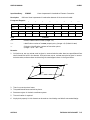
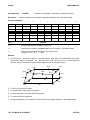
Figure 7-1. Bulk Data Entry Formats . . . . . . . . . . . . . . . . . . . . . . . . . . . 7-3
Figure 8-1. BAR Element Coordinate System . . . . . . . . . . . . . . . . . . . . .
8-11
Figure 8-2. BAR Element Forces Sign Conventions . . . . . . . . . . . . . . . . . .
8-11
Figure 8-3. IHEX1 Element Geometry . . . . . . . . . . . . . . . . . . . . . . . . .
8-14
Figure 8-4. IHEX2 Element Geometry . . . . . . . . . . . . . . . . . . . . . . . . .
8-15
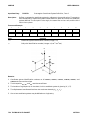
Figure 8-5. IHEX3 Element
. . . . . . . . . . . . . . . . . . . . . . . . . . . . . .
8-16
Figure 8-6. ROD Element Coordinate System . . . . . . . . . . . . . . . . . . . . .
8-17
Figure 8-7. QDMEM1 Element Coordinate System . . . . . . . . . . . . . . . . . .
8-18
Figure 8-8. TRMEM Element Coordinate System . . . . . . . . . . . . . . . . . . .
8-19
ASTROS
ix
USER’S MANUAL
Figure 8-9. QUAD4 Element Coordinate System . . . . . . . . . . . . . . . . . . . . 8-20
Figure 8-10. TRIA3 Element Coordinate System
. . . . . . . . . . . . . . . . . . . . 8-20
Figure 8-11. Shear Panel Forces . . . . . . . . . . . . . . . . . . . . . . . . . . . . 8-23
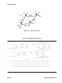
Figure 9-1. Schematic Representation of Relation . . . . . . . . . . . . . . . . . . . . 9-9
Figure 9-2. MAPOL Program Using Relational Procedures . . . . . . . . . . . . . . . 9-31
x
ASTROS
USER’S MANUAL
LIST OF TABLES
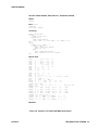
Table 1-1. Command Syntax Conventions . . . . . . . . . . . . . . . . . . . . . . . . 1-3
Table 2-1. The Preference File Format . . . . . . . . . . . . . . . . . . . . . . . . . . 2-4
Table 3-1. Executive (MAPOL) Debug Commands
. . . . . . . . . . . . . . . . . .
3-13
Table 3-2. Database Debug Commands . . . . . . . . . . . . . . . . . . . . . . . .
3-14
Table 3-3. Intermediate Results Debug Commands . . . . . . . . . . . . . . . . . .
3-16
Table 3-4. Miscellaneous Debug Commands
. . . . . . . . . . . . . . . . . . . . .
3-17
Table 3-5. Sequencer Debug Commands . . . . . . . . . . . . . . . . . . . . . . .
3-18
Table 4-1. MAPOL Edit Commands . . . . . . . . . . . . . . . . . . . . . . . . . . . 4-3
Table 4-2. Real Parameters in the Standard Sequence . . . . . . . . . . . . . . . . . 4-7
Table 4-3. Integer Modelling Parameters . . . . . . . . . . . . . . . . . . . . . . . . . 4-8
Table 4-4. Integer Design Parameters . . . . . . . . . . . . . . . . . . . . . . . . . . 4-9
Table 4-5. Integer Aerodynamic Parameters . . . . . . . . . . . . . . . . . . . . . . . 4-9
Table 4-6. Integer Discipline Parameters . . . . . . . . . . . . . . . . . . . . . . . .
4-10
Table 4-7. Logical Discipline Parameters . . . . . . . . . . . . . . . . . . . . . . . .
4-11
Table 4-8. Summary of ASTROS Modules . . . . . . . . . . . . . . . . . . . . . . .
4-13
Table 5-1. Levels of Solution Control . . . . . . . . . . . . . . . . . . . . . . . . . . . 5-2
Table 5-2. Summary of ASTROS Disciplines . . . . . . . . . . . . . . . . . . . . . . . 5-8
ASTROS
xi
USER’S MANUAL
Table 5-3. Summary of Discipline Options . . . . . . . . . . . . . . . . . . . . . . . . 5-11
Table 5-4. Response Quantity Output Options . . . . . . . . . . . . . . . . . . . . . . 5-18
Table 5-5. Response Quantities by Discipline . . . . . . . . . . . . . . . . . . . . . . 5-19
Table 6-1. Mathematical Intrinsics . . . . . . . . . . . . . . . . . . . . . . . . . . . . 6-6
Table 6-2. Selection Functions . . . . . . . . . . . . . . . . . . . . . . . . . . . . . . 6-7
Table 6-3. Element Response Components . . . . . . . . . . . . . . . . . . . . . . . 6-10
Table 8-1. DEBUG and ASSIGN DATABASE Output . . . . . . . . . . . . . . . . . . 8-3
Table 8-2. Boundary Condition Summary . . . . . . . . . . . . . . . . . . . . . . . . 8-3
Table 8-3. Active Boundary and Constraint Summary . . . . . . . . . . . . . . . . . . 8-4
Table 8-4. Resequencing Summary . . . . . . . . . . . . . . . . . . . . . . . . . . . 8-4
Table 8-5. Active Constraint Summary . . . . . . . . . . . . . . . . . . . . . . . . . . 8-5
Table 8-6. Approximate Optimization Summary . . . . . . . . . . . . . . . . . . . . . 8-5
Table 8-7. Design Iteration History . . . . . . . . . . . . . . . . . . . . . . . . . . . . 8-6
Table 8-8. ASTROS Execution Summary . . . . . . . . . . . . . . . . . . . . . . . . 8-7
Table 8-9. ASTROS Aerodynamic and Structural Elements . . . . . . . . . . . . . . 8-10
Table 8-10. BAR Element Output Quantities . . . . . . . . . . . . . . . . . . . . . . . 8-12
Table 8-11. IHEX1 Element Solution Quantities . . . . . . . . . . . . . . . . . . . . . 8-14
Table 8-12. ROD Element Solution Quantities . . . . . . . . . . . . . . . . . . . . . . 8-18
Table 8-13. QDMEM1 Solution Quantities . . . . . . . . . . . . . . . . . . . . . . . . 8-20
Table 8-14. QUAD4 and TRIA3 Solution Quantities . . . . . . . . . . . . . . . . . . . 8-21
Table 8-15. SHEAR Solution Quantities . . . . . . . . . . . . . . . . . . . . . . . . . 8-23
Table 8-16. Displacement Vector
. . . . . . . . . . . . . . . . . . . . . . . . . . . . 8-24
Table 8-17. Complex Displacement Vector . . . . . . . . . . . . . . . . . . . . . . . 8-24
Table 8-18. Design Variable Values . . . . . . . . . . . . . . . . . . . . . . . . . . . 8-27
Table 8-19. Design Constraint Summary . . . . . . . . . . . . . . . . . . . . . . . . . 8-27
Table 8-20. Flutter Solution Results . . . . . . . . . . . . . . . . . . . . . . . . . . . 8-29
Table 8-21. Modal Participation Factors . . . . . . . . . . . . . . . . . . . . . . . . . 8-30
xii
ASTROS
USER’S MANUAL
Table 8-22. Real Eigenanalysis Results . . . . . . . . . . . . . . . . . . . . . . . .
8-30
Table 8-23. Symmetric Trim Results . . . . . . . . . . . . . . . . . . . . . . . . . .
8-32
Table 8-24. Antisymmetric Trim Results . . . . . . . . . . . . . . . . . . . . . . . .
8-34
Table 8-25. Summary of Output Quantities . . . . . . . . . . . . . . . . . . . . . . .
8-35
Table 9-1. MAPOL Command Options . . . . . . . . . . . . . . . . . . . . . . . . . . 9-2
Table 9-2. Summary of MAPOL User Options . . . . . . . . . . . . . . . . . . . . . . 9-4
Table 9-3. MAPOL Arithmetic Operators . . . . . . . . . . . . . . . . . . . . . . . .
9-11
Table 9-4. MAPOL Operation Rules . . . . . . . . . . . . . . . . . . . . . . . . . .
9-13
Table 9-5. MAPOL Logical Operators . . . . . . . . . . . . . . . . . . . . . . . . .
9-13
Table 9-6. Evaluation of MAPOL Logical Expressions . . . . . . . . . . . . . . . . .
9-14
Table 9-7. Relational Operators in MAPOL . . . . . . . . . . . . . . . . . . . . . . .
9-15
Table 9-8. Matrix Operators in MAPOL . . . . . . . . . . . . . . . . . . . . . . . . .
9-16
Table 9-9. Assignment Rules in MAPOL . . . . . . . . . . . . . . . . . . . . . . . .
9-18
Table 9-10. Intrinsic Mathematical Functions in MAPOL . . . . . . . . . . . . . . . .
9-29
Table 9-11. Intrinsic Relational Procedures in MAPOL . . . . . . . . . . . . . . . . .
9-30
ASTROS
xiii
USER’S MANUAL
This page is intentionally blank.
xiv
ASTROS
USER’S MANUAL
Chapter 1
INTRODUCTION
There are five manuals documenting ASTROS, the Automated Structural Optimization System:
•
•
•
•
•
The User’s Reference Manual
The Theoretical Manual
The Programmer’s Manual
The ASTROS eBASE Schemata Definition
The Installation and System Support Manual
This User’s Manual provides a complete description of the user interface to the ASTROS system in order
to facilitate the preparation of input data. It introduces the features of the ASTROS system that enable
the user to direct the software system and documents the mechanisms by which the user can communicate with the system. It is assumed that the reader is familiar, from a study of the Theoretical Manual,
with the engineering capabilities of the ASTROS system and is using this manual to define the form of
the particular input that directs the system to perform a desired function.
The Theoretical Manual describes the range of capabilities of the ASTROS system, while the Programmer’s Manual is provided to give details of the internal function of the engineering and programming
utility modules. The eBASE Schemata Manual documents all of the database entities. The Installation
and System Support Manual describes how ASTROS is installed on host computers, and how it may be
configured for customized use.
This manual is intended to provide the user with a convenient reference for all forms of input to the
system and is therefore organized along the same lines as the input data stream. The discussion of each
topic is brief and generic and is followed by detailed documentation of the user inputs. Information on
ASTROS output formats is in a separate chapter as is the description of the Matrix Analysis Problem
Oriented Language (MAPOL) used for programming ASTROS.
ASTROS
INTRODUCTION 1-1
USER’S MANUAL
Finally, this manual is directed toward the engineer/designer/analyst who is using ASTROS to perform
engineering design or analysis. While ASTROS is perfectly capable of performing many tasks not explicitly supported in the standard execution, the user must know the engineering software in considerable
detail to direct the system to perform these alternative functions. The mechanisms by which these more
advanced features are invoked are included in this manual but no attempt is made to provide sufficient
information to the user to generate new analysis features or to grossly modify the existing capabilities of
the system. These more advanced topics are treated in the Programmer’s Manual which documents the
individual modules in the system and their interactions. Rudimentary modifications to the execution
sequence and changes to execution parameters are discussed in detail in this manual.
Machine and installation-dependent aspects of ASTROS are also contained in the Programmer’s Manuals
rather than in the User’s Manual. Only those machine-dependent issues that are logically related to the
preparation of the input are discussed in this manual. Machine-dependencies in the input are limited to
the naming conventions for the run time database files and the parameters that can be used on the
ASSIGN DATABASE entry. Other machine dependencies are handled as part of the installation of the
system on each particular host machine. These issues are documented in the Programmer’s Manual since
they are relevant only to the system manager, not to the user.
It will be apparent to many readers that the NASTRAN structural analysis system was used as a guide
in the design of the ASTROS program. Both NASTRAN and ASTROS comprise large scale, finite element
structural analysis in executive driven software systems. Therefore, many of the input and output
features are similar. NASTRAN has become an industry-standard in finite element structural analysis
with many pre- and post-processors developed around NASTRAN data. To maintain maximal compatibility, many aspects of the ASTROS input are similar in form or purpose to those in NASTRAN and, in
many other cases, the same nomenclature has been adopted. In some instances in this document, therefore, ASTROS input will be compared and contrasted to NASTRAN input in order to present a concise
picture of the ASTROS input and to assist the reader familiar with NASTRAN in making the connection
to the equivalent item in ASTROS. Although familiarity with NASTRAN is not a prerequisite to understanding the ASTROS documentation, sufficient numbers of potential ASTROS users are expected to be
familiar with the NASTRAN system to justify the sometimes casual reference to NASTRAN features.
Chapter 1 contains a description of the ASTROS input file, database assignment and debug control
inputs. Chapters 2 through 5 are organized to parallel the input file structure. Within each of these
chapters, the function of the particular input packet is presented along with illustrations of how the data
are prepared. Each packet is described in a generic fashion so as to indicate how the sophisticated user
can make use of the more advanced features of the system without cluttering the discussion with details
of the input structures. The detailed documentation of the separate input structures of the data packet
then follow within each Chapter. This form of documentation enables this manual to be useful as a guide
to the beginning user as well as a reference for the experienced user. While there are a number of
advanced input features, the required input for most jobs is the ASSIGN DATABASE command, described
in Section 1.3, and the Solution Control and Bulk Data packets described in Chapters 3 and 5, respectively.
In Chapter 6, following the input stream descriptions, the output features of the ASTROS system are
documented. While these features are selected through directives in the input data stream, they are
sufficiently numerous and complex to justify a separate chapter devoted solely to output requests. The
1-2 INTRODUCTION
ASTROS
USER’S MANUAL
output capabilities of the system are described in very general terms while the output requests available
for each analysis discipline and optimization feature are documented in detail. Most output is selected
through Solution Control directives that are documented in Chapter 3, but some are selected through
modifications to the executive (MAPOL) sequence. Chapter 2 documents all of the output utilities available to the user through MAPOL directives and gives several examples of modifying the MAPOL sequence to obtain additional output. Other features are described in the MAPOL Programmer’s Manual
which comprises Chapter 7.
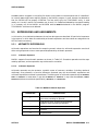
Many examples of user input are used throughout this document. In order to ease the burden of interpretation, the conventions shown in Table 1-1 are used in the examples unless otherwise noted. Chapter 7,
which describes the MAPOL programming interface, describes additional conventions required for the
programming syntax of MAPOL.
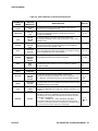
Table 1-1. Command Syntax Conventions
MAPOL NOGO
Capital letters indicate that the phrase must appear exactly as shown
MAPOL params
Lower case italic symbols act as generic place holders indicating that
an option or options can or must be included
MAPOL GO
NOGO
Symbol(s) enclosed in brackets [ ] are optional. If more than one
symbol is available they will be stacked in vector notation with any
defaults denoted by boldface.
INCLUDE < filename >
A required symbol is enclosed in angle brackets. If the angle brackets
surround an option list, at least one of the available options must be
selected.
BEGIN_BULK
The underscore (_) is used to signify a required blank space.
ASTROS
INTRODUCTION 1-3
USER’S MANUAL
This page is intentionally blank.
1-4 INTRODUCTION
ASTROS
USER’S MANUAL
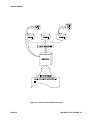
Chapter 2
RUNNING ASTROS
As is the case with all major software systems that are available across a broad spectrum of host
computers and operating systems† ASTROS has features which are implemented differently on different
computers. The most common differences are in the way you execute ASTROS and other UAI software
products, the management of dynamic memory, and the manner in which files are handled during
execution. This Chapter describes these for the most commonly used operating systems.
†
All computer models and operating system names are trademarks of their respective manufacturers and
vendors.
ASTROS
RUNNING ASTROS 2-1
USER’S MANUAL
2.1.OVERVIEW
This section provides you with an overview of the areas of ASTROS that are directly affected by your host
computer and its operating system.
2.1.1.Executing ASTROS
The manner in which you invoke a ASTROS execution is completely dependent on the operating system
of your host computer. Subsequent sections of this chapter describe this operation for the most common
host computers upon which ASTROS is currently available. You will note that Section 2.2 includes all of
the host computers using the Unix operating system and its derivatives.
2.1.2.The ASTROS Configuration and Preference Files
In general, UAI’s suite of engineering software products uses computing resources intensively. As a
result, there are a number of parameters that must be set to achieve optimal resource management on a
given host computer. These parameters, taken as a group, are called the Configuration of the products.
The configuration is provided through one or more files. These files include parameters which are used
for controlling database locations, physical file characteristics, memory utilization, and algorithm control.
For maximum flexibility, configurations may be controlled by the site, i.e. the UAI support specialist, or
the end user. Many different configurations may be defined for a site. For example, when configuring
ASTROS, the UAI support specialist may create different configurations for very small and for very large
analyses.
The starting point for configuring the UAI products is the Default Preference File, uaidef, included in
your delivery. The other modifications described above are made in other Preference Files. The actual
configuration used for a given execution is determined by applying the specified Preference Files in the
following sequence:
•
First, the Default Preference File is processed and all parameters included in this file are set
to their specified values
• Second, the System Preference File is processed, and any parameters included in it replace
those previously defined
• Third, the User Preference File is processed, and again, any parameters included in it replace
those previously defined.
In summary, the final configuration is the union of the Preference files. The Default Preference file
contains a value for every parameter used by the product suite. The other Preference Files need only
contain those parameters that differ from, and override, the default values.
2-2 RUNNING ASTROS
ASTROS
USER’S MANUAL
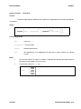
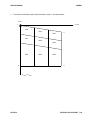
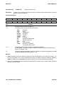
Each Preference File is composed of as many as six Sections:
•
•
•
•
•
•
The Host Section
The eBase Section
The eBase:applib Section
The eBase:matlib Section
The eShell Section
The ASTROS Section
The format of the Preference File and a brief description of its various sections are described in the
following sections.
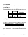
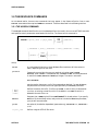
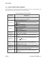
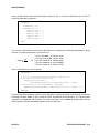
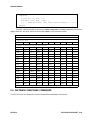
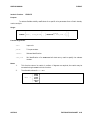
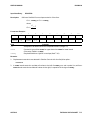
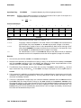
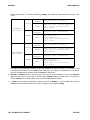
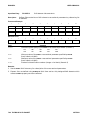
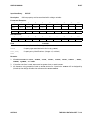
2.1.2.1. The Format of Preference Files
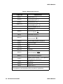
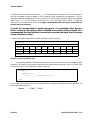
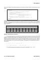
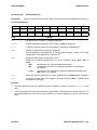
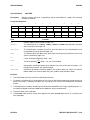
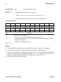
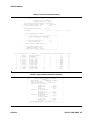
A Preference File is a text file which is composed of as many as six Sections indicated above. Each
Section includes a header followed by the parameters associated with the Section. For ease-of-use, the
[eBase] and [ASTROS] Sections are subdivided into groups which contain related parameters. The form
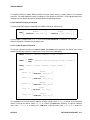
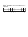
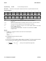
of the file is shown in Table 2-1.
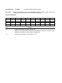
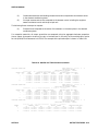
2.1.3.Configuration Parameters
Configuration parameters are defined using one of the forms:
param_name = value
param_name = ( value,value,...,value )
The param_names are case-insensitive. The values, when character strings or floating point numbers
with exponents, are also case-insensitive unless they are enclosed in single quotations (tics) as:
param_name = ’This is a Case-Sensitive String’
Only one parameter may be specified on each line of the file. Any characters that appear after value are
treated as commentary and ignored. You may also enter comments into the file by beginning a line with
any of the characters $, *, or #.
2.1.4.The Configuration Sections
The following sections provide an overview of the six Configuration Sections. Details of each section, as
well as information needed to define specific configuration parameters, are found in the ASTROS System
Support Manual. Contact your System Support Specialist if you require this information.
2.1.4.1. The Host Configuration Section
The Host Configuration Section includes parameters which identify the type of the host computer, and
specify the Preference File templates.
ASTROS
RUNNING ASTROS 2-3
USER’S MANUAL
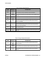
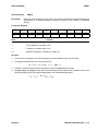
Table 2-1. The Preference File Format
[Host]
HOST_params
[eBase]
< Computing Resources >
eBase_params
< I/O System Parameters >
eBase_params
< Program Authorization >
eBase_params
[eBase:applib]
eBase:applib_params
[eBase:matlib]
eBase:matlib_params
[ASTROS]
< Print File Controls >
ASTROS_params
< Computing Resources >
ASTROS_params
< Matrix Conditioning >
ASTROS_params
< Data Checking >
ASTROS_params
< Analysis Output Control >
ASTROS_params
< Solution Techniques >
ASTROS_params
< Element Options >
ASTROS_params
< I/O System Parameters >
ASTROS_params
< Optimization Control Options >
ASTROS_params
< Program Authorization >
ASTROS_params
[eShell]
eShell_params
2-4 RUNNING ASTROS
ASTROS
USER’S MANUAL
2.1.4.2. The eBase Kernel Configuration Section
The eBase Configuration File Section includes parameters which control the eBase Engineering Database Management System kernel. These include such information as default paths were databases are
stored, physical block sizes for databases, and security information.
2.1.4.3. The ASTROS Configuration Section
The ASTROS Configuration Section includes parameters which control the program. These include controls on peripheral and computing resources, model data checking, program defaults, and so forth.
2.1.4.4. The eBase:applib and eBase:matlib Sections
The eBase:applib and eBase:matlib Configuration Sections include such items as dynamic memory
sizes for applib, and timing constants for the matlib high-performance matrix utilities.
2.1.4.5. The eShell Configuration Section
The eShell Configuration Section includes parameters which control the eShell interactive interface to
eBase. It includes such items as system database locations and dynamic memory specifications.
2.1.5.Dynamic Memory
The architecture of ASTROS allows the modeling and analysis of finite element models of virtually
unlimited size. Most numerical calculations perform at maximum efficiency when all data for the operation fits in the working memory space of the program. Many operations may be performed even when
all data that they require does not fit in memory by using what is called spill logic. Spill logic simply
involves the paging of data to and from disk storage devices as necessary. For very large jobs, spill
commonly occurs. In such cases, providing ASTROS with additional working memory can often improve
performance. On the other hand, you do not want to give ASTROS excess memory, because it will reduce
resources that could be used for other processes on your system. Under certain circumstances, excess
memory may actually degrade the performance of ASTROS and, in extreme cases, even your computer
system.
ASTROS has a second independent dynamic memory which is used to operate on databases that are
attached to the execution. This memory is typically much smaller than the working memory. The main
factor influencing the amount of database memory required is the block size used by the active databases.
This is described in detail in subsequent sections.
The working memory for ASTROS is dynamically acquired during execution. The amount of space that is
actually used by the program is typically controlled by the ASTROS execution procedure or the MEMORY
Executive Control command. Some host computers have alternate means of controlling this memory.
ASTROS
RUNNING ASTROS 2-5
USER’S MANUAL
2.1.6.The eBase Database
With ASTROS Version 13, UAI introduced the Engineering Database Management System, eBase, into
ASTROS. This advanced scientific database technology greatly enhances the data handling capabilities of
ASTROS compared with the older CADDB database found in the original ASTROS program.
2.1.6.1. The Two Types of Databases
There are two types of eBase databases in ASTROS. The first type is the run-time database, or
RUNDB. This database is used to store the relations and matrices which are used in performing your
analysis task. At the end of your job, the RUNDB may be deleted. The second type is the archival
database. This type of database represents any eBase database that you wish to use during an ASTROS
execution. The database may be created by ASTROS, or by a second application which uses the eBase
applib or matlib Applications Programming Interface (API).
2.1.6.2. The Logical and Physical Views of the Database
To fully understand the database technology, you must understand the two views of the database. Each
database is called a logical database. This term is used because from an engineering viewpoint, the
database is a single entity which is used in its entirety. The manner in which the logical database is
stored on your host computer depends on the amount of data it contains and the availability of disk
storage devices. The physical view is a mapping of a logical database to some number of physical files on
your host computer. It may be necessary for you to understand the physical model because, for very large
analyses, it may be more efficient to organize the actual files in a manner that allows higher performance
on your host.
2.1.6.3. The Physical Model
Each eBase database, regardless of its use, has two components manifested as a minimum of two
physical files. The first of these components is called the INDEX component. This component is always a
single physical file. It contains information which identifies and locates actual database entities. These
entities themselves are stored in the DATA component. To provide the maximum flexibility for a wide
variety of data storage requirements, the data components may be stored in a number of different
physical files. Most database systems are organized in this manner, because the index component is
generally small in size and referenced often, while the data component may be extremely large and not fit
in a single file or even on a single disk drive.
2.1.6.4. ASSIGNing Databases
Each logical database must be defined in the ASTROS job stream. Details of this are found in Chapter 2.
2.1.6.5. Database File Names
The naming of database files follows a convention that is different from that of other UAI/NASTRAN
files. The file names are generated automatically at execution time. The conventions used are also
described starting in Section 2.2 of this chapter.
2-6 RUNNING ASTROS
ASTROS
USER’S MANUAL
2.1.6.6. Very Large Databases
You may be solving extremely large problems with ASTROS. In such cases it may be possible that a
databases exceeds the capacity of a single disk drive. ASTROS has made provision for this and you must
contact your UAI System Support Specialist for details describing the use of this advanced feature.
2.1.7.Host Computer Dependencies
The sections that follow provide detailed information describing the differences in ASTROS execution
procedures and commands which depend on your host computer system.
2.2.UNIX-BASED COMPUTERS
This section describes the host-dependent information that you need to execute ASTROS on Unix-based
computer systems. UAI supports a wide variety of manufacturers including Silicon Graphics, Hewlett
Packard, IBM RS/6000, Sun, and more. For a complete list of platforms, please contact your UAI sales
representative.
2.2.1.Executing ASTROS
An sh script file, called astros, is provided to execute ASTROS. To execute you enter:
astros −m
W
memory K P [ -p prefname ]
M B
[ -e astros_exe ] [ -c config_file ] filelist
where memory specifies the amount of memory that the job will use. Options allow you to use shorthand
notation for large values and allocation types. The options K and M indicate that the memory value is
specified in thousands or millions of units, respectively. The units may be specified in single precision
words (W), bytes (B), or machine precision words (P). If none of these arguments are used, then memory is
assumed to be single precision words. Chapter 3 has a further discussion of memory allocation. The
prefname specifies the substitution string used to generate Preference File names. When performing
software development with ASTROS, there may be several versions of the program. The name astros_exe specifies the name of the ASTROS executable program version to use. By default, a file named
astros.out located in the local directory, or the version in the installation directory, will be used. The
config_file allows you to override the default uaidef file that is referenced through the UAICONFIG
global variable. This may be a useful option if more than one ASTROS system is available at your site.
Finally, filelist specifies a list of one or more file names, separated by spaces, that contain ASTROS
input data streams. The actual file names must have the proper trailing component, which is usually .d.
The script file will execute ASTROS using each of the data files that you provide. Examples illustrating
the use of the script are shown below.
ASTROS
RUNNING ASTROS 2-7
USER’S MANUAL
1.
Execute ASTROS using the input file test.d
astros test
2.
Execute ASTROS in the background for all of the input files in directory
/astros/demodata.
astros /astros/demodata/*.d &
3.
Execute ASTROS using the input file test.d and request one million words of memory.
astros -m 1000000 test or
astros -m 1mw test or
astros -m 1000kw
4.
Suppose that you have created a Preference File name my.pref, execute ASTROS using
the input file test.d using these preferences.
astros -p my test
5.
Suppose you have created your own version of ASTROS, named myastros.out, in your
local directory. Execute input file test.d using this program version.
astros -e myastros test
2-8 RUNNING ASTROS
ASTROS
USER’S MANUAL
2.2.2.ASTROS File Names
When you execute the astros script a number of files may be created which have names that are
automatically generated by the program. These are described in this section.
2.2.2.1. Unique ASTROS files
There are three unique files that are used frequently by ASTROS. These are unique in the sense the
program will automatically define file names for these if you do not explicitly ASSIGN them. These files,
and their default names, are shown in the table below:
FILE
May Override with
ASSIGN
Command?
Generated Name if ASSIGN
Command is Not Used
The print file
NO
filename.prt
The log file
NO
filename.log
The PUNCH file
YES
filename.pch
The filename represents the name of the file containing the ASTROS input data stream. The log file is
a special file that contains the history of your execution. You may monitor the progress of your job by
viewing the log file periodically. Upon completion of the job, the log file is appended to the print file, and
then deleted.
2.2.2.2. Databases
Each database that you use during an execution is comprised of at least two physical files. The trailing
components of these file names is always generated by ASTROS. When you ASSIGN a database with a
status of NEW and provide a physical file name, phys_name, the program generates the file names:
phys_name.EDB and phys_name.00
There may be times, most often in the case of the RUNDB, that you ASSIGN a database with a status of
TEMP. In such cases, the program internally generates file names that are unique to your job. The
detailed rules used to generate these names are given in the System Support Manual. These simple
rules pertain to the simplest and most used ASSIGNments of databases. If you are using very large
databases, then there are additional rules. These will be provided by your ASTROS System Support
Specialist.
ASTROS
RUNNING ASTROS 2-9
2.2.3.The eShell Program
If your site has the eShell interactive eBase interface program, then to execute this program you enter:
eshell [-ps prefname] [-pu prefname]
[-pl prefname] [database]
where:
prefname
Specifies the substitution string used to generate Preference File names. You may specify a
different string for the System (-ps), the User (-pu) and the Local (-pl) preference files. If
you have the unusual case where all of these files have the same name, you may use the
option -p followed by the prefname.
database
Is the name of a database to be opened with read access.
This places you in the command mode. Unless directed otherwise by eShell commands, all subsequent
output will be sent to the terminal device. The optional prefname information is an advanced feature
used for customizing eShell which is described in the Installation Guide and System Support Manual.
The eShell Tutorial Problem library is available. Contact your Systems Support Specialist to obtain the
name of the directory where these problems may be found. A description of how you may use them is
given in the eShell User’s Manual.
2.2.4.Au22
USER’S MANUAL
2.2.5.Online Manuals
The entire suite of ASTROS manuals is available online in the Adobe Portable Document Format (PDF).
This allows you to view the documentation on any computer that has the Adobe ® Acrobat® Reader 3.0.
Readers for the MAC, PC, Sun (OS and Solaris), and HP were delivered with your system.
To use the documents, from the command line you enter:
uaidoc [manual_name]
If you omit the manual_name, then you will see a splash screen that allows you to navigate to the
appropriate manual. You may also go directly to a manual by placing its name on the command lines.
The names of the astros manuals are:
•
•
•
•
•
•
ASTROS
astros_theory
astros_prog
astros_ref
astros_schema
eshell
system_support
RUNNING ASTROS 2-11
USER’S MANUAL
This page is intentionally blank.
2-12 RUNNING ASTROS
ASTROS
USER’S MANUAL
Chapter 3.
THE INPUT DATA STREAM
3.1.INTRODUCTION
The ASTROS user directs the system through an input data stream composed of a Resource Section,
which allocates ASTROS databases and specifies memory utilization, which is followed by multiple Data
Packets. Each packet contains a set of related data providing the information needed to execute ASTROS. The packets begin with a keyword indicating the nature of the data within the packet and
terminate with an ending keyword or with the start of the next data packet. All the packets in the input
data stream are optional, although the order in which they must appear is fixed. The purpose of this
section is to document the structure of the input data stream. Detailed documentation of the data within
each data packet is then presented in separate chapters.
Figure 3-1 shows the general form of the input data stream and Figure 3-2 illustrates the actual input
stream features with a sample stream for a ten bar truss model. The first non-blank record of the input
file must be either the ASSIGN command or a Resource Section. If an ASSIGN command is used, then this
command will enable you to attach the run-time database(s) that are used during the execution of the
ASTROS system. There are four optional data packets following the ASSIGN command which, if they are
present, must appear in the order shown. The first is the DEBUG packet which contains debug commands to control or select specific actions within the executive and database management systems. The
second packet is the MAPOL packet containing the executive system control directives consisting of
either a standalone MAPOL program or EDIT commands to modify the standard MAPOL program. If the
MAPOL packet is absent, the unmodified standard MAPOL sequence directs the execution. The Solution
Control commands appear in the third optional packet denoted by the keyword SOLUTION. These
commands select the engineering data to be used in each subcase from the set of data provided in the
Bulk Data packet. The fourth packet is the FUNCTION packet. It contains the definition of functions
which allow the user to define new design constraints or an objective function. These functions may
combine nodal and element response quantities for various boundary conditions and disciplines. The final
ASTROS
THE INPUT DATA STREAM 3-1
USER’S MANUAL
——————
——————
——————
Any number of leading blank lines
The Resource Section
ASSIGN RUNDB = <name> <status> <PASSWORD=password> [params]
MEMORY
DEBUG
——————
——————
DEBUG directives
used for tracing input stream errors
MAPOL [option-list]
or
EDIT [option-list]
MAPOL program or EDIT commands allow user
modifications to the standard ASTROS solution sequence
——————
——————
SOLUTION
Solution Control Directives
select optimization and analysis disciplines
——————
——————
FUNCTIONS [option_list]
Function definitions
Used to define objective or constraint functions
——————
——————
BEGIN_BULK [option_list]
——————
——————
…
…
…
Bulk Data Entries
defines the structural and aero models, boundary
conditions, loading cases, and other engineering data and the
design model — design variables and constraints — required
when performing design. Similar to NASTRAN
[ENDDATA]
Bulk Data Terminator
Figure 3-1. Structure of the ASTROS Input Data Stream
3-2 THE INPUT DATA STREAM
ASTROS
USER’S MANUAL
ASSIGN RUNDB=TENBAR,NEW,REALLOC,PASSWORD=SHAZAM
DEBUG
DESIGN=5
EDIT
NOLIST
INSERT 1463
CALL UTMPRT (,[AMAT]);
SOLUTION
TITLE = TEN BAR TRUSS
OPTIMIZE
PRINT DCON=ALL, HIST
BOUNDARY SPC = 1
LABEL = STATIC ANALYSIS
STATICS (MECH = 1), CONST (STRESS = 100, GENERAL = 100)
END
ANALYZE
BOUNDARY SPC = 1, METHOD = 2
STATICS ( MECH = 1 )
LABEL = FINAL STATIC ANALYSIS
PRINT DISP = ALL
MODES
LABEL = FINAL MODAL ANALYSIS
PRINT (MODES=ALL) DISP = ALL, ROOT=ALL
END
BEGIN BULK
GRID,
1,
, 720.0, 360.0,
0.0
GRID,
2,
, 720.0,
0.0,
0.0
GRID,
3,
, 360.0, 360.0,
0.0
GRID,
4,
, 360.0,
0.0,
0.0
GRID,
5,
,
0.0, 360.0,
0.0
GRID,
6,
,
0.0,
0.0,
0.0
CROD,
1, 10,
3,
5
CROD,
2, 10,
1,
3
CROD,
3, 10,
4,
6
...
CROD,
9, 10,
2,
3
CROD,
10, 10,
1,
4
PROD,
10,
2, 15.0
MAT1,
2, 1.E+7, , 0.3, 0.1, , , , 25000.0,
SPC1,
1,
123456, 5,
6
SPC1,
1,
3456,
1,
THRU, 4
FORCE,
1,
2, , -1.E5,
0.0,
1.0,
0.0
FORCE,
1,
4, , -1.E5,
0.0,
1.0,
0.0
CONVERT, MASS, 2.59E-3
EIGR,
2,
GIV, 0.0, 700.0,
2,
2, ,
MPPARM, ISCAL, 1
DESELM, 1, 1, CROD, 6.667E-3, 1000.0,
2.0,
DESELM, 2, 2, CROD, 6.667E-3, 1000.0,
2.0,
...
DESELM, 9, 9, CROD, 6.667E-3, 1000.0,
2.0,
DESELM, 10, 10, CROD, 6.667E-3, 1000.0,
2.0,
DCONVMM, 100, 2.5+4, -2.5+4, , 2
DCONDSP, 100, 1, UPPER, 2.0, POSNOD1, 1, 2,
DCONDSP, 100, 2, UPPER, 2.0, POSNOD2, 2, 2,
...
DCONDSP, 100, 8, LOWER, -2.0, NEGNOD1, 4, 2,
-25000.0
, ABC, +BC,
,
,
ROD1
ROD2
,
,
ROD9
ROD10
MAX
1.0
1.0
1.0
ENDDATA
Figure 3-2. Features of a Sample ASTROS Input Stream
ASTROS
THE INPUT DATA STREAM 3-3
USER’S MANUAL
data packet is the BULK DATA packet. The BULK DATA packet contains the engineering data describing the finite element structural model, the aerodynamic model(s), and the design model, as well as all
the data needed to perform the specific analysis and/or optimization tasks. The MAPOL, SOLUTION and
BULK DATA packets are analogous to the NASTRAN executive control, case control and bulk data
decks, respectively.
In interpreting the input data stream, ASTROS recognizes the keywords shown in Figure 3-1. These
keywords must be the first nonblank characters on the line (leading blanks are allowed) and have the
structure shown. In some cases the keyword is also a command line that makes up part of the data
packet which it initiates. In these cases, the command parameters are documented in the User’s Manual
chapter discussing the details of the associated data packet. For example, the MAPOL keyword is part of
a command that directs the MAPOL compiler to take certain actions. The detailed discussion of the
MAPOL command is therefore contained in Chapters 2 and 7 of this manual. ASTROS automatically
converts the case of the input data stream when necessary. The only portions of the data which are not
converted are file names which are used in the INCLUDE command, the Resource Section, and the
Solution Control commands TITLE, SUBTITLE and LABEL. This allows the user to freely enter data in
any case. Be aware, however, that file names are never converted and that when using an ASTROS host
computer in which case is important, such as Unix, then the correct case must always be used in file
names.
The section of the ASTROS input data steam that appears before the first packet header (e.g. DEBUG,
EDIT, or SOLUTION) is called the Resource Section. This section may contain any number of ASSIGN
commands and a MEMORY command. The INCLUDE command is used only as a convenience. These are
discussed in detail in the following sections.
3-4 THE INPUT DATA STREAM
ASTROS
USER’S MANUAL
3.2.THE RESOURCE COMMANDS
As introduced earlier, there are two commands that may appear in the Resource Section. One or more
ASSIGN commands and an optional MEMORY command. These are described in the following sections.
3.2.1.THE ASSIGN COMMAND
The ASSIGN command identifies the run-time database files to be used in the current ASTROS execution
and specifies certain parameters associated with the files. The format of this command is:
NEW
ASSIGN logical_name [= phys_name] , OLD [,REALLOC]
TEMP
[,PASSWORD = pass][,IBLKSIZE = nwib][,DBLKSIZE = nwdb]
READ
,ACCESS = WRITE [,params]
ADMIN
where,
dbname
is a name identifying the run time database files (maximum of 8 characters or
fewer, depending on the local host.
password
Passwords are used, but they are not required, only when USE is RUNDB,
ARCHIVE, SOF or NLDB. For databases with a STATUS of NEW, the same password
is used for the READ, WRITE and ADMIN privileges. The eSHELL command:
SET PASSWORD
may be used to change any or all of the passwords as desired. For OLD databases,
the password must match the access type specified by the ACCESS parameter.
NEW
OLD
TEMP
Defines the status of the file. The file may be NEW, in which case it is allocated at
run-time, an existing or OLD file, which is the default, or a TEMP file which is
deleted at the end of the run.
REALLOC
Requests that a new physical file be reallocated if it already exists. If you specify
NEW for a file that already exists, and you do not include the REALLOC parameter,
your job will be terminated.
params
are optional (installation dependent) parameters e.g., DBLKSIZE = n, IBLKSIZE =
n, etc.
logical_name
Defines a logical ASTROS file name.
ASTROS
THE INPUT DATA STREAM 3-5
USER’S MANUAL
The entries on the ASSIGN commands are keyword controlled, but the options within the command must
be entered in the order shown. The keywords may be separated by commas or blanks. An example is:
ASSIGN RUNDB=ASTDB,OLD,PASSWORD=SECRET
Figure 3-3 illustrates the function of the ASSIGN command. In the case shown, the installation dependent
parameters DLOC and ILOC have been used to select the physical devices on which the requested files for
DB1 reside.
The optional params on the ASSIGN command may or may not be keyword controlled and are installation
dependent. They provide a mechanism for the user to direct machine or installation dependent file
operations to be performed by the ASTROS procedure. At each site, the installation of the code involves a
definition of these parameters and the form they must take. The ASTROS system is currently functional
on numerous host systems including VAX/Ultrix, IBM/AIX, SGI 4D series and Crimson/Indigo series,
HP/9000 series, CRAY/UNICOS, DECStation, Convex, and SunSparcstation. The availability on a specific computer may be obtained by contacting UAI.
The next section documents the installation-dependent ASSIGN parameters for some of the more common
features/hosts. These features, however, may be customized to a very high degree and may be modified by
the local system manager. Further documentation of the ASSIGN command is left to the local installation
or will be included in the delivery material. The Programmer’s Manual contains the detailed description
of how these and other machine dependent parameters are defined.
3.2.2. ASSIGN COMMAND DESCRIPTIONS FOR HOST COMPUTERS
This section contains the descriptions of the machine and installation dependent parameters on the
ASSIGN command for three machines on which ASTROS is currently functional. The parameters that are
available at each site are listed and details of their use are presented. The user is cautioned that these
are site dependent parameters which may be different for each installation even if the host system is the
same. This documentation is provided both as an example to the system programmer and because the
features that have been made available on these machines are very likely to exist on most machines that
may be used. The user is referred to their ASTROS system manager for the particulars of the interface
between the local host system and ASTROS. The following section describes parameters for computers
using Unix-based Operating Systems
3.2.2.1.
UNIX SYSTEM IMPLEMENTATION
The ASSIGN command supplies the ASTROS system with the root name of the database files, the status
of those files, and a set of user parameters. The status is selected from NEW, OLD or TEMP and the set of
user parameters can be any of the following keyword commands:
ILOC= path
Specifies the location of the Index Component file.
DLOC= path
Specifies the location of the Data Component files.
DBLKSIZE= n
CADDB data files block size in words.
IBLKSIZE= n
CADDB index file block size in words.
3-6 THE INPUT DATA STREAM
ASTROS
USER’S MANUAL
Figure 3-3. Function of the ASSIGN Command
ASTROS
THE INPUT DATA STREAM 3-7
USER’S MANUAL
Note that the DLOC parameter may specify a series of locations when very large databases are being
created. The format is then:
DLOC=(path_1,path2,...)
TEMP Database Example:
When the status is TEMP a temporary database is created and no data is kept after the run. The other
legal optional parameters are DBLKSIZE and IBLKSIZE.
ASSIGN RUNDB=MYDB,TEMP,PASSWORD=X,DBLKSIZE=2048,IBLKSIZE=256
NEW Database Example:
When the status is NEW, a new database is created. If the files already exist, they will be overwritten.
voldbroot.EDB - index file
voldbroot.00 - data file 1
Other legal parameters are DLOC, ILOC, DBLKSIZE and IBLKSIZE.
ASSIGN RUNDB=MYDB,NEW,PASSWORD=X,REALLOC,DLOC=/tmp/,ILOC=/tmp/
In this example, a database with files /tmp/MYDB.EDB and /tmp/MYDB.00 are created. If existing files
are found they will be overwritten.
OLD Database Example:
When the status is OLD, an old database is used. The physical files that make up the database must exist.
Two, or more, files are used to store the database. The names of these files are as follows:
voldbroot.EDB - index file
voldbroot.00 - data file 1
The DLOC and ILOC parameters, along with the root database name, are used to form the names. No
other parameters are legal. Here is an example:
ASSIGN RUNDB=X,OLD,PASSWORD=X,DLOC=/home/dir1/,ILOC=/home/dir1/
In this example a database with files /home/dir1/MYDB.EDB and /home/dir1/MYDB.00 are used.
3-8 THE INPUT DATA STREAM
ASTROS
USER’S MANUAL
3.2.3.THE MEMORY COMMAND
The MEMORY command specifies the amount of memory ASTROS will use for the internal storage of
data. The format of this command is:
work_mem
WORKING = work_mem
MEMORY
EBASE = eb_mem PHYSICAL = phys_mem
work_mem
Specifies the dynamic working memory size used by ASTROS modules. The
working memory may be increased for large problems to reduce the amount of
physical I/O. Note, however, that this may cause increased paging. Contact
your ASTROS Support Specialist for additional details.
eb_mem
Specifies the eBASE database memory size. This memory is a separate
memory pool used by the database during execution. Normally the default
value in the Preference File is sufficient, but if you use block sizes larger than
the default for any database, this value may need to be increased.
phys_mem
Specifies the real physical memory memory size. The physical memory is used
to control certain advanced algorithms. Contact your ASTROS Support
Specialist for additional details.
The units of the memory size are determined by the two optional command arguments.
M
K
W
B
P
The first argument indicates an order of magnitude for memory_space, M for millions, K for thousands.
The second argument indicates the unit specifier as single precision words (W), bytes (B), or computer
precision words (P). If neither is present, then memory_space is taken to be single precision computer
words. The working memory for ASTROS is dynamically acquired during execution. The amount of
memory used is determined, in order of precedence, by the MEMORY Resource command, the - m option of
the astros script, and the configuration parameter working_memory.
You may provide default values for this command in the <Computing Resources> group of the [ASTROS] Section of the Preference File.
ASTROS has two high-performance solvers which take advantage of the latest developments in sparse
matrix algorithm technology. The first of these is the symmetric matrix decomposition used in static
analyses, and the second is the Lanczos eigenextraction method. This latter method is used for extracting
a modest number of eigenvalues from very large systems. When these solvers are used, memory requirements may become significant. The figures below give upper and lower bound estimates for the amount of
ASTROS
THE INPUT DATA STREAM 3-9
USER’S MANUAL
UPPER
BOUND
UPPER
BOUND
LOWER
BOUND
Cray
LOWER
BOUND
Others
memory that you should specify on your MEMORY Command. Although the eigensolver takes slightly
more memory, about 20%, the same figures may be used to approximate the requirements for either
solver. Note, that in the case of the Linear Solver, if you do not specify enough memory for the new
algorithm, the program will revert to the old solution algorithm. This is not the case for Lanczos — the
job will terminate. These curves have been created using a representative sample of real analysis jobs.
They are intended only to be used as guidelines — a specific job may take significantly more or less
memory than indicated.
For example, to execute ASTROS using 12 million words of working memory, any of the following
commands may be used:
MEMORY = 12000000; or
MEMORY = 12000KW; or
MEMORY = 12MW
3.3. THE INCLUDE DIRECTIVE
The input data stream typically resides in a single file, but the user can direct the input stream
interpreter to include other files through the use of the INCLUDE directive in the primary input stream.
The format of the INCLUDE command is:
INCLUDE <filename>
where,
filename
is a name identifying the file to be included (maximum of 72 characters).
The filename, which is used in a FORTRAN OPEN statement, must satisfy the requirements of the
particular host system for file names. Beyond this restriction, the user is free to have any set of contigu-
3-10 THE INPUT DATA STREAM
ASTROS
USER’S MANUAL
ous non-blank characters in the filename. In order to avoid the possibility of an infinite recursion, there is
a restriction on the include feature that no INCLUDE statement can appear in a file that is being included.
For example, if the file "TENBAR" is being included, it may not itself contain an INCLUDE directive. The
input stream interpreter will terminate with an appropriate error message should this occur.
The INCLUDE directive can appear anywhere in the input stream after the ASSIGN command. The
ASSIGN must always appear as the first non-blank line in order to allow the use of the run time database
in the subsequent input stream interpretation. A single data packet can be split among included files or
an INCLUDE file may contain parts of multiple data packets. The input interpreter merely replaces the
INCLUDE directive with the data contained in the named file so the only requirement is that the input
stream that results from the combination of all INCLUDEs have the form of a normal input stream. The
INCLUDE feature can be very useful in certain circumstances. For example, a special user developed
MAPOL sequence can be stored and maintained external to the files containing the engineering data for
particular runs; or, conversely, the bulk data representing a large model can be included into the file
containing the solution control directives.
ASTROS
THE INPUT DATA STREAM 3-11
USER’S MANUAL
3.4. THE DEBUG PACKET
The debug packet represents a development tool and is intended to be used primarily by those responsible for maintaining the software. The debug packet provides the system programmer with the means to
invoke or control certain executive and database management system functions that are helpful in
tracking the ASTROS execution and/or testing the executive and database management system software.
However, because some of the debug options can be useful to the general user, the debug packet is fully
documented in the User’s Manual rather than in the Programmer’s Manual. This section documents each
of the debug options and indicates how the option can be useful in debugging the ASTROS procedure.
Emphasis is placed on those debug options that are of interest to the general user.
The debug packet is initiated by the keyword DEBUG, which must appear alone on the line of the input
stream that follows the last command in the Resource Section, and that precedes any other data packet.
Following the initiator, any number of debug lines can be included in the data stream. Each debug
command line can be composed of a number of debug commands, appearing in any order, separated by
blanks or commas. The DEBUG packet is terminated when a new data packet initiator, or the end of the
input stream, is encountered. Most debug commands consist of single keywords which toggle flags
activating the debug functions. The appearance of these debug keywords is all that is required to activate
the option. Other debug commands select that a flag take on a particular value. These commands have
the form:
<command> = <value>
There can be any number of blanks between the end of the command keyword, the value and the equal
sign, but neither the command nor the value can contain imbedded blanks. Any errors in the DEBUG
packet input will result in warnings but will not terminate the execution and the erroneous command
will be ignored.
The tables shown in this section indicate the list of keywords that can be included in the DEBUG packet.
The debug commands are grouped into executive system and database management system debugs. Each
of these groups is described in greater detail in the following sections.
3-12 THE INPUT DATA STREAM
ASTROS
USER’S MANUAL
3.4.1. EXECUTIVE SYSTEM DEBUG COMMANDS
The first four executive system keywords are intended to assist the system programmer in following the
actions of the MAPOL compiler and execution monitor. The options are shown in Table 3-1.
As such, they are of limited value to the general user. The MATRIX option, however, can be useful in
tracking the execution of the MAPOL program. It echoes the matrix utility calls for all matrix operations
that are in the MAPOL sequence. For example, if the MAPOL program includes the expression:
[A] := TRANS( [B] ) * [C] + [D];
the MATRIX trace echoes the resultant call to the MPYAD large matrix utility with the arguments shown in
detail. This trace can be very useful in determining which particular MAPOL instruction is being executed when a problem occurs. Large MAPOL programs with many loops and a large number of matrix
expressions can be debugged quite simply using the MATRIX trace. All MAPOL statements that result in
calls to any of the large matrix utilities, such as PARTN, MERGE, MPYAD, and MXADD are echoed.
LOGBEGIN and LOGMODULE provide expanded echoes of the module timing summary that is found at the
end of each ASTROS output file. When problems cause early termination of the job, these options provide
the name of the last module entered prior to the failure. This provides a starting point to diagnose the
problem.
Table 3-1. Executive (MAPOL) Debug Commands
KEYWORD
MSTACK
MEXEC
MOBJ
MAPOL compiler stack output
MAPOL execution debug flag
MAPOL object code debug packet
MTRACE
MAPOL trace debug output
MATRIX
MAPOL peeper matrix operation trace
LOGMODULE
Expanded log entries for each module
LOGBEGIN
ASTROS
DESCRIPTION
Beginning entries for each module in log file
THE INPUT DATA STREAM 3-13
USER’S MANUAL
3.4.2. DATABASE AND MEMORY MANAGER DEBUG COMMANDS
The database management system has a number of debug options which can be divided into three
categories: trace options, control options and memory manager options. These are shown in Table 3-2.
The first group of database debug commands contain two tracing options: TRACE and IOSTAT. The
IOSTAT keyword selects either a FULL tracing or a SUMmary. The first of these options and the
IOSTAT=FULL option are further controlled by the ENTITY option which completes the first group of
keywords. Note: the tracing keywords generate an overwhelming amount of data which are often of
limited use unless the user is familiar with the internal structure of the database files. The ENTITY
keyword limits the activation of the tracing options to those times when the named database matrix,
relation or unstructured entity is open. If no entity specification is made, the traces are active for all
database operations. In addition to their role in debugging the database software, the trace options
provide a useful means of debugging the interface between a user written module and the database.
The database control options CALLSTAT and NOCOREDIR provide user control over two internal database
functions. The CALLSTAT option compiles a summary of the number of calls made to each database
subroutine. This summary, in combination with the IOSTAT option, provides statistics on the number of
database operations in the execution. The NOCOREDIR option is made available for machines with limited
core memory resources. If NOCOREDIR is selected, the database manager stores the database directories
on the database files rather than in core. This can substantially reduce the database memory requirements at the cost of increasing the number of input/output operations.
Table 3-2. Database Debug Commands
KEYWORD
TRACE
DESCRIPTION
Traces all database CALLs
Database I/O tracing
IOSTAT=parm
ENTITY=name
CALLSTAT
NOCOREDIR
NODELAYCRE
MEMORY
FULL
Full trace of I/O activity
SUM
Summary of I/O activity
Restricts tracing to entity name
Compiles statistics on the number of calls to each database routine at
the end of a job.
Turns off the option to store directories in core
Turns off the option that delays entity creation until the entity is
opened
Memory manager debug print
3-14 THE INPUT DATA STREAM
ASTROS
USER’S MANUAL
The last group of database debug options consists of the MEMORY command. This option causes an echo of
all the memory management calls made in the modules. The user can then track the ASTROS execution
into the engineering modules themselves. In addition to the echo, the MEMORY option invokes a checksum
operation which checks for the integrity of the memory block headers on every memory manager operation. If the checksum fails, a message is written to the effect that a block header has been overwritten.
This option is very effective in uncovering errors in engineering modules that make use of dynamic
memory allocation.
3.4.3. INTERMEDIATE RESULTS PRINTING COMMANDS
Many of the ASTROS engineering modules have intermediate output print options that are useful in
tracing the details of an analysis or in reviewing the quality of the inputs. These many options are listed
in Table 3-3.
ASTROS
THE INPUT DATA STREAM 3-15
USER’S MANUAL
Table 3-3. Intermediate Results Debug Commands
KEYWORD
DESCRIPTION
Intermediate unsteady Aero matrices
AMP=n
1
>1
DESIGN=n
Prints the SKJ matrix and, if only one group, includes AJJ,
QKJ and QJJ if they exist
Includes D1JK, D2JK and AJJT matrices
1
Prints initial design information
2
Includes function values at each iteration
3
Includes internal Microdot parameters
4
Includes search directions
5
Includes gradient information
6
Includes scaling information
7
Includes one-dimensional search information
Additional flutter eigenextraction information
FLUTTRAN=n
1
>1
Prints the number of iterations required to find each flutter root
Includes the estimated roots for each iteration
MKUSET redundant set warnings
MKUSET=n
>0
Prints warning messages if the same degree of freedom is
placed in a set more than once.
Planar steady aerodynamics geometry option
SAROGEOM=n
>0
ASTROS execution stops in module STEADY after the steady
aerodynamic geometry has been computed. No printed output
is generated unless the STEADY debug is also used.
Prints additional constraint data
SCEVAL=n
>0
Prints the stress or strain components, the constraint type and
the constraint value for each constrained element/layer.
Prints or punches SHAPE or SHAPEM Bulk Data entries automatically
created by the SHPGEN capability.
SHPGEN=opt
PRINT to print the generated Bulk Data entries
PUNCH to punch the generated Bulk Data entries
BOTH to print and punch the generated Bulk Data entries
Steady preface USSAERO output
STEADY=n
1
Prints steady aerodynamic model geometry
2
Includes stability coefficient data
3
Includes pressure data
4
Includes velocity components and matrix output
3-16 THE INPUT DATA STREAM
ASTROS
USER’S MANUAL
3.4.4. MISCELLANEOUS DEBUG COMMANDS
Table 3-4 shows several miscellaneous DEBUG commands which are used to control optimization and
looping, optimization scaling, and geometry checking of plate elements.
Table 3-4. Miscellaneous Debug Commands
KEYWORD
DVWARNING=opt
DESCRIPTION
Sets a limit for the number of design override linking warnings (e.g.
Torsion Set to Zero for Design) issued by any one element type. Use
keyword ALL or integer value n. Default=50.
Controls scaling of design variables
MPSCAL=opt
ON
OFF
Scales global variables to unity before Microdot is invoked
(Default).
Does not scale variables.
Enables Panel Buckling diagnostics
0
Turn off diagnostic print.
1
Print roots only.
2
Print roots and eigenmatrix.
PBKNINIT=n
n
Initial number of terms in the Panel Buckling series solution,
must be less than PBKNMAX.
PBKNMAX=n
n
Maximum number of terms in the Panel Buckling series
solution.
PBKDIAG=n
Power used in linearizing the Panel Buckling constraint
1
λreq val
G=F
Default = 3.0.
λ
PBKPWER=val
val
STRESS_DV=opt
opt
Determines whether the check for stress constraints on
undesigned elements will be a warning or fatal error. Value is
WARNING (Default) or FATAL.
WARPMX=val
val
The maximum allowed warping value for QUAD4 elements.
ZERODOBJ=val
val
Specifies a tolerance value for defining the objective function to
be the same from one iteration to the next.
ZEROITER=n
n
ASTROS
Specifies the maximum number of design iterations that may
have the same objective function value before ASTROS is
terminated.
THE INPUT DATA STREAM 3-17
USER’S MANUAL
3.4.5. SEQUENCER INTERMEDIATE PRINT COMMANDS
There are a number of print and control options for the grid point sequencer that are shown in Table 3-5.
Table 3-5. Sequencer Debug Commands
KEYWORD
DESCRIPTION
Selects sequencing intermediate print
SEQPRINT=opt
DETAIL
DIAGNOSTIC
Requests detailed print of sequencing
Requests diagnostic print
Select sequencer method
CM
SEQMETH=meth
NOSEQMPC
Selects the Cuthill-McKee Method
GPS
Selects the Gibbs-Poole-Stockmayer Method
ALL
Selects the best of both 1 and 2
Requests that MPCs not be processed during sequencing
Selects sequencing method
BAND
Selects minimum bandwidth criteria
PROF
Selects profile criteria
SEQCRIT=crit
RMS
WAVE
SEQPUNCH
SEQOFF
Selects RMS criteria
elects minimum wavefront criteria
Requests punching of SEQGP bulk data entries
Deselects sequencing
3-18 THE INPUT DATA STREAM
ASTROS
USER’S MANUAL
Chapter 4.
THE EXECUTIVE SYSTEM AND MAPOL
The ASTROS system is controlled by an Executive System. One of the functions of the ASTROS
executive system, described in detail in Reference 1, is to determine the sequence in which the modules of
the program are invoked. For ASTROS, the Matrix Analysis Problem Oriented Language (MAPOL) has
been developed to perform this executive system task. The MAPOL language has its conceptual roots in
the Direct Matrix Abstraction Program (DMAP) capability developed for the NASTRAN structural analysis system (Reference 2). MAPOL provides the same advantages to the ASTROS system and represents a
considerable advance over DMAP in that MAPOL is a structured, procedural language that directly
supports high order matrix operations, manipulation of database entities and complex data types. Moreover, the syntax of the language looks much like that of any scientific programming language and so is
easily learned by anyone who knows FORTRAN or PASCAL.
From the user’s point of view, ASTROS is directed by a sequence of control statements "coded" in the
MAPOL language just as a NASTRAN rigid format is coded in the DMAP "language."
☞
The majority of users will use the standard MAPOL sequence. This is the default,
and as such it requires no special action. Advanced users may optionally edit the
standard sequence or write their own "program". The methods used to do this are
described in this Chapter. Because changes to the executive system are an advanced
topic, first-time users may proceed directly to Chapter 4.
The executive system within ASTROS compiles the MAPOL program and executes the resultant "ASTROS machine code" which directs the execution of the ASTROS procedure. (Note that ASTROS is NOT
written in MAPOL, only the executive control algorithm is written in the MAPOL language. In fact,
ANSI standard FORTRAN was used to write the compiler for MAPOL and for all the engineering
software of the ASTROS system.) MAPOL allows you to manipulate the software system in many ways to
tailor the available capabilities to perform particular tasks. At a higher level of sophistication, you may
add modules to the system or replace modules that already exist. Obviously, some of these features
ASTROS
THE EXECUTIVE SYSTEM AND MAPOL 4-1
USER’S MANUAL
require a knowledge of the ASTROS system that is beyond the scope of the User’s Manual. Those
features that require detailed information are more fully discussed in the Programmer’s Manual, but
their existence is emphasized here in order to introduce you to the flexibility that the executive system
provides.
This Chapter presents the mechanics of the MAPOL packet. The potential of the executive system to
tailor the ASTROS software is explored in this discussion of the standard sequence. In addition to this
Chapter, Chapter 8 presents a detailed description of the MAPOL language, its syntax and features. It
cannot be overemphasized that, while the capabilities implemented in the ASTROS software are significant, the true power embodied in the ASTROS system is its immense flexibility, largely provided by the
executive system and its MAPOL language.
The MAPOL packet is initiated either by the keyword MAPOL or by the keyword EDIT and is terminated
upon encountering the SOLUTION CONTROL packet, the BULK DATA packet or the end of the input
stream. In addition, each of the initiator keyword commands act as directives to the MAPOL compiler to
take specific actions. The MAPOL and EDIT commands are:
MAPOL GO
NOGO
EDIT GO
NOGO
LIST
NOLIST
LIST
NOLIST
where:
GO
NOGO
LIST
NOLIST
selects whether the MAPOL program is to be executed after compilation.
selects whether the MAPOL source code is to be written to the output file.
The MAPOL command is followed by a MAPOL program which can be any syntactically complete set of
MAPOL statements as described in the chapter on MAPOL Programming (Chapter 9). The EDIT command indicates that the MAPOL packet will consist of edit commands that INSERT, DELETE or REPLACE lines of the standard executive sequence.
4.1. THE MAPOL PROGRAM
If the MAPOL packet begins with the MAPOL command line, the compiler assumes that the remaining
statements in the packet constitute a complete MAPOL program. That program can be any set of
MAPOL statements that satisfy the rules of the language as presented in Chapter 8. The program can
call any of a number of intrinsic functions (including most of the common FORTRAN intrinsic functions)
and any of the "engineering" utilities and modules that are available in ASTROS. You can access these
modules in any desired order, subject only to limits imposed by the engineering modules themselves. In
addition, you can write special purpose modules and define them to the compiler through the SYSTEM
GENERATION (SYSGEN) program discussed in the Programmer’s Manual. Thus, a wide range of tasks
can be performed using the ASTROS system in combination with a MAPOL program.
4-2 THE EXECUTIVE SYSTEM AND MAPOL
ASTROS
USER’S MANUAL
The MAPOL language can be read and written easily by anyone familiar with a scientific programming
language. This feature opens the advantages of the executive system to the average user without requiring specialized knowledge in computer science or requiring effort to learn a radically different programming language. You will often find the simplicity and power of the MAPOL language enables many tasks
to be performed using the ASTROS system that are not explicitly supported in the standard executive
sequence.
4.2. MAPOL EDIT COMMANDS
If the MAPOL packet begins with the EDIT command line, the compiler assumes that the remainder of
the packet (if any) is composed of MAPOL edit commands and new MAPOL statements that modify the
standard executive sequence. The set of edit commands is given in Table 4-1. They allow you to insert,
delete and replace lines of the standard MAPOL sequence. All of the edit commands reference a line
number or range of line numbers. The line numbers are those in a compiled listing of the standard
MAPOL sequence which is written as part of the system generation task. When editing the standard
sequence, you are cautioned to obtain the most recent listing either from the SYSGEN output or by
executing ASTROS with an input stream containing only an ASSIGN command and the one line MAPOL
packet:
EDIT LIST NOGO
This input stream will result in an output file containing the current listing of the standard executive
sequence.
4.3. THE STANDARD EXECUTIVE SEQUENCE
As previously mentioned, the MAPOL language has its conceptual roots in the DMAP "language". In
order to allow the user of NASTRAN to perform certain predefined analyses, a set of "rigid formats" or
DMAP algorithms were written, alleviating the user of the need to learn the details of the control
language. Each rigid format allowed the user to perform analyses in a different engineering discipline; for
example, static structural analyses, normal modes analyses, or transient analyses. In a similar manner, a
standard executive sequence or MAPOL algorithm is available in the ASTROS system which supports all
Table 4-1. MAPOL Edit Commands
STATEMENT
Modify the standard solution
EDIT
DELETE
REPLACE
INSERT a
ASTROS
FUNCTION
a[,b]
a[,b]
Remove lines a through b inclusive
Removes lines a through b inclusive and replaces them
with the following lines
Insert the lines following the command after line a
THE EXECUTIVE SYSTEM AND MAPOL 4-3
USER’S MANUAL
the engineering disciplines and optimization features of the procedure. Unlike the multiple DMAP rigid
formats, however, there is a single MAPOL sequence that supports all the available engineering disciplines as well as optimization. This fundamental difference is necessary to permit multidisciplinary
optimization.
One consequence of having a single multidisciplinary algorithm is that the standard sequence appears to
be very complicated. The purpose of this section is to present the internal structure and flow of the
standard MAPOL sequence thereby providing the user with sufficient information to tailor the standard
sequence to suit individual needs. The discussion in this section will be general in order to provide the
necessary overview and to introduce the concepts embodied in the standard sequence. Modifications to
the standard sequence will be presented primarily in terms of capabilities but the presentation will be
supported by examples that represent both simple and more complex modifications. Finally, the Chapter
closes with a detailed line-by-line presentation of the standard executive sequence. The reader is also
referred to the Programmer’s Manual for information on the addition of modules to the ASTROS engineering library.
4.4. STANDARD EXECUTIVE SEQUENCE STRUCTURE
The standard MAPOL sequence consists of two major components: the variable declarations and the
solution algorithm. The solution algorithm can be further divided into preface modules, the optimization segment and the final analysis segment. The declaration segment declares all variables used in
the MAPOL sequence. This includes all integer and real scalar variables as well as high order variables:
relations, matrices and unstructured database entities. Within the solution algorithm, the preface modules comprise a group of engineering modules exercised prior to the boundary condition loops to perform
a number of system initialization tasks; e.g. loads generation and the computation of invariant aerodynamic matrices. The separate optimization and analysis segments consist of a loop on the number of
(optimization or analysis) boundary conditions in the current execution. In the optimization segment, a
second boundary condition loop is performed to obtain the sensitivities of active boundary condition
dependent constraints in preparation for the optimization task.
Figure 4-1 provides the standard algorithm structure showing how multidisciplinary optimization is
performed in ASTROS. It is readily apparent that the structure of the standard MAPOL sequence has
been determined by the requirement to perform multidisciplinary optimization. Each of the segments of
the standard sequence are discussed in greater detail in the following sections.
4-4 THE EXECUTIVE SYSTEM AND MAPOL
ASTROS
USER’S MANUAL
PREFACE SEGMENT
Initialization (PREFACE) Segment
WHILE NOT CONVERGED DO
For Each Boundary Condition Do
ANALYSIS
PHASE
Discipline 1
Subcase 1
Subcase 2
…
Discipline 2
…
Constraints
Constraints
End Do
Select Active Constraints
OPTIMIZATION
SEGMENT
For Each Active Boundary Condition Do
SENSITIVITY
PHASE
Active Discipline 1
Active Subcase 1
Active Subcase 1
…
Active Discipline 2
…
Constraint Sensitivities
Constraint Sensitivities
End Do
OPTIMIZATION
PHASE
Redesign Based on Current Active Constraints
and Constraint Sensitivities
END DO
For Each Boundary Condition Do
FINAL
ANALYSIS
SEGMENT
Discipline 1
Subcase 1
Subcase 2
…
Discipline 2
…
End Do
Figure 4-1. Structure of the Standard MAPOL Sequence
ASTROS
THE EXECUTIVE SYSTEM AND MAPOL 4-5
USER’S MANUAL
4.4.1. MAPOL Declarations
MAPOL is a strongly typed language that requires all variables used in a program unit (either the main
program or a procedure) to be declared. This applies to both simple variables like real and integer scalar
or array variables and to high order variables (like MATRIX) that refer to database entities. The first
several hundred lines of the standard sequence consist solely of these variable declarations. Tables 4-2
through 4-7 give a summary of the scalar parameters used in the standard MAPOL sequence. These
parameters, initialized in engineering modules or in the MAPOL sequence, are used as either logic
control flags or arguments to the engineering modules. The tables, which are catagorized by function,
provide a brief description of each variable and a list of modules (where applicable) that use the parameter. For a description of all the variables used as arguments of the engineering modules, refer to the
ASTROS Programmer’s Manual. It should be noted that all of these variables can be directly modified
within the MAPOL algorithm at your discretion. A discussion of those parameters that you are most
likely to want to modify is given in Section 4.4.3, but the experienced user is free to change any variable
in the MAPOL sequence.
Higher order variables fall into two categories: MAPOL entities and hidden entities. MAPOL entities
are those that actually appear in the MAPOL sequence while hidden entities are those that are declared
but do not subsequently appear in the sequence. Their declaration ensures that the corresponding
database entity is created and can be used by a number of engineering modules without requiring the
entity name to appear in the argument list. Hidden entities are typically those that contain the raw data
needed by many modules; e.g. bulk data, geometry data and connectivity data. The declarations of the
higher order variables are arranged to place logically related entities together. Several of the matrix
entities, it should be noted, are subscripted, for example [KLLINV(1000)]. The subscripted matrix
entity allows the ASTROS software to perform multiple analyses in several boundary conditions and
retain the information needed to compute the sensitivities of the active constraints retained from each of
these boundary conditions. The ASTROS executive system generates a name for each subscripted variable, and that name is used by all the engineering modules receiving the subscripted entity name as an
argument. The actual database entity name need not be known. This does, however, impose the following
restriction: a subscripted entity may not be used as a hidden entity in any engineering module; it must
appear in the calling list for the module because only the executive system knows the actual name of the
database entity corresponding to the current subscript value. In the standard sequence, provision has
been made for up to 1000 entities (doubly subscripted arrays of entities are set up for 30 boundary
conditions and 33 secondary subscript values), but you can change the declared number of subscripts to
match the required range of indices.
4-6 THE EXECUTIVE SYSTEM AND MAPOL
ASTROS
USER’S MANUAL
Table 4-2. Real Parameters in the Standard Sequence
PARAMETER
NAME
USED IN
MODULES
ALPHA
SOLUTION
FSD
Exponential move limit for fully stressed design. Set through the
Solution Control OPTIMIZE command.
0.90
CNVRGLIM
DESIGN
FSD
Convergence test limit specifying the maximum percent objective
change for the appropriate problem to be considered converged.
Output from SOLUTION.
0.50
CTL
ACTCON
DESIGN
FSD
Criteria for defining a constraint to be active in determining
convergence in ACTCON. If value > CTL, the constraint is active. Set in
DESIGN or FSD.
CTLMIN
ACTCON
DESIGN
FSD
Criteria for denoting a constraint to be feasible in determining
convergence in ACTCON. If maximum constraint value <CTLMIN, the
design is feasible. Set in DESIGN, or FSD.
EPS
SOLUTION
ACTCON
Criteria used in ACTCON for selecting active constraints. All constraints
with values greater than EPS will be retained. Set through the Solution
Control OPTIMIZE command. (See also NRFAC)
-0.10
FDSTEP
NLEMG
EBKLEVAL
MAKDFV
MAKDFU
Finite difference step size for sensitivity calculations.
0.001
FMAX
GRD1
GRD2
K6ROT
EMG
DESCRIPTION
The maximum frequency value associated with the NEIV eigenvalues
computed for dynamic reduction in the current boundary condition.
Output from GDR1.
Stiffness value for plate element drilling degrees of freedom.
MACH
SAERODRV
Mach number for the current case. Set in SAERODRV.
MOVLIM
SOLUTION
DESIGN
MAKDFV
TCEVAL
A move limit applied to the physical design variable (V) for
mathematical programming methods. The move is: V/MOVLIM < V <
V * MOVLIM. Set through the Solution Control OPTIMIZE command.
NRFAC
SOLUTION
ACTCON
Criteria used in ACTCON for selecting active constraints. At least NRFAC
times NDV constraints will be retained. Set through the Solution Control
OPTIMIZE command. (See also EPS)
QDP
SAERODRV
SAERO
others
Dynamic pressure value used in the current steady aeroelastic subcase.
Output from SAERODRV used subsequently in MAPOL expressions and
modules.
TCEVAL
The window in which the MOVLIM bound is overridden to allow local
variables to change sign. If WINDOW is 0.0, then the local variable may
not change sign. If it is nonzero, the half-width of a band around zero,
called EPS, is computed by:
EPS = WINDOW/100 * MAX( ABS(TMIN),ABS(TMAX) )
If the local variable falls within the band, then the new minimum or
maximum for the current iteration is changed to lie on the other side of
zero from the local variable. Output from SOLUTION.
WINDOW
ASTROS
DEFAULT
0.0
2.0
( >1.0)
3.0
0.0
(≥0.0)
THE EXECUTIVE SYSTEM AND MAPOL 4-7
NAME
MODULES
DESCRIPTION
ASIZE
GDR3
BC
N/A
BCID
many
DDFLG
DDLOAD
ESIZE
BCBGPDT
others
GNORM
GDR3
GSIZEB
IFP
others
The number of structural degrees of freedom in the model. Output from IFP and
subsequently used in many modules.
GSIZE
GDR4
others
GSIZEB modified subject to dynamic reduction.
HSIZE
FLUTTRAN
OFPEDR
REIG
others
LJSET
GDRi
Number of degrees of freedom in the j-set in dynamic reduction. Set in GDR1.
LKSET
GDRi
Number of degrees of freedom in the k-set in dynamic reduction. Set in GDR1.
LSIZE
GDR1
The number of l-set degrees of freedom.
NEIV
GDR1
GDR2
An output from GDR1 indicating the number of eigenvalues below the maximum
frequency specified for dynamic reduction.
NGDR
BOUND
Logical flag equal to negative one if dynamic reduction is selected for the current
boundary condition.
NMPC
BOUND
ABOUND
NOMIT
BOUND
ABOUND
The number of a-set degrees of freedom.
Boundary condition loop counter.
Boundary condition identification number.
Indicates if the current statics subcases contain design dependent (gravity or thermal)
loads. Output by DDLOAD.
The number of extra points in the boundary condition.
The sum of LJSET and LKSET.
Number of eigenvectors extracted by the REIG module. Set in REIG.
Logical flag equal to the number of degrees of freedom in the multipoint constraint set
for the current boundary condition.
USER’S MANUAL
Table 4-4. Integer Design Parameters
NAME
MODULES
DESCRIPTION
FSDE
SOLUTION
The last iteration to use fully stressed design. Output from SOLUTION.
FSDS
SOLUTION
FSD
The first iteration to use fully stressed design. Output from SOLUTION.
MAXITER
SOLUTION
ACTCON
Parameter set in the MAPOL sequence indicating the maximum number of resizing
cycles that are to be performed. Set through the Solution Control OPTIMIZE command.
(Def = 15)
MPE
SOLUTION
The last iteration to use mathematical programming. Output from SOLUTION.
MPS
SOLUTION
FSD
The first iteration to use mathematical programming. Output from SOLUTION.
NACSD
ABOUND
The number of active stress and displacement constraints in the current active boundary
condition. Used to select either the virtual load or gradient method in sensitivity
analysis. Set in ABOUND.
NAUS
ABOUND
The number of active displacement vectors for statics. Set in ABOUND.
NBNDCOND
SOLUTION
NDV
MAKEST,
others
NITER
N/A
NUMOPTBC
SOLUTION
The total number of boundary conditions in the solution control packet. Equal to the
number of optimization boundary conditions plus the number of analysis boundary
conditions. Output from SOLUTION.
The number of global design variables in the design model. Set by MAKEST and used in
many subsequent modules.
The current optimization iteration number.
The number of optimization boundary conditions in the solution control packer. Set in
SOLUTION.
Table 4-5. Integer Aerodynamic Parameters
NAME
MODULES
MINDEX
ABOUND,
AEROSENS,
BOUND,
PFAERO
The index value for the Mach number dependent subscripted steady aerodynamic
matrices. Typically has a value used to select the proper matrices for the current
boundary condition.
SUB
S
SAERODRV
SAERO
others
Identifies the subcase subscript. SAERO subcases with the same symmetry Mach
number, MINDEX, trim type, and dynamic pressure are processed using the same
subscript. This occurs with multiple load conditions with the same aero correction.
SYM
BOUND
A control flag denoting whether the symmetric (SYM=1) or antisymmetric (SYM=-1)
steady aeroelastic matrices are to be used are to be used in the current boundary
condition.
ASTROS
DESCRIPTION
THE EXECUTIVE SYSTEM AND MAPOL 4-9
USER’S MANUAL
Table 4-6. Integer Discipline Parameters
NAME
MODULES
DESCRIPTION
BDFR
BOUND
Indicates if there are any direct FREQUENCY response subcases in the current boundary
condition.
BDRSP
BOUND
Indicates if there are either TRANSIENT or FREQUENCY response disciplines in the
current boundary condition.
BDTR
BOUND
Indicates if there are any direct TRANSIENT response subcases in the current boundary
condition.
BDYN
BOUND
Indicates if there are any dynamic analyses (FLUTTER, TRANSIENT or FREQUENCY) in
the current boundary condition.
BFLUTR
BOUND
Indicates if there are any FLUTTER analyses in the current boundary condition.
BGUST
BOUND
Indicates if there are any gust loads for either TRANSIENT or FREQUENCY disciplines in
the current boundary condition.
BLOAD
BOUND
Indicates if there are any mechanical, thermal or gravity static applied loads in the
current boundary condition.
BMASS
BOUND
Indicates if a mass matrix exists in the current boundary condition.
BMFR
BOUND
Indicates if there are any modal FREQUENCY response subcases in the current boundary
condition.
BMODES
BOUND
Indicates if there are any disciplines that require that a normal MODES analysis be
performed.
BMTR
BOUND
Indicates if there are any modal TRANSIENT response subcases in the current boundary
condition.
BSAERO
BOUND
Indicates if there are any SAERO subcases in the current boundary condition.
DMODES
BOUND
Indicates if there are any modal disciplines in the current boundary condition.
NGDR
BOUND
Indicates if dynamic reduction is selected for the current boundary condition.
4-10 THE EXECUTIVE SYSTEM AND MAPOL
ASTROS
USER’S MANUAL
Table 4-7. Logical Discipline Parameters
NAME
MODULES
ACTAEFF
ABOUND
TRUE if the current boundary condition has any active aeroelastic effectiveness
constraints.
ACTAERO
ABOUND
TRUE if the current boundary condition has any active constraints associated with
SAERO analyses.
ACTBAR
ABOUND
TRUE if the current boundary condition has any active Euler buckling constraints.
ACTBOUND
ABOUND
TRUE if the current boundary condition has any active constraints.
ACTDYN
ABOUND
TRUE if the current boundary condition has any active frequency constraints.
ACTFLUT
ABOUND
TRUE if the current boundary condition has any active flutter constraints.
ACTPNL
ABOUND
TRUE if the current boundary condition has any active panel buckling constraints.
ACTUAG
AROSNSDR
ACTUAGG
MAKDFU
TRUE if the current boundary condition has any active displacement or stress constraint
sensitivities.
AEFLG
SAERO
Logical array which indicates whether the current SAERO subscript value has aeroelastic
effectiveness constraints applied to it.
APPCNVRG
DESIGN
ACTCON
TRUE when the approximate problem was converged in a previous iteration.
GLBCNVRG
ACTCON
TRUE when global convergence has been reached.
K2GGFLG
MK2GG
LOOP
—
M2GGFLG
MK2GG
PFLAG
ACTCON
DESPUNCH
ASTROS
DESCRIPTION
TRUE if the current boundary condition has any active displacements or accelerations.
Set TRUE in MK2GG if a K2GG matrix is input for the current boundary condition.
General logical used to control DO-WHILE loops.
Set TRUE in MK2GG if an M2GG matrix is input for the current boundary condition.
Set TRUE in ACTCON if DESPUNCH needs to punch a new model.
THE EXECUTIVE SYSTEM AND MAPOL 4-11
USER’S MANUAL
4.4.2. The Solution Algorithm
Finite element structural analysis, which forms the core of the ASTROS system, requires the manipulation of large matrices. The MAPOL control language is designed with this requirement in mind and,
therefore, is able to directly support the manipulation of matrices. Consequently, the majority of the
MAPOL sequence consists of matrix equations. The algorithmic nature of the MAPOL syntax allows the
reader to follow these matrix operations fairly easily, and the notation roughly follows that used in the
Theoretical Manual. Therefore, the focus of this section is the description of modules called by the
MAPOL sequence.
There are a number of engineering and utility modules called to perform tasks associated with the
several analysis disciplines supported by the ASTROS system. Table 4-8 of Section 4.4.2.1 lists the
modules defined to the ASTROS executive system, and provides a brief description of each. Not all of
these modules appear in the standard solution sequence. These are included in the table to ensure its
completeness and usefulness in modifying the standard sequence. The use of these modules is discussed
in more detail in the section on modifying the standard MAPOL sequence and are more fully documented
in the Programmer’s Manual. The brief descriptions of the remaining segments of the standard algorithm
that follow, coupled with the inherent readability of MAPOL syntax, provide a complete picture of the
flow through the standard sequence.
4-12 THE EXECUTIVE SYSTEM AND MAPOL
ASTROS
USER’S MANUAL
4.4.2.1.
MAPOL Engineering and Utility Modules
This section contains a brief description, shown in Table 4-8, of each of the MAPOL addressable modules
defined to the ASTROS executive system. The intrinsic mathematical functions of the MAPOL language
are not included. The TYPE column indicates whether a module is used for ENGineering functions,
MATrix manipulations, UTILity operations, or to address the eBASE database.
Table 4-8. Summary of ASTROS Modules
MODULE
TYPE
DESCRIPTION
ABOUND
ENG
Generates flags for the current boundary condition during the sensitivity calculation. These are
then returned to the executive sequence to direct the execution of the required sensitivity
analyses.
ACTCON
ENG
Determines whether the design task has converged. If the optimization has not converged, this
module selects which constraints are to be included in the current redesign. On termination or
print request, this routine computes the values of the local design variables.
AEROEFFS
ENG
Evaluates aeroelastic effectiveness sensitivities.
AEROSENS
ENG
Computes the sensitivities to active strength constraints and/or aeroelastic effectiveness
constraints for active steady aeroelastic optimization boundary conditions.
AMP
ENG
Computes the discipline dependent unsteady aerodynamic matrices for FLUTTER and GUST
analyses.
ANALINIT
ENG
Initializes the final analysis pass.
APFLUSH
ENG
Flushes the current values of user function responses and gradients at the beginning of each
design iteration.
APPEND
MAT
Appends one matrix to another.
AROSNSDR
ENG
Driver for SAERO sensitivity analysis.
AROSNSMR
ENG
Merges SAERO sensitivities for each subscript into [MATOUT] in case order for active subcases.
BCBGPDT
ENG
Builds the boundary condition dependent grid point coordinate relation, BGPDT, for the specified
boundary condition.
BCBULK
ENG
Builds boundary condition dependent matrices, transfer functions and initial conditions.
BCEVAL
ENG
Evaluates the constraints of PBAR1 cross-sectional parameters.
BCIDVAL
ENG
Converts the boundary condition index value (BC) into the user assigned value.
ASTROS
THE EXECUTIVE SYSTEM AND MAPOL 4-13
USER’S MANUAL
Table 3-8. Summary of ASTROS Modules — Continued
MODULE
NAME
TYPE
BOUND
ENG
Returns flags to the MAPOL sequence that define the matrix reduction path for the current
boundary condition.
BOUNDUPD
ENG
Updates boundary condition definitions.
CEIG
ENG
Computes the complex eigenvalues and eigenvectors of a matrix.
COLMERGE
MAT
Merges two or more submatrices into a single matrix based on column partitioning vectors.
COLPART
MAT
Partitions a matrix into two or more submatrices based on column partitioning vectors.
CONORDER
ENG
Reorders constraints in boundary condition order to match the order in which constraint
sensitivities are computed.
DCEVAL
ENG
Evaluates displacement constraints in the current boundary condition.
DDLOAD
ENG
Computes the sensitivities of design dependent loads for active boundary conditions.
DECOMP
MAT
Decomposes a matrix into its triangular factors.
DESIGN
ENG
Performs redesign by math programming methods based on the current set of active constraints
and constraint sensitivities.
DESPUNCH
UTIL
Writes new modified Bulk Data entries for the current design iteration to the PUNCH file.
DMA
ENG
Assembles the direct and/or modal stiffness, mass and/ or damping matrices including extra
point degrees of freedom for dynamic analysis disciplines.
DYNLOAD
ENG
Assembles the direct and/or modal time and/or frequency dependent loads including extra point
degrees of freedom for dynamic response disciplines.
DYNRSP
ENG
Computes the direct or modal displacements, velocities and accelerations for TRANSIENT and
FREQUENCY analyses.
EBKLEVAL
ENG
Evaluates Euler buckling constraints.
EBKLSENS
ENG
Evaluates Euler buckling constraint sensitivity.
EDR
ENG
Computes the stresses, strains, grid point forces and strain energies for elements selected for
output for the particular boundary condition.
EMA1
ENG
Assembles the linear element stiffness and mass matrices (stored in the KELM and MELM
entities) into the linear design sensitivity matrices DKVI, DMVI.
EMA2
ENG
Assembles the element stiffness and mass matrix sensitivities (stored in the DKVI and DMVI
entities) into the global stiffness and mass matrices for the current design iteration.
EMG
ENG
Computes the element linear stiffness, mass, thermal load and stress component sensitivities for
all structural elements.
EXIT
UTIL
Terminates the execution of the MAPOL sequence. Useful to terminate modified MAPOL
sequences.
FBS
MAT
Performs the forward-backward substitution to solve systems of linear equations.
FCEVAL
ENG
Evaluates the current value of all frequency constraints.
FLUTDMA
ENG
Assembles the dynamic matrices for the FLUTTER disciplines.
FLUTDRV
ENG
Driver for FLUTTER analyses.
DESCRIPTION
4-14 THE EXECUTIVE SYSTEM AND MAPOL
ASTROS
USER’S MANUAL
Table 3-8. Summary of ASTROS Modules — Continued
MODULE
NAME
TYPE
FLUTQHHL
ENG
Processes the [QKKL] matrix with normal modes for FLUTTER.
FLUTSENS
ENG
Computes the sensitivities of active flutter constraints in the current active boundary condition.
FLUTTRAN
ENG
Performs flutter analyses in the current boundary condition and evaluates any flutter
constraints if it is an optimization boundary condition with applied flutter constraints.
FNEVAL
ENG
Evaluates user-defined objective and constraint functions.
FPKEVL
ENG
Compiles the FUNCTION Packet and instantiates user functions that have been invoked in
Solution Control.
FREDUCE
ENG
Reduces the symmetric or asymmetric f-set stiffness, mass and/or loads matrix to the a-set if
there are omitted degrees of freedom.
FREQSENS
ENG
Computes the sensitivities of active frequency constraints in the current active boundary
condition.
FSD
ENG
Performs redesign by fully stressed design methods based on the set of applied stress
constraints. All other applied constraints are ignored.
GDR1
ENG
Computes the shifted stiffness matrix and the rigid body transformation matrix [GGO] to be
used in Phase 2 of Generalized Dynamic Reduction.
GDR2
ENG
Computes the orthogonal basis [PHIOK] for the general Krylov subspace to be used in Phase 3
of Generalized Dynamic Reduction.
GDR3
ENG
Computes the transformation matrix [GSUBO] for Generalized Dynamic Reduction.
GDR4
ENG
Computes transformations between displacement sets useful for data recovery from Generalized
Dynamic Reduction.
GDVGRAD
ENG
Computes design variable sensitivity for intricsic functions.
GDVRESP
ENG
Computes design variable responses for intrinsic functions.
GFBS
MAT
Performs the forward-backward substitution phase to solve general systems of linear equations
that have been decomposed with module DECOMP.
GPSP
ENG
Processes the n-set stiffness matrix to identify singularities and, if requested, automatically
remove them.
GPWG
ENG
Grid point weight generator module.
GREDUCE
ENG
Reduces the symmetric g-set stiffness, mass or loads matrix to the n-set if there are multipoint
constraints in the boundary condition.
GTLOAD
ENG
Assembles the current static applied loads matrix for any statics subcases in the current
boundary condition from the constant simple load vectors and the design dependent load
sensitivities.
IFP
ENG
Reads the Bulk Data File and loads the input data to relations. Computes the external
coordinate system transformation matrices and creates the basic grid point data. Also performs
bandwidth minimization.
INERTIA
ENG
Computes the rigid body accelerations for statics analyses with inertia relief.
ITERINIT
ENG
Initializes the CONST relation for the current iteration.
LAMINCON
ENG
Computes constraint values for laminate thickness constraints.
ASTROS
DESCRIPTION
THE EXECUTIVE SYSTEM AND MAPOL 4-15
USER’S MANUAL
Table 3-8. Summary of ASTROS Modules — Continued
MODULE
NAME
TYPE
LAMINSNS
ENG
Computes constraint sensitivities for laminate thickness constraints.
LODGEN
ENG
Assembles the simple load vectors and simple load sensitivities for all applied loads in the Bulk
Data File.
MAKDFU
ENG
Assembles the sensitivities to the displacements of active stress and displacement constraints in
the current active boundary condition.
MAKDFV
ENG
Assembles the sensitivities of active thickness constraints.
MAKDVU
ENG
Multiplies the stiffness or mass design sensitivities by the active displacements or accelerations.
MAKEST
ENG
Generates the element summary relational entities for all structural elements. Determines the
design variable linking and generates sensitivities for any thickness constraints.
MERGE
MAT
Merges two or more submatrices into a single matrix based on row and column partitioning
vectors.
MKAMAT
ENG
Assembles the constraint sensitivity matrix from the sensitivity matrices formed by MAKDFU and
the sensitivities of the displacements for active static load conditions in the current active
boundary condition.
MKDFDV
ENG
Computes the sensitivity of PBAR1 cross-sectional parameters with respect to design variables.
MKDFSV
ENG
Computes the matrix [DFSV] which contains the design variable nonlinear s-matrix derivatives
related to active stress and strain constraint sensitivity terms.
MKPVECT
MAT
Generates partitioning vectors.
MKUSET
ENG
Generates the structural set definition entity USET for each boundary condition and forms the
partitioning vectors and transformation matrices used in matrix reduction.
MK2GG
ENG
Interprets solution control and generates the [M2GG] and [K2GG] matrices if necessary.
MSWGRESP
ENG
Computes element mass or weight intricsic response function.
NLEMA1
ENG
Assembles the element design variable linear and nonlinear stiffness and mass matrices into the
design sensitivity matrices.
NLEMG
ENG
Computes the element nonlinear stiffness, mass, thermal load and stress component
sensitivities for all structural elements.
NLLODGEN
ENG
Assembles the simple nonlinear load vectors and simple nonlinear load sensitivities for all
applied loads in the Bulk Data File.
NREDUCE
ENG
Reduces the symmetric n-set stiffness, mass or loads matrix to the f-set if there are single point
constraints in the boundary condition.
NULLMAT
ENG
Breaks database equivalences from previous boundary conditions.
OFPAEROM
ENG
Solves for the SAERO applied loads and displacements on aero boxes for output requests.
OFPDISP
ENG
Prints selected displacements, velocities and/or accelerations from any analyses in the current
boundary condition.
OFPALOAD
ENG
Solves for the SAERO applied loads and constraint forces for output processing.
OFPDLOAD
ENG
Processes output requests for dynamics loads (transient frequency, and gust).
OFPEDR
ENG
Prints selected element stress, strain, force and/or strain energies from any analyses in the
current boundary condition.
DESCRIPTION
4-16 THE EXECUTIVE SYSTEM AND MAPOL
ASTROS
USER’S MANUAL
Table 3-8. Summary of ASTROS Modules — Continued
MODULE
NAME
TYPE
OFPGRAD
ENG
Processes output requests for objective and constraint gradients.
OFPLOAD
ENG
Prints selected applied external loads from any analyses in the current boundary condition.
OFPMROOT
ENG
Processes output requests for normal modes.
OFPSPCF
ENG
Processes output requests for single-point constraint forces.
PARTN
MAT
Partitions a matrix into two or more submatrices based on row and column partitioning vectors.
PBKLEVAL
ENG
Evaluates panal buckling constraints.
PBKLSENS
ENG
Evaluates panal buckling constraint sensitivity.
PFBULK
ENG
Performs a number of preface operations to form additional collections of data.
QHHLGEN
ENG
Computes the discipline dependent unsteady aerodynamic matrices for GUST analyses in the
modal structural system.
RBCHECK
ENG
Outputs to the print file the rigid body checks computed for each support point.
RECEND
CADDB
RECOVA
ENG
Recovers the symmetric or asymmetric f-set displacements or accelerations if there are omitted
degrees of freedom.
REIG
ENG
Computes the eigenvalues and eigenvectors of the system as directed by the boundary METHOD
selection.
RELCND
CADDB
Sets conditions on attribute values for MAPOL retrieval of relational entities.
RELADD
CADDB
Adds a tuple to an entity opened with RELUSE.
RELEND
CADDB
Closes an entity opened from the MAPOL sequence using RELUSE.
RELGET
CADDB
Retrieves a relational tuple into execution memory for a relation opened for use in the MAPOL
sequence.
RELUPD
CADDB
Performs a relational update from execution memory of a tuple retrieved using RELGET.
RELUSE
CADDB
Opens a relational entity for access from the executive sequence.
ROWMERGE
MAT
Merges two or more submatrices into a single matrix based on row partitioning vectors.
ROWPART
MAT
Partitions a matrix into two or more submatrices based on row partitioning vectors.
SAERO
ENG
Solves the trim equation for steady aeroelastic trim analyses. Computes the rigid and flexible
stability coefficients for steady aeroelastic analyses and the aerodynamic effectiveness
constraints for constrained optimization steady aerodynamic analyses.
SAERODRV
ENG
Driver for SAERO disciplines.
SAEROMRG
ENG
Merges the SAERO results into [MATOUT] in case order.
SCEVAL
ENG
Computes the stress and/or strain constraint values for the statics or steady aeroelastic trim
analyses in the current boundary condition.
SDCOMP
MAT
Decomposes a symmetric matrix into its lower triangular factor and a diagonal matrix.
SHAPEGEN
UTIL
Generates a set of SHAPE entries based on the element centroidal locations for a group of
selected elements.
ASTROS
DESCRIPTION
Terminates setting conditions on a MAPOL relational access.
THE EXECUTIVE SYSTEM AND MAPOL 4-17
USER’S MANUAL
Table 3-8. Summary of ASTROS Modules — Continued
MODULE
NAME
TYPE
SOLUTION
ENG
Interprets the solution control packet, forms the CASE entity and outputs certain key
parameters to the executive sequence.
SPLINES
ENG
Generates interpolation matrix relating displacements and forces between the steady aero and
structural models.
SPLINEU
ENG
Generates interpolation matrix relating displacements and forces between the unsteady aero
and structural models.
STEADY
ENG
Computes rigid unit forces and aeroelastic corrections for steady aero.
STEADYNP
ENG
Computes rigid trimmed forces for non-planar models.
TCEVAL
ENG
Computes the current values of thickness constraints for this optimization iteration.
TRNSPOSE
MAT
Transposes a matrix.
UNSTEADY
ENG
Computes unsteady generalized forces.
USETPRT
UTIL
Prints the structural set definition table from the USET entity for the specified boundary condition.
UTGPRT
UTIL
Prints several specific matrix entities in an interpretable form.
UTMPRG
UTIL
Purges matrix entities.
UTMPRT
UTIL
To print any matrix entity.
UTRPRG
UTIL
Purges relational entities.
UTRPRT
UTIL
To print any relational entity. Only the first twelve attributes are printed and character
attributes must be eight characters in length or they will be ignored.
UTUPRG
UTIL
Purges unstructured entities.
UTUPRT
UTIL
To print any unstructured entity.
WOBJGRAD
ENG
Computes the default objective function (weight) sensitivity.
YSMERGE
ENG
A special purpose merge utility for merging YS-like vectors (vectors of enforced displacements)
into matrices for data recovery.
DESCRIPTION
4-18 THE EXECUTIVE SYSTEM AND MAPOL
ASTROS
USER’S MANUAL
4.4.2.2.
The Preface Segment
In the context of optimization, invariant data is computed only once and reused subsequently for each
iteration. This is the underlying principle used in defining preface modules. In each instance, the data
generated are invariant with respect to the design variables.
The preface segment begins with a call to the solution control interpreter to determine the number and
types of analyses to be performed. The input file processor (IFP) is then called. The element connection
data and element matrices are then formed. PFBULK is then called to perform error checking operations
on a variety of user input data. The EMA1 is called to compute the design invariant stiffness and mass
sensitivities to the global design variables. Then the simple loads and load sensitivities are computed in
LODGEN. If any planar static aerodynamic analyses are requested in the solution control, the STEADY and
SPLINES modules are called to create the aerodynamic matrices required for the aeroelastic analysis.
Finally, unsteady aerodynamics matrices are computed for GUST and FLUTTER analyses in UNSTEADY,
AMP and SPLINEU.
4.4.2.3.
The Analysis/Optimization Segments
The remainder of the MAPOL algorithm consists of the optimization and analysis segments. Any particular boundary condition is either an optimization boundary condition (implying that the quantities computed in the disciplines selected in the solution control are constrained and that the structure is to be
optimized subject to those constraints) or an analysis boundary condition. The design of the ASTROS
system requires that all optimization boundary conditions precede any analysis boundary conditions. The
analysis segment (labeled the "final analysis") is intended to follow an optimization with analyses in
disciplines whose output values are not constrained but are of interest to the designer or to provide the
user with an opportunity to view additional output not desired within the optimization loop. Also the
analysis segment can be used on a stand alone basis to perform any desired analyses.
Both the optimization and analysis segments consist of an initial loop on the number of boundary
conditions. The analyses in these loops support all the disciplines currently available in the ASTROS
system and differ only in the respect that the analysis segment does not have calls to constraint evaluation modules and the optimization segment has convergence tests and design iteration initialization
outside the analysis boundary condition loop. The first step in these loops is to assemble the boundary
condition dependent number of degrees of freedom (extra points are BC selectable in ASTROS). Then
additional PFBULK-like operations are performed in BCBULK to ensure that BC-dependent user input is
correct. Then the global stiffness and/or mass matrices are assembled and, if needed, the global loads
matrix. Following these tasks, there are several BLOCK IF statements on the various dependent structural sets. In executing each block, the required matrix partitions and reductions are performed. Once
the reduced matrices have been obtained for the analyses being performed within the loop, the lowest
level response quantities (e.g. displacements, eigenvalues, etc.) are computed. Following the solution, the
execution proceeds through another group of dependent set BLOCK IF’s to recover the solution vectors to
the global set. At this point, the analysis segment is completed with calls to the output file processor
modules to compute and output high level response quantities (e.g. stresses).
In the optimization phase of the optimization segment, the ACTCON module determines the status of the
global convergence flag CONVERGE and, if the optimization is not complete, the redesign task is per-
ASTROS
THE EXECUTIVE SYSTEM AND MAPOL 4-19
USER’S MANUAL
formed. Three redesign methods are supported by the standard sequence and selected through the
Solution Control. If the option for Fully Stressed Design (FSD) is selected, the redesign is performed in
the FSD modules. The mathematical programming method only requires sensitivity information. In this
case, the sensitivities of the active constraints (chosen by ACTCON based on the NRFAC and EPS parameters) are computed.
The sensitivities of the active constraints which are explicit functions of the design variables are computed first in the MAKDFV module. Then the second boundary condition loop within the optimization
segment begins. The ABOUND routine determines the types of active constraints in each boundary condition and outputs logic flags to control the subsequent sensitivity computations. Then boundary condition
dependent constraints which are explicit functions of the design variables (frequency and flutter) are
computed. Next, the sensitivities of the constraints to the displacements for those STATICS constraints
which are explicit functions of the displacements (e.g., stress and displacement constraints) are computed
using the MAKDFU module. For these types of constraints, the product of the stiffness sensitivities and the
displacements and the mass sensitivities and the accelerations are also computed and modified appropriately to account for design dependent loads and inertia relief. The resulting matrix is then reduced and
used to solve for the sensitivities of the displacements to the design variables. This matrix is recovered to
the free displacement set in a manner similar to the recovery of the outputs in the analysis phase of the
optimization segment. The final module within the boundary condition loop for sensitivity evaluation is
MKAMAT. Within this module the constraint sensitivities to the design variables are formed from the
product of the two sensitivity matrices previously obtained.
For static aeroelastic analyses, a procedure similar to that for STATICS is used twice: once for "pseudodisplacements" that allow computation of aeroelastic effectiveness derivatives and once for real displacements that support the static strength constraints. The static aeroelastic sensitivity code is further
complicated by the generality of the aeroelastic correction matrix selections, which are subcase dependent.
After all the active optimization boundary conditions have been processed, the DESIGN module is called.
Within this module, the approximate design problem is arranged for use by the optimizer and is solved.
Following convergence of the approximate problem, execution returns to the top of the optimization loop
and a complete reanalysis of all the boundary conditions is performed. Once completed, the ACTCON
module determines if the global problem is converged and, if so, sets the global convergence flag to TRUE
causing the execution to pass to the top of the analysis segment. If any analysis boundary conditions
exist, they will be processed in a manner similar to the analysis phase of the optimization segment. After
performing the requested final analyses (if any) the executive system terminates the ASTROS execution.
4.4.3. Modifying the Standard MAPOL Sequence
The standard MAPOL sequence is provided to allow you to run the ASTROS system without detailed
knowledge of the MAPOL language or the standard sequence. There is not, however, any requirement
that the standard sequence be used. Chapter 8 outlines the procedure for writing a valid MAPOL
sequence, and any series of syntactically correct MAPOL statements may be used to direct the ASTROS
procedure. All the engineering, utility and matrix manipulation modules shown in Subsection 4.4.2.1 are
available to any MAPOL sequence used to direct the system. In addition, there are a number of intrinsic
functions, such as SIN and ABS, that are also available. Their use is detailed in the MAPOL Programming chapter. The sophisticated MAPOL user is thus provided with a very flexible control language to
4-20 THE EXECUTIVE SYSTEM AND MAPOL
ASTROS
USER’S MANUAL
manipulate the ASTROS system. This Section describes simple modifications to the standard algorithm
to print out additional data items, to fine tune the optimization algorithm and to restore an ASTROS
analysis that was partially executed on a previous run. No set of examples, however, can possibly
indicate the full range of available capabilities; the user is therefore cautioned not to be overly constrained by this discussion.
In order to avoid vast quantities of output and to limit the execution time, the standard output is kept to
a minimum. Several utilities, listed in Section 4.4.2.1, can, however, be inserted in the standard sequence
to output data stored on the database. In addition, a utility has been written to print out the structural
set definition table to aid in the debugging of the structural model. The UTMPRT, UTGPRT, UTRPRT and
UTUPRT print utilities dump the contents of specified database entities to the user’s output file. These can
be used anywhere in the MAPOL sequence after the specified entity has been filled with data. The
USETPRT utility provides the user with the ability to print the structural set definition table (USET) in a
format which aids in debugging the structural model. These utilities provide the user with some simple
tools to allow closer interaction with the data stored on the database and to provide capability to more
closely track the execution.
The print utilities provide data visibility without modifying the basic execution of the standard sequence.
At a slightly more complex level, the user might desire to fine tune the optimization procedure or to track
the iterations of the optimizer more closely. Table 4-4 includes a number of parameters which are used by
ASTROS to direct the optimization. All of these parameters can be modified through the OPTIMIZE
command in solution control. That modification, however, only occurs once. Any of these parameters can
be changed by the user at any point in the MAPOL sequence. For example, the MOVLIM parameter could
be changed to a different value after the fifth iteration by placing the following statement immediately
after the WHILE test on GLBCNVRG:
IF NITER > 5 MOVLIM = 1.5;
Obviously, the conditional testing can become as complex as the MAPOL programmer desires.
The brief discussion above does not begin to describe all the options open to the sophisticated ASTROS
user. It does, however, outline some of the most commonly performed modifications to the standard
MAPOL algorithm. The concepts described can be extended to a large number of similar changes; e.g.,
modifying the input dynamic pressure value within the MAPOL sequence could be done to avoid re-running the base run of an ASTROS execution. At a more advanced level, the MAPOL relational database
entity utilities can be used to directly modify the design variable values or objective sensitivities.
ASTROS
THE EXECUTIVE SYSTEM AND MAPOL 4-21
USER’S MANUAL
4.4.4. Restart Capability
Although ASTROS does not support a formal restart capability, this does not imply that restarts cannot
be performed in ASTROS. The restart capability in ASTROS is limited in that you must use a modified
MAPOL sequence in order to terminate the system early and the restarted job MUST use a tailored
MAPOL sequence to restart the job at the desired point. Otherwise, there are no limits to what can be
done by the experienced user. The ASTROS restart capability is best described as a full featured Manual
Restart — ASTROS does not have an Automated Restart.
There are several reasons why you may wish to suspend an ASTROS execution and then perform a
restart, and the program supports this basic capability. For example, you may wish to examine the
progress of a design after each optimization iteration. With the run stopped, you would then have the
freedom to use eSHELL and alter ASTROS data to redirect the optimization path, if desired. As a second
example, you may suspend execution and, again using eSHELL, replace ASTROS-computed data with
their external equivalent (such as the QHHL or QKKL matrices of unsteady aerodynamic influence coefficients). Clearly, the ability to suspend/restart executions in combination with the eSHELL environment
opens limitless possibilities.
Without an automated restart, however, you are responsible for ensuring that several requisite tasks are
completed. These are
☞
☞
☞
Ensuring that the run-time database has the proper STATUS on suspension and on restart.
☞
Ensuring that those scalar variable(s) that are common to both the original and the restart
MAPOL sequences are initialized to the correct value(s)
Selecting where in the MAPOL sequence to suspend execution.
Writing a MAPOL sequence to restart execution. This may or may not be a modification to the
standard sequence.
Each of these tasks are discussed in the following sections.
4.4.4.1.
Ensuring proper STATUS of the run-time database
When suspending execution, the run-time database must be saved. ASTROS stores all the information
that it has generated during the execution on the run-time database and, on any restart, the downstream
modules will expect that those data will exist when they are executed in the restart environment. The
run-time database is also the location of the data that the user may wish to modify or add to using
eSHELL prior to initiating the restart. Saving the run-time database is done by selecting a STATUS of
NEW (with the optional user parameter, KEEP, if required on the local host) on the ASSIGN DATABASE
entry. For example,
ASSIGN DATABASE CALVIN HOBBES NEW
ASSIGN DATABASE CALVIN HOBBES NEW KEEP
4-22 THE EXECUTIVE SYSTEM AND MAPOL
ASTROS
USER’S MANUAL
When restarting ASTROS using an existing database whose contents are to be preserved, ASTROS must
be notified to attach the existing run-time database files without re-initializing them. This is done by
selecting a STATUS of OLD on the ASSIGN DATABASE entry. For example
ASSIGN DATABASE CALVIN HOBBES OLD
If the STATUS of OLD is not given, existing database files are typically overwritten by the system. The
STATUS flag indicates the status of the data not of the files so the files may exist with a STATUS of NEW
and will result in the database contents being replaced by the new execution.
4.4.4.2.
Suspending/Restarting Execution
ASTROS execution is controlled by the MAPOL sequence that is supplied in the MAPOL packet. This
may be the standard sequence (if the packet is omitted), an edited version of the standard sequence, or a
user supplied sequence. To suspend execution, a MAPOL sequence must be defined which results in clean
termination (one without fatal errors) of the ASTROS execution. This may be the standard execution or,
more typically, an edited standard sequence or even a standalone MAPOL program.
Most commonly, the suspension is performed by editing the standard MAPOL sequence and inserting an
EXIT call after the last line that is to be executed in the current execution. Alternatively, if no missing
IF-THEN-ENDIFs or ENDDOs result, portions of the sequence can simply be deleted. Some care should be
taken in suspending execution in the middle of DO and DO WHILE loops or block IFs. Although possible to
do, suspensions during execution of these repetitive segments can leave the system in a state that is more
difficult to reinitialize on the restart exectution. Some experience with MAPOL and with ASTROS is
needed before attempting these more complex suspensions. Suspending execution at the beginning or end
of the preface, analysis phase (of either the optimization or final analysis segements) or the sensitivity
phase is most likely to yield success.
To restart the execution, you must generate a special MAPOL program either by editing the standard
sequence or by writing a new sequence. The restart execution of ASTROS does not have any information
on where the initial execution terminated. Only the data on the database is saved (i.e., available for the
current execution). Obviously, the new execution may start up at any point the user wishes and need not
be associated with the area where the initial run terminated (although only experienced ASTROS users
should attempt to drastically alter the flow of the MAPOL sequence).
To generate the special MAPOL sequence, the user may use a GOTO statement to jump ahead in the
standard sequence to the restart point or the user may use the EDIT commands to delete those initial
sections that no longer need execution. The latter is typically the case when the preface segment is
"saved" for restart. If the user deletes lines, care should be taken not to delete half of a looping construct
or block IF since that will result in a MAPOL compilation error. The restart MAPOL sequence must also
contain any new statements that are required to reset values of MAPOL scalar parameters.
4.4.4.3. Resetting MAPOL Parameters
In the ASTROS system, all the values of MAPOL variables are stored on the database. For the complex
data types like RELATIONs and MATRICEs, this is obvious, since their data resides on the database for
ASTROS
THE EXECUTIVE SYSTEM AND MAPOL 4-23
USER’S MANUAL
eSHELL execution or other processing. Less obviously, the simple data types like REAL and INTEGER
(including arrays) are also saved on the database. These data are not easily viewed in the eSEHLL
context, but are saved in a way that the MAPOL compiler can recognize. When a restart job is performed,
the existence of these old data causes the MAPOL compiler to determine the correspondence between the
original data and the new MAPOL sequence. Whenever a variable of the same name and type is found,
its initial value is recovered from the old data thus "restoring" the value of the original variable to the
last value it contained.
In the restart execution, however, the user must make sure that the last value of the variable is the
desired initial value for restart. In some cases, the variables contain "invariants" like the variable NDV
which contains the number of global design variables. In other cases, like BC, the variable is a loop
counter that should be reset. The MAPOL sequence may perform the reinitialization automatically (for
example if a DO loop is re-executed for values 1 through 10, the do loop counter will be reset to 1 no
matter what value it contains). If, however, the restart MAPOL omits the loop, the last loop counter that
was achieved will be stored in the loop counter on restart.
Determining which MAPOL parameters should be left alone and which should be reset (rather than
default to their last value) is the challenge of the manual restart. Tables 4-2 through 4-7 (section 4.4.1) of
this Manual have a list of all the MAPOL parameters. These tables list each parameter and give a
description of how and where the parameter is used. Together with the ASTROS Programmer’s Manual,
which document the actions that occur in each ASTROS module, the user can decide which parameters
should be reset and which should be allowed to default to the value set in the initial execution.
4.5. MAPOL PROGRAM LISTING
The current MAPOL listing is not given here because it is subject to change, if you wish to obtain the
current listing, you may print the file MAPOLSEQ.DAT, which is delivered with your software, or use
the method described in Section 4.2. Contact your UAI Systems Support Specialist for information about
this file.
4-24 THE EXECUTIVE SYSTEM AND MAPOL
ASTROS
USER’S MANUAL
Chapter 5.
THE SOLUTION CONTROL PACKET
The solution control packet provides the means by which the user selects the optimization and analysis
tasks to be performed by the ASTROS system, their order of execution and the engineering data related
to each. The solution control commands are analogous in purpose to the NASTRAN Case Control commands but they are very different in form and subtly different in interpretation. Understanding the
differences between ASTROS and NASTRAN in the area of solution control is fundamental in understanding multidisciplinary optimization in the ASTROS system because the solution control command
structure follows directly from the ASTROS capability to perform multidisciplinary analyses in a single
run. It is critical that the user clearly understand the subtleties of solution control syntax and hierarchies. This section, therefore, augments the presentation of the solution control mechanics with a discussion of the design considerations that are embodied in the solution control commands. The detailed
definition of all solution control commands follows at the end of the chapter.
In ASTROS, the solution control is very closely linked to the structure of the standard MAPOL sequence.
It may be advantageous for the beginning user to read the standard MAPOL sequence discussion in the
preceding section and to study the Theoretical Manual discussion of multidisciplinary optimization before
reading the remainder of this section.
The solution control packet is initiated with the keyword SOLUTION which follows the DEBUG and
MAPOL packets (if present) in the input data stream. The packet is terminated when the BULK DATA
packet, or the end of the input stream, is encountered. The data are composed of solution control
statements which can begin in any column and can extend over multiple physical records. Each statement is formed from a combination of keywords separated by blanks or commas as indicated in the
detailed syntactical descriptions at the end of the chapter. Further, each command keyword can be
abbreviated by the first four (or more) characters of the keyword. The solution control packet follows a
prescribed hierarchy with the following levels:
ASTROS
THE SOLUTION CONTROL PACKET 5-1
USER’S MANUAL
INITIAL LEVEL (Level 1)
TYPE OF BOUNDARY CONDITION (Level 2)
BOUNDARY CONDITION(S) (Level 3)
DISCIPLINE(S) (Level 4)
Each of these levels is discussed in the following sections and compared and contrasted to their NASTRAN counterparts. In addition to these hierarchical commands, there are commands for output processing that can occur at several levels in the hierarchy. This section presents the available commands and
output quantities, but the reader is referred to Chapter 5 of this document for the in-depth presentation
of ASTROS output processing.
The hierarchical nature of solution control means that, if the user enters a command at one level in the
hierarchy, it remains in effect at all subsequent levels at or below the current one unless overridden. If
it is overridden at the same level, that overwrites the original command. If, on the other hand, the
command is overridden at a lower level, it only supercedes the original command for the duration of that
level and lower levels. Solution Control reverts to use the higher level default after the lower level has
been left. Table 5-1 describes how the commands move from one level to the next and the defaults that
they use in each.
Table 5-1. Levels of Solution Control
INCREASING LEVELS
CURRENT
LEVEL
IS:
IF
COMMAND
IS:
USE
DEFAULTS
FROM:
THEN
MOVE
TO:
LEVEL 1
(Initial)
ANALYZE
OPTIMIZE
LEVEL 1
LEVEL 2
LEVEL 2
BOUNDARY
LEVEL 2
LEVEL 3
LEVEL 3
Discipline
commands
LEVEL 3
LEVEL 4
DECREASING LEVELS
IF
COMMAND
IS:
USE
DEFAULTS
FROM:
THEN
MOVE
TO:
Discipline
commands
LEVEL 3
LEVEL 4
BOUNDARY
LEVEL 2
LEVEL 3
END
LEVEL 1
LEVEL 1
(e .g .S TA TI CS )
LEVEL 4
5-2 THE SOLUTION CONTROL PACKET
(e.g.STATICS)
ASTROS
USER’S MANUAL
The user must be aware of these hierarchies especially when requesting output at higher levels. It is
possible to get print requests by default where they are not expected if one is not careful with the solution
control hierarchy. Another common problem is to place an output request on the wrong side of a level-incrementing solution command thus placing a command at a higher level than expected. Consider the
following two examples:
EXAMPLE 1
OPTIMIZE
BOUNDARY SPC=1
LABEL = CASE 1
STATICS (MECH=10)
...
LABEL = CASE 2
STATICS (MECH=20)
...
LABEL = CASE 3
STATICS (MECH=30)
...
END
EXAMPLE 2
OPTIMIZE
BOUNDARY SPC=1
STATICS (MECH=10)
LABEL = CASE 1
...
STATICS (MECH=20)
LABEL = CASE 2
...
STATICS (MECH=30)
LABEL = CASE 3
...
END
In example 1, there are three discipline commands, STATICS, and three LABEL commands, one for each
discipline. The indenture in the example helps to explain the results of these commands. The first
STATICS case will be labelled CASE 2, because the LABEL command appears at LEVEL 4 with the
STATICS (MECH=10) command. Similarly, the second STATICS case will be labelled CASE 3. Finally,
the third STATICS case will be labelled CASE 1 because that particular LABEL command appeared at
LEVEL 3 prior to STATICS (MECH=10). Example 2 illustrates the probable intent of the user. Here, the
LABEL commands are placed below the STATICS command. As a result, the LABELs match the cases.
5.1. OPTIMIZE AND ANALYZE SUBPACKETS
ASTROS has been designed primarily to be an automated design tool, but it can also perform analyses
without doing any design. This is reflected in the division of the solution control packet into two subpackets, either of which is optional. The first, or OPTIMIZE, subpacket defines the boundary condition(s) and
discipline(s) which will generate design constraints to be used in the redesign task. In defining an optimization
boundary condition, the user either implicitly or explicitly specifies that constraints be applied to certain
(discipline dependent) response quantities. ASTROS then considers the complete set of constraints from all
disciplines in all optimization boundary conditions in the redesign task. The second, ANALYZE, subpacket defines
analyses that are to be performed on the possibly redesigned structure. The ANALYZE subpacket is intended to
provide the designer with the means to obtain additional output that is not desired during the optimization
phase or to perform additional analyses which were not performed in the design task. It can also be used to
perform analyses on structures that are not to be designed at all. The form of the solution control packet
is then:
ASTROS
THE SOLUTION CONTROL PACKET 5-3
USER’S MANUAL
SOLUTION
OPTIMIZE
...
...
Optimization Subpacket
...
END
ANALYZE
...
...
Analysis Subpacket
...
END
If optimization is being performed, the OPTIMIZE subpacket must precede the ANALYZE subpacket. Any
number of boundary conditions and/or disciplines can be performed in either subpacket.
5.2. BOUNDARY CONDITIONS
Each analysis discipline requires a set of physical boundary conditions and, in the case of unrestrained
structures, a set of fictitious supports. These are defined in ASTROS in a manner very similar to that in
NASTRAN; namely, through the definition of multipoint constraints (MPC), single point constraints (SPC)
and support points (SUPORT). Unlike NASTRAN, however, ASTROS requires a more rigorous definition
of a boundary condition. The reason for this is that the user must ensure that the system matrices at
each stage of matrix reduction up to the analysis set are uniquely defined by the boundary condition
specification.
At or below the analysis set, certain disciplines allow looping over families of direct matrix input,
damping options, transfer functions, etc. For example, if the user intends to perform a normal modes
analysis, a modal transient analysis and a modal flutter analysis in the same boundary condition,
ASTROS requires that the modal representation of the system under analysis be the same for each
discipline in the boundary condition. This requirement, which is necessary to efficiently perform multidisciplinary analysis, adds a number of additional parameters to the boundary condition definition beyond
the MPC, SPC and SUPORT definitions. They include definitions to perform matrix reductions (available in
NASTRAN through Bulk Data but not always selectable in the Case Control Packet) as well as selection
of additional point degrees of freedom. In NASTRAN, these data are either implicitly selected through
the rigid format selection and/or bulk data or are a "discipline option" in the case control packet. While
the boundary condition definition in ASTROS appears to be very complex, it is relatively simple if one
realizes that the fundamental purpose of the BOUNDARY command is to uniquely specify the system level
matrices and the matrix reductions that should be performed on them. The ASTROS automatic singularity feature, AUTOSPC, is the default in all cases. Unlike NASTRAN, this feature is selectable by boundary
condition.
There is one level of boundary condition specification which is not treated in the BOUNDARY command. It
deals with symmetry options which play a restrictive role in multidisciplinary analysis, especially for
aerodynamic disciplines. The symmetry options are often limited by the nature of the structural and/or
aerodynamic models that are defined in the bulk data packet. For example, if the structural model is a
half model only, the user cannot specify that asymmetric structural boundary conditions be analyzed. As
a more common example, the user might want to perform an asymmetric aeroelastic analysis with a
5-4 THE SOLUTION CONTROL PACKET
ASTROS
USER’S MANUAL
structural half model. Unfortunately, this is not possible in ASTROS. Whenever possible, the implicit
(model-defined) boundary condition specifications that existed in the NASTRAN bulk data definitions
and in the interface between bulk data and solution control have been replaced with solution control
dependent options. There are, however, still limitations imposed through the interactions between the
model and the solution control on combining symmetric/antisymmetric and asymmetric boundary conditions within a single run. The eleven boundary condition specifications in ASTROS are shown in the
following table:
OPTION
AUTOSPC
BCID
CMETHOD
DYNRED
ESET
INERTIA
DESCRIPTION
Controls the automatic singularity processor.
Optional boundary condition identification number.
Specifies an EIGC bulk data entry which gives eigenvalue extraction
data if an eigenanalysis is to be performed.
Invokes dynamic reduction.
Specifies the extra point DOF’s to be included in dynamic response
analyses.
Specifies a JSET bulk data set for dynamic reduction.
M2GG
Specifies the name of the direct mass matrix input in the structural set
(g-set) to be included in ALL analyses.
K2GG
Specifies the name of the direct stiffness matrix input in the structural
set (g-set) to be included in ALL analyses.
METHOD
Specifies an EIGR bulk data entry which gives eigenvalue extraction
data if an eigenanalysis is to be performed.
MPC
Selects multi-point constraints defining dependency relations among
specific DOF’s.
REDUCE
SPC
SUPPORT
Defines the DOF’s to be retained after a Guyan reduction.
Selects single point constraints defining DOF’s with fixed or prescribed
motion.
Defines DOF’s to provide support conditions for free-free modal
extraction, inertial relief and aeroelastic analyses.
A boundary condition is defined by the BOUNDARY request and one or more of these further specifications,
all of which, except BCID and AUTOSPC, point to bulk data entries. The boundary condition identification
number, BCID, is only used by the Function Packet (see Section 4) when user-defined constraint functions
are defined which span two or more different boundary conditions. Note that all boundary conditions
must have identification numbers, or none may have them. User functions may still span boundary
conditions by using default BCID values. The default is the ordinal numbering of the boundaries from 1 to
n.
As enumerated above, the specification of METHOD and ESET at this level in the hierarchy is in recognition of the fact that a number of the disciplines could require different sets of data for the associated
items and it is desirable to group operations with one set of items together. This does, by definition,
create a restriction that only one eigenanalysis and only one size of p-size matrices can be accommodated
per boundary condition. Examples of boundary definitions are:
ASTROS
THE SOLUTION CONTROL PACKET 5-5
USER’S MANUAL
BOUNDARY
BOUNDARY
BOUNDARY
BOUNDARY
BOUNDARY
BOUNDARY
SPC
MPC
SPC
SPC
SPC
SPC
=
=
=
=
=
=
100
10, SPC = 100
10, MPC = 20, REDUCE = 30, SUPPORT = 40
10, REDUCE = 20, AUTOSPC = NO, METHOD = 100
1, K2GG = STIFF, M2GG = MASS
4, DYNRED = 2, INERTIA = 4
Note that all desired specifications are listed and that their order of appearance is not important. At least
one option is required.
Several boundary conditions may appear within a given subpacket. For example:
ANALYZE
BOUNDARY SPC = 10
STATICS (MECH=5)
...
...
BOUNDARY SPC = 20, REDUCE = 30, METHOD = 1111
STATICS (THERM=10)
...
...
MODES
...
...
END
In this case, a STATICS analysis is performed using the first boundary condition followed by a STATICS
and modes analysis for the second boundary condition. Note that unlike NASTRAN, the sets of points to
be retained in the Guyan reduction and used for the support definition are selected.
The appearance of a BOUNDARY command leads to expensive matrix partitioning and decomposition
operations. Therefore, some thought should be expended to avoid unnecessary computer resource use. For
example, suppose an ASTROS execution was directed to perform static analyses with two boundaries:
SPC=10 and SPC=20, and a dynamic analysis with two boundaries: SPC=10 and SPC=100. The direct
solution sequence could be:
5-6 THE SOLUTION CONTROL PACKET
ASTROS
USER’S MANUAL
ANALYZE
BOUNDARY SPC = 10
STATICS (MECH=10)
BOUNDARY SPC = 20
STATICS (MECH=20)
...
...
BOUNDARY SPC = 10, METHOD = 30
MODES
...
...
BOUNDARY SPC = 100, METHOD = 40
MODES
...
...
END
This sequence would cause four separate partitionings of the system level matrices. On the other hand,
the sequence:
ANALYZE
BOUNDARY SPC = 10, METHOD=30
STATICS (MECH=10)
...
MODES
...
BOUNDARY SPC = 20
STATICS ((MECH=20)
...
...
BOUNDARY SPC = 100, METHOD = 40
MODES
...
...
END
eliminates one of the four partitioning operations.
5.3. DISCIPLINES
A number of types of analyses, or disciplines, can be performed during a given ANALYZE or OPTIMIZE
boundary condition. In fact, it is this multidisciplinary capability that makes the ASTROS code viable in
a preliminary design context. The preceding sections have already alluded to the fact that each of these
disciplines has an associated set of commands:
ASTROS
THE SOLUTION CONTROL PACKET 5-7
USER’S MANUAL
ANALYZE
BOUNDARY SPC = 30
DISCIPLINE 1
...
...
DISCIPLINE 2
...
...
END
A suite of eight disciplines are available in ASTROS as shown in Table 5-2. Of these options, TRANSIENT
and FREQUENCY do not generate any design constraints and so are not useful in OPTIMIZE boundary
conditions. Should the user wish to see output from these disciplines during the optimization, however,
they are supported in the OPTIMIZE subpacket.
The standard MAPOL sequence contains almost no restrictions on the combination of disciplines and
subcases in a boundary condition. SAERO disciplines, for example, require multiple symmetry, Mach
number and dynamic pressure dependent correction matrices. The standard algorithm automatically
re-sorts the input subcases to solve the maximum number of right hand sides for a given aeroelastic
correction matrix. The results are then returned to the order specified by the user, with no limitations
imposed. Similarly, the flutter discipline loops over a set of direct dynamic input matrices to accommodate multiple closed loop systems using a single set of structural matrices. The only limits are those of
symmetry discussed earlier in which the structural and aerodynamic symmetries should be the same for
all subcases in a boundary condition and the restriction to a single transient and a single frequency
response per boundary condition.
Table 5-2. Summary of ASTROS Disciplines
DISCIPLINE
STATICS
5-8 THE SOLUTION CONTROL PACKET
DESCRIPTION
Static structural analysis
MODES
Normal modes of vibration
SAERO
Steady-state aeroelastic analysis
FLUTTER
Aeroelastic stability analysis
TRANSIENT
Transient response analysis
FREQUENCY
Frequency response analysis
ASTROS
USER’S MANUAL
5.3.1. DISCIPLINE OPTIONS
Each of the disciplines requires further options to completely define the execution process. These options
point to set IDs in the bulk data packet that define engineering data. For example, the STATICS
discipline requires that loads information be supplied. This is implemented in ASTROS by a parenthetical "phrase" attached to the STATICS discipline:
SOLUTION
OPTIMIZE STRATEGY=FSD
...
...
STATICS (MECH=10)
...
...
END
In this case, bulk data applied load entries with a set ID of 10 are used to construct a mechanical load
vector in a STATICS analysis. In general, the discipline commands have the form:
<disc> <type> [<caseid>] [(<option> = <n>, <option> = <n>)]
The discipline options that are available are:
OPTION
MECHANICAL
GRAVITY
THERMAL
TRIM
DCON
DCONSTRAINT
DCFUNCTION
Specify load set IDs for the STATIC discipline.
Specifies a TRIM bulk data entry which gives flight condition
information for the SAERO discipline.
Specifies the set IDs of constraint bulk data entries that apply for the
given discipline.
Specifies the set ID of a DCFUNC Bulk Data entry.
STRESS
STRESSCONSTRAINT
Specifies the set IDs of stress constraint bulk data entries that apply
for the given STATICS or SAERO discipline.
STRAIN
STRAINCONSTRAINT
Specifies the set IDs of strain constraint bulk data entries that apply
for the given STATICS or SAERO discipline.
DLOAD
Specifies applied loads for the TRANSIENT and FREQUENCY disciplines.
TSTEP
Specifies the time step for the TRANSIENT discipline as well as for the
discrete form of the GUST discipline.
FSTEP
Specifies the frequencies for the FREQUENCY and the harmonic form of
the GUST discipline.
IC
Specifies the initial conditions that are to be used in the direct method
for the TRANSIENT discipline.
FFT
ASTROS
DESCRIPTION
Specifies that the Fast Fourier technique is to be used in the
TRANSIENT or GUST disciplines.
THE SOLUTION CONTROL PACKET 5-9
USER’S MANUAL
OPTION
FLCOND
CONTROL
DESCRIPTION
Specifies parameters for the FLUTTER discipline.
Specifies the name of a control surface modifier matrix for flutter
analysis.
GUST
Specifies that a gust analysis is to be performed for the accompanying
transient or frequency discipline.
K2PP
Specifies an input stiffness matrix on the physical degrees of freedom
for FREQUENCY, TRANSIENT and FLUTTER disciplines.
M2PP
Specifies an input mass matrix on the physical degrees of freedom for
FREQUENCY, TRANSIENT and FLUTTER disciplines.
B2PP
Specifies an input damping matrix on the physical degrees of freedom
for FREQUENCY, TRANSIENT and FLUTTER disciplines.
TFL
Specifies transfer functions that are to be included in FREQUENCY,
TRANSIENT and FLUTTER disciplines.
DAMPING
Specifies structural or viscous damping to be used in FREQUENCY,
TRANSIENT and FLUTTER disciplines.
The discipline types are:
OPTION
DESCRIPTION
DIRECT
Specifies that the direct method is to be used in the TRANSIENT or
FREQUENCY disciplines.
MODAL
Specifies that the modal method is to be used in the TRANSIENT or
FREQUENCY disciplines.
SYMMETRIC
Specifies that the SAERO subcase is to use aerodynamics derived with
symmetric conditions about the Y=0 plane.
ANTISYMMETRIC
Specifies that the SAERO subcase is to use aerodynamics derived with
antisymmetric conditions about the Y=0 plane.
The case identification number, caseid, is only used by the Function Packet (see Section 4) when
user-defined constraint functions are defined which span two or more different analysis disciplines. Note
that all disciplines must have identification numbers, or none may have them. User functions may still
span disciplines by using default caseid values. The default is the ordinal numbering of the disciplines
from 1 to n.
Table 5-3 presents a matrix that defines options and types available for each of the disciplines. In
addition, disciplines requiring particular boundary condition specifications are noted; for example, modal
disciplines require a METHOD specification on the BOUNDARY command. The following subsections present
each discipline in turn to more explicitly define the discipline options. Most importantly, these subsections present the definition of a "subcase" of the discipline as it is defined in the ASTROS system and
present the response quantities that can be constrained in the optimization task.
5-10 THE SOLUTION CONTROL PACKET
ASTROS
USER’S MANUAL
Table 5-3. Summary of Discipline Options
DISCIPLINE
COMMAND
STAT
TRAN
FREQ
DLOAD
●
●
TSTEP
●
MECH
❍
GRAV
❍
THERM
❍
MODE
SAER
FLUT
●
TRIM
DCONSTRAINT
❍
❍
❍
❍
DCFUNCTION
❍
❍
❍
❍
STRESS
❍
❍
STRAIN
❍
❍
●
FSTEP
IC
❍
FFT
❍
❍
DIRECT
❍
❍
MODAL
❍
❍
●
FLCOND
GUST
❍
❍
❍
K2PP
❍
❍
❍
M2PP
❍
❍
❍
B2PP
❍
❍
❍
TFL
❍
❍
❍
DAMPING
❍
❍
❍
SYMMETRIC
❍
ANTISYMMETRIC
❍
Notes:
Required Commands:
●
Optional Commands:
❍
ASTROS
THE SOLUTION CONTROL PACKET 5-11
USER’S MANUAL
5.3.2. STATICS Discipline Options
One or more of the MECHANICAL, GRAVITY or THERMAL load specifications must be called out as a
discipline option for STATICS. Each STATICS discipline constitutes one subcase (one load vector) so
specifying a combination of load types will generate a linear combination of the selected loads. A reference to the LOAD bulk data entry as a MECHANICAL load can also be used to obtain linear load combinations. If the STATICS discipline appears in the OPTIMIZE subpacket, the DCONSTRAINT option can be
used to refer to DCONDSP bulk data entries to apply displacement constraints. Stress constraints defined
on DCONTW, DCONTWM, DCONTWP, DCONVM, DCONVMM, DCONVMP are selected by the STRESSCONSTRAINT
option. Strain constraints defined on DCONFT, DCONFTM, DCONFTP, DCONEP, DCONEPM and DCONEPP are
selected by the STRAINCONSTRAINT option. All DCONxxx bulk data entries, such as DCONTHK, that do not
have SETID fields will be applied to the model in combination with set selectable constraints to make up
the set of design constraints. Finally, the DCFUNCTION option may be used to select functional constaints
that are applied to the STATIC responses from the current solution.
5.3.3. MODES Discipline Options
MODES is completely defined for analysis by the METHOD boundary specification, which refers to an EIGR
bulk data entry selecting the eigenvalue extraction method. If, however, the modal analysis is performed
in the OPTIMIZE subpacket, the DCONSTRAINT option can be used to apply frequency constraints through
the DCONFRQ bulk data entry. Note that more than one frequency can be constrained and that more that
one constraint can be placed on the same modal frequency. The user is warned against defining the
frequency constraints in such a way as to specify an excluded range of frequencies for a mode; for
example, requiring that a modal frequency be below 10 Hz OR above 20 Hz. ASTROS treats all applied
constraints as Boolean AND statements so the above example would be interpreted by ASTROS as an
inconsistent requirement that the frequency be both above 20 Hz and below 10 Hz. All DCONxxx bulk
data entries, such as DCONTHK, that do not have SETID fields will be applied to the model in combination
with set selectable constraints to make up the set of design constraints. Additionally, the DCFUNCTION
option may be used to select functional constaints that are applied to the MODES responses from the
current solution.
In ASTROS, each eigenvector is considered to be a separate subcase. It is important to note in this case
that more than one subcase is represented by a single solution control discipline statement. In output
requests, therefore, the subcases for which output is desired must be explicitly selected. This is presented
in greater detail in Section 5.4 and in Chapter 6.
5.3.4. SAERO Discipline Options
The SAERO discipline must have a TRIM condition and symmetry type specified in the solution control.
The symmetry default is SYMMETRIC. For analysis, this selection completes the specification of the
discipline with each TRIM condition generating one subcase. In the OPTIMIZE subpacket, the DCONSTRAINT option can be used to select a number of different constraint types which depend on the type of
TRIM analysis selected. In general the DCONSTRAINT can refer to DCONDSP bulk data entries for displacement constraints, DCONCLA for lift effectiveness constraints, DCONALE for aileron effectiveness constraints, DCONSCF for stability coefficient constraints and DCONTRM for constraints on trim parameters.
The SAERO discipline always generates a static displacement field to which any static constraint may be
applied. Stress constraints defined on DCONTW, DCONTWM, DCONTWP, DCONVM, DCONVMM, DCONVMP are
5-12 THE SOLUTION CONTROL PACKET
ASTROS
USER’S MANUAL
selected by the STRESSCONSTRAINT option. Strain constraints defined on DCONFT, DCONFTM, DCONFTP,
DCONEP, DCONEPM and DCONEPP are selected by the STRAINCONSTRAINT option. All DCONxxx bulk data
entries, such as DCONTHK, that do not have SETID fields will be applied to the model in combination with
set selectable constraints to make up the set of design constraints. Finally, the DCFUNCTION option may
be used to select functional constaints that are applied to the SAERO responses from the current solution.
5.3.5. FLUTTER Discipline Options
The FLUTTER discipline must have a flight condition specified in the solution control through the FLCOND
option. In addition, the K2PP, B2PP, M2PP, TFL and DAMPING options may be used with or without an
ESET Boundary Condition option to impose a case-by-case set of additional inputs/degrees-of-freedom for
modelling control systems, etc. For analysis, this selection completes the specification of the discipline
with each FLCOND condition generating up to one "subcase" (consisting of up to one flutter eigenvector)
for each Mach number and density ratio if flutter occurs. In the OPTIMIZE subpacket, the DCONSTRAINT
option can be used to select DCONFLT bulk data entries to place a required damping limit on each of the
roots extracted in the flutter analysis. The DCFUNCTION option may also be used to select functional
constaints that are applied to the FLUTTER responses in the current solution.The actual flutter root and
eigenvector cannot be obtained in the OPTIMIZE subpacket.
5.3.6. TRANSIENT Discipline Options
The TRANSIENT discipline must have time step and load information specified in the solution control
through the TSTEP and DLOAD options. This discipline has no associated constraints and, while it is fully
supported in the OPTIMIZE subpacket, it will not generate data for use in the re-design task. There are
many additional options which can be selected in transient analysis. These are 1) initial conditions,
which can be selected through the IC option for DIRECT transient analyses; 2) Fast Fourier Transform
techniques, which are selected with the FFT option; and 3) discrete gust loads, which are applied using
the GUST option. In each case, the solution control option points to a bulk data entry having the same
name. In addition, the K2PP, B2PP, M2PP, TFL and DAMPING options may be used with or without an
ESET Boundary Condition option to impose a case-by-case set of additional inputs/degrees-of-freedom for
modelling control systems, etc.
In ASTROS, each time step for which output is saved is considered to be a separate subcase. It is
important to note that, like the MODES discipline, more than one subcase is represented by a single
solution control discipline statement. In output requests, therefore, the subcases for which output is
desired must be explicitly selected. This is presented in greater detail in section 5.4 and in Chapter 6.
5.3.7. FREQUENCY Discipline Options
The FREQUENCY discipline is very similar to the TRANSIENT discipline presented in the preceding subsection. Frequency step and load information are specified in the solution control through the FSTEP and
DLOAD options. This discipline has no associated constraints and, while it is fully supported in the
OPTIMIZE subpacket, it will not generate data for use in the re-design task. There are two additional
options which can be selected in frequency response analysis. These are 1) Fast Fourier Transform
techniques, which are selected with the FFT option; and 2) harmonic gust loads, which are applied using
the GUST option. In each case, the solution control option points to a bulk data entry having the same
name. In addition, the K2PP, B2PP, M2PP, TFL and DAMPING options may be used with or without an
ASTROS
THE SOLUTION CONTROL PACKET 5-13
USER’S MANUAL
ESET Boundary Condition option to impose a case-by-case set of additional inputs/degrees-of-freedom for
modelling control systems, etc.
In ASTROS, each frequency step for which output is saved is considered to be a separate subcase. It is
important to note that, like the MODES discipline, more than one subcase is represented by a single
solution control discipline statement. In output requests, therefore, the subcases for which output is
desired must be explicitly selected. This is presented in greater detail in Subsection 5.4 and in Chapter 6.
5.4. OUTPUT REQUESTS
Most analysis disciplines in ASTROS have response quantities (displacements, stresses, strains, etc.)
computed at either grid points, structural elements or aerodynamic elements. The user can select that
these results be written to the print (output) file through the PRINT command and its associated options
or written to a punch file through the PUNCH command. In addition, there are a number of solution
control commands that can be used to label the output. This subsection documents the PRINT and PUNCH
commands and the labeling commands and discusses their use. The PRINT and PUNCH commands are
identical in form and interpretation, so the PRINT command will be used to represent both commands in
the following discussion. There are also many features and utilities available to the user to obtain output
through modifications to the executive MAPOL sequence. These include direct use of MAPOL utilities,
modification of print parameters in functional module calling sequences and user written procedures or
modules. These output capabilities and a more complete discussion of the output processing ( PRINT and
PUNCH ) capabilities of the ASTROS system is presented in Chapter 6 of this manual.
The PRINT and PUNCH commands have a number of options which can be separated into three groups:
subset options, response quantity options and form options. The subset options select a set of subcases
and/or design iterations to which the PRINT command applies while the remaining options select the
actual data quantities that are desired; (e.g. stresses, strains, and displacements) and the form in which
complex quantities are to be printed. The output selection can appear at any level of the solution control
hierarchy and will apply at that level until it is overridden. When more than one discipline is covered by
a print request at the boundary level, ASTROS will consider only the relevant print requests for each
discipline. For example, if STATICS and FLUTTER are performed, the STATICS discipline will ignore any
ROOTS requests and the flutter discipline will ignore any STRESS requests.
5.4.1. Subset Options
As indicated in the preceding subsections, some disciplines have more than one subcase per solution
control statement. Others, like STATICS and SAERO have a separate solution control statement for each
subcase. In all cases, disciplines within the OPTIMIZE subpacket may be analyzed at one or more design
iterations. When one subcase is defined per statement, the user is free to modify the print requests from
subcase to subcase; for example:
ANALYZE
BOUNDARY SPC = 10
STATICS ( MECH = 10 )
PRINT STRESS = ALL, DISP = 100
STATICS ( MECH = 20, GRAV = 100 )
PRINT DISP = ALL
5-14 THE SOLUTION CONTROL PACKET
ASTROS
USER’S MANUAL
specifies that stresses for all elements and displacements for nodes listed in set 100 be printed for the
first subcase (mechanical loads with set identification 10) and only the displacements be printed for the
next load condition. When the discipline generates more than one subcase, however, the user must
specify the subcases to which the PRINT request applies. For example:
ANALYZE
BOUNDARY SPC=10, METHOD=1000
MODES
PRINT (MODES=ALL) DISP=100
selects the displacements (eigenvectors) for all the computed mode shapes be printed. If the MODES=ALL
selection were not included in the PRINT statement, the user would get no output at all. The user is
cautioned that the output processing in ASTROS is designed to limit output to those quantities that are
explicitly selected and, therefore, the default for subcase option MODES is that no modes are selected.
Whenever multiple subcases are generated by a discipline, as in the case of MODES, TRANSIENT and
FREQUENCY, a subcase selection option is required on the PRINT command in order to get any output.
If the discipline appears in the OPTIMIZE subpacket, the user may request that the output appear only at
certain iterations. For example:
OPTIMIZE
BOUNDARY SPC=10, METHOD=1000
MODES (DCON=1000)
PRINT (ITER=10, MODES=ALL) DISP=100
selects the displacements (eigenvectors) for all the computed mode shapes be printed at the iterations
given in ITERLIST 10. Unlike the other subset selectors, the default for ITER is ALL. Omission of the
ITER selector therefore implies that the quantity will be printed at every iteration. This default is a
consequence of compatibility with early versions of ASTROS in which there was no ITERATION selection
at all.
The subset selections can be specified at two levels as parenthetical phrases attached to the print or
punch statement. At the higher level, the subset options generate defaults for the entire print or punch
statement. For example:
PRINT (ITER=10, TIME=ALL) STRESS=ALL, STRAIN=ALL
requests that all stresses and strains at all time steps for the iterations in ITERLIST 10 be printed. In
addition, the subset options can be attached to the individual quantity options to override the print
default. For example:
PRINT (ITER=10, TIME=ALL) STRESS=ALL, STRAIN(TIME=10)=ALL
overrides the TIME=ALL default for the strain output. At both levels, the defaults are NONE for TIME,
FREQ and MODE and ALL for ITER.
ASTROS
THE SOLUTION CONTROL PACKET 5-15
USER’S MANUAL
The subset options in ASTROS are:
OPTION
DESCRIPTION
FREQUENCY
Selects the frequency steps of frequency response disciplines at which
output is desired by referencing a FREQLIST bulk data entry.
ITERATION
Selects the design iterations at which output is desired by referencing a
ITERLIST bulk data entry.
MODE
Selects the eigenvectors of a normal modes discipline at which output
is desired by referencing a MODELIST bulk data entry.
TIME
Selects the time steps of transient response analysis at which output is
desired by referencing a TIMELIST bulk data entry.
5.4.2. Response Quantity Options
ASTROS is able to compute a number of response quantities for each discipline type. Each discipline type
generates a different set of quantities so that the quantity selected by a particular keyword can sometimes change from one discipline to another. In addition, the available quantities are sometimes a
function of the boundary condition type. For example, the flutter mode shape is not available as an
output from a flutter analysis performed in the OPTIMIZE subpacket. This subsection will present the
available quantities, the PRINT options which select them and the limitations (if any) on their availability. Table 5-4 summarizes the available PRINT and PUNCH response quantity options.
As in NASTRAN, stresses, strains and element forces are computed in the element coordinate system at
predetermined or user selected points in the element. Nodal quantities are computed in the global
coordinate system. CGRA, DCON, GDES, KSNS, MODEL, MSNS, OGRA and HIST are only applicable in the
OPTIMIZE subpacket above the first BOUNDARY (since these requests transcend all analyses). The DISP
option for flutter analyses is only applicable in the ANALYZE subpacket. Other options are available
independent of the boundary condition type. Table 5-5 presents a matrix of response quantity options for
each discipline type, showing the applicability of each option. Any requests for quantities that do not
apply to the particular discipline will be ignored by the output processor without warning.
Most options can be ALL, NONE or an integer value which selects bulk data entry sets listing the items
for which the response quantity is desired. For example, the STRESS option points to the ELEMLIST bulk
data entity which lists the elements for which stresses are desired. The NONE option is used to override a
default established through a print or punch request at a higher level in the hierarchy. The ASTROS
output philosophy is similar to that of NASTRAN in that it is assumed that mistakes in the output
requests should not terminate execution. If, for example, the requested structural element does not exist
in the model, the output request will be ignored without any warning to the user. Other output request
errors in ASTROS are treated in a similar manner, occasionally generating a warning message, but more
typically resulting in no visible indication that the request was in error. Therefore the user can, in most
cases, request output that does not apply to the discipline, for entities (nodes or elements) which do not
exist and/or for subcases that are not defined without causing termination of the execution.
5-16 THE SOLUTION CONTROL PACKET
ASTROS
USER’S MANUAL
5.4.3. Form Options
For complex response quantities, the form option is provided to select either RECTANGULAR or POLAR
form. Rectangular form gives the cartesian components of the quantity in the rectangular complex plane
in which the first number represents the real component and the second number the imaginary component. Polar form gives the components in polar coordinates in which the first number represents the
radial distance from the origin (the magnitude) and the second represents the angular displacement from
the real coordinate axis (the phase angle). The phase angle is computed in degrees.
The form can be specified at two levels as parenthetical phrases attached to the print or punch statement.
At the higher level, the form option generates a default for the entire print or punch statement. For
example:
PRINT (POLAR) STRESS=ALL, STRAIN=ALL
requests that polar form be used for both stress and strain response quantities. In addition, the form
option can be attached to the individual quantity options to override the print default. For example:
PRINT (POLAR) STRESS=ALL, STRAIN(RECT)=ALL
overrides the polar default for the strain output. At both levels, the default form is rectangular and any
polar requests for real output quantities are ignored.
5.4.4. Labeling Options
Labeling of printed output is performed through the use of three optional commands identical in form to
their NASTRAN counterparts:
OPTION
DESCRIPTION
TITLE
A title header that will appear as the first line on each page of output.
SUBTITLE
A secondary header that will appear on the second line of each page of
output.
LABEL
A tertiary header that is typically used to identify subcase (discipline
level) output.
Each of these commands can appear at any level in the solution control hierarchy and will be applied
until superseded.
5.5. SOLUTION CONTROL COMMANDS
The ASTROS Solution Control Commands are described in this section.
ASTROS
THE SOLUTION CONTROL PACKET 5-17
USER’S MANUAL
Table 5-4. Response Quantity Output Options
OPTION
ACCELERATION
AIRDISPLACEMENT
CGRADIENT
DCONSTRAINT
DISPLACEMENTS
DESCRIPTION
Selects accelerations at nodal points.
Selects displacements on aerodynamic boxes.
Selects gradients of active constraints.
Selects active constraints at each iteration.
Selects displacements at nodal points.
ENERGY
Selects strain energy at structural elements.
FORCE
Selects element forces at structural elements.
GDESIGN
Selects global design variables.
GPFORCE
Selects grid point forces at nodal points.
GPWG
Selects print of grid point weight summary.
KSNS
Selects stiffness sensitivities at design variables.
LDESIGN
Selects local design variables.
LOAD
Selects applied loads at nodal points.
MASS
Selects mass matrix at nodal points.
MODEL
MSNS
OGRADIENT
Selects Bulk Data at current design point. (PUNCH only)
Selects mass sensitivities at design variables.
Selects gradient of the objective function.
QHH
Selects QHH generalized unsteady aerodynamic forces at modes.
QHJ
Selects QHJ generalized unsteady aerodynamic forces at modes.
ROOT
SPCFORCE
STIFFNESS
Selects flutter and normal modes roots (eigenvalues).
Selects forces of single point constraint at nodal points.
Selects stiffness matrix at nodal points.
STRAIN
Selects strains at structural elements.
STRESS
Selects stresses at structural elements.
TPRESSURE
TRIM
VELOCITY
Selects trim pressures at aerodynamic boxes.
Selects trim and stability coefficients for steady aeroelastic analyses.
Selects velocities at nodal points.
5-18 THE SOLUTION CONTROL PACKET
ASTROS
USER’S MANUAL
Table 5-5. Response Quantities by Discipline
OPTION
DESIGN
STAT
MODE
✓
ACCEL
DCONSTRAINT
✓
✓
✓
ENERGY
FORCE
✓
✓
GPWG
LDESIGN
✓
✓
MASS
MSNS
OGRADIENT
✓
✓
✓
✓
✓
✓
✓
✓
✓
✓
✓
✓
✓
✓
✓
✓
✓
✓
✓
✓
✓
✓
✓
✓
✓
✓
✓
✓
✓
LOAD
MODEL
FREQ
✓
GPFORCE
KSNS
TRANS
✓
✓
DISP
GDESIGN
FLUT
✓
✓
AIRDISP
CGRADIENT
SAERO
✓
✓
✓
✓
QHH
✓
✓
QHJ
✓
ROOT
SPFORCE
STIFFNESS
STRAIN
STRESS
TPRESSURE
TRIM
VELO
ASTROS
✓
✓
✓
✓
✓
✓
✓
✓
✓
✓
✓
✓
✓
✓
✓
✓
✓
✓
✓
✓
✓
THE SOLUTION CONTROL PACKET 5-19
USER’S MANUAL
This page is intentionally blank.
5-20 THE SOLUTION CONTROL PACKET
ASTROS
USER’S MANUAL
Solution Control Command:
$
$
Description: Allows commentary data to be placed in the Solution Control packet.
Hierarchy Level: Various
Format:
$ THIS IS A COMMENT
ASTROS
THE SOLUTION CONTROL PACKET 5-21
ANALYZE
Solution Control Command:
USER’S MANUAL
ANALYZE
Description: The first command in the ANALYZE subpacket
Hierarchy Level: Type of run
Format:
ANALYZE
5-22 THE SOLUTION CONTROL PACKET
ASTROS
USER’S MANUAL
Solution Control Command:
BOUNDARY
BOUNDARY
Description: Specifies the displacement sets and related data used in a particular boundary condition.
Hierarchy Level: Boundary condition
Format and Examples:
BOUNDARY [BCID = bcid,] MPC = i, SPC = j, REDUCE = k, SUPPORT = l,
METHOD = m, CMETHOD = t,
PRINT
_______ [,PUNCH USING s] [,EPS = x] =
AUTOSPC NOPRINT
____
YES
NO
DYNRED = n, INERTIA = o, ESET = p, K2GG = q, M2GG = r
BOUNDARY SPC = 6
BOUNDARY SPC = 10, REDUCE = 20, SUPPORT = 30
BOUNDARY SPC = 12, DYNRED = 100, INERTIA = 100, K2GG = FUSSTIFF
BOUNDARY AUTOSPC(NOPRINT, PUNCH USING 1001) = YES, SUPPORT = 101
Option
Meaning
bcid
Boundary condition identification number. (Integer>0)
i
Set identification of a multipoint constraint set. Invokes MPC and MPCADD bulk
data entries. (Integer>0)
j
Set identification of a single point constraint set. Invokes SPC, SPC1 and SPCADD
bulk data entries. (Integer>0)
k
Set identification of a static condensation set. Invokes ASET, ASET1, OMIT and
OMIT1 bulk data entries. (Integer>0)
l
Set identification of the free body support. Invokes SUPORT bulk data entries.
(Integer>0)
m
Set identification of the EIGR bulk data entry to be used. (Integer>0)
n
Selects the dynamic reduction parameters from the DYNRED bulk data entry
(Integer>0)
o
Selects the JSETi bulk data entries identifying inertia relief degrees of freedom
for performing dynamic reduction (Integer>0)
p
Set identification of the extra degrees of freedom for the boundary condition.
Invokes EPOINT bulk data entries. (Integer>0)
q
Selects the direct input stiffness matrix in the g-set. This matrix will be added to
KGG for this boundary condition. Refers to a DMI or DMIG Bulk Data entry.
ASTROS
THE SOLUTION CONTROL PACKET 5-23
BOUNDARY
USER’S MANUAL
r
Selects the direct input mass matrix in the g-set. This matrix will be added to MGG
for this boundary condition. Refers to a DMI or DMIG Bulk Data entry.
s
Specifies a set identification number to be used for punching the SPC Bulk Data
entries generated by the AUTOSPC option. (Integer>0, less than 9 digits)
t
Defines a default EIGC set identification to be used by the CEIG module if it is
passed a zero value in its call sequence.
x
Defines the AUTOSPC threshhold. Singularities with values less than x are automatically constrained. (Real, Default=10-8)
Remarks:
1. If any BOUNDARY has a bcid, then all boundaries must have a bcid. All bcid values must be
unique, but they need not be in any particular order. Boundaries are implicitly numbered
from 1 to n if no bcid values are specified. The bcid is only used as a reference from user
defined functions in the Function Packet.
2. Note that the REDUCE and ESET set specifications are innovative relative to NASTRAN.
3. The bulk data entries will not be used in ASTROS unless selected in Solution Control.
4. None of the options are required but at least one must appear.
5. K2GG and M2GG affect the system stiffness and mass matrices, respectively, for all disciplines
within the boundary condition.
6. K2GG and M2GG names will typically refer to DMI or DMIG entries but may refer to any data
base matrix entity of the proper dimension.
7. The AUTOSPC command:
AUTOSPC(PRINT,EPS=1.0E-8) = YES
is the default value. To disable the feature, use:
AUTOSPC = NO
5-24 THE SOLUTION CONTROL PACKET
ASTROS
USER’S MANUAL
Solution Control Command:
END
END
Description: Indicates the end of a subpacket.
Hierarchy Level: End
Format:
END
Remarks:
1. The ANALYZE and OPTIMIZE subpackets each require an END command.
ASTROS
THE SOLUTION CONTROL PACKET 5-25
FLUTTER
USER’S MANUAL
Solution Control Command:
FLUTTER
Description: Invokes the flutter analysis discipline
Hierarchy Level: Discipline
Format and Examples:
FLUTTER [caseid] (FLCOND = i, DCONSTRAINT = j, DCFUNCTION = q, CONTROL = k,
K2PP = l, M2PP = m, B2PP = n , TFL = o, DAMPING = p,
DCFUNCTION = q)
FLUTTER (FLCOND = 100)
FLUTTER (FLCOND = 100, CONTROL = AILERON, K2PP = KAIL, TFL = 5)
Option
Meaning
caseid
Case identification number. (Integer>0)
i
Set identification of a FLUTTER bulk data entry that provides flutter parameters.
j
Set identification of a DCONFLT bulk data entry that defines flutter constraint
conditions.
k
Selects the input matrix for splining the extra points to the aerodynamic model.
Refers to a DMI bulk data entry.
l
Selects the direct input stiffness matrix. Refers to a DMI or DMIG bulk data entry.
m
Selects the direct input mass matrix. Refers to a DMI or DMIG bulk data entry.
n
Selects the direct input damping matrix. Refers to a DMI or DMIG bulk data entry.
o
Selects the transfer function set to be added to the input matrices. Refers to TF
bulk data entries.
p
Set identification of VSDAMP and/or TABDMP bulk data entries that define damping
data.
q
Set identification of DCONF constraint functions.
Remarks:
1. If any discipline has a caseid, then all disciplines must have a caseid. All caseid values
must be unique, but they need not be in any particular order. Disciplines are implicitly
numbered from 1 to n if no caseid values are specified. The caseid is only used as a
reference from user defined functions in the Function Packet.
2. The FLCOND option is required, all others are optional.
3. M2PP, B2PP and K2PP and CONTROL names will typically refer to DMI and DMIG entries, but
may refer to any existing database entity of the proper dimension.
4. The use of the CONTROL matrix requires that extra points be defined in the boundary condition.
5-26 THE SOLUTION CONTROL PACKET
ASTROS
USER’S MANUAL
Solution Control Command:
FREQUENCY
FREQUENCY
Description: Invokes the frequency response analysis discipline
Hierarchy Level: Discipline
Format and Examples:
FREQUENCY type [caseid] (DLOAD = i, FSTEP = j, GUST = k, K2PP = l,
M2PP = m,B2PP = n, TFL = o, DAMPING = p)
FREQUENCY DIRECT (DLOAD = 10, FSTEP = 20)
FREQUENCY MODAL (DLOAD = 100, FSTEP = 30, M2PP = MFREQ, TFL = 5)
FREQUENCY DIRECT (DLOAD = 100, FSTEP = 20 , GUST = 55)
Option
Meaning
type
Selects the solution approach from DIRECT or MODAL.
caseid
Case identification number. (Integer>0)
i
Set identification of a DLOAD bulk data entry.
j
Set identification of frequency bulk data entries (FREQ, FREQ1, or FREQ2) that
define the frequency steps for the analysis.
k
Set identification of a GUST bulk data entry which defines the gust parameters.
l
Selects the direct input stiffness matrix. Refers to a DMI or DMIG bulk data entry.
m
Selects the direct input mass matrix. Refers to a DMI or DMIG bulk data entry.
n
Selects the direct input damping matrix. Refers to a DMI or DMIG bulk data entry.
o
Selects the transfer function set to be added to the input matrices. Refers to TF
bulk data entries.
p
Set identification of VSDAMP and/or TABDMP bulk data entries that define damping
data.
Remarks:
1. If any discipline has a caseid, then all disciplines must have a caseid. All caseid values
must be unique, but they need not be in any particular order. Disciplines are implicitly
numbered from 1 to n if no caseid values are specified. The caseid is only used as a
reference from user defined functions in the Function Packet.
2. The FREQUENCY discipline does not generate design constraints for optimization.
3. type, DLOAD and FSTEP are required.
4. No more than one FREQUENCY analysis can be done in a single boundary condition.
5. M2PP, B2PP and K2PP names will typically refer to DMI and DMIG entries, but may refer to
any existing database entity of the proper dimension.
ASTROS
THE SOLUTION CONTROL PACKET 5-27
K6ROT
USER’S MANUAL
Solution Control Command:
K6ROT
Description: Provides a stiffness value for in-plane stiffnesses for plate elements.
Hierarchy Level: Initial level (above ANALYZE/OPTIMIZE)
Format and Examples:
K6ROT = val
K6ROT = 1.0
K6ROT = 10.0E3
Option
val
Meaning
Real value used to compute the stiffness associated with the in-plane rotations of
plate elements (Default K6ROT = 0.0, K6ROT ≥ 0.0)
5-28 THE SOLUTION CONTROL PACKET
ASTROS
USER’S MANUAL
Solution Control Command:
LABEL
LABEL
Description: Provides identifying information on subcase output.
Hierarchy Level: Label information
Format and Examples:
LABEL = n
LABEL = SYMMETRIC MANEUVER LOAD
Option
n
Meaning
Any descriptive message that the user wishes to use to distinquish output.
Remarks:
1. LABEL information is used until it is superseded.
2. The LABEL command is optional.
3. Labels are limited to no more than 72 characters.
ASTROS
THE SOLUTION CONTROL PACKET 5-29
MODES
USER’S MANUAL
Solution Control Command:
MODES
Description: Selects the Normal Modes discipline.
Hierarchy Level: Discipline
Format and Examples:
MODES [caseid] (DCONS = n, DCFUNCTION = o)
MODES
MODES (DCONS = 10)
Option
Meaning
caseid
Case identification number. (Integer>0)
n
Set identification of DCONFRQ bulk data entries which define frequency constraints for the optimization task.
o
Set identification of DCONF constraint functions.
Remarks:
1. If any discipline has a caseid, then all disciplines must have a caseid. All caseid values
must be unique, but they need not be in any particular order. Disciplines are implicitly
numbered from 1 to n if no caseid values are specified. The caseid is only used as a
reference from user defined functions in the Function Packet.
2. Only one modal analysis can be performed in a boundary condition using the EIGR bulk data
entry selected on the BOUNDARY command.
5-30 THE SOLUTION CONTROL PACKET
ASTROS
USER’S MANUAL
Solution Control Command:
OPTIMIZE
OPTIMIZE
Description: Invokes the ASTROS design capability
Hierarchy Level: Type of boundary condition
Format and Examples:
OPTIMIZE
MINIMIZE STRATEGY = ((m1,niter1),(m2,niter2),(m3,niter3)), MAXITER = n,
MAXIMIZE
MOVLIM = o, WINDOW = p, ALPHA = r,
CNVRGLIM = s, NRFAC = t, EPS = u, FDSTEP = v,
________, DCFUNCTION = x
FDSTEP = v, OBJECTIVE = WEIGHT
w
OPTIMIZE
OPTIMIZE MAXITER = 10, NRFAC = 0.6, EPS = -.05, MOVLIM = 1.3
OPTIMIZE STRATEGY = FSD, ALPHA = 0.8, MAXFSD = 10
OPTIMIZE STRATEGY = (FSD, 3), ALPHA = 0.8, MAXFSD = 10
Option
Meaning
m1,m2,m3
The strategy to be used in optimization. Either MP for math programming methods or FSD for fully stressed design. The order of input on the strategy command
is the order that will be used. Each strategy, MP or FSD, may only appear once.
Default for m1=MP. (Only MP methods will be used)
niter1,
niter2,
niter3
The number of iterations for m1, m2 and m3 respectively. The default for each is to
use the last named method for those iterations remaining up to MAXITER. If
MAXITER is less than the sum of specified iterations, ASTROS will warn the user
but stop at MAXITER iterations.
STRATEGY
MP for iterations 1 thru MAXITER
STRATEGY = MP
MP for iterations 1 thru MAXITER
STRATEGY = FSD,5
FSD for iterations 1 thru 5 MP for
iterations 6 thru MAXITER
STRATEGY = ((FSD,5),MP)
FSD for iterations 1 thru 5 MP for
iterations 6 thru MAXITER
n
The maximum number of iterations to be performed using MPor FSD.
Default = 15.
o
The move limit applied to local design variables in MP. The local variable after
each redesign will lie between t/MOVLIM and t*MOVLIM where t is the initial
value. Default = 2.0, must be greater than 1.0.
p
The window around zero in which the MOVLIM bound is overridden to allow the
local variable to change sign. If WINDOW=0.0, the local variable may not change
sign. If WINDOW is nonzero, the half width of a band around zero, EPS is computed
ASTROS
THE SOLUTION CONTROL PACKET 5-31
OPTIMIZE
USER’S MANUAL
EPS = WINDOW/100 * MAX ( ABS(TMIN), ABS(TMAX) )
If the local variable falls within the band, the new minimum or maximum for the
current iteration is changed to lie on the other side of zero from the local variable.
The bandwidth EPS is a percentage of the larger of TMAX or TMIN where WINDOW
specifies the percentage. Default = 0.0, must be greater than or equal to 0.0.
r
Exponential move limit for FSD. Numbers less than 1.0 result in a smaller move
with smoother convergence. Ignored if STRAT=MP, Default = 0.90, must be greater
than 0.0
s
Convergence limit specifying the maximum percentage change in the objective
function that can be considered converged. Default = 1.0, must be greater than
0.0.
t
Constraint retention factor for MP methods. The number of active constraints will
be at least NRFAC times the number of design variables. Default = 3.0.
u
Constraint retention parameter in which all constraints having a value greater
than EPS will be considered active. Default = -0.10
v
Finite difference step size for nonlinear design variables. The relative design
FDSTEP ⋅ v ; v ≠ 0.0
for finite difference computavariable increment ∆ v =
FDSTEP ; v = 0.0
tion. Default = 0.001 must be greater than zero.
w
Objective function selected from WEIGHT, the default value, or the set identification of a single scalar DCONF function.
x
Identification number of DCONF Bulk Data entries defining subcase independent
functions.
Remarks:
1. None of the options are required.
2. MAXITER and CNVRGLIM are global parameters that apply to the MP and FSD strategies.
3. MOVLIM and WINDOW control the move limits for MP. WINDOW is only useful for LOCAL design
variables that need to cross between positive and negative values.
4. NRFAC and EPS control the constraint deletion algorithm for MP, both values are always
applied.
5-32 THE SOLUTION CONTROL PACKET
ASTROS
USER’S MANUAL
Solution Control Command:
PRINT
PRINT
Description: Specifies the required output file processing for the print file or CADDB database.
Hierarchy Level: Various
Format and Examples:
PRINT
(Form, FREQ = a, ITER = b, MODE
ACCE (Form, FREQ = a, ITER = b,
AIRD (Form, ITER = b, MODE = c,
BUCK (ITER = b) = ag
CGRA (ITER = b) = h,
DCON (ITER = b) = i,
DISP (Form, FREQ = a, ITER = b,
ENER (Form, FREQ = a, ITER = b,
FORC (Form, FREQ = a, ITER = b,
GDES (ITER = b) = m,
GPFO (Form, FREQ = a, ITER = b,
GPWG (ITER = b) = n1,
KSNS (ITER = b) = o,
LDES (ITER = b) = p,
LOAD (Form, FREQ = a, ITER = b,
MASS (ITER = b) = r,
MSNS (ITER = b) = t,
OGRA (ITER = b) = u,
QHH (ITER = b, MODE = c) = x,
QHJ (ITER = b, MODE = c) = y,
ROOT (Form, ITER = b, MODE = c)
SPCF (Form, FREQ = a, ITER = b,
STIF (ITER = b) = ab,
STRA (Form, FREQ = a, ITER = b,
STRE (Form, FREQ = a, ITER = b,
TPRE (ITER = b) = ae,
VELO (Form, FREQ = a, ITER = b,
TRIM
= c, TIME = d)
TIME = d) = e,
TIME = d) = f,
MODE = c, TIME = d) = j,
MODE = c, TIME = d) = k,
MODE = c, TIME = d) = l,
MODE = c, TIME = d) = n,
MODE = c, TIME = d) = q,
= z,
MODE = c, TIME = d) = aa,
MODE = c, TIME = d, ah) = ac,
MODE = c, TIME = d, ah) = ad,
MODE = c, TIME = d) = af
PRINT DISP = ALL
PRINT (RECT, MODE = 10, ITER = 20) DISP(ITER = LAST) = 6, ENERGY(POLA) = 10
PRINT (MODE = NONE)
Options
Meaning
Form
RECT or POLA requests output in RECTangular or POLAr format
(See Remarks 1 and 2).
a
Set identification of a FREQLIST bulk data entry that is used to request the
frequencies at which output is to be printed (See Remark 2).
b
Set identification of an ITERLIST bulk data entry that is used to request the
optimization iterations at which output is to be printed (See Remark 2).
ASTROS
THE SOLUTION CONTROL PACKET 5-33
PRINT
USER’S MANUAL
c
Set identification of a MODELIST bulk data entry that is used to request the
modes at which output is to be printed (See Remark 2).
d
Set identification of a TIMELIST bulk data entry that is used to request the times
at which output is to be printed (See Remark 2).
e
Set identification of a GRIDLIST bulk data entry that is used to request the grid
points at which accelerations are to be printed.
f
Set identification of an ELEMLIST bulk data entry that is used to request the aerodynamic box elements at which displacements for the aerodynamic model are to be printed.
h
Set identification of an DCONLIST bulk data entry that is used to request the the
subset of active constraints for which gradients are to be printed (See Remark 2).
i
Set identification of an DCONLIST bulk data entry that is used to request the the
subset of active constraints which are to be printed (See Remark 2).
j
Set identification of a GRIDLIST bulk data entry that is used to request the grid
points at which displacements are to be printed.
k
Set identification of an ELEMLIST bulk data entry that is used to request the
elements for which strain energies are to be printed.
l
Set identification of an ELEMLIST bulk data entry that is used to request the
elements for which forces are to be printed.
m
Set identification of a GDVLIST bulk data entry that is used to request the global
design variable IDs for which global design variables are to be printed.
n
Set identification of a GRIDLIST bulk data entry that is used to request the grid
points at which grid point forces are to be printed.
n1
Either ALL or NONE depending on whether the GPWG is to be computed/printed. If
a GPWG entry is in the Bulk Data file, it will be used by the algorithm.
o
Set identification of an LDVLIST and/or a GDVLIST bulk data entry that is used
to request the design variables for which stiffness sensitivities are to printed.
p
Set identification of an LDVLIST bulk data entry that is used to request the local
design variable IDs for which local design variables are to be printed.
q
Set identification of a GRIDLIST bulk data entry that is used to request the grid
points at which applied loads are to be printed.
r
Set identification of a GRIDLIST bulk data entry that is used to request the grid
points degrees of freedom for which the mass matrix is to be printed.
t
Set identification of an LDVLIST and/or a GDVLIST bulk data entry that is used
to request the design variables for which mass sensitivities are to printed.
u
Set identification of a GDVLIST bulk data entry that is used to request the design
variables for which objective function gradients are to be printed.
x
Set identification of an ELEMLIST bulk data entry that is used to request the
aerodynamic elements for which QHH is to be printed.
y
Set identification of an ELEMLIST bulk data entry that is used to request the
aerodynamic elements for which QHJ is to be printed.
z
Set identification of an MODELIST bulk data entry that is used to request the
modes for which flutter and normal modes eigenvalue results are to be printed.
5-34 THE SOLUTION CONTROL PACKET
ASTROS
USER’S MANUAL
PRINT
aa
Set identification of a GRIDLIST bulk data entry that is used to request the grid
points at which SPC forces are to be printed.
ab
Set identification of a GRIDLIST bulk data entry that is used to request the grid
points degrees of freedom for which the stiffness matrix is to be printed.
ac
Set identification of an ELEMLIST bulk data entry that is used to request the
elements at which strains are to be printed.
ad
Set identification of an ELEMLIST bulk data entry that is used to request the
elements for which stresses are be printed.
ae
Set identification of an ELEMLIST bulk data entry that is used to request the aerodynamic elements for which the pressure coefficients at aeroelastic trim are to be printed.
af
Set identification of a GRIDLIST bulk data entry that is used to request the grid
points at which velocities are to be printed.
ag
Specifies the elements for which local buckling results are to be printed, may be
ALL or NONE.
ah
Selects the type of stresses or strains to be output for composite elements. The
options are: LAYER, LAMINATE or BOTH. The default is LAYER.
Remarks:
1. Form is an optional parameter for printing complex data. RECTangular data outputs complex
data with real and imaginary components while POLAr outputs complex data using magnitude and phase.
2. If used with the PRINT command, all data that are not otherwise specified use the requested
Form, FREQ, ITER, MODE, and TIME, if applicable for that type of data. If used with an option,
Form, FREQ, ITER, MODE, and TIME override the global request. Options a through af can be
either ALL, NONE, or a positive integer, and additionally, option b (ITER) can be LAST, and
options h (CGRA) and i (DCON) can be ACTIVE. ALL requests all values. NONE turns off a
request from a previous hierarchy while an integer value refers to a bulk data entry. LAST
requests that output be printed for only the final value in a list. For example, ITER=LAST
selects output for the final iteration in an optimization. ACTIVE selects the active constraints.
3. HIST and TRIM are toggles. If they are present, the specified data are printed. TRIM indicates
that stability derivative data associated with an aeroelastic trim are to be printed. HIST
indicates that the design iteration history summary is to be printed.
4. Aerodynamic macro elements are selected indirectly. A macro element is chosen by selecting
one or more aerodynamic box elements contained within the macro element.
5. See Table 47 for a summary of how the items are printed or written to the CADDB database.
ASTROS
THE SOLUTION CONTROL PACKET 5-35
PUNCH
USER’S MANUAL
Solution Control Command:
PUNCH
Description: Specifies the required output file processing for the punch file
Hierarchy Level: Various
Format and Examples:
PUNCH
(Form, FREQ = a, ITER = b, MODE
ACCE (Form, FREQ = a, ITER = b,
AIRD (Form, ITER = b, MODE = c,
BUCK (ITER = b) = ah,
CGRA (ITER = b) = h,
DCON (ITER = b) = i,
DISP (Form, FREQ = a, ITER = b,
ENER (Form, FREQ = a, ITER = b,
FORC (Form, FREQ = a, ITER = b,
GDES (ITER = b) = m,
GPFO (Form, FREQ = a, ITER = b,
GPWG (ITER = b) = n1,
KSNS (ITER = b) = o,
LDES (ITER = b) = p,
LOAD (Form, FREQ = a, ITER = b,
MASS (ITER = b) = r,
MODEL (ITER = ag) = ah
MSNS (ITER = b) = t,
OGRA (ITER = b) = u,
QHH (ITER = b,MODE=c) = x,
QHJ (ITER = b,MODE=c) = y,
ROOT (Form, ITER = b, MODE = c)
SPCF (Form, FREQ = a, ITER = b,
STIF (ITER = b) = ab,
STRA (Form, FREQ = a, ITER = b,
STRE (Form, FREQ = a, ITER = b,
TPRE (ITER = b) = ae,
VELO (Form, FREQ = a, ITER = b,
TRIM
= c, TIME = d)
TIME = d) = e,
TIME = d) = f,
MODE = c, TIME = d) = j,
MODE = c, TIME = d) = k,
MODE = c, TIME = d) = l,
MODE = c, TIME = d) = n,
MODE = c, TIME = d) = q,
= z,
MODE = c, TIME = d) = aa,
MODE = c, TIME = d, aj) = ac,
MODE = c, TIME = d, aj) = ad,
MODE = c, TIME = d) = af
PUNCH DISP = ALL
PUNCH (RECT, MODE = 10, ITER = 20) DISP(ITER = LAST) = 6, ENERGY(POLA) = 10
PUNCH (MODE=NONE)
Options
Meaning
Form
RECT or POLA requests output in RECTangular or POLAr format (See Remarks 1 and 2).
a
Set identification of a FREQLIST bulk data entry that is used to request the
frequencies at which output is to be punched (See Remark 2).
b
Set identification of an ITERLIST bulk data entry that is used to request the
optimization iterations at which output is to be punched (See Remark 2).
5-36 THE SOLUTION CONTROL PACKET
ASTROS
USER’S MANUAL
PUNCH
c
Set identification of a MODELIST bulk data entry that is used to request the
modes at which output is to be punched (See Remark 2).
d
Set identification of a TIMELIST bulk data entry that is used to request the times
at which output is to be punched (See Remark 2).
e
Set identification of a GRIDLIST bulk data entry that is used to request the grid
points at which accelerations are to be punched.
f
Set identification of an ELEMLIST bulk data entry that is used to request the
aerodynamic box elements at which displacements for the aerodynamic model are
to be punched.
h
Set identification of an DCONLIST bulk data entry that is used to request the the
subset of active constraints for which gradients are to be punched (See Remark 2).
i
Set identification of an DCONLIST bulk data entry that is used to request the the
subset of active constraints which are to be punched (See Remark 2).
j
Set identification of a GRIDLIST bulk data entry that is used to request the grid
points at which displacements are to be punched.
k
Set identification of an ELEMLIST bulk data entry that is used to request the
elements for which strain energies are to be punched.
l
Set identification of an ELEMLIST bulk data entry that is used to request the
elements for which forces are to be punched.
m
Set identification of a GDVLIST bulk data entry that is used to request the global
design variable IDs for which global design variables are to be punched.
n
Set identification of a GRIDLIST bulk data entry that is used to request the grid
points at which grid point forces are to be punched.
n1
Either ALL or NONE depending on whether the GPWG is to be computed/punched.
If a GPWG entry is in the Bulk Data file, it will be used by the algorithm.
o
Set identification of an LDVLIST and/or a GDVLIST bulk data entry that is used to
request the design variables for which stiffness sensitivities are to punched.
p
Set identification of an LDVLIST bulk data entry that is used to request the local
design variable IDs for which local design variables are to be punched.
q
Set identification of a GRIDLIST bulk data entry that is used to request the grid
points at which applied loads are to be punched.
r
Set identification of a GRIDLIST bulk data entry that is used to request the grid
points degrees of freedom for which the mass matrix is to be punched.
t
Set identification of an LDVLIST and/or a GDVLIST bulk data entry that is used to
request the design variables for which mass sensitivities are to punched.
u
Set identification of a GDVLIST bulk data entry that is used to request the design
variables for which objective function gradients are to be punched.
x
Set identification of an ELEMLIST bulk data entry that is used to request the
aerodynamic elements for which QHH is to be punched.
y
Set identification of an ELEMLIST bulk data entry that is used to request the
aerodynamic elements for which QHJ is to be punched.
z
Set identification of an MODELIST bulk data entry that is used to request the
modes for which flutter and normal modes eigenvalue results are to be punched.
ASTROS
THE SOLUTION CONTROL PACKET 5-37
PUNCH
USER’S MANUAL
aa
Set identification of a GRIDLIST bulk data entry that is used to request the grid
points at which SPC forces are to be punched.
ab
Set identification of a GRIDLIST bulk data entry that is used to request the grid
points degrees of freedom for which the stiffness matrix is to be punched.
ac
Set identification of an ELEMLIST bulk data entry that is used to request the elements at
which strains are to be punched.
ad
Set identification of an ELEMLIST bulk data entry that is used to request the
elements for which stresses are be punched.
ae
Set identification of an ELEMLIST bulk data entry that is used to request the
aerodynamic elements for which the pressure coefficients at aeroelastic trim are
to be punched.
af
Set identification of a GRIDLIST bulk data entry that is used to request the grid
points at which velocities are to be punched.
ag
Specifies the iterations at which the design model will be punched. May be ALL,
NONE, LAST, or the set identification of an ITERLIST bulk data entry which
specifies the iterations at which to punch the model.
ah
Specifies the portion of the model which will be punched. May be ALL or NONE.
(Note: an integer value is accepted and treated as ALL)
ai
Specifies the elements for which local buckling results are to be punched, may be
ALL or NONE.
aj
Selects the type of stresses or strains to be output for composite elements. The
options are: LAYER, LAMINATE or BOTH. The default is LAYER.
Remarks:
1. Form is an optional parameter for printing complex data. RECTangular data outputs complex
data with real and imaginary components while POLAr outputs complex data using magnitude and phase.
2. If used with the PRINT command, all data that are not otherwise specified use the requested
Form, FREQ, ITER, MODE, and TIME, if applicable for that type of data. If used with an option,
Form, FREQ, ITER, MODE, and TIME override the global request. Options a through af can be
either ALL, NONE, or a positive integer, and additionally, option b (ITER) can be LAST, and
options h (CGRA) and i (DCON) can be ACTIVE. ALL requests all values. NONE turns off a
request from a previous hierarchy while an integer value refers to a bulk data entry. LAST
requests that output be printed for only the final value in a list. For example, ITER=LAST
selects output for the final iteration in an optimization. ACTIVE selects the active constraints.
3. HIST and TRIM are toggles. If they are present, the specified data are punched. TRIM indicates
that stability derivative data associated with an aeroelastic trim are to be punched. HIST
indicates that the design iteration history summary is to be punched.
4. Aerodynamic macro elements are selected indirectly. A macro element is chosen by selecting
one or more aerodynamic box elements contained within the macro element.
5. See Table 47 for a summary of how the items are punched or written to the CADDB database.
5-38 THE SOLUTION CONTROL PACKET
ASTROS
USER’S MANUAL
Solution Control Command:
SAERO
SAERO
Description: Invokes the static aerodynamics discipline
Hierarchy Level: Discipline
Format and Examples:
SAERO [caseid] [symtype] ( TRIM = k ,DCON = o, STRESS = m,
STRAIN = n, DCFUNCTION = p)
SAERO (TRIM = 60)
SAERO ANTISYMMETRIC (TRIM = 70, STRESS = 100)
Option
Meaning
caseid
Case identification number. (Integer>0)
symtype
Selects the symmetry type for the subcase from SYMMETRIC or ANTISYMMETRIC.
(Default is SYMMETRIC)
k
Set identification of a TRIM bulk data entry which provides flight condition information.
m
Set identification for stress constraints as defined by DCONVM, DCONVMM,
DCONVMP, DCONTW, DCONTWM, or DCONTWP bulk data entries.
n
Set identification for strain constraints as defined by DCONEP, DCONEPM,
DCONEPP, DCONFT, DCONFTM, or DCONFTP bulk data entries.
o
Set identification for displacement constraints as defined by DCONDSP, DCONTRM,
DCONCLA, DCONALE, or DCONSCF bulk data entries.
p
Set identification of DCONF constraint functions.
Remarks:
1. If any discipline has a caseid, then all disciplines must have a caseid. All caseid values
must be unique, but they need not be in any particular order. Disciplines are implicitly
numbered from 1 to n if no caseid values are specified. The caseid is only used as a
reference from user defined functions in the Function Packet.
2. TRIM is required. Both symtyp and the CONSTRAINT section are optional.
3. SAERO disciplines may be freely combined with other ASTROS disciplines.
4. For compatibility, the alternate form of constraint specification shown below is also allowed.
Its use is, however, discouraged.
SAERO [ symtype ] ( TRIM = k ),CONSTRAINT(STRESS=m,STRAIN=n,GENERAL=o)
ASTROS
THE SOLUTION CONTROL PACKET 5-39
SOLUTION
Solution Control Command:
USER’S MANUAL
SOLUTION
Description: The first command in the solution control packet.
Hierarchy Level: Beginning of solution
Format:
SOLUTION
Remarks:
1. One SOLUTION command must always appear as the first command of the solution control
packet.
5-40 THE SOLUTION CONTROL PACKET
ASTROS
USER’S MANUAL
Solution Control Command:
STATICS
STATICS
Description: Invokes the statics analysis discipline
Hierarchy level: Discipline
Format and Examples:
STATICS [caseid] (MECH = i, THERMAL = j, GRAVITY = k, DCON = o,
STRESS = m, STRAIN = n, DCFUNCTION = p)
STATICS (MECH = 10)
STATICS (MECH = 4, THERMAL = 6, DCFUNCTION = 10)
Option
Meaning
caseid
Case identification number. (Integer>0)
i
Set identification for external loads as defined by LOAD, PLOAD, FORCE, FORCE1,
MOMENT, and MOMENT1 bulk data entries.
j
Set identification for temperatures defined by TEMP or TEMPD bulk data entries.
k
Set identificaton of GRAV bulk data entries which define gravity forces.
m
Set identification for stress constraints defined by DCONVM, DCONVMM, DCONVMP,
DCONTW, DCONTWM, or DCONTWP bulk data entries.
n
Set identification for strain constraints defined by DCONEP, DCONEPM, DCONEPP,
DCONFT, DCONFTM, or DCONFTP bulk data entries.
o
Set identification of DCONDSP bulk data entries which define displacement constraints.
p
Set identification of DCONF constraint functions.
Remarks.
1. If any discipline has a caseid, then all disciplines must have a caseid. All caseid values
must be unique, but they need not be in any particular order. Disciplines are implicitly
numbered from 1 to n if no caseid values are specified. The caseid is only used as a
reference from user defined functions in the Function Packet.
2. The sum of all the loads forms a single right hand side for a statics analysis.
3. At least one of the load types must be present. The CONSTRAINT section is optional.
4. Gravity forces may be included indirectly if referenced by the LOAD bulk data entry.
5. For compatibility, the alternate form of constraint specification shown below is also allowed.
Its use is, however, discouraged.
STATICS (MECH = i, THERMAL = j, GRAVITY = k),
CONSTRAINT(STRESS=m,STRAIN=n,GENERAL=o)
ASTROS
THE SOLUTION CONTROL PACKET 5-41
SUBTITLE
USER’S MANUAL
Solution Control Command:
SUBTITLE
Description: Defines a subtitle which will appear in the output.
Hierarchy Level: Label information
Format and Example:
SUBTITLE = n
SUBTITLE = SUPERSONIC DESIGN CONDITION
Option
n
Meaning
Any descriptive information can be inserted here
Remarks:
1. SUBTITLE information is used until it is superseded.
2. The SUBTITLE command is optional.
3. Subtitles are limited to 72 characters.
5-42 THE SOLUTION CONTROL PACKET
ASTROS
USER’S MANUAL
Solution Control Command:
TITLE
TITLE
Description: Defines a title which will appear in the output.
Hierarchy Level: Label information
Format and Examples:
TITLE = n
TITLE = DESIGN OF A FORWARD SWEPT WING MODEL
Option
n
Meaning
Any descriptive information can be inserted here
Remarks:
1. TITLE information is used until it is superseded.
2. The TITLE command is optional.
3. Titles are limited to no more that 72 characters.
ASTROS
THE SOLUTION CONTROL PACKET 5-43
TRANSIENT
USER’S MANUAL
Solution Control Command:
TRANSIENT
Description: Invokes the transient analysis discipline
Hierarchy Level: Discipline
Format and Examples:
TRANSIENT type [caseid] (DLOAD = i, TSTEP = j, FFT = k, IC = l,
GUST = m, K2PP = n, M2PP = o, B2PP = p, TFL = q, DAMPING = r )
TRANSIENT MODAL (DLOAD = 10, TSTEP = 20)
TRANSIENT DIRECT (DLOAD = 100, TSTEP = 30, K2PP = KFREQ, IC = 45, TFL = 5)
TRANSIENT MODAL (DLOAD = 100, TSTEP = 20 , FFT = 999, GUST = 55)
Option
Meaning
caseid
Case identification number. (Integer>0)
type
Selects the solution approach from DIRECT or MODAL.
i
Set identification of a DLOAD bulk data entry.
j
Set identification of TSTEP bulk data entries which provide the time step information for the analysis.
k
Set identification of an FFT bulk data entry which provides parameters to use the
Fast Fourier Transform methods in performing the transient analysis.
l
Set identification of IC bulk data entries which define the initial conditions.
m
Set identification of a GUST bulk data entry which defines the gust parameters.
n
Selects the direct input stiffness matrix. Refers to a DMI or DMIG bulk data entry.
o
Selects the direct input mass matrix. Refers to a DMI or DMIG bulk data entry.
p
Selects the direct input damping matrix. Refers to a DMI or DMIG bulk data
entry.
q
Selects the transfer function set to be added to the input matrices. Refers to TF
bulk data entries.
r
Set identification of VSDAMP and/or TABDMP bulk data entries that define damping
data.
Remarks:
1. If any discipline has a caseid, then all disciplines must have a caseid. All caseid values
must be unique, but they need not be in any particular order. Disciplines are implicitly
numbered from 1 to n if no caseid values are specified. The caseid is only used as a
reference from user defined functions in the Function Packet.
5-44 THE SOLUTION CONTROL PACKET
ASTROS
USER’S MANUAL
2. The TRANSIENT discipline does not generate design constraints for optimization.
3. type, DLOAD and TSTEP are required.
4. If GUST is present, FFT must also be used.
5. Initial conditions, IC, are only valid for DIRECT analyses. IC cannot be used with GUST or
FFT.
6. No more than one TRANSIENT analysis can be done in a single boundary condition.
7. M2PP, B2PP and K2PP names will typically refer to DMI and DMIG entries, but may refer to
any existing database entity of the proper dimension.
ASTROS
THE SOLUTION CONTROL PACKET 5-45
USER’S MANUAL
This page is intentionally blank.
5-46 THE SOLUTION CONTROL PACKET
ASTROS
USER’S MANUAL
Chapter 6.
THE FUNCTION PACKET
6.1. BACKGROUND
The Function Packet allows the user to define one or more functional forms that may be used to define an
objective function or synthetic design constraints beyond those available directly through the Bulk
Data packet. The Function Packet consists of functions that define mathematical equations which may
reference intrinsic response functions for grid point and element response quantities, such as displacements and stresses. Furthermore, these responses may be selected from any of the optimization boundary
conditions or discipline cases.
6.2. THE FUNCTION EVALUATION PROCEDURE
The user references the functions defined in the Function Packet from the Bulk Data Packet. The Bulk
Data Packet, in turn, is referenced from the Solution Control Packet. Specifically, the Solution Control
Packet references the functional design constraint or objective in the Bulk Data Packet in a manner
similar to the way it currently references other design constraints. The Bulk Data Packet then links the
design constraint to the functions within the the Function Packet. The Function Packet, in turn, defines
the function specifications.
The Function Packet is compiled by ASTROS at run-time. The compiled code, which is stored on the
ASTROS CADDB database (see the Programmer’s Manual for a detailed description of CADDB), is then
used to evaluate functions as necessary during the design process. The Function Packet, while it may
look like a Fortran program, is non-procedural. This means that the functional definitions, including
any intermediate terms used in the functions, may be specified in any order. When it is necessary to
evaluate a function during an ASTROS execution, the evaluation is performed by a process called
ASTROS
THE FUNCTION PACKET 6-1
USER’S MANUAL
instantiation. Instantiation is the process of determining the value of a function by retrieving the
components needed to evaluate it.
During instantiation, ASTROS determines the validity of each function both in terms of its syntax and
that of the other functions it may use. This process determines that each function is legal, completely
defined, and that the supporting Bulk Data, if any, are present on the database. As part of this operation,
the actual number of function evaluations (or "instances") is determined. The user may define one
function in the function packet but invoke it many times. Each of the invocations must be legal and
complete.
The instantiation process results in the creation of data structures that describe each instance (constraint or function evaluation). These data structures are used by ASTROS to control the computation of
the constituent responses. For example, if a function calls for the SIGX stress of QUAD4 100, ASTROS
will ensure that the stress component is computed.
Following the normal constraint screening process, active synthetic constraints along with these data
structures are used to compute required sensitivities. This is done by explicitly differentiating the user
functions and using the chain rule to compute constraint gradients from the necessary response derivatives. The response gradients are computed in the normal ASTROS manner.
The following sections describe the relationship between the Solution Control Packet (including the
OPTIMIZE command), the Bulk Data Packet and the Function Packet.
6.2.1. Solution Control Packet
The Solution Control packet is used to select functions for use as either design constraints or as the
objective function. The relevant commands are described in the following sections.
6.2.1.1. Synthetic Objective Function
The ASTROS OPTIMIZE command is used to specify the objective function and the type of optimization
to be performed. The general form of the command is:
OPTIMIZE
WEIGHT
MINIMIZE OBJECTIVE = set−id
MAXIMIZE
[ DCFUNCTION =
indep-set-id ] other-options
WEIGHT is a keyword that selects the weight as objective function (the original ASTROS objective function) while set-id is the identification number of ONE DCONF Bulk Data entry that may be used to
define a synthetic objective. The DCONF entry MUST be one that resolves to a single scalar value. If the
optional OBJECTIVE specifier is omitted, WEIGHT is selected by default. The OPTIMIZE and MINIMIZE
options direct ASTROS to minimize the objective function while MAXIMIZE directs the opposite. The
indep-set-id allows the user to specify a single subcase independent functional constraint. (See Chapter 3 for details about the other-options.)
6-2 THE FUNCTION PACKET
USER’S MANUAL
USER’S MANUAL
To illustrate the use of the OPTIMIZE command, consider the following examples. For the standard
weight minimization problem, the following are equivalent:
OPTIMIZE MAXITER = 10, CNVRGLIM = 1.3
OPTIMIZE OBJECTIVE = WEIGHT, MAXITER = 10, CNVRGLIM = 1.3
MINIMIZE OBJECTIVE = WEIGHT, MAXITER = 10, CNVRGLIM = 1.3
To minimize the scalar function defined by DCONF 101:
MINIMIZE OBJECTIVE = 101, MAXITER = 10, MOVLIM = 1.7
OPTIMIZE OBJECTIVE = 101, MAXITER = 10, MOVLIM = 1.7
To maximize the scalar function defined by DCONF 2001:
MAXIMIZE OBJECTIVE = 2001, MAXITER = 15,
CNVRGLIM = 1.5, MOVLIM = 1.3
6.2.1.2. Synthetic Design Constraints
Subcase independent constraints, such as weight and thickness, may be selected directly using the
DCFUNCTION option of the OPTIMIZE command:
OPTIMIZE DCFUNCTION = indep-set-id
The DCFUNCTION defines a Design Constraint Function. In addition, the user has a mechanism to
specify subcase-dependent constraints by using the DCFUNCTION option within the four disciplines:
•
STATICS— Static structural analysis
MODES — Normal modes of vibration
• SAERO — Steady-state aeroelastic analysis
• FLUTTER — Aeroelastic stability analysis
•
When defining functional constraints which are subcase dependent, a similar DCFUNCTION option is
included within each discipline:
<disc> <type> [<case_id>] (DCFUNCTION = set-id)
where set-id is the identification number of one or more DCONF Bulk Data entries. For example:
OPTIMIZE DCFUNCTION = 1000 Subcase Independent Functional Contraint
BOUNDARY SPC = 1
STATICS (...,DCFUNCTION = 101,...) Subcase Dependent Functional Contraint
...
BOUNDARY SPC = 2, METHOD = 10
MODES (...,DCFUNCTION = 201,...) Subcase Dependent Functional Contraint
...
...
END
ASTROS
THE FUNCTION PACKET 6-3
USER’S MANUAL
An additional option is available for each of the ASTROS discipline commands. Each discipline may
include an identification number, case-id, which can be used in selecting response quantities for user
functions. This identification number simply follows the discipline name:
STATICS [case-id] (...)
MODES [case-id] (...)
If case-ids are not specified, then they are numbered consecutively from 1 to n. If case-ids are
specified, then they must appear for all discipline commands. In a typical case, the case-id associated
with a constrained response will be inherited from the discipline that references the function. It is
possible, however, to explicitly reference a case-id in a user function. You use this feature to create
synthetic functions that combine results from many subcases.
6.2.2. Bulk Data Packet
The calling arguments that instantiate functional design constraints are defined using the DCONF entry
in the Bulk Data packet. The primary use of functions is for synthetic response constraints, and synthetic
objective functions that are requested in the Solution Control packet.
In the following example, the Bulk Data Packet defines values for the element identification numbers
and the allowable stress resultant for functional design constraint 101. It points to the function, SIG, in
the Function Packet. This will be more fully explained in subsequent sections.
BEGIN BULK
DCONF
101
+DCN1
EID
SIG
10
ALLOW
+DCN1
45000.0
ENDDATA
The DCONF Bulk Data defines the calling arguments for the named function, SIG. Each argument is
defined by its name (e.g. EID) and the value to be used in this invocation of the function. Notice that, by
using name/value pairs, there is no order dependence. While arguments may thus be defined on the
DCONF entry, it is still required to define all of the function arguments.
6.3. FUNCTION SYNTAX
The function packet contains the functional specification equations that are used as either the design
constraints or the objective function. This packet has the general form:
FUNCTIONS
...
func_def
...
ENDFUNC
where func_def is the definition of a specific function.
Each function, func_def, must have a single variable specified on the left of an equality expression:
6-4 THE FUNCTION PACKET
USER’S MANUAL
USER’S MANUAL
var_name [ (argi) ] = expression;
Where variable names, var_name, may be any string of one to eight alphanumeric characters starting
with a letter. Arguments, argi, may also be passed to the function and used in the expression. These
arguments must be referenced in the expression and on the design constraint Bulk Data entry, DCONF.
Expressions combine arguments, constants and other functions. They may be continued over multiple
lines as long as the final line ends with a semicolon (;) character. All of the rules for arithmetic
expression evaluation follow the standard rules of FORTRAN. Note that unlike FORTRAN, arguments
which are not used may be omitted from the calling list, as is the case with the MAPOL language.
Examples of this will be shown in later Subsections.
The following example defines a function which computes the allowable value of the stress resultant for
an element.
FUNCTIONS
...
SIG(eid,allow)= (SQRT( STRESS(eid,SIGX)**2
+ STRESS(eid,SIGY)**2 ) / allow ) - 1.0;
...
ENDFUNC
In this example, the function name is SIG which has two arguments, the element identification number,
eid, and the allowable stress, allow. It also references one intrinsic response function, STRESS, and one
mathematical intrinsic, SQRT. Specifically, intrinsic functions are built-in functions which retrieve either
standard mathematical functions such as sine and cosine, or they are the functions which recover the
solution results, which are called response functions. There are 20 mathematical functions and 27
response functions which may be used in the Function Packet.
6.3.1. Mathematical Functions
There are 20 intrinsic mathematical functions. The definitions for these functions are shown in Table 6-1.
6.3.2. Response Functions
The 27 available response functions fall into the following categories:
•
•
•
•
•
•
•
•
Design Variables
Selection
Geometry
Grid Point Response
Element Response
Natural Frequency
Flutter
Static Aero
Each of these is described in the following Sections.
ASTROS
THE FUNCTION PACKET 6-5
USER’S MANUAL
Table 6-1. Mathematical Intrinsics
FUNCTION
DESCRIPTION
ABS(a)
Absolute value: a
ACOS(a)
Inverse cosine: cos−1( a )
ASIN(a)
Inverse sine: sin−1( a )
ATAN2(a,b)
Inverse tangent: tan−1 ( a⁄b )
CMPLX(a,b)
Convert to complex: a + bi
COS(a)
DEGS(a)
Cosine: cos ( a )
Convert to degrees:
aπ
180
EXP(a)
Exponential function ea
HERTZ(a)
a
Convert to hertz
2π
IMAG(a)
Use the imaginary part of complex a
INT(a)
Convert to integer
LOG(a)
Loge
LOG10(a)
Log10
MOD(a,b)
Remainder
RADS(a)
180 a
Convert to radians
π
REAL(a)
Use the real part of complex a
SIGN(a)
Algebraic sense function, -1 for negative a,
+1 for positive a, and 0 if a=0
SIN(a)
Sine: sin( a )
SQRT(a)
Square root
TAN(a)
Tangent: tan( a )
The arguments a and b represent either constants or expressions.
6-6 THE FUNCTION PACKET
USER’S MANUAL
USER’S MANUAL
6.3.2.1. Design Variable Function
To specify the current value of a design variable, the function:
DV
dvid
GDVLIST ( sid )
is used, where the design variable is specified in the Bulk Data Packet as an identification, dvid, or as a
set, GDVLIST.
6.3.2.2. Selection Functions
Selection functions are provided to aid in the reference of data items, such as grid or element identifications. The data items may be referenced by either individual data entries through the definition of values
passed in the DCONF argument list or by data lists through the passing of a list defined in the Bulk Data
packet. The functions that represent data lists are shown in Table 6-2 along with the Bulk Data entries
which define the set lists. The argument represents a list, sid, defined by the parameters in DCONF Bulk
Data.
6.3.2.3. Geometric Functions
Geometric functions are provided to facilitate the eventual definition of geometry based design variable
linking and to define kinematic admissibility constraints. The first function is:
Table 6-2. Selection Functions
SELECTION FUNCTION
BULK DATA ENTRY
DESCRIPTION
CASELIST( sid)
CASELIST
Case List
DENSLIST( sid)
DENSLIST
Density List
ELEMLIST( sid)
ELEMLIST
Element List
GDVLIST(sid )
GDVLIST
Global design variable List
GRIDLIST( sid)
GRIDLIST
Grid List
ITERLIST( sid)
ITERLIST
Iteration List
LDVLIST(sid )
LDVLIST
Local design variable List
MACHLIST( sid)
MACHLIST
Mach List
MODELIST( sid)
MODELIST
Mode List
PLYLIST(sid )
PLYLIST
Ply List
VELOLIST( sid)
VELOLIST
Velocity List
ASTROS
THE FUNCTION PACKET 6-7
USER’S MANUAL
gid
COORD
,
GRIDLIST ( sid )
X1
X2
X3
[ , cid ]
The COORD function retrieves the current value of a geometric coordinate X1, X2, or X3 for the requested
grid points referenced either as a grid value or a grid list, GRIDLIST. The grid point will be retrieved in
the selected coordinate system, cid. If the cid reference is omitted, then the coordinate value is returned
in the input coordinate system of the GRID point, i.e. the CP field of the Bulk Data entry GRID. A cid
of 0 requests that the coordinate be returned in the basic coordinate system.
The interpretation of X1, X2, and X3 depends on whether the cid coordinate system is rectangular,
cylindrical, or spherical. In addition to the grid point geometry, there are functions which return information about the specific finite elements. These are:
eid
plyid
THICK
,
ELEMLIST ( elem_sid )
PLYLIST ( ply_sid )
X1
eid
CENTROID
,
X2 [,cid]
ELEMLIST
(
elem
_
sid
)
X3
eid
plyid
WEIGHT
,
ELEMLIST ( elem_sid )
PLYLIST ( ply_sid )
eid
plyid
MASS
,
ELEMLIST ( elem_sid )
PLYLIST ( ply_sid )
The THICK function returns the thickness of the requested two-dimensional element. The CENTROID
function returns the centroid of the requested one-dimensional, two-dimensional and three-dimensional
element in the coordinate system cid. The WEIGHT function returns the weight of the element selected
and the MASS function returns the mass of the element selected.
The element is referenced either by an element identification, eid, or an element list, ELEMLIST. If an
element identification number is used, then the eid must be unique. If element identification numbers
are not unique, then an element list must be used. If the cid reference is omitted, or is 0, then the
coordinate is returned in the basic coordinate system. Otherwise, it is returned in the specified coordinate
system. Composite elements must have their layer numbers specified by a layer number, plyid, or a
layer list, PLYLIST. The PLYLIST is not required for non-composite elements, and if present, it is
ignored.
6-8 THE FUNCTION PACKET
USER’S MANUAL
USER’S MANUAL
6.3.2.4. Grid Point Response Functions
The grid point response function is defined by:
T1
T2
T3
gid
caseid
DISP
, R1 [, cid ] ,
GRIDLIST ( grid_sid )
CASELIST ( case_sid )
R2
R3
where DISP represents displacements. This function allows the current grid result values in the coordinate system, cid, of a component T1, T2, T3, R1, R2 or R3 for the requested grid points, defined either by
its value, gid, or a grid point list, GRIDLIST, to be retrieved in the requested CASE value or list. If the
subcase reference is omitted, then the specific discipline request defines the requested subcase. If the cid
reference is omitted, then the coordinate value is returned in the displacement coordinate system of the
grid points. A cid of 0 requests that the coordinate be returned in the basic coordinate system.
6.3.2.5. Element Response Functions
The element response functions are defined by:
STRESS ( elemop,stress_comp[,plyop][,caseop][,modeop] )
STRAIN ( elemop,strain_comp[,plyop][,caseop][,modeop] )
where:
elemop
plyop
=>
=>
eid
ELEMLIST ( elem_sid )
plyid
PLYLIST ( ply_sid )
caseop
=>
caseid
CASELIST ( case sid )
modeop
=>
modeid
MODELIST ( mode_sid )
These functions allow a component of the requested element results, referenced either by its value, eid,
or a list, ELEMLIST, to be retrieved for the requested CASEs and MODEs value or list. When an element
identification is used then the eid must be unique and if the eid is not unique, then an element list
must be used. Composite elements must have their layer numbers specified by a layer number, plyid, or
a layer list, PLYLIST. The element response components, for composite elements, will always be recovered at the center of the layer. The allowable response components for each element type are shown in
Table 6-3.
ASTROS
THE FUNCTION PACKET 6-9
USER’S MANUAL
Table 6-3. Element Response Components
ELEMENT
SIGAXL
SIGTOR
SIG1
SIG2
MAXSHEAR
ROD
BAR
QUAD4
TRIA3
stress_comp
SIGAXL
SIGCA
SIGDA
SIGEA
SIGFA
SIGCB
SIGDB
SIGEB
SIGFB
strain_comp
EPSAXL
EPSCA
EPSDA
EPSEA
EPSFA
EPSCB
EPSDB
EPSEB
EPSFB
SHEAR
MAXSHEAR
MAXSHEAR
QDMEM1
TRMEM
SIGX
SIGY
TAUXY
SIG1
SIG2
MAXSHEAR
FIBER
TRANSV
EPSX
EPSY
EPSXY
EPS1
EPS2
MAXSHEAR
FIBER
TRANSV
MIDPLANE
SIGX
SIGY
TAUXY
SIG1
SIG2
MAXSHEAR
FIBER
TRANSV
EPSX
EPSY
EPSXY
EPS1
EPS2
MAXSHEAR
FIBER
TRANSV
TOP SURFACE
TSIGX
TSIGY
TTAUXY
TSIG1
TSIG2
TMAXSHEAR
TFIBER
TTRANSV
TEPSX
TEPSY
TEPSXY
TEPS1
TEPS2
TMAXSHEAR
TFIBER
TTRANSV
BOTTOM
SURFACE
BSIGX
BSIGY
BTAUXY
BSIG1
BSIG2
BMAXSHEAR
BFIBER
BTRANSV
BEPSX
BEPSY
BEPSXY
BEPS1
BEPS2
BMAXSHEAR
BFIBER
BTRANSV
6-10 THE FUNCTION PACKET
USER’S MANUAL
USER’S MANUAL
The specific discipline request defines whether the case and/or mode is a valid request in the response
functions. The mode sequence number is used only if the discipline is MODES. If the subcase reference is
omitted, then the specific discipline request defines the requested subcase.
6.3.2.6. Natural Frequency Constraints
To select a natural frequency computed in a MODES discipline, the function:
modeid
caseid
FREQ
,
MODELIST ( mode_sid )
CASELIST ( case_sid )
is used. Again, a single mode, modeid, or a list of modes, MODELIST, is selected. The optional caseid
allows the selection of modes from a specific case.
6.3.2.7. Flutter Response Functions
The flutter response functions are FROOT, FDAMP, and FFREQ which represent the flutter root, flutter
damping, and flutter frequency, respectively. These functions are defined by:
FROOT ( machop [,densop][,modeop][,velop][,caseop] )
FDAMP
GAMMA [,machop][,densop][,modeop][,velop][,caseop]
ZETA
FFREQ ( machop [,densop][,modeop][,velop][,caseop] )
where:
machop
=>
MACHLIST ( mach_sid )
densop
=>
DENSLIST ( dens_sid )
modeop
=>
MODELIST ( mode_sid )
velop
caseop
=>
=>
mvalue
dvalue
modeid
vvalue
VELOLIST ( vel_sid )
caseid
CASELIST ( case_sid )
The arguments to the first function, FROOT, includes a Mach value, machop, in either of the two forms
shown. It may be an explicit value, mvalue, or a Mach list, MACHLIST. Similarly, it requires a density
ratio value, dvalue, or a density list, DENSLIST, selected mode index, modeid, or a mode list,
ASTROS
THE FUNCTION PACKET 6-11
USER’S MANUAL
MODELIST, for the modes in the flutter set and the analysis velocity value, vvalue, or a velocity list,
VELOLIST. The function FROOT then returns a complex number representing the flutter root:
p = k(γ+i)
The arguments to the second function, FDAMP, are a component, GAMMA or ZETA, the Mach value, a
density ratio, a selected mode index for the modes in the flutter set and the analysis velocity. The
function then returns the specified flutter damping coefficient as defined below.
Re (p)
Im (p)
γ =
Re (p)
ln 2
Re (p)
ζ =
Im (p)
; for complex p
; for real p
2
2
+ Re (p)
1⁄
2
; for complex p
The third function, FFREQ, has the same arguments as FROOT and returns the frequency in radians.
Conversion to Hertz may be accomplished by using the HERTZ intrinsic function.
6.3.2.8. Static Aero Response Functions
The static aero response functions are defined by:
caseid
FLEXCF axis , trim_param ,
CASELIST ( case_sid )
caseid
RIGIDCF axis , trim_param ,
CASELIST ( case_sid )
caseid
TRIM trim_param ,
CASELIST ( case_sid )
where FLEXCF, RIGIDCF and TRIM represent flexible stability coefficient, rigid direct stability coefficient, and trim parameter values, respectively. The flex and rigid functions allow as input the axis, axis,
and the trim parameters, trim_param. The trim function inputs only the trim parameters. When axis
(see below) is ROLL, PITCH or YAW, these functions return their appropriate results in radians. If degrees
are required, the results may be converted using the DEGS intrinisic function. The optional caseid
allows the selection of a specific case.
6-12 THE FUNCTION PACKET
USER’S MANUAL
USER’S MANUAL
The allowable values for axis are:
axis
=
DRAG
SIDE
LIFT
ROLL
PITCH
YAW
The allowable control surfaces, trim_param, are:
trim_param
=
ALPHA
BETA
PRATE
QRATE
RRATE
PACCEL
QACCEL
RACCEL
…
User Surfaces
where the User Surfaces are defined using either AESURF or CONLINK Bulk Data entries.
6.3.3. Ordered Sets
As seen, functions allow the user to define synthetic response constraints and synthetic objective functions. To allow maximum flexibility, a single function may be referenced many times. Because multiple
references may become verbose, a special provision has been made to allow the use of sets.
When using a single set in a function, the results are straight-forward. The function is instantiated for
every entry in the set. When multiple sets are used, there are several ways to define the resulting values
of a function. Specifically, these methods relate to the number of members, or cardinality, and the order
of the resulting sets.
An unambiguous definition of multiple set use has been implemented. Each set that appears in the
function MUST have the same cardinality, or, one or more of the sets may have a single member. When
the function is evaluated, the members of each set are placed in a one-to-one correspondence with each
other. Consider the following example:
FUNCTIONS
...
FUN1 = DISP(GRIDLIST(1),T1,,CASELIST(1001));
...
ENDFUNC
BEGIN BULK
...
GRIDLIST,1,1,2
CASELIST,1001,3,4
...
ENDDATA
ASTROS
THE FUNCTION PACKET 6-13
USER’S MANUAL
This results in two function evaluations:
DISP(1,T1,,3)
DISP(2,T1,,4)
Other examples of set use are presented in the following Section.
6.4. EXAMPLES
The following examples demonstrate how the definition and linking of the functions with the Solution
Control, Bulk Data, and the Function Packet is accomplished. For each of the examples, the Solution
Control packet references the functional design constraint in the Bulk Data Packet. The Bulk Data
Packet then links the design constraint to the Functional Packet and the Function Packet defines the
function specifications.
Example 1: Displaced Coordinate Limit
The following example computes four constraints for the displaced coordinate, X, for a set of four
grid points, assuming that XOLD and T1 are in the same coordinate system. First, the Solution Control
packet references the functional design constraint, 101, in the Bulk Data Packet for the STATICS
discipline of boundary condition 1.
OPTIMIZE
...
BOUNDARY SPC = 1
STATICS (..., DCFUNCTION = 101, ...)
...
END
The Function Packet defines the function specification for computing the allowable displaced coordinates.
The general expression for the Function packet is:
XNEW = XOLD + T1 for grids 5, 10, 15, 20
This expression is then coded in the Function packet as:
FUNCTIONS
...
$ Location of the X coordinate for the supplied Grid list
XOLD(GLIST)= COORD(GLIST, X1);
$ Location of the displaced coordinate
XNEW(GLIST)= XOLD(GLIST) + DISP(GLIST, T1);
$ Constraint for the displaced coordinate
CONST(GLIST,ALLOW)= ( XNEW(GRIDLIST(GLIST)) / ALLOW ) - 1.0;
...
ENDFUNC
6-14 THE FUNCTION PACKET
USER’S MANUAL
USER’S MANUAL
The Bulk Data Packet defines the grid list, glist, and arguments for constraint set 101 The constraint
set links the design constraint, CONST, to the Functional Packet, and defines two arguments. The first
argument identifies the GRIDLIST to use in the function and the second argument defines the allowable
upper limit, allow, of the constraint. Note that this is the technique used to define a normalized
constraint for the optimization step. It is highly recommended that functional constraints be
normalized in this manner.
In order for the optimizer to perform properly, it is mandatory that the synthetic constraint be negative when satisfied and positive when violated. It is
recommended that the synthetic constraint be normalized such that its values
are on the order of unity.
The Bulk Data used to define the functional parameters is then given by:
BEGIN BULK
...
GRIDLIST 1
DCONF
101
+DCN1
GLIST
5
10
15
20
CONST
1
ALLOW
+DCN1
100.0
ENDDATA
Example 2: Stress Resultant Limits
The following example computes multiple constraints for the stress resultants of selected QUAD4
elements. The Solution Control packet references the functional design constraint, 101, in the Bulk Data
Packet for the STATICS discipline of boundary condition 1.
OPTIMIZE
...
BOUNDARY SPC = 1
STATICS (..., DCFUNCTION = 101, ...)
...
END
The Function Packet defines the function specification for computing the allowable stress resultant. The
general expression for this is:
RESULT =
ASTROS
SIGX 2 + SIGY 2
√
THE FUNCTION PACKET 6-15
USER’S MANUAL
This is then applied to all QUAD4 elements in the range of 1 through 10000 by the following Function
Packet:
FUNCTIONS
...
$ Alias for the element list selection function
ELST(ELIST)= ELEMLIST(elist);
$ Stress resultant
RESULT(ELIST)= SQRT(STRESS(ELST(ELIST),SIGX)**2 +
STRESS(ELST(ELIST),SIGY)**2);
$ Constraint for the Stress resultant
CONST(ELIST,ALLOW)= ( RESULT(ELIST) / ALLOW ) - 1.0;
...
ENDFUNC
The Bulk Data Packet defines the element list for the QUAD4 elements, defines functions and arguments
for design constraint set 101, which points to the design constraint function, CONST. The first argument
identifies the ELEMLIST to use in the function and the second argument defines the allowable upper limit
of each constraint.
BEGIN BULK
...
ELEMLIST 1
DCONF
101
+DCN1
ELIST
QUAD4
1
THRU
10000
CONST
1
ALLOW
+DCN1
100.0+3
ENDDATA
Example 3: Noninterference Constraints
This example computes 16 constraints for the relative location between two sets of grid points, G1
and G2. The relative location equals the magnitude of the square root of the sum of the squares of the
displaced coordinate divided by the sense of the dot product between the points such that a positive
number means that the two points are not touching. This algorithm assumes that the geometric locations
and the displacements are in the same coordinate system. The equations to be programmed are shown in
the following:
G1
=
5 , 6 ,7 ,..., 18 , 19 , 20
G2
=
105 , 106 ,107 ,..., 118 , 119 , 120
In the following equations the elements of these sets are denoted by i ∈ G2 , j ∈ G1 :
6-16 THE FUNCTION PACKET
USER’S MANUAL
USER’S MANUAL
XMAGij = T1i + δT1i − T1j + δT1j
2
T2i + δT2i − T2j + δT2j
+
2
+
T3i + δT3i − T3j + δT3j
2
1⁄
2
;
i ∈ G1 , j ∈ G2
SDOTij = sign T1i − T1j T1i + δT1i − T1j + δT1j +
T2i − T2j T2i + δT2i − T2j + δT2j +
T3i − T3j T3i + δT3i − T3j + δT3j
RDISPij =
;
i ∈ G1 , j ∈ G2
XMAGij
SDOT ij
The solution control packet references the functional design constraint, 101, in the Bulk Data
Packet for the STATICS discipline of boundary condition 1.
OPTIMIZE
...
BOUNDARY SPC = 1
STATICS (..., DCFUNCTION = 101, ...)
...
END
ASTROS
THE FUNCTION PACKET 6-17
USER’S MANUAL
The Function Packet defines the function specifications for computing the relative displacements between
two sets of grid points.
FUNCTIONS
...
$
$ Alias for the grid list
GLST(GLIST) = GRIDLIST(GLIST);
$ XMAG = magnitude
XMAG(GLIST1,GLIST2) =
SQRT(((COORD(GLIST1,X1)+DISP(GLIST1,T1))-(COORD(GLIST2,X1)+DISP(GLIST2,T1)))**2+
((COORD(GLIST1,X2)+DISP(GLIST1,T2))-(COORD(GLIST2,X2)+DISP(GLIST2,T2)))**2+
((COORD(GLIST1,X3)+DISP(GLIST1,T3))-(COORD(GLIST2,X3)+DISP(GLIST2,T3)))**2);
$ SDOT = Sign of the dot product
Continued on following page.
SDOT(GLIST1,GLIST2) =
SIGN((COORD(GLIST2,X1)+DISP(GLIST2,T1)-COORD(GLIST1,X1)-DISP(GLIST1,T1)) *
(COORD(GLIST2,X1) - COORD(GLIST1,X1)) +
(COORD(GLIST2,X2)+DISP(GLIST2,T2)-COORD(GLIST1,X2)-DISP(GLIST1,T2)) *
(COORD(GLIST2,X2) - COORD(GLIST1,X2)) +
(COORD(GLIST2,X3)+DISP(GLIST2,T3)-COORD(GLIST1,X3)-DISP(GLIST1,T3)) *
(COORD(GLIST2,X3) - COORD(GLIST1,X3)));
$ Constraint for relative disp
$ RDISP = -(XMAG/SDOT)
RDISP(GLIST1,GLIST2) = -XMAG(GLST(GLIST1),GLST(GLIST2)) /
SDOT(GLST(GLIST1),GLST(GLIST2));
ENDFUNC
The Bulk Data Packet defines two grid lists, references design constraint 101, which links the design
variable, RDISP, to the Functional Packet, and defines two arguments. The arguments identify the
GRIDLISTs to use in the function.
BEGIN BULK
...
GRIDLIST 1
5
THRU
20
GRIDLIST 2
105
THRU
120
DCONF
101
RDISP
+DCN1
GLIST1 1
GLIST2 2
+DCN1
ENDDATA
Example 4: Constraint Instantiation with Explicit Subcases
The following example computes five constraints from subcases defined independently of the
analysis discipline. The function evaluates the expression which takes the displacement component T3
and divides by 2.0 for a set of grid points recovered for a set of unique displacements. The solution
6-18 THE FUNCTION PACKET
USER’S MANUAL
USER’S MANUAL
control packet references the functional design constraint, 101, in the Bulk Data Packet for the STATIC
discipline of boundary condition 1.
OPTIMIZE
...
DCFUNCTION = 101
BOUNDARY SPC = 1
STATICS 1000
STATICS 2000
STATICS 3000
STATICS 4000
STATICS 5000
...
END
(...)
(...)
(...)
(...)
(...)
The Function Packet defines the function specification for computing the allowable displacement component T3. The general expression for the function is:
COMP =
T3
2.0
for
grid
grid
grid
grid
grid
5 recovered at
10 rec o veredat
15 recovered at
20 recovered at
25 recovered at
subcase 1000
subcase 2000
subcase 3000
subc ase 4000
subcase 5000
which is defined by the Function packet:
FUNCTIONS
...
$ Recover the Normalized Displacement component T3
$ for given grid and subcase list
COMP(GLIST,CLIST,FACT) =
DISP(GRIDLIST(GLIST),T3,,CASELIST(CLIST)) / FACT;
$ Constraint for the displacement component
CONST(GLIST,CLIST,ALLOW)=( COMP(GLIST,CLIST,2.0)/ALLOW )-1.0;
...
ENDFUNC
The Bulk Data Packet defines a grid list and a subcase list, references design constraint 101, which links
the design variable, CONST, to the Functional Packet, and defines three arguments. The first argument
represents the GRIDLIST identification, the second argument is the CASELIST identification and the
third argument defines the allowable upper limit of the constraint.
ASTROS
THE FUNCTION PACKET 6-19
USER’S MANUAL
BEGIN BULK
...
GRIDLIST 1
5
10
15
20
25
CASELIST 101
1000
2000
3000
4000
5000
DCONF
101
+DCN1
GLIST
CONST
1
CLIST
+DCN1
101
ALLOW
0.2
ENDDATA
Example 5: Multiple Function Evaluations
The following example will compute 25 constraints. The function evaluates the expression which
takes two times the displacement component T3 for a set of grid points recovered for subcases 1, 2, 3, 4,
5. The solution control packet references the functional design constraint, 101, in the Bulk Data Packet
for the STATICS discipline of boundary condition 1.
OPTIMIZE
...
BOUNDARY SPC = 1
STATICS (..., DCFUNCTION = 101, ...)
...
END
The Function Packet defines the function specification for computing the allowable displacement component for T3. The general expression for the Function packet is:
COMP = 2*T3 for grids 5, 10, 15, 20, 25
which is defined by the Function packet:
FUNCTIONS
...
$ Recover the Displacement component, T3, times 2.0
COMP(GLIST,CASEID,MULPT) = MULPT *
DISP(GRIDLIST(GLIST),T3,,CASEID);
$ Constraint for the component value
CONST(GLIST,CASEID,MULPT,ALLOW) = ( COMP(GLIST,CASEID,MULPT)
/ ALLOW ) - 1.0;
...
ENDFUNC
The Bulk Data Packet gives the grid list, defines five invocations of design constraint 101, references the
design constraint function, CONST, and defines its four arguments. The arguments identify the multiplier
used with the displacement component, the GRIDLIST, the subcase identification and the allowable
upper limit of the constraint.
6-20 THE FUNCTION PACKET
USER’S MANUAL
USER’S MANUAL
BEGIN BULK
...
GRIDLIST 1
5
10
15
DCONF
101
CASE1
CONST
+DCN1
GLIST
1
CASEID 1
DCONF
101
CASE2
CONST
+DCN1
GLIST
1
CASEID 2
DCONF
101
CASE3
CONST
+DCN1
GLIST
1
CASEID 3
DCONF
101
CASE4
CONST
+DCN1
GLIST
1
CASEID 4
DCONF
101
CASE5
CONST
+DCN1
GLIST
1
CASEID 5
20
25
+DCN1
MULPT
2
ALLOW
20.0
+DCN1
MULPT
2
ALLOW
20.0
+DCN1
MULPT
2
ALLOW
20.0
+DCN1
MULPT
2
ALLOW
20.0
+DCN1
MULPT
2
ALLOW
20.0
ENDDATA
Example 6: Invalid List Cardinality
The following example demonstrates an invalid request for a set of grid point data recovered for a
list of unique subcases. The solution control packet references the functional design constraint 101, in the
Bulk Data Packet for the STATICS discipline of boundary condition 1.
OPTIMIZE
...
BOUNDARY SPC = 1
STATICS (..., DCFUNCTION = 101, ...)
...
END
The Function Packet defines the function specification for computing the allowable displacements component for T3. The general expression for the Function packet is:
COMP = 2∗T3
for
grid
grid
grid
grid
5 recovered
10 recovered
15 recovered
20 recovered
at
at
at
at
subcase
subcase
subcase
subcase
1
2
3
4
which is defined by the Function packet:
ASTROS
THE FUNCTION PACKET 6-21
USER’S MANUAL
FUNCTIONS
...
$ Recover the Displacement component, T3, times 2.0
COMP(GLIST,CLIST,MULT) =
MULT * DISP(GRIDLIST(GLIST),T3,,CASELIST(MLIST));
$ Constraint for the Component Value
CONST(GLIST,CLIST,MULT,ALLOW)=
( COMP(GLIST,CLIST,MULT) / ALLOW ) - 1.0;
...
ENDFUNC
The Bulk Data Packet defines the grid list and subcase identification list, defines the design
constraints 101, which references the design constraint function, CONST, and defines its four arguments.
The arguments identify the GRIDLIST, the CASELIST, the multiplier used with the displacement component, and the allowable upper limit of the constraint.
BEGIN BULK
...
$ Grid list with 4 Grid points identified
GRIDLIST 1
5
10
15
20
$ Subcase list with 5 Subcases identified
CASELIST 101
DCONF
101
+DCN1
GLIST
1
2
3
4
5
CONST
1
CLIST
+DCN1
101
MULT
2
ALLOW
100
ENDDATA
There are no constraints generated because the GRIDLIST contains four values and the CASELIST contains five values. ASTROS will terminate during the processing of the user input data. As
indicated earlier, the cardinality of the sets must be equal.
Example 7: Missing Bulk Data
The following example demonstrates an invalid request for constraints of the normal stress in the
element’s X direction. The solution control packet references the functional design constraint, 101, in the
Bulk Data Packet for the STATICS discipline of boundary condition 1.
OPTIMIZE
...
BOUNDARY SPC = 1
STATICS (..., DCFUNCTION = 101, ...)
...
END
The Function Packet defines the function specification for computing the allowable normal stress
in the element X-direction. The general expression for the Function packet is:
6-22 THE FUNCTION PACKET
USER’S MANUAL
USER’S MANUAL
VALUE = SIGX
for elements 5, 10, 15, 20
which is defined by the Function packet:
FUNCTIONS
...
$ Constraint for Element Stress
VALUE(ELIST) = ( STRESS(ELEMLIST(ELIST),SIGX) / 25000.0 ) - 1.0;
...
ENDFUNC
The Bulk Data Packet defines design constraint 101, defines the design constraint function, VALUE, and
defines one argument, the ELEMLIST identification (1), for the function.
BEGIN BULK
...
$ Design Constraint Function
DCONF
101
+DCN1
ELIST
VALUE
+DCN1
1
ENDDATA
No constraints will be generated because element list 1 is not defined in the Bulk Data
packet.
Example 8: Missing Argument Definitions
The following example demonstrates an invalid request to compute the constraints for the normal
stress in the element’s X direction. The solution control packet references the functional design constraint, 101, in the Bulk Data Packet for the STATICS discipline of boundary condition 1.
OPTIMIZE
...
BOUNDARY SPC = 1
STATICS (..., DCFUNCTION = 101, ...)
...
END
The Function Packet defines the function specification for computing the allowable normal stress in the
element’s X direction. The general expression for the Function packet is:
VALUE = SIGX for elements 5, 10, 15, 20
which is defined by the Function packet:
ASTROS
THE FUNCTION PACKET 6-23
USER’S MANUAL
FUNCTIONS
...
$ Constraint for Element stress
VALUE(ELIST) = (STRESS(ELEMLIST(ELIST),SIGX)/45000.0 ) - 1.0;
...
ENDFUNC
The Bulk Data Packet defines design constraint 101, which referenced the design constraint
function, VALUE:
BEGIN BULK
...
ELEMLIST 1
DCONF
101
+DCN1
GLIST
5
10
15
20
VALUE
+DCN1
1
ENDDATA
No constraints will be generated because there is no definition in the DCONF bulk data
entry for the element list argument.
Example 9: Modified Flutter Damping Constraint
The following example will compute 32 constraints on the critical damping ratio ζ for mach
values of 0.8 and 1.2, density ratio values of 0.8 and 1.0, mode index list of 1 and 2, and a velocity list
from 600.0 through 1000.0. The solution control packet references the functional design constraint,
101, in the Bulk Data Packet for the FLUTTER discipline of boundary condition 1.
OPTIMIZE
...
BOUNDARY SPC = 1
FLUTTER (..., DCFUNCTION = 101, ...)
...
END
The Function Packet defines the function specification for computing the constraint values for ζ .
The general expression for the Function packet is:
Re (p)
ζ =
Im (p)
2
+ Re (p) 2
1⁄
2
; where p is the flutter eigenvalue.
which is defined by the Function packet:
6-24 THE FUNCTION PACKET
USER’S MANUAL
USER’S MANUAL
FUNCTIONS
...
$ Constraint for ZETA 0.15
ZETA(MACH, DENS, MODE, VINDX ) =
1.0 - ( FDAMP(ZETA,MACH, DENS, MODE, VELOLIST(VINDX)) / 0.15);
...
ENDFUNC
The Bulk Data Packet defines values for the MACH, DENS, MODE, and VELO arguments, for function
design constraint 101 which points to the function, ZETA, in the Functional Packet.
BEGIN BULK
...
$ Velocity list
VELOLIST 4
600.
800.
900.
1000.
$ Design constraint function request
DCONF
101
M0P810K ZETA
+DCN1
MACH
0.8
DENS
DCONF
101
M0P8SL
ZETA
+DCN1
MACH
0.8
DENS
DCONF
101
M1P210K ZETA
+DCN1
MACH
1.2
DENS
DCONF
101
M1P2SL
ZETA
+DCN1
MACH
1.2
DENS
DCONF
101
M0P810K ZETA
+DCN1
MACH
0.8
DENS
DCONF
101
M0P8SL
ZETA
+DCN1
MACH
0.8
DENS
DCONF
101
M1P210K ZETA
+DCN1
MACH
1.2
DENS
DCONF
101
M1P2SL
ZETA
+DCN1
MACH
1.2
DENS
+DCN1
0.8
MODE
1
VINDX
4
+DCN1
1.0
MODE
1
VINDX
4
0.8
MODE
1
VINDX
4
+DCN1
+DCN1
1.0
MODE
1
VINDX
4
+DCN1
0.8
MODE
2
VINDX
4
+DCN1
1.0
MODE
2
VINDX
4
+DCN1
0.8
MODE
2
VINDX
4
+DCN1
1.0
MODE
2
VINDX
4
ENDDATA
6.5. INSTRINSIC RESPONSE COMMANDS
The ASTROS Instrinsic Response Function Commands are described in this section.
ASTROS
THE FUNCTION PACKET 6-25
$
Comment:
USER’S MANUAL
$
Purpose:
To insert commentary text into the Function packet.
Usage:
$ any text may appear here
6-26 THE FUNCTION PACKET
USER’S MANUAL
USER’S MANUAL
Intrinsic Function:
CENTROID
CENTROID
Purpose:
To return the centroidal coordinates of the requested elements.
Usage:
X1
eid
CENTROID
, X2 [,cid]
ELEMLIST ( elem_sid )
X3
Function Argument:
eid
Identification of an element specified in the Bulk Data Packet.
elem_sid
Set identification of an ELEMLIST bulk data entry used to specify an element.
Xi
Component for the geometric coordinate.
cid
Identification of a coordinate system specified in the Bulk Data Packet.
Notes:
1.
When an element identification is used then the eid must be unique and if the eid is not
unique, then an element list must be used.
2.
If the cid reference is omitted, then the coordinate value is returned in the input coordinate
system of the element.
3.
A cid of 0 requests that the coordinate be returned in the basic coordinate system.
4.
The interpretation of X1, X2, and X3 depends on whether the cid coordinate system is
rectangular, cylindrical, or spherical.
ASTROS
THE FUNCTION PACKET 6-27
COORD
USER’S MANUAL
Intrinsic Function:
COORD
Purpose:
To retrieve the current value of a geometric coordinate.
Usage:
gid
COORD
,
GRIDLIST
(
grid
_
sid
)
X1
X2
X3
[ , cid ]
Function Arguments:
gid
Identification of a grid specified in the Bulk Data Packet.
grid_sid
Set identification of a GRIDLIST bulk data entry used to specify the grid.
Xi
Component for the geometric coordinate.
cid
Identification of a coordinate system specified in the Bulk Data Packet.
Notes:
1.
If the cid reference is omitted, then the coordinate value is returned in the input
coordinate system of the GRID point.
2.
A cid of 0 requests that the coordinate be returned in the basic coordinate system.
3.
The interpretation of X1, X2, and X3 depends on whether the cid coordinate system is
rectangular, cylindrical, or spherical.
6-28 THE FUNCTION PACKET
USER’S MANUAL
USER’S MANUAL
Intrinsic Function:
DISP
DISP
Purpose:
To retrieve the current value of a displacement.
Usage:
T1
T2
T3
gid
caseid
DISP
, R1 [, cid ] ,
GRIDLIST ( grid_sid )
CASELIST ( case_sid )
R2
R3
Function Arguments:
gid
Identification of a grid point specified in the Bulk Data Packet.
grid_sid
Set identification of a GRIDLIST bulk data entry used to specify the grid.
Ti,Ri
Displacement component to recover.
cid
Identification of a coordinate system specified in the Bulk Data Packet.
caseid
Identification of a subcase.
case_sid
Set identification of a CASELIST bulk data entry used to specify the subcase
identification number.
Notes:
1.
If the subcase reference is omitted, then the specific discipline request defines the requested
subcase.
2.
If the cid reference is omitted, then the coordinate value is returned in the output coordinate
system of the grid points.
3.
A cid of 0 requests that the coordinate be returned in the basic coordinate system.
ASTROS
THE FUNCTION PACKET 6-29
DV
USER’S MANUAL
Intrinsic Response Function:
DV
Purpose:
To retrieve the current value of a design variable.
Usage:
dvid
DV
GDVLIST
(
gdv
_
sid
)
Function Arguments:
dvid
Identification of a design variable specified in the Bulk Data packet.
gdv_sid
Set identification of a GDVLIST Bulk Data entry used to specify the design variable.
6-30 THE FUNCTION PACKET
USER’S MANUAL
USER’S MANUAL
Intrinsic Function:
FDAMP
FDAMP
Purpose:
To retrieve the current value of flutter damping.
Usage:
FDAMP
GAMMA [,machop][,densop][,modeop][,velop][,caseop]
ZETA
where:
machop
=>
MACHLIST ( mach_sid )
densop
=>
DENSLIST ( dens_sid )
modeop
=>
MODELIST ( mode_sid )
=>
velop
caseop
=>
mvalue
dvalue
modeid
vvalue
VELOLIST ( vel_sid )
caseid
CASELIST ( case_sid )
Fucntion Arguments:
mvalue
Mach value
mach_sid
Set identification of a MACHLIST bulk data entry used to specify the mach value.
dvalue
Density ratio value,
dens_sid
Set identification of a DENSLIST bulk data entry used to specify the density ratio
value.
modeid
Mode index.
mode_sid
Set identification of a MODELIST bulk data entry used to specify the mode index.
vvalue
Velocity value.
vel_sid
Set identification of a VELOLIST bulk data entry used to specify the velocity
value.
ASTROS
THE FUNCTION PACKET 6-31
FDAMP
USER’S MANUAL
caseid
Subcase identification.
case_sid
Set identification of a CASELIST bulk data entry used to specify the subcase
number.
Notes:
1.
When the component GAMMA is specified the following equation is used.
Re (p)
Im (p)
γ =
Re (p)
ln 2
; for complex p
; for real p
When the component ZETA is specified the following equation is used.
Re (p)
ζ =
Im (p)
2
+ Re (p) 2
1⁄
2
; for complex p
2.
The specific discipline request defines whether the case and/or mode is a valid request in
the response functions.
3.
If the subcase reference is omitted, then the specific discipline request defines the requested
subcase.
6-32 THE FUNCTION PACKET
USER’S MANUAL
USER’S MANUAL
Intrinsic Function:
FFREQ
FFREQ
Purpose:
To retrieve the current value of the flutter frequency.
Usage:
FFREQ ( machop [,densop][,modeop][,velop][,caseop] )
where:
machop
=>
mvalue
MACHLIST ( mach_sid )
densop
=>
dvalue
DENSLIST
(
sid
)
dens
_
modeop
=>
modeid
MODELIST
(
sid
)
mode
_
=>
velop
caseop
=>
vvalue
VELOLIST
(
vel
sid
)
_
caseid
CASELIST
(
case
sid
)
_
Function Arguments:
mvalue
Mach value
mach_sid
Set identification of a MACHLIST bulk data entry used to specify the mach value.
dvalue
Density ratio value,
dens_sid
Set identification of a DENSLIST bulk data entry used to specify the density ratio
value.
modeid
Mode index.
mode_sid
Set identification of a MODELIST bulk data entry used to specify the mode index.
vvalue
Velocity value.
vel_sid
Set identification of a VELOLIST bulk data entry used to specify the velocity
value.
caseid
Subcase identification.
ASTROS
THE FUNCTION PACKET 6-33
FFREQ
USER’S MANUAL
case_sid
Set identification of a CASELIST bulk data entry used to specify the subcase
number.
Notes:
1.
The frequency is returned in Radians. Conversion to Hertz may be accomplished by using
the HERTZ intrinsic function.
2.
The specific discipline request defines whether the case and/or mode is a valid request in
the response functions.
3.
If the subcase reference is omitted, then the specific discipline request defines the requested
subcase.
6-34 THE FUNCTION PACKET
USER’S MANUAL
USER’S MANUAL
FLEXCF
FLEXCF
Intrinsic Function:
Purpose:
To retrieve flexible stability coefficients for a specific trim parameter from a Static Aerodynamics analysis.
Usage:
caseid
FLEXCF axis , trim_param ,
CASELIST ( case_sid )
Function Arguments:
axis
Input axis.
param
Trim parameters.
caseid
Subcase identification.
case_sid
Set identification of a CASELIST bulk data entry used to specify the subcase
number.
Notes:
1.
This function returns its results in radians. If degrees are required, the results may be
converted using the DEGS intrinisic function.
2.
The allowable values for axis are:
axis
ASTROS
=
DRAG
SIDE
LIFT
ROLL
PITCH
YAW
THE FUNCTION PACKET 6-35
FLEXCF
3.
USER’S MANUAL
The allowable control surfaces, trim_param, are:
trim_param
=
ALPHA
BETA
PRATE
QRATE
RRATE
PACCEL
QACCEL
RACCEL
…
User Surfaces
The User Surfaces are defined using AESURF Bulk Data entries.
4.
If the subcase reference is omitted, then the specific discipline request defines the requested
subcase.
6-36 THE FUNCTION PACKET
USER’S MANUAL
USER’S MANUAL
FREQ
FREQ
Intrinsic Function:
Purpose:
To retrieve the current value of the natural frequency computed in a Normal Modes analysis.
Usage:
FREQ
modeid
MODELIST ( mode_sid )
caseid
, CASELIST ( case_sid )
Function Arguments:
modeid
Identification of a mode index.
mode_sid
Set identification of a MODELIST bulk data entry used to specify the mode index.
caseid
Subcase identification.
case_sid
Set identification of a CASELIST bulk data entry used to specify the subcase
identification number.
Notes:
1.
If the subcase reference is omitted, then the specific discipline request defines the requested
subcase.
ASTROS
THE FUNCTION PACKET 6-37
FROOT
USER’S MANUAL
Intrinsic Function:
FROOT
Purpose:
To retrieve the current value of the flutter root: p = k ( γ + i )
Usage:
FROOT ( machop [,densop][,modeop][,velop][,caseop] )
where:
machop
=>
mvalue
MACHLIST
(
mach
_
sid
)
densop
=>
dvalue
DENSLIST
(
dens
_
sid
)
modeop
=>
modeid
MODELIST
(
mode
_
sid
)
=>
velop
caseop
vvalue
VELOLIST
(
vel
_
sid
)
=>
caseid
CASELIST
(
case
_
sid
)
Function Arguments:
mvalue
Mach value
mach_sid
Set identification of a MACHLIST bulk data entry used to specify the mach value.
dvalue
Density ratio value.
dens_sid
Set identification of a DENSLIST bulk data entry used to specify the density ratio
value.
modeid
Mode index.
mode_sid
Set identification of a MODELIST bulk data entry used to specify the mode index.
vvalue
Velocity value.
vel_sid
Set identification of a VELOLIST bulk data entry used to specify the velocity
value.
caseid
Subcase identification.
6-38 THE FUNCTION PACKET
USER’S MANUAL
USER’S MANUAL
FROOT
case_sid
Set identification of a CASELIST bulk data entry used to specify the subcase
number.
Notes:
1.
The specific discipline request defines whether the case and/or mode is a valid request in
the response functions.
2.
If the subcase reference is omitted, then the specific discipline request defines the requested
subcase.
3.
The function returns the Real part of the flutter root. If the Imaginary part is required, then
the IMAG intrinsic function must be used.
ASTROS
THE FUNCTION PACKET 6-39
MASS
USER’S MANUAL
Intrinsic Function:
MASS
Purpose:
To return the mass of selected elements.
Usage:
eid
plyid
MASS
,
ELEMLIST ( elem_sid )
PLYLIST ( ply_sid )
Function Arguments:
eid
Identification of an element specified in the Bulk Data Packet.
elem_sid
Set identification of an ELEMLIST bulk data entry used to specify an element.
plyid
Identification of a layer number for a composite element.
ply_sid
Set identification of a PLYLIST bulk data entry used to specify the layer number
for a composite element.
Notes:
1.
When an element identification is used then the eid must be unique and if the eid is not
unique, then an element list must be used.
2.
Composite elements must have their layer number specified.
6-40 THE FUNCTION PACKET
USER’S MANUAL
USER’S MANUAL
RIGIDCF
RIGIDCF
Intrinsic Function:
Purpose:
To retrieve rigid stability coefficients for a specific trim parameter from a Static Aerodynamics analysis.
Usage:
caseid
RIGIDCF axis , trim_param ,
CASELIST ( case_sid )
Function Arguments:
axis
Input axis.
trim_param
Trim parameters.
caseid
Subcase identification.
sid
Set identification of a CASELIST bulk data entry used to specify the subcase
number.
Notes:
1.
This function returns its results in radians. If degrees are required, the results may be
converted using the DEGS intrinisic function.
2.
The allowable values for axis are:
axis
ASTROS
=
DRAG
SIDE
LIFT
ROLL
PITCH
YAW
THE FUNCTION PACKET 6-41
RIGIDCF
3.
USER’S MANUAL
The allowable control surfaces, trim_param, are:
trim_param
=
ALPHA
BETA
PRATE
QRATE
RRATE
PACCEL
QACCEL
RACCEL
…
User Surfaces
The User Surfaces are defined using AESURF Bulk Data entries.
4.
If the subcase reference is omitted, then the specific discipline request defines the requested
subcase.
6-42 THE FUNCTION PACKET
USER’S MANUAL
USER’S MANUAL
Intrinsic Function:
STRAIN
STRAIN
Purpose:
To retrieve current element STRAIN values.
Usage:
STRAIN ( elemop,strain_comp[,plyop][,caseop][,modeop] )
where:
elemop
=>
plyop
=>
eid
ELEMLIST ( elem_sid )
plyid
PLYLIST ( ply_sid )
caseop
=>
caseid
CASELIST ( case_sid )
modeop
=>
modeid
MODELIST ( mode_sid )
Function Arguments:
eid
Identification of an element specified in the Bulk Data Packet.
elem_sid
Set identification of an ELEMLIST bulk data entry used to specify an element.
strain_comp Element response component.
plyid
Identification of a layer number for a composite element.
ply_sid
Set identification of a PLYLIST bulk data entry used to specify the layer number
for a composite element.
caseid
Subcase identification.
case_sid
Set identification of a CASELIST bulk data entry used to specify the subcase
number.
modeid
Identification of a mode index.
mode_sid
Set identification of a MODELIST bulk data entry used to specify the mode index.
ASTROS
THE FUNCTION PACKET 6-43
STRAIN
USER’S MANUAL
Notes:
1.
When an element identification is used then the eid must be unique and if the eid is not
unique, then an element list must be used.
2.
The allowable response components for each element type are shown in Table 20.
3.
Composite elements must have their layer identification number specified.
4.
Strain components will always be recovered at the center of the layer for composite elements.
5.
The specific discipline request defines whether the case and/or mode is a valid request in
the response functions.
6.
The mode sequence number is used only if the discipline is MODES.
7.
If the subcase reference is omitted, then the specific discipline request defines the requested
subcase.
6-44 THE FUNCTION PACKET
USER’S MANUAL
USER’S MANUAL
Intrinsic Function:
STRESS
STRESS
Purpose:
To retrieve current element STRESS values.
Usage:
STRESS ( elemop,stress_comp[,plyop][,caseop][,modeop] )
where:
elemop
=>
plyop
=>
eid
ELEMLIST ( elem_sid )
plyid
PLYLIST ( ply_sid )
caseop
=>
caseid
CASELIST ( case_sid )
modeop
=>
modeid
MODELIST ( mode_sid )
Function Arguments:
eid
Identification of an element specified in the Bulk Data Packet.
elem_sid
Set identification of an ELEMLIST bulk data entry used to specify an element.
stress_comp Element response component.
plyid
Identification of a layer number for a composite element.
ply_sid
Set identification of a PLYLIST bulk data entry used to specify the layer number
for a composite element.
caseid
Subcase identification.
case_sid
Set identification of a CASELIST bulk data entry used to specify the subcase
number.
modeid
Identification of a mode index.
mode_sid
Set identification of a MODELIST bulk data entry used to specify the mode index.
ASTROS
THE FUNCTION PACKET 6-45
STRESS
USER’S MANUAL
Notes:
1.
When an element identification is used then the eid must be unique and if the eid is not
unique, then an element list must be used.
2.
The allowable response components for each element type are shown in Table 20.
3.
Composite elements must have their layer identification number specified.
4.
Stress components will always be recovered at the center of the layer for composite elements.
5.
The specific discipline request defines whether the case and/or mode is a valid request in
the response functions.
6.
The mode sequence number is used only if the discipline is MODES.
7.
If the subcase reference is omitted, then the specific discipline request defines the requested
subcase.
6-46 THE FUNCTION PACKET
USER’S MANUAL
USER’S MANUAL
Intrinsic Function:
THICK
THICK
Purpose:
To return the thickness of the requested two-dimensional elements.
Usage:
THICK
eid
ELEMLIST ( elem_sid )
plyid
, PLYLIST ( ply_sid )
Function Arguments:
eid
Identification of an element specified in the Bulk Data Packet.
elem_sid
Set identification of an ELEMLIST bulk data entry used to specify an element.
plyid
Identification of a layer number for a composite element.
ply_sid
Set identification of a PLYLIST bulk data entry used to specify the layer number
for a composite element.
Notes:
1.
When an element identification is used then the eid must be unique and if the eid is not
unique, then an element list must be used.
2.
Composite elements must have their layer number specified.
ASTROS
THE FUNCTION PACKET 6-47
TRIM
USER’S MANUAL
TRIM
Intrinsic Function:
Purpose:
To retrieve trim parameters from a Static Aerodynamics analysis.
Usage:
TRIM trim_param ,
caseid
CASELIST ( case_sid )
Function Arguments:
trim_param
Trim parameters.
caseid
Subcase identification.
case_sid
Set identification of a CASELIST bulk data entry used to specify the subcase
number.
Notes:
1.
This function return its results in radians. If degrees are required, the results may be
converted using the DEGS intrinisic function.
2.
The allowable control surfaces, trim_param, are:
trim_param
=
ALPHA
BETA
PRATE
QRATE
RRATE
PACCEL
QACCEL
RACCEL
…
User Surfaces
The User Surfaces are defined using AESURF Bulk Data entries.
3.
If the subcase reference is omitted, then the specific discipline request defines the requested
subcase.
6-48 THE FUNCTION PACKET
USER’S MANUAL
USER’S MANUAL
Intrinsic Function:
WEIGHT
WEIGHT
Purpose:
To return the weight of selected elements.
Usage:
WEIGHT
eid
ELEMLIST ( elem_sid )
,
plyid
PLYLIST ( ply_sid )
Function Arguments:
eid
Identification of an element specified in the Bulk Data Packet.
elem_sid
Set identification of an ELEMLIST bulk data entry used to specify an element.
plyid
Identification of a layer number for a composite element.
ply_sid
Set identification of a PLYLIST bulk data entry used to specify the layer number
for a composite element.
Notes:
1.
When an element identification is used then the eid must be unique and if the eid is not
unique, then an element list must be used.
2.
Composite elements must have their layer number specified.
ASTROS
THE FUNCTION PACKET 6-49
USER’S MANUAL
This page is intentionally blank.
6-50 THE FUNCTION PACKET
USER’S MANUAL
USER’S MANUAL
Chapter 7.
THE BULK DATA PACKET
The bulk data packet provides the ASTROS system with the engineering data needed to perform the
specific tasks requested by the user. It contains the model geometries for the structural model, the
aerodynamic model(s) and the design model as well as the pool of data from which the solution control
requests are made. Finally, specialized information required by the analysis disciplines (e.g., Mach
number and reduced frequency pairs for unsteady aerodynamic analyses) is also provided to the system
through the bulk data packet. The basic input item is the bulk data entry which is directly analogous to
the NASTRAN bulk data card. In fact, NASTRAN compatible formats were chosen for the ASTROS bulk
data entries whenever possible because modern structures are often analyzed using large NASTRAN
finite element models having tens of thousands of lines of bulk data. Further, these large models are
usually prepared using software designed specifically to generate NASTRAN models. Thus, by utilizing
NASTRAN bulk data structures where possible and by using the NASTRAN bulk data style for the
additional engineering data, ASTROS is highly compatible with existing NASTRAN models and with
current finite element model generation methods.
Just as in NASTRAN, the bulk data packet begins with the keyword BEGIN BULK (which may be
abbreviated BEGIN) and is terminated by the optional keyword ENDDATA or by the end of the input
stream. The intervening bulk data entries can appear in any order. An alphabetically sorted listing of the
bulk data input will be echoed to the output file unless suppressed by the user through the BEGIN BULK
command line options.
All the input entries are interpreted by IFP through templates that are defined as part of the system
generation task. The templates provide for basic error checking, establish defaults and direct the placement of the raw data onto the database. The use of templates allows additional entries to be added to the
system very simply without software changes. The definition of the templates and the means of adding
new entries are documented in the Programmer’s Manual. In addition, the complete listing of ASTROS
ASTROS
THE BULK DATA PACKET 7-1
USER’S MANUAL
bulk data templates is included in the output summary generated by the SYSGEN system generation
utility during the creation of the system database files.
On restart with a bulk data packet in the input stream, the IFP module will append the new data onto
the data from the previous run(s). There is no provision for deleting existing bulk data except through
MAPOL sequence modifications or direct interaction using the ICE program (Reference 7). This restart
feature, while limited, can be useful in many instances; e.g. when additional analysis disciplines are
desired or when different output requests are desired. The remainder of this section presents the structure of the bulk data entry for ASTROS and discusses some features of the IFP module that are useful to
the general user. ASTROS bulk data entries have been carefully designed to be NASTRAN compatible, so
the NASTRAN User’s Manual (Reference 2) has provided much of the information in the following
discussion as well as having directed the design of the IFP software. The reader is also referred to the
ASTROS Programmer’s Manual for more information on the IFP module and for information on the
addition of new bulk data entries.
7.1. BULK DATA ECHO OPTIONS
There are special options on the BEGIN BULK command which allow the user to control the echoing of the
Bulk Data. The format of this command is:
BEGIN BULK
ECHO
NOECHO
PRINT
PUNCH
BOTH
SORT
NOSORT
The following table describes the actions which are performed for the various options.
ECHO
FILE
ORDER
SORT
ACTION
Sorted echo to the output file.
PRINT
UNSORT
ECHO
SORT
Unsorted echo to the output file.
Sorted echo to punch file.
PUNCH
UNSORT
SORT
Unsorted echo to punch file.
Sorted echo to both output and punch files.
BOTH
UNSORT
NOECHO
7-2 THE BULK DATA PACKET
Unsorted echo to both output and punch files.
No echo to either output or punch file.
ASTROS
USER’S MANUAL
7.2. FORMAT OF THE BULK DATA ENTRY
Each bulk data entry consists of a required parent line followed by a number of optional continuation
lines. Therefore, a single bulk data entry resides on one or more lines. The basic bulk data line has one
mnemonic field of eight characters followed by either eight data fields of eight characters or by four data
fields of 16 characters and terminates with an eight character continuation field as shown in Figure 7-1.
The data field size (either eight or 16 characters) is determined by the presence of the optional large
field marker in the first mnemonic field of each bulk data line. The parent line begins with a character
mnemonic identifying the entry followed by 4 or 8 data fields and ending with a continuation field. The
continuation lines are identical except that the leading mnemonic field contains a continuation label
which is used to link it to its parent line. This structure is identical to that in NASTRAN. One important
exception to NASTRAN compatibility is that ASTROS requires that the continuation lines follow continuously from the parent line although the bulk data entries themselves can be in any order. Random
placement of continuations in NASTRAN is an artifact from using physical cards that were punched with
the bulk data. If the card deck were dropped, the resulting random order still had to be interpretable by
the code. This feature no longer needs to be supported in light of modern computer storage methods but
NASTRAN compatibility dictated that similar continuation labeling be used.
A continuation line is defined for a bulk data entry that requires more than eight (or four large) data
fields. The last field of the parent line is used in conjunction with the first field of the continuation line as
Small Field Entry with a Small Field Continuation
NAME
ABC
+BC
Small Field Entry with a Large Field Continuation
NAME
ABC
*BC
Large Field Entry with both Large and Small Field Continuations
NAME*
ABC
*BC
DEF
+EF
Large Field Entry with a Large Field Continuation
NAME*
ABC
*BC
Figure 7-1. Bulk Data Entry Formats
ASTROS
THE BULK DATA PACKET 7-3
USER’S MANUAL
an identifier. The parent continuation field can contain any alphanumeric entry while the first field of the
continuation line contains a plus (+) as a continuation character in column 1 followed by the last 7
characters from the parent continuation label. For the parent line, the large field marker is an asterisk
(*) following the name of the entry which signifies that large data fields are to be used. For continuation
lines, the asterisk used as the continuation character plays the role of the large field marker as shown
below. Each bulk data line must be either all narrow field or all large field, although separate lines of a
single bulk data entry can have different field widths simply by using the proper field marker. This
means that the same bulk data entry in wide and narrow formats are functionally identical with no need
for separate templates. Unlike NASTRAN, the continuation mnemonics need not be unique among all the
bulk data entries in the bulk data packet since there is no provision for randomly sorted continuations.
The input on a bulk data line can either be in fixed format, in which each item must reside within the
field to which it belongs, or in free format, in which fields are separated by commas and can be positioned
anywhere to the left of the column in which the fixed field would normally start. Free format input is
indicated by the appearance of a comma in the first 10 characters of the input line. ASTROS requires
that each line (not each bulk data entry) be either all fixed or all free format and that each free format
field be separated by a comma. The NASTRAN use of a blank character as a field separator is not
supported. When free format input is used, the continuation lines can reside on the same physical line of
input with the continuation labels either included or not as in the following equivalent examples:
MKAERO1, 1, , 0.3, 0.5, , , , , ABC , +BC, 0.01, 0.05, 0.1, 0.2
MKAERO1, 1, , 0.3, 0.5, , , , , 0.01, 0.05, 0.1, 0.2
In the latter case, ASTROS will automatically generate the missing continuation mnemonics. Care must
be taken, however, that the first two data fields of the continuation line be non-blank. If not, there is an
ambiguity as to whether the first continuation field constitutes a continuation label or a data field. This
ambiguity causes the IFP to terminate execution with an error indicating that there is a missing
continuation line. Free format input in which the parent and continuation lines are broken into separate
physical lines or which explicitly include the continuation mnemonics do not suffer this limitation. Free
format input is further restricted in that the break between physical lines, if needed, must occur at a
break in the logical line, that is, the split must occur between the ending continuation field on the current
logical line and the continuation field of the next logical line. This means, for the preceding example, that
the first example entry could be broken into two lines between the ABC and +BC fields but nowhere else.
When an entry is broken into multiple physical lines, the continuation mnemonics must be supplied.
Obviously, fixed format input requires continuation mnemonics for any bulk data entries having continuation lines.
7.3. DATA FIELD FORMATS
The interior fields of a bulk data line can contain either integer data, real data, character data or certain
combinations (e.g. either integer or real data). The template for each entry defines which types of data
are acceptable in each field. Each data item is limited to the number of characters that fit in the length of
the field. For narrow width fields no more than eight characters can be used in the data item. Unlike
NASTRAN, any extra characters will spill to the next field and will result in IFP errors, there is no
provision for rounding real data to fit the field size.
7-4 THE BULK DATA PACKET
ASTROS
USER’S MANUAL
In order to be considered valid, the data item must first satisfy the data type requirement as specified on
the template. Real numbers, including zero, must contain a decimal point, although there are a number
of formats supported. For example, the real number 3.1 may be encoded as shown or as 3.1E0,
+3.1D00, 0.31E1, or 3.1+0. Unlike NASTRAN, however, there cannot be embedded blanks anywhere
in the real number and a D edit descriptor is treated as a single precision number until actually loaded to
a double precision relational attribute. Blank fields that do not have other defaults specified on the
template, will be interpreted as blank characters, an integer zero or a real zero as required. Integer
values must be formed from the ten decimal digits with an optional leading plus or minus sign. Character
data consist of any combination of alphanumeric characters including any digits, decimal points, etc.,
with no restriction that the first character be alphabetic.
7.4. ERROR CHECKING IN THE INPUT FILE PROCESSOR
As mentioned in the preceding subsection, the IFP module performs basic error checking to ensure that
the input data is of the correct type. In addition, the templates provide for error checks that enable the
IFP to check that the data satisfy particular requirements. For example, the IFP can be directed to
require that a particular value be greater than zero or be one of a finite number of selections. At its most
complex, the bulk data processor checks to ensure specific relationships among data on a single bulk data
entry. It is important to understand, however, that no error checks occur in the IFP to ensure that
references to, and interrelationships among, multiple bulk data entries are satisfied. These more complex
checks occur in subsequent engineering modules. A complete description of the available template error
checks and the mechanism provided to add additional error checks is presented in the Programmer’s
Manual. The reader may find it helpful to study this documentation since the bulk data packet and the
bulk data entries are closely linked to the software in both the SYSGEN utility and the IFP module.
7.5. BULK DATA ENTRY SUMMARY
This section contains a summary of all the bulk data entries in the ASTROS system separated into
logically related groups. The groups are composed of either model definition entries, subcase definition
entries or general list entries. This is followed by a detailed description of each of the entries listed in this
section. Section 7.6 discusses the differences between NASTRAN and ASTROS for those entries that
have been changed or are completely different than in NASTRAN but that use the same mnemonic and
serve a similar purpose. Entries indicated by * are unchanged from NASTRAN.
7.5.1. Aerodynamic Load Transfer
Rigid load transfer definition.
ATTACH
SET1
*
A structural grid point list for spline interpolation or a mode list for
omitting normal modes in flutter analysis.
SET2*
SPLINE1
Structural grid point list in term of aerodynamic macroelements.
*
SPLINE2*
ASTROS
Surface spline definition for out-of-plane motion.
Beam spline definition for interpolating panels and bodies.
THE BULK DATA PACKET 7-5
USER’S MANUAL
7.5.2. Applied Dynamic Loads
Time and phase lag definition for a spatial load.
DLAGS
*
Linear combination of dynamic load sets.
DLONLY
Direct definition of dynamic spatial load.
GUST
Stationary vertical gust definition.
RLOAD1
Frequency dependent dynamic load definition.
RLOAD2
Frequency dependent dynamic load definition.
TABLED1
Tabular function definition for dynamic load generation.
TLOAD1
Time dependent dynamic load definition.
TLOAD2
Time dependent dynamic load definition.
DLOAD
7.5.3. Applied Static Loads
FORCE*
FORCE1
GRAV
Definition of a concentrated load at a grid point.
*
Definition of a concentrated load at a grid point.
*
Definition of an acceleration vector for gravity loads.
LOAD*
Definition of linear load combinations.
MOMENT
*
MOMENT1
PLOAD
*
Definition of a moment at a grid point.
*
Definition of a moment at a grid point.
Definition of a pressure load over an area.
PLOAD2
*
Definition of a pressure load on plate elements.
PLOAD4
*
Definition of a pressure load on plate elements in a specified direction.
TEMP
*
TEMPD
Definition of a temperature at a structural node.
*
Definition of default nodal temperatures.
7.5.4. Boundary Condition Constraints
ASET*
ASET1
Analysis set definition.
*
Analysis set definition.
DYNRED
Dynamic reduction parameters.
JSET
Inertia relief mode shape parameter definition.
JSET1
Inertia relief mode shape parameter definition.
MPC
*
MPCADD
Multipoint constraint definition.
*
Definition of combinations of MPC sets.
OMIT
Omit set definition.
OMIT1
Omit set definition.
RBAR
Rigid bar element
RBE1
Rigid body element
RBE2
Rigid body element
RBE3
Rigid body element
RROD
Rigid rod element
7-6 THE BULK DATA PACKET
ASTROS
USER’S MANUAL
SPC*
SPC1
Single point constraint/enforced displacement definition.
*
SPCADD
Single point constraint definition.
*
SUPORT
Definition of combinations of SPC sets.
Definition of coordinates for determinate reactions.
7.5.5. Design Constraints
DCONALE
Aileron effectiveness constraint definition.
DCONBK
Buckling constraint definition.
DCONBKE
Euler buckling constraint definition.
DCONCLA
Lift effectiveness constraint definition.
DCONDSP
Displacement constraint definition.
DCONEP
Principal strain constraint definition.
DCONEPM
Principal strain constraint definition.
DCONEPP
Principal strain constraint definition.
DCONF
Functional constraint definition.
DCONFLT
Flutter constraint definition.
DCONFRQ
Modal frequency constraint definition.
DCONFT
Fiber/transverse strain constraint definition.
DCONFTM
Fiber/transverse strain constraint definition.
DCONFTP
Fiber/transverse strain constraint definition.
DCONLAM
Composite laminate constraint definition.
DCONLMN
Composite laminate minimum gauge constraint definition.
DCONPMN
Composite element ply minimum gauge constraint definition.
DCONSCF
Flexible stability coefficient constraint definition.
DCONSDE
BAR element cross-sectional parameter side constraint definition.
DCONSDL
BAR element cross-sectional parameter side constraint definition.
DCONTH2
Composite layer thickness constraint definition for shape linking.
DCONTH3
BAR element cross-sectional parameter definition for shpae linking.
DCONTHK
Thickness constraint definition for use with shape function design
variable linking.
DCONTRM
Aeroelastic trim parameter constraint definition.
DCONTW
Tsai-Wu stress constraint definition.
DCONTWM
Tsai-Wu stress constraint definition.
DCONTWP
Tsai-Wu stress constraint definition.
DCONVM
Von-Mises stress constraint definition.
DCONVMM
Von-Mises stress constraint definition.
DCONVMP
Von-Mises stress constraint definition.
ASTROS
THE BULK DATA PACKET 7-7
USER’S MANUAL
7.5.6. Design Variables, Linking and Optimization Parameters
DESELM
Unique physical design variable definition.
DESVARP
Linked physical design variable definition
DESVARS
Linked shape function design variable definition.
DVTOPTE
Thickness variation type definition for bending plate element design.
DVTOPTL
Thickness variation type definition for an element list.
DVTOPTP
Thickness variation type definition based on element properties.
ELIST
Element list for physical linking.
ELISTM
Element list for physical linking of different local design variables.
MPPARM
Mathematical programming default parameter override.
PLIST
Physical design variable linking definition.
PLISTM
Physical design variable linking of different local design variables.
SHAPE
Definition of element linking factors to define a shape variable.
SHAPEM
Definition of element linking factors of different local design variables to
define a shape variable.
SHPGEN
Definition of design variables using the SHAPE generation utility.
7.5.7. Geometry
CORD1C*
Cylindrical coordinate system definition.
CORD1R
*
Rectangular coordinate system definition.
CORD1S
*
Spherical coordinate system definition.
CORD2C
*
Cylindrical coordinate system definition.
CORD2R
*
Rectangular coordinate system definition.
CORD2S
*
Spherical coordinate system definition.
EPOINT
*
Extra point definition for dynamics.
GRDSET
*
Default parameters for fields on the GRID entry.
GRID
*
SPOINT*
Grid point location and coordinate system selection.
Scalar point definition.
7.5.8. Material Properties
MAT1*
MAT2
*
MAT8*
MAT9
*
Isotropic elastic properties definition.
Two-dimensional anisotropic properties definition.
Orthotropic properties definition.
Anisotropic properties definition for isoparametric hexahedral elements.
7.5.9. Miscellaneous Inputs
$*
Commentary data.
CONVERT
Conversion factor definitions.
DMI
Direct matrix input.
7-8 THE BULK DATA PACKET
ASTROS
USER’S MANUAL
DMIG
Direct matrix input at structural nodes.
MFORM
Mass matrix form (LUMPED or COUPLED).
List of database entities not to be purged.
SAVE
SEQGP
*
Structural set resequencing definition.
7.5.10. Selection Lists
CASELIST
List of subcase identification numbers.
DCONLIST
List of design constraint identification numbers.
DENSLIST
List of density ratio values.
ELEMLIST
List of element identification numbers.
FREQLIST
List of frequency step values.
GDVLIST
List of global design variable identification numbers.
GPWG
Definition of the location to perform grid point weight generation
GRIDLIST
List of GRID point identification numbers.
ITERLIST
List of iteration step identification numbers.
LDVLIST
List of local design variable identification numbers.
MACHLIST
List of Mach number values.
MODELIST
List of normal mode identification numbers.
PLYLIST
List of GRID point identification numbers.
TIMELIST
List of time step values.
VELOLIST
List of velocity values.
7.5.11. Steady Aerodynamics
AEROS
Reference parameters
AEFACT
List of real parameters.
AESURF
Aerodynamic control surface definition.
AIRFOIL
Airfoil property definition.
AXSTA
Body axial station parameter definition.
BODY
Body configuration definition.
CAERO6
Macroelement (panel) definition.
CONEFFS
Definition of static aerodnamic control effectiveness
CONLINK
Definition of linked control surfaces.
PAERO6
Body parameter definition.
7.5.12. Structural Element Connection
BAROR
Definition of default parameters for the CBAR bar element.
CBAR
Prismatic beam element.
CELAS1
Scalar elastic spring element.
CELAS2
Scalar elastic spring element.
ASTROS
THE BULK DATA PACKET 7-9
USER’S MANUAL
CIHEX1*
Linear isoparametric hexahedral element.
CIHEX2
*
Quadratic isoparametric hexahedral element.
CIHEX3
*
Cubic isoparametric hexahedral element.
CMASS1
Scalar mass element.
CMASS2
Scalar mass element.
CONM1
*
Direct 6 x 6 mass matrix definition at a structural node.
CONM2
Concentrated mass at a structural node.
CONROD
Rod element.
CQDMEM1
Isoparametric quadrilateral membrane element.
CQUAD4
Isoparametric quadrilateral element with bending and membrane
stiffness.
CROD
Rod element.
CSHEAR
Shear panel.
CTRIA3
Isoparametric triangular element with bending and membrane stiffness.
CTRMEM
Constant strain triangular membrane element.
GENEL
*
General element.
7.5.13. Structural Element Properties
PBAR
Prismatic beam element.
PBAR1
Prosmatic beam element defined with standard cross-sectional parameters.
PCOMP
Composite laminate definition for CQDMEM1, CQUAD4, CTRIA3, and CTRMEM
elements.
PCOMP1
Composite laminate definition for CQUAD4 and CTRIA3 elements.
PCOMP2
Composite laminate definition for CQUAD4 and CTRIA3 elements.
PELAS
Scalar elastic spring element.
PIHEX
*
Linear, quadratic and cubic isoparametric hexahedral element.
PMASS
Scalar mass element
PQDMEM1
Isoparametric quadrilateral membrane element.
PROD
Rod element.
PSHEAR
Shear panel.
PSHELL
Definition of shell element properties for CQUAD4 and CTRIA3 elements.
PTRMEM
Constant strain triangular membrane element.
7.5.14. Unsteady Aerodynamics
Reference parameters
AERO
CAERO1
*
Aerodynamic macroelement (panel) definition.
CAERO2
*
Body configuration definition.
CONEFFF
FLFACT
*
Definition of flutter aerodynamic control effectiveness
Parameter definition for flutter analysis.
7-10 THE BULK DATA PACKET
ASTROS
USER’S MANUAL
MKAERO1
Table of symmetries, Mach numbers, and reduced frequencies.
MKAERO2
Table of symmetries, Mach numbers, and reduced frequencies.
PAERO1
*
Association between bodies and macroelements.
PAERO2
*
Body cross-section property definition.
7.5.15. Discipline Dependent Problem Control
The following bulk data entries are the controlling entries referenced by Solution Control in selecting
specific disciplines and subcases. In each case, many of these inputs can appear in the bulk data packet
with the particular input to be used for the subcase referenced in the Solution Control Packet.
FLUTTER
Basic parameters for flutter analyses.
TRIM
Flight condition for steady aeroelastic trim analyses.
Complex eigenvalue extraction parameters
EIGC
EIGR
*
Real eigenvalue extraction parameters.
Fast Fourier Transform parameter definition.
FFT
FREQ
*
Frequency step definition for frequency response.
*
Frequency step definition for frequency response.
FREQ2*
Frequency step definition for frequency response.
IC
Initial condition definition for direct transient response (same as
NASTRAN TIC entry).
FREQ1
TABDMP1
TF
*
TSTEP
Modal damping table for modal dynamic response.
Dynamic transfer function definition.
*
VSDAMP
Time step definition for transient response
Definition of viscous damping based on equivalent structural damping.
7.6. DIFFERENCES BETWEEN ASTROS AND NASTRAN BULK DATA
Some of the bulk data entries listed in the preceding Section do not exist in the NASTRAN versions that
guided the definition of the bulk data entries. Some of them do exist in other NASTRAN systems,
however; the DYNRED, JSET, JSET1, PCOMP1, and PCOMP2 entries are examples. Others take the
place of the NASTRAN PARAM entry which was felt to have been overused to the point where it had lost
all utility. Examples of these inputs are the CONVERT, MFORM and VSDAMP entries. The steady aeroelastic model is completely new to ASTROS since NASTRAN uses the same modeling for both steady and
unsteady analysis. Also, it was felt that the NASTRAN mechanism for defining dynamic loads was
needlessly complicated. Working from the NASTRAN inputs, a simpler, but equally general set of entries
was developed. This resulted in the generation of a number of new entries and the modification of others.
The definition of the design variables, design variable linking and the design constraints is, of course,
completely new for ASTROS.
The majority of the changed entries have been modified to accommodate the design task. In these cases,
the bulk data entry is often identical to the NASTRAN version for use in analysis with optional additional fields to specify the design data. The element connectivity and property entries are all examples of
this type of change in that additional field(s) have been added to specify the maximum and minimum
ASTROS
THE BULK DATA PACKET 7-11
USER’S MANUAL
allowable physical design variable value if shape function design variable linking is used. In cases where
data from NASTRAN preprocessors are used, there are no changes required unless shape function
linking is desired.
A more subtle set of changes was required to perform multidisciplinary analysis. In NASTRAN, as was
mentioned in the discussion of the Solution Control packet, many parameters were specified as part of
the model definition or discipline specification because the code was limited to performing a single
analysis of the given discipline. In order to remove these artificial restrictions, these data have been
moved to the proper discipline’s subcase definition. Examples of this form of modification are the addition
of symmetry options to the MKAEROi, GUST, FLUTTER, and TRIM entries and the removal of subcase
dependent data from the AERO entry. Further, the rigid elements, ASETi, OMITi and EPOINT entries
were modified to include a set identification number to enable multiple boundary conditions and multiple
control systems to be analyzed simultaneously.
The last type of modification came about because of the nature of the ASTROS database management
system. These were limited to the DMI and DMIG entries for direct loading of database entities. The
NASTRAN inputs were not compatible with the ASTROS database and so had to be modified. In fact,
these entries, while having the same name as a NASTRAN entry, are completely new entries for ASTROS. A minor additional modification to the input definitions was made for the TABDMP1 entry to make
it more compact and to remove the spurious ENDT table termination symbol. In ASTROS, all tabular
input entries are terminated when no more data appears and require no specific declaration of the table
end.
While a seemingly large number of bulk data entries have been changed relative to their NASTRAN
counterparts, in fact only a few have been changed in such a way that the NASTRAN version will not
work in analysis. By far, the majority of the modeling bulk data entries are completely unchanged except
for certain design variable linking options. In unsteady and steady aerodynamic disciplines care must be
taken to account for the subcase dependencies that NASTRAN defined implicitly or with PARAM entries.
Finally, the use of ASET and OMIT entries will cause minor problems in that ASTROS requires a set
identification for these entries. While this latter restriction can require some effort to fix, the gain in
capability simply required that the bulk data entry be modified.
The most serious potential problem using NASTRAN models in ASTROS is that the set of bulk data
entries is more limited in ASTROS than in NASTRAN. The ASTROS system has been developed primarily as a multidisciplinary preliminary design tool and does not yet contain the wide range of options
supported by a mature code like NASTRAN. The many NASTRAN input entries supporting these options, therefore, have not been defined to the ASTROS system because they are not supported by any
ASTROS code. Thus, there will be instances where a NASTRAN input deck will have to be modified to
remove these entries which serve no purpose in ASTROS. The majority of these bulk data entries deal
with unsupported elements, plotting options, output options, etc., which are not felt to present a major
problem. More important is the support for NASTRAN’s model definitions, most of which have already
been adopted by ASTROS.
7-12 THE BULK DATA PACKET
ASTROS
USER’S MANUAL
7.7. BULK DATA DESCRIPTIONS
This Section contains a complete description of each of the ASTROS Bulk Data entries.
ASTROS
THE BULK DATA PACKET 7-13
USER’S MANUAL
This page is intentionally blank.
7-14 THE BULK DATA PACKET
ASTROS
USER’S MANUAL
Input Data Entry:
Description:
$
$
Comment
Allows commentary text to be inserted into the unsorted echo of the input Bulk Data
Deck. The $ entry is otherwise ignored by the program. These entries do not appear in a
sorted echo.
Format and Example:
1
2
3
4
5
6
7
8
9
10
$ Followed by any legitimate characters in columns 2-80
$ THIS (*,,"$$)--/
Remarks:
1. The comment entry may also be used in the Solution Control packet.
ASTROS
THE BULK DATA PACKET 7-15
USER’S MANUAL
Input Data Entry:
Description:
AERO
AERO
Aerodynamic Physical Data
Gives basic aerodynamic parameters for unsteady aerodynamic disciplines.
Format and Example:
1
2
3
4
AERO
ACSID
REFC
RHOREF
AERO
100
300.0
1.1E-7
Field
5
6
7
8
9
10
Contents
ACSID
Aerodynamic coordinate system identification (Integer ≥ 0 or Blank). See Remark 2.
REFC
Reference length (for reduced frequency) (Real ≥ 0).
RHOREF
Reference density (Real ≥ 0).
Remarks:
1. This entry is required for unsteady aerodynamic disciplines. Only one AERO entry is allowed.
2. The ACSID must be a rectangular coordinate system. Flow is in the positive x-direction. If blank, the
basic coordinate system is used.
ASTROS
THE BULK DATA PACKET 7-17
AEROS
USER’S MANUAL
Input Data Entry:
Description:
AEROS
Steady Aero Physical Data
Gives basic aerodynamic parameters for the steady aerodynamic discipline.
Format and Example:
1
2
3
4
5
6
7
8
9
REFD
REFL
AEROS
ACSID
RCSID
REFC
REFB
REFS
GREF
AEROS
10
20
10.
100.
1000.
1
Field
10
Contents
ACSID
Aerodynamic coordinate system identification (Integer > 0) or blank. See Remark 2.
RCSID
Reference coordinate system identification for rigid body motions.
(Integer > 0, or blank)
REFC
Reference chord length (Real > 0.0) (D = 1.0)
REFB
Reference span (Real > 0.0) (D = 1.0)
REFS
Reference wing area (Real > 0.0) (D = 1.0)
GREF
Reference grid point for stability derivative calculations (Integer > 0).
REFD
Fuselage reference diameter (Real > 0) or blank (D = 1.0)
REFL
Fuselage reference length (Real > 0) or blank (D = 1.0)
Remarks:
1. This entry is required for static aeroelasticity problems. Only one AEROS entry is allowed.
2. The ACSID must be a rectangular coordinate system. Flow is in the positive x-direction. If ACSID is
blank, the Basic Coordinate system is used.
3. The RCSID must be a rectangular coordinate system. All degrees of freedom defining trim variables
will be defined in this coordinate system. If RCSID is blank, the Basic Coordinate system is used.
7-18 THE BULK DATA PACKET
ASTROS
Input Data Entry
Description:
AESURF
Aerodynamic Control Surface
Specifies an Aerodynamic Control Surface.
Format and Example:
1
2
3
4
5
6
7
CID
FBOXID
LBOXID
6010
6030
AESURF
LABEL
TYPE
ACID
AESURF
ELEV
SYM
6000
Field
8
9
10
Contents
LABEL
Unique alphanumeric string of up to eight characters used to identify the control
surface
TYPE
Surface type (Character) (Remark 2)
SYM symmetric surface
ANTISYM
AIRFOIL
USER’S MANUAL
Input Data Entry
AIRFOIL
Defines airfoil properties for the static aerodynamic model.
Description:
Format and Example:
1
2
AIRFOIL
CONT
Airfoil Definition
3
4
5
6
7
8
ACID
CMPNT
CP
CHORD
USO/THK
LSO
CAM
X1
Y1
Z1
X12
IPANEL
AIRFOIL 1
WING
1
10
+BC
0.0
0.0
50.0
0.0
Field
20
9
10
RADIUS CONT
30
ABC
Contents
ACID
Associated aircraft component identification number referenced by a matching
CAERO6 bulk data entry. (Integer > 0)
CMPNT
Type of aircraft component (Character) selected from: (See Remark 3)
WING
FIN
CANARD
CP
Coordinate system for airfoil. (Integer > 0, or blank) (See Remark 4)
CHORD
Identification number of an AEFACT data entry containing a list of division points (in
terms of percent chord) at which airfoil thickness and camber data are specified.
(Integer > 0)
USO/THK
Identification number of an AEFACT data entry defining either the upper surface
ordinates in percent chord if LSO is not blank, or the half thicknesses about the
camber ordinates if CAM is not blank. (Integer > 0, or blank) (See Remark 3)
LSO
Identification number of an AEFACT data entry defining the lower surface ordinates in
percent chord. Must be used in conjunction with USO. (Integer > 0, or blank)
(See Remark 3)
CAM
Identification number of an AEFACT data entry defining the mean line (camber line)
ordinates in percent chord. (Integer) (See Remark 3)
RADIUS
Radius of leading edge in percent chord. (Real ≥ 0.0)
X1,Y1,Z1
Location of the airfoil leading edge in coordinate system CP. (Real, Y1 ≥ 0.0)
X12
Airfoil chord length in x-axis coordinate of system CP. (Real > 0 or blank)
IPANEL
Identification number of an AEFACT data entry containing a list of chord wise cuts in
percent chord for wing paneling. (Integer > 0, or blank)
Remarks:
1. If the RADIUS field is blank, a round leading edge of radius zero is used.
2. IPANEL is optional and is used when different chord-wise cuts on each end of the panel are desired.
7-20 THE BULK DATA PACKET
ASTROS
USER’S MANUAL
AIRFOIL
3.
For WING components, the options for USO, LSO, THK and CAM are:
All Blank
Default flat plat airfoil generated automatically
USO alone
Lower and upper surface ordinates of airfoil are defined with
effectively LSO=USO internally generated
USO/LSO
Lower and upper surface ordinates of airfoil are defined; CAM Must
be blank
THK/CAM
Half thicknesses about the camber line are defined. LSO Must be
blank
USO/LSO/CAM
Illegal over-specification of data
LSO/CAM
Illegal, must use THK field for half thickness
CAM alone
Illegal under-specification of data
For CANARD components, the options are as above except that camber is not allowed so
CAM Must be blank
All Blank
Default flat plat airfoil generated automatically
USO alone
Lower and upper surface ordinates of airfoil are defined with
effectively LSO=USO internally generated
USO/LSO
Lower and upper surface ordinates of airfoil are defined; CAM Must
be blank
THK/CAM
Illegal specification, CAM must be blank
USO/LSO/CAM
Illegal over-specification of data
LSO/CAM
Illegal, CAM must be blank
CAM alone
Illegal under-specification of data and CAM must be blank for
CANARD
For FIN components, the options are very limited: only symmetric airfoils are allowed
and they must be entered as an upper surface ordinate (the lower surface ordinates are
then defaulted)
All Blank
Default flat plat airfoil generated automatically
USO alone
Lower and upper surface ordinates of airfoil are defined with
effectively LSO=USO internally generated. Only Legal Nonblank
Fin Option
4. The basic coordinate system must be used ( CP blank ). This field exists to allow the addition of user
defined coordinate systems in the future.
ASTROS
THE BULK DATA PACKET 7-21
ASET
USER’S MANUAL
Input Data Entry:
Description:
ASET
Selected Coordinates for the a-set
Defines degrees of freedom that the user desires to place in the analysis set. Used to
define the number of independent degrees of freedom.
Format and Examples:
1
2
3
4
5
6
7
8
C
ID
C
ASET
SETID
ID
C
ID
ASET
16
2
23
3516
Field
9
10
Contents
SETID
The set identification number of the REDUCE set. (Integer > 0)
ID
Grid or scalar point identification number (Integer > 0)
C
Component number, zero or blank for scalar points, any unique combinations of the
digits 1 through 6 for grid points.
Remarks:
1. When ASET and/or ASET1 entries are present, all degrees of freedom not otherwise constrained will
be placed on the o-set. The o-set is a mutually exclusive set. Degrees of freedom may not be specified
on other entries that define mutually exclusive sets.
2. ASET entries must be selected in Solution Control (REDUCE=SETID) to be used.
7-22 THE BULK DATA PACKET
ASTROS
USER’S MANUAL
Input Data Entry:
ASET1
ASET1
Selected Coordinates for the a-set, Alternate Form
Defines degrees of freedom that the user desires to place in the analysis set. Used to
define the number of independent degrees of freedom.
Description:
Format and Examples:
1
2
3
4
5
6
7
8
9
SETID
C
G
G
G
G
G
G
CONT
CONT
G
G
G
-etc-
ASET1
345
2
1
3
10
9
6
15
ABC
7
8
Alternate Form:
1
2
3
4
5
6
7
8
9
C
ID1
"THRU"
ID2
ASET1
+bc
ASET1
Field
SETI
10
10
Contents
SETID
The REDUCE set identification number (Integer > 0)
C
Component number (any unique combination of the digits 1 through 6 with no embedded blanks) when point identification numbers are grid points; must be null or zero if
point identification numbers are scalar points.
G,ID1,ID2
Grid or scalar point identification numbers (Integer > 0, ID2 > ID1)
Remarks:
1. When ASET and/or ASET1 entries are present, all degrees of freedom not otherwise constrained will
be placed in the o-set. The o-set is a mutually exclusive set. Degrees of freedom may not be specified
on other entries that define mutually exclusive sets.
2. If the alternate form is used, all points in the sequence ID1 through ID2 are required to exist.
3. ASET1 entries must be selected in Solution Control (REDUCE=SETID) to be used.
ASTROS
THE BULK DATA PACKET 7-23
ATTACH
USER’S MANUAL
Input Data Entry:
Description:
ATTACH
Defines the aerodynamic control points to be attached to a reference grid for load
transfer.
Format and Example:
1
2
3
4
5
6
7
ATTACH
EID
MACROID
BOX1
BOX2
RGRID
ATTACH
100
111
111
118
1
Field
8
9
10
Contents
EID
Element identification number (Integer > 0)
MACROID
Element identification of a CAEROi or PAEROi element which contains the specified
aerodynamic control points (Integer > 0)
BOX1,BOX2
Starting and final box whose force is to be transferred to the referenced grid
(Integer > 0, BOX2 > BOX1)
RGRID
Grid point identification of reference grid point (Integer > 0)
Remarks:
1. The EID is used only for error messages.
2. This entry applies to both the steady and unsteady aerodynamic models.
3. The attached aerodynamic boxes are selected as shown below:
111
7-24 THE BULK DATA PACKET
114
117
120
112
115
118
121
116
119
122
113
ASTROS
USER’S MANUAL
Input Data Entry:
AXSTA
AXSTA
Defines body axial station parameters. There is one AXSTA for each axial station at
which the surface points are defined.
Description:
Format and Examples:
1
2
3
4
5
6
7
ABOD
LYRAD
LZRAD
10
20
AXSTA
BCID
XSTA
CBOD
AXSTA
10
10.00
0.5
Field
8
9
10
Contents
BCID
Body component identification number (Integer > 0)
XSTA
Value of the x-ordinate of the body station (Real)
CBOD
Value of the z-ordinate of the center line at this station. This defines the body camber
(Real).
ABOD
Cross sectional area of the body at this station (Real ≥ 0.0).
LYRAD,LZRAD
Identification number of an AEFACT data entry containing a list of the y-ordinates
(z-ordinates) of the body section. (Integer ≥ 0.0)
Remarks:
1. If ABOD is present, the body is assumed to be circular and the radial ordinates are computed at NRAD
(cf. the BODY bulk data entry) equal intervals. No LYRAD and LZRAD data are allowed when ABOD is
present.
2. If ABOD is blank, LYRAD and LZRAD data must be present.
3. For Pods, CBOD, LYRAD and LZRAD data are not permitted.
4. For the fuselage, XSTA is actual x location; for pods, XSTA is relative to the XLOC value given on the
BODY bulk data entry.
ASTROS
THE BULK DATA PACKET 7-25
BAROR
USER’S MANUAL
Input Data Entry:
Description:
BAROR
Simple Beam (BAR) Orientation Default Values
Defines default values for fields 3 and 6 - 8 of the CBAR entry.
Format and Examples:
1
2
3
4
5
6
7
8
BAROR
PID
X1,GO
X2
X3
BAROR
39
0.6
2.9
-5.87
Field
9
10
Contents
PID
Identification number of PBAR property entry (Integer > 0 or blank)
Xi
Vector components measured in displacement coordinate system at GA to determine
(with the vector from end A to end B) the orientation of the element coordinate system
for the bar element (Real or blank)
GO
Grid point identification number (Integer > 0)
Remarks:
1. The contents of fields on this entry are used for any CBAR entry whose corresponding fields are blank.
2. Only one BAROR entry may appear in the Bulk Data Packet.
7-26 THE BULK DATA PACKET
ASTROS
USER’S MANUAL
Input Data Entry:
Description:
BODY
BODY
Defines body configuration parameters for steady aeroelasticity.
Format and Example:
1
2
3
4
5
6
7
8
XLOC
YLOC
ZLOC
BODY
BCID
CMPNT
CP
NRAD
BODY
10
FUSEL
0
3
Field
9
10
Contents
BCID
Body component identification number (Integer > 0)
CMPNT
Component type (FUSEL for the fuselage and POD for a pod)
CP
Coordinate system of the geometry input (Integer ≥ 0, or blank)
NRAD
Number of equal radial cuts used to define the body (Integer ≥ 0, or blank)
XLOC,YLOC,
ZLOC
Ordinates of the nose of the pod in the CP coordinate system (Real)
Remarks:
1. NRAD is input if equally spaced radial cuts are desired. Arbitrary radial cuts are specified using the
AXSTA and AEFACT data entries.
2. The geometry given with the XLOC, YLOC, ZLOC entries is used only with POD components.
ASTROS
THE BULK DATA PACKET 7-27
CAERO1
USER’S MANUAL
Input Data Entry:
Description:
CAERO1
Defines an aerodynamic macroelement (panel) in terms of two leading edge locations and
side chords. This is used for Doublet-Lattice theory.
Format and Example:
1
2
CAERO1
+BC
CAERO1
+BC
Aerodynamic Panel Element Connection
3
4
5
6
7
8
9
EID
PID
CP
NSPAN
NCHORD
LSPAN
LCHORD
IGID
X1
Y1
Z1
X12
X4
Y4
Z4
X43
1000
1
2
1
3
10
CONT
ABC
0.0
Field
Contents
EID
Element identification number (Integer > 0)
PID
Identification number of property entry
associated bodies
CP
Coordinate system for locating points 1 and 4 (Integer ≥ 0 or blank)
NSPAN
Number of span-wise boxes; if a positive value is given NSPAN, equal divisions are
assumed; if zero or blank, a list of division points is given at LSPAN
(Integer ≥ 0 or blank)
NCHORD
Number of chord-wise boxes; if a positive value is given NCHORD, equal divisions are
assumed; if zero of blank, a list of division points is given at LCHORD
(Integer ≥ 0 or blank)
LSPAN
Identification number of an AEFACT data entry containing a list of division points for
span-wise boxes. Used only if NSPAN is zero or blank (Integer ≥ 0 or blank)
LCHORD
Identification number of an AEFACT data entry containing a list of division points for
chord-wise boxes. Used only if NCHORD is zero or blank (Integer ≥ 0 or blank)
IGID
Interference group identification (aerodynamic elements with different IGIDs are
uncoupled) (Integer > 0)
X1,Y1,Z1;
X4,Y4,Z4
Location of points 1 and 4, in coordinate system CP (Real)
X12, X43
Edge chord lengths (in aerodynamic coordinate system) (Real ≥ 0, and not both zero)
(Integer > 0, or blank). Used to specify
Remarks:
1. The boxes are numbered sequentially, beginning with EID.
2. The continuation entry is required.
3. The number of division points is one greater than the number of boxes. Thus, if NSPAN = 3, the
division points are 0.0, 0.333, 0.667, 1.000. If the user supplies division points, the first and last
points need not be 0. and 1. (in which the corners to the panel would not be at the reference points).
4. A triangular element is formed if X12 or X43 = 0.0.
7-28 THE BULK DATA PACKET
ASTROS
USER’S MANUAL
CAERO1
5. The element coordinate system (right-handed) is shown in the sketch below.
Z elem
1
Y elem
1000
1003
4
1006
1001
1004
1007
1002
2
1005
1008
3
X aero = X elem
ASTROS
THE BULK DATA PACKET 7-29
CAERO2
USER’S MANUAL
Input Data Entry:
Description:
CAERO2
Unsteady Aerodynamic Body Connection
Defines an aerodynamic body for Doublet-Lattice aerodynamics.
Format and Examples:
1
2
3
4
5
6
7
8
9
EID
PID
CP
NSB
NINT
LSB
LINT
IGID
X1
Y1
Z1
X12
CAERO2
1500
2
100
4
99
+BC
-1.0
100
-30
CAERO2
+BC
Field
10
CONT
1
ABC
175
Contents
EID
Element identification number (Integer > 0)
PID
Property identification number (Integer > 0)
CP
Coordinate system for locating point 1 (Integer ≥ 0, or blank)
NSB
Grid point identification number of connection points (Integer > 0)
NINT
Number of interference elements; if a positive number is given, NSB equal divisions
are assumed; if zero or blank, see LSB for a list of divisions (Integer ≥ 0, or blank)
LSB
Identification number of an AEFACT data entry for slender body division points; used
only if NSB is zero or blank (Integer ≥ ,0 or blank)
LINT
Identification number of an AEFACT data entry containing a list of division points for
interference elements; used only if NINT is zero or blank (Integer ≥ 0, or blank
IGID
Interference group identification (aerodynamic elements with different IGID’s are
uncoupled) (Integer > 0)
X1,Y1,Z1
Location of points 1 and 4, in coordinate system CP (Real)
X12
Edge chord lengths (in aerodynamic coordinate system) (Real ≥ 0, and not both zero)
Remarks:
1. Point 1 is the leading point of the body.
2. All CAERO1 (panels) and CAERO2 (bodies) in the same group (IGID) will have aerodynamic interaction.
3. At least one interference element is required for each aerodynamic body specified by this entry.
4. Element identification numbers on the aerodynamic bodies must have the following sequence:
(A) Panels first
(B) Z bodies (see PAERO2 orientation flag)
(C) ZY bodies
(D) Y bodies
7-30 THE BULK DATA PACKET
ASTROS
USER’S MANUAL
Input Data Entry:
Description:
CAERO6
CAERO6
Defines an aerodynamic macroelement (panel) for USSAERO.
Format and Example:
1
2
3
4
5
6
7
CP
IGRP
LCHORD
LSPAN
1
20
30
CAERO6
ACID
CMPNT
CAERO6
1
WING
Field
8
9
10
Contents
ACID
Component identification number (Integer > 0)
CMPNT
Aircraft component (Character) selected from:
WING
FIN
CANARD
CP
Coordinate system (Integer ≥ 0, or blank) (See Remark 4)
IGRP
Group number for this component (Integer > 0)
LCHORD
Identification number of an AEFACT Bulk Data entry containing a list of division
points in percent chord for chord-wise boxes for the aerodynamic surface. If LCHORD is
zero, the chord-wise divisions are identified by the IPANEL entry on the AIRFOIL
Bulk Data entry (Integer ≥ ,0 or blank)
LSPAN
Identification number of an AEFACT Bulk Data entry containing a list of division
points for spanwise boxes. For WINGs and CANARDs use the y (lateral) dimensional
coordinates of the stations, and for FINs, use the z (vertical) dimensional coordinates.
If LSPAN is zero or blank, the y/z locations from the AIRFOIL Bulk Data entries for
the component ACID are used (Integer ≥ ,0 or blank)
Remarks:
1. The IGRP field allows related components to be processed together for interference effects; e.g., one
group could be a wing/body/tail combination while a second group could be a pod/fin combination.
2. Note that the chord-wise cuts are in percent while the span-wise cuts require physical coordinates.
For span-wise cuts, y-coordinates are input for wings and canards while z-coordinates are input for
fins.
3. Only the right half-plane can be modeled in USSAERO. As such, all y-coordinates specified by LSPAN
must be positive.
4. The basic coordinate system must be used (CP blank). This field exists for the addition of a user
defined coordinate system in the future.
ASTROS
THE BULK DATA PACKET 7-31
CASELIST
USER’S MANUAL
CASELIST
Input Data Entry:
Description:
Defines a list of Subcase identification numbers.
Format and Example:
1
2
CASELIST
CONT
CASELIST
3
4
5
6
7
8
9
SID
CASE1
CASE2
CASE3
CASE4
CASE5
CASE6
CASE7
CASE8
CASE9
-etc-
101
1
THRU
6
3
4
5
6
7
8
9
CASE1
THRU
CASE2
Alternate Form:
1
2
CASELIST
SID
Field
10
CONT
10
Contents
SID
Subcase set identification number (Integer > 0)
CASEi
Subcase identification number (Integer > 0)
Remarks:
1. CASELIST Bulk Data entries are selected in the Function Packet.
2. Refer to the Solution Control discipline commands for details on assigning subcase identification
numbers.
7-32 THE BULK DATA PACKET
ASTROS
USER’S MANUAL
Input Data Entry:
CBAR
CBAR
Simple Beam Element Connection
Defines a simple beam element (BAR) of the structural model.
Description:
Format and Example:
1
2
3
4
5
6
7
8
9
CBAR
EID
PID
GA
GB
X1,GO
X2
X3
TMAX
CONT
PA
PB
W1A
W2A
W3A
W1B
W2B
W3B
CBAR
2
39
7
3
13
+23
10
CONT
123
Field
Contents
EID
Unique element identification number (Integer > 0).
PID
Identification number of a PBAR property entry (Default is EID unless BAROR entry
has nonzero entry in Field 3) (Integer > 0)
GA,GB
Grid point identification numbers of connection points (Integer > 0).
Xi
Components of vector {v}, at end A, measured at end A, parallel to the components of
the displacement coordinate system for GA, to determine (with the vector from end A
to end B) the orientation of the element coordinate system for the BAR element (Real)
GO
Grid point identification number to optionally supply Xi (Integer > 0). Direction of
orientation vector is GA to GO
TMAX
Maximum allowable cross-sectional area in design (Real > 0.0, or blank). Default = 104.
PA,PB
Pin flags for bar ends A and B, respectively (up to 5 of the unique digits 1 through 6
anywhere in the fields with no embedded blanks; Integer > 0 or blank). Used to
remove connections between the grid point and selected degrees of freedom of the bar.
The degrees of freedom are defined in the element’s coordinate system. The bar must
have stiffness associated with the pin flag. For example, if PA=4 is specified, the
PBAR entry must have a value for J, the torsional stiffness.
W1A,W2A,W3A
W1B,W2B,W3B
Components of offset vectors wa and wb, respectively, in displacement coordinate
systems at points GA and GB, respectively (Real or blank).
ASTROS
THE BULK DATA PACKET 7-33
CBAR
USER’S MANUAL
Remarks:
1. The element coordinate system is shown in the following figure:
Ze
Plane 2
End A
WA
Plane 1
Ye
V
WB
End B
GIDO
GID1
GID2
Xe
2. If there are no pin flags or offsets, the continuation entry may be omitted.
3. The TMAX value is used only for shape function design variable linking.
4. See the BAROR entry for default options for Fields 3 and 6 through 8.
7-34 THE BULK DATA PACKET
ASTROS
USER’S MANUAL
Input Data Entry:
Description:
CELAS1
CELAS1
Defines a scalar spring element of the structural model
Format and Example:
1
2
3
4
5
6
7
8
G1
C1
G2
C2
TMAX
8
1
CELAS1
EID
PID
CELAS1
2
6
Field
Scalar Spring Connection
9
10
Contents
EID
Element identification number (Integer > 0)
PID
Identification number of a PELAS property entry (Default is EID) (Integer > 0)
Gi
Geometric grid point identification number (Integer ≥ 0)
Ci
Component number (6 ≥ Integer ≥ 0)
TMAX
Maximum value for design (Real, Default = 1.0 E4)
Remarks:
1. Scalar points may be used for G1 and/or G2 in which case the corresponding C1 and/or C2 must be
zero or blank. Zero or blank may be used to indicate a grounded terminal G1 or G2 with a corresponding blank or zero C1 or C2. A grounded terminal is a point whose displacement is constrained to zero.
2. The two connection points (G1, C1) and (G2, C2) must be distinct.
3. TMAX is ignored unless the element is designed using shape function linking.
ASTROS
THE BULK DATA PACKET 7-35
CELAS2
USER’S MANUAL
Input Data Entry:
Description:
CELAS2
Defines a scalar spring element of the structural model without reference to a property
entry.
Format and Example:
1
2
CELAS2
CONT
CELAS2
Scalar Spring Property and Connection
3
4
5
6
7
8
9
EID
K
G1
C1
G2
C2
GE
S
TMIN
TMAX
28
6.2+3
19
4
Field
32
10
CONT
Contents
EID
Element identification number (Integer > 0)
K
The value of the scalar spring (Real > 0.0)
Gi
Geometric grid point identification number (Integer ≥ 0)
Ci
Component number (6 ≥ Integer ≥ 0)
GE
Damping coefficient (Real ≥ 0.0)
S
Stress coefficient (Real ≥ 0.0)
TMIN,TMAX
Minimum and maximum values for design (Real)
Remarks:
1. Scalar points may be used for G1 and/or G2 in which case the corresponding C1 and/or C2 must be
zero or blank. Zero or blank may be used to indicate a grounded terminal G1 or G2 with a corresponding blank or zero C1 or C2. A grounded terminal is a point whose displacement is constrained to zero.
2. This single entry completely defines the element since no material or geometric properties are
required.
3. The two connection points (G1, C1) and (G2, C2) must be distinct.
4. The TMIN and TMAX values are ignored unless shape function design variable linking is used.
7-36 THE BULK DATA PACKET
ASTROS
USER’S MANUAL
Input Data Entry:
Description:
CIHEX1
CIHEX1
Defines a linear isoparametric hexahedron element of the structural model.
Format and Example:
1
2
CIHEX1
CONT
CIHEX1
+BC
Linear Isoparametric Hexahedron Element Connection
3
4
5
6
7
8
9
EID
PID
G1
G2
G3
G4
G5
G6
CONT
G7
G8
137
5
3
8
5
4
9
14
ABC
88
602
Field
10
Contents
EID
Element identification number (Integer > 0).
PID
Identification number of a PIHEX property entry (Integer > 0). (Default is EID)
Gi
Grid point identification numbers of connection points
(Integer > 0, G1 ≠ G2 ≠...G8).
Remarks:
1. Grid points G1, G2, G3, and G4 must be given in counterclockwise order about one quadrilateral face
when viewed from within the element. Grid points G5, G6, G7, and G8 must also be given in counterclockwise order, and G1 and G5 must be along the same edge as shown in the figure below:
G7
G6
G8
G5
G3
G2
G4
G1
2. There is no nonstructural mass.
3. The quadrilateral faces need not be planar.
4. Stresses are given in the basic coordinate system.
5. The continuation is required.
6. No physical property in this element can be used as a local design variable for automated design.
ASTROS
THE BULK DATA PACKET 7-37
CIHEX2
USER’S MANUAL
Input Data Entry:
Description:
CIHEX2
Quadratic Isoparametric Hexahedron Element Connection
Defines a quadratic isoparametric hexahedron element of the structural model.
Format and Example:
1
2
3
4
5
6
7
8
9
EID
PID
G1
G2
G3
G4
G5
G6
CONT
CONT
G7
G8
G9
G10
G11
G12
G13
G14
CONT
CONT
G15
G16
G17
G18
G19
G20
CIHEX1
110
7
3
8
12
13
14
9
ABC
+BC
5
4
16
19
20
17
23
27
DEF
+EF
31
32
33
28
25
24
CIHEX1
Field
10
Contents
EID
Element identification number (Integer > 0)
PID
Identification number of a PIHEX property entry (Integer > 0) (Default is EID)
Gi
Grid point identification numbers of connection points
(Integer > 0, G1 ≠ G2 ≠ ....≠ G20).
Remarks:
1. Grid points G1,...,G8 must be given in counterclockwise order about one quadrilateral face when
viewed from within the element. G9,...,G12 and G13,...,G20 must also be in a counterclockwise
direction with G1, G9 and G13 along the same edge as shown in the figure below:
G16
G17
G18
G15
G14
G19
G20
G13
G10
G11
G12
G3
G5
G4
G9
G2
G6
G7
G8
G1
2. There is no nonstructural mass.
3. The quadrilateral faces need not be planar.
4. Stresses are given in the basic coordinate system.
5. The continuations are required.
6. No physical property in this element can be used as a local design variable for automated design.
7-38 THE BULK DATA PACKET
ASTROS
CIHEX3
Input Data Entry:
Description:
Cubic Isoparametric Hexahedron Element Connection
Defines a cubic isoparametric hexahedron element of the structural model.
Format and Example:
1
2
3
4
5
6
7
8
9
EID
PID
G1
G2
G3
G4
G5
G6
CONT
CONT
G7
G8
G9
G10
G11
G12
G13
G14
CONT
CONT
G15
G16
G17
G18
G19
G20
G21
G22
CONT
CONT
G23
G24
G25
G26
G27
G28
G29
G30
CONT
CONT
G31
G32
CIHEX1
15
3
4
9
12
17
18
19
ABC
+BC
20
13
10
7
6
5
22
25
DEF
+EF
31
32
33
28
25
24
108
214
GHI
+HI
106
213
413
95
67
40
45
90
+KL
+KL
38
37
CIHEX1
Field
10
Contents
EID
Element identification number (Integer > 0).
PID
Identification number of a PIHEX property entry (Integer > 0) (Default is EID)
Gi
Grid point identification number of connection points
(Integer > 0, G1 ≠ G2 ≠ ... ≠ G32).
G7
G15
G19
G27
G8
G9
G26
G10
G25
G18
G4
G3
G12
G24
G14
G23
G2
G22
G1
G13
G17
G21
CIHEX3
USER’S MANUAL
Remarks:
1. Grid points G1,...,G12 must be given in counterclockwise order about one quadrilateral face when
viewed from inside the element. G13,...,G16; G17,...,G20; and G21,..., G32 must also be in a counterclockwise direction with G1, G13, G17, and G21 along the same edge as shown in the previous figure.
2. There is no nonstructural mass.
3. The quadrilateral faces need not be planar.
4. Stresses are given in the basic coordinate system.
5. The continuations are required.
6. No physical property in this element can be used as a local design for automated design.
7-40 THE BULK DATA PACKET
ASTROS
USER’S MANUAL
Input Data Entry:
Description:
CMASS1
CMASS1
Scalar Mass Connection
Defines a scalar mass element of the structural model.
Format and Example:
1
2
3
4
5
6
7
8
G2
C2
TMAX
CMASS1
EID
PID
G1
C1
CMASS1
32
6
2
1
Field
9
10
Contents
EID
Element identification number (Integer > 0)
PID
Identification number of a PMASS property entry (Default is EID) (Integer > 0)
Gi
Geometric grid point identification number (Integer > 0)
Ci
Component number (6 ≥ Integer ≥ 0)
TMAX
The maximum mass value allowed in design (Real, Default = 104)
Remarks:
1. Scalar points may be used for G1 and/or G2 in which case the corresponding C1 and/or C2 must be
zero or blank. Zero or blank may be used to indicate a grounded terminal G1 or G2 with a corresponding blank or zero C1 or C2. A grounded terminal is a point whose displacement is constrained to zero.
2. The two connection points (G1, C1) and (G2, C2), must be distinct. Except in unusual circumstances,
one of them will be a grounded terminal with blank entries for G and C.
3. The TMAX value is used only for shape function design variable linking.
ASTROS
THE BULK DATA PACKET 7-41
CMASS2
USER’S MANUAL
Input Data Entry:
Description:
CMASS2
Scalar Mass Property and Connection
Defines a scalar mass element of the structural model without reference to a property
entry.
Format and Example:
1
2
3
4
5
6
7
8
9
G2
C2
TMIN
TMAX
CMASS2
EID
M
G1
C1
CMASS2
32
9.25
6
1
Field
10
Contents
EID
Element identification number (Integer > 0)
M
The value of the scalar mass (Real)
Gi
Geometric grid point identification number (Integer > 0)
Ci
Component number 6 ≥ Integer ≥ 0)
TMIN,TMAX
The minimum and maximum mass values in design (Real)
Remarks:
1. Scalar points may be used for G1 and/or G2 in which case the corresponding C1 and/or C2 must be
zero or blank. Zero or blank may be used to indicate a grounded terminal G1 or G2 with a corresponding blank or zero C1 or C2. A grounded terminal is a point whose displacement is constrained to zero.
2. This single entry completely defines the element since no material or geometric properties are
required.
3. The two connection points (G1, C1) and (G2, C2), must be distinct. Except in unusual circumstances,
one of them will be a grounded terminal with blank entries for G and C.
4. The TMIN and TMAX values are used only for shape function design variable linking.
7-42 THE BULK DATA PACKET
ASTROS
USER’S MANUAL
Input Data Entry:
CONEFFF
CONEFFF
Flutter aerodynamic control effectiveness data
Defines adjustment factors of control surface effectiveness values for use in flutter analysis.
Description:
Format and Example:
1
2
3
4
5
6
7
CONEFFF
EFFID
EFF
MODE
MACROID
BOX1
BOX2
CONEFFF
10
0.60
6
1001
1007
1021
Field
8
9
10
Contents
EFFID
Effectiveness identification number (Integer > 0)
EFF
Effectiveness value (Real)
MODE
Structural mode to which the effectiveness is to be applied (Integer > 0)
MACROID
Aerodynamic component (macroelement) on which the control surface lies
BOX1, BOX2
First and last box whose effectiveness is to be altered (Integer > 0, BOX2 > BOX1)
Remarks:
1. The EFFID is referenced by the FLUTTER bulk data entry.
2. The EFFID need not be unique.
3. The pressures for the referenced mode and all the referenced boxes will be modified by the EFF
parameter. For example, EFF = 0.60 indicates a 40 percent reduction in the effectiveness for the
affected boxes.
4. Refer to the SPLINE1 bulk data entry for the interpretation of BOX1 and BOX2.
ASTROS
THE BULK DATA PACKET 7-43
CONEFFS
USER’S MANUAL
CONEFFS
Input Data Entry:
Description:
Static aerodynamic control effectiveness data
Defines adjustment factors for control surface effectiveness values for use in static aeroelastic analysis and nonplanar aerodynamic analysis.
Format and Example:
1
2
3
4
5
6
7
8
LABEL2
EFF2
LABEL3
EFF3
INBORD
0.55
CONEFFS
EFFID
LABEL1
EFF1
CONT
LABEL4
EFF4
-etc-
10
AIL1
0.65
CONEFFS
Field
9
10
CONT
Contents
EFFID
A unique identification number identifying the set
LABELi
A unique alphanumeric string of up to eight characters to identify a control surface
defined by an AESURF entry
EFFi
Effectiveness value for the associated surface (Real)
Remarks:
1. The set identification number is referenced by the TRIM bulk data entry.
2. All aerodynamic forces created by the control surface will be reduced to the reference amount. For
example, EFF1 = 0.70 indicates a 30 percent reduction in the forces.
7-44 THE BULK DATA PACKET
ASTROS
USER’S MANUAL
CONLINK
CONLINK
Input Data Entry:
Description:
Linked Control Surfaces
Causes control surfaces to vary in a prescribed fashion relative to one another.
Format and Example:
1
2
CONLINK
LABEL
CONT
LABEL4
CONLINK
ROLL1
3
VAL4
4
5
6
7
8
9
LABEL1
VAL1
LABEL2
VAL2
LABEL3
VAL3
1.0
LEFLAP
1.0
10
CONT
-etcAIL
Field
Contents
LABEL
A unique alphanumeric string of up to eight characters to identify the control surface
taht is composed of other control surfaces.
LABELi
A unique alphanumeric string of up to eight characters to identify a control surface
defined by an AESURF entry
VALi
Participation factor (Real)
Remarks:
1. All of the LABEL surfaces must be of the same TYPE, e.g. SYM. See the AESURF entry for additional
information.
2. An arbitrary number of entries are allowed.
3. The CONLINK entry may not reference the LABEL of another CONLINK entry.
ASTROS
THE BULK DATA PACKET 7-45
CONM1
USER’S MANUAL
Input Data Entry:
Description:
CONM1
Concentrated Mass Element Connection, General Form
Defines a 6 x 6 symmetric matrix at a geometric grid point of the structural model.
Format and Example:
1
2
3
4
5
6
7
8
9
10
CONM1
EID
G
CID
M11
M21
M22
M31
M32
CONT
CONT
M33
M41
M42
M43
M44
M51
M52
M53
CONT
CONT
M54
M55
M61
M62
M63
M64
M65
M66
CONM1
2
22
2
2.9
6.3
+1
+1
+2
4.8
+1
28.6
28.6
Field
+2
28.6
Contents
EID
Element identification number (Integer > 0).
G
Grid point identification number (Integer > 0).
CID
Coordinate system identification number for the mass matrix (Integer ≥ 0 or blank)
Mij
Mass matrix values (Real).
Remarks:
1. For a less general means of defining concentrated mass at grid points, see CONM2.
2. No physical property in this element can be used as a local design variable for automated design.
7-46 THE BULK DATA PACKET
ASTROS
USER’S MANUAL
Input Data Entry:
Description:
CONM2
CONM2
Concentrated Mass Element Connection, Rigid Body Form
Defines a concentrated mass at a grid point of the structural model.
Format and Example:
1
2
3
4
5
6
7
8
CONM2
EID
G
CID
M
X1
X2
X3
CONT
I11
I21
I22
I31
I32
I33
TMIN
CONM2
2
15
6
49.7
+23
16.2
16.2
Field
9
10
CONT
TMAX
123
7.8
Contents
EID
Element identification number (Integer > 0).
G
Grid point identification number (Integer > 0).
CID
Coordinate system identification number (Integer ≥ -1). A CID of –1 (integer) allows
the user to input Xi as the center of gravity location in the basic coordinate system. A
CID of 0 implies the basic coordinate system
M
Mass value (Real).
Xi
Offset distances from the grid point to the center of gravity of the mass in the
coordinate system defined in Field 4, unless CID = –1, in which case Xi are the
coordinates of the center of gravity of the mass in the basic coordinate system (Real).
Iij
Mass moments of inertia measured at the mass c.g., in coordinate system defined by
Field 4 (Real). If CID = –1, the basic coordinate system is implied.
TMIN,TMAX
The minimum and maximum mass values for design (Real)
Remarks:
1. The continuation entry may be omitted.
2. If CID = –1, offsets are internally computed as the difference between the grid point location and
Xi. The grid point locations may be defined in a nonbasic coordinate system. In this case, the values
of Iij must be in a coordinate system that parallels the basic coordinate system.
ASTROS
THE BULK DATA PACKET 7-47
CONM2
USER’S MANUAL
3. The form of the inertia matrix about its c.g. is taken as:
M
M
SYM
M
M =
I
11
−I21 I 22
−I31 −I 32 I 33
where:
M=
∫
ρ dv
I11 =
∫
ρ ( x 22 + x 23 ) dv
I22 =
∫
ρ ( x 21 + x 23 ) dv
I33 =
∫
ρ ( x 21 + x 22 ) dv
I21 =
∫
ρ x 1 x 2 dv
I31 =
∫
ρ x 1 x 3 dv
I32 =
∫
ρ x 2 x 3 dv
and x1, x2, x3 are components of distance from the center of gravity in the coordinate system defined
in Field 4. The negative signs for the off-diagonal terms are supplied by the program. A warning
message is issued if the inertia matrix is non-positive definite, as this may cause fatal errors in
dynamic analysis modules.
4. For design, the mass moments of inertia must be zero.
5. The TMIN and TMAX values are used only for shape function design variable linking.
7-48 THE BULK DATA PACKET
ASTROS
USER’S MANUAL
Input Data Entry:
Description:
CONROD
CONROD
Defines a rod element of the structural model without reference to a property entry.
Format and Example:
1
2
CONROD
CONT
CONROD
Rod Element Property and Connection
3
4
5
6
7
8
9
EID
G1
G2
MID
A
J
C
NSM
TMIN
TMAX
2
16
17
23
2.69
Field
10
CONT
Contents
EID
Element identification number (Integer > 0).
G1,G2
Grid point identification numbers of connection points (Integer > 0)
MID
Material identification number (Integer > 0).
A
Area of rod (Real ≥ 0.0 ).
J
Torsional constant (Real ≥ 0.0 ).
C
Coefficient for torsional stress determination (Real).
NSM
Nonstructural mass per unit length (Real).
TMIN,TMAX
Minimum and maximum allowable cross-sectional areas in design
(Real > 0.0, or blank)
Remarks:
1. For structural problems, CONROD entries may only reference MAT1 material entries.
2. The continuation entry is optional.
3. TMAX and TMIN are ignored unless element is linked to global design variable through a SHAPE
entry.
ASTROS
THE BULK DATA PACKET 7-49
CONVERT
USER’S MANUAL
CONVERT
Input Data Entry:
Description:
Defines conversion factors for various physical quantities.
Format and Example:
1
2
3
4
5
6
7
8
QUANT1
FACTOR
QUANT2
FACTOR
QUANT5
FACTOR
QUANT4
CONT
QUANT
FACTOR
QUANT
FACTOR
-etc-
CONVERT
MASS
0.00259
CONVERT
Field
QUANTi
9
10
FACTOR CONT
Contents
A character string identifying the physical quantity to be converted
= MASS, or VELOCITY
FACTOR
The conversion factor (Real ≠ 0.0)
Remarks:
1. Any number of valid quantity-factor combinations can be entered on a single entry.
2. Only MASS and VELOCITY are currently valid quantity entries.
3. Input mass values will be multiplied by the input factor. Input velocities will be multiplied by the
factor.
7-50 THE BULK DATA PACKET
ASTROS
USER’S MANUAL
Input Data Entry:
Description:
CORD1C
CORD1C
Cylindrical Coordinate System Definition, Form 1
Defines a cylindrical coordinate system by reference to three grid points. These points
must be defined in coordinate systems whose definition does not involve the coordinate
system being defined. The first point is the origin, the second lies on the z-axis, and the
third lies in the plane of the azimuthal origin.
Format and Example:
1
2
3
4
5
6
7
8
9
CID
G1
G2
G3
CORD1C
CID
G1
G2
G3
CORD1C
3
16
32
19
Field
10
Contents
CID
Coordinate system identification number (Integer > 0)
Gi
Grid point identification number (Integer > 0; G1 ≠ G2 ≠ G3).
z
G2
uz
uθ
G3
P
ur
G1
Z
x
θ
R
y
Remarks:
1. Coordinate system identification numbers on all CORD1R, CORD1C, CORD1S, CORD2R, CORD2C, and
CORD2S entries must be unique.
2. The three points G1, G2, and G3 must be noncollinear.
3. The location of a grid point (P in the sketch) in this coordinate system is given by (R, θ, Z) where θ is
measured in degrees.
4. The displacement coordinate directions at P are dependent on the location of P as shown above by
(ur, uθ, uz, ).
5. Points on the z-axis may not have their displacement directions defined in this coordinate system
since an ambiguity results.
6. One or two coordinate systems may be defined on a single entry.
ASTROS
THE BULK DATA PACKET 7-51
CORD1R
USER’S MANUAL
Input Data Entry:
Description:
CORD1R
Rectangular Coordinate System Definition, Form 1
Defines a rectangular coordinate system by reference to three grid points. These points
must be defined in coordinate systems whose definition does not involve the coordinate
systems defined. The first point is the origin, the second lies on the z-axis, and the third
lies in the x-z plane.
Format and Example:
1
2
3
4
5
6
7
8
9
CID
G1
G2
G3
CORD1R
CID
G1
G2
G3
CORD1R
3
16
32
19
Field
10
Contents
CID
Coordinate system identification number (Integer > 0)
Gi
Grid point identification number (Integer > 0; G1 ≠ G2 ≠ G3).
z
G2
uZ
ux
G3
P
uY
G1
Z
x
Y
X
y
Remarks:
1. Coordinate system identification numbers on all CORD1R, CORD1C, CORD1S, CORD2R, CORD2C, and
CORD2S entries must be unique.
2. The three points G1, G2, and G3 must be noncollinear.
3. The location of a grid point (P in the sketch) in this coordinate system is given by (X, Y, Z).
4. The displacement coordinate directions at P are shown above by (ux, uy, uz)
5. One or two coordinate systems may be defined on a single entry.
7-52 THE BULK DATA PACKET
ASTROS
USER’S MANUAL
Input Data Entry:
Description:
CORD1S
CORD1S
Spherical Coordinate System Definition, Form 1
Defines a spherical coordinate system by reference to three grid points. These points
must be defined in coordinate systems whose definition does not involve the coordinate
systems defined. The first point is the origin, the second lies on the z-axis, and the third
lies in the plane of the azimuthal origin.
Format and Examples:
1
2
3
4
5
6
7
8
9
CID
G1
G2
G3
CORD1S
CID
G1
G2
G3
CORD1S
3
16
32
19
Field
10
Contents
CID
Coordinate system identification number (Integer > 0)
Gi
Grid point identification number (Integer > 0; G1 ≠ G2 ≠ G3).
z
G2
θ
G3
x
G1
R
ur
P
uφ
uθ
φ
y
Remarks:
1. Coordinate system identification numbers on all CORD1R, CORD1C, CORD1S, CORD2R, CORD2C, and
CORD2S entries must be unique.
2. The three points G1, G2, and G3 must be noncollinear.
3. The location of a grid point (P in the sketch) in this coordinate system is given by (R, θ, φ) where θ
and ϕ are measured in degrees.
4. The displacement coordinate directions at P are dependent on the locations of P as shown above by
(ur, uθ, uϕ).
5. Points in the polar axis may not have their displacement direction defined in this coordinate system
since an ambiguity results.
6. One or two coordinate systems may be defined on a single entry.
ASTROS
THE BULK DATA PACKET 7-53
CORD2C
USER’S MANUAL
Input Data Entry:
Description:
CORD2C
Cylindrical Coordinate System Definition, Form 2
Defines a cylindrical coordinate system by reference to the coordinates of three grid
points. The first point defines the origin. The second point defines the direction of the
z-axis. The third lies in the plane of the azimuthal origin. The reference coordinate
system must be independently defined.
Format and Example:
1
2
3
4
5
6
7
8
9
CID
RID
A1
A2
A3
B1
B2
B3
CONT
CONT
C1
C2
C3
CORD2C
3
17
-2.9
1.0
0.0
3.6
0.0
1.0
123
5.2
1.0
-2.9
CORD2C
+23
Field
10
Contents
CID
Coordinate system identification number (Integer > 0)
RID
Reference to a coordinate system which is defined independently of new coordinate
system (Integer ≥ 0, or blank)
Ai,Bi,Ci
Coordinates of three points in coordinate system defined by RID (Real)
z
B
uz
uθ
P
C
ur
A
Z
x
θ
R
y
Remarks:
1. Continuation entry must be present.
2. The three points (A1, A2, A3), (B1, B2, B3), (C1, C2, C3) must be unique and noncollinear, Noncollinearity is checked by the geometry processor.
3. Coordinate system identification numbers on all CORD1R, CORD1C, CORD1S, CORD2R, CORD2C, and
CORD2S entries must all be unique.
7-54 THE BULK DATA PACKET
ASTROS
USER’S MANUAL
CORD2C
4. An RID of zero references the basic ordinate system.
5. The location of a grid point (P in the sketch) in this coordinate is given by (R, θ, Z) where θ is
measured in degrees.
6. The displacement coordinate directions at P are dependent on the location of P as shown above by
(ur, uθ, uz).
7. Points on the z-axis may not have their displacement direction defined in this coordinate system
since an ambiguity results.
ASTROS
THE BULK DATA PACKET 7-55
CORD2R
USER’S MANUAL
Input Data Entry:
Description:
CORD2R
Rectangular Coordinate System Definition, Form 2
Defines a rectangular coordinate system by reference to coordinates of three points. The
first point defines the origin. The second defines the direction of the z-axis. The third
point defines a vector which, with the z-axis, defines the x-z plane. The reference coordinate system must be independently defined.
Format and Example:
1
2
3
4
5
6
7
8
9
CID
RID
A1
A2
A3
B1
B2
B3
CONT
CONT
C1
C2
C3
CORD2R
3
17
-2.9
1.0
0.0
3.6
0.0
1.0
123
5.2
1.O
-2.9
CORD2R
+23
Field
10
Contents
CID
Coordinate system identification number (Integer > 0)
RID
Reference to a coordinate system which is defined independently of new coordinate
system (Integer ≥ 0, or blank)
Ai,Bi,Ci
Coordinates of three points in coordinate system defined by RID (Real)
z
B
uZ
ux
C
P
uY
A
Z
Y
x
y
X
Remarks:
1. The continuation entry must be present.
2. The three points (A1, A2, A3), (B1, B2, B3), (C1, C2, C3) must be unique and noncollinear. Noncollinearity is checked by the geometry processor.
3. Coordinate system identification numbers on all CORD1R, CORD1C, CORD1S, CORD2R, CORD2C, and
CORD2S entries must all be unique.
4. An RID of zero references the basic coordinate system.
5. The location of a grid point (P in the sketch) in this coordinate system is given by (X, Y, Z)
6. The displacement coordinate directions at P are shown by (ux, uy, uz)
7-56 THE BULK DATA PACKET
ASTROS
USER’S MANUAL
Input Data Entry:
Description:
CORD2S
CORD2S
Spherical Coordinate System Definition, Form 2
Defines a spherical coordinate system by reference to the coordinates of three points. The
first point defines the origin. The second point defines the direction of the z-axis. The
third lies in the plane of the azimuthal origin. The reference coordinate system must be
independently defined.
Format and Example:
1
2
3
4
5
6
7
8
9
CID
RID
A1
A2
A3
B1
B2
B3
CONT
CONT
C1
C2
C3
CORD2S
3
17
-2.9
1.0
0.0
3.6
0.0
1.0
123
5.2
1.0
-2.9
CORD2S
+23
Field
10
Contents
CID
Coordinate system identification number (Integer > 0)
RID
Reference to a coordinate system which is defined independently of of new coordinate
system (Integer ≥ 0, or blank)
Ai,Bi,Ci
Coordinates of three points in coordinate system defined by RID (Real)
z
B
θ
C
A
x
R
φ
ur
P
uφ
uθ
y
Remarks:
1. The continuation entry must be present.
2. The three points (A1, A2, A3), (B1, B2, B3), (C1, C2, C3) must be unique and noncollinear.
3. Coordinate system identification numbers on all CORD1R, CORD1C, CORD1S, CORD2R, CORD2C and
CORD2S entries must all be unique.
4. An RID of zero references the basic coordinate system.
ASTROS
THE BULK DATA PACKET 7-57
CORD2S
USER’S MANUAL
5. The location of a grid point (P in the sketch) in this coordinate system is given by (R, θ, ϕ) where θ,
and ϕ are measured in degrees.
6. The displacement coordinate directions at P are shown above by (ur, uθ, uϕ).
7. Points on the polar axis may not have their displacement directions defined in this coordinate system
since an ambiguity results.
7-58 THE BULK DATA PACKET
ASTROS
USER’S MANUAL
Input Data Entry:
Description:
CQDMEM1
CQDMEM1
Isoparametric Quadrilateral Element Connection
Defines the isoparametric quadrilateral membrane element.
Format and Example:
1
2
3
4
5
6
7
8
9
TMAX
CQDMEM1
EID
PID
G1
G2
G3
G4
TM
CQDMEM1
72
13
13
14
15
16
29.2
Field
10
Contents
EID
Element identification number (Integer > 0).
PID
Identification number of a PQDMEM1 or PCOMP property entry (Default is EID)
(Integer > 0).
Gi
Grid point identification numbers of connection points (Integer > 0)
TM
Material property orientation angle. If TM is real, the sketch below gives the sign
convention for TM. If TM is an integer, the material x-axis is along the projection onto
the plane of the element of the x-axis of coordinate system identified by the integer.
TMAX
Maximum allowable element thickness in design (Real > 0.0 or blank). (Default=104)
Remarks:
1. Grid points G1 through G4 must be ordered consecutively around the perimeter of the element as
shown in the figure below.
Ye
G3
Xm
G4
TM
Xe
G2
G1
2. All interior angles must be less than 180°.
3. TMAX is ignored unless element is linked to global design variable by a SHAPE entry.
ASTROS
THE BULK DATA PACKET 7-59
CQUAD4
USER’S MANUAL
Input Data Entry:
Description:
CQUAD4
Quadrilateral plate element (QUAD4) of the structural model. This is an isoparametric
membrane-bending element.
Format and Example:
1
2
CQUAD4
EID
CONT
CQUAD4
Quadrilateral Element Connection
101
3
4
5
6
7
8
9
PID
G1
G2
G3
G4
TM
ZOFF
CONT
TMAX
T1
T2
T3
T4
17
1001
1005
1010
1024
45.0
0.01
ABC
0.03
0.125
0.05
0.04
+BC
Field
10
Contents
EID
Element identification number (Integer > 0)
PID
Identification number of a PSHELL or PCOMPi entry (Default is EID) (Integer > 0).
Gi
Grid point identification numbers of connection points (Integer > 0).
TM
Material property orientation specification (Real or blank; or 0 ≤ Integer < 1,000,000).
If Real or blank, specifies the material property orientation angle in degrees. If
Integer, the orientation of the material x-axis is along the projection onto the plane of
the element of the x-axis of the coordinate system specified by the integer value.
ZOFF
Offset of the element reference plane from the plane of grid points. A positive value
means the +ze direction. (Real or blank, see Remark 2 for default).
TMAX
Maximum allowable element thickness in design (Real > 0.0).
Ti
Membrane thickness of element at grid points Gi (Real or blank, see Remark 3 for
default).
Remarks:
1. The QUAD4 geometry, coordinate systems and numbering are shown in the figure below:
Ye
G3
Xm
G4
TM
Xe
G2
G1
7-60 THE BULK DATA PACKET
ASTROS
USER’S MANUAL
CQUAD4
2. The material coordinate system (TM) and the offset (ZOFF) may also be provided on the PSHELL entry.
The property data will be used if the corresponding field on the CQUAD4 entry is blank. The element
reference plane is located at the mid-thickness of the element parallel to the element mean plane.
3. The Ti are optional, if not supplied they will be set to the value of T specified on the PSHELL entry.
In such cases, the continuation entry is not required.
4. TMAX is ignored unless the element is linked to the global design variables by a SHAPE entry.
ASTROS
THE BULK DATA PACKET 7-61
CROD
USER’S MANUAL
Input Data Entry:
Description:
CROD
Rod Element Connection
Defines a tension-compression-torsion element (ROD) of the structural model.
Format and Examples:
1
2
3
4
5
6
TMAX
CROD
EID
PID
G1
G2
CROD
12
13
21
23
Field
7
8
9
10
Contents
EID
Element identification number (Integer > 0).
PID
Identification number of a PROD property entry (Default is EID) (Integer > 0).
Gi
Grid point identification numbers of connection points (Integer > 0)
TMAX
Maximum allowable rod area in design (Real > 0.0 or blank)
Remarks:
1. See CONROD for alternative method of rod definition.
2. Only one ROD element may be defined on a single entry.
3. TMAX is ignored unless the element is linked to global design variables by a SHAPE entry.
7-62 THE BULK DATA PACKET
ASTROS
CTRIA3
USER’S MANUAL
Input Data Entry:
Description:
CTRIA3
Defines a triangular shell element (TRIA3) of the structural model.
Format and Example:
1
2
CTRIA3
EID
CONT
CTRIA3
Triangular Element Connection
101
3
4
5
6
7
8
PID
G1
G2
G3
TM
ZOFF
CONT
TMAX
T1
T2
T3
17
1001
1005
1010
45.0
0.01
ABC
0.03
0.125
0.05
+BC
Field
9
10
Contents
EID
Element identification number (Integer > 0)
PID
Identification number of a PSHELL or PCOMPi property entry (Default is EID)
(Integer > 0).
Gi
Grid point identification numbers of connection points (Integer > 0).
TM
Material property orientation specification (Real or blank; or 0 ≤ Integer < 1,000,000).
If Real or blank, specifies the material property orientation angle in degrees. If
Integer, the orientation of the material x-axis is along the projection onto the plane of
the element of the x-axis of the coordinate system specified by the integer value.
ZOFF
Offset of the element reference plane from the plane of grid points. A positive value
means the +ze direction. (Real or blank, see Remark 2 for default).
TMAX
Maximum allowable element thickness in design (Real > 0.0) (Default = 104)
Ti
Membrane thickness of element at grid points Gi (Real or blank, see Remark 3 for
default).
Remarks:
1. The TRIA3 geometry, coordinate systems and numbering are shown in the figure below:
Ye
G3
Xm
TM
Xe
G2
G1
7-64 THE BULK DATA PACKET
ASTROS
USER’S MANUAL
CTRIA3
2. The material coordinate system (TM) and the offset (ZOFF) may also be provided on the PSHELL entry.
The property data will be used if the corresponding field on the CTRIA3 entry is blank. The element
reference plane is located at the mid-thickness of the element parallel to the element mean plane.
3. The Ti are optional, if not supplied they will be set to the value of T specified on the PSHELL entry.
In such cases, the continuation entry is not required.
4. TMAX is ignored unless the element is linked to the global design variables by a SHAPE entry.
ASTROS
THE BULK DATA PACKET 7-65
CTRMEM
USER’S MANUAL
Input Data Entry:
Description:
CTRMEM
Defines a triangular membrane element.
Format and Examples:
1
2
3
4
5
6
7
8
TM
TMAX
CTRMEM
EID
PID
G1
G2
G3
CTRMEM
100
500
1
7
12
Field
9
10
Contents
EID
Element identification number (Integer > 0).
PID
Identification of PTRMEM or PCOMP entry (Integer > 0) Default = EID.
Gi
Grid point identifications of connection points (Integer > 0).
TM
Material orientation angle (Real) or 0 < Integer < 1,000,000. If integer, then material
x-axis lies along the projection onto the plane of the element of the x-axis of coordinate system identified by the integer.
TMAX
Maximum allowable thickness in design. (Real ≥ 0., Default = 104)
Remarks:
1. The TMAX value is used only for shape function design variable linking.
7-66 THE BULK DATA PACKET
ASTROS
USER’S MANUAL
Input Data Entry:
Description:
DCONALE
DCONALE
Defines an aileron effectiveness constraint of the form:
AE ≤ AEREQ (upper bound) or AE ≥ AEREQ (lower bound)
where,
AE =
– C lδa
C l pb
2v
Format and Example:
1
2
3
4
5
DCONALE
SID
LABEL
CTYPE
AEREQ
DCONALE
25
OUTBDAIL
LOWER
0.4
6
7
8
9
10
Field
Contents
SID
Aerodynamic set identification for the imposed constraint (Integer > 0)
LABEL
A string of up to eight characters to identify the AESURF or CONLINK control surface.
LABELs must be unique.
CTYPE
Constraint type: either UPPER for upper bound or LOWER for lower bound
(Character, Default = LOWER)
AEREQ
Required aileron effectiveness (Real ≠ 0.0)
Remarks:
1. This constraint constraint will only be applied if selected by the Solution Control discipline option
DCON=SID and if an antisymmetric aeroelastic trim analysis is being performed.
2. A LOWER bound constraint excludes all values to the left of AEREQ on a real number line, while an
UPPER bound constraint excludes all values to the right, irrespective of the sign of AEREQ.
3. The effectiveness in roll of multiple control surfaces may be specified using multiple DCONALE entries
with one constraint generated for each LABEL/CTYPE combination.
ASTROS
THE BULK DATA PACKET 7-67
DCONBK
USER’S MANUAL
DCONBK
Input Data Entry:
Description:
Buckling Constraint Definition
Defines a local panel buckling constraint of the form:
λREQ
Lower Bound: g lower =
λ
1⁄
3
− 1.0 ≤ 0.0 for λ ≥ λREQ
or:
λREQ
Upper Bound: g upper = 1.0 −
λ
Format and Example:
1
2
3
4
5
6
WIDTH
DCONBK
SID
ETYPE
EID
LENGTH
DCONBK
25
QUAD4
101
1.5
Field
1⁄
3
≤ 0.0 for λ < λREQ
7
8
9
CTYPE
λREQ
LOWER
3.65
10
Contents
SID
Plate buckling panel constraint set identification. (Integer > 0)
ETYPE
Plate buckling control element type. May be QUAD4 or TRIA3 (Character)
EID
Element identification number. (Integer > 0)
LENGTH
Plate buckling panel length in consistant length units. (Real > 0.0 or blank)
(See Remark 3)
WIDTH
Plate buckling panel width in consistant length units. (Real > 0.0 or blank)
(See Remark 3)
CTYPE
Constraint type: either LOWER for lower bound or UPPER for upper bound.
(Character)
λREQ
Buckling eigenvalue limit. (Real, Default = 1.0)
Remarks:
1. Buckling constraints are selected in Solution Control
with the discipline option:
Y
DCON = sid
G3
2. The buckling control element (which must be a designed element) supplies the running loads Nx, Ny
and Nxy and material properties to the rectangular
pseudo-panel of dimension LENGTH x WIDTH.
3. If LENGTH or WIDTH are omitted, the corresponding
value will be computed from the rectangle that circumscribes the control element. LENGTH is defined
as the side most closely associated with the element
x-axis as shown in the adjoining figure.
7-68 THE BULK DATA PACKET
WIDTH
G4
ex
ey
G2
G1
LENGTH
X
ASTROS
USER’S MANUAL
DCONBKE
DCONBKE
Input Data Entry:
Description:
Euler Buckling Constraint Definition
Defines an Euler buckling constraint of the form:
λREQ
Lower Bound: g lower =
− 1.0 ≤ 0.0 for λ ≥ λREQ
λ
or:
λREQ
Upper Bound: g upper = 1.0 −
≤ 0.0 for λ < λREQ
λ
Format and Example:
1
2
DCONBKE
CONT
DCONBKE
3
4
5
6
7
8
SID
ETYPE
EID
LENGTH
BCTYPE
CTYPE
λREQ
RSQR
ALPHA
25
BAR
101
1.5
FIX-FIX
LOWER
3.65
Field
9
10
CONT
Contents
SID
Euler buckling constraint set identification. (Integer > 0)
ETYPE
Euler buckling control element type (Character) selected from:
BAR
ROD
EID
Control element identification number. (Integer > 0)
LENGTH
Rod buckling length in consistant length units. (Real > 0.0 or blank) (See Remark 2)
BCTYPE
Boundary conditions for control element. (Character) (See Remark 3)
CTYPE
Constraint type: either LOWER for lower bound or UPPER for upper bound.
(Character)
λREQ
Buckling constraint value. (Real, Default = 1.0)
RSQR
ALPHA
Parameters which define inertia linking when ETYPE is the ROD element.
(Real or blank) (See Remark 4)
Remarks:
1. Buckling constraints are selected in Solution Control with the discipline option:
DCON = sid
2. If the LENGTH is omitted, the corresponding value will be computed from the length of the control
element.
ASTROS
THE BULK DATA PACKET 7-69
DCONBKE
USER’S MANUAL
3. The boundary condition types are defined in the following table:
Boundary Condition
BCTYPE
PIN-PIN
Pin connected at both ends.
PIN-FIX
Pinned at one end, fixed at the other.
FIX-FIX
Fixed at both ends.
A free column: one end fixed, the other free.
FREE-COL
Only PIN-PIN may be used for a ROD element, while all types may apply to the BAR.
4. The inertia is computed from the relation:
I
=
RSQR
×
AREAALPHA
where AREA is the area of the control element. If not specified, a solid circular cross-section is
assumed.
7-70 THE BULK DATA PACKET
ASTROS
USER’S MANUAL
Input Data Entry:
Description:
DCONCLA
DCONCLA
Defines a flexible lift curve slope constraint of the form:
CLA ≤ CLAREQ or CLA ≥ CLAREQ
where,
CLA =
Format and Example:
1
2
(C l α)f
(C l α)r
3
4
DCONCLA
SID
CTYPE
CLAREQ
DCONCLA
25
UPPER
0.8
5
6
7
8
9
Field
Contents
SID
Aerodynamic set identification for the imposed constraint (Integer > 0)
CTYPE
Constraint type: either UPPER for upper bound or LOWER for lower bound
(Character, Default = LOWER)
CLAREQ
Required flexible-to-rigid lift curve slope (Real ≠ 0.0)
10
Remarks:
1. Displacement constraints are selected in Solution Control with the discipline option:
DCON=SID
2. A LOWER bound constraint excludes all values to the left of CLAREQ on a real number line, while an
UPPER bound constraint excludes all values to the right, irrespective of the sign of CLAREQ.
ASTROS
THE BULK DATA PACKET 7-71
DCONDSP
USER’S MANUAL
DCONDSP
Input Data Entry:
Description:
Defines a deflection constraint of the form:
∑
Aj uj ≤ δ all (UPPER BOUND) or ∑ Aj uj ≥ δ (LOWER BOUND)
j
Format and Example:
1
2
DCONDSP
CTSET
CONT
DCONDSP
1
+BC
j
3
4
5
6
7
8
9
DCID
CTYPE
DALL
LABEL
G
C
A
G
C
A
G
C
A
–etc–
10
LOWER
-2.3
TIP
32
3
2.0
7
3
-4.0
Field
10
CONT
ABC
Contents
CTSET
Constraint set identification number (Integer > 0)
DCID
Constraint identification number (Integer > 0)
CTYPE
Constraint type, either UPPER or LOWER bound (Character, Default = UPPER)
DALL
Allowable displacement (Real)
LABEL
User specified label to identify constraint (Character)
G
Grid identification (Integer > 0)
C
Component number—any one of digits 1 through 6
A
Real coefficient (Real ≠ 0.0)
Remarks:
1. Displacement constraints are selected in Solution Control with the discipline option:
DCON=CTSET
The CTSET is the constraint set identification number and DCID is an arbitrary constraint identifier
supplied by the user. All DCONDSP that share the same CTSET and DCID will form one constraint
equation.
2. Both upper and lower bounds on the deflections can be specified by this entry. For example, if
constraints of the form |u| ≤ 2.0 are to be imposed, one DCONDSP entry would use CTYPE = UPPER,
DALL = 2.0, G = 32, C = 3, A = 1.0 while a second entry would use CTYPE = LOWER, DALL = -2.0, G =
32, C = 3, A = 1.0.
3. Twist constraints can be specified by differencing two displacements while camber constraints can be
expressed as a weighted sum of three displacements.
4. Any number of continuation entries are permitted.
5. A LOWER bound constraint excludes all values to the left of DALL on a real number line, while an
UPPER bound constraint excludes all values to the right, irrespective of the sign of DALL.
7-72 THE BULK DATA PACKET
ASTROS
Input Data Entry
Description:
DCONEP
Principal Strain Constraint Definition
Defines a principal strain constraint by specifying the identification numbers of constrained elements.
Format and Example:
1
2
3
4
5
6
7
8
9
SS
ETYPE
LAYRNUM
EID1
EID2
DCONEP
SID
ST
SC
CONT
EID3
EID4
-etc-
DCONEP
100
1.-2
-1.-2
+BC
107
108
142
Alternate Form:
1
2
3
4
1.-2
5
BAR
101
6
7
8
102
10
CONT
ABC
9
10
DCONEPM
USER’S MANUAL
DCONEPM
Input Data Entry
Description:
Principal Strain Constraint Definition
Defines a principal strain constraint by specifying material identification numbers.
Format and Example:
1
2
3
4
5
6
7
8
9
SS
MID1
MID2
MID3
MID4
DCONEPM
SID
ST
SC
CONT
MID5
MID6
-etc-
DCONEPM
100
1.-2
+BC
111
123
Alternate Form:
1
2
DCONEPM
SID
-1.-2
1.-2
8888
9999
1
99
3
4
5
6
7
8
ST
SC
SS
MAT1
THRU
MAT2
Field
10
CONT
ABC
9
10
Contents
SID
Strain constraint set identification (Integer > 0)
ST
Principal strain limit in tension (Real > 0.0)
SC
Principal strain limit in compression (Real, Default = ST)
SS
Principal strain limit in shear (Real > 0.0)
MIDi
Material identification numbers (Integer > 0)
Remarks:
1. Strain constraints are selected in Solution Control with the discipline option:
STRAIN=sid
2. If the alternate form is used, MID2 must be greater than or equal to MID1. Material properties in the
range which do not exist are ignored.
3. The shear strain limit, SS, is used only with the SHEAR element.
4. The strain limit for compression, SC, is always treated as a negative value regardless of the sign of
the input value.
7-74 THE BULK DATA PACKET
ASTROS
USER’S MANUAL
DCONEPP
DCONEPP
Input Data Entry
Description:
Principal Strain Constraint Definition
Defines a principal strain constraint by specifying element property identification numbers.
Format and Example:
1
2
3
4
5
6
7
8
9
SS
PTYPE
LAYRNUM
PID1
PID2
DCONEPP
SID
ST
SC
CONT
PID3
PID4
-etc-
DCONEPP
100
1.-2
-1.-2
+BC
300
400
500
Alternate Form:
1
2
DCONEPP
SID
+BC
PID2
1.-2
PBAR
100
200
CONT
ABC
3
4
5
6
7
8
9
ST
SC
SS
PTYPE
LAYRNUM
PID1
THRU
Field
10
10
ABC
Contents
SID
Strain constraint set identification (Integer > 0)
ST
Principal strain limit in tension (Real > 0.0 )
SC
Principal strain limit in compression (Real, Default = ST)
SS
Principal strain limit in shear (Real > 0.0)
PTYPE
Property type (Character) selected from:
PBAR
PSHEAR
PCOMP
PROD
PQDMEM1
PCOMP1
PTRMEM
PCOMP2
PSHELL
LAYRNUM
Layer number of a composite element (Integer > 0 or Blank)
PIDi
Property identification numbers (Integer > 0)
Remarks:
1. Strain constraints are selected in Solution Control with the discipline option:
STRAIN=sid
2. If the alternate form is used, PID2 must be greater than or equal to PID1. Property identification
numbers in the range which do not exist are ignored.
3. The shear strain limit, SS, is used only with the SHEAR element.
4. The strain limit for compression, SC, is always treated as a negative value regardless of the sign of
the input value.
5. LAYRNUM is only used if the element is composed of a composite material defined with PCOMP Bulk
Data entries.
ASTROS
THE BULK DATA PACKET 7-75
DCONF
USER’S MANUAL
Input Data Entry:
Description:
DCONF
Functional Design Constraint
Define one or more synthetic response constraints or a synthetic objective function.
Format and Example:
1
2
3
4
SID
LNAME
FNAME
CONT
ARG1
VAL1
ARG2
DCONF
101
+DCN1
MACH
DCONF
5
6
7
8
9
CONT
VAL2
ARG3
VAL3
-etc-
ZETA
0.8
DENS
Field
10
+DCN1
0.8
MODE
1
VELO
600.0
Contents
SID
Set Identification number selected by Solution Control (See Remark 1).
(Integer > 0)
LNAME
Optional User-defined label for the design constraint function. (Character or blank)
FNAME
The name of a function defined in the Functions packet. (Character)
ARGi
The name of an argument, as given in the Functions packet, defined in the named
function, FNAME. (Character)
VALi
The value of the parameter ARGi to be used in the named function, FNAME.
(Integer or Real)
Remarks:
1. The DCONF entry is selected in Solution Control with one of the two options:
DCFUNCTION = sid
or
OBJECT = sid
of the OPTIMIZE command, and/or by the option:
DCFUNCTION = sid
on the discipline commands STATICS, MODES, SAERO and FLUTTER. The following example computes
ζ for a mach value of 0.8, a density value of 0.8, a mode index of 1 and a velocity of 600.0.
2
Re ( p )
2
+
Re
(
ζ =
)
p
Im ( p )
7-76 THE BULK DATA PACKET
1⁄
2
; where p is the complex flutter eigenvalue.
ASTROS
USER’S MANUAL
DCONF
The solution control packet references the functional design constraint, 101, in the Bulk Data Packet
for the FLUTTER discipline of boundary condition 1.
ANALYZE
...
BOUNDARY SPC = 1
FLUTTER (..., DCFUNCTION=101, ...)
...
END
The Function Packet defines the function specification for computing the design constraint ζ > 0.15.
FUNCTIONS
...
ZETA(mach, dens, mode, velo )=
1.0 - ( FDAMP( ZETA ,mach, dens, mode, velo ) / 0.15)
...
ENDFUNC
The Bulk Data Packet defines values for the MACH, DENS, MODE, and VELO arguments, for function
design constraint 101 which points to the function, ZETA, in the Functional Packet.
BEGIN BULK
...
DCONF,101,,ZETA,,,,,,+DCN1
+DCN1,MACH,0.8,DENS,0.8,MODE,1,VELO,600.0
...
ENDDATA
2. ARGi and VALi must be defined together. They represent, by name, the substitution parameters for
the function FNAME. The following example computes the normal stress in the element’s X direction
for element 1. The Function Packet defines the function specification for recovering the allowable
normal stress in the element’s X direction.
FUNCTIONS
...
VALUE(eid,allow)= ( STRESS(eid,SIGX) / allow ) - 1.0
...
ENDFUNC
The Bulk Data Packet defines the element identification and references design constraint 101 which
links the design constraint, VALUE, to the Functional Packet.
BEGIN BULK
...
DCONF,101,EID1,VALUE,,,,,,+DCN1
+DCN1,EID,1,ALLOW,57.0+3
...
ENDDATA
ASTROS
THE BULK DATA PACKET 7-77
DCONF
USER’S MANUAL
3. The DCONF entry must uniquely define each argument to the named function and constitutes one or
more references to the function FNAME. The following example computes the normal stress in the
element’s X direction for elements 1 and 2. The Function Packet defines the function specification for
recovering the allowable normal stress in the element’s X direction.
FUNCTIONS
...
VALUE(eid,allow)= ( STRESS(eid,SIGX) / allow ) - 1.0
...
ENDFUNC
The Bulk Data Packet defines two design constraint function requests for the elements 1 and 2, and
references design constraint 101 which links the design constraint, VALUE, to the Functional Packet.
BEGIN BULK
...
DCONF,101,EID1,VALUE,,,,,,+DCN1
+DCN1,EID,1,ALLOW,60.+3
DCONF,101,EID2,VALUE,,,,,,+DCN1
+DCN1,EID,2,ALLOW,60.+3
...
ENDDATA
More than one constraint can be created by a single DCONF entry if list identification arguments are
used:
FUNCTIONS
...
VALUE2(list,allow)= ( STRESS(ELEMLIST(list),SIGX) / allow ) - 1.0
...
ENDFUNC
BEGIN BULK
...
DCONF,101,EID1,VALUE2,,,,,,+DCN1
+DCN1,LIST,101,ALLOW,60.+3
...
ELEMLIST,101,QUAD4,1,2
ENDDATA
4. VALi must be of the type, either integer or real required by the function FNAME.
7-78 THE BULK DATA PACKET
ASTROS
USER’S MANUAL
DCONFLT
DCONFLT
Input Data Entry:
Description:
Flutter Constraint Definition
Defines a flutter constraint in the form of a table:
γ − γREQ
≤ 0.0
GFACT
Format and Example:
1
2
DCONFLT
CONT
DCONFLT
3
4
5
6
7
8
SID
VTYPE
GFACT
V1
GAM1
V2
GAM2
V3
GAM3
V4
GAM4
-etc-
100
EQUIV
0.1
0.0
Field
0.0
35.
9
10
CONT
0.05
Contents
SID
Constraint set identification, the constraints are referenced by the design constraint
id in Solution Control (Integer > 0)
VTYPE
Nature of the velocity referred to in the table. Either TRUE for true velocity or EQUIV
for equivalent air speed. Default = TRUE.
GFACT
Constraint scaling factor (Real > 0.0, Default = 0.10)
Vi
Velocity value (Real ≥ 0.0)
GAMi
Required damping value (Real)
Remarks:
1. Flutter constraints are selected in Solution Control with the discipline option:
DCON=SID
2. A negative value of GAMi refers to a stable system.
3. The Vi must be in either ascending or descending order.
4. Linear interpolation is used to determine GAMA for a given velocity.
5. At least two pairs must be entered.
6. Jumps between two points (Vi = Vi+1) are allowed, but not at the end points. If the jump point is
used, the average of the two GAMi will be returned.
ASTROS
THE BULK DATA PACKET 7-79
DCONFRQ
USER’S MANUAL
Input Data Entry:
Description:
DCONFRQ
Defines a frequency constraint of the form:
f ≤ fall or f ≥ fall
Format and Example:
1
2
3
4
5
DCONFRQ
SID
MODE
CTYPE
FRQALL
DCONFRQ
3
1
LOWER
6.0
Field
6
7
8
9
10
Contents
SID
Constraint set identification (Integer > 0)
MODE
Modal number of the frequency to be constrained (Integer > 0)
CTYPE
Constraint type: either UPPER for upper bound or LOWER for lower bound
(Character, Default = LOWER)
FRQALL
Frequency constraint (in Hz.).
Remarks:
1. More than one constraint can be placed on a mode allowing specification of pseudo-equality constraints.
7-80 THE BULK DATA PACKET
ASTROS
USER’S MANUAL
DCONFT
DCONFT
Input Data Entry
Description:
Fiber/Transverse Strain Constraint Definition
Defines fiber/transverse strain constraints for composite elements by specifying the identification numbers of constrained elements.
Format and Example:
1
2
3
4
5
ETT
DCONFT
SID
EFT
EFC
CONT
EID2
EID3
-etc-
DCONFT
100
1.-2
+BC
102
110
Alternate Form:
1
2
-1.-2
1.-3
3
4
5
EFC
ETT
DCONFT
SID
EFT
CONT
THRU
EID2
Field
6
7
ETC
ETYPE
-1.-3
QUAD4
6
7
ETC
ETYPE
8
9
LAYRNUM
EID1
1
101
8
9
LAYRNUM
EID1
10
CONT
ABC
10
CONT
Contents
SID
Strain constraint set identification (Integer > 0)
EFT
Tensile strain limit in the fiber direction (Real > 0.0)
EFC
Compressive strain limit in the fiber direction (Real, Default = EFT)
ETT
Tensile strain limit in the transverse direction (Real > 0.0)
ETC
Compressive strain limit in the transverse direction (Real, Default = ETT)
ETYPE
Element type (Character) selected from:
QDMEM1
TRMEM
QUAD4
TRIA3
LAYRNUM
The layer number of a composite element (Integer > 0, or blank)
EIDi
Element identification numbers (Integer > 0)
Remarks:
1. Strain constraints are selected in Solution Control with the discipline option:
STRAIN=sid
2. Fiber/transverse strain constraints may only be applied to elements defined using composite materials.
3. If the alternate form is used, EID2 must be greater than or equal to EID1. Elements in the range
which do not exist are ignored.
4. The strain limits for compression, EFC and ETC, are always treated as negative values regardless of
the signs of the input values.
ASTROS
THE BULK DATA PACKET 7-81
DCONFTM
USER’S MANUAL
DCONFTM
Input Data Entry
Fiber/Transverse Strain Constraint Definition
Defines fiber/transverse strain constraints for composite elements by specifying material
identification numbers.
Description:
Format and Example:
1
2
3
4
5
ETT
DCONFTM
SID
EFT
EFC
CONT
MID4
MID5
-etc-
DCONFTM
100
1.-2
+BC
19
14
Alternate Form:
1
2
DCONFTM
SID
-1.-2
1.-3
3
4
5
EFT
EFC
ETT
Field
6
7
ETC
-1.-3
MID1
11
6
ETC
8
9
MID2
MID3
16
7
MID1
101
8
9
THRU
MID2
10
CONT
ABC
10
Contents
SID
Strain constraint set identification (Integer > 0)
EFT
Tensile strain limit in the fiber direction (Real > 0.0).
EFC
Compressive strain limit in the fiber direction (Real, Default = EFT)
ETT
Tensile strain limit in the transverse direction (Real > 0.0)
ETC
Compressive strain limit in the transverse direction (Real, Default = ETT).
MIDi
Material identification numbers (Integer > 0)
Remarks:
1. Strain constraints are selected in Solution Control with the discipline option:
STRAIN=sid
2. Fiber/transverse strain constraints may only be applied to elements defined using composite materials.
3. If the alternate form is used, MID2 must be greater than or equal to MID1. Material properties in the
range which do not exist are ignored.
4. The strain limits for compression, EFC and ETC, are always treated as negative values regardless of
the signs of the input values.
7-82 THE BULK DATA PACKET
ASTROS
USER’S MANUAL
DCONFTP
DCONFTP
Input Data Entry
Description:
Fiber/Transverse Strain Constraint Definition
Defines fiber/transverse strain constraints for composite elements by specifying property
identification numbers.
Format and Example:
1
2
3
4
5
ETT
ETC
3.-3
DCONFTP
SID
EFT
EFC
CONT
PID2
PID3
-etc-
DCONFTP
100
1.-2
1.-2
2.-3
CONT
110
120
3
4
5
EFC
ETT
Alternate Form:
1
2
DCONFTP
SID
EFT
CONT
THRU
PID2
Field
6
7
8
9
PTYPE
LAYRNUM
PID1
CONT
PCOMP
2
100
CONT
7
8
9
LAYRNUM
PID1
6
ETC
ETYPE
10
10
CONT
Contents
SID
Strain constraint set identification (Integer > 0).
EFT
Tensile strain limit in the fiber direction (Real > 0.0)
EFC
Compressive strain limit in the fiber direction (Real, Default = EFT)
ETT
Tensile strain limit in the transverse direction (Real > 0.0).
ETC
Compressive strain limit in the transverse direction (Real, Default = ETT)
PTYPE
Property type (Character) selected from:
PCOMP
PCOMP1
PCOMP2.
LAYRNUM
The layer number of a composite element (Integer > 0 or blank)
PIDi
Property identification numbers (Integer > 0)
Remarks:
1. Strain constraints are selected in Solution Control with the discipline option:
STRAIN=sid
2. Fiber/transverse strain constraints may only be applied to elements defined using composite materials.
3. If the alternate form is used, PID2 must be greater than or equal to PID1. Properties in the range
which do not exist are ignored.
4. The strain limits for compression, EFC and ETC, are always treated as negative values regardless of
the signs of the input values.
ASTROS
THE BULK DATA PACKET 7-83
DCONLAM
USER’S MANUAL
Input Data Entry:
Description:
DCONLAM
Composite laminate composition constraint.
Defines a constraint on the relative thickness of a ply that is part of a laminate. The
constraint is of the form:
tply
%req
−
≤ 0 (lower bound)
100
tlam
tply
%req
−
≤ 0 (upper bound)
100
tlam
Format and Example:
1
2
DCONLAM
CONT
DCONLAM
3
4
5
6
7
8
9
CTYPE
%REQ
PLYNUM
PLYSET
LAM
SID
SID
SID
SID
SID
-etc-
UPPER
40.0
100
ALL
1000
1001
Field
10
CONT
Contents
CTYPE
Constraint type: either UPPER for upper bound or LOWER for lower bound.
(Character, Default = UPPER)
%REQ
Minimum (lower bound) or maximum (upper bound) PERCENTAGE (0.0 to 100.0) of the
total laminate thickness that is to be made up of the ply thickness. (see Remark 2)
( Real > 0.0 )
PLYNUM
Single ply number (numbered in the order used on the PCOMPi) that constitutes the
ply thickness. Only one of PLYNUM or PLYSET may be used. (Integer > 0 or blank)
PLYSET
Set identification number of one or more PLYLIST bulk data entries naming a set of
plies whose summed thicknesses constitute the ply thickness in the constraint. Only
one of PLYNUM or PLYSET may be used. (Integer > 0 or blank)
LAM
The character string ALL or the set identification number of one or more PLYLIST
entries naming a set of plies whose summed thicknesses constitute the laminate
thickness in the constraint. If ALL, the laminate is defined to be all the layers on the
PCOMPs of the elements selected by SIDi.
(Character = ALL or Integer > 0, Default = ALL)
SID
Set identification of one or more ELEMLIST entries that define the set of composite
elements to which this composition constraint will be applied. (Integer > 0 or blank)
Remarks:
1. One and only one of either PLYNUM or PLYSET must be given.
2. The definition of ply and laminate thickness can vary from entry to entry. If PLYNUM is used to define
tply that one layer constitutes a ply; otherwise tply is the sum of the layer thicknesses of all the layers
listed in PLYSET.
7-84 THE BULK DATA PACKET
ASTROS
USER’S MANUAL
DCONLAM
Similar rules are applied for tlam. If ALL is used, every layer of the element is used to compute tlam
(including undesigned layers-see Remark 3); otherwise the summed thicknesses of the layers specified by the PLYLIST set will be used. As a result, there is no real distinction between a ply thickness
and a laminate thickness. Typically, the ply will be a subset of the layers that define the laminate, but
that is not a requirement.
3. If this constraint is applied to a composite element with undesigned layers, these layers may be freely
included in the layer(s) composing the ply and/or the layer(s) composing the laminate. The only
restriction is that at least one layer in the ply must be a local design variable and at least one layer
in the laminate must be a local design variable.
ASTROS
THE BULK DATA PACKET 7-85
DCONLIST
USER’S MANUAL
DCONLIST
Input Data Entry
Description:
Defines a list of design constraints for which constraint value output and/or constraint
gradient output are desired.
Format and Example:
1
2
DCONLIST
Design Constraint List
SID
DCONLIST 1000
3
4
5
TYPE
NRFAC
EPS
DISP
Field
0.6
6
7
8
9
10
-.05
Contents
SID
Set identification number (Integer > 0)
TYPE
The design constraint type. One of the following:
FREQ
FLUT
DISP
VMISES
TSAIWU
STRAIN
THICK
EFF
SCF
TRIM
ALL
OTHER
frequency
flutter
displacement
Von Mises
Tsai-Wu
strain
thickness
aeroelastic effectiveness
stability coefficient
trim
all of the above
all EXCEPT the above
The Default value is ALL
NRFAC
Constraint retention factor for math programming methods.
At least NRFAC * (number of design variables) constraints will be considered active.
(Real > 0.0, Default = 3.0)
EPS
Constraint retention parameter in which all constraints having a value greater than EPS
will be considered active. (Real, Default = – 0.1)
Remarks:
1. NRFAC and EPS control the number of constraints that are selected for print and punch output. For
constraint gradients, only those considered active by the global constraint screening algorithm
(NRFAC and EPS from the OPTIMIZE command in Solution control) are available to be selected.
2. More than one DCONLIST with the same set identification number may be used to select subsets of
different constraint types.
7-86 THE BULK DATA PACKET
ASTROS
USER’S MANUAL
DCONLMN
DCONLMN
Input Data Entry:
Description:
Defines a lower bound constraint on the total thickness of all or part of the layers of a
composite element. The constraint is of the form:
1.0 −
Format and Example:
1
2
DCONLMN
CONT
DCONLMN
Field
Composite laminate minimum gauge constraint.
tlam
≤ 0
tmin
3
4
5
6
7
8
9
MINTHK
LAM
SID
SID
SID
SID
SID
SID
SID
SID
-etc-
0.20
ALL
1001
1002
10
CONT
,
Contents
MINTHK
Minimum laminate thickness. (Real > 0.0, Default = 10-4)
LAM
The character string ALL or the set identification number of one or more PLYLIST
entries naming a set of plies whose summed thicknesses constitute the laminate
thickness in the constraint. If ALL, the laminate is defined to be all the layers on the
PCOMPs of the elements selected by SIDi.
(Character = ALL or Integer > 0, Default = ALL)
SID
Set identification of one or more ELEMLIST entries that define the set of composite
elements to which this composition constraint will be applied. (Integer > 0 or blank)
Remarks:
1. Because of the generality of the definition of the laminate, there is no real distinction between the
DCONLMN and the DCONPMN constraints. Only the defaults are different to allow simple definitions of
the common laminate in DCONLMN (ALL) or ply (PLYNUM) in DCONPMN.
2. The definition of laminate thickness can vary from entry to entry. If ALL is used, every layer of the
element is used to compute tlam (including undesigned layers-see Remark 3); otherwise the summed
thicknesses of the layers specified by the PLYLIST set will be used.
3. If this constraint is applied to a composite element with undesigned layers, these layers may be freely
included in the layer(s) composing the ply and/or the layer(s) composing the laminate. The only
restriction is that at least one layer in the laminate must be a local design variable.
4. If the laminate is composed of a single layer, this constraint becomes redundant with the TMIN
entered on the PCOMPi field (for shape function linking) or the VMIN entered on the DESELM or
DESVARP entry (for physical linking). In this case, the most critical limit will be determined from
among all sources (DCONPMN, DCONLMN, TMIN/VMIN) and will be used to update the local variable
side constraint. The DCONxxx entry will then be automatically removed since it will no longer be
necessary. A summary of this action will be echoed to the print file.
ASTROS
THE BULK DATA PACKET 7-87
DCONPMN
USER’S MANUAL
DCONPMN
Input Data Entry:
Description:
Defines a lower bound constraint on the total thickness of all or part of the layers of a
composite element. The constraint is of the form:
1.0 −
Format and Example:
1
2
DCONPMN
Composite element ply minimum gauge constraint.
tply
≤ 0
tmin
3
4
5
6
7
8
9
MINTHK
PLYNUM
PLYSET
SID
SID
SID
SID
SID
SID
SID
-etc-
0.010
3
1001
1002
CONT
DCONPMN
Field
10
CONT
,
Contents
MINTHK
Minimum ply thickness. (Real > 0.0, Default = 10-4)
PLYNUM
Single ply number (numbered in the order used on the PCOMPi) that constitutes the
ply thickness. Only one of PLYNUM or PLYSET may be used. (Integer > 0 or blank)
PLYSET
Set identification number of one or more PLYLIST bulk data entries naming a set of
plies whose summed thicknesses constitute the ply thickness in the constraint. Only
one of PLYNUM or PLYSET may be used. (Integer > 0 or blank)
SID
Set identification of one or more ELEMLIST entries that define the set of composite
elements to which this composition constraint will be applied. (Integer > 0 or blank)
Remarks:
1. One and only one of either PLYNUM or PLYSET must be given.
2. Because of the generality of the definition of the ply, there is no real distinction between the DCONLMN
and the DCONPMN constraints. Only the defaults are different to allow simple definitions of the
common laminate in DCONLMN (ALL) or ply (PLYNUM) in DCONPMN.
3. The definition of ply thickness can vary from entry to entry. If PLYNUM is used to define tply, that one
layer constitutes a ply; otherwise tply is the sum of the layer thicknesses of all the layers listed in
PLYSET.
4. If this constraint is applied to a composite element with undesigned layers, these layers may be freely
included in the layer(s) composing the ply. The only restriction is that at least one layer in the ply
must be a local design variable.
5. If the ply is composed of a single layer, this constraint becomes redundant with the TMIN entered on
the PCOMPi field (for shape function linking) or the VMIN entered on the DESELM or DESVARP entry
(for physical linking). In this case, the most critical limit will be determined from among all sources
(DCONPMN, DCONLMN, TMIN/VMIN) and will be used to update the local variable side constraint. The
DCONxxx entry will then be automatically removed since it will no longer be necessary. A summary of
this action will be echoed to the print file.
7-88 THE BULK DATA PACKET
ASTROS
USER’S MANUAL
Input Data Entry
Description:
DCONSCF
DCONSCF
Stability Derivative Constraint
Defines a constraint on the flexible stability derivative at the reference grid point associated with the force or moment due to a trim parameter or control surface deflection of
the form:
∂CF
∂CF
∂CF
≤
≤
∂δ
∂δ trim
∂δ trim upper
trim lower
Format and Example:
1
2
3
4
5
6
7
8
DCONSCF
SETID
ACCLAB
PRMLAB
CTYPE
PRMREQ
UNITS
DCONSCF
999
PACCEL
AILERON
LOWER
1.0
RADIANS
Field
9
10
Contents
SETID
Set identification number referenced by the DCONSTRAINT Solution Control option of
the SAERO command. (Integer > 0)
ACCLAB
Alphanumeric string identifying the aerodynamic force or moment by naming the
corresponding structural acceleration in a manner consistent with the TRIM entry. See
Remarks 2 and 4.
PRMLAB
Alphanumeric string identifying a constrained control surface or aeroelastic trim
parameter (e.g. ALPHA or PRATE). See Remarks 3 and 4.
CTYPE
Constraint type; either UPPER, for upper bound, or LOWER for lower bound.
(Character, default=UPPER)
PRMREQ
Bound for the stability coefficient. For units, see Remarks 5 and 6. (Real)
UNITS
Units for the stability coefficient. Either RADIANS or DEGREES. See Remark 6.
(Real,Default=DEGREES)
Remarks:
1. The DCONSCF entry is selected in Solution Control with the DCONSTRAINT=SETID option of the
SAERO command.
2. The ACCLAB may refer to any of the TRIM Bulk Data entry trim parameters that are structural
accelerations. Valid trim parameters are NX, NY, NZ, PACCEL, QACCEL, and RACCEL.
3. The PRMLAB may refer to AESURF or CONLINK control surfaces or to any of the TRIM entry parameters except the structural accelerations. Valid selections are: PRATE, QRATE, RRATE, ALPHA,
BETA, THKCAM and any control surface label. Invalid trim parameters are: NX, NY, NZ, PACCEL,
QACCEL and RACCEL
4. Any combination of forces or moments and trim parameters/control surfaces may be used on this
entry provided they have the same symmetry as the associated TRIM entry.
Furthermore, to apply the constraint to the flexible derivative, the degree of freedom corresponding to
the force or moment must be supported in the boundary condition. For example, to constrain the
pitching moment, QACCEL, due to angle of attack, ALPHA, the y-rotation of the support point must be
on the SUPPORT entry for the boundary condition in which the TRIM is analyzed.
5. The stability derivatives are nondimensional quantities derived from the flexible forces and moments
due to "unit" parameters. The constraint is applied to the nondimensional derivative at the user-de-
ASTROS
THE BULK DATA PACKET 7-89
DCONSCF
USER’S MANUAL
fined reference point. To assist the defining PRMREQ, the following normalizations are used in ASTROS:
CONTROL
SURFACES
FORCES
RATES
SYMMETRIC
DERVIATIVES
CONTROL
SURFACES
MOMENTS
RATES
CONTROL
SURFACES
FORCES
RATES
ANTISYMMETRIC
DERVIATIVES
CONTROL
SURFACES
MOMENTS
RATES
stability coeff = F/(QDP*S)
stability coeff = F*2*VO/(QDP*S*C)
"unit" rate = unit dimensional
rate * C/2*VO
stability coeff = M/(QDP*S*C)
stability coeff =
M*4*VO/(QDP*S*C**2)
"unit" rate = unit dimensional
rate * C/2*VO
stability coeff = F/(QDP*S)
stability coeff = F*2*VO/(QDP*S*B)
"unit" rate = unit dimensional
rate * B/2*VO
stability coeff = M/(QDP*S*B)
stability coeff =
M*4*VO/(QDP*S*B**2)
"unit" rate = unit dimensional
rate * B/2*VO
F and M are the dimensional flexible forces and moments for the full vehicle; S, C, and B are the
non-dimensional factors from the AEROS Bulk Data entry (the inputs are assumed to be for the full
vehicle); and QDP and VO are defined on the TRIM Bulk Data entry.
6. RADIANS or DEGREES refer to the units of the unit control surface deflection or unit rate. RADIANS
imply the value due to a unit RAD or RAD/S while DEGREES imply the value due to a unit DEG or
DEG/S. THKCAM has no valid angular unit, hence the UNITS field is ignored.
7. A LOWER bound constraint excludes all values to the left of PRMREQ on a real number line, while an
UPPER bound excludes all values to the right, irrespective of the sign of PRMREQ.
7-90 THE BULK DATA PACKET
ASTROS
USER’S MANUAL
Input Data Entry:
DCONSDE
DCONSDE
Defines Side constraints on BAR element cross-sectional parameters.
Description:
Format and Example:
1
2
DCONSDE
CONT
DCONSDE
3
4
5
6
7
8
9
DVSYM
TMIN
TMAX
ETYPE
EID1
EID2
EID3
EID4
EID5
EID6
-etc-
D1
0.1
0.3
BAR
200
205
206
3
4
5
6
7
8
TMIN
TMAX
ETYPE
EID1
THRU
EID2
Alternate Form:
1
2
DCONSDE
BAR element side constraints
DVSYM
Field
DVSYM
10
CONT
9
10
Contents
Character symbol specifying the PBAR1 cross-sectional parameter. (Remark 1)
D1
D6
D2
D7
D3
D8
D4
D9
D5
D10
TMIN
Minimum value of the PBAR1 cross-sectional parameter specified by DVSYM.
(Real, Default = 0.0001)
TMAX
Maximum value of the PBAR1 cross-sectional parameter specified by DVSYM.
(Real, Default = 0.0001)
ETYPE
Character input identifying the element type. Must be:
BAR
EIDi
Element identification numbers (Integer > 0 or blank)
Remarks:
1. See the PBAR1 Bulk Data entry for a description of the cross-sectional parameters.
ASTROS
THE BULK DATA PACKET 7-91
DCONSDL
USER’S MANUAL
Input Data Entry:
DCONSDL
BAR element side constraints
Defines Side constraints on BAR element cross-sectional parameters by referencing list
of elements.
Description:
Format and Example:
1
2
3
4
5
6
7
8
9
ELID1
ELID2
ELID3
ELID4
ELID5
8
9
DCONSDL
DVSYM
TMIN
TMAX
CONT
ELID6
ELID7
-etc-
D3
0.001
0.05
99
3
4
5
6
7
TMIN
TMAX
ELID1
THRU
ELID2
DCONSDL
Alternate Form:
1
2
DCONSDL
DVSYM
Field
DVSYM
10
CONT
10
Contents
Character symbol specifying the PBAR1 cross-sectional parameter. (Remark 1)
D1
D6
D2
D7
D3
D8
D4
D9
D5
D10
TMIN
Minimum value of the PBAR1 cross-sectional parameter specified by DVSYM.
(Real, Default = 0.0001)
TMAX
Maximum value of the PBAR1 cross-sectional parameter specified by DVSYM.
(Real, Default = 0.0001)
ELIDi
Element list identification numbers (Integer > 0 or blank) (Remark 2)
Remarks:
1. See the PBAR1 Bulk Data entry for a description of the cross-sectional parameters.
2. Element lists are defined using ELEMLIST Bulk Data entries. Only designed BAR elements which
reference PBAR1 property entries are affected.
7-92 THE BULK DATA PACKET
ASTROS
USER’S MANUAL
Input Data Entry:
DCONTH2
DCONTH2
Defines a set of layers for a list of elements linked using SHAPE entries for which the ply
thickness constraints are to be retained on all design iterations.
Description:
Format and Example:
1
2
DCONTH2
CONT
DCONTHK
ETYPE
EID
3
ETYPE
4
5
6
7
8
9
EID
EID
EID
EID
EID
100
101
200
205
4
5
6
7
8
9
EID
THRU
EID
LAYRNUM LAYRLST
EID
QUAD4
Alternate Form:
1
2
DCONTH2
Thickness constraints on layers of composite elements
3
CONT
-etc-
LAYRNUM LAYRLST
Field
ETYPE
10
10
Contents
Character input identifying the element type. One of the following:
QUAD4
QDMEM1
TRIA3
TRMEM
LAYRNUM
Layer number of the layer(s) to be retained. The given layer will be retained for each
element in the list of elements (Integer > 0 or blank, See Remark 1)
LAYRLST
Set identification number of a PLYLIST bulk data entry naming a set of plies to be
retained as active for each element. (Integer > 0 or blank, See Remark 1)
EID
Element identification number (Integer > 0 or blank)
Remarks:
1. One and only one of either LAYRNUM or LAYRLST must be given. Noncomposite elements must be
called out on DCONTHK entries.
2. The purpose of this bulk data list is to ensure that adequate physical move limits are retained in
optimization with shape function design variable linking without requiring retention of all move
limits. For problems with large numbers of local variables using shape functions, the move limits
often cause too many minimum thickness constraints (see Remark 3) to be retained in the optimization task. Using this bulk data entry or its noncomposite counterpart DCONTHK to name "critical"
minimum gauge constraints (see Remark 4) will cause only the named elements’ thickness constraints to be computed and retained. All layers of composite elements named on DCONTHK will be
retained. Note that all thickness constraints for an element will always be computed irrespective of
the DCONTHK entries, but may be deleted in the constraint deletion.
3. The global design variable in shape function linking is non-physical and no reasonable restriction for
a global variable move limit (side constraint) can be defined. Therefore, constraints on the local
design variables controlled by shape functions are generated by ASTROS to ensure that the design is
reasonable (ie, nonnegative thicknesses).
ASTROS
THE BULK DATA PACKET 7-93
DCONTH2
USER’S MANUAL
4. The DCONTH2 entry should select a minimum number of elements linked to shape functions that will
enable the optimizer to select physically reasonable designs without retaining all the minimum
thickness constraints (potentially a very large number). Typically, this means N+1 elements spread
over the range of the shape function (e.g. span or chord) where N is the order of the shape (N=O,
UNIFORM: N=1, LINEAR, etc.).
7-94 THE BULK DATA PACKET
ASTROS
USER’S MANUAL
Input Data Entry:
DCONTH3
DCONTH3
Defines a set of BAR element cross-sectional properties for a list of elements which are
linked using SHAPE entries, and for which side constraints are to be retained for all
design iterations.
Description:
Format and Example:
1
2
3
4
5
6
7
8
9
ETYPE
DVSYM
EID1
EID2
EID3
EID4
EID5
EID6
CONT
EID7
EID8
-etc-
DCONTH3
BAR
D1
100
101
3
4
5
6
7
8
9
DVSYM
EID1
THRU
EID2
DCONTH3
Alternate Form:
1
2
DCONTH3
ETYPE
Field
CONT
10
Contents
ETYPE
Character input identifying the element type. Must be BAR.
DVSYM
Symbol selecting one of the PBAR1 cross-sectional parameters. (Character)
D1
D6
EIDi
10
D2
D7
D3
D8
D4
D9
D5
D10
Element identification numbers (Integer > 0 or blank)
Remarks:
1. The purpose of this bulk data list is to ensure that adequate physical move limits are retained in
optimization with shape function design variable linking without requiring retention of all move
limits. For problems with large numbers of local variables using shape functions, the move limits
often cause too many minimum thickness constraints (see Remark 3) to be retained in the optimization task. Using this bulk data entry to name "critical" minimum gauge constraints (see Remark 4)
will cause only the named elements’ thickness constraints to be computed and retained. Note that all
thickness constraints for an element will always be computed irrespective of the DCONTH3 entries,
but may be deleted in the constraint deletion.
2. The global design variable in shape function linking is non-physical and no reasonable restriction for
a global variable move limit (side constraint) can be defined. Therefore, constraints on the local
design variables controlled by shape functions are generated by ASTROS to ensure that the design is
reasonable.
3. The global design variable in shape function linking is non-physical and no reasonable restriction for
a global variable move limit (side constraint) can be defined. Therefore, constraints on the local
design variables controlled by shape functions are generated by ASTROS to ensure that the design is
reasonable (ie, nonnegative thicknesses).
4. The DCONTH2 entry should select a minimum number of elements linked to shape functions that will
enable the optimizer to select physically reasonable designs without retaining all the minimum
thickness constraints (potentially a very large number). Typically, this means N+1 elements spread
over the range of the shape function (e.g. span or chord) where N is the order of the shape (N=O,
UNIFORM: N=1, LINEAR, etc.).
ASTROS
THE BULK DATA PACKET 7-95
DCONTHK
USER’S MANUAL
DCONTHK
Input Data Entry:
Defines a list of elements linked using SHAPE entries for which thickness constraints are
to be retained on all design iterations.
Description:
Format and Example:
1
2
DCONTHK
CONT
DCONTHK
3
4
5
6
7
8
9
ETYPE
EID
EID
EID
EID
EID
EID
EID
EID
EID
-etc-
QDMEM1
100
101
200
205
3
4
5
6
7
8
9
EID
THRU
EID
Alternate Form:
1
2
DCONTHK
Thickness constraints on elements
ETYPE
Field
ETYPE
CONT
10
Contents
Character input identifying the element type. One of the following:
BAR
CONM2
ELAS
MASS
QDMEM1
EID
10
QUAD4
ROD
SHEAR
TRIA3
TRMEM
Element identification number (Integer > 0 or blank)
Remarks:
1. The purpose of this bulk data list is to ensure that adequate physical move limits are retained in
optimization with shape function design variable linking without requiring retention of all move
limits. For problems with large numbers of local variables using shape functions, the move limits
often cause too many minimum thickness constraints (see Remark 2) to be retained in the optimization task. Using this bulk data entry OR its composite counterpart DCONTH2 to name "critical"
minimum gauge constraints (see Remark 3) will cause only the named elements’ thickness constraints to be computed and retained. All layers of composite elements named on DCONTHK will be
retained.
NOTE that all elements’ thickness constraints will always be computed irrespective of the DCONTHK
entries, but may be deleted in the constraint deletion.
2. The global design variable in shape function linking is non-physical and no reasonable restriction for
a global variable move limit (side constraint) can be defined. Therefore, constraints on the local
design variables controlled by shape functions are generated by ASTROS to ensure that the design is
reasonable (ie, nonnegative thicknesses).
3. The DCONTHK entry should select a minimum number of elements linked to shape functions that will
enable the optimizer to select physically reasonable designs without retaining all the minimum
thickness constraints (potentially a very large number). Typically, this means N+1 elements spread
over the range of the shape function (e.g. span or chord) where N is the order of the shape (N=O,
UNIFORM: N=1, LINEAR, etc.). Use DCONTH2 for composite elements in which linking across layers
may allow certain layers to be omitted from the retention set.
7-96 THE BULK DATA PACKET
ASTROS
USER’S MANUAL
DCONTRM
DCONTRM
Input Data Entry
Description:
Aeroelastic Trim Parameter Constraint
Defines a trim parameter constraint of the form:
δtrim ≤ δtrimReq or δtrim ≥ δtrimReq
Format and Example:
1
2
3
4
5
DCONTRM
SETID
PRMLAB
CTYPE
PRMREQ
DCONTRM
100
AILERON
UPPER
25.0
Field
6
7
8
9
10
Contents
SETID
Set identification number referenced by the DCONSTRAINT Solution Control command. (Integer > 0)
PRMLAB
Alphanumeric string identifying a constrained control surface or aeroelastic trim
parameter (e.g. ALPHA or PRATE). (See Remark 2.)
CTYPE
Constraint type; either UPPER, for upper bound, or LOWER for lower bound. (Character, Default = UPPER)
PRMREQ
Bound for the trim parameter. For units, see Remark 3. (Real)
Remarks:
1. The DCONTRM entry is selected in Solution Control with the DCONSTRAINT=SETID option of the
SAERO command.
2. The PRMLAB may refer to AESURF or CONLINK control surfaces or to any of the TRIM entry parameters, NX, NY, NZ, PACCEL, QACCEL, RACCEL, PRATE, QRATE, RRATE, ALPHA, or BETA. The only requirement is that the constrained control surface must be declared on the TRIM entry. The user will be
warned if trim parameters not on the TRIM entry are constrained (since these parameters are fixed,
they are design invariant).
3. The units for control surface deflections are degrees. For rates, the units should be radians/sec. For
linear accelerations NX, NY, NZ, the units should be consistent, (length/sec/sec) or, if a CONVERT,MASS
entry was used, should be dimensionless. Angular accelerations should be in radians/sec/sec.
4. A LOWER bound constraint excludes all values to the left of PRMREQ on a real number line, while an
UPPER bound excludes all values to the right, irrespective of the sign of PRMREQ.
ASTROS
THE BULK DATA PACKET 7-97
DCONTW
USER’S MANUAL
DCONTW
Input Data Entry
Defines Tsai-Wu stress constraints by specifying the identification numbers of constrained elements
Description:
Format and Example:
1
2
3
4
5
6
7
8
9
SID
XT
XC
YT
YC
SS
F12
ETYPE
LAYRNUM
EID1
EID2
EID3
-etc-
DCONTW
CONT
Tsai-Wu Stress Constraint Definition
DCONTW
100
1.+6
-1.+6
1.+4
+BC
1
102
106
110
Alternate Form:
1
2
DCONTW
CONT
-1.+4
1.5+3
QUAD4
3
4
5
6
7
8
9
SID
XT
XC
YT
YC
SS
F12
ETYPE
LAYRNUM
EID1
THRU
EID2
Field
10
CONT
ABC
10
CONT
Contents
SID
Stress constraint set identification (Integer > 0)
XT
Tensile stress limit in the longitudinal direction (Real > 0.0)
XC
Compressive stress limit in the longitudinal direction (Real, Default = XT)
YT
Tensile stress limit in the transverse direction (Real > 0.0)
YC
Compressive stress limit in the transverse direction (Real, Default = YT)
SS
Shear stress limit for in-plane stress (Real > 0.0)
F12
Tsai-Wu interaction term (Real)
ETYPE
Element type (Character) selected from:
QDMEM1
TRMEM
QUAD4
TRIA3
LAYRNUM
The layer number of a composite element (Integer > 0 or blank)
EIDi
Element identification numbers (Integer > 0)
Remarks:
1. Stress constraints are selected in Solution Control with the discipline option:
STRESS=sid
2. If the alternate form is used, EID2 must be greater than or equal to EID1. Elements in the range
which do not exist are ignored.
3. The strain limits for compression, XC and YC, are always treated as negative values regardless of the
sign of the input values.
4. LAYRNUM is only used if the element is composed of a composite material defined with PCOMP Bulk Data entries.
7-98 THE BULK DATA PACKET
ASTROS
USER’S MANUAL
DCONTWM
DCONTWM
Input Data Entry
Description:
Tsai-Wu Stress Constraint Definition
Defines Tsai-Wu stress constraints by specifying material identification numbers
Format and Example:
1
2
3
4
5
6
7
8
9
YC
SS
F12
MID1
-1.+4
1.5+3
DCONTWM
SID
XT
XC
YT
CONT
MID2
MID3
MID4
-etc-
DCONTWM
100
1.+6
-1.+6
+BC
102
200
310
Alternate Form:
1
2
101
3
4
5
6
7
8
9
XC
YT
YC
SS
F12
MID1
DCONTWM
SID
XT
CONT
THRU
MID2
Field
1.+4
10
CONT
ABC
10
CONT
Contents
SID
Stress constraint set identification (Integer > 0)
XT
Tensile stress limit in the longitudinal direction (Real > 0.0)
XC
Compressive stress limit in the longitudinal direction (Real, Default = XT)
YT
Tensile stress limit in the transverse direction (Real > 0.0)
YC
Compressive stress limit in the transverse direction (Real, Default = YT)
SS
Shear stress limit for in-plane stress (Real > 0.0)
F12
Tsai-Wu interaction term (Real)
MIDi
Material identification numbers (Integer > 0)
Remarks:
1. Stress constraints are selected in Solution Control with the discipline option:
STRESS=sid
2. If the alternate form is used, MID2 must be greater than or equal to MID1. Materials in the range
which do not exist are ignored.
3. The stress limits for compression, XC and YC, are always treated as negative values regardless of the
sign of the input values.
ASTROS
THE BULK DATA PACKET 7-99
DCONTWP
USER’S MANUAL
DCONTWP
Input Data Entry
Description:
Defines Tsai-Wu stress constraints by specifying element property identification numbers
Format and Example:
1
2
DCONTWP
CONT
Tsai-Wu Stress Constraint Definition
3
4
5
6
7
8
9
SID
XT
XC
YT
YC
SS
F12
PTYPE
LAYRNUM
PID1
PID2
PID3
-etc-
DCONTWP
100
1.+6
-1.+6
+BC
100
200
300
Alternate Form:
1
2
DCONTWP
CONT
1.+4
-1.+4
1.5+3
PCOMP
3
4
5
6
7
8
9
SID
XT
XC
YT
YC
SS
F12
PTYPE
LAYRNUM
PID1
THRU
PID2
Field
10
CONT
ABC
10
CONT
Contents
SID
Stress constraint set identification (Integer > 0)
XT
Tensile stress limit in the longitudinal direction (Real > 0.0)
XC
Compressive stress limit in the longitudinal direction (Real, Default = XT)
YT
Tensile stress limit in the transverse direction (Real > 0.0)
YC
Compressive stress limit in the transverse direction (Real, Default = YT)
SS
Shear stress limit for in-plane stress (Real > 0.0)
F12
Tsai-Wu interaction term (Real)
PTYPE
Property type (Character) selected from:
PQDMEM1
PTRMEM
PSHELL
PCOMP
PCOMP1
LAYRNUM
The layer number of a composite element (Integer > 0 or blank)
PIDi
Property identification numbers (Integer > 0)
PCOMP2
Remarks:
1. Stress constraints are selected in Solution Control with the discipline option:
STRESS=sid
2. If the alternate form is used, PID2 must be greater than or equal to PID1. Properties in the range
which do not exist are ignored.
3. The stress limits for compression, XC and YC, are always treated as negative values regardless of the
sign of the input values.
4. LAYRNUM is only used if the element is composed of a composite material defined with PCOMP Bulk
Data entries.
7-100 THE BULK DATA PACKET
ASTROS
USER’S MANUAL
DCONVM
DCONVM
Input Data Entry
Description:
Von-Mises Stress Constraint Definition
Defines a Von-Mises stress constraint by specifying the identification numbers of constrained elements
Format and Example:
1
2
3
4
5
6
7
8
9
SS
ETYPE
LAYRNUM
EID1
EID2
DCONVM
SID
ST
SC
CONT
EID3
EID4
-etc-
DCONVM
100
1.+6
-1.+6
+BC
107
108
142
Alternate Form:
1
2
DCONVM
SID
CONT
EID2
1.+4
BAR
101
102
CONT
ABC
3
4
5
6
7
8
9
ST
SC
SS
ETYPE
LAYRNUM
EID1
THRU
Field
10
10
CONT
Contents
SID
Stress constraint set identification (Integer > 0)
ST
Tensile stress limit (Real > 0.0 or blank)
SC
Compressive stress limit (Real, Default = ST).
SS
Shear stress limit (Real > 0.0 or blank)
ETYPE
Element type (Character) selected from:
BAR
QDMEM1
ROD
TRMEM
QUAD4
TRIA3
LAYRNUM
The layer number of a composite element (Integer > 0 or blank)
EIDi
Element identification numbers (Integer > 0)
Remarks:
1. Stress constraints are selected in Solution Control with the discipline option:
STRESS=sid
2. If the alternate form is used, EID2 must be greater than or equal to EID1. Elements in the range
which do not exist are ignored.
3. The stress limit for compression, SC, is always treated as a negative value regardless of the sign of
the input value.
4. LAYRNUM is only used if the element is composed of a composite material defined with PCOMP Bulk
Data entries.
ASTROS
THE BULK DATA PACKET 7-101
DCONVMM
USER’S MANUAL
DCONVMM
Input Data Entry
Description:
Von-Mises Stress Constraint Definition
Defines a Von-Mises stress constraint by specifying material identification numbers.
Format and Example:
1
2
3
4
5
6
7
8
9
SS
MID1
MID2
MID3
MID4
DCONVMM
SID
ST
SC
CONT
MID5
MID6
-etc-
DCONVMM
100
1.+6
-1.+6
+BC
501
601
701
Alternate Form:
1
2
DCONVMM
SID
1.+4
101
201
301
3
4
5
6
7
8
ST
SC
SS
MID1
THRU
MID2
Field
401
10
CONT
ABC
9
10
Contents
SID
Stress constraint set identification (Integer > 0)
ST
Tensile stress limit (Real > 0.0 or blank)
SC
Compressive stress limit (Real, Default = ST)
SS
Shear stress limit (Real > 0.0 or blank)
MIDi
Material identification numbers (Integer > 0)
Remarks:
1. Stress constraints are selected in Solution Control with the discipline option:
STRESS=sid
2. If the alternate form is used, MID2 must be greater than or equal to MID1. Materials in the range
which do not exist are ignored.
3. The stress limit for compression, SC, is always treated as a negative value regardless of the sign of
the input value.
7-102 THE BULK DATA PACKET
ASTROS
USER’S MANUAL
DCONVMP
DCONVMP
Input Data Entry
Description:
Von-Mises Stress Constraint Definition
Defines a Von-Mises stress constraint by specifying property identification numbers.
Format and Example:
1
2
3
4
5
6
7
8
9
SS
PTYPE
LAYRNUM
PID1
PID2
DCONVMP
SID
ST
SC
CONT
PID3
PID4
-etc-
DCONVMP
100
1.+6
-1.+6
+BC
107
108
142
Alternate Form:
1
2
DCONVMP
SID
CONT
PID2
1.+4
PBAR
102
103
CONT
ABC
3
4
5
6
7
8
9
ST
SC
SS
PTYPE
LAYRNUM
PID1
THRU
Field
10
10
CONT
Contents
SID
Stress constraint set identification (Integer > 0).
ST
Tensile stress limit (Real > 0.0 or blank)
SC
Compressive stress limit (Real, Default = ST)
SS
Shear stress limit (Real > 0.0 or blank)
PTYPE
Property type (Character) selected from:
PBAR
PSHEAR
PCOMP
PROD
PQDMEM1
PCOMP1
PTRMEM
PCOMP2
PSHELL
LAYRNUM
The layer number of a composite element (Integer > 0 or blank)
PIDi
Property identification numbers (Integer > 0)
Remarks:
1. Stress constraints are selected in Solution Control with the discipline option:
STRESS=sid
2. If the alternate form is used, PID2 must be greater than or equal to PID1. Properties in the range
which do not exist are ignored.
3. The stress limit for compression, SC, is always treated as a negative value regardless of the sign of
the input value.
4. LAYRNUM is only used if the element is composed of a composite material defined with PCOMP Bulk
Data entries.
ASTROS
THE BULK DATA PACKET 7-103
DENSLIST
USER’S MANUAL
DENSLIST
Input Data Entry:
Description:
Defines a list of density ratio values.
Format and Example:
1
2
DENSLIST
CONT
DENSLIST
3
4
5
6
7
8
9
SID
DENS1
DENS2
DENS3
DENS4
DENS5
DENS6
DENS7
DENS8
DENS9
-etc-
201
1.0
0.5
Field
10
CONT
0.7
Contents
SID
Density set identification number (Integer > 0)
DENSi
Density ratio value (Real > 0.0)
Remarks:
1. DENSLIST Bulk Data entries are selected in the Function Packet.
2. The density ratios will be used to select particular intrinsic function values for those intrinsics that
are associated with a density ratio; e.g. flutter roots.
7-104 THE BULK DATA PACKET
ASTROS
USER’S MANUAL
DESELM
DESELM
Input Data Entry:
Designates design variable properties when the design variable is uniquely associated
with a single finite element
Description:
Format and Example:
1
2
DESELM
CONT
DVID
3
4
5
6
7
8
9
LAYERNUM
LABEL
EID
ETYPE
VMIN
VMAX
VINIT
10
CBAR
0.01
10.0
1.0
10
CONT
DVSYMBL
DESELM
1
+BC
D1
Field
+ABC
Contents
DVID
Design variable identification (Integer > 0)
EID
Element identification (Integer > 0)
ETYPE
Element type (Character) selected from:
CELASi
CBAR
CSHEAR
CMASSi
CROD
CQDMEM1
CONM2
CONROD
CTRMEM
CQUAD4
CTRIA3
VMIN
Minimum allowable value of the design variable (Real ≥ 0.0) (Default = .001)
VMAX
Maximum allowable value of the design variable (Real ≥ 0.0) (Default = 1000.)
VINIT
Initial value of the design variable (Real, VMIN ≤ VINIT ≤ VMAX) (Default = 1.0)
LAYERNUM
The layer number of a composite element to be designed (Integer > 0, or blank)
LABEL
Optional user-supplied label to define the design variable (Character)
DVSYMBL
Design variable symbol associated with this local design variable (Remark 3)
Remarks:
1. The initial element thickness or area used in the structural analysis is derived from the VINIT value
and the property value on the associated property entry:
tinit
=
VINIT ∗ property_value
Similarly, the minimum and maximum values are the VMIN and VMAX values of the element property
are derived from:
tmin
=
VMIN ∗ property_value
tmax
=
VMAX ∗ property_value
2. DVID must be unique among all DESELM, DESVARP and DESVARS entries.
ASTROS
THE BULK DATA PACKET 7-105
DESELM
USER’S MANUAL
3. If the designed element has only one designable property, the continuation containing DVSYMBL
may be omitted. Otherwise, a selection must be made from the following table:
ELEMENTS
ALLOWABLE DVSYMBL VALUES
ELASi
K
MASSi, CONM2
M
BAR (PBAR), ROD, CONROD
A
BAR (PBAR1)
D1, D2, D3, D4, D5, D6, D7, D8, D9, D10
SHEAR,QDMEM1,TRMEM,QUAD4,TRIA3
T
7-106 THE BULK DATA PACKET
ASTROS
USER’S MANUAL
Input Data Entry:
DESVARP
DESVARP
Designates physically linked global design variable properties
Description:
Format and Example:
1
2
DESVARP
DVID
DESVARP
1
3
4
5
6
LINKID
VMIN
VMAX
VINIT
0.01
2.0
1.0
Field
7
8
LAYERNUM LAYRLST
13
9
10
LABEL
NBDTOP
Contents
DVID
Design variable identification (Integer > 0)
LINKID
link identification number referring to ELIST, ELISTM and/or PLIST, PLISTM
entries (Integer > 0, or blank) (Default = DVID)
VMIN
Minimum allowable value of the design variable (Real ≥ 0.0) (Default = 0.001)
VMAX
Maximum allowable value of the design variable (Real ≥ 0.0) (Default = 1000.0)
VINIT
Initial value of the design variable (Real, VMIN ≤ VINIT ≤ VMAX) (Default = 1.0)
LAYRNUM
Layer number if referencing a single layer of composite element(s)
(Integer > 0 or blank)
LAYRLST
Set identification number of PLYLIST entries specifying a set of composite layers to
be linked (Integer > 0 or blank)
LABEL
Optional user supplied label to define the design variable (Character)
Remarks:
1. The elements linked to the DESVARP are specified using one or more ELIST, ELISTM, PLIST, and
PLISTM entries.
2. The initial element thickness or area used in the structural analysis is derived from the VINIT value
and the property value on the associated property entry:
tinit
=
VINIT ∗ property_value
Similarly, the minimum and maximum values are the VMIN and VMAX values of the element property
are derived from:
tmin
=
VMIN ∗ property_value
tmax
=
VMAX ∗ property_value
3. LAYRNUM and LAYRLST are mutually exclusive.
4. Noncomposite elements may be linked to composite layers by including them in the ELIST, ELISTM
and/or PLIST, PLISTM sets.
ASTROS
THE BULK DATA PACKET 7-107
DESVARS
USER’S MANUAL
DESVARS
Input Data Entry:
Designates shape function linked global design variable properties.
Description:
Format and Example:
1
2
DESVARS
DVID
DESVARS
1
3
4
5
6
SHAPEID
VMIN
VMAX
VINIT
0.01
2.0
1.0
Field
7
8
9
LAYERNUM LAYRLST
13
10
LABEL
INBDTOP
Contents
DVID
Design variable identification (Integer > 0)
SHAPEID
Identification number of SHAPE, SHAPEM, or SHPGEN Bulk Data entries defining the
shape function (Integer > 0, or blank) (Default = DVID)
VMIN
Minimum allowable value of the design variable (Real) (Default = –1020)
VMAX
Maximum allowable value of the design variable (Real) (Default = 1020)
VINIT
Initial value of the design variable (Real, VMIN ≤ VINIT ≤ VMAX) (No default, a value
must be supplied )
LAYRNUM
Layer number if referencing a single layer of composite element(s)
(Integer > 0 or blank)
LAYRLST
Set identification of PLYLIST entries specifying a set of composite layers to be linked
(Integer > 0 or blank)
LABEL
Optional user supplied label to define the design variable (Character)
Remarks:
1. The elements linked to the DESVARS are specified using SHAPE and/or SHAPEM Bulk Data entries.
2. The initial local variables are computed from:
{tinit}
=
P {VINIT}
Where P is the design variable linking matrix and the minimum and maximum values for the local
variables are taken from the TMIN and TMAX values on the property and connectivity entries, respectively.
3. LAYRNUM and LAYRLST are mutually exclusive.
4. Noncomposite elements may be linked to composite layers by including them in the referenced SHAPE
or SHAPEM set.
7-108 THE BULK DATA PACKET
ASTROS
USER’S MANUAL
Input Data Entry:
Description:
DLAGS
DLAGS
This entry is used in conjunction with RLOAD1, RLOAD2, TLOAD1 and TLOAD2 data
entries and defines time lags and phase lags as well as the set identification of the static
load.
Format and Example:
1
2
3
4
5
6
7
8
DLAGS
SID
LID
TAU
PHASE
LID
TAU
PHASE
DLAGS
5
21
0.04
20.0
10
0.0
45.0
Field
9
10
Contents
SID
Identification number of DLAGS set (Integer > 0)
LID
Identification number of time (or frequency) independent applied load (Integer > 0)
TAU
Time delay for the designated load set (Real)
PHASE
Phase lag (in degrees) for the designated load set (Real)
Remarks:
1. One or two dynamic load sets may be defined on a single entry.
2. Refer to RLOAD1, RLOAD2, TLOAD1 or TLOAD2 entries for formulas which define the manner in which
TAU and PHASE are used.
3. The phase parameter is used only in conjunction with RLOAD1 and RLOAD2 data entries.
4. The LID set can refer to statically applied loads as well as to additional dynamic loads input on
DLONLY entries.
5. TAU and PHASE can be defaulted to zero, but LID must not be zero.
ASTROS
THE BULK DATA PACKET 7-109
DLOAD
USER’S MANUAL
DLOAD
Input Data Entry:
Defines a dynamic loading condition for frequency response or transient response problems as a linear combination of load sets defined using RLOAD1 or RLOAD2 entries (for
frequency response) or TLOAD1 or TLOAD2 entries (for transient response)
Description:
Format and Example:
1
2
3
4
5
6
7
8
9
SID
S
S1
L1
S2
L2
S3
L3
CONT
S4
L4
DLOAD
17
1.0
-2.0
7
2.0
8
-2.0
9
DLOAD
+A
10
CONT
–etc–
2.0
Field
6
+A
Contents
SID
Load set identification number (Integer > 0)
S
Scale factor (Real ≠ 0.0)
Si
Scale Factors (Real ≠ 0.0)
Li
Load set identification numbers defined via bulk data entries enumerated above
(Integer > 0)
Remarks:
1. The load vector being defined by this entry is given by
[P]
=
S
∑
SiPi
j
2. The Li must be unique.
3. SID must be unique from all Li.
4. TLOAD1 and TLOAD2 loads may be combined only through the use of the DLOAD entry.
5. RLOAD1 and RLOAD2 loads may be combined only through the use of the DLOAD entry.
6. SID must be unique for all TLOAD1, TLOAD2, RLOAD1 and RLOAD2 entries.
7. Linear load sets must be selected by a solution control command (DLOAD = SID).
7-110 THE BULK DATA PACKET
ASTROS
USER’S MANUAL
Input Data Entry:
Description:
DLONLY
DLONLY
This entry is used in conjunction with the RLOAD1, RLOAD2, TLOAD1 and TLOAD2 entries
and defines the point where the dynamic load is to be applied with the scale factor A.
Format and Example:
1
2
3
4
5
6
7
8
DLONLY
SID
P
C
A
P
C
A
DLONLY
3
6
2
8.2
15
1
10.1
Field
9
10
Contents
SID
Identification number of DLONLY set (Integer > 0)
P
Grid, extra point or scalar point identification number (Integer > 0)
C
Component number (1 through 6 for grid point; blank or 0 for extra points or scalar
points)
A
Load factor A for the designated coordinate (Real)
Remarks:
1. One or two load factors may be defined on a single entry.
2. Refer to RLOAD1, RLOAD2, TLOAD1 or TLOAD2 entries for the formulas which define the load factor A.
3. Component numbers refer to global coordinates.
4. The SID field is referred to as the DLAGS entry.
5. The scale factor, A, applied to any grid/component will be the sum of all Ai for that degree of freedom
on all DLONLY entries with the same SID.
ASTROS
THE BULK DATA PACKET 7-111
DMI
USER’S MANUAL
Input Data Entry:
Description:
DMI
Direct Matrix Input
Used to input matrix data base entities directly. Generates a real or complex matrix of
the form:
A11 A12 … A1n
A21 A22 … A2n
A =
… … … …
An1 Am2 … Amn
where the elements Aij may be real or complex
Format and Example:
1
2
3
4
5
6
NAME
PREC
FORM
M
N
CONT
C1
R1
A(R1, C1)
C2
R2
CONT
R1
A(R1, C3)
C4
R2
A(R2, C4)
DMI
TEST
RDP
REC
3
4
+BC
1
2
2.0
2
1
+EF
1
5.0
4
3
6.5
DMI
Field
7
8
9
CONT
A(R1, C2) A(R1+1, C2)
C3
CONT
ABC
3.0
4.0
4
DEF
Contents
NAME
Any valid data base entity name (Character)
PREC
The precision of the matrix entity to be loaded (Character) selected from:
RSP
FORM
10
CSP
RDP
CDP
The form of the matrix entity to be loaded. Any one of the following
REC
SYM
DIAG
IDENT
SQUARE
M
The number of rows in the matrix (Integer > 0)
N
The number of columns in the matrix (Integer > 0)
Ci
The column number of the column being loaded (Integer)
Ri
The row number of the first row in the string being loaded (Integer)
A(Ri,Ci)
Matrix terms (Real)
Remarks:
1. If the named entity exists, it will be flushed and reloaded. If the entity does not exist, it will be
created.
2. Column and row identifiers (Ci, Ri) must always appear together although they can appear in any
two contiguous fields.
3. Columns must be loaded in increasing column number order. If more than one string is to be loaded
for a particular column, the Ci field must contain the same value as in the previous string. Strings
must be loaded in increasing row order without overlap. Complex matrices require two real values for
each matrix term. These can be split across physical entry boundaries.
7-112 THE BULK DATA PACKET
ASTROS
USER’S MANUAL
Input Data Entry:
Description:
DMIG
DMIG
Direct Matrix Input at Grid Points
Defines structure-related direct input matrices with terms located by external grid/component values.
Format and Example:
1
2
3
4
5
6
7
8
9
10
DMIG
NAME
PREC
FORM
CONT
GCOL
CCOL
GROW
CROW
Xij
Yij
CONT
CONT
GCOL
CCOL
GROW
CROW
Xij
Yij
CONT
DMIG
TEST
RDP
REC
+BC
1001
4
2001
2
1.25+5
+EF
1001
4
3001
3
2.67+4
Field
CONT
ABC
DEF
-etc-
Contents
NAME
Any valid data base entity name (Character)
PREC
The precision of the matrix entity to be loaded. Any one of the following character
strings: RSP, RDP, CSP, or CDP
FORM
The form of the matrix entity to be loaded. Any one of the following: REC, SYM,
DIAG, IDENT, SQUARE, TRIANG
GCOL
Grid, scalar or extra point identification for column index (Integer)
CCOL
Component number for GCOL, 0 ≤ CCOL ≤ 6 if GCOL is a grid point, zero or blank for
scalar or extra points. (Integer)
GROW
Grid, scalar or extra point identification for row index. (Integer)
CROW
Component number for GROW, 0 ≤ CROW ≤ 6 if GROW is a grid point, zero or blank for
scalar or extra points. (Integer)
Xij, Yij
Matrix term. Xij is real part for real or complex matrices. Yij is the imaginary part for
complex matrices and is ignored for real matrices.(Real)
Remarks:
1. If the named entity exists, it will be flushed and reloaded. If the entity does not exist, it will be
created.
2. The number of rows and columns will be either p-set size or g-set size depending on whether the
named entity is requested by K2PP, M2PP, B2PP or K2GG, M2GG, etc.
3. Each non-null term in the matrix requires a continuation entry. The column index and row index
values can appear any number of times on a logical entry but a fatal error will occur if the same term
is entered more than once.
4. The matrix terms can be entered in any order.
5. The TRIANG input FORM implies that only the upper or lower triangular portion of the symmetric
matrix is input. ASTROS will automatically expand the input across the diagonal.
ASTROS
THE BULK DATA PACKET 7-113
DVTOPTE
USER’S MANUAL
Input Data Entry:
DVTOPTE
Type definition for designed element thickness variation
Defines the thickness variation type for a designed element by specifying the element
identification numbers.
Description:
Format and Examples:
1
2
3
4
5
6
7
8
9
EID2
EID3
EID4
EID5
EID6
7
8
9
DVTOPTE
TYPE
ETYPE
EID1
CONT
EID7
EID8
-etc-
DVTOPTE
TOP
QUAD4
101
102
104
3
4
5
6
ETYPE
EID1
THRU
EID2
Alternate Form:
1
2
DVTOPTE
TYPE
Field
10
CONT
10
Contents
TYPE
Designed element thickness variation type, one of the character values, CENTER, TOP
or BOTTOM. (Character, default = CENTER)
Element thickness varies about a fixed element reference plane
CENTER
Element thickness varies about a fixed element top plane
TOP
Element thickness varies about a fixed element bottom plane
BOTTOM
ETYPE
Element type (Character) selected from:
QUAD4
EIDi
TRIA3
Element identification number (Integer > 0)
Remarks:
1. The thickness option for a selected element will be ignored if it is not a designed plate bending
element.
7-114 THE BULK DATA PACKET
ASTROS
USER’S MANUAL
Input Data Entry:
Description:
DVTOPTL
DVTOPTL
Type definition for designed element thickness variation.
Defines the thickness variation type for a designed element by specifying the element
list set ID number.
Format and Examples:
1
2
3
4
5
6
7
8
9
ELID3
ELID4
ELID5
ELID6
ELID7
DVTOPTL
TYPE
ELID1
ELID2
CONT
ELID8
ELID9
-etc-
TOP
10
99
DVTOPTL
Field
10
CONT
999
Contents
TYPE
Designed element thickness variation type, one of the character values, CENTER, TOP
or BOTTOM. (Character, default = CENTER)
Element thickness varies about a fixed element reference plane
CENTER
Element thickness varies about a fixed element top plane
TOP
Element thickness varies about a fixed element bottom plane
BOTTOM
ELIDi
Element list set identification number (Integer > 0)
Remarks:
1. The thickness option for a selected element will be ignored if it is not a design bending element.
2. The elements in the specified list will be ignored if they are not QUAD4 or TRIA3.
ASTROS
THE BULK DATA PACKET 7-115
DVTOPTP
USER’S MANUAL
Input Data Entry:
DVTOPTP
Type definition for designed element thickness variation.
Defines the thickness variation type for a designed element by specifying the element
property identification numbers.
Description:
Format and Examples:
1
2
3
4
5
6
7
8
9
PID2
PID3
PID4
PID5
PID6
7
8
9
DVTOPTP
TYPE
PTYPE
PID1
CONT
PID7
PID8
-etc-
DVTOPTP
TOP
PSHELL
100
200
3
4
5
6
PTYPE
PID1
THRU
PID2
Alternate Form:
1
2
DVTOPTP
TYPE
Field
10
CONT
10
Contents
TYPE
Designed element thickness variation type, one of the character values, CENTER, TOP
or BOTTOM. (Character, default = CENTER)
Element thickness varies about a fixed element reference plane
CENTER
Element thickness varies about a fixed element top plane
TOP
Element thickness varies about a fixed element bottom plane
BOTTOM
PTYPE
Property type (Character) selected from:
PSHELL
PIDi
PCOMP
PCOMP1
PCOMP2
Property identification number (Integer > 0)
Remarks:
1. The thickness option for elements connected to the specified properties will be ignored if it they are
not designed bending plate elements.
USER’S MANUAL
DYNRED
DYNRED
Input Data Entry:
Description:
Dynamic Reduction Data
Defines dynamic reduction control data.
Format and Example:
1
2
3
4
NVEC
DYNRED
SID
FMAX
DYNRED
1
50.0
Field
5
6
7
8
9
10
Contents
SID
Set identification number (Integer > 0)
FMAX
Highest frequency of interest (Hertz) (Real > 0 or blank)
NVEC
Number of generalized coordinates desired (Integer > 0 or blank)
Remarks:
1. Dynamic reduction data must be requested in the Solution Control packet with:
DYNRED=SID
2. The user should select either an FMAX, or both the FMAX and NVEC fields. FMAX should not be greater
than necessary for the specific dynamic analysis. NVEC, if specified, should be significantly less than
the size of the f-set to realize any computational cost savings. NVEC will limit dynamic reduction to
using NVEC flexible vectors.
3. Dynamic reduction transforms the motions of the f-set to the motions of the user defined A-set plus
motions of generalized coordinates created in the process. The generalized coordinates represent
overall structure displacements which are approximate normal mode shapes. The generalized coordinates are identified by SCALAR points that are automatically generated. The SCALAR point identification numbers begin with 1 greater than the highest user GRID, SCALAR, or EXTRA point
identification number.
ASTROS
THE BULK DATA PACKET 7-117
EIGC
USER’S MANUAL
Input Data Entry:
Description:
EIGC
Complex Eigenvalue Extraction Data.
Specifies complex eigensolution control data.
Format and Example:
1
2
3
4
5
6
7
8
EIGC
SID
METHOD
NORM
G
C
E
CONT
PA1
QA1
PB1
QB1
W1
NE1
ND1
CONT
PA2
QA2
PB2
QB2
W2
NE2
ND2
EIGC
14
INV
POINT
27
+BC
2.0
5.6
2.0
-3.4
2.0
4
4
+EF
-5.5
-5.5
5.6
5.6
1.5
6
3
Field
9
10
CONT
1.-8
CONT
ABC
DEF
Contents
SID
Set identification number (Unique integer > 0)
METHOD
Method of complex eigenvalue extraction, one of the strings INV or HESS
INV - Inverse power method
HESS - Upper Hessenberg method
NORM
Method for normalizing eigenvectors, one of the strings MAX or POINT
MAX - Normalize to a unit value for the real part and a zero value for the imaginary
part, the component having the largest magnitude.
POINT - Normalize to unit value of the component G,C (defaults to MAX if point is not
defined)
G
Grid or scalar point identification number (Required if and only if NORM = POINT
(Integer > 0)
C
Component number (Required if and only if NORM = POINT and G is a geometric grid
point) (0 < Integer ≤ 6)
E
Convergence test (Real, Default = 10-6)
PAi, QAi
PBi, QBi
Two complex points defining a line in the complex plane (Real)
W
Width of region in complex plane (Real > 0)
NEi
Estimated number of roots in each region (Integer > 0)
NDi
Desired number of roots in each region (Default is 3*NEi) (Integer > 0)
7-118 THE BULK DATA PACKET
ASTROS
USER’S MANUAL
EIGC
Remarks:
1. The SID may be called out directly in the CEIG module call or may be entered via the Solution
Control CMETHOD in the BOUNDARY command. One of these methods must be used.
2. Each continuation entry defines a rectangular search region. Any number of regions may be used and
they may overlap. Roots in overlapping regions will not be extracted more than once.
Q (Imaginary Axis)
A1
W2
B2
P (Real Axis)
A2
B1
W1
3. The units of P, Q, and W are radians per unit time.
4. At least one continuation entry is required.
5. For the Upper Hessenberg method, ND1 controls the number of vectors computed. Only one continuation entry is considered and the (P, Q) pairs, along with the parameters W1 and NE1 are ignored. All
eigenvalues are computed for this method.
6. If (P, Q) pairs and parameters W1 and NE1 are provided, and insufficient memory exists for the Upper
Hessenberg method , ASTROS will switch to the Inverse power method.
7. A pair (P, Q) defines a complex eigenvalue. From this pair the following may be computed:
1
P2 + Q
√
2
fN = undamped frequency =
2π
ξ = damping coefficient =
P
P2+Q
√
2
fD = damped frequency = fN
1 − ξ2
√
for lightly damped systems, Q is a measure of the radian frequency and P is a measure of the
damping.
8. Parameter Wi should be kept greater than 5 percent of the segment length Ai to Bi for relatively
efficient processing.
ASTROS
THE BULK DATA PACKET 7-119
EIGR(GIVENS and Modified GIVENS)
Input Data Entry
EIGR(GIVENS and Modified GIVENS)
Specifies real eigensolution control data for the Givens methods which are used to
extract all eigenvalues.
Description:
Format and Examples:
1
2
3
4
5
SID
METHOD
FL
FU
NORM
GID
DOF
EIGR
-cont-
USER’S MANUAL
6
7
NVEC
8
9
E
10
-cont-
Requesting Eigenvectors in a Frequency Range:
EIGR
13
GIV
.0
+A
POINT
32
4
20.0
+A
Requesting a Specified Number of Eigenvectors:
EIGR
13
MGIV
+A
POINT
32
10
+A
4
Field
Contents
SID
Set identification number. (Required,Integer>0) [1]
METHOD
Method of eigenvalue extraction. [2,3]
GIV
MGIV
Given’s method
Modified Given’s method
FL,FU
Frequency range for eigenvector computations. (cycles/sec) (Real>0.0, FL<FU) [4]
NVEC
Number of eigenvectors to compute. (Integer>0, default 1)
E
Mass orthogonality test parameter. A non-zero value requests a check of the mass
orthogonality of the eigenvectors. (Real>0.0, default 10-10)
NORM
Method for eigenvectors normalization. [5,6]
Method for normalizing eigenvectors, one of the character values, MASS, MAX, or
POINT
MASS - Normalize to unit value of the generalized mass
MAX - Normalize to unit value of the largest component in the analysis set (Default)
POINT - Normalize to unit value of the component defined by G,C (defaults to "MAX" if
point is not defined)
GID
Grid or scalar point identification number. (Required only if NORM=POINT) (Integer>0)
DOF
Component number (One of the integers 1-6) (Required only if NORM = "POINT" and
GID is a geometric grid point)
Remarks:
1. The real eigenvalue extraction method set must be selected in Solution Control (METHOD=SID) to be
used.
2. Both the GIV and MGIV methods are full-spectrum tridiagonalization procedures which compute all
eigenvalues and a range of eigenvectors selected by the user. The GIV method requires that the a-set
7-120 THE BULK DATA PACKET
ASTROS
USER’S MANUAL
EIGR(GIVENS and Modified GIVENS)
mass matrix be positive definite. The MGIV method uses an additional transformation to remove this
requirement.
3. If METHOD is GIV, the mass matrix for the analysis set must be positive definite. This means that all
degrees of freedom, including rotations, must have mass properties.
4. The number of eigenvalues which are computed depend on the values of FL, FU, and NVEC. The
following table summarizes the options.
FU
Blank
Blank
Blank
The lowest mode only.
Blank
Blank
n_val
The first n_val modes.
Blank
All modes between − ∞ and hi_val.
Blank
hi_val
Blank
hi_val
low_val
Blank
low_val
Blank
low_val
hi_val
low_val
hi_val
NVEC
Mode Shapes Computed
FL
n_val
Blank
n_val
Blank
n_val
First n_val modes in the range − ∞ and
hi_val.
First mode above low_val.
First n_val modes above low_val.
All modes between low_val and hi_val.
First n_val modes between low_val
and hi_val.
If you are extracting rigid body modes you should leave the FL Field blank.
5. If you select NORM=MASS, the eigenvectors are normalized to a unit value of the generalized mass. If
you select NORM=MAX, the eigenvectors are normalized with respect to the largest component value in the
g-set. When using the MAX normalization with Dynamic Reduction, the g-set degrees of freedom, excluding
the dynamic reduction generalized coordinates, are used in the normalization process. Finally, if you select
NORM=POINT, the eigenvectors are normalized with respect to the value of the component defined by
GID and DOF. This component must be in the analysis set.
ASTROS
THE BULK DATA PACKET 7-121
EIGR (INVERSE POWER)
EIGR (INVERSE POWER)
Bulk Data Entry
Specifies real eigensolution control data for the Inverse Power method which is used to
extract a few eigenvalues in a specified frequency range.
Description:
Format and Example:
1
2
3
4
5
6
7
SID
METHOD
FL
FU
NEST
NVEC
NORM
GID
DOF
EIGR
-cont-
USER’S MANUAL
EIGR
13
INV
1.9
+A
POINT
32
4
Field
15.6
10
8
12
9
E
1.-6
10
-cont-
+A
Contents
SID
Set identification number. [1] Integer>0 Required
METHOD
Method of eigenvalue extraction. Character SINV Required
FL,FU
Frequency range of interest (cycles/sec). [2] Real FL<FU Required
NEST
Estimated number of roots in the frequency range FL to FU. (Integer>0, Required)
NVEC
The number of eigenvectors to be computed. [2] (Integer>0, default= 3*NEST)
E
The mass orthogonality test and eigenvalue convergence parameter. A non-zero value
requests a check of the mass orthogonality of the eigenvectors.( Real>0.0, default
10-10)
NORM
Method for eigenvectors normalization. [5,6]
Method for normalizing eigenvectors, one of the character values, MASS, MAX, or
POINT
MASS - Normalize to unit value of the generalized mass
MAX - Normalize to unit value of the largest component in the analysis set (Default)
POINT - Normalize to unit value of the component defined by G,C (defaults to "MAX" if
point is not defined)
GID
Grid or scalar point identification number. (Required only if NORM=POINT) (Integer>0)
DOF
Component number (One of the integers 1-6) (Required only if NORM = "POINT" and G
is a geometric grid point)
Remarks:
1. The real eigenvalue extraction method set must be selected in Solution Control (METHOD=SID) to be
used.
2. The number of eigenvalues and eigenvectors extracted depends on the FL,FU and NVEC values. A
summary is given in the table found with entry EIGR (Lanczos).
3. If you select NORM=MASS, the eigenvectors are normalized to a unit value of the generalized mass. If
you select NORM=MAX, the eigenvectors are normalized with respect to the largest component value in the
g-set. When using the MAX normalization with Dynamic Reduction, the g-set degrees of freedom, excluding
the dynamic reduction generalized coordinates, are used in the normalization process. Finally, if you select
NORM=POINT, the eigenvectors are normalized with respect to the value of the component defined by
GID and DOF. This component must be in the analysis set.
7-122 THE BULK DATA PACKET
ASTROS
USER’S MANUAL
EIGR(LANCZOS)
Bulk Data Entry
Description:
EIGR(LANCZOS)
Specifies real eigensolution control data for the Lanczos method of eigenvalue extraction.
Format and Examples:
1
2
3
4
5
FU
EIGR
SID
METHOD
FL
CONT
NORM
GID
DOF
EIGR
Field
1
LANCZOS
.0
6
7
8
NVEC
9
E
10
CONT
20.0
Contents
SID
Set identification number. [1] Integer>0 Required
METHOD
Method of eigenvalue extraction. [2] Character LANCZOS Required
FL,FU
Frequency range for eigenvector computations. (cycles/sec) Real FL<FU [3]
NVEC
Number of eigenvectors to compute. Integer [3]
E
Mass orthogonality test parameter. A non-zero value requests a check of the mass
orthogonality of the eigenvectors. Real>0.0 10-10
NORM
Method for eigenvectors normalization. [5,6]
Method for normalizing eigenvectors, one of the character values, MASS, MAX, or
POINT:
Normalize to unit value of the generalized mass
MASS
Normalize to unit value of the largest component in the analysis
MAX
set (Default)
Normalize to unit value of the component defined by G,C (defaults to
POINT
MAX if point is not defined)
GID
Grid or scalar point identification number. (Required only if NORM=POINT) (Integer>0)
DOF
Component number (One of the integers 1-6) (Required only if NORM = "POINT" and G
is a geometric grid point)
Remarks:
1. The real eigenvalue extraction method set must be selected in Solution Control (METHOD=SID) to be
used.
2. The Lanczos eigenvalue extraction technique is optimized for processing large, sparse matrices. It is
not recommended to perform either Guyan reduction or Dynamic Reduction with the Lanczos technique.
ASTROS
THE BULK DATA PACKET 7-123
EIGR(LANCZOS)
USER’S MANUAL
3. The number of eigenvalues and eigenvectors extracted depends on the FL,FU and NVEC values. A
summary is given in the following table:
FL
FU
Blank
Blank
Blank
Blank
Blank
hi_val
Blank
hi_val
low_val
Blank
low_val
Blank
low_val
hi_val
low_val
hi_val
NVEC
Blank
n_val
Blank
n_val
Blank
n_val
Blank
n_val
Eigenvalues and Mode Shapes Computed
The lowest mode only.
The first n_val modes.
All modes between − ∞ and hi_val.
First n_val modes in the range − ∞ and
hi_val.
First mode above low_val.
First n_val modes above low_val.
All modes between low_val and hi_val.
First n_val modes between low_val
and hi_val.
If you are extracting rigid body modes you should leave the FL Field blank.
4. If you select NORM=MASS, the eigenvectors are normalized to a unit value of the generalized mass. If
you select NORM=MAX, the eigenvectors are normalized with respect to the largest component value in the
g-set. When using the MAX normalization with Dynamic Reduction, the g-set degrees of freedom, excluding
the dynamic reduction generalized coordinates, are used in the normalization process. Finally, if you select
NORM=POINT, the eigenvectors are normalized with respect to the value of the component defined by
GID and DOF. This component must be in the analysis set.
7-124 THE BULK DATA PACKET
ASTROS
USER’S MANUAL
Input Data Entry:
ELEMLIST
ELEMLIST
Defines a list of elements.
Description:
Format and Example:
1
2
3
4
5
6
7
8
9
SID
ETYPE
EID1
EID2
EID3
EID4
EID5
EID6
CONT
EID7
EID8
-etc-
ELEMLIST
100
QDMEM1
100
101
200
205
3
4
5
6
7
ETYPE
EID1
THRU
EID2
ELEMLIST
Alternate Form:
1
2
ELEMLIST
SID
Field
10
CONT
CONT
8
9
10
Contents
SID
Set identification number referenced by Solution Controlcommands or Bulk Data
entries. (Integer > 0 )
ETYPE
Character input identifying the element type. One of the following:
BAR
ELAS
IHEX2
MASS
EIDi
QDMEM1
ROD
TRIA3
CONROD
CONM2
IHEX1
IHEX3
QUAD4
SHEAR
TRMEM
Element identification numbers (Integer > 0 or blank)
Remarks:
1. If the alternate form is used, EID2 must be greater than or equal to EID1.
2. Nonexistent elements may be referenced, and if so, no error messages are issued.
3. Any number of continuations is allowed.
ASTROS
THE BULK DATA PACKET 7-125
ELIST
Input Data Entry:
Defines elements associated with a design variable.
Description:
Format and Example:
1
2
3
4
5
6
7
8
9
LINKID
ETYPE
EID1
EID2
EID3
EID4
EID5
EID6
CONT
EID7
EID8
EID9
-etc-
ELIST
6
CROD
12
14
22
3
4
5
6
ETYPE
EID1
THRU
EID2
ELIST
Alternate form:
1
2
ELIST
LINKID
Field
7
8
LINKID
Element list identifier (Integer > 0)
ETYPE
Character input identifying the element type. One of the following:
EIDi
CELAS2
CROD
CQDMEM1
CMASS1
CONROD
CTRMEM
CONT
CONT
Contents
CELAS1
CBAR
CSHEAR
10
CMASS2
CONM2
CQUAD4
CTRIA3
Element identification numbers (Integer > 0, or blank)
9
10
USER’S MANUAL
ELISTM
ELISTM
Input Data Entry:
Description:
Defines elements, and their local design variables, associated with a design variable.
Format and Example:
1
2
ELISTM
CONT
ELISTM
3
4
5
6
7
8
LINKID
ETYPE
EID1
DVSYM1
EID2
DVSYM2
EID3
EID4
DVSYM4
-etc-
6
BAR
12
Field
9
10
DVSYM3 CONT
CONT
A
22
A
Contents
LINKID
Element list identifier (Integer > 0)
ETYPE
Character input identifying the element type. One of the following:
CELAS1
CBAR
CSHEAR
CELAS2
CROD
CQDMEM1
CMASS1
CONROD
CTRMEM
CMASS2
CONM2
CQUAD4
CTRIA3
EIDi
Element identification numbers (Integer > 0, or blank)
DVSYMi
Symbol defining the local design variable. (Remarks 2 and 3)
Remarks:
1. The LINKID is referenced by DESVARP data to connect the global design variable to the local variables.
2. The following symbols may be used for the different types of elements:
ELEMENTS
ALLOWABLE DVSYM VALUES
ELASi
K
MASSi, CONM2
M
BAR (PBAR), ROD, CONROD
A
BAR (PBAR1)
D1, D2, D3, D4, D5, D6, D7, D8, D9, D10
SHEAR,QDMEM1,TRMEM,QUAD4,TRIA3
T
3. If all elements to be linked have only one possible DVSYM (e.g. K), the ELIST Bulk Data entry may be
used.
ASTROS
THE BULK DATA PACKET 7-127
EPOINT
USER’S MANUAL
Input Data Entry:
EPOINT
Defines extra points of the structural model for use in dynamics problems.
Description:
Format and Example:
1
2
EPOINT
CONT
EPOINT
3
4
5
6
7
8
9
SETID
ID1
ID2
ID3
ID4
ID5
ID6
ID7
ID8
ID9
-etc-
1000
3
18
1
4
16
2
3
4
5
6
7
8
ID1
THRU
ID2
Alternate Form:
1
2
EPOINT
Extra Point List
SETIC
Field
9
10
CONT
10
Contents
SETID
Extra point sets identification numbers. (Integer > 0)
IDi
Extra point identification number (Integer > 0)
Remarks:
1. The extra point set identification is selected on the BOUNDARY entry. All extra points defined with
this SETID will be used in dynamic analyses in the boundary condition.
2. All extra point identification numbers must be unique with respect to all other structural and scalar
points.
3. This entry is used to define coordinates used in transfer function definitions (see TF entry) and
Direct Matrix input.
4. If the alternate form is used, ID2 must be greater than or equal to ID1.
7-128 THE BULK DATA PACKET
ASTROS
USER’S MANUAL
Input Data Entry:
Description:
FFT
FFT
Defines parameters for controlling the Fast Fourier Transformation (FFT) during time
domain response analysis.
Format and Example:
1
2
3
4
5
6
7
8
9
RF
FRIM
OTYPE
FLIM
FFT
SID
TIME
NT
RDELTF
FFT
3
20.
1024
1.0
Field
10
Contents
SID
FFT set identification number (Integer > 0 )
TIME
Length of time period to be analyzed (Real > 0.0)
NT
Number of time points to be used for the FFT (Integer ≥ 2)
RDELTF
Ratio of incremental frequency (del F) to 1 / T. See remarks 4 and 6. (Default = 1.0,
Real > 0.0)
RF
Ratio of total frequency duration (F ) to NT / 2*T. See remarks 5 and 6. (Default = 1.0,
Real > 0.0)
FRIM
Frequency response interpolation method. Character string LINEAR or CUBIC. Default is LINEAR.
OTYPE
Type of response to be output. Character string TIME, FREQ or BOTH. Default is TIME.
FLIM
Frequency load interpolation method. Character string LINEAR or CUBIC. Default is
LINEAR.
Remarks:
1. SID must be selected by a FFT option on a TRANSIENT command in solution control.
2. TIME is the period for periodic dynamic loads defined in the time domain. For non-periodic loads, T is
the total time duration of the excitation plus any quiet portion desired for response decay. T may be
larger than the time duration defined by TLOAD1 or TLOAD2 data, in which case the forcing function
will be automatically set to zero for the additional time.
3. NT should be a power of 2; i.e., NT = 2**m, m = 1,2,...; or NT = 2, 4, 8, ... . If NT is not a power of 2, it
will be automatically set to the next highest power of 2 value.
4. The incremental frequency, ∆ F, required by the FFT algorithm, is 1 / T. The value of ∆ F may be
adjusted by the user with the RDELTF factor. However, the most accurate results are normally
obtained with the default case of RDELTF = 1.0.
5. The frequency duration required by the FFT algorithm is F = NT / 2*T. This is the frequency duration
used when the default value of RF = 1.0 is used. If RF < 1.0, the response between RF and 1.0 is set to
zero when using the inverse Fourier transform to compute time domain responses.
6. The frequency list used in the frequency response calculations is generated using a constant incremental frequency of del F = RDELTF * ∆ F , and the total frequency duration is F = RF * F.
ASTROS
THE BULK DATA PACKET 7-129
FLFACT
USER’S MANUAL
Input Data Entry:
Description:
FLFACT
Aerodynamic Physical Data
Used to specify density ratios, velocity lists, and reduced frequencies for FLUTTER analysis.
Format and Example:
1
2
3
4
5
6
7
8
9
SID
F1
F2
F3
F4
F5
F6
F7
CONT
F8
F9
-etc-
FLFACT
97
.3
.7
FLFACT
10
CONT
3.5
Field
Contents
SID
Set identification number (Integer > 0).
Fi
Aerodynamic factor (Real).
Remarks:
1. Only the factors selected by a FLUTTER data entry will be used.
2. Embedded blank fields are forbidden.
3. Parameters must be listed in the order in which they are to be used within the looping of FLUTTER
analysis.
4. All FLFACT entries having the same SETID will be treated as a single set.
7-130 THE BULK DATA PACKET
ASTROS
USER’S MANUAL
Input Data Entry:
Description:
FLUTTER
FLUTTER
Aerodynamic FLUTTER Data
Defines data needed to perform FLUTTER analysis.
Format and Example:
1
2
3
4
5
6
7
8
9
SID
METHOD
DENS
MACH
VEL
MLIST
KLIST
EFFID
SYMXZ
SYMXY
EPS
CURFIT
NROOT
VTYPE
GFLUT
GFILTER
FLUTTER
19
PKIT
119
0.85
319
+BC
-1
0.01
CUBIC
FLUTTER
CONT
Field
10
CONT
ABC
EQUIV
Contents
SID
Set identification number (See Remark 1) (Integer > 0)
METHOD
FLUTTER analysis method, PK or PKIT (See Remark 2) (Character, Default=PK)
DENS
Identification number of an FLFACT set specifying density ratios to be used in FLUTTER analysis (See Remark 3) (Integer > 0).
MACH
Mach number to be used in the FLUTTER analysis (Real ≥ 0.0)
VEL
Identification number of an FLFACT set specifying velocities to be used in the FLUTTER analysis. (Integer > 0).
MLIST
Identification number of a SET1 set specifying a list of normal modes to be omitted
from the FLUTTER analysis (See Remark 4) (Integer > 0, or blank).
KLIST
Identification number of an FLFACT set specifying a list of hard point reduced
frequencies for the given Mach number for use in the FLUTTER analysis (See Remark
5) (Integer ≥ 0, or blank)
EFFID
Identification number of a CONEFFF set specifying control surface effectiveness values
(See Remark 6) (Integer ≥ 0, or blank)
SYMXZ,
SYMXY
Symmetry flags associated with the aerodynamics (See Remark 7) (Integer)
+1
Symmetric
0 or blank Asymmetric
-1
Antisymmetric
EPS
Convergence parameter for FLUTTER eigenvalue (Real, Default = 10-5)
CURFIT
Type of curve fit to be used in the PK FLUTTER analysis. One of LINEAR, QUAD,
CUBIC, or ORIG (See Remarks 8, 9, and 10) (Character, Default = LINEAR)
NROOT
Requests that only the first NROOT eigenvalues be found (Integer or blank)
VTYPE
Input velocities are in units of true, TRUE, or equivalent, EQUIV, speed.
(See Remark 11) (Character, Default=TRUE)
GFLUT
The damping a mode must exceed to be considered a flutter crossing (See Remark 12)
(Real ≥ 0, Default=0.0)
GFILTER
The damping a mode must attain to be considered stable before a flutter crossing
(See Remark 12) (Real, Default=0.0)
ASTROS
THE BULK DATA PACKET 7-131
FLUTTER
USER’S MANUAL
Remarks:
1. The FLUTTER data entry must be selected in the Solution Control packet. Only those Mach numbers
and symmetries selected in Solution will be processed in the UNSTEADY aerodynamic preface.
2. When PK is selected Muller’s method is used, and when PKIT is selected the iterative method is used.
3. The density is given by ρ × ρref , where ρref is the reference value given on the AERO Bulk Data entry,
and ρ is the density ratio from the FLFACT entry.
4. If the MLIST is blank or zero, all computed eigenvectors will be retained in the FLUTTER analysis.
5. If the KLIST is blank or zero, all "hard point" k values (those on the MKAEROi entries) associated with
the Mach number/symmetries on the FLUTTER entry will be used in the interpolation of the aerodynamics. Specifying a subset may be used to improve the ORIG interpolation. Those MKAEROi hard
point k values nearest in value to those listed on the FLFACT will be used. No duplicate hard point k’s
will be used and no errors will be printed.
6. If the EFFID is blank or zero, no effectiveness corrections will be made.
7. The symmetry flags are used to select the appropriate unsteady aerodynamic matrices generated
from the list on the MKAEROi entries.
8. The LINEAR, QUAD, and CUBIC fits are separate first, second and third order, respectively, fits of
the real and complex terms of the generalized aerodynamic matrix between each hard point k. Only
the closest 2, 3 or 4, respectively, k’s are utilized for each fit and LINEAR fitting is used off the ends of
the hard point KLIST. The program automatically reduces the order of the fit if too few points are
available for the higher order fit (e.g., CUBIC becomes QUAD if only 3 k’s are used in the KLIST) (Refer
to the Version 9.0 Release Notes for more information).
9. The ORIGinal fit (documented in the Theoretical Manual) is a cubic fit over all the hard point k’s. Its
use is not recommended since it tends to experience numerical problems for any but small k ranges
and small numbers of k’s.
10. For all fitting options, the generalized aerodynamic matrices are normalized by the hard point k
value before fitting, as documented on the Theoretical Manual.
11. Equivalent velocity is defined as the true velocity multiplied by the density ratio (See Remark 3).
7-132 THE BULK DATA PACKET
ASTROS
USER’S MANUAL
FLUTTER
12. When PKIT is selected, the fields GFLUT and GFILTER effect the flutter crossings reported during a
flutter analysis. GFLUT defines the damping value at which flutter occurs. GFILTER is used to filter
out crossings of lightly damped modes. A flutter crossing will only be identified if the damping in the
mode drops below GFILTER before exceeding GFLUT. This allows lightly damped modes to be filtered
even if GFLUT otherwise defines a flutter crossing, i.e. has damping of zero. The figure below shows
two example curves. GFLUT is 0.005 and GFILTER is -0.03. Point 1 on Curve A would not be
considered a flutter crossing even though the curve exceeds GFLUT. This occurs because the damping
was not less than GFILTER before GFLUT was exceeded. Point 2 on Curve B would be reported as a
flutter crossing at the velocity where the curve crosses GFLUT. GFLUT and GFILTER have no effect
during optimization.
ASTROS
THE BULK DATA PACKET 7-133
FORCE
USER’S MANUAL
Input Data Entry:
Description:
FORCE
Static Load
Defines a static load at a grid point by specifying a vector.
Format and Example:
1
2
3
4
5
6
7
8
FORCE
SID
G
CID
F
N1
N2
N3
FORCE
2
5
6
2.9
0.0
1.0
0.0
Field
9
10
Contents
SID
Load set identification number (Integer > 0)
G
Grid point identification number (Integer > 0)
CID
Coordinate system identification number (Integer ≥ 0, or blank) (Default = 0)
F
Scale factor (Real)
Ni
Components of a vector measured in the coordinate system defined by CID (Real;
must have at least one nonzero component)
Remarks:
1. The static load applied to grid point G is given by
{f} = F {N}
where {N} is the vector defined in Fields 6, 7 and 8.
2. A CID of zero references the basic coordinate system.
7-134 THE BULK DATA PACKET
ASTROS
USER’S MANUAL
Input Data Entry:
Description:
FORCE1
FORCE1
Static Load, Alternate Form 1
Used to define a static load by specification of a value and two grid points which determine the direction.
Format and Example:
1
2
3
4
5
6
FORCE1
SID
G
F
G1
G2
FORCE1
6
13
-2.93
16
13
Field
7
8
9
10
Contents
SID
Load set identification number (Integer > 0)
G
Grid point identification number (Integer > 0)
F
Value of load (Real)
Gi
Grid point identification numbers (Integer > 0; G1 ≠ G2)
Remarks:
1. The direction of the force is determined by the vector from G1 to G2.
ASTROS
THE BULK DATA PACKET 7-135
FREQ
USER’S MANUAL
Input Data Entry:
Description:
FREQ
Defines a set of frequencies to be used in the solution of frequency response problems.
Format and Example:
1
2
3
4
5
6
7
8
9
F3
F4
F5
F6
F7
FREQ
SID
F1
F2
CONT
F8
F9
-etc-
FREQ
3
2.98
3.05
29.2
22.4
19.3
+BC
Field
10
CONT
CONT
17.9
21.3
25.6
28.8
31.2
ABC
Contents
SID
Frequency set identification number (Integer > 0)
Fi
Frequency value (Real ≥ 0.0)
Remarks:
1. The units for the frequencies are cycles per unit time.
2. Frequency sets must be selected by the Solution Control (FSTEP=SID) to be used.
3. All FREQ, FREQ1 and FREQ2 entries with the same frequency set identification numbers will be used.
Duplicate frequencies will be ignored. fN and fN-1 are considered duplicated if
| fN − fN−1 | < 10−5 ∗(fMAX − fMIN )
7-136 THE BULK DATA PACKET
ASTROS
USER’S MANUAL
Input Data Entry:
Description:
FREQ1
FREQ1
Defines a set of frequencies to be used in the solution of frequency response problems by
specification of a starting frequency, frequency increment, and number of increments
desired.
Format and Example:
1
2
3
4
5
FREQ1
SID
F1
DF
NDF
FREQ1
6
2.9
0.5
13
Field
6
7
8
9
10
Contents
SID
Frequency set identification number (Integer > 0)
F1
First frequency in set (Real ≥ 0.0)
DF
Frequency increment (Real > 0.0)
NDF
Number of frequency increments (Integer > 0)
Remarks:
1. The units for the frequency F1 and the frequency increment DF are cycles per unit time.
2. The frequencies defined by this entry are given by:
fi = F1 + (i-1) DF, i = 1, NDF + 1
3. Frequency sets must be selected by the Solution Control (FSTEP=SID) to be used.
4. All FREQ, FREQ1 and FREQ2 entries with the same frequency set identification numbers will be used.
Duplicate frequencies will be ignored. fN and fN-1 are considered duplicated if
| fN − f N−1 | < 10−5 ∗(fMAX − fMIN )
ASTROS
THE BULK DATA PACKET 7-137
FREQ2
USER’S MANUAL
Input Data Entry:
Description:
FREQ2
Defines a set of frequencies to be used in the solution of frequency response problems by
specification of a starting frequency, final frequency, and number of logarithmic increments desired.
Format and Example:
1
2
3
4
5
FREQ2
SID
F1
F2
NF
FREQ2
6
1.0
8.0
6
Field
6
7
8
9
10
Contents
SID
Frequency set identification number (Integer > 0)
F1
First frequency (Real > 0.0)
F2
Last frequency (Real > 0.0; F2 > F1)
NF
Number of logarithmic intervals (Integer > 0)
Remarks:
1. The units for the frequencies F1 and F2 are cycles per unit time.
2. The frequencies defined by this entry are given by:
fi = F1 e( i−1 ) d
where,
f2
1
d =
ln f
NF
1
For the example shown, the list of frequencies will be 1.0, 1.4142, 2.0, 2.8284, 4.0, 5.6569 and 8.0
cycles per unit time.
3. Frequency sets must be selected by the Solution Control (FSTEP=SID) to be used.
4. All FREQ, FREQ1 and FREQ2 entries with the same frequency set identification numbers will be used.
Duplicate frequencies will be ignored. fN and fN-1 are considered duplicated if:
| fN − f N−1 | < 10−5 ∗(fMAX − fMIN )
7-138 THE BULK DATA PACKET
ASTROS
USER’S MANUAL
Input Data Entry:
Description:
FREQLIST
FREQLIST
Defines a list of frequencies for which outputs are defined.
Format and Example:
1
2
FREQLIST
CONT
FREQLIST
3
4
5
6
7
8
9
SID
FREQ1
FREQ2
FREQ3
FREQ4
FREQ5
FREQ6
FREQ7
FREQ8
FREQ9
-etc-
100
10.0
20.0
50.0
100.0
Field
10
CONT
Contents
SID
Set identification number referenced by Solution Control (Integer > 0)
FREQi
Frequency (in Hertz) at which outputs are desired (Real)
Remarks:
1. In order to be used, the SID must be referenced by Solution Control.
2. The nearest frequency to FREQ, either above or below, which was used in the Frequency Response
analysis will be used to satisfy the output requests.
3. Any number of continuations is allowed.
ASTROS
THE BULK DATA PACKET 7-139
GDVLIST
USER’S MANUAL
GDVLIST
Input Data Entry
Description:
Defines a list of global design variables for which outputs are desired.
Format and Example:
1
2
GDVLIST
CONT
GDVLIST
SID
GDVID8
100
3
SID
4
5
GDVID1 GDVID23 GDVID3
GDVID9
1
Alternate Form
1
2
GDVLIST
Global Design Variable List
6
7
8
GDVID4
GDVID5
GDVID6
9
10
GDVID7 CONT
-etc2
3
5
3
4
5
GDVID1
THRU
GDVID2
Field
7
6
9
7
8
9
10
Contents
SID
Set identification number referenced by Solution Control (Integer > 0)
GDVID
Global design variable identification number (Integer > 0 or blank)
Remarks:
1. In order to be used, the SID must be referenced by Solution Control.
2. If the alternate form is used, GDVID2 must be greater than or equal to GDVID1.
3. Nonexistent global design variables may be referenced and will result in no error message.
4. Any number of continuations is allowed, except when using the alternate form, which allows no
continuations.
7-140 THE BULK DATA PACKET
ASTROS
USER’S MANUAL
GENEL
GENEL
Input Data Entry
Description:
Defines a general element of the structural model by a stiffness or flexibility matrix.
Format and Example:
1
2
GENEL
General Element
3
EID
4
5
6
7
8
9
GIDI1
DOFI1
GIDI2
DOFI2
GIDI3
DOFI3
CONTINUES IN GROUPS OF 2
CONT
CONT
GIDI4
CONT
"UD"
CONT
GIDD4
DOFD4
CONT
"K"/"Z"
K11
K21
K31
CONT
...
K33
K43
K53
CONT
"S"
S11
S12
S13
CONT
S23
...
S31
S32
GENEL
3000
3
1
3
2
3
6
+G31
+G31
UD
4
1
4
2
4
6
+G32
+G32
K
6.0
0.0
0.0
6.0
3.0
2.0
+G33
S
1.0
0.0
0.0
0.0
1.0
-1.0
+G34
0.0
1.0
Field
DOFI4
10
GIDD1
DOFD1
GIDD2
DOFD2
GIDD3
CONT
DOFD3
CONTINUES IN GROUPS OF 2
...
K22
K32
CONT
K42
CONTINUES WITH LIST OF TERMS
S14
...
S21
CONT
S22
CONTINUES WITH LIST OF TERMS
CONT
CONT
CONT
CONT
+G33
0.0
+G34
Contents
EID
Element identification number. See Remark 1 (Integer>0) (Required)
GIDIi
Grid or scalar point identification numbers of points in the UI list. (Integer>0)
(Required)
DOFIi
Single degree of freedom corresponding to the points GIDIi. (DOF Code) (Required)
"UD"
Indicates the start of the UD degrees of freedom. (Character) (Required)
GIDDi
Grid or scalar point identification numbers of points in the UD list. (Integer>0)
(Required)
DOFDi
Single degree of freedom corresponding to the points GIDDi. (DOF Code) (Required)
"K","Z"
Indicates the start of the element stiffness, K, or flexibility, Z, matrix. (Character)
(Required)
Kij
Elements of the K or Z matrix. See Remark 2 (Real) (Default = 0.0)
"S"
Indicates the start of data defining the rigid body, S, matrix. (Character)
(Required)
Sij
Elements of the S matrix. See Remark 3 (Real) (Default = 0.0)
Remarks:
ASTROS
THE BULK DATA PACKET 7-141
GENEL
USER’S MANUAL
1. Element identification numbers must be unique.
2. The K or Z matrices are entered as lower triangular matrices by columns. High precision input format
may be used.
3. The S matrix is entered by rows.
4. There are four distinct sections of data to input; the UI list, the UD list, the K or Z matrix, and the S
matrix.
5. The stiffness approach:
K
fi
=
T
f
d
−S K
− K S ui
, or
S TK S ud
6. The flexibility approach:
Z
ui
=
T
fd
−S
S fi
O ud
where
u i = [ ui1 , ui2 , … , uim]
T
u d = [ud1 , ud2 , … , udn]
T
K Z11 K Z12 … K Z1m
K Z22 …
⋅
⋅
K Z = I or Z =
⋅ and K Z T = K Z
⋅
⋅
⋅
⋅
⋅
⋅
⋅
…
… K Zmm
K Zm1
S11 … … … S1n
⋅
⋅
S =
⋅
⋅
Sm1 … … … Smn
The required input is the Ui list and the lower triangular portion of K or Z. Additional input may
include the Ud list and S. If S is input, Ud must also be input. If Ud is input but S is omitted, S is
internally calculated. In this case, Ud must contain six and only six degrees of freedom.
The forms shown above for both the stiffness and flexibility approaches assume that the element is a
free body whose rigid body motions are defined by Ui = S Ud.
7-142 THE BULK DATA PACKET
ASTROS
USER’S MANUAL
GPWG
GPWG
Input Data Entry
Description:
Contains definition of the location about which to perform grid point weight generation
Format and Example:
1
2
GPWG
GPWG
Field
Weight Generator Data
GID/X0
3
4
Y0
Z0
5
6
7
8
9
10
10
Contents
GID
Grid point identification of the GPWG reference point (Integer)
X0
X component of basic coordinates of the reference point (Real)
Y0
Y component of basic coordinates of the reference point (Real)
Z0
Z component of basic coordinates of the reference point (Real)
Remarks:
1. Either a grid point identification number or the basic x, y, z components of the reference point may be
given.
2. If no GPWG data entry exists, the grid point weight generation will be computed about the origin of the
basic coordinate system.
3. If more than one GPWG entry exists, the first one appearing in the sorted bulk data echo will be used.
ASTROS
THE BULK DATA PACKET 7-143
GRAV
USER’S MANUAL
Input Data Entry:
Description:
GRAV
Gravity Vector
Used to define gravity vectors for use in determining gravity loading for the structural
model.
Format and Example:
1
2
3
4
5
6
7
GRAV
SID
CID
G
N1
N2
N3
GRAV
1
3
32.2
0.0
0.0
-1.0
Field
8
9
10
Contents
SID
Set identification number (Integer > 0)
CID
Coordinate system identification number (Integer ≥ 0)
G
Gravity vector scale factor (Real ≠ 0.0)
Ni
Gravity vector components (Real; at least one nonzero component)
Remarks:
1. The gravity vector is defined by {g} = G{Ni}. The direction of {g} is the direction of free fall.
2. A CID of zero references the basic coordinate system.
3. Gravity loads may be combined with "simple loads" (e.g., FORCE, MOMENT) by specification on a LOAD
entry or by GRAV = SID. Gravity loads with the same SID as simple load entries will not be used
unless referenced by one of these methods.
4. Load sets must be selected in Solution Control to be used.
5. The units of G should be length/sec2 in consistent length units.
7-144 THE BULK DATA PACKET
ASTROS
USER’S MANUAL
Input Data Entry:
Description:
GRDSET
GRDSET
Grid Point Default
Defines default options for Fields 3, 7, and 8 of all GRID entries.
Format and Example:
1
2
3
4
5
6
7
8
GRDSET
CP
CD
PS
GRDSET
16
32
3456
Field
9
10
Contents
CP
Identification number of coordinate system in which the location of the grid point is
defined (Integer ≥ 0)
CD
Identification number of coordinate system in which the displacements are measured
at grid point (Integer ≥ 0)
PS
Permanent single-point constraints associated with grid point (any of the digits 1
through 6 with no embedded blanks) (Integer ≥ 0)
Remarks:
1. The contents of Fields 3, 7, or 8 of this entry are assumed for the corresponding fields of any GRID
entry whose Field 3, 7, and 8 are blank. If any of these fields on the GRID entry are blank, the
default option defined by this entry occurs for that field. If no permanent single-point constraints are
desired or one of the coordinate systems is basic, the default may be overridden on the GRID entry by
making one of the Fields 3, 7, or 8 zero (rather than blank). Only one GRDSET entry may appear in
the user’s Bulk Data packet.
2. The primary purpose if this entry is to minimize the burden of preparing data for problems with a
large amount of repetition (e.g., two-dimensional pinned-joint problems).
3. At least one of the entries CP, CD, or PS must be nonzero.
ASTROS
THE BULK DATA PACKET 7-145
GRID
USER’S MANUAL
Input Data Entry:
Description:
GRID
Grid Point
Defines the location of a geometric grid point of the structural model, the directions of its
displacement, and its permanent single-point constraints.
Format and Example:
1
2
3
4
5
6
7
8
CD
PS
GRID
ID
CP
X1
X2
X3
GRID
2
3
1.0
2.0
3.0
Field
9
10
315
Contents
ID
Grid point identification number (Integer > 0)
CP
Identification number of coordinate system in which the location of the grid point is
defined (Integer > 0 or blank)
Xi
Location of the grid point in coordinate system CP (Real)
CD
Identification number of coordinate system in which displacements, degrees of freedom, constraints, and solution vectors are defined at the grid point (Integer > 0 or
blank)
PS
Permanent single-point constraints associated with grid point (any of the digits 1-6
with no embedded blanks) (Integer > 0 or blank)
Remarks:
1. All grid point identification numbers must be unique with respect to all other structural and scalar
points.
2. The meaning of X1, X2, and X3 depend on the type of coordinate system, CP, as follows:
TYPE
X1
X2
X3
Rectangular
X
Y
Z
Cylindrical
R
θ (deg)
Z
Spherical
R
θ (deg)
ϕ (deg)
Also see CORDij entry descriptions.
3. The collection of all CD coordinate systems defined on all GRID entries is called the Global Coordinate
System. All degrees-of-freedom, constraints, and solution vectors are expressed in the Global Coordinate System.
7-146 THE BULK DATA PACKET
ASTROS
USER’S MANUAL
GRIDLIST
GRIDLIST
Input Data Entry:
Defines a list of points at which outputs are desired.
Description:
Format and Example:
1
2
GRIDLIST
3
4
SID
GID1
GID2
CONT
GID8
GID9
-etc-
GRIDLIST
100
1001
1010
Alternate Form:
1
2
GRIDLIST
SID
3
GID1
4
THRU
Field
5
GID3
6
7
8
9
GID4
GID5
GID6
GID7
6
7
8
9
10
CONT
1020
5
10
GID2
Contents
SID
Set identification number referenced by Solution Control (Integer > 0 )
GIDi
Grid, scalar or extra point id at which outputs are desired (Integer > 0 )
Remarks:
1. In order to be used, the SID must be referenced by Solution Control.
2. If the alternate form is used, GID2 must be greater than or equal to GID1.
3. Nonexistent points may be referenced and will result in no error message.
4. Any number of continuations is allowed.
ASTROS
THE BULK DATA PACKET 7-147
GUST
USER’S MANUAL
Input Data Entry:
GUST
Aerodynamic Gust Load Description
Defines a stationary vertical gust for use in aeroelastic analysis.
Description:
Format and Example:
1
2
3
4
5
6
7
8
WG
XO
V
QDP
MACH
1.0
0.
1.+4
13.5
0.9
GUST
SID
GLOAD
CONT
SYMXZ
SYMXY
GUST
133
61
1
0
+BC
Field
9
10
CONT
ABC
Contents
SID
Gust set identification number (Integer > 0)
GLOAD
The SID of a TLOAD or RLOAD data entry which defines the time or frequency dependence (Integer > 0)
WG
Scale factor (gust velocity/forward velocity) for gust velocity (Real ≠ 0.)
XO
Location of reference plane in aerodynamic coordinates (Real).
V
Velocity of vehicle (Real > 0.0)
QDP
Dynamic pressure (Real > 0.0)
MACH
Mach number (Real ≥ 0.0)
SYMXZ,SYMXY
Symmetry flags associated with aerodynamics (Integer)
Symmetric
+1
0 or Blank Asymmetric
Antisymmetric
-1
Remarks:
1. The GUST entry is selected as a discipline option for FREQUENCY or TRANSIENT in Solution Control.
2. The gust angle is in the +z direction of the aerodynamic coordinate system. The value is,
WG = T [ t −
x − xo
]
v
where T is the tabular function.
3. The symmetry flags will be used to select the appropriate unsteady aerodynamic matrices from the
list of m-k pairs for each symmetry option given on the MKAEROi entries.
7-148 THE BULK DATA PACKET
ASTROS
USER’S MANUAL
Input Data Entry:
Description:
IC
IC
Transient Initial Condition
Defines values for the initial conditions of coordinates used in transient analysis. Both
displacement and velocity values may be specified at independent coordinates of the
structural model.
Format and Example:
1
2
3
4
5
6
IC
SID
G
C
UO
VO
IC
1
3
2
5.0
-6.0
Field
7
8
9
10
Contents
SID
Set identification number (Integer > 0)
G
Grid or scalar or extra point identification number (Integer > 0)
C
Component number (blank or zero for scalar or extra points, any one of the digits 1
through 6 for a grid point)
UO
Initial displacement value (Real)
VO
Initial velocity value (Real)
Remarks:
1. Transient initial condition sets must be selected in the Solution Control (IC=SID) to be used.
2. If no IC set is selected, all initial conditions are assumed zero.
3. Initial conditions for coordinates not specified on IC entries will be assumed zero.
4. Initial conditions may be used only in direct formulation. In a modal formulation the initial conditions are all zero.
ASTROS
THE BULK DATA PACKET 7-149
ITERLIST
USER’S MANUAL
ITERLIST
Input Data Entry
Description:
Iteration List
Defines a list of iteration steps for which outputs are desired.
Format and Example:
1
2
3
4
5
6
7
8
9
ITER
ITER
ITER
ITER
ITER
8
9
ITERLIST
SID
ITER
ITER
CONT
ITER
ITER
-etc-
ITERLIST 100
1
Alternate Form:
1
2
ITERLIST
SID
2
3
5
3
4
5
ITER
THRU
ITER
Field
7
6
10
CONT
9
7
10
Contents
SID
Set identification number referenced by Solution Control.
(Integer > 0)
ITER
Iteration step number. (Integer > 0 or blank)
Remarks:
1. In order to be used, the SID must be referenced by Solution Control.
2. Nonexistent iteration steps may be referenced and will result in no error message.
3. Any number of continuations is allowed, except when using the alternate form, which allows no
continuations.
7-150 THE BULK DATA PACKET
ASTROS
USER’S MANUAL
Input Data Entry:
Description:
JSET
JSET
Select Coordinates for the j-set
Defines coordinates (degrees of freedom) that the user desires to use in the computation
of inertia relief mode shape in Dynamic Reduction.
Format and Example:
1
2
3
4
5
6
7
8
ID
C
JSET
SETID
ID
C
ID
C
CONT
ID
C
ID
C
-etc-
JSET
16
2
23
3516
Field
9
10
CONT
Contents
SETID
The set identification number of the INERTIA set. (Integer > 0)
ID
Grid or scalar point identification number (Integer > 0).
C
Component number, zero or blank for scalar points, any unique combination of the
digits 1 through 6 for grid points. (Integer)
Remarks:
1. Coordinates specified on this entry form members of a mutually exclusive set. They may not be
specified on other entries that define mutually exclusive sets.
2. When JSET and/or JSET1 entries are present, all degrees of freedom not otherwise constrained will
be placed on the o-set.
3. Use of JSET in dynamic reduction:
a. JSET defines the structural/nonstructural j-set degrees of freedom (inertia relief shapes). An
alternate input format is provided by the JSET1 entry.
b. The SID is selected by the Solution Control Command BOUNDARY INERTIA = n.
c. Use "0" as the grid point identification number to select the origin of the basic coordinate system as
one of the j-set degrees of freedom.
4. Any number of continuations are allowed.
ASTROS
THE BULK DATA PACKET 7-151
JSET1
USER’S MANUAL
Input Data Entry:
JSET1
Select Coordinates for the j-set, Alternate Form
Defines coordinates (degrees of freedom) that the user desires to use in the computation
of inertia relief mode shape(s) in Dynamic Reduction.
Description:
Format and Example:
1
2
3
4
5
6
7
8
9
SETID
C
GID1
GID2
GID3
GID4
GID5
GID6
CONT
GID7
GID8
-etc-
JSET1
345
2
1
3
10
9
6
7
8
Alternate Form:
1
2
3
4
5
6
7
8
C
GID1
THRU
GID2
JSET1
+bc
JSET1
SETID
Field
10
CONT
ABC
9
10
Contents
SETID
The INERTIA set identification number
C
Component number (any unique combination of the digits 1 through 6 (with no
embedded blanks) when point identification numbers are grid points; must be blank
or zero if point identification numbers are scalar points.
GIDi
Grid or scalar point identification numbers (Integer > 0).
Remarks:
1. Coordinates specified on this entry form members of a set that is exclusive from other sets defined by
bulk data entries.
2. When JSET and/or JSET1 entries are present, all degrees of freedom not otherwise constrained will
be placed in the o-set.
3. If the alternate form is used, all points in the sequence ID1 through ID2 are required to exist and
ID2 must be greater than or equal to ID1.
4. Use of JSET1 in dynamic reduction:
a. JSET1 defines the structural and nonstructural j-set degrees of freedom (inertia relief shapes). An
alternate input format is provided by the JSET entry.
b. The SID is selected by Solution Control Command BOUNDARY INERTIA = n.
c. Use "0" as the grid point identification number to select the origin of the basic coordinate system as
one of the j-set degrees freedom.
7-152 THE BULK DATA PACKET
ASTROS
USER’S MANUAL
Input Data Entry
LDVLIST
LDVLIST
Local Design Variable List
Defines a list of local design variables for which outputs are desired.
Description:
Format and Example:
1
2
3
4
5
6
7
8
9
DVSYMBL
EID1
EID2
EID3
EID4
LDVLIST
SID
ETYPE
LAYER
CONT
EID5
EID6
-etc-
LDVLIST 100
Alternate Form
1
2
LDVLIST
SID
QUAD4
2
100
100
200
300
3
4
5
6
7
ETYPE
LAYER
EID1
THRU
EID2
Field
10
CONT
700
8
9
10
Contents
SID
Set identification number referenced by Solution Control. (Integer > 0)
ETYPE
Character input identifying the element type. One of the following:
BAR
CONM2
ELAS
MASS
QDMEM1
QUAD4
ROD
SHEAR
TRIA3
TRMEM
LAYER
Layer number if element is composite laminate.
(Integer > 0 or blank)
DVSYMBL
Character symbol specifying the PBAR1 cross-sectional parameter if ETYPE is PBAR.
D1
D6
EIDi
D2
D7
D3
D8
D4
D9
D5
D10
Element identification number. (Integer > 0 or blank)
Remarks:
1. In order to be used, the SID must be referenced by Solution Control.
2. If the alternate form is used EID2 must be greater than or equal to EID1.
3. Nonexistent elements may be referenced and will result in no error message.
4. If a layer number is omitted for a composite laminate element then all layers in that element will be
selected.
5. Any number of continuations is allowed.
6. See the PBAR1 Bulk Data entry for a description of the cross-sectional parameters.
ASTROS
THE BULK DATA PACKET 7-153
LOAD
USER’S MANUAL
LOAD
Input Data Entry:
Static Load Combination (Superposition)
Defines a static load as a linear combination of load sets defined using FORCE, MOMENT,
FORCE1, MOMENT1, PLOAD, and GRAV entries.
Description:
Format and Example:
1
2
3
4
5
6
7
8
9
S1
L1
S2
L2
S3
L3
CONT
1.0
3
6.2
4
4.5
10
ABC
LOAD
SID
S
CONT
S4
L4
LOAD
101
-0.5
+BC
2.3
115
Field
10
Contents
SID
Load set identification number (Integer >0)
S
Scale factor (Real ≠ 0.0)
Si
Scale factors (Real ≠ 0.0)
Li
Load set identification numbers defined via data entry types enumerated above
(Integer > 0)
Remarks:
1. The load vector defined is given by
P = S
∑
SiLi
2. The Li must be unique. The remainder of the physical entry containing the last entry must be blank.
3. Load sets must be selected in the Solution Control if they are to be applied to the structural model.
4. A LOAD entry may not reference a set identification number defined by another LOAD entry.
7-154 THE BULK DATA PACKET
ASTROS
USER’S MANUAL
MACHLIST
MACHLIST
Input Data Entry:
Description:
Defines a list of Mach numbers.
Format and Example:
1
2
MACHLIST
CONT
MACHLIST
3
4
5
6
7
8
9
SID
MACH1
MACH2
MACH3
MACH4
MACH5
MACH6
MACH7
MACH8
MACH9
-etc-
201
1.0
0.5
Field
10
CONT
0.7
Contents
SID
Mach set identification number (Integer > 0)
MACHi
Mach number (Real > 0.0)
Remarks:
1. MACHLIST Bulk Data entries are selected in the Function Packet.
ASTROS
THE BULK DATA PACKET 7-155
MAT1
USER’S MANUAL
Input Data Entry:
MAT1
Material Property Definition, Form 1
Defines the material properties for linear, temperature-independent, isotropic materials
Description:
Format and Example:
1
2
3
4
5
6
7
8
9
RHO
A
TREF
GE
CONT
4.28
6.5-6
5.37-6
0.23
ABC
MAT1
MID
E
G
NU
CONT
ST
SC
SS
MCSID
MAT1
17
3.+7
20.+4
15.+4
+B
0.33
10
12.+4
Field
Contents
MID
Material identification number (Integer >0)
E
Young’s modulus (Real > 0.0, or blank)
G
Shear modulus (Real or blank)
NU
Poisson’s ratio (–1.0 < Real ≤ 0.5 or blank)
RHO
Mass density (Real ≥ 0.0)
A
Thermal expansion coefficient (Real)
TREF
Thermal expansion reference temperature (Real)
GE
Structural element damping coefficient (Real)
ST, SC, SS
Stress limits for tension, compression, and shear (Real). (Used to compute margins of
safety in certain elements).
MCSID
Material Coordinate System identification number (Integer > 0 or blank).
Remarks:
1. The material identification number must be unique for all MAT1, MAT2, MAT8, and MAT9 bulk data
entries.
2. The mass density, RHO, will be used to automatically compute mass for all structural elements.
3. Weight density may be used in Field 6 if the value 1/g is entered on the CONVERT entry where g is the
acceleration of gravity.
4. Either E or G must be specified (i.e., nonblank).
5. If any one of E, G, or NU is blank, it will be computed to satisfy the identity E = 2 *(1+NU)*G;
otherwise, values supplied by the user will be used.
6. If E and NU or G and NU are both blank, they will both be given the values 0.0.
7. Implausible data on one or more MAT1 entries will result in a warning message. Implausible data is
defined as any of E <0.0 or G < 0.0 or NU > 0.5 or NU < 0.0 or |1 - E/(2(1+NU)G)|
>0.01 except for cases covered by Remark 6.
8. It is strongly recommended that only two of the three values E, G, and NU be input. The three values
may be input independently on the MAT2 entry.
7-156 THE BULK DATA PACKET
ASTROS
USER’S MANUAL
Input Data Entry:
MAT2
MAT2
Material Property Definition, Form 2
Defines the material properties for linear, temperature-independent, anisotropic materials for two-dimensional elements.
Description:
Format and Example:
1
2
3
4
5
6
7
8
9
10
MAT2
MID
G11
G12
G13
G22
G23
G33
RHO
CONT
CONT
A1
A2
A12
TO
GE
ST
SC
SS
CONT
CONT
MCSID
MAT2
13
6.2+3
5.1+3
0.056
ABC
6.5-6
6.5-6
+BC
6.2+3
-500.0
Field
0.002
20.+5
Contents
MID
Material identification number (Integer > 0)
Gij
The material property matrix (Real)
RHO
Mass density (Real ≥ 0.0)
Ai
Thermal expansion coefficient vector (Real)
TO
Thermal expansion reference temperature (Real)
GE
Structural element damping coefficient (Real)
ST, SC, SS
Stress limits for tension, compression, and shear (Real). (Used to compute margins of
safety in certain elements).
MCSID
Material Coordinate System identification number (Integer > 0 or blank).
Remarks:
1. Material identification numbers must be unique for all MAT1, MAT2, MAT8, and MAT9 bulk data entries.
2. The mass density, RHO, will be used to automatically compute mass for all structural elements.
3. Weight density may be entered in Field 9 if the value 1/g, where g is the acceleration of gravity, is
entered on the CONVERT entry.
4. The convention for the Gij in Fields 3 through 8 are represented by the matrix relationship
σ1
G11 G12 G13
σ
2 = G12 G22 G23
τ
G G G
13 23 33
12
ε1
ε2 − ( T − To )
γ
12
A1
A2
A
12
5. 2x2 matrices (for example, transverse shear) use elements G11, G12, and G22. For this case, G33
must be blank.
6. If the MAT2 entry is referenced by the PCOMP entry, the transverse shear flexibility for the referenced
laminae is zero.
7. Unlike the MAT1 entry, data from the MAT2 entry are used directly, without adjustment of equivalent
E, G, or NU values.
ASTROS
THE BULK DATA PACKET 7-157
MAT8
USER’S MANUAL
Input Data Entry:
Description:
MAT8
Material Property Definition, Form 8
Defines the material property for an orthotropic material.
Format and Example:
1
2
3
4
5
6
7
8
9
10
MAT8
MID
E1
E2
NU12
G12
G1, Z
G2, Z
RHO
CONT
CONT
A1
A2
TREF
Xt
Xc
Yt
Yc
S
CONT
CONT
GE
F12
MAT8
171
30.+6
1.+6
0.3
2.+6
3.+6
1.5+6
0.056
+ABC
+BC
28.-6
1.5-6
155.0
1.+4
1.5+4
2.+2
8.+2
1.+3
+DEF
+EF
1.-4
Field
Contents
MID
Material identification number (Integer > 0)
E1
Modulus of elasticity in longitudinal direction (also defined as fiber direction or 1-direction) (Real ≠ 0.0)
E2
Modulus of elasticity in lateral direction (also defined as matrix direction or 2-direction) (Real ≠ 0.0)
NU12
( ε2 )
( ε1 )
for uniaxial loading in 1-direction]. Note that NU21 =
for
( ε1 )
( ε2 )
uniaxial loading in 2-direction is related to NU12, E1, E2 by the relation
NU12*E2 = NU21*E1. (Real)
Poisson’s ratio [
G12
In-plane shear modulus (Real > 0.0)
G1,Z
Transverse shear modulus for shear in 1-Z plane (Real > 0.0 or blank)
(default implies infinity)
G2,Z
Transverse shear modulus for shear in 2-Z plane (Real > 0.0 or blank)
(default implies infinity)
RHO
Mass density (Real ≥ 0.0)
A1
Thermal expansion coefficient in the 1-direction (Real)
A2
Thermal expansion coefficient in the 2-direction (Real)
TREF
Thermal expansion reference temperature (Real)
Xt, Xc
Allowable stresses in tension and compression, respectively, in the longitudinal direction. Required if failure index is desired. (Real ≥ 0.0) (Default value for Xc is Xt)
Yt, Yc
Allowable stresses in tension and compression, respectively, in the transverse direction. Required if failure index is desired. (Real ≥ 0.0) (Default value for Yc is Yt)
S
Allowable stress for in-plane shear (Real ≥ 0.0)
GE
Structural damping coefficient (Real)
7-158 THE BULK DATA PACKET
ASTROS
USER’S MANUAL
F12
MAT8
Interaction term in the tensor polynomial theory of Tsai-Wu (Real). Required if failure
index or stress constraint by Tsai-Wu theory is desired and if value of F12 is different
from 0.0.
Remarks:
1. If G1,Z and G2,Z values specified as zero, or are not supplied, transverse shear flexibility calculations
will not be performed.
2. An approximate value for G1,Z and G2,Z is the in-plane shear modulus G12.. If test data are not
available to accurately determine G1,Z and G2,Z for the material and transverse shear calculations
are deemed essential, the value of G12 may be supplied for G1,Z and G2,Z.
3. Xt,Xc, Yt, Yc and SS are used for composite element failure calculations when requested in the FT
field of the PCOMPi entry.
4. The mass density, RHO, is used to automatically compute mass for all structural elements.
5. Weight density may be entered in Field 9 if the value 1/g, where g is the acceleration of gravity, is
entered on the CONVERT entry.
ASTROS
THE BULK DATA PACKET 7-159
MAT9
USER’S MANUAL
Input Data Entry:
Description:
MAT9
Material Property Definition, Form 9
Defines the material properties for linear, temperature-independent, anistropic materials for solid isoparametric elements
Format and Example:
1
2
3
4
5
6
7
8
9
10
MAT9
MID
G11
G12
G13
G14
G15
G16
G22
CONT
CONT
G23
G24
G25
G26
G33
G34
G35
G36
CONT
CONT
G44
G45
G46
G55
G56
G66
RHO
A1
CONT
CONT
A2
A3
A4
A5
A6
TREF
GE
MAT9
17
6.2+3
6.2+3
ABC
+BC
+EF
DEF
5.1+3
5.1+3
Field
5.1+3
3.2
6.6-6
Contents
MID
Material identification number (Integer > 0)
Gij
Elements of the 6x6 symmetric material property matrix (Real ≥ 0.0)
RHO
Mass density (Real ≥ 0.0)
Ai
Thermal expansion coefficient vector (Real)
TREF
Thermal expansion reference temperature (Real)
GE
Structural element damping coefficient (Real)
Remarks:
1. The material identification numbers must be unique for all MAT1, MAT2, MAT8, and MAT9 entries.
2. The mass density RHO will be used to automatically compute mass in a structural dynamics problem.
3. Weight density may be entered in Field 9 if the value 1/g, where g is the acceleration of gravity, is
entered on the CONVERT entry.
4. Continuation number 4 need not be used.
5. The subscripts 1 through 6 refer to x, y, z, xy, yz, zx, for example:
σx
G11
σy
SYM
G12 G22
σz
G13 G23 G33
=
G
G
G
G
τxy
14 24 34 44
G G G G G
τyz
15 25 35 45 55
G G G G G
G66
τzx
16
26
36
46
56
εx
A1
A2
εy
A3
εz
γ − A ( T − To )
xy
4
γ
A5
yz
γ
A6
zx
6. The damping coefficient, GE is:
C
GE = 2
C0
7-160 THE BULK DATA PACKET
ASTROS
USER’S MANUAL
MFORM
MFORM
Input Data Entry:
Description:
Defines the form of the mass matrix as consistent (coupled) or lumped.
Format and Example:
1
2
MFORM
VALUE
MFORM
LUMPED
3
Field
VALUE
Mass Matrix Form
4
6
5
7
8
9
10
Contents
A character string denoting the form of the mass matrix. The available forms are:
1) LUMPED
2) COUPLED
Remarks:
1. If more than one MFORM is included in the Bulk Data, any COUPLED value will result in coupled mass
being used.
2. If no MFORM is indicated, the LUMPED formulation will be used.
ASTROS
THE BULK DATA PACKET 7-161
Input Data Entry:
MKAERO1
Mach Number - Frequency Table
Provides a table of Mach numbers (m) and reduced frequencies (k) for unsteady aerodynamic matrix calculation.
Description:
Format and Example:
1
2
3
4
5
6
7
8
9
SYMXZ
SYMXY
m1
m2
m3
m4
m5
m6
CONT
k1
k2
k3
k4
k5
k6
k7
k8
MKAERO1
1
0
0.1
0.7
0.3
0.6
1.0
MKAERO1
+ABC
Field
SYMXZ, SYMXY
Contents
10
CONT
+ABC
USER’S MANUAL
Input Data Entry:
MKAERO2
MKAERO2
Mach Number - Frequency Table
Provides a list of Mach numbers (m) and reduced frequencies (k) for aerodynamic matrix
calculation.
Description:
Format and Example:
1
2
3
4
5
6
7
8
9
SYMXZ
SYMXY
m1
k1
m2
k2
m3
k3
CONT
CONT
m4
k4
m5
k5
-etc-
MKAERO2
0
0
0.10
0.60
0.70
0.30
0.70
1.0
ABC
0.8
0.9
0.8
1.0
MKAERO2
+BC
Field
10
Contents
SYMYZ, SYMXY
Symmetry flags (Integer). See Remarks 4 and 6.
mi,ki
List of pairs of Mach numbers (Real ≥ 0.) and reduced frequencies (real ≥ 0.)
Remarks:
1. This entry will cause the aerodynamic matrices to be computed for the given sets of parameter pairs.
2. Several MKAEROi entries may be in the input packet. If these data entries are in the packet, they will
be used.
3. Any number of continuations are allowed.
4. The symmetry flags have the following definition:
+1 for symmetric (Cannot be used with SYMXY option)
0 for asymmetric
-1 for antisymmetric
The m-k pairs listed on the entry will generate aerodynamic matrices having the symmetries selected.
5. m-k pairs may be repeated with different symmetry options.
6. The following restrictions are imposed on the symmetry flags:
a) Ground effect (if present) must be antisymmetric SYMXY = 0 or -1.
b) Ground effect is not available at all for supersonic flow.
7. Reduced frequency is computed using:
k =
bω
2v
where b is the reference chord defined by an AERO entry, ω is the frequency in radians per sec, and v
is the true velocity.
ASTROS
THE BULK DATA PACKET 7-163
MODELIST
USER’S MANUAL
Input Data Entry:
MODELIST
Defines a list of modes at which outputs are desired.
Description:
Format and Example:
1
2
MODELIST
CONT
MODELIST
3
4
5
6
7
8
9
SID
MODE1
MODE2
MODE3
MODE4
MODE5
MODE6
MODE7
MODE8
MODE9
-etc-
100
1
2
4
3
4
5
MODE1
THRU
MODE2
Alternate Form:
1
2
MODELIST
SID
Field
10
CONT
CONT
6
7
8
9
10
Contents
SID
Set identification number referenced by Solution Control (Integer > 0 )
MODEi
Mode number of mode at which outputs are desired. (Integer > 0 )
Remarks:
1. In order to be used, the SID must be referenced by Solution Control.
2. If the alternate form is used MODE2 must be greater than or equal to MODE1.
3. Modes are numbered from 1 to n, starting at the lowest frequency for which a eigenvector was
computed.
4. Nonexistent modes may be referenced and will result in no error message.
7-164 THE BULK DATA PACKET
ASTROS
USER’S MANUAL
Input Data Entry:
Description:
MOMENT
MOMENT
Static Moment
Defines a static moment at a grid point by specifying a vector.
Format and Example:
1
2
3
4
5
6
7
8
MOMENT
SID
G
CID
M
N1
N2
N3
MOMENT
2
5
6
2.9
0.0
1.0
0.0
Field
9
10
Contents
SID
Load set identification number (Integer > 0)
G
Grid point identification number (Integer > 0)
CID
Coordinate system identification number (Integer ≥ 0)
M
Scale factor (Real)
Ni
Components of vector measured in coordinate system defined by CID (Real; at least
one nonzero component)
Remarks:
1. The static moment applied to grid point G is given by
{m} = M {N}
2. A CID of zero references the basic coordinate system.
ASTROS
THE BULK DATA PACKET 7-165
MOMENT1
USER’S MANUAL
Input Data Entry:
Description:
MOMENT1
Static Moment, Alternate Form 1
Defines a static moment by specification of a value and two grid points which determine
the direction.
Format and Example:
1
2
3
4
5
6
MOMENT
SID
G
M
G1
G2
MOMENT
6
13
-2.93
16
13
Field
7
8
9
10
Contents
SID
Load set identification number (Integer > 0)
G
Grid point identification number (Integer > 0)
M
Value of moment (Real)
Gi
Grid point identification numbers (Integer > 0; G1 ≠ G2)
Remarks:
1. The direction of the moment vector is determined by the vector from G1 and G2.
7-166 THE BULK DATA PACKET
ASTROS
USER’S MANUAL
Input Data Entry:
Description:
MPC
MPC
Multipoint Constraint
Defines a multipoint constraint equation of the form
∑
Aj uj = 0.0
j
Format and Example:
1
2
MPC
SID
CONT
MPC
+B
Field
3
3
4
5
6
7
8
G0
C0
A0
G
C
A
G
C
A
G
C
A
28
3
6.2
2
3
4.29
1
4
-2.91
9
10
CONT
+B
Contents
SID
Set identification (Integer > 0)
G0,G
Identification number of grid or scalar point (Integer > 0)
C0,C
Component number - any one of the digits 1 through 6 in the case of geometric grid
points; blank or zero in the case of scalar points (Integer)
A0,A
Coefficient (Real; A0 must be nonzero)
Remarks:
1. The first coordinate (G0, C0) in the sequence is assumed to be the dependent coordinate. A dependent
degree of freedom assigned by one MPC entry cannot be assigned dependent by another MPC entry or
by a rigid element.
2. Forces of multipoint constraint are not recovered.
3. Multipoint constraint sets must be selected in Solution Control (MPC = SID) to be used.
4. The m-set coordinates specified on this entry may not be specified on other entries that define
mutually exclusive sets.
ASTROS
THE BULK DATA PACKET 7-167
MPCADD
USER’S MANUAL
Input Data Entry:
Description:
MPCADD
Defines a multipoint constraint set as a union of multipoint constraint sets defined via
MPC entries.
Format and Example:
1
2
MPCADD
CONT
MPCADD
Multipoint Constraint Set Combination
3
4
5
6
7
8
9
SID
S1
S2
S3
S4
S5
S6
S7
S8
S9
-etc-
101
2
3
1
6
4
Field
10
CONT
Contents
SID
Set identification number (Integer > 0)
Sj
Set identification numbers of multipoint constraint sets defined via MPC entries
(Integer > 0)
Remarks:
1. The Sj must be unique.
2. Multipoint constraint sets must be selected in Solution Control (MPC = SID) to be used.
3. Sj may not be the identification number of a multipoint constraint set defined by another MPCADD
entry.
4. MPCADD entries take precedence over MPC entries. If both have the same set identification number,
only the MPCADD entry will be used.
7-168 THE BULK DATA PACKET
ASTROS
USER’S MANUAL
MPPARM
MPPARM
Input Data Entry:
Description:
Identify values of user defined optimizer parameters that overrides the default values.
Format and Example:
1
2
3
4
5
6
7
8
9
VALUE
PARAM
VALUE
PARAM
VALUE
MPPARM
PARAM
VALUE
PARAM
CONT
PARAM
VALUE
-etc-
MPPARM
ISCAL
0
STOL
Field
10
CONT
0.005
Contents
PARAM
Name of parameter to be overridden (Character)
VALUE
Integer or real value to be used for the parameter.
Remarks:
1. Any number of PARAM-VALUE combinations can be specified on an MPPARM entry.
2. See the EDO software manual (ADS V 1.10) for a definition of parameters, but the most useful are
shown below:
REAL
PARAMETER
DEFINITION
DEFAULT
CT
Constraint tolerance in the Method of Feasible
Directions or the Modified Method of Feasible
Directions. A constraint is active if its numerical
value is more positive than CT.
-0.003
CTL
Same as CT, but for linear constraints.
-0.003
Same as CTMIN, but for linear constraints.
0.0005
CTMIN
Minimum constraint tolerance for nonlinear
constraints. If a constraint is more positive than
CTMIN, it is considered to be violated.
0.0005
DABOBJ
Maximum absolute change in the objective
between two consecutive iterations to indicate
convergence in optimization.
max(0.001 Fo ,0.0001)
DABOBM
Absolute convergence criterion for the
optimization sub-problem when using
sequential minimization techniques.
(Note 3)
DABSTR
Same as DABOBJ, but used at the strategy level.
(Note 3)
DELOBJ
Maximum relative change in the objective
between two consecutive iterations to indicate
convergence in optimization.
0.001
CTLMIN
ASTROS
THE BULK DATA PACKET 7-169
MPPARM
USER’S MANUAL
REAL
PARAMETER
DEFINITION
DEFAULT
DELOBM
Relative convergence criterion for the
optimization sub-problem when using
sequential minimization techniques.
(Note 3)
DELSTR
Same as DELOBJ, but used at the strategy level.
(Note 3)
DOBJ1
Relative change in the objective
attempted on the first optimization
Used to estimate initial move in
dimensional search. Updated
optimization progresses.
function
iteration.
the oneas the
DOBJ2
Absolute change in the objective
attempted on the first optimization
Used to estimate initial move in
dimensional search. Updated
optimization progresses.
function
iteration.
the oneas the
0.1
0.2 max(Xi)
DX1
Maximum relative change in a design variable
attempted on the first optimization iteration.
Used to estimate initial move in the onedimensional search. Updated as the
optimization progresses.
0.01
DX2
Maximum absolute change in a design variable
attempted on the first optimization iteration.
Used to estimate initial move in the onedimensional search. Updated as the
optimization progresses.
0.02
EXTRAP
Maximum multiplier on the one-dimensional
search parameter, ALPHA in the one-dimensional
search
using
polynomial
interpolation/extrapolation.
(Note 3)
SCFO
The user-simplified value of the scale factor for
the objective function if the default or calculated
value is to be overridden.
(Note 3)
SCLMIN
Maximum numerical value of any scale factor
allowed.
(Note 3)
STOL
Tolerance on the components of the calculated
search direction to indicate that the KuhnTucker conditions are satisfied.
(Note 3)
THETAZ
nominal value of the push-off factor in the
Method of Feasible Directions.
(Note 3)
7-170 THE BULK DATA PACKET
ASTROS
USER’S MANUAL
MPPARM
REAL
PARAMETER
DEFINITION
DEFAULT
XMULT
Multiplier on the move parameter, ALPHA, in the
one-dimensional search to find bounds on the
solution.
(Note 3)
ZRO
Numerical estimate of zero on the computer.
Usually the default value is adequate. If a
computer with a short word length is used, ZRO
= 1.0E-4 may be preferred.
(Note 3)
INTEGER
PARAMETER
DEFINITION
DEFAULT
ISCAL
Scaling parameter. By default, scaling is done
every NDV iterations, otherwise scaling is
performed every ISCA iterations.
-1
ITMAX
Maximum number of iterations allowed at the
optimizer level.
40
ITROMP
The number of consecutive iterations for which
the absolute or relative convergence criteria
must be met to indicate convergence at the
optimizer level.
2
ITRMST
The number of consecutive iterations for which
the absolute or relative convergence criteria
must be met to indicate convergence at the
optimizer level.
(Note 3)
JTMAX
Maximum of iterations allowed at the strategy
level.
(Note 3)
3. Some of these parameters, indicated in the tables, are used only with the original version of the ADS
optimizer. They are not used in MicroDOT.
ASTROS
THE BULK DATA PACKET 7-171
OMIT
USER’S MANUAL
Input Data Entry:
Description:
OMIT
Omitted Coordinates
Defines degrees of freedom that the user desires to omit from the problem through
matrix partitioning. Used to reduce the number of independent degrees of freedom.
Format and Example:
1
2
3
4
5
6
7
8
OMIT
SETID
ID
C
ID
C
ID
C
OMIT
10
16
2
23
3516
54
23
Field
9
10
Contents
SETID
The reduce set identification number (Integer > 0).
ID
Grid or scalar point identification number (Integer > 0).
C
Component number, zero or blank for scalar points, any unique combination of the
digits 1 through 6 for grid points.
Remarks:
1. Coordinates specified on this entry form members of a mutually exclusive set. They may not be
specified on other entries that define mutually exclusive sets.
2. In many cases it may be more convenient to use OMIT1, ASET or ASET1 entries.
7-172 THE BULK DATA PACKET
ASTROS
USER’S MANUAL
Input Data Entry:
OMIT1
OMIT1
Omitted Coordinates, Alternate Form
Defines degrees of freedom that the user desires to omit from the problem through
matrix partitioning. Used to reduce the number of independent degrees of freedom.
Description:
Format and Example:
1
2
3
4
5
6
7
8
9
SETID
C
GID1
GID2
GID3
GID4
GID5
GID6
CONT
CONT
GID7
GID8
-etc-
OMIT1
3
2
1
3
10
9
6
5
ABC
+BC
7
8
Alternate Form:
1
2
3
4
5
6
7
8
9
C
GID1
THRU
GID2
OMIT1
OMIT1
Field
SETID
10
10
Contents
SETID
The reduce set identification number (Integer > 0).
C
Component number (Any unique combination of the digits 1 through 6 (with no
embedded blanks) when point identification numbers are grid points; must be null or
zero if point identification numbers are scalar points).
GIDi
Grid or scalar point identification number (Integer > 0).
Remarks:
1. Coordinates specified on this entry form members of a mutually exclusive set. They may not be
specified on other entries that define mutually exclusive sets.
2. If the alternate form is used, points in the sequence ID1 through ID2 are required to exist and ID2
must be greater than or equal to ID1.
ASTROS
THE BULK DATA PACKET 7-173
PAERO1
USER’S MANUAL
Input Data Entry:
Description:
PAERO1
Aerodynamic Panel Property
Gives associated bodies for the panels in the unsteady aerodynamic model.
Format and Examples:
1
2
3
4
5
6
7
8
B2
B3
B4
B5
B6
PAERO1
PID
B1
PAERO1
1
3
Field
9
10
Contents
PID
Property identification number (referenced by CAERO1) (Integer > 0)
Bi
Identification number of CAERO2 entries for associated bodies (Integer ≥ 0, or blank)
Remarks:
1. The associated bodies must be in the same aerodynamic group.
2. The Bi numbers above must appear on a CAERO2 entry to define these bodies completely.
7-174 THE BULK DATA PACKET
ASTROS
USER’S MANUAL
Input Data Entry:
Description:
PAERO2
PAERO2
Aerodynamic Body Properties
Defines the cross-section properties of unsteady aerodynamic bodies.
Format and Examples:
1
2
3
4
5
6
7
8
9
PID
ORIENT
WIDTH
AR
LRSB
LRIB
LTH1
LTH2
THI1
THN1
THI2
THN2
THI3
THN3
PAERO2
2
Z
6.0
1.0
22
91
+bc
1
3
PAERO2
CONT
Field
100
10
CONT
abc
Contents
PID
Property identification number (Integer > 0)
ORIENT
Orientation flag "Z", "Y", or "ZY". Type of motion allowed for bodies (Character).
Refers to the aerodynamic coordinate system "y" and "z" directions (see AERO data
entry)
WIDTH
Reference half-width of body (Real > 0.0)
AR
Aspect ratio (height/width) (Real > 0.0)
LRSB
Identification number of an AEFACT data entry containing a list of slender body halfwidths. If blank, the value of WIDTH will be used (Integer > 0 or blank)
LRIB
Identification number of an AEFACT data entry containing a list of interference body
half-widths. If blank, the value of WIDTH will be used (Integer > 0 or blank)
LTH1, LTH2
Identification number of AEFACT data entries for defining theta arrays for interference calculations (Integer ≥ 0)
THIi, THNi
The first and last interference element of a body to use the θi array (Integer ≥ 0)
Remarks:
1. The EID of all CAERO2 elements in any IGID group must be ordered, so that their corresponding
ORIENT values appear in the order Z, ZY, Y.
2. The half-widths (given on AEFACT data entries referenced in fields 6 and 7) are specified at division
points. The number of entries on an AEFACT data entry used to specify half-widths must be one
greater than the number of elements.
3. The half-width at the first point (i.e., the nose) on a slender body is usually 0.; thus, it is recommended (but not required) that the LRSB data is supplied with a zero first entry.
4. THIi and THNi are interference element locations on a body. The element numbering begins at one
for each body.
5. A body is represented by a slender body surrounded by an interference body. The slender body creates
the down wash due to the motion of the body, while the interference body represents the effects upon
panels and other bodies. This is illustrated in the following Figure.
ASTROS
THE BULK DATA PACKET 7-175
PAERO2
7-176 THE BULK DATA PACKET
USER’S MANUAL
ASTROS
USER’S MANUAL
Input Data Entry:
Description:
PAERO6
PAERO6
Defines body analysis parameters for steady aerodynamics.
Format and Examples:
1
2
3
4
5
6
7
8
LRAD
LAXIAL
PAERO6
BCID
CMPNT
CP
IGRP
NRAD
PAERO6
10
FUSEL
0
3
4
Field
9
10
Contents
BCID
Body component identification number (Integer > 0)
CMPNT
Component type (FUSEL for the fuselage and POD for a POD)
CP
Coordinate system of the geometry input (Integer ≥ 0, or blank)
IGRP
Group flag (Integer > 0)
NRAD
Number of equal radial cuts used to define the body panels (Integer ≥ 0 or blank)
LRAD
Identification number of an AEFACT data entry which defines the angular locations in
degrees of the body panels (Integer ≥ 0 or blank)
LAXIAL
Identification number of an AEFACT data entry which defines the axial locations of in
degrees of the body panels (Integer ≥ 0 or blank)
Remarks:
1. NRAD and LRAD are mutually exclusive.
2. If LRAD iand NRAD are zero or blank, the radial cuts specified by the BODY or AXSTA entries are used.
3. LAXIAL is used only for FUSEL components. Inputs on the AEFACT entry are the dimensional fuselage
stations.
4. If LAXIAL is blank, the axial locations are the same as those given by AXSTA data entries for the
given body component.
ASTROS
THE BULK DATA PACKET 7-177
Input Data Entry:
PBAR
Simple Beam Property
Defines the properties of a simple beam (bar) which is used to create bar elements via
the CBAR entry.
Description:
Format and Examples:
1
2
3
4
5
6
7
8
9
10
PBAR
PID
MID
A
I1
I2
J
NSM
TMIN
CONT
CONT
C1
C2
D1
D2
E1
E2
F1
F2
CONT
CONT
K1
K2
I12
R12
R22
ALPHA
PBAR
39
6
2.9
+23
2.0
5.97
123
4.0
Field
Contents
PID
Property identification number (Integer > 0)
MID
Material identification number (Integer > 0)
A
Area of bar cross-section (Real ≥ 0.0)
Ii
Area moments of inertia (Real) (I1 ≥ 0.0, I2 ≥ 0.0, I1I2 > I122)
J
Torsional constant (Real ≥ 0.0)
NSM
Nonstructural mass per unit length (Real ≥ 0.0)
TMIN
The minimum cross-sectional area in design (Real, Default = 0.0001)
K1,K2
Area factor for shear (Real)
Ci,Di,Ei,Fi
Stress recovery coefficients (Real)
R12,R22,ALPHA
Inertia linking terms for design (see Remark 6)
Remarks:
1. The BAR element geometry and coordinate system is shown in the Figure on the following page.
2. PBAR entries may only reference MAT1 material entries.
3. The transverse shear stiffnesses in planes 1 and 2 are (K1)AG and (K2)AG, respectivelynts8.002 Tcı˝(PBAR)Tjı˝
USER’S MANUAL
PBAR
6. For design, the following applies to the R12 and R22 values. The moments of inertia are linked to the
Ze
Plane 2
End A
WA
Ye
Plane 1
V
WB
End B
GIDO
GID1
GID2
Xe
cross-sectional area by the following expressions:
I1 = R12 * A**ALPHA
I2 = R22 * A**ALPHA
(A) If R12 = 0.0 then the missing value is computed from R12=I1/(A**ALPHA) . The same is true
for R22 and I2.
(B) The ALPHA value defaults to 1.0 and must be ≥ 1.0.
(C) If both I1 and R12 or I2 and R22 are given, the linking expression will override the input Ii
values.
7. If the CBAR is to be designed, the following restrictions apply.
(A) J = NSM = K1 = K2 = I12 = 0.0
If any of these values are not zero, a warning message will be issued and the value set to zero.
ASTROS
THE BULK DATA PACKET 7-179
PBAR1
USER’S MANUAL
Input Data Entry
PBAR1
Geometric BAR element property
Defines the properties of a BAR element by specifying its cross-sectional characteristics.
Description:
Format and Example:
1
2
PBAR1
PID
-cont-
NSM
PBAR1
101
+A
1.25
56
3
4
5
6
7
8
9
MID
SHAPE
D1
D2
D3
D4
D5
D6
D7
D8
D9
D10
TUBE
Field
2.0
0.1
10
-cont-
+A
Contents
PID
Property identification number (Integer>0).
MID
Material identification number (Integer>0). (See Remark 1)
SHAPE
Cross-sectional shape (Character I, T, BOX, BAR, TUBE, ROD, HAT or GBOX). (See
Remark 2)
Di
Cross-sectional dimensions (Real>0.0). (See Remark 2)
NSM
Nonstructural mass per unit length (Real).
Remarks:
1. PBAR1 entries may only reference MAT1 material data.
2. The cross-sectional properties and shear flexibility factors of the BAR are computed using the SHAPE
and Di geometric data as defined by the figures on the following page. The stress recovery points are
also shown. Note that the orientation of the element coordinate system is important for the element
definition.
7-180 THE BULK DATA PACKET
ASTROS
USER’S MANUAL
PBAR1
Definition of Cross-Sectional Geometry and Stress Recovery Points
ASTROS
THE BULK DATA PACKET 7-181
PCOMP
USER’S MANUAL
Input Data Entry:
Description:
PCOMP
Layered Composite Element Property
Defines the properties of an n-ply composite material laminate.
Format and Examples:
1
2
3
4
5
6
7
PID
Z0
NSM
SBOND
F.T.
TMIN
CONT
MID1
T1
THi
SOUT1
MID2
T2
CONT
MID3
T3
TH3
SOUT3
-etc-
PCOMP
100
-0.5
1.5
5.+3
HOFF
+BC
150
0.05
90.
YES
PCOMP
+EF
8
TH2
9
10
LOPT
CONT
SOUT2
CONT
MEM
ABC
-45.
DEF
45.0
Field
Contents
PID
Property identification number (Integer > 0).
Z0
Offset of the laminate lower surface from the element mean plane. A positive value
means the +ze direction. (Real or blank, see Remark 2)
NSM
Nonstructural mass per unit area (Real ≥ 0.0).
SBOND
Allowable shear stress of the bonding material. (Real ≥ 0.0)
F.T.
Failure theory, one of the strings HILL, HOFF, TSAI, STRESS, or STRAIN. See Remark 4.
TMIN
Minimum ply thickness for design (Real > 0.0 or blank). (Default = 10-4)
LOPT
Lamination generation option, MEM or blank. (See Remark 5).
MIDi
Material identification number of the i-th layer. (Integer > 0 or blank)
Ti
Thickness of the i(th) layer (Real > 0.0 or blank).
THi
Angle between the longitudinal direction of the fibers of the i-th layer and the material X-axis. (Real or blank)
SOUTi
Stress output request for i-th layer,one of the strings YES or NO. (Default = NO)
Remarks:
1. For non-designed elements, the plies are numbered from 1 to n beginning with the bottom layer.
7-182 THE BULK DATA PACKET
ASTROS
USER’S MANUAL
PCOMP
2. For composities there are two methods for specifying the offset of the element reference plane from
the element mean plane: Z0 on this entry and ZOFF on the CQUAD4 or CTRIA3 Bulk Data entries. The
distinction is shown in the figure below:
UPPER SURFACE
t
ELEMENT REFERENCE
LOWER SURFACE
ZOFF
Z0
ELEMENT MEAN PLANE
You may only specify a Z0 on this entry if the ZOFF field of any CQUAD4 or CTRIA3 referencing it is
blank. The default value for Z0 is -t/2 where t is the overall thickness of the laminate.
3. SBOND is required if bonding material failure index calculations are desired.
4. The failure theory is used to determine the element failure on a ply-by-ply basis. The available
theories are:
- Hill Theory
HILL
- Hoffman Theory
HOFF
- Tsai-Wu Theory
TSAI
- For Maximum Stress Theory
STRESS
- For Maximum Strain Theory
STRAIN
5. MEM indicates a layup of membrane only plies.
6. The material properties, MIDi, may reference only MAT1, MAT2, and MAT8 Bulk Data entries.
7. If any of the MIDi, Ti or THi are blank, then the last non-blank values specified for each will be used
to define the values for the ply.
8. TMIN will be ignored unless the element is linked to design variables by SHAPE entries.
ASTROS
THE BULK DATA PACKET 7-183
PCOMP1
USER’S MANUAL
Input Data Entry:
Description:
PCOMP1
Layered Composite Element Property
Defines the properties of an n-ply laminated composite material where all plies are
composed of the same material and are of equal thickness.
Format and Examples:
1
2
3
4
5
6
7
8
9
PID
Z0
NSM
SBOND
F.T.
TMIN
MID
LOPT
CONT
CONT
TPLY
TH1
TH2
TH3
TH4
TH5
TH6
TH7
CONT
CONT
TH8
TH9
TH10
-etc-
PCOMP1
100
-0.5
1.7
5.+3
STRAIN
+BC
0.25
-45.0
45.0
90.0
90.0
PCOMP1
Field
200
10
ABC
45.0
Contents
PID
Property identification number (1,000,000 > Integer > 0).
Z0
Offset of the laminate lower surface from the element mean plane. A positive value
means the +ze direction. (Real or blank, see Remark 2)
NSM
Nonstructural mass per unit area (Real ≥ 0.0).
SBOND
Allowable shear stress of the bonding material. (Real ≥ 0.0)
F.T.
Failure theory, one of the strings HILL, HOFF, TSAI, STRESS or STRAIN.
(See Remark 4).
TMIN
Minimum ply thickness for design (Real > 0.0 or blank) (Default = 0.0001)
MID
Material identification number for all layers. (Integer > 0.0 or blank)
LOPT
Lamination generation option, MEM.or blank. (See Remark 5).
TPLY
Thickness of each layer. (Real > 0.0).
THi
Angle between the longitudinal direction of the fibers of the i(th) layer and the
material X-axis. (Real or blank)
Remarks:
1. For nondesigned elements, the plies are numbered from 1 to n beginning with the bottom layer.
7-184 THE BULK DATA PACKET
ASTROS
USER’S MANUAL
PCOMP1
2. For composities there are two methods for specifying the offset of the element reference plane from
the element mean plane: Z0 on this entry and ZOFF on the CQUAD4 or CTRIA3 Bulk Data entries. The
distinction is shown in the figure below:
UPPER SURFACE
t
ELEMENT REFERENCE
LOWER SURFACE
ZOFF
Z0
ELEMENT MEAN PLANE
You may only specify a Z0 on this entry if the ZOFF field of any CQUAD4 or CTRIA3 referencing it is
blank. The default value for Z0 is -t/2 where t is the overall thickness of the laminate.
3. SBOND is required if bonding material failure index calculations are desired.
4. The failure theory is used to determine the element failure on a ply-by-ply basis. The available
theories are:
- Hill Theory
HILL
- Hoffman Theory
HOFF
- Tsai-Wu Theory
TSAI
- For Maximum Stress Theory
STRESS
- For Maximum Strain Theory
STRAIN
5. MEM indicates a layup of membrane only plies.
6. The material properties, MIDi, may reference only MAT1, MAT2, and MAT8 Bulk Data entries.
7. TMIN will be ignored unless the element is linked to design variables by SHAPE entries.
ASTROS
THE BULK DATA PACKET 7-185
Input Data Entry:
Description:
PCOMP2
Layered Composite Element Property
Defines the properties of an n-ply laminated composite material where all plies are
composed of the same material but are of different thickness.
Format and Examples:
1
2
3
4
5
6
7
8
9
PID
Z0
NSM
SBOND
F.T.
TMIN
MID
LOPT
T1
TH1
T2
TH2
T3
TH3
-etc-
PCOMP2
100
-0.5
1.7
5.+3
TSAI
+BC
0.25
-45.0
0.5
90.0
0.25
PCOMP2
CONT
Field
200
10
CONT
ABC
45.0
Contents
PID
Property identification number (Integer > 0).
Z0
Offset of the laminate lower surface from the element mean plane. A positive value
means the +ze direction. (Real or blank, see Remark 2)
NSM
Nonstructural mass per unit area (Real ≥ 0.0).
USER’S MANUAL
PCOMP2
2. For composities there are two methods for specifying the offset of the element reference plane from
the element mean plane: Z0 on this entry and ZOFF on the CQUAD4 or CTRIA3 Bulk Data entries. The
distinction is shown in the figure below:
UPPER SURFACE
t
ELEMENT REFERENCE
LOWER SURFACE
ZOFF
Z0
ELEMENT MEAN PLANE
You may only specify a Z0 on this entry if the ZOFF field of any CQUAD4 or CTRIA3 referencing it is
blank. The default value for Z0 is -t/2 where t is the overall thickness of the laminate.
3. SBOND is required if bonding material failure index calculations are desired.
4. The failure theory is used to determine the element failure on a ply-by-ply basis. The available
theories are:
- Hill Theory
HILL
- Hoffman Theory
HOFF
- Tsai-Wu Theory
TSAI
- For Maximum Stress Theory
STRESS
- For Maximum Strain Theory
STRAIN
5. MEM indicates a layup of membrane only plies.
6. The material properties, MIDi, may reference only MAT1, MAT2, and MAT8 Bulk Data entries.
7. If any of the Ti or THi are blank, then the last non-blank values specified for each will be used to
define the values for the ply.
8. TMIN will be ignored unless the element is linked to design variables by SHAPE entries.
ASTROS
THE BULK DATA PACKET 7-187
PELAS
USER’S MANUAL
Input Data Entry:
Description:
PELAS
Scalar Elastic Property
Used to define the stiffness, damping coefficient, and stress coefficient of a scalar elastic
element (spring) defined by means of the CELAS1 entry.
Format and Example:
1
2
3
4
5
6
TMIN
PELAS
PID
K
GE
S
PELAS
7
4.29
0.06
7.92
Field
7
8
9
10
Contents
PID
Property identification number (Integer > 0)
K
Elastic property value (Real)
GE
Damping coefficient (Real ≥ 0.0)
S
Stress coefficient (Real)
TMIN
Minimum value for design (Real > 0.0, or blank, Default = 0.0001)
Remarks:
1. The user is cautioned to be careful using negative spring values.
2. TMIN is ignored unless the element is designed using shape function design variable linking.
7-188 THE BULK DATA PACKET
ASTROS
USER’S MANUAL
Input Data Entry:
Description:
PIHEX
PIHEX
Defines the properties of an isoparametric solid element, including a material reference
and the number of integration points. Referenced by the CIHEX1, CIHEX2, and CIHEX3
entries.
Format and Examples:
1
2
3
4
5
6
7
8
CID
NIP
AR
ALPHA
BETA
PIHEX
PID
MID
PIHEX
15
3
Field
Isoparametric Hexahedron Property
3
9
10
5.0
Contents
PID
Property identification number (Integer > 0)
MID
Material identification number (Integer > 0)
CID
Identification number of the coordinate system in which the material referenced by
MID is defined (Integer ≥ or blank)
NIP
Number of integration points along each edge of the element
(Integer = 2, 3, 4, or blank)
AR
Maximum aspect ratio (ratio of longest to shortest edge) of the element
(Real > 1.0 or blank)
ALPHA
Maximum angle in degrees between the normals of two subtriangles comprising a
quadrilateral face (Real, 0.0 ≤ ALPHA ≤ 180.0 or blank) (Default = 45.0)
BETA
Maximum angle in degrees between the vector connecting a corner point to an adjacent midside point and the vector connecting that midside point and the other midside or corner point (Real, 0.0 < BETA < 180.0 or blank) (Default = 45.0)
ASTROS
THE BULK DATA PACKET 7-189
Examples of Field Definitions:
Remarks:
1. All PIHEX entries must have unique identification numbers.
2. CID is not used for isotropic materials.
3. The default for CID is the basic coordinate system.
4. The default for NIP is 2 for IHEX and 3 for IHEX2 and IHEX3.
5. AR, ALPHA, and BETA are used for checking the geometry of the element. The defaults are:
AR
ALPHA
(degrees)
BETA
(degrees)
—
CIHEX1
5.0
45.0
CIHEX2
10.0
45.0
45.0
CIHEX3
15.0
45.0
45.0
USER’S MANUAL
PLIST
PLIST
Input Data Entry:
Defines property entries associated with a design variable.
Description:
Format and Examples:
1
2
3
4
5
6
7
8
9
LINKID
PTYPE
PID1
PID2
PID3
PID4
PID5
PID6
CONT
PID7
PID8
PID9
-etc-
PLIST
6
PROD
12
14
22
3
4
5
6
7
8
9
PTYPE
PID1
THRU
PID2
PLIST
Alternate Form:
1
2
PLIST
Field
DVID
10
CONT
10
Contents
LINKID
Property list identifier (Integer > 0).
PTYPE
Property type associated with this list (e.g., PROD).
PID1,PID2,
PID3
Property entry identifications. (Integer > 0, or blank)
Remarks:
1. Allowable PTYPES are: PROD, PSHEAR, PCOMP, PCOMP1, PCOMP2, PELAS, PSHELL , PMASS,
PTRMEM, PQDMEM1, and PBAR.
2. If the alternate form is used, PID2 must be greater than or equal to PID1.
3. All elements using properties listed on PLIST entries for a particular LINKID will be designed by
(linked to) that design variable that references the PLIST LINKID.
ASTROS
THE BULK DATA PACKET 7-191
PLISTM
USER’S MANUAL
PLISTM
Input Data Entry:
Description:
Defines elements, and their local design variables, associated with a design variable by
referencing an element property entry.
Format and Example:
1
2
PLISTM
CONT
PLISTM
3
4
5
6
7
8
9
LINKID
PTYPE
PID1
DVSYM1
PID2
DVSYM2
PID3
DVSYM3
PID4
DVSYM4
-etc-
6
PBAR1
12
D1
22
D1
Field
10
Contents
LINKID
Element list identifier (Integer > 0)
PTYPE
Character input identifying the property type. One of the following:
PELAS
PBAR
PSHEAR
PCOMP
PMASS
PBAR1
PQDMEM1
PCOMP1
PROD
PTRMEM
PCOMP2
PSHELL
PIDi
Property identification numbers (Integer > 0, or blank)
DVSYMi
Symbol defining the local design variable. (Remarks 2 and 3)
Remarks:
1. The LINKID is referenced by DESVARP data to connect the global design variable to the local variables.
2. The following symbols may be used for the different types of properties:
ELEMENTS
ALLOWABLE DVSYM VALUES
PELAS
K
PMASS
M
PBAR, PROD
A
PBAR1
D1, D2, D3, D4, D5, D6, D7, D8, D9, D10
SHEAR,QDMEM1,TRMEM,PSHELL
PCOMP,PCOMP1,PCOMP2
T
3. If all elements to be linked have only one possible DVSYM (e.g. K), then the PLIST Bulk Data entry
may be used.
7-192 THE BULK DATA PACKET
ASTROS
Input Data Entry:
Description:
PLOAD
Static Pressure Load
Defines a static pressure load on a triangular or quadrilateral surface.
Format and Examples:
1
2
3
4
5
6
7
G4
PLOAD
SID
P
G1
G2
G3
PLOAD
1
-4.0
16
32
11
Field
8
9
10
Contents
SID
Load set identification number (Integer > 0)
P
Pressure (Real)
Gi
Grid point identification numbers (Integer > 0; G4 may be zero)
Remarks:
1. The grid points define either a triangular or a quadrilateral surface to which a pressure is applied. If
G4 is zero or blank, the surface is assumed to be triangular.
2. In the case of a triangular surface, the assumed direction of the pressure is computed according to the
right-hand rule using the sequence of grid points G1, G2, and G3 as illustrated below.
The total load on the surface, AP, is divided into three equal parts and applied to the grid points as
concentrated loads. A minus sign in field 3 reverses the direction of the load.
3. In the case of a quadrilateral surface, the grid points G1, G2, G3, and G4 should form a consecutive
sequence around the perimeter. The right-hand rule is applied to find the assumed direction of the
pressure. Four concentrated loads are applied to the grid points in approximately the same manner
as for a triangular surface. The following specific procedures are adopted to accommodate irregular
and/or warped surfaces:
a. The surface is divided into two sets of overlapping triangular surfaces. Each triangular surface is
bounded by two of the sides and one of the diagonals of the quadrilateral.
b. One-half of the pressure is applied to each triangle which is then treated in the manner described
in Remark 2.
4. Load sets must be selected in Solution Control to be used.
PLOAD2
USER’S MANUAL
Input Data Entry
PLOAD2
Defines a uniform static pressure load applied to plate elements.
Description:
Format and Example:
1
2
PLOAD2
PLOAD2
LID
156
Alternate Form:
1
2
PLOAD2
Plate element static pressure load
LID
3
4
5
6
7
8
9
P
EID1
EID2
EID3
EID4
EID5
EID6
7
8
9
98.2
101
432
657
3
4
5
6
P
EID1
"THRU"
EID2
Field
10
10
Contents
LID
Load set identification number (Integer>0).
P
Pressure value (Real). [1,2]
EIDi
Element identification numbers (Integer>0). (Remark 3)
Remarks:
1. The pressure intensity is the load per unit surface area.
2. The direction of the pressure is computed according to the right-hand rule using the grid point
sequence specified on the element connection entry. If the surface of an element is curved, the
direction of the pressure may vary over the surface. Refer to PLOAD4 for a more general pressure load
capability.
3. For compatibility with commercial NASTRAN products, ASTROS element type identifiers are not
used. Therefore, the referenced element identification numbers must be unique among the plate
element types.
4. Equivalent grid point loads are computed which depend on the specific element geometry and type. A
uniform pressure may not result in equal grid point loads.
7-194 THE BULK DATA PACKET
ASTROS
USER’S MANUAL
Input Data Entry
PLOAD4
PLOAD4
Plate element static pressure load
Defines a load on the surface of a TRIA3 or QUAD4 element.
Description:
Format and Examples:
1
2
3
4
5
6
7
P3
P4
PLOAD4
LID
EID
P1
P2
CONT
CID
V1
V2
V3
PLOAD4
101
2043
15.
18.
+BC
52
1.0
0.0
0.0
Alternate Form:
1
2
6
7
8
9
P3
P4
"THRU"
EID2
P1
P2
CONT
CID
V1
V2
V3
Field
101
+ABC
5
EID1
10.
10.
20.
20.
10
CONT
4
LID
1
12.4
9
3
PLOAD4
PLOAD4
23.6
8
THRU
10
CONT
201
Contents
LID
Load set identification number (Integer>0).
EID
Element identification number (Integer>0). (Remark 1)
Pi
Pressure at the grid points defining the element surface (Real). (Remarks 2,3,4)
CID
Coordinate system identification number (Integer>0). (Remarks 3,4)
Vi
Components of a vector in system CID that defines the direction of the grid point
loads generated by the pressure (Real). (Remarks 3,4)
Remarks:
1. For compatibility with commercial NASTRAN products, ASTROS element type identifiers are not
used. Therefore, the referenced element identification numbers must be unique among the plate
element types.
2. If only P1 is given, the pressure is assumed to be uniform over the element surface. The P4 value is
ignored for a triangular face. The pressure intensity is the load per unit surface area.
3. If a direction vector is not specified, the direction of the grid point loads is normal to the element
mid-surface at each grid point in the local +z direction. If the surface of the element is curved, the
direction of pressure may vary from point to point.
4. When the direction vector is defined and a value for CID is not entered, the grid point load vectors are
applied in the Basic Coordinate System.
5. Equivalent grid point loads are computed which depend on the specific element geometry and type. A
uniform pressure may not result in equal grid point loads.
ASTROS
THE BULK DATA PACKET 7-195
PLYLIST
USER’S MANUAL
Input Data Entry:
PLYLIST
A list of composite element layer numbers.
Defines a set of layers of composite elements by a list.
Description:
Format and Examples:
1
2
3
4
5
6
7
8
9
SID
P1
P2
P3
P4
P5
P6
P7
CONT
CONT
P8
-etc-
PLYLIST
3
1
2
3
4
16
15
14
ABC
+BC
13
3
4
5
6
7
8
9
P1
THRU
P2
PLYLIST
Alternate Form:
1
2
PLYLIST
SID
Field
10
10
Contents
SID
Set of identification numbers (Integer > 0)
Pi
List of ply numbers (Integer > 0)
Remarks:
1. These entries are referenced by the DESVARP, DESVARS, DCONLMN, DCONPMN, DCONLAM and DCONTH2
data entries.
2. When using the THRU option, all intermediate plies will be assumed to exist.
3. When used by DESVARS and DESVARP, the entry refers to composite layer numbers to be linked
together in the design model.
4. When used by DCONLMN, DCONPMN and DCONLAM, the entry refers to composite layers that, together,
define a "ply" or a "laminate" whose summed thicknesses will be contribute to the constraint.
7-196 THE BULK DATA PACKET
ASTROS
USER’S MANUAL
Input Data Entry:
Description:
PMASS
PMASS
Scalar Mass Property
Used to define the mass value of a scalar mass element which is defined by means of the
CMASS1 entries.
Format and Examples:
1
2
3
4
5
6
7
PMASS
PID
M
TMIN
PID
M
TMIN
PMASS
7
4.29
0.2
6
13.2
0.1
Field
8
9
10
Contents
PID
Property identification number (Integer > 0).
M
Value of scalar mass (Real).
TMIN
The minimum mass value in design. Default = 0.0001
Remarks:
1. This entry defines a mass value.
2. Up to 2 mass values may be defined by this entry.
3. TMIN is ignored unless the mass element is linked to design variables through SHAPE entries.
ASTROS
THE BULK DATA PACKET 7-197
PQDMEM1
USER’S MANUAL
Input Data Entry:
Description:
PQDMEM1
Quadrilateral Membrane Property
Used to define the properties of a quadrilateral membrane referenced by the CQDMEM1
entry. No bending properties are included.
Format and Examples:
1
2
3
4
5
6
TMIN
PQDMEM1
PID
MID
T
NSM
PQDMEM1
235
2
0.5
0.0
Field
7
8
9
10
Contents
PID
Property identification number (Integer > 0).
MID
Material identification number (Integer > 0).
T
Thickness of membrane (Real ≥ 0.0)
NSM
Nonstructural mass per unit area (Real ≥ 0.0).
TMIN
Minimum thickness for design (Real > 0.0 or blank) (Default = 0.0001)
Remarks:
1. All PQDMEM1 entries must have unique property identification numbers.
2. TMIN is ignored unless the element is linked to the global design variables by a SHAPE entry.
7-198 THE BULK DATA PACKET
ASTROS
USER’S MANUAL
Input Data Entry:
Description:
PROD
PROD
Rod Property
Defines the properties of a rod which is referenced by the CROD entry.
Format and Examples:
1
2
3
4
5
6
7
8
TMIN
PROD
PID
MID
A
J
C
NSM
PROD
17
23
42.6
17.92
4.236
0.5
Field
9
10
Contents
PID
Property identification number (Integer > 0)
MID
Material identification number (Integer > 0)
A
Area of rod (Real ≥ 0.0, or blank)
J
Torsional constant (Real ≥ 0.0, or blank)
C
Coefficient to determine torsional stress (Real ≥ 0.0, or blank)
NSM
Nonstructural mass per unit length (Real ≥ 0.0, or blank)
TMIN
Minimum rod area for design (Real > 0.0, or blank). Default = 0.0001
Remarks:
1. PROD entries must all have unique property identification numbers.
2. For structural problems, PROD entries may only reference MAT1 material entries.
3. The formula used to compute torsional stress is:
cMθ
τ =
J
where Mθ is the torsional moment.
4. TMIN is ignored unless the rod element is linked to the design variables by SHAPE entries.
ASTROS
THE BULK DATA PACKET 7-199
PSHEAR
USER’S MANUAL
Input Data Entry:
Description:
PSHEAR
Shear Panel Property
Defines the elastic properties of a shear panel. Referenced by the CSHEAR entry.
Format and Examples:
1
2
3
4
5
6
TMIN
PSHEAR
PID
MID
T
NSM
PSHEAR
13
2
4.9
16.2
Field
7
8
9
10
Contents
PID
Property identification number (Integer > 0)
MID
Material identification number (Integer > 0)
T
Thickness of shear panel (Real > 0.0)
NSM
Nonstructural mass per unit area (Real ≥ 0.0, or blank)
TMIN
Minimum panel thickness for design (Real ≥ 0.0, or blank). Default = 0.0001
Remarks:
1. All PSHEAR entries must have unique identification numbers.
2. PSHEAR entries may reference only MAT1 material entries.
3. TMIN is ignored unless the element is linked to global design variables by SHAPE entries.
7-200 THE BULK DATA PACKET
ASTROS
USER’S MANUAL
Input Data Entry:
Description:
PSHELL
PSHELL
Shell Element Property
Defines the membrane, bending, transverse shear, and coupling properties of the shell
elements. (QUAD4 and TRIA3)
Format and Examples:
1
2
3
4
5
6
7
8
9
PID
MID1
T
MID2
12I/T3
MID3
TS/T
NSM
CONT
Z1
Z2
MID4
MCSID
SCSID
ZOFF
TMIN
PSHELL
203
204
1.90
205
1.2
206
0.8
6.32
ABC
+BC
+.95
-.95
0
0
0.01
PSHELL
CONT
Field
10
Contents
PID
Property identification number (Integer > 0)
MID1
Material identification number for membrane (Integer > 0 or blank)
T
Default value for membrane thickness (Real > 0.0, or blank)
MID2
Material identification number for bending (Integer > 0, or blank)
12I/T3
Bending stiffness parameter (Real > 0.0, or blank, Default = 1.0)
MID3
Material identification number for transverse shear (Integer > 0, or blank), must be
blank unless MID2 > 0)
TS/T
Transverse shear thickness divided by membrane thickness (Real > 0.0 or blank,
Default = .833333).
NSM
Nonstructural mass per unit area (Real > 0.0, or blank)
Z1,Z2
Fiber distances for stress computation. The positive direction is determined by the
right-hand rule and the order in which the grid points are listed on the connection
entry. (Real or blank, defaults are -1/2 T for Z1 and 1/2 T for Z2.)
MID4
Material identification number for membrane-bending coupling (Integer > 0 or blank,
must be blank unless MID1 > 0 and MID2 > 0, may not equal MID1 or MID2)
MCSID
Identification number of material coordinate system (Real or blank, or Integer ≥ 0)
(See Remark 9)
SCSID
Identification number of stress coordinate system (Real or blank, or Integer ≥ 0) (See
Remark 9)
ZOFF
Offset of the element reference plane from the plane of grid points. A positive value
means the +ze direction. (Real or blank, default = 0.0) (See Remark 10)
TMIN
Minimum thickness for design (Real > 0.0 or blank) (Default = 0.0001)
Remarks:
1. All PSHELL property entries must have unique identification numbers.
2. The structural mass is computed from the density using the membrane material properties.
ASTROS
THE BULK DATA PACKET 7-201
PSHELL
USER’S MANUAL
3. The results of leaving an MID field blank are:
MID1 No membrane or coupling stiffness.
MID2 No bending, coupling, or transverse shear stiffness.
MID3 No transverse shear flexibility.
MID4 No bending-membrane coupling.
4. The continuation entry is not required.
5. The MID4 field should be left blank if the material properties are symmetric with respect to the
middle surface of the shell.
6. This entry is used only with the QUAD4 and TRIA3 elements.
7. For structural problems, PSHELL entries may reference MAT1, MAT2, or MAT8 material property
entries.
8. If the transverse shear material, MID3, references MAT2 data, then G33 must be zero. If MID3
references MAT8 data, then G1, Z and G2, Z must not be zero.
9. If MCSID/SCSID is left blank (0.0) or is real, it is considered to be the angle of rotation of the X axis of
the material/stress coordinate system with respect to the X axis of the element coordinate system in
the XY plane of the latter. If Integer, the orientation of the material/stress x-axis is along the
projection of the x-axis of the specified coordinate system onto the x-y plane of the element system.
The value of MCSID is the default value for the TM field on CQUAD4 Bulk Data entries.
10. The offset ZOFF may also be provided on the CQUAD4 or CTRIA3 Bulk Data entry. The element
reference plane is located at the mid-thickness of the element parallel to the element mean plane.
11. TMIN is ignored unless element is linked to global design variables by SHAPE entries.
12. The hierarchy of local coordinate systems is:
MCSID supplies the default value for the TM field on the element connectivity entry
TM overrides MCSID if TM is not blank
SCSID defaults to the material coordinate system if SCSID is blank
7-202 THE BULK DATA PACKET
ASTROS
USER’S MANUAL
Input Data Entry:
Description:
PTRMEM
PTRMEM
Defines property data for TRMEM element.
Format and Examples:
1
2
3
4
5
6
NSM
TMIN
PTRMEM
PID
MID
T
PTRMEM
500
1000
0.15
Field
7
8
9
10
Contents
PID
Property entry identification number (Integer > 0)
MID
Material property identification (Integer > 0)
T
Thickness of membrane element (Real > 0.0)
NSM
Nonstructural mass associated with the element (Real > 0.0, or blank)
TMIN
Minimum thickness for design (Real > 0.0 or blank) (Default = 0.0001)
Remarks:
1. The PTRMEM entry can reference either MAT1, MAT2 or MAT8 entries.
2. TMIN is ignored unless the element is linked to global design variables by SHAPE entries.
ASTROS
THE BULK DATA PACKET 7-203
RBAR
USER’S MANUAL
Input Data Entry
Description:
RBAR
Rigid Bar
Defines a Rigid Bar element with 6 degrees of freedom at each end.
Format and Example:
1
2
3
4
5
6
7
8
9
CMA
CMB
RBAR
SETID
EID
GA
GB
CNA
CNB
RBAR
1001
5
1
2
234
123
Field
10
Contents
SETID
Multipoint constraint set identification number specified in Solution Control. (Integer > 0)
EID
Rigid Bar element identification number. (Integer > 0)
GA,GB
Grid point identification numbers of connection points. (Integer > 0)
CNA,
CNB
Independent degrees of freedom in the global coordinate system for the elements at
grid point GA and GB. Indicated by any of the digits 1 through 6 with no embedded
blanks. (Integer ≥ 0, or blank) (Remark 2)
CMA,
CMB
Component numbers of dependent degrees of freedom in the global coordinate system
assigned by the element at grid point GA and GB. Indicated by any of the digits 1
through 6 with no embedded blanks. (Integer > 0 or blank) (Remarks 3 and 4)
Remarks:
1. The RBAR entry is selected in the Solution Control with the MPC=SETID option of the BOUNDARY
command. THIS IS AN ENHANCEMENT TO THE NASTRAN METHOD, WHICH DOES NOT
ALLOW RIGID CONNECTIONS TO BE CHANGED FOR DIFFERENT BOUNDARY CONDITIONS.
2. The total number of components in CNA and CNB must be six; for example, CNA=1236, CNB=34. The
components must jointly be capable of representing any general rigid body motion of the element.
3. If both CMA and CMB are zero or blank, all of the degrees of freedom not in CNA and CNB will be made
dependent, i.e. they will be placed in the m-set.
4. The m-set degrees of freedom specified on this entry may not be specified on other entries that define
mutually exclusive sets.
5. Rigid element identification numbers must be unique within each element type for each MPC set
identification number.
7-204 THE BULK DATA PACKET
ASTROS
USER’S MANUAL
Input Data Entry
Description:
RBE1
RBE1
Defines a rigid body connected to an arbitrary number of grid points.
Format and Example:
1
2
RBE1
SETID
CONT
CONT
"UM"
CONT
RBE1
1001
+BC
+EF
Field
Rigid Body Element, Form 1
UM
3
4
5
6
7
8
9
EID
GN1
CN1
GN2
CN2
GN3
CN3
GN4
CN4
GN5
CN5
GN6
CN6
CONT
GM1
CM1
GM2
CM2
GM3
CM3
CONT
GM4
CM4
GM5
CM5
-etc-
11
1
2
2
134
4
2
1
13
3
5
10
CONT
ABC
DEF
2
1
12
5
Contents
SETID
Multipoint constraint set identification number specified in Solution Control. (Integer > 0)
EID
Rigid body element identification number. (Integer > 0)
GNi
Grid point identification numbers at which independent degrees of freedom are assigned. (Integer > 0)
CNi
Component numbers of independent degrees of freedom in the global coordinate system at grid points GNi, indicated by any of the digits 1 through 6 with no embedded
blanks. (Integer > 0) (Remark 2)
"UM"
Character string indicating the start of the list of dependent degrees of freedom.
GMj
Grid point identification numbers at which dependent degrees of freedom are assigned. (Integer > 0)
CMj
Component numbers of dependent degrees of freedom in the global coordinate system
at grid points GMj, indicated by any of the digits 1 through 6 with no embedded
blanks. (Integer > 0) (Remark 2)
Remarks:
1. The RBE1 entry is selected in the Solution Control with the MPC=SETID option of the BOUNDARY
command. THIS IS AN ENHANCEMENT TO THE NASTRAN METHOD, WHICH DOES NOT
ALLOW RIGID CONNECTIONS TO BE CHANGED FOR DIFFERENT BOUNDARY CONDITIONS.
2. The total number of components in CNi must be six; for example, CN1=123, CN2=3, CN3=2 and
CN4=3. The components must jointly be capable of representing any general rigid body motion of the
element. The m-set degrees of freedom specified on this entry may not be specified on other entries
that define mutually exclusive sets.
3. A degree-of-freedom cannot be both independent and dependent for the same element. However, both
independent and dependent components may exist at the same grid point.
4. Rigid element identification numbers must be unique within each element type for each MPC set
identification number.
ASTROS
THE BULK DATA PACKET 7-205
RBE2
USER’S MANUAL
Input Data Entry
Description:
RBE2
Rigid Body Element, Form 2
Defines a body whose independent degrees of freedom are specified at a single grid point
and whose dependent degrees of freedom are specified at an arbitrary number of grid
points.
Format and Example:
1
2
3
4
5
6
7
8
9
GM2
GM3
GM4
CONT
12
14
15
ABC
RBE2
SETID
EID
GN
CM
GM1
CONT
GM5
GM6
GM7
GM8
-etc-
RBE2
1001
9
8
12
10
16
20
+BC
Field
10
Contents
SETID
Multipoint constraint set identification number specified in Solution Control. (Integer > 0)
EID
Rigid body element identification number. (Integer > 0)
GN
Grid point identification number at which all 6 independent degrees of freedom are
assigned. (Integer > 0)
CM
Component numbers of dependent degrees of freedom in the global coordinate system
assigned by the element at grid points GM1, GM2, etc. Indicated by any of the digits 1
through 6 with no embedded blanks. (Integer > 0 or blank)
GMi
Grid point identification number at which dependent degrees of freedom are assigned.
(Integer > 0)
Remarks:
1. The RBE2 entry is selected in the Solution Control with the MPC=SETID option of the BOUNDARY
command. THIS IS AN ENHANCEMENT TO THE NASTRAN METHOD, WHICH DOES NOT
ALLOW RIGID CONNECTIONS TO BE CHANGED FOR DIFFERENT BOUNDARY CONDITIONS.
2. The components indicated by CM are made dependent at all grid points GMi.
3. The m-set degrees of freedom specified on this entry may not be specified on other entries that define
mutually exclusive sets.
4. Rigid element identification numbers must be unique within each element type for each MPC set
identification number.
7-206 THE BULK DATA PACKET
ASTROS
USER’S MANUAL
Input Data Entry
Description:
RBE3
RBE3
Rigid Body Element, Form 3
Defines the motion of a reference grid point as the weighted average of motions at a set
of other grid points.
Format and Example:
1
2
3
4
5
6
7
8
9
EID
REFG
REFC
WT1
C1
G1,1
G1,2
CONT
CONT
G1,3
WT2
C2
G2,1
G2,2
-etc-
WT3
CONT
CONT
C3
G3,1
-etc-
-etc-
WT4
C4
G4,1
CONT
CONT
G4,2
-etc-
GM1
CM1
GM2
GM4
CM4
-etc-
14
100
+BC
5
+EF
2
+HI
16
RBE3
CONT
SETID
"UM"
CONT
RBE3
+KL
Field
1001
UM
100
10
CONT
CM2
GM3
CM3
CONT
1234
1.0
123
1
3
ABC
4.7
1
2
4
6
5.2
DEF
7
8
9
5.1
1
15
GHI
JKL
14
5
3
7
2
Contents
SETID
Multipoint constraint set identification number specified in Solution Control. (Integer > 0)
EID
Rigid body element identification number. (Integer > 0)
REFG
Reference grid point identification number. (Integer > 0)
REFC
Component numbers of degrees of freedom in the global coordinate system that will
be computed at REFG, Indicated by any of the digits 1 through 6 with no embedded
blanks. (Integer > 0)
WTi
Weighting factor for most common defined by Gi,j. (Real)
Ci
Component numbers of degrees of freedom in the global coordinate system which
have weighting factor WTi, at grid points Gi,j. Indicated by any of the digits 1
through 6 with no embedded blanks. (Integer > 0)
Gi,j
Grid point identification number whose components Ci have weighting factor WTi.
(Integer > 0)
"UM"
Character string indicating the start of the list of dependent degrees of freedom. The
default is that all of the components in REFC at REFG, and no others, will be placed in
the m-set.
GMi
Grid point identification numbers with components in the m-set. (Integer > 0)
CMi
Component numbers in the global coordinate system at grid points GMi which are
placed in the m-set. Indicated by any of the digits 1 through 6 with no embedded
blanks. (Integer > 0 or blank) (Remark 2)
ASTROS
THE BULK DATA PACKET 7-207
RBE3
USER’S MANUAL
Remarks:
1. The RBE3 entry is selected in the Solution Control with the MPC=SETID option of the BOUNDARY
command. THIS IS AN ENHANCEMENT TO THE NASTRAN METHOD, WHICH DOES NOT
ALLOW RIGID CONNECTIONS TO BE CHANGED FOR DIFFERENT BOUNDARY CONDITIONS.
2. The form of Gi,j is different than NASTRAN. The first data field on the continuations has been
reserved for the "UM" identifier. The Gi,j list must be contained within data fields 3 through 9.
Blanks may appear anywhere in the list.
3. The default for "UM" should be used except in cases where the user wishes to include some or all of
the REFC components in displacement sets other that the m-set. If the default is not used for "UM"
then:
the total number of components in "UM" must equal the number of components in REFC.
the components in "UM" must be a subset of the components specified in the (REFG,REFC) and
(Gi,j,Ci).
the m-set coefficient matrix in the constraint equation must be nonsingular.
4. The m-set degrees of freedom specified on this entry may not be specified on other entries that define
mutually exclusive sets.
5. Rigid element identification numbers must be unique within each element type for each MPC set
identification number.
7-208 THE BULK DATA PACKET
ASTROS
USER’S MANUAL
Input Data Entry:
Description:
RLOAD1
RLOAD1
Defines a frequency dependent dynamic load of the form.
P(f) = A [C(f) + iD(f)] ei(θ−2πfτ)
Format and Examples:
1
2
3
4
5
RLOAD1
SID
DLAGID
TC
TD
RLOAD1
10
3
1
2
Field
6
7
8
9
10
Contents
SID
Set identification number (Integer > 0)
DLAGID
Identification number of a DLAGS set which defines A, θ and τ (Integer > 0)
TC
Set identification number of TABLEDi entry which gives C(f) (Integer ≥ 0; TC + TD > 0)
TD
Set identification number of TABLEDi entry which gives D(f) (Integer ≥ 0; TC + TD > 0)
Remarks:
1. RLOAD1 loads may be combined with RLOAD2 loads only by specification on a DLOAD entry.
2. SID must be unique for all RLOAD1, RLOAD2, TLOAD1 and TLOAD2 entries.
ASTROS
THE BULK DATA PACKET 7-209
RLOAD2
USER’S MANUAL
Input Data Entry:
Description:
RLOAD2
Defines a frequency dependent dynamic load of the form.
P(f) = AB(f) ei(ϕ(f) + θ−2πfτ)
Format and Examples:
1
2
3
4
5
RLOAD2
SID
DLAGID
TB
TP
RLOAD2
10
6
100
101
Field
6
7
8
9
10
Contents
SID
Set identification number (Integer > 0)
DLAGID
Identification of a DLAGS entry which defines A, θ and τ (Integer > 0)
TB
Set identification number of TABLEDi entry which gives B(f) (Integer > 0)
TP
Set identification number of TABLEDi entry which gives ϕ(f) in degrees (Integer ≥ 0)
Remarks:
1. RLOAD2 loads may be combined with RLOAD1 loads only by specification on a DLOAD entry. That is,
the SID on a RLOAD2 entry may not be the same as that on a RLOAD1 entry.
2. SID must be unique for all RLOAD1, RLOAD2, TLOAD1 and TLOAD2 entries.
7-210 THE BULK DATA PACKET
ASTROS
USER’S MANUAL
Input Data Entry
Description:
RROD
RROD
Rigid Rod
Defines a pin-ended rod that is rigid in extension.
Format and Example:
1
2
3
4
5
6
7
CMB
RROD
SETID
EID
GA
GB
CMA
RROD
1001
14
1
2
2
Field
8
9
10
Contents
SETID
Multipoint constraint set identification number specified in Solution Control. (Integer > 0)
EID
Rigid Rod element identification number. (Integer > 0)
GA,GB
Grid point identification numbers of connection points. (Integer > 0)
CMA,
CMB
Component number of one, and only one, dependent degree-of-freedom in the global
coordinate system assigned by the element at either grid point GA or GB. (Integer 1,2
or 3, either CMA or CMB may contain the digit and the other must be blank)
Remarks:
1. The RROD entry is selected in the Solution Control with the MPC=SETID option of the BOUNDARY
command. THIS IS AN ENHANCEMENT TO THE NASTRAN METHOD, WHICH DOES NOT
ALLOW RIGID CONNECTIONS TO BE CHANGED FOR DIFFERENT BOUNDARY CONDITIONS.
2. The degree-of-freedom selected to be dependent must have a nonzero component along the axis of the
rod; which also implies that the rod must have a finite length.
3. The m-set degrees of freedom specified on this entry may not be specified on other entries that define
mutually exclusive sets.
4. Rigid element identification numbers must be unique within each element type for each MPC set
identification number.
ASTROS
THE BULK DATA PACKET 7-211
SAVE
USER’S MANUAL
Input Data Entry:
Description:
SAVE
Defines a list of data base entities that are not to be purged.
Format and Examples:
1
2
3
4
5
6
7
8
9
NAME5
NAME6
NAME7
NAME8
SAVE
NAME1
NAME2
NAME3
NAME4
CONT
NAME9
NAME10
NAME11
-etc-
SAVE
DVCT
Field
NAMEi
10
CONT
Contents
The name of a data base entity whose contents are not to be purged.
Remarks:
1. Any number of continuations are allowed.
2. This data entry is used by the UTPURG utility to determine if a requested purge of an entity will take
place.
7-212 THE BULK DATA PACKET
ASTROS
USER’S MANUAL
Input Data Entry:
Description:
SEQGP
SEQGP
Grid and Scalar Point Resequencing
Used to manually order the grid points and scalar points of the problem. The purpose of
this card is to allow the user to reidentify the formation sequence of the grid and scalar
points of the structural model in such a way as to optimize bandwidth.
Format and Examples:
1
2
3
4
5
6
7
8
9
SEQID
ID
SEQID
ID
SEQID
0.2
2
1.9.2.6
3
SEQGP
ID
SEQID
ID
CONT
ID
SEQID
-etc-
SEQGP
5392
15.6
596
Field
10
CONT
Contents
ID
Grid point identification number (Integer > 0 )
SEQID
Sequenced identification number (a special number described below)
Remarks:
1. ID is any grid or scalar point identification number which is to be reidentified for sequencing
purposes. The sequence number identifies a special number which may have any of the following
forms where X is a decimal integer digit - XXXX.X.X.X, XXXX.X.X, XXXX.X or XXXX where any of
the leading Xes may be omitted. This number must contain no embedded blanks. The leading
character must not be a decimal point.
2. If the user wishes to insert a point between two already existing grid or scalar points, such as 15 and
16, for example, he would define it as, say 5392, and then use this card to insert extra point number
5392 between them by equivalencing it to, say, 15.6. All output referencing this point will refer to
5392.3. The SEQID numbers must be unique and may not be the same as a point ID which is not
being changed. No extra point ID may be referenced more than once.
3. The SEQID numbers must be unique and may not be the same as a point ID which is not being
changed. No extra point ID may be referenced more than once.
4. If a point ID is referenced more than once, the last reference will determine its sequence.
ASTROS
THE BULK DATA PACKET 7-213
SET1
USER’S MANUAL
Input Data Entry:
SET1
Set definition for aerodynamic analysis.
Defines a set of integers by a list.
Description:
Format and Examples:
1
2
3
4
5
6
7
8
9
G2
G3
G4
G5
G6
G7
CONT
ABC
SET1
SID
G1
CONT
G8
-etc-
SET1
3
31
62
93
124
16
17
18
3
4
5
6
7
8
9
G1
THRU
G2
+BC
19
Alternate Form:
1
2
SET1
10
SID
Field
10
Contents
SID
Set of identification numbers (Integer > 0)
Gi
List of integers (Integer > 0)
Remarks:
1. These entries are referenced by the SPLINE1 and FLUTTER data entries.
2. When using the THRU option, all intermediate quantities will be assumed to exist.
3. When used by SPLINE1, the entry refers to a list of structural grid points.
4. When used by FLUTTER, the entry refers to mode numbers to be omitted in the flutter analysis.
7-214 THE BULK DATA PACKET
ASTROS
USER’S MANUAL
Input Data Entry:
Description:
SET2
SET2
Grid Point List
Defines a set of structural grid points in terms of aerodynamic macro elements.
Format and Examples:
1
2
3
4
5
6
7
8
SET2
SID
SP1
SP2
CH1
CH2
ZMAX
ZMIN
SET2
3
0.0
0.73
0.0
0.667
1.0
-3.51
Field
9
10
Contents
SID
Set identification number (Integer > 0)
SP1,SP2
Lower and higher span division points defining prism containing set
(1.01 > Real > –0.01)
CH1,CH2
Lower and higher chord division points defining prism containing set
(1.01 > Real > –0.01)
ZMAX,ZMIN
Z-coordinates of top and bottom (using right-hand rule with the order of the corners
as listed on a CAEROi entry) of the prism containing set (Real).
Usually ZMAX > 0.0, ZMIN < 0.0
Remarks:
1. These entries are referenced by the SPLINE1 data entries.
2. Every grid point, within the defined prism and within the height range, will be in the set. For
example,
111
114
117
120
112
115
118
121
116
119
122
113
The shaded area in the figure defines the cross-section of the prism for the sample data given above.
Points exactly on the boundary may be missed, hence, to get all the grid points within the area of the
macro element, use SP1 = -0.01, SP2 = 1.01, etc.
3. A zero value for ZMAX or ZMIN implies infinity is to be used.
ASTROS
THE BULK DATA PACKET 7-215
SHAPE
USER’S MANUAL
SHAPE
Input Data Entry:
Description:
Defines element connectivity entries associated with a design variable.
Format and Examples:
1
2
3
4
5
6
7
8
9
SHAPEID
ETYPE
EID1
PREF1
EID2
PREF2
EID3
PREF3
CONT
EID4
PREF4
EID5
PREF5
-etc-
SHAPE
10
CROD
12
12.0
22
SHAPE
Field
10
CONT
1.0
Contents
SID
Shape function identification number (Integer > 0)
ETYPE
Character input identifying the element type. One of the following:
CELASi
CBAR
CSHEAR
CMASSi
CROD
CQDMEM1
CONM2
CONROD
CTRMEM
CQUAD4
CTRIA3
EIDi
Element identification numbers (Integer > 0, or blank)
PREFi
Linking factor for the associated EID (Real)
Remarks:
1. The shape function identification is referenced by the DESVARS entry to connect the global variable to
the shape.
2. The linking factors define a shape function to be used as the global design variable.
3. Designed properties (e.g., thicknesses) of elements listed on SHAPE entries will be set to unity to
ensure proper shape function definition; that is, the PREF values define the shape to be applied to a
uniform property distribution.
4. If PBAR1 cross-sectional parameters are used as design variables, the SHAPEM Bulk Data entry must
be used.
7-216 THE BULK DATA PACKET
ASTROS
USER’S MANUAL
SHAPEM
SHAPEM
Input Data Entry:
Description:
Defines element connectivity entries, and their local variables, associated with a design
variable.
Format and Examples:
1
2
SHAPEM
3
4
5
6
7
8
9
SHAPEID
ETYPE
EID1
DVSYM1
PREF1
EID2
DVSYM2
PREF2
EID3
DVSYM3
PREF3
-etc-
10
CROD
12
A
1.0
22
A
0.5
CONT
SHAPEM
Field
10
CONT
Contents
SHAPEID
Shape function identification (Integer > 0)
ETYPE
Character input identifying the element type. One of the following:
CELASi
CBAR
CSHEAR
CMASSi
CROD
CQDMEM1
CONM2
CONROD
CTRMEM
CQUAD4
CTRIA3
EIDi
Element identification numbers (Integer > 0, or blank)
DVSYMi
Symbol defining the local design variable. (Remarks 2 and 3)
PREFi
Linking factor for the associated local design variable (Real)
Remarks:
1. The shape function identification number is referenced by the DESVARS entry to connect the global
variable to the shape.
2. The following symbols may be used for the different types of properties:
ELEMENTS
ALLOWABLE DVSYM VALUES
PELAS
K
PMASS
M
PBAR, PROD
A
PBAR1
D1, D2, D3, D4, D5, D6, D7, D8, D9, D10
SHEAR,QDMEM1,TRMEM,PSHELL
PCOMP,PCOMP1,PCOMP2
T
3. If all elements to be linked have only one possible DVSYM (e.g. K), then the SHAPE Bulk Data entry
may be used.
ASTROS
THE BULK DATA PACKET 7-217
SHPGEN
USER’S MANUAL
Input Data Entry:
Description:
SHPGEN
Defines a design variable which performs shape linking using the automatic shape
generation capability.
Format and Examples:
1
2
SHPGEN
SHPGEN
3
SHAPEID ESETID
10
4
5
6
7
8
SHAPE
X0,CID
Y0
Z0
DVSYMBL
12
12.0
22.0
1.0
11
Field
9
10
Contents
SHAPEID
Shape function identification (Integer > 0)
ESETID
Identification number of an ELEMLIST Bulk Data entry (Integer > 0)
SHAPE
Desired shape function (Character) (Remark 1)
CID
The identification number of a user-defined coordinate system in which the origin is
the new origin for shape generation, and the shape function contribution is in the
direction of these coordinate axes.
X0
The x-coordinate, in the basic system, of the new origin for shape generation (Real)
Y0
The y-coordinate, in the basic system, of the new origin for shape generation (Real)
Z0
The z-coordinate, in the basic system, of the new origin for shape generation (Real)
DVSYMBL
Character symbol specifying the PBAR1 cross-sectional parameter if ETYPE is PBAR.
D1
D6
D2
D7
D3
D8
D4
D9
D5
D10
Remarks:
1. SHAPEID is referenced by a DESVARS Bulk Data entry which defines the shape used for the global
variable.
2. To print or punch the resulting SHAPE or SHAPEM entries, you may use the DEBUG command SHPGEN.
3. The SHAPE is a character string that consists of one, two or three digits. The first digit specifies the
order of the contribution to the shape of the basic x-coordinate of the element centroid. The second
and third digits represent the same data for the y-coordinate and z-coordinate of the centroid,
respectively. The value of each digit may vary from 0 to 9, which represents the order of the shape
term, as:
232 indicates to use the terms x − xo
2
3
; y − yo ; z − zo
2
4. The shape function contributions are about the specified point in the basic coordinate system unless
you specify a CID. Then the contributions are relative to this system.
7-218 THE BULK DATA PACKET
ASTROS
USER’S MANUAL
Input Data Entry:
Description:
SPC
SPC
Single-Point Constraint
Defines sets of single-point constraints and enforced displacements.
Format and Examples:
1
2
3
4
5
6
7
8
C
D
SPC
SID
G
C
D
G
SPC
2
32
436
-2.6
5
9
10
+2.9
Field
Contents
SID
Identification number of single-point constraint set (Integer > 0)
G
Grid or scalar point identification number (Integer > 0)
C
Component number of global coordinate (6 ≥ Integer ≥ 0; up to 6 unique digits may be
placed in the field with no embedded blanks.)
D
Value of enforced displacement for all coordinates designed by G and C (Real)
Remarks:
1. Degrees of freedom specified on this entry form members of a mutually exclusive set. They may not
be specified on other entries that define mutually exclusive sets.
2. Single-point forces of constraint are recovered during stress data recovery.
3. Single-point constraint sets must be selected in Solution Control (SPC= SID) to be used.
4. SPC degrees of freedom may be redundantly specified as permanent constraints on the GRID entry.
ASTROS
THE BULK DATA PACKET 7-219
SPCADD
USER’S MANUAL
Input Data Entry:
Description:
SPCADD
Defines a single-point constraint set as a union of single-point constraint sets defined via
SPC or SPC1 entries.
Format and Examples:
1
2
SPCADD
CONT
SPCADD
Single-Point Constraint Set Combination
3
4
5
6
7
8
9
SID
S1
S2
S3
S4
S5
S6
S7
S8
S9
-etc-
101
3
2
9
1
Field
10
CONT
Contents
SID
Identification number for new single-point constraint set
(Integer > 0)
Si
Identification numbers of single-point constraint sets defined via SPC or by SPC1
entries (Integer > 0; SID ≠ Si)
Remarks:
1. Single-point constraint sets must be selected in Solution Control (SPC = SID) to be used.
2. No Si may be the identification number of a single-point constraint set defined by another SPCADD
entry.
3. The Si values must be unique.
4. SPCADD entries take precedence over SPC or SPC1 entries. If both have the same set ID, only the
SPCADD entry will be used.
7-220 THE BULK DATA PACKET
ASTROS
USER’S MANUAL
Input Data Entry:
SPC1
SPC1
Single-Point Constraint, Alternate Form 1
Defines sets of single-point constraints
Description:
Format and Examples:
1
2
3
4
5
6
7
8
9
G3
G4
G5
G6
CONT
ABC
SPC1
SID
C
G1
G2
CONT
G7
G8
G9
-etc-
SPC1
3
2
1
3
10
9
6
5
+BC
2
8
Alternate Form:
1
2
3
4
5
6
7
8
9
SPC1
SID
C
GID1
THRU
GID2
SPC1
313
456
10
THRU
1000
10
10
Field
Contents
SID
Identification number of single-point constraint set (Integer > 0)
C
Component number of global coordinate (any unique combination of the digits 1
through 6 (with no embedded blanks) when point identification numbers are grid
points; must be null if point identification numbers are scalar points)
Gi,GIDi
Grid or scalar point identification numbers (Integer > 0)
Remarks:
1. Note that enforced displacements are not available via this entry. As many continuation entries as
desired may appear.
2. Coordinates specified on this entry form members of a mutually exclusive set. They may not be
specified on other entries that define mutually exclusive sets.
3. Single-point constraint sets must be selected in Solution Control (SPC = SID) to be used.
4. SPC degrees of freedom may be redundantly specified as permanent constraints on the GRID entry.
5. If the alternate form is used, points in the sequence GID1 through GID2 are required to exist.
ASTROS
THE BULK DATA PACKET 7-221
SPLINE1
USER’S MANUAL
Input Data Entry:
Description:
SPLINE1
Surface Spline
Defines a surface spline for interpolating out-of-plane motion for aeroelastic problems.
Format and Examples:
1
2
3
4
5
6
7
8
SPLINE1
EID
CP
MACROID
BOX1
BOX2
SETG
DZ
SPLINE1
3
111
111
118
14
0.0
Field
9
10
Contents
EID
Element identification number (Integer > 0)
CP
Coordinate system defining the spline plane (Integer ≥ 0, or blank)
MACROID
Identification number of a CAEROi entry which defines plane of spline (Integer > 0)
BOX1,BOX2
First and last box whose motions are interpolated using this spline (Integer > 0)
SETG
Refers to a SETi entry which lists the structural grid points to which the spline is
attached (Integer > 0)
DZ
Linear attachment flexibility (Real ≥ 0.0)
Remarks:
1. The interpolated points (k-set) will be defined by aero-cells. The sketch shows the cells for which u k is
interpolated if BOX1 = 111 and BOX2 = 118.
111
114
117
120
112
115
118
121
116
119
122
113
2. The attachment flexibility (units of area) is used for smoothing the interpolation. If DZ = 0.0, the
spline will pass through all deflected grid points. If DZ >> (area of spline), a least squares plane fit
will occur. Intermediate values will provide smoothing.
3. If no CP is specified, the spline plane is assumed to be the CAERO macro element plane.
4. The SPLINE EID is used only for error messages and need not be related to the macroelement
identification number.
7-222 THE BULK DATA PACKET
ASTROS
USER’S MANUAL
Input Data Entry:
Description:
SPLINE2
SPLINE2
Defines a beam spline for interpolating panels and bodies for steady and unsteady
aeroelastic analyses.
Format and Examples:
1
2
3
4
5
6
7
8
9
EID
MACROID
BOX1
BOX2
SETG
DZ
DTOR
CID
CONT
CONT
DTHX
DTHY
SPLINE2
1000
5000
5000
5100
10
0.
1.0
4
+ABC
SPLINE2
+BC
10
-1.
Field
Contents
EID
Element identification number (Integer > 0)
MACROID
The identification of a CAERO1, CAERO2, CAERO6 or PAERO6 aerodynamic macroelement to be splined (Integer > 0)
BOX1,BOX2
The identification numbers of the first and last boxes on the macroelement to be
interpolated using this spline (Integer > 0)
SETG
The identification of a SETi entry which lists the structural grid points to which the
spline is attached (Integer > 0)
DZ
Linear attachment flexibility (Real ≥ 0.0)
DTOR
Torsional flexibility,
EI
(Real ≥ 0.0; use 1.0 for bodies)
GJ
CID
Rectangular coordinate system which defines the y-axis of the spline (Integer > 0 if
lifting surface or blank; not used for bodies)
DTHX,DTHY
Rotational attachment flexibility. DTHX is for rotation about the x-axis; not used for
bodies. DTHY is for rotation about the y-axis; used for slope of bodies. (Real)
Remarks:
1. The interpolation points (k-set) will be defined by aero-cells.
2. For panels, the spline axis is the projection of the y-axis of coordinate system CID, projected onto the
plane of the panel. For bodies, the spline axis is parallel to the x-axis of the aerodynamic coordinate
system.
3. The flexibilities are used for smoothing. Zero attachment flexibilities will imply rigid attachment, i.e.,
no smoothing. Negative values of DTHX and /or DTHY will imply no attachment.
4. The continuation card is optional.
5. The SPLINE2 EID must be unique with respect to all other SPLINEi data entries, it is used only for
error messages.
ASTROS
THE BULK DATA PACKET 7-223
SPOINT
USER’S MANUAL
Input Data Entry:
SPOINT
Scalar Point List
Defines scalar points of the structural model
Description:
Format and Examples:
1
2
3
4
5
6
7
8
9
ID7
ID8
8
9
SPOINT
ID1
ID2
ID3
ID4
ID5
ID6
SPOINT
3
18
1
4
16
2
3
4
5
6
7
"THRU"
ID2
Alternate Form:
1
2
SPOINT
ID1
Field
IDi,ID1,ID2
10
10
Contents
Scalar point identification number (Integer > 0; ID1 < ID2)
Remarks:
1. If the alternate form is used, all scalar points ID1 through ID2 are defined.
7-224 THE BULK DATA PACKET
ASTROS
USER’S MANUAL
Input Data Entry:
Description:
SUPORT
SUPORT
Fictitious Support
Defines coordinates at which the user desires determinate reactions to be applied to a
free body during analysis.
Format and Examples:
1
2
3
4
5
6
7
8
ID
C
ID
C
SUPORT
SETID
ID
C
SUPORT
1000
16
215
Field
9
10
Contents
SETID
Solution control SUPPORT set identification (Integer > 0)
ID
Grid or scalar point identification number (Integer > 0)
C
Component number (zero or blank for scalar points; any unique combination of the
digits 1 through 6 for grid points)
Remarks:
1. Coordinates specified on this entry form members of a mutually exclusive set. They may not be
specified on other entries that define mutually exclusive sets.
2. From one to three support coordinates may be defined on a single entry.
3. Continuation entries are not allowed.
ASTROS
THE BULK DATA PACKET 7-225
TABDMP1
USER’S MANUAL
Input Data Entry:
Description:
TABDMP1
Modal Damping Table
Defines modal damping as a tabular function of frequency.
Format and Examples:
1
2
3
4
5
6
7
8
9
G3
CONT
0.001
ABC
TABDMP1
ID
TYPE
F1
G1
F2
G2
F3
CONT
F4
G4
F5
G5
F6
G6
-etc-
TABDMP1
3
G
0.0
0.005
1.0
0.008
2.0
2.5
0.01057
2.6
0.01362
+BC
Field
10
Contents
ID
Table identification number (Integer > 0)
TYPE
Data word which indicates the type of damping units, G, CRIT, Q, or blank. Default is G.
Fi
Frequency value in cycles per unit time (Real ≥ 0.0).
Gi
Damping value (Real).
Remarks:
1. The Fi must be in either ascending or descending order but not both.
2. Jumps between two points (Fi = Fi+1) are allowed, but not at the end points.
3. At least two entries must be present.
4. Any Fi, Gi entry may be ignored by placing the BCD string SKIP in either of two fields used for that
entry.
5. The TABDMP1 mnemonic infers the use of the algorithm
g = gt (F)
where F is input to the table and g is returned. The table look-up gT (F) is performed using linear
interpolation within the table and linear extrapolation outside the table using the last two end points
at the appropriate table end. At jump points the average gT (F) is used. There are no error returns
from this table look-up procedure.
6. If TYPE is G or blank, the damping values are in structural damping units, that is, the value of g in
(1+ig)K. If TYPE is CRIT, the damping values are in the units of fraction of critical damping, C/C0. If
TYPE is Q, the damping values are in the units of the amplification or quality factor, Q. These
constants are related by the following equations:
C/C0 = g/2,
1
2C
C
Q = 0
1
g
7-226 THE BULK DATA PACKET
ASTROS
USER’S MANUAL
Input Data Entry:
Description:
TABLED1
TABLED1
Defines a tabular function for use in generating frequency-dependent and time-dependent dynamic loads.
Format and Examples:
1
2
TABLED1
ID
CONT
x1
TABDMP1
32
+BC
-3.0
3
4
5
6
7
8
9
10
CONT
y1
x2
y2
x3
y3
-etcABC
6.9
2.0
Field
5.6
3.0
5.6
Contents
ID
Table identification number (Integer > 0)
xi,yi
Tabular entries (Real)
Remarks:
1. The xi must be in either ascending or descending order but not both.
2. Jumps between two points (xi = xi+1) are allowed, but not at the end points.
3. At least two entries must be present.
4. Any x-y entry may be ignored by placing the string SKIP in either of the two fields used for that
entry.
5. The generated function is:
y
=
yT (X)
where X is input to the table and Y is returned. The table look-up yT (x) is performed using linear
interpolation within the table and linear extrapolation outside the table using the last two end points
at the appropriate table end. At jump points the average yT (x) is used. There are no error returns
from this table look-up procedure.
ASTROS
THE BULK DATA PACKET 7-227
TEMP
USER’S MANUAL
Input Data Entry:
Description:
TEMP
Grid Point Temperature Field
Defines temperature at grid points for determination of
(1) Thermal Loading; and (2) data recovery.
Format and Examples:
1
2
3
4
5
6
7
8
G
T
TEMP
SID
G
T
G
T
TEMP
3
94
316.2
49
219.8
Field
9
10
Contents
SID
Temperature set identification number (Integer > 0)
G
Grid point identification number (Integer > 0)
T
Temperature (Real)
Remarks:
1. From one to three grid point temperatures may be defined on a single entry.
2. Average element temperatures are obtained as a simple average of the connecting grid point temperatures when no element temperature data are defined.
3. For each thermal load, temperatures must be specified for all grid points using either TEMP or TEMPD
entries.
7-228 THE BULK DATA PACKET
ASTROS
USER’S MANUAL
Input Data Entry:
Description:
TEMPD
TEMPD
Defines a temperature value for all grid points of the structural model which have not
been given a temperature on a TEMP entry.
Format and Examples:
1
2
3
4
5
6
7
8
9
SID
T
SID
T
SID
T
TEMPD
SID
T
TEMPD
1
215.3
Field
Grid Point Temperature Field Default
10
Contents
SID
Temperature set identification number (Integer > 0)
T
Default temperature value (Real)
Remarks:
1. From one to four default temperatures may be defined on a single entry.
2. Average element temperatures are obtained as a simple average of the connecting grid point temperatures when no element temperature data are defined.
3. For each thermal load, temperatures must be specified for all grid points using either TEMP or TEMPD
entries.
ASTROS
THE BULK DATA PACKET 7-229
TF
USER’S MANUAL
Input Data Entry:
TF
Dynamic Transfer Function
Description:
1.
Used to define a transfer function of the form
(B0 + B1 p + B2 p2 ) ud + ∑ ( A0(i) + A1 (i) p + A2 (i) p2 ) ui = 0
i
2.
May also be used as a means of direct matrix input. See Remark 3.
Format and Examples:
1
2
TF
CONT
TF
+ABC
3
4
5
6
7
SID
GD
CD
B0
B1
B2
CONT
G(1)
C(1)
A0(1)
A1(1)
A2(1)
1
2
3
4.0
5.0
6.0
+ABC
13
4
5.0
6.0
7.0
Field
8
9
10
Contents
SID
Set identification (Integer > 0).
GD,G(i)
Grid, scalar or extra point identification numbers (Integer > 0).
CD,C(i)
Component numbers (null or zero for scalar or extra points, any one of the digits 1
through 6 for a grid point).
B0, B1, B2,
A0(i),A1(i),
A2(i)
Transfer function coefficients (Real).
Remarks:
1. The matrix elements defined by this entry are added to the dynamic matrices for the problem.
2. Transfer function sets must be selected in Solution Control (TFL = SID) to be used.
3. The constraint relation given in Equation 1 will hold only if no structural elements or other matrix
elements are connected to the dependent coordinate, ud. In fact, the terms on the left side of
Equation 1 are simply added to the terms from all other sources in the row for ud.
4. Any number of continuations are allowed.
7-230 THE BULK DATA PACKET
ASTROS
USER’S MANUAL
Input Data Entry:
Description:
TIMELIST
TIMELIST
Defines a list of times at which outputs are desired.
Format and Examples:
1
2
3
4
5
6
7
8
9
SID
TIME
TIME
TIME
TIME
TIME
TIME
TIME
CONT
TIME
TIME
-etc-
TIMELIST
100
0.1
0.2
0.5
1.0
TIMELIST
Field
10
CONT
Contents
SID
Set identification number referenced by Solution Control (Integer > 0 )
TIME
Time, (in consistent time unit) at which outputs are desired. (Real)
Remarks:
1. In order to be used, the SID must be referenced by Solution Control.
2. The nearest time to TIME, either above or below, which was used in the Transient Response analysis
will be used to satisfy the output requests.
3. Any number of continuations is allowed.
ASTROS
THE BULK DATA PACKET 7-231
TLOAD1
USER’S MANUAL
Input Data Entry:
Description:
TLOAD1
Defines a time dependent function of the form:
P(t) = AF(t − τ)
for use in a transient response problem.
Format and Examples:
1
2
3
4
TLOAD1
SID
DLAGID
TID
TLOAD1
10
8
13
Field
5
6
7
8
9
10
Contents
SID
Set identification number (Integer > 0)
DLAGID
Identification number of DLAGS set which defines A and τ (Integer > 0)
TID
Identification number of a TABLED1 entry which gives F(t−τ) (Integer > 0)
Remarks:
1. SID must be unique for all TLOAD1, TLOAD2, RLOAD1, and RLOAD2 entries.
7-232 THE BULK DATA PACKET
ASTROS
USER’S MANUAL
Input Data Entry:
Description:
TLOAD2
TLOAD2
Defines a time-dependent dynamic load of the form:
_
_
0
0
o
r
w
hen
t
<
t > t2 −t1
_
_
_
_
P(t) =
B Ct
w hen 0 ≤ t ≤ t2 −t1
cos(2π f t+θ)
At e
w here
Format and Examples:
1
2
_
t = t − t1 − τ
3
4
5
6
7
8
9
TLOAD2
SID
DLAGID
T1
T2
FREQ
PHASE
CTEXP
GROWTH
TLOAD2
10
6
2.1
4.7
12.0
30.0
2.0
3.0
Field
10
Contents
SID
Set identification number (Integer > 0)
DLAGID
Identification number of the DLAGS entry set which define the time invariant load A
and the time delay (Integer >0)
T1
Time constant (Real ≥ 0.0)
T2
Time constant (Real, T2 > T1)
FREQ
Frequency in cycles per unit time (Real ≥ 0.0)
PHASE
Phase angle in degrees (Real)
CTEXP
Exponential coefficient (Real)
GROWTH
Growth coefficient (Real)
Remarks:
1. TLOAD2 loads may be combined with TLOAD1 loads only by specification on a DLOAD entry.
2. SID must be unique for all TLOAD1, TLOAD2, RLOAD1 and RLOAD2 entries.
ASTROS
THE BULK DATA PACKET 7-233
TRIM
USER’S MANUAL
TRIM
Input Data Entry
Description:
Trim Variable Specification
Specifies conditions for steady aeroelastic trim or nonplanar steady aerodynamic analysis.
Format and Example:
1
2
3
4
5
6
7
TRIM
TRIMID
MACH
QDP
TRMTYP
EFFID
VO
CONT
LABEL1
VAL1
LABEL2
VAL2
LABEL3
VAL3
TRIM
1001
0.90
1200.
LIFT
100
926.3
+ABC
NZ
8.0
QRATE
0.243
ELEV
FREE
Field
8
9
10
CONT
LABEL4
VAL4
-etc+ABC
ALPHA
FREE
Contents
TRIMID
Trim set identification number (Integer>0)
MACH
Mach number (Real ≥ 0.0)
QDP
Dynamic pressure (Real>0.0)
TRMTYP
Type of trim required (Character or blank) (See Remark 3)
blank
ROLL
LIFT
PITCH
SUPORT controlled trim.
Axisymmetric roll trim (1 DOF)
Symmetric trim of lift forces (1 DOF)
Symmetric trim of lift and pitching moment (2 DOF)
EFFID
Identification number of CONEFFS Bulk Data entries which modify control surface
effectiveness values (Integer ≥ 0, or blank)(Remark 2)
VO
True velocity (Real>0.0, or blank) (See Remark 12)
LABELi
Label defining aerodynamic trim parameters.
VALi
Magnitude of the specified trim parameter (Real) or the character string FREE.
Remarks:
1. The TRIM entry is selected in Solution Control in the SAERO and NPSAERO disciplines with the TRIM
option.
2. All aerodynamic forces created by the control surface will be reduced to the referenced amount. For
example, an EFF1 of 0.70 indicates a 30% reduction in the forces.
3. The TRMTYP field has the following interpretation:
LIFT
Implies that the vertical acceleration will be trimmed by one FREE symmetric
control parameter or surface, or, the acceleration computed for some set of
symmetric parameters/surfaces.
7-234 THE BULK DATA PACKET
ASTROS
ROLL
implies that the roll acceleration, PACCEL, will be trimmed by some one FREE
antisymmetric control parameter or surface — OR — the acceleration
computed for some set of antisymmetric parameters/surfaces. Any number of
antisymmetric parameters may be fixed, but the FREE parameters are limited
to PACCEL — OR — any one antisymmetric parameter or surface. For example,
PACCEL=0.0; AILERON=1.0; PRATE=FREE
PITCH
implies that the vertical acceleration, NZ, and the pitch acceleration, QACCEL,
will be trimmed by no more than two FREE symmetric control parameters or
surfaces — OR — the accelerations computed for some set of symmetric
parameters/surfaces. Any number of symmetric parameters may be fixed, but
the FREE parameters are limited to QACCEL and NZ — OR — up to two
symmetric parameters or surfaces — OR — some combination. For example,
NZ=8.0g’s; QACCEL=0.0; ALPHA=FREE; ELEV=FREE
TRIM
USER’S MANUAL
8. The number of FREE Values of VALUEi must correspond exactly to the number of unknowns in the
trim analysis. If TRMTYP is blank, the number of SUPORT DOF.
9. If TRIMID is referenced by an NPSAERO discipline, TRMTYP must be blank and FREE is not allowed for
VALUEi.
10. For NX, NY and NZ, units are length per second in consistent units unless a CONVERT/MASS Bulk Data
entry is provided. In this case, the values are dimensionless.
11. The angular accelerations, QACCEL, PACCEL, and RACCEL, are entered in units of radians per second
per second.
12. QRATE, PRATE, and RRATE, are entered in units of radians per second. The velocity must be input if
any of the "rate" parameters are given since its value is needed to dimensionalize the forces computed
for a unit rate per velocity in the aerodynamic preface.
13. The THKCAM label refers to thickness and camber effects and its corresponding value is usually set to
1.0. Non-unit values of the THKCAM parameter are available only to provide added generality.
14. Any control surfaces, trim parameters, or structural accelerations not specified on the TRIM entry will
not participate in the analysis: they will be given fixed values of 0.0. This includes THKCAM.
15. Refer to the STATIC AEROELASTIC TRIM Application Note for more information.
7-236 THE BULK DATA PACKET
ASTROS
USER’S MANUAL
Input Data Entry:
Description:
TSTEP
TSTEP
Defines time step intervals at which a solution will be generated and output in transient
analysis.
Format and Examples:
1
2
TSTEP
SID
CONT
TSTEP
+ABC
Field
2
3
4
5
N(1)
DT(1)
N0(1)
N(2)
DT(2)
N0(2)
10
.001
5
9
0.01
1
6
7
8
9
10
CONT
+ABC
Contents
SID
Set identification number (Integer > 0)
N(i)
Number of time steps of value DT(i) (Integer ≥ 2)
DI(i)
Time increment (Real > 0.0)
N0(i)
Skip factor for output (every N0(i)th step will be saved for output) (Integer > 0)
Remarks:
1. TSTEP entries must be selected in the Solution Control (TSTEP=SID).
2. Note that the entry permits changes in the size of the time step during the course of the solution.
Thus, in the example shown, there are 10 time steps of value 0.001 followed by 9 time steps of value
.01. Also, the user has requested that output be recorded for t = 0.0, 0.005, 0.01, 0.02, 0.03, etc.
ASTROS
THE BULK DATA PACKET 7-237
VELOLIST
USER’S MANUAL
VELOLIST
Input Data Entry:
Description:
Defines a list of velocity values.
Format and Example:
1
2
VELOLIST
CONT
VELOLIST
3
4
5
6
7
8
9
SID
VELO1
VELO2
VELO3
VELO4
VELO5
VELO6
VELO7
VELO8
VELO9
-etc-
201
100.0
80.0
Field
10
CONT
200.0
Contents
SID
Velocity set identification number (Integer > 0)
VELOi
Velocity value (Real > 0.0)
Remarks:
1. VELOLIST Bulk Data entries are selected in the Function Packet.
7-238 THE BULK DATA PACKET
ASTROS
USER’S MANUAL
Input Data Entry:
Description:
VSDAMP
VSDAMP
Specifies values of g and/or ω3 to generate either viscous damping that has the same
damping forces as structural damping of magnitude g at the frequency ω3 or to specify
the structural damping g (see Remarks 3 and 4)
Format and Examples:
1
2
3
4
5
6
7
SID
G
ω3
VSDAMP
SID
G
ω3
VSDAMP
100
0.005
15.0
Field
8
9
10
Contents
SID
Set identification number (Integer > 0)
G
Damping value (Real)
ω3
Frequency value in Hertz (Real ≥ 0.0)
Remarks:
1. The setid is selected by the DAMPING=n command in Solution Control.
2. Up to two values of g and ω3 can be defined on a single entry.
3. If ω3 is zero, g will be used to generate a complex stiffness matrix 3 of the form K = ( 1 + ig ) K
4.
g
If ω3 is nonzero, a viscous damping matrix of the form B =
K is generated.
2πω3
ASTROS
THE BULK DATA PACKET 7-239
VSDAMP
USER’S MANUAL
This page is intentionally blank.
7-240 THE BULK DATA PACKET
ASTROS
USER’S MANUAL
Chapter 8.
OUTPUT FEATURES
In a software system the magnitude of ASTROS, the amount of data that may be of interest to you is very
large. In multidisciplinary optimization, the quantity of data is even larger and the expense involved in
its computation even more critical. It is worthwhile, therefore, to limit the amount of output to a
minimum and to provide a mechanism for you to select those data that are of importance in each
particular case. Chapter 4 of this manual described one mechanism provided to select particular iterations, disciplines, subcases and response quantities: that of the Solution Control output request. This
Chapter endeavors to present the totality of output options available. The system controlled outputs from
the engineering modules are described in order to establish a familiarity with an ASTROS output listing.
This is followed by a more complete description of output from each Solution Control request than is
contained in Chapter 4, with different disciplines, elements, design constraints and node types accounted
for in some detail. These represent the outputs that are fully supported by the ASTROS software and
require little or no user intervention to obtain. The presentation of these features assumes that the
standard executive sequence is used. If the user substantially modifies the standard sequence (to the
point where certain modules are not called), some or all of the presented output features may no longer
be available.
The more advanced forms of user output requests are also presented in this section. The most basic of
these forms involve changing the engineering module print control levels through the use of the DEBUG
packet. Then, the MAPOL addressable print utilities are presented. The use of these utilities, in conjunction with the general versatility of the MAPOL language, provides the user with the capacity both to look
at existing data and to compute and view additional data. In fact, these options enable the user to obtain
virtually any data that reside on the data base or that can be computed and stored on the data base.
Finally, a quick overview of the Interactive eBASE Environment (eSHELL) is given. The eSHELL
program provides for complete Standard Query Language interactive queries on the eBASE entities.
ASTROS
OUTPUT FEATURES 8-1
USER’S MANUAL
8.1. SYSTEM CONTROLLED OUTPUT
Many of the engineering and executive system program units write data to the ASTROS output listing
automatically. As enumerated in the introduction to this section, output of this nature in ASTROS is very
limited, but sufficient amounts exist to justify a brief presentation of the data and their formats. It is also
useful to present the basic ASTROS listing in order to facilitate contrasting it to listings containing user
selected output quantities. The first page of ASTROS output is the title page showing the version
number, date and host machine. Each page of output following the solution control listing is labeled with
six lines of header information including the user selected title, subtitle and label. The version number,
date and, if applicable, the design iteration number will also appear in the header of each page.
8.1.1. Default Output Printed by Modules
The DEBUG packet echo and the ASSIGN DATABASE entries, shown in Table 8-1, are the first output
following the title page. Immediately following these, the solution control commands are echoed to the
output listing. This listing is helpful in identifying the particular disciplines and cases selected in the
run. The multidisciplinary nature of ASTROS requires further output labeling. Therefore, in addition to
the solution control summary, the BOUND module writes a summary of selected disciplines for each
boundary condition at the top of the boundary condition loop, as shown in Table 8-2. It indicates all
disciplines and most discipline options in the current boundary condition to assist you in determining the
particular path that will be taken through the standard MAPOL sequence. A similar printout, Table 8-3,
from the ABOUND module appears at the top of the sensitivity phase boundary condition loop to indicate
the nature of the active boundary conditions and active design constraints.
The next set of output, Table 8-4, comes from the bandwidth minimizer. It details the method selected,
numbers of grids and elements in the model and the values of the measures of merit in the resequencing
of grid points.
Active constraint information is provided in the Active Constraint Summary from the ACTCON module. It
indicates the total number of constraints considered active according to the current constraint deletion
criteria. You may select a complete listing of the active constraints with the PRINT DCONSTRAINT
solution control option, but you may not suppress the table header indicating the number of constraints
retained of the total number applied. This number is computed even if the current design is considered to
be the converged optimum. A summary of the convergence criteria and of the critical constraint value is
included in the Active Constraint Summary header, illustrated in Table 8-5, if the approximate problem
was considered converged following the preceding redesign step.
Each redesign step is summarized in a small table, shown in Table 8-6, entitled the Approximate
Optimization Summary. It indicates the optimization method used in resizing and the changes in three
measures of convergence. The first measure is the change in the value of the objective function during the
solution of the approximate optimization problem. The second is the change in the Euclidean norm of the
design variable vector and finally, the maximum absolute change in any component of the design variable
vector. Each of the values are computed as an absolute change and a percentage change. These values are
then printed. You may compare the first two percentage values against your input convergence limit,
denoted UPPER BOUND PERCENT MOVE, to determine which (if either) is greater than the limit. If either
8-2 OUTPUT FEATURES
ASTROS
USER’S MANUAL
Table 8-1. DEBUG and ASSIGN DATABASE Output
::::::::::::::::::::::::::::::::::::::::::::::::::
::
::
::
AUTOMATED STRUCTURAL OPTIMIZATION SYSTEM
::
::
::
::
***** ***** ***** ***** ***** *****
::
::
*
* *
*
*
* *
* *
::
::
***** *****
*
***** *
* *****
::
::
*
*
*
*
* *
*
*
*
::
::
*
* *****
*
*
* ***** *****
::
::
::
::
VERSION 9.0
::
::
::
::
IBM RISC SYSTEM/6000
::
::
JUL 01, 1992
::
::
::
::::::::::::::::::::::::::::::::::::::::::::::::::
***** ASTROS DEBUG PACKET ECHO
*****
DEBUG KEY "LOGBEGIN " HAS BEEN SELECTED
DEBUG KEY "LOGMODULE " HAS BEEN SELECTED
DEBUG KEY "MATRIX
" HAS BEEN SELECTED
*****
ASTROS ASSIGN DATABASE COMMAND ECHO
*****
*...10...**...20...**...30...**...40...**...50...**...60...**...70...**...80...*
ASSIGN DATABASE COMB SHAZAM NEW
*...10...**...20...**...30...**...40...**...50...**...60...**...70...**...80...*
DATA BASE NAME
= COMB
DATA BASE PASSWORD = SHAZAM
DATA BASE STATUS
= NEW
USER PARAMETERS ARE:
** NONE GIVEN **
Table 8-2. Boundary Condition Summary
B O U N D A R Y
C O N D I T I O N
S U M M A R Y
MATRIX REDUCTION SUMMARY:
THE PHYSICAL SET CONTAINS
AND
F O R
B O U N D A R Y
C O N D I T I O N
2
3948 DEGREES OF FREEDOM (DOFS)
3948 PHYSICAL DOFS ARE STRUCTURAL
0 PHYSICAL DOFS ARE EXTRA POINTS
THERE ARE
12 DEPENDENT MULTIPOINT CONSTRAINT DOFS LEAVING
3936 INDEPENDENT DOFS
THERE ARE
1563 SINGLE POINT CONSTRAINT DOFS LEAVING
2373 FREE DOFS
THE FREE DOFS ARE REDUCED USING STATIC CONDENSATION
THERE ARE
2221 OMITTED DOFS LEAVING
152 ANALYSIS SET DOFS
0 OF WHICH ARE "SUPPORTED" LEAVING
152 DOFS LEFT OVER
DISCIPLINE-SUBCASE SUMMARY:
*** STATICS HAS BEEN SELECTED
5 SUBCASE(S) ARE DEFINED
*** FLUTTER HAS BEEN SELECTED
A REAL EIGENANALYSIS WILL
1 SUBCASE(S) ARE DEFINED
ASTROS
***
BY SOLUTION CONTROL
***
ALSO BE DONE IF NOT ALREADY SELECTED
BY SOLUTION CONTROL
OUTPUT FEATURES 8-3
USER’S MANUAL
Table 8-3. Active Boundary and Constraint Summary
S E N S I T I V I T Y
S U M M A R Y
F O R
B O U N D A R Y
C O N D I T I O N
: 1
C O N D I T I O N
: 2
4 FLUTTER CONSTRAINTS
-----4 TOTAL ACTIVE CONSTRAINTS FOR THIS BOUNDARY CONDITION.
S E N S I T I V I T Y
2
6
4
-----12
S U M M A R Y
F O R
B O U N D A R Y
TSAI-WU STRESS CONSTRAINTS ON STATIC SUBCASE
TSAI-WU STRESS CONSTRAINTS ON STATIC SUBCASE
FLUTTER CONSTRAINTS
1
2
TOTAL ACTIVE CONSTRAINTS FOR THIS BOUNDARY CONDITION.
Table 8-4. Resequencing Summary
***
S U M M A R Y
O F
A U T O M A T I C
R E S E Q U E N C I N G
METHOD SELECTED
CRITERION
BANDWIDTH
PROFILE
MAXIMUM WAVEFRONT
AVERAGE WAVEFRONT
RMS WAVEFRONT
***
CM
RMS WAVEFRONT
BEFORE
648
25960
50
39.453
40.632
NUMBER OF GRID POINTS
MAXIMUM NODAL DEGREE
AFTER
60
23960
60
36.413
38.159
658
14
NUMBER OF MPC EQUATIONS PROCESSED
12
ELEMENTS PROCESSED
CSHEAR
CTRMEM
CONROD
CONM2
CBAR
CQUAD4
TOTAL ELEMENTS
8-4 OUTPUT FEATURES
565
40
305
35
152
662
1759
ASTROS
USER’S MANUAL
Table 8-5. Active Constraint Summary
S U M M A R Y
O F
A C T I V E
C O N S T R A I N T S
AFTER ANALYSIS 4 OF A MAXIMUM 16
12 CONSTRAINTS RETAINED OF 60 APPLIED
THE APPROXIMATE OPTIMIZATION PROBLEM WAS CONVERGED WITH
FEASIBLE CONSTRAINT CRITERIA (CTLMIN)...:
5.00000E-04 AND
ACTIVE CONSTRAINT CRITERIA
(CTL)......:
-7.50000E-04
CURRENT MAXIMUM CONSTRAINT VALUE...:
TO TERMINATE
-4.97155E-04
...:
-2.25000E-03
<
-4.97155E-04
<=
1.00000E-03
*** ASTROS OPTIMIZATION HAS CONVERGED ***
****************************************************************
*
CONSTRAINT RETENTION ALGORITHM SUMMARY
*
*
RFAC =
3.000, EPS =
-.100, NDV =
4
*
*
*
* # OF CONSTRAINTS RETAINED BY RFAC
=
12
*
*
CUTOFF CONSTRAINT VALUE
=
-.981
*
*
*
* # ADDED WITH VALUES GREATER THAN EPS =
0
*
*
*
* # OF ADDITIONAL MINIMUM THICKNESS
*
*
CONSTRAINTS RETAINED ONLY FOR
*
*
CONTROLLING MOVE LIMITS (DCONTHK)
=
0
*
****************************************************************
COUNT
1
2
3
4
5
6
7
8
9
10
11
12
CONSTRAINT VALUE
-7.09291E-02
-4.97155E-04
-4.20226E-01
-8.19597E-01
-8.42767E-01
-5.62036E-01
-4.38053E-01
-8.14886E-01
-8.52344E-01
-5.76223E-01
-9.77223E-01
-9.81333E-01
CONSTRAINT TYPE
UPPER BND LIFT EFFECT
DISPLACEMENT
VON MISES STRESS
VON MISES STRESS
VON MISES STRESS
VON MISES STRESS
VON MISES STRESS
VON MISES STRESS
VON MISES STRESS
VON MISES STRESS
VON MISES STRESS
VON MISES STRESS
TYPE COUNT
1
1
1
2
3
4
5
6
7
8
10
28
BOUNDARY ID
1
1
1
1
1
1
1
1
1
1
1
1
SUBCASE
1
1
1
1
1
1
1
1
1
1
1
1
ELEMENT TYPE
N/A
N/A
QDMEM1
QDMEM1
QDMEM1
QDMEM1
QDMEM1
QDMEM1
QDMEM1
QDMEM1
ROD
SHEAR
EID/LAYR
N/A
N/A
13
14
16
17
20
21
23
26
2
29
Table 8-6. Approximate Optimization Summary
****
ASTROS APPROXIMATE OPTIMIZATION SUMMARY
****
***
ITERATION 1
***
**
RESIZING METHOD
= MATHEMATICAL PROGRAMMING
**
**
DESIGN VAR. MOVE LIMIT
=
2.000000
*
*
UPPER BOUND PERCENT MOVE =
1.000000 PERCENT
*
*
CRITERION 1: OBJECTIVE CHANGE
*
*
CURRENT VALUE
=
4.3531E+01
*
*
PREVIOUS VALUE
=
2.7840E+01
*
*
DELTA
=
1.5691E+01
*
*
PERCENT MOVE
=
56.3603
*
*
CRITERION 2: DESIGN VECTOR MOVE
*
*
NORM OF X-X0
=
1.3076E+00
*
*
EUCLIDEAN NORM OF X0 =
2.3200E+00
*
*
PERCENT MOVE
=
56.3603
*
*
CRITERION 3: DESIGN VARIABLE MOVE
*
*
MAXIMUM MOVE
=
3.6390E-01
*
*
AT DESIGN VARIABLE
=
3
*
*
CURRENT VALUE
=
1.2339E+00
*
*
PREVIOUS VALUE
=
8.7000E-01
*
*
PERCENT MOVE
=
41.8275
*
*
THE APPROXIMATE PROBLEM IS NOT CONVERGED
*
********************************************************************
ASTROS
OUTPUT FEATURES 8-5
USER’S MANUAL
value is greater, the approximate problem will not be considered converged, otherwise it will be. A
message indicating the state of convergence closes the Approximate Optimization Summary.
The last default design print, Table 8-7, is generated by the ACTCON module on the final design iteration.
The ACTCON module prints out the design iteration history. The iteration history includes statistics
summarizing each approximate optimization problem and shows the increments in the objective function. All values in this table are associated with the approximate problem. Since weight in ASTROS is
explicitly linear in the design variables, the objective function values are exact.
The final default outputs are a trailer indicating the status of the termination (either with or without
errors), the date and the time the run was completed and an execution timing summary. The timing
summary, shown in Table 8-8, indicates the CPU time spent in each phase of the execution. The elapsed
clock time is shown upon leaving each phase of the MAPOL execution. This summary is useful in
determining where a problem may have occurred and in confirming that the proper path was taken
through the MAPOL sequence. It is, of course, also useful as an indication of the relative CPU costs of
each phase of execution.
8.1.2. Error Message Output
Error messages can be printed from virtually all the modules of the ASTROS system as well as from the
data base management software. Database errors should not occur unless you have modified or otherwise
written a special MAPOL sequence, incorrectly assigned file names or used other incorrect or inconsistent
database information. Typically, database errors cause immediate termination of the execution. The
system administrator should be able to assist in solving such problems which, it is felt, will most likely be
Table 8-7. Design Iteration History
A S T R O S
ITERATION
NUMBER
1
2
3
4
5
6
7
8
9
10
11
12
13
14
15
OBJECTIVE
FUNCTION
VALUE
NUMBER
FUNCTION
EVAL
1.25894E+04
7.12705E+03
6.36273E+03
6.08681E+03
5.89348E+03
5.74943E+03
5.62364E+03
5.50224E+03
5.38496E+03
5.27604E+03
5.18694E+03
5.14224E+03
5.13861E+03
5.13618E+03
5.11049E+03
D E S I G N
NUMBER
GRADIENT
EVAL
NUMBER
RETAINED
CONSTRAINTS
(INITIAL FUNCTION VALUE)
31
4
18
30
6
18
39
8
18
47
11
18
56
13
18
38
9
18
40
10
18
24
7
18
36
8
18
43
11
18
33
5
18
10
2
18
10
1
18
18
3
18
THE FINAL OBJECTIVE FUNCTION VALUE IS:
FIXED =
+ DESIGNED =
TOTAL =
8-6 OUTPUT FEATURES
I T E R A T I O N
H I S T O R Y
NUMBER
ACTIVE
CONSTRAINTS
NUMBER
VIOLATED
CONSTRAINTS
1
1
1
1
1
1
1
1
2
2
2
2
2
2
0
0
0
0
0
0
0
0
0
0
0
0
0
0
NUMBER
LOWER
BOUNDS
0
1
3
4
4
4
4
4
4
4
4
4
4
4
NUMBER
UPPER
BOUNDS
0
1
1
0
0
1
1
1
1
1
1
1
1
1
APPROXIMATE
PROBLEM
CONVERGENCE
NOT CONVERGED
NOT CONVERGED
NOT CONVERGED
NOT CONVERGED
NOT CONVERGED
NOT CONVERGED
NOT CONVERGED
NOT CONVERGED
NOT CONVERGED
NOT CONVERGED
NOT CONVERGED
NOT CONVERGED
NOT CONVERGED
CONVERGED
0.00000E+00
5.11049E+03
-------------5.11049E+03
ASTROS
USER’S MANUAL
Table 8-8. ASTROS Execution Summary
****************************************
***
***
*** A S T R O S T E R M I N A T E D ***
***
02/16/93
11:45:50
***
***
***
****************************************
A S T R O S
ELAPSED
TIME
-------00:00:00
00:00:02
00:00:12
00:04:43
00:04:43
00:05:54
00:05:55
00:05:55
00:07:56
00:07:56
00:07:56
00:07:56
00:08:22
00:08:28
00:09:03
00:09:07
00:10:12
00:10:15
00:10:33
00:10:33
00:10:34
00:10:34
00:10:34
00:10:34
00:10:35
TOTAL
CPU
---------00:00:00.0
00:00:01.9
00:00:10.4
00:03:07.4
00:03:07.4
00:03:37.8
00:03:38.0
00:03:38.1
00:05:15.1
00:05:15.1
00:05:15.1
00:05:15.1
00:05:23.3
00:05:26.1
00:05:54.9
00:05:58.5
00:06:52.9
00:06:54.8
00:07:04.0
00:07:04.1
00:07:04.8
00:07:05.0
00:07:05.4
00:07:05.4
00:07:05.5
00:12:34
00:13:20
00:13:20
00:14:47
00:14:52
00:14:52
00:08:48.0
00:09:07.8
00:09:07.9
00:09:52.7
00:09:56.1
00:09:56.1
01:30:33 00:45:23.8
T I M I N G
S U M M A R Y
STEP
CPU
----------
*** BEGIN ASTROS ***
BEGIN PREFACE MODULES
ELEMENT MATRIX GENERATION
NON-PLANAR STEADY AERODYNAMICS
PHASE 1 ELEM. MATRIX ASSEMBLY
PHASE 1 STATIC LOADS GENER.
STEADY AERODYNAMICS
UNSTEADY AERODYNAMICS
******************************
BEGIN OPTIMIZATION
---------------------------DESIGN ITERATION
1
BOUNDARY CONDITION
1
MPC REDUCTION
SPC REDUCTION
STATIC CONDENSATION
>>>DISCIPLINE: NORMAL MODES
>>>DISCIPLINE: FLUTTER
DATA RECOVERY
STATIC CONDENSATION RECOVERY
SPC RECOVERY
MPC RECOVERY
CONSTRAINT EVALUATION
OUTPUT PROCESSING
BOUNDARY CONDITION
2
.........
.........
.........
CONSTRAINT EVALUATION
OUTPUT PROCESSING
SENSITIVITY ANALYSIS
DESIGN MODULE
---------------------------DESIGN ITERATION
2
.........
.........
.........
*** END ASTROS ***
00:00:08.4
00:02:56.9
00:00:00.0
00:00:30.4
00:00:00.2
00:00:00.0
00:01:36.9
00:00:00.0
00:00:00.0
00:00:00.0
00:00:08.1
00:00:02.8
00:00:28.7
00:00:03.6
00:00:54.3
00:00:01.9
00:00:09.1
00:00:00.0
00:00:00.7
00:00:00.2
00:00:00.3
00:00:00.0
00:00:00.1
00:00:00.7
00:00:19.7
00:00:00.1
00:00:44.7
00:00:03.3
00:00:00.0
00:00:08.2
caused by incorrect use of the system or by incorrect system installation. The ASTROS Programmer’s
Manual contains further information on the causes of particular database errors.
The standard ASTROS error messages are printed by the UTMWRT utility module and represent error
checks that the modules are coded to perform or errors that may cause problems in the current module’s
algorithm. As much as possible, these error messages are intended to be standalone in that the user
should be able to interpret the message without referring to the Programmer’s Manual. There are four
different levels of errors that can occur in ASTROS, each labeled differently when printed:
(1)
ASTROS
System Fatal Message
These messages come about due to errors or inconsistencies in the system definitions.
Usually, these relate to erroneous input to the system generation utility, SYSGEN, or are
a result of using an outdated system data base. You should contact your system adminis-
OUTPUT FEATURES 8-7
USER’S MANUAL
(2)
(3)
(4)
trator to effect a correction. Hopefully, these errors will rarely occur and should never occur in an unmodified ASTROS system.
User Information Message
These messages are written when the system encounters data that may represent an input error or may later generate a problem but that may only be a special user input that
falls outside the expected range. Usually, these messages can be ignored. This is the least
serious type of user message in ASTROS.
User Warning Message
These messages are written when the system encounters data that are incorrect but
which may not cause termination. In some cases, this level of error is issued to signify
that the system will continue to search for errors but will terminate abnormally following
the search.
User Fatal Message
These messages are written when the system encounters data that are in error to the extent that continuation is impossible. The system will terminate execution either immediately or after some minor clean up.
If the user is unable to decipher the error message, the following steps can be helpful in determining the
source of the error:
(1)
(2)
Check the timing summary with the LOGBEGIN and LOGMODULE options in the DEBUG packet against the MAPOL sequence path to determine which module generated
the error message. Also, check the SYSGEN output to determine the module that wrote
the message. Note that the "message number" is included in the error message print if
the message is a standard one and the message number can be used to trace the module
that uses the message.
Check the Programmer’s Manual documentation for the relevant module to determine
the error checks it performs and to get further information on the source of the error.
8.2. SOLUTION CONTROL OUTPUT OPTIONS
This Section presents a detailed description of the output quantities that can be selected through the
solution control packet. These quantities fall into five categories: (1) element; (2) nodal; (3) design; (4)
eigenvalues for flutter and normal modes; and (5) aeroelastic trim quantities. Each of these categories is
presented in the separate subsections that follow.
The PRINT and PUNCH solution control commands are used to request the desired output quantities.
These commands have three groups of options: subset options, quantity options and form options. These
options are fully described in Chapter 4 of this manual, but one point must be stressed: subset options
play an extremely important role in ASTROS output requests. Subset options allow you to identify the
set of iterations or subcases to which the print selection will apply. This selection is necessary because
many disciplines (MODES, for example) generate more than one subcase (eigenvector) with a single
solution control directive. The critical point is that the default selection for subcases is that there be no
output. In other words, if there are no subcases selected, ASTROS will, by default, print nothing.
Unlike NASTRAN, ASTROS has no options to reorder the output. The multidisciplinary nature of
ASTROS completely negates the utility of the SORT1 and SORT2 options found in NASTRAN variants,
and any other sort options become impossibly complex very quickly. Instead, a reasonable, fixed sort is
8-8 OUTPUT FEATURES
ASTROS
USER’S MANUAL
established in which each boundary condition is treated separately and in the order given in the solution
control packet. If the standard sequence is used, the response quantities will appear in the following
order within each optimize or analyze boundary condition:
(1)
(2)
(3)
(4)
(5)
Steady aerodynamic trim parameters.
Flutter roots and flutter mode shape modal participation factors -- note that the mode
shape is only available if flutter has occurred and if the FLUTTER discipline is within an
ANALYZE boundary condition.
Applied LOAD print requests.
The "displacement" nodal response quantities: DISPLACEMENTs, VELOCITYs, and ACCELERATIONs.
Element response quantities in the order STRESS, STRAIN, FORCE and STRAIN ENERGY
for each subcase, elements are processed alphabetically within each quantity type.
In the OPTIMIZE subpacket, these data are followed by the selected design and resizing prints in the
following order:
(7)
(8)
Active constraint summary (either the default abbreviated print or the full print if the
DCONSTRAINT print option is selected).
The print of the global and then local design variables representing the current design depeding on the GDESIGN and LDESIGN PRINT requests. On the final design iteration, the
iteration history precedes the design variable output by default.
Within each response quantity’s print module, the disciplines are not treated in the order given in the
solution control packet; instead, they are treated, where applicable, in the following order:
(A)
(B)
(C)
(D)
(E)
STATICS
MODES
SAERO
TRANSIENT
FREQUENCY
The subcases within each discipline are treated in the order given in the solution control packet. In the
case of MODES, the eigenvectors are ordered in increasing eigenvalue order. TRANSIENT and FREQUENCY
subcases are ordered in increasing time or frequency step.
8.2.1. Element Response Quantities
ASTROS has two basic forms of elements: aerodynamic elements and structural elements. An aerodynamic element is defined as a "box" of an aerodynamic macroelement, e.g., wing component or fuselage
segment. The nature of the macroelement varies among both aerodynamic models and among aerodynamic components within each model. In general, however, a box is the smallest subdivision of the
aerodynamic component for which data (e.g., pressures, forces, and moments) are computed. Structural
elements are either metric elements, which connect structural node points (grids); scalar elements, which
connect pairs of degrees of freedom or pairs of scalar points; or mass elements. Table 8-9 shows the list of
aerodynamic and structural elements in ASTROS for which element output exist. The following subsections document the quantities that are available as output for each of these elements. The structural
mass elements are not included in this table since they have no element response quantities. The
NASTRAN User’s Manual (Reference 2) was used as a major resource in writing this section and you are
referred to it for additional information on the structural elements.
ASTROS
OUTPUT FEATURES 8-9
USER’S MANUAL
Table 8-9. ASTROS Aerodynamic and Structural Elements
AERODYNAMIC
CAERO1
CAERO2
CAERO6
PAERO6
STRUCTURAL
CBAR
CELAS1, CELAS2
CIHEX1. CIHEX2, CIHEX3
CROD, CONROD
CQDMEM1, CTRMEM
CTRIA3, CQUAD4
Structural element output is available for all disciplines that result in a real displacement field. This
includes STATICS, MODES, TRANSIENT, and SAERO analyses. Complex displacement fields (from FLUTTER
and FREQUENCY analyses) result in computation of the selected (complex) element response quantities,
but their formatted print is not available except through executive sequence print utilities described in
Subsection 3.4. For all disciplines in ASTROS, the solution control print options STRESS, STRAIN, FORCE,
and ENERGY are used to select print of the structural element quantities. The AIRDISP and TPRESSURE
options are used for aerodynamic element quantities. Each of these print options selects either ALL, NONE
or an integer set identification number that refers to one or more ELEMLIST bulk data entries specifying
which elements are to have output computed and printed. Chapter 4 contains the complete description of
the solution control print command. Each output is carefully labeled as to its boundary condition number,
discipline generating the response field and load condition, mode number, time step, frequency step or
flight condition represented by the output.
8.2.1.1.
Aerodynamic Element Output
The solution control PRINT option TPRESSURE provides the trimmed pressures on the aerodynamic boxes
for SAERO. The trimmed pressures are computed and stored in the relational entity OAGRDLOD. The
AIRDISP print option is available for the SAERO discipline and provides the out-of-plane displacements
and streamwise slopes of the aerodynamic boxes that coorespond to the structural displacements. These
data are computed and stored on the relational entity OAGRDDSP.
Aerodynamic geometry data are computed and stored by default to a set of relational entities that
parallel the structural model. These data forms are designed primarily for model checkout of the SAERO
model using existing FE preprocessors that support NASTRAN-style input data. These relations are:
AEROGEOM which supplies the GRID-like data and CAROGEOM which provides connectivity data for the
boxes in a ROD or QUAD4 form. The ROD is used to model the outline of the airfoils and the QUAD4
elements are used to model the boxes.
For unsteady aerodynamics, the box-on-box aerodynamic forces are only available through the DEBUG/UNSTEADY and DEBUG/AMP options (see Chapter 2). The geometry data are not available.
8-10 OUTPUT FEATURES
ASTROS
USER’S MANUAL
Ze
Plane 2
End A
WA
Plane 1
Ye
V
End B
WB
GIDO
GID1
Xe
GID2
Figure 8-1. BAR Element Coordinate System
8.2.1.2.
Bar Element Output
The BAR element includes extension, torsion, bending in two perpendicular planes and the associated
shears. The shear center is assumed to coincide with the elastic axis. The BAR element coordinate
system is shown in Figure 8-1. The orientation of the BAR element is described in terms of two reference
planes defined through the use of the orientation vector, v, as shown in that figure. The positive directions for the element forces are shown in Figure 8-2. Additional information on the structural elements is
contained in Chapter 5 of the ASTROS Theoretical Manual.
Fx
M 2a
Ye
Ta
V 1a
V 2a
M 1b
M 1a
V 2b
F xb
V 2a
M 2b
Xe
Tb
Figure 8-2. BAR Element Forces Sign Conventions
ASTROS
OUTPUT FEATURES 8-11
USER’S MANUAL
Stresses, strains, forces and strain energies are available as output for the BAR element through the
STRESS, STRAIN, FORCE, and ENERGY solution control print options. The following element forces are
output on request:
(1)
(2)
(3)
(4)
Bending moments at each end in both reference planes.
Shear forces in each reference plane.
Average axial force.
Torque about the bar axis.
The following element stresses and strains in the element coordinate system are output on request:
(1)
(2)
(3)
(4)
Average axial stress or strain.
Extensional stress or strain due to bending at 4 points on the cross-section at each end.
Maximum and minimum stress or strain at each end.
Stress margins of safety for the element in both tension and compression.
Tensile stresses and strains are given a positive value while compressive stresses and strains are given a
negative value. The bending contribution to the stresses are always computed at the four points on the
element cross-section that were specified on the connectivity entry for the BAR element. This means that
the safety margins are computed using all eight stress values even if all four stress points at each end are
Table 8-10. BAR Element Output Quantities
1
ELEMENT
SA1
ID.
SB1
106 -2.810616E+03
7.498176E-02
ASTROS VERSION 9.0
03/03/93
P.
16
FINAL ANALYSIS SEGMENT
TRANSIENT ANALYSIS: BOUNDARY 1, TIME = 4.9999997E-02
S T R E S S E S
I N
B A R
E L E M E N T S
( B A R )
SA2
SA3
SA4
AXIAL
SA-MAX
SA-MIN
M.S.-T
SB2
SB3
SB4
STRESS
SB-MAX
SB-MIN
M.S.-C
0.000000E+00 -2.810616E+03 2.810616E+03 0.000000E+00 2.810616E+03 -2.810616E+03 1.7E+38
0.000000E+00 7.498176E-02 -7.498176E-02
7.498176E-02 -7.498176E-02 1.7E+38
ELEMENT
SA1
ID.
SB1
106 -1.963023E-04
5.857950E-10
ASTROS VERSION 9.0
03/03/93
P.
23
FINAL ANALYSIS SEGMENT
TRANSIENT ANALYSIS: BOUNDARY 1, TIME = 9.9999998E-03
S T R A I N S
I N
B A R
E L E M E N T S
( B A R )
SA2
SA3
SA4
AXIAL
SA-MAX
SA-MIN
SB2
SB3
SB4
STRAIN
SB-MAX
SB-MIN
0.000000E+00 -1.963023E-04 1.963023E-04 0.000000E+00 1.963023E-04 -1.963023E-04
0.000000E+00 5.857950E-10 -5.857950E-10
5.857950E-10 -5.857950E-10
1
1
ELEMENT
ID.
106
1
ASTROS VERSION 9.0
03/03/93
P.
31
FINAL ANALYSIS SEGMENT
TRANSIENT ANALYSIS: BOUNDARY 1, TIME = 9.9999998E-03
F O R C E S
I N
B A R
E L E M E N T S
( B A R )
BEND-MOMENT END-A
BEND-MOMENT END-B
- SHEAR AXIAL
PLANE 1
PLANE 2
PLANE 1
PLANE 2
PLANE 1
PLANE 2
FORCE
TORQUE
0.000000E+00 3.195801E+00 0.000000E+00 -9.536743E-06 0.000000E+00 6.391621E-01 0.000000E+00 0.000000E+00
ASTROS VERSION 9.0
03/03/93
P.
31
FINAL ANALYSIS SEGMENT
TRANSIENT ANALYSIS: BOUNDARY 1, TIME = 9.9999998E-03
E L E M E N T
BAR
ELEMENTS
BAR
ELEMENT ID
101
102
103
104
105
106
ELEMENTS
SUBTOTAL
8-12 OUTPUT FEATURES
S T R A I N
E N E R G I E S
TOTAL ENERGY OF ALL ELEMENTS IN THE SUBCASE
STRAIN ENERGY
1.430531E-03
4.057172E-04
4.288774E-03
1.405888E-02
1.847305E-02
5.228124E-03
4.388508E-02
=
4.388508E-02
PERCENT OF TOTAL
3.259722
.924499
9.772738
32.035667
42.094154
11.913216
100.000000
ASTROS
USER’S MANUAL
the same and/or coincide with the element axis. Also, margins of safety are printed even if no stress
limits were given on the material entry. In these cases, a very large value for the margin of safety is used
to indicate that no limits were specified. In addition, ASTROS fully supports strain output for the BAR
element. Strain energies may also be requested for the BAR element. The strain energy print (which is
identical for all ASTROS structural elements) is patterned after that in NASTRAN. It shows the total
strain energy for the given displacement field, the strain energy in each selected element and the total
strain energy for all the elements of a given type, e.g., all the BAR elements. Examples of each of these
outputs are shown in Table 8-10.
8.2.1.3.
ELAS Element Output
The ELAS element is a scalar spring element which relates the displacements at a pair of scalar points or
degrees of freedom or that relates a single degree of freedom to a ground state. The element force and
strain energy are directly available for the element and the user can, if desired, input a scalar quantity
that relates the "stress" in the element to the displacement(s) of the connected degree(s) of freedom. On
output, these values will be printed for each output request for each selected ELAS element. Strains have
no meaning for the scalar spring element and any such requests will be ignored without warning.
Element strain energies, however, are available for the element and are computed from the spring
constant and the nodal displacement(s). The strain energy print for the ELAS is identical to that for the
BAR element and includes a breakdown by element and by element type. If no scalar value is given for
the element stress but the stress value is requested, a value of zero will be computed and printed for the
response quantity with no warnings given.
8.2.1.4.
IHEX1 Element Output
The IHEX1 element is a linear isoparametric solid hexahedron element with three extensional degrees of
freedom for each of its eight nodes.
Stresses, strains, and strain energies are available as output for the IHEX1 element through the STRESS,
STRAIN, and ENERGY solution control print command options. Force output is not available for the IHEX1
element. On request, the following stresses and strains are output in the basic coordinate system at the
center and at each corner grid point:
(1)
(2)
(3)
(4)
(5)
Normal stresses or strains in all three directions.
Shear stresses or strains in all three planes.
Principal stresses or strains in all three directions with associated direction cosines.
Mean stress or strain.
Octahedral shear stress or strain.
The stress and strain output at each of the nine points is identified by a stress or strain point ID. The
stress and strain point IDs are numbered 1 through 9, with the first eight ordered as on the associated
CIHEX1 input data entry, and the ninth located at the element center, as illustrated in Figure 8-3. All
output is provided in the basic coordinate system, since there is no naturally occurring element coordinate system for the IHEX1. An example of the output for the IHEX family of elements is shown in Table
8-11. The IHEX1 element is shown with the IHEX2 and IHEX3 elements differing only in the number of
data recovery points.
ASTROS
OUTPUT FEATURES 8-13
Strain energy output may be requested for the IHEX1 element. The strain energy print for the IHEX1 is
identical to that for the BAR element and includes a breakdown by element and by element type.
Table 8-11. IHEX1 Element Solution Quantities
ELEMENT
ID.
123
S T R E S S E S
STRESS
-----CENTER
POINT
NORMAL
1
X -7.617902E+01
Y -3.264816E+01
Z -3.264816E+01
123
2
123
9
ELEMENT
ID.
123
X
Y
Z
7.238755E+01
3.102324E+01
3.102324E+01
............
............
............
X 0.000000E+00
Y 9.217892E+00
Z -3.504066E-01
I N
8 - N O D E D
S O L I D
AND CORNER POINT STRESSES-----SHEAR
PRINCIPAL
XY -2.852164E+01 A -6.942204E+00
YZ 0.000000E+00 B -1.018850E+02
ZX -3.108560E+01 C -3.264816E+01
E L E M E
DIRECTION
A
LX
.52
LY -.58
LZ -.63
XY -2.909098E+01
YZ 0.000000E+00
ZX 3.477372E+01
A
B
C
1.015376E+02
1.873196E+00
3.102325E+01
LX
LY
LZ
.84
-.35
.41
.54
.54
-.65
.00
.77
.64
-4.481134E+01
4.183963E+01
XY -2.000000E+01
YZ -3.080879E+00
ZX 0.000000E+00
A 2.535997E+01
B -1.615026E+01
C -3.422195E-01
LX
LY
LZ
.62
-.78
.09
.77
.62
.12
.15
.00
-.99
-2.955829E+00
1.710619E+01
S T R A I N S
I N
8 - N O D E
STRAIN
------CENTER AND CORNER POINT
POINT
NORMAL
SHEAR
1
X -5.659012E-06 XY -7.415626E-06
Y 0.000000E+00 YZ 0.000000E+00
Z 0.000000E+00 ZX -8.082256E-06
123
2
123
9
X
Y
Z
5.377361E-06
0.000000E+00
0.000000E+00
............
............
............
X -2.660247E-07
Y 9.323016E-07
N T
( I H E X 1 )
COSINES
MEAN
B
C
STRESS
.85
.00
4.715845E+01
.35
.74
.38 -.68
D
S O L I D
E L E M E N T
( I H E X 1 )
STRAINS-----DIRECTION COSINES
MEAN
PRINCIPAL
A
B
C
STRAIN
A 8.498356E-06 LX
.61
.79
.00
1.886337E-06
B -1.415737E-05 LY -.53
.41
.00
C 0.000000E+00 LZ -.58
.45
.00
OCTAHEDRAL
SHEAR STRESS
4.009525E+01
OCTAHEDRAL
SHEAR STRAIN
9.344843E-06
XY -7.563655E-06
YZ 0.000000E+00
ZX 9.041167E-06
A 1.477920E-05
B -9.401835E-06
C 0.000000E+00
LX
LY
LZ
.78
-.40
.48
.62
.50
-.60
.00
.00
.00
-1.792454E-06
9.952897E-06
XY -5.200001E-06
YZ -8.010304E-07
A 5.628016E-06
B -4.962797E-06
LX
LY
.66
-.75
.74
.67
.15
.00
-1.182329E-07
4.334298E-06
8.2.1.5.
IHEX2 Element Output
The IHEX2 element is a quadratic isoparametric solid hexahedron element with three extensional degrees of freedom for each of its 20 nodes.
Stresses, strains, and strain energies are available as output for the IHEX2 element through the STRESS,
STRAIN, and ENERGY solution control print command options. Force output is not available for the IHEX2
element. On request, the following stresses and strains are output in the basic coordinate system at the
twenty-one points located at the center, corners, and mid-edges of the element:
(1)
(2)
(3)
(4)
(5)
Normal stresses or strains in all three directions.
Shear stresses or strains in all three planes.
Principal stresses or strains in all three directions with associated direction cosines.
Mean stress or strain.
Octahedral shear stress or strain.
The stress and strain output at each of the 21 points is identified by a stress or strain point ID. The
stress and strain point IDs are numbered 1 through 21, with the first 20 ordered as on the associated
CIHEX2 input data entry, and the 21st located at the element center. Although the corner stress and
strain points are located at the corner grid points of the element, the mid-edge stress and strain points
may or may not be located at the mid-edge grid points, depending on the location of those grid points. The
stress/strain points for the IHEX2 are illustrated in Figure 8-4. All output is given in the element
coordinate system for the IHEX2.
Strain energy output may be requested for the IHEX2 element. The strain energy print for the IHEX2 is
identical to that for the BAR element and includes a breakdown by element and by element type.
8.2.1.6.
IHEX3 Element Output
The IHEX3 element is a cubic isoparametric solid hexahedron element with three extensional degrees of
freedom for each of its 32 nodes.
Stresses, strains, and strain energies are available as output for the IHEX3 element through the STRESS,
STRAIN, and ENERGY solution control print command options. Force output is not available for the IHEX3
element. On request, the following stresses and strains are output in the basic coordinate system at the
21 points located at the center, corners, and mid-edges of the element:
(1)
(2)
(3)
(4)
(5)
Normal stresses or strains in all three directions.
Shear stresses or strains in all three planes.
Principal stresses or strains in all three directions with associated direction cosines.
Mean stress or strain.
Octahedral shear stress or strain.
The stress and strain output at each of the 21 points is identified by a stress or strain point ID. The
stress and strain point IDs are numbered 1 through 21. The first 20 points are ordered as on the
associated CIHEX3 input data entry, except that there is only one mid-edge point per edge, instead of two,
and the 21st point is located at the element center. Although the corner stress and strain points are
located at the corner grid points of the element, the mid-edge stress and strain points may or may not be
located at a grid point, depending on the location of the mid-edge grid points. The stress/strain points for
the IHEX3 are illustrated in Figure 8-5. All output is provided in the basic coordinate system, since there
is no naturally occurring element coordinate system for the IHEX3.
Strain energy output may be requested for the IHEX3 element. The strain energy print for the IHEX3 is
identical to that for the BAR element and includes a breakdown by element and by element type.
USER’S MANUAL
8.2.1.7.
Rod Element Output
The ASTROS ROD element supports both extensional and rotational properties. The element coordinate
system and sign conventions are shown in Figure 8-6. ASTROS supports stress, strain, force and strain
energy output for the ROD. The forces that are computed are:
(1)
(2)
Axial force.
Torque about the element axis.
The torque and force are both computed even if the particular element does not support torsional or
extensional forces, respectively. In these cases, a value of zero will be printed for the appropriate response quantity. The stresses and/or strains that are available are:
(1)
(2)
(3)
(4)
Axial stress or strain.
Torsional stress or strain.
Margin of safety for axial stress.
Margin of safety for torsional stress.
The margins of safety for strain are not available and the stress margins are computed even if there are
no limits specified on the material property entry. In these cases, a large safety margin value is used to
signify that no limits were imposed. An example of the ROD element output prints is shown in Table
8-12. The strain energy print for the ROD is identical to that for the BAR element and includes a
breakdown by element and by element type.
Fx
GID1
T
Fx
GID2
Xe
T
Figure 8-6. ROD Element Coordinate System
8.2.1.8.
QDMEM1/TRMEM Element Output
The QDMEM1 isoparametric element and the TRMEM constant strain triangular element are membrane
elements which support isotropic, orthotropic and composite membrane properties. If the element is
composite, the individual layers are treated as independent, stacked elements in which each "layer," as
defined on the PCOMP bulk data entry, represents an element. In the case of composite elements, the
layers are numbered sequentially starting with the first layer appearing on the PCOMP entry. Non-composite elements will show a layer number of zero.
ASTROS
OUTPUT FEATURES 8-17
USER’S MANUAL
Table 8-12. ROD Element Solution Quantities
ELEMENT
AXIAL
ID.
STRESS
1 6.512166E+03
3 -6.821167E+03
1TEN BAR TRUSS
FINAL STATIC ANALYSIS
ELEMENT
AXIAL
ID.
STRAIN
1 6.512166E-04
3 -6.821167E-04
1TEN BAR TRUSS
FINAL STATIC ANALYSIS
ELEMENT
AXIAL
ID.
FORCE
1 1.953650E+05
3 -2.046350E+05
S T R E S S E S
I N
R O D
SAFETY
TORSIONAL
SAFETY
MARGIN
STRESS
MARGIN
2.8E+00 0.000000E+00 1.7E+38
2.7E+00 0.000000E+00 1.7E+38
E L E M E N T S
( R O D )
ELEMENT
AXIAL
SAFETY
TORSIONAL
SAFETY
ID.
STRESS
MARGIN
STRESS
MARGIN
2 1.337487E+03 1.8E+01 0.000000E+00 1.7E+38
4 -1.995846E+03 1.2E+01 0.000000E+00 1.7E+38
ASTROS VERSION 9.0
03/03/93
FINAL ANALYSIS SEGMENT
STATICS ANALYSIS: BOUNDARY 1, SUBCASE 1
S T R A I N S
I N
R O D
E L E M E N T S
( R O D )
TORSIONAL
ELEMENT
AXIAL
TORSIONAL
STRAIN
ID.
STRAIN
STRAIN
0.000000E+00
2 1.337487E-04
0.000000E+00
0.000000E+00
4
ASTROS VERSION 9.0
03/03/93
FINAL ANALYSIS SEGMENT
STATICS ANALYSIS: BOUNDARY 1, SUBCASE 1
F O R C E S
I N
R O D
E L E M E N T S
( R O D )
ELEMENT
AXIAL
TORQUE
ID.
FORCE
TORQUE
0.000000E+00
2 4.012462E+04
0.000000E+00
0.000000E+00
4
P.
11
P.
12
Stresses, strains, forces and strain energies are available for each element or layer of a composite
element. Since the stresses, strains, and forces vary within a CQDMEM1 element, the intersection point of
the diagonals projected onto the mean plane of a warped element has been chosen as the point at which
the stresses, strains, forces and strain energies for the element are computed. The stresses, strains and
element forces are computed in the element coordinate system. The element coordinate system and the
stress computation point for the QDMEM1 element are shown in Figure 8-7 and those for the TRMEM in
Figure 8-8.
G3
G4
Xm
y
x
G1
θm
G2
Figure 8-7. QDMEM1 Element Coordinate System
8-18 OUTPUT FEATURES
ASTROS
USER’S MANUAL
y
G3
Xm
θm
x
G2
G1
Figure 8-8. TRMEM Element Coordinate System
ASTROS computes the running loads associated with the stresses for the QDMEM1 element. These
forces are:
(1)
The force components in the element coordinate system at the stress computation point.
The QDMEM1 stress and strain print includes the following:
(2)
(3)
(4)
(5)
(6)
The normal stresses or strains at the stress point in the element x- and y-directions.
The shear stress or strain on the element x face in the element y-direction.
The angle in degrees between the element x-axis and the major principal axis.
The major and minor principal (zero shear) stresses or strains.
The maximum shear stress or strain.
An example of the printed output for the QDMEM1 is shown in Table 8-13. The output for the TRMEM is
identical except for the titling. The strain energy print for the QDMEM1 is identical to that for the BAR
element and includes a breakdown by element and by element type.
8.2.1.9.
QUAD4/TRIA3 Element Output
The QUAD4 and TRIA4 isoparametric quadrilateral and triangular plate elements include both membrane and bending behavior. Transverse shear flexibility may be requested, as can the coupling of
membrane and bending behavior. The QUAD4 element coordinate system and node numbering are
shown in Figure 8-9. The TRIA3 element coordinate system and node numbering are shown in Figure
8-10. These elements may be assigned general anisotropic or composite material properties. For designed
composites, the layers are treated as stacked membrane elements similar to the QDMEM1 element. In
this case, the layers are identified by number in the order specified on the PCOMP, PCOMP1 or PCOMP2
entry. For design invariant composite laminates, the output always refers to the aggregate laminate
properties and refers to layer number zero. The reference plane of the QUAD4/TRIA3 elements may be
offset from the plane of the grid points and variation in the element thickness may be modeled by
ASTROS
OUTPUT FEATURES 8-19
USER’S MANUAL
(1)
Combined extensional and bending stresses and strains computed at the element center
in the element coordinate system.
Principal stresses and strains computed at the element center including the angle between the element x-axis and the principal axis.
(2)
The following forces are output on request:
(1)
Element forces computed at the center of the element in the mean plane in the element
coordinate system.
For composite materials, all output quantities are computed using the aggregate laminate properties.
Hence, output of stresses or strains at the ply or laminae level is currently not an available print option
for the QUAD4/TRIA3 elements in ASTROS. An example of the printed output is shown in Table 8-14.
Table 8-14. QUAD4 and TRIA3 Solution Quantities
1SIMPLIFIED FIGHTER WING
ELEMENT
ID
3
7
13
S T R E S S E S
LAYER
FIBER
NO.
DISTANCE
0 -1.00000E-01
1.00000E-01
0 -1.00000E-01
1.00000E-01
0 -1.00000E-01
1.00000E-01
ASTROS VERSION 9.0
03/03/93
FINAL ANALYSIS SEGMENT
STATICS ANALYSIS: BOUNDARY 1, SUBCASE 1
I N
Q U A D R I L A T E R A L
P L A T E S
( Q U A D 4 )
STRESSES IN STRESS COORD SYSTEM
PRINCIPAL STRESSES (ZERO SHEAR)
NORMAL-X
NORMAL-Y
SHEAR-XY
ANGLE
MAJOR
MINOR
6.91372E+02 -8.33210E+03 -2.21727E+03
-13.0858
1.20677E+03 -8.84749E+03
6.91372E+02 -8.33210E+03 -2.21727E+03
-13.0858
1.20677E+03 -8.84749E+03
-5.43684E+02 -7.64178E+03 -2.58719E+03
-18.0457
2.99228E+02 -8.48469E+03
-5.43683E+02 -7.64178E+03 -2.58719E+03
-18.0457
2.99228E+02 -8.48469E+03
-6.16923E+02
3.07066E+03
1.17650E+03
73.7292
3.41404E+03 -9.60305E+02
-6.16923E+02
3.07066E+03
1.17650E+03
73.7292
3.41404E+03 -9.60305E+02
P.
13
1SIMPLIFIED FIGHTER WING
ASTROS VERSION 9.0
03/03/93
P.
14
FINAL ANALYSIS SEGMENT
STATICS ANALYSIS: BOUNDARY 1, SUBCASE 1
S T R A I N S
I N
Q U A D R I L A T E R A L
P L A T E S
( Q U A D 4 )
ELEMENT LAYER
FIBER
STRAINS IN STRESS COORD SYSTEM
PRINCIPAL STRAINS (ZERO SHEAR)
ID
NO.
DISTANCE
NORMAL-X
NORMAL-Y
SHEAR-XY
ANGLE
MAJOR
MINOR
3
0 -1.00000E-01
3.50886E-04 -8.56139E-04 -5.91205E-04
-13.0479
4.19391E-04 -9.24645E-04
1.00000E-01
3.50886E-04 -8.56139E-04 -5.91205E-04
-13.0479
4.19391E-04 -9.24645E-04
7
0 -1.00000E-01
1.93048E-04 -7.46862E-04 -6.85105E-04
-18.0443
3.04642E-04 -8.58457E-04
1.00000E-01
1.93048E-04 -7.46862E-04 -6.85105E-04
-18.0443
3.04642E-04 -8.58457E-04
13
0 -1.00000E-01 -1.64593E-04
3.26487E-04
3.13462E-04
73.7247
3.72245E-04 -2.10351E-04
1.00000E-01 -1.64593E-04
3.26487E-04
3.13462E-04
73.7247
3.72245E-04 -2.10351E-04
1SIMPLIFIED FIGHTER WING
ASTROS VERSION 9.0
03/03/93
P.
15
FINAL ANALYSIS SEGMENT
STATICS ANALYSIS: BOUNDARY 1, SUBCASE 1
F O R C E S
I N
Q U A D R I L A T E R A L
P L A T E S
( Q U A D 4 )
ELEMENT
- MEMBRANE
FORCES - BENDING
MOMENTS -TRANSVERSE SHEAR FORCESID
FX
FY
FXY
MX
MY
MXY
QX
QY
3
2.10645E+02 -1.73879E+03 -2.46591E+02 0.00000E+00 0.00000E+00 0.00000E+00 0.00000E+00 0.00000E+00
7
5.97852E+01 -1.69688E+03 1.03084E+01 2.03451E-07 0.00000E+00 0.00000E+00 0.00000E+00 0.00000E+00
13
-1.89788E+02 6.80536E+02 -4.45374E+01 0.00000E+00 0.00000E+00 0.00000E+00 0.00000E+00 0.00000E+00
ASTROS
OUTPUT FEATURES 8-21
USER’S MANUAL
8.2.1.10. Shear Panel Output
The shear panel is an element which resists the action of tangential forces applied to its edges. In
ASTROS, the shear panel supports only isotropic material properties and makes use of the shear flow
distribution approximation of Garvey (Reference 4) with special handling for warped, parallel edge and
general trapezoidal geometries. The element force sign convention is shown in Figure 8-11. The stresses,
strains, forces and strain energies are available for the shear panel. The element forces that are computed include the following:
(1)
(2)
(3)
The eight forces between each pair of nodes; each force is directed along the line connecting the adjacent nodes (the element edge).
The four "kick" forces at each node, normal to the plane formed by the two adjacent element edges.
The shear flows (forces/unit length) along each edge.
When stresses or strains are requested, they are computed at the node points in skewed coordinates
parallel to the adjacent edges. Both the average and maximum shear stress or strain are then printed. A
safety margin based on the maximum stress value is computed for stress output. A large safety margin is
printed if not limits were specified on the material property entry. Table 8-15 contains a sample of the
SHEAR panel element output.
The strain energy print for the SHEAR panel is identical to that for the BAR element and includes a
breakdown by element and by element type.
8.2.2. Nodal Response Quantities
ASTROS has two basic forms of node point: the structural node and the extra point. The structural node
is defined as either a "grid" point having 6 degrees of freedom (three translations and three rotations) or
a "scalar" point having a single degree of freedom. These node points can be used to connect metric and
scalar structural elements. The extra point is similar to the scalar point in that it has a single degree of
freedom, but differs in that extra points included in the model are selected in the boundary condition
rather than being implicitly included in the model. Further, they cannot be connected directly to either
metric or scalar structural elements; instead, these elements are connected through terms introduced by
direct matrix input or by transfer functions. Extra points are used in dynamic analyses for modeling
control systems and other nonstructural mechanisms in the system under analysis. These degrees of
freedom do not appear in the system matrices until after the dynamic matrix assembly and do not appear
in any but the dynamic response disciplines (FLUTTER, TRANSIENT and FREQUENCY). When nodal output
is requested for dynamic analyses, any extra point results may be selected using the GRIDLIST entry just
as are grid and scalar point results.
Nodal output is available for all disciplines in ASTROS, although particular nodal response quantities
may not be available for all disciplines. The solution control print options VELOCITY, DISPLACEMENT,
GPFORCE, LOAD, SPCFORCE, and ACCELERATION are used to select print of the nodal response quantities.
Each of these print options selects either ALL, NONE or an integer set identification number that refers to
one or more GRIDLIST bulk data entries. Chapter 3 contains the complete description of the solution
control print command. Each output is carefully labeled as to its boundary condition number, which
discipline generated the output quantities and which load condition, mode shape, time step, frequency
step or flight condition is represented by the output.
8-22 OUTPUT FEATURES
ASTROS
USER’S MANUAL
K3
F 41
K4
F 32
q3
F 43
F 34
q4
K2
q2
K1
F 21
F 12
q1
F 23
F 14
Figure 8-11. Shear Panel Forces
Table 8-15. SHEAR Solution Quantities
SIMPLIFIED FIGHTER WING
ASTROS VERSION 9.0
03/03/93
P.
FINAL ANALYSIS SEGMENT
STATICS ANALYSIS: BOUNDARY 1, SUBCASE 1
S T R E S S E S
I N
S H E A R
P A N E L S
( S H E A R )
ELEMENT
MAX
AVERAGE
SAFETY
ELEMENT
MAX
AVERAGE
SAFETY
ID.
SHEAR
SHEAR
MARGIN
ID.
SHEAR
SHEAR
MARGIN
17
4.728344E+03
3.414915E+03
4.9E+00
21
1.600469E+03
1.250366E+03
1.6E+01
25
5.703891E+03
4.119477E+03
3.9E+00
29
2.716250E+02
2.716250E+02
1.0E+02
32
7.276465E+02
-7.276465E+02
3.7E+01
36
3.413748E+03
-3.413748E+03
7.2E+00
SIMPLIFIED FIGHTER WING
ASTROS VERSION 9.0
03/03/93
P.
FINAL ANALYSIS SEGMENT
STATICS ANALYSIS: BOUNDARY 1, SUBCASE 1
S T R A I N S
I N
S H E A R
P A N E L S
( S H E A R )
ELEMENT
MAX
AVERAGE
ELEMENT
MAX
AVERAGE
ID.
SHEAR
SHEAR
ID.
SHEAR
SHEAR
17
1.257538E-03
9.082221E-04
21
4.256566E-04
3.325442E-04
25
1.516992E-03
1.095605E-03
29
7.224069E-05
7.224069E-05
32
1.935230E-04
-1.935230E-04
36
9.079117E-04
-9.079117E-04
SIMPLIFIED FIGHTER WING
ASTROS VERSION 9.0
03/03/93
P.
FINAL ANALYSIS SEGMENT
STATICS ANALYSIS: BOUNDARY 1, SUBCASE 1
F O R C E S
I N
S H E A R
P A N E L S
( S H E A R )
16
18
====== POINT 1 ======
====== POINT 2 ======
====== POINT 3 ======
====== POINT 4 ======
F-FROM-4
F-FROM-2
F-FROM-1
F-FROM-3
F-FROM-2
F-FROM-4
F-FROM-3
F-FROM-1
KICK-1
SHEAR-12
KICK2
SHEAR-23
KICK-3
SHEAR-34
KICK-4
SHEAR-41
ELEMENT
ID.
17
14
6.30889E+03 1.41850E+03 -1.41850E+03 -6.30889E+03 6.30889E+03 9.45669E+02 -9.45669E+02 -6.30889E+03
0.00000E+00 9.45669E+02 0.00000E+00 6.30446E+02 0.00000E+00 4.20297E+02 0.00000E+00 6.30446E+02
32 -2.91059E+03 -6.54882E+02 6.54882E+02 2.91059E+03 -2.91059E+03 -6.54882E+02 6.54882E+02 2.91059E+03
0.00000E+00 -1.45529E+02 0.00000E+00 -1.45529E+02 0.00000E+00 -1.45529E+02 0.00000E+00 -1.45529E+02
ASTROS
OUTPUT FEATURES 8-23
USER’S MANUAL
The form of nodal output in ASTROS is very similar for all nodal output quantities; therefore, only general
descriptions will be given rather than individually describing each response quantity in turn. In general, the
nodal output includes the node point identification number (sorted by external identification number) and
node type: (G)rid, (S)calar point or (E)xtra point. This is followed by either one or six quantities associated
with the node point. The columns of the print are labeled Ti for the translations and Ri for the rotation where
i = 1, 2 or 3. An example is shown in Table 8-16. Complex nodal quantities are generated by FLUTTER and
FREQUENCY disciplines and can be printed in either polar coordinates or cartesian coordinates through the
form option on the PRINT or PUNCH command. Cartesian print is the default. Complex quantities are printed
using the same columns as real nodal data but use two lines of output. The first line contains either the real
part or the magnitude and the second line either the imaginary part or the phase angle in degrees. An
example of POLAR complex print is shown in Table8-17.
All structural disciplines generate DISPLACEMENT output except some FLUTTER analyses. Flutter mode
shapes are generated only if a flutter condition occurs in the selected range of velocities and then only if
the FLUTTER discipline occurs in the ANALYZE subpacket of the solution control. VELOCITYs are only
available for TRANSIENT and FREQUENCY analyses. ACCELERATIONs are available for STATICS with
inertia relief, SAERO, TRANSIENT and FREQUENCY analyses.
The LOAD option selects output of externally applied loads at the nodal points. For STATICS, the applied
mechanical, thermal and/or gravity loads are output for the selected nodes and subcases. Steady aeroelastic loads output prints, for each trim condition, those trimmed forces applied to the structure following
transformation from the aerodynamic model. The SAERO "applied" load is the sum of the trimmed rigid
loads and the flexible correction. Each component is stored independently in the relation OGRIDLOD, but
Table 8-16. Displacement Vector
TEN BAR TRUSS
ASTROS VERSION 9.0
03/03/93
FINAL ANALYSIS SEGMENT
STATICS ANALYSIS: BOUNDARY 1, SUBCASE 1
FINAL STATIC ANALYSIS
D I S P L A C E M E N T
POINT ID.
1
2
3
4
5
6
TYPE
G
G
G
G
G
G
T1
2.82588E-01
-3.17412E-01
2.34438E-01
-2.45562E-01
0.00000E+00
0.00000E+00
T2
-1.26504E+00
-1.31319E+00
-5.58118E-01
-6.00705E-01
0.00000E+00
0.00000E+00
P.
7
V E C T O R
T3
0.00000E+00
0.00000E+00
0.00000E+00
0.00000E+00
0.00000E+00
0.00000E+00
R1
0.00000E+00
0.00000E+00
0.00000E+00
0.00000E+00
0.00000E+00
0.00000E+00
R2
0.00000E+00
0.00000E+00
0.00000E+00
0.00000E+00
0.00000E+00
0.00000E+00
R3
0.00000E+00
0.00000E+00
0.00000E+00
0.00000E+00
0.00000E+00
0.00000E+00
Table 8-17. Complex Displacement Vector
ASTROS VERSION 9.0
03/03/93
P.
8
FINAL ANALYSIS SEGMENT
FREQUENCY ANALYSIS: BOUNDARY 1, FREQ = 3.2179463E+00
C O M P L E X
POINT ID.
7
TYPE
G
T1
0.00000E+00
0.00000E+00
8-24 OUTPUT FEATURES
D I S P L A C E M E N T
P O L A R
F O R M
T2
0.00000E+00
0.00000E+00
T3
1.17367E+01
3.47650E+02
V E C T O R
R1
0.00000E+00
0.00000E+00
R2
5.63383E-01
1.67894E+02
R3
0.00000E+00
0.00000E+00
ASTROS
USER’S MANUAL
the APPLIED component is printed on request. TRANSIENT and FREQUENCY disciplines compute loads at
user specified time or frequency steps which may be printed. The FLUTTER and MODES disciplines have no
loads output.
The print of single point forces of constraint, the PRINT SPCF option, has been implemented in a
computational sense with the PRINT or PUNCH request generating the SPCFORCE forces for all disciplines
(including SAERO) and storing the terms in the relation OGRIDLOD. In SAERO, the "applied" load that is
used is the sum of the trimmed rigid load and the flexible correction. The actual printing of the SPCFORCES to the output file is not available.
The GPFORCE PRINT/PUNCH request does not send data to the output file or to the punch file. Instead, a
PRINT or PUNCH request will result in the storage of the data on the database. The relation used to store
GPFORCE data is called GPFDATA and is loaded in module EDR. The format of the relational tuple is:
ATTRIBUTE
NITER
BC
DISC
SUBCASE
EID
DESCRIPTION
Iteration Number
Boundary Condition id
Discipline Type (as in CASE relation)
Subcase number
Element id
ETYPE
Element Type
CMPLX
Complex Flag (1=Real, 2=Complex)
SIL
FLAG
Internal DOF number
Type of DOF (6=GRID, 1=SCALAR)
RFORCE
Real Part of Forces
IFORCE
Imaginary Part of Forces
where BC, NITER, DISC and SUBCASE identify the ASTROS analysis; EID and ETYPE identify the
element; SIL identifies which degree(s) of freedom these forces are associated with (obviously it is one of
those attached to the element EID/ETYPE) and the forces are stored in RFORCE (and IFORCE) with scalar
points using only word 1 of each array. Notice that there will be one entry for each grid/scalar for each
element for each subcase for each discipline for each boundary condition for each iteration for which data
are requested in Solution Control.
8.2.3. Design Variables and Design Constraints
There is an important distinction between global design variables and local design variables in ASTROS.
A number of linking options relating global variables to local variables are provided and are described in
ASTROS
OUTPUT FEATURES 8-25
USER’S MANUAL
Section 2 of the Theoretical Manual. Briefly, the local variable is the physical element property (e.g.,
thickness or cross-sectional area) that is free to change in the design process while the global variables
are the actual variables that are modified by the resizing module. The resultant physical variables are
then computed based on the user’s linking options and the current global design variable values.
The GDESIGN solution control print option allows the user to request that a set of the global design
variables be printed at some set of iterations. The global variable print displays the user assigned design
variable identification number, the current value, the minimum and maximum values allowed for the
global variable, the sensitivity of the objective function to the design variable and the linking option used
to relate it to local design variables. The linking options are:
(1)
(2)
(3)
Unique Physical. The user has related the global variable to a single local variable
through a DESELM entry.
Linked Physical. The user has related the global variable to some number of local variables through a combination of DESVARP and ELIST/PLIST entries.
Shape Function. The user has related this and possibly other global variables to some
number of local variables through a combination of DESVARS/SHAPE entries.
The final item in the global design variable print is an eight character user label identifying the design
variable. An example of this print for the initial iteration of the ten bar truss problem is shown in Table
8-18 along with the LDESIGN print output.
The LDESIGN solution control print option allows the user to request that some set of local design
variables be printed at some set of iterations. The local design variables are, of course, element dependent. Each element type that has elements connected to global design variables is printed separately. The
elements are identified by element identification number and, if appropriate, the layer number. The
linking option used to connect them to the global variables is also shown. This print can be very helpful
in checking the correctness of the design model. Following these general data are the element dependent
local variable value and the allowable range that the primary value can take. Note that the BAR element
links the moments of inertia to the cross-sectional area so all three "design variables" are shown but the
area is the only independent variable. The local variable print accounts for all scalar factors that might
appear in the design variable linking and therefore, indicates the true physical values represented by the
current design. Finally, the two-dimensional elements include a print of the ratio of the current thickness
to the minimum thickness. This additional item is included as a convenience to allow a quick computation of the number of composite plys represented by a particular design if the user inputs the ply
thickness as the minimum thickness and if the element has composite material properties.
The solution control print option DCONSTRAINT selects that the active constraint summary print should
include a table indicating which constraints are active, their current value, the constraint type and other
identifying data connecting the constraints to a particular element, subcase and/or discipline. Table 8-18
shows the DCONSTRAINT print in addition to the default ACTCON summary. The identifying data for each
constraint in the print includes the TYPE COUNT, which is a running count (by constraint type) of all
active and inactive constraints. This allows the user to identify exactly which constraint is active; e.g.,
the fourth flutter constraint or the 3000th Von Mises stress constraint. Additionally, if the constraint is
associated with a particular boundary condition, the associated boundary condition identification is
shown. Similar connections are made for subcase and element dependent constraints. If the constraint is
not boundary condition, subcase or element dependent, zeros, blanks or the string N/A will appear in the
corresponding columns of the active constraint summary. The user is cautioned that the constraint
8-26 OUTPUT FEATURES
ASTROS
USER’S MANUAL
Table 8-18. Design Variable Values
1TEN BAR TRUSS
ASTROS VERSION 9.0
ASTROS ITERATION 1
03/03/93
P.
7
STATIC ANALYSIS
A S T R O S
DESIGN
VARIABLE
ID
DESIGN
VARIABLE
VALUE
1
2
3
4
5
2.00000E+00
2.00000E+00
2.00000E+00
2.00000E+00
2.00000E+00
D E S I G N
V A R I A B L E
V A L U E S
MINIMUM
MAXIMUM
OBJECTIVE
VALUE
VALUE
SENSITIVITY
6.66700E-03
6.66700E-03
6.66700E-03
6.66700E-03
6.66700E-03
1.00000E+03
1.00000E+03
1.00000E+03
1.00000E+03
1.00000E+03
5.40000D+02
5.40000D+02
5.40000D+02
5.40000D+02
5.40000D+02
UNIQUE
UNIQUE
UNIQUE
UNIQUE
UNIQUE
LINKING
LAYER
LAYER
USER
OPTION
NUMBER
LIST
LABEL
PHYSICAL
PHYSICAL
PHYSICAL
PHYSICAL
PHYSICAL
1TEN BAR TRUSS
N/A
N/A
N/A
N/A
N/A
N/A
N/A
N/A
N/A
N/A
ASTROS VERSION 9.0
ASTROS ITERATION 1
STATIC ANALYSIS
S U M M A R Y
O F
L O C A L
EID
1
2
3
4
5
D E S I G
R O D
LINKING OPTION
UNIQUE PHYSICAL
UNIQUE PHYSICAL
UNIQUE PHYSICAL
UNIQUE PHYSICAL
UNIQUE PHYSICAL
N
V A R I A B L E S
-E L E M E N T S
AREA
MINIMUM
3.00000000E+01
1.000E-01
3.00000000E+01
1.000E-01
3.00000000E+01
1.000E-01
3.00000000E+01
1.000E-01
3.00000000E+01
1.000E-01
I T E R A T I O N
03/03/93
ROD1
ROD2
ROD3
ROD4
ROD5
P.
8
1
MAXIMUM
1.500E+04
1.500E+04
1.500E+04
1.500E+04
1.500E+04
Table 8-19. Design Constraint Summary
TEN BAR TRUSS
ASTROS VERSION 11.0 04/06/95
ASTROS ITERATION 13
P.
56
STATIC ANALYSIS
S U M M A R Y
O F
A C T I V E
C O N S T R A I N T S
AFTER ANALYSIS 13 OF A MAXIMUM 16
18 CONSTRAINTS RETAINED OF 18 APPLIED
****************************************************************
*
CONSTRAINT RETENTION ALGORITHM SUMMARY
*
*
RFAC =
3.000, EPS =
-.100, NDV =
10
*
*
*
* # OF CONSTRAINTS RETAINED BY RFAC
=
18
*
*
CUTOFF CONSTRAINT VALUE
=
-2.000
*
*
*
* # ADDED WITH VALUES GREATER THAN EPS =
0
*
*
*
* # OF ADDITIONAL MINIMUM THICKNESS
*
*
CONSTRAINTS RETAINED ONLY FOR
*
*
CONTROLLING MOVE LIMITS (DCONTHK)
=
0
*
****************************************************************
COUNT
1
2
3
4
5
6
7
8
9
10
11
12
ASTROS
CONSTRAINT VALUE
-1.99999E+00
-1.99999E+00
-1.36685E+00
-1.73042E+00
-8.14951E-06
-6.63099E-06
-6.33147E-01
-2.69576E-01
-7.30348E-01
-9.99997E-01
-6.70627E-01
-7.28571E-01
CONSTRAINT TYPE
DISP/DCID
DISP/DCID
DISP/DCID
DISP/DCID
DISP/DCID
DISP/DCID
DISP/DCID
DISP/DCID
VON MISES
VON MISES
VON MISES
VON MISES
= 1
= 2
= 3
= 4
= 5
= 6
= 7
= 8
STRESS
STRESS
STRESS
STRESS
TYPE COUNT
1
2
3
4
5
6
7
8
1
2
3
4
BOUNDARY ID
1
1
1
1
1
1
1
1
1
1
1
1
SUBCASE
1
1
1
1
1
1
1
1
1
1
1
1
ELEMENT TYPE
N/A
N/A
N/A
N/A
N/A
N/A
N/A
N/A
ROD
ROD
ROD
ROD
EID/LAYR/DIMENSION
N/A
N/A
N/A
N/A
N/A
N/A
N/A
N/A
1
2
3
4
OUTPUT FEATURES 8-27
USER’S MANUAL
ordering in the active constraint summary is not necessarily the order that constraints appear in the
sensitivity matrices, the DESIGN module or other discipline dependent output.
Finally, in interpreting the constraint values, the user must be aware of some features of ASTROS design
constraints. The constraints in ASTROS are all formulated such that a value greater than zero represents a violated constraint. Also, all the constraints are normalized in some manner by the design
allowable. The normalization has been formulated in such a way as to provide the best behavior under
the linear approximations used in the approximate optimization problem but this has the effect of
obscuring the physical meaning of the constraint. The user is referred to the Theoretical Manual for the
exact form of each constraint.
8-28 OUTPUT FEATURES
ASTROS
USER’S MANUAL
8.2.4. Flutter/Normal Modes Response Quantities
The solution control print option ROOTS for flutter selects that the root extraction summary for flutter
analyses be printed. In addition, if the flutter analyses appear in the ANALYZE subpacket of the solution
control packet, the modal participation factors of any flutter conditions will be printed. The roots are
ordered such that the lowest frequency root at each velocity is associated with the lowest frequency
normal mode and so on in increasing frequency order. For each normal mode, the corresponding velocity
value, damping ratio, frequency and complex eigenvalue are shown. For OPTIMIZE flutter analyses, only
the user’s input velocities are used in the root extraction algorithm. ANALYZE flutter analyses may
generate additional velocities in the process of converging to a flutter crossing. Further, OPTIMIZE flutter
analyses assume that constraints are imposed and print out the TYPE COUNT and CONSTRAINT VALUE
as shown in Table 8-20. These columns do not appear for analysis cases.
The complex modal participation factors for each of the normal modes in the modal representation of the
structure are printed if the ROOTS PRINT option is selected in ANALYZE flutter disciplines and a flutter
crossing is found. A flutter crossing can occur for each Mach number and density ratio combination in the
flutter analysis. Therefore, the flutter condition is identified by velocity, Mach number and density ratio
to distinguish among multiple flutter conditions in the same analysis. An example is given in Table 8-21
in which the INDEX is the normal mode and REAL/IMAG are the complex factor. Note that a zero
participation factor will be shown for normal modes that the user omitted from the flutter analysis.
Table 8-20. Flutter Solution Results
1
ASTROS VERSION 9.0
ASTROS ITERATION 4
S U M M A R Y
MODE =
1
VEL TYPE CONSTRAINT
NO. COUNT
VALUE
1
2
3
4
5
1
7
13
19
25
-1.890E+00
-1.008E+01
-2.202E+00
-1.711E+00
-1.536E+00
MODE =
2
VEL TYPE CONSTRAINT
NO. COUNT
VALUE
1
2
3
4
5
2
8
14
20
26
-2.292E+00
-1.017E+00
-3.128E-01
-2.659E-02
1.055E-01
ASTROS
MACH NUMBER =
.8000
VELOCITY
EQUIVALENT
1.01150E+04
1.51725E+04
1.71955E+04
1.82070E+04
1.87128E+04
MACH NUMBER =
P - K
DENSITY RATIO =
DAMPING
RATIO
TRUE
1.01150E+04
1.51725E+04
1.71955E+04
1.82070E+04
1.87128E+04
-3.78041E-01
-2.01653E+00
-4.40401E-01
-3.42128E-01
-3.07225E-01
.8000
VELOCITY
EQUIVALENT
1.01150E+04
1.51725E+04
1.71955E+04
1.82070E+04
1.87128E+04
O F
TRUE
DENSITY RATIO =
1.01150E+04
1.51725E+04
1.71955E+04
1.82070E+04
1.87128E+04
DAMPING
RATIO
-4.58386E-01
-2.03466E-01
-6.25583E-02
-5.31809E-03
2.11023E-02
F L U T T E R
03/03/93
P.
20
E V A L U A T I O N
1.0000E+00
FREQUENCY
CYC/SEC
RAD/SEC
2.28032E+01
2.49806E+01
0.00000E+00
0.00000E+00
0.00000E+00
1.43276E+02
1.56958E+02
0.00000E+00
0.00000E+00
0.00000E+00
COMPLEX EIGENVALUE
REAL
IMAGINARY
-6.42583E-02
-2.50330E-01
-1.52631E-01
-1.18573E-01
-1.06476E-01
3.39954E-01
2.48278E-01
5.78939E-08
2.59419E-11
1.89918E-14
1.0000E+00
FREQUENCY
CYC/SEC
RAD/SEC
4.39390E+01
2.88941E+01
2.99157E+01
3.02772E+01
3.04440E+01
2.76077E+02
1.81547E+02
1.87966E+02
1.90237E+02
1.91285E+02
COMPLEX EIGENVALUE
REAL
IMAGINARY
-1.50133E-01
-2.92149E-02
-8.20597E-03
-6.66799E-04
2.58853E-03
6.55051E-01
2.87173E-01
2.62346E-01
2.50766E-01
2.45332E-01
OUTPUT FEATURES 8-29
ff
Table 8-21. Modal Participation Factors
ASTROS VERSION 9.0
03/03/93
FINAL ANALYSIS SEGMENT
MODES ANALYSIS: BOUNDARY 2
P.
31
MODAL PARTICIPATION FACTORS FOR CRITICAL FLUTTER SPEED OF:
MACH
V(TRUE)
V(EQ)
DENSITY RATIO
FREQUENCY
INDEX
1
4
REAL
IMAG
9.8031E-01
1.1690E-02
0.0000E+00
-8.5903E-03
INDEX
2
5
=
=
=
=
=
.8000
18306.8594
18306.8594
1.000000
30.310659 HZ,
REAL
6.4565E-02
5.0619E-03
IMAG
-1.8495E-01
-2.7755E-03
190.447495 RAD/S
INDEX
3
6
REAL
-1.5952E-02
5.2087E-03
IMAG
-9.2147E-03
8.6489E-04
The ROOTS print option for normal modes, illustrated in Table 8-22, selects that the eigenvalue extraction
table be printed. It will appear immediately ahead of any eigenvectors, if any were selected. The table is
patterned after that in NASTRAN and includes the eigenvalues (in sorted order), the extraction order,
the cyclic and radian frequency and generalized mass and generalized stiffness for each eigenvector
computed. The table is prefaced by data identifying the eigenvalue extraction method and some self-explanatory method dependent data.
8.2.5. Aeroelastic Trim Quantities
The TRIM solution control print option select that the aeroelastic trim parameters and stability coefficients be printed. There are two types of aeroelastic trim analyses in ASTROS: (1) SYMMETRIC and (2)
ANTISYMMETRIC. The number of degrees of freedom SUPORTed at the support point determine the
number of trim degrees of freedom. SYMMETRIC analyses may have DOF’s 1, 3 and/or 5 (thrust, lift, pitch)
or any combination. ANTISYMMETRIC analyses may have 2, 4, and/or 6 (side-force, roll, yaw) or any
t0O1E-01
620(ff D 9.96 AHff D 9.96
ffff)(io (
f)(i2-2IIII2III4.ffff)(i3SS9.96
3
-1.5952E-02
-9.2147E-03)Tjı˝0 -1.3 TD
3
-1.5
L2 287.88 4R REAL
0 -1.Pd2dS -1.5242´G2147E-03)Tjı˝0 -9 -9 52
s
( )]TJı˝/3600
eL
3 r -9.214w y4R 5
0boi(21. Mo)84 afffffffffff
-1TISYMMETRIC
USER’S MANUAL
combination. The thrust DOF should never be free since ASTROS has no mechanism to input thrust and
the drag computations based on potential aerodynamics are invariably poor. The code does not impose
any restriction, however. Each TRIM print is labeled with the Mach number, dynamic pressure, reference
grid point, and the appropriate normalization parameters. These parameters are the reference area and
chord length for longitudinal coefficients and reference area and span for lateral coefficients.
The SYMMETRIC trim print includes, in the most general case, the drag, lift and pitching moment
stability coefficients for:
CD
-
Thickness and camber effects
CD , C L , C M ,
α
α
α
-
Angle of attack (α) in both radians and degrees
C D , CL , CM
δ
δ
δ
-
User defined control surface deflection(s) (δ) (both radians and degrees)
CD , C L , C M
q
q
q
-
Pitch rate (q) in both radians and degrees.
o,
CL
o,
CM
o
These nondimensional factors are implicitly defined in the following equations:
Drag =
_
qc
q S CD + CD α + CD
+ CD δi for i = 1 , … nSYM
o
δ
α
q 2V
i
Lift =
_
qc
q S CL + CL α + CL
+ CL δi fo r i = 1 , … nSYM
o
2V
δ
α
q
i
Pitching
_
qc
Moment = q S c CM + CM α + CM
+ CM δi fo r i = 1 , … nSYM
o
2V
α
δ
q
i
where,
_
q
=
Dynamic Pressure
S
=
Reference Area
c
=
Reference Chord
V
=
Reference Velocity
nSYM
=
The number of symmetric control surfaces
These definitions are the standard forms used in aircraft stability and control (see Reference 5).
Each of these three quantities (drag, lift and pitching moment coefficients) is shown in up to three forms
(Table 8-23):
ASTROS
OUTPUT FEATURES 8-31
USER’S MANUAL
Table 8-23. Symmetric Trim Results
1SIMPLIFIED WING STRUCTURE DESIGN
STRESS, DISP, LIFT AND AILERON EFFECTIVENESS CONSTRAINTS
SYMMETRIC CONDITION
ASTROS VERSION 9.0
ASTROS ITERATION 1
03/03/93
P.
9
NONDIMENSIONAL LONGITUDINAL STABILITY DERIVATIVES
COMPUTED AT THE AERODYNAMIC REFERENCE GRID AND INCLUDING ANY CONTROL EFFECTIVENESS
TRIM IDENTIFICATION
REFERENCE AREA
<<<
RIGID
DIRECT
------.0012
DRAG
RIGID
SPLINED
------N/A
=
=
100
2.4000E+03
>>> <<<
FLEXIBLE
RIGID
DIRECT
------------N/A
.0099
REFERENCE GRID
REFERENCE CHORD
LIFT
RIGID
SPLINED
------.0099
=
=
20
2.0000E+01
>>> <<<
PITCHING MOMENT
>>>
FLEXIBLE
RIGID
RIGID
FLEXIBLE
DIRECT
SPLINED
------------------- -------.0173
.0057
.0057
.0069
PARAMETER
LABEL
------------THICKNESS/CAMBER "THKCAM
"
ANGLE OF ATTACK
ANGLE OF ATTACK
"ALPHA
"ALPHA
" 1/DEG
" 1/RAD
.0010
.0582
N/A
N/A
N/A
N/A
.1173
6.7223
.1173
6.7223
.1928
11.0489
-.0062
-.3552
-.0062
-.3552
.0080
.4573
PITCH RATE
PITCH RATE
"QRATE
"QRATE
" S/DEG
" S/RAD
-.0015
-.0870
N/A
N/A
N/A
N/A
.0923
5.2878
.0923
5.2878
.1004
5.7517
-.2034
-11.6513
-.2034
-11.6513
-.1999
-11.4535
CONTROL SURFACE "ELEV
" 1/DEG
-.0012
N/A
N/A
.0118
.0118
.0128
-.0431
-.0431
-.0420
CONTROL SURFACE "ELEV
" 1/RAD
-.0670
N/A
N/A
.6775
.6775
.7346
-2.4704
-2.4704
-2.4069
--------------------------------------------------------------------------------------------------------------------------COMPUTED DRAG VALUES ARE INCLUDED FOR COMPLETENESS AND MODEL CHECK-OUT ONLY
USE CAUTION IN INTERPRETING THEIR PHYSICAL VALIDITY
VALUES MARKED "N/A" CANNOT BE COMPUTED UNLESS THE CORRESPONDING DOF IS SUPPORTED
---------------------------------------------------------------------------------------------------------------------------
TRIM RESULTS FOR TRIM SET
100 OF TYPE PITCH
----------------------------------------------MACH NUMBER
DYNAMIC PRESSURE
VELOCITY
8.00000E-01
6.50000E+00
9.86400E+03
TRIM PARAMETERS:
DEFINITION
---------LOAD FACTOR
PITCH RATE
ANGLE OF ATTACK
CONTROL SURFACE ROTATION
THICKNESS/CAMBER
(1)
(2)
(3)
LABEL
----"NZ
"QRATE
"ALPHA
"ELEV
"THKCAM
"
"
"
"
"
FLEXIBLE
-------3.09119E+03
1.56990E+01
1.26089E+00
-2.11388E+00
1.00000E+00
RIGID
----3.09119E+03
1.56990E+01
2.17052E+00
-2.63485E+00
1.00000E+00
DEG/S
DEG
DEG
(USER INPUT)
(USER INPUT)
(COMPUTED)
(COMPUTED)
(USER INPUT)
The stability derivative for the rigid aerodynamic model as computed directly from the
forces acting on the aerodynamic boxes (termed DIRECT in the output). This output always appears since it comes directly from the aerodynamic model.
The stability derivative for the rigid aerodynamic model as computed from the forces
transformed to the structural degrees of freedom (termed SPLINEd in the output). This
output only appears if the associated DOF is SUPORTed.
The flexible derivative which includes corrections for the flexibility and inertia relief effects. This output only appears if the associated DOF is SUPORTed.
If the first two forms do not agree closely (within 1-2 percent), the spline transformation may be incorrect
or some of the applied load is being reacted by model SPCs or MPCs before reaching the SUPORT points.
This latter is the most common occurrence so that SPCFORCE and GPFORCE data are the first place to look
to correct the problem. The SPLINEd and FLEXIBLE forms are used in the stability coefficient constraint
calculations (DCONALE, DCONCLA, DCONSCF).
8-32 OUTPUT FEATURES
ASTROS
USER’S MANUAL
Finally, the trim parameters that were computed for the current flight condition are shown. In general,
these are the angle of attack in degrees, the pitch rate in deg/s, and the SYMMETRIC control surface
deflection angle(s) in degrees. In each case, the rigid and flexible "trim" state is shown (the rigid is
informational only) and the parameter is labeled as COMPUTED if it was a free parameter in the trim
analysis or USER INPUT if it was a fixed user input trim parameter. Only those parameters explicitly
called out on the TRIM bulk data entry are listed.
The ANTISYMMETRIC trim print is similar except that the degrees of freedom that are available result in
coefficients for side force, rolling moment and yawing moment.
CY ,Cl ,CN
β
β
β
= Yaw angle (β), in both radians and degrees.
CY ,Cl ,CN
r
r
r
= Yaw rate (r), in both radians and degrees.
CY ,Cl ,CN
p
p
p
= Roll rate (p), in both radians and degrees.
CY ,Cl ,CN
δ
δ
δ
= User defined control surface deflection(s) (δ), in both radians and degrees.
These nondimensional factors are implicitly defined in the following equations:
Side Force
_
rb
pb
+ CY
+ CY δi fo r i = 1 ,..., nANTI
= qS CY β + CY
2V
2V
β
δ
r
p
i
Roll Moment
_
rb
pb
= qSb Cl β + Cl
+ Cl
+ Cl δi fo ri = 1 ,..., nANTI
2V
2V
β
δ
r
p
i
Yaw Moment
_
rb
pb
= qSb CN β + CN
+ CN
+ CN δi fo ri = 1 ,..., nANTI
β
δ
r 2V
p 2V
i
b
=
reference semispan
nANTI
=
The number of antisymmetric control surfaces
where,
These quantities are shown in three forms as shown in Table 8-24:
(1)
(2)
(3)
ASTROS
The stability derivative for the rigid aerodynamic model as computed directly from the
forces acting on the aerodynamic boxes (termed DIRECT in the output). This output always appears since it comes directly from the aerodynamic model.
The stability derivative for the rigid aerodynamic model as computed from the forces
transformed to the structural degrees of freedom (termed SPLINEd in the output). This
output only appears if the associated DOF is SUPORTed.
The flexible derivative which includes corrections for the flexibility and inertia relief effects. This output only appears if the associated DOF is SUPORTed.
OUTPUT FEATURES 8-33
USER’S MANUAL
Table 8-24. Antisymmetric Trim Results
1SIMPLIFIED WING STRUCTURE DESIGN
STRESS, DISP, LIFT AND AILERON EFFECTIVENESS CONSTRAINTS
ANITSYMMETRIC CONDITION
ASTROS VERSION 9.0
ASTROS ITERATION 2
03/03/93
P.
26
NONDIMENSIONAL LATERAL STABILITY DERIVATIVES
COMPUTED AT THE AERODYNAMIC REFERENCE GRID AND INCLUDING ANY CONTROL EFFECTIVENESS
TRIM IDENTIFICATION
REFERENCE AREA
=
=
200
2.4000E+03
REFERENCE GRID
REFERENCE SPAN
=
=
20
6.0000E+01
<<<
SIDE FORCE
>>> <<<
ROLLING MOMENT
>>> <<<
YAWING MOMENT
>>>
RIGID
RIGID
FLEXIBLE
RIGID
RIGID
FLEXIBLE
RIGID
RIGID
FLEXIBLE
DIRECT
SPLINED
DIRECT
SPLINED
DIRECT
SPLINED
------------ ------------------- ------------------- -------.0000
N/A
N/A
.0000
.0000
.0000
.0000
N/A
N/A
.0000
N/A
N/A
.0000
.0000
.0000
.0000
N/A
N/A
PARAMETER
--------YAW ANGLE
YAW ANGLE
LABEL
----"BETA
"BETA
" 1/DEG
" 1/RAD
YAW RATE
YAW RATE
"RRATE
"RRATE
" S/DEG
" S/RAD
.0000
.0000
N/A
N/A
N/A
N/A
.0000
.0000
.0000
.0000
.0000
.0000
.0000
.0000
N/A
N/A
N/A
N/A
ROLL RATE
ROLL RATE
"PRATE
"PRATE
" S/DEG
" S/RAD
.0000
.0000
N/A
N/A
N/A
N/A
-.0418
-2.3951
-.0418
-2.3951
-.0510
-2.9248
-.0002
-.0112
N/A
N/A
N/A
N/A
CONTROL SURFACE "AILERON " 1/DEG
.0000
N/A
N/A
.0166
.0166
.0160
.0000
N/A
N/A
CONTROL SURFACE "AILERON " 1/RAD
.0000
N/A
N/A
.9508
.9508
.9191
.0018
N/A
N/A
--------------------------------------------------------------------------------------------------------------------------VALUES MARKED "N/A" CANNOT BE COMPUTED UNLESS THE CORRESPONDING DOF IS SUPPORTED
---------------------------------------------------------------------------------------------------------------------------
TRIM RESULTS FOR TRIM SET
200 OF TYPE ROLL
----------------------------------------------MACH NUMBER
DYNAMIC PRESSURE
VELOCITY
8.00000E-01
6.50000E+00
9.86400E+03
TRIM PARAMETERS:
DEFINITION
---------CONTROL SURFACE ROTATION
ROLL RATE
LABEL
----"AILERON "
"PRATE
"
FLEXIBLE
-------1.00000E+00
1.03324E+02
RIGID
----1.00000E+00
1.30519E+02
DEG
DEG/S
(USER INPUT)
(COMPUTED)
As in the longitudinal case, discrepancies between the data for the first two forms may indicate an error
in the spline transformations or, more likely, the boundary conditions to allow the applied load to reach
the SUPORT point unreacted. The effectiveness calculations are performed using the third form.
Finally, the trim parameters that were computed for the current flight condition are shown. In general,
these are the yaw angle in degrees, the yaw rate in deg/s, the roll rate in deg/s, and the ANTISYMMETRIC
control surface deflection angle(s) in degrees. In each case, the rigid and flexible "trim" state is shown
(the rigid is informational only) and the parameter is labeled as COMPUTED if it was a free parameter in
the trim analysis or USER INPUT if it was a fixed user input trim parameter. Only those parameters
explicitly called out on the TRIM bulk data entry are listed.
8.3. SUMMARY OF SOLUTION RESULTS
Some of the solution results of ASTROS are written to the print file while others are placed on the
CADDB database. In the latter case, they can be accessed using the ICE interactive program. Table 8-25
8-34 OUTPUT FEATURES
ASTROS
USER’S MANUAL
provides a summary of each quantity and indicates whether the data are printed or stored. In each case,
if the PUNCH request results in storage of the data, the PRINT request also stores the data even if the
actual printing of the data occurs.
Table 8-25. Summary of Output Quantities
QUANTITY
IF PRINT IS REQUESTED
IF PUNCH IS REQUESTED
ACCEL
PRINT File
Relation OGRDDISP
AIRDISP
Relation OAGRDDSP
Relation OAGRDDSP
BUCK
PRINT File
Relations OPNLBUCK/OEULBUCK
CGRAD
Relation GRADIENT
Relation GRADIENT
DCON
PRINT File
Relation CONST
DISP
PRINT File
Relation OGRIDDSP
ENERGY
PRINT File
Relation EOxxxx1
FORCE
PRINT File
Relation EOxxxx 1
GDESIGN
PRINT File
Relation GLBDES
GPFORCE
Relation GPFDATA
Relation GPFDATA
GPWG
PRINT File
Relation OGPWG
KSNS
Unstructured DKVI
Unstructured DKVI
LDESIGN
PRINT File
Relation OLOCALDV
LOAD
Relation OGRIDLOD
Relation OGRIDLOD
MASS
Matrix MGG
Matrix MGG
PUNCH File
MODEL
MSNS
Unstructured DMVI
Unstructured DMVI
OGRADIENT
Relation GRADIENT
Relation GRADIENT
QHH
Matrix QHHL/QHHLFL
Matrix QHHL/QHHLFL
QHJ
Matrix QHJL
Matrix QHJL
ROOT
PRINT File
Relations LAMBDA/CLAMBDA
SPCF
Relation OGRIDLOD
Relation OGRIDLOD
STIFFNESS
Matrix KGG
Matrix KGG
STRAIN
PRINT File
Relation EOxxxx1
STRESS
PRINT File
Relation EOxxxx1
TPRESSURE
PRINT File
Relation OAGRDLOD
VELOCITY
PRINT File
Relation OGRIDDSP
TRIM
PRINT File
1 - xxxx represents an element name: BAR, ELAS, HEX1, HEX2, HEX3, QDMM1, QUAD4,
ROD, SHEAR, TRIA3 or TRMEM.
ASTROS
OUTPUT FEATURES 8-35
USER’S MANUAL
8.4. OTHER SELECTABLE QUANTITIES
The DEBUG packet has been used to control several low level outputs in a number of ASTROS modules.
This subsection documents the outputs generated by those DEBUG parameters that relate to modifying
the level or form of output from an ASTROS module.
8.4.1. Intermediate Steady Aerodynamic Matrix Output
The preface aerodynamic module, STEADY, has a selectable print-level DEBUGs called STEADY. These
options will generate output from the USSAERO submodule of the preface aerodynamics modules. There
are four print levels available:
PRINT
ACTION
1
Prints steady aerodynamic model geometry and a few miscellaneous debugs.
2
Prints the above and stability coefficient data.
3
Prints the above and pressure data from the USOLVE submodule.
4
Prints the above and voluminous data from the calculation of velocity
components and intermediate matrices from the USSAERO submodule.
The user is cautioned that a print level of 4 generates a large amount of data. Most of these prints are
vestigial prints from the USSAERO code that was adapted for use in the ASTROS system. In cases where
the output data is not self-evident, the user is referred to the USSAERO documentation (Reference 6).
8.4.2. Intermediate Unsteady Aerodynamic Matrix Output
The secondary unsteady aerodynamic preface module, AMP, has an optional print DEBUG called AMP and
an optional matrix argument as its last argument.
CALL AMP ([AJJTL],[D1JK],[D2JK],[SKJ],[QKKL],QKJL],[QJJL],[ajjdc]);
The AMP option controls the output of several intermediate matrices or of individual matrices from the
matrix lists QKKL, QKJL and QJJL that are formed in AMP for FLUTTER and GUST analyses, respectively.
The user is referred to the Programmer’s Manual for complete documentation of these data base entities.
The following matrices are output:
8-36 OUTPUT FEATURES
ASTROS
USER’S MANUAL
IF
PRINT
IS:
AND:
AND:
THEN:
The SKJ matrix.
1
If there is only one
aerodynamic group
If flutter entries are in
the bulk data packet
The above and the matrix, [X], representing
the solution to the equation:
[AJJ] * [X] = ( [D1JK] + (ik)[D2JK] )
If gust entries are in the
bulk data packet
The above and the matrix [QKJ] from the
corresponding matrix list.
If flutter entries are in
the bulk data packet
The above and the matrices [D1JK] and
[D2JK].
>1
The above and the matrix [AJJT] after
extraction from the corresponding matrix list.
The optional matrix [AJJDC] is used to store the intermediate matrix [X] described in the options
shown above. If [AJJDC] is blank, a scratch data base entity is used to store [X]. In either case, [X]
may be printed through the AMP option. Only the last [X] matrix calculated will be returned to the
executive sequence in [AJJDC] for use in additional processing.
8.4.3. Flutter Root Iteration Output
The flutter analysis module, FLUTTRAN, has an optional DEBUG print control called FLUTTRAN to
generate additional information on the flutter eigenvalue extraction:
The FLUTTRAN option in this case pertains to prints that give information on the iterative solution of the
flutter matrices. It has the following meaning:
PRINT
1
>1
ACTION
Print the number of iterations required to find each flutter root.
Print the above plus information on each of the estimated roots for each
iteration. This voluminous information may sometimes be of use, when the
flutter solution goes astray, in determining if a modified set of velocities would
give improved results.
8.4.4. Stress Constraint Computation Output
The stress/strain constraint evaluation module, SCEVAL, has an optional DEBUG parameter called
SCEVAL. The SCEVAL argument, if non-zero, will generate a listing, by element type, of all the constrained elements, the current value of their stress components and the resultant constraint value for
each design load condition. Also included in the print, is the running "type count" for stress and strain
constraints that appears in the Active Constraint Summary print described in Subsection 5.2.3. This
allows the user to identify exactly which elements and subcases are associated with each particular
stress or strain constraint. This print is a remnant from the ASTROS development when the element
stresses were not available, but it may still be useful in checking out the constraint modeling for large
problems.
ASTROS
OUTPUT FEATURES 8-37
USER’S MANUAL
8.4.5. Intermediate Optimization Output
The DESIGN module for resizing via mathematical programming methods has a DEBUG option called
DESIGN that selects a print of intermediate data:
The DESIGN debug value is passed directly to the MicroDOT optimization package which makes the
following intermediate quantities available:
PRINT
ACTION
1
Initial design information and final results.
2
The above and function values at each iteration.
3
The above and internal MicroDOT parameters.
4
The above and search directions.
5
The above and gradient information.
6
The above and scaling information.
7
The above and one-dimensional search information.
These DESIGN/DEBUG options allow the user to view the detailed calculations used in the solution of the
approximate constrained optimization problem that ASTROS generates at each iteration. The user is
cautioned that the data printed from the DESIGN module are not necessarily ordered in the same manner
as in other design prints and not identified by user supplied design variable identification numbers.
8.5. EXECUTIVE SEQUENCE OUTPUT UTILITIES
In recognition of the inability to provide for the print of all useful response quantities, utilities have been
included in the set of MAPOL modules to augment the solution control print options. These utilities may
be placed in any MAPOL program where the user desires to see additional information. In general, these
utilities print the data contained in either general or specific data base entities. The formats of these
prints are more general and therefore, less well identified than the special print options described in the
preceding subsections. The generality of these utilities, however, is felt to be a vital addition to the output
features of the ASTROS procedure in that almost any data on the user’s data base files can be written to
the output file. These utilities provide a primitive link between ASTROS and external post-processing
systems. ICE now provides a very sophisticated link.
8.5.1. Structural Set Definition Print Utility, USETPRT
The USETPRT utility has been provided to print, for each boundary condition in the solution control
packet, the structural set definition table stored in the ASTROS data base entity, USET. This utility
exactly mimics the capabilities provided by the NASTRAN PARAM/USETPRT option. The USETPRT module
has the following calling sequence:
CALL USETPRT ( USET(BC), BGPDT(BC) );
8-38 OUTPUT FEATURES
ASTROS
USER’S MANUAL
For the selected boundary condition, BC, each degree of freedom in the structural model is listed in a
table which shows the structural sets to which the degree of freedom belongs. The reader is referred to
Section 4 of the Theoretical Manual for more information on the structural set definitions in ASTROS.
8.5.2. Special Matrix Print Utility, UTGPRT
The print utility, UTGPRT, has been provided in order to view particular matrices whose rows correspond
to the structural degrees of freedom. In general, these matrices are very large and virtually impossible to
interpret without some additional formatting beyond that which is available for more general matrix
prints. Therefore, for the supported matrix entities, the matrix columns are printed in a form similar to
that used for the nodal response quantities as presented in Section 5.2.2. The UTGPRT utility has the
following calling sequence:
CALL UTGPRT ( BC, USET(BC), [mat1], [mat2], ... [mat10] );
where up to ten matrix arguments may be supplied. The BC integer argument and the name of the USET
entity for the BC’th boundary condition identifies the associated boundary condition so that the utility can
make use of the USET entity in formatting the output. The following entities are supported:
[DKUG], [DMUG], [DPVJ], [DUG], [DPGV], [DUGV]
[DPTHVI], [DPGRVI], [PG], [DFDU]
The utility keys off the entity names, so the above names must be used, although the matrices can be
subscripted if the user wishes. The reader is referred to the Programmer’s Manual for additional information on the data contained in these entities.
8.5.3. General Matrix Print Utility, UTMPRT
The matrix print utility, UTMPRT, has been written such that any data base matrix entity can be printed
to the output file. The calling sequence for UTMPRT is:
CALL UTMPRT ( method, [mat1], [mat2], ... [mat10] );
where up to ten matrices can be printed in a single call. The optional integer METHOD argument selects
from among two formats that are available. If METHOD is zero or absent, the entire matrix column,
starting with the first non-zero term and ending with the last non-zero term, will be printed, including all
intermediate zeros. If METHOD is non-zero, only the non-zero terms of each column will be printed.
8.5.4. General Relation Print Utility, UTRPRT
The print utility, UTRPRT, has been written such that any data base relational entity can be printed to
the output file. The calling sequence for UTRPRT is:
CALL UTRPRT ( rel1, rel2, ... rel10 );
where up to ten relations can be printed in a single call. Relational entities are tables in which the
columns are called attributes. The UTRPRT utility attempts to print the relation in a format in which each
ASTROS
OUTPUT FEATURES 8-39
USER’S MANUAL
column represents one attribute and each row represents a single entry in the relation. The utility is not
very sophisticated, however, and relations having more attributes than can fit in the width of a page (128
characters or approximately 12 attributes) will have the trailing attributes ignored. Also, string attributes are only printed if they are eight characters long. Despite its limitations, the UTRPRT utility can be
very useful in viewing ASTROS data base relations.
8.5.5. General Unstructured Print Utility, UTUPRT
The print utility, UTUPRT, has been written such that any data base unstructured entity can be printed to
the output file. The calling sequence for UTUPRT is:
CALL UTUPRT ( UNSTRUCT, type );
Unlike other data base entities, there is no information in an unstructured entity to identify what type of
data is stored in its records. The user, therefore, must supply the TYPE argument to select the proper
format to use in the print. The following TYPE’s are available:
TYPE
<0
prints only the record length (in single precision words) of each
record in the entity
TYPE
=0
prints each record using an integer format
TYPE
=1
prints each record using a real single precision format
TYPE
=2
prints each record using a double precision format.
For TYPE values greater than or equal to zero, each record will be printed, in its entirety, in the selected
format. If, as is typical, the record contains mixed data, e.g., both integer and real data, the user can
make multiple calls to UTUPRT to view first the integer format and then the real format. No errors will
occur, but the real data will give spurious looking integer prints and vice versa.
8.6. THE eSHELL INTERACTIVE PROGRAM
A code like ASTROS is so general that to make all possible response quantities available would take
decades of effort, if it could be done at all. In fact, a mature finite element code like NASTRAN is
continuously adding new output capabilities as the user community dictates. Naturally, a relatively new
code like ASTROS cannot attempt to address all these features. Instead, the ASTROS designers considered it important to focus on design optimization and provide a large, but finite, number of options for
post-processing outside this area. To support a powerful and general purpose ability to query solution
results, UAI provides the program called eSHELL. This special program allows users to access any
ASTROS data, to view it interactively and to generate files which can be moved from one computer to
another or used as input to other application programs.
8-40 OUTPUT FEATURES
ASTROS
USER’S MANUAL
Chapter 9.
MAPOL PROGRAMMING
This chapter contains the programmer’s manual for the ASTROS executive language, MAPOL. It presents the syntax and features of the MAPOL language and it contains the general information needed to
make syntactically correct modifications to the ASTROS standard MAPOL sequence and to write independent MAPOL programs to direct the ASTROS system. All variable types, statement forms, input/output features and intrinsic functions are presented.
9.1. INTRODUCTION AND USER OPTIONS
The Matrix Analysis Problem Oriented Language (MAPOL) is a high level computer language that has
been designed to support the large-scale matrix operations typically encountered in engineering analysis.
Its conceptual roots may be traced to the Direct Matrix Abstraction Program (DMAP) capability found in
the NASTRAN® system developed by NASA in the late 1960’s. The DMAP language used to create
NASTRAN’s solution algorithms is very crude; however, it has been a prime factor in extending the life
cycle of the system. It has done this by providing a simple method of installing new code and functional
capabilities into the system. It also affords the user an opportunity to interact with the software.
MAPOL has been selected to provide the same advantages to the ASTROS system. Additionally, it
extends the primitive DMAP design by assimilating the many advances that were made in computer
science over the intervening two decades. MAPOL is a structured procedural language that directly
supports high-order matrix operations, the manipulation of database entities and complex data types.
The syntax of the language is similar to PASCAL, and it should be easily learned by anyone familiar with
Fortran or PASCAL. This Chapter details all of the features of the MAPOL language and gives examples
of their use.
ASTROS
MAPOL PROGRAMMING 9-1
USER’S MANUAL
9.1.1. USER OPTIONS
In this section, the different kinds of MAPOL programs and their uses are discussed. MAPOL is the
control language of the ASTROS system and, as such, the multidisciplinary solution algorithm is simply
a MAPOL program that is embedded in the system. the user is free to modify this standard algorithm
and can also create individual MAPOL programs or specialized procedures.
9.1.2. MAPOL PROGRAM FORM
If an ASTROS analysis is not using the standard solution, then a MAPOL program is required as the
first part of the input data stream. The MAPOL data packet must be formed as shown:
MAPOL [<option-list>] ;
...
...
...
END;
As introduced in Chapter 1, all bold capitalized words (e.g., MAPOL) must appear exactly as they are
written. A symbol enclosed in angle brackets (e.g., <option-list> ) represents one or more choices to be
made. If the symbol is enclosed in square brackets (e.g., [<id>]), the choice is optional.
The MAPOL command, which must be the first statement in the program, selects compiler options. These
options are shown in Table 9-1 where the default option options are indicated by boldface.
Table 9-1. MAPOL Command Options
NAME
OPTION
LIST
NOLIST
Lists the MAPOL source program
GO
NOGO
Selects, or deselects, execution after program compilation.
As an example, the statement:
MAPOL NOLIST;
will cause the MAPOL program to be compiled and executed with no listings produced, while the
statement:
MAPOL NOGO;
will cause the MAPOL program to be compiled and a listing of the source code produced. After compilation, ASTROS will terminate without executing the program.
9-2 MAPOL PROGRAMMING
ASTROS
USER’S MANUAL
9.1.3. THE STANDARD ASTROS SOLUTION
As mentioned earlier, the ASTROS multidiscpliniary solution algorithm is a MAPOL program. The code
resides on the ASTROS system database. It is retrieved and used whenever a MAPOL program is not
found in the input data stream. While Chapter 2 provides a complete listing of the standard MAPOL
algorithm for ASTROS, the actual program changes with each release of the system. Because of this, it is
recommended that the user request the current listing if it is needed. This may be done by executing the
ASTROS system generation program, SYSGEN. This program provides a listing of the standard solution
algorithm as part of its output.
9.1.4. MODIFYING THE STANDARD SOLUTION
In some cases, the user may wish to modify the standard ASTROS solution in order to, for example,
perform some auxiliary computations not currently available or to execute only a portion of the solution.
Special MAPOL editing commands allow for these modifications:
DELETE
REPLACE
INSERT
a [
a [
a
,b]
,b]
DELETE is used to remove one or more statements starting with line "a" and, optionally ending with line
"b" inclusively. REPLACE performs a deletion of the specified line, or lines, and replaces them with any
following MAPOL statements. The INSERT command allows any number of MAPOL statements to be
inserted after line "a".
For example:
EDIT;
INSERT 1
$ MY MODIFICATION $
REPLACE 20,23
A := 2 * B;
DELETE 101,237
Note that rather than entering the MAPOL command, the special EDIT declaration is used.
In the example, a comment is added at the beginning of the algorithm to document the modification.
Several lines (20-23) are replaced by a new computational expression, and a larger block of lines (101237) is removed from the program.
9.1.5. CREATING MAPOL PROGRAMS
If the standard executive sequence is not selected, the MAPOL compiler assumes that a new program is
being created. This new program may perform any operations that use any of the matrix and database
utilities available in the ASTROS system. All of these are described in subsequent chapters of this
manual.
ASTROS
MAPOL PROGRAMMING 9-3
USER’S MANUAL
Table 9-2. Summary of MAPOL User Options
STATEMENT
FUNCTION
MAPOL [<option-list>]
Begins a MAPOL program and selects its name and compiler options
END
Terminates the MAPOL program
EDIT [<option-list>]
Modifies the standard solution sequence
DELETE a [,b]
Removes line a or lines a through b when editing
REPLACE a [,b]
Removes old line a or lines a through b and inserts new ones when
editing
INSERT a
Inserts new lines after a when editing
9.1.6. SUMMARY
Table 9-2 summarizes the MAPOL statements that have been described in this section, along with their
uses.
9-4 MAPOL PROGRAMMING
ASTROS
USER’S MANUAL
9.2. DATA TYPES AND DECLARATIONS
This section describes the data types that are available in the MAPOL language. It discusses their
specifications during programming and how they are represented in the ASTROS machine.
9.2.1. DEFINITIONS AND NOTATION
All programming languages are composed of two kinds of symbols. The first kind of symbol is an explicit
part of the language. In MAPOL, such symbols include special characters such as:
=
-
*
:=
;
and "reserved words" such as:
REAL, RELATION, IF, ELSE, WHILE
In this Chapter, reserved words are indicated by bold capitalized names.
The second kind of symbol is an identifier, or variable name, which may be chosen by the programmer.
Identifiers are composed of letters and digits, but the first character must always be a letter. This and
other definitions in this manual are shown as:
<ident> := <letter> | <ident>
<letter> | <ident> <digit>
The vertical line "|" is read as "or". This definition clearly specifies all possible legal identifiers, because
no matter how many times the rules:
<ident> := <ident> <letter>
or
<letter> := <ident> <digit>
are used, the user must finally use the rule:
<ident> := <letter>
This final rule ensures that the identifier begins with a <letter>. In MAPOL <letter> refers to any
of the upper case letters from A to Z, and digit to the integers from 0 to 9.
Note that although this open-ended definition of an identifier, which is called recursive, implies that
arbitrarily long names may be used, the MAPOL compiler has an implementation limit of eight characters for a variable name. However, for subscripted database entities, the implementation limit is five
characters — the subscipt is later appended to this basic name. If such a name is too long to accomodate
a subscript, then characters are truncated on the right with warning.
ASTROS
MAPOL PROGRAMMING 9-5
USER’S MANUAL
9.2.2. COMMENTARY
Commentary may be included in the MAPOL program by enclosing the text between two dollar signs ($).
Comments may be one or more complete lines, or they may be embedded in a line as shown below:
A := 2;
SET B TO 4 $
B := 4;
THIS IS A MULTI
LINE COMMENT
THAT SHOWS HOW IT MUST ONLY START
AND END WITH DOLLAR $
C := A * B; $ THIS IS AN INTERLINE COMMENT $
$
$
9.2.3. SIMPLE DATA TYPES
The MAPOL language supports five simple data types:
•
•
•
•
•
INTEGER
REAL
COMPLEX
LOGICAL
LABEL
MAPOL is a strongly typed language, and as such, all variables must be declared at the beginning of a
program unit. This is done with one or more declaration statements. The syntax of a declaration statement is defined by the rules shown below:
<decl>
:= <type> <var-list>
<type>
:= REAL | INTEGER | COMPLEX | LOGICAL | LABEL
<var-list> := <var> | <var>, <var-list>
Each simple variable, with the exception of LABEL, may be an array with one subscript. This is defined
by:
<var> := | <ident> (<sub1>) | <ident> (<sub1>)
<sub1> := INTEGER
9.2.3.1.
Data Type INTEGER
INTEGERs are whole numbers such as 157, 83, or 22. An INTEGER may also have a sign associated with it
such as -47 or +1024. The range of integers depends upon the ASTROS host computer.
9.2.3.2.
Data Type REAL
REAL data represents floating point numbers. Such numbers include 1.75, 0.00025, 1.78E-6 and 3.00271E+36. REAL numbers are represented in a manner determined by the machine precision of the
9-6 MAPOL PROGRAMMING
ASTROS
USER’S MANUAL
host computer automatically. MAPOL, therefore, does not distinguish between the REAL and DOUBLE
PRECISION types such as is found in Fortran.
9.2.3.3.
Data Type COMPLEX
COMPLEX numbers are those which may be represented in the form:
a+bi
Because some host computers automatically handle COMPLEX data while others do not, MAPOL and
ASTROS handle such data in a manner totally independent of the host computer. In the ASTROS
machine, both a and b are represented as a pair of machine precision floating point numbers. Most
available mathematical functions operate on COMPLEX data.
9.2.3.4.
Data Type LOGICAL
LOGICAL variables have a value of true or false. The ASTROS machine represents true by the Fortran
.TRUE. and false by the Fortran value .FALSE. Logical constants may only be used in assignment
statements.
9.2.3.5.
Data Type LABEL
LABELs are used to define statement locations within a MAPOL program. Typically, they are only used
with the GOTO statement (see Section 9.4).
ASTROS
MAPOL PROGRAMMING 9-7
USER’S MANUAL
9.2.4. COMPLEX DATA TYPES
To best support comprehensive engineering analysis capabilities, MAPOL supports five complex, or high
level data types:
•
•
•
•
•
MATRIX
IMATRIX
RELATION
UNSTRUCT
IUNSTRUCT
All of these types represent database entities. Matrices and unstructured entities may be handled only in
their entirety in MAPOL. Relations may be accessed on an entry-by-entry and attribute-by-attribute
basis. Use of the IMATRIX and IUNSTRUCT, ("I" for indexed) data types allows for more efficient retrieval
of data that are accessed in a random order.
9.2.4.1.
Data Types MATRIX and IMATRIX
Matrix database entities are declared in a slightly different manner from the remaining data types. The
rules for their declaration are:
<decl>
<mat-list>
<mat-var>
<sub1>
<sub2>
:=
:=
:=
:=
:=
MATRIX <mat-list>
<mat-list> , <mat-var> | <mat-var>
[<ident>] | [<ident> (sub1 , sub 2)]
INTEGER
INTEGER
Note that the matrix <ident> is enclosed in square brackets (i.e., [ ]) for clarity and ease-of reading
of MAPOL programs. Matrix expressions, then, look as they do written in standard mathematical notation. Matrix variables may also be subscripted to allow multiple entities to be referenced using the same
<ident> . This feature is used in ASTROS to allow data from multiple boundary conditions to be saved
for subsequent evaluation. There is an implementation limit of two subscripts, each of which may take on
any integer value from 1 to 1000. However, no more than 1000 entities may result from this declaration.
When subscripted matrix entities are used, the executive system generates a CADDB entity name and
relates that name to the subscript value. The MAPOL programmer is therefore cautioned that, unlike
other high-order variables, subscripted variables, and subscripted matrix entities do not have a corresponding CADDB entity of the same name. Due to the nature of the name generation algorithm, subscripted entity names must be unique in their first five characters.
9.2.4.2.
Data Type Relation
The most complex and powerful MAPOL data type is the RELATION. Briefly, a relation can be thought of
simply as a table. The rows of the table are called entries and the columns attributes The CADDB is a
collection of such relations as shown in Figure 9-1. In the figure, a single relation, called GRID, has been
highlighted. The GRID relation has four attributes: an identification number, GID, and three spatial
coordinates (X, Y, and Z). The formats, or schemas, of relations that reside on CADDB are fixed.
9-8 MAPOL PROGRAMMING
ASTROS
USER’S MANUAL
ENT1
ENT2
ENT3
Database
ENT4
Attributes
GRID
ENT6
GID
X
Y
Z
101
0.0
0.0
0.0
102
1.0
0.0
0.0
103
1.0
1.0
0.0
104
0.0
1.0
0.0
Entries
Figure 9-1. Schematic Representation of Relation
All of the relations that are generated by the ASTROS modules that appear in the MAPOL program must
be declared. The rules for these declarations are:
<decl> := RELATION <rel-list>
<rel-list>:= <rel-list> , <rel-var> | <rel-var>
<rel-var>
:= <ident>
If the user wishes to use the individual attributes of a relation, or to define a new relation, the PROJECT
declaration is used:
<decl> := PROJECT <rel-var> USING <att-list>
<rel-var>
:= <ident>
<att-list>:= <att-list> , <attname> | <attname>
<attname>
:= <ident>
The names of each of the attributes, <attname>, must match those defined in the CADDB schema if the
relation already exists; otherwise, they are used to define the schema for the new relation. Note that in
MAPOL, the attribute names cannot be shared among relations. This is the pure relational model which
is not enforced within ASTROS itself.
ASTROS
MAPOL PROGRAMMING 9-9
USER’S MANUAL
As an example, the GRID relation of Figure 9-1 would be:
INTEGER GID;
REAL X,Y,Z;
PROJECT GRID USING GID,X,Y,Z;
Note that each attribute must be declared and be of the appropriate type.
Once a relation and its projection have been declared, specific entries may be retrieved. After a retrieval,
any or all of the relation’s attributes may be used directly by variables of the form:
<relname> . <attname>
This is illustrated in the following program segment:
INTEGER GID,ID;
REAL X,Y,Z;
REAL C1,C2,C3;
PROJECT GRID USING GID,X,Y,Z;
...
...
ID := GRID.GID;
C1 := GRID.X;
C2 := GRID.Y;
C3 := GRID.Z;
...
The value of an attribute within a relation may be modified if an assignment is made and then the entry
is written onto CADDB (refer to Chapter 9.8).
9.2.4.3.
Data Types UNSTRUCT and IUNSTRUCT
The simplest CADDB data structure is called an UNSTRUCTured entity. The form and content of such an
entity is the responsibility of the ASTROS programmer. The only use of the UNSTRUCT entity is for
inter-module communications: UNSTRUCT entities, which may not be subscripted, are declared with:
<decl>
:= UNSTRUCT <un-list>
<un-list> := <un-list> , <un-var> | <un-var>
<un-var> := <ident>
9.2.4.4.
Data Base Entity Declaration Requirements
All of the ASTROS database entities may be divided into three classes: (1) MAPOL entities, (2) HIDDEN
entities, and (3) TEMPORARY entities. MAPOL entities are those that are used and appear in the
MAPOL program such as matrices or relations used in calculations and any entity appearing as an
argument in a functional module call. HIDDEN entities represent data that are used by a functional
module but whose contents are generated from required physical data. As an example, the GRID Bulk
Data are stored in a relation called GRID. Many modules might wish to access this GRID data. Requiring
9-10 MAPOL PROGRAMMING
ASTROS
USER’S MANUAL
the GRID relation to appear in the calling list of each such module is more disruptive than it is beneficial.
As a result, GRID might never explicitly appear in the MAPOL program. It must, however, be declared so
that the CADDB will be properly initialized. The last entity type, the TEMPORARY entity, is used
mostly as a "scratch" area for intra-module use. As such it is created and deleted by the module needing
it. In summary, all of the MAPOL and HIDDEN entities must be declared in the MAPOL program.
TEMPORARY entities are not declared.
9.3. EXPRESSIONS AND ASSIGNMENTS
In this section, the relationships between the various data types are described. Of particular importance
is the manner in which data are combined by arithmetic expressions and how values are assigned to the
ASTROS machine memory.
9.3.1. ARITHMETIC EXPRESSIONS
Arithmetic expressions are formulae for computing numeric values. An arithmetic expression consists of
either a single operand or two or more operands separated by arithmetic operators.
9.3.1.1.
Arithmetic Operators
MAPOL supports five arithmetic operators as shown in Table 9-3. Successive operands must be separated by operators, and two operators may not be used in succession.
9.3.1.2.
Arithmetic Operands
Arithmetic operands may be constants, symbolic names of constants, variables, (including relational
attributes), array elements, or function references. Operands may also be arithmetic expressions and
arithmetic expressions enclosed in parentheses. The data type of an arithmetic operand may be INTEGER,
REAL or COMPLEX. In some cases, it may also be MATRIX or IMATRIX. It may never be LOGICAL, LABEL,
RELATION (without an attribute specification), UNSTRUCT, or IUNSTRUCT.
Table 9-3. MAPOL Arithmetic Operators
OPERATOR
+
Addition when connecting two operands. Unary
plus when preceding an operand.
-
Subtraction when connecting two operands.
Negation when preceding an operand.
*
Multiplication
/
Division
**
ASTROS
DESCRIPTION
Exponentiation
MAPOL PROGRAMMING 9-11
USER’S MANUAL
9.3.1.3.
Evaluation of Arithmetic Expressions
Expressions are evaluated from left to right according to the following hierarchy of operations:
PRIORITY
1
OPERATOR
FUNCTION Evaluation
2
**
3
* and /
4
+ and -
This hierarchy is used to determine which of two sequential operations is to be performed first. If two
sequential operations are of unequal rank, the higher ranking operation is performed first. When a unary
minus or plus appears in an arithmetic expression, it follows the same hierarchy as a minus or plus used
for subtraction or addition. For example:
R = -S**T is evaluated as R = -(S**T)
R = -S/T is evaluated as R = - (S/T)
R = -S+T is evaluated as R = (-S)+T
The division of operands in an expression may result in a truncated value for integer operands or a
fractional value for non integer operands. Therefore, parentheses should be used when a specific order of
evaluation other than left to right is desired for the operands. For example, the expression 8*7/4 has a
resultant value of 14; the expression 8*(7/4) has a resultant value of 8; the resultant value of the
expression 3.0/(2.0*6.0) is 0.25.
9.3.1.4.
The Uses of Parentheses
Parentheses may be used in arithmetic expressions to specify the order of operation. This allows an
evaluation that is different from the standard hierarchy. Whenever parentheses are used, the enclosed
expression is evaluated prior to its use. When such expressions are nested, the innermost expressions are
evaluated first. The expression
X := A - SQRT(B) / (C-D) * E**2 * (F-G);
is therefore evaluated in the following order:
SQRT(B)
(C-D)
TEMP1/TEMP2
E ** 2
TEMP3*TEMP4
(F-G)
TEMP5*TEMP6
A - TEMP7
→
→
→
→
→
→
→
→
9-12 MAPOL PROGRAMMING
TEMP1
TEMP2
TEMP3
TEMP4
TEMP5
TEMP6
TEMP7
X
ASTROS
USER’S MANUAL
Table 9-4. MAPOL Operation Rules
FOR:
Binary Operators
X op Y
Exponentiation
X ** Y
9.3.1.5.
TYPE OF X
INTEGER
REAL
COMPLEX
INTEGER
INTEGER
REAL
COMPLEX
REAL
REAL
REAL
COMPLEX
COMPLEX
COMPLEX
COMPLEX
COMPLEX
INTEGER
INTEGER
REAL
ILLEGAL
REAL
REAL
REAL
ILLEGAL
COMPLEX
COMPLEX
ILLEGAL
ILLEGAL
Type and Value of Arithmetic Expressions
Type conversions are performed when mixed expressions are evaluated. The final value of an arithmetic
expression may depend upon this type conversion. Table 9-4 shows the conversions that occur when two
operands are combined with an arithmetic operator:
Special rules apply to operations when one or more of the operations is of the type MATRIX. These rules
are discussed in Section 9.5.
9.3.2. LOGICAL EXPRESSIONS
A logical expression produces a logical data type result with a value of TRUE or FALSE.
9.3.2.1.
Logical Operators
Table 9-5 lists the logical operators that may be used in logical expressions.
Table 9-5. MAPOL Logical Operators
OPERATOR
ASTROS
DESCRIPTION
NOT
Negation (Unary)
AND
Conjunction
OPERATOR
DESCRIPTION
OR
Disjunction
XOR
Equivalence
MAPOL PROGRAMMING 9-13
USER’S MANUAL
Logical operators must be separated by logical operands except for the following cases:
AND NOT
OR NOT
9.3.2.2.
Logical Operands
Any of the following operands may be used in logical expressions:
•
•
•
•
•
•
LOGICAL CONSTANTS
LOGICAL VARIABLES
LOGICAL ARRAY ELEMENTS
LOGICAL FUNCTION REFERENCE
LOGICAL EXPRESSION
RELATIONAL EXPRESSION
Both logical and relational expressions may be enclosed on parentheses
9.3.2.3.
Evaluation of Logical Expressions
Logical expressions are evaluated based on “truth tables” shown in Table 9-6. L1 and L2 are logical
variables, T and F signify TRUE and FALSE:
Table 9-6. Evaluation of MAPOL Logical Expressions
VARIABLES
RESULT
L1
L2
NOT L1
L1 OR L2
L1 AND L2
L1 XOR L2
T
T
F
F
T
F
T
F
F
F
T
T
T
T
T
F
T
F
F
F
F
T
T
F
9-14 MAPOL PROGRAMMING
ASTROS
USER’S MANUAL
Logical operators have a hierarchy similar to the arithmetic operations:
PRIORITY
OPERATOR
1
Logical FUNCTION
2
NOT
3
AND
4
OR
5
XOR
Any operation in a logical expression may be enclosed in parentheses; the parenthetical expression is
evaluated, and the resulting value is used as an operand. Thus, parentheses may be used to alter the
order in which operations are to be performed. When parenthetical expressions are nested, evaluation
begins with the innermost set of parentheses and proceeds to the outermost set.
9.3.3. RELATIONAL EXPRESSIONS
A relational expression uses relational operators to compare two arithmetic expressions. A relational
expression produces a logical data type with a value of TRUE or FALSE. Thus, a relational expression may
be an operand in a logical expression.
9.3.3.1.
Relational Operators
Table 9-7 summarizes the relational operators available in MAPOL.
Table 9-7. Relational Operators in MAPOL
OPERATOR
=
<>
>
>=
<
<=
ASTROS
DESCRIPTION
Equality
Inequality
Greater than
Greater than or equal to
Less than
Less than or equal to
MAPOL PROGRAMMING 9-15
USER’S MANUAL
9.3.3.2.
Relational Operands
Relational operands must be of an arithmetic type integer or real. A complex operand is permitted only
when the relational operator is = or <>.
9.3.3.3.
Evaluation of Relational Expressions
In a relational expression involving the comparison of arithmetic operands, each of the arithmetic operands is evaluated prior to testing the relation. When the data type of two arithmetic operands differs, one
operand is converted to the type of the other before the comparison is made. (See Section 3.2.5 for data
type conversions.) The numeric values of the arithmetic operands are compared as specified by the
relational operator, and the resulting value is either TRUE or FALSE.
9.3.4. MATRIX EXPRESSIONS
Matrix expressions are those which combine two or more matrices to yield a matrix result.
9.3.4.1.
Matrix Operators
MAPOL allows four computational matrix operators as shown in Table 9-8. All matrices must be conformable in order to perform these operations. In the case of addition and subtraction, this means that
the number of rows and columns in A and B must be the same. In the case of multiplications, the number
of columns of the premultiplier must equal the number of rows in the post multiplier.
Table 9-8. Matrix Operators in MAPOL
OPERATOR
DESCRIPTION
A+B
Aij + Bij
A-B
Aij − Bij
A*B
∑
Aik Bkj
k
-A
9-16 MAPOL PROGRAMMING
− Aij
ASTROS
USER’S MANUAL
Matrix equations are written with the square brackets just as they are when declared. Examples of these
equations are:
[A]
:= [B] * [C];
[X]
:= [Q(I)] * [Z];
[P(2)] := [R] - [S(2 * K + 1)]
Matrix operands may also be grouped to direct the order of operation. Instead of the parentheses used in
scalar expressions, the square brackets are again used as shown below:
[A]
:= [ [B] + [C] * [D] ] + [E];
[A(I)] := [ [B] * [[C] + [D] ] * [E]]] * [F];
All matrix algebra is optimized to provide the most effective use of computer resources. Matrices may
also be multiplied by scalars or scalar expressions which may be INTEGER, REAL, or COMPLEX. These
operations are written in the natural way; e.g.:
[A]
:= (X) [B];
[Q(2)] := (R + S * T) [C] + [D];
All scalar multipliers must be placed on the left as shown. Note also that the multiplication operator is
implied by the parentheses when multiplying a matrix by a scalar.
In addition to the matrix operations of Table 41, MAPOL allows for matrix transpose and inverse using
the syntax of the following example:
[A] := TRANS([B]) * [C];
[X] := INV([KGG])*[PG];
[U] := TRANS([A]) * INV([A]*TRANS([A])0*[B];
Note that these operations are functions and, as such, the arguments are enclosed in parentheses. Also,
the use of TRANS is only allowed in expressions. See Section 9.6.9 for a discussion of the TRANS function.
9.3.4.2.
Matrix Operands and Expressions
Only matrix operands may be used in matrix expressions with the exception noted in Section 9.5.1. The
matrix expressions are evaluated with the same hierarchy as that of arithmetic types.
9.3.5. ASSIGNMENT STATEMENTS
Assignment statements are used to compute and assign values to variables and array elements. The
syntax of a MAPOL assignment is:
<var> := <expr> ;
The type of the expression <expr> is converted to the type of the variable <var> based on the rules of
Table 9-9 where the following definitions are used.
ASTROS
MAPOL PROGRAMMING 9-17
USER’S MANUAL
VAL(X)
- value of X
FIX(X)
- convert X to an integer value
FLOAT(X)
- convert X to a floating point value
REAL(C)
- convert to the real part of a complex number
Table 9-9. Assignment Rules in MAPOL
TYPE OF
<var>
TYPE OF
<expr>
INTEGER
INTEGER
REAL
COMPLEX
VAL(<expr>) ⇒ <VAR>
FLOAT(VAL(<expr>)) ⇒ <VAR>
FIX(REAL(VAL(<expr>))) ⇒ <VAR>
REAL
INTEGER
REAL
COMPLEX
FLOAT(VAL(<expr>)) ⇒ <VAR>
VAL(<expr>) ⇒ <VAR>
REAL(VAL(<expr>)) ⇒ <VAR>
COMPLEX
INTEGER
REAL
COMPLEX
FLOAT(VAL(<expr>)) ⇒ REAL(<VAR>)
VAL(<expr>) ⇒ REAL(<VAR>)
VAL(<expr>) ⇒ <VAR>
9-18 MAPOL PROGRAMMING
ASSIGNMENT RULE
ASTROS
USER’S MANUAL
9.4. CONTROL STATEMENTS
9.4.1. INTRODUCTION
Control statements are statements used to alter and control the normally sequential execution of
MAPOL instructions. There are five MAPOL control statements:
•
•
•
•
•
GOTO
FOR...DO
WHILE...DO
IF...THEN...ELSE
END , ENDP
9.4.2. THE UNCONDITIONAL GOTO STATEMENT
The GOTO statement causes MAPOL program to jump unconditionally to the specified statement label.
This label must exist in the same program unit (see Section 9.6) as the GOTO statement. The label
identifier must also have been declared in the program unit’s specification statements. The general
syntax is:
GOTO <label>;
where <label> is any legal identifier that has been declared. When used, the label is denoted by
<label> : followed by any valid MAPOL statement.
For example:
IF A < B GOTO SKIP;
...
...
...
SKIP: C:= B - A;
Note that the label must be followed by a colon.
9.4.3. ITERATION
It is often necessary to execute a group of statements repeatedly. Generally, although the statements
themselves remain the same, the data on which they operate changes. This iteration or looping must
terminate after a finite number of iterations; therefore, a decision must be made to determine whether to
continue or terminate the loop. MAPOL supports two iteration forms: Each is described in this section.
9.4.3.1.
The FOR...DO Loop
It is often necessary to perform a set of calculations a specific number of times, and that number does not
depend on the statements within the loop. Consider the problem of summing the first 20 integers:
ASTROS
MAPOL PROGRAMMING 9-19
USER’S MANUAL
20
SUM = ∑ n
n=1
Such a problem is ideally suited to the FOR loop and could be evaluated using the following MAPOL
program:
MAPOL
INTEGER N,SUM,TOP;
TOP := 20;
SUM := 0;
FOR N = 1 TO TOP DO
SUM := SUM + N;
ENDDO;
PRINT ("(1X,’SUM = ’,15)" , SUM );
END;
The general syntax of the FOR loop is
FOR <var> = <expl> TO <exp2> [ BY <exp3> ] DO
...
...
ENDDO;
The loop counter var is called the control variable and may be any integer or real variable. <exp1>,
<exp2>, and <exp3> are called the initial, terminal and incremental parameters, respectively. Note the
incrementation clause
BY <exp3>
is optional, as in the example. If it does not appear, the increment is taken to be one.
Each loop terminates with the instruction ENDDO. The following rules must be noted:
(1)
(2)
(3)
9.4.3.2.
If <exp1> > <exp2>, then the body of the loop will still be executed once.
The type of the control variable and the three expressions must be the same.
The control variable may not be redefined inside of the the loop.
The WHILE...DO Loop
Another way to execute a group of statements repeatedly is with a WHILE loop. This type of loop is used
to repeat groups of statements that typically modify a more complex condition than the simpler incrementation of the FOR loop. As an example, suppose it is desired to compute the cube root of a number X.
If a is an approximation to the answer, then
b =
2a +
x2
a
3
is an improved guess. The program shown below will compute the cube root of 10 to 3 significant figures:
9-20 MAPOL PROGRAMMING
ASTROS
USER’S MANUAL
MAPOL
REAL X,OLD,NEW,TEMP,EPS;
X := 10;
OLD := 2.0; $ THE INITIAL GUESS $
EPS := 0.001 $ THE CONVERGENCE CRITERION $
WHILE ABS(OLD-NEW) > EPS DO
TEMP := NEW;
NEW := (2.0*OLD+X/OLD**2) / 3.0;
OLD := TEMP;
ENDDO;
PRINT ("(1X,’X,CUBERT(X) ’,2F15.5)",X,NEW);
END;
The general form of the WHILE loop is:
WHILE <cond> DO
...
...
ENDDO;
The <cond> is any conditional expression that results in a logical outcome.
9.4.4. THE IF STATEMENT
It is often necessary in a program to specify two or more alternatives that must be selected depending
upon other program results. The IF statement allows this selection. There are three types of IF statements in MAPOL:
•
LOGICAL IF
•
BLOCK IF
IF...THEN...ELSE
•
9.4.4.1.
The Logical IF
The logical IF is used if a single expression is to be executed based on a particular condition. The syntax
of this statement is
IF <cond> <statement> ;
where <cond> is any logical expression and <statement> is any legal executable MAPOL statement
except:
1.
2.
3.
4.
ASTROS
A WHILE or FOR loop
Another logical IF
An END, ENDP, ENDIF, or ENDDO instruction
A PROC definition
MAPOL PROGRAMMING 9-21
USER’S MANUAL
Examples of the logical IF are:
IF A<B PRINT("1X,’A= ’,15)" ,A);
IF ABS(NEW-OLD) >EXP NEW := OLD;
IF A AND B OR C CALL UTMPRT (,[KMAT]);
9.4.4.2.
The Block IF
It is often necessary to perform a number of instructions based on a given condition. This can be
accomplished by a block IF statement, the syntax of which is:
IF <cond> THEN
...
...
ENDIF;
Rather than a single statement, the body on the block may contain any number of statements:
IF A < B THEN
C := 1.0;
D := 4.0;
CALL UTMPRT (, [MMAT]);
ENDIF;
9.4.4.3. The IF...THEN...ELSE
The IF...THEN...ELSE statement is used to execute one of two separate blocks of code depending on a
specific condition. The syntax of this statement is:
IF <cond> THEN
...
...
BLOCK 1
...
ELSE
...
...
BLOCK 2
...
ENDIF;
If the <cond> is satisfied, the instructions in BLOCK 1 are executed. If <cond> is not satisfied, then
BLOCK 2 is executed.
9-22 MAPOL PROGRAMMING
ASTROS
USER’S MANUAL
9.4.4.4.
Nested IF Statements
IF statements may be nested to any level. That is, each IF or ELSE part may contain another IF
statement, as shown below:
IF A > B THEN
A := 100;
ELSE IF C<D THEN
C := 200;
ELSE
C := 0;
ENDIF;
ENDIF;
Note that each IF...THEN...ELSE must terminate with its own ENDIF. It is helpful to indent code so
that the blocks are obvious.
9.4.5. THE END AND ENDP STATEMENTS
The END and ENDP statements are used to indicate the physical end of a MAPOL program or in-line
procedure, respectively.
9.5. INPUT/OUTPUT STATEMENTS
The MAPOL compiler does not have facilities for input in the programming language. All input is
handled by the ASTROS executive system. MAPOL does, however, allow direct output to the system
print device as defined by the ASTROS host computer. Output is merged with the same file that contains
all of the other ASTROS print output.
9.5.1. THE PRINT STATEMENT
Output printing is requested with the PRINT statement, the syntax of which is:
PRINT (<format> [, <print-list>]);
In order to allow maximum power and flexibility while minimizing training, the format specifications
used by MAPOL are identical to those used by Fortran. The format is entered as a literal string, enclosed
by quotation marks; i.e.,
"(1X,5E1.6)"
"(//1X,’ X= ’,F15.5)"
The <print-list> is a list of one or more defined variables to be printed. If only heading information is
being printed, the <print-list> may be omitted. Examples of print statements are:
PRINT ("(1X,3I15)",I,J,K);
ASTROS
MAPOL PROGRAMMING 9-23
USER’S MANUAL
which prints the three integer variables I, J, and K using the indicated format and
PRINT ("(1X,’THIS IS A HEADER’)");
which prints this message "THIS IS A HEADER".
ASTROS does not attempt to check the validity of a format statement with the data types being printed.
As a result, it is possible to cause a Fortran run-time error condition.
9.6. PROCEDURES AND FUNCTIONS
9.6.1. INTRODUCTION
One of the most powerful features of a programming language is the ability to define procedures, or
subroutines, that perform specialized tasks. Some procedures with special characteristics are called
"functions". Each MAPOL main program, procedure or function is called a program unit. This section
explains the use of procedures and provides examples of their use.
9.6.2. PROGRAM UNITS AND SCOPE OF VARIABLES
Earlier, a MAPOL program was defined very simply as having the form:
MAPOL
...
...
...
END;
This form is called a main program. A main program may also contain other program units that may be
procedures or functions such as:
MAPOL
PROC A;
...
...
ENDP;
REAL FUNC B;
...
...
ENDP;
...
...
END;
All procedures must appear in the main program before any executable statements. Each procedure, or
function, may have variable declarations within it. If it does, these variables are called local to the
procedure. Variables defined in the main program prior to the definition of the procedures are called
global. The value of a local variable is not available outside of the procedure in which it is defined, while
9-24 MAPOL PROGRAMMING
ASTROS
global variables are available to all procedures that are defined after the declaration of the variable. Note
that global variables must be defined in the main program preceding procedure definitions. Declarations
following the procedures are local to the main program.
9.6.3. DEFINING A PROCEDURE
A procedure is defined in MAPOL by a declaration:
PROC <procname> [ <params> ];
where <procname> is any identifier. If this name is the same as a run-time procedure, the new procedure will be used. <params> is an optional list of formal parameters that are used to pass information
into and retrieve information from the procedure.
<params>
:= ( <paramlist> )
<paramlist> := <ident> | <paramlist> , <ident>
Examples are:
PROC MYPROC ( A, B, C ) ;
PROC GETONE ;
The PROC statement is called the procedure head. It is followed by the body and an ENDP statement:
PROC TEST;
...
...
...
ENDP;
PROCEDURE BODY
"
"
This defines the procedure program unit. As an example, to find the square root of a real number
1
a = (b) 2
a Newton-Raphson iteration technique can be used
an
USER’S MANUAL
A MAPOL procedure for this is shown below:
PROC USQRT(A,SQRTA);
REAL A,SQRTA,EPS,DELTA,AOLD;
EPS
:= 0.0001;
SQRTA := 1.0;
DELTA := 1.0;
WHILE ABS(DELTA) > EPS DO
AOLD = SQRTA;
SQRTA := AOLD - ((AOLD*AOLD-A) / (2.0*AOLD));
DELTA := SQRTA - AOLD;
ENDDO;
END;
9.6.4. INVOKING A PROCEDURE
Once procedures are defined, they may be used anywhere within the main program or in a subsequent
procedure. This is done with the MAPOL statement:
CALL <procname> [ <userparm> ];
where <procname> is one of the defined procedures. The optional <userparm> are the actual user-defined
variables to be passed to the procedure. They must agree in number and type with the PROC definition.
Parameters are passed by name. For example, a program segment using the square root procedure of the
last Section is:
MAPOL;
REAL X,Y;
...
...
X := 5;
CALL USQRT(X,Y);
...
...
END;
The parameters X and Y are the actual variables that will be used in place of the formal parameters in
the procedure definition. Note that procedures may call other procedures if the called procedure has
already been defined.
9.6.5. FUNCTION PROCEDURES
A special kind of procedure that can have only one output value is called a FUNCTION. Because it is a
value, the type of the function must be declared. Valid types are integer, real, complex or logical.
Therefore, the function head differs slightly from that of the procedure:
<type> FUNC <funcname> [ <params> ]
Again, <type> must be included and all other rules are the same as those for a regular procedure.
9-26 MAPOL PROGRAMMING
ASTROS
USER’S MANUAL
Unlike procedures, functions are invoked with their name and arguments as in Fortran and they can,
therefore, be used directly in assignment statements and expressions, e.g.,
A := SIN(X);
B := X + Y * SQRT(Z);
9.6.5.1. Examples of Variable Scope
To clarify the concept of variable scope, consider the following example:
MAPOL;
INTEGER A;
PROC MYPROG(B,C);
INTEGER B,C;
...
...
C := B*A; $ A is available, E and F are not
ENDP;
PROC YOURPG(H,I);
REAL H,I;
...
...
ENDP;
REAL E,F;
RELATION FOO,BAR;
...
...
END;
In this example, the variable A is global to all procedures because its declaration precedes the PROC
declarations. B and C are local to MYPROG because their declarations appear in the body of that procedure. Finally, E, F, FOO and BAR are local to the main program and cannot be used by either procedure.
Variables may be global to all PROCs or local to the main program. All PROC definitions must appear
contiguously in the program with no intervening declarations.
9.6.6. INTRINSIC FUNCTION PROCEDURES AND INTRINSIC PROCEDURES
In addition to the user defined procedures and functions within a MAPOL main program unit, MAPOL
provides a set of predefined functions and procedures to perform certain tasks in a similar manner to
other high level languages such as Fortran. These intrinsic procedures are in addition to the engineering
modules defined as part of the ASTROS system generation process. The set of intrinsic procedures within
the MAPOL language can be broken into three groups: intrinsic mathematical functions, intrinsic relational procedures and general intrinsic procedures. Each group is discussed separately in the following
sections.
9.6.7. INTRINSIC MATHEMATICAL FUNCTIONS
Table 57 shows the list of intrinsic mathematical functions available in MAPOL. These functions make
up the mathematical function library within the MAPOL language and provide the user with the capacity
ASTROS
MAPOL PROGRAMMING 9-27
USER’S MANUAL
to perform a wide variety of tasks within the MAPOL program units. With very few exceptions, the
MAPOL mathematical functions are identical in form to those in the Fortran language; the exceptions
are noted in Table 9-10. Trigonometric functions in MAPOL use radian angles as arguments and result in
radian angles just as in Fortran. All MAPOL functions are "generic" in the sense that they support
multiple data types (INTEGER, REAL) as arguments and perform the appropriate conversions.
9.6.8. INTRINSIC RELATIONAL PROCEDURES
As discussed in Section 9.4, MAPOL has provided a means by which individual relational entries (row/attribute combinations) may be accessed directly. Table 9-11 shows the argument lists to the set of intrinsic
procedures provided to enable the MAPOL programmer to open relations, to retrieve particular rows, to
update or add rows and to close the relation. In combination with the RELATION and PROJECT declarations, these procedures provide a direct database interface that neatly matches the full relational application programming interface in CADDB. There is an implementation maximum of five open relational
variables at any time during the execution of a MAPOL program.
Figure 9-2 shows a simple MAPOL procedure that manipulates a relation called GPOINT. Two rows are
placed in the relation followed by a conditional retrieval to obtain one of the tuples for use in an
additional operation.
9.6.9. GENERAL INTRINSIC PROCEDURES
Two other intrinsic procedures have been provided to enhance the utility of MAPOL: the EXIT and
TRNSPOSE procedures. The first is identical to the common Fortran extension EXIT. The MAPOL statement
CALL EXIT;
will cleanly terminate the ASTROS execution without requiring the user to jump to the end of the
MAPOL sequence. This is particularly useful when an edited standard solution sequence is used. The
TRNSPOSE procedure provides an additional MATRIX operation that is otherwise missing from the language. While the operation
[A] := TRANS (B) * [C];
is available within the syntax of MAPOL expression, the operation
[A] := TRANS (B);
is not. The intrinsic procedure TRNSPOSE allows this matrix operation to be performed. The form of
TRNSPOSE
CALL TRNSPOSE ([A], [TRANSA]);
where [A] is the matrix to be transposed and [TRANSA] is the resultant transposed matrix.
9-28 MAPOL PROGRAMMING
ASTROS
USER’S MANUAL
Table 9-10. Intrinsic Mathematical Functions in MAPOL
PROCEDURE
DESCRIPTION
USAGE
ABS
Absolute value
A := ABS(B);
ACOS
Cosine
A := ACOS(B);
ASIN
Arcsine
A := ASIN(B);
ATAN
Arctangent
A := ATAN(B);
CMPLX
Complex
A := CMPLX(B,C);
COS
Cosine
A := COS(B);
COSH
Hyperbolic cosine
A := COSH(B);
EXP
Exponential
A := EXP(B);
IMAG
Imaginary (Equivalent to FORTRAN AIMAG)
A := IMAG(B);
LN
Natural Logarithm (Equivalent to FORTRAN LOG)
A := LN(B);
LOG
Common Logarithm (Equivalent to FORTRAN LOG10)
A := LOG(B);
MAX
Selects largest value
A := MAX(B,C,..);
RE
Real component (Equivalent to FORTRAN REAL)
A := RE(B);
SIN
Sine
A := SIN(B);
SINH
Hyperbolic sine
A := SINH(B);
SQRT
Square root
A := SQRT(B);
TAN
Tangent
A := TAN(B);
TANH
Hyperbolic tangent
A := TANH(B);
ASTROS
MAPOL PROGRAMMING 9-29
USER’S MANUAL
Table 9-11. Intrinsic Relational Procedures in MAPOL
PROCEDURE
RECEND
DESCRIPTION AND CALLING SEQUENCE
To end the definition of relational conditions. (A maximum of 10 may be applied per
relation)
CALL RECEND( <rel-var> );
To define relational conditions
CALL RELCND(<rel-var>, <attr>, <relop>, <value>);
RELCND
<attr>
is an attribute named in quotation marks
<relop>
is one of "GT", "LT", "EQ", "NE", "GE", "LE"
<value>
is the conditional value
(A maximum of 10 may be applied per relation)
To add a tuple to a relation
RELADD
CALL RELADD ( <rel-var> );
To close a relation
RELEND
CALL RELEND ( <rel-var>);
To retrieve a tuple form an open relation
RELGET
CALL RELGET ( <rel-var>, <status> );
<status>
is an integer variable that is non-zero if an error occurred
To update the fields in an existing tuple.
RELUPD
CALL RELUPD ( <rel-var> );
To open a relation.
CALL RELUSE ( <rel-var>, <ntuple>, <status> );
RELUSE
<ntuple>
is an integer variable which contains the number of tuples in the
relation on output
<status>
is an integer variable that is non-zero if an error occurred
9-30 MAPOL PROGRAMMING
ASTROS
USER’S MANUAL
MAPOL
RELATION GPOINT;
INTEGER GID, NTUPLES, ERRSTAT;
REAL X,Y,Z;
PROJECT GPOINT USING GID,X,Y,Z;
CALL RELUSE( GPOINT, NTUPLES, ERRSTAT );
PRINT( "(’ NTUPLES = ’, I6)", NTUPLES );
IF ERRSTAT <> 0 THEN
PRINT( "(’ ERRSTAT IS ’, I6)", ERRSTAT );
CALL EXIT;
ENDIF;
GPOINT.GID:=1;
GPOINT.X :=5.0;
GPOINT.Y :=6.0;
GPOINT.Z :=7.0;
CALL RELADD( GPOINT );
GPOINT.GID:=2;
GPOINT.X :=15.0;
GPOINT.Y :=16.0;
GPOINT.Z :=17.0;
CALL RELADD( GPOINT );
GPOINT.GID:=3;
GPOINT.X :=.05;
GPOINT.Y :=.06;
GPOINT.Z :=.07;
CALL RELADD( GPOINT );
CALL RELEND( GPOINT );
Figure 9-2. MAPOL Program Using Relational Procedures
ASTROS
MAPOL PROGRAMMING 9-31
USER’S MANUAL
This page is intentionally blank.
9-32 MAPOL PROGRAMMING
ASTROS
USER’S MANUAL
Chapter 10.
REFERENCES
1.
Herendeen, D. L., Hoesly, R. L. and Johnson, E. H., "Automated Strength-Aeroelastic Design of Aerospace Structures," AFWAL-TR-85-3025, September 1985.
2.
The NASTRAN User’s Manual (Level 17.5), National Aeronautics and Space Administration, NASA SP-222(05), December 1978.
3.
Garvey, S. J., "The Quadrilateral Shear Panel," Aircraft Engineering, May 1951, p. 134.
4.
Etkin, B., Dynamics of Flight, John Wiley and Sons, Inc., New York, May 1967.
5.
Woodward, F. S., "USSAERO Computer Program Development, Versions B and C,"
NASA CR 3227, 1980.
6.
Herendeen, D.L. and Ludwig, M.R., "Interactive Computer Automated Design Database
(CADDB) Environment User’s Manual," AFWAL-TR-88-3060, August 1988.
ASTROS
REFERENCES 10-1
USER’S MANUAL
This page is intentionally blank.
10-2 REFERENCES
ASTROS